LA—SJOiM-HS

DE82 010025

LA-9094-MS

UC-38 Issued: November 1981

Analysis of Ventilation Systems

Subjected to Explosive Transients

Far-Field Analysis

P. K. Tang R. W. Andrae J. W. Bolstad K. H. Duerre

W. S. Gregory

-DISCLAIMER .

Los Alamos National Laboratory Los Alamos, New Mexico 87545

ANALYSIS OF VENTILATION SYSTEMS SUBJECTED

TO EXPLOSIVE TRANSIENTS

Far-Field Analysis

by

P. K. Tang, R. W. Andrae, J. W. Bolstad,

K. H. Duerre, W. S. Gregory

ABSTRACT

This report outlines progress in developing a far-field explosion simulation computer code. The term far-field implies that this computer code is suitable for modeling explosive transients in ventilation systems that are far removed from the explosive event and are rather insensitive to the particular characteristics of the explosive event. This type of analysis is useful when little detailed information is available and the explosive event is described parametrically. The code retains all the features of the TVENT code and allows completely compressible flow with inertia and choking effects. Problems that illustrate the capabilities and limitations of the code are described.

I. INTRODUCTION

This report discusses development of a computer code that will predict

flow dynamics within structures subjected to internal explosions. We believe

that this analysis tool will aid analyses of nuclear and nonnuclear Department

of Energy facilities. The computer code places emphasis on flow dynamics

within a complex interconnected facility ventilation system, but it is also

applicable to other airflow pathways within structures.

1

The report describes the evolution of the explosion code from the TVENT

code. We will -eview our approach to the development of an explosion com¬

puter code mid outline the desirable features of TVENT that are retained. We

also describe the mass and energy equations added to the code to describe com¬

pressible fluid dynamics resulting from explosive events. The incompressible

duct flow requirement in TVENT is eliminated by using a form of the momentum

equation that includes both inertia and choking effects. This equation will

be discussed in considerable detail because it forms the basis for the

far-field version of the explosion code. Several examples are jsed to illus¬

trate the capability and limitations of this far-field version.

II. BACKGROUND

A. Approach

Our general approach in developing a computer code to model explosive 2

transienrs within structures was described in an earlier report. In this

report we will review our approach to the explosion computer code, partic¬

ularly with respect to the relationship between the TVENT formulation and the

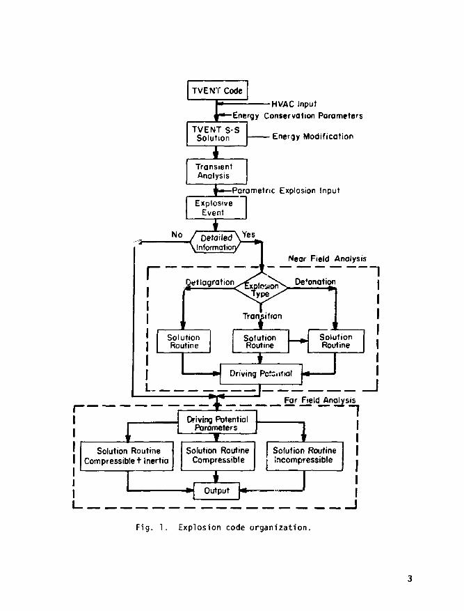
first far-field version. The organization of the explosion code is shown in

Fig. 1.

The explosior, code evolution from the TVENT code with the necessary

modifications is also shown in Fig. 1. When the explosive event is con¬

sidered, we subdivide the code for near-field or far-field analysis. The

distinction between near-field and far-field regions is illustrated in a

different manner in Fig. 2, which shows a ventilatior system that has been

subdivided into near and far-field regions. A near-field region surrounds the

explosive event location where the phenomenology is sensitive to the detailed

hydrodynamics of the explosion. Far-field regions are those farther from the

explosive event where the flow dynamics are relatively insensitive to the

detailed characteristics of the explosive event.

In any case, as shown in Fig. 1, the user must decide whether to make a

near or a far-field analysis. Results of a near-field analysis will provide

the driving potential for analyses in the far-field region. However, in many

cases the near-field analysis can be bypassed in favor of a far-field analysis

only. This decision will probably be based on (1) the availability of

TVENT Code

E. -HVAC Input

TVENT S-S Solution

Energy Conservation Parameters

— Energy Modification

Transient Analysis

Parametric Explosion Input Explosive

Event

No 1

Detoiled \ Y e s . Informotio

r Near Field Analysis

- I I " 1 ~ __ Far Field Analysis

Driving Potential Parameters

Solution Routine Compressible + inertia

Solution Routine Compressible

1 i Solution Routine I Incompressible

Output

Fig. 1. Explosion code organization.

detailed information describing the characteristics of the explosive event and

the system geometry, and (2) the desirability of performing a highly detailed

analysis before undertaking a less detailed or first-order analysis.

We have chosen to develop far-field analysis methods first for the fol¬

lowing reasons.

• First-order results can be obtained with this version of the

code. (In many cases this may be the only analysis required.)

• It is a logical and simple next step in development from the

TVENT code.

• An early first version of the explosion code can be released.

B. TVENT Basis

In developing the new code, we intend to retain as much of the original

TVENT code as possible because we will use TVENT as a foundation on which to

build the explosion code. TVENT features to be retained are the code super¬

structure, its portability, and the numerical approach to solving the govern¬

ing equations.

(I)

(19)

EXPLOSION

(221

(15) ;i6) ' ' (17) (18)

(II) (12) ' ' (13) (14)

(7) (8) ' * 19) (10)

FAR-FIELD

M ) (5) (6)

H3 Vr^-§ 1 (2) • ' (3)

Fig. 2. Near- and far-field regions in a ventilation system.

The TVENT superstructure will allow the explosion code to keep the same

general organization. The input and the output routines will be retained

because they are particularly suited for the heating, ventilating, and air

conditioning (HVAC) designer and analyst. The type of output (line printer)

found in TVENT will still be used, which will also help to retain portabil¬

ity. TVENT has been run on several types of computers, and we intend that the

explosion code have this feature. This may be difficult to achieve because

additional equations must be solved for explosive phenomena, which increases

computer storage and running time.

The steady-state analysis capability of TVENT will also be preserved in

the explosion code. However, special provisions for solving the full set of

equations, particularly the equation of state, must be made because steady-

state conditions mean that air density and temperature variations are small.

Perhaps the most difficult feature to retain from TVENT is the numerical

procedure for solving the governing fluid dynamic equations.

The lumped-parameter method is the basic TVENT formulation that describes

a ventilation system. No spatial distribution of parameters is considered in

this approach. Network theory, using the lumped-parameter method, .ncludes a

number of system elements, called branches, joined at certain points, called

nodes. Ventilation system components that exhibit resistance, such as damp¬

ers, filters, and blowers, are located within the branches of the system. The

ductwork of a ventilation system is considered a resistive element because of

the frictional resistance to fluid flow.

The connection points (nodes) of the system elements or branches are at

the upstream and downstream ends of the branches. Components that have larger

volumes, such as rooms, gloveboxes, and plenums, are located at nodal points.

Therefore, a node may possess some volume or capacitance where fluid storage or

compressibility may be accounted for.

Governing equations in TVENT require that the continuity equation be sat¬

isfied at every node and that a pressure-flow equation be satisfied for each

element or branch. Variations in the node equations depend on whether the

node represents a volume or a simple connection of two branches. If the node

rep1 eseni'. a finite volume, the equation of state for a perfect gas must be

satir, iiu. ihis variation also exists for the branches, depending on whether

the branch is simply a duct or contains a filter, blower, or damper.

The relationship between pressure and flow for the elements is nonlinear

and is written in general form

0 = R(p. - P j ) N . (i)

The volumetric flow rate is represented by 0, resistance by R, pressures at

the ends of a branch by p. and p., and an arbitrary exponent by U. This

numerical scheme uses a perturbation technique coupled with a Taylor series

expansion of Eq. (1). For a small perturbation (£p) the correct value for

pressure p, is

p. = p. + Ap , (2)

where the sign ~ indicates a temporary value. Substituting Eq. (2) in Eq. (1)

gives

Q = R(Pj - Pj - A P ) N . (3)

Using a Taylor series expansion of Eq. (3) gives a linear relationship between

flow and pressure as

Q = A - C AP , (4)

where A and C are temporary iterative values based upon previous values of

pressure. The flow-pressure relationship in the branches for the ducts,

dampers, filters, and blowers can all be formulated as Eq. (4). Now all flows

must satisfy the continuity equation at the nodal points. Summing all flows

at a nodal point allows us to solve for the perturbation pressure Ap. The

numerical process then iterates through a set of equations for &p until that

value is very small. Then we say that the numerical process has converged and

all the governing equations are satisfied. This numerical scheme is a fully

implicit iterative process.

Retaining the TVENT numerical scheme makes it imperative to be able to

write the equations describing compressible duct flow in the form of Eq. (4).

6

The equations describing compressible flow can indeed be arranged as in Eq.

(4), as described in Sec. V.

Summarizing, an implicit numerical scheme is used to solve for the

pressure correction at each node. The iterative process continues until the

pressure correction Z\» approaches zero and the system is balanced. The

numerical scheme is altered slightly by using the equation of state for a node

that represents a volume or some capacitance. Thus, altering the modeling of

flow in the elements or branches to account for compressible flow effects such

as inertia or choking requires a linearized form for flow similar to Eq. (4).

C. Far-Field Modeling Requirements

Having reviewed the basic formulations and numerical scheme used in TVENT

and recalling items listed in Ref. 2 that must be considered in modeling ex¬

plosive phenomena, we now proceed with development of the far-field explosion

code. To use TVENT as a basis for the explosion computer code requires the

following modifications.

t Addition of the equation of state

t Calculation of system densities

• Calculation of system mass flows

• Addition of the energy equation

• Calculation of system temperatures

• Addition of the momentum equation, ircluding inertia

• Calculation of system velocities

t Addition of compressible choking effects with dissipation

• Altering boundary conditions to accept parametric explosion

parameters

• Input modification to accept additional information

• Altering output to obtain mass flow, temperature, density, etc.

The features listed above were incorporated in developing the first ver¬

sion of a far-field explosion code. Other major steps involve many debugging

runs of the computer code and exercis'ng most of the features of the code on

sample problems. Details of these steps and sample problems are described in

the sections that follow. Also note that experiments must be performed to

verify the inertia and choking effects. Experimental data are also needed on

blower response to explosive transients. Little is known about this type of

blower response, and it is not included in this far-field explosion code;

therefore caution should be exercised in analyzing large pressure faisients

imposed across elements containing blowers.

D. Explosive Event Description

In this far-field analysis, the explosive event requires some form of sim¬

ulation where the detail of the event is of no significance. Basically, an

explosion can be defined by a rapid pressure rise, sometimes along with a

rapid temperature rise. These pressure and temperature increases can result

frofr physical, chemical, or even nuclear processes; for example, the rupture

of a highly pressurized vessel (physical), the combustion or detonation of

explosive materials (chemical), or criticality excursion of fissionable

nuclear materials (nuclear) can cause a rapid pressure rise with or without a

corresponding rapid temperature rise. All these processes involve a rapid

mass a.id energy addition to a system, whether the system is closed or open.

Analyses of explosions with rapid ma's and energy additions are common and

give good results if sufficient rate information is available. These ap¬

proaches are useful for simulating an explosion inside a system and need

detailed mass and energy source terms in the mass and energy equations. When

the energy release rate is not known, we can use other information such as

pressure-time or temperature-time profiles at a particular location in com¬

bination with mass addition information. The last two approaches require

experimental data on the system that can be difficult to obtain. For ar>

explosion outside a system, the pressure and temperature-time profiles can

provide information needed to investigate a system response.

III. MASS EQUATION

As noted, the continuity equation must be applied at each node. In TVENT,

where only incompressible flow is considered, a volumetric flow form can be

used. To model compressible flows, we must account for density variations

rather than simply balancing volumetric flows. Therefore, we must modify our

continuity conditions in the explosion code at each node to include density

and use a mass equation strictly for balancing. The mass equation for nodal

points that have no mass storage is

EVk = EVA = ° • (5)

k k *

where P. and Q, are the mass flow rate and volumetric flow rate in branch K K

k, and p. is the air density in branch k. The value q. is used tc adjust

for the proper flow direction in relation to the node; q, = +1 for the down¬

stream node of a branch or -1 for the upstream node.

The mass equation for nodal points that allow mass accumulation {capac¬

itance nodes) is

where M is the user-specified mass source per ui.it time for the volume and

V is the volume of the node. We use the ideal gas equation of state

where p, T, and R are the node pressure, temperature, and gas constant for

air. Putting the equation of state into Eq. (6) gives

Expanding and rearranging this equation gives

As in TVENT [see Ref. 1, Eq. (E-6)], g£ is replaced by

P n + 1 - p" P * Ap - p" . (9) At &t

with superscripts n+1 and n indicating the new tune and eld time. £p is the

pressure correction term and p the current pressure. The equation far Ap is

[from Eq. (8)]

aoj

The mass equation is implemented in two forms, depending on whether the

room temperature is known (user-specified room condition) or unknown.

A. Temperature Specified

As in TVENT we can express the flow rate in terms of pfc-ssure [Ref. i,

Eq. (E-8) or Eq. (4)].

Using Eq. (6) in Eq. (5) and solvi;,^ for &p gives

The pressure correction term can be calculated explicitly from Eq. (12) by

evaluating the other unknown quantities at the old time.

B. Temperature Unknown

When the temperature is not known, the temperature derivativ term is

eliminated from the mass equation [Eq. (10)] by evaluating it from the energy

equation.

10

IV. ENERGY EQUATION

Both the amount and rate of energy r e l d s e frcni an explosive event can

have profound effects on tlie gas dynamics of i system. This becomes appsre^t

when we recall that the pressure correction cerm dp derived in Sec. 113 is

dependent on both temperature and 'sme-rate of change of temperature. By

maintaining an energy balance similar to the mass balance discussed in Sec.

Ill, we can calculate the necessary ;ysiem temperatures. lh<- energy equation

used in the far-field version of the explosion (o(k- with its corresponding

effect on both nodal temperatures and the pref.sure correction tern -is outlined

below.

A. Arbitrary Node

The basic energy equation employed is

where ru represents U ° internal energy per unit volume and c, is the specif¬

ic internal energy of the branch. The er.thalpy associated with the mass oddi-

tion is denoted by h , and F is an arbitrary energy source term. We make

the additional assumption that

— - (14) PU = pu , ^ '

where o is the average density in the volume and u the average specific inter¬

nal energy. Then Eq. (13) becomes

,, du ,.— dp Vp-rr + VU -jr = dt dt

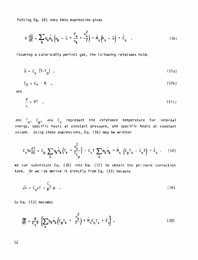
Putting Eq. (6) into this expression gives

P v2

Assuming a calorically perfect gas, the following relations hold.

U = Cv (T-To) , (17a)

Cp = Cv > R , (17b)

and

- = RT , (Vc) D

and T , C , and C represent the reference temperature for internal

energy, specific heats at constant pressure, and specific heats at constant

volume. Using these expressions, Eq. (16) may be written

C Vp^ j l v dt v

= C y q . m , (j. + ^ - ) - C T V q . m . + M / C T - t T l + E . (18) p Z w k k \ k 2^ / v Z - * k k s \ p s v ^ s • '

k p k p k

We can substitute Eq. (18) into Eq. (12) to obtain the pr;;sure correction

term. Or we ran derive it directly from Eq. (13) because

pu = CvoT = p . (19)

So Eq. (13) becomes

[ l \ m ( C T + > ) + "CT + ^] (20)

12

K

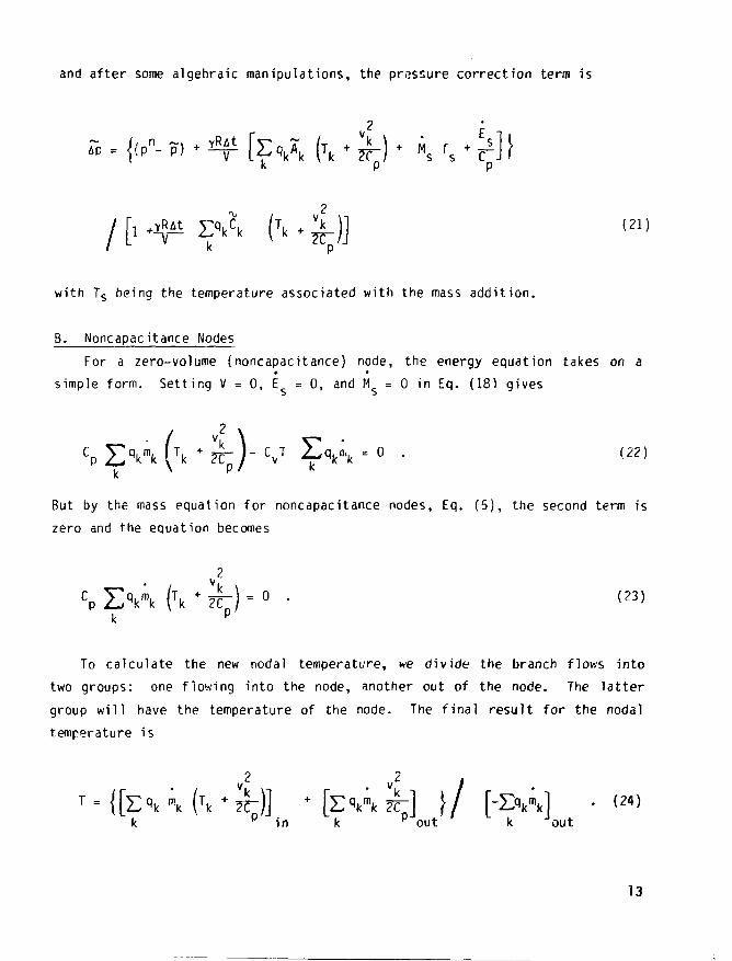
and after some algebraic manipulations, the pressure correction term is

I [1 f

2 + _^'n (21)

with Ts being the temperature associated with the mass addition.

B. Noncapacitance Nodes

For a zero-volume (noncapacitance) node, the energy equation takes on a

simple form. Setting V = 0, E = 0 , and M = 0 in Eq. (18) gives

But by the mass equation for noncapacitance nodes, Eq. (5), the second term is

zero and the equation becomes

2

To calculate the new nodal temperature, we divide the branch flows into

two groups: one flowing into the node, another out of the node. The latter

group will have the temperature of the node. The final result for the nodal

temperature is

v2 v2

in ~k H"out ' "• k Jout

13

Once the temperature is know, density is calculated from the equation of

state.

V. MOMENTUM EQUATION WITH INERTIA

A. Motivation

The momentum equation used in the TVENT code is basicaPy quasi-steady; it

is an orifice flow relationship that is auequate for slow-flow transierts such

as the type induced by a tornado. However, in the case of an explosion, the

pressure rise can be quite rapid and the effect of inertia must be taken into

account, no matter how small it r.ay seem to be. The development and implemen¬

tation of the momentum equation with inertia into the explosion code should

make it useful in a much broader range of far-field problems.

B. Development of Equation

We start with the momentum equation in differential form for one-dimen¬

sional, constant-area, compressible, unsteady adiabatic gas flow with fric¬

tion.3

^ ^ ( ) ^ I i ^ A , (25)

where t and x are time and space coordinates; p, v, A, p, f, and D represent

dei.sity, velocity, flow area, pressure, Darcy friction factor, ana hydraulic

diameter, respectively. The last teim on the right side of the equation is a

loss term where loss is due to wall friction. Definii.g mass flow rate m,

m = ovA , (26)

Eq. (25) can be rewritten as

•o

m

14

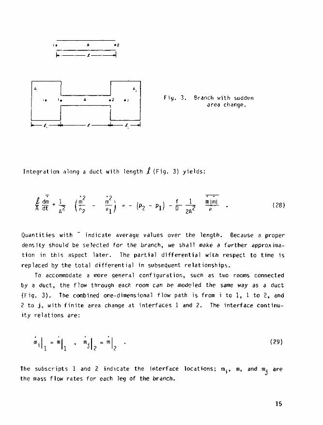
' . I . a . 2 . 1 Fig. 3. Branch with sudden change.

Integration along a duct with length £ (Fig. 3) yields:

/dmj m2 m? \ f 1 m|m| (28)

Quantities with indicate average values over the length. Because a proper

density should be selected for the branch, we shall make a further approxima¬

tion in this aspect later. The partial differential with respect to time is

replaced by the total differential in subsequent relationships.

To accommodate a more general configuration, such as two rooms connected

by a duct, the flow through Q&CY, room can be modeled the same way as a duct

(Fig. 3). The combined one-dimensional flow path is from i to 1, 1 to 2, and

2 to j, with finite area change at interfaces 1 and 2. The interface continu¬

ity relations are:

m. = m 1 ll

m = m J o

(29)

The subscripts 1 and 2 indicate the interface locations; m., m, and m- are

the mass flow rates for each leg of the branch.

15

Application of this momentum equation is limited to the far-field region,

and the flow remains subsonic, although choking is allowed. A step further,

we assume the spatial variation of the mass flow rate is negligible,

30>

Also, we assume the difference in kinetic energy at both ends is negligible,

.2 .2 (m \ ( m \ n

which leads to a momentjm equation of incompressible form from Eq. (28),

£ dm / \ f 1 m N A dt * {P » )

The associated with m can be dropped. Adding the momentum equations

for the three legs and using the interface continuity relations we obtain

• d m i v „ 1 m I m I 1 dt = (pi - pj) " Keff ^ -jr

where

A ' '5A~ ' O1IU vr34) i J

e f f = i 57T" K i J \S~I rT K + I -5TT- K J ! ~ J - t J b /

I represents the inertia effect of the flow path, including the rooms as well

as the duct. K „ is the total effective resistance coefficient; the minor

losses, such as turning, entrance, and exit are represented by the K's. The

first and the third terms in Eq. (35) are usually ^uite small because the area

16

ratios are squared and can be neglected. Notice that only naif the room char¬

acteristic length £ in the flow direction is used in the inertia and friction

calculations for that branch because the other half contributes the same to

the branch on the other side of the room. This is consistent with the one-

dimensional approach for a pipe divided into a number of control volumes. For

a room with only one branch, the other half will be considered as a stagnant

(no-flow) region. For a pure node (room with zero volume), there is no effect

on the inertia or friction, as seen in Eqs. (34) and (35). Note that I and

K ,, are input quantities.

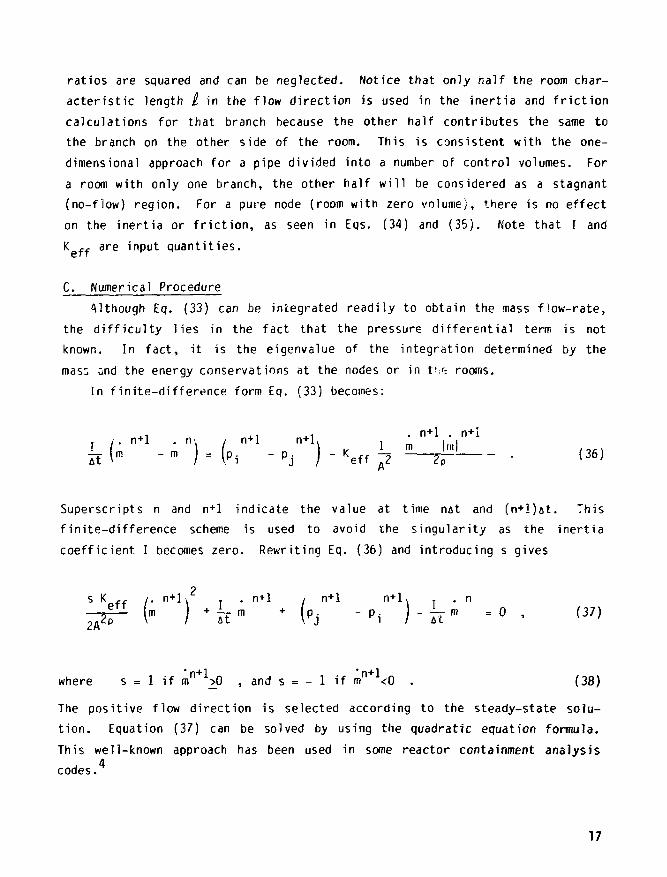
C. Numerical Procedure

Although Eq. (33) can be integrated readily to obtain the mass flow-rate,

the difficulty lies in the fact that the pressure differential term is not

known. In fact, it is the eigenvalue of the integration determined by the

mass and the energy conservations at the nodes or in t>^ rooms.

In finite-difference form Eq. (33) becomes:

n+1 . n-. / n+l n+l

- • ) • (P, " >i ) - « .ff *!

Superscripts n and n+l indicate the value at time nit and (n+l)flt. This

finite-difference scheme is used to avoid the singularity as the inertia

coefficient I becomes zero. Rewriting Eq. (36) and introducing s gives

/. n+l'. . . n+l / n+l n+l, . . n (m ) + ^ m + (p. - p . J - i ^ i = 0 , (37)

where s = 1 if m"* 1^ , and s = - 1 if m n + i<0 . (38)

The positive flow direction is selected according to the steady-state solu¬

tion. Equation (37) can be solved by using the quadratic equation formula.

This well-known approach has been used in some reactor containment analysis 4

codes.

17

m = Y^T (- b + Vb 2 - 4asc) , (39)

with

K a = ~- , (40a;

?A

b = |Y , (4Gb)

and

/ n+1 n+l\ I ' n c = (PJ " Pi ) " It m

The positive sign is needed in Eq. (39) for realistic solution; s is selected

to maintain -4asc > 0 at all times.

Eq. (39) is incomplete because the pressure differential term through c is

not yet known. The mass and energy flow rates must satisfy conservation re¬

quirements at nodes and rooms. Following the iteration process used in the

TVENT code, Eq. (39) can be put in a perturbation form similar to Eq. (4):

m = A - C Ap . (41)

Here, we drop superscript n+1 but add ~ to indicate temporary value. Ap rep¬

resents the pressure perturbation at a certain node j; its vanishing value

means convergence is reached. For a small perturbation, we substitute

Pj = p. + Ap (42a)

18

or

c = c + AP (42b)

into Eq. (39) and obtain

and

r q

with

B = b 2 - 4asc (43c)

and

c = (p. _ p.| _ ' m . (43d)

Again, quantities with - are adjusted at each iteration, q takes the value of

+1 if the pressure correction is performed on the downstream node; otherwise

it is -1. The amount of pressure correction for a node is determined by the

mass conservation equation

m, = 0 . (44)

19

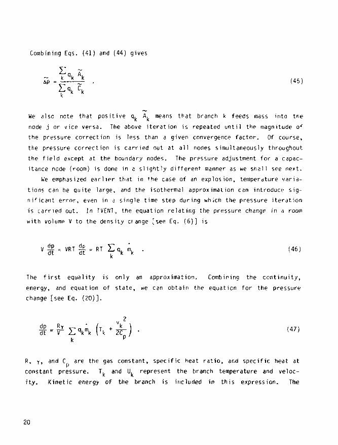
Combining Eqs. (41) and (44) gives

~ k qk k

Ap = 1—*—1 . (45)

We also note that positive q. A. means that branch k feeds mass into the

node j or vice versa. The above iteration is repeated until the magnitude of

the pressure correction is less than a given convergence factor. Of course,

the pressure correction is carried out at all nodes simultaneously throughout

the field except at the boundary nodes. The prpssure adjustment for a capac¬

itance node (room) is done in a slightly different manner as we shall see next.

We emphasized earlier that in the case of an explosion, temperature varia¬

tions can be quite large, and the isothermal approximation can introduce sig¬

nificant error, even in a single time step during which the pressure iteration

is carried out. In TV'ENT, the equation relating the pressure change in a room

with volume V to the density change [see Eq. (6)] is

d£ = V R T ^ = R T E q k m k . (46) K

The first equality is only an approximation. Combining the continuity,

energy, and equation of state, we can obtain the equation for the pressure

change [see Eq. (20)].

R, y> and C. are the gas constant, specific heat ratio, and specific heat at

constant pressure. T. and U. represent the branch temperature and veloc¬

ity. Kinetic energy of the branch is included in this expression. The

20

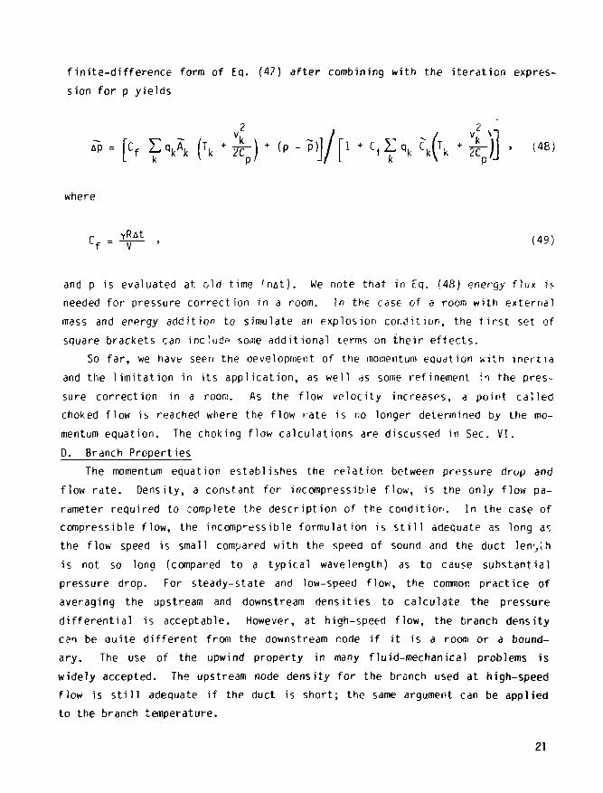
finite-difference form of Eq. (47) after combining with the iteration expres¬

sion for p yields

= [Cf Ea kA k (T, • (p -P)]/[l + C f £ \ Ck(lk * j j . (48)

where

C f =

and p is evaluated at old time ''nat). We note that in Eq. (48) energy f)ux is

needed for pressure correction in a room. In the case of a room with external

mass and energy addition to simulate an explosion condition, the first set of

square brackets can include sane additional terms on their effects.

So far, we have seen the development of the momentum equation with inertia

and the limitation in its application, as well as some refinement ii the pres¬

sure correction in a room. As the flow velocity increasps, a point called

choked flow is reached where the flow rate is no longer determined by the mo¬

mentum equation. The choking flow calculations are discussed in Sec. VI.

D. Branch Properties

The momentum equation establishes the relation between pressure drop and

flow rate. Density, a constant for incompressible flow, is the only flow pa¬

rameter required to complete the description of the condition. In the case of

compressible flow, the incompressible formulation is still adequate as long as

the flow speed is small compared with the speed of sound and the duct len'jih

is not so long (compared to a typical wavelength) as to cause substantial

pressure drop. For steady-state and low-speed flow, the common practice of

averaging the upstream and downstream densities to calculate the pressure

differential is acceptable. However, at high-speed flow, the branch density

can be quite different from the downstream node if it is a room or a bound¬

ary. The use of the upwind property in many fluid-mechanical problems is

widely accepted. The upstream node density for the branch used at high-speed

flow is still adequate if the duct is short; the same argument can be applied

to the branch temperature.

21

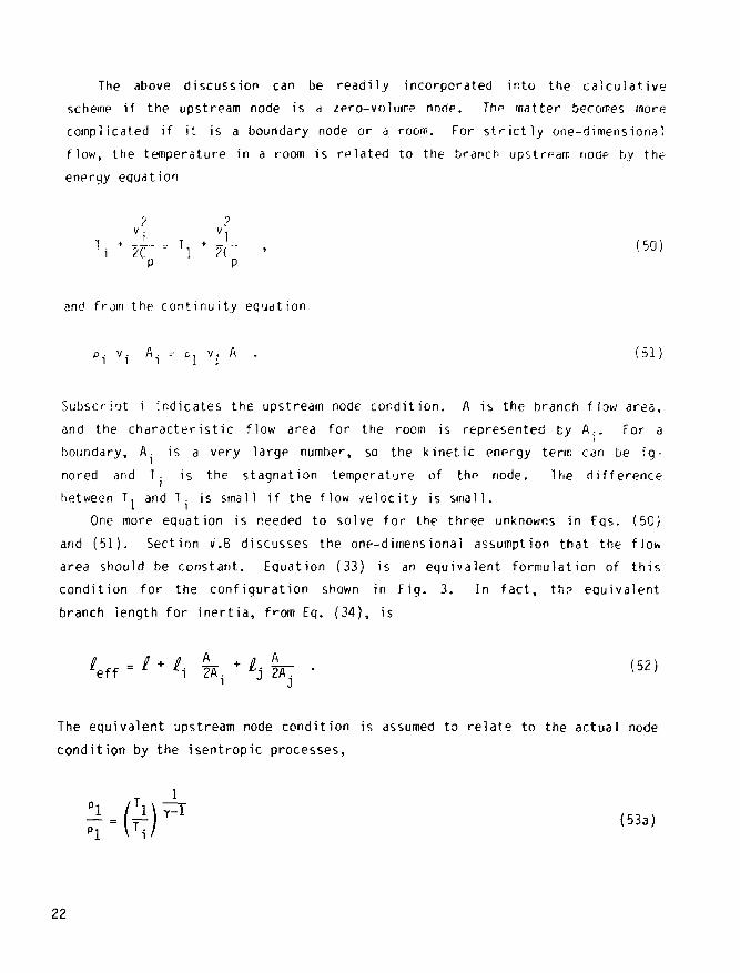
The above discussion can be readily incorporated into the calculative

scheme if the upstream node is a zero-volume node. The matter becomes more

complicated if it is a boundary node or a room. For strictly one-dimensional

flow, the temperature in a roan is related to the branch upstream node by the

energy equation

and from the continuity equation

pi vi Ai = cl vl A • (51)

Subscriot i indicates the upstream node condition. A is the branch flow area,

and the characteristic flow area for the room is represented by A.. For a

boundary, A. is a very large number, so the kinetic energy term can be ig¬

nored and T. is the stagnation temperature of the node. The difference

between T, and T. is small if the flow velocity is small.

One more equation is needed to solve for the three unknowns in Eqs. (50)

and (51). Section v.B discusses the one-dimensional assumption that the flow

area should be constant. Equation (33) is an equivalent formulation of this

condition for the configuration shown in Fig. 3. In fact, th? equivalent

branch length for inertia, f>-om Eq. (34), is

The equivalent jpstream node condition is assumed to relate to the actual node

condition by the isentropic processes,

1

(53a)

22

and ^ = U i ) , (53b) i \ i

because we have already combined all the losses (friction and minor) of the

room into the K ,,, Eq. (35), which belong to the branch downstream of this

node. Equations (50)—(53a) can be solved numerically, and then the equivalent

upstream node pressure can be calculated by Eq. (-33b). There is no similar

pressure calculation for the downstream end of the branch because the pressure

should be the same as the nodal pressure according to the theory of jet dissi¬

pation.

Finally, the pressure differential term in Eq. (36) should be adjuster if

the upstream node is a room or boundary. Throughout the pressure iteration

process, the nodal temperature is allowed to vary, as well as the branch tem¬

perature and density, 3S in Eqs. (50) and (51).

VI. CHOKIr.'G OF COMPRESSIBLE FLOW WITH DISSIPATION

A. Motivation

The steady-state flow rate in incompressible flow is determined by the

pressure drop. In compressible flow, the flow rate will re^ch a maximum value

regardless of how mucn the downstream pressure is decreased if the upstream

pressure is constant. This phenomenon is called choking. In a ventilation

system with tornado-induced pressure transients, choking is not expected to

occur, but in an explosion, large pressure differentials will exist at some

nodal points. Hence, we must use the proper flow rate for a branch under

choking conditions. For isentropic (adiabatic, frictionless) flow, choking

can be easily established and the maximum flow rate is uniquely determined by

the upstream condition. This is no longer a simple matter when dissipation is

present.

B. Critical Upstream Mach Number

We will investigate the quasi-steady compressible flow inside a constant-

area duct, where the usual one-dimensional approximation is assumed. Heat

transfer is not allowed but friction effect is present. In general, this duct

23

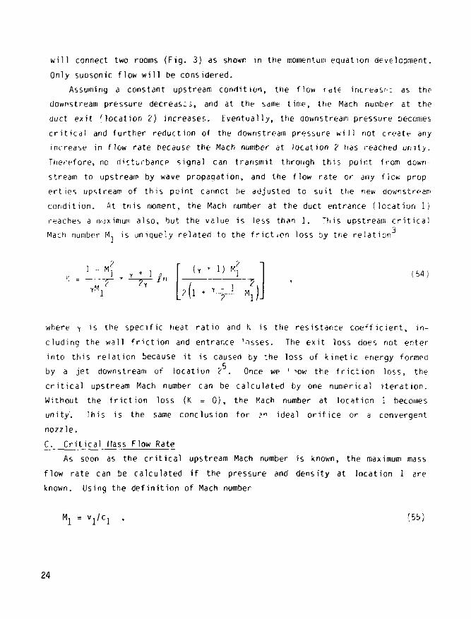
will connect two rooms (Fig. 3) as shown in the momentum equation oeveiopment.

Only subsonic flow will be considered.

Assuming a constant upstream condition, the flow rate increasr-: as the

downstream pressure decreases, and at the same time, the Mach number at the

duct exit 'location 2) increases. Eventually, the downstream pressure becomes

critical and further reduction of the downstream pressure will not create any

increase in flow rate because the Mach number at location 2 has reached unity.

Therefore, no disturbance signal can transmit through this point from down¬

stream to upstream by wave propagation, and the flow rate or any flow prop¬

erties upstream of this point cannot be adjusted to suit the new downstream

condition. At this moment, the Mach number at the duct entrance (location 1)

reaches a mjximum also, but the value is less than 1. This upstream critical

Mach number M, is uniquely related to the friction loss by the relation

(Y + 1) «i

V s «.)J where y is the specific heat ratio and K is the resistance coefficient, in¬

cluding the wall friction and entrance 'osses. The exit loss does not enter

into this relation because it is caused by the loss of kinetic energy formed

by a jet downstream of location 2 . Once we ' ">ow the friction loss, the

critical upstream Mach number can be calculated by one numerical iteration.

Without the friction loss (K = 0 ) , the Mach number at location 1 becomes

unity'. This is the same conclusion for ?" ideal orifice or a convergent

nozzle.

C. Critical Mass Flow Rate

As soon as the critical upstream Mach number is known, the maximum mass

flow rate can be calculated if the pressure and density at location 1 are

known. Using the definition of Mach number

Mj = V J / C J , (55)

24

where v, and c, are the local gas velocity and local speed of sound, which

in turn is a function of pressure p. and density t,, with

(56;

for an ideal gas, we have

This is the maximum allowable mass flow rate that s particular trench can

supply for a given condition at 1. We emphasise the importance of using p,

and IJ1 . For a true node, p, and r, represent the actual nodel values.

If the upstream node is a room (or boundary) as see in Fio. 3, p, and j,

are not the same ab p. end p. -- in tact they are related to the upstrearr.

room conditions as described in Sec. V.D. For a room with a very larue flow

cross section and with some algebraic manipulation,

which is the familiar expression for the ideal orifice flow rate if the stag¬

nation temperature T., the local pressure, and the local Mach number are 3 1

known.

D. Numerical Procedure

Equation (57) is similar to the equation for incompressible orifice flow,

except that the pressure differential is replaced by the upstream pressure

only. The pressure correction can b<= achieved by introducing a small pertur¬

bation quantity ap and we have

m = A - C ap , (59)

where

A = S A M J ^ 7 P 1 PJ , (60a)

25

and

j * (60b)

All quantities with - are the updated values during the iteration process.

M, is constant because it is a unique function of the friction loss. Equa¬

tion (59) fits the numerical scheme used previously if "VENT. Because the

mass flow rate depends on the upstream pressure only, ano if a node is down¬

stream of a branch through which the choking occurs, nc pressure correction

should be made on that node by this branch. In this case, the pressure ad¬

justment coefficient C must be set equal to zero. That condition is deter¬

mined by the combined effect of s and q defined in Sec. V.

VII. VESSEL DISCHARGE AND CHARGING VESSEL PROBLEMS

Some experimental data in Ref. b describe the discharge of high-pressure

gas (air) from a vessel to the atmosphere. This referpnee also discusses the

pressurization of a vessel by a high-pressure air supply reservoir. These are

interesting test cases for our computer code, especially in the areas of mass

and energy conservation, orifice flow relation and choked flow. In both

cases, shown schematically in Fig. 4, the initial pressure differential is

quite large, und the flow is choked during the eariy ph<:>e of the transient.

As the vessel pressure approaches that of ambience or of the supply reservoir,

the unchoked orifice flow relationship applies. Although the unchoked orifice

relation is essentially an incompressible formulation, the choked flow cal¬

culation does include the effect of dissipation.

The experimental and analytical pressure transients and all pertinent

parameters are shown in Figs. 5 and 6. For the numerical calculation, the

dimensionless resistance coefficient is first estimated based on some typical

orifice information, and then the dimensional resistance coefficient is cal¬

culated, because the latter is the required input used in the code. The

figures show that the analytical result compares well with the experiment,

even though there is some uncertainty about the orifice resistance. The

transition from choked flow to unchoked flow is best illustrated in the

charging vessel case (Fig. 6). The constant mass and energy supply from an

26

L Ambient Prpssur

1.0 1105 Po H i 5 ps

I""™ A. 7 92 • 10** n?

Pressure i 079 > 10* Po (?i4 f> PSJOI

mg Vessel (o)

Jl a . 7 92 > 10 ,-6 2

Initial Pressure IO « IO'PO (14.5 pnol Initial Temperoture 294 K (69"<ri Supply Pressure 6 83 < IO5PQ (99 ps.ol v,> >v, 1 (b) Charging Vessel

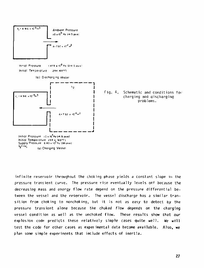
Fig. 4. Schematic and conditions for charging and discharging

probiems.

infinite reservoir throughout the choking phase yields a constant slope in the

pressure transient curve. The pressure rise eventually levels otf because the

decreasing mass and energy flow rate depend on the pressure differential be¬

tween the vessel and the reservoir. The vessel discharge has a similar tran¬

sition from choking to nonchoking, but it is not as easy to detect by the

pressure transient alone because the choked flow depends on the charging

vessel condition as well as the unchoked flow. These results show that our

explosion code predicts these relatively simple cases quite well. We will

test the code for other cases as experimental data become available. Also, we

plan some simple experiments that include effects of inertia.

27

20 25 30 S3 40 4 i JO Time (5l

Vsssel Dschorge

Fig. 5. Analytical and experimental results for discharging

problem.

Chorgmg Vessel

Fig. 6. Analytical and experimental results for charging problem.

VIIi. EXAMPLE PROBLEMS USING THE EXPLOSION CODE

The problems discussed in Sec. VI illustrate the capability of the com¬

puter code to mode1 effects of mass and energy conservation, the orifice flow

relation used, and choking. However, other types of problems are better suited

to demonstrate the code's capability to model simulated explosions.

A. Modeling Considerations

Use of our explosion code for modeling requires n^r? information than that

required for TVENT. For example, the flow algorithms for inertia and choking

effects are based on the properties of the ducts, and therefore detailed duct

dimensions are required in those parts of the system where inertia and choking

are to be modeled. In general, the lumping of elements in the model can be

done as coarsely as in TVENT, but a capability exists to allow subdivision of

the network elements into finer zones.

An explosion can be modeled in several ways; the options differ only in the

manner of specifying the energy of the explosion. The more direct approach is

to specify the injection of mass and the energy associated with an explosion.

An indirect approach is to specify the injection of mass, but to express-c.iergy

in terms of a pressure or temperature rise. Theoretically, either approach is

28

valid. However, the option used will depend on the information available; that

is, the lack of good detail about the explosion might determine which option to

use. The use of the indirect approach with the room temperature rise is the

most demanding because the shape of the temperature rise function is used to

determine the time derivative of temperature.

B. Example Problems

The first example problem demonstrates options that are available for

specifying an explosion. We have also analyzed this model for a tornado-pres¬

sure transient with both TVENT and the explosion code to provide a compar¬

ison. The second sample problem emphasizes the importance of using volume

distribution or element subdivision in obtaining detailed distribution of

results.

Although the primary purpose of these sample problems is to demonstrate the

capability of the explosion code, they also show some things to consider in

preparing the required input. The selection of these examples was arbitrary,

and no consideration was given to simulation of actual facilities.

1. Example 1. This problem is taken from the existing wasre calcining

facility ventilation system at the Idaho Chemical Processing Plant (ICPP) in

Idaho Falls, Idaho. This facility was used to test TVENT during its develop¬

ment stage and results were reported.

The original TVENT model, modified to account for explosive effects, was

poorly defined because there was little information about the older ICPP

structures. That information is still not available, but the problem was

chosen because it is relatively simple and has been analyzed with TVFNT.

The model used in our explosion code is shown in Fig. 7. The explosion is

applied to the small room at node No. ?. It was not applied to noces 3 or 4

because explosion effects would have been greatly diminished in these large

volumes. The node 7 location could simulate an explosion in a glovebox near

the exhaust of the large room at node 4. A filter was added to the system

simply to include all types of elements. The model is terminated at node 11.

This sample problem shows four equivalent option? available for specifying

an explosion. This problem is also a comparison of TVENT and our explosion

code for a tjrnado transient.

29

2. Example 2. This fictitious problem was designed to provide detailed

information on the effects of inertia, choked flow, and subdivision of a duct.

The system consists of an explosion chamber connected to a long pipe that has a 2 ?

constant area of 0.0729 m (0.785 ft ). A typical smooth-pipe friction

drop has been assumed for calculating the branch resistances. This problem has

no initial flow and so must be handled as a restart problem. The explosion

code model used for this problem is shown in Fig. 8. The pipe has been broken

arbitrarily into eight segments to provide additional detailed information

along the length of the duct. Two explosion magnitudes are used—a high-

intensity explosion and a low-intensity explosion. These levels were chosen

arbitrarily for demonstration. The high yield is equivalent to a 378 kg/s

(3.0X106 lb/hr) mass injection at a temperature of 538°C (1000° F) for a

duration of 0.1 s. The lower intensity is the same except that mass injection

has been reduced by a factor of 10.

L. Results

The explosion code output formats are the same as those generated by TVENT

except that temperature has been adoed to the list of parameters. A comment

statement has been added to the table called "Problem Summary of Extreme

Values," to indicate the occurrence of choking. The plotting formats used in

this report were made by a program called DISSPLA. Tiie values of pressures,

flow, and temperature are given in standard output units; that is, inches of

water, cfm, and degrees F. Equivalent SI unit values are not shown because the

only purpose is comparison of the codes.

1. Example Problem 1. The four options are based on different ways of

expressing the energy of the explosion as indicated by the numbers in paren¬

theses following the title, Explosion in Glovebox, shown in Figs. 9—11.

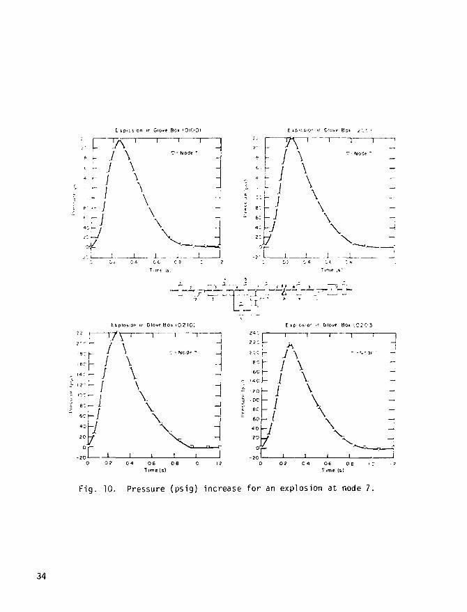
( 0 1 0 0 ) = temperature of injected mass specified,

( 1 2 0 0 ) = energy of injected mass specified,

( 0 2 1 0 ) = pressure transferred to confined air specified, and

( 0 2 0 3 ) = temperature transferred to confined air specified.

30

(4) (5)

I 1 I

o - Nodol Pom;

- Blower

-Valve ond/or Dud

-Volume

-Filter

Fig. 7. Model ventilation system for example 1.

1 z v>

3

Vk 4

VV 5 6 7 8 9

(I) (2) (3) (4) (5) (6) (7) (8)

-Duct (Bronch)

o -Nodal Point

-Volume

Fig. 8. Computer code model for example 2.

(9)

31

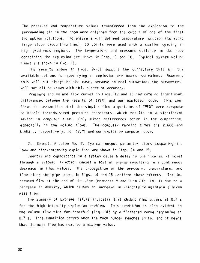
The pressure and temperature values transferred from the explosion to the

surrounding air in the room were obtained from the output of one of the first

two option solutions. To ensure a well-defined temperature function (to avoid

large slope discontinuities), 50 points were used with a smaller spacing in

high gradients regions. The temperature and pressure build-up in the room

containing the explosion are shown in Figs. 9 and 10. Typical system volume

flows are shown in Fig. 11.

The results shown in Figs. 9—11 support the conjecture that all the

available cptions for specifying an explosion are indeec equivalent. However,

this will not always be the case, because in real situations the parameters

will not all be known with this degree of accuracy.

Pressure and volume flow curves in Figs. 1? and 13 indicate no significant

differences between the results of TVENT and our explosion code. This con¬

firms the assumption that the simpler flow algorithms of TVENT were adequate

to handle tornado-sized pressure transients, which results in a significant

saving in computer time. Only minor differences occur in the comparison,

especially in the volume flows. The computer running times are 2\688 and

6.683 s, respectively, for TVENT and our explosion computer code.

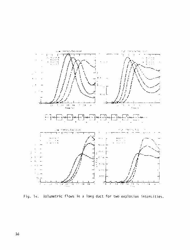
2. Example Problem No. 2. Typical output parameter plots comparing the

low- and high-intensity explosions are shown in Figs. 14 and 15.

Inertia and capacitance in a system cause a delay in the flow as it moves

through a system. Friction causes a loss of energy resulting in a continuous

decrease in flow values. The propagation of the pressure, temperature, and

flow along the pipe shown in Figs. 14 and 15 confirms these effects. The in¬

creased flow at the end of the pipe (branches 8 and 9 in Fig. 14) is due to a

decrease in density, which causes an increase in velocity to maintain a given

mass flow.

The Summary of Extreme Values indicates that choked flow occurs at 0.7 s

for the high-intensity explosion problem. This condition is also evident in

the volume flow plot for branch 9 (Fig. 14) by a fattened curve beginning at

0.7 s. This condition occurs when the Wach number reaches unity, and it means

that the mass flow has reached a maximum value.

32

t i p o s c . ' G i c » e 6 - » 1 O 1 O O 1 t I f ' O S <>' • ' G 'Oyf B C » ' '• ^ ''

JSO

JOG : :r->•• * I .

l

* t 7 c" "

I I

/ 5 0 ' -

• s . • /

02 0 ' 0 ' oe

Fig. 9. Temperature ( F) increase f"r explosion at node 7.

33

G'O*e Bo* l O i O Q ) 6c»

I I I

J \

1 : i

4

\ \ \ -i \ \ \

- t: — J \ \

\

x _ J ot c e

in Glove B o » . 0 2 1 0 )

"1" ' - I

" ' - I -

E»p 'o * . iO ' i r Glovf Bo* ! .CZ'C3

T r 1 T r

h J \ 1 ?0

• oc

ec

60 —

<o —

° c L o? c< oe oe

Time (s!

Fig. 10. Pressure (psig) increase for an explosion at node 7.

34

I »r- •>•> or. ' O-cft Bo*

\

- «•(>•«* (,

r - K =.—i

bo*

]\ V.

! • • . - •

] /

06 ;B Time (s)

Fig. 11. System flows (cfm) for an explosion at node 7.

35

^

• 1 , 1 . • I

\

- • \\

* \ \

V U i s

\ 1

Fig. 12. Pressure transients for TVE/JT and the explosion computer code.

36

:r \

B-a^:" 8

- 9-3"-- 9 9'Or-f 0

i 5 « 5 fc -it *'

Fig. 13. Volumetric flow for TVENT and the explosion computer code.

37

"1~~I T"

///A\ y ; / J

J

ill In

'r]—i-WJ-^-'- -Vr- -" *- -Vr[~ "'Y*!—'

T—i—T ~~\—i—r

^ 4 ^ - : •

: , w5 L /? 1!

• ; J L

Ui I I ! )

1 " 4 yV? i

Fig. 14. Volumetric Hows in a long duct f o r two explosion i n t e n s i t i e s .

/

ii " i i

' • • ^ e ' s ;

? 3 4 •

' 2 15!

V 7 /

Fig. 15. Temperature and pressure distribution in a long duct for two explosion intensities.

39

IX. STATUS

The computer code has been released in preliminary form to friendly users

to allow it to be exercised. Their suggestions for improvement will be con¬

sidered when we release the final version. These users will apply the code to

the analyses of structures where explosive potentials exist. This will insure

that the code can model realistic conditions and point out facility deficien¬

cies thrt must be remedied.

We plan to release the code and documentation unconditionally to the Na¬

tional Energy Software Center at the Argonne National Laboratory by the end of

FY 1980.

X. SUMMARY

We have described development of a first-version computer code that can be

used to calculate explosively induced transients within the ventilation sys¬

tems of nuclear facilities. This explosion code version is suitable for mod¬

eling far-field explosive effects; that is, it can he used to model pressure,

density, and temperature fields that are somewhat remote from or relatively

insensitive to the explosive event. This version of the code will be useful

to obtain a first-order solution to a problem and indeed may be the only anal¬

ysis required in many situations. This approach and future developments of

the explosion computer code were outlined in Ref. 2.

The code retains all the features of the TVENT code but uses a mass equa¬

tion, .an energy equation, and a momentum equation for calculating compressible

flow throughout a network system. Th^ numerical technique used in TVENT is

preserved,and both inertia and choking effects are included. Example problems

chat demonstrate the capabilities and limitation of the code are described.

40

REFERENCES

1. K. H. Duerre, R. W. Andrae, and W. S. Gregory, "TVENT - A Computer Program for Analysis of Tornado-Induced Transients in Ventilation Systems," Los Alamos Scientific Laboratory report LA-7397-M (July 1978).

2. W. S. Gregory, P. R. Smith, J. W. Bolstad, and K. H. Duerre, "Analysis of Ventilation Systems Subjected to Explosive Transients — Initial Analysis and Proposed Approach," Los Alamos Scientific Laboratory report LA-7964-MS (August 1979).

3. A. H. Shapiro, The Dynamics and Thermodynamics of Compressible Fluid clow (Ronald Tress, New York, 1953).

4. R. G. Gido, C. I. Grimes, R. G. Lawton, and J. A. Kudrick, "COMPARE: A Computer Program for the Transient Calculation of System of Volumes Connected by Flowing Vents," Lc<; Alamos Scientific Laboratory report LA-NUREG-6488-MS (September 1976).

5. V. Ingard and H. Ising, "Acoustic Nonlinearity of an Orifice," Journal of the Acoustic Society of America 42, 6-17 (1967).

6. A. L. Addy and B. J. Walker, "Rapid Discharging of a Vessel Through a Nozzle or an Orifice," ASME paper 72-FE-4O (1972).

7. W. S. Gregory, R. W. Andrae, K. H. Duerre, and R. C. Dove, "Ventilation System Analysis During Tornado Conditions," Los Alamos Scientific Laboratory report LA-6999-PR (October 1977).

41 &U.S. GOVERNMENT PRINTING OFFICE: 1 98 1-O-576-020/ 1 61