Compressible and low Mach number LES of a swirl experimental burner

This article appeared in a journal published by Elsevier. The attachedcopy is furnished to the author for internal non-commercial researchand education use, including for instruction at the authors institution

and sharing with colleagues.

Other uses, including reproduction and distribution, or selling orlicensing copies, or posting to personal, institutional or third party

websites are prohibited.

In most cases authors are permitted to post their version of thearticle (e.g. in Word or Tex form) to their personal website orinstitutional repository. Authors requiring further information

regarding Elsevier’s archiving and manuscript policies areencouraged to visit:

http://www.elsevier.com/copyright

http://www.elsevier.com/copyright

Author's personal copy

C. R. Mecanique 341 (2013) 277–287

Contents lists available at SciVerse ScienceDirect

Comptes Rendus Mecanique

www.sciencedirect.com

Combustion, flow and spray dynamics for aerospace propulsion

Compressible and low Mach number LES of a swirl experimental burner

David Barré a,∗, Matthias Kraushaar a, Gabriel Staffelbach a, Vincent Moureau b,Laurent Y.M. Gicquel a

a CERFACS, 42, avenue G. Coriolis, 31057 Toulouse cedex 01, Franceb CORIA, campus du Madrillet, 76801 St Etienne du Rouvray, France

a r t i c l e i n f o a b s t r a c t

Article history:Available online 10 January 2013

Keywords:Large-Eddy SimulationWall treatmentPressure drop

Mots-clés :Simulation aux Grandes ÉchellesTraitement des paroisPerte de charge

Large-Eddy Simulations (LES) of a swirl experimental burner are performed using acompressible and a low Mach number solver. The investigations are focused on themodeling strategies in LES aimed at validating the flow predictions and principallythe associated pressure losses. Accurate prediction of pressure drop through complexgeometries, such as those typically encountered in industrial swirlers, is indeed ofparamount importance to design and optimize the engine efficiency. LES is here probedand tested to identify the model parameters affecting pressure losses: grid resolution,wall treatment or solver accuracy, with the aim of highlighting the requirements foraccurate pressure drop predictions. Results show that for the high Reynolds number flowconsidered, the wall law model provides the best predictions and minimizes the errorcompared to experimental findings with a reasonable overall CPU cost.

© 2012 Académie des sciences. Published by Elsevier Masson SAS. All rights reserved.

r é s u m é

Des Simulations aux Grandes Échelles d’un brûleur expérimental swirlé sont réaliséesau moyen de deux codes, l’un compressible et l’autre bas Mach. Les simulations sontobtenues utilisant les deux codes pour évaluer leur performance et déduire une stratégiepotentielle de modélisation. Les champs moyens de vitesse sont comparés aux résultatsexpérimentaux. La suite de cet article s’oriente sur la détermination des pertes de chargeau travers du système d’injection, fortement dépendantes de paramètres tels que larésolution du maillage, le traitement des parois et le code. Deux approches numériquessont disponibles, soit le choix de résoudre entièrement l’écoulement, soit d’utiliser uneloi de paroi. Les résultats montrent que pour des écoulements à nombres de Reynoldsélevés, la loi de paroi fournit de meilleures prédictions en réduisant l’erreur par rapportaux résultats expérimentaux avec un coût global de calcul raisonnable.

© 2012 Académie des sciences. Published by Elsevier Masson SAS. All rights reserved.

1. Introduction

Although LES is becoming a routine CFD tool for engineers and researchers, predicting accurately pressure drops incomplex industrial geometries still remains a challenge. Within the framework of the KIAI1 European project, we intend

* Corresponding author.E-mail addresses: [email protected] (D. Barré), [email protected] (M. Kraushaar), [email protected] (G. Staffelbach),

[email protected] (V. Moureau), [email protected] (L.Y.M. Gicquel).1 KIAI: Knowledge for Ignition, Acoustics and Instabilities.

1631-0721/$ – see front matter © 2012 Académie des sciences. Published by Elsevier Masson SAS. All rights reserved.http://dx.doi.org/10.1016/j.crme.2012.11.010


278 D. Barré et al. / C. R. Mecanique 341 (2013) 277–287

to investigate this topic on an academic methane/air single-burner operating under premixed conditions targeting ignitionphenomena as they occur in real gas turbine engines. Prior to this specific transient flow context, non-reacting simulationsof the experimental KIAI burner are carried out using two different LES codes, namely the compressible solver AVBP and thelow Mach number code YALES2, in order to assess the different modeling strategies as well as their performance. AVBP is amassively-parallel finite-volume code for compressible reacting flows [1] developed by CERFACS and IFPEN, which solves theNavier–Stokes equations explicitly on unstructured and hybrid grids. It relies on the cell-vertex discretization method [2].Lartigue [3] added characteristic decomposition according to the Navier–Stokes Characteristic Boundary Condition (NSCBC)formalism [4] and extended the code to handle multi-component flows [5]. The LES code YALES2 is also a finite-volume codefor massively parallel computations [6–8] developed at CORIA, Rouen. It uses a vertex-centered method and is conceived fortwo-phase combustion simulations on massive complex meshes. Each solver owns different abilities which could be usedin the investigation of pressure loss predictions. YALES2 possesses an automatic homogeneous mesh refinement algorithmallowing to achieve very high resolution especially in the near wall regions. Although this creates very large meshes, itslow Mach number approach keeps the computational costs reasonable due to the larger time step. As for AVBP, it has theadvantage of handling hybrid meshes and also benefits from multiple LES models, wall treatments and has demonstrated itscapacity on many industrial applications. Comparing these two LES codes in the context of pressure loss predictions seemstherefore judicious for proper understanding of the leading parameters.

Section 2 introduces theoretical considerations of pressure loss. Section 3 of this article is dedicated to the presentationof the swirl experimental burner and the validation of the flow by comparing averaged flow quantities to experimentalmeasurements. In Section 4, pressure drop predictions are gauged through two different approaches, the wall-resolved LESor the use of a wall law model.

2. Pressure loss qualification and quantification

The objective of this section is to present the basic notions in fluid dynamics with the introduction of the Bernoulliequation and the concept of pressure loss. Bernoulli’s principle states that the kinetic, potential and flow energies of a fluidparticle are constant along a streamline for steady flows with compressibility and frictional effects are negligible. Therefore,the kinetic and potential energies of the fluid can be converted into flow energy, causing the pressure to change (and viceversa). Mathematically, this can be expressed as follows:

P + ρV 2

2+ ρgz = constant (1)

where P and V are respectively the pressure and the fluid flow speed at a point on a streamline, g is the acceleration dueto gravity, z is the elevation above a reference plane, and ρ the density of the fluid. Each term of Eq. (1) represents some

kind of pressure: P is the static pressure, ρV 2

2 is the dynamic pressure and corresponds to the pressure rise when the fluidin motion is brought to a stop. Finally, ρgz is the hydrostatic pressure term and takes into account the elevation effectswhich are neglected thereafter. The sum of the static and dynamic pressures is usually called stagnation or total pressureand is defined by:

Pstagn = P + ρV 2

2(2)

The stagnation pressure of a compressible flow represents the pressure at a point where the fluid is brought to a completestop isentropically. It is the highest pressure found anywhere in the flow field, and it occurs at the stagnation point whereall kinetic energy has been converted into pressure. Bernoulli’s equation for steady, isentropic and incompressible flowsobtained for an ideal gas along a streamline translates the fact that no losses occur so Pstagn = Cste . This principle of energyconservation can be extended to simple compressible flows [9]. In this case, stagnation pressure can be written as a functionof the flow Mach number M:

Pstagn

P=

(1 + γ − 1

2M2

) γγ −1

(3)

where T is the temperature and γ the ratio of specific heat capacities. This relationship describes the variation of thestatic pressure as the velocity (Mach number) changes under isentropic conditions in simple flows. It therefore includesthermodynamic effects that are not present in Bernoulli’s expression.

Losses are, however, inevitable in real applications and these origins are multiple. Viscosity and non-isentropicity aretypical sources. Friction by viscous effects will carry out energy from the incompressible flow even along a streamline sothe Bernoulli constants upstream and downstream differ, which can be simply expressed as:

Pstagn2 = Pstagn1 + �P (4)

where �P is called a head loss. The main consequence of pressure losses is the transformation of mechanical energy linkedto fluid transport into thermal energy. In complex flows, which are usually bounded by walls, two kinds of losses are


D. Barré et al. / C. R. Mecanique 341 (2013) 277–287 279

possible: the linear loss and the singular loss. Linear loss is induced by friction through the length of the system, causedby viscosity while a singular loss results from a flow perturbation in magnitude or direction as encountered when rotationappears. These losses or flow adaptations often occur because of sudden or gradual geometrical changes of the boundaries.Typical examples are sudden or smooth geometrical restrictions of the configuration through which the fluid has to flow. Inextreme cases singular losses find their origin in the wall boundary layer transitional state (attached or detached flows) aswell as recirculation bubbles encountered in current swirled combustor flows. Numerous studies were carried out to qualifyand measure the different types of pressure losses. Julius Weisbach in 1855 was the first to find a relation for the headlosses [10]. Henry Darcy contributed to the application of the derived relation, therefore commonly known as the Darcy–Weisbach formula. It links the head loss in a smooth pipe �P f , the friction coefficient, the bulk flow velocity V and thepipe dimensions:

�P f = f DL

D

ρV 2

2(5)

where f D is called the Darcy friction factor and is a complicated function of the Reynolds number and the relative wallroughness. L and D are respectively the length and the diameter of the pipe. The Darcy–Weisbach equation is valid for fullydeveloped, steady sate and incompressible flows. Head losses due to flow singularities �Pm are commonly termed minorhead losses and can be expressed as:

�Pm = KmL

D

ρV 2

2(6)

where Km is the singular head loss coefficient. More generally, the global pressure losses are expressed as the sum of thesetwo expressions:

�P = f DL

D

ρV 2

2+ Km

L

D

ρV 2

2(7)

although for complex flows f D and Km are difficult to determine independently. From an engineering point of view, it isconvenient to use a discharge coefficient in an equivalent simpler configuration to characterize an element in a hydrauliccircuit for which a pressure drop appears in a streamtube of velocity V . However, the determination of each contributionof singular and linear losses with their respective discharge coefficients in the swirler system turns out to be an intricatetask. The main reason stems from the difficulty of determining clearly the relationship between f D and Km . In the case ofswirlers, these relationships essentially result from the potential interactions between the different passages. Therefore, thisstudy will remain concentrated only on the industrial objective which is to obtain a global estimation of head loss throughthis complex geometry. The global pressure loss will hence be evaluated from LES by the differential stagnation pressurebetween two points in the flow field:

�P =(

P + ρV 2

2

)2−

(P + ρV 2

2

)1

(8)

subscript (1) being relative close to the swirler inlet (common to all passages) and subscript (2) relates to the combustionchamber.

3. LES of the KIAI burner

The objective of this section is to provide a detailed comparison of the two codes for the single burner configuration ofthe KIAI project. This is assured by keeping the numerical setup identical wherever possible. If exactly matching numericalsettings are not possible due to code maturity or code design, default recommended settings are retained.

3.1. Description of the experimental setup: the KIAI burner

The burner configuration comprises four major components (cf. Fig. 1): A plenum which serves to tranquilize the flowbefore entering the injection system. A grid placed in the lower part of the plenum destroys the large structures of theflow initiated by the air feeding lines. Note that this grid is not taken into account in the numerical simulations. The swirlinjection system is composed of two admissions. In the center a tube (d = 4 mm) acts as fuel injector, which is surroundedby a radial air swirler (D = 20 mm). The latter one is composed of 18 channels inclined at 45◦ . The combustion chamberhas a square cross section with an edge length of 100 mm, assuring a symmetric flow field, and a total chamber lengthof 260 mm. Synthetic quartz is used to provide an optical access of 228 × 78 mm2 on at least three sides of the chamber,allowing to perform diagnostics such as PIV and PLIF. Finally, the convergent exhaust avoids negative mean axial velocities.During the cold flow simulations, the temperature is at T = 298 K and the pressure in the combustion chamber is atambient pressure P = 101 325 Pa.



Fig. 1. Global view of the KIAI burner: computational domain retained for LES.

Table 1Computational parameters of the different LES. Left: Computational mesh, Right: Computational parameters.

Numerical parameters AVBP YALES2

Numerical scheme TTG4A TRK4

CFL 0.7 (acoustic) 1.5 (convective)

SGS-model WALE Dynamic Smagorinsky

Boundary conditions

Inlet swirler m = 5.248 · 10−3 kg s−1

Inlet jet m = 0.2371 · 10−3 kg s−1

Outlet p = 101 325 Pa

Central injection tube Adiabatic slip wall

Plenum Adiabatic no-slip wall

Combustion chamber Adiabatic no-slip wall

Swirler Adiabatic no-slip wall

Exhaust cone Adiabatic no-slip wall

3.2. Numerical setup

The mesh is unstructured, composed of 4 million tetrahedral elements, refined in the injector region, where the meshsize is set to 0.3 mm. The computational grid, the boundary conditions and the numerical setup are presented in Table 1. Forthe AVBP simulation, inlet and outlet conditions are of the characteristic NSCBC type [4], defined by imposing the volumetricmass flow rates and the pressure, respectively. The wall boundary conditions are specified as wall no-slip conditions on allwalls except for the central injection and the surrounding crown for which a slip condition is used. AVBP provides high-order numerical schemes of the Taylor–Galerkin family, namely TTGC [11] and TTG4A [12,13]. The latter one is used for thesimulations presented in the following. This finite-element scheme is fourth-order accurate in time and third-order accuratein space on uniform meshes. The WALE [14] model is used as subgrid scale model.

For the YALES2 simulations, the inlet and outlet boundary conditions are adapted to the low Mach number approach.Throughout the whole domain, the pressure gradient at the boundaries is set to 0. At the inlet, the volumetric mass flowrate is imposed. The convective boundary condition is used at the outlet [15]. YALES2 solves the incompressible Navier–Stokesequations with a projection method [16]. The first step of this fractional step method, which consists in computing a velocitypredictor, is advanced explicitly in time with the TRK4 scheme [17], which is fourth-order accurate. The spatial discretizationof YALES2 is also fourth-order accurate. For the closure of the subgrid-scales, the localized dynamic Smagorinsky model [18]is chosen.

3.3. Preliminary validations

The accuracy of the LES predictions is evaluated by comparing mean and fluctuation velocity profiles to experimentaldata for 5 axial positions (cf. Fig. 2) downstream of the swirler exit at z/D = {0.25,0.5,1,1.5,2}. Figs. 3 and 6 display thecomparison of the different components of the velocity fields and RMS.

The profiles of the averaged axial and tangential velocity components are presented in Figs. 3(b) and 4(b). The magnitudeof the mean velocity is globally close to experimental measurements. Differences occur near the central jet where the axial



Profiles Axial sections coordinates

1 z/D = 0.252 z/D = 0.53 z/D = 14 z/D = 1.55 z/D = 2

Fig. 2. Position of the measurement cross-sections z/D = {0.25,0.5,1,1.5,2}.

Fig. 3. (a) Comparison of the mean axial velocity fields obtained with the two solvers and (b) the mean axial velocity profiles compared to experimentaldata.

velocity peak is reproduced accurately by YALES2 and overestimated by AVBP. The sensitivity of the central zone leads todifferent predictions of the jet penetration in part due to the numerical approaches. Furthermore, both codes overpredictthe lateral peaks of the tangential mean velocity. A similar behavior can be observed for the velocity fluctuation profilesshown in Figs. 5(b) and 6(b)), which suitably follow experimental values but still overpredict measurements. Note thatthe computational grid remains too coarse for the no-slip condition, which requires a good refinement close to the wallto resolve accurately the boundary layers [19]. Regarding performance, the KIAI experimental burner represents a low-Mach number flow (Minjector = 0.064) and therefore the time needed for one through-flow is in favor to YALES2 which isapproximately 10 times faster than AVBP for this simulation.

4. Pressure drop LES predictions

A crucial ingredient for many LES applications in internal flows is the capacity of the method to provide a correctprediction of the pressure drop, in particular in complex geometries. This part of the study consists in evaluating theinfluence of the grid resolution and wall treatment on the pressure loss predictions, produced by both linear and singularpressure losses through the swirler system. The probes, for which the mean quantities are evaluated are placed in relativelycalm zones in the plenum and the chamber (cf. Fig. 7 ). At these points, the velocity field does not contribute to head lossesso that the relative pressure drop is defined by Eq. (8).

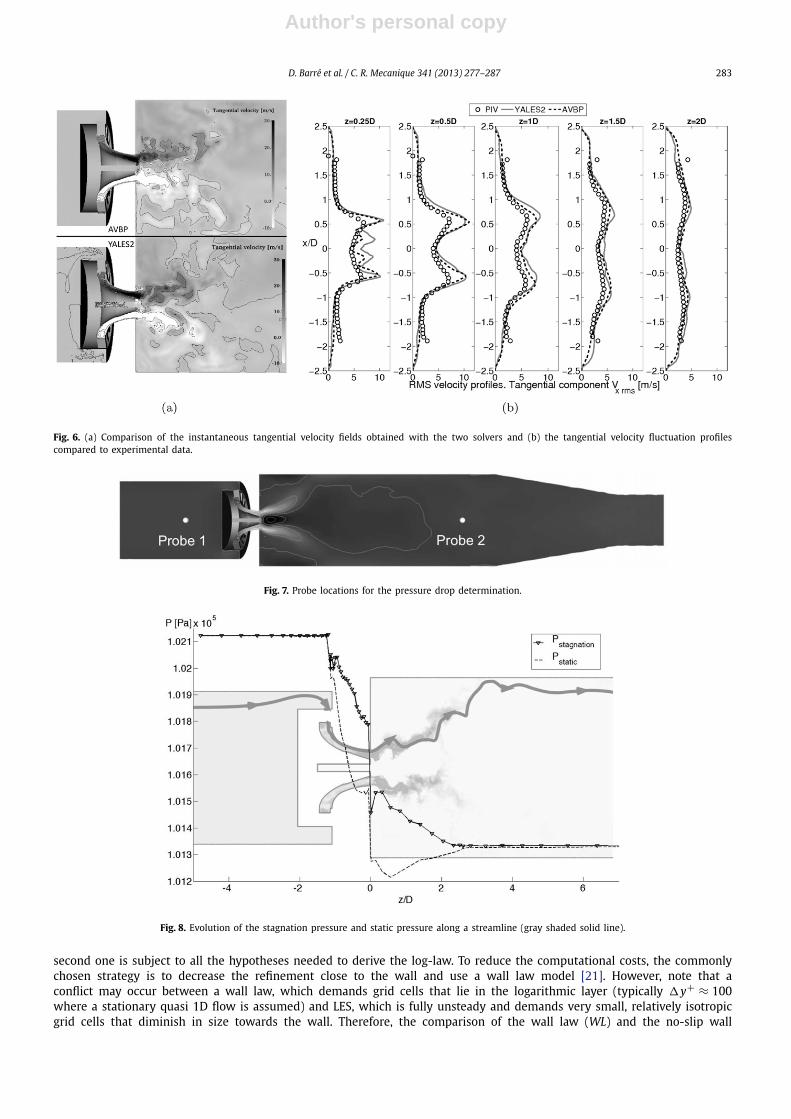
The evolution of the stagnation pressure along a streamline obtained based on the AVBP prediction of this low Machnumber flow (cf. Fig. 8) shows a decrease due to friction. In parallel, the dynamic pressure has increased because of the flowacceleration in the swirler system inducing a reduction of the static pressure. We can also notice that as fluid moves throughthe expansion area in the combustion chamber, the static pressure tends to the stagnation pressure where kinetic energyhas become negligible. Finally, the injection system proves to be the location of mechanisms affecting the flow dynamics.



Fig. 4. (a) Comparison of the mean tangential velocity fields obtained with the two solvers and (b) the mean tangential velocity profiles compared toexperimental data.

Fig. 5. (a) Comparison of the instantaneous axial velocity fields obtained with the two solvers and (b) the axial velocity fluctuation profiles compared toexperimental data.

Numerical difficulties lie in the turbulence modeling of the near wall region usually used to evaluated the wall friction,which can then affect linear and singular losses. The quality of the mesh combined with a suitable boundary condition inthe swirler is hence susceptible to be a critical contributor to the quality of the results. For a clearer understanding and anevaluation of grid/modeling issues, two boundary conditions associated with an adequate SGS model and several meshesare tested in Section 4.1.

4.1. Influence of the mesh and boundary conditions

The wall treatment combined with the mesh resolution is known to influence on the accuracy of the pressure lossprediction. Two strategies are relevant to LES: first, a wall resolved LES where all the scales of importance of the boundarylayer [20] are aimed to be adequately resolved within the limits of the subgrid-scale model and second, a simulation usingwall layer models to reproduce the flow close to solid boundaries. While the first approach is computationally intensive, the



Fig. 6. (a) Comparison of the instantaneous tangential velocity fields obtained with the two solvers and (b) the tangential velocity fluctuation profilescompared to experimental data.

Fig. 7. Probe locations for the pressure drop determination.

Fig. 8. Evolution of the stagnation pressure and static pressure along a streamline (gray shaded solid line).

second one is subject to all the hypotheses needed to derive the log-law. To reduce the computational costs, the commonlychosen strategy is to decrease the refinement close to the wall and use a wall law model [21]. However, note that aconflict may occur between a wall law, which demands grid cells that lie in the logarithmic layer (typically �y+ ≈ 100where a stationary quasi 1D flow is assumed) and LES, which is fully unsteady and demands very small, relatively isotropicgrid cells that diminish in size towards the wall. Therefore, the comparison of the wall law (WL) and the no-slip wall



Table 2Wall mesh resolutions used for the cold flow simulations (reference case in bold).

MESH M1 M2 M3 M4

Characteristics Tetra 2M Tetra 4M Tetra 24 Tetra 35My+ ∼60 ∼30 ∼20 ∼15

Table 3Summary of the pressure drop predictions – experimental pressure loss �Pexp = 594 Pa.

Pressure drop predictions �P [Pa]

Configuration AVBP YALES2

Wall conditions No-slip wall Wall law No-slip wall Wall law

Tetra Mesh 2M 1220 800 1200 /Tetra Mesh 4M 945 790 1010 740Tetra Mesh 24M 900 700 / /Tetra Mesh 35M / / 915 /

formulation (W N S) are considered for four meshes, whose main characteristics are summarized in Table 2. All meshes areunstructured with tetrahedral elements. The indicated y+ are the average values of the dimensionless wall distance withinthe air admission of the swirler. All numerical parameters are identical to the first test cases (cf. Table 1) except for boundaryconditions and SGS models. Indeed, it was demonstrated in our case that a better turbulence model (WALE) leads to worseresults when used in conjunction with a wall function approach because of an apparent incompatibility [22]. Theoretically,a wall law stems from Reynolds-averaged Navier–Stokes (RANS) technique and is not conceived for LES. A novel conceptfor the near-wall treatment of wall modeled LES has been recently presented by modifying the LES eddy-viscosity using adynamic correction based on the resolved turbulent stress near the wall [23–25]. Such researches are however still underdevelopment and remains outside of the scope of this work.

4.2. Results and discussion

Before investigating the pressure drop predictions, the LES results are first evaluated by comparing mean axial andtangential velocity profiles to experimental data at z/D = 0.25 (cf. Fig. 9).

The no-slip condition requires a good refinement close to the wall to resolve accurately the boundary layers. An impactof this local increase in resolution is seen in the magnitude of the main velocity peak at the jet exit which is clearly affectedby this parameter. It is only reproduced with high accuracy with a refined mesh otherwise it is overestimated. For tangentialvelocities, the mesh refinement has no real influence and all predictions follow the same trend. The lateral mean peaks areglobally overestimated compared with experimental results except for the YALES2 simulation using the refined mesh M4.Both observations confirm the assumption that a poorly resolved mesh cannot reproduce the physics correctly.

Use of a wall-model shows that the central peak magnitude remains over-estimated for the axial mean velocity on thecoarse mesh M1 as well as on the refined one M3. LES establishes a compromise to integrate wall models coherently intoa standard LES by requiring a computational grid small enough to capture a sufficient number of turbulent structures aswell as large enough to justify the application of a wall model. The wall model demands relatively large grid cells thatreach into the logarithmic layer. Note that the characteristic mesh size of mesh M3 (y+ ∼ 20) is in the intermediate part(5 < y+ < 30) of the boundary layer: i.e. between the logarithmic and the linear law domain. The wall law may thereforenot correctly model the boundary layer and have an impact on axial velocity profiles near the injector system. Note thatexperimental uncertainties have also been reported in this specific flow region.

After having analyzed the influence of some parameters on the topology of the flow, this remaining part is dedicated tothe influence of the modeling on the determination of the pressure loss. The experimental pressure loss measured by CORIAequals �Pexp = 594 Pa [26] with an uncertainty of 3 percent. Figs. 10(a) and 10(b) display the evolution of the pressure dropalong the central axis with the use of the no-slip wall boundary condition while Figs. 10(c) and 10(d) show the pressureloss profiles with the use of a wall law. First, the results reveal the same trend for both codes. The mesh quality is also seento have a crucial influence on the accuracy of pressure loss predictions notably with a no-slip boundary condition. Similarlyto the remarks made previously regarding the velocity profiles, the determination of pressure losses is directly related tothe computational grid resolution combined with the boundary condition. Pressure drop results are summarized in Table 3.

Fig. 11 shows the evolution of the pressure loss as a function of the mean computational y+ in the swirler. For bothcodes a quasi linear decrease of the pressure loss towards the experimental finding is observed for the no-slip boundarycondition. For equivalent y+ , the pressure drop estimation is clearly improved if the wall-model is used and proves to bevery effective in the logarithmic law domain. In the intermediate part of this model application (here with y+ ∼ 20), theboundary layer may not be correctly modeled but results turn out to be better in part because of the number of points forwhich y+ is in the linear regime (a switch being included in the wall law formulation).



Fig. 9. Influence of the mesh (cf. Table 2) and boundary conditions on the mean axial (a) and tangential (b) velocity profiles at z/D = 0.25. The followingnotations apply: Wall Law (WL) and the No-Slip Wall formulation (WNS).

5. Conclusion and perspectives

LES of a single swirler system is reported under cold flow conditions using the low Mach number code YALES2 and thecompressible AVBP code. Flow predictions show that calculations performed for this low Mach number case are appropriatefor the mean flow. From a strategic point of view, a no-slip boundary condition requires a mesh refinement of high qualityto resolve accurately the boundary layers. Therefore, the use of a wall law model turns out to be a good way to determineapproximatively the pressure loss by resolving the problem on a reasonable mesh in terms of discretization. Regarding theglobal error of the pressure loss prediction, the gain in terms of precision is considerable (with an error near 15% whentaking into account the experimental uncertainty). However, it needs to be underlined that the wall law approach suffersfrom theoretical limitations and may lead to a lack of accuracy in some cases. New perspectives are conceivable by usingmore sophisticated models such as the implementation method based on the conjugation of wall functions and no-slipcondition at the wall, leading to the necessity of using hexahedral or prismatic meshes in near-wall regions [22]. Thistechnique could turn out to be advantageous in terms of the overall number of cells, because the near-wall grid refinementcan easily be controlled by adapting the prism aspect ratio without leading to an excessive number of near-wall tetrahedra.



Fig. 10. Influence of the mesh refinement on the pressure loss distribution along the central axis of the configuration: (a) and (c) with the use of a no-slipboundary condition, (b) and (d) with the use of a wall law boundary condition.

Fig. 11. Evolution of the pressure loss as function of the average values of the dimensionless wall distance y+: with the use of a no-slip boundary condition(W N S) and the use of a wall law boundary condition (W L).

Acknowledgements

The research leading to these results has received funding from the European Community’s Seventh Framework Program(FP7/2007-2013) under Grant Agreement n◦ ACP8-GA-2009-234009. This study is part of the 4-year KIAI project started inMay 2009, a European initiative financed under the FP7 and which addresses innovative solutions for the development ofnew combustors in aero-engines. It aims at providing low NOx methodologies to be applied to design these combustors.

References

[1] M. Rudgyard, Integrated preprocessing tools for unstructured parallel cfd applications, Technical report TR/CFD/95/08, CERFACS, 1995.[2] R.-H. Ni, A multiple grid scheme for solving the Euler equations, Am. Inst. Aeronaut. Astronaut. J. 20 (1982) 1565–1571.[3] G. Lartigue, Simulation aux grandes échelles de la combustion turbulente, PhD thesis, INP Toulouse, 2004.



[4] T. Poinsot, S. Lele, Boundary conditions for direct simulations of compressible viscous flows, J. Comput. Phys. 101 (1) (1992) 104–129.[5] V. Moureau, G. Lartigue, Y. Sommerer, C. Angelberger, O. Colin, T. Poinsot, Numerical methods for unsteady compressible multi-component reacting

flows on fixed and moving grids, J. Comput. Phys. 202 (2) (2005) 710–736.[6] V. Moureau, P. Domingo, L. Vervisch, Design of a massively parallel cfd code for complex geometries, C. R. Mécanique 339 (2–3) (2011) 141–148.[7] V. Moureau, YALES2 home page on, www.coria-cfd.fr.[8] V. Moureau, P. Domingo, L. Vervisch, From large-eddy simulation to direct numerical simulation of a lean premixed swirl flame: Filtered laminar

flame-pdf modeling, Combust. Flame 158 (7) (2011) 1340–1357.[9] J. Laufer, United States, National Advisory Committee for Aeronautics, The structure of turbulence in fully developed pipe flow, NACA, 1953.

[10] J. Weisbach, Die Experimental-Hydraulik, Engelhardt, 1855.[11] O. Colin, M. Rudgyard, Development of high-order Taylor–Galerkin schemes for unsteady calculations, J. Comput. Phys. 162 (2) (2000) 338–371.[12] L. Quartapelle, V. Selmin, High-order Taylor–Galerkin methods for nonlinear multidimensional problems, Finite Elem. Fluids 76 (1993) 90.[13] J. Donea, A. Huerta, Finite Element Methods for Flow Problems, Wiley, 2003.[14] F. Ducros, F. Nicoud, T. Poinsot, Wall-adapting local eddy-viscosity models for simulations in complex geometries, in: M.J. Baines (Ed.), Numerical

Methods for Fluid Dynamics VI, 1998, pp. 293–299.[15] Laura L. Pauley, Parviz Moin, William C. Reynolds, The structure of two-dimensional separation, J. Fluid Mech. (1990) 397–411.[16] A.J. Chorin, Numerical solution of the Navier–Stokes equations, Math. Comput. 22 (104) (1968) 745–762.[17] M. Kraushaar, Application of the compressible and low-Mach number approaches to Large-Eddy Simulation of turbulent flows in aero-engines, PhD

thesis, Université de Toulouse, 2011.[18] M. Germano, U. Piomelli, P. Moin, W.H. Cabot, A dynamic subgrid-scale eddy viscosity model, Phys. Fluids A Fluid Dyn. 3 (7) (1991) 1760–1765.[19] J. Jimenez, P. Moin, The minimal flow unit in near-wall turbulence, J. Fluid Mech. 225 (213–240) (1991).[20] J. Kim, P. Moin, R. Moser, Turbulence statistics in fully developed channel flow at low Reynolds number, J. Fluid Mech. 177 (1987) 133–166.[21] U. Piomelli, E. Balaras, H. Pasinato, K.D. Squires, P.R. Spalart, The inner–outer layer interface in large-Eddy simulations with wall-layer models, Int. J.

Heat Fluid Flow 24 (4) (August 2003) 538–550.[22] F. Jaegle, O. Cabrit, S. Mendez, T. Poinsot, Implementation methods of wall functions in cell-vertex numerical solvers, Flow Turbul. Combust. 85 (2)

(2010) 245–272.[23] M. Wang, P. Moin, Computation of trailing-edge flow and noise using large-Eddy simulation, Am. Inst. Aeronaut. Astronaut. J. 38 (12) (2012).[24] J.A. Templeton, G. Medic, G. Kalitzin, An eddy-viscosity based near-wall treatment for coarse grid large-Eddy simulation, Phys. Fluids 17 (2005) 105101.[25] S. Bocquet, P. Sagaut, J. Jouhaud, A compressible wall model for large-Eddy simulation with application to prediction of aerothermal quantities, Phys.

Fluids 24 (2012) 065103.[26] J.P. Frenillot, Etude phénoménologique des processus d’allumage et de stabilisation dans les chambres de combustion turbulente swirlées, PhD thesis,

CORIA, 2011.

Compressible and low Mach number LES of a swirl experimental burner

Documents

Transcript of Compressible and low Mach number LES of a swirl experimental burner