sigma22-019.pdf - EMIS

Symmetry, Integrability and Geometry: Methods and Applications SIGMA 18 (2022), 019, 28 pages

Classification of the Orthogonal Separable Webs

for the Hamilton–Jacobi and Klein–Gordon Equations

on 3-Dimensional Minkowski Space

Carlos VALERO a and Raymond G. MCLENAGHAN b

aq Department of Mathematics and Statistics, McGill University,Montreal, Quebec, H3A 0G4, Canada

E-mail: [email protected]

bq Department of Applied Mathematics, University of Waterloo,Waterloo, Ontario, N2L 3G1, Canada

E-mail: [email protected]

Received July 03, 2021, in final form March 02, 2022; Published online March 12, 2022

https://doi.org/10.3842/SIGMA.2022.019

Abstract. We review a new theory of orthogonal separation of variables on pseudo-Rieman-nian spaces of constant zero curvature via concircular tensors and warped products. We thenapply this theory to three-dimensional Minkowski space, obtaining an invariant classificationof the forty-five orthogonal separable webs modulo the action of the isometry group. Theeighty-eight inequivalent coordinate charts adapted to the webs are also determined andlisted. We find a number of separable webs which do not appear in previous works in theliterature. Further, the method used seems to be more efficient and concise than thoseemployed in earlier works.

Key words: Hamilton–Jacobi equation; Laplace–Beltrami equation; separation of variables;Minkowski space; concircular tensors; warped products

2020 Mathematics Subject Classification: 53Z05; 70H20; 83A05

1 Introduction

In this paper we consider the Hamilton–Jacobi equation for geodesics on an n-dimensionalpseudo-Riemannian manifold pM, gq

1

2gijpqqBWBqi

BWBqj � E, (1.1)

where q � �q1, . . . , qn

�denotes a local coordinate system, gij the contravariant components of

the metric tensor g, and E is a non-zero constant. We also consider the Klein–Gordon equation

1a|det g|

BBqi

�a|det g|gij BφBqj

�m2φ � 0, (1.2)

where det g denotes the determinant of pgijq, and m � 0 is constant.

By additive separability of equation (1.1) with respect to a coordinate system q, we meanthat the equation admits a complete integral, i.e., a solution of the form

W pq, cq �n

i�1

Wi

�qi, c

�,

mailto:[email protected]

mailto:[email protected]


2 C. Valero and R.G. McLenaghan

where c � pc1, . . . , cnq denotes n constants which satisfy the completeness relation

det

� B2WBciBqj

� 0.

Product separability of equation (1.2) in a coordinates system q means that the equation pos-sesses a complete separated solution of the form [2]

φpq, cq �n¹

i�1

φi

�qi, c

�,

that depend on 2n parameters c � pc1, . . . , c2nq which satisfy the completeness relation [2]

det

��BuiBcBviBc

�� 0, ui � φ1i

φi, vi � φ2i

φi.

Separation of variables with respect to coordinates q is said to be orthogonal if the coordinates qare orthogonal, i.e., if gij � 0, for all i � j. The separation of variables property for a coordinatesystem q is preserved by any coordinate transformation with diagonal Jacobian. An orthogonalweb on pM, gq is a set of n mutually transversal and orthogonal foliations of dimension n � 1.A coordinate system q is adapted to the web if its leaves are represented locally by qi � ci, wherethe ci are constant parameters. An orthogonal web is said to be separable if the Hamilton–Jacobiequation is separable in any system of coordinates adapted to the web [2]. Such a web is calledan orthogonal separable web. It may be shown that if the Klein–Gordon equation is separablein coordinates q, then the Hamilton–Jacobi equation is separable in the same coordinates [29].However, in a space of constant curvature where the Riemann curvature tensor has the form

Rijkl � kpgikgjl � gilgjkq,where k is constant, the separability of the Klein–Gordon equation in coordinates q is equivalentto the separability of the Hamilton–Jacobi equation in the same system [9]. Furthermore, theseparable coordinates are necessarily orthogonal [20]. We will say that two orthogonal webs ina pseudo-Riemannian manifold are inequivalent if they cannot be mapped into each other by anisometry.

The purpose of the present paper is to determine by a new method the inequivalent orthogonalwebs on flat 3-dimensional Minkowski space, E3

1, whose adapted coordinate systems permitadditive (resp. product) separation for the Hamilton–Jacobi equation for the geodesics (resp.Klein–Gordon equation) and to contrast our solution with previously known results. The articleis an extension of the work of Rajaratnam, McLenaghan and Valero [28] who solved a similarproblem for 2-dimensional Minkowski space E2

1 and de Sitter space dS2. McLenaghan andValero have also used this method to obtain a classification of the orthogonal separable webs for3-dimensional hyperbolic and de Sitter spaces [31]. A classification of separable webs in thesespacetimes could be used to solve boundary value problems whose geometries are adapted to oneof these coordinate systems, or to study the integrability of Hamilton–Jacobi or Klein–Gordonequations when coupled to an external field. For example, in [21], all separable webs that separatethe Hamilton–Jacobi equation for a test charge moving in the electromagnetic field producedby a point particle are classified, and it is therein concluded that only the Cavendish-Coulombfield admits complete separation.

The approach used in this paper is based on the theory of concircular tensors and warpedproducts developed by Rajaratnam [25] and Rajaratnam and McLenaghan [26, 27]. It is a syn-thesis of the results of Kalnins [17], Crampin [7] and Benenti [1] that has been extended to include

Classification of the Orthogonal Separable Webs 3

general pseudo-Riemannian spaces with application to pseudo-Riemannian spaces of constantcurvature [28, 31]. This theory is derived from Eisenhart’s [9] characterization of orthogonalseparability by means of valence-two Killing tensors which have simple eigenvalues and orthog-onally integrable eigendirections, called characteristic Killing tensors. We recall that a Killingtensor is a symmetric tensor Kij which satisfies the equation [9]

∇iKjk �∇jKki �∇kKij � 0,

where ∇ denotes the covariant derivative associated to the Levi-Civita connection of g.

This problem has been studied via other methods by different authors including Kalnins [16],Kalnins and Miller [19], Kalnins, Kress and Miller [18], Hinterleitner [10, 11], and Horwoodand McLenaghan [14]. In [19] it is shown by a method based on the use of pentasphericalcoordinates [3] that the coordinate systems which allow separation have the property that thecoordinate surfaces are orthogonal families of confocal quadrics or their limits. The distinctclasses of separable coordinates are then classified under the action of the isometry group.In [10, 11] the coordinate domains and horizons for the coordinate systems of Kalnins and Millerwhich cannot be reduced to separable coordinate systems in two dimensions are constructed bymeans of projective plane coordinates. This work adds global considerations to the otherwiselocal aspects of separable of variables in this case.

In [14] the canonical separable coordinates and their associated webs are found by a purelygeometric method which involves the systematic integration of the Killing tensor equationstogether with the flatness condition in a general orthogonal coordinate system. The transfor-mation to pseudo-Cartesian coordinates is then obtained by the method described in [13]. Thecomponents of these tensors with respect to pseudo-Cartesian coordinates are obtained fromthe components in canonical separable coordinates by applying the tensor transformation law.This procedure defines the Killing tensor in question on a coordinate patch of E3

1. Because thecomponents of the general Killing tensor are polynomial functions in pseudo-Cartesian coordi-nates, the Killing tensor is defined on all of E3

1 by analytic continuation. The separable websare finally obtained as the integral curves of the eigenvector fields of the Killing tensor. Usingthis procedure Horwood and McLenaghan [12] found thirty-nine orthogonally separable websand fifty-eight inequivalent metrics in adapted coordinate systems which permit orthogonal sep-aration of variables for the associated Hamilton–Jacobi equation and Klein–Gordon equations.In a subsequent paper Horwood, McLenaghan and Smirnov [15] employ the invariant theory ofKilling tensors [5, 6, 12, 22, 23, 30] to classify the separable webs of E3

1 by sets of functions ofthe coefficients of the characteristic Killing tensors which are invariant under the action of theisometry group Ep2, 1q of E3

1.

The use of the Rajaratnam et al. [26, 27] theory to solve this problem has a number ofadvantages:

1. It gives directly the coordinate transformation between the separable coordinates andpseudo-Cartesian coordinates.

2. It gives directly the expression for the metric tensor in the separable coordinates.

3. It gives a partially invariant characterization of the separable webs under the appropriateequivalence relation (see Section 2).

4. It provides an apparently more compact treatment compared to the other methods de-scribed above.

Our calculations yield forty-five orthogonal separable webs which include the thirty-ninefound in [14] as well as six additional webs, one of which does not appear in [11]. We also notethat the number of inequivalent adapted coordinate systems we obtain does not agree with the


number given in [11]. In this paper we shall provide what appear to be the missing webs in [14]and discuss the discrepancies with the results of [11].

The paper is organized as follows: in Section 2 we review the theory of concircular tensors,their algebraic classification and how certain classes of concircular tensors can be used to con-struct separable coordinates. In Section 3 the theory of warped products is summarized and analgorithm is given for the construction of reducible separable webs. In both Sections 2 and 3, werestrict ourselves to the case of constant zero curvature; for a compact review of the theory in thecase of constant non-zero curvature, we direct the reader to [31, Sections 2 and 3]. In Section 4,the theory reviewed in Sections 2 and 3 are applied to obtain a complete list of the separablewebs and inequivalent adapted coordinate systems on E3

1. For ease of comparison with previousresults we indicate in parentheses how the web is classified in [14]; we also indicate which websare not found therein. For the irreducible webs, we also give in square brackets the notationused by [11] and [19], again indicating which webs are not found therein. Concluding remarksare given in Section 5.

We end this section with a word on notation and conventions. We denote the n-dimensio-nal pseudo-Euclidean space with signature ν by En

ν . By n-dimensional Minkowski space, wemean En

1 . As Enν is a vector space, we make liberal use of the canonical isomorphism between En

ν

and TpEnν to identify points and tangent vectors. Accordingly, we denote the metric in En

ν byboth g and x�, �y. Furthermore, as the metric induces an isomorphism between tensor spacesvia ‘raising and lowering indices’, we will adopt the standard practice of identifying tensorsunder this correspondence, using the same symbol regardless of type. It may be convenientto sometimes make this distinction explicit for vectors. In that case, we will write v5 for theone-form corresponding to the vector v via the isomorphism induced by the metric.

Finally, this paper relies heavily on some elementary results regarding the classification ofself-adjoint linear operators on En

ν . A review of the relevant material may be found in [28];for convenience, in the appendix we have summarized the main results for the special case ofMinkowski space. Any reader not familiar with this subject should look at the appendix beforeproceeding. The notation and definitions found therein will be used hereafter without comment.

2 Concircular tensors in Enν

We recall the basic properties of concircular tensors as they relate to separation of variables. Inthis section, let pM, gq be a pseudo-Riemannian manifold. A concircular tensor (CT) L on Mis a 2-tensor satisfying

∇kLij � αigjk � αjgik

for some 1-form α on M . These tensors are generalization of concircular vectors, which wereso-called since they arise as gradients ∇ρ of functions ρ such that the conformal scaling g ÞÑ ρ2gmaps circles to circles; for more information on concircular vectors, see [8].

We say that L is an orthogonal, concircular tensor, if it is pointwise diagonalizable. We saythat L is a Benenti tensor if its eigenfunctions are pointwise simple, i.e., if its eigenvalues at eachpoint are distinct. We call L an irreducible concircular tensor, if its eigenfunctions λ1, . . . , λn arefunctionally independent. A CT that is not irreducible is called reducible. One can show thatan orthogonal CT is irreducible if and only if none of its eigenfunctions are constant [27]. Wewill only need to work with orthogonal CTs in classifying separable webs on spaces of constantcurvature. It is therefore of no harm in assuming all CTs to be orthogonal from this pointforward.

One can show [7] that the general concircular tensor L in Enν is given by

L � A� 2w d r �mr d r,


where A is a constant symmetric tensor, w P Enν , m P R, d is the symmetric tensor product,

and r is the dilatational vector field, defined in pseudo-Cartesian coordinates pxiq by r :� xiBi.If L is irreducible, then the distributions orthogonal to its eigenspaces are integrable and

define a separable web [27]. In this case, the eigenfunctions of L themselves give separablecoordinates adapted to this web. If L is reducible, then there are often multiple separable websadapted to its eigenspaces; for this case we will need a warped product decomposition of M todetermine all the separable coordinates associated with L. This will be the subject of the nextsection.

Therefore, any orthogonal CT induces at least one separable web. It is a remarkable factthat in spaces of constant curvature, all such separable webs arise in this fashion; see [26, 27]for a proof of this theorem. However, it is clear that distinct orthogonal CTs may give rise toseparable webs which are related by an isometry. So, to classify separable webs modulo isometry,we must classify orthogonal CTs modulo an appropriate equivalence relation. More precisely,let L and L1 be two concircular tensors on a pseudo-Riemannian manifold pM, gq. We say that Land L1 are geometrically equivalent if there exists a P Rzt0u, b P R, and an isometry Λ P IpMqsuch that L1 � a

�Λ�1

��L�bg. The reason for studying the equivalence classes of CTs under this

relation lies in the following result: if L and L1 are orthogonal CTs on a connected manifold M ,with at least one being non-constant, then their associated separable webs are related by anisometry if and only if they are geometrically equivalent [27].

This is a good place to mention some useful results which allow one to connect concirculartensors with the general theory of separation using Killing tensors, as is done in [12, 14]. Werefer the reader to [28] for details on the following construction. If L is a CT, we first define

K1 :� trpLqg � L,

where trpLq denotes the trace of L. K1 is a Killing tensor with the same eigenspaces as L; inparticular if L is Benenti, then K1 is a characteristic Killing tensor called the Killing–Bertrand–Darboux tensor pKBDTq associated with L. We may then define inductively, for 2 ¤ m ¤ n� 1,

Km :� 1

mtrpKm�1Lqg �Km�1L,

where Km�1L is a product of endomorphisms. One can show [1] that tg,K1, . . . ,Kn�1u generatea real n-dimensional vector space of Killing tensors which are all diagonalized in the separablecoordinates induced by L. This space is called the Killing–Stackel algebra associated with theweb; it plays an important role in the Killing tensor approach to separation of variables.

We now quote the following theorem from [28] which will be absolutely paramount in ourclassification of concircular tensors (and hence separable webs) in E3

1. For simplicity, we statethe theorem for the special case of En

1 , which shall be sufficient for our purposes.

Theorem 2.1. Any orthogonal concircular tensor L � A�wbr5�rbw5�mrbr5 in En1 , after

a possible change of origin and after passing to a geometrically equivalent concircular tensor L,admits precisely one of the following canonical forms:

� Cartesian, if m � 0 and w � 0, then L � A,

� central, if m � 0, then L � A� r b r5,

� non-null axial, if m � 0 and xw,wy � 0, then there exists a vector e1 P spantwu such thatL � A� e1 b r5 � r b e51, Ae1 � 0, and xe1, e1y � ε � �1,

� null axial, if m � 0, w � 0 and xw,wy � 0, then there is a skew-normal sequence psee theappendix for the definition of a skew-normal sequenceq β � te1, . . . , eku with e1 P spantwuand xe1, eky � ε, which is A-invariant, such that L � A�e1br5�rbe51 and the restrictionof A to spantβu is represented by Jkp0qT. In Minkowski space, either k � 2, in which caseε � �1, or k � 3, in which case ε � 1.


In Theorem 2.1, ε is called the sign of L. For central CTs, the sign is defined to be 1, and forCartesian CTs, the sign is not defined. For a proof of Theorem 2.1 in a flat space of arbitrarysignature, the reader should consult [25].

Let L be a CT in its canonical form. Then we let D denote the A-invariant subspace spannedby

w,Aw,A2w, . . .

(. This subspace is either zero (if w � 0), or non-degenerate. We define

Ac :� A|DKas well as the following two characteristic polynomials:

ppzq :� detpzI � Lq, Bpzq :� detpzI �Acq,where the latter determinant is evaluated in DK. We therefore have that the classification of CTswithin each of the cases listed in Theorem 2.1, is reducible to a classification of the metric-Jordancanonical forms for Ac.

We also note that in the classification of orthogonal CTs as per Theorem 2.1, CTs whichdiffer by multiples of the metric in DK induce the same separable webs if dimD ¤ 2. While notexplicitly stated in [25], this result is implied by the proof of Theorem 2.1 given therein. Weshall use this result frequently to simplify our canonical forms for the axial concircular tensors.

We finish this section with some results that will allows us to extract explicit formulae for sep-arable coordinates from an irreducible CT. Recall that an irreducible CT determines a separableweb, and its eigenfunctions are separable coordinates adapted to this web; we call these canonicalcoordinates associated with the irreducible CT. Furthermore, one can show that a non-constantCT L � A� 2wd r�mrd r in En

ν (for ν ¤ 1) is an irreducible CT if and only if Ac has no mul-tidimensional eigenspaces; equivalently, L is reducible if and only if Ac has a multidimensionaleigenspace [25].

The following technical results are derived in [25] and allow one to obtain, given an irreducibleCT L, the transformation equations between the induced canonical coordinates

�ui�, and the

lightcone-Cartesian coordinates�xi�in which pA, gq take the prescribed form. First, if L �

A� rb r5 is a central irreducible CT in canonical form, and if A and g take the following formsin coordinates

�xi�, where the matrices Jkpλq and Sk are defined in Appendix A:

A � Jkp0qT ` diagpλk�1, . . . , λnq, g � ϵ0Sk ` diagpϵk�1, . . . , ϵnq (2.1)

then, from [25], we have the following equations:

l�1

i�1

xixl�2�i � �ϵ0l!

�d

dz

l � ppzqBUKpzq

��z�0

, l � 0, . . . , k � 1, (2.2)

�xi�2 � �ϵi ppλiq

B1pλiq , i � k � 1, . . . , n, (2.3)

where U is the subspace corresponding to Jkp0qT, and BUKpzq is the characteristic polynomialof A restricted to UK. The transformation equations from the canonical coordinates

�ui�and

the coordinates�xi�can then be obtained by writing

ppzq �n¹

i�1

�z � ui

�. (2.4)

Now let L � A� e1b r5� rb e51 be an axial irreducible CT in canonical form and suppose thatin coordinates

�xi�, we have A � Ad ` Ac with Ad � Jkp0qT and g � ϵ0Sk ` gc. Then we have

from [25] that the characteristic polynomial of L takes the form

ppzq � pdpzqBpzq � ϵ0ppcpzq �Bpzqq, (2.5)


where pdpzq is the characteristic polynomial of L restricted to the subspace corresponding to Ad,and is given explicitly as follows (for k ¥ 2):

pdpzq � zk �k

l�2

l�1

i�1

xk�1�i�lxk�1�izk�l � 2ϵ0

k

i�1

xk�i�1zk�i. (2.6)

Again, the coordinate transformations from lightcone-Cartesian coordinates�xi�to the canon-

ical coordinates puiq may be obtained by using the equations (2.5) and (2.6), along with thefactorization of ppzq, just as with central CTs. We note that in the case A � Ad, we of coursehave ppzq � pdpzq. Furthermore, for k � 1, it is clear that pdpzq � z � 2ϵ0x

1.The last result from [25] that we quote in this section allows one to quickly write down the

expression for the metric in canonical coordinates puiq associated with an irreducible CT L. Fori � 1, . . . , n,

gii � ε

4

±j�i

�ui � uj

�±n�k

j�1

�ui � λj

� , (2.7)

where λ1, . . . , λn�k are the roots of Bpzq, and ε is the sign of L (see the remarks followingTheorem 2.1). Of course the separable coordinates

�ui�are orthogonal, so gij � 0 for i � j.

3 Warped products in Enν and reducible concircular tensors

Here we recall warped product decompositions of Enν and their importance for constructing

separable webs in Enν . In this section, we quote the relevant results, referring the reader to [31]

or [25] for details. Recall that given pseudo-Riemannian manifolds pNi, giq for 0 ¤ i ¤ k andsmooth positive functions ρj for 1 ¤ j ¤ k, we define the warped product N0 �ρ1 � � � � �ρk Nk

to be the product manifold equipped with the metric

g :� π�0g0 �k

i�1

�ρ2i � π0

�π�i gi,

where πi : N0 � � � � �Nk Ñ Ni is the i-th projection. We call N0 the geodesic factor and Ni fori ¡ 0 the spherical factors. A warped product decomposition of a manifoldM is a diffeomorphismψ : N0 �ρ1 N1 � � � � �ρk Nk Ñ M . We will often speak of warped product decompositions ofopen subsets of M without much distinction. Moreover, we may at times use the terms warpedproduct and warped product decomposition interchangeably.

Let L be a CT in M and let ψ : N0�ρ1 � � � �ρn Nk ÑM be a warped product decompositionof M . We say that ψ is adapted to L if for each i ¡ 0 and for all points p P Ni, ψ�pTpNiq is aninvariant subspace of L, meaning that L acting as an endomorphism maps this subspace intoitself. In this case, one can show [27] that the restriction (via ψ) of L to N0 is a Benenti tensor,and therefore induces a separable web on N0 which we may lift to M using ψ. In particular, ifthe restriction of L to N0 is an irreducible CT, then its eigenfunctions yield a set of separablecoordinates on N0. By choosing a separable web for each of the spherical factors and liftingthem to M via ψ, we hence obtain a separable web in M . Therefore, our method for dealingwith a reducible CT L will be to find warped product decompositions of En

ν adapted to L.Suppose we are given the following data: a point p P M ; an orthogonal decomposition

TpM � V0 k � � � k Vk into non-trivial and non-degenerate subspaces; and k mutually orthogonaland linearly independent vectors a1, . . . , ak P V0. We can without loss of generality assume thatxp, aiy � 1 for all i such that ai � 0; we say that this data is in canonical form. Then one canconstruct a warped product N0 �ρ1 � � � � �ρk Nk of En

ν adapted to L, passing through p, such


that TpNi � Vi and Ni is a spherical submanifold of Enν having mean curvature normal ai at p.

A detailed exposition of this construction is given in [31], for example. For the classification inSection 4, we shall only need warped products with 2 factors; we thus recall the relevant resultsfrom [31].

Let ψ : N0 �ρ1 N1 Ñ Enν be a warped product determined by initial data pp;V0 k V1; a1q. If

a1 � 0, then the warped product is in fact an ordinary Cartesian product, and

ψpp0, p1q � p0 � p1.

In this case, the image of ψ is all of Enν , and the warping function is of course just 1. Now

assume that a1 is non-null. Define W0 :� V0 X aK1 , and let P0 : Enν ÑW0 denote the orthogonal

projection. Then ψ takes the form

ψpp0, p1q � P0p0 � xa1, p0ypp1 � cq,

where c :� p � xa1, a1y�1a1. The warping function is given by ρpp0q � xp0, a1y. In this case, ifP1 : En

ν Ñ Ra1 k V1 denotes the orthogonal projection, we have [25]

Impψq � tp P Enν | signxP1ppq, P1ppqy � signxa1, a1yu. (3.1)

If we restrict our warped product to a domain such thatN1 is connected, then we must impose theextra condition xa1, P1ppqy ¡ 0 in (3.1). Now consider the case where a1 is lightlike. Then thereis another lightlike vector b P V0 such that xa1, by � 1. Here, we define W0 :� V0 X spanta1, buKand W1 :� V1, and let Pi : En

ν ÑWi for i � 0, 1 denote the orthogonal projection. Then ψ takesthe form

ψpp0, p1q � P0p0 ��xb, p0y � 1

2xa1, p0yxP1p1, P1p1y

a1 � xa1, p0yb� xa1, p0yP1p1.

The warping function is ρpp0q � xa1, p0y and the image of this warped product is

Impψq � p P En

ν | xa1, py ¡ 0(.

For the remainder of this section, we restrict ourselves to Euclidean and Minkowski spaces,i.e., ν � 0 and ν � 1 respectively. Let L � A � 2w d r �mr d r be a reducible CT in En

ν . Asν ¤ 1, we have that L is reducible iff it is constant, or if Ac has a multi-dimensional eigenspace(see the remarks following Theorem 2.1 for the definition of Ac). If L is constant, then it isdiagonalizable with real eigenspaces, and the Cartesian product of these eigenspaces is in factthe warped product adapted to L. If L is non-constant, then we may use the following algorithmfrom [31], which yields a warped product decomposition adapted to L.

Algorithm 3.1. Let L � A� 2w d r �mr d r be a reducible, non-constant CT, and let tEiuibe the multidimensional eigenspaces of Ac. For each i:

(i) If Ei is non-degenerate, choose a unit vector ai P Ei and define Vi :� Ei X aKi .

(ii) If Ei is a degenerate subspace, then there is a cycle v1, . . . , vr of generalized eigenvectorsof A, such that vr P Ei is lightlike. Let ai :� vr, and define Vi :� Ei X vK1 . Note that Vi isnon-degenerate, and in En

1 , we have r ¤ 3.

Define V0 :� V K1 X� � �XV K

k , and let p P Enν be such that the warped product ψ : N0�ρ1 � � ��ρkNk

Ñ Enν determined by initial data pp;V0 k � � � k Vk; a1, . . . , akq is in canonical form. Then ψ is

a warped product adapted to L.


Let us denote the restriction of L to N0 via ψ by L. It is given by

L � ��ψ�1

��L��

N0� A� 2w d r �mr d r,

where A � A|V0 and r is the dilatational vector field in N0. As discussed above, L is Benentiand so induces separable coordinates

�uj0�on N0 which we may lift to En

ν via ψ. We choose

separable coordinates�uji�on the spherical factors Ni, and lift all of these to En

ν with ψ. Then

the product coordinates�uj0, u

j1, . . . , u

jk

�parametrize a separable web on En

ν .

This finally gives us a procedure for constructing separable webs from reducible CTs in Enν .

Note that obtaining all separable webs induced by a reducible CT L requires knowledge ofall the separable webs in the lower-dimensional spaces that could appear as spherical factors inAlgorithm 3.1. In particular, our classification of the separable webs in E3

1 will require knowledgeof all separable webs in E2, E2

1, H2 and dS2. These can be found for example in [28].

4 Classification of separable webs on E31

In this section we apply the theory of concircular tensors reviewed in the last two sections toclassify all 45 separable webs on E3

1 modulo action of the isometry group. We further determinethe inequivalent coordinate charts adapted to the webs; recall that two coordinate charts aresaid to be equivalent if they can be mapped into each other by an isometry. In the following,we make liberal use of the results presented in the previous two sections, particularly equations(2.2)–(2.7) for irreducible CTs, and Algorithm 3.1 for reducible CTs.

For the purposes of comparison, beside the name of each separable web below, we indicate inparentheses how the web is classified in [14] using the invariant theory of Killing tensors; we alsoindicate which webs are not found therein. For the irreducible webs, we also give the notationused by [11] and [19] in square brackets, again indicating which webs are not found therein.

For each separable web below, we give the transformation equations between the separablecoordinates and Cartesian coordinates, the form of the metric in the separable coordinates, andthe coordinate ranges; if a web has more than one inequivalent region, we give the coordinatecharts for each. Note that while we only give the charts for a particular domain in each equiv-alence class, all other charts of the web can be obtained by isometry (often x Ø y or somecombination of t ÞÑ �t, x ÞÑ �x and y ÞÑ �y).

For consistency, we shall adopt the convention of using the same lightcone coordinates pη, ξqthroughout this section, defined by η � x � t, ξ � 1

2px � tq. Notice that xBη, Bξy � 1. Lettingξ ÞÑ �ξ gives lightcone coordinates whose basis vectors have scalar product �1.

4.1 Cartesian CTs, L � A

In the Cartesian case, L � A is constant and diagonalizable with real eigenvalues. If A hasdistinct eigenvalues, L is Benenti and the induced separable web coincides with the eigenspacesof A. We therefore obtain the familiar Cartesian coordinates pt, x, yq on E3

1.

If A has only one eigenvalue, then it is a multiple of the metric, say λg. Thus, being geomet-rically equivalent to A�λg � 0, it is trivial. The only other cases we have to consider are thosewhere A has a 2-dimensional eigenspace. There are two possibilities:

4.1.i. A � J�1p1q ` J1p0q ` J1p0q. If A has a spacelike multidimensional eigenspace, thenupon passing to a geometric equivalent tensor, we may choose a basis such that A takes theabove form; i.e., A � e0be50 for some timelike unit vector e0. It is easy to see that this CartesianCT is reducible. By the remarks preceding Algorithm 3.1, we see that a warped product which


decomposes L is

ψ : E11 �1 E2 Ñ E3

1,

pte0, pq ÞÑ te0 � p.

We get a separable web on E31 by taking t in the above map as our coordinate on E1

1, and liftingany separable web on E2. These are the timelike-cylindrical webs, one of which is the Cartesianweb already obtained. The separable webs on E2 can be found throughout the literature; see,for instance, [28, Table 1]. We thus obtain the following four separable webs from this CT viathe above warped product.

1. Cartesian web (spacelike translational web I)$'&'%ds2 � �du2 � dv2 � dw2,

t � u, x � v, y � w,

�8 u 8, �8 v 8, �8 w 8.2. Timelike-cylindrical polar web (timelike translational web I)$'&

'%ds2 � �du2 � dv2 � v2dw2,

t � u, x � v cosw, y � v sinw,

�8 u 8, 0 v 8, 0 w 2π.

3. Timelike-cylindrical elliptic web (timelike translational web III)$'&'%ds2 � �du2 � a2

�cosh2 v � cos2w

��dv2 � dw2

�,

t � u, x � a cosh v cosw, y � a sinh v sinw,

�8 u 8, 0 v 8, 0 w 2π, a ¡ 0.

4. Timelike-cylindrical parabolic web (timelike translational web II)$'&'%ds2 � �du2 � �

v2 � w2��dv2 � dw2

�,

t � u, x � 12

�v2 � w2

�, y � vw,

�8 u 8, 0 v 8, �8 w 8.4.1.ii. A � J�1p0q ` J1p0q ` J1p1q. If A has a multidimensional Lorentzian eigenspace,

then using geometric equivalence, we may choose a basis such that A takes the above form; i.e.,A � e1 b e51 for some spacelike unit vector e1. This CT is reducible, and by Algorithm 3.1, wesee that a warped product which decomposes L is

ψ : E1 �1 E21 Ñ E3

1,

pye1, pq ÞÑ p� ye1.

We obtain a separable web on E31 by taking y in the above map as our coordinate on E1, and

choosing any separable web on E21. These are the spacelike-cylindrical webs, one of which is the

Cartesian web already obtained. The separable webs on E21 may be found in [28, Table 2], for

instance. Hence we obtain the following 9 (omitting Cartesian coordinates) separable webs fromthe above warped product.

5. Spacelike-cylindrical Rindler web (spacelike translational web II),for �t2 � x2 0$'&

'%ds2 � �du2 � u2dv2 � dw2,

t � u cosh v, x � u sinh v, y � w,

0 u 8, �8 v 8, �8 w 8;


for �t2 � x2 ¡ 0

$'&'%ds2 � du2 � u2dv2 � dw2,

t � u sinh v, x � u cosh v, y � w,

0 u 8, �8 v 8, �8 w 8.

6. Spacelike-cylindrical elliptic web I (spacelike translational web VI)

$'&'%ds2 � a2

�cosh2 u� sinh2 v

��du2 � dv2

�� dw2,

t � a coshu sinh v, x � a cosh v sinhu, y � w,

0 u 8, 0 v 8, �8 w 8, a ¡ 0.

7. Spacelike-cylindrical elliptic web II (spacelike translational web VII),for |t| � |x| ¡ a

$'&'%ds2 � a2

�cosh2 v � cosh2 u

��du2 � dv2

�� dw2,

t � a coshu cosh v, x � a sinh v sinhu, y � w,

0 u v 8, �8 w 8, a ¡ 0;

for |t| � |x| �a$'&'%ds2 � a2

�cosh2 u� cosh2 v

��du2 � dv2

�� dw2,

t � a sinhu sinh v, x � a cosh v coshu, y � w,

0 v u 8, �8 w 8, a ¡ 0;

for |t| � |x| a

$'&'%ds2 � a2

�cos2 u� cos2 v

��du2 � dv2

�� dw2,

t � a cosu cos v, x � a sin v sinu, y � w,

0 v u π2 , �8 w 8, a ¡ 0.

8. Spacelike-cylindrical complex elliptic web (spacelike translational web VIII)

$'&'%ds2 � a2psinh 2u� sinh 2vq�du2 � dv2

�� dw2,

t� x � a cosh pu� vq, t� x � a sinh pu� vq, y � w,

0 |v| u 8, �8 w 8, a ¡ 0.

9. Spacelike-cylindrical null elliptic web I (spacelike translational web IX)

$'&'%ds2 � �

e2u � e2v��du2 � dv2

�� dw2,

t� x � eu�v, t� x � 2 sinh pu� vq, y � w,

�8 u 8, �8 v 8, �8 w 8.

10. Spacelike-cylindrical null elliptic web II (spacelike translational web X),for �t2 � x2 ¡ |t� x|

$'&'%ds2 � �

e2u � e2v�pdu2 � dv2q � dw2,

t� x � �eu�v, t� x � 2 cosh pu� vq, y � w,

�8 v u 8, �8 w 8;


for �t2 � x2 �|t� x|$'&'%ds2 � �

e2v � e2u��du2 � dv2

�� dw2,

t� x � eu�v, t� x � 2 cosh pu� vq, y � w,

�8 u v 8, �8 w 8.

11. Spacelike-cylindrical timelike parabolic web (spacelike translational web III)

$'&'%ds2 � �

u2 � v2��du2 � dv2

�� dw2,

t � 12

�u2 � v2

�, x � uv, y � w,

0 v u 8, �8 w 8.

12. Spacelike-cylindrical spacelike parabolic web (spacelike translational web IV)

$'&'%ds2 � �

u2 � v2��du2 � dv2

�� dw2,

t � uv, x � 12

�u2 � v2

�, y � w,

0 v u 8, �8 w 8.

13. Spacelike-cylindrical null parabolic web (spacelike translational web V)

$'&'%ds2 � pu� vq��du2 � dv2

�� dw2,

t� x � u� v, t� x � �12pu� vq2, y � w,

0 |v| u 8, �8 w 8.

4.2 Central CTs, L � A � r b r5

Since all central CTs have the this canonical form, we need only classify the inequivalent canon-ical forms for A. Since Ac � A in this case, a central CT L � A� rb r5 is reducible if and onlyif A has a multidimensional eigenspace.

4.2.i. A � 0. In this case, L � r b r5 is reducible, and hence Algorithm 3.1 must be used toconstruct a warped product which yields the separable webs induced by L. This decompositiondepends on the point p with which we construct our warped product (see Algorithm 3.1).

For a timelike unit vector e0, Algorithm 3.1 gives the following warped product which de-composes L in the connected timelike region containing e0:

ψ : N0 �ρ H2 Ñ E31,

p�ue0, pq ÞÑ up,

where N0 � �ue0 P E3

1 |u ¡ 0(, and ρp�ue0q � u. For a spacelike unit vector e1, Algorithm 3.1

gives the following warped product in the spacelike region:

ψ : N0 �ρ dS2 Ñ E31,

pwe1, pq ÞÑ wp,

where N0 � we1 P E3

1 |w ¡ 0(, and ρpwe1q � w. We obtain an induced separable web in the

timelike (resp. spacelike) region by taking the coordinate u (resp. w) on the geodesic factor,and lifting any separable web on H2 (resp. dS2). We hence construct a separable web on E3

1 bychoosing a separable web in the timelike regions, and a corresponding web in the spacelike region(i.e., the webs in each region should correspond to the same characteristic Killing tensor). Theseparable webs and coordinate systems on dS2 may be found in [28, Table 3], while those for H2


may be found in, say, [24] or [4]. We so obtain the following nine dilatationally invariant webs,in which Kpaq denotes the complete elliptic integral of the first kind with elliptic modulus a, for0 a 1.

14. Dilatational elliptic web I (not in [14]),

for �t2 � x2 � y2 ¡ 0

$'&'%ds2 � w2

�dc2pu; aq � a2 sn2pv; aq��du2 � dv2

�� dw2,

t � w scpu; aqdnpv; aq, x � w ncpu; aq cnpv; aq, y � w dcpu; aq snpv; aq,0 u Kpaq, 0 v Kpaq, 0 w 8, 0 a 1;

for �t2 � x2 � y2 0

$'&'%ds2 � �du2 � u2

�a2 cd2pv; aq � cs2pw; bq��dv2 � dw2

�,

t � undpv; aqnspw; bq, x � u sdpv; aqdspw; bq, y � u cdpv; aq cspw; bq,0 u 8, 0 v Kpaq, 0 w Kpbq, 0 a 1, 0 b 1, a2 � b2 � 1.

15. Dilatational elliptic web II (dilatational web IV),

for �t2 � x2 � y2 ¡ 0, a|t| � |x| ¡ ba�t2 � x2 � y2

$'&'%ds2 � w2

�dc2pu; aq � dc2pv; aq��du2 � dv2

�� dw2,

t � wba ncpu; aqncpv; aq, x � wb scpu; aq scpv; aq, y � w

a dcpu; aqdcpv; aq,0 v u Kpaq, 0 w 8, 0 a 1, 0 b 1, a2 � b2 � 1;

for �t2 � x2 � y2 ¡ 0, a|t| � |x| ba�t2 � x2 � y2

$'&'%ds2 � w2a2

�nd2pu; bq � nd2pv; bq��du2 � dv2

�� dw2,

t � wab sdpu; bq sdpv; bq, x � wb cdpu; bq cdpv; bq, y � wandpu; bq ndpv; bq,0 v u Kpbq, 0 w 8, 0 a 1, 0 b 1, a2 � b2 � 1;

for �t2 � x2 � y2 0

$'&'%ds2 � �du2 � u2pdc2pv; aq � a2 sc2pw; bqq�dv2 � dw2

�,

t � uncpv; aqncpw; bq, x � u scpv; aqdcpw; bq, y � udcpv; aq scpw; bq,0 u 8, 0 v Kpaq, 0 w Kpbq, 0 a 1, 0 b 1, a2 � b2 � 1.

16. Spherical web I (timelike rotational web I),

for �t2 � x2 � y2 ¡ 0

$'&'%ds2 � w2

��du2 � cosh2 udv2�� dw2,

t � w sinhu, x � w coshu cos v, y � w coshu sin v,

�8 u 8, 0 v 2π, 0 w 8;

for �t2 � x2 � y2 0

$'&'%ds2 � �du2 � u2

�dv2 � sinh2 vdw2

�,

t � u cosh v, x � u sinh v cosw, y � u sinh v sinw,

0 u 8, 0 v 8, 0 w 2π.


17. Spherical web II (spacelike rotational web I),for �t2 � x2 � y2 ¡ 0, �t2 � x2 ¡ 0

$'&'%ds2 � w2

�du2 � sin2 udv2

�� dw2,

t � w sinu sinh v, x � w sinu cosh v, y � w cosu,

0 u π, �8 v 8, 0 w 8;

for �t2 � x2 � y2 ¡ 0, �t2 � x2 0

$'&'%ds2 � w2

��du2 � sinh2 udv2�� dw2,

t � w sinhu cosh v, x � w sinhu sinh v, y � w coshu,

0 u 8, �8 v 8, 0 w 8;

for �t2 � x2 � y2 0

$'&'%ds2 � �du2 � u2

�dv2 � cosh2 vdw2

�,

t � u cosh v coshw, x � u cosh v sinhw, y � u sinh v,

0 u 8, �8 v 8, �8 w 8.

18. Dilatational complex elliptic web (dilatational web V),

for �t2 � x2 � y2 ¡ 0

$'''''''''&'''''''''%

ds2 � w2�sn2pu; aq dc2pu; aq � sn2pv; aq dc2pv; aq��du2 � dv2

�� dw2,

t2 � x2 � 2w2 dnp2u; aqdnp2v; aqabp1� cnp2u; aqqp1� cnp2v; aqq ,

�t2 � x2 � 2w2pcnp2u; aq � cnp2v; aqqp1� cnp2u; aqqp1� cnp2v; aqq ,

y � snpu; aqdcpu; aq snpv; aq dcpv; aq,0 v u Kpaq, 0 w 8, 0 a 1, 0 b 1, a2 � b2 � 1.

for �t2 � x2 � y2 0

$'''''''''&'''''''''%

ds2 � �du2 � u2�sn2pv; aqdc2pv; aq � sn2pw; bqdc2pw; bq��dv2 � dw2

�,

t2 � x2 � 2u2 dnp2v; aqdnp2w; bqabp1� cnp2v; aqqp1� cnp2w; bqq ,

t2 � x2 � 2u2p1� cnp2v; aq cnp2w; bqqp1� cnp2v; aqqp1� cnp2w; bqq ,

y � u snpv; aq dcpv; aq snpw; bqdcpw; bq,0 u 8, 0 v Kpaq, 0 w Kpbq, 0 a 1, 0 b 1, a2 � b2 � 1.

19. Dilatational null elliptic web I (dilatational web II),

for �t2 � x2 � y2 ¡ 0

$''''&''''%

ds2 � w2�sech2 u� csch2 v

��du2 � dv2

�� dw2,

t� x � w sechu csch v, x� t � w coshu sinh v�1� tanh2 u coth2 v

�,

y � w tanhu coth v,

0 u 8, 0 v 8, 0 w 8;


for �t2 � x2 � y2 0$''''&''''%

ds2 � �du2 � u2�sec2 v � sech2w

��dv2 � dw2

�,

t� x � u sec v sechw, t� x � u cos v coshw�1� tan2 v tanh2w

�,

y � u tan v tanhw,

0 u 8, 0 v π2 , 0 w 8.

20. Dilatational null elliptic web II (dilatational web III),for �t2 � x2 � y2 ¡ 0, |x| ¡

a�t2 � x2 � y2, tx ¡ 0

$''''&''''%

ds2 � w2�sec2 u� sec2 v

��du2 � dv2�� dw2,

t� x � w secu sec v, t� x � �w cosu cos v�1� tan2 u tan2 v

�,

y � w tanu tan v,

0 v u π2 , 0 w 8;

for �t2 � x2 � y2 ¡ 0, |x| ¡a�t2 � x2 � y2, tx 0, |y| ¡

a�t2 � x2 � y2

$''''&''''%

ds2 � w2�csch2 v � csch2 u

��du2 � dv2

�� dw2,

t� x � w cschu csch v, t� x � �w sinhu sinh v�1� coth2 u coth2 v

�,

y � w cothu coth v,

0 v u 8, 0 w 8;

for �t2 � x2 � y2 ¡ 0, |x| ¡a�t2 � x2 � y2, tx 0, |y|

a�t2 � x2 � y2

$''''&''''%

ds2 � w2�sech2 u� sech2 v

��du2 � dv2

�� dw2,

t� x � w sechu sech v, t� x � �w coshu cosh v�1� tanh2 u tanh2 v

�,

y � w tanhu tanh v,

0 u v 8, 0 w 8;

for �t2 � x2 � y2 0$''''&''''%

ds2 � �du2 � u2�csch2 v � sec2w

��dv2 � dw2

�,

t� x � u csch v secw, t� x � u sinh v cosw�1� coth2 v tan2w

�,

y � u coth v tanw,

0 u 8, 0 v 8, 0 w π2 .

21. Null spherical web (null rotational web I),for �t2 � x2 � y2 ¡ 0

$'&'%ds2 � w2

��du2 � e2udv2�� dw2,

t� x � w�e�u � v2eu

�, t� x � �weu, y � wveu,

�8 u 8, �8 v 8, 0 w 8;

for �t2 � x2 � y2 0

$'&'%ds2 � �du2 � u2

�dv2 � e2vdw2

�,

t� x � uev, t� x � u�e�v � w2ev

�, y � uwev,

0 u 8, �8 v 8, �8 w 8.


22. Dilatational null elliptic web III (dilatational web I),for �t2 � x2 � y2 ¡ 0

$''''&''''%

ds2 � w2

�1

u2� 1

v2

��du2 � dv2�� dw2,

t� x � w

uv, t� x � w

�u2 � v2

�24uv

, y � w�u2 � v2

�2uv

,

0 u v 8, 0 w 8;

for �t2 � x2 � y2 0

$''''&''''%

ds2 � �du2 � u2�

1

v2� 1

w2

�dv2 � dw2

�,

t� x � u

vw, t� x � u

�v2 � w2

�24vw

, y � u�w2 � v2

�2vw

,

0 u 8, 0 v 8, 0 w 8.

4.2.ii. A � J�1pa2q ` J1p0q ` J1p0q, a ¡ 0. If A has a multidimensional spacelike eigenspacecorresponding to the smallest eigenvalue, we can cast A into this form using geometric equiva-lence. Hence, A � a2e0 b e50 for some timelike unit vector e0. L is reducible, and Algorithm 3.1gives the following warped product (letting e1 be a spacelike unit vector orthogonal to e0):

ψ : N0 �ρ S1 Ñ E31,

pte0 � xe1, pq ÞÑ te0 � xp,

where N0 � te0 � xe1 P E3

1 | x ¡ 0(and ρpte0 � xe1q � x. Following Algorithm 3.1, the

restriction of L to N0 induces elliptic coordinates of type II on N0, upon identifying spante0, e1uwith E2

1. Choosing the standard coordinate on S1, we thus obtain the following web.23. Elliptic-circular web II (timelike rotational web IV),

for |t| �ax2 � y2 ¡ a

$'&'%ds2 � a2


��du2 � dv2

�� a2 sinh2 v sinh2 udw2,

t � a coshu cosh v, x � a sinh v sinhu cosw, y � a sinh v sinhu sinw,

0 u v 8, 0 w 2π, a ¡ 0,

for |t| �ax2 � y2 �a

$'&'%ds2 � a2


��du2 � dv2

�� a2 cosh2 v cosh2 udw2,

t � a sinh v sinhu, x � a coshu cosh v cosw, y � a coshu cosh v sinw,

0 v u 8, 0 w 2π, a ¡ 0;

for |t| �ax2 � y2 a

$'&'%ds2 � a2

�cos2 u� cos2 v

��du2 � dv2

�� a2 sin2 u sin2 vdw2,

t � a cosu cos v, x � a sin v sinu cosw, y � a sin v sinu sinw,

0 v u π2 , 0 w 2π, a ¡ 0,

4.2.iii. A � J�1

��a2� ` J1p0q ` J1p0q, a ¡ 0. If A has a multidimensional spacelikeeigenspace corresponding to the largest eigenvalue, we may cast A into the above form usinggeometric equivalence. Hence, A � �a2e0 b e50 for some timelike unit vector e0. L is reducible,


and Algorithm 3.1 gives precisely the same warped product as in the previous case. In this case,however, the restriction of L to N0 induces elliptic coordinates of type I on N0.

24. Elliptic-circular web I (timelike rotational web III)$'&'%ds2 � a2


��du2 � dv2

�� a2 cosh2 v sinh2 udw2,

t � a coshu sinh v, x � a cosh v sinhu cosw, y � a cosh v sinhu sinw,

0 u 8, 0 v 8, 0 w 2π, a ¡ 0.

4.2.iv. A � J�1p0q ` J1p0q ` J1�a2�, a ¡ 0. If A has a multidimensional Lorentzian

eigenspace corresponding to its smallest eigenvalue, we may cast it into this canonical form; i.e.,A � a2e2 b e52 for some spacelike unit vector e2. L is reducible, and following Algorithm 3.1,we must choose a unit vector in the multidimensional eigenspace of A. Since this vector can bespacelike or timelike, we obtain two warped products, corresponding to different regions.

For a warped product with a spacelike vector e1, Algorithm 3.1 gives

ψ : N0 �ρ dS1 Ñ E31,

pye2 � xe1, pq ÞÑ ye2 � xp,

where N0 � ye2 � xe1 P E3

1 | x ¡ 0(and ρpye2 � xe1q � x. The restriction of L to N0 induces

elliptic coordinates on N0, upon identifying spante1, e2u with E2. For a warped product witha timelike vector e0, Algorithm 3.1 gives

ψ : N0 �ρ H1 Ñ E31,

p�te0 � xe2, pq ÞÑ p� xe2,

where N0 � �te0� xe2 P E3

1 | t ¡ 0(and ρp�te0� xe2q � t. The restriction of L to N0 induces

elliptic coordinates of type I on N0, upon identifying spante0, e2u with E21. So, choosing the

standard coordinate on dS1 (resp. H1), we obtain the following web.25. Elliptic-hyperbolic web I (spacelike rotational web III),

for �t2 � x2 ¡ 0$'&'%ds2 � �a2 cosh2 v cos2wdu2 � a2


��dv2 � dw2

�,

t � a sinhu cosh v cosw, x � a coshu cosh v cosw, y � a sinh v sinw,

0 u 8, 0 v 8, 0 w π2 , a ¡ 0;

for �t2 � x2 0$'&'%ds2 � a2


��du2 � dv2

�� a2 cosh2 u sinh2 vdw2,

t � a coshu sinh v coshw, x � a coshu sinh v sinhw, y � a sinhu cosh v,

0 u 8, 0 v 8, 0 w 8, a ¡ 0.

4.2.v. A � J�1p0q ` J1p0q ` J1��a2�, a ¡ 0. If A has a multidimensional Lorentzian

eigenspace corresponding to the largest eigenvalue, we may cast A into the above form, i.e.,A � �a2e2 b e52. L is reducible, and Algorithm 3.1 gives precisely the same warped products asin the previous case. In this case, however, the restriction of L to N0 induces elliptic coordinatesin the first case, and elliptic coordinates of type II in the second. We thus obtain at the followingweb.

26. Elliptic-hyperbolic web II, (spacelike rotational web IV),for �t2 � x2 ¡ 0$'&

'%ds2 � �a2 sinh2 v sin2wdu2 � a2


��dv2 � dw2

�,

t � a sinhu sinh v sinw, x � a coshu sinh v sinw, y � a cosh v cosw,

0 u 8, 0 v 8, 0 w π, a ¡ 0;


for �t2 � x2 0,?t2 � x2 � |y| ¡ a

$'&'%ds2 � a2


��du2 � dv2

�� a2 cosh2 u cosh2 vdw2,

t � a coshu cosh v coshw, x � a coshu cosh v sinhw, y � a sinhu sinh v,

0 u v 8, 0 w 8, a ¡ 0;

for �t2 � x2 0,?t2 � x2 � |y| �a

$'&'%ds2 � a2


��du2 � dv2

�� a2 sinh2 u sinh2 vdw2,

t � a sinhu sinh v coshw, x � a sinhu sinh v sinhw, y � a coshu cosh v,

0 v u 8, 0 w 8, a ¡ 0;

for �t2 � x2 0,?t2 � x2 � |y| a

$'&'%ds2 � a2

�cos2 u� cos2 v

��du2 � dv2

�� a2 cos2 u cos2 vdw2,

t � a cosu cos v coshw, x � a cosu cos v sinhw, y � a sinu sin v,

0 v u π2 , 0 w 8, a ¡ 0.

4.2.vi. A � J2p0qT ` J1p0q. We now consider the above canonical form, i.e., A � k b k5 forsome nonzero lightlike vector k. Then A has a degenerate two-dimensional eigenspace, and so Lis reducible. If k1 is a null vector such that xk, k1y � 1, Algorithm 3.1 gives the following nullwarped product which decomposes L

ψ : N0 �ρ E1 Ñ E31,

pηk � ξk1, pq ÞÑ ξpk1 � p� 1

2p2kq � ηk,

where N0 � ηk � ξk1 P E3

1 | ξ ¡ 0(and ρpηk � ξk1q � ξ. The restriction of L to N0 induces

null elliptic coordinates of type II on N0, upon identifying spantk, k1u with E21. Thus, choosing

the standard coordinate w on E1 and rewriting in terms of Cartesian coordinates, we obtain thefollowing web.

27. Parabolically-embedded null elliptic web II (null rotational web III),

for �t2 � x2 � y2 ¡ |t� x|$'&'%ds2 � �


�� e2pu�vqdw2,

t� x � �eu�v, t� x � 2 cosh pu� vq � w2eu�v, y � weu�v,

�8 v u 8, �8 w 8;

for �t2 � x2 � y2 �|t� x|$'&'%ds2 � �

e2v � e2u��du2 � dv2


t� x � eu�v, t� x � 2 cosh pu� vq � w2eu�v, y � weu�v,

�8 u v 8, �8 w 8.

4.2.vii. A � J�2p0qT ` J1p0q. Consider now the above canonical form, i.e., A � �k b k5

for some nonzero null vector k. Then A again has a degenerate two-dimensional eigenspace,L is once again reducible, and Algorithm 3.1 gives precisely the same warped product as in theprevious case. In this case, however, the restriction of L to N0 yields null elliptic coordinates oftype I on N0. We therefore obtain the following web:


28. Parabolically-embedded null elliptic web I (null rotational web II)$'&'%ds2 � �



t� x � eu�v, t� x � 2 sinh pu� vq � w2eu�v, y � weu�v,

�8 u 8, �8 v 8, �8 w 8.4.2.viii. A � J�1p0q ` J1paq ` J1pbq, 0 a b. If A is diagonalizable with real distinct

eigenvalues, and has a timelike eigenvector corresponding to the smallest eigenvalue, then modulogeometric equivalence, A takes the above form in some Cartesian coordinates pt, x, yq. L isa central irreducible CT in canonical form, and in these coordinates, A and g take the form (2.1)with k � 0; therefore, equation (2.2) is superfluous and the subspace U referred to therein istrivial. So we need only equations (2.3) and (2.4) to obtain the transformation between Cartesiancoordinates pt, x, yq and the separable coordinates pu, v, wq induced by L.

The characteristic polynomial of A is given by Bpzq � zpz � aqpz � bq. The eigenvalues 0, aand b of A correspond to t, x and y respectively, and writing the characteristic polynomial of L asppzq � pz�uqpz�vqpz�wq, we obtain the transformation equations via equation (2.3). Moreover,the metric coefficients in canonical coordinates are readily obtained from (2.7). The metric andtransformation equations for all other irreducible CTs below follow just as straightforwardly byan application of equations (2.1)–(2.7) as appropriate.

Therefore, in this case, we see the above irreducible CT induces the following web.29. Ellipsoidal web I (asymmetric web IX) [B.1.a]$''&

''%ds2 � pu� vqpu� wq

4upu� aqpu� bqdu2 � pv � uqpv � wq

4vpv � aqpv � bqdv2 � pw � uqpw � vq

4wpw � aqpw � bqdw2,

t2 � �uvwab

, x2 � pa� uqpa� vqpa� wqapb� aq , y2 � �pb� uqpb� vqpb� wq

bpb� aq .

We may find the ranges of the coordinates by imposing the constraints that the metric haveLorentzian signature, and that the Cartesian coordinates are real. We thus have, assumingw v u without loss of generality,

w 0 a v b u (w timelike).

In order to find the coordinate domains one would need to analyze the discriminant ∆ ofthe characteristic polynomial of L, which is here a polynomial of degree 8 in t, x and y. Theregions where ∆ ¡ 0 give the coordinate domains. While this task is generally intractable, wecan deduce from the coordinate ranges that, for this web, there is only one adapted coordinatechart up to isometry. For a much more detailed exposition on the coordinate domains andsingularities, we refer the reader to [11].

At this point we would like to mention that in this web, and in all of the irreducible webs tofollow, it is possible to set one of the parameters (in this case a or b) equal to 1 via a homothetictransformation of E3

1, reducing the number of parameters. Indeed, this is what is typically donein [11]. However, under isometries, the above parameters (or more precisely, the number ofparameters) are essential and cannot be removed.

4.2.ix. A � J�1paq ` J1pbq ` J1p0q, 0 a b. In the case that A has the above canonicalform modulo geometric equivalence, L is irreducible and we readily obtain the transformationfrom Cartesian coordinates and the form of the metric from equations (2.1)–(2.7).

30. Ellipsoidal web II (not in [14]) [B.1.d]$''&''%ds2 � pu� vqpu� wq

4upu� aqpu� bqdu2 � pv � uqpv � wq

4vpv � aqpv � bqdv2 � pw � uqpw � vq

4wpw � aqpw � bqdw2,

t2 � �pa� uqpa� vqpa� wqapb� aq , x2 � �pb� uqpb� vqpb� wq

bpb� aq , y2 � uvw

ab.


We find the coordinate ranges by requiring that the Cartesian coordinates are real-valued, andthat the metric is Lorentzian. Taking, without loss of generality, w v u, we have that theonly possible coordinate ranges are the following

w v 0 a b u (w timelike),

0 w v a b u (v timelike),

0 a w v b u (w timelike),

0 a b w v u (v timelike).

Just as in the previous case, we cannot solve for the coordinate domains explicitly, but wecan deduce from the above coordinate ranges that this web has four isometrically inequivalentregions, each of which realizes one of the above possibilities for the coordinate ranges.

4.2.x. A � J�1pbq ` J1paq ` J1p0q, 0 a b. If A takes the above canonical form up togeometric equivalence, then L is irreducible and we readily obtain the transformation equationsfrom Cartesian coordinates, as well as the form of the metric in canonical coordinates fromequations (2.1)–(2.7).

31. Ellipsoidal web III (not in [14]) [B.1.c]

$''&''%ds2 � pu� vqpu� wq

4upu� bqpu� aqdu2 � pv � uqpv � wq

4vpv � bqpv � aqdv2 � pw � uqpw � vq

4wpw � bqpw � aqdw2,

t2 � pb� uqpb� vqpb� wqbpb� aq , x2 � pa� uqpa� vqpa� wq

apb� aq , y2 � uvw

ab.

Imposing the usual constraints, and taking w v u without loss of generality, we find theonly possibilities for the coordinates ranges are the following:

w v 0 u a b (w timelike),

0 w v u a b (v timelike),

0 w a v u b (u timelike),

0 w a b v u (v timelike).

This web has four isometrically inequivalent regions, each of which realizes one of the abovepossibilities for the coordinate ranges.

4.2.xi. A � J1pibq ` J1p�ibq ` J1pcq, b ¡ 0. If A has (non-real) complex eigenvalues,then using geometric equivalence, we may assume A takes the above form in complex-Cartesiancoordinates pz, z, yq. Then, using equations (2.3) and (2.7), we obtain the form of the metric,as well as the transformation equations between the canonical coordinates and the complex-Cartesian coordinates. One obtains the equations for standard Cartesian coordinates using thetransformation

z � 1?2px� itq

and observing that Re�z2� � 1

2

�x2 � t2

�and |z|2 � 1

2

�x2 � t2

�. This yields the following web.

32. Complex ellipsoidal web (asymmetric web X) [B.1.f]$'''''''&'''''''%

ds2 � pu� vqpu� wq4�u2 � b2

�pu� cqdu2 � pv � uqpv � wq

4�v2 � b2

�pv � cqdv2 � pw � uqpw � vq

4�w2 � b2

�pw � cqdw2,

x2 � t2 � b2pu� v � w � cq � cpuv � uw � vwq � uvw

b2 � c2,

x2 � t2 �?u2 � b2

?v2 � b2

?w2 � b2

b?b2 � c2

, y2 � �pc� uqpc� vqpc� wqc2 � b2

.


Imposing the usual constraints, and taking w v u without loss of generality, we find theonly possibilities for the coordinates ranges are the following:

c w v u (v timelike),

w v c u (w timelike).

4.2.xii. A � J2p0qT ` J1pcq, c ¡ 0. In this case, since A does not have a multidimensionaleigenspace, L is an irreducible CT. So, using equations (2.2)–(2.3) and (2.7), we obtain theform of the metric, and the transformation equations between canonical coordinates and thelightcone coordinates pη, ξ, yq in which A takes the above form. Rewriting in terms of Cartesiancoordinates, we have the following web.

33. Null ellipsoidal web I (asymmetric web VIII) [D.1.d]

$'''''&'''''%

ds2 � pu� vqpu� wq4u2pu� cq du2 � pv � uqpv � wq

4v2pv � cq dv2 � pw � uqpw � vq4w2pw � cq dw2,

px� tq2 � �uvwc, x2 � t2 � 1

cpuv � uw � vwq � 1

c2uvw,

y2 � �pc� uqpc� vqpc� wqc2

.

Imposing the usual constraints, and taking w v u, we have

w 0 v c u (w timelike).

4.2.xiii. A � J2p0qT` J1p�cq, c ¡ 0. In this case, L is irreducible and we readily obtain theform of the metric and the transformation equations between the canonical coordinates and thelightcone coordinates pη, ξ, yq in which A takes the above form. Rewriting in terms of Cartesiancoordinates, we have the following web.

34. Null ellipsoidal web II (not in [14]) [not in [11]]

$'''''&'''''%



px� tq2 � uvw

c, x2 � t2 � �1


c2uvw,

y2 � pc� uqpc� vqpc� wqc2

.


�c 0 w v u (v timelike),

�c w v 0 u (v timelike).

4.2.xiv. A � J�2p0qT ` J1pcq, c ¡ 0. In this case, L is irreducible and we readily obtainthe form of the metric and the transformation equations between the canonical coordinates andthe lightcone coordinates pη,�ξ, yq in which A takes the above form. Rewriting in terms ofCartesian coordinates, we have the following web.

35. Null ellipsoidal web III (not in [14]) [D.1.a]

$'''''&'''''%



px� tq2 � uvw

c, x2 � t2 � 1


c2uvw,

y2 � �pc� uqpc� vqpc� wqc2

.



0 c w v u (v timelike),

0 w v c u (w timelike),

w v 0 c u (w timelike).

4.2.xv. A � J�2p0qT ` J1p�cq, c ¡ 0. In this case, L is irreducible and we readily obtainthe form of the metric and the transformation equations between the canonical coordinates andthe lightcone coordinates pη,�ξ, yq in which A takes the above form. Rewriting in terms ofCartesian coordinates, we have the following web.

36. Null ellipsoidal web IV (not in [14]) [D.1.b]

$'''''&'''''%



px� tq2 � �uvwc, x2 � t2 � �1


c2uvw,

y2 � pc� uqpc� vqpc� wqc2

.


�c w 0 v u (v timelike),

�c w v u 0 (v timelike),

w v �c u 0 (w timelike).

4.2.xvi. A � J3p0qT. If A takes the above canonical form modulo geometric equivalence,then L is irreducible and we readily obtain the form of the metric, and the transformationequations between the canonical coordinates and the lightcone coordinates pη, y, ξq in which Atakes the above form. Passing to the standard Cartesian coordinates, we have the following web.

37. Null ellipsoidal web V (asymmetric web VII) [F.1.a]$'&'%ds2 � pu� vqpu� wq

4u3du2 � pv � uqpv � wq

4v3dv2 � pu� wqpv � wq

4w3dw2,

px� tq2 � uvw, px� tqy � �1

2puv � uw � vwq, �t2 � x2 � y2 � u� v � w.

Imposing the usual constraints, and taking w v u, we find

0 w v u (v timelike),

w v 0 u (w timelike).

4.3 Non-null axial CTs, L � A � w b r5 � r b w5, xw,wy � 0

Since any non-null axial CT takes the above canonical form with Aw � 0, we need only classifythe geometrically inequivalent forms for Ac � AwK ; furthermore, in classifying canonical formsfor non-null axial CTs, we may apply geometric equivalence in the subspace wK, since in thiscase dim spantwu � 1 (cf. the remarks following Theorem 2.1). For convenience, we choosecoordinates such that w � Bt when w is timelike, and w � By when w is spacelike.

4.3.i. xw,wy � �1, A � 0. The above canonical form corresponds to any timelike axial CTfor which wK is an eigenspace of A. L is then reducible and Algorithm 3.1 gives the followingwarped product which decomposes L (upon choosing a unit vector e1 in wK)

ψ : N0 �ρ S1 Ñ E31,

ptw � xe1, pq ÞÑ tw � xp,


where N0 � tw � xe1 P E3

1 | x ¡ 0(and ρptw � xe1q � x. The restriction of L to N0 induces

timelike parabolic coordinates on N0, upon identifying spantw, e1u with E21. Choosing the

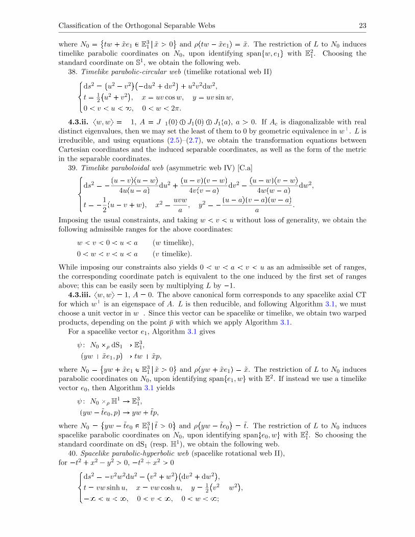
standard coordinate on S1, we obtain the following web.38. Timelike parabolic-circular web (timelike rotational web II)$'&

'%ds2 � �

u2 � v2��du2 � dv2

�� u2v2dw2,

t � 12

�u2 � v2

�, x � uv cosw, y � uv sinw,

0 v u 8, 0 w 2π.

4.3.ii. xw,wy � �1, A � J�1p0q ` J1p0q ` J1paq, a ¡ 0. If Ac is diagonalizable with realdistinct eigenvalues, then we may set the least of them to 0 by geometric equivalence in wK. L isirreducible, and using equations (2.5)–(2.7), we obtain the transformation equations betweenCartesian coordinates and the induced separable coordinates, as well as the form of the metricin the separable coordinates.

39. Timelike paraboloidal web (asymmetric web IV) [C.a]$''&''%ds2 � �pu� vqpu� wq

4upu� aq du2 � pu� vqpv � wq4vpv � aq dv2 � pu� wqpv � wq

4wpw � aq dw2,

t � �1

2pu� v � wq, x2 � uvw

a, y2 � �pu� aqpv � aqpw � aq

a.

Imposing the usual constraints, and taking w v u without loss of generality, we obtain thefollowing admissible ranges for the above coordinates:

w v 0 u a (w timelike),

0 w v u a (v timelike).

While imposing our constraints also yields 0 w a v u as an admissible set of ranges,the corresponding coordinate patch is equivalent to the one induced by the first set of rangesabove; this can be easily seen by multiplying L by �1.

4.3.iii. xw,wy � 1, A � 0. The above canonical form corresponds to any spacelike axial CTfor which wK is an eigenspace of A. L is then reducible, and following Algorithm 3.1, we mustchoose a unit vector in wK. Since this vector can be spacelike or timelike, we obtain two warpedproducts, depending on the point p with which we apply Algorithm 3.1.

For a spacelike vector e1, Algorithm 3.1 gives

ψ : N0 �ρ dS1 Ñ E31,

pyw � xe1, pq ÞÑ tw � xp,

where N0 � yw � xe1 P E3

1 | x ¡ 0(and ρpyw � xe1q � x. The restriction of L to N0 induces

parabolic coordinates on N0, upon identifying spante1, wu with E2. If instead we use a timelikevector e0, then Algorithm 3.1 yields

ψ : N0 �ρ H1 Ñ E31,

pyw � te0, pq ÞÑ yw � tp,

where N0 � yw � te0 P E3

1 | t ¡ 0(and ρ

�yw � te0

� � t. The restriction of L to N0 inducesspacelike parabolic coordinates on N0, upon identifying spante0, wu with E2

1. So choosing thestandard coordinate on dS1 (resp. H1), we obtain the following web.

40. Spacelike parabolic-hyperbolic web (spacelike rotational web II),for �t2 � x2 � y2 ¡ 0, �t2 � x2 ¡ 0$'&

'%ds2 � �v2w2du2 � �

v2 � w2��dv2 � dw2

�,

t � vw sinhu, x � vw coshu, y � 12

�v2 � w2

�,

�8 u 8, 0 v 8, 0 w 8;


for �t2 � x2 � y2 ¡ 0, �t2 � x2 0

$'&'%ds2 � �

u2 � v2��du2 � dv2

�� u2v2dw2,

t � uv coshw, x � uv sinhw, y � 12

�u2 � v2

�,

0 v u 8, �8 w 8.

4.3.iv. xw,wy � 1, A � J�1paq ` J1p0q ` J1p0q, a ¡ 0. If Ac is diagonalizable with realdistinct eigenvalues, then modulo geometric equivalence in wK, A has the above form in someCartesian coordinates. So L is an irreducible CT and we readily obtain the form of the metricas well as the transformation equations.

41. Spacelike paraboloidal web (asymmetric web IV) [C.b]

$''&''%ds2 � pu� vqpu� wq

4upu� aq du2 � pv � uqpv � wq4vpv � aq dv2 � pw � uqpw � vq

4wpw � aq dw2,

t2 � �pu� aqpv � aqpw � aqa

, x2 � �uvwa, y � 1

2pu� v � wq.


w 0 a v u (v timelike),

w 0 v u a (u timelike),

w v u 0 a (v timelike).

4.3.v. xw,wy � 1, A � J1pibq ` J1p�ibq ` J1p0q, b ¡ 0. If Ac has (non-real) complexeigenvalues, then by geometric equivalence, we may assume A takes the above form in complex-Cartesian coordinates pz, z, yq. Since L is an irreducible CT, we readily obtain the form of themetric as well as the transformation equations between the separable coordinates and pz, z, yq.We pass to standard Cartesian coordinates pt, x, yq precisely as described in 4.2.xi.

42. Spacelike complex-paraboloidal web (asymmetric web VI) [C.d]

$''''''&''''''%

ds2 � pu� vqpu� wq4�u2 � b2

� du2 � pv � uqpv � wq4�v2 � b2

� dv2 � pw � uqpw � vq4�w2 � b2

� dw2,

t2 � x2 � uv � uw � vw � b2, y � 1

2pu� v � wq,

t2 � x2 �?u2 � b2

?v2 � b2

?w2 � b2

b.

Assuming as usual that w v u, we see that this gives a unique set of coordinate ranges, andthe timelike coordinate is v.

4.3.vi. xw,wy � 1, A � J2p0qT ` J1p0q. We consider now the above canonical form, i.e.,Ac � kb k5 for some nonzero null vector k P wK. Note that this canonical form is equivalent tothe one with Ac � �k b k5, which can be easily seen by multiplying L by �1. Now, since L isirreducible, using equations (2.5)–(2.7), we obtain the metric and the transformation equationsfrom the separable coordinates to the lightcone coordinates in which A takes the above form.Passing to standard Cartesian coordinates, we have the following web.

43. Spacelike null-paraboloidal web (asymmetric web III) [F.1.c]

$'&'%ds2 � pu� vqpu� wq

4u2du2 � pu� vqpv � wq

4v2dv2 � pv � wqpu� wq

4w2dw2,

pt� xq2 � uvw, t2 � x2 � uv � uw � vw, y � 1

2pu� v � wq.




w v 0 u (v timelike).

4.4 Null axial CTs, L � A � w b r5 � r b w5, w � 0, xw,wy � 0

Any null axial CT can be put into the above form using geometric equivalence, with the canonicalform for A given by Theorem 2.1. Recall from the remarks following Theorem 2.1 that D is theA-invariant subspace span

w,Aw,A2w, . . .

(. In classifying canonical forms for null axial CTs,

we may apply geometric equivalence in the subspace DK insofar that dimD ¤ 2 (this is onlyrelevant for 4.4.i below). For convenience, we choose coordinates such that w � Bη � Bt � Bx.

4.4.i. w � 0, xw,wy � 0, A � J2p0qT ` J1p0q. We consider the above canonical form, i.e.,A � kbk5 for some nonzero null vector k such that xw, ky � 1. This case is equivalent to the nullaxial CT with A � �kbk5. Since L is an irreducible CT, using equations (2.5)–(2.7), we obtainthe metric and the transformation equations from the separable coordinates to the lightconecoordinates in which A takes the above form. Passing to standard Cartesian coordinates, wehave the following web.

44. Null paraboloidal web I (asymmetric web II) [E.1.a]

$'&'%ds2 � pu� vqpu� wq

4udu2 � pu� vqpv � wq

4vdv2 � pv � wqpu� wq

4wdw2,

x� t � 1

8

�u2 � v2 � w2

�� 1

4puv � uw � vwq, x� t � u� v � w, y2 � uvw.



w v 0 u (w timelike).

4.4.ii. w � 0, xw,wy � 0, A � J3p0qT. We finally consider the above canonical form fora null axial CT L, which is easily seen to be irreducible. We readily obtain the metric andthe transformation equations between the separable coordinates and the lightcone coordinatesin which A takes the above form. Passing to standard Cartesian coordinates, we obtain thefollowing final web.

45. Null paraboloidal web II (asymmetric web I) [G]

$'''''&'''''%

ds2 � 1

4pu� vqpu� wqdu2 � 1

4pu� vqpv � wqdv2 � 1

4pu� wqpv � wqdw2,

x� t � 1

16pu� v � wqpu� v � wqpu� v � wq, x� t � u� v � w,

y � 1

8

�u2 � v2 � w2

�� 1

4puv � uw � vwq.

Assuming as usual that w v u, we see that this gives a unique set of coordinate ranges, andthe timelike coordinate is v.

5 Concluding remarks

The above analysis illustrates the ease with which the method of concircular tensors yields an in-variant classification of the orthogonal separable webs in E3

1. This approach appears to be much


less computationally demanding than other methods described in the introduction, and is inmany ways much more elementary, since the crux of this method is essentially a problem of linearalgebra. Furthermore, provided we have determined all possible canonical forms modulo geomet-ric equivalence, the theory presented in [25] and [26] guarantees that the above 45 webs are all theorthogonal separable webs in E3

1; and insofar that our analysis of each case is complete, we can beconfident that the 88 inequivalent adapted coordinate charts determined above are exhaustive.

It is worth noting that the use of concircular tensors in classifying separable webs is likely tobe fruitful only in spaces of constant curvature, since in spaces of non-constant curvature thespace of concircular tensors will in general be very small.

In [11], one finds 31 inequivalent coordinate charts corresponding to irreducible webs; more-over, it is asserted therein that there are 51 inequivalent coordinate systems arising from re-ducible webs, based on computations done in [11]. Counting up the results from Section 4,we find 33 inequivalent charts from the irreducible webs, and 55 inequivalent charts from thereducible webs. As indicated above, the only two coordinate charts not appearing in [11] arethose from null ellipsoidal web II (web number 34 above). The discrepancy in the number ofreducible chart domains seems to be a result of overlooked equivalences. For instance, in [11]it appears that the Rindler web (web number 5 above and coordinate system B.6.b in [11]) iscounted as inducing only one inequivalent chart domain instead of two.

Any other discrepancies between the equations appearing here, and those appearing in [11]or [14] can be attributed to the various freedoms in defining the separable coordinates (i.e.,geometric equivalence and reparametrizations of the web. See also the remarks following 4.2.viiiabove).

The method presented here achieves simultaneously both a global classification of the orthog-onal separable webs, as well as the equations for the separable coordinates adapted to each web;the former gives the intrinsic geometric object of interest, while the latter gives the informationnecessary to orthogonally separate the Hamilton–Jacobi and Klein–Gordon equations given inthe introduction.

A Self-adjoint operators in Minkowski space

In this appendix, we review some of the key results regarding self-adjoint operators on n-dimensional Minkowski space En

1 , whose theory and classification differ tremendously from theEuclidean case. We simply quote the main results in this section, and refer the reader to [25]for details and proofs.

We first define a k-dimensional Jordan block with eigenvalue λ, Jkpλq, and a k-dimensionalskew-normal matrix Sk, to be the following k � k matrices:

Jkpλq :�

��

λ 1 0

λ. . .

. . . 1λ 1

0 λ

�� , Sk :�

��

0 11

. ..

11 0

�� .

A sequence of vectors in which the metric (restricted to their span) takes the form εSk iscalled a skew-normal sequence. Recall that a linear operator A : En

ν Ñ Enν is self-adjoint with

respect to the scalar product if xAx, yy � xx,Ayy for all x and y. This holds if and only if thecontravariant or covariant tensor metrically equivalent to A is symmetric. Since the metric isnot positive definite in En

1 , our classification of self-adjoint operators will specify the forms takenby both A and g in an appropriate basis. The canonical form for the pair pA, gq is called themetric-canonical form or metric-Jordan form for A.


For this purpose, we introduce a signed integer εk P Z, where ε � �1 and k P N, and writeA � Jεkpλq as a shorthand for the pair A � Jkpλq and g � εSk. For square matrices A1 and A2,we also define the block diagonal matrix

A1 `A2 :��A1 00 A2

.

We write Jεkpλq ` Jδmpµq as a shorthand the pair Jkpλq ` Jmpµq and g � εSk ` δSm. We nowsummarize the different possible canonical forms for a self-adjoint operator A in En

1 :Case 1. A is diagonalizable with real eigenvalues. In this case, there is a basis such that

A � J�1pλ1q ` J1pλ2q ` � � � ` J1pλnq.

Equivalently, A is diagonalized in Cartesian coordinates.Case 2. A has a complex eigenvalue λ � a � ib with b � 0. Since A is real, λ must be

another eigenvalue; in Minkowski space, all other eigenvalues must be real. Then,

A � J1pλq ` J1pλq ` J1pλ3q ` � � � ` J1pλnq

in some orthogonal basis where the first two vectors are complex. Notice that since they arecomplex, we may assume they have length squared �1.

Case 3. A has real eigenvalues but is not diagonalizable. Then there are three possibilitiesfor the metric-canonical form. The first two occur when

A � Jε2pλq ` J1pλ3q ` � � � ` J1pλnq

with ε � �1, in some basis where the first two vectors are null. The last case occurs when

A � J3pλq ` J1pλ4q ` � � � ` J1pλnq

in some basis where the first and third vectors are null; the second is spacelike. Notice that inMinkowski space, a metric-Jordan block J�3pλq is inadmissible. These are all the possibilitiesfor the canonical forms of self-adjoint endomorphisms in Minkowski space.

Acknowledgements

The authors wish to thank K. Rajaratnam and the anonymous referees for their careful readingof the paper and a number of helpful suggestions and comments. We also wish to acknowledgefinancial support from the Natural Sciences and Engineering Research Council of Canada in theform of a Undergraduate Student Research Award (CV) and a Discovery Grant (RGM).

References

[1] Benenti S., Special symmetric two-tensors, equivalent dynamical systems, cofactor and bi-cofactor systems,Acta Appl. Math. 87 (2005), 33–91.

[2] Benenti S., Chanu C., Rastelli G., Remarks on the connection between the additive separation of theHamilton–Jacobi equation and the multiplicative separation of the Schrodinger equation. I. The completenessand Robertson conditions, J. Math. Phys. 43 (2002), 5183–5222.

[3] Bocher M., Uber die Riehenentwickelungen der Potentialtheory, B.G. Teubner, Leipzig, 1894.

[4] Bruce A.T., McLenaghan R.G., Smirnov R.G., A geometrical approach to the problem of integrability ofHamiltonian systems by separation of variables, J. Geom. Phys. 39 (2001), 301–322.

[5] Cochran C.M., McLenaghan R.G., Smirnov R.G., Equivalence problem for the orthogonal webs on the3-sphere, J. Math. Phys. 52 (2011), 053509, 22 pages, arXiv:1009.4244.

[6] Cochran C.M., McLenaghan R.G., Smirnov R.G., Equivalence problem for the orthogonal separable websin 3-dimensional hyperbolic space, J. Math. Phys. 58 (2017), 063513, 43 pages.

https://doi.org/10.1007/s10440-005-1138-9

https://doi.org/10.1063/1.1506180

https://doi.org/10.1016/S0393-0440(01)00017-1

https://doi.org/10.1063/1.3578773

https://arxiv.org/abs/1009.4244

https://doi.org/10.1063/1.4983998


[7] Crampin M., Conformal Killing tensors with vanishing torsion and the separation of variables in theHamilton–Jacobi equation, Differential Geom. Appl. 18 (2003), 87–102.

[8] Crampin M., Concircular vector fields and special conformal Killing tensors, in Differential Geometric Me-thods in Mechanics and Field Theory, Academia Press, Gent, 2007, 57–70.

[9] Eisenhart L.P., Separable systems of Stackel, Ann. of Math. 35 (1934), 284–305.

[10] Hinterleitner F., Examples of separating coordinates for the Klein–Gordon equation in p2� 1q-dimensionalflat space-time, J. Math. Phys. 37 (1996), 3032–3040.

[11] Hinterleitner F., Global properties of orthogonal separable coordinates for the Klein–Gordon equation inp2 � 1q-dimensional flat space-time, Osterreich. Akad. Wiss. Math.-Natur. Kl. Sitzungsber. II 207 (1998),133–171.

[12] Horwood J.T., On the theory of algebraic invariants of vector spaces of Killing tensors, J. Geom. Phys. 58(2008), 487–501.

[13] Horwood J.T., McLenaghan R.G., Transformation to pseudo-Cartesian coordinates in locally flat pseudo-Riemannian spaces, J. Geom. Phys. 57 (2007), 1435–1440.

[14] Horwood J.T., McLenaghan R.G., Orthogonal separation of variables for the Hamilton–Jacobi andwave equations in three-dimensional Minkowski space, J. Math. Phys. 49 (2008), 023501, 48 pages,arXiv:10.1063/1.2823971.

[15] Horwood J.T., McLenaghan R.G., Smirnov R.G., Hamilton–Jacobi theory in three-dimensional Minkowskispace via Cartan geometry, J. Math. Phys. 50 (2009), 053507, 41 pages.

[16] Kalnins E.G., On the separation of variables for the Laplace equation ∆Ψ �K2Ψ � 0 in two- and three-dimensional Minkowski space, SIAM J. Math. Anal. 6 (1975), 340–374.

[17] Kalnins E.G., Separation of variables for Riemannian spaces of constant curvature, Pitman Monographs andSurveys in Pure and Applied Mathematics, Vol. 28, Longman Scientific & Technical, Harlow, John Wiley &Sons, Inc., New York, 1986.

[18] Kalnins E.G., Kress J.M., Miller Jr. W., Separation of variables and superintegrability. The symmetry ofsolvable systems, IOP Expanding Physics, IOP Publishing, Bristol, 2018.

[19] Kalnins E.G., Miller Jr. W., Lie theory and separation of variables. IX. Orthogonal R-separable coordinatesystems for the wave equation ψtt �∆2ψ � 0, J. Math. Phys. 17 (1976), 331–355.

[20] Kalnins E.G., Miller Jr. W., Separation of variables on n-dimensional Riemannian manifolds. I. The n-sphereSn and Euclidean n-space Rn, J. Math. Phys. 27 (1986), 1721–1736.

[21] McLenaghan R.G., Rastelli G., Valero C., Complete separability of the Hamilton–Jacobi equation for thecharged particle orbits in a Lienard–Wiechert field, J. Math. Phys. 61 (2020), 122903, 29 pages.

[22] McLenaghan R.G., Smirnov R.G., Intrinsic characterizations of orthogonal separability for natural Hamil-tonians with scalar potentials on pseudo-Riemannian spaces, J. Nonlinear Math. Phys. 9 (2002), suppl. 1,140–151.

[23] McLenaghan R.G., Smirnov R.G., The D., An extension of the classical theory of algebraic invariants topseudo-Riemannian geometry and Hamiltonian mechanics, J. Math. Phys. 45 (2004), 1079–1120.

[24] Olevsky M.N., Triorthogonal systems in spaces of constant curvature in which the equation ∆2u � λu � 0admits complete separation of variables, Math. USSR. Sb. 27 (1950), 379–427.

[25] Rajaratnam K., Orthogonal separation of the Hamilton–Jacobi equation on spaces of constant curvature,Master’s Thesis, University of Waterloo, 2014, available at http://hdl.handle.net/10012/8350.

[26] Rajaratnam K., McLenaghan R.G., Classification of Hamilton–Jacobi separation in orthogonal coordinateswith diagonal curvature, J. Math. Phys. 55 (2014), 083521, 16 pages, arXiv:1404.2565.

[27] Rajaratnam K., McLenaghan R.G., Killing tensors, warped products and the orthogonal separation of theHamilton–Jacobi equation, J. Math. Phys. 55 (2014), 013505, 27 pages, arXiv:1404.3161.

[28] Rajaratnam K., McLenaghan R.G., Valero C., Orthogonal separation of the Hamilton–Jacobi equation onspaces of constant curvature, SIGMA 12 (2016), 117, 30 pages, arXiv:1607.00712.

[29] Robertson H.P., Bemerkung uber separierbare Systeme in der Wellenmechanik, Math. Ann. 98 (1928),749–752.

[30] Smirnov R.G., Yue J., Covariants, joint invariants and the problem of equivalence in the invariant theoryof Killing tensors defined in pseudo-Riemannian spaces of constant curvature, J. Math. Phys. 45 (2004),4141–4163, arXiv:math-ph/0407028.

[31] Valero C., McLenaghan R.G., Classification of the orthogonal separable webs for the Hamilton–Jacobi andLaplace–Beltrami equations on 3-dimensional hyperbolic and de Sitter spaces, J. Math. Phys. 60 (2019),033501, 30 pages, arXiv:1811.04536.

https://doi.org/10.1016/S0926-2245(02)00140-7

https://doi.org/10.2307/1968433

https://doi.org/10.1063/1.531552

https://doi.org/10.1016/j.geomphys.2007.12.004

https://doi.org/10.1016/j.geomphys.2006.12.001

https://doi.org/10.1063/1.2823971

https://arxiv.org/abs/#2

https://doi.org/10.1063/1.3094719

https://doi.org/10.1137/0506033

https://doi.org/10.1088/978-0-7503-1314-8

https://doi.org/10.1063/1.522900

https://doi.org/10.1063/1.527088

https://doi.org/10.1063/5.0030305

https://doi.org/10.2991/jnmp.2002.9.s1.12

https://doi.org/10.1063/1.1644902

http://hdl.handle.net/10012/8350

https://doi.org/10.1063/1.4893335


https://doi.org/10.1063/1.4861707




https://doi.org/10.1007/BF01451624

https://doi.org/10.1063/1.1805728

https://arxiv.org/abs/math-ph/0407028

https://doi.org/10.1063/1.5043066


sigma22-019.pdf - EMIS

Documents

Transcript of sigma22-019.pdf - EMIS