Shoreline Change Analysis for the Northern Parts of Coramandel Coast

Available online at www.sciencedirect.com

ScienceDirectScienceDirect

Aquatic Procedia 4 ( 2015 ) 317 – 324

2214-241X © 2015 The Authors. Published by Elsevier B.V. This is an open access article under the CC BY-NC-ND license (http://creativecommons.org/licenses/by-nc-nd/4.0/).Peer-review under responsibility of organizing committee of ICWRCOE 2015doi: 10.1016/j.aqpro.2015.02.043

INTERNATIONAL CONFERENCE ON WATER RESOURCES, COASTAL AND OCEAN ENGINEERING (ICWRCOE 2015)

Shoreline Change Analysis For Northern Part Of The Coromandel Coast

N.N.Salghunaa*, S.Aravind Bharathvaja

aCenter for Remote Sensing, Bharathidasan University, Tiruchirappalli, TamilNadu, India

Abstract

The shoreline is a more dynamic, and complex region of all geological features present, as it has a mixed results of tidal, Aeolian, tectonic, and sometimes riverine activity. The shoreline change has its impact, but which is not so visible. To observe this we need a long and continuous set of data. The following project is done for a shoreline length of approximately 112 km of the North of the Coramandal Coast, as a trial and error work covering the major settlements of Puducherry, Cuddalore, and Chidambaram. Data used are derived from 1972 (from SOI Toposheets), to TM data of 2013. To derive the Shoreline from the satellite data, band ratio of Red band to IR band is done. The shorelines are digitized and saved along with the appropriate MM/DD/YYYY added to the attribute table. Digital Shoreline Analysis System (DSAS) is an extension for the ArcGIS, developed by USGS. Using the extension, transects are laid for every 50 m. Then using LINEAR REGRESSION RATE (LRR), the change for every 50 meter is analysed and stored in a table. And using the table, the Erosion and Accretion, are analysed, and understood. Total area eroded is 12.93 sq. Km, and the length is of 99.36 Km. The area of Accretion is 1.73 Km2, in a length of 22 Km. © 2015 The Authors. Published by Elsevier B.V. Peer-review under responsibility of organizing committee of ICWRCOE 2015.

Keywords: Shoreline change; Remote Sensin; GIS; DSAS

* Corresponding author. Tel.: +0-000-000-0000 ; fax: +0-000-000-0000 .

E-mail address: [email protected]

© 2015 The Authors. Published by Elsevier B.V. This is an open access article under the CC BY-NC-ND license (http://creativecommons.org/licenses/by-nc-nd/4.0/).Peer-review under responsibility of organizing committee of ICWRCOE 2015

http://crossmark.crossref.org/dialog/?doi=10.1016/j.aqpro.2015.02.043&domain=pdf




318 N.N. Salghuna and S. Aravind Bharathvaj / Aquatic Procedia 4 ( 2015 ) 317 – 324

1. Shoreline

The boundary between land and sea keeps changing its shape and position continuously due to dynamic environmental conditions. The change in shoreline is mainly associated with waves, tides, winds, periodic storms, sea-level change, and the geomorphic processes of erosion and accretion and human activities. Shoreline also depicts the recent formations and destructions that have happened along the shore. Waves change the coastline morphology and form the distinctive coastal landforms. The loose granular sediments continuously respond to the ever-changing waves and currents. The beach profile is important, in that it can be viewed as an effective natural mechanism, which causes waves to break and dissipate their energy. When breakwaters are constructed, they upset the natural equilibrium between the sources of beach sediment and the littoral drift pattern. In response, shoreline changes its configuration in attempt to reach a new equilibrium (Ramesh and Ramachandran 2001). Monitoring changes in shoreline helps to identify the nature and processes that caused these changes in any specific area, to assess the human impact and to plan management strategies. Remote sensing data could be used effectively to monitor the changes along the coastal zone including shoreline with reasonable accuracy.

1.1 Natural shoreline dynamics

Shoreline ‘state’, that is the trend in the location of the shoreline, can generally be classified into three categories viz. Eroding (shoreline is retreating landward), Equilibrium (shoreline is generally stable) and Accreting (shoreline is extending seaward). These three states are related to five key factors, namely, sediment supply to the beach, wave energy, sea-level change, location of shoreline and man-made modification to shoreline. The regional scale analysis suggests that the shoreline plays a significant role in the estuarine system. (Lisa Cowart et.al, 2011)

2. Study Area

2.1 Location

In the globe, the study area lies from 12˚16’ N and 80˚ E to 11˚15’ N and 79˚50’ E. The total length of the coast under study is 122.158 kilometres. The study area comprises of major settlements such as Pondicherry, Cuddalore, Chidambaram, and Sirkazhi and number of minor settlements. NH 65 and other number of roads are been sufficiently used by the public for the transportation. There are number of water bodies that are seen in the study area. Generally fishing on the shore, aqua cultural by the near shore area and agricultural cultivation in the land is being mainly adapted. The rivers flowing are Sankarabarani, Ponnaiyar, Gadilam, Uppanar, Vellar and Coleroon

2.2 Methodology and Data Acquisition

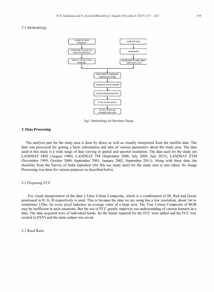
The methodology flowchart, adopted for the entire study is given in the figure 1. The satellite data used for this study is acquired from the GLOVIS and EARTH EXPLORER sites, maintained by USGS. The MSS, TM, ETM+ data products of the LANDSAT series for various years from 1980 to 2009. The data used for the study were selected based on the criteria of Cloud cover less than 10%, season in which the data was acquired. Because of this, the periodical gap was not possible to maintain. The Survey of India toposheet of scale 1:50,000 was taken as the control for the satellite data, and also the base line for the study was derived from it.


2.3 Methodology

Fig1: Methodology for Shoreline Change

3. Data Processing

The analysis part for the study area is done by direct as well as visually interpreted from the satellite data. The

data was processed for getting a basic information and idea of various parameters about the study area. The data used in this study is a wide range of data varying in spatial and spectral resolution. The data used for the study are LANDSAT MSS (August 1980), LANDSAT TM (September 2006; July 2009, July 2013), LANDSAT ETM (November 1999; October 2000; September 2001; January 2002, September 2011). Along with these data, the shoreline from the Survey of India toposheet (for IDs see study area) for the study area is also taken. So Image Processing was done for various purposes as described below.

3.1 Preparing FCC

For visual interpretation of the data a False Colour Composite, which is a combination of IR, Red and Green positioned in R, G, B respectively is used. This is because the data we are using has a low resolution, about 1m to sometimes 120m. So every pixel indicates an average value of a large area. The True Colour Composite of RGB may be inefficient in such situations. But the use of FCC greatly improves our understanding of various features in a data. The data acquired were of individual bands. So the bands required for the FCC were added and the FCC was created in ENVI and the same output was saved.

3.2 Band Ratio


For analysing the shoreline change, we have to derive it from the satellite data. But the FCC has its own characteristics such as the transmissivity of water in shallow depth and the suspended sediments influence in the satellite data. The extension of the sand in the beach into the sea for shallow depth will influence error in delineating the land and water boundary. So the BAND RATIOING technique is used for delineation of the shoreline. The Red band (Band 2 in TM, ETM and Band 4 in MSS) has its property of being absorbed by water, and only will be reflected in land. But on the other hand in the Infrared, this work in adverse, i.e., the water reflects the spectrum more in comparison to land. So the Band Red is divided by Band IR which provides the clear demarcation of water bodies and land. From the output, the shoreline was created in GIS. The shorelines were prepared for the years 1980, 1999, 2000, 2001, 2002 2006, 2009, 2011 and 2013 4. Analysis The shoreline change analysis is done by using the USGS provided DSAS 4.3 (Digital Shoreline Analysis System) which is an additional ‘Extension’ for ArcGIS. Shorelines were created from the output of band ratio of bands Red and IR. All the shorelines were added in a single shape file in a Personal Geodatabase. For every shoreline, the date from which the shoreline is made must be added in the attribute as MM/DD/YYYY. A Baseline, from which the changes are to be calculated, is required in another shape file in the same Database. The actual baseline taken is 1972. But Since then, the coast has undergone both erosion and accretion in various regions. So the coastline of the 1972 toposheet was buffered for a 1000 meters in the offshore and it is used as baseline. Using DSAS, transects are laid for 2500 meters perpendicular to the shore for every 50 meters along the shore for the entire shoreline from the baseline.

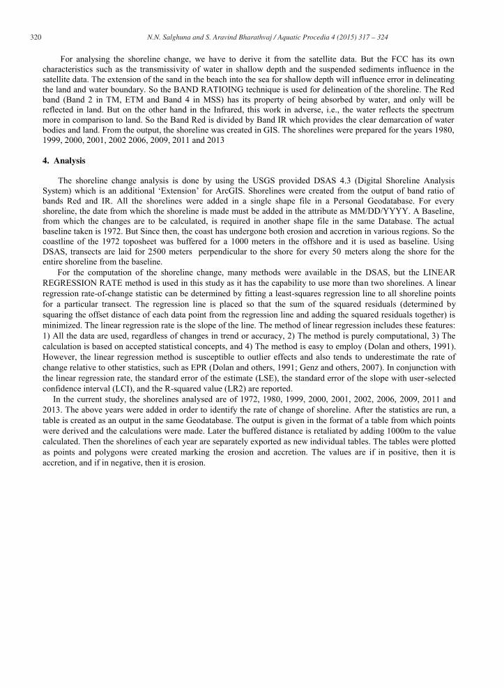
For the computation of the shoreline change, many methods were available in the DSAS, but the LINEAR REGRESSION RATE method is used in this study as it has the capability to use more than two shorelines. A linear regression rate-of-change statistic can be determined by fitting a least-squares regression line to all shoreline points for a particular transect. The regression line is placed so that the sum of the squared residuals (determined by squaring the offset distance of each data point from the regression line and adding the squared residuals together) is minimized. The linear regression rate is the slope of the line. The method of linear regression includes these features: 1) All the data are used, regardless of changes in trend or accuracy, 2) The method is purely computational, 3) The calculation is based on accepted statistical concepts, and 4) The method is easy to employ (Dolan and others, 1991). However, the linear regression method is susceptible to outlier effects and also tends to underestimate the rate of change relative to other statistics, such as EPR (Dolan and others, 1991; Genz and others, 2007). In conjunction with the linear regression rate, the standard error of the estimate (LSE), the standard error of the slope with user-selected confidence interval (LCI), and the R-squared value (LR2) are reported.

In the current study, the shorelines analysed are of 1972, 1980, 1999, 2000, 2001, 2002, 2006, 2009, 2011 and 2013. The above years were added in order to identify the rate of change of shoreline. After the statistics are run, a table is created as an output in the same Geodatabase. The output is given in the format of a table from which points were derived and the calculations were made. Later the buffered distance is retaliated by adding 1000m to the value calculated. Then the shorelines of each year are separately exported as new individual tables. The tables were plotted as points and polygons were created marking the erosion and accretion. The values are if in positive, then it is accretion, and if in negative, then it is erosion.


Fig 2 Example for Linear Regression Rate Calculation

5. Results and Discussion:

The analysis from the various above said coastlines using the DSAS toolbar have shown that the current coast is clearly an eroding coast. Accretion is seen in minor scale in some parts of the coast, that too intermittently. Of the 112 Km long coast, approximately 82% of the coast is eroding. This is mainly because of

The coast of Puducherry and Cuddalore, by many evidences and various theories, is subsiding. The French Government which ruled the Puducherry once has created a Sea Wall in the coast of the Heritage town to prevent sea water coming into the land.

This natural process is further accelerated due to construction of Ports and Harbours without any prior understanding of the effect of the littoral currents in the region. This has evidently increased the erosion on the Northern part of the harbour, and accretion in the southern part, in accordance to the littoral current pattern of our country. The shoreline change has made the local people such as the fishermen, to move into the land. Many houses were built over the stable Sand Dunes. The paleo-beach ridges were also destroyed due to continuous erosion. There is a severe change in the erosion and accretion. The erosion has gone at some places above 400 meters whereas accretion is only 235 meters is the maximum accretion seen from the year 1972. Maximum erosion is seen where a spit was present in 1972 survey of India toposheet. The total length and area of accretion and erosion is given below

Table 1- Summary of the Result

Result Area (Sq. Km) Length (Km)

Erosion 14.7856 95.3408


Accretion 1.85607 23.0998

No Change N/A 0.31369

From the various data sets, used to estimate the shoreline change, the change rate of the coast varies randomly for every alternating erosion and accretion. But the overall average change of the coast shows an erosion rate of around 1 meter. According to the length eroded and accreted the erosion and accretion and erosion is categorized into Very high, High, Moderate, Low erosion and accretion.

Conclusions

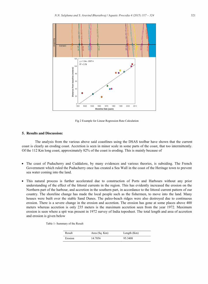
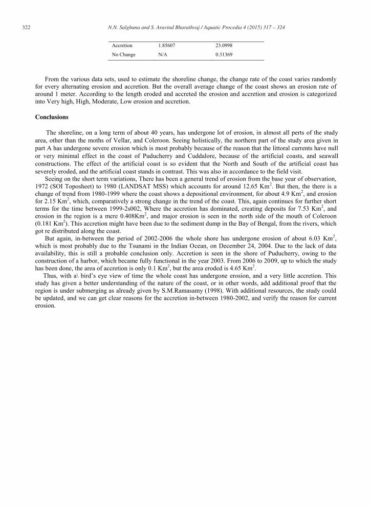
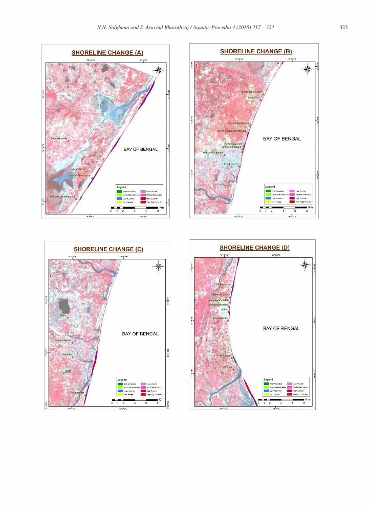
The shoreline, on a long term of about 40 years, has undergone lot of erosion, in almost all perts of the study area, other than the moths of Vellar, and Coleroon. Seeing holistically, the northern part of the study area given in part A has undergone severe erosion which is most probably because of the reason that the littoral currents have null or very minimal effect in the coast of Puducherry and Cuddalore, because of the artificial coasts, and seawall constructions. The effect of the artificial coast is so evident that the North and South of the artificial coast has severely eroded, and the artificial coast stands in contrast. This was also in accordance to the field visit. Seeing on the short term variations, There has been a general trend of erosion from the base year of observation, 1972 (SOI Toposheet) to 1980 (LANDSAT MSS) which accounts for around 12.65 Km2. But then, the there is a change of trend from 1980-1999 where the coast shows a depositional environment, for about 4.9 Km2, and erosion for 2.15 Km2, which, comparatively a strong change in the trend of the coast. This, again continues for further short terms for the time between 1999-2s002, Where the accretion has dominated, creating deposits for 7.53 Km2, and erosion in the region is a mere 0.408Km2, and major erosion is seen in the north side of the mouth of Coleroon (0.181 Km2). This accretion might have been due to the sediment dump in the Bay of Bengal, from the rivers, which got re distributed along the coast. But again, in-between the period of 2002-2006 the whole shore has undergone erosion of about 6.03 Km2, which is most probably due to the Tsunami in the Indian Ocean, on December 24, 2004. Due to the lack of data availability, this is still a probable conclusion only. Accretion is seen in the shore of Puducherry, owing to the construction of a harbor, which became fully functional in the year 2003. From 2006 to 2009, up to which the study has been done, the area of accretion is only 0.1 Km2, but the area eroded is 4.65 Km2. Thus, with a\ bird’s eye view of time the whole coast has undergone erosion, and a very little accretion. This study has given a better understanding of the nature of the coast, or in other words, add additional proof that the region is under submerging as already given by S.M.Ramasamy (1998). With additional resources, the study could be updated, and we can get clear reasons for the accretion in-between 1980-2002, and verify the reason for current erosion.


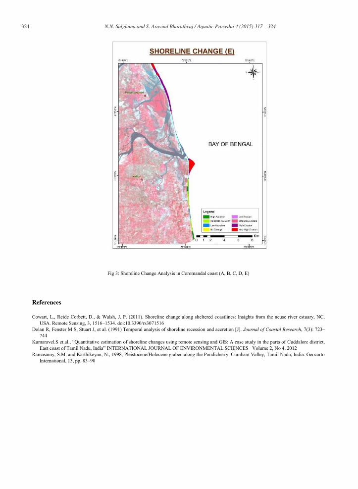
Fig 3: Shoreline Change Analysis in Coromandal coast (A, B, C, D, E)

References

Cowart, L., Reide Corbett, D., & Walsh, J. P. (2011). Shoreline change along sheltered coastlines: Insights from the neuse river estuary, NC, USA. Remote Sensing, 3, 1516–1534. doi:10.3390/rs3071516

Dolan R, Fenster M S, Stuart J, et al. (1991) Temporal analysis of shoreline recession and accretion [J]. Journal of Coastal Research, 7(3): 723–744

Kumaravel.S et.al., “Quantitative estimation of shoreline changes using remote sensing and GIS: A case study in the parts of Cuddalore district, East coast of Tamil Nadu, India” INTERNATIONAL JOURNAL OF ENVIRONMENTAL SCIENCES Volume 2, No 4, 2012

Ramasamy, S.M. and Karthikeyan, N., 1998, Pleistocene/Holocene graben along the Pondicherry–Cumbam Valley, Tamil Nadu, India. Geocarto International, 13, pp. 83–90

Shoreline Change Analysis for the Northern Parts of Coramandel Coast

Documents

Transcript of Shoreline Change Analysis for the Northern Parts of Coramandel Coast