EUROPEAN ORGANIZATION FOR NUCLEAR RESEARCH (CERN)

CERN-SHiP-INT-2019-008January 27, 2020

SHiP Hidden Sector SpectrometerMagnet

Autumn 2019 status

A. Perez 1 , P. Wertelaers 1 2

1 CERN, Geneva, Switzerland.

2 Corresponding author.

Abstract

The current status of the general design is reported. Three-dimensional finite element fieldcomputations are treated, reporting on spectrometer performance, magnet yoke saturation,and electromagnetic forces. The yoke is a stack of sheets, and the studs keeping thatstack together, are reviewed. A first proposal on support structures and yoke assembly isdiscussed. The emphasis of this status report is on the yoke, and on purpose so. Indeed,even if the current baseline is a warm magnet, a future superconducting option shouldgive minimal perturbation to the magnet project.

Contents

1 Introduction 2

2 General design : the numbers ! 42.1 Yoke . . . . . . . . . . . . . . . . . . . . . . . . . . . . . . . . . . . . . . . . . . 42.2 Coil . . . . . . . . . . . . . . . . . . . . . . . . . . . . . . . . . . . . . . . . . . 42.3 Grand totals . . . . . . . . . . . . . . . . . . . . . . . . . . . . . . . . . . . . . . 52.4 A remark on assembly . . . . . . . . . . . . . . . . . . . . . . . . . . . . . . . . 52.5 The current baseline design of the magnet . . . . . . . . . . . . . . . . . . . . . 6

3 Magnetic field by finite element modelling 7

4 The M30 studs keeping the yoke pack together 144.1 Introduction . . . . . . . . . . . . . . . . . . . . . . . . . . . . . . . . . . . . . . 144.2 Stud design . . . . . . . . . . . . . . . . . . . . . . . . . . . . . . . . . . . . . . 144.3 Transverse deformations (bending) of yoke sheet . . . . . . . . . . . . . . . . . . 174.4 Cementing the magnet yoke corners . . . . . . . . . . . . . . . . . . . . . . . . 204.5 The possible need for intermediate studs on the vertical leg . . . . . . . . . . . . 234.6 Inventory of yoke fixation elements . . . . . . . . . . . . . . . . . . . . . . . . . 254.7 The combined axial effect : seismic z-accelerations . . . . . . . . . . . . . . . . . 26

5 Support structure for yoke 275.1 Introduction . . . . . . . . . . . . . . . . . . . . . . . . . . . . . . . . . . . . . . 275.2 Model of a monolithic letter “A” . . . . . . . . . . . . . . . . . . . . . . . . . . 285.3 Assessment of top interface and its welds . . . . . . . . . . . . . . . . . . . . . . 30

6 Yoke assembly 326.1 Introduction and overview . . . . . . . . . . . . . . . . . . . . . . . . . . . . . . 326.2 Fixation of vertical sheets to “letter A” . . . . . . . . . . . . . . . . . . . . . . . 326.3 Sow and grow with precision . . . . . . . . . . . . . . . . . . . . . . . . . . . . . 356.4 Slideshow of yoke assembly . . . . . . . . . . . . . . . . . . . . . . . . . . . . . . 376.5 Loading and deformation of tooling under growing yoke stack . . . . . . . . . . 416.6 Insertion of top sheets . . . . . . . . . . . . . . . . . . . . . . . . . . . . . . . . 426.7 List of tooling – preliminary . . . . . . . . . . . . . . . . . . . . . . . . . . . . . 43

A Rehearsal on the Scalar Potential method 44A.1 Scalar Potential, basic form . . . . . . . . . . . . . . . . . . . . . . . . . . . . . 44A.2 Variant : Two Scalar Potential . . . . . . . . . . . . . . . . . . . . . . . . . . . . 45A.3 Variant : Difference Scalar Potential . . . . . . . . . . . . . . . . . . . . . . . . 46

B Far-field elements 48B.1 One-dimensional . . . . . . . . . . . . . . . . . . . . . . . . . . . . . . . . . . . 48B.2 Two-dimensional . . . . . . . . . . . . . . . . . . . . . . . . . . . . . . . . . . . 49B.3 Practical considerations . . . . . . . . . . . . . . . . . . . . . . . . . . . . . . . 50

C Flux-normal boundary condition 51

D Electromagnetic forces 54D.1 Lorentz forces FLFLFL on coil . . . . . . . . . . . . . . . . . . . . . . . . . . . . . . . 54D.2 Maxwell tractions FMFMFM on inner yoke skin . . . . . . . . . . . . . . . . . . . . . . 55D.3 Interpretation . . . . . . . . . . . . . . . . . . . . . . . . . . . . . . . . . . . . . 55

1

1 Introduction

The Spectrometer Magnet has to provide a (vertical) bending power of about 0.65 Tm in anet aperture of 5 m across (x) and 10 m high (y) .

In the SHiP Technical Proposal (TP) [1] , it was established that a 3.5 m thick (z) yokewould be appropriate. This number is considered fixed.

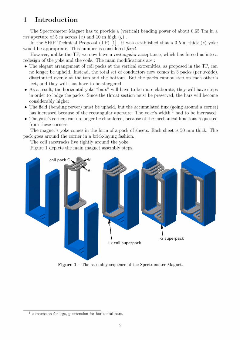
However, unlike the TP, we now have a rectangular acceptance, which has forced us into aredesign of the yoke and the coils. The main modifications are :• The elegant arrangement of coil packs at the vertical extremities, as proposed in the TP, can

no longer be upheld. Instead, the total set of conductors now comes in 3 packs (per x-side),distributed over x at the top and the bottom. But the packs cannot step on each other’sfeet, and they will thus have to be staggered.• As a result, the horizontal yoke “bars” will have to be more elaborate, they will have steps

in order to lodge the packs. Since the throat section must be preserved, the bars will becomeconsiderably higher.• The field (bending power) must be upheld, but the accumulated flux (going around a corner)

has increased because of the rectangular aperture. The yoke’s width 1 had to be increased.• The yoke’s corners can no longer be chamfered, because of the mechanical functions requested

from these corners.The magnet’s yoke comes in the form of a pack of sheets. Each sheet is 50 mm thick. The

pack goes around the corner in a brick-laying fashion.The coil racetracks live tightly around the yoke.Figure 1 depicts the main magnet assembly steps.

Figure 1 – The assembly sequence of the Spectrometer Magnet.

1 x extension for legs, y extension for horizontal bars.

2

The vacuum vessel “races through” the magnet bore. Thus, the effective opening to beprovided by the magnet, is the addition of the net aperture and the vessel construction. Forthe vessel part racing through, a lightweight sandwich panel construction is foreseen, and athickness budget of (only !) 100 mm is reserved. By restricting this budget so severely, we tryto prevent the magnet from becoming even much bigger still.

These panels are wholly unable to sustain the atmospheric pressure over a multi-metre range.We foresee anchoring by rods, in a matrix-like scheme with a pitch of order 0.8 m . These rodsrun through the magnet yoke, and are arrested – to the yoke – on the exterior surface, seeFigure 2 . They are loaded in tension only, and thus can be slender, thereby eating away onlyminute portions of yoke flesh.

The direct anchoring by rods can be used for the vertical chamber walls in a straightforwardmanner. But the floor and roof segments deserve extra attention, because the rods can be inconflict with the coils. We try to lodge them in the small openings between adjacent coil packs.

The current baseline design is a warm magnet, and this Note reports on such design. Butenergy consumption is a possible concern, and it is useful to reflect briefly on what could happenwith this design in case of a future switch to a superconducting alternative.

Without doubt, a normal-conducting coil superpack (A-B-C) would then be replaced by onecryostat. Now, the Spectrometer Vacuum Vessel never interacts with any coil or cryostat. Thismeans that a superconducting option will not threaten any vactank integration, provided thecryostat stays inside the volume currently taken by the superpack.

There is even hope of a flatter arrangement at the top and bottom, and this could result insavings in the yoke’s horizontal parts.

However, a very severe challenge would come from the Vessel wall anchoring requirement.This anchoring function would have to run “through” the cryostat, see Figure 3 .

z

x

Figure 2 – Cartoon depicting the spirit ofanchoring the panels of the vacuum vessel(green) racing through the magnet aperture.The anchoring is by rods (red) penetrating themagnet yoke (blue) and fixed to the yoke’s outersurface. The cartoon is not to scale, and shallnot be seen as realistic design. The Experimentaxis is horizontal, and far away South.

y

x

Figure 3 – In case a superconducting magnetwere to be chosen, a solution must be foundwhereby the Spectrometer Vacuum Vessel(green) can still be anchored to the yoke (blue)as if the rods (red) were running through thecryostat ((shaded) brown). The Experimentaxis is perpendicular to the Figure, and in theSouth-West.

3

2 General design : the numbers !

2.1 Yoke

The yoke is assembled from 70 layers, each 50 mm thick. Each layer is a patch of 4 sheets,see Figure 4 , left. The assembly is kept together by an array of elastic studs, pre-tensioned byhydraulic jacks, providing intense friction locking. Details about this bolting are in Section 4 .Assumed iron mass density for the bookkeeping : 7.9 kg/ltr .

The principal yoke numbers are in Table 1 . It would appear that only two types of sheetwould suffice for the entire yoke. Construction details frustrate such dreams, however.

sheet type horizontal vertical grand totalsurfacial area [ m2 ] 7.632 13.26

unit mass [ kg ] 3015. 5236.quantity 140 140

total mass [ t ] 422.1 733.1 1155.1

Table 1 – Bookkeeping of yoke sheets.

2.2 Coil

Per x-side, the coil is materialized in 3 “packs” : A, B and C , see Figure 1. Each pack hasthe same cross-section – see Figure 4 , right – and the same bending radii. However, the lengthsof the straight portions (apart from the z-portion) differ between them. The results below areobtained from an approximation : a length development of a constant cross-section. Hence, anyelectrical (and hydraulic) connectivity issue is discarded, and the dissipated power is obtainedsimply from :

Pdiss =

∫V olAlu

ρel J2 dV ,

where J is the current density. Assumed resistivity for the aluminium conductor :

ρel = 2.8 · 10−8 Ωm .

The input cross-sectional properties are very comparable to those of LHCb :• conductor current : 3 kA ;• conductor square size : 50 mm ;• diameter of bore hole : 25 mm ;• composite layer (glass fibre & resin) thickness : 2 mm (4 mm at inter-pancake interfaces).

The assumed mass densities are 2.7 kg/ltr for aluminium and 1.2 kg/ltr for composite.The resulting cross-sectional properties are :

• current density : 1.493 A/mm2 ;• mass of pack per unit length : 232.7 kg/m .

We the above assumptions and intermediate results, we obtain the coil pack bookkeeping ofTable 2 . In [2] is an extensive discussion of the coil cooling design.

coil pack A B Clength [ m ] 37.03 35.96 34.89mass [ kg ] 8617. 8368. 8118.

dissipation [ kW ] 185.8 180.4 175.0

Table 2 – Racetrack results.

4

odd layer even layer

horizontal

ver

tica

l

522

21

6 (

4 p

anca

kes

)

one pack:

Figure 4 – Left : The philosophy of layers and sheets. Right : Cross-section of a coil packconsisting of 4 pancakes.

2.3 Grand totals

For the entirety of yoke and 6 coil packs, we obtain :• mass : 1205 tonnes ;• dissipation : 1.083 MW .

2.4 A remark on assembly

It is proposed to erect the yoke partially, to a U-shape, then to load the coils, and thento insert the roof sheets of the yoke. In spite of this apparent liberty, the coil packs A-B-Cimprison each other distinctly. It seems mandatory to lower a coil superpack into the U , seeagain Figure 1. The net mass of such superpack being about 25 tonnes, the required capacity ofthe assigned surface hall overhead crane may surpass 300 kN . No crane(s) in the undergroundexperiment hall is (are) affected.

5

2.5 The current baseline design of the magnet

Figure 5 rehearses the dimensions [ mm ] of the design as of today.

bumper rod

tunnels for He needle

(vactank midway flange leak test)

allowance for coil support

vactank boundary

vactank sheet

z−arrest (mounting)

z−arrest (mounting)

6818

5496

6373

5768

5928

4906

3122

2230

1338

446

5712

360 1080

1800

2520

3120

3588

6100

2680

4000

(ob

lig

ed b

y v

acta

nk

)

advancing stud goes here

oddeven

odd

even

limit of acceptance

51005000

5848

5416

5200

5632

3398

522 (10 conductors)

one pancake :

216 (

4 p

anca

kes

)

522

A

B

C

C

B

A

A B C

6898

3640

2600

2500

1750

R 350 (12x)

R 350 (3x)

200

722

900

1422

1600

2122

2272

3182

2966

2750

mm

sheet : 50 ?m

0

1

2

3

4

5

6

7

m

0

1

2

3

4

5

6

7

2 1 0 m 1 2 3 4

0 m 1 2 3 4

z

y

xz

02−Jul−2019

Figure 5 – Magnet design as of July 2019. European (first-angle) projection.

6

3 Magnetic field by finite element modelling

A three-dimensional magnetostatic finite element model has been constructed, in parallelwith the modelling work done by CERN’s TE/MSC group reported in [2] .

All geometry and grid density setting is parametrized, by fully exploiting the programmingcapability of the code’s command input language.

The modelling is part of a long and on-going campaign, and in this Section, we report onthe results of run 21.

The scalar potential method is used, this is the obvious choice in our case. It necessitatesonly one degree of freedom per node, and is thus economical. With this method, the coils arenot present as such in the finite element model ; instead, they are primitives for Biot-Savartintegration, see Appendix A . Whence another important advantage of the method : the modelgrid is not “disturbed” by any coil ; instead, it only needs to take account of changes of materialpermeability. Indeed, there is the notion of generalized “air”, also encompassing aluminium(coil) and austenitic steel (spectrometer vacuum vessel), without needing to bother about theoutline of these objects ! The disadvantage is that Lorentz forces on the coil are not available.

The coordinate system is a z-shifted Experiment system, with origin in the centre of themagnet. The finite element model contains only 1/8 volume, because of symmetry 2 . Incontrast, the coil primitives shall be present with their full extent, see Figure 6 .

The code used is Ansys, and the method variant is Difference Scalar Potential, see againAppendix A . A large-size finite volume – encompassing the iron yoke and the “air” – is erectedwith bricks with low-order shape functions 3 . They always have 8 nodes in this model, meaningthat they are never degenerating.

The size of the finite volume :• 8 m along x ;• 10.5 m along y ;• 10 m along z .

This finite volume is surrounded by a layer of far-field elements 4 , see Appendix B . Figure 7shows this layer. It has not been too hard to automate the generation of these elements (andtheir outer nodes), because the elements of the inner finite volume had never degenerated, andbecause that inner volume had been produced without automatic meshing. And likewise, thefar-field elements themselves never degenerate.

The not-too-small finite volume, in combination with the far-field layer, should guaranteeaccurate results even in this case of huge stray. And this in a rational way. Indeed, run 21comprises only 82336 elements 5 :• 9480 yoke elements ;• 67320 “air” elements in the finite volume ;• 5536 far-field elements.

The model is handcrafted such that a regular grid prevails inside a user-defined “acceptance”volume.

The model is set up such that future additions in permeable material – Decay Vessel and/orcalorimeters – can be incorporated. In this run 21, they are absent, whence the 1/8 symmetry.As such, the results can be compared to those reported in [2] .

Various material curves circulate for the material properties of “iron” (yoke steel), and thereis some spread/uncertainty. The material law used here, is a pessimistic compilation (alwayslowest B-values retained), and is plotted in Figure 8 . A safe estimate of the degree of saturation

2 Flux normal on the x=0 plane ; flux parallel on the y=0 and z=0 planes.3 SOLID96 in Ansys parlance.4 INFIN111 .5 Excluding the coil primitives.

7

Figure 6 – The brick elements of the iron yoke.Also shown are the coil primitives.

Figure 7 – The layer of far-field elements. Theinner void is the standard finite volume of ironand “air” bricks, excluded from this plot forclarity.

is important 6 , and, in order to keep this saturation within limits, the secant permeability ofany working point anywhere in the yoke volume, shall remain very high compared to unity (inrelative units), possibly a few hundred. From Figure 8 , we then learn that we should keepH-values in the yoke to within a handful kA/m .

The yoke has been modelled as if it were an undisturbed, monolithic block. This is yetanother reason to be careful with saturation. We have neglected material cut-outs due to fixationelements, see again Figure 5 for a reminder. Also, the sheet granularity has been omitted.

Upon solution, the full “load” (excitation current) was applied at once, and 15 equilibriumiterations were needed in the second step (see again Appendix A ) to reach convergence 7 .That is a reasonable number, hinting at not-too-severe saturation.

Below is a selection of results. The model is in SI units, and thus, all B-values are in T andall H-values in A/m . Sometimes, the contour values are set by hand, resulting in some greyfall-out regions in the plots.

Figures 9 and 10 depict the yoke field. The degree of saturation is reasonable, but at thesame time, we can conclude that the yoke dimensions are well-balanced.

Staying at z = 0 , Figures 11 and 12 portray the “air” field. The global pattern – insidethe Tracker acceptance – is within expectation. The gradients at the top are an unavoidableconsequence of the routing of the coil packs and the steps in the yoke bridge.

Figure 13 shows maps of the “field integral” or “bending power”. Because of the assumedsymmetry, its modified definition is :

FI(x, y) = 2

∫ Zint

0

Bx dz ,

where the integration is done over a line segment of limited extension, at constant x and y .Two values of integration path length Zint have been examined :

6 Especially in the normal-conducting coil design variant, which is described here.7 With the default convergence criterion on out-of-balance force, which is adequately stringent.

8

µsecantr

(2000)

(1333)

(395)

(176)

(263)

(593)

(889)

(3000)

[ T

]B

H [ kA/m ]

0.8

1

1.2

1.4

1.6

1.8

0.1 1 10

Figure 8 – Material constitutive curve for “iron”, i.e. the yoke steel. Any path dependence(hysteresis) is neglected. ( In case of the scalar potential, one shall always demand the FE code toplot a µ vs. H curve, and check the smoothness of that curve. )

Figure 9 – Field in yoke. Plot of B near z = 0 ; more precisely, at the centroid of the elementsmaking up the first layer.

• 2.5 metres, in line with the convention used in the SHiP TP ;• 5.5 metres, currently about the most remote layer of the most remote Tracker station.

The field integral maps could not be produced by standard postprocessing instructions inAnsys. Instead, some extreme artefacts had to be deployed ; they are especially heavy in termsof I/O.

Other plots of field at various locations and from various viewpoints, are inFigures 14 , 15 and 16 .

9

Figure 10 – Field in yoke. Contours of ‖H‖ for different viewpoints. Left : seen from the rear,the z=0 plane, and thus halfway inside the (actual) yoke body. Right : seen from the front, andthus on the outer skin.

Figure 11 – Field in “air”. Plot of B near z = 0 ; more precisely, at the centroid of the elementsmaking up the first layer.

10

Figure 12 – Field in “air” portion inside, at z = 0 . Left : Bx . Right : By .

Figure 13 – Field integral in [Tm] as function of x and y , in the Tracker acceptance ; the map isprojected onto the z=0 plane. Left : for Zint = 2.5 m . Right : for Zint = 5.5 m .

11

Figure 14 – Field in remote air. Plot of B near y = 0 ; more precisely, at the centroid of theelements making up the first layer.

Figure 15 – Field in “air”. Contour plot of Bx at x = 0 .

12

Figure 16 – Field in yoke and in nearby “air”. Plot of B near y = 0 ; more precisely, at thecentroid of the elements making up the first layer. The outline of the yoke is in bold black line.Also in bold black line is the exterior edge of the coil A-B-C superpack, which coincides with “air”element boundaries, at least in x-y for the vertical run of the superpack. The model has indeedbeen set up this way, enabling us to do at least a bit of Lorentz force postprocessing, even if only“by hand”.

13

4 The M30 studs keeping the yoke pack together

4.1 Introduction

The yoke pack needs to be kept together by an array of studs (evidently running along z),firmly compressing the pack at all times. Indeed, adequate friction locking shall exist betweenadjacent layers in the pack, thereby effectively “cementing” the corners. Some studs need toprovide an additional function : the Spectrometer Vacuum Vessel is to be anchored to theMagnet yoke.

Each (waisted) stud is pre-tensioned by a hydraulic cylinder (a “jack”) in order to optimizeits performance. That normally results in studs sticking out of the yoke pack. However, suchprotrusion is sometimes forbidden, at places where it would be incompatible with the coil. Atthese places, special “hidden” studs are to be assigned, in contrast to the “standard” studs, thelatter making up the clear majority.

Materializing a 3.5 metre thick yoke with 50 mm thin sheets may look fine-grained overkill.The rationale is to be found in the rules of friction locking.

Consider two partners to be locked against each other by a an external compression Fn ,which, in real life, would come from the studs. Each partner is now a composite body, comprisedof N members, see Figure 17 . In such case, the load capacity of the joint attains :

Ft,max = (2N − 1) f Fn ,

where f is the sliding friction coefficient. A very attractive prospect !

Fn

Fn

Ft

Ft

Figure 17 – Capacity of a friction-locked joint with multiple members ; depicted is N = 3 .

Unlike the above cartoon, the task is not so much translational, but rather producing thecorner moment – see also Section 4.4 – which typically ranges in the MNm order. Nevertheless,the spirit may be clear.

4.2 Stud design

Figure 18 shows a longitudinal cut through the yoke 8 and represents the two stud types.It turns out that M30 is a reasonable form factor for the task at hand. The waist diameter

is chosen to be 24 mm , which is safely smaller than the male thread root diameter of about25.7 mm 9 . This will avoid plastic straining of the thread, even in case the waist were to bestrained to the elastic limit. This thin waist is now flexible enough to act as a longitudinal spring.It is of interest to select a material of high yield strength, say bolt grade 10.9 10 or comparable.Fixing 750 MPa as a tractional pre-stress in the waist, will result in Tstud = 339 kN of

8 Obviously, the gross part of the 3.5 m along z is cut away..9 The (standard) pitch for M30 is 3.5 mm , and thus d3 = d - 4.294 mm .

10 Indeed, there is currently no reason known why one would be obliged to select an austenitic steel.

14

Figure 18 – Top : “standard” stud. Bottom : “hidden” stud.

total force. The stress gives a strain of 3.57 per mille, which produces about 12.5 mm ofelongation over an integration length of 3.5 m 11 .

The nut can be stock, but evidently of adequate strength class. In contrast, the washer willhave to be of non-standard dimensions. We currently foresee a radial clearance of 4 mm betweenthe rod (thread) and the through holes in the yoke sheets. That is a lot to bridge. The hope isthat only the washer’s thickness needs to be increased, and not its diameter. But this needsfurther confirmation.

Figure 19 illustrates many of the practical and budgeting headaches. The insertion is assumedto take place from the left to the right. A 3.5 metre long rod with threaded end is an uneasyobject to fiddle into a horizontal tunnel of that length. A polyethylene (PE) “nose” – withsearch and centring cone – with a smooth cylidrical mantle around the thread, may be needed.Upon arrival of the stud, this nose shall be dismounted. Further PE jackets may have to bedistributed over the waist’s length ; they shall stay in place.

PE

PE

pack very thick

pack very thin

elongated

un−stressed

Ø 2

4

50( yoke sheet )

budget for combatting toleranceon thickness of yoke pack

6

stud insertion

M30

15

budget for elongation under pullingspecial washer

pulling by hydraulic cylinder on this side (step 2) adjustment to pack thickness on this side (step 1)

Figure 19 – Study of “hidden” stud insertion, pre-traction, and length budgets.

The length budgeting is delicate, especially in case of the “hidden” stud. The context is

11 ..obvioulsy somewhat less for the “hidden” studs.

15

uncertain, mainly due to tolerances (and pile-up) of 70 yoke layers.In a first step, the stud is axially adjusted (with the nut) at the righthand side, such that

is “protrusion” on the lefthand side equal the design value, in spite of the aforementioneduncertainties. The (thread) length of the rightmost terminal must therefore have adequatereserves. And the hole in the yoke pack must be deep enough to ascertain that the stud willnever stick out.

The second step is to apply the pretension jack on the lefthand side. The hole in the pack onthis side, must be deep enough such that the elongated stud will not stick out. And this in spiteof a stud terminal which has to be long enough to receive the jack safely in the non-elongatedstate. An unconventional jack design will be needed in order to prevent a prohibitive pack holediameter.

In spite of all the care, a “hidden” stud will not imprison the first and the last yoke sheet.The stud can therefore not be applied at places where this handicap can be critical.

Furthermore, a non-negligible cutaway of yoke flesh is equally unavoidable, and this meansthat “hidden” studs are undesirable at places where magnetic saturation is of concern.

We have implicitly assumed that the stroke of the jack equals the stud elongation. That onlyapplies if the yoke pack is incompressible, an assumption easily frustrated if the yoke sheets arenot flat. Even if it is a bit early days for these details, they should not be forgotten.

The “standard” stud is of symmetrical (left-right) design. This is because (some) studs ofthis type also provide anchoring points for the Spectrometer Vacuum Vessel, see Figure 20 .

z

y

Figure 20 – Whereas the vacuum in normal operation compresses the vactank (brown) axiallyagainst the magnet yoke, seismic incidents will necessitate this interface to be traction-proof. Aspecially-tailored “bolerhat washer” (light grey) will cover the principal nut (green) to the stud,without interacting with that nut. The additional nut (black) then imprisons the vactank againstthe stud/yoke. The tightening of that additional nut is believed to be uncritical, and thus couldbe done with traditional means.

16

4.3 Transverse deformations (bending) of yoke sheet

One could be worried about (distributed) perpendicular forces, resulting in the bulging-outof the 50 mm thin yoke sheet, or, in other words, question if the x and y spacings of the studarray would be sufficiently small in this regard.

There are two obvious force systems to be considered :• Maxwell stresses on the yoke skin ;• inertia forces in a seismic incident.

Figure 21 illustrates the conventions to be used in the computational mechanical model. Weregard a (periodic) segment of the vertical leg of the outermost 12 yoke sheet. We assume studsto be present only at the x-extremities, whereas they would be spaced by 2Ly along y , whereLy is the model’s height. The length of the model along x has been 1.04 m , which correspondsto the actual design value of the yoke’s width, and that value also prevailed in the magneticmodel. Because we needed to import Maxwell stress results, this correspondence was mandatory.The studs’ x position is thus not honoured, and hence, the mechanical model is pessimisticalong x . A round estimate of 0.7 m had been assumed for Ly . However, in the most recentdesign version, the y-spacing is about 0.9 rather than 1.4 m ; the mechanical model has beenpessimistic along y as well..

L

vac

tan

k

y

z’

y

stud

stud

x’

other yoke s

heets

Figure 21 – Preparation of a computational model to assert out-of-plane deformations of outermostyoke sheet. Full blue lines represent the physical edge of the yoke. Dash-dotted blue lines indicatethe model boundaries where symmetry conditions exist. The sheet thickness is drafted for clarityonly ; the finite element model is with shells.

Maxwell stresses from magnetic model

Magnetic field emanating from a permeable solid, causes a force density – or stress – on theexterior skin of that body. In case the effective permeability is very high (no saturation), therecipe simplifies to a purely normal stress :

σM ≈|B|2

2µ0

≈ B2n

2µ0

, (1)

where Bn is the normal component of the flux density 13 , and µ0 is the permeability of vacuum(air..).

Figure 22 shows some results of a 3D finite element magnetic model 14 , cut at the altitudey = 0 of the Experiment axis – at the far left – and viewed from the top. The B-values are in

12 Relevant for the Maxwell stress load case.13 Whether the limit should be taken on the iron side, or on the air side, is moot in this specific case, since

the normal component is continuous across the material frontier.14 Run 15.

17

tesla. The yoke skin of interest is depicted in bold black line. Clearly, the normal component isBz , see the rightmost plot. Path data along the bold line are then used to produce the stressprofile of Figure 23 . This is done by fitting a polynomial of fifth degree through the Bz data,after which Equation 1 is applied. Such a transmission of a (polynomial) law – rather than adata set – has a safety advantage : the x-grids between magnetic and mechanical model neednot be in sync.

Figure 22 – Results of magnetic 3D model : flux density in [ T ]. Left : vector plot. Right : z-component. The plot is zone-restrained : there is much more surrounding air in the actual model.Because of the Scalar Potential method, the coils are not part of the finite element model in astrict sense and thus not explicitly visible. The Bz scalar field should be continuous across theboundary of interest, and this seems to come true only approximately. The iso-value plot has beenproduced without nodal averaging across material boundaries, and thus, the FE approximation isclearly visible, especially in view of the rather coarse grid.

x’ [ m ]

Maxw

ell

tracti

on

[

bar ]

0

0.1

0.2

0.3

0.4

0.5

0.6

0.7

0.8

0 0.2 0.4 0.6 0.8 1

Figure 23 – Resulting Maxwell stress as function of (local) x .

The bar is a practical unit in this case ; note however, that the Maxwell stress is alwaystractional : the iron skin is always pulled. This profile is applied to the frontal (yoke-exterior)surface of the mechanical model, see again Figure 21 . The load is assumed to be constantalong y.

The rear face of the sheet carries no surface load ; we have believed this contribution to benegligible. Not a lot of flux should (want to) cross adjacent yoke sheets, in spite of what theresults in Figure 22 would hint at. Indeed, the magnetic model assumes a homogeneous block,thus neglects the sheet nature. Then, there is the quadratic influence of field upon stress.

18

Seismic loading

We simplify to a quasi-static acceleration exercise, thus with a gravity-type of loading. Thiscase turns out to be much less severe than the Maxwell loading, and this can already be deducedfrom working out an equivalent surface load :

σeq = ρA0 t = 0.0158 bar ,

where ρ = 7.9 kg/ltr , A0 = 4 m/s2 , and t = 50 mm .

Results of mechanical model

See Figures 24 and 25 .

Figure 24 – Magnetic load case. Left : deflected shape and iso-plot for z-displacements in [ m ].Right : von Mises equivalent stress in [ Pa ]. Stud reaction forces : left stud : 13.5 kN ; rightstud : 3.6 kN .

Figure 25 – Seismic load case. Left : deflected shape and iso-plot for z-displacements in [ m ].Right : von Mises equivalent stress in [ Pa ]. Stud reaction forces : left stud : 0.575 kN on each.

The reassuring conclusionTransverse loading/deformation of yoke sheet is not likely to become an issue requesting a

fine stud granularity.

19

4.4 Cementing the magnet yoke corners

Note : in this Subsection, we simplify the horizontal yoke segments to be strictly rectangular,meaning : we discard the steps lodging the three staggered coil packs.

Because of the brick-layering type of yoke sheet overlapping in the corners, an inadequatecementing in these places would endanger the load-carrying capabililities of the Magnet, on whichthe entire Spectrometer region relies so much. This is illustrated cartoon-wise in Figure 26 .

σ

σ

v

h

x

y

?!

Figure 26 – Insufficient friction locking makes a yoke corner fail as a “moment connection”.

Cementing must be provided by friction locking, brought about by the studs compressingthe pack together... where these studs live !

Corner cementing is an important issue, and needs great care, especially because our optionsare limited. Going around the corner is always accompanied by concentration effects : thecorner’s inside is (by far) the “hottest”. Now, this is the region 15 where we cannot add studs atfree will, or put heavier ones. This is because it is where the magnetic flux in the yoke is aboutto peak, and thus, sacrifices in yoke flesh come at a cost.

The inward loading depicted in the cartoon, are the vacuum forces 16 . Combined effects incase of a seismic incident, are discarded for the time being. Also discarded are (electro-)magneticforces. Indeed, the integrated effect of the Maxwell tensions is about cancelled by the Lorentzforce on the coil... which has to be anchored to the yoke. This is treated in Appendix D .

A finite element model has been built for the special purpose of the examination of theseeffects, see Figure 27 . The yoke sheets are now modelled as 3D solids, and the FE grid isdriven by the placement of the studs. Only two layers have been included. This captures thebrick-layering, without exhaustive repetitions. The z-gap between layers has been exaggerated,for reasons of clarity. The load is on a prorata basis. The model is 3D only for graphical clarity.Indeed, we are only interested in x-y effects. The model is simply z-constrained 17 . No studsare modelled ; instead, the x and y degrees of freedom of the underlying sheet nodes are coupled.That means that we assume the studs to provide adequate friction locking for in-plane effects,at all times. However, one exception to this rule is examined, as explained further below. Anx-y quarter is modelled, and the usual symmetry conditions prevail at the boundaries. This issomewhat disputable on the y=0 frontier ; the reason is that the yoke’s own weight has beenincluded in the loading.

The model dimensions are derived from the January-2019 baseline design, and are also visiblein Figure 28. The sheets are always 50 mm thick.

The Spectrometer vactank seeks support from the Magnet yoke, and from this observation,an estimate of surface loading is to be established. Obviously, the yoke supports the vactankover the z extent of the yoke itself. Now, additional load comes from a zone beyond that extent.

15 More accurately : one of the regions..16 A lazy denominator for the effect of atmospheric pressure on an evacuated vactank.17 ...but with care ! A plane stress (rather than plane strain) situation must prevail in the sheets !

20

Figure 27 – Two layers of yoke sheet modelled with 3D bricks.

Figure 28 – Node plots, with the placement of “studs” highlighted as red crosses. Left : withhidden studs, yoke dimensions in [ mm ]. Right : without hidden studs, stud placement in [ mm ].

21

The reason is that the yoke will provide a much stiffer basis against sardine tin deformationsthan the vactank itself. How this play of stiffness and force distribution works out in detail,cannot be clarified in this early stage of the design projects. As a rough estimate, we state thatthe yoke must carry the vacuum forces of an additional 0.9 metres (along z) per side.

On the vertical leg, we thus apply a traction :

σv =1.75 + 0.9

1.75patm , patm = 1 bar ,

whereas, on the horizontal bridge, we add a provision for the missing weight (due to theoversimplified model of that bridge) :

σh = σv + 20 kPa .

This recipe has elegantly “washed gray” : it distributed the possible force inrush effectsevenly over z ; the model is thus (too) optimisistic. Future design details shall minimizeconcentration on the z-extremities of the yoke.

Below, we examine three cases :• Case A : “with hidden studs” : a fine-grained and regular array of studs. But two of these

studs will have to be of the “hidden” type, because of conflicts with the coil.• Case B : “without hidden studs” : these two hidden studs are not desirable, because in a

region where the magnetic flux is high. We remove them here.• Case C : “corner stud gives way” : same configuration as case B, but now, the most exposed

stud does no longer friction-lock, but instead, yoke sheet sliding beneath it is occurring atwith a sliding friction force which is 60% of the locking force obtained in case B.

Results of these cases are depicted in Figures 29 and 30 . All studs – except the corner studin case C – are assumed to effectively friction-lock, and the friction forces are results of the runs.

Figure 29 – In-plane (friction) forces. Left : case A. Centre : case B. Right : case C.

The obtained friction forces compare favourably with a reference value :

Ffric,max = f Tstud = 135.6 kN , f = 0.4 , Tstud = 339 kN .

We may conclude that the concept is inherently robust. Neither of the two fall-outs – missingstuds , accidental sliding – cause significant degradation.

Because we only modelled two layers, we may have captured the interface at a z-extremity.However, other – inner – interfaces always concern layers having two neighbours, and are thuseven safer friction-encapsulated. Yet another reason to believe that the concept is safe.

But remember that we have not treated combined loading as result of a seismic incident.Especially an x-acceleration is meaningful. A full treatment will be very laborious, and willneed an in-depth understanding of the yoke’s anchoring to the floor, among other things. It is

22

Figure 30 – Deflections. Left : case A , max. 1.06 mm . Centre : case B , max.1.09 mm . Right : case C , max. 1.12 mm , 0.02 mm sliding under the stud giving way.The plotted exaggeration of deflections is always 600.

clearly too early days for such an intensive undertaking. The effect is believed to be neitheroverwhelming nor negligible.

4.5 The possible need for intermediate studs on the vertical leg

Until now, we had assumed studs to be present at the x-extremities of the yoke’s vertical leg.This may not be sufficiently stiff a configuration in case of a seismic incident, see Figure 31 .The yoke is anchored to the floor by a structure mounted to the outer x-extremity.

The leftmost stud is depicted to remain parallel to the rightmost stud. This does not lookcredible, will however come true approximately in the real case of a pile-up of 70 layers.

The red “paint lines” hint at the problem : each sheet is allowed to deform into S-bendingindividually.

Now, the effect is surely very small if the yoke’s own inertia is the only player. This is readilydemonstrated on the following beam bending case, see Figure 32 . Everything is on a per unitheight (y) basis.

The peak transverse delection :

w =pL4

24E i=ρA0 L

4

2E t2,

because the transverse load p and the bending moment of inertia 18 i :

p = ρ tA0 , i = t3/12 ,

and with the obvious input values : ρ = 7.9 kg/ltr , A0 = 4 m/s2 , L = 1.04 m , E = 205 GPa ,t = 50 mm , we get :

w = 0.036 mm .

Let us keep in mind the simplicity of the model above. The constraint of perfect clamping iseasily frustrated in real life, and the performance may drop dramatically.

We should also be wary of additional 19 and concentration effects. Moreover, one could have

18 We neglect the plate stiffening factor 1/(1− ν2) where ν is the Poisson transverse contraction ratio.19 Anchoring and arrest of vactank.

23

kick !!

z

x

Figure 31 – For such type of (inertia) loading,the yoke pack may not be so stiff... In green :studs. In red : imaginary paint lines.

p

w

tL

Figure 32 – Very simplified model :S-bending of beam.

a comparable argument about the torsion stiffness of a vertical leg. Because of all this, we haveforeseen some optional studs at (about) half-way x , for the vertical legs. These would have tobe of “hidden” type, because of potential conflict with the coil.

24

4.6 Inventory of yoke fixation elements

Figure 33 repeats the pattern of the yoke fixation elements, and rehearses the functions.

z−arrest (mounting)

y

x

imposed by vactank

could be omitted ??

needed for corner strength

02−Jul−2019

abse

nt,

bec

ause

hid

den

stu

ds

would

tak

e aw

ay m

uch

yoke

fles

h i

n h

igh f

lux r

egio

n

asse

mbly

/ s

eism

ic s

ecuri

ng

x i

mpose

d b

y v

acta

nk

des

ired

for

reduci

ng S

−ben

din

g x

−z

seis

mic

Figure 33 – Pattern of yoke fixation elements.

25

4.7 The combined axial effect : seismic z-accelerations

As mentioned in Subection 4.2 , some studs anchor the vactank. As a result, they areloaded by an “external” disturbance Fext , which upsets the internal stack compression regime.Figure 34 illustrates the problem. In absence of such disturbance, we obviously obtain the fulleffect of the stud pretraction Tstud as internal compression Ni :

Ni = Tstud ,

whereas a nonzero Fext disturbs the above quantities,... but to what extent ?

T’stud

extF

N’i

N

Tstud

i

Figure 34 – An “external” disturbance to the stud modifies the compression household.

When the stack’s axial stiffness is much greater than that of the stud, we obtain that thestud’s traction is unaltered, but the stack compression decreases by the amount of the externaldisturbance :

T ′stud ≈ Tstud , N ′i ≈ Ni − Fext .

The first news is good – the stud is not at risk – but the second is potentially bad : we needto ensure to have sufficient reserves.

A back-of-the-envelope may help here. The average external stud load :

Fext =mupA0

n= 57.8 kN ,

is established from :• an estimated upstream mass mup = 636 tonnes ( 550 for the Decay Vessel, 70 for the

Spectrometer vactank half, and 8 for each Straw Tracker station ) ;• a reference seismic acceleration A0 = 4 m/s2 ;• a conservative pick n = 44 for the number of studs involved .

The above result is to be confronted with a nominal :

Tstud = 339 kN .

Let us also note that the studs assigned to vactank anchoring are not critical to yoke cornercementing, see again Figure 33 .

Now, the above reasoning is painfully incomplete. Not only the inertia of the upstreamexternals has to be dealt with, but also the inertia of the yoke itself. However, the internal playof forces does not lend itself to a back-of-the-envelope, and depends upon the details of yokestabilisation. Again, too early days for exhaustive exercises. As a first-aid measure, again someballpark numbers ( myoke = 1155 t ; nall = 100 is again a conservative pick ) :

myokeA0

nall= 46.2 kN .

26

5 Support structure for yoke

5.1 Introduction

In this Section, we concentrate on the axial (z) seismic loading, and thus only look at the“capital A” part(s) of the structure, and more specifically, only at their principal sheets (in they − z plane). Some perpendicular stiffeners will be needed in reality, but they essentially secureagainst buckling, and do not play a significant role in the channelling of z seismic forces intothe concrete floor. Such stiffeners will thus remain absent in our computational model to follow.

There is no reason why the principal sheets should be very thick (at least the “legs”), andwe assume 12 mm throughout.

We focus our attention to the top region of the structure.Figure 35 shows the design and the FE model of a first version, of poor performance.

Figure 35 – The first – and now obsolete – version of the support structure. Left : design, xstabilizers to be removed after magnet assembly. Right : deformation under seismic load. Max.deflection (magnitude of vector) : 70 mm .

The top and bottom horizontal members of the “A” each contain an array of holes, suchthat each of the 70 (vertical) yoke sheets can be grasped. We intend to secure this coupling byfriction locking.

We assume a mass of 550 tonnes for the Decay Tank, 70 t for each Spectrometer Vactank half,8 t per Straw Tracker Station, and 1205 t for the magnet incl. coils, whence 1927 t total. Witha seismic acceleration of 0.4 g 20 , we obtain a total z force of about 7.7 MN, or F0 = 1.93 MNper horizontal member.

Thus, 27.5 kN of shear is to be transmitted per bolt 21 . This is reasonable. Indeed, with a(sliding) friction coefficient of 0.4 , that would demand a pre-traction of 69 kN per bolt providingthe friction locking.

We will first establish a 2D FE model, simulating a monolithic letter “A” as if it had beentaken out of a single 12 mm sheet. The force densities obtained at the interface line of interest,will then serve as input for the dimensioning of the welds which will occur in real life.

20 We simplify : quasi-static !21 Simplified : assuming a uniform distribution. But not dangerously over-optimistic : we always work with

the sliding friction coefficient.

27

5.2 Model of a monolithic letter “A”

It has taken a few iterations before a good shape was found, and we only report on the finalversion. The yz dimensions are in Figure 36. Note that we now better approximate a trussconfiguration. The reduction of leg width (from 1.5 to 1 m) helps in achieving that goal. Thelegs’ inclination has improved, whilst they still stay in the Spectrometer z envelope.

1000

200

27.5°

4000

4000

400

1200

400

400

3000

F0

F0

m

1

2

3

4

5

6

7

0

1

2

3

4

5

6

7

7 6 5 4 m 3 2 1 76543210

z

y

Figure 36 – The letter to be modelled is in bold black line. In bold black dashed are possiblereal-life extensions not modelled (because irrelevant in the channelling of the seismic force). In thebackground : the magnet, with its coils (pink/red) and yoke pack (blue). Remember that the yokepack contains 70 layers, and some of the studs keeping it together are visible as well (green). Theblack dash-dotted lines indicate where the yoke sheets are coupled to the letter.

The even (top/bottom) distribution of the seismic force (F0) is disputable. But this simplisticassumption tends to over-estimate the force at the top, and this is the region of main interest inthis Report. As a result, we are on the pessimistic – i.e. safe – side.

A two-dimensional model (plane stress) suffices. However, the model plane is then obliged tobe xy . And thus, apart from origin offsets :

xFE = zSHiP , yFE = ySHiP ,

and we will report on all results – and do the weld verifications – in the FE system.Figures 37 , 38 and 39 give a model overview and some results of interest. In the stress plots,

contour values have been set manually, in order to obtain clarity in the regions of interest ; thisexplains the grey fall-out zones. The von Mises equivalent stress is, because of plane stress :

σvM =√σ2x + σ2

y − σx σy + 3 τ 2xy .

28

Figure 37 – Left : nodes, support, forces (the fudge in the bottom is done for convenience).Right : deformation under load ; deflection exaggerated by factor 20 ; max. defl. (magnitude ofvector) 33.5 mm .

Figure 38 – Normal stresses in Pa . Left : σx . Right : σy .

Figure 39 – Stresses in Pa . Left : shear τxy . Right : von Mises σvM .

29

5.3 Assessment of top interface and its welds

We now define a local x axis, see Figure 40 . It is running where a leg 22 meets the (top)horizontal member. We can now speak of two interface force “density” functions (of x) :

fy = tσy , fxy = tτxy ,

with dimensions of a force per unit (x-)length.

t

yf

xyfx

0 L

Figure 40 – The members (leg and top sheet) are displayed separated in order to clarify thenotion of interface force (density).

Now to the real-life configuration. The “letter” will not be monolithic, but instead, weldedtogether. We will assume a pair of identical fillet welds of throat thickness a , all along,uninterrupted ; see Figure 41 . This arrangement involves a small overlap of sheets, a featureabsent in Subsection 5.2 . The (moment effects induced by the) small eccentricities e1 and e2will be neglected.

fyw

fxyw

y

zfzw

aft

fs

t

e1

t

a

a

L

45o

e 2

weld interface plane

x

z

y

Figure 41 – Dimensions and force conventions for the welded interface.

For the force densities relevant to the weld interface plane :

fyw =fy2

, fxyw =fxy2

, fzw = 0 ,

because of symmetry.The translation into force densities for the throat section, again making abstraction of small

eccentricities :

fs =1√2

(fyw + fzw) , ft =1√2

(−fyw + fzw) ,

22 It is important to select the proper leg, in function of the sign of the load. This is because one of the twoEurocode weld criteria is sign-borne.

30

from which the (design) stress components for the throat :

σ⊥ =fsa

, τ⊥ =fta

, τ‖ =fxywa

.

The von Mises equivalent stress in the throat :

σvM =

√σ2⊥ + 3

(τ 2⊥ + τ 2‖

).

Figure 42 shows results for our “letter”.

[ m ]x

f[

N/m

m ]

[ M

Pa ]

σ

[ m ]x

fxy

fy

vMσ

t xσ

σ

0

500

1000

1500

2000

2500

0 0.2 0.4 0.6 0.8 1 1.2

= 1 mma

400

600

800

1000

1200

1400

1600

1800

2000

2200

0 0.2 0.4 0.6 0.8 1 1.2

Figure 42 – Various functions of local x as defined above. Left : the sheet interface forces fromthe monolithic model of previous Section ; added is the longitudinal normal stress for info, it hasno interfacial importance. Right : the resulting throat design stresses for verification against thecriteria, normalized to unit throat thickness.

Now, the Eurocode [8] criteria :

σvM <fu

βw γMw

, σ⊥ <fuγMw

,

where fu is the ultimate engineering stress, the traditional tensile strength. Concerning thedimensionless coefficients : γMw = 1.25 , and βw ranges between 0.8 and 0.9 , see further. Notethat the second criterion is of traction type, it is sign-borne, and compression (negative valuesof σ⊥) is not considered.

We will add our own – considerably more severe – von Mises criterion :

σvM < fy ,

where fy is the yield strength.These stress criteria are in Table 3 , for the three common variants of ferro-pearlitic

structural steel. However, the applicability of these materials is subject to further magneticfield investigations !

allow. stress for crit. [ MPa ] βw [ - ]steel σvM EC σvM own σ⊥ EC EC

Fe 360 360 235 288 0.80Fe 430 405 275 344 0.85Fe 510 453 355 408 0.90

Table 3 – Allowable throat design stresses, as function of steel type, and against various criteria.

Conclusion in a nutshell : unreasonably thick fillet welds can be avoided !

31

6 Yoke assembly

6.1 Introduction and overview

The general assembly of the yoke must be done on-site, and our options are severely limited,because of both size and weight. In 2017, there was some reflection on an entire Magnet assemblyon the surface, followed by an air-pad (horizontal) and gantry (vertical) transfer, in the CMSstyle. This idea is now off the table. Instead, the current baseline is to do the assembly in place.

The main steps – illustrated in Subsection 6.4 – are :• Prepare the Magnet site : floor base with adjustments, “letters A” and their ancillaries.• Provide intermediate storage for the sheets in the Surface Hall. The sheets stay in the

same lying position as they have been transported. The floor space needed, will depend onthe number of sheet types. The weight load on the floor should be kept within limits ; ifjust-in-time delivery cannot materialize, then buffer storage must be found.• Lift off the sheet of the type next needed and lay it at rest on its assigned tipping table.• Rotate the sheet upward. For the sheets of “leg” (vertical) type, the lower part will be

tipped/dived inside the transfer hole. This is to keep the height of the Surface Hall withinlimits.• Hang down the sheet from the Surface Hall overhead crane, then lower it in place.• Adjust the sheet and lock in place.• Grow the “U” along z .• Once the “U” complete, put 23 a selection of final studs, including the “hidden” studs.• Put the coil superpacks in place.• Shuffle in the sheets at the top.• Put the remaining studs.

As this note concentrates on the yoke, we will not discuss coil manipulations, but insteadfocus on the assembly – and securing – of the “U”.

In case a superconducting magnet variant were chosen, the general spirit outlined here,should still prevail, even if some numbers/dimensions would then change.

There are two main challenges with this assembly strategy.The first is precision. The stack must be precise by itself : the studs must go through, the

coils must go in, the Spectrometer Vacuum Vessel must be supported (and located) from it.And because of this vactank, the yoke shall also be located precisely in the Experiment. Due tothe 70 layers, tolerance pile-up along z is a major issue.

The second headache is safety. However unlikely, a seismic incident might occur (long) beforethe yoke is complete. The “U” must be adequately secured at all times.

The assembly concept outlined in this Section, is not undisputed. We expect dedicatedinteractions with CERN’s EN/MME and EN/SMM groups to take place in 2020.

6.2 Fixation of vertical sheets to “letter A”

In Section 5 , it was mentioned that each vertical yoke sheet is anchored to the supportstructure.

The details of this interface are discussed in this Subsection. The current status of the studyis depicted in Figure 43 .

A hollow bolt – red – arrests the yoke sheet – blue – in x, in an adjustable fashion, thanksto the fine M36 thread with which this bolt interfaces with the support structure or “letter A” –grey. A high-performance stud – green – anchors into the yoke sheet and is pulled against thehollow bolt. As a result, x of the yoke sheet is completely defined. This operation takes place

23 ... and normally : provide the pre-traction by the application of the hydraulic cylinder.

32

M36 x 1.5

(milled free on neighbouring sheet)

sheet of magnet yoke

sheet of magnet yoke

support structure

M16 ; 85 kN ; 12 mm ; 750 MPa

should not jam !

z

y

x

y

z

0 mm 50 100 150 200

Figure 43 – Interface between a vertical yoke sheet and the “letter A” support structure. European(first-angle) projection. Legend in main text.

at y = 4000 mm and at y = - 4000 mm . And thus, also θz is defined. The adjustment can bevery precise, because it can – and should – be steered by surveying operations. However, thesupport structure must be steady, such that we do not lose that precision afterwards.

The stud shall be pre-stressed by hydraulic cylinder. The pre-traction shall be very high, soas to produce adequate friction locking in z . The achoring into the soft yoke iron is through anintermediate nut of adequate strength/hardness – brown. This nut is floating in a horizontalrail, providing generous z adjustment margin.

The radial clearance between the stud and the shaft in the hollow bolt, provides y adjustmentmargin 24 – currently 4 mm –, and further increases the aforementioned z adjustment budget –up to a total of 13 mm .

For the stud, it turns out that M16 is a reasonable form factor for the task at hand. Thewaist diameter is chosen to be 12 mm , which is safely smaller than the male thread rootdiameter of about 13.55 mm 25 . This will avoid plastic straining of the thread, even in case thewaist were to be strained to the elastic limit. This thin waist is now flexible enough to act as alongitudinal spring. It is of interest to select a material of high yield strength, say bolt grade10.9 26 or comparable. Fixing 750 MPa as a tractional pre-stress in the waist, will result inTstud = 84.8 kN of total force. The stress gives a strain of 3.57 per mille, which producesabout 0.236 mm of elongation over an integration length of 66 mm . The hydraulic cylinderfor stud pre-traction – not depicted – shall rest onto the hollow bolt.

The washer below the stud’s permanent nut – green – is custom, i.e. of non-standarddimensions ; this is because of the great clearance and the important pre-traction. The washerhas not been studied yet ; chances are that it needs to be even thicker than in the sketch.

One could execute the arrest surface of the hollow bolt (to the yoke) “lively”, so that the hardbolt effectively bites into the soft yoke, thereby boosting the z-anchoring capacity. However, suchan artefact does not seem to be needed, as things currently stand. Indeed, the friction-lockedcapacity (per stud) would be about 33.9 kN , assuming a sliding friction coefficient of 0.4 . Thisshould suffice as such.

Keep in mind that the z shear force itself is channeled mainly through the hollow bolt, intothe support structure. The thin, flexible stud plays a negligible role in this transfer.

Altogether, the construction takes quite some headroom along z , thereby possibly trespassingthe neighbouring yoke sheet. The remedy is straightforward : stagger in y between even andodd yoke layers, as hinted in Figure 44 .

Every (vertical) yoke sheet must be secured right after its landing (and adjustment), andthus, before it liberates the overhead crane. Obviously, the securing is done by the fixation just

24 These values are from zero (nominal) to max. , and thus not peak-to-peak.25 The (standard) pitch for M16 is 2 mm , and thus d3 = d - 2.454 mm .26 Indeed, there is currently no reason known why one would be obliged to select an austenitic steel.

33

discussed. The problem is, that this method freezes z .The magnet yoke is a pile of 70 layers of sheet, and z tolerances – and possibly pile-up – are

among our main points of attention. It is most important to distinguish between the differenttypes of imperfection :• sheet thickness (deviation from nominal) ;• variation of thickness within a sheet ;• lack of flatness.

A thickness deviation is typically (mainly) systematic, especially if the sheets have all beenproduced in one batch. The defect thus piles up. The pack may then not fit into the “letterA”, the M30 stack studs may be too long or short, the Spectrometer Vacuum Tank does notfit. The execution of all these objects could be delayed until the sheets have been measured ?Concerning the letter A, that may be tricky, because it is the key part of the support structurefor the yoke’s assembly, and thus needed right away. For the time being, we propose the floatingnut – see above – in order to boost the z accomodation range. For the M30 studs, one couldconsider it. Indeed, they do not come into play before completion of the “U”. Concerning thevactank, it would only affect a small part, and also on this front, the idea of delayed executionshould and will be considered.

The danger with the other two types of yoke sheet imperfection, is that these are compressible.The M30 yoke studs are surely going to push the stack compact, but that will endanger theinterface we introduced above, because that fixation had already frozen the z positions of thesheets. Such conflict could easily lead to damage, and it must be avoided.

For some time, we thought about liberating somewhat the M16 interface studs at the momentof acting on the M30 yoke studs. We abandoned this idea. There are very serious safety concernswith it. Then, it would require an even much more enormous z accomodation budget in theinterface design described above. Other problems exist ; they become clearer afterwards.

So the only remaining – and acceptable – strategy is : make sure the stack is compact, atleast in the regions of the interfaces with the letter A. But how could the compacting forcesbe produced ? It is unreasonable to demand that they come from an external tooling. Thealternative is to make use of the nearby holes for the M30 studs, and populate these withadvancing studs, see Figure 44 .

An advancing stud is in fact nothing more but a long M30 rod 27 – green – which is to beshuffled along the growing yoke stack – shaded blue. The stack is assumed to grow from left toright, i.e. a new (vertical) yoke sheet is to be loaded in the east.• Step 1 . Two yoke sheets are already frozen to the letter A ; the grey targets represent this.

In the west is the equipment to put the advancing stud under traction upon demand. Apair of COTS hydraulic jacks – unshaded magenta – sit on a base plate – shaded red/pink –which in itself is mounted to the first yoke layer. The force is transmitted to the special nut –green – through an actuating plate – shaded blue – which is kept strictly parallel thanks to aleaf spring swing – black/grey. This guidance is friction-free, and hence will never jam.• Step 2 . Another yoke sheet is loaded. This sheet may not lay entirely compact, e.g. because

of lack-of-flatness (possibly long-range and thus not visible in the cartoon).• Step 3 . Advance the threaded rod.• Step 4 . Put washer and nut in the east, arrest to yoke (without torque).• Step 5 . Apply pressure to the pair of jacks (typically 100 kN each), thereby pulling (200 kN)

on the rod, and pushing the yoke stack compact. Freeze the newly-loaded yoke sheet to theletter A whilst the pressure in the jacks is still present, thus ascertaining that the force doesnot diminish.

27 .. of sufficient strength class. And the hexagonal socket is added for practical reasons.

34

lock !

zy

3

5

21

4

Figure 44 – The various steps involving an advancing M30 stud, ensuring the yoke pack is compactwhen frozen to the letter A.

6.3 Sow and grow with precision

The previous Section gave the impression that the stack would be frozen compact only atthe M16 interface studs to the letters A. But that would mean, at only 4 locations on the yoke’sexterior perimeter. This does not look sufficient.

Moreover, it is not a priori clear how many advancing M30 studs will be needed. They area must near the letter A interfaces, surely. This strict minimum is highlighted in the shadedgreen occupation of the b3 hole, see Figure 45 .

So we would have – with this strict minimum – a temporary compression (b3) and a freezing(alternate a1;a2) in the east. There is a very real risk that the stack may stand open in the

35

z−arrest (mounting)

x

b1 b2 b3

c1

c2

b2

b2

b2

b2

a1

a2

asse

mbly

/ s

eism

ic s

ecu

rin

g

y

Figure 45 – Yoke fixation elements. Provisions for a precise and compact yoke stack.

west. We have foreseen to add internal bolts (alternate c1;c2) ; they are short, and lock anewly-loaded sheet to the previous one. As an option, hole b1 can be populated by an advancingstud, in order to facilitate stack compression in the west. Once the stack finished (up to the “U”level), holes b2 are to be populated by – permanent – studs of “hidden” type. These studs,together with a and c freezing, ensure sufficient stack compactness for coil insertion. The holesfor the internal short bolts c take away yoke flesh, but they are situated at y positions wherethe magnetic flux is still far away from peaking, and thus, they are innocent.

But, before all things, the “seed” of the stack growth, shall be precise. The first layer ofyoke sheets (one bottom sheet and two legs) shall be arrested against a frame. This arrest shallprovide precise z over the surface of that layer. By satisfying this demand, θx and θy are definedas well.

The bottom sheet is to be landed on the floor base plate (see Figure 46), thereby definingy and θz . One of the two leg sheets also lands on the floor base plate. The other leg sheetlands on top of the bottom sheet. As mentioned before, the letter A interfaces assist in preciselydefining θz for the leg sheets.

Were the floor not sufficiently precise for direct landing, then shims 28 can always be organized.

28 This may not be as straightforward as it seems, especially when the floor deforms under weight.

36

The adequate landing of leg sheet onto bottom sheet, shall be ascertained by careful tolerancingof the outline of the sheets.

Each bottom sheet shall be x adjusted upon landing.

6.4 Slideshow of yoke assembly

The pictures to follow – Figures 46 through 60 – are taken from a realistic 3D CAD model.The explanation of steps and actions is in the captions. We assume stack growth along positive z.It is likely that each yoke sheet must be surveyed upon its freezing.

Figure 46 – Step 01 : Install the floor base (1), the letters A withtheir x-stabilizers (2), and frontal supports (3) to arrest and definez of the first yoke layer(s). Keep in mind that seismic securing – tothe yoke, partially or entirely assembled – is provided by the lettersA, and thus, the frontal support structures are exonerated from thattask. The floor base includes the z arrests for the bottom bits of thefirst yoke layer, and the x adjustment devices for the bottom regionsof all sheets of the “U” stack. Thanks to the multiple, distributed zdefinition, we can say in confidence that the combined tooling alsoprovides θx and θy definition for the first yoke layer.

Figure 47 – Step 02 :Lower in place the bottomsheet of the first yoke layer.

Figure 48 – Step 03 : Arrest/adjust in z (and θx andθy) the bottom sheet against the frontal wall of the floorbase. Adjust in x against the side wall. Figure 49 – Step 04 : Detail of z

arrest. Note the insert in the yokesheet. This is to receive the bolt fromthe following yoke sheet later on.

37

Figure 50 – Step 05 :Detail of the x adjustand freezing, provided bythe floor base tooling ;situated by the red arrowin Figure 46 . The conceptof Figure 43 can be copied. Figure 51 – Step 06 : Lower in place one of the leg sheets, here :

the one resting on the floor. The bottom region thus receives thesame treatment as the bottom sheet. The rest of the frontal surfaceis arrested against the frontal support structure. Engage the letterA interfaces.

Figure 52 – Step 07 : Detail of thez arrest provided by frontal supportstructure. The precision of thatarrest is guaranteed by adjustment.

Figure 53 – Step 08 : Lower in place the other leg sheet :the one resting on the bottom sheet.

38

Figure 54 – Step 09 : Attach thesecond yoke layer to the first, withthe internal bolt c of Figure 45 nowcoming in action.

Figure 55 – Step 10 : Grow the entire “U”.

Figure 56 – Step 11 : Remove the frontalframes. Deploy the “hidden” M30 studs, and aselection of standard M30 studs.

Figure 57 – Step 12 : Insert the coilsuperpacks.

39

Figure 58 – Step 13 : Insert top sheets. Figure 59 – Step 14 : Yoke stack complete.Deploy the remaining M30 studs.

Figure 60 – Step 15 : Remove the x stabilizers.Magnet ready for services connection.

Note to step 11 : which of the standard M30studs ? Those in the bottom region can all beput. Then, on the legs, only the ones which willnot threaten coil lowering ; and not too high up,because some breathing must still exist in orderto allow the top sheets to be shuffled in.

Note to step 13 : must be elaborated in moredetail. A temporary weight support must befound.

Note on safety : until the yoke has become anentire “O”, and all the M30 studs are operational,we are vulnerable to seismic incidents along x .This is clearly an issue needing future attention.

40

6.5 Loading and deformation of tooling under growing yoke stack

Imperfections can cause eccentricities of the action of weight load, and put spurious momentloads in the support structures. A systematic imperfection can cause the loads to growsignificantly, up to a point where the deformation of these structures may endanger the precisionof the stack. Remember that the stack is frozen as it grows, or at least, to some extent. Risks ofdeformation of the support structures must be alleviated at the moment of threat, not afterwards.

The first such phenomenon that springs to mind, is the Mz moment introduced in theletter A as a result of an imperfect resting of a vertical sheet on its bottom edge. In an extremecase, that moment would equal the product of sheet weight and half-width, corresponding to apoint resting in a corner. Figure 61, left, shows a finite element model, aimed at investigatingto which extent this extreme moment would be reduced in case of small(er) skewness. For theactual geometry, the extreme moment would give rise to about 3.6 kN of x force in each of theletter A supports.

Figure 61 – Two-dimensional finite element model investigating imperfect landing of verticalyoke shield. Left : elements and boundary conditions. For clarity, the “gap” here is an enormous50 mm . The higher and lower supports from the letter A can be seen on the left flank. Highup is a soft spring, serving as artefact avoiding floating y in the very beginning, before contactclosure. Right : von Mises equivalent stress, in [Pa], in the touching left corner, for a modelvariant with a gap of 5 mm (still very large).

The results in Figure 62 show that the skewness must be very small for the force to decreasesignificantly below the extreme. The in-plane stiffness of the sheet 29 is too big for the base toaccomodate to skewness. For real-life values of that skewness, we may expect an order 3 kNlateral force induced in the letter A, not very dependent on the precise value of that imperfection.In real life, we will about always have the (nearly) full-blown effect.

The simulations have been done with linear elastic material, and this seems justified byexamining the stress results in Figure 61, right : there is no plastic deformation (making theresponse milder) at the horizon.

The message is : the magnitude does not matter much,... but obviously, the sign does. So, asystematic pattern would lead to order 200 kN accumulated. And this is a very uncomfortablethought, keeping in mind that the support structure should not only survive this load, but dothis with so little deformation that the yoke assembly is not impaired, so order 1 mm .

29 For info : sagging under own weight, measured on top : order 0.03 mm .

41

forc

e le

tter

A [

kN

]x

gap [ mm ]

nodes

clo

sed (

out

of

11)

0.05 0.1 0.51

2

3

4

gap [ mm ]0.05 0.1 0.5

+1 slope

0

2

4

6

8

10

12

Figure 62 – Results of various finite element runs, each run corresponding to a different valueof “gap” being the initial y opening at the right bottom corner ; “initial” meaning in absence ofweight loading. The red dashed plateau is the extreme value. Only below 0.1 mm (!) becomes theinduced force about proportional with that gap, and becomes the base significantly closed.

Such a systematic pattern is not so exotic : it can easily be brought about by a floor saggingunder weight load.

The remedy shall be twofold. First, a frequent surveying of the support structure(s) isneeded. Second, as soon as accumulation becomes apparent, the next sheet shall be landed on acorner shim, in order to change sign. Thankfully, the precise thickness of that shim does notmatter much : it does not have to be to a tenth of a millimetre.

6.6 Insertion of top sheets

There is a fundamental issue with systematic thickness deviations. In order to ensure smoothinsertion, one would be tempted to request the top sheets to be somewhat thinner than the legsheets. This reasoning is naive, see Figure 63 , left. Fundamental problems would occur uponcompressing (the top part of) the stack :• either the pressure executed by the M30 studs forced the stack compact in spite of thickness

shortages : ugly deformations would result from the z pile-up ;• or that pressure was not sufficient : corner cementing would be endangered.It is not hard to see that any of the two above scenarios is to be avoided. Thus, we must strivefor equal thickness, at least on average.

Machining (of thickness) may become a never-ending story. Instead, we shall try if asingle-batch rolling of all sheets can be enforced with very low tolerance on what matters tous 30 .

In the leg sheets, no final M30 stud (or any other stack compression fixation element) shallbe present above y = 4000 mm . The shuffling-in business starts at y = 5848 mm . Imaginea top sheet insertion as the shuffling-in of a foil into a comb (or rather comb pair : Jura andSaleve). Now, the comb is rather flexible. This argument even applies for a ”later” top sheet.The upstream mass has become rather sturdy, but the downstream comb finger is still flexible(because still on its own). This “make way !” strategy is depicted in Figure 63 , right.

In fact, for this strategy to have good chances of success, the upstream stack part shall bepushed compact, also in the top region. This is depicted by the short green dash-dotted line bits,representing short bolt locking as in Figure 54 . And as before, we should not rely on torquingthese short bolts to provide stack compression, but rather have this done by advancing studs.

30 Rather vague language, and on purpose so ; it will not be entirely trivial to set a good requirement, severeenough and at the same time realistic.

42

z

highest M30 stud

Figure 63 – Left : the catastrophy that may result from thinner top sheets. Right : exploitinga flexible comb.

6.7 List of tooling – preliminary

The following list is non-exhaustive and will undoubtedly be edited.

• Lifting gear for grasping lying yoke sheets, incl. unloading them from transport : “palonniera ventouses”.• Tipping table for yoke sheets of “horizontal” type.• Tipping table for yoke sheets of “vertical” type. Tipping partially into the transfer hole in

the floor of the Surface Hall.• Lifting gear for sheets of “horizontal” type in vertical position.• Lifting gear for sheets of “vertical” type in vertical position.• Floor base ; letters A with their x-stabilizers ; frontal supports. See Figure 46 .• Advancing studs and their services.• Hydraulic jacks for M30 yoke stack studs, and their services.• Scaffoldings.• Tooling for coil manipulation.

43

Appendix A Rehearsal on the Scalar Potential method

A.1 Scalar Potential, basic form

Consider a 3D magnetostatic configuration energized by a (source) current density JsJsJs . Letthe magnetic field HHH be the sum of two components :

HHH = HmHmHm +HsHsHs , (2)

where HsHsHs is obtained from the Biot-Savart rule :

HsHsHs =1

4 π

∫V ol,coil

JsJsJs × rrrr3

dV ol , r = ‖rrr‖ . (3)

As a result, HsHsHs in itself satisfies Ampere’s law :

curlHsHsHs = JsJsJs , (4)

and thus, the remainder HmHmHm is irrotational, and can be derived from a scalar field, the “scalarpotential” V :

HmHmHm = −grad V . (5)

Gauss’s law for magnetism ( [µ] is the material permittivity tensor ) :

div ( [µ]HHH ) = 0 , (6)

is then finite-element solved – after the above substitutions – for V .

The Biot-Savart integration is not, by itself, a finite element exercise. But the target points –end points of the vector rrr – correspond to the nodes in the finite element model. The integral hasto be evaluated for each target, over and over again. And the integration is over the volume ofthe coil, which is (normally) not part of the finite element model. The work load is thus drivenby the complexity of the coil racetrack and by the size of the air/iron FE model. Fortunately,simplifications/savings are often possible [3] . In all our runs so far, the B-S evaluation has beenquite fast. Keep in mind that it has nothing to do with (permeable) materials, and thus, is tobe done only once, also with non-linear materials. The workload of Biot-Savart integration isnot felt to be a heavy argument against the Scalar Potential method.

Implementing the coil primitives, is a manual and errorprone undertaking. It is highlyrecommended to check the resulting HsHsHs field in great detail. Ansys does not provide directpostprocessing capability to this end, and an artefact must be deployed : solve a test run withthe potential forced to zero value at all nodes. The analyst can use her physical insight to greatbenefit here : HsHsHs would have been the total field if all permeable objects had been renderednon-permeable !

The finite-element implementation of Equation 6 is done in the traditional way : Galerkinweighted residuals, weak form, isoparametric elements 31 . For example, the resulting elementstiffness matrix in case of linear materials :

[KLe ] =

∫V ol,elem

[DN ]T [µ] [DN ] dV ol , (7)

where the matrix [DN ] contains the first derivatives (D) of the shape functions (N) . A nodalload is a magnetic flux (into the element). This can already be guessed from a look at thephysical dimensions. In SI units : potential in [A] ; stiffness entry in [H] ; thus : nodal loadin [Wb] .

31 A small exception is the far-field element, see Appendix B.

44

A flux-parallel boundary condition – for HmHmHm – translates into :

∂V

∂n= 0 , (8)

which is a homogeneous Neumann condition, automatically satisfied because of the weak form.In other words, not specifying anything on a “naked” 32 outer boundary results in imposing aflux-parallel condition there ! Another way of looking at it : “do nothing” logically means : noexterior nodal load ( = flux ) into the bordering elements.

A flux-normal boundary condition – for HmHmHm – translates into :

V = constant , (9)

and has to be set explicitly by the user. Now, the Ansys manual suggests to impose V = 0on such boundary, and in Opera, this is even the only way to set the condition. It looks likeover-specifying, and a few observations are in Appendix C .

Note that the above boundary conditions – obligatorily expressed in terms of potential – havean effect on the HmHmHm component, whereas, without doubt, the user rather had the total field HHHin mind. And thus, the Biot-Savart component HsHsHs shall then satisfy the boundary condition(s)in its own right.

The two types of boundary condition inevitably come into force at symmetry boundaries. Itshould now become clear that the coils must be present entirely. In other words, they cannotbe amputated in the same way the FE model has been, see e.g. Figure 6 . Again, it is mostimportant that the user verify that the HsHsHs component satisfies itself the symmetry conditions.

Energizing by permanent magnet(s) can also be handled. The remanent magnetism isaccounted for as a volume load. In fact, the Biot-Savart field HsHsHs also appears as a volume load.There are yet more ways of energizing, albeit exotic : nodal loads, imposed nodal potentials.

In case of the presence of non-linear permeable materials, the Newton-Rahpson iterationscheme is commonly used, based upon a momentaneous tangent stiffness matrix :

[Ke] = [KLe ] + [KNL

e ] , (10)

in which the term added now :

[KNLe ] =

∫V ol,elem

1

H

dµhdH

(HHHT [DN ])T (HHHT [DN ]) dV ol , H = ‖HHH‖ , (11)

features the derivative of the (isotropic) permeability with respect to the magnitude of the fieldstrength. The user normally provides (non-linear) material data in tabular B vs. H format.The FE program has to fit a function through these input points ; the fit is typically a spline.Now, because of the derivative in Equation 11 , it is important to check the resulting fit in µ vs.H format. The curve should be smooth and “rigid” ; any nervous wiggle in it can impact theiteration/convergence most dramatically.

A.2 Variant : Two Scalar Potential

The method described above, can suffer from serious numerical trouble [4] in case ofconfigurations where source currents and permeable materials are both present, and this isoften 33 the case. The magnetic field HHH in the permeable regions is very small in magnitude,especially where there is little or no saturation. In such cases, the summation of Equation 2becomes a troublesome operation, having to produce a (very) small – but significant – result by

32 Not covered by far-field elements.33 ... but now always. The other ways of energizing, mentioned above, are irrotational, and produce the

equivalent of a stationary heat conduction or of an electrostatic problem.

45

de-facto subtracting two sub-results of about equal magnitude, each of which carrying their ownimperfections.

The longest-established remedy is the “Two Scalar Potential” method, incorporated in theTOSCA solver, now part of the OPERA software suite. The entire model domain is split in twosub-domains 34 , say region A and region B.

Region A shall at least encompass the volume portions where the field is rotational 35 , andshall not contain any permeable material. Let VA be the scalar potential prevailing here :

HHH = HAHAHA = HsHsHs − gradVA . (12)

In contrast, region B shall at least contain all iron, but no source currents, and its ownpotential VB can adhere to simply :

HHH = HBHBHB = −gradVB , (13)

neatly avoiding the cancellation issue. As an extra bonus, the Biot-Savart integration does nothave to be done for nodes interior to this region B.

The difficulty is to cope with two domains, and to handle the mechanism tying these together.The tying mechanism is [4] :

VB = VA +

∫ s

0

HsHsHs · dsdsds , (14)

a line integral “running straight through the solver”. It expresses the continuity of the tangentialcomponent(s) of HHH . The continuity of the normal component of BBB is automatically satisfied bythe weak form of the FE formulation.

A.3 Variant : Difference Scalar Potential

Traditional general-pupose FE solvers cannot digest the two-domain/line-integral feature,and an artefact was searched and found : the “Difference Scalar Potential” method [5] . Itfeatures a two-step solution. Let us – at least for now – assume that we do have two sub-domains :iron and “air” (meaning : all the rest).

Step 1 , in air only :

HdHdHd = HsHsHs − gradV1 , (15)

and FE-solve for V1 :

divHdHdHd = 0 , (16)

but subject to a flux-normal condition on the boundary with iron :

nnn×HdHdHd = 000 . (17)

Step 2 , in air and in iron :

air : HHH = HdHdHd − gradV2,air , (18)

iron : HHH = −gradV2,iron , (19)

and FE-solve for V2 :

everywhere : div ( [µ]HHH ) = 0 . (20)

Again, cancellation is avoided. Now, in order to avoid the sub-domaining mentioned above,step 1 is carried out over the entire domain, but whilst forcing the permeability in iron to (inprinciple) infinity. That will make condition 17 come true. Step 2 is also carried out over the

34 It goes without saying that the two shall be non-overlapping, and at the same time, complete.35 Where the source currents are, but that can be confusing language, because the coils are disconnected from

any finite element domain.

46

entire domain, with a single potential V2 prevailing everywhere. Equations 18 and 19 coalesce,because HdHdHd = 000 in iron thanks to infinite permeability in step 1.

It is immediately clear that Ampere’s law is satisfied. Continuity – at the air-iron interface –of the tangential component(s) of HHH is safeguarded because the single-valued potential V2 isC0 continuous 36 and condition 17 prevailed. The continuity of the normal component of BBB isautomatically satisfied.

In reality, the iron permeability in step 1 is set to a very high value. One could argue thatcancellation errors then still pop up. It does not matter much, however. The goal is to obtainan air field which satisfies Ampere’s law and which bumps perpendicular onto the iron. In theiron, HdHdHd is forced to zero after solution. Another issue could be the condition of the assembledstiffness matrix (of step 1) : the iron elements have huge stiffness. However, so far, there hasnot been evidence of numerical trouble, in any of the (Ansys-)runs.

The extra cost of the two-step method is modest in many real-life cases. Firstly, the Biot-Savart integration has to be carried out anyhow. Secondly, non-linear iterations are only forstep 2.

Experience so far indicates that the Difference Scalar Potential seems an efficient and reliablemethod.

The method fails – in step 1 – for configurations with a magnetic short-circuit. In such cases,a three-step method, the “General Scalar Potential”, comes into play. Its discussion is beyondour scope.

36 Guaranteed by the FE shape functions.

47

Appendix B Far-field elements

How to let the field decay gracefully for increasing remoteness ? The standard way is tomodel lots of air around. But which condition prevails at the (outer) boundary of the largeair volume ? Not specifying anything, actually means : imposing a homogeneous Neumanncondition. In case of the Scalar Potential, that means : a flux-parallel condition. It may be apoor choice. Conversely, specifying a flux-normal condition may be even worse. The handicapis often remedied by modelling huge amounts of air around, this quickly becoming prohibitivein three dimensions. The issue is especially acute with configurations with large “air gaps”or “stray”, and there are plenty of these in Particle Physics and in medical applications ofradiation. Whence our interest in a special type of element, which elegantly remedies the aboveshortcoming. Special about the element is its outbound geometry mapping and shape functions.Below is an attempt at an ergonomic compilation of [6] and [7] .

B.1 One-dimensional

An “eastward” far-field element PQ(R) has its physical (x) geometry described by followingmapping from the “natural” coordinate (ξ) :

x =xQ − xC ξ

1− ξ, (21)

where the pole C – the “centre from which the disturbance originates” [6] – is located throughthe length of the PQ segment :

xp =xC + xQ

2. (22)

(asymptotes)r

r

x

ξ

x

x

x

−1 1

Q

P

C

x

Q

map

ξP Q R

ξ = −1 0 +1

R (at + )8PC

= =

C (at − )8

Let now r be the “radial” remoteness from the pole C :

r = x− xC , (23)

after which we can express ξ as a function of that radius :

ξ = 1− ∆x

r, ∆x = xQ − xC , (24)

or, in words : the mapping is steered by the location of the pole, not by the location of the(global) origin of the FE model 37 .

The user will define the element merely by the segment PQ 38 , and the mapping can beput in the traditional FE format :

x = NP,ξ xP +NQ,ξ xQ , (25)

37 But nothing prevents these two points from coinciding ! Indeed, the wording “centre from which thedisturbance originates” in [6] was accompanied by an example being the Boussinesq problem, where the“disturbance” is clearly the point load. For magnetic problems, we will typically have the magnet centre as globalorigin, and it is often tempting – and even wise – to put the pole(s) there as well.

38 Why this has to be so, is left as an alcohol test to the reader.

48

where the geometry mapping functions, from Equations 21 and 22 :

NP,ξ =−2 ξ

1− ξ, NQ,ξ =

1 + ξ

1− ξ. (26)

Note that the user input PQ defines the pole C through the segment-length equality CP=PQ ,see Equation 22 .

The field variable 39 φ is expressed in terms of an interpolation, in standard polynomialformat :

φ(ξ) = α0 + α1 ξ + α2 ξ2 , (27)

and its coefficients αi are to be established from the conditions :

φ(−1) = φP , φ(0) = φQ , limξ→+1

φ(ξ) = 0 , (28)

resulting in :

φ = NP,φ φP +NQ,φ φQ , (29)

where the shape functions :

NP,φ =1

2ξ(ξ − 1) , NQ,φ = 1− ξ2 , (30)

are clearly different from the mapping functions N.,ξ : far-field elements are not isoparametricin their outbound natural coordinate. The “potential” φ has 1/r and 1/r2 components (fromEquation 24 ), and limits to zero value, and hence decays gracefully on all fronts. It goes withoutsaying that, in such case, derived quantities of the FE solution – thermal gradient/flux, electricfield, magnetic field, depending upon problem type – decay gracefully as well.

B.2 Two-dimensional

The outbound natural coordinate ξ adheres to the same recipes as above, whereas thetransverse natural coordinate η copies the recipes from the classic brick. The element isisoparametric in its transverse coordinate.

Let us first discuss the linear (low-order) version of the element.

P Q R

P’ Q’ R’

ξη

η

0

+1

= −1

x

y

R

R’

C PQ

Q’P’

C’

map

The poles C and C’ are not required to be coincident, but the element shall not “fan in”.The mapping functions :

x(ξ, η) = (NP,ξ xP +NQ,ξ xQ)1 + η

2+(NP,ξ xP′ +NQ,ξ xQ′

) 1− η2

, (31)

y(ξ, η) = (NP,ξ yP +NQ,ξ yQ)1 + η

2+(NP,ξ yP′ +NQ,ξ yQ′

) 1− η2

. (32)

In the same spirit as for the 1D case, user input is the quad PP’Q’Q .The quadratic (high-order) version of the far-field element features the quadratic

mapping=shape functions from the classic quadratic brick,.. for its transverse coordinate.

39 The variable to solve for. In case of a heat conduction problem : the temperature. In our case : themagnetic potential, not the magnetic field.

49

The outbound functions remain the ones from above. The element can gracefully connect to aquadratic brick at its inbound edge. The first mapping function :

x = (NP,ξ xP +NQ,ξ xQ) ηη + 1

2+(NP,ξ xP′′ +NQ,ξ xQ′′

)(1− η2) +

(NP,ξ xP′ +NQ,ξ xQ′

)ηη − 1

2(33)

P Q R

P’ Q’ R’

ξη

x

y

R

R’

C P

P’C’

map

P" R"Q" C"

R"P" Q"

Q’

Q

The 3D case is a straightforward extension from the 2D : there are now two transversenatural coordinates, both of which are – unsurprisingly – handled the same way as for thetraditional brick.

It is not unambiguously clear where Ansys 40 has the sampling points for Gauss quadrature.Along η (and ζ in 3D cases), they will surely be at the same locations as the standard brick.The theory manual [7] seems to suggest in Section 12.2.3 that all (natural) locations are as thestandard brick (so, also ξ). This appears to be in line with [6] : “... in the element generation,only 41 the Jacobian differs from standard forms...integration is again over the usual parentelement”.

B.3 Practical considerations

The inbound edge PP’ connects gracefully to a standard FE brick 42 . The side edges PQand P’Q’ connect to neighbouring far-field elements. The outbound edge QQ’ shall be left inpeace ; remember that the decay to zero value is embedded in the shape functions.

There can only be one outbound face (per element). However trivial this may be afterthe above description, this requirement can give organizational headaches when creating anall-covering layer around a rectangular finite volume. Already from this point of view, it provesquite practical to have one common pole for all elements of the layer. And indeed, this is whatis visible in Figure 7 , where the common pole coincides with the global origin, see the triad ontop of the plot.

Q

P

?!

forbidden possiblewise

The finite volume is connected to “infinity” through a non-zero stiffness, and remember thatthe potential has zero value there. Thus, we will not encounter a solution abortion on floatingpotential, not even in absence of any user-defined Dirichlet 43 condition. We have more on thisto say in Appendix C .

40 Element types INFIN110 and INFIN111, for 2D and 3D, respectively.41 ... the outbound shape functions seem to have been forgotten here..42... of the same element order.43 Value of potential imposed.

50

Appendix C Flux-normal boundary condition

Whereas, in principle, we should merely specify the potential to be constant on the boundary(we continue working with the Scalar Potential), in practice, it is suggested (Ansys) or evenimposed (Opera) to specify the value. This sounds like an over-constraining, at least in caseswhere the model is already constrained by the presence of far-field elements. If, in such case thevalue is set, and it is set to anything but zero, then the over-constraining is surely erroneous.

But would over-constraining to zero value be erroneous ?And what if, alternatively, the value is left free ?Below is a test model of extreme simplicity ; a field result can be estimated by a back-of-the-

envelope, being the integral form of Ampere’s law. The model treats a circular yoke racetrack,energized by an array of four wedding-ring coils. The racetrack (its centre-line) is running inthe (horizontal) xy plane.

WH

gap

R

gap

45°

iron

coil

x

z

y

r

θ

R = 1.0W = 0.2H = 0.2gap = 0.05

The coils are “collaborating”, meaning that they provide mutual assistance in sweeping fluxthrough the yoke, i.e. the iron annulus. This annulus is interrupted by a narrow air gap, atpolar locations θ of 0, 90, 180 and 270 degrees. The – equal – current in the coils is set suchthat the gap field from the back-of-the-envelope is unity (units are arbitrary). The FE modelcan again be amputated to 1/8 volume :• only a quarter in θ : the +x+y quadrant ; the xz and yz “walls” are flux-normal symmetry

planes ;• only half in z, only retain the upper half of the yoke ; the xy “floor” is a flux-parallel

symmetry plane.

We test two variants of outer air modelling :• only the finite volume, albeit with generous amounts of air around ;• the same finite volume backed by a layer of far-field elements.

Evidently, we also test two variants of applying the flux-normal condition :• “unconstrained” : constant potential is enforced on the xz wall, whilst a comparable, but

separate condition exists on the yz wall (the nodes on the z axis are discarded in both walls) ;• “constrained” : constant potential is enforced on the “L” comprising both walls, and thus

including the z axis.

In cases where there are no far-field elements, we must do something extra in order to avoidthe potential to float. To this end, we single out a node on which to impose a zero-valuedpotential. We take the node at the outer radius, at 45 polar angle and at zero altitude ; the45 are an attempt to preserve the symmetry brought about by the coil locations at 45 etc.

With far-field present, there is no need to impose any potential value, wall or elsewhere.This is because the finite volume is coupled to “infinity” with nonzero stiffness, and there, the

51

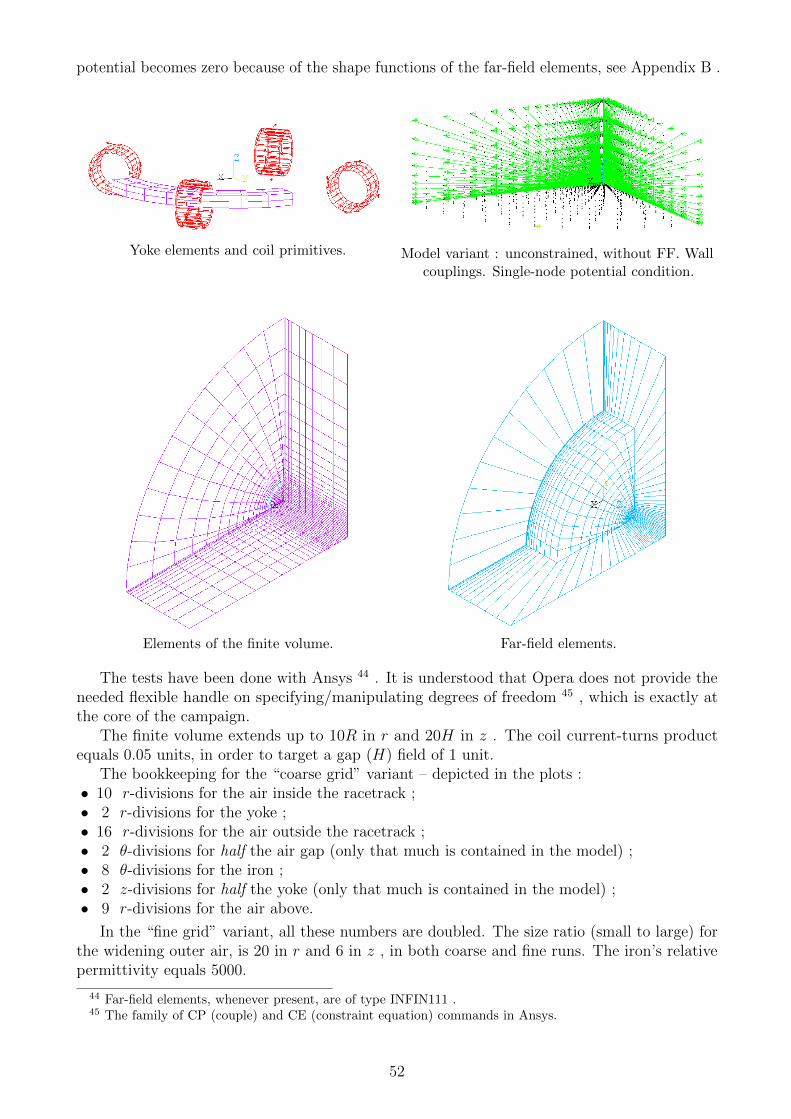
potential becomes zero because of the shape functions of the far-field elements, see Appendix B .

Yoke elements and coil primitives. Model variant : unconstrained, without FF. Wallcouplings. Single-node potential condition.

Elements of the finite volume. Far-field elements.

The tests have been done with Ansys 44 . It is understood that Opera does not provide theneeded flexible handle on specifying/manipulating degrees of freedom 45 , which is exactly atthe core of the campaign.

The finite volume extends up to 10R in r and 20H in z . The coil current-turns productequals 0.05 units, in order to target a gap (H) field of 1 unit.

The bookkeeping for the “coarse grid” variant – depicted in the plots :• 10 r-divisions for the air inside the racetrack ;• 2 r-divisions for the yoke ;• 16 r-divisions for the air outside the racetrack ;• 2 θ-divisions for half the air gap (only that much is contained in the model) ;• 8 θ-divisions for the iron ;• 2 z-divisions for half the yoke (only that much is contained in the model) ;• 9 r-divisions for the air above.

In the “fine grid” variant, all these numbers are doubled. The size ratio (small to large) forthe widening outer air, is 20 in r and 6 in z , in both coarse and fine runs. The iron’s relativepermittivity equals 5000.

44 Far-field elements, whenever present, are of type INFIN111 .45 The family of CP (couple) and CE (constraint equation) commands in Ansys.

52

It can be shown that (over)constraining both walls to zero value, is theoretically correct.But could acceptable results be obtained without such overconstraining ? Or, put differently,would overconstraining improve results to a meaningful extent ?

See the tables for the results. The air gap field at 0 and at 90 has always been the sameup to 5 digits ; it is denoted simply as H in the table. The obtained potential values V0 andV90 are for the xz and yz walls, respectively. In cases where the entire L-wall is coupled, weexpect the resulting potential value to be zero – or at worst, merely a handful orders away from“epsilon” 46 ; this is because of symmetry. The expectation does not always come true...

coarse grid unconstrained constrainedH = 0.8924 H = 0.9791

without FF V0 = 3.72 · 10−5 V0 = V90 = 4.2 · 10−8

V90 = −3.76 · 10−5

H = 0.9525 H = 0.9791with FF V0 = −3.02 · 10−4 V0 = V90 = −2.1 · 10−12

V90 = 3.02 · 10−4

fine grid unconstrained constrainedH = 0.9075 H = 0.9774

without FF V0 = 2.75 · 10−5 V0 = V90 = 2.3 · 10−7

V90 = −2.76 · 10−5

H = 0.9559 H = 0.9774with FF V0 = −2.47 · 10−4 V0 = V90 = −7.8 · 10−12

V90 = 2.47 · 10−4

Without far-field elements, the H results are poor for the unconstrained case, whereas thepotential value on the L-constrained wall is not as minute as expected. Refining the grid doesnot improve in a meaningful manner. Neither is the Difference Scalar Potential method theculprit. Indeed, tests with permanent magnet sectors replacing coils, give similar signature ;these tests have been done with the basic form of Scalar Potential. It all indicates that weshould better keep the far-field elements on board.

Admittedly, the test above was not very spectacular. However, more drama had unfolded inthe long history of modelling of the Spectrometer Magnet. Also there, the suggested method ofzero-value constraining is theoretically correct. But, between May 2018 and June 2019, the workstalled. The yoke field results differed in order 20% between constrained and unconstrained.Even more so, whenever a magnetic (but very simplified) Decay Tank was added, results becameoverwhelmingly unreliable (depending upon the case/variant). Back then, the far-field modellingwas done with legacy INFIN47 elements, not discussed in Appendix B . And the unconstrainedracetrack variant dicussed above, also failed much more spectacularly with INFIN47. Dedicatedelement stiffness testing revealed a bug 47 in the INFIN47 implementation. Since early Summer2019, all models are fitted with INFIN111, and confidence is re-established.

ConclusionIt appears that “playing” with the flux-normal condition can reveal – or increase the visibility

of – shortcomings or indeed anomalies in the model.

46 In numerical algebra, the smallest positive number for which 1.0 + ε > 1.0 still prevails in floating pointarithmetic. For IEEE 754 double/long precision (binary64) : ε ≈ 2 · 10−16 .

47 ... likely. Currently an active support ticket with Ansys Inc.

53

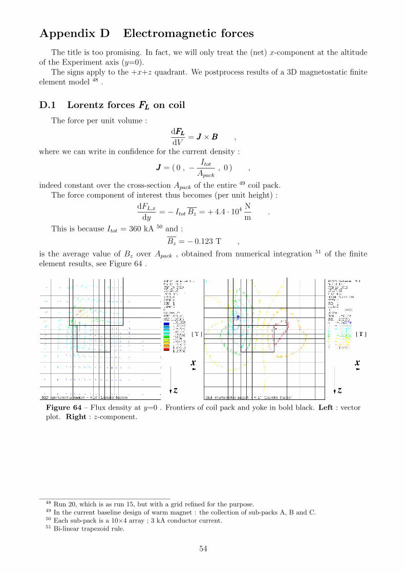
Appendix D Electromagnetic forces

The title is too promising. In fact, we will only treat the (net) x-component at the altitudeof the Experiment axis (y=0).

The signs apply to the +x+z quadrant. We postprocess results of a 3D magnetostatic finiteelement model 48 .

D.1 Lorentz forces FLFLFL on coil

The force per unit volume :

dFLFLFLdV

= JJJ ×BBB ,

where we can write in confidence for the current density :

JJJ = ( 0 , − ItotApack

, 0 ) ,

indeed constant over the cross-section Apack of the entire 49 coil pack.The force component of interest thus becomes (per unit height) :

dFL,xdy

= − ItotBz = + 4.4 · 104 N

m.

This is because Itot = 360 kA 50 and :

Bz = − 0.123 T ,

is the average value of Bz over Apack , obtained from numerical integration 51 of the finiteelement results, see Figure 64 .

Figure 64 – Flux density at y=0 . Frontiers of coil pack and yoke in bold black. Left : vectorplot. Right : z-component.

48 Run 20, which is as run 15, but with a grid refined for the purpose.49 In the current baseline design of warm magnet : the collection of sub-packs A, B and C.50 Each sub-pack is a 10×4 array ; 3 kA conductor current.51 Bi-linear trapezoid rule.

54

D.2 Maxwell tractions FMFMFM on inner yoke skin

We have – with Z0 = 1.75 m :

dFM,x

dy= − 1

2µ0

Int = − 4.7 · 104 N

m,

because :

Int =

∫ Z0

0

B2x dz = 0.118 T2 m ,

obtained from numerical integration of postprocessing FE path data, see Figure 65 .

[ m ]z

[ T ]xB

0.1

0.2

0.3

0.4

0.5

0.6

0 0.2 0.4 0.6 0.8 1 1.2 1.4 1.6

Figure 65 – Bx at the inner skin of the yoke, x = xyoke,min , y = 0 .

Note : the quadrature was trapezoidal on Bx , not on B2x . To illustrate this, take a function

f(u) and a quadrature segment [0,U] with f(0) = F1 and f(U) = F2 . We assume f(u) to varylinearly over the segment, not f 2(u) , and thus :

1

U

∫ U

0

f 2(u) du =F 21 + F1F2 + F 2

2

3.

The contribution of the outer yoke skin is neglected.

D.3 Interpretation

The two contributions annihilate each other,... or perhaps not ; difficult to tell in view of thenumerous approximations. In the end, it is not so important, because the residual obtained – oforder 3 103 N/m but highly uncertain – must be compared with the canonical vacuum effect,which is at least of order 2 105 N/m ! This residual can therefore be discarded in confidence.

55

Acknowledgement

We are indebted to P.-A. Giudici for his advice.

References

[1] The SHiP Collaboration, Technical Proposal. An Experiment to Search for Hidden Particles(SHiP) at the SPS, CERN-SPSC-2015-016, SPSC-P-350 (2015).Link to CERN Document Server page : https://cds.cern.ch/record/2007512

[2] Kurdej, J. , SHiP spectrometer magnet. OPERA simulations ; coil cooling design.

[3] Gyimesi, Lavers, Pawlak, Ostergaard, Biot-Savart Integration for Bars and Arcs, IEEETrans. Magn. , Vol.29 , No.6 , (1993).

[4] Simkin, Trowbridge, On the use of the Total Scalar Potential in the numerical solution offield problems in electromagnetics, Int. J. Num. Meth. Eng. , Vol.14 , pp. 423-440, (1979).

[5] Mayergoyz, Chari, D’Angelo, A new Scalar Potential formulation for three-dimensionalmagnetostatic problems, IEEE Trans. Magn. , Vol.23 , No.6 , (1987).

[6] Zienkiewicz, Taylor, Zhu, The Finite Element Method : Its Basis and Fundamentals , 6thEd., Elsevier, ISBN 0 7506 6320 0 , (2005). Section 5.14.

[7] Ansys Mechanical APDL, Theory Reference, section 13.110 , (on-line).

[8] Eurocode 3 - Calcul des structures en acier

• 6.6 Assemblages soudes• ANNEXE M (Normative) Autre methode possible de calcul des soudures d’angle

ANSYS R© (finite element software) is a trademark of ANSYS Inc. , Canonsburg, PA, USA.

OPERA (software for electromagnetic design) is commercialized by Dassault Systemes,Velizy-Villacoublay, F. It was previously from Vector Fields Ltd., UK , then from COBHAMplc., UK.

56