Alexander Edström

Theoretical Magnet Design

From the electronic structure of solid matter to new

permanent magnets.

Abstract

A good permanent magnet should possess a large saturation magnetisation (Ms), large mag-

netocrystalline anisotropy energy (MAE) and a high Curie temperature (TC). A difficult but

important challenge to overcome for a sustainable permanent magnet industry is to find novel

magnetic materials, exhibiting a large MAE, without the use of scarcely available elements

such as rare-earth metals. The purpose of this thesis is to apply computational methods, includ-

ing density functional theory and Monte Carlo simulations, to assess the three above mentioned

permanent magnet properties and in particular to discover new replacement materials with large

MAE without the use of critical materials such as rare-earths.

One of the key results is the theoretical prediction of a tetragonal phase of Fe1−xCox-C with

large Ms and significantly increased MAE which is later also experimentally confirmed. Fur-

thermore, other potential materials are surveyed and in particular the properties of a number of

binary alloys in the L10 structure, FeNi, CoNi, MnAl and MnGa, are thoroughly investigated

and shown to posses the desired properties under certain conditions.

AcknowledgementsFirstly, I wish to thank my supervisor, Jan Rusz, for all his kind and invalu-able guidance through the work behind this thesis. I also thank my secondsupervisor, Olle Eriksson, for sharing his knowledge and wisdom as well asfor providing a positive and encouraging research environment at the divisionof materials theory. Furthermore, I would like to thank Mirosław Werwinskiand Pablo Maldonado for their company, for answering many questions, ques-tioning many answers and for all the discussions on physics, Feynman, Bono-bos and all the other stuff. Finally, I am grateful to all my other colleaguesat the division of materials theory, those I have worked with at other partsof the Ångström laboratory and to collaborators from the REFREEPERMAGproject.

List of papers

This thesis is based on the following papers, which are referred to in the textby their Roman numerals.

I Stabilization of the tetragonal distortion of FexCo1−x alloys by C

impurities - a potential new permanent magnet

E. K. Delczeg-Czirjak, A. Edström, M. Werwinski, J. Rusz, N. V.Skorodumova, L. Vitos, and O. Eriksson.Phys. Rev. B 89, 144403 (2014).

II Increased magnetocrystalline anisotropy in epitaxial Fe-Co-C thin

films with spontaneous strain

L. Reichel, G. Giannopoulos, S. Kauffman-Weiss, M. Hoffmann, D.Pohl, A. Edström, S. Oswald, D. Niarchos, J. Rusz, L. Schultz, S.Fähler.Submitted.

III Electronic structure and magnetic properties of L10 binary alloys

A. Edström, J. Chico, A. Jakobsson, A. Bergman, J. Rusz.Phys. Rev. B 90, 014402 (2014) .

Reprints were made with permission from the publishers.

Contents

1 Introduction . . . . . . . . . . . . . . . . . . . . . . . . . . . . . . . . . . . . . . . . . . . . . . . . . . . . . . . . . . . . . . . . . . . . . . . . . . . . . . . . . . . . . . . . . . . . . . . . . . 9

2 Elements of the Theory of Magnetism . . . . . . . . . . . . . . . . . . . . . . . . . . . . . . . . . . . . . . . . . . . . . . . . . . . . . 112.1 Relativistic Electrons . . . . . . . . . . . . . . . . . . . . . . . . . . . . . . . . . . . . . . . . . . . . . . . . . . . . . . . . . . . . . . . . . . . . . 11

2.1.1 Non-Relativistic Limit and the Scalar RelativisticApproximation . . . . . . . . . . . . . . . . . . . . . . . . . . . . . . . . . . . . . . . . . . . . . . . . . . . . . . . . . . . . . . . . . 13

2.1.2 Spin-Orbit Coupling and the MagnetocrystallineAnisotropy . . . . . . . . . . . . . . . . . . . . . . . . . . . . . . . . . . . . . . . . . . . . . . . . . . . . . . . . . . . . . . . . . . . . . . . . 14

2.2 Exchange Interactions and the Heisenberg Hamiltonian . . . . . . . . . . . . . 16

3 Computational Methods . . . . . . . . . . . . . . . . . . . . . . . . . . . . . . . . . . . . . . . . . . . . . . . . . . . . . . . . . . . . . . . . . . . . . . . . . . . . 213.1 Density Functional Theory . . . . . . . . . . . . . . . . . . . . . . . . . . . . . . . . . . . . . . . . . . . . . . . . . . . . . . . . . . . . 21

3.1.1 FP-LAPW . . . . . . . . . . . . . . . . . . . . . . . . . . . . . . . . . . . . . . . . . . . . . . . . . . . . . . . . . . . . . . . . . . . . . . . . 233.1.2 SPR-KKR . . . . . . . . . . . . . . . . . . . . . . . . . . . . . . . . . . . . . . . . . . . . . . . . . . . . . . . . . . . . . . . . . . . . . . . . . 233.1.3 Models to Treat Disorder . . . . . . . . . . . . . . . . . . . . . . . . . . . . . . . . . . . . . . . . . . . . . . . . 243.1.4 Computing the MAE . . . . . . . . . . . . . . . . . . . . . . . . . . . . . . . . . . . . . . . . . . . . . . . . . . . . . . . 263.1.5 Exchange Coupling Parameters . . . . . . . . . . . . . . . . . . . . . . . . . . . . . . . . . . . . . . 30

3.2 Monte Carlo Simulations . . . . . . . . . . . . . . . . . . . . . . . . . . . . . . . . . . . . . . . . . . . . . . . . . . . . . . . . . . . . . . . 30

4 Results . . . . . . . . . . . . . . . . . . . . . . . . . . . . . . . . . . . . . . . . . . . . . . . . . . . . . . . . . . . . . . . . . . . . . . . . . . . . . . . . . . . . . . . . . . . . . . . . . . . . . . . . 334.1 Fe1−xCox Alloys . . . . . . . . . . . . . . . . . . . . . . . . . . . . . . . . . . . . . . . . . . . . . . . . . . . . . . . . . . . . . . . . . . . . . . . . . . . . . 33

4.1.1 (Fe1−xCox)-C . . . . . . . . . . . . . . . . . . . . . . . . . . . . . . . . . . . . . . . . . . . . . . . . . . . . . . . . . . . . . . . . . . . 344.1.2 (Fe1−xCox)-B . . . . . . . . . . . . . . . . . . . . . . . . . . . . . . . . . . . . . . . . . . . . . . . . . . . . . . . . . . . . . . . . . . . 35

4.2 L10 Binary Compounds . . . . . . . . . . . . . . . . . . . . . . . . . . . . . . . . . . . . . . . . . . . . . . . . . . . . . . . . . . . . . . . . . 364.3 Other Potential Materials . . . . . . . . . . . . . . . . . . . . . . . . . . . . . . . . . . . . . . . . . . . . . . . . . . . . . . . . . . . . . . . 38

4.3.1 (Fe1−xCox)2B . . . . . . . . . . . . . . . . . . . . . . . . . . . . . . . . . . . . . . . . . . . . . . . . . . . . . . . . . . . . . . . . . . . 384.3.2 Heusler Alloys . . . . . . . . . . . . . . . . . . . . . . . . . . . . . . . . . . . . . . . . . . . . . . . . . . . . . . . . . . . . . . . . . 40

5 Conclusions . . . . . . . . . . . . . . . . . . . . . . . . . . . . . . . . . . . . . . . . . . . . . . . . . . . . . . . . . . . . . . . . . . . . . . . . . . . . . . . . . . . . . . . . . . . . . . . . 42

References . . . . . . . . . . . . . . . . . . . . . . . . . . . . . . . . . . . . . . . . . . . . . . . . . . . . . . . . . . . . . . . . . . . . . . . . . . . . . . . . . . . . . . . . . . . . . . . . . . . . . . . . 44

1. Introduction

Albeit being a phenomena known since ancient times, to this day magnetismremains under vast research activity due to its theoretical complexity and far-reaching technological importance. One important field for magnetic materialsis found in the area of permanent magnets [1, 2, 3, 4, 5] with applications inlarge scale industries including those for motors, generators and actuators.With a growing demand from emerging industries, such as that of wind powergeneration, the need of sustainable high performance permanent magnets isgreater than ever.

In the last decades of the 20th century came the development of perma-nent magnets consisting of compounds of rare-earths and transition metals,such as SmCo5 and Nd2Fe14B which to this day possess properties supe-rior to all alternatives. However, in recent years due to economic reasons,a need for alternative materials which do not contain rare-earth elements hasarisen [6, 1, 4]. The figures of merit of a permanent magnet are the coercivityHc and the energy product (BH)max, and in addition to this a high Curie tem-perature is needed in order for the magnets to operate with good performanceat reasonable temperatures. The extrinsic property requirement of high coer-civity and large energy product translates, in terms of intrinsic properties, intoa large saturation magnetisation Ms and magnetocrystalline anisotropy energy(MAE). Table 1.1 contains a summary of relevant properties of some of themost common rare-earth permanent magnets, one of the common alternativematerials, namely ferrite magnet BaFe12O19 and for comparison also transi-tion metals bcc Fe and hcp Co. It is apparent that the remarkable propertiesof the rare-earth based magnets stem from their large MAE. As a matter, offact the cheap and highly abundant bcc Fe has higher Ms and TC than the rare-earth magnets, but the MAE is orders of magnitude smaller making bcc Feuseless as a permanent magnet. As will become clear in chapter 2 there aretwo reasons for the MAE being so low in Fe while it is so high in for ex-ample Nd2Fe14B; first of all the cubic bcc crystal of Fe does not allow forthe large MAE mainly found in uniaxial crystals and secondly the MAE isclosely related to the spin-orbit coupling which tends to be strong in heavyelements in the lower part of the periodic table. These elements are often alsoless abundant which is the main challenge in finding new materials suitable aspermanent magnets and the main purpose of this thesis is to provide potentialsolutions to this problem.

One useful path to finding new materials with the desired properties isthrough computational methods, such as electronic structure calculations, which

9

Table 1.1. A summary of the properties of some high performing rare-earth magnets,

a ferrite alternative and the transition metals bcc Fe and hcp Co. The relevant perma-

nent magnet properties provided are Curie temperature (TC), coercivity (Hc), energy

product ((BH)max), saturation magnetisation (Ms), and magnetocrystalline anisotropy

energy (MAE). Data was taken from Ref. [1, 7, 8]. The extrinsic properties depend

on the microstructure of the material and should be considered an estimate of what is

practically realisable.

Nd2Fe14B SmCo5 BaFe12O19 bcc Fe hcp CoTC (K) 588 1020 740 1043 1388μ0Hc (T) 1.21 0.90 0.15 7 ·10−5 5 ·10−3

(BH)max (kJ/m3) 512 231 45 - -μ0Ms (T) 1.61 1.22 0.48 2.21 1.81MAE (MJ/m3) 4.9 17.2 0.33 0.048 0.53

allow for exploring the properties of various materials with relative ease com-pared to experimental work and it is this path which is to be taken in thisthesis. Density functional theory (DFT) provides a powerful tool for study-ing the electronic structure and ground state properties of materials, includingthe Ms and MAE which are essential for permanent magnets. In combinationwith other computational methods, such as Monte Carlo (MC) simulations,also the Curie temperature can be determined and hence all of the three mainproperties of interest are obtainable.

This thesis will begin with an overview of those parts of the theory of mag-netism especially important for this work in Chapter 2. In particular the rel-ativistic spin-orbit coupling and its relation to MAE will be brought up inSec. 2.1 and exchange interactions and the Heisenberg Hamiltonian which re-sult in spontaneous magnetic ordering will be briefly discussed in Sec. 2.2.The relevant computational methods will then be introduced in Chapter 3 withDFT being discussed in Sec. 3.1 and MC in 3.2. In Chapter 4 the main re-sults, based on the work presented in papers I-III, are summarized. Theseresults mainly regard two groups of materials. Firstly C-doping is suggestedas a method of causing a tetragonal distortion in FeCo alloys in paper I, whichis then experimentally realized in paper II. The properties of various binaryalloys in the L10 structure are then explored in paper III and found to showpromising qualities under certain conditions. In addition to this a brief surveyis given over other materials which might be of interest in a permanent magnetcontext.

10

2. Elements of the Theory of Magnetism

This chapter gives an introduction and overview of those areas of the theoryof magnetism which are most important to understand the theoretical aspectsof permanent magnets most relevant to the work behind this thesis. It begins,in Sec. 2.1, by discussing the relativistic nature of magnetism and in particularin Sec. 2.1.2, the spin-orbit coupling and its relation to the magnetocrystallineanisotropy. It continues in Sec. 2.2 by discussing the exchange interactionswhich lead to magnetic ordering and how it can be described in terms of ex-change coupling parameters and the Heisenberg Hamiltonian.

2.1 Relativistic ElectronsMagnetism arises due to the quantum mechanical spin or orbital angular mo-mentum of electrons. The spin angular momentum was initially rather arti-ficially introduced into the theory of quantum mechanics to explain the finestructure of the hydrogen atom [9]. It was not until Dirac introduced a rela-tivistic wave equation [10, 11] for the electron that the spin became well un-derstood as an intrinsic angular momentum necessary for a Lorentz symmet-ric version of quantum mechanics. Moreover, relativistic effects neglected inthe Schrödinger equation are of importance in describing electrons in atomiccore states and the relativistic spin-orbit coupling, which will be discussedfurther later on, brings in a rich new array of physical phenomena includingthe magnetocrystalline anisotropy which is essential for the field of permanentmagnets.

The Dirac equation may, including electromagnetic interactions, be writtenin the following way [12][

γμ(i∂μ − eAμ

)−m]

ψ = 0, (2.1)

where e is the electron charge, γμ are the Dirac matrices, Aμ is the electro-magnetic potential and m is the electron mass. Alternatively it might, afterseparating out the time dependence, be written[

α · (−i∇− eA)+ eV +βm]

ψ = Eψ, (2.2)

where A is the magnetic vector potential, V is the scalar potential,

β = γ0 =

(I2×2 0

0 −I2×2

)and α =

(0 σσ 0

), (2.3)

11

where σ = (σx,σy,σz) contains the Pauli matrices. In principle, Eq. 2.2 willprovide all of the information required to understand the magnetic phenomenadiscussed here and it is the equation which is solved for all electrons in theSPR-KKR method and for the core electrons only in the FP-LAPW method,as will be further discussed in Sections 3.1.1-3.1.2. Often however, solvingEq. 2.2 is more complicated than what is necessary to describe the phenomenaof interest with good accuracy, so that simplifications and approximations canbeneficially be applied. One such simplification is to expand the equation inthe non-relativistic limit v/c � 1 as discussed in Sec. 2.1.2. This naturallyintroduces a term describing the spin-orbit coupling, which is essential formagnetocrystalline anisotropy, and allows for applying the so called scalarrelativistic approximation.

For spherically symmetric potentials, such as the Coulomb potential forhydrogen-like atoms, certain exact analytical results can be obtained for theDirac equation [12, 13]. The solution may in general be written [12]

ψkj,m(r,θ ,φ) =

(f k(r)Y k

j,m(θ ,φ)

igk(r)Y −kj,m (θ ,φ)

), (2.4)

where f and g are two-component radial dependent functions, Y kj,m(θ ,φ)

are generalised spherical harmonics, j,m denote the total angular momentumquantum numbers and

k =

{l if l = j+ 1

2

−(l +1) if l = j− 12

(2.5)

is a quantum number related to the parity of the solution. The generalisedspherical harmonics are related to regular spherical harmonics, Yl,m, accordingto

Ykj,m(θ ,φ) =−sgnk

√k+ 1

2 −m

2k+1αY

l,m− 12+

√k+ 1

2 +m

2k+1βY

l,m+ 12, (2.6)

where

α =

(10

)β =

(01

). (2.7)

Here can be noted that the orbital or spin angular momentum operators in-dividually do not commute with the Dirac Hamiltonian while total angularmomentum and parity do. Typically in solid matter, those electrons for whichrelativistic effects tend to be important are tightly bound core states. Theseare also, to a very good approximation, in a spherical potential so that it isappropriate to describe them with solutions of the form given in Eq. 2.4.

12

2.1.1 Non-Relativistic Limit and the Scalar RelativisticApproximation

If one does not wish to work with the full four-component Dirac formalismintroduced in the previous section but still wishes to retain certain relativisticeffects, it is appropriate to make an expansion in the non-relativistic limit,vc� 1, and only keep terms up to a certain order. The first step in doing so is

to assume a solution of the form [12]

ψ(r) =

(χ(r)η(r)

), (2.8)

where χ and η each has two components. A useful next step is to performa Foldy-Wouthuysen transformation, where one introduces a hermitian andunitary operator

U =U−1 =U† = Aβ +α ·p2m

A =

√1− p2

4m2 . (2.9)

Transforming the Dirac equation according to H ′ = UHU−1 and ψ ′ = Uψ ,

performing some algebra and eventually only keeping terms to order(

vc

)2

leads to a decoupling of χ and η and a Hamiltonian

H =(p− eA)2

2m+ eV − e

2mσ ·B− p4

8c2m3 +e∇2V

8c2m2 +eh

4c2m2 σ · (∇V ×p) .

(2.10)The first three terms in this equation make up the non-relativistic SchrödingerHamiltonian, including the Zeeman term

HZeeman =− e

2mσ ·B, (2.11)

where B = ∇×A is the magnetic flux density. After that comes a so called

mass correction term − p4

8c2m3 , the Darwin term e∇2V8c2m2 and finally the spin-orbit

coupling (SOC) e4c2m2 σ · (∇V ×p) which, if one assumes the scalar potential

to be spherically symmetric, takes on the more common form

HSOC =e

4c2m2r

dV (r)

drσ ·L = ξ L ·S, (2.12)

where L = r×p is the orbital angular momentum operator, S = h2 σ is the spin

operator and

ξ =e

2hc2m2r

dV (r)

dr(2.13)

is the spin-orbit coupling constant. Furthermore, for the spherical potential ofa hydrogen-like atom, the SOC constant is [7]

ξ =mZ4α4c2

2n3l(l + 12)(l +1)

, (2.14)

13

where Z is the atomic number, α = e2

hcis the fine structure constant and n

and l denote principal and angular momentum quantum numbers, respectively.From this expression it is clear that the SOC becomes particularly importantfor states with low angular momentum in heavy atoms with large Z. This isthe source to one of the main challenges in obtaining magnetic materials withlarge MAE without the use of scarcely available and expensive elements. Alarge MAE requires a large Z but materials with Z significantly larger than thevalue of Z = 26 for Fe tend to be much less abundant than those elements withsmaller Z. Furthermore, such elements are typically not magnetic.

The above Hamiltonian in Eq. 2.10 acts on a two-component spinor

ψ(r) =

(ψ+

ψ−

), (2.15)

where ψ+ and ψ− represent spin up and spin down electrons, respectively.The SOC term is the only term in Eq. 2.10 containing off-diagonal terms andhence coupling the spin up and spin down electrons to each other. Ignoringthe SOC and using only the diagonal terms in the Hamiltonian is known as thescalar relativistic approximation.

2.1.2 Spin-Orbit Coupling and the MagnetocrystallineAnisotropy

Magnetocrystalline anisotropy is the internal energy dependence on magneti-sation direction, i.e. E = E(M), where M = (sinθ cosφ ,sinθ sinφ ,cosθ) isthe direction of the magnetisation relative to the crystal lattice. This effectwas first experimentally observed and described phenomenologically, basedon anisotropy constants and crystal symmetries. For example, in a uniaxialcrystal the energy may be written [8]

E = Eiso +K1 sin2 θ +K2 sin4 θ +K3 sin6 θ +K4 sin6 θ cos6φ + ..., (2.16)

where Eiso contains all isotropic energy contributions, Ki are the anisotropyconstants and θ and φ are the angles describing the magnetisation direction asgiven above. For a cubic structure on the other hand, the energy is

E = Eiso +K1(α21 α2

2 +α21 α2

3 +α22 α2

3 )+K2α21 α2

2 α23 + ..., (2.17)

where αi are the directional cosines of the magnetisation direction.That the microscopic origin of this anisotropy is related to the SOC, intro-

duced in the previous section, was suggested by Van Vleck [14], as this is thelink coupling the spin to the real space crystal symmetry via the orbital angularmomentum. If we are mainly interested in the transition metal d-electron mag-netism, then the SOC can be considered as a perturbation. The SOC energy

14

shift to second order is

ESOC = ξ ∑n

〈n|L ·S |n〉+ξ 2 ∑n �=k

∣∣〈n|L ·S |k〉∣∣2En−Ek

, (2.18)

where |n〉 and |k〉 denote eigenstates of the unperturbed Hamiltonian and En

and Ek are the associated energy eigenvalues. When considering d-electronsin a solid with a crystal field lifting the degeneracy of the d-orbitals, there isa quenching of orbital angular momentum [15, 16] because 〈L〉= 〈i|L |i〉= 0for any non-degenerate states |i〉, so that the diagonal matrix elements of theSOC Hamiltonian appearing in the first order term of the perturbation expan-sion are all zero. Furthermore, if both |n〉 and |k〉 are occupied or if both areunoccupied, there is a cancellation of terms in the sum so that the only termswhich need to be included are those which couple occupied and unoccupiedstates. Hence, we can express the SOC, based on second order perturbationtheory, as

ESOC = ξ 2 ∑occ. n

unocc. k

∣∣〈n|L ·S |k〉∣∣2En−Ek

, (2.19)

where the summation is over all occupied states |n〉 and unoccupied states |k〉.For uniaxial crystals, the expression in Eq. 2.19 is non-zero and the MAE is oforder ξ 2. For a cubic crystal on the other hand, the second order perturbationterm is also zero and one would have to go to fourth order perturbation theoryto find non-zero contributions to the MAE [17]. Hence, cubic materials tendto have orders of magnitude smaller MAE than uniaxial ones and this explainswhy the MAE of bcc Fe is so much smaller than that of hcp Co, as was seen intable 1.1. Therefore, in searching for good permanent magnet materials withlarge MAE, one should focus on materials with non-cubic crystal structures.Eq. 2.19 also provides another key insight for the search of transition metalbased magnets with large MAE. When there is a weak SOC and hence a smallξ , the only way to obtain a large value for MAE is to have a large number ofoccupied states |n〉 and unoccupied states |k〉 with a small energy differenceEn−Ek. The optimal 3d based permanent magnet material should therefore beone with a uniaxial crystal structure and flat energy bands close to each otherjust above and below the Fermi energy. This insight was used by Burkert et

al. [18] to explain the unusually large MAE of certain compositions of tetrag-onally strained Fe1−xCox, which provides an important background for thework in papers I-II, and it is discussed further in Sec. 4.1.1. Similar argumentshave also been used, for example, by Costa et al. [19] to analyze the largeMAE of Fe2P and insightful illustrations of how the MAE depends sensitivelyon the band structure around the Fermi energy are provided in Ref. [20].

Based on a perturbation expression such as that in Eq. 2.19, assuming thatthe exchange splitting is significantly larger than the SOC and ignoring spin-flip terms and deformations of the Fermi surface, Bruno [21] found a simple

15

relation between the MAE and the orbital moment anisotropy which states that

EMAE = ΔESOC =ξ

4G

HΔL =

ξ

4ΔL, (2.20)

if ξ = ξ GH

and G and H are density of states integrals which should often be ofsimilar size so that ξ ∼ ξ . Eq. 2.20 tends to give a qualitatively correct descrip-tion in that there is a proportionality between the change in the orbital momentand the SOC and that the easy axis coincides with the direction where the or-bital moment has its maximum. It happens, however, that the relation breaksdown, for example due to hybridisation effects in complex materials [22]. Onoccasion Eq. 2.20 has also been incorrectly applied in explaining the origin oflarge MAE in transition metal alloys, such as FeNi [23, 24], as being due toanisotropy in the orbital moment. This way of looking at it is incorrect in thesense that Eq. 2.20 does not provide causality in the relation between EMAEand ΔL but the relation between the two quantities is rather due to the origin ofboth being the SOC. The key to understanding the MAE of a crystalline solidlies instead in the SOC and the details of the band structure near the Fermienergy, as revealed by Eq. 2.19.

Fig. 2.1 shows how the energy and orbital, as well as spin moments varywith the angle between the magnetisation direction and the z-direction as themagnetisation direction varies from [001] to [100]-direction, based on calcula-tions done with WIEN2k. From Fig. 2.1b, which shows the change in energyplotted against the change in orbital moment, it is clear that there is a propor-tionality between these two quantities as predicted by Eq. 2.20 and that theeasy axis of magnetisation coincides with direction where the orbital momenthas its maximum. In Fig. 2.1c one can also observe that, as pointed out inreferences [23, 24], the largest change in orbital moment is on the Fe atomwhile that on the Ni atom is smaller and of opposite sign.

2.2 Exchange Interactions and the HeisenbergHamiltonian

The quantised spin and orbital angular momentum and the associated magneticmoments allow us to understand the appearance of para- and diamagnetism.To understand spontaneous magnetic ordering, such as ferro-, ferri- or anti-ferromagnetism, we need to include also an interaction between the atomicmagnetic moments. Interactions, such as dipole-dipole, between atomic mo-ments are typically negligibly small and would not allow magnetic orderingat the significant temperatures where it is observed. The relevant interac-tion is instead the exchange interaction due to the Coulomb repulsion and thefermionic character of electrons. This can be seen, for example, in movingfrom Hartree to Hartree-Fock theory where the inclusion of antisymmetry of

16

0 20 40 60 80

0

10

20

30

40

Angle (deg)

ΔES

OC

(μe

V/a

tom

)

(a) Change in total energy as function ofangle between magnetisation direction andz-axis.

−3 −2 −1 0

0

10

20

30

40

ΔmL (10−3μ

B/atom)

ΔES

OC

(μe

V/a

tom

) Calculated pointsLinear fit

(b) Change in energy versus change in or-bital moment as angle is varied.

0 20 40 60 8035

40

45

50

Angle (deg)

mL (

10−

3 μ B/a

tom

)

FeNi

(c) Orbital moment as a function of angle.

0 20 40 60 800.5

1

1.5

2

2.5

3

Angle (deg)

mS (

μ B/a

tom

)

FeNi

(d) Spin moment as a function of angle.

Figure 2.1. Variations in energy and moments of FeNi as functions of the angle θbetween the direction of magnetisation and the z-axis.

the wavefunction leads to an exchange term, which results in a lowering ofenergy for parallel spin ordering [15]. From, for example, the Heitler-Londonmodel one can see that localised spins tend to interact in a way so that theenergy is proportional to the scalar product of the spin operators [16]. Eventhough the Heitler-London model only describes a simple system consistingof two atoms with one localised electron each, the result regarding the form ofthe spin-spin interaction turns out to be rather general and in many cases welldescribes also magnetism in a solid [15, 16]. This result is represented by theHeisenberg Hamiltonian

HHeisenberg =−12 ∑

i�= j

Ji jSi ·S j, (2.21)

where Si and S j are the atomic spins on sites i and j respectively and Ji j isthe exchange coupling parameter between these spins. For a magnetic systemdescribed by Eq. 2.21 the magnetic ordering and its TC is now determined bythe exchange coupling parameters Ji j. For a given material, these parameterscan be obtained from the electronic structure as discussed in Sec. 3.1.5. Once

17

one has the Ji j, one can then study the magnetic ordering and transition tem-peratures via, for example, Monte Carlo simulations which will be discussedin Sec. 3.2. One can also estimate magnetic transition temperatures via meanfield theory, according to which [15, 25]

TC =J0S(S+1)

3kB, (2.22)

where S is the atomic spin, J0 = ∑i J0i is the sum of the exchange interactionsand kB is the Boltzmann constant, from which it is clear that the Curie tem-perature is proportional to the strength of the exchange interactions. Eq. 2.22overestimates the transition temperature by around twenty percent or more de-pending on dimensionality and coordination number [15], but can be useful ineffortlessly establishing an upper limit for TC and it is applied to some extentand compared with MC results in Paper III.

In ferromagnetic metals, which are the materials of main interest in thisthesis, the exchange coupling tends to be mediated by conduction electronsand the coupling is said to be of RKKY-type. The typical form of the ex-change coupling parameters in such a system is, asymptotically in the longrange limit [25],

JRKKYi j ∼ n4/3 sin(2kFRi j)−2kFRi j cos(2kFRi j)

(kFRi j)4 , (2.23)

where n is the density of conduction electrons, kF is the Fermi wave vector andRi j is the distance between sites i and j. Eq. 2.23 shows how RKKY-type inter-actions exhibit an oscillatory behaviour with a long range decay proportionalto R−3

i j . Strictly speaking, Eq. 2.23 is derived assuming localised moments ina metal and only in this type of system one can formally expect the Heisen-berg Hamiltonian with exchange coupling parameters given by Eq. 2.23 to bea good model. Hence, one would not expect the model to work for magnetic3d metals as these tend to exhibit itinerant ferromagnetism with an exchangesplitting of the conduction bands. However, it turns out that the same type ofbehaviour is often found also in itinerant ferromagnets [26, 27].

Fig. 2.2 illustrates the exchange coupling parameters for Fe and random al-loy Fe0.4Co0.6 in the bcc structure, calculated by the SPR-KKR method whichis described in the next chapter. Fig. 2.2b illustrates that the exchange cou-pling parameters decay approximately as R−3

i j , as expected from Eq. 2.23. InFig. 2.2c it is seen that the strength of the Fe-Fe interactions increase as Cois alloyed into the material while also Fe-Co and Co-Co interactions are verystrong. This explains the observed effect that TC increases as one alloys Cointo bcc Fe [28] and application of mean field theory on the exchange cou-pling parameters in Fig. 2.2 results in TC = 1298 K and TC = 1554 K for Feand Fe0.4Co0.6 respectively. Looking at Eq. 2.23 it can be speculated that theincrease in the strength of the Ji j is due to an increase in the density of con-duction electrons as Co is added into the material.

18

0 2 4 6

0

5

10

15

Rij / a

J ij (m

eV)

(a) bcc Fe

0 2 4 6

−50

0

50

Rij / a

Rij3

⋅ Jij (

a3⋅ m

eV)

(b) bcc Fe

0 2 4 6

0

10

20

30

Rij / a

J ij (m

eV)

Fe-FeFe-CoCo-Co

(c) bcc Fe0.4Co0.6

Figure 2.2. Exchange coupling parameters, Ji j, for bcc Fe and bcc Fe0.4Co0.6, asa function of interatomic distances. 2.2b shows Ji j ·R3

i j to illustrate the RKKY-typelong-range behavior of exchange interactions in bcc Fe.

19

The Hamiltonian in Eq. 2.21 is rotationally invariant and hence does notinclude any form of magnetic anisotropy. The Heisenberg Hamiltonian can beexpanded with a term to take into account magnetocrystalline anisotropy andin the case of a uniaxial crystal, based on Eq. 2.16 if one keeps only the twofirst anisotropy constants, such a Hamiltonian is

HMAE = ∑i

[K1(mi · ez)

2 +K2(mi · ez)4], (2.24)

where mi is the direction of the moment at site i and ez is the direction of thecrystal axis.

20

3. Computational Methods

This chapter provides a brief description of the computational methods utilisedin the work behind this thesis. Density functional theory (DFT) [29, 30, 31]is used to calculate ground state properties of materials and it is described inSec. 3.1. In particular the full potential linearised augmented plane waves andthe spin polarised relativistic KKR methods are used to solve the DFT equa-tions and an introduction to these methods is given in Sec 3.1.1 and Sec. 3.1.2.As we are interested in disordered alloys, models to describe these are dis-cussed in Sec. 3.1.3 while Sec. 3.1.4 provides a discussion on specifics re-garding the computation of MAE. In order to calculate Curie temperatures,Monte Carlo simulations [32] are employed as discussed in Sec. 3.2.

3.1 Density Functional TheoryDensity functional theory (DFT) is our method of choice for finding the groundstate solution to an N-electron Schrödinger equation of the form⎛

⎝− h2

2m

N

∑i=1

∇2i +

N

∑i

Vext(ri)+12

N

∑i�= j

w(∣∣ri− r j

∣∣)⎞⎠Ψ = EΨ, (3.1)

where Vext(r) is an external potential, w(∣∣ri− r j

∣∣) is a Coulomb interactionbetween an electron at ri and one at r j and Ψ is an N-electron wavefunction.The first key ingredients of DFT are the Hohenberg-Kohn theorems [33] whichallow us to focus on electron densities, rather than wavefunctions, and findingthe ground state properties of the system by minimising the total energy as afunctional with respect to the density. The practical method of doing this isprovided by the Kohn-Sham approach[34] where the many-body problem inEq. 3.1 is simplified to a number of single particle problems(

− h2

2m∇2 +Veff(r)

)ψi(r) = εiψi(r), (3.2)

where εi and ψi are the Kohn-Sham eigenvalues and orbitals which, in gen-eral, individually lack clear physical interpretation, although the ground statedensity is

n(r) =N

∑i

∣∣ψi(r)∣∣2 , (3.3)

21

with summation over the N eigenstates with lowest energy. In making thissimplification, we have introduced the effective single particle potential

Veff(r) =Vext(r)+∫

dr′n(r)

|r− r′| +δExc[n(r)]

δn(r), (3.4)

including the exchange-correlation potential Vxc =δExc[n(r)]

δn(r) , which containsthe many-body effects. This unknown quantity, Vxc, is the cost of our simpli-fication from a many-electron wavefunction into single particle problems andfinding good approximations for Vxc is the grand challenge in making DFT ac-curate and useful. For some very simple model systems it might be possible tofind an exact exchange-correlation functional [35] but realistic systems mustbe treated by approximations. The most commonly used approximations forthe exchange-correlation potential are the local density approximation [36, 37](LDA), which locally approximates the Vxc(r) with that of a homogeneouselectron gas with the same density n(r), and the generalised gradient approxi-mation [38] (GGA), which also takes into account gradients in the density. Formany systems, these approximations are sufficient to reproduce ground stateproperties with satisfying accuracy although for so called strongly correlatedsystems other corrections, such as LDA+U [29, 30] or dynamical mean fieldtheory (DMFT) [39, 30], are required.

In this thesis, we are mainly interested in the magnetic properties of 3dmetals and their alloys and compounds. For these systems GGA tends to ac-curately describe the desired properties[40, 41, 42], whereby this is the mainexchange-correlation potential employed in the calculations behind this work.

In the discussion above no spin dependence was included. In order todescribe magnetism, spin polarised DFT must be used. The density shouldthen be split up into spin up and spin down parts so n(r) = n↑(r) + n↓(r)and spin dependence should be included into the effective potential. Fur-thermore, as discussed in Sec. 2.1, relativistic effects are often important andcan be taken into account, for example by solving the Dirac equation ratherthan the Schrödinger equation or by using the scalar relativistic approxima-tion discussed in Sec. 2.1.1. In particular, spin-orbit coupling is essential forcalculating magnetocrystalline anisotropy and specifics regarding this will bediscussed in Sec. 3.1.4.

The next step in DFT is to solve the equations in Eq. 3.2. Many methodshave been developed for doing this and, as usual in numerical problem solv-ing, one typically needs to weigh computational speed against accuracy andgenerality. Those methods of solving the Kohn-Sham equations which areused in the work behind this thesis will be briefly described in the coming twosections. Since the density, which is calculated from the solutions ψi, is alsoneeded to calculate the potential Veff which appears in the equations, the prob-lem is solved self-consistently by iteration until a solution is converged withrequired accuracy.

22

3.1.1 FP-LAPWOne of the computational methods used here is the full potential linearisedaugmented plane waves [43] (FP-LAPW) method as implemented in the WIEN2kcode [44]. Full potential implies that no shape approximation is applied forthe potential, in contrast to the commonly used atomic sphere approxima-tion (ASA), where the potentials are assumed to be spherically symmetricaround atoms. LAPW is the linearised[45] version of Slater’s augmentedplane wave [46] (APW) method, in the sense that energy dependence is re-moved from the basis functions. Space is partitioned into muffin-tin (MT)regions of atomic spheres Sα and an interstitial region I, whereupon the Kohn-Sham orbitals in Eq. 3.2 are expanded in basis functions consisting of radialsolutions uα

l (r′,Eα

l ) to the Schrödinger equation of a free atom with energyEα

l and its energy derivative uαl (r

′,Eαl ) within Sα , while in I, plane waves are

used according to

ϕk,K(r) =

⎧⎨⎩

1√V

ei(k+K)·r r ∈ I

∑l,m

(A

α ,k+Kl,m uα

l (r′,Eα

l )+Bα ,k+Kl,m uα

l (r′,Eα

l ))

Y lm(r

′) r ∈ Sα

.

(3.5)Here k is a point in the Brillouin zone, K is a reciprocal lattice vector, V isthe volume of the unit cell, Y l

m(r′) are spherical harmonics and r′ is the posi-

tion relative to the position coordinate of atomic sphere Sα . On the boundaryof the atomic spheres a matching is done so that ϕk,K(r) is continuous anddifferentiable in all space. The number of basis functions used are usuallydetermined so that one basis vector is included for each vector K such that|K|< Kmax with RMTKmax = convergence parameter, where RMT is the radiusof the smallest atomic sphere. The Kohn-Sham equations can then be solvedas an eigenvalue problem for a dense enough grid of k-vectors to obtain anaccurate solution to the problem. RMTKmax is a good parameter to describe theaccuracy of the number of basis functions used since smaller radii of atomicsphere will require more basis functions to be included to describe the morerapid real space variations closer to the nuclei.

In the WIEN2k code, core state electrons are treated fully relativisticallyby solving the spherically symmetric Dirac equation, while valence states inatomic spheres are treated within the scalar relativistic approximation dis-cussed in Sec. 2.1.1. In order to calculate MAE, one needs to include theSOC also for valence states which can be done in a second variational ap-proach [47, 48].

3.1.2 SPR-KKRAs in the previously discussed scheme, the spin-polarised relativistic Korringa-Kohn-Rohstocker method [49, 50] relies on simplifying the many-body Schrödingerequation to a number of single particle Kohn-Sham equations. This method

23

goes back to the work of Korringa [51] and Kohn and Rohstocker [51] (KKR)and allows for exact solutions to an MT potential which is spherically symmet-ric around atoms and constant in the interstitial region. The SPR-KKR methodevaluates the Green’s function [52] (GF), G(r,r′,E), defined according to

(E−H )G(r,r′,E) = δ (r− r′), (3.6)

where H is the Hamiltonian of the system. With a free electron GF G0(r,r′,E),the single-site GF can be introduced via a Dyson equation

Gn(r,r′,E) = G0(r,r′,E)+G0(r,r′,E)tnG0(r,r′,E), (3.7)

where tn is the single site t-matrix. In SPR-KKR, the full GF is then evaluatedthrough a multiple-scattering formalism [50, 53] so that

G(r,r′,E) = G0(r,r′,E)+G0(r,r′,E)T G0(r,r′,E), (3.8)

whereT = ∑

n,n′τnn′ (3.9)

and τnn′ is the scattering path operator which brings an incoming electron atsite n to an outgoing at site n′. For a crystal these may be evaluated via Lloyd’sformula [50, 53].

The method outlined above allows for evaluation of the energy dispersionrelation E(k). For a disordered crystal, which will be further discussed in thecoming section, the ordinary dispersion relation is, however, not well defined.Instead one can evaluate the more general Bloch spectral functions [54, 50],A(E,k), an example of which will be provided in Fig. 3.3. For an orderedcrystal these reduce to the ordinary dispersion relations.

3.1.3 Models to Treat DisorderWe will be interested in studying randomly disordered alloys where, for exam-ple, one might be interested in the magnetic properties of Fe1−xCox as a func-tion of the concentration x. Hence, we need models to describe this type of dis-order and there are various methods available[55]. In super cell calculations,one creates a large system with many atoms and by means of some appropriatestochastic method, such as special quasirandom structures (SQS) [56], placesthe desired concentration of atoms in an appropriate configuration and evalu-ates the electronic structure. This should often be the most accurate model, inparticular as it keeps the specific atomic character of each atom and correctlyallows for local relaxation, but it quickly becomes computationally demandingand does not allow one to easily vary the concentration in small increments.Two other models, namely virtual crystal approximation (VCA) and the coher-ent potential approximation (CPA) are therefore utilised to great extent in this

24

thesis and will be discussed in more detail. Some comparison to SQS supercell calculations can be found in Paper I.

VCA is a single site approach and perhaps one of the simplest methodswhich can be used. Here one introduces a virtual atom C to describe the bi-nary alloy A1−xBx and this virtual atom should have a possibly non-integeratomic number ZC = (1−x)ZA +xZB. This simple model has been confirmedto yield a correct behaviour for various properties when alloying elementssuch as Fe and Co, which are neighbours in the periodic table, while it breaksdown for elements further away from each other, such as Fe and Ni [57, 58].Alternatively formulated, the potential

VC = (1− x)VA + xVB (3.10)

yields a correct description of the random alloy consisting of atoms A and Bwith potentials VA and VB respectively in the limit where VA =VB [55]. How-ever, the MAE which is one of the key properties studied in this thesis, tendsto be quantitatively severely overestimated by VCA, even when the qualitativebehaviour is correct [59, 60]. This is highly relevant for Papers I and II whereit is also discussed.

A more sophisticated single site model of disorder is provided by the CPA [61].Here, an impurity of each atom type, A or B, is placed in an effective CPAmedium. One then considers the alloy to be described by the weighted av-erage of the two different impurity solutions, as illustrated in Fig. 3.1. Thismethod is suitable for use with the GF approach where one solves the CPAequations

(1− x)τAnn + xτB

nn = τCPAnn (3.11)

andτα

nn = [(tα)−1− (tCPA)−1− (τCPA)−1]−1, α = A, B, (3.12)

self consistently, whereupon an average GF,

G(r,r′,E) = (1− x)GA(r,r′,E)+ xGB(r,r′,E), (3.13)

is obtained.

Figure 3.1. In the CPA, each atomic type is embedded in an effective CPA mediumand the average solution is used.

Fig. 3.2 shows a comparison between a VCA calculation in WIEN2k anda CPA calculation using SPR-KKR. The MAE and magnetic moments have

25

been calculated as functions of the tetragonal strain c/a for an alloy of Fe0.4Co0.6,similarly as has been done in Ref. [59]. The MAE has been evaluated by totalenergy difference and magnetic force theorem in WIEN2k and with total energydifference and the torque method in SPR-KKR. These methods of computingthe MAE will be described in the coming section 3.1.4. Fig. 3.2a illustrates

1 1.1 1.2 1.3 1.4−100

0

100

200

300

400

500

600

700

MA

E (

μeV

/ato

m)

c/a

VCA, E-diff.VCA, F.T.CPA, E-diffCPA, TorqueLDA

(a) MAE(c/a)

1 1.1 1.2 1.3 1.41.6

1.8

2

2.2

2.4

2.6

2.8

3

Mag

netic

mom

ent (

μ B)

c/a

mFe, CPAmCo, CPAmavg, CPAmavg, VCA

(b) m(c/a)

Figure 3.2. MAE and magnetic moments of Fe0.4Co0.6 as functions of c/a, calculatedby various methods. All calculations were done with the exchange-correlation treatedwith the GGA, except the MAE calculation marked LDA, which was performed withSPR-KKR, CPA and total energy difference calculation.

how the VCA qualitatively describes the correct behaviour of the MAE, al-though it overestimates the maximum values significantly compared to theCPA. From Fig. 3.2b it is clear that the moment provided by the VCA coin-cides very well with the average moment provided by CPA, but CPA yieldsmore information as it also provides the atom specific moments, not only theaverage.

Fig. 3.3 illustrates the Bloch spectral functions around the Fermi energyfor the disordered tetragonal alloy Fe0.4Co0.6 with three different tetragonalstrains around that of c/a= 1.2, with maximum MAE as was found in Fig. 3.2.It can be observed how there are regions with occupied and unoccupied energybands getting particularly close to the EF for c/a = 1.2 and based on the dis-cussion in Sec. 2.1.2 one can hypothesise that this is the reason for the largeMAE.

3.1.4 Computing the MAEWhen defining the MAE as the largest possible energy difference between twodifferent magnetisation directions (the easy and the hard axes), it is clear thatthis can be calculated by performing total energy calculations, including SOC,for a magnetisation in each of the two directions n1 and n2 and taking thedifference according to

EMAE = E(n1)−E(n2). (3.14)

26

k−vectors

Ene

rgy

(eV

)

[0 0 0] [0 1 0] [0 1 1] [1/2 1/2 1] [0 1/2 1] [0 0 0]

0.3

0.2

0.1

0

−0.1

−0.2

−0.3

arb.

uni

ts

0

1

2

3

4

5

6

(a) c/a = 1.15, MAE = 79.3 μeV/atom

k−vectors

Ene

rgy

(eV

)

[0 0 0] [0 1 0] [0 1 1] [1/2 1/2 1] [0 1/2 1] [0 0 0]

0.4

0.3

0.2

0.1

0

−0.1

−0.2

−0.3

−0.4

arb.

uni

ts

0

1

2

3

4

5

6

(b) c/a = 1.2, MAE = 124.6 μeV/atom

k−vectors

Ene

rgy

(eV

)

[0 0 0] [0 1 0] [0 1 1] [1/2 1/2 1] [0 1/2 1] [0 0 0]

0.4

0.3

0.2

0.1

0

−0.1

−0.2

−0.3

−0.4

arb.

uni

ts

0

1

2

3

4

5

6

(c) c/a = 1.25, MAE = 118.9 μeV/atom

Figure 3.3. Bloch spectral functions around the Fermi energy for bct Fe0.4Co0.6 withvarious tetragonal strains.

27

The first problem here is determining which axis is easy and which is hardwhen there is infinitely many directions to probe. This however, does nottend to be a problem since the directions of interest are typically some of thehigh symmetry directions which can be seen in the phenomenological expres-sions in Sec. 2.1.2. Furthermore, in a uniaxial crystal, it is typically enoughto probe the energy in the uniaxial direction and in one arbitrary directionin the orthogonal plane as energy variations within the plane tend to be or-ders of magnitude smaller. For example, in the tetragonal Fe0.4Co0.6 alloywith c/a = 1.2, the energy difference between magnetisation directions alongz-axis or in the xy-plane is MAE = 1.2 ·10−4 eV/atom, while the energy vari-ations within the plane are too small to be resolved with a numerical accuracyof 10−8 Ry/atom = 1.36 · 10−7 eV/atom. What is on the other hand a prob-lem is that the MAE tends to be a very small energy difference, compared tofor example exchange interactions, which are still only in the order of a fewmeV/atom. Hence, one is required to compute a small difference betweentwo large energy values and this makes the MAE difficult to evaluate withhigh numerical accuracy and thus also computationally costly. Fig. 3.4 showsthe convergence of the MAE as a function of the number of k-points used inintegration over the Brillouin zone. This is evaluated as the difference of totalenergies for FeNi, one of the materials studied in Paper III. The calculationis done using WIEN2k where the Brillouin zone integration is performed withthe modified tetrahedron method[62]. It is clear that, at least, more than 104

k-points should sampled over the full Brillouin zone in order to obtain a valueof the MAE with numerical accuracy within a few percent.

0 1 2 3 4 5

55

60

65

70

Nr of k−points (104)

MA

E (

μeV

/f.u.

)

Figure 3.4. MAE as a function of the number of k-points used for numerical integra-tion of the Brillouin zone for L10 structured alloy FeNi.

Approximative methods have been developed to evaluate the MAE fromDFT with greater ease and less computational cost. Two such methods, whichhave been utilised in this work and will be described here, are the force the-orem used in Papers I and II and the torque method which is used to a largeextent in Paper III.

Force Theorem

When calculating the MAE as a difference of total energies as described above,one needs to perform highly accurate, full self consistent calculations, includ-

28

ing SOC, in each of the two magnetisation directions. By considering thechange in energy within first order perturbation theory, the magnetic forcetheorem[63] tells us that it is enough to consider the change in the single par-ticle Kohn-Sham eigenvalues, rather than the total energy. The MAE can thenbe evaluated as [64]

EMAE ≈ Es.p.(n1)−Es.p.(n2), (3.15)

where

Es.p. = ∑occ. i

εi (3.16)

is the sum over occupied single particle Kohn-Sham energy eigenvalues. Thisallows running only one full self consistent calculation and evaluating the εi,including SOC, for each magnetisation direction, saving about half of the com-putational effort. Fig. 3.2 contains a comparison of the MAE calculated bytotal energy difference or using the force theorem and illustrates that, withinthe VCA, the force theorem provides a good approximation of the MAE forthe given system.

Torque Method

Another method for calculating the MAE, implemented in SPR-KKR and em-ployed to considerable extent in Paper III, is the torque method[65]. For auniaxial magnet, considering the first two θ -dependent terms in Eq. 2.16, onefinds that the torque on a magnetic moment in direction (sinθ cosφ ,sinθ sinφ ,cosθ)is

T (θ) =dE

dθ= K1 sin2θ +2K2 sin2 θ sin2θ . (3.17)

From Eq. 3.17 it is easy to evaluate the MAE as

EMAE = T (π

4) = K1 +K2 = E(0)−E(

π

2), (3.18)

if a method to evaluate torque is available. In the multiple scattering formalismadopted in SPR-KKR, the torque can be obtained through the formula [66]

T (θ) =− 1π

Im∫ εF

dε ∑n

Tr

(∂ t−1

n

∂θτnn(ε)

). (3.19)

Fig. 3.2 contains a comparison between torque method calculations and totalenergy difference calculations for the MAE of Fe0.4Co0.6 as a function of c/a

and the agreement is excellent. In the work behind Paper I on the other hand,the torque method was found to not describe the MAE of C-doped FeCo alloyswell, most likely due to the local disorder introduced by the C-atom.

29

3.1.5 Exchange Coupling ParametersThe exchange coupling parameters Ji j of the Heisenberg Hamiltonian dis-cussed in Sec. 2.2 can, within KKR multiple scattering formalism, be eval-uated via the formula of Liechtenstein et al. [67, 68] as

Ji j =− 14π

Im∫ εF

dεTr[(t−1

i↑ − t−1i↓ )τ i j

↑ (t−1j↑ − t−1

j↓ )τji

↓]. (3.20)

Calculation of exchange coupling parameters via Eq. 3.20 is implemented inSPR-KKR and the result of such a calculation was shown in Fig. 2.2. Withthese Ji j as input, one can model finite temperature effects in various waysincluding mean field theory, Monte Carlo simulations or spin dynamics basedon the Landau-Lifshitz-Gilbert equation [69]. The main method used in thiswork and in Paper III in particular is Monte Carlo simulations which will bediscussed further in the coming section.

3.2 Monte Carlo SimulationsIn statistical mechanics [70] one wishes to evaluate partition functions

Z = Tre−H/kbT (3.21)

and expectation values such as

〈A〉= 1Z

TrAe−H/kBT . (3.22)

Calculating these traces for complicated systems, containing many particles,amounts to evaluating sums or integrals over a phase space with a large numberof dimensions. This soon becomes insurmountable with deterministic meth-ods but it turns out that stochastic methods such as Monte Carlo (MC) [71, 32]simulations, which calculate averages from large sets of random numbers, arewell suited to solve these problems. In general MC allows for efficient eval-uation of multidimensional integrals, as an integral may be considered an ex-pectation value of a probability distribution, and is often more efficient thandeterministic methods in more than three dimensions [71]. When it comesto solving the problems of classical statistical mechanics, the algorithm ofMetropolis et al.[72] provides a powerful method of solution.

Here, we are mainly interested in the Heisenberg Hamiltonian in Eq. 2.21.The state of such a system is described by the directions of all the N spins inthe system, i.e. the set {mi}. The average moment of a particular configurationis m = 1

N ∑i mi and the energy E({mi}) is easily calculated from Eq. 2.21. Bygenerating many different states based on random numbers one can evaluatethermodynamic averages such as average energy per spin e = 〈H〉/N, specificheat capacity

c =∂e

∂T=〈H2〉−〈H〉2

NT 2 (3.23)

30

or magnetic susceptibility

χ =∂m

∂h=〈m2〉−〈m〉2

NT, (3.24)

where h is an applied field.The Metropolis algorithm applied on this type of system can be summarised

as follows:1. Generate an appropriate initial configuration, e.g., random or all spins

aligned.2. For each i, randomly generate a new trial state where mi is changed to m′

i

and calculate the change in energy ΔE. Generate a uniformly distributedrandom number r ∈ [0,1] and accept the new trial state if r < e−ΔE/kBT ,otherwise keep the old state as the new state. To do this for each of theN spins is known as one MC sweep.

3. Repeat the second step and after every other sweep measure wantedquantities and evaluate thermodynamic averages. Repeat the procedurefor a large enough number of sweeps so that the averages are well con-verged.

Before taking measurements one should run a number of sweeps to make thesystem unbiased from the initial state and often it is also good to do a simu-lated annealing where the temperature is slowly lowered to the measurementtemperature from a higher temperature in order to stop the system from beingtrapped in a local energy minimum [32].

In practice when performing simulations one is limited to particle num-bers which are very small compared to the sizes of real systems with ∼ 1023

particles. Recurrently, one might wish to analyse system properties in thethermodynamic limit, i.e., where the size of the system goes to infinity underconstant density, which can be done using the methods of finite size scaling.Critical points can be analysed using critical exponents and the Binder cumu-lant method [71, 32]. One is then interested in the Binder cumulant,

U = 1− 〈m4〉〈m2〉2

, (3.25)

which is independent of system size at the critical point where a second or-der phase transition occurs. Hence, plotting this quantity as a function of athermodynamic variable, such as temperature, for various system sizes andfinding the point of intersection allows one to identify the critical point in thethermodynamic limit.

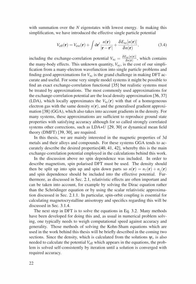
Figure 3.5 shows the average moment and the magnetic susceptibility asfunctions of temperature for L10 alloy FeNi with various system sizes de-scribed by L so that there is a total L3 unit cells included in the simulation.The particular MC implementation used here and in the work behind Paper IIIis that of the UppASD code [69]. In Fig. 3.5a one can observe how the aver-age moment decreases with temperature and how it decreases particularly fast

31

close to the transition temperature of TC = 916 K. One can also see that forlarger L, the drop in the moment is steeper and the value above TC goes closerto the value of zero which is expected in the thermodynamic limit. In Fig. 3.5bit is shown how the susceptibility diverges at the critical point and the peak be-comes sharper for larger L. A fast and easy way to identify the point of thephase transition is to look for peaks in the susceptibility. Fig. 3.6 shows the

0 500 10000

0.5

1

1.5

T (K)

<m

>μ B

L=10L=14L=18L=22

(a) Average moment.

0 500 10000

0.01

0.02

0.03

0.04

T (K)

χ

(b) Susceptibility.

Figure 3.5. Average moment and magnetic susceptibility as functions of temperaturefor L10 alloy FeNi with system sizes L.

Binder cumulant as function of temperature for the FeNi systems of size L.The inset shows a close-up of the region around the critical point where onecan see how the curves for different L intersect at TC.

0 500 10000.4

0.5

0.6

0.7

T (K)

Bin

der

cum

ulan

t

L=10L=14L=18L=22

880 900 920

0.6

0.62

0.64

0.66

Figure 3.6. Binder cumulant as a function of temperature for L10 alloy FeNi withsystem sizes L.

32

4. Results

This chapter presents a brief overview of the key results of this thesis, whilereaders interested in more details are referred to the papers. First, a generaldiscussion on FeCo alloys is provided in Sec. 4.1 and results regarding FeCoalloys with C impurities, related to the work in papers I and II, are presented inSec. 4.1.1. The possibility of using B instead of C is discussed in Sec. 4.1.2. InSec. 4.2 results regarding binary alloys in the L10 structure, based on the workin paper III, are presented. Finally a number of other interesting materials arebriefly discussed.

4.1 Fe1−xCox AlloysAs Fe1−xCox alloys provide large saturation magnetisation, being on top of theSlater-Pauling curve [73, 8], as well as high Curie temperature, they would beideal candidates for permanent magnet applications if a large MAE can be ob-tained as well. Burkert et al. [18] showed that an enormous MAE could be ob-tained in tetragonally strained Fe1−xCox given specific conditions of c/a≈ 1.2and x ≈ 0.65. The work of Burkert et al. was based on the VCA and as seenin Sec. 3.1.3 it overestimates the MAE, but more realistic CPA or supercelltreatment of disorder showed that indeed large MAE can be obtained evenif maximum values are smaller than those originally proposed by Burkert et

al. [59, 60]. These theoretically predicted results were also experimentallyverified in thin film multilayers [74, 75, 76]. Unfortunately, most of the Fe-Cophase diagram below 1100 K is bcc [77] and exhibits a minute MAE so in or-der to produce bulk magnets based on Fe1−xCox for permanent magnets newroutes must be explored. Papers I and II provide such a new route by intro-ducing doping with C atoms which cause a tetragonal strain of the Fe1−xCox

crystal as will be discussed in the coming Section 4.1.1. If this route is possi-ble with C atoms, one can also imagine using other similar atoms, such as Bor N, out of which B will be discussed in Sec. 4.1.2.

Pure Co is found in the uniaxial hcp structure at normal conditions, whichallows it to have a significantly higher MAE compared to bcc Fe. Anotherpossible system to explore could hence be Fe1−xCox in the hcp structure. Thefirst apparent problem with this system is that hcp is only the stable phase fora very narrow range of x ∼ 1 [77]. However, FP-LAPW simulations werestill performed to explore the magnetic properties of the hypothetical hcpFe1−xCox system for a complete range of x ∈ [0,1], also varying the lattice

33

parameters around their equilibrium values. It is found that very large valuesof EMAE > 400 μeV/atom are obtained for x ∼ 0.3 or smaller, but the sys-tem also appears to be antiferromagnetic for x ≥ 0.5 so that no magnetisationwould be left, making the system unsuitable as a permanent magnet even ifone would manage to alloy large amounts of Fe into the hcp crystal.

4.1.1 (Fe1−xCox)-CThe metastable Fe-C martensite phase is an old and well known system whereC atoms go into octahedral interstitial positions of the bcc Fe crystal, wherethey cause a tetragonal distortion [78, 79, 80]. This metastable phase is prac-tically obtained by rapid quenching of the high temperature fcc phase. Dueto similarities in the phase diagrams of Fe-C and Fe-Co-C systems [77, 81],it is reasonable to imagine the same type of structure occurring in an alloy ofFe1−xCox-C. This would allow one to produce a tetragonal Fe1−xCox basedsystem potentially possessing the desired permanent magnet properties, in-cluding a large MAE, if the desired conditions of c/a ≈ 1.2 and x ≈ 0.65pointed out in Ref. [18] can be achieved.

In Paper I, stable energy minima with c/a > 1 are presented for a numberof internally relaxed (Fe1−xCox)yC systems with y = 8, 16 and 24 and C inoctahedral interstitial positions as illustrated in Fig. 4.1a-4.1c and a few dif-ferent values of x around 0.65 as suggested by Ref. [18]. This indicates thatit could indeed be possible to find the desired type of martensite structuresdescribed above. For systems with y = 16, relatively large tetragonal strainsup to c/a ≈ 1.17 are found so that potentially large values of the MAE canbe obtained. For systems with a lower C content, i.e. y = 24, the strain issignificantly lower and c/a≈ 1.035.

For each of these systems the MAE, is calculated by both WIEN2k with VCAand the force theorem and by SPR-KKR with CPA and total energy differ-ences. As expected, the VCA calculations overestimate the MAE significantly,but even with the CPA significant MAE’s of up to EMAE = 41.6 μeV/atom =0.59 MJ/m3 are found. Supercell calculations, utilising special quasirandomstructures (SQS), provide an even slightly larger value of EMAE = 0.75 MJ/m3.These systems also exhibit large saturation magnetisations of μ0MS ≈ 2 T andif one might guess that a small amount of non-magnetic C does not drasticallyaffect the strong exchange interactions of Fe and Co atoms, it is reasonableto suspect also a significant Curie temperature, which in summary makes thesystem highly promising as a permanent magnet if possible to synthesise.

These results provide a potential route to a new permanent magnet but thusfar all results are theoretical suggestions and the next step should be an ex-perimental confirmation. Such a confirmation is provided in Paper II, wherepulsed laser deposition is used for epitaxial growth of the (Fe1−xCox)yC sys-tem described above. It is found that when the ternary (Fe1−xCox)yC system is

34

(a) (Fe1−xCox)8C (b) (Fe1−xCox)16C (c) (Fe1−xCox)24C (d) (Fe1−xCox)32C

Figure 4.1. Illustrations of the various (Fe1−xCox)yC structures with interstitial Catoms studied in Papers I and II.

grown on a CuAu buffer the tetragonal strain saturates towards c/a≈ 1.03 asthe film is grown thicker, in contrast to the binary Fe1−xCox system whichrapidly saturates towards c/a = 1, clearly indicating that the C atoms in-deed induce a tetragonal strain. A magnetocrystalline anisotropy as large asEMAE = 0.44 MJ/m3 was measured for x = 0.6. However, only a small Ccontent of around 2 at.% appears to enter the system which makes direct com-parison to data in Paper I difficult. Hence, calculations were performed fora (Fe0.4Co0.6)32C system as that illustrated in Fig. 4.1d with the experimen-tally measured lattice parameters a = 2.81 and c/a = 1.03. Calculations us-ing WIEN2k with VCA and force theorem indicate EMAE = 0.51 MJ/m3 whileSPR-KKR with CPA and total energy differences yields EMAE = 0.22 MJ/m3.The experimental value is in between the two theoretical ones and theory andexperiment can be considered to be in good agreement. One would, however,expect the CPA to provide a more reliable result than the VCA but in this casethe VCA result is slightly closer to the experimental value.

4.1.2 (Fe1−xCox)-BIf it is possible for C to go into interstitial positions, as discussed above, it iseasy to imagine also other atoms with similar size and properties, such as Bor N, to do the same. Consequently, the procedure performed in Paper I wasrepeated with B substituting C and the results, shown in Table 4.1, are overallsimilar. What can be noted is, however, that the tetragonal strain and thus alsothe MAE, is now larger for systems with y= 24 than what was the case with C.Hence, it appears that compared to C impurities, low amounts of B can causelarger tetragonal strains and thus lead to higher MAE per impurity content.

35

Table 4.1. c/a and MAE of various (Fe1−xCox)yB systems.

Composition c/a MAEtorque ( μeVatom ) MAE ( μeV

atom ) MAE ( MJm3 )

(Fe0.5Co0.5)8B 1.247 76.2 104.6 1.51(Fe0.35Co0.65)16B 1.116 15.5 40.3 0.58(Fe0.4Co0.6)16B 1.103 31.1 48.7 0.69(Fe0.45Co0.55)16B 1.091 43.8 48.3 0.69(Fe0.50Co0.50)16B 1.086 41.3 43.5 0.62(Fe0.35Co0.65)24B 1.083 21.0 37.1 0.53(Fe0.4Co0.6)24B 1.079 31.2 41.8 0.59(Fe0.45Co0.55)24B 1.076 36.1 41.3 0.58(Fe0.50Co0.50)24B 1.074 39.7 44.4 0.63

The results in Table 4.1 were calculated with SPR-KKR and the CPA andthe MAE was evaluated both using the torque method and as difference oftotal energies. Although the MAE is of the same order of magnitude whencalculated with the two methods, the agreement is far from excellent and forsome cases, such as that of (Fe0.35Co0.65)16B, there is a discrepancy by morethan a factor two. Similar problems occurred when studying the (Fe1−xCox)-C systems in the previous section so it appears that the torque method, or atleast the implementation utilised here, is not reliable for these systems. Thisis in contrast to the case of Fe1−xCox as was seen in Fig. 3.2 which impliesthat the local distortion introduced by the C or B makes the torque methodinappropriate.

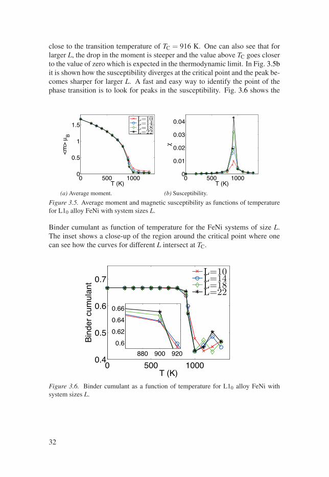
4.2 L10 Binary CompoundsFig. 4.2 illustrates two different unit cells of the L10 crystal structure, onefct-like cell with volume V1 = a2c and one bct-like rotated by π

4 with vol-ume V2 = a′2c = V1

2 . The structure is often described in terms of the fct-likestructure but for computations it is beneficial to use the smaller bct-like struc-ture to reduce the system size and hence also computational effort. Certainbinary alloys, such as FePt [82, 83, 84, 85], can exhibit enormous MAE inthis ordered structure. Interestingly, it is sometimes possible to obtain largeMAE also without heavy elements such as Pt, providing large SOC, and ma-terials of this kind have received attention for permanent magnet applications.In Paper III a thorough investigation into the electronic structure and mag-netic properties of the binary alloys FeNi [23, 82, 86, 87, 88, 24], CoNi [89],MnAl [90, 91, 92, 93] and MnGa [94, 95, 96] is presented. In addition to theevaluation of MS and MAE via DFT, TC is also calculated using MC simu-lations to obtain a complete picture of the three important permanent magnetproperties. It is found that under certain circumstances all of the investigated

36

compounds exhibit interesting properties from a permanent magnet perspec-tive.

Figure 4.2. Illustration of two different perspectives on the L10 structure.

MAE and MS are significant in all of the compounds, although MS is smallerin the Mn-based materials which also contain a non-magnetic element. InFeNi and CoNi, also the TC is found to be high but by studying substitutionaldisorder, where there is intermixing of the atoms in the two different sublat-tices, it is found that both TC and, in particular, MAE decrease notably, evenfor rather small amounts of disorder.

0 100 2000

0.5

1

T (K)

<m

> (

μ B)

(a) MnGa

0 200 400 6000

0.2

0.4

0.6

T (K)

<m

> (

μ B)

(b) Mn1.12Ga0.88

0 200 400 600 8000

0.5

1

1.5

T (K)

<m

> (

μ B)

(c) Mn1.2Ga0.8

0 100 2000

0.01

0.02

0.03

T (K)

χ

(d) MnGa

0 200 400 6000

0.01

0.02

0.03

T (K)

χ

(e) Mn1.12Ga0.88

0 200 400 600 8000

0.005

0.01

0.015

T (K)

χ

(f) Mn1.2Ga0.8

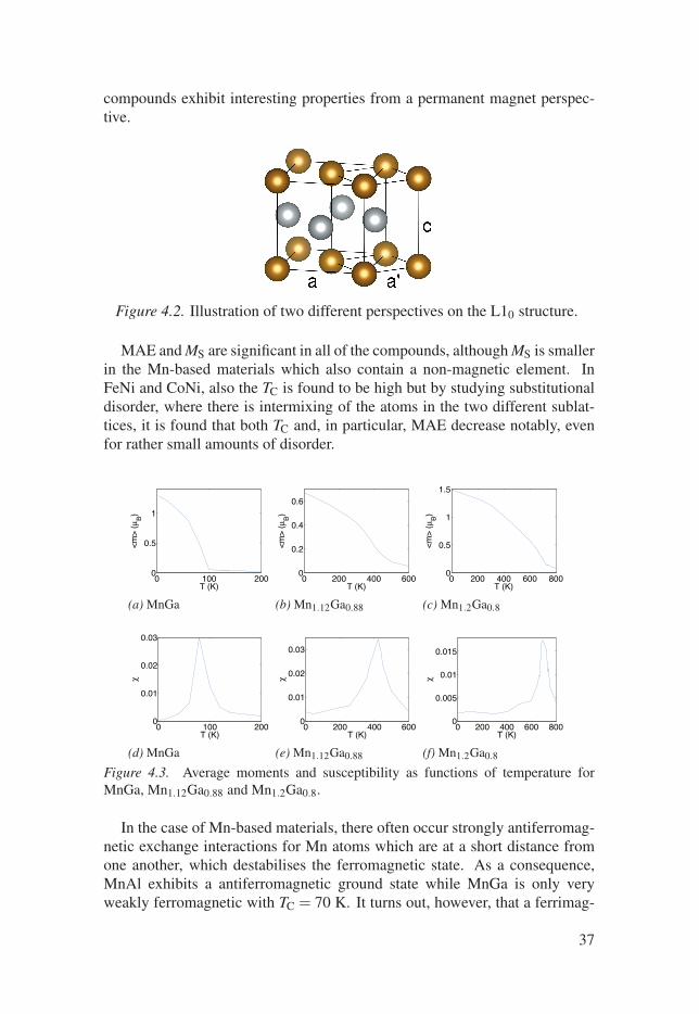
Figure 4.3. Average moments and susceptibility as functions of temperature forMnGa, Mn1.12Ga0.88 and Mn1.2Ga0.8.

In the case of Mn-based materials, there often occur strongly antiferromag-netic exchange interactions for Mn atoms which are at a short distance fromone another, which destabilises the ferromagnetic state. As a consequence,MnAl exhibits a antiferromagnetic ground state while MnGa is only veryweakly ferromagnetic with TC = 70 K. It turns out, however, that a ferrimag-

37

netic state with significant Curie temperature up to TC ≈ 700 K is attainablein both compounds by going off-stoichiometry and adding excess Mn into thesecond sublattice. Fig. 4.3 shows the effect of increasing the Mn-content inMnGa on the average moment and susceptibility as function of temperature,as found from MC simulations in UppASD. It is clear that the phase transitionoccurs for higher temperatures with higher Mn-content, which appears to beconsistent with experimental observations [96]. Fig. 4.4 illustrates the result-ing ferrimagnetic ordering.

Figure 4.4. Ferrimagnetic Mn1+xGa1−x

4.3 Other Potential MaterialsVarious other materials have been discussed as potential candidates for re-placement permanent magnets without rare earths or Pt. One candidate whichhas received interest is Fe2P, due to its huge MAE [19], but unfortunately ithas rather low TC which might however be possible to raise by alloying withsmall amounts of other elements [97, 98, 99, 100, 101]. Another candidatewhich has shown potential as a permanent magnet is MnBi [102, 103, 104]with the anomalous behaviour of an MAE which increases strongly with tem-perature [105]. Two other materials which could posses interesting propertiesare (Fe1−xCox)2B and Heusler alloys which will be described further in thecoming two Sections 4.3.1-4.3.2.

4.3.1 (Fe1−xCox)2BThe tetragonal (Fe1−xCox)2B system, in the space group 140 structure shownin Fig. 4.5, with four equivalent Fe/Co atoms and two equivalent B atoms,was studied by Iga [106] and for certain values of x it exhibits a relativelylarge uniaxial MAE. Consequently, by tuning the composition of Fe and Co itmight be possible to obtain a material with the desired properties for a usefulhard magnet.

38

Figure 4.5. One unit cell of (Fe1−xCox)2B. Large, red balls represent Fe/Co atoms,while the small green balls represent B atoms.

Fig. 4.6 contains results of SPR-KKR calculations with alloying treatedwithin the CPA and MAE evaluated by the torque method. Fig. 4.6a andFig. 4.6b show the saturation magnetisation and MAE as functions of x and it isrevealed that the MAE is uniaxial in the region 0.1≤ x≤ 0.6 with a maximumvalue of EMAE = 0.77 MJ/m3 around x = 0.3. The saturation magnetisation isa monotonously decreasing function of x since Co has a smaller moment thanthat of Fe but even at the cobalt rich side it remains reasonably high aroundμ0MS = 1.0 T.

0 0.5 11

1.2

1.4

1.6

1.8

Co concentration x

μ 0Ms (

T)

0 0.5 1−6

−4

−2

0

2

Co concentration x

MA

E (

MJ/

m3 )

72 74 76 78 80100

150

200

MA

E (

μeV

/f.u.

)

Z

Figure 4.6. Magnetisation and MAE as functions of x in (Fe1−xCox)2B as well asMAE for various atomic numbers Z in (Fe0.675Co275Z0.05)2B.

Hybridisation effects can induce increased MAE even by adding non-magneticelements which contribute with strong SOC [107]. One possible route to fur-ther increasing the MAE of the material could therefore be to add heavierelements from a few rows down in the periodic table. Fig. 4.6c shows theeffect on MAE of exchanging 5 at.% of Fe and Co for various elements ofatomic number Z from the 5d row of elements (Hf is missing because a wellconverged calculation was not obtained) with a dotted line indicating the valueobtained for the ternary system. It appears from these results that only the firstelements in the row are useful for this purpose and W and Re seem particularlyuseful as they allow for a two-fold increase of the MAE.

39

4.3.2 Heusler AlloysThe Heusler alloys consist of a wide range of materials with tunable proper-ties making them interesting for a variety of applications [108]. Most of theHeusler alloys are cubic but some can exist in a tetragonal phase [108, 109]allowing for the possibility of finding materials with large MAE. It appearsthat most magnetic tetragonal Heuslers are Mn-based of the form Mn2YZ andcan exhibit large MAE but tend to be ferrimagnetic with rather low magneticmoments. The case of Y=Mn, Z=Ga, shown in Fig. 4.7, exhibits an enor-mous MAE as the results of FP-LAPW calculations in WIEN2k presented inTable 4.2 show.

Figure 4.7. The DO22 tetragonal Heusler structure of Mn3Ga with arrows indicatingmagnetic moments on the Mn atoms.

As seen in Fig. 4.8, the ferrimagnetic state with the magnetic orderingshown in Fig. 4.7 is favoured over a ferromagnetic state by around 0.4 eV.The ferrimagnetic ordering also appears to favour a slightly larger distancebetween atoms, with larger volume and c/a than would be the case for a fer-romagnetic structure and it allows for an even larger value of the MAE thanwhat would have been the case for ferromagnetic ordering.

With the large MAE of EMAE = 1.3 MJ/m3 observed in ferrimagnetic Mn3Gait could have significant potential as a permanent magnet. Unfortunately, thetotal moment in the unit cell is only m = 1.76μB, corresponding to a satura-tion magnetisation of μ0MS = 0.20 T making it less suitable. Similar systemscould be of interest if elements which tend to prefer ferromagnetic alignment,such as Fe, could be used as a substitute for Mn. However, it appears thatsuch materials tend to prefer the cubic phase [110] resulting in tiny MAE andmaking them less suitable in the context of interest.

40

640 660 680 700 7200

0.1

0.2

0.3

0.4

V (au3)

E (

eV)

FerroFerri

1.8 1.9 2

0

0.1

0.2

0.3

0.4

c/aE

(eV

)

FerroFerri

Figure 4.8. Total energy as a function of volume and c/a for ferro- or ferrimagneticMn3Ga.

Table 4.2. Table summarising the properties of ferro- and ferrimagnetic Mn3Ga.

Quantity Ferro Mn3Ga Ferri Mn3Gaa (a.u.) 7.11 7.13c (a.u.) 13.07 13.44a (Å) 3.76 3.77c (Å) 6.92 7.11mMn-1 (µB) 0.68 -2.79mMn-2 = mMn-3 (µB) 2.17 2.28mGa (µB) -0.05 -0.03EMAE (µeV/f.u.) 532.8 830.1

41

5. Conclusions

After giving a brief background to the theory of magnetism most relevant tounderstanding permanent magnets and an introduction to computational meth-ods suitable to study permanent magnet material properties, a number of rare-earth free materials with promising properties for the given purpose have beenpresented. In particular, a novel material consisting of an FeCo alloy withC atoms causing a tetragonal distortion with a resulting increased MAE hasbeen presented based on theoretical work and then also in an experimentalrealisation. In addition to this, the properties of various binary alloys in theL10 structure have been thoroughly assessed and turn out to exhibit highlyinteresting properties if a high degree of ordering in the right alloy concentra-tions is achieved. An overview has also been given over other materials withpotentially useful properties.

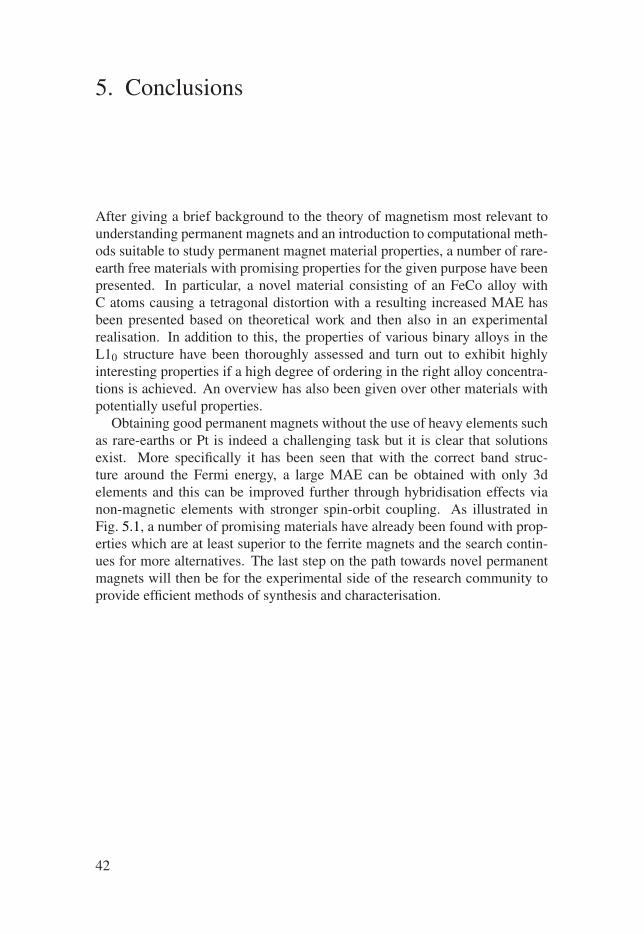
Obtaining good permanent magnets without the use of heavy elements suchas rare-earths or Pt is indeed a challenging task but it is clear that solutionsexist. More specifically it has been seen that with the correct band struc-ture around the Fermi energy, a large MAE can be obtained with only 3delements and this can be improved further through hybridisation effects vianon-magnetic elements with stronger spin-orbit coupling. As illustrated inFig. 5.1, a number of promising materials have already been found with prop-erties which are at least superior to the ferrite magnets and the search contin-ues for more alternatives. The last step on the path towards novel permanentmagnets will then be for the experimental side of the research community toprovide efficient methods of synthesis and characterisation.

42

0 0.5 1 1.5 2 2.510

−1

100

101

102

MA

E (

MJ/

m3 )

μ0 M

s (T)

REsFerriteFe/Co−C/BL1

0(Fe

0.7Co

0.3)2B

Figure 5.1. Summarising comparison of permanent magnet properties for materialspresented in this thesis and existing rare-earth and ferrite alternatives.

43

References

[1] J. M. D. Coey, “Advances in Magnetics Hard Magnetic Materials : APerspective,” IEEE Transactions on Magnetics, vol. 47, no. 12,pp. 4671–4681, 2011.

[2] J. Coey, “Permanent magnets: Plugging the gap,” Scripta Materialia, vol. 67,pp. 524–529, Sept. 2012.

[3] J. M. D. Coey, “Permanent Magnetism,” Solid State Communications,vol. 102, no. 2, pp. 101–105, 2000.

[4] L. H. Lewis and F. Jiménez-Villacorta, “Perspectives on Permanent MagneticMaterials for Energy Conversion and Power Generation,” Metallurgical and

Materials Transactions A, vol. 44, pp. 2–20, July 2012.[5] R. Skomski and J. M. D. Coey, Permanent Magnetism. Institute of Physics

Publishing, 1999.[6] D. Kramer, “Concern grows over China’s dominance of rare-earth metals,”

Physics Today, vol. 63, no. 5, p. 22, 2010.[7] R. Skomski, Simple Models of Magnetism. Oxford University Press, 2008.[8] S. Chikazumi, Physics of Ferromagnetism. Oxford University Press, 1997.[9] G. E. Uhlenbeck and S. Goudsmit, “Ersetzung der Hypothese vom

ummechanischen Zwang durch eine Forderung Besüglich des innerenVerhaltens jedes einzelnen Elektrons,” Die Naturwissenschaften, vol. 13,pp. 953–954, 1925.

[10] P. A. M. Dirac, “The Quantum Theory of the Electron.,” Proceedings of the

Royal Society A, vol. 117, no. 778, pp. 610–624, 1928.[11] P. A. M. Dirac, “The Quantum Theory of the Electron. Part II,” Proceedings of

the Royal Society A: Mathematical, Physical and Engineering Sciences,vol. 118, pp. 351–361, Mar. 1928.

[12] F. Gross, Relativistic Quantum Mechanics and Field Theory. John Wiley &Sons, Inc., 1993.

[13] T. Ohlsson, Relativistic Quantum Physics. Cambridge University Press, 2011.[14] J. H. V. Vleck, “On the Anisotropy of Cubic Ferromagnetic Crystals,” Physical

Review, vol. 52, pp. 1178–1198, 1937.[15] N. W. Ashcroft and D. N. Mermin, Solid State Physics. Belmont, USA:

Brooks/Cole, 1976.[16] P. Mohn, Magnetism in the Solid State An Introduction. Springer-Verlag, 2002.[17] H. Brooks, “Ferromagnetic Anisotropy and the Itinerant Electron Model,”

Physical Review, vol. 58, 1940.[18] T. Burkert, L. Nordström, O. Eriksson, and O. Heinonen, “Giant Magnetic

Anisotropy in Tetragonal FeCo Alloys,” Physical Review Letters, vol. 93,p. 027203, July 2004.

[19] M. Costa, O. Grånäs, A. Bergman, P. Venezuela, P. Nordblad, M. Klintenberg,and O. Eriksson, “Large magnetic anisotropy of Fe2P investigated via ab initio

44

density functional theory calculations,” Physical Review B, vol. 86, p. 085125,Aug. 2012.

[20] R. Wu and A. Freeman, “Spin-orbit induced magnetic phenomena in bulkmetals and their surfaces and interfaces,” Journal of Magnetism and Magnetic

Materials, vol. 200, pp. 498–514, Oct. 1999.[21] P. Bruno, “Tight-binding approach to the orbital magnetic moment and

magnetocrystalline anisotropy of transition-metal monolayers,” Physical

Review B, vol. 39, no. 1, pp. 865–868, 1989.[22] C. Andersson, B. Sanyal, O. Eriksson, L. Nordström, O. Karis, D. Arvanitis,

T. Konishi, E. Holub-Krappe, and J. Dunn, “Influence of Ligand States on theRelationship between Orbital Moment and Magnetocrystalline Anisotropy,”Physical Review Letters, vol. 99, p. 177207, Oct. 2007.

[23] Y. Miura, S. Ozaki, Y. Kuwahara, M. Tsujikawa, K. Abe, and M. Shirai, “Theorigin of perpendicular magneto-crystalline anisotropy in L10-FeNi undertetragonal distortion.,” Journal of physics. Condensed matter : an Institute of

Physics journal, vol. 25, p. 106005, Mar. 2013.[24] M. Kotsugi, M. Mizuguchi, S. Sekiya, M. Mizumaki, T. Kojima, T. Nakamura,

H. Osawa, K. Kodama, T. Ohtsuki, T. Ohkochi, K. Takanashi, andY. Watanabe, “Origin of strong magnetic anisotropy in L10-FeNi probed byangular-dependent magnetic circular dichroism,” Journal of Magnetism and

Magnetic Materials, vol. 326, pp. 235–239, Jan. 2013.[25] W. Nolting and A. Ramakanth, Quantum Theory of Magnetism.

Springer-Verlag, 2009.[26] J. Rusz, L. Bergqvist, J. Kudrnovský, and I. Turek, “Exchange interactions and

Curie temperatures in Ni2−xMnSb alloys: First-principles study,” Physical

Review B, vol. 73, p. 214412, Jun 2006.[27] Pajda, M. and Kudrnovský, J. and Turek, I. and Drchal, V. and Bruno, P., “Ab

initio calculations of exchange interactions, spin-wave stiffness constants, andCurie temperatures of Fe, Co, and Ni,” Physical Review B, vol. 64, p. 174402,Oct 2001.

[28] D. Bonnenberg, K. A. Hempel, and H. P. J. Wijn, Figs. 94 - 114, Tables 18 -

19, vol. 19a of Landolt-Börnstein - Group III Condensed Matter, ch. 3d, 4dand 5d Elements, Alloys and Compounds. Springer, 1986.

[29] H. Eschrig, The Fundamentals of Density Functional Theory. Dresden, 2003.[30] J. M. Wills, M. Alouani, P. Andersson, A. Delin, O. Eriksson, and

O. Grechnyev, Full-Potential Electronic Structure Method. Springer, 2010.[31] R. M. Martin, Electronic Structure. Cambridge University Press, 2004.[32] D. P. Landau and K. Binder, A Guide to Monte Carlo Simulations in Statistical

Physics. Cambridge University Press, 2000.[33] P. Hohenberg and W. Kohn, “Inhomogeneous Electron Gas,” Physical Review,

vol. 136, no. 1962, pp. 864–871, 1964.[34] W. Kohn and L. J. Sham, “Self-Consistent Equations Including Exchange and

Correlation Effects,” Physical Review, vol. 140, no. 4a, pp. 1133–1138, 1965.[35] L. O. Wagner, T. E. Baker, E. M. Stoudenmire, K. Burke, and S. R. White,

“Kohn-sham calculations with the exact functional,” Physical Review B,vol. 90, p. 045109, Jul 2014.

[36] A. Zunger and J. P. Perdew, “Self-interaction correction to density-functional

45

approximations for many-electron systems,” Physical Review B, vol. 23,no. 10, pp. 5048–5079, 1981.

[37] J. P. Perdew and Y. Wang, “Accurate and simple analytic representation of theelectron-gas correlation energy,” Physical Review B, vol. 45, pp. 13244–13249,Jun 1992.

[38] J. P. Perdew, K. Burke, and M. Ernzerhof, “Generalized GradientApproximation Made Simple.,” Physical Review Letters, vol. 77,pp. 3865–3868, Oct. 1996.

[39] G. Kotliar, S. Savrasov, K. Haule, V. Oudovenko, O. Parcollet, andC. Marianetti, “Electronic structure calculations with dynamical mean-fieldtheory,” Reviews of Modern Physics, vol. 78, pp. 865–951, Aug. 2006.

[40] F. Tran, R. Laskowski, P. Blaha, and K. Schwarz, “Performance on molecules,surfaces, and solids of the Wu-Cohen GGA exchange-correlation energyfunctional,” Physical Review B, vol. 75, p. 115131, Mar 2007.

[41] V. Ozolinš and M. Körling, “Full-potential calculations using the generalizedgradient approximation: Structural properties of transition metals,” Physical

Review B, vol. 48, pp. 18304–18307, Dec 1993.[42] P. Bagno, O. Jepsen, and O. Gunnarsson, “Ground-state properties of third-row

elements with nonlocal density functionals,” Physical Review B, vol. 40,pp. 1997–2000, Jul 1989.

[43] S. Cottenier, Density Functional Theory and the Family of (L)APW-methods: a

step-by-step introduction. Instituut voor Kern- en Stralingsfysica, K.U.Leuven,Belgium, 2002.

[44] P. Blaha, G. Madsen, K. Schwarz, D. Kvasnicka, and J. Luitz, “WIEN2k, AnAugmented Plane Wave + Local Orbitals Program for Calculating CrystalProperties,” 2001.

[45] O. K. Andersen, “Linear methods in band theory,” Physical Review B, vol. 12,pp. 3060–3083, Oct 1975.

[46] J. C. Slater, “Wave functions in a periodic potential,” Physical Review, vol. 51,pp. 846–851, May 1937.

[47] D. D. Koelling and H. N. Harmon, “A technique for relativistic spin-polarisedcalculations,” Journal of Physics C: Solid State Physics, vol. 10, 1977.

[48] A. H. MacDonald, W. E. Picket, and D. D. Koelling, “A linearised relativisticaugmented-plane-wave method utilising approximate pure spin basisfunctions,” Journal of Physics C: Solid State Physics, vol. 13, pp. 2675–83,1980.

[49] H. Ebert, “The Munich SPR-KKR package, version 6.3,” 2012.[50] H. Ebert, D. Ködderitzsch, and J. Minár, “Calculating condensed matter

properties using the KKR-Green’s function method -recent developments andapplications,” Reports on Progress in Physics, vol. 74, p. 096501, Sept. 2011.

[51] J. Korringa, “On the calculation of the energy of a bloch wave in a metal,”Physica, vol. 13, no. 6-7, pp. 392 – 400, 1947.

[52] E. N. Economou, Green’s Functions in Quantum Physics. Springer BerlinHeidelberg, 2006.

[53] J. Zabloudil, R. Hammerling, P. Weinberger, and L. Szunyogh, Electron

Scattering in Solid Matter. Springer, 2005.[54] J. S. Faulkner and G. M. Stocks, “Calculating properties with the

46

coherent-potential approximation,” Physical Review B, vol. 21, pp. 3222–3244,Apr 1980.

[55] J. S. Faulkner, “The modern theory of alloys,” Progress in Materials Science,vol. 27, no. 1-2, pp. 1–187, 1982.

[56] A. Zunger, S.-H. Wei, L. G. Ferreira, and J. E. Bernard, “Special quasirandomstructures,” Physical Review Letters, vol. 65, pp. 353–356, Jul 1990.

[57] P. James, Calculation of magnetism and its crystal structure dependence. PhDthesis, Uppsala University, 1999.

[58] P. Söderlind, B. Johansson, and O. Eriksson, “Spin and orbital magnetism inFe-Co and Co-Ni alloys.,” Journal of Magnetism and Magnetic Materials,vol. 45, June 1992.

[59] I. Turek, J. Kudrnovský, and K. Carva, “Magnetic anisotropy energy ofdisordered tetragonal Fe-Co systems from ab initio alloy theory,” Physical

Review B, vol. 86, p. 174430, Nov. 2012.[60] C. Neise, S. Schönecker, M. Richter, K. Koepernik, and H. Eschrig, “The

effect of chemical disorder on the magnetic anisotropy of strained Fe-Cofilms,” Physica Status Solidi (B), vol. 248, pp. 2398–2403, Oct. 2011.

[61] P. Soven, “Coherent-Potential Model of Substitutional Disordered Alloys,”Physical Review, vol. 156, no. 3, 1967.

[62] P. E. Blöchl, O. Jepsen, and O. K. Andersen, “Improved tetrahedron methodfor Brillouin-zone integrations,” Physical Review B, vol. 49, no. 23, 1994.

[63] A. I. Liechtenstein, M. I. Katsnelson, V. P. Antropov, and V. A. Gubanov,“Local Spin Density Functional Approach To The Theory Of ExchangeIinteractions In Ferromagnetic Metals And Alloys,” Journal of Magnetism and

Magnetic Materials, vol. 67, pp. 65–74, 1987.[64] G. H. O. Daalderop, P. J. Kelly, and M. F. H. Schuurmans, “First-principles

calculation of the magnetocrystalline anisotropy energy of iron, cobalt, andnickel,” Physical Review B, vol. 41, pp. 11919–11937, Jun 1990.

[65] X. Wang, R. Wu, D. Wang, and A. Freeman, “Torque method for thetheoretical determination of magnetocrystalline anisotropy.,” Physical Review

B, vol. 54, pp. 61–64, July 1996.[66] J. Staunton, L. Szunyogh, a. Buruzs, B. Gyorffy, S. Ostanin, and L. Udvardi,

“Temperature dependence of magnetic anisotropy: An ab initio approach,”Physical Review B, vol. 74, p. 144411, Oct. 2006.

[67] A. I. Liechtenstein, M. I. Katsnelson, and V. A. Gubanov, “Exchangeinteractions and spin-wave stiffness in ferromagnetic metals,” Journal of

Physics F: Metal Physics, vol. 14, 1984.[68] A. I. Liechtenstein, M. I. Katsnelson, V. P. Antropov, and V. A. Gubanov,

“LSDF-Approach to the theory of exchange interactions in magnetic metals,”Journal of Magnetism and Magnetic Materials, vol. 54-57, pp. 965–966, 1986.

[69] B. Skubic, J. Hellsvik, L. Nordström, and O. Eriksson, “A method foratomistic spin dynamics simulations: implementation and examples,” Journal

of Physics: Condensed Matter, vol. 20, p. 315203, Aug. 2008.[70] R. K. Pathria, Statistical Mechanics. Elsevier, 2nd ed., 1996.[71] M. Wallin, Monte Carlo Simulations in Statistical Physics. KTH, Stockholm,

Sweden, 2005.[72] N. Metropolis, A. W. Rosenbluth, M. N. Rosenbluth, A. H. Teller, and

47

E. Teller, “Equation of state calculations by fast computing machines,” The

Journal of Chemical Physics, vol. 21, no. 6, pp. 1087–1092, 1953.[73] A. R. Williams, V. L. Moruzzi, A. P. Malozemoff, and K. Terakura,

“Generalized Slater-Pauling Curve for Transition-Metal Magnets,” IEEE

Transactions on Magnetics, vol. 19, no. 5, pp. 1983–1988, 1983.[74] G. Andersson, T. Burkert, P. Warnicke, M. Björck, B. Sanyal, C. Chacon,

C. Zlotea, L. Nordström, P. Nordblad, and O. Eriksson, “PerpendicularMagnetocrystalline Anisotropy in Tetragonally Distorted Fe-Co Alloys,”Physical Review Letters, vol. 96, p. 037205, Jan. 2006.

[75] F. Yildiz, M. Przybylski, X.-D. Ma, and J. Kirschner, “Strong perpendicularanisotropy in Fe1−xCox alloy films epitaxially grown on mismatching Pd(001),Ir(001), and Rh(001) substrates,” Physical Review B, vol. 80, p. 064415, Aug.2009.

[76] P. Warnicke, G. Andersson, M. Björck, J. Ferré, and P. Nordblad, “Magneticanisotropy of tetragonal FeCo/Pt(001) superlattices,” Journal of Physics:

Condensed Matter, vol. 19, p. 226218, June 2007.[77] D. Bonnenberg, K. A. Hempel, and H. P. J. Wijn, 1.2.1 Alloys between Fe, Co

or Ni, 1.2.1.1 Phase diagrams, lattice parameters, vol. 19a ofLandolt-Börnstein - Group III Condensed Matter, ch. 3d, 4d and 5d Elements,Alloys and Compounds. Springer, 1986.

[78] G. Kurdjumov, “Martensite crystal lattice, mechanism of austenite-martensitetransformation and behavior of carbon atoms in martensite,” Metallurgical

Transactions A, vol. 7, no. 7, pp. 999–1011, 1976.[79] R. Naraghi, M. Selleby, and J. A. gren, “Thermodynamics of stable and

metastable structures in Fe-C system ,” Calphad, vol. 46, no. 0, pp. 148 – 158,2014.

[80] G. Kurdjumov and A. Khachaturyan, “Nature of axial ratio anomalies of themartensite lattice and mechanism of diffusionless γ → α transformation,” Acta

Metallurgica, vol. 23, no. 9, pp. 1077 – 1088, 1975.[81] L. C. Materials Science International Team MSIT, Andy Watson, Carbon -

Cobalt - Iron, iron systems: phase diagrams, crystallographic and

thermodynamic data, 1.2.1.1 Phase diagrams, lattice parameters, vol. 11D1:Iron Systems, Part 1 of Landolt-Börnstein - Group IV Physical Chemistry,ch. 3d, 4d and 5d Elements, Alloys and Compounds. Springer, 2008.

[82] Y. Kota and A. Sakuma, “Relationship between Magnetocrystalline Anisotropyand Orbital Magnetic Moment in L10 -Type Ordered and Disordered Alloys,”Journal of the Physical Society of Japan, vol. 81, pp. 1–6, 2012.

[83] T. Burkert, O. Eriksson, S. Simak, A. Ruban, B. Sanyal, L. Nordström, andJ. Wills, “Magnetic anisotropy of L10 FePt and Fe1−xMnxPt,” Physical Review

B, vol. 71, p. 134411, Apr. 2005.[84] J. B. Staunton, S. Ostanin, S. S. A. Razee, B. Gyorffy, L. Szunyogh,

B. Ginatempo, and E. Bruno, “Long-range chemical order effects upon themagnetic anisotropy of FePt alloys from an ab initio electronic structuretheory,” Journal of Physics: Condensed Matter, vol. 16, pp. S5623–S5631,Dec. 2004.

[85] P. Ravindran, a. Kjekshus, H. Fjellvåg, P. James, L. Nordström, B. Johansson,and O. Eriksson, “Large magnetocrystalline anisotropy in bilayer transition

48

metal phases from first-principles full-potential calculations,” Physical Review

B, vol. 63, p. 144409, Mar. 2001.[86] T. Kojima, M. Mizuguchi, and K. Takanashi, “L10-ordered FeNi film grown on

Cu-Ni binary buffer layer,” in Journal of Physics: Conference Series, vol. 266,p. 012119, Jan. 2011.

[87] L. Néel, J. Pauleve, R. Pauthenet, J. Laugier, and D. Dautreppe, “MagneticProperties of an Iron-Nickel Single Crystal Ordered by NeutronBombardment,” Journal of Applied Physics, vol. 35, no. 3, p. 873, 1964.

[88] T. Kojima, M. Mizuguchi, T. Koganezawa, K. Osaka, M. Kotsugi, andK. Takanashi, “Magnetic Anisotropy and Chemical Order of ArtificiallySynthesized L10-Ordered FeNi Films on Au-Cu-Ni Buffer Layers,” Japanese

Journal of Applied Physics, vol. 51, p. 010204, Jan. 2012.[89] S. Fukami, H. Sato, M. Yamanouchi, S. Ikeda, and H. Ohno, “CoNi Films with

Perpendicular Magnetic Anisotropy Prepared by Alternate Monoatomic LayerDeposition,” Applied Physics Express, vol. 6, p. 073010, July 2013.

[90] A. J. J. Koch, P. Hokkeling, M. G. v. d. Steeg, and K. J. de Vos, “New Materialfor Permanent Magnets on a Base of Mn and Al,” Journal of Applied Physics,vol. 31, no. 5, p. S75, 1960.

[91] J. H. Park, Y. K. Hong, S. Bae, J. J. Lee, J. Jalli, G. S. Abo, N. Neveu, S. G.Kim, C. J. Choi, and J. G. Lee, “Saturation magnetization and crystallineanisotropy calculations for MnAl permanent magnet,” Journal of Applied

Physics, vol. 107, no. 9, p. 09A731, 2010.[92] S. H. Nie, L. J. Zhu, J. Lu, D. Pan, H. L. Wang, X. Z. Yu, J. X. Xiao, and J. H.

Zhao, “Perpendicularly magnetized τ-MnAl (001) thin films epitaxied onGaAs,” Applied Physics Letters, vol. 102, no. 15, p. 152405, 2013.

[93] J. M. D. Coey, “New permanent magnets; manganese compounds.,” Journal of

physics. Condensed matter : an Institute of Physics journal, vol. 26,p. 064211, Jan. 2014.

[94] A. Sakuma, “Electronic structures and magnetism of CuAu-type MnNi andMnGa,” Journal of Magnetism and Magnetic Materials, vol. 187, pp. 105–112,Aug. 1998.

[95] K. Wang, E. Lu, J. W. Knepper, F. Yang, and A. R. Smith, “Structuralcontrolled magnetic anisotropy in Heusler L10-MnGa epitaxial thin films,”Applied Physics Letters, vol. 98, no. 16, p. 162507, 2011.

[96] E. Lu, D. Ingram, A. Smith, J. Knepper, and F. Yang, “Reconstruction Controlof Magnetic Properties during Epitaxial Growth of Ferromagnetic Mn3Ga onWurtzite GaN(0001),” Physical Review Letters, vol. 97, p. 146101, Oct. 2006.

[97] R. Fruchart, “Crystallographic and Magnetic Properties of Solid Solutions ofthe Phosphides M2P, M = Cr, Mn, Fe, Co, and Ni,” Journal of Applied Physics,vol. 40, no. 3, p. 1250, 1969.

[98] Catalano, A. and Arnott, R. J. and Wold, A, “Magnetic and CrystallographicProperties of the System Fe2P1−xAsx,” Journal of Solid State Chemistry,vol. 7, pp. 262–268, 1973.

[99] C. Jian-wang, L. He-lie, and Z. Qing-qi, “Electronic structures and magneticproperties of Fe2P and the effects of doping with Ni,” Journal of Physics:

Condensed Matter, vol. 5, pp. 9307–9316, 1993.[100] S. N. Doli, A. Krishnamurthy, V. Ghose, and B. K. Srivastava, “Magnetic

49

behaviour of Ni-substituted Fe2P,” Journal of Physics: Condensed Matter,vol. 5, pp. 451–458, 1993.

[101] J. Leitão, M. van der Haar, a. Lefering, and E. Brück, “Magnetic andmagnetocaloric exploration of Fe rich (Mn,Fe)2(P,Ge),” Journal of Magnetism

and Magnetic Materials, vol. 344, pp. 49–54, Oct. 2013.[102] A. Sakuma, Y. Manabe, and Y. Kota, “First Principles Calculation of

Magnetocrystalline Anisotropy Energy of MnBi and MnBi1−xSnx,” Journal of

the Physical Society of Japan, vol. 82, no. 7, p. 73704, 2013.[103] N. V. R. Rao, A. M. Gabay, W. F. Li, and G. C. Hadjipanayis, “Nanostructured

bulk MnBi magnets fabricated by hot compaction of cryomilled powders,”Journal of Physics D: Applied Physics, vol. 46, no. 26, p. 265001, 2013.

[104] N. V. R. Rao, A. M. Gabay, and G. C. Hadjipanayis, “Anisotropic fully denseMnBi permanent magnet with high energy product and high coercivity atelevated temperatures,” Journal of Physics D: Applied Physics, vol. 46, no. 6,p. 062001, 2013.

[105] P. A. Albert and W. J. Carr, “Temperature Dependence of Magnetostriction andAnisotropy in MnBi,” Journal of Applied Physics, vol. 32, no. 3,pp. S201–S202, 1961.

[106] A. Iga, “Magnetocrystalline Anisotropy in (Fe1−xCox)2B System,” Japanese

Journal of Applied Physics, vol. 9, pp. 415–416, 1970.[107] S. Bhandary, O. Grånäs, L. Szunyogh, B. Sanyal, L. Nordström, and

O. Eriksson, “Route towards finding large magnetic anisotropy innanocomposites: Application to a W1−xRe4/Fe multilayer,” Physical Review

B, vol. 84, p. 092401, Sept. 2011.[108] T. Graf, C. Felser, and S. S. Parkin, “Simple rules for the understanding of

Heusler compounds,” Progress in Solid State Chemistry, vol. 39, pp. 1–50,May 2011.

[109] C. Felser, V. Alijani, J. Winterlik, S. Chadov, and A. K. Nayak, “TetragonalHeusler Compounds for Spintronics,” IEEE Transactions on Magnetics,vol. 49, no. 2, pp. 682–685, 2013.

[110] J. Kiss, S. Chadov, G. H. Fecher, and C. Felser, “Disorder-induced cubic phasein Fe2-based Heusler alloys,” Physical Review B, vol. 87, p. 224403, June2013.

50