High Frequency Permanent Magnet Generator for Pulse ...

High Frequency Permanent Magnet Generator for Pulse Density Modulating Converters

By

Bo Jiang

A thesis submitted in partial fulfilment of the requirements for the degree of

Doctor of Philosophy

The University of Sheffield

Faculty of Engineering

Department of Electronic and Electrical Engineering

March 2020

I

Abstract

This thesis describes an investigation of high frequency permanent magnet

generators for use in a novel power generation system for aerospace applications.

The system consists of a high frequency generator (in the 10s of kHz range)

which feeds a full-wave rectifier to produce to a high frequency pulse train as

input to a pulse-density modulated soft-switched converter.

Various topologies of flux-switching, flux-reversal and Vernier machines are

investigated using electric-circuit coupled finite element analysis. Having

demonstrated the limitations of these topologies, a comprehensive design study

into a single-phase, surface mounted permanent magnet machine based on a

single turn serpentine winding is described. This study covers both internal and

external rotor machines with pole numbers of 192 and 96 which correspond to

generator fundamental frequencies of 32kHz and 16kHz at the rated speed of

20,000rpm. Several aspects of the machine design are optimised through

extensive use of finite element modelling, including mechanical analysis of the

rotor containment. This study includes a detailed consideration of iron loss,

including consideration of iron powder based cores. This study has resulted in a

down-selected design based on a low permeability but high resistivity powdered

iron core.

The manufacture of a demonstrator is described including the need to re-design

the machine to employ ultra-thin Nickel Iron laminations because of the

difficulties encountered in the machining of a powdered iron core. The

performance of this Nickel Iron variant is investigated and a final design

established. The numerous challenges involved in manufacturing this novel

machine are described.

II

Acknowledgements

I would like to express my deep sincere gratitude to my supervisor Professor

Geraint Jewell. During this five years research, I have gone through a lot of

challenges, difficulties and failures. Without his patience, invaluable help and

guidance, I cannot have courage to complete this project. More than that, I also

would like to appreciate every professional suggestion and idea he made. It’s

truly helpful in each step of research.

I would like to acknowledge all my colleagues in Rolls-Royce Sheffield

University Technique Centre (UTC), especially Jason and Steve. Also, I would

like to acknowledge technical staff in workshop, especially Clive, Sam, Karl and

David. All of them gave me a lot of support and advice during my research.

Particularly, I would like to thank two women in my life. One is my mother. She

had shown her great characteristic of brave, strong and optimistic even in her last

time while suffering cancer. That leads me overcome frustration and setback

throughout these years during research. Another one is my wife. Her encourage

and support bring faith and confidence back to me and give me strength and

courage.

Further, I would like to thank my friends and all other family members for their

care and support, which I really appreciate. I would like to thank the Electrical

Machine Drive Group for delight, warmly working environment.

Last but not least, I am indebted to previous research in this area. I would like to

thank the architecture of electrical machine research that makes it possible to give

me a chance to stand in frontier of science.

III

Contents

Abstract ..................................................................................................................................... I

Acknowledgements ................................................................................................................. II

List of symbols ...................................................................................................................... VII

Chapter 1 Introduction............................................................................................................ 1

1.1 More electric aircraft .................................................................................................... 1

1.2 Proposed system concept ................................................................................................ 4

1.2.1 System architecture ................................................................................................. 4

1.2.2 Top-level performance requirements ...................................................................... 8

1.3 Review of candidate electrical machine topologies ........................................................ 9

1.3.1 Conventional surface mounted permanent magnet machines ............................... 10

1.3.2 Flux-switching PM machines ................................................................................ 11

1.3.3 Flux-reversal machines .......................................................................................... 13

1.3.4 Magnetically geared machines .............................................................................. 14

1.3.5 Hybrid stepper machines ....................................................................................... 16

1.4 Research methodology .................................................................................................. 17

1.4.1 Overall research aims ............................................................................................ 17

1.4.2 Baseline reference design of conventional brushless DC machine ....................... 20

1.4.3 Modelling tools ...................................................................................................... 21

1.5 Thesis outline ................................................................................................................ 21

1.6 References ..................................................................................................................... 23

Chapter 2 Modelling of a Pulse Density Modulation Converter ....................................... 30

2.1 Introduction ................................................................................................................... 30

IV

2.2 Simulink model of PDM inverter fed with a full-wave rectified .................................. 30

2.2.1 Voltage source and full wave rectifier ................................................................... 31

2.2.2 Converter power stage ........................................................................................... 32

2.2.3 Converter controller ............................................................................................... 33

2.2.4 Load and converter output filter ............................................................................ 36

2.3 Simulated converter performance ................................................................................. 37

2.3.1 Unfiltered performance ......................................................................................... 38

2.3.2 Performance with first-order filter ......................................................................... 42

2.2.3 Performance with second order filters ................................................................... 45

2.4 Conclusions ................................................................................................................... 50

2.5 References ..................................................................................................................... 51

Chapter 3 Alternative concept studies on different topologies .......................................... 53

3.1 Introduction ................................................................................................................... 53

3.2 Baseline machine design ............................................................................................... 53

3.3 Modified baseline design for assessment of alternative topologies .............................. 56

3.3.1 Performance predictions for original and modified baseline designs ................... 57

3.4 Methodology for evaluation of different topologies ..................................................... 58

3.5 Topologies of machines analysed ................................................................................. 60

3.6 Performance evaluation of different machine types ...................................................... 64

3.6.1 Finite element modelling of flux linkage variation in different machine

topologies ....................................................................................................................... 64

3.6.2 Influence of number of rotor teeth ......................................................................... 65

3.6.3 Finite element analysis of regulation and power curves ....................................... 67

3.6.4 Influence of magnet geometry on performance ..................................................... 69

V

3.7 Conclusions ................................................................................................................... 71

3.8 References ..................................................................................................................... 72

Chapter 4 Design and analysis of a single-phase permanent magnet machines .............. 74

4.1 Introduction ................................................................................................................... 74

4.1 Design of internal rotor machine ................................................................................... 75

4.1.1 Surface mounted PM machine topology designs .................................................. 75

4.1.2 Interior permanent magnet rotor designs ............................................................... 90

4.2 Design of External rotor machine ............................................................................... 105

4.3 Evaluation of iron loss and candidate core materials .................................................. 111

4.3.1 Soft magnetic composites .................................................................................... 113

4.3.2 Machine performance with SMC core materials ................................................. 119

4.4 Iron loss calculation for machine designs ................................................................... 123

4.4.1 Calculation of machine losses ............................................................................. 126

4.5 Design of a reduced pole number (96 poles) machine with material PCHF ............... 132

4.6 Conclusions ................................................................................................................. 145

4.7 REFERENCES ............................................................................................................ 147

Chapter 5 Prototype machine manufacture and testing .................................................. 150

5.1 Introduction ................................................................................................................. 150

5.2 Manufacture of a stator core of iron powder core high flux (PCHF) .......................... 150

5.3 Design of a laminated stator core ................................................................................ 153

5.3.1 Design revisions for Nickel Iron core ................................................................. 154

5.3.2. Stator core segmentation .................................................................................... 158

5.3.3 Iron losses for Nickel iron design ........................................................................ 162

5.4 Manufacture of the demonstrator machine components ............................................. 164

VI

5.4.1 Stator core manufacture ....................................................................................... 164

5.4.2 Manufacture of the stator assembly ..................................................................... 166

5.4.3 Coil manufacture ................................................................................................. 168

5.4.4 Rotor manufacture ............................................................................................... 170

5.4.5 Final assembly ..................................................................................................... 177

5.5 Conclusions ................................................................................................................. 179

5.6 References ................................................................................................................... 180

Chapter 6 Conclusions ......................................................................................................... 181

6.1 Introduction ................................................................................................................. 181

6.2 Key conclusions .......................................................................................................... 181

6.3 Suggestions for future work ........................................................................................ 184

Appendix A Design designation system used in chapter 4 and 5 ..................................... 186

Appendix B PDM Simulink model explore in chapter 2 .................................................. 187

Appendix C Example script of Opera 2D on final design ................................................ 188

VII

List of symbols

Symbol Explanation Unit

ts Simple time s

𝑓𝑝𝑢𝑙𝑠𝑒 DC pulse frequency Hz

𝑓𝑠 PDM switching frequency Hz

𝑓𝑎𝑐 Machine side AC frequency Hz

𝑉𝑑𝑐 Rectified voltage in average value V

𝐼𝑑𝑐 Rectified current in average value A

Ts Number of small teeth

sp Split ratio

𝜎𝑚𝑎𝑥 Maximum stress Pa

𝛿𝑐 Containment mass density kg/m3

𝜔 Angular speed rad/s

𝜈𝑐 Poisson ratio of containment

𝑑𝑐𝑜 Outer diameter of the containment mm

𝑑𝑐𝑖 Inner diameter of the containment mm

𝑚𝑒𝑞 Equivalent dead mass acting on the containment kg

𝑟𝑚𝑒𝑞 Equivalent radius of the dead mass mm

𝑑𝑚𝑜 Magnet outer diameter mm

𝑑𝑚𝑖 Magnet inner diameter mm

𝛼 Magnet pole arc degree

𝛿𝑚 Magnet mass density kg/m3

𝛿𝑖𝑝 Inter-pole material mass density kg/m3

Rt Ratio of rotor teeth (depth/width)

ag Airgap length mm

br Magnet bridge thickness mm

SH Stator hub ratio (stator hub diameter/machine

outside diameter)

B Flux density T

f frequency Hz

𝛿𝐹𝑒 Iron mass density kg/m3

VIII

𝜎 Conductivity S/m

𝑑 Lamination thickness mm

T Period of one cycle s

𝐾ℎ

Steinmetz coefficient

𝐾𝑒𝑥𝑒

𝐾𝑐𝑙

𝛼

𝛽

𝐾𝑙𝑜𝑜𝑝 Coefficient of hysteresis minor loop

pk Slot area packing factor

𝜌 Electrical resistivity μΩcm

1

Chapter 1 Introduction


1.1 More electric aircraft

In common with many other transport sectors, aerospace is gradually moving towards

increased electrification. In the short to medium term future, it is unlikely that full-

electric propulsion will be realised in anything other than very small, short-range,

personal mobility platforms such as those in [1-3]. Hybrid-propulsion which uses a

conventional gas-turbine to drive a generator to provide electrical power for distributed

electrical propulsors may emerge in the medium term for smaller passenger aircraft.

Larger aircraft are likely to focus on the concept of a ‘more-electric aircraft’ (MEA) to

reduce fuel consumption, limit emissions and improve controllability by replacing

mechanical, pneumatic or hydraulic power systems with electrical counterparts [4-10].

The most prominent commercial example of an MEA is the Boeing 787 which contains

some, but by no means all, of the features proposed for a MEA. The 787 is equipped with

main engine electrical starters and has adopted a bleed-less architecture in which the

environmental control system (ECS) is powered electrically rather than from engine

bleed-air [11]. Despite it being a significant change compared to previous commercial

aircraft, it still has conventional oil and fuel pumps on the engine and the aircraft flight

control surface and many other actuators remain hydraulic systems.

The mechanical, hydraulic and pneumatic systems on a modern aircraft have many

drawbacks compared to electrical alternatives in terms of low efficiency, low reliability,

high noise and high maintenance cost [5, 8]. Converting these systems to electrical power

offers many advantages providing the electrical systems are competitive in terms of mass

and cost and can achieve the very high levels of reliability required in aerospace systems.

Given the potential benefits, increasing numbers of research and government/commercial

projects have focused on the MEA concept over past decades [4, 5]. As components of

this concept, numerous advanced power electronic converter [12-14] and electrical machines

[9, 10] have been developed for aircraft. The main research area in MEA technologies have

been categorized in [8], as shown in Figure 1.1.

2


Figure 1.1 The main research area in MEA technologies (Source: [8])

The ultimate goal of a truly MEA is towards using electrical system to replace all the

mechanical, pneumatic or hydraulic power, called ‘All Electric Aircraft’ (AEA). In the

future, an increasing number of electrified technologies is likely to be adopted in aircraft

such as electric environmental control systems [15, 16], electric taxi equipment [2, 3],

and electro-mechanical or electro-hydraulic systems on flight surface control [17-19].

The adoption of more electrical systems on an aircraft will inevitably increase, the

electrical load which will also increase the complexity of the electrical distribution

network [20]. This places greater demands further increases in main engine generator

capacity [21]. Figure 1.2 has shown the evolution of single generator power rating over year

for commercial aircraft.

3


Figure 1.2 Single main generator power rating over years (Source: [10]). (Red dots indicate

medium to long haul aircraft; black dots indicate short to medium haul aircraft)

The increasing power capacity and complex of power distribution also demand consideration

of higher voltage in power distribution systems [22], in order to ensure competitive cable

mass. In this regards, 270V DC distribution system is already accepted by MIL-STD-704F

standard, furthermore, 540V DC distribution systems (based often on 270V) is being

adopted [22].

Permanent magnet machines offer the highest levels of power density of electrical machines,

particularly for high-speed generators up to 250kW or so, and significant weight savings can

be made by replacing wound-field generators (which are the dominant incumbent technology)

with equivalent permanent magnet machines, at least at the machine level. However, some

form of controlled power converter is necessary in order to interface a permanent magnet

generator to a power network. In order to optimise overall system mass, there is a need to

consider generator types that are able to operate with converters that offer advantages in

weight and efficiency when compared to more conventional power converters [23].

The power distribution network also affects the design of power converters in terms of

increased power density, higher temperature capability and wider switching frequency range

[24, 25]. The switching of power electronics converters contributes electromagnetic

interference and compromises power quality delivered by the generator to the electrical

4


network [26, 27]. To limit interference and distortions, the increased switching frequency

of power electronics devices are preferred [28, 29].

1.2 Proposed system concept

1.2.1 System architecture

This thesis is concerned with an in-depth investigation into a novel electrical generation

architecture proposed by Rolls-Royce [30]. Comparing the conventional generation

system with controller shown in Figure 1.3, the key novelty in this concept is the

combination of a high frequency output generator (up to tens of kHz) with a diode

rectifier acting as input to a soft-switched pulse density modulation (PDM) converter,

shown in Figure 1.6. Soft-switching in power converters generally involves switching

the individual power switches when the voltage across them is zero, thus in principle

eliminating switching losses. This improves converter efficiency and reduces cooling

requirements at a particular frequency and allows a high switching frequency to be used

(which has advantages for example in reducing filter size) without large increases in

converter loss. In order to achieve soft-switching in a three-phase six-switch converter it

is necessary for the input voltage applied to the converter ‘link’ to be periodically zero

(or very close to zero) so that soft-switching can take place. Soft-switching of converters

from a varying link is a well-established concept which has previously been based on

generation of a so-called resonant DC link. Converter configurations of this type are not

capable of bi-directional power flow and are hence limited to motoring or generating

operation.

A block diagram showing a traditional approach to a soft-switched power converter

operating in a generating system is shown in Figure 1.3: the more widely used system for

PWM control and the soft switching PDM control system. It is worth noting that the vast

majority of studies have considered their use as motor drives operating in motoring mode.

The soft switching control strategies of Zero-voltage-switching (ZVS) or zero-current-

switching (ZCS) allow the almost complete elimination switching loss and can also prove

useful in reducing electromagnetic interference emission. [31 - 33]. Pulse Density

Modulation (PDM) is a control strategy applied to drive DC/AC converters which

operate with soft switching. Under the direction of a digital controller, the converter

power switches either pass or block each input pulse in a pattern which adjusts average

5


output voltage or current. Compared to the far more widely Pulse Width Modulation

(PWM), then PDM offers the ability to achieve soft switching under all load conditions

[34], with further advantages in high efficiency, good dynamic response and low

interference emission [26, 35, 36].

(a) Conventional generation system for PWM control

(b) Conventional generation system for PDM control

Figure 1.3 Conventional generation system with controller

A key element in the system of Figure 1.3 is the so-called resonant tank which uses a

combination of a power switch and an LC network to generate the fluctuating input to

the converter stage. A schematic representation of a typical three-phase resonant link

converter is shown in Figure 1.4 in which the resonant tank elements are clearly evident

on the input side of the circuit.

Figure 1.4 Basic voltage-fed resonant link converter (Source: [37])

6


The resonant tank is controlled to produce a high frequency fluctuating input voltage to

the converter which oscillates between zero and a defined peak voltage at a frequency of

many 10s of kHz [37] as shown schematically in Figure 1.5. The L-C network will exhibit

the desired resonance effect when the switching frequency is equal to the resonance

frequency. When switch S is in Figure 1.4 closed, all the capacitance is shorted while the

inductance L draws energy from the supply Vs. When the current in inductance L has

reached a particular value, switch S turns off, which results in the capacitor being charged

by the current in the inductor. The voltage at the converters input increases sinusoidally.

By switching S on and off periodically, the pulse train shown in Figure 1.5 will be

generated at the converter input. Using the same principle, more complex resonant

circuits [38-46] with different inductance-capacitor networks and even the combination

passive and active components have been used to produce zero voltage across inverter

devices. The control circuit of PDM converter includes a phase-locked loop that locks on

to this resonant input voltage to ensure that the inverter switches at zero voltage switching

[34] thereby reducing the switching loss to almost zero.

This applied input voltage can then be used by the converter to generate a controlled

output voltage using a switching control strategy known as pulse density modulation

(PDM). The mathematical basis of this modulating strategy is discussed in chapter 2, but

in effect it controls the average voltage at the output by controlling the proportion of the

voltage pulses at the input that are applied to the load. In order to have reasonable

resolution of control over the output voltage, it is essential that the input voltage

frequency is much higher than the fundamental frequency of the desired output voltage.

Although it has been demonstrated that the performance of the converter stage itself can

be improved by PDM soft-switching, the volume, mass and loss of the resonant tank have

proved to be major drawbacks.

7


Figure 1.5 Basic principle of resonant L-C network (Source: [37])

In order to overcome the penalty of a resonant-tank, the system studies in this thesis

dispenses with the resonant tank as shown in the block diagram of Figure 1.6. In this case

the rectified output of the high-frequency genertor directly produces a high frequency

voltage waveform which is similar to that shown previously in Figure 1.5 by the resonant

tank, although there is no controlled dead- time at zero volts. It is worth noting that the

generator does need to be a 3-phase generator in this system. Indeed, a normal 6 pulse,

3-phase rectifier would not produce the voltage zero conditions required at the input to

the PDM converter and a single-phase machine is preferable as otherwise the power

channels would need to be split.

Figure 1.6 Proposed generator system architecture with high frequency generator and

soft-switched converter

The design of the machines and the soft-switching PDM converter are strongly coupled,

in particular the influence of the fundamental electrical frequency of the machine on the

converter performance. In order establish the generator output frequency required in a

particular application, it is necessary to understand the operation of the switching strategy

and its effect on converter power quality.

8


1.2.2 Top-level performance requirements

The design of the machine and its associated power converter is strongly coupled, in

particular the influence of the fundamental electrical frequency of the machine on the

converter performance. In order to optimise overall system mass of the proposed

generation system, there is a need to consider machine types that are able to operate with

converters that offer advantages in weight and efficiency when compared to more

conventional power converters [23]. The key to realising the system in Figure 1.6 are

machines that can directly generate high frequency output power that can be fed to PDM

converters following a rectification. This allows the mass of resonant circuit to be

eliminated reducing the whole system weight. However, achieving a high frequency

output may involve a compromise in the mass of the machine itself. They key to this

research is whether an overall system mass benefit can be achieved, including

recognising that converter efficiency is important because of the system wide mass

penalty of removing the heat. Typical requirements for machine that would provide this

functionality are:

• Single phase output

• High frequency – at least 20 kHz and ideally 30-40 kHz

• Low impedance in order to possible operate with an uncontrolled full-wave

rectifier

• Competitive power densities with more conventional machine types such as

permanent magnet brushless DC machines

The research has been performed within the context of aerospace generators, in which

power ratings of several 10s of kW, standard aerospace voltages, i.e. 115Vrms phase

voltage, rotational speeds of 20,000rpm are required and rotor diameters of 100-150mm

are likely to be required.

In all aircraft, generators and any associated power conversion electronics which connect

to the main bus need to meet standards such as MIL-STD 704 series. In many older

aircraft, three phase 115V RMS at a fixed frequency of 400Hz AC power is used as main

load supply and 28V DC power bus is used for avionics and battery system [4, 5]. In

more recent aircraft (e.g. Boeing 787), power buses with variable frequency (350Hz to

800Hz) AC power supply many loads and are supplemented by 540V DC sub-bus

9


(270VDC) [4, 5]. Since the proposed system concept includes a power converter it is

able to supply both variable frequency or fixed frequency output. In order to establish

filter parameters in chapter 2, an 115V 400Hz AC power bus was adopted as the target

application. The requirements for an 115V 400Hz AC power bus as set out in MIL-STD

704 are shown in Table 1.1 while Figure 1.6 distortion amplitudes of AC operations at

400Hz.

Table 1.1 AC normal operation characteristics –for 400 Hz operation

(as set out in - MIL-STD-704F)

Figure 1.7 Distortion amplitudes of AC operations at 400Hz (source: MIL-STD-704F)

1.3 Review of candidate electrical machine topologies

The machine topologies which may be suitable for this application need to exhibit several

generic features that are required in all electrical machines for aerospace generators, i.e.

high power density, high efficiency and low reactance. However, the key requirement for

any machine for feeding a soft-switched converter with an appropriate input voltage

1.

10


waveform is a large multiplier between the mechanical frequency (determined by

rotational speed) and electrical frequency. For example, in order to generate 20 kHz from

a machine rotating at 20,000rpm, a 60-fold increase is required. When full wave rectified,

this would give 40,000 pulses per second. In a conventional machine, this would require

60 pole-pairs on the rotor. Although such high pole numbers are common in very large,

low-speed direct-drive wind generators [47] such pole numbers are not used in medium

and high speed machines, and hence there is very little, if any, published literature on

permanent magnet machines with output frequencies in the tens of kHz range.

A number of potential machines are reviewed in this section in terms of the features that

could be used to generate output frequencies in the tens of kHz range. These different

machines can meet several requirements, but not all of them in some cases. The merits

and drawbacks of each machine topology are discussed in the context of the unusual

demands of this particular application.

1.3.1 Conventional surface mounted permanent magnet machines

The merits of surface mounted permanent magnet (PM) machines, and example of which

is shown in Figure 1.8, are well recognized and hence they have been widely adopted in

a vast range of applications and power ratings. In conventional surface mounted PM

machines, S pole and N pole magnets are arranged alternately on the surface of the rotor

directly facing the working airgap.

Figure 1.8 Typical arrangement of a conventional surface-mounted PM machine

[48]

11


In order to achieve a high frequency output in the 10s of kHz range, a very high pole

number would need to be used in surface mounted PM machines. Although generally the

range of pole number in this kind of machines is wide, the high pole number would

require a corresponding increase in the number of stator teeth, which would be

prohibitive in most medium powered machines. For example, a 120 pole rotor with a

conventional 1.5 slots per pole, 3-phase winding would require 180 slots. Even a single-

phase machine would require 120 slots, a number that would be challenging to

accommodate around a stator bore with a diameter of ~100-150mm and lead to very

narrow slots. Hence, alternative machine topologies were explored with various features

that machine can produce output frequencies which are many multiples of the rotational

speed.

1.3.2 Flux-switching PM machines

Various types of so-called flux switching permanent magnet (FSPM) machines have a

long history of development over 60 years or so [49]. Many developments have occurred

with the progress of power electronics in more recent times. FSPM machines combine

the benefit of surface mounted PM machines and switched reluctance machines, i.e.

FSPM machines have the high airgap flux density of surface mounted PM machines and

the robust rotor of switched reluctance machines [50]. There are many different types of

FPSM but they all have the same basic double salient structure which is shown in Figure

1.9.

Figure 1.9 Flux switching PM machines:

(a) all poles wound (b) alternative poles wound [51]

12


The stator contains both coils and permanent magnets, with the permanent magnets

embedded within the stator teeth. The rotor has a simple and rugged salient construction,

with the number of teeth determining the multiplier between mechanical frequency and

electrical frequency.

The most conventional FSPM machines are so-called ‘all-poles wound’ machines, also

called double layer machines, where all stator poles are wound with coils. An example is

shown in Figure 1.9 (a). The all poles wound FSPM machines have short end winding,

giving slightly lower copper losses, and high power factor [52]. At same time, the mutual

inductance between each coil is often cited as a reason for using a C core structure, which

means higher magnetic coupling.

In [51], alternative poles wound FSPM machines were investigated. In this type of

machine, stator poles are wounded alternately as shown in Figure 1.9 (b). Although the

end winding length is increased, one attractive feature is lower mutual inductance

between coils. In some other structures, further reductions of inductance have been

realised, e.g. the fault tolerance FSPM machines [53-54], shown in Figure 1.10. This type

of machine has modularised stator cores, in which each coil is isolated from the

remaining coil other both electrically and magnetically, which makes in turn reduces the

effective synchronous inductance.

Figure 1.10 Fault tolerance FSPM machines investigated from [53]

13


1.3.3 Flux-reversal machines

Another machine topology which may be well suited to high frequency output are the

various types of Flux Reversal (FR) machines. These have a similar salient rotor to

switched reluctance machines, but employ a pair of alternate pole permanent magnets on

the stator teeth, as shown in Figure 1.11. Comparing to the conventional PMSM machines,

the attractive benefits of FR machines are simple rotor structure, low self- and mutual

inductance, high torque density and high fault tolerance [55-57].

Figure 1.11 Flux Reversal Machines in different topologies (Source: [56])

As shown in Figure 1.11, a number of permanent magnets are mounted on the surface of

each stator tooth. The number of PM poles on each stator tooth can exceed two (e.g. the

4 magnet poles in the left hand example of Figure 1.11). Hence, the number of PM pole-

pairs on each tooth have can be high, which in turn dictates that the ratio of the number

of PM pole pairs and the number of stator teeth number can be high. A high rotor pole

number is essential in order to realise a high frequency generator output, which is well

suited to the requirements of the application considered in this thesis.

The operating principles of FR machines can be seen in the machine on the left of Figure

1.11. Taking phase C as an example, the rotor teeth are aligned with N pole magnet in

one stator teeth and another aligned to S pole magnet. When the rotor has rotated one

magnet pitch, the flux through this path will be reversed.

14


A series of three phase FR machines were analysed in [55] which demonstrated that FR

machines have good performance in high speed or high frequency applications. Low self-

inductance and mutual inductance (due to the large effective airgap caused in the

presence of the stator magnets) is useful for extracting power at high frequency, with

some capability for fault tolerance. Pellegrino et al [56] observed that a high number of

PM poles in each tooth can yield benefits in magnetic loading and shear stress, but at the

expense of a decrease in the power factor.

1.3.4 Magnetically geared machines

Many flux modulating machines rely on a highly salient rotor to modulate the flux

produced by a series of permanent magnets in the stator. These machines produce

unipolar variations in the coil flux. There are many different types, including the topology

described previously in section 1.3.2 and section 1.3.3. A mechanically complex type has

been proposed in [58-60] and is shown in Figure 1.12. This magnetically geared (MG)

machines, has several claimed advantages including high torque, high power density, low

PM content and low weight. The flux distribution in the air gap is affected by the flux

modulator. In this type of MG machine, there are three elements i.e. high pole number

rotor, flux modulator and armature, although various topologies have proposed that some

element, can be combined as a single assembly to form various flux modulation machines

[60].

15


Figure 1.12 A kind of magnetically geared (MG) machine (Source: [60])

As shown in Figure 1.12, the pole number of the field exciter and flux modulator are

necessarily different, which make the machine act in some respects like a magnetic gear.

This gearing can be used in generate a high frequency output with is many multiples of

the rotational speed.

A useful review of the various flux modulation machine types [60] also shows the

relationship between flux reversal machines and flux switching machines, as well as

magnetically geared machines and Vernier machines, as shown in Figure 1.13 and Figure

1.14. In flux reversal machines, the excitation coil and permanent magnet can be

interchanged, so that the machine evolves into doubly-salient PM machine, where flux

barriers are incorporated into the stator teeth to reduce the flux leakage. If the flux barriers

are replaced by permanent magnet, the machine becomes a flux switching machine.

Similarly, in magnetically geared machines, if the airgap between flux modulator and

stator teeth is removed, then this topology changes to Vernier machines. These illustrate

that these various flux modulation machine types have much in common in terms of their

operating principles. Table 1.2 has compared advantage and disadvantage among FS, FR

and Vernier machines.

16


Figure 1.13 Machine topologies evolution from FR machine to FS machine [60]

Figure 1.14 Machine topologies evolution from MG machine to Vernier machine [60]

Table 1.2 Comparison of FS, FR and Vernier machines

Switched-flux Flux-reversal Vernier

Torque density High Medium Good

Power density High Medium Good

PM consumption High Low Medium

PM immunity High Low Low

Copper area Low Good Good

1.3.5 Hybrid stepper machines

Hybrid stepper machines are widely used as motors in many applications, as they can

provide high accuracy open-loop positioning without a sensor or any other feedback

control [61, 62]. This ability to generate a small mechanical step from a single applied

17


pulse of current, in principle can be exploited in generation mode to produce a high

frequency pulse-train from continuous rotation. In many hybrid stepper machines, a high

number of small teeth are incorporated into both the stator and rotor which results in a

step pitch in a range of 0.6 to 1.8 [61]. An axially magnetised permanent magnet ring

is incorporated in the rotor between two rotor-cores with multiple teeth that force the flux

go from one lamination stack to another. The two lamination stacks are rotated relative

to each other by half pitch of small teeth as shown in Figure 1.15.

Figure 1.15 the rotor structure of a hybrid stepper motor [62]

Hybrid stepper machines have some features that may be useful in the application in this

thesis. However, there are some significant challengers for use as a generator, the main

one being the high reactance which would limit output power. Even when used as a motor

at modest speeds (i.e. a few thousands of rpm) the high inductance tends to limit

performance.

1.4 Research methodology

1.4.1 Overall research aims

The overall aim of this thesis is to assess the feasibility of the generator system

architecture concept shown previously in Figure 1.6. The core of the research is the

18


development of machine designs which are capable of producing output frequencies in

the tens of kHz with competitive power densities and to evaluate their performance in

detail. The requirements of this application are very different from the majority of

permanent magnet generator applications and hence several non-standard machine types

and extreme operating conditions are explored. In order to assess the performance of

different machine high output frequency machine types in a consistent manner, a set of

baseline overall dimensions were selected and the performance of each different design

predicted. Figure 1.16 shows a schematic representation of the various research activities

undertaken during this research.

19


Figure 1.16 Summary of research activities

20


1.4.2 Baseline reference design of conventional brushless DC machine

The baseline dimensions were based on an existing 3-phase, 10-pole brushless PM

machine design with surface mounted magnets which was developed in [63]. The

machine has a machine outer diameter of 160mm, active axial length of 50mm and a

rotor outer diameter of 118mm (more detailed dimensions will be shown in chapter 3).

A cross-section through the machine is shown in Figure 1.17. The machine was designed

to operate in generating mode only in combination with a three-phase uncontrolled

rectifier. When generating 50kW output power via an uncontrolled rectifier into a purely

resistive load, the machine has a stator current density of 14A/mm2 rms. It is worth noting

that this baseline machine has a fundamental frequency of 1.667 kHz at its maximum

operating speed of 20,000rpm. Hence, it provides a useful baseline in terms of power

density against which to judge high different machine topologies and designs, but does

not have the high frequency output capability required. Further details of this machine

are presented in chapter 3.

Figure 1.17 Reference machine design

21


1.4.3 Modelling tools

A series of different modelling tools were used to undertake the research described in

this thesis.

• Electromagnetic finite element modelling, including electric circuit-coupled

simulations, were undertaken using the OPERA package from Cobham.

• For the calculation of iron loss in chapters 4 and 5, OPERA was combined with an

existing in-house developed finite element post-processing tool.

• The mechanical stress modelling reported in chapter 4 was undertaken using

ANSYS.

• SIMULINK was used with various toolkits to simulate the converter performance in

chapter 2.

1.5 Thesis outline

This thesis describes a series of design studies on a variety of different machine types to

suit the unusual demands of the target application. These studies span electromagnetic,

thermal and mechanical aspects of machine performance and address many

manufacturing challenges and issues. Although focused on the machine design and

manufacture, a chapter is devoted to the modelling of the converter as this provides

valuable information in terms of setting the output frequency specification for the

generator. The thesis is structured as follows:

Chapter 1 describes the system concept and reviews potential machine types.

Chapter 2 describes the SIMULINK modelling of PDM converter with a view to

understanding the output frequency requirements for a generator design

Chapter 3 explores several alternative machine topologies, including various flux

switching, flux modulating and hybrid stepper type structures. The chapter concludes by

identifying a preferred topology.

22


Chapter 4 describes an extensive and detailed study into the performance of the

preferred topology and considers numerous variants and design features. It includes a

detailed consideration of the likely stator core is on preferred topology

Chapter 5 reports on the build of a prototype machine, including a re-design with Nickel

iron laminations, and preliminary testing

Chapter 6 Conclusions and Future Research.

23


1.6 References

[1] A. W. Schäfer, S. R. H Barrett, K. Doyme, L. M. Dray, A. R. Gnadt, R. Self, A.

O’Sullivan, A.P. Synodinos, J. Torija, ‘Technological, economic and environmental

prospects of all-electric aircraft’, Nature Energy volume 4, pp. 160–166 (2019).

[2] A. Teo, K. Rajashekara, J. Hill, and B. Simmers, “Examination of aircraft electric

wheel drive taxiing concept,” in Proc. SAE Power Syst. Conf., 2008, pp. 1–5.

[3] F. Re, “Viability and state of the art of environmentally friendly aircraft taxiing

systems,” in Proc. IEEE Conf. Elect. Syst. Aircr. Railway Ship Propul., 2012, pp. 1–6.

[4] A. Boglietti, A. Cavagnino, A. Tenconi, and S. Vaschetto, "The safety critical electric

machines and drives in the more electric aircraft: A survey," in Industrial Electronics,

2009. IECON '09. 35th Annual Conference of IEEE, 2009, pp. 2587-2594.

[5] B. Sarlioglu and C. T. Morris, "More Electric Aircraft: Review, Challenges, and

Opportunities for Commercial Transport Aircraft," Transportation Electrification, IEEE

Transactions on, vol. 1, pp. 54-64, 2015.

[6] T. Feehally and J. Apsley, "The doubly-fed induction machine as an aero generator,"

in Energy Conversion Congress and Exposition (ECCE), 2014 IEEE, 2014, pp. 1340-

1347.

[7] T. Sebastian and G. R. Slemon, “Operating limits of inverter-driven permanent

magnet motor drives”, IEEE Trans. on Industry Applications, Vol. IA-23, No.2, pp. 327-

333, March/April, 1987.

[8] K. Ni et al., "Electrical and Electronic Technologies in More-Electric Aircraft: A

Review," in IEEE Access, vol. 7, pp. 76145-76166, 2019.

[9] W. Cao, B. C. Mecrow, G. J. Atkinson, J. W. Bennett, D. J. Atkinson, "Overview of

electric motor technologies used for more electric aircraft (MEA)", IEEE Trans. Ind.

Electron., vol. 59, no. 9, pp. 3523-3531, Sep. 2012.

[10] V. Madonna, P. Giangrande, M. Galea, "Electrical power generation in aircraft:

Review challenges and opportunities", IEEE Trans. Transport. Electrific., vol. 4, no. 3,

pp. 646-659, Sep. 2018.

24


[11] M. Sinnett, “787 No-Bleed Systems: saving fuel and enhancing operational

efficiencies,” Boeing Aero Mag., vol. 4, pp. 6–11, 2007.

[12] A. Trentin, P. Zanchetta, P. Wheeler, J. Clare, "Performance evaluation of high-

voltage 1.2 kV silicon carbide metal oxide semi-conductor field effect transistors for

three-phase buck-type PWM rectifiers in aircraft applications", IET Power Electron., vol.

5, no. 9, pp. 1873-1881, Nov. 2012.

[13] A. Nawawi, C. F. Tong, S. Yin, A. Sakanova, Y. Liu, Y. Liu, M. Kai, K. Y. See, K.

J. Tseng, R. Simanjorang, C. J. Gajanayake, "Design and demonstration of high power

density inverter for aircraft applications", IEEE Trans. Ind. Appl., vol. 53, no. 2, pp.

1168-1176, Mar./Apr. 2017.

[14] Y. Liu, K. Y. See, S. Yin, R. Simanjorang, C. F. Tong, A. Nawawi, J. S. J. Lai, "LCL

filter design of a 50-kW 60-kHz SiC inverter with size and thermal considerations for

aerospace applications", IEEE Trans. Ind. Electron., vol. 64, no. 10, pp. 8321-8333, Oct.

2017.

[15] M. J. Cronin, “All electric environmental control system for advanced transport

aircraft,” U.S. Patent 4 523 517, Jun. 18, 1985.

[16] H. Saito, S. Uryu, N. Morioka, and H. Oyori, “Study of VCS design for energy

optimization of non-bleed electric aircraft prerequisite conditions to replace ACS,” SAE

Tech. Pap. 2014-01-2225, 2014.

[17] A. R. Behbahani and K. J. Semega, “Control strategy for electromechanical

actuators versus hydraulic actuation systems for aerospace applications,” SAE Tech. Pap.

2010-01-1747, 2010.

[18] D. R. Trainer and C. R. Whitley, “Electric actuation–Power quality management of

aerospace flight control systems,” in Proc. IET Int. Conf. Power Electron. Mach. Drives,

2002, pp. 229–234.

[19] M. Liu and Y. Zhou, “The reliability prediction of an electro-mechanical actuator of

aircraft with the hybrid redundant structure,” in Proc. IEEE Veh. Power Propul. Conf.,

2008, pp. 1–5.

25


[20] T. Nelson, 787 Systems and Performance, Dec. 2017, [online] Available:

http://myhres.com/Boeing-787-Systems-and-Performance.pdf.

[21] I. Moir, "More-electric aircraft-system considerations," in Electrical Machines and

Systems for the More Electric Aircraft (Ref. No. 1999/180), IEE Colloquium on, 1999,

pp. 10/1-10/9.

[22] J. Brombach, T. Schröter, A. Lücken, D. Schulz, "Optimized cabin power supply

with a +/− 270 V DC grid on a modern aircraft", Proc. 7th Int. Conf.-Workshop Compat.

Power Electron. (CPE), pp. 425-428, 2011.

[23] J. J. Pierro and J. E. Phillips "Investigation of High-Frequency Power Conversion

and Generator Techniques", IEEE Transactions on Aerospace (Volume: AS-3, Issue: 2),

June 1965, pp411-422

[24] R. Raju, “Silicon carbide high voltage, high frequency conversion,” in Proc. NIST

High Megawatt Variable Speed Drive Technol. Workshop, 2014, pp. 5–8.

[25] H. Zhang and L. M. Tolbert, “Efficiency impact of silicon carbide power electronics

for modern wind turbine full scale frequency converter,” IEEE Trans. Ind. Electron., vol.

58, no. 1, pp. 21–28, Jan. 2011.

[26] Pimentel, D., M.B. Slima, and A. Cheriti. Power Control for Pulse-Density

Modulation Resonant Converters. in Industrial Electronics, 2006 IEEE International

Symposium on. 2006.

[27] M. Nakaok, H.Yonemori, and K. Yurugi, "Zero-Voltage soft-switched PDM three

phase AC-DC active power converter operating at unity power factor and sinewave line

current" Proc. of PESC'93, 24th Annual IEEE 20-24 June 1993 pp. 787-794

[28] R. Li, D. Xu, "A zero-voltage switching three-phase inverter", IEEE Trans. Power

Electron., vol. 29, no. 3, pp. 1200-1210, 2014.

[29] M. C. Cavalcanti, E. R. da Silva, D. Boroyevich, Wei Dong, C. B. Jacobina, "A

feasible loss model for IGBT in soft-switching inverters", Power Electronics Specialist

Conference 2003. PESC '03. 2003 IEEE 34th Annual, vol. 4, pp. 1845-1850, 4, June 2003.

26


[30] E.Chong, Internal Rolls-Royce correspondence, 2014.

[31] T.S. Wu, M.D. Bellar, A. Tchamjdou, J. Mahdavi, and M. Ehsani, “A review of soft-

switched DC-AC converters”, in Proceedings of the IEEE IAS, 1996, pp. 1134-1144.

[32] K.M. Smith and K.M. Smedley, “A comparison of voltage mode soft switching

methods for PWM converters,” in Proceedings of The IEEE APEC, 1996, pp. 291-298.

[33] F.T. Wakabayashi and C.A. Canesin, “A new HPF-PWM boost rectifier,” in

Proceedings of the COBEP (Brazilian Conference on Power Electronics), 1999, pp. 417-

422.

[34] H. Fujita, H. Akagi, "Control and Performance of a Pulse-Density-Modulated

Series-Resonant Inverter for Corona Discharge Process", IEEE Transactions on Industry

Applications, vol. 35, no. 3, pp. 621-627, May/June 1999.

[35] Wei Liu, Jiasheng Zhang, Rong Chen, "Modelling and control of a novel zero-

current-switching inverter with sinusoidal current output", Power Electronics IET, vol. 9,

no. 11, pp. 2205-2215, 2016.

[36] Chandan Suthar, Jeemut B. Sangiri, Suman Maiti, Chandan Chakraborty, "A Pulse

density modulated LLC resonant converter based battery charger for HEV/PHEV

application", Electrical Computer and Communication Technologies (ICECCT) 2019

IEEE International Conference on, pp. 1-7, 2019.

[37] J. B. Bell and R. M. Nelms, "Speed Control of a Brushless DC Motor Using Pulse

Density Modulation and MCTs", IEEE-APEC, pp. 356-362, 1994

[38] D. M. Divan, "The Resonant dc Link Converter - A New Concept in Static Power

Conversion", Annual Meeting IEEE Ind. Appl. Soc., pp. 648-655, 1986

[39] D. M. Divan and G. Skibinski, “Zero switching loss inverters for high power

applications,” in Proc. IEEE IAS Conf. Rec., 1987, pp. 627–634.

[40] J. He, N. Mohan, and B. Wold, “Zero voltage switching PWM inverter for high

frequency DC-AC power conversion,” IEEE Trans. Ind. Appl., vol. 29, pp. 959–968,

Sep./Oct. 1993.

27


[41] J. G. Cho, H. S. Kim, and G. H. Cho, “Novel soft switching PWM converter using

a new parallel resonant dc-link,” in Proc. IEEE Power Electron. Spec. Conf., 1991, pp.

241–247.

[42] Q. Li, J. Wu, and H. Jiang, “Design of parallel resonant dc-link soft switching

inverter based on DSP,” in Proc. World Congr. Intell. Control Autom., 2004, pp. 5595–

5599.

[43] Z. Y. Pan and F. L. Luo, “Transformer based resonant dc-link inverter for brushless

DC motor drive system,” IEEE Trans. Power Electron., vol. 20, no. 4, pp. 939–947, Jul.

2005.

[44] H. Hucheng, D. Jingyi, C. Xiaosheng, and L. Weiguo, “Three-phase soft switching

PWM inverter for brushless DC motor,” in Proc. IEEE Ind. Electron. Appl., pp. 3362–

3365, May 2009.

[45] A. Sikorski and T. Citko, “Quasi-resonant parallel DC link circuit for high-

frequency DC-AC inverters,” in Proc. Eur. Conf. Power Electron. Appl., 1993, pp. 174–

177.

[46] L. Malesani, P. Tenti, P. Tomasin, and V. Toigo, “High efficiency quasiresonant DC

link three-phase power inverter for full-range PWM,” IEEE Trans. Ind. Appl., vol. 31,

no. 1, pp. 141–148, Jan./Feb. 1995.

[47] R. S. Semken, M. Polikarpova, P. Roytta, J. Alexandrova, J. Pyrhonen, J. Nerg, A.

Mikkola1, J. Backman “Direct-drive permanent magnet generators for highpower wind

turbines: Benefits and limiting factors,” IET Renewable Power Generation, vol. 6, no. 1,

pp. 1–8, Jan. 2012.

[48] D. Wu; Z. Q. Zhu “Influence of Slot and Pole Number Combinations on Voltage

Distortion in Surface-Mounted Permanent Magnet Machines with Local Magnetic

Saturation”, IEEE Transactions on Energy Conversion (Volume: 30, Issue: 4), 05 June

2015, pp 1460 – 1471

[49] S. E. Rauch and L. J. Johnson, “Design principles of flux-switching alternators,”

AIEE Trans., vol. 74III, pp. 1261–1268, 1955.

28


[50] A.S. Thomas, Z.Q. Zhu, R.L. Owen, G.W. Jewell, and D. Howe, "Multiphase Flux-

Switching Permanent-Magnet Brushless Machine for Aerospace Application," IEEE

Trans. Ind. Appl, vol. 45, no. 6, pp. 1971-1981, Nov./dec. 2009.

[51] J. T. Chen, and Z. Q. Zhu, “Comparison of all and alternate poles wound flux-

switching pm machines having different stator and rotor pole numbers,” Proc. IEEE

Energy Conversion Congress and Exposition (ECCE2009), San Jose, USA, 20-24

September, 2009, pp. 1705-1712.

[52] G. Li, J. Ojeda, E. Hoang, and Gabsi, “Double and single layers flux- switching

permanent magnet motors: fault tolerant model for critical applications,” in Proc. Int.

Conf. Elec. Mach. Syst., Aug. 2011, pp. 1-6.

[53] R. Owen, Z.Q. Zhu, A. Thomas, G. W. Jewell, and D. Howe, “Fault tolerant flux

switching permanent magnet brushless AC machines,” IEEE Trans. Ind. Appl., vol. 46,

no. 2, pp. 790-797, 2010.

[54] T. Rominosoa and Chris Gerada, “Fault tolerant winding technology comparison of

flux switching machine,” in Proc. Int. Conf. Elec. Mach., Sep. 2012, pp.1-6.

[55] C. Wang, S. A. Nasar, and I. Boldea, “Three phase flux reversal machine (FRM),”

IEEE Trans. Electr. Power Appl., vol. 146, no. 2, pp. 139–146, Mar. 1999.

[56] Gianmario Pellegrino and C. Gerada, " Modelling of Flux Reversal Machines for

direct drive applications " Power Electronics and Applications (EPE 2011), Proceedings

of the 2011-14th European Conference on Sept. 1 2011

[57] R. P. Deodhar, S. Anderson, I. Boldea, and T. J. E. Miller, “The flux reversal

machine: A new doubly salient permanent magnet machine,” IEEE Trans. Ind. Appl., vol.

33, no. 4, pp. 925–934, Jul./Aug. 1997.

[58] W. Fu and S. Ho, "A flux-modulated low-speed motor with an improved structure

and its performance analysis using finite-element method," in Electromagnetic Field

Computation (CEFC), 2010 14th Biennial IEEE Conference on, p. 1, may 2010.

29


[59] Fu, W N; Ho, S L, "A Quantitative Comparative Analysis of a Novel Flux-

Modulated Permanent-Magnet Motor for Low-Speed Drive" IEEE Transactions on

Magnetics46.1 (Jan. 2010): 127-134.

[60] D. Li, R. Qu, and J. Li, "Topologies and Analysis of Flux-Modulation Machines"

Energy Conversion Congress and Exposition (ECCE), 2015 IEEE, Sept. 2015, pp2153 –

2160

[61] M. Bodson, J. N. Chiasson, R. T. Novotnak, R. B. Rekowski, “High performance

nonlinear feedback control of a permanent magnet stepper motor,” IEEE Transactions on

Control Systems Technology, vol. 1, no 1, pp. 5 –14, Mar. 1993.

[62] A. Oswald and H.G. Herzog, “Investigation of the usability of 2D- and 3D-FEM for

a hybrid stepper motor,” in Proc. 6th IEEE Int. Elect. Mach. Drives Conf., Miami, FL,

USA, May 3–6, 2009, pp. 535–542.

[63] M. Shortte, ‘Electro-thermal optimisation of a 50kW synchronous permanent

magnet generator for aerospace application’. PhD thesis, University of Sheffield, 2016.

30

Chapter 2 Modelling of a Pulse Density Modulation Converter

Chapter 2 Modelling of a Pulse Density Modulation

Converter

2.1 Introduction

The basic principles, benefits and challenges of a soft-switching power electronic

converter with a fluctuating DC link were discussed in chapter 1. The main focus of this

thesis is the electromagnetic design of the generator and not the detailed design and

control of a power converter. However, since the switching frequency of the converter is

fixed by the rectified output frequency of the generator, there is a need to establish a

suitable converter switching frequency in order to set a pole number for the generator

design. Establishing a generator output frequency and hence converter switching

frequency involves a trade-off between selecting a lower frequency to reduce the machine

core loss and converter switching loss and selecting a higher switching frequency to

provide greater resolution of control, improved power quality or reduced filter size [1-9].

This chapter focusses on the modelling of a three-phase bridge to operate in the system

outlined in Chapter 1, in particular on establishing an understanding of the electrical

output frequency specification for a generator. In addition, given that the converter output

needs to meet an amplitude specification set by industry standards, the converter model

provides a means of estimating the amplitude of the converter input produce a given

output amplitude with account of the modulating effect of the converter and the

attenuation in the filter. It does not consider detailed aspects of closed loop control or

converter switching loss.

2.2 Simulink model of PDM inverter fed with a full-wave rectified

A top level block diagram of the PDM inverter system model is shown in Figure 2.1. A

model representing this block diagram was developed in SIMULINK, including

extensive use of elements and sub-systems from the Simscape Electrical Library. The

overall SIMULINK model is made up from a number of sub-systems which are described

in the next section.

31


Figure 2.1 Block diagram of a PDM converter model

2.2.1 Voltage source and full wave rectifier

This simple sub-system models an idealised representation of the generator and its

rectifier. It is based on a sinusoidal AC source with zero output impedance. An AC

sinusoidal voltage source (with user settable magnitude and frequency) is connected to a

full wave bridge rectifier consisting of diodes which have a fixed forward voltage drop

of 1 V but are otherwise ideal. The SIMULINK implementation of this sub-system is

shown in Figure 2.2, while Figure 2.3 shows typical output generated by this model for

the case of a 520V, 32 kHz sinusoidal supply.

Figure 2.2 SIMULINK sub-system for zero output impedance source

(a) MATLAB model (b) Principle model

32


Figure 2.3 SIMULINK generated waveform of rectified DC pulses (upper) and AC

source (lower) for a 520V peak, 32kHz sinusoidal supply

2.2.2 Converter power stage

This sub-system model implements a standard three-phase IGBT converter with

clamping diodes using the Universal Bridge block from the SIMULINK SIMSCAPE

Electrical Library. The SIMULINK block is shown in Figure 2.4. The 6 gate signals are

provided via a single bus (labelled g) and control the individual switches in the bridge.

The converter input supply voltage (which in this case is the full-rectified output from

the source shown previously in Figure 2.2) is connected via the ports labelled + and –,

and the three phase outputs are labelled as A, B and C. The elements within this block

are also shown in Figure 2.4. The individual switches are IGBTs (with ideal switching

behaviour) and the clamping diodes also have ideal switching behaviour and have a

forward voltage drop of 1V.

33


(a) Top level block (b) Detailed layout of block elements

Figure 2.4 SIMULINK model of converter power stage

2.2.3 Converter controller

As introduced in chapter 1, pulse density modulation (PDM) is based on regulating the

converter output voltage by controlling the proportion of the converter input voltage

pulses that are allowed to pass to the output [10-13]. The converter switching is

synchronised to the zero voltage intervals of the input voltage in order to ensure soft

switching of the main power devices. The core of the controller are the sub-systems

which generate the synchronised gate signals to control the six switches in the three-

phase power stage of the converter.

The SIMULINK implementation of the sub-system which generates the gate drive

signals for one phase leg is shown in Figure 2.5. The full model consists of three of

these sub-systems, one for each phase. The input to this gate signal generator is a

reference sine wave (with the reference sine waves for the other two phases being

shifted by 120° and 240°). It is worth noting that a practical controller for a PDM system

would also include features such as closed loop control of the output voltage and not

simply an open-loop reference signal as used in this simplified representation of a

controller. The output of sub-system is pair of complementary digital outputs which

control the upper and lower power switches of the phase leg.

34


(a) MATLAB model

(b) Principle model

Figure 2.5 SIMULINK implementation of the PDC control subsystem

To generate the PDM switching pattern for a given phase-leg, the reference signal is

modulated to generate a binary stream using delta-sigma modulation [14-17]. In this

particular analogue to digital conversion process, a single bit quantizer produces a 1 or 0

bit stream. An output of 1 or 0 is generated based on amplitude of the input analogue

signal [18]. As shown, the modulator incorporates a feedback loop to limit error between

binary signal and analogue signal. In delta-sigma modulator, the Z-transform has been

used for input and output signals in discrete time and discrete frequency domain, giving

X(z) and Y(z) respectively. The delta-sigma modulation can be represented as:

𝑌(𝑧) = 𝐸(𝑧) + [𝑋(𝑧) − 𝑌(𝑧)𝑧−1] (1

1 − 𝑧−1)

(2. 1)

where E(z) is the frequency-domain quantization error.

35


The memory element in the system model of Figure 2.5 introduces a delay (Z-1) and the

discrete zero pole element acts as a high pass filter. The two block outputs (labelled as

Out1 and Out2 in Figure 2.5) are complementary signals which drive the upper and lower

switches in a phase leg of the power stage. In this control system, the reciprocal of

discrete simple time (ts) represents maximum switching frequency, so that the discrete

simple time (ts) in the model needs to be set to reciprocal of frequency of DC rectified

pulses (1/f pulse). Figure 2.6 and Figure 2.7 shows a typical gate drive signals generated

from modulation of a 400Hz sinusoidal reference signal with rectified DC pulses at 64

kHz and 32 kHz respectively.

Figure 2.6 Switching signal (upper) and reference signal (lower) from subsystem.

Conditions: 400Hz fundamental reference signal and rectified pulse rate of 64 kHz

(corresponds to a generator AC output frequency of 32kHz)

36


Figure 2.7 Switching signal (upper) and reference signal (lower) from subsystem.


(corresponds to a generator AC output frequency of 16kHz)

2.2.4 Load and converter output filter

The three-phase load connected to the converter output is an entirely passive and

simplified representation of the wider network of loads that the PDM converter would

feed in an actual aerospace application and consists simply of a star connected

arrangement of resistors with a floating star point. The output voltage filter in the first

instance are simply standard filter blocks from the SIMULINK library which filter the

measured phase voltages across the load resistors. These filters therefore provide a good

indicator of the voltage waveforms that could be achieved with a particular power filter

design but do not represent physical power filters directly. The SIMULINK

implementation of these elements is shown in Figure 2.8, in which first and second order

filters are used to filter the phase voltage of phase A. The two second order filters have

different damping ratio (0.3 and 0.707) but the same corner frequency and provide a

means of establishing the influence of the filter damping.

37


(a) MATLAB model

(b) Principle model

Figure 2.8 SIMULINK implementation of output voltage filters and converter load

2.3 Simulated converter performance

This section presents the simulated performance of a PDM converter for various

combinations of output filter and switching frequency, with a particular focus on

understanding the effect on power quality of the frequency of the DC rectified input to

the converter and the frequency of the sinusoidal reference voltage. The filtered output

voltage needs to meet the aerospace AC power standards described previously in chapter

1. Although there many factors in these standards, the particular focus in these

simulations was voltage distortion of the load voltage. In the initial simulations, the load

38


resistances were set to 1M to provide open-circuit voltage characteristics of the

converter.

2.3.1 Unfiltered performance

Figure 2.9 shows the converter power stage output voltage waveform, i.e. prior to the

actions of any filtering, and the normalised reference sinusoid which acts as the input to

the PDM modulator, in this case for a 64kHZ rectifier output pulse train. Figure 2.10

shows a zoomed in plot of the same waveform in which the rectified DC link voltage is

more evident in each pulse.

Figure 2.9 Waveform of un-filtered phase voltage (upper) and reference signal (lower)


(corresponds to a generator AC output frequency of 32 kHz)

39


Figure. 2.10 Close up of waveforms of Figure 2.9 from 9.3 to 9.5ms

The Fast Fourier Transform of this unfiltered waveform is shown in Figure 2.11 which,

as would be expected, contains many prominent harmonics. The overall total harmonic

distortion (THD) is 108.05%, which significantly exceeds that permissible by the

aerospace standards. A particular interesting feature is the very high harmonic at 64 kHz.

Whereas normal switching converters have prominent harmonics around the switching

frequency, the fact that their voltage pulses are square waves mean that the resulting

spectrum is somewhat spread out across numerous harmonics of the switching frequency.

However, in a PDM waveform, the sinusoidal shape of the individual pulses tends to

concentrate the switching harmonics. A corresponding FFT for a reduced rectifier pulse

train output of 32 kHz (equivalent to a generator AC output frequency of 16 kHz) is

shown in Figure 2.12. In this reduced input frequency case, the THD is marginally

reduced at 106.7% but still nearly two orders of magnitude outside acceptable limits. As

would be expected there are prominent related harmonics at 32 kHz. A further halving

of the generator AC frequency to 8kHz (16kHz pulse train from the rectifier) yields the

FFT spectrum shown in Figure 2.13 with a THD of 106.8% while Figure 2.14 further

having of the generator frequency to 8kHz (16kHz pulse train from the rectifier).

40


Figure 2.11 FFT analysis of waveform of phase voltage






41








42


2.3.2 Performance with first-order filter

In order to improve the quality of the output voltage to even approach the requirements

of aerospace standards is essential to add an output filter. The simplest form of passive

filter which can be applied to the output of the PDM converter is a simple first-order low-

pass filter. This would be realised in practice by a combination of a series resistance and

parallel capacitor. The initial investigation of first-order filter performance was done with

the built-in first-order filter block in SIMULINK Simscape. In this block, the filter is

specified simply in terms of a time constant and hence cut-off frequency (also referred to

as corner frequency or -3dB frequency) rather than a particular combination of resistance

and capacitance. The selection of the cut-off frequency involves establishing a

compromise between placing the cut-off frequency too low so that it starts to significantly

attenuate the fundamental and too high so that it does not attenuate some key harmonics

sufficiently. It is common practice in many power filters to place a significant separation

between the fundamental and the switching frequencies. However, as shown by the FFTs

shown previously in Figure 2.11, there are significant harmonics in the sub kHz range of

unfiltered waveforms when producing a 400Hz fundamental output for many of the

switching frequencies simulated in section 2.3.1.

Figure 2.15 shows a series of typical voltage waveforms produced with a first order filter,

in this specific case for a 400Hz sinusoidal demand reference, a generator AC output

frequency of 32kHz and a series of first order filter cut-off frequency over the range

400Hz to 1000Hz. As will be apparent, several of these filter designs results in significant

residual harmonics in the voltage waveforms, with appreciable attenuation of the voltage

with the first-order filter having a cut-off frequency of 400Hz. Since this cut-off

frequency corresponds to the fundamental of the reference waveform, then the -3dB

attenuation is to be expected.

43


40

0H

z cut-o

ff frequ

ency

600H

z cut-o

ff frequen

cy

800H

z cut-o

ff frequen

cy

1000H

z cut-o

ff frequen

cy

Figure 2.15 Simulated filtered output voltages for various first-order filter designs

with a generator AC output frequency of 32 kHz

44


An FFT was performed on each output voltage waveform in Figure 2.15 to determine the

magnitude of the fundamental and the total harmonic distortion (THD), with a sampling

window spanning 5 cycles and taken after 5ms in order to eliminate the influence of any

start-up transients. By way of examples, Figure 2.16 and Figure 2.17 show FFTs for a

generator AC output frequency of 32kHz (i.e. a rectified pulse rate at the input of the

converter of 64kHz) for the case of first-order filters with cut-off frequencies of 400Hz

and 1000Hz.

Figure 2.16 Predicted FFT with a first-order filter with a cut-off frequency of 400Hz

Figure 2.17 Predicted FFT with a first-order filter with a cut-off frequency of 1000Hz

45


As would be expected with the higher cut-off frequency filter, there are significantly

more prominent harmonics in the spectrum of Figure 2.17 in the low kHz range than in

Figure 2.16 (noting the different axis scales). A summary of the predicated performance

for a range of generator AC output frequency range from 8 kHz to 32 kHz in combination

with various first-order filter designs is shown in Table 2.1. As will be apparent, almost

all combinations in Table 2.1 exceed the THD limit of 5% required to meet one element

on the MIL-STD-704 standard (many by a great distance) with only two combinations

(32 kHz input frequency with either a 400Hz or 600Hz cut-off frequency) meeting the 5%

limit. However, both of these involve significant attenuation of the fundamental.

Table 2.1 Summary of predicted first-order filter performance

Generator AC output frequency

4kHz 8kHz 16kHz 32kHz

Filter cut-off

frequency

Fundamental

(V peak)

THD (%) Fundamental

(V peak)

THD (%) Fundament

al (V peak)

THD (%) Fundamental

(V peak)

THD (%)

400Hz 112.5 21.56 117.9 13.94 116.5 8.17 116.2 3.92

600Hz 132.4 26.58 138.7 17.31 137.1 10.26 136.8 4.95

800Hz 142.3 31.69 149.1 20.83 147.3 12.51 147 6.07

1kHz 147.8 36.52 154.8 24.32 152.9 14.80 152.6 7.22

1.2kHz 151 40.96 158.2 27.68 156.3 17.09 155.9 8.39

1.4kHz 153 44.97 160.3 30.89 158.4 19.34 158.1 9.55

No filter 159.1 99.86 166.7 106.82 164.5 106.76 163.6 108.03

2.2.3 Performance with second order filters

In the design of second order power filters it is common to select a low damping factor

(order of 0.2-0.3) in order to maintain a reasonable filter efficiency. However if the filter

natural frequency is close to the fundamental, then some resonant behaviour can occur

with a net increase in the voltage occurring due to the action of the filter. On the other

hand, a higher level of damping such as 0.7 results in a less pronounced resonant peak

46


around the natural frequency (i.e. higher Q factor) but at the expense of increased filter

losses. Figure 2.17 shows a series of predicted output voltages for a series of second-

order filter designs (all with a damping factor of 0.3 in this case) for a 400Hz fundamental

reference waveform and an AC rectifier input frequency of 32kHz.

Adopting the same approach as the first-order filters, an extensive series of simulations

and subsequent FFTs were performed on output voltage waveforms with second-order

filters for different combinations of rectifier input frequencies, filter cut-off frequencies,

and damping factors. Table 2.2 and Table 2.3 summarise the predicted performance of a

range of filters for damping factors of 0.3 and 0.707 respectively. As will be apparent,

there are many more combination of filter parameters and switching frequencies which

satisfy the <5% THD threshold. However, with the damping factor of 0.3 there is some

degree of resonant behaviour with the filters that have natural frequencies close to the

400Hz fundamental. This is evident in the significant increase in the magnitude of the

fundamental from the ~160V of the unfiltered cases. As an example, Figure 2.19 shows

the voltage waveforms for a generator output frequency of 32kHz and a second-order

filter with a natural frequency of 600Hz and a damping ratio of 0.707. As will be apparent,

there is significant evidence of resonance in this case, which ultimately could lead to

stability issues. Finally, it is worth noting that the THD for a given combination of

rectifier input frequency and output filter natural frequency is lower with the higher

damping factor.

47


40

0H

z cut-o

ff frequ

ency

60

0H

z cut-o

ff frequen

cy

800H

z cut-o

ff frequen

cy

10

00

Hz cu

t-off freq

uen

cy

Figure 2.18 Simulated filtered output voltages for various second-order filter designs

with an AC rectifier input frequency of 32kHz – all filters with a damping ratio of 0.3

48


Table 2.2 Summary of predicted second-order filter performance (damping factor of 0.3)


4kHz 8kHz 16kHz 32kHz Filter natural

frequency Fundamental

(V peak) THD (%)

Fundamental (V peak)

THD (%) Fundamental

(V peak) THD (%)


THD (%)

400Hz 264.7 2.73 277.4 1.73 274.1 0.81 273.5 0.46

600Hz 232.4 8.06 243.5 5.11 240.6 2.29 240.1 0.92

800Hz 197 18.52 206.4 11.68 203.9 5.24 203.5 2.04

1kHz 182.2 30.65 190.8 18.13 188.5 8.09 188.2 2.75

1.2kHz 174.7 44.67 183 24.91 180.8 11.03 180.4 3.75

1.4kHz 170.3 56.71 178.5 28.68 176.3 12.49 176 5.25

No filter 159.1 99.86 166.7 106.82 164.5 106.76 163.6 108.03

Table 2.3 Summary of predicted second-order filter performance

(damping factor of 0.707)


4kHz 8kHz 16kHz 32kHz Filter natural

frequency Fundamental

(V peak) THD (%)


THD (%) Fundamental

(V peak) THD (%)


THD (%)

400Hz 112.5 5.67 117.9 3.38 116.5 1.52 116.3 0.60

600Hz 145.4 9.52 152.4 5.60 150.5 2.51 150.2 0.98

800Hz 154.4 14.91 161.8 8.53 159.8 3.82 159.5 1.48

1kHz 157.1 20.99 164.6 11.63 162.7 5.20 162.3 2.04

1.2kHz 158.2 27.26 165.7 14.70 163.7 6.57 163.4 2.64

1.4kHz 158.6 33.42 166.2 17.68 164.2 7.93 163.8 3.27

No filter 159.1 99.86 166.7 106.82 164.5 106.76 163.6 108.03

49


Figure 2.19 Simulated voltage waveform for a generator output frequency of 32kHz

and a second-order filter with a natural frequency of 600Hz and a damping ratio of

0.707

As noted at the beginning of this chapter, the main aim of the converter modelling

described in this chapter was to provide a basis for selecting a switching frequency of

PDM converters then an output frequency for the generator design rather than the

development of converter control algorithms or extensive characterisation at different

power levels and with different loads. The predicted performance of the various filters

demonstrate that second-order filters are likely to be preferred to first-order filters in this

case. This is consistent with practice in many commercial drives where second or even

higher order filters are used. To aid the selection of a generator frequency, Table 2.4

provides a summary of filter performance from which it can be seen that in order to both

meet a 5% THD limit on voltage distortion (on no-load) and maximise the gap between

the filter natural frequency and the 400Hz fundamental, a generator AC output frequency

of 32kHz is preferable and indeed is the minimum frequency of those considered that can

meet these two selection criteria.

50


Table 2.4 Summary of converter and filter performance

Generator

AC output

frequency

Highest natural frequency*

for second order filter with a

THD <5%

Magnitude of 400Hz

fundamental for selected

filter

0.3

damping

0.707

damping

0.3

damping

0.707

damping

4kHz 400 N/A 264.7 N/A

8kHz 400 400 277.4 117.9

16kHz 600 800 240.6 159.8

32kHz 1200 >1400 180.4 163.8

* 200Hz increments

2.4 Conclusions

This chapter has developed and employed a simplified model of a PDM converter in

order to provide a quantitative basis for selecting a generator output frequency as a pre-

cursor to its electromagnetic design in subsequent chapters. The analysis presented has

established a well-founded basis for setting an initial generator output frequency of

32kHz. This is well beyond the electrical frequencies adopted in conventional machines

and requires a significant departure from normal design practice and guidelines as

discussed later in chapters 3 and 4.

51


2.5 References

[1] T. W. Ching and K. U. Chan, "Review of soft-switching techniques for high-

frequency switched-mode power converters," 2008 IEEE Vehicle Power and Propulsion

Conference, Harbin, 2008, pp. 1-6.

[2] G. Hua and F. C. Lee, "Soft-switching techniques in PWM converters," in IEEE

Transactions on Industrial Electronics, vol. 42, no. 6, pp. 595-603, Dec. 1995.

[3] A. Mertens, "Design of a 20 kva resonant dc link igbt inverter on the base of

experimental device evaluation," in European Conference on Power Electronics and

Applications Conf. Proc., pp. 4.172-4.177, 1991.

[4] J. Dudrik, and J. Oetter, "High-Frequency Soft-Switching DC-DC con-verters for

Voltage and Current DC Power Sources," Acta Polytechnica Hungarica, Vol. 4, No. 2,

2007.

[5] Krogemann, Markus, "The parallel resonant DC link inverter: a soft-switching

inverter topology with PWM capability." PhD thesis, University of Nottingham. 1997

[6] Xiao Yao, "The method for designing the third order filter," 8th International

Conference on Harmonics and Quality of Power. Proceedings (Cat. No.98EX227),

Athens, Greece, 1998, pp. 139-142 vol.1.

[7] R. W. Erickson, "Optimal single resistors damping of input filters," APEC '99.

Fourteenth Annual Applied Power Electronics Conference and Exposition. 1999

Conference Proceedings (Cat. No.99CH36285), Dallas, TX, USA, 1999, pp. 1073-1079

vol.2.

[8] D. M. Divan, "The resonant de-link converter- a new concept in power conversion"

IEEE Trans on Industrial Applications, Volume 25, Issue 2, March-April 1989

Page(s):317-325

[9] D. M. Divan and G. Skibinski, “Zero switching loss inverters for high power

applications,” in Proc. IEEE IAS Conf. Rec., 1987, pp. 627–634.

[10] J. Essadaoui et al., "Power Inverter Control for Induction Heating by Pulse Density

Modulation with Improved Power Factor", IEEE Canadian Conference on Electrical and

Computer Engineering-Toward a Caring and Human Technology, May 2003.

52


[11] D. Pimentel, M.B. Slima, and A. Cheriti. Power Control for Pulse-Density

Modulation Resonant Converters. in Industrial Electronics, 2006 IEEE International

Symposium on. 2006.

[12] M. Nakaok, H.Yonemori, and K. Yurugi, "Zero-Voltage soft-switched PDM three

phase AC-DC active power converter operating at unity power factor and sinewave line

current" Proc. of PESC'93, 24th Annual IEEE 20-24 June 1993 pp. 787-794

[13] A. Sandali, A. Chériti, P. Sicard, "Comparison of the Various PDM Control Modes",

IEEE International Conference on Industrial Technology, 2004.

[14] O. Feely, "Theory of lowpass and bandpass sigma-delta modulation," IEE

Colloquium on Oversampling and Sigma-Delta Strategies for DSP, London, UK, 1995,

pp. 7/1-7/8.

[15] S. Dai, A. von Jouanne, A. Wallace and G. C. Temes, "Delta-sigma modulation

applications in neutral-point clamped inverters," 38th IAS Annual Meeting on

Conference Record of the Industry Applications Conference, 2003., Salt Lake City, UT,

USA, 2003, pp. 678-683 vol.1.

[16] A. Mertens, "Performance analysis of three-phase inverters controlled by

synchronous delta-modulation systems," in IEEE Transactions on Industry Applications,

vol. 30, no. 4, pp. 1016-1027, July-Aug. 1994.

[17] J. Nieznanski, "Performance characterization of vector sigma-delta modulation,"

IECON '98. Proceedings of the 24th Annual Conference of the IEEE Industrial

Electronics Society (Cat. No.98CH36200), Aachen, Germany, 1998, pp. 531-536 vol.1.

[18] K.C. Pohlmann, Principles of Digital Audio, 3rd ed., McGraw-Hill, 1995

53

Chapter 3 Alternative concept studies on different topologies


3.1 Introduction

The conventional low frequency generators connected in generation system for the PDM

control shown previously in Figure 1.3 (b) are usually perfered 3 phase surface mounted

permanent magnet machines (SPM) with fractional slot concentrated winding (FSCW).

This kind of machine earned lots of attention recently because of some significant

benefits such as high power density, high efficiency, low loss (both in copper and iron)

and fault-tolerance [1-9]. However, with the same topology it is impossble to generate

high frequency suitable for the input of PDM converter, because in most time, the pole

pair number is way too low in conventional machine. For the most machine topology,

when the pole pair numbers increased to a high value like several tens or a hundred, the

power capacity of machine will declined dramaticilly, for the reason of flux leakage and

high self impedance. In this chapter, numbers of topologies have been studied to compare

their potential advantages especially in power output. All high frequency designs attempt

to have competitive power capacity and power density, even compared with conventional

low frequency generator in similar usage situation.

3.2 Baseline machine design

The starting point for the concepts studies was an existing design of a conventional SPM

derived from [10]. A cross-section through this machine is shown in Figure 3.1 while

Table 3.1 summarises the key dimensions and parameters. This reference machine was

designed to be connected to a 270V DC bus through a three-phase uncontrolled diode

bridge rectifier and a DC/DC converter. This machine is an oil-cooled permanent magnet

synchronous generator with 15 stator slots and 10 rotor poles, equipped with surface

mounted loaf shaped rotor magnets. The machine direct flood oil of the stator allows a

high electric loading to be used (equivalent to a conductor current density of 12A/mm2

rms). The stator is manufactured with high performance 49% Cobalt iron in both stator

and rotor core. As noted in chapter 1, although not capable of producing the high

frequency output required in the application considered in this thesis, it provides a useful

benchmark in terms of power density.

54


Figure 3.1 Cross –section of 15-10 baseline SPM machine (Source: [10])

Figure 3.2 Side-view of rotor for the 15-10 baseline design

55


Table 3.1 Design parameters of the MS’s design [10]

Stator Dimensions Value (mm)

Number of stator slots 15

Stator outer diameter 160

Stator bore diameter 122

Effective magnetic air-gap 4.0

Stator back iron thickness 2.8

Stator bore coolant retention sleeve thickness 1.0

Tooth body width 4.9

Tooth tip height 0.5

½ Slot area (mm2) 174

Stator slot packing factor 0.5

Turns per coil 5

Series connected coils per phase 5

Machine active length 50

Resistance per coil (mΩ) 1.38

Inductance per coil (Including End-winding) 6.97μH

Rotor Dimensions Value

Number of poles 10

Magnet height (from centre) 9

Containment thickness 2

Rotor outer diameter (include containment) 118

Rotor inner diameter 85

Active weight (kg) 4.77

The rated power capability of this machine was 50kW at 17,000rpm achieved with an

RMS current density of 12A/mm2. The use of flooded oil cooling of the stator allows a

compact stator winding to be produced. As a consequence of the high stator current

density, this machine has a relatively high split ratio for an SPM of 0.7125 (based on the

rotor magnet outer diameter to stator outer diameter).

The machine design of Figure 3.1 has an active mass of 4.77kg (i.e. excludes casing,

shaft and rotor hub) and hence an active power density of 10.57kW/kg. The various

contributions to the overall mass are summarised in Table 3.2.

Table 3.2 Mass breakdown of baseline machine design [10]

56


3.3 Modified baseline design for assessment of alternative topologies

Whereas the baseline machine of Figure 3.1 provides a useful starting point in terms of

overall dimensions and power density, the split ratio is higher than the typical optimal

split ratios identified for various flux switching / reversal machines and indeed many

SPMs. To provide a more direct comparison for subsequent investigations at a topology

level the starting design in Figure 3.2 was modified to achieve a split ratio of 0.6, by

increasing the stator outer diameter to 196.6mm and leaving the rotor diameter at 118mm.

This modified design will become the principal baseline in this chapter where alternative

topologies are considered. However, the original design (stator outer diameter of 160mm)

from [10] will feature as the baseline in Chapter 4 for comparison with the preferred

topology in terms of power density and performance.

A cross-section though the baseline design for this chapter (based on a split ratio of 0.6

and stator outer diameter of 196.6mm) is shown in Figure 3.3, while the leading

parameters are summarized in Table 3.3. The pole and slot numbers were kept at 10-15

and the rotor diameter maintained at 118mm. The increase in outer diameter required to

realise the new split ratio of 0.6 was achieved by simply increasing the slot depth, keeping

the back iron thickness fixed at 2.8mm. This results in an increase of the active mass

from 4.77kg for the original baseline machine of Figure 3.1 to 8.33kg for this modified

baseline.

Figure 3.3 Cross-section through modified baseline machine

57


Table 3.3 Design parameters of the modified baseline machine

Stator Dimensions Value (mm)

Number of stator slots 15

Stator outer diameter 196.6

Stator bore diameter 122

Effective magnetic air-gap 4.0

Stator back iron thickness 2.8

Tooth body width 4.9

Tooth tip height 0.5

½ Slot area (mm2) 468

Turns per coil 5

Series connected coils per phase 5

Machine active length 50

Rotor Dimensions Value

Number of poles 10

Magnet height (from centre) 9

Rotor outer diameter 118

Rotor inner diameter 85

3.3.1 Performance predictions for original and modified baseline designs

The performance of the modified 196.6mm baseline designs was predicted using an

electric-circuit coupled finite element simulation in OPERA and compared with that of

the 160mm original baseline. Three cases were considered:

• The original baseline machine with rotor outside diameter 160mm from [10] at

17,000rpm (its nominal rated speed). This provided a means of comparing the

calculated average load voltage versus current characteristics with those published

in [10].

• The original baseline machine with rotor outside diameter 160mm from [10] at a

speed of 20,000rpm which is the rated speed for the proposed generation system.

• The modified baseline machine with rotor outside diameter 196.6mm at a speed of

20,000rpm which is the rated speed for the proposed generation system.

Figure 3.3 shows electric-circuit coupled finite element predicted average load voltage

versus average load current characteristics for the three cases listed above along with a

50kW power contour. Also shown in Figure 3.3 is the corresponding curve for the

original bassline taken directly from [10] which provides some correlation between the

models used (FLUX2D in [10]). The modified baseline with the 196.6mm diameter stator

has a reduced power envelope compared to the original 160mm baseline design at the

58


same speed since it has the same rotor but deeper stator slots. Although these deeper slots

would allow a lower current density to be achieved, they increase the reactance of the

machine and do not increase the flux-linkage due to the permanent magnets and hence

the power capability is reduced.

Figure 3.4 Simulated Current-Voltage characteristics of reference machine and

modified baseline machine

3.4 Methodology for evaluation of different topologies

In order to provide some consistency in the comparison of competing topologies, the

following specifications and constraints were applied:

• All machine topologies analysed in this chapter have the same overall stator outer

diameter of 196.6mm and axial length of 50mm as the modified baseline design.

• The material in the stator and rotor core is assumed to be VacoFlux 50 Cobalt Iron

manufactured by Vacuumschmelze. The magnetisation curve for this material is shown

in Figure 3.5 below. Also shown in Figure 3.5 are the corresponding magnetisation

characteristics for competing soft magnetic materials which are often used in high

performance electrical machines. As will be apparent, the main benefit of adopting

59


Vacoflux 50 is its high flux saturation level of 2.35T [11]. It also exhibits low core loss

compared to many other laminated soft magnetic materials.

Figure 3.5 Comparison of the BH curves of soft magnetic material (Source: [11])

• The rotor permanent magnet material was assumed to be Vacomax 225 Sm2Co17

magnets, also produced by Vacuumschmelze [12]. The demagnetisation

characteristic of this material at a series of temperatures is shown in Figure 3.6.

Because of its linear behaviour of demagnetisation in the working area (fourth

quadrant) in wide temperature range, this kind of magnet is suitable for high

temperature, heavy load applications. For the purposes of this design study, a

magnet operating temperature of 150◦C was assumed, resulting in a remnant flux

density for use in the electromagnetic modelling of 1.075T.

60


Figure 3.6 Demagnetisation curves of Vacomax-225 Samarium Cobalt magnets at a

range of operating temperature (Source: [12])

3.5 Topologies of machines analysed

Five topologies of single-phase permanent magnet machines were considered in the

initial phase of this investigation, all potentially being suitable for very high pole numbers.

They are all variants of flux modulation machines. All the topologies, which are shown

in Figure 3.7, are all based on salient rotors which contain no magnets. The permanent

magnets are located at various positions in the stator and the rotating salient rotor has the

effect of modulating the permanent magnet flux linking the multi-phase stator winding.

The specific topologies considered were:

• Vernier PM Machines (VPMM)

• Flux Switching Machines (FSM);

• Flux Reversal Machines (FRM);

• Flux Reversal Machines B type (FRMB)

• Flux Reversal Machines (FRM) with core modifications

In this first phase of design, all the machines were based on stator split ratio of 0.6

and a stator outer diameter of 196.6mm, i.e. the same combination as the modified

baseline design of Figure 3.2. Each machine topology was equipped with a salient

rotor having 96 teeth, with the rotor tooth slots having both width of the slots in

the salient stator were set to 1.9mm, a value which yields a rotor tooth width to

slot pitch ratio of 0.5, as shown Figure 3.7 (f).The rotor slot depth in all cases was

61


set to the same 1.9mm. The remaining dimensions of each design were established

by application of standard machine design practice, e.g. ensuring that the stator

core has sufficient cross-section throughout to avoid magnetic saturation. In this

preliminary design phase, the radial airgap between the stator and rotor was set to

0.2mm. It was recognised that realising this in a prototype and in a production

environment would be extremely challenging, but it was adopted to provide an

indication of the upper limit of the electromagnetic performance of these machine

topologies. Cross-sections through the resulting designs are shown in Figure 3.7.

(a) Flux Modulation Machines (b) Flux Switching Machines

(c) Flux Reversal Machine-Type A (d) Flux Reversal Machines–Type B

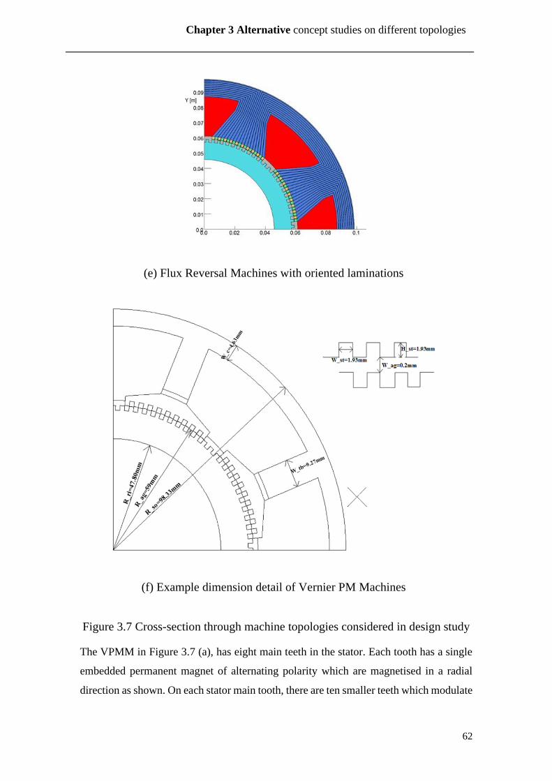
62


(e) Flux Reversal Machines with oriented laminations

(f) Example dimension detail of Vernier PM Machines

Figure 3.7 Cross-section through machine topologies considered in design study

The VPMM in Figure 3.7 (a), has eight main teeth in the stator. Each tooth has a single

embedded permanent magnet of alternating polarity which are magnetised in a radial

direction as shown. On each stator main tooth, there are ten smaller teeth which modulate

63


the flux produced by permanent magnet. The width of the smaller stator matches the pitch

of the rotor teeth and hence come into alignment simultaneously. This is achieved by

setting the width of main slot opening between the 8 large teeth to be an odd integer

number of the width of the smaller slots, in this particular case. When the rotor and stator

teeth are aligned the coil flux linkage due to the permanent magnet will increase. When

the rotor rotates to unaligned position, with the reluctance in the flux path increased, the

flux linkage will be reduced. There is no change in the polarity of the coil flux-linkage,

simply a modulation about some mean value.

The FSM in Figure 3.7 (b) shares many features with VPMM of Figure 3.7 (a), except

that the permanent magnet is located in the middle of main stator tooth. When the rotor

rotates, the flux will switch direction in main teeth like conventional flux switching

machines. However, compared to a conventional flux switching machine, in this machine

the small teeth increase the output frequency.

The Type A FRM shown in Figure 3.7 (c), has the same rotor and main teeth structure as

the VPMM. However, the permanent magnets are not embedded in the main teeth, but

mounted on the surface teeth. On each main tooth, there are ten S poles and ten N poles.

When the rotor teeth align to S poles on one main tooth, they will align to N poles on

another main tooth. The flux will reverse in the main teeth with the rotor rotation.

The Type B FRM (FRMB) shown in Figure 3.7 (d) is similar to the FRM, but only half

of main teeth are equipped with PMs, saving half volume of PM material. The main teeth

without magnets are aligned to rotor teeth all the time.

The main drawback of both FRMs is the small pole-pitch of the permanent magnets

mounted on the stator teeth, which leads to significant leakage flux. One concept which

was developed and investigated in an attempt to address this is shown in Figure 3.7 (e).

The stator core includes a large number of narrow gaps (0.2mm wide in the designs

analysed) which attempt to direct the magnet flux to link with the stator coils. The

practicality of this stator core is questionable, but it nevertheless provides an interesting

electromagnetic option.

64


3.6 Performance evaluation of different machine types

3.6.1 Finite element modelling of flux linkage variation in different machine

topologies

The first performance assessment undertaken was to employ two-dimensional finite

element analysis to predict the variation in flux linkage with rotor angular position for all

the machine designs in Figure 3.7. In order to provide some degree of generality, the

predicted variation in flux-linkage was normalised on a per tooth and per turn basis with

the values shown being for a core axial length of 50mm in all cases. The resulting

predicted variations in flux-linkage are shown in Figure 4.1. The waveforms in Figure

4.1 which correspond to the VPMM when initially calculated contains a significant DC

offset of 0.000565Wb. This DC offset has been removed in Figure 3.8 to aid a direct

comparison.

Figure 3.8 Flux linkages versus rotor mechanical position comparing the average

flux for each machine in open circuited

As shown in Figure 3.8, the various flux reversal machines produce a much larger

variation in flux linkage with amplitudes that are some 4-5 times higher those for

the FSM or VPMM. The main reason for the poor performance of VPMM and

-0.00015

-0.0001

-0.00005

0

0.00005

0.0001

0.00015

0 1 2 3 4 5 6 7

Flu

x Li

nka

ge p

er t

urn

per

to

oth

(W

b)

Mechanical position (°)

VPMM FRM FRM with gaps FRMB FSM

65


FSM is the very small size of the teeth which results in a significant leakage and

hence a small variation in the reluctance between the aligned position and

unaligned positions.

As discussed above, to reduce the flux leakage between reversed PM in FRM, a

series of complex airgaps were introduced into the main teeth as shown in Figure

3.7 (e). The increase in flux linkage amplitude produced by this stator core is only

some 3%-5% higher than the normal FRM. This modest increase in unlikely to be

sufficient to justify the manufacturing difficulties of incorporating these gaps into

an FRM.

3.6.2 Influence of number of rotor teeth

The small size of the rotor teeth and the magnet poles in the FRM designs dictates that

leakage in an important factor in limiting performance. It would be expected that the

performance of FRMs would improve in terms of the magnitude of the flux change if the

number of rotor teeth was reduced. As series of finite element simulations were

performed for variations on the FRM design in Figure 3.7(c) for a range of rotor teeth

between 48 and 192. In all cases, the main dimensions such as rotor diameter and radial

thickness of the magnets were kept fixed. Figure 3.9 shows the resulting variation in flux

linkage with rotor angular displacement. As will be seen, although the flux change does

increase with 48 teeth compared the 96 tooth designs previously, the rate of change of

flux with angular position is lower. As shown, the rate of change of flux linkage keeps

improving marginally with increasing numbers of rotor teeth.

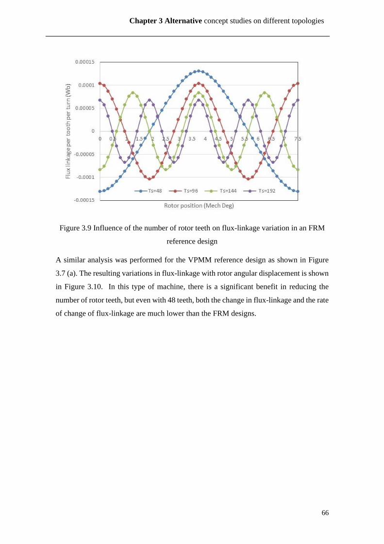
66


Figure 3.9 Influence of the number of rotor teeth on flux-linkage variation in an FRM

reference design

A similar analysis was performed for the VPMM reference design as shown in Figure

3.7 (a). The resulting variations in flux-linkage with rotor angular displacement is shown

in Figure 3.10. In this type of machine, there is a significant benefit in reducing the

number of rotor teeth, but even with 48 teeth, both the change in flux-linkage and the rate

of change of flux-linkage are much lower than the FRM designs.

67


Figure 3.10 Influence of the number of rotor teeth on flux-linkage variation in an

VPMM reference design

3.6.3 Finite element analysis of regulation and power curves

It has been shown that for the high pole numbers required in this application, FRMs tend

to have superior performances in terms of open-circuit flux variations compared to

VPMM and FSM topologies. FRMs were therefore selected for further analysis. The

output power capability of various FRM designs was predicted using an electric circuit-

coupled finite element simulation using the Opera 2D RM analysis for a standard FRM

with 96 rotor teeth. The electric coupled circuit used in these finite element simulations

is shown in Figure 3.11. The coils which couple into the finite element model are

connected to a full wave diodes bridge rectifier consisting of four uncontrolled rectifier

diodes (D1, D2, D3 and D4) with a fixed forward voltage drop set to 1 V. The load

resistor on the rectifier output (R1) can be varied to set different current operating points.

68


Figure 3.11 Coupled electric circuit used in finite element simulations

In all following simulations in this chapter, the rotational speed was set to 20,000 rpm

which results in a generator AC output electrical frequency of 32kHz for the 96 rotor

teeth. The number of series turns per coil was initially selected as 2 in order to maintain

an output voltage below 270 V (as was the case in the reference 3-phase brushless

machine design shown previously in Figure 3.1). Initial simulations were performed for

a split ratio of 0.6. The predicted electrical output power as a function of average load

current is shown in Figure 3.12.

Figure 3.12 Finite element predicted output power characteristic for a reference FRM

design with a split ratio of 0.6

As can be seen from this characteristic, the power level is very modest compared to the

50kW that can be achieved by the reference brushless machine design at 20,000rpm when

0

200

400

600

800

1000

1200

1400

1600

1800

0 5 10 15 20

Ou

tpu

t P

ow

er (

W)

Average Dc current (A)

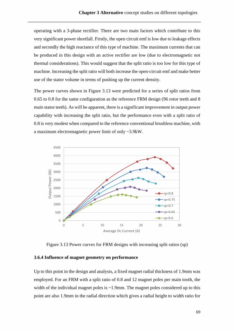
69


operating with a 3-phase rectifier. There are two main factors which contribute to this

very significant power shortfall. Firstly, the open circuit emf is low due to leakage effects

and secondly the high reactance of this type of machine. The maximum currents that can

be produced in this design with an active rectifier are low (due to electromagnetic not

thermal considerations). This would suggest that the split ratio is too low for this type of

machine. Increasing the split ratio will both increase the open-circuit emf and make better

use of the stator volume in terms of pushing up the current density.

The power curves shown in Figure 3.13 were predicted for a series of split ratios from

0.65 to 0.8 for the same configuration as the reference FRM design (96 rotor teeth and 8

main stator teeth). As will be apparent, there is a significant improvement in output power

capability with increasing the split ratio, but the performance even with a split ratio of

0.8 is very modest when compared to the reference conventional brushless machine, with

a maximum electromagnetic power limit of only ~3.9kW.

Figure 3.13 Power curves for FRM designs with increasing split ratios (sp)

3.6.4 Influence of magnet geometry on performance

Up to this point in the design and analysis, a fixed magnet radial thickness of 1.9mm was

employed. For an FRM with a split ratio of 0.8 and 12 magnet poles per main tooth, the

width of the individual magnet poles is ~1.9mm. The magnet poles considered up to this

point are also 1.9mm in the radial direction which gives a radial height to width ratio for

0

500

1000

1500

2000

2500

3000

3500

4000

4500

0 5 10 15 20 25 30

Ou

tpu

t P

ow

er (

W)

Average Dc Current (A)

sp=0.8

sp=0.75

sp=0.7

sp=0.65

sp=0.6

70


the poles of 1.0. Increasing the height of the magnet in the radial direction will tend to

decrease the reactance (by virtue of a larger effective magnetic airgap) but may reduce

the change in magnet flux. For the design with a split ratio of 0.8, the magnet height to

width ratio was varied between 0.10 (a magnet thickness of only 0.2mm) up to the

original value of 1.0. The predicted variations in the maximum power for each of these

designs is shown in Figure 4.7. As can be seen, the maximum output power can be

increased up to 7.4kW with the optimum magnet proportions. However, this is a very

thin magnet of thickness of 0.25mm which would be prone to demagnetisation.

Figure 3.14 Variation in maximum output power with aspect ratio for an FRM design

with 96 rotor teeth, a split ratio of 0.8 of magnet width of 1.9mm per pieces

A cross-section through the optimised design up to this point is shown in Figure 3.15.

For the 50mm axial length, this design has an active mass (cores, coils, magnets,

Aluminium hub and shaft but excluding casing) of 6.95kg, which gives a power density

for active mass of 1.07kW/kg. Although still a long way short of the baseline oil-cooled

brushless machine, this is starting to be competitive with many other machine types,

particularly given the requirement for a high frequency output.

71


Figure 3.15 Cross-section through 96 tooth optimal design with a split ratio of 0.8

(axial length of 50mmm)

3.7 Conclusions

This chapter has considered several machine types which would appear to offer a high

multiplier between mechanical rotation speed and electrical output frequency. Even

though significant optimisation has resulted in some improvements in performance, the

maximum power capability of the machine of Figure 3.15 is still much lower at 7kW

than the 50kW achieved for the baseline SPM design. Furthermore, the airgap required

in this machine for it small at 0.2mm.

Overall, this type of machine with a low number of coils (and hence a large coil

inductance per turn) and significant inter-polar magnet leakage flux will always struggle

to be competitive as a high power density generator. This type of machine does

nevertheless provide the functionality of high frequency output with a simple coil

structure.

72


3.8 References

[1] N. Bianchi, S. Bolognani and P. Frare, "Design criteria of high efficiency SPM

synchronous motors," IEEE International Electric Machines and Drives Conference,

2003. IEMDC'03., Madison, WI, USA, 2003, pp. 1042-1048 vol.2.

[2] A. M. El-Refaie, "Fractional-Slot Concentrated-Windings Synchronous Permanent

Magnet Machines: Opportunities and Challenges", IEEE Transactions on Industrial

Electronics, vol. 57, no. 1, pp. 107-121, Jan. 2010.

[3] Massimo Barcaro, "Analysis and Tests of a Dual Three-Phase 12-Slot 10-Pole

Permanent-Magnet Motor", IEEE Transactions on Industry Applications, vol. 46, no. 6,

November/December 2010.

[4] D. Wu and Z. Q. Zhu, "Influence of Slot and Pole Number Combinations on Voltage

Distortion in Surface-Mounted Permanent Magnet Machines With Local Magnetic

Saturation," in IEEE Transactions on Energy Conversion, vol. 30, no. 4, pp. 1460-1471,

Dec. 2015.

[5] J. Cros, P. Viarouge, "Synthesis of high performance PM motors with concentrated

windings", IEEE Trans. Energy Convers., vol. 17, no. 2, pp. 248-253, Jun. 2002.

[6] F. Magnussen and C. Sadarangani, "Winding factors and Joule losses of permanent

magnet machines with concentrated windings," IEEE International Electric Machines

and Drives Conference, 2003. IEMDC'03., Madison, WI, USA, 2003, pp. 333-339 vol.1.

[7] I. E. K. Koukouvini, C. T. Krasopoulos and A. G. Kladas, "Fault tolerant design of

fractional slot concentrated winding PM motor for electric traction," 2017 IEEE 11th

International Symposium on Diagnostics for Electrical Machines, Power Electronics and

Drives (SDEMPED), Tinos, 2017, pp. 181-187.

[8] B. Sen and J. Wang, "Stator inter-turn fault detection in SPM machines using PWM

ripple current measurement," 7th IET International Conference on Power Electronics,

Machines and Drives (PEMD 2014), Manchester, 2014, pp. 1-6.

[9] H. Kang, L. Zhou, J. Wang and X. Peng, "Investigation of multiphase modular stator

SPM with fault tolerance," 2014 17th International Conference on Electrical Machines

and Systems (ICEMS), Hangzhou, 2014, pp. 1572-1575.

73


[10] M. Shortte, ‘Electro-thermal optimisation of a 50kW synchronous permanent

magnet generator for aerospace application’. PhD thesis, University of Sheffield, 2016.

[11] R.Boll “Soft Magnetic Materials: Fundamentals, Alloys, Properties, Products,

Applications: The Vacuumschmelze Handbook”, Heyden 1979, ISBN: 3800912724.

[12] Vacuumschmelze GmbH & Co., “Rare-Earth Permanent Magnets,” vol. 3, no. 1,

2010.

74

Chapter 4 Design and analysis of a single-phase permanent magnet machines

Chapter 4 Design and analysis of a single-phase permanent

magnet machines

4.1 Introduction

Chapter 3 focussed on machine topologies which employ various types of flux

modulation to achieve high frequency output with a relatively low number of stator coils.

These produce an output frequency equivalent to that of a 96 pole-pair machine, i.e. 32

kHz at 20,000rpm. However, this approach resulted in machines with low power density,

due to the combination significant inter-polar flux leakage and high reactance. This

chapter is concerned with more conventional machine topologies in which the number of

stator coils equals the number of rotor pole-pairs, as is the case in a standard single-phase

permanent magnet machine. These are very high pole number variants of standard

surface-mounted and interior and exterior rotor permanent magnet machines, although

they are unusual in that they have single-phase outputs. The very high number of stator

slots which must be accommodated around the stator periphery, inevitably means that

the slots and teeth are very narrow. The single-phase stator winding in this type of

machine could be realised with a simple serpentine coil as shown schematically in Figure

4.1. As will be shown in this chapter, the number of turns required in each slot could be

as low as one, allowing a rectangular section Litz wire to be used.

Throughout this chapter, a consistent numbering system has been used to identify

machine designs. A full list of these design numbers is included as Appendix A of this

thesis.

75


Figure 4.1 Schematic of a stator with a single phase serpentine winding (end-on and

unrolled views of 12 slot variant)

4.1 Design of internal rotor machine

4.1.1 Surface mounted PM machine topology designs

The starting design in this chapter is a single-phase, inner rotor, surface-mounted

permanent magnet machine with a stator outer diameter of 160mm, 96 permanent magnet

pole-pairs and 192 stator teeth which generates a machine output frequency of 32 kHz at

20,000rpm (which would generate a 64 kHz pulse train when rectified). For this high

number of poles, each PM pole pitch will be only ~2mm wide and each coil slot is likely

to be 1-2mm wide. In order to ensure competitive airgap flux densities, it is necessary to

employ a radial magnetic airgap which is several times smaller than the magnet pole

pitch. In order to determine the upper limit on the electromagnetic capability of this type

of machine the radial length of the effective magnetic airgap for the first series of designs

was set to 0.2mm despite the inevitable mechanical challenges that this would present.

A key feature of any electrical machine initial sizing and design is the selection of the

machine split ratio, i.e. the ratio of the rotor diameter to the overall stator diameter. For

many medium power (10s of kW) SPMs reported in literature, split ratios of 0.55-0.65

are commonly used as these are claimed to generally offer optimum torque density [1].

However, these tend to have much lower number of stator teeth than in this application,

76


particularly for concentrated wound machines. When a very high pole number is used

such as the 192 considered here, the aspect ratio of the teeth, the shape of the slot and the

back-iron thickness become extreme (and likely impractical) and split ratios below 0.8

or so. As an example, Figure 4.2 shows a close-up of a pair of slots for 192 pole machine

designs with a stator outer of 160mm. As will be apparent, the more ‘sensible looking’

design are those at high split ratios. Although the lower end of the split ratio range may

cause practical difficulties and have poor electromagnetic performance due to slot-

leakage and hence higher reactance, as shown in Table 4.2, these were still modelled to

establish the variation in performance with split ratio. The initial set of designs shown in

Figure 4.2 all include tooth tips which enhance the capture of rotor magnet flux. In all

these designs, the ratio of stator tooth tip angle to stator tooth pitch is 0.8 while the ratio

of stator tooth body width to stator tooth tip width is 0.6.

SP=0.65 SP=0.7

SP=0.75 SP=0.8

SP=0.85 SP=0.9

Figure 4.2 Surface mounted PM machine with split ratio from 0.65 to 0.9 (design 4.1.1)

(Colour key: Blue – stator core; Red – stator coil; Green – rotor permanent magnet N

pole; Yellow – rotor permanent magnet S pole.)

The leading dimensions of the initial designs which were analysed are summarised in

Table 4.1. The magnetic materials used in these machines are same with that in chapter

77


3, i.e. stator and rotor core of VacoFlux 50 Cobalt Iron [2] and the permeant magnets are

Vacomax 225 Sm2Co17 [3].

Table 4.1 Leading dimensions of designs analysed (design 4.1.1)

Split ratio

0.60 0.65 0.70 0.75 0.80 0.85 0.90

Stator outer diameter (mm) 160 160 160 160 160 160 160

Stator inner diameter (mm) 96.4 104.4 112.4 120.4 128.4 136.4 144.4

Rotor outer diameter (mm) 96 104 112 120 128 136 144

Magnet pole pitch (mm) 1.571 1.702 1.833 1.963 2.094 2.225 2.356

Stator tooth width (mm) 0.757 0.820 0.883 0.946 1.008 1.071 1.134

Stator slot depth (mm) 33.12 29.21 25.30 21.40 17.49 13.58 9.676

Available slot area (mm2) 41.46 36.10 30.73 25.34 19.94 14.52 9.082

As would be expected given the high frequencies involved in these machines, the winding

impedance is dominated by the winding reactance. Table 4.2 shows the per-slot

calculated resistance and reactance in designs with split ratios from 0.6 to 0.9 (based on

a packing factor of 0.75 and a 20% increase in overall conductor length for end-windings).

As will be apparent, at 32 kHz, the coil reactance completely dominates the impedance,

being three order of magnitude greater than the resistance. Indeed, in all the design in

this chapter the coil impedance is dominated by its reactance, and hence the resistance

component (which in any case will be dependent on the packing factor that can be

achieved) can be neglected in terms of predicting electromagnetic performance with no

meaningful error.

78


Table 4.2 Summary comparison for SPM in different split ratio (design 4.1.1)

Split

ratio

Inductance/slot

(µH)

Area of conductor

for each slot (mm2)

Resistance

per slot (µΩ)

Reactance per

slot at 32kHz(m)

0.60 0.57 41.46 32.4 114.6

0.65 0.53 36.10 37.2 106.6

0.70 0.48 30.73 43.7 96.5

0.75 0.42 25.34 53.0 84.4

0.80 0.35 19.94 67.4 70.4

0.85 0.28 14.52 92.6 56.3

0.90 0.21 9.082 148 42.2

The symmetry in these machines allows a single pair of stator teeth to represent the finite

problem domain. The finite element coupled electric circuit employed to simulate

machine performance is shown in Figure 4.3. The symmetry and associated scaling set

up in the finite element model means that the circuit element W1 represents a series

connection all 96 positively oriented conductors. Similarly, W2 represents a series

connection of the 96 negative oriented conductors. The machine windings are connected

to a full wave bridge rectifier and a pure resistive load. The diodes in the model have a

fixed on-state voltage drop of 1V. This is typical of the voltage drop of a power diode.

The voltage regulation and power curves for a particular design are generated by running

a series of simulations with various values of load resistance.

Figure 4.3 Finite element coupled electric circuit for a generator connected to a full-

wave rectifier bridge and load resistance

79


The finite element predicted flux linkage per tooth per turn under open-circuit conditions

is shown in Figure 4.4. As would be expected, the increased rotor radius which follows

from a higher split ratio increases the stator flux linkage per tooth by increasing magnet

volume and reducing magnetic reluctance. A finite element predicted field distribution

under open-circuit conditions for a split ratio of 0.9 is shown in Figure 4.5.

Figure 4.4 Open-circuit flux linkage per tooth per turn as a function of rotor angular

position (design 4.1.1)

Figure 4.5 Finite element predicted field distribution under no-load conditions (design

4.1.1) (Blue – stator core; Red – coil; Light blue – rotor core; Yellow – magnet N pole;

Green – magnet S pole)

A single phase machine with the same number of rotor poles and stator teeth will generate

a large cogging torque as all the poles come into alignment with the teeth at the same

-0.0001

-0.00008

-0.00006

-0.00004

-0.00002

0

0.00002

0.00004

0.00006

0.00008

0.0001

0.00 0.50 1.00 1.50 2.00 2.50 3.00 3.50

Flu

xlin

kage

per

to

oth

per

tu

rn (

Wb

)

Mech Degree (°)

sp=0.6 sp=0.65 sp=0.7 sp=0.75

sp=0.8 sp=0.85 sp=0.9

80


time. Figure 4.6 shows the no-load cogging torque predicted for the machine design with

a split ration of 0.90 whose leading dimensions were shown previously in Table 4.1. As

shown, the peak cogging torque of 12.1Nm which is ~50% of the rated torque of 23.9Nm

(which corresponds to 50kW at 20,000rpm). In many applications where a maximum

cogging torque forms part of the specification, this level would be regarded as excessive.

However, there is in general no cogging torque specification for aerospace generators of

this type since they are generally driven from a very high power and high moment of

inertia prime-mover and hence this high cogging torque is not a problem in this case.

Figure 4.6 Finite element predicted no-load cogging torque for the machine (design

4.1.1)

The initial set of machine designs was based on a single serpentine wound coil, which

resulted in a series connection of the conductors in all slots. At this stage in the design

process, the serpentine coil has a single turn, i.e. only one effective series connected

conductor per slot (although this would be made up from several multiple parallel

strands). As will be demonstrated in this chapter, even a single turn results in an open-

circuit EMF in the 700V+ range for some design. In a practical machine for an aerospace

application it is likely that the stator would need to be wound in two or more sectors

which are then connected in parallel to achieve an appropriate output voltage, e.g. of the

order of 300V peak.

Providing the resistance can be neglected, the electromagnetic performance of a

particular design can be established without specifying a coil packing factor (i.e. the

-15

-10

-5

0

5

10

15

0.0 0.5 1.0 1.5 2.0 2.5 3.0 3.5 4.0

Co

gin

g To

rqu

e (N

m)

Mechanical angle (°)

81


proportion of each stator slot which is occupied by conductor rather than insulation, gaps

etc.). However, the viability of a machine in terms of delivering the maximum

electromagnetic power with a sustainable power loss and acceptable efficiency, is

dependent on the achievable packing factor. The parallel sided slots and the use of a

single turn serpentine coil should enable a high packing factor to be achieved particularly

if a rectangular rolled rectangular section Litz wire is matched to the slot shape. Figure

4.7 shows published manufacturer guidance on fill factor of compacted rectangular Litz

wire. This suggests an overall packing factors in the range 0.6-0.8 depending on the Litz

type used, the slot-liner thickness and the fit to the slot dimensions of the bundle profile.

For the rest of this chapter, conductor current densities are quoted for both packing

factors of 0.6 and 0.8 which should cover the range that can be realised in practice.

Figure 4.7 Published manufacturer design guidelines for rectangular (profiled)

compacted Litz wire (Source: [4])

A series of electric-circuit coupled finite element simulations were performed using the

rectifier circuit shown previously in Figure 4.3. For a particular machine design, the load

resistance was decreased in steps to gradually increase the average load current. The

predicted variations in the average load voltage as a function of the average load current

is shown in Figure 4.8a. Figure 4.8b shows the corresponding predicted variations in the

average load power. As shown, the electromagnetic output power capability of the

82


machine with split ratio in 0.6 is only ~4.1kW. However, with the split ratio increased to

0.9, the average output power capability increases to 43.4kW. This is due to a

combination of increased magnet flux from the larger rotor and the reduced reactance of

the shallower slots which improves the load regulation.

(a) Output V-I curve of the machine in different split ratios at 20,000rpm

(b) Output power in different split ratios at 20,000rpm

Figure 4.8 Output performance of the machine in different split ratios (design 4.1.1)

0

100

200

300

400

500

600

700

800

0 20 40 60 80 100 120

Ave

rage

DC

Vo

ltag

e (V

)

Average DC current (A)

sp=0.6 sp=0.65

sp=0.7 sp=0.75

sp=0.8 sp=0.85

sp=0.9

0

5000

10000

15000

20000

25000

30000

35000

40000

45000

50000

0 20 40 60 80 100 120

Ou

tou

t P

ow

er (

W)

Average DC Current (A)

sp=0.6 sp=0.65

sp=0.7 sp=0.75

sp=0.8 sp=0.85

sp=0.9

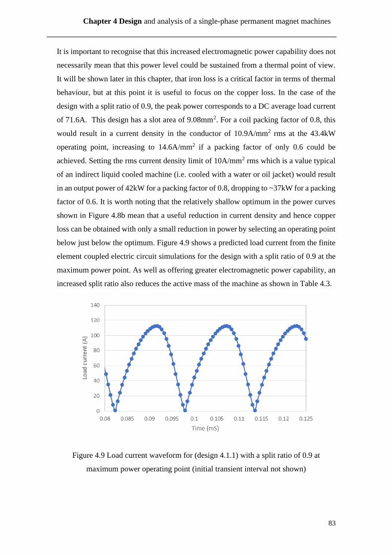
83


It is important to recognise that this increased electromagnetic power capability does not

necessarily mean that this power level could be sustained from a thermal point of view.

It will be shown later in this chapter, that iron loss is a critical factor in terms of thermal

behaviour, but at this point it is useful to focus on the copper loss. In the case of the

design with a split ratio of 0.9, the peak power corresponds to a DC average load current

of 71.6A. This design has a slot area of 9.08mm2. For a coil packing factor of 0.8, this

would result in a current density in the conductor of 10.9A/mm2 rms at the 43.4kW

operating point, increasing to 14.6A/mm2 if a packing factor of only 0.6 could be

achieved. Setting the rms current density limit of 10A/mm2 rms which is a value typical

of an indirect liquid cooled machine (i.e. cooled with a water or oil jacket) would result

in an output power of 42kW for a packing factor of 0.8, dropping to ~37kW for a packing

factor of 0.6. It is worth noting that the relatively shallow optimum in the power curves

shown in Figure 4.8b mean that a useful reduction in current density and hence copper

loss can be obtained with only a small reduction in power by selecting an operating point

below just below the optimum. Figure 4.9 shows a predicted load current from the finite

element coupled electric circuit simulations for the design with a split ratio of 0.9 at the

maximum power point. As well as offering greater electromagnetic power capability, an

increased split ratio also reduces the active mass of the machine as shown in Table 4.3.

Figure 4.9 Load current waveform for (design 4.1.1) with a split ratio of 0.9 at

maximum power operating point (initial transient interval not shown)

84


Table 4.3 Calculated active mass of the machine designs (neglects rotor shaft, rotor hub

and stator casing) (design 4.1.1)

Split ratio 0.60 0.65 0.70 0.75 0.80 0.85 0.90

Active mass (kg) - packing factor 0.8 5.09 4.69 4.24 3.76 3.24 2.69 2.10

Active mass (kg) - packing factor 0.6 4.39 4.07 3.72 3.33 2.90 2.44 1.94

The machine designs shown previously in Figure 4.2 have stator cores with tooth tips.

Although these tooth tips will tend to increase the induced emf from the permanent

magnet field they will also increase the reactance of the stator winding and hence degrade

the load regulation. Eliminating the tooth tips to produce open and parallel stator slots

will tend to reduce the stator reactance of the machine but at the expense of a reduced

emf. Other effects include making the machine easier to manufacture but at the expense

of exposing the windings to an increased field from the rotating permanent magnet fields

hence potentially increasing AC losses in the winding.

In order to determine whether removing the tooth tips would increase the power

capability of this type of machine, a further series of electric-circuit coupled finite

element simulations were performed on the machine designs shown in Figure 4.10, which

again have split ratios from 0.6 to 0.9. As was the case with the versions with tooth tips,

the stator winding was a single serpentine winding with one turn per slot. In the machine

with the tooth-tips the winding is retained to some degree by the tooth tips although a

trapezoidal shaped slot-wedge could be incorporated to fully retain the winding. In the

case of stator teeth with no tips, a region of the slot at the slot opening was left with no

coil as shown in Figure 4.5 and 4.6 to allow for either resin potting and/or a slot wedge

to retain the winding. The depth of this void was set to 0.4mm (twice the length of the

airgap). The slot areas quoted in this analysis and for calculation of losses does not

include this void, i.e. the packing factor is applied to the red region only in Figure 4.5

and Figure 4.6 for example.

However, the width of the magnet poles was reduced to reflect the reduced flux capture

capability of the parallel-sided tooth. The predicted variations in average load voltage

and average load power as a function of average load current are shown in Figure 4.11(a)

85


and Figure 4.11(b) respectively. As would be expected, there is reduction in the open-

circuit output voltage compared to the equivalent machine with tooth tips, e.g. from 679V

to 659V for a split ratio of 0.9. Although there is some improvement in the load regulation,

overall the absence of tooth tips results in a lower electromagnetic power capability, with

a maximum of ~40kW.

Figure 4.10 Machine designs with no tooth tips (design 4.1.2) (example shown has a

split ratio of 0.6)

(a) Output V-I curve of the machine in different split ratios at 20,000rpm

0

100

200

300

400

500

600

700

0 10 20 30 40 50 60 70 80 90

Ave

rage

DC

Vo

ltag

e (V

)


sp=0.6 sp=0.65

sp=0.7 sp=0.75

sp=0.8 sp=0.85

sp=0.9

86


(b) Output power in different split ratios at 20,000rpm

Figure 4.11 Finite element predicted output performance of the machine in different

split ratios (design 4.1.2)

Although these SPM machines have shown some useful potential in terms of the

electromagnetic power capability, particularly at the higher split ratio, these are based on

a 0.2mm airgap which is likely to prevent a practical containment sleeve from being

employed to the retain the rotor magnets against the influence of centrifugal loading. An

estimate of the containment thickness required to retain the magnets in the designs of

Figures 4.2 can be obtained using analytical stress calculation formulae from [5].

Taking a worst-case assumption that the magnets act as a dead-weight on the containment

sleeve (i.e. neglecting the effect of an adhesive bond between the individual magnets and

the rotor core) then the containment sleeve can be analysed as a homogenous rotating

thick-walled cylinder. If the inner and outer diameters and the pole arc being defined as

dmo, dmi, and α, as well as dco and dci of the containment sleeve, the maximum hoop

stress σmax in a containment sleeve at a rotational speed of 𝜔 is given by:

(4.1)

0

5000

10000

15000

20000

25000

30000

35000

40000

45000

0 10 20 30 40 50 60 70 80 90

Ou

tou

t P

ow

er (

W)


sp=0.6 sp=0.65

sp=0.7 sp=0.75

sp=0.8 sp=0.85

sp=0.9

87


Where 𝛿𝑐 and 𝜈𝑐 presents the mass density and the Poisson’s ratio of the containment, and

the effective mass and radius of the arc shaped magnet pieces are given by:

These analytical formulae from [5] were used to calculate the stress in a range of different

containment sleeves. Table 4.4 shows the calculated stresses for split ratios for a nominal

sleeve thickness of 0.5mm and the containment sleeve thickness required to limit the

stress to 1GPa which is at the upper end of the stress capability of filament-wound carbon

fibre sleeves. As shown by Table 4.4, there is a significant increase in stress with

increasing split ratio. This is due to a combination of increased rotor radius and increased

magnet radial thickness and hence mass since the individual magnet poles were all based

on a 1:1 aspect ratio between radial thickness and pole pitch. The calculated values in

Table 4.4 show that a minimum a sleeve thickness of 0.65mm would be required for a

split ratio of 0.9 (and thicker if a greater safety margin than that with 1GPa was required).

When added to a minimum mechanical clearance of ~0.2mm, this would result in an

effective magnet airgap of 0.8-0.9mm for this split ratio. It is worth noting that in terms

of mechanical analysis, the split ratio is setting the rotor diameter and hence the results

in Table 4.4 suggest that a smaller diameter but axially longer machine might be a viable

option. However, the reduced pole pitch and hence the increased leakage would work

against a machine with a smaller rotor diameter. This option of changing the aspect ratio

was not considered further, since the design study was focussed on a direct comparison

with the reference design. The issue of aspect ratio could be returned to in a future study.

88


Table 4.4 Analytically predicted containment sleeve performance at 20,000rpm for a

series of machine design from Figure 4.2 with different split ratios

SP = 0.6 SP=0.75 SP=0.9

Containment hoop stress

for 0.5mm thick

containment sleeve

408MPa 737MPa 1.20GPa

Containment sleeve

thickness for a maximum

stress of 1GPa

0.153mm 0.330mm 0.65mm

In order to understand the electromagnetic impact of increasing the gap between the

surface of the magnets and the stator bore, a further series of finite element simulations

were performed for a machine design with tooth tips and a split ratio of 0.9 for magnetic

airgaps of 0.4mm, 0.6mm and 0.8mm. Figure 4.12 shows magneto-static finite element

predicted field distributions for the various airgaps. As would be expected, the inter-polar

airgap leakage flux increases significantly with increasing airgap.

(a) Open circuit flux distribution in SPM machine with a radial airgap of 0.2mm

(b) Open circuit flux distribution in SPM machine with a radial airgap of 0.4mm

89


(c) Open circuit flux distribution in SPM machine with a radial airgap of 0.6mm

(d) Open circuit flux distribution in SPM machine with a radial airgap of 0.8mm

Figure 4.12 Open circuit Flux distribution in machine (design 4.1.1-ag) with different

air gaps for machines with a split ratio of 0.9

Figure 4.13a shows the predicted variation in the average output voltage with increasing

load current while Figure 4.13b shows the corresponding variation in the average output

power for the various airgap lengths. As will be apparent, increasing the airgap even by

a further 0.2mm to 0.4mm results in a dramatic reduction in the average output DC

voltage and power. On the basis of the predictions of Figure 4.13b, it was concluded that

a mechanically viable machine, i.e. an airgap of at least 0.8mm to accommodate a

0.65mm thick containment sleeve (operating at 1GPa), does not provide a competitive

power output for the particular combination of speed and power.

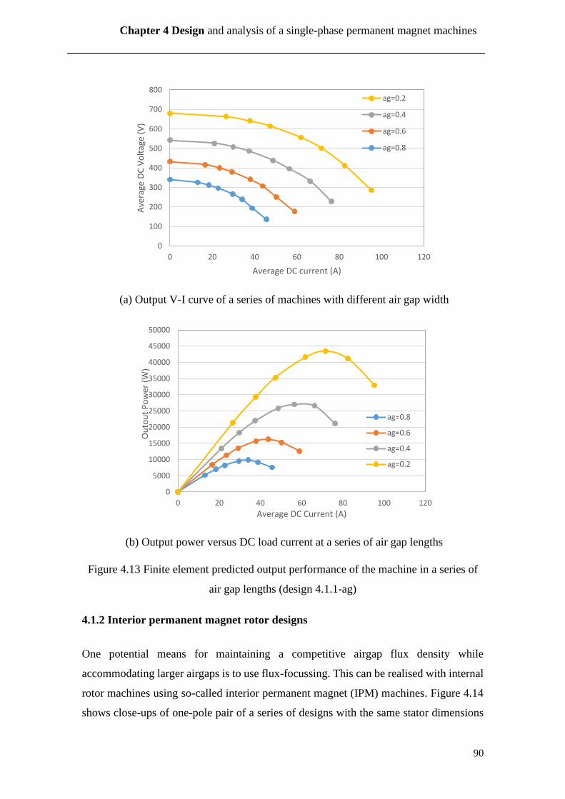
90


(a) Output V-I curve of a series of machines with different air gap width

(b) Output power versus DC load current at a series of air gap lengths

Figure 4.13 Finite element predicted output performance of the machine in a series of

air gap lengths (design 4.1.1-ag)

4.1.2 Interior permanent magnet rotor designs

One potential means for maintaining a competitive airgap flux density while

accommodating larger airgaps is to use flux-focussing. This can be realised with internal

rotor machines using so-called interior permanent magnet (IPM) machines. Figure 4.14

shows close-ups of one-pole pair of a series of designs with the same stator dimensions

0

100

200

300

400

500

600

700

800

0 20 40 60 80 100 120

Ave

rage

DC

Vo

ltag

e (V

)


ag=0.2

ag=0.4

ag=0.6

ag=0.8

0

5000

10000

15000

20000

25000

30000

35000

40000

45000

50000

0 20 40 60 80 100 120

Ou

tou

t P

ow

er (

W)


ag=0.8

ag=0.6

ag=0.4

ag=0.2

91


but with a series of different rotor magnet dimensions. In each case, the green regions in

the rotor represent circumferentially magnetised magnets of alternating polarity as shown

while the light blue regions represent iron pole pieces. In principle, these iron pole pieces

could be keyed into the non-magnetic rotor hub (grey region) to provide some mechanical

retention although this could increase leakage flux around the inner edge of the magnets.

The dimensions of each rotor design are defined in terms of the rotor magnet aspect ratio

(Rt) which is defined as the ratio of radial depth of a magnet pole to its width. In all cases,

the stator design remains fixed. The increasing magnet radial depth is accommodated by

reducing the outer diameter of the non-magnetic rotor hub.

Figure 4.14 Inset PM Machine designs (design 4.2.1) (Darker blue – stator core; red –

stator coil; green – rotor magnets; light blue – rotor core pole-pieces)

The finite element predicted field distribution under open circuit conditions is shown in

Figure 4.15 for the case of Rt=2 and an airgap of 0.2mm. This demonstrates that although

there is still some flux leakage at the inner edge of the rotor shaft, the majority of flux

from magnet is focussed in to the stator teeth when the rotor iron inter-poles are aligned

with the stator teeth. The benefit of increasing the ratio Rt in terms of increasing the stator

flux-linkage is clearly shown in the flux density distributions of Figure 4.16 and Figure

4.17. As shown, the stator tooth bulk flux density is ~2T for Rt=2 compared to only ~1.2T

for Rt=05.

Rt=0.5 Rt=1

Rt=1.5 Rt=2

92


Figure 4.15 Open circuit field distribution in IPM machine with Rt = 2 and an airgap of

0.2mm (design 4.2.1)

Figure 4.16 Open circuit flux density distribution in IPM machine with Rt=0.5 and

airgap of 0.2mm (design 4.2.1)

Figure 4.17 Open circuit flux density distribution in IPM machine with Rt=2 and airgap

of 0.2mm (design 4.2.1)

93


The corresponding load voltage and power curves for designs which have identical

stators but different values of Rt are shown in Figure 4.18(a) and Figure 4.18(b)

respectively. As shown, for an Rt value of 2, the maximum output power output is

~135kW. This power is the electromagnetic limit and not necessarily realisable thermally

on a steady-state basis. An indication of the practicality of these machines from a thermal

perspective can be obtained by considering the current density in the stator conductors.

As was the case for all the designs simulated previously in this chapter, for this particular

stator, it is assumed that the conductors in all 192 slots (1 conductor per slot) are series

connected. Each stator slot in this stator design has a cross-sectional area of 9.08mm2.

Assuming a coil packing factor of 0.8, the peak power of 11.5kW occurs at a DC average

current of 118A for Rt = 2 corresponds to an average current density of 18.04A/mm2 rms.

A more pessimistic packing factor of 0.6, would increase this to 24.06A/mm2 rms. Both

of these values are likely to be higher than could be sustained in continuous operation. A

reduction to 10A/mm2 rms at a packing factor of 0.8 (equivalent to 13.3 A/mm2 rms for

a packing factor of 0.6) which is arguably more realistic in terms of a thermal

performance corresponds to an average DC load current of 65.4A, still produces a load

power of ~98kW.

94


(a) Output V-I curve of the machine in different magnet depth/width ratio

(b) Output power of the machine in different magnet depth/width ratio

Figure 4.18 Finite element predicted output performance of the machine in different

magnet depth/width ratio (design 4.2.1)

Although the topology shown in Figure 4.14 with a value of Rt=2 provides excellent

level of output power even with a reduced current density of 10A/mm2 rms, it is still

based on a very small airgap of 0.2mm. The large radial thickness of the magnet for Rt=2

is 4.71mm which inevitably means that retaining the magnets against centrifugal forces

will require a potentially thick containment layer. It may be possible to incorporate some

0

200

400

600

800

1000

1200

1400

1600

0 20 40 60 80 100 120 140 160

Ave

rage

DC

Vo

ltag

e (V

)


RT=2.0

RT=1.5

RT=1.0

RT=0.5

0

20000

40000

60000

80000

100000

120000

140000

160000

0 20 40 60 80 100 120 140 160

Ou

tou

t P

ow

er (

W)


RT=2.0RT=1.5RT=1.0RT=0.5

95


retaining features on the inner surface of pole pieces which would lock into the non-

magnetic rotor hub (e.g. fir-tree as in gas turbine blades [6]). However, this would not be

possible for the magnets since they are very weak and their mechanical behaviour is

unpredictable in tension. The thickness of a carbon fibre sleeve required to retain the

magnets in the machine design of Figure 4.17 (which has a value of Rt=2) can be

calculated using equation 4.1 shown previously. For a carbon fibre stress limit of 1GPa

(which is at the upper end of the range that could be used), the thickness would vary

between 0.51mm for loading by the magnet only (i.e. the pole pieces are completely

retained by the mechanical retention feature into the hub) and 1.11mm assuming that

both the magnets and the pole-pieces act as a deadweight on the containment sleeve.

The electromagnetic impact of such a thick non-magnetic sleeve was investigated by

considering the impact of increasing the effective magnetic airgap from 0.2mm to 0.6mm.

Figure 4.19 shows the open-circuit flux distribution for an airgap of 0.6mm which shows

the significant leakage flux, both within the airgap and at inner edge of the magnet

through the non-magnetic rotor hub. The resulting voltage versus current and load power

versus current characteristics for different airgaps are shown in Figure 4.20. As will be

apparent, there is a very significant reduction in performance with a non-magnetic

containment sleeve even when it is only 0.6mm thick. Although even larger airgaps could

have been considered, e.g. up to 1.2-1.4mmmm to accommodate the worst case of a 1.11

mm containment sleeve to contacting dead-weight iron pole-piece, the electromagnetic

performance at 0.6 has deteriorated to the point where it is not a competitive solution.

Figure 4.19 Finite element predicted field distribution in a design with an airgap of

0.6mm

96


(a) Output V-I curve of a series of machines with different air gap lengths

(b) Output power versus DC load current at a series of air gap lengths

Figure 4.20 Finite element predicted output performance of the machine in a series of

air gap lengths (design 4.2.1-ag)

Rather than incorporating a separate sleeve to retain the magnets, the alternative rotor

structure shown in Figure 4.21 was considered. This is an interior permanent magnet

machine in which the rotor magnets are contained within the rotor core structure by

bridges between the main rotor core pole-pieces, forming a single continuous rotor core.

This type of rotor has the benefit of reducing the effective magnetic airgap to the

permanent magnet flux passing across the airgap but at the expense of promoting leakage

0

200

400

600

800

1000

1200

1400

1600

0 20 40 60 80 100 120 140 160

Ave

rage

DC

Vo

ltag

e (V

)


ag=0.6

ag=0.4

ag=0.2

0

20000

40000

60000

80000

100000

120000

140000

160000

0 20 40 60 80 100 120 140 160

Ou

tou

t P

ow

er (

W)


ag=0.6

ag=0.4

ag=0.2

97


flux within the bridge region outside each magnet. The bridge would need to be laminated

because of slotting harmonics and would need to be high-strength soft magnetic material.

Figure 4.21 IPM topology with bridge structure (design 4.2.2 with bridge thickness of

0.48mm)

In selecting the radial thickness of the bridge region, there is a trade-off between

mechanical strength and electromagnetic performance since the bridge acts as a magnetic

short-circuit for some of the rotor magnet flux. Figure 4.22 shows magneto-static finite

element predicted field distributions for bridge radial thickness of 0.16mm and 0.48mm

which shows the tendency of significant magnet flux to pass through these regions rather

than crossing the airgap and the high level of magnetic saturation that occurs in these

bridge regions.

The corresponding flux density distributions are shown in Figure 4.23. The flux density

in the stator tooth is a useful indication of the electromagnetic effectiveness of the rotor.

As will be seen, with a bridge which is only 0.16mm thick, the bulk stator tooth flux

density is ~ 1.5T under open circuit conditions, but this reduces to a corresponding value

of 0.7T when the bridge thickness increases to 0.48mm. It is clear from Figure 4.21 that

very high levels of flux density are encountered in the bridge sections in the rotor.

98


(a) Bridge thickness = 0.16mm

(b) Bridge thickness = 0.48mm

Figure 4.22 Finite element open-circuit predicted field distributions for an IPM design

with bridge radial thicknesses of 0.16mm and 0.48mm (design 4.2.2)

99


(a) Machine with 0.16 mm thick bridge

(b) Machine with 0.48 mm thickness bridge

Figure 4.23 Open circuit flux density in the machine (design 4.2.2)

The output voltage and power curves for a range of bridge thicknesses are shown in

Figure 4.24. Although the machine is able to achieve a maximum load power output of

greater than 50kW with a 0.32mm thick bridge, the power capability drops very

significantly to 23kW for a modest increase in bridge thickness to 0.48mm.

100


(a) Output V-I curve of a series of machines with different bridge thickness

(b) Output power versus DC load current at a series of different bridge thickness

Figure 4.24 Finite element predicted output performance of the machine with different

bridge thickness (design 4.2.2)

In an attempt to enhance the airgap flux density and hence maintain a competitive

electromagnetic power density, a trapezoid magnet geometry was investigated. This

geometry is shown in Figure 4.25 which used the same stator dimensions as that used in

the designs of Figure 4.19. The main reason for using a trapezoidal magnet is to minimise

0

200

400

600

800

1000

1200

1400

0 20 40 60 80 100 120 140

Ave

rage

DC

Vo

ltag

e (V

)


br=0.48

br=0.32

br=0.16

0

20000

40000

60000

80000

100000

120000

0 20 40 60 80 100 120 140

Ou

tou

t P

ow

er (

W)


br=0.48

br=0.32

br=0.16

101


the flux linkage on the inner edge of the magnet. The open circuit magnetic field

distribution and flux density variation in this machine are shown in Figure 4.25 and

Figure 4.26, which shows that the trapezoidal magnet shape is effective in reducing the

flux leakage through rotor hub. As a consequence, the flux density in both airgap and

stator teeth were increased to competitive level compared with IPM with bridge.

Figure 4.25 Open circuit flux distribution in Trapezoid magnet IPM machine

Figure 4.26 Open circuit flux density in Trapezoid magnet IPM machine (Br=0.32mm)

The corresponding output characteristics predicted with the electrical circuit coupled

finite element model for this design are shown in Figure 4.27, again for the case of a

single turn series wound coil. As will be apparent when Figure 4.27 is compared with

Figure 4.22, the machine with trapezoidal magnets have a higher power capability than

an IPM machine with the same bridge thickness, e.g. for a bridge thickness of 0.48mm,

the maximum power capability increases from 83.4kW to 97.5kW. However, even with

the trapezoidal magnets, when the bridge thickness is increased to 0.6mm, the output

power capability falls dramatically to only 25kW.

102


(a) Output V-I curve of the machine in different bridge thickness

(b) Output power versus DC load current with different bridge thickness

Figure 4.27 Finite element predicted output performance of the machine with different

bridge thickness (for trapezoid PM machine design 4.2.3)

The key to establishing the viability of an IPM machine in which Cobalt-Iron bridges

retain the magnet is the stress in the bridge regions. In order to establish the mechanical

viability of such thin bridge regions, a series of ANSYS simulations were performed at

20,000rpm for an IPM machine with trapezoidal magnets. The key mechanical properties

0

200

400

600

800

1000

1200

1400

0 20 40 60 80 100 120 140

Ave

rage

DC

Vo

ltag

e (V

)


br=0.6

br=0.48

br=0.32

br=0.16

0

20000

40000

60000

80000

100000

120000

140000

0 20 40 60 80 100 120 140

Ou

tpu

t P

ow

er (

W)


br=0.6

br=0.48

br=0.32

br=0.16

103


for Vacodur S+ Cobalt Iron which can be heat-treated to optimise the mechanical

properties are shown in Table 4.5 which draws on published data from [7].

Table 4.5 Manufacturer data for physical properties of Vacodur S+ with heat-treatment

to optimise mechanical properties

0.2% Yield strength 800MPa

Young’s modulus 250GPa

Tensile strength 1200MPa

Initially the geometry shown previously in Figure 4.25 was modelled, but this resulted in

very stress concentrations in the rotor core bridges around the outer corners of the

trapezoidal magnets. To reduce the stress concentration a radius of 0.2mm was

introduced into the narrow end of the magnet poles. The resulting Von-Mises stress

distributions at 20,000rpm for 0.48mm and 0.60mm bridge thicknesses are shown in

Figure 4.28. The maximum localised stress in all case occurs in the region of the rotor

core near the outer edges of the magnets. It is interesting to note that the reduction in

localised maximum stress from thickening the bridge is only from 596MPa to 560MPa,

i.e. a 6% reduction in stress for a 25% increase in bridge thickness. Although the relative

displacements of the rotor components are greatly exaggerated by scaling to aid clarity,

the rotor hub and magnets would detach from the hub at these speeds. This could be

eliminated by shrink-fitting the rotor core to the hub thus putting a significant

compressive force on the magnets at standstill. If the correct level of pre-compression is

applied, then this would result in the same stress levels in the rotor core bridges as shown

in Figure 4.28 at 20,000rpm [5]. The predicted stresses in Figure 4.28 are well outside

the capability of the rotor core material since the likely design stress in-service operation

would be ~400MPa (based on a safety margin of ~2 applied to the 0.2% yield stress of

800MPa to allow for fatigue and manufacturing tolerances). Hence, this approach does

not offer a viable solution from a mechanical perspective at 20,000rpm and also results

in modest electromagnetic performance.

104


20C

(a) 0.48mm thick rotor bridge

(b) 0.48mm thick rotor bridge

Figure 4.28 ANSYS finite element predicted Von-Mises mechanical stress in rotor at

20,000rpm.

Some of these interior rotor machines, when constrained to the same stator outer diameter

of 160mm and axial length of 50mm, as the baseline SPM described in section 3.1, show

superior electromagnetic power capability, e.g. 80-90kW, although this is for small

airgaps of 0.2mm and/or narrow magnet bridge in 0.16mm. However, the

electromagnetic power diminishes significantly with only small increases in the length

of the airgap thickness of the bridging sections of the rotor cores, such that more practical

mechanical arranges are not capable of meeting the 50kW output power specification.

However, it is important when considering these designs to recognise that for the higher

split ratio of 0.9 with the same 160mm stator outer diameter, the mass of the active

elements is considerably lower than the baseline for the same axial length, e.g. 2.62kg in

the case of a 192 pole machine with a split ratio of 0.9 compared to 4.77kg for the baseline.

Hence, to provide a direct comparison, it would be reasonable to increase the axial length

of the 0.9 split ratio machines from the 50mm of the baseline to 91mm to yield the same

active mass. This would scale the powers obtained in Figure 4.28(b) for example by a

105


factor of 1.82. Applying this scaling to a machine with a 0.6mm thick bridge, increases

the power capability to 55.6kW for a DC average load current of 56.2A which

corresponds to a current density 8.6A/mm2 rms for a packing factor of 0.8 increasing to

11.5/mm2 rms for a packing factor of 0.6.

Despite the promising electromagnetic performance of many designs with an internal

rotor, the need to increase the effective magnetic airgap to at least 0.6mm (and arguably

greater to maintain a practical mechanical clearance in a high speed machine) results in

a large reduction in performance. Hence, the focus on the design was shifted to external

rotor machines.

4.2 Design of External rotor machine

The analysis in section 4.1 has shown that although the various internal rotor topologies

investigated are capable of producing a rectified output power which exceed the power

specification of 50kW, this is only realised with very small magnetic airgaps of <0.5mm.

As discussed previously, the need to mechanically contain the rotor magnets with a sleeve

means that this topology is unlikely to be a practical solution for high-speed machines of

such high pole numbers. One potential solution to change to an external rotor topology

in which the magnet containment is located outside the rotor and hence does not sit in

the airgap. The containment sleeve thickness can then be dimensioned to contain the

magnet reliably with an appropriate safety margin with no first-order electromagnetic

implications. Figure 4.29 shows a typical design of a 96 pole-pair IPM machine with an

external rotor, in this case with a split ratio of 0.9. It is worth noting that in this topology,

the stator slot depth is not set by the split ratio (as is largely the case with an internal rotor

machine). Hence, there is likely to be some optimisation of slot depth required in terms

of a trade-off between mass, current density and stator reactance.

106


Figure 4.29 External rotor machine topology with an interior permanent magnet rotor

geometry (design 4.3.1)

For the machine design shown in Figure 4.29, the split ratio (airgap diameter to outer

rotor diameter) was maintained at 0.9. It is useful to define the rotor dimensions in terms

of the stator hub ratio (inner stator diameter/ outer rotor diameter) and this was initially

set to 0.7. The same grade of Cobalt Iron was used for the stator core. However, although

the rotor iron does not need to counter the centrifugal force on the magnets, it may still

be useful to have a bridge between the iron pole pieces to produce a single piece rotor

core.

Four types of rotor structures were explored for this machine and are shown in Figure

4.30. Type A and type C employ rectangular iron pole pieces while type B and type D

employ trapezoidal pole-pieces. As shown in Figure 4.30, rotor types A and B have a

bridge adjacent to the airgap side, when type C and type D put bridge on outside edge of

the rotor. In all cases, the bridge thickness was fixed at 0.5mm. The outer diameter of

active section of the rotor was maintained at 160mm and the same axial length of 50mm

was also maintained.

107


Figure 4.30 Four rotor structures considered in analysis (designated as design 4.3.1-

4.3.4) – Stator core -dark blue; Rotor magnet - green; Stator coil - red; Rotor core –

light blue; Rotor mechanical containment – grey)

The finite element predicted voltage and power curves for these four designs are shown

in Figure 4.31, again with a single turn per slot. As will be seen, despite these designs

having the same leading dimensions, the location of the soft magnetic bridge has a very

significant effect on the power capability of the machines. Types C and D which employ

bridges on the outer edge of the rotor provide competitive power even though these still

provide a magnet flux short-circuit path.

Rotor type A Rotor type B

Rotor type C Rotor type D

108


(a) Output V-I curve of the machine in different rotor type

(b) Output power versus DC load current for the machine in different rotor type

Figure 4.31 Finite element predicted output performance of the machine (design 4.3.1-

4.3.4 as shown in Figure 4.30)

The stator teeth in the external rotor design shown previously in Figures 4.29 and 4.30

are based on stator teeth with constant width. This results in a gradual narrowing of the

slot with increasing slot depth. In order to accommodate rectangular rolled Litz wire into

this type of a slot, it would be necessary to size the wire on the basis of the minimum slot

width which would result in a gradually increasing triangular void in the slot. This under-

utilisation of the slot would result in an increased copper loss. An alternative approach is

0

200

400

600

800

1000

1200

1400

1600

0 20 40 60 80 100

Ave

rage

DC

Vo

ltag

e (V

)


A

B

C

D

0

10000

20000

30000

40000

50000

60000

70000

80000

90000

100000

0 20 40 60 80 100

Ou

tpu

t P

ow

er (

W)


A

B

C

D

109


to design the stator with a fixed slot width. This is results in a gradual narrowing of the

stator core tooth which it is recognised will increase the stator core loss. A stator design

based on a parallel sided slot is shown in Figure 4.32, in this case for a stator hub ratio

of 0.7.

Figure 4.32 External rotor machine with a parallel sided stator slot (design 4.4.1).

Stator core -dark blue; Rotor magnet - green; Stator coil - red; Rotor core – light blue;

Rotor mechanical containment - grey

The stator also can also be optimised by varying the stator slot depth, which can be simply

achieved by changing the stator hub ratio (i.e. the ratio of the stator hub diameter to the

overall machine diameter) while keeping the airgap, rotor inner and outer diameter fixed.

When the stator hub ratio is increased, the length of stator tooth and the hence the depth

of the stator slot decreases. This has three advantages and one disadvantage:

• The cross-slot leakage flux will reduce, which reduce the stator self-inductance and

hence the stator reactance which will improve the voltage regulation.

• If there is the any magnetic saturation in the stator core, reducing the flux path length

will reduce the effect on the stator magnetic reluctance and so reducing the influence

of magnetic saturation on the stator flux-linkage.

• It will tend to reduce the stator iron loss because of the reduced stator tooth volume.

• The reduced slot area will increase the current density and hence losses for a given

stator ampere turns.

Figure 4.33 shows the electromagnetic performance of a series of machine designs with

a range of different stator hub ratios from 0.7 (previous design shown in Figure 4.32) to

0.8, (denoted as design 4.4.1-4.4.3 in sequence).

110


(a) Output V-I curve of the machine with a series of different stator hub ratio

(b) Output power with different stator hub ratio

Figure 4.33 Finite element predicted output performance of the machine (design 4.4.1-

4.4.3)

As shown in Figure 4.33, as the stator hub ratio increases from to 0.70 and 0.8, the

maximum power increases from 56.8kW at a current of 54A to 104.2kW at a current of

94.7A respectively. However, due to combination of the higher current at the maximum

power point and the shallower slots, there is a significant increase in the current density

for the shaft hub ratio of 0.8. The slot depths are 15mm, 10.4mm and 6.4mm for stator

0

200

400

600

800

1000

1200

1400

1600

0 20 40 60 80 100 120 140

Ave

vo

ltag

e (V

)

Ave Current (A)

SH=0.7

SH=0.75

SH=0.8

0

20000

40000

60000

80000

100000

120000

0 20 40 60 80 100 120 140

Ou

tpu

t P

ow

er (

W)

Ave Current (A)

SH=0.7

SH=0.75

SH=0.8

111


hub ratios of 0.7, 0.75 and 0.8 respectively). For a stator hub ratio of 0.7 operating at its

maximum power point with a DC average output current of 54A (corresponds to an rms

machine current of 60.0A) then at a packing factor of 0.8 the current density in the

conductors is 5.0A/mm2 rms. When the stator hub ratio is increased to 0.8 with a

maximum operating point current of 95A, the rms current density in the machine for a

packing factor of 0.8, increases to 20.6A/mm2. The corresponding current densities at a

coil packing factor of 0.6 are 6.7 A/mm2 and 27.5A/mm2 respectively. It is also worth

noting however that a lower value of stator hub ratio leads to longer stator teeth and hence

an increased core loss.

4.3 Evaluation of iron loss and candidate core materials

The analysis up to this point has been concerned with the electromagnetic power limit of

the machines, which is determined predominantly by the combination of induced EMF

and coil reactance, and some consideration of the current density in the stator coil. It has

been shown that from a maximum power capability. However, it is also necessary to

establish thermal limitations on the achievable power as these may well be lower than

the electromagnetic limit. The combination of a very high fundamental frequency and

high stator flux densities in the machines considered previously means that iron loss will

be a particular concern. It is also worth noting that the use of a diode rectifier will lead

to some distortion of the machine current.

Figure 4.34 shows a representative machine-side current waveform, in this case for

design 563 at its peak power of 104.2kW at a DC average load current of 94.7A

(corresponding to a peak AC machine current of 149Apk). The waveform of Figure 4.34

contains relatively little harmonic distortion and evidenced by an FFT which gives 3rd,

5th and 7the harmonic magnitudes of 2.26A, 1.83A and 0.42A. In the calculation of iron

loss described later in this chapter, the use of a circuit-coupled finite element model

ensures that these harmonics in the current waveform are included in the loss calculation.

112


Figure 4.34 Predicted machine current waveform for design 4.4.3 at its peak power

operating point of 104.2kW

The analysis presented up to this point in this chapter has been based on stator cores with

Vacoflux 50 cores which is the same material as that used in the baseline machine design

of chapter 3. As noted in chapter 3, this is a high performance soft magnetic material

which is widely used in aerospace electrical machines because of its combination of low

iron loss and high saturation flux density. This section describes the properties of several

alternative soft magnetic materials that might be more suitable for the stator core in this

high frequency application and predicts machine performance for the most promising

materials.

In the high frequency applications, iron loss tends to be dominated by the eddy current

component of loss. There are two fundamental approaches to reducing eddy currents in

magnetic cores:

1. Modify the composition of the material to increase electrical resistivity, e.g. by add

silicon or other alloying elements.

2. Modify the geometry of the individual soft magnetic elements, e.g. through the use of

very thin laminations or the use of cores manufactured from electrically insulated

powder particles.

Soft magnetic composites (SMCs) in which a ferromagnetic powder is bonded together

to form a net-shape component is a technology which is well suited to high frequency

-200

-150

-100

-50

0

50

100

150

200

0.00004 0.00005 0.00006 0.00007 0.00008 0.00009 0.00010 0.00011 0.00012 0.00013

Co

il C

urr

ent

(A)

Time (S)

113


applications in which the losses are likely to be dominated by eddy current loss. Hence,

the focus in this design optimisation was establishing either a soft magnetic composite

which offers a lower loss than the Cobalt Iron baseline design.

4.3.1 Soft magnetic composites

In a soft magnetic composite (SMC), particles of very fine soft magnetic powders are

bonded together with some form of binder to form a net-shape soft magnetic component.

In some cases, this type of material is referred to as powdered-iron or powder cores.

Although they have generated significant interest in recent years, they have been

proposed for more than 100 years [8]. Whereas powdered iron cores with permeability

of a few 10s have been around for many years, it is only since the 1990s that SMCs have

been developed for electrical machines with permeabilities of several hundred [9]. Figure

4.35 shows a schematic representation of an SMC. It consists of an iron powder coated

with organic insulation which are the pressed under a high pressure (typically up to

800MPa [10]) to achieve near full density (typically up to 98-99% dense). Careful control

of the pressing and processing is required in order to maintain the insulation layer

between iron powder particles (to retain a high electrical resistivity) while also ensuring

near full density (in order to achieve a relative permeability of several hundreds).

Figure 4.35 Schematic picture of component elements of SMC material (Source: [10])

The hysteresis loss in SMCs tends to be higher than in electrical steel laminations because

of the significant mechanical stresses which are applied to the iron particles during

pressing which cannot be relieved by annealing at high temperature as this would damage

the binder. However, since the individual iron particles remain largely insulated from

each other, the eddy current loss tends to be lower than a laminated electrical steel.

114


Figure 4.36 shows published guidance on the operating range of SMCs which

demonstrates that they offer a greater useable frequency range that SiFe lamination, and

potentially in the 10s of kHz range, albeit at lower flux densities [11] [12]. In this section,

several SMC materials which offer a range of properties are reviewed, viz. Somaloy 130i

5P, CSC high flux 125μ and CSC mega flux 60μ.

Figure 4.36 Manufacturer published operating range for SMCs (Source: [11])

4.3.1.1 Somaloy 130i 5p

Somaloy is a commercially produced family of grades of SMC material manufactured by

Hoganas. It contains three product groups, in which Somaloy 5P materials has lowest

iron losses [13]. One specific grade which is evaluated in this project is Somaloy 130i 5P

which has a maximum relative permeability of 350 and a material bulk electrical

resistivity of 20000 μΩm. This is highest electrical resistivity in the Somaloy product

family (as of 2018) but this is gained at the expense of a reduced permeability compared

to other grades which are better suited to lower frequency applications. Figure 4.37 shows

manufacturers key performance data for Somaloy 130i 5P.

Figure 4.37 Manufacturer published key magnetic data for Somaloy 130i 5P (Source:

[13])

Figure 4.38 shows the manufacturer published magnetisation curve for Somaloy 130i 5P.

The material is fully saturated at ~ 2T with the onset of significant saturation from ~1.5T

115


onwards. In the product data sheet for this material, the manufacturer provides a

simplified loss estimation model for this material with accompanying material coefficient

as shown in Figure 4.39.

Figure 4.38 B-H curve of Somaloy 130i 5P material (Source: [13])

Kh Hysterisis loss coefficient Kep In particle eddy current coefficient

f Frequency [Hz] B Field strength [T]

ρ Density [g/cm3] resistivity [μΩm]

d Smallest cross section of component [mm]

Figure 4.39 Iron loss estimation model for Somaloy 130i 5P material (Source: [13])

4.3.1.2 CSC Powder Core High Flux 125u/Mega Flux 60u

An alternative type of soft magnetic composite cores are the various powder composites

with more modest relative permeability (usually <200). These are manufactured in a

116


similar manner to the Somaloy composites, but with a lower pressing force. Hence, they

do not achieve the same density and hence relative permeability as Somaloy but they do

maintain better insulation integrity and hence have higher electrical resistivity. The

Chang Sung Corporation (CSC) produce four types of soft magnetic composite cores:

MPP (Ni-Fe-Mo powder); High Flux (Ni-Fe powder); Sendust (Fe-Si-Al powder); Mega

Flux (Fe-Si powder). The main magnetic properties of these materials is summarised in

Figure 4.40. Of the materials listed in Figure 4.40, High-Flux and Mega-Flux powder

composites are the best fit in terms of electrical machine applications.

Figure 4.40 Comparison of commercial powdered iron (Source: [14])

CSC High Flux is a series of Fe-Ni powder cores with a magnetic saturation level of

~1.5T (denoted as 15,000 Gauss in Figure 4.40). Of particular relevance to this

application is that Mega Flux and High Flux are available in large circular cores up to

200mm or so in diameter which would allow a core for the candidate designs considered

in this chapter to be manufactured from a single piece or a stack of cores, i.e. no

segmentation within the cross-section. The values of relative permeability listed in Figure

4.40 span a large range to recognise that the permeability reduces significantly with DC

magnetizing field strength as magnetic saturation starts to play a role as shown in Figure

4.41. The manufacturer published variation in core loss with flux density at a series of

frequencies are shown in Figure 4.42. A key requirement for this application is the

availability of commercial cores that are large enough to produce the stator core, ideally

as a single piece. CSC High Flux 125μ is both the highest permeability product in this

series and available in large toroidal cores suitable for machining a full stator core from

a single piece.

117


Figure 4.41 Manufacturer published permeability vs DC Bias Curves for High Flux

125μ powder core (Source: [14])

Figure 4.42 Manufacturer published variation in iron loss for High Flux 125μ powder

core (Source: [14])

118


CSC Mega-Flux core is a series of core consisting of pressed Fe-Si alloy powder with

non-organic insulation, which has higher flux saturation level of 1.6T (16,000 Gauss)

and improved permeability compared to CSC High Flux cores. There are no thermal

aging effects in this core, which gives it excellent thermal performance [14]. However,

the iron loss performance of CSC Mega Flux is inferior to that of a corresponding CSC

High Flux Core. CSC Mega Flux 60μ is the highest permeability product in this series

which is available in the required size. Figures 4.43 and 4.44 show the corresponding

permeability and iron loss characteristics for this material.

Figure 4.43 Manufacturer published permeability vs DC bias curves for PCMF (Mega

Flux powder core) (Source: [14])

119


Figure 4.44 Manufacturer published variation in iron loss model for Mega Flux powder

core (Source: [14])

4.3.2 Machine performance with SMC core materials

External rotor machine design 4.4.2 and 4.4.3 i.e. machines with stator hub ratio (SH) of

0.75 and 0.8 respectively, were modelled with a series of different stator core materials.

The original designs for these designs, which were modelled previously in this chapter

were based on Vacoflux 50 Cobalt Iron. All the designs were based on direct substitution

of the stator core material with no modifications to dimensions to allow for any

limitations of the various materials. The available area of one slot for stator hub ratios of

0.75 and 0.80 are 10.4mm2 and 6.4mm2.

The resulting variation in output power with 3 grades of SMC type material (Somaloy

130i5p, PCHF125 and PCMF60) are shown in Figure 4.45 along with the corresponding

power curve for the original Vacoflux 50 design. In all cases, these characteristics are

based on a single-turn in each slot. As would be expected given the direct substitution

method adopted, there is reduction in the electromagnetic power capability with all of

these materials, although at this stage no consideration has been given to iron loss. This

120


deterioration in performance results from a combination of a lower saturation flux density

and/or lower permeability. It is worth noting that whereas the Somaloy 130i5p machine

at SH=0.8 is capable of a maximum power of 80.0kW at a DC average load current of

103A at load, this is achieved at a current density of 22.4A/mm2 rms and a copper loss

of 427W for a winding temperature of 180C and a packing factor of 0.8, increasing to

29.8A/mm2 rms and 569W for a packing factor of 0.6. The shift of the peak power point

to higher current is due to a combination of increased magnetic reluctance of the core

which tends to reduce the core reactance and hence improves the voltage regulation.

Similar behaviour is observed with PCHF125 and PCMF60 with current densities of

21.1A/mm2 rms and 20.7A/mm2 rms at the maximum power point respectively for a

packing factor of 0.8.

Figure 4.45 Finite element predicted output V-I curve of the machine with different

stator materials (design 4.4.3 at SH=0.8)

0

200

400

600

800

1000

1200

1400

1600

0 20 40 60 80 100 120 140 160

Ave

rage

DC

Vo

ltag

e (V

)


Vacoflux 50

Somaloy

PCHF125

PCMF60

121


Figure 4.46 Finite element predicted output power characteristics with different stator

materials (design 4.4.3 at SH=0.8)

The corresponding voltage and power curves for a stator hub ratio of 0.75 are shown in

Figure 4.47 and 4.48. As will be apparent, the same trends are exhibited in terms of the

reduction in no-load voltage with different stator core materials, with the powder iron

cores showing the lowest performance in terms of load voltage and power capability.

Figure 4.47 Finite element predicted output V-I curve of the machine with different

stator materials (design 4.4.2 at SH=0.75)

0

20000

40000

60000

80000

100000

120000

0 20 40 60 80 100 120 140 160

Ou

tpu

t P

ow

er (

W)


Vacoflux 50

Somaloy

PCHF125

PCMF60

0

200

400

600

800

1000

1200

1400

1600

0 20 40 60 80 100 120

Ave

rage

DC

Vo

ltag

e (V

)


Vacoflux 50

Somaloy

PCHF125

PCMF60

122


Figure 4.48 Finite element predicted output power characteristics with different stator

materials (design 4.4.2 at SH=0.75)

As will be apparent, the increase in the slot depth from the reduced stator hub ratio results

in a significant decrease in the electromagnetic power capability of the machine. This is

due to increased stator reactance, recalling that the airgap diameter remains fixed with

varying stator hub ratio. The combination of a reduced power capability and increased

slot area results in a very significant reduction in the rms current density at the maximum

power point as shown in Table 4.7, with several of the designs not achieving a 50kW

operating point.

Table 4.7 Summary of key operating point performance for different core materials

Material Somaloy® PCMF60 PCHF125

Stator hub ratio 0.75 0.80 0.75 0.80 0.75 0.80

Maximum power (kW) 51.3 80.0 23.8 41.9 33.7 58.2

Current density at maximum

power (A/mm2 rms) * 10.0 22.3 11.7 20.7 9.8 21.1

Current density at 50kW

operating point (A/mm2 rms)* 9.2 9.3 N/A N/A N/A 14.7

* - assuming 0.8 coil packing factor

0

10000

20000

30000

40000

50000

60000

70000

80000

90000

0 20 40 60 80 100 120

Ou

tpu

t P

ow

er (

W)


Vacoflux 50

Somaloy

PCHF125

PCMF60

123


4.4 Iron loss calculation for machine designs

As noted previously in the description of the various materials, material suppliers provide

a number of different formulae for calculating iron loss at a range of frequencies and flux

densities. These are often based on simple empirical curve fits to measured loss curves.

These formulas are often quoted with operating ranges (combination of frequency and

flux density) over which they remain valid. Although these manufacturer equations

provide a useful indication of losses under sinusoidal conditions, in the calculation of

iron loss for the various machine design and material combinations a well-established

loss separation method was used. This is able to accommodate arbitrary non-sinusoidal

flux density waveforms. This made use of an existing post-processing tool which takes

in element-by-element time based flux density waveforms from a series of time-stepped

finite element solutions and uses the standard equation below based on the model

reported in [15] to predict loss:

𝑃𝐹𝑒 = 𝑘ℎ𝐵𝛼+𝑏𝐵𝑓 +√𝜎

𝛿𝐹𝑒𝐾𝑒𝑥𝑐

1

𝑇∫ |

𝑑𝐵

𝑑𝑡|1.5

𝑑𝑡 + 𝐾𝑐𝑙𝑇

1

𝑇∫ |

𝑑𝐵

𝑑𝑡|

2

𝑑𝑡𝑇

(𝑊 𝑘𝑔−1) (4.2)

In the case of laminated materials, the coefficient associated with the classical eddy

current component of the loss, 𝐾𝑐𝑙, can be expressed in terms of conductivity, density

and lamination thickness based on well-established analytical equation for eddy current

loss in a ‘thin’ sheet, i.e. a sheet which is sufficiently thin so that no significant skin effect

occurs [16].

𝐾𝑐𝑙 =𝜎𝑑2

12𝛿𝐹𝑒 (4.3)

Where σ, δ and 𝑑 are the electrical conductivity, mass density and the thickness of the

lamination respectively. The above equation is capable of calculating loss for arbitrary

flux density waveforms and not just sinusoidal flux density waveforms. Although

coefficients are available for various electrical steels and Cobalt Iron from published

studies such as [17] [18]. These particular model parameters were not available for

Somaloy, PCMF and PCHF. Although a series of experimental loss measurements could

be performed from which to extract the coefficients, the equipment and suitable material

samples were not available for this project. A method was used which combined the

manufacturer supplied models to generate loss data as a function of flux density and

frequency which was then fitted to produce the coefficients required for equation 4.2.

124


The resulting coefficients for the various materials considered are summarised in Table

4.8. In the case of the powder based materials, the classical eddy current coefficients are

derived directly from the measurement while for the laminated Cobalt Iron, these are

calculated on the basis of electrical conductivity and lamination thickness using equation

4.3.

Table 4.8 Iron loss coefficients for the materials considered

* - not accounted for in manufacturer model used to generate data

Figure 4.49 (a) to (c) show comparisons of the predicted loss variation with frequency

for the three powder based materials based on equation 4.2 using coefficients above and

manufacturer data for a peak flux density of 1T. As will be apparent, these combinations

of coefficients provide a good fit over the range of frequencies considered.

Vacoflux 50 Somaloy 130i 5P PCMF PCHF

Kh 0.016 0.079 0.1737 0.0341

α 1.405 1.75 2.145 2.165

β 0.075 0 0 0

Kloop 0.65 0.65 0.65 0.65

Bulk Conductivity (S/m) 1.79106 50 50 56

Lamination thickness

(mm) 0.1 N/A N/A. N/A

Mass density 8120 7440 7131 7131

Kexc 3.7x10-5 N/A* N/A* N/A*

Kcl 1.86x10-7 7.07 x10-7 5.57x10-8 6.52x10-8

125


Figure 4.49 (a) Predicted variation in iron loss with frequency for Somaloy 130i 5P

Figure 4.49 (b) Predicted variation in iron loss with frequency for PCMF

0

5000

10000

15000

20000

25000

30000

35000

40000

45000

0 10000 20000 30000 40000 50000 60000

Iro

n lo

ss (

W/k

g)

Frequency (Hz)

manufacturer data in 1T

equation predicted in 1T

0

5000

10000

15000

20000

25000

30000

35000

0 20000 40000 60000 80000 100000 120000

Iro

n lo

ss (

W/k

g)

frequency (Hz)



126


Figure 4.49 (c) Predicted variation in iron loss with frequency for PCHF

In addition to the contribution to the hysteresis loss from the major hysteresis loop

(determined by positive and negative peaks of the flux density during one cycle) there

will also be additional hysteresis loss from minor loops due to harmonics in the flux

density waveforms. For this series of iron loss calculations, the minor loop loss was

calculated within the post-processing tool using the method proposed by Lavers et al [19].

In this method, the additional loss from each minor loop excursion is scaled by a factor

Kloop. In the absence of detailed minor loop loss data for the various materials, in this

series of calculations Kloop was set to 0.65 for all materials. This value is the mid-point

of the range 0.6-0.7 identified by Lavers in as covering most commercial soft magnetic

materials.

4.4.1 Calculation of machine losses

Having established coefficients for each material, the time-stepped finite element

simulation results for each material, specifically time variation of flux density in each

individual element of the stator cores, were used as input to the core loss post processor.

This existing post-processor implements equation 4.2 on an element-by-element basis to

establish both instantaneous and average loss in each element, which can then be summed

to provide overall average loss.

Figures 4.50 shows a typical example of post-processor output generated by this post-

processor which shows the spatial distribution of core loss in a Vacoflux 50 Cobalt-Iron

stator (design 4.4.3 with an SH ratio of 0.8) operating at its maximum power point of

0

2000

4000

6000

8000

10000

12000

14000

16000

18000

20000

0 20000 40000 60000 80000 100000 120000

Iro

n lo

ss (

W/k

g)

frequency (Hz)



127


103.4kW at a DC load current of 94.7A. The values of total loss in Figure 4.52 is for the

problem domain shown (i.e. one-half of a stator tooth) and not the overall machines. In

the case of this 96 pole-pair and hence 192 tooth design, this calculated loss must be

scaled by 384 to establish the overall loss, i.e. 5,587W in this example.

The loss distribution plot demonstrates that there is a large variation in the loss density

throughout the stator core, with particularly high levels near the front of the stator teeth.

It is also worth noting that as shown in the plot of radial versus circumferential flux

density variations that there are regions of significant rotational fields (the point taken

being near the front of the stator tooth). It is also interesting to note the breakdown of

the core loss with hysteresis, excess loss and eddy current loss contributing 10.6%, 6.4%

and 83% respectively. As would be expected in this low hysteresis loss Cobalt Iron, the

losses are dominated by eddy current losses in this case, despite the use of 0.1mm thick

laminations. The corresponding breakdown of losses for Somaloy 130i 5P is 14.0%, 0.5%

and 85.5%.

Figure 4.50 Output from iron loss post-processing tools for peak power point (103.4kW

at 20,000rpm) for design 4.4.3 (SH=0.8) with core material Vacoflux 50 (Values shown

are for half stator tooth and an axial length of 50mm). Colour scale refers to loss

density in W/kg. Total machine loss is 5,587W.

128


Figure 4.51 shows the corresponding loss distributions for the various SMCs and

powdered iron cores along with the loss distribution for the other Vacoflux 50 design (i.e.

with SH=0.75). In all cases, these are losses at the maximum power operating point. As

shown, there is a significant variation in the total losses, with the lowest loss for the

PCHF cores. As will be apparent, the eddy current losses for the Somaloy cores (which

as discussed previously make up 85% of the loss) are so high as to make this material not

viable in this application.

It is recognised that there are several simplifications and approximations in this loss

separation model, e.g. assumption of negligible skin effect within a single lamination

which may be problematic at such high frequencies and no account of end-effects in the

single-piece powder cores. However, despite these simplifications, the loss distributions

and total losses in Figure 4.10 provides a useful indication of design viability and the

relative merits of different materials.

(a) Design 4.4.2 (SH=0.75) at 76.1kW / 20,000rpm with Vacoflux 50 core – total loss of 8,813W

(b) Design 4.4.3-S (SH=0.8) 80.0kW /

20,000rpm with Somaloy 130i 5P core - total

loss of 11,581W

(c) Design 4.4.2-S (SH=0.75) at 51.3kW /

20,000rpm with Somaloy 130i 5P core – total

loss of 14,991W

129


(d) Design 4.4.3-M (SH=0.8) at

41.9kW/20,000rpm with PCMF core – total

loss of 1,778W

(e) Design 4.4.2-M (SH=0.75) at

23.7kW/20,000rpm with PCMF core – total

loss of 1,809W

(f) Design 4.4.3-H (SH=0.8) at 58.2kW

/20,000rpm with PCHF core – total loss of

1,160W

(g) Design 4.4.2-H (SH=0.75) at

33.8kW/20,000rpm with PCHF core – total

loss of 1,171W

Figure 4.51 Finite element predicted core loss distributions in a series of machine

designs.

A summary of the overall loss for various designs and materials is shown in Table 4.9,

in each case at the individual maximum power operating point. The copper loss shown

in Table 4.9 was calculated on the basis of a Litz wire packing factor of 0.8, as discussed

in connection with Figure 4.7, and a temperature corrected value of resistance assuming

a winding temperature of 180C. In order to account for the small additional end-winding

of a serpentine winding, the mean length per turn was calculated as 120% of the stator

core length.

130


Table 4.9 Calculated loss performance for each machine at maximum power operating

point

Design

number

Stator

hub

ratio

Output

power at

optimal

load (kW)

DC load

current at

optimal load

(A)

Stator Iron

loss for

entire

stator (W)

Total copper

loss * (W)

Efficiency at

peak power

operating

point

Cobalt Iron

4.4.2 0.75 76.1 70.4 8,813 123 89.5%

4.4.3 0.8 103.4 94.7 5,587 361 94.6%

Somaloy

130i 5P

4.4.2-S 0.75 51.3 74.6 14,911 138 77.3%

4.4.3-S 0.8 80.0 102.0 11,581 419 87.0%

PCMF

4.4.2-M 0.75 23.7 88.0 1,809 192 92.2%

4.4.3-M 0.8 41.9 95.4 1,778 366 95.1%

PCHF

4.4.2-H 0.75 33.8 85.6 1,171 181 96.2%

4.4.3-H 0.8 58.2 97.4 1,160 382 97.4%

* - based on 0.8 packing factor and an assumed winding temperature of 180C

In comparing the losses predicted for each material in Table 4.9, it is important to

recognise that many of the designs with different materials produce more power than the

50kW baseline operating point. However, whereas reducing the output current to produce

only 50kW will inevitably reduce the copper losses, the reduced armature reaction field

in generating mode has the potential to increase the stator core loss. This was investigated

by re-calculating the core loss for an operating point of 50kW for the 4 designs from

Table 4.9 with a stator hub ratio of 0.8 whose maximum output power exceeds 50kW,

i.e. design 4.4.3 with a Cobalt Iron core, design, design 4.4.3-S with a Somaloy 130i 5P

core and design 4.4.3-H with a PCHF core. Since no PCMF designs were able to meet

the 50kW operating point, these were not included in this further analysis.

Table 4.10 shows a comparison of the core loss for these two designs at their maximum

power point and a 50kW operating point. As will be apparent, in both cases, there is a

significant increase in the core loss at the 50kW operating point. A further series of core

loss calculations were performed for these designs under open-circuit conditions. The

open-circuit core losses are also shown in Table 4.10.

131


Table 4.10 Calculated losses in four selected designs with a stator hub ratio of 0.8

which are operating at 50kW operating point

Design

number

DC average

current at

50kW

Stator

Iron loss

(W)

Total copper

loss *

(W)

Efficiency at

peak operating

point

Cobalt Iron 4.4.3 32.5A 9300 42.5 81.3%

Somaloy

130i 5P 4.4.3-S 42.3A 17833 72 64.2%

PCHF 4.4.3-H 68.3A 1452 188 96.7%

* - based on 0.8 packing factor and an assumed winding temperature of 180C

High power density machines with efficiencies of <90% or so are very difficult, and

likely impossible, to cool in terms of their loss per unit volume. Only the design with a

PCHF core is meeting this criterion when producing 50kW. However, the average loss

density throughout this PCHF core is still very high at 1927W/kg. Ultimately, the

feasibility of any design will be determined by the ability of the cooling system employed

to remove the predicted losses (both core loss and copper loss) from the stator core. There

are reasonably well established design guides for setting current densities based on

cooling [20] [21], e.g. 3-5 A/mm2 for natural convection, 8-10A/mm2 for liquid jacket

cooling. However, in terms of removing overall loss, there are no such straightforward

guidelines. One useful approach is to consider the likely ranges of heat-flux (i.e. heat

removal per unit surface area) that can be removed. This approach was adopted by Yu

[22] in which a constraint of a total stator loss heat flux of 25kW/m2 was imposed at the

back of the stator core. The basis of this value was not explored in any detail in terms of

its viability, but was simply taken as the value for the baseline reference design used in

the study. In order to assess the viability of the machine design 4.4.3, 4.4.3-S and 4.4.3-

H in the table above in terms of overall loss, it is necessary to establish some basis for

specifying a maximum heat-flux for the stator core.

It is worth noting that the balance between copper and core loss in these designs is very

different from mainstream electrical machines. Taking the examples shown in Table 4.9,

the predicted copper loss ranges between 1% and 25% of the overall loss. In many

conventional electric machines, the copper loss is often around 50% of the total loss at

132


the rated power point, although it can form a higher proportion in machines operating

with very aggressive current densities of >10A/mm2 rms.

On the basis of the heat-flux calculations and the very intensive heating that will occur

on the front edges of the teeth, the benefits of reducing the pole number by a factor of

two was investigated. This should, at least in principle, lead to a reduction in core loss

by a factor of up to four since the loss at high frequencies is likely to be dominated by

the eddy current component of loss.

4.5 Design of a reduced pole number (96 poles) machine with material

PCHF

To investigate the benefits of reducing the fundamental frequency a series of further

external rotor machine designs with 96 poles (i.e. 48 pole-pairs) were established their

performance predicted. These machines produce a machine output frequency of 16 kHz

(and hence a rectified 32 kHz pulse train into the converter). As noted in chapter 2, this

reduction in frequency would require an increase in the size and weight of the converter

output filter. A machine design based on a reduced pole number is shown in Figure 4.52

in this case a split ratio of 0.9 and a stator hub ratio of 0.8 (design 574). The

circumferential width of stator slot and magnet are both set to 2mm. The stator slot is

5.2mm deep. The stator core material is assumed to be PCHF which is same material that

produced the lowest loss for the 192 pole design. The finite element predicted output

voltage and power curves for this machine as a function of the load current is shown in

Figure 4.53, in this case for a series connection of a single turn in each slot.

This 96 pole design shows a significant improvement in peak electromagnetic power

capability compared to the equivalent 192 pole machine, with a maximum

electromagnetic power capability of 139kW at an output average current of ~300A,

which corresponds to a machine rms current of 334Arms. This compares with 58.2kW

for a similar 192 pole design. The slot area available in this 96 pole design is 10.40mm2,

which results in an rms current density at this operating power of is 40.2A/mm2 for a

packing factor of 0.8, increasing to 53.6A/mm2 for a reduced packing factor of 0.6. Both

of these current densities are clearly unsustainable in terms of temperature rise in the

winding. At the rated power of 50kW, the average output DC load current is 75.4A which

corresponds to an rms current in the machine of 83.7Arms and hence an rms current

133


density of 10.1A/mm2 rms for a packing factor of 0.8, increasing to 13.4A/mm2 for a

reduced packing factor of 0.6.

Figure 4.52 Cross-section though 96 pole external rotor machine with a split ratio of 0.9

and a shaft hub ratio of 0.8 (design 4.5.1)

0

100

200

300

400

500

600

700

0 50 100 150 200 250 300 350 400 450

Ave

age

DC

vo

ltag

e (V

)

Aveage DC Current (A)

134


Figure 4.53 Finite element predicted variation in output voltage and power with current

for 96 pole machine (design 4.5.1)

Figure 4.54 shows the output from the iron loss post-processor for this machine design

at the 139kW operating point, which predicts an overall iron loss of 916W. When

combined with the predicted copper loss of 2.23kW for a packing factor of 0.8 (increasing

to 2.97kW for a packing factor of 0.6) the efficiency of this machine at this maximum

power operating point is 97.8% (reducing to 97.2% for a packing factor of 0.6).

0

20000

40000

60000

80000

100000

120000

140000

160000

0 100 200 300 400

Ou

tpu

t P

ow

er (

W)

Aveage DC Current (A)

135


Figure 4.54 Output from iron loss post-processing tools for peak power point (139kW

at 20,000rpm) for design 4.5.1 with core material PCHF (Values shown are for half

stator tooth and an axial length of 50mm). Total machine iron loss of 916W.

When the load resistance is increased to operate the machine at an output power of 50kW,

the machine and hence average DC load current is reduced to 75.4A. This results in a

very significant reduction in the copper loss to 141W at a packing factor of 0.8 at 180C

(increasing to 188W for a packing factor of 0.6). However, as observed with the 192 pole

machines, reducing the armature reaction field from the stator current tends to increase

the iron loss. Figure 4.55 shows the output from iron loss post-processing tools for a

50kW operating point, with an overall machine loss of 1121W as compared to 916W at

the 139kW maximum power point. This gives efficiencies of 97.5% for a packing factor

of 0.8 reducing to 97.4% for a packing factor of 0.6. This compares favourably with the

corresponding PCHF 192 pole design which had an iron loss at ~50kW operating point

of 1452W and an efficiency of 96.7%.

136


Figure 4.55 Output from iron loss post-processing tools for peak power point (~50kW

at 20,000rpm) for design No.4.5.1 with core material PCHF (Values shown are for half

stator tooth and an axial length of 50mm).

Although the 50kW working point brings the rms current density down to a more

manageable value at ~10A/mm2, the large electromagnetic power capability of this

design provides an opportunity to optimise aspects of mechanical and thermal

performance. Hence, a series of modifications were made to this design:

• The airgap was increased from 0.2mm to 0.5mm.

• A Halbach array magnet was used in the rotor.

• The magnet pole width of the Halbach array was increased from 2mm to 2.2mm.

• The stator slot width was also increased to 2.2 mm.

There are two different types of Halbach arrays as shown in Figure 4.56. A pure Halbach

array is based on a continuous co-sinusoidal variation the direction of magnetisation

137


within a single magnet piece while the other type involves an approximation to a Halbach

magnetisation pattern and is made up of a discrete series of segments, each of which has

a single direction of magnetisation. Although a true Halbach magnetisation can be

produced within an isotropic bonded magnet [23] such materials have modest magnetic

properties and poor temperature resistance. Hence, the use of discrete magnet array using

high performance sintered magnets is far more common [24] [25]. A Halbach array tends

to produce a more sinusoidal airgap field compared to a normal radially magnetised set

of magnets [26], which can lead to a reduced iron loss in stator. Additionally, a Halbach

magnet array is almost entirely self-shielding and can eliminate the need for a back iron.

Furthermore, the working point of the magnet in Halbach array is raised up the

demagnetisation curve compared conventional radially magnetised magnet [27] and also

the flux density variation due to stator slotting and armature reactance tends to be lower,

which can reduce rotor magnet loss.

Figure 4.56 Halbach magnetic array with flux distribution (Source: [28])

Table 4.11 summarises the influence of these changes on the electromagnetic power

capability. As shown by Table 4.11, a simple increase in the airgap with a conventional

radially magnetised magnet array results in a very dramatic reduction in the

electromagnetic power capability, although it still comfortably meets the 50kW

requirement with maximum power operating point of 60.6kW. However, when this

increase in airgap is combined with a two-piece Halbach array (the simplest and coarsest

implementation of a Halbach array) the power capability recovers to 102.1kW which

138


demonstrates the usefulness of Halbach magnet arrays in directing flux and

accommodating larger airgaps.

Table 4.11 Power capability resulting from design changes

Design number EM power

capacity (kW)

Description of design change

4.5.1 140.0 Interior magnet machine, airgap=0.2mm, width of

stator slot=2mm

4.5.2 60.6 Interior magnet machine, airgap=0.5mm, width of

stator slot=2mm

4.6.1 102.1 Two pieces per pole Halbach array magnet

machine, airgap=0.5mm, width of slot=2.2mm

The four different types of Halbach magnet arrays shown in Figure 4.57 were considered

further in this investigation. Each of these four designs has a stator hub ratio of 0.8. Two

of the variants, (a) and (c), use two pieces per pole which result in a 90° change in

magnetisation for successive magnet pieces. The other two variants, (b) and (d), use four

pieces per pole which results in a 45° change in magnetisation for successive magnet

pieces. In all 4 cases, the light grey structure around the outer edge of the rotor in a non-

magnetic structural component. In Figure 4.57 (a) and (b), the magnets are located within

a soft magnetic rotor frame, while in Figure 4.57 (c) and (d) the rotor frame is non-

magnetic. Since rectangular magnets are used in both cases, the rotor frames incorporate

thin triangular shaped separators between successive magnets, which are 0.1~0.2mm

wide.

139


(a) Rotor with 2 pieces Halbach array

magnet and magnetic frame

(design 4.6.1).

(b) Rotor with 4 pieces Halbach

array magnet and magnetic frame

(design 4.6.2)

(c) Rotor with 2 pieces Halbach array

magnet and non-magnetic frame

(design 4.6.3)

(d) Rotor with 4 pieces Halbach

array magnet and non-magnetic

frame

(design 4.6.4)

Figure 4.57 External rotor machines with Halbach magnet array (magnetic frame is

light blue region between and around individual magnet pieces). All designs have a

stator hub ratio of 0.8.

Figure 4.58 shows a comparison between open circuit finite elements predicted flux

distribution for cases of two pieces per pole and four magnet piece pole Halbach magnet

array with both magnetic and non-magnetic magnet frames.

140


(a) Two pieces Halbach magnet array

with magnetic frame (region in light

blue)

(b) Four pieces Halbach magnet array

with magnetic frame (region in light

blue)

(c) Two pieces Halbach magnet array

with non-magnetic frame

(d) Four pieces Halbach magnet array

with non-magnetic frame

Figure 4.58 Open circuit flux distribution in two different Halbach magnet arrays

The output power versus DC load current characteristics for this series of Halbach array

rotors with both magnetic and non-magnetic magnet frames are shown in Figure 4.59.

These characteristics demonstrate that all four designs have similar performance,

although the version with four magnet pieces per pole with the magnetic frame (labelled

as h4p-magfra in Figure 4.59) has the highest maximum power capability of 115.5kW.

As shown by Figure 4.59, all the machine designs have very similar performance at a

50kW operating point in terms of DC load current.

141


Figure 4.59 Finite element predicted variation in output voltage and power with current

for a series of machine design with different Halbach arrays and magnet frame designs.

The stator core losses for these machines were again calculated using time-stepped two-

dimensional finite element analysis in combination with the custom post-processor

described previously in section 4.4.1. A summary of the losses is shown in Figure 4.60,

in each case for the maximum power operating point.

0

50

100

150

200

250

300

350

400

450

500

0 100 200 300 400 500

Ave

rage

DC

vo

ltag

e (V

)


h2p-magfra

h4p-magfra

h2p-nonmagfra

h4p-nonmagfra

0

20000

40000

60000

80000

100000

120000

140000

0 100 200 300 400 500

Ou

tpu

t P

ow

er (

W)


h2p-magfra

h4p-magfra

h2p-nonmagfra

h4p-nonmagfra

142


Given the closeness in performance between the four designs, manufacturing and

mechanical issues can be considered to establish the preferred option. A two-piece

Halbach array involves half the number of individual magnet pieces and given the high

number of magnets already involved in producing a 96 pole rotor, this is an important

consideration. Furthermore, the potential to integrate the frame which locates individual

magnets and the rotor containment into a single-piece structure makes the two piece

Halbach array with a non-magnetic frame the preferred choice.

(a) Design 4.6.1 with 2 piece 96-pole Halbach

array and magnetic frame with PCHF stator

core at 102kW operating point (total machine

loss of 464W)

(b) Design 4.6.2 with 4 piece 96-pole Halbach

array and magnetic frame with PCHF stator

core at 115kW operating point (total machine

loss of 518W)

(c) Design 4.6.3 with 2 piece 96-pole Halbach

array and non-magnetic frame with PCHF

stator core at 99.7kW operating point (total

machine loss of 447W)

(d) Design 4.6.4 with 4 piece 96-pole Halbach

array and non-magnetic frame with PCHF

stator core at 113kW operating point (total

machine loss of 509W)

Figure 4.60 Finite element predicted stator core loss distributions in a series of machine

designs (scale bar in each case refers to W/kg loss). All machines have a stator hub

ratio of 0.8.

143


In addition to the iron loss distribution at peak power point for this two-piece Halbach

array non-magnetic frame machine (design 4.6.3), the iron loss distribution at a 50kW

operating point (DC load current of 105A) was calculated. The iron loss post-processor

output at this operating point is shown in Figure 4.61. As would be expected with the

reduced stator current mmf opposing the magnet flux, the iron loss increases significantly

at this 50kW operating point compared to the peak power working point. Specifically, at

~50kW, the loss increases to 735W as compared to 447W for the same machine at its

maximum power operating point of 99.7kW. The losses and resulting heat flux per unit

surface area of the three cases considered are compared in Table 4.12.

Figure 4.61 Output from iron loss post-processing tools for 50kW point (at 20,000rpm)

for design 4.6.3 (h2p-nonmag) with core material PCHF (loss values shown are for half

stator tooth and an axial length of 50mm). Total machine iron loss of 735W.

Table 4.12 compares the performance of design 4.6.3 (i.e. 2 piece Halbach magnet pole)

with a stator hub ratio of 0.8 when operating at its maximum power point of 99.7 kW and

at a 50kW operating point. It is worth noting that the maximum power point of 99.7kW

is the peak of a relatively flat power versus current characteristic, e.g. a reduction in the

144


current to 242A (which would reduce the copper loss from 3.44kW to 1.57kW) would

only reduce the output power to 91.3kW. As shown, reducing the operating point of this

design to 50kW brings the heat flux close to 50kW/m2. This could well be manageable

with liquid jacket cooling, particular given that ~70% of this loss is in the core.

Table 4.12 Comparison of losses and stator bore heat flux for design 4.6.3 (assumes a

copper packing factor of 0.8)

Stator

hub

ratio

Load

power

Average

DC load

current

Stator

Iron loss

(W)

Conductor

area for

each slot

(mm2)

Copper

loss at

180C

(W)

Back

iron

area

(m2)

Heat Flux

from total

loss

(W/m2)

0.8 99.7kW 358 447 9.59 3444 0.02011 193,486

0.8 50kW 105 735 9.59 296 0.02011 51,268

A comparison between the predicted loss for the 96 pole machine (design 4.6.3) and the

best 192 pole machine (design 4.4.3-H from section 4.4.1 of this chapter) is shown in

Table 4.13 for a 50kW operating point. In both cases, the data presented is for the variant

with a stator hub ratio of 0.8 and an assumed slot packing factor of 0.8.

Table 4.13 Comparison between 96 pole (design 4.6.3) and 192 pole (design 4.4.3-H) at

a nominal 50kW operating point

Poles Iron loss Copper loss

at 180C

Total loss Efficiency Heat flux

through core

back

96 735 W 296W 1,031W 98.0% 51.3 kW/m2

192 1452W 188W 1,640W 96.8% 81.6kW/m2

As will be apparent, with the 96 pole design, there is a significant reduction of in the

overall heat flux compared to the 192 pole design. Although the reduction in pole number

has resulted in a significant reduction in the iron loss, it has only about halved. This

reduction is less than would be expected on a simple like-for-like basis in which only the

fundamental frequency changes. A simple scaling by frequency would have suggested a

145


reduction to a half (if the loss was dominated by hysteresis loss) and to quarter if eddy

currents (which are proportional to the square of frequency were dominant). For these

two designs, it is interesting to consider the contributions to the overall loss from the

various components as shown in Table 4.14. As will be apparent from Table 4.14, the

powdered nature of these cores means that even at these high frequencies, the hysteresis

loss forms a significant fraction of the loss. It is also worth noting that there all several

difference in some important aspects of the two design, e.g. use of Halbach arrays in 96

pole machine which will tend to increase the flux density, the 8% greater iron volume in

the 96 pole machine. Despite not achieving a bigger reduction in the iron loss, it was

concluded that the significantly lower heat flux of the 96 pole makes this the preferred

option for a demonstrator machine.

Table 4.14 Breakdown of iron loss for 96 pole (design 4.6.3) and 192 pole (design

4.4.3-H) machines

Poles Operating

point

Hysteresis

loss

Excess loss Eddy

current loss

Iron loss

96 50kW 403.2 W 57.6 W 274.6 W 735 W

192 50kW 552.9 W 122.8 W 779.5 W 1452 W

4.6 Conclusions

This chapter has considered a large number of single-phase machine designs including

both 192 pole and 96 pole designs, numerous internal and external rotor designs and

machines with Halbach and radially magnetised rotors. Many of these designs had

electromagnetic power capability that greatly exceeded the output power that could be

sustained thermally. However, with some optimisation of various features a highly

competitive 96 pole design based on a PCHF core was established. This has an efficiency

of 98% and a power density of 20.4kW/kg based on active mass only of 2.45kg (both at

a 50kW operating point). The main features and leading dimensions of this design along

with some key performance values are summarised in Table 4.15

146


Table 4.15 Features of the selected demonstrator design

Parameter Value Notes

Rotor configuration External rotor

Stator core material PCHF 125u

Pole and slot number 96

Stator and rotor axial length 50

Stator outer diameter 144 Corresponds to a split

ratio of 0.9

Stator inner diameter 128 Corresponds to a stator

hub ratio of 0.8

Stator slot width 2.2

Stator slot radial depth 5.32

Stator tooth width 2.51mm at airgap

2.16mm at back of slot

Trapezoidal shaped

tooth to accommodate

parallel slot

Rotor outer diameter 160

Rotor magnet pole arrangement Halbach array

Number of magnet poles 96

Number of magnet pieces per

Pole

4

Magnet radial depth 7mm

Number of turns per slot 1

Calculated active mass*

Predicted rms current density

at 50kW operating point*

128A

Predicted copper loss at 50kW

operating point*

296W

Predicted iron loss at 50kW

operating point

735W

Efficiency at 50kW operating

point

97.9%

* - based on 0.8 coil packing factor

147


4.7 REFERENCES

[1] Y. Pang, Z.Q. Zhu, and D.Howe, “Analytical determination of optimal split ratio for

permanent magnet brushless motors”, IEE Proc. Electrical Power Applications, vol.153,

no.1, pp.7-13, Jan 2006.

[2] R.Boll “Soft Magnetic Materials: Fundamentals, Alloys, Properties, Products,

Applications: The Vacuumschmelze Handbook”, Heyden 1979, ISBN: 3800912724.

[3] Vacuumschmelze GmbH & Co., “Rare-Earth Permanent Magnets,” vol. 3, no. 1, 2010.

[4] Elektrisola Dr. Gerd Schildbach GmbH&Co. KG ‘Technical basics and calculation

of Litz products’ 2018

[5] J J H Paulides, “High performance 1.5MW 20,000rpm permanent magnet generator

with uncontrolled rectifier for 'more electric' ship applications”, Thesis (Ph.D.) -

University of Sheffield, Department of Electronic and Electrical Engineering, 2006.

[6] ‘The Jet Engine’, John Wiley and Sons Ltd, 2015, ISBN10: 1119065992.

[7] Vacuumschmelze GmbH & Co., “Soft magnetic Cobalt-iron Alloys:Vacoflux and

Vacodur”, 2016 Edition

[8] G.A.V. Sowter, “Soft magnetic materials for audio transformers: history, production

and applications”, J. Audio Eng. Soc. 35 (1987) 760–777.

[9] Y.G. GUO, J.G. ZHU, and W. WU. “Design and analysis of electric motors with soft

magnetic composite core”. Studies in Applied Electromagnetics and Mechanics,

15(1):93–99, 2004. Japan Society of Applied Electromagnetics and Mechanics.

[10] L. O. Hultman, and A. G. Jack, “Soft magnetic composites-materials and

applications,” in Electric Machines and Drives Conference, 2003, IEMDC'03, vol.1, 1-4

June 2003, pp. 516-522.

[11] F. Magnussen, D. Svechkarenko, P. Thelin, C. Sadarangani,’Analysis of a PM

machine with concentrated fractional pitch windings Proceedings of Nordic Workshop

on Power and Industrial Electronics (NORPIE), Trondheim, Norway, June 14–16 (2004)

148


[12] H. Shokrollahi, K. Janghorban, ‘Soft magnetic composite materials (SMCs)’, J.

Mater. Process Tech., 189 (2007), pp. 1-12

[13] Somaloy Material Data, Höganäs AB, SE-263 83 Höganäs, Sweden, 2016

[14] Magnetic Powder Cores - E-Brochure, Changsung Corporation, Incheon, Korea,

2014

[15] K. Atallah, D. Howe, “The calculation of iron losses in brushless permanent magnet

dc motors”, Journal of Magnetism and Magnetic Materials, Vol. 133, Issues 1–3, 1994,

pp. 578-582.

[16] R.L. Stoll, ‘The analysis of eddy currents’, Clarendon Press 1974.

[17] L.K. Rodrigues, “High temperature embedded electrical machines for aerospace

turbine applications”, Thesis (Ph.D.) - University of Sheffield, Department of Electronic

and Electrical Engineering, 2014.

[18] Johannes J. H. Paulides, Geraint W. Jewell, & David Howe, "An Evaluation of

Alternative Stator Lamination Materials for a High-Speed, 1.5 MW, Permanent Magnet

Generator," IEEE Transactions on Magnetics. Vol. 40, No. 4, July 2004.

[19] J. D. Lavers, P. P. Biringer, and H. Hollitscher, "Simple Method of Estimating Minor

Loop Hysteresis Loss in Thin Laminations," IEEE Transactions on Magnetics, vol. 14,

pp. 386-388, 1978.

[20] J. Gieras, ‘Advancements in electric machines’, ser. Power Systems. Springer

London.

[21] P. Ponomarev, ‘Tooth-Coil Permanent Magnet Synchronous Machine Design for

Special Applications’, DSc Dissertation, Lappeenranta University of Technology, 2013,

ISBN 978-952-265-470-

[22] A. Yu and G. W. Jewell, "Systematic design study into the influence of rotational

speed on the torque density of surface-mounted permanent magnet machines," in The

Journal of Engineering, vol. 2019, no. 17, pp. 4595-4600, 6 2019.

[23] Z. Q. Zhu, Z. P. Xia, K. Atallah, G. W. Jewell and D. Howe, "Powder alignment

system for anisotropic bonded NdFeB Halbach cylinders," in IEEE Transactions on

Magnetics, vol. 36, no. 5, pp. 3349-3352, Sept 2000.

149


[24] M. Marinescu and N. Marinescu, "New concept of permanent magnet excitation for

electrical machines: analytical and numerical computation," in IEEE Transactions on

Magnetics, vol. 28, no. 2, pp. 1390-1393, March 1992.

[25] K. Atallah and D. Howe, "The application of Halbach cylinders to brushless AC

servo motors," in IEEE Transactions on Magnetics, vol. 34, no. 4, pp. 2060-2062, July

1998.

[26] K. Halbach, ‘Design of permanent magnet multipole magnets with oriented rare

earth cobalt material’, Nucl. Instrum. Meth., 169, pp. 1-10, 1980.

[27] Z. Q. Zhu and D. Howe, “Halbach permanent magnet machines and applications: A

review,” IEE Proc.-Elect. Power Appl., vol. 148, no. 4, pp. 299–308, Jul. 2001.

[28] D. Mansson, “On the Optimization of Halbach Arrays as Energy Storage Media”,

Progress In Electromagnetics Research B, Vol. 62, 277–288, 2015.

150

Chapter 5 Prototype machine manufacture and testing


5.1 Introduction

This chapter describes the construction and testing of a prototype machine. The initial

machine considered is design 4.6.3 from section 4.5 of chapter 4. Figure 5.1 shows a

cross-section through the machine. This is 96 pole machine with a PCHF powdered iron

core.

Figure 5.1. Design selected for manufacture

(Design 4.6.3 with dimensions shown previously in Table 4.15)

5.2 Manufacture of a stator core of iron powder core high flux (PCHF)

Magnetic components such as transformer and inductor cores which are made from

powdered iron are normally pressed to their final shape in volume production although

sometimes key surfaces are the precision ground. However, even for simple shapes, this

requires expensive custom tooling. The narrow teeth in this stator could pose challenges

for a pressed part and even if it was possible to press the part, this would probably only

be possible in short axial length parts and several pressed cores would be needed to make

up the 50mm stack length. Although in principle a press-tool could be manufactured to

151


press the stator core geometry shown previously in Figure 5.1, for one-off or low volume

manufacture it is necessary to machine the stator core from a suitable plain ring.

In order to produce a stator core for the prototype machine, eight large toroid shaped

PCHF cores were purchased, which included a number of spares for machining trials.

The cores in their as-delivered conditions are shown in Figure 5.2(a). These cores have

an inner diameter of 88.9mm, and outer diameter of 165mm and an axial length of

25.4mm, i.e. two machined cores would be required to make up the full axial length of

50mm. The rings were supplied with an insulating coating which is the green coating

shown in Figure 5.2(a). The first stage in the manufacture involved the bore and the outer

surface of the cores being turned to the correct diameters. Figure 5.2(b) shows the

machined ring prior to machining of the individual slots.

(a) As delivered (b) Turned rings prior to slot milling

Figure 5.2 PCHF cores during manufacture

The core was then clamped between two Aluminium end-plates, arranged on a rotary

table and successive slots milled with a CNC milling machine. Although the first few

machined without any damage to the core, a number of teeth became damaged as

machining progressed as shown in Figure 5.3.

152


Figure 5.3 Damaged stator core teeth

After several attempts to machine a core with a range of different cutting parameters and

the use of supporting PTFE strips into the other finished slots, it was concluded that these

cores are too fragile and contain too many cracks (resulting from the original

manufacturing process) to reliably machine a core from PCHF. Some of the subsequent

cores contained large cracks even during the initial turning phase as shown by the

example in Figure 5.4.

Figure 5.4 Cracked core following initial turning

Hence despite promising performance of this material in terms of machine performance

(maximum power of 99.7kW at an efficiency of 96.1%) a one-off prototype stator core

could not be machined and unfortunately this route to a prototype was abandoned. It may

be possible to revisit this material if a geometry specific press-tool was manufactures to

press the geometry of the stator as single piece and coat it, but the narrow teeth might be

difficult to press and may still be too fragile to withstand the forces applied during coil

winding. Alternatively, smaller block could well contain fewer flaws and it might be

possible to build up a stator from a large number of small pieces.

153


5.3 Design of a laminated stator core

The failure to establish a method of stator manufacture for the PCHF required a re-

appraisal of the option to produce a machine with a laminated core as opposed to a

composite core. In order to manage eddy current losses at the high frequencies

encountered in this type machine it is necessary to consider ultra-thin laminations. As

was shown in chapter 4, the machine designs with 0.1mm thick Cobalt-iron laminations

was not competitive in terms of iron loss even though it is regarded as a high performance

and low loss material for many applications. The material whose mechanical properties

are suitable for rolling into ultra-thin laminations is Nickel iron which, in available

commercially down to 0.02mm, although at high cost [1]. There are many grades of

magnetic Nickel iron with Nickel content between 36% and 80% with properties suited

a wide variety of applications [2].

Nickel iron is not widely used in electrical machines due to a combination of lower

saturation flux density (up to a maximum of 1.6T in the case of 48% NiFe) and cost. Of

the various grades available, grades around 48-50% Nickel content offer the best option

for electrical machines because of their higher saturation flux density. Although 49%

Nickel iron since eddy current loss is likely to be the dominant loss mechanism at

frequencies of a few tens of kHz, it is useful to simply compare candidate lamination

materials in terms of their electrical resistivity and availability of lamination thickness.

Table 4.3 shows a comparison for typical commercial grades of each category of alloy.

Although 6.5% Silicon-iron has the highest electrical resistivity [3] [4], it is not available

commercially in laminations thinner than 0.1mm. A useful comparator of the

performance is the combination of electrical resistivity and thickness factors which

comprise the eddy current loss coefficient of the overall iron loss, i.e.

1/(𝜌𝑑2). The values of this quantity for the various materials are shown in Table 5.1 for

4 different lamination materials. As shown, the ability to produce very thin sheets of

Nickel-iron make it by far the preferred material in terms of eddy current loss despite its

resistivity being lower than 6.5% Silicon-iron.

154


Table 5.1 Comparison for typical commercial soft-magnetic materials

Material Composition Electrical

resistivity,

𝜌, (μΩcm)

Minimum

lamination

thickness, 𝑑,*

1

𝜌𝑑2

Source of

data

3%

Silicon

Iron

3% Si, Bal. Fe 52 0.1mm 1.92 [5]

6.5%

Silicon

Iron

6.5% Si, Bal. Fe 82 0.1mm 1.22 [4]

Cobalt

iron

49% Co, 2%V,

Bal. Fe 40 0.1mm 2.50 [6]

Nickel

Iron

(Alloy 49)

0.02% C, 0.50%

Mn, 0.35% Si,

48% Ni, Bal. Fe

48 0.02mm 52.08 [1] [2]

* - commercially available in some cases by special order with high set-up costs

5.3.1 Design revisions for Nickel Iron core

The starting point for the Nickel Iron demonstrator (designated as design 5.1.1) was a

design which was identical in geometry and magnet arrangement to the final preferred

design at the end of chapter 4 with a PCHF core and whose attempted manufacture was

described previously in this chapter (design 4.6.3). With Nickel iron laminations, this

machine produces the V-I curves and the power versus current characteristic shown in

Figures 5.5 and 5.6 has a total active mass of 2.51kg (for the case of a coil packing factor

of 0.8). As shown in Figure 5.6, the combination of a higher permeability results in a

significant increase in power compared to the PCHF core, with a maximum power

capability of 144kW. However, this is achieved at an average DC load current of 344A.

The slot dimensions for this design is 2.2mm wide and 5.36mm deep and hence this DC

load current of 344A corresponds to a rms current density of 49.8A/mm2 at a coil packing

factor of 0.8, increasing to 66.4A/mm2 rms for a coil packing factor of 0.6 At the more

sustainable current density of 10A/mm2 with a 0.8 coil packing factor (corresponds to an

average DC load output current of 69.3A), the load power is reduced to ~40.9kW. The

corresponding output power at a current density of 10A/mm2 rms for a coil packing factor

of 0.6 (correspond to a DC load current of 52A) is only 30.9kW.

155


Figure 5.5 Finite element predicted output V-I curve of the Nickel iron machine (design

5.1.1)

Figure 5.6 Finite element predicted variation in output power with DC load current for

Nickel iron machine (design 5.1.1)

It is important to recognise that the slot depth was chosen for the PCHF machine at which

a peak power of 99.7kW was achieved at a DC average load current of 358A (corresponds

to 51.8A/mm2 rms or 69.1A/mm2 rms at coil packing factors of 0.8 and 0,6 respectively).

Hence, in order to make use of the additional power capability of the Nickel iron machine,

an increase in the slot depth of the Nickel iron machine was explored. Specifically, a

further design (designated design 5.1.2) was analysed in which the slot depth was

0

100

200

300

400

500

600

0 50 100 150 200 250 300 350 400 450

DC

Vo

ltag

e (V

)

DC current (A)

0

20000

40000

60000

80000

100000

120000

140000

160000

0 50 100 150 200 250 300 350 400

Ou

tpu

t P

ow

er (

W)

DC current (A)

156


increased by 2mm from 5.36mm to 7.36mm, A comparison between cross-sections

between these two designs is shown in Figure 5.7.

(a) Design 5.1.1 with 5.36mm deep slot (b) Design 5.1.2 with 7.36mm deep slot

Figure 5.7 Cross-sections through Nickel iron designs with different slot depths

The resulting predicted performance of this modified design with the increased slot depth

is shown in Figures 5.8 and 5.9. As would be expected, this modified design has a lower

maximum power capability (121kW compared to 144kW) due to the increased reactance

resulting from the increased slot-depth. It is also worth noting that the DC load current

at the maximum power point is 287A compared to 344A in design 5.1.1 with the

shallower slots. Due to a reduced DC load current and an increased slot area, the current

density at the maximum power operating point is reduced to 28.4A/mm2 rms at a coil

packing factor of 0.8 and 37.9A/mm2 rms at a coil packing factor of 0.6. Another useful

comparison of the benefits of increasing the slot depth is the power capability at a current

density of 10A/mm2 rms. At a coil packing factor of 0.8, the power capability at 10A/mm2

rms for the 5.36mm slot depth was 40.9kW which increases to 57.5kW for the 7.36mm

slot design. The corresponding values for a coil packing factor of 0.6 are 30.9kW and

44.1kW respectively.

157


Figure 5.8 Finite element predicted output V-I curve of the Nickel iron design 5.1.2

(7.36mm deep stator slots)

Figure 5.9 Finite element predicted variation in output power with average DC load

current for Nickel iron design 5.1.2 (7.36mm deep stator slots)

A further 2mm increase in slot depth to 9.36mm was considered, but this resulted in a

further reduction in power capability with a maximum power of 104.8kW at a DC

average load current of 313A (corresponding to current densities of 23.6A/mm2 and

0

100

200

300

400

500

600

0 50 100 150 200 250 300 350 400

DC

Vo

ltag

e (V

)

DC current (A)

0

20000

40000

60000

80000

100000

120000

140000

0 50 100 150 200 250 300 350 400

Ou

tpu

t P

ow

er (

W)

DC current (A)

158


31.5A/mm2 at coil packing factors of 0.8 and 0.6 respectively). The predicted output

power at a current density of 10A/mm2 rms was 58.3kW and 44.9kW at coil packing

factors of 0.8 and 0.6 respectively. Given that there are on benefits in terms of the power

at a current density of 10A/mm2 rms, this further increase in slot depth was not adopted

and the slot depth of 7.36mm (design 5.1.2) was selected as the final Nickel Iron design.

5.3.2. Stator core segmentation

Most electrical machine stator cores are formed from a stack of laminations, each of

which spans the full cross-section of the machine, i.e. the cross-section is made up of a

single lamination. However, in some machines such as very large generators the stator

core dimensions are several meters and it is necessary to make-up the stator core from

many segments [7].

In the case of the prototype machine considered in this thesis, the stator outer diameter is

well within the size that can be produced from commercially available Nickel iron strip.

However, for larger stator hub ratios machines such as the designs shown previously in

Figure 5.7, a single piece lamination leads to very poor utilisation of the expensive core

material. For example, a single piece lamination of the design in Figure 5.7b would need

to be cut (by laser, wire-erosion or stamping) from a square sheet for 180mm x 180mm

(allowing 15mm residual edge width). This leads to a material utilisation of 8.58%.

Hence even is volume production, there may be a case for using a segmented approach

in which better utilisation of this high value material can be achieved. If the same stator

lamination was made in 24 segments, this could be cut from a rectangular sheet of

~12.5mm x 20mm as shown in Figure 5.10. The utilisation of the material within this

12.5mm x 20mm rectangle is 53%.

159


Figure 5.10 Segmented stator arrangement (24 segments) and material requirements

For the one-off prototype in this thesis, material availability in small quantities was also

a constraining factor. Although 0.02mm thick material (0.007”) is produced

commercially by Arnold Magnetics this is manufactured to order with a minimum order

of 40lbs (~20kg) at a cost of the order of £800/kg for such small volumes because of the

set-up costs. This minimum order requirement made this option prohibitive in terms cost

for a one-off prototype recalling that the stator core mass is only ~1kg. An in-stock

quantity of 0.03mm thick Nickel iron laminations was identified following an extensive

search. In the case of available thin sheets of Nickel Iron, the widest strip available in a

small quantity was 170mm which would have allowed a single piece lamination, but

unfortunately the total stock of material available was only ~11kg, which necessitated at

least segmentation into four 90 (as shown in Figure 5.11) to get a full stator core from

this stock.

160


Figure 5.11 Segmented stator arrangement (4 segments) and material requirements

Segmenting a lamination introduces additional airgaps into the stator core which may

influence electromagnetic performance, e.g. additional harmonics in the back emf and/or

a change in power capability. In order to determine the influence of stator segmentation

on machine performance, a series of different degrees of segmentation of the stator core

cross-section were simulated. It is worth noting that segmentation requires the

incorporation of some means of locating and retaining the stator core modules. In this

study, dovetails were introduced on the stator core modules to engage with a stator hub

and these were included in the electromagnetic model even though they were not

expected to have a significant influence. The gap between segments was represented by

a fixed 0.1mm gap in the finite element models.

Figures 5.12 and 5.13 show predicted V-I curves and power versus DC load current

characteristics for machines with a single lamination (with no dovetail) and

corresponding machine designs which are identical other than segmentation of the stator

into 4 and 24 pieces, in both cases with the addition of dovetails for location into the

stator hub as shown previously in Figure 5.10 and 5.11. As will be apparent, in terms of

these measures of performance, there is no significant effect from segmentation, even

with 24 segments. The gaps between segments was assumed to be 0.1mm in the finite

element calculations.

161


Figure 5.12 Average DC output voltage versus DC load current characteristics for

different levels of stator lamination segmentation (single series turn)

Figure 5.13 Average output power versus DC load current characteristics for different

levels of stator lamination segmentationa (airgap 0.5mm in all cases)

0

100

200

300

400

500

600

0 50 100 150 200 250 300 350 400

DC

Vo

ltag

e (V

)

DC current (A)

single piece

24 segments

4 segments

0

20000

40000

60000

80000

100000

120000

140000

0 50 100 150 200 250 300 350 400

Ou

tpu

t P

ow

er (

W)

DC current (A)

single piece

24 segments

4 segments

162


On the basis of the characteristics in Figure 5.13 and the limited stock of material, a stator

segmentation of four sections was adopted. The remaining dimensions and design

features for the final machine selected for prototyping are summarised in Table 5.1.

Table 5.1 Design parameters of the prototype design

Stator Dimensions

Number of stator segments 4

Number of stator teeth 96mm

Stator outer diameter 148mm

Stator core inner diameter 128mm

Stator dovetail depth 2.00mm

Stator core depth 2.64mm

Stator slot width 2.20mm

Stator slot depth 7.36mm

Stator coil depth 6.36mm

Turns per coil 1

Gaps assumed between segments for FE modelling 0.10mm

Machine active length 50.00mm

Airgap width 0.50mm

Rotor outer diameter 160mm

Magnet circumferential width 2.20mm

Rotor pole pairs 48

Rotor inner diameter 74.5mm

Magnet radial depth 5.00mm

Magnet pieces per pole pair 4

Magnet arrangement Halbach Array

Angle between magnet 90

5.3.3 Iron losses for Nickel iron design

The iron loss for this final Nickel-iron design was calculated using the time-stepped finite

element method and post-processing tool described in chapter 4. The loss coefficients for

48% Nickel iron are shown in Table 5.2. These coefficients were derived from curve

fitting of the published losses of a commercial grade of similar composition (VDM®

Magnifer 50) to the material sourced for the demonstrator [8]. The classical eddy current

term was established from the electrical resistivity and lamination thickness of 0.03mm

for the sample. The finite element predicted iron for this set of material parameters were

calculated at a rotational speed of 20,000rpm for the maximum power point of 118kW

and a 50kW operating point. The finite element predicted loss distributions are shown in

163


Figure 5.14. It is interesting to note that for the direct comparison point of an output

power of 50kW, the predicted iron loss with this particular Nickel-iron grade in a 0.03mm

lamination thickness is lower than the PCHF core as well as offering a higher maximum

power capability. Hence, this particular grade of Nickel iron would be a preferred option

providing a competitive lamination stacking factor could be realised.

Table 5.2 Iron loss coefficient for 0.03mm thick 48% Nickel-iron laminations

(a) At 118kW/20,000rpm with Nickel iron core

– total loss of 394W

(b) At 50kW /20,000rpm with Nickel iron core

– total loss of 739W

Figure 5.14 Predicted iron loss for the final demonstrator design

Kh 0.025

α 1.430

β 0.06

Kloop 0.65

Electrical Conductivity

(S/m) 2.22106

Lamination thickness (mm) 0.03

Mass density (kg/m3) 8165

Kexc 0

Kcl 2.08x10-8

164


5.4 Manufacture of the demonstrator machine components

The general arrangement of the machine components is shown in the cross-section of

Figure 5.15. In some external rotor machines, the load such as an EV wheel hub is

mounted directly onto the rotor outer surface. However, for this machine it is proposed

to still use a conventional shaft for coupling to the dynamometer for testing. Both the

stator and rotor components are mounted on a central stator shaft. The right hand end of

this stator shaft serves as the stationary connection surface for locating and mounting the

machine onto a test-rig face-plate hub or rotor hub. In order to connect the machine to an

external circuit, it is necessary to feed the ends of the stator winding though the hollow

stator shaft.

Figure 5.15 General arrangement schematic of machine structure

5.4.1 Stator core manufacture

The first component manufactured was the stator core segments. A 370mm wide roll of

Nickel iron was guillotined into 370mm 70mm rectangular strips and a ~50mm tall

stack of these strips (~1515 strips each 0.03mm thick) was assembled and clamped along

with a steel top and bottom plates for wire electro-discharge machining (EDM) as shown

in Figure 5.16. This stack was welded at several locations around the edge to retain the

clamping force during wire EDM and to ensure a good electrical contact between

laminations during the EDM process (which is necessary for the current flow involved

in the EDM process).

165


Figure 5.16 Stack of nickel iron materials

Following EDM cutting of each of the four segments, laser welding was used on the inner

surface of the stator core segments to join the laminations before release of a clamp

applied near the end of cutting (which maintains alignment and compression of the stack

during welding). The welded segments are shown in Figure 5.17. There are four thin

welding lines in each segment, which are all aligned with a tooth. The small bulging

associated with the individual weld lines were removed with abrasive paper. The

penetration of each of these precision laser welds was visually estimated to be 0.2-0.4mm

in depth, which should not have a major effect on electromagnetic performance given

that the stator core back iron is 2.64mm thick. When the clamping was released after

welding the height of segments increased to ~53mm due to some spring-back of the stack.

Figure 5.17 Wire eroded and welded stator core segments

166


5.4.2 Manufacture of the stator assembly

An exploded CAD drawing of the main structural parts are shown in Figure 5.18. The

stator hub which locates and retains the stator core segments was manufactured in

aluminium using a combination of machining and wire EDM. It incorporates a series of

shaped slots which fit the 12 dovetails on the back of the stator core (3 dovetails in each

of the 4 segments). These were dimensioned with a 0.1mm clearance relative to the

dovetails. The manufactured stator Hub is shown in Figure 5.19. To clamp the stator

core segments in place, the two stator end-plates shown in Figure 5.20 were

manufactured in aluminium using standard machining methods. These end-caps

incorporate bearing housings.

Figure 5.18 Exploded view CAD drawing of structural components

167


Figure 5.19 Manufactured stator hub prior to fitting of the stator core segments

Figure 5.20 Manufactured stator end-caps

Prior to the assembly of the stator segments with in the hub and end-caps a thin (1mm)

glass fibre reinforced board was CNC machined with the stator core profile to act as

insulating end-plate for the stator core. This plate is useful in terms of avoiding damage

to the coil insulation near the ends of the stator core. One of the insulating end-plates is

shown in the close-up of Figure 5.21 while the assembled stator structure is shown in

Figure 5.22.

168


Figure 5.21 Close-up of assembled stator with glass-fibre reinforced plates on the ends

of the stator core

Figure 5.22 Assembled stator

5.4.3 Coil manufacture

As discussed in Chapter 4 preformed rectangular section Litz wire offers the possibility

of achieving a good slot factor in a single-turn winding. As shown previously in Figure

4.7 Litz wire manufacturers predict slot fill factors up to 0.8 for tight fitting Litz wire, a

condition that requires the manufacture of custom Litz wire. The manufacture of custom

wire is often subject a minimum quantity order, usually in the hundreds of kg. Ideally,

custom Litz wire would be sourced to suit the exact slot dimensions. However, for this

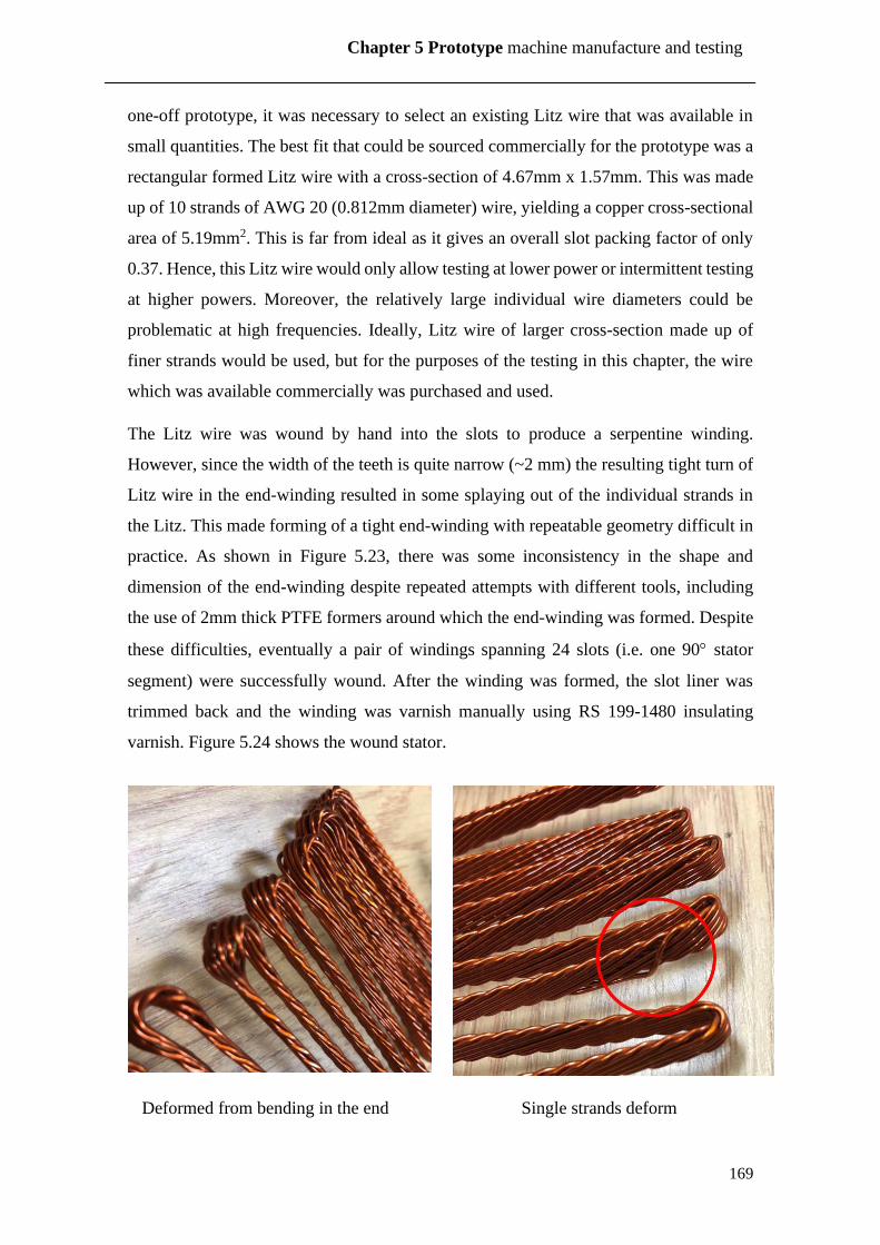
169


one-off prototype, it was necessary to select an existing Litz wire that was available in

small quantities. The best fit that could be sourced commercially for the prototype was a

rectangular formed Litz wire with a cross-section of 4.67mm x 1.57mm. This was made

up of 10 strands of AWG 20 (0.812mm diameter) wire, yielding a copper cross-sectional

area of 5.19mm2. This is far from ideal as it gives an overall slot packing factor of only

0.37. Hence, this Litz wire would only allow testing at lower power or intermittent testing

at higher powers. Moreover, the relatively large individual wire diameters could be

problematic at high frequencies. Ideally, Litz wire of larger cross-section made up of

finer strands would be used, but for the purposes of the testing in this chapter, the wire

which was available commercially was purchased and used.

The Litz wire was wound by hand into the slots to produce a serpentine winding.

However, since the width of the teeth is quite narrow (~2 mm) the resulting tight turn of

Litz wire in the end-winding resulted in some splaying out of the individual strands in

the Litz. This made forming of a tight end-winding with repeatable geometry difficult in

practice. As shown in Figure 5.23, there was some inconsistency in the shape and

dimension of the end-winding despite repeated attempts with different tools, including

the use of 2mm thick PTFE formers around which the end-winding was formed. Despite

these difficulties, eventually a pair of windings spanning 24 slots (i.e. one 90 stator

segment) were successfully wound. After the winding was formed, the slot liner was

trimmed back and the winding was varnish manually using RS 199-1480 insulating

varnish. Figure 5.24 shows the wound stator.

Deformed from bending in the end Single strands deform

170


Figure 5.23 Litz wire end-winding deformation

Prior to varnishing After varnishing

Figure 5.24 Wound stator

5.4.4 Rotor manufacture

The rotor hub is a component that is required to rotate at high speed while retaining the

magnets against centrifugal forces. It is also worth noting that the hub will include

locating features to allow the precise construction of the very high pole number magnet

array. The Halbach array used for the rotor hub means that a non-magnetic hub can be

used. The following mechanical properties are the most important in terms of selecting

the preferred material for the hub

• Low mass density – this will help in terms of both the overall machine mass the

centrifugal self-loading of the hub.

• High Young modulus and hence stiffness to avoid excessive strain of the rotor and

hence a change in magnetic airgap.

• High yield stress – It is common in design practice to set the maximum component

stress to some fraction of the material yield stress (usually the 0.2% yield stress

point). Hence, a high yield stress allows a thinner hub to be employed.

As a non-magnetic component in electrical machine, there are two main material options

for the rotor hub: Aluminium and Titanium. A summary of key physical properties for

these materials are shown in Table 5.2 along with the properties of the Sm2Co17 magnets.

As shown, although Titanium has a higher density than Aluminium and hence will have

a greater self-loading due to centrifugal forces, it has a significantly higher yield stress.

171


Another important factor in material selection is the potential for thermal expansion mis-

match between different elements of the rotor. As shown by the date in Table 5.2,

Titanium is a much close match to the rotor magnets which have a typical coefficient of

thermal expansion of 8-12 μm/m.K.

Table 5.2 physical properties of materials used in the prototype

Density

(kg/m3)

Young’s

modulus

(GPa)

0.2% Yield

Stress

(MPa)

Ultimate

Tensile

Strength

(MPa)

Thermal

expansion

(μm/m.K)

Aluminium 7000 Series

(7075-T60) 2820 70 503 572 21.4-22.5

Titanium Grade 5 4430 113.8 880 950 9.2

Taking a worst case assumption that the magnets act as a dead-weight on the containment

sleeve (i.e. neglecting the effect of an adhesive bond between the individual magnets and

the rotor core) then the maximum stress in a containment sleeve at a rotational speed of

𝜔 is given by the following equations [9] which were used previously in Chapter 4 for

calculating containment sleeve thickness for an internal rotor machine:

(5.1)

Where the effective mass and radius of the arc shaped magnet pieces (which are a

reasonable mechanical representation of the Halbach array) are given by:

These analytical formulae were used to calculate the stress in various designs of rotor

hub in both Aluminium and Titanium with the full magnet array acting as a uniformly

distributed dead-weight on the hub. Figure 5.25 shows the analytically predicted hoop

172


stress in the hub as a function of rotor hub wall thicknesses at 20,000rpm. It is common

design practice to operate a metal at some proportion of its yield stress, typically 50-60%

to allow some margin to account for fatigue etc [10]. Applying a 50% yield stress design

criterion gives maximum operating stress levels of 250 MPa and 440MPa for Aluminium

and Titanium respectively. As shown by Figure 5.25, a 4 mm thick Titanium hub can

meet this stress criteria while a 9mm thick Aluminium hub would be required.

Although the hoop stress in the Titanium hub is higher at a given thickness than an

Aluminium hub, the higher stiffness of Titanium means that the growth in airgap for a

particular hub thickness is smaller with a Titanium hub as shown in Figure 5.26. The

combination of a much thinner hub, greater stiffness and improved thermal expansion

match with the rotor magnets, make Titanium the preferred material for this application.

However, rather than adopt the 4mm hub thickness to limit the stress to 50% of the yield,

the Titanium hub thickness was increased to 6mm to limit the change in airgap to

<0.25mm.

Figure 5.25 Hoop stress in two material rotor hub at 20,000 rpm

0

200

400

600

800

1000

1200

1400

1600

0 5 10 15 20

Ho

op

str

ess

(MP

a)

Hub thickness (mm)

Aluminium

Titanium

173


Figure 5.26 Airgap growth from hoop stress in two material rotor hub at 20,000 rpm

Figure 5.27 shows the Titanium rotor hub used to hold the individual magnet poles. This

was manufactured by wire electro-discharge machining from a solid Titanium billet. The

initial internal bore was first cut by EDM and then the first 15mm from each end was

turned out to form a step which corresponds with the end of the frame which locate the

magnet pieces. A series of 192 thin ribs were subsequently cut to hold the magnets. These

were dimensioned taking into account the manufacturer specified tolerance of ±0.2mm.

Finally, the outer profile, which includes a series of bosses for tie-rods, was cut by wire

EDM.

Figure 5.27 Titanium rotor hub

0

0.2

0.4

0.6

0.8

1

1.2

1.4

1.6

0 5 10 15 20

airg

ap g

row

th (

mm

)

Hub thickness (mm)

Aluminium

Titanium

174


One feature of the wire EDM process is that internal corners are left with a small radius

in the corner (order of 0.16mm in the case of the 0.25mm wire used). To allow for this

and to prevent the magnets from sitting proud of the specified rotor bore, and additional

0.2mm was added to the slot depth. Following several trial methods, eventually a method

for inserting and gluing the magnets was established which used a series of specifically

sized PTFE spacers and a series of miniature clamps to define precisely the location of

the magnet to be inserted. This still posed challenges in terms of the force exerted on the

magnets during manual assembly.

Figure 5.28 shows a typical arrangement of the spacers and the rotor assembly with one

of the four magnet pieces per pole inserted in all poles. The first pass shown in Figure

5.28 in which a quarter of the magnet pieces were inserted was more straightforward,

both in terms of the forces on the magnets during assembly and the fit of the magnets

into the Titanium frame. Whereas each of these first set of magnets fitted into the slots

in the Titanium rotor housing, it did result in some flexure of the thin-walled Titanium

separators between adjacent poles. When it came to inserting the remaining pieces, many

of these did not fit into the remaining slots. An attempt was made to thin down the magnet

pieces by ~0.2mm using a holding jig and a wire-eroder, in which the wire made a pass

along the surface of an array of magnets to erode a thin layer. The set-up used is shown

in Figure 5.29. Unfortunately, this did not result in a sufficient consistent thinning down

and resulted in considerable agglomeration of magnetised powder on the magnets. Hence,

it was concluded that a new set of slightly narrower magnet pieces were required to

complete the third and fourth passes of the rotor magnets. Unfortunately, a second set of

narrower Sm2Co17 magnets were only available on a very long lead-time while a set of

NdFeB of similar remanence and energy product were available from stock. Specifically,

the Sm2Co17 used in the rotor had a manufacturer quoted remanence of 1.10T while the

N35 grade NdFeB has a remanence of 1.17-1.22T. Hence, the rotor was finished with a

mixture of Sm2Co17 and NdFeB. Although not directly comparable in terms of elevated

temperature performance etc., this substitution was deemed appropriate for the testing

which was scheduled to be undertaken.

175


Figure 5.28 Rotor magnet assembly – first pass of one piece in each pole pair

Figure 5.29 Schematic of wire-eroder arrangement used to attempt to thin-down the

Sm2Co17 magnets

Figure 5.30 shows the rotor following insertion of all 1920 magnet pieces (10 magnets

in each of 192 slots). Inspection of this rotor revealed a small number instances of the

magnet pieces being proud of the nominal bore. Hence, a finishing cut using wire EDM

was used to produce a smooth bore. The effect of this finishing cut is shown in Figure

176


5.30, in which it can be seen that only a proportion of the magnets were cut-back (shown

by the absence of the Nickel coating applied to the magnets).

Figure 5.30 Rotor frame fully populated with rotor magnets

Figure 5.31 Section of the rotor showing the effect of a finishing cut using EDM

177


The remaining mechanical components of the rotor, which are shown in Figures 5.32

were manufactured in Aluminium by a combination of CNC machining and wire EDM.

In order accommodate the irregular end-winding shown previously in Figure 5.24, it

proved necessary to adapt the rotor end-plate to incorporate a recess to accommodate the

extra overhang compared to that assumed in the design stage.

(a) Rotor end-plate inward-facing face (b) Rotor end-plate inward-facing face

(c) Rotor shaft (d) Rotor shaft

Figure 5.32 Rotor mechanical components

5.4.5 Final assembly

The fully assembled machine is shown in Figure 5.33. The first attempt at assembly

resulted in some asymmetry in the final airgap to the extent that the rotor and stator were

in contact at some points around the periphery. The full set of sub-assemblies were

checked for dimensional tolerance and concentricity. The rotor, as noted previously in

this chapter was skimmed using a wire eroder and was found to be circular to within

±0.064mm and with a measured bore diameter of 148.946mm. The assembled stator was

178


measured using a clock and found to be circular within ±0.10mm with a measured

diameter of 148.09mm. The concentricity of the rotor endcap locating shoulders and

bearing housing were checked with a clock. Hence, in principle with a working airgap of

0.5mm, the entire machine should have come together with a clear airgap all round.

However, when assembled, the rotor was binding on the stator bore and 0.25mm shims

could not be inserted down the airgap at some locations around the periphery. It was

concluded that the process of assembling itself was causing some degree of asymmetry

in the rotor / stator alignment, e.g. radial displacement of the stator sections due to

magnetic attraction forces.

Figure 5.33 Assembled machine

The machine was dis-assembled on several occasions and many measurements and

checks performed but it did not provide possible to retain a clearance around the full

airgap. The two un-wound stator core segments were removed and this showed up a

small amount of radial play in the dovetail joints which secure the segments to stator hub

which may be a contributing factor to a closing of the gap at some locations given the

large radial magnetic force in the airgap. There is also the possibility that the central

stator shaft and end-caps are not sufficiently stiff to resist unbalanced magnetic pull

resulting in deformation on the scale of a few tenths of millimetres. Ultimately it was

concluded that although significant progress had been made in manufacturing a

demonstrator machine, the numerous challenges in manufacturing such a novel and

different topology could not be resolved within the time-frame of this research

179


programme (see several suggestions for future work in this field in Chapter 6) and hence

no testing was performed on the demonstrator machine.

5.5 Conclusions

This chapter has described two attempts at manufacturing a demonstrator machine for

testing. It has shown the complexity of manufacturing such a high pole number machine,

particularly with it being an external rotor topology, has led to several challenges which

could not be resolved within the time-frame of this project. Several potential

modifications and further areas of work to overcome these challenges are described in

chapter 6.

180


5.6 References

[1] ‘Nickel Irons and Soft Magnetics Specification Sheet’. Arnold Magnetic

Technologies, 2017.

[2] B. Gehrmann, ‘Nickel–iron alloys with special soft magnetic properties for specific

applications’, Journal of Magnetism and Magnetic Materials, Volumes 290–291, Part 2,

April 2005, Pages 1419-1422.

[3] G. Ouyang, X. Chen, Y.Liang, C. Macziewskia, J. Cui, ‘Review of Fe-6.5 wt%Si high

silicon steel—A promising soft magnetic material for sub-kHz application’, Journal of

Magnetism and Magnetic Materials, Volume 481, 1 July 2019, Pages 234-250.

[4] ‘Super Core TM - Electrical steel sheets for high-frequency application’, JFE Steel

Corporation, Cat.No.F1E-002-02.

[5] Non-oriented electrical steel - Typical data. Cogent Surahammars Bruks AB,

Surahammar, Sweden, 2016

[6] Hiperco 50 alloy data Carpenter Technology Corporation, US, 2005 Vacoflux50

(0.025mm 280mm/width) P248

[7] M. Znidarich, “Hydro generator stator cores part 1- constructional features and core

losses,” in Proc. Australasian Univ. Power Eng. Conf., Sydney, Australia, 2008, pp. 1–8.

[8] VDM Metals, ‘VDM® Magnifer 50’, Material Data Sheet No. 9002, 2002.

[9] J. J. H Paulides, “High performance 1.5MW 20,000rpm permanent magnet generator

with uncontrolled rectifier for 'more electric' ship applications”, Thesis (Ph.D.) -

University of Sheffield, Department of Electronic and Electrical Engineering, 2006.

[10] J.M. Gere, S.P. Timoshenko, ‘Mechanics of materials’, Third SI Edition, Chapman

& Hall, 1991

181

Chapter 6 Conclusions


6.1 Introduction

This thesis has described a comprehensive investigation into a novel type of permanent

magnet machine to produce a very high output frequency as the direct input to a soft-

switched pulse density modulation converter. The thesis has focussed on the

electromagnetic design of machines capable of meeting the very unusual performance

specification of this application. This performance specification, in particular the high

output frequency, has resulted in several novel aspects in this thesis compared to

mainstream permanent magnet machines covering topology, material selection and

winding configuration. One important factor in this respect is the overriding importance

of iron loss in selecting the preferred topology and core material, including consideration

of several powder based and ultra-thin laminated core materials which are not normally

considered for mainstream high performance electrical machines. This chapter discusses

the key outcomes from the research and identifies several aspects for future research.

6.2 Key conclusions

Each individual chapter in this thesis has drawn chapter-specific conclusions. This

discussion of key conclusions is not intended to repeat these individual chapter level

conclusions. This discussion will instead focus on some key outcomes which provide

useful guidance for any future design or research on very high output frequency

permanent magnet machines.

Chapter 2 developed a simplified model of a PDM converter and demonstrated the

benefits of a higher generator output frequency in terms of minimising converter output

voltage distortion and filter requirements. A generator output frequency of 32kHz

allowed the THD specification to be met while also allowing a gap between the natural

frequency of the second-order filter and the 400Hz fundamental of a AC system. Whereas

an output frequency of 16kHz can meet THD requirements under some circumstances,

the resulting filter natural frequency is far closer to the fundamental than would normally

be considered as good filter design practice with some risk of resonant behaviour. The

need for such high generator frequencies in order to produce an acceptable voltage

waveform is also partly due to the 400Hz fundamental required for aircraft. A 50Hz

182


fundamental in a non-aerospace application would have been easier to accommodate with

a 16kHz or possibly even an 8kHz output.

The numerous flux-switching and flux-modulation machines considered in chapter 3

were only capable of producing very modest output power levels although they were able

to produce the required output frequency with a low number of conventional coils. This

poor performance was due to a combination of significant inter-pole leakage which is

inevitable with very fine magnet pole-pitches and the high machine reactance which

limited the electromagnetic power capability.

Single-phase surface mounted permanent magnet machines with a serpentine winding of

the type adopted as the preferred solution in chapter 4 of this thesis are able to achieve

very high electromagnetic power limits of >100kW, though often at excessive current

densities and hence unsustainable copper loss. In the case of very fine pole pitches

considered (2.36mm with 192 rotor poles) predicted performance is very sensitive to the

length of the magnetic airgap, which required a shift to an external rotor machine in

which the magnet retaining structure is not in the working airgap.

Several different powder based soft magnetic materials were evaluated in chapter 4.

These spanned a range of permeabilities and loss coefficient. At 32kHz, the lowest

permeability material (PCHF powdered iron) offered the best performance in terms of

minimising loss while retaining sufficient power capability. However, for 192 pole

machines (32kHz AC output frequency) considered in chapter 4, the iron losses were

extremely high and unsustainable and it proved necessary to move to a 16kHz generator

(96 poles). Not only did this change in frequency considerably reduce the machine core

loss but it also resulted in a useful increase in the electromagnetic power capability.

Chapter 4 contains numerous predictions of electromagnetic power and losses, but the

basic electromagnetic potential of the adopted machine topology is shown by the

predicted performance of the final design at the end of chapter 4. For this machine

(detailed in Table 4.15) the power density (based on active mass only) is 20.4kW/kg at

an efficiency of 98.0% at a 50kW operating point of 50kW and 40.7kW/kg at 96.2% for

the maximum electromagnetic power operating point of 99.7kW. Other important

outcomes included the benefits of a Halbach array and the significant influence of stator

slot depth on the reactance in such narrow slots and hence the limitations on

electromagnetic power capability.

183


The manufacture of a demonstrator machine was reported in chapter 5. Initially, many

attempts were made to produce a PCHF powdered iron core but ultimately this route was

not successful. The manufacturing route selected attempted to produce a single piece core

from a large ring but this proved not possible due to a combination of cracks, material

flaws and residual stress within the large rings and the poor mechanical strength of

narrow teeth. The cracks and residual stresses are likely to be more of a concern in very

large rings because of the greater stresses induced during heating and cooling. An

alternative approach which could be considered in future attempts would be to

manufacture a modular stator in which a number of smaller stator segments are machined

or, even better, pressed in custom tooling. These stator modules could then be combined

into a full stator core. The problems with the manufacture of a powder core required a

change to using ultra-thin Nickel iron laminations. Although predictions of performance

in terms of electromagnetic power capability and core loss for ultra-thin Nickel iron

laminations were promising, the availability of material in small quantities and at

reasonable cost was problematic. It is difficult to extrapolate small batch prices (such as

the £1000/kg quoted for custom manufacture of ~20kg which include significant set-up

costs) with production volume costs, but it is inevitable that very thin laminations of

Nickel Iron will be an expensive material option (likely £100s per kg). In this regard, is

worth recognising that the demonstrator in Chapter 5 only contains 1kg of Nickel Iron.

The high frequency, small slot dimensions and the need for a single turn per slot for the

performance specification in this study offered scope to produce a precise winding with

a good slot packing factor. Although some Litz wire was sourced from the stock range

of a manufacturer this did not result in an adequate slot packing factor. Furthermore, the

low number of strands limited the flexibility of the overall wire and resulted in some

challenges in producing neat and consistent end-windings, with individual conductors

tending to come out of the bundle on sharp turns. The manufacture of a custom Litz wire

(typical minimum orders being ~300kg) would result in a profile which would be a better

fit to the stator slot and a more flexible wire with many more strands of smaller individual

diameter.

The problems encountered in building the components of the prototype machine and the

assembly of the full machine demonstrated the many manufacturing challenges involved

in this unusual machine. Several of the arising issues are discussed in the future research

section later in this chapter. The most likely cause of the difficulty is the limited stiffness

184


of the central stator supporting shaft and its ability to resist deflection and hence lead to

some loss of concentricity.

Finally, despite the numerous difficulties encountered in the manufacture of a prototype

machines, the designs developed in this thesis have resulted in very competitive predicted

power densities, e.g. 25.5kW/kg for the final Nickel-iron design in chapter 5 at a

predicted efficiency of 98.2% at 50kW and 60.2kW/kg and 98.5% at its maximum power

point of 118kW. Hence, this study has demonstrated, at least from an electromagnetic

perspective, the promise of this type of machine, both for the specific application

considered in this thesis, but also more widely as a high power density single-phase

generator.

6.3 Suggestions for future work

There are several aspects of the research undertaken in thesis which have identified future

opportunities for research. Many of these relate to mechanical design and manufacturing

issues. The following are specific issues that would drive-forward the realisation of state-

of-the-art high frequency and power dense permanent magnet machines:

Mechanical re-design of demonstrator machine - The main limitation of the research

reported in this thesis was the failure to produce a working prototype for testing. This

was despite effort on two different stators and the manufacture of several high precision

components. It is worth noting that even if a prototype which could maintain an airgap

clearance had been successfully manufactured, a risk assessment would have limited the

operation of this prototype to no more than ¼ of the rated speed of 20,000rpm because

of simplifications in mechanical attachment of the rotor end-plates to the rotor hub and

the uncertainty over the bonding of each and every individual magnet. The key to

realising a robust demonstrator machine would be to develop a full mechanical model of

the stator and rotor structural parts to ensure that designs they can resist deformation from

any unbalanced magnetic forces and provide the necessary rotor-dynamic stiffness.

Manufacturing process development for serpentine winding of Litz wire – The

various attempts at manual coil winding of the serpentine coils in chapter 5 demonstrated

the challenges of winding a rectangular Litz wire (~2mm wide) around a semi-circular

path of similar diameter. The automation of this process with tooling to produce a more

repeatable coil would be beneficial in terms of adopting this type of winding.

185


Use of amorphous soft magnetic materials for stator core – The results presented in

chapter 5 showed the benefits of ultra-thin laminations in reducing losses. One class of

materials that was not investigated because of the lack of availability in a form suitable

for manufacture of a prototype was amorphous material. These are produced directly as

very thin (~20𝜇m) foils but are very difficult to process into sheets and stator components.

The development of a reliable and cost-effective method for processing amorphous

materials into complex geometry core parts would make this type of material attractive

in this application.

Improved converter model - The converter model developed and investigated in

Chapter 2 contained many simplifications such as no closed loop controller, open-circuit

only considerations of output voltage THD and ideal representation of the generator

output voltage. This was adequate in order to establish a frequency specification for the

generator voltage but could be expanded to provide a full-closed loop model of the

controller with a more detailed representation of a particular generator design and a series

of load models. This would provide system level evaluation of the proposed generation

system.

186

Appendix A Design designation system used in chapter 4 and 5

Appendix A Design designation system used in chapter 4 and 5

Table A Numbering system of machine designs through chapter 4 and 5

Design

number

Stator core

material

Machine

frequency Description

4.1.1 Cobalt iron 32kHz Surface mounted PM Machine (SPM)

4.1.2 Cobalt iron 32kHz SPM without tips

4.1.1-ag Cobalt iron 32kHz Enhance airgap from 4.1.1 with sp=0.9

4.2.1 Cobalt iron 32kHz interior permanent magnet (IPM) machines

4.2.2 Cobalt iron 32kHz IPM machine with magnet bridge

4.2.1-ag Cobalt iron 32kHz Enhance airgap from 4.2.1

4.2.3 Cobalt iron 32kHz Trapezoid magnet IPM

4.3.1 Cobalt iron 32kHz External rotor machine (ERM) with rotor

type A


type B


type C


type D

4.4.1 Cobalt iron 32kHz ERM 433 with a parallel sided stator slot

4.4.2 Cobalt iron 32kHz Increased stator hub ratio (0.75) from 4.4.1

4.4.3 Cobalt iron 32kHz Increased stator hub ratio (0.8) from 4.4.1

4.4.2-S Somaloy 32kHz Somaloy based on 4.4.2

4.4.3-S Somaloy 32kHz Somaloy based on 4.4.3

4.4.2-M PCMF 32kHz PCMF 4.4.2

4.4.3-M PCMF 32kHz PCMF 4.4.3

4.4.2-H PCHF 32kHz PCHF 4.4.2

4.4.3-H PCHF 32kHz PCHF 4.4.3

4.5.1 PCHF 16kHz 16 kHz design with stator hub ratio (0.8)

4.5.2 PCHF 16kHz Increase airgap to 0.5mm (sh=0.8)

4.6.1 PCHF 16kHz Two pieces per pole Halbach

array/magnetic pole frame

4.6.2 PCHF 16kHz Four pieces per pole Halbach

array/magnetic pole frame

4.6.3 PCHF 16kHz Two pieces per pole Halbach array/non-

magnetic pole frame

4.6.4 PCHF 16kHz Four pieces per pole Halbach array/non-

magnetic pole frame

5.1.1 Nickel iron 16kHz Nickel iron design based on 4.6.3 design

5.1.2 Nickel iron 16kHz Increase airgap radius to 76mm (sh=0.8)

187

Appendix B PDM Simulink model explore in chapter 2

Appendix B PDM Simulink model explore in chapter 2

Figure B PDM Simulink model explore in chapter 2

188

Appendix C Example script of Opera 2D on final design


$COMI | reco

///editor: Bo Jiang

$constant #vn 1.1

//clear all the regions and circuits in the model before modelling

Erase reg1=1 reg2=* erase=yes

external

delete c1=1 c2=* |quit

//////////////

$constant #m 1 description='phase number'

$constant #r_ro 80e-3 description='rotor outer radius in m'

$constant #r_so 74e-3 description='stator outer radius in m'

$constant #r_si 64e-3 description='stator inner radius in m'

$constant #W_ag 0.5e-3 description='air gap width'

$constant #W_sg 0.1e-3 description='stator gap width'

$constant #num_Ts 96 description='stator teeth number'

$constant #num_Tr 48 description='rotor pole pairs number'

//////////////////////////////////////////////////////////////////////////////

$constant #c_rt 2.5

$constant #w_br 0.5e-3 description='bridge thickness'

$constant #r_ri #r_so+#W_ag description='rotor inner radius in m'

$constant #r_st #r_so-#W_ag description='stator tips radius in m'

$constant #r_stt #r_st-#W_ag description='stator teeth tips ends radius in m'

$constant #r_rb #r_ro+(3e-3) description='rotor outside air radius in m'

$constant #ang_rt 360/#num_Ts description='rotor pole pitch'

$constant #r_sit 63.2e-3

$constant #r_skt 61.5e-3

189


$constant #r_sk 60.5e-3

$constant #r_sbg 58e-3 description='stator bg'

/$constant #ang_stt 0.8*#ang_rt description='stator teeth angle'

$constant #w_cb 2.2e-3 description='stator coil body width'

/$constant #w_cb 0.8*pi*#r_so*#ang_rt/360 description='stator coil body width'

$constant #r_ag 0.5*(#r_so+#r_ri) description='airgap radius for calculating the torque'

/$constant #r_sy #r_st+(0.5*#w_tb) description='stator main teeth inner radius'

$constant #w_bi 1.2*#w_cb description='back iron width'

$constant #r_cy #r_si+#w_bi description='conductor inners radius'

$constant #ang_stt 2*asin(#w_cb/2/#r_stt)*180/pi description='stator teeth angle'

//////////mesh size

$constant #Esize_air pi*#r_ag/#num_Tr/36

$constant #Esize_mt 2*#Esize_air

$constant #Esize_tt 2*#Esize_mt

$constant #Esize_iron 4*#Esize_mt

$constant #Esize_bg 12*#Esize_mt

//outer radius of airlayer on stator side

/$constant #r_air_s #r_ag

$constant #r_air_s #r_ag-#Esize_air/2

//inner radius of airlayer on rotor side

/$constant #r_air_r #r_ag

$constant #r_air_r #r_ag+0.5*#Esize_air

////////////////////

$constant #num_sym #num_Tr/12

/// tolerance for calculations

$constant #tole 1e-8

//////////////////////////////////////////////////

$constant #al 50e-3

190


$constant #Irms 0

$constant #phaseA #Irms

$constant #Num_turn 1

$const #speed_mec 2e4

$const #freq_elec #num_Tr*#speed_mec/60

$const #ts 1/#freq_elec/60

$const #endtime 1/#freq_elec

//////////stator teeth/////////////

draw shape=poly mat=4 perm=4500 den=0 cond=0 n=0 sym=0 vel=0 xcen=0 ycen=0

angle=0 nx=1 ny=1 dx=0 dy=0 tmirr=0 mirr=no rotation=0 trotation=0 TMIRROR=0

rotation=0 trotation=0

quitdraw

polygon data=yes option=text polar=yes radius=(#r_so) theta=0.5*(#ang_rt)-

atan(#w_cb/2/#r_so)*180/pi

polygon data=no size=yes esize=#Esize_air bias=0.5 line=straight f=no

polygon data=yes option=text polar=yes radius=(#r_st) theta=0.5*(#ang_rt)-

atan(#w_cb/2/#r_st)*180/pi

polygon data=no size=yes esize=#Esize_mt bias=0.5 line=straight f=no

polygon data=yes option=text polar=yes radius=(#r_stt) theta=0.5*(#ang_rt)-

atan(#w_cb/2/#r_stt)*180/pi

polygon data=no size=yes esize=#Esize_tt bias=0.5 line=straight f=no

polygon data=yes option=text polar=yes radius=(#r_cy) theta=0.5*(#ang_rt)-

atan(#w_cb/2/#r_cy)*180/pi

polygon data=no size=yes esize=#Esize_tt bias=0.5 line=curvature curvature=-1/(#r_cy)

f=no

polygon data=yes option=text polar=yes radius=(#r_cy) theta=0.5*#ang_rt

polygon data=no size=yes esize=#Esize_iron bias=0.5 line=straight f=no

polygon data=yes option=text polar=yes radius=(#r_si) theta=0.5*#ang_rt

polygon data=no size=yes esize=#Esize_tt bias=0.5 line=curvature curvature=1/(#r_si)

f=no

polygon data=yes option=text polar=yes radius=(#r_si)

theta=atan(#w_sg/2/#r_si)*180/pi

191



polygon data=yes option=text polar=yes radius=(#r_cy)

theta=atan(#w_sg/2/#r_cy)*180/pi


polygon data=yes option=text polar=yes radius=(#r_stt)

theta=atan(#w_sg/2/#r_stt)*180/pi


polygon data=yes option=text polar=yes radius=(#r_st)

theta=atan(#w_sg/2/#r_st)*180/pi


polygon data=yes option=text polar=yes radius=(#r_so)

theta=atan(#w_sg/2/#r_so)*180/pi

polygon data=no size=yes esize=#Esize_air bias=0.5 line=curvature curvature=-1/(#r_si)

f=no

polygon option=close




quitdraw


theta=0.5*(#ang_rt)+atan(#w_cb/2/#r_so)*180/pi



theta=0.5*(#ang_rt)+atan(#w_cb/2/#r_st)*180/pi



theta=0.5*(#ang_rt)+atan(#w_cb/2/#r_stt)*180/pi



theta=0.5*(#ang_rt)+atan(#w_cb/2/#r_cy)*180/pi

polygon data=no size=yes esize=#Esize_tt bias=0.5 line=curvature curvature=1/(#r_cy)

f=no

polygon data=yes option=text polar=yes radius=(#r_cy) theta=0.5*#ang_rt

192



polygon data=yes option=text polar=yes radius=(#r_si) theta=0.5*#ang_rt

polygon data=no size=yes esize=#Esize_iron bias=0.5 line=curvature curvature=-

1/(#r_si) f=no

polygon data=yes option=text polar=yes radius=(#r_si) theta=#ang_rt


polygon data=yes option=text polar=yes radius=(#r_cy) theta=#ang_rt


polygon data=yes option=text polar=yes radius=(#r_stt) theta=#ang_rt


polygon data=yes option=text polar=yes radius=(#r_st) theta=#ang_rt


polygon data=yes option=text polar=yes radius=(#r_so) theta=#ang_rt

polygon data=no size=yes esize=#Esize_air bias=0.5 line=curvature curvature=1/(#r_si)

f=no


COPY REG1=2 REG2=2 DX=0 DY=0 MIRROR=yes THETA=#ang_rt

//COPY REG1=2 REG2=2 DX=0 DY=0 MIRROR=no THETA=#ang_rt

$DO #cloop 1 22 1

COPY REG1=2 REG2=3 DX=0 DY=0 MIRROR=no THETA=#ang_rt*#cloop

$end do

COPY REG1=1 REG2=1 DX=0 DY=0 MIRROR=yes THETA=45

////////////////////////////////////

///////air in stator///////////

/////////////////////////////////////////




193


quitdraw

polygon data=yes option=text polar=yes radius=(#r_so) theta=0.5*(#ang_rt)-

atan(#w_cb/2/#r_so)*180/pi


polygon data=yes option=text polar=yes radius=(#r_st) theta=0.5*(#ang_rt)-

atan(#w_cb/2/#r_st)*180/pi




polygon data=no size=yes esize=#Esize_mt bias=0.5 line=curvature curvature=-1/(#r_stt)

f=no

polygon data=yes option=text polar=yes radius=(#r_stt) theta=0.5*#ang_rt





theta=0.5*(#ang_rt)+atan(#w_cb/2/#r_st)*180/pi



theta=0.5*(#ang_rt)+atan(#w_cb/2/#r_so)*180/pi

polygon data=no size=yes esize=#Esize_air bias=0.5 line=curvature curvature=1/(#r_si)

f=no


$DO #cloop 1 23 1


$end do

/COPY REG1=49 REG2=49 DX=0 DY=0 MIRROR=yes THETA=#ang_rt

/////////////////////////////////////////////

///////air gap on stator side//

///////////////////////////////////////////////////////////////////////////////////////////////////////




194


quitdraw


polygon data=no size=yes esize=#Esize_air bias=0.5 line=curvature curvature=1/(#r_so)

f=no


theta=(0.5*#ang_rt+atan(#w_cb/2/#r_so)*180/pi)

polygon data=yes option=text polar=yes radius=(#r_so) theta=(0.5*#ang_rt-

atan(#w_cb/2/#r_so)*180/pi)



polygon data=yes option=text polar=yes radius=(#r_so) theta=0


polygon data=yes option=text polar=yes radius=(#r_air_s) theta=0

polygon data=no size=yes esize=#Esize_air bias=0.5 line=curvature curvature=-

1/(#r_air_s) f=no

polygon data=yes option=text polar=yes radius=(#r_air_s) theta=#ang_rt






quitdraw

polygon data=yes option=text polar=yes radius=(#r_so) theta=2*#ang_rt


f=no


theta=(1.5*#ang_rt+atan(#w_cb/2/#r_so)*180/pi)

polygon data=yes option=text polar=yes radius=(#r_so) theta=(1.5*#ang_rt-

atan(#w_cb/2/#r_so)*180/pi)



polygon data=yes option=text polar=yes radius=(#r_air_s) theta=#ang_rt

polygon data=no size=yes esize=#Esize_air bias=0.5 line=curvature curvature=-

1/(#r_air_s) f=no

195


polygon data=yes option=text polar=yes radius=(#r_air_s) theta=2*#ang_rt



/COPY REG1=74 REG2=74 DX=0 DY=0 MIRROR=yes THETA=2*#ang_rt

$DO #cloop 1 21 1


$end do

COPY REG1=73 REG2=73 DX=0 DY=0 MIRROR=yes THETA=45

//////////////////////////////////////////////////////////////////////////////////////////////////////////////////////////////

///////////////////

/////////////////////////////////////////////////////////////////////////////////////////////////////

////////////// draw of conductor, number 1, material 1//////////////////

/////////////////////////////////////////////////////////////////////////////////////


angle=0 nx=1 ny=1 dx=0 dy=0 tmirr=0 mirr=no rotation=0 trotation=0

quitdraw




polygon data=yes option=text polar=yes radius=(#r_cy) theta=0.5*(#ang_rt)-

atan(#w_cb/2/#r_cy)*180/pi

polygon data=no size=yes esize=#Esize_tt bias=0.5 line=curvature curvature=-1/(#r_cy)

f=no

polygon data=yes option=text polar=yes radius=(#r_cy) theta=(0.5*#ang_rt)


theta=0.5*(#ang_rt)+atan(#w_cb/2/#r_cy)*180/pi


196




polygon data=no size=yes esize=#Esize_mt bias=0.5 line=curvature curvature=1/(#r_stt)

f=no

polygon data=yes option=text polar=yes radius=(#r_stt) theta=(0.5*#ang_rt)


/MODIFY REG1=1 REG2=1 N=1 ERASE=YES

$DO #cloop 1 23 1

COPY REG1=121-24 REG2=121-24 DX=0 DY=0 MIRROR=no

THETA=#ang_rt*#cloop

MODIFY REG1=121-24+#cloop REG2=121-24+#cloop N=1+#cloop ERASE=YES

$end do

//////////////////gap between segment///////////




quitdraw





theta=atan(#w_sg/2/#r_cy)*180/pi



theta=atan(#w_sg/2/#r_stt)*180/pi



theta=atan(#w_sg/2/#r_st)*180/pi




197



f=no

polygon data=yes option=text polar=yes radius=(#r_so) theta=0


polygon data=yes option=text polar=yes radius=(#r_st) theta=0


polygon data=yes option=text polar=yes radius=(#r_cy) theta=0


polygon data=yes option=text polar=yes radius=(#r_si) theta=0

polygon data=no size=yes esize=#Esize_tt bias=0.5 line=curvature curvature=-1/(#r_si)

f=no


COPY REG1=145-24 REG2=145-24 DX=0 DY=0 MIRROR=yes THETA=45

/++ $DO #cloop 1 3 1

/++ COPY REG1=81 REG2=82 DX=0 DY=0 MIRROR=no THETA=#ang_rt*4*#cloop

/++ $end do

////////////////////stator key/////




quitdraw

polygon data=yes option=text polar=yes radius=(#r_si) theta=45+0.5*#ang_rt


polygon data=yes option=text polar=yes radius=(#r_sit) theta=45+0.5*#ang_rt

polygon data=yes option=text polar=yes radius=(#r_skt) theta=45+4.7

polygon data=yes option=text polar=yes radius=(#r_sk) theta=45+4.7


polygon data=yes option=text polar=yes radius=(#r_sk) theta=45-4.7


polygon data=yes option=text polar=yes radius=(#r_skt) theta=45-4.7

198


polygon data=yes option=text polar=yes radius=(#r_sit) theta=45-0.5*#ang_rt

polygon data=yes option=text polar=yes radius=(#r_si) theta=45-0.5*#ang_rt


1/(#r_si) f=no



COPY REG1=147-24 REG2=147-24 DX=0 DY=0 MIRROR=no THETA=-30

COPY REG1=147-24 REG2=147-24 DX=0 DY=0 MIRROR=no THETA=30

/////background of stator//////////////////




quitdraw












polygon data=no size=yes esize=#Esize_iron bias=0.5 line=curvature curvature=1/(#r_si)

f=no

$DO #cloop 2 8 1

polygon data=yes option=text polar=yes radius=(#r_si) theta=45-0.5*#ang_rt*#cloop

$end do

199



polygon data=yes option=text polar=yes radius=(#r_sbg) theta=30


1/(#r_sbg) f=v





f=no

$DO #cloop 1 6 1


$end do














f=no

$DO #cloop 2 7 1


200


$end do







1/(#r_sbg) f=v





f=no

$DO #cloop 1 6 1


$end do


COPY REG1=151-24 REG2=151-24 DX=0 DY=0 MIRROR=yes THETA=45

///////////////////////////////////

/////////rotor///////////////

///////////////////////////////////

////////rotor pm////////////

/////////////////////////////////

Draw shape=poly mat=6 perm=1.05 CONDUCTIVITY=0 PERM=1 DENSITY=0

VELOCITY=0 MIRROR=no ROTATIONS=0, DX=0 DY=0 NX=1 NY=1

TMIRROR=0 rotation=0 TROTATION=0, XCENTRE=0 YCENTRE=0 ANGLE=0

201


QUITDRAW

polygon data=yes option=text polar=yes radius=(#r_ri) theta=0

polygon data=no size=yes esize=#Esize_air bias=0.5 line=curvature curvature=-1/(#r_ri)

f=no

polygon data=yes option=text polar=yes radius=(#r_ri)

theta=(atan(#w_cb/2/#r_ri)*180/pi)


polygon data=yes option=text polar=yes radius=(#r_ro-#w_br)

theta=(atan(#w_cb/2/(#r_ro-#w_br))*180/pi)

polygon data=no size=yes esize=#Esize_tt bias=0.5 line=curvature curvature=1/(#r_ro-

#w_br) f=no

polygon data=yes option=text polar=yes radius=(#r_ro-#w_br) theta=0



COPY REG1=153-24 REG2=153-24 DX=0 DY=0 MIRROR=yes

THETA=0.25*#ang_rt

COPY REG1=153-24 REG2=154-24 DX=0 DY=0 MIRROR=no THETA=0.5*#ang_rt

$DO #cloop 1 23 1


THETA=#ang_rt*#cloop

$end do

$DO #cloop 0 88 8

MODIFY REG1=153-24+#cloop REG2=153-24+#cloop

PHASE=0.25*#cloop*#ang_rt+180 ERASE=no

$end do

$DO #cloop 0 88 8


PHASE=0.5*#ang_rt+0.25*#cloop*#ang_rt-90 ERASE=no

$end do

$DO #cloop 0 88 8

202



PHASE=#ang_rt+0.25*#cloop*#ang_rt ERASE=no

$end do

$DO #cloop 0 88 8


PHASE=1.5*#ang_rt+0.25*#cloop*#ang_rt+90 ERASE=no

$end do

$DO #cloop 0 88 8


PHASE=2*#ang_rt+0.25*#cloop*#ang_rt+180 ERASE=no

$end do

////////rotor core////////////

/////////////////////////////////




quitdraw

polygon data=yes option=text polar=yes radius=(#r_ri) theta=0.25*#ang_rt


f=no

polygon data=yes option=text polar=yes radius=(#r_ri) theta=(0.5*#ang_rt-

atan(#w_cb/2/#r_ri)*180/pi)


polygon data=yes option=text polar=yes radius=(#r_ro-#w_br) theta=(0.5*#ang_rt-

atan(#w_cb/2/(#r_ro-#w_br))*180/pi)

polygon data=no size=yes esize=#Esize_tt bias=0.5 line=curvature curvature=-1/(#r_ro-

#w_br) f=no

polygon data=yes option=text polar=yes radius=(#r_ro-#w_br) theta=0.5*#ang_rt

203



polygon data=yes option=text polar=yes radius=(#r_ro) theta=0.5*#ang_rt

polygon data=no size=yes esize=#Esize_tt bias=0.5 line=curvature curvature=1/(#r_ro)

f=no



polygon data=yes option=text polar=yes radius=(#r_ri+#w_br) theta=0.25*#ang_rt



COPY REG1=249-24 REG2=249-24 DX=0 DY=0 MIRROR=YES

THETA=0.25*#ang_rt

/MODIFY REG1=13 REG2=13 PHASE=#ang_rt+180 ERASE=no

/////////////air gap in rotor side///////////////////////////////////////////////////////////////




quitdraw

polygon data=yes option=text polar=yes radius=(#r_ri) theta=0


f=no

polygon data=yes option=text polar=yes radius=(#r_ri)

theta=(atan(#w_cb/2/#r_ri)*180/pi)


polygon data=yes option=text polar=yes radius=(#r_ri) theta=(0.5*#ang_rt-

atan(#w_cb/2/#r_ri)*180/pi)



polygon data=yes option=text polar=yes radius=(#r_air_r) theta=0.5*#ang_rt

polygon data=no size=yes esize=#Esize_air bias=0.5 line=curvature

curvature=1/(#r_air_r) f=no

polygon data=yes option=text polar=yes radius=(#r_air_r) theta=0

204




/COPY REG1=147 REG2=147 DX=0 DY=0 MIRROR=YES THETA=#ang_rt

/////////////rotor outside air////////////




quitdraw

polygon data=yes option=text polar=yes radius=(#r_ro) theta=0

polygon data=no size=yes esize=#Esize_tt bias=0.5 line=curvature curvature=-1/(#r_ro)

f=no




polygon data=yes option=text polar=yes radius=(#r_rb) theta=0.5*#ang_rt

polygon data=no size=yes esize=#Esize_iron bias=0.5 line=curvature

curvature=1/(#r_rb) f=v

polygon data=yes option=text polar=yes radius=(#r_rb) theta=0



$DO #cloop 1 47 1


THETA=0.5*#cloop*#ang_rt

$end do

/////////////////////////////////////////////////////////////////////////////////////////////////////

// end of geometry draw

/////////////////////////////////////////////////////////////////////////////////////////////////////

205


GAP include=one RADIUS=#r_ag SYMMETRY=#num_sym

mesh tol=#tole dis=no

////////////////////////////////////////////////////////////////////////////////////////////////////////////////

BHDATA MATERIAL=4 TYPE=ISOTROPIC PHASE=0 PACK=1

DELETEBH N1=1 N2=*

LOADBH FILE='E:\Opera backup programming\nife.bh'

DEMAGQUAD COMMAND=CLEAR

QUIT

// rotor laminations


DELETEBH N1=1 N2=*

LOADBH FILE='E:\Opera backup programming\Sura NO20.bh'


QUIT

/// permanent magnets

$constant #num_BH 10


DELETEBH N1=1 N2=*

$do #m 0 #num_BH 1

ADD BVALUE=1.075*#m/#num_BH HVALUE=-(1-#m/#num_BH)*740e3

$end do


QUIT

//////////////////////////////////////////////////////////

///$string filename 'IPM_1turns_40_%int(#w_br*100000)br'

206


/////////////////////////////////////

$const #i 0

$do #i 1 4*int(#endtime/#ts)

SOLVE TYPE=RM

CASE COMM=ADD POSITION=#i VALUE=#ts*#i |QUIT

$end do

SOLVE TYPE=RM

LOGFILE LOGGING=SOLUTION COL1=TTIME COL2=R1_I COL3=R1_V

/COL4=W1_V COL5=W2_V COL6=W3_V COL7=W4_V COL8=W5_V

COL9=W6_V COL10=W7_V COL11=W8_V COL12=W9_V COL13=W10_V

COL14=W11_V COL15=W12_V COL16=W13_V COL17=W14_V COL18=W15_V

COL19=W16_V

DATA LINEAR=no TSTYPE=FIXED TSTEP=#ts MOTIONTYPE=FIXED

RMVEL=2e4 |QUIT

CEDITOR OPTION=load FILENAME='E:\Opera backup programming\Opera

2D\Part_9\9.1.3_nife_seg_h2p_870_64_74_80\2_999k.vfc'

OPTION=update

SET FIELD=MAGNETIC SYMMETRY=XY AUTOMATIC=YES

ELEMENT=LINEAR

$string path 'E:\Opera backup programming\Opera

2D\Part_9\9.1.3_nife_seg_h2p_870_64_74_80'

$cd directory='&path&'

$string filename 'ORM_1turns_999k_test'

WRITE FILE='&filename&.op2'

$OS OPERAANL rm '&filename&.op2' BACK

CEDITOR OPTION=clear

207



2D\Part_9\9.1.3_nife_seg_h2p_870_64_74_80\R1_10.vfc'

OPTION=update


ELEMENT=LINEAR


2D\Part_9\9.1.3_nife_seg_h2p_870_64_74_80'


$string filename 'ORM_1turns_1_10'




$DO #ld 1 1 -5


2D\Part_9\9.1.3_nife_seg_h2p_870_64_74_80\2_00.vfc'

ceditor option=modify COMPONENTNAME=r1 PROPERTYNAME=resistance

VALUE=#ld

OPTION=update


ELEMENT=LINEAR


2D\Part_9\9.1.3_nife_seg_h2p_870_64_74_80'


$string filename 'ORM_1turns_%int(#ld*100)_100_test'



208



$end do

High Frequency Permanent Magnet Generator for Pulse ...

Documents

Transcript of High Frequency Permanent Magnet Generator for Pulse ...