Magnet Design - ICTP

Magnet Design

Joint ICTP-IAEA Workshop on Accelerator Technologies, Basic Instruments and Analytical Techniques

21 – 29 October 2019

Trieste ItalyLowry Conradie

Joint ICTP-IAEA Workshop 21 – 29 October 2019 Trieste Italy

MAGNETS1. Introduction

Magnets in everyday life, in history,

Understanding magnetism, Glossary,

Units

2. General Principles of magnets

Type, number of poles, Field shapes

Pole shape, Fringe fields, Saturation,

Shims, Field quality, Magneto-motive

force

3. Magneto-motive force

Dipole and Quadrupole

4. Magnetization of iron

Hysteresis, permeability, materials

6. Magnet design

Computer programs

Steps in designing a magnet

Design a magnet (example - tutorial)


Magnets in Everyday Life

Rubber mat magnets


Accelerators – mainly electromagnets.

•Dipoles for bending a charged particle beam

•Quadrupoles for focusing a beam

•Sextupoles, octupoles, etc for higher order beam corrections

•Fast deflecting magnets for beam injection and extraction

Permanent magnets in vacuum pumps, gauges and sweeping

devices, but nowadays also as beam optical devices

Particle detectors

Magnets in Everyday Life


How strong are magnets?Typical Values

Here is a list of how strong some magnetic fields can be:

Smallest value in a magnetically shielded room 10-14 Tesla

Interstellar space 10-10 Tesla

Earth's magnetic field 0.00005 Tesla = 0.5 Gauss

Small bar magnet 0.01 Tesla

Within a sunspot 0.15 Tesla

Small NIB magnet 0.2 Tesla

Big electromagnet 2 Tesla

Surface of neutron star 100,000,000 Tesla

Magstar 100,000,000,000 Tesla

What is a Tesla? It is a unit of magnetic flux density. It is also equivalent to these other units:

1 weber per square meter

10,000 Gauss (10 kilogauss)

10,000 magnetic field lines per square centimeter

65,000 magnetic field lines per square inch.

1Gauss is about 6.5 magnetic field lines per square inch.

If you place the tip of your index finger to the tip of your thumb, enclosing approximately 1 square inch, four magnetic field lines would pass

through that hole due to the earth's magnetic field!


Charged Particle properties

Particle energy : 1eV = (1.6x10-19 C)(1V) = 1.6x10-19 J

Current i in ampere (A), current density j in (A/m2)

Number of conductor turns in a coil is N

Magnetic Field Strength H : 1 Oe = (103/4) A/m = 79.58 A/m (mmf)

Magnetic Flux : 1 Wb = 1 Vs

Magnetic Flux Density B : 104 G = 1 Wb/m2 = 1 Vs/m2 = 1 T

Permeability of any material = = 0 r (unit = Vs/Am = H/m)

Permeability of vacuum = = 0 r = (4 x 10-7) x 1 = 4 x 10-7 H/m

Some Units and Conversion Numbers in Electromagnetism

Magnetic Flux Density in relation to its magneto-motive force (mmf) :

B = H


TYPES OF MAGNETISMA. DIAMAGNETISM

• due to the modification of the electron orbit magnetic moment by an external field (a pure orbit effect)

• Present in all materials, independent of temperature

• Shows no hysteresis

• Very weak

B. PARAMAGNETISM

• atoms present a permanent magnetic moment, e.g. odd number of electrons

(mostly an electron spin effect)

• Incomplete inner electronic shells (transition and rare earth elements)

• Can be orders of magnitude bigger than diamagnetism

• No hysteresis effect

C. FERROMAGNETISM

• Larger inter-atomic distances

• Electron spin effect – line up from atom to atom – polarization

• “conduction electrons” from the 4s-shell free to wander between atoms


TYPES OF MAGNETS

A. Permanent Magnets (magneto-motive force from intrinsic material properties)

B. Electro-magnets (magneto-motive force generated from applied electric current)

DC-current

AC-current (pulsed, eddy-currents, laminations)

Super-conducting electro-magnets and materials


N S

N

S

VISUAL PERCEPTION -

FIELD LINES

Permanent Magnets : Field Shape

GENERAL RULES FOR USING LINES TO

VISUALIZE MAGNET FIELDS

1. Any line (all lines) must close on itself

or end according to a specified boundary

condition.

2. Lines may NOT cross or touch.

3. Lines usually cross an air/iron interface

perpendicularly.

4. The higher the field density, the denser

the line representation.

.B = 0

Joint ICTP-IAEA Workshop 21 – 29

October 2019 Trieste Italy

Electro-Magnets : n = 2, 4, 6, etc. poles

Dipole for bending/steering a beam

Quadrupole for focussing/defocussing a beam

Higher orders for creating magnetic bottles,

beam profile shaping and corrections to

inadequate fields from other magnets

Combinations, active and passive components

C MagnetAdvantages:

• Easy asses

• Simple design

Disadvantages:

• Pole shims needed

• Field asymmetric

• Less rigid

H Magnet• Advantages

• Symmetric

• Rigid

Disadvantage:

• Need shims

• Difficult to access

Window frame MagnetAdvantages:

• No shims

• Symmetric

• Compact

• Rigid

Disadvantages:

• Access problems

• Insulation thickness

Different Dipole geometries


Electro-Magnets : Pole Shape

R

y

x

xy=+R2/2

} g/2

y

0

For normal fields:

Dipole:

Y= ± g/2;

(g is pole gap).

Quadrupole:

xy= ± R2/2;

(R is radius of pole

opening).

Sextupole:

3x2y – y3=±R3;

Equations of ideal pole shape


Electro-Magnets : Field Shape

R

y

x

xy=+R2/2

} g/2

y

0


14

Electro-Magnets : Fringe Fields & Field Saturation

Magnetic field distribution and

magnet ends

Control of the longitudinal field at magnet ends

Square ends:• Display non linear effects due to saturation

• Influence the radial distribution in the fringe field

Chamfered ends:• Magnetic length better define

• Prevent saturation

Control of the longitudinal field at magnet ends

MAGNETO-MOTIVE FORCE : DIPOLE MAGNET

Ampere’s Law ∮H.dl = NI (ampere-turns)

NI = ∮H.dl = (Hair.gair + Hiron.liron) ;

H=B/

NI = ∮B/.dl = Bair.gair /0 + Biron.liron/iron

neglect 2nd term with iron about 5000 larger then` 0

NI = Bair .g/0

0 = 4 x 10-7 (webers/amperemeter)

Electrical power P = I2R0 g2

R0 = r L/A,

with r = resistivity of conductor material

L = length of the conductor and A the

crossectional area of the coil

gair

B

liron

x

x

Saturation effect : keep field in yoke < 1.5 T by

providing enough area of steel.


Quadrupole with hyperbolic pole faces

and with aperture a, such that the field

at radius r from the axis is B(r)= K.r

Ampere’s Law

H.dl = NI (ampere-turns)

NI = H.dl = (𝐵𝑎𝑖𝑟

𝜇0gair +

𝐵𝑖𝑟𝑜𝑛

𝜇0𝜇𝑟liron) ;

NI = 0 ∫a

B(r)/0 .dr + (iron path)

+ (path perpendicular to field)

On the first path (red) B(r) = K.r/μ0. The

second integral (green) is very small for

μr >> 1. The third integral (blue)

vanishes since B is perpendicular to the

direction of integration, ds. So we get in

good NI

NI = (1/0) 0∫a

Kr.dr

NI = (1/0) Ka2/2, but Ka = Bpoletip

NI = (Bpoletip .a)/(20 )

Power (I)2 a4

MAGNETO-MOTIVE FORCE : QUADRUPOLE MAGNET


MAGNETIZATION CURVE and PERMEABILITY

B = H = 0 r H

saturation

B = H

r = 0B/H


Relative permeabilities µ= µ0 µr=(4πx10-7) µr

Substance Group type Relative permeability, µr

Bismuth Diamagnetic 0.99983

Silver Diamagnetic 0.99998

Lead Diamagnetic 0.999983

Copper Diamagnetic 0.999991

Water Diamagnetic 0.999991

Vacuum Nonmagnetic 1+

Air Paramagnetic 1.0000004

Aluminium Paramagnetic 1.00002

Palladium Paramagnetic 1.0008

2-81 Permalloy powder (2 Mo, 81 Ni) ‡ Ferromagnetic 130

Cobalt Ferromagnetic 250

Nickel Ferromagnetic 600

Ferroxcube 3 (Mn-Zn-ferrite powder) Ferromagnetic 1,500

Mild steel (0.2 C) Ferromagnetic 2,000

Iron (0.2 impurity) Ferromagnetic 5,000

Silicon iron (4 Si) Ferromagnetic 7,000

78 Permalloy (78.5 Ni) Ferromagnetic 100,00

Mumetal (75 Ni, 5 Cu, 2 Cr) Ferromagnetic 100,000

Purified iron (0.05 impurity) Ferromagnetic 200,000

Superalloy (5 Mo, 79 Ni) ‡ Ferromagnetic 1,000,000

Magnetic Materials: relative permeability


Permanent magnets defined by curve in 2nd

quadrant

HYSTERESIS


SOME USEFUL GUIDES FOR DESIGN OF

CONVENTIONAL MAGNETS

A. Magnet steel begins to saturate around 1.5 T

B. Coils with current density < 1 A/mm2 may not need cooling

C. Max. current density for normal water cooled conductor is < 10 A/mm2

D. Water flow should be turbulent (v > 1.5-2 m/s)

E. Know the price of Power consumption

F. Cost of putting magnet into service (measurement, installation, cables, power

supply) is the same as the capital cost of the magnet


COMPUTER PROGRAMS for MAGNET DESIGN

2d : POISSON / SUPERFISH & OPERA-2d

¼ Geometry of H-type Dipole Magnet

pole

Return

yoke

coil

Finite elements

Magnetic flux lines



3d : OPERA-3d (Pre- and Post-Processor, TOSCA, ELEKTRA,

SOPRANO, Geometric Modeller, SCALA,

CONCERTO, TEMPO)

COIL

YOKE

POLES SHIMS

COIL



3d : OPERA-3d (Pre- and Post-Processor, TOSCA, ELEKTRA,

SOPRANO, Geometric Modeller, SCALA,

CONCERTO, TEMPO)

Magnetic flux in the iron


DESIGNING A BENDING MAGNET

SOURCE

TARGET

Assignment: Design a 90-degree bending magnet for beam analysis with the duoplasmatronion source and injection into an accelerator.

The magnet must adhere to the following requirements:

Bending angle = 90 degrees, Radius of curvature = 220 mm

Pole gap = 70 mm, Beam width in pole gap 40 mm

Maximum energy of protons injected into the accelerator = 20 keV

Maximum current by power supply is 6 A

Therefore : Calculate the main parameters

of the magnet that will transfer the beam

from the source to the target.

rigidity and magnetic flux density

maximum B field

pole width (homogenity of the field)

thickness of iron yoke

the mmf

the number of coil turns

voltage and power at a max. 6 A

Then: Measure and calculate the excitation curve, effective length and field homogenity


MAGNET DESIGN : POLE WIDTH

0.01x

pole

beam

0.001x

Pole width, w = x + ?

Pole gap, g

? ?

And for a variation of less than 0.1% it becomes

If the horizontal beam diameter is about 40 mm

then the minimum pole gap width can be computed

within 0.1% variation in the magnetic flux density

region across the beam width, using the above

relation, is

And for a maximum variation of 1% the pole width is

0.0012 2 70 40 180w g x mm mm mm

0.01 70 40 110w g x mm mm mm

For a magnet with a pole width w and gap g the width Δx0.01 over which the field varies less than 1%, is more of less given by:

∆𝑥0.01 = 𝑤 − 𝑔

∆𝑥0.01 = 𝑤 − 2𝑔


26

Shims for dipole magnet to improve the

uniformity of magnetic field

Shim Area≅ .021𝑔2

Shim area = s x d

With 0.2≤ 𝑠/𝑔 ≤ 0.6

𝑔 = pole gap

w = width of pole

s = width of shim

d = height of shim

MAGNET DESIGN : MAGNETIC RIGIDITY, FLUX DENSITY, YOKE THICKNESSFor a particle with charge q, mass m and speed v moving in a

uniform, time-independent magnetic field, B, on a circular orbit with

radius of curvature, r, at a right angle to the uniform magnetic field,

the Lorentz force equal to the centrifugal force:

2mvqvB

r

mv

qBr

The momentum, mv, can, for a given charge q, be expressed by the

product Br. The product Br is called the magnetic rigidity of the

particle and is a direct measure of the particle’s momentum. The

expression relating the total energy E and the momentum p of a

particle is:

2 2 2 2 2E p c m c

Using the energy relations 0 kE E E 2E mcand

with c = speed of light,

E0 = the rest energy of the particle

Ek = the kinetic energy of the particle

2

02k kE E EB

Qcr

and with an absolute charge state

Q and energy in eV, it becomes

2

02k kE E EmvB

q qcr

The rigidity (in SI-units)

The magnetic rigidity of a 20 keV proton (maximum injection

energy), is

0.0204B Tmr

With the radius of the magnet known (the radius was fixed by the

double focusing distance) the maximum flux density for the magnet

is:

0.02040.0927

0.22

TmB T

m

If we assume that saturation will only be reached when the magnetic flux

density in the iron is about 1.2 T, and that the flux that passes through the

iron is the same as that which passes through the pole gap, the following

calculation can be used to determine the minimum thickness of the iron

yoke pieces.

Magnetic flux through air (pole gap) = Magnetic flux through iron

g g i iA B y A B

where,

Ag = cross sectional area of the pole gap,

Ai = cross sectional area of the iron yoke,

Bg = magnetic flux density in the pole gap,

Bi = magnetic flux density in the iron yoke,

y = number of yoke pieces for closing of the magnetic flux loop,

which is determined by the magnet shape (i.e. y=1 for a C-magnet

and y=2 for an H-magnet)


MAGNET DESIGN : YOKE THICKNESS, MAGNETO-MOTIVE FORCEThe path-length, L, of a 900 circular bend is given by:

2 2 220346

4 4

mmL mm

r r

Assuming a H-shape magnet, the minimum thickness of the

yoke pieces can thus be calculated as follows:

2

g g

i

i i

A BThickness

B length

346 110 0.0927

346 2 1.2

mm mm T

mm T

4.3 mm

The yoke thickness was chosen, a practical 20 mm.

To create the magnetic field in the magnet a certain magneto-

motive force (mmf) per centimeter length (or field strength)

that will give the maximum flux density through the magnet

has to be applied. The required mmf is generated by the coil

windings in the magnet through which a current is sent.

Following Ampere’s law (the integral of the magnetic field

along a closed path equals the enclosed total current):

H d l NI

°where,

H = magnetic intensity or the field strength in A/m,

N = number of turns in the windings,

I = current in A through the windings.

2g g i i iiA B y A B length thickness B

a

b

c

d

e

g

w

It is assumed that the magnetic flux density in the iron is

constant and the flux density between the poles is constant

and that the direction of the field is parallel to the arrows of

path a-b-c-d-e-g (as shown in the figure). The mmf is

where,

Hg = magnetic intensity in the air between the poles,

Hi = magnetic intensity in the iron,

l = a + b + c + d + e,

g = pole-gap.

The relationship between the magnetic flux density B and magnetic intensity H is

g lH g H l NI

0 rB H

g lg H nH NI

Where r = relative permeability of the material,

And 0 = permeability of free space.

With the path l = n x g it becomes


MAGNET DESIGN : MAGNETO-MOTIVE FORCE, MAXIMUM CURRENT, NUMBER OF COIL TURNS,

CURRENT DENSITY, LENGTH OF COIL, COIL RESISTANCE, VOLTAGE, POWER CONSUMPTION

The mmf now becomes:0 0

g i

air iron

B nBg NI

The second term in the relation can be neglected for flux

densities below 1.2 T. Hence the following approximation for

mmf:

0

g

air

gBNI

To obtain a magnetic flux density of 0.0927 T in the air gap

(air = 1), the mmf is then :

The maximum tolerable current density for air-cooled coils is

between 2 and 3 A/mm2, depending on the coil geometry and

we decided not to exceed 2 A/mm2. The available copper wire

with 2 mm diameter can thus have a maximum current of

6.28 A. With the maximum current known the minimum

number of windings for the required magnetic field can be

calculated as:

7

0.07 0.09275614 .

4 10 /

m Tmmf NI ampere turns

Tm A

5164 .822

6.28

mmf ampere turnsN turns

I A

A safety factor of 25% is added to the number of windings,

hence the minimum total number of about 1027 windings for

the coils. Round up to say 1040 and split the turns equally

between the upper and lower coils with 520 turns each.

At 6.28 A the magnetic field B will now be 0.11725 T.

Require only 0.0927 T and therefore 4.965 A is adequate

(1.58 A/mm2).

A rough estimate of the length of one turn in the coils is 1 m.

Total length of coil required is about 1040 m.

The resistance of the 1040 m copper wire with thickness of 2

mm is:2

2

1040 0.01754 /5.81

3.14

coil

wire

L m mm mR

A mmr

where,

Lcoil = length of the coils in m,

r = resistivity of copper (= 0.01754 mm2/m at 25o C),

Awire = cross-sectional area of the coil.

The voltage required for the maximum current of 6 A is:

.

And the power consumption of the magnet is:

6 5.81 34.86V I R A V

6 34.86 209P I V A V W

Must still determine the following parameters through

calculation and measurement on the manufactured

magnet :

Analyzing power of the magnet (resolution)

Edge angles

Excitation curve

Effective length

Field homogenity


MAGNET DESIGN : EXCITATION CURVE

EXCITATION CURVE OF BENDING MAGNET

0.00

0.02

0.04

0.06

0.08

0.10

0.12

0.14

0.16

0.18

0.20

0 1 2 3 4 5 6 7 8 9 10

Current (A)

Ma

gn

eti

c F

ield

(T

)

MEASURED

CALCULATED


MAGNET DESIGN : EFFECTIVE LENGTH

VERTICAL MAGNETIC FIELD COMPONENT ALONG A STRAIGHT

LINE ON THE MAGNETIC MEDIAN PLANE

0

0.02

0.04

0.06

0.08

0.1

0.12

-300 -200 -100 0 100 200 300

POSITION (mm)

MA

GN

ET

IC F

IEL

D (

T)

CALCULATED

MEASURED

Leff = By.dl / B0

B0

Leff = 320 mm

Area under BLUE = Area under RED


MAGNET DESIGN : EFFECTIVE LENGTH The empirical result (for small gaps):

The effective length (Leff) of the magnet can be taken as the region in the magnet median plane

through which the magnetic field is almost constant and is approximated by the following

expression:effL L L

1.1 772

0.63 44.12

Lg mm

Lg mm

where L/2 is the contribution of one end to the effective length for an H-magnet

With a magnet length (L) = 256 mm410

344eff

mmL

mm

0.63

1.1k

where k is a parameter that varies from 0.63 g to 1.1 g

With a magnet pole gap (g) = 70 mm

Effective length results:

• Numerical field analysis : 320 mm

• Measured : 324 mm

• Empirical : 344 – 410 mm

pole

pole

L

2

L

2

L


Calculate the number ampere turns required for a quadrupole magnet

with aperture of 100mm and maximum field gradient of 12 T/m

NI = Ka2 / 2μ0 = 12 x (.05)2 / (2 x 4 x π x 10-7 ) = 11940 ampere turns

With

N = the number of turns on a pole

I = Current in the coils for desired gradient

K = Field gradient

For a quadrupole power supply that can deliver a maximum current of 100A the required

number of turns on each coil is:

Number or turns = NI/Imax = 11940/100 = 119.4 turns (make it 120 turns)


Calculate the magnetic field at the pole tip of a quadrupole

magnet with aperture of 100 mm and current of 100 A The

number of turns per pole is 120

B= N x I x 2 x μ0 / r = 120 x 100 x 2 x 4π x 10-7 / 0.05 = 0.6032 T

The gradient K = Bpole / r = 0.6032/.05 = 12.064 T/m

If the number of turns on the quadrupole is not known

one needs a tesla meter to measure the pole field. For

calculations with the program TRANSPORT the gradient

of a quadrupole as function of current must be known.

Normally there is a calibration table of current against

the measured magnetic field for each quadrupole

magnet available.Joint ICTP-IAEA Workshop 21 – 29 October 2019 Trieste Italy

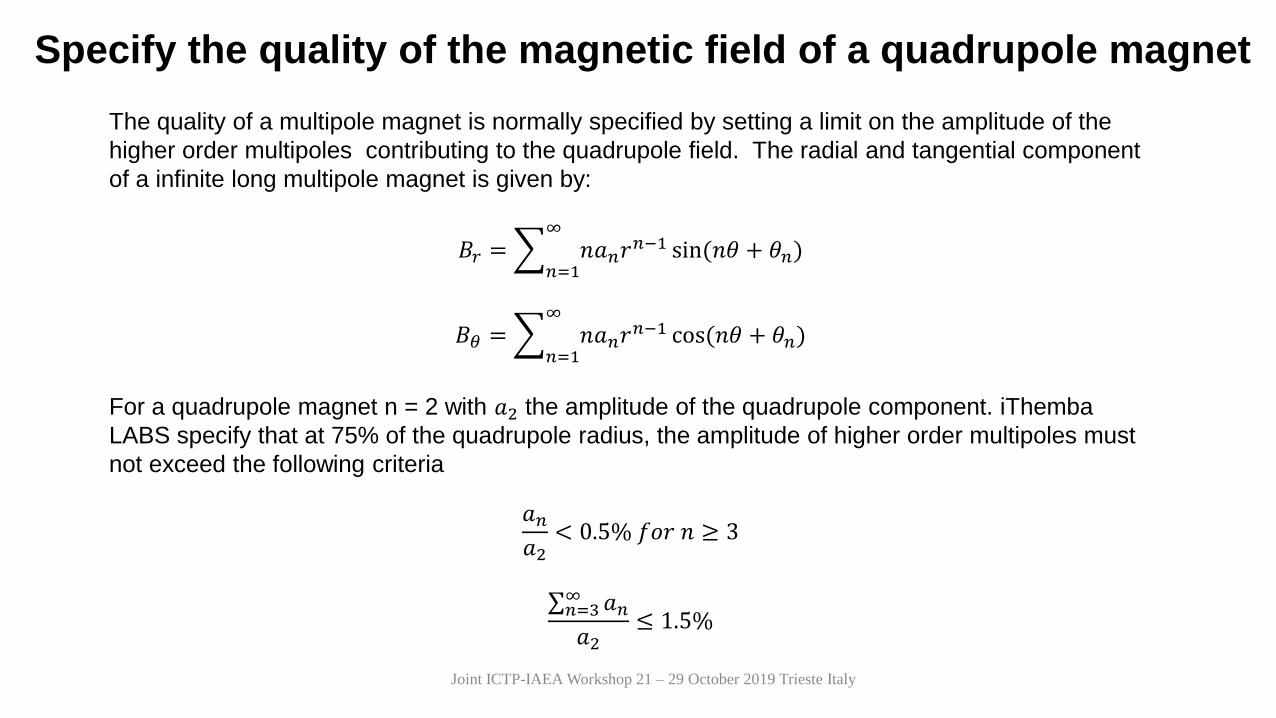
Specify the quality of the magnetic field of a quadrupole magnet

The quality of a multipole magnet is normally specified by setting a limit on the amplitude of the

higher order multipoles contributing to the quadrupole field. The radial and tangential component

of a infinite long multipole magnet is given by:

𝐵𝑟 = 𝑛=1

∞

𝑛𝑎𝑛𝑟𝑛−1 sin(𝑛𝜃 + 𝜃𝑛)

𝐵𝜃 = 𝑛=1

∞

𝑛𝑎𝑛𝑟𝑛−1 cos(𝑛𝜃 + 𝜃𝑛)

For a quadrupole magnet n = 2 with 𝑎2 the amplitude of the quadrupole component. iThemba

LABS specify that at 75% of the quadrupole radius, the amplitude of higher order multipoles must

not exceed the following criteria

𝑎𝑛𝑎2< 0.5% 𝑓𝑜𝑟 𝑛 ≥ 3

𝑛=3∞ 𝑎𝑛𝑎2≤ 1.5%


Measurement on Quadrupole magnet

Determine the magnetic

centre of the Quadrupole

magnet with a suspension

of magnetite in glycerol

and two light sources


Transfer of the magnetic

centre to top of magnet

for future alignment of

quadrupole magnet in a

beam line




• Measure the relation

between the magnetic

field and current

• Measure the effective

length of the magnet


Measuring the multipole components of

quadrupole magnet


6.4 mV

28.4 mV

7360 mV

16.2 mV

11.6 mV11 mV

4.2 mV

10 20 30 40 50 60 100

Frequency

Measured multipole components of Quadrupole magnet


FIELD MEASURING METHODS

(used at iThemba LABS)

1. Fluxmeter (based on induction law)

- rotating coil in fixed field

- fixed coil in dynamic field

- accurate with field value and direction

- harmonic analysis (multipole analysis)

2. Hall Effect Method

- simple and fast

- requires temperature stabilization

- requires frequent recalibration of probes

- well suited for fields of all gradients

3. Nuclear Magnetic Resonance (NMR)

- classical method for measuring absolute value of field

- high precision

- restricted field gradients

41

• The NMR20 gaussmeter (NMR teslameter) have the

characteristic of measuring weak fields from 140 G (14

mT) up to 13 T.

• Possibility to measure fields from 14 mT to 13 Tesla

with only 6 probes. And from 14mT to 2.1T with only 3

probes.

Nuclear Magnetic Resonance (NMR) tesla meter

Advantages of NMR

• Can make absolute measurements

• resolution of 1 mG (0.1 μT)

• Use for calibration of other magnetic field measuring

devices

Disadvantages

• Probe is relatively large

• Cannot measure magnetic field with a large gradient

• Need a number of different probes to measure

magnetic fields from low to high field values

• Expensive

The nuclear magnetic resonance (NMR) phenomenon was first described experimentally by both

Bloch and Purcell in 1946, for which they were both awarded the Nobel Prize for Physics in 1952


Magnet that will be used for energy measurements of the

beam make provision for mounting a NMR Tesla meter

NMR pad


Magnetic field measurement

Only discuss Nuclear Resonance Meter and the Hall probe

Hall probe

Advantages of hall probe

Small active area can be used to map magnetic field and make point measurements

Can be used to measure fast varying magnetic fields

Can measure field less than 1 gauss

One can measure over a large range with only one probe

Relatively cheap compared to an NMR meter

Three axis measurement possible

Disadvantages of hall probe

Have to be calibrated against an NMR meter

Have to be calibrated on a regular basis

Sensitive to temperature changes

Hand-held Gauss meter

measures magnetic

fields up to 2 T down to

fine resolution (0.1G).

Hall probe active area of

0.1 mm2



MAGNET DESIGN : BY YOURSELFYour accelerator lab requires the design of a H-type electro-magnet which can bend a 220 MeV proton beam by 3x10-3 radians.

The beam pipe that must fit in the pole gap has an outer diameter of 104 mm. The length of the magnet in the direction of the

beam, must not exceed 300 mm (use 200 mm). The maximum horizontal and vertical space available for the magnet is 1m in

both directions. The beam diameter inside the pole gap will be about 40 mm and we require a magnetic field homogenity of

about 0.8% over the width of the beam. Assume you have a good quality magnet steel available for the manufacturing of the

magnet and 2 mm copper wire for the coil. The current from the power supply may not exceed 6 A. Assume the average length

per turn is 0.924 m.

Guidelines to assist you :

1. Make a simple sketch of the magnet you intend to design (yoke, pole and coils)

2. Calculate the rigidity

3. Calculate the pole gap

4. Determine the effective length of the magnet (and then use a value of 250 mm for further calculations)

5. Calculate the bending radius

6. Calculate the Magnetic flux density B

7. Calculate the width of the pole

8. Calculate the cross sectional surface of the yoke

9. Decide on acceptable values to use for the yoke dimensions

10. Calculate the required mmf

11. Add 25% extra mmf for safety margin

• Decide on a final practical number of turns to be used for the coil

• Calculate current and current density in the coil

• Calculate the total length of conductor

• Calculate resistance of the coil

• Calculate voltage required from power supply

• Calculate power consumption of the coils

• Mass of the magnet (assume the iron volume as

1.2328x104 cm3 )

• Tabulate the magnet specification parameters

Determine the pole polarity for a deflection of the beam to the right from its original direction and also the current direction in the coils.

Joint ICTP-IAEA Workshop 21 – 29

October 2019 Trieste Italy

Thank you

104 mm


2. Rigidity

Particle = proton

Proton rest mass energy E0 = 938.25 MeV

Proton kinetic energy T = 220 MeV

Proton charge q = 1.6 x 10-19 C

Charge state Q = +1

Velocity of light c = 2.9979 x 108 m/s

6 2 6 6

8

1(220 10 ) 2(938.25 10 )(220 10 )

1 (2.9979 10 )

2.265 .T m

2

0

12BR T E T

Qc


3,4,5,6. Pole Gap, Magnet effective length, Radius of

curvature, Magnetic flux densityPole gap

The beam pipe must obviously fit into the pole gap. With the outer diameter of the beam pipe at 104 mm, select a pole gap value of 106 mm

Magnet Length

Physical length = 200 mm (given)

Effective length = physical length + (extra)

(use 250 mm)

( ) ( )R path length effective length angle radians 3/ 0.250 /3 10 83.333R S m rad m

/ 2.265 /83.333 0.02718B BR R Tm m T

2.265S

B

Magnetic flux density


Radius of curvature

7. Pole width

With the pole gap = 106 mm and the beam width about 40 mm, the pole width for a field homogenity of 1% is

0.01 106 40 146w gap x mm

0.0012 212 40 252w gap x mm

In order to obtain about 0.8% field homogenity, linear interpolation gives a total width of about 170 mm, which is

the same as if a beam width of 64 mm with 1% homogenity was assumed.

And for a field homogenity of 0.1% it is

0.01 106 64 170w gap x mm


8,9. Cross sectional surface of the yoke

In our magnet, with a magnetic flux density much less than 1.5 T

(iron saturation point), we can assume that all the magnetic flux

through the pole surface, P, will return through the yoke surfaces, Y.

Magnetic flux through the air gap = magnetic flux through the iron

air air iron ironarea flux density area flux density

170 200 0.027181.54

2 1.5 200y

mm mm TW mm

T mm

A yoke width of 1.54 mm is impractical and therefore select any dimension > 1.54 mm that is

readily available in the commercial market.

Select (say) 30 mm. It will provide a stable, rigid construction to support the coil weight and

definitely have no problem with magnetic flux saturation in the yokes.

The minimum yoke width, which will ensure that the flux through the return yokes, is at

saturation of 1.5 T, is

2A air B ironarea flux density area flux density

2p air y ironW L B W L B

PY Y

Physical length, L

Yoke width,

Wy

coil

Pole width,

Wp


10,11. Magneto-motive force

a

b

c

d

e

g

w

Use Ampere’s law

where,

H = magnetic intensity in A/m,

N = number of coil turns

I = current in the coil

,air ironH g H l NI l a b c d e

g lNI g H nH

In order to make sure that we can ignore the second term, we can use the iron yoke

width calculation to estimate the magnetic flux density in the iron.

.NI H dl

With l n g in our magnet, it becomes :

0 0

g iron

air iron

B nBNI g

2pole pole air yoke yoke ironW L B W L B

0.170 0.2 0.027180.07701 1.5

2 2 0.2 0.03

pole pole air

iron

yoke yoke

W L B m m TB T T

L W m m

In ferromagnetic materials is iron > 1000 for flux densities < 1.5 T. Therefore the second term is ignored.

7

0

0.106 0.027182293 .

4 10

g

air

B m TNI g ampere turns

Add 25% for extra bending power:

Total mmf = 2866 ampere. turns

With the total mmf divided between a coil around each pole tip, the mmf for each coil is 1433 ampere.turnsJoint ICTP-IAEA Workshop 21 – 29 October 2019 Trieste Italy

The final choice of number of turns depends on the power supply. With 652 turns x 4.4 A will provide the 2866 ampere.turns,

which is the required mmf.

The current density in a 2 mm diameter wire will then be 4.4/(πr2) = 1.4 A/mm2, which is a comfortable number for air-cooled

coils. [If the current density is > 2 to 3 A/mm2, a conductor with another type of cooling has to be considered.]

The total length of coil can be calculated by taking the average length per turn x number of turns – AFTER DECIDING ON THE

WIDTH AND HEIGHT TO BE USED FOR THE COIL.

Length per one coil = 0.924 (given for our calculation purposes) x 326 = 301 m

Total length of wire required for 2 coils = 602 m

AB B

Physical length, L

coil

Pole width, Wp

12,13,14. Number of turns, Currents, Total length of coil


The resistance of each coil is

15,16,17. Coil Resistance, Power supply current, Voltage and Power

2

3010.01754 1.6805

l mR

A rr

with l = length of conductor in meter

r = resistivity of copper at 25° C

= 0.01754 .mm2/m

A = cross sectional conducting area of a single conductor

r = radius of wire conductor

Current from power supply:

Voltage required for one coil:

With the two coils in series, the total voltage required:

NOTE: Care should be taken to provide extra voltage for the connection cables as well as the

effect of temperature rise in the conductors.

Power:

28664.4

652

mmfI A

N

4.4 1.6805 7.39V I R V

2 7.39 14.8totV V

14.8 4.4 65.12P V I W


18. Mass of the magnet

Volume of iron = volume of pole + volume of yoke = 1.2328 x 104 cm3 (given)

Mass of magnet (iron only) = volume x density of Fe = 1.2328 x 104 cm3 x 7.85 g/cm3

= 97 kg

Total length of wire = 2 x 3.05x104 cm= 6.1 x 104 cm

Volume of copper wire = cross sectional area x length = x 10-2 cm2 x 6.02x104 cm

= 1891 cm3

Mass of conductor = Volume x density of copper = 1891 cm3 x 8.96 g/cm3

17 kg

Total mass of magnet = mass iron + mass copper = 97 + 17 kg

= 114 kg


19. Table of parameters

Pole gap = 106 mm

Mass of magnet = 114 kg

Mass of conductor = 17 kg

Mass of iron = 97 kg

Maximum Voltage = 17 V

Maximum Current = 5 A

Maximum Power = 85 W

Maximum magnetic flux density = 0.0431 T

Physical length = 200 mm (given)

Effective length = 0.25 m (empirical calculation)

Bending of 220 MeV protons = 3.0 x 10-3 rad


Magnet Design - ICTP

Documents

Transcript of Magnet Design - ICTP