Permanent Magnet Modeling for Lorentz Force Evaluation

0018-9464 (c) 2015 IEEE. Personal use is permitted, but republication/redistribution requires IEEE permission. Seehttp://www.ieee.org/publications_standards/publications/rights/index.html for more information.

This article has been accepted for publication in a future issue of this journal, but has not been fully edited. Content may change prior to final publication. Citation information: DOI10.1109/TMAG.2015.2392082, IEEE Transactions on Magnetics

Permanent Magnet Modeling for Lorentz Force Evaluation 1

Judith Mengelkamp1, Marek Ziolkowski2,3, Konstantin Weise2, Matthias Carlstedt2, Hartmut Brauer2, 2

and Jens Haueisen1 3

1Institute for Biomedical Engineering and Informatics, Technische Universität Ilmenau, DE-98693 Ilmenau, Germany 4 2Institute for Information Technology, Technische Universität Ilmenau, DE-98693 Ilmenau, Germany 5 3Dept. of Applied Informatics, West Pomeranian University of Technology, Sikorskiego 37, PL-70313 Szczecin, Poland 6 7 Keywords: nondestructive testing, analytic modeling, force measurements, forward solution, inverse 8

solution 9

Abstract 10

Lorentz Force Evaluation (LFE) is a technique to reconstruct defects in electrically conductive materials. 11

The accuracy of the forward and inverse solution highly depends on the applied model of the permanent 12

magnet. The resolution of the technique relies upon the shape and size of the permanent magnet. Further, 13

the application of an existing forward solution requires an analytic integral of the magnetic flux density. 14

Motivated by these aspects we propose a magnetic dipoles model, in which the permanent magnet is 15

substituted with an assembly of magnetic dipoles. This approach allows modeling of magnets of 16

arbitrary shape by appropriate positioning of the dipoles and the integral can be expressed by elementary 17

mathematical functions. We apply the magnetic dipoles model to cuboidal and cylindrically shaped 18

magnets and evaluate the obtained magnetic flux density by comparing it to reference solutions. We 19

consider distances of 2-6 mm to the permanent magnet. The representation of a cuboidal magnet with 20

832 dipoles yields a maximum error of 0.02 % between the computed magnetic field of the magnetic 21

dipoles model and the reference solution. Comparable accuracy for the cylindrical magnet is achieved 22

with 1890 dipoles. Additionally, we embed the magnetic dipoles model of the cuboidal magnet into an 23

existing forward solution for LFE and find that the errors of the magnetic flux density are partly 24

compensated by the forward calculations. We conclude that our modeling approach can be used to 25

determine the most efficient magnetic dipole models for LFE. 26

1 Introduction 27

The aim of this paper is to investigate and compare different modeling approaches for permanent 28

magnets applied in Lorentz Force Evaluation (LFE). LFE is a newly developed nondestructive testing 29

technique for detection and reconstruction of defects in laminated electrically conductive materials 30

[1, 2]. A conductive specimen moves with constant velocity v with respect to a permanent magnet 31

(Fig. 1). The depth of a defect can be modified in the experimental setup easily if the specimen consists 32

of stacked sheets. The permanent magnet has a homogenous magnetization along the z-axis M = Mez 33

and is located at a liftoff distance δz above the top surface of the conductor. The specimen is assumed 34

to have the conductivity σ0. Due to the relative movement eddy currents are induced in the conductor. 35

The interaction of the eddy currents with the magnetic field of the permanent magnet results in three-36

1

https://www.researchgate.net/publication/257422472_Lorentz_force_evaluation_A_new_approximation_method_for_defect_reconstruction?el=1_x_8&enrichId=rgreq-2d8901c2abe9f4928dd6ff403e1ecc3a-XXX&enrichSource=Y292ZXJQYWdlOzI3MzMzNTkyNjtBUzoyMzM2Mzc0OTI4MTc5MjFAMTQzMjcxNDkyNzkzMw==

https://www.researchgate.net/publication/3102919_Evaluation_of_inverse_algorithms_in_the_analysis_of_magnetic_flux_leakage_data?el=1_x_8&enrichId=rgreq-2d8901c2abe9f4928dd6ff403e1ecc3a-XXX&enrichSource=Y292ZXJQYWdlOzI3MzMzNTkyNjtBUzoyMzM2Mzc0OTI4MTc5MjFAMTQzMjcxNDkyNzkzMw==



component Lorentz forces exerted on the conductor. Instead of determining the Lorentz forces on the 37

moving conductor we measure the forces exerted on the fixed permanent magnet. Due to Newton’s third 38

axiom they have equal magnitude but opposite direction as the Lorentz forces on the conductor. The 39

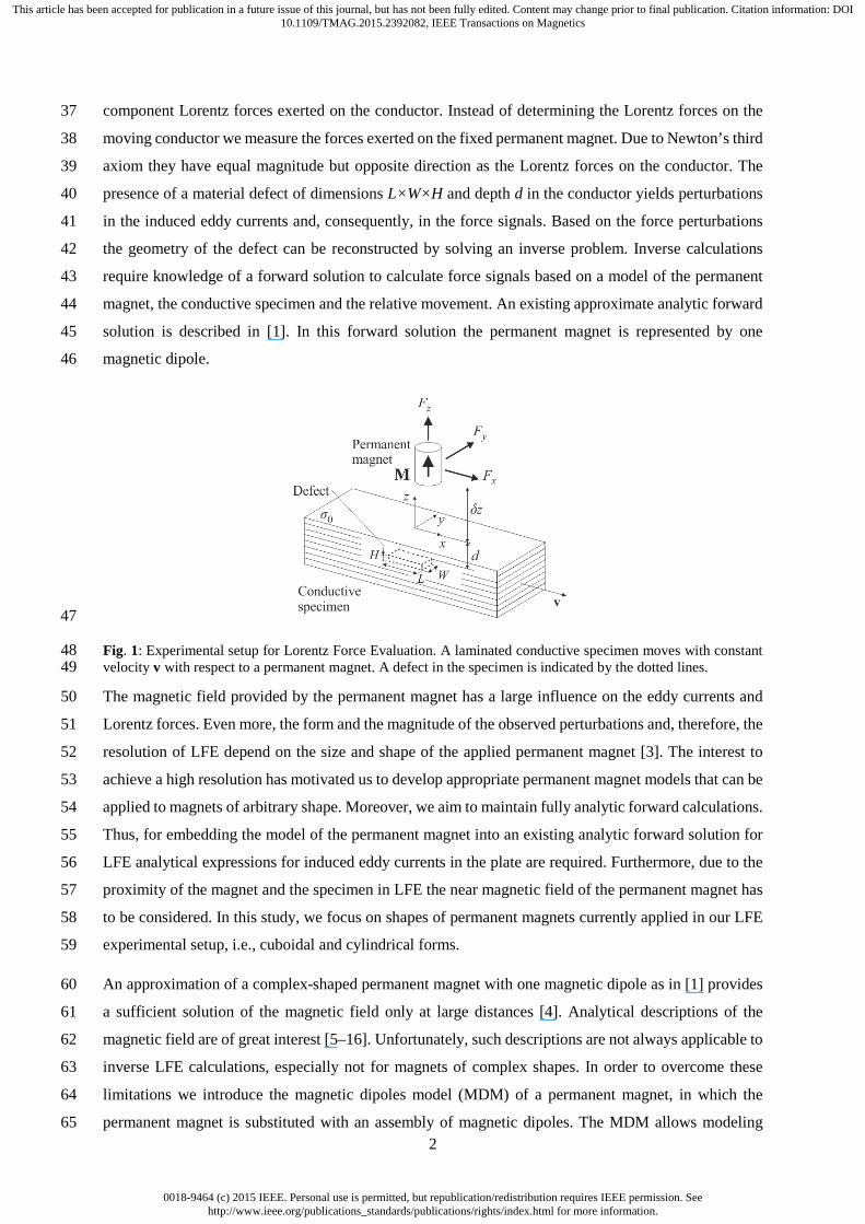
presence of a material defect of dimensions L×W×H and depth d in the conductor yields perturbations 40

in the induced eddy currents and, consequently, in the force signals. Based on the force perturbations 41

the geometry of the defect can be reconstructed by solving an inverse problem. Inverse calculations 42

require knowledge of a forward solution to calculate force signals based on a model of the permanent 43

magnet, the conductive specimen and the relative movement. An existing approximate analytic forward 44

solution is described in [1]. In this forward solution the permanent magnet is represented by one 45

magnetic dipole. 46

47

Fig. 1: Experimental setup for Lorentz Force Evaluation. A laminated conductive specimen moves with constant 48 velocity v with respect to a permanent magnet. A defect in the specimen is indicated by the dotted lines. 49

The magnetic field provided by the permanent magnet has a large influence on the eddy currents and 50

Lorentz forces. Even more, the form and the magnitude of the observed perturbations and, therefore, the 51

resolution of LFE depend on the size and shape of the applied permanent magnet [3]. The interest to 52

achieve a high resolution has motivated us to develop appropriate permanent magnet models that can be 53

applied to magnets of arbitrary shape. Moreover, we aim to maintain fully analytic forward calculations. 54

Thus, for embedding the model of the permanent magnet into an existing analytic forward solution for 55

LFE analytical expressions for induced eddy currents in the plate are required. Furthermore, due to the 56

proximity of the magnet and the specimen in LFE the near magnetic field of the permanent magnet has 57

to be considered. In this study, we focus on shapes of permanent magnets currently applied in our LFE 58

experimental setup, i.e., cuboidal and cylindrical forms. 59

An approximation of a complex-shaped permanent magnet with one magnetic dipole as in [1] provides 60

a sufficient solution of the magnetic field only at large distances [4]. Analytical descriptions of the 61

magnetic field are of great interest [5–16]. Unfortunately, such descriptions are not always applicable to 62

inverse LFE calculations, especially not for magnets of complex shapes. In order to overcome these 63

limitations we introduce the magnetic dipoles model (MDM) of a permanent magnet, in which the 64

permanent magnet is substituted with an assembly of magnetic dipoles. The MDM allows modeling 65 2

https://www.researchgate.net/publication/3113388_Analytical_Calculation_of_the_Magnetic_Field_Created_by_Permanent-Magnet_Rings?el=1_x_8&enrichId=rgreq-2d8901c2abe9f4928dd6ff403e1ecc3a-XXX&enrichSource=Y292ZXJQYWdlOzI3MzMzNTkyNjtBUzoyMzM2Mzc0OTI4MTc5MjFAMTQzMjcxNDkyNzkzMw==



https://www.researchgate.net/publication/260329992_Optimal_Permanent-Magnet_Geometries_for_Dipole_Field_Approximation?el=1_x_8&enrichId=rgreq-2d8901c2abe9f4928dd6ff403e1ecc3a-XXX&enrichSource=Y292ZXJQYWdlOzI3MzMzNTkyNjtBUzoyMzM2Mzc0OTI4MTc5MjFAMTQzMjcxNDkyNzkzMw==



permanent magnets of arbitrary shape by appropriate placing of magnetic dipoles in the volume of the 66

magnet. The integral of the magnetic flux density provided by the MDM is the linear sum of the integrals 67

of the single magnetic dipoles. 68

In the near field the accuracy of the approximation with one magnetic dipole depends on the shape of 69

the modeled magnet [4]. Based on this aspect, we expect the position of the dipoles to have an impact 70

as well. Therefore, we develop an optimization procedure to determine optimal dipole positions, instead 71

of defining the positions of the magnetic dipoles arbitrarily. An MDM with optimal dipole positions has 72

among all MDMs using equal number of dipoles the minimum error in the magnetic flux density 73

compared to a reference solution. Since the accuracy of the MDM depends on the number of magnetic 74

dipoles, we evaluate MDMs with varying number of dipoles. Further, we evaluate the improvement in 75

the MDMs due to the use of optimal dipole positions by comparing the magnetic flux densities of MDMs 76

with optimal and non-optimal dipole positions. 77

For the investigated cuboidal and cylindrical permanent magnets analytic solutions of the magnetic field 78

at any point outside the permanent magnet exist and serve as a reference solution for the MDMs. The 79

charge model, also referred to as the coulombian model, provides an analytic solution of the magnetic 80

field of the cuboidal magnet in terms of elementary functions [15, 17]. Alternatively to the charge model, 81

we apply a surface current model (amperian model) for the cylindrically shaped magnet. Using this 82

model the magnetic flux density of an axially magnetized cylindrical permanent magnet can be described 83

with the help of generalized complete elliptic integrals [16]. 84

Additionally, we demonstrate how the accuracy of the model of the permanent magnet influences the 85

exactness of the forward solution. Therefore, we embed selected MDMs of the cuboidal permanent 86

magnet with optimal dipole positions into the existing forward solution for LFE and evaluate the 87

resulting Lorentz forces. 88

The paper is structured as follows. In Section 2 we outline the applied methods. We describe the MDMs 89

followed by the charge and the surface current model of the cuboidal and cylindrical permanent magnets, 90

respectively. Then, we explain our optimization procedure. In Section 3, we show the results, i.e., the 91

optimal MDMs of the cuboidal and cylindrical magnets. Further, we evaluate the performance of the 92

optimization procedure and the accuracy of the forward computed Lorentz forces. Finally in Section 4, 93

we discuss the results and draw conclusions. 94

2 Methodology 95

2.1 Magnetic Dipoles Models 96

The idea of the magnetic dipoles models consists in representing the permanent magnet by a regular grid 97

of ND volume elements of identical volume, i.e., voxels. The shape of the voxels depends on the shape 98

of the permanent magnet. For cuboidal magnets the voxels are cuboids whereas for cylindrical magnets 99

the central voxels are cylinders and the others are hollow cylinder sectors (Fig. 2). One magnetic dipole 100 3


https://www.researchgate.net/publication/260246683_Permanent_Magnet_And_Electromechanical_Devices?el=1_x_8&enrichId=rgreq-2d8901c2abe9f4928dd6ff403e1ecc3a-XXX&enrichSource=Y292ZXJQYWdlOzI3MzMzNTkyNjtBUzoyMzM2Mzc0OTI4MTc5MjFAMTQzMjcxNDkyNzkzMw==



is positioned in each voxel. The voxels have the same volume. Consequently, the magnetic moments of 101

the inserted magnetic dipoles are equal. The dipole positions in the MDM depend on one parameter α 102

for the cuboidal permanent magnet and two parameters (α,β) for the cylindrical magnet. 103

104

Fig. 2: Magnetic dipoles model of a) a cuboidal and b) a cylindrical permanent magnet. 105

α-MDM of Cuboidal Permanent Magnet 106

The cuboidal permanent magnet has the base edge length a, height h, volume V0 = a2h, and is located at 107

point P0 = [x0, y0, z0]T corresponding to the center of gravity of the lower face of the magnet (Fig. 2a). 108

The edges of the magnet are parallel to the axes of the global Cartesian coordinate system. 109

According to the idea of the MDM, the permanent magnet is composed of a set of ND = Na2Nh voxels, 110

with Na being the number of voxels along the base edges and Nh the number of voxels along the height 111

edge. The volume of each voxel equals VE = Δa2Δh = (a/Na)2(h/Nh) = V0/ND. The magnetic dipoles 112

positioned in the voxels have an equal magnetic moment m = mez = MV0/ND = MVE, with V0 and VE 113

denoting the volume of the permanent magnet and an elementary voxel, respectively. The magnetic flux 114

density B = [Bx, By, Bz]T at any point P = [x, y, z]T outside the permanent magnet can be calculated as a 115

linear superposition of the magnetic flux densities of all magnetic dipoles of the α-MDM 116

1

( , , ) ( , , | , , )DN

m m m mm

x y z x y z x y z=

= ∑B b , (1) 117

4



with bm being the magnetic flux density of the m-th dipole located at Qm = [xm, ym, zm]T. 118

Due to the symmetry of the cuboidal permanent magnet and the identity of all voxels it is not expected 119

that any (xm, ym) position of the magnetic dipoles other than the center of gravity (COG) of the bottom 120

and top face of the voxels results in an improvement of the α-MDM. Thus, the coordinates (xm, ym) are 121

fixed to this position. However, we expect the z-coordinates of the magnetic dipoles to have an impact 122

on the model accuracy in the near magnetic field below the permanent magnet. Exploiting this aspect 123

the z-coordinate of the magnetic dipoles depends on a parameter zα = α∆h, which defines a local z-124

position of the magnetic dipole in the corresponding voxel. The magnetic flux density of the α-MDM 125

depends on a proper selection of the parameter α. Then, the position Qm of the m-th magnetic dipole is 126

defined as 127

10 2 2

10 0 2 2

0

( ) 1,...,( ) , 1,...,

1,...,( 1)

am a

am ijk m m a

m h

x i ax i Ny y j a j Nz k Nz k h z

Q P q q

α

− + − ∆ = = + + = = − + − ∆ = =+ − ∆ +

, (2) 128

with m = i+(j-1)Na+(k-1)Na2. The variable qijk denotes the position (COG) of the corresponding voxel 129

with respect to the COG of the permanent magnet, and qm describes the position of the magnetic dipole 130

with respect to a local coordinate system having its origin at the center of the lower face of the 131

corresponding voxel. The parameter α is constraint on the interval [0, 1] with 0 and 1 corresponding to 132

the bottom and top face of the voxels. All magnetic dipoles in the α-MDM have an equal local position 133

inside their respective voxel. 134

(α,β )-MDM of Cylindrical Permanent Magnet 135

The axially magnetized cylindrical permanent magnet has radius R, height h, and volume V0 = πR2h. It 136

is positioned at the center of the cylinder bottom face (P0 = [x0, y0, z0]T) and the cylinder axis is parallel 137

to the z-axis (Fig. 2b). The (α,β)-MDM is composed of Nh layers. Each layer contains one central 138

cylindrical voxel (axial voxel) of radius r0 and height ∆h, and NR concentric rings consisting of voxels 139

of the form of hollow cylinder segments. They are described with the inner radius ri, the outer radius 140

ri+1 with i indexing the i-th ring of voxels, the segment angle ϕ0, and the height ∆h. Thus, the total 141

number of magnetic dipoles ND is calculated as 142

1

1 .RN

iD h S

iN N N

=

= +

∑ (3) 143

The variable NSi denotes the number of voxels in the i-th concentric ring and is defined as 144

124 ( ) 4, 1,..., .

2iS RN i i Nπ = − ≥ =

(4) 145

5




It is always a multiple of 4 to ensure the symmetry of the (α,β)-MDM. The operator ⋅ denotes the floor 146

(greatest integer) function. The magnetic dipoles in the central voxels are positioned on the main axis 147

of the cylinder. Further, the radius r0 of the central voxels is defined as 148

0EVrhπ

=∆

. (5) 149

The magnetic dipoles in the ring voxels are located on the symmetry plane of the corresponding voxel. 150

Thus they are positioned at half of the segment angle spanning the ring voxel ϕ0/2. The inner radius ri 151

and outer radius ri+1 of the voxels in the concentric rings are calculated by the recurrence 152

21 1 0,

iE S

i iV Nr r r r

hπ+ = + =∆

. (6) 153

The radial and axial positions of the dipoles in the ring voxels depend on the parameters α and β, 154

respectively. The parameters α and β are equal for all voxels and are constraint to the interval [0, 1] 155

ensuring that the dipoles are located inside the corresponding voxels. With respect to a local coordinate 156

system placed at the center of the bottom face of the respective layer of voxels (on the z-axis), the 157

positions of the dipoles can be summarized as 158

1

0, 0 (axial voxel)(1 ) , 1,..., (ring voxels)i

i i R

ir

r r i Nz h

β

α

β βα

+

== − + =

= ∆

. (7) 159

Then, the position Qm = [xm, ym, zm]T of the m-th magnetic dipole in the global Cartesian coordinate 160

system is calculated as 161

0

12

0 0

0

cos 1,...,sin , 2 , 1,...,

1,...,( 1)

i j Rmi

m ijk m i j j SiS

m H

x r i Nxjy y r j NN

z k Nz k h zQ P q

β

β

α

θ

θ θ π

+ = − = + = = + = =

=+ − ∆ +

, (8) 162

with qijk denoting the position of the dipole with respect to a local coordinate system placed at the center 163

of the bottom face of the cylindrical magnet. The magnetic flux density B = [Bx, By, Bz]T at any point 164

P = [x, y, z]T outside the permanent magnet is calculated according to (1). 165

2.2 Analytic Models of the Magnetic Flux Density 166

The analytic models of the magnetic flux density of a cuboidal and a cylindrical permanent magnet are 167

shown in Fig. 3. Applying the charge model the cuboidal permanent magnet is represented by fictitious 168

magnetic charges situated on the bottom and top face of the magnet (Fig. 3a) [15, 17, 18]. The surface 169

charge density equals σm = M⋅n = M⋅ez =M for the top face located at z = δz+h and σm = M⋅n = M⋅(-170

6





ez) = -M for the bottom face positioned at z = δz. Using the magnetic charges as a source term the 171

magnetic flux density at any point P = [x, y, z]T outside a cuboidal permanent magnet is calculated as 172

03

/2 /2 /2 /20

3 3/2 /2 /2 /2

( ')( ')( ) '4 | ' |

( ') ( ')' ' ' ' ,4 | ' | | ' |

m

S

a a a a

a a a az h z z z

ds

M dx dy dx dy

P P PB PP P

P P P PP P P P

(9) 173

with P´ = [x´, y´, z´]T, and B = [Bx, By, Bz]T. An expression of the integrals in (9) in terms of elementary 174

functions is given in [15] and Appendix A. 175

176 Fig. 3: Analytic models of the magnetic flux density: (a) charge model for cuboidal and (b) surface current model 177 for cylindrical permanent magnets. 178

In the surface current model the cylindrical permanent magnet is represented by an equivalent infinite 179

thin solenoid of radius R and height h. Thus, the magnet is reduced to a current flowing in azimuthal 180

direction on the lateral surface of the cylinder. The surface current density is calculated as 181

JS = M×n = M×er = Meϕ and the magnetic flux density at any point outside the cylindrical permanent 182

magnet is expressed as 183

03

( )́ ( )́( ) ´4 ´

S

S

dsJ P P PB PP P

, (10) 184

with S denoting the lateral surface of the cylinder. An analytic expression of the integral in (10) is based 185

on generalized complete elliptic integrals [6]. The mathematical formulations of the magnetic field 186

components are given in Appendix B. 187

2.3 Optimization Procedure 188

The aim of the following optimization procedure is to determine optimal parameters αo for the α-MDM 189

(2) as well as optimal parameters αo and βo for the (α,β)-MDM (8). We perform the optimization for a 190

7



predefined number of magnetic dipoles. We define a test region G in the specimen, which is positioned 191

in the region below the permanent magnet. Motivated by the laminated structure of the specimen 192

explained in Section 1, the test region consists of Nz XY-layers: G = {Gk, k=1…Nz}. The XY-layers are 193

equidistantly distributed along the z-axis {zk = -d0-(k-1)∆z, k=1…Nz}, with d0 indexing the z-coordinate 194

of the uppermost layer and ∆z the distance between adjacent layers. Each layer is composed of a regular 195

grid of Nx and Ny points in the x- and y-coordinate directions, respectively. Thus, it holds Gk: {xi = (i-196

1)∆x, yj = (j-1)∆y, i=1…Nx, j=1…Ny }, with ∆x and ∆y denoting the distance between the grid points. 197

Due to the symmetry of the permanent magnets, we restrict the test region in the specimen to the first 198

quadrant (x≥0, y≥0). In the test region we evaluate the global normalized root mean square error 199

NRMSEG between the magnetic flux density obtained from the α- or (α,β)-MDM and the flux density 200

provided by the corresponding reference solution. The reference solutions are the charge model for the 201

cuboidal and the current model for the cylindrical permanent magnet (Section 2.2). The objective 202

function to be minimized is defined as 203

2

1

1 ( ) .zN

kG G

kz

NRMSE NRMSEN =

= ⋅ ∑ (11) 204

The NRMSE in the k-th XY-layer NRMSEGk(⋅) is calculated as 205

( ) ( )

3 2

1 1 1

3 32 2

1 1

1 ( , , ) ( , , )( ) 100 %

max min

yx

k

NND An i j k n i j k

n i jx ykG

A An n

n nz z

B x y z B x y zN N

NRMSE

B B

= = =

= ==

− ⋅ = ⋅

−

∑∑∑

∑ ∑ , (12) 206

with BnD being the n-th component of the magnetic flux density obtained from the α- or (α,β)-MDM, 207

and BnA being the n-th component of the reference solution. Further, the index n∈{1,2,3} corresponds 208

to the {x,y,z}-components of B. 209

In order to minimize (11) for the α-MDM and (α,β)-MDM we apply the golden section algorithm [19] 210

and the simplex search method [20], respectively. The parameters are bounded to the interval 211

(α,β) ∈ [0, 1] and the initial values are set to α0 = β0 = 0.5. 212

3 Results 213

3.1 Magnetic Dipoles Models 214

α-MDM of Cuboidal Permanent Magnet 215

The cuboidal permanent magnet under investigation has the parameters a = 15 mm, h = 25 mm, 216

δz=1 mm, and the remanence Br =1.17 T. The COG of the magnet is located at x = y = 0. These are 217

characteristic values for benchmark problems in LFE, e.g., in [21]. We optimize the parameter α for 218

8




different α-MDMs specified by combinations of Na = {2:2:14} and Nh = {1:1:25} by applying the 219

optimization procedure explained in Section 2.3. The test region G consists of Nz = 5 XY-layers, with 220

d0 = -1 mm and ∆z = 1 mm, i.e., the closest layer is located at a distance of 2 mm below the permanent 221

magnet. Each layer is composed of a grid of Nx×Ny = 31×31 points, which are equidistantly distributed 222

in the range of 0 ≤ (x,y) ≤ 30 mm in the first quadrant of the XY-layer. Hereinafter, we refer to the MDMs 223

with optimal parameter αo resulting from the optimization procedure as αo-MDMs. 224

The results are depicted using semi-logarithmic scaling in Fig. 4. We evaluate the accuracy of the 225

magnetic flux density obtained from the αo-MDM by assessing their NRMSEG in groups with the group 226

parameter Na and the function argument Nh. Thus, an increase of the total number of magnetic dipoles 227

ND is caused by an increase of Nh (Fig. 4a). The results show that for each group228

229

Fig. 4: Results of the optimization of the α-MDM of the cuboidal permanent magnet: (a) the NRMSEG between 230 the αo-MDM and the charge model depending on the number of dipoles along the base edge Na and the number of 231 layers Nh in the αo-MDM, and (b) the optimal parameter αo for the number of dipoles ND in the αo-MDMs 232 corresponding to the minima in (a). The dashed line indicates the dipole positions without optimization. 233

indexed by Na an optimal number of layers Noh,min = {2, 5, 9, 13, 16, 20, 23} with corresponding 234

minimum errors NRMSEoG,min = {1.52, 0.32, 0.07, 0.017, 0.006, 0.002, 0.001} % exists. The NRMSE for 235

these MDM configurations with not optimized dipole positions, i.e., the dipoles are located at to α = 0.5 236

corresponding to the COG of the voxels, equals {3.9, 0.61, 0.1, 0.019, 0.011, 0.003, 0.002} %. Further, 237

an increase of Na yields an increase of Noh,min. Using the results of a least squares fit, the optimal number 238

of layers depends on Na as Noh,min = [1.79Na – 1.71] with [·] denoting the nearest integer function. Further, 239

with increasing Na the edge-to-height ratio of the voxels converges to one. Thus, for high numbers of 240

dipoles the optimal number of layers can be estimated by Noh,min = h/Δa. The optimal parameter αo of 241

the αo-MDMs corresponding to the minimum error in each group is depicted in Fig. 4b as a function of 242

ND. For small ND the optimal position of the magnetic dipoles is lower than the standard choice, i.e., the 243

COG of the voxels indicated by the dashed line. With increasing number of magnetic dipoles αo 244

converges to 0.5. Thus, the optimization has significant influence for MDMs with small numbers of 245

dipoles. 246

9



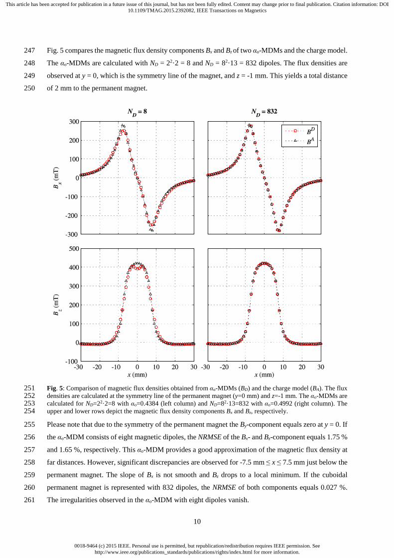
Fig. 5 compares the magnetic flux density components Bx and Bz of two αo-MDMs and the charge model. 247

The αo-MDMs are calculated with ND = 22·2 = 8 and ND = 82·13 = 832 dipoles. The flux densities are 248

observed at y = 0, which is the symmetry line of the magnet, and z = -1 mm. This yields a total distance 249

of 2 mm to the permanent magnet. 250

Fig. 5: Comparison of magnetic flux densities obtained from αo-MDMs (BD) and the charge model (BA). The flux 251 densities are calculated at the symmetry line of the permanent magnet (y=0 mm) and z=-1 mm. The αo-MDMs are 252 calculated for ND=22·2=8 with αo=0.4384 (left column) and ND=82·13=832 with αo=0.4992 (right column). The 253 upper and lower rows depict the magnetic flux density components Bx and Bz, respectively. 254

Please note that due to the symmetry of the permanent magnet the By-component equals zero at y = 0. If 255

the αo-MDM consists of eight magnetic dipoles, the NRMSE of the Bx- and Bz-component equals 1.75 % 256

and 1.65 %, respectively. This αo-MDM provides a good approximation of the magnetic flux density at 257

far distances. However, significant discrepancies are observed for -7.5 mm ≤ x ≤ 7.5 mm just below the 258

permanent magnet. The slope of Bx is not smooth and Bz drops to a local minimum. If the cuboidal 259

permanent magnet is represented with 832 dipoles, the NRMSE of both components equals 0.027 %. 260

The irregularities observed in the αo-MDM with eight dipoles vanish. 261

10



(α,β)-MDM of Cylindrical Permanent Magnet 262

The cylindrical permanent magnet under investigation has the parameters 2R×h = 15×25 mm, δz = 1 mm 263

and the magnetization µ0M = 1.17 T. We optimize the radial and axial positions of the dipoles in a 264

number of (α,β)-MDMs, which are specified by combinations of the number of concentric rings in one 265

slice NR∈{1:1:7}, and the number of slices Nh∈{1:1:25}. The test region G is the same as in the previous 266

section. Similar to the cuboidal permanent magnet, the NRMSEG between the (αo,βo)-MDMs with 267

optimal parameters and the current model are depicted in groups using Nh as the group parameter and 268

NR as the function parameter (Fig. 6a). A minimum for each NR indicates the optimal number of dipole 269

layers Noh,min = {2, 5, 8, 12, 15, 18, 23} for the (αo,βo)-MDMs. The corresponding errors equal 270

NRMSEoG,min={2.19, 0.89, 0.36, 0.122, 0.048, 0.024, 0.012} %. The NRMSE for the MDMs which have 271

the same NR, Nh-combinations but the dipole positions are not optimized, i.e., α = 0.5, equals 272

{4.99, 1.05, 0.41, 0.133, 0.064, 0.051, 0.047} %. Fig. 6b shows the optimal parameters αo and βo for 273

the (αo,βo)-MDMs corresponding to the minimum error in Fig. 6a as a function of ND. For intermediate 274

ND the MDMs tend to smaller z-coordinate (αo), but slightly larger radial coordinate (βo) compared to 275

(α,β) = 0.5. With enlarging ND the parameters converge to 0.5. Therefore, the optimization yields 276

significant improvement for MDMs with small numbers of dipoles. 277

278 Fig. 6: Results of the optimization of the (α,β)-MDM of the cylindrical permanent magnet: (a) the NRMSEG 279 between the (αo,βo)-MDM and the current model as a function of the number of concentric rings NR and the number 280 of layers Nh in the (αo,βo)-MDM, and (b) the optimal parameters αo and βo in dependence of ND of the (αo,βo)-281 MDMs corresponding to the minima in (a). The dashed line in (b) indicates the COG of the voxels, i.e., the dipole 282 positions if the optimization is not applied. 283

Instances of the magnetic flux densities obtained from two (αo,βo)-MDMs and the current model are 284

compared in Fig. 7. The flux densities are calculated at y=0 and z = -1 mm yielding a total distance of 285

2 mm to the permanent magnet. If it holds ND = 10 (NR = 2, Noh,min = 2), the NRMSE equal 2.78 % and 286

2.56 % for the Bx- and Bz-component, respectively. Similar to the cuboidal magnet, differences are 287

observed in the region of -7.5 mm ≤ x ≤ 7.5 mm. The Bx-component of the MDM is too small, whereas 288

the Bz-component overshoots the current model. If the (αo,βo)-MDM consists of 1890 magnetic dipoles 289

11



(NR = 6, Noh,min = 18), the NRMSE of the Bx- and Bz-component result into 0.034 % and 0.039 %, 290

respectively. 291

292

Fig. 7: Comparison of magnetic flux densities obtained from (αo,βo)-MDMs (BD) and the current model (BA). The 293 flux densities are calculated at the symmetry line of the permanent magnet (y = 0 mm) and z = -1 mm. The (αo,βo)-294 MDMs are calculated for ND=10 with αo=0.44, βo=0.3892 (left column) and ND=1890 with αo=0.4992, βo=0.5078 295 (right column). The upper and lower rows depict the magnetic flux density components Bx and Bz, respectively. 296

297 Comparison of the Optimal Number of Layers and the Accuracy of Optimized and not Optimized 298

Magnetic Dipoles Models 299

For evaluation of the efficiency of the optimization procedure we compare for the cuboidal as well as 300

for the cylindrical permanent magnet MDMs with optimal Nh and optimized dipole positions described 301

in the previous sections to the MDMs with optimal Nh but standard dipole positions. We define that 302

standard positioning is indicated by αs = 0.5 as well as (αs,βs) = (0.5,0.5) for the cuboidal and cylindrical 303

magnets, respectively. We evaluate the NRMSEG of the αs-MDM and (αs,βs)-MDM for same (Na,Nh)- 304

and (NR,Nh)-combinations and test region as in the previous sections. The results show similar curves as 305 12



for the optimized MDMs, but the minimum errors NRMSEsG,min of the group parameters correspond to 306

different numbers of layers Nsh,min and have different values. For further analysis, we calculate the 307

differences in the number of layers ΔNh,min and in the normalized errors ΔNRMSEG,min between the 308

MDMs corresponding to the minimum errors for optimized and standard positioning of dipoles as 309

,min ,min ,min

,min ,min ,min

o sh h h

o sG G G

N N N

NRMSE NRMSE NRMSE

∆ = −

∆ = − . (13) 310

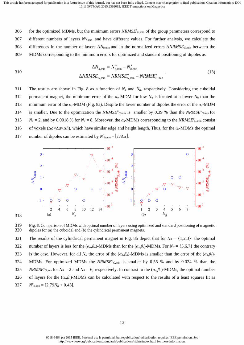
The results are shown in Fig. 8 as a function of Na and NR, respectively. Considering the cuboidal 311

permanent magnet, the minimum error of the αo-MDM for low Na is located at a lower Nh than the 312

minimum error of the αs-MDM (Fig. 8a). Despite the lower number of dipoles the error of the αo-MDM 313

is smaller. Due to the optimization the NRMSEoG,min is smaller by 0.39 % than the NRMSEs

G,min for 314

Na = 2, and by 0.0018 % for Na = 8. Moreover, the αs-MDMs corresponding to the NRMSEsG,min consist 315

of voxels (∆a×∆a×∆h), which have similar edge and height length. Thus, for the αs-MDMs the optimal 316

number of dipoles can be estimated by Noh,min = h/Δa. 317

318

Fig. 8: Comparison of MDMs with optimal number of layers using optimized and standard positioning of magnetic 319 dipoles for (a) the cuboidal and (b) the cylindrical permanent magnets. 320

The results of the cylindrical permanent magnet in Fig. 8b depict that for NR = {1,2,3} the optimal 321

number of layers is less for the (αo,βo)-MDMs than for the (αs,βs)-MDMs. For NR = {5,6,7} the contrary 322

is the case. However, for all NR the error of the (αo,βo)-MDMs is smaller than the error of the (αs,βs)-323

MDMs. For optimized MDMs the NRMSEoG,min is smaller by 0.55 % and by 0.024 % than the 324

NRMSEsG,min for NR = 2 and NR = 6, respectively. In contrast to the (αo,βo)-MDMs, the optimal number 325

of layers for the (αs,βs)-MDMs can be calculated with respect to the results of a least squares fit as 326

Noh,min = [2.79NR + 0.43]. 327

13



3.2 Lorentz Force Evaluation Using Magnetic Dipoles Models of Cuboidal Permanent 328

Magnet 329

In this section we investigate how the dipole optimization influences the error of the forward calculated 330

Lorentz forces exerted on the permanent magnet. We embed the MDMs with optimized positions (αo-331

MDMs) corresponding to NRMSEoG,min of the cuboidal permanent magnet obtained in Section 3.1 and 332

the αs-MDMs with the same (Na,Nh)-combinations into an existing approximate forward solution for 333

LFE from [1]. Further, we put the charge model (Section 2.2, Fig. 3a) into the forward solution and use 334

the force signals calculated with this model as a reference solution. Then, we calculate the NRMSE∆F 335

between the three-component Lorentz force perturbations obtained by the α-MDMs and the charge 336

model using a similar formula to (12). This approach ensures that we only investigate signal errors of 337

the α-MDMs and not the total error of the approximate forward solution. We restrict the analysis to the 338

cuboidal permanent magnet, because we were able to find analytical expressions for eddy currents 339

induced in the plate only for the magnet model in the form of a cuboid but not in the form of a cylinder. 340

As a benchmark problem we investigate the LFE problem (Fig. 1) with a cuboidal permanent magnet 341

a×a×h = 15 mm × 15 mm × 25 mm fixed above a moving laminated specimen consisting of 50 aluminum 342

alloy sheets. The sheets have a thickness of 1 mm. Because the sheets are isolated from each other, the 343

conductivity of the specimen can be approximated by an anisotropic conductivity described by a 344

diagonal tensor [σ] = diag(σ0,σ0,0) where σ0 = 30.61 MS/m. A cuboidal defect with the dimensions 345

6 mm × 6 mm × 1 mm is positioned in the third upper sheet, i.e., at depth d = 2 mm. The COG of the 346

defect is located at x = y = 0. The relative velocity equals 0.01 m/s. We examine the profiles of the 347

Lorentz force perturbations exerted on the permanent magnet. The observation points are equidistantly 348

distributed in the range of 0 ≤ x ≤ 20 mm, 0 ≤ y ≤ 10 mm at z = 1 mm. Due to the symmetry of the 349

problem setup the investigated region can be restricted to the first quadrant. The distance between 350

adjacent observation points equals 1 mm. 351

Fig. 9 presents the resulting NRMSE∆F as a function of ND in the αo- and αs-MDMs. The perturbation 352

force signals calculated with the αo-MDM have a significant smaller error than the signals calculated 353

with the αs-MDMs. NRMSE∆F errors introduced by αo-MDMs equal 0.8 % and 0.002 % for ND = 8 and 354

ND = 832, respectively. For the αs-MDMs with the same number of magnetic dipoles, the error equals 355

8.2 % and 0.019 %, respectively. For large ND the errors approach each other. A comparison to the 356

NRMSEoG,min of the magnetic flux density of the αo-MDMs (Section 3.1, Fig. 4a) shows that the errors 357

of the force signals for the αo-MDMs are smaller by half the value for ND = 8 and one decimal place for 358

ND = 832. However, if the standard models (αs-MDM) are used the errors of force signals are 359

significantly higher for both ND = 8 and for ND = 832 than the NRMSE of the corresponding magnetic 360

flux density outlined in Section 3.1. 361

14




362

Fig. 9: NRMSE∆F between the Lorentz force perturbation signals using the αo- and αs-MDMs and the charge model. 363

A comparison of the Lorentz force perturbations caused by a defect using the αo- and the αs-MDM with 364

8 magnetic dipoles and the charge model is shown in Fig. 10. 365

366 Fig. 10: Comparison of Lorentz force perturbations ΔFx, ΔFy, and ΔFz. The perturbations due to the defect are 367 obtained by subtracting the force signals coming from a specimen with and without a defect. The Lorentz forces 368 are computed by applying an existing analytic forward solution including the αo- and αs-MDM with 8 dipoles and 369 the charge model (Ana). The force components are depicted at y = 2 mm. 370

The perturbations of the force signals ΔF are obtained after subtracting the force signals calculated for 371

a specimen with and without a defect. Thus, the profiles of perturbation force components tend to zero 372

far away from the defect region [1]. The signals are depicted at y = 2 mm, because due to the symmetry 373

the side force Fy as well as the ΔFy-component vanish at the symmetry line (y = 0). It can be observed 374

that the signals calculated with the αo-MDM are in excellent agreement with the perturbations calculated 375

with the charge model. The NRMSE of the ΔFx-, ΔFy-, and ΔFz-component calculated for the profile at 376

y = 2 mm equals 0.47 %, 1.54 %, and 1.68 %, respectively. On the contrary, significant deviations are 377

observed in the Lorentz force perturbations calculated with the αs-MDM. Here, the NRMSE of the ΔFx-378

, ΔFy-, and ΔFz-component equals 7.41 %, 10.11 %, and 6.88 %, respectively. 379

4 Discussion 380

This contribution was motivated by the necessity to provide an accurate model of the permanent magnet 381

for the forward solution of LFE, which is the basis for successful inverse calculations of defects. We 382

introduced the magnetic dipoles model allowing modeling of permanent magnets of arbitrary shape. The 383

model can be embedded into an analytic forward solution for LFE and the advantage to calculate the 384

15




flux density and the eddy currents induced in the conductor with elementary analytic mathematics is 385

maintained. Our results showed that 832 magnetic dipoles are necessary to provide a sufficiently 386

accurate model of the magnetic flux density of a cuboidal magnet. A cylindrical magnet is efficiently 387

modeled with 1890 dipoles. In the near field of the permanent magnet the NRMSE of the magnetic flux 388

density of both configurations equals 0.02 %. Since the errors for the (α,β)-MDM of the cylindrically 389

magnet are generally higher than that for an α-MDM of the cuboidal magnet with equal number of 390

dipoles, more dipoles for the (α,β)-MDM have to be considered to achieve a comparable model accuracy. 391

The increased number of dipoles compensates the fact, that the approximation with one magnetic dipole 392

is, because of the more complex geometry for cylindrical voxels and hollow cylinder segments, less 393

accurate than for cuboidal voxels [4]. 394

The comparison of the magnetic flux density (Section 3.1) and the forward calculated Lorentz forces 395

(Section 3.3) obtained from the αo-MDM and αs-MDMs shows, that the use of optimized dipole positions 396

yields a significant improvement for MDMs with small numbers of dipoles. With increasing number of 397

dipoles the influence of the optimization is reduced. This is especially valid for inverse calculations, 398

since the computational costs can be reduced by using optimized instead of a larger number of dipoles 399

whereas both approaches yield a reduction of the modeling error. The optimization is performed only 400

once before any forward and inverse calculation and, thus, the computational demand is comparatively 401

low. Therefore, we also recommend using optimal dipole positions even if the enhancement is small. 402

Further, the comparison of the error differences of the magnetic flux density and the Lorentz force 403

signals (Fig. 4a and 9) show that for the αo-MDMs the error in the magnetic flux density is partly 404

compensated by the analytic forward calculations. However, this is not the case for the αs-MDMs. For 405

ND = 8 a large error in the amplitude of the Lorentz forces can be observed. This is likely to be explained 406

by the large differences in the α-parameter (αo = 0.41) determining a difference of 0.8 mm in the z-407

position of the dipoles. This aspect strongly supports the use of the αo-MDMs. In order to evaluate the 408

outlined behavior in detail it is necessary to consider the models of the specimen and the relative 409

movement in the forward solution, which will be a subject of future investigations. 410

Without showing the results here, we included in our study a cubic permanent magnet with dimensions 411

a = h = 15 mm. We optimized the same α-MDM-configurations as for the cuboidal magnet and evaluated 412

the forward computed Lorentz forces. The results show that for Na = {2,4,6} the optimal number of 413

layers equals Noh.min = Na-1, whereas for larger Na it holds No

h.min = Na. The ΔNRMSEG,min is 414

monotonically increasing and the NRMSEF is monotonically decreasing for increasing number of 415

dipoles. Further, the dependence of the optimal number of layers and Na is similar as for the cuboidal 416

magnet. 417

The results show an approximate linear dependence between the dipole distribution in one layer and the 418

optimal number of layers for the αo- and αs-MDM of the cubic and cuboidal and the (αs,βs)-MDM of the 419

cylindrical magnet. No similar relationship was observed for the (αo,βo)-MDM. These results are likely 420 16




explained by the structure of the MDMs. In our study the dipole distributions in the MDMs are 421

symmetric. Because the definition of the MDMs implies that the dipoles for MDMs with varying number 422

of dipoles are positioned according to the same principle, the symmetry lines are equal for all evaluated 423

MDMs. Further, the dipoles represent an equal volume of the permanent magnet and have the same 424

moment. Merely the (αo,βo)-MDM depends on two parameters. These show a greater and non-425

monotonous variation in its values than the one parameter of the cuboidal permanent magnet (Fig. 4b 426

and 6b). Apart from symmetric dipole distributions non-symmetric distributions can be applied. The 427

author in [22] presents a variety of non-symmetric distributions for the dipoles in the layers with the 428

required weighting coefficients, which are different for the individual dipole moments. 429

The Bz-component of the magnetic flux density of the αo-MDM with ND = 8 depicted in Fig. 5 shows a 430

drop at x = 0. In Fig. 7, the Bz-component of the cylindrical magnet shows a higher maximum than the 431

reference solution. Further, the extremal values of the Bx-component are closer to the origin of the 432

coordinate system and the slopes are steeper. These effects can be attributed to the close distance of the 433

respective dipoles in the lower plane of the MDMs and the test region (near field of the dipoles). In the 434

near field the inter-dipole distances have a stronger influence on the resulting magnetic flux density for 435

MDMs when a small number of dipoles is considered. In the (αo,βo)-MDM with ND = 10, the distance 436

between the ring dipoles and the central dipole is reduced, because the parameter βo is smaller than 0.5 437

(Fig. 2b and 6b). Since the dipoles in the αo-MDM with ND=8 are fixed to the COG of the bottom and 438

top face, the dipoles in the (αo,βo)-MDM are closer to the symmetry axis (y=0), at which the magnetic 439

flux density is evaluated. 440

Since in this paper we have focused only on analytical models of ideal permanent magnets described by 441

a constant magnetization vector, we aim to evaluate models based on measurement data in future 442

investigations. These include an analysis of the experimental setup. 443

Especially in inverse LFE calculations with noisy measurement data, an accurate and fast forward solver 444

with an efficient model of the permanent magnet is required to obtain valuable results. In conclusion, 445

we recommend embedding the αo-MDM with 832 and the (αo,βo)-MDM with 1890 magnetic dipoles in 446

inverse calculation in LFE in order to obtain enhanced reconstruction results. Further, our approach can 447

be used in other applications, in which precise simulations of permanent magnets are required. 448

Appendix A 449

Magnetic Flux Density of Cuboidal Permanent Magnet 450

The magnetic flux density components Bx, By, and Bz at the point P = [x, y, z]T outside a cuboidal 451

permanent magnet, which has dimensions 2a×2b×2c, a homogenous magnetization along the z-axis 452

M = Mez, a COG located at the origin of the coordinate system and all edges parallel to the coordinate 453

axis, can be calculated as [15] 454

17



0 2 2

2 2

( , , ) ( , , )( , , ) ln4 ( , , ) ( , , )x

M F x y z F x y zB x y zF x y z F x y z

µπ

− −=

− − , (14) 455

0 2 2

2 2

( , , ) ( , , )( , , ) ln4 ( , x, ) ( , , )y

M F y x z F y x zB x y zF y z F y x z

µπ

− −=

− − , (15) 456

0

1 1 1 1

1 1 1 1

( , , ) [ ( , , ) ( , , ) ( , , ) ( , , )4

( , , ) ( , , ) ( , , ) ( , , )]

zMB x y z F x y z F x y z F x y z F x y z

F x y z F x y z F x y z F x y z

µπ

= + − + − − + − − +

− + − − + − + − . (16) 457

The functions F1(⋅) and F2(⋅) are defined as 458

1 2 2 2

( )( )( , , ) arctan( ) ( ) ( ) ( )

x a y bF x y zz c x a y b z c

+ +=

+ + + + + + , (17) 459

2 2 2

2 2 2 2

( ) ( ) ( )( , , )

( ) ( ) ( )x a y b z c b y

F x y zx a y b z c b y

+ + − + + + −=

+ + + + + − − . (18) 460

Appendix B 461

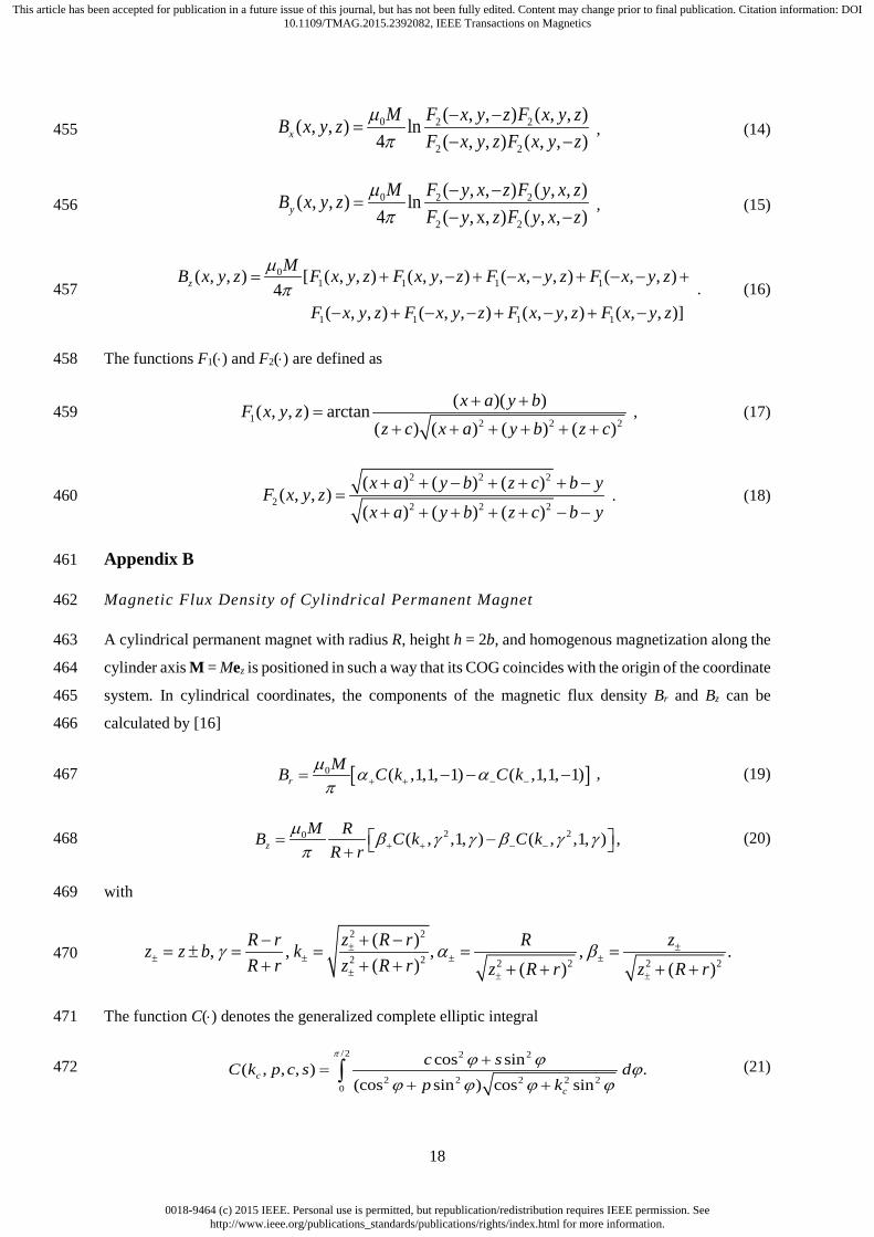
Magnetic Flux Density of Cylindrical Permanent Magnet 462

A cylindrical permanent magnet with radius R, height h = 2b, and homogenous magnetization along the 463

cylinder axis M = Mez is positioned in such a way that its COG coincides with the origin of the coordinate 464

system. In cylindrical coordinates, the components of the magnetic flux density Br and Bz can be 465

calculated by [16] 466

[ ]0 ( ,1,1, 1) ( ,1,1, 1)rMB C k C kµ α α

π + + − −= − − − , (19) 467

2 20 ( , ,1, ) ( , ,1, ) ,zM RB C k C k

R rµ β γ γ β γ γ

π + + − − = − + (20) 468

with 469

2 2

2 2 2 2 2 2

( ), , , , .( ) ( ) ( )

z R r zR r Rz z b kR r z R r z R r z R r

γ α β± ±± ± ± ±

± ± ±

+ −−= ± = = = =

+ + + + + + + 470

The function C(⋅) denotes the generalized complete elliptic integral 471

/2 2 2

2 2 2 2 20

cos sin( , , , ) .(cos sin ) cos sin

c

c

c sC k p c s dp k

π ϕ ϕ ϕϕ ϕ ϕ ϕ

+=

+ +∫ (21) 472

18



Acknowledgment 473

The presented work was supported by the Deutsche Forschungsgemeinschaft (DFG) in the framework 474

of the Research Training Group “Lorentz force velocimetry and Lorentz force eddy current testing” (GK 475

1567) at the Technische Universität Ilmenau. 476

5 References 477

[1] B. Petković, J. Haueisen, M. Zec, R. Uhlig, H. Brauer, and M. Ziolkowski, “Lorentz force 478

evaluation: A new approximation method for defect reconstruction,” NDT & E International, vol. 479

59, pp. 57–67, 2013. 480

[2] J. Haueisen, R. Unger, T. Beuker, and M. Bellemann, “Evaluation of inverse algorithms in the 481

analysis of magnetic flux leakage data,” IEEE Trans. Magn, vol. 38, no. 3, pp. 1481–1488, 2002. 482

[3] M. Zec, R. P. Uhlig, M. Ziolkowski, and H. Brauer, “Fast technique for Lorentz force calculations 483

in non-destructive testing applications,” IEEE Trans. Magn, vol. 50, no. 2, pp. 133–136, 2014. 484

[4] A. J. Petruska and J. J. Abbott, “Optimal permanent-magnet geometries for dipole field 485

approximation,” IEEE Trans. Magn, vol. 49, no. 2, pp. 811–819, 2013. 486

[5] R. Ravaud, G. Lemarquand, V. Lemarquand, and C. Depollier, “Analytical calculation of the 487

magnetic field created by permanent-magnet rings,” IEEE Trans. Magn, vol. 44, no. 8, pp. 1982–488

1989, 2008. 489

[6] J. P. Selvaggi, S. Salon, O.-M. Kwon, M. V. K. Chari, and M. DeBortoli, “Computation of the 490

External Magnetic Field, Near-Field or Far-Field, From a Circular Cylindrical Magnetic Source 491

Using Toroidal Functions,” IEEE Trans. Magn, vol. 43, no. 4, pp. 1153–1156, 2007. 492

[7] H. L. Rakotoarison, J.-P. Yonnet, and B. Delinchant, “Using coulombian approach for modeling 493

scalar potential and magnetic field of a permanent magnet With Radial Polarization,” IEEE Trans. 494

Magn, vol. 43, no. 4, pp. 1261–1264, 2007. 495

[8] F. Bancel, “Magnetic nodes,” J. Phys. D: Appl. Phys, vol. 32, pp. 2155–2161, 1999. 496

[9] E. Furlani, S. Reznik, and A. Kroll, “A three-dimensional field solution for radially polarized 497

cylinders,” IEEE Trans. Magn, vol. 31, no. 1, pp. 844–851, 1995. 498

[10] E. Furlani, “A three-dimensional field solution for axially-polarized multipole disks,” Jour. 499

Magn. Magn. Mater, vol. 135, no. 2, pp. 205–214, 1994. 500

[11] M. A. Green, “Modeling the behavior of oriented permanent magnet material using current 501

doublet theory,” IEEE Trans. Magn, vol. 24, no. 2, pp. 1528–1531, 1988. 502

[12] L. Uranker, “High accuracy field computation of magnetized bodies,” IEEE Trans. Magn, vol. 503

MAG-21, no. 6, pp. 2169–2172, 1985. 504

[13] G. Akoun and J.-P. Yonnet, “3D analytical calculations of the forces extened between two 505

cuboidal magnets,” IEEE Trans. Magn, vol. MAG-20, no. 5, pp. 1962–1964, 1984. 506

[14] M. W. Garrett, “Calculation of Fields, Forces, and Mutual Inductances of Current Systems by 507

Elliptic Integrals,” J. Appl. Phys, vol. 34, no. 9, pp. 2567–2573, 1963. 508

19























[15] Z. J. Yang, T. H. Johansen, H. Bratsberg, G. Helgesen, and A. T. Skjeltorp, “Potential and force 509

between a magnet and a bulk superconductor studied by a mechanical pendulum,” Supercond. 510

Sci. Technol, vol. 3, pp. 591–597, 1990. 511

[16] N. Derby and S. Olbert, “Cylindrical magnets and ideal solenoids,” Am. J. Phys, vol. 78, no. 3, 512

pp. 229–235, 2010. 513

[17] Edward P. Furlani, Permanent magnet and electromechanical devices. New York: Academic 514

Press, 2001. 515

[18] H. Hofmann, Das elektromagnetische Feld: Theorie und grundlegende Anwendungen. Wien: 516

Springer, 1986. 517

[19] W. H. Press, S. A. Teukolsky, W. T. Vetterling, and B. Flannery, Numerical recipes in C. 518

Cambridge: University Press, 1992. 519

[20] J. A. Nelder and R. Mead, “A simplex method for function minimization,” The Comp. J, vol. 7, 520

pp. 308–313, 1965. 521

[21] H. Brauer, K. Porzig, J. Mengelkamp, M. Carlstedt, M. Ziolkowski, and H. Töpfer, “Lorentz force 522

eddy current testing: a novel NDE-technique,” COMPEL: The International Journal for 523

Computation and Mathematics in Electrical and Electronic Engineering, vol. 33, no. 6, pp. 1965–524

1977, 2014. 525

[22] A. H. Stroud, Approximate calculation of multiple integrals. New Jersey: Prentice Hall, 1971. 526

20







Permanent Magnet Modeling for Lorentz Force Evaluation

Documents

Transcript of Permanent Magnet Modeling for Lorentz Force Evaluation