DEVELOPMENT OF DOUBLE-SIDED INTERIOR PERMANENT MAGNET FLAT

LINEAR BRUSHLESS MOTOR AND ITS CONTROL USING LINEAR OPTICAL

POTENTIOMETER

A Dissertation

by

YOUNG SHIN KWON

Submitted to the Office of Graduate and Professional Studies of Texas A&M University

in partial fulfillment of the requirements for the degree of

DOCTOR OF PHILOSOPHY

Chair of Committee, Won-jong Kim Committee Members, Hamid A. Toliyat Alexander Parlos Bryan Rasmussen Head of Department, Andreas A. Polycarpou

August 2016

Major Subject: Mechanical Engineering

Copyright 2016 Young-shin Kwon

ii

ABSTRACT

A new 6/4 double-sided interior permanent-magnet (IPM) flat linear brushless

motor (IPM-FLBM) and novel optical potentiometer mechanism for a linear motion-

control system are presented in this dissertation.

For this purpose, new detent-force-minimization methodologies for the IPM-

FLBM are studied on the basis of the superposition principle. The end-effect force is

reduced by a new two-dimensional optimization using the step-shaped end frames. The

cogging force is minimized through a destructive interference using the slot-phase shift

between the upper and lower stators. A base model prototype with the detent force of only

1.5% of the maximum thrust force is developed using the electrical solid steel. Analytic

modeling techniques of the base model prototype with slot-phase shift and alternate teeth

windings are investigated. A variable winding function is newly developed to evaluate

the inductances of the salient motor with the alternate teeth windings. The steady-state

thrust force is modeled for this linear brushless AC (BLAC) motor. Their validities are

demonstrated experimentally. The electromagnetic and steady-state performance

analyses of a new prototype using a soft magnetic composite (SMC) material are also

studied using a simplified nonlinear magnetic equivalent circuit (MEC) analysis. Its iron

and copper losses are investigated in terms of the thermal limitation. The feasibility of

the IPM-FLBM using the SMC material is demonstrated through the comparisons of the

average steady-state thrust and ripple forces for these two prototype linear motors.

iii

A novel low-cost high-precision absolute displacement-sensing mechanism using

optoelectronic components is developed. The working principle that is based on the

change of the optical power that is reflected off the monotone-colored pattern track from

a light emitting diode (LED) to a red-green-blue (RGB) photo diode (PD) is presented.

The performance of the proposed optical potentiometer (OP) mechanism is verified by

the bandwidth (BW) of 4.42 kHz and nonlinearity of 2.8% are achieved.

A novel low-ripple 12-step current control scheme using a single current sensing

resistor is developed using the six Hall-effect sensors for the force control of the IPM-

FLBM. Its performances are experimentally verified and compared with a conventional

field-oriented control (FOC) scheme. In the end, the position-control loop, which includes

the 12-step current control loop, double-sided IPM-FLBM, and linear optical

potentiometer (LOP), is designed using a proportional controller with a lead compensator.

The performances of the linear motion-control system are demonstrated through the

various experiments in the time and frequency domains.

iv

ACKNOWLEDGMENTS

First and foremost, I would like to express my sincere gratitude towards my

advisor, Prof. Won-jong Kim, for his support, encouragement, and patience during my

Ph.D. career. I enjoyed working with him, for all his considerate, thoughtful principles,

and learning from him, for his vast knowledge about design and development of

electromechanical systems.

I am grateful to Profs. Hamid Toliyat, Alexander Parlos, and Bryan Rasmussen

for serving as my committee members. I especially thank Prof. Toliyat for all his

invaluable lectures on electric machine design and control.

Thanks also go to my friends and colleagues in the Precision Mechatronics Lab

for their support. I am very thankful to Mr. Eunseok Kim and Minsuk Kong for being

such a good friend in this school.

I would certainly be remiss to mention and sincerely thank my friend, Hyeong-

rae, and former colleague Jun-ki. Without their essential helps in hardware construction,

this research and dissertation would not be complete.

Finally, I can never thank my wife, Soo-jung, and my son, Jung-woo, enough for

their patience and understanding. They have always been great friends and wonderful

counselors of mine. I would like to thank my parents, Tae-yong Kwon and Jung-hee Baik,

and Soo-jung’s parents Byung-in Choi and Young-hee Jun. Without their player and

support, this level of doctoral work would not have been successful.

v

TABLE OF CONTENTS

Page

ABSTRACT .............................................................................................................ii 

ACKNOWLEDGMENTS ...................................................................................... iv 

TABLE OF CONTENTS ........................................................................................ v 

LIST OF FIGURES.............................................................................................. viii 

LIST OF TABLES ............................................................................................. xviii 

CHAPTER I INTRODUCTION ............................................................................ 1 

1.1  Background ................................................................................................. 1 1.2  Literature Survey ......................................................................................... 3 

1.2.1  Electromagnetic Linear Motors ......................................................... 3 1.2.2  Linear Displacement Sensors ............................................................. 7 1.2.3  Linear Motor Control Techniques ..................................................... 9 1.2.4  Dissertation Overview ..................................................................... 10 1.2.5  Contribution of Dissertation ............................................................ 12 

CHAPTER II DESIGN AND ANALYSIS OF IPM-FLBM ............................... 13 

2.1  Conceptual Design of IPM-FLBM ............................................................ 14 2.1.1  Conventional Rotary Brushless Motors ........................................... 14 2.1.2  6 /4 IPM Brushless Motor with Alternate Teeth Windings ............. 15 2.1.3  6-Slot/4-Pole IPM FLBM ................................................................ 16 2.1.4  Design Parameters of Double-Sided 6/4 IPM-FLBM ..................... 17 

2.2  Detent Force Minimization of Double-Sided 6/4 IPM-FLBM ................. 19 2.2.1  Steady-State Thrust and Detent Forces of Base Model ................... 20 2.2.2  End-Effect Force Minimization ....................................................... 21 2.2.3  Cogging Force Minimization ........................................................... 31 2.2.4  Detent Force-Free Stator .................................................................. 35 2.2.5  Total Detent- and Steady-state Thrust Force Measurements ........... 37 

2.3  Steady-State Modeling and Analysis of Double-Sided IPM-FLBM ......... 40 2.3.1  Detent Force-Free Base Model Description .................................... 43 2.3.2  Simplified Magnetic Equivalent Circuit .......................................... 45 2.3.3  No-Load Flux Density and Stator Relative Permeance ................... 48 2.3.4  DC Resistance of Armature Winding .............................................. 50 

vi

2.3.5  No-Load Flux Linkage and Back-EMF Voltage ............................. 52 2.3.6  Inductance Calculations ................................................................... 56 2.3.7  Thrust Force Calculation ................................................................. 63 2.3.8  Steady-State Force Validation ......................................................... 65 

2.4  IPM-FLBM Using SMC ............................................................................ 70 2.4.1  Inductance Calculations ................................................................... 72 2.4.2  No-Load Flux Linkage and Back-EMF Voltage ............................. 74 2.4.3  Simplified Nonlinear Magnetic Equivalent Circuit ......................... 75 2.4.4  Magnetic Field Analysis .................................................................. 79 2.4.5  Loss Analysis and Thermal Consideration ...................................... 83 2.4.6  Steady-State Performance Validation .............................................. 86 

CHAPTER III OPTICAL POTENTIOMETER ................................................... 92 

3.1  Light and Its Terminologies ...................................................................... 92 3.1.1  Light ................................................................................................. 92 3.1.2  Radiometry and Photometry ............................................................ 93 

3.2  Optoelectronic Devices ............................................................................. 96 3.2.1  Light-Emitting Diodes (LEDs) ........................................................ 96 3.2.2  Photo Diodes (PDs) ....................................................................... 102 

3.3  Optical Potentiometer Concept and Dynamic Model .............................. 107 3.3.1  Position-Sensing Mechanism Using Indirect Light ....................... 107 3.3.2  Dynamic Model of Optical Potentiometer ..................................... 108 

3.4  Rotary Optical Potentiometer .................................................................. 111 3.4.1  Mechanical Geometry Configuration ............................................ 111 3.4.2  Steady-State Propagation Model in Color Coded Track ................ 112 3.4.3  Steady-State Propagation Model in V-Shaped Track .................... 118 

3.5  Design Parameter Optimization and Calibration ..................................... 120 3.5.1  Design Parameter Optimization ..................................................... 120 3.5.2  Calibration of Colored-Coded Track and Sensing Constant.......... 122 3.5.3  Calibration of V-Shaped Track and Angle-Sensing Constant ....... 125 

3.6  Performance Validation ........................................................................... 127 3.6.1  Hardware Implementation and Controller ..................................... 127 3.6.2  Experimental Results ..................................................................... 129 

CHAPTER IV SYSTEM MODELING AND ITS CONTROL ......................... 133 

4.1  Current Control of Double-Sided IPM-FLBM ........................................ 134 4.1.1  Electromechanical Specification .................................................... 134 4.1.2  12-Step Current Control. ................................................................ 136 4.1.3  Field-Oriented Control ................................................................... 149 4.1.4  Performance Comparisons ............................................................. 153 

4.2  Linear Motion System Model.................................................................. 159 4.2.1  Lumped-Parameter Model ............................................................. 159 

vii

4.2.2  Identification of Equivalent Stiffness ............................................ 160 4.2.3  Simplified Model of Linear Motion Platform ................................ 164 4.2.4  Dynamic Friction Model ................................................................ 167 

4.3  Position Loop Design and Performance .................................................. 169 4.3.1  Frequency Response of Uncompensated System .......................... 170 4.3.2  Design of Proportional Controller and Lead Compensator ........... 172 4.3.3  Performance Validation and Comparisons .................................... 176 

CHAPTER V CONCLUSIONS AND SUGGESTIONS ................................... 183 

5.1  Conclusions ............................................................................................. 183 5.2  Suggestions for Future Work .................................................................. 185 

REFERENCES .................................................................................................... 186 

APPENDIX A MECHANICAL ENGINEERING DRAWINGS ...................... 196 

APPENDIX B ELECTRICAL ENGINEERING SCHEMATICS .................... 209 

APPENDIX C PROGRAM CODES ................................................................. 222 

viii

LIST OF FIGURES

Page

Fig. 1. Linear motion-control system using LOP. ............................................................ 2 

Fig. 2. Magnetization curves of various soft iron-core materials. .................................... 6 

Fig. 3. PM rotor configurations: (a) surface-mounted magnets and (b) buried PMs with circumference magnetization. ..................................................................... 15 

Fig. 4. 6/4-IPM brushless motors: (a) all teeth and (b) alternate teeth windings. ........... 16 

Fig. 5. 6/4 IPM-FLBM with all teeth windings .............................................................. 16 

Fig. 6. 6/4 IPM-FLBM with all teeth windings and additional end frames .................... 17 

Fig. 7. 6/4 IPM-FLBM with alternate teeth windings. ................................................... 17 

Fig. 8. Base model of the double-sided 6/4 IPM-FLBM with alternate teeth windings. ............................................................................................................ 18 

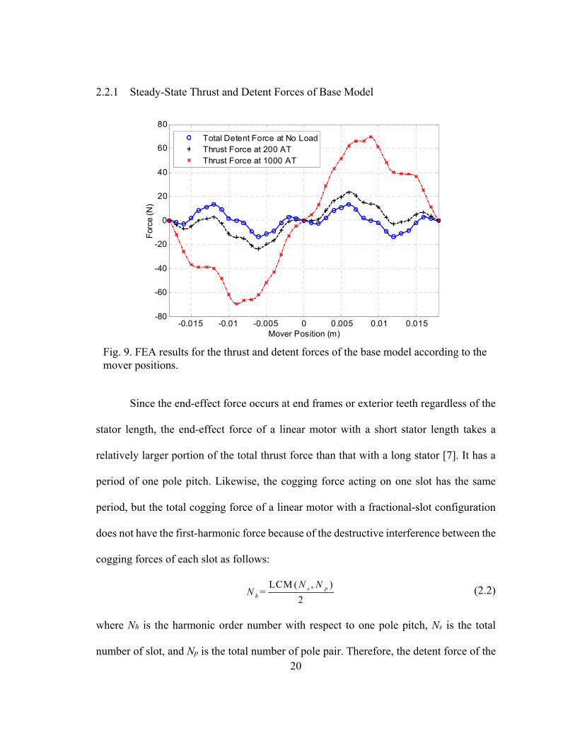
Fig. 9. FEA results for the thrust and detent forces of the base model according to the mover positions. ........................................................................................... 20 

Fig. 10. Left end-effect force measurement using the slotless rectangular prim iron-core stator when the mover’s position is at zero. ............................................... 22 

Fig. 11. Measured left end-effect force according to mover positions when the pole pitch is 0.018 m, and the magnet length is 0.006 m. .......................................... 23 

Fig. 12. Measured end-effect forces according to the slotless stator’s overall lengths and mover positions: slotless stators (top) and end-effect forces (bottom). ...... 24 

Fig. 13. (a) Optimal stator length analysis according to mover positions with respect to the peak-to-peak end-effect forces, (b) rms end-effect force according to the stator lengths. ............................................................................................... 24 

Fig. 14. Dimension definition of the slotless stator with two different lengths. ............. 26 

Fig. 15. Measured end-effect forces according to the mover positions with respect to the stack depths of the long-length portion. ................................................... 28 

ix

Fig. 16. Effective stack width ratio according to the mechanical stack width ratio of the long-length portion in the stator when Lss Ls = 0.009 m and = 0.001 m. ....................................................................................................................... 30 

Fig. 17. End-effect force comparison of the one-dimensional optimization (Ls = 0.0788) and two-dimensional optimization (Lss = 0.0835 m, Ls = 0.0745 m, Ds = 0.02 m and Dss = 0.006 m). ....................................................................... 31 

Fig. 18. Infinite-length stator model for the cogging force analysis. .............................. 32 

Fig. 19. FEA results for cogging forces of the infinite-length stator model according to the mover positions with respect to the stator’s tooth widths. ...................... 33 

Fig. 20. Concept of the slot-phase shift configuration in the double-sided IPM-FLBM, where s is the slot-phase shift. ............................................................ 34 

Fig. 21. FEA results for the stator with the slot-phase shift of Tp/6 between the upper and lower stators. (a) Total cogging forces and (b) the rms cogging force according to the tooth widths. ........................................................................... 35 

Fig. 22. Comparison of two different arrangements for double-sided stators: (a) non-slot-phase-shift configuration, and (b) slot-phase-shift configuration. ...... 36 

Fig. 23. Photograph of the experimental setup to measure the total detent- and steady-state thrust forces. .................................................................................. 37 

Fig. 24. Comparison of the predicted and measured thrust forces (top), and comparison of the predicted cogging and measured detent forces (bottom) when Tt = 0.0076 m. .......................................................................................... 38 

Fig. 25. Maximum thrust force and detent force comparison (top), and magnified view of the detent force from the top figure (bottom). ..................................... 39 

Fig. 26. 3-D rendering for the proposed double-sided 6/4 IPM-FLBM with slot-phase shift and alternate teeth windings. ........................................................... 40 

Fig. 27. Analysis flowchart for the double-sided 6/4 IPM-FLBM with the slot-phase shift and alternate teeth windings. ..................................................................... 42 

Fig. 28. Cross-sectional dimensions and coordinates of the double-sided 6/4 IPM-FLBM prototype using the electrical solid steel SS400. ................................... 43 

Fig. 29. (a) Flux paths of the single-sided model when the d-axis is aligned with the stator reference axis under no-load condition. (b) Simplified MEC model with slot leakage reluctance under no-load condition. ...................................... 46 

x

Fig. 30. FE flux density vector paths in the mid-cross-section plane when the d-axis is aligned with the stator reference axis under the no-load condition. .............. 50 

Fig. 31. Predicted air-gap flux density distributions (the top and bottom plots are for the upper- and lower-side air gaps) when the d-axis is aligned with the stator reference axis under the no-load condition ............................................. 50 

Fig. 32. Uniformly concentrated rectangular winding: (a) the dimension definitions of the armature winding and (b) a photograph of the armature winding. ......... 51 

Fig. 33. Superposed winding functions of phases a, b, and c when a coil has the number of turns of 85. ....................................................................................... 54 

Fig. 34. Analytic and FEA results of the no-load flux linkages for each phase according to the mover positions. ..................................................................... 55 

Fig. 35. Analytic and FEA results of the phase-to-neutral back-EMFs for each phase when the mover has the linear speed of 0.5 m/s. .............................................. 56 

Fig. 36. Variable winding function model in the IPM-FLBM: flux paths when the d-axis is aligned with the winding tooth center (top) and when the q-axis is aligned with the winding tooth center (bottom). ........................................... 58 

Fig. 37. Variable winding function of phase b in the upper and lower sides when the d-axis is aligned with the stator reference axis (top) and when the q-axis is aligned with the stator reference axis (bottom). ..................................... 59 

Fig. 38. Self-inductance distributions of each phase according to the mover positions. ........................................................................................................... 62 

Fig. 39. Mutual inductance distributions of each phase according to the mover positions. ........................................................................................................... 62 

Fig. 40. Photograph of the experimental setup to measure the inductances and steady-state thrust force. .................................................................................... 66 

Fig. 41. Thrust force components accordin to the current phase angle when the magnitude of the current vector Is of 10 A is applied. ...................................... 67 

Fig. 42. Force-to-current ratios in the MFC and FOC scheme. ...................................... 68 

Fig. 43. Steady-state force and detent force according to the mover positions when Iqs and Ids are controlled as 10 A and 0 A, respectively. ................................... 70 

xi

Fig. 44. Photograph of the stator core with the phase coils (right) and mover with PMs (left). ......................................................................................................... 71 

Fig. 45. The air-gap permeance models when the phase b is an armature MMF source: (a) the q-axis is aligned with the tooth center of phase b, (b) the d-axis is aligned with the tooth center of phase b. ............................................... 72 

Fig. 46. Flux paths of the single-sided models due to (a) PM and (b) armature current when the d-axis is aligned with the stator tooth centerline of phase b. Corresponding simplified nonlinear MEC models under (c) the no-load condition and (d) the electrical load condition. ................................................. 76 

Fig. 47. B-H curves of the SS400 and SPM. .................................................................. 76 

Fig. 48. Stator-tooth flux curves (top) and air-gap flux density curves (bottom) according to the armature current. .................................................................... 79 

Fig. 49. Stator-tooth flux 3 (mWb) contour plot according to the PM and stator tooth widths when Ia = 10 A. ............................................................................ 80 

Fig. 50. Air-gap flux density curves according to the PM height for the three different load conditions when Tm = 0.006 m and Tt = 0.0076 m. .................... 81 

Fig. 51. Air-gap flux density curves according to the air-gap size for the three different load conditions when Tm = 0.006 m and Tt = 0.0076 m. .................... 82 

Fig. 52. Air-gap flux density variation curve in the mover core according to the back-iron height under the 10-A electrical load condition when Tm = 0.006 m and Tt = 0.0076 m. ......................................................................................... 82 

Fig. 53. Steady-state temperature responses (top) and iron loss ratios (bottom) of the stator-winding assembly according to the phase current and operating frequency under the natural convection condition when Aes = 0.0079 m2 and ms = 0.0936 kg. ........................................................................................... 86 

Fig. 54. Analytic and measurement results of the back-EMFs for each phase when the mover has the linear speed of 0.2 m/s. ........................................................ 86 

Fig. 55. Self-inductance distributions of the SPM prototype according to positions ..... 87 

Fig. 56. Mutual inductance distributions of the SPM prototype according to positions. ........................................................................................................... 88 

xii

Fig. 57. Steady-state thrust forces of the SPM and base model (SS400) prototypes according to the mover positions when Ia = 8.66 A, Ib = 0 A and Ic = 8.66 A. ....................................................................................................................... 89 

Fig. 58. Steady-state forces (top) and detent forces (bottom) of the SPM and base model (SS400) prototypes according to the mover positions when Iqs and Ids are controlled as 10 A and 0 A, respectively. ............................................... 90 

Fig. 59. Temperature responses in the end winding of the stator-winding assembly according to the magnitude of the phase current. ............................................. 91 

Fig. 60. Light emitting diodes and photo diodes: (a) Precision optical Performance Red color LED (HLMP-EG08_YZ000, Avago Technology), (b) High power Tri-Color LED (Moonstone, Avago Technology), (c) Red-green-blue (RGB) Photodiode (S7505-5, Hamamatsu, and (d) Gap Photodiode (FGAP71, ThorLabs. ......................................................................................... 96 

Fig. 61. LED electroluminescene mechanism: (a) standard structure and (b) point source. emitter structure. ................................................................................... 97 

Fig. 62. Forward diode voltage versus bandgap energy of various LEDs using materials. ........................................................................................................... 98 

Fig. 63. (a) Definition of the critical angle. (b) Area element of calotte-shaped surface of the sphere defined by radius r and the critical angle. ....................... 99 

Fig. 64. (a) Viewing angle, (b) Emission spectrum and FWHM. ................................. 102 

Fig. 65. Photoelectric current mechanism (left) and symbol of PD (right) .................. 102 

Fig. 66. (a) Equivalent circuit model of PD. (b) Steady-state model of PD. ................ 104 

Fig. 67. Responsivity of silicon diode (OPA 101). ....................................................... 104 

Fig. 68. Photoconductive mode (PC) and Photovoltaic Mode (PV). ............................ 106 

Fig. 69. Optical potentiometer sensing mechanism: (a) RGB coded track. (b) V-shaped track. .................................................................................................... 108 

Fig. 70. Dynamic analysis between LED and RGB: (a) Test scheme. (b) Time responses. ........................................................................................................ 108 

Fig. 71. 2-D cross-sectional view of the rotary optical potentiometer. ......................... 111 

xiii

Fig. 72. (a) Normalized 3-D Lambertian radiant intensity pattern of the LED. (b) Normalized radiant intensity according to the angle displacement of the LED (HLMP-EG08-Y2000). .......................................................................... 113 

Fig. 73. Expected normalized reflected power density on the tangential surface (( ( ) ( , ,0))/ (0)ts v ss i r tsE E E with = 0.2, sk = 0.4, and s =10). ................. 114 

Fig. 74. Power densities due to the red RGB colored track and the incident area illuminated by the LED. .................................................................................. 116 

Fig. 75. V-shaped track and the rectangular mask for linearization of the received optical power. .................................................................................................. 120 

Fig. 76. Diameter of the incident-beam area and the visible viewing angle of the LED according to the displacement of dLS when IF is 20 mA. ......................... 121 

Fig. 77. (a) Experiment photo for optimal distance (dSR). (b)The output voltages of the red color channel of the RGB sensor according to circular white-colored area and distance (dSR). ....................................................................... 122 

Fig. 78. Non-compensated and compensated angle of the optical potentiometer in color-coded Track. (when IF = 20 mA, dLS = 0.015 m, dSR = 0.0065 m, and the physical cell size of each color code on the cylinder is 0.0005236 0.1 m2 ). ................................................................................................................. 124 

Fig. 79. Output voltage of the differential OP-amp with gain of 4.5. ........................... 125 

Fig. 80. Optical potentiometer angle vs. resistive potentiometer angle in V-shaped Track (when IF = 20 mA, dLS= 0.015 m, dSR= 0.0065 m). ............................... 127 

Fig. 81. Hardware block diagram of the rotary-position control system. ..................... 128 

Fig. 82. Rotary position-control system with ROP. ...................................................... 129 

Fig. 83. Step responses of the position-control loop using the ROP with the CCT for various reference commands (±10, ±20, ±40, and ±80). ..................... 130 

Fig. 84. Step responses of the position-control loop using the ROP with the VST for various reference commands (±10, ±20, ±30, and ±60). ..................... 131 

Fig. 85. Sinusoidal response to a 1-Hz sinusoidal reference input with the magnitude of 60 and the period of 1 s (Position control using RRP (Top figure), position control using ROP with CCT (middle figure), and position control using ROP with VST (bottom). .......................................................... 132 

xiv

Fig. 86. Photograph of the new double-sided 6/4 IPM-FLBM prototype .................... 134 

Fig. 87. Coordinate definitions of the double-sided 6/4 IPM-FLBM: (a) 3-D cross-sectional view of the mechanical model, (b) electrical angle model using the current vector coordinates with slot-phase shift, and (c) simplified equivalent electrical angle model using the resultant current vector coordinates. ..................................................................................................... 135 

Fig. 88. Measured Hall-effect sensor outputs (top) and back-EMF voltages (bottom) according to the mover positions when the mover moves at 0.2 m/s. ............ 137 

Fig. 89. Predicted 12-step quasi-sinusoidal phase current waveforms according to the electrical angles when Im = 10.0 A. ........................................................... 138 

Fig. 90. Predicted ripple forces according to the commutation schemes and electrical angle when the phase current of 10 A is applied. ............................ 138 

Fig. 91. Hardware block diagram of the 12-step current control for the double-sided IPM-FLBM with slot-phase shift. ................................................................... 139 

Fig. 92. 12-Step commutation sequence during one electrical angle cycle. ................. 141 

Fig. 93. Actual phase, measured, and corrected dc-link currents according to the duty cycle variation in the switching modes when the dc-link voltage of 30 V is applied. .................................................................................................... 143 

Fig. 94. Block diagram of the 12-step current control using the dc-link current. ......... 146 

Fig. 95. Open-loop frequency responses of the phase current I for the current command I*

dc in the two-phase conduction mode (a) and three-phase conduction mode (b) when the dc-link voltage is 30.0 V, and the proportional gain Kp and integral gain Wi are 0.7 Duty Cycle/A and 754 rad/s, respectively. ........................................................................................... 148 

Fig. 96. Control block diagram of the indirect FOC scheme for the double-sided IPM-FLBM with the slot-phase shift. ............................................................. 149 

Fig. 97. (a) A representation of the space vectors V1 to V6, and a voltage vector Vref. (b) The space vector modulation of the three-phase voltages in sector I. ....... 151 

Fig. 98. The dc-link current (top) and phase current waveforms (bottom) with respect to the mover positions when the step current command of 1.0 A is applied in the 12-step current control scheme. ................................................ 154 

xv

Fig. 99. The measured q- and d-axis current (top) and phase current waveforms (bottom) according to the mover positions when the step current command of 1.0 A is applied in the FOC scheme. ........................................ 155 

Fig. 100. The current vector trajectories in the stationary -reference frame: (a) 12-step current control scheme and (b) FOC scheme. .................................. 155 

Fig. 101. Thrust forces of the 12-step current control and FOC schemes according to the sinusoidal current command of 1.0 A and 3.0 Hz: thrust forces (top), current command I*

dc and dc-link current Idc-link (middle), and current command I*

q, q-axis current Iq, and d-axis current Id = 0 (bottom). .............. 156 

Fig. 102. Pulsating forces (top), detent force (middle), and ripple forces (bottom) of the 12-step current control and FOC schemes when the mover moves at the constant speed of 0.1 m/s. .................................................................... 158 

Fig. 103. (a) Thrust force versus current command (Kf = 6.05 and 6.18 N/A for the 12-step current control and FOC schemes, respectively). (b) Electric power consumption comparison according to the thrust force. .................... 158 

Fig. 104. Lumped-parameter model concept for linear motion platform. .................... 159 

Fig. 105. Isometric view of the FEA model to evaluate the equivalent stiffness. ........ 161 

Fig. 106. Static deformation of the mover assembly when the x-directional loading force of 100 N is applied. .............................................................................. 162 

Fig. 107. X-directional deformation according to the applied forces and the mover positions. ....................................................................................................... 163 

Fig. 108. Equivalent spring constant of the mover assembly according to the mover positions. ....................................................................................................... 164 

Fig. 109. Parameters and variables in the lumped-parameter model. ........................... 164 

Fig. 110. Simplified pure mass model with a friction model........................................ 166 

Fig. 111. Velocity control loop to measure the friction coefficients. ........................... 168 

Fig. 112. Measured and modeled frictions.................................................................... 168 

Fig. 113. Current loop model of the linear motion system. .......................................... 169 

Fig. 114. Simplified open-loop model for the linear motion system. ........................... 170 

Fig. 115. Open-loop frequency responses of the uncompensated system. ................... 171 

xvi

Fig. 116. Closed-loop control block diagram of the linear motion system. ................. 172 

Fig. 117. Open-loop frequency responses of the uncompensated and compensated systems when Kd = 3.5, A = 10.7, 1 = 26.4 rad/s, and 1 = 282.6 rad/s. .... 175 

Fig. 118. Photograph of the experimental setup to measure the performances of the linear motion platform. .................................................................................. 176 

Fig. 119. Step responses of the same position-control loops according to the two different current control schemes. ................................................................. 177 

Fig. 120. The responses of the same position-control loops according to the two different current control schemes for the ramp input command of 10 mm/s. ............................................................................................................. 178 

Fig. 121. The responses of two position-control loops using the different current control schemes for the sinusoidal input command of 15 mm at 1 Hz. ........ 179 

Fig. 122. Responses for various step inputs in the position-control loop using the 12-step current control and LOP. .................................................................. 180 

Fig. 123. The responses of the position-control loops using the FOC and LOP for the ramp input command of 10 mm/s. ........................................................... 181 

Fig. 124. The responses of the position-control loops using the FOC and LOP for the sinusoidal input command of 15mm with 1 Hz. ..................................... 182 

Fig. 125. The linear motion platform with LOP sensor module. .................................. 196 

Fig. 126. High level components of the linear motion platform. .................................. 197 

Fig. 127. Components of the double-sided IPM-FLBM assembly. .............................. 198 

Fig. 128. Components of the dummy load assembly. ................................................... 199 

Fig. 129. Stator housing part 1. ..................................................................................... 200 

Fig. 130. Stator housing part 2. ..................................................................................... 201 

Fig. 131. SMC stator. .................................................................................................... 202 

Fig. 132. Armature coil holder. ..................................................................................... 203 

Fig. 133. Mover frame front. ........................................................................................ 204 

Fig. 134. Mover core. .................................................................................................... 205 

xvii

Fig. 135. Permanent magnet. ........................................................................................ 206 

Fig. 136. Mover frame side. .......................................................................................... 207 

Fig. 137. Mover loader. ................................................................................................ 208 

Fig. 138. Photograph of the controller assembly for the linear-motion control. .......... 209 

Fig. 139. Photograph of the DSP breakout board ......................................................... 210 

Fig. 140. Photograph of the digital interface board. ..................................................... 212 

Fig. 141. Digital interface board schematic (1/2). ........................................................ 213 

Fig. 142. Digital interface board schematic (2/2). ........................................................ 214 

Fig. 143. Photograph of the analog interface board. ..................................................... 215 

Fig. 144. Electric circuit schematic of the analog interface board (1/3). ...................... 216 

Fig. 145. Electric circuit schematic of the analog interface board (2/3). ...................... 217 

Fig. 146. Electric circuit schematic of the analog interface board (3/3) ....................... 218 

Fig. 147. Photograph of the PWM amplifier board. ..................................................... 219 

Fig. 148. Electric circuit schematic of the PWM amplifier board. ............................... 220 

Fig. 149. Wiring diagram of the linear control system. ................................................ 221 

xviii

LIST OF TABLES

Page

Table 1. Possible topologies and configurations of linear motors [1], [2]. ....................... 3 

Table 2. Linear displacement sensors [25]. ...................................................................... 8 

Table 3. Driving methods for the LBM [35][42]. ......................................................... 10 

Table 4 Mechanical design specifications of the base model ......................................... 18 

Table 5 Estimated Fourier coefficient of the left end-effect force .................................. 23 

Table 6. Final design parameter of the stator .................................................................. 36 

Table 7 Mechanical specifications of the base model prototype .................................... 44 

Table 8. Average values of the inductances.................................................................... 63 

Table 9. Iron loss per kilogram of the SPM [57]. ........................................................... 84 

Table 10. Average inductances of the SPM and base model prototypes. ....................... 88 

Table 11. Performance comparison of the SS400 and SPM prototypes. ........................ 90 

Table 12. Thermal conductivity and material thickness. ................................................ 91 

Table 13. Photometric and corresponding radiometric unit. ........................................... 93 

Table 14. Performance parameters of LED, RGB Sensor, and PD. ............................. 110 

Table 15. Statistic performance of uncompensated and compensated tracks in the range of 60 to 60. ................................................................................... 124 

Table 16. Statistical performance analysis between 60 and 60 for printer DPI. ..... 126 

Table 17. Specification of the double-sided IPM-FLBM ............................................. 135 

Table 18. Phase current measured according to switching states. ................................ 142 

Table 19. Coefficients of the error function according to switching modes ................. 144 

Table 20. Open-loop performance of 12-step current control scheme ......................... 147 

xix

Table 21. Open-loop performance of FOC scheme ...................................................... 153 

Table 22. Material properties used in FEA ................................................................... 162 

Table 23. Simulation parameters .................................................................................. 170 

Table 24. Open-loop frequency response characteristics of the uncompensated systems ......................................................................................................... 171 

Table 25. Open-loop frequency-response characteristics in two different current control schemes ............................................................................................ 175 

Table 26. Pin descriptions of CN9100 and CN9101 headers ....................................... 211 

Table 27. Pin description of CN9200 and CN9201 headers ......................................... 211 

1

CHAPTER I

INTRODUCTION

1.1 Background

Linear motion-control systems are found in many industrial applications and are

extensively used in machine-tool sliding tables, semiconductor fabrication, biomedical

equipment, and precision factory automation. Many of them often use a conventional

linear platform driven by electric rotary actuators with rotary or linear displacement

sensors for linear position-control. Such linear motion-control systems have been

combined with gear reducers and ball or lead screws to increase force capability for

generating linear motion. This approach, although effective in many applications,

requires the added complexity of a speed reducer as well as causes backlash. Moreover,

it may be too sluggish for the applications that require rapid responses and maneuvering.

Therefore, the demands replacing rotary magnetic actuators with direct-driven linear

actuators increase faster than ever before. Many researchers have been seeking for the

way to develop the cost-effective direct-driven linear motor that can generate high force

density within a confined volume. A decade ago, it was a significant challenge to

construct a commercially viable linear motor that can provide fast dynamic responses,

exact positioning, and long life with less maintenance. Recently, thanks to the

advancement of key technologies such as rare-earth magnets, high permeable soft-core

materials, high-precision linear displacement sensors, and low-cost high performance

digital signal processors, the linear motors having the mover directly connected to the

2

load without backlash and elasticity are being developed. This leads to the improvement

of the dynamic behavior of linear motors and results in the higher accuracy.

The objective of this research is to develop a precision linear position-control

system using a double-sided IPM-FLBM and a cost-effective novel LOP. For this

purpose, this research addresses five parts: (1) detent force minimization of the double-

sided IPM-FLBM with 6/4 configuration (two 6-pole stators having three active coils and

a 4-pole mover), (2) optimal design and fabrication of the IPM-FLBM using the SMC

material, (3) design and development of the high-precision absolute LOP, (4) new current

control scheme for the new proposed linear motor, and finally, (5) development and

performance validation of the linear motion-control system using the 12-step current

control and LOP. Fig. 1 shows the drawing for the linear motion-control system using the

LOP.

Fig. 1. Linear motion-control system using LOP.

3

1.2 Literature Survey

1.2.1 Electromagnetic Linear Motors

Since the first working model for linear motors was invented by Laithwaite in the

1960s [1], the linear motor fabrication and control techniques have been remarkably

developed. The linear motor becomes an indispensable component in linear motion-

control systems [1], [2]. As shown in Table 1, linear motors can be classified in three

types according to their operating principles, such as linear induction motor (LIM), linear

reluctance motor (LRM), and linear synchronous motor (LSM).

Table 1. Possible topologies and configurations of linear motors [1], [2].

Type Shape Number of Stator

Type of

Stator

Mover core

Permanent Configuration

Force Density

Detent Force

Linear induction

motor (LIM)

tubular single

slotted iron none

medium none

flat single low none

double medium none

Linear synchronous motor (LSM)

or

Linear brushless

motor (LBM)

tubular single

slotted iron SPM or IPM high high

none

(air coil)

none longitudinal

stack on mover low none

flat

single

slotted iron SPM or IPM high high

slotless iron SPM on stator medium low

air SPM on stator low none

double slotted iron SPM or IPM high high

slotless air SPM on stator medium none

Linear reluctance

motor (LRM)

tubular single

slotted iron none

medium high

flat single low high

double medium high

* SPM is the abbreviation of the surface-mounted permanent magnet.

4

The LIM is mainly employed in constant-speed applications or long travel

applications. The LRM has no permanent magnet, and also has an advantage that can

control motion with no position sensor, but its force density is not high because its thrust

force is mainly generated by the variable reluctance. In contrast, the LSM can perform

precision position control as well as generate high force density due to the advancement

of rare-earth permanent magnet (PM) with high remanence. Especially, the linear

brushless motor (LBM), which is one of the specialized LSMs, has several advantages:

(1) easy to install the armature coils, (2) easy to assemble the unit modules, (3) easy to

adjust the air-gap, (4) shorter end-winding length, and (5) smaller armature DC resistance.

In this sense, the LBM can be the best candidate as an actuator of the linear motion-

control system.

Since the slotted iron-core linear motors using the SPM or interior IPM

configurations listed in Table 1 can produce much larger force than other types of linear

motors, they are suitable in high-force density applications. However, their detent forces

such as the end-effect force due to stator’s finite length and the cogging force are

drawbacks in the high-precision motion control in low-speed applications. Thus, air-core

linear motors without such detent forces have been used as an alternative in precision

linear motion-control systems that do not require high-force density, but their lower force

density become another disadvantage. For these reasons, many researchers and industries

have attempted to minimize the detent forces of the iron-core PM linear motor on the

basis of the studies of the cogging force of the conventional rotary PM motors. Due to the

advancement of the numerical analysis based on FEA tools, however, various detent-

5

force-minimization techniques such as skewed PM placement [3], semi-closed slots [3],

[4], stator having auxiliary teeth [4], [5], overall length extension of stator [6], alternative

fractional slot-pole structure [7], and asymmetric PM placement [8], [9] were developed

previously. Although these techniques reduced the detent forces effectively, some

methods increased fabrication difficulties such as oversized magnet, elaborated winding

process, post-optimization for additional teeth, excessively lengthy stator, and various

sized iron-cores [3][9]. Recently, a PM pole-shift method useful for mass production

was introduced for a double-sided SPM linear motor [10], but this technique cannot be

applied to an IPM linear motor.

Many studies related to the design, modeling, and performance analysis for linear

motors have mainly focused on the SPM-FLBMs: the improved MEC circuit models of

the single-sided iron-core SPM-FLBM were introduced in [11], [12], and the modeling

and analysis for the double-sided SPM-FLBM were investigated for an electromagnetic

aircraft launcher [13]. The performance analysis for the single-sided IPM-FLBM with

vertical magnetization and distributed windings was performed in [14], and the design

criteria and optimization for slotted IPM-tubular linear motors with the axial

magnetization were also presented in [15], [16]. Nevertheless, little research has been

previously done in modeling and analysis for the double-sided IPM-FLBM.

Most slotted iron-core types listed in Table 1 use the laminated thin silicon steel

sheets as the soft magnetic material for the minimization of the eddy-current loss. In order

to overcome such drawbacks, new powder iron-composite material was developed in the

early 2000s [17]. This SMC material has several advantages such as low eddy-current

6

loss, flexible machine design and assembly, three-dimensional isotropic ferromagnetic

behavior, relatively good recyclability, and reduced production costs [18].

However, as shown in Fig. 2, the lower permeability than the conventional

laminated steel core has hindered the extensive use of the SMC material in electric

machines. Therefore, various studies considering such characteristics of the SMC

material have been done on the various electric machine designs over the past decade.

The optimal stator core teeth of a PM synchronous motor (PMSM) using the SMC

material was studied [19]. The SMC hybrid BLDC motor and SMC claw-pole motors

were analyzed [20], [21]. The axial-flux PMSM was introduced [22], [23]. The design

optimizations for a tubular linear motor using the SMC were investigated with a finite-

element analysis (FEA) [24].

Fig. 2. Magnetization curves of various soft iron-core materials.

0 2000 4000 6000 8000 100000

0.5

1

1.5

2

2.5B-H Curves Comparison

H (A/m)

T (

tesl

a)

Hiperco 50AST1006ST1008SS400Somaly800

7

1.2.2 Linear Displacement Sensors

Linear displacement sensors in linear position-control systems play an

indispensable role as a feedback device measuring the current position. Table 2 shows

the pros and cons of these sensors. The conventional linear displacement sensors can be

classified into the contact type like linear potentiometers and the non-contact types such

as optical linear encoders, magnetic linear encoders, and linear variable differential

transformers (LVDTs). The main advantage of the latter sensors is that high measurement

accuracy, resolution, and reliability can be achieved without wearing-out. However, the

high prices of these sensors and their electronics often act as an entry barrier in low-cost

commercial applications. In contrast, low-cost linear resistive potentiometers (LRPs)

have expanded the market share in commercial control applications. However, the

drawbacks such as the debris accumulation or resistive surface wearing-out due to the

inherent contact-sensing mechanism remain an unsettled problem during a long-term

operation [25]. Therefore, the demands of new cost-effective noncontact linear

displacement sensor that can replace the conventional linear displacement sensors are

increasing in order to reduce the total cost of the linear motion systems.

Several new non-contact displacement sensors such as Hall-effect sensors and

inductive sensors have been developed [26][29]. The first attempt to measure the linear

displacement from the received optical power variation by the beam path interruption

between a LED and a PD was introduced without an exact model of the interaction

between an optoelectronics couple and a movable interrupter [30]. A LOP using the

optical power change from a light passing through the cylindrical track with a triangular

8

aperture was conceptually designed [31]. However, the new sensors using the Hall-effect

and inductance variation still need expensive interpolating converters to obtain a linear

displacement from measured electrical signals. The introduced LOP that senses the

variation of the direct optical power passing through the slit track do not consider the

analytical derivation for its optical power propagation, and has the application limit due

to the separated structure of the transmitter and receiver.

Table 2. Linear displacement sensors [25].

Transducers Working principle Advantages Disadvantages

Linear optical encoder

quadratic pulse generation by interaction between optoelectronic pair and patterned scale

accurate

high resolution

unlimited life time

medium cost

required decoder

Magnetic linear encoder

quadratic pulse generation by interaction between magnetoresistive pickup and magnetic tape

accurate

high resolution

unlimited life time

medium cost

required decoder

weak to electromagnetic noise

long measurement range

LVDT analog voltage induction due to magnetic field between windings and movable core

rugged

accurate

infinite resolution

unlimited life time

high cost

limited distance

signal conditioning electronics needed

Resistive Linear

potentiometer

resistance change between the wiper and resistive strip

low cost

infinite resolution

no electronics needed

limited lifetime due to wear

nonlinearity

limited distance

9

1.2.3 Linear Motor Control Techniques

Especially, the linear brushless motor (LBM) is being used extensively thanks to

the simple control scheme, higher efficiency and reliability, as well as its easy

maintenance. The LBM commonly uses the concentrated windings with the fractional

pitch, and its flux linkage and back electromotive force (back-EMF) can have either the

trapezoidal or sinusoidal waveforms according to its permanent-magnet (PM)

configuration [32]. Thus, the LBM can be classified into the brushless direct current

(BLDC) and brushless alternate current (BLAC) types [33]. Generally, the BLDC motor

has a greater force density than the BLAC type whereas the BLAC motor has the wider

speed range and lower ripple force than the BLDC type. Thus, the BLAC motor is

preferred for high-performance motion control applications [32][34]. Like conventional

force control techniques for the rotary BLAC motor, various control schemes such as the

6-step commutation method based on the three Hall-effect sensors [35], [36], sinusoidal

drive control [37], [38], direct torque control (DTC) [39][41] and FOC [35], [37], [42]

can be employed in the precision linear BLAC motors. Although the conventional 6-step

commutation method using Hall-effect sensors has an inevitable ripple force due to the

coarse commutation based on the low resolution, this control scheme has strong

advantages such as a cost effectiveness and simple control structure in comparison with

the conventional FOC. Recently, to overcome this drawback in such cost-effective control

scheme, Buja et al. [43] proposed the ripple-free operation using the petal-wave current

form based on the Hall-effect sensor. Wang et al. and Kim et al. [44], [45] introduced

twelve-step commutation methods to reduce the torque ripple in the sensorless BLDC

10

motor speed control without current control. Yang et al. [36] proposed an improved

angular displacement estimation using Hall-effect sensor.

Table 3. Driving methods for the LBM [35][42].

Driving method

Advantages Disadvantages Remarks

Trapezoidal commutation

simple control scheme

low cost

Hall device

ripple force and low efficiency due to the misalignment from 0 to 30 low precision at low speed

only six different directional current space vectors

two-phase current control

Sinusoidal commutation

precise motion control at low speed

less ripple force

require precision feedback sensors such as encoder or LVDT

large error at high speed due to controller type and bandwidth

rotating current space vector in the quadrature direction

third current is the sum of other two currents

Direct thrust control

simple control scheme

no vector transformation

ripple torque

require precision feedback sensors such as encoder or LVDT

electromagnetic torque and flux linkage directly and independently

two hysteresis controllers

Field oriented control

high efficiency

less ripple force

precision motion control at high and low speed

high performance DSP or processors are needed

isolating the PI controller from the time-varying current through d-q reference frame

transform is usually needed

1.2.4 Dissertation Overview

This dissertation contains five chapters. Chapter I presents a literature review of

existing conventional linear motors, position sensors, and their control schemes. The

various types of linear motors are investigated, and their differences are reviewed. The

pros and cons of the various displacement sensors are discussed. In addition, the current

control techniques for the conventional motor are introduced.

11

In Chapter II, the conceptual design of the double-sided linear motor is performed

on the basis of the conventional rotary motor with alternate teeth windings. The detent

force minimization techniques are proposed using the experimental approach and finite-

element analysis (FEA). The comprehensive analytic solutions for the performance

parameters in the detent force-free model are presented. Especially, the variable winding

function theory is newly presented. The new double-sided IPM-FLBM using the SMC

material is developed using a nonlinear electromagnetic analysis, and its potential is

discussed through the performance comparisons with the motor using the conventional

electrical steel.

Chapter III covers the fundamental terminologies to understand the optical

system. The typical optoelectronics devices are introduced. The working principle of the

optical potentiometer is presented and its design is performed using the analytic solution

and experimental optimization. The performance validations are provided using the rotary

motion control system.

In Chapter IV, the various current control techniques for the BLAC motor are

introduced. The detail design producers for the newly proposed 12-step current control

scheme and its performances are presented. The analytic model for the linear motion

system using the proposed linear motor is derived from the system identification based

on the lumped-parameter method and FEA. The proportional controller with a lead

compensator is designed from the open-loop frequency analysis and time responses under

the given performance requirements. In the end, the performance comparisons of the two

position-control loop with different current control scheme and LOP are presented.

12

Chapter V is devoted to the conclusions and suggestions for future work.

1.2.5 Contribution of Dissertation

The main contribution of this dissertation is the development of a novel double-

sided IPM-FLBM and LOP. To reduce the detent force of the linear motor, new detent

force minimization techniques were developed. The IPM-FLBM using the SMC material

was optimized on basis of the nonlinear MEC analysis and developed. The novel cost-

effective LOP as a displacement sensor is developed using optoelectronic devices. In

addition, the new cost-effective 12-step current control scheme for the BLAC motor with

slot-phase shift was developed. The applicability of the linear motion-control system

constructed with newly developed actuator and sensor was demonstrated experimentally.

13

CHAPTER II

DESIGN AND ANALYSIS OF IPM-FLBM1

In Chapter II, firstly, the conceptual design of the double-sided linear motor is

discussed on the basis of the conventional rotary motor with alternate teeth windings. The

differences between the linear and rotary motor are discussed. In the following section,

the detent force minimization techniques are investigated using the experimental

approach and finite-element analysis (FEA). The analytic solutions for the detent force

minimization in the double-sided IPM FLBM are presented. In the third section, the

comprehensive analytic solution for the performance parameters are derived using the

superposition theory. Especially, the new variable winding function theory is discussed

and generalized for the same types of motors. In the last section, the electromagnetic

analysis and steady-state performance for the double-sided IPM-FLBM using the SMC

material is presented using a nonlinear MEC, and its potential is discussed through

comparisons with the base model prototype using the conventional electrical steel.

1 2016 IEEE. Reprinted in part with permission from “DetentForce Minimization of DoubleSided Interior PermanentMagnet Flat Linear Brushless Motor,” by Y. S. Kwon and W. J. Kim, IEEE Trans. Magnetics, vol. 52, no. 4, pp. 8201609, Apr. 2016.

14

2.1 Conceptual Design of IPM-FLBM

2.1.1 Conventional Rotary Brushless Motors

The conventional rotary brushless motor can be defined as a rotary synchronous

motor using the PMs and the concentrated windings based on the fractional slot pitch.

This structural configuration can reduce the space harmonic flux distribution and the end-

turn, increase the energy efficiency, as well as make the controller simple. This brushless

motor can be classified into the BLDC motor with the trapezoidal back-EMF waveform

and the BLAC motor with the sinusoidal back-EMF waveform, respectively. The back-

EMF waveform in the brushless motor is mainly determined by the PM configuration

because the brushless motor has the concentrated winding. The PM of the rotor can be

configured with surface-mounted magnets, inset magnets, buried magnets with radial

magnetization, and interior magnets with circumferential magnetization. Fig. 3 shows

the axial views of two brushless motors with 3 stator poles and 4 rotor poles. The SPM

configuration of Fig. 3(a) has a large air gap due to the relative permeability of the PM,

has a low inductance in magnetized direction, and has a trapezoidal back-EMF. In

contrast, the IPM configuration of Fig. 3(b) has greater air-gap flux density than that of

the SPM configuration because of the flux-focusing effect, has much higher inductance

in magnetized direction, as well as has the back-EMF close to the sinusoidal waveform.

Thus, the IPM brushless motor can produce much more torque if the reluctance torque is

used in the IPM brushless motor under the condition of the same weight and volume, as

well as generate less ripple than those of the SPM brushless motor.

15

2.1.2 6 /4 IPM Brushless Motor with Alternate Teeth Windings

The maximized linkage and torque of the rotary synchronous motor are obtained

when the coil pitch is equal to the pole pitch. However, since it is impossible for the pitch

of the concentrated windings of the three-phase brushless motor to be equal to the pole

pitch, it is desirable for the coil pitch to be close to the pole pitch as it is possible. The

minimum difference between the number of slots Ns and the number of pole pair Np can

be determined by 2Np = Ns±1 as shown in Fig. 3. However, such configuration results in

the excessive noise and vibration due to the unbalanced magnetic scheme. Hence, in

practice, the general relation for Ns and Np is given by

2 2p sN N . (2.1)

From (2.1), the possible Ns/(2Np) combination in the three-phase brushless motor

can be 6/4, 6/8, 12/10, 12/14, 18/16, and 18/20. These combinations can produce a high-

torque density due to the similar pitch between the magnet and stator poles, reduce the

end-winding due to the non-overlapping winding, as well as generate a low cogging

torque due to the fractional ratio of slot number to pole number. Fig. 4 shows two different

6/4 configurations using all teeth and alternate teeth windings, respectively [46].

(a) (b)

Fig. 3. PM rotor configurations: (a) surface-mounted magnets and (b) buried PMs with circumference magnetization.

16

2.1.3 6-Slot/4-Pole IPM FLBM

Since a linear motor can be defined as the result of splitting a cylindrical rotary

machine along a radial plane, and unrolling it, its fundamental working principle of LBMs

is the same as that of the rotary brushless motor. Therefore, the IPM brushless motor with

all teeth windings shown in Fig. 4(a) can be transformed into the IPM-FLBM depicted in

Fig. 5 through cutting and unrolling of the rotary motor.

However, this structure cannot effectively use three-phase conduction mode

because the flux path between the phases a and c′ does not exist. This implies that the

above structure can be driven by using three 120 quasi-square wave currents, but cannot

be driven by the 180 quasi-sinusoidal wave current or space vector control using three-

phase current conduction mode. Thus, the end frames shown in Fig. 6 should structurally

be considered on both the end sides of stator in order to make the balanced magnetic flux

(a) (b)

Fig. 4. 6/4-IPM brushless motors: (a) all teeth and (b) alternate teeth windings.

Fig. 5. 6/4 IPM-FLBM with all teeth windings

17

path in the three-phase conduction mode. As a result, the additional length (= one slot

pitch) is needed for balanced magnetic circuit, as well as the weight and volume increase.

In contrast, the 6/4 configuration with alternate teeth windings shown in Fig. 4(b)

can be transformed to Fig. 7 with no additional end frames because the empty teeth

without a winding can play a role of the end frame. Thus, although the end-turns of each

winding increase in order to generate the same magnetomotive force (MMF), this

alternate teeth winding configuration can be more suitable in the small-sized linear

brushless motor than all teeth winding configuration with respect to the overall volume

and weight. This configuration also uses the three-phase current conduction mode..

2.1.4 Design Parameters of Double-Sided 6/4 IPM-FLBM

An advantage of linear motors compared to their rotary counterparts is that a

double-sided configuration is possible. Since this configuration can produce a much

larger thrust force than the single-sided type in a given volume, it is suitable for the

applications that require high thrust forces. Fig. 8 shows the base model for the 6/4

Fig. 6. 6/4 IPM-FLBM with all teeth windings and additional end frames

Fig. 7. 6/4 IPM-FLBM with alternate teeth windings.

18

double-sided IPM-FLBM with alternate teeth windings, configured on the basis of the

stator of a rotary brushless DC (BLDC) motor [10], [11]. Therefore, the passive tooth

between phases a and c in a rotary motor is substituted with two exterior teeth at both

ends of the stator for the 180 six-step current control mode or the FOC. The mechanical

specifications of this base model are listed in Table 4 .

Table 4 Mechanical design specifications of the base model

Parameters Symbols Values (m)

Air gap 0.001

Stack width of stator Ds 0.020

Stack width of mover Dm 0.020

Stator height Hs 0.011

Stator tooth height Ht 0.007

One half off PM height Hm 0.004

PM width Tm 0.006

Pole pitch Tp 0.018

Slot pitch Ts 0.012

Tooth width Tt 0.006

Overall stator length Ls 0.072

Mover core mount hole Rc 0.003

Fig. 8. Base model of the double-sided 6/4 IPM-FLBM with alternate teeth windings.

19

2.2 Detent Force Minimization of Double-Sided 6/4 IPM-FLBM

Since the double-sided configuration can produce much larger force in a given

volume, it is appropriate in high-force density applications [2]. However, its large detent

force due to the end-effect and cogging forces is a significant drawback in high-precision

motion control at a low speed. Especially, the end-effect force that is caused by the

stator’s finite length does not exist in a rotary motor. This end-effect force can also be a

major or minor detent force depending on the configuration of the number of slots and

poles with respect to its cogging force. Furthermore, it is not easy to formulate these

detent forces with high nonlinearity with a generalized analytic solution.

In this section, new detent-force minimization techniques for the double-sided 6/4

IPM-FLBM having two short-length stators configured with alternate teeth windings are

presented. The end-effect and cogging forces are separately investigated to minimize the

total detent force by two independent techniques. The end-effect force is reduced by a

two-dimensional optimization using an analytic solution and verified by experimental

measurements for the slotless stator with an adjustable length and various stack widths.

The net cogging force is minimized by a destructive interference technique using the slot-

phase shift between the upper and lower stators. The optimal slot-phase shift is

determined by an analytic solution using Fourier series and also verified with 3D-FEA

and measurements. The optimal slot-phase-shift model is merged with the optimized

slotless model. Finally, the steady-state thrust force and the minimized effective detent

force according to mover positions are measured, and compared with the 3D-FEA result

and analytic solution.

20

2.2.1 Steady-State Thrust and Detent Forces of Base Model

Since the end-effect force occurs at end frames or exterior teeth regardless of the

stator length, the end-effect force of a linear motor with a short stator length takes a

relatively larger portion of the total thrust force than that with a long stator [7]. It has a

period of one pole pitch. Likewise, the cogging force acting on one slot has the same

period, but the total cogging force of a linear motor with a fractional-slot configuration

does not have the first-harmonic force because of the destructive interference between the

cogging forces of each slot as follows:

LCM ( , )=

2s p

h

N NN (2.2)

where Nh is the harmonic order number with respect to one pole pitch, Ns is the total

number of slot, and Np is the total number of pole pair. Therefore, the detent force of the

Fig. 9. FEA results for the thrust and detent forces of the base model according to the mover positions.

-0.015 -0.01 -0.005 0 0.005 0.01 0.015-80

-60

-40

-20

0

20

40

60

80

Mover Position (m)

For

ce (

N)

Total Detent Force at No LoadThrust Force at 200 ATThrust Force at 1000 AT

21

base model shown in Fig. 9 implies that since it is mainly governed by the first-harmonic

force term with respect to one pole pitch, the end-effect force is the major detent force in

the base model. These FEA analysis also shows that the thrust force in the low-current

(200 A-turns) and high-current modes (1000 A-turns) are distorted by the detent force

over the entire travel range of the mover. These results indicate that the total effective

thrust force cannot be expected as a sinusoidal thrust force, and the detent force should

be minimized in order to produce the undistorted thrust force according to the mover

positions.

2.2.2 End-Effect Force Minimization

2.2.2.A One-Dimensional End-Effect-Force Minimization

As mentioned in the previous section, since the end-effect force is dominant in

the detent force in the base model, the minimization of the end-effect force is the most

effective way to reduce the total detent force. Since the end-effect force is governed by

the finite distance between only the two end frames in the stator, the end-effect force can

be minimized by the stator’s overall length adjustment [6], [47]. According to [47], the

cogging force of a single rectangular prism iron-core structure can be expressed in Fourier

series with the period of the pole pitch. The end-effect forces for the left and right ends,

and the total resultant force of a single rectangular prism iron-core structure can be given

respectively by

01 1

2 2cos sin

2 2s s

L n nn np p

n L n LF a a x b x

T T

(2.3)

01 1

2 2= cos sin

2 2s s

R L s n nn np p

n L n LF F x L a a x b x

T T

(2.4)

22

1

22 sin cos sins s

E L R n nn p p p

nL nL nF F F a b x

T T T

(2.5)

where FL is the left end-effect force, FR is the right end-effect force, FE is the total end-

effect force, and an and bn are the Fourier coefficients. The total end-effect force (2.5)

indicates that it can be minimized if the overall length of the stator has the following

relationship.

1sin cos 0 2 tanps s nn n s p p

p p n

TnL nL ba b L N T

T T n a

(2.6)

where Np is the number of pole pairs of the mover. Hence, if the Fourier coefficients in

(2.3) can be determined from the left end-effect force experimentally, the specific

harmonic term of the end-effect force can be removed through the stator’s length

adjustment.

In order to verify this method, the left end-effect force of the slotless iron-core stator

shown in Fig. 10 was measured experimentally instead of using the FEA because there is

a difference between the mechanical and magnetic lengths [6].

Fig. 10. Left end-effect force measurement using the slotless rectangular prim iron-core stator when the mover’s position is at zero.

23

Table 5 Estimated Fourier coefficient of the left end-effect force

Harmonic order (n) an BN

0 7.943 0.000

1 2.441 5.924

2 0.387 2.311

3 0.449 0.275

4 0.167 0.267

5 0.059 0.095

6 0.002 0.052

7 0.065 0.027

Fig. 11. Measured left end-effect force according to mover positions when the pole pitch is 0.018 m, and the magnet length is 0.006 m.

0 0.002 0.004 0.006 0.008 0.01 0.012 0.014 0.016 0.0180

2

4

6

8

10

12

14

16

18

Mover Position (m)

End

-Eff

ect F

orce

(N)

ME when Ls = 0.072 m

24

Fig. 12. Measured end-effect forces according to the slotless stator’s overall lengths

and mover positions: slotless stators (top) and end-effect forces (bottom).

(a) (b)

Fig. 13. (a) Optimal stator length analysis according to mover positions with respect to the peak-to-peak end-effect forces, (b) rms end-effect force according to the stator lengths.

0.075 0.08 0.0850

2

4

6

8

10

Stator Length (m)

rms

End

-Effe

ct F

orc

e (N

)

0 0.005 0.01 0.015-4

-3

-2

-1

0

1

2

3

4

Mover Position (m)

End

-Effe

ct F

orce

(N)

Ls = 0.0786 m

Ls = 0.0788 m

Ls = 0.0790 m

Optimal Region

25

The measured end-effect force in Fig. 11 describes that the end-effect force has

the maximum value at 0.006 m. The period of 0.018 m is the same as the pole pitch (Tp).

Table 5 shows the Fourier coefficients of (2.3) calculated by curve-fitting from the

measurement given in Fig. 11. These coefficients show that the first-harmonic force is

dominant. Thus, if applying (2.6) in order to remove the first-harmonic force, the optimal

overall stator length can be computed as 0.0788 m with n = 1 and Np = 2. The experimental

results in Fig. 12 show that the end-effect forces vary according to the slotless stator’s

overall lengths and the mover positions. The maximum end-effect force of over 15 N is

generated in the base model. The end-effect force analysis in Fig. 13(a) and (b) describes

that the optimal overall length is around 0.0788 m to minimize the end-effect force. This

result is in good agreement with the optimal overall length estimated by (2.6) for the first-

harmonic force. This also shows that the conventional approach using a half-pitch

extension of the stator is not optimal although it can reduce the end-effect force to some

extent.

2.2.2.B Two-Dimensional End-Effect-Force Minimization

The end-effect force was reduced by 83% through the one-dimensional overall

length optimization as compared with the base model. However, the result in Fig. 13(b)

shows that the second-harmonic force still remains because the proposed method can

remove only one selected harmonic force according to (2.6). Thus, in order to further

minimize the end-effect force, the second-harmonic force should be removed. In [6], the

smooth-formed edge shape is added at both ends of the stator for the further reduction of

26

the remaining end-effect force. However, since this technique needs the optimal length

plus an additional two pole-pitch length in the base model, it is not appropriate for the

stator requiring a short length. In this sense, the experimental results in Fig. 12 illustrate

that since the two end-effect forces for the lengths of 0.0745 m and 0.0833 m have an

opposite phase, the end-effect force can be further reduced without the excessive length

extension of the stator if a slotless stator with two different lengths shown in Fig. 14 is

employed.

Therefore, assuming no lateral force perpendicular to the step faces formed by the

two different lengths, and the mechanical stack width (Dss) of the long-length portion is

the same as the effective stack width (Dsse), the end forces acting on the end faces of the

long length portion and the short length portion can be expressed as (2.7) and (2.8) from

(2.5), respectively.

1

22 sin cos sinsse ss ss

LSS n nns p p p

D nL nL nF a b x

D T T T

(2.7)

sL

ssDsD

ssL

sH

Fig. 14. Dimension definition of the slotless stator with two different lengths.

27

1

22 sin cos sins sse s s

LS n nns p p p

D D nL nL nF a b x

D T T T

(2.8)

where FLSS and FLS are the end-effect forces of the long- and short-length portions,

respectively. Lss is the longer stator length, Ls is the shorter stator length, and Ds is the

total stack width of the stator. In (2.7) and (2.8), assuming that the Dsse is a half of Ds, the

total end-effect force of the upper and lower stators with two different lengths is given as

1

22 sinE LSS LS n n

pn

nF F F A B x

T

(2.9)

where sin cos2 2n n SS S n SS S

p p

n nA a L L b L L

T T

and cos

2n SS Sp

nB L L

T

.

The above equation indicates that the total end-effect force can be minimized when either

An or Bn is zero. From these two conditions, equations between the two different lengths

in a stator and the harmonic order can be given by

122 2 tanp n

ss s p pn

T bL L N T

n a

(2.10)

pss s

TL L

n (2.11)

The above two equations states that two selected harmonic forces can be removed

by two different lengths (Lss and Ls) of a stator depicted in Fig. 14. Thus, removing the

dominant components in the end-effect force is very effective. In this case, (2.10) and

(2.11) can be used to remove the first- and second-harmonic forces, respectively. The

choice of these harmonic orders can also be switched, but the overall stator length would

be longer than that from the former choice. Equation (2.12) shows the two different

28

lengths implemented in a stator when the harmonic orders (n) for (2.10) and (2.11) are 1

and 2, respectively, in order to remove the first and second-harmonic forces.

1 11 12 2 2 tan1 1

1 1 2

p p pSS

S p

N T T b aL

L T

. (2.12)

Since such optimal lengths can be established when assuming no lateral force on

the four step faces formed between the long and short lengths, the effect for the four step

faces should be considered. In order to investigate this effect, the two lengths of 0.0745

m and 0.0835 m obtained from Table 5 and (2.12) were employed in both the upper and

Fig. 15. Measured end-effect forces according to the mover positions with respect to the stack depths of the long-length portion.

29

lower stators. And then, the total end-effect forces were measured according to the stack

widths of the long length portion of the stator. As expected, the results in Fig. 15 show

that the end-effect force has been increased rather in a half stack width (Dss = 0.01 m) for

the precondition of (2.9) as compared with the one-dimensional optimization. This

implies that the effective stack width to satisfy (2.9) is not the same as the mechanical

stack width. This is the same as taking Carter’s principle into account when calculating

the air-gap permeance in the slotted stator [48].

Therefore, from (2.7) and (2.8), and the measured end-effect forces in Fig. 15, the

effective stack-width ratio for the mechanical stack-width ratio is investigated as shown

in Fig. 16. The dashed line shows the relationship when there is no lateral force on the

step faces. The circles illustrate the values computed through comparisons of the

measured results in Fig. 15 and the sum of (2.7) and (2.8) for the corresponding stack

width. The dotted line describes a conversion function fitting the circled data and given

as

1ln 1 2

2sse ss

s s

D D

D D

(2.13)

Thus, applying the conversion function (2.13) to (2.7) and (2.8), they can be rewritten as

1

2ln 1 2 sinss

LSS nns p

D nF C x

D T

(2.14)

1

22 ln 1 2 sinss

LS nns p

D nF D x

D T

(2.15)

where sin cosss ssn n n

p p

nL nLC a b

T T

and sin coss s

n n np p

nL nLD a b

T T

.

30

According to the above equations, when the mechanical stack width of the long-

length portion is 0.0055 m, the effective stack width ratio of the long-length and short-

length portions is 0.5. Thus, (2.9) becomes valid, and the end-effect force can be

minimized through the two lengths obtained from (2.12). The empirical conversion

function (2.13) obtained in this paper needs more experiments for other cases in order to

be a general formula. However, if (2.14) is chosen to remove the second-harmonic force

as the same manner in (2.12), since the optimal-length difference between the two lengths

always has a half of pole pitch in every case, (2.13) can be used in various pole-pitches

of the same inset-type IPM configuration with the air gap of 0.001 m. Fig. 17 shows that

the two-dimensional optimization can reduce the detent force further than that with one-

dimensional optimization. The second-harmonic force that remains in the one-

dimensional optimization was removed in the two-dimensional optimization. As a result,

the end-effect force was reduced by 83% with the one-dimensional optimization and by

94% with the two-dimensional optimization, respectively, with respect to the base model.

Fig. 16. Effective stack width ratio according to the mechanical stack width ratio of the long-length portion in the stator when Lss Ls = 0.009 m and = 0.001 m.

0 0.2 0.4 0.6 0.8 10

0.2

0.4

0.6

0.8

1

Mechanical Stack Width Ratio (Dss

/Ds)

Effe

ctiv

e S

tack

Wid

th R

atio

(Dss

e/Ds)

Estimated FunctionWith Lateral Force (real)Without lateral Force (Ideal)

31

2.2.3 Cogging Force Minimization

In this section, the cogging force minimization is discussed. Fig. 18 shows the 6-

slot stator and 4-pole mover model with an infinite length. The left edge of each slot has

an attractive force with the right edge of the mover core, and the right edge of each slot

has an attractive force with the left edge of the mover core. Thus, if the previous end-

effect force model in (2.5) is employed, the cogging force acting on one slot can be given

as

,1

2sin 1cog m k s

k p

kF F x m T

T

(2.16)

where m is the slot number, and Fk is the magnitude of the kth-harmonic component. If

there is no change in the ratio of the pole and slot pitches, the above relationship is valid

although the magnitude of each harmonic component may change depending on the slot

width and magnetic saturation condition. Thus, since the total number of slots in the 6/4

configuration is 6, the total cogging force can be expressed as

Fig. 17. End-effect force comparison of the one-dimensional optimization (Ls = 0.0788) and two-dimensional optimization (Lss = 0.0835 m, Ls = 0.0745 m, Ds = 0.02 m and Dss = 0.006 m).

0 0.002 0.004 0.006 0.008 0.01 0.012 0.014 0.016 0.018

-4

-3

-2

-1

0

1

2

3

Mover Position (m)

End

-Eff

ect F

orce

(N)

One Dimensional Optimization (ME)Two Dimensional Optimization (ME)

32

6

1 1

2sin 1cog k s

pm k

kF F x m T

T

. (2.17)

Since the 6/4 configuration has the relation (2Tp = 3Ts), the cogging forces of the mth and

(m+3)th slots are theoretically equal. Thus, (2.17) can be rewritten as

3

1 1

1

22 sin 1

2 2 2 1 2cos sin

0, for 3

2=2 1 2cos

cog k spm k

k sp pk

k

kF F x m T

T

k kF T x

T T

k n

kF

T

1

2sin , for 3 s

p pk

kT x k n

T

(2.18)

The above equation implies that the total cogging force has only triple-nth-harmonic

components whereas the other components cancel each other regardless of the values of

Fk even if the magnitude of the triple-nth-harmonic forces becomes twice as larger. The

FEA results in Fig. 19 show that the first- and second-harmonic forces are eliminated by

the destructive interference of the 6/4 configuration, and the third-harmonic force is

dominant regardless of the force-magnitude change by the slot width. This also implies

that (2.18) is valid. Although the first- and second-harmonic cogging forces are cancelled

Fig. 18. Infinite-length stator model for the cogging force analysis.

33

by the destructive interference of each slot, the remaining third-harmonic force is still

large for the precision control of a linear motor.

Thus, adopting a semi-closed slot geometry or increasing the least common

multiple (LCM) between the number of stator slots and the number of rotor poles can be

an alternative way to reduce the remaining harmonic forces [4], [7]. However, these

methods would complicate the winding fabrication, as well as are inappropriate in

compact-sized motors. The asymmetrical PM placement presented in [8], [9] is

ineffective in the IPM configuration because this technique needs variously sized magnets

and iron-cores, as well as the previously minimized end-effect force is not applicable.

The PM pole-shift technique introduced in [10] is also unavailable in the double-sided

IPM configuration. However, if the basic principle for the stepped rotor skew in rotary

motors or the PM phase-shift in SPM linear motors is adopted as a form of the slot-phase

shift between the upper and lower stators as shown in Fig. 20, the remaining triple-nth-

harmonic cogging forces can be removed without the modification for the fractional slot

or winding configuration.

Fig. 19. FEA results for cogging forces of the infinite-length stator model according to the mover positions with respect to the stator’s tooth widths.

0 0.005 0.01 0.015-5

-4

-3

-2

-1

0

1

2

3

4

5

Mover Position (m)

Cog

ging

For

ce (

N)

Tt = 0.005 m (FE)

Tt = 0.006 m (FE)

Tt = 0.007 m (FE)

Tt = 0.008 m (FE)

34

Furthermore, since the lower stator is just the rotation of the upper stator with

respect to the lateral axis, only a single type of iron-core lamination plates is required.

Therefore, this new method has an advantage in manufacturability as well and can be

implemented on the double-sided SPM structure, and its performance can be predicted

by the analytic solution developed in this section. From this conceptual design, the total

cogging force of (2.18) can be decomposed into the cogging forces of the upper and lower

stators as

1 1

Cogging Force of Upper Stator Cogging Force of Lower Stator

2 2 2 2 1 2cos sin + 1 2cos sincog k s s k s s

p p p pk k

k k k kF F T x F T x

T T T T

1

2 2 2 = 2 1 2cos cos sins

k sp p pk

k k kF T x

T T T

(2.19)

Eventually, when the design parameter s is Tp /12, and 2Tp = 3Ts, the total cogging force

has only the sixth-harmonic force as (2.20) regardless of Fk

1

0, for 6

4 22 1 2 cos cos sin , for 6

3 6cog

kpk

k n

F k k kF x k n

T

(2.20)

s

s Fig. 20. Concept of the slot-phase shift configuration in the double-sided IPM-FLBM, where s is the slot-phase shift.

35

The FEA results in Fig. 21(a) shows that the cogging forces have only the sixth-harmonic

term when the slot-phase shift of Tp/12 is employed in the upper and lower stators,

respectively. These results are in good agreement with (2.20). In addition, these results in

Fig. 21 show that the magnitudes of the sixth-harmonic forces are determined by the

magnitude of Fk according to slot widths. The rms cogging force in Fig. 21(b) shows that

the slot width of 0.0084 m is optimal to minimize the cogging force.

2.2.4 Detent Force-Free Stator

Table 6 shows the final design parameters implemented on a new stator in the

double-sided 6/4 IPM-FLBM. The lengths of the long- and short-length portions in the

stator were determined as 0.0835 m and 0.0745 m, respectively. The stack width of the

long-length portion was determined as 0.0060 m in order to use the available machined

(a) (b)

Fig. 21. FEA results for the stator with the slot-phase shift of Tp/6 between the upper and lower stators. (a) Total cogging forces and (b) the rms cogging force according to the tooth widths.

0 0.005 0.01 0.015-2

-1.5

-1

-0.5

0

0.5

1

1.5

2

Mover Position (m)

Cog

gin

g F

orc

e (

N)

T

t = 0.0060 m (FE)

Tt = 0.0070 m (FE)

Tt = 0.0076 m (FE)

Tt = 0.0080 m (FE)

Tt = 0.0090 m (FE)

6 7 8 9

x 10-3

0

0.2

0.4

Tooth Width (m)

rms

Co

ggi

ng

For

ce (

N)

36

pieces although 0.0055 m is the optimal stack width of the long-length portion according

to (2.13). The slot-phase shifts of +0.0015 m and 0.0015 m were applied in the upper

and lower stators with respect to the stator center line. As a result, the total slot phase

shift of 0.0030 m between the upper and lower stators was introduced. In addition,

according the result in Fig. 21(b), the minimized cogging force can be achieved when the

stator tooth width is 0.0084 m, but the tooth width of 0.0076 m was used in order to secure

a sufficient coil volume. Fig. 22(a) and (b) show the non-slot-phase and slot-phase-shift

configurations with the same stators, respectively.

Table 6. Final design parameter of the stator

Parameters Symbols Value (M)

Stator’s stack width of short-length portion Ds 0.0200

Stator’s stack width of long-length portion Dss 0.0060

Tooth width Tt 0.0076

Shorter length of stator Ls 0.0745

Longer length of stator Lss 0.0835

Slot-phase shift s 0.0015

(a) (b)

Fig. 22. Comparison of two different arrangements for double-sided stators: (a) non-slot-phase-shift configuration, and (b) slot-phase-shift configuration.

37

2.2.5 Total Detent- and Steady-state Thrust Force Measurements

The experimental setup to measure the total detent- and steady-state thrust forces

according to the mover positions is shown in Fig. 23. The copper wire of 26 AWG is used

for the phase coils with the number of turns of 85 for each coil. The same phase coils in

the upper and lower stators are connected in series in order to apply the phase currents.

Fig. 24 illustrates the comparison of the predicted thrust forces of the infinite-

length model and the measured thrust forces of the prototype configured with the step-

shaped end frames and without slot-phase-shift as shown in Fig. 22(a). The steady-state

thrust forces were evaluated according to the mover positions in the case that the currents

of 5 A (425 A-turns), 10 A (850 A-turns), and 5 A (425 A-turns) are supplied to

phases a, b, and c, respectively. The FEA results estimated a slightly smaller force than

Fig. 23. Photograph of the experimental setup to measure the total detent- and steady-state thrust forces.

38

the real measurements. This seems to be due to the fact that the practical permeability of

the physical material was higher than the simulation value. The total detent force was also

measured under the condition that all phase currents are set to be zero. It is apparent that

the total cogging force becomes the dominant detent force due to the significant reduction

of the end-effect force. This result also validates the proposed techniques using the

separate optimal approaches for the cogging and end-effect forces. In addition, although

the measured detent force was reduced to be 23% of that of the base model as compared

with the results given in Fig. 9, the thrust force is still distorted by the 6th-harmonic

cogging force.

Fig. 24. Comparison of the predicted and measured thrust forces (top), and comparison of the predicted cogging and measured detent forces (bottom) when Tt = 0.0076 m.

-0.015 -0.01 -0.005 0 0.005 0.01 0.015-80

-60

-40

-20

0

20

40

60

80

Thr

ust

For

ce (

N) a

nd D

eten

t For

ce (

N)

FEA Thrust Force

Measured Thrust Force

Measured Detent Force

FEA Cogging Force

-0.015 -0.01 -0.005 0 0.005 0.01 0.015-4

-2

0

2

4

Mover Position (m)

Det

ent

For

ce (N

)

Measured Detent Force

FEA Cogging Force

39

The results in Fig. 25 also illustrate the thrust-force comparisons of the slot-phase-

shifted infinite length model and the prototype shown in Fig. 22(b). The same current

conditions were applied. The thrust force was also calculated by analytic force equation.

The analytic solution for the thrust force is in good agreement with the measurement, but

the FEA result is estimated as a slightly smaller force than the real measurement like the

above FEA result. The measured detent force was reduced to be 6% of that of the base

model through the proposed detent-force-free techniques. Its value was about 1.5% of the

maximum thrust force ( 63.5 N). In other words, the thrust force corresponding to the

mover positions can be generated with no significant force distortion due to the

minimization of the detent forces. In addition, high-precision motion control of the

double-sided 6/4 IPM-FLBM can be achieved with a proper controller.

Fig. 25. Maximum thrust force and detent force comparison (top), and magnified view of the detent force from the top figure (bottom).

-0.015 -0.01 -0.005 0 0.005 0.01 0.015-80

-60

-40

-20

0

20

40

60

80

Thr

ust F

orce

(N)

-0.015 -0.01 -0.005 0 0.005 0.01 0.015-1

0

1

Mover Position (m)

Det

ent F

orce

(N)

Analytical Thrust ForceFEA Thrust ForceMeasured Thrust ForceMeasured Detent Force

40

2.3 Steady-State Modeling and Analysis of Double-Sided IPM-FLBM

The IPM motors can produce the synchronous electromagnetic as well as

reluctance forces because of their saliency. Generally, the LBM has a trapezoidal or

sinusoidal back-EMF profile depending on the air-gap flux density shape or its winding

configuration. In the case of the buried-type IPM-LBM, since its back-EMF is close to a

sinusoidal rather than trapezoidal waveform [49], its optimal performance can be

achieved when it is used in conjunction with vector control. In addition, since the FLBM

can have the double-sided stators for a mover, a twice larger force can be generated.

Therefore, the double-sided IPM-LBM exhibits superior performance in terms of the

high-force density, low noise, as well as field weakening capability compared to other

types of linear motors.

Fig. 26. 3-D rendering for the proposed double-sided 6/4 IPM-FLBM with slot-phase shift and alternate teeth windings.

41

In this section, the closed-form modeling methodologies for the new double-side

6/4 IPM-FLBM with slot-phase shift and alternate teeth windings shown in Fig. 26 are

presented. The flowchart in Fig. 27 illustrates the modeling procedure in this paper. First,

the mechanical dimension and the electrical configuration are described. The no-load

maximum air-gap flux is estimated using a simplified MEC analysis. The no-load air-gap

flux density function is modeled using the 2-D Fourier series based on the permeance of

the stator. The superposed winding functions due to the slot-phase shift between the upper

and lower stators are also evaluated. The no-load flux-linkages and back-EMF voltages

are investigated. The inductances are calculated using a new variable winding function,

incorporating the saliency of the mover. All analytic models are verified with 3-D FEAs

in each modeling step. The steady-state thrust force is derived with a two-phase

equivalent-circuit model, and the maximized static thrust force is studied. They are

compared with the measured ones. Finally, the static end-effect and cogging forces for

the ripple force evaluation are investigated using FEA.

42

Fig. 27. Analysis flowchart for the double-sided 6/4 IPM-FLBM with the slot-phase shift and alternate teeth windings.

43

2.3.1 Detent Force-Free Base Model Description

sx

mx

Fig. 28. Cross-sectional dimensions and coordinates of the double-sided 6/4 IPM-FLBM prototype using the electrical solid steel SS400.

44

Table 7 Mechanical specifications of the base model prototype

Parameters Symbols Values (m)

Longer length of stator Sllen 0.0835

Shorter length of stator Sslen 0.0745

Length of stator housing hole Shlen 0.0600

Air gap 0.0010

Stator’s stack width of long-length portion Dss 0.0050

Stator’s stack width of short-length portion Ds 0.0200

Stack width of mover Dm 0.0200

Length of stator housing height Ha 0.0080

Stator height Hs 0.0110

Stator tooth height Ht 0.0070

One half of PM height Hm 0.0040

PM width Tm 0.0060

Pole pitch Tp 0.0180

Stator slot pitch Ts 0.0120

Stator tooth width Tt 0.0076

Slot-phase shift s 0.0015

Outer length of winding lo 0.0278

Inner length of winding li 0.0210

Outer width of winding wo 0.0164

Inner width of winding wi 0.0076

Winding height Hc 0.0050

A cross-sectional schematic diagram in Fig. 28 illustrates the dimension

definitions and reference frames of the base model prototype using the SS400 electrical

solid steel. The step-shaped end frames and slot-phase-shift configuration between the

upper and lower stators are employed to reduce the end-effect force and cogging force,

respectively. Thus, all teeth’s centerlines in the upper stator are shifted by s ahead of the

stator centerline, and the lower teeth’s centerlines are shifted by s. The horizontally

45

magnetized PMs are buried in the mover’s iron core. The alternate teeth windings with a

fractional pitch are used. Each phase consists of two series-connected coils of the upper

and lower stators. The stator centerline is chosen as a stator reference axis. The mover

reference axis follows the convention. Hence, the center of the iron core with the outgoing

magnetic flux is defined as the d-axis. The q-axis leads the d-axis by Tp/2. The major

mechanical design parameters of the base model using the electrical solid steel are

tabulated in Table 7.

2.3.2 Simplified Magnetic Equivalent Circuit

Whenever the d-axis is aligned with the stator tooth centerline, a single-sided

model of Fig. 29(a) can be made using the skew-symmetric characteristic with respect to

the horizontal centerline of the mover shown in Fig. 28. In addition, the magnetic fluxes

is symmetric with respect to the stator tooth centerline, the half-sided model in the dashed

box of Fig. 29(a) can be used for a simplified nonlinear MEC shown in Fig. 29(b). The

factor 2 multiplied in the reluctances is applied for the calculation convenience. Since this

IPM structure has a relatively large effective air-gap due to the buried PMs, as well as the

magnetomotive force (MMF) of the armature current is significantly smaller than that of

the PM, an unsaturated model is considered in this section. The leakage reluctance

between teeth is included in the model. The reluctances of the end frames are neglected

assuming an infinitely long stator. From the MEC model, the maximum flux coming into

and out of the stator teeth can be computed as

46

Since this IPM structure has a relatively large effective air-gap due to the buried

PMs, as well as the magnetomotive force (MMF) of the armature current is significantly

smaller than that of the PM, an unsaturated model is considered in this paper. The leakage

reluctance between teeth is included in the model. The reluctances of the end frames are

neglected assuming an infinitely long stator. From the MEC model, the maximum flux

coming into and out of the stator teeth can be computed as

22 2

2

pm

st slmc mm

st sl

(2.21)

where the MMF of the permanent magnet is given by

0

r mpm

m

B T

(2.22)

pm

2 mc2 mm

2 2 2

2 st 2 st

2 mc

2 sl

(a) (b)

Fig. 29. (a) Flux paths of the single-sided model when the d-axis is aligned with the stator reference axis under no-load condition. (b) Simplified MEC model with slot leakage reluctance under no-load condition.

47

where Br is the residual flux density (= 1.37 T), o is the permeability of free space, and

m is the relative permeability of the PM (= 1.05) on the recoil line on its B-H curve. The

air-gap reluctance with the symmetric fringing flux path is considered to calculate an

accurate air-gap flux. According to [50], the air-gap reluctance with the symmetric

fringing flux path with respect to the tooth centerline when the d-axis is aligned with the

stator reference axis can be expressed as

1

0

41 ln

4t t

m

T HD

. (2.23)

The reluctance of the PM is calculated as

01.55m

mmm m m

T

H D (2.24)

where the factor 1.55 is used to describe the effective contact face area reduced due to the

PM with the H-shaped cross-section and all round edges with the radius of about 0.5 mm.

The slot leakage, mover iron core [51], and stator tooth reluctances are obtained as

02s t

slt s

T T

H D

(2.25)

08mcc mD

(2.26)

02s t

stc t s

H H

T D

(2.27)

where c is the relative permeability of the iron core and the back-iron thickness Hb = Hs

Ht. When the maximum permeability value is given as 1550, the flux in the air-gap is

estimated as 0.1417 mWb from (2.21).

48

2.3.3 No-Load Flux Density and Stator Relative Permeance

The air-gap MMF is produced by the armature currents and PMs. Especially, the

air-gap MMF due to the PMs is the fundamental source of the thrust force in PM linear

motors. The maximum air-gap MMF due to the PMs is given by

m (2.28)

Assuming the stator to have smooth surfaces, the no-load air-gap MMF distribution

function according to the mover positions with respect to the stator reference axis can be

represented as a Fourier series

,

1,3,5

sin m ss m m n

pn

n x xx x F

T

[A] (2.29)

where the nth-spatial harmonic component Fn is given by

1

2cos 28

12

np m p

n

p m p

n T T TF

n n T T T

. (2.30)

The no-load air-gap flux density function of the slotted linear motor can also be

given by the product of the no-load air-gap MMF and permeance of the stator as in [13],

[52].

0,, , ,s m s s s s s mB x x P x x x

[T] (2.31)

where the relative permeance function of the stator Ps (xs,s) has a value between 0 and

1, and s is the slot-phase shift. The actual air-gap flux density is distributed nonlinearly

in the slot opening. This slotting affects the distribution of the air-gap flux density as well

as decreases the total flux per pole. Several models have been introduced previously to

49

consider such slotting effects [48], [52]. Likewise, the stator model with the infinitely

deep rectilinear slots is used to derive the relative permeance function of the stator as

0 0

1,3,5

, 1 coss s s n s ssn

nP x P P P x

T

(2.32)

where P0 is calculated as

20 2 1cs s sP K u u (2.33)

where the Carter coefficient Kcs and us are calculated as

s scs

s seo s s so

T TK

T T T k T

and

2

12 2

so sos

T Tu

(2.34)

where the slot opening Tso is Ts Tt , and ks is determined by

5so

sso

Tk

T

(2.35)

and the nth-harmonic component Pn is computed as

1

2sin 1 4 14

1 cos1 4 4

ns so s s so

ns so s s

n k T T n k TP

n k T T T

. (2.36)

The 3-D FEA result in Fig. 30 shows the flux density vector paths and magnitude

in the middle cross-sectional plane when the d-axis is aligned with the stator reference

axis. The top and bottom plots in Fig. 31 illustrate the air-gap flux density distributions

including the slot-phase shift and slotting effect in the upper and lower air gaps. The

analytic distribution with the maximum air-gap flux density of 0.642 T are in good

agreement with the FEA result of 0.639 T. This implies that the air-gap flux and relative

permeance functions are modeled accurately.

50

2.3.4 DC Resistance of Armature Winding

The armature DC resistance is one of the most important electrical parameters in

electric machines from the efficiency point of view. Assuming that the skin effect by the

alternating current and the flux in the winding are negligible, the DC resistance

Fig. 30. FE flux density vector paths in the mid-cross-section plane when the d-axis is aligned with the stator reference axis under the no-load condition.

Fig. 31. Predicted air-gap flux density distributions (the top and bottom plots are for the upper- and lower-side air gaps) when the d-axis is aligned with the stator reference axis under the no-load condition

-0.04 -0.03 -0.02 -0.01 0 0.01 0.02 0.03 0.04-1

0

1

B(x

s, xm

, s)

(T)

-0.04 -0.03 -0.02 -0.01 0 0.01 0.02 0.03 0.04-1

0

1

B(x

s, xm

, -

s) (T

)

Position on Stator Frame X s (m)

AnalyticFEA

AnalyticFEA

51

calculation of the uniformly concentrated rectangular winding is straightforward. Fig.

32(a) and (b) show the dimensions and photograph of the uniformly concentrated

rectangular armature winding used in this study.

The DC resistance of a winding is dependent on the operation temperature of the

electric machine. The variation of resistance in the temperature range from 0°C to 150°C

is expressed by

25 251 25aR R T (2.37)

where R25 and 25 are the resistance and the temperature coefficient at 25°C, respectively,

T is the given temperature, and 25 is 0.00393 1/°C for the copper wire. According to

Ohm’s law, the resistance R25 at 25°C is given by

25 2

4cu cu cu cu

cu c

l l NR

S D

(2.38)

where cu is the resistivity of copper (1.7108 -m), lcu is the total length of a winding,

Scu and Dc are the cross-sectional area of conductor and the diameter of the copper wire,

respectively. The average length lac per turn can be estimated as 2Ts + lo+ li where lo and

(a) (b)

Fig. 32. Uniformly concentrated rectangular winding: (a) the dimension definitions of the armature winding and (b) a photograph of the armature winding.

52

li are the outer and inner lengths of a coil, respectively. The number of turns N per winding

can be calculated as

2 2

f cu f c so

ci ci

k A k H TN

D D (2.39)

where Dci is the diameter of copper wire with the insulation layer, Acu is the cross-

sectional area of the slot, kf is the fill factor of the slot. From (2.37)(2.39), the DC

resistance per winding can be written as

25

25 252

4 1 251 25

cu cu

ac

l NR R T

D

. (2.40)

where Hc, lo, li, the outer width wo, and the inner width wi of a coil were chosen as 0.005

m, 0.028 m, 0.021 m, 0.016 m, and 0.0078 m, respectively. The wire of the diameter Dci

of 0.00045 m (bondable cooper wire of 26 AWG) was used. As a result, the number of

turns of 85 was achieved. The DC resistance per winding was calculated as 0.825 and

1.25 at 25°C and 150°C, respectively. The actual resistance per winding was measured

as 0.836 . Thus, the total DC resistance per phase of the double-sided model became

1.672 .

2.3.5 No-Load Flux Linkage and Back-EMF Voltage

The total flux linkage in the IPM-FLBM is expressed as

phase a pm (2.41)

where a is the armature flux linkage due to the phase currents and pm is the no-load flux

linkage due to the mover PMs. The no-load flux linkage of a winding is maximized when

53

the d-axis is aligned with the centerline of the winding tooth of each winding. The no-

load flux linkage per winding with the slot-phase shift can be calculated as follow:

2

_2

, , , , , ,p

p

T

pm coil m s s s s s m s sT

x D N x B x x dx

(2.42)

where N(xs,s, ) is the generalized winding function [53], is 2Ts, 0, and 2Ts for phases

a, b, and c, respectively. The slot-phase-shift term is s and s for the upper and lower

stators, respectively. Assuming the stator has a smooth surface, the generalized winding

function is given as

, , , , , ,s s s s s sN x n x n x (2.43)

where the first term of the right-hand side is the turns function and the second term is the

average turns function. Therefore, if each winding is uniformly concentrated as illustrated

in Fig. 32, and has the period of 2Ts by the alternate teeth winding arrangement, the

winding function with the slot-phase shift can be written in the form of a Fourier series

as follows:

1

sin / 4, , 2 cos

2s s

s s nn p

n n xN x N N

n T

(2.44)

where the nth-spatial harmonic winding factor Nn for the uniformly concentrated winding

is given by

4

sin sinsin 4 4 4

p s son

so p p

T n T n TN

n T n T T

. (2.45)

From (2.44), six winding functions are made, and a pair of winding functions for the same

phase have the offset of Ts/6 between each other. However, since the windings of the

54

upper and lower stators for the same phase are connected in series, the two winding

functions of the upper and lower sides are spatially superposed. Consequently, new three

superposed winding functions can be derived as

1

, , , , ,

sin / 4 = 4 cos cos

2 2

phase s s s s s

ssn

p pn

N x N x N x

n n xnN N

n T T

(2.46)

Fig. 33 shows the six slot-phase-shift winding functions and new three superposed

winding functions of phases a, b and c.

Eventually, the no-load flux linkages for each phase can be obtained using the superposed

winding functions (2.46) and the air-gap flux density function (2.31) as follows:

Fig. 33. Superposed winding functions of phases a, b, and c when a coil has the number of turns of 85.

-0.03 -0.02 -0.01 0 0.01 0.02 0.03-50

0

50

100

150

Nc(

x s)

Position on Stator Frame xs [ m ]

-0.03 -0.02 -0.01 0 0.01 0.02 0.03-50

0

50

100

150

Na(

x s)

-0.03 -0.02 -0.01 0 0.01 0.02 0.03-50

0

50

100

150

Nb(

x s)

Superposed

Upper side

Lower side

SuperposedUpper sideLower side

SuperposedUpper sideLower side

55

2

_2

, , , ,0p

p

T

pm phase m s phase s s m sT

x D N x B x x dx

. (2.47)

Fig. 34 illustrates that the no-load flux linkages of (2.47) has the very sinusoidal

waveforms. As expected, the maximum no-load flux linkage for each phase occurs when

the d-axis is aligned with the superposed winding centerline rather than the individual

winding tooth centerline. This good agreement between the FEA and analytic solution

indicates that the superposed winding function is valid in the slot-phase-shift structure.

The maximum flux linkage is calculated as around 22.1 mW-turns.

The phase-to-neutral back-EMF can be derived through differentiating the flux linkage

in (2.47) for the mover displacement xm with respect to time as follows:

2

2

, ,0, , .

p

p

Tpm s m

phase m s phase s sT

d dB x xe x D N x dx

dt dt

(2.48)

Fig. 35 shows that the phase-to-neutral back-EMFs of the analytic model are in good

agreement with the FEA results for each phase. The eddy current loss is not considered

Fig. 34. Analytic and FEA results of the no-load flux linkages for each phase according to the mover positions.

-0.015 -0.01 -0.005 0 0.005 0.01 0.015-30

-20

-10

0

10

20

30

Mover Position xm

(m)

Flu

x Li

nkag

e (m

Wb-

turn

s)

apm (Analytic)

bpm (Analytic)

cpm (Analytic)

apm (FEA)

bpm (FEA)

cpm (FEA)

56

in this simulation. The phase-to-neutral back-EMF constant is calculated as around 3.85

V-s/m.

2.3.6 Inductance Calculations

The inductance is an important parameter to calculate the armature flux linkage

in (2.41). The self-inductance consists of the magnetizing, harmonic-leakage, slot-

leakage, end-winding-leakage, and tooth-top-leakage (zig-zag-leakage) inductances [48],

[53]. The end-winding- and tooth-top-leakage inductances in a common design practice

are often ignored because their values are much smaller than other components. Thus, it

is assumed that the tooth-top-leakage inductance of the open slot is negligible in this

paper. However, since the end-winding-leakage inductance cannot be ignored in the non-

overlapping winding machine with a short stack width close to the pole pitch, the self-

inductance of a phase configured with two series-connected non-overlapping

concentrated windings of the upper and lower stators can be expressed as [55]

3 6s m u ew m mL x Q L Q L L x (2.49)

Fig. 35. Analytic and FEA results of the phase-to-neutral back-EMFs for each phase when the mover has the linear speed of 0.5 m/s.

-0.015 -0.01 -0.005 0 0.005 0.01 0.015

-2

-1

0

1

2

Mover Position xm

(m)

Bac

k E

MF

(V)

ea (Analytic)

eb (Analytic)

ec (Analytic)

ea (FEA)

eb (FEA)

ec (FEA)

57

where Lu is the slot leakage inductance per slot, Q is the total slot number of the upper

and lower stator, Lew is the end-winding-leakage inductance per winding, and Lm is the

total magnetizing inductance per phase. In the case of the iron-core SPM configured with

the distributed winding, the magnetizing inductance can be calculated using the

generalized winding function given in (2.43) and constant air gap. This is because the

generalized winding function is defined under the assumption that the sum of incoming

and outgoing fluxes in the entire air gap between the stator and mover are zero as follows:

2

00N d

. (2.50)

However, as shown in the top and bottom diagrams of Fig. 36, the fluxes induced by the

armature MMF in the buried-type IPM configuration are not distributed to the entire air

gap because of the alternate teeth windings and the large air gap between the mover iron

cores. Thus, the generalized winding function is unavailable to calculate the inductance

of this configuration. Furthermore, the generalized winding function cannot evaluate the

variation of the maximum magnitude of MMF in the air gap according to the mover

positions. For example, when the d-axis is aligned with the winding tooth center as shown

in the top diagram of Fig. 36, the air-gap flux density is significantly decreased due to the

large air gap between stator teeth and both sides of the iron core, and its magnitude is

much less when the q-axis is aligned with the same tooth center as shown in the bottom

diagram of Fig. 36. However, since the inductance calculation using (2.44) can evaluate

only the cross-sectional area corresponding to the mover permeance profile, the

inductance of the d-axis is calculated with much larger value than that of the q-axis.

58

Therefore, a new variable winding function based on the modified winding function [56]

is developed in this study.

The variable winding function has the flux distribution range of from 2min to 2max. They

are determined by the variation of the average permeance of the observing window

according to the mover position versus the average permeance of the reference window.

The distribution range variable with respect to the winding tooth center can be

calculated as

0

00 , ,

2p

p

T

m s m m s m T

kP x x P x x

(2.51)

where Pm (xs,xm) is the average relative permeance function of the mover in a given range.

The relative permeance function of the mover is given as

0 0

1,3,5

, 1 cos2m s m n s m

pn

n nP x x P P P x x

T

(2.52)

min

, p

p

T

m s m TP x x

0

0

,m s mP x x

max0

Fig. 36. Variable winding function model in the IPM-FLBM: flux paths when the d-axis is aligned with the winding tooth center (top) and when the q-axis is aligned with the winding tooth center (bottom).

59

where all coefficients in (2.52) can be calculated using (2.33)(2.36) after replacing Ts

and Tso with Tp and Tm, respectively. The observing range 20 is given as 2Tp Tm from

Fig. 36. The coefficient k is chosen as a number that makes the minimum value of the

calculation result of (2.51) be equal to min (= 2Ts) as shown in Fig. 36. Thus, the new

winding function of phase b in the upper side using the variable range is given by

( , ) ,, , ( , )

2 ,

x s s m s m s

x s m s x s s

m s m

n x P x x dxVM x x n x

P x x

(2.53)

The variable winding function in the lower side can be achieved replacing s with s.

Fig. 37 illustrates that both the magnitude and the distribution range are minimized when

the d-axis is aligned with the winding tooth center, and they are maximized when the q-

axis is aligned with the winding tooth center.

Therefore, the magnetizing inductance of the double-sided IPM-FLBM using (2.53) can

be represented as

Fig. 37. Variable winding function of phase b in the upper and lower sides when the d-axis is aligned with the stator reference axis (top) and when the q-axis is aligned with the stator reference axis (bottom).

60

2

2 20

2

, , , , , .p

p

Ts

xm m x s m s x s m s m s m sT

DL x VM x x VM x x P x x dx

(2.54)

where the subscript x presents the each phase. Similarly, the mutual inductance is also

given as

20

2

, , , ,

, , , , ,

p

p

Ts

xy m x s m s y s m sT

x s m s y s m s m s m s

DL x VM x x VM x x

VM x x VM x x P x x dx

. (2.55)

The slot-leakage inductance per slot is calculated as 0.151 mH by using a classical

equation as [52], [53].

20 2

3s

u t cso

D NL H H

T

. (2.56)

The analytic model for the end-winding leakage inductance in the non-overlapping

winding PM machine is developed in [54] .This equation takes the end-winding geometry

and laminated stack effect into account. If adopting this equation into the double-sided

IPM linear motor, since the average coil radius can be assumed to be 3Ts/, the end-

winding-leakage inductance per winding can be expressed as

26

1.257 s eew

o i

T lL KN

w w

(2.57)

where the average end-length le is wo + (li Ds)/2 and the constant K is given as

1 2K k k (2.58)

with k1 and k2 are written as a function of the dimensional variables a, b, and c in [54].

These variables can be given as 3Ts/, wo wi, and Hc, respectively, in the double-sided

IPM-FLBM. The end-winding-leakage inductance per winding is computed as 0.140 mH.

61

The self-inductance distributions in Fig. 38 illustrate illustrate that each

inductance has its maximum value when the q-axis is aligned with the corresponding

superposed axis. Although the FEA results and analytic solutions have slightly larger

values than those of the measured self-inductances, they are in good agreement with each

other in the perspective of a function of mover position. The average self-inductance

comparison in Table II shows that the measured self-inductances have around 7% smaller

values than FEA results and analytic solutions.

As shown in Fig. 36, since the passive teeth in the alternate-teeth-winding

configuration play the role of alternate flux path, the mutual flux linkages between two

adjacent phase windings have very small values [46]. Especially, the mutual inductance

Lac between phases a and c is much close to zero because the linear motor stator has the

open circuit in its end frame. The mutual inductances in Fig. 14 obtained from the analytic

solution, FEA, and measurement illustrate such an expected behavior. Although the

varying amplitude of the analytic solution is much larger than those of the measured

inductances because of the resolution limitation of the winding function model based on

Fourier series, its trend according to the mover positions is in good agreement with the

measurement one, and its average value is within the error of 20%. The FEA result shows

the much more ideal case than others. This result also implies that the mutual inductances’

roles in electromagnetic circuit are negligible as compared with the self-inductances. The

average inductance comparisons in Table 8 imply that that our analytic inductance models

are well established as well as the mutual inductance has around 3% of the self-inductance

62

value in the alternate-teeth-winding configuration. This value is even smaller than those

of the conventional all teeth winding or sinusoidal winding structure.

Fig. 38. Self-inductance distributions of each phase according to the mover positions.

Fig. 39. Mutual inductance distributions of each phase according to the mover positions.

63

Table 8. Average values of the inductances.

Laa Lbb LCC Lab, Lab Lbc, Lcb Lac, Lca

Measured (mH) 2.092 2.042 1.952 -0.065 -0.067 -0.010

FE analysis (mH) 2.200 2.200 2.200 -0.078 -0.078 -0.007

Calculated (mH) 2.151 2.151 2.151 -0.054 -0.054 -0.011

2.3.7 Thrust Force Calculation

In this section, the steady-state thrust-force calculation is presented using the d-q

model of the three-phase IPM-FLBM. On the basis of the analyses presented in Section

III, the following assumptions are made: (1) the no-load flux linkage is sinusoidal, and

the space harmonics in the air gap are neglected, (2) the armature linkage flux is also

sinusoidal, and the space harmonics in the air gap are neglected, (3) the balanced three-

phase currents and voltages are considered, and (4) the eddy-current and hysteretic effects

are neglected.

2.3.7.A Voltage Equations

The matrix form of the voltage equations in terms of the phase currents and flux

linkages is given by

0 0

0 0

0 0

a s as aa ab ac as ma

b s bs ba bb bc bs mb

c s cs ca cb cc cs ma

v R i L L L id

v R i L L L idt

v R i L L L i

(2.59)

where Rs is the armature resistance. The balanced three-phase armature currents ias, ibs,

and ics are given by

cos 2 3

cos

cos 2 3

e

abc m e

e

t

I t

t

i (2.60)

64

where Im is the magnitude of applied current, and e is the electric frequency. The no-

load linkage terms can be given from the results in Fig. 34 and assumption in this Section

as

sin 2 3

sin

sin 2 3m m

λ (2.61)

where = xm/Tp. According to [35], the generalized inductance of the salient PM

synchronous motor can be modeled with the function of the mover positions as below

2

2

2

4 2 cos 2 2 3

4 2 cos 2

4 2 cos 2 2 3

aa m u ew ma m ls os s

bb m u ew mb m ls os s

cc m u ew mc m ls os s

L x L L L x L L L

L x L L L x L L L

L x L L L x L L L

(2.62)

where Lma, Lmb, and Lmc are the magnetizing inductances of each phase, Lls is the sum of

the leakage inductance, Los is the constant value of the magnetizing inductance, and L2s

is the amplitude of the second-harmonic term of the magnetizing inductance. From the

inductance-distribution plots in Fig. 38, the parameters Lls, Los, and L2s in (2.62) can be

evaluated as 0.886 mH, 1.12 mH, and 0.34 mH, respectively. From Fig. 39 and Table 8,

the mutual inductances are assumed as zeros in the inductance matrix of (2.59) as follows:

( ) ( ) ( ) ( ) ( ) ( ) 0ab m ba m bc m cb m ca m ca mL x L x L x L x L x L x (2.63)

2.3.7.B Steady-State Thrust Force Calculation

In the rotary machine, the general scalar voltage equations of the two-phase circuit

through the d-q decomposition of (2.59) are given by

65

( )

( )

qs s q qs d ds dm

ds s d ds q qs

V R L p I L I

V R L p I L I

(2.64)

where p is d/dt, Iq and Id are the q-axis and d-axis currents, is the mechanical angular

rotating speed, and dm is the d-axis flux linkage. Lq and Ld are the q-axis and d-axis

inductances that are given as

2q ls os sL L L L and 2d ls os sL L L L . (2.65)

Thus, the q- and d-axis inductances are calculated as 2.34 mH and 1.66 mH, respectively.

Since the linear speed Vm of the linear motor is equal to the synchronous speed of the

traveling magnetic field, the linear and rotating speeds have the following relationship

m pV T . (2.66)

From (2.64)(2.66), the voltage equations according to the mover speed are given as

( )

( ) .

qs s q qs p d ds dm m

ds s d ds p q qs m

V R L p I T L I V

V R L p I T L I V

(2.67)

The mechanical power can be obtained by subtracting the ohmic loss and the rate

of the change of the stored energy in the magnetic circuit from the instantaneous power

computed with (2.66) [56]. The developed thrust force can be expressed in terms of the

d- and q-axis current variables as below:

3( )

2x dm qs d q ds qsp

F I L L I IT

. (2.68)

2.3.8 Steady-State Force Validation

The photograph in Fig. 40 shows the experimental setup that measures the

inductances and steady-state thrust force of the double-sided 6/4 IPM-FLBM modeled in

66

this paper. A 300 W DC power supply was used. A precision bidirectional load cell with

the 0.1% nonlinearity and a micrometer head with the accuracy of 0.0005 mm were

employed to measure the steady-state thrust forces according to the mover positions. The

inductances were measured using a 60-Hz sinusoidal current source of 1.0 A.

The thrust force of (2.68) is composed of two distinct mechanisms. The first term

corresponds to the magnetizing force occurring between Iqs and the PM, whereas the

second term is the reluctance force generated due to the differences between the d-axis

and q-axis inductances. Assuming that the supply voltage and current are limited and the

supplied current vector leads the q-axis current by the phase angle in steady state, (2.68)

can be rewritten using the magnitude of the current vector Is as

Fig. 40. Photograph of the experimental setup to measure the inductances and steady-state thrust force.

67

23 1cos sin2

2 2x m s q d sp

F I L L IT

(2.69)

where Is is given as

2 2s q dI I I . (2.70)

Thus, the maximized thrust force can be obtained through field weakening due to the d-

axis armature reaction. Fig. 41 shows that the maximum thrust force is produced when

the phase angle (= tan1(Id/Iq)) is around 15 although the reluctance force at the current

vector of 10 A is not significantly large due to the small difference between the q- and d-

axis inductances. The measured total thrust forces are achieved within maximum 2% error

when compared with the total thrust forces in the calculation and FEA. The predicted total

thrust force using a closed-form analysis matches quite well with the measurement and

FEA.

Fig. 41. Thrust force components accordin to the current phase angle when the magnitude of the current vector Is of 10 A is applied.

0 10 20 30 40 50 60 70 80 900

10

20

30

40

50

60

70

Phase Angle (deg)

Thr

ust F

orce

(N)

Total Thrust Force (Measurement)Total Thrust Force (Analytic)Total Thrust Force (FEA)Magnetizing Force (Analytic)Reluctance Force (Analytic)

max

68

The plots in Fig. 42 show that the maximum force control (MFC) scheme using the

reluctance force can produce more force than that of the FOC scheme for the same input

power. This implies that if the residual flux density of the PM is not deteriorated by d-

axis armature reaction in the high temperature, the more the current increases, the larger

force difference is produced. The calculated force constants of the FOC and MFC were

evaluated as 5.8 N/A and 6.1 N/A, and the measured ones were estimated as 5.9 N/A and

6.2 N/A, respectively, in the given current range. The measured force constants for both

cases are slightly higher than the calculated ones. It seems that the residual flux density

of the actual PM is slightly higher than that used in the calculation and FEA.

The force pulsation, also called force ripple, is caused by the detent force and the

switching power circuit. Unlike the conventional rotary motor, the detent force in an iron-

Fig. 42. Force-to-current ratios in the MFC and FOC scheme.

0 2 4 6 8 10 120

10

20

30

40

50

60

70

Magnitude of Current Vector I s(A)

Thr

ust

For

ce (N

)

Maximum Force Control (Analytic)Maximum Force Control (Measurement)Field-Oriented Control (Analytic)Field-Oriented Control (Measurement)

69

cored PM linear motor has not only the cogging force but also the end-effect force [7],

[57]. Furthermore, since the end-effect force acting on the complex end frame in the linear

motor exhibits the highly nonlinear behavior, there is no analytic solution for the end-

effect force until now. Therefore, in this paper, the cogging force for the infinite-long

stator model was simulated using 3-D FEA for the ripple force comparison. The top and

bottom plots in Fig. 43 show the steady-state thrust forces when Iq = 10 A and Id = 0 A,

and the detent forces when Iq = Id = 0 A, respectively. The measured detent force in the

bottom plot of Fig. 43 shows that the cogging force predicted in an ideal FEA model is

distorted by the residual harmonic term of the end-effect force. As a result, the actual

detent force becomes much larger than the cogging force of the ideal FEA model. Thus,

the peak-to-peak cogging force in the FEA model was evaluated as around 1.2 N, but the

actual detent force was measured as 2.4 N, corresponding to approximately 2% and 4%

of the rated thrust force. In addition, the resultant detent force directly affects the steady-

state ripple force as shown in the upper plot of Fig. 43. Hence, the standard deviations of

the steady-state forces in the FEA and measurement were evaluated as 0.81 N and 1.13

N, respectively. The averages of the steady-state forces in the FEA and measurement

were calculated as 58.4 N and 58.9 N, respectively. Similar to the previous result, the

measured average force has a 1% higher value than the simulated one.

70

2.4 IPM-FLBM Using SMC

Most iron-core types use the laminated thin silicon steel sheets as the soft

magnetic material for the minimization of the eddy-current loss. In order to overcome

such drawbacks, new powder iron-composite material was developed in the early 2000s.

This SMC material has several advantages such as low eddy-current loss, flexible

machine design and assembly, three-dimensional isotropic ferromagnetic behavior,

relatively good recyclability, and reduced production costs.

However, its lower permeability than that of the laminated steel core hindered the

extensive use of the SMC material in electric machines. Therefore, many studies

Fig. 43. Steady-state force and detent force according to the mover positions when Iqs and Ids are controlled as 10 A and 0 A, respectively.

71

considering such characteristics of the SMC material have been performed on the various

electric machine designs over the past decade.

In this section, the applicability of the SMC material to a small-sized IPM linear

motor is presented. A 6/4 double-sided IPM-FLBM machined with SS400 electrical solid

steel shown in Section 2.3.1 is used as the base model prototype. The electromagnetic

analysis for the new prototype using a Somaloy prototyping material (SPM) is studied

with a simplified nonlinear MEC analysis under the no-load and electrical-load

conditions. The back-EMFs and inductances are measured experimentally, and compared

with the analytic solutions. The iron and copper losses were investigated in the aspect of

the heat dissipation capability. The steady-state thrust and ripple forces of the base model

and SPM prototypes are measured and compared experimentally. Fig. 44 shows the stator

and mover cores of the IPM-FLBM prototype were machined using the SPM.

Fig. 44. Photograph of the stator core with the phase coils (right) and mover with PMs (left).

72

2.4.1 Inductance Calculations

From the inductance model using the variable winding function in Section 2.3.6,

it is shown that the inductance of phase b in a single-sided IPM-FLBM with the saliency

can be generalized using the function of the mover position as follows:

_ 22 = cosbb s m u ew mb m ls os s m pL x L L L x L L L p x T (2.71)

where Lmb is the total magnetizing inductance of phase b, Lu is the slot leakage inductance

per slot, Lew is the end-winding leakage, Lls is the sum of the leakage inductances, Los is

the constant value of the magnetizing inductance, L2s is the amplitude of the second

harmonic term of the magnetizing inductance, and p is the number of pole pairs.

Assuming that the permeance of the iron core is infinite under the unsaturation

condition, the magnetizing inductances of the self- and mutual inductances can be

obtained from the q- and d-axis air-gap permeances in the single-sided IPM-FLBM model

shown in Fig. 45.

Fig. 45. The air-gap permeance models when the phase b is an armature MMF source: (a) the q-axis is aligned with the tooth center of phase b, (b) the d-axis is aligned with the tooth center of phase b.

73

The q- and d-axis magnetizing inductances of phase b can be given as, respectively.

21 2

2 1 1 21 2 1 1 2 1 3 1

2

|| || ||qm os s

N P PL L L

P P P P P P P P

(2.72)

2

2 1 1 21 2 5 1 2 5 1 1 5 5

2

|| || || || || ||dm os s

NL L L

P P P P P P P P P P

(2.73)

where the permeance P1, P2, P3, P4, and P5, are given as

0

1 422

s t p mD T T TP P

(2.74)

02 0.95

m s m

m

D HP

T

(2.75)

4 0

22 1 ln

4 18t m t

s

T T HP D

(2.76)

05

0.125 0.25

0.5s t m

m m

D T HP

T H

(2.77)

From (2.56), (2.57), and (2.72)(2.77), the parameters Lls, Los, and L2s can be evaluated.

As a results, the self-inductance function of phase b in the double-sided model with the

slot-phase shift can be written as

22 2 2 cos 2 cos 2bb m ls os s s p m pL x L L L T x T . (2.78)

where the first cosine term is the coefficient due to the slot-phase shift. The magnetizing

inductance functions for other phases are shifted by 120 electrically from phase b. The

mutual inductances Lba and Lbc in Fig. 45 can be expressed as

2

_ _ 1 1 21 1 1 2 1 3 1|| || ||

ba q bc q

NL L

P P P P P P P

(2.79)

74

2

_ _ 1 1 25 1 2 5 1 1 5 52 || || || ||

ba d bc d

NL L

P P P P P P P P

. (2.80)

Since the mutual inductances in two different positions have the interval of , a half of

the sum of two inductances is the average mutual inductance, and the reduced magnitude

ratio of the mutual inductance that is 2Ts away from the armature MMF source can be

calculated by

222 2 cos 2 cos 120

pbc m os s s p mTL x mL mL T x (2.81)

The two other mutual inductances are shifted by electrically 120 from Lbc. However,

since the Lac has the distance of 4Ts due to the open-circuit structure of linear motor’s

stator, its magnitude can be approximated as

2 2 222 2 cos 2 cos

pca m os s s p mTL x m L m L T x (2.82)

2.4.2 No-Load Flux Linkage and Back-EMF Voltage

From the integral form of (2.47), the no-load flux linkage of the phase b can be

represented using a Fourier series.

_

4sins b avg p n n

pm b m mn p

B D N P T N B nx x

n T

(2.83)

where Nb is the number of turns per winding, Bn is the Fourier coefficient of the air-gap

flux density distribution function is described as

8sin 2cos

2 2p m p m

np p

n T T n T TnB

T Tn

, (2.84)

the winding factor Nn for the superimposed rectangular winding function is given as

75

sin cos sin2 22 2

s s so son

p pp p

n T n n T n TN

T TT T

, (2.85)

and Pavg is the unitless average value of the relative permeance function of the slotted

stator, which is given as

2

2

10.8037

s

s

T

avg s sTp

P P x dxT

(2.86)

where the relative permeance function P(xs) is described in (2.82)(2.86). The phase-to-

neutral back-EMF of the phase b can be derived through differentiating the no-load flux

linkage in (2.83) for the mover displacement xm with respect to time as follows.

1

4 cosphase m s b avg m n n m pn

e x B D N P V N B n x T

(2.87)

where Vm [m/s] is the mover speed. The voltages induced in other phases are shifted by

120 electrically from phase b.

2.4.3 Simplified Nonlinear Magnetic Equivalent Circuit

Unlike the MEC model in Section 2.3.2, the half flux-path models in the dashed

boxes of Figs. 46(a) and (b) can be used according to the no-load and electrical load

conditions, respectively. Since the flux path due to the armature current is partially

different from that of the PM, it is not easy to apply a single circuit model. Therefore, the

flux values under the no-load condition in Fig. 46(c) are calculated according to the

design parameters, and then the stator tooth flux 1 is used as the initial value to compute

the ingoing flux 3 into the stator tooth under the electrical load condition of Fig. 46(d).

The factor 2 is presented since the reluctance is doubled from the half-sided model. All

76

reluctances in the stator and mover cores are defined as the variable reluctances according

to the B-H curves shown in Fig. 47.

12 32

(a) (b)

(c) (d) Fig. 46. Flux paths of the single-sided models due to (a) PM and (b) armature current when the d-axis is aligned with the stator tooth centerline of phase b. Corresponding simplified nonlinear MEC models under (c) the no-load condition and (d) the electrical load condition.

Fig. 47. B-H curves of the SS400 and SPM.

0 5 10 15 200

0.5

1

1.5

2

Field Intensity (kA/m)

Flu

x D

ensi

ty B

(T

)

SS400SPM

77

From the simplified MEC model of Fig. 46(c), the fluxes in the stator and mover

cores under the no-load condition can be written as a reluctance matrix and the

magnetomotive forces (MMFs) generated due to the PM as follows.

1

2

0

pm

1RΦ A (2.88)

where the reluctance matrix AR is given as

4

4 4sb st sl sl

sl mc mm sl

RA (2.89)

and pm is the MMF of the PM which is given as

0

r mpm

m

B T

(2.90)

where Br is the residual flux density, o is the permeability of free space, and m (= 1.05)

is the relative permeability of the PM on the recoil line on its B-H curve. From the

simplified MEC model of Fig. 46(d), the incoming flux into the stator tooth is given as

3 14a

eq st sb

NI

R

(2.91)

where N is the number turns of a winding, Ia is the magnitude of the armature current,

and eq is written by

5 52 2 2 2eq sl mc sl mc (2.92)

where 5 is the inverse of P5. Unlike (2.24), the reluctance of the PM is redefined in order

for the calculation convenience as

00.775

mmm

m m m

T

H D (2.93)

78

The factor 0.775 was introduced to describe the effective contact face area reduced due

to the PM with the H-shaped cross-section and all round edges with the radius of about

0.5 mm. Likewise, the slot leakage reluctances are also redefined by

02

sosl

t s

T

H D and

2

slu

N

L (2.94)

where the open-slot width Tso is Ts Tt. The mover iron core, stator tooth, stator back-

iron reluctances are written as

016mccm mD

(2.95)

02s t

stcs t s

H H

T D

(2.96)

0

ssb

cs s t s

T

H H D

(2.97)

where cm and cs are the variable relative permeabilities of the mover and stator cores,

respectively. The flux densities in the stator tooth under no-load and electrical conditions

can be calculated by, respectively,

11

2s

t s

BT D

and 3

3

2s

t s

BT D

(2.98)

The relative permeance values of the stator and mover cores are updated using (2.98) by

the B-H curves of the corresponding materials. Finally, the air-gap flux density of the

incoming stator tooth flux can be calculated as

0 32B . (2.99)

79

2.4.4 Magnetic Field Analysis

Since the magnetizing thrust force of (2.68) is determined by the no-load flux

linkage and armature current, the magnetic-field analysis for the ingoing flux into the

stator tooth is very important. Fig. 48 shows that the SPM prototype has lower flux values

than those of the base model prototype when the SPM prototype has the same dimensions

as the base model prototype. Moreover, this flux difference increases as the armature

current increases. This prediction indicates that the design parameter modification is

needed to produce the same or more thrust force than the base model prototype. Thus, the

following constraints are made for the magnetic-field analysis of the SPM prototype: (1)

the step-shaped end frame does not change, (2) the same slot pitch (= 0.012 m) and pole

pitch (= 0.018 m) as those of the base model are employed to obtain the similar detent

force, and (3) the open-slot width of larger than the minimum of 0.003 m is used.

Fig. 48. Stator-tooth flux curves (top) and air-gap flux density curves (bottom) according to the armature current.

0 5 10 15 20 25 300.1

0.15

0.2

0.25

0.3

Sta

tor T

ooth

Flu

x

3 (m

Wb)

0 5 10 15 20 25 30

0.8

1

1.2

1.4

Air-

Gap

Flu

x D

ensi

ty

B

(T)

Armature Current (A)

Base Model Prototype

SPM Prototype

Base Model PrototypeSPM Prototype

0.1404 mWb(No Load)

0.1967 mWb

0.2395 mWb

0.2513 mWb

0.1366 mWb (No Load)

0.6184 T (No Load)

0.6355T (No Load)

0.8906 T

0.8664 T

1.138 T

1.084 T

0.1914 mWb

80

2.4.4.A Analysis for PM and Stator Tooth Widths

According to the given design constraints and machinability of the PM and SPM

materials, the possible mechanical dimensions for the stator tooth and PM widths can be

given by

0.005 Tt 0.009 and 0.003 Tm 0.015 [m]. (2.100)

The flux contour plot in Fig. 49 illustrates that the extended PM width increases the stator

tooth flux. If the tooth width is larger than 0.007 m in terms of the same PM width, the

tooth flux is rather decreased by the reduction of the applied total current amount. Thus,

if the stator tooth and PM widths are chosen depending on the required power

consumption in the optimal region, the SPM prototype becomes to obtain much larger

stator tooth flux than the base model prototype under the same electrical load condition

of 10 A. This indicates that the base model is not fully optimized neither with respect to

the magnetic field. The same or higher flux than that of the base model can also be

achieved through other design parameter optimization methods

Fig. 49. Stator-tooth flux 3 (mWb) contour plot according to the PM and stator tooth widths when Ia = 10 A.

0.18

6

0.186

0.18

8

0.1

88

0.188

0.19

0.1

9

0.19

0.19

2

0.1

92

0.192

0.19

4

0.1

94

0.194

0.19

6

0.19

6

0.196

0.1960 196

0.198

0.19

8

0.198

0.198 0.198

0.2

0.2

0.2

0.2

0.2

0.2

0.202

PM Width Tm

(m)

Sta

tor T

ooth

Wid

th T

t (m

)

4 6 8 10 12 14

x 10-3

5

6

7

8

x 10-3

Optimal Region

Base ModelDimension (850 A-turns)

81

2.4.4.B Analysis for Height of PM and Mover Core

The MEC analysis according to the PM height in Fig. 50 shows that when the

stator tooth and PM widths have the same dimensions as the base model prototype, the

stator tooth fluxes in two different loads except the 20-A electrical load achieve larger

values than those of the base model prototype if the PM height increment of more than

0.0004 m is employed. However, unlike the previous method presented in Section 2.4.4.A

this approach resulted in the 5.0% mover weight increment due to the increased mover

volume in order to produce the same thrust force.

2.4.4.C Analysis for Air Gap

The air-gap size analysis in Fig. 51 illustrates that when the air gap of 0.0009 m

is used, the air-gap flux density can be increased for two load conditions except the 20-A

electrical load condition as compared with the flux density of the base model prototype

shown in the bottom plot of Fig. 5. This implies that the SPM prototype will produce the

same or more thrust force than that of the base model prototype under the electrical-load

Fig. 50. Air-gap flux density curves according to the PM height for the three different load conditions when Tm = 0.006 m and Tt = 0.0076 m.

7 7.5 8 8.5 9

x 10-3

0.4

0.6

0.8

1

1.2

1.4

2Hm

(m)

Air-

Gap

Flu

x D

ensi

ty

B (

T)

Ia = 20 A I

a = 10 A No-load Condition

0.8913 T

0.6431 T

1.106 T

82

condition of less than 10 A. The air-gap size adjustment can be achieved without the

mover’s weight increase or the use of the newly sized PM and mover cores.

2.4.4.D Analysis for Back Iron Height

The back-iron height Hb (i.e. Hs Ht) analysis in Fig. 52 shows that the air-gap

flux density of the SPM prototype is hardly increased in the height of larger than 0.004

m, and cannot be larger than that of the base model prototype. Therefore, this approach

is not an effective way to increase the magnetic field capability.

Fig. 51. Air-gap flux density curves according to the air-gap size for the three different load conditions when Tm = 0.006 m and Tt = 0.0076 m.

5 6 7 8 9 10 11 12

x 10-4

0.6

0.8

1

1.2

1.4

Air Gap (m)

Air-

Gap

Flu

x D

ensi

ty

B (

T)

Ia = 20 A I

a = 10 A No-load Condition

1.116 T0.8938 T

0.6395 T

Fig. 52. Air-gap flux density variation curve in the mover core according to the back-iron height under the 10-A electrical load condition when Tm = 0.006 m and Tt = 0.0076 m.

1 2 3 4 5 6

x 10-3

0.82

0.84

0.86

0.88

0.9

Back-Iron Height H b (m)

Air-

Gap

Flu

x D

ens

ity B

(T)

Base Model PrototypeSPM Prototype

83

From the magnetic-field analysis using the MEC, it is found that the relatively

low magnetic field performance of the SPM can be improved through modifying various

design parameters in the buried-type PM linear motor using a limited armature current.

In this paper, although the analysis results indicate that the method in Section 2.4.4.A can

have the further improved magnetic field than the method in Section 2.4.4.C with no

increase of the weight or volume, the reduced air-gap size of 0.0009 m that can reuse the

PMs of the base model is employed in terms of cost saving and detent force suppression.

2.4.5 Loss Analysis and Thermal Consideration

The iron loss is generally expressed as a form of the sum of the hysteresis loss Ph

and eddy-current loss Pe. The hysterectic loss originated from the residual energy during

the energy exchange by the applied current. The eddy current loss is generated by the

magnetic flux density changing in the core due to the PM. Since the SMC material does

not use the lamination unlike the conventional electrical steel, the total iron loss of the

SMC material is

2 2airon h e h s e sP P P K B f K B f [W/kg] (2.101)

where a varies in the range from 1.5 to 2.5, f is the operating frequency, and Kh and Ke

can be empirically determined. From Table II, Kh, Ke, and a can be evaluated as 0.092,

0.000058, and 1.6, respectively.

84

Table 9. Iron loss per kilogram of the SPM [58].

Flux Density (T) FREQUENCY (HZ)

50 60 100 200 300 400 500 600 700 800

0.5 1.5 1.8 3.1 6.6 10 14 18 23 27 32

1.0 4.9 5.9 10 21 34 47 61 75 91 105

1.5 9.3 11 19 44 71 102 132 166 202 241

On the other hand, the copper loss is governed by the winding resistance and the

magnitude of the phase current regardless of its operating frequency. From (2.40), the

copper loss in the balanced three-phase operation can be written as

2253 2 1 25cu a cP I R T [W] (2.102)

where Ia is the magnitude of the phase current.

Assuming that the thermal contact resistance between the stator tooth and the coil

is negligible, they have the same temperatures in steady state. The dissipation capability

of the winding-stator assembly can be expressed with the sum of the iron and copper

losses as

es s iron cuhA T m P P (2.103)

where h is the average natural convection coefficient, ms is the SPM stator mass, Aes is

the effective dissipation surface area exposed to the air, and T is the temperature rise of

the winding-stator assembly. Thus, the steady-state temperature according to the phase

current can approximately be formulated using (2.98) and (2.101)(2.103) as

1.6 2 2 2

225

3 225

3 2

s h s a e s a a a

sses a a

m K B I f K B I f I RT

hA I R

(2.104)

85

where Bs(Ia) is the flux density function of (2.98), h is empirically obtained from the

temperature measurement in the stator winding assembly as

h 16.1 [W/m2-K], (2.105)

Aes is calculated as

2 2 2

2 6 2

3 2 2 2

es s s s s s a s a

ss s s ss t s s t

c o o s s s t o c

A L D L D H L D H

L L H D H D T T

H W L D D T T W H

, (2.106)

and ms is given as

6s s s s s ss s ss s s t s tm L D H L L D H T T D H (2.107)

where s is the mass density of the SPM (= 7300 kg/m3). The steady-state temperature

prediction in Fig. 53 indicates that when the maximum permissible temperature is 100C,

the maximum continuous-rated current can be 2.4 A at 30 Hz. Although these predicted

results do not include the convection coefficient variation h according to the mover

motion, the ratio of the iron loss to the total loss in (2.103) does not change because this

varying coefficient is evenly applied in the total loss. The iron-loss ratio in the bottom

plot of Fig. 53 shows that the iron loss is not critical in the perspective of the permissible

temperature limit. Although the hysteretic loss of the SMC material is relatively larger

than that of the laminated thin steel, as compared with the copper loss, the iron loss is not

the major concern in a small-size lightweight IPM-FLBM operating at a low frequency

of less than 30 Hz.

86

2.4.6 Steady-State Performance Validation

Fig. 54 shows that although the measured phase-to-neutral back-EMF voltages

are slightly more distorted than those of the analytic solutions by the third harmonic term,

they are in good agreement with the predicted ones. The back-EMF constant is estimated

as 3.81 V-s/m per phase.

Fig. 53. Steady-state temperature responses (top) and iron loss ratios (bottom) of the stator-winding assembly according to the phase current and operating frequency under the natural convection condition when Aes = 0.0079 m2 and ms = 0.0936 kg.

0.5 1 1.5 2 2.50

20

40

60

80

100

Win

ding

-Sta

tor

Ass

embl

y

T

empe

ratu

re (

�)

0.5 1 1.5 2 2.50

10

20

Magnitude of Phase Current Ia (A)

Iro

n Lo

ss %

in

Tot

al L

oss

90 Hz (= 3.24 m/s)60 Hz (= 2.16 m/s)30 Hz (= 1.08 m/s)0 Hz (Copper Loss)

90 Hz 60 Hz 30 Hz

104.6 �

71.3 �

76 �73.7 �

Fig. 54. Analytic and measurement results of the back-EMFs for each phase when the mover has the linear speed of 0.2 m/s.

-0.015 -0.01 -0.005 0 0.005 0.01 0.015-1

-0.5

0

0.5

1

Mover Position xm

(m)

Bac

k E

MF

Vol

tage

s (V

)

ea (Anal.)

eb (Anal.)

ec (Anal.)

ea (Meas.)

eb (Meas.)

ec (Meas.)

87

The inductances were measured using the 1.0-A current source at 60 Hz. The

self-inductance distributions in Fig. 55 illustrate that each inductance has its maximum

value whenever the q-axis is aligned with the resultant phase axis. Since the analytic

solution assumes the permeance of the core as infinite, they seem to have 3% larger values

than the measured inductances in their maximum amplitudes. Especially, these measured

inductances are almost the same as those of the base model using the electrical solid steel

and the air gap of 0.001 mm. This points out that the self-inductances do not much

increase although the air gap is reduced to be 0.0009 m.

The mutual inductances in Fig. 56 show that although the amplitudes of the

analytic solutions for Lba and Lcb are twice than measured ones, their average values in

Table III are very small as expected, and their trends are in good agreement with the

analytic ones. This implies that the mutual inductances can be ignored in the buried-type

IPM motor with the alternate teeth windings and large longitudinal air gap. Table 10

shows that the analytic inductance models are well established.

Fig. 55. Self-inductance distributions of the SPM prototype according to positions

-0.02 -0.01 0 0.01 0.021.5

2

2.5

Mover Position xm

(m)

Sel

f-In

duc

tanc

es (m

H)

Laa (Anal)

Lbb (Anal)

Lcc

(Anal)

Laa (Meas)

Lbb

(Meas)

Lcc

(Meas)

88

Table 10. Average inductances of the SPM and base model prototypes.

Laa Lbb LCC Lab, Lba Lbc, Lcb Lac, Lca

SPM calculated (mH) 2.015 2.015 2.015 0.074 0.074 0.005

SPM measured (mH) 2.022 2.006 1.973 0.070 0.070 0.007

SS400 measured (mH) 2.034 2.042 1.975 0.065 0.067 0.019

The results in Fig. 57 illustrate that the thrust force profile of the SPM prototype

is slightly larger than that of the base model prototype. This implies that the magnetic

flux has been increased by the reduced air gap. Although the developed reluctance force

is not significantly large because of the small difference between the d- and q-axis

inductances, the maximum thrust force can be achieved when the phase current leads the

q-axis current by around 15. The analytic magnetizing force term of (2.68) was

computed using the maximum no-load flux linkage ( 22 mWb-turns) obtained from

(2.83), and the analytic reluctance force was calculated using the d- and q- axis

inductances (Ld = 1.676 mH and Lq = 2.352 mH) obtained from the maximum and

minimum values of (2.78). Herein, the reluctance force was predicted as around 19% of

the magnetizing force. The analytic total thrust force for the SPM prototype was estimated

Fig. 56. Mutual inductance distributions of the SPM prototype according to positions.

-0.02 -0.01 0 0.01 0.02

-0.1

-0.05

0

0.05

Mover Position xm

(m)

Mu

tual

Indu

ctan

ces

(mH

)

Lab (Anal)

Lbc

(Anal)

Lca

(Anal)

Lab

(Meas)

Lbc

(Meas)

Lca

(Meas)

89

as 3 % less than both measurement results. The residual flux density of the actual PM

seems to be slightly higher than the analytic model.

Unlike the conventional rotary motor, the detent force in an iron-core PM linear

motor has not only the cogging force but also the end-effect force. This detent force is

one of the causes of the force pulsation. The top and bottom plots in Fig. 58 show the

steady-state thrust forces in the base model and SPM prototypes according to the mover

positions when Iq = 10 A and Id = 0 A, and the detent forces when Iq = Id = 0 A,

respectively. The average steady-state thrust forces of the SPM prototype are slightly

improved as compared with those of the base model prototype, and the detent force is

also slightly increased due to the reduced air-gap in the SPM prototype. Table 11 shows

the steady-state performance comparisons between the two prototypes for the

measurements and analytic solutions.

Fig. 57. Steady-state thrust forces of the SPM and base model (SS400) prototypes according to the mover positions when Ia = 8.66 A, Ib = 0 A and Ic = 8.66 A.

-0.015 -0.01 -0.005 0 0.005 0.01 0.015-80

-60

-40

-20

0

20

40

60

80

Mover Position Xm

(m)

Thr

ust F

orce

(N

)

SPM Thrust Force (Meas.)Base Model Thrust Force (Meas.)Thrust Force (Analytic)Magnetizing Force (Analytic)Reluctance Force (Analytic)

Maximum Force = 62.5 N(Base Model Prototype)Maximum Force = 63.5 N(SPM prototype)

90

Table 11. Performance comparison of the SS400 and SPM prototypes.

Base Model SPM

Thrust force in the field-oriented control (N) 58.9 (57.1) 59.8 (57.6)

Thrust force in the maximum force control (N) 62.5 (59.2) 63.5 (60.7)

Peak-to-peak detent force (N) 2.4 2.8

Ripple force due to the detent force (%) 4 4.7

q-axis inductance (mH) 2.322 (2.277) 2.338 (2.352)

d-axis inductance (mH) 1.685 (1.611) 1.671 (1.676)

Air gap (m) 0.001 0.0009

*( ) is the analytic solution

The transient response of the temperature rise due to the instantaneous current is

important to determine the stall current defined when the speed of the mover is zero under

a full-load condition. In addition, since there is no motion, the copper loss can be

considered the only heat source in the natural convection condition. The measured

temperature responses in Fig. 59 illustrate that when the phase current of 10 A is applied,

the temperature reaches 100C within 29 s. This implies that if the stall current is defined

Fig. 58. Steady-state forces (top) and detent forces (bottom) of the SPM and base model (SS400) prototypes according to the mover positions when Iqs and Ids are controlled as 10 A and 0 A, respectively.

-0.015 -0.01 -0.005 0 0.005 0.01 0.01550

60

70

Thr

ust F

orce

(N

)

-0.015 -0.01 -0.005 0 0.005 0.01 0.015-2

0

2

Mover Position Xm

(m)

Det

ent

F

orce

(N

)

SPM Prototype (Measurement)Base Model Prototype (Measurement)

91

as 10 A when the speed of the mover is zero under the full-load condition, the

corresponding operating time should be less than 29 s in order to protect the winding

insulator. The steady-state temperature for the phase currents of 2.5 A at around 2600 s

is agreement with the prediction of Fig. 53. Since the temperature according to the

operating frequencies of the phase current of 2.0A did not reach the steady state

responses, the temperature difference per 30-Hz increment was measured as around

1.5C. Although the difference is less than the prediction of Fig. 53, this result indicates

that the iron loss is not critical in lightweight SMC motor. Table 12 summarizes the

thermal conductivities of the materials between the winding and stator in this paper.

Table 12. Thermal conductivity and material thickness.

Materials Path thickness

Ln (mm) THERMAL CONDUCTIVITIES

KN (W/(M-K)) MAXIMUM ALLOWABLE

TEMPERATURE (C)

Polyurethane 0.0178 0.03 155

Thermal compound 0.2500 8.50 180

Kapton 0.0500 0.42 285

.

Fig. 59. Temperature responses in the end winding of the stator-winding assembly according to the magnitude of the phase current.

0 500 1000 1500 2000 250020

30

40

50

60

70

80

90

100

110

Time (s)

End

Win

ding

Tem

per

atur

e (

�)

Ia = 4.0 A (DC)

Ia = 10.0 A (DC)

Ia = 8.0 A (DC)

Ia = 6.0 A (DC)

Ia = 3.0 A (DC)

Ia = 2.5 A (DC)

105.7 �

Ia = 2.0 A (60 Hz)

Ia = 2.0 A (DC)

Ia = 2.0 A (30 Hz)

92

CHAPTER III

OPTICAL POTENTIOMETER2

In Chapter III, firstly, the nature of light and the terminologies for its optical

properties are briefly introduced. In the following sections, the fundamental theories and

properties for the LED and PD are introduced in order to understand the new optical

potentiometer in this study. The basic sensing mechanism of this optical potentiometer is

presented. The dynamic and steady-state models of the sensor are also discussed. The

specific patterns and various color tracks are investigated to generate the reflected power

that is directly proportional to physical displacement through the optimal designs. Finally,

its performance verification as a feedback sensor in the rotary position-control system are

discussed.

3.1 Light and Its Terminologies

3.1.1 Light

Before discussing optoelectronic device, it is essential to understand the

fundamental nature of light. Light is a type of electromagnetic wave like radio wave. This

wave consists of the time varying electric and magnetic fields propagating through space.

2 ⓒ 2014 IEEE. Reprinted in part with permission from “Development of a new high resolution angle sensing mechanism using an RGB sensor,” by Y. S. Kwon and W. J. Kim, IEEE/ASME Trans. Mechatronics, vol. 19, no. 5, pp. 17071715, Oct. 2014.

93

According to its wavelength, this can be divided into high frequency (HF), medium

frequency (MF), low frequency (LF), and very low frequency (VLF). These

electromagnetic waves have the characteristics of both waves and particles (photons). The

photoelectric effect when light illuminates onto a substance is one example of particle

property of light. The energy of one photon at a certain frequency is given by

E h hc (3.1)

where h is the Planck’s constant (= 6.6261034 Js), is the frequency of light (Hz), c is

the speed of light in vacuum (= 2.998 108 m/s), and is the wavelength (m). The light

level can be expressed by the number of photons per one second using

pt ptW N E N h Nhc (3.2)

where W is the light level, and Npt is the number of photons per second.

3.1.2 Radiometry and Photometry

Table 13. Photometric and corresponding radiometric unit.

Light Level Condition Photometric Unit Dimension Radiometric Unit Dimensi

on

Total radiant energy emitted from a light source

Luminous flux (v)

lm Radiant flux

(optical power) (e) W

energy emitted from a point light source per unit

solid angle

Luminous intensity (Iv)

lm/sr = cd Radiant intensity (Ie) W/sr

Luminous and radiant flux incident on a surface.

Iluminance (Ev) lm/m2 = lux Irradiance

(power density) (Ee) W/m2

Luminous or radiant flux per unit solid angle per

unit projected source area Luminance (Lv) 2 2

lm cd

sr m m

Radiance (Le) 2

W

sr m

94

The properties of light are generally characterized by two types of

unitsradiometric and photometric. In contrast, the radiometric units characterize light in

terms of physical quantities such as optical power. The photometric units are

characterized on the basis of perception by a human being. According to the SI Unit, the

definition of luminous intensity is the optical power of 1/683 W at the wavelength of 555

nm into the solid angle of 1 steradian (sr) is 1 cd. Table 13 shows the definitions of the

radiometric and photometric units.

Understanding the technical terminologies for the optical measurement is a

prerequisite of studying the optical potentiometer. Thus, the physical meaning of the

fundamental terminologies are presented as follows:

Luminous flux (v) and radiant flux (e): as the definitions for the optical power (Pt)

in the photometric and radiometric units, the luminous flux’s unit is lumen and the

radiant flux's unit is watt. Hence, radiant flux can be called as optical power. The

relation between two quantities is given by

v

lm683 ( ) ( )

WV P d

[lm], e ( )P d

[W] (3.3)

where V() is the eye sensitivity function, P() is the power spectral density, and the

prefactor 683 lm/W is a normalized factor.

Luminous efficacy (v): is defined as the conversion efficiency from optical power to

luminous flux.

v v e

lm683 ( ) ( ) ( )

WV P d P d

[lm/W] (3.4)

95

Solid angle (): is the ratio of a portion of the area on the surface of a sphere to the

square of the radius r of the sphere. For instance, the solid angle of circular cone is

2(1cos ) = 4sin2(/2).

2

dAd

r [sr] (3.5)

Luminous intensity (Iv) and radiant intensity (Ie): are defined as luminous flux per unit

solid angle and optical power per unit solid angle, respectively, and both quantities

don't depend on the distance.

vv

dI

d

[lm/sr or cd] , e

e

dI

d

[W/sr] (3.6)

Illuminance (Ev) and Irradiance (Ee): are defined as luminous flux and radiant flux per

square meter, respectively. These are also inversely proportional to the square of the

distance from the light source.

vv

s

dE

dA

[lm/m2],

ee

s

dE

dA

[W/m2] (3.7)

Luminance (Lv) and Radiance (Le): are defined as luminous flux and radiant flux per

unit steradian and square meter, respectively. This quantity plays a special role in

optics because it is the propagation of the radiance that is conserved in a lossless

optical system

vv

d d

d d s

LA

[lm/sr-m2], ee

d d

d d s

LA

[W/sr-m2] (3.8)

Reflectance (): are defined as the ratio of incident radiant flux to the reflected radiant

flux. This term is related to the material properties.

96

ei er (3.9)

Projection Area: Area of surface element dA as viewed from an angle .

3.2 Optoelectronic Devices

Optoelectronics is a terminology involving both electronics and optics. It can be

defined as the study for electronic devices interacting with light. Thus, LED and the PD

can be defined as primary components in optoelectronics. Fig. 60 shows the typical

optoelectronic devices that are easily available in market.

3.2.1 Light-Emitting Diodes (LEDs)

An LED is a diode that convert electrical energy into light energy. Most high-

intensity LEDs use the heterojunction rather than homojunction in order to have much

higher carrier in active region. LEDs are mainly used in the forward bias region of the p-

n diode. Generally, when the forward-bias current flows in the silicon or germanium p-n

junction diode, the recombination between the holes and electrons gives off most of

Fig. 60. Light emitting diodes and photo diodes: (a) Precision optical Performance Red color LED (HLMP-EG08_YZ000, Avago Technology), (b) High power Tri-Color LED (Moonstone, Avago Technology), (c) Red-green-blue (RGB) Photodiode (S7505-5, Hamamatsu, and (d) Gap Photodiode (FGAP71, ThorLabs.

97

energy as a form of heat. On the other hand, the materials such as gallium arsenide

phosphide (GaAsP) or gallium phosphide (GaP) emits a significant number of photons to

create a visible light. Fig. 61 (a) and (b) show the LED electroluminescene mechanism

of the standard structure and point source emitter structure, respectively.

In an ideal diode, assuming that every electron that injects into the active region

can create a photon, the required energy to electron-hole recombination is equal to the

phone energy of (3.1) according to energy conservation. Thus, the threshold voltage to

drive the LED can be written as

gg th

Eh E E qV V

q (3.10)

For example, the drive voltage of the red LED with the wavelength of 650 nm can be

evaluated as around 1.9 V (= h /q = hc/(q) = (6.6261034)(2.998108)/(650106

1.6021019 )). Fig. 62 shows the forward voltage at a diode current of 20 mA versus

bandgap energy of various LEDs made from different materials [59]. This plot illustrates

(a) (b)

Fig. 61. LED electroluminescene mechanism: (a) standard structure and (b) point source. emitter structure.

98

that the required forward voltages of most LEDs except LEDs based on nitrides are in

good agreement with the expected solid line made by

1 for TV VS TI I e V V (3.11)

where V is the applied voltage, is the emission coefficient of diode (Si: = 2, Ge: =

1), Is is the reverse saturation current (106 A at silicon), and VT is the thermal voltage.

This also indicates that the threshold voltages of the LEDs are higher than the pure p-n

type diode as well as vary depending on its adding material.

Photons generated in the active region should pass through two different mediums

in order to emit the visible light. However, the internal reflection reduces the external

efficiency significantly due to oblique and grazing-angle incidence. According to Snell’s

law, when a light ray travels from a higher refractive index medium into a lower refractive

index medium, the emitted light can pass through the semiconductor-air interface only if

Fig. 62. Forward diode voltage versus bandgap energy of various LEDs using materials.

99

the angle of incidence of a light ray is less than the critical angle. Fig. 63 shows the critical

angle and the definition of the escape cone for the point light source. Since the critical

angle for the internal reflection is defined when the incidence of air is 90 as shown in

Fig. 63(a), the critical angle can be given as the below from the Snell’s law.

1sin sin sin sin90 sin as c a a s c a c

s

nn n n n

n

(3.12)

where sn and an are the refractive indices of the semiconductor and the air, respectively,

c is the critical angle.

Assuming that the light source is a point-like source, the fractional power for the source

power can be written as (3.13) using the thermal voltage (i.e. VT = kT/q) and the area

element described in Fig. 63(b). This equation implies that the only 4% optical power can

escape from the semiconductor if the semiconductor refractive index is 2.5.

2 2

2 2 2

2 1 cos 1 cos1

4 4 2 4c c esc a

esc src src srcsrc s

r P nP P dA P P

r r P n

(3.13)

an

sn

a

2a

sc

rs

s

d

srdsin sr

2 sin s sdA r rd

s c

(a) (b)

Fig. 63. (a) Definition of the critical angle. (b) Area element of calotte-shaped surface of the sphere defined by radius r and the critical angle.

100

The light extraction efficiency can be improved through the dome-shaped epoxy

encapsulation. The refractive indices of typical epoxies have the range between 1.4 and

1.8 [59]. Therefore, assuming that all photons leave the semiconductor die, the optical

power (radiant flux) emitted in air for the applied electric power can be computed as

2

24epx a

t f fs

nP V I

n

[W] (3.14)

where epx is the efficiency of encapsulated dome, Vf and If are the applied diode voltage

and current, respectively. For example, assuming that the red LED (AlGaAs) of Fig. 62

has the semiconductor refractive index of 2.5 and the extraction efficiency ratio for air of

2.25, the ideal optical power emitted in air can be expected as 3.24 mW when the forward

current of 20 mA and the forward bias voltage of 1.8 V are applied. Since the forward

DC resistance in the forward bias region of the p-n diode after the threshold voltage has

the following relation

dc f fR V I , (3.15)

where the diode forward voltage and current in the steady-state conditions should be

constant in order to keep the constant optical power. In case that a constant-voltage supply

is used, however, the small variation of input voltage or temperature even causes a

significant change because the diode current is the exponential function of the forward

voltage due to the V-I characteristics curve of the p-n diode. When a constant-current

source is used, it can be the best driving method if there are no temperature variations,

but cannot avoid the decrease of the emission intensity due to non-radiative

recombination if there are any temperature variations. Thus, theoretically, since the

101

constant-voltage source with an external series resistor can compensate for the change of

forward voltage due to temperature variations through the load line on the I-V curve of

the p-n diode, it can be the best way to keep the constant optical power for temperature

variations.

Correct understanding for the optical specifications of LED is a prerequisite to

select and employ the proper LED to meet its purpose. Thus, the definitions and meanings

of the main optical specifications are introduced.

Luminous efficiency (e), is defined in units of lm/W, and is given as luminous flux

divided by the electrical input. The equation is given as

e v e v f fP V I [lm/W] (3.16)

where Vf and If are the forward LED voltage and current. From (3.11) and (3.13).

Since the optical power efficiency for the electrical input power can be computed as

e/v, the optical power for electrical input power can be given as

2e

2v 4

epx at f f f f

s

nP V I V I

n

[W]. (3.17)

Response time (Tr) and bandwidth (BW): response time is defined as the rise time of

light emission for a squared-wave pulse current. The bandwidth can usually be

computed as 0.35/Tr.

Viewing angle (½): is the angle at which the light output is a half of the maximum

output or a half of the maximum intensity. Fig. 64(a) shows its definition [59].

Spectral half width: is defined as full width at half magnitude (FWHM) in emission

spectrums of LEDs. Fig. 64(b) shows the definition of the spectral half width. The

peak wavelength vary by the epitaxial material, and it determines its color emitted

102

from LED. The horizon axis on upper side of Fig. 62 also shows the corresponding

wavelengths for various colors.

3.2.2 Photo Diodes (PDs)

PD is a diode that generate a current from illumination. Unlike the LED that emit

light through the hole-electron recombination in the active region under the condition of

the forward bias, the PDs operate on the basis of the photoelectric effect that the free

electron-hole pairs generated through absorbing photons produces a current through

electric field in the reverse bias region. Fig. 65 shows the mechanism for the photoelectric

effect.

122θ

(a) (b)

Fig. 64. (a) Viewing angle, (b) Emission spectrum and FWHM.

Fig. 65. Photoelectric current mechanism (left) and symbol of PD (right)

103

Fig. 66(a) shows the PD model using discrete circuit components. The circuit

model includes the current source, the ideal diode, the dark resistance, the series

resistance, and the junction capacitance. The current source Ip presents the current

generated by the incident radiation. Since the dark (shunt) resistance has high value, its

effect is little, and can be ignored. The series resistance determines the linearity in

photovoltaic mode, but it can generally be ignored because of its small value. The

capacitance CD presents the stored charge effect of the PD junction. It is proportional to

the diffusion area and inversely proportional to the width of the depletion width.

Assuming that CD0 is the junction capacitance at zero bias (V = 0), the junction

capacitance with respect to the reverse bias voltage is given by

0 1D D R BC C V (3.18)

where VR is the reverse bias voltage and B is the built-in voltage of diode junction [60].

The bandwidth of PD can be determined by the rise time tr for the square waved light.

The equation is given as

2 2 20.35 , BW r r dr dif RCf t t t t t (3.19)

where tdr is the charge collection time in depletion layer, tdif is the carrier generation time

outside of the depletion layer, and tRC is determined by the terminal capacitance and load

resistance. Since most of PDs have extremely high bandwidth (more than 1 GHz),

although this capacitance is very important element that affects the dynamic performance

of PD, it can also be ignored in the analysis for the steady-state IV characteristics or low

frequency applications. Thus, the simplified steady-state model of PD can be described

as Fig. 66(b).

104

For a given PD and wavelength, the responsivity r of the PD is defined as a sensitivity

of generated electrical current to input radiant flux as the below [61].

Q.E.P

e

I qr

hc

[A/W] (3.20)

where Q.E. is the quantum efficiency. The spectral responsivity of the typical silicon PD

shown in Fig. 67 reveals that its responsivity is a function of the incident wavelength as

well as has relatively higher value as the wavelength increases.

(a) (b)

Fig. 66. (a) Equivalent circuit model of PD. (b) Steady-state model of PD.

PI

SR

DRDC

dI

pePI

dI

pe

T d PI I I

Fig. 67. Responsivity of silicon diode (OPA 101).

105

From the simplified model of Fig. 66(a), the current-voltage characteristic of a PD can be

achieved as below by adding the photocurrent term to (3.11).

1TV VS PI I e I (3.21)

The above equation can be defined as three states. The first state is that when the diode

voltage is zero (= short circuit), the output current of PD becomes equal to the photo

current (I = IP). The second state is that when the reverse bias voltage is applied, the dark

current becomes the reverse saturation current, and diode current becomes the sum of the

dark current and photo current. The last is the case that the forward bias voltage is applied.

The first case is called as the photovoltaic mode (PV). An operational amplifier with

transimpedance configuration should be used to measure the photo current. This

operation mode is usually used in low frequency applications (< 350 Hz), and is suitable

for the ultra-low light condition. The right side in Fig. 68 describes the concept of the PV

mode. The second case is named as the Photoconductive mode (PC). This configuration

using the reverse bias can enhance the response speed and linearity. The equal spacing

between the curves for the same increment in luminous flux reveals that the reverse

current and luminous flux are almost linearly related. The only drawback is the dark and

noise current increase due to the reverse bias. This operational mode is often employed

in high speed applications such as short pulse measurement [60]. The right side in Fig.

68 presents the concept of the PC mode. Assuming that the junction capacitance is much

smaller than the feedback capacitance of the preamplifier, the dynamic bandwidth of both

configurations can be evaluated as

1 2BW F Ff R C . (3.22)

106

There are two types of noises in a PD. The one is shot noise, and the other is thermal

noise. The shot noise is defined as statistical fluctuation of the photo current and dark

current. The individual pulses illustrated are exponentially decaying step functions but

they can assume an arbitrary shape. Its magnitude is given by

2sn P DI q I I f (3.23)

where f is the measurement bandwidth. The thermal noise (also kwon as Johnson noise)

is associated with the parallel resistance. It is due to the thermal generation of carrier. The

magnitude is given by

V

(mA)I

SI

( A)I

F DR RS PI I

BV

e

2e

3e

FC

FR

oV

BV

o F pV R I

FC

FR

oV

o F pV R I

Fig. 68. Photoconductive mode (PC) and Photovoltaic Mode (PV).

107

4jn DI kT f R (3.24)

Therefore, the total noise can be written as

2 2tn sn jnI I I

(3.25)

The noise equivalent power (NEP) is evaluated as below from (3.26) and the responsivity.

tnNEP I r (3.26)

3.3 Optical Potentiometer Concept and Dynamic Model

3.3.1 Position-Sensing Mechanism Using Indirect Light

Unlike the conventional approaches that directly senses the optical power

penetrated through the mechanical structures with slit or cavity, new optical

potentiometer sensing the indirect optical power reflected from the track pattern (or

colors) illuminated by an LED light source is presented in this research. The two

conceptual drawings shown in the below illustrate the optical potentiometer’s working

principle. Although two schemes have different types of tracks (one uses color variation,

the other uses area variation), their working principle are fundamentally identical. The

light emitted from a red LED illuminates the track with the specific pattern or color codes

designated corresponding to absolute position. The RGB sensor (or PD) senses the

irradiance variation reflected from the track and generates a reverse-bias current in

proportion to the irradiance of the reflected light. A built-in transimpedance amplifier in

the RGB sensor (or PD) transforms the reverse-bias current to a measurable voltage level.

The measured voltage signal is translated into a physical displacement through a

conversion constant.

108

3.3.2 Dynamic Model of Optical Potentiometer

As mentioned in previous section, the LED and PD have very fast responses by

themselves. Thus, in case that the LED is used as a constant light source, the dynamic

model between the LED source and the RGB sensor (or PD) can be derived from the time

delay due to propagation distance and the time constant of the transimpedance amplifier

built in the RGB sensor (or PD) as shown in Fig. 70.

From the dynamic test scheme in Fig. 70, the propagation delay ( d ) can be calculated by

(a) (b)

Fig. 69. Optical potentiometer sensing mechanism: (a) RGB coded track. (b) V-shaped track.

(a) (b)

Fig. 70. Dynamic analysis between LED and RGB: (a) Test scheme. (b) Time responses.

109

( ) /d LS SRd d c (3.27)

where c is the speed of light, dLS is the distance between the LED center and the light

incident point of the track, and dSR is the distance between the light incident point and the

sensing face of the RGB sensor (or PD). The transfer function of the output voltage of the

RGB (or PD) sensor for the photocurrent due to the irradiance can also be derived as

( ) ( ) ( )1 1

F Fo P P

F F RC

R RV s I s I s

R C s s

(3.28)

where Rr and Cr are the feedback resistance and the capacitance in the transimpedance

amplifier circuit, RC is the time constant of the amplifier circuit, and IP is the photocurrent

current of the photodiode. From (3.27) and (3.28), the BW of the propagation mechanism

can be approximated as

1

2 ( )BWd RC

f

. (3.29)

Since the propagation-delay time constant is much smaller than the time constant

of the current-to-voltage converter, the bandwidth (BW) is mainly governed by the RGB

sensor (or PD). Eventually, the effective BWs of this sensing mechanism in the RGB

sensor and PD are computed as about 4.42 kHz and 14 kHz at the maximum-gain

condition, respectively. This BWs implies that this sensing mechanism can be modeled

from the steady-state scale factor in the low-frequency control system. The steady-state

output voltage of the RGB sensor (or PD) can be written as the below from (3.28).

o F PV R I (3.30)

The photocurrent of the RGB sensor (or PD) is expressed linearly in terms of the diode’s

responsivity (r) and the received radiant flux (e) as [60], [61].

110

p eI r (3.31)

Thus, from (3.30) and (3.31), the output voltages of the RGB sensor for the received irradiance

and the PD for the incident optical power can respectively be derived as.

for RGB sensor

for PDF e F R rr e rr

oF e

R r R r A E r EV

R r

, (3.32)

where AR is the effective sensing area of the RGB sensor and Err is the received irradiance. The

irradiance responsivity coefficient re is given in Table 14.

Table 14. Performance parameters of LED, RGB Sensor, and PD.

Devices Specs Typical Values Unit

LED

(HLMP-EG08-Y2000)

Wavelength 635 (Red) nm

Emitted radiant power (e) 0.0033

at IF =20 mA

W

Viewing angle at half power (1/2) 4 deg

Radiant intensity (Ie) 0.062 ~ 0.180 W/sr

RGB

sensor

(HDJD-S822-QR999)

Irradiant responsivity coefficient (re)

2.73 at 645nm

2.04 at 542nm

1.54 at 460nm

V/mW/cm2

Detector effective area (AR) 0.1 0.1 cm2

Dark voltage (VD) 15 mV

PD

(OPT101)

Radiant flux responsivity (r) 0.45 at 650 nm A/W

Dark current(Is) 7.5 mA

Bandwidth 14 kHz

Supply voltage 2.7 ~ 36 V

Feedback resistance (RF) 1.0 M

Photodiode area (AR) 2.29 2.29 mm2

111

3.4 Rotary Optical Potentiometer

3.4.1 Mechanical Geometry Configuration

The schematic diagram shown in Fig. 71 illustrates the geometrical configuration

of the ROP using the indirect optical power and non-contact sensing scheme.

As shown in Fig. 71, the rotary optical potentiometer (ROP) consists of a red LED

light source, an RGB sensor, and a cylindrical color coded (or V-shaped) track, and

stationary rectangular mask window for linearization of the received optical power (is

only applied in V-shaped track). In this research, assuming that the roughness of the

printed plain paper is slightly less than the wavelength of the LED light, a conventional

directional-diffusion model is used as the surface reflectance model [62], [63]. In such a

case, since the main transmitting power still lies on the specular line as shown in Fig. 71,

when the viewing angle ( v) of the LED is zero, the optimal angle to obtain the maximum

optical power is given as

2 2( ) 2R L i L C L C L (3.33)

Fig. 71. 2-D cross-sectional view of the rotary optical potentiometer.

RL

i

r

n

SRd

LSd

C

Cr

v

A

m

s

112

where R is the mechanical angle of the RGB sensor, L is the mechanical angle of the

LED, and C is the arc angle of the point A, and their values are determined as 90, 30,

and 60, respectively so that the specular line lies in perpendicular to the sensing face. As

a result, the incident angle (i) becomes equal to the reflection angle (r). This is also the

purpose to avoid the refraction effect due to the plastic cover of the RGB sensor and the

direct interference due to the direct emitted light from the full viewing angle of the LED.

The incident angle according to the arbitrary viewing angle of the LED can be written as

i C L v C (3.34)

where sin cosc LS v C C L vd r , dLS is the distance from the light origin of

the LED to the point A, and rc is the radius of the cylindrical track.

3.4.2 Steady-State Propagation Model in Color Coded Track

The received power of the RGB sensor transmitted from the LED source can be

computed effectively by considering the line-of-sight (LOS) propagation path and

directed-non-LOS path. Assuming that the emission of the LED light source has a

Lambertian radiation pattern, the radiant intensity according to the viewing angle of the

LED is given by [59], [64].

1cos

2m

e v t v

mI P

(3.35)

where tP is the radiant flux (optical power) emitted from the LED, m is the order of the

Lambertian emission, and given by the semi-angle at half power as 1 2ln2/ln(cos( ))m

[59], [65], and the half power angle 21 is given from the LED datasheet. Fig. 72 shows

113

the normalized 3-D Lambertian radiant intensity pattern and the definitions for the full

power-viewing angle, and a half power-viewing angle of the LED used in this study.

The irradiance (Ets) and the received optical power (Pts) on the tangential surface

on the crossing point A can be written as, respectively.

2

1 cos( )( ) cos ( )

2m i

ts v t vLS

mE P

d

(3.36)

ts v ts v IP E A (3.37)

where IdA is the infinitesimal incident-beam area in the vicinity of the point A. The

received optical power on the incident surface becomes the new light source of the RGB

sensor. The emitted power ( rsP ) from the surface at point A can be expressed by the

linear combination of the Lambertian irradiance and the specular irradiance as [66].

(a) (b)

Fig. 72. (a) Normalized 3-D Lambertian radiant intensity pattern of the LED. (b) Normalized radiant intensity according to the angle displacement of the LED (HLMP-EG08-Y2000).

-40 -20 0 20 400

0.1

0.2

0.3

0.4

0.5

0.6

0.7

0.8

0.9

1

Viewing Angle (deg)

No

rma

lize

d In

ten

sity

-0.04-0.02

00.02

0.04

-0.04-0.020

0.020.04

0

0.2

0.4

0.6

0.8

1

Normalizedradiant intensity

Normalizedradiant intensity

No

rma

lized

rad

ian

t int

ens

ity

114

2 2

, , , ,

1 ( ) exp

2 2

rs v r r ts v ss i r r I

i r rts v I

s s

dP E E dA

E dA

(3.38)

where is the reflectance factor which varies according to the reflector type and has the

value between 0 and 1, ssE is the irradiance of the specular diffusion function, s is the

standard deviation of roughness of the surface, 2 2e s LS sI k d , where sk that takes

the value between 0 and 1 is determined by , and r is the azimuth angle on the surface.

The directional diffusion pattern of irradiance in Fig. 73 illustrates that the expected

reflected optical power density decreased due to the surface color, the surface roughness,

and the viewing angle of the LED for the single color surface.

The received irradiance ( rrE ) on the sensing face of the RGB sensor is given as

2

, ,, , cosrs v r r

rr v r r sSR

dPdE

d

, (3.39)

Fig. 73. Expected normalized reflected power density on the tangential surface (

( ( ) ( , ,0))/ (0)ts v ss i r tsE E E with = 0.2, sk = 0.4, and s =10).

-0.25 -0.2 -0.15 -0.1 -0.05 0 0.05 0.1 0.15 0.2 0.250

0.05

0.1

0.15

0.2

0.25

0.3

Normalized Power Density

v= -

1/2

v=0

v=

1/2

Average Power Density

115

where s is the incident angle of the reflected light with respect to the normal vector of

the RGB sensing face. The received power is a constant if the stationary system with a

constant optical power source has a constant reflectance factor such as a wall or a fixed

color surface. However, if the reflectance factor is defined as a function of the rotation

angle of the cylindrical color track, the RGB sensor’s output voltage can be derived as

the below by plugging (3.38) and (3.39).

2 2 2

, , , , , ,

1 cos cos cos( )

2I

o m v r r e rr m v r r

mv s

e t m i ILS SRA

V r E

mr P B dA

d d

(3.40)

where 2exp( 0.5 ) 2s sB k , 2 22i r s r s and )( m is the reflectance-

factor function according to the rotation angle of the cylindrical color track. The RGB

coded pattern using the red color depicted in Fig. 74 shows that the angular resolution of

the RGB sensor is determined by the diameter of the beam and the rectangular cell printed

with a designated RGB code per the interval of 1.0. For example, if the diameter of the

incident-beam area is less than the rectangular cell width, the resolution will be 1.0

because the irradiance change can occur only whenever the incident cell changes. In

contrast, if the diameter of the incident-beam area is larger than the cell width, the analog

output voltage of the RGB sensor becomes the sum of irradiance reflected from several

red RGB coded colors. This reveals that since the value of the sum can vary even with a

tiny motion, the angle-sensing resolution becomes theoretically infinite. Thus, the actual

resolution is limited by the resolution of the analog-to-digital converter (ADC) if there is

no noise or nonlinearities. The normal distributions described in Fig. 74 show the varying

116

power densities of the reflected light in accordance with the movement of the incident-

beam area due to the rotation of the cylindrical color track. As a result, the output of the

RGB sensor indicates the mechanical angular displacement.

Therefore, the integration in (3.4.8) can be rewritten as a sum (3.4.9) with the small cell

size and the reflectance factor corresponding to each designated color code in Fig. 3.20.

2

1, , ,

2

n

o m v r r e t k m m Ik n

mV r P k H k A

(3.41)

where H(k) is 2 2cos cos cosmvk sk ik k LSk SRkB d d and 2n+1 is the total number of

the RGB cells in the incident area. Assuming that the light source with a small viewing

angle also has the small incident-beam area due to the short distance, the irradiance on

Fig. 74. Power densities due to the red RGB colored track and the incident area illuminated by the LED.

117

the incident surface area is the same on the entire incident-beam area. Thus, the output

voltage of the RGB sensor can be presented as the product of the constant H(0) and the

sum of the each reflectance factor of the RGB cells in the incident-beam area

corresponding to the rotation angle. This relation can be rewritten by means of the average

reflectance factor because the reflectance function is assumed as a function of the rotating

angle ( )k m k m .

02

12

10 ( ) ( ) ( )

21 2 1

02

o m e t n m m m n m m I

e t I m m

mV r P H n n A

m nr P H A h

(3.42)

where is the average reflectance factor of the incident area and, h1 is

21 2 1 2 (0)e t Ir P m n H A . Since the output voltage in the above physically implies

the sensing-angle of the RGB sensor for the mechanical angle, the initial angle -sensing

constant of the output voltage for the input angle can be derived as follows:

2 11

2 1

o m o mRGB

m m

V Vh K

(3.43)

where m1 and m2 are the minimum and maximum angles of the color track with a full

scale range, respectively, 1( )o mV and 2( )o mV are the output voltages corresponding to the

each rotating angle, respectively, and Kr is the angle-sensing constant between the RGB

sensor and the color track. From (3.43), the directional angle can be obtained in (3.44) by

defining the RGB code 127 as 0.0.

127o RGB m RGBV K V (3.44)

118

3.4.3 Steady-State Propagation Model in V-Shaped Track

In this section, the steady-state propagation model for the V-shaped track is

presented. Although the color-coded track in the previous section is replaced with the V-

shaped track, the received optical power density is the same as (3.37). Thus, the

derivations for the equations after the received optical power density are presented. The

received optical power on the incident surface becomes the new light source of the RGB

sensor. The emitted power (Prs) from the surface at point A can be expressed by

, ,rs v r r w ts v Iw b ts v IbdP E dA E dA (3.45)

where w and b are the reflectance factor on the whited-colored and black-colored

surfaces (01), respectively. AIw and AIb are the white-colored and black-colored areas of

AI on the point A, respectively. In addition, assuming that reflectance factor of black color

is zero, the effective emitted optical power of (3.45) can be rewritten as the below by

using the average irradiance (Etsa) in the viewing angle range.

, ,rs v r r w tsa IwdP E dA (3.46)

The received irradiance ( rrE ) on the sensing face of the RGB sensor is given as

2 2

, , cos( , , ) cosrs v r r w tsa s

rr v r r s IwSR SR

dP EdE dA

d d

. (3.47)

Since the viewing angle of the LED and the incident angle of the RGB sensor’s surface

are very small, the cosine terms of (3.47) can be assumed to be unity. Thus, the RGB

sensor’s output voltage can be derived from (3.32) and (3.47) as follows.

119

2 2 2

2 2 2

1 cos cos( , , , ) , , ,

2

1

2

Iw

mv s

o m v r r e rr m v r r e w t IwLS SRA

e w tIw m

LS SR

mV r E r P dA

d d

r P mA

d d

(3.48)

This equation implies that the RGB sensor’s output voltage can be determined by

the white-colored area portion in the incident-beam area of the point A if the design

parameters such as dLS and dSR are properly determined in the linear response region of

the RGB sensor. Since the incident-beam area by the LED has circular shape with the

origin at the point A, the white-colored area on the black-colored V-shape track pattern is

formulated with nonlinear terms. Thus, the RGB sensor output is also presented by a

nonlinear function for the corresponding angle. However, if the additional stationary

mask with a rectangular window shown in Fig. 75 is employed, the received optical power

can theoretically be linearized because the rectangular window makes the white-colored

area vary linearly with the corresponding rotating angle as

2 2 2 2 22 2 2

r r rIw C C C r C m r

L L LA w m x m x mx wL mr wL

(3.49)

where Lr is the length of rectangular window of mask, Lt is the entire length of the V-

shaped track, w is the maximum gap width between upper and lower line, m is the slope

of the V-shaped line, and xC is linear distance of the measured angle from the reference

axis on the black-colored V-shape track. This is expressed by rCm, and m is computed as

w/2Lt.

120

Eventually, the RGB sensor’s output voltage can be rewritten by (3.50) as a linear

function for the moving angle.

2 2 2

( 1)( ) 2

2t

o m e w C m VS m osLS SR

P mV r mr wL K V

d d

(3.50)

where 2 2 22 1 2VS C e w t LS SRK mr r P m d d and 2 2 21 2os e w t LS SRV wLr P m d d .

3.5 Design Parameter Optimization and Calibration

3.5.1 Design Parameter Optimization

The red LED (HLMP-EG08-Y2000) that has a wavelength of 635 nm and a half

power at the viewing angle of 4 was used in this paper as shown in Fig. 72(b). The

incident-beam area is given by the visible viewing angle that is larger than the half-

powered viewing angle. The solid and dash lines in Fig. 76 show the visible viewing angle

and the diameter of the incident–beam area according to the displacement of dLS,

respectively. These measurement results reveal that dLS should be less than 0.042 m due

to the critical viewing angle defined in (3.51) as well as less than 0.017 m due to the

Fig. 75. V-shaped track and the rectangular mask for linearization of the received optical power.

121

maximum allowable incident-beam area. For instances, if the distance is longer than

0.042 m, the larger beam than the critical viewing angle is reflected in the opposite

direction. Also, if the distance is longer than 0.017 m, the diameter of the incident area is

bigger than the width of the track of 0.01 m depicted in Fig. 74 and 75. Finally, the

distance of less than 0.015 m causes the direct interference from the visible viewing angle

and blocks the reflected beam path with respect to the configuration of Fig. 71. Hence,

the distance was selected as 0.015 m in this study. The critical angle for the full viewing

angle and LED’s XY-coordinates from the center of the cylinder can be written by

1 sin sintan

cos cosC C LS L

CA LC C LS L

r d

r d

. (3.51)

sin sin , cos cosc C LS L c C LS Lr d r d (3.52)

The experimental data given in Fig. 77 reveal that when dLS is 15 mm and the LED forward

current IF is 20 mA, the optimal dSR for the geometrical configuration given in Fig. 71 is

6.5 mm in order to obtain the maximum received power in the red channel voltage of the

Fig. 76. Diameter of the incident-beam area and the visible viewing angle of the LED according to the displacement of dLS when IF is 20 mA.

5 10 15 20 25 30 35 40 4510

15

20

dLS (mm)

Off

-Cen

ter

Ang

le (

deg)

: S

olid

lines

5 10 15 20 25 30 35 40 450

10

20

Dia

met

er

of I

ncid

ent

Are

a (m

m)

: D

ashl

ine

Critcal Angle Boundary LineHalf Beam Angle Boundary LineDiameter of Incident-Beam Area

122

RGB sensor (HDJD-S822-QR999) and avoid the blocking of the incident beam due to

the sensor module.

3.5.2 Calibration of Colored-Coded Track and Sensing Constant

The color laser printer was used to print the color track with only red RGB codes

on plain paper. Each cell with its own red RGB code from 0 to 255 (where G = 0 and B

= 0) was sequentially printed with the interval of 1.0 (0.0005236 m) and the track width

of 0.01 m as shown in Fig. 74. Since the undesired ambient light source affects the bias

voltage of the RGB sensor, a black plastic cover is used to minimize the magnitude and

fluctuation of the bias voltage. Although the measured bias voltage of 36.8 mV (when the

LED light source is turned off in our indoor lab) was larger than the dark voltage of RGB

sensor of 15 mV, this voltage is still much smaller than the peak voltage for the full RGB

(a) (b)

Fig. 77. (a) Experiment photo for optimal distance (dSR). (b)The output voltages of the red color channel of the RGB sensor according to circular white-colored area and distance (dSR).

123

code as shown in Fig. 77. Thus, the configuration of Fig. 71 is applicable to angle sensing

within the desired angular range.

The color track expressed as the reflectance-factor function in (3.48) is mainly

affected by the printer’s color variety. The uncompensated result of Fig. 78 shows that

the color track using the initially designated sequential red RGB codes from 0 to 255

exhibits the nonlinear characteristics. This implies that the sequential RGB codes should

be compensated for to be employed for a new angle-sensing mechanism. For this purpose,

the errors of the uncompensated sensing angle were iteratively calibrated with a quarter-

error compensation formula (3.53) and the reference angles measured by a precision

potentiometer (Samuris HP-200) with the nonlinearity of less than 0.1 %.

( ) / 4ce p rgb , (3.53)

where p is the potentiometer angle, rgb is the angle of the RGB sensor, and ce is the

compensated angle. The factor of 4 was empirically selected to make the error converge

to zero without error-bounce. This is due to the fact that an error is correlated with the

other errors in the range of the same incident beam area. And then, the new RGB code of

each angle cell was generated by using (3.53) and

[255( )]RGB rgb ceCODE round , (3.54)

where CODERGB is the digital RGB value from 0 to 255. The results in Fig. 78 indicate

that the nonlinearity for the scaling factor is remarkably improved after four iterations.

Eventually, if the bias voltage of (3.44) is defined as 0, the transfer function of the RGB

angle sensor with a high BW can be expressed as (3.55) with the angle-sensing constant

124

( *RGBK ) compensated for by the quarter-error compensation formula and the least-square

estimation.

*o RGB mV K (3.55)

The statistic performance index for the uncompensated and compensated sensing angles

in Table 15 demonstrates that the uncertainties of this RGB angle-sensing mechanism are

reduced by the compensation formula given in (3.53).

Table 15. Statistic performance of uncompensated and compensated tracks in the range of 60 to 60.

Uncompensated Compensated

Least-square slope ( /op rp ) 1.05 1.02

Nonlinearity (%FSO) 19.97 6.631

RMS error (deg) 13.08 2.617

Standard deviation (deg) 6.994 2.582

Fig. 78. Non-compensated and compensated angle of the optical potentiometer in color-coded Track. (when IF = 20 mA, dLS = 0.015 m, dSR = 0.0065 m, and the physical cell size of each color code on the cylinder is 0.0005236 0.1 m2 ).

-100 -80 -60 -40 -20 0 20 40 60 80 100-100

-80

-60

-40

-20

0

20

40

60

80

100

Resistive Potentiometer Angle rp (deg)

Opt

ical

Pot

en

tiom

ete

r A

ng

le

op (

deg

)

NoncompensatedCompensated

125

3.5.3 Calibration of V-Shaped Track and Angle-Sensing Constant

When dSR is 0.0065 m, the result in Fig. 77 shows that the output signal is saturated

for the circular area of larger than 10 mm2, and it is too small to measure the circular area

of smaller than 1 mm2 correctly. Thus, the differential op-amp with the gain of 4.5 is

employed to amplify the signal in the linear region of the RGB sensor. Fig. 79 shows the

voltage of the analog-to-digital converter (ADC) input stage through this differential op-

amp. The usable linear region is well located in the range between 2 mm2 and 7.5 mm2

when dLS = 15 mm and dSR = 6.5 mm.

A commercial laser printer (Brother HL-4150) was used to print the black-colored

V-shape track on plain paper. The resolution options with 600 DPI and 2400 DPI were

setup in order to compare their performances. The maximum width of the white-colored

region in Fig. 75 was determined as 4.0 mm on the basis of the result of Fig. 79 and the

overall length of the V-shape track was designed as longer than 125 mm so as to cover

the angle range from –120 to 120. The width and the length of the rectangular window

Fig. 79. Output voltage of the differential OP-amp with gain of 4.5.

0 5 10 15 20 25 300

1

2

3

4

Area (mm2)

AD

C In

put

Vo

ltag

e (

V)

Linrear Response Region

126

of the mask are determined as 8.0 mm and 3.0 mm, respectively. The bidirectional angle

representation can be formulated as (3.57) through subtracting the voltage of the

mechanically defined center of (3.56) from (3.50).

rc VS mc osV K V (3.56)

( ) ( ) ( )o m rc VS m mc op bmV V K V , (3.57)

where KVS is computed as 0.01183 V/deg. Thus, the relation between the mechanical

angle and the output voltage of the optical potentiometer can be simply written as

op VS bmV K . (3.58)

The results in Fig. 80 show the measured angles by the optical potentiometers

using the 600 DPI and 2400 DPI tracks. The measured angles by the resistive

potentiometer (Samuris HP-200) are assumed to be real mechanical angles. The angles

larger than of 80 exhibit some distortion due to the saturation effect. The statistical

analysis results in Table 16 reveal that the resolution of the printer cannot be the major

factor affecting the position-sensing performance.

Table 16. Statistical performance analysis between 60 and 60 for printer DPI.

600 DPI 2400 DPI

Least-square slope ( /op rp ) 0.9987 1.000

Nonlinearity (% FSO) 3.0728 2.8036

RMS error (deg) 0.7308 0.6500

Standard deviation (deg) 0.8791 0.7966

127

3.6 Performance Validation

3.6.1 Hardware Implementation and Controller

The hardware block diagram in Fig. 81 shows the test bed of the rotary position-

control system implemented with six components: the mechanical part consisting of a

cylindrical inertia, a brush-type DC motor, a mechanical coupler, and a rotary

potentiometer; the OP module; the sensor interface board between a color sensor and a

DSP (digital signal processor) module; the TMS320F28069 module (control stick by

Texas Instruments) running the digital controller and the real time serial communication

with a LabVIEW console on a PC; a DAQ (data acquisition, ACPI-3120 by ADDI data)

board generating the analog voltage output corresponding to the control command

received from the DSP; the analog output circuit board interfacing between the DAQ

board and transconductance amplifier. The DSP with a 1-kHz update rate generates the

Fig. 80. Optical potentiometer angle vs. resistive potentiometer angle in V-shaped Track (when IF = 20 mA, dLS = 0.015 m, dSR = 0.0065 m).

-100 -80 -60 -40 -20 0 20 40 60 80 100-100

-80

-60

-40

-20

0

20

40

60

80

100

Resistive Potentiometer Angle rp(deg)

Opt

ical

Pot

en

tiom

ete

r A

ng

le

op(d

eg)

600 DPI Track2400 DPI Track

128

control command using the error between the reference command and the filtered output

voltage of the ROP through an internal 12-bit ADC built in the DSP. The lead

compensator implemented on the DSP outputs the control command into the DAQ board

through the RS422 real-time serial communication at 250 Hz. This command is conveyed

through the DAC of the DAQ board by LabVIEW. The output voltage of the DAC is

delivered as a current output through the transconductance amplifier. The motor starts to

rotate to meet the desired reference angle. The OP module measures the irradiance change

of the reflected light corresponding to the rotating angle, and then converts it into the

voltage output proportional to the reflected luminous intensity. Fig. 82 shows the photo

of experimental setup for the rotary-position control system.

Fig. 81. Hardware block diagram of the rotary-position control system.

129

3.6.2 Experimental Results

Fig. 83 shows the step responses of the position-control loop using the ROP with

the color-coded track (CCT) for various step angle commands. Although there happen

jerks or ridges due to the nonlinearity for the sensing angle during the transient interval,

most of step responses well keep track of the angle commands at steady state. Also, the

steady-state errors for the command inputs are within the range of less than 0.4 due to

the controller's performance. However, assuming that the rotary resistive potentiometer

(RRP) angles are very close to the true values, the angle differences between the solid

line and dash line in certain angles reveals that there are still large accuracy errors in the

ROP using the CCT.

Fig. 82. Rotary position-control system with ROP.

130

In order to verify the performance of the ROP using V-shaped track (VST), the

black-colored VST printed at 2400 DPI is used. Fig. 84 shows the step responses for

various reference angle commands. Although the ROP angles have some distortions due

to the nonlinearity in the transient interval, the step responses follow the reference angle

commands very well. The number of the jerks in transient interval are remarkably

decreased comparing with the ROP using the CCT. In addition, the angle differences

between the RRP and ROP are significantly reduced by the accuracy improvement

through adopting the VST. These results reveals that the ROP using VST can be a good

candidate for the cost-effective angle sensor.

Fig. 83. Step responses of the position-control loop using the ROP with the CCT for various reference commands (±10, ±20, ±40, and ±80).

0.8 0.9 1 1.1 1.2 1.3 1.4 1.5

-80

-60

-40

-20

0

20

40

60

80

Time (s)

Rot

atin

g A

ngle

(de

g)

Angle Command

RRP Angle

ROP Angle Using CCT as Feedback

131

The responses to a sinusoidal reference command with the magnitude of 60 and the

period of 1 s are investigated for two types of ROPs. The response in the top of Fig. 85

shows RRP angle and command angle when the RRP is used as a feedback sensor. The

response follows the reference angle command very smoothly well without any jerks. The

response in the middle of Fig. 85 shows the response of the ROP with CCT when the

ROP is employed as the feedback sensor in the rotary position-control system. The

response to a sinusoidal reference command with the magnitude of 60 tracks the input

command well. However, there are still large angle difference between the RRP and ROP.

This implies that the ROP using the CCT can be used in the sinusoidal motion system,

but cannot guarantee the accuracy, assuming the RRP angle is the true values. The

response in the bottom on Fig. 85 shows the response of the ROP with VS when the ROP

Fig. 84. Step responses of the position-control loop using the ROP with the VST for various reference commands (±10, ±20, ±30, and ±60).

0.8 0.9 1 1.1 1.2 1.3 1.4 1.5

-60

-40

-20

0

20

40

60

Time (s)

Rot

atin

g A

ngle

(de

g)

Angle Command

RRP Angle

ROP Angle Using CCT as Feedback

132

is employed as the feedback sensor in the rotary position-control system. Although these

nonlinearity of 2.80% degrades the angle accuracy as compared with the high precision

RRP, its response is better than the response of the ROP with CCT. The response tracks

the input command very well. These results reveals that this cost-effective sensing

mechanism is still sufficient to be used in a fast position-control system with permissible

error bounds. Thus, both step and sinusoidal responses validate the feasibility that this

new angle-sensing mechanism can be employed in a rotary or linear position-control

system.

Fig. 85. Sinusoidal response to a 1-Hz sinusoidal reference input with the magnitude of 60 and the period of 1 s (Position control using RRP (Top figure), position control using ROP with CCT (middle figure), and position control using ROP with VST (bottom).

1 1.1 1.2 1.3 1.4 1.5 1.6 1.7 1.8 1.9 2

-50

0

50

Ang

le (

deg)

1 1.1 1.2 1.3 1.4 1.5 1.6 1.7 1.8 1.9 2

-50

0

50

Ang

le (

deg)

1 1.1 1.2 1.3 1.4 1.5 1.6 1.7 1.8 1.9 2

-50

0

50

Time (s)

Ang

le (

deg)

Angle Command

RRP Angle as Feedback

Angle CommandROP Angle Using CCT as FeedbackRRP Angle

Angle CommandROP Angle Using VST as FeedbackRRP Angle

133

CHAPTER IV

SYSTEM MODELING AND ITS CONTROL

In Chapter IV, firstly, the detail design and implementation procedure for the new

cost-effective 12-step current control scheme with a low ripple force is presented for the

new double-sided IPM-FLBM with slot-phase shift. The conventional FOC scheme is

also implemented for the performance comparison with the proposed 12-step current

controller.

In following section, the mechanical modeling and identification for the linear

motion platform using the double-sided IPM-FLBM are investigated using the lumped-

parameter method and FEA tool (i.e. SolidWorks static analysis). The dynamic friction

model is established from measurement. A simplified single-mass model is presented

with the dynamic frictions.

In the last section, the transfer function including the position controller and the

dynamic frictions is derived. The control parameters in the position loop are determined

by the error analysis at steady state. The performances for the designed position-control

loop are verified using the time- and frequency-domain response experimentally. In the

end, the applicability in the position-control loop using the LOP is demonstrated using

the time response for various input commands.

134

4.1 Current Control of Double-Sided IPM-FLBM

4.1.1 Electromechanical Specification

Fig. 86 shows the double-sided 6/4 IPM-FLBM prototype using the SMC. A

cross-sectional schematic diagram in Fig. 87(a) illustrates the internal structure and

reference frames of the upper and lower stators in the double-sided IPM-FLBM

prototype. Fig. 87(b) illustrates the electrical angle model with slot-phase shift for a pole

pair. Herein, L is the inductance, R is the armature resistance, e is the phase-to-neutral

back-EMF voltage, e is the electrical angle, the subscript a, b, and c present each phase,

and the subscript u and l are the upper and lower components, respectively. Fig. 87(c)

describes a further simplified equivalent model using the resultant phase winding

superimposed by each phase winding of the upper and lower stators. Herein, Va, Vb, and

Vc are the phase voltages, Vn is the neutral voltage, and Ia, Ib, and Ic are the phase currents.

These notations are used throughout this paper. Since the mutual inductances in the

alternate teeth winding configuration have almost zero values, they are not considered in

this model. The major electrical and mechanical parameters are given in Table 17.

Fig. 86. Photograph of the new double-sided 6/4 IPM-FLBM prototype

135

Table 17. Specification of the double-sided IPM-FLBM

Parameters Symbols Values Tolerances Phase resistance () Ra, Rb, Rc 1.672 5%

q-axis inductance (mH) Lq 2.322 5% d-axis inductance (mH) Ld 1.646 5% Force constant (N/A) Kf 5.980 5%

Phase-to-neutral back EMF constant (V-s/m)

Kemf 3.81 5%

Peak-to-peak detent force (N) Fd < 2.4 - Stall current (A) Istall 10.0 < 30 s

Continuous rated current (A) Icont 2.5 Maximum travel range of mover (m) 0.01

Mover mass (kg) Mm 0.718

(a)

(b) (c)

Fig. 87. Coordinate definitions of the double-sided 6/4 IPM-FLBM: (a) 3-D cross-sectional view of the mechanical model, (b) electrical angle model using the current vector coordinates with slot-phase shift, and (c) simplified equivalent electrical angle model using the resultant current vector coordinates.

136

4.1.2 12-Step Current Control.

As shown in Fig. 87(a), the three Hall-effect sensors are embedded in the upper

and lower stators, respectively, in order to detect the mover-pole position with respect to

each reference axis of the upper and lower stators. Therefore, two independent 6-step

commutation controllers and PWM drivers can be used. However, if the phase windings

of the upper and lower stators are connected in series as shown in Fig. 87(b), the 12-step

commutation (150 conduction mode) sequence that generates a quasi-sinusoidal current

waveform can be designed using a single controller and the six Hall-effect sensors with

respect to the resultant vector of each phase in Fig. 87(c).

4.1.2.A 12-Step Current Control Principle

Assuming that the reluctance force is negligible or the d-axis current is controlled

as zero, the instantaneous electromagnetic thrust force F of the double-sided IPM-FLBM

can be given by

a a b b c c

m

e i e i e iF

v

. (4.1)

where vm is the mover speed (m/s). The measured back-EMF voltages in the bottom of

Fig. 3 show that they can be modeled as a sinusoidal form on the resultant phase axes

defined in Fig. 2(c) as follows:

cos 2 3

cos

cos 2 3

a e m emf e

b e m emf e

c e m emf e

e v K

e v K

e v K

(4.2)

137

In addition, if the quasi-sinusoidal phase current waveform shown in Fig. 89 can

be made using the six Hall-effect sensors, the current waveform of the phase b with the

12 steps can be represented as a Fourier series

1

2sin cos

2m n

b e en

I I ni n

n

(4.3)

where Im is the magnitude of the phase current, In is given as

5cos 3 1 cos 2 3 cos

12 4 12n

n n nI

, (4.4)

and the currents for phases a and c are shifted by 120 electrically from phase b

Fig. 88. Measured Hall-effect sensor outputs (top) and back-EMF voltages (bottom) according to the mover positions when the mover moves at 0.2 m/s.

0

1

0

1H

all-e

ffect

Sen

sor

Out

put

(ON

/OF

F)

-150 -100 -50 0 50 100 150

0

1

-150 -100 -50 0 50 100 150

-1

0

1

Electrical Angle (deg)

Pha

se-to-

neut

ral

Bac

k-E

MF

Vol

tage

(V

)

Hall A0Hall A1

Hall B0Hall B1

Hall C0Hall C1

Phase A Phase B Phase C

30º

138

The results in Fig. 90 show that the steady-state force of the proposed 12-step

current control calculated from (4.1) to (4.3) can produce a much smaller ripple force than

those of two other conventional 6-step commutation methods (i.e. two-phase conduction

and three-phase conduction) in the double-sided IPM-FLBM. This implies that the 12-

step current control scheme is suitable in the low-speed precision motion-control

applications. Furthermore, the thrust force of (4.1) can be approximated as

3

2 emf m f mF K I K I . (4.5)

Fig. 89. Predicted 12-step quasi-sinusoidal phase current waveforms according to the electrical angles when Im = 10.0 A.

-300 -200 -100 0 100 200 300

-10

-5

0

5

10

Electrical Angle (deg)

Cur

rent

(A

)

Phase APhase BPhase C

0.866Im 0.5Im

Im

Fig. 90. Predicted ripple forces according to the commutation schemes and electrical angle when the phase current of 10 A is applied.

-150 -100 -50 0 50 100 1500

10

20

30

40

50

60

70

Electrical Angle (deg)

Ste

ady-

Sta

te T

hru

st F

orce

(N

)

6-Step Commutation (Two-Phase Conduction)Peak-to-Peak F

ripple = 9.12 N (~15%)

6-Step Commutation (Three-Phase Conduction)Peak-to-Peak F

ripple= 7.7 N (~13%)

12-Step Commutation (150º conduction)Peak-to-Peak F

ripple= 1.9 N (~3%)

139

Fig. 91. Hardware block diagram of the 12-step current control for the double-sided IPM-FLBM with slot-phase shift.

Digital Isolator (HCPL-9030)

PWM Modulator

140

4.1.2.B 12-Step Commutation Sequence

Fig. 91 shows the hardware block diagram that consists of the three high-side N-

channel MOSFET switches (Q1, Q3, and Q5), three low-side N-channel MOSFET

switches (Q2, Q4, and Q6), three Hall-effect sensors (HA0, HB0, and HC0) in the upper

stator, and three Hall-effect sensors (HA1, HB1, and HC1) in the lower stator. As shown

in Fig. 91, since the upper and lower Hall sensors are placed at the electrical angle of 15

for each resultant phase axis, the twelve position states from the six Hall-effect sensors

as shown in Fig. 92 can be achieved for the electrical angle of 360. Thus, the three quasi-

sinusoidal phase voltages are generated using the voltage source inverter (VSI).

Furthermore, assuming that the current controller with a high bandwidth is employed, the

current space vector at the motor terminal is always located within the nearest 15 of the

q-axis. This 12-commutation process alternately consists of six two-phase conduction

modes (③ in Fig. 92) and six three-phase conduction modes (ⓛ and ②). The three-phase

conduction mode has two different switching modes. The unipolar pulse-width

modulation (PWM) drive is employed for a single DC power supply. The PWM carrier

frequency of 20 kHz is used. In addition, in order to reduce the power consumption and

increase the lifetime of the VSI, the high-side switches are driven by the PWM, and the

low-side MOSFETs are used as an on-off switch for the commutation. Thus, the dead

band between the switching times is not considered. The dc-link current is used to

estimate the phase current as depicted in

Fig. 91. The voltage drop across a single shunt resistor at the dc-link is amplified

through the high-bandwidth isolation amplifier with the bandwidth of 200 kHz (AVAGO

141

ACPL-C79B). Since the dc-link current in the single-side PWM drive scheme can only

be detected during the PWM duty cycle [67], [68], it is sampled using an analog-to-digital

converter (ADC) at the center of the PWM duty cycle. Hence, no anti-aliasing analog

prefilter is needed in the input stage of the ADC.

Fig. 92. 12-Step commutation sequence during one electrical angle cycle.

142

4.1.2.C DC-Link Current Correction

In the single side PWM drive, the dc-link current is one of three phase currents

depending on the inverter switching state as listed in Table 18.

Table 18. Phase current measured according to switching states.

Hall

States Electrical Angle

Q DC-Link Current Idc1 3 5 2 4 6

6 180 ~ 165 1 0 1 0 1 0 ib

7 165 ~ 135 1 0 0 0 1 0 ia = ib

8 135 ~ 105 1 0 0 0 1 1 ia

9 135 ~ 75 1 0 0 0 0 1 ia = ic

10 75 ~ 45 1 1 0 0 0 1 ic

11 45 ~ 15 0 1 0 0 0 1 ib = ic

0 15 ~ 15 0 1 0 1 0 1 ib

1 15 ~ 45 0 1 0 1 0 0 ib = ia

2 45 ~ 75 0 1 1 1 0 0 ia

3 75 ~ 105 0 0 1 1 0 0 ic = ia

4 105 ~ 135 0 0 1 1 1 0 ic

5 135 ~ 165 0 0 1 0 1 0 ic = ib

6 165 ~ 180 1 0 1 0 1 0 ib

Hence, it can be used to estimate the phase current in each commutation step. The

drawback of this simple method is that when the PWM duty cycle is small, the dc-link

current is distorted from the ripple current due to the dc-link capacitor and inductance

[67]. However, it can be expressed as a function of the duty cycle. Thus, this distortion is

assumed to be a deterministic error due to the applied duty cycle and can be corrected

using an error-correction equation as follows:

143

* 1dc ex dc dcI I T I (4.6)

where *dcI and dcI are the corrected and measured dc-link currents, respectively, dcT is

the duty cycle, and ex dcI T is the error function. The results in Fig. 93 show that the

maximum current errors of 0.3 A at the switching mode ① is reduced to 0.02 A by using

(4.6) in the range of the duty cycle of 50%. In the same way, the maximum errors of 0.4

and 0.45 A at switching modes ② and ③ are also reduced to 0.02 A by using (4.6). The

error function is obtained from subtracting the actual phase current from the

uncompensated dc-link current. This function with the two piecewise square curves is

given as

2

2 1 0

2

2 1

10 + , 7%

10 , 7% 23%

, 23%

dc dc

e dc dc

dc dc

a T a a T

I b T b T

I T

(4.7)

where the coefficients of the error function are listed in Table VI.

Fig. 93. Actual phase, measured, and corrected dc-link currents according to the duty cycle variation in the switching modes when the dc-link voltage of 30 V is applied.

0 10 20 30 40 500

2

4

6

(b) Duty Cycle (%)

Pha

se C

urre

nt (

A)

Actual Phase CurrentMeasured DC-Link CurrentCorrected DC-Link Current

Maximum Error of Measured Current:0.3 A at 5% duty cycle

144

Table 19. Coefficients of the error function according to switching modes

Switching Modes a2 a1 a0 b2 b1

1 1.2 0.50 0.30 0.098 2.3

2 1.8 0.48 0.40 0.139 2.2

3 2.0 0.48 0.45 0.156 2.2

4.1.2.D Current Control Loop Design

Although the inductances of the IPM motor vary as a sinusoidal function of the

mover positions [35], from the q- and d-inductance values given in Table 17, the only two

possible combinations for the equivalent inductance and resistance of the armature

winding can be made with respect to the 12-step commutation positions as follows:

3.23 mH, 2.52 , for three-phase conduction

4.31 mH, 3.36 , for two-phase conduction.e e

e e

L R

L R

(4.8)

This result implies that the bandwidths of the two different conduction modes are

the same, but the dc-gain difference of 2.5 dB exists. However, if the high-gain current

control loop is achieved by a proportional-integral (PI) controller, this difference becomes

negligible. Therefore, the admittance of the armature winding, P1(s) of Fig. 94 can be

written using the average inductance Lea and resistance Rea.

1

1( )

ea ea

P sL s R

. (4.9)

The duty cycle in the 30-V dc-link voltage can be modeled as an equivalent

voltage conversion coefficient Kdv of Fig. 94. This coefficient can be calculated by (4.10)

using the slope of the phase current curve for the duty cycle obtained in Fig. 93. In this

145

research, since the corresponding value from 0 to 100% duty cycle is implemented as 0

to 10.0, Kdv is calculated as

* 2.85dv dc dc eK I T R [V/Duty Cycle]. (4.11)

The magnitude of the phase current in the three-phase conduction mode is the

same as that of the q-axis current whenever the q-axis is aligned with the center position

of each Hall state described in Table 18. However, if the same current command is applied

in the two-phase conduction mode, the magnitude of the q-axis current becomes much

larger than that of the three-phase conduction mode. Thus, the predetermined coefficient

for the corresponding current vector is employed to avoid the force pulsation as follows:

1.0, in three-phase conduction

3 2, in two-phase conductioncK

. (4.12)

The transfer function of Fig. 94 for the sample and hold delay is given by

SsTSHT s e (4.13)

where TS is the delay time of the current control loop with the update rate of 3.3 kHz.

Since the measured dc-link current has only the positive value in the unipolar PWM drive,

the absolute value of the current command is used to generate the corresponding current

error, and the output sign of the PI controller is determined by the sign of the current

command. Thus, the response to either the positive or negative commands with a non-

zero value follows the linear model, but its behavior for a bipolar command does not

follow the linear model at high frequency. This is due to the dc-bias component of the

absolute values generated by the phase lag at high frequency.

146

Fig. 94. Block diagram of the 12-step current control using the dc-link current.

Cu

rren

t

Co

mm

and

I* dc

Co

rre

cte

d P

has

e C

urr

ent

I dc_

link

P1(s

)K

c 1 Kc

Co

ndu

ctio

n M

ode

Arm

atu

reW

indi

ng

Sam

ple

&

Hol

d

Kdv

VS

I

Trig

ge

rS

igna

l

PW

M S

ign

al

Abs

olut

eF

unct

ion

DS

P

I dc

DC

-Lin

k C

urre

ntT

SH(s

)

AD

C O

utpu

t

Pha

se C

urre

ntI

1 sW

i

Kp

AD

C S

ampl

e

PI C

ontr

olle

rG

c(s)

1-I

e(T

dc)

Sig

n F

unc

tion

Sta

tor

Win

din

g

147

Therefore, in this paper, the linear open-loop transfer function obtained from (4.9)

to (4.12) is used to determine the initial open-loop gains and relative stability, and the

optimal gains of the PI controller are tuned using the empirical approach based on the

open-loop frequency response. The open-loop frequency responses in Fig. 95 illustrate

that the measured frequency responses for the non-negative sinusoidal current command

in the two- and three-phase conduction modes are in good agreement with the calculated

ones, but the measured frequency responses for the bipolar sinusoidal command have

much higher zero-crossover frequencies than that in the linear models. This is caused by

the dc-component error term of the absolute function. As a result, the current control loop

has a variable control bandwidth according to the input types. Although its magnitude in

the closed-loop has an overshoot of around 1.2 dB at around 450 Hz by the reduced phase

margin, this design is still useful in the current control loop with respect to the stability

margin. The three-phase conduction mode also has the similar responses. Table 20 shows

the performance parameters of the designed current control loop.

Table 20. Open-loop performance of 12-step current control scheme

Kp = 0.7 Duty Cycle/A

and Wi = 754 rad/s

Equivalent Linear Model

Measured Values

Minimum Maximum

Open-loop gain at 1.0 Hz (dB) 38.2 34.5 37.5

Crossover frequency (Hz) 82 67.0 316

Phase margin (deg) 83.6 52 83

Gain margin (dB) 21.5 9.4 20.3

148

(a)

(b)

Fig. 95. Open-loop frequency responses of the phase current I for the current command I*

dc in the two-phase conduction mode (a) and three-phase conduction mode (b) when the dc-link voltage is 30.0 V, and the proportional gain Kp and integral gain Wi are 0.7 Duty Cycle/A and 754 rad/s, respectively.

100

101

102

103

-20

0

20

40

Mag

nitu

de (

dB)

100

101

102

103

-250

-200

-150

-100

-50

0

Frequency (Hz)

Pha

se (

deg

)

Linear Model (Cal.)Nonlinear (Meas.)Linear (Meas.)

100

101

102

103

-20

0

20

40

Ma

gnitu

de

(dB

)

Linear Model (Cal.)

Nonlinear (Meas.)

Linear (Meas.)

100

101

102

103

-250

-200

-150

-100

-50

0

Frequency (Hz)

Pha

se (

deg

)

149

4.1.3 Field-Oriented Control

Recently, the FOC, a branch of vector control emerged in the mid-1980s, is

becoming an industrial standard for the force control due to its remarkable advantages

such as wide speed range and little ripple force [42]. Therefore, the conventional indirect

FOC scheme in Fig. 96 is also implemented on the resultant vector coordinates defined

in Fig. 87(c) for the performance comparison with the proposed 12-step current control

scheme.

Fig. 96. Control block diagram of the indirect FOC scheme for the double-sided IPM-FLBM with the slot-phase shift.

150

4.1.3.A Clarke and Park Transformation

As shown in the control block diagram in Fig. 96, Clarke and Park transformations

[35] are used to transform the stator currents into the current space vector in the d-q

reference frame. The stationary two-axis currents for the three-phase currents in the stator

frame defined in Fig.2(c) are given through the Clarke transformation as follows:

3

b

c a

i i

i i i

(4.13)

By using Park transformation, the currents in the d-q reference frame are given as

cos sin

sin cosq e e

d e e

I i i

I i i

(4.14)

4.1.3.B Space Vector Pulse Width Modulation

The space vector PWM (SVM) method that can generate a higher modulation

index and lower current harmonics as compared with other PWM drive methods [69],

[70] is used in this study. Thus, the complimentary PWM drive scheme is also employed

to implement this SVM. Fig. 97(a) shows the eight states according to the eight switching

positions of the VSI [70]. Since the resultant axis of the phase b is defined as the reference

axis as shown in Fig. 87(c), the space vector sequences are rotated counterclockwise by

120 as compared with [69], [70]. The magnitude Vref and angle of the reference

voltage space vector are calculated by

2 2 1, tanrefV V V V V (4.15)

151

(a)

(b)

Fig. 97. (a) A representation of the space vectors V1 to V6, and a voltage vector Vref. (b) The space vector modulation of the three-phase voltages in sector I.

152

The reference voltage space vector is represented using two adjacent vectors in the sector

determined by (4.15) as follows:

1 1

0 1

ref pwm n n n n

pwm n n

V T V T V T

T T T T

(4.16)

where Tpwm is the period of the PWM carrier frequency. The sector number n is calculated

using the sector detect algorithm in [71]. The switching times of Q1, Q2, and Q3 during

the next period PWM shown in Fig. 97(b) are defined as

1

0 1

3 sin 3

3 sin 1 3

n pwm ref dc

n pwm ref dc

pwm n n

T T V V n

T T V V n

T T T T

(4.17)

4.1.3.C Current Measurement and PI Controller

The current sensor (Melexis, MLX91205LB) with a 0.5% nonlinearity and 100-

kHz bandwidth is implemented to measure the phase current. The two high-gain PI

controllers are independently designed for the q- and d-axes. Like the 12-step current

control loop, the current control loop with the update rate of 3.3 kHz is used. The voltage

commands in the d-q reference frame calculated from the two PI controllers are

transformed to the stationary two-axis voltage commands using the inverse Park

transformation as follows:

cos sin

sin cosq e d e

q e d e

V V V

V V V

, (4.18)

153

and then are fed to the SVM. The open-loop performance parameters in Table 21 illustrate

that the measured frequency responses are in good agreement with the calculated ones.

Table 21. Open-loop performance of FOC scheme

q-axis

Kp = 2.6 V/V,

Wi = 522 rad/s

d-axis

Kp = 1.7 V/V,

Wi = 691 rad/s

Calculations Measurements Calculations Measurements

Open-loop gain (dB) at 1.0 Hz 38.6 38.5 38.6 38.3

Zero-crossover frequency (Hz) 103 96 100 88

Phase margin (deg) 64.2 71.7 62.1 69.3

Gain margin (dB) 6.6 7.0 7.3 7.7

4.1.4 Performance Comparisons

A 150-W DC power supply was used for the VSI. A precision bidirectional load

cell with the 0.1% nonlinearity was employed to measure the steady-state thrust and

pulsating forces. The linear potentiometer with the 0.1% nonlinearity was also used to

estimate the electrical angle of the mover. The measured signals were recorded with the

update rate of 1.2 ms through the control area network (CAN) between the DSP and the

LabVIEW GUI command console.

Fig. 98 shows the dc-link current and the phase current waveforms for the step

current command of 1.0 A in the 12-step current control scheme. Although the phase

current spike by the overshoot of the current loop exists whenever the conduction mode

154

is switched, the three 12-step phase currents are well generated as the electrical angle

interval of 30 (i.e. 3.0 mm in linear displacement) with respect to the mover positions.

The results of Fig. 99 for the step current command of 1.0A in the FOC scheme

illustrate that although the noise in the d-axis current increases whenever each sinusoidal

phase current passes through the zero-cross point, the q-axis current does follow the

current command.

The unit current vector trajectories of Fig. 100 obtained from the results of Fig.

98 and 97 show that the 12-step current control is in good agreement with the dodecagon

calculated from (4.3), and the FOC scheme follows the unit-circle trajectory as expected.

The magnitude of the current vector in stationary -reference frame is given as

2 2sI i i .

Fig. 98. The dc-link current (top) and phase current waveforms (bottom) with respect to the mover positions when the step current command of 1.0 A is applied in the 12-step current control scheme.

-40 -30 -20 -10 0 10 20 30 400

0.5

1

1.5

Cur

rent

(A

)

-40 -30 -20 -10 0 10 20 30 40

-1

0

1

Mover Position (mm)

Cur

rent

(A

)

Current Command I*dc

Idc-link

Phase A Phase B Phase C

Current Spike by overshoot of PI controller

155

Fig. 99. The measured q- and d-axis current (top) and phase current waveforms (bottom) according to the mover positions when the step current command of 1.0 A is applied in the FOC scheme.

-40 -30 -20 -10 0 10 20 30 40-2

0

2

Cur

rent

(A

)

-40 -30 -20 -10 0 10 20 30 40

-1

0

1

Mover Position (mm)

Cur

rent

(A

)

Phase A Phase B Phase C

Current Command I* q

Iq

Id

(a) (b)

Fig. 100. The current vector trajectories in the stationary -reference frame: (a) 12-step current control scheme and (b) FOC scheme.

-1 0 1

-1

-0.5

0

0.5

1

I/ I

s

I /

I s

-1 0 1

-1

-0.5

0

0.5

1

I/ I

s

I /

I s

Meas.Cal.

Meas.

156

The results in the top plot of Fig. 101 show the thrust forces for the sinusoidal

current command of 1.0 A with 3.0 Hz in two different current control schemes. Since

the measured thrust force is not the blocked force, it can directly be expressed by the

simple equation using the force constant, but the results illustrate that the FOC scheme

produces around 3% more force than the 12-step current-control scheme. The middle and

bottom plots in Fig. 101 show the corresponding dc-link current and q-axis current in two

different current control schemes.

Fig. 101. Thrust forces of the 12-step current control and FOC schemes according to the sinusoidal current command of 1.0 A and 3.0 Hz: thrust forces (top), current command I*

dc and dc-link current Idc-link (middle), and current command I*q, q-axis

current Iq, and d-axis current Id = 0 (bottom).

2 2.5 3 3.5 4

-10

-5

0

5

10

For

ce (

N)

12-Step Scheme FOC Scheme

2 2.5 3 3.5 4-4

-2

0

2

Cur

rent

(A

)

Idcbus Current Command I*

dc

2 2.5 3 3.5 4-4

-2

0

2

Time (s)

Cur

rent

(A

)

Current Command I* q

Fpp2Fpp1

Fpp1 / Fpp2 ≒ /2 0.3

Commutation mode switching

157

The top plot of Fig. 102 gives the measured pulsating forces when the mover

connected with the dummy load of 1.1 kg is moved at a constant speed of 0.1 m/s. The

results are governed by the periodic detent force (i.e. the cogging and end-effect forces)

and friction force (i.e. Coulomb and viscous friction) because the ripple force was

relatively small. However, since the average force of the measured pulsating force is the

friction force at a constant speed, and the detent force can be measured under no electrical

load condition, the ripple force due to the control scheme can be calculated by

ripple pls frn dntF F F F (4.19)

where Fpls, Ffrn, and Fdnt are the pulsating, friction, and detent forces, respectively. In

theory, the FOC has much lower ripple force than the 12-step current control.

Nonetheless, the measurements in the bottom of Fig. 102 show that both current control

schemes exhibit almost the same performance. This is because the ripple force was

generated by the mechanical imperfection rather than the electrical commutation in the

case that the controller performance was improved. The ripple force of approximately

316 Hz shown in the FOC scheme was caused by the mechanical vibration between the

roller and mover guide. The peak-to-peak, standard deviation, and rms ripple forces of

the 12-step current control and FOC schemes are measured as 1.697 N, 1.597 N, 0.177

N, 0.194 N, 0.255 N, and 0.277 N, respectively. The peak-to-peak ripple forces in both

current control schemes are a 2.8% of the maximum thrust force given in Table 17. The

results in Fig. 103 show the force-constant and power-consumption comparisons between

the two current control schemes in this paper. The FOC consumes much more electric

power due to the SVM nature than the 12-step current control scheme.

158

Fig. 102. Pulsating forces (top), detent force (middle), and ripple forces (bottom) of the 12-step current control and FOC schemes when the mover moves at the constant speed of 0.1 m/s.

-40 -30 -20 -10 0 10 20 30 400

2

4

Fpl

s (N

)

-40 -30 -20 -10 0 10 20 30 40-1

0

1

Fdn

t (N

)

-40 -30 -20 -10 0 10 20 30 40-1

0

1

Mover Position (mm)

Frip

ple (

N)

12 Step FOC

12 StepFOC

Fig. 103. (a) Thrust force versus current command (Kf = 6.05 and 6.18 N/A for the 12-step current control and FOC schemes, respectively). (b) Electric power consumption comparison according to the thrust force.

0 2 40

10

20

30

40

Current Command (A)

Thr

ust F

orce

(N)

FOC(N.L. = 0.78%)12 Step( N.L. = 0.47%)

0 10 20 300

50

100

Thrust Force (N)

Con

sum

ptio

n P

ower

(W)

FOC12-Step

159

4.2 Linear Motion System Model

4.2.1 Lumped-Parameter Model

Since the dynamic modeling presents its inherent behavior, obtaining a proper

model is very important to design a controller. In this sense, a lumped-parameter approach

for a dynamic system with a low control bandwidth can be an effective tool to model the

control objectives in the initial design phase.

Therefore, the system identification of the linear motion platform is investigated

using the lumped-parameter model as shown in Fig. 104. The mover of the IPM-FLBM

is assumed to be a composite rod with a concentrated mass. Since the dummy mass and

mover are constrained by a linear guide rail and the eight roller bearings of the stator

housing, respectively, the x-direction motion is only considered. The equivalent spring

constants of the mover, two side frames, and front frame are employed between the mover

and dummy masses. The loading force due to the gravity and the structural damping of

the mover are not considered.

Fig. 104. Lumped-parameter model concept for linear motion platform.

160

4.2.2 Identification of Equivalent Stiffness

The mover of the IPM-FLBM consists of three different materials such as PM,

iron core, and aluminum alloy. Thus, the stiffness of the mover can be represented by the

spring constant of a composite material with three different stiffness values. The effective

stiffness of the mover can be expressed as

2

2

ic sf pm

m

sf pm ic

K K KK

n K K K

(4.20)

where Km is the equivalent stiffness of the mover, Ksf is the stiffness of the side frame for

one pole pitch, Kic is the stiffness of the iron-core block, Kpm is the stiffness of the PM

block, and n is the number of the pole pitches pushed out from the stator housing. This

equation indicates that its value varies depending on the mover position because the

stiffness of the mover is inversely proportional to the displacement of mover pushed out

from the stator due to its operating structure. The equivalent stiffness of the side and front

frame can be given by

2

2sf ff

efsf ff

K KK

K K

. (4.21)

where Kff is the stiffness of the front frame. As a result, the total equivalent stiffness

between two masses can be approximated as

2 2

2 2 2 2sf ff ic sf pmm ef

em ef sf pm sf ff ic sf ff sf pm ic

K K K K KK KK n

K K K K K K K nK K K K K

(4.22)

Equation (4.22) indicates that the exact stiffness evaluation per a node in the composite

structure is required in order to calculate the equivalent stiffness of the mover assembly.

161

However, it is not easy to compute its exact values and boundaries. In this study, thus,

the FEA using Solidworks is used to evaluate the equivalent stiffness of the mover

assembly. The FEA model in Fig. 105 shows the constraints and materials employed in

the mover model when the mover is fully deployed from the stator housing. The four iron

cores of the mover are assumed to be fixed by the electromagnetic force. The component

contacts between the iron cores, PMs, and side frames are assumed to be bonded.

The simulation result in Fig. 106 shows the static deformation for the x-directional

loading force of 100 N. The maximum cumulative deformation in the x-direction occurs

at the center of the front frame, and its value is evaluated as 0.00065 mm. The maximum

cumulative deformations in the y- and z-directions are evaluated as 0.000018 mm and

Fig. 105. Isometric view of the FEA model to evaluate the equivalent stiffness.

162

0.000056 mm, respectively at the center and side of the front frame. As expected, the

deformations in the y- and z-directions are much smaller than the x-directional

deformation. Table 22 describes the material properties used in this study.

Table 22. Material properties used in FEA

Characteristic Unit AL 7050 ST 316 PM Somaloy

Density kg/m3 2830 8000 7474 7300

Young’s modulus 1011N/m2 7.2 1.93 1.6 1.9

Tensile mtress 106 N/m2 550 550 75 448

Poisson’s ratio 0.33 0.3 0.24 0.26

The result in Fig. 107 illustrates the x-directional deformation of the mover assembly

according to the applied forces and mover positions. The more the mover moves to the

Fig. 106. Static deformation of the mover assembly when the x-directional loading force of 100 N is applied.

163

positive displacement limit, the larger deformation the mover assembly has under the

same applied force. The larger the applied force is, the larger deformation the mover

assembly has at the same mover position.

The result in Fig. 108 shows the equivalent spring constant calculated using

Hookes’ law and the result of Fig. 107. As expected, the equivalent stiffness Ke is given

as a nonlinear function for the mover position. The equivalent spring constant has the

range from 153710 N/m to 275260 N/m. However, since it is not easy to employ this

nonlinear spring constant in the control loop design, the equivalent spring constant when

the mover is located at the zero position is used as a typical value in this study.

Fig. 107. X-directional deformation according to the applied forces and the mover positions.

-0.1-0.05

00.05

0.1

0

50

1000

2

4

6

8

x 10-7

Mover Position (m)Applied Force (N)

X-D

irect

ion

al D

efo

rma

tion

(m

)

164

4.2.3 Simplified Model of Linear Motion Platform

The schematic diagram in Fig. 109 shows the 2-DOF lumped-parameter model of

the linear motion system modeled on the basis of Section 4.2.14.2.2.

Here Ke and Ce are the equivalent stiffness and structural damping between the

mover and dummy mass, respectively, Mm is the mover mass including the connecting

rod, Md is the dummy mass, xm and xd are the x-directional motion variables of the mover

Fig. 108. Equivalent spring constant of the mover assembly according to the mover positions.

-0.08 -0.06 -0.04 -0.02 0 0.02 0.04 0.06 0.081.4

1.6

1.8

2

2.2

2.4

2.6

2.8x 10

8

Mover Position (m)

Spr

ing

Con

stan

t (N

/m)

Fig. 109. Parameters and variables in the lumped-parameter model.

165

and dummy masses, respectively, Cm is the viscous friction of the mover mass, Cd is the

viscous friction of the linear guide rail of the dummy mass, Ft is the thrust forces of the

IPM-FLBM, and Fe is the external disturbance acting on the dummy mass. The state-

space matrix form for the lumped-parameter model in Fig. 109 can be written as

x Ax Bu

y Cx

(4.23)

where A, B, and C are the system, input, and output matrices, respectively, and x and u

are the state and input vectors, respectively. Assuming that the measurable output is only

Xd from the position sensor attached in the dummy mass, the elements in each matrix can

be given as

0 1 0 0

0 0 1 0

e m e e e

m m m m

e e e d e

d d d d

K C C K C

M M M M

K C K C C

M M M M

A (4.24)

0 0

10

0 0

10

m

d

M

M

B (4.25)

0 0 0 0

0 0 1 0

C (4.26)

Therefore, the transfer function for the input force is given by

166

1

4 3

2

( )

( )

d

t

e e

m d m d e d m e

e m d d m m e d e e m d

X ss

F s

C s K

M M s M C C M C C s

K M M C C C C C C s K C C s

C I A B

(4.27)

From the above transfer function, assuming that the damping coefficients are negligible

because the values are much smaller than the spring constants, the resonant frequency is

governed by the spring constant and its value can be expressed as

1

2e m d

resm d

K M Mf

M M

[Hz] (4.28)

where the mover mass Mm and dummy mass Md are given as 0718 kg and 1.0936 kg,

respectively. If the equivalent stiffness Ke is chosen as around 2108 N/m from Fig. 108,

the lowest resonant frequency due to the mechanical system is calculated as 1.081 kHz.

This implies that the linear motion platform can be modeled as a pure mass system (i.e. a

rigid-body motion) at the position loop with a low bandwidth. As a result, the linear

motion platform in this study can be simplified as Fig. 110.

Fig. 110. Simplified pure mass model with a friction model.

167

4.2.4 Dynamic Friction Model

The friction in the mechanical motion system can be defined as an external

disturbance in a control loop. This friction is generally expressed as the function of a

velocity as

2

( ) ( )m sx xf m v m c s c mF x F x F F F e sgn x (4.29)

where Fc is the Coulomb friction, Fv is the viscous friction coefficient, Fs is the stiction,

sx is the Stribeck velocity, and mx is the velocity of the mover. Since the friction is one

of major disturbances which degrade the position tracking performance of the position

control loop, its proper modeling plays a key role in minimizing the error between the

simulation and real system. However, since it is difficult to use this model in the

frequency response analysis, the friction model of (4.29) is used for the time response

analysis. The first order function of (4.30) is separately employed in the frequency

response analysis.

1( ) vf

s FF s

s

(4.30)

where 1 is the empirical coefficient corresponding to the Coulomb friction. This value

can be obtained from the frequency response of the real system. Since the Fv and Fc can

be determined by measuring the steady-state friction force when the velocity is held

constant, the velocity control loop shown with a unity feedback gain in Fig. 111 is made

to measure the error command according to the velocity command.

( )v a f s v m c mK K K e F x F sgn x (4.31)

168

where Kv is the proportional gain of the velocity control loop, Ka is the current controller

gain, Kf is the force constant of the IPM-FLBM, and es is the velocity error. Fig. 112

illustrates the measured friction and the friction model obtained from the least-square

curve fit. The detent force is not considered in the measurement and simulation model.

Fig. 111. Velocity control loop to measure the friction coefficients.

Fig. 112. Measured and modeled frictions.

-0.8 -0.6 -0.4 -0.2 0 0.2 0.4 0.6 0.8-6

-4

-2

0

2

4

6

Mover Velocity (m/s)

Fric

tion

(N)

Measurement

Curve Fit

Positive Direction Viscous Friction CoefficientF

v = 3.05 N-s/m

Positive Direction Coulomb FrictionF

c = 1.73 N

Positive Direction Viscous Friction CoefficientF

v = 3.52 N-s/m

Positive Direction Coulomb FrictionFc = -1.57 N

Positive Stiction Fs = 2.36 N

Negative Stiction Fs = -2.07 N

169

4.3 Position Loop Design and Performance

The current controllers with a high gain are designed in Section 4.1. These current

control loops with the BLAC can be considered as a DC motor with a current controller

as shown in Fig. 113. When the Coulomb friction is zero, the transfer function can be

written as

2

( )A A

a a

A fd r a rK K

e e v v e f vK K

K KX s V s G s V s

M Ls M R F L m s F R K K F

(4.32)

Equation (4.3.1) implies that the gain KA of the current amplifier is larger than

other parameters, the transfer function can be simplified as

*lim ( )A

f ad a cmd r

Ke v

K KX s G s V V s

M s F

(4.33)

where Me is the sum of the mover Mm and dummy masses Md, KA is the current amplifier

gain, Ka is the feedback gain of current loop, Ke is the back-emf of the IPM-FLBM, Kf is

thrust force constant, L is the inductance, R is the armature resistance, and Vr is the

Fig. 113. Current loop model of the linear motion system.

170

reference voltage command. Thus, the simplified linear motion system with the current

controller can be described as Fig. 114. Table 23 shows the simulation parameters used

in the time- and frequency-domain analyses. The average values of the viscous and

Coulomb frictions in the positive and negative directions are used in the model.

Table 23. Simulation parameters

Parameters Symbols Units Values

Equivalent mass Me Kg 1.82

Force constant Kf N/A 5.9

Transconductance gain Ka A/V 1.0

Potentiometer scale factor Kpot V/m 200

Viscous friction Fv N-s/m 3.28

Coulomb friction Fc N 1.65

4.3.1 Frequency Response of Uncompensated System

In order to design the position controller, the open-loop frequency response for

the analytical model of the uncompensated system shown in Fig. 114 is compared the

measured frequency responses in the 12-step current controller and FOC. The attenuated

Fig. 114. Simplified open-loop model for the linear motion system.

171

magnitude and lagged phase due to the Coulomb friction is modeled using (4.31). The

value of 1 is assigned as 15 in order to match with the measurements. Although there

are slight distortions due to the small signal level in the high frequency region of the

measured phase response, the open-loop frequency responses in Fig. 115 show the

analytic response are in good agreement with measured ones. Table 24 shows the

characteristic comparisons between the analytic model and measured ones.

Table 24. Open-loop frequency response characteristics of the uncompensated systems

Characteristics Analytic Model 12-Step Current Control FOC

Open-loop gain 18.8 18.6 19.1

Zero-cross over frequency (Hz) 3.9 3.3 3.5

Phase margin (deg) 22.3 23.9 24.6

Gain margin (dB) 31.6 41.1 40.7

Fig. 115. Open-loop frequency responses of the uncompensated system.

100

101

102

-100

-50

0

50

Mag

nitu

de (

dB)

100

101

102

-250

-200

-150

-100

Frequency (Hz)

Pha

se (

deg)

Analytic Model12-StepFOC

Analytic Model12-StepFOC

172

4.3.2 Design of Proportional Controller and Lead Compensator

The majority of motion-control applications require precise velocity and position

control. As shown in Fig. 114, the phase margin in the position loop with a double

integrator is usually insufficient to provide a good response for the abrupt step input

command without overshoot in a fast position-control system. To mitigate this drawback,

a lead compensator can be a good candidate, leading to a desirable open-loop gain at low

frequency. Fig. 116 illustrates the closed-loop block diagram of the position-control loop.

Since the sampling rate (833 Hz) of the position controller is much faster than the position

loop BW ( 10 Hz), the transfer function is described as a continuous form instead of a

discrete form as shown in (4.34).

1 2pot d a fd r c

K K K K s sX s X s F s

D s D s

(4.34)

where 3 22 2 1e v e v pot d a f pot d a fD s M s F M s F K K K K s K K K K .

For the position controller using the proportional controller and lead compensator, the

following requirements are established: (1) the steady-state error for the step of 0.03 m

Fig. 116. Closed-loop control block diagram of the linear motion system.

173

should be less than 0.0005 m, (2) the steady-state error for the ramp input of 0.01 m/s

should be less than 0.0005 m, (3) the required steady-state error for the maximum input

command should be reached within 0.2 s, (4) the phase margin should be larger than 50,

and (5) the gain margin should be larger than 10 dB. The first and second design

conditions can be determined by the error analysis using the error transfer function.

2 2( ) e vx r c

s s M s F sE s X s F s

D s D s

(4.35)

From (4.35), the proportional gains that satisfies the required steady-state errors for the

step and ramp input commands are given by

cd

pot a f ss

FK

K K K e for the step input command (4.36)

v r cd

pot a f ss

FV FK

K K K e

for the ramp input command (4.37)

where ess is the steady-state error, Vr is the slope of the ramp input. The third design

condition can be determined by the settling time specification. In this study, the settling

time is defined as a 10% error condition. Thus, assuming that there is no lead compensator,

the cutoff frequency that satisfies the 10% error condition in the settling time is given by

2 4 2 2e v

dpot a f

M FK

K K K

where

max

2.3ln ss

s

e

t X

(4.38)

where ts is the required settling time, and Xmax is the maximum travel distance of the

mover. In a practical system, the thrust force is mainly limited by the current capability

of the power supply. Thus, this constraint should be considered in the design procedure

as follows:

174

2 4 2 2e v

dpot a f

M FK

K K K

where maxmax

max max

2 24 4

f

e e

K IF

M X M X (4.39)

where Fmax is the maximum developed thrust force, and Imax is the maximum allowable

supply current of the power supply. From (4.36)(4.39), the desirable proportional gain

is given as

3.41 4.84dK (4.40)

From the result of (4.40), the proportional gain of 3.5 is chosen to minimize the phase

margin loss due to the new zero-crossover frequency. The transfer function of the lead

compensator is given by

1

2

sL s A

s

(4.41)

The coefficient A of (4.41) can be determined by the desired phase as follows.

1 sin

1 sinds

ds

A

(4.42)

where ds is the desired phase. The center, zero, and pole frequencies is calculated using

max 1d pK G A (4.43)

1 max 2 1 and A A (4.44)

where Gp(s) is the open-loop transfer function of the uncompensated system shown in

Fig. 114. The results in Fig. 117 show the frequency responses of the compensated

systems with the proportional controller and lead compensator in the position-control

loop using the two different current control schemes. Both the responses are in good

agreement with the analytic response although the open-loop gains are slightly less than

175

the analytic one. This is because the detent force is not included in the friction model of

(4.30). Table 25 shows the performance comparisons between the analytic model, 12-step

current control, and FOC scheme.

Table 25. Open-loop frequency-response characteristics in two different current control schemes

Characteristics Analytic Model 12-Step current control FOC

Open-loop gain 29.1 28.3 28.1

Zero-cross over frequency (Hz) 13.2 11.75 11.6

Phase margin (deg) 52.3 57.1 60.2

Gain margin (dB) 15.4 18.3 15.9

Fig. 117. Open-loop frequency responses of the uncompensated and compensated systems when Kd = 3.5, A = 10.7, 1 = 26.4 rad/s, and 1 = 282.6 rad/s.

100

101

102

-60

-40

-20

0

20

40

Mag

nitu

de (

dB)

100

101

102

-250

-200

-150

-100

Frequency (Hz)

Pha

se (

deg)

Uncompensated System (ANAL.)Compensated System (ANAL.)Compensated System with 12-Step Current Control (Meas.)Compensated System with FOC (Meas.)

176

4.3.3 Performance Validation and Comparisons

The photograph in Fig. 118 shows the experimental setup to measure the

performances according to the current control schemes. A 150-W (30 V, 5 A) DC power

supply was used for the VSI. The LRP with the 0.1% nonlinearity was also used to

estimate the electrical angle of the mover. The LOP with the 2.8% nonlinearity developed

in Section 3.5.3 was employed in order to demonstrate the feasibility of the new LOP

sensor. The TMS320F28335 module for implementing the digital controller was

employed, and the control area network (CAN) with a 1 Mbps was used for the real-time

serial communication between the DSP and the LabVIEW GUI command console on a

PC. The measured signals were recorded at the update rate of 1.2 ms. The frequency

responses were measured using a K35670A dynamic signal analyzer.

Fig. 118. Photograph of the experimental setup to measure the performances of the linear motion platform.

177

4.3.3.A Position-Control Loop Test Using LRP

Fig. 119 shows that the step responses in two position-control loops according to

the current control schemes. Although the same position controller is used, the position-

control loop using the 12-step current control scheme is less affected from the saturation

interval than the position-control loop using the FOC scheme. As a result, there is no

overshoot, and its steady-state error is larger than the design error criterion because of the

detent force. On the contrary, the steady-state error of the position loop using the FOC is

smaller than the design error criterion because of the initial overshoot.

Fig. 119. Step responses of the same position-control loops according to the two different current control schemes.

0 0.05 0.1 0.15 0.20

2

4

6

8

10

Pos

ition

(m

m)

Reference

P + Lead Compensator + 12S

P + Lead Compensator +FOC

0 0.05 0.1 0.15 0.2-2

0

2

4

6

8

Pos

ition

Err

or (m

m)

0 0.05 0.1 0.15 0.2-10

-5

0

5

10

Time (s)

Cur

rent

Com

man

d (A

)

-0.158 mm

0.833 mm

Actual Positive Current Limit

Actual Negtive Current Limit

178

The responses of Fig. 120 for the ramp input command of 10 mm/s show that the

two position-control control loops using the different current control schemes have the

same performance as predicted in the frequency responses. The average steady-state

errors are calculated as 0.72 mm and 0.71 mm in the 12-step current control and FOC

scheme, respectively. These steady-state errors slightly larger than the design criteria are

caused by the detent force of the IPM-FLBM. In addition, the current command of the

position-control loop using the FOC illustrates that the current command is much more

sensitive to the detent force.

Fig. 120. The responses of the same position-control loops according to the two different current control schemes for the ramp input command of 10 mm/s.

0 2 4 6 8-50

0

50

Pos

ition

(m

m)

ReferenceP + Lead Compensator + 12SP + Lead Compensator +FOC

0 2 4 6 80

1

2

3

Pos

ition

Err

or (m

m)

0 2 4 6 8-1

0

1

2

Time (s)

Cur

rent

Com

man

d (A

)

179

Like the results in Fig. 120, the responses to the sinusoidal input command of 15

mm at 1.0 Hz in Fig. 121 show that the two position-control loops for the two different

current control schemes have the same performance if there is no current saturation in the

physical system. The position error in steady state illustrates that it has a form of the

sinusoidal waveform distorted by the detent force waveform. The peak-to-peak error of

around 2.4 mm occurs in both the position-control loops.

Fig. 121. The responses of two position-control loops using the different current control schemes for the sinusoidal input command of 15 mm at 1 Hz.

0 1 2 3 4 5-20

-10

0

10

20

Pos

ition

(m

m)

ReferenceP + Lead Compensator + 12SP + Lead Compensator +FOC

0 1 2 3 4 5-2

0

2

Pos

ition

Err

or (m

m)

0 1 2 3 4 5-2

0

2

Time (s)

Cur

rent

Com

man

d (A

)

180

4.3.3.B. Position-Control Loop Test Using LOP

The plots in Fig. 122 show the responses for various step inputs in the position-

control loop using the 12-step current control scheme. The LOP is used as the position-

feedback sensor, and the LRP is employed for the observation and comparison. The

middle plot of Fig. 122 illustrates that although there is an error between the LLP and the

LOP due to the nonlinearity of the LOP, the steady-state errors for the reference command

in the region where the detent force is relatively small under the design criteria.

Fig. 122. Responses for various step inputs in the position-control loop using the 12-step current control and LOP.

0 2 4 6 8 10 12 14-40

-20

0

20

40

Pos

ition

(m

m)

ReferenceLRPLOP

0 2 4 6 8 10 12 14

-2

0

2

Pos

ition

E

rror

(mm

)

Reference - LOPLOP - LRP

0 2 4 6 8 10 12 14-10

0

10

Time (s)

Cur

rent

Com

man

d (A

)

181

The results in Fig. 123 show the responses of the position-control loop using the

FOC for the ramp input command of 10 mm/s. The LOP is used as a position-feedback

sensor, and the LRP is employed for the observation and comparison. The steady-state

errors for the reference command is almost the same as the result of Fig. 120. This implies

that the LOP sensor can be a cost-effective alternative in a low-cost system if the

nonlinearity is improved. The maximum error between the LRP and LOP is estimated as

2.8 mm through subtracting the LLP from LOP in the middle plot of Fig. 123.

Fig. 123. The responses of the position-control loops using the FOC and LOP for the ramp input command of 10 mm/s.

0 2 4 6 8-50

-25

0

25

50

Pos

ition

(m

m)

ReferenceLRPLOP

0 2 4 6 8

-2

0

2

Pos

ition

E

rror

(mm

)

Reference - LOPLOP - LRP

0 2 4 6 8

-2

0

2

Time (s)

Cur

rent

Com

man

d (A

)

182

The sinusoidal response in Fig. 124 shows that although the position errors for the

reference command are slightly increased due to the nonlinearity of the LOP as compared

with the result of the position-control loop using the LRP, the response follows the

reference command as shown in the top plot of Fig. 124. This also implies that the

dynamic response of the LOP is appropriate to the cost-effective motion-control

applications.

Fig. 124. The responses of the position-control loops using the FOC and LOP for the sinusoidal input command of 15mm with 1 Hz.

0 1 2 3 4 5-20

-10

0

10

20

Pos

ition

(m

m)

ReferenceLRPLOP

0 1 2 3 4 5

-2

0

2

Pos

ition

E

rror

(mm

)

Reference - LOPLOP - LRP

0 1 2 3 4 5

-2

0

2

Time (s)

Cur

rent

Com

man

d (A

)

183

CHAPTER V

CONCLUSIONS AND SUGGESTIONS

In this chapter the accomplishment in this research is summarized, and the

suggestions for future work are provided to improve the performance of the linear motion

system.

5.1 Conclusions

A new double-sided IPM-FLBM was designed on the basis of the conventional

brushless rotary motor with the alternate teeth windings. New practical detent-force

minimization methodologies for this new linear motor were developed in terms of the

two-dimensional minimization and slot-phase-shift techniques for the end-effect and

cogging forces, respectively. Consequently, the IPM-FLBM with a detent force of 1.5%

of the maximum thrust force was constructed using the electrical solid steel.

Analytic modeling techniques were developed to analyze the double-sided IPM-

FLBM with slot-phase shift and alternate teeth windings. A superposed winding function

was established in the slot-phase shift configuration. A variable winding function method

was newly developed in order to evaluate the inductances of the linear motor configured

with the salient iron core and alternate teeth winding. This was also sufficiently

generalized to handle the same types of motor as an effective and reliable method.

The magnetic-field analysis for the double-sided IPM-FLBM machined with the

SMC material was performed using a simplified nonlinear MEC without using an FEA

tool. In addition, through the analysis for the iron and copper losses, it was found that the

184

iron loss is not critical in the lightweight and small-sized motor using the SMC. Finally,

it was demonstrated that the low-magnetic-field performance of the SMC in the PM-based

motor can be improved by the design analysis through comparing the measured steady-

state thrust forces between the electrical steel and SPM prototypes.

The new angle-sensing mechanism to be employed in a low-cost rotary or linear

position-control systems was studied using the photo diode and LED. The red color-coded

and black-colored V-shape tracks were developed using plain paper by a commercial laser

printer. A comprehensive dynamic model and a steady-state propagation model for this

sensing mechanism were derived on the basis of the LOS path, the directed non-LOS path,

and the Lambertian emission pattern of the LED light source. In addition, the feasibility

of this cost-effective high-precision non-contact sensing system was demonstrated by the

promising experimental results such as the high bandwidth of 4.42 kHz and the

nonlinearity of 2.80%.

The new cost-effective 12-step current control scheme with a low ripple force was

developed for the new double-sided IPM-FLBM with slot-phase shift. The 12-step

commutation sequence and the current feedback loop design using the dc-link current and

six Hall-effect sensors were presented in detail. Its performances were experimentally

verified through the comparison with the conventional FOC scheme.

In the end, the linear motion-control system using the new double-sided IPM-

FLBM and LOP was modeled analytically. Its performances were demonstrated through

various experiments in the time and frequency domains.

185

5.2 Suggestions for Future Work

Although all objectives of this research were satisfied, there are still some aspects

of this linear motion system that have been unexplored. Based on that, I list the suggested

future works as follows:

Although the detent force of the linear motor with the iron core was significantly

reduced using the proposed new techniques as compared with the base model, the

remaining detent force is not sufficiently small for the purpose of precision motion control

applications. Therefore, in the future, more advanced control techniques can also be

implemented to minimize the position error due to the remaining detent force.

The LOP that was effective in meeting the initial requirements, but its nonlinearity

might not be suitable for precision-motion control applications. In order to improve the

positioning accuracy and nonlinearity, the double-track scaler or phase-differential

tracking method using multiple LEDs and photodiodes can be investigated.

The thermal analysis the steady state was presented in the double-sided IPM-

FLBM using the SMC material. However, the analytic solution for the transient response

to determine the maximum stall current was not investigated because of the lack of the

experimental material and setup. Furthermore, since most research papers have focused

on the rated operation condition, there are not many relevant studies. Hence, the analytic

transient response model can be explored on the basis of a lumped-parameter method and

empirical experiments.

186

REFERENCES

[1] E. R. Laithwaite and S. A. Nasar, “Linear-motion electrical machines,” Proc. IEEE.

vol. 58. no. 4, Apr. 1970.

[2] J. F. Gieras, Z. J. Piech, and B. Z. Tomczuk, “Topologies and Selection,” in Linear

Synchronous Motors, 2nd Ed., CRC Press, 2012, pp. 122.

[3] I. S. Jung, J. Hur, and D. S. Hyun, “Performance analysis of skewed PM linear

synchronous motor according to various design parameters,” IEEE Trans. Magnetics,

vol. 37, no. 5, pp. 36533657, Sep. 2001.

[4] Y. W. Zhu, D. H. Koo, and Y. H. Cho, “Detent force minimization of permanent

magnet linear synchronous motor by means of two different methods,” IEEE Trans.

Magnetics, vol. 44, no. 11, pp. 43454348, Nov. 2008.

[5] C. C. Hwang, P. L. Li, and C. T. Liu, “Optimal design of permanent magnet

synchronous motor with low cogging force,” IEEE Trans. Magnetics, vol. 48, no. 2,

pp. 10391042, Feb. 2012.

[6] M. Inoue and K. Sato, “An approach to a suitable stator length for minimizing the

detent force of permanent magnet linear synchronous motors,” IEEE Trans.

Magnetics, vol. 36, no. 4, pp. 18901893, Jul. 2000.

[7] S. W. Youn, J. J. Lee, H. S. Yoon, and C. S. Koh, “A new cogging-free permanent

magnet linear motor,” IEEE Trans. Magnetics, vol. 44, no. 7, pp. 17851790, Jul.

2008.

187

[8] N. Bianchi, S. Bolognani, and A. D. F. Cappello, “Reduction of cogging force in PM

linear motors by pole-shifting,” IEE Proc-Electro. Power Appl., vol. 152, no. 3, pp.

703709, May 2005.

[9] K. C. Lim, J. K. Woo, G. H. Kang, J. P. Hong, and G. T. Kim, “Detent force

minimization techniques in permanent magnet linear synchronous motors,” IEEE

Trans. Magnetics, vol. 38, no. 2, pp. 11571160, Mar. 2002.

[10] S. G. Lee, S. A. Kim, S. Saha, Y. W. Zhu, and Y. H. Cho, “Optimal structure design

for minimizing detent force of PMLSM for a ropeless elevator,” IEEE Trans.

Magnetics, vol. 50, no. 1, article no. 4001104, Jan. 2014.

[11] H. Polinder, J. G. Slootweg, and M. J. Hoeijmakers, “Modeling of a linear PM

machine including magnetic saturation and end effects: maximum force-to-current

ratio,” IEEE Trans. Industrial Applications, vol. 39, no. 6, pp. 16811688, Nov.

2003.

[12] B. S. Ghalavand, S. V. Zadeh, and A. H. Isfahani, “An improved magnetic equivalent

circuit model for iron-core linear permanent magnet synchronous motors,” IEEE

Trans, Magnetics, vol. 46, no. 1, pp. 112120, Jan. 2010.

[13] G. Srumberger, D. Zarko, M. Timur, and T. A. Lipo, “Design and comparison of

linear synchronous motor and linear induction motor for electromagnetic aircraft

launch system,” in Proc. IEEE Int. Conf. Electric Machines and Drives, vol. 1, pp.

494500, Jun. 2003.

188

[14] M. Sanada, S. Morimoto, and Y. Takeda, “Interior permanent magnet linear

synchronous motor for high-performance drives,” IEEE Trans. Industrial

Applications, vol. 33, no. 4, pp. 966972, Jul. 1997.

[15] N. Bianchi, S. Bolognani, and F. Tonel, “Design criteria of a tubular linear IPM

motor,” in Proc. IEEE Int. Conf. Electric Machines and Drives, vol. 1, pp. 17, Jun.

2001.

[16] J. Wang, D. Howe, and G. W. Jewell, “Analysis and design optimization of an

improved axially magnetized tubular permanent-magnet machine,” IEEE Trans.

Energy Conversion, vol. 19, no. 2, pp. 289295, Jun. 2004.

[17] L. O. Hultman and A. G. Jack, “Soft magnet composites-material and application,”

in Proc. IEEE Int. Elect. Mach. Drives Conf., Jun. 2003, pp. 516522.

[18] H. Shokrollahi and K. Janghorban, “Soft magnetic composite materials (SMCs),” J.

Mater. Process. Technol., vol. 189, pp. 1–12, Jul. 2007.

[19] G. Cvetkovski and L. Petkovska, “Performance improvement of PM synchronous

motor by using soft magnetic composite material,” IEEE Trans. Magnetics, vol. 44,

no. 11, pp. 38123815, Nov. 2008.

[20] T. Ishikawa, K. Takahashi, Q. V. Ho, M. Matsunami, and N. Kurita, “Analysis of

novel brushless DC motors made of soft magnetic composite core,” IEEE Trans.

Magnetics, vol. 48, no. 2, pp. 971974, Feb. 2012.

[21] Y. G. Guo, J. G. Zhu, and D. G. Dorell, “Design and analysis of a claw pole

permanent magnet motor with molded soft magnetic composite core,” IEEE Trans.

Magnetics, vol. 45, no. 10, pp. 45824585, Oct. 2009.

189

[22] R. D. Stefano and F. Marignetti, “Electromagnetic analysis of axial-flux permanent

magnet synchronous machines with fractional windings with experimental

validation,” IEEE Trans. Ind. Elect., vol. 59, no. 6, pp. 25732581, Jun. 2012.

[23] H. Vansompel, P. Sergeant, L. Dupré, and A. den Bossche “Axial-flux PM machines

with variable air gap,” IEEE Trans. Ind. Elect., vol. 61, no. 2, pp. 730737, Feb.

2014.

[24] J. Wang, D. Howe, and Z. Lin, “Design optimization of short-stroke single-phase

tubular permanent-magnet motor for refrigeration applications,” IEEE Trans. Ind.

Elect., vol. 57, no. 10, pp. 327334, Jan. 2010

[25] D. S. Nyce, Linear position sensors: theory and application. 1th Ed., John Wiley &

Sons, 2004.

[26] M. Gasulia, X. Li, G. C. M. Miijer, L. Ham, and J. W. Spronck, “A contactless

capacitive angular-position sensor,” IEEE Sensors J., vol. 3, no. 5, pp. 607–613, Sep.,

2005.

[27] F. Seco, J. M. Martin, A. R. Jimenez, “A high accuracy magnetostrictive linear

position sensor,” Sensors and Actuators A: Physical, vol. 124124, pp. 216223,

Nov., 2013.

[28] Z. Zhang, F. Ni, Y. Dong, M. Jin, and H. Liu, “A novel absolute angular position

sensor based on electromagnetism,” Sensors and Actuators A: Physical, vol. 194, pp.

196203, Nov., 2013.

[29] J. B. Finlay, “High speed linear analog position transducer,” IEEE Trans. Instrumt.

Meas., vol. 26, no. 2, pp. 184185, Jun., 1977.

190

[30] H. Guretzky, “Angle-position transducer,” U.S. Patent 4,320,293, 1982.

[31] G. Palli and S. Pirozzi, “Optical sensor for angular position measurements embedded

in robotic figure joints,” Advanced Robotics, vol. 27, no. 15, pp. 12091220, Jun.,

2013.

[32] T. M. Jahns and W. L. Soong, “Pulsating minimization techniques for permanent

magnet AC motor drivesA review,” IEEE Trans. Ind. Electron., vol. 43, no. 2, pp.

321330, Apr. 1996.

[33] M. Bertoluzzo, G. Buja, R. K. Keshri, and R. Menis, “Sinusoidal versus square-wave

current supply of PM brushless DC drives: A convenience analysis,” IEEE Trans.

Ind. Electron., vol. 62, no. 12, pp. 73397349, Dec. 2015.

[34] P. Pillay and R. Krishnan, “Application characteristics of permanent magnet

synchronous and brushless dc motors for servo drive,” IEEE Trans. Ind. Appl., vol.

27, no. 5, pp. 986996, Sep. 1991.

[35] D. W. Novotny and T. A. Lipo, Vector Control and Dynamics of AC Drives. 1st Ed,

Oxford University Press Inc., New York, 1996.

[36] Y. P. Yang and Y. Y. Ting, “Improved angular displacement estimation based on

Hall-effect sensors for driving a brushless permanent-magnet motor,” IEEE Trans.

Ind. Electron., vol. 61, no. 1, pp. 504511, Jan. 2014.

[37] M. P. Kamierkowski and L. Malesani, “Current control techniques for three-phase

voltage source PWM converters: a survey,” IEEE Trans. Ind. Electron., vol. 45, no.

5, pp. 691703, Oct. 1998.

191

[38] F. Caricchi, F. G. Capponi, F. Crescimbini, and L. Solero, “Sinusoidal brushless

drive with low-cost linear hall effect position sensors,” in Proc. IEEE Int. Conf.

Power Electron. Special, vol. 2, pp. 799804, Jun. 2001.

[39] L. Zhong, M. F. Rahman, W. Y. Hu, and K. W. Lim, “Analysis of direct torque

control in permanent magnet synchronous motor drive,” IEEE Trans. Ind. Electron.,

vol. 12, no. 3, pp. 528536, May 1997.

[40] Y. Liu, Z. Q. Zhu, and D. Howe, “Direct torque control of brushless DC drives with

reduced torque ripple,” IEEE Trans. Ind. Appl., vol. 41, no. 2, pp. 599608, Mar.

2005.

[41] G. S. Buja and M. P. Kazmierkowski, “Direct torque control of PWM inverted-fed

AC motorsA survey,” IEEE Trans. Ind. Electron., vol. 51, no. 4, pp. 744757, Aug.

2004.

[42] D. Casadei, F. Profumo, G. Serra, and A. Tani, “FOC and DTC: Two viable schemes

for induction motors torque control,” IEEE Trans. Power Electronics, vol. 17, no. 5,

pp. 779787, Sep. 2002.

[43] G. Buja, M. Bertoluzzo, R. K. Keshri, “Torque ripple-free operation of PM BLDC

drives with petal-wave current supply,” IEEE Trans. Ind. Electron., vol. 62, no. 7,

pp. 40344043, Jul. 2015.

[44] C. M. Wang, S. J. Wang, S. K. Lin, and H. Y. Lin, “A novel twelve-step sensorless

drive scheme for a brushless DC motor,” IEEE Trans. Magnetics, vol. 43, no. 6, pp.

25552557, Jun. 2007.

192

[45] S. A. Kim, S. G. Lee, G, S. Choi, and Y. H. Cho, “A novel twelve-step sensor-less

control for torque reduction in brushless DC motor,” in Proc. IEEE. Conf. Power

mach. and Syst., pp. 10621068, Oct. 2014.

[46] D. Ishak, Z. Q. Zhu, and D. Howe, “Comparison of PM brushless motors, having

either all teeth or alternate teeth wound,” IEEE Trans. Energy Conversion, vol. 21,

no. 1, pp. 95103, 2006.

[47] P. J. Hor, Z. Q. Zhu, D. Howe, and J. R. Jones, “Minimization of cogging force in a

linear permanent motor,” IEEE Trans. Magnetics, vol. 34, no. 5, pp. 35443547,

Sep. 1998.

[48] J. Pyrhönen, T. Jokinen, and V. Hrabovcová, Design of Rotating Electrical

Machines, 1st Ed. John Wiley & Sons, Ltd, 2008.

[49] P. C. Sen, “Synchronous machines,” in Principles of Electric Machines and Power

Electronics. 2nd Ed., John Wiley & Sons, 1997, pp. 350357.

[50] A. Balakrishnan, W. T. Joines, and T. G. Wilson, “Air-gap reluctance and inductance

calculations for magnetic circuits using a Schwarz-Christoffel transformation,”

IEEE Trans. Power Electronics, vol. 12, no. 4, pp. 654663, Jul. 1997.

[51] J. Mühlethaler, J. W. Kolar, and A. Ecklebe, “A novel approach for 3D air gap

reluctance calculation,” in Proc. IEEE 8th ICPE, ECCE Asia, pp. 446452, Jun.,

2011.

[52] Z. Q. Zhu and D. Howe, “Instantaneous magnetic field distribution in brushless

permanent magnet dc motors, part III: Effect of stator slotting,” IEEE Trans,

Magnetics, vol. 29, no. 1, pp. 143151, Jan. 1993.

193

[53] T. A. Lipo, Analysis of Synchronous Machines. 2nd Ed., CRC Press, 2012.

[54] J. H. J. Potgieter and M. Kamper, “Evaluation of calculation methods and the effect

of end-winding inductance on the performance of non-overlapping winding PM

machines,” in Proc. 20th ICEM, Mar. 2012, pp. 243-249.

[55] A. M. El-Refaie, Z. Q. Zhu, T. M. Jahns, and D. Howe, “Winding inductances of

fractional slot surface-mounted permanent magnet brushless machine,” in Proc.

IEEE IAS’08, pp. 18, Oct. 2008.

[56] N. A. Al-Nuaim and H. A. Toliyat, “A novel method for modeling dynamic air-gap

eccentricity in synchronous machine based on modified winding function theory,”

IEEE Trans. Energy Conversion, vol. 13, no. 2, pp. 156162, Jun. 1998.

[57] Y. W. Zhu, S. G. Lee, K. S. Chung, and Y. H. Cho, “Investigation of auxiliary poles

design criteria on reduction of end effect of detent force for PMLSM,” IEEE Trans,

Magnetics, vol. 45, no. 6, pp. 28632866, Jun. 2009.

[58] O. Anderson and P. Hofecker, “Advances in soft magnetic composites materials and

application,” in Proc. Int. Conf. Powder Metallurgy Particulate Mater., Las Vegas,

NV, USA, 2009, pp. 112.

[59] E. F. Schubert, Light-emitting diodes. second Ed., Cambridge, 2006.

[60] OSI Optoelectronics, Photodiode Characteristics and Applications. (2013) [Online].

Available: www.osioptpelectronics.com.

[61] J. Graeme, Photodiode amplifiers. first Ed., Prentice-Hall, 1995.

[62] H. Li and K. E. Torrance, “A practical, comprehensive light reflection model,”

Program of Computer Graphics, Technical Report PCG-05-03, 2005.

194

[63] S. K. Nayar, K. Ikeuchi, and T. Kanade, “Surface reflection: physical and

geometrical perspective,” IEEE Trans. Pattern Analysis and Machine Intelligence,

vol. 13, no. 7, pp. 611633, Jul. 1991.

[64] T. Komine and M. Nakagawa “Fundamental analysis for visible-light

communication system using LED light,” IEEE Trans. on Consumer Electronics,

vol. 50, no. 1, pp. 100–107. Feb. 2004.

[65] AVAGO Technologies, HLMP-EG08-Y2000 AllnGap LED Lamps Data Sheet,

www.avagotech.com.

[66] S. K. Nayar, K. Ikeuchi, and T. Kanade, “Surface reflection: physical and

geometrical perspective,” IEEE Trans. Pattern Analysis and Machine Intelligence,

vol. 13, no. 7, pp. 611633, Jul. 1991.

[67] H. Tan and S. L. Ho, “A novel single current sensor technique suitable for BLDCM

drives,” in Proc. IEEE Int. Conf. Power Electron. and Drive Sys., vol. 3, pp.

133138, Jul. 1999.

[68] M. Armstrong, D. J. Atkinson, C. M. Johnson, and T. D. Abeyasekera, “Auto-

calibrating dc link current sensing technique for transformerless, grid connected, H-

bridge inverter systems,” IEEE Trans. Power Electronics, vol. 21, no. 5, pp.

13851393, Sep. 2006.

[69] H. W. Van Der Broeck, H. C. Skudelny, and G. V. Stanke, “ Analysis and realization

of a pulsewidth modulatior based on voltage space vectors,” IEEE Trans. Industrial

Applications, vol. 24, no. 1, pp. 142150, Jan. 1988.

195

[70] K. Zhou and D. Wang, “Relationship between space-vector modulation and three-

phase carrier-based PWM: a comprehensive analysis,” IEEE Trans. Industrial

Electronics, vol. 49, no. 49, pp. 186196, Feb. 2002.

[71] H. W. van der Broeck, H. C. Skudelny, and G. V. Stanke, “ Analysis and realization

of a pulsewidth modulator based on voltage space vectors,” IEEE Trans. Ind. Appl.,

vol. 24, no. 1, pp. 142150, Jan. 1988.

196

APPENDIX A

MECHANICAL ENGINEERING DRAWINGS

The key mechanical drawings used when machining the mechanical parts are

presented in this appendix. Therefore, some sub-level drawings made in this study will

not be shown in this thesis. The Photograph in Fig. 125 shows the linear motion platform

with the LOP sensor.

Fig. 125. The linear motion platform with LOP sensor module.

197

Fig. 126. High level components of the linear motion platform.

198

Fig. 127. Components of the double-sided IPM-FLBM assembly.

199

Fig. 128. Components of the dummy load assembly.

200

Fig. 129. Stator housing part 1.

201

Fig. 130. Stator housing part 2.

202

Fig. 131. SMC stator.

203

Fig. 132. Armature coil holder.

204

Fig. 133. Mover frame front.

205

Fig. 134. Mover core.

206

Fig. 135. Permanent magnet.

207

Fig. 136. Mover frame side.

208

Fig. 137. Mover loader.

209

APPENDIX B

ELECTRICAL ENGINEERING SCHEMATICS

The controller assembly consists of four functional boards connected in a stack

structure as shown in Fig. 138. These can be classified as the PWM amplifier, analog

signal interface, digital signal interface, and digital signal processor boards depending on

their functions. The high power (30.0 Vdc, 5.0 A) is used to produce the PWM output to

drive the motor. The low power (15.0 V, 1.0 A) is used in the analog and digital boards.

The high- and low-power sources are isolated by the PCB circuit to avoid the noise

interference from the PWM output. Thus, the external chassis ground is used for their

common ground. All print circuit boards (PCB) has the dimension of 120 80 1.6 mm3

except for the DSP breakout board. The six layers are used for circuit fabrication, and the

copper of 2 oz are used in the component and solder layers.

Fig. 138. Photograph of the controller assembly for the linear-motion control.

210

B.1. DSP Breakout Board

The cost-effective commercial TMS320F28335 (manufactured by TI instrument)

DSP is used for convenience and reliability. This DSP based on the harvard BUS

architecture can access various peripherial devices by using a 16- or 32-bit data bus. The

operating clock up to 150 MHz can be used as a system clock. The 512 KB frash ROM

and 68-KB SRAM are internally imbedded. The sixteen 12-bit ADC and six enhanced

PWM channels are also included. Various serial communications are supported. The

photograph in Fig. 139 shows the DSP breakout board used in this study. Table 26 and

27 describe the definitions of the external header pins.

Fig. 139. Photograph of the DSP breakout board

211

Table 26. Pin descriptions of CN9100 and CN9101 headers CN9100 CN9101

1 2 N/C AGND 1 GPIO30/CANRXA/XA18 3 4 ADCINA0 ADCINA1 2 GPIO31/CANTXA/XA17 5 6 ADCINA2 ADCINA3 3 GPIO39/XA16 7 8 ADCINA4 ADCINA5 4 GPIO87/XA15 9 10 ADCINA6 ADCINA7 5 GPIO86/XA14

11 12 ADCINB0 ADCINB1 6 GPIO85/XA13 13 14 ADCINB2 ADCINB3 7 GPIO84/XA12 15 16 ADCINB4 ADCINB5 8 GPIO83/XA11 17 18 ADCINB6 ADCINB7 9 GPIO82/XA10 19 20 5V GND 10 GPIO81/XA9 21 22 GPIO28/SCIRXDA/XZCS6 GPIO33/SCLA/ADCSOCBO 11 GPIO80/XA8 23 24 /XRD GPIO29/SCITXDA/XA19 12 GPIO47/XA7 25 26 GPIO54/SPIMOA/XD25 GPIO55/SPISOMIA/XD24 13 GPIO46/XA6 27 28 GPIO56/SPICKLA/XD23 GPIO57/SPISTES/XD22 14 GPIO45/XA5 29 30 GPIO35/SCITXDA/XR/W GPIO36/SCIRXDA/XZCS0 15 GPIO44/XA4 31 32 GPIO19/SCIRXDB/CANTXA GPIO18/SPICLKA/SCITXDB/CANRXA 16 GPIO43/X3 33 34 GPIO19/EQEP1S/SCITXDB GPIO7/EPWM4B/SCAP2 17 GPIO42/XA2 35 36 GPIO23/EQEP1I/SCIRXDB GPIO5/EPWM3B/ECAP1 18 GPIO41/XA1 37 38 GPIO20/EQEP1A/CANTXB GPIO21/EQEP1B/CANRXB 19 GPIO40/XA0/XWE1 39 40 GPIO9/EPWM5B/SCITXDB GPIO11/EPWM6B/SCIRXDB/ECAP4 20 GPIO38/XWE0

Table 27. Pin description of CN9200 and CN9201 headers CN9201 CN9200

1 GPIO60/MCLKRB/XD19 1 2 GPIO0/EPWM1A GPIO1/EPWM1B/ECAP6 3 GPIO61/MFSRB/XD18 3 4 GPIO2/EPWM2A GPIO3/EPWM2B/ECAP5 5 GPIO62/SCIRXDC/XD17 5 6 GPIO4/EPWM3A GPIO5/EPWM3B/ECAP1 7 GPIO63/SCITXDC/XD16 7 8 GPIO34/ECAP1/XREADY GPIO37/ECAP2/XZCS7 9 GPIO64/XD15 9 10 GPIO24/ECAP1/EQEP2A/MDXB GPIO25/ECAP2/EQEP2B

11 GPIO65/XD14 11 12 GPIO26/ECAP3/EQEP2I GPIO27/ECAP4/EQEP2S 13 GPIO65/XD14 13 14 GPIO26/ECAP3/EQEP2I GPIO12/TZ1/CANTXB 15 GPIO66/XD13 15 16 GPIO3/TZ2/CANRXB/MDRB GPIO14/TZ3/XHOLD/SCITXDB 17 GPIO67/XD12 17 18 GPIO3/TZ2/CANRXB/MDRB GPIO32/SDAA/EPWMSYNCI 19 GPIO68/XD11 19 20 GPIO6/EPWM4A/EPWMSYNCI GPIO7/EPWM4B/MCLKRA 21 GPIO69/XD10 21 22 GPIO8/EPWM5A/ADCSOCAO GPIO9/EPWM5B/SCITXDB 23 GPIO70/XD9 23 24 GPIO10/EPWM6A/ADCSOCBO GPIO11/EPWM6B/SCIRXDB 25 GPIO71/XD8 25 26 GPIO17/ECAP4/EQEP2S GPIO48/ECAP5/XD31 27 GPIO72/XD7 27 28 GPIO50/EQEP1A/XD29 GPIO51/EQEP1B/XD28 29 GPIO73/XD6 29 30 GPIO53/EQEP1I/XD26 GPIO52/EQEP1S/XD27 31 GPIO75/XD5 31 32 GPIO49/ECAP6/XD30 GPIO15/TZ4/XHOLDA/SCIRXDB 33 GPIO76/XD4 33 34 GPIO16/TZ5/SPISIMOA/CANTXB GPIO17/TZ6/SPISOMIA/CANRXB35 GPIO77/XD2 35 36 GPIO16/TZ5/SPISIMOA/CANTXB GPIO33/SCLA/EPWMSYNCO 37 GPIO78/XD1 37 38 GPIO59/MFSRA/XD20 GPIO58/MCLKRA/XD21 39 GPIO79/XD0 39 40 XCLKOUT /XRS

212

B.2. Digital Interface Board

The digital interface board interfaces the DSP board with the peripheral devices

such as ADC, DAC, serial communication, state display, and TTL. The voltages of analog

5.0 Vdc (AVCC), digital 5.0 Vdc (DVCC), digital 3.3 Vdc (DVDD), analog 12.0 Vdc

(VCC), and analog 12.0 Vdc (VSS) are used to drive the electric components. The serial

communication driver chips are implemented to support the real-time serial

communications such as the CAN and RS485. The 16-bit, 6-channel ADC and 14-bit, 4-

channel DAC are implemented to interface with the external analog signal. These

peripheral devices have their own addresses that the DSP can access. The six Hall-effect

sensors can be connected at the same time. The 24-bit decoder chip is also equipped to

interpret the output of the linear optical encoder (LOE). The two LOEs can be connected

at the same time.

Fig. 140. Photograph of the digital interface board.

213

Fig. 141. Digital interface board schematic (1/2).

214

Fig. 142. Digital interface board schematic (2/2).

215

B.3. Analog Interface Board

The analog interface board acts as the signal conditioning board. The two

functions are performed in this board: (1) to regulate the given supply voltage at the

required low voltage level or generate the precision reference voltages supplied to the

sensors, and (2) to attenuate the external input noise imbedded in signals using an anti-

aliasing LPF, or amplifies the small signal with the desired gain. The two instrument

amplifiers (INA118s) are used to amplify the low sensing voltage of the load cell, and to

minimize the sensing value variation due to the potentiometer deterioration. All analog

inputs passing the LPFs are fed to the external ADC input stages or the internal ADC

input stages of the DSP. The gain of 100 is used for the load cell output signal.

Fig. 143. Photograph of the analog interface board.

216

Fig. 144. Electric circuit schematic of the analog interface board (1/3).

217

Fig. 145. Electric circuit schematic of the analog interface board (2/3).

218

Fig. 146. Electric circuit schematic of the analog interface board (3/3)

219

B.4. PWM Amplifier Board

The PWM amplifier board transforms the 3.3-V PWM signals fed from the DSP

into the dc-link voltage level using the six electrical switches. In this study, a hybrid IC

(MSK4400U) that has the six built-in N-channel MOSFETs is used as the VSI. The

isolators (HCPL-9030s) between PWM amplifier board and digital interface board are

employed in order to avoid the damage or interferences caused from the high power-

source fluctuations. The phase currents are measured using the contactless current sensor

(MLX91205ABL) based on the Hall-effect. The dc-link current is measured using a

current-sensing shunt resistor and an isolation amplifier (ACPL-79B). The maximum

voltage and current of 75 V and 10 A can be supplied as the dc-link voltage The

photograph in Fig. 147 shows the PWM amplifier board. Fig. 148 and 149 illustrate the

schematic of the PWM amplifier board.

Fig. 147. Photograph of the PWM amplifier board.

220

Fig. 148. Electric circuit schematic of the PWM amplifier board.

221

B.5. System Harness Diagram

Fig. 149. Wiring diagram of the linear control system.

222

APPENDIX C

PROGRAM CODES

In this appendix, the C codes employed in the proportional controller with a lead

compensator, the 12-step current controller scheme, and FOC scheme are presented. The

real-time control code is implemented in the TMS28F335 DSP. The loop function

Task300uS() is called every 300 s using a cpu-timer interrupt built in the DSP. Based

on this fundamental interrupt, the loop with a 300-s interval is used in the current control

loop for the fast response, and the loop time of 1.2 ms is employed in the position-control

loop with a low control bandwidth. Every controllers designed in the continuous-time

domain are transformed to be the discrete controllers using the Tustin’s method. The Code

Composer V5.5. of Texas Instrument is used as the debugging software tool. The general

codes to access the peripheral devices such as ADC, DAC, LCD, CAN, and general

purpose input-outputs (GPIOs) are not included in this appendix.

C.1. C code for the proportional controller with a lead compensator

//===== Set of control parameter of the P controller and lead compensator ========== const float C51 = 3.5*10.7*(4.2*6.28*0.0012+2.0)/(45*6.28*0.0012+2.0); const float C52 = 3.5*10.7*(4.2*6.28*0.0012-2.0)/(45*6.28*0.0012+2.0); const float C53 = (45*6.28*0.0012-2.0)/(45*6.28*0.0012+2.0); DeErrPs = PosCmd - PotenVolt; // When using a feedback sensor as the LRP. DeErrPs = PosCmd - PDPosition; // When using a feedback sensor as the LOP. //===== P controller and lead compensator and update of variables===== ========== DeLeaPs = C51*DeErrPs + C52*DeErrPv - C53*DeLeaPv; CurrentCmd = DeLeaPs; DeErrPv = DeErrPs; DeLpfPv = DeLpfPs; DeLeaPv = DeLeaPs;

223

C.2. C codes for the FOC scheme

//=======PI Current Controller Gains for the q-axis ========================= const float C11 = (90*6.28*0.0003+2.0)/2.0; const float C12 = (90*6.28*0.0003-2.0)/2.0; const float C13 = 2.6; //======= PI Current Controller Gains for the d-axis========================= const float C21 = (110*6.28*0.0003+2.0)/2.0; const float C22 = (110*6.28*0.0003-2.0)/2.0; const float C23 = 1.7; void FieldOrientedCon() {

if (PWMAmpBit==0) {

PWMAmpInh = 0; // PWMAMP ON

// (STEP1) Transform the abc-frame to the alpha-beta frame ==================== Ialpha = CurrentIb; Ibeta = 0.5774*(CurrentIc-CurrentIa);

// (STEP2) Transform the alpha-beta frame to d-q frame ======================= PositionX = (0.005)*PotenVolt; // Unit Change: Voltage to meter when using LRP

PositionX = (0.005)*PDPosition; // Unit Change: Voltage to meter when using LOP Theta_e = PI_TP*PositionX; // Electrical angle CosTerm = cos(Theta_e); SinTerm = sin(Theta_e); Iq = Ialpha*CosTerm + Ibeta*SinTerm; Id = Ialpha*SinTerm - Ibeta*CosTerm;

// (STEP3) PI current controller ======================================== IqCrntErrPs = (float)(CurrentCmd - Iq); IqCrntIn1Ps = IqCrntIn1Pv + C11*IqCrntErrPs + C12*IqCrntErrPv; Vq = C13*IqCrntIn1Ps; IdCrntErrPs = (float)(0.0 - Id); IdCrntIn1Ps = IdCrntIn1Pv + C21*IdCrntErrPs + C22*IdCrntErrPv;

Vd = C23*IdCrntIn1Ps; IqCrntErrPv = IqCrntErrPs; IqCrntIn1Pv = IqCrntIn1Ps; IdCrntErrPv = IdCrntErrPs; IdCrntIn1Pv = IdCrntIn1Ps;

// (STEP4) Inverse Transformation for the calculated Vq and Vd ================= Valpha = Vq*CosTerm + Vd*SinTerm; Vbeta = Vq*SinTerm - Vd*CosTerm; Vref = sqrt(Valpha*Valpha + Vbeta*Vbeta);

// (STEP5) Sector Determination Algorithm ================================ if (Vbeta >= 0.0 ) {

224

if(Valpha >= 0.0 ) { if(Vbeta <= 1.732*Valpha) Sector = 1; else Sector = 2; Theta = asin(Vbeta/Vref); } else if(Valpha < 0.0) { if(Vbeta <= -1.732*Valpha) Sector = 3; else Sector = 2; Theta = 3.142 - asin(Vbeta/Vref); } } else if (Vbeta < 0.0 ) { if(Valpha <= 0.0) { if(Vbeta >= 1.732*Valpha) Sector = 4; else Sector = 5; Theta = 3.142 - asin(Vbeta/Vref); } else if(Valpha > 0.0) { if(Vbeta >= -1.732*Valpha) Sector = 6; else Sector = 5; Theta = 6.283 + asin(Vbeta/Vref); } }

// (STEP6) Computing the duty cycle for each high-side switch using SVM ========== T1 = SVMC1*Vref*sin(1.047*Sector - Theta); T2 = SVMC1*Vref*sin(Theta - 1.047*(Sector - 1)); T0 = Ts - (T1 + T2); switch(Sector) { case 1 : VasTime = 0.5*T0; VbsTime = T1+T2+0.5*T0; VcsTime = T1+0.5*T0; break; case 2 : VasTime = 0.5*T0; VbsTime = T1+0.5*T0; VcsTime = T1+T2+0.5*T0; break; case 3 : VasTime = T1+0.5*T0; VbsTime = 0.5*T0; VcsTime = T1+T2+0.5*T0; break; case 4 : VasTime = T1+T2+0.5*T0;

225

VbsTime = 0.5*T0; VcsTime = T1+0.5*T0; break; case 5 : VasTime = T1+T2+0.5*T0; VbsTime = T1+0.5*T0; VcsTime = 0.5*T0; break; case 6 : VasTime = T1+0.5*T0; VbsTime = T1+T2+0.5*T0; VcsTime = 0.5*T0; break; default : break;

}

// (STEP 7) Generating PWM signal========================== ========== EPwm1Regs.CMPA.half.CMPA = (Uint16)(EPwm1Regs.TBPRD - (EPwm1Regs.TBPRD * VasTime)); EPwm2Regs.CMPA.half.CMPA = (Uint16)(EPwm2Regs.TBPRD - (EPwm1Regs.TBPRD * VbsTime)); EPwm3Regs.CMPA.half.CMPA = (Uint16)(EPwm3Regs.TBPRD - (EPwm1Regs.TBPRD * VcsTime));

}

// (STEP 7) Set to zero for PWM amp off ================================== else if((PWMAmpBit==1)||(CurrentCmd==0.0)) { PWMAmpInh = 1; // PWMAMP OFF EPwm1Regs.CMPA.half.CMPA = (Uint16)(EPwm1Regs.TBPRD); EPwm2Regs.CMPA.half.CMPA = (Uint16)(EPwm2Regs.TBPRD); EPwm3Regs.CMPA.half.CMPA = (Uint16)(EPwm3Regs.TBPRD);

// (STEP 8) Initialization of all variables ================================== DutyCycle = 0.0; IqCrntErrPv = 0.0; IdCrntErrPv = 0.0; IqCrntErrPs = 0.0; IdCrntErrPs = 0.0; IqCrntIn1Pv = 0.0; IdCrntIn1Pv = 0.0; IqCrntIn1Ps = 0.0; IdCrntIn1Ps = 0.0; Vq = 0.0; Vd = 0.0; } }

226

C.3 C codes for the 12-step current control scheme

//=======PI Current Controller Gains ================================== const float C11 = (120*6.28*0.0003+2.0)/2.0; const float C12 = (120*6.28*0.0003-2.0)/2.0;; const float C13 = 0.7; void BLAC12StepCrntConV1(void) {

if (PWMAmpBit==0) // PWMAMP ON {

// (STEP 1) Gain control according to the conduction modes ===================

PWMAmpInh = 0; if (CondMode == SWITCHINGMODE3) CrntCmd12StepPs = 0.82*CurrentCmd; else CrntCmd12StepPs = CurrentCmd;

// (STEP 2) Calculation of the absolute error ============================== if ( CrntCmd12StepPs >= 0) { CrntErrPs = (float)(CrntCmd12StepPs - DCBusCrnt); } else if ( CrntCmd12StepPs < 0) { CrntErrPs = (float)(-1.0*CrntCmd12StepPs - DCBusCrnt); }

// (STEP 3) Current Control with PI-controller =============================

CrntIn1Ps = CrntIn1Pv + C21*CrntErrPs + C22*CrntErrPv; CrntCmdPs = C23*CrntIn1Ps; // (STEP 4) Maximum duty cycle limit ===================================

if(CrntCmdPs >= 0.0) { DutyCycle = CrntCmdPs; if(DutyCycle >= 10.0) DutyCycle = 10.0; } else if(CrntCmdPs < 0) { DutyCycle = 0.0; }

// (STEP 5) Developing the positive force for the positive command ==============

if (CrntCmd12StepPs >= 0) { if (Hall == 60) { EPwm1Regs.CMPA.half.CMPA = EPwm1Regs.TBPRD; GpioDataRegs.GPASET.bit.GPIO1 = 1; EPwm2Regs.CMPA.half.CMPA = (Uint16)(EPwm2Regs.TBPRD - (EPwm2Regs.TBPRD * DutyCycle/DMax1)); GpioDataRegs.GPACLEAR.bit.GPIO3 = 1;

227

EPwm3Regs.CMPA.half.CMPA = EPwm3Regs.TBPRD; GpioDataRegs.GPACLEAR.bit.GPIO5 = 1; } else if (Hall == 56) { EPwm1Regs.CMPA.half.CMPA = EPwm1Regs.TBPRD; GpioDataRegs.GPASET.bit.GPIO1 = 1; EPwm2Regs.CMPA.half.CMPA = (Uint16)(EPwm2Regs.TBPRD - (EPwm2Regs.TBPRD * DutyCycle/DMax2)); GpioDataRegs.GPACLEAR.bit.GPIO3 = 1; EPwm3Regs.CMPA.half.CMPA = EPwm3Regs.TBPRD; GpioDataRegs.GPASET.bit.GPIO5 = 1; } else if (Hall == 51) { EPwm1Regs.CMPA.half.CMPA = (Uint16)(EPwm1Regs.TBPRD - (EPwm1Regs.TBPRD * DutyCycle/DMax1)); GpioDataRegs.GPACLEAR.bit.GPIO1 = 1; EPwm2Regs.CMPA.half.CMPA = EPwm2Regs.TBPRD; GpioDataRegs.GPACLEAR.bit.GPIO3 = 1; EPwm3Regs.CMPA.half.CMPA = EPwm3Regs.TBPRD; GpioDataRegs.GPASET.bit.GPIO5 = 1; } else if (Hall == 49) { EPwm1Regs.CMPA.half.CMPA = (Uint16)(EPwm1Regs.TBPRD - (EPwm1Regs.TBPRD * DutyCycle/DMax2)); GpioDataRegs.GPACLEAR.bit.GPIO1 = 1; EPwm2Regs.CMPA.half.CMPA = (Uint16)(EPwm2Regs.TBPRD - (EPwm2Regs.TBPRD * DutyCycle/DMax2)); GpioDataRegs.GPACLEAR.bit.GPIO3 = 1; EPwm3Regs.CMPA.half.CMPA = EPwm3Regs.TBPRD; GpioDataRegs.GPASET.bit.GPIO5 = 1; } else if (Hall == 48) { EPwm1Regs.CMPA.half.CMPA = EPwm1Regs.TBPRD; GpioDataRegs.GPACLEAR.bit.GPIO1 = 1; EPwm2Regs.CMPA.half.CMPA = (Uint16)(EPwm2Regs.TBPRD - (EPwm2Regs.TBPRD * DutyCycle/DMax1)); GpioDataRegs.GPACLEAR.bit.GPIO3 = 1; EPwm3Regs.CMPA.half.CMPA = EPwm3Regs.TBPRD; GpioDataRegs.GPADAT.bit.GPIO5 = 1; } else if (Hall == 35) { EPwm1Regs.CMPA.half.CMPA = (Uint16)(EPwm1Regs.TBPRD - (EPwm1Regs.TBPRD * DutyCycle/DMax2)); GpioDataRegs.GPACLEAR.bit.GPIO1 = 1; EPwm2Regs.CMPA.half.CMPA = EPwm2Regs.TBPRD; GpioDataRegs.GPASET.bit.GPIO3 = 1; EPwm3Regs.CMPA.half.CMPA = EPwm3Regs.TBPRD;

228

GpioDataRegs.GPASET.bit.GPIO5 = 1; } else if (Hall == 28) { EPwm1Regs.CMPA.half.CMPA = EPwm1Regs.TBPRD; GpioDataRegs.GPASET.bit.GPIO1 = 1; EPwm2Regs.CMPA.half.CMPA = (Uint16)(EPwm2Regs.TBPRD - (EPwm2Regs.TBPRD * DutyCycle/DMax2)); GpioDataRegs.GPACLEAR.bit.GPIO3 = 1; EPwm3Regs.CMPA.half.CMPA = (Uint16)(EPwm3Regs.TBPRD - (EPwm3Regs.TBPRD * DutyCycle/DMax2)); GpioDataRegs.GPACLEAR.bit.GPIO5 = 1; } else if (Hall == 15) { EPwm1Regs.CMPA.half.CMPA = EPwm1Regs.TBPRD; GpioDataRegs.GPACLEAR.bit.GPIO1 = 1; EPwm2Regs.CMPA.half.CMPA = EPwm2Regs.TBPRD; GpioDataRegs.GPASET.bit.GPIO3 = 1; EPwm3Regs.CMPA.half.CMPA = (Uint16)(EPwm3Regs.TBPRD - (EPwm3Regs.TBPRD * DutyCycle/DMax1)); GpioDataRegs.GPACLEAR.bit.GPIO5 = 1; } else if (Hall == 14) { EPwm1Regs.CMPA.half.CMPA = EPwm1Regs.TBPRD; GpioDataRegs.GPASET.bit.GPIO1 = 1; EPwm2Regs.CMPA.half.CMPA = EPwm2Regs.TBPRD; GpioDataRegs.GPASET.bit.GPIO3 = 1; EPwm3Regs.CMPA.half.CMPA = (Uint16)(EPwm3Regs.TBPRD - (EPwm3Regs.TBPRD * DutyCycle/DMax2)); GpioDataRegs.GPACLEAR.bit.GPIO5 = 1; } else if (Hall == 12) { EPwm1Regs.CMPA.half.CMPA = EPwm1Regs.TBPRD; GpioDataRegs.GPASET.bit.GPIO1 = 1; EPwm2Regs.CMPA.half.CMPA = EPwm2Regs.TBPRD; GpioDataRegs.GPACLEAR.bit.GPIO3 = 1; EPwm3Regs.CMPA.half.CMPA = (Uint16)(EPwm3Regs.TBPRD - (EPwm3Regs.TBPRD * DutyCycle/DMax1)); GpioDataRegs.GPACLEAR.bit.GPIO5 = 1; } else if (Hall == 7) { EPwm1Regs.CMPA.half.CMPA = (Uint16)(EPwm1Regs.TBPRD - (EPwm1Regs.TBPRD * DutyCycle/DMax2)); GpioDataRegs.GPACLEAR.bit.GPIO1 = 1; EPwm2Regs.CMPA.half.CMPA = EPwm2Regs.TBPRD; GpioDataRegs.GPASET.bit.GPIO3 = 1; EPwm3Regs.CMPA.half.CMPA = (Uint16)(EPwm3Regs.TBPRD - (EPwm3Regs.TBPRD * DutyCycle/DMax2)); GpioDataRegs.GPACLEAR.bit.GPIO5 = 1;

229

} else if (Hall == 3) { EPwm1Regs.CMPA.half.CMPA = (Uint16)(EPwm1Regs.TBPRD - (EPwm1Regs.TBPRD * DutyCycle/DMax1)); GpioDataRegs.GPACLEAR.bit.GPIO1 = 1; EPwm2Regs.CMPA.half.CMPA = EPwm2Regs.TBPRD; GpioDataRegs.GPASET.bit.GPIO3 = 1; EPwm3Regs.CMPA.half.CMPA = EPwm3Regs.TBPRD; GpioDataRegs.GPACLEAR.bit.GPIO5 = 1; } }

// (STEP 5) Developing the positive force for the negative command ============== else if (CrntCmd12StepPs < 0) { if (Hall == 60) { EPwm1Regs.CMPA.half.CMPA = (Uint16)(EPwm1Regs.TBPRD - (EPwm1Regs.TBPRD * DutyCycle/DMax1)); GpioDataRegs.GPACLEAR.bit.GPIO1 = 1; EPwm2Regs.CMPA.half.CMPA = EPwm2Regs.TBPRD; GpioDataRegs.GPASET.bit.GPIO3 = 1; EPwm3Regs.CMPA.half.CMPA = EPwm3Regs.TBPRD; GpioDataRegs.GPACLEAR.bit.GPIO5 = 1; } else if (Hall == 56) { EPwm1Regs.CMPA.half.CMPA = (Uint16)(EPwm1Regs.TBPRD - (EPwm1Regs.TBPRD * DutyCycle/DMax2)); GpioDataRegs.GPACLEAR.bit.GPIO1 = 1; EPwm2Regs.CMPA.half.CMPA = EPwm2Regs.TBPRD; GpioDataRegs.GPASET.bit.GPIO3 = 1; EPwm3Regs.CMPA.half.CMPA = (Uint16)(EPwm3Regs.TBPRD - (EPwm3Regs.TBPRD * DutyCycle/DMax2)); GpioDataRegs.GPACLEAR.bit.GPIO5 = 1; } else if (Hall == 51) { EPwm1Regs.CMPA.half.CMPA = EPwm1Regs.TBPRD; GpioDataRegs.GPASET.bit.GPIO1 = 1; EPwm2Regs.CMPA.half.CMPA = EPwm2Regs.TBPRD; GpioDataRegs.GPACLEAR.bit.GPIO3 = 1; EPwm3Regs.CMPA.half.CMPA = (Uint16)(EPwm3Regs.TBPRD - (EPwm3Regs.TBPRD * DutyCycle/DMax1)); GpioDataRegs.GPACLEAR.bit.GPIO5 = 1; } else if (Hall == 49) { EPwm1Regs.CMPA.half.CMPA = EPwm1Regs.TBPRD; GpioDataRegs.GPASET.bit.GPIO1 = 1; EPwm2Regs.CMPA.half.CMPA = EPwm2Regs.TBPRD; GpioDataRegs.GPASET.bit.GPIO3 = 1;

230

EPwm3Regs.CMPA.half.CMPA = (Uint16)(EPwm3Regs.TBPRD - (EPwm3Regs.TBPRD * DutyCycle/DMax2)); GpioDataRegs.GPACLEAR.bit.GPIO5 = 1; } else if (Hall == 48) { EPwm1Regs.CMPA.half.CMPA = EPwm1Regs.TBPRD; GpioDataRegs.GPACLEAR.bit.GPIO1 = 1; EPwm2Regs.CMPA.half.CMPA = EPwm2Regs.TBPRD; GpioDataRegs.GPASET.bit.GPIO3 = 1; EPwm3Regs.CMPA.half.CMPA = (Uint16)(EPwm3Regs.TBPRD - (EPwm3Regs.TBPRD * DutyCycle/DMax1)); GpioDataRegs.GPACLEAR.bit.GPIO5 = 1; } else if (Hall == 35) { EPwm1Regs.CMPA.half.CMPA = EPwm1Regs.TBPRD; GpioDataRegs.GPASET.bit.GPIO1 = 1; EPwm2Regs.CMPA.half.CMPA = (Uint16)(EPwm2Regs.TBPRD - (EPwm2Regs.TBPRD * DutyCycle/DMax2)); GpioDataRegs.GPACLEAR.bit.GPIO3 = 1; EPwm3Regs.CMPA.half.CMPA = (Uint16)(EPwm3Regs.TBPRD - (EPwm3Regs.TBPRD * DutyCycle/DMax2)); GpioDataRegs.GPACLEAR.bit.GPIO5 = 1; } else if (Hall == 28) { EPwm1Regs.CMPA.half.CMPA = (Uint16)(EPwm1Regs.TBPRD - (EPwm1Regs.TBPRD * DutyCycle/DMax2)); GpioDataRegs.GPACLEAR.bit.GPIO1 = 1; EPwm2Regs.CMPA.half.CMPA = EPwm2Regs.TBPRD; GpioDataRegs.GPASET.bit.GPIO3 = 1; EPwm3Regs.CMPA.half.CMPA = EPwm3Regs.TBPRD; GpioDataRegs.GPASET.bit.GPIO5 = 1; } else if (Hall == 15) { EPwm1Regs.CMPA.half.CMPA = EPwm1Regs.TBPRD; GpioDataRegs.GPACLEAR.bit.GPIO1 = 1; EPwm2Regs.CMPA.half.CMPA = (Uint16)(EPwm2Regs.TBPRD - (EPwm2Regs.TBPRD * DutyCycle/DMax1)); GpioDataRegs.GPACLEAR.bit.GPIO3 = 1; EPwm3Regs.CMPA.half.CMPA = EPwm3Regs.TBPRD; GpioDataRegs.GPASET.bit.GPIO5 = 1; } else if (Hall == 14) { EPwm1Regs.CMPA.half.CMPA = (Uint16)(EPwm1Regs.TBPRD - (EPwm1Regs.TBPRD * DutyCycle/DMax2)); GpioDataRegs.GPACLEAR.bit.GPIO1 = 1; EPwm2Regs.CMPA.half.CMPA = (Uint16)(EPwm2Regs.TBPRD - (EPwm2Regs.TBPRD * DutyCycle/DMax2)); GpioDataRegs.GPACLEAR.bit.GPIO3 = 1;

231

EPwm3Regs.CMPA.half.CMPA = EPwm3Regs.TBPRD; GpioDataRegs.GPASET.bit.GPIO5 = 1; } else if (Hall == 12) { EPwm1Regs.CMPA.half.CMPA = (Uint16)(EPwm1Regs.TBPRD - (EPwm1Regs.TBPRD * DutyCycle/DMax1)); GpioDataRegs.GPACLEAR.bit.GPIO1 = 1; EPwm2Regs.CMPA.half.CMPA = EPwm2Regs.TBPRD; GpioDataRegs.GPACLEAR.bit.GPIO3 = 1; EPwm3Regs.CMPA.half.CMPA = EPwm3Regs.TBPRD; GpioDataRegs.GPASET.bit.GPIO5 = 1; } else if (Hall == 7) { EPwm1Regs.CMPA.half.CMPA = EPwm1Regs.TBPRD; GpioDataRegs.GPASET.bit.GPIO1 = 1; EPwm2Regs.CMPA.half.CMPA = (Uint16)(EPwm2Regs.TBPRD - (EPwm2Regs.TBPRD * DutyCycle/DMax2)); GpioDataRegs.GPACLEAR.bit.GPIO3 = 1; EPwm3Regs.CMPA.half.CMPA = EPwm3Regs.TBPRD; GpioDataRegs.GPASET.bit.GPIO5 = 1; } else if (Hall == 3) { EPwm1Regs.CMPA.half.CMPA = EPwm1Regs.TBPRD; GpioDataRegs.GPASET.bit.GPIO1 = 1; EPwm2Regs.CMPA.half.CMPA = (Uint16)(EPwm2Regs.TBPRD - (EPwm2Regs.TBPRD * DutyCycle/DMax1)); GpioDataRegs.GPACLEAR.bit.GPIO3 = 1; EPwm3Regs.CMPA.half.CMPA = EPwm3Regs.TBPRD; GpioDataRegs.GPACLEAR.bit.GPIO5 = 1; } } CrntErrPv = CrntErrPs; CrntIn1Pv = CrntIn1Ps; } else if((PWMAmpBit==1)||(CurrentCmd==0.0)) // PWMAMP OFF { PWMAmpInh = 1; EPwm1Regs.CMPA.half.CMPA = EPwm1Regs.TBPRD; GpioDataRegs.GPADAT.bit.GPIO1 = 0; EPwm2Regs.CMPA.half.CMPA = EPwm1Regs.TBPRD; GpioDataRegs.GPADAT.bit.GPIO3 = 0; EPwm3Regs.CMPA.half.CMPA = EPwm1Regs.TBPRD; GpioDataRegs.GPADAT.bit.GPIO5 = 0;

CrntCmd12StepPs = 0.0; CrntErrPv = 0.0; CrntErrPs = 0.0;

232

CrntIn1Pv = 0.0; CrntIn1Ps = 0.0; CrntCmdPs = 0.0; DutyCycle = 0.0; }

}