One-sided Steel Shear Connections in Column Removal ...

University of Alberta

One-sided Steel Shear Connections in Column Removal Scenario

by

Hossein Daneshvar

A thesis submitted to the Faculty of Graduate Studies and Research in partial

fulfilment of the requirements for the degree of

Doctor of Philosophy

in

Structural Engineering

Department of Civil and Environmental Engineering

©Hossein Daneshvar Fall 2013

Edmonton, Alberta

Permission is hereby granted to the University of Alberta Libraries to reproduce single copies of this thesis

and to lend or sell such copies for private, scholarly or scientific research purposes only. Where the thesis is

converted to, or otherwise made available in digital form, the University of Alberta will advise potential users

of the thesis of these terms.

The author reserves all other publication and other rights in association with the copyright in the thesis and,

except as herein before provided, neither the thesis nor any substantial portion thereof may be printed or

otherwise reproduced in any material form whatsoever without the author's prior written permission.

DEDICATION

To my parents

ABSTRACT

There are many design methodologies and philosophies intended to provide structural

integrity or increase structural robustness, thereby making structures resistant to

progressive collapse. However, there is little information that reveals sources and

levels of inherent robustness in structural steel members and systems. The present

study seeks to begin the process of behaviour evaluation of components and

assemblages initially designed for other purposes than progressive collapse, such as

gravity loads, and make recommendations regarding their performance and possible

methods for improvements for the new scenario. These recommendations can lead to

more economical design and safer structural steel systems in the event of localised

damage that has the potential to spread to a disproportionately large part of the

structure.

Connections play a major role in ensuring general integrity of different types of steel

structural systems. Hence, numerical investigations have been performed to extend

the current body of knowledge on connections and, consequently, the structural

response in the event of progressive collapse. This study is intended to examine the

response of steel frames with simple shear connections in the aftermath of unusual

and extreme localized loads. The main goal of this research is to evaluate the

behaviour of some prevalent and economical one-sided (i.e., connected only on one

side of the supported beam web) shear connection types—shear tab, tee (WT), and

single angle—in buildings, and perform numerical analyses on those connection

configurations under extreme loading scenarios represented generically by the so-

called “column removal scenario”. Characteristic features of the connection response,

such as the potential to develop a reliable alternative path load through catenary

action and ultimate rotational capacities, are discussed to provide a solid foundation

for assessing the performance of buildings with these types of connections.

Observations regarding the analysis results are synthesized and conclusions are drawn

with respect to the demands placed on the connections. The results of this research

project should contribute to a better understanding of the resistance of steel structures

with one-sided shear connections to progressive collapse.

ACKNOWLEDGEMENT

I express my gratitude to the creator of this world for providing me persistence,

patience and courage to make this job accomplished.

I wish to express my deep gratitude to my parents for their unconditional love and

inspiration. I am unable to find a word to express my appreciation to them. I must

express my gratitude to my sister and brother for the love, support and constant

encouragement.

The author is deeply indebted to his supervisor for his support, continuous guidance,

and interest, Dr. Robert G. Driver. I learnt a lot from him not just academically but

also personally and professionally. It was a great honour to do the PhD study under

his supervision. His wise comments, valuable support and constructive advices

throughout this project are greatly appreciated.

I would like to thank Dr. Christopher Raebel from Milwaukee School of Engineering

and Dr. Christopher Foley from Marquette University for their support and generosity

for providing me with the experimental data used for verification in this research and

also serving as external committee member. The suggestions and recommendations of

other committee members, Dr. Roger Cheng, Dr. Gary Faulkner, Dr. Marwan El-rich

and Dr. Rick Chalaturnyk are also acknowledged.

I would like to thank all my fellow graduate students in our research group for their

comments and help.

I acknowledge the support from my supervisor at work, Ayman Kamel, who was

thoroughly supporting me since he had gone through the same journey as a graduate

student. I also would like to thank my colleagues at Ghods-Niroo Consulting

Engineers particularly Mr. Amir Homayoun Fathi for all his support.

Last but not the least, I gratefully acknowledge my beloved Mahshid for her

continuous support.

This page is intentionally left blank

TABLE OF CONTENTS

1 INTRODUCTION.................................................................................................1

1.1 Overview ..................................................................................................................1

1.2 Research Motivation............................................................................................... 2

1.3 Progressive collapse definition .............................................................................. 4

1.4 Progressive collapse – historic perspective........................................................... 5

1.5 Research objectives and scope .............................................................................. 6

1.6 Research methodology ........................................................................................... 7

1.7 Thesis organization................................................................................................. 8

2 BEHAVIOUR OF SIMPLE SHEAR CONNECTIONS IN COLUMN

REMOVAL SCENARIO................................................................................. 21

2.1 Introduction............................................................................................................ 21

2.2 Scope of the research and objective...................................................................... 24

2.3 Shear connections under conventional loading................................................... 25

2.4 Shear connections in progressive collapse scenario............................................ 27

2.4.1 Steel connection experiments simulating column removal scenario………... 31

2.4.2 Sub-structural idealization for column removal studies.................................. 31

2.5 Introduction of connection model assembly to investigate column removal scenario................................................................................................................... 32

2.6 Selected Experimental Study................................................................................. 33

2.7 Experimental result calculation............................................................................ 33

2.8 Possibility of existence of arch action ................................................................. 34

2.9 Modelling of steel connections using FEA............................................................ 35

2.10 Summary and conclusions................................................................................... 36

3 BENCHMARK IN FINITE ELEMENT MODELLING OF STEEL SHEAR

CONNECTIONS IN COLUMN REMOVAL SCENARIO.......................... 55

3.1 Introduction........................................................................................................... 55

3.2 Scope of the research and objectives................................................................... 58

3.3 Literature review on finite element modelling of steel connections………….. 59

3.4 Concept of convergence........................................................................................ 62

3.5 Introduction of the case study model...................................................................63

3.5.1 Selected study program.................................................................................... 63

3.5.2 Finite element modelling assembly................................................................. 63

3.5.2.1 Parts geometry...................................................................................... 64

3.5.2.2 Material definition................................................................................ 64

3.5.2.3 Loading steps........................................................................................ 64

3.5.2.3.1 Bolt pre-tensioning....................................................................... 64

3.5.2.3.2 Push-down loading....................................................................... 65

3.5.2.4 Interaction properties............................................................................. 65

3.5.2.5 Constraints............................................................................................. 65

3.5.2.6 Boundary condition............................................................................... 66

3.6 Element selection................................................................................................... 66

3.7 Meshing.................................................................................................................. 69

3.7.1 Mesh generation procedure............................................................................. 70

3.7.2 Mesh Convergence Study............................................................................... 71

3.8 Sources of nonlinearity......................................................................................... 71

3.8.1 Material nonlinearity....................................................................................... 72

3.8.1.1 Hot rolled sections and plates............................................................... 73

3.8.1.2 High Strength Bolts.............................................................................. 73

3.8.2 Geometric nonlinearity.................................................................................... 73

3.8.3 Boundary nonlinearity..................................................................................... 74

3.8.3.1 Introduction........................................................................................... 74

3.8.3.2 Surface-based contact............................................................................ 75

3.8.3.2.1 General versus contact pairs......................................................... 75

3.8.3.2.2 Contact discretization method (surface-to-surface versus node-to-surface) ................................................................................................ 76

3.8.3.2.2.1 Contact properties............................................................... 77

3.8.3.2.2.1.1 Normal behaviour...................................................... 77

3.8.3.2.2.1.1.1 Penalty contact stiffness…… .......................... 78

3.8.3.2.2.1.1.2 Linear versus nonlinear penalty contact………………………………………………..… 79

3.8.3.2.2.1.2 Tangential behaviour................................................. 80

3.8.3.2.3 Contact tracking (relative sliding) ............................................... 81

3.8.3.3 Element-based contact.......................................................................... 81

3.9 Solving techniques................................................................................................. 82

3.9.1 Solving a nonlinear problem........................................................................... 83

3.9.1.1 Newton-Raphson technique.................................................................. 84

3.9.1.2 Quasi-Newton technique....................................................................... 86

3.9.1.3 Contact solution..................................................................................... 87

3.9.2 Convergence Criteria....................................................................................... 87

3.9.3 Stabilization of initial rigid body motion… .................................................... 89

3.9.4 Time incrementation........................................................................................ 90

3.9.5 Riks versus general static methods.................................................................. 91

3.10 Numerical failure criteria................................................................................... 91

3.10.1 Steel sections and plate.................................................................................. 92

3.10.2 High strength bolts......................................................................................... 93

3.11 Results extraction................................................................................................. 94

3.12 Sensitivity analysis................................................................................................ 94

3.12.1 Element Type................................................................................................. 95

3.12.2 Coefficient of friction.................................................................................... 96

3.12.3 Hole size........................................................................................................ 96

3.12.4 Contact stiffness............................................................................................ 96

3.12.5 Pre-tensioning................................................................................................ 97

3.12.6 Material definition......................................................................................... 97

3.12.7 Mesh size....................................................................................................... 97

3.13 Final results........................................................................................................... 98

3.14 General tips for reaching converged solution.................................................... 99

3.15 Summary and conclusions................................................................................... 100

4 COMPRESSIVE ARCHING AND TENSILE CATENARY ACTION IN

STEEL SHEAR CONNECTIONS UNDER COLUMN REMOVAL

SCENARIO....................................................................................................... 132

4.1 Introduction........................................................................................................... 132

4.2 Literature survey................................................................................................... 133

4.3 Axial response of steel connection in column removal scenario....................... 134

4.3.1 Numerical approach......................................................................................... 135

4.3.2 Analytical approach......................................................................................... 137

4.4 Results.................................................................................................................... 139

4.5 Conclusion............................................................................................................. 139

5 BEHAVIOUR OF SHEAR TAB CONNECTIONS IN COLUMN REMOVAL

SCENARIO........................................................................................................ 154

5.1 Introduction........................................................................................................... 154

5.2 Objectives and scope............................................................................................. 155

5.3 Selected previous research on shear tab connections........................................ 156

5.4 Numerical study methods..................................................................................... 163

5.4.1 Selected experimental program....................................................................... 163

5.4.2 Finite element models description................................................................... 163

5.5 Verification results................................................................................................ 164

5.5.1 Three bolt shear tab connections (3ST) .......................................................... 165

5.5.1.1 Deformed shapes and failure modes...................................................... 165

5.5.1.2 Shear-tension and moment interaction graphs...................................... 166

5.5.2 Four bolt shear tab connections (4ST) ............................................................ 167



5.5.3 Five bolt shear tab connections (5ST) ............................................................ 169



5.6 Parametric study results....................................................................................... 170

5.6.1 Three bolt shear tab connections (3ST) .......................................................... 170



5.7 Comparison of the results..................................................................................... 177

5.7.1 Three bolt shear tab connections (3ST)........................................................... 177

5.7.1.1 Plate thickness....................................................................................... 177

5.7.1.2 Bolt size................................................................................................. 178

5.7.1.3 Bolt type................................................................................................ 179


5.7.2.1 Plate thickness....................................................................................... 179

5.7.2.2 Bolt size................................................................................................. 180

5.7.2.3 Bolt type................................................................................................ 180


5.7.3.1 Plate thickness....................................................................................... 180

5.7.3.2 Bolt size................................................................................................. 181

5.7.3.3 Bolt type................................................................................................ 181

5.8 Rotational ductility of shear tab connections in column removal scenario......182

5.9 Summary and conclusion...................................................................................... 183

6 BEHAVIOUR OF WT CONNECTIONS IN COLUMN REMOVAL

SCENARIO…………………............................................................................ 230

6.1 Introduction............................................................................................................ 230

6.2 Objective and scope................................................................................................ 231

6.3 Selected previous research..................................................................................... 232

6.4 Numerical study method....................................................................................... 234


6.4.2 Finite element model description.................................................................... 235

6.5 Verification results................................................................................................. 236

6.5.1 Three bolt WT connections (3WT) ................................................................. 236

6.5.1.1 Deformed shapes and failure modes ..................................................... 236

6.5.1.2 Shear, tension, and moment interaction................................................ 237

6.5.2 Four bolt WT connections (4WT) .................................................................. 238

6.5.2.1 Deformed shapes and failure modes..................................................... 238


6.5.3 Five bolt WT connections (5WT) ................................................................... 240



6.6 Parametric study results........................................................................................ 241




6.7 Comparison of the results...................................................................................... 250


6.7.1.1 WT size.................................................................................................. 250

6.7.1.2 Bolt size................................................................................................. 251

6.7.1.3 Bolt type................................................................................................ 251


6.7.2.1 WT size.................................................................................................. 252

6.7.2.2 Bolt size................................................................................................. 253

6.7.2.3 Bolt type................................................................................................ 253


6.7.3.1 WT size.................................................................................................. 254

6.7.3.2 Bolt type................................................................................................ 254

6.7.3.3 Bolt type................................................................................................ 255

6.8 Rotational ductility of WT connections in column removal scenario……….…255

6.9 Summary and conclusion....................................................................................... 257

7 BEHAVIOUR OF SINGLE ANGLE CONNECTIONS UNDER COLUMN

REMOVAL SCENARIO.............................................................................. 303

7.1 Introduction........................................................................................................... 303

7.2 Objectives and scope............................................................................................. 304

7.3 Selected previous research................................................................................... 304

7.4 Numerical study method....................................................................................... 308


7.4.2 Finite element model description.................................................................... 308

7.5 Verification results................................................................................................ 309

7.6 Parametric study results....................................................................................... 310

7.6.1 Three bolt single angle connections (3SA) ..................................................... 310

7.6.2 Four bolt single angle connections (4SA) ....................................................... 313

7.6.3 Five bolt single angle connections (5SA)... .................................................... 315

7.7 Comparison of the results.................................................................................... 318

7.7.1 Three bolt single angle connections (3SA) ..................................................... 318

7.7.1.1 Plate thickness....................................................................................... 318

7.7.1.2 Bolt size................................................................................................. 319

7.7.1.3 Bolt type................................................................................................ 319

7.7.2 Four bolt single angle connections (4SA) .................................................. 320

7.7.2.1 Plate thickness....................................................................................... 320

7.7.2.2 Bolt size................................................................................................. 320

7.7.2.3 Bolt type................................................................................................ 320

7.7.3 Five bolt single angle connections (5SA) .................................................... 321

7.7.3.1 Plate thickness....................................................................................... 321

7.7.3.2 Bolt size................................................................................................. 322

7.7.3.3 Bolt type................................................................................................ 322

7.8 Rotational ductility of single angle connections in column removal scenario..322

7.9 Conclusion............................................................................................................ 324

8 SUMMARY, CONCLUSIONS, AND RECOMMENDATIONS FOR FUTURE

RESEARCH....................................................................................................... 357

8.1 Summary................................................................................................................ 357

8.2 Conclusions............................................................................................................ 358

8.3 Recommendations for future research................................................................ 363

LIST OF REFERENCES…………………............................................................ 365

APPENDIX A: MATERIAL PROPERTIES......................................................... 373

LIST OF TABLES

Table 1.1: Progressive collapse case studies........................................................................................ 10

Table 2.1: Simple beam-to-column connections.................................................................................. 38

Table 2.2: Types of material used in shear connections...................................................................... 38

Table 2.3: Selected column removal scenario experiments for steel structures.................................. 39

Table 3.1: Different phases in finite element analysis of bolted steel connections (Krishnamurthy 1980)................................................................................................................................ 102

Table 3.2: Finite element model summary........................................................................................... 103

Table 3.3: Integration order of element available in Abaqus (Daneshvar and Driver 2012)…………………………………………………………………………..……….. 104

Table 3.4: Full versus partial element integration available in Abaqus (Daneshvar and Driver 2012)................................................................................................................................ 104

Table 3.5: Mesh refinement analysis results; refinement across the thickn......................................... 105

Table 3.6: Master and slave surfaces in the shear tab connection........................................................ 105

Table 3.7: Nonlinear penalty contact parameters (Dassault Systèmes 2009) ..................................... 105

Table 3.8: Direct Lagrange Multiplier versus penalty method (Dassault Systèmes 2009)………….. 106

Table 3.9: Implicit versus explicit analysis method (Dassault Systèmes 2011c) ................................ 106

Table 3.10: Sensitivity analysis............................................................................................................ 107

Table 3.11: Benchmark results; verification with experimental work (Thompson 2009)................... 108

Table 4.1: Geometric properties of ST test specimens (Thompson 2009) .......................................... 141

Table 4.2: Geometric properties of WT test specimens (Friedman 2009) .......................................... 141

Table 4.3: Geometric properties of SA test specimens (Johnson 2009) ............................................. 141

Table 5.1: Typical materials used for shear tab connections............................................................... 186

Table 5.2: Limitations of conventional shear tab connections (AISC 2010) ...................................... 186

Table 5.3: Summary of characteristic features of FE models of ST connections................................ 187

Table 5.4: Comparison of numerical and experimental (Thompson 2009) responses of shear tab connections with three bolts at initial failure................................................................... 188

Table 5.5: Comparison of numerical and experimental (Thompson 2009) responses of shear tab connections with four bolts at initial failure.................................................................... 188

Table 5.7: Summary of numerical and experimental responses of shear tab connections at initial failure............................................................................................................................... 190

Table 5.8: Comparison of plastic rotational capacities of shear tab connections based on ASCE 41 (2006), DoD (2009), and proposed equation................................................................... 191

Table 6.1: Typical material used for WT connections........................................................................ 261

Table 6.2: Summary of shear strength tests by Astaneh and Nader (1990) ........................................ 261

Table 6.3: Summary of characteristic features of FE models of WT connections............................... 262

Table 6.4: Comparison of numerical and experimental (Friedman 2009) responses of shear tab connections with three bolts (3WT) at initial failure....................................................... 263

Table 6.5: Comparison of numerical and experimental (Friedman 2009) responses of shear tab connections with four bolts (4WT) at initial failure........................................................263

Table 6.6: Comparison of numerical and experimental (Friedman 2009) responses of shear tab connections with five bolts (5WT) at initial failure......................................................... 264

Table 7.1: Advantages and disadvantages of single-sided connections (Murray 2013)...................... 327

Table 7.2: Typical material used for SA connections.......................................................................... 327

Table 7.3: Summary of characteristic features of FE models of SA connections................................ 328

Table 7.4: Summary of numerical responses of single angle connections at initial failure…………. 329

LIST OF FIGURES

Figure 1.1: Frames with shear connections: (a) braced frame (b) moment resisting frame…………. 13

Figure 1.2: Progressive collapse scenario: (a) in braced frame (b) in moment resisting frame……………………………………………………………………………..…….. 14

Figure 1.3: Ronan Point apartment tower in Newham, England (Nair 2003) ………………...……. 15

Figure 1.4: Skyline Plaza, Kansas City, USA (Crowder 2005) …………………………………..... 15

Figure 1.5: Hyatt Regency Hotel Skywalks, Kansas City, USA…………………………………….. 16

Figure 1.6: L’ambiance Plaza, Bridgeport, USA (NIST 2007) …………………………...………… 16

Figure 1.7: Alfred P. Murrah Federal Building, Oklahoma City, USA (NIST 2005) …………...….. 17

Figure 1.8: Khobar towers, Alkhobar, Saudi Arabia (NIST 2005) ……………………………..…... 17

Figure 1.9: WTC 1 and WTC 2, New York, USA (NIST 2005) …………………………...……….. 18

Figure 1.10: WTC 7, New York, USA (NIST 2007) ……………………………………..………… 18

Figure 1.11: Pentagon, Arlington, USA (NIST 2005) ……………………………..…………..……19

Figure 1.12: Bankers Trust Building (Deutsche Bank), New York, USA (NIST 2007)…………..... 19

Figure 1.13: Project objectives at a glance………………………………………………..………… 20

Figure 2.1: Connection definition…………………………………………………...………………. 40

Figure 2.2: Typical moment–rotation curves for different types of connection (Kameshki and Saka 2003) ………………………………………………………...………………………… 40

Figure 2.3: Common types of single-sided shear connections (a) shear tab, (b) tee, (c) single angle…………………………………………………….……………………………… 41

Figure 2.4: Frames with shear connections under conventional loads (a) frame under vertical loadings, (b) member response to vertical loading………………………….…………………… 42

Figure 2.5: Frames with shear connections under conventional loads (a) frame under lateral loadings, (b) member response to lateral loading (AISC 2010) ………………………..……….. 43

Figure 2.6: Moment–rotation behaviour of steel connections under conventional loading (AISC 2010) …………………………………………………………………………………………. 44

Figure 2.7: Fully-restrained (FR), partially-restrained (PR) and shear connection definitions (AISC 2010) ……………………………………...…………………………………………… 44

Figure 2.8: Semi-rigid plane member with (a) rotational springs, (b) axial and rotational springs………………………………….……………………………………………… 45

Figure 2.9: (a) Generalized component force–deformation relations for depicting modelling and acceptance criteria (Fema 2000) (b) the effective force–deformation relationship for a

typical component in an earthquake and progressive collapse scenario (Powell 2005) ………………………………………………………….……………………………… 45

Figure 2.10: (a) Frame with shear connections in column removal scenario (b) member response (c) simplified member response…………………………………………………………… 46

Figure 2.11: Simultaneous presence of shear, tension and moment at connection location in column removal scenario……………………………………………………………………….. 47

Figure 2.12: Formation of catenary behaviour in beams (a) isolated double span (b) deformed shape under gravity load (c) small rotation: flexural phase (d) large rotation: catenary phase………………………………………………………………..… ………………. 48

Figure 2.13: Generalized component force-deformation relations for depicting modelling for 152 mm, 228 mm and 304 mm shear tab connections……………………………………...……. 49

Figure 2.14: Possible sub-structuring options for column removal scenario……………………..… 50

Figure 2.15: Common test setups for beam-to-column connection tests under column removal scenario, pertaining to (a) substructure 1 (b) substructure 2 (c) substructure 3 (d) substructure 4……………………………………………………………………………………..…. 51

Figure 2.16: Proposed connection assembly model under column removal scenario: (a) undeformed configuration (b) small rotation: flexural phase (c) large rotation: catenary phase (d) simplified model……………………………………….………………………………. 52

Figure 2.17: Test setup assembly (Thompson 2009) ……………………………..………………… 53

Figure 2.18: Possibility of formation of compressive arch action in column removal scenario………………………………………………………………………………… 53

Figure 2.19: Finite element model of shear tab connections……………………………..…………. 54

Figure 3.1: Test setup of selected experimental program (Thompson 2009) ……………………….. 109

Figure 3.2: Part dimensions (a) shear tab (b) stub column (c) beam (Thompson 2009) ………….... 110

Figure 3.3: Finite element model of steel shear tab connection……………………………...……… 111

Figure 3.4: Applying bolt pretension………………………………………………………...……… 111

Figure 3.5: Symmetry constraint at the centerline of the stub column; rigid surface and horizontal spring at far end………………………………………………………………...……… 112

Figure 3.6: Structural elements in Abaqus/Standard (a) continuum solid element (b) shell element (c) membrane element (d) rigid element (e) beam element (f) truss element (g) spring/dashpot (Dassault Systèmes 2009) ……………………………………………………..……… 112

Figure 3.7: Continuum solid elements in abaqus/standard (a) linear element (eight node brick, C3d8) (b) quadratic element (twenty node brick, C3D20)(c) modified second-order element (ten node tetrahedron, C3D10m) (d) linear element ( four node tetrahedron, C3d4) (Dassault Systèmes 2009) ……………………………………………………………………..… 113

Figure 3.8: Mesh size in different segments of the beam……………………………………………. 113

Figure 3.9: Mesh refinement across the thickness: (a) coarse: one element in thickness; (b) normal: two elements in thickness; (c) fine: three elements in thickness…………………….……... 114

Figure 3.10: ASTM A325 versus Astm A490 (Kulak et al. 2001) ……………………………….... 114

Figure 3.11: Contact definition (a) constraint not active (b) constraint activated (Dassault Systèmes 2011b) ……………………………………………………………………………….. 115

Figure 3.12: Bolt-hole interaction (Ashakul 2004) (a) before installation of gap elements (b) after installation of gap element……………………………………………..……………… 115

Figure 3.13: (A) Contact element (b) general contact (c) contact pair……………………..……….. 116

Figure 3.14: Different types of surface-based contact (a) Node-to-Surface (b) Surface-to-Surface………………………………………………………………..………………... 117

Figure 3.15: Contact pressure versus penetration diagram for direct Lagrange Multiplier and penalty method…………………………………………………………………………………. 117

Figure 3.16: Penalty method diagram……………………………..………………………………… 117

Figure 3.17: Penalty contact pressure–overclosure diagram: linear versus nonlinear stiffness method……………………………………………………………………………..…... 118

Figure 3.18: Contact pressure–penetration diagram: Lagrange Multiplier versus penalty method…………………………………………………………………………………. 118

Figure 3.19: Sources of nonlinearity in the implicit formulation………………………..………….. 119

Figure 3.20: Step, increment and iteration definition in Newton–Raphson method……………..…. 119

Figure 3.21: Newton–Raphson method diagram (Dassault Systèmes 2011c) ………………..…….. 120

Figure 3.22: Severe discontinuity iteration (SDI) in the shank–hole interaction (a) undeformed (b) deformed (c) contact force versus displacement diagram……………………………… 120

Figure 3.23: Solution flowchart for contact problem; severe discontinuity iterations (SDI) (Dassault Systèmes 2011c) ……………………………………………………………………..... 121

Figure 3.24: Solution flowchart for a nonlinear problem including contact (Dassault Systèmes 2011c) ………………………………………………………………………………..………... 121

Figure 3.25: Bolted connection subjected to simultaneous moment, tension and shear loads………………………………………………………………………………..….. 122

Figure 3.26: Tension coupon test (a) geometry and meshing (b)loading and boundary conditions (c) stress distribution before failure (d) element removal at PEEQ=0.55 to simulate initiation of rupture……………………………………………………………………….……… 122

Figure 3.27: Numerical model of ASTM A325 bolts under shear loading (a) geometry and meshing (b) loading and boundary conditions (c) stress distribution before failure (d) element removal at PEEQ=0.55 to simulate initiation of rupture……………………………………….. 123

Figure 3.28: Numerical and experimental response of ASTM A325 bolt under shear loading………………………………………………………………………..………... 124

Figure 3.29: Numerical and experimental response of ASTM A490 bolt under shear loading…………………………………………………………………………..……... 124

Figure 3.30: Shear force versus chord rotation curves at the bolt line; Experimental (Thompson 2009) and finite element results for different types of elements………………………….…... 125

Figure 3.31: Shear force versus chord rotation curves at the bolt line; experimental (Thompson 2009) and finite element results for different coefficients of friction…………………….…... 125

Figure 3.32: Shear force versus chord rotation curves at the bolt line; Experimental (Thompson 2009) and finite element results for different hole sizes……………………………….……... 126

Figure 3.33: Shear force versus chord rotation curves at the bolt line; experimental (Thompson 2009) and finite element results for different linear penalty stiffness scale factors……………………………………………………………………..…………… 126

Figure 3.34: Shear force versus chord rotation curves at the bolt line; Experimental (Thompson 2009) and finite element results for different pretension displacement…………………….… 127

Figure 3.35: Shear force versus chord rotation curves at the bolt line; experimental (Thompson 2009) and finite element results for different material properties…………………….………. 127

Figure 3.36: (a) Deformed shapes of assembly: (b) Shear tab from experiment (Thompson 2009); (c) Shear tab from finite element simulation………………………………………………. 128

Figure 3.37: Shear force versus chord rotation curves at the bolt line; experimental (Thompson 2009) and finite element results………………………………………………………….…… 129

Figure 3.38: Axial force versus chord rotation curves at the bolt line; experimental (Thompson 2009) and finite element results……………………………………………………….……… 129

Figure 3.39: Moment versus chord rotation curves at the bolt line; experimental (Thompson 2009) and finite element results…………………………………………………………….……... 130

Figure 3.40: Convergence difficulties at the corners (a) S-To-S (b) N-To-S………………..……… 130

Figure 3.41: Actual geometry versus faceted geometry………………………………………..…… 131

Figure 4.1: Axial response of a gravity framing system after column removal…………………..… 142

Figure 4.2: (a) Compressive arching action accompanied by (b) tensile catenary response of a gravity framing system after column removal………………………………………..………... 142

Figure 4.3: Double span analytical/experimental models and axial response of a connection in a column removal scenario (a) Girhammar (1980), (b) Izzuddin et al. (2008a), (c) Astaneh Asl (2007) ……………………………………………………………………………... 143

Figure 4.4: Development of compressive arching and catenary tension under column removal scenario (a) top and bottom seated angle connection (b) single angle connection with real hinges and axial springs at the ends (Daneshvar et al. 2012)…………………………………. 144

Figure 4.5: Test setup of selected experimental program (Thompson 2009)………………..……… 145

Figure 4.6: Finite element models of (a) 3 bolt shear tab (3ST), (b) 4 bolt shear tab (4ST), (c) 5 bolt shear tab (5ST) ………………………………………………………………..………. 146

Figure 4.7: Comparison of numerical and experimental axial responses of connection 3ST…………………………………………………………………………..………… 147

Figure 4.8: Comparison of numerical and experimental axial responses of connection 4ST……………………………………………………………………………………... 147

Figure 4.9: Comparison of numerical and experimental axial responses of connection 5ST……………………………………………………………………………..……… 148

Figure 4.10: Comparison of numerical and experimental axial responses of connection 3WT…………………………………………………………………….……………... 148

Figure 4.11: Comparison of numerical and experimental axial responses of connection 4WT……………………………………………………………………………..……... 149

Figure 4.12: Comparison of numerical and experimental axial responses of connection 5WT…………………………………………………………………..………………... 149

Figure 4.13: Comparison of numerical and experimental axial responses of connection 3SA………………………………………………………………………………..…… 150

Figure 4.14: Comparison of numerical and experimental axial responses of connection 4SA………………………………………………………………………..…………… 150

Figure 4.15: Comparison of numerical and experimental axial responses of connection 5SA………………………………………………………………………..…………… 151

Figure 4.16: Axial deformation from (a) vertical deflection, and (b) eccentric connection rotation (Daneshvar et al. 2012) …………………………………………………………………………………..……... 152

Figure 4.17: Comparison of axial deformations of numerical and simplified analytical models for ST connections (Daneshvar et al. 2012) …………………………………………………... 153

Figure 4.18: Axial response of connection 3ST for different end spring stiffnesses (Daneshvar et al. 2012) ………………………………………………………………………………….. 153

Figure 5.1: Types of shear tab connections: (a) welded-bolted (b) welded-welded………………... 192

Figure 5.2: Different parameters of conventional shear tab…………………………………..…….. 192

Figure 5.3: Finite element grid for the beam model……………………………..………………….. 193

Figure 5.4: Moment-rotation relationship in the beam-line model (Richard et al. 1980)…………... 193

Figure 5.5: Test setup (Richard et al. 1980) ………………………………………………..………. 194

Figure 5.6: Eccentricity defined by Richard et al. (1980) ………………………………………..… 194

Figure 5.7: Off-axis shear tab connections Hormby et al. (1984) ……………………..…………… 195

Figure 5.8: Beam line definitions for Fy=36 and Fy=50 steel beams (Hormby et al. 1984)………... 195

Figure 5.9: Directions of plate deformations at bolt holes after tests (Astaneh et al. 1989)………… 196

Figure 5.10: Loading history applied to shear connections under gravity loads (Astaneh et al. 2002) …………………………………………………………………………………………. 196

Figure 5.11: Hierarchy of failure modes: ductile and brittle (Astaneh et al. 2002)…………..……... 197

Figure 5.12: Typical moment–rotation curves (Astaneh et al. 2002) …………………..…………... 197

Figure 5.13: Moment–rotation curves proposed for shear tabs in composite beams (Astaneh 2005) …………………………………………………………………………..……………... 198

Figure 5.14: Selected experimental program test setup (Thompson 2009) ……………..………….. 198

Figure 5.15: FE models of: (a) full connection assembly, (b) 3 bolt ST connection (3ST), (c) 4 bolt ST connection (4ST), (d) 5 bolt ST connection (5ST) ……………………………….…… 199

Figure 5.16: Deformed shape of the connection assembly (a) experiment (Thompson 2009) (b) finite element…………………………………………………………………………………. 200

Figure 5.17: Main source of ductility: bottom hole deformation: (a) experimental (Thompson 2009) (b) numerical results (c) magnified view of bottom hole region………………….…… 201

Figure 5.18: Failure of 3ST at the bottom hole by bearing deformation and rupture (a) experimental (Thompson 2009) and (b) numerical results (c) magnified view of bottom hole region……………………………………………………………………………..…… 202

Figure 5.19: Failure of 4ST at the bottom hole by bearing deformation and rupture (a) experimental (Thompson 2009) and (b) numerical results (c) magnified view of bottom hole region………………………………………………………………..………………… 203

Figure 5.20: Failure of 5ST at the bottom hole by bearing deformation and rupture (a) experimental (Thompson 2009) and (b) numerical results (c) magnified view of bottom hole region……………………………………………………………………………..…… 204

Figure 5.21: Typical bolt shear deformation and failure (a) experimental (Thompson 2009) and (b) numerical results……………………………….……………………………………… 205

Figure 5.22: Comparison of numerical and experimental shear response of connection 3ST………………………………………………………………………..…………… 205

Figure 5.23: Comparison of numerical and experimental tensile response of connection 3ST……………………………………………………..……………………………… 206

Figure 5.24: Comparison of numerical and experimental flexural response of connection 3ST…………………………………………………………………..………………… 206

Figure 5.25: Comparison of numerical and experimental shear response of connection 4ST……………………………………………………………………………………. 207

Figure 5.26: Comparison of numerical and experimental tensile response of connection 4ST……………………………………………………………………………….…… 207

Figure 5.27: Comparison of numerical and experimental flexural response of connection 4ST…………………………………………………………………………………… 208

Figure 5.28: Comparison of numerical and experimental shear response of connection 5ST…………………………………………………………………………………..… 208

Figure 5.29: Comparison of numerical and experimental tensile response of connection 5ST…………………………………………………………………………..………… 209

Figure 5.30: Comparison of numerical and experimental flexural response of connection 5ST………………………………………………………………………………..…… 209

Figure 5.31: Bolt line forces versus beam end rotation – Specimen 3ST-3/8-3/4…………….……. 210

Figure 5.32: Bolt line forces versus beam end rotation – specimen 3ST-1/4-3/4………………..…. 210

Figure 5.33: Bolt line forces versus beam end rotation – Specimen 3ST-1/2-3/4………….………. 211

Figure 5.34: Bolt line forces versus beam end rotation – specimen 3ST-3/8-5/8……………..……. 211

Figure 5.35: Bolt line forces versus beam end rotation – Specimen 3ST-3/8-7/8……………….…. 212

Figure 5.36: Bolt line forces versus beam end rotation – specimen 3ST-3/8-3/4-A490…………..... 212






Figure 5.42: Bolt line forces versus beam end rotation – Specimen 4ST-3/8-3/4-A490………….... 215


Figure 5.44: Bolt line forces versus beam end rotation – Specimen 5ST-1/4-3/4……………….…. 216



Figure 5.47: Bolt line forces versus beam end rotation – Specimen 5ST-3/8-7/8……………..……. 218

Figure 5.48: Bolt line forces versus beam end rotation – SPECIMEN 5ST-3/8-3/4-A490……….... 218

Figure 5.49: Comparison of shear response of 3ST connections with different plate thicknesses…………………………………………………………………………..… 219

Figure 5.50: Comparison of tensile response of 3ST connections with different plate thicknesses…………………………………………………………………………..… 219

Figure 5.51: Comparison of flexural response of 3ST connections with different plate thicknesses…………………………………………………………………….………. 220

Figure 5.52: Comparison of shear response of 3ST connections with different bolt sizes………….. 220

Figure 5.53: Comparison of tensile response of 3ST connections with different bolt sizes……….... 221

Figure 5.54: Comparison of flexural response of 3ST connections with different bolt sizes………………………………………………………………………………..…... 221

Figure 5.55: Comparison of shear response of 4ST connections with different plate thicknesses………………………………………………………………………..……. 222

Figure 5.56: Comparison of tensile response of 4ST connections with different plate thicknesses…………………………………………………………………..…………. 222

Figure 5.57: Comparison of flexural response of 4ST connections with different plate thicknesses……………………………………………………………………….……. 223

Figure 5.58: Comparison of shear response of 4ST connections with different bolt sizes……….… 223

Figure 5.59: Comparison of tensile response of 4ST connections with different bolt sizes………... 224

Figure 5.60: Comparison of flexural response of 4ST connections with different bolt sizes……………………………………………………………………..……………... 224

Figure 5.61: Comparison of shear response of 5ST connections with different plate thicknesses……………………………………………………………………..………. 225

Figure 5.62: Comparison of tensile response of 5ST connections with different plate thicknesses……………………………………………………………………..………. 225

Figure 5.63: Comparison of flexural response of 5ST connections with different plate thicknesses…………………………………………………………………..…………. 226

Figure 5.64: Comparison of shear response of 5ST connections with different bolt sizes……….… 226

Figure 5.65: Comparison of tensile response of 5ST connections with different bolt sizes……….... 227

Figure 5.66: Comparison of flexural response of 5ST connections with different bolt sizes…………………………………………………………………………..………... 227

Figure 5.67: Shear tab connection rotation capacities versus connection depth for all the experimental and numerical data…………………………………………………………………….. 228

Figure 5.68: Proposed equation for shear tab connection rotation capacities versus connection depth…………………………………………………..……………………………….. 228

Figure 5.69: Comparison of plastic rotation capacities of shear tab connections based on ASCE 41 (2006), DoD (2009) and proposed equation………………………………..…………. 229

Figure 6.1: Types of WT shear connections: (a) welded-bolted (b) bolted-welded (c) welded-welded (d) bolted-bolted (Astaneh and Nader 1990) …………………………………..……... 266

Figure 6.2: Typical failure modes (Astaneh and Nader 1989) ……………………………….…….. 266

Figure 6.3: Assumed induced force on WT and bolts (Thornton 1996)………………………..…… 267

Figure 6.4: Yield lines in WT shear connection: (a) welded (b) bolted (Thornton 1996)…………... 267

Figure 6.5: Test setup (Friedman 2009) ……………………..……………………………………… 268

Figure 6.6: FE models of: (a) full connection assembly, (b) 3 bolt WT connection (3WT), (c) 4 bolt WT connection (4WT), (d) 5 bolt WT connection (5WT) …………………….……… 268

Figure 6.7: Deformed shape of the connection assembly: (a) experiment (b) finite element. …………………………………………………………………………………..…….. 269

Figure 6.8: Failure of 3WT, experimental (Friedman 2009) and numerical results: (a) deformed shape (b) bolt rupture (c) bottom hole bearing deformation…………………………………. 270

Figure 6.9: Failure of 4WT, experimental (Friedman 2009) and numerical results: (a) deformed shape (b) bolt rupture (c) bottom hole bearing deformation……………………………….…. 271

Figure 6.10: Failure of 5WT, experimental (Friedman 2009) and numerical results: (a) deformed shape (b) bolt rupture (c) bottom hole bearing deformation…………………………………. 272

Figure 6.11: Comparison of numerical and experimental shear response of connection 3WT……………………………………………………………………..……………... 273

Figure 6.12: Comparison of numerical and experimental tensile response of connection 3WT…………………………………………………………………..………………... 273

Figure 6.13: Comparison of numerical and experimental flexural response of connection 3WT………………………………………………………………………..…………... 274

Figure 6.14: Comparison of numerical and experimental shear response of connection 4WT……………………………………………………………………………..…….. 274

Figure 6.15: Comparison of numerical and experimental tensile response of connection 4WT………………………………………………………………………………..….. 275

Figure 6.16: Comparison of numerical and experimental flexural response of connection 4WT…………………………………………………………………………..……….. 275

Figure 6.17: Comparison of numerical and experimental shear response of connection 5WT………………………………………………………………………………….... 276

Figure 6.18: Comparison of numerical and experimental tensile response of connection 5WT………………………………………………………………………………..….. 276

Figure 6.19: Comparison of numerical and experimental flexural response of connection 5WT………………………………………………………………………………..….. 277

Figure 6.20: Bolt line forces versus beam end rotation – specimen 3WT125X33.5-3/4………….... 277

Figure 6.21: Bolt line forces versus beam end rotation – specimen 3WT100X26-3/4…………..…. 278


Figure 6.23: Bolt line forces versus beam end rotation – specimen 3WT125X33.5-5/8…………... 279


Figure 6.25: Bolt line forces versus beam end rotation – Specimen 3WT125X33.5-3/4-A490……………………………………………………………………………..…….. 280


Figure 6.27: Bolt line forces versus beam end rotation – specimen 4WT100X26-3/4………….….. 281


Figure 6.29: Bolt line forces versus beam end rotation – SPECIMEN 4WT125X33.5-5/8……….... 282


Figure 6.31: Bolt line forces versus beam end rotation – specimen 4WT125X33.5-3/4-A490………………………………………………………………………………..….. 283


Figure 6.33: Bolt line forces versus beam end rotation – specimen 5WT100X26-3/4………….….. 284

Figure 6.34: Bolt line forces versus beam end rotation – specimen 5WT155X33.5-3/4……………. 284

Figure 6.35: Bolt line forces versus beam end rotation – specimen 5WT125X33.5-5/8…………..... 285


Figure 6.37: Bolt line forces versus beam end rotation – specimen 5WT125X33.5-3/4-A490……………………………………………………………………………………. 286

Figure 6.38: Comparison of shear response of 3WT connections with different WT sections…………………………………………………………………………………. 286

Figure 6.39: Comparison of tensile response of 3WT connections with different WT sections………………………………………………………………………..……….. 287

Figure 6.40: Comparison of flexural response of 3WT connections with different WT sections………………………………………………………………………..……….. 287

Figure 6.41: Comparison of shear response of 3WT connections with different bolt sizes.. 288

Figure 6.42: Comparison of tensile response of 3WT connections with different bolt sizes…………………………………………………………………………..………... 288

Figure 6.43: Comparison of flexural response of 3WT connections with different bolt sizes…………………………………………………………………………..………... 289

Figure 6.44: Comparison of shear response of 3WT connections with different bolt types………………………………………………………………………………….... 289

Figure 6.45: Comparison of tensile response of 3WT connections with different bolt types……………………………………………………………………………..…….. 290

Figure 6.46: Comparison of flexural response of 3WT connections with different bolt types……………………………………………………………………………..…….. 290

Figure 6.47: Comparison of shear response of 4WT connections with different WT sections…………………………………………………………………………..…….. 291

Figure 6.48: Comparison of tensile response of 4WT connections with different WT sections……………………………………………………………………..………….. 291


Figure 6.50: Comparison of shear response of 4WT connections with different bolt sizes...…………………………………………………………………………………... 292

Figure 6.51: Comparison of tensile response of 4WT connections with different bolt sizes………………………………………………………………………………..…... 293

Figure 6.52: Comparison of flexural response of 4WT connections with different bolt sizes……………………………………………………………………………..……... 293

Figure 6.53: Comparison of shear response of 4WT connections with different bolt types………………………………………………………………………………..….. 294


Figure 6.55: Comparison of flexural response of 4WT connections with different bolt types………………………………………………………………………..………….. 295

Figure 6.56: Comparison of shear response of 5WT connections with different WT sections……………………………………………………………………..………….. 295

Figure 6.57: Comparison of tensile response of 5WT connections with different WT sections………………………………………………………………………..……….. 296


Figure 6.59: Comparison of shear response of 5WT connections with different bolt sizes……….... 297

Figure 6.60: Comparison of tensile response of 5WT connections with different bolt sizes………………………………………………………………………………..…... 297

Figure 6.61: Comparison of flexural response of 5WT connections with different bolt sizes………………………………………………………………………..…………... 298

Figure 6.62: Comparison of shear response of 5WT connections with different bolt types…………………………………………………………………..……………….. 298


Figure 6.64: Comparison of flexural response of 5WT connections with different bolt types…………………………………………………………………….……………... 299

Figure 6.65: WT connection total rotation capacities versus connection depth…………..………… 300

Figure 6.66: Proposed equation for WT connection total rotation capacities versus connection depth – bolt shear rupture limit state………………………………………………………….. 300

Figure 6.67: Proposed equation for WT connection total rotation capacities versus connection depth – WT rupture limit state………………………………………………………………….. 301

Figure 6.68: Proposed equation for WT connection plastic rotation capacities versus connection depth – bolt shear rupture limit state…………………………………………………………. 301

Figure 6.69: Proposed equation for WT connection plastic rotation capacities versus connection depth – WT rupture limit state……………………………………………………………….. 302

Figure 7.1: Types of SA shear connections: (a) welded-bolted (b) bolted-welded (c) welded-welded (d) bolted-bolted…………………………………………………………………………… 330

Figure 7.2: Elastic-perfectly plastic moment-rotation curves (Kishi and Chen 1990)…………..….. 331

Figure 7.3: General deformation pattern of single angle connection (Kishi and Chen 1990) …………………………………………………………………………………………. 331

Figure 7.4: Modelling of angle performed by Kishi and Chen (1990) ……………………..………. 332

Figure 7.5: Application of yield line theory for single angle connection (Gong 2009)………….…. 332

Figure 7.6: Finite element models of: (a) full connection assembly, (b) three bolt single angle connection (3SA), (c) four bolt single angle connection (4SA), (d) five bolt single angle connection (5SA) ……………………………………………………………………… 333

Figure 7.7: Deformed shape of finite element connection assembly……………………….………. 333

Figure 7.8: Failure of 3SA, numerical results: (a) deformed shape of connection assembly, (b) angle deformed shape – front view, (c) failure initiation – back view, (d) bolt shear deformation…………………………………………………………….……………… 334

Figure 7.9: Failure of 4SA, numerical results: (a) deformed shape of connection assembly, (b) angle deformed shape – front view, (c) failure initiation – back view, (d) bolt shear deformation…………………………………………………….……………………… 335

Figure 7.10: Failure of 5SA, numerical results: (a) deformed shape of connection assembly, (b) angle deformed shape – front view, (c) failure initiation – back view, (d) bolt shear deformation……………………………………………………..……………………… 336

Figure 7.11: Comparison of numerical and experimental shear response of connection 3SA…………………………………………………………………..………………… 337

Figure 7.12: Comparison of numerical and experimental tensile response of connection 3SA…………………………………………………………………..………………… 337

Figure 7.13: Comparison of numerical and experimental flexural response of connection 3SA……………………………………………………………………………..……… 338

Figure 7.14: Bolt line forces versus beam end rotation – specimen 3SA-3/8-3/4…………………. 338

Figure 7.15: Bolt line forces versus beam end rotation – specimen 3SA-1/4-3/4…………………. 339

Figure 7.16: Bolt line forces versus beam end rotation – specimen 3SA-1/2-3/4……………….… 339

Figure 7.17: Bolt line forces versus beam end rotation – specimen 3SA-3/8-5/8…………….……. 340

Figure 7.18: Bolt line forces versus beam end rotation – specimen 3SA-3/8-7/8…………….……. 340

Figure 7.19: Bolt line forces versus beam end rotation – specimen 4SA-3/8-3/4…………..………. 341



Figure 7.22: Bolt line forces versus beam end rotation – specimen 4SA-3/8-5/8……………..……. 342


Figure 7.24: Bolt line forces versus beam end rotation – specimen 5SA-3/8-3/4………………..…. 343




Figure 7.28: Bolt line forces versus beam end rotation – specimen 5SA-3/8-7/8………………..…. 345

Figure 7.29: Comparison of shear response of 3SA connections with different angle thicknesses………………………………………………………………………..…… 346

Figure 7.30: Comparison of tensile response of 3SA connections with different angle thicknesses………………………………………………………………………..…… 346

Figure 7.31: Comparison of flexural response of 3SA connections with different angle thicknesses 347

Figure 7.32: Comparison of shear response of 3SA connections with different bolt sizes……….... 347

Figure 7.33: Comparison of tensile response of 3SA connections with different bolt sizes……………………………………………………………………..……………... 348

Figure 7.34: Comparison of tensile response of 3SA connections with different bolt sizes…………………………………………………………………..………………... 348

Figure 7.35: Comparison of shear response of 4SA connections with different angle thicknesses………………………………………………………………..…………… 349

Figure 7.36: Comparison of tensile response of 4SA connections with different angle thicknesses…………………………………………………………..………………… 349

Figure 7.37: Comparison of flexural response of 4SA connections with different angle thicknesses…………………………………………………………..………………… 350

Figure 7.38: Comparison of shear response of 4SA connections with different bolt sizes……….... 350

Figure 7.39: Comparison of tensile response of 4SA connections with different bolt sizes…………………………………………………………………………..………... 351

Figure 7.40: Comparison of flexural response of 4SA connections with different bolt sizes…………………………………………………………………..………………... 351

Figure 7.41: Comparison of shear response of 5SA connections with different angle thicknesses………………………………………………………………..…………… 352

Figure 7.42: Comparison of tensile response of 5SA connections with different angle thicknesses……………………………………………………………………..……… 352

Figure 7.43: Comparison of flexural response of 5SA connections with different angle thicknesses…………………………………………………………..………………… 353

Figure 7.44: Comparison of shear response of 5SA connections with different bolt sizes………..... 353

Figure 7.45: Comparison of tensile response of 5SA connections with different bolt sizes…………………………………………………………………………..………... 354

Figure 7.46: Comparison of flexural response of 5SA connections with different bolt sizes………………………………………………………………………..…………... 354

Figure 7.47: Single angle connection total rotation capacities versus connection depth………….... 355

Figure 7.48: Proposed equation for single angle connection total rotation capacities versus connection depth…………………………………………………………………………….……... 355

Figure 7.49: Proposed equation for single angle connection plastic rotations versus connection depth……………………………………………………………………….…….…….. 356

Figure 7.50: Comparison of proposed equations for plastic rotation of shear tab, single angle, and WT connections……………………………………………………………………………. 356

LIST OF SYMBOLS

A beam cross section area

a distance from the bolt line to the weld line

B relationship between displacement and strain increments

C0 clearance at which contact pressure is zero

maximum displacement correction

correction to displacement vector

D relationship between stress and strain matrix

d upper quadratic limit in nonlinear penalty stiffness

db bolt diameter

dconn distance between the centres of the top and bottom bolts

E modulus of elasticity for steel (200 GPa)

EI bending rigidity of the beam

e lower quadratic limit in nonlinear penalty stiffness; eccentricity of the load

e36 eccentricity of the load using Grade 36 steel

e50 eccentricity of the load using Grade 50 steel

eb eccentricity for designing bolts

enew relative error at current iteration

eold relative error at previous iteration

er lower quadratic limit ratio in nonlinear penalty stiffness

ew eccentricity for designing welds

ev vertical distance between centres of rotation

Fy minimum yield strength f average force concept in Abaqus

h the current clearance between two nodes of the gap element; depth of the bolt pattern

I summation of internal loads

K0 stiffness matrix

Ka-con axial stiffness of the connection

Ka-str stiffness of the springs represent the stiffness of the test setup or surrounding structure

Kf final stiffness in nonlinear penalty stiffness

Ki connection initial stiffness; initial stiffness in nonlinear penalty stiffness

Klin linear stiffness in linear penalty contact

Kp penalty contact

secant stiffness of the connection at service loads

Kθ-con flexural stiffness of the connection

L length of the beam

Lb horizontal distance from the true pin to the bolt line

Lc horizontal distance from the true pin to the interior column flange

Leh horizontal edge distance in shear tab

Lev vertical edge distance in shear tab

Lst the horizontal distance from the true pin to the strain guage location

LST length of shear tab

M moment at the connection location

M36 moment at the connection location using Grade 36 steel plate

M50 moment at the connection location using Grade 50 steel plate

Mb moment at the bolt line

Mn maximum flexural strength of connection

Mref reference moment based on a pure moment

Ms moment at service load

Mst moment at the strain guage line

Mu ultimate moment capacity of the connection

My yield moment strength of the connection

M* intermediate non-dimensional moment

positive moment causing slip in the shear tab connection

maximum positive moment of shear tab connection

negative moment causing slip in the shear tab connection

maximum negative moment of shear tan connection

bending moment of shear tab connection after failure of the slab

n number of bolts; shape parameter

n direction of contact

P applied concentrated force; axial force

p external load

PT bolt pretension displacement q time average force concept in Abaqus

R general behaviour of springs

Ra-str axial behaviour of the rest of the structure or test setup

Ra-con axial behaviour of the connection

Rθ-con flexural behaviour of the connection

R(u) residual at displacement u

Rmax maximum residual

plastic connection stiffness

initial connection stiffness

R∝ residual at iteration ∝

T tension force at the connection location; distance between k area of wide flange section

tp plate thickness

tw weld size

U displacement vector; total displacements at the first and second hole forming the GAPUNI element

Us vertical displacement of middle column in column removal scenario

V shear force at the connection location

W applied uniform load

Δ1 beam axial deformation caused by vertical displacement of removed column

Δ2 beam axial deformation caused by the eccentricity of the centres of rotation of the two connections

Δaxial total axial deformation accumulates between the beam supports

Δbeam axial deformation of the beam

Δconnection total axial deformation of the connections at each end of the beam

Δrestraint axial deformation of the surrounding structure

Δumax maximum displacement increment ɛ nominal or engineering stress ɛ true strain ɛ equivalent plastic strain ɛ Mises plastic strain

ϴ connection rotation; chord rotation

reference plastic rotation

ϴb beam end rotation

ϴs rotation at service load

ϴp plastic rotational capacity

ϴu maximum connection rotation

ϴtot total rotational capacity

rotation when positive moment causing a slip in the shear tab is reached

rotation when the moment has dropped to the level of the bare shear tab moment

rotation of shear tab when the maximum positive moment is reached

rotational ductility of shear tab in the positive moment direction

rotation of shear tab when negative moment causing a slip in the bolts is reached

rotation of shear tab when the maximum negative moment is reached

rotational ductility of shear tab in the negative moment direction

Φ* free end rotation of the beam divided by a reference rotation Ϭ stress in the model Ϭ nominal or engineering stress Ϭ true stress

LIST OF ABBREVIATIONS

Abaqus/CAE Complete Abaqus Environment

ACI American Concrete Institute

AISC American Institute of Steel Construction

ANSI American National Standards Institute

ASCE American Society of Civil Engineers

ASTM American Society for Testing and Materials

CEN European Committee for Standardization

CRS Column removal scenario

CSA Canadian Standard Association

DoD Department of Defence

DWT Draw Wire Transducer

EN European Standard

EP Expected Properties of steel

FEA Finite Element Analysis

FEM Finite Element Modeling

FEMA Federal Emergency Management Agency

FR Fully Restrained connections

GSA General Service Administration

LB Lower Bound for steel

MANS Maximum Nominal Strength

MINS Minimum Nominal Strength

NFORC Element Force Nodal output in Abaqus

NSF National Science Foundation

N-to-S Node to Surface

PEEQ Equivalent plastic strain

PEEQMAX Maximum equivalent plastic strain

PR Partially restrained connections

SA Single Angle connection

SDI Severe discontinuity iteration

ST Shear Tab connection

S-to-S Surface to Surface

UEL User Element subroutine in Abaqus

UFC Uniform Facilities Criteria

UMAT User Material subroutine in Abaqus

WT Tee Shear connection

WTC World Trade Center

1

1 Introduction

1.1 Overview

There are many design methodologies and philosophies intended to provide structural

integrity or increase structural robustness, i.e., make steel structures resistant to

progressive collapse. However, there is little information that reveals sources and

levels of inherent robustness in structural members and systems. Furthermore, in

available codes and specifications, the level of structural system integrity has not

been quantified precisely (Foley et al. 2007). The present study seeks to begin the

process of behaviour evaluation of components and assemblages initially designed for

other purposes than progressive collapse, such as gravity loads, and make

recommendations on their performance and possible methods for improvements for

the new scenario. These recommendations can lead to more economical design and

safer structural steel systems in the event of localised damage that has the potential to

progress to a disproportionately large part of the structure.

To meet the stated goals, an extended literature survey was conducted to gain insights

from past experience all over the world. All available design code provisions for

mitigating progressive collapse, as well as the current state-of-the-art related to

modelling steel structural components against progressive collapse scenarios, were

reviewed. Experimental efforts were also studied to create a solid foundation to

validate design concepts and analytical methods. It is observed that connections play

a significant role in general integrity of different types of steel structural systems.

Hence, numerical investigations have been performed to extend the current body of

knowledge on connections and, consequently, the structural response in the event of

progressive collapse.

The study of connection behaviour is the main part of this research and is intended to

examine the response of steel frames with simple shear connections in the aftermath

2

of unusual and extreme loads, regardless of their lateral load resisting systems.

Figure 1.1 shows examples of braced and moment frames with shear connections. As

can be seen, most of the connections in the steel frames are shear connections. As a

result, the main goal of the research is to evaluate the behaviour of some prevalent

connection types that are used as shear connections, e.g., shear tab (ST), tee (WT) and

single angle (SA) in buildings today, and perform numerical analyses on those

connection configurations under loading scenarios that could trigger progressive

collapse. After that, characteristic features of the connection response, e.g., alternative

catenary path load mechanism and ultimate rotational capacities, are discussed to

provide a solid foundation for assessing the performance of buildings with these types

of connections. Observations regarding the analysis results are synthesized and

conclusions are drawn with respect to the demands placed on the connections. The

results of this research project should contribute to a better understanding of the

resistance of steel structures with one-sided shear connections to progressive collapse.

1.2 Research Motivation

Progressive collapse has been an important issue in building failure characterization

since the Ronan Point collapse (Griffiths 1968). Unfortunately, progressive collapse

had not received much attention between the early 1970s and 2001; however, it has

been an interesting and increasing concern specifically after the terrorist attack of the

World Trade Center Towers in 2001. This incident caught the attention of

practitioners and researchers and focussed scrutiny on potential deficiencies in

structural designs, and also the fact that there is an urgent need to move steadily

forward on research in this area. Obviously, complexities exist in the responses of

both individual components and assemblages of components that require a mix of

empirical, analytical and numerical methods (Marchand and Alfawakhiri 2004).

Progressive collapse is a rare event in western nations; however, considerable

casualties can occur when it happens. Besides terrorist attacks, potential progressive

3

collapse triggers include accidental explosions, vehicular impact, design and

construction flaws, extreme environmental loading, etc. Based on this fact, there are

many pressures arising from governmental and defence interests, particularly in the

United States, but there has also been a widespread recognition among professionals

that our understanding in this area is relatively weak. Some design criteria have been

codified in the United States, but they are clearly in their infancy. Issues pertaining to

structural integrity and inherent robustness are discussed in concrete codes such as

ACI 318-10 (ACI 2010) and CSA A23.3 (CSA 2004), but the analogous steel codes,

AISC (AISC 2010) and S16 (CSA 2009), do not discuss important structural integrity

issues such as robustness of simple connections in depth.

Evaluation of connection behaviour during progressive collapse is a relatively new

topic in steel structures research, and more study is needed. For instance, the U.S.

General Services Administration, in its primer on progressive collapse, notes that

limited test data exist for steel frame beam-to-column connections subjected to the

type of loading conditions that accompany removal of a column (GSA 2003).

Furthermore, the American Institute of Steel Construction has published a primer on

blast and progressive collapse (Marchand and Alfawakhiri 2004) in which current

research needs for progressive collapse have been highlighted. It states that steel

connections should meet the ANSI/AISC 341-02 seismic provisions (AISC 2002) for

inelastic rotational capacity until more tests and numerical studies have been

conducted on the performance of steel connections, including the effects of moment

and axial tension interaction.

Progressive collapse vulnerability is rarely considered explicitly in general design

work. The main concern is that as the pressures to consider it mount, requirements

will be put in place without a complete understanding of the behaviour of steel

structures in this regard. This could have considerable adverse economic

consequences to the steel industry, when a great deal of progressive collapse

resistance may well exist from conventional construction methods. For instance,

certain types of shear connections likely have substantial inherent tensile capacity, or

4

at least could have with minor modifications, and could be relied upon for collapse

prevention in the event of the loss of a single column. Additionally, structures

designed to prevent progressive collapse do not necessarily have a higher cost of

construction. For example, well-detailed ductile joints that would have been used in a

well-designed structure anyway, might help the general integrity of the structure

significantly (Taylor 1975).

1.3 Progressive collapse definition

Progressive collapse is characterized by a cascading progression of damage that is not

proportionate to the initial failure. When a member of a structure, usually a column, is

removed or destroyed because of severe natural or manmade hazards, the internal

forces in the neighbouring structural members change and increase in an attempt to

redistribute the supported loads. If the additional internal forces as a result of local

failure can’t be redistributed, partial or total collapse of the structure happens (Song

and Sezen 2009). The concept is illustrated in Figure 1.2.

There are different definitions for progressive collapse available in the literature.

Foley et al. (2007) defines progressive collapse resisting structural design "as having

a level of robustness such that an event that compromises (renders ineffective) a

relatively small portion of the structural system cannot grow to encompass a portion

of the structure much greater than the area involved in the initial event."

UFC 2009 (DoD 2009) defines progressive collapse as "a chain reation of failures

following damage to a relatively small portion of a structure. The damage resulting

from progressive collapse is out of proportion to the damage that initiated the

collapse."

GSA 2003 (GSA 2003) defines progressive collapse as a situation where local failure

of a primary structural component leads to the collapse of adjoining members which,

5

in turn, leads to additional collapse. Hence, the total damage is disproportionate to the

original cause.

ASCE 7-10 (ASCE 2010) defines progressive collapse as "the spread of an initial

local failure from element to element, eventually resulting in the collapse of an entire

structure or a disproportionately large part of it".

European standard (CEN 1990) EN 1990:2002 uses the term "disproportionate"

collapse instead of "progressive" collapse, stated as: "A structure shall be designed

and executed in such a way that it will not be damaged by events such as explosion,

impact, and the consequences of human errors, to an extent disproportionate to the

original cause."

Basically, progressive collapse can be proportionate or disproportinate to the initial

damage based on the level of total damage and the acceptable limits assumed or

chosen. However, in this research, the use of the term progressive implies

disproportionate implicitly.

Based on ASCE’s definition, two conditions are needed for occurance of progressive

collapse: first, an external cause such as abnormal loading to initiate damage and,

second, inadequacy in structural continuity, redundancy, and/or ductility. Since

connections play an important role in providing continuity and ductility, the reponse

of steel connections under such abnormal situations has received renewed interest.

(Marchand 2008).

1.4 Progressive collapse – historic perspective

In Table 1.1, some historic cases of progressive collapse are explained in order to

provide insight into the importance of the issue under consideration. This historic

summary re-emphasizes the fact that the topic selected for this research project is of

primary concern, due to the fact that connections play an important role in providing

robustness.

6

There are several lessons that could be learnt from the past cases of progressive

collapse. However, the most important ones that are common in almost all cases are

issues regarding structural integrity, redundancy and, more particularly, alternative

paths for transferring loads. Structural integrity needs to be considered at the design

level and also different stages of construction to prevent progressive collapse in case

local damage happens. Providing redundancy and alternative load path s can mitigate

the potential for progressive collapse significantly. Structures should be able to

redistribute the loads and to remain stable after loss of a main load-bearing member,

such as a wall or a column. Ductility in all components of the structure, but

particularly in the connections, helps greatly to mitigate the progressive collapse

effect.

1.5 Research objectives and scope

As mentioned previously, the main goal of this project is to provide the foundation to

evaluate the behaviour of steel frames with shear connections subjected to

progressive collapse scenarios more realistically. For this purpose, the key elements

are to establish the behavioural characteristics of the connections initially designed

for purposes other than progressive collapse for the new need. The main focus of the

research is shear connections that are initially designed to transfer only shear force

from the supported beam to the supporting column. Because of the single-purpose

method generally used for designing such connections, some might think that they are

prone to brittle failure under unanticipated loading, without providing alternative load

paths, resulting in a progressive type of collapse.

To answer this question, three types of connections are considered: shear tab, WT and

single angle. The main identical feature of the selected shear connections is that they

are not symmetric about the vertical axis, and are thus referred to herein as "one-

sided" shear connections. After determining the behaviour of all of these types of

connections, characteristic behavioural features, such as rotational ductility, are

7

established and discussed. These results, in terms of force–rotation curves, can be

assigned to the connection locations in the whole-structural model for simulating the

column removal scenario. Catenary action is considered in connection behaviour

determination as a key difference between traditional seismic and progressive

collapse-type connection performance.

1.6 Research methodology

The flowchart illustrated in Figure 1.13 shows the proposed method to achieved the

objectives of the project stated in section 1.5. The main research comprises a variety

of numerical investigations, with validation of the results being achieved using

available experimental data. For shear tab,WT and single angle connections, the test

results of Thompson (2009), Friedman (2009) and Johnston (2009), respectively, as a

part of an extensive experimental program performed at the Milwakee School of

Engineering, are used. Numerical studies performed were mainly aimed at providing

the internal force–rotation characteristics of bolted shear connections that can be

utilized in progressive collapse analysis of steel frames. Shear, axial force, and

flexural responses are presented for different types of shear connections. Numerical

and experimental results are compared, and conclusions are made.

Abaqus/CAE (Dassault Systèmes 2009) is used for all stages in the simulations.

Although the Abaqus finite element program was used in this study, with correct

definition of the models, as discussed in chapter 3, other commercially-available

software with similar capabilities could also be used. A benchmark example is

established, also with current state-of-the-art simulation techniques, for the sake of

the current study goals and for use with any other numerical research intended to

focus on the behaviour of shear connections in a column removal scenario.

Based on available references, there is a limited understanding of the concept of

ductility demands placed on connections in steel structures and members subjected to

abnormal loading events. Recent major advances in knowledge related to the ductile

8

design of structures for resisting earthquakes, e.g., ASCE 41 (ASCE 2006), have

opened the door to important research on progressive collapse that can make use of

many of the same principles. Similar methodology is adopted in two progressive

collapse guidelines: Progressive Collapse Analysis and Design Guidelines for New

Federal Office Buildings and Major Modernization Projects (GSA 2003) and Design

of Buildings to Resist Progressive Collapse (DoD 2009). Both guidelines, GSA and

DoD, propose the same approaches based on threat-independent methodology for

new and existing buildings that has been accepted in this research. The focus of this

project will be on the “alternate load path” methods in which loads that were resisted

by damaged or removed elements must be transferred to undamaged elements,

thereby preventing collapse. This method involves removing a vertical element and

analyzing the remaining elements for their ability to “bridge” over. More discussion

on these issues is presented in chapters 2 and 3.

1.7 Thesis organization

Chapter 1 is dedicated to a brief overview of the project, including the main

motivations for the research. Progressive collapse, as the main impetus for looking at

shear connections again, is defined. After that, the main objectives of the project are

established and appropriate methodology is proposed to reach the objectives stated.

Chapter 2 contains the general introduction to shear connections and describes their

behaviour under conventional and progressive collapse types of loading. A finite

element model is proposed based on selected experimental data to accomplish the

objectives stated in chapter 1.

Chapter 3 introduces a benchmark finite element example for modelling steel shear

connections in the column removal scenario. All the numerical challenges to solve

this highly nonlinear problem, including those related to the material, geometry and

contact between surfaces, are discussed and solutions are proposed.

9

Chapter 4 takes a close look at the axial behaviour of shear connections during a

column removal scenario, and particularly the possibility of formation of a

compressive strut in the connection assembly.

Chapters 5, 6 and 7 contain the main results of the research, including the shear,

tension, and moment response curves of the shear tab, WT and single angle

connections, respectively. The effects of different parameters, such as the depth and

thickness of the connecting part and bolt size and type, are investigated and

observations are reported. The rotational capacity of each type is investigated in detail

and equations are proposed as modelling parameters for use with the alternative load

path method.

In chapter 8, a summary of the methodology and conclusions of the research are

presented. Recommendations for future research are also included in this chapter.

Table 1.1: progressive collapse case studies

Name of Building

Location Structural system Year Picture Threat Initial Failure Consequences

1 Ronan Point

Newham, England

precast concrete panel 1968 Figure

1.3 gas

explosion

failure of precast exterior

concrete wall at one upper

storey

collapse of the entire corner of the building

2 Skyline Plaza

Kansas City, USA

reinforced concrete flat plate type

1973 Figure

1.4 construction

defect

premature removal of the shoring on one

of the floors

punching shear failure of the slab around the removed shore; consequently, full

height collapse

3

Hyatt Regency

Hotel Skywalks

Kansas City, USA

tower with atrium floor and three

pedestrian walkways constructed of structural steel

suspended overhead by steel rods

1981 Figure

1.5 crowd

failure of single

connection

4th floor walkway collapsed onto the 2nd floor walkway

10

4 L’Ambiance Plaza

Bridgeport, Connecticut

post-tensioned concrete slab

supported on steel columns

1987 Figure

1.6 construction

defect

sudden loss of support for one or more

slabs

entire collapse of both wings of the building

5

Alfred P. Murrah Federal Building

Oklahoma City,

Oklahoma

reinforced concrete OMRF one way slab

system 1995

Figure 1.7

bomb explosion

failure of columns

supporting the transfer girder

progressive collapse of all the floors above the transfer girder

6 Khobar Towers

Alkhobar, Saudi Arabia

precast concrete wall and floor

1996 Figure

1.8 bomb

explosion

the facade wall of the closest building and some interior floor and wall components

were destroyed

collapse did not spread out much beyond the affected area

7 WTC 1 and WTC 2

New York, USA

an innovative frame-tube concept including exterior wall, the core, the floor system and

the hat truss

2001 Figure

1.9 airplane

crash

structural members are

severely damaged on

several upper floors of the

buildings

fire ensued and consequently, the whole structures collapsed

11

8 WTC 7 New York,

USA

braced frames with transfer truss and transfer girders

2001

Figure

1.10

flaming debris

failure of some columns due to impact of

debris or exposing to

fire

global collapse

9

Pentagon Arlington, Virginia,

USA

cast-in-place reinforced concrete

2001 Figure

1.11 airplane

crash

about fifty columns on

the first floor were removed

relatively small portion of the affected area collapsed but

only after sufficient time for excavating

10

Bankers Trust

Building (Deutsche

Bank)

New York, USA

steel structure -ordinary moment

frame in both directions

2001 Figure

1.12 debris

shedding

debris from South WTC tower impact the 23rd floor

of the building

although the vertical column destroyed between 18th and 9th

floors, no further damage greater than what was caused by debris collision reported

12

13

Braced Frame Braced FrameFrame with shear connections

(a)

Moment Frame Moment FrameFrame with shear connections

(b)

Figure 1.1: Frames with shear connections: (a) braced frame (b) moment resisting frame

14

Localized damage

Affected Zone

(a)

Localized damage

Affected Zone

(b)

Figure 1.2: Progressive collapse scenario: (a) in braced frame (b) in moment resisting frame

Figure 1.3

Fig

Source: https

3: Ronan Poi

gure 1.4: Sky

s://pdc.usace.

int apartmen

yline Plaza, K

army.mil/libr

15

nt tower in N

Kansas City,

rary/ufc/4-023

Newham, Eng

, USA (Cro

3-03/pc_histo

gland (Nair

wder 2005)

orical_perspec

2003)

ctive.pdf

Fig

S

Figu

ure 1.5: Hya

Source: http:/

ure 1.6: L’A

att Regency H

//www.nytime

Ambiance Pl

16

Hotel Skywa

es.com/2008/

laza, Bridgep

alks, Kansas

/07/27/us/27h

port, USA (N

s City, USA

hyatt.html

NIST 2007)

17

Figure 1.7: Alfred P. Murrah Federal Building, Oklahoma City, USA (NIST 2005)

Source: http://en.wikipedia.org/wiki/Alfred_P._Murrah_Federal_Building

Figure 1.8: Khobar Towers, Alkhobar, Saudi Arabia (NIST 2005)

Figuure 1.9: WT

Figure 1.1

TC 1 and WT

0: WTC 7,

18

TC 2, New Y

New York, U

York, USA (

USA (NIST

(NIST 2005)

T 2007)

)

Fig

gure 1.12: Ba

Figure 1.11

Source

ankers Trust

1: Pentagon

e: http://www

t Building (D

19

n, Arlington,

w.loc.gov/rr/frd

Deutsche Ba

USA (NIST

d/Pentagon.h

ank), New Y

T 2005)

htm

ork, USA (N

NIST 2007)

Connec

ConnecBehavio

Figur

ConnTtion

tion our

SimSh

Conn(one

ty

re 1.13: Proj

Cnection Type

mple hear nection e-sided ype)

S

T

20

ect objective

onnection Name

Shear tab (ST)

Tee Shear (WT)

Single Angle (SA)

es at a glanc

Connection Model

M-Θ / T-Θ / V-Θ

ce

Outcom

Discussand

Conclus

me

sion d

sions

21

2 Behaviour of Simple Shear Connections in Column Removal Scenario

2.1 Introduction

Shear connections in beams are conventionally designed to transfer shear forces

only. It is assumed that there is no substantial moment transfer due to the fact that

beam end rotation is allowable. Additionally, the amount of axial force applied to

the shear connections subjected to vertical loads is typically negligible. There are

different types of shear connections, such as shear tab, WT, single angle and

double angle connections. Although the behaviour of these connections under

gravity load and, to some extent, in cyclic loading has been established during the

past several decades, their response to the column removal scenario that is

commonly considered for progressive collapse analysis is still relatively

unknown. In this case, the connection is exposed to the simultaneous presence of

shear, tension and moment.

In this study, the behaviour of shear connections under conventional loading is

introduced and discussed. After that, the new double span scenario, and the

demands it imposes on the connections, are established. Subsequently, a rational

procedure is proposed to investigate the behaviour of steel shear connections

when a column is compromised, through the process of numerical modelling. It is

concluded that the numerical models, verified by appropriately-selected

experimental data, are accurate tools to determine the desired behaviour of shear

connections in a column-loss event. A general nonlinear finite element model is

suggested to conduct the connection analyses. The experimental program used for

verification of the results is described, and the results-extraction process is

discussed.

22

A connection is defined herein as a region joining a column and a beam using a

connecting element such as an angle or a plate and also fasteners (welds or bolts),

as shown in Figure 2.1. It is customary in conventional structural analysis to

assume fixed or pinned connections at the intersection of beams and columns in

steel structures. The assumption might be acceptable in terms of conventional

design methods, but when it comes to performance evaluation and performance-

based design concepts, more realistic modelling techniques may be required.

Based on existing experiments, the actual behaviour of a connection is somewhere

between these two idealized conditions (Kameshki and Saka 2003). Beam-to-

column joint deformation is complicated due to local distortions, giving rise to

mechanical and geometrical nonlinearities, and also the influence of interaction

among different elements.

Figure 2.2 shows typical moment–rotation curves of different types of

connections. Nonlinearities in

Figure 2.2 are also the results of yielding of connection components or slip of the

fasteners (William 1988).

There are several forms of shear connection used in steel structures, with common

examples shown in Table 2.1. Although beams with shear connections are often

assumed to rotate freely, they do possess rotational restraint (AISC 2010). This

small amount of restraint can be neglected and the connection idealized as a hinge

when subjected to the gravity load. Based on the definition generally accepted in

the literature, connections with moment capacities less than 20 % of the plastic

moment capacity of the connected beams can be called shear connections

(Astaneh-Asl 2005).

From a structural integrity point of view, behaviour of shear connections might be

different from what is normally assumed. DeStefano (2006) suggested utilizing

ductile connections with high axial load resistance, such as symmetric two-sided

connections (e.g., double angle rather than single-sided connections such as shear

23

tab, WT or single angle) to increase the structural robustness against progressive

collapse. This was one of the main motivations for focusing on the performance

of three types of all-bolted connections, shown in Figure 2.3, that are all

single-sided. One of the main advantages of one-sided, bolted connections is the

reduced labour on-site. Table 2.2 summarizes the materials usually utilized in

these types of connection.

Based on the definition of progressive collapse in chapter 1, two conditions are

required for occurrence of progressive collapse: first, an external cause such as

abnormal loading to initiate damage and, second, inadequacy of structural

continuity, redundancy and ductility. Since connections play an important role in

providing continuity and also ductility, the response of steel connections under

such an abnormal situation has received renewed interest (Marchand 2008). Shear

connections are deemed to be the most vulnerable regions in a steel frame because

they are normally designed to resist shear forces only. However, it is believed that

a properly-designed bolted shear connection is capable of transferring tension and

moment in addition to shear forces.

Due to the fact that progressive collapse is a relatively new topic faced by

structural engineers and researchers, few experiments have been completed on

connections loaded under the so-called “column removal” scenario, which is

commonly used for progressive collapse analysis and design. Connection

behaviour is a significant portion of the whole performance evaluation procedure

in order to characterize the performance of framed buildings against progressive

collapse. After modelling the real behaviour of each component, structural

evaluation can be achieved with a fully nonlinear analysis for the damaged

structure subjected to the column removal scenario. The main focus of this

research is on the former part because without the accurate behaviour of the

components, performing the system analysis is based on simplifying assumptions

that might lead to inaccurate and, in some cases, misleading results.

24

In this chapter, after establishing the scope and objectives of the chapter, the shear

connection behaviour subjected to conventional loading is discussed in section

2.3. To provide a solid background for the current study, the applicable research

regarding the behaviour of shear connections in progressive collapse conditions—

including the available physical tests, the structural idealization and the selected

experimental programs—are discussed in section 2.4. In section 2.5, a connection

subassembly model is proposed to investigate the behaviour of different types of

shear connections in the future chapters. The possibility of the formation of

arching forces is acknowledged in section 2.8 to provide a basis for a more

elaborate discussion in chapter 4. At the end, a general finite element model is

proposed to be used for shear tab, WT and single angle types of connections in

chapters 5, 6 and 7 respectively.

2.2 Scope of the research and objective

This research is focused upon three types of shear connections, but the modelling

procedures outlined can be applied to other types as well. The intents of this

chapter are to:

• establish the key differences between the behaviour of shear connections

in conventional loading and in a double-span event;

• select an appropriate substructure to investigate the behaviour of shear

connection assemblies that can mimic the behaviour and failure modes in a

progressive collapse event;

• develop a model for shear connections subjected to a column loss event;

• gain insight into the response of steel shear connections subjected to

combined bending, shear and tension.

Since the main interest in this research is the connection performance in

progressive collapse type of loading, the effect of the floor slab has been ignored.

25

The column and the beam remain elastic in this extreme load-effect simulation

and the focus is on the connection itself.

2.3 Shear connections under conventional loading

Figure 2.4(a) shows a frame with shear connections under vertical gravity loads.

One specific member with shear connections at both ends is isolated and shown

with its responses in Figure 2.4(b). As observed, axial force in the beam is

negligible when the structure is subjected just to the gravity loads. The amount of

shear at the beam ends is substantial. This shear is the force that the shear

connections are designed for in conventional design. Nonetheless, shear

connections are not designed to resist moment under gravity loads. However, as

can be seen from the figure, there are some flexural demands at the location of the

connections that depend on the rotational stiffness of the connection.

Figure 2.5(a) shows a frame with shear connections under lateral loads (seismic or

wind). One specific member with shear connections at both ends is isolated and

its responses are shown in Figure 2.5(b). Depending on the nature of the braced

frames and the loads themselves, axial forces in the beam may be significant.

However, the amount of shear is small. There are some flexural demands at the

locations of the connections as well. Nevertheless, shear connections are not

normally considered part of lateral load bearing system.

It is generally assumed that the most important behavioural characteristics of the

connection under conventional loads can be modelled by the moment–rotation

(M-Θ) curve. Various components of these characteristics, including stiffness,

strength and ductility of a connection, are demonstrated in the M-Θ curve. The

nonlinear behaviour of the connection begins at low moment–rotation levels; the

initial stiffness of the connection, represented by Ki in Figure 2.6, does not

26

adequately characterize connection response at the service load. Furthermore,

many connection types do not exhibit a reliable initial stiffness. The secant

stiffness, Ks, at service loads is taken as an index property of the connection

stiffness (AISC 2010), as follows:

= MΘ (2-1)

where Ms is the moment at the service load and Θs is the rotation at the same

point. If ⩾ 20, the connection is called a “moment” or “fully-restrained” (FR)

connection. In cases where ⩽ 2, the connection is considered a “simple” shear

connection. Anything between these two limits is considered a “partially-

restrained” (PR) connection. In the above terms, L and EI are the length and

bending rigidity of the beam, respectively. The concept is illustrated in Figure 2.7.

The strength of a connection, Mn, is the maximum moment that the connection is

capable of carrying. It can be determined based on the principles of ultimate limit

state design of the connection or on the basis of physical experiments or high

fidelity numerical modelling with well-defined failure criteria. AISC (2010)

suggests that if the moment–rotation response does not have a peak load then the

strength at the rotation of 0.02 radians may be taken as Mn. Fully-restrained

connections may have strength less than the beam strength. However, partially-

restrained connections might exhibit strength greater than the beam's (AISC

2010). In case of shear connections, the possibility of Mn exceeding the beam

strength is almost zero.

Generally the strength of the connection must be adequate to resist the moment

demand induced by the combination of gravity and lateral load. In the case of

shear connections, since the strength of the beam exceeds the strength of the

connection most of the inelastic deformation is concentrated in the connection

(AISC 2010). In seismic applications, rotational springs are often used to simulate

27

nonlinear behaviour of the connection, as shown in Figure 2.8(a). This simulation

is based on assuming that the moment–curvature relationship dominates its

behaviour (Krauthammer 2006). Determination of such a spring's definition is of

primary importance.

In order to approach the real behaviour of the structure under seismic loading,

consideration of joint behaviour, including the connection itself, is mandatory.

There are many seismic design codes and guidelines available, but when it comes

to performance-based design and evaluation of seismic behaviour of structures,

the number of the key documents and guidelines decreases substantially. One of

the most influential documents on this issue is “ASCE 41-06: Seismic

Rehabilitation of Existing Buildings” (ASCE 2007) that is a revised version of

“FEMA 356: Prestandard and Commentary for the Seismic Rehabilitation of

Buildings” (FEMA 2000). In their proposed nonlinear analysis procedures,

including static and dynamic, one concentrated plasticity method, called the

plastic hinge method, is used. Plastic hinges are the locations where a structure

absorbs kinematic energy of an earthquake (Marchand 2008). ASCE 41-06 and

FEMA 356 define the plastic hinge model as a linearized force–deformation

curve, as shown in Figure 2.9(a). The curves are the definitions of the rotational

springs at the connections that were discussed earlier. Therefore, the connections

can be substituted by rotational springs with appropriately-selected moment–

rotation relationships for evaluating the performance of buildings under seismic

loading.

AISC 41-06 and FEMA 356 propose identical values for a, b and c (Figure 2.9(a))

for both fully- and partially-restrained moment connections. This information

comes from various research programs on cyclic behaviour of steel connections

over several decades. This large database is worth examining to learn if and how

it is possible to apply the data for new needs such as progressive collapse

mitigation (Daneshvar and Driver 2010).

28

2.4 Shear connections in progressive collapse scenario

Progressive collapse evaluation is conducted based on two major available

guidelines that were published by GSA (2003) and DoD (2009). For instance, the

DoD (2009) guideline proposes three approaches based on threat-independent

methodology for both new and existing buildings: tie forces, alternative load path

analysis and enhanced local resistance. Alternative load path is a widely accepted

method in which the loads resisted by damaged or removed elements must be

transferred to the undamaged elements. It involves removing a vertical element

and analyzing the remaining elements for their ability to “bridge” over. The loss

of a member can be modelled either by abrupt dynamic or quasi-static removal,

depending on the method. This method is the origin of the column removal

scenario for progressive collapse evaluation.

The deformed shape of the frame with shear connections after removal of a

column is shown in Figure 2.10(a). In order to simplify the problem, the double

span is isolated with a concentrated load at the middle column as shown in Figure

2.10(b). Figure 2.10(c) illustrates the response of double-span beams. As can be

seen from Figure 2.10, a substantial amount of shear, axial force and moment are

present at the location of the connection, which distinguishes the column removal

event from traditional connection design methods. This simultaneous presence of

internal forces is illustrated in Figure 2.11. The responses of the member shown in

Figure 2.12 are rotation-dependent since the problem is a nonlinear large-

deformation one. It means that catenary axial force will become significant after a

certain amount of rotation. In other words, there is a specific mechanics sequence

by which a simple shear connection devolves from a flexure-dominant

connection, as shown in the Figure 2.12(c), into a catenary-dominant

subassembly, depicted in Figure 2.12(d). The rotational demand on connections at

this devolution point is difficult to define. Also, the maximum rotational capacity

of the connections in this scenario is another issue that needs to be determined to

establish the performance of connections.

29

Similar to the seismic evaluation codes discussed in section 2.3, the localized

plastic hinge concept is adopted in the alternative load path method as well.

Evaluation of collapse behavior of buildings that include frames with shear

connections requires considering the shear connections with well-defined

responses in a column loss event. The GSA (2003) guidelines neglect the frames

with shear connections in progressive collapse evaluation of the structure. DoD

(2009) recognizes the frames with shear connections as a vertical collapse

resistance system. It provides a table that includes the moment–rotation behaviour

of shear tab and double angle shear connections. DoD’s connection table is very

similar to the one in ASCE 41-06. Both seismic and progressive collapse codes

and guidelines quantify and linearize the real moment–rotation curve as shown in

Figure 2.9(a).

Based on the available references, there is a limited understanding of the concept

of ductility demands placed on connections in steel structures and members

subjected to abnormal loading events (Foley et al. 2007). Figure 2.13 compares

the response of shear tab connections with different depths based on a progressive

collapse guideline, DoD, and a seismic code, ASCE 41. As depicted, the DoD

model predicts considerably lower connection ductility in comparison with ASCE

41 for all the connections considered. Nevertheless, Powell (2005) believes that

less ductility is expected under earthquake loads, where there are several

deformation cycles and hence more degradation. For progressive collapse loads

there is only one half-cycle. Hence, it can be expected that the ductility limits for

progressive collapse loads will be larger than those given by ASCE 41, as

observed in Figure 2.9(b), and that the amounts of strength loss will be smaller

(Powell 2005). Figure 2.13 does not confirm Powell's idea. Another important

issue is the presence of tension in the DoD curves, although it is hidden. This

tension might reduce the ductility of connection in the push-down type of

progressive collapse analysis. In the ASCE 41 definition, there is no effect of

tension. These issues are investigated in chapter 5 for shear tabs and in chapters 6

and 7 for WT and single angle connections, respectively.

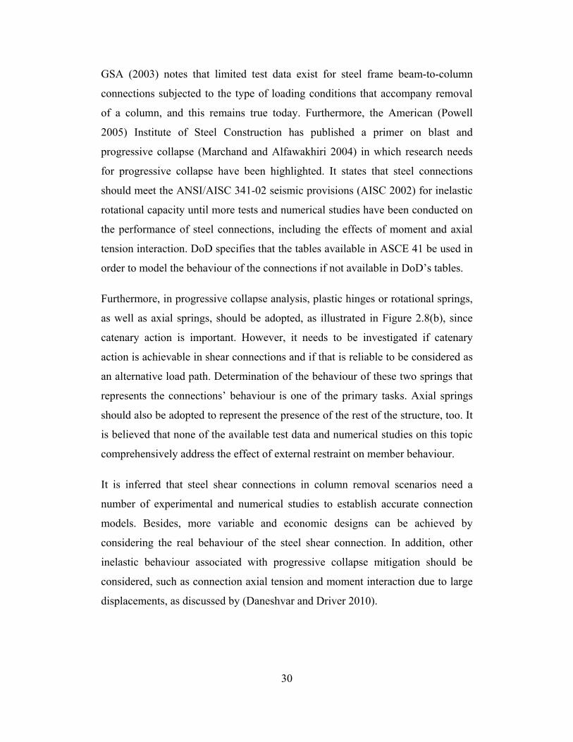
30

GSA (2003) notes that limited test data exist for steel frame beam-to-column

connections subjected to the type of loading conditions that accompany removal

of a column, and this remains true today. Furthermore, the American (Powell

2005) Institute of Steel Construction has published a primer on blast and

progressive collapse (Marchand and Alfawakhiri 2004) in which research needs

for progressive collapse have been highlighted. It states that steel connections

should meet the ANSI/AISC 341-02 seismic provisions (AISC 2002) for inelastic

rotational capacity until more tests and numerical studies have been conducted on

the performance of steel connections, including the effects of moment and axial

tension interaction. DoD specifies that the tables available in ASCE 41 be used in

order to model the behaviour of the connections if not available in DoD’s tables.

Furthermore, in progressive collapse analysis, plastic hinges or rotational springs,

as well as axial springs, should be adopted, as illustrated in Figure 2.8(b), since

catenary action is important. However, it needs to be investigated if catenary

action is achievable in shear connections and if that is reliable to be considered as

an alternative load path. Determination of the behaviour of these two springs that

represents the connections’ behaviour is one of the primary tasks. Axial springs

should also be adopted to represent the presence of the rest of the structure, too. It

is believed that none of the available test data and numerical studies on this topic

comprehensively address the effect of external restraint on member behaviour.

It is inferred that steel shear connections in column removal scenarios need a

number of experimental and numerical studies to establish accurate connection

models. Besides, more variable and economic designs can be achieved by

considering the real behaviour of the steel shear connection. In addition, other

inelastic behaviour associated with progressive collapse mitigation should be

considered, such as connection axial tension and moment interaction due to large

displacements, as discussed by (Daneshvar and Driver 2010).

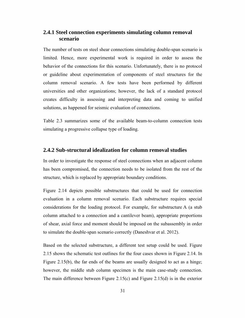
31

2.4.1 Steel connection experiments simulating column removal scenario

The number of tests on steel shear connections simulating double-span scenario is

limited. Hence, more experimental work is required in order to assess the

behavior of the connections for this scenario. Unfortunately, there is no protocol

or guideline about experimentation of components of steel structures for the

column removal scenario. A few tests have been performed by different

universities and other organizations; however, the lack of a standard protocol

creates difficulty in assessing and interpreting data and coming to unified

solutions, as happened for seismic evaluation of connections.

Table 2.3 summarizes some of the available beam-to-column connection tests

simulating a progressive collapse type of loading.

2.4.2 Sub-structural idealization for column removal studies

In order to investigate the response of steel connections when an adjacent column

has been compromised, the connection needs to be isolated from the rest of the

structure, which is replaced by appropriate boundary conditions.

Figure 2.14 depicts possible substructures that could be used for connection

evaluation in a column removal scenario. Each substructure requires special

considerations for the loading protocol. For example, for substructure A (a stub

column attached to a connection and a cantilever beam), appropriate proportions

of shear, axial force and moment should be imposed on the subassembly in order

to simulate the double-span scenario correctly (Daneshvar et al. 2012).

Based on the selected substructure, a different test setup could be used. Figure

2.15 shows the schematic test outlines for the four cases shown in Figure 2.14. In

Figure 2.15(b), the far ends of the beams are usually designed to act as a hinge;

however, the middle stub column specimen is the main case-study connection.

The main difference between Figure 2.15(c) and Figure 2.15(d) is in the exterior

32

columns and their boundary conditions. In Figure 2.15(a) and (c), the effect of the

rest of the structure has been neglected implicitly, albeit Figure 2.15(b) and (d)

possess more control on boundary conditions to simulate the effect of the rest of

the structure on the connection behaviour.

2.5 Introduction of connection model assembly to investigate column removal scenario

Based on the structural idealization discussed in section 2.4.2, a connection

assembly model has been proposed to simulate the column removal scenario, as

illustrated in Figure 2.16(a). The model is a refined version of the model by

Astaneh (Astaneh-Asl 2007), which consists of a middle stub column, two beams

with axial and rotational springs at each end, and two springs at far ends to

simulate the surrounding structure. Ra-con and Rθ-con are the axial and flexural

response of the connection, respectively, and Ra-str represents axial behaviour of

the rest of the structure or test setup. In this model, connection performance is

evaluated by a push down test in which vertical load/displacement is applied to

the connection assembly. Unlike Astaneh's model, the constitutive laws that

govern the behaviour of Ra-str , Ra-con and Rθ-con are not just the stiffness values.

These R values represent the general behaviour of springs, including an elastic

stage, ductile inelastic stage and degrading or softening branch. The model is

developed based on the assumption that at small rotations, the connection

assembly takes load through flexural behaviour, as illustrated in Figure 2.16(b).

As the rotation increases, the connection subassembly develops catenary action,

as shown in Figure 2.16(c). Since numerical analysis of two connections with all

details is time-consuming and tedious, the model in Figure 2.16(a) was simplified

to the model shown in Figure 2.16(d) to focus on the middle connections.

33

2.6 Selected Experimental Study

Three test programs were conducted in conjunction with each other on shear tab,

WT and single angle connections by Thompson (2009), Friedman (2009) and

Johnston (2009) at the Milwaukee School of Engineering. These tests have been

used to verify the numerical study. Figure 2.17 shows the test setup according to

all three sets of tests performed.

The test specimens consisted of a planar two-span beam, with the beams attached

to a central column stub by a plate, angle or WT and to “true pin” connections at

the far ends of the beams. A vertical displacement was applied to the central stub

column in order to simulate a controlled collapse of an interior column. The main

reasons that these suites of experiments are selected for the current research are:

• the test setup simulates a double-span scenario, as described in available

progressive collapse design guidelines; it is also compatible with the

proposed connection model in section 2.5;

• the destructive nature of the test: the assembly is pushed down to its

ultimate capacity. The connection goes through large rotations, in contrast

to many previous tests on the shear connections;

• the reporting of catenary force (axial force): catenary resistance is

recognized as one of the main distinguishing factors in the characterization

of a connection's robustness for progressive collapse prevention. It is also

an alternative path for transferring loads for resisting against collapse after

a column has been compromised. Catenary action is explicitly reported in

the test reports, which is contrary to most previous tests on shear

connections.

34

2.7 Experimental result calculation

The procedure taken by Thompson (2009) and Friedman (2009) are used to

achieve the internal forces from the experiment. It is noted that the same

procedure was applied to the single angle data to produce the internal force versus

rotation curves (Johnson 2009). Solving a system of simultaneous equations using

the stress values on opposite sides of the beam neutral axis, will lead to the

determination of axial and flexural force at the location of strain gauges.

It is noted that strain gauge 2 and 3 on the left beam and 5 and 8 on the right beam

are selected for the purpose of load calculation. As it is shown in Figure 2.10 (c),

the axial tensile force is constant within the length of the beam. In order to

calculate the moment at the bolt line, linear moment distribution is assumed,

considering a zero moment location at the points of simulated true pin. Hence, the

moment at the bolt line can be determined based on Equation (2-2) using linear

interpolation:

=

(2-2)

where is the horizontal distance from the true pin to the bolt line; is the

horizontal distance from the true pin to the strain guage location; is the

moment at the bolt line; and is the moment at the strain gauge location.

Hereinafter, whenever moment is mentioned, is the main purpose (Thompson

2009).

2.8 Possibility of existence of arch action

Formation of catenary action in the connection is highly dependent on the

boundary condition of the test assembly. In other words, the external axial

restraint provided by the test setup is very influential on the axial response of the

35

connection, as the system goes through large displacements. The precise amount

of this external restraint is unknown, but due to the small span-to-depth ratio of

the beam utilized in the experiments, there is a high probability that a compressive

arch action would form as the middle column is pushed down. This phenomenon

is shown in Figure 2.18. In this research, the external restraint provided to the

beam by the surrounding frame is simulated by axial springs at the far ends of the

beams. Further study is needed to characterise the influence of support flexibility

on the catenary behaviour of shear connections under the column removal

scenario. Moreover, non-linear springs or springs with different behaviour in

compression and tension may be required to achieve an accurate axial response.

2.9 Modelling of steel connections using FEA

There are several unknowns in the model shown in Figure 2.16(c) that makes

analysing the system with certainty impossible. For instance, it is necessary to

establish the ultimate value of the angle θ in Figure 2.10(b), called θu when

referring to the maximum rotation that the shear connection can tolerate before

failure. The commonly assumed beam end rotation for simply-supported framing

under gravity loads, 0.03 radians, underestimates the connection rotational

capacity considerably. Besides, there is an interaction among the three mentioned

springs, e.g., the moment and axial responses of the connection have mutual

effects on each other. Furthermore, the axial response of the rest of the structure

influences the axial behaviour of the connection considerably. However, it is not

yet clear how the effect of the rest of the structure can influence the connection

behaviour and to what extent the external spring may have played role in the

connection behaviour.

Numerical simulation is deemed to be an appropriate tool to solve the model

proposed in section 2.5. The finite element models consist of the central column

and adjacent beams, as well as the connections with complete detailing, as shown

36

for shear tabs in Figure 2.19. Shear connections might be welded or bolted to the

column flange and beam web. Since the connection is the point of interest, all

characteristic features of the connections need to be included in the model. The

central column is pushed down, while the connection performance is monitored.

Beams are extended only to the point of zero moment and a true pin was

simulated at each end of the assembly by applying a rigid plate to the cross-

section, connected to a horizontal axial spring to approximate the flexibility of the

test setup and any bolt slippage or local hole deformation. This spring is

representative of the restraint from the surrounding structure in the building. All

other characteristic features of the finite element model are discussed in chapter3.

2.10 Summary and conclusions

• In keeping with the current trend towards the robustness evaluation of steel

structures, specific methods need to be considered to determine the behaviour

of steel shear connections and extreme demands.

• Shear connection behaviour subjected to conventional loading and progressive

collapse conditions, including the available physical tests, structural

idealization and the selected experimental program, are discussed.

• A connection subassembly model is proposed to investigate the behaviour of

different types of shear connections when a column is compromised.

• Although the effect of axial catenary behaviour is implicitly considered in the

flexural response of the connection in the current progressive collapse

guidelines, it is important to monitor axial response of the connection in a

column removal scenario due to its significant role as an alternative path load.

• In a column removal scenario, large deflections are acceptable without

collapse. It is possible to take advantage of catenary action so that the

37

connections can be detailed for this new need, but to do this the amount of

reserve axial strength available in conventional shear connections must be

determined.

• The possibility of formation of arch forces at small beam rotations is

acknowledged.

• A general finite element model is proposed as a tool for investigating the

behaviour of shear connections under the column removal scenario. Finite

element modelling techniques can be utilized to simulate the ability of a design

to withstand extreme loading conditions that are not considered in the regular

design process.

38

Table 2.1: Simple beam-to-column connections

Category Type

Double angle beam connection

bolted - bolted bolted - welded

welded - bolted

welded - welded

End plate connection bolted

welded

Single angle beam connection

bolted - bolted

bolted - welded

welded - bolted

welded - welded

Shear tab beam connection bolted

welded

WT beam connection

bolted - bolted

bolted - welded

welded - bolted

welded - welded

Seated beam connection

welded unstiffened angle seats

bolted unstiffened angle seats

stiffened seated

Table 2.2: Types of material used in shear connections

Connection Type

Abbreviation Component Material Description

Shear tab ST

plate ASTM A36/300W -

bolts ASTM A325, A490 standard/slotted

hole

welds E70XX electrode fillet welds

WT WT WT section ASTM A992/350W -


hole

Single angle SA angle ASTM A36/300W -


hole

39

Table 2.3: Selected column removal scenario experiments for steel structures

No Summarized test description Organization Reference

1 Behavior of bolted beam-column

connections under catenary action in damaged steel structures

Swedish Council for

Building (Girhammar 1980)

2 Progressive collapse resistance of steel

building floors

University of California, Berkeley

(Astaneh-Asl et al. 2002)

3 Behaviour of simple shear connections

under combined effect of shear and tension

University of New

Brunswick

(Guravich and Dawe 2006)

4 Performance of seismic moment resisting

connections under column removal scenario

National Institute of

Standards and Technology

(NIST 2010)

5 Recommended performance levels for

alternate path analysis of blast-damaged steel connections

Protection Engineering Consultants

(Marchand 2008)

6 Axial, shear and moment interaction of

WT connections

Milwaukee School of

Engineering (Friedman 2009)


single plate “shear tab” connections

Milwaukee School of

Engineering (Thompson 2009)


single plate “shear tab” connections

Milwaukee School of

Engineering (Johnson 2009)

9 Performance of steel shear connections

under combined moment, shear, and tension

University of Alberta

(Oosterhof and Driver 2012)

10 Overview of AISC/NSF structural

integrity research and preliminary results AISC/NSF (Weigand et al. 2012)

40

B e a m

C o lu m n

C o n n e c t io n

Figure 2.1: Connection definition

Moment

Relative Connection Rotation

Single Web Angle

Double Web Angle

Header Plate

Top and Seat Angle

End-Plate

T-Stub

Figure 2.2: Typical moment–rotation curves for different types of connection

(Kameshki and Saka 2003)

Beam

Column

Beam

Column

Beam

Column

(a) (b) (c)

Figure 2.3: Common types of single-sided shear connections (a) shear tab, (b) tee, (c) single angle

41

42


(a)

Axial

Shear

Moment

(b)

Figure 2.4: Frames with shear connections under conventional loads (a) frame under vertical loadings, (b) member response to vertical loading

43

Braced Frame Braced FrameFrame with shear connectionBraced Frame Braced FrameFrame with shear connections

(a)

Axial

Shear

Moment

(b)

Figure 2.5: Frames with shear connections under conventional loads (a) frame under lateral loadings, (b) member response to lateral loading (AISC 2010)

44

Moment

Rotation

MMn

u

Ms

s n u

Ki Ks

Figure 2.6: Moment–rotation behaviour of steel connections under conventional loading (AISC 2010)

Simple Beam Rotation

Rotation

End Moment

Simple Shear Connection

FR Moment Connection

PR Moment Connection

Fixed End Moment Ks=20EI/L

Ks=2EI/L

Figure 2.7: Fully-restrained (FR), partially-restrained (PR) and shear connection

definitions (AISC 2010)

45

Kθ-con Kθ-con

L

(a)

Ka-con Kθ-con Kθ-con Ka-con

L

(b)

Figure 2.8: Semi-rigid plane member with (a) rotational springs, (b) axial and rotational springs

Force

Deformation

Progressive collapse

Earthquake

Force

Deformation

Real force-deformation relationship

Linearized simplification

A

B

C

D E

a

b

c

(a) (b)

Figure 2.9: (a) Generalized component force–deformation relations for depicting modelling and acceptance criteria (FEMA 2000) (b) The effective force–deformation

relationship for a typical component in an earthquake and progressive collapse scenario (Powell 2005)

46

(a)

P

(b)

Axial

Shear

Moment

(c)

Figure 2.10: (a) Frame with shear connections in column removal scenario (b) member response (c) simplified member response

M

TV

MM

V T

V

M

M V

T

V

MM V

TVV

M

TV

MM

V T

V

M

M

T

V

MM V

TVV

M

TV

MM

V T

V

M

M

T

V

MM V

TVV

M

TV

MM

V T

V

M

M

T

V

MM V

TVV

M

TV

MM

V T

V

M

M

T

V

MM V

TVV

V

V

V

V

h

h

h

h

h

L L L L L

Figure 2.11: Simultaneous presence of shear, tension and moment at connection location in column removal scenario

47

48

(a)

(b)

M

M

M

M

(c)

TT

TT

(d)

Figure 2.12: Formation of catenary behaviour in beams (a) isolated double span (b)

deformed shape under gravity load (c) small rotation: flexural phase (d) large

rotation: catenary phase

49

(a)

(b)

(c)

Figure 2.13: Generalized component force-deformation relations for depicting modelling for 152 mm, 228 mm and 304 mm shear tab connections

0

0.2

0.4

0.6

0.8

1

1.2

1.4

0 0.05 0.1 0.15

M/M

y

Rotation (Rad)

DOD2009

ASCE-41

0

0.2

0.4

0.6

0.8

1

1.2

1.4

0 0.05 0.1 0.15

M/M

y

Rotation (Rad)

DOD2009

ASCE-41

0

0.2

0.4

0.6

0.8

1

1.2

1.4

0 0.05 0.1 0.15

M/M

y

Rotation (Rad)

DOD2009

ASCE-41

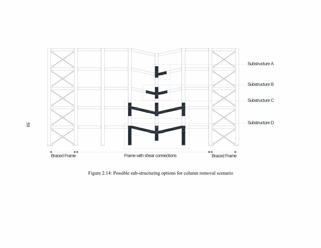
Substructure C

Substructure D

Substructure B

Substructure A


Figure 2.14: Possible sub-structuring options for column removal scenario

50

51

(a)

(b)

(c)

(d)

Figure 2.15: Common test setups for beam-to-column connection tests under column removal scenario, pertaining to (a) substructure 1 (b) substructure 2 (c) substructure 3

(d) substructure 4

52

R a-con

R R R a-str

R R a-con

R R R a-str

R

a-con a-con

a-con a-con

a-con a-con

(a)

R a-str

R a-con

R R

R

a-con a-con

a-con

R a-str

R a-con

R a-conR

R

a-con

a-con

(b)

R a-con

R a-con

R a-con

R a-conR a-con

R a-con

R a-con

R a-con

R a-str R a-str

(c)

R a -s trR

R

a -co n

a -co n

R

R

a -co n

a -co n

R a -s tr

(d)

Figure 2.16: Proposed connection assembly model under column removal scenario: (a) undeformed configuration (b) small rotation: flexural phase (c) large rotation:

catenary phase (d) simplified model

53

SG1

SG2

SG3

SG4

SG1

SG2

SG3

SG4

Test Frame

DWT Supports

True Pin Connection

Strain gauges

Hydraulic Jack

Test Beam

Stub Column

True Pin Connection

Figure 2.17: Test setup assembly (Thompson 2009)

Column

R a-strSymmetry

Figure 2.18: Possibility of formation of compressive arch action in column removal

scenario

Fiigure 2.19: FFinite elemen

54

nt model of shear tab co

onnections

55

3 Benchmark in Finite Element Modelling of Steel Shear Connections in Column Removal Scenario

3.1 Introduction

As a general fact, knowledge of connection behaviour and how it affects the

overall frame performance is a prerequisite to the evaluation of steel structures

against conventional loads such as gravity loads or wind/earthquake lateral loads.

The importance of connection behaviour is even more significant when it comes

to extreme loading scenarios such as progressive collapse. Due to the fact that

progressive collapse is a relatively new topic faced by structural engineers and

researchers, few experiments were conducted on connections loaded under the so-

called “column removal” scenario, which is commonly used for progressive

collapse analysis and design. Experimental programs are also difficult and

expensive to conduct. Therefore, numerical studies are needed to extend the

database on different connection behaviour in the new scenario. Besides,

modelling techniques for steel connections cannot be directly transferred between

different loading situations, thus raising the need for more research on this issue.

The finite element modelling technique is one of the most attractive and powerful

methods in determining the response of steel connection assemblies. Finite

element analysis of steel connections is challenging due to complex geometry,

unknown boundary conditions, sequence of loading and nonlinearities. Nowadays,

there are substantial improvements in the sophisticated commercial finite element

analysis software such as Abaqus (Dassault Systèmes 2009) that makes it possible

to simulate highly nonlinear complex behaviours. Although Abaqus software was

used in this study, any other commercially available software with similar

capabilities could have obtained the same results with correct definition of the

models. However, some challenges exist that need to be resolved in order to reach

acceptable results.

56

Previously, some researchers such as Bursi and Jaspart (1997) and also Selamet

and Garlock (2010) tried to come up with some benchmark examples for finite

element modelling of bolted steel connections. Although the models they

proposed in their research, such as those of tee connections or lap joints in direct

tension, can provide insight on contact simulation and nonlinearity definitions,

they cannot act as a benchmark for finite element models in the column removal

scenario due to the differences in how the connection is loaded. The simultaneous

presence of shear, tension and moments at large rotations with the specific load

proportions that the column loss event has imposed, makes the problem complex

and unique in its own fashion that requires verification in its own way.

Modelling the detailed steel connection in the column removal scenario requires

knowledge of solid mechanics, contact mechanics, simulation techniques and

convergence algorithms (Selamet and Garlock 2010). Mainly, there are some

convergence difficulties that need to be solved in order to reach a validated and

verified finite element model using an implicit analysis method. Most of the

convergence issues are derived from the discontinuous nonlinear contact and also

localized yielding that are the main focuses of this chapter. It is necessary to

understand the logic for solving nonlinear problems—and more particularly

contact problems—in steel connection modelling in order to reduce convergence

difficulties and obtain an accurate response.

In this chapter, after discussing the scope and motivations of the research, a brief

literature review is provided to give insight on the previous numerical efforts to

model steel connections. After establishing the definition of convergence in

nonlinear finite element problems, a benchmark example is introduced and

discussed in section 3.5, including the geometry, material definition, loading

steps, interaction, constraints and boundary conditions. The process of element

selection, mesh generation and mesh sensitivity studies are discussed in sections

3.6 and 3.7.

57

It is believed that the challenges involved in numerical studies for simulating the

performance of connections when a column has been compromised are derived

chiefly from nonlinearity sources. Therefore, a significant part of the chapter is

dedicated to nonlinearity definitions, and especially highly nonlinear behaviour of

contact, that are discussed in section 3.8.

In section 3.9, the solution technique is discussed to provide a rigid foundation for

the validity of all the numerical models utilized in this research. It is shown that a

general static implicit analysis is an appropriate tool to achieve the objectives of

the research.

It is also necessary to present the failure criterion to predict the failure loads and

modes using finite element analysis. Rupture, either in structural members or

fasteners, is one of the common limit states that play an important role in failure

of steel bolted connections. Traditional fracture mechanics techniques rely on the

response of a crack in the model, although in bolted steel connections, there are

no pre-existing sharp cracks or flaws. Therefore, applying the traditional fracture

technique could have some issues (Kanvinde and Deierlein 2004). In section 3.10,

the global failure criteria that have been used throughout the research are

established.

A brief explanation of the process of extracting results of the experimental and

numerical models is provided in section 3.11. After that, sensitivity analyses

performed for this research are reported in section 3.12, considering some of the

selected parameters in the selected range.

After ensuring the validity of the numerical models, the final results are reported

in section 3.13. The outcome of the research is not only helpful to estimate the

failure load, but also to trace the entire internal load versus rotation path. This

force–rotation behaviour of shear connections in a column loss event is required

in order to perform progressive collapse analysis of a whole building. In

summary, this study can help in the prediction, development and interpretation of

the performance of steel shear connections in a column removal scenario.

58

In section 3.14, some fundamental recommendations are made regarding how to

obtain a converged solution. The guidelines and recommendations provided in

this chapter are applicable not only to shear tab connections, but also to all other

types of bolted steel shear connections.

In chapters 4, 5, 6 and 7, the established procedures are applied to other

geometries and different types of shear connections including WT and single

angle, and comparisons with experimental results are performed. The additional

verifications confirm the correctness and accuracy of the proposed numerical

modelling procedure.

3.2 Scope of the research and objectives

The main objectives of this chapter are:

• to present a rational approach to establish and calibrate a finite element

model for simple shear connections;

• to introduce a simple shear tab connection model that can be used as a

benchmark to validate finite element models of simple shear connections

subjected to extreme loading effects such as a column removal scenario;

and

• to discuss and provide recommendations on how to achieve a converged

solution in steel shear connections using state-of-the-art simulation

techniques.

The welds are not considered explicitly in the models based on the assumption of

flawless welding processes and material. Besides, no weld failure was reported in

the pertaining experimental program that was used for the verification. The

dynamic and/or cyclic nature of the column removal scenario is out of the scope

of this research. Residual stresses and initial geometric imperfections were

59

ignored in the analyses due to the fact that the actual residual stress distribution or

size and distribution of geometric imperfections are unknown.

3.3 Literature review on finite element modelling of steel connections

There are different numerical studies on various types of connections during the

last few decades. These studies utilized two- or three-dimensional (3D) models

with various levels of simplifying assumptions. Many simplifications were

assumed in early studies of bolted connections using the finite element method

since the computational power was limited. Avoidance of detailed modelling and

reducing the computational cost were the main reasons for these simplifying

assumptions. The following literature survey is focused on the highlights of finite

element modelling assumptions for steel beam-to-column connections under a

monotonic loading regime. Research on seismic (cyclic/dynamic) performance of

steel connection models and modelling of steel connections in a fire scenario are

beyond the scope of this research.

It is believed that Krishnamurthy (1980) took the first steps in applying finite

element simulations in steel bolted connection modelling. He established the

sources of complex highly nonlinear response of the connection and, based on

that, he concluded that the traditional concepts of elastic continuum mechanics,

analytical approaches based on structural theory and yield line theories are not the

appropriate tools for assessing the response of bolted connections due to the

presence of highly nonlinear behaviours. He developed a methodology to predict

the behaviour of different types of moment connections, including seat and top

angle, tee-stub and end plate connections. Table 3.1 summarizes his proposed

phases for finite element analysis of steel connections.

Due to the limitations of computational capabilities, three-dimensional analyses of

large models were not feasible at that time. Krishnamurthy (1980) assumed linear

elastic material for 3D analyses and bilinear elastic-perfectly plastic or tri-linear

60

stress-strain curves, for 2D analyses. The clearance between the bolt shank and

the hole was ignored in his models. He assumed that the supporting members are

rigid. His models contain pretension in the bolts as well. A series of cycles of

nodal releases, reattachments and displacements and reaction calculations were

repeated in order to simulate contact interaction. Each analysis was terminated if

the capacity of the component is reached or divergence occurred because of local

yielding. He used a constant strain triangle for two-dimensional and sub-

parametric eight node brick elements for three-dimensional models. He also

established the correlation between two-dimensional and three dimensional finite

element models of bolted steel connections (Krishnamurthy and Graddy 1976).

He defined "correlation factor" as the ratio of three-dimensional to two-

dimensional result variable and proposed the correlation factor of 1.4 for

displacement and rotation, 1.2 for average stress and 1.8 for maximum stress for

the studied particular configurations. However, due to the three-dimensional

nature of the problem, they are incapable of reproducing some characteristic

features such as three-dimensional failure modes.

Bursi and Jaspart (1997) introduced benchmarks for finite element connection

model validation. They modelled two tee stub connections, pre-loaded and non-

preloaded, with different failure modes by brick elements in the large deformation

regime using LAGAMINE software. They simulated the interaction between

different components via contact elements using a penalty technique. However,

they stated that the Lagrange multiplier approach is superior to the penalty

method, which needs an arbitrary penalty stiffness number that may have

significant effects on the accuracy of the results and the convergence rate (Bursi

and Jaspart 1998). They noted that shell elements, no matter how thin or thick, are

not suitable for modelling the connection components and especially the bolts and

concluded that at least three layers of brick elements should be used for bending-

dominated problems to capture the stiffness and strength of the component

accurately. In bolt discretization, they used three-dimensional brick elements

assuming the washers were attached to the bolt head. In order to account for this

assumption, which imposes additional flexibility because of the nuts and the

61

threaded part of the shank, they used Agerskov's model (1976) to utilize an

effective bolt length. In the follow-up paper (Bursi and Jaspart 1998), they used

Abaqus code to simulate end plate connections and their failure modes. By

comparing the results of element performance for different formulations, Bursi

and Jaspart concluded that incompatible brick elements, called C3D8I element in

Abaqus (Dassault Systèmes 2009), predict better results for bending-dominated

problems with relatively small thickness.

There are numerous numerical studies on end-plate connections. As an example,

Kukreti et al. (1987) established a methodology to develop moment–rotation

relationships for end plate connections by following the same procedure as

Krishnamurthy (Krishnamurthy and Graddy 1976). They used a nonlinear

material model and imposed a strain limit as the failure criteria criterion (0.02 for

plate elements and 0.006 for the bolt shank). Another numerical study was carried

out by Yang et al. (2000) on double web angles, bolted to the column flange and

welded to beam web. Although they included contact between the bolt head and

angle, they ignored the interaction between the bolt shank and the hole.

Citipitioglu et al. (2002) used available experimental programs to examine the

ability of 3D models to mimic the overall test results. They use imposed

deformation as a calibration procedure for applying a pretension force in the bolts'

shanks. They included the effects of slip by recognizing interaction between all

the components in Abaqus. Nonlinear 3D continuum elements were used for all

parts of the connections except the bolts that were modelled as elastic components

in order to ease the convergence problems. The results of their studies showed

that the response of finite element bolted partially-restrained connections are

highly dependent on bolt pretension and slip definition of contact, since the forces

are transferred through friction due to clamping between the members caused by

the pre-tensioning of the bolts. The connection model is discretized using C3D8I

eight-node brick elements with full integration and incompatible modes. C3D6

six-node wedge elements were used to model the core of the bolts.

62

Barth et al. (2002) conducted finite element analyses of the WT connections.

They monitored the entire load versus deflection path of the connection in

addition to estimating the failure load. They assumed that the bolts are rigid and

modelled just the flange of the supporting column assuming that column's

stiffness makes a rigid part. The bolts were modelled as elastic components in

order to ease the convergence problems.

Ju et al. (2004) used finite element modelling to analyze butt-type bolted

connections. They used a node-to-Hermit-surface contact element and found

similarity between the capacities of the finite element models of bolted

connections and those calculated using the AISC specification (1986), despite the

complexity of the stress and strain fields during loading. They observed that

thinner plate causes a minor bending effect on the bolt. However, the locations of

the maximum bolt plastic strains are different because of the bolt bending effect

and shear force. As a result, although plate thickness dominates the amount of

bending effect, it does not affect the bolt failure.

Although improvements in computational power and advanced finite element

technology have enabled the researchers to simulate elaborate and sophisticated

tasks such as connection assembly modelling, some issues such as convergence

problems, justification with the experimental results and modelling the failure

modes remain challenging and to some extent unknown. This chapter deals with

all the mentioned difficulties in order to provide a solid base for the next chapters.

3.4 Concept of convergence

"Convergence" can imply different meanings in finite element analysis, including

mesh convergence, nonlinear solution convergence and also convergence to the

accurate solution. For transient loading of the connection, accuracy of the time

integration method might be an issue but not for quasi-static loading. (Dassault

Systèmes 2011c). In implicit solution techniques of finite element analysis of steel

63

connection modelling, obtaining the converged solution in the nonlinear region is

the main obstacle due to the presence of all types of nonlinearity, including

material, geometric and contact nonlinearities. Satisfying all the convergence

issues in addition to good engineering judgment in creating a finite element model

will lead to an accurate solution.

3.5 Introduction of the case study model

In order to propose a benchmark example in numerical modelling of the

behaviour of steel shear connections in progressive collapse, an adaptive

experimental program is needed.

3.5.1 Selected study program

In this research, the experiments conducted by Thompson (2009) are utilized to

verify the numerical study as discussed in chapter 2. The full-depth shear

connection with one column of five bolts is selected as a benchmark example. The

test setup is shown in Figure 3.1. A detailed sketch of all components of the test

assembly is illustrated in Figure 3.2.

3.5.2 Finite element modelling assembly

The finite element models consist of the central column, the adjacent beams, as

well as the connections with complete detailing; all modelled with

three-dimensional solid elements as shown in Figure 3.3. Since the connection is

the point of interest, all the characteristic features of the connections are included

in the model. Model information is summarized in Table 3.2 and the details are

explained in the following sections.

64

3.5.2.1 Parts geometry

All the parts are modelled exactly based on the dimensions shown in Figure 3.2.

The dimensions of the bolt head and nut are taken from the AISC Handbook

(AISC 2010). The head and the nut are simplified to cylinders, since their

geometry does not have any effect on the analysis results. Since in the

experimental program, the bolts were assembled with the threads excluded from

shear planes, the finite element bolt models are assumed to be smooth cylinder.

No fillet was modelled on the hot-rolled sections as well.

3.5.2.2 Material definition

All hot-rolled sections are made of ASTM A992 (2011) . The shear tab and the

bolts are made of ASTM A36 (2008) and ASTM A325 (2009) steel, respectively.

The material behaviour is discussed in Appendix A.

3.5.2.3 Loading steps

The whole loading sequence is performed in two separate steps: first applying the

bolt pre-tension and then the push-down vertical load.

3.5.2.3.1 Bolt pre-tensioning

Based on the experiment reports, the bolts are installed to a “snug-tight” condition

(Thompson 2009). “Snug-tight" condition requires that the holes be properly

aligned, the bolt to be inserted and then the nuts to be turned on until all the plies

in the joint are in firm contact. It can be attained by the ordinary attempt of a

worker using a spud wrench. As such, the amount of any initial tension in the bolt

can be expected to be both small and variable. This can affect the load transfer

mechanism.

In the numerical model, a small amount of pre-tensioning is required not only to

simulate the snug-tight condition but also to prevent the rigid body motion of the

bolts in the standard size holes. There are several methods to apply pre-tensioning

to the bolts such as applying a temperature gradient in order to impose a pre-

65

determined amount of axial force directly. In this research, the bolt pretension has

been incorporated by applying displacement to one end on the shank surface, as

illustrated in Figure 3.4. The application of this displacement considerably

improves the convergence as well. It is noted that the main purpose of applying

pretension is that the connected parts be in firm contact with each other. It is not

intended to use “pre-tensioned” bolts in the model. However, the effect of pre-

tensioning is investigated in the section 3.12.

3.5.2.3.2 Push-down loading

The central column is pushed down, while the connection performance is

monitored. This is performed by a hydraulic jack located at the bottom of the

central stub column. Two load cells measured the applied load. In the numerical

model, the middle stub column was loaded via displacement control, which is

much more stable than force control during contact simulation. In order to

produce the quasi-static behaviour, displacements are increased at a slow rate.

3.5.2.4 Interaction properties

Interaction properties play an important role in connection modelling. Contact

should be defined between each two surfaces that might come to touch, such as

bolt shank–beam hole contact, etc. The properties can be divided into normal and

tangential behaviour. Because of the importance of the issue, it is discussed

thoroughly in section 3.8.3.

3.5.2.5 Constraints

Different constraints are applied to the model in order to simulate the desirable

response. First of all, a symmetry constraint is imposed to take advantage of axial

symmetry in the connection assembly. Only one-half of the subassembly is

modelled and the symmetry condition is applied at the centerline of the stub

column web as shown in Figure 3.5.

66

Fully constrained contact behaviour (tie constraint) is used for modelling welds to

bond the shear tab to the column flange. Tie constraint uses a master–slave

formulation. The constraint prevents slave nodes from separating or sliding

relative to the master surface. Slave nodes can be moved on to the master surface

in the initial configuration strain free. In order to avoid out-of-plane displacement

of the test assembly, out-of-plane displacement of one joint in the beam is

restricted.

3.5.2.6 Boundary condition

In common connection modelling for either cyclic or monotonic loading,

elaborate support models are not considered due to the relative insensitivity of the

subassembly response to the variation in the support condition. However, in

connection modelling subjected to extreme loading such as the column removal

scenario, the boundary condition is deemed to be of significant importance. As

shown in Figure 3.1, the true pin connection is designed so that the whole

assembly can rotate freely. In the experiment, it is achieved by 1-1/4 inch

diameter ASTM A490 bolts in the standard size hole, reinforced by 3/8 inch thick

a ASTM A36 doubler plate on one side of the web. The main purpose of such a

connection is to provide a zero-moment location that can resist unidirectional

tensile force in the line of the beam centroid. In order to simulate the same

condition in the numerical model, a thin rigid plate (Figure 3.5) with two axial

springs at the far ends of the beams is applied. The springs are representative of

the flexibility of the test setup and the rest of the structure adjacent to the double-

span scenario in the experiments and the real structure, respectively. More

description is available in chapter 4.

3.6 Element selection

It is possible to simplify the process of simulation of steel connections by

accepting the two-dimensional simulation assumption. Some studies have

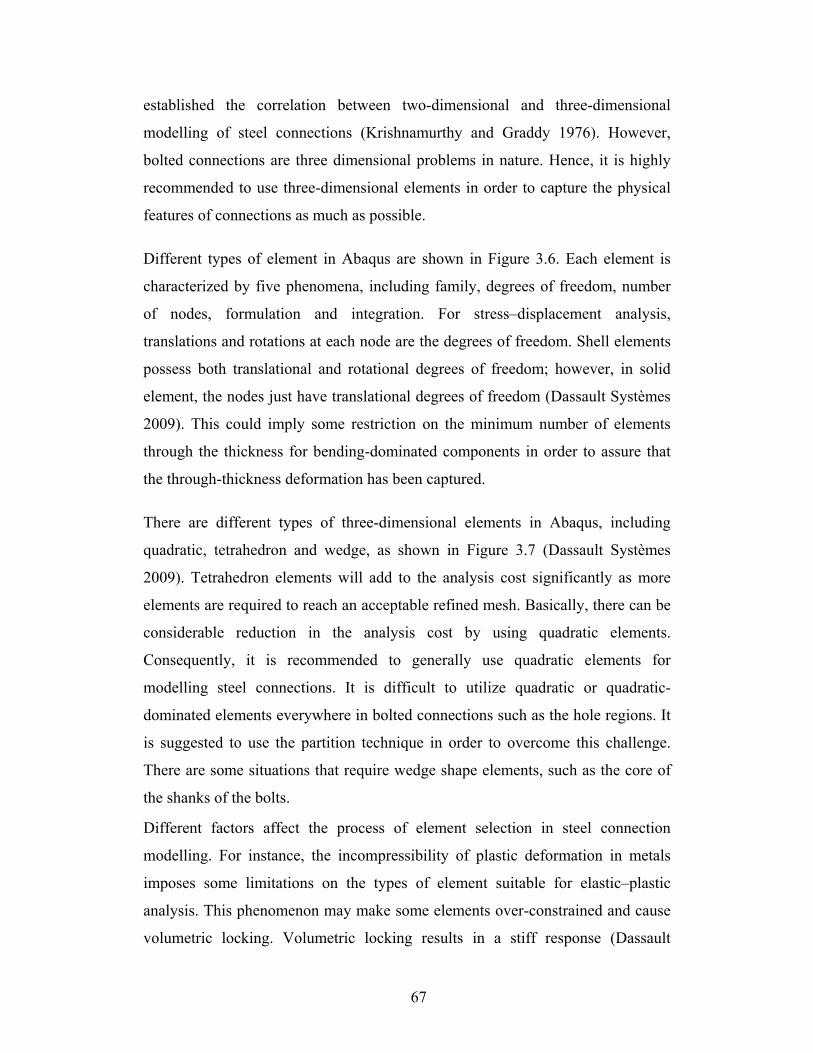
67

established the correlation between two-dimensional and three-dimensional

modelling of steel connections (Krishnamurthy and Graddy 1976). However,

bolted connections are three dimensional problems in nature. Hence, it is highly

recommended to use three-dimensional elements in order to capture the physical

features of connections as much as possible.

Different types of element in Abaqus are shown in Figure 3.6. Each element is

characterized by five phenomena, including family, degrees of freedom, number

of nodes, formulation and integration. For stress–displacement analysis,

translations and rotations at each node are the degrees of freedom. Shell elements

possess both translational and rotational degrees of freedom; however, in solid

element, the nodes just have translational degrees of freedom (Dassault Systèmes

2009). This could imply some restriction on the minimum number of elements

through the thickness for bending-dominated components in order to assure that

the through-thickness deformation has been captured.

There are different types of three-dimensional elements in Abaqus, including

quadratic, tetrahedron and wedge, as shown in Figure 3.7 (Dassault Systèmes

2009). Tetrahedron elements will add to the analysis cost significantly as more

elements are required to reach an acceptable refined mesh. Basically, there can be

considerable reduction in the analysis cost by using quadratic elements.

Consequently, it is recommended to generally use quadratic elements for

modelling steel connections. It is difficult to utilize quadratic or quadratic-

dominated elements everywhere in bolted connections such as the hole regions. It

is suggested to use the partition technique in order to overcome this challenge.

There are some situations that require wedge shape elements, such as the core of

the shanks of the bolts.

Different factors affect the process of element selection in steel connection

modelling. For instance, the incompressibility of plastic deformation in metals

imposes some limitations on the types of element suitable for elastic–plastic

analysis. This phenomenon may make some elements over-constrained and cause

volumetric locking. Volumetric locking results in a stiff response (Dassault

68

Systèmes 2009). Table 3.3 and Table 3.4 summarize the properties of different

types of continuum elements available in Abaqus that might be considered in steel

connection modelling; focusing on order and integration method of elements,

respectively. Based on the information that Table 3.3 provides, the order of

element for the application under consideration is implied. Because of large

plastic deformation and also high strain gradients in bolt hole regions of

connection models, and also the presence of contact, it is suggested to use first

order elements.

Reduced integration elements are efficient and no less accurate than fully

integrated elements, although they possess fewer integration points. As a result,

incompressibility constraints are satisfied with ease. Therefore, they are not over-

constrained in the steel connection simulations. The primary difficulty with first

order reduced integration elements is that they are vulnerable to hourglassing,

which is the possibility of zero strains at integration points. Abaqus's hourglass

control feature accompanied with fine mesh controls this behaviour (Dassault

Systèmes 2009).

Regular first-order displacement elements are usually too stiff in bending-

dominated problems. In order to eliminate the parasitic shear stresses and also the

Poisson's effect that stiffens the response of such models, additional incompatible

deformation modes might be defined for the elements. These incompatible modes

increase the internal degrees of freedom of the element (13 for C3D8I), while

enhancing the bending behaviour. Although the computational cost increases, they

are still less expensive than second-order elements. The incompatible mode

elements do not suffer from hourglassing since they utilize full integration

(Dassault Systèmes 2009).

Considering the issues mentioned in Table 3.3 and Table 3.4, and taking into

account different factors involved in the connection assembly model (e.g.,

presence of large strain and complex contact definition), it is recommended to

adopt the first-order reduced-integration (C3D8R) type of element for the

69

majority of the model that stress-strain accuracy is not required. The C3D8R

element uses one integration point to represent the element. Generally the

incompatible mode elements should be used in the regions where bending

response must be modeled accurately, and they should be of rectangular shape to

provide the most accuracy. Hence, the main connecting part of the connection,

here the shear tab, is modeled with the C3D8I element. The bolts also require

sufficient accuracy in stress values to predict the failure mode and behaviour.

Therefore, using the reduced integrated element for them is not suggested. On the

other hand, their behaviour is not dominated by bending. As a result, a full-

integration type of element is suggested for all types of bolts. The effect of using

different types of elements in the connecting parts is investigated in section

3.12.1.

3.7 Meshing

In order to make sure that the result of finite element simulation is adequately

precise, a mesh refinement study is necessary. Increasing the mesh density leads

to a unique value that represents the response of the model. Basically, if the same

results are produced with different meshes, it is confirmed that the solution is

mathematically accurate. This solution is an approximation of the physical

response of the model. Potential sources of difference in the response include the

geometry of model, material model, boundary conditions, and loads. This concept

is applied to h-based element technology used in Abaqus (Dassault Systèmes

2009).

There are some exceptions to the mesh convergence rule, such as fracture or

localization problem (Dassault Systèmes 2011c). Obviously, determination of

bolted connection behaviour to failure in a progressive collapse analysis is a

localization problem because the damage is accumulated at certain parts of the

connection assembly, such as the bolt shank or around the bolt hole. Therefore,

the principle of mesh convergence is not applied. Additionally, due to the

70

presence of contacts, all parts are mesh dependent in terms of acceptable

proportionality of element size in different parts. Master and slave surfaces should

be defined with respect to the associated mesh density. This will prevent

excessive penetration of surfaces and consequently, inaccurate results. Therefore,

the size of the mesh should be determined in the assembly. However, in order to

approach the real behaviour of the physical model, a decent mesh size is

necessary. Based on this fact, the approximate size of the elements is selected as

6.25 mm x 6.5 mm in the connecting part, the shear tab. This size gets smaller as

we approach the hole due to the presence of a radial mesh. Nevertheless, a mesh

study needs to be done to realize the number of the elements within the part

thickness in order to capture the out-of-plane deformation as is discussed in

section 3.7.2.

3.7.1 Mesh generation procedure

Since the problem is three-dimensional in nature, continuum solid elements were

used in a hexahedral shape mesh. The only elements that were not hexahedral in

shape were in the core areas of the bolts. Triangular prisms (wedges) are used in

such areas by applying hex-dominated meshing techniques to the bolts. For

modelling of shear tabs, three elements through the thickness is used as is

investigated in section 3.7.2. In the beams, the mesh was fine around the bolt hole

and gradually got coarser moving towards the far ends of the beam. The average

size of element in the different segments of the beam is shown in .

It is recommended to use mapped mesh in the connection modelling. It has

several advantages, such as complete control of the size and shape of the

elements. Definitely, densely packed elements are desirable around the bolt hole

with high stress concentration. Using radial mesh around the bolt hole makes the

smallest elements around the hole, which is the area where the highest values and

variations of stresses are expected. Furthermore, high strain concentration

observed near the bolt holes requires a reasonably fine mesh to reach

convergence.

71

3.7.2 Mesh Convergence Study

For the purpose of mesh refinement analysis, the shear tab plate with five holes is

isolated from the assembly, since the main goal of the research is to determine the

behaviour of the shear tab. Bolt mesh size is investigated separately. Besides,

preliminary analyses and experimental evidence show that most of the nonlinear

behaviour is accumulated in the shear tab region and the bolt shank. Instead of

including complex bolt–plate interactions, distributed pressure over the bottom

half of the holes is considered in order to load the model. In reality, the pressure

magnitude varies around the hole circumference, but it is assumed to be uniform.

In this study, the influences of mesh density across the thickness of the plate

(Figure 3.9) are investigated for two particular results: the maximum von Mises

stress and the vertical displacement of the bottom of the top hole. The results for

these three mesh refinement studies are summarized in Table 3.5.

It is observed that the mesh density with two elements across the thickness is

adequate. There is no considerable advantage in terms of more accurate results

using more elements through the thickness. Although the "two element through

the thickness" mesh is deemed to be sufficient, in order to capture out-of-plane

deformation in the shear tab, it is suggested to use a minimum of three elements

through the thickness. For the sake of consistency, the three element rule within

the thickness at the connecting part is respected in the whole research program.

3.8 Sources of nonlinearity

The behaviour of steel connections cannot be approximated adequately as linear

due to the presence of types of nonlinearities. It is necessary to perform a

nonlinear analysis, since the behaviour of each component of the connection

individually is highly nonlinear, as is the behaviour of the whole assembly as a

system. All three sources of nonlinearity that are common in structural

simulations exist in connection modelling for progressive collapse, including

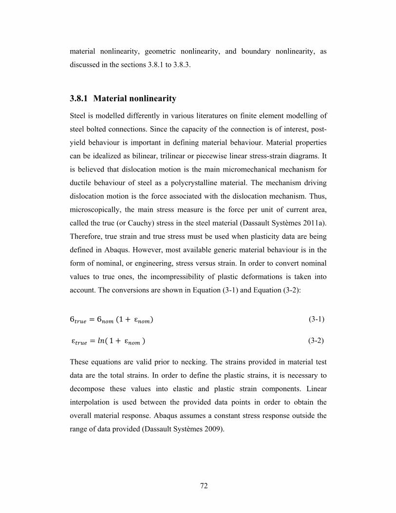
72

material nonlinearity, geometric nonlinearity, and boundary nonlinearity, as

discussed in the sections 3.8.1 to 3.8.3.

3.8.1 Material nonlinearity

Steel is modelled differently in various literatures on finite element modelling of

steel bolted connections. Since the capacity of the connection is of interest, post-

yield behaviour is important in defining material behaviour. Material properties

can be idealized as bilinear, trilinear or piecewise linear stress-strain diagrams. It

is believed that dislocation motion is the main micromechanical mechanism for

ductile behaviour of steel as a polycrystalline material. The mechanism driving

dislocation motion is the force associated with the dislocation mechanism. Thus,

microscopically, the main stress measure is the force per unit of current area,

called the true (or Cauchy) stress in the steel material (Dassault Systèmes 2011a).

Therefore, true strain and true stress must be used when plasticity data are being

defined in Abaqus. However, most available generic material behaviour is in the

form of nominal, or engineering, stress versus strain. In order to convert nominal

values to true ones, the incompressibility of plastic deformations is taken into

account. The conversions are shown in Equation (3-1) and Equation (3-2):

Ϭ = Ϭ (1 +ɛ ) (3-1) ɛ = ( 1 +ɛ ) (3-2)

These equations are valid prior to necking. The strains provided in material test

data are the total strains. In order to define the plastic strains, it is necessary to

decompose these values into elastic and plastic strain components. Linear

interpolation is used between the provided data points in order to obtain the

overall material response. Abaqus assumes a constant stress response outside the

range of data provided (Dassault Systèmes 2009).

73

3.8.1.1 Hot rolled sections and plates

Due to the variation of steel mechanical properties, it is good to perform tension

coupon tests for the sake of accuracy of numerical modelling. In lieu of tension

coupon tests results, generic material curves should be used for all components.

The approaches to develop the material model for each steel type are summarized

in Appendix A. All types of steel used in this study are assumed to be

homogenous and isotropic with an elastic modulus of 200 GPa and Poisson's ratio

of 0.3 and, hence, a shear modulus of 77.2 GPa. Due to the fact that material

definition could contribute to the accuracy of the results, sensitivity analyses are

performed to investigate this issue, as discussed in section 3.12.6.

3.8.1.2 High Strength Bolts

High strength bolts are used in structural steel most frequently. They are made

from heat-treated steel—either high-strength bolt (ASTM A325 bolts) or

quenched and tempered alloy steel (ASTM A490 bolts) (Kulak et al. 2001). The

response of single ASTM A325 and A490 bolts to a loading producing shear on

two planes are shown in Figure 3.10. As illustrated, the A490 bolt is a higher

strength bolt than the ASTM A3235 bolt, with slightly lower ductility. All the

details regarding the bolt material property calculations used in this thesis are

discussed in Appendix A. Furthermore, the behaviour of individual bolts was

verified versus the available shear load versus deformation relationship curves

reported by Kulak et al. (2001), as discussed in section 3.10.

3.8.2 Geometric nonlinearity

Large displacements may cause a nonlinear relationship between displacement

and strain increments. For many structural applications, it is necessary to write the

equilibrium equations based on the deformed structure. If loading on the structure

causes large deformations, nonlinearity in geometry is involved and superposition

cannot be applied. Due to the presence of large deformation in the model under

74

investigation, geometric nonlinearity must be included. In Abaqus, the effect of

nonlinear geometry is included when the loading step is defined.

3.8.3 Boundary nonlinearity

3.8.3.1 Introduction

Steel bolted connection modelling involves contact simulations of different

components, allowing transmission of force from one part to another. The force

could be in the form of normal stress or, in the presence of friction, a limited

amount of shear stress. In the numerical modelling, the mere physical proximity

of two surfaces in the connection assembly model is not enough for contact

definition. The analysis engine should detect when the surfaces are separated or

are in contact, as simplified in Figure 3.11, and also when they slip or stick in

order to apply appropriate contact constraint correctly. Numerically, contact

behaviour is highly nonlinear and causes large and instantaneous changes in the

behaviour of the assembly (severely discontinuous form of nonlinearity).

Consequently, convergence difficulties that occasionally cause inaccurate results

are inevitable. The user is responsible for all physical and the majority of the

numerical aspects of the models. It is also necessary to understand the logic for

solving contact problems in steel connection modelling in order to reduce

convergence problems. The solving procedure will be discussed in section 3.9.

Previously, interaction between different parts of the connection assembly was

modeled by a contact element. For instance, in order to capture the interaction

between the hole and the bolt shank, gap elements were modeled in the probable

contact zones of the finite element model.

Figure 3.12 shows a schematic view of such a contact modelling. A schematic

view of one type of contact element is shown in Figure 3.13(a). A brief discussion

on element-based contact is provided in section 3.8.3.3 as well. After that,

element-based contact evolved to a surface-based contact simulation method

75

which is more representative of the physics of contact simulation.

Abaqus/Standard supports both surface-based and element-based approaches in

contact modelling. In this research, the surface-based method is utilized. All the

basic theory of surface-based contact is discussed in section 3.8.3.2.

3.8.3.2 Surface-based contact

Due to greater flexibility and ease of use of surface-based contact approach,

compared to the element-based method, it is recommended to use this method in

connection modelling. Abaqus/Standard offers two surface-based contact

approaches called general contact and contact pairs.

3.8.3.2.1 General versus contact pairs

General contact definitions are highly automated, and all contact surfaces of parts

can interact in one single domain, as shown in Figure 3.13(b). Any exterior

surface can interact with any other exterior surface. Nevertheless, contact pairs

allow contact between two designated surfaces, shown in Figure 3.13(c). In

contact pairs, all potential contact pairs must be defined separately. In this

method, one surface is called the master surface and another the slave surface.

Each of these surfaces possesses some characteristic features. The master surface

can penetrate the slave surface but not vice versa. The stiffer, less-refined region

should be the master. The active contact region should change more rapidly on the

master surface in order to minimize contact status changes. Besides, the master

surface normal should point toward the slave surface; all the elements underlying

a surface should be compatible in terms of dimension and order of interpolation

(first or second order). If the mentioned criteria are not respected in the finite

element simulation, a convergence problem is highly probable in the connection

simulation.

Contact pairs are more efficient, since the surfaces are limited in scope. Utilizing

general contact is a trade-off between the ease of defining the contact and the

analysis performance. Although general contact is suitable for complex topology,

76

it is not highly efficient in models like connections that are complex in terms of

the number of interactions; and consequently, it often does not lead to a

converged solution. The general contact was initially developed for

Abaqus/Explicit. It is robust and high-performance (Dassault Systèmes 2009).

However, there is some lag in its performance in Abaqus/Standard. Therefore, the

contact-pair algorithm is recommended in steel connection simulation, although it

requires more effort in terms of pre-processing. It is noted that both methods can

be used in the same model together.

There are totally six contact pairs in the shear tab connection model: bottom

surface of bolt head and shear tab, bolt shank and shear tab, bolt shank and beam

web, bolt nut and beam web, shear tab and beam web, and beam end and column

flange. The last one is the potential contact that might occur in case of a small gap

between the beam end and column flange. In this research, this gap is selected in a

fashion that “prying” of the connection due to contact of the beam flange on the

column flange may not occur. Table 3.6 shows which surface is selected as master

or slave in the analysis.

3.8.3.2.2 Contact discretization method (surface-to-surface versus node-to-surface)

In terms of contact discretization methods, two methods of "Surface-to-Surface"

versus "Node-to-Surface" exist in Abaqus. In the traditional Node-to-Surface

method, contact is enforced between a node and its neighboring surface facet. In

the Surface-to-Surface method, contact is enforced between a node in the slave

surface and a larger number of master surface facets local to it. In other words,

contact enforcement has an average weighted sense. The concept is shown at

Figure 3.14 for the bolt-hole interaction definition.

For steel connection modelling, it is recommended to use Surface-to-Surface

methods due to considerable advantages such as reduction in snagging of

surfaces, surface penetration, and contact stress inaccuracy. The most important

issue is that the Surface-to-Surface reduces the possibility of penetration of master

77

nodes into the slave surface in comparison with the Node-to-Surface method. It is

noted that the Surface-to-Surface contact discretization generates asymmetric

terms in the system of equations. These terms have a strong influence on

convergence in regions where the master and slave surface are not parallel to each

other. Therefore, an asymmetric solver is recommended for all finite-sliding

Surface-to-Surface contact problems, including steel connection simulation.

Snagging is one of the main problems with the Node-to-Surface method.

Abaqus/Standard automatically applies a smoothing procedure for Node-to-

Surface. However, there is no smoothing problem with the Surface-to-Surface

discretization method. The Surface-to-Surface discretization method possesses an

inherent smoothing which leads to a better convergence rate. Although the

Surface-to-Surface contact formulation has no special issues for any quadratic

elements, first-order type of elements are preferred for the model, as discussed in

section 3.6.

3.8.3.2.2.1 Contact properties

The concept of contact modelling can be split into normal and tangential contact.

3.8.3.2.2.1.1 Normal behaviour

There are two primary methods in Abaqus to enforce normal direction contact

constraints: the "direct Lagrange multiplier" method and a "penalty" method. The

fundamental difference between the two methods is that the Lagrange multiplier

method exactly enforces the contact constraint by adding degrees of freedom to

the problem, while the penalty method approximately enforces the contact

constraint without applying additional degrees of freedom by using axial springs.

This approximation leads to a small amount of penetration in the penalty method,

comparing to the direct Lagrange multiplier, as illustrated in Figure 3.15. The

penalty method is depicted schematically in Figure 3.16. The upper surface is the

master, and the lower surface is the slave. While the over-closure has been

exaggerated, it is clear that the stiffness of the spring resists the penetration of the

master node into the master surface in proportion to its degree of penetration.

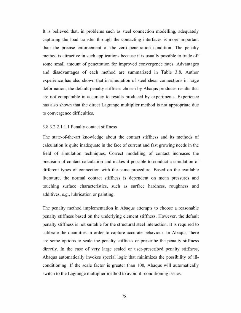
78

It is believed that, in problems such as steel connection modelling, adequately

capturing the load transfer through the contacting interfaces is more important

than the precise enforcement of the zero penetration condition. The penalty

method is attractive in such applications because it is usually possible to trade off

some small amount of penetration for improved convergence rates. Advantages

and disadvantages of each method are summarized in Table 3.8. Author

experience has also shown that in simulation of steel shear connections in large

deformation, the default penalty stiffness chosen by Abaqus produces results that

are not comparable in accuracy to results produced by experiments. Experience

has also shown that the direct Lagrange multiplier method is not appropriate due

to convergence difficulties.

3.8.3.2.2.1.1.1 Penalty contact stiffness

The state-of-the-art knowledge about the contact stiffness and its methods of

calculation is quite inadequate in the face of current and fast growing needs in the

field of simulation techniques. Correct modelling of contact increases the

precision of contact calculation and makes it possible to conduct a simulation of

different types of connection with the same procedure. Based on the available

literature, the normal contact stiffness is dependent on mean pressures and

touching surface characteristics, such as surface hardness, roughness and

additives, e.g., lubrication or painting.

The penalty method implementation in Abaqus attempts to choose a reasonable

penalty stiffness based on the underlying element stiffness. However, the default

penalty stiffness is not suitable for the structural steel interaction. It is required to

calibrate the quantities in order to capture accurate behaviour. In Abaqus, there

are some options to scale the penalty stiffness or prescribe the penalty stiffness

directly. In the case of very large scaled or user-prescribed penalty stiffness,

Abaqus automatically invokes special logic that minimizes the possibility of ill-

conditioning. If the scale factor is greater than 100, Abaqus will automatically

switch to the Lagrange multiplier method to avoid ill-conditioning issues.

79

In this research, the penalty stiffness has been calibrated and estimated based on

the available experimental results. It is observed that the penalty stiffness varies

for different type of steel, e.g., ASTM A36 and ASTM A992. The reason is

related to the difference in the casting and rolling procedure and also the

difference in the material properties such as roughness and hardness. However,

exact determination of this issue is out of the scope of this research. Based on

experience, a value for the scale factor between 0.001 and 0.003 is recommended

for structural steel. ASTM A36, with a lower yield and ultimate strength, is close

to the lower margin (0.001) and ASTM A992 is approaching the upper bound of

the proposed range (0.003). Sensitivity of the results to the penalty stiffness factor

is discussed in section 3.12.4.

3.8.3.2.2.1.1.2 Linear versus nonlinear penalty contact

The penalty stiffness used for enforcing contact constraints can be constant or

variable. Hence, the contact pressure–overclosure relationship can be linear or

nonlinear. In the nonlinear approach, the penalty stiffness has constant initial and

final values; these values serve as bounds for an intermediate overclosure regime

in which the stiffness varies quadratically. A schematic comparison of the

pressure–overclosure relationships for the linear and nonlinear penalty methods is

given in Figure 3.17. The various parameters used for defining the nonlinear

pressure–overclosure relationship with the default values are summarized in Table

3.7 based on the characteristics of the underlying elements of the slave surface.

User control for changing the default values is provided, but the nonlinear penalty

possesses a large number of parameters to set before applying. These parameters

are not defined in the existing literature for structural steel and there are too many

parameters to calibrate for each model. However, the nonlinear penalty method

has some characteristics that make it appropriate for steel connection modelling.

For instance, relatively low penalty stiffness is used while the contact pressure is

small. This serves to reduce the severity of the discontinuity in contact stiffness

when the contact status changes. Besides, the smooth increase of the penalty

80

stiffness with overclosure helps to avoid inaccuracies associated with significant

penetrations, without introducing additional discontinuities.

The low initial penalty stiffness typically results in better convergence for steel

connection problems that are prone to divergence with linear penalty contact, and

the higher final stiffness keeps the overclosure at an acceptable level. Nonlinear

penalty contact tends to reduce the number of severe discontinuity iterations due

to a smaller initial stiffness; however, it will increase the number of equilibrium

iterations due to the nonlinear pressure–overclosure behaviour significantly.

Hence, application of nonlinear penalty contact will not result in a reduction of

the total iteration count compared to linear penalty contact. As a result, for normal

behaviour, it is suggested to apply a hard-contact formulation with a penalty

constraint enforcement method considering linear stiffness. The related

parameters should be calibrated with experimental data.

3.8.3.2.2.1.2 Tangential behaviour

Friction between contact interfaces produces shear stresses. The response in the

tangential direction can be divided into two phases of stick and slip. If the shear

stress reaches a critical value, one surface slides on the other one. In the stick

phase, there is no tangential displacement. Friction is highly nonlinear and

nonconservative. Therefore, it produces unsymmetrical terms in the system of

equations.

There are several formulations available in Abaqus for friction, including

frictionless, rough, penalty and Lagrange Multiplier. In the first method, surfaces

slide freely without friction; however, the rough formulation assumes an infinite

coefficient of friction. The penalty method permits some relative motion of the

surfaces, called "elastic slip", when they should be sticking. Lagrange multiplier

enforces exact sticking constraints at an interface between two surfaces with no

relative motion. Figure 3.18 compares the last two methods that represent friction

more realistically (Dassault Systèmes 2009).

81

For steel connections, it is recommended to use the penalty formulation with the

Isotropic Coulomb friction model. It is also suggested to use a coefficient of

friction equal to 0.3 for steel material. The Lagrange multiplier formulation

prevents convergence of the solution since there are many points that are iterating

between sticking and slipping conditions. Furthermore, there is a strong

interaction between local slipping/sticking conditions and contact stresses in the

steel connections that increase the computational cost of the analysis due to

adding more degrees of freedom to the model.

3.8.3.2.3 Contact tracking (relative sliding)

Relative sliding of the connection components interacting with each other is

another important phenomenon that needs to be included in the model. Abaqus

uses two different analysis methods to deal with this phenomenon: "small sliding"

and "finite sliding". Small sliding is less computationally expensive, but sliding

must not exceed a fraction of a typical element dimension (Dassault Systèmes

2009). In the column removal connection modelling scenario, sliding in the

connection assembly can be much more than what is assumed to be acceptable for

"small sliding"; therefore, it is recommended to apply the "finite sliding" method

in this case.

3.8.3.3 Element-based contact

There are certain types of modelling problems in which the element-based contact

approach has some advantages over a surface-based definition, such as contact

between two pipelines. Steel connection modelling is not one of them due to large

number of contact points. As mentioned in section 3.8.3.1, it is recommended to

use surface-based contact in the steel connection modelling due to its simplicity

and ease of use. However, for the sake of completeness, this section provides a

brief discussion on element-based contact applicable to the steel connection

modelling.

82

Most concepts that have already been discussed in the earlier sections for surface-

based contacts are valid also for contact elements. The Lagrange multiplier

formulation approach for normal behaviour and penalty and Lagrange approaches

for friction modelling are available. The solving algorithm for contact elements is

the severe discontinuity iterations method, similar to surface-based contact. There

are different types of contact-type elements available in commercial finite element

software such as Abaqus. Among them, GAP elements are an appropriate option

for connection modelling. GAPUNI elements, one type of GAP elements in

Abaqus, monitor small-sliding node-to-node contact based on Equation (3-3): ℎ = + · ( − ) ⩾ 0 (3-3)

in which h is the current clearance between two nodes of the gap, d is the initial

gap and n is the direction of contact. and are the total displacements at the

first and second node forming the GAPUNI element. When h becomes negative,

the gap contact element is closed and the constraint h = 0 is imposed. Figure

3.13(a) illustrates a schematic view of such an element.

3.9 Solving techniques

There are two distinctive methods to solve finite element problems: implicit and

explicit. The implicit method solves for static or dynamic equilibrium, while the

explicit method solves transient dynamic response using explicit direct-integration

procedures. In the implicit method, each increment must reach convergence. Due

to the presence of a large number of contact surfaces in the connection model

assembly, convergence difficulties may occur in this method, while the explicit

solver might exhibit fewer convergence difficulties (DassaultSystèmes 2011b). It

is inferred that convergence is not an issue in the explicit numerical integration

solution scheme; however, the results might be less reliable than using the implicit

solver. Therefore, the results of the explicit solver should be verified closely.

83

Table 3.9 summarizes the key differences between the implicit and explicit

methods. Based on the mentioned logic, the implicit method has been selected for

the research.

3.9.1 Solving a nonlinear problem

As mentioned before, connection modelling is a highly nonlinear problem in

nature. To solve the convergence problems associated with nonlinearity, the

software solving techniques must be understood. For static nonlinear problems,

the system of governing equations needed to be solved is shown in Equation

(3-4) to satisfy equilibrium:

− = (3-4)

where P is the external load and I is the summation of the internal loads,

determined according to Equation (3-5):

= Ϭ (3-5)

where B is the relationship between displacement and strain increments and Ϭ is

the stress in the model.

Figure 3.19 shows how each parameter in Equation (3-5) presents different types

of nonlinearities. The equilibrium Equation (3-4) could be linearized by

expanding the Taylor series and canceling the higher order terms, as stated in

Equation (3-6): = (3-6)

in which:

= (3-7)

84

where represents the undeformed shape of the model under investigation and

is defined in Equation (3-8): Ϭ = (3-8)

There are different techniques to solve such a nonlinear system of equations. In all

of the methods, the total applied load or displacement is broken into small

increments. Then, an approximate solution is obtained for each load increment.

Several iterations might be needed to obtain a sufficiently accurate approximate

solution. Two robust incremental/iterative methods for solving the nonlinear

problems are Newton-Raphson and Quasi-Newton techniques (Dassault Systèmes

2011c). These methods are discussed in the section 3.9.1.1 and 3.9.1.2.

3.9.1.1 Newton-Raphson technique

The Newton-Raphson method is the most robust method to solve nonlinear

systems. As discussed earlier, in this method each step is made up of several

increments and the total load history is divided into several load steps based on

the loading nature. The total load/displacement applied in each step is broken into

smaller increment in order to capture the nonlinear solution path. Each increment

needs several iterations (Figure 3.20). In order to solve Newton-Raphson iteration,

a linear equation in cu is being solved using Equation (3-9): = − (3-9)

where cu is the correction to u, called the displacement correction. To obtain the

linear system of equations, Equation (3-9) can be rewritten as Equation (3-10): ( ) = − (3-10)

where R(u) is the residual at u. Residual represents the out-of-balance force at u.

When R(u)=0, it means that the system reaches equilibrium. Physically, residuals

represent the magnitude and distribution of extra external force at each degree

needed to bring the structure into equilibrium at u. It is noted that u is an

85

equilibrium position for P-R(u), not P; hence, R(u) ≠ 0. It is intended to find cu,

so that u + cu is in equilibrium or, in other words, Equation (3-11) is satisfied: ( + ) = (3-11)

Expanding the Taylor series for the Equation (3-11) leads to Equation (3-12):

( + ) = + + ⋯ = (3-12)

Ignoring the higher-order terms in the Equation (3-13) results in Equation (3-14):

= − (3-13)

Substituting (3-13 into (3-9 leads to an equation that is known at u and linear in

cu. Once cu is calculated using the Newton-Raphson formula, u will be updated

using Equation (3-14): = + (3-14)

Figure 3.21 is an illustration of the method. Two criteria should be satisfied for

the convergence test to see if is an equilibrium position. The first one is the

sum of all the forces acting on each node and the other one is the displacement

correction. In order to achieve convergence in each load increment, the load

magnitude should be reduced. The main goal is to limit the number of iterations to

five at each load increment. If there are too many attempts in a single increment,

Abaqus fails to converge and terminates. Each iteration in the Newton-Raphson

technique includes the formulation (building the stiffness matrix) and solution of

linearized equilibrium equations. Each iteration is assumed to be correct if the

error of the equations is smaller than certain user-defined tolerances: − = ∝ < (3-15)

86

The magnitude of accepted tolerances in the Newton-Raphson method is defined

in section 3.9.2. It is noted that this method is unconditionally stable for any

increment size. However, there are some cases in which finding a converged

solution is not possible.

By default, Abaqus/Standard will extrapolate the Δu calculated in the previous

increment and use it as the estimate for Δu in the current increment. This method

usually helps to improve the rate of convergence in the analysis and speeds up the

simulation. Newton-Raphson exhibits quadratic convergence. Relative error, e,

between successive iterations decreased by relative error itself: ∝ (3-16)

3.9.1.2 Quasi-Newton technique

The Quasi-Newton technique is also an incremental–iterative solution for

nonlinear problems. The main difference between this method and the

conventional Newton-Raphson method is how frequently the stiffness matrix is

recalculated. In the full Newton-Raphson technique, the stiffness matrix is

recalculated at each iteration. However, when utilizing the quasi-Newton

technique the stiffness matrix reforms after a certain number of iterations. It may

save substantial computational effort, particularly in problems with a large system

of equations in which the stiffness matrix is not changing much from one iteration

to the next.

The quasi-Newton method is not recommended in steel connection analysis due to

alteration in the contact status and, as a result, in the stiffness matrix from one

iteration to another. Additionally, the current version of Abaqus/Standard does not

support the quasi-Newton method with asymmetric problems, e.g., problems with

high friction coefficients. This is another reason to use the full Newton-Raphson

method.

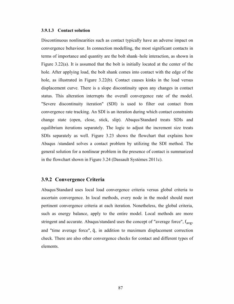
87

3.9.1.3 Contact solution

Discontinuous nonlinearities such as contact typically have an adverse impact on

convergence behaviour. In connection modelling, the most significant contacts in

terms of importance and quantity are the bolt shank–hole interaction, as shown in

Figure 3.22(a). It is assumed that the bolt is initially located at the center of the

hole. After applying load, the bolt shank comes into contact with the edge of the

hole, as illustrated in Figure 3.22(b). Contact causes kinks in the load versus

displacement curve. There is a slope discontinuity upon any changes in contact

status. This alteration interrupts the overall convergence rate of the model.

"Severe discontinuity iteration" (SDI) is used to filter out contact from

convergence rate tracking. An SDI is an iteration during which contact constraints

change state (open, close, stick, slip). Abaqus/Standard treats SDIs and

equilibrium iterations separately. The logic to adjust the increment size treats

SDIs separately as well. Figure 3.23 shows the flowchart that explains how

Abaqus /standard solves a contact problem by utilizing the SDI method. The

general solution for a nonlinear problem in the presence of contact is summarized

in the flowchart shown in Figure 3.24 (Dassault Systèmes 2011c).

3.9.2 Convergence Criteria

Abaqus/Standard uses local load convergence criteria versus global criteria to

ascertain convergence. In local methods, every node in the model should meet

pertinent convergence criteria at each iteration. Nonetheless, the global criteria,

such as energy balance, apply to the entire model. Local methods are more

stringent and accurate. Abaqus/standard uses the concept of "average force", f ,

and "time average force", q, in addition to maximum displacement correction

check. There are also other convergence checks for contact and different types of

elements.

88

The average of all of the nodal force components in all the elements of the model

is called the average force, as calculated by Equation (3-17) (Dassault Systèmes

2011c):

= ∑ ∑ ∑ | | + ∑ f

(3-17)

An average nodal force,q, for the whole model at each iteration is calculated

based on (3-18) (Dassault Systèmes 2011c) :

= ( ) + ( )( . ) + ( . ) (3-18))

Applying the definition of q, the "time average force", q,is determined as shown

in Equation (3-19) (Dassault Systèmes 2011c):

= ( ℎ )( . ℎ , ℎ )

(3-19)

The parameter q is calculated for the model throughout each step at each iteration

of the current increment.

It is also crucial to set an acceptable residual tolerance. In Abaqus/standard, the

iteration is accepted as converged when R is reached, as shown in Equation

(3-20): = 0.005 (3-20)

R is the maximum residual (out-of-balance force) and qis time average force

for every node in the model. The 0.005 value is selected based on previous

experience and engineering judgment, and is considered to provide a reasonable

trade-off between accuracy and efficiency for quadratic convergence.

89

There are other convergence criteria that Abaqus/Standard uses in order to

ascertain the accuracy of the implicit analysis results. Another convergence

criterion is the "maximum displacement correction" check. This criterion limits

the maximum displacement correction to less than or equal to 1% of the

maximum displacement increment, as shown in the Equation (3-21): = 0.01 (3-21)

wherec is the maximum displacement correction and Δu is the maximum

displacement increment. In addition to all the mentioned convergence controls,

there are other convergence criteria for contact problems.

All of these criteria can be altered by the user in case of convergence difficulties.

However, for steel connection simulations, it is recommended to look for

modelling issues rather than changing the default parameters for convergence. It

is noted that relaxing the default convergence criteria may lead to divergent or

inaccurate results. In certain cases of connection modelling, user intervention

might be useful, such as when a model contains a crack or includes fracture, or the

models contain user elements (UEL) or user material subroutines (UMAT). If the

final behaviour of a specific type of connection is important, relaxing

convergence criteria during initial analysis stages might help the cost; however, if

the history of the connection performance is important, this is not recommended.

Based on what was mentioned, no alteration has been applied to the default

convergence rules in this research.

3.9.3 Stabilization of initial rigid body motion

Bolted connection assemblies rely on contact between bolts and different

components to prevent unconstrained rigid body motion. Due to uncertainty of the

location of the bolt shank in the hole, it is often impractical to model such systems

with initially established contact. The initial play between the bolt and the other

components causes initial unconstrained rigid body motion. Displacement-

90

controlled loading prior to establishing contact will lead to a non-singular

solution. However, after establishment of contact, the system of equations is also

stable for force-controlled loading. Pre-tensioning the bolts helps to establish

contact and prevent rigid body motion, before applying the actual load step.

Abaqus/standard can also automatically control rigid body motions in static

problems before contact closure and friction restrains such motions. This

stabilization is based on the stiffness of the underlying elements. In this automated

stabilization contact method, additional forces are imposed to all contact pairs

equally in the normal tangential direction that will influence the solution during

the step. At the end of the step, these newly introduced forces are ramped down to

zero. The method is applicable only when the distance between the contact

surfaces is smaller than a characteristic surface dimension. This method helps the

convergence significantly, even though no true rigid body modes exist in the

model. In the sample bolted connection without stabilization, the analysis requires

a special analysis sequence, many SDIs, and non-default contact controls.

3.9.4 Time incrementation

Abaqus uses a sequence of steps, increments and iterations for defining the load

history by applying an empirical algorithm automatically to control the increment

size. Although there are many logical principles applied in these algorithms, the

basics include two simple rules: first, the increment size is increased by a factor of

1.5 after obtaining convergence in four iterations and, second, the increment size

is decreased by a factor of 0.25 after not obtaining convergence in more than 10

iterations.

The user provides an initial increment size for every step in nonlinear analysis. It

is suggested to use a small fraction of the total step size (0.1-0.01). Maximum and

minimum increment sizes should be specified by the user as well. Selection of

approximate values for maximum and minimum increment size is also important.

Abaqus requires input of the maximum number of increments allowed per step. If

91

the increment size is reduced due to cutbacks to a value below this minimum

value, the analysis will terminate. In order to avoid termination, it is suggested to

use a value between 10-15 to 10-10 for highly nonlinear connection models.

Although there is no restriction on maximum allowable increment size—i.e., the

entire load can be applied in a single increment—a reasonable value can lead to

efficient solution and avoids cutbacks.

3.9.5 Riks versus general static methods

The Riks method (Riks 1979) is recommended for globally unstable problems.

This method works well with contact as long as the contact itself is stable. Riks

runs into problems where there is a loss of contact, such as a contact-driven snap-

through problem, where the structure moves away from the contact. In this case,

the Riks algorithm can’t scale the load up or down to keep the model in contact

and convergence failure will occur. The arc length method proposed by Riks

generally cannot be applied to connection models due to the large number of

contact surfaces and contact status changes. Figure 3.25 illustrates how contact

status is changing due to the presence of different loads in the connection model

in a column removal scenario. The general-static method implemented in Abaqus

is therefore used in this study.

3.10 Numerical Failure Criteria

Failure in the experimental program is considered a situation at which the

assembly has lost a considerable load carrying capacity or a rupture mechanism

occurs. In the numerical model, the implicit analysis will continue until the model

cannot find the solution due to excessive yielding, which is far beyond the failure

point in the experiment. In order to capture the correct failure load and mode, it is

necessary to establish numerical failure criteria. These criteria could be global,

which include all the possible limit states of the connection, or could be more

case-specific, and varied for each particular limit state. Each method has its pros

92

and cons, but the global failure criteria are more versatile and complete, although

difficult to set effectively for general use. This criterion should be satisfied when

some elements or nodes reach a certain stress or strain value. Stress criteria could

be principal stress, in a specific direction, von Mises, Tresca, etc. Strain criteria

could be also the principal strain or the equivalent strain. In this research, the

equivalent plastic strain, PEEQ in Abaqus, has been selected as a variable upon

which to impose a failure criterion. PEEQ is defined in Equation (3-22):

PEEQ = ɛ + ɛ dt (3-22)

where ɛ is the initial equivalent plastic strain. The definition of ɛ depends on

the material model. For classical (Mises) plasticity ɛ is defined in Equation

(3-23):

ɛ = 23 ɛ : ɛ (3-23)

PEEQMAX is the maximum of the equivalent plastic strains among all of the

section points. For a solid element, it represents the maximum PEEQ at the

integration points. As mentioned in section 3.7.2, since the problem is mesh-

dependent, an appropriate mesh size should be selected in order to capture the

failure modes and loads accurately. PEEQ failure values for steel sections/plates

and high strength bolts are introduced in sections 3.10.1 and 3.10.2, respectively.

3.10.1 Steel sections and plate

Rupture strain is very mesh-dependent and different researchers have proposed

different values. For instance, for structural-grade steel, Khoo et al. (2002)

showed that the localized rupture strain is approximately 80% to 120%. Huns et

al. (2002) used tension coupon test in order to measure the localized rupture

strain. Huns et al. considered a rupture strain of 100%, which was a lower bound

93

of their material test and an average of the range of values reported by Khoo et al.

(2002). Epstein and Chamarajanagar (1996) proposed a rupture strain equal to

five times the yield strain.

Unfortunately, there was no material tension coupon test performed for the

selected experimental program; hence, it is hard to establish a failure value.

However, the verified finite element model with available experimental results

show that the shear tab starts to fail at approximate PEEQ equal to 0.55. This

value is valid for the applied mesh size. As the mesh gets finer, a larger value for

strain should be selected as a rupture point for the material. The proposed rupture

strain criterion is observed in other experiments for other types of connections,

such as WT. Hence, it is selected for all the other models in the subsequent

chapters.

In order to make sure that the defined material model with the selected mesh size

can capture necking and the required localized strain, a tension coupon with the

same mesh size of the shear tab in the connection assembly is modeled, as shown

in Figure 3.26. When the strain reaches the rupture point, the element is removed

from the mesh in order to simulate the initiation of steel rupture. It is noted that in

the current research, rupture initiation is of main interest due to the fact that

rupture propagation is rapid and unstable with lots of uncertainties, and is beyond

the point of maximum capacity of the localized connected part. Rupture

propagation is therefore outside the scope of the research.

3.10.2 High strength bolts

In order to calibrate the ASTM A325 and ASTM A490 bolt types used in this

research, and also establish a rupture strain value, a solid element model of the

bolt in a double shear test is developed, as shown in Figure 3.27. The behaviour of

the finite element model is compared to the typical result of the shear tests

reported by Kulak et al (2001). As can be seen in Figure 3.28 and Figure 3.28,

there is good correlation between the experimental and numerical results. These

94

figures also establish the rupture strain equal to 0.55 for this type of bolt with the

mentioned mesh size. A mesh with the same size elements is used in the

connection assembly.

3.11 Results extraction

Axial and moment forces in each step were obtained through strain measurements

using strain gauges in the experiments (Thompson 2009). These data are used to

determine the forces at the bolt line of the connections. The strains are converted

to stress using Hooke's law, which assumes that the beam material at the strain

gauge locations remains elastic. Numerical simulation confirmed the validity of

this assumption. The measured strains are combinations of axial and flexural

stress at the location of the strain gauges. The axial force at any section through

the length of the beam remains unchanged. Assuming a triangular moment

distribution, the flexural force at the bolt line was determined from extrapolation

of flexural forces at the strain gauge location. The procedure is explained in

chapter 2.

The same procedure was applied to determine the internal forces at the bolt line

location of the simulated models. The toolset called "Free Body toolset" was used

to record the resultant forces and moments at the location of the strain gauges on

the test specimens. This toolset simply adds the forces at the nodes corresponding

to the defined section. Hence, the element force nodal output (NFORC) is needed

in order to create a free body cut. Since free body cuts cannot be saved in the

output database file, a Macro (a set of Abaqus Scripting Interface commands) has

been managed.

3.12 Sensitivity analysis

In order to gain confidence in the correctness and accuracy of the proposed finite

element model, detailed sensitivity analyses are performed. Table 3.10

95

summarizes the variables on which the analyses are performed. For the sake of

brevity, just the shear response of the connection is plotted. In sections 3.12.1 to

3.12.7, observations regarding different variables are discussed. Three tests were

carried out on each configuration of shear tab connection (Thompson 2009) and

each test produced results for two identical shear tabs, although their responses

might be different. Therefore, six different responses from the experiments are

available for comparison. The results of the third experiments on 5ST (five-bolt)

connections are shown in Figure 3.30 to Figure 3.35 for the purpose of comparing

with numerical results. The dashed lines and solid lines represent the results of the

experiments and simulations, respectively. The termination point of the numerical

simulation curves is based on the selected failure criterion, as discussed in section

3.10.

3.12.1 Element Type

It is observed that the global response of the connection assembly including shear,

axial and flexural responses is not sensitive to the type of element for different

components in terms of load path. However, different types of elements have

different capabilities in capturing localized strain. Figure 3.30 shows the shear

force versus rotation of the shear tab connection assembly for shear tabs

consisting of element types C3D8R, C3D8, and C3D8I. The model with C3D8R

elements reaches the established failure criterion far from the models with C3D8

and C3D8I elements, as well as initial failure observed in the experiments. It can

be inferred that reduced integration elements (C3D8R) cannot capture the highly

localized strain values precisely. Although the difference between C3D8 and

C3D8I is small, C3D8I illustrates a better match with the experimental results.

Based on what was discussed in section 3.6, it is recommended to use an

incompatible type of element in regions where bending is dominant and the

failure mode is of interest.

96

3.12.2 Coefficient of friction

The behaviour of the connection assembly is not significantly varied with the

coefficient of friction between different components, and particularly the axial

response. However, the closest response to the experimental results belongs to the

model with the coefficient of friction equal to 0.3, as shown in Figure 3.31.

Physical evidence for steel material shows that the selected value is reasonable.

3.12.3 Hole size

Figure 3.32 shows the shear response of the connection with different hole

diameters. When the diameter of the hole is exactly equal to bolt diameter, the

connection starts to capture load from the beginning. For the standard hole, a drop

is observed in the load path until the contacts are established. For the oversized

hole, the drop region is even larger. It can be concluded that any kind of variation

in the relative bolt-to-hole size, including construction tolerances, will affect the

load path. Slippage in the bolts results in a drop in the moment as well until

bearing is achieved between the bolt shank and the hole in the plate. Furthermore,

the location of the bolt in the hole is also important, since it determines when the

contact is established. Due to the unknown nature of the problem and its

variability, it is assumed that the bolts are located at the centers of the holes. This

assumption is expected to affect only the initial part of the response curve.

3.12.4 Contact stiffness

illustrates the shear response of the connection with different penalty scale

factors. Both load path and the convergence of the model are sensitive to this

parameter. As a result, a model with an appropriately-selected parameter needs to

be established for developing the benchmark example. Herein, the penalty scale

factor of 0.0012 produced the best agreement with the experimental results, along

with an acceptable convergence rate. Extensive research on different models leads

97

to the proposed range given in section 3.8.3.2.2.1.1.1, which are appropriate for

all types of structural steel used in this research.

3.12.5 Pre-tensioning

Figure 3.34 depicts the shear–rotation curves for the models with different

pretension forces in the bolts. Pre-tensioning, in terms of displacement applied to

the bolt shanks, does not affect the overall load path significantly. However, it

does influence the load path at early stages; e.g., the model with PT=0.5 mm

produces better agreement with the experimental load path at the beginning of the

load transfer. However, based on the argument in section 3.5.2.3.1, the

connections in the selected experimental program are considered snug-tight, not

pre-tensioned. As a result, the model with PT=0.1 mm is deemed to produce

results with acceptable accuracy. It is noted that the PT equal to 0.02, 0.1 and 0.5

mm impose 12, 59 and 294 MPa initial stress in the bolts, respectively.

3.12.6 Material definition

illustrates the shear response of the connection with different material definitions

discussed in section 3.5.2.2 and Appendix A. As can be seen in , the difference in

the definition of material used in this research affects the load curves slightly.

Selecting "minimum nominal strength" (MINS) and "maximum nominal strength"

(MANS) material properties underestimates and overestimates, respectively, the

response slightly. "Lower-bound" (LBS) and "expected-strength" (EPS) are

appropriate properties to get acceptable results. The expected-strength (EPS)

definition is utilized for all types of steel, including the bolts, in the finite element

studies, as discussed in Appendix A.

3.12.7 Mesh size

The failure criterion definition utilized in this research is mesh sensitive. Besides,

appropriate relative mesh densities of different parts in the assembly is a

98

challenge when contact exists. As mentioned in section 3.7, the principle of

classical mesh convergence study does not apply due to the localized nature of the

stress fields in the connection model. As a result, an appropriate mesh size is

established as discussed in section 3.7. The effect of mesh size is investigated and

it is observed that the model is not sensitive to the refinement of the mesh size in

either the connecting part or the bolts. Moreover, convergence difficulties may

occur if very refined meshing is used in the assembly.

3.13 Final results

The deformed shape of the overall test assembly and a direct comparison of the

shear tab deformations and tearing observed in the model and the experiment are

shown in Figure 3.36. It can be seen that there is close similarity between the

experiment and the numerical simulation results. The numerical model can predict

the location of failure initiation accurately. Plastic deformation is mostly

accumulated around the bottom hole where the failure begins. Besides, the

ductility of the system is mostly provided by bearing deformation developed

around the holes, based on both numerical and experimental results.

Table 3.11 compares the experimental and finite element model results. Errors are

calculated based on the assumption that the experimental results are the correct

values. Final results show that different modelling assumptions, e.g., the location

of the bolts at the center of the holes, are valid due to good agreement with the

experimental results. As observed, the errors are all less than 7%, which is

acceptable in such a complex model with numerous physical and numerical

features and variables. The agreement for shear and rotation is particularly close.

The internal forces—including shear, axial force, and moment—at the bolt line

location versus chord rotation of the connection assembly are shown in Figure

3.37 to Figure 3.39. These curves verify the simulated model based on the

acceptable agreement with the associated experimental results and the variability

within the experimental results of nominally-identical specimens themselves.

99

3.14 General tips for reaching converged solution

As mentioned earlier, there are several causes for convergence problems,

including allowing rigid body motion, conflicting constraints between boundary

conditions, contacts, inadequate material data, inappropriate element types, and

instability of the physical model such as development of load instabilities or

severe localized plastic strain. Hence, the correct element type, appropriate

boundary conditions and constraints, sufficient material data and an appropriate

analysis technique should be utilized. In addition to all mentioned suggestions and

recommendations to assist in model development of shear connections under a

column removal scenario, to reach a converged solution some basic notes are

provided in this section. Although basic, they are fundamental and help to reach

convergence in the numerical modelling of steel connections:

• Most of the convergence problems arise from inappropriate definition of

various aspects of the model, such as constraints, boundary conditions,

material and element types. Although achieving a converged solution

using implicit analysis with all different types of nonlinearity is a difficult

task, the majority of convergence problems can be explained and

corrected.

• It is suggested to add complexity to the model step by step, not

simultaneously. Start with a simple connection model without plasticity,

friction, and even contact (use tie constraint instead) in the geometry.

After getting insight into the behaviour, add complexity as needed to

achieve the modelling goals.

• As a general comment, avoid sharp corners in numerical models of

connections. Particularly, when the physical connection surface is

reasonably smooth, the numerical model should be smooth as well.

However, in places that they are inevitable, it is recommended to use

Surface-to-Surface formulation at corners because two constraints are

applied, as shown in Figure 3.40, which is accurate and stable. Node-to-

Surface applies just a single constraint in an "average" normal direction at

100

the corner, which is not stable and may cause a large penetration and

snagging. The corner should be approximated by an adequately fine mesh

to help convergence considerably. In modelling round corners, mesh

refinement will tend to help convergence.

• Another source of convergence difficulties is the difference between the

actual geometry and faceted geometry. Faceted geometry may cause a

“noisy” solution; nevertheless, by geometric corrections an accurate

solution can be obtained. It must be noted that geometric corrections might

not be helpful in large deformation models. The shank section of bolts

should be adjusted to conform to hole facets, as shown in Figure 3.41.

• Friction is an issue that could produce unsymmetrical terms in the stiffness

matrix. The unsymmetrical solver is recommended for all finite-sliding

Surface-to-Surface contact problems. It is noted that the unsymmetrical

solver of Abaqus is automatically activated for friction coefficients greater

than 0.2.

• It is recommended to select the stiffer surface as the master surface,

although it has a coarser mesh. The master surface normal should point

toward the slave surface; otherwise, convergence difficulties will occur.

• Since Abaqus does not have any specific built-in system of units, all the

input data must be in consistency. SI (N-mm) is recommended to be the

consistent units in all models. Make sure that the units and material

properties are consistent.

• Providing reasonable values for the minimum and maximum increment

size will help the convergence considerably.

3.15 Summary and conclusions

The following conclusions can be drawn from the finite element study presented

in this chapter:

101

• The present study is aimed at proposing an efficient and unified methodology

for finite element modelling of steel shear connections in a column removal

scenario. The main goal of this chapter is establishing confidence in the

proposed modelling approach by verifying simple shear tab connections

subjected to extreme loading conditions caused by the loss of a primary

supporting column.

• The finite element analysis user has to decide on several issues such as mesh

discretization, element types and the solving algorithm. These selections may

have tremendous effects on the model response and can lead to inaccurate

results. Nonlinearity definitions, including material, geometric, and boundary

(contact) nonlinearities, are the most challenging part of finite element

modelling of connections, and recommendations have been established and

verified.

• In connection modelling, obtaining the converged nonlinear solution is the

main obstacle. Satisfying all the mentioned convergence issues in addition to

good engineering judgment to create a finite element model leads to an

accurate solution. Although experimental results are needed for model

validation, it is not necessary to have them for each specific type of connection

to verify the response. Following the same procedure that was previously

verified can lead to “converged” (accurate) response. The example can be

taken as a benchmark for validating the finite element modelling of shear

connections in the column removal scenario.

102

Table 3.1: Different phases in finite element analysis of bolted steel connections

(Krishnamurthy 1980)

Phase Description Goal

Feasibility studies trial, development and modification of

different models

build a model with satisfactory physical

attributes

Sensitivity studies vary one quantity at a time while the other characteristics of the model are

kept constant

understand the effect of modelling variables on

overall behaviour of connection assembly

Correlation studies

validate the model using benchmark cases or pertinent experimental results

ascertain that the results are correct and accurate enough

Convergence studies

model three or more progressively finer meshes of connection to evaluate

the accuracy of the solution

determine the appropriate element sizes considering the

accuracy and cost

Parametric studies vary the most significant variables to

accomplish the desired task

investigate the effect of design variables by

producing statistically valid results

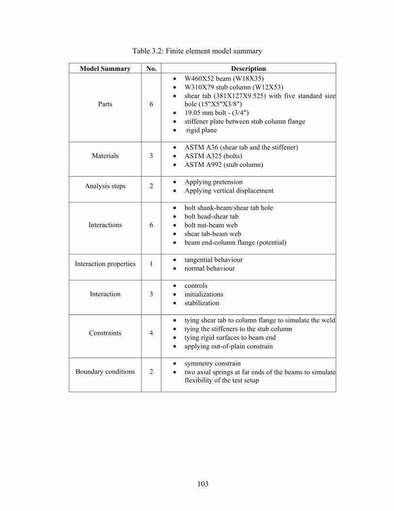
103

Table 3.2: Finite element model summary

Model Summary No. Description

Parts 6

• W460X52 beam (W18X35) • W310X79 stub column (W12X53) • shear tab (381X127X9.525) with five standard size

hole (15"X5"X3/8") • 19.05 mm bolt - (3/4") • stiffener plate between stub column flange • rigid plane

Materials 3 • ASTM A36 (shear tab and the stiffener) • ASTM A325 (bolts) • ASTM A992 (stub column)

Analysis steps 2 • Applying pretension • Applying vertical displacement

Interactions 6

• bolt shank-beam/shear tab hole • bolt head-shear tab • bolt nut-beam web • shear tab-beam web • beam end-column flange (potential)

Interaction properties 1 • tangential behaviour • normal behaviour

Interaction 3 • controls • initializations • stabilization

Constraints 4

• tying shear tab to column flange to simulate the weld• tying the stiffeners to the stub column • tying rigid surfaces to beam end • applying out-of-plain constrain

Boundary conditions 2 • symmetry constrain • two axial springs at far ends of the beams to simulate

flexibility of the test setup

104

Table 3.3: Integration order of element available in Abaqus (Daneshvar and Driver 2012)

Element Type

Description

First order elements

• constant strain throughout the element that prevents mesh locking when the material is approximately incompressible e.g. steel

• accuracy achieved with full integration versus reduced integration depends on the nature of the problem

• recommended in cases of large strains or high strain gradients

• Works well with contact

Second order elements

• provide higher accuracy for problems not containing contact simulations or element distortion

• better modelling geometric features, e.g., modelling a curved surface with fewer elements

• effective in bending-dominated analysis

• the second-order reduced-integration elements may suffer from volumetric locking when strains exceed 20– 40%.

Table 3.4: Full versus partial element integration available in Abaqus (Daneshvar and Driver 2012)

Element Type

Description

Reduced-integration Elements

• use lower-order integration just for the element matrix, not mass and loading – No locking concern

• reduces the time of analysis, especially in three-dimensional analysis

• less accuracy in the area of stress concentration

Full-integration Elements

• may suffer from locking behaviour, including both shear and volumetric locking

• volumetric locking happens when the material behaviour is almost incompressible

105

Table 3.5: Mesh refinement analysis results; refinement across the thickness

Mesh density (No. of elements

in thickness)

Displacement at the bottom

of the top hole (mm)

Stress at the bottom of the top

hole (MPa)

Stress at the top

corner of shear tab

(MPa)

Relative CPU time

(Sec)

1 (Coarse) 0.37 279.5 250.3 4.3

2 (Normal) 0.56 276.7 253.0 8.5

3 (Fine) 0.58 277.0 253.3 12.9

Table 3.6: Master and slave surfaces in the shear tab connection

No. Label Master Slave

1 Head-ST bolt head shear tab

2 Nut-Bm bolt's nut beam's web

3 ST-Bm beam's web shear tab

4 Shk-Hol-Bm bolt's shank beam's web hole

5 Shk-Hol-ST bolt's shank shear tab

6 Bm-Clm beam cross section column flange

Table 3.7: Nonlinear penalty contact parameters (Dassault Systèmes 2009)

Parameter Symbol Default value

Linear stiffness used for linear penalty contact Klin 10 times the representative

underlying element stiffness

Initial stiffness Ki 1/10 of the linear penalty stiffness

Final stiffness Kf 10 times the linear penalty

stiffness

Clearance at which contact pressure is zero C0 zero

Upper quadratic limit d 3% of the characteristic length1

Lower quadratic limit e 1% of the characteristic length1

Lower quadratic limit ratio er 0.33332

1 computed by Abaqus/Standard to represent a typical facet size

2 From the default values of the parameters d and e

106

Table 3.8: Direct Lagrange multiplier versus penalty method (Dassault Systèmes 2009)

Direct Lagrange multiplier contact Penalty contact

Advantages Disadvantages Advantages Disadvantages

• exact constraint enforcement (zero penetration)

• no need to define contact stiffness

• larger system of equations

• slow convergence rate

• number of equations does not increase

• improved convergence rate

• approximate constraint enforcement (finite amount of penetration)

• difficult to choose proper stiffness

Table 3.9: Implicit versus explicit analysis method (Dassault Systèmes 2011c)

Explicit Implicit

Convergence not an issue must be obtained at each increment

Stability conditionally stable unconditionally stable

Time increment limited large ones can be used Result

Reliability need to verify more precisely high

107

Table 3.10: Sensitivity analysis

Parameter Variable

Element type C3D8

C3D8R C3D8I

Coefficient of friction μ = 0.15 μ = 0.3

μ = 0.5

Hole size bolt size standard oversize

Linear penalty contact: scale factor

0.0012 0.001 0.005 0.01 0.1 1

Pretension - Adjust length 0.02 mm 0.1 mm 0.5 mm

Material- shear tab - ASTM A36

EPS LBS

MANS MINS

108

Table 3.11: Benchmark results; verification with experimental work (Thompson 2009)

Spec. Label

Side Moment,

M (kN.m)

Shear, V (kN)

Axial, P (kN)

Rotation, Θ

(radians) Failure Mode

5ST1 Left - - - - -

Right 55.90 47.11 147.73 0.073 Block Shear Rupture

5ST2 Left - - - - -


5ST3 Left 68.49 45.46 151.42 0.071 Tension Rupture

Right - - - - -

5ST-Mean 61.64 48.19 167.09 0.071

5ST-FEA 65.85 47.31 177.48 0.069 Shear tab bottom hole rupture

Deviation % 6.83 1.82 6.22 2.82

109

SG1

SG2

SG3

SG4

SG1

SG2

SG3

SG4

Test Frame

DWT Supports

True Pin Connection

Strain gauges

Hydraulic Jack

Test Beam

Stub Column

True Pin Connection

Shear tab connection (5ST)

Figure 3.1: Test setup of selected experimental program (Thompson 2009)

110

38,1

76,2

76,2

76,2

76,2

38,1

381

38,188,9

127 9,53

(a)

112,71 131,76

2549,53

306

76,2

12,7

114,

338

111

4,3

609,

6

609,

6

520,

7

(b)

SG1

SG2

SG3

SG4

38,1957,26 993,78

1989,14

76,2

76,2

76,2

76,2

76,2

69

450

165,

1

165,1

(c)

Figure 3.2: Part dimensions (a) shear tab (b) stub column (c) beam (Thompson 2009)

Fig

Be

gure 3.3: Fin

eam web

Fig

nite element m

gure 3.4: Ap

111

model of ste

Applied

pplying bolt

eel shear tab

d pre-tension

pretension

connection

Shear taab

112

Figure 3.5: Symmetry constraint at the centerline of the stub column; rigid surface and horizontal spring at far end

(a) (b)

(e)

(d)

(g)

(c)

(f)

Figure 3.6: Structural elements in Abaqus/Standard (a) Continuum solid element (b) Shell element (c) Membrane element (d) Rigid element (e) Beam element (f)

Truss element (g) Spring/dashpot (Dassault Systèmes 2009)

113

(a) (b) (d)(c)

Figure 3.7: Continuum solid elements in Abaqus/Standard (a) Linear element (eight node brick, C3D8) (b) Quadratic element (twenty node brick, C3D20)(c)

Modified second-order element (ten node tetrahedron, C3D10M) (d) Linear element ( four node tetrahedron, C3D4) (Dassault Systèmes 2009)

Figure 3.8: Mesh size in different segments of the beam

Segment 2 Segment 3 Segment 4

Segment 1

114

(a) (b) (c)

Figure 3.9: Mesh refinement across the thickness: (a) Coarse: one element in thickness; (b) Normal: two elements in thickness; (c) Fine: three elements in

thickness

Deformation

Shear StressASTM A490

ASTM A325

Figure 3.10: ASTM A325 versus ASTM A490 (Kulak et al. 2001)

F

Figure 3.11

Figure 3.12:

: Contact de

Bolt-hole inelemen

efinition (a) c(Dassault

(a)

nteraction (Ants (b) after i

115

h < 0

h = 0

constraint noSystèmes 2

Ashakul 2004nstallation o

ot active (b) 011b)

4) (a) beforeof GAP elem

constraint a

(b)

e installationment

activated

n of GAP

116

n

h

1

2

(a)

Beam

Column

(b)

Beam Column

(c)

Figure 3.13: (a) Contact element (b) general contact (c) contact pair

117

Oversize HoleBolt Shank


Free to penetrateFree to penetrate

(a) (b)

Figure 3.14: Different types of surface-based contact (a) Node-to-Surface (b) Surface-to-Surface

Penetration

Contact pressure

Direct enforcement - Lagrange multiplier

Penalty method

Clearance

penalty stiffness

No contact

Figure 3.15: Contact pressure versus penetration diagram for direct Lagrange multiplier and penalty method (Dassault Systèmes 2011b)

penetration

Master

SlaveKp

Figure 3.16: Penalty method diagram (Dassault Systèmes 2011b)

118

C e=d/3 d U

P

K lin

K nonlin = 10 K lin

K nonlin = 0.1 K lin

Nonlinear penalty

Linear penalty

=0 0

Figure 3.17: Penalty contact pressure–overclosure diagram: Linear versus nonlinear stiffness method

Slip

Shear stress

Lagrange multiplier

Penalty method

Figure 3.18: Contact pressure–penetration diagram: Lagrange multiplier versus penalty method (Dassault Systèmes 2011c)

119

Ϭ =

Geometric nonlinearity Material nonlinearity Boundary nonlinearity

Figure 3.19: Sources of nonlinearity in the implicit formulation (Dassault Systèmes 2011c)

Step Increment Iteration

Figure 3.20: Step, increment and iteration definition in Newton–Raphson method

120

U0 U1 U2 U3 U*

P0

P*

K(U0)

K(U1)

K(U2)R(U0)

R(U1)

R(U2)

U

P

Figure 3.21: Newton–Raphson method diagram (Dassault Systèmes 2011c)

P0

P*

U1/2(R-r)

1

2



(a)

(b)(c)

U

v

r

R

Figure 3.22: Severe discontinuity iteration (SDI) in the shank–hole interaction (a) undeformed (b) deformed (c) contact force versus displacement diagram

121

Figure 3.23: Solution flowchart for contact problem; severe discontinuity iterations (SDI) (Dassault Systèmes 2011c)

Figure 3.24: Solution flowchart for a nonlinear problem including contact (Dassault Systèmes 2011c)

122

MP

+ =P

MV+

V

Figure 3.25: Bolted connection subjected to simultaneous moment, tension and shear loads

(a) (b)

(c) (d)

Figure 3.26: Tension coupon test (a) geometry and meshing (b)loading and boundary conditions (c) stress distribution before failure (d) element removal at

PEEQ=0.55 to simulate initiation of rupture

123

(a) (b)

(c) (d)

Figure 3.27: Numerical model of ASTM A325 bolts under shear loading (a) geometry and meshing (b) loading and boundary conditions (c) stress distribution before failure (d) element removal at PEEQ=0.55 to simulate initiation of rupture

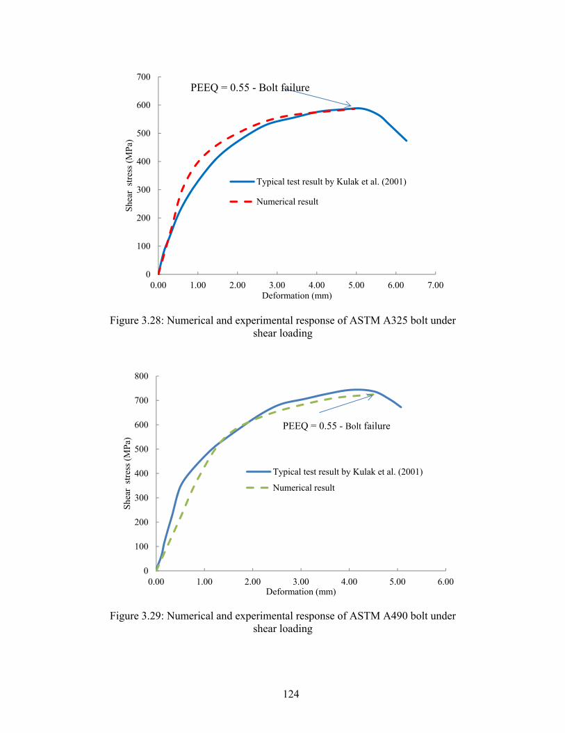
124

Figure 3.28: Numerical and experimental response of ASTM A325 bolt under shear loading

Figure 3.29: Numerical and experimental response of ASTM A490 bolt under shear loading

0

100

200

300

400

500

600

700

0.00 1.00 2.00 3.00 4.00 5.00 6.00 7.00

She

ar s

tres

s (M

Pa)

Deformation (mm)

Typical test result by Kulak et al. (2001)

Numerical result

0

100

200

300

400

500

600

700

800

0.00 1.00 2.00 3.00 4.00 5.00 6.00

She

ar s

tres

s (M

Pa)

Deformation (mm)

Typical test result by Kulak et al. (2001)

Numerical result

PEEQ = 0.55 - Bolt failure

PEEQ = 0.55 - Bolt failure

125

Figure 3.30: Shear force versus chord rotation curves at the bolt line; Experimental (Thompson 2009) and finite element results for different types of

elements

Figure 3.31: Shear force versus chord rotation curves at the bolt line; Experimental (Thompson 2009) and finite element results for different

coefficients of friction

0.0

5.0

10.0

15.0

20.0

25.0

30.0

35.0

40.0

45.0

50.0

55.0

60.0

0.00 0.02 0.04 0.06 0.08 0.10

She

ar (

kN)

Beam End Rotation (Rad)

EXP-5STL3

EXP-5STR3

FE Model - 5ST-C3D8

FE Model - 5ST-C3D8R

FE Model - 5ST-C3D8I

0.0

5.0

10.0

15.0

20.0

25.0

30.0

35.0

40.0

45.0

50.0

55.0

60.0

0.00 0.02 0.04 0.06 0.08 0.10

She

ar (

kN)


EXP-5STL3

EXP-5STR3

FE Model - 5ST - CF=0.5



126

Figure 3.32: Shear force versus chord rotation curves at the bolt line; Experimental (Thompson 2009) and finite element results for different hole sizes

Figure 3.33: Shear force versus chord rotation curves at the bolt line;

Experimental (Thompson 2009) and finite element results for different linear penalty stiffness scale factors

0.0

5.0

10.0

15.0

20.0

25.0

30.0

35.0

40.0

45.0

50.0

55.0

60.0

0.00 0.02 0.04 0.06 0.08 0.10

She

ar (

kN)


EXP-5STL3

EXP-5STR3

FE Model - 5ST - HoleSize=BoltSize

FE Model - 5ST

FE Model - 5ST - OverSizeHole

0.0

5.0

10.0

15.0

20.0

25.0

30.0

35.0

40.0

45.0

50.0

55.0

60.0

0.00 0.02 0.04 0.06 0.08 0.10

She

ar (

kN)


EXP-5STL3EXP-5STR3FE Model - 5ST - LC-SF=1FE Model - 5ST - LC-SF=0.1FE Model - 5ST - LC-SF=0.01FE Model - 5ST - LC-SF=0.005FE Model - 5ST - LC-SF=0.0012FE Model - 5ST - LC-SF=0.001

127

Figure 3.34: Shear force versus chord rotation curves at the bolt line; Experimental (Thompson 2009) and finite element results for different pretension

displacement

Figure 3.35: Shear force versus chord rotation curves at the bolt line; Experimental (Thompson 2009) and finite element results for different material

properties

0.0

5.0

10.0

15.0

20.0

25.0

30.0

35.0

40.0

45.0

50.0

55.0

60.0

0.00 0.02 0.04 0.06 0.08 0.10

She

ar (

kN)


EXP-5STL3

EXP-5STR3

FE Model - 5ST - PT=0.5



0.0

5.0

10.0

15.0

20.0

25.0

30.0

35.0

40.0

45.0

50.0

55.0

60.0

0.00 0.02 0.04 0.06 0.08 0.10

She

ar (

kN)


EXP-5STL3EXP-5STR3FE Model - 5ST - A36 - MANSFE Model - 5ST - A36 - EPFE Model - 5ST - A36 - LBFE Model - 5ST - A36 - MINS

128

(a)

(b) (c)

Figure 3.36: (a) Deformed shapes of assembly: (b) Shear tab from experiment (Thompson 2009); (c) Shear tab from finite element simulation

Damage initiation simulated by

element removal

129

Figure 3.37: Shear force versus chord rotation curves at the bolt line; Experimental (Thompson 2009) and finite element results

Figure 3.38: Axial force versus chord rotation curves at the bolt line; Experimental (Thompson 2009) and finite element results

0.0

10.0

20.0

30.0

40.0

50.0

60.0

0.00 0.02 0.04 0.06 0.08 0.10 0.12

She

ar (

kN)


EXP-5STL1EXP-5STR1EXP-5STL1-aEXP-5STR1-aEXP-5STL2EXP-5STR2EXP-5STL3EXP-5STR3FE Model - 5ST

0.0

40.0

80.0

120.0

160.0

200.0

240.0

280.0

0.00 0.02 0.04 0.06 0.08 0.10 0.12

Ten

sion

(kN

)



130

Figure 3.39: Moment versus chord rotation curves at the bolt line; Experimental (Thompson 2009) and finite element results

Figure 3.40: Convergence difficulties at the corners (a) S-to-S (b) N-to-S

0.0

20.0

40.0

60.0

80.0

0.00 0.02 0.04 0.06 0.08 0.10 0.12

Mom

ent (

kN.m

)



131


Cad geometry

Mesh geometry

overlap

gap

Magnified View

Figure 3.41: Actual geometry versus faceted geometry

132

4 Compressive Arching and Tensile Catenary Action in Steel Shear Connections under Column Removal Scenario

4.1 Introduction

Although the behaviour of many types of shear connection under conventional

gravity loading has been established through research, their response to a column

removal scenario is still relatively unknown. It is widely believed that beams

adjacent to a lost column will develop cable-like tensile action, as illustrated

schematically in Figure 4.1. In frames with shear connections, this requires the

connections to continue to transfer shear forces, in addition to developing tensile

catenary forces under large rotations. This tensile resistance can provide an

alternative load path in a column removal scenario. In essence, structural collapse

can be arrested following localized damage to a column if the adjacent shear

connections can sustain sufficiently large rotations and tensile forces through

catenary action.

In this research, the development of compressive arching action followed by

tensile catenary action is investigated. It is shown that in a column removal

scenario the connection may develop a considerable axial compressive force at

small beam rotations before catenary action develops, as shown in Figure 4.2.

This compressive force has typically been neglected in previous assessments of

connection robustness.

After a brief review of the literature related to the axial response of steel shear

connections in a column removal scenario, finite element analysis results of

bolted steel connection assemblies, considering material, geometric and contact

nonlinearities are presented. The models were verified using the available column

133

loss experiments performed on shear connections. A simplified analytical model

is presented and compared to the observed axial response of the connections.

4.2 Literature survey

Girhammar (1980) appears to be the first researcher to acknowledge the presence

of compressive arching action in steel assemblies in a column removal scenario.

He conducted column-loss experiments on two types of bolted beam-to-column

connections: seated “heel” connections and end-plate connections. Figure 4.3(a)

shows a schematic view of the test assembly and the idealized axial response of

the connection. Based on this study, end plate connections, as an example of a

semi-rigid connection, exhibited three distinct response phases in a column

removal scenario: arching, bending, and catenary actions. An equation was

proposed for the compressive arching force based on the beam section properties,

the moments at the ends, the connection eccentricity (discussed in section 4.3),

and the horizontal play in the connection assembly (Girhammar 1980).

Izzuddin et al. (2008) proposed a simplified model for nonlinear static response of

a beam, applicable to a column removal scenario, including connection response

and external axial restraint (Figure 4.3(b)). For partially-restrained connections,

special attention was drawn to the centre of rotation of the connection, which

influenced the development of compressive arching (Izzuddin et al. 2008). The

authors concluded that although this arching action was not of primary importance

to connection design, it could enhance the nonlinear response of the beam

assembly in a column loss event, especially with respect to dynamic load carrying

capacity (Izzuddin et al. 2008).

134

Astaneh (2007) also discussed the progressive collapse resistance of steel frames

with simple shear connections. An analogy of a three-hinged beam subjected to a

concentrated load at mid-span—a classical problem discussed by Timoshenko

(1955)—was used in order to simplify the problem of the loss of the middle

column. Figure 4.3(c) shows the conceptual model and the idealized axial

response of the connection. He also suggested a method to determine the catenary

force and ultimate rotational capacity of the connection that can be utilized for

design. However, the possibility of an axial compressive force developing in the

shear connection was not discussed.

4.3 Axial response of steel connection in column removal scenario

The overall geometry of a symmetric two-bay frame with the central column

removed is shown in Figure 4.4. The case considered includes flexible shear

connections made up of seat and top angles. These connections tend to rotate

about points at different elevations at the two beam ends, separated by an

eccentricity, ev. The “unrestrained path of motion” in the figure shows that if

rotation were to occur about the points at the remaining columns, the points at the

removed column (if unrestrained) would initially move towards each other at

small beam rotations because of this eccentricity. Since the condition of symmetry

restrains the central column to move vertically, a compressive “arch” (two

compressive struts) forms. At larger beam rotations, catenary tension is developed

as the unrestrained paths of motion of the two beams diverge (Daneshvar et al.

2012).

As seen in Figure 4.4, the axial shortening of the beam and connection at the early

stage of the column removal scenario, which causes the compressive force, is very

small in comparison with the vertical displacement of the severed column. In a

135

real structure or test assembly, this small deformation may be accommodated by

bolt slippage or flexibility of the surrounding structure. In order to simplify the

problem and focus on just one detailed connection, the test setup shown in Figure

4.5 is selected. In this connection assembly, the beams are cut at the inflection

point; and far ends are substituted by true pin connections. A verified high-fidelity

finite element model is used as a tool to monitor the response of shear connection

assemblies in a column removal scenario as arching action forms. The model

development is discussed in section 4.3.1. The analytical approach used to study

arching behaviour in a column removal scenario is explained in section 4.3.2.

4.3.1 Numerical approach

Shear tab, WT and single angle connections have been selected for the finite

element modelling due to the availability of suitable experimental data. The

procedure and results can be extended to other types of shear connection, such as

seated angle connections. Pre- and post-processing procedures were completed

using Abaqus/CAE, and Abaqus/standard was used as the analysis engine

(Systèmes Dassault 2009). Experiments performed by Thompson (2009),

Friedman (2009) and Johnston (2009) were used to verify the results of the

numerical models. A total of nine full-scale tests were carried out, keeping the

connection depth (number of bolts) as the sole variable. The geometric properties

of the test specimens are summarized in Table 4.1 to Table 4.3.

Three, four and five bolt shear tab, WT and single angle connections were

modelled. Models consist of the central column and the adjacent beams, as well as

the connections with complete detailing. Figure 4.6 shows the finite element

models of shear tab connections, as an example. Shear tabs are welded to the

column flange and bolted to the beam web. The central column is pushed down,

while the connection performance is monitored. It is assumed that the welds are

136

flawless and of greater strength than the base material; therefore, the shear tab was

tied directly to the flange of the column stub. This idealization was confirmed to

be appropriate, since the strain in the vicinity of the weld line did not exceed the

weld's rupture strain. (In addition, no weld rupture was reported from the

experiments.)

Steel properties were not reported for the test specimens, so based on the

identified steel grades (ASTM A36 for the shear tabs and ASTM A992 for the

rolled sections), the material strengths were estimated using the nominal values

multiplied by industry-established strength increase factors (GSA 2003). For the

ASTM A325 bolts, an appropriate value of the strength increase factor was

selected based on previous tests on bolts of the same grade. Pins at the inflection

points were simulated by applying a rigid plate across the beam cross-section that

is permitted to rotate about the beam’s bending axis, and invoking a horizontal

linear axial spring with a stiffness of 100 kN/mm to approximate the combined

effects of the flexibility of the test setup and any slippage or deformation at the

far-end pin supports. All other characteristic features of the numerical models,

including contact behaviour, element types, and failure criteria, are presented in

chapter 3. The 5ST connection used in this chapter is the same connection detail

discussed in chapter 3 as a benchmark example. Good agreement of the numerical

simulation and experimental results provides confidence to use the same

principles for other types of shear connections.

Figure 4.7 to Figure 4.9 show the axial responses of connections 3ST, 4ST and

5ST, respectively, in the column removal scenario. Axial responses of 3WT, 4WT

and 5WT are illustrated in Figure 4.10 to Figure 4.12. Figure 4.13 to Figure 4.15

show the same curves for 3SA, 4SA and 5SA. The figures show that the

numerical model predicts the ultimate axial capacity of the connections well;

however, there are some discrepancies in the axial load path. The magnitude of

137

arching action that formed during the experiments is less than what was observed

in the simulation. The reason is that the accumulation of axial compression is

sensitive to the axial restraint provided to the beams at the ends away from the

lost column support, so any inaccuracies in the stiffness of the spring used in the

model to represent the flexibility of the reaction frame and bolt slippage could

cause the magnitudes of the compressive forces measured in the laboratory

experiments to be different from those observed in the finite element results.

Connections with three bolts (3ST, 3WT and 3SA), which have the greatest

vertical eccentricity because the connecting parts are positioned farthest from the

central beam axis where the far-end pin was located in the tests, exhibit the

greatest compressive arching forces. As the connection eccentricity decreases, the

arching action decreases as well, which leads to almost no compressive force in

connections 5ST and 5WT (which have no eccentricity because the shear tab and

WT are centered on the beam axis), as shown in Figure 4.9 and Figure 4.12. The

behaviour of the SA connections is a little different due to more flexibility of the

angle in comparison with the plate and WT. The center of rotation of 5SA tends to

move up towards the top of the connection. As a result, even in 5SA, vertical

eccentricity exists and arching action forms, as shown in Figure 4.15.

4.3.2 Analytical approach

Simplified analytical calculations based on compatibility of displacements can be

used to estimate the total axial deformation, ∆Axial, that accumulates between the

beam supports as a function of the chord rotation, θ, in a column removal

scenario. If the horizontal restraint at the “remaining” column is not infinitely stiff

due to the flexibility of the surrounding structure, displacement of the support

point is included in this total deformation (Daneshvar et al. 2012).

138

The magnitude of ∆Axial (measured along the axis of the beam between

horizontally fixed reference points at the original column face locations) can be

decomposed into two components: ∆ (resulting from the vertical motion

downwards at the removed column), and ∆ (resulting from the eccentricity of the

centres of rotation of the two connections). The geometries of these two

components for the case of a seat and top angle are shown in Figure 4.16(a) and

(b), and the combined effect is solved in Equation (4-1). At small rotations, the

second (compressive) term, ∆ , tends to be dominant; at larger rotations, the first

(tensile) term, ∆ , dominates the total axial deformation and leads to catenary

action. Short span lengths and large centre of rotation eccentricities increase the

dominance of arching action at small rotations. In the absence of such an

eccentricity, catenary tension develops immediately following the column

removal (Daneshvar et al. 2012).

shows potential components of the total axial deformation, ∆Axial , where

deformation contributing to the elongation of the system is taken as positive. The

first term, ∆Connection, includes the total axial deformation of the connections at

each end of the beam due to bolt slip, bolt deformation, and deformation of the

connecting elements (typically, a plate or angles). Axial deformation of the beam, ∆Beam, is typically much smaller than the connection deformation, since the beam

tends to remain elastic for the case of shear connections. The deformation of the

surrounding structure, ∆Restraint, also contributes to the total axial deformation in

the system (Daneshvar et al. 2012).

∆Axial= ∆ − ∆ = 1 − 1 − (4-1)

∆Axial= ∆Connection + ∆Beam + ∆Restraint (4-2)

139

Applying Equation (4-1) and to the shear tab connection models in Figure 4.6

leads to the results presented in section 4.4.

4.4 Results

Figure 4.17 demonstrates good agreement between the axial deformations from

the finite element models of the test assemblies shown in Figure 4.6 and those

calculated using Equation (4-1) and Equation (4-2). Figure 4.18 shows the effect

of the boundary condition on the axial response of the connection assembly based

on the finite element model. Ka-str is the stiffness of the springs at the far ends of

the beam assembly that represents the stiffness of the test setup or surrounding

structure in the experiment or the real structure, respectively. As demonstrated in

Figure 4.18, the axial response of the shear connection, in the phases of both arch

and catenary action, are highly dependent on the stiffness of surrounding

structure. In this research, Ka-str is assumed equals to 100 kN/mm to be a realistic

value based on the approximate dimensions and section sizes of the test setup. For

comparison, a one-bay portal frame with W610X217 columns, a W460X52 beam

and 3 m in height possesses an approximate lateral stiffness of 100 kN/mm. Ka-str

equal to 10 kN/mm and 1000 kN/mm represent two extremes for lateral stiffness

of stories in elastic frames, manifesting flexible and stiff storeys, respectively.

4.5 Conclusion

The following conclusions can be drawn from the discussion in chapter 4:

• In a column removal scenario, considerable axial compressive force may

develop via arching action before catenary action begins. This

phenomenon has been simulated numerically and the results show that the

140

vertical eccentricity between the centres of rotations of the connections at

the ends of a beam is a primary parameter leading to the presence of this

compressive force.

• Another important factor that affects the development of arching action is

the stiffness of the surrounding structure. Whether the arching action

forms in the connection assembly or not, the catenary resistance of the

connection can act as an alternative load path in a column loss event.

• Since the arching action might occur at an early stage of connection

response, it will not affect the ultimate capacity of the frame. Therefore,

tensile catenary action is still the reliable alternative load path in response

to a column removal scenario, and therefore the connection must be

designed to resist these tensile loads.

• Good correlation of force–rotation curves obtained from the finite element

model was achieved with those obtained from the tests in the tensile

regime. However, there are some discrepancies in the magnitude of

compression experienced during arching action. Finite element modelling

could capture the arching action phase more precisely if the restraint at the

beam's far ends in the experiments were known accurately. Good

agreement between the results of analytical and numerical methods is also

observed.

• Although the acknowledgement of the presence of compressive arching

action as a part of axial response of shear connections in the column

removal scenario is important, it is unlikely to enhance the connection

performance to assist in bridging over the localized damage. As a result,

its magnitude is not the point of concern in this research. Hence, the

tensile part of axial behaviour of shear connections as an active alternative

path load is reported in the remaining chapters.

141

Table 4.1: Geometric properties of ST test specimens (Thompson 2009)

No. Specimen

Label Plate Type

Plate thickness

(mm) Bolt Type

Bolt diameter

(mm)

Beam size

Column size

1 3ST ASTM A36 9.5 ASTM A325

19.1 W460X52 W310X79


19.1 W460X52 W310X79


19.1 W460X52 W310X79

Table 4.2: Geometric properties of WT test specimens (Friedman 2009)

No. Specimen

Label WT Type WT Section Bolt Type

Bolt diameter

(mm)

Beam size

Column size

1 3WT ASTM A992

WT125X33.5ASTM A325

19.1 W460X52 W310X79

2 4WT ASTM A992

WT125X33.5ASTM A325

19.1 W460X52 W310X79

3 5WT ASTM A992

WT125X33.5ASTM A325

19.1 W460X52 W310X79

Table 4.3: Geometric properties of SA test specimens (Johnson 2009)

No. Specimen

Label Angle Type

Angle Section

Bolt Type Bolt

diameter (mm)

Beam size

Column size

1 3SA ASTM A36 L152X89X9.5ASTM A325

19.1 W460X52 W310X79


19.1 W460X52 W310X79


19.1 W460X52 W310X79

142

Column loss

Double-span zone

Figure 4.1: Axial response of a gravity framing system after column removal

PP P P

(a)

P

P

P

P

(b)

Figure 4.2: (a) Compressive arching action accompanied by (b) tensile catenary response of a gravity framing system after column removal

143

P

(a)5000 mm

1000

mm

T

5000 mm

L/2(b)

WK a-str

L/2

P

(c)

Us

L/2

K a-str

L/2

Us

Us

Us

W

Elas

tic

P

Us

Us

TT(a)

(b)

(c)

Double spananalytical/experimental

model

Axial response ofconnection in CRS

Archaction

Bendingaction

Catenaryaction

Elasticcatenaryregion

Catenary:transient

Catenary:final

Compressivearching

Post-yieldcatenaryregion

Figure 4.3: Double span analytical/experimental models and axial response of a connection in a column removal scenario (a) Girhammar (1980), (b) Izzuddin et

al. (2008a), (c) Astaneh-Asl (2007)

144

Connection centre of rotation


Unrestrained path of motion

Compressive arching action region

Tensile catenary action region

Line of arching action

e

(a)


Unrestrained path of motion

Compressive arching action region

Tensile catenary action region

Line of arching action

Real hinge

ev

Real hinge

(b)

Figure 4.4: Development of compressive arching and catenary tension under column removal scenario (a) top and bottom seated angle connection (b) single angle connection with real hinges and axial springs at the ends (Daneshvar et al.

2012)

SG1

SG2

SG3

SG4

SG1

SG2

SG3

SG4

Test Frame

DWT Supports

True Pin Connection

Strain gauges

Hydraulic Jack

Test Beam

Stub Column

True Pin Connection

Shear connection

Figure 4.5: Test setup of selected experimental program (Thompson 2009)

145

146

(a)

(b)

(c)

Figure 4.6: Finite element models of (a) 3-bolt shear tab (3ST), (b) 4-bolt shear tab (4ST), (c) 5-bolt shear tab (5ST)

147

Figure 4.7: Comparison of numerical and experimental axial responses of connection 3ST


-60.0

-20.0

20.0

60.0

100.0

140.0

180.0

220.0

0.00 0.02 0.04 0.06 0.08 0.10 0.12 0.14

Axi

al f

orce

(kN

)


3STL13STR13STL23STR23STL33STR33ST-3/8-3/4

-20.0

20.0

60.0

100.0

140.0

180.0

220.0

0.00 0.02 0.04 0.06 0.08 0.10

Axi

al f

orce

(kN

)



148


Figure 4.10: Comparison of numerical and experimental axial responses of connection 3WT

-60.0

-20.0

20.0

60.0

100.0

140.0

180.0

220.0

260.0

0.00 0.02 0.04 0.06 0.08 0.10

Axi

al f

orce

(kN

)


5STL15STR15STL1-a5STR1-a5STL25STR25STL35STR35ST-3/8-3/4

-80.0

-40.0

0.0

40.0

80.0

120.0

160.0

200.0

240.0

280.0

0.00 0.02 0.04 0.06 0.08 0.10 0.12 0.14 0.16

Axi

al f

orce

(kN

)


3WTL1

3WTR1

3WTL2

3WTR2

3WTL3

3WTR3

3WT125X33.5-3/4

149



-40.0

0.0

40.0

80.0

120.0

160.0

200.0

0.00 0.02 0.04 0.06 0.08 0.10 0.12

Axi

al f

orce

(kN

)

Beam End Rotation (kN)

4WTL14WTR14WTL24WTR24WTL34WTR34WT125X33.5-3/4

-40.0

0.0

40.0

80.0

120.0

160.0

200.0

0.00 0.02 0.04 0.06 0.08 0.10

Axi

al f

orce

(kN

)

Beam End Rotation

5WTL1

5WTR1

5WTL2

5WTR2

5WTL3

5WTR3

5WT125X33.5-3/4

150

Figure 4.13: Comparison of numerical and experimental axial responses of connection 3SA


-100.0

-60.0

-20.0

20.0

60.0

100.0

140.0

180.0

220.0

260.0

0.00 0.02 0.04 0.06 0.08 0.10 0.12 0.14 0.16 0.18 0.20 0.22 0.24

Axi

al f

orce

(kN

)


3SAL1

3SAR1

3SA-3/8-3/4

-100.0

-60.0

-20.0

20.0

60.0

100.0

140.0

180.0

220.0

260.0

300.0

0.00 0.02 0.04 0.06 0.08 0.10 0.12 0.14 0.16 0.18 0.20

Axi

al f

orce

(kN

)


4SAL1

4SAR1

4SAL2

4SAR2

4SAL3

4SAR3

4SA-3/8-3/4

151


-60.0

-20.0

20.0

60.0

100.0

140.0

180.0

220.0

260.0

300.0

0.00 0.02 0.04 0.06 0.08 0.10 0.12 0.14 0.16 0.18

Axi

al f

orce

(kN

)


5SAL1

5SAR1

5SAL2

5SAR2

5SA-3/8-3/4

152

Initial position of Beam centreline

Beam centreline after removal of column

L + 1

Vertical Restrained path of motion

ev

(a)

L - 2

ev

(b)

Figure 4.16: Axial deformation from (a) vertical deflection, and (b) eccentric connection rotation (Daneshvar et al. 2012)

153

Figure 4.17: Comparison of axial deformations of numerical and simplified analytical models for ST connections (Daneshvar et al. 2012)

Figure 4.18: Axial response of connection 3ST for different end spring stiffnesses (Daneshvar et al. 2012)

-2

0

2

4

6

8

10

0 0.02 0.04 0.06 0.08 0.1 0.12 0.14

Axi

al d

ispl

acem

ent (

mm

)

Chord Rotation (radians)

Analytical Appr. - 3ST

Numerical Appr. 3ST


Numerical Appr. 4ST


Numerical Appr. 5ST

-100

-50

0

50

100

150

200

0.00 0.02 0.04 0.06 0.08 0.10 0.12 0.14

Axi

al f

orce

at b

olt l

ine

(kN

)

Chord Rotation (Rad)

FE Model - 3ST- Ka-str=10 kN/mm



154

5 Behaviour of Shear Tab Connections in Column Removal Scenario

5.1 Introduction

The shear tab, fin plate, or single plate connection is one of the simplest and most

cost-effective shear connection types. It can either be bolted or welded to the

beam web and welded to the column flange, as shown in . Common types of

material used in shear tab connections are stated in Table 5.1. Shear tabs in beam-

to-column connections are conventionally designed to transfer shear forces only.

It is assumed that there is no substantial moment transfer due to the fact that beam

end rotation occurs when the beam is loaded. Research on the strength and

ductility of shear tab connections in conventional design is extensive. Although its

behaviour under gravity and cyclic loading has been established, its response to

the column removal scenario is still relatively unknown. In order to model the

behaviour of such a connection in progressive collapse analyses, the DoD (2009)

guideline provides a table that includes models for shear tab connections.

However, as discussed in chapter 2, more research is required to shed light on the

characteristic features of such connections to improve the current modelling

definitions. The actual load path and stress distributions should be well-

understood to propose modelling parameters in the column loss event.

In this chapter, numerical methods are applied to simulate the response of shear

tab connections when a column is compromised. The finite element models are

verified by available experimental data following the same loading regime.

Verified models are then utilized to expand the database of the test results. Shear,

axial force, and moment versus chord rotation diagrams are presented for both

numerical and experimental results and conclusions are made. A parametric study

is performed to extend the database on the behaviour of shear tab connections in

column loss event. The results are utilized to develop the modelling parameters

that can predict the rotational behaviour of shear tab connections in the new

155

scenario. At the end, the results are compared with the available codes and

guidelines for earthquake and progressive collapse.

5.2 Objectives and scope

The main goal of this chapter is to investigate the behaviour of shear tab

connections in the column removal scenario. The research study is intended to

verify the results of high-fidelity finite element models of shear tab connections in

terms of both load path and failure modes. These models can shed more light on

the performance and the sources of ductility in shear tab connections. The results

can be used to select suitable connection modeling parameters for progressive

collapse evaluations of steel frames with similar shear connections.

The focus of the research is on bolted shear tab connections, shown in Figure

5.1(a). Numerically, this type of shear tab connection is perhaps the more

challenging one in terms of analysis cost due to the presence of bolts, which leads

to many contact surfaces and, consequently, potential convergence problems.

Connection depth is the sole variable in the experimental models discussed herein.

However, extensive parametric study is performed to expand the database on the

behaviour of such connections by changing factors such as the plate thickness,

bolt grade and diameter.

The Steel Construction Manual (2010) discusses two types of single plate beam-

to-column connections called "conventional configuration" versus "extended

configuration". The former, also referred to as "shear tab" or "fin plate"

connections, has one vertical row of bolts at the supported beam web. There are

several conditions—Table 5.2 summarizes the limitations and defines several of

the parameters utilized in Table 5.1 (the others can be found in the list of

symbols)—that need to be met to categorize a single plate in the conventional

group. The "extended configuration" of single plate beam-to-column connection,

utilizes one or more vertical rows of bolts. There have been several research

programs on the behaviour of extended shear tabs, such as those performed by

156

Sherman and Ghorbanpour (2002) and Goodrich (2005). The focus of this

research is on the "conventional configuration" definition, hereinafter called

simply “shear tab”. Moreover, this research is focused on the behaviour of shear

connections in a subassembly, rather than on isolated shear connections. The

process of subassembly selection is discussed in chapter 2.

5.3 Selected previous research on shear tab connections

In this section, a selective chronological progression of work related to research

on shear tab connections is presented as background to the current research.

Lipson (1968) initiated the investigation and attempted to establish characteristic

features of these connections, including the behaviour of the connection under

working loads and maximum rotational capacity by performing several tests.

Nonetheless, the main purpose of Lipson's research was to determine if shear tab

connections can qualify as "flexible" connections. Three types of connections

were investigated including "welded-bolted" shear tab connections. All plates

were ASTM A36 type and bolts were ASTM A325 and the bolt diameter was

confined to 19.1 mm (3/4 in). The welding was made with the E70 series of

electrodes. He tested the specimens under pure bending moment and also a

combination of shear and moment, with or without rotation. Lipson observed

three failure modes including weld rupture, vertical bolt tear-out of the bottom

bolt and tensile yielding of the plate. He also observed a significant deformation

of the bolt holes. He showed that the magnitude of the slip value for the bolts

varied substantially for shear tab specimens. Besides, the effect of changing the

gauge distance has only a small effect on the slip value. His experiments could not

develop the full plastic moment of the connection because of small beam rotation.

The connection was determined to be partially-restrained, with characteristics of

both flexible and rigid connections.

Caccavale (1975) verified Lipson’s experimental results using finite element

analysis. He also performed several single shear tests on individual bolts to

157

determine the load–deformation response. He observed that the main source of

shear tab connection ductility is distortion of the bolt holes providing that bolts

have the necessary strength.

Richard et al. (1980) distinguished ductility sources in single plate connections:

(1) bolt shear deformation (2) plate and/or beam web hole distortion (3) out-of-

plane bending of the plate and/or beam web (4) bolt slippage. Based on his tests

and the ones performed by Lipson (1968), he concluded that the amount of end

moment transferred to the supporting member could be significant and depend on

five factors: (1) number, size, and configuration of bolt pattern (2) thickness of the

plate and/or beam web (3) beam span/depth ratio (4) beam loading pattern

(concentrated or uniform force) (5) relative flexibility of supporting member. He

acknowledged the effect of the flexibility of the supporting elements on the

flexural response of one-sided connections. However, he assumed full restraint at

the welded edge of the plate in his analytical models and physical tests.

Richard et al. (1980) also performed a series of "single bolt–single shear"

experimental and numerical studies for various bolt sizes and plate thicknesses

typically used in shear tab connections. Figure 5.3 shows a sample mesh grid they

used for their finite element models. They developed the moment–rotation curves

for two, three, five and seven bolt connections for different eccentricities by

constructing the non-dimensional relationship demonstrated in Equation (5-1). In

their work, eccentricity, e, was defined as the distance between the bolt line and

the point of inflection in the beam. They proposed Equation (5-1) for defining the

moment–rotation relationship of the studied connections.

= ∗(1 − 1 − ℎ . ) (5-1)

In the Equation (5-1), M is the connection moment; M is the reference moment

based on a pure moment assuming all bolts at their maximum capacities; M∗ is the

intermediate non-dimensional moment determined by Equation (5-2); Φ∗is the

free end rotation of the beam divided by a reference rotation; Φ is the reference

158

rotation calculated by Equation (5-3); n is the number of bolts; e is the

eccentricity of the load; and h is the depth of the bolt pattern.

∗ = ∗( ∗. ) / (5-2)

= . ( )( ) (5-3)

Figure 5.4 illustrates the concept of beam line method—construction of a linear

action of a beam on a nonlinear moment–rotation relationship of a connection—

applied. The intersections of the beam line and the vertical and horizontal axes are

the beam fixed-end moment and simple span end rotation, respectively. Full scale

beam tests, shown in Figure 5.5 were performed to establish the validity of the

applied models and methods. ASTM A325 bolts with 19.1 mm (3/4 in) and 22.2

mm (7/8 in) diameter were utilized. Plate material was ASTM A36 and ASTM

A575 Grade 50 steel. Based on all the studies, Richard et al. (1980) proposed a

design procedure for shear tab connections. The bolts were designed with an

eccentricity, e, determined from Equation (5-4):

ℎ = (ℎ) ( )( ) . (5-4)

where h is the connection depth; n is number of bolts; N is 5 for 19.1 mm (3/4 in)

and 22.2 mm (7/8 in) bolts, and 7 for 25.4 mm (1 in) ones; S is 100 for 19.1 mm

(3/4 in) bolts, 175 for 22.2 mm (7/8 in) bolts, and 450 for 25.4 mm (1 in) ones;

and S is the section modulus of beam. ( ) is determined by Equation (5-5) and

Equation (5-6):

(ℎ) = 0.06 ⁄ − 0.15 ⁄ ⩾ 6 (5-5) (ℎ) = 0.035 ⁄ ⁄ < 6 (5-6)

L/ d is the length-to-depth ratio.

159

The welds in the procedure were also designed to resist moment, determined by

Equation (5-7) : = ( + ) (5-7)

where is the beam shear force; and a is the distance from the bolt line to the

weld line. The concept is shown in Figure 5.6. Young and Disque (1981)

developed tabular design aids based on Richard's proposed procedure that can

significantly reduce the time required to design such connections.

In a later study, Richard et al. (1982) examined the application of ASTM A307

bolts in shear tab connections considering slotted holes. This connection was

desirable because of more ductility and also less connection moment due to bolt

movement in the slotted holes. Use of short-slotted holes avoids the large bolt

diameter to plate thickness ratio providing ductility by preventing the bolt shear

mode of failure.

Hormby et al. (1984) expanded the previous research by including connections

with (1) slotted holes, (2) off-axis bolt groups, (3) Grade 50 steel beams, and (4)

composite beams. An off-axis bolt group is defined as one whose center of gravity

does not line up with the neutral axis of the beam, as shown in Figure 5.7. They

observed that high strength A325 and A490 bolts behave similarly in round and

slotted holes. The center of rotation for all the off-axis bolt group connections is at

the center of the bolt group. The eccentricity of the connections with off-axis bolt

groups varied, at most, ± 9% of the symmetric concentric connection eccentricity.

In the experiments using ASTM A572 Grade 50 steel beams, it was suggested that

the eccentricity be modified as shown in Equation (5-8):

= (3650) (5-8)

The beam line method was also modified to be used with different types of steel,

as shown in Figure 5.8 .

160

Astaneh (1889) investigated the demand and supply of ductility—the latter being

defined as "the amount of rotation that a connection can tolerate before failure

occurs"—in steel shear connections and proposed a refined beam line where both

inelastic properties of the beam and the connection were considered to be applied

in both service and ultimate load conditions. He (Astaneh et al. 1989) also

performed a suite of experimental studies on shear tab connections and observed

considerable shear and bearing yielding before failure, which caused a reduction

of the rotational stiffness and also a release of end moment. Figure 5.9 shows a

schematic view of bolt hole deformations after his tests. The tested beams showed

ductile behaviour, tolerating rotations of 0.026 to 0.061 radians at the point of

maximum shear. An increase in the number of bolts led to a decrease in rotational

flexibility and ductility. Based on these experiments, five limit states were

identified: (1) plate yielding (2) net section fracture of plate (3) bolt fracture (4)

weld fracture (5) bolt hole bearing failure. Based on the test results, he proposed

more realistic empirical values for the eccentricity definitions for designing bolts

and weld, calculated by Equation (5-9) to Equation (5-11). Equation (5-9) and

Equation (5-10) assume rigid and rotationally-flexible supports for the shear tab,

respectively, although no experimental tests were completed on flexible supports: = ( − 1)(1.0) − (5-9) = ( − 1)(1.0) − , (5-10) = ( )(1.0), (5-11)

where n and a were defined previously.

Astaneh (Astaneh et al. 1989) also developed a strength-based design procedure

taking into account the required shear capacity as well as the necessary

connection rotation. He recommended providing vertical and horizontal edge

distances of at least 1.5 times the bolt diameter in order to avoid bearing fracture.

Ductile yielding of the plate was ensured to be reached prior to brittle failure, by

161

limiting the plate thickness to less than db/2 + 1/16 in, where db is the bolt

diameter. He limited the weld size to 3/4 of the plate thickness to make sure that

the plate would yield prior to weld yielding. It is noted that the 14th edition of the

Steel Construction Manual (AISC 2010) recommends using 5/8 instead of 3/4.

Astaneh et al. (2002) examined more single plate shear connections subjected to

gravity loading under the loading regime shown in . The researchers identified

similar limit states to those found in the previous work (Astaneh et al. 1989),

separating the bearing failure of the beam web or plate into bearing on bolt holes

in the plate and the beam web (ductile limit state) and fracture of edge distances

of bolt holes (brittle limit state). They observed that the contribution of shear

deformations and distortions are significant above service loading. A design

procedure was developed such that, first, ductile failure modes would happen,

followed by brittle limit states, as shown in Figure 5.11. It was also observed that

shear connections under gravity loads could tolerate rotations varying from 0.026

to 0.103 radians. Typical moment–rotation curves of the test specimens are

illustrated in Figure 5.12.

Tests of beam-to-column-flange shear tab connections with floor slabs under

combined gravity and cyclic lateral loading were also included in this study.

These connections showed the same hierarchy of limit states as those with gravity

loading alone. Typically, the composite action was lost after reaching a drift of

approximately 0.04 radians. Then, a significant drop in the load capacity was

observed, almost to that of the equivalent bare steel connections. Generally, the

rotation capacity of shear tab connections is decreased by an increase in the depth

of connection. Based on the test results, he proposed a simplified model for the

moment–rotation response of shear tab connections shown in Figure 5.13

(Astaneh 2005).

Ashakul (2004) created a series of finite element models to evaluate the

experimental work performed by Astaneh (1989c) and Sarkar (1992). The models

were used to investigate several connection parameters such the a-distance—

defined as the distance between the bolt line and the weld line—plate material and

162

thickness, and the connection position with respect to the beam neutral axis. He

also studied single plate connections with two columns of bolts, which are not

considered as “conventional” configuration as discussed in section 5.2. The

results show that the a-distance will not affect the bolt shear rupture strength of a

connection. He observed significant induced horizontal forces at the bolts if the

plate materials and thicknesses do not satisfy the ductility criterion for the plate

thickness shown in Equation (5-12): = 0.7 36 (5-12)

where is the plate thickness; is the bolt diameter; and is the minimum

yield strength of the plate. This horizontal force reduces the shear strength of a

bolt group and creates a moment that must be considered in design. A new design

model for shear tab connections with single-column bolt pattern (“conventional”

configuration) is proposed in his work.

There is very little research published on shear tab connections subjected to shear,

moment and tension. Guravich et al. (2006) investigated the behaviour of simple

beam-to-column connections subjected to combined shear and tension by

performing experiments on different types of connections, including the shear tab

configuration. Specimens were rotated to 0.03 radians and then a shear between

zero and the design shear resistance was applied and held constant while the

tensile load was applied until failure. They observed significant differences in

interactions, ductility, and ultimate tensile strength. The main sources of the

ductility were yielding due to bearing at bolt holes and shear yielding of the gross

section of the components of the connections. They concluded that that most shear

connections can take significant amounts of tensile force accompanied by the

design shear capacity.

As discussed, there is extensive research performed on shear tab connections,

attempting to characterize their behaviour, including the limit states and rotational

capacity, under vertical shear load. However, the interaction of shear, tension and

moment occurring in the event of column removal has been largely neglected. The

163

above review illustrates that there have been limited studies on the performance of

shear connections subjected to progressive collapse type of loading scenarios.

5.4 Numerical study methods

The behaviour of shear tab connections subjected to the simultaneous presence of

shear, moment, and tension is investigated using high-fidelity finite element

models. All stages of simulation, including pre- and post-processing procedures,

were performed using Abaqus/CAE, with Abaqus/standard used as the analysis

engine (Dassault Systèmes 2009), as discussed in chapter 2.

5.4.1 Selected experimental program

Experiments performed by Thompson (2009) were utilized to verify the results of

the numerical models. Figure 5.14 demonstrates the connection subassembly and

the test setup. A total of nine full-scale tests were carried out, with the connection

depth as the sole varying factor. The procedure of results extraction is discussed

in chapter two. Although some of the tests were continued after the initial failure,

the results up to this point are of interest in this research.

5.4.2 Finite element models description

Three-dimensional solid elements were used for all the components of the model

due to the nature of the connection modeling problem. The models consist of the

central column stub and the adjacent beams, as well as the connections with

complete detailing, as shown in Figure 5.15(a). Three, four and five bolt shear tab

connections were modeled, as illustrated in Figure 5.15(b) to Figure 5.15(d). The

central stub column is pushed down, while the connection performance is

monitored.

164

Since the connection is the point of interest, all characteristic features of the

connections are included in the models. Strain-based fracture criteria were

established and verified in chapter 3 for both the plate and the bolts in order to

predict the failure modes. All other characteristic features of the models, including

bolt pre-tensioning, material properties, contact calibration and element types are

also discussed in chapter 3. The complete list including characteristic features of

all the connections numerically studied is summarized in Table 5.3. A sample of

the deformed shape of the connection assembly after the experiment is compared

with its corresponding result from the finite element analysis in Figure 5.16.

The models are labeled based on the following method: first the number of the

bolts, then ST, which is the abbreviation for shear tab connections utilized in this

research, then the plate thickness and the bolt diameter, in imperial units. For

example, 3ST-3/8-3/4 refers to the shear tab with three bolts; 3/8 in (9.5mm) plate

thickness and 3/4 in (19.1 mm) diameter bolts. The bolts are all ASTM A325,

unless at the end of label A490 is added. Material properties for all the plates

correspond to ASTM A36. For the ones where experimental data is available,

verification as well as comprehensive comparison of experimental and numerical

results are performed.

5.5 Verification results

Although based on the benchmark example provided in chapter 2, following the

procedure outlined is expected to produce valid results for all types of shear

connections in the column loss event; however, the verification process is

performed for all other shear tab connections with three and four bolts since the

experimental results are available. It is noted that the benchmark example

provided in chapter 2 was for a five-bolt shear tab connection. For the purpose of

verification, deformed shapes, failure modes and internal force diagrams are

compared with the experimental results.

165

Figure 5.17 to Figure 5.21 compare the experimental versus numerical deformed

shape of shear tab connection components for all the experiments utilized in this

study. Although there are similarities in the behaviour of each type, there are

some differences that are discussed in the following sections. To ensure that a

shear tab connection will survive the column removal scenario, it should be

capable of carrying the combined effects of shear and moment, as well as a large

catenary tensile force. The internal forces at the bolt line versus the chord rotation

of connection assemblies 3ST, 4ST and 5ST are shown in Figure 5.22 to Figure 5-

30. The dashed and solid lines represent the results of the experiments and

simulations, respectively. While the general trends in all force responses of the

connections correlate well, some discrepancies between the experimental and

numerical results exist which are discussed in section 5.5.1 to 5.5.3:

5.5.1 Three bolt shear tab connections (3ST)

The comparison of the test results is performed based on the deformed shapes and

the internal force interaction.

5.5.1.1 Deformed shapes and failure modes

Figure 5.17 shows the numerical versus experimental deformed shape of the 3ST

connections before failure. The distribution of bearing stress at the bottom hole at

thirty degree angle from the horizontal line is recorded in both the test report

(Thompson 2009) and numerical results, as depicted in Figure 5.17. The trend of

30 degrees in the suite of experiments as well as the numerical model is illustrated

in a magnified view of bottom hole region comparing with plastic strain

distribution obtained by finite element model in Figure 5.17(c). The numerical

stress distribution around the holes in the shear tab confirms a similar stress

distribution to that in the experimental program by comparing to the flaking of

mill scale. 4ST and 5ST connections are similar to 3ST to some extent in terms of

distribution of stress at the bottom hole.

166

Figure 5.18 depicts the numerical versus experimental deformed shape of the 3ST

connection after failure. As can be seen, most of the plastic deformation occurred

around the bottom hole of the shear plate in which the rupture occurred,

ultimately. No visible distortion occurred around the second hole. Presence of

force couple is obvious in both the numerical model and experimental results,

imposing compressive and tensile forces to the top and bottom hole, respectively.

Figure 5.21 shows a typical bolt shear deformation obtained from the tests and

finite element simulation. A substantial amount of shear deformation happens at

the bottom bolt before failure.

Basically, the governing failure mode for all the 3ST experiments was shear tab

failure. The numerical model predicts the shear tab bottom hole failure well with

removed elements, as shown in Figure 5.18(b) and (c). Bolt shear rupture

observed just in one of the test specimen. Based on the test record, there was an

initial misalignment at the second hole location that had to be manually reamed to

provide proper fit-up. Based on the test report, this might affect the failure mode

due to interference in the bearing surface (Thompson 2009).

5.5.1.2 Shear-tension and moment interaction graphs

The internal forces at the bolt line versus the chord rotation of connection

assemblies 3ST are shown in Figure 5.22 to Figure 5.24. The shear response of

the connections (Figure 5.22), tensile behaviour (Figure 5.23) and moment

response (Figure 5.24) serve to verify the models based on acceptable correlation

with the associated experimental results.

There are some differences at the beginning of the experimental response of the

3ST connections, mostly tension and moment, in comparison with the numerical

results. This difference is directly related to the location of the bolts in the holes in

the experimental program. It is assumed that bolts are located exactly at the center

of the holes in the finite element models. However, determination of the precise

location of the bolts’ shanks inside the holes is impracticable. As a result, some

discrepancies at the early stage of loading are inevitable. Furthermore, some of

167

the holes are reamed in order to make them fit during erection of the test setup.

This will add more complication to the problem in terms of variability and

unknown issues embedded. Discrepancies observed in the tensile behaviour also

can be assigned to the sensitivity of these responses to the unknown axial

boundary conditions. However, it is also necessary to note that this matter does

not influence the accuracy of desired result significantly.

Table 5.4 summarizes the test and finite element analysis values of the shear,

moment, and tension at the initial failure—as discussed in chapter 3—for 3ST

connection. Internal forces and chord rotations determined from the numerical

models are in acceptable agreement with the experimental results. The largest

deviation is related to the axial tensile force—about 12% deviation from

experimental results—due to the sensitivity of the axial response to axial restraint

provided to the beam and to possible inaccuracies in the stiffness of the springs.

As seen in Table 5.4, the failure mode for the majority of the tests is tension

rupture or block shear rupture at the bottom hole, and the finite element results

portray the same type of ultimate limit state.

5.5.2 Four bolt shear tab connections (4ST)

Similar to shear tab connections with three bolts, a comparison of the test results

is performed based on the deformed shapes and the internal force interaction.


Figure 5.19 shows the numerical versus experimental deformed shape of the 4ST

connection after failure. Similar to 3ST connection, most of the plastic

deformation occurred around the bottom hole of the shear plate in which finally

the rupture occurred. No distortion occurred around the second hole from top. The

top and bottom bolts provided a greater percentage of flexural resistance.

Presence of a force couple is obvious in both the numerical model and

experimental results about the approximate location of the centroid of the bolt

168

group, closer to the second top bolt, imposing compressive force to the top hole

and tensile force to the two bottom ones. Shear deformation occurred at the

bottom bolt shank before failure, similar to what is shown in Figure 5.21. The

stress distribution around the holes in the shear tab confirms the stress distribution

happening in the experimental program following the 30 degree trend observed in

the 3ST connections.



assemblies 4ST are shown in Figure 5.25 to Figure 5.27. The shear response of

the connections (Figure 5.25), tensile behaviour (Figure 5.26) and moment

response (Figure 5.27) serve to verify the models based on acceptable agreement

with the associated experimental results. Similar to the 3ST connections, some

differences exist in the load paths, particularly at the beginning of the

experimental response of 4ST connections in comparison with the numerical

results. The same reason mentioned for 3ST connection can be stated, including

the location of the bolts in the holes in the experimental program and also the

unknown axial stiffness of the test setup.


moment, and tension at the initial failure of the 4ST connections. As can be

observed, shear and tensile forces, as well as chord rotations, determined from the

numerical models are in acceptable agreement with the experimental results. The

largest difference is related to the moment, which is about a 30% deviation from

the mean of the experimental results. This difference comes from the small

difference in the average experimental chord rotation and corresponding

numerical value. In the experiments, just before failure, the flexural resistance of

all specimens reduced drastically. The failure of the finite element model happens

slightly sooner before experiencing the huge reduction in bending resistance.

However, the flexural load path is similar to the experimental curves as shown in

Figure 5.27, so this deviation is not considered as a disagreement between the

169

finite element model and experiments. As can be seen in Table 5.5, the failure

mode for the tests is tension rupture or the block shear rupture at the bottom hole,

and the finite element results convey the same type of ultimate limit state.

5.5.3 Five bolt shear tab connections (5ST)

Similar to the shear tab connections with three and four bolts, discussed in

sections 5.5.1 and 5.5.2, respectively, the comparison of the test results is

performed based on the deformed shapes and the internal forces. It is noted that

this connection simulation is proposed as a benchmark in finite element modelling

of shear connections in the column removal scenario in chapter 2. Because of

initial error in the instrumentation of test 5ST1, the measured data was skewed

(Thompson 2009).


Figure 5.20 illustrates the numerical versus experimental deformed shape of the

5ST connection after failure. Similar to the 4ST connection, most of the plastic

deformation occurred around the bottom hole of the shear plate in which the

rupture occurred, ultimately. There is no distortion around the second and third

hole from the top. The top and bottom two bolts provided a greater percentage of

flexural resistance by forming a couple force about the approximate location of

the centroid of the bolt group. Shear deformation accompanied by substantial

plastic deformation of the bottom hole provides the ductility of the connection.



assemblies 5ST are shown in Figure 5.28 to Figure 5.30. Table 5.6 summarizes

the experimental and finite element analysis values of the shear, moment, and

tension at the initial failure for 5ST connections. Since this is the benchmark

example, all quantities including shear, tension and moment, as well as chord

rotations, determined from the numerical models are in acceptable agreement with

170

the experimental results. As observed in Table 5.6, the failure mode for the tests is

tension rupture or the block shear rupture at the bottom hole, and the finite

element results portray the same type of ultimate limit state.

5.6 Parametric study results

After verifying the finite element models with the test results, a parametric study

is performed in order to investigate the effects of different design parameters such

as plate thickness, bolt size and type, and also connection depth according to

Table 5.3.


Figure 5.31 to shows the interactions of shear, tension and moment for the shear

tab connections with three bolts (3ST). The behaviour of 3ST-3/8-3/4 was

discussed in section 5.5.1 since experimental results were available. Its response

without the test curves is shown again in Figure 5.31 for the sake of completeness

of the report. As labeled in Figure 5.31, the point that the flexural phase

domination ends and catenary force begins to provide the major resistance is

named the “devolution point”. For the 3ST-3/8-3/4 connection, the devolution

point is located at the rotation corresponding to the maximum moment. The main

reason for this is the fact that in 3-bolt connections the bottom and top bolts resist

the moment demand through bearing resistance of the bolt–hole interaction. As

soon as localized yielding happens around the contact surface, the flexural

resistance starts to vanish and the connection finds another load path to take more

load until failure. The failure will be in the catenary phase.

Figure 5.32 shows the interaction of internal forces at the bolt line for the model

3ST-1/4-3/4. In this model, the failure is initiated in the shear tab bottom hole

region, as expected. A slight reduction in the ductility of the connection is

observed in comparison with 3ST-3/8-3/4 due to the thinner plate and

171

consequently earlier failure. There are no significant plastic shear deformations

observed in the bolts—even the bottom bolt—since most of the bearing

deformation happens in the thin plate. The tensile force starts to come into

existence exactly at the point of maximum moment. Shear force increases almost

linearly up to the point of failure, interacting with tension and moment, especially

at high rotations.


3ST-1/2-3/4. In this model, the failure mode is shifted from the shear tab plate to

the bottom bolt due to the increase in the thickness of the plate. However, the

ductility of the connection is not increased significantly in comparison with 3ST-

3/8-3/4. There is a significant plastic deformation in the bottom bolt shank prior to

failure, although the other bolts remained nearly elastic. The tensile force starts to

come into existence slightly before the point of maximum moment. This could be

attributed to the thicker plate that still possesses additional flexural resistance

when tensile catenary force starts to exist.


3ST-3/8-5/8. In this model, both the bottom bolt and bottom hole region of the

shear tab were close to failure. The rupture is initiated in the shear tab bottom hole

region, followed closely by plate tearing behind the bolt. A substantial amount of

plastic deformation developed in the bolt shank, which could have caused the bolt

shear failure instead of plate rupture. Any variation in the material properties of

the bolt or plate could cause the alteration in the failure mode of this connection.

The ductility of the connection is slightly lower, but still comparable to the 3ST-

3/8-3/4 model. There are significant plastic deformations around the bottom bolt

hole area and also at the bottom bolt shank before failure. The tensile force starts

to come into existence exactly at the point of maximum moment again.



region as expected. Due to the larger bolt diameter compared to the previously-

described models, only a slight amount of plastic deformation occurred in the bolt

172

shank, which is considered negligible. There are significant plastic deformations

around the bottom bolt hole area. The tensile force starts to come into existence

almost at the point of maximum moment again.

shows the interaction of internal forces at the bolt line for the model

3ST-3/8-3/4-A490. The behaviour of model 3ST-3/8-3/4-A490 is very similar to

the 3ST-3/8-3/4 with ASTM A325 bolts. The dominated limit state of the

connection is plate failure, as expected. However, unlike the similar model with

A325 bolts, there is no substantial shear deformation in the bottom bolt shank

observed. Since the dominant failure mode of 3ST-3/8-3/4 was bottom hole

rupture, substituting the ASTM A325 bolts with ASTM A490 bolts has little

effect on the connection performance. Changing the bolt type might vary the

connection response in the models that fail due to bolt shear rupture, such as 3ST-

3/8-5/8.

As observed in 3ST connections, regardless of the plate thickness, bolt size and

type, as the flexural stiffness of the connection become zero and subsequently

negative, the tensile catenary forces increased rapidly until the failure of the

connection. Tensile catenary resistance starts to grow at the approximate chord

rotation angle of 0.08, at which time the maximum flexural strength is reached.

Basically, the amount of moment at failure of the connection is about or less than

10 kN.m, which for practical purposes could be considered negligible. Therefore,

it can be inferred that the 3ST connections fail mainly because of catenary

actions. The dominant failure mode of 3ST connections is shear tab rupture at the

bottom bolt hole, although bolt shear rupture is also possible.


Figure 5.37 to show the interactions of shear, tension and moment for the shear

tab connections with four bolts (4ST). The behaviour of 4ST-3/8-3/4 was

discussed in section 5.5.2. Its response without the test result curves is shown

again in the Figure 5.37 for the sake of completeness of the report. The

173

“devolution point" in this connection is not as clear as was the case for the 3ST

connections. A point might be distinguished as a devolution point in which a

substantial decrease in flexural stiffness and an increase in axial stiffness occur, as

shown in Figure 5.37. However, since the moment is still growing, for the 4ST

connections this point is considered the onset of the “flexural–catenary phase”.


4ST-1/4-3/4. The general behaviour of 4ST-1/4-3/4 is similar to the 3ST-1/4-3/4

model due to the same geometric and mechanical properties. The failure is

initiated in the shear tab bottom hole region, as expected. A slight reduction in the

ductility of the connection is observed in comparison with 4ST-3/8-3/4 because of

the earlier failure of the thinner plate. No significant plastic shear deformation is

observed in the bolts—even the bottom one—since most of the bearing

deformations happen in the thin plate. The tensile force starts to grow at the

rotation of 0.04. The rate of increase of the resisting moment diminishes gradually

at this point as well. However, a range could be recognized that substantial

amount of shear, tension and moment are interacting until failure of the

connection happens.


4ST-1/2-3/4. Similar to 3ST-1/2-3/4, in the 4ST-1/2-3/4 connection model

assembly, the failure mode is shifted to the bottom bolt due to the increase in the

thickness of shear tab plate over the previously-mentioned models. There is a

slight increase in the rotational ductility of the connection in comparison with

4ST-3/8-3/4, but it is not significant. There are also substantial amounts of plastic

deformations in the bottom bolt shank prior to failure. The top bolt also

experienced some plastic deformation, but the other ones remained almost elastic.

The devolution from flexural behaviour to the catenary phase is more obvious in

this connection assembly. At the rotation of about 0.05, the tensile force starts to

increase more rapidly as the slope of the flexural response reduced abruptly,

making the "devolution point" more obvious in this connection.

174

shows the interaction of internal forces at the bolt line for the model 4ST-3/8-5/8.

In the 4ST-3/8-5/8 model, the failures at the shear tab bottom hole and bottom

bolt shank region happen at the same time. A substantial amount of plastic

deformation happens in the bolt shank, accompanied by considerable bearing

deformation at the bottom hole before failure. Any variation in the material

properties of the bolt or plate could cause the domination of one over the other.

The ductility of the connection is almost the same as the 4ST-3/8-3/4 model. The

tensile force starts to become significant at the approximate chord rotation of

0.042. At the same rotation angle, the slope of flexural behaviour reduces

drastically, which shows the switch from flexural behaviour to the flexural–

catenary phase.



region. A slight amount of plastic deformation developed in the bolt shank, which

can be ignored. There are significant plastic deformations around the bottom bolt

hole area. The devolution from flexural behaviour to the catenary phase occurs at

the rotation of about 0.04. At this point, the tensile force starts to increase more

rapidly as the slope of the flexural response reduces gradually. Similar to the other

curves, shear force increases linearly after the approximate rotation of 0.02,

interacting with tension and moment.

shows the interaction of internal forces at the bolt line for the model 3ST-3/8-

3/4-A490. The behaviour of this model is very similar to 3ST-3/8-3/4 with ASTM

A325 bolts. The dominated limit state of the connection is plate failure as

expected. However, unlike the similar model with A325 bolts, there is no

substantial shear deformation in the bolt shank observed.

The “devolution point' in 4ST connections is not clear, as was the case for 3ST

connections, but still definable. A point might be distinguished as a devolution

point in which a substantial decrease in flexural stiffness and an increase in axial

stiffness occur simultaneously. After this point, the tensile catenary forces

increase rapidly until the failure of the connection, in the presence of shear and

175

moment. Tensile catenary resistance starts to grow at the approximate chord

rotation angle of 0.04, at which point the flexural response starts to degrade.

Basically, the amount of moment at the failure is substantial and should not be

ignored. Therefore, it can be inferred that the 4ST connections fail mainly because

of flexural-catenary actions. The dominated failure mode of 4ST connections is

shear tab rupture, although bolt shear rupture is also possible for smaller bolts.


to Figure 5.48 depict the simultaneous presence of shear, tension and moment for

the shear tab connections with five bolts (5ST). The behaviour of 5ST-3/8-3/4 was

discussed in section 5.5.3. Its response without the test curves is shown again in

the Figure 5.43 for the sake of completeness of the report. Similar to 4ST

connections, the “devolution” point in this connection is not as clear as for the

3ST connections. A point might be distinguished as a devolution point in which a

substantial decrease in flexural stiffness occurs. After that, tensile force and

moment interact until the connection failure.

shows the interaction of internal forces at the bolt line for the model 5ST-1/4-3/4.

Its behaviour is similar to the 4ST-1/4-3/4 and 3ST-1/4-3/4 models due to the

same geometric and mechanical properties. The failure is initiated in the shear tab

bottom hole region similarly. A slight reduction in the ductility of the connection

is observed in comparison with 5ST-3/8-3/4 because of the earlier failure of the

thinner plate. There is no significant plastic shear deformation observed in the

bolts—even the bottom bolt—since most of the bearing deformations happen in

the thin plate. In the five bolt connections the interaction of shear, tension and

moment starts at the early stages of loading, after the establishment of contacts,

which is about 0.01 radian of rotation. As a result, the devolution from flexural to

the catenary phase happens in the range, not at a point. However, a point that the

flexural stiffness reduced drastically is still noticeable at the approximate rotation

of 0.03 radians.

176

Figure 5.45 shows the interaction of internal forces at the bolt line for model 5ST-

1/2-3/4. Similar to 3ST-1/2-3/4 and 4ST-1/2-3/4, in the 5ST-1/2-3/4 connection

model assembly, the failure mode is shifted to the bottom bolt due to the increase

in the thickness of shear tab plate. There is a slight increase in the rotational

ductility of the connection in comparison with 5ST-3/8-3/4. There is also a

substantial amount of plastic deformation in the two bottom bolts and the one at

the top prior to failure. The other two bolts remained essentially elastic. The

devolution from flexural behaviour to the catenary phase is more obvious in this

connection assembly. At the rotation of about 0.045 a small increase in the rate of

tensile development of the connection occurs, which causes a reduction in the

slope of the flexural response.


5ST-3/8-5/8. In this model, the failure at the shear tab bottom hole and bottom

bolt shank region occurs simultaneously, similar to 4ST-3/8-5/8. A substantial

amount of plastic deformation was happening in the bolt shank accompanied by

considerable bearing deformation at the bottom hole. Any variation in the material

properties of the bolt or plate could cause the failure of one to dominate the

overall behaviour. The ductility of the connection is almost the same as the

5ST-3/8-3/4 model. Similar to other five bolt shear tabs, it is hard to distinguish a

devolution point to the tensile behaviour; however, the chord rotation of 0.035

might be considered as a point where the reduction in the flexural response starts

more rapidly.

Figure 5.47 shows the interaction of shear, tension and moment at the bolt line

for the model 5ST-3/8-7/8, in which the failure is initiated in the shear tab bottom

hole region. A slight amount of plastic deformation happened in the bolt shank,

which can be ignored. There are significant plastic deformations around the

bottom bolt hole area. The devolution from flexural behaviour to the flexural-

catenary phase occurs at the rotation of about 0.04. After 0.04 radians, although

the rate of increase in moment is reduced, there is still a substantial moment at the

177

connection; as a result, the connection fails because of flexural and tensile

demand at its ultimate limit state.


5ST-3/8-3/4-A490. The behaviour of model 5ST-3/8-3/4-A490 is very similar to

the 5ST-3/8-3/4 with ASTM A325 bolts. The dominant limit state of the

connection is plate failure, as expected. However, unlike the similar model with

A325 bolts, no substantial shear deformation in the bottom bolt shank was

observed.

Unlike 3ST connections, the “devolution point" in 5ST connections is not clear. A

point might be distinguished as a devolution point at which a substantial decrease

in flexural stiffness happens. The tensile catenary forces increased rapidly,

interacting with moment, until the failure of the connection. Tensile catenary

resistance starts to grow from the beginning, after establishment of contact at the

approximate chord rotation angle of 0.01 when flexural response starts to increase

rapidly. The amount of moment and tension at the failure is substantial. Therefore,

it can be inferred that the 5ST connections fail mainly because of flexural–

catenary actions. The dominated failure mode of 5ST connections is shear tab

rupture and bolt shear rupture in some cases, similar to 3ST and 4ST connections.

5.7 Comparison of the results

In this section, the effect of plate thickness, bolt size and bolt type are discussed

separately for three, four and five bolt connections.


5.7.1.1 Plate thickness

Figure 5.49 to Figure 5.51 illustrate the shear, tensile and flexural responses of

3ST connections with different plate thicknesses and 3/4 in. bolts. Generally, an

178

increase in plate thickness causes an increase in shear, tensile and flexural

strengths of 3ST connections. The difference at small rotations is negligible, and

as the rotation increases, the difference becomes more substantial. In terms of

axial load path response, the difference among the curves is minimal, although the

increase is still noticeable. In terms of load path, the axial response of the

connection does not change by altering the shear tab thickness significantly.

However, the maximum tensile catenary force they can develop is highly

dependent on the plate thickness. The shear strength of connections with 6 mm

(1/4 in) thickness is about half of the one with the 9.5 mm (3/8 in) shear tab plate.

In terms of axial strength, this value is reduced to even less than 45%. Model

3ST-1/2-3/8, with the thickest plate, shows higher ductility due to postponing

failure to higher rotations, which eventually occurred by bolt shear rupture. The

maximum moment happens at approximately the same rotation for all thicknesses.

All the flexural responses possess a descending branch after the peak moment

until failure, as observed in Figure 5.51.

5.7.1.2 Bolt size

Figure 5.52 to Figure 5.54 illustrate the shear, tensile and flexural response of the

3ST connections with different bolt sizes. Similar to the effect of plate thickness,

an increase in bolt diameter causes an increase in the flexural and shear responses

of 3ST connections. However, in terms of axial response, the behaviours are

almost the same, as shown in Figure 5.53, although the smaller bolt size, 5/8 in

diameter, fails sooner than the other two. The change in the rotational capacity of

3ST connections due to a change in bolt diameter is very small and considered

negligible. The shear and tensile strength of the 3ST-3/8-5/8 connection is

approximately 70% of the other comparable two connections. The maximum

moment happens at approximately the same rotation (0.08 radians) for all bolt

sizes. All the flexural responses possess a descending branch after the peak

moment until failure, as observed in Figure 5.54. In general, since the

deformation capacity of bolts is relatively small, the use of larger bolts could

179

improve connection ductility by changing the failure mode from bolt rupture to

infill plate bearing failure at the bolt hole.

5.7.1.3 Bolt type

The effect of the bolt grade—ASTM A325 versus ASTM A490—is also

investigated for the 3ST-3/8-3/4 model. It is observed that the shear, axial and

flexural response of the connection assembly with two different types of bolts are

almost the same, with a minor difference in the rotational ductility. The

connection with ASTM A325 bolts shows more ductility. As can be seen, there is

no benefit in utilizing ASTM A490 bolts in terms of improved performance in the

studied type of loading.




4ST connections with different plate thicknesses. The effect of plate thickness is

almost the same as for the 3ST connections. It can be inferred that axial response

of the connection does not change significantly by altering the shear tab thickness.

The shear strength of connections with 6 mm (1/4 in) thickness is about 60% of

the one with 9.5 mm (3/8 in) shear tab plate. In terms of axial strength, this value

is reduced to less than 55%. The maximum moment happens at the approximate

same rotation (0.09 radians) for the models with 9.5 mm (3/8 in) and 12.7 mm

(1/2 in) that differs for the 6 mm (1/4 in) model. The limit state of the two thinner

plates was plate rupture; nonetheless, the thicker plate shows more ductile

behaviour and ultimately fails due to bolt shear rupture. 4ST-1/2-3/4 possesses the

only flexural response with small descending branch after the peak moment until

failure, as observed in Figure 5.56.

180

5.7.2.2 Bolt size


3ST connection with different bolt sizes. An increase in bolt diameter causes an

increase in the flexural and shear response of 4ST connections. However, in terms

of axial response, the behaviours are almost the same, as shown in Figure 5.59.

The rotational ductility of 4ST connections with different bolt diameters is almost

the same. The shear and tensile strengths of 4ST-3/8-5/8 are almost 85% of the

4ST-3/8-3/4 connections. The maximum moment happens at the approximate

same rotation (0.08 radians) for all bolt size, which happens to be the moments at

failure. None of the flexural responses possess a descending branch after the peak

moment, as observed in Figure 5.60.

5.7.2.3 Bolt type

Similar to 3ST connection explanation, the effect of different bolt type—ASTM

A325 versus ASTM A490—is also investigated for the 3ST-3/8-3/4 model. It is

observed that the shears, axial and flexural response of connection assembly with

two different types of bolts are almost the same, with a minor difference in the

rotational ductility.




5ST connections with different plate thickness. The effect of plate thickness is

almost the same as for the 3ST and 4ST connections. Generally, increase in plate

thickness causes an increase in shear, tensile and flexural strength of 3ST

connections. The difference at small rotations (up to 0.02 radians) is small; and as

the rotation increases, the difference becomes more substantial. 5ST-3/8-3/4

behaviour is closer to the thicker plate model, 5ST-1/2-3/4, than the thinner one.

In terms of load path, the axial response of the connection does not change

181

significantly by altering the shear tab thickness. However, the maximum tensile

catenary force they can develop is highly dependent on the plate thickness, as

observed in Figure 5.62. All the models start to go through tensile catenary force

at the same rotation. It can be inferred that axial response of the connection does

not change significantly by altering the shear tab thickness. The shear and tensile

strength of connections with 6 mm (1/4 in) thickness is about 60% of the one with

9.5 mm (3/8 in) shear tab plate. The maximum moment corresponds to the failure

moment for all the thicknesses. The limit state of the thicker plates was bolt shear

rupture and that of the thinner plates is plate rupture. None of the curves possess a

descending branch after the peak moment, as observed in Figure 5.63.

5.7.3.2 Bolt size


5ST connection with different bolt sizes. An increase in bolt diameter causes an

increase in the flexural and shear response of 5ST connections. However, in terms

of axial response, the behaviours are almost the same, as shown in Figure 5.65.

The rotational ductility of 5ST connections with different bolt diameter is almost

the same. The shear and tensile strength of 5ST-3/8-5/8 is about 80% of the 3ST-

3/8-3/4 connections. The maximum moment happens at the approximate same

rotation (0.065 radians) for all bolt size, which is the moment at failure. 5ST-3/8-

3/4 is slightly more ductile than the other two connection models. None of the

flexural responses possess a descending branch after the peak moment, as

observed in Figure 5.66.

5.7.3.3 Bolt type

Similar to the 3ST and 4ST connection explanation, the effect of different bolt

types—ASTM A325 versus ASTM A490—is also investigated for 3ST-3/8-3/4

model. It is observed that the shears, axial and flexural response of connection

assembly with two different types of bolts are almost the same, with a minor

difference in the rotational ductility.

182

Table 5.7 summarizes the results of the numerical models in addition to the

experimental specimens at the initial failure of the connections.

5.8 Rotational ductility of shear tab connections in column removal scenario

Rotational capacity of shear tab connections is not affected greatly by variables

such as plate thickness, bolt size and type. Within the scope of what has been

studied in this research, the change in the failure mode does not significantly

affect the rotational ductility either. However, the number of rows of bolts (depth

of the connection) does have an effect. Rotational capacity is estimated based on

the depth of the connection in current codes and guidelines. Figure 5.67 illustrates

the distribution of rotational capacity of shear tab connections studied in this

research versus connection depth. Experimental values (EXP) are the average

values observed in the tests obtained from Table 5.4 to Table 5.6, producing

totally three points in Figure 5.67. Finite element (FE) models add eighteen other

points in order to increase the number of data points and, hence, making the

regression analysis more accurate.

Figure 5.68 shows the best-fit regression line considering all of the data. As a

result, Equation (5-13) in imperial and Equation (5-14) in SI units is proposed to

determine rotational capacity of shear tabs in the column removal scenario. = −0.0094 + 0.179 (dconn in inches) (5-13)

= −0.00037 + 0.179 (dconn in millimetres) (5-14)

where dconn is the distance between the centres of the top and bottom bolts, and

is the total rotational capacity of the shear tab connection in radians.

consists of elastic and plastic components. The plastic rotation is the rotation

that guidelines such as ASCE 41 (2006) and DoD (2009) utilize to define the

connection behaviour. By aid of finite element models, plastic rotation can be

183

separated from the elastic part and, through a regression analysis of the data for all

cases considered, is reported as in Equation (5-15) and Equation (5-16): = −0.0066 + 0.125 (dconn in inches) (5-15) = −0.00026 + 0.125 (dconn in millimetres) (5-16) It is noted that the average elastic rotations observed in the studied three, four and

five bolt shear tab connections are 0.035, 0.03 and 0.02, respectively. Table 5.8

and Figure 5.69 compare the results for plastic rotational capacities of all shear

connections based on ASCE 41 (2006) and shear tab connections according to

DoD (2009) to the results of Equation (5-15). As can be seen, the amount of

ultimate rotation that can be resisted by shear tab connections in the column

removal scenario is generally less than what is proposed by the seismic guideline,

ASCE 41 (2006). This is directly related to presence of tension in the column loss

event at large rotations, which does not exist in a seismic scenario. However, the

proposed methods gives rotational ductilities that tend to be slightly larger than

what is proposed by DoD (2009) for deep connections and significantly larger for

shallow ones. As expected, the DoD values are more conservative than what is

proposed based on the current research.

5.9 Summary and Conclusion

In this research, the simultaneous presence of shear, moment and tension in shear

tab connections was investigated. The comparison between the experimental and

the numerical quantities emphasized the effectiveness and correctness of the

proposed finite element models. Tensile catenary force as the alternative load path

mechanism in a column removal scenario is observed interacting with flexural

response at the connection location. Ductility of shear tab connections is derived

largely from the local deformation of bolt holes, especially bottom holes, and to a

lesser degree the bolt slippage and bolt shear deformation before failure. Tension

rupture of the bottom hole was the governing failure mode in most of the cases;

184

however, bolt shear rupture was also observed. Other conclusions that can be

drawn are:

• It cannot be assumed that all of the fasteners in a line share equally in carrying

the load. In fact, the fasteners towards the bottom of the joint carry the largest

portion of the load. This unequal loading of the fasteners is accentuated as the

rotation increases.

• The maximum rotational capacity of the shear tab connections studied was

between 0.06 and 0.13 for five to three bolts. For comparison, based on

previous research the maximum value of rotational demand on a shear

connection under gravity load is about 0.03 radians. The maximum rotational

demand due to seismic loading is approximately 0.05 radians (Astaneh 2005).

Even the accumulative effect of both gravity and seismic forces is

approximately 0.08 radians, which is generally smaller than the rotational

demand in the column removal scenario. The pattern of bolt hole deformation

in conventional loading is different than in the column removal scenario.

• The point that the flexural phase domination ends and catenary force begins to

provide the major resistance is named the “devolution point”. For 3ST

connections, this point is located at the maximum moment. The main reason

for this is the fact that in 3-bolt connections the bottom and top bolts are

resisting the moment through bearing resistance of the bolt–hole interaction.

As soon as localized yielding occurs around the contact surface, the flexural

resistance starts to vanish and the connection attempts to find another load

path to take more load until failure. The failure will be in the catenary phase.

Generally, the switch between flexural behaviour and the tensile phase in 3ST

connections can be distinguished more precisely than in 4ST and 5ST

connections. In the latter types, after local yielding at the location of the top

and bottom hole, the contact of the other bolts with holes may resist additional

moment. As a result, part of the connection will go through tension, although

there is a substantial amount of flexural resistance remaining in the

connection. A point might be distinguished as a "devolution point" in which a

substantial decrease in flexural stiffness happens. This decrease might be

185

accompanied by an increase in tensile response rate (4ST connections) or not

(5ST connections). After this point, tension and moment will interact with

each other until failure occurs. Therefore, it can be inferred that the 4ST and

5ST connections fail mainly because of flexural–catenary actions.

• The resulting response curves can be used as input for shear tab connection

models in full-building progressive collapse analyses. Continuing research in

this area has resulted in a better understanding of connection performance and

more economical design of joints with shear tab connections in the column

loss event.

186

Table 5.1: Typical materials used for shear tab connections

Component Material Description Plate A36, A572, 300W, 350W -

Bolts ASTM A325, A490 standard/slotted hole

Welds E70XX electrode fillet welds

Table 5.2: Limitations of conventional shear tab connections (AISC 2010)

No. Limitation

1 tp or tw ⩽ limits

2 Leh ⩾ 2db for the plate or beam web

3 Lev ⩾ limits

4 a ⩽ 3 1/2 in

5 2 ⩽ n ⩽ 12

6 LST ⩾ T/2

7 fillet weld size = 5/8 tp

Table 5.3: Summary of characteristic features of FE models of ST connections

No. Specimen Label1 Plate Type Plate thickness Bolt Type Bolt diameter Remarks

1 3ST-3/8-3/4 ASTM A36 9.5mm (3/8 in) ASTM A325 19.1 mm (3/4 in) Used for verification2

2 3ST-1/4-3/4 ASTM A36 6.4 mm (1/4" in) ASTM A325 19.1 mm (3/4 in) -

3 3ST-1/2-3/4 ASTM A36 12.7 mm (1/2 in) ASTM A325 19.1 mm (3/4 in) -
















1 Imperial units are utilized in labelling the models since the experimental program was designed based on imperial unit.

2 Test results are available for these models.

187

Table 5.4: Comparison of numerical and experimental (Thompson 2009) responses of shear tab connections with three bolts at initial failure

Spec. Label Side Moment, M (kN.m)

Shear, V (kN)

Axial, P (kN)

Rotation, Θ


3ST1 Left - - - - -

Right Negligible 30.07 217.74 0.128 Bolt Shear Rupture

3ST2 Left - - - - -

Right Negligible 28.60 188.12 0.125 Tension Rupture

3ST3 Left - - - - -

Right Negligible 24.06 217.47 0.128 Tension Rupture

3ST-Mean 27.58 207.78 0.127

3ST-FEA 27.24 182.31 0.129 Shear tab bottom hole rupture

Deviation % 1.23 12.26 1.57

Table 5.5: Comparison of numerical and experimental (Thompson 2009) responses of shear tab connections with four bolts at initial failure


Shear, V (kN)

Axial, P (kN)

Rotation, Θ


4ST1 Left - - - - -


4ST2 Left - - - - -

Right 31.53 38.34 185.22 0.093 Bolt Shear Rupture


Right - - - - -

4ST-Mean 29.06 32.59 151.57 0.094


Deviation % 29.61 3.89 1.70 3.91

188

Table 5.6: Comparison of numerical and experimental (Thompson 2009) responses of shear tab connections with five bolts at initial failure

Spec. Label Side Moment,

M (kN.m)

Shear, V (kN)

Axial, P (kN)

Rotation, Θ


5ST1 Left - - - - -


5ST2 Left - - - - -



Right - - - - -

5ST-Mean 61.64 48.19 167.09 0.071


Deviation % 6.83 1.82 6.22 2.82

189

Table 5.7: Summary of numerical and experimental responses of shear tab connections at initial failure

No. Specimen/Model

Label Connection Depth (mm)

Rotation (Rad)

V (kN)

T (kN)

M (kN.m) Failure Mode

1 3ST-3/8-3/4-EXP 152.4 0.127 27.6 207.8 Negligible Bolt shear rupture and ST bottom hole rupture

2 3ST-3/8-3/4 152.4 0.129 27.2 182.3 7.1 ST bottom hole rupture


4 3ST-1/2-3/4 152.4 0.136 34.6 233.8 5.8 Bolt shear failure

5 3ST-3/8-5/8 152.4 0.121 20.1 131.0 8.2 ST bottom hole rupture (Bolt close to shear rupture)


7 3ST-3/8-3/4-A490 152.4 0.122 23.3 144.4 10.8 ST bottom hole rupture

8 4ST-3/8-3/4-EXP 228.6 0.094 32.6 151.6 29.1 Block shear rupture; ST bottom hole rupture


10 4ST-1/4-3/4 228.6 0.077 20.6 84.7 26.6 ST bottom hole rupture 11 4ST-1/2-3/4 228.6 0.103 43.9 214.8 41.5 Bolt shear failure

12 4ST-3/8-5/8 228.6 0.087 28.2 134.4 31.3 ST bottom hole rupture and bolt shear rupture



15 5ST-3/8-3/4-EXP 304.8 0.071 48.2 167.1 61.6 Block shear rupture; ST bottom hole rupture



18 5ST-1/2-3/4 304.8 0.081 61.0 247.8 77.3 Bolt shear rupture

19 5ST-3/8-5/8 304.8 0.065 38.4 148.4 54.3 ST bottom hole rupture and bolt shear rupture



190

191

Table 5.8: Comparison of plastic rotational capacities of shear tab connections based on ASCE 41 (2006), DoD (2009), and proposed equation

Connection depth Connection rotation (rad)

ASCE 41 DoD 2009 Proposed

3 in (76.2 mm) 0.139 0.046 0.105

6 in (152.4 mm) 0.128 0.041 0.085

9 in (228.6 mm) 0.118 0.037 0.065

12 in (304.8 mm) 0.107 0.032 0.045

15 in (381 mm) 0.096 0.028 0.026

192

Beam

Column

Beam

Column

(a) (b)

Figure 5.1: Types of shear tab connections: (a) welded-bolted (b) welded-welded

Leh a

(n-1) 3 in

Lev

Lev

Figure 5.2: Different parameters of conventional shear tab

193

Figure 5.3: Finite element grid for the beam model

Connection Moment-Rotation Curve

Moment

Rotation

Beam Line

M

A B

M

W

Ms

Figure 5.4: Moment-rotation relationship in the beam-line model (Richard et al. 1980)

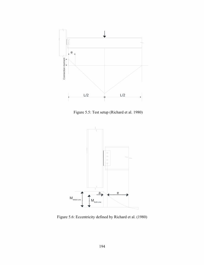
194

e

Con

nect

ion

mom

ent

L/2 L/2

Figure 5.5: Test setup (Richard et al. 1980)

eaMWeld-Line MBolt-Line

Figure 5.6: Eccentricity defined by Richard et al. (1980)

195

44.5 mm 76.2 mm

[email protected] mm

44.5 mm 76.2 mm

[email protected] mm

Figure 5.7: Off-axis shear tab connections Hormby et al. (1984)

Moment-rotation curve

Moment

Rotation

MM

Beam Line: F = 50 ksi

Beam Line: F = 36 ksi

50

36

36 50

y

y

Figure 5.8: Beam line definitions for Fy=36 and Fy=50 steel beams (Hormby et al. 1984)

FFigure 5.9: D

End Shea

B

0.5

1.0

1.5

1.12

Figure 5.10

Directions of

ar : V/V

0.01 0.02

Beam un

Beam reaches M

Propo

by

0: Loading h

plate deform

0.03 0.04

ndergoes strain

M

Beam yields

sed load path

p

history applie(Astan

196

mations at bo1989)

M

0.05 0.06

n hardening

ed to shear cneh et al. 200

olt holes afte

Moment-rotation

connections u02)

er tests (Asta

n curve

End Ro

under gravit

aneh et al.

otation

ty loads

197

Loading Starts

Plate yielding

Bearing yielding

Edge distance fracture

Net section fracture

Bolt fracture

Weld fracture

Ductile Brittle

Figure 5.11: Hierarchy of failure modes: ductile and brittle (Astaneh et al. 2002)

Figure 5.12: Typical moment–rotation curves (Astaneh et al. 2002)

FFigure 5.13: M

True Pin Co

Figure 5

Moment–rot

nnection

.14: Selected

tation curves(As

SG1

SG2

SG3

SG4

DWT Su

Strain

d experimen

198

s proposed ftaneh 2005)

upports

n gauges

Te

Shear ta

ntal program

for shear tabs

SG1

SG2

SG3

SG4

Hydraulic Jack

est Beam

Stub Column

ab connection (5S

m test setup (T

s in compos

Test Frame

k

True

ST)

Thompson 2

ite beams

e Pin Connection

2009)

n

FFigure 5.15: (3ST),

(b)

FE models o(c) 4 bolt ST

of: (a) full coT connection

199

(a)

(c)

onnection asn (4ST), (d) 5

ssembly, (b)5 bolt ST co

(d)

3 bolt ST coonnection (5S

onnection ST)

200

(a)

(b)

Figure 5.16: Deformed shape of the connection assembly (a) experiment (Thompson 2009) (b) finite element

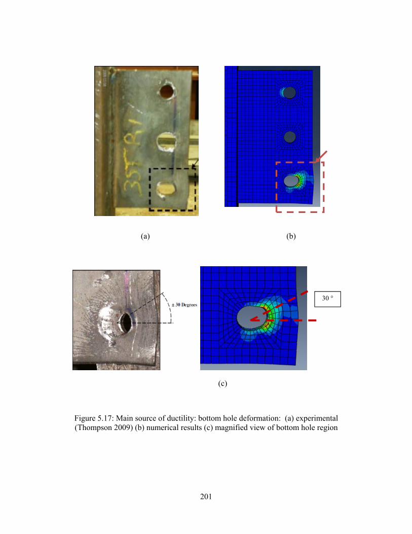
201

(a) (b)

(c)

Figure 5.17: Main source of ductility: bottom hole deformation: (a) experimental (Thompson 2009) (b) numerical results (c) magnified view of bottom hole region

30 °

202

(a) (b)

(c)

Figure 5.18: Failure of 3ST at the bottom hole by bearing deformation and rupture (a) experimental (Thompson 2009) and (b) numerical results (c) magnified view

of bottom hole region

203

(a) (b)

(c)



204

(a) (b)

(c)



205

(a)

(b)

Figure 5.21: Typical bolt shear deformation and failure (a) experimental (Thompson 2009) and (b) numerical results

Figure 5.22: Comparison of numerical and experimental shear response of connection 3ST

0.0

5.0

10.0

15.0

20.0

25.0

30.0

35.0

40.0

0.00 0.02 0.04 0.06 0.08 0.10 0.12 0.14

She

ar (

kN)


3STL1

3STR1

3STL2

3STR2

3STL3

3STR3

3ST-3/8-3/4

206

Figure 5.23: Comparison of numerical and experimental tensile response of connection 3ST

Figure 5.24: Comparison of numerical and experimental flexural response of connection 3ST

0.0

20.0

40.0

60.0

80.0

100.0

120.0

140.0

160.0

180.0

200.0

220.0

240.0

0.00 0.02 0.04 0.06 0.08 0.10 0.12 0.14

Ten

sion

(kN

)



0.0

2.0

4.0

6.0

8.0

10.0

12.0

14.0

16.0

18.0

20.0

22.0

24.0

26.0

0.00 0.02 0.04 0.06 0.08 0.10 0.12 0.14

Mom

ent (

kN.m

)


3STL1

3STR1

3STL2

3STR2

3STL3

3STR3

3ST-3/8-3/4

207



0.0

5.0

10.0

15.0

20.0

25.0

30.0

35.0

40.0

45.0

0.00 0.02 0.04 0.06 0.08 0.10

She

ar (

kN)



0.0

20.0

40.0

60.0

80.0

100.0

120.0

140.0

160.0

180.0

200.0

220.0

0.00 0.02 0.04 0.06 0.08 0.10

Ten

sion

(kN

)



208



0.0

5.0

10.0

15.0

20.0

25.0

30.0

35.0

40.0

45.0

0.00 0.02 0.04 0.06 0.08 0.10

Mom

ent(

kN.m

)



0.0

5.0

10.0

15.0

20.0

25.0

30.0

35.0

40.0

45.0

50.0

55.0

60.0

0.00 0.02 0.04 0.06 0.08 0.10

She

ar (

kN)



209



0.0

20.0

40.0

60.0

80.0

100.0

120.0

140.0

160.0

180.0

200.0

220.0

240.0

260.0

0.00 0.02 0.04 0.06 0.08 0.10

Ten

sion

(kN

)



0.05.0

10.015.020.025.030.035.040.045.050.055.060.065.070.075.080.0

0.00 0.02 0.04 0.06 0.08 0.10

Mom

ent (

kN)



Figure 5.31

Figure 5.32

0.0

2.0

4.0

6.0

8.0

10.0

12.0

14.0

16.0

18.0

20.0

22.0

24.0

26.0

0.00

Mom

ent (

kN.m

)

0.0

2.0

4.0

6.0

8.0

10.0

12.0

14.0

16.0

18.0

20.0

22.0

24.0

26.0

0.00

Mom

ent (

kN.m

)

: Bolt line fo

: Bolt line fo

0.02

Mom

Tensi

Shear

0 0.02

Mom

Tens

Shea

orces versus

orces versus

0.04Beam

ment

ion

r

0.04Beam

ment

sion

ar

210

beam end ro

beam end ro

0.06 0.0m End Rotation


otation – Spe

otation – Spe

08 0.10n (Rad)

08 0.10n (Rad)

ecimen 3ST

ecimen 3ST

0.12

0.12

-3/8-3/4

-1/4-3/4

0.0

20.0

40.0

60.0

80.0

100.0

120.0

140.0

160.0

180.0

200.0

220.0

240.0

0.14

0.0

20.0

40.0

60.0

80.0

100.0

120.0

140.0

160.0

180.0

200.0

220.0

240.0

0.14

Ten

sion

and

She

ar (

kN)

Ten

sion

and

She

ar (

kN)

Figure 5.33

Figure 5.34

0.0

2.0

4.0

6.0

8.0

10.0

12.0

14.0

16.0

18.0

20.0

22.0

24.0

26.0

0.00

Mom

ent (

kN.m

)

0.0

2.0

4.0

6.0

8.0

10.0

12.0

14.0

16.0

18.0

20.0

22.0

24.0

26.0

0.00

Mom

ent (

kN.m

)

: Bolt line fo

: Bolt line fo

0.02

Momen

Tension

Shear

0 0.02

Mo

Ten

She

orces versus

orces versus

0.04Beam

nt

n

0.04Bea

oment

nsion

ear

211

beam end ro

beam end ro


0.06 0am End Rotatio

otation – Spe

otation – Spe

08 0.10n (Rad)

0.08 0.10on (Rad)

ecimen 3ST

ecimen 3ST

0.12

0 0.12

-1/2-3/4

-3/8-5/8

0.0

20.0

40.0

60.0

80.0

100.0

120.0

140.0

160.0

180.0

200.0

220.0

240.0

0.14

0.0

20.0

40.0

60.0

80.0

100.0

120.0

140.0

160.0

180.0

200.0

220.0

240.0

0.14

0

0

0

0

0

0

0

0

Ten

sion

and

She

ar (

kN)

0

0

0

0

0

0

0

0

Ten

sion

and

She

ar (

kN)

Mt(

kN)

Figure 5.35

Figur

0.0

2.0

4.0

6.0

8.0

10.0

12.0

14.0

16.0

18.0

20.0

22.0

24.0

26.0

0.00

Mom

ent (

kN.m

)

0.0

2.0

4.0

6.0

8.0

10.0

12.0

14.0

16.0

18.0

20.0

22.0

24.0

26.0

0.00

Mom

ent (

kN.m

)

: Bolt line fo

re 5.36: Bolt

0.02

Mome

Tensio

Shear

0.02

Mome

Tensio

Shear

orces versus

t line forces v3ST-3

0.04 0Beam

ent

on

0.04 0

Beam

ent

on

212

beam end ro

versus beam3/8-3/4-A49

0.06 0.08End Rotation

0.06 0.08

End Rotation

otation – Spe

m end rotation90

8 0.10(Rad)

8 0.10

(Rad)

ecimen 3ST

n – Specime

0.12

0.12

-3/8-7/8

en

0.0

20.0

40.0

60.0

80.0

100.0

120.0

140.0

160.0

180.0

200.0

220.0

240.0

0.14

0.0

20.0

40.0

60.0

80.0

100.0

120.0

140.0

160.0

180.0

200.0

220.0

240.0

0.14

Ten

sion

and

She

ar (

kN)

Ten

sion

and

She

ar (

kN)

Mt(

kN)

Figure 5.37

Figure 5.38:

0.0

3.0

6.0

9.0

12.0

15.0

18.0

21.0

24.0

27.0

30.0

33.0

36.0

39.0

42.0

45.0

0.00

Mom

ent (

kN.m

)

0.0

3.0

6.0

9.0

12.0

15.0

18.0

21.0

24.0

27.0

30.0

33.0

36.0

39.0

42.0

45.0

0.00

Mom

ent (

kN.m

)

: Bolt line fo

: Bolt line fo

0.02

Momen

Tensio

Shear

0.02

Moment

Tension

Shear

orces versus

orces versus

0.04Beam E

nt

on

0.04Beam

t

n

213

beam end ro

beam end ro

0.06End Rotation (R

0.06End Rotation (

otation – Spe

otation – Spe

0.08Rad)

0.08(Rad)

Change iof tensile

ecimen 4ST

ecimen 4ST

0.10

0.10

in the slope e response

-3/8-3/4

T-1/4-3/4

0.0

20.0

40.0

60.0

80.0

100.0

120.0

140.0

160.0

180.0

200.0

220.0

Ten

sion

and

She

ar (

kN)

0.0

20.0

40.0

60.0

80.0

100.0

120.0

140.0

160.0

180.0

200.0

220.0

Ten

sion

and

She

ar (

kN)

()

Figure 5.39

Figure 5.40

0.0

3.0

6.0

9.0

12.0

15.0

18.0

21.0

24.0

27.0

30.0

33.0

36.0

39.0

42.0

45.0

0.00

Mom

ent (

kN.m

)

0.0

3.0

6.0

9.0

12.0

15.0

18.0

21.0

24.0

27.0

30.0

33.0

36.0

39.0

42.0

45.0

0.00

Mom

ent (

kN.m

)

: Bolt line fo

: Bolt line fo

0.02

Mom

Tens

Shea

0.02

Mo

Ten

She

orces versus

orces versus

0.04Beam

ment

sion

ar

0.04Beam

oment

nsion

ear

214

beam end ro

beam end ro

0.06m End Rotation

0.06m End Rotation

otation – Spe

otation – Spe

0.08(Rad)

0.08n (Rad)

ecimen 4ST

ecimen 4ST

0.10

0.10

-1/2-3/4

-3/8-5/8

0.0

20.0

40.0

60.0

80.0

100.0

120.0

140.0

160.0

180.0

200.0

220.0

Ten

sion

and

She

ar (

kN)

0.0

20.0

40.0

60.0

80.0

100.0

120.0

140.0

160.0

180.0

200.0

220.0

Ten

sion

and

She

ar(k

N)

()

Ten

sion

and

She

ar (

kN)

Figure 5.41

Figur

0.0

3.0

6.0

9.0

12.0

15.0

18.0

21.0

24.0

27.0

30.0

33.0

36.0

39.0

42.0

45.0

0.00

Mom

ent (

kN.m

)

0.0

3.0

6.0

9.0

12.0

15.0

18.0

21.0

24.0

27.0

30.0

33.0

36.0

39.0

42.0

45.0

0.00

Mom

ent (

kN.m

)

: Bolt line fo

re 5.42: Bolt

0 0.02

Mom

Tens

Shea

0.02

Mo

Ten

She

orces versus

t line forces v4ST-3

2 0.04Beam

ment

sion

ar

0.04Beam

oment

nsion

ear

215

beam end ro


0.06m End Rotation

0.06End Rotation (

otation – Spe

m end rotation90

0.08n (Rad)

0.08(Rad)

ecimen 4ST

n – Specime

0.10

0.10

-3/8-7/8

en

0.0

20.0

40.0

60.0

80.0

100.0

120.0

140.0

160.0

180.0

200.0

220.0

Ten

sion

and

She

ar (

kN)

0.0

20.0

40.0

60.0

80.0

100.0

120.0

140.0

160.0

180.0

200.0

220.0

Ten

sion

and

She

ar (

kN)

Figure 5.43

Figure 5.44

0.0

5.0

10.0

15.0

20.0

25.0

30.0

35.0

40.0

45.0

50.0

55.0

60.0

65.0

70.0

75.0

80.0

0.00

Mom

ent (

kN.m

)

0.05.0

10.015.020.025.030.035.040.045.050.055.060.065.070.075.080.0

0.00

Mom

ent (

kN.m

)

: Bolt line fo

: Bolt line fo

0 0

Mo

Ten

She

0

Momen

Tension

Shear

orces versus

orces versus

0.02

Beam

oment

nsion

ear

.02

Beam

nt

n

216

beam end ro

beam end ro

0.04

m End Rotatio

0.04

m End Rotatio

otation – Spe

otation – Spe

0.06

n (Rad)

0.06

on (Rad)

ecimen 5ST

ecimen 5ST

0.08

0.08

-3/8-3/4

-1/4-3/4

0.0

20.0

40.0

60.0

80.0

100.0

120.0

140.0

160.0

180.0

200.0

220.0

240.0

260.0

id

h(k

)

0.0

20.0

40.0

60.0

80.0

100.0

120.0

140.0

160.0

180.0

200.0

220.0

240.0

260.0

Ten

sion

and

She

ar (

kN)

Ten

sion

and

She

ar (

kN)

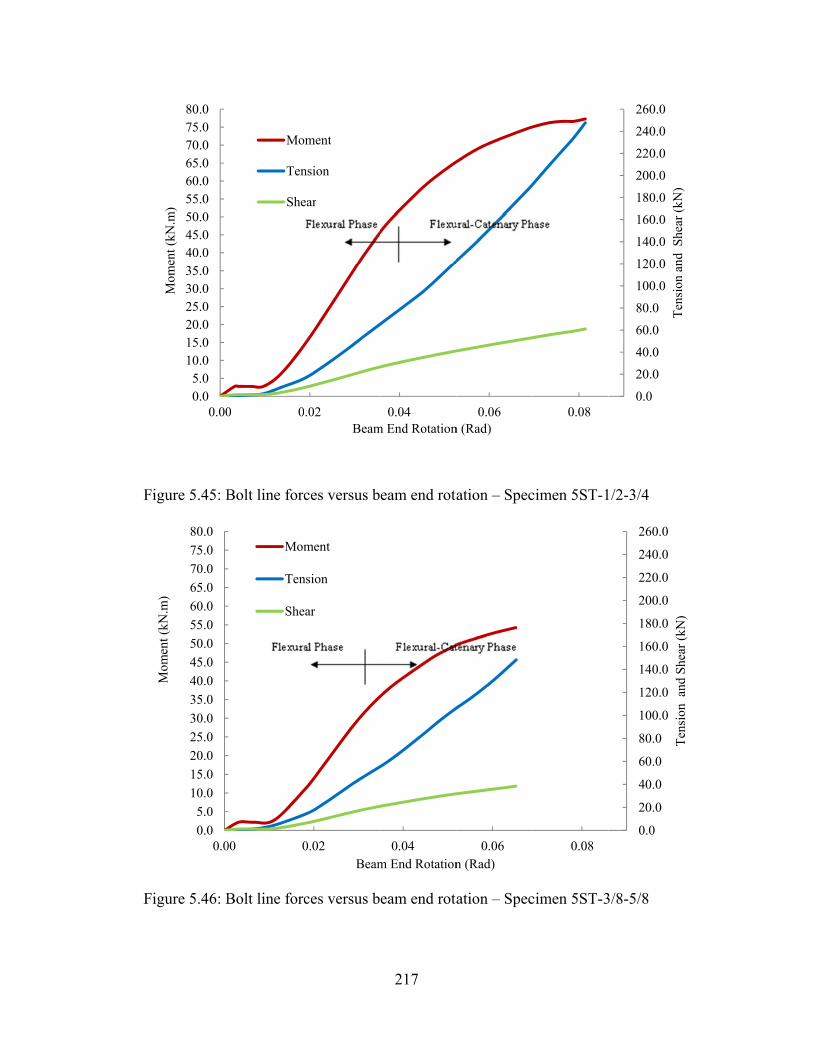
F

F

igure 5.45: B

igure 5.46: B

0.05.0

10.015.020.025.030.035.040.045.050.055.060.065.070.075.080.0

0.00

Mom

ent (

kN.m

)

0.0

5.0

10.0

15.0

20.0

25.0

30.0

35.0

40.0

45.0

50.0

55.0

60.0

65.0

70.0

75.0

80.0

0.0

Mom

ent (

kN.m

)

Bolt line forc

Bolt line forc

0 0

Mo

Ten

She

00 0

Mom

Ten

She

ces versus b

ces versus b

.02Beam

oment

nsion

ear

0.02Beam

ment

nsion

ear

217

eam end rota

eam end rota

0.04m End Rotation

0.04m End Rotation

ation – Spec

ation – Spec

0.06n (Rad)

0.06n (Rad)

cimen 5ST-1

cimen 5ST-3

0.08

0.08

1/2-3/4

3/8-5/8

0.0

20.0

40.0

60.0

80.0

100.0

120.0

140.0

160.0

180.0

200.0

220.0

240.0

260.0

Ten

sion

and

She

ar (

kN)

0.0

20.0

40.0

60.0

80.0

100.0

120.0

140.0

160.0

180.0

200.0

220.0

240.0

260.0

Ten

sion

and

She

ar(k

N)

()

Ten

sion

and

She

ar (

kN)

Figure 5.47

Figur

0.0

5.0

10.015.0

20.0

25.0

30.0

35.0

40.045.0

50.0

55.0

60.0

65.070.0

75.0

80.0

0.0

Mom

ent (

kN.m

)

0.05.0

10.015.020.025.030.035.040.045.050.055.060.065.070.075.080.0

0.00

Mom

ent (

kN.m

)

: Bolt line fo

re 5.48: Bolt

00

Mo

Ten

She

0

Mo

Ten

She

orces versus

t line forces vST-3

0.02Bea

oment

nsion

ear

0.02

Beam

oment

nsion

ear

218

beam end ro


0.04am End Rotatio

0.04

m End Rotatio

otation – Spe

m end rotation0

0.06on (Rad)

0.06

on (Rad)

ecimen 5ST

n – Specime

0.08

0.08

-3/8-7/8

en

0.0

20.0

40.0

60.0

80.0

100.0

120.0

140.0

160.0

180.0

200.0

220.0

240.0

260.0

0.0

20.0

40.0

60.0

80.0

100.0

120.0

140.0

160.0

180.0

200.0

220.0

240.0

260.0

Ten

sion

and

She

ar (

kN)

Ten

sion

and

She

ar (

kN)

219

Figure 5.49: Comparison of shear response of 3ST connections with different plate thicknesses

Figure 5.50: Comparison of tensile response of 3ST connections with different plate thicknesses

0.0

5.0

10.0

15.0

20.0

25.0

30.0

35.0

40.0

0.00 0.02 0.04 0.06 0.08 0.10 0.12 0.14

She

ar (

kN)


3ST-1/2-3/4

3ST-3/8-3/4

3ST-1/4-3/4

0.0

20.0

40.0

60.0

80.0

100.0

120.0

140.0

160.0

180.0

200.0

220.0

240.0

0.00 0.02 0.04 0.06 0.08 0.10 0.12 0.14

Ten

sion

(kN

)


3ST-1/2-3/4

3ST-3/8-3/4

3ST-1/4-3/4

220

Figure 5.51: Comparison of flexural response of 3ST connections with different plate thicknesses

Figure 5.52: Comparison of shear response of 3ST connections with different bolt sizes

0.0

2.0

4.0

6.0

8.0

10.0

12.0

14.0

16.0

18.0

20.0

22.0

24.0

26.0

0.00 0.02 0.04 0.06 0.08 0.10 0.12 0.14

Mom

ent (

kN.m

)


3ST-1/2-3/4

3ST-3/8-3/4

3ST-1/4-3/4

0.0

5.0

10.0

15.0

20.0

25.0

30.0

35.0

40.0

0.00 0.02 0.04 0.06 0.08 0.10 0.12 0.14

She

ar (

kN)


3ST-3/8-7/8

3ST-3/8-3/4

3ST-3/8-5/8

221

Figure 5.53: Comparison of tensile response of 3ST connections with different bolt sizes

Figure 5.54: Comparison of flexural response of 3ST connections with different bolt sizes

0.0

20.0

40.0

60.0

80.0

100.0

120.0

140.0

160.0

180.0

200.0

220.0

240.0

0.00 0.02 0.04 0.06 0.08 0.10 0.12 0.14

Ten

sion

(kN

)


3ST-3/8-7/8

3ST-3/8-3/4

3ST-3/8-5/8

0.0

2.0

4.0

6.0

8.0

10.0

12.0

14.0

16.0

18.0

20.0

22.0

24.0

26.0

0.00 0.02 0.04 0.06 0.08 0.10 0.12 0.14

Mom

ent (

kN.m

)


3ST-3/8-7/8

3ST-3/8-3/4

3ST-3/8-5/8

222



0.0

5.0

10.0

15.0

20.0

25.0

30.0

35.0

40.0

45.0

50.0

0.00 0.02 0.04 0.06 0.08 0.10

She

ar (

kN)


4ST-1/2-3/4

4ST-3/8-3/4

4ST-1/4-3/4

0.0

20.0

40.0

60.0

80.0

100.0

120.0

140.0

160.0

180.0

200.0

220.0

0.00 0.02 0.04 0.06 0.08 0.10

Ten

sion

(kN

)


4ST-1/2-3/4

4ST-3/8-3/4

4ST-1/4-3/4

223



0.0

5.0

10.0

15.0

20.0

25.0

30.0

35.0

40.0

45.0

0.00 0.02 0.04 0.06 0.08 0.10

Mom

ent(

kN.m

)


4ST-1/2-3/4

4ST-3/8-3/4

4ST-1/4-3/4

0.0

5.0

10.0

15.0

20.0

25.0

30.0

35.0

40.0

45.0

50.0

0.00 0.02 0.04 0.06 0.08 0.10

She

ar (

kN)


4ST-3/8-7/8

4ST-3/8-3/4

4ST-3/8-5/8

224



0.0

20.0

40.0

60.0

80.0

100.0

120.0

140.0

160.0

180.0

200.0

220.0

0.00 0.02 0.04 0.06 0.08 0.10

Ten

sion

(kN

)


4ST-3/8-7/8

4ST-3/8-3/4

4ST-3/8-5/8

0.0

5.0

10.0

15.0

20.0

25.0

30.0

35.0

40.0

45.0

0.00 0.02 0.04 0.06 0.08 0.10

Mom

ent(

kN.m

)


4ST-3/8-7/8

4ST-3/8-3/4

4ST-3/8-5/8

225



0.0

5.0

10.0

15.0

20.0

25.0

30.0

35.0

40.0

45.0

50.0

55.0

60.0

65.0

0.00 0.02 0.04 0.06 0.08

She

ar (

kN)


5ST-1/2-3/4

5ST-3/8-3/4

5ST-1/4-3/4

0.0

20.0

40.0

60.0

80.0

100.0

120.0

140.0

160.0

180.0

200.0

220.0

240.0

260.0

0.00 0.02 0.04 0.06 0.08

Ten

sion

(kN

)


5ST-1/2-3/4

5ST-3/8-3/4

5ST-1/4-3/4

226



0.05.0

10.015.020.025.030.035.040.045.050.055.060.065.070.075.080.0

0.00 0.02 0.04 0.06 0.08

Mom

ent (

kN)


5ST-1/2-3/4

5ST-3/8-3/4

5ST-1/4-3/4

0.0

5.0

10.0

15.0

20.0

25.0

30.0

35.0

40.0

45.0

50.0

55.0

60.0

65.0

0.00 0.02 0.04 0.06 0.08

She

ar (

kN)


5ST-3/8-7/8

5ST-3/8-3/4

5ST-3/8-5/8

227



0.0

20.0

40.0

60.0

80.0

100.0

120.0

140.0

160.0

180.0

200.0

220.0

240.0

260.0

0.00 0.02 0.04 0.06 0.08

Ten

sion

(kN

)


5ST-3/8-7/8

5ST-3/8-3/4

5ST-3/8-5/8

0.05.0

10.015.020.025.030.035.040.045.050.055.060.065.070.075.080.0

0.00 0.02 0.04 0.06 0.08

Mom

ent (

kN)


5ST-3/8-7/8

5ST-3/8-3/4

5ST-3/8-5/8

228

Figure 5.67: Shear tab connection rotation capacities versus connection depth for all the experimental and numerical data

Figure 5.68: Proposed equation for shear tab connection rotation capacities versus connection depth

0.000

0.020

0.040

0.060

0.080

0.100

0.120

0.140

0.160

0 2 4 6 8 10 12 14

Rot

atio

n (R

ad)

Connection Depth (in)

3ST-EXP

3ST-FEA

4ST-EXP

4ST-FEA

5ST-EXP

5ST-FEA

ϴ = -0.0094 dconn + 0.179

0.000

0.020

0.040

0.060

0.080

0.100

0.120

0.140

0.160

0 2 4 6 8 10 12 14

Rot

atio

n (R

ad)


EXP & FEA Results

Linear (EXP & FEA Results)

229

Figure 5.69: Comparison of plastic rotation capacities of shear tab connections based on ASCE 41 (2006), DoD (2009) and proposed equation

ϴ = -0.0066 dconn + 0.125

ϴ = -0.0036 dconn + 0.15

ϴ = -0.0015 dconn + 0.0502

0.000

0.020

0.040

0.060

0.080

0.100

0.120

0.140

0.160

0 2 4 6 8 10 12 14

Rot

atio

n (R

ad)


EXP & FE ResultsASCE 41DoD 2009

230

6 Behaviour of WT Connections in Column Removal Scenario

6.1 Introduction

WT connections are another relatively common option for steel gravity frames

with simple shear connections. They can either be bolted or welded to the column

flange and the beam web, as shown in Figure 6.1. Common types of material used

in WT connections are mentioned in Table 6.1. A properly-designed WT shear

connection is able to transfer shear force from a simply supported beam to an

adjacent supporting column without developing significant moment. Sustaining

tensile force is not generally considered in the common practice of designing

shear connections. Meanwhile, since current progressive collapse design

guidelines, such as those by the DoD (2009) and GSA (2003), ask designers to

specify robust connections that maintain their integrity in a double-span “column

removal” scenario, there is a necessity to investigate anticipated shear connection

performance under the simultaneous presence of shear, moment, and tension.

Currently, little is known about how WT connections would perform under these

conditions.

In order to model the behaviour of steel connections in progressive collapse

analyses, the DoD (2009) guidelines provide a table that includes models for

double angle and shear tab connections. However, some important types of shear

connections, such as WTs, are excluded. For these cases, engineers are directed to

tables available in seismic design codes and guidelines, such as ASCE 41 (2006),

although there are substantial differences between connection performances when

subjected to seismic loading as opposed to a column loss event as discussed in

chapter 2. Therefore, the behaviour of WT connections needs to be characterized

in the new scenario. Behaviour characterization in this study of WT connections

includes the investigation of the possible failure modes and the shear, axial and

231

moment interaction response of the connection when an adjacent column is

compromised.

In this chapter, the finite element method is adopted to simulate the response of

WT connections when a column is lost, regardless of the cause. The finite element

models are verified by available experimental data following the same loading

regime. Verified models are utilized to expand the database of the test results.

Simultaneous presence of shear, axial force, and moment versus chord rotation

diagrams are presented for both the numerical and experimental results. Effects of

changes in WT size, bolt size and type are also investigated and conclusions are

made. The results are utilized to develop the modelling parameters that can

predict the rotational behaviour of WT connections in the new scenario.

6.2 Objective and scope

This chapter is focused on the behaviour of WT shear connections under

simultaneous presence of shear, tension and moment. High-fidelity finite element

models of WT shear connections in the column removal scenario are developed

and verified in terms of both load path and failure modes. These models can shed

more light on the performance and the sources of ductility in WT connections.

The results can be used to select suitable connection modelling parameters for

progressive collapse evaluations of steel frames with similar WT shear

connections.

The focus of the research is on bolted-bolted WT shear connections, shown in

Figure 6.1(d). This type of WT connection is perhaps the most challenging one in

the whole research in terms of analysis cost due to the presence of numerous

bolts, which leads to many contact surfaces and consequently potential

convergence problems. Connection depth (and the resulting number of bolts) is

the sole variable in the experimental specimens discussed herein. However,

232

extensive parametric study is performed to expand the database on the behaviour

of such connections by changing factors such as the WT cross-sectional size, bolt

grade and diameter.

6.3 Selected previous research

Astaneh (1989) investigated the demand and supply of ductility in steel shear

connections, which became a basis for his later work on different types of shear

connections including WT connections. Astaneh acknowledged shear, axial and

moment as the major forces present in simple shear connections. While axial

forces often also exist in industrial structures, shear is the most prevalent one.

Among the associated displacements, including shear and axial displacements and

also rotation, he concluded that rotation is the major component. He stated that

there were no records of effects of axial loading on the behaviour of simple

connections at that time. As a result, the main characteristic features he focused

on were: (1) shear–moment interaction; (2) moment–rotation response; (3) shear

force–shear displacement behaviour; (4) failure modes; and (5) shear force–

rotation interaction. Due to the presence of irregularities, discontinuities,

constraints, inelasticity and material hardening and softening that complicate the

stress and strain fields in a shear connections, Astaneh recommended that

experiments be conducted to measure mechanical features and sources of strength

and ductility.

Astaneh and Nader (1989) studied the behaviour of WT connections by

performing nine full-scale tests on WT connections that were welded to the

column flange and bolted to the beam web with either three or five bolts (Figure

6.1(a)). Table 6.2 summarizes the results of the tests performed. The materials

were ASTM A36 for the WT and ASTM A325 or ASTM A490 for the bolts. The

connections were subjected to: (1) moments to measure the rotational ductility,

and (2) combinations of shear and rotation—representative of a typical simply

233

supported beam—to measure the shear strength. Based on the experimental

results, the authors concluded that WT connections subjected to shear are quite

flexible and able to accommodate rotational demands as large as 0.07 radians.

They observed a substantial amount of shear yielding in the stem and flange of the

WT before failure happened. The failure limit states were: (1) WT stem yielding,

(2) WT stem fracture, (3) bolt shear fracture, (4) weld fracture, (5) WT flange

yielding, or (6) bolt hole bearing failure, all shown in Figure 6.2. The failure

mode possible in thin-flange WTs is shear yielding of the WT flange, which was

not observed during the tests. They suggested using at least a minimum of 1.5

times the diameter of the bolts as the horizontal and vertical edge distances. Their

test results indicated that one of the major factors that provided ductility to the

WT connections was the WT flange out-of-plane bending.

In a later work, Astaneh (2005) discussed three sources of rotational ductility in

WT connections subjected to simultaneously applied shear and rotation: (a) out-

of-plane bending of the WT flange; (b) yielding of the WT stem; (c) bolt slippage;

and (d) bolt hole bearing deformation. The location of the inflection point in a WT

connection of a simply supported beam is between the bolt and weld lines, similar

to double angle connections. Hence, double angle and WT connections develop a

relatively small moment.

Thornton (1996) applied an analytical approach to propose a design algorithm for

WT connections bolted to the beam web and either welded or bolted to the

support (Figure 6.1(a) and (d)). He used the results of Astaneh's experiments to

verify the method for the welded-bolted connections; however, for the bolted-

bolted connections he used the results of bolted double angle connections due to

the lack of more appropriate experimental data. He assumed that WT connections

under shear loading rotate about their lower edge, which produces the load

distribution shown in Figure 6.3, where V is the net transverse shear distribution

in the WT flange considering both sides of the stem at the vertical yield lines. He

ignored the reduction effect of the shear force on the plastic moment capacity.

234

Based on yield line theory, the moment and shear capacity of the connection can

be evaluated as shown in Figure 6.4. The equations derived in his research are

used to analytically compare with the experimental research by Astaneh and

Nader (1989). The same procedure is applied for the bolted connections, although

there were no experiments for comparison. He proposed equations for minimum

weld size and bolt diameter to ensure the required ductility.

In supplementary research, Thornton (1997) considered shear connections

subjected to axial forces in addition to shear force. He concluded that the

additional axial load tends to make shear connections less flexible. He developed

equations that can be used to distinguish if this reduced flexibility will lead to

progressive fracture of the connection. He also provided a design method that

provides adequate strength with maximum flexibility for three types of shear

connections including WTs.

6.4 Numerical study method

The behaviour of WT connections subjected to simultaneous shear, moment, and

tension is investigated using high-fidelity finite element models. All stages of

simulation, including pre- and post-processing procedures, were performed using

Abaqus/CAE, with Abaqus/standard used as the analysis engine (Dassault

Systèmes 2009).


Experiments performed by Friedman (2009) were used to verify the results of the

numerical models. Figure 6.5 demonstrates the connection subassembly and the

test setup. A total of nine full-scale tests were carried out, with the connection

depth as the sole varying factor. Some of the tests were continued after the initial

failure; however, only the results up to this point are of interest in this research.

235

6.4.2 Finite element model description

Three-dimensional solid elements were used for all the components of the model

due to the nature of the connection modelling problem. The models consist of the

central column stub and the adjacent beams, as well as the connections with

complete detailing, as shown in Figure 6.6(a). Three, four and five bolt shear tab

connections were modelled, as illustrated in Figure 6.6(b) to Figure 6.6(d). The

plates are welded to the column flange and bolted to the beam web. The central

stub column is pushed down, while the connection performance is monitored.

Since the connection is the point of interest, all characteristic features of the

connections are included in the models. Strain-based fracture criteria established

in chapter 3 were utilized for the WT connections after verification in order to

predict the failure modes. All other characteristic features of the models, including

bolt pre-tensioning, material properties, contact calibration and element types are

discussed in chapter 3. Characteristic features of all the connections numerically

studied are summarized in Table 6.3. A sample of the deformed shape of the

connection assembly after the experiment is compared with its corresponding

finite element analysis result in Figure 6.7.

The models are labelled based on the following method: first the number of bolts

in a vertical line, then WT, which is the abbreviation for tee connections utilized

in this research, then the WT section size in SI units and the bolt diameter in

imperial units. For example, 3WT125X33.5-3/4 refers to the WT connection with

three bolts; WT125X33.5 tee size, and 3/4 in (19.1 mm) diameter bolts. The bolts

are all ASTM A325; unless at the end of label, “A490” is added. All the WT

sections are made of ASTM A992 steel. For the ones for which experimental data

is available (see Table 6.3), verification—as well as comprehensive comparisons

of experimental and numerical results—is performed.

236


Although based on the benchmark example provided in chapter 2 (following the

procedure outlined is expected to produce valid results for all types of shear

connections, including WT type, in the column loss event), the verification

process is performed for WT connections with three, four, and five bolts since

experimental results are available. For the purpose of verification, deformed

shapes, failure modes, and internal force diagrams are compared with the

experimental results.

Figure 6.8 to Figure 6.10 compare the experimental versus numerical deformed

shape of WT connection components for all the experiments utilized in this study.

Although there are similarities in the behaviour of each connection depth (i.e.,

three, four or five bolt), there are some differences that are discussed in the

following sections. To ensure that a WT connection will survive the column

removal scenario, it should be capable of carrying the combined effects of shear

and moment, as well as a large catenary tensile force. The internal forces (i.e.,

shear, tension, and moment) at the bolt line versus the chord rotation of

connection assemblies 3WT, 4WT and 5WT are shown in Figure 6.11 to Figure

6.19. The dashed and solid lines represent the results of the experiments and

simulations, respectively. While the general trends in all force responses of the

connections correlate well, some discrepancies between the experimental and

numerical results exist, which are discussed in section 6.5.1 to 6.5.3:

6.5.1 Three bolt WT connections (3WT)


Figure 6.8(a) shows the numerical and experimental deformed shapes of the 3WT

connections before failure.

237

Figure 6.8(b) shows a typical bolt shear deformation and rupture obtained from

the tests and finite element deformed shapes of the WT-to-beam bolts. Shear

deformation in the bottom bolt leads to bolt shear rupture, which was the

governing failure mode for all the 3WT experiments. The middle bolt remains

almost elastic throughout the loading; meanwhile, the top bolt starts to experience

plastic deformation due to compressive action from the force couple at early

stages of loading, which is released after catenary action is developed in the

connection. The numerical model predicts the bottom bolt shear rupture very well

with removed elements, as shown in

Figure 6.8(b). Bolts connecting the WT flange to the stub column flange remain

almost elastic (not shown in Figure 6.8(b)). The distribution of bearing stress at

the bottom hole at a 15-to-30 degree angle from the horizontal line is recorded in

both the test report (Friedman 2009) and the numerical results, as depicted in

Figure 6.8(c) accompanied by a magnified view of the bottom hole region

comparing with the plastic strain distribution obtained by the finite element

model. Most of the plastic deformation occurred around the bottom hole of the

WT section. No distortion occurred around the second hole. Presence of the force

couple is obvious in both the numerical model and experimental results, imposing

compressive and tensile forces to the top and bottom holes, respectively.

6.5.1.2 Shear, tension, and moment interaction

Internal forces at the bolt line versus the chord rotation of connection assemblies

3WT are shown in Figure 6.11 to Figure 6.13. The shear response of the

connections (Figure 6.11), tensile behaviour (Figure 6.12) and moment response

(Figure 6.13) serve to verify the models based on acceptable correlation with the

associated experimental results.

There are some differences at the beginning of the experimental response of 3WT

connections, mostly shear and moment, in comparison with numerical results.

This difference is directly related to the location of the bolts in the holes in the

238

experimental program. It is assumed that the bolts are located exactly at the centre

of the holes in the finite element models. However, determination of the precise

locations of the bolts’ shanks inside the holes is unfeasible. As a result, this

discrepancy at the early stage of loading is inevitable. Furthermore, some of the

holes were reamed due to minor misalignment in order to make them fit during

erection of the test setup. This will add complication to the problem in terms of

variability and unknown issues embedded. Table 6.4 summarizes the test and

finite element analysis values of the shear, moment, and tension at the initial

failure for the 3WT connections. Internal forces and chord rotations determined

from the numerical models are in acceptable agreement with the experimental

results, with less than a 9% deviation. Rotation at the initial failure, as one of the

main studied parameters, has a deviation of less than 2%. As observed in Table

6.4, the failure mode for all of the tests is bolt shear rupture at the bottom hole,

and the finite element results portray the same type of ultimate limit state.

6.5.2 Four bolt WT connections (4WT)


Figure 6.9(a) shows the numerical and experimental deformed shapes of the 4WT

connections at failure. Shear deformation at the bottom bolt shank led to a failure

similar to what is shown in Figure 6.9(b). The top bolt and the third from the top

experienced some plastic deformation; nevertheless, the rest of the bolts,

including the WT-to-column-flange ones remained elastic. Similar to the 3WT

connections, most of the plastic deformation occurred around the bottom hole of

the WT and the bottom bolt, in which finally the rupture occurred. No distortion

occurred around the second hole from the top. The top and bottom bolts provided

a greater percentage of flexural resistance than the middle two. Presence of a force

couple is obvious in both the numerical model and experimental results about the

approximate location of the centroid of the bolt group, closer to the second top

239

bolt, imposing compressive force to the top hole and tensile force to the two

bottom ones. Illustrated in Figure 6.9(c), the stress distribution around the bottom

hole in the 4WT confirms the stress distribution happening in the experimental

program following the 15-to-30 degree trend observed in the 3WT connections.



assemblies 4WT are shown in Figure 6.14 to Figure 6.16. The shear response of

the connections (Figure 6.14), tensile behaviour (Figure 6.15), and moment

response (Figure 6.16) serve to verify the models based on acceptable agreement

with the associated experimental results. Similar to the 3WT connections, some

differences exist in the load paths, particularly at the beginning of the

experimental response of 4WT connections, in comparison with numerical result.

The same reasons mentioned for 3WT connection can be stated, including the

location of the bolts in the holes in the experimental program. Unknown

horizontal stiffness of the test setup causes the difference observed in the Figure

6.15.


moment, and tension at the initial failure of the 4WT connections. As can be

observed, shear and tension forces, as well as the chord rotations, determined

from the numerical models are in acceptable agreement with the experimental

results. The largest difference is related to the tension, which is about a 10%

deviation from the experimental results, which is still considered acceptable. As

can be seen in Table 6.5, the failure mode for the tests is bolt shear rupture at the

bottom hole, and the finite element results convey the same type of ultimate limit

state.

240

6.5.3 Five bolt WT connections (5WT)


Figure 6.10(a) illustrates the numerical versus experimental deformed shapes of

the 5WT connections. Similar to the 3WT and 4WT connections, most of the

plastic deformation occurred around the bottom hole of the WT and the bottom

bolt shank in which the rupture ultimately occurred, as shown in Figure 6.10(b).

The top and the two bottom bolts connecting the WT to the beam web are the

ones that experienced plastic deformation. The rest of the bolts, including the ones

that connect the WT flange to the column, remained elastic. No distortion

occurred around the second and third hole from the top, as shown in Figure

6.10(c). The top and bottom two bolts provided a greater percentage of flexural

resistance than the other bolts by forming a force couple about the approximate

location of the centroid of the bolt group. Shear deformation of the bolts

accompanied by substantial plastic deformation of the bottom hole provides the

ductility of the connection, along with flexural deformation of the WT flange.

Similar to the 3WT and 4WT connections, the stress distribution around the

bottom hole in the 5WT (15-to-30 degree trend) is in agreement with the stress

distribution observed in the experimental program.



assemblies 5WT are shown in Figure 6.17 to Figure 6.19. Table 6.6 summarizes

the experimental and finite element analysis values of the shear, moment, and

tension at the initial failure for the 5WT connections. As observed, all

quantities—including shear, tension, and moment, as well as chord rotations—

determined from the numerical models are in acceptable agreement with the

experimental results, with less than 10% deviation from the experimental results.

241

The failure mode for the tests is bolt shear rupture at the bottom hole, confirmed

by the finite element results.


After verifying the finite element models with the test results, a parametric study

is performed in order to investigate the effects of different design parameters such

as WT size, bolt size and type, and also connection depth, according to Table 6.3.


Figure 6.20 to Figure 6.25 show the interactions of shear, tension and moment for

the WT connections with three bolts (3WT). The behaviour of 3WT125X33.5-3/4

was discussed in section 6.5.1 since experimental results were available. Its

response without the test curves is shown again in Figure 6.20 for the sake of

completeness of the report. As labelled in Figure 6.20, the point that the flexural

phase domination ends and catenary force begins to provide the major resistance

is distinguished. This point is called the “devolution point”, similar to the shear

tab connections discussed in chapter 5. For 3WT125X33.5-3/4, the devolution

point occurs when the flexural response starts to degrade after the maximum

moment is reached. The main reason for this is the fact that in three bolt

connections the bottom and top bolts resist the moment through bearing resistance

and out-of-plane bending of the WT’s flange. As soon as the localized yielding

around the contact surface accompanied by out-of-plane bending deformation of

the bottom of the WT’s flange happen, the flexural resistance starts to vanish and

the connection attempts to find another path to take additional load. The eventual

failure will be in the catenary phase. It is noted that for shear tab connections with

three bolts (3ST), the devolution point was located almost at the maximum

moment. In the 3WT connections, this point is shifted to after the maximum

242

moment due to out-of-plane bending of the WT, which does not exist in shear tab

connections. Although this out-of-plane deformation is small in a WT125X33.5

section (with 15.7 mm and 8.9 mm flange and stem thickness, respectively), it

exists particularly at the bottom of the connection and can act as one source of

providing ductility.


3WT100X26-3/4. In this model, the failure is initiated in the WT stem bottom

hole region. An increase in the ductility of the connection is observed in

comparison with 3WT125X33.5-3/4 due to the thinner stem and flange (12.6 mm

and 7.9 mm flange and stem thickness, respectively). At the same time, thickness

of the web is not so low that it causes premature failure. There are no significant

plastic shear deformations observed in the bolts connecting the WT flange to the

column. However, the top and bottom bolt connecting the WT stem to the beam

web experience major shear deformations prior to failure. Most of the bearing

deformation happens in the WT stem. Similar to 3WT125X33.5-3/4, the tensile

force starts to come into existence after the point of maximum moment, when the

flexural resistance starts to degrade. Shear force increases almost linearly up to

the rotation of 0.11 and after that with an increased rate up to the failure,

interacting with tension and moment especially at high rotations.


3WT155X33.5-3/4. The flange and stem thickness of 3WT155X33.5 are 14.6 mm

and 8.5 mm, respectively. This model fails due to WT bottom hole rupture,

similar to 3WT100X26-3/4. However, the ductility of the connection is not

increased significantly in comparison with 3WT125X33.5-3/4. It can be inferred

that the reduction in the thickness causes the change in the failure mode of

connection, but cannot increase the ductility of the connection significantly. There

is a significant plastic deformation in the top and bottom bolt shank (WT-to-beam

web bolts), particularly the bottom one, prior to failure, although the other bolts

(WT-to-column bolts) remain almost elastic. The tensile force starts to come into

243

existence slightly after the point of maximum moment. This could be assigned to

the contribution of out-of-plane deformation of WT flange that contributes to the

flexural resistance of the WT connection after local yielding around the bolt holes,

similar to what is discussed for 3WT125X33.5-3/4.


3WT125X33.5-5/8. In this model, the failure happens in the bottom bolt. The

amount of plastic deformation due to bearing is small around the top and bottom

holes. The connection does not show significant tensile resistance due to

premature failure of the bottom bolt. As a result, the ductility of the connection is

also reduced in comparison with 3WT125X33.5-3/4, but is still comparable.

There are significant plastic deformations at the top and bottom bolt shank before

failure, which were the main source of ductility of the connection. Contribution of

out-of-plane deformation of the WT flange is negligible. Although the devolution

from flexural to catenary is obvious in the connection response, it could not go

through the catenary phase significantly (about 0.02 radians).


3WT125X33.5-7/8. In this model, the failure is initiated in the WT bottom hole

region. Due to a larger bolt diameter, the amount of plastic deformation

happening in the bolt shank is small but distinguishable. There are significant

plastic deformations around the bottom bolt hole area in the WT stem. The tensile

force starts to come into existence after the point of maximum moment, similar to

the other 3WT connections.


3WT125X33.5-3/4-A490. The behaviour of this model is similar to that of

3WT125X33.5-3/4 with ASTM A325 bolts. However, the dominant limit state of

the connection is different. Using ASTM A490 bolts shifted the failure mode from

the bottom bolt to the WT bottom hole region. The ductility of the connection is

also reduced, which results in a reduction of the shear and tensile strength of the

connection in comparison with the one with ASTM A325 bolts.

244

As observed in the foregoing discussion, in 3WT connections, regardless of the

WT section, bolt size and type, as the flexural stiffness of the connection

approaches zero and then starts to degrade subsequently, the tensile catenary force

increases rapidly until the failure of the connection occurs. Tensile catenary

resistance starts to grow at the approximate chord rotation angle of 0.085, at

which time flexural response starts to reduce. The amount of moment present

immediately prior to failure of the connection is variable, and in some cases

substantial. However, it can be inferred that the 3WT connections fail mainly

because of catenary action. The dominant failure mode of 3WT connections is the

WT bottom hole rupture and bolt shear rupture.


Figure 6.26 to Figure 6.31 show the interactions of shear, tension, and moment for

WT shear connections with four bolts (4WT). The behaviour of 4WT125X33.5-

3/4 was discussed in section 6.5.2, but its response without the test result curves is

shown again in the Figure 6.26 for the sake of completeness of the report. The

“devolution point" for this connection is not as clear as for the 3WT connections.

Actually, there is a point that can be assigned as the “devolution point” in which

after substantial decrease in flexural stiffness, the tensile force starts to ramp up,

as shown in Figure 6.26. At the approximate rotation of 0.03 radians, yielding

starts to happen around the top and bottom holes; however, the system still can

capture more plastic deformation around the holes and also through out-of-plane

bending of the WT flange. As a result, the moment increases further, but with

reduced stiffness. Gradually, the amount of tensile force exceeds the compressive

value and the whole section goes through catenary action, after the rotation of

about 0.05. However, the connection fails in the flexural-catenary phase due to the

presence of a significant amount of moment and tension at the time of failure.


4WT100X26-3/4. In this model, the failure is initiated in the WT bottom hole

245

region. An increase in the ductility of the connection is observed in comparison

with 3WT125X33.5-3/4 due to the thinner web and flange. At the same time,

thickness of the web is not so low that it causes premature failure. The amount of

out-of-plane deformation of the flange is significantly higher than for the

4WT125X33.5-3/4 model. There are no significant plastic shear deformations

observed in the bolts connecting the WT flange to the column. However, the top

and bottom bolt connecting the WT stem to the beam web experience significant

shear deformation. Most of the bearing deformation happens around the top and

bottom hole in the WT stem. Similar to 4WT125X33.5-3/4, the tensile force starts

to come into existence after the devolution point (0.05 radians). This connection

possesses the highest ductility, and, consequently, the highest tensile resistance.

Shear force increases almost linearly after the 0.02 radians rotation, up to the

point of failure.


4WT155X33.5-3/4. This model fails due to WT bottom hole rupture, similar to

4WT100X26-3/4. However, the ductility of the connection is not increased

significantly in comparison with 3WT125X33.5-3/4. There is a significant plastic

deformation in the top and bottom bolt shank (WT-to-beam bolts), particularly the

bottom one, prior to the failure, although the other bolts (WT-to-column) remain

almost elastic. The tensile force starts to come into existence after the devolution

point (0.03), similar to 4WT125X33.5-3/4 and 4WT100X26-3/4. The tensile

catenary resistance of this model is slightly more than for the 4WT125X33.5-3/4

connection due to higher ductility. Shear force increases almost linearly after the

0.02 radians rotation, up to the point of failure, interacting with tension and

moment especially at high rotations.


4WT125X33.5-5/8. In this model, due to the reduction of bolt diameter

comparing with 4WT125X33.5-3/4, the failure happens in the bottom bolt, as

expected. The amount of plastic deformation due to bearing is small around the

246

top and bottom holes. The tensile capacity of the connection drops significantly

due to premature failure of the bolts. As a result, the ductility of the connection is

also reduced comparing to the 4WT125X33.5-3/4 model. There are significant

plastic deformations at the top and bottom bolt shank before failure, which are the

main source of ductility of the connection. Contribution of out-of-plane

deformation of the WT flange is negligible in this case. Similar to the

3WT125X33.5-5/8 model, the flexural-catenary phase does not last (about 0.03

radians) due to early shear rupture of a 5/8 in (15.9 mm) bolt.



region. Due to the larger bolt size, only a small amount of plastic deformation

happens in the bottom bolt shank. Top and bottom bolts of the WT-to-beam

connection are the only bolts which deformed significantly; the rest of the bolts

are almost elastic. There are significant plastic deformations around the bottom

bolt hole area at the WT stem. Devolution from one phase to another is similar to

other 4WT connections.


4WT125X33.5-3/4-A490. The behaviour of model 4WT125X33.5-3/4-A490 is

similar to that of 4WT125X33.5-3/4 with ASTM A325 bolts; however, the

dominant limit state is changed due to the change in the bolt grade. Using ASTM

A490 bolts shifts the failure mode from the bottom bolt to the WT bottom hole

region, similar to what was observed in the 3WT connections. The ductilities of

the connections are almost the same. The shear and flexural resistance of

4WT125X33.5-3/4-A490 is slightly higher than the similar connection with the

ASTM A325 bolts.

The “devolution” point between load-carrying mechanisms for 4WT connections

is not as clear as for 3WT connections, but still definable as a point. There is a

point in which the tensile force starts to ramp up after a substantial decrease in

flexural stiffness occurs. After this devolution point, the tensile catenary force

247

begins to play a role and grows rapidly until the failure of the connection, in the

presence of shear and moment. Tensile catenary resistance starts to grow at the

approximate chord rotation angle of 0.05 radians. The amount of moment at

failure is substantial and cannot be ignored. Besides, where the tensile force starts

to increase rapidly, the moment is still rising. Therefore, it can be inferred that the

4WT connections fail mainly because of flexural-catenary actions. The dominated

failure mode of 4WT connections is the WT bottom hole rupture and bolt shear

rupture, similar to 3WT connections.


Figure 6.32 to Figure 6.37 depict simultaneous presence of shear, tension, and

moment for the WT connections with five bolts (5WT). The behaviour of

5WT125X33.5-3/4 was discussed in section 6.5.3, but its response without the test

curves is shown again in the Figure 6.32 for the sake of completeness of the

report. A point is distinguished as a devolution point (at about the rotation of

0.025 radians) in which a substantial decrease in flexural stiffness occurs

accompanied by an increase in the rate of tensile response of the connection until

the failure.


5WT100X26-3/4. Its behaviour is similar to the 4WT100X26-3/4 and

3WT100X26-3/4 models due to the same geometric and mechanical properties.

The failure is initiated in the WT bottom hole region similarly. An increase in the

ductility of the connection is observed in comparison with 5WT125X33.5-3/4 due

to thinner web and flange. Out-of-plane deformation of the WT flange contributes

to the ductility of the connection, particularly at the bottom part, which makes the

connection more ductile than the other ones with different WT sections. There is

no significant plastic shear deformation observed in the bolts—even the bottom

bolt—since most of the bearing deformations happen in the thin plate. In the five

bolt connections, the interaction of shear, tension, and moment starts at the early

248

stages of loading, after the establishment of contacts, which is about 0.01 radians

of rotation. However, the devolution from the flexural to the catenary phase

happens at a point of about 0.025 radians, at which point the flexural stiffness

reduces drastically and the tension rate increases noticeably.


5WT155X33.5-3/4. Similar to 3WT155X33.5-3/4 and 4WT155X33.5-3/4, in the

5WT155X33.5-3/4 connection model assembly, the failure mode is shifted to the

bottom bolt due to the decrease in the thickness of WT stem. There is a slight

increase in the rotational ductility of the connection in comparison with

5WT125X33.5-3/4. There is also a substantial amount of plastic deformation in

the two bottom bolts and the one at the top prior to the failure. The other two bolts

are almost elastic. The devolution from flexural behaviour to the flexural-catenary

phase is obvious in Figure 6.34. At the rotation of about 0.022, a change happens

at the rate of tensile response of the connection which causes a reduction in the

slope of the flexural response.


5WT125X33.5-5/8. In this model, due to the reduction of bolt diameter

comparing with 4WT125X33.5-3/4 the failure happens in the bottom bolt, similar

to 3WT and 4WT connections with same configuration. The amount of plastic

deformation due to bearing is small around the top and bottom holes. The tensile

capacity of the connection drops significantly due to premature failure of the

bolts. As a result, the ductility of the connection is also reduced compared to the

5WT125X33.5-3/4 model. There are significant plastic deformations at the top

and bottom bolt shank before failure, which are the main source of ductility of the

connection. Contribution of out-of-plane deformation of the WT flange is

negligible. Due to early shear rupture of a 5/8 in (15.9 mm) diameter bolt, the

flexural-catenary phase does not have a large extent. However, at an approximate

rotation of 0.022 radians a change happens in the rate of increase of tensile force,

accompanied by a reduction in the slope of the flexural response.

249



region. Due to the larger bolt diameter, the amount of plastic deformation in the

bottom bolt shank is small, but still distinguishable. The top and the two bottom

bolts of the WT-to-beam connection are the only bolts that deformed slightly; the

rest of the bolts are elastic. There are significant plastic deformations around the

bottom bolt hole area. The devolution from flexural behaviour to the flexural-

catenary phase is obvious. Similar to all the other 5WT models, 0.022 radians of

rotation can be distinguished as a transition point in which the rate of tensile

response of the connection increases accompanied by a reduction in the slope of

the flexural response.


5WT125X33.5-3/4-A490. The behaviour of this model is similar to that of

5WT125X33.5-3/4 with ASTM A325 bolts. However, the dominant limit state of

the connection is different. Using ASTM A490 bolts shifted the failure mode from

the bottom bolt to the WT bottom hole region. The ductility of the

5WT125X33.5-3/4-A490 connection is slightly less than that of 5WT125X33.5-

3/4 with A325 bolts.

It is noted that 5WT connections go into catenary tension from the beginning, as

discussed in chapter 4. Since the depth of the connection was almost the same as

that of the beam, there is no vertical eccentricity in the 5WT connections

comparing with 4WT ones (see chapter 4 for further explanation). As a result,

tension does not need to cancel the compressive arching force in the connection,

unlike for the 4WT connections. Consequently, a reduction in the flexural

stiffness happens where the tensile response starts to ramp up rapidly where the

devolution “point” can be distinguished in 5WT connections. Regardless of the

WT section, bolt size and type, at the approximate rotation of 0.022 radians, a

significant decrease and increase in the slope of the flexural and tensile responses,

respectively, of the 5WT connections are observable. The amount of moment at

250

failure is significant. As a result, it can be inferred that the 5WT connections fail

mainly because of flexural-catenary actions. The dominant failure mode of 5WT

connections is the WT bottom hole rupture and bolt shear rupture, similar to what

was observed for WT connections with three (3WT) and four (4WT) bolts.

Table 6.7 summarizes the results of the numerical models in addition to the

experimental specimens at the initial failure of the connections.


In this section, the effect of WT size, bolt size and bolt type are discussed

separately for three, four and five bolt connections.


6.7.1.1 WT size

Figure 6.38 to Figure 6.40 illustrate the shear, tensile, and flexural responses of

3WT connections with different WT section sizes. Generally, the model

3WT100X26-3/4 behaves in a more ductile manner than the other two WT

connections. As can be seen, the thinner stem and flange causes an increase in

shear and tensile strengths of 3WT100X26-3/4 connections at the initial failure

rotation. At small rotations, the difference of shear and flexural response is

negligible, but as the rotation increases, the difference increases. In terms of

tensile response, the difference among the curves is minimal for a given rotation,

although the 3WT100X26-3/4 possesses more tensile capacity due to more

ductility. In terms of load path, the tensile response of the connection does not

change significantly by altering the WT section size. However, the maximum

tensile catenary force they can develop is highly dependent on the WT geometry.

The shear strengths of the 3WT125X33.5-3/4 and 3WT155X33.5-3/4 connections

251

are almost the same, but are smaller than that of 3WT100X26-3/4 (about 70%) at

the initiation of failure. In terms of axial strength, this value reduces to about

67%. Model 3WT100X26-3/4, with thinner cross-sectional elements, shows

higher ductility due to postponing failure to higher rotations; eventually it fails by

WT bottom hole rupture. The maximum moment happens at approximately the

same rotation for all the WT sizes. All the flexural responses possess a descending

branch after the peak moment until failure, as observed in Figure 6.40.

3WT100X26-3/4 is the only connection among the three that possesses no

flexural resistance at the time of failure due to tensile catenary behaviour.

6.7.1.2 Bolt size


the 3WT connections with different bolt sizes. An increase in bolt diameter causes

an increase in the flexural and shear response of 3WT connections. However, in

terms of axial response, the behaviours are almost the same, as shown in Figure

6.42, although the smaller bolt size—5/8 in diameter—fails earlier than the other

two since large plastic strains occur in its bottom bolt shank. 3WT125X33.5-3/4 is

more ductile than the connections with the larger and smaller bolt sizes because of

the lower shear deformation in the bolts of 3WT125X33.5-7/8 and the early shear

failure of the bolts in 3WT125X33.5-5/8. Therefore, the change in the rotational

capacity of the 3WT connections due to a change in bolt diameter is dependent on

the governing failure mode. The maximum moment happens at approximately the

same rotation (0.065 radians) for all sizes. All the flexural responses possess a

descending branch after the peak moment until failure, as observed in Figure 6.42.

6.7.1.3 Bolt type


the 3WT connections with different bolt types, ASTM A325 versus ASTM A490,

for the 3WT125X33.5-3/4 model. It is observed that using A490 bolts changes the

252

connection failure mode from bolt shear failure to WT bottom hole rupture. In

terms of load path, the shear, axial, and flexural responses of the connection

assemblies with two different types of bolts are almost the same. There is an

increase in the flexural curve due to usage of ASTM A490 bolts. However, the

rotational ductility of 3WT125X33.5-3/4 with ASTM A325 bolts is slightly

higher than the 3WT125X33.5-3/4-A490 model.


6.7.2.1 WT size

Figure 6.47 to Figure 6.49 illustrates the shear, tensile, and flexural responses of



connections. As can be seen, the thinner stem and flange cause an increase in

shear and tensile strengths and also the rotational ductility. The difference in shear

and flexural response at small rotations is small, and as the rotation increases, the

difference increases. In terms of axial load path response, the difference among

the curves is minimal, although 3WT100X26-3/4 possesses more tensile capacity

due to more ductility. It can be inferred that the axial response of the connection

does not change significantly by altering the WT section size for a given rotation.

However, the maximum tensile catenary force they can develop is highly

dependent on the WT geometry. The shear and tensile capacity of the connection

increase with the reduction in the thickness of the WT stem and flange. Model

4WT100X26-3/4, with thinner cross-sectional element thicknesses, shows higher

ductility due to postponing failure to higher rotations; it eventually fails by WT

bottom hole rupture. The maximum moment happens at approximately the same

rotation for all the WT sizes (0.08 radians). All the flexural responses possess a

descending branch after the peak moment until failure, as observed in the Figure

6.49.

253

6.7.2.2 Bolt size


the 4WT connections with different bolt sizes. Generally, an increase in bolt

diameter causes an increase in the flexural and shear response of 4WT

connections. However, in terms of axial response, the behaviours are almost the

same, as shown in Figure 6.51, although the smaller bolt size, 5/8 in (15.9 mm)

diameter, fails sooner than the other two due to an excessive amount of plastic

strain in the bottom bolt shank. Ductility of the 4WT125X33.5-3/4 and

4WT125X33.5-7/8 is almost the same. Change in the rotational capacity of 4WT

connections due to a change in bolt diameter is dependent on the failure mode,

similar to the 3WT connections. The maximum moment happens at the

approximate same rotation (0.08 radians) for the 3WT125X33.5-3/4 and

3WT125X33.5-7/8 models. All the flexural responses possess a small descending

branch after the peak moment until failure, as observed in Figure 6.52.

6.7.2.3 Bolt type


the 4WT connection with different bolt type. It is observed that using ASTM

A490 bolts changes the connection failure mode from bolt shear failure to WT

bottom hole rupture. In terms of load path, the shear, axial, and flexural responses

of the connection assemblies with two different types of bolts are almost the

same, with a slight increase in the shear and flexural strength after the rotation of

0.03 radians. However, the rotational ductility of the connections with different

types of bolts is nearly identical.

254


6.7.3.1 WT size




connections. As can be seen, a decrease in stem and flange thickness causes a

slight increase in shear and tensile strength and also in rotational ductility. The

difference in shear and flexural response at small rotations is negligible, but and

as the rotation increases, the difference becomes more significant. In terms of

axial tensile load path response, the difference among the curves is minimal,

although the 5WT100X26-3/4 possesses more tensile capacity due to more

ductility. The axial response of the connection does not change significantly by

altering the WT section size. However, the maximum tensile catenary force it can

develop is dependent on the WT geometry. The shear and tensile capacity of the

connection increases with a reduction in the thickness of the WT stem and flange.

Model 5WT100X26-3/4, with thinner cross-sectional element thicknesses, shows

higher ductility due to postponing failure to higher rotations; eventually it fails by

WT bottom hole rupture. The maximum moment happens at the approximate

same rotation for all the WT sizes (about 0.08 radians). 5WT125X33.5-3/4 and

5WT155X33.5-3/4 possess almost the same flexural behaviour. The flexural

response of 5WT100X26-3/4 is almost flat at the peak until failure, as observed in

Figure 6.58.

6.7.3.2 Bolt type

Figure 6.59 to Figure 6.61 illustrate the shear, tensile, and flexural response of the

5WT connections with different bolt sizes. An increase in bolt diameter causes an

increase in the flexural and shear responses of 5WT connections. However, in

terms of axial response, the behaviours are almost the same, as shown in Figure

255

6.60, although the connection with the smallest bolt size, 5/8 in (15.9 mm)

diameter, fails sooner than the other two due to the development of an excessive

amount of plastic strains in the bottom bolt shank. The ductilities of

5WT125X33.5-3/4 and 5WT125X33.5-7/8 are almost the same. The change in

rotational capacity of 5WT connections due to the change in bolt diameter is

dependent on the failure mode, similar to 3WT and 4WT connections. The

maximum moment happens at the approximate same rotation (0.08 radians) for

the 5WT125X33.5-3/4 and 5WT125X33.5-7/8 models. None of the flexural

responses possess a descending branch after the peak moment, as shown in Figure

6.61.

6.7.3.3 Bolt type


the 5WT connections with different bolt type. The effect of different bolt types,

ASTM A325 versus ASTM A490, is similar to what was discussed for 3WT and

4WT connections in sections 6.7.1.3 and 6.7.2.3, respectively.

6.8 Rotational ductility of WT connections in column

removal scenario

Based on what was discussed earlier in the chapter, the rotational capacity of WT

connections is not significantly affected by variables such as WT section size, bolt

size and type. However, a change in the failure mode does affect the rotational

ductility of the connection. Moreover, the number of rows of bolts is making a

difference, as well. As a result, rotational capacity can be estimated based on the

depth of the connection, similar to common practice in current codes and

guidelines. Figure 6.65 illustrates the distribution of rotational capacity of shear

tab connections studied in this research versus connection depth. Experimental

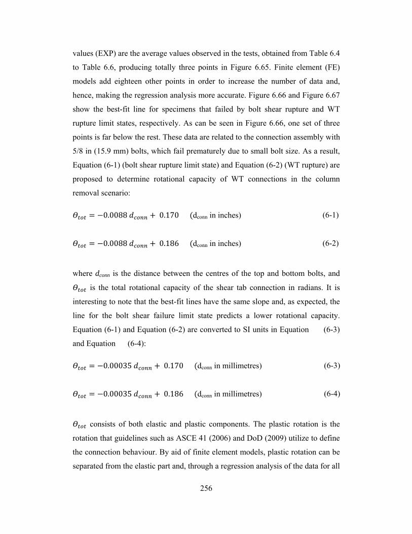
256

values (EXP) are the average values observed in the tests, obtained from Table 6.4

to Table 6.6, producing totally three points in Figure 6.65. Finite element (FE)

models add eighteen other points in order to increase the number of data and,

hence, making the regression analysis more accurate. Figure 6.66 and Figure 6.67

show the best-fit line for specimens that failed by bolt shear rupture and WT

rupture limit states, respectively. As can be seen in Figure 6.66, one set of three

points is far below the rest. These data are related to the connection assembly with

5/8 in (15.9 mm) bolts, which fail prematurely due to small bolt size. As a result,

Equation (6-1) (bolt shear rupture limit state) and Equation (6-2) (WT rupture) are

proposed to determine rotational capacity of WT connections in the column

removal scenario: = −0.0088 + 0.170 (dconn in inches) (6-1)

= −0.0088 + 0.186 (dconn in inches) (6-2)


is the total rotational capacity of the shear tab connection in radians. It is

interesting to note that the best-fit lines have the same slope and, as expected, the

line for the bolt shear failure limit state predicts a lower rotational capacity.

Equation (6-1) and Equation (6-2) are converted to SI units in Equation (6-3)

and Equation (6-4): = −0.00035 + 0.170 (dconn in millimetres)

(6-3)


consists of both elastic and plastic components. The plastic rotation is the

rotation that guidelines such as ASCE 41 (2006) and DoD (2009) utilize to define

the connection behaviour. By aid of finite element models, plastic rotation can be


257

cases considered (see Figure 6.68 and Figure 6.69), is reported as Equation (6-5)

for the bolt shear rupture limit state and Equation (6-6) for WT rupture: = −0.0078 + 0.141 (dconn in inches) (6-5)

= −0.0076 + 0.152 (dconn in inches) (6-6)

As observable in Figure 6.69, one set of points plots higher than the others. These

are the data related to connections WT100X26-3/4 with three, four, and five bolts.

As discussed earlier, these connections possess higher ductility because they have

a thinner WT flange and, consequently, receive a higher contribution to rotational

capacity from out-of-plane flange bending.

Converting Equation (6-5) and Equation Equation (6-6) to SI units produces

Equation (6-7) and Equation (6-8): = −0.00031 + 0.141 (dconn in millimetres) (6-7)


Elastic rotation ends when the first sign of plastic strain starts to appear in the

connection assembly. It is noted that the average elastic rotations observed in the

three, four and five bolt WT connections studied are 0.024, 0.023 and 0.017

radians, respectively. Therefore, in the absence of appropriate tools to determine

the elastic rotation limit for a WT connection, a value of 0.02 radians is a

reasonable assumption for connections resembling those considered in this study.

6.9 Summary and Conclusion

In this chapter, the simultaneous presence of shear, moment and tension in WT

connections was researched. Tensile catenary action is acknowledged as the load

258

transfer mechanism in a column removal scenario. Ductility of WT connections is

derived largely from the local deformation in the stem adjacent to the bottom

holes and the bolt slippage and deformation before failure. Out-of-plane bending

of the WT flange between the bolt lines is another source; however, it was not

significant in the connections with a thick flange. Either shear failure of the

bottom bolt or WT bottom hole rupture was the governing failure mode in all

cases. The response curves can be used as input for WT connection models in

full-building progressive collapse analyses. Other conclusions that can be drawn

are:

• It cannot be assumed that all of the fasteners in a line share equally in

carrying the load. In fact, the fasteners towards the bottom of the joint

carry the largest portion of the load. This unequal loading of the

fasteners is accentuated as the rotation increased.

• The maximum rotation of these WT connections was between 0.075

and 0.127 radians for three to five bolts. Based on Astaneh's

experiments (Astaneh and Nader 1990), the shear deformation and

distortion of the WT section are the main sources of ductile behaviour

for a simply supported beam under gravity loading. For the column

removal scenario, on the other hand, the contribution of bolt hole

bearing deformation, especially the one at the bottom, is also

significant. Out-of-plane bending of the WT's flange, as another source

of ductility, is not uniformly distributed over the length of the WT in

the column removal scenario. Based on the results of the numerical

analyses, out-of-plane flange deformation is at a maximum at the

bottom of all three connections considered and is almost zero at the top.

• Most of the plastic deformation occurred around the bottom hole of the

WT section and also in the bottom bolt shank, in which the rupture

occurred. Plastic deformation in the other bolts is small in comparison

with the bottom bolt. The numerical model predicts the bolt failure very

well with removed elements.

259

• The point that the flexural phase domination ends and catenary force

begins to provide the major resistance is named the “devolution point”.

For 3WT connections, the devolution point happens after the maximum

moment rotation. The main reason for this is the fact that in three bolt

connections the bottom and top bolts resist the demanded moment

through bearing resistance of the bolt-hole interaction. As soon as the

localized yielding around the contact surface accompanied by out-of-

plane bending deformation of the bottom of the WT’s flange occur, the

flexural resistance starts to vanish and the connection tries to find

another load path. The failure will take place in the catenary phase.

Generally, the switch between flexural behaviour and the tensile phase

in 3WT connections can be distinguished more accurately than for 4WT

connections. In this case, there is a point that can be assigned as the

devolution point, in which a tensile response starts to ramp up rapidly.

Before the devolution point, yielding starts to happen around the top

and bottom holes; however, the system still can capture more plastic

deformation around the holes and also through out-of-plane bending of

WT flange. As a result, more moment is captured, but with reduced

stiffness. Gradually, the amount of tensile force exceeds the

compression value and the whole section develops catenary action.

However, the connection fails in the flexural-catenary phase due to the

presence of a significant amount of moment and tension at the time of

failure. It is noted that the 5WT connections go into catenary tension

from the beginning. Tension does not need to cancel the compressive

force at the connection, unlike for the 4WT connections. At the

devolution point, a significant decrease in the slope of the flexural

response and an increase in the tensile response of the 5WT

connections are observable. Basically, the amount of moment at the

failure is significant. As a result, it can be inferred that the 5WT

connections fail mainly because of flexural-catenary action.

260

• The resulting response curves can be used as input for WT connection

models in full-building progressive collapse analyses. Equations are

proposed for determination of WT connection total rotational capacity

and also plastic rotational capacity based on regression analyses of the

cases studied.

Table 6.1: Typical material used for WT connections

Component Material Description WT ASTM A992, 350W -


Table 6.2: Summary of shear strength tests by Astaneh and Nader (1990)

Test No.

WT section No.

Bolts

Bolt diameter

[ in (mm)]

Type of

bolts

Rotation (radians)

Test shear capacity

[ kips (kN) ]

Moment at bolt line [

kip.in (kN.m) ]

Observed failure mode

1 WT4X7.5 3 7/8 (22) A325 0.034 55 (245) 143 (16.1) Yielding of gross area of tee stem

2 WT7X19 5 7/8 (22) A325 0.032 160 (712) 281 (31.7) Yielding of gross area of tee stem

3 WT7X19 3 7/8 (22) A325 0.067 107 (476) 14 (1.6) Fracture of net area of tee stem

4 WT4X7.5 5 7/8 (22) A325 - - - Specimen failed during first phase 5 WT4X20 5 7/8 (22) A325 0.035 183 (814) 300 (33.9) Fracture of gross area of tee stem

6 WT4X20 3 7/8 (22) A325 0.034 111 (494) 128 (14.5) Fracture of gross area of tee stem

7 WT7X19 + 0.5-in web (13 mm)

5 7/8 (22) A325 0.038 238 (1059) 37 (4.2) Shear fracture of bolts

8 WT4X20 + 0.5-in web (13 mm)1

3 7/8 (22) A490 0.039 141 (627) 393 (44.4) Fracture of welds

9 WT4X20 + 0.5-in web (13 mm)1

5 7/8 (22) A490 0.033 209 (930) 270 (30.5) Shear fracture of bolts

1 Web of WT was cut and replaced by ½ in thick (12.7 mm) ASTM A36 plate.

261

Table 6.3: Summary of characteristic features of FE models of WT connections

No. Specimen Label1 WT Type WT Section Bolt Type Bolt diameter Remarks

1 3WT125X33.5-3/4 ASTM A992 WT125X33.5 ASTM A325 19.1 mm (3/4 in) Used for verification2

2 3WT100X26-3/4 ASTM A992 WT100X26 ASTM A325 19.1 mm (3/4 in) -

3 3WT155X33.5-3/4 ASTM A992 WT155X33.5 ASTM A325 19.1 mm (3/4 in) -



6 3WT125X33.5-3/4-A490 ASTM A992 WT125X33.5 ASTM A490 19.1 mm (3/4 in) -





11 4WT125X33.5-7/8 ASTM A992 WT125X33.5 ASTM A325 22.2 mm (7/8 in) - 12 4WT125X33.5-3/4-A490 ASTM A992 WT125X33.5 ASTM A490 19.1 mm (3/4 in) -






18 5WT125X33.5-3/4-A490 ASTM A992 WT125X33.5 ASTM A490 19.1 mm (3/4 in) -

1 Imperial units are utilized in labelling the bolts since the experimental program utilized imperial bolts.

2 Test results are available for these models.

262

Table 6.4: Comparison of numerical and experimental (Friedman 2009) responses of shear tab connections with three bolts (3WT) at initial failure


Shear, V (kN)

Axial, P (kN)

Rotation, Θ


3WT1 Left 9.30 23.66 158.89 0.13 Bottom bolt shear rupture

Right 4.77 23.66 162.76 0.133 -

3WT2 Left 9.19 23.22 155.95 0.13 -

Right 7.12 23.22 160.71 0.125 Bottom bolt shear rupture


Right 1.69 24.24 184.29 0.128 -

3WT-Mean 5.90 23.71 167.01 0.129 -

3WT-FEA 6.43 25.71 170.81 0.131 Bottom bolt shear rupture

Deviation % 8.94 8.44 2.28 1.95 -

Table 6.5: Comparison of numerical and experimental (Friedman 2009) responses of shear tab connections with four bolts (4WT) at initial failure


Shear, V (kN)

Axial, P (kN)

Rotation, Θ


4WT1 Left 41.07 33.09 143.41 0.10 -


4WT2 Left 38.25 31.58 128.38 0.093 -


4WT3 Left 36.99 31.09 137.32 0.091 -


4WT-Mean 36.42 31.92 136.10 0.094 -

4WT-FEA 35.05 32.76 149.95 0.096 Bottom bolt shear rupture

Deviation % 3.77 2.62 10.18 2.49 -

263

Table 6.6: Comparison of numerical and experimental (Friedman 2009) responses of shear tab connections with five bolts (5WT) at initial failure

Spec. Label Side Moment,

M (kN.m)

Shear, V (kN)

Axial, P (kN)

Rotation, Θ



Right 61.04 44.35 130.78 0.073 -


Right 63.17 43.55 112.81 0.069 -


Right 63.90 47.28 148.57 0.069 -

5WT-Mean 69.99 47.28 142.48 0.071 -

5WT-FEA 63.34 45.1 155.35 0.075 Bottom bolt shear rupture Deviation % 9.50 4.62 9.04 5.63 -

264

Table 6.7: Summary of characteristic features of experimental and numerical models of WT connections

No. Specimen/Model Label Connection Depth (mm)

Rotation (Rad)

V (kN)

T (kN)

M (kN.m)

Failure Mode

1 3WT125X33.5-3/4-EXP 152.4 0.129 23.7 167.0 5.9 Bottom bolt shear rupture

2 3WT125X33.5-3/4 152.4 0.131 25.7 170.8 6.4 Bottom bolt shear rupture

3 3WT100X26-3/4 152.4 0.163 36.5 260.3 - WT bottom hole rupture

4 3WT155X33.5-3/4 152.4 0.135 26.6 180.8 4.5 WT bottom hole rupture



7 3WT125X33.5-3/4-A490 152.4 0.120 20.4 104.3 15.2 WT bottom hole rupture



10 4WT100X26-3/4 228.6 0.120 38.7 195.0 24.9 WT bottom hole rupture 11 4WT155X33.5-3/4 228.6 0.107 35.7 176.6 32.1 WT bottom hole rupture






17 5WT100X26-3/4 304.8 0.096 47.4 186.8 54.5 WT bottom hole rupture





265

F

Figure 6.1: T(c) w

Fig

Bea

Bea

Types of WTwelded-weld

gure 6.2: Ty

(a)

(c)

am

Column

am

Column

T shear connded (d) bolte

ypical failure

266

Beam

Beam

ections: (a) wed-bolted (A

e modes (Ast

Column

(d)

(b)

Column

welded-boltAstaneh and N

taneh and N

ted (b) boltedNader 1990)

ader 1989)

d-welded )

267

M

V

Figure 6.3: Assumed induced force on WT and bolts (Thornton 1996)

bWT bWT

aWT

LWT

bWT bWT

aWT

t f-WT

t w-WT

t f-WT

t w-WT

LWT

(a) (b)

Figure 6.4: Yield lines in WT shear connection: (a) welded (b) bolted (Thornton 1996)

268

SG1

SG2

SG3

SG4

SG1

SG2

SG3

SG4

Test Frame

DWT Supports

True Pin Connection

Strain gauges

Hydraulic Jack

Test Beam

Stub Column

True Pin Connection

Shear connection

Figure 6.5: Test setup (Friedman 2009)

(a)

(b) (c) (d)

Figure 6.6: FE models of: (a) full connection assembly, (b) 3 bolt WT connection (3WT), (c) 4 bolt WT connection (4WT), (d) 5 bolt WT connection (5WT)

269

(a)

(b)

Figure 6.7: Deformed shape of the connection assembly: (a) experiment (b) finite element

F

Magnifiethe bofrom the

Figure 6.8: F(a) defor

ed view of ottom hole e other side

Failure of 3Wrmed shape

f

WT, experime(b) bolt rupt

270

(a)

(b)

(c)

ental (Friedmture (c) botto

man 2009) aom hole bear

De

and numericaring deforma

15

eformed hole

Deformed a

al results: ation

° - 30 °

e

area

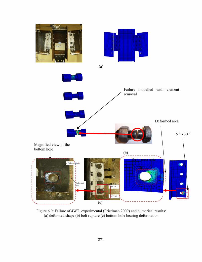
F

Mabo

Figure 6.9: F(a) defor

agnified viewottom hole

Failure of 4Wrmed shape

w of the

WT, experime(b) bolt rupt

271

(a)

(c)

ental (Friedmture (c) botto

(b)

man 2009) aom hole bear

Failurremov

D

and numericaring deforma

re modelleval

Deformed ho

al results: ation

d with ele

Deformed

ole

ement

d area

15 ° - 30 °°

r

Magnifiebottom hother sid

Figure 6.1results: (a) d

ed view of thole from tde of the W

10: Failure odeformed sha

he he

WT

of 5WT, expeape (b) bolt r

272

(a)

(b)

(c)

erimental (Frupture (c) b

Fairem

Friedman 200bottom hole

ilure modemoval

Defor

09) and numbearing defo

elled with

Deforme

rmed hole

merical ormation

element

ed area

15 ° - 300 °

273

Figure 6.11: Comparison of numerical and experimental shear response of connection 3WT

Figure 6.12: Comparison of numerical and experimental tensile response of connection 3WT

0.0

5.0

10.0

15.0

20.0

25.0

30.0

35.0

40.0

45.0

50.0

0.00 0.02 0.04 0.06 0.08 0.10 0.12 0.14 0.16

She

ar (

kN)


3WTL1

3WTR1

3WTL2

3WTR2

3WTL3

3WTR3

3WT125X33.5-3/4

0.0

20.0

40.0

60.0

80.0

100.0

120.0

140.0

160.0

180.0

200.0

220.0

240.0

260.0

280.0

0.00 0.02 0.04 0.06 0.08 0.10 0.12 0.14 0.16

Ten

sion

(kN

)


3WTL1

3WTR1

3WTL2

3WTR2

3WTL3

3WTR3

3WT125X33.5-3/4

274

Figure 6.13: Comparison of numerical and experimental flexural response of connection 3WT


0.0

2.0

4.0

6.0

8.0

10.0

12.0

14.0

16.0

18.0

20.0

22.0

24.0

26.0

28.0

0.00 0.02 0.04 0.06 0.08 0.10 0.12 0.14 0.16

Mom

ent (

kN.m

)


3WTL1

3WTR1

3WTL2

3WTR2

3WTL3

3WTR3

3WT125X33.5-3/4

0.0

5.0

10.0

15.0

20.0

25.0

30.0

35.0

40.0

45.0

0.00 0.02 0.04 0.06 0.08 0.10 0.12

She

ar (

kN)


4WTL1

4WTR1

4WTL2

4WTR2

4WTL3

4WTR3

4WT125X33.5-3/4

275


Figure 6.16: Comparison of numerical and experimental flexural response of connection 4WT

0.0

15.0

30.0

45.0

60.0

75.0

90.0

105.0

120.0

135.0

150.0

165.0

180.0

195.0

0.00 0.02 0.04 0.06 0.08 0.10 0.12

Ten

sion

(kN

)


4WTL1

4WTR1

4WTL2

4WTR2

4WTL3

4WTR3

4WT125X33.5-3/4

0.03.06.09.0

12.015.018.021.024.027.030.033.036.039.042.045.0

0.00 0.02 0.04 0.06 0.08 0.10 0.12

Mom

ent (

kN.m

)


4WTL1

4WTR1

4WTL2

4WTR2

4WTL3

4WTR3

4WT125X33.5-3/4

276



0.0

5.0

10.0

15.0

20.0

25.0

30.0

35.0

40.0

45.0

50.0

0.00 0.02 0.04 0.06 0.08 0.10

She

ar (

kN)


5WTL1

5WTR1

5WTL2

5WTR2

5WTL3

5WTR3

5WT125X33.5-3/4

0.0

20.0

40.0

60.0

80.0

100.0

120.0

140.0

160.0

180.0

200.0

0.00 0.02 0.04 0.06 0.08 0.10

Ten

sion

(kN

)


5WTL15WTR15WTL25WTR25WTL35WTR35WT125X33.5-3/4

Figure 6.19

Figur

0.05.0

10.015.020.025.030.035.040.045.050.055.060.065.070.075.080.0

0.00

Mom

ent (

kN.m

)

0.02.04.06.08.0

10.012.014.016.018.020.022.024.026.028.0

0.00

Mom

ent (

kN.m

)

9: Comparis

re 6.20: Bolt

0.02

5WTL1

5WTR1

5WTL2

5WTR2

5WTL3

5WTR3

5WT125X

0.02 0.0

Momen

Tension

Shear

son of numerconn

t line forces v3WT

2 0

Bea

X33.5-3/4

04 0.06

Beam En

nt

n

277

rical and expnection 5WT

versus beam125X33.5-3/

0.04

am End Rotati

0.08 0.10

nd Rotation (R

perimental flT

m end rotation/4

0.06

ion (Rad)

0.12 0.14

Rad)

flexural respo

n – Specime

0.08

024681111122222

4 0.16

onse of

en

0.10

0.020.040.060.080.0100.0120.0140.0160.0180.0200.0220.0240.0260.0280.0

Ten

sion

and

She

ar (

kN)

F

F

Figure 6.21:

igure 6.22: B

0.0

2.0

4.0

6.0

8.0

10.0

12.0

14.0

16.0

18.0

20.0

22.0

24.0

26.0

28.0

0.00

Mom

ent (

kN.m

)

0.0

2.0

4.0

6.0

8.0

10.0

12.0

14.0

16.0

18.0

20.0

22.0

24.0

26.0

28.0

0.00

Mom

ent (

kN.m

)

Bolt line forc

Bolt line forc

0.02 0.04

Momen

Tension

Shear

0.02 0.0

Mome

Tensio

Shear

ces versus be

es versus bea

4 0.06

Beam En

nt

n

04 0.06

Beam E

nt

on

278

eam end rotat

am end rotati

0.08 0.10

nd Rotation (R

0.08 0.10

End Rotation (R

tion – Specim

ion – Specim

0.12 0

Rad)

0 0.12 0

Rad)

men 3WT100

men 3WT155X

0.14 0.16

0.14 0.16

0X26-3/4

X33.5-3/4

0.0

20.0

40.0

60.0

80.0

100.0

120.0

140.0

160.0

180.0

200.0

220.0

240.0

260.0

280.0

Ten

sion

l and

She

ar (

kN)

0.0

20.0

40.0

60.0

80.0

100.0

120.0

140.0

160.0

180.0

200.0

220.0

240.0

260.0

280.0

Ten

sion

and

She

ar (

kN)

F

F

igure 6.23: B

igure 6.24: B

0.0

2.0

4.0

6.0

8.0

10.0

12.0

14.0

16.0

18.0

20.0

22.0

24.0

26.0

28.0

0.00

Mom

ent (

kN.m

)

0.0

2.0

4.0

6.0

8.0

10.0

12.0

14.0

16.0

18.0

20.0

22.0

24.0

26.0

28.0

0.00

Mom

ent (

kN.m

)

Bolt line forc

Bolt line forc

0.02 0.

Mo

Ten

She

0.02 0.0

Moment

Tension

Shear

es versus bea

es versus bea

04 0.06

Beam E

ment

nsion

ear

04 0.06Beam E

t

279

am end rotati

am end rotati

0.08 0.10

End Rotation (R

0.08 0.10End Rotation (R

ion – Specim

ion – Specim

0.12 0.

Rad)

0.12 0.Rad)

men 3WT125X

men 3WT125X

.14 0.16

.14 0.16

X33.5-5/8

X33.5-7/8

0.0

20.0

40.0

60.0

80.0

100.0

120.0

140.0

160.0

180.0

200.0

220.0

240.0

260.0

280.0

Ten

sion

and

She

ar (

kN)

0.0

20.0

40.0

60.0

80.0

100.0

120.0

140.0

160.0

180.0

200.0

220.0

240.0

260.0

280.0

Ten

sion

and

She

ar (

kN)

F

Figu

igure 6.26: B

0.0

2.0

4.0

6.0

8.0

10.0

12.0

14.0

16.0

18.0

20.0

22.0

24.0

26.0

28.0

0.00

Mom

ent (

kN.m

)

0.0

3.0

6.0

9.0

12.0

15.0

18.0

21.0

24.0

27.0

30.0

33.0

36.0

39.0

42.0

45.0

0.00

Mom

ent (

kN.m

)

ure 6.25: Bol

Bolt line force

0.02 0.0

Moment

Tension

Shear

0.02

Momen

Tensio

Shear

lt line forces 3WT125

es versus bea

04 0.06

Beam E

t

0.04

Beam E

nt

n

280

versus beam5X33.5-3/4-A

am end rotati

0.08 0.10

End Rotation (R

0.06 0.0

End Rotation (R

m end rotationA490

ion – Specim

0.12 0.

Rad)

08 0.10

Rad)

n – Specimen

men 4WT125X

.14 0.16

0.12

n

X33.5-3/4

0.0

20.0

40.0

60.0

80.0

100.0

120.0

140.0

160.0

180.0

200.0

220.0

240.0

260.0

280.0

Ten

sion

and

She

ar (

kN)

0.0

20.0

40.0

60.0

80.0

100.0

120.0

140.0

160.0

180.0

200.0

Ten

sion

and

She

ar (

kN)

F

F

igure 6.27: B

igure 6.28: B

0.0

3.0

6.0

9.0

12.0

15.0

18.0

21.0

24.0

27.0

30.0

33.0

36.0

39.0

42.0

45.0

0.00

Mom

ent (

kN.m

)

0.0

3.0

6.0

9.0

12.0

15.0

18.0

21.0

24.0

27.0

30.0

33.0

36.0

39.0

42.0

45.0

0.00

Mom

ent (

kN.m

)

Bolt line force

Bolt line force

0.02

Moment

Tension

Shear

0 0.02

Mom

Tensi

Shear

es versus bea

es versus bea

0.04

Beam En

0.04

Beam E

ment

ion

r

281

am end rotati

am end rotati

0.06 0.0

nd Rotation (R

0.06 0.

End Rotation (

ion – Specim

ion – Specim

08 0.10

Rad)

.08 0.10

(Rad)

men 4WT100X

men 4WT155X

0.12

0.12

X26-3/4

X33.5-3/4

0.0

20.0

40.0

60.0

80.0

100.0

120.0

140.0

160.0

180.0

200.0

Ten

sion

and

She

ar (

kN)

0.0

20.0

40.0

60.0

80.0

100.0

120.0

140.0

160.0

180.0

200.0

Ten

sion

and

She

ar (

kN)

F

F

Mt(

kN)

igure 6.29: B

igure 6.30: B

0.03.06.09.0

12.015.018.021.024.027.030.033.036.039.042.045.0

0.00

Mom

ent (

kN.m

)

0.0

3.0

6.0

9.0

12.0

15.0

18.0

21.0

24.0

27.0

30.0

33.0

36.0

39.0

42.0

45.0

0.00

Mom

ent (

kN.m

)

Bolt line force

Bolt line force

0.02

Mom

Tensi

Shear

0.02

Moment

Tension

Shear

es versus bea

es versus bea

0.04

Beam E

ent

ion

r

0.04

Beam E

282

am end rotati

am end rotati

0.06 0.0

End Rotation (R

0.06 0.0

End Rotation (R

ion – Specim

ion – Specim

08 0.10

Rad)

08 0.10

Rad)

men 4WT125X

men 4WT125X

0.12

0.12

X33.5-5/8

X33.5-7/8

0.0

20.0

40.0

60.0

80.0

100.0

120.0

140.0

160.0

180.0

200.0

Ten

sion

and

She

ar (

kN)

0.0

20.0

40.0

60.0

80.0

100.0

120.0

140.0

160.0

180.0

200.0

Ten

sion

and

She

ar (

kN)

F

Mt(

kN)

Mt(

kN)

Figu

igure 6.32: B

0.0

3.0

6.0

9.0

12.0

15.0

18.0

21.0

24.0

27.0

30.0

33.0

36.0

39.0

42.0

45.0

0.00

Mom

ent (

kN.m

)

0.0

5.0

10.0

15.0

20.0

25.0

30.0

35.0

40.0

45.0

50.0

55.0

60.0

65.0

70.0

75.0

80.0

0.00

Mom

ent (

kN.m

)

ure 6.31: Bol

Bolt line force

0.02

Moment

Tension

Shear

0.02

Mom

Tensi

Shear


es versus bea

0.04 0.Beam End

0.04

Beam End

ent

ion

r

283


am end rotati

06 0.08d Rotation (Rad

0.06

d Rotation (Rad

m end rotationA490

ion – Specim

0.10d)

0.08

d)

n – Specimen

men 5WT125X

0

2

4

6

8

2

0.12

0

20

40

60

80

10

12

14

16

1

20

0.10

n

X33.5-3/4

0.0

20.0

40.0

60.0

80.0

100.0

120.0

140.0

160.0

180.0

200.0

Ten

sion

and

She

ar (

kN)

.0

0.0

0.0

0.0

0.0

00.0

20.0

40.0

60.0

80.0

00.0

Ten

sion

and

She

ar (

kN)

F

F

M(k

N)

igure 6.33: B

igure 6.34: B

0.0

5.0

10.0

15.0

20.0

25.0

30.0

35.0

40.0

45.0

50.0

55.0

60.0

65.0

70.0

75.0

80.0

0.00

Mom

ent (

kN.m

)

0.0

5.0

10.0

15.0

20.0

25.0

30.0

35.0

40.0

45.0

50.0

55.0

60.0

65.0

70.0

75.0

80.0

0.00

Mom

ent (

kN.m

)

Bolt line force

Bolt line force

0.02

Mom

Tensi

Shear

0.02

Mome

Tensio

Shear

es versus bea

es versus bea

0.04Beam E

ment

ion

r

0.04Beam E

ent

on

284

am end rotati

am end rotati

4 0.06End Rotation (R

4 0.0End Rotation (

ion – Specim

ion – Specim

6 0.0Rad)

06 0.(Rad)

men 5WT100X

men 5WT155X

08 0.

.08 0

X26-3/4

X33.5-3/4

0.0

20.0

40.0

60.0

80.0

100.0

120.0

140.0

160.0

180.0

200.0

10

Ten

sion

and

She

ar (

kN)

0.0

20.0

40.0

60.0

80.0

100.0

120.0

140.0

160.0

180.0

200.0

0.10

Ten

sion

and

She

ar (

kN)

F

F

igure 6.35: B

igure 6.36: B

0.0

5.0

10.0

15.0

20.0

25.0

30.0

35.0

40.0

45.0

50.0

55.0

60.0

65.0

70.0

75.0

80.0

0.00

Mom

ent (

kN.m

)

0.0

5.0

10.0

15.0

20.0

25.0

30.0

35.0

40.0

45.0

50.0

55.0

60.0

65.0

70.0

75.0

80.0

0.00

Mom

ent (

kN.m

)

Bolt line force

Bolt line force

0.02

Mom

Ten

She

0.02

Mome

Tensi

Shear

es versus bea

es versus bea

0.04Beam E

ment

nsion

ar

0.04Beam E

ent

on

r

285

am end rotati

am end rotati

4 0.0End Rotation (R

0.0End Rotation (R

ion – Specim

ion – Specim

06 0.Rad)

6 0.Rad)

men 5WT125X

men 5WT125X

.08 0

08 0

X33.5-5/8

X33.5-7/8

0.0

20.0

40.0

60.0

80.0

100.0

120.0

140.0

160.0

180.0

200.0

0.10

Ten

sion

and

She

ar (

kN)

0.0

20.0

40.0

60.0

80.0

100.0

120.0

140.0

160.0

180.0

200.0

0.10

Ten

sion

and

She

ar (

kN)

Figu

Figure 6.38

0.0

5.0

10.0

15.0

20.0

25.0

30.0

35.0

40.0

45.0

50.0

55.0

60.0

65.0

70.0

75.0

80.0

0.00

Mom

ent (

kN.m

)

0.0

5.0

10.0

15.0

20.0

25.0

30.0

35.0

40.0

0.00

She

ar (

kN)

ure 6.37: Bol

8: Compariso

0.02

Mom

Tens

Shea

0.02 0

3W

3W

3W


on of shear rW

0.04Beam En

ment

sion

ar

0.04 0.06

Beam

WT125X33.5-3/

WT155X33.5-3/

WT100X26-3/4

286


response of 3WT sections

0.06nd Rotation (R

0.08 0.1

m End Rotatio

/4

/4

m end rotationA490

3WT connec

6 0.08Rad)

0 0.12

on (Rad)

n – Specimen

ctions with d

8 0.10

0.14 0.16

n

different

0.0

20.0

40.0

60.0

80.0

100.0

120.0

140.0

160.0

180.0

200.0

0

Ten

sion

and

She

ar (

kN)

0.18

287

Figure 6.39: Comparison of tensile response of 3WT connections with different WT sections

Figure 6.40: Comparison of flexural response of 3WT connections with different WT sections

0.0

20.0

40.0

60.0

80.0

100.0

120.0

140.0

160.0

180.0

200.0

220.0

240.0

260.0

280.0

0.00 0.02 0.04 0.06 0.08 0.10 0.12 0.14 0.16 0.18

Ten

sion

(kN

)


3WT125X33.5-3/4

3WT155X33.5-3/4

3WT100X26-3/4

0.0

2.0

4.0

6.0

8.0

10.0

12.0

14.0

16.0

18.0

20.0

22.0

24.0

26.0

28.0

0.00 0.02 0.04 0.06 0.08 0.10 0.12 0.14 0.16 0.18

Mom

ent (

kN.m

)


3WT125X33.5-3/4

3WT155X33.5-3/4

3WT100X26-3/4

288

Figure 6.41: Comparison of shear response of 3WT connections with different bolt sizes

Figure 6.42: Comparison of tensile response of 3WT connections with different bolt sizes

0.0

5.0

10.0

15.0

20.0

25.0

30.0

35.0

40.0

0.00 0.02 0.04 0.06 0.08 0.10 0.12 0.14 0.16 0.18

She

ar (

kN)


3WT125X33.5-7/8

3WT125X33.5-3/4

3WT125X33.5-5/8

0.0

20.0

40.0

60.0

80.0

100.0

120.0

140.0

160.0

180.0

200.0

220.0

240.0

260.0

280.0

0.00 0.02 0.04 0.06 0.08 0.10 0.12 0.14 0.16 0.18

Ten

sion

(kN

)


3WT125X33.5-7/8

3WT125X33.5-3/4

3WT125X33.5-5/8

289

Figure 6.43: Comparison of flexural response of 3WT connections with different bolt sizes

Figure 6.44: Comparison of shear response of 3WT connections with different bolt types

0.0

2.0

4.0

6.0

8.0

10.0

12.0

14.0

16.0

18.0

20.0

22.0

24.0

26.0

28.0

0.00 0.02 0.04 0.06 0.08 0.10 0.12 0.14 0.16 0.18

Mom

ent (

kN.m

)


3WT125X33.5-7/8

3WT125X33.5-3/4

3WT125X33.5-5/8

0.0

5.0

10.0

15.0

20.0

25.0

30.0

35.0

40.0

0.00 0.02 0.04 0.06 0.08 0.10 0.12 0.14 0.16 0.18

She

ar (

kN)


3WT125X33.5-3/4-A490

3WT125X33.5-3/4

290

Figure 6.45: Comparison of tensile response of 3WT connections with different bolt types

Figure 6.46: Comparison of flexural response of 3WT connections with different bolt types

0.0

20.0

40.0

60.0

80.0

100.0

120.0

140.0

160.0

180.0

200.0

220.0

240.0

260.0

280.0

0.00 0.02 0.04 0.06 0.08 0.10 0.12 0.14 0.16 0.18

Ten

sion

(kN

)


3WT125X33.5-3/4-A490

3WT125X33.5-3/4

0.0

2.0

4.0

6.0

8.0

10.0

12.0

14.0

16.0

18.0

20.0

22.0

24.0

26.0

28.0

0.00 0.02 0.04 0.06 0.08 0.10 0.12 0.14 0.16 0.18

Mom

ent (

kN.m

)


3WT125X33.5-3/4-A490

3WT125X33.5-3/4

291

Figure 6.47: Comparison of shear response of 4WT connections with different WT sections


0.0

5.0

10.0

15.0

20.0

25.0

30.0

35.0

40.0

45.0

0.00 0.02 0.04 0.06 0.08 0.10 0.12 0.14

She

ar (

kN)


4WT125X33.5-3/4

4WT155X33.5-3/4

4WT100X26-3/4

0.0

20.0

40.0

60.0

80.0

100.0

120.0

140.0

160.0

180.0

200.0

0.00 0.02 0.04 0.06 0.08 0.10 0.12 0.14

Ten

sion

(kN

)


4WT125X33.5-3/4

4WT155X33.5-3/4

4WT100X26-3/4

292



0.0

3.0

6.0

9.0

12.0

15.0

18.0

21.0

24.0

27.0

30.0

33.0

36.0

39.0

42.0

45.0

0.00 0.02 0.04 0.06 0.08 0.10 0.12 0.14

Mom

ent (

kN.m

)


4WT125X33.5-3/4

4WT155X33.5-3/4

4WT100X26-3/4

0.0

5.0

10.0

15.0

20.0

25.0

30.0

35.0

40.0

45.0

0.00 0.02 0.04 0.06 0.08 0.10 0.12 0.14

She

ar (

kN)


4WT125X33.5-7/8

4WT125X33.5-3/4

4WT125X33.5-5/8

293



0.0

20.0

40.0

60.0

80.0

100.0

120.0

140.0

160.0

180.0

200.0

0.00 0.02 0.04 0.06 0.08 0.10 0.12 0.14

Ten

sion

(kN

)


4WT125X33.5-7/8

4WT125X33.5-3/4

4WT125X33.5-5/8

0.03.06.09.0

12.015.018.021.024.027.030.033.036.039.042.045.0

0.00 0.02 0.04 0.06 0.08 0.10 0.12 0.14

Mom

ent (

kN.m

)


4WT125X33.5-7/8

4WT125X33.5-3/4

4WT125X33.5-5/8

294



0.0

5.0

10.0

15.0

20.0

25.0

30.0

35.0

40.0

45.0

0.00 0.02 0.04 0.06 0.08 0.10 0.12 0.14

She

ar (

kN)


4WT125X33.5-3/4-A490

4WT125X33.5-3/4

0.0

20.0

40.0

60.0

80.0

100.0

120.0

140.0

160.0

180.0

200.0

0.00 0.02 0.04 0.06 0.08 0.10 0.12 0.14

Ten

sion

(kN

)


4WT125X33.5-3/4-A490

4WT125X33.5-3/4

295


Figure 6.56: Comparison of shear response of 5WT connections with different WT sections

0.03.06.09.0

12.015.018.021.024.027.030.033.036.039.042.045.0

0.00 0.02 0.04 0.06 0.08 0.10 0.12 0.14

Mom

ent (

kN.m

)


4WT125X33.5-3/4-A490

4WT125X33.5-3/4

0.0

5.0

10.0

15.0

20.0

25.0

30.0

35.0

40.0

45.0

50.0

0.00 0.02 0.04 0.06 0.08 0.10

She

ar (

kN)


5WT125X33.5-3/4

5WT155X33.5-3/4

5WT100X26-3/4

296



0.0

20.0

40.0

60.0

80.0

100.0

120.0

140.0

160.0

180.0

200.0

0.00 0.02 0.04 0.06 0.08 0.10

Ten

sion

(kN

)


5WT125X33.5-3/4

5WT155X33.5-3/4

5WT100X26-3/4

0.05.0

10.015.020.025.030.035.040.045.050.055.060.065.070.075.080.0

0.00 0.02 0.04 0.06 0.08 0.10

Mom

ent (

kN.m

)


5WT125X33.5-3/4

5WT155X33.5-3/4

5WT100X26-3/4

297



0.0

5.0

10.0

15.0

20.0

25.0

30.0

35.0

40.0

45.0

50.0

0.00 0.02 0.04 0.06 0.08 0.10

She

ar (

kN)


5WT125X33.5-7/8

5WT125X33.5-3/4

5WT125X33.5-5/8

0.0

20.0

40.0

60.0

80.0

100.0

120.0

140.0

160.0

180.0

200.0

0.00 0.02 0.04 0.06 0.08 0.10

Ten

sion

(kN

)


5WT125X33.5-7/8

5WT125X33.5-3/4

5WT125X33.5-5/8

298



0.05.0

10.015.020.025.030.035.040.045.050.055.060.065.070.075.080.0

0.00 0.02 0.04 0.06 0.08 0.10

Mom

ent (

kN.m

)


5WT125X33.5-7/8

5WT125X33.5-3/4

5WT125X33.5-5/8

0.0

5.0

10.0

15.0

20.0

25.0

30.0

35.0

40.0

45.0

50.0

0.00 0.02 0.04 0.06 0.08 0.10

She

ar (

kN)


5WT125X33.5-3/4-A490

5WT125X33.5-3/4

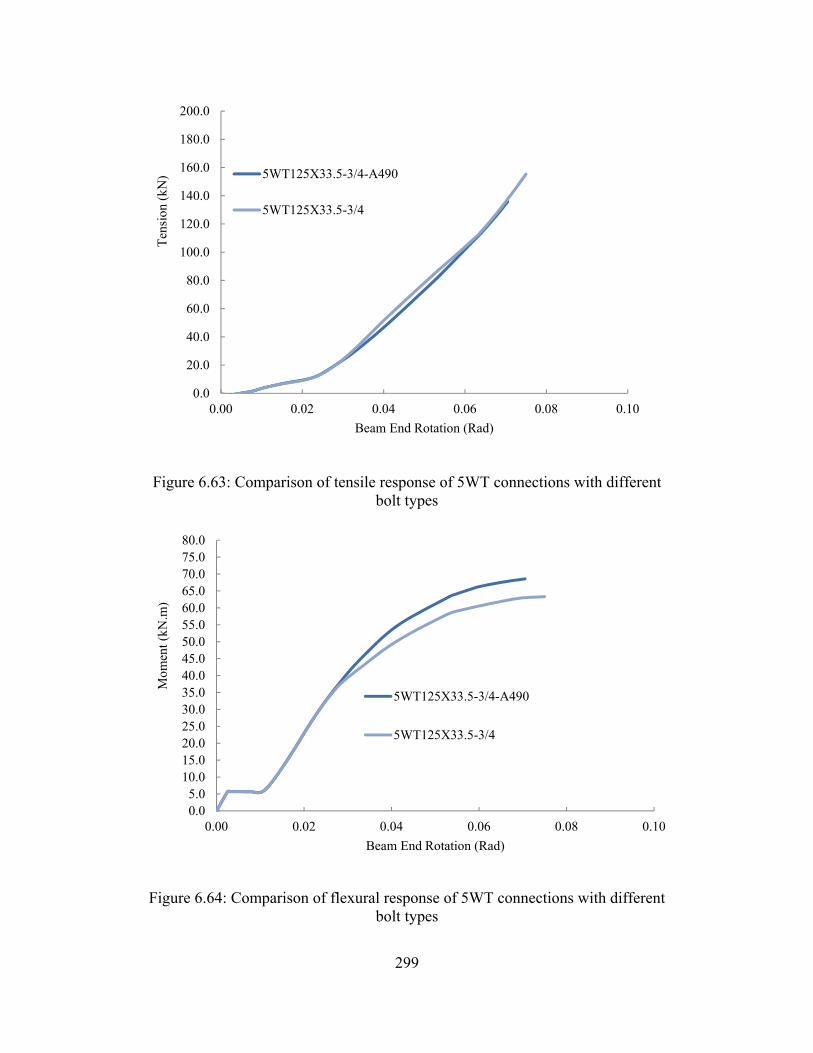
299



0.0

20.0

40.0

60.0

80.0

100.0

120.0

140.0

160.0

180.0

200.0

0.00 0.02 0.04 0.06 0.08 0.10

Ten

sion

(kN

)


5WT125X33.5-3/4-A490

5WT125X33.5-3/4

0.05.0

10.015.020.025.030.035.040.045.050.055.060.065.070.075.080.0

0.00 0.02 0.04 0.06 0.08 0.10

Mom

ent (

kN.m

)


5WT125X33.5-3/4-A490

5WT125X33.5-3/4

300

Figure 6.65: WT connection total rotation capacities versus connection depth

Figure 6.66: Proposed equation for WT connection total rotation capacities versus connection depth – Bolt shear rupture limit state

0.000

0.020

0.040

0.060

0.080

0.100

0.120

0.140

0.160

0.180

0 2 4 6 8 10 12 14

Rot

atio

n (R

ad)


3WT-EXP

3WT-FEA

4WT-EXP

4WT-FEA

5WT-EXP

5WT-FEA

ϴ = -0.0088 dconn + 0.170

0.000

0.020

0.040

0.060

0.080

0.100

0.120

0.140

0.160

0.180

0 2 4 6 8 10 12 14

Rot

atio

n (R

ad)


EXP & FEA Results

301

Figure 6.67: Proposed equation for WT connection total rotation capacities versus connection depth – WT rupture limit state

Figure 6.68: Proposed equation for WT connection plastic rotation capacities versus connection depth – Bolt shear rupture limit state

ϴ = -0.0088 dconn + 0.186

0.000

0.020

0.040

0.060

0.080

0.100

0.120

0.140

0.160

0.180

0 2 4 6 8 10 12 14

Rot

atio

n (R

ad)


EXP & FEA Results

ϴ = -0.0078 dconn + 0.141

0.000

0.020

0.040

0.060

0.080

0.100

0.120

0.140

0.160

0.180

0 2 4 6 8 10 12 14

Rot

atio

n (R

ad)


EXP & FEA Results


302

Figure 6.69: Proposed equation for WT connection plastic rotation capacities versus connection depth – WT rupture limit state

ϴ = -0.0076 dconn + 0.152

0.000

0.020

0.040

0.060

0.080

0.100

0.120

0.140

0.160

0.180

0 2 4 6 8 10 12 14

Rot

atio

n (R

ad)


EXP & FEA Results

Linear (EXP & FEAResults)

303

7 Behaviour of Single Angle Connections under Column Removal Scenario

7.1 Introduction

Single angle connections are one of the common single-sided shear connections

used in steel construction. They are more economical than double angle

connections due to reduction in both material and labour. They are also more

favorable to fabricators due to ease of fabrication and beam installation. The main

advantages and disadvantages of single angle connections compared with other

types of single-sided connections are summarized in Table 7.1. The angle can

either be bolted or welded to the beam web and bolted or welded to the column

flange, as shown in . The leg that is bolted or welded to the supporting member is

called the “outstanding leg”; meanwhile, the other leg that is connected to the

supported beam is called the “web-framing” leg (CISC 2006). Common types of

material used in single angle connections are stated in Table 7.2. Similar to shear

tab and WT types of shear connections, single angles in beam-to-column

connections are conventionally designed to transfer shear forces, while the

rotation is not restrained. As a result, there is no substantial moment transfer.

Research on the strength and ductility of single angle connections in conventional

design is limited. Besides, its response to the column removal scenario is also

relatively unknown. For example, the DoD (2009) guideline provides a table that

includes models for rotational ductility of shear tab and double angle connections,

but not single angles. As a result, more research is required to establish the

characteristic features of such connections in order to improve the current

modelling definitions of shear connections in the column loss event. The actual

load path, stress distributions, sources of ductility, and failure modes should be

well-researched to propose modelling parameters in the column removal scenario.

304

In this chapter, numerical methods are applied to simulate the response of single

angle connections when a column is compromised. The finite element models are

verified by available experimental data following the same loading regime.

Verified models are utilized to expand the database of the connection models.

Shear, tension, and moment versus chord rotation diagrams are presented for

numerical results and conclusions are made. The results are utilized to develop the

modelling parameter that can predict the rotational behaviour of single angle

connections in the new scenario.

7.2 Objectives and scope

This chapter is focused on the behaviour of single angle shear connections under

simultaneous presence of shear, tension, and moment. The finite element models

proposed in this chapter can shed more light on the performance and the sources

of ductility in single angle connections. The results can be used to select suitable

connection modelling parameters for progressive collapse evaluations of steel

frames with similar single angle shear connections. The focus of the research is on

bolted-bolted single angle shear connections, shown in Figure7.1(d). Connection

depth, angle thickness, bolt size and type are the main variables in the numerical

models discussed herein. Equations, based on the connection depth, are proposed

to predict the rotational ductility of single angle connections.

7.3 Selected previous research

Lipson (1968) appears to have initiated the investigations on single angle shear

connections by performing several tests. He attempted to establish characteristic

features of these connections, including the behaviour of the connection under

working loads and their rotational capacities. The main purpose of Lipson's

research was to determine if single angle connections can qualify as "flexible"

connections. Three types of connections were well-researched, including "bolted-

305

bolted" and "welded-bolted" single angles. All angles were ASTM A36 type and

the bolts were ASTM A325 with a 19.1 mm (3/4 inch) diameter. The welding was

made with E60 electrodes. He tested the specimens under pure bending moment

and also under a combination of shear and moment with or without rotation. He

observed that the magnitude of the slip value for the bolts varied substantially for

single angle specimens. Besides, the effect of changing the gauge distance in

either leg of the bolted-bolted angles on the slip value is minimal. His

experiments could not develop the full plastic moment of the connection because

of the small beam rotation. (Lipson 1968).

Lipson’s studies also questioned the assumed flexibility of shear connections due

to the observed restraining moment developed. He attempted to ease the restraint

through modifying the connection details, such as using slotted holes or different

weld patterns. He concluded that the connections with short-slotted holes were as

reliable as connections with round holes but with lower moment developed at the

bolts. Lipsons’s connections were designed to transfer shear only. The

connections were able to reach an ultimate rotation of 0.022 radians (Lipson and

Antonio 1980). He also proposed an equation for determining the maximum

moment at the bolt line based on the results for connections with round holes.

Kishi and Chen (1990) proposed a power model relationship for moment–rotation

response of semi-rigid steel beam-to-column connections, including single angles.

They utilized the model shown in Equation (7-1) to define the moment–rotation

( − ) curve:

= 1 + ( ) + (7-1)

where is the plastic connection stiffness; is a reference plastic rotation; n

is a shape parameter; and R is defined in Equation (7-2): = − (7-2)

306

in which R is the initial connection stiffness.

In order to simplify the moment–rotation curve, they assumed that the curve

flattens close to ultimate strength of the connection. As a result, becomes

zero and Equation (7-1) can be re-written as Equation (7-3):

= 1 + ( ) (7-3)

where is defined in Equation (7-4):

= (7-4)

where is the ultimate moment capacity of the connection.

Figure 7.2 shows the shape of the moment–rotation curve based on Equation

(7-3). They calculated the shape parameter, , by applying the method of least

squares to the differences between the predicted and experimental moments. As

observed, a power relationship is one method to quantify the rotational behaviour

of the connections. However, in this research, the methodology adopted by

current seismic and progressive collapse codes is applied, as discussed in chapter

2.

The general deformation pattern of the single angle connection shown in Figure

7.3 was based on the following assumptions: (1) the shear force has a negligible

effect on connection deformation, (2) the segment of the angle connected to the

column and beam behave linearly elastic and as a rigid body, respectively; (3) the

segment of the angle attached to the column flange behaves as a fairly thick plate

and, as a result, the fastener-nut edge is assumed to be fixed, as shown in Figure

7.4; (4) the concentrated torsional moment and connection moment applied at the

free edge are in equilibrium (Figure 7.4). Applying bending-torsion theory and

using the mentioned assumptions, the initial stiffness, R , for the single angle

connections is determined. Gong (2009) reported the results of tests on 19 full-

307

scale all-bolted single angle shear connections under the combined effects of

shear and rotation, in order to determine the shear strength of the two bolt groups

on two legs of the connection angles. In all the tests, the bolts were 19 mm

diameter ASTM A325 bolts and the angle was L102X102X9.5, keeping the angle

length as the main varying parameter. He determined the moment capacity of the

connection with reasonable accuracy based on yield line theory, similar to what

Thornton (1996) did for the WT connections. Figure 7.5 illustrates the concept of

yield line theory applied to the single angle connection (Gong 2009).

Gong (2009) also acknowledged the major effect of lateral–torsional restraints of

the connection on the ultimate strength of the beam. Based on the test results, he

also observed that lateral support can reduce the load eccentricity and, hence,

increase the strength of the connection.

Little experimental data is available on single angle connections subjected to

simultaneous presence of shear, tension, and moment. Guravich and Dawe (2006)

investigated the behaviour of simple beam-to-column connections subjected to

simultaneous application of shear and tension by conducting an experimental

program on different types, including single angle welded-bolted configurations.

They tested two angles with different thicknesses: 7.9 and 9.5mm. Rotations of

0.03 radians were applied while maintaining a constant shear between zero and

the design shear resistance. After that, tensile force was applied to the connections

up to the failure point. As the tension force increased, the framing leg of the angle

yielded in bearing next to the bolts. There was also the effect of shear yielding of

the framing leg between the bolts, but to a lesser degree. The dominant failure

mode was shear fracture of the angle at the tension zone bolt hole of the web-

framing leg, which was followed by shear yielding of the compression zone for

the 7.9 mm thick angle. The 9.5 mm thick ones failed due to bolt shear. The main

sources of ductility were bearing around the bolt holes and bending of the legs of

the angles. It was observed that single angle connections can sustain significant

amounts of tension accompanied by the design shear capacity of the connection.

308

The thinner angle can provide slightly higher tensile resistance due to higher

ductility (Guravich and Dawe 2006).

7.4 Numerical study method

The behaviour of single angle connections subjected to simultaneous shear,

moment, and tension is investigated using high-fidelity finite element models. All

stages of simulation, including pre- and post-processing procedures, were

performed by Abaqus/CAE, with Abaqus/standard used as the analysis engine

(Dassault Systèmes 2009).


Unpublished experiments performed by Johnson (2009) were used to verify the

results of the numerical models. The same test setup used by (Thompson 2009)

and Friedman (2009), discussed in chapters 5 and 6, was utilized for this suite of

experiments as well. A true pin condition was applied to both far ends of the

beams and the middle stub column was pushed down in order to simulate the

column loss event. Due to the limited information available, the results of three

bolt connections are utilized to verify the finite element models.

7.4.2 Finite element model description

Three-dimensional solid elements were used for all components of the finite

element models. The models consist of the central column stub and the adjacent

beams, as well as the connections with complete detailing, as shown in Figure

7.6(a). Three, four, and five bolt single angle connections were modelled, as

illustrated in Figure 7.6(b) to Figure 7.6(d). The single angle connections are

bolted to both the column flange and beam web. The central column stub is

pushed down, while the connection performance is monitored. Since the

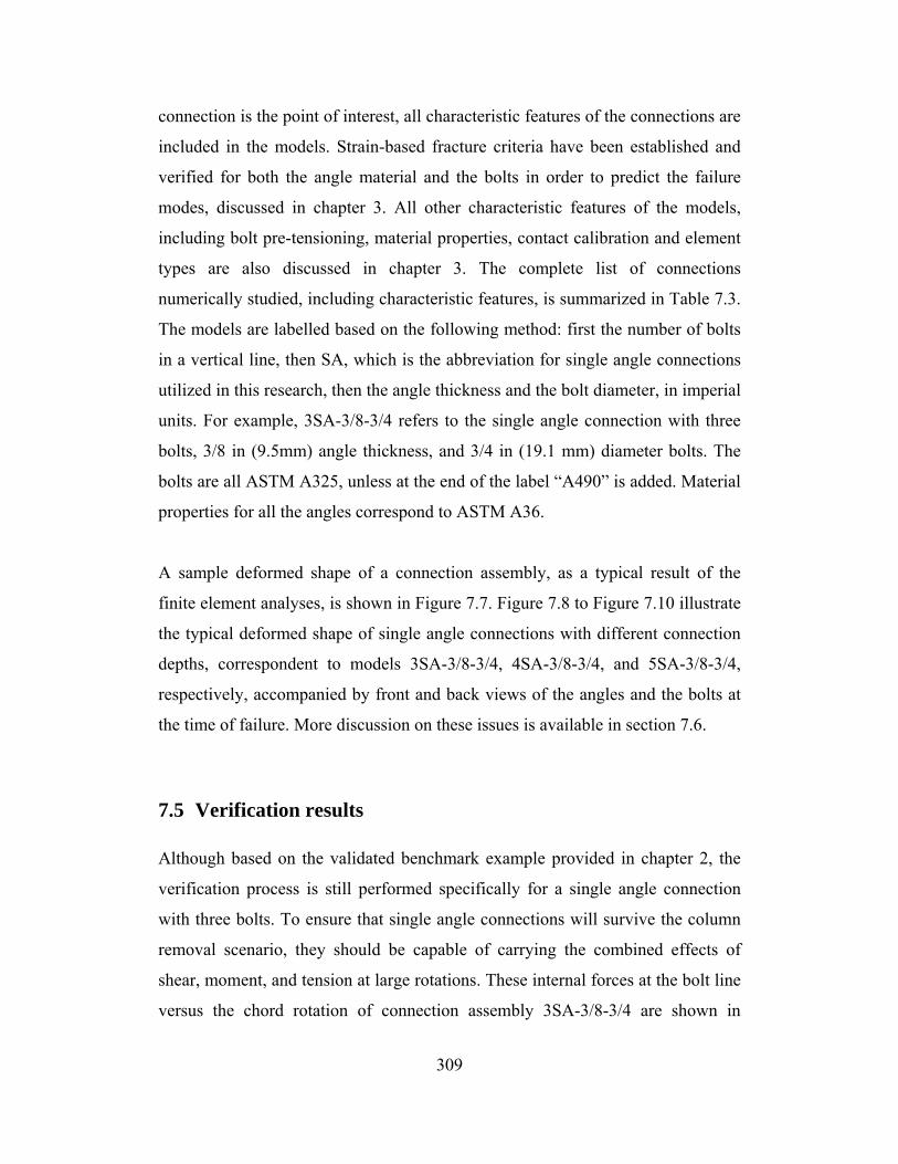
309

connection is the point of interest, all characteristic features of the connections are

included in the models. Strain-based fracture criteria have been established and

verified for both the angle material and the bolts in order to predict the failure

modes, discussed in chapter 3. All other characteristic features of the models,

including bolt pre-tensioning, material properties, contact calibration and element

types are also discussed in chapter 3. The complete list of connections

numerically studied, including characteristic features, is summarized in Table 7.3.

The models are labelled based on the following method: first the number of bolts

in a vertical line, then SA, which is the abbreviation for single angle connections

utilized in this research, then the angle thickness and the bolt diameter, in imperial

units. For example, 3SA-3/8-3/4 refers to the single angle connection with three

bolts, 3/8 in (9.5mm) angle thickness, and 3/4 in (19.1 mm) diameter bolts. The

bolts are all ASTM A325, unless at the end of the label “A490” is added. Material

properties for all the angles correspond to ASTM A36.

A sample deformed shape of a connection assembly, as a typical result of the

finite element analyses, is shown in Figure 7.7. Figure 7.8 to Figure 7.10 illustrate

the typical deformed shape of single angle connections with different connection

depths, correspondent to models 3SA-3/8-3/4, 4SA-3/8-3/4, and 5SA-3/8-3/4,

respectively, accompanied by front and back views of the angles and the bolts at

the time of failure. More discussion on these issues is available in section 7.6.


Although based on the validated benchmark example provided in chapter 2, the

verification process is still performed specifically for a single angle connection

with three bolts. To ensure that single angle connections will survive the column

removal scenario, they should be capable of carrying the combined effects of

shear, moment, and tension at large rotations. These internal forces at the bolt line

versus the chord rotation of connection assembly 3SA-3/8-3/4 are shown in

310

Figure 7.11 to Figure 7.13 to illustrate the shear, tension, and flexural responses.

The dashed and solid lines represent the results of the experiments and

simulations, respectively. The shear responses of the connections, demonstrated in

Figure 7.11, tensile curve in Figure 7.12, and the moment response, in Figure

7.13, serve to verify the models based on acceptable correlation with the

associated experimental results. The agreement between the experiment and

numerical results is deemed to be satisfactory, considering the differences

between the nominally identical test connections themselves.


A parametric study is performed using the verified model to investigate the effects

of different design parameters, such as angle thickness, bolt size and type, and

also connection depth, according to Table 7.3. This investigation is discussed in

sections 7.6.1 to 7.6.3.

7.6.1 Three bolt single angle connections (3SA)

to show the interactions of shear, tension, and moment for the single angle

connections with three bolts (3SA). shows the behaviour of 3SA-3/8-3/4 without

the test curves. The maximum moment happens at the approximate rotation of

0.08 radians. At this point, the couple force action is distinguished by compressive

force at the top hole in the web-framing leg and tensile action at the bottom hole

of the outstanding leg. There is some local yielding at the top of the web-framing

leg due to teh compressive force, which reduces the flexural resistance after the

peak. As labelled in the figure, the point that the flexural phase domination ends

and catenary force begins to provide the major resistance is named the

“devolution point”, similar to what was discussed for shear tab and WT

connections. For the 3SA-3/8-3/4 connection, the devolution point is located at

the rotation of 0.12 radians, when the flexural resistance of the connection has

311

already reduced significantly. The main reason for this is the fact that in 3-bolt

connections, the top bolt resists the moment demand through bearing resistance of

the bolt–hole interaction; meanwhile, the bottom part of the section resists

moment through combined effects of bending action of the outstanding leg and

through tension force in the bottom bolt of the outstanding leg. As soon as

localized yielding happens around the contact surface at the top of the web

framing leg, the flexural resistance starts to vanish and the connection finds

another load path to take more load. The failure will be in the catenary phase. The

same phenomenon is observed in the 4SA and 5SA connection assemblies. Unlike

the WT connection bolts, the bolts of the web framing leg remain almost elastic,

although there is some plastic elongation in the two bottom bolts of the

outstanding leg due to tension. The connection can sustain a large amount of

rotation (0.22 radians) by providing ductility through yielding of web-framing leg

and also out-of-plane deformation of the outstanding leg. The connection

eventually fails because of excessive plastic deformation at the bottom hole of the

outstanding leg. The deformed shape of the connection at the time of failure is

shown in Figure 7.8.

shows the interaction of internal forces at the bolt line for the model 3SA-1/4-3/4.

In this model, the failure is initiated in the single angle bottom hole region in the

outstanding leg. A slight increase in the ductility of the connection is observed in

comparison with 3SA-3/8-3/4 due to the thinner angle thickness and,

consequently, more out-of-plane deformation of the outstanding leg. There are no

significant plastic shear deformations observed in the bolts—even the bottom bolt

of the outstanding leg—since most of the deformation happens in the thin angle.

The tensile force starts to come into existence at the point of almost zero moment,

which signifies the complete separation of the flexural phase from the catenary

action. Although the shear response of the connection is small in comparison with

the tensile forces, a “snap–through” kind of behaviour is observable. The shear

force of connection 3SA-1/4-3/4 increases almost linearly up to the point of

almost 0.04 radians, then it starts to reduce until 0.1 radians of rotation. After that,

312

it increases almost linearly, interacting with tension, at high rotations. The reason

for such behaviour is that at the rotation of 0.04 radians, the heel of the angle

starts to yield, which causes a reduction in the shear resistance of the connection.

However, after the rotation of 0.1 radians, bearing of the bolts in the outstanding

leg begins to play a role, and the shear force increases subsequently. This

phenomenon is observed in 4SA and 5SA connections with thin angles (6 mm or

¼ in) as well.


No difference is observed in the failure mode of this connection compared to

other models with different angle thicknesses. The ductility of the connection is

not changed either, in comparison with 3SA-3/8-3/4 and 3SA-1/4-3/4. There is

tensile plastic deformation in the bolts of the outstanding leg, although the other

bolts remained nearly elastic. The tensile force starts to come into existence after

the point of maximum moment. This could be attributed to the thicker angle size

that still possesses additional flexural resistance when tensile catenary force starts

to develop. The share of out-of-plane deformation of the outstanding leg in

providing the ductility of the connection is quite substantial. Similar to the other

two angle connections (3SA-3/8-3/4 and 3SA-1/4-3/4), although the connection

failed due to initiation of rupture at the outstanding leg bottom hole region, heel

rupture is also possible due to an excessive amount of plastic deformation.

and show the interaction of internal forces at the bolt line for the models 3SA-

3/8-5/8 and 3ST-3/8-7/8, respectively. There is a small amount of plastic strain

observed at the top 5/8 in (15.9 mm) bolt of web framing leg, which is not

observed in the 7/8 in (22.2 mm) bolts. The other characteristic features of the

connection are similar to 3ST-3/8-3/4. The tensile force starts to come into

existence at some point on the descending branch of flexural response, which is

an indication of a flexural-phase to catenary-phase transition point. The

connections can accommodate large rotations up to 0.21 radians prior to failure.

313

The behaviour of model 3SA-3/8-3/4-A490 is very similar to 3SA-3/8-3/4 with

ASTM A325 bolts. The dominant limit state of the connection is similar, as

expected. 3SA-3/8-3/4 was slightly more ductile due to a higher inherent ductility

of ASTM A325 bolts. As observed, substituting the ASTM A325 bolts with

ASTM A490 bolts has little effect on the connection performance.

Generally, in 3SA connections, regardless of the angle thickness, bolt size and

type, as the flexural stiffness of the connection becomes zero and subsequently

negative and then ramps down to zero, the tensile catenary forces increase rapidly

until the failure of the connection. Tensile catenary resistance starts to grow at the

approximate chord rotation angle of 0.12 radians, where the maximum flexural

strength is already been reached. Basically, the connections do not have

considerable flexural resistance at the time of failure. Therefore, it can be inferred

that the 3SA connections fail because of catenary action. The dominant failure

mode of 3SA connections is outstanding leg rupture at the bottom bolt hole

region, although heel rupture is also possible due to high plastic deformation. The

average rotational capacity of the 3SA connections studied in this research is

about 0.22 radians, which is significantly higher than three bolt shear tab and WT

connections.

7.6.2 Four bolt single angle connections (4SA)

to show the interactions of shear, tension, and moment for the single angle

connections with four bolts (4SA). shows the interaction curves of the model

4SA-3/8-3/4. A point might be distinguished as a devolution point after the

maximum moment occurs, as shown in , while the moment is degrading. For the

4SA connections this point is the onset of the catenary phase. There is a change in

the slope of the tensile response at the approximate rotation of 0.17 radians. At

this point, another yield line starts to develop at the angle heel in the outstanding

leg, labelled as secondary yield line in Figure 7.9. Similar to the 3SA connections,

the primary yield lines are the main sources of ductility, shown in as well.

314


The general behaviour of 4SA-1/4-3/4 is similar to the 3SA-1/4-3/4 model due to

the same geometric and mechanical properties. The failure is initiated in the angle

bottom hole region in the outstanding leg. The ductility of the connection is

similar to 4SA-3/8-3/4. No significant plastic shear deformation is observed in the

bolts—even the bottom one—since most of the bearing deformations happen in

the thin angle. The tensile force starts to grow at the rotation of 0.12 radians,

when the resisting moment is diminishing gradually.


The rotational ductility of the connection is comparable with 4SA-1/4-3/4 and

4SA-3/8-3/4. Most of the bolts remain elastic except the two bottom bolts at the

outstanding leg. The bottom bolt at the web-framing leg also experienced some

plastic deformation. The devolution to the catenary phase happens at the

approximate rotation of 0.10 radians in this connection assembly.


In this model, the failure initiated at the outstanding leg of the bottom hole. A

small amount of plastic deformation happens in the bolt shank of the bottom three

bolts at the column face, accompanied by slight plastic strains appearing at the

bottom and top bolts in the web framing leg before failure. The ductility of the

connection is almost the same as for the 4SA-3/8-3/4 model. The tensile force

starts to become significant at the approximate chord rotation of 0.11 radians. At

this rotation angle, the flexural behaviour keeps reducing, indicating the switch

from flexural behaviour to the catenary phase.


In this model, the failure mode is similar to other four bolt angle connections. A

very slight amount of plastic deformation developed in the bolt shanks. There are

significant plastic deformations along the yield lines similar to the 4SA-3/8-3/4

connection model. The devolution from flexural behaviour to the catenary phase

occurs at the rotation of about 0.11 radians.

315

As observed in the 4SA connections, a point is distinguished as a devolution point

in which the tensile force appears as an alternative load path in the connection

internal force interaction curve. After this point, the tensile catenary force

increases rapidly until the failure of the connection, in the presence of shear and

moment. Tensile catenary resistance starts to grow at the approximate chord

rotation angle of 0.11 radians, at which point the flexural response continues to

degrade. Basically, the amount of moment at the failure is negligible in most of

the cases. Therefore, it can be inferred that the 4SA connections fail mainly

because of catenary actions. The dominant failure mode of 4SA connections is

outstanding leg rupture, initiated at the bottom hole region.

7.6.3 Five bolt single angle connections (5SA)

to depict the simultaneous presence of shear, tension, and moment for the single

angle connections with five bolts (5SA). The interaction of internal forces of 5SA-

3/8-3/4 is demonstrated in . Similar to 4SA and 3SA connections, the

“devolution” point in this connection is located on the degrading branch of

flexural curve. A point is distinguished as a devolution point in which the

connection cross-section goes to catenary action. After that, tensile force and

moment interact until the connection failure. In this connection, all the bolts

remain elastic except the three bottom bolts at the column face. Three yield lines

are distinguished in the angle at the time of failure, as indicated in Figure 7.10.

Local bearing yielding at the top and bottom hole of web framing web is also

distinguishable; however, its magnitude is negligible in comparison with the

yielding at the bolt line outstanding leg and also the heel of the angle.


Its behaviour is similar to the 4SA-1/4-3/4 and 3SA-1/4-3/4 models due to the

same geometric and mechanical properties. The failure is initiated in the bottom

hole region of the outstanding leg, similarly. A slight increase in the ductility of

the connection is observed in comparison with the 5SA-3/8-3/4 model because of

316

the more ductile behaviour of the thinner plate. There is no significant plastic

shear deformation observed in the bolts—even the bottom bolts—since most of

the bearing deformations happen in the thin angle. In this five bolt connection, the

tensile force comes to play at the rotation of about 0.11 radians. After that, an

increase in the tensile force continues until failure, while the flexural strength

degrades. At the approximate rotation of 0.16, a reduction in the slope of the

tensile response is observed, which was discussed in the section 7.6.2. As a result,

the devolution of this connection is distinguished as flexural to the catenary phase.

shows the interaction of internal forces at the bolt line for model 5SA-1/2-3/4,

with similar behaviour as 3SA-1/2-3/4 and 4SA-1/2-3/4 connections. There is a

slight increase in the rotational ductility of the connection in comparison with

5SA-3/8-3/4 and 5SA-3/8-3/4. There are also plastic strains in the bottom three

bolts at the column face and the bottom one at the web-framing leg prior to

failure. The other bolts remained essentially elastic. The devolution from flexural

behaviour to the catenary phase is obvious in this connection assembly at the

rotation of 0.08 radians. This chord rotation corresponds to the maximum moment

as well, after which a reduction in the flexural strength of the connection happens.


In this model, despite the usage of smaller bolts, still the failure happens in the

angle, similar to the 4SA-3/8-5/8 and 3SA-3/8-5/8 connection models. A

substantial amount of plastic deformation was happening in the bolt shank,

accompanied by considerable bearing deformation at the bottom hole. The

ductility of the connection is almost the same as for the 5SA-3/8-3/4 model. The

tensile catenary force comes to play a role at the rotation of 0.10 radians, which is

deemed to be the devolution point to the tensile behaviour from the flexural

phase. The amount of plastic strain in the bolts is more substantial in the 5SA-3/8-

5/8 connection compared to the other five bolt single angle connections.

shows the interaction of shear, tension, and moment at the bolt line for the model

5SA-3/8-7/8, with the same failure mode as other types of five bolt connections

317

studied in this research. A very slight amount of plastic deformation happened in

the bolt shank. There are significant plastic deformations around the bottom bolt

hole area in the outstanding leg. The devolution from flexural behaviour to the

catenary phase occurs at the rotation of about 0.10 radians. After 0.10 radians,

although the decrease in moment strength happens continuously, there is still a

substantial moment at the connection prior to failure; however, since the increase

in tension is accompanied by a decrease in the moment resistance, the connection

fails mainly in tension.

The behaviour of model 5SA-3/8-3/4-A490 is very similar to that of 5SA-3/8-3/4

with ASTM A325 bolts. The dominant limit state of the connection is plate

failure, as expected. However, unlike the similar model with A325 bolts, no

substantial shear deformation in the bottom bolt shank was observed. The

ductility of the 5SA-3/8-3/4 connection is slightly more than the similar one with

ASTM A490 bolts.

Generally, similar to the 3SA and 4SA connections, the “devolution point" in 5SA

connections happens almost at or after the rotation at which the maximum rotation

happens. A point is distinguished as a devolution point where a tensile force

comes to play a role. The tensile catenary forces increased rapidly, interacting

with moment, until the failure of the connection. Tensile catenary resistance starts

to grow after the approximate chord rotation angle of 0.08 radians when flexural

response starts to decrease. Although, the amount of moment and tension at the

failure is substantial, it is deemed that the connections fail mainly because of

catenary action due to gradual reduction in the moment curve. The dominant

failure mode of 5SA connections is angle rupture at the bottom hole area of the

outstanding leg, similar to 3SA and 4SA connections.

318


In this section, the effect of angle thickness, bolt size, and bolt type are discussed

separately for three, four, and five bolt single angle connections.

7.7.1 Three bolt single angle connections (3SA)



3SA connections with different angle thicknesses. Generally, an increase in

thickness causes an increase in shear, tensile, and flexural strengths of 3SA

connections. There is a flat plateau in the shear response of 3SA-3/8-3/4 until 0.10

rad, which shows up as degradation of shear response in the connection 3SA-1/4-

3/4 due to formation of a second yield line at the angle web-framing leg. This

phenomenon does not cause a reduction of shear in the thicker plate. In terms of

axial load path response, the difference among the curves is substantial, although

the ductilities of the connections are almost the same. It can be inferred that the

ductility of the connection does not change significantly by altering the angle

thickness.

The maximum tensile catenary force the angles can develop is highly dependent

on the angle thickness. There is an abrupt change in the axial stiffness of all

thicknesses, at the approximate rotation of 0.16 radians, which is related to the

initiation of yielding in the bottom of the heel of the connection at the outstanding

leg. The shear strength of the connection with the 6 mm (1/4 in) thickness is about

40% that of the one with the 9.5 mm (3/8 in) thick angle. In terms of axial

strength, this value is reduced to even less than 35%. Model 3SA-1/4-3/4, with the

thinnest angle, shows slightly higher ductility due to the higher contribution from

out-of-plane deformation of the outstanding leg. The maximum moment happens

at approximately the same rotation (0.08 radians) for all thicknesses. All the

319

flexural responses possess a descending branch after the peak moment until zero

flexural resistance, as observed in Figure 7.31.

7.7.1.2 Bolt size


the 3SA connections with different bolt sizes. Unlike the effect of angle thickness,

an increase in bolt diameter does not cause a significant increase in the shear and

shear responses of 3SA connections; the behaviour is almost the same, as shown

in Figure 7.32 and Figure 7.33, although a slight increase is observed with an

increase in bolt diameter. The change in the rotational capacity of 3SA

connections due to a change in bolt diameter is also very small and considered

negligible. The shear and tensile strengths of the 3SA-3/8-5/8 connection are

approximately 85% those of the 3SA-3/8-3/4 connection. The maximum moment

happens at approximately the same rotation (0.08 radians) for all bolt sizes. All

the flexural responses possess a descending branch after the peak moment and

degrade to zero, as observed in Figure 7.34. In general, since the deformation

capacity of bolts is relatively small compared with the ductility provided by the

angles themselves, the use of larger bolts could not improve connection ductility

other than if the increase served to prevent premature bolt failure.

7.7.1.3 Bolt type

The effect of the bolt grade—ASTM A325 versus ASTM A490—is also

investigated for the 3SA-3/8-3/4 model. It is observed that the shear, axial, and

flexural responses of the connection assembly with two different types of bolts are

almost the same, with a minor difference in the rotational ductility. The

connection with ASTM A325 bolts shows slightly more ductility.

320

7.7.2 Four bolt single angle connections (4SA)



4SA connections with different angle sizes. The effect of angle thickness is almost

the same as for the 3SA connections. It can be inferred that shear and axial

strength of the connection does change significantly by altering the angle

thickness. The shear strength of the connection with the 6 mm (1/4 in) thickness is

about 60% of the one with the 9.5 mm (3/8 in) thick angle. In terms of axial

strength, this value is reduced to less than 55%. The maximum moment happens

at the same approximate rotation (0.08 radians) for all the models. All the

connection models possess the flexural response with a complete descending

branch after the peak moment until almost zero flexural resistance, as observed in

the Figure 7.37.

7.7.2.2 Bolt size


the 4SA connections with different bolt sizes. An increase in bolt diameter causes

a minor increase in the axial and shear responses of 4SA connections. The

rotational ductility of 4SA connections with different bolt diameters is almost the

same. The maximum moment happens at the approximate same rotation (0.08

radians) for all bolt sizes. All of the flexural responses possess a descending

branch after the peak moment to zero flexural resistance, as observed in Figure

7.40.

7.7.2.3 Bolt type

Similar to the explanation for the 3SA connections, the effect of different bolt

type—ASTM A325 versus ASTM A490—is also investigated for the 4SA-3/8-3/4

model. The shears, axial, and flexural responses of the connection assembly with

321

two different types of bolts are almost the same, with only a minor difference in

the rotational ductility.

7.7.3 Five bolt single angle connections (5SA)



5SA connections with different angle sizes. The effect of angle thickness is almost

the same as for the 3SA and 4SA connections. Generally, an increase in angle

thickness causes an increase in shear, tensile, and flexural strength of 5SA

connections. The difference in the shear and flexural responses at the beginning

(up to 0.02 radians) is small and as the rotation increases, the difference becomes

more substantial. In terms of load path, the axial response of the connection

changes significantly by altering the angle thickness. From the strength point of

view, the maximum tensile catenary force they can develop is highly dependent

on the angle thickness, as observed in Figure 7.42. However, the ductility of the

three connections is almost the same. The models start to go through tensile

catenary force at different rotations. This issue is due to a shift of the centre of

rotation of the connection towards the top of the connection. This shift is more

significant in the thin angle. As a result, catenary action starts to appear at the

connection at higher rotation. It can be inferred that axial response of the

connection changes by altering the angle thickness. The shear and tensile strength

of the connections with the 6 mm (1/4 in) thick angle is about 55% of the one with

the 9.5 mm (3/8 in) angle. All of the moment curves possess a descending branch

after the peak value, as observed in Figure 7.43, although the connections still

possess significant flexural resistance at the time of failure.

322

7.7.3.2 Bolt size


the 5SA connections with different bolt sizes. An increase in bolt diameter causes

a minor increase in the flexural and shear responses of 5SA connections, similar

to the 4SA and 3SA connection assemblies. However, in terms of axial response,

the behaviour is almost the same, as shown in Figure 7.45. The rotational ductility

of 5SA connections with different bolt diameters is almost the same. The shear

and tensile strength of 5ST-3/8-5/8 is more than 90% of the 3ST-3/8-3/4

connection. The maximum moment happens at the approximate same rotation

(0.08 radians) for all bolt sizes. All the flexural responses possess a descending

branch after the peak moment, as observed in Figure 7.46. The moment at the

failure is almost half of the peak moment.

7.7.3.3 Bolt type

Similar to the explanation for the 3SA and 4SA connections, the effect of

different bolt types—ASTM A325 versus ASTM A490—is also investigated for

3SA-3/8-3/4 model. It is observed that the shear, axial, and flexural responses of

the connection assembly with two different types of bolts are almost the same,

with only a minor difference in the rotational ductility.

Table 7.4 summarizes the results of the numerical models at the initial failure of

the connections.

7.8 Rotational ductility of single angle connections in column removal scenario

As observed, the rotational capacity of single angle connections is not affected

greatly by variables such as angle thickness, bolt size and type. However, the

number of rows of bolts (depth of the connection) does have an effect. Within the

scope of what has been studied in this research, the main failure mode was rupture

323

of the bottom bolt hole region in the outstanding leg. Rotational capacity is

estimated based on the depth of the connection in current codes and guidelines.

Figure 7.47 illustrates the distribution of rotational capacity of single angle

connections studied in this research versus connection depth. Validated finite

element analysis (FEA) models portray eighteen points in order to produce a

reasonably sufficient number of data points for conducting a regression analysis.

Figure 7.48 shows the best-fit regression line considering all of the data. As a

result, Equation (7-5) in imperial and Equation (7-6) in SI units are proposed to

determine rotational capacities of single angle connections in the column removal

scenario. = −0.0086 + 0.271 (dconn in inches) (7-5)



is the total rotational capacity of the single angle connections in radians.

consists of both elastic and plastic components. The plastic rotation is the

rotation that guidelines such as ASCE 41 (2006) and DoD (2009) utilize to define

the connection behaviour. By aid of finite element models, plastic rotation can be


cases considered (Figure 7.49), is reported in Equations (7-7) and (7-8): = −0.0059 + 0.219 (dconn in inches) (7-7)


Elastic rotation ends when the first sign of plastic strain starts to appear in the

connection assembly. It is noted that the average elastic rotations observed in the

studied three, four and five bolt single angle connections are 0.035, 0.030, and

324

0.020 radians, respectively. As a result, in the absence of appropriate tools to

determine the elastic rotation limit for a single angle connection, the mentioned

values can be used based on the depth of the connection, assuming angles made of

ASTM A36 steel material.

Figure 7.50 compares the proposed equation for estimating the plastic rotational

capacity of single angle connections with those suggested for shear tab (chapter 5)

and WT (chapter 6) connections for two to six bolts. It is noted that the equations

shown in Figure 7.50 are all based on the assumption that failure happens in the

steel connection element and not in the bolts because the bolt shear failure mode

should be avoided by design. As such, the equation for shear tabs is modified

slightly from the one given in chapter 5 to discount the three cases that failed by

bolt shear failure (i.e., cases 4, 11, and 18 in Table 5.7). As can be seen, the

plastic rotational capacities of single angle connections are considerably higher

than those of WT and shear tab connections of the same depth, although the

slopes of all the curves are similar. The main reason for the high rotational

capacities in the SA connections is the significant contribution of out-of-plane

deformation of the angle outstanding leg, as discussed earlier in the chapter.

Comparing the WT and shear tab connections, the shear tab possess less plastic

rotational ductility than the WT connections due to out-of-plane deformation of

the WT flange, although its contribution is significantly less than the one observed

in the angle leg. As a result, single angle and shear tab connections are considered

to be the most and least ductile connections in the column loss event, respectively,

and the WT connection behaviour is somewhere in between, closer to shear tab

connection.

7.9 Conclusion

In this chapter, interaction of shear, tension, and moment in single angle

connections is investigated. The main source of ductility was out-of-plane

325

bending of the outstanding angle leg. Other sources of ductility, such as bolt hole

bearing deformation, were not significant in the studied connections. The

maximum rotation of single angle connections was between 0.23 and 0.16 radians

for three to five bolt connections. The response curves can be used as input for

single angle connection models in full-building progressive collapse analyses.

Unlike the other two types of one-sided shear connections, the flexural and

catenary phases of single angle connections are effectively independent from each

other for all three depths of connections studied. Other conclusions that can be

drawn are:

• It cannot be assumed that all of the fasteners in a line share equally in carrying

the shear and tensile load. In fact, the fasteners towards the bottom of the joint

carry the largest portion of the load. This unequal loading of the fasteners is

accentuated as the rotation increases, similar to shear tab and WT connections.

• The point that the flexural phase domination ends and catenary force begins to

provide the major resistance is named the “devolution point”. For 3SA

connections, this point occurs at a large rotation and the flexural resistance of

the connection is almost zero, whereas for 5SA connections, the devolution

point is close to the rotation at which the peak moment occurs. The 4SA

devolution point is somewhere between these two cases. The main reason for

this difference in behaviour is the fact that in the 3-bolt angle connections the

bottom and top bolts resist the moment through bearing resistance of the bolt–

hole interaction. However, for the bottom bolt, due to the presence of out-of-

plane deformation of the angle outstanding leg, the ductility demand shifts

from the bolt hole regions of the web-framing leg to a combination of out-of-

plane bending of the angle leg and yielding of the angle heel at the column

face. Due to the inherent flexibility of the connection, it attempts to find

another load path to take additional load until failure when the flexural

resistance almost vanishes. In the 4SA and 5SA connections, due to the

geometry of the connection the catenary action starts earlier but still during the

326

degrading branch of the flexural curve. After the devolution point, tension

dominates the behaviour until failure occurs. Therefore, it can be inferred that

the single angle connections fail mainly because of catenary action.

327

Table 7.1: Advantages and disadvantages of single-sided connections (Murray 2013)

Type of connection

Advantages Disadvantages

Tee (WT) • can be used in composite construction

• stiffer than other types except shear tab

• tee can be heavy

Shear tab

• simple – few parts • can be designed to resist axial

force

• stiffer than other types • requires careful design

Single angle • eliminate erection problem1 • fewer parts1

• cannot resist axial load not recommended for laterally unbraced beams

• larger angle and bolts required1

1: comparing with double angle connections.

Table 7.2: Typical material used for SA connections

Component Material Description

Angle ASTM A36, 300W, 350W -


Welds E70XX electrode fillet welds

Table 7.3: Summary of characteristic features of FE models of SA connections

No. Specimen Label Angle Type Angle Section Bolt Type Bolt diameter Remarks

1 3SA-3/8-3/4 ASTM A36 L152X89X9.5 ASTM A325 19.1 mm (3/4 in) Used for

verification 2 3SA-1/4-3/4 ASTM A36 L152X89X6.4 ASTM A325 19.1 mm (3/4 in) - 3 3SA-1/2-3/4 ASTM A36 L152X89X13 ASTM A325 19.1 mm (3/4 in) - 4 3SA-3/8-5/8 ASTM A36 L152X89X9.5 ASTM A325 15.9 mm (5/8 in) - 5 3SA-3/8-7/8 ASTM A36 L152X89X9.5 ASTM A325 22.2 mm (7/8 in) - 6 3SA-3/8-3/4-A490 ASTM A36 L152X89X9.5 ASTM A490 19.1 mm (3/4 in) - 7 4SA-3/8-3/4 ASTM A36 L152X89X9.5 ASTM A325 19.1 mm (3/4 in) - 8 4SA-1/4-3/4 ASTM A36 L152X89X6.4 ASTM A325 19.1 mm (3/4 in) - 9 4SA-1/2-3/4 ASTM A36 L152X89X13 ASTM A325 19.1 mm (3/4 in) -

10 4SA-3/8-5/8 ASTM A36 L152X89X9.5 ASTM A325 15.9 mm (5/8 in) - 11 4SA-3/8-7/8 ASTM A36 L152X89X9.5 ASTM A325 22.2 mm (7/8 in) - 12 4SA-3/8-3/4-A490 ASTM A36 L152X89X9.5 ASTM A490 19.1 mm (3/4 in) - 13 5SA-3/8-3/4 ASTM A36 L152X89X9.5 ASTM A325 19.1 mm (3/4 in) - 14 5SA-1/4-3/4 ASTM A36 L152X89X6.4 ASTM A325 19.1 mm (3/4 in) - 15 5SA-1/2-3/4 ASTM A36 L152X89X13 ASTM A325 19.1 mm (3/4 in) - 16 5SA-3/8-5/8 ASTM A36 L152X89X9.5 ASTM A325 15.9 mm (5/8 in) - 17 5SA-3/8-7/8 ASTM A36 L152X89X9.5 ASTM A325 22.2 mm (7/8 in) - 18 5SA-3/8-3/4-A490 ASTM A36 L152X89X9.5 ASTM A490 19.1 mm (3/4 in) -

328

Table 7.4: Summary of numerical responses of single angle connections at initial failure

No. Specimen/Model

Label Connection Depth (mm)

Rotation (Rad)

V (kN) T (kN) M (kN.m) Failure Mode

1 3SA-3/8-3/4 152.4 0.222 32.2 151.0 Negligible SA bottom hole rupture





6 3SA-3/8-3/4-A490 152.4 0.213 32.8 152.7 Negligible SA bottom hole rupture

7 4SA-3/8-3/4 228.6 0.193 34.9 179.2 1.4 SA bottom hole rupture



10 4SA-3/8-5/8 228.6 0.193 34.1 167.2 1.2 SA bottom hole rupture 11 4SA-3/8-7/8 228.6 0.189 35.7 186.8 2.1 SA bottom hole rupture

12 4SA-3/8-3/4-A490 228.6 0.185 36.9 178.5 1.5 SA bottom hole rupture






18 5SA-3/8-3/4-A490 304.8 0.162 41.4 183.7 16.7 SA bottom hole rupture

329

330

Beam

Column

(a)

(c) (d)

(d)

Beam

Column

Beam

Column

Beam

Column

Figure 7.1: Types of SA shear connections: (a) welded-bolted (b) bolted-welded (c) welded-welded (d) bolted-bolted

Figure 7.2

Figure 7.3:

: Elastic-per

General def

rfectly plastic

formation paCh

331

c moment-ro1990)

attern of singhen 1990)

otation curve

gle angle con

es (Kishi and

nnection (Ki

d Chen

ishi and

Figure

Figure 7.5:

e 7.4: Model

Application

ling of angle

n of yield lin

332

e performed

ne theory for 2009)

by Kishi an

r single angle

nd Chen (199

e connection

90)

n (Gong

333

(a)

(b) (c) (d)

Figure 7.6: Finite element models of: (a) full connection assembly, (b) three bolt single angle connection (3SA), (c) four bolt single angle connection (4SA),

(d) five bolt single angle connection (5SA)

Figure 7.7: Deformed shape of finite element connection assembly

334

(a)

(b) (c) (d)

Figure 7.8: Failure of 3SA, numerical results: (a) deformed shape of connection assembly, (b) angle deformed shape – front view, (c) failure initiation

– back view, (d) bolt shear deformation

Primary yield lines

Secondary yield line Failure modelled by element removal

335

(a)

(b) (c) (d)

Figure 7.9: Failure of 4SA, numerical results: (a) deformed shape of connection assembly, (b) angle deformed shape – front view, (c) failure initiation – back

view, (d) bolt shear deformation

Primary yield lines

Secondary yield line Failure modelled with element removal

336

(a)

(b) (c) (d)

Figure 7.10: Failure of 5SA, numerical results: (a) deformed shape of connection assembly, (b) angle deformed shape – front view, (c) failure initiation – back

view, (d) bolt shear deformation

Primary yield lines

Secondary yield line

Failure modelled with element removal

337

Figure 7.11: Comparison of numerical and experimental shear response of connection 3SA

Figure 7.12: Comparison of numerical and experimental tensile response of connection 3SA

0.0

5.0

10.0

15.0

20.0

25.0

30.0

35.0

40.0

45.0

50.0

55.0

60.0

0.00 0.02 0.04 0.06 0.08 0.10 0.12 0.14 0.16 0.18 0.20 0.22 0.24

She

ar (

kN.m

)


3SAL1

3SAR1

3SA-3/8-3/4

0.0

20.0

40.0

60.0

80.0

100.0

120.0

140.0

160.0

180.0

200.0

220.0

240.0

260.0

0.00 0.02 0.04 0.06 0.08 0.10 0.12 0.14 0.16 0.18 0.20 0.22 0.24

Ten

sion

(kN

)


3SAL1

3SAR1

3SA-3/8-3/4

Figure 7.1

Figure 7.14

0.000

2.000

4.000

6.000

8.000

10.000

12.000

14.000

16.000

18.000

20.000

22.000

0.0

Mom

ent (

kN.m

)

0.0

2.0

4.0

6.0

8.0

10.0

12.0

14.0

16.0

18.0

20.0

22.0

0.00

Mom

ent (

kN.m

)

3: Comparis

: Bolt line fo

00 0.02 0.04

0.02 0.04 0.

son of numerconn

orces versus

0.06 0.08

Beam

06 0.08 0.10

Beam End

338

rical and expnection 3SA

beam end ro

0.10 0.12 0.

m End Rotation

0.12 0.14 0

d Rotation (Ra

perimental flA

otation – Spe

.14 0.16 0.1

n (Rad)

3SAL1

3SAR1

3SA-3/8-3/

0.16 0.18 0.20

ad)

Moment

Tension

Shear

flexural respo

ecimen 3SA

8 0.20 0.22

/4

0.

20

40

60

80

10

12

14

16

18

20

22

24

26

0 0.22 0.24

onse of

A-3/8-3/4

0.24

0

0.0

0.0

0.0

0.0

00.0

20.0

40.0

60.0

80.0

00.0

20.0

40.0

60.0

Ten

sion

and

She

ar (

kN)

Figure 7.15

Figure 7.16

0.0

2.0

4.0

6.0

8.0

10.0

12.0

14.0

16.0

18.0

20.0

22.0

0.00

Mom

ent (

kN.m

)

0.0

2.0

4.0

6.0

8.0

10.0

12.0

14.0

16.0

18.0

20.0

22.0

0.00

Mom

ent (

kN.m

)

: Bolt line fo

: Bolt line fo

0.02 0.04 0

Mom

Tens

Shea

0.02 0.04 0

Moment

Tension

Shear

orces versus

orces versus

.06 0.08 0.10Beam En

ment

sion

ar

0.06 0.08 0.1

Beam E

339

beam end ro

beam end ro

0 0.12 0.14nd Rotation (R

0 0.12 0.14

End Rotation (R

otation – Spe

otation – Spe

0.16 0.18 0.Rad)

0.16 0.18 0

Rad)

ecimen 3SA

ecimen 3SA

.20 0.22 0.24

0.20 0.22 0.2

A-1/4-3/4

A-1/2-3/4

0.0

20.0

40.0

60.0

80.0

100.0

120.0

140.0

160.0

180.0

200.0

220.0

240.0

260.0

4

Ten

sion

and

She

ar (

kN)

0.0

20.0

40.0

60.0

80.0

100.0

120.0

140.0

160.0

180.0

200.0

220.0

240.0

260.0

24

Ten

sion

and

She

ar (

kN)

M(k

N)

Mt(

kN)

Figure 7.17

Figure 7.18

0.01.53.04.56.07.59.0

10.512.013.515.016.518.019.521.022.524.0

0.00 0

Mom

ent (

kN.m

)

0.0

2.0

4.0

6.0

8.0

10.0

12.0

14.0

16.0

18.0

20.0

22.0

24.0

0.00 0

Mom

ent (

kN.m

)

: Bolt line fo

: Bolt line fo

0.02 0.04 0.0

Mom

Tens

Shea

0.02 0.04 0.0

orces versus

orces versus

06 0.08 0.10Beam En

ment

sion

ar

06 0.08 0.10

Beam End

Moment

Tension

Shear

340

beam end ro

beam end ro

0.12 0.14nd Rotation (Ra

0.12 0.14 0

d Rotation (Ra

otation – Spe

otation – Spe

0.16 0.18 0.ad)

0.16 0.18 0.2

ad)

ecimen 3SA

ecimen 3SA

.20 0.22 0.24

20 0.22 0.24

A-3/8-5/8

A-3/8-7/8

0.0

20.0

40.0

60.0

80.0

100.0

120.0

140.0

160.0

180.0

200.0

220.0

240.0

260.0

4

Ten

sion

and

She

ar (

kN)

0.0

20.0

40.0

60.0

80.0

100.0

120.0

140.0

160.0

180.0

200.0

220.0

240.0

260.0

4

Ten

sion

l and

She

ar (

kN)

Figure 7.19

Figure 7.20

0.0

3.0

6.0

9.0

12.0

15.0

18.0

21.0

24.0

27.0

30.0

33.0

0.00

Mom

ent (

kN.m

)

0.0

3.0

6.0

9.0

12.0

15.0

18.0

21.0

24.0

27.0

30.0

33.0

0.00

Mom

ent (

kN.m

)

: Bolt line fo

: Bolt line fo

0.02 0.04

Mome

Tensio

Shear

0.02 0.04

Mom

Tensi

Shear

orces versus

orces versus

4 0.06 0.0Beam

ent

on

0.06 0.08Beam E

ment

ion

r

341

beam end ro

beam end ro

08 0.10 0.End Rotation

8 0.10 0.1End Rotation (

otation – Spe

otation – Spe

.12 0.14 0(Rad)

12 0.14 0.Rad)

ecimen 4SA

ecimen 4SA

0.16 0.18

16 0.18 0

A-3/8-3/4

A-1/4-3/4

0.0

20.0

40.0

60.0

80.0

100.0

120.0

140.0

160.0

180.0

200.0

220.0

240.0

260.0

280.0

0.20

Ten

sion

and

She

ar (

kN)

0.0

20.0

40.0

60.0

80.0

100.0

120.0

140.0

160.0

180.0

200.0

220.0

240.0

260.0

280.0

0.20

Ten

sion

and

She

ar (

kN)

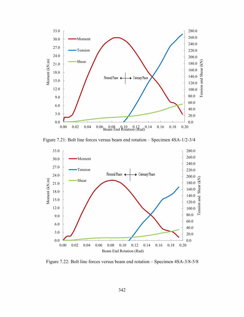
Figure 7.21: B

Figure 7.22

0.0

3.0

6.0

9.0

12.0

15.0

18.0

21.0

24.0

27.0

30.0

33.0

0.00

Mom

ent (

kN.m

)

0.0

3.0

6.0

9.0

12.0

15.0

18.0

21.0

24.0

27.0

30.0

33.0

0.00

Mom

ent (

kN.m

)

Bolt line forc

: Bolt line fo

0.02 0.04

Moment

Tension

Shear

0.02 0.04

Moment

Tension

Shear

ces versus b

orces versus

0.06 0.08Beam E

0.06 0.08

Beam E

342

eam end rota

beam end ro

8 0.10 0.1End Rotation (

0.10 0.12

End Rotation (R

ation – Spec

otation – Spe

12 0.14 0.(Rad)

2 0.14 0.1

Rad)

cimen 4SA-1

ecimen 4SA

16 0.18 0

16 0.18 0.2

1/2-3/4

A-3/8-5/8

0.0

20.0

40.0

60.0

80.0

100.0

120.0

140.0

160.0

180.0

200.0

220.0

240.0

260.0

280.0

0.20

Ten

sion

and

She

ar (

kN)

0.0

20.0

40.0

60.0

80.0

100.0

120.0

140.0

160.0

180.0

200.0

220.0

240.0

260.0

280.0

20

Ten

sion

and

She

ar (

kN)

Mt(

kN)

Figure 7.23

Figure 7.24

0.0

3.0

6.0

9.0

12.0

15.0

18.0

21.0

24.0

27.0

30.0

33.0

0.00

Mom

ent (

kN.m

)

0.0

5.0

10.0

15.0

20.0

25.0

30.0

35.0

40.0

45.0

50.0

0.00

Mom

ent (

kN.m

)

: Bolt line fo

: Bolt line fo

0.02 0.04

0.02 0.04

Mome

Tensio

Shear

orces versus

orces versus

0.06 0.08Beam En

Momen

Tension

Shear

4 0.06 0.

Beam En

ent

on

343

beam end ro

beam end ro

0.10 0.12nd Rotation (Ra

nt

n

.08 0.10

nd Rotation (R

otation – Spe

otation – Spe

0.14 0.16ad)

0.12 0.14

Rad)

ecimen 4SA

ecimen 5SA

0.18 0.20

0.16 0.1

A-3/8-7/8

A-3/8-3/4

0.0

20.0

40.0

60.0

80.0

100.0

120.0

140.0

160.0

180.0

200.0

220.0

240.0

260.0

280.0

0

Ten

sion

and

She

ar (

kN)

0.0

20.0

40.0

60.0

80.0

100.0

120.0

140.0

160.0

180.0

200.0

220.0

240.0

260.0

280.0

300.0

8

Ten

sion

and

She

ar (

kN)

F

F

igure 7.25: B

igure 7.26: B

0.0

5.0

10.0

15.0

20.0

25.0

30.0

35.0

40.0

45.0

50.0

0.00

Mom

ent (

kN.m

)

0.0

5.0

10.0

15.0

20.0

25.0

30.0

35.0

40.0

45.0

50.0

0.00

Mom

ent (

kN.m

)

Bolt line forc

Bolt line forc

0.02 0.0

Momen

Tension

Shear

0.02 0.0

Mome

Tensio

Shear

ces versus b

ces versus b

4 0.06 0

Beam En

nt

n

04 0.06 0

Beam E

ent

on

344

eam end rota

eam end rota

.08 0.10

nd Rotation (R

0.08 0.10

End Rotation (R

ation – Spec

ation – Spec

0.12 0.14

Rad)

0.12 0.14

Rad)

cimen 5SA-1

cimen 5SA-1

0.16 0.18

0.16 0.

1/4-3/4

1/2-3/4

0.0

20.0

40.0

60.0

80.0

100.0

120.0

140.0

160.0

180.0

200.0

220.0

240.0

260.0

280.0

300.0

8

Ten

sion

and

She

ar (

kN)

0.0

20.0

40.0

60.0

80.0

100.0

120.0

140.0

160.0

180.0

200.0

220.0

240.0

260.0

280.0

300.0

18

Ten

sion

and

She

ar (

kN)

F

F

igure 7.27: B

igure 7.28: B

0.0

5.0

10.0

15.0

20.0

25.0

30.0

35.0

40.0

45.0

50.0

0.00

Mom

ent (

kN.m

)

0.0

5.0

10.0

15.0

20.0

25.0

30.0

35.0

40.0

45.0

50.0

0.00

Mom

ent (

kN.m

)

Bolt line forc

Bolt line forc

0.02 0.0

Mom

Tensi

Shear

0.02 0.0

Momen

Tension

Shear

ces versus b

ces versus b

04 0.06 0

Beam E

ment

ion

r

04 0.06 0

Beam E

nt

n

345

eam end rota

eam end rota

0.08 0.10

End Rotation (R

0.08 0.10

End Rotation (R

ation – Spec

ation – Spec

0.12 0.14

Rad)

0.12 0.14

Rad)

cimen 5SA-3

cimen 5SA-3

0.16 0.18

0.16 0.18

3/8-5/8

3/8-7/8

0.0

20.0

40.0

60.0

80.0

100.0

120.0

140.0

160.0

180.0

200.0

220.0

240.0

260.0

280.0

300.0

8

Ten

sion

and

She

ar (

kN)

0.0

20.0

40.0

60.0

80.0

100.0

120.0

140.0

160.0

180.0

200.0

220.0

240.0

260.0

280.0

300.0

8

Ten

sion

and

She

ar (

kN)

346

Figure 7.29: Comparison of shear response of 3SA connections with different angle thicknesses

Figure 7.30: Comparison of tensile response of 3SA connections with different angle thicknesses

0.0

5.0

10.0

15.0

20.0

25.0

30.0

35.0

40.0

45.0

50.0

55.0

60.0

0.00 0.02 0.04 0.06 0.08 0.10 0.12 0.14 0.16 0.18 0.20 0.22 0.24

She

ar (

kN)


3SA-1/2-3/4

3SA-3/8-3/4

3SA-1/4-3/4

0.0

20.0

40.0

60.0

80.0

100.0

120.0

140.0

160.0

180.0

200.0

220.0

240.0

260.0

0.00 0.02 0.04 0.06 0.08 0.10 0.12 0.14 0.16 0.18 0.20 0.22 0.24

Ten

sion

(kN

)


3SA-1/2-3/4

3SA-3/8-3/4

3SA-1/4-3/4

347

Figure 7.31: Comparison of flexural response of 3SA connections with different angle thicknesses

Figure 7.32: Comparison of shear response of 3SA connections with different bolt sizes

0.0

2.0

4.0

6.0

8.0

10.0

12.0

14.0

16.0

18.0

20.0

22.0

0.00 0.02 0.04 0.06 0.08 0.10 0.12 0.14 0.16 0.18 0.20 0.22 0.24

Mom

ent (

kN.m

)


3SA-1/2-3/4

3SA-3/8-3/4

3SA-1/4-3/4

0.0

5.0

10.0

15.0

20.0

25.0

30.0

35.0

40.0

45.0

50.0

55.0

60.0

0.00 0.02 0.04 0.06 0.08 0.10 0.12 0.14 0.16 0.18 0.20 0.22 0.24

She

ar (

kN)


3SA-3/8-7/8

3SA-3/8-3/4

3SA-3/8-5/8

348

Figure 7.33: Comparison of tensile response of 3SA connections with different bolt sizes


0.0

20.0

40.0

60.0

80.0

100.0

120.0

140.0

160.0

180.0

200.0

220.0

240.0

260.0

0.00 0.02 0.04 0.06 0.08 0.10 0.12 0.14 0.16 0.18 0.20 0.22 0.24

Ten

sion

(kN

)


3SA-3/8-7/8

3SA-3/8-3/4

3SA-3/8-5/8

0.0

2.0

4.0

6.0

8.0

10.0

12.0

14.0

16.0

18.0

20.0

22.0

0.00 0.02 0.04 0.06 0.08 0.10 0.12 0.14 0.16 0.18 0.20 0.22 0.24

Mom

ent (

kN.m

)


3SA-3/8-7/8

3SA-3/8-3/4

3SA-3/8-5/8

349



0.0

5.0

10.0

15.0

20.0

25.0

30.0

35.0

40.0

45.0

50.0

55.0

60.0

0.00 0.02 0.04 0.06 0.08 0.10 0.12 0.14 0.16 0.18 0.20

She

ar (

kN.m

)


4SA-1/2-3/4

4SA-3/8-3/4

4SA-1/4-3/4

0.020.0

40.0

60.080.0

100.0

120.0140.0

160.0

180.0200.0

220.0240.0

260.0

280.0300.0

0.00 0.02 0.04 0.06 0.08 0.10 0.12 0.14 0.16 0.18 0.20

Ten

sion

(kN

)


4SA-1/2-3/4

4SA-3/8-3/4

4SA-1/4-3/4

350



0.0

3.0

6.0

9.0

12.0

15.0

18.0

21.0

24.0

27.0

30.0

33.0

0.00 0.02 0.04 0.06 0.08 0.10 0.12 0.14 0.16 0.18 0.20

Mom

ent (

kN.m

)


4SA-1/2-3/4

4SA-3/8-3/4

4SA-1/4-3/4

0.0

5.0

10.0

15.0

20.0

25.0

30.0

35.0

40.0

45.0

50.0

55.0

60.0

0.00 0.02 0.04 0.06 0.08 0.10 0.12 0.14 0.16 0.18 0.20

She

ar (

kN.m

)


3SA-3/8-7/8

4SA-3/8-3/4

3SA-3/8-5/8

351


Figure 7.40: Comparison of flexural response of 4SA connections with different bolt sizes

0.0

20.0

40.0

60.0

80.0

100.0

120.0

140.0

160.0

180.0

200.0

220.0

240.0

260.0

280.0

300.0

0.00 0.02 0.04 0.06 0.08 0.10 0.12 0.14 0.16 0.18 0.20

Ten

sion

(kN

)


3SA-3/8-7/8

4SA-3/8-3/4

3SA-3/8-5/8

0.0

3.0

6.0

9.0

12.0

15.0

18.0

21.0

24.0

27.0

30.0

33.0

0.00 0.02 0.04 0.06 0.08 0.10 0.12 0.14 0.16 0.18 0.20

Mom

ent (

kN.m

)


3SA-3/8-7/8

4SA-3/8-3/4

3SA-3/8-5/8

352



0.0

5.0

10.0

15.0

20.0

25.0

30.0

35.0

40.0

45.0

50.0

55.0

60.0

65.0

70.0

0.00 0.02 0.04 0.06 0.08 0.10 0.12 0.14 0.16 0.18

She

ar (

kN)


5SA-1/2-3/4

5SA-3/8-3/4

5SA-1/4-3/4

0.0

20.0

40.0

60.0

80.0

100.0

120.0

140.0

160.0

180.0

200.0

220.0

240.0

260.0

280.0

300.0

0.00 0.02 0.04 0.06 0.08 0.10 0.12 0.14 0.16 0.18

Ten

sion

(kN

)


5SA-1/2-3/4

5SA-3/8-3/4

5SA-1/4-3/4

353



0.0

5.0

10.0

15.0

20.0

25.0

30.0

35.0

40.0

45.0

50.0

55.0

60.0

65.0

70.0

0.00 0.02 0.04 0.06 0.08 0.10 0.12 0.14 0.16 0.18 0.20

Mom

ent (

kN.m

)


5SA-1/2-3/4

5SA-3/8-3/4

5SA-1/4-3/4

0.0

5.0

10.0

15.0

20.0

25.0

30.0

35.0

40.0

45.0

50.0

55.0

60.0

65.0

70.0

0.00 0.02 0.04 0.06 0.08 0.10 0.12 0.14 0.16 0.18

She

ar (

kN)


5SA-3/4-7/8

5SA-3/8-3/4

5SA-3/4-5/8

354


Figure 7.46: Comparison of flexural response of 5SA connections with different bolt sizes

0.0

20.0

40.0

60.0

80.0

100.0

120.0

140.0

160.0

180.0

200.0

220.0

240.0

260.0

280.0

300.0

0.00 0.02 0.04 0.06 0.08 0.10 0.12 0.14 0.16 0.18

Ten

sion

(kN

)


5SA-3/4-7/8

5SA-3/8-3/4

5SA-3/4-5/8

0.0

5.0

10.0

15.0

20.0

25.0

30.0

35.0

40.0

45.0

50.0

0.00 0.02 0.04 0.06 0.08 0.10 0.12 0.14 0.16 0.18

Mom

ent (

kN.m

)


5SA-3/4-7/8

5SA-3/8-3/4

5SA-3/4-5/8

355

Figure 7.47: Single angle connection total rotation capacities versus connection depth

Figure 7.48: Proposed equation for single angle connection total rotation capacities versus connection depth

0.000

0.050

0.100

0.150

0.200

0.250

0 2 4 6 8 10 12 14

Rot

atio

n (R

ad)


3SA-FEA

4SA-FEA

5SA-FEA

ϴ = -0.0086 dconn + 0.271

0.000

0.050

0.100

0.150

0.200

0.250

0 2 4 6 8 10 12 14

Rot

atio

n (R

ad)


EXP & FEA Results


356

Figure 7.49: Proposed equation for single angle connection plastic rotations versus connection depth

Figure 7.50: Comparison of proposed equations for plastic rotation of shear tab, single angle, and WT connections

ϴ = -0.0059 dconn + 0.219

0.000

0.050

0.100

0.150

0.200

0.250

0 2 4 6 8 10 12 14

Rot

atio

n (R

ad)


EXP & FEA Results


ϴSA = -0.0059 dconn + 0.219

ϴWT = -0.0076 dconn + 0.152

ϴST = -0.0070 dconn + 0.1280.000

0.050

0.100

0.150

0.200

0.250

0 2 4 6 8 10 12 14 16

Rot

atio

n (R

ad)


SA

WT

ST

357

8 Summary, Conclusions, and Recommendations for Future Research

8.1 Summary

This study is intended to quantify sources of inherent robustness of one-sided

steel shear connections in order to enhance the understanding of connection

robustness and, consequently, improve the analysis and design methods to

mitigate the vulnerability of steel structures to a column loss event. Progressive

collapse, as the main impetus for looking at steel shear connections again, is

defined and discussed. The key differences between the behaviour of shear

connections under conventional loading and in a double-span (column loss) event

are established, including the presence of a tensile catenary force and large beam

rotation. An appropriate substructure to investigate the behaviour of shear

connection assemblies that can mimic the behaviour and failure modes in a

progressive collapse event is selected. Subsequently, a model is developed for

shear connections subjected to a column loss event and a rational approach

presented to establish and calibrate a finite element model for simple shear

connections. A shear tab connection model is introduced that can be used as a

benchmark to validate finite element models of simple shear connections

subjected to extreme loading effects such as a column removal scenario.

Recommendations are provided on how to achieve a converged solution in steel

shear connections using state-of-the-art simulation techniques. In a column

removal scenario, considerable axial compressive force may develop via arching

action before catenary action begins. This phenomenon has been simulated

numerically and the results show that the vertical eccentricity between the centres

of rotation of the connections at the ends of a beam is a primary parameter leading

to the presence of this compressive force. Another important factor that affects the

development of arching action is the stiffness of the surrounding structure.

358

The simultaneous presence of shear, moment and tension in shear tab, WT and

single angle connections was investigated in different chapters, separately.

Comparisons between the experimental and the numerical quantities emphasized

the effectiveness and correctness of the proposed finite element models. It is

observed that one-sided shear connections are capable of developing an

alternative (catenary) load path when an adjacent column is compromised. The

research also quantified the rotational capacities of the connection types studied,

indicating that deeper connections possess less rotational capacity. It is observed

that the rotational capacity of single angle connections is significantly higher than

those of shear tab and WT types. Equations are proposed to calculate this

characteristic feature of the connection and also the plastic rotational capacities

based on connection depth. The effect of factors such as plate thickness, section

size, bolt size and type on the connection response are also investigated. The

concept of the “devolution point”, defined as the point that the flexural phase

domination ends and catenary force or a combination of flexural-catenary action

begins to provide the major resistance, is introduced. It is observed that shallow

shear tab and WT connections and all single angle connections transfer from the

flexural phase to the catenary phase at the devolution point; however, shear tab

and WT connections with four and five bolts transfer from the flexural phase to a

flexural-catenary phase. The results of this research project should contribute to a

better understanding of the resistance of steel structures with one-sided shear

connections to progressive collapse.

8.2 Conclusions

The following conclusions can be drawn from this research:

• In the finite element modelling of connections, obtaining the converged

nonlinear solution is the most challenging part due to the nonlinearity

definitions, including material, geometric, and boundary (contact)

nonlinearities. The analyst has to decide on several issues such as mesh

359

discretization, element types and the solving algorithm. These selections

may have significant effects on the model response and can lead to

inaccurate results if not carried out properly. Satisfying the convergence

issues in addition to good engineering judgment led to an accurate

solution. Although experimental results are needed for model validation, it

is not necessary to have them for each specific type of connection to verify

the response. Following the same procedure that was previously verified

can lead to “converged” (accurate) response. The example proposed in this

research can be taken as a benchmark for validating the finite element

modelling of shear connections in the column removal scenario.

• In a column removal scenario, considerable axial compressive force may

develop via arching action before catenary action begins. This

phenomenon has been simulated numerically and the results show that the

vertical eccentricity between the centres of rotation of the connections at

the ends of a beam is a primary parameter leading to the presence of this

compressive force. Another important factor that affects the development

of arching action is the stiffness of the surrounding structure. Whether the

arching action forms in the connection assembly or not, the catenary

resistance of the connection can act as an alternative load path in a column

loss event. Since the arching action, if present, occurs at an early stage of

connection response, it will not affect the ultimate capacity of the frame.

Therefore, tensile catenary action is still the desired alternative load path

in response to a column removal scenario, and therefore the connection

must be designed to resist these tensile loads.

• Tensile catenary force, as the alternative load path mechanism in a column

removal scenario, is observed interacting with flexural response at the

shear tab connection location. Ductility of shear tab connections is derived

largely from the local deformation of bolt holes, especially bottom holes,

and to a lesser degree the bolt slippage and bolt shear deformation before

failure. Tension rupture of the bottom hole was the governing failure mode

in most of the cases; however, bolt shear rupture was also observed. The

360

maximum rotational capacity of the shear tab connections studied was

between 0.06 and 0.13 radians for five to three bolts.

• The point that the flexural phase domination ends and catenary force or

flexural-catenary action begins to provide the major resistance is named

the “devolution point”. For shear tab connections with three bolts, this

point is located at the maximum moment and the failure will be in the

catenary phase. In the shear tabs with four and five bolts, a point is

distinguished as a "devolution point" at which a substantial decrease in

flexural stiffness happens. This decrease might be accompanied by an

increase in tensile force development rate (four bolt shear tabs) or not (five

bolt shear tabs). After this point, tension and moment interact until failure

occurs. Therefore, it can be inferred that the four and five bolt shear tab

connections fail mainly because of flexural-catenary actions.

• Tensile catenary action is acknowledged as the alternative load mechanism

in a column removal scenario of the WT connections as well. Ductility of

WT connections is derived largely from the local deformation in the stem

adjacent to the bottom holes and the bolt slippage and deformation before

failure. Out-of-plane bending of the WT flange between the bolt lines is

another source; however, it was not significant in the connections with

thick flanges. Based on the results of the numerical analyses, out-of-plane

flange deformation is a maximum at the bottom of all three connections

considered and is almost zero at the top. Either shear failure of the bottom

bolt or WT-stem bottom hole rupture was the governing failure mode in

all cases. The maximum rotational capacity of the WT connections studied

was between 0.05 and 0.16 radians for five to three bolts.

• For three bolt WT connections, the "devolution point" happened after the

maximum moment was reached and the failure was in the catenary phase.

Generally, the switch between flexural behaviour and the tensile phase in

WT connections with three bolts can be distinguished more accurately

than for the ones with four and five bolts. In the latter cases, there is a

point that can be assigned as the “devolution point”, at which the tensile

361

response starts to ramp up rapidly. The connection fails in the flexural-

catenary phase due to the presence of a significant amount of moment and

tension at the time of failure. It is noted that the WTs with five bolts go

into catenary tension from the beginning. At the “devolution point”, a

significant decrease in the slope of the flexural response and an increase in

the tensile response are observable. Basically, the amount of moment at

the failure is significant. As a result, it can be inferred that the WT

connections with five bolts fail mainly because of flexural-catenary action,

similar to four bolt WTs.

• Tensile catenary action is also acknowledged as the alternative load

mechanism in a column removal scenario of single angle connections. The

main source of ductility was out-of-plane bending of the angle. Other

sources, such as bolt hole bearing deformation, were not significant in the

studied connections. The maximum rotation of single angle connections

was between 0.23 and 0.16 radians for three to five bolt connections.

• For three bolt single angle connections, the “devolution point” is located at

a large rotation where the flexural resistance of the connection is almost

zero. For single angles with five bolts, this point is close to the rotation at

which the peak moment occurs. The four bolt devolution point is

somewhere between these two cases. In four and five bolt single angle

connections, due to the geometry of the connection, the catenary action

starts earlier but still during the degrading branch of the flexural curve.

After the devolution point, tension dominates the behaviour until failure

occurs. Therefore, it can be inferred that all single angle connections fail

mainly because of catenary action, unlike four and five bolt shear tab and

WT connections. This phenomenon is related to the inherent flexibility of

single angle connections in comparison with the two other types of

connections.

• It cannot be assumed that all of the fasteners in a line share equally in

carrying the load. In fact, the fasteners towards the bottom of the joint

362

carry the largest portion. This unequal loading of the fasteners is

accentuated as the rotation increases.

• Different types of one-sided shear connections possess different types of

failure modes. In the shear tab connections studied, the dominant mode of

failure was tearing of the plate. However, in the WTs the failure mode was

either bolt shear rupture or WT-stem hole tearing, depending on the bolt

diameter and WT web thickness. In the single angle shear connections, the

failure mode was tearing of the bottom bolt hole region of the angle leg at

the column face.

• Regarding the demand on the bolts, in shear tab connections the bottom

and top bolts experienced large amounts of plastic deformation. In the WT

connections, bolts at the beam web had a similar response to that of the

shear tab bolts. However, the bolts connecting the WT flange to the

column remained mainly elastic. All bolts in the single angle connections

also remained elastic, except the bottom ones at the column face that were

exposed to the greatest tension as well as shear. As the inelastic bolt

deformations contributed little to the overall connection ductility, as

compared to bolt bearing deformations and flexure of the connection

elements, bolts should be sized in design to be large enough to invoke a

more ductile failure mode.

• Local yielding regions, also called local plastic hinges, are defined as the

points of accumulation of plastic strain in the connecting part. These

hinges are the locations where failure will initiate. It was observed that

shear tab, WT and single angle connections possess different potential

hinge locations. In the column removal scenario, the probable hinge

locations are at the beam web bolt line for shear tabs and WTs, and the

column face bolt line for single angle connections. The other potential

plastic hinge locations in the single angle connections are at the angle heel

in both the web-framing and outstanding legs.

• Equations are provided for determining both the total rotational capacity

of the connection and the plastic rotational capacity. The plastic rotational

363

capacity of single angle connections is higher than that of WT and shear

tabs. The main reason is the significant contribution of out-of-plane

deformation of the angle outstanding leg. Comparing WT and shear tab

connections, the shear tab possesses less plastic rotational ductility than

the WT connections due to out-of-plane deformation of the WT flange,

although its contribution is significantly less than the deformation

observed in the angle leg. As a result, single angle and shear tab

connections are considered to be the most and least ductile connections,

respectively, in the column loss event, and the WT connection behaviour

is somewhere in between, but closer to shear tab connection.

• The resulting interactive response curves can be used as input for one-

sided connection models in full-building progressive collapse analyses.

Continuing research in this area will result in a better understanding of

connection performance and more economical design of joints with one-

sided connections in the column loss event.

8.3 Recommendations for future research

• All the connections in this study possess the edge distance of 38.1 mm

(1.5 in). It is recommended that other edge distances be investigated in

order to determine the effects on behaviour and failure mode. Since

tension rupture is one the probable modes of failure, increased edge

distance might be helpful.

• The effect of different span lengths is of interest to understand the

variation of demand at the location of shear connections as the span length

alters.

• Numerical modelling of other types of shear connections, such as end

plate and double angles, should be carried out based on the benchmark

example offered in chapter 3.

364

• It is suggested that the effect of a floor slab be considered to determine the

changes in the connection strength, rotational capacity, and also possible

changes in the demands at the connections.

• Other types of shear connections with welds are of interest in the column

loss event, such as welded-bolted or welded-welded WT connections. The

weld can be modelled as a tie constraint—similar to the approach taken in

this research—or as a discrete component with unique material properties.

It is recommended that models including weld behaviour be developed

with associated failure criteria.

365

LIST OF REFERECES

ACI. (2010). 318-10, Building Code Requirements for Reinforced Concrete. American Concrete Institute, Farmington Hills, MI.

Agerskov, H. (1976). “High-strength bolted connections subject to prying.” Journal of Structural Engineering, ASCE, 102(1), 161-175.

AISC. (1986). Specification for Structural Steel Buildings. American Institute of Steel Construction, Chicago, IL.

AISC. (2002). Seismic Provisions for Structural Steel Buildings. American Institute of Steel Construction, Chicago, IL.

AISC. (2005). Manual of Steel Construction 13th Edition. American Institute of Steel Construction, Chicago, IL.

AISC. (2010). Manual of Steel Construction 14th Edition. American Institute of Steel Construction, Chicago, IL.

ASCE. (2006). ASCE/SEI 41-06, Seismic Rehabilitation of Existing Buildings. American Society of Civil Engineers, Reston, VA.

ASCE. (2010). ASCE/SEI7-10:Minimum Design Loads of Buildings and Other Structures. American Society of Civil Engineers, Reston, VA.

Ashakul, A. (2004). “Finite element analysis of single plate shear connections.” Ph.D. Thesis, Virginia Polytechnic Institute of State University, Blacksburg, VA.

Astaneh, A. (1989). “Demand and supply of ductility in steel shear connections.” Journal of Constructional Steel Research, 14(1), 1-19.

Astaneh, A., and Nader, M. N. (1989). “Design of tee framing shear connections.” AISC Engineering Journal, First Quarter, 9-20.

Astaneh, A., and Nader, M. N. (1990). “Experimental studies and design of steel tee shear.” Journal of Structural Engineering, ASCE,, 116(10), 2882-2902.

Astaneh, A., Call, S. M., and Mcmullin, K. M. (1989). “Design of single plate shear connections.” AISC Engineering Journal, First Quarter, 21-32.

Astaneh, A. (2005). “Design of shear tab connections for gravity and seismic loads.”, Steel TIPS, Structural Steel Educational Council, Moraga, CA.

Astaneh, A. (2007). “Progressive collapse prevention of steel frames with shear connections.” Steel TIPS, Structural Steel Educational Council, Moraga, CA.

366

Astaneh, A., Jones, B., and Zhao, Y. (2002). “Progressive collapse resistance of steel building floors.” Steel TIPS, Structural Steel Educational Council, Moraga, CA.

Astaneh, A., Liu, J., and McMullin, K. M. (2002). “Behavior and design of single plate shear connections.” Journal of Constructional Steel Research, 58 , 1121-1141.

ASTM. (2008). A 36/A 36M – 08, Standard Specification for Carbon Structural Steel. American Society for Testing and Material, West Conshohocken, PA.

ASTM. (2009). A 325M – 09, Standard Specification for Structural Bolts, Steel, Heat Treated 830 MPa Minimum Tensile Strength (Metric). American Society for Testing and Material, West Conshohocken, PA.

ASTM. (2010). A490M – 10, Standard Specification for High-Strength Steel Bolts, Classes 10.9 and 10.9.3, for Structural Steel Joints (Metric). American Society for Testing and Material, West Conshohocken, PA.

ASTM. (2011). A992/A992M – 11, Standard Specification for Structural Steel Shapes. American Society for Testing and Material, West Conshohocken, PA.

Barth, K., Orbison, J., and Nukala, R. (2002). “Behavior of steel tension members subjected to uniaxial loading.” Journal of Constructional Steel Research, 58, 1103-1120.

Bursi, O., and Jaspart, J. (1998). “Basic issues in the finite element simulation of extended end plate connections.” Computers & Structures, 69, 361-382.

Bursi, O., and P., J. J. (1997). “Benchmarks for finite element modelling of bolted steel connections.” Journal of Constructional Steel Research, 43, 17-42.

Caccavale, S. E. (1975). “Ductility of single plate framing connections.” M.Sc. Thesis, University of Arizona, Tucson, Arizona.

CEN. (1990). Eurocode 0-BS EN 1990:2002, Basis of structural design, European Committee for Standardisation, Brussels, Belgium.

CISC. (2006). Handbook of steel construction. 9th edition. Canadian Institute of Steel Construction, Toronto, ON.

Citipitioglu, A., Haj-Ali, R., and White, D. (2002). “Refined 3D finite element modeling of partially- restrained connections including slip”. Journal of Constructional Steel Research, 58, 995-1013.

367

Crowder, B. (2005). Progressive collapse - Historical Perspective. Presentation by Naval Facilities Engineering Command.

CSA. (2001). CSA-S16-01, Limit states design of steel structures. Canadian Standard Association, Toronto, ON.

CSA. (2004). CAN/CSA-A23.3-04: Design of Concrete Structures. Canadian Standard Association, Toronto, ON.

CSA. (2009). CSA-S16-09:Limit states design of steel structures. Canadian Standard Association, Toronto, ON.

Daneshvar, H., and Driver, R. G. (2010). “Application of Seismic Steel Connection Experiments to Column Removal Scenario.” Proc., 2nd Specialty Conference on Disaster Mitigation,CSCE, Winnipeg, MB.

Daneshvar, H., and Driver, R. G. (2011). “Behavior of Shear Tab Connections under Column Removal Scenario.” Proc., Structures Congress, ASCE, Las Vegas, NV.

Daneshvar, H., Oosterhof, S. A., & Driver, R. G. (2012). “Compressive arching and tensile catenary action in steel shear connections under column removal scenario.” Proc., 3rd International Structural Specialty Conferenc, CSCE, Edmonton, AB.

Dassault Systèmes. (2009). “Getting started with Abaqus: Interactive Edition.” Abaqus Manual, Dassault Systèmes Simulia Corp, Providence, RI.

Dassault Systèmes. (2011a). “Metal Inelasticity in Abaqus.” Abaqus Course Notes, Dassault Systèmes Simulia Corp, Providence, RI.

Dassault Systèmes. (2011b). “Modeling contact using Abaqus/Standard.”, Abaqus Manual, Dassault Systèmes Simulia Corp, Providence, RI.

Dassault Systèmes. (2011c). “Obtaining a converged solution with Abaqus.”, Abaqus Manual, Dassault Systèmes Simulia Corp, Providence, RI.

DeStefano, J. (2006). “Detailing to prevent progressive collapse.” Structure magazine, 66-67.

DoD. (2009). UFC 4-023-03, Design of buildings to resist progressive collapse. Department of Defense, Washington, DC. Ellingwood, B. R., Smilowitz, R., Dusenberry, D. O., Duthinh, D., Lew, H., and Carino, N. J. (2007). “Best practices for reducing the potential for progressive

368

collapse in buildings.” NISTIR 7396: National Institute of Standards and Technology, Technology Administration and Department of Commerce, U.S.

Epstein, H., and Chamarajanagar, R. (1996). “Finite element studies for correlation with block shear tests.” Computers and Structures, 61(5), 967–974.

FEMA. (2000). FEMA-356: NEHRP Guidelines for seismic rehabilitation of buildings. Federal Emergency Management Agency, Washington, DC.

Foley, C. M., Martin, K., and Schneeman, C. (2007). “Robustness in structural steel framing systems.” Report MU-CEEN-SE-07-01,Final report submitted to American Institute of Steel Construction, Marquette University, Milwaekee, WI.

Friedman, A. D. (2009). “Axial, shear and moment interaction of WT connections.” M.Sc. Thesis , Milwaukee School of Engineering, Milwaukee, WI.

Girhammar, U. A. (1980). “Behaviour of bolted beam-to connections under catenary action in damaged steel structures.” Swedish council for building research, Lulea, Sweden.

Gong, Y. (2009). “Single-angle all-bolted shear connections.” Journal of Constructional Steel Research, 65, 1337-1345.

Goodrich, W. (2005). “Behavior of extended shear tabs in stiffened beam-to-column web connection.” M.Sc Thesis; Vanderbilt University, Nashville, TN.

Griffiths, H. P. (1968). “Report of the inquiry into the collapse of flats at Ronan Point, Canning Town.” Ministry of Housing and Local Government, London, UK.

GSA. (2003). “Progressive collapse analysis and design guidelines for new federal office buildings and major modernization projects.” U.S. General Services Administration, Washington, DC.

Guravich, S. J., and Dawe, J. L. (2006). “Simple beam connections in combined shear and tension.” Canadian journal of civil engineering, 33(4), 357-372.

Hormby, D. E., Richard, R. M., and Kriegh, J. D. (1984). “Single-Plate Framing Connections with Grade-50 Steel and Composite Construction.” AISC Engineering Journal, Third Quarter, 125-138.

Huns, B. B., Grondin, G. Y., and Driver, R. G. (2002). “Block shear behaviour of bolted gusset plates.” Structural Engineering Report 248, University of Alberta, Edmonton, AB.

369

Iwankiw, N., and Griffis, L. G. (2004). “Comparison of structural performance of multi- story buildings under extreme events.” American Institute of Steel Construction, Chicago, IL.

Izzuddin, B., Vlassis, A., Elghazouli, A., and Nethercot, D. (2008a). “Progressive collapse of multi-storey buildings due to sudden column loss — Part I: Simplified assessment framework.” Engineering Structures, 30(5), 1308-1318.

Izzuddin, B., Vlassis, A., Elghazouli, A., and Nethercot, D. (2008b). “Progressive collapse of multi-storey buildings due to sudden column loss—Part II: Application.” Engineering Structures, 30(5), 1424-1438.

Johnson, M. (2009). “Axial, shear and moment interaction of single angle connections.” Unpublished M.Sc. Thesis, Milwaukee, WI.

Ju, S. -H., Fan, C. -Y., and Wu, G. H. (2004). “Three-dimensional finite elements of steel bolted connections.” Engineering Structures, 26(3), 403-413.

Kameshki, E., and Saka, M. (2003). “Genetic algorithm based optimum design of nonlinear planar steel frames with various semi-rigid connections.” Journal of Constructional Steel Research, 59(1), 109-134.

Kanvinde, A., and Deierlein, G. (2004). “Prediction of ductile fracture in steel moment connections during earthquakes using micromechanical fracture models.” Proc. 13th World Conference on Earthquake Engineering 13 WCEE. (Paper No. 297), Vancouver, B.C.

Khoo, H., Cheng, J., and Hrudey, T. (2002). “Determine steel properties for large strain from a standard tension test.” Proc. Second Material Specialty Conference of the Canadian Society for Civil Engineering, Toronto, ON.

Kishi, N., and Chen, W. F. (1990). “Moment-Rotation Relations of Semirigid Connections With Angles.” Journal of Structural Engineering, ASCE, 116(7), 1813-1834.

Krishnamurthy, N. (1980). “Modelling and prediction of steel bolted connection behavior.” Computers & Structures, 11(1–2), 75-82.

Krishnamurthy, N., and Graddy, D. E. (1976). “Correlation between 2- and 3-dimensional finite element analysis of steel bolted end-plate connections.” Computers & Structures, 6(4–5), 381-389.

Kukreti, A., Murray, T., and Abolmaali, A. (1987). “End-Plate Connection Moment-Rotation relationship.” Journal of Constructional Steel Research, 8, 137-157.

370

Kulak, G. L., Fisher, J. W., and Struik, J. H. (2001). Guide to Design Criteria for Bolted and Riveted Joints. John Wiley & Sons Inc, Chicago, IL.

Lim, J And Krauthammer, T. (2006). “Progressive collapse analyses of 2D steel-framed structures with different connection models.” AISC Engineering Journal, Third Quarter, 201-215.

Lipson, S. (1968). “Single-angle and single-plate beam framing connections.” Proc. of the Canadian structural engineering conference. Canadian Steel Industries Construction Council. Toronto, ON, 141-162.

Lipson, S. L., and Antonio, M. E. (1980). “Single-angle welded-bolted beam connections.” Canadian Journal of Civil Engineering, 7(2), 315-324.

Marchand, K. (2008). “Guidance for progressive collapse analysis: recommended performance levels for alternate path analysis of blast-damaged steel connections.” Proc. Structures Congress/North American Steel Construction Conference (NASCC), Nashville, TN.

Marchand, K. A., and Alfawakhiri, F. (2004). “Facts for Steel Buildings: Blast and progressive collapse.” American Institute of Steel Construction. Chicago, IL.

Mlakar, P. F., Dusenberry, D. O., Harris, J. R., Haynes, G., and Phan, L. T. (2003a). “Findings and Recommendations from the Pentagon Crash. Third Forensic Engineering Congres. American Society of Civil Engineers, San Diego, CA, 43-45.

Mlakar, P. F., Dusenberry, D. O., Harris, J. R., Haynes, G., & Phan, L. T. (2003b). “Structural Analysis of the Damaged Structure at the Pentagon.” Third Forensic Engineering Congress. American Society of Civil Engineers, San Diego, CA, 21-30.

Mlakar, P. F., Dusenberry, D. O., Harris, J. R., Haynes, G., & Phan, L. T. (2003c). “Structural Damage Induced by a Terrorist Attack on the Pentagon.” Third Forensic Engineering Congress. American Society of Civil Engineers, San Diego, CA, 9-20.

Murray, T. (2013). “AISC Night School: Fundamentals of Connection Design.” Professor Emeritus; Virginia Tech: American Institute of Steel Construction. Chicago, IL.

Nair, R. S. (2003). “Progressive collapse basics. Steel Building Symposium: Blast and Progressive Collapse Resistance.” Blast and Progressive Collapse

371

Symposium, American Institute of Steel Construction and the Steel Institute of New York, New York, NY.

NIST. (2005). “Final report on the collapse of world trade center towers.” NIST NCSTAR 1: National institute of standards and technology. Gaithersburg, MD.

NIST. (2007). “Best Practices for Reducing the Potential for Progressive Collapse in Buildings.” National Institute of Standards and Technology. Gaithersburg, MD.

NIST. (2008). “Final report on the collapse of world trade center building 7.” National Institute of Standards and Technology. Gaithersburg, MD.

NIST. (2010). “An Experimental and Computational Study of Steel Moment Connections under a Column Removal Scenario.” National Institute of Standards and Technology: NIST Technical Note 1669. Gaithersburg, MD.

Oosterhof, S., and Driver, R. (2012). “Performance of Steel Shear Connections under Combined .” Proc. 2012 Structures Congress., ASCE, Chicago, Illinois.

Powell, G. (2005). “Progressive collapse: case studies using nonlinear analysis.” Proc. 2005 Structures Congress and the 2005 Forensic Engineering Symposium. American Society of Civil Engineers. New York, NY.

Richard, R. M., Gillett, P. E., Kriegh, J. D., & Lewis, B. A. (1980). “The Analysis and Design of Single Plate Framing Connections.” AISC Engineering Journal, Second Quarter, 38-52.

Riks, E. (1979). “An incremental approach to the solution of snapping and buckling problems.” Journal of Solids and Structures, 15(7) 529-551.

Selamet, S., and Garlock, M. (2010). “Guidelines for modeling three dimensional structural connection models using finite element methods.” International Symposium “Steel Structures: Culture & Sustainability, ( Paper No: 14). Istanbul, Turkey.

Sherman, D. R., and Ghorbanpour, A. (2002). “Design of extended shear tabs.”, Final report submitted to American institute of steel construction, University of Wisconsin-Milwaukee, Wisconsin, WI.

Song, B., and and Sezen, H. (2009). “Evaluation of an existing steel frame building against progressive collapse.” Proc., 41th Structural Conference, ASCE, Austin, TX, 1878-1885.

Taylor, D. A. (1975). “Progressive Collapse.” Canadian Journal of Civil Engineering, 2(4) ,517 , 517-529.

372

Thompson, S. L. (2009). “Axial, shear and moment interaction of single plate shear tab connections.” M.Sc. Thesis , Milwaukee School of Engineering. Milwaukee, WI.

Thornton, W. A. (1996). “A rational approach to design of tee shear connections.” AISC Engineering journal, First Quarter, 34-37.

Thornton, W. A. (1997). “Load, Strength and ductility requirements for simple shear connections with shear and axial.” AISC Conference Proceedings, 38-1 – 38-17.

Timoshenko. (1955). Strength of Materials., Van Nostrand Company, New York, NY.

Weigand, J., Meissner, J., Francisco, T., Berman, J., Fahnestock, L., and Liu, J. (2012). “Overview of AISC/NSF Structural Integrity Research and Preliminary Results.” Proc. of the 2012 Structures Congress., ASCE, Chicago, IL.

William, M. (1988). “Introduction into steel beam-to-column building connection.” Elsevier Science Publishers Ltd, New York, NY.

Yang, J.-G., Murray, T., and Plaut, R. (2000). “Three-dimensional finite element analysis of double angle connections under tension and shear.” Journal of Constructional Steel Research, 54, 227-244.

Young, N. W., and Disque, R. O. (1981). “Design Aids for Single Plate Framing Connections.” AISC Engineering Journal, Fourth Quarter, 129-148.

373

APPENDIX A

Material Properties

374

No material tests were performed on the test specimen used for verification in this

research. Therefore, generic material properties have been used for all types of

steel including the hot rolled sections, plates and bolts. There are totally four types

of steel utilized, including ASTM A36 (ASTM 2008) and ASTM A992 (ASTM

2011) for plates and sections and ASTM A325 (ASTM 2009) and ASTM A490

(ASTM 2010) for bolts. Table A.1 and Table A.2 summarize the required material

properties for the mentioned types of steel based on ASTM standards. It is

assumed that all types of steel materials that have been considered have satisfied

the requirements of their respective standards. The yield and tensile strengths

define the minimum and maximum strengths that the material could have possibly

possessed, which are called as “minimum nominal strength” (MINS) and

“maximum nominal strength” (MANS), respectively. Table A.1 and Table A.2 are

used for extracting the MINSs and MANSs for all types of steel utilized in this

research.

Variability of steel material properties is much less than other construction

material such as concrete. Therefore, in some circumstances, testing of steel

material is not necessary. In lieu of material test data, the default nominal strength

values, MINS and MANS, are commonly used for numerical modeling of the

material. Although the nominal values are conservative and therefore, appropriate

for design purposes, they are not necessarily representative of the probable

behaviour of the material. Accordingly, available codes introduce "expected-

strength" (EPS) of the material, most commonly used in seismic design, which

basically anticipates the actual properties of the material more accurately.

Basically, EPS is determined by multiplying the lower-bound strength (LBS)

values by an appropriate translation factor (TF), as shown in Equation (A-1).

EPS = LBS * TF (A-1)

Lower bound strength values are typically approximately minus one standard

deviation from the statistical data, as reported in Table A.3. Applicable TFs for

the types of steel utilized in this research are summarized in Table A.4. All

375

mentioned definitions, including MINS, MANS, LBS and EPS, should be

converted to true stress using Equations (A-2) and (A-3) in order to be applicable

as Abaqus input. These equations are just valid before the occurrence of localized

necking. The schematic diagram of all the above definitions is shown in Figure

A.1 (ASCE 2007).

ASTM A36:

For ASTM A36 (2008) material type, engineering and true MINS, MANS, LBS

and EPS are calculated as shown Table A.5 and Table A.6 for shear tabs and

Table A.8 and Table A.9 for single angle connections. The difference between the

assumed material properties for the shear tab and angle come from the fact that

TF of the yield strength for the plates and sections are not the same, as shown in

Table A.4. Figure A.2 to Figure A.5 show the mentioned definitions compared

with a sample steel material reported by Kulak et al. (2001). Table A.7 and Table

A.10 show the Abaqus input data for the material ASTM A36 (2008) based on

Table A.6 for the shear tab and Table A.9 for the angle.

ASTM A992:

For ASTM A992 (2011) material type, engineering and true MINS, MANS, LBS

and EPS are calculated as shown in Table A.11 and Table A.12. Figure A.6 and

Figure A.7 show the mentioned definitions compared with a sample steel ASTM

A992 (2011) material reported by Kulak et al. (2001). Table A.13 shows the input

data for the material ASTM A992 (2011) based on Table A.12.

Beams, stub columns and WT sections are made from ASTM A992 (2011) steel

material. Based on the test report on shear tab (Thompson 2009) and WT

Ϭtrue = Ϭeng (1+ Ϭeng) (A-2)

ɛtrue = ln (1 + ɛeng) (A-3)

376

(Friedman 2009) shear connections, to ensure that bolt bearing deformations were

minimized at the beam test specimen bolt hole locations, and hence to prevent

damage to the beam during the test, a ASTM A36 (2008) web doubler plate was

welded to the side of the beam web opposite that of the connection element. The

thickness of the plate is, respectively, 3/8 and 1/2 inch in shear tab and WT shear

connection. For the single angle connection, same plate thickness as shear tab

connections is assumed. In order to avoid complexity of the geometry of the

connection by adding an additional plate, the effect of additional material at the

location of the connection was simulated by amplifying the yield and ultimate

strength of the beam material by the factors determined in Equation (A-4).

Ω = 1 + t1/ t2 (A-4)

in which t1 is the thickness of the web doubler plate, and t2 is the thickness of the

beam web. Table A.12 specifies the mentioned modifications.

ASTM A325 and A490:

High strength bolts are used in structural steelwork most frequently. They are

made from heat-treated steel, either carbon steel (ASTM A325 bolts (2009)) or

high-strength low alloy steel (ASTM bolts A490 (2010)). The variability of bolt

properties is higher than hot rolled steel sections and plates. Based on this fact,

available guidelines do not provide any specific values for LBS and TF for

different types of bolts. As discussed in chapter 2, in order to reach acceptable

material properties for the bolts, the MINS is increased by 0%, 10%, and 20% for

each specific test as shown in Table A.14 to Table A.16. Similar data have been

re-produced for ATSM A490 bolts in Table A.18 to Table A.20. The assembly

with the bolts that can capture the failure modes observed in the test setup was

chosen as the bolt’s EPS. Since there is no test result for ASTM A490 (2010)

bolts, the selection of the EPS for this type was based on the ASTM A325 (2009)

bolts. In other words, whatever TF that was selected for the ASTM A325 (2009)

bolts, the same factor is applied to the ASTM A490 (2010) bolts. Figure A.8 to

377

Figure A.11 compare the true and engineering MINS, increased MINS by 10%,

20% and a sample bolt borrowed from Kulak et al. (1987) for ASTM A325 and

ASTM A490 (2010), respectively. In Table A.17 and Table A.21, sample Abaqus

input is shown for both types of bolts.

378

Table A.1: Steel sections and plate’s material properties (ASTM 2008) (ASTM 2011)

ASTM A992/A992M ASTM A 36/A 36M

Tensile Strength, min (MPa) 450 400

Tensile Strength, max (MPa) - 550

Yield point, min (MPa) 345 250

Yield point, max (MPa) 450 -

Yield to tensile ratio, max 0.85 -

Elongation in 200 mm, min 0.18 0.2

Elongation in 50 mm, min 0.21 0.23 (Plates) - 0.21 (Shapes)

Table A.2: Bolt’s material properties (ASTM 2009) (ASTM 2010)

ASTM A325/A325M ASTM A490/A490M

Nominal Diameter, mm M12 to M36 M12 to M36

Tensile Strength, min (MPa) 830 1040

Tensile Strength, max (MPa) - 1210

Yield Strength, min (MPa) 660 940

Reduction in area 0.35 0.4

Elongation in 50 mm, min 0.14 0.14

Table A.3: Default lower-bound material strengths (ASCE 2007)

Date Specification Tensile

Strength (MPa)

Yield Strength

(MPa)

1990-Present ASTM A36/A36M-04 and Dual Grade - Group 1 455.1 337.8

1998-Present ASTM A992/A992M-04 448.2 344.7

Table A.4: Factors to translate lower-bound steel properties to expected-strength properties (ASCE 2007)

Property Year Specification Factor

Yield Strength

1990-Present ASTM A36/A36M-04 - Plates 1.10

1990-Present ASTM A36/A36M-04 and Dual Grade - Group 1 1.05

1998-Present ASTM A992/A992M-04 1.10

Tensile Strength

1990-Present ASTM A36/A36M-04 and Dual Grade - Group 1 1.05

1998-Present ASTM A992/A992M-04 1.10

379

Table A.5: ASTM A36 - Engineering strain–stress properties - Shear Tab (ST)

ɛeng Ϭeng(MPa) -

MINS Ϭeng(MPa) -

MANS Ϭeng(MPa) -

LB TF

Ϭeng(MPa) - EP

0 250.0 400 337.8 1.1 371.6

0.013 250.0 400 337.8 1.1 371.6

0.228 400.0 550 455.1 1.05 477.8

Table A.6: ASTM A36 - True strain–stress properties - Shear Tab (ST)

ɛtrue Ϭtrue(MPa) -

MINS Ϭtrue(MPa) -

MANS Ϭtrue(MPa) -

LB Ϭtrue(MPa) -

EP

0.000 250.0 400.0 337.8 371.6

0.013 253.3 405.2 342.2 376.5

0.205 491.2 675.4 558.8 586.7

Table A.7: ASTM A36 - Abaqus input file - ST

Ϭtrue Ϭtrue(MPa)

0.000 371.6

0.013 376.5

0.205 586.7

Table A.8: ASTM A36 - Engineering strain–stress properties - SA

ɛeng Ϭeng(MPa) -

MINS Ϭeng(MPa) -

MANS Ϭeng(MPa) -

LB TF

Ϭeng(MPa) - EP

0 250.0 400 337.8 1.05 354.7

0.013 250.0 400 337.8 1.05 354.7

0.228 400.0 550 455.1 1.05 477.8

380

Table A.9: ASTM A36 - True strain–stress properties - SA

ɛtrue Ϭtrue(MPa) -

MINS Ϭtrue(MPa) -

MANS Ϭtrue(MPa) -

LB Ϭtrue(MPa) -

EP

0.000 250.0 400.0 337.8 354.7

0.013 253.3 405.2 342.2 359.3

0.205 491.2 675.4 558.8 586.7

Table A.10: ASTM A36 - Abaqus input file - SA

ɛtrue Ϭtrue(MPa)

0.000 354.7

0.013 359.3

0.205 586.7

Table A.11: ASTM A992 - Engineering strain–stress properties

ɛeng Ϭeng(MPa) -

MINS Ϭeng(MPa) -

MANS Ϭeng(MPa) -

LB TF

Ϭeng(MPa) - EP

0 345.0 450 345.0 1.1 379.2

0.013 345.0 450 345.0 1.1 379.2

0.208 450.0 555 450.0 1.1 493.0

Table A.12: ASTM A992 - True strain–stress properties

ɛtrue Ϭtrue(MPa)

- MINS Ϭtrue(MPa) -

MANS Ϭtrue(MPa)

- LB Ϭtrue(MPa) -

EP

Ϭtrue(MPa) - EP -

Increased for ST and SA Beam

Ϭtrue(MPa) - EP -

Increased for WT Beam

0.000 345.0 450.0 345.0 379.2 713.7 825.136

0.013 349.5 455.9 349.5 384.1 722.9 835.863

0.189 543.6 670.4 543.6 595.5 1120.7 1295.794

381

Table A.13: ASTM A992 - Abaqus input file

ɛtrue Ϭtrue(MPa) - Ϭtrue(MPa) - ST & SA

Beam

Ϭtrue(MPa) - WT Beam

0.000 379.2 713.7 825.1

0.013 384.1 722.9 835.9

0.189 595.5 1120.7 1295.8

Table A.14: ASTM A325 - Engineering and true strain–stress properties – Translate factor = 1

ɛeng Ϭeng(MPa)

- MINS TF

Ϭeng(MPa) - EPS

ɛtrue Ϭtrue(MPa)

- MINS Ϭtrue(MPa)

- EPS

0 660 1 660 0.000 660.0 660.0

0.138 830 1 830 0.129 944.5 944.5

Table A.15: ASTM A325 - Engineering and true strain–stress properties – Translate factor = 1.1

ɛeng Ϭeng(MPa)

- MINS TF

Ϭeng(MPa) - EPS

ɛtrue Ϭtrue(MPa)

- MINS Ϭtrue(MPa)

- EPS

0 660 1.1 726 0.000 660.0 726.0

0.138 830 1.1 913 0.129 944.5 1039.0


ɛeng Ϭeng(MPa)

- MINS TF

Ϭeng(MPa) - EPS

ɛtrue Ϭtrue(MPa)

- MINS Ϭtrue(MPa)

- EPS

0 660 1.2 792 0.000 660.0 792.0

0.138 830 1.2 996 0.129 944.5 1133.4

Table A.17: ASTM A325 – Sample Abaqus input file

ɛtrue Ϭtrue(MPa)

0.000 660.0

0.129 944.5

382

Table A.18: ASTM A490 - Engineering and true strain–stress properties – Translate factor = 1

ɛeng Ϭeng(MPa)

- MINS TF

Ϭeng(MPa) - EPS

ɛtrue Ϭtrue(MPa)

- MINS Ϭtrue(MPa)

- EPS

0 940 1 940 0.000 940.0 940.0

0.138 1040 1 1040 0.129 1183.5 1183.5


ɛeng Ϭeng(MPa)

- MINS TF

Ϭeng(MPa) - EPS

ɛtrue Ϭtrue(MPa)

- MINS Ϭtrue(MPa)

- EPS

0 940 1.1 1034 0.000 940.0 1034.0

0.138 1040 1.1 1144 0.129 1183.5 1301.9


ɛeng Ϭeng(MPa)

- MINS TF

Ϭeng(MPa) - EPS

ɛtrue Ϭtrue(MPa)

- MINS Ϭtrue(MPa)

- EPS

0 940 1.2 1128 0.000 940.0 1128.0

0.138 1040 1.2 1248 0.129 1183.5 1420.2

Table A.21: ASTM A490 – Sample Abaqus input file

ɛtrue Ϭtrue(MPa)

0.000 940.0

0.129 1183.5

383

Strain

Stress

Minimum Nominal Strength (MINS)

Lower Bound Strength (LBS)

Expected Strength (EPS) Maximum Nominal Strength (MANS)

Figure A.1: Schematic material properties of steel

Figure A.2: ASTM A36 - Engineering Stress–Strain Behaviour - ST

0

100

200

300

400

500

600

700

0.00 0.05 0.10 0.15 0.20 0.25

Str

ess

(MP

a)

Strain (mm/mm)

Ϭeng(MPa) - MINS

Ϭeng(MPa) - MANS

Ϭeng(MPa) - LBS

Ϭeng(MPa) - EPS

ASTM A36 Typical Coupon Test (Kulak et al.) - Engineering

384

Figure A.3: ASTM A36 - True Stress–Strain Behaviour – ST

Figure A.4: ASTM A36 - Engineering Stress–Strain Behaviour - SA

0

100

200

300

400

500

600

700

0.00 0.05 0.10 0.15 0.20 0.25

Str

ess

(MP

a)

Strain (mm/mm)

Ϭtrue(MPa) - MINSϬtrue(MPa) - MANSϬtrue(MPa) - LBSϬtrue(MPa) - EPS ASTM A36 Typical Coupon Test (Kulak et al.) - True

0

100

200

300

400

500

600

700

0.00 0.05 0.10 0.15 0.20 0.25

Str

ess

(MP

a)

Strain (mm/mm)

Ϭeng(MPa) - MINS

Ϭeng(MPa) - MANS

Ϭeng(MPa) - LBS

Ϭeng(MPa) - EPS


385

Figure A.5: ASTM A36 - True Stress–Strain Behaviour – SA

Figure A.6: ASTM A992 - Engineering Stress–Strain Behaviour

0

100

200

300

400

500

600

700

0.00 0.05 0.10 0.15 0.20 0.25

Str

ess

(MP

a)

Strain (mm/mm)

Ϭtrue(MPa) - MINSϬtrue(MPa) - MANSϬtrue(MPa) - LBSϬtrue(MPa) - EPS ASTM A36 Typical Coupon Test (Kulak et al.) - True

0

100

200

300

400

500

600

700

0.00 0.05 0.10 0.15 0.20 0.25

Str

ess

(MP

a)

Strain (mm/mm)

Ϭeng(MPa) - MINS

Ϭeng(MPa) - MANS

Ϭeng(MPa) - LBS

Ϭeng(MPa) - EPS


386

Figure A.7: ASTM A992 - True Stress–Strain Behaviour


0

200

400

600

800

1000

1200

0.00 0.05 0.10 0.15 0.20 0.25

Str

ess

(MP

a)

Strain (mm/mm)

Ϭtrue(MPa) - MINSϬtrue(MPa) - MANSϬtrue(MPa) - LBSϬtrue(MPa) - EPS ASTM A992 Typical Coupon Test (Kulak et al.) - TrueϬtrue(MPa) - EPS - Increased for ST and SA BeamϬtrue(MPa) - EPS - Increased for WT Beam

0

200

400

600

800

1000

1200

0.00 0.05 0.10 0.15 0.20 0.25

Str

ess

(MP

a)

Strain (mm/mm)

ASTM A325 - Typical Coupon Test (Kulak et al.) - Engineering

Ϭeng(MPa) - EPS - TF=1

Ϭeng(MPa) - EPS - TF=1.1


387



0.0

200.0

400.0

600.0

800.0

1000.0

1200.0

1400.0

0.000 0.050 0.100 0.150 0.200 0.250

Str

ess

(MP

a)

Strain (mm/mm)

ASTM A325 - Typical Coupon Test (Kulak et al.) - True

Ϭtrue(MPa) - EPS - TF=1

Ϭtrue(MPa) - EPS - TF=1.1


0

200

400

600

800

1000

1200

1400

0.00 0.05 0.10 0.15 0.20 0.25

Str

ess

(MP

a)

Strain (mm/mm)

ASTM A490 - Typical Coupon Test (Kulak et al.) - Engineering

Ϭeng(MPa) - EPS - TF=1



388


0

200

400

600

800

1000

1200

1400

1600

0.00 0.05 0.10 0.15 0.20 0.25

Str

ess

(MP

a)

Strain (mm/mm)

ASTM A490 - Typical Coupon Test (Kulak et al.) - True

Ϭtrue(MPa) - EPS - TF=1



One-sided Steel Shear Connections in Column Removal ...

Documents

Transcript of One-sided Steel Shear Connections in Column Removal ...