Shaping femtosecond coherent anti-Stokes Raman spectra using optimal control theory

Shaping femtosecond coherent anti-Stokes Raman spectra using optimal

control theory

Soroosh Pezeshki,a Michael Schreiberb and Ulrich Kleinekathofer*a

Received 18th September 2007, Accepted 19th December 2007

First published as an Advance Article on the web 6th February 2008

DOI: 10.1039/b714268d

Optimal control theory is used to tailor laser pulses which enhance a femtosecond time-resolved

coherent anti-Stokes Raman scattering (fs-CARS) spectrum in a certain frequency range. For this

aim the optimal control theory has to be applied to a target state distributed in time. Explicit

control mechanisms are given for shaping either the Stokes or the probe pulse in the four-wave

mixing process. A simple molecule for which highly accurate potential energy surfaces are

available, namely molecular iodine, is used to test the procedure. This approach of controlling

vibrational motion and delivering higher intensities to certain frequency ranges might also be

important for the improvement of CARS microscopy.

I. Introduction

Nonlinear spectroscopy is still a rapidly developing field of

research.1–3 Especially the possibilities of laser pulses on the

femto- and even attosecond time scales lead to new and

improved techniques in connection with coherent control

schemes. One of these nonlinear spectroscopic approaches is

femtosecond time-resolved coherent anti-Stokes Raman scat-

tering (fs-CARS).4 Time-resolved CARS is theoretically well

studied starting with early investigations5,6 to present-day

comparisons with experiments for simple systems.7–15 Re-

cently CARS spectroscopy has been extended to CARS micro-

scopy.16 This technique holds great promise for future

developments since it is a technique for non-invasive, label-

free high resolution, fast, three-dimensional microscopy. Im-

plementing femtosecond pulse techniques in order to shape the

spectral components, i.e. the vibrational motion, in CARS

microscopy can result in high peak intensity for a given laser

pulse energy. In ref. 17 this is theoretically attempted using

chirped-pulse adiabatic control while in the present contribu-

tion optimal control theory is applied.

In CARS a pump laser excites the sample and a Stokes laser

de-excites it back to the electronic ground state. Therefore the

vibrational excited state in the electronic ground state is the

result of the interaction of these two fields with the molecule. In

a next step the probe laser excites the sample again and an anti-

Stokes signal is emitted. This scenario can be implemented using

monochromatic laser fields or femtosecond pulses leading to

fs-CARS. Depending on the delay times between the pulses in

fs-CARS, it is possible to investigate the dynamics on ground

and excited potential energy surfaces (PESs). In order to simu-

late the data obtained in experiments one usually performs wave

packet calculations. In most of these simulations a perturbative

expansion of the wave function is used to calculate the third-

order polarization7,8,12,14,15 though a non-perturbative treatment

is also possible.2,13 The non-perturbative approaches are more

CPU-time consuming and using them together with control

algorithms is not so straightforward. From the polarization in

the time domain one can then determine nonlinear signals or

spectra. In addition, some of these investigations include the

effect of the rotational dynamics. The rovibrational coherence

has, for example, been included in the studies of time-gated,

frequency-resolved CARS.18–20

To get signals with high spectral resolution one usually

applies CARS with monochromatic lasers. Recently femtose-

cond laser pulses have also been used to enhance nonlinear

signals in regions where spectral resolution is demanded. This

is done despite the fact that femtosecond pulses have a broad

spectral width and excite several modes coherently when these

modes lie within this spectral range. But with closed-loop

coherent control techniques, experimental groups21–26 were

able to design laser pulses to such an extent that only certain

modes in a molecule are excited. In this way certain frequency

ranges of a CARS spectrum can be enhanced while others are

suppressed.

First approaches to coherent control of molecular dynamics

were based on intuitive schemes like the Brumer–Shapiro

scheme in the frequency domain27 or the pump-dump scheme

of Tannor, Kosloff and Rice in the time domain.28 The control

algorithms by Rabitz and coworkers29 as well as the Krotov

algorithm30 give complete freedom to the laser pulses to be

shaped. Recently the optimal control formalism was extended to

handle also target states distributed in time.31–34 With this

formalism frequency dispersed transient absorption signals were

enhanced in predefined frequency ranges.32,33 In the present

contribution we combine this approach with the calculation of

fs-CARS spectra in order to tailor these. This is achieved by

either shaping the probe or the Stokes pulse. In addition, the

shaped laser pulse can be limited to a certain fluence and to a

certain frequency range.33,35 These techniques will be employed

below. The fluence of the laser pulse has to be limited to ensure

that the strength of the laser pulse is within the validity range of

perturbation theory while the limitation to certain frequency

a School of Engineering and Science, Jacobs University Bremen,Campus Ring 1, 28759 Bremen, Germany. E-mail:[email protected]

b Institut fur Physik, Technische Universitat Chemnitz, 09107Chemnitz, Germany

2058 | Phys. Chem. Chem. Phys., 2008, 10, 2058–2066 This journal is �c the Owner Societies 2008

PAPER www.rsc.org/pccp | Physical Chemistry Chemical Physics

ranges allows us to ensure that CARS processes and not other

excitation processes are the outcome of the control algorithm.

In the next section the perturbation theory for the calcula-

tion of fs-CARS signals is reviewed and the optimal control

formalism for the spectra is developed. The results will be

presented in Section III. Optimal control theory is used with a

test target, i.e. the control of a wave packet on the excited PES

using three laser pulses, in the first subsection of Section III. In

the second part of that section, CARS spectra are controlled

by optimizing the probe or the Stokes pulse. A summary and

conclusions will be given in the last section. Throughout the

paper the Planck constant �h is set to unity.

II. Theory

A. Perturbation theory and spectra

To simulate fs-CARS spectra as well as other nonlinear

spectra the third-order polarization P(3) is of fundamental

importance. In the time domain the time-dependent Schrodin-

ger equation

i@

@tjCðtÞi ¼ ðH � mEðtÞÞjCðtÞi ð2:1Þ

for the vibrational wave function |C(t)i has to be solved to

obtain P(3)(t). The laser field is denoted E(t) and may be a sum

of several fields Ej(t). The dipole moment m is assumed to be

constant, i.e. the Franck–Condon approximation is invoked.

Since we focus on resonant CARS processes in the following, a

ground and an excited state are taken into account. For the

example of the iodine molecules treated below, these are the

ground X1S+g and first excited B3P�u PES (see Fig. 1). The

parameters of the corresponding Morse potentials VM are

given in ref. 36 and 37. These states are chosen to yield results

comparable with previous investigations.12 As the initial state

we always use the lowest vibrational level of the electronic

ground state.

In the following the wave function |C(t)i is expanded in a

perturbation series

jCðtÞi ¼Xm

jCðmÞðtÞi ð2:2Þ

where the perturbation order is labeled by the superscript m.

By an iterative scheme which is discrete in time one can

determine the wave functions which are perturbed by the

electric field Ej7,38

|C(m+1)(t + Dt)i = U(Dt)|C(m+1)(t)i+ iDtmEj(t + Dt)|C(m)(t + Dt)i. (2.3)

The time evolution operator U(Dt) = exp(�iHDt) propagates|C(m+1)(t)i to |C(m+1)(t + Dt)i without any laser field. In the

following the wave vector, and therefore the direction of the

pump pulse, is denoted by kpu, of the Stokes pulse by kSt and

that of the probe pulse by kpr. One has to note that, for

example, the first-order wave function has contributions from

all different laser pulses:

|C(1)(t)i = |C(1)(kpu, t)i + |C(1)(kSt, t)i + |C(1)(kpr, t)i.(2.4)

Higher-order wave functions have contributions from all

possible combinations of the different laser pulses.

The lowest perturbation order in the polarization P(t) =

hC(t)|m|C(t)i to which all three laser pulses—pump, Stokes

and probe—contribute is the third order P(3)(t) and from this

order the spatial dependence of the fields can also be

determined. The polarization in anti-Stokes direction kaS =

kpu � kSt + kpr is given by7,39

P(3)(kpu� kSt+ kpr,t)=2Re(hC(0)(t)|m|C(3)(kpu� kSt+ kpr,t)i+ hC(0)(t)|m|C(3)(kpr � kSt + kpu, t)i+ hC(2)(kSt � kpu, t)|m|C

(1)(kpr, t)i+ hC(2)(kSt � kpr, t)|m|C

(1)(kpu, t)i). (2.5)

For positive time delays, i.e. the probe pulse occurs after

the Stokes pulse, the second term vanishes while for negative

time delays the first and the fourth term are zero.7,39 Below

we concentrate on scenarios with positive time delays and

assume that there is no time delay between pump and Stokes

pulse.

In experiments the polarization P(3)(t) is not detected

directly but its time integral

S ¼Zte�1

dtjPð3ÞðtÞj2 ð2:6Þ

is measured. The upper limit te of this integral is defined by the

integration interval of the photon detector. Of course one

should always bear in mind that the signal S depends on the

time delays between the different pulses. Another experimen-

tally accessible quantity is the spectrally dispersed transient

CARS spectrum:10,40

S(o) = |P(3)(o)|2 (2.7)

which is nothing else than the squared absolute value of the

Fourier transform F of P(3)(t)

Pð3ÞðoÞ ¼Z1�1

dtPð3ÞðtÞ eiot �FPð3ÞðtÞ: ð2:8Þ

For later convenience we rewrite S(o) in the form

S(o) = (RdtP(3)(t)cos(ot))2 + (

RdtP(3)(t)sin(ot))2. (2.9)

The calculation and control of the fs-CARS spectrum S(o) isthe main topic of this contribution.

Fig. 1 Ground and first excited PES of the iodine dimer and the

excitation scheme for a CARS experiment; a0 denotes the Bohr radius.

This journal is �c the Owner Societies 2008 Phys. Chem. Chem. Phys., 2008, 10, 2058–2066 | 2059

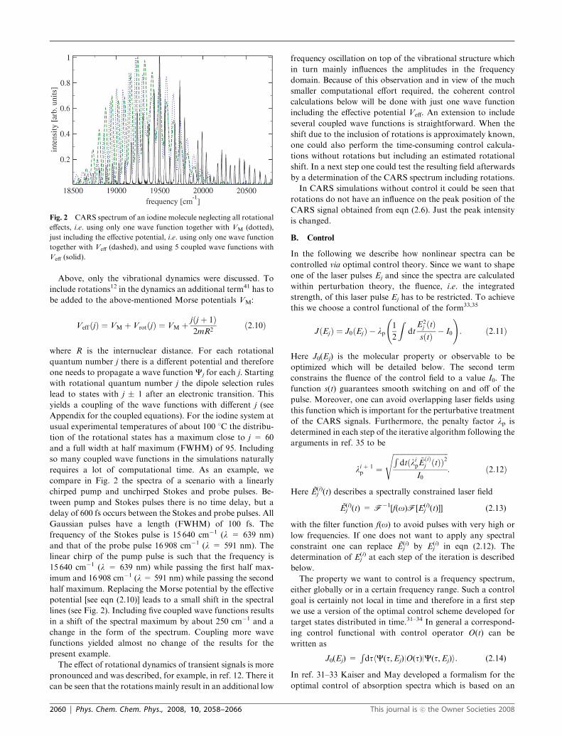
Above, only the vibrational dynamics were discussed. To

include rotations12 in the dynamics an additional term41 has to

be added to the above-mentioned Morse potentials VM:

VeffðjÞ ¼ VM þ VrotðjÞ ¼ VM þjðj þ 1Þ2mR2

ð2:10Þ

where R is the internuclear distance. For each rotational

quantum number j there is a different potential and therefore

one needs to propagate a wave function Cj for each j. Starting

with rotational quantum number j the dipole selection rules

lead to states with j � 1 after an electronic transition. This

yields a coupling of the wave functions with different j (see

Appendix for the coupled equations). For the iodine system at

usual experimental temperatures of about 100 1C the distribu-

tion of the rotational states has a maximum close to j = 60

and a full width at half maximum (FWHM) of 95. Including

so many coupled wave functions in the simulations naturally

requires a lot of computational time. As an example, we

compare in Fig. 2 the spectra of a scenario with a linearly

chirped pump and unchirped Stokes and probe pulses. Be-

tween pump and Stokes pulses there is no time delay, but a

delay of 600 fs occurs between the Stokes and probe pulses. All

Gaussian pulses have a length (FWHM) of 100 fs. The

frequency of the Stokes pulse is 15 640 cm�1 (l = 639 nm)

and that of the probe pulse 16 908 cm�1 (l = 591 nm). The

linear chirp of the pump pulse is such that the frequency is

15 640 cm�1 (l = 639 nm) while passing the first half max-

imum and 16 908 cm�1 (l = 591 nm) while passing the second

half maximum. Replacing the Morse potential by the effective

potential [see eqn (2.10)] leads to a small shift in the spectral

lines (see Fig. 2). Including five coupled wave functions results

in a shift of the spectral maximum by about 250 cm�1 and a

change in the form of the spectrum. Coupling more wave

functions yielded almost no change of the results for the

present example.

The effect of rotational dynamics of transient signals is more

pronounced and was described, for example, in ref. 12. There it

can be seen that the rotations mainly result in an additional low

frequency oscillation on top of the vibrational structure which

in turn mainly influences the amplitudes in the frequency

domain. Because of this observation and in view of the much

smaller computational effort required, the coherent control

calculations below will be done with just one wave function

including the effective potential Veff. An extension to include

several coupled wave functions is straightforward. When the

shift due to the inclusion of rotations is approximately known,

one could also perform the time-consuming control calcula-

tions without rotations but including an estimated rotational

shift. In a next step one could test the resulting field afterwards

by a determination of the CARS spectrum including rotations.

In CARS simulations without control it could be seen that

rotations do not have an influence on the peak position of the

CARS signal obtained from eqn (2.6). Just the peak intensity

is changed.

B. Control

In the following we describe how nonlinear spectra can be

controlled via optimal control theory. Since we want to shape

one of the laser pulses Ej and since the spectra are calculated

within perturbation theory, the fluence, i.e. the integrated

strength, of this laser pulse Ej has to be restricted. To achieve

this we choose a control functional of the form33,35

JðEjÞ ¼ J0ðEjÞ � lp1

2

Zdt

E2j ðtÞsðtÞ � I0

!: ð2:11Þ

Here J0(Ej) is the molecular property or observable to be

optimized which will be detailed below. The second term

constrains the fluence of the control field to a value I0. The

function s(t) guarantees smooth switching on and off of the

pulse. Moreover, one can avoid overlapping laser fields using

this function which is important for the perturbative treatment

of the CARS signals. Furthermore, the penalty factor lp is

determined in each step of the iterative algorithm following the

arguments in ref. 35 to be

li þ 1p ¼

ffiffiffiffiffiffiffiffiffiffiffiffiffiffiffiffiffiffiffiffiffiffiffiffiffiffiffiffiffiffiffiRdtðlip ~E

ðiÞj ðtÞÞ

2

I0

s: ð2:12Þ

Here E(i)j (t) describes a spectrally constrained laser field

E(i)j (t) = F�1[f(o)F[E(i)

j (t)]] (2.13)

with the filter function f(o) to avoid pulses with very high or

low frequencies. If one does not want to apply any spectral

constraint one can replace E(i)j by E(i)

j in eqn (2.12). The

determination of E(i)j at each step of the iteration is described

below.

The property we want to control is a frequency spectrum,

either globally or in a certain frequency range. Such a control

goal is certainly not local in time and therefore in a first step

we use a version of the optimal control scheme developed for

target states distributed in time.31–34 In general a correspond-

ing control functional with control operator O(t) can be

written as

J0(Ej) =RdthC(t,Ej)|O(t)|C(t,Ej)i. (2.14)

In ref. 31–33 Kaiser and May developed a formalism for the

optimal control of absorption spectra which is based on an

Fig. 2 CARS spectrum of an iodine molecule neglecting all rotational

effects, i.e. using only one wave function together with VM (dotted),

just including the effective potential, i.e. using only one wave function

together with Veff (dashed), and using 5 coupled wave functions with

Veff (solid).


exact treatment of the time-evolution operator. Here we will

use the above-mentioned perturbative treatment. Time-local

control goals are a special case of these generalized target

functions. If we want, for example, to shape wave packets to

have the form |Ctari at the final time tf, one can use

O(t) = d(t � tf)|CtarihCtar|. (2.15)

This will be used as a test case below.

To determine the control pulse we have to maximize the

control goal with respect to the control pulse Ej:

dJðEjÞdEj

¼ 0: ð2:16Þ

Using the above definitions of J(Ej) and J0(Ej) yields

EjðtÞ ¼2sðtÞlp

Re

Zdt CðtÞ

�� OðtÞ dCðtÞdEjðtÞ

��

: ð2:17Þ

In a next step the wave function |C(t)i is replaced by its

perturbation expansion (2.2). One has to keep in mind that

each of these perturbation orders consists of contributions

from the different laser pulses as detailed in eqn (2.4) for the

first-order wave function. Within perturbation theory the

temporal order of the laser pulses is important. To make

notation simpler we assume that the pump pulse comes first,

the Stokes pulse is applied at the same time as the pump pulse

or later, and finally the probe pulse occurs. In experiments

with negative time delay, for example, the probe pulse is first.

The results below can also be applied to these cases after a

proper renaming of the pulses.

1. Control of a time-distributed target state with the probe

pulse. Let us start by controlling the probe pulse and keeping

the pump and Stokes pulses fixed. For this case the ket vector

in eqn (2.17) can be written as a sum of those terms contribut-

ing to the wave function which depend on the probe pulse

dCðtÞdEprðtÞ

��¼ dCð1Þðkpr; tÞ

dEprðtÞ

��+þ dCð2Þðkpu � kpr; tÞ

dEprðtÞ

��+

þ dCð2ÞðkSt � kpr; tÞdEprðtÞ

��+þ dCð3Þðkpu � kSt þ kpr; tÞ

dEprðtÞ

��+

þ dCð3ÞðkSt � kpu þ kpr; tÞdEprðtÞ

��+:

ð2:18Þ

A detailed look at the first term on the right-hand side of eqn

(2.18) yields

dCð1Þðkpr; tÞdEprðtÞ

��+¼� i

ddEprðtÞ

Z t

0

dt0eiHðt0�tÞmEprðt0ÞjCð0Þðt0Þi

¼ � i

Z t

0

dt0eiHðt0�tÞmdðt0 � tÞjCð0Þðt0Þi

¼ � iYðt� tÞeiHðt�tÞmjCð0ÞðtÞi:ð2:19Þ

This equation is very similar to the one obtained from an exact

propagation of the wave function (see Appendix of ref. 31). So

one proceeds in the same way as in ref. 31 in order to calculate

the integral in eqn (2.17):Zdt CðtÞ

�� OðtÞ dCðkpr; tÞdEjðtÞ

��

¼ hwðtÞjmjCð0ÞðtÞi ð2:20Þ

with the auxiliary function |w(t)i which propagates according

to

@jwðtÞi@t

¼ �iHjwðtÞi �OðtÞjCðtÞi: ð2:21Þ

Here |C(t)i has to be calculated as the sum of the different

perturbation orders. The other terms in eqn (2.18) can be

treated in a similar fashion leading to an expression for the

controlled probe pulse:

EprðtÞ ¼2sðtÞlp

RehwðtÞjmjCð0ÞðtÞ þCð1Þðkpu; tÞ

þCð1ÞðkSt; tÞ þCð2Þðkpu � kSt; tÞ þCð2ÞðkSt � kpu; tÞi:ð2:22Þ

Using this expression time-local control targets (like shaping a

wave packet at a certain moment in time) and time-nonlocal

targets (like maximizing the intensity of a whole spectrum) can

be achieved. To determine the control field, one first propa-

gates |C(t)i from t = 0 to t = tf with an initial guess for the

laser field. Then one propagates |C(t)i and |w(t)i backwards intime and calculates the laser field. This procedure is repeated

iteratively. The time evolution within the perturbative treat-

ment (2.3) is performed using the split operator method.42–44

2. Control of CARS spectra with the probe pulse. To be

able to increase the amplitude of certain frequency regions in

the CARS spectrum we have to modify the control goal

because of the terms involved in the expressions for P(3)(t).

The target functional is now given by

J0ðEjÞ ¼Zo0þDo=2

o0�Do=2

dojPðoÞj2: ð2:23Þ

Taking the functional derivative of the integrand with respect

to the control field Ej yields

ddEjðtÞ

jPðo0Þj2

¼ 2ðZ

dtPð3ÞðtÞ cosðotÞÞ ddEjðtÞ

ðZ

dtPð3ÞðtÞ cosðotÞÞ

þ 2ðZ

dtPð3ÞðtÞ sinðotÞÞ ddEjðtÞ

ðZ

dtPð3ÞðtÞ sinðotÞÞ:

ð2:24Þ

Since we concentrate on positive time delays, only three terms

contribute to P(3)(t) in eqn (2.5). Similar to the results above,

for controlling the probe pulse we get

ddEprðtÞ

Zdt cosðotÞhCð0ÞðtÞjmjCð3Þðkpu � kSt þ kpr; tÞi

¼ hw1ðtÞjmjCð2Þðkpu � kSt; tÞið2:25Þ


with

@jw1ðtÞi@t

¼ �iHjw1ðtÞi � imjCð0ÞðtÞi cosðotÞ; ð2:26Þ

and

ddEprðtÞ

Rdt cosðotÞhCð2ÞðkSt � kpu; tÞjmjCð1Þðkpr; tÞi

¼ hw2ðtÞjmjCð0ÞðtÞið2:27Þ

with

@jw2ðtÞi@t

¼ �iHjw2ðtÞi � imjCð2ÞðkSt � kpu; tÞi cosðotÞ;

ð2:28Þ

as well as

ddEprðtÞ

Rdt cosðotÞhCð2ÞðkSt � kpr; tÞjmjCð1Þðkpu; tÞi

¼ hw3ðtÞjmjCð1ÞðkSt; tÞið2:29Þ

with

@jw3ðtÞi@t

¼ �iHjw3ðtÞi � imjCð1Þðkpu; tÞi cosðotÞ: ð2:30Þ

If we want to control the spectra, for example enhance them in

the range o0 � Do by controlling the probe pulse, the final

expression is given by

EprðtÞ ¼2sðtÞlp

Re

Zo0þDo

o0�Do

do½ðRdtPð3Þ cosðotÞÞ

� ðhw1ðtÞjmjCð2Þðkpu � kSt; tÞi þ hw2ðtÞjmjCð0ÞðtÞi

þ hw3ðtÞjmjCð1ÞðkSt; tÞiÞ þ ðRdtPð3Þ sinðotÞÞ

� ðhw4ðtÞjmjCð2Þðkpu � kSt; tÞi þ hw5ðtÞjmjCð0ÞðtÞi

þ hw6ðtÞjmjCð1ÞðkSt; tÞiÞ�ð2:31Þ

where |w4(t)i, |w5(t)i and |w6(t)i equal |w1(t)i, |w2(t)i and |w3(t)ibut with sine instead of cosine functions in the respective

differentials eqn (2.26), (2.28) and (2.30). Therefore, in addi-

tion to the differential equations for the various perturbation

orders of |C(t)i with different combinations of the laser pulses

one gets six inhomogeneous differential equations, which also

can be solved by propagating |C(t)i and |wn(t)i forward and

backward in time. The integral over o in eqn (2.31) is

performed below in a discretized version.

3. Control of CARS spectra with the Stokes pulse.

To control the Stokes pulse instead of the probe pulse one

has to take the functional derivative (2.24) with respect to

ESt. But since now the derivative is taken with respect to

the second field the resulting equations are more involved.

Instead of having auxiliary functions |wji one has a two-level

hierarchy of such equations. The optimized Stokes field is

given by

EStðtÞ ¼2sðtÞlp

Re

Zo0þDo

o0�Do

do½ðZ

dtPð3Þ cosðotÞÞ

� ðhw1ðtÞjmjCð1Þðkpu; tÞi

þ hCð0ÞðtÞjmjw2ðtÞi þ hCð0ÞðtÞjmjw3ðtÞiÞ

þ ðZ

dtPð3Þ sinðotÞÞðhw4ðtÞjmjCð1Þðkpu; tÞi

þ hCð0ÞðtÞjmjw5ðtÞi þ hCð0ÞðtÞjmjw6ðtÞiÞ�ð2:32Þ

with

@jw1ðtÞi@t

¼ �iHjw1ðtÞi � imEprj~w1ðtÞi ð2:33Þ

@jw2ðtÞi@t

¼ �iHjw2ðtÞi � imEprj ~w2ðtÞi ð2:34Þ

@jw3ðtÞi@t

¼ �iHjw3ðtÞi � imEpuj ~w3ðtÞi ð2:35Þ

and

@j ~w1ðtÞi@t

¼ �iHj ~w1ðtÞi � imjCð0ÞðtÞi cosðotÞ ð2:36Þ

@j ~w2ðtÞi@t

¼ �iHj ~w2ðtÞi � imjCð1Þðkpu; tÞi cosðotÞ ð2:37Þ

@j ~w3ðtÞi@t

¼ �iHj ~w3ðtÞi � imjCð1Þðkpr; tÞi cosðotÞ ð2:38Þ

where again |~w4(t)i, |~w5(t)i, and |~w6(t)i have sine instead

of cosine functions in the differential equations equaling

eqn (2.36), (2.37) and (2.38) respectively. So the control

of the Stokes pulse leads to more coupled differential

equations than the shaping of the probe pulse. The

control of the pump pulse leads to even more complicated

equations. In particular, some of the integrals cannot

be calculated by the trick of auxiliary differential equations.

Therefore we restrict ourselves here to the shaping of probe

and Stokes pulses.

III. Results

A. Wave packet control

In this first application we want to test the formalism

developed above for a simple goal, namely the shaping of a

wave packet in the upper electronic state using three

pulses. This target could of course be reached using just one

pulse but here it serves as a test of the three-pulse approach.

The control goal is to get a Gaussian wave packet centered

at x = 5.4 a0 on the excited state (cf. Fig. 1) at final time

tf = 800 fs by shaping the probe pulse. The pump and the

Stokes pulses have a Gaussian shape with a maximum at 200 fs

(no delay time between pump and Stokes) and a FWHM

of 100 fs. The pump pulse has the frequency o = 18675 cm�1


(l = 535 nm) and the Stokes pulse o= 17140 cm�1 (l = 583

nm). As an initial probe we use a Gaussian pulse, centered

at 800 fs, i.e. with 600 fs time delay, and the same frequency as

the pump pulse. As smoothing function s(t) we use a sine

function which takes 10% of the propagation time to increase

from 0 to 1 at the beginning and the same time to decrease

from 1 to 0 at the end. In between these times the smoothing

function is set to unity. In this way we also ensure that there is

always a delay between the Stokes and the probe pulse. In

Fig. 3 the wave function up to the third order for the unshaped

initial pulse and for the shaped pulse is shown. In addition, the

(scaled) control goal is displayed to emphasize how accurately

the control goal is achieved. The absolute value of the resulting

wave packet is of course small since it is created within a third-

order process.

B. Control of CARS spectra with the probe pulse

The above control scenario of shaping a wave packet in

a third-order process serves as a good test for our algorithm

but is not easily accessible in experiments. In the next step

we come to the control of fs-CARS spectra which can be

measured experimentally. Our goal is to increase the

amplitude of the spectrum in a predefined frequency interval.

The parameters of pump and Stokes pulses are the same as

in the previous subsection, as are those of the unshaped

Gaussian probe pulse. Using the Gaussian laser pulse one

gets a broad Gaussian-shaped CARS spectrum with a

maximum at 20 110 cm�1, a FWHM of 407 cm�1 and an

enhanced high-frequency tail. In the first scenario the goal is to

increase the amplitude of the spectrum in the frequency range

20 410 � 50 cm�1, i.e. for frequencies that are significantly

larger than the maximum of the spectrum with the Gaussian

pulse. In Fig. 4 the spectra using the unshaped Gaussian and

the shaped probe pulse are shown. In addition the interval of

the target frequencies is marked. In this target frequency

region the spectrum certainly increases while an obvious

oscillatory pattern arises. The frequency of this pattern of

200 cm�1 correlates with the energy difference between two

vibrational levels. A splitting of the spectra into vibrational

modes is also observed for the unshaped pulse if the integra-

tion time te is increased.

The power spectrum of the shaped probe pulse is displayed

in the upper panel of Fig. 5. It is determined via45

Ftðo; tÞ ¼Ztþt=2

t�t=2

dt0Wðt0 � t; tÞEðt0Þe�iot0��

�� ð3:39Þ

with the electric field E(t0) and the Blackman window

Wðt0 � t; tÞ ¼ 0:42� 0:5 cos2pðt0 � tÞ

t

� �

� 0:08 cos4pðt0 � tÞ

t

� �ð3:40Þ

with the time resolution t which is limited from below by the

time step of the wave packet propagation. The power spectra

give similar information concerning the laser pulse as the

experimentally used frequency-resolved optical gating

(FROG) traces do.

As one can see in Fig. 5 the shaped probe pulse clearly

consists of two parts in the time domain which are about 160 fs

apart. It also shows an oscillatory behavior on the frequency

scale. The time between the two peaks in the shaped probe

pulse is approximately equal to the cycle duration T = 168 fs

of the second-order wave packet, i.e. the wave packet after the

pump and Stokes pulses, on the ground state. Each time the

wave function is in the correct position the probe pulse is

non-vanishing. Shaped control pulses with more than one

peak, so-called pulse trains, were observed experimentally by

Dudovich et al.46

In the next step we want to increase the amplitude of the

spectrum in a frequency range below the maximum of the

unshaped Gaussian pulse to show that the algorithm works in

both regions. For this aim we choose the target region 20 010

Fig. 3 Probability of the wave function for an unshaped Gaussian

initial pulse (solid line) and for the shaped probe pulse (dashed line).

The control goal is a Gaussian wave function centered at 5.4 a0 (dotted

line). The square of the wave function resulting from the unshaped

Gaussian pulse is multiplied by a factor of 10.

Fig. 4 fs-CARS spectra using the unshaped Gaussian pulse (solid

line) and shaped probe pulses for the target regions 20 010 � 20 cm�1

(dash-dotted line) and 20 410 � 50 cm�1 (dashed line) which lie

between the vertical dotted lines.


� 20 cm�1. The result is also shown in Fig. 4. Obviously the

control algorithm is successful, but one observes again the

oscillatory pattern in the frequency domain. The power spec-

trum of the corresponding shaped pulse is displayed in the

lower panel of Fig. 5. This time the larger part of the laser

energy goes into the first of the two sub-pulses which are again

about 160 fs apart. For the previous scenario this was the

other way round. In further calculations (not shown) it was

observed that the ratio of the amplitudes of the two sub-pulses

depends on the frequency interval in which the CARS spec-

trum should be enhanced.

C. Control of CARS spectra with the Stokes pulse

Now we keep the pump and the probe pulses fixed and shape

the Stokes pulse. The pump pulse has the frequency 20 020

cm�1 (l = 500 nm) while the probe pulse has the frequency

19 250 cm�1 (l = 520 nm). Both pulses have a FWHM of 100

fs. The pump pulse is centered at 200 fs and the probe pulse at

800 fs. As the initial Stokes pulse we use a Gaussian pulse

centered at 200 fs with the same parameters as the probe pulse.

The control goal is to increase the intensity in the frequency

interval 21 000 � 43 cm�1 which is marked in Fig. 6 by vertical

lines. In Fig. 6 one can see that the calculated spectrum using

the shaped Stokes pulse is larger than that using the Gaussian

pulse. Applying the shaped Stokes pulse the maximal ampli-

tude is smaller but within the target frequency range the signal

resulting from the shaped pulse is indeed larger and the

maximum of the shaped spectrum is close to the target region.

In this case the power spectrum of the Stokes pulse (not

shown) features only one peak centered at approximately

210 fs and 18 700 cm�1.

In a second example of shaping the Stokes pulse different

parameters for the fixed pulses are used. This time the pump

pulse has the frequency 18 675 cm�1 (l = 535 nm) while the

probe pulse has the frequency 18 069 cm�1 (l = 553 nm).

Again both pulses have a FWHM of 100 fs and are centered at

200 and 800 fs respectively. The initial Stokes pulse is chosen

as in the previous example but now the target frequency region

is lower in energy than the maximum of the spectrum with the

unshaped Stokes pulse, namely 18 675 � 43 cm�1. The result is

shown in Fig. 7 and clearly a large increase of the spectrum

within the target region is achieved but again an oscillatory

pattern shows up as in Fig. 4. This time the shaped pulse

consists of a series of three pulses as can be seen in Fig. 8.

IV. Conclusions

The aim in this paper was to shape fs-CARS spectra using the

theory of optimal control. Experimentally it was shown21–26

that this control goal is feasible which might be very important

Fig. 5 Power spectrum of the shaped probe pulses used for the target 20 410 � 50 cm�1 (upper panel) and for the target 20 010 � 20 cm�1 (lower

panel). The shades scale reflects the intensity in arbitrary units.

Fig. 6 Spectra of the simulation with Gaussian Stokes pulse (solid

line) and shaped Stokes pulse (dashed line). The control goal is to

increase the spectra around 21 000 cm�1 (vertical dash-dotted lines).


for the developing field of CARS microscopy16 with a large

potentiality for applications in biological systems. In most

experiments the ratio between the intensities in two frequency

ranges was enhanced. Here we enhanced the absolute value of

the spectral amplitude in a predefined frequency range but an

extension of our method to two frequency ranges should be

straightforward though the equations become more involved.

To be able to develop a control algorithm for fs-CARS

spectra we first reviewed the perturbative calculation of these

kind of spectra. The modifications to include the influence of

rotations on the dynamics were given. Using these formulas

transient signals as well as CARS spectra can be determined

for given probe, Stokes and pump pulses. An alternative non-

perturbative determination of the CARS signal and spectra

can be done at the expense of a higher numerical effort.2,13

This would also allow for arbitrarily overlapping pulses but

incorporating these techniques into a control algorithm might

be more cumbersome.

A coherent control mechanism for time-distributed targets in

a three-pulse setup was developed by extending previous stu-

dies.31–34 As a first test a wave packet in the excited electronic

state was shaped. In this case, pump and Stokes pulses were pre-

defined while the probe pulse was successfully controlled to get a

maximum control yield. However, the main goal of the paper

was to develop and test an algorithm to control fs-CARS

spectra. This was indeed possible by shaping either the probe

or the Stokes pulse. We did not control the pump pulse since the

final equations are numerically much more involved compared

to the cases of controlling the probe or the Stokes pulse.

We not only developed the formalism but also tested it in

the case of the iodine dimer. This is of course a very simple

model in which the electronic ground and first excited state are

known to a high degree of accuracy. Nevertheless this simple

case can be used as a starting point to explain the spectra of

more complicated systems.40,47

A limitation of utilizing the iodine dimer as a test system is,

of course, its single reaction coordinate. In more complex

systems it should be possible to enhance one peak in the

spectrum stemming from one reaction coordinate while sup-

pressing some of the other peaks resulting from different

reaction coordinates, i.e. an excitation of single modes should

be possible. We showed that fs-CARS spectra could be

enhanced in predefined frequency regions using shaped pulses.

Actually in some of the resulting structures a damped oscilla-

tory pattern arose especially when shaping the probe pulse.

Allowing for longer delay times between the Stokes and probe

pulses (not shown) leads to non-oscillatory spectra with quite

different pulse forms.

During our investigations the shape of the laser pulse was left

free, i.e. both amplitude and phase of the pulse were controlled.

In most of the experimental realizations only the phase was

controlled while amplitudes were kept fixed. Performing simula-

tions with a restricted pulse form needs different control algo-

rithms but has been done for other control scenarios.48

Appendix

The aim of this Appendix is to show the modifications in some

of the equations in section IIA when rotational dynamics are

Fig. 7 Same as in Fig. 6 but with control goal to increase the spectra

in the region 18 675 � 43 cm�1.

Fig. 8 Power spectrum of the shaped Stokes pulse used for the spectrum in Fig. 7.


included. As mentioned above, one needs to propagate more

than one wave function to include rotational states in the

calculations. The coupling of the wave functions is done by

changing eqn (2.3) into

jCðmþ1Þk;j ðt þ DtÞi ¼ UðDtÞjCðmþ1Þk;j ðtÞi þ iDtmEiðt þ DtÞ

� ðjCðmÞl;jþ1ðt þ DtÞi þ jCðmÞl;j�1ðt þ DtÞiÞðA:41Þ

with the electronic states k and l (ka l), the rotational states j,

j + 1 and j � 1 and the ith laser pulse. The determination of

the polarization eqn (2.5) also has to be altered to

Pð3Þðkpu � kSt þ kpr; tÞ

¼ 2Xj

Xj0¼j�1

Re½hCð0Þj ðtÞjmjCð3Þj0 ðkpu � kSt þ kpr; tÞi

þ hCð0Þj ðtÞjmjCð3Þj0 ðkpr � kSt þ kpu; tÞi

þ hCð2Þj ðkSt � kpu; tÞjmjCð1Þj0 ðkpr; tÞi

þ hCð2Þj ðkSt � kpr; tÞjmjCð1Þj0 ðkpu; tÞi�:ðA:42Þ

References

1 S. Mukamel, Principles of Nonlinear Optical Spectroscopy, OxfordUniversity Press, New York, 1995.

2 W. Domcke and G. Stock, Adv. Chem. Phys., 1997, 100, 1.3 B. I. Grimberg, V. V. Lozovoy, M. Dantos and S. Mukamel, J.Phys. Chem. A, 2002, 106, 697.

4 W. Kiefer, J. Raman Spectrosc., 2002, 31.5 D. J. Tannor, S. A. Rice and P. M. Weber, J. Chem. Phys., 1985,83, 6158.

6 V. F. Kamalov and Y. P. Svirko, Chem. Phys. Lett., 1992, 194, 13.7 S. Meyer, M. Schmitt, A. Materny, W. Kiefer and V. Engel, Chem.Phys. Lett., 1997, 281, 332.

8 S. Meyer, M. Schmitt, A. Materny, W. Kiefer and V. Engel, Chem.Phys. Lett., 1999, 301, 248.

9 T. Chen, A. Vierheilig, P. Waltner, M. Heid, W. Kiefer and A.Materny, Chem. Phys. Lett., 2000, 326, 375.

10 M. Heid, T. Chen, U. Schmitt and W. Kiefer, Chem. Phys. Lett.,2001, 334, 119.

11 A. Materny, T. Chen, M. Schmitt, T. Siebert, A. Vierheilig, V.Engel and W. Kiefer, Appl. Phys. B, 2000, 71, 299.

12 S. Meyer and V. Engel, J. Raman Spectrosc., 2000, 31, 33.13 S. Meyer and V. Engel, Appl. Phys. B, 2000, 71, 293.14 J. Faeder, I. Pinkas, G. Knopp, Y. Prior and D. J. Tannor, J.

Chem. Phys., 2001, 115, 8440.15 T. Hornung, R. Meier, R. de Vivie-Riedle and M. Motzkus, Chem.

Phys., 2001, 267, 261.

16 J.-X. Cheng and X. S. Xie, J. Phys. Chem. B, 2004, 108,827.

17 S. A. Malinovskaya and V. S. Malinovsky, Opt. Lett., 2007, 32,707.

18 R. Zadoyan and V. A. Apkarian, Chem. Phys. Lett., 2000,326, 1.

19 R. Zadoyan, D. Kohen, D. A. Lidar and V. A. Apkarian, Chem.Phys., 2001, 266, 323.

20 D. R. Glenn, D. A. Lidar and V. A. Apkarian, Mol. Phys., 2006,104, 1249.

21 D. Oron, N. Dudovich, D. Yelin and Y. Silberberg, Phys. Rev. A,2002, 65, 043408.

22 D. Oron, N. Dudovich, D. Yelin and Y. Silberberg, Phys. Rev.Lett., 2002, 88, 063004.

23 D. Oron, N. Dudovich and Y. Silberberg, Phys. Rev. Lett., 2002,89, 273001.

24 J. Konradi, A. K. Singh and A. Materny, Phys. Chem. Chem.Phys., 2005, 7, 3574.

25 J. Konradi, A. K. Singh and A. Materny, J. Photochem. Photobiol.,A, 2006, 180, 289.

26 J. Konradi, A. K. Singh, A. V. Scaria and A. Materny, J. RamanSpectrosc., 2006, 37, 697.

27 P. Brumer and M. Shapiro, Chem. Phys. Lett., 1986, 126, 541.28 D. J. Tannor, R. Kosloff and S. A. Rice, J. Chem. Phys., 1986, 85,

5805.29 R. S. Judson and H. Rabitz, Phys. Rev. Lett., 1992, 68, 1500.30 D. J. Tannor, V. Kazakov and V. Orlov, in Time Dependent

Quantum Molecular Dynamics, ed. J. Broeckhove and L.Lathouwers, Plenum, New York, 1992, pp. 347–360.

31 A. Kaiser and V. May, J. Chem. Phys., 2004, 121, 2528.32 A. Kaiser and V. May, Chem. Phys. Lett., 2005, 405, 339.33 A. Kaiser and V. May, Chem. Phys., 2006, 320, 95.34 I. Serban, J. Werschnik and E. K. U. Gross, Phys. Rev. A, 2005, 71,

053810.35 J. Werschnik and E. K. U. Gross, J. Opt. B, 2005, 7, S300.36 M. Ben-Nun, R. D. Levine, D. M. Jonas and G. R. Fleming,

Chem. Phys. Lett., 1995, 245, 629.37 V. V. Yakovlev, C. J. Bardeen, J. Che, J. Cao and K. R. Wilson, J.

Chem. Phys., 1997, 108, 2309.38 V. Engel, Comput. Phys. Commun., 1991, 63, 228.39 S. Meyer, M. Schmitt, A. Materny, W. Kiefer and V. Engel, Chem.

Phys. Lett., 1997, 287, 753.40 M. Heid, S. Schlucker, U. Schmitt, T. Chen, R. Schweitzer-

Stenner, V. Engel and W. Kiefer, J. Raman Spectrosc., 2001, 32,771.

41 M. Karplus and R. N. Porter, Atoms & Molecules, Benjamin/Cummings, Menlo Park, 1970.

42 M. D. Feit, J. A. Fleck and A. Steiger, J. Comput. Phys., 1982, 47,412.

43 M. D. Feit and J. A. Fleck, J. Chem. Phys., 1983, 78, 301.44 C. Leforestier, R. H. Bisseling, C. Cerjan, M. D. Feit, R. Friesner,

A. Guldberg, A. Hammerich, G. Jolicard, W. Karrlein, H.-D.Meyer, N. Lipkin, O. Roncero and R. Kosloff, J. Comp. Phys.,1991, 94, 59.

45 M. Sugawara, J. Chem. Phys., 2003, 118, 6784.46 N. Dudovich, D. Oron and Y. Silberberg, J. Chem. Phys., 2003,

118, 9208.47 O. Rubner, M. Schmitt, G. Knopp, A. Materny, W. Kiefer and V.

Engel, J. Phys. Chem. A, 1998, 102, 9734.48 D. Abramavicius and S. Mukamel, J. Chem. Phys., 2004, 120,

8373.


Shaping femtosecond coherent anti-Stokes Raman spectra using optimal control theory

Documents

Transcript of Shaping femtosecond coherent anti-Stokes Raman spectra using optimal control theory