Femtosecond and Attosecond Chiral Dynamics Investigated ...
296
´ Ecole doctorale des Sciences Physiques et de l’Ing´ enieur Femtosecond and Attosecond Chiral Dynamics Investigated by Velocity Map Imaging and Photoelectron-Photoion Coincidence Spectroscopy TH ` ESE pr´ esent´ ee et soutenue publiquement le 16/10/2020 pour l’obtention du Doctorat de l’universit´ e de Bordeaux Sp´ ecialit´ e lasers, mati` ere et nanosciences par Etienne BLOCH Directeur : Yann MAIRESSE Composition du Jury : Thierry RUCHON Chercheur au CEA, LIDYL Rapporteur, Pr´ esident Gustavo GARCIA-MACIAS Scientifique de Ligne de Lumi` ere au synchrotron SOLEIL Rapporteur Danielle DOWEK Directrice de Recherche au CNRS, ISMO Examinatrice Maria-Novella PIANCASTELLI Professeure ` a Sorbonne Universit´ e, LCPMR Examinatrice Till JAHNKE Professeur ` a la Goethe-Universit¨ at, Institut f¨ ur Kernphysik Examinateur Stefan HAACKE Professeur ` a l’Universit´ e de Strasbourg, IPCMS Examinateur Yann MAIRESSE Directeur de Recherche au CNRS, CELIA Directeur de th` ese
-
Upload
khangminh22 -
Category
Documents
-
view
2 -
download
0
Transcript of Femtosecond and Attosecond Chiral Dynamics Investigated ...

Ecole doctorale des Sciences Physiques et de l’Ingenieur
Femtosecond and Attosecond Chiral Dynamics Investigatedby Velocity Map Imaging and Photoelectron-Photoion
Coincidence Spectroscopy
THESE
presentee et soutenue publiquement le
16/10/2020
pour l’obtention du
Doctorat de l’universite de Bordeaux
Specialite lasers, matiere et nanosciences
par
Etienne BLOCH
Directeur : Yann MAIRESSE
Composition du Jury :
Thierry RUCHON Chercheur au CEA, LIDYL Rapporteur, President
Gustavo GARCIA-MACIAS Scientifique de Ligne de Lumiere au synchrotron SOLEIL Rapporteur
Danielle DOWEK Directrice de Recherche au CNRS, ISMO Examinatrice
Maria-Novella PIANCASTELLI Professeure a Sorbonne Universite, LCPMR Examinatrice
Till JAHNKE Professeur a la Goethe-Universitat, Institut fur Kernphysik Examinateur
Stefan HAACKE Professeur a l’Universite de Strasbourg, IPCMS Examinateur
Yann MAIRESSE Directeur de Recherche au CNRS, CELIA Directeur de these

Centre Lasers Intenses et Applications, UMR 5107Universite de Bordeaux, CNRS, CEA
43 rue Pierre Noailles, 33400, Talence, France
ii

Contents
Acknowledgements 5
Personal Journey 11
Resume 13
Abstract 19
1 General Introduction 25
I Chirality . . . . . . . . . . . . . . . . . . . . . . . . . . . . . . . . . . . . . . . . . 25
II Ultrafast Dynamics and Observable . . . . . . . . . . . . . . . . . . . . . . . . . . 31
III Photoelectron Circular Dichroism . . . . . . . . . . . . . . . . . . . . . . . . . . . 33
IV COLTRIMS or Reaction Microscope . . . . . . . . . . . . . . . . . . . . . . . . . 42
2 Experimental Development 47
I High-Repetition Rate Laser Beamline . . . . . . . . . . . . . . . . . . . . . . . . 48
I. 1 Fiber Laser Source . . . . . . . . . . . . . . . . . . . . . . . . . . . . . . . 48
I. 2 Frequency conversion : 2ω, 3ω, 4ω . . . . . . . . . . . . . . . . . . . . . . 52
I. 3 High-Order Harmonic Generation . . . . . . . . . . . . . . . . . . . . . . . 53
I. 4 Postcompression . . . . . . . . . . . . . . . . . . . . . . . . . . . . . . . . 60
I. 5 Optical Parametric Amplifier . . . . . . . . . . . . . . . . . . . . . . . . . 61
II Velocity Map Imaging Spectrometer . . . . . . . . . . . . . . . . . . . . . . . . . 65
II. 1 Device . . . . . . . . . . . . . . . . . . . . . . . . . . . . . . . . . . . . . . 65
II. 2 Inversion of the Photoelectron Distributions . . . . . . . . . . . . . . . . . 69
II. 3 Tomographic Reconstruction . . . . . . . . . . . . . . . . . . . . . . . . . 71
III Development of the COLTRIMS . . . . . . . . . . . . . . . . . . . . . . . . . . . 73
III. 1 Brief History . . . . . . . . . . . . . . . . . . . . . . . . . . . . . . . . . . 73
III. 2 Detectors . . . . . . . . . . . . . . . . . . . . . . . . . . . . . . . . . . . . 74
III. 3 Design of the Spectrometer . . . . . . . . . . . . . . . . . . . . . . . . . . 79
III. 4 Interaction : Jet, Vacuum, Photons . . . . . . . . . . . . . . . . . . . . . . 85
III. 5 Reconstruction Algorithm . . . . . . . . . . . . . . . . . . . . . . . . . . . 89
IV Characterization of the COLTRIMS . . . . . . . . . . . . . . . . . . . . . . . . . 96
IV. 1 Constraints : Noise Filtering and Acquisition Rate . . . . . . . . . . . . . 96
IV. 2 Calibration and Resolution . . . . . . . . . . . . . . . . . . . . . . . . . . 105
1

CONTENTS
V Conclusions and Outlook . . . . . . . . . . . . . . . . . . . . . . . . . . . . . . . 114
3 Multiphoton Regime - Molecular Sensitivity 119
I Introduction . . . . . . . . . . . . . . . . . . . . . . . . . . . . . . . . . . . . . . . 120
I. 1 Resonance-Enhanced MultiPhoton Ionization (REMPI) . . . . . . . . . . 120
I. 2 Disentangling the Excitation and the Ionization . . . . . . . . . . . . . . . 123
I. 3 Beyond Circular Field Polarization . . . . . . . . . . . . . . . . . . . . . . 126
II Real-Time Determination of Enantiomeric and Isomeric Content . . . . . . . . . 127
II. 1 Photoelectron ELliptical Dichroism (PEELD) . . . . . . . . . . . . . . . . 129
II. 2 Lock-in Detection : Continuous Modulation of S3 . . . . . . . . . . . . . . 134
II. 3 Accurate Measurement of the Enantiomeric Excess . . . . . . . . . . . . . 137
II. 4 Continuous Measurement of the Enantiomeric Excess . . . . . . . . . . . 141
II. 5 High-Dimensional Molecular Fingerprint : Multi-Component Analysis . . 143
III Elliptical Dichroism Studied in the COLTRIMS . . . . . . . . . . . . . . . . . . . 149
III. 1 Direct COLTRIMS Measurement and VMI Tomography . . . . . . . . . . 149
III. 2 Elliptical Dichroism in Ethyl- and Methyl-Lactate . . . . . . . . . . . . . 154
III. 3 Coincidence Measurement : Dependency to the Fragmentation . . . . . . 161
III. 4 Fragmentation Mechanisms . . . . . . . . . . . . . . . . . . . . . . . . . . 167
III. 5 TDDFT Calculations . . . . . . . . . . . . . . . . . . . . . . . . . . . . . 170
III. 6 Perspectives . . . . . . . . . . . . . . . . . . . . . . . . . . . . . . . . . . . 172
IV Time-Resolved PhotoElectron Circular Dichroism . . . . . . . . . . . . . . . . . . 172
IV. 1 Few-Optical Cycle UV-IR Beamline . . . . . . . . . . . . . . . . . . . . . 175
IV. 2 Characterization and Analysis of the Measurements . . . . . . . . . . . . 179
IV. 3 Experimental Results . . . . . . . . . . . . . . . . . . . . . . . . . . . . . 184
IV. 4 Interpretation and Theoretical Modeling . . . . . . . . . . . . . . . . . . . 189
V Conclusion and Perspectives . . . . . . . . . . . . . . . . . . . . . . . . . . . . . . 190
4 Strong Field Regime 193
. 1 Context . . . . . . . . . . . . . . . . . . . . . . . . . . . . . . . . . . . . . 193
. 2 From the Perturbative Description . . . . . . . . . . . . . . . . . . . . . . 193
I Introduction of the Strong Field Regime . . . . . . . . . . . . . . . . . . . . . . . 195
I. 1 Strong Field Approximation (SFA) . . . . . . . . . . . . . . . . . . . . . . 195
I. 2 Variety of Processes . . . . . . . . . . . . . . . . . . . . . . . . . . . . . . 196
I. 3 High-order Harmonics Generation (HHG) . . . . . . . . . . . . . . . . . . 198
I. 4 Strong Field Photoelectron Spectroscopy . . . . . . . . . . . . . . . . . . 202
I. 5 Chirality in the Strong Field Regime . . . . . . . . . . . . . . . . . . . . . 208
II Enantioselective Sub-Cycle Antisymmetric Response Gated by electric-field rO-
Tation (ESCARGOT) . . . . . . . . . . . . . . . . . . . . . . . . . . . . . . . . . 210
II. 1 Orthogonal Bilinear Bichromatic Field . . . . . . . . . . . . . . . . . . . . 211
II. 2 Velocity Map Imaging Experiment . . . . . . . . . . . . . . . . . . . . . . 213
II. 3 Numerical Time-Dependent Schrodinger Equation Resolution . . . . . . . 218
II. 4 Interpretation in Terms of Electron Trajectories . . . . . . . . . . . . . . . 223
2

CONTENTS
II. 5 Discussion and Perspective . . . . . . . . . . . . . . . . . . . . . . . . . . 226
III Three-Dimensional Chiral Photoelectron Interferometry . . . . . . . . . . . . . . 226
III. 1 Mapping of the Vector Potential . . . . . . . . . . . . . . . . . . . . . . . 226
III. 2 Chirality in the Photoelectron Interferometry : TDSE Support . . . . . . 229
III. 3 Experimental Measurements . . . . . . . . . . . . . . . . . . . . . . . . . 234
III. 4 Explicit Description of the Trajectories : SFA Calculations . . . . . . . . 236
III. 5 Coulomb Focusing and Yukawa Screened Potential . . . . . . . . . . . . . 241
III. 6 Perspectives . . . . . . . . . . . . . . . . . . . . . . . . . . . . . . . . . . . 247
IV Chiral Attoclock . . . . . . . . . . . . . . . . . . . . . . . . . . . . . . . . . . . . 247
IV. 1 Counter-Rotating Bicircular Bichromatic Field . . . . . . . . . . . . . . . 248
IV. 2 Families of Trajectories . . . . . . . . . . . . . . . . . . . . . . . . . . . . 248
IV. 3 Sensitivity to Chirality . . . . . . . . . . . . . . . . . . . . . . . . . . . . . 252
IV. 4 Discussion . . . . . . . . . . . . . . . . . . . . . . . . . . . . . . . . . . . . 253
V Conclusion and Perspectives . . . . . . . . . . . . . . . . . . . . . . . . . . . . . . 254
5 General Conclusion and Perspectives 257
Bibliography 265
3

CONTENTS
4

Acknowledgements
First and foremost, I would like to warmly acknowledge the members of my jury, Thierry
Ruchon, Gustavo Garcia, Danielle Dowek, Maria-Novella Piancastelli, Till Jahnke and Stefan
Haacke, for reviewing my PhD thesis and attending my defence. Even if their fields of research
cover a broader range than the questions addressed in this thesis, and that the reading of such
a document can be tedious, they all have enthusiastically accepted this task and I am sincerely
grateful for it.
Of course, I would also like to thank my PhD supervisor, Yann Mairesse, for these three
years. Firstly, you have set the bar quite high in the lab by managing to put together this
amazing experimental setup. It is a beamline on which everybody would love to do a PhD,
and you provided me this chance. Secondly, you have been there for substantially steering the
researches and developments towards really refreshing and exciting directions. This ability you
have has always impressed me, along with your capacity to make complicated things simple.
And thirdly, you unite this wonderful team in which it has been a great pleasure to be. I know
you absolutely hate being described as a group leader (because it is all about teamplay, right?),
so in Dota terms, let us just say that you play carry.
I also thank Valerie Blanchet, my unofficial second supervisor. We have spent quite a lot
of time in the lab struggling on painful and burdensome developments, and you have always
been there for support. So, even if every time I thank you for your help, you just answer ”don’t
thank me, it’s my job”, still, thank you.
I think the very best side of these three years was the team and the lab I was part of,
and they all deserve to be acknowledged. Let us begin with the theoreticians, who cheerfully
burnt my left leg with their endless days of calculations. Bernard, the king of the croco,
for patiently teaching me theory so many times, and showing me how to be twice as young
while being twice as aged. Baptiste, who I far too little interacted with because he can not
help doing so many thing, and doing it well. Fabrice, for all these discussions, randomly
jumping from quantum mechanics to economy. But life is not only made of H3+4 . I can not
count how many times I asked stupid laser questions to Dominique during the ”pauses clopes”
(often the same question several times in a row, in fact). I hope I am Descamps-approved
now (gold standard, above peer-review). I would also like to thank all the other people
I have closely interacted with : Stephane, for your endless support when the laser goes
reaaally bad, Jerome, for your refreshing not-pessimistic-at-all vision of things (only challenged
5

CONTENTS
by our Vin-ke du 37 haha), Nikita, my Russian master in terms of random-idea-why-not-
to-make-a-windmill-with-a-beer-tank, along with Romain and Anatoly for your advice for
my absurd Arduino and Raspberry projects. I also warmly thank the administrative staff,
Celine, Sonia and Sophie, whose kindness makes paperwork almost pleasant. The mechanics,
Laurent and more recently Franck, also deserve a special thank for patiently showing me
how to drill and cut like a pro (it’s crazy how satisfying this can be), but also helping me
fixing my daaamn bike so many times. And of course a few words for the IT, Richard and
Gaetan, that I bothered sooo many times and who saved my life at least as many times. I
can not cite every single person of the lab for all the good moments spent together, but let
me guarantee here that I have really enjoyed being in the nice atmosphere you all contributed to.
The collaborations were also a very enriching part of my thesis. For this reason, I thank
Francesca for welcoming me in her so, so nice team and lab in Hamburg. And also Nirit, for
sending us her coolest students. I also really appreciated to work with Jason, Caoihme, Nadia
and Marie-Catherine. Even if this was before my thesis, some people have greatly impacted my
present work. I must acknowledge Steve and his ultrafast team, in particular Ashley and Erika,
for this wonderful semester I spent in Berkeley, and Reinhard and his ultimate-COLTRIMS-guru
team in Frankfurt, especially my two lost Mexikaner Giammarco and Isabel, and of course all
the others.
That’s also the place for a big big thank to all the PhD students of the group, for these
endless hours of work that you have turned into a lot of fun, and also beyond the lab. Antoine,
the talented experimenter that has no control over its wandering hands (AKA the tac-tac-
bin-pouf guy), and Alex, the talented theoretician that has no control over its computer (just
kidding, I don’t either). Split between the phalanx-crushing, knuckle-grinding, tendon-wrecking
sessions (in other words, bouldering, just in case we don’t have enough tryhard all day long
already), countless beers (I actually believe we should have had more of them, I can’t wait for
the end of the lockdown) and much more. Bitching-Bouldering-Beers, it’s like the perfect trinity
of a PhD, thanks to you guys. Alex, I keep your recipe for beer brewing and motherboard
cooking. Let us not forget Sandra and Sylvain, my cell mates. I’m so sorry for inflicting you
my obsessive-compulsory disorder of tidily insulting my computer on a quarter-hour basis.
With these random conversations ranging from K-pop to parking lot multilevel progressive
hostile takeover, I really enjoyed being locked with you two. I don’t know if you know, but you
contributed to change my vision about PhD. But we will discuss this again next year (have
fun with the manuscript, ha-ha-ha). And Debobrata, always using your poker face to distill
so much fun. I hope you enjoy yourself here in France, and in the lab with my painful legacy.
It’s probably time to mention the ones gone too early (in postdoc, i mean). A little nostalgia
for the pastis de trop with Sam, our official Quebecois never-resting war machine (no idea
how you do, man, let me know one day). And also for Quentin and Geoffrey, the definitions
of power-to-mass ratio. And finally let me thank the other PhD students that I had fun with
during terribly painful experiments in collaboration. Shaked, never give up your convulsion-
inducing colorbars, they are perfect. We’ll also have to figure out this High-Phone startup at
6

CONTENTS
some point, but never without hula-hoop ! And Vincent, our official Quebecois never-resting
kebab machine, the chillest dude I have ever met in a lab, and yet, with a weirdly acute sense
of mobility (more seriously, I would also rent luggage vans for only 9 cents per minute if I could).
There are also some other people who deserve some credit for this thesis. The ones I wish
I could have seen so much more often.
Firstly, my scattered mates from the ENS in Paris. You are all insane in your own manner
(like, for real, we have mental conditions). That’s a lot of fun, but more importantly, you are all
so inspirational to me. Marius-S.l.C. (I won’t tell the meaning), crazy enough to s’en balek of
everything (I could acknowledge you much further, but we all know you balekouyfrerr). Thomas,
the exact opposite, always wondering what is the sense of life even if his life makes more sense
than any other (and by the way, about the surfer lifestyle, we will have to discuss again, because
-no offense-, I don’t have any memory of you actually standing on a board hehe). Aurelien,
The Chaeef, I think you deserve the trophy of insanity here. Seriously man, I don’t know how
you managed to stay alive so far. But your homeless-businessman-Gypsy-kite-instructor-scam-
professor model is worth a try. Note that my life won’t be complete before I witness the retour
de baton, I look forward to it. Not to forget, Guillaume (the nightmare is over... or has just
begun haha), Seb-the-fdp (#norage #pumpiron), Pierre-the-Camarade-fdp (you were right, I’ll
just boil booze for the rest of my life), Hugo-the-fdp (#norage #tesconcestfacile), the whole
Couscousbangbang team (#yallahyallah), Grosnico, Faussexx...
Secondly, the originalz, the realz, the homies from Nancy. I don’t know where to start.
It’s not that I just missed you, in fact, it was a real misery to see you so sparsely for such a
long time. Seriously, what’s the point of it all if at the end of the day you can’t hang out with
your friends. Getting a PhD I guess, but from now on, we might operate a few adjustments
of the targets. The good news is that even if we don’t see each others for a long time, I
know you will still be there. The acknowledgements are already getting too long, and if I
start explaining why I owe you all so much, it will never end. So let met just thank you all :
Chlou, AlmaXgros, Repier-the-Pastavorus, Charlot-Chucky-Chuck-the-Cheezy-Fromagist, Lobo
El-Chien-Loup-dla-Sseca, Cheddar-Fiemax, Socrate-the-Chillum-Mastah, Raton-sur-Roussette,
Djodjo, Paula, Babat’s, Maud, the whole gang-of-Huberts, Sylvia, Binouz, Nitnelav (the only
one who could actually be there for the defence haha)... and so many more that I have lost
on the way. I hope to find you all again just where I left you, we’ll have time to catch up the
missing pints.
And finally, I think my family deserves the biggest thank of all. You have all loved me
unconditionally, and that’s be basis of everything else. In particular, my parents have gave me
so much that I can’t even describe it. They have always let me do whatever I wanted to do,
but always supported me. Well, at the end, I’m still alive and I did a PhD. I’ve always wanted
to make you proud of me, not because you wanted it, but because you deserve it. You are just
the best. Everybody says this about their parents, but in my case, it’s just an objective fact.
7

CONTENTS
Even when you are not there and even when what I do is completely unrelated to you, it’s
thank to you. It’s no coincidence if all of my friends want to see Patou et Gege even when I’m
not there. You are my model of art and science, literature and general knowledge, sociability
and grumpiness. And my brother, Nino, you’re the least stupid lawyer I’ve ever seen. On paper
we are so different, and yet we’re quite the same. That’s what I like with you, you bring me
refreshing perspectives that I can find in no other place. I know I can have blind trust in you,
and it’s always so much fun to hang out together. A final word for my grandparents. Even if
we can’t discuss my thesis too much in details for reasons of different orders, you have greatly
influenced me, and I’m proud of you four.
Last but not least, these three years of my life have not only corresponded to my PhD.
They have also been three years alongside Laurie. You were here to bring me back to reality so
many times, to prevent me from working all night so many times. To remind me that life is
also about discovering new countries for pleasure and not for beamtimes, reading books which
are not about quantum mechanics, to meet people who have no idea what a Fourier-limited
laser pulse is, and to have all these little pleasures that are not productive and that’s exactly
the point. And don’t worry, I don’t mind at all if your friends and family don’t study chirality,
that’s exactly why I like them !
Thank you all ! And call me doctor haha
8

CONTENTS
9

CONTENTS
10

Personal Journey
I have had a hard time choosing between chemistry and physics during my studies, which is
why I more or less picked both. I had the opportunity in bachelor to study Density Functional
Theory with Gilles Frison in a laboratory of the Ecole Polytechnique. I enjoyed it a lot, but I
wanted to dig deeper into the foundations of chemistry. In this respect, I think that Richard
Taıeb and Jeremie Caillait from the LCPMR, who taught me spectroscopy, quantum mechanics
and light-matter interaction at the Ecole Normale Superieure of Paris, played a decisive role.
I found a good balance between theory and applications in their courses. I had the chance, in
their laboratory, to approach numerical resolution of the Schrodinger equation, applied to the
generation of high-order harmonics (HHG). A this moment, I knew that ultrafast spectroscopy
was what I was looking for. I also wanted to experience the experimental side of research, which
I did with Amelle Zaır at the Imperial College of London, again on HHG and non-linear optics.
At the time, we had a collaboration with the CELIA in Bordeaux, where I found an interesting
place for my next internship. I studied there transient emission spectroscopy with Yann Mairesse
and all the team I know much better now. I also learned the field of research of the group about
chiral molecules, which I found particularly interesting, from its basis of physics and laser science
to its stakes in organic chemistry and biology. We thus set up a plan for a PhD project, but not
directly at the time. In the meantime, between my Master’s degree and my PhD, I had the chance
to have an funded year of additional scientific experience, which I again enjoyed a lot. I took
this opportunity to improve my knowledge in both optical and photoelectron spectroscopy, in
particular towards ultrafast techniques that can be extended to molecular systems. I could spend
a semester in the group of Stephen Leone in Berkeley, focusing on attosecond four-wave mixing.
My other semester was dedicated to learn photoelectron-photoion coincidence spectrometry in
the laboratory of Reinhard Dorner in Frankfurt, which has been a decisive asset for my PhD.
Back in Bordeaux, I could import my (modest) experience to this new activity of the group, right
in time for the development of the new apparatus and the new high-repetition rate beamline.
The rest of this manuscript will take up from here.
Looking back at my initial quandary : Physics or chemistry? I could find a field where
there is no such distinction. Optical or photoelectron spectroscopy? Both are cool! Theory or
experiment? Well, there are only 24 hours in a day... And at the end of the day, what is this all
about? Having fun doing research with nice people, I think.
(For the record, it actually started when I was 5-years-old when my chemist grandpa used
to show me explosive, fragrant and colorful chemical reactions in his basement to make me laugh.
It undoubtedly made me laugh, but perhaps not only.)
11

CONTENTS
12

Resume
Cette these rend compte de l’etude experimentale de dynamiques chirales dans des systemes
moleculaires en phase gazeuse. Elle a pour but de sonder ces proprietes a leur echelle ultrarapide
naturelle, par l’utilisation d’impulsions laser ultracourtes et d’une observable tres sensible, le
dichroısme circulaire de photoelectrons. Ces avancees dans la comprehension des interactions
lumiere-matiere chirales peuvent aussi etre replacees dans un contexte plus general de resolution
des mecanismes de la reconnaissance chirale.
Chapitre 1 : Introduction Generale
Un objet est dit chiral lorsqu’il n’est pas superposable a son image miroir. Comme nous le
verrons dans la section 1.I, cette propriete geometrique peut se retrouver a l’echelle moleculaire,
et est d’importance fondamentale dans un large champs de domaines, de la biologie a la chimie,
jusqu’a la synthese de medicaments et la physique. Neanmoins, son etude est principalement
basee sur des mesures statiques, en particulier en phase gaz ou des composes isoles peuvent
etre etudies. Comme introduit dans 1.II, nous utiliserons des impulsions laser ultracourtes pour
resoudre les aspects dynamiques de la chiralite a son echelle de temps naturelle, de la femtosec-
onde (10−15 s) a l’attoseconde ((10−18 s). L’acces a la chiralite moleculaire n’est pas direct, car
la sonde doit etre elle meme chirale pour des raisons de symetrie. La lumiere polarisee circu-
lairement peut jouer ce role. Une observable de choix, le dichroısme circulaire de photoelectrons
(PECD), se manifeste comme une forte asymetrie chirosensible dans la distribution angulaire
de photoelectrons produite lorqu’une cible chirale gazeuse est photoionisee. Initialement etablie
dans le regime d’ionisation a un photon, elle dispose d’une grande gamme de sensibilites, comme
presentees dans 1.III. La mesure des distributions de photoelectrons necessite un appareillage
particulier. Une partie consequente de cette these a ete consacree au developpement d’un des
systemes de detection les plus complets pour les processus de photoionisation, un spectrometre
de photoelectrons-photoions en coıncidence, globalement presente dans 1.IV. Il permet de lever
les ambiguıtes qui pesent quant aux differentes voies d’ionisation qui peuvent se superposer
dans les spectres complexes, pour separer les processus d’ionisation de differentes especes, ou
encore pour retrouver les informations d’orientation dans des echantillons orientes aleatoirement.
Chapitre 2 : Developpement Experimental
Le second chapitre 2 presente les developpements experimentaux mis en œuvre.
Notre source laser a haute cadence de nouvelle generation sera tout d’abord presentee dans
2.I. Ses capacites de vitesse d’acquisition sans precedent constituent une avancee significative
13

CONTENTS
par rapport aux technologies laser existantes, bien que de nouveaux defis se presentent. Nous
verrons ensuite comment la ligne de lumiere a ete concue pour etre aussi adaptable que possi-
ble, et d’acceder a une grande gamme de regime d’interaction lumiere-matiere. Cela est realise
en particulier par la conversion de frequence de la longueur d’onde fondamentale, la genera-
tion de hautes harmoniques (HHG) pour la production de photons de plus haute energie, et
l’amplification parametrique optique pour l’obtention d’une accordabilite continue en longueur
d’onde. La question de la duree des impulsions sera discutee avec une breve presentation de la
technique de postcompression.
Notre spectrometre imageur de vecteur vitesse (VMI) sera decrit dans 2.II. C’est un ap-
pareil relativement simple, couramment employe pour la detection de distributions angulaires de
photoelectrons. Nous verrons ensuite comment les distributions completes peuvent etre retrou-
vees a partir des projections mesurees, avec l’inversion d’image pour les distributions presentant
une symetrie cylindrique ou en utilisant la reconstruction tomographique pour les distributions
arbitraires.
Dans la section suivante 2.III, nous verrons comment les limites du VMI peuvent etre de-
passees, en particulier comment la mesure directe des distributions angulaires de photoelectrons
en 3D peuvent etre effectuees et comment les differentes voies d’ionisation peuvent etre differen-
ciees, en utilisant la detection de photoelectrons-photoions en coıncidence. Dans cette optique,
le developpement d’un COLTRIMS, ou microscope reactionnel, sera presentee. Apres un bref
historique de la detection en coıncidence, nous detaillerons le principe de fonctionnement des
detecteurs. Nous discuterons ensuite de la conception du spectrometre qui est adapte a notre
objectif, a savoir la detection des parties chirosensibles dans les distributions angulaires de pho-
toelectrons en coıncidence avec le spectre de masses correspondant. La detection requiert une
interaction lumiere-matiere en phase gazeuse dans des conditions particulieres. Une descrip-
tion de la configuration du jet, du vide et du faisceau sera alors proposee. Enfin, l’algorithme
de reconstruction, utilise pour assigner les coıncidences et reconstituer les distributions, sera
presente.
Ce type d’appareil necessite une attention particuliere pour fonctionner a ses pleines
capacites en termes de taux d’acquisition et de resolution, comme nous le discuterons dans
la section 2.IV. La caracterisation du COLTRIMS sera effectuee, puis nous identifierons les
differentes contraintes de la detection en coıncidence, tels que le filtrage du bruit et le taux de
comptage, qui sont des questions centrales pour obtenir une detection efficace. Nous verrons
que la resolution et la vitesse d’acquisition necessitent de faire des compromis. Des efforts
importants ont aussi ete dedies dans l’optimisation du taux d’acquisition, et nous discuterons
des perspectives d’ameliorations dans le but de realiser des experiences pompe-sonde en
coıncidence, l’un des schemas les plus exigeants. Enfin, la calibration et la resolution de notre
nouveau spectrometre seront presentees.
Chapitre 3 : Regime Multiphotonique
Ce chapitre 3 presentera l’etude de la chiralite moleculaire dans le regime d’ionisation
multiphotonique.
Nous introduirons tout d’abord dans 3.I les aspects interessants de l’ionisation multipho-
14

CONTENTS
tonique augmentee par les resonances (REMPI), en particulier sa grande sensibilite a de multiples
processus moleculaires, mais aussi comment elle peut etre utilisee pour decoupler l’excitation
et l’ionisation. Nous verrons ensuite comment des effects dichroıques au dela des polarisations
purement circulaires peuvent fournir de bonnes perspectives dans ce contexte. En comparaison
de l’ionisation a un photon, ce regime presente aussi l’avantage d’etre adapte aux experiences
pompe-sonde resolues en temps.
La seconde section 3.II presentera une nouvelle technique analytique de determination
d’exces enantiomeriques et de contenu isomerique en temps reel. Un nouvel effet chiroptique
sera introduit, le dichroısme elliptique de photoelectrons (PEELD), qui consiste en l’extension
du PECD a des champs polarises elliptiquement. Nous verrons comment cela enrichit la sensi-
bilite aux processus moleculaires, en particulier en terme d’anisotropie d’excitation creee dans
le paquet d’onde excite. Les resultats sont obtenus dans le VMI, et nous verrons que la source
a haute cadence permet une acquisition tres rapide. En particulier, un schema de detection
synchrone permettant un filtrage du bruit particulierement efficace sera presente. Nous ver-
rons ensuite comment cela peut etre utilise pour effectuer des mesures d’exces enantiomerique
avec une grande justesse, ainsi que des mesures continues d’exces enantiomerique. Cet effet etant
hautement specifique a chaque molecule, nous verrons que des ’empreintes digitales’ moleculaires
peuvent etre determinees et utilisees pour la caracterisation de melanges a composants multi-
ples. Cela rend la technique particulierement competitive par rapport aux solutions industrielles
existantes.
L’etude du dichroısme elliptique de photoelectrons sera ensuite etendue au COLTRIMS dans
la section 3.III. Cela constitue aussi la premiere mise en œvre experimentale du spectrometre.
Pour commencer, la capacite de detection directe en 3D de notre nouveau COLTRIMS sera
comparee a la reconstruction tomographique depuis des images VMI, dans le but d’evaluer les
avantages et les inconvenients de chaque methode. Nous etenderons ensuite l’etude du PEELD
a deux nouveaux systemes chiraux, l’Ethyl- et le Methyl-Lactate. Ces molecules ont ete choisies
pour leur grande propension a former des dimeres mais doivent etre caracterisees de zero. La
detection en coıncidence sera aussi utilisee pour etudier la dependance a la fragmentation des
spectres de photoelectrons, ainsi que les mecanismes de fragmentation en jeu. Cela constituera
aussi une bonne base de discussion pour montrer les capacites du COLTRIMS et les defis qui
restent a resoudre dans le but de combiner toutes ses capacites en une meme experience, ce qui
necessite des ordres de grandeur supplementaires de temps d’acquisition. Enfin, nous presen-
terons des calculs de theorie de la fonctionnelle de la densite dependants du temps (TDDFT),
qui representent un excellent support pour des etudes plus approfondies. En particulier, les
pespectives en terme de resolution des voies d’ionisation, et de fragmentation lors de processus
complexes, seront soulignees.
Dans une derniere section 3.IV, une etude du PECD resolue en temps a l’echelle de la
femtoseconde, reposant sur un schema pompe-sonde dans le Methyl-Lactate, sera presentee.
Ce travail a ete effectue en collaboration, sur une source externe IR-UV de quelques cycles
optiques, qui est complementaire de la notre. Elle a en effet une plus faible cadence mais une
meilleure resolution temporelle. La ligne de lumiere sera presentee, ainsi que sa caracterisation
et le schema d’analyse utilise. Le rapport signal sur bruit fut en effet un enjeu sensible et
15

CONTENTS
doit etre caracterise attentivement. De plus, le large support spectral des impulsions courtes
melange de nombreux processus. Les resultats experimentaux et leur interpretation seront dis-
cutes, avec l’aide de modelisations numeriques. En particulier, l’evolution transitoire du PECD
a l’echelle femtoseconde pourrait reveler des dynamiques electroniques ou nucleaires ultrarapides.
Chapitre 4 : Regime Champs Forts
Le chapitre 4 de ce manuscrit explorera la chiralite dans le regime d’interaction lumiere-
matiere en champs forts.
Nous commencerons par introduire les specificites du cadre champs-forts dans la premiere
section 4.I. De maniere interessante, lorsque le potentiel d’un champ laser devient comparable
avec le potentiel moleculaire, une description semi-classique simplifiee des processus peut etre
faite. Nous presenterons une approximation largement utilisee : l’approximation des champs
forts (SFA), ainsi que ses consequences. En particulier, la generation d’harmoniques d’ordre
eleve et la spectroscopie de photoelectrons en champs forts seront detaillees. L’effet de la chiralite
moleculaire n’est ici pas trivial, car le potentiel moleculaire joue un role de moindre importance.
Nous verrons comment les processus chiroptiques peuvent neanmoins apparaıtre dans le regime
des champs forts.
La section 4.II sera basee sur une nouvelle technique que nous avons developpe, appelee
Enantioselective Sub-Cycle Antisymmetric response Gated by electric-field rOTation (ESCAR-
GOT). Elle est basee sur l’utilisation de champs orthogonaux a deux couleurs (OTC), un champs
optique vectoriel dont la chiralite instantanee alterne a l’interieur meme du cycle optique. Nous
verrons qu’une telle quantite, qui va au dela de la definition habituelle de l’ellipticite, basee sur
une vision moyennee sur les cycles optiques, est pertinente et peut etre utilisee pour acceder aux
dynamiques sous-cycle optique des processus chiroptiques. L’etude est basee sur des mesures
VMI et sur la resolution numerique de l’equation de Schrodinger dependante du temps (TDSE).
L’interpretation en terme de trajectoires semi-classiques de photoelectrons sera ensuite discutee.
Dans une troisieme section 4.III, l’extension de la technique ESCARGOT en trois dimen-
sions sera etudiee. Elle donne la possibilite d’acceder aux phenomenes en jeu par l’utilisation de
l’interferometrie de photoelectrons, augmentee ici par la signature sensible a la chiralite. Nous
introduirons la cartographie du vecteur potentiel sur l’impulsion des photoelectrons, un effet
typique des champs forts, qui peut etre utilise pour resoudre plus en profondeur les dynamiques
intra-cycle optique a l’œuvre dans les champs OTC. Nous verrons ensuite comment la chiralite
peut etre finement encodee dans l’interferometrie de photoelectrons, a l’aide de calculs TDSE
et de mesures COLTRIMS. Differents types de trajectoires de photoelectrons seront identifiees,
et nous verrons qu’elle peuvent etre affectees differemment par le potentiel moleculaire chiral.
Une description explicite des trajectoires sera proposee avec un modele SFA etendu, et nous
verrons en particulier comment le Coulomb focusing peut jouer un role. Des potentiels ecrantes
de Yukawa seront aussi utilises dans des calculs TDSE dans le but de distinguer les effets de
courte et de longue portee du potentiel moleculaire chiral.
Enfin, une autre configuration de champs exotique, les champs bicirculaires bichromatiques
contrarotatifs, sera brievement discutee dans une derniere section 4.IV. Ce champ vectoriel en
forme de trefle sera utilise pour voir les processus chiraux de photoelectrons sous un autre point
16

CONTENTS
de vue. Notamment, des familles de trajectoires seront identifiees et leur sensibilites respectives
a la chiralite seront devoilees. L’observable la plus frappante sera un effet d’attoclock chiral.
Il est habituellement applique aux cibles achirales de maniere a lire, a travers des decalages
angulaires des distributions de photoelectrons, de fins delais dans la photoionisation. Son
extension aux systemes chiraux permet de specifiquement encoder l’interaction chirale avec le
cœur ionique de maniere quantitative.
Chapitre 5 : Conclusions Generales et Perspectives
Le chapitre 5 sera consacre au resume des resultats obtenus tout au long de cette these
et a la discussion des perspectives d’etudes a venir. En particulier, la ligne de lumiere laser
a haute candence est un pas en avant significatif en terme de taux d’acquisition de signal, et
elle peut etre utilisee dans un vaste champ de regimes d’interaction. Neanmoins, des defis de
stabilite a long terme et de duree d’impulsions restent a resoudre. L’adaptation du spectrometre
de photoelectrons-photoions en coıncidence a cette nouvelle source compacte presente de vastes
perspectives pour la resolution complete de processus moleculaires de photofragmentation et
photoionisation, quand bien meme une grande marge de progression reste disponible pour son
optimisation. Nous soulignerons aussi le fait que le PECD multiphotonique est hautement sensi-
ble a l’anisotropie d’excitation. Cette propriete peut etre, entre autre, utilisee tres efficacement
dans des applications analytiques. L’etude resolue en temps du PECD, utilisant un schema
pompe-sonde, ouvre aussi la voie a la resolution femtoseconde de processus moleculaires chi-
raux, c’est-a-dire l’echelle a laquelle les reactions chimiques se deroulent. Pour finir, la vision en
profondeur dans les interactions chirales sous-cycle optique fournie dans le regime d’ionisation
en champs forts est d’interet fondamental pour comprendre la nature de notre observable de
choix de la chiralite. Cela ajoute aussi un angle de vue supplementaire tres prometteur dans la
boıte a outils des champs forts, qui presente de nos jours un grand interet pour saisir l’essence
de l’interaction lumiere-matiere aux echelles de temps attosecondes.
17

CONTENTS
18

Abstract
This thesis reports on the experimental investigation of chiral dynamics in molecular systems in
the gas phase. It aims at probing these properties at their natural ultrafast timescale, with the
use of ultrashort lases pulses and a very sensitive observable, photoelectron circular dichroism.
These advances in the understanding of chiral light-matter interaction can be also related to
the global context of resolving the mechanism of molecular chiral recognition.
Chapter 1 : General Introduction
A object is chiral when it is not superimposable with its mirror image. As will be introduced
in Section 1.I, this geometrical property can arise at the molecular scale, and is of fundamental
importance in a broad range of fields, from biology, chemistry, to drug synthesis, and physics.
However, most of its studies are based on static measurements, in particular in the gas phase,
where isolated compounds can be studied. As introduced in 1.II, we will use ultrashort laser
pulses to resolve the dynamical aspects of chirality at its natural timescale, from femtosecond
(10−15 s) to attosecond (10−18 s). Accessing molecular chirality is not straightforward, since the
probe used must be chiral itself for symmetry reasons. Circularly polarized light can play this
role. An observable of choice, photoelectron circular dichroism (PECD), arises as a strong chi-
rosensitive asymmetry in the photoelectron angular distribution produced when a gaseous chiral
target is photoionized. Firstly established in the one-photon ionization regime, it has a great
range of sensitivities, as presented in 1.III. The measurement of the photoelectron distributions
requires particular apparatus. A significant part of this thesis was dedicated to developing one
of the most complete detection system for photoionization processes, a photoelectron-photoion
coincidence spectrometer, broadly presented in 1.IV. It enables one to lift ambiguities on
the ionization channels overlapping in complex spectra, to disentangle ionization from differ-
ent species, and to retrieve orientation-dependent information from a randomly oriented sample.
Chapter 2 : Experimental Development
The second Chapter 2 presents the experimental developments implemented.
Our new generation high-repetition rate laser source will be firstly presented in 2.I. Its ca-
pacities of unprecedented signal acquisition rate constitute a significant breakthrough compared
to the previous laser technologies, even if new challenges arise. We will then see how the beam-
line has been designed to be as versatile as possible, and access a broad range of light-matter
interaction regimes. This is achieved in particular by using frequency conversion of the funda-
mental wavelength, high-order harmonic generation to produce high-energy photons, and optical
19

CONTENTS
parametric amplification to get a continuous tunability of the wavelength. The question of the
pulse duration will be addressed with the brief presentation of the postcompression technique.
Our velocity map imaging (VMI) spectrometer will be described in 2.II. It is a relatively
simple device, commonly employed for the detection of photoelectron angular distributions. We
will then see how the complete distributions can be retrieved from the measured projections,
with the inversion of the images for the distributions having a cylindrical symmetry or by using
tomographic reconstruction for any arbitrary distribution.
In the next Section 2.III, we will see how the limitations of a VMI can be overcome, in
particular how the direct measurement of the photoelectron angular distributions in 3D can be
performed and how the different ionization channels can be distinguished using a photoelectron-
photoion coincidence detection. For this purpose, the development of a COLTRIMS, or reaction
microscope, will be presented. After a brief history of the coincidence detection, we will detail the
operation principle of the detectors. We will then discuss the design of the spectrometer, which
is adapted to our purpose, i.e. the detection of chirosensitive parts in the photoelectron angular
distributions in coincidence with the corresponding mass spectrum. The detection requires the
light-matter interaction to happen in the gas phase in particular conditions. The jet, vacuum
and beam configuration will then be described. Finally, the reconstruction algorithm, used to
assign the coincidence and reconstitute the distributions, will be introduced.
Such a device requires particular attention to operate at its full acquisition rate and resolu-
tion capacities, as will be discussed in Section 2.IV. The characterization of the COLTRIMS will
be performed, and we will discuss the different constraints of the coincidence detection, such
as noise filtering and counting rate, which are central questions to get an efficient detection.
We will see that the resolution and the acquisition rate result from compromises. Important
efforts have also been put into the optimization of the acquisition rate, and the perspective to
further increase it in order to perform pump-probe experiments in coincidence, one of the most
challenging scheme, will be discussed. Finally, the calibration and the resolution or our new
spectrometer will be presented.
Chapter 3 : Multiphoton Regime
This Chapter 3 will present the study of molecular chirality in the multiphoton ionization
regime.
We will firstly introduce in 3.I the interesting aspects of resonance-enhanced multiphoton
ionization (REMPI), in particular its great sensitivity to multiple molecular processes, and also
discuss discuss how it can be used to decouple the excitation and the ionization. We will then
see how dichroic effects beyond purely circular polarizations can provide good perspectives in
this context. Compared to the single-photon ionization, this regime has also the advantage of
being suited for time-resolved pump-probe experiments.
The second Section 3.II will present a new analytical technique of real-time determination of
enantiomeric and isomeric content. A new chiroptical effect, photoelectron elliptical dichroism
(PEELD), consisting in extending PECD to elliptically polarized fields, will be introduced.
We will see how this enriches the sensitivity to molecular processes, in particular in terms of
anisotropy of excitation created in the excited wavepacket. The results are obtained in the
20

CONTENTS
VMI, and we will see that the high repetition rate source enables for a very fast acquisition.
In particular, a lock-in detection scheme, providing a particularly efficient noise filtering will be
presented. We will then introduce how this can be used to perform accurate measurements of
enantiomeric excess as well as continuous enantiomeric excess measurements. We will see that
this effect being highly molecule-specific, molecular fingerprints can be determined and used
for the characterization of multicomponent mixtures. This renders the technique particularly
competitive to the current solutions existing at an industrial grade.
The study of the photoelectron elliptical dichroism will then be extended in Section 3.III in
the COLTRIMS. This also constitutes the first experimental implementation of the spectrometer.
At first, the direct 3D detection capacity of our new detection device will be compared to the
tomographic reconstruction from VMI images, in order to assess the pros and cons of each
methods. We will then extend the PEELD study to two chiral systems, Ethyl- and Methyl-
Lactate. These molecules have been chosen for their great tendency to form dimers but have to be
characterized from scratch. Coincidence detection will also be used to study the fragmentation-
dependent photoelectron spectra, as well as the fragmentation mechanisms at play. This will
also constitute a good basis of discussion to show the capability of the COLTRIMS and the
challenges that remain to be solved in order to use all its capabilities at the same time, which
requires orders of magnitude more acquisition time. Finally, time-dependent density functional
theory (TDDFT) calculations, providing an excellent support for further investigations, will be
presented. In particular, the perspectives provided in term of resolution of the ionization and
fragmentation channels in intricate processes will be highlighted.
In a last Section 3.IV, a time-resolved study of the PECD at the femtosecond scale using
a pump-probe scheme in Methyl-Lactate will be presented. This work has been performed in
collaboration on an external few-optical cycles IR-UV beamline, which is complementary to
ours. It has indeed a lower repetition rate, but a greater temporal resolution. The beamline will
be presented, as well as its characterization and the analysis scheme used. The signal-to-noise
ratio was indeed a challenge and has to be characterized carefully. In addition, the broad
spectral support of the short pulses mixed numerous processes. Experimental results and
their interpretation will be discussed, with the help of numerical modeling. In particular, the
transient evolution of the PECD at the femtosecond timescale might reveal electronic or nuclear
ultrafast chiral dynamics.
Chapter 4 : Strong Field Regime
The last Chapter 4 of this manuscript will explore chirality in the strong-field light-matter
interaction regime.
We will start by introducing the specificity of the strong-field framework in the first Section
4.I. Interestingly when the laser field potential becomes comparable with the molecular poten-
tial, a simplified semi-classical description of the processes can be made. We will present this
widely used strong field approximation (SFA), and its consequences. In particular, high-order
harmonic generation and strong field photoelectron spectroscopy will also be detailed. The effect
of molecular chirality is not trivial here, since the fine details of the molecular potential should
not matter in this framework. We will discuss how chiroptical processes can nevertheless arise
21

CONTENTS
in the strong field regime.
The second Section 4.II will be based on a new technique we have developed, named the
Enantioselective Sub-Cycle Antisymmetric Response Gated by electric-field rOTation (ESCAR-
GOT). It is based on the use of orthogonal two-color (OTC) fields, a vectorial optical field
whose instantaneous chirality alternates within the optical cycle. We will see that such a quan-
tity, which goes beyond the usual cycle-averaged definition of the ellipticity, is relevant and can
be used to access the sub-optical cycle dynamics of chiroptical processes. The study is based
on VMI measurements and time-dependent Schrodinger equation (TDSE) calculations. The
interpretation in terms of semi-classical electron trajectories will then be discussed.
In a third Section 4.III, the extension of the ESCARGOT technique in three dimensions will
be studied. It provides the possibility to access the phenomena at play by using photoelectron
interferometry, enhanced here with the chiral-sensitive signature. We will introduce the mapping
of the vector potential on the photoelectron momentum, a typical strong-field effect, which can
be used to further resolve the sub-optical cycle dynamics at play in OTC fields. We will then see
how chirality can be finely encoded in photoelectron interferometry, with TDSE calculations and
COLTRIMS measurements. Different types of photoelectron trajectories will be identified, and
we will see that they can be affected differently by the chiral molecular potential. An explicit
description of the trajectories will be proposed with an extended SFA model, and in particular
we will investigate how Coulomb focusing can play a role. Yukawa screened potentials will also
be used in TDSE calculations in order to disentangle the short- and long-range effects of the
chiral molecular potential.
Finally, another exotic field configuration, the counter-rotating bicircular bichromatic
fields, will be more briefly discussed in the last Section 4.IV. This clover-shaped vectorial field
will be used to obtain an other angle of view on chiral photoelectron processes. In particular,
families of trajectories will be identified, and their respective sensitivity to chirality will be
unveiled. The most striking observable will be a chiral attoclock effect. It is usually applied in
achiral targets to read fine delays in the photoionization as angular offsets in the photoelectron
distributions. Its extension to chiral systems enables specific encoding of the chiral interaction
with the ionic core in a quantitative manner.
Chapter 5 : General Conclusion and Perspectives
Chapter 5 will summarize the results obtained during this thesis and discuss the perspectives
of future studies. In particular, the high repetition rate laser beamline is a major step forward in
terms of signal acquisition rate, and can be used in a broad range of interaction regimes. However,
challenges regarding long term stability and pulse duration remain to be tackled. The adaptation
of the photoelectron-photoion coincidence spectrometer to this new table-top source presents
great perspectives for the complete resolution of molecular processes in photofragmentation and
photoionization, even if a great margin remains for its optimization. We will also underline
the fact that multiphoton PECD is indeed highly sensitive to anisotropy of excitation. This
property can, among others, be used for analytical purposes very efficiently. The study of time-
resolved PECD using a pump-probe scheme also paves the way to resolving femtosecond chiral
molecular processes, i.e. the scale at which chemical reactions occur. Finally, the deep insight
22

CONTENTS
into the sub-optical cycle chiral interaction provided in the strong field ionization regime is of
fundamental interest for understanding the nature of our observable of choice of chirality. This
also adds a very promising angle of view to the strong field tools, which are nowadays of high
interest to grasp the essence of light-matter interaction at the attosecond timescale.
Figure 1 – Table of content of this thesis manuscript.
23

CONTENTS
24

Chapter 1
General Introduction
This thesis aims at investigating chiral molecular systems in the gas phase, in particular
the chiral ultrafast dynamics by the use of ultrashort laser pulses and photoelectron/photoion
spectroscopy. The central concepts which will be used throughout this manuscript are presented
in this introduction chapter.
I Chirality
Concept
Chirality is a general geometric property of asymmetry. An object is chiral if it is not
superimposable onto its mirror image, or in other words if it does not have a mirror symmetry.
The best illustration is perhaps given by hands (χειρ, or kheir in Greek), as the mirror image of
a right hand is a left hand, and are of course distinct (Fig. 1.1 (a)). Many everyday life objects
are chiral, such as gloves, scissors, guitars and so on, and all of them can exist in two forms,
the ’left’ or ’right’ handedness to keep the example of the hands. A central property associated
is that chiral objects do not interact the same way with other chiral objects depending on
their handedness. For instance, a right hand fits in a right glove, but does not in a left glove.
Oppositely, they interact the same way with achiral objects (for instance, a pen, which has a
mirror symmetry, can be held on both hands).
It turns out that chirality can also take place at the microscopic scale. Organic molecules,
among others, can be achiral or chiral, depending on their structures. The latter case often
(but not always) involves asymmetric carbons (bound to four different groups) denoted with a
star in the example in Fig. 1.1 (b). Like macroscopic objects, chiral molecules can be found
in two forms called enantiomers, labeled dextro (+) or levo (-). Enantiomers have exactly the
same chemical and physical properties (melting point, density, vibrational spectrum, ionization
potential...), except in one specific case : chiral molecules do not interact or react with each other
the same way depending on their handedness. Chemical reactions can thus be enantiospecific,
meaning that depending on the handedness of the enantiomers involved, the reaction can occur,
differ or even be forbidden. A intuitive parallel can be drawn with handshakes, where two right
hands can fit in each other, two left hands can fit in each other but a right hand can not shake
25

CHAPTER 1. GENERAL INTRODUCTION
Figure 1.1 – Concept of chirality, illustrated at the macroscopic scale (a) and molecular scale (b).
a left hand. Similarly, molecules can fit the same way, fit differently or not fit in each other
depending on their symmetry.
Note that in the cases where the molecule contains several asymmetric carbons, enan-
tiomerism occurs with the inversion of all the chiral centers (global mirror imaging) while
diastereoisomerism arises when the configuration reversal is not applied to all the centers (local
mirroring). Since this latter modifies the whole structure of the molecule, and not only its
global symmetry, diastereoisomers have different chemical and physical properties. They can
thus be simply considered as different chiral molecules. This type of isomerism is then excluded
from this study.
Homochirality of Life
The concept of chirality is particularly visible at the macroscopic scale since many items
are designed for right-handers (have you ever tried to use a corkscrew with your left hand?).
However, a chemical reaction of achiral reagents can only yield an equal mixture of enantiomers
(racemic). At first sight, enantiomers should thus be found in equal abundance in nature and
the story could have ended there, but a fascinating property at the molecular scale changes
everything, namely homochirality of life. It happens that most of the chiral molecules found in
living systems only occur naturally under one enantiomer. This is the case for the vast majority
of the elementary components of life : sugars, amino acids (and thus proteins), nucleotide basis
(and thus DNA) and so on. For instance, every single DNA helix in physiological condition,
whether found in a human body, an elephant, a bacteria or a potato, rotates towards the right
(note that a few counter-examples can be found in very isolated environments, such as abysses).
This property has been conserved since the origin of life, as it transmits by descendancy. How-
ever, its origin remains an open question, and a wide variety of scenarios have been considered.
Two main families of hypothesis exists : the deterministic and the random ones. To cite a
few examples, they range from spontaneous separation (random), parity violation in the weak
interaction (deterministic), to asymmetric interstellar photoreactions [Hadidi 18] (deterministic,
26

CHAPTER 1. GENERAL INTRODUCTION
see reviews in [Jorissen 02, Evans 12]). At some point, an excess of a compounds’ enantiomer
had to occur to break the symmetry of the chemical reaction from achiral bricks. Even a
small excess could have led to a complete homochirality, by chiroselective amplification [Soai 00].
Figure 1.2 – Examples of chiral organic molecules, whose effect on the human body differs dependingon the enantiomer.
Because of the enantiospecificity of a wide variety of reactions, living systems do not nec-
essarily interact the same way with the two enantiomers of a molecule. For instance, neuronal
receptors can be chiral and found in only one handedness (say ’right glove’), which can only
be activated by the adequate drug enantiomer (corresponding ’right hand’). A great variety
of examples can be found, as depicted in Fig. 1.2. For instance, (-)-Carvone has a minty
smell, while (+)-Carvone smells like caraway. Perhaps more importantly, some drugs can have
different effects depending on their handedness. Thalidomide was used in the 1960s’ as an
anti-nausea medicine for pregnant women. However, while its (-) form was actually beneficial,
it could racemize in the human body in its (+) form which induces teratogenic effects, and
caused a medical scandal. (+)-Methamphetamine is a strong psychotropic synthetic drug while
(-)-Methamphetamine is an over-the-counter nasal decongestant. Intermediate situations also
exist, such as the (-)-Ibuprofen which has the same anti-inflammatory properties as the (+)
enantiomer, but is simply 3 times less effective. Nevertheless, using a enantiopure compound is
even beneficial in this case, in particular to minimize side effects which can be of equal impact
27

CHAPTER 1. GENERAL INTRODUCTION
for both forms.
For these reasons, the ability to produce pure enantiopure compounds (asymmetric
synthesis) and to characterize such compounds is of crucial importance for biology, chemistry,
and physics, and is worth billions of dollars in the pharmaceutical industry.
Asymmetric Chemistry
Molecular chirality is particular in the sense that, conversely to conformational isomerism
for instance, the transformation of an enantiomer to the opposite one requires to break chemical
bounds, and no exchange between the two forms can occur without chemical reaction. In this
sense, an enantiomer is very rarely obtained from the opposite one.
Several ways exist to produce enantiopure compounds, or at least an excess of enantiomers in
a mixture. It is for example possible to derive a compound from a plant or animal extract, already
naturally enantiopure because of the homochirality of life. In this case, the chiral centers can
be conserved upon chemical reaction to the products. Interestingly, compounds directly derived
from naturally abundant precursors are often much less costly than the opposite enantiomer,
which has to be obtained another way. A widely used technique to obtain a pure enantiomer
from achiral reagents is asymmetric catalysis, awarded by the 2001 Chemistry Nobel Prize,
which consists in using a chiral catalyst to kinetically foster a given symmetry. This is used
at an industrial scale despite the need for expensive chiral catalysts, since these latter are not
consumed upon reaction. Biocatalysis can also be highly enantioselective, and plays a central role
in living systems. As mentioned above, enzymes are only naturally found in one symmetry, and
like the hand and the glove, they are usually effective at producing one enantiomer only. This is
perhaps one of the most important mechanism involved in the conservation of life homochirality.
An alternative solution to produce enantiopure compounds is to perform enantiomer sep-
aration from racemic mixtures. This method is not straightforward, since enantiomers have
exactly the same chemical and physical properties. The only way to separate them is, again, by
making them interact with an external chiral reference. For instance in chiral chromatography,
a chiral substrate can be used and interacts differently with the two enantiomers of a chiral
molecule. As a consequence, these latter can have a different migration time in the column, and
be separated.
Broadly speaking, despite being powerful, no technique is universally applicable. Their use
is defined on a case-by-case basis, and constitutes a fascinating field of chemistry. Interestingly,
they all dwell on the use of an already asymmetric (and pure) external reference. This makes
the origin of life homochirality even more puzzling.
First Observation and Characterization
As previously mentioned, enantiomers only differ by a mirror symmetry, and thus have
exactly the same chemical and physical properties (except when interacting with other chiral
objects). As a consequence, characterizing the enantiomeric content of a sample can be a chal-
lenging task.
Molecular chirality was initially discovered by Louis Pasteur in 1848 [Pasteur 48], when he
noticed that synthesized tartaric acid crystals could be faceted with two opposite symmetries
28

CHAPTER 1. GENERAL INTRODUCTION
(see Fig. 1.3 (a)). The crystallization indeed brought to the macroscopic scale a microscopic
property. He also observed by the way that tartaric acid derived from living things only
crystallized under one form. Beyond this particular case, molecular chirality was historically
studied with the optical activity, i.e. the fact that chiral molecules can rotate the polarization
plane of linearly polarized light upon transmission (Fig. 1.3 (b)). Opposite enantiomers rotate
it in opposite directions, with a magnitude defined by the compound-specific optical rotation.
This effect, discovered before chirality in 1815 by Jean-Baptiste Biot, has yielded the dextro
(+) and levo (-) designation.
Figure 1.3 – (a) Representation of enantiopure crystals obtained with opposite enantiomers. (b)Illustration of the optical activity.
Chiroptical Processes
The asymmetric interaction of light with chiral compounds paved the way to what is nowa-
days referred to as chiroptical processes. Molecular chirality can only be probed by chiral objects,
but molecules are not the only chiral tool available : light can also be chiral. A left-circularly
polarized (LCP) electromagnetic field is indeed the mirror image or a right-circularly polarized
(RCP) one. As a result, light can interact differently with an enantiomer depending on its
polarization and the molecule’s handedness. For symmetry reasons, RCP interacts with (+)
enantiomers the same way that LCP does with (-) ones, but differently than RCP with (-)
and LCP with (+). These processes are called dichroic effects, and will be the bedrock of this
manuscript.
The most common chiroptical process is absorption circular dichroism (CD), which is a
difference of absorption of the enantiomers depending on the rotation of circularly polarized
light. Since absorption and dispersion are linked, the physical origin of this process is common
to the optical activity mentioned above. Depending on the wavelength, different types of
transitions can be addressed with various sensitivities. Rotational transitions can be probed
in the microwave range, but the dichroism is weak as the wavelength is much longer than the
size of the molecule. Infrared wavelengths can be used to access vibrational circular dichroism.
One of its advantage is that the vibrational spectra can be quantitatively calculated with
standard quantum chemistry packages. Finally, electronic circular dichroism can also arise
with visible/ultraviolet light. A more exhaustive description of widely used modern chiroptical
processes is proposed in Section 3.II. Unfortunately, these effects are relatively weak (absorption
29

CHAPTER 1. GENERAL INTRODUCTION
CD of the other of 10−4). This is due to the fact that they originate from magnetic dipolar
transitions, electric quadrupolar, or higher perturbative orders.
Chiral Recognition
The understanding of the processes involved in chiroselective and chirosensitive chemical
reactions is of crucial importance, but can be difficult to access. Typically, this issue is in fact
often completely dodged. For instance, one can test many reagents or catalysts in an systematic
manner to determine the most suited ones. While this can be a practical solution, this is of
course fundamentally unsatisfactory. Different intermolecular interactions can play a role in
chemical reactions, with different ranges and different strengths [Berthod 06], as summarized in
Table 1.1. A few examples are depicted in Fig. 1.4.
Type of Interaction Strength Direction Range
Steric Hindrance Very strong Repulsive Very Short
Coulomb Very strong Attractive/repulsive Medium (1/d2)
Hydrogen Bond Very strong Attractive Long
π-π Strong Attractive/repulsive Medium
Ion - Dipole Strong Attractive Short
Dipole - Dipole Intermediate Attractive Short (1/d3)
Dipole - Induced Dipole Weak Attractive Very short (1/d6)
Induced Dipole - Induced Dipole Very weak Attractive Very short (1/d6)
Table 1.1 – Characteristics of intermolecular interactions. Adapted from [Berthod 06].
Figure 1.4 – Illustration of various types of intermolecular interactions.
The way these intermolecular processes induce an enantiomer-specific interaction is
referred to as chiral recognition mechanisms. They are typically studied statically using various
static spectroscopic techniques combined with theoretical modeling, such as fluorescence
or infrared spectra, in order to determine the structures and the bindings during chemical
reactions between different enantiomers [Zehnacker 08, Scuderi 11] (see for instance Fig.
1.5). The structures are then obtained with different combinations of enantiomers, and the
chiral selection mechanisms are deduced. The effects can be very diverse depending on the
30

CHAPTER 1. GENERAL INTRODUCTION
molecules involved [Berthod 06], and constitute a wide field of exploration. For instance, π-π
interaction can be a chiral selector in π-complexes, while Coulomb or ion-dipole interaction
typically play this role in ligand exchange. Natural chiral selectors can be, for example in
polysaccharides, hydrogen bonds, dipolar interaction or steric hindrance. These interactions can
typically lead to chirosensitive reaction mechanisms with an asymmetric configuration of mul-
tiple binding sites, a key-and-lock association or for instance the insertion into a helical structure.
Figure 1.5 – (a) Experimental Fourier-transform infrared (FTIR) spectrum of the OH stretchingfrequency in hydrogen-bonded Trifluoroethanol dimers. (b-d) Simulated spectra of the monomer (M),hydrogen bound donor (D) and acceptor (A), for different bonding geometries. Reproduced from[Zehnacker 08], adapted from [Scharge 07].
Yet, these studies remain static and rely mostly on structural informations. In this context,
the perspective to directly access the temporal dynamics of chirosensitive processes is of high
interest. Can we use time-resolved spectroscopy to experimentally resolve the reaction mech-
anisms and obtain the interaction types and ranges? Can we track the evolution of molecular
chirality upon chemical reaction?
The timescale at which such dynamics occur sets a strong constraint on the techniques at
our disposal. In other words, how can we investigate molecular chirality at its natural timescale,
which is orders of magnitude faster than what any detector can reach?
II Ultrafast Dynamics and Observable
Timescale
We will here briefly discuss the tools used for time-resolved investigations of dynamics. A
historical timeline of time-resolved Physics is proposed in Fig. 1.6. The foundation of this field
is attributed to Eadweard Muybridge, who decomposed in 1878 the motion of a running horse in
31

CHAPTER 1. GENERAL INTRODUCTION
several photographs using a mechanical shutter. By doing so, he demonstrated that a galloping
horse does not always have a hoof in contact with the ground. This was the first time something
too fast for the naked eye was resolved, in this case of the order of milliseconds. Going further
in the timescales, stroboscopes can be used down to microsecond processes. At this stage, the
development of electronics took the lead, and has nowadays a ∼ 100 ps resolution.
Figure 1.6 – Timescales at which different dynamics occur, and typical technologies able to resolvethem.
Nevertheless, the molecular dynamics we are interested in occurs at a much faster
level. Molecular rotation happens in the picosecond timescale, vibration at the dozens of
femtoseconds timescale and electron motion in few femtoseconds or hundreds of attoseconds
ranges. An incredibly useful tool that has revolutionized the time-resolved studies of such
dynamics is pulsed laser. Similarly to the exposure time of a camera, or the duration of
a stroboscope flash, the duration of the laser pulse determines the thickness of the slices
of time that can be resolved. Pulsed lasers are a whole field of Physics by themselves and
are beyond the scope of this manuscript. Let us simply mention that such pulses can be
obtained by phase-locking the modes of a laser cavity, which periodically add up constructively.
Since the early 2000s’, lasers able to deliver ∼ 30 fs-long light pulses have become widely
available. The short pulse duration comes along with a breakthrough in the peak intensities
the laser field can reach, while maintaining the average power manageable. In particular,
this became possible thanks to the chirped pulse amplification (CPA) technique, initiated in
the 1980s’, and honored by the Nobel prize of Physics in 2018. Since then, more advanced
technologies, which will be mentioned in this thesis, enable the generation of few-femtosecond
pulses in the visible range (postcompression), or sub-femtosecond, down to dozens of at-
toseconds in the XUV range (high-order harmonic generation). At this level, the wavelength
becomes a limitation, since at least a few optical cycles (2.7 fs at 800 nm) are necessary to
define an optical pulse. Even if such short pulses are available, they can not be used like a
stroboscope, and the question of the observables that can carry the information becomes central.
Observable : Light or Matter
Since in any case, no detection device can have a sub-100 fs resolution, the observation
of ultrafast dynamics can not be direct. Instead, a scheme commonly used is pump-probe
experiment, in which two laser shots are employed. The first one (pump) initiates a molecular
32

CHAPTER 1. GENERAL INTRODUCTION
dynamics, while the second one (probe) probes the state of the system at a variable ulterior
delay. By repeating the measurement several times with a varying delay, the temporal evolution
can be reconstructed. This delay can be finely tuned by changing the relative optical path of
the two pulses. The only limitation of the temporal resolution is thus the pulse duration. This
paved the way to the resolution of molecular processes at the femtosecond timescale, namely
femtochemistry, that was awarded with the Nobel prize of Chemistry of Ahmed Zewail, in 1999.
We will see in this manuscript that other spectroscopic techniques can provide sub-optical cycle
resolution without the need of a pump-probe configuration.
Two types of observables can be used : light or matter. In the first case, the absorption
or the emission of photons can be used to probe the system at a given delay. In the context of
chirality we are interested in here, this can for instance arise as circular absorption dichroism.
However, pump-probe experiments typically require an additional order of magnitude of sensi-
tivity compared to the static case. As mentioned previously, most of the chiroptical processes
are already weak, requiring liquid-phase samples involving interaction between molecules and
with a solvent. Even if this scheme is challenging, it is worth mentioning that the first experi-
mental demonstration of time-resolved absorption circular dichroism was very recently published
[Oppermann 19]. Other fully optical techniques will be mentioned along this document.
Conversely, the information can be accessed by detecting particles, in particular if the chiral
molecules get ionized. This thesis will dwell on photoelectron/photoion spectroscopy produced
by multiphoton ionization or tunnel ionization. We will see that the chirosensitive information
can be encoded specifically in the photoelectron distributions with a very high sensitivity, as
presented in the next paragraph.
III Photoelectron Circular Dichroism
Effect and Interpretation
Photoelectron circular dichroism (PECD) is a forward/backward asymmetry in the photo-
electron angular distribution along the laser propagation axis, that arises when a chiral molecule
is ionized by a circularly polarized electromagnetic field. This asymmetry reverses with the
light helicity or the enantiomer handedness. Conversely to asymmetries that can be observed
in oriented or aligned molecules, namely where the medium is anisotropic, PECD takes place
for a sample of randomly aligned chiral molecules, and is thus experimentally simple to access.
Unlike other chiroptical processes, this one is described under the electric dipole approximation,
and is thus much greater, up to dozens of percents of the total signal. With such an ampli-
tude, this effect can be used to study chiral molecules in the gas phase, where the systems are
free from solvatation effects. Higher electromagnetic orders, such as electric quadrupolar and
magnetic dipolar effects, can also induce asymmetries in the photoelectron angular distributions
[Hemmers 04]. However, these phenomena are not inevitably related with the chirality of the
sample. They do not necessarily reverse with the light helicity and can arise with achiral tar-
gets. In any case, they remain weak compared to the PECD we are interested in, at least in the
dipole-allowed transitions we will investigate in this manuscript.
33

CHAPTER 1. GENERAL INTRODUCTION
The information about the chirality is encoded angularly here, but where does it come from?
When ionized, the photoelectrons scatter into the (chiral) molecular potential under the influence
of the (chiral) circularly polarized field. The scattering process is very sensitive to this potential
in general, but for symmetry reasons, the interplay of the asymmetry of the potential with the
asymmetry of the field will arise as an asymmetry in the final photoelectron distribution. Note
that with a linearly polarized or unpolarized field or an achiral target, such distributions are
necessarily forward/backward symmetric. This observable thus isolates specifically the chiral
part of the interaction. We will see that this provides a very high sensitivity to molecular
properties.
Figure 1.7 – Schematized interpretation of the photoelectron circular dichroism. In this parallel, therotation is imposed by the electric field, the nut is the electron and the bolt is the molecule (or themolecular potential). The effect reverses only if one reverses the rotation (the field helicity), or thethreads (the enantiomer).
The physics underlying this effect will be extensively discussed in this manuscript. A
schematized interpretation, introduced by Ivan Powis [Powis 08], is illustrated in Fig. 1.7.
When ones rotates a nut on a bolt, the threads convert a rotational motion into a translational
motion. Remarkably, for a given rotation and a given handedness of the threads, the nut will
always go the same direction, regardless of the orientation of the bolt. In this parallel, the
rotation is imposed by the electric field, the nut is the electron and the bolt is the molecule (or
the molecular potential). The effect reverses only if one reverses the rotation (the field helicity),
or the threads (the enantiomer). Of course, this is just an image. The molecule does not have to
be helically-shaped for PECD to take place, and the photoelectrons are not always, but simply
preferentially in average (< 30%), ejected forward or backward along the laser propagation axis.
Single-Photon Ionization
PECD was first theoretically predicted in 1976 [Ritchie 76], but only more recently accu-
rately modeled in 2000 [Powis 00] and experimentally demonstrated in 2001 [Bowering 01]. In
the following decade, many interesting properties were demonstrated in the one-photon ioniza-
tion regime. Most of the organic molecules have an ionization potential of the order of 10 eV,
and XUV photons are thus used to ionize. In this case, the PECD has a simple angular struc-
34

CHAPTER 1. GENERAL INTRODUCTION
ture, as shown in Fig. 1.8 (1) in Camphor ionized at ~ω = 10.3 eV. Obtained by subtracting
the photoelectron angular distributions measured with left circular polarization and right cir-
cular polarization (1-b), it clearly appears as a forward/backward asymmetry along the laser
propagation axis (vertical here), and reverses with the enantiomer handedness (1-c). Since its
angular structure is simple, the PAD and PECD are often represented as angularly-integrated
quantities, where the radius is the photoelectron kinetic energy, as depicted in Fig. 1.8 (2).
Importantly, single-photon PECD is known to be remarkably sensitive to the whole dynamics
of the photoionization process, and strongly depends on several factors :
(i) Ionized orbital : The initial orbital from which the electron is emitted plays an impor-
tant role [Turchini 04, Nahon 06]. For instance in Fig. 1.8 reproduced from [Nahon 06], the
photoelectron kinetic energy spectrum of Camphor can be split into four regions (labeled I-IV
in panel (2)). These regions can be assigned to different ionized orbitals. In particular, the
regions I and II can be associated respectively with the HOMO and HOMO-1. Fig. 1.8 (3)
shows the PECD as a function of the photon energy for the different regions. It appears clear,
in particular, that the sign of the PECD from the HOMO and HOMO-1 has an opposite sign.
The calculated electron densities obtained with two types of calculations is depicted in panel
(4) for comparison, and are clearly not localized at the same part of the molecule. Interestingly,
one-photon ionization from inner-shell, atomic-like spherically symmetric orbitals still shows a
significant PECD [Hergenhahn 04]. This means that the ionized photoelectron is not only sen-
sitive to the localization of its initial density : it explores the molecular potential before being
ejected, and is thus sensitive to its global chirality.
(ii) Molecular structure : For this reason, single-photon PECD is very sensitive to the
whole structure of the ionized molecule. For instance, [Nahon 16] compares (+)-Camphor and
(-)-Fenchone, two similarly-structured isomers with the same asymmetric carbon configuration,
i.e. the same chiral skeleton (see Fig. 1.9 (a)). The only difference between the two compounds
is the substitution of two methyl groups that are not bonded to asymmetric carbons. While
the photoelectron spectrum is relatively similar for the two molecules (panel (b), where only an
offset can be noted), their PECD has an opposite sign (Fig. 1.9 (c)). Note that the HOMO
from which the ionization is performed here is not even mainly located on the substituted groups
(Fig. 1.8 (4)) and are very similar to each other. This underlines even more the sensitivity of
PECD to the global molecular structure.
The substitution- and orbital-dependency of PECD has also been demonstrated [Stener 04].
An example of this property, adapted from [Garcia 04], comparing (-)-Methyloxirane and (+)-
Trifluoromethyloxirane is depicted respectively in Fig. 1.9 (d) and (e). The effect is even more
spectacular here, as these two molecules only differ by the substitution of terminal hydrogen
atoms by fluorine. In particular, the PECD from the HOMO is drastically affected, even if its
density is completely away from the substituted group.
Because of this effect, single-photon PECD is furthermore sensitive to the conformational
geometry of the chiral target [Turchini 09, Turchini 13]. For instance in Fig. 1.10 adapted from
[Turchini 13], the experimental PECD (right) of the two dominating conformations (left) has
been shown to have opposite signs. Despite being an interesting property, this can significantly
complicate the observation of PECD in samples at room temperature. In addition, this con-
35

CHAPTER 1. GENERAL INTRODUCTION
Figure 1.8 – (1) (a) Raw photoelectron angular distribution (PAD) produced in one-photon ionizationof Camphor at ~ω = 10.3 eV. (b) Corresponding subtraction between the signals obtained with leftcircular polarization and right circular polarization, in the (+) enantiomer. The PECD clearlyappears as a forward/backward asymmetry along the laser propagation axis. (c) Same as (b) in the(-) enantiomer. The asymmetry clearly reverses. (2) Angularly-integrated photoelectron spectrum(PES) and PECD as a function of the photoelectron kinetic energy in Camphor. (Top) PES obtainedat ~ω = 95 eV (blue line), compared to a reference at 20 eV (green line). (Bottom) CorrespondingPECD measured for the two enantiomers. The spectrum can be cut into four regions, assigned todifferent orbitals ionized. (3) PECD of the four labeled regions as a function of the photon energy.Region I is assigned to the ionization from the HOMO, region II to the HOMO-1 and region III tothe HOMO-2 and HOMO-3. (4) Electron density of the HOMO and HOMO-1 obtained using twotypes of calculation. Reproduced from [Nahon 06].
36

CHAPTER 1. GENERAL INTRODUCTION
Figure 1.9 – (a) Structure of (+)-Camphor and (-)-Fenchone, two similarly-structured isomers withthe same asymmetric carbon configuration (labeled 1 and 4 here). (b) PES of Camphor and Fenchone,recorded respectively at ~ω = 10.3 eV and 10.5 eV. (c) Corresponding measurement of the PECD of(+)-Camphor and (-)-Fenchone. Adapted from [Nahon 16]. (d) Structure, densities of the HOMOand HOMO-1 and associated PECD of (-)-Methyloxirane. The datapoints are indicated with thecircles and the lines correspond to calculations. (e) Same as (d) with (+)-Trifluoromethyloxirane.Adapted from [Garcia 14].
stitutes a major additional computational cost for quantitative calculations of PECD. The use
of constrained structures, such as the bicyclic ketones previously mentioned, can remove this
parameter.
(iii) Kinetic energy : PECD is also a function of the kinetic energy with which the photo-
electron is ejected. Electrons emitted from the same orbital and differing only by a few eV can
show opposite dichroic signals [Powis 08]. Futhermore, PECD tends to vanish at high photoelec-
tron kinetic energy (above a few dozens of eV). This can be understood as the electrons escape
the molecular potential too quickly to be imprinted with its chirality. Note that PECD can be
recovered at high kinetic energies in particular cases, for instance involving an autoionizing state
at severals hundreds of eV [Hartmann 19]. The influence of the photoelectron kinetic energy on
PECD can be decoupled from other effects and properly identified as in [Ganjitabar 20].
(iv) Vibrational excitation : The Born-Oppenheimer approximation consists in the factor-
37

CHAPTER 1. GENERAL INTRODUCTION
Figure 1.10 – (Left) Calculated structure of the two conformers Peq and Pax of the (+)-3-Methylcyclopentanone. (Right) Experimental dichroism Deq (black dots) and Dax (grey dots) forthe HOMO state, together with the theoretical dispersions for Peq and Pax (black and grey solidcurves, respectively). Adapted from [Turchini 13].
ization of the molecular wavefunction into an electronic and a nuclear part. It is justified by the
fact that the nuclei are much heavier than the electrons, in such a way that the dynamics of the
nuclei is effectively frozen at the timescale of the electronic motion. The electronic part thus
only depends parametrically on the nuclear geometry. Furthermore, under the Franck-Condon
approximation, the electronic transition matrix elements are assumed to vary negligibly with the
nuclear coordinate. In other words, it does not depend on the nuclear geometry sampled during
vibrational motion. As a result, the electronic and nuclear motions are effectively decoupled.
Since this approximation is widely used in molecular physics, one might expect PECD, which
results from an electronic transition, to be insensitive to the vibrational dynamics.
Figure 1.11 – (Top) PES associated with the HOMO of (-)-Methyloxirane measured at ~ω = 10.4 eV.The red arrows correspond to the calculated vibrational spectrum. (Bottom) Corresponding PECD.Adapted from [Garcia 13].
However, it has been shown that PECD was actually sensitive to the vibrational excitation
[Garcia 13, Powis 14], as shown in Fig. 1.11 adapted from [Garcia 13]. The PES associated with
38

CHAPTER 1. GENERAL INTRODUCTION
the ionization from the HOMO of (-)-Methyloxirane at ~ω = 10.4 eV is shown in the top panel.
The calculated vibrational spectrum is indicated by the red vertical arrows. The bottom panel
presents the corresponding PECD. It appears that a sign change of the dichroism associated
with two consecutive vibrational states can be observed. This property was later observed in
other chiral compounds [Ganjitabar 18, Ganjitabar 20].
This is a clear breakdown of the Franck-Condon approximation. It is remarkable since the
effect is general. In particular, shape resonances, which can typically break this approximation
[Piancastelli 99], are not involved here. This shows again an interesting sensitivity of PECD.
(v) Molecular orientation : PECD is generally measured in samples of randomly oriented
molecules. The nut/bolt analogy qualitatively explains how it can survive molecular orientation
averaging. However, PECD is of course expected to depend on molecular orientation. More
generally, the photoelectron angular distribution obtained for instance with aligned diatomic
(achiral) molecules molecules are known to be anisotropic, as shown in Fig. 1.12 (1-a) and
(1-b), adapted from [Tia 17]. However, they still conserve a mirror symmetry corresponding to
the polarization plane. Effects of circular dichroism in oriented achiral samples [Westphal 89]
or in their molecular frame [Dowek 07] are indeed well-known. The corresponding asymmetries
maximize in the light polarization plane, and are then different from circular dichroism in
randomly aligned chiral molecules. The two effects can thus be combined. In the case
of an oriented chiral molecule, the target has lost any symmetry, in such a way that the
distribution also has no symmetry anymore (1-c). The inversion of the field helicity does not
even reverse the distribution, but globally modifies it (1-d). The experimental measurement
of the evolution of PECD as a function of the molecular alignment is show in panel (2), for
the two enantiomers of Methyloxirane. It appears clear here that the PECD reverses with
the enantiomer, greatly evolves with the molecular alignment, and can even change sign.
The randomly-aligned PECD is simply what survives the summation over all the molecu-
lar orientations. This simple observable has thus a good sensitivity to anisotropies of the sample.
Single-photon PECD is thus a powerful probe of many aspects of molecular chirality, and
is still of high interest nowadays for fundamental and analytical purposes. In addition to this,
such process can occur naturally in interstellar environment, and has astrophysical implications
[Hadidi 18]. Indeed, partially circularly polarized radiation can be found in the interstellar
merdium (particularly at the Lyman α radiation) and could induce a chiral bias, which might
be at the origin of the homochirality of life. This hypothesis is supported by the observation of
enantiomer-enriched amino acids in carbonaceous meteorites.
The XUV photons required to ionize the systems are most of the time obtained from
a synchrotron source. It has great advantages, among others high flux, high stability, full
wavelength tunability, polarization tunability, and a very high repetition rate, up to hundreds
of MHz. However, it not always suited for time-resolved experiments since their pulse duration
is typically of tens of picoseconds. Alternatively, particular schemes of high-order harmonics
generation can yield attosecond pulses of circularly polarized XUV photons [Ferre 15b], as will
be discussed later. Nevertheless in any case, a simple single-photon ionization scheme does not
allow for pump-probe experiments.
39

CHAPTER 1. GENERAL INTRODUCTION
Figure 1.12 – (1) 3D molecular frame photoelectron angular distributions from (a-b) the C 1s-electronsemitted from CO for left (a) and right (b) circularly polarized light. (c-d) Theoretical distributionscomputed here for the O 1s-ionization of (+)-Methyloxirane by left (c) and right (d) circularly po-larized light. The molecules are oriented as depicted in the insets. (2) PECD as a function of thephotoelectron emission angle θ and the molecular orientation angle β after O 1s-photoionization of(-) (a) and (+) (b) Methyloxirane. Adapted from [Tia 17]. The two situations where the molecule isaligned along the field propagation axis are depicted with the nut and bolt parallel.
We will see how changing the interaction regime can provide a new angle of vision into
molecular chirality. It has been demonstrated in the 2010s’ that PECD could also take place
in other ionization regimes. How does replacing the ionizing XUV radiation by an intense
ultrashort infrared or visible laser pulse affect the PECD? As we will see, one-photon PECD
has a simple angular structure, where the information is only encoded in the forward/backward
asymmetry. By increasing the number of photons absorbed, the photoelectron angular
distribution gets sharper along the polarization of the field, and PECD can become much more
structured. Can we use these structures to enhance the sensitivity of the observable and gain a
new insight into chiral molecular processes?
Multiphoton Ionization
The pioneering works of the Kassel [Lux 12] and the Amsterdam/Nottingham groups
[Lehmann 13] in the early 2010s’ established the existence of multiphoton-PECD. Using three-
40

CHAPTER 1. GENERAL INTRODUCTION
photon absorption of circularly polarized 400 nm femtosecond laser pulses to ionize chiral
molecules, they observed strong forward/backward asymmetries, as shown in Fig. 1.13
Figure 1.13 – (Top rows) Photoelectron angular distributions measured in the 3-photon ionization ofthe two enantiomers of Camphor (a) and Fenchone (b) at 400 nm, for linear (LIN), left circularpolarization (LCP) and right circular polarization (RCP). (Bottom row) PECD signal obtained withthe two enantiomers and their subtraction. Reproduced from [Lux 12].
Since then, most of the single-photon properties presented above were also extended to this
regime. Essentially, the sensitivity of multiphoton PECD to the molecular structure [Lux 12,
Lux 15] the orbital ionized [Rafiee Fanood 14] and the excited vibrational state [Beaulieu 16a]
is also established. In addition, intermediate excited states can be reached during a multiphoton
ionization process. PECD can be very sensitive to them [Beaulieu 16a, Kastner 17], and consti-
tutes an additional sensitivity to molecular chiraly. These characteristics will be presented more
thoroughly in the introduction of Section 3.I.
While PECD occurs for randomly aligned samples, the creation of a wavepacket by a laser
field can break the isotropy of the excited medium. Does it have consequences in multiphoton
PECD? Conversely, can PECD be used to access such anisotropy of excitation? We will see
that this complexification of the light-matter interaction will be encoded in particular in the
angular structures of the photoelectron distributions. Since PECD is enantiomer-specific, it has
already been used for analytical purposes, in particular to determine the enantiomeric excess
of samples [Rafiee Fanood 15, Kastner 16, Miles 17]. Can we use the additional sensitivity that
the anisotropy of excitation could bring to enhance the accuracy of the technique?
On the other hand, one might think that by being sensitive to too many parameters,
multiphoton PECD can end up being unusable. Indeed, interpretation of experimental results
can be challenging, and as will be presented, theoretical support can be of great importance.
Finally, resonance-enhanced multiphoton ionization (REMPI) processes present a massive
advantage : the excitation and the ionization from the excited states can be decoupled. The use
of pump-probe scheme with ultrashort laser pulses enables one to access the dynamics at the
molecular timescale. While this type of scheme has already been used to resolve chiral dynamics
at the hundreds of femtoseconds timescale [Comby 16], the characteristics of PECD at a shorter
41

CHAPTER 1. GENERAL INTRODUCTION
scale remains unexplored. Can we access chiral molecular dynamics in the femtosecond range,
which is the timescale of the electronic and vibrational processes? Can the sensitivities of PECD
be used to have an additional insight into these dynamics, compared to achiral photoelectron
spectroscopy?
These questions will be addressed in Chapter 3.
Strong Field Ionization
Ionization can also be performed beyond the perturbative regimes discussed so far, by using
higher laser intensities and longer wavelengths. One can expect that increasing the number
of photons absorbed will even further complicate the interaction. Paradoxically, it turns out
that the latter is actually simplified. In strong field conditions, the electric potential of the
laser indeed dominates the molecular potential, and the photoionization can be described semi-
classically without paying so much attention to the exact molecular structure. This description
and its wide consequences will be discussed in the introduction of Section 4.I.
This might seem like a bad omen for the investigation of molecular chiraly with PECD.
If the molecular potential is dominated, can it still be imprinted to the photoelectrons? It has
been shown that PECD still takes place in the strong field ionization regime [Beaulieu 16a], as
shown in Fig. 1.14. It is weaker, in the few percents range, but still remains much greater than
many other chiroptical processes. Can the simplification of the description of photoionization
be used in order to get a simple picture of the scattering process? Strong field physics is known
to be very sensitive to the vectorial properties of the field applied, since this latter dominates.
This domain has been recently of high interest for the resolution of dynamical processes at
an unprecedented timescale, namely at the sub-optical cycle scale. Can these achievements be
extended to chirality and in particular, is PECD defined at such a timescale? In other words,
for how long should light be circular to produce a PECD? Chapter 4 will tackle these questions.
Figure 1.14 – Photoelectron angular distribution (left) and corresponding PECD (right) obtained instrong field ionization of (+)-Fenchone with 1850 nm pulses at I ∼ 4 ×10¹³ W.cm−2. Extracted from[Beaulieu 16a].
IV COLTRIMS or Reaction Microscope
In order to collect the photoelectron produced by the photoionization of chiral molecules in the
gas phase by ultrashort laser pulses, a particle detection device is required. In particular, it
has to resolve the angular dependence of such distributions to access PECD, our observable of
choice. Our group in CELIA has been using a velocity map imaging (VMI) spectrometer since
42

CHAPTER 1. GENERAL INTRODUCTION
2013, presented in Section 2.II, which can either detect photoions or photoelectrons. In this
latter case, 2D projections of the photoelectron momentum distributions can be measured. One
dimension resolved being the laser propagation axis, PECD can be accessed. The VMI is a
relatively simple apparatus, and a significant part of the results obtained during this thesis were
obtained with it.
However, while the photoelectron spectra tend to be relatively simple for atomic targets,
their complexity dramatically increases in large molecular systems. Indeed, many ionization
channels can overlap, and since PECD is highly sensitive to many parameters, their relative
contributions can be hard to disentangle in the final distributions. In order to overcome this
limitation, the construction and characterization of a new spectrometer, a COLTRIMS (or
reaction microscope), was decided and constituted a significant part of this thesis. Such a device
is capable of measuring both the photoelectrons and photoions distributions in coincidence,
meaning that each photoelectron is associated with its photoion counterpart. Furthermore, the
distributions are measured directly in 3D. A thorough presentation of the device is proposed in
Section 2.III.
Range of Applications
The knowledge of both the photoelectron and photoion momenta, or kinetic energies, en-
ables one to fully reconstruct photoionization processes. This capacity makes such a spectrometer
extremely powerful and used in a broad range of studies, ranging way beyond the scope of this
thesis. To give a few examples, multiple fragmentation pathways can be disentangled by mon-
itoring the fragment-dependent photoelectron spectra, for instance from Auger photoemission
subsequent to core excitation with high energy photons [Miron 08]. Since several photoelectrons
can be detected, this tool is also particularly suited for the study of electron-electron correlation
[Zhang 14b]. Interestingly, since the vectorial recoil of the ions acquired during photofragmenta-
tion processes can be measured, the orientation or alignment of the molecule at the moment of
ionization can be obtained in small systems. As a result, the photoelectron angular distribution
can be retrieved in the molecular frame [Dowek 09, Billaud 12, Menssen 16] (see Fig. 1.15 (a)).
The access to the ion recoil can also be used in Coulomb explosion imaging, which consists in
performing multiple ionization leading to an explosion of the molecule because of the Coulomb
repulsion. This can be for instance used to retrieve the molecular orientation [Jahnke 04], or the
absolute configuration of a chiral molecule [Pitzer 13], which is not a trivial task. Other strong
field processes can also be studied with this device. Laser-induced electron diffraction (consisting
in ionizing an electron and scatter it back on the ionic core within an optical cycle) can, for
instance, provide structural information about the molecular skeleton and orbitals [Meckel 08]
(see Fig. 1.15 (b)). COLTRIMS are thus tools of choice to investigate matter at the molecular
scale, and are sometimes called Reaction Microscopes.
Pump-probe schemes can of course be applied to investigate dynamical evolutions
[Sturm 17]. Temporal resolution can alternatively be retrieved from static measurements thanks
to their high level of completeness. Typically, the fragmentation coordinate of a dissociative state
can be encoded energetically if this state decays to a lower state whose potential energy surface
is not parallel. As a result, the photoelectron kinetic energy can map the fragmentation coordi-
43

CHAPTER 1. GENERAL INTRODUCTION
Figure 1.15 – (a) Examples of molecular-frame photoelectron angular distributions (MFPAD) mea-sured in H2. Adapted from [Billaud 12]. (b) Photoelectron holographic patterns obtained by laser-induced electron diffraction from O2 and N2, whose HOMO is depicted above. Reproduced from[Meckel 08]. (c) (Top) Sketch of the mapping between fragmentation coordinate and Auger photo-electron kinetic energy, during single-photon induced ultrafast dissociation. (Bottom) Correspondingmeasurement of the evolution of the molecular orbital during the fragmentation of HCl. Adapted from[Sann 16].
nate, which is somehow equivalent to time. This has been used for instance to dynamically study
interatomic Coulombic decay, which is the long-range energy transfer that can occur in loosely
bound matter (Van der Waals or hydrogen bounded complexes) [Trinter 13]. Similarly employed
with Auger decay, the spatial evolution of molecular orbitals during the ultrafast dissociation
of HCl have been retrieved [Sann 16] (depicted in Fig. 1.15 (c)). Finally, temporal information
can be encoded by the mapping between the vector potential at the ionization time with the
final photoelectron momentum, which stands in the strong field regime. This has been used
for instance to resolve the sub-optical cycle delays in nonsequential double ionization [Eckart 16].
Not all these types of studies can be carried out with a single spectrometer. In our
case, we are particularly interested in resolving the asymmetries in the photoelectron angular
44

CHAPTER 1. GENERAL INTRODUCTION
distributions, tagged with the corresponding ion or fragment mass. A few similar studies have
also been performed in other teams, for instance in the single-photon [Garcia 14], multiphoton
[Lehmann 13, Rafiee Fanood 14] or strong field ionization regimes [Fehre 19], but the surface of
this growing field has only begun to be scratched.
Challenges
To associate the photoelectrons with their respective photoions, a strong limitation stands
: at most one event must occur per light pulse. As a consequence, the light source must have a
high enough repetition rate in order to have a good statistics in an reasonable time. For this
reason, COLTRIMS have been primarily used with synchrotron sources. Despite being very
powerful and versatile sources, their accessibility is often limited. In addition, their long pulse
duration usually prevents pump-probe experiments, in such a way that the aforementioned
more complex ways around are required to access dynamical informations.
The recent advances in high repetition rate laser sources is significantly extending the
scope of the coincidence spectrometers. The development of a COLTRIMS, coupled to a new
generation high repetition rate fiber laser system will be presented in Chapter 2. Such a table-top
beamline not only allows for more routinely accessible coincidence measurements, it also brings
the perspective of applying the tools of time-resolved pump-probe studies. New challenges
in terms of source stability, implementation and temporal resolution will be addressed. The
versatility of the beamline is of course a significant goal, in order to access the different interaction
regimes at which PECD takes place. We will see how frequency conversion is used to perform
studies in the multiphoton regime, tailored laser fields are employed for strong field interaction
and high-order harmonic generation is implemented to obtain high-energy photons. We will
also see that the new high-repetition rate beamline does not only enable for a fundamental
breakthrough in coincidence detection, but also provides a unprecedented signal acquisition rate
in more standard photoelectron detection, which can then be pushed to another level.
45

CHAPTER 1. GENERAL INTRODUCTION
46

Chapter 2
Experimental Development
The development and implementation of experimental setups have been at the core of the
presented thesis, such that about half of the timespan of my PhD was dedicated to it. This
was motivated by the scientific challenges presented in the introduction chapter, and can be
split into two major lines : the laser source and the detection apparatus. The first one started
with the delivery of the new generation Yb-doped fiber laser system, a few month before the
beginning of my project. Despite being a commercial system, its implementation in academic
research was very recent, and a lot of effort has been put in adapting it for state-of-the-art
experiment and make it as versatile as possible to study single-photon, multiphoton and strong
field processes. Unless mentioned otherwise, I have been personally involved in the presented
developments. The other end of the beamline was initially constituted of an XUV spectrometer,
for high-order harmonic spectroscopy, and a Velocity Map Imaging spectrometer, that will be
presented, for photoelectron studies. To go beyond the capacities of this apparatus, I have been
in charge of building and implementing the photoelectron-photoion coincidence detection device,
also discussed in this chapter.
These challenges are motivated by the broad range of physical processes we could access.
They will be discussed throughout this manuscript, but we can already cite a few important
ones. The high repetition rate table-top source not only delivers a high photon flux, providing
cutting-edge signal-to-noise ratio, but also breaks through the fundamental limitations of the
coincidence detection. The wavelength accordability is of high importance for the possibility
of controlling the excitation scheme in resonance-enhanced multiphoton ionization. In partic-
ular, aiming or avoiding some resonances of interest, or being able to change the number of
photons involved or the interaction regime is an interesting degree of freedom. The continuous
wavelength tunability is also attractive to finely select and scan across the resonances. Broadly
speaking, we are interested in resolving the ultrafast molecular processes by using the photoion-
ization as an observable. Being able to use either a strong laser field or high energy photons,
using high-order harmonic generation, is thus valuable. The information provided is not only
contained in the photoelectron kinetic energy spectrum, but is also encoded in the angular dis-
tributions. In particular, the forward/backward asymmetry along the laser propagation axis,
namely photoelectron circular dichroism, reveals the asymmetric interaction between circularly
47

CHAPTER 2. EXPERIMENTAL DEVELOPMENT
polarized light and chiral molecules. One must thus have the adequate detection devices to
resolve this information. In addition, the photoion mass spectrum completes the picture, for
example by unraveling the associated fragmentations, and its detection in coincidence with the
photoelectron angular distributions is a major step forward.
I High-Repetition Rate Laser Beamline
I. 1 Fiber Laser Source
Titanium-Sapphire (Ti:Sa) laser systems have become a reference in the generation of fem-
tosecond pulses [Keller 03], in particular for ultrafast spectroscopy. Thanks to their large gain
spectral range, they are able to deliver typically 20 fs pulses, around 800 nm, with nowadays
energies of 30 J at a repetition rate of 0.01 Hz, or an average power up to 30 W at 1-10 kHz
or 1 W at 100-250 kHz. This technology has been optimized for decades and has reached its
inherent limitations, especially in terms of average power and repetition rate without damaging
the crystal. This is mainly due to the short upper state lifetime and the large quantum defect
of the Ti:Sa, requiring an intense pumping, typically from frequency-doubled Nd:YAG around
530 nm.
A more recent technology has been holding great promises to address this issue, by using
ytterbium-doped optical fibers instead of crystals as the gain medium. By doing so, the thermal
load can be spread on meters of material and handled more efficiently. Nevertheless, since the
damage threshold of the optical fibers is also limited, this technology has primarily gone towards
the high repetition rates, with a limited energy per pulse. Additionally, fibers are self-guiding
elements and can be wrapped, such that they can be implemented into intrinsically stable and
compact sources. For these reasons, this technology has gone beyond the academic research and
is nowadays commercially available. Note that for different applications, bulk ytterbium sources
can be interesting because of their low quantum defect (three-level system, 980 nm pumping,
1030 nm lasing) but have a longer pulse duration (∼ 1 ps). Thin disk geometries can also be of
interest, providing a good handling of the thermal load at the cost of a less efficient amplification.
The source used throughout this thesis, the BlastBeat system at CELIA, is a commercial
Yb-doped rod-type fiber laser system, made of two Tangerine SP (Short Pulse) amplifiers seeded
by a common fully fiber-integrated oscillator (Amplitude Systemes). Each amplifier can deliver
50 W at a central wavelength of 1030 nm (FWHM = 18.5 nm), with a pulse duration of 135 fs.
The repetition rate can be tuned from 166 kHz to 2 MHz, providing energies between 300 µJ
and 25 µJ with a constant average power. The lower bound of the repetition rate is imposed
by the energy acceptance of the fiber, while the upper one can be in principle higher. The
output beam has a diameter of 2.7 mm and its quality is specified with a M2 = 1.2. Phase
distortions induced by non-linear effects in the fiber are corrected with a liquid crystal phase
mask in the amplifier cavity. A set of predefined corrections is optimized for a 50 W output
power and for various repetition rate ranges. For this reason, the amplifiers are always operated
at full power and the power modulation is performed using a half waveplate and a polarizer, as
48

CHAPTER 2. EXPERIMENTAL DEVELOPMENT
depicted in Fig. 2.1. The seeding oscillator is boxed in a rack and connected to the amplifiers
on the optical table with fibers. The two amplifiers can be operated independently, except for
the repetition rate that is controlled with a common pulse picker. Along with the reliability
and a convenient daily operation, the best attribute of such a laser is the high repetition rate,
breaking the barriers in terms of signal acquisition time and average flux. It is also beneficial
for applications requiring high flux but low energy such as coincidence detection. On the other
hand, it goes with a high average power that has to be dealt with, a longer pulse duration and a
different wavelength compared to the standard Ti:Sa lasers, that very often serves as a reference.
Notably, all the reflective optics have to be highly reflective (R > 99.9 %) to avoid absorption,
the optical mounts are specifically designed against thermal drift, the transmittive optics and
the coatings have to be chosen with care. An overview of the beamline has been published in
[Comby 20a].
Figure 2.1 – Fiber laser source, with the active pointing stabilization and the power modulation setup,see text for details. BP = Brewster plate, 4Q = 4-quadrants, AS = active stabilization feedback, P= polarizer, BD = beam dump.
Stability Tests
The commercial specifications for the stability of the laser are 1.2 % RMS shot-to-shot and
a long term stability of 0.1 %. This long-term stability is essential for long acquisition time
experiments. As the output of the amplifiers are mostly used for highly non-linear processes,
such as high harmonics generation or multiphoton/strong field ionization, even small fluctuations
are magnified and can affect the signal. A stability test has been performed to monitor the slow
drifts and fluctuations. The results, starting from a cold amplifier, are displayed in Fig. 2.2 and
are slightly different for the first and second amplifier (respectively left and right columns).
The stability of the first amplifier is the best. Globally, the laser stabilizes after a ∼ 30 mn
transient, corresponding to the warm-up. The output power (Fig. 2.2 (a)) is relatively constant
around the 51.45 ± 0.5 W. The intermediate field pointing evolution along the horizontal and
vertical axis are shown respectively in panels (b) and (c), and have the same converging tendency.
The measurements presented here were monitored ∼ 50 cm away from the amplifier, and a f =
-7.5 cm lens was placed before the pointing-sensitive powermeter to magnify the fluctuations.
49

CHAPTER 2. EXPERIMENTAL DEVELOPMENT
Figure 2.2 – Stability test on the first (left column) and second (right column) amplifiers, ran over afew hours. (a) Output power, (b) horizontal pointing, (c) vertical pointing and (d) temperature nearthe amplifiers. The pointing was acquired ∼ 50 cm away from the amplifier, and a f = -7.5 cm lenswas placed before the detector to magnify the fluctuations.
The second amplifier shows an additional behavior (Fig. 2.2, right column). While the warm-up
duration seems to be longer, especially up to 1h30 in the power evolution, the power and pointing
oscillate at a ∼ 20 mn period. The output power oscillation amplitude is about ±0.15 W and
the pointing one up to 0.2 mm peak-to-peak. We found out that these oscillations were in phase
with the room temperature in the vicinity of the amplifiers, which is about 21.5± 0.5°C for the
second one. The ±0.5°C oscillation of the room temperature is caused by a defect in the air
conditioning stabilization setting. The problem should thus be solvable. Such a behavior is not
found in the first amplifier, despite being affected by the same room temperature fluctuations.
This is probably due to a slightly different internal alignment in the two Tangerines that induces
a different dynamics of the internal temperature regulation.
In order to contain the pointing oscillations, an active pointing stabilization has been im-
plemented directly at the output of the two amplifiers (see Fig. 2.1). Each one is corrected with
a mirror steered by a piezoelectric mount controlled by a 4-quadrant detector. A focusing lens
is placed before the 4-quadrant so that this latter images the far field. We assumed that a single
mirror correction was sufficient since the experiments and sensitive optical elements are at least
a few meters away from the source. This setup reduced the peak-to-peak fluctuations of the
beam pointing by a factor ∼ 2.7.
Note that a slight effect of the air conditioning fluctuations has also been noticed in the
laser pulse duration. After a relatively long investigation, we found out that it was due to the
fact that the active thermal stabilization of the oscillator breadboard was utilizing the same
power supply as the pumping diodes. As a result, when some current was used to keep the
temperature at the setting point, the diodes were not inducing exactly the same nonlinearities
in the amplification medium, effectively moving the optimal compression point. This effect was
50

CHAPTER 2. EXPERIMENTAL DEVELOPMENT
not visible in the output power as the pumping is saturated anyway. We have solved the issue
recently by simply decoupling the power supplies. Before this upgrade, the slight fluctuations of
the compression were not a crucial issue, as the acquisitions were either much shorter (VMI) or
much longer (COLTRIMS) than the typical oscillation period. We can now avoid the averaging
of the fluctuations in the COLTRIMS acquisitions, which is a significant improvement for the
very long acquisitions we aim at performing.
More recent measurements of the stability of the second amplifier, where all the improve-
ments mentioned above are implemented, are shown in Fig. 2.3. The configuration is close to an
actual experiment : the 1030 nm fundamental beam is split in two, and one arm is frequency-
doubled in a BBO crystal. The power and pointing of both beams are monitored 5.5 m away
from the amplifier, corresponding to the entrance of the COLTRIMS. Even if the measurement
is not directly comparable with the one presented in Fig. 2.2, one can see that the oscillations
of the power, compression (visible trough the 515 nm power) and pointing have been mainly
eradicated. The only notable issue is a slow horizontal pointing drift of the 515 nm beam only
(e). It was due to a defective mirror mounting, and has been fixed since then. Perhaps most
interestingly, the short-term pointing stability at the entrance of the COLTRIMS is then of the
order of tens of micrometers, as resolved for the 515 nm beam in the panels (e) and (f). Such
deviations should be negligible for the apparatus resolution, as will be discussed in Section 2.IV.
The implementation of a second active pointing stabilization just before the spectrometer is
currently ongoing, so that possible slow, larger drifts are avoided during very long acquisitions.
Figure 2.3 – Stability test performed on the fundamental and second harmonic of the second amplifiers.(a) Power, (b) horizontal pointing and (c) vertical pointing of the unused part of the 1030 nm beam.Note that the position resolution is of 0.1 mm here. (d), (e), (f) are the same, with a much higherspatial resolution, for the 515 nm beam obtained by second harmonic generation in a BBO crystal.Both pointings were monitored without lens 5.5 m away from the amplifier, corresponding to theentrance of the COLTRIMS. (g) Room temperature near the amplifier.
51

CHAPTER 2. EXPERIMENTAL DEVELOPMENT
I. 2 Frequency conversion : 2ω, 3ω, 4ω
The primary use of the source is the study of ultrafast molecular dynamics. In this context,
laser wavelength tunability is an important degree of freedom, which enables resonant excitation
or changing the light-matter interaction regime. However, the central wavelength of a fiber laser
source is of course fixed, hence the various solutions presented here that have been implemented.
Second, third and fourth harmonics generation of the fundamental frequency of the laser ωL
(λ− L = 1030 nm) are performed at 166 kHz, as the non-linear frequency conversion efficiency
scales with the pulse energy. The optimization has primarily been performed by Antoine Comby,
Stephane Petit and the team of Amplitude Systemes.
The second harmonic generation (SHG), at 515 nm, is simply obtained through a 1 mm
thick type-I BBO crystal, and a pair of dichroic mirrors are used to isolate it. The power of 2ωL
obtained was 19 W, corresponding to a 36% conversion efficiency and a pulse energy of 114 µJ.
The second harmonic pulse duration has been measured to be 130 fs FWHM with a home-made
SHG-FROG.
The third harmonic generation (THG), at 343 nm, is slightly more complicated and has
been implemented with an in-line frequency conversion setup. A first 1 mm thick type-I BBO
crystal (θ = 23°) is used to partially convert the fundamental beam in 2ωL radiation, collinearly
to the ωL one, with orthogonal polarization. A 1 mm thick calcite plate in inserted to adjust
the relative delay between the two frequencies. A second type-I 0.75 mm thick BBO crystal is
then placed to generate the 3ωL. The 3ωL frequency is then isolated with 3 dichroic mirrors and
measured at 12 W of average power (72 µJ, 24% conversion efficiency). We noticed, however,
that thermal effects can occur in the setup beyond 9.5 W, particularly in the second BBO,
appearing as pointing drifts. The pulse duration has been calculated with the SNLO software,
and has been estimated around 140 fs.
The fourth harmonic generation, at 257 nm, consists in a two-stage SHG setup mounted
on a compact breadboard for convenience. The first one is the same as described above, and the
generated 2ωL is sent into a second 200 µm thick type-I BBO crystal. A thin crystal is required
here to minimize the dispersion caused by the large difference in the group velocities of the 2ωL
and 4ωL, that limits the phase matching. Thermal effects once again had to be handled, in
particular the two-photon absorption in the second BBO. For this reason, the 2ωL beam was
magnified with a -150/250 mm telescope before the second BBO, which did not induce losses in
the efficiency. The final power at 4ωL reached 2 W (12 µJ, 4% efficiency from the fundamental).
Once again the duration of the 257 nm pulses was calculated with SNLO and estimated to be
135 fs. At this wavelength, only high quality CaF2 transmittive optics can be used in the rest
of the setup without thermally inducing wavefront distortion and colored centers.
A summary of the frequency conversion performances obtained is presented in Table 2.1.
Note that the frequency conversions were saturated, in such a way that the pulse durations of
the harmonics are similar to the fundamental, as well as the energy widths.
52

CHAPTER 2. EXPERIMENTAL DEVELOPMENT
Figure 2.4 – Third harmonic generation (THG) and Fourth harmonic generation (FHG) breadboards,see text for more details. BBO = beta barium borate, DM = dichroic mirror, BD = beam dump, PH= pinhole.
Harmonic 1 2 3 4
Frequency ωL 2ωL 3ωL 4ωLWavelength (nm) 1030 515 343 257
Photon Energy (eV) 1.2 2.4 3.6 4.8
Average Power (W) 50 19 9.5 2
Energy (µJ/pulse) 300 115 57 12
Conversion Efficiency - 38% 19 % 4%
Pulse Duration (fs) 135 (m) 130 (m) 140 (e) 135 (e)
Bandwidth (meV) 22 22 22 22
Table 2.1 – Summary of the frequency conversion performances obtained with the setup presented inthe text, from the output of one amplifier, at 166 kHz. The pulse durations are either measured (m)or estimated with SNLO software (e).
I. 3 High-Order Harmonic Generation
Fundamental Aspects
When a gas target, made of rare gas or small molecules, is irradiated at an intensity of
about 1014 W.cm−2, high harmonics of the laser field can be produced. The frequencies gen-
erated are much higher than what the perturbation theory could predict, and is referred to as
high-order harmonics generation (HHG). Initially discovered in Saclay [Ferray 88] and Chicago
[McPherson 87] in the 1980s, this process has raised a great interest primarily for three reasons.
Firstly, HHG enables the generation of coherent radiation at very short wavelength ranging
from the extreme ultra-violet (XUV) to the x-rays domain [Popmintchev 12], being nowadays
able to reach hundreds of eV photons, in particular in the water window (282-533 eV) [Chen 10,
Ren 18, Cousin 17, Johnson 18, Barreau 20] which is of great interest for biological studies. This
property is for example central in coherent imaging applications, such as high-quality diffraction
on periodic samples [Gardner 17].
Secondly, HHG was shown to generate extremely short pulses [Paul 01, Hentschel 01], down
to only a few dozens of attoseconds long [Li 17, Gaumnitz 17, Zhao 20]. This is of particular
interest for pump-probe time-resolved experiment, where the pulse duration limits the tempo-
53

CHAPTER 2. EXPERIMENTAL DEVELOPMENT
ral resolution. It initiated major advances in atomic, molecular and solid state physics, with
unprecedented temporal resolution [L’Huillier 03, Krausz 09, Lepine 14, Nisoli 17]. HHG-based
sources are routinely being used to measure or instance attosecond electronic dynamics in atoms
[Goulielmakis 10], molecules [Calegari 16, Warrick 17], and solids [Tao 16], through photoion-
ization or transient absorption spectroscopy. Remarkably, this has been used for instance to
observe the real-time evolution of valence electrons in rare gas [Goulielmakis 10], or to track the
dynamics of chemical reactions [Pertot 17].
Thirdly, the HHG process can be used to probe the structure and dynamics of the generat-
ing medium itself, in a scheme referred to as high-harmonics spectroscopy [Itatani 05, Baker 06].
This technique was initially restricted to diatomic and triatomic molecules, but was recently
extended to polyatomic organic molecules [Marangos 16]. The sensitivity of the HHG process
to the generating medium is a direct consequence of its strong-field nature of the interaction,
and can be understood within the three-steps model, based on the SFA description.
The underlying strong field process is presented in Section 4.I of this manuscript.
Technological Aspects
The discovery of the HHG process was primarily performed using 36 ps pulses at 1060 nm
from a Nd:YAG laser [Ferray 88] and sub-ps pulses at 248 nm from a dye laser [McPherson 87].
Later on, HHG was pushed to a higher level by the advent of Ti:Sa lasers, which can pro-
vide in a reliable manner intensities about 1014 W.cm−2 at visible or near-infrared (NIR)
wavelengths. The short and energetic pulses produced by the Ti:Sa technology is valu-
able for the production of short (single attosecond pulses) or intense XUV pulses (up to
the µJ/pulse [Hergott 02, Takahashi 02, Nayak 18], enough for non-linear XUV interaction
[Tzallas 03, Takahashi 13, Senfftleben 20]). Note that high energy photons, up to the water
window, are preferentially generated from long wavelengths, mainly obtained from parametric
sources [Ren 18, Barreau 20]. The latter will not be extensively discussed in this manuscript,
but can present interesting characteristics.
In any case, the relatively low repetition rate of the Ti:Sa technology and the limited
conversion efficiency of the HHG essentially caps the average flux of XUV photons available
at low pulse energy. This is deleterious in numerous applications, such as for instance photo-
electron coincidence detection (due to the coincidence condition, discussed in Section 2.IV and
angle-resolved photoemission spectroscopy from surfaces (where space charge has to be avoided).
More recent Yb fiber-based lasers, able to operate at a higher repetition rate, give appealing
perspectives to circumvent these issues. While high XUV fluxes were restricted to synchrotron
sources for a long time, the HHG process is starting to be an interesting table-top alternative.
Setup Implementation
The design, implementation and optimization of the high-order harmonic generation (HHG)
chamber has also been essentially performed by Antoine Comby, and constitutes a central ele-
ment in the beamline in terms of high-energy photon production. Its performances are presented
54

CHAPTER 2. EXPERIMENTAL DEVELOPMENT
and discussed in [Comby 19].
Figure 2.5 – Overview of the high-order harmonics generation beamline. The beam from an ytterbium-doped fiber amplifier is frequency upconverted before being focused into a vacuum chamber to produceHHG. A telescope made of two spherical XUV mirrors can be inserted to spectrally select someharmonics, and refocus them 3 m away into the interaction chamber of a COLTRIMS . Adaptedfrom [Comby 20a].
The table-top HHG setup developed for the BlastBeat beamline is presented in Fig.
2.5. The driving beam is initially magnified with a telescope (x3) and focused (f = 20-30
cm, depending on the wavelength) onto a motorized gas jet placed in a vacuum chamber to
perform the non-linear generation process. A camera monitoring the plasma created in the
jet enables a convenient optimization of the generation conditions, as well as an absolute gas
density profiling (more details in [Comby 18]). This interaction chamber is directly pumped
with a 600 m3/h root pump to ∼ 5 × 10⁻² mbar and connected to the rest of the line with a
differential pumping hole, of diameter gradually increasing from 0.5 mm to 5 mm over 8 cm,
placed at 3 mm of the laser focus. Turbomolecular pumps keep a low pressure in the chambers
downstream (∼ 5 × 10⁻⁷ mbar) to ensure a low reabsorption of the harmonics. The beam can
be then guided and collimated by two motorized XUV mirrors (f = 60 cm and f = 300 cm) into
the photoelectron detection part, with a typical ∼ 50 µm spot size. Despite showing a lower
reflectivity, the normal incidence reflective optics do not affect the polarization state, compared
to e.g. grazing incidence toroidal mirrors. This matter of high importance for the generation of
circularly or elliptically polarized harmonics to study chiral molecules. The beamline has been
designed for versatility. Monochromatization of the harmonics comb and removal of the driving
beam can be performed in three different manners, either using multilayer XUV mirrors, fused
silica plates coated with Nb2O5 under 20° grazing incidence or thin metallic foils (Al, In). In
practice, the foils cannot hold the full power of the incident beam without the couple of fused
55

CHAPTER 2. EXPERIMENTAL DEVELOPMENT
silica plates. These latter respectively reflect 42% and 0.7% of the s and p polarizations at
1030 nm and 60% and 0.7% at 515 nm, while in the 20-45 eV range, they reflect 20-50% in s
and 10-30% in p polarization. The characterization of the high harmonics generated can be
performed with an XUV spectrometer, made of a gold-coated grating with variable groove
spacing (1200 mm−1 average). It images the spectrum spatially on a set of chevron-stacked
MicroChannel Plates (MCP) coupled with a phosphor (P46) screen and a CCD camera. The
decay time of the screen is fast enough (10% of the signal reached in 500 ns) to avoid memory
effect between each pulses (6 µs at 166 kHz). The grating is placed on a translation stage to be
removed easily, to let the beam reach the photoelectron device. A calibrated XUV photodiode
can also be inserted for precise flux measurements, after two metallic filters whose transmission
can thus be calibrated independently. Finally, a drilled recombination mirror can be placed at
the end of the beamline to perform pump-probe experiments.
Cascaded HHG
Depending on the application, the most adapted driving wavelength can vary. A systematic
study of the HHG from our high-repetition rate system as a function of the frequency used has
thus been performed [Comby 19]. It turns out that the high-order harmonics generation from
the harmonic of the laser field, namely cascaded HHG, shows great performances. Typical
harmonics comb, generated in argon with a driving beam frequency ωL, 2ωL, 3ωL and 4ωL,
measured with the XUV spectrometer, is shown in Fig. 2.6. Using higher generating frequencies
presents advantages and drawbacks. On the one hand, it increases the conversion efficiency
(dHHG ∝ ωα, α ∈ [4 : 8]) and reduces the required laser power, which is especially interesting
with such a high-repetition rate source. Moreover, it increases the spectral separation between
the harmonics (= 2~ω), which helps a lot for the monochromatization and the reduction of the
complexity of the photoelectron spectra obtained. On the other hand, cascaded HHG shows a
lower cutoff (scaling as ∝ λ2), and adequate transmittive UV optics have to be found. On our
case, the only entrance window material that could resist more than 8 hours at 2 W of 257 nm
radiation without showing colored centers was high quality CaF2 (Crystran Ltd.).
The photon flux for several harmonics in the XUV generated from the wavelength presented
in Table 2.1, measured with the calibrated photodiode, are shown in Table 2.2. Essentially,
doubling the driving wavelength increases the HHG fluxes by two orders of magnitude. Using
the third harmonic increases it even further, so that the source reaches the mW range at 18
eV. Using the fourth harmonic seems to be detrimental, because the cutoff energy is very low
(expected at 17 eV here), such that the generation regime is not really HHG.
Our results can be compared to the state of the art. Comparable fluxes have been reached,
for example generated after a postcompression stage (0.83 mW at 21.3 eV) [Klas 16] or in a
cavity (2 mW at 12.7 eV and 0.9 mW at 19.7 eV) [Porat 18b] in krypton, showing respectively a
conversion efficiency of 7×10⁻⁶ and 2.5×10⁻⁵. These results are of course remarkable, but they
rely on highly complex and costly setups. Conversely, the cascaded high-harmonics generation
scheme presented here remains relatively simple, and presents benefits in terms of efficiency, up
to (3.8 ± 0.8) × 10−5. It also shows that our relatively long laser pulse duration and low en-
ergy per pulse are not detrimental for the HHG yield, as far as tight focusing conditions are used.
56

CHAPTER 2. EXPERIMENTAL DEVELOPMENT
Figure 2.6 – (a)-(d) Spatially resolved high-harmonic spectra generated in argon using a driving laserat 1,2,3 and 4ωL, with respective intensities of 1.5, 2.8, 3.4 and 1.6 × 10¹⁴ W.cm−2. The peakdensity in the generating medium is 4.5 × 10¹⁸ at./cm3 at ωL and 3.5 × 10¹⁸ at./cm3 at 2,3 and4ωL. The spectra at 1 and 2 ωL are recorded after reflection on two Nb2O5 plates. The spectra at 3and 4 ωL are recorded after transmission through an Al filter. Note that the edges of the harmonicscan be spatially cut by apertures here, and that the energy resolution is limited by the spectrometer.Adapted from [Comby 19].
Stability
High-order harmonics generation is a highly non-linear process. As a result, it magnifies
the fluctuations of the driving laser. The harmonic signal presents two kinds of instabilities.
The first one is the fast fluctuations, which are primarily caused by jet fluctuations and laser
fluctuations, for example because of the propagation in air. If their amplitude remains small (say
∼ 10 % range), they are not such an issue since they are used in one-photon ionization processes,
and only induce a fluctuation of the signal of the same magnitude. The second instability is
the slow decay of the signal. This one can be more problematic for experiments requiring long
acquisitions, such as in the COLTRIMS. We identified in particular a transient corresponding
to the thermalisation of the XUV optics specifically under vacuum, which take more time than
in the air as it can only efficiently occur through the heat conduction of the mounts (typically
dozens of minutes). As mentioned previously, cascaded HHG helps minimizing this effect. In
principle, alignment drifts can be iteratively corrected until the thermalisation is completed.
57

CHAPTER 2. EXPERIMENTAL DEVELOPMENT
Driving Field Generated Harmonics
ωL Photon Energy (eV) 25.2 (H21) 39.6 (H33) 44.4 (H37)1030 nm Photon Flux (×1010 photons/s) 1.2 ± 0.2 8.2 ± 1.5 1.4 ± 0.3
45 W Power (nW) 50 ± 10 520 ± 100 100 ± 20
2ωL Photon Energy (eV) 21.6 (H9) 26.4 (H11) 31.2 (H13)515 nm Photon Flux (×1013 photons/s) 2.3 ± 0.4 2.1 ± 0.4 0.3 ± 0.0519 W Power (µW) 80 ± 15 90 ± 20 15 ± 3
3ωL Photon Energy (eV) 18.0 (H5) 25.2 (H7) -343 nm Photon Flux (×1014 photons/s) 6.6 ± 1.3 0.5 ± 0.1 -7.3 W Power (mW) 1.9 ± 0.4 0.20 ± 0.04 -
4ωL Photon Energy (eV) 14.4 (H3) 24.0 (H5) -257 nm Photon Flux (×1012 photons/s) 9 ± 2 0.8 ± 0.2 -
2 W Power (µW) 21 ± 4 3 ± 1 -
Table 2.2 – Measured XUV photon flux in optimized conditions obtained by cascaded HHG from afundamental at 1,2,3 and 4ωL. Adapted from [Comby 20a].
However, the alignment in the HHG chamber is usually very tight, for example through the
differential pumping holes, and over long distances (typical angular acceptance of 10−3 rad). We
have for instance observed that slight pointing drifts before the generation could result in ablating
the tip of the harmonic generation jet nozzle, depositing matter on the surrounding optics and
irreversibly damaging them. An ongoing project to prevent it is the active stabilization of
the pointing both before and throughout the HHG chambers. Other sources of drifts can be
various and are not necessarily specific to high repetition rate beamlines. Let us simply mention
that they can be usually compensated from time to time during an acquisition, for example
by correcting the jet density accordingly. For the same reason as the fast fluctuations, this
usually does not affect the experiments validity in our case. Finally, a last issue specific to the
high driving field flux have been noticed in some cases. In an experiment where a solid organic
sample was used, carbon impurities were released and deposited on the optics under vacuum,
inducing an irreversible darkening. With gaseous targets, the purity of our vacuum is however
good enough to avoid this issue.
The high flux and stability of our source has been already used in recent experiments. For
instance, the third harmonic of the 4ω has been used successfully as an irradiation EUV source
to investigate the photochemical processes of Titan’s Atmosphere. By exposing a reactor for
more than 6 hours, the formation of species twice as heavy as previously detected with a similar
HHG-EUV-monochromatized source at 1 kHz has been observed [Bourgalais 20].
Generation of Circular or Elliptical Harmonics
The capacity to generate circular, or at least highly elliptical high energy radiation is pivotal
for many applications such as magnetic circular dichroism or photoelectron circular dichroism.
This has been a challenge in HHG, as the efficiency of the process quickly diminishes with the
driving field ellipticity (the process is discussed in Section 4.I), but several ways around have
emerged. We have tested, on our high-repetition rate beamline, the use of bicircular bichromatic
driving field where the clover-shaped electric fields enables to generate high-harmonics, which is
58

CHAPTER 2. EXPERIMENTAL DEVELOPMENT
impossible using a simple circular polarization [Fleischer 14, Kfir 15]. The comb of harmonics
generated presents a particular structure due to the momentum conservation. Instead of being
constituted only by odd orders, it consists in a consecutive threefold sequence of harmonic at a
given helicity, followed by the opposite helicity and a forbidden harmonic, as shown in Fig. 2.7.
The spectral selection capacity previously mentioned can thus be of great interest here to select
a single harmonic of given ellipticity sign. The optical setup used to generate the driving field
was in-line for a better stability, namely using the Mazel-Tov technique [Kfir 16].
Figure 2.7 – Bichromatic bicircular HHG. (a) Intensity dependency of the HHG spectrum. Spatiallyresolved bichromatic bicircular HHG spectrum before (b) and after (c) multilayer mirrors at 35 eV,showing both the spectral selection and refocusing. Extracted from [Comby 20a].
Another possibility to generate elliptically polarized harmonics is the use of intermediate
resonances in the target. It has been demonstrated that this effect could lead to 80 % ellipticity
from only 20 % ellipticity of the driving elliptical field in SF6 molecules with Ti:Sa sources
[Ferre 15b]. However, this target was not suited to the ytterbium source since the photons do
not match the resonance energies. This process has thus been tested in argon, where it worked
in this case only if the pulses are short enough (using the postcompression described in the
next paragraph), reaching up to 50 % ellipticity in the harmonics with 30 % ellipticity of the
fundamental field.
The characterization of the ellipticity of the harmonics can also be challenging. For this
purpose, Antoine Comby has build a grazing-incidence reflective XUV polarizer, based on
four mirrors, that has an extinction ratio of more than 20 at least in the 15-30 eV range. It
can be rotated under vacuum for the measurement of Malus’ law curves. Note that, however,
this method can not distinguish the unpolarized light from the circular one. For the complete
characterization of the XUV polarization state, other techniques based on complex optical
detection [Koide 91, Schafers 99, Nahon 04] or coincidence imaging [Veyrinas 13, Barreau 18]
can be employed.
59

CHAPTER 2. EXPERIMENTAL DEVELOPMENT
I. 4 Postcompression
The 135 fs duration of the pulses delivered by our fiber laser can be a critical issue in terms of
temporal resolution on the molecular dynamics compared to the Ti:Sa sources. Techniques to
reduce the pulse duration exist, such as the postcompression demonstrated in the late 1990’s
[Nisoli 96], which is nowadays routinely used on Ti:Sa lasers to produce few-cycles pulses. Its ap-
plicability to high-repetition rate Yb-doped fiber lasers has been more recently demonstrated, for
example compressing a source with a duration similar to ours (130 fs) down to 14 fs [Lavenu 17].
A double-stage postcompression can even be used in this case to reach sub-6 fs from an initial
340 fs duration [Hadrich 16].
The pulse duration ∆t is limited by its spectral bandwidth ∆ν through the Fourier limit,
which can been seen as an Heisenberg uncertainty principle. For Gaussian profiles, it writes
∆ν∆t ≥ 0.441. This implies that a spectral broadening is necessary to shorten the pulses.
This is performed in postcompression by using the self-phase modulation process, which is a
third-order polarizability response P (3) = ε0χ(3)ijkEiEjEk, that can be expressed, for a single
laser field, as an intensity-dependent optical index : n = n0 + n2I(t). The result is a symmetric
broadening of the spectrum. Since this specific order cannot be isolated from others, this process
is always associated with lower order ones, such as dispersion, and higher order ones, for instance
self-steepening, inducing an asymmetry in the spectrum. While this latter can be minimized
by tempering the field intensity, the linear dispersion must be compensated, typically using
chirped mirrors. Note that recent alternatives have been developed, for example solitonic self-
compression, where the dispersion is finely balanced within the optical fiber itself [Travers 19].
The postcompression is a spatio-spectral coupling that can become very complex. Simply put,
it is most of the time performed in hollow-core capillary filled with rare gas on the TEM00
Gaussian mode. This way, the beam is focused on a long distance, rendering the process efficient,
and spatially homogeneous. Note that other recent alternatives also display nice perspectives,
especially at high average power, such as multipath cells [Lavenu 18].
In our case, Dominique Descamps has implemented a hollow-core capillary module devel-
oped by Amplitude Systemes, in a collaborative work with this company. The details will not
be discussed extensively in this manuscript. Briefly, the setup has been optimized, at 166 kHz,
on the SHG at 515 nm. As we have seen above, the 2ω shows indeed a good balance between
the HHG generation efficiency and the energy spacing of the harmonics. This wavelength is
also relevant for us in the context of time-resolved pump-probe experiments in the multiphoton
regime, while the fundamental 1030 nm tends more to the strong field ionization regime. We will
see in Chapter 4 that in this latter regime, one can use another way to overcome the temporal
resolution of the pulse duration. 19 W of the second harmonic were focused on a 150 µm spot,
corresponding to an intensity of ∼ 9×10¹² W.cm−2 in a 1.1 m long, 250 µm diameter hollow-core
capillary. The capillary was placed in a chamber filled with krypton, as its non-linear optical
index n2 is relatively high. About 1200 fs2 of second-order dispersion were compressed at the
output using chirped mirrors specifically designed for this wavelength, which were challenging
to find. The final duration was measured with a home-made SHG-FROG. An example of mea-
surements done with an initial 18.2 W of SHG is presented in Fig. 2.8. The output power was
60

CHAPTER 2. EXPERIMENTAL DEVELOPMENT
12.3 W (74 µJ/pulse), corresponding to 67% transmission before compression, and 7.8 W (47
µJ, 43%) after. A 50 nm spectral broadening has been obtained with 1 bar of krypton. The
corresponding temporal profile retrieved is shown on Fig. 2.8 (b), with a 18.7 pulse duration
FWHM.
Figure 2.8 – Result of the postcompression of the 2ωL frequency, using krypton in a hollow-corecapillary. (a) Spectrum broadening for various gas pressures. (b) Best duration obtained, measuredwith a SHG-FROG.
High-order harmonics generation has been performed with the postcompressed pulses but
is beyond the scope of this thesis. Simply put, the shorter duration allows a higher intensity,
yielding an extended cutoff energy (e.g. from 25 eV to 35 eV in argon in the same conditions,
but partially tempered by some spatial chirp from the focusing lens). It also enables a better
conversion efficiency, but does not provide an overall higher XUV flux.
I. 5 Optical Parametric Amplifier
Continuous wavelength tunability is an important asset in molecular spectroscopy, as it provides
the possibility to compare or select on-resonance and off-resonance processes, but this param-
eter of freedom remains challenging in the multi-kHz domain. Historically, dye lasers have
provided such a accordability but most of the time bounded to picosecond pulses. While they
remain sometimes used for their fine spectral resolution [Kastner 20], a much more widespread
alternative can be found in parametric sources. In this latter, the tunability originates from
the generation of a light supercontinuum from femtosecond filamentation in a bulk material
[Dubietis 17]. A fraction of the broad spectrum generated can be amplified in a crystal with a
second laser pulse (in practice, the two pulses come from the same source). The supercontinuum
produced is chirped, in such a way that the spectral selection practically appears by setting the
temporal delay between the two pulses.
We had the opportunity to implement and characterize such an Optical Parametric Am-
plifier (OPA) in a 6 weeks collaboration with Amplitude and APE. This product, the MANGO
SP, was adapted to fit our Tangerine SP source. A schematic view of the setup is depicted in
61

CHAPTER 2. EXPERIMENTAL DEVELOPMENT
Fig. 2.9.
Figure 2.9 – Setup of the optical parametric amplification. The principle of the OPA is schematizedand dwells on the generation of chirped white light. A fraction of the fundamental beam is used toamplify a narrow part of the spectrum, which can be chosen by tuning the relative delay τ . Thetunable pulses are then compressed in a prism compressor and undergo second harmonic generation.The pulses can be characterized both in spectrum and duration by a spectrometer and the MINIautocorrelator module. BP = Brewster plate, FL = focusing lens, 4Q = 4-quadrants, AS = activestabilization feedback, WLG = white light generation, AC = amplification crystal, FB = foldableblocker, FM = foldable mirror.
The OPA is set to work with a 50 W, 135 fs pulses at 1030 nm input beam, at a repetition
rate of 166 kHz. Typical spectrum of the OPA signal are presented in Fig. 2.10.
Figure 2.10 – Normalized spectrum of the OPA signal, at different central wavelengths.
One can notice that the spectra obtained present a relatively Gaussian shape between 660
62

CHAPTER 2. EXPERIMENTAL DEVELOPMENT
nm and 840 nm and become more structured between 840 nm and 950 nm. These modulations
typically come from the properties of the amplification crystal. A major challenge in a commer-
cial OPA is the capacity to be a turn-key system. In particular, the central wavelength is always
coupled with other parameters, such as the amplification efficiency, the pointing, the divergence,
the beam shape and quality and the pulse dispersion. The value (and cost) of such a system lies
in the calibration and automatic compensation of all these variations. In the best case scenario,
the wavelength constitutes an independent degree of freedom in the experiment. Otherwise,
the source is rather used at one wavelength at a time, and requires a re-optimization at every
wavelength modification. The second case applied here, but further time investment could have
been largely beneficial. Firstly, the output spatial mode could deteriorate at certain wavelengths.
Moreover, the output of the module was compressed with an external prism compressor that had
to be tuned manually. Obviously, this implies a specific alignment for every photon energy, but
this could ultimately be automated. The restricted duration of the experiment did not enable
a full optimization of the NOPA geometry, since we preferred to use it as is for photoionization
experiments.
Our main interest was the generation of UV photons with a tunable wavelength, which is
more relevant for our molecular studies. The ionization potentials of our chiral molecules of
interest are typically above 8 eV, and a two-photon absorption in the UV range reaches the
Rydberg state manifold in most of the cases. For this reason, we doubled the compressed output
with a second harmonic generation module (based on a BBO crystal). The final pulses were
characterized with a spectrometer (HR2000, Ocean Optics) and the pulse duration was measured
with a two-photon absorption photodiode autocorrelator (MINI TPA, APE). This module could
retrieve durations down to 50 fs, at wavelengths ranging from the infrared down to 250 nm
depending on the photodiode head mounted.
From the spectrally clean ∼ 690-850 nm range, the central wavelength obtained from the
SHG module ranged from 427 nm to 343 nm, with a energy in the 0.72-3.2 µJ/pulse range,
and pulse durations between 63 fs and 110 fs. The efficiency of the whole frequency conversion
process, from the output of the laser, is comprised between 1.1 % and 0.24 %. A difficulty
was that not all the parameters were optimized at best at the same time. For instance, strong
filamentation conditions in the continuum generation usually yielded the strongest output, at
the cost of a poor spectrum and poor spatial profile. Similarly in the second harmonic generation
module, the strongest frequency conversion efficiency was not necessarily the one yielding the
shortest pulses. The values indicated have been obtained from a compromise, having at least a
decent beam quality, spectrum and pulse duration.
The evolution of the performances with respect to the wavelength is presented in Table 2.3.
One can see that the pulse duration increases with the photon energy, but remains remarkably
shorter than the initial 135 fs. Conversely, the yield does not present a monotonous behavior.
This is partly due to the manual re-optimization that has to be performed at every wavelength,
but also reflects an intrinsic challenge of the parametric sources. This implies that in a sys-
tematic study of the wavelength-dependence of a process, the power has to be carefully leveled
to keep a constant intensity. The intensities obtained were not sufficient to detect signal in
our COLTRIMS detector (see further parts in this chapter for details). Nevertheless, we could
63

CHAPTER 2. EXPERIMENTAL DEVELOPMENT
OPA Output Second Harmonic
Wavelength Power Wavelength Power Energy Yield Duration(nm) (eV) (W) (nm) (eV) (W) (µJ/pulse) (h) (fs)
853 (1.45) 1.65 427 (2.90) 0.37 2.2 7.4 63
840 (1.48) 1.55 420 (2.95) 0.53 3.2 11 72
828 (1.50) 1.36 414 (2.99) 0.48 2.9 9.6 73
799 (1.55) 0.43 399 (3.11) 0.12 0.72 2.4 70
735 (1.69) 0.71 367 (3.38) 0.29 1.7 5.8 100
701 (1.77) 1.11 350 (3.54) 0.34 2.0 6.8 110
686 (1.81) 1.02 343 (3.61) 0.34 2.0 6.8 110
Table 2.3 – Overview of the measurements of the OPA signal after compression and after the SHGmodule, at a repetition rate of 166 kHz, from the initial 50 W at 1030 nm. The wavelength indicatedare the central values.
perform acquisitions in the VMI, which has a much denser molecular jet and accepts tighter
focusing conditions (f = 300 mm can be used with the VMI while and only f = 400 mm in the
COLTRIMS). A few photoelectron distributions measured with the VMI, produced at different
wavelengths, are shown in Fig. 2.11.
These images were recorded during 20 minutes each. The ionization is a 3-photon process
for all the wavelengths presented here. Conveniently, the tunability range covers 400 nm, which
corresponds to the second harmonic of a Ti:Sa source, and 343 nm, which is the third harmonic
of our Yb-fiber laser, two energies at which we have extensively investigated the photoionization
of chiral molecules. The first influence of the photon energy is of course the kinetic energy at
which the electrons are emitted, corresponding here to the radius (Ekin ∝ R2). The REMPI
process at play, discussed more extensively in Chapter 3, appears to evolve with the wavelength
(as expected at less than 2 eV below the ionization threshold, where the density of vibronic
states is very high). In particular, the relative importance of different rings varies, with each one
having an opposite dichroic signal. This is in nice agreement with similar studies [Kastner 17],
where the process is more extensively discussed.
The last point to address is the OPA stability. The repeatability was good, since the condi-
tions obtained one day could be retrieved the day after. This is important for the perspective of
automation. Note that it required the complete thermalization of the amplifier, then the ther-
malization of the OPA, which typically took in total ∼ 3 hours. Note that this thermalization
time of the amplifier was later reduced by increasing the setting point of the thermalized bench
in the laser head. While the pointing stability was more or less the one of the amplifier (see
Fig. 2.2), the spectrum stability greatly depended on the output wavelength. Some wavelength
often failed to provide stable spatial mode and energy, in particular in the range around 400 nm.
At some others, typically when the spectrum had a double peak structure, we could observe a
slow (∼ 10 min) oscillation between the two spectral components, uncorrelated to the air con-
ditioning. Still, we managed to reach situations where the parameters were stable for several
hours. Unfortunately, we did not have enough time to perform a systematic study of the long
term stability. To summarize our observations, let us simply say that a nicely Gaussian OPA
signal spectrum is usually a basis for good stability. Conversely, the wavelengths at which such
64

CHAPTER 2. EXPERIMENTAL DEVELOPMENT
Figure 2.11 – Photoelectron angular distributions (a) and corresponding forward/backward antisym-metric parts (b), at different wavelengths generated in the OPA, obtained with (+)-Fenchone in theVMI using the PEELD technique (see Chapter III.II for details of the analysis).
a spectrum could not be obtained were often associated with difficulties to control all the other
parameters.
II Velocity Map Imaging Spectrometer
II. 1 Device
Principle
The Velocity Map Imaging (VMI) device is one of the most widely used photoelectron
imaging technique for gaseous targets, due to its 4π collection angle. While some other
detectors manipulate the charged species with magnetic field or a combination of magnetic
and electric fields, the VMI uses only electric fields, which are most of the time static. It
consists of an array of plates at different voltages, imposing an electric field that extracts the
charged particles created by the interaction between a matter jet and a radiation beam, and
directed towards a detector, as depicted in Fig. 2.12. A homogeneous field configuration is
65

CHAPTER 2. EXPERIMENTAL DEVELOPMENT
the most simple, but suffers from the spatial extension of the source and the initial velocity of
the particles. The modern designs thus result from several practical improvements that have
become the norm. The first milestone, reached in the 1950’s, is the Wiley-McLaren geometry
[Wiley 55], which consists in splitting the spectrometer into three homogeneous field regions. A
first field is applied in the ionization region to extract the species, then a second one accelerates
them towards the third one, which is a field-free drift tube, ending on the detector. With a
carefully chosen set of fields and region lengths, the time-of-flight (TOF) resolution can be
significantly improved. This can be understood as the particles emitted further away from the
detector are more accelerated in the field regions and ”catch-up” the others in the field-free
region. Another major step forward initiated in the 1980’s is the use of spatially-resolved
detectors [Chandler 87]. Such a detector, still widely used today, is made of a microchannel
plates (MCP) which multiply the particle signal in a cascade of electrons, and a phosphor
screen which converts the electrons into visible light recorded with a camera (instead of the
simple cathode of the Wiley-McLaren TOF). This paved the way toward particle imaging,
in particular photoelectron imaging [Helm 93, Bordas 96, Whitaker 03, Ashfold 06]. A final
important improvement is the use of electrostatic lens, introduced in the late 1990’s [Eppink 97].
Instead of using metallic meshes which clearly define homogeneous and isotropic electric field
regions, imposing the potentials with centrally hollowed plates (such as in Fig. 2.12) creates a
gradient of electric field. The corresponding potential isolines, depicted in blue in Fig. 2.12, act
like the refraction index gradient of an optical lens, and focus the particles on the detector. In
the correct field conditions, corresponding to the correct ”focal length”, the source is imaged on
the detector and the measured particle position is proportional to the initial momentum in the
detection plane. The detected distribution is then a 2D projection of the 3D particle momentum
distribution. In good imaging conditions, it is neither sensitive to the spatial extension of the
source nor to the momentum along the axis of the spectrometer (as far as the source volume is
contained typically below 2-3 mm3). Note that the gravitational force is completely negligible,
but that the geomagnetic field must be compensated with Helmholtz coils, or more conveniently
shielded by enclosing the spectrometer in a µ-metal tube (heat-treated Ni-Fe-Mo alloy with
high magnetic permeability).
Implemented Apparatus
The VMI used in our group has been developed during the PhD of Charles Handschin in
2010-2013. Its plan is displayed in Fig. 2.13. The continuous molecular jet is created from a 200
µm capillary at 6 cm of the interaction spot, and mounted on a positioning system for alignment.
It is supplied by a manifold of flasks containing chiral molecules that can be heated in a bath to
increase the vapor pressure, and connected by a gradually heated pipe to avoid condensation.
The jet is sprayed in an expansion chamber, pumped by 600 L/s capacity of turbomolecular
pumps, and its central part goes to the interaction chamber through a 1 mm skimmer placed at
6-10 mm from the nozzle. The gas jet density is estimated to be ∼ 1011 molecules.cm−3 in the
interaction region. The total pumping capacity of the interaction chamber is 2000 L/s, providing
a pressure below 10−6 mbar with the jet, which is necessary to operate the MCP. The MCPs
and phosphor screen, of radius 80 mm, can be isolated with a valve. The images are recorded
66

CHAPTER 2. EXPERIMENTAL DEVELOPMENT
Figure 2.12 – Principle of a Velocity Map Imaging spectrometer (VMI). With the correct voltages,the array of plates forms an electrostatic lens which images the photoelectron momentum onto the2D spatially-resolved detector. Typical voltages used on the VMI at CELIA are VRep = 1.5-3 kV andVFoc/VRep = 0.714.
with a scientific CMOS camera (Orca Flash 4.0, Hamamatsu) with no deadtime between
images. The jet and laser can enter through 10 mm holes in the µ-metal shield. The repeller
and extractors are separated by 23 mm and the extractor and mass plate by 34 mm. The plates
diameter is 11 cm and the drilled ones have a 2.5 cm hole at their centers. The drift region
is 500 mm long. This geometry was decided to minimize the aberrations of the electrostatic
lens, and be able to detect typical kinetic energies up to 9 eV using VRep = 2 kV (up to 35 eV
with VRep = 8 kV, at the cost of a lower resolution). The imaging conditions are fulfilled if the
potential ratio between the repeller and the extractor is VExtVRep
= 0.714. The voltages can then be
scaled accordingly to get the desired compromise between the resolution and the detection range.
Ion Detection Mode
A VMI can be operated in two ways, the ion mode or the electron mode, depending on
the voltages polarity. In ion mode, the first information of interest is the mass spectrum. It is
obtained by measuring the time-of-flight (TOF) on an oscilloscope, by connecting a high pass
filter and an amplifier to the MCPs. An important relationship links the TOF and the mass
spectrum. In a typical VMI configuration, the acceleration length can be considered as small
compared to the one of the drift region Ld, and yields the relationship :
67

CHAPTER 2. EXPERIMENTAL DEVELOPMENT
Figure 2.13 – Plan of the velocity map imaging spectrometer used. Additional turbomolecular pumpsare indicated with the arrows. Extracted from Charles Handschin PhD thesis.
TOF = Ld
√m
2qVRep∝√m
q(2.1)
where Ld is the drift region length, q and m are respectively the charge and the mass of
the species and VRep is the repeller voltage. The mass resolution ∆m can be derived from this
equation to :
∆m
m= 2
∆T
TOF(2.2)
where ∆T is the time resolution, driven by the MCP and high pass filter response time and
the resolution of the electronics (≤ 15 ns). With a typical VRep = 2 kV, the resolution is about
∆m ≤ 1 amu up to 75 amu and ∆m ≤ 2 amu up to 300 amu.
Furthermore, the spatial resolution of the detection provides information about the momen-
tum of the ions. We will not extensively discuss this question is the case of the VMI detection,
but a similar approach will be presented in the COLTRIMS further in this chapter. Let us
simply give a point of reference in the present configuration, where the theoretical resolution is
about ∆E/E = 3.9 ×10⁻³ (135 meV at 35 eV, VRep = 8 kV), even if this number varies with
the energy. In particular, the ion momentum can be interesting to access its recoil energy in
the case of photofragmentation processes, and even the axis of fragmentation. Another property
of the spatially-resolved detection is the ability to visualize the mass spectrum spatially along
68

CHAPTER 2. EXPERIMENTAL DEVELOPMENT
the jet axis. Indeed, the different masses are encoded as spots along this axis as their initial
velocity distribution in the jet is fixed by the carrier gas pressure and by the nozzle conductance
whatever the species contained in the jet.
Finally, the momentum imaging conditions can be detuned to get a sensitivity to the location
of the source. This can be done in order to precisely adjust the focus position of the laser to
place it at the center of the VMI. Overall, the ion mode is the more sensitive and is usually
the one used for optimization of the laser and jet alignment, and the beam overlap in case of
pump-probe studies.
II. 2 Inversion of the Photoelectron Distributions
The electron mode is the more useful one for us as we are mainly interested in the photoelectron
angular asymmetries induced by dichroic light-matter interaction. In this case, the electrons
are ejected with a kinetic energy given by the conservation law Eeleckin = n~ω − Ei, where n
is the number of photons absorbed, ω their frequency and Ei the transition energy between
the molecular orbital ionized and the final ionic state, potentially vibrationally excited. The 3D
photoelectron momentum distributions are thus made of concentric spheres or radius r ∝√Ekin,
for the different transitions involved and the different number of photons absorbed, projected on
the 2D detector. These spheres are not isotropic and information is contained in their angular
dependency, for instance depending on the symmetry of the orbital ionized, the number of
photons, the polarization of the field and the chirality of the field and target. The point is thus
to recover this angular information partially lost along the projection axis. To illustrate the
concepts, we will start by considering unphysical isotropic distributions. The projection of such
spheres is schematically represented in Fig. 2.14 (a), for three spheres of different radii and
different relative weights. A typical cut of the 2D signal (purple rectangle) is shown in panel
(b).
The raw data carries information, such as the maximal ejection momentum materialized
by the outer edge of each ring indicating the levels ionized, or qualitative information about the
angular structure (missing in the example of isotropic spheres presented here). However, most of
the quantitative information can only be accessed by processing the raw signal. Several methods
exist, and rely on the cylindrical symmetry of the distributions to retrieve the corresponding 3D
distributions. Note that the cylindrical symmetry axis can be either the polarization axis for
linearly polarized light or the light propagation axis for circular polarizations. This cylindrical
symmetry results from the fact that the molecules are randomly oriented in the jet. One con-
dition must be fulfilled to retrieve the 3D distributions : the symmetry axis must be contained
in the detector plane. A first method, called onion peeling [Manzhos 03], consists in angularly
integrating the 2D signal, fitting and ”peeling” each ”layer”, from the external to the internal
ones, as schematized in Fig. 2.14 (c). This typically can, however, introduce artifacts towards
the center by oversubstracting the outer features. Another method is based on the inverse Abel
transform [Heck 95], which corresponds to the inverse Hankel transform of the Fourier transform
of the projection, and is usually less sensitive to the noise than the onion peeling [Dasch 92].
An improvement in the reliability was achieved with the BASEX method (BAsis Set Extension)
69

CHAPTER 2. EXPERIMENTAL DEVELOPMENT
Figure 2.14 – Principle of the VMI projection of a 3D photoelectron momentum distribution. Idealisotropic spheres are schemed here for illustration. (a) 2D projection of three isotropic spheres ofdifferent radius, that would correspond to different electron kinetic energies. (b) 1D lineout of thedistribution. (c) Principle of the onion peeling, where the peak are fitted and subtracted from greatto small radius.
[Dribinski 02]. It is performed by expanding the projections on a basis of known Gaussian-like
functions and fitting the relative contributions. Finally, the BASEX method has been imple-
mented in polar coordinates, namely pBASEX, and is more adapted to the symmetry of the
distributions, requiring less functions and less computational power to correctly fit [Garcia 04].
In particular, the pBASEX technique allows on the one hand to directly fit the angular struc-
tures in terms of Legendre polynomials P 0i , and on the other hand the radial structures in terms
of Gaussian functions :
S(r, θ) =∑k
∑i
ck,ie−(r−rk)
2
σ2 P 0i (cos(θ)) (2.3)
where k are the initial spheres of radius rk, i the order of the polynomials and ck,i a weight
coefficient. The angle θ is defined according to the axis of cylindrical symmetry, i.e. the laser
propagation axis for circularly polarized fields (or unpolarized light) or the polarization axis for
linear polarizations. Indeed, in the electric dipole approximation, the field is homogeneous at
the scale of the molecule, in such a way that the polarization effectively describes a circle circle
or a line, respectively.
Indeed, while the quantitative retrieval of the radial structures indicates the relative weight
of the contributions, the observable we are the most interested in is, as mentioned, the angu-
lar structure. Firstly, the angular distributions are never isotropic and are maximized along
the light polarization axis, for linear polarizations, or polarization plane for circular ones. Sec-
ondly, the photoelectron circular dichroism, extensively discussed in this manuscript, is the
forward/backward asymmetry along the laser propagation axis. Essentially, the angular struc-
70

CHAPTER 2. EXPERIMENTAL DEVELOPMENT
tured can be naturally described on a basis of Legendre polynomials. More details about their
interpretation is given in Chapter 3.
The reconstruction algorithm used in Section 3.IV was developed in our group by Baptiste
Fabre and is based on the pBASEX method. The results are usually presented as 2D cuts passing
trough the center of the reconstructed distribution and containing the cylindrical symmetry axis,
or simply in terms of retrieved coefficients bi for each radius r on the basis :
S(r, θ) =∑i
bi(r)P0i (cos(θ)) (2.4)
where S is the signal in the VMI plane, θ is the electron ejection angle relatively to the
cylindrical symmetry axis and P 0i are the Legendre polynomials of order i.
An example of processing on quite noisy PECD data is presented in Fig. 2.15. The hor-
izontal axis corresponds the laser propagation and is the cylindrical symmetry axis here. The
pBASEX algorithm is applied to the raw distribution (far left), and the best fit found is pre-
sented as ’Rec’. The corresponding central cut ’Inv’ reveals features of opposite sign along the
horizontal axis that were hidden under the dominant features, but retrieved from the modulation
of this latter. Finally, the difference between the raw and reconstructed distributions is depicted
on the far right, and has angular symmetries that were not included in the Legendre polynomial
basis used (up to the third order here).
Figure 2.15 – Abel inversion of a noisy dataset, recorded using Methyl-Lactate in a [2x400 nm + 800nm] REMPI process, using Legendre polynomials up to the 5th order. (Raw) raw PECD image, (Rec)reconstructed image, (Inv) Inverted image, (Diff) difference between the reconstructed image and theraw data, which presents contributions of symmetries that can not be fitted with the basis used.
II. 3 Tomographic Reconstruction
Unfortunately, all the reconstruction techniques presented above are only valid if the photoelec-
tron angular distribution has a cylindrical symmetry. They can still be applied with any arbitrary
distributions, but the result can lose some of its meaning. In several experiments presented in
this manuscript, this cylindrical symmetry is broken : the ionizing radiation can be elliptically
polarized (Sections 3.II-3.III), a combination of linearly and circularly polarized pulses can be
used in a pump-probe configuration (Section 3.IV) or a tailored vectorial laser field can be em-
ployed (Chapter 4). While a VMI projection already provides some information on the process
and can be used for a first analysis in some of these cases, retrieving the 3D distribution would be
interesting. This can be achieved by tomographic reconstruction [Wollenhaupt 09, Smeenk 09].
For doing so, one needs to record n 2D-projections Pθi(p′x, pz) of the 3D distribution along
71

CHAPTER 2. EXPERIMENTAL DEVELOPMENT
different axis p′y perpendicularly to the laser propagation pz, for angles θi = i × ∆θ with an
angular spacing ∆θ = π/n (see Fig. 2.16). In practice, this is done by rotating the ionizing
field along the axis z. A discrete inverse Radon transform is then performed on the measured
projections Pθi(p′x, pz) to retrieve the 3D distribution S as :
S(px, py, pz) =π
n
n∑i=0
Pθi(px · cos(θi)− py · sin(θi), pz) (2.5)
Note that despite having the same name, this technique is completely distinct from medical
tomography for example, in which the measurements are actually performed in spatial slices of
the samples.
Figure 2.16 – Schematic principle of the tomographic reconstruction of an arbitrary 3D object from2D projections along several axis y′ in the polarization plane (x, y). z is the laser propagation axis.
The tomographic reconstruction takes significantly more acquisition time than the cylindri-
cal symmetry inversion, since it requires n VMI acquisitions for every distribution. Moreover,
one can understand from simple sampling considerations that structures finer than ∆θ can not
be correctly retrieved. This means that complex distributions will require a large number of
projections, increasing even more the acquisition time. Nevertheless, the great reduction of the
acquisition time provided by our high repetition rate source helps overcoming this issue.
We will see in the next section that we have implemented another photoelectron detector,
using delay lines, that is capable of directly access the 3D distributions in a single measurement,
at the cost of a slower acquisition rate. Without prior knowledge, determining which technique
is the fastest and provides the best resolution is not trivial. A comparison is proposed in Section
3.III of this manuscript.
72

CHAPTER 2. EXPERIMENTAL DEVELOPMENT
III Development of the COLTRIMS
I have been the main person in charge of designing, developing, implementing and testing the
COLTRIMS in our group. This was a major task of my PhD and took approximately the entire
first year. The unmounted parts, software and technical support were provided by Roentdek
GmbH.
After introducing the context, we will see in this section the subtleties of the apparatus,
presented in a bottom up progression since the entire setup is designed relatively to the particular
detection capacity. Firstly, we will detail the functional principle of the single-particle time-
of-flight- and position-sensitive detectors, which is at the core of the device. Secondly, the
associated spectrometer bringing the photoions and photoelectrons to their respective detectors
will be presented. The ensemble requires a particular arrangement of the interacting molecular
target and ionizing radiation, which will be discussed in a third part. Finally, the algorithm
used to fully reconstruct the events from the raw data will be detailed.
III. 1 Brief History
Broadly speaking, the complete investigation of the quantum dynamics of fragmentation pro-
cesses in the gas phase requires, for each event, the measurement of both the ions and the elec-
trons momenta. A tool, the COLd Target Recoil Ion Momentum Spectrometer (COLTRIMS),
or reaction microscope (REMI), has become a staple of this experimentally challenging task.
Historically initiated from the Recoil Ion Momentum Spectrometers (RIMS) in particle colli-
sions in Frankfurt in the late 1980’s [Ullrich 87, Ullrich 88], continuous improvements have been
added by a few groups, mainly at the University of Frankfurt, the Max-Planck Institute of Hei-
delberg, the Kansas State University and the GANIL in Caen [Dorner 00]. With the advances in
light sources, the technique has gradually been adapted to the ”photon-matter” collisions, as the
kinematic framework remains essentially the same [Ullrich 03], with an unprecedented temporal
resolution. Since the 1990’s, these detectors are capable of resolving the vectorial momenta
of several particles (photoelectrons, photoions, photofragments) with a complete 4π angle of
collection [Moshammer 94, Ullrich 95, Moshammer 96]. Importantly, the technique enables to
determine which particles come from the same event, the so-called coincidence. The target can
be carried by cold jets, yielding an unprecedented resolution of the order of magnitude of 1 meV
for slow photoelectrons and 1 µeV for the ions, corresponding to few mK temperatures. The
ground-breaking completeness of the accessible observables has led to major advances in many
light-matter processes, which were discussed in the introduction chapter of this manuscript.
Depending on the particle energies and the resolution required, not all the capacities are
necessarily desired. To cite the most common schemes employed, PhotoElectron-PhotoElectron
COincidence (PEPECO) can be used to study electron correlations, PhotoElectron-PhotoIon
COincidence (PEPICO) resolves the energy distribution between the electrons and ions or the
ion- or fragment-dependent photoelectron momenta, and the PhotoIon-PhotoIon COincidence
(PIPICO) gives an insight into multifragmentation processes. In particular, if the fragments
73

CHAPTER 2. EXPERIMENTAL DEVELOPMENT
are ejected under the axial recoil approximation, the angular distributions can be retrieved in
the molecular frame (Molecular-Frame Photoelectron Angular Distribution, MFPAD) without
actual orientation or alignment of the molecules.
III. 2 Detectors
The core of the COLTRIMS capacity lies in the particle detectors (ions and electrons). The
signal is firstly amplified by a pair of two microchannel plates (MCPs) (Photonis for the ions,
Hamamatsu for the electrons) of diameter 80 mm, stacked in chevron and contacted by a shim
(Fig. 2.17). This configuration, where the two plates are relatively rotated by ∼ 180° with
respect to each other, is commonly used to have a more uniform amplification efficiency with
respect to the angle of incidence of the particles. This latter, whether it is an ion or an electron,
initiates a cascade of electrons in the channel that exit at the back. Since the detection has
to be single-particle sensitive, the bias voltage of the MCP is quite high, +2400 V in our case
(+1200 V for each plate). The multiplied signal can then be detected by the delay lines, placed
at 7-10 mm from the back of the MCPs. A slight voltage difference is applied here (+260 V) to
make sure the electrons reach the delay lines.
Figure 2.17 – Principle of the COLTRIMS ion and electron detector. The microchannel plates (MCP)multiply the particle signal and the stack of delay lines detect the time-of-flight and position, eachone along one dimension.
Delay Lines
The delay lines are, properly speaking, the detectors and are made of a grid of conductive
copper wires. Each layer of the grid is made of a single wire, wrapped in a way that each winding
of the wire is parallel to the previous one, with a slight spatial offset, as depicted on Fig. 2.18
(a). When an electron burst comes from a channel, it is partially captured by the wire at one
spot. These captured electrons induce a bell-shaped transient signal that propagates in both
directions in the wire. The two resulting pulses are detected electronically, and their timings
constitute the observable. Each layer provides two timings, say t1 and t2, one for each end of
the wire. The position and time of detection of the electron burst can then be calculated, using
:
74

CHAPTER 2. EXPERIMENTAL DEVELOPMENT
xhit = (t1 − t2)/2
thit = t1 + t2(2.6)
Importantly, the expression of xhit does not depend on the absolute time of detection thit.
Moreover, the expression of thit does not depend on the position of detection xhit and simply
corresponds to the sum of the (known) time of travel along the entire wire from a (known)
timing reference and the time of travel of the particle, which is the observable. These formulas
voluntarily omit the calibration factors, which will be discussed more extensively in the last part
of this section. Note that the t1,2 timing resolution (∼ 100 ps) is not fine enough to resolve
the spatial dimension parallel to the winding. Each layer thus gives a one-dimensional spatial
resolution perpendicularly to the winding (see Fig. 2.18 (a)), denoted xhit here, and the time of
detection thit. Note that the spatial resolution can look limited here by grid grooving (1 mm).
Nevertheless, in practice, the cloud of electrons ejected from the MCP shines across several
windings of the wire. The pulses smear out into a single peak during the signal propagation,
in such a way that the position is reconstructed from their center of mass [Jagutzki 02]. This
means that the spatially discrete collection is actually not encoded in the final signal, and the
spatial resolutions are ultimately given by the timing resolution, equivalent to 100 µm.
In order to get the complete spatial information, for instance along y, one needs additional
lines. Two solutions exist. The first and simpler one consists in adding a second similar layer
orthogonally to the first one (Fig. 2.18 (b)). The front one has enough transmittance to let
some signal reach the second one, that then gives from its two timings t3 and t4 :
yhit = (t3 − t4)/2
thit = t3 + t4(2.7)
that provide the wanted set (xhit, yhit, thit) of the particle. The thit measurement is redun-
dant here. An additional redundancy, for timing but also position, can be achieved by using
three delay lines layers in a hexagonal configuration (Fig. 2.18 (c)). This configuration enables a
greater detection efficiency, since an event can be retrieved even if one layer missed the electron
burst, and has a better multi-hit capacity because two concomitant hits can be more efficiently
disentangled. In the hexagonal geometry, the redundancy of the measurement reads :
75

CHAPTER 2. EXPERIMENTAL DEVELOPMENT
Figure 2.18 – Front view of the delay lines. (a) Each line captures some electrons from the MCPthat generates a signal that propagates in both directions in the line. The position and time-of-flightare calculated from the timings of these signals. veff is the effective transverse velocity of the signalin the line. (b) Square delay line configuration, in order to resolve the position in 2D. (c) Hexagonalconfiguration, to have redundancy of the detection.
xhit = (t1 − t2)/2
= (t3 − t4)/2 + (t5 − t6)/2
yhit = ((t1 − t2)− 2(t3 − t4)) /2√
3
= (2(t5 − t6)− (t1 − t2)) /2√
3
= ((t5 − t6)− (t3 − t4)) /2√
3
thit = t1 + t2
= t3 + t4
= t5 + t6
(2.8)
In our case, the ion detector is made of two layers (DLD80, Roentdek GmbH) and the
electron detector has the hexagonal configuration (HEX75, Roentdek GmbH), shown in Fig.
2.19.
Note that in practice, each wire is doubled, with a spacing of 0.5 mm. The first wire (SIG
for signal) has a VSIG = +260 V bias compared to the back MCP to collect the electron burst
76

CHAPTER 2. EXPERIMENTAL DEVELOPMENT
Figure 2.19 – Picture of the electron hexagonal delay lines with the MCP, mounted on the chamberflange.
as explained so far. The second one (REF for reference) has a voltage VREF = VSIG − 36 V.
This way, the REF does not collect the electrons but is as sensitive to the local electromagnetic
noise as the SIG. Each end i = 1, 2 of each line j = 1, 2 or j = 1, 2, 3 is made of the difference
Si,j = Si,j,SIG − Si,j,REF (2.9)
to remove the noise. Additionally, the timings of the voltage variation of the back MCPs
caused by the electron multiplication on both the ion and electron side, tMCPi and tMCPe , are
used, as we will see in the last part of this section discussing the reconstruction algorithm.
Finally, the timing from the pulse picker of the oscillator of the laser tpulse is also recorded to
get a reference. At the end, one ionization event made of potentially several ions m and several
electrons n is completely described by the set of timing :
event = tm,i,j , tn,i′,j′ , tMCPi , tMCPe , tpulse (2.10)
in our case, 4+6+3 = 13 timing threads.
Contrarily to the phosphor screen used in the VMI, this detector is position- and time-
sensitive. Nevertheless, it is not capable of measuring more than a few events at a time (i.e. per
laser shot), setting a severe restriction in term of acquisition time, even without coincidence. A
high repetition rate laser source is thus largely beneficial, even in this latter case. Note that
multianode detectors also exist [Gethyn Timothy 16], consisting of an array of anodes which
encode directly the spatial information into independent pixels. This type of devices has a
better spatial resolution, but is much more complex, and is typically used in space telescopes.
77

CHAPTER 2. EXPERIMENTAL DEVELOPMENT
Electronics
The entire detection apparatus relies on the measurement of the timings. To do so, the
signals are extracted from the DC voltage of the different sources with high pass filters. These
filters, as well as the SIG-REF subtracters are contained in two modules (FT12-TP, Roentdek
GmbH). The electron MCP signal was isolated with an external decoupler (HFSD). The signals
are then carried with shielded wires to the electronics rack to undergo several processing steps,
as shown in Fig. 2.20.
Figure 2.20 – Scheme of the cabling of the COLTRIMS spectrometer, with the associated electronics.See text for description.
Each signal thread is amplified from 0.2-2 mV to about 1 V in fast timing amplifier units
(FAMP8 for the electron lines and back MCP, two ATR19-2 and FAMP1+ for the ion lines and
back MCP). However, the timings can not be readily measured here. If they were obtained for
instance from a simple voltage threshold, they would be sensitive to the amplitude fluctuations
(see Fig. 2.21 (a)). Indeed, one hit means one particle and the exact amplitude only depends on
the distribution of the MCP gain and the delay lines collection fluctuations, which are completely
irrelevant. To avoid this issue, Constant Fraction Discrimination (CFD) modules are used
(CFD7x for the electron lines and MCP, FAMP1+ and CFD1c for the ions lines and MCP,
Roentdek GmbH).
The principle of the CFD is depicted on Fig. 2.21 (b). The first step consists in splitting
the signal S(t) in two with a ratio R. One arm is delayed by a time τ and the other one is
inverted. They are finally summed. The resulting signal SCFD = R · S(t − τ) − (1 − R) · S(t)
has a temporal profile that starts in the negative values, and goes to the positives. Since an
amplitude modulation of the initial signal S(t) would equally affect the terms R · S(T − τ) and
−(1−R) · S(T ), the SCFD = 0 line is crossed at one given time T that does not depend on the
initial amplitude. The amplitude-free timings are thus recorded as the zero crossing point. In
most cases, a ratio R=0.5 and a delay τ = FWHM/2 (typically a few ns) is used so that this
point is crossed with the steepest slope. In some cases, for example for very noisy or saturated
78

CHAPTER 2. EXPERIMENTAL DEVELOPMENT
signal, different settings can be used. The CFD modules have a few additional settings that
have to be finely tuned. In particular, the zero crossing trigger has to be enabled from preceding
threshold trigger to prevent it from activating from the noise in the early rising edge, as shown
in Fig. 2.21 (c). This latter trigger must be tuned for each specific noise and signal level of
each line. This also means that the settings are defined for one given MCP gain. Fortunately,
each line behavior can be checked on the software and it is pretty straightforward to see if one
of them is not enough or too sensitive, as discussed at the end of the section, or if one of the
modules failed.
Figure 2.21 – Principle of the timing measurement. (a) Simple threshold, giving a dependency to thesignal amplitude. (b) Principle of the constant fraction discriminator (CFD). The timing is definedwhere the signal crosses 0 V, which is in principle not sensitive to the signal amplitude. (c) Tuningof the CFD. The trigger threshold depicted enables the measurement of the timing, and must be highenough to avoid the noise in the leading edge but low enough to not miss an actual count.
The output of the CFD modules, as well as the clock signal from the laser (conditioned with
a Digital Pulse Generator, DG535, SRS), are delivered to a time-to-digital converter (TDC8HP,
< 35 ps resolution). The global resolution of the timings is estimated to be about 100 ps in
good conditions, and is actually determined by the electronic noise level, whatever its origin.
III. 3 Design of the Spectrometer
Purpose
A lot can be done with COLTRIMSs, but not everything with the same COLTRIMS.
Indeed, the capacities of such a device result from a rather subtle interplay between parameters
in the spectrometer design, with constraints and compromises, that will be discussed in this
section. As a result, each setup is purpose-oriented. In our case, we are mainly interested in
the mass spectrum resolution of the ions for typical organic chiral species (about 150 amu for
79

CHAPTER 2. EXPERIMENTAL DEVELOPMENT
fenchone, up to a few hundreds of amu for the dimers or trimers), and not really in the vectorial
momentum resolution. For example, the measurement of the ions recoil or multi-ions processes
are quite secondary. Also, recoil-frame and molecular-frame photoelectron angular distributions
(RFPAD and MFPAD) are likely to be inaccessible anyway since the axial recoil approximation
(assuming that fragmentation is fast enough compared to the rotation and vibration of the ion)
is hardly applicable for these large polyatomic molecules with our quite low energy photons (≤100 eV). We aim at resolving the photoelectron angular distributions for low kinetic energies,
within ∼ 0-10 eV, as the photoelectron circular dichroism quickly vanishes at higher energy.
Double ionization processes are not the main goal, but can be of interest. Moreover, we want
the first implementation to be rather simple and robust. A simple field configuration is thus pre-
ferred. Finally, the chiral molecules have to be carried in the supersonic gas jet, involving a high
backing pressure, with a decent density. With that in mind, we converged to the following design.
Spectrometer Configuration
Conversely to the VMI, this spectrometer does not require spatial imaging of the momentum
on the detectors. Indeed, as we have seen in the previous section, the detectors are position
and time-of-flight sensitive, so that the electron trajectories can be explicitly reconstructed,
in our case with the commercially available Cobold softwave (Roentdek, GmbH). The entire
spectrometer thus consists in an array of plates, spaced by 5.2 mm, imposing a unidirectional
gradient of voltage. This generates a homogeneous, constant and isotropic electric field along
the spectrometer axis as shown on Fig. 2.22.
Figure 2.22 – Scheme of the spectrometer and detectors of the COLTRIMS.
The plates are connected in series with resistors (R = 100 kΩ), so that only two voltage
supplies are required to polarize the spectrometer. In our case, we maximized the distance of the
electron side (55 spacers, Le = 28.6 cm) to get the best resolution and we have chosen a small
80

CHAPTER 2. EXPERIMENTAL DEVELOPMENT
one in the ion side (8 spacers, Li = 4.16 cm) to keep the time-of-flight short. The electric field
generated is in general relatively weak in COLTRIMS, of the order of 10 V.cm−1, in order to
have a decent resolution. However, the MCP efficiency drops significantly for low kinetic energy
ions and electrons, as shown in the MCP specifications in Fig. 2.23. For this reason, each side
of the spectrometer ends with a short acceleration zone, separated with a metallic mesh placed
at 6 mm from the front MCPs. The meshes’ transmission is about 80 %. Note that with such a
short distance between the interaction spot and the ion mesh, the electric field must be greater
than 4.9 V.cm−1 to prevent the electrons up to 20 eV to hit the ion mesh, which would cut the
electron collection angle and create unwanted signal on the ion detector.
Figure 2.23 – Microchannel plates detection efficiency as a function of the particle kinetic energy forelectrons (a) and ions (b). The efficiency of the electrons maximizes at 500 eV. The one of the ionsrequires at least 1 kV and increases with the kinetic energy until saturation around 64 %, more orless quickly depending on the ion mass. We have mostly used total accelerations of +340 V and -2160V, respectively for the electrons and the ions. Figures adapted from the Hamamatsu MCP manualand [Oberheide 97].
The entire spectrometer and the ion detector are held on ceramic rods from the vacuum
flange, and the electron detector is fixed to the opposite flange. The assembly is shown on Fig.
2.24.
The complete voltage configuration that we have mainly used is displayed in Fig. 2.25.
It uses in total only six voltage supplies (HV2/4, Roentdek GmbH), as the detectors voltages
are distributed with passive adjustment boxes (HVZ-BA3). The homogeneous electric field
generated in the spectrometer is E ≈ 8 V.cm−1. We have noticed that the holes in the
electrodes that let the laser and the jet enter the spectrometer can create distortions of the
electric field. This imposes that in the area of the interaction volume, the voltages must be
about 0 V. This condition and the voltage limitations without creating sparks (especially
between the meshes and the MCPs and between the high voltage of the electron detector and
the ground), we converged to mesh-front MCP acceleration potentials of -2127 V for the ions
and +111 V for the electrons. Including the spectrometer, a total of respectively -2160 V and
+340 V are applied. An issue can occur when a low voltage supply is ”pulled up” by a higher
81

CHAPTER 2. EXPERIMENTAL DEVELOPMENT
Figure 2.24 – (left) Picture of the spectrometer, made of 64 copper electrodes, mounted with the iondetector on a vacuum flange. The electron detector is build on the opposite flange. (right) Vacuumchamber containing the spectrometer. The main Helmholtz coils (120 cm diameter) defining themagnetic field along the spectrometer (vertical) are visible. With this point of view, the laser beam ishorizontal and points towards us, while the jet goes from left to right.
one, though the MCPs or the spectrometer for example. This is circumvented by using load
resistors (1 MΩ) connected to the ground (HVT in Fig. 2.20).
Figure 2.25 – Field and voltage configuration of the spectrometer. Only six power supplies are used,thanks to the HVZ (passive adjustment modules).
Magnetic Field
With this electric field and spectrometer geometry, the solid angle of collection of the
82

CHAPTER 2. EXPERIMENTAL DEVELOPMENT
electrons is lower than 4π at a few eV of kinetic energy (Fig. 2.26 (a)). This could be avoided
with a stronger field, but it would severely affect the temporal resolution, translated into the
ion mass spectrum and the component of the electron momentum along the spectrometer. The
solution thus consists in confining the electrons in the spectrometer by applying a homogeneous
magnetic field along the spectrometer axis (typically of the order of 10 Gauss). This is done
using external Helmholtz coils (60 cm radius, 60 cm spacing, 60 windings, horizontal on the Fig.
2.24, right), while smaller ones are used orthogonally to cancel the geomagnetic field. Let us
parametrize the space as (x, y, z) = (r, θ, z), where z is the spectrometer axis and (x, y) = (r, θ)
the detection plane. The trajectories of the photoelectrons will follow a helical motion in the
plane of the detectors while their velocity component along the spectrometer (and especially
their TOF) is unaffected, as depicted in Fig. 2.26 (b) and (c). The radius of the helix Rhelix
and its angular velocity ωhelix are given by :
Rhelix =prqB
ωhelix =qB
m
(2.11)
where pr is the initial photoelectron momentum component in the (r, θ) plane, B is the
magnetic field amplitude and m and q are the electron mass and charge. This formula also
applies for the ions, but their much higher mass/charge ratio renders the helical motion negligible
(Rhelix → +∞).
Figure 2.26 – (a) Typical photoelectron trajectories in the spectrometer without magnetic field. Onlya fraction of the solid angle of emission is collected. (b) Typical photoelectron trajectories in thespectrometer in the presence of the magnetic field. The helical motion keeps the electron in thespectrometer. (b) Parametrization of the helical motion.
Importantly, the radius of the photoelectrons from the center of the detector rwiggle will
oscillate, or wiggle, according to the formula :
rwiggle = 2Rhelix|sin(ωhelix · TOF/2)| (2.12)
83

CHAPTER 2. EXPERIMENTAL DEVELOPMENT
This means that all the electrons whose TOF is a multiple of 2/ωhelix end up at the center
of the detector, regardless of their initial momentum in this plane pr. This completely erases
the momentum resolution and must be avoided as much as possible. In practice, B has to be
set such that the electrons ejected with zero momentum along the spectrometer axis reach the
detector at the maximum rwiggle and make sure that the rest of the electrons, within a certain
kinetic energy range, does not spread too much in TOF from this value.
Choice of Parameters
The optimization of the geometry and fields used has multiple factors. With an electric
field of E=8 V.cm−1, the time-of-flight of the zero kinetic energy electrons is expected to be
63.8 ns. We chose a magnetic field of B=8.05 Gauss so that the first wiggle (rwiggle = 0) occurs
at 44.4 ns and the second one at 88.8 ns. For the electrons with kinetic energy of 20 eV, the
TOF of the ones ejected towards the electron detector is 47.6 ns (3.2 ns after the first wiggle)
and the ones ejected oppositely to the detector is 85.3 ns (3.5 ns before the second wiggle). The
spatial resolution is thus significantly reduced for the electrons that have a strong momentum
component along the spectrometer axis. With these fields, the maximum radius 2Rhelix, which
is reached for a 20 eV kinetic energy with pz = 0, is 37.5 mm, meaning we should approximately
use the full surface of the detector. The TOF of the ions at 152 amu (Fenchone) is expected to
be 12.8 µs, and 12.75 µs at 151 amu, which should be largely sufficient to resolve the species
with a precision above 1 amu with the ∼ 100 ps resolution of the electronics.
We have originally calculated a few other configurations, such as a magnetic field-free one
with E=17.5 V.cm−1 and a shorter spectrometer length Le. This latter configuration optimized
the electron spatial resolution up to 5 eV but diminished too much their TOF resolution, as it
was in the 24-32 ns range. We have also tried E=3 V.cm−1 and B=5 Gauss, which is close to
the finally chosen parameters. The detector radius used by the 5 eV electrons was 30 mm and
the TOF spread in the 82-132 ns range. However, for reason discussed in the next section, the
ion TOF at 152 amu (20.9 µs) was limiting the counting rate because it was too long compared
to the maximum time separating two consecutive laser pulses (6 µs at 166 kHz). A summary of
the parameters used is given in Table 2.4.
Spectro. E and B Ion Electron ElectronLength fields TOF Max Radius TOF
Li = 6.24 mm 17.5 V.cm−1 10.6 µs (152 amu) 37.4 mm (5 eV) 24-32 ns (5 eV)Le = 11.96 mm 0 Gauss 10.56 µs (151 amu) 5.22 mm (0.1 eV) 27.3-28.5 ns (0.1 eV)
Li = 4.16 mm 3 V.cm−1 20.9 µs (152 amu) 30.0 mm (5 eV) 82-132 ns (5 eV)Le = 28.6 mm 5 Gauss 20.83 µs (151 amu) 4.2 mm (0.1 eV) 100-108 ns (0.1 eV)
Li = 4.16 mm 8 V.cm−1 12.8 µs (152 amu) 37.5 mm (20 eV) 47.6-85.3 ns (20 eV)Le = 28.6 mm 8.05 Gauss 12.75 µs (151 amu) 2.54 mm (0.1 eV) 62-65 ns (0.1 eV)
Table 2.4 – Examples of parameter set used in the COLTRIMS spectrometer. The first line is mag-netic field-free but does not provide enough electron TOF resolution. The second line was originallydesigned to optimize the electron resolution up to 5 eV, but resulted in a too long ion TOF. The lastline has been found to be a good compromise for a first utilization of the COLTRIMS.
To summarize, in our simple spectrometer configuration, the degrees of freedom are the
84

CHAPTER 2. EXPERIMENTAL DEVELOPMENT
spectrometer length of the ion Li and electron Le side, the electric field E and the magnetic
field B. The goal is to get a short ion TOF, with a decent 1 amu resolution, which is always
the case here. One also needs to optimize the electron TOF resolution (with E and Le) and the
electron spatial resolution (from B and the electron TOF), for the desired kinetic energy range.
The constrains are the radius of the detector, the size of the vacuum chamber, and the voltage
limitations previously mentioned.
The actual momentum resolution is hard to get directly from these parameters and will be
discussed in Section 2.IV.
III. 4 Interaction : Jet, Vacuum, Photons
Supersonic Jet
The target atoms or molecules are brought in the spectrometer in a supersonic gas jet. In
such a jet, the high translational velocity acquired during the expansion translates in a cooling
of the internal degrees of freedom (rotation and vibration [Scoles 88]). It is produced with a 30
µm diameter nozzle connected to a 3/2 mm gas tube with a high backing pressure of carrier
gas, typically 2 bars of nitrogen or helium. With a low enough residual pressure (typically
10−4− 10−5 mbar), the jet expands in a supersonic regime, following the profile depicted in Fig.
2.27. The exact hydrodynamics of the jet is beyond the scope of this manuscript. In brief, the
center of the zone of silence is selected with a 200 µm skimmer placed at 9 mm from the nozzle,
in order to get a clean jet profile. A two-skimmers configuration could have been used to have
a very narrow translation distribution, but we prefer in our case keeping the distance between
the nozzle and the laser short (10 cm) to leave a high target density since one goal is to create
Van der Waals complexes. For instance, a helium jet velocity with a backing pressure of 1 bar
has been measured from the ion distribution to be 1500 m.s−1 in our apparatus.
Figure 2.27 – Profile of the supersonic flow produced at the nozzle, extracted from [Scoles 88]. Thegoal is to select the central part of the zone of silence with the skimmer.
85

CHAPTER 2. EXPERIMENTAL DEVELOPMENT
The nozzle is supplied by a line of carrier gas that goes into a bubbler containing the
liquid chiral molecules, as shown in Fig. 2.28 (a). This configuration has been chosen since
the saturation vapor pressure of the chiral organic compounds is too low to obtain a supersonic
expansion (see Fig. 2.28 (b)). The bubbler can be heated in the 20-100°C range to modulate
the partial pressure of the chiral molecules. The lines between the bubbler are gradually heated
(80-110°C) to avoid condensation. The nozzle is also heated for the same reason, up to 120°C.
We expect the jet to have a composition of the order of 1 % of chiral compounds.
Figure 2.28 – (a) Drawings of the bubbler used to evaporate chiral compounds in the carrier gas. (b)Vapor pressure curves of Fenchone and Camphor. These compounds are volatile, but not enough toproduce a supersonic expansion. The carrier gas is thus required.
At the end, the diameter of the jet at the interaction spot with the laser is about 2.5
mm and its density in chiral molecules is estimated around 1010 molecules.cm−3. It must be
finely directed in the spectrometer to overlap with the laser beam at its center. In principle,
they should all be perfectly centered respectively to the vacuum chamber, and in particular
with respect to the optical windows. However in practice, since the spectrometer is fixed from
the upper flange, we have noticed that this latter was positioned 1 mm below the expected
value. The jet nozzle, skimmer, dump (presented just below) and the laser were thus redefined
accordingly.
Vacuum System
The vacuum in the spectrometer must be kept at least below 10−6 mbar for normal operation
86

CHAPTER 2. EXPERIMENTAL DEVELOPMENT
of the MCPs and high voltages. In practice a much lower value is required to avoid events coming
from the interaction between the laser and the residual pressure, especially with XUV photons.
For this reason, the COLTRIMS is split into three chambers, as depicted in Fig. 2.29 (a). The
first one is the jet expansion chamber. The gas skimmed out from the jet remains in this part
and must be pumped with a high capacity turbomolecular pump (1800 L.s−1), for a residual
pressure of the order of 10−4 mbar. The spectrometer and the detectors are in the interaction
chamber at the center of the apparatus. It is pumped with two 700 L.s−1 turbomolecular pumps
for a vaccum reaching a few 10−10 mbar after two weeks of pumping without jet and about 5
×10−8 mbar with jet. The molecular beam goes from the skimmer, through the spectrometer
and ends in the dual-stage jet dump (see Fig. 2.29 (e)). It is made of two consecutive tubes
of respective diameters 10 mm and 15 mm, and of 80 mm lengths that end in two separate
chambers. The tubes are designed so that the jet can go though but minimizes the backflow
diffusion of the pressure. The first dump is pumped with a 300 L.s−1 pump and the second one
with a 80 L.s−1 one. Each jet dump stage provides an improvement of the pressure of one order
of magnitude. With the jet, the typical pressure in the second dump is about 10−6 mbar.
Figure 2.29 – Side (a), tilted (b) and upper (c) view of the COLTRIMS apparatus. (d) Details ofthe optical elements, from upper view. (e) Details of the jet elements, from upper view. See text fordetails.
The expansion (or source) chamber and the jet dumps handle high pressure fluxes and
87

CHAPTER 2. EXPERIMENTAL DEVELOPMENT
require a good pumping capacity. They are directly backed with a 120 m3/h primary pump.
Conversely, the interaction chamber necessitates a good limit vacuum. For this reason, the
corresponding turbomolecular pumps backed with a secondary pumping station made of a
turbomolecular pump (33 L.s−1) connected to a diaphragm pump (HiCube, Pfeiffer Vacuum).
Laser or HHG Handling
The photons directly obtained from the laser (1.2 eV) or its second (2.4 eV), third (3.6 eV)
or fourth (4.8 eV) harmonic are focused on the jet with a lens placed outside the chamber and
enter it through a EUV-grade fused silica window, perpendicularly to the molecular jet (Fig.
2.29 (c)). Due to the size of the chamber, the focal length must be of at least 400 mm. With
the ∼ 1 mm beam diameter, the focal spot is about 100 µm for the ωL wavelength, 50 µm
for 2ωL, 34 µm for 3ωL and , 25 µm for 4ωL, with a Rayleigh length of respectively 8.4 mm,
4.2 mm, 2.8 mm and 2.1 mm (see Table 2.7). Up to the third harmonic, the photon energy is
lower than the work function of copper (4.65 eV) or stainless steel (4.4 eV) and the scattering
light does not raise any issue. In this case, the beam directly exits the chamber with an exit
window and is sent into a beam dump. However, using the fourth harmonic to interact with
the target constituted a big challenge that we have not managed to solve so far. Two types of
noise have been identified at 4ω. The first one came from scattering light directly hitting the ion
MCP, as this latter is 5 cm away from the laser beam, generating fake ion counts and creating
electrons that traveled to the electron detector. In principle, these counts could be filtered out
since the false ion TOF are instantaneous and the electron noise comes with a longer TOF that
the one from the jet. A second source of electron noise came from the photoelectric effect of
the scattering light on the copper plates of the spectrometer of the stainless steel walls of the
chamber. This one was harder to distinguish from the actual signal. In any case, the sources of
noise must be minimized to optimize the useful counting rate since the absolute counting rate
is caped by the coincidence condition, as discussed in the next section.
We have found two efficient ways to temper them (see Fig. 2.29 (d)). Firstly, two optical
skimmers have been placed before the target (9 mm diameter at 204 mm of the jet and 4 mm
diameter at 102 mm) to get rid of the potential halo around the entering beam. This halo can
caused by the imperfections of the mirrors and the scattering processes in the lens (even high
quality CaF2) and the vacuum window. Secondly, an exit optical skimmer has been placed after
the target (9 mm diameter at 204 mm) to avoid backscattering or backreflections. Moreover,
the window on this side has been placed 1 m away to minimize the solid angle able to go back
into the skimmer. Finally, an XUV mirror has been placed at 45° downwards to direct the beam
into a dump that does not have direct vision to the skimmer.
These implementations have also been important for the use of the high order harmonics.
The problem was less critical in this case, because the HHG beam is less divergent and can
be skimmed more efficiently and because the ionization of the target was performed in a one-
photon process, requiring a much lower flux. When using the high harmonics, the COLTRIMS
was connected to the HHG line with a differential pumping hole of 5 mm diameter and 47.5 mm
length, mounted on a frame that could be tilted from outside. With the beamline shown in Fig.
2.5, the focal length of the HHG beam is of 300 cm resulting in a ∼ 55 µm spot with a much
88

CHAPTER 2. EXPERIMENTAL DEVELOPMENT
longer 34 mm Rayleigh length. The implications of this will be discussed in the next section.
III. 5 Reconstruction Algorithm
The COLTRIMS system described so far is built to detect photoionization of species at a punc-
tual interaction spot in the center of the spectrometer, and measure the momenta of the resulting
electrons and mass spectrum of the ions, with a single-particle sensitivity. The measurement
of the spatial and temporal detection coordinates are retrieved from the delay lines timings,
and are used to reconstruct the photoelectron momentum distribution. This section focuses on
the complete reconstruction algorithm, mostly based on the Cobold software (Roentdek GmbH).
Detector Calibration
One can start the calibration with noise from an ionization gauge, which is a continuous
source of electrons, for example. For now, one ”event” is defined with a hit detected on the
MCP. The first step is to make sure that all the delay lines work properly. This can be done
by plotting the histogram, for each line, of the number of counts detected per MCP hit. An
example is given in Fig. 2.30. In the best case, each MCP hit gives one line hit, on each line.
In practice, some shots are always missing, meaning the signal captured by the line was not
sufficient to trigger the Constant Fraction Discriminator module. To solve this, one could be
tempted to increase the sensitivity of this trigger, but this could also induce false counts from
the noise. The sensitivity is thus adjusted such that the histogram bars of zero and two counts
per MCP hit are close, as shown on the figure. Afterwards, these histograms can be used to
easily identify defective lines or electronics.
Figure 2.30 – Histogram of the number of counts detected per event, for one electron delay line end.In the ideal case, one count should be detected per event. The bar at 0 represents the missing events,and the ones at 2 and higher are mainly due to noise counting. The sensitivity threshold of theelectronics is set to balance the lines at 0 and 2.
Secondly, one must perform at least once the detector calibration, which is specific to
the delay lines geometry used. The effective velocity of the pulse though the lines (across
the resolved spatial dimension, not along the wire) is calibrated for each line i. This is done
so that the spatial distribution of the signal matches the MCP radius, and is about vsi = 1
89

CHAPTER 2. EXPERIMENTAL DEVELOPMENT
mm/ns. This relates the 100 µm resolution to the 100 ps timing precision. The distribution
is also centered with a parameter ∆xi, which is proportional to the relative offset between
the two ends of each line. Secondly, the delay offset ∆ti between the different lines i is
determined so that the time sum between the two ends of each line ti + t′i are the same.
This correction ∆ti accounts for the difference in the total length of the lines and cables to
the electronics, and is only set relatively between each lines i. From there, one needs to get
signal from the laser source. The last parameter that must be found to get the actual TOF
is the absolute time offset ∆t0 from the reference, given by the laser clock tpulse. It depends
on the optical pathway of the beam, and has to be found for each detector since they are
not synchronous so far. At this point, t0 can be set roughly, and will be refine further in the
process. The position and time-of-flight is thus obtained for each line timings ti and t′i measured :
xi =ti − t′i2vsi
−∆xi
TOFi = ti + t′i −∆ti −∆t0 − tpulse(2.13)
Physical Observable Reconstruction
The detection capacity is in principle the same for the photoelectrons and the photoions.
However, in our case, the ions side will be primarily used as a mass spectrometer. In this case,
the ion TOF spectrum simply has to be calibrated with the ion TOF reference ∆tion0 in Eq.
2.13 and a square scaling. This can be done explicitly from the spectrometer configuration
characterized by the electric field E and the length of the ion side Li, as :
m
q=
E
2Li(TOF ion)2 (2.14)
but in most cases, it is eventually done with a few known species of mass mref , following :
m
q=mref
qref·
(TOF ion
TOF ionref
)2
(2.15)
Most of the complexity lies in the reconstruction of the 3D photoelectron momentum dis-
tributions (at the target). In our simple field configuration, it can be calculated explicitly from
the detected quantities. All the axis are not equivalent, and one must start with the one along
the spectrometer, denoted z, as it is not affected by the magnetic field. From the electron ac-
celeration length Le and the electric field E, pelecz can be retrieved from the measurement only
of the electron TOF as :
pelecz = me · velecz = meLe
TOF elec− eE
2TOF elec (2.16)
The electron detector global offset ∆telec0 in Eq. 2.13 can be precisely adjusted here to get
the zero kinetic energy electrons time-of-flight by centering the pz on zero, as shown in Fig. 2.31.
After this calibration, the photoelectron momentum in the detector plane (x, y) can be cal-
90

CHAPTER 2. EXPERIMENTAL DEVELOPMENT
Figure 2.31 – Reconstructed distributions of the photoelectron momentum along the spectrometeraxis, for different timings references. The central panel is retrieved with optimal parameters, whilethe panel on the left (right) shows the deviation with a -10 ns (+10 ns) error. Note that a ± 1 mmdrift of the laser pointing, which is of the order of the aperture of the COLTRIMS, only induces a ±0.1 ns deviation.
culated. Primarily, the geomagnetic field must be compensated with small correction Helmholz
coils, placed along the laser axis and along the jet axis. The currents are tuned so that the elec-
tron distribution is centered on the detector, as shown in Fig. 2.32 (a). This can also be used
to shift the distribution, to avoid damage on the detector for example. As this magnetic field
is relatively weak, one can consider the deflection as almost linear, but non-linearity corrections
can be implemented in the software. A stronger magnetic field B along the spectrometer axis is
generated with the main Helmholtz coils. It imposes a helical motion in the detector plane, as
depicted in Fig. 2.32. The angular frequency only depends on the magnetic field as ωhelix = eBme
,
and with a polar parametrization (r =√x2 + y2, θ = arctan( yx)), the radius of the helix is can
be written Rhelix = preB = r
2 |sin(ωhelix · TOF/2)|. The projection on the (x, y) plane of the
emission momentum pr and its angle ϕ can be found from the detected r, θ and TOF as :
pr =e ·B · r
2|sin(ωhelix · TOF/2)|
ϕ = θ − ωhelix · TOF2
(2.17)
or, in Cartesian coordinates :
px = pr · cos(ϕ)
py = pr · sin(ϕ)(2.18)
A relevant plot to tune the physical value of the magnetic field is x = f(TOF ) (or y =
f(TOF ), r = f(TOF )), shown in Fig. 2.32 (c), in logarithmic color scale. The electron wiggles
are perceptible in the spread, weak signal baseline here in the tail of the distribution of hits,
highlighted with the while lines. This graph enables to make sure that the TOF of the zero
kinetic energy electrons (65 ns) matches the maximum radius of the wiggle, i.e. has the best
spatial resolution. In addition, this also illustrates the fact that the electrons in the range of
interest in the experiments (around 65 ns) with a strong momentum component pz (i.e. with
91

CHAPTER 2. EXPERIMENTAL DEVELOPMENT
Figure 2.32 – (a) Photoelectron (x, y) spatial distributions with and without the compensation of thegeomagnetic field, (b) Parametrization in the detector plane of the helical motion (wiggles) of thephotoelectron trajectories, for an initial momentum component pr in the detection plane (x, y) atan angle ϕ and a detected radius r and angle θ, (c) Photoelectron spatial detection coordinate asa function of the time-of-flight, in logarithmic color scale. The spread, weak baseline distributionfollows the radius oscillation with the time-of-flight, highlighted with the white lines. The magneticfield is set so that the resolution of the signal, in the first wiggle, is maximized.
a TOF much greater or smaller than the central value) have a lower spatial resolution as they
come closer to the wiggle nodes.
A schematic representation of the reconstruction algorithm is presented in Fig. 2.33. In
principle, all the parameters result directly from the spectrometer configuration, and have been
chosen with the simulations based on the desired resolution and range of detection. However,
their actual values in the physical setup can slightly vary compared to the prediction (for
instance E = 8.2 V.cm−1 instead of 8.0 V.cm−1, or B = 8.25 Gauss instead of 8.05 Gauss).
While this does not really affect the spectrometer capacity, the reconstruction parameters used
in the algorithm must be precisely adjusted. This is based on physically relevant observations,
for example a wrong magnetic field parameter induces an elliptical shape of the distributions.
Most of the time, each parameter adjustment have multiple effects, in such a way that their
optimization is done iteratively and can be fastidious. Importantly, they can be a source of
loss of resolution, which can be non trivial to quantify. This question will be discussed in the
section of this chapter dealing with the characterization of the resolution of our setup.
Coincident Events
92

CHAPTER 2. EXPERIMENTAL DEVELOPMENT
Figure 2.33 – Scheme of the reconstruction algorithm described in the text. The raw data onlyconsists in timings, from which the physical observables are reconstructed knowing the spectrometerconfiguration and fields.
Once the software is set to reconstruct the detected ion and electron counts, an important
task is to assign the coincident events, meaning grouping the particles that came from the
same ionization event. To do so, no more than one ionization must be done per laser shot,
otherwise it is almost impossible to know which electron came from which ion. This is
achieved by adjusting the energy per pulse (tuning the laser intensity and repetition rate).
Ultimately if the laser conditions are fixed it is possible to modulate the rate of ionization
per shot with the gas jet density (with the backing pressure, by heating the bubbler or
with a different skimmer configuration). Practically, the number of ionization per shot is
set to be statistically about 1/10, namely the coincidence condition. This, of course, limits
the counting rate (∼16 kHz at a repetition rate of 166 kHz), and does not completely ex-
clude the double events. For this purpose, filters can be applied, as developed in the next section.
The events assignment can be done in two ways, in a window mode or in continuous mode.
In window mode, which is the mode that we have used throughout this thesis, a trigger is
defined on one channel event (electron, ion or laser short). A time window is then open for
a given duration, and any detected event in the window is labeled as coming from the same
ionization event. In our case, the trigger was set on the electron detector. The window is
93

CHAPTER 2. EXPERIMENTAL DEVELOPMENT
opened 500 ns backward in time (with a buffer) to detect the preceding laser timing, and a few
dozens of µs forward in time to collect the ions (see Fig. 2.34 (a)). In this configuration, the
trigger could be activated from a background electron that does not come from the jet. To avoid
this, the window is not triggered if no laser shot was found just before the electron (meaning if
the electron TOF is not consistent with a regular kinetic energy). The advantage here is that
the reference shot is found easily. Different configurations have been tested, for example using
the ion as the trigger and using a longer backward window to collect the corresponding electron
(Fig. 2.34 (b)). This could be an advantage as the ion detection efficiency is usually lower than
the one of the electrons. It is thus less likely to open a window for nothing from an ion with a
missing electron than from an electron with a missing ion. However with the trigger on the ions,
the electron could be wrongly assigned to the previous window, meaning a window would be
opened for nothing (Fig. 2.34 (c)). Additional issues can occur with ion trigger, in such a way
that we prefer triggering on the electrons. For instance, if several electrons and ions are ionized
from different laser shots but are recorded in the same window, a filter can be straighforwardly
applied to recover at least the event that has opened the window if this latter is triggered by an
electron, while this is much more complex if it is triggered by an ion.
Figure 2.34 – Timeline of the window acquisition mode. (a) Trigger on the electrons. The window isopen backward in time in a buffer to get the laser shot reference and forward to get the coincident ion,up to the heavier mass. (b) Trigger on the ions. The window is open backward to get the electron andlaser short. Note that in principle only one of the potential ions depicted in (a) and (b) is producedfor one electron. (c) Example of issue encountered with the trigger on the ions, where the coincidentelectrons is counted in the previous window.
94
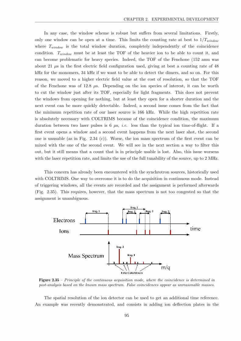
CHAPTER 2. EXPERIMENTAL DEVELOPMENT
In any case, the window scheme is robust but suffers from several limitations. Firstly,
only one window can be open at a time. This limits the counting rate at best to 1/Twindow
where Twindow is the total window duration, completely independently of the coincidence
condition. Twindow must be at least the TOF of the heavier ion to be able to count it, and
can become problematic for heavy species. Indeed, the TOF of the Fenchone (152 amu was
about 21 µs in the first electric field configuration used, giving at best a counting rate of 48
kHz for the monomers, 34 kHz if we want to be able to detect the dimers, and so on. For this
reason, we moved to a higher electric field value at the cost of resolution, so that the TOF
of the Fenchone was of 12.8 µs. Depending on the ion species of interest, it can be worth
to cut the window just after its TOF, especially for light fragments. This does not prevent
the windows from opening for nothing, but at least they open for a shorter duration and the
next event can be more quickly detectable. Indeed, a second issue comes from the fact that
the minimum repetition rate of our laser source is 166 kHz. While the high repetition rate
is absolutely necessary with COLTRIMS because of the coincidence condition, the maximum
duration between two laser pulses is 6 µs, i.e. less than the typical ion time-of-flight. If a
first event opens a window and a second event happens from the next laser shot, the second
one is unusable (as in Fig. 2.34 (c)). Worse, the ion mass spectrum of the first event can be
mixed with the one of the second event. We will see in the next section a way to filter this
out, but it still means that a count that is in principle usable is lost. Also, this issue worsens
with the laser repetition rate, and limits the use of the full tunability of the source, up to 2 MHz.
This concern has already been encountered with the synchrotron sources, historically used
with COLTRIMS. One way to overcome it is to do the acquisition in continuous mode. Instead
of triggering windows, all the events are recorded and the assignment is performed afterwards
(Fig. 2.35). This requires, however, that the mass spectrum is not too congested so that the
assignment is unambiguous.
Figure 2.35 – Principle of the continuous acquisition mode, where the coincidence is determined inpost-analysis based on the known mass spectrum. False coincidences appear as unreasonable masses.
The spatial resolution of the ion detector can be used to get an additional time reference.
An example was recently demonstrated, and consists in adding ion deflection plates in the
95

CHAPTER 2. EXPERIMENTAL DEVELOPMENT
spectrometer [Osborn 16]. Supplied with varying voltages, the deflection, i.e. the detected
ion position, depends on the time at which the ionization was performed. Combined with
the time-of-flight, one can retrieve the original laser shot without the electron informations.
The electrons and ions can thus be unambiguously assigned, regardless of the mass spectrum
complexity. We will see in the next section that we also use the ion spatial information in a
similar fashion.
Up to this date, the Cobold software we are using is based on the window mode. Im-
plementing a continuous acquisition mode is an appealing perspective that is currently being
investigated, in order to increase the repetition rate limitation. Note that in the studies where
we were only interested in the photoelectron angular distribution, the window mode could be
used with a much shorter window duration. Without this limitation and the coincidence condi-
tion, the electron counting rate could be easily increased up to 100 kHz. This was very useful to
quickly measure 3D distributions with good statistics. Beyond this counting rate, the recovery
time of the individual channels of the MCPs becomes comparable to the time between two hits
(∼ 1 ms). This diminishes the multiplication efficiency and the hits can not trigger the CFD
modules anymore. This is typically indicated by a depleted signal at the location where it is
supposed to be maximized and must be avoided.
Note that with a decent CPU, the Cobold software is able to reconstruct the events at about
100 kHz, and that several instances can be launched in parallel for offline analysis. Nevertheless,
the acquisition of the raw timings can be performed at a much higher rate, which has never
limited us.
IV Characterization of the COLTRIMS
The development of the COLTRIMS has been presented in the previous section. The present one
will focus on its characterization. Indeed, the great dimensionality of the measurement enables
to filter the noise from the signal. As we will see, this is to be balanced with the acquisition rate
and compromises have to be made. Additionally, the accuracy and resolution of the apparatus
depend on several factors that will be discussed. Lastly, a typical example of 3D photoelectron
angular distribution reconstruction will be given.
IV. 1 Constraints : Noise Filtering and Acquisition Rate
Detection Efficiency
The particle detection efficiency is of great importance in coincidence measurements, as an
incomplete event can not be used but still counts in the ionization per shot ratio. Additionally,
it can lead to wrong coincidence particle coincidence assignment. The global detection efficiency
depends on three factors.
The first one is the number of particles that actually reach the detector. Thanks to the
magnetic field, the collection angle of the photoelectrons up to 20 eV of kinetic energy is 4π.
However, the metallic meshes used in the spectrometer to define homogeneous electric field
96

CHAPTER 2. EXPERIMENTAL DEVELOPMENT
regions have a certain transmission, which depends on the distance between the strands and
their thickness. The greater the distance between the strands, the higher the transmission,
but a small electrostatic lens effect can start to appear within the grid if they are too much
spaced. The particle transmission of the meshes is thus generally about ∼ 80 %. For this
reason, spectrometer configurations requiring many meshes can be problematic. In our case, we
only use one on each detector side to impose a short acceleration just before the MCPs.
This is related to the second factor affecting the detection efficiency, namely the MCP
efficiency. It depends on various parameters, such as the particle type, its velocity and angle
of incidence, and the MCP characteristics such as the cross section of the microchannels. A
typical curve of the ion detection efficiency, as a function of kinetic energy and species, is given
in Fig. 2.23. In our case, the ions are accelerated at 2160 eV which corresponds to 45-55% of
MCP efficiency depending on the ion mass, up to 150 amu. The electrons reach the detector
with about 340 eV, corresponding to a 80% MCP detection efficiency.
The final limitation to particle counting efficiency is the ability of the delay lines and
electronics to detect a retrievable signal. This is a function of the delay line collection efficiency
and the CFD modules sensitivity, considering that one needs at least four delay lines timings to
reconstruct a particle hit (out of four for the ions, out of six for the electrons). This factor can
be globally determined by comparing the number of hits counted on the MCP back and the one
actually reconstructed in the momentum space for the photoelectrons, or in the detector space
for the ions. We have estimated it to be ∼ 77 % for the electrons and ∼ 54 % for the ions.
This number is probably better for the electrons because of the redundant hexagonal delay lines.
At the end, the global electron detection efficiency is about 50 % and the one of the ions
around 22 %. Combining these two numbers gives, for the one-electron one-ion events we are
interested in, a 11 % probability to fully retrieve an event that occurred. This number can
look poor at first sight, but is typically of the order of magnitude for this dual single-particle
spectrometer. Improvements could be made by, for instance, using a hexagonal delay line
detection on both sides, accelerating the ions closer to the efficiency saturation (about 64 %)
or moving to a spectrometer geometry which does not use metallic meshes. Conversely, the
electron MCP detection efficiency is around a maximum. Note that the detection efficiency
of the MCPs could be potentially increased by using funnel type microchannels, for instance.
Overall, this 11 % factor adds up to the coincidence condition, since this latter stands for the
actual ionization events. To this regard, the use of a high repetition rate source is even more
justified.
Laser Shot Reference
As we have seen in the previous section, a window event is triggered by an electron count
(see Fig 2.34 (a)). To avoid it to be on an fake count, from the MCP noise or from an electron
that does not come from a laser shot, the window is only activated if a laser shot was detected
about 100 ns before the electron (the order of magnitude of the electron TOF). The coincidence
assignation works straightforwardly if two consecutive events are well separated in time, namely
by more than the window duration and in principle only one ion should be measured in the
97

CHAPTER 2. EXPERIMENTAL DEVELOPMENT
window. But since the ion time-of-flight (up to 21 µs at 450 amu, Fenchone trimers) is greater
than the duration between two laser shots (at most 6 µs, at 166 kHz), there is a probability to
collect other events generated by other lasers pulses detected in the same window. With a 1/10
ionization per shot ratio, this probability is thus of at least 20% at 166 kHz, and increases a
lot with the laser repetition rate. The electrons that have not triggered the window are easily
discarded. However, the corresponding ions can be more problematic. Indeed, they appear in
the time-of-flight spectrum, and thus in the mass spectrum, as replicas of the actual spectrum
shifted in time by n times 1/(repetition rate), as displayed in Fig. 2.36. In practice, the replicas
often overlap with actual TOF peaks, even if this can be sometimes avoided by fine-tuning the
laser repetition rate. If the actual spectrum is very simple, the irrelevant TOFs can be discarded,
but this is not a general solution and it worsens with a higher laser repetition rate.
Figure 2.36 – Ion time-of-flight (a) and mass spectrum (b) of Methyl-Lactate, with 515 nm laserfield. Complete (red) and filtered (blue) are displayed. In addition to the parent ion (104 amu) and afew fragments in the 35-50 amu range, fake masses appear in the unfiltered case, coming from eventsfrom the next or previous laser shots.
A rough solution could consist in simply discarding all the events containing more than one
ion in the window. Besides significantly affecting the usable events counting rate, the imperfect
ion detection efficiency would lead to a very high fraction of wrong assignations, as the actual
ion of interest is not always detected, without possibility to discriminate them.
The solution chosen uses the spatial resolution of the ion detector. The ions are spread
along the detector axis corresponding to the molecular jet axis, as shown in Fig. 2.37 (a). Since
the species carried in the jet have approximately the same velocity, this position is proportional
to their time-of-flight. A relevant representation is Y = f(TOF ), displayed in Fig. 2.37 (b),
where the slope α corresponding to the jet velocity clearly appears. This is a precise manner to
determine the velocity, that depends on the carrier gas and the backing pressure (1500 m/s in
98

CHAPTER 2. EXPERIMENTAL DEVELOPMENT
the example given, with 1 bar of helium). Importantly in this plot, the position is proportional
to the actual TOF, while the abscissa is the reconstructed TOF. These two quantities match
along the TOF = α · Y line, meaning that any count along this axis are ions with a good TOF
reference (within a certain margin to account for the velocity dispersion and the recoil of the
fragments). On the contrary, any count outside of this range has a wrong reference and can
be discarded. One can identify the features due to the previous or next laser shots along the
TOF = α · Y + nT where T=1/(rep. rate) and n ∈ Z, as highlighted in Fig. 2.37 (c).
Figure 2.37 – (a) Spatial ion distribution, from the same dataset as Fig. 2.36. The signal alongthe laser axis comes from the residual pressure while the one along the jet axis comes from it. (b)Corresponding spatially-resolved time-of-flight spectrum, along the jet axis. The jet velocity is visiblein the slope indicated. (c) Same as (b) where areas of interest are indicated. The signal that comesfrom the jet and the right laser shot is in the green box, while the signal that has a wrong laser shotreference is highlighted in red and the signal from the residual pressure is in orange.
99

CHAPTER 2. EXPERIMENTAL DEVELOPMENT
By selecting the green area only, the cleaned mass spectrum can be safely obtained. So
far, this multidimensional filtering is performed offline. We have planned to implement it in
the online analysis in the perspective of using a continuous acquisition scheme, in order to be
able to directly get the ion laser shot reference and electron, without need of triggered window.
However, this requires the assistance of Roentdek since we can only implement minor custom
modifications to the C++ code of the software by ourselves.
Residual Pressure and Interaction Volume
Another feature identified in Fig. 2.37 (c) are ions detected with a zero mean momentum,
i.e. along Y = 0. They corresponds to molecules that were not in the supersonic jet, but in the
residual pressure in the interaction chamber (about 10−8 mbar). They can not be distinguished
from the bare mass spectrum and could contribute to the usable signal. However, their TOF
replicas can not be filtered as they do not spatially spread on the detector, and must thus be
entirely discarded with the spatial filtering discussed above (orange box in Fig. 2.37 (c)). These
ionization events thus constitute a limitation to the usable counting rate and must be minimized.
This can be achieved by increasing the pumping capacity, which we have done, using a multiple
jet skimmers configuration or adding a jet dump stage (if this latter is limiting the vacuum).
One can also magnify the incident beam to have a shorter Rayleigh length, up to the maximum
angular acceptance (40 mrad here with the optical skimmers).
More specifically, the relative importance of the residual pressure counts compared to the
jet counts depends on the photon wavelength and the beam focusing conditions. The size of
the interaction volume and its consequences on the spectrometer resolution will be discussed in
this section. Let us simply mention here that loose focus conditions, i.e. long Rayleigh range,
deteriorates this ratio. A highly nonlinear ionization (with a large number of photons involved)
tends to be localized only at the focus, while a one-photon ionization has a probability to occur
all along the laser path. This can be seen in Fig. 2.38 which shows typical spatial distributions
of the ions produced in the conditions given in Table 2.5. At 2ωL with Methyl-Lactate (a),
a significant fraction of the signal comes from the jet. At 4ωL (b), the majority of the signal
comes from the residual pressure and the diffuse background from the scattered light. When
using XUV radiation (16.9 eV) to ionize xenon (c), the ratio between the jet and the residual
pressure is relatively balanced as the focus is much more spread, from the one-photon process.
When higher photon energy (35 eV) are used in helium and Fenchone (d), the carrier gas can
be ionized and prevails, both in the jet and along the beam. This illustrates the relative ease to
study strong field and multiphoton studies, compared to the more challenging XUV experiments.
The ratio between the counts originating from the jet and from the residual pressure can
be accurately determined with these figures, and is summarized in Table 2.5, for the focusing
conditions presented in Table 2.7. Note that these plots are also used to finely center the
beam waist (along the laser) on the jet, and adjust the pointing (along the spectrometer) by
maximizing the signal from the jet.
At 2ωL, the part of the beam in which the intensity is high enough to ionize is mainly in
the jet, giving a quite low count loss due to the residual pressure along the laser (23 %). At
4ωL, it constitutes more of an issue, at 47 %. A solution could consist in using tighter focusing,
100

CHAPTER 2. EXPERIMENTAL DEVELOPMENT
Figure 2.38 – Ion spatial distribution for several field wavelengths an targets, indicated in Table 2.5and 2.7. The signal along the horizontal line comes from the residual pressure while the signal alongthe vertical axis comes from the jet. Note that the left side of the detector is damaged. ML =Methyl-Lactate, F = Fenchone
Harmonic Target Number of Jet Residual BackgroundOrder Molecule Photons Counts Pressure Noise
2ωL ML 5 69 % 23 % 8 %
4ωL ML 3 5 % 47 % 48 %
14ωL Xe 1 53 % 40 % 7 %
29ωL He + F 1 23 % + 14 % 50 % 13 %
Table 2.5 – Counts ratio between events originating from the jet, from the residual pressure andbackground counts (which consists of the rest of the counts spatially spread on the detector). Inany case, the noise counting rate without laser is very low, typically a few dozens of Hz. ML =Methyl-Lactate, F = Fenchone
but this goes against another issue already mentioned at this wavelength, which is the scattered
light producing a high level of background from the metallic surfaces. This quandary has not
been solved so far despite several attempts, in such a way that we have not used this wavelength
efficiently.
In the case of high-order harmonics, the ionization is a one-photon process (the ionization
yield is directly proportional to the intensity) and the jet/residual ratio does not benefit from
the focusing, since the intensity flux is constant along the beam propagation. For this reason,
the pumping capacity has been increased to the values mentioned in the description of the
apparatus (we added a 700 L.s−1 turbomolecular pump). The next step would be to increase
the distance between the nozzle and the skimmer to introduce a second skimmer as previously
discussed.
Balancing Noise and Acquisition Rate
The optimization of the usable counting rate merges all the parameters presented so far
and can be quite complex. Let us consider the following simplified model, to get a hint of the
interacting parameters. We will assume here that the setup is already optimized, so the ion
detection efficiency α, the ratio of signal from the residual gas β and the event window duration
Twin are fixed. The degrees of freedom are the ionization probability P per laser shot and the
laser repetition rate. The probability of detection of a single event is αP . The probability to
101

CHAPTER 2. EXPERIMENTAL DEVELOPMENT
get two ionization events per shot is P 2, in which either the two ions are detected (α2P 2), one
is detected (2α(1−α)P 2) or none is detected ((1−α)2P 2). The first case can be discarded, the
second one can not be identified as such and causes a non-filtrable background (false coincidence),
and the last one is simply undetected. Additionally, the probability to get an event from the
residual pressure is βαP . Finally, the probability that an event (already counted) is discarded
as a replica is kα2P 2(1 + β), where k = round(rep.rate · Twin) is the number of additional laser
shots contained in the event window. This corresponds to the red boxes in Fig. 2.36. For
simplicity, we omit the high order terms as β and P are relatively small.
The total number of ionization events per shot Revent is thus :
Revent = P + P 2 + βP (2.19)
The total counting rate per shot Rcount is :
Rcount = αP + (α2 + 2α(1− α))P 2 + βαP − kα2P 2(1 + β) (2.20)
in which the usable rate Ruse, the discarded rate Rdisc and the fake coincidence Rfake are
respectively :
Rcount = Ruse +Rdisc +Rfake
Ruse = αP − kα2P 2
Rdisc = α2P 2 + βαP − kα2P 2β
Rfake = 2α(1− α)P 2
(2.21)
Note that the undetected events Rund and the replica rate Rrepl are respectively :
Revent = Rcount +Rund +Rrepl
Rund = (1− α)P + (1− α)2P 2 + (1− α)βP
Rrepl = kα2P 2(1 + β)
(2.22)
The evolution of these quantities for a good detection efficiency α = 0.9 is depicted in
Fig. 2.39 (1). Panel (a) show the evolution of Ruse, Rfake and Rdisc, which sum accounts
for the detected counting rate, and Rrepl and Rund as a function of the ionization probability
P , at a repetition rate of 166 kHz. One can see that a very low P does not give a good signal
acquisition rate. Conversely, a high P , a lot of the acquired signal is discarded, which diminishes
the usable counting rate. In between, a maximum of Ruse can be found around P ∼ 0.28. At
this probability, about 30 % of the total counting is usable and ∼ 10 % of the usable signal
actually comes from fake coincidences (panel (b)). From there, one can be tempted to increase
the laser repetition rate. The evolution of the usable counting Ruse × (rep.rate) as a function
of P and the repetition rate is shown in Fig. 2.39 (1-c). Lineout of this map, depicted by the
black lines, are plotted in panels (d) and (e). The saw teeth pattern originates from the fact
102

CHAPTER 2. EXPERIMENTAL DEVELOPMENT
that the number of replica suddenly increases when an additional laser shot comes in the event
window. The increase within each teeth is due to the increase of the global acquisition rate with
the repetition rate. The effect of the replicas appears very detrimental, in such a way that in
this case the only optimization consists in increasing the repetition rate from 166 kHz to 230
kHz, yielding about 29 kHz of usable events. This number must be tempered, since 10 % of fake
coincidences is quite high. In practice, one uses a lower value of P , about 1/10.
The result of the same procedure for a lower detection efficiency (α = 0.5) is shown on Fig.
2.39 (2). Of course, the first effect is the larger fraction of undetected counts. Also, the curve of
Ruse is more spread across P , and the number of fake coincidences drastically increases as they
correspond to two events from the same laser shot with only one ion detected. For this reason,
the optimal value of Ruse can not be chosen and a much lower P is required to have 10 % of
fake coincidences, in this case P ∼ 0.10. This shifts the optimal repetition rate up to 840 kHz
before the replicas become problematic, for a final ∼ 21 kHz of usable events. However, this
does not take into account several other factors. Firstly, panels (a) and (b) also evolve with the
repetition rate, meaning that the procedure must be done iteratively as 840 kHz is far from the
initial 166 kHz, pushing it to an even higher value. Secondly, the laser average power is limited,
and the choice of P can be constrained by the repetition rate. Thirdly, beyond the lenient
fake coincidence acceptance, increasing P as much as possible increases a lot the signal on the
detectors, and especially the unusable and the undetected one. This induces a quicker aging
of the MCPs, and more problematically the dynamical limit of the detectors can be reached
(about 100-150 kHz). In the same trend, increasing the repetition rate linearly increases the
fraction of unusable signal (replicas), thus quadratically increases counting rate of unusable
events, while it only increases the usable rate linearly, quickly leading to the saturation of the
detectors for a minor increase of the usable counting rate. Finally, independently of all this
reasoning, the acquisition mode limits the total acquisition rate at 1/Twindow because only one
window can be open at a time. This number is usually between 40 and 75 kHz depending on
the mass of the species of interest, and puts a much higher cost on the unusable detected events.
The statistical model discussed here underlines and illustrates the effect of the different
parameters at play but is approximate. At the end, we have determined the best usable counting
rate empirically. Discrepancies with the model can be noted, in particular due to the fact that
this latter does not take into account the deadtime of the detectors. This implies that some
events can not be correctly reconstructed, decreasing the effective α depending on the counting
rate. By varying the laser repetition rate and the energy per shot, we have experimentally
determined that the best usable counting rate was reached when the total acquisition rate was
about 10-15 kHz, and that increasing the repetition rate did not help significantly. This is in
contradiction with the model presented, and we have been investigating the causes of this effect
in order to verify if it is an intrinsic limitation or not, but the multiple parameters at play render
the task tedious. Nevertheless, various factors of loss of counts can be retrieved from the analysis
of recorded sets of data. Table 2.6 shows these numbers obtained in two cases. One uses two
high-order harmonics at 12.0 and 16.85 eV generated from a 515 nm wavelength shot on Xe,
at an event counting rate of 13-15 kHz. The other one was recorded in Methyl-Lactate directly
103

CHAPTER 2. EXPERIMENTAL DEVELOPMENT
Figure 2.39 – Evolution of the usable counting rate with the ionization probability and repetitionrate, calculated with the simplified statistical model presented, for a detection efficiency of 0.9 (1)and 0.5 (2), and Twin = 13 µs. (a) Evolution of the different types of rate per shot composing thetotal counting rate and total ionization rate, as a function of the ionization per shot probability at arepetition rate of 166 kHz. (b) Fraction of usable counts and false coincidence counts, as a functionof the ionization per shot probability, at 166 kHz. (c) Map of the final usable counting rate, as afunction of the ionization per shot probability and of the repetition rate. The black lines indicate theoptimal value. (d) Lineout of (c) along the ionization per shot probability for the optimal repetitionrate of 230 kHz (1) and 840 kHz (2). (e) Lineout of (c) along the repetition for the optimal ionizationper shot value of 0.28 (1) and 0.10 (2).
104

CHAPTER 2. EXPERIMENTAL DEVELOPMENT
ionized by the 515 nm beam, at a counting rate of 10-12 kHz. Note that the ion MCP efficiency
was deteriorated by a factor 4 in the first case due to a damage. One has to keep in mind
that the electron detection efficiency indicated in this table only accounts for the electronics
efficiency, as these values are retrieved from measurements and not from the actual, unknown
event probability.
Photons Detection False Fraction Replica Event& Efficiency Coincidence from the Filter Total Counting
Target Electron/Ion (%) Filter (%) Jet (%) (%) (%) Rate (kHz)
HHG12.0-16.9 eV 78/6.2 94 53 67 1.6 13-15
in Xe
515 nm2.4 eV 76/24 92 69 82 9.5 10-12in ML
Table 2.6 – Summary of the factors of loss of usable counting rate, experimentally measured in twotypical conditions given in the first column, at a repetition rate of 166 kHz. These numbers arededucted from the different quantities accessible in the analysis software, and by filtering the eventsof interest.
The comparison between these two cases shows two characteristic trends. The first one
is that the signal from the residual pressure represents about half of the signal in one-photon
ionization while it decreases about one third in multiphoton ionization, as previously explained.
The second one is that more events are lost in the replica in the first case, as the probability P
was slightly higher than in the second one. This usable counting rate loss is, however, almost
exactly counterbalanced by the higher acquisition rate.
Finally one must add a last factor in the HHG case that is not comprised in this table,
which is the size of the interaction volume in the jet. Due to its extension along the radiation
beam axis, only the central part of the ion distribution (about two thirds) yielded a decent
reconstructed photoelectron distribution. This is more related to the calibration of the detector,
and is presented in the next section.
IV. 2 Calibration and Resolution
The determination of the resolution of the COLTRIMS depends on several elements, and can
be quite indirect since the physical quantities are reconstructed from timings. We will address
in this section the different factors.
Physical Resolution
The first key element defining the resolution is the precision of the measured quantities,
which are the delay lines timings. The temporal resolution of the detectors is ∼ 100 ps in
good conditions, i.e. with a very low electronic noise. From Eq. 2.13, one can estimate the
time-of-flight resolution to ∆TOF = 200 ps, assuming a good detector calibration. The ion
mass spectrum resolution ∆(m/q) and relative resolution ∆(m/q)(m/q) can be derived from Eq. 2.14,
reading :
105

CHAPTER 2. EXPERIMENTAL DEVELOPMENT
∆(m/q) =
√2E
Li∆TOF
√m/q
∆(m/q)
m/q=
√2E
Li∆TOF
√m/q
−1(2.23)
Fig. 2.40 shows the evolution of these two quantities for the spectrometer configuration
mainly used (E = 8 V.cm−1, B = 8.05 Gauss, Li = 4.16 cm, last line in Table 2.4). The
theoretical ∆(m/q) is much lower than 1 for the masses we are interested in (∼ 150 amu for
monomers and fragments, up to 450 amu for trimers of fenchone), but other factors will play a
role here, such as the size of the interaction volume discussed in a further paragraph.
Figure 2.40 – Evolution of the ion mass spectrum physical resolution of the spectrometer ∆(m/q) and∆(m/q)(m/q) , as a function of (m/q) in our range of interest.
For the electrons, the calculation is a bit more complex since the quantities of interest are
the momenta, that are reconstructed from the equations 2.16 and 2.17. The momentum along
the spectrometer pz is simpler as it only depends on the time-of-flight. From Eq. 2.16, the
resolution ∆pz can be derived as :
∆pz =
(2meLee
2E2
(−pz +√p2z + 2eEmeLe)2
+ eE/2
)∆TOF (2.24)
Fig. 2.41 shows the evolution of ∆pz for values of pz between -1.2 and 1.2 a.u., corresponding
to kinetic energies within 20 eV. The resolution is between 0.020 and 0.036 a.u., i.e. between 5
and 18 meV in energy (in comparison the laser energy width up to 4ω is a bout 22 meV FWHM).
106

CHAPTER 2. EXPERIMENTAL DEVELOPMENT
Figure 2.41 – Evolution of the physical photoelectron momentum resolution ∆pz as a function of pz.
The assessment of the photoelectron momentum resolution in the detector plane ∆px and
∆py (or pr, ϕ in radial coordinates) requires the spatially-resolved detection. The spatial reso-
lution of ∆X = ∆Y = 200 µm is related to the timing resolution, as previously explained. Note
that the diameter and the pitch of the holes of the microchannel plates are respectively of 25
µm and 32 µm for both the ions and the electrons, and thus do not limit the spatial resolution.
In addition, the resolution will also depend on the time-of-flight, or pz, because of the helical
trajectories caused by the magnetic field. Indeed, the spatial resolution is maximized at the tip
of the wiggle, set at pz = 0, and reduces with |pz|. From Eq. 2.17, one can obtain :
∆pr =eB
2sin( ω
2eE(−pz +
√p2z + 2eEmeLe)
)∆r + |pr|
ω
2tan−1
( ω
2eE(−pz +
√p2z + 2eEmeLe)
)∆TOF
∆ϕ =X∆Y + Y∆X
X2 + Y 2+ω
2∆TOF
(2.25)
∆pr can here be reduced to be a function of pr and pz, and is plotted in Fig. 2.42 (a), in
logarithmic scale. The black circles represent the momentum spheres of the 20 eV, 5 eV, 1 eV
and 0.1 eV electrons. This figure underlines a crucial property of the wiggles : the resolution in
pr is maximized when the time-of-flight is close to a half-integer value of ωhelix and is seriously
affected close to a integer value of ωhelix. Moreover, is also reduced with |pr|. Combining these
two effects, ∆pr is the best for pr = 0 and pz = 0 at a given photoelectron energy. This can be
an issue for our main goal which is resolving the angular asymmetries in the distribution, as we
will see further in this section. The evolution of ∆pr as a function of pr and pz are respectively
plotted in panels (b) and (c), for kinetic energies respectively along z and r of 0, 0.1, 1, 5 and
20 eV. Overall, ∆pr is within 0.010 a.u. for photoelectrons with a total kinetic energy up to 5
eV, corresponding to 1.6 meV. Once again, this will not be the only factor.
The evolution of ∆ϕ explicitly depends on the detected position (X,Y ) and can not be
107

CHAPTER 2. EXPERIMENTAL DEVELOPMENT
Figure 2.42 – (a) Evolution of the physical radial photoelectron momentum resolution ∆pr as afunction of pr and pz, in logarithmic scale. The black circles indicate the momentum sphere ofkinetic energies of 20 eV, 5 eV, 1 eV and 0.1 eV. (b) Evolution of ∆pr with pr, at fixed EKEz. (c)Evolution of ∆pr with pz, at fixed EKEr.
reduced to the physical momenta. Let us simply mention that the error decreases with the
radius of detection r, as the angular resolution increases at high radius.
Reconstruction Parameters
The equations presented above do not take into account the error that could originate from
the reconstruction parameters. Some physical quantities, such as the electric and magnetic fields
or the delay offsets are roughly known from the voltage or the current generators. However,
their actual values have to be much more precisely defined in the reconstruction algorithm.
The best way to refine them is to minimize some typical defaults in the reconstructed events.
This specifically applies to the electron momentum distributions, since the mass spectrum is
ultimately calibrated on known species. From Eq. 2.16 and 2.17, one can see that pz depends
on the spectrometer length Le and the electric field E and the timing reference. Practically,
they all have the same effect, which is shifting the pz distribution, i.e. the zero kinetic energy
108

CHAPTER 2. EXPERIMENTAL DEVELOPMENT
time-of-flight. The evolution of the kinetic energy spectrum (i.e. the angular integration of the
distributions) are shown in Fig. 2.43 (a), for E field parameters of 98 %, 99 %, 100 %, 101 %
and 102 % of the optimal value found. They are all calculated from the same raw data set of
75×106 events generated in Methyl-Lactate at 515 nm, that is used in Section 3.III. This shows
that variations of 1 % of the parameter used can induce significant loss of resolution.
px and py additionally depend on the magnetic field B parameter. Reconstructions with
variations of ±10% from the optimal value are presented in Fig. 2.43 (b). Errors on B induce a
asymmetric distortion of the distribution. Of course, the deviation can be mainly corrected by
correcting the parameter to get a rounder distribution, but the precision of this procedure is hard
to assess. Importantly, these asymmetries can be in competition with the actual asymmetries
we are interested in. In principle, they can be partially canceled out by subtracting distributions
obtained with opposite laser helicities, but still remains hard to quantify. Note that this effect
is amplified at high photoelectron kinetic energy.
Figure 2.43 – Evolution of (a) reconstructed photoelectron kinetic energy and (b) (px, pz) reconstructedmomentum distributions, as a function of the reconstruction parameters, for the same set of raw data(7.5 M events recorded by ionizing Methyl-Lacate with a circularly polarized field at 515 nm). Eopti
and Bopti are the optimal values found, respectively being 8.2 V.cm−1 and 8.25 Gauss.
Finally, the drifts of the laser pointing can introduce a time dependency to the recon-
struction parameters, in particular the distances between the target and the detectors Li and
Le. Nevertheless, two solutions can be found. The first one consists in splitting the data into
subsets, and adapt the reconstruction parameters to each subset. This can be tedious and is
only satisfactory if a sudden pointing offsets occur only a few times. The other possibility
109

CHAPTER 2. EXPERIMENTAL DEVELOPMENT
consists in actively stabilizing the pointing. We aim at implementing such a stabilization with a
precision of a few dozens of µm, so that this effect becomes negligible in terms of reconstruction
parameters (the question of the interaction volume is discussed in the next paragraph). Note
also that the laser temporal jitter is in the femtosecond range and is completely marginal.
Interaction Volume
As already mentioned, the reconstruction of the mass spectrum and photoelectron momen-
tum distribution is performed assuming a punctual source. Taking into account the size of the
interaction volume can lead to a broadening of the spectra. Assuming a Gaussian beam shape,
the intensity profile is given by :
I(r, z) = I0
(w0
w(z)
)exp
(−2r2
w(z)2
)(2.26)
where w0 = λπθ is the beam waist, zR =
πw20
λ is the Rayleigh range, w(z) = w0
√1 +
(zzR
)2
and I0 is the intensity at the waist, as parametrized on Fig. 2.44.
Figure 2.44 – Parametrization of a Gaussian beam profile.
The interaction volume is defined along the spectrometer and the jet axis (both orthogonal
to the laser) by the waist w0, and along the laser axis by the Rayleigh range zR and the width
of the jet. A table of these parameters in the typical condition used with the laser fundamental
ωL and 2ωL, 3ωL, 4ωL and high-order harmonics 14ωL is shown on Table 2.7. The focal lengths
f indicated are the shortest one that can be used in the current beamline configuration.
The more nonlinear the ionization is (i.e. the longer the wavelength), the more localized
is the ionization area. In the perturbative ionization regime (single photon or multiphoton),
the ionization probability scales with In where n is the number of photon involved. We will
110

CHAPTER 2. EXPERIMENTAL DEVELOPMENT
Harmonic Photon Energy Wavelength f Divergence w0 zROrder (eV) (nm) (mm) (mrad) (µm) (mm)
ωL 1.2 1030 400 6.2 52 8.4
2ωL 2.4 515 400 6.2 26 4.2
3ωL 3.6 343 400 6.2 17 2.8
4ωL 4.8 257 400 6.2 13 2.1
14ωL 16.85 74 3000 0.84 28 34
Table 2.7 – Typical focusing conditions used, for a beam diameter of 10 mm.
simply assume that the effective interaction volume (in which I2 > 0.1I20 ) extends on a cylinder
of diameter√
2ln(10)w0/√n and of length 2zR
√n√
10− 1. Note that this last value can be
limited by the jet width (∼ 10 mm for a quite high assumption).
The mass spectrum is only affected by the extension of the interaction volume along the
time-of-flight axis, corresponding to the spectrometer axis. It will appear as a distribution
∆Li ∼√
2ln(10)w0/√n of Li in Eq. 2.14. The corresponding broadening in m/q can be
obtained with :
∆(m/q) =E
2L2i
TOF 2ion∆Li (2.27)
The extension of the beam waist also appears as a distribution ∆Le = ∆Li in Eq. 2.16.
The broadening in the photoelectron momentum pz due to this uncertainty can be obtained with
:
∆pz =me
TOF∆Le (2.28)
Once again the situation is much more complex for the distributions in the polarization
plane. Its resolution is both affected by the broadening in pz (or in time-of-flight) and by
the spatial broadening of the detection. Especially, the spatial distributions are broadened by
∼√
2ln(10)w0/√n along the jet axis and by ∼ 2zR
√n√
10− 1 or the jet width along the laser
axis. This last term always dominates, so assuming ∆r = 2zR√n√
10− 1 (up to 10 mm), the
resolution ∆pr and ∆θ can be derived from Eq. 2.17 as :
∆pr =eB
2|sin
(ω2TOF
)|∆r +
e2B2r
4me|cos
(ω2TOF
)|∆TOF
∆ϕ = ∆θ +ω
2∆TOF
(2.29)
These equations have multiple implicit dependencies and do not take into account the
anisotropy of ∆r. Let us just calculate the order of magnitude of the broadening :
∆pr ≈1
2
eB
2∆r +
1
2
e2B2r0
4me∆TOF (2.30)
111

CHAPTER 2. EXPERIMENTAL DEVELOPMENT
where ∆TOF ≈√
2meeE
∆LeLe
and r0 = 10 mm is the typical distribution radius.
Harmonic Number of ∆Li = ∆Le ∆r ∆(m/q) ∆pz ∆pz ∆pr ∆prOrder Photons n (mm) (mm) (amu/e) (a.u.) (eV) (a.u.) (eV)
ωL 8 0.039 9.7 0.15 3×10⁻⁴ 1×10⁻⁶ 0.16 0.34
2ωL 4 0.028 7.4 0.10 2×10⁻⁴ 5×10⁻⁷ 0.12 0.20
3ωL 3 0.021 6.0 0.08 1.5×10⁻⁴ 3×10⁻⁷ 0.10 0.13
4ωL 2 0.020 6.2 0.073 1.4×10⁻⁴ 3×10⁻⁷ 0.10 0.14
14ωL 1 0.060 ∼ 10 0.22 4×10⁻⁴ 2.5×10⁻⁶ 0.16 0.36
Table 2.8 – Overview of the different factors of broadening due to the spatial extension of the in-teraction volume, from the simplified model presented in the text, at the wavelengths and focusingconditions given in Table 2.7. The number of photons involved and masses are given for m = 152amu and Ip=8.6 eV, corresponding to Fenchone.
A summary of the broadening induced by the extension of the interaction volume is pre-
sented in Table 2.8, with the laser conditions given in Table 2.7. Overall, this effect of the
ionization volume is more critical than the intrinsic resolution of the spectrometer. Regarding
the photoelectron momentum resolution, the spatial extension of the source along the laser axis
dominates in such a way that the pointing fluctuations of the laser should be negligible. In
the worst case, corresponding to the ∼ 1 mm acceptancy of the optical skimmers, ∆pz remains
below 1 meV and ∆pr only increases by 3 %. Nevertheless, it would induce a ∆(m/q)(m/q) ≈ 3% which
is problematic. For this reason and the global continuity of the acquisitions, we are currently
working on implementing a pointing stabilization with a precision close to the beam waist, which
will be largely sufficient to keep the mass resolution well below 1 amu in our range of interest
(up to 450 amu), at least regarding the ionization volume.
Generally speaking, the dominant effect on the photoelectron momentum resolution
(the extension of the source along the laser axis) could be tempered by using very tight
focusing conditions, highly nonlinear ionization or a narrower jet, by using a double skimmer
configuration.
Experimental Measurements
We can compare the experimental width of the mass spectra and the electron kinetic energy
spectra in two typical cases, the first one using a 515 nm wavelength to ionize Methyl-Lactate
molecules (Ip = 10.3 eV) and the second one where we ionized xenon (Ip = 12.1 eV) with the
7th harmonic of a 515 nm driving field.
The mass spectrum around the species of interest are shown in Fig. 2.45. In panel (a), the
Methyl-Lactate has a mass of 104 amu and one can observe, in addition to a fragment at 102
amu, small peaks at 103 and 105 amu due to 13C isotopes. The mass resolution is clearly below 1
amu/e, as the main peak is fitted with a Gaussian profile of σ = 0.06 amu/e. The mass spectrum
of xenon in panel (b) is a bit more congested because of its natural isotopic composition. The
fit is thus performed over all the atomic masses with a fixed relative weight, shown in black
lines. The fit does not manage to reproduce the experimental data very well, but still gives a
reasonable σ = 0.77 amu/e. This is enough to distinguish the isotopes, but here the large volume
112

CHAPTER 2. EXPERIMENTAL DEVELOPMENT
of interaction (due to the EUV ionization wavelength) significantly reduces the mass resolution.
In the case of the multiphoton ionization of Methyl-Lactate, the mass spectrum resolution is
in good agreement with the predictions. Nevertheless, the theoretical values of the resolution
seem underestimated in the HHG case. This could be attributed to additional processes, such
as the photodissociation of xenon dimers during the flight in the spectrometer, inducing a recoil
that broadens the distributions. A perspective to avoid this situation can be to use a mixture
of xenon and helium, or by heating the nozzle.
Figure 2.45 – Measured ion mass spectrum of (a) Methyl-Lactate and (b) Xenon, respectively producedby a 5-photon ionization at 515 nm and one-photon ionization by the 7th harmonics of a 515 nmfield (16.85 eV).
The corresponding photoelectron spectra are shown in Fig. 2.46, in coincidence with the
Methyl-Lactate parent ion (a) and the xenon monomers (b). In the first case, a single photo-
electron peak appears and is fitted with σ = 0.27 eV. The value at which the peak arises can
not be compared to any reference of ionization potential since this latter has not been measured
elsewhere. The center of the line, found at 1.75 eV, corresponds to a 5-photon ionization at 515
nm (2.401 eV), resulting in a 10.29 eV estimation of the vertical ionization energy. Conversely,
xenon is suited for calibration as its energy levels are well known. The kinetic energy spectrum
of the xenon shows two lines that are fitted independently. They correspond to the ionization
to the 5s25p5 2P 012
and 5s25p5 2P 032
of respective ionization thresholds of 13.44 eV and 12.13 eV,
by the 7th harmonic (16.85 eV). They are respectively fitted with σ = 0.33 eV and σ = 0.49 eV.
The kinetic energies at which the lines are located are measured at 3.10 eV and 4.35 eV, where
values found in the NIST database were respectively 3.41 eV and 4.72 eV.
It thus seems like our detector systematically overestimates the electron kinetic energies.
In practice, such a measurement on a known target enables one to apply a scaling correction
on the kinetic energy range, which would be in our case about x1.1. The spin-orbit coupling
measured here is of 1.25 eV, while the expected value is 1.31 eV, confirming the importance of
the empirical calibration to obtain such a precision.
Regarding the energy resolution, the values found experimentally are always above the one
predicted from the theoretical uncertainties, but are of the same order of magnitude. Part of
the additional error could be attributed to imperfect reconstruction parameters, inhomogeneity
113

CHAPTER 2. EXPERIMENTAL DEVELOPMENT
Figure 2.46 – Measured photoelectron kinetic energy spectrum of (a) Methyl-Lactate in coincidencewith the unfragmented molecule and (b) Xenon in coincidence with the monomer, respectively ionizedin multiphoton by 515 nm radiation and one-photon by the 7th harmonics of a 515 nm field.
in the electric or magnetic fields, especially since the resolution reduces quite quickly with the
photoelectron kinetic energy, and also due to the energy width of the photons. Note that this
latter is not accessible in our case, since the resolution of our XUV spectrometer is too great (of
the order of 100 meV).
V Conclusions and Outlook
This chapter has mentioned some of the advances of the group on the new generation high
repetition rate beamline. Great efforts have been put to characterize and enhance the capacities
of the laser source in order to make it as versatile as possible. In particular, frequency conversion
setups have been implemented and optical parametric amplification have been tested. One
of the original activity of the group, high-harmonics generation, has been adapted to the
new source (mostly by other group members). The generation of circular or highly elliptical
high-order harmonics remains challenging, and several techniques have been tested, such as
using bicircular bichromatic driving fields or resonant HHG. Even if this Yb-doped fiber laser
provides a unprecedented signal acquisition rate, its main drawback is its pulse duration (135
fs) which is longer than the widely used Ti:Sa lasers. We have achieved so far postcompression
below 20 fs, and expect great advances in this way as new technologies become available. We
look forward to further improvements in the global stability of the beamline in order to run
experiments that require very long acquisitions, over several days in a row. In addition, we aim
at implementing continuous wavelength tunability.
Regarding the photoionization experiments, the new source has pushed the velocity map
imaging spectrometer, which has been used for a long time on crystal lasers, to a new level
of sensitivity. Moreover, the tunability of the repetition rate between 166 kHz and 2 MHz
introduces a revolutionary concept for the study of resonant multiphoton processes : the energy
per pulse can be widely modulated without affecting the acquisition time. The high and tunable
repetition rate of the source is also crucial for the new detection apparatus. An important
114

CHAPTER 2. EXPERIMENTAL DEVELOPMENT
part of this thesis consisted in building and characterizing a coincidence spectrometer, which
enables the direct measurement of the 3D photoelectron momentum distributions in coincidence
with the corresponding mass spectra. It has been fruitfully used so far, but remains dependent
on very long acquisitions. Indeed, even if a decent 3D distribution can be measured in a few
minutes, the acquisitions increases by an order of magnitude when the coincidence is required.
Moreover, the measurements of the photoelectron circular dichroism, our chiral observable of
choice, requires an additional order of magnitude, up to dozens of hours. This step has been
reached recently, but we are willing to carry out time-resolved pump-probe experiments, that
require even more runtime. Beyond the stability of the laser source (in particular related to the
thermal drifts over several days), this could be achieved by enhancing the window coincidence
scheme to a continuous acquisition scheme.
115

CHAPTER 2. EXPERIMENTAL DEVELOPMENT
Figure 2.47 – Pictures of the high repetition rate beamline. (Up, right) Dual fiber amplifiers onthe optical table, (Up, left) Optical setup, (Middle) HHG beamline coupled to the COLTRIMS, withthe VMI and the laser in the background. (Bottom) Example of photoelectron angular distributionsproduced with HHG beam and measured in coincidence with xenon monomers (a), xenon dimers (b)and without coincidence (c).
116

CHAPTER 2. EXPERIMENTAL DEVELOPMENT
117

CHAPTER 2. EXPERIMENTAL DEVELOPMENT
118

Chapter 3
Multiphoton Regime -
Molecular Sensitivity
As we see throughout this manuscript, Photoelectron Circular Dichroism is a powerful tool
to investigate molecular chirality in a wide variety of ionization regimes [Beaulieu 16b], ranging
from the single-photon, the multiphoton to the ATI and tunnel ionization regimes. In this
chapter, we will focus on the multiphoton regime and more specifically on the opportunity it
provides in terms of sensitivity to the excited molecular states and dynamics.
Figure 3.1 – Illustration of the different ionization regimes at which the PECD arises. In particular inthe resonance-enhanced multiphoton ionization, the intermediate excited states can play an importantrole, in this chapter mainly through the anisotropy of excitation that they induce. The Rydberg statesdensity of Fenchone is depicted here as an example. Extracted from [Beaulieu 16b].
119

CHAPTER 3. MULTIPHOTON REGIME - MOLECULAR SENSITIVITY
I Introduction
I. 1 Resonance-Enhanced MultiPhoton Ionization (REMPI)
Properties of the Single-Photon PECD
As we have seen in the introduction chapter, the sensitivity of the PECD was initially
demonstrated in the single-photon ionization regime. In this case, PECD is known to be
remarkably sensitive to the whole dynamics of the photoionization process, and strongly
depends on several factors. Firstly, the initial orbital from which the electron is ionized plays
a role, for instance the PECD associated to the HOMO or HOMO-1 can have an opposite sign
[Turchini 04, Nahon 06]. Secondly, it depends on the whole structure of the ionized molecule.
Substituting a group far away from the ionized orbital can lead to an inversion of the PECD
[Nahon 16]. This reflects the non-local character of this observable, the chiral response being
imprinted during the electron scattering onto the whole molecular potential. As a result, it
is also sensitive to the conformational geometry [Turchini 09, Turchini 13]. Thirdly, PECD is
a function of the kinetic energy with which the photoelectron is ejected [Powis 08]. Electrons
emitted from the same orbital and differing only by a few eV can show opposite dichroic signals.
Fourthly, it is affected by the vibrational excitation. Sign change of the dichroism associated
with two consecutive vibrational states of the Methyloxyrane ion were observed [Garcia 13],
and this property was later observed in other chiral compounds [Ganjitabar 18, Ganjitabar 20].
Finally, single-photon PECD depends on the molecular orientation of the target [Tia 17], even
if it survives the averaging over all the orientations in randomly aligned samples.
Extension to the Multiphoton Ionization Regime
Replacing the XUV radiation by a femtosecond laser pulse affects the structure of the
PECD as we will see in the next paragraph, but most of the aforementioned properties still
apply. In addition to them, a new element will play an important role. When performing
multiphoton ionization of an atomic or molecular systems, intermediate excited states can
indeed be reached (see Fig. 3.1) and drastically affect the process. Generally, transitions to
the excited states enhance the ionization yield compared to the non-resonant case, leading to
the so-called Resonance-Enhanced MultiPhoton Ionization (REMPI). This situation is very
common, including when chiral molecules are ionized with femtosecond laser pulses. The
ionization potential of these molecules is typically below 10 eV, with a high density of states
above 6-7 eV (the typical threshold of the Rydberg series), in a range that can easily be reached
by absorption of a few photons of the fundamental laser (1030 nm i.e. 1.20 eV with our Yb
fiber laser, 800 nm i.e. 1.55 eV with a Ti:Sa laser) or its harmonics. These processes are usually
denoted as [n+m] REMPI, where n is the number of photons required to reach the resonance
and m is the number of photons from this resonance to the continuum.
The observation of the PECD in the multiphoton regime (MP-PECD) was first established
by the Kassel [Lux 12] and the Amsterdam/Nottingham groups [Lehmann 13]. In [Lux 12]
in 2012, multiphoton PECD was measured in Fenchone and Camphor, two bicyclic ketones
120

CHAPTER 3. MULTIPHOTON REGIME - MOLECULAR SENSITIVITY
isomers. Comparing the signal from these two isomers and from Norcamphor revealed significant
differences, even though these molecules have relatively similar structures, close electronic
densities and ionization thresholds (respectively 8.6 , 8.7 eV and 9.2 eV vertical Ip) [Lux 15].
This demonstrated a high sensitivity of MP-PECD to the precise molecular structure. Since
then, REMPI-PECD has also been measured in a few other chiral compounds such as Limonene
[Rafiee Fanood 15, Beaulieu 18a], Iboprofen [Comby 20b], Ethyl-Lactate, Methyl-Lactate and
thus happens to be a general effect.
Studies have shown for example in [2+1] ionization of Fenchone with a wavelength ranging
from 359 nm to 431 nm that the sign of the PECD can be inverted if the intermediate resonant
state was the 3s (6.10 eV ) or one of the three 3p (6.58 eV ) [Kastner 17]. This effect has been
reproduced with nanosecond pulses [Kastner 19], even if the mechanism is more sequential than
with femtosecond pulses. More generally, it turns out that the PECD is also sensitive to the
orbital excited (for example HOMO or HOMO-1 of Limonene [Beaulieu 18a] or HOMO-(0-2)
of Fenchone [Beaulieu 16a]) and to the vibrational state. Fine resolution of the vibrational
levels has been performed with nanosecond dye lasers, but this study, made only in Fenchone,
suggested that the PECD was not drastically sensitive to it under these conditions [Kastner 20].
The generality of this latter observation remains to be confirmed, however. At the end, the
signal very often comes from a manifold of excited states and calculations typically based on
Density Functional Theory (DFT) [Rafiee Fanood 15, Beaulieu 16a, Beaulieu 16b] method helps
assigning the excited state density, but is quite challenging in the Rydberg states manifold.
As a result, the process depends also on the precise laser wavelength and [n+m] REMPI
scheme [Lehmann 13, Beaulieu 16a, Beaulieu 16b, Demekhin 18]. Quantitative numerical
simulations of the PECD itself in the multiphoton regime can be possible using for example
Time-Dependent Single Center (TDSC) method [Demekhin 18]. It can also be calculated by
using or a combination of ab initio calculation (to get the transition dipoles) and perturbative
theory for the description of the excitation and a single-center description of the ionization
step [Goetz 17, Goetz 19]. Multi-center basis set can also be employed [Turchini 13]. Finally,
it seems credible that MP-PECD can be sensitive to the conformational state of the molecules,
even if this effect has only been described in single-photon ionization. This layer of complexity
can be avoided, typically in strained molecules such as the bicyclic ketones previously mentioned.
As a result, the MP-PECD is a double-edged sword. On one hand, it is a very rich
observable to investigate the chiral response of molecular system. It is experimentally handy, as
it survives molecular orientation averaging, and provides a remarkably high signal (1-10% range)
with a relatively simple setup. On the other hand, the high sensitivity of MP-PECD to many
parameters (initial orbital, intermediate state, vibrational ionic state, electron kinetic energy...)
makes the physical interpretation quite indirect, and it can be challenging to disentangle the
molecular effects involved.
Quantifying the MP-PECD
The structure itself of the MP-PECD differs from the single-photon case. The higher number
121

CHAPTER 3. MULTIPHOTON REGIME - MOLECULAR SENSITIVITY
of photons involved leads to sharper structures in the photoelectron angular distributions. These
angular features contain information which can be quantified. Typically when the measurements
are performed with a Velocity Map Imaging spectrometer, the photoelectron angular distribution
Sp(E, θ) can be expressed on a basis of Legendre polynomials P 0i :
Sp(E, θ) =
2N∑i=0
bpi (E)P 0i (cos(θ)) (3.1)
where E is the photoelectron kinetic energy, p = ±1 is the light helicity, θ is the ejection
angle and i is the order of the polynomial. Note that the even order ones are symmetric along
the laser propagation axis and the odd ones are antisymmetric. In the simple case where the
field is circularly polarized, or more generally when the field has a cylindrical symmetry (and
that the symmetry axis in contained in the VMI projection), the maximal order of polynomial
2N corresponds to twice the number of photons N involved in the ionization [Reid 12]. This can
be understood as a consequence of angular momentum conservation. The distribution yielded by
a single photon ionization is thus necessarily simply described by P 00 and P 0
2 , grasping the non-
chiral part, and P 01 , expressing the chiral-specific response. In the multiphoton regime however,
the distribution can be significantly more complex, and the different orders of polynomial can
be associated with specific physical interpretation as we will see in this chapter. In any case, the
odd orders vanish when using linearly polarized fields or achiral targets, and their sign reverses
with the light helicity otherwise, unlike the even orders.
With such a decomposition, it becomes possible to define an angularly integrated quantity
which gives the overall asymmetry, the MPPECD. It quantifies the excess of electrons emitted
forward compared to backward along the field propagation axis, which can be normalized and
expressed at the third order as :
MPPECD(E) = (2b1(E)− 1
2b3(E))/b0(E) (3.2)
where b0 is the total number of photoelectrons and E is their kinetic energy. This expression
is valid as far as the cylindrical symmetry in maintained in the ionization process, which is not
the case for instance when the sample is not randomly oriented.
Note that the normalization of the PECD found in the literature can differ depend-
ing on the authors, and can be either with respect to the total number of photoelectrons
[Kastner 17], as presented above, or relatively to the number of electrons emitted by hemisphere
[Rafiee Fanood 15]. The first case will apply throughout this manuscript, except in the fast
enantiomeric excess measurements presented in this chapter. In any case, the quantities are
defined in every corresponding sections.
Finally, using a REMPI scheme in PECD experiments provides an additional degree of
freedom as the exciting and ionizing fields can be independently manipulated in a pump-probe
experiment fashion. This can, of course, be used to get temporal resolution on the processes.
This aspect will be discussed in the last section of this chapter. This can also be used in order
to disentangle the respective influence of the excitation and the ionization steps, as we will see
122

CHAPTER 3. MULTIPHOTON REGIME - MOLECULAR SENSITIVITY
Figure 3.2 – (a) Schematic of the decomposition of the photoelectron angular distributions on a basisof Legendre polynomial. The total distribution has a symmetric and antisymmetric part along thelaser propagation axis (horizontal). The antisymmetric part reverses with the light helicity whilethe symmetric one remains unchainged. Note that the distribution is fully symmetric if the lightis linearly polarized of if the molecule is achiral. The PECD depicted is typical of a one-photonionization, where the first order Legendre polynomial fully described the antisymmetric part. (b)Decomposition of a typical multiphoton PECD, where higher Legendre polynomial orders are reached(here for a two-photon ionization).
in the next paragraph.
I. 2 Disentangling the Excitation and the Ionization
Bound-Bound and Bound-Continuum Transitions
An important question in MP-PECD is the role of the bound-bound and bound-continuum
transitions in the emergence of the dichroic signal. A previous study was carried out in our
team [Beaulieu 18a] to investigate this question in the REMPI-PECD in Limonene (Ip = 8.5
eV ). Firstly, they compared [2+1] (396 nm) with [2+2’] (396 nm + 800 nm) and [1+1’] (199 nm
+ 402 nm) REMPI schemes, where the intermediate states lie in the same 3s and 3p Rydberg
states manifold around 6 eV , and the final energy was about 9.3−9.4 eV in all cases (Fig. 3.3 (a)).
Interestingly, the PECD was sensitive to the number of photons involved in the excitation. This
was interpreted as the consequence of a different anisotropy of excitation. Indeed, the PECD is
a quantity that arises as an average over randomly aligned molecules, but it is known that the
dichroic response of aligned molecules can be very strong and not necessarily similar to the PECD
for all orientations [Tia 17]. The stronger the bound-bound transition is compared to the non-
resonant ionization, the more this transition selects the subset of molecules whose transition
123

CHAPTER 3. MULTIPHOTON REGIME - MOLECULAR SENSITIVITY
dipole matches the laser polarization plane. In the most dramatic cases of photoexcitation
anisotropy, the sign of the PECD can even be inverted. Generally speaking, a higher number of
photon involved leads to a higher maximal order of Legendre polynomials, and the anisotropy
of excitation tends to appear in the high-order terms (b(2k+1), (2k + 1) ≥ 3).
A two-color REMPI scheme allows an independent control of the polarization state of
the fields performing either the excitation or the ionization (Fig. 3.3 (b)). Firstly, it appears
that a circularly polarized ionizing field with a linearly polarized exciting field are sufficient
to produce significant PECD, as also theoretically predicted in [Goetz 17]. It can even yield
greater MP-PECD values compared to the fully circular case. This is due to the significant
anisotropy of excitation induced, as the linear polarization not only preferentially selects a
plane, but an axis of molecular orientations. Secondly, when comparing the distributions
yielded by circularly polarized fields for both the excitation and ionization, measurements
indicate that PECD hardly varies when switching the handedness of the excitation field. This
indicates that the pump does not dominate the dichroic response of the light-matter interaction
in the photoionization. This is confirmed by the fact that the asymmetries in the photoelectron
angular distributions are strongly reduced when using a circular pump and a linear probe (see
also [Beaulieu 18b]).
Figure 3.3 – Photoelectron angular distributions in (+)-Limonene in different REMPI schemes. ThePECD and the PES are depicted respectively in the upper half and the lower half of each panel. (a)Wavelength dependency of the distributions. (b) Pump and probe polarization dependency of thedistributions. Adapted from [Beaulieu 18a].
Indeed, PECD is not expected to occur with linearly polarized ionizing fields. However,
experiments have shown that non-zero forward/backward asymmetries could exist in such a
case, meaning that the bound-bound transitions can induce a chiroptical effect, as we will see
in the next paragraph.
PhotoeXcitation Circular Dichroism (PXCD)
124

CHAPTER 3. MULTIPHOTON REGIME - MOLECULAR SENSITIVITY
A recent study previously performed in our team demonstrated that a chiroptical interaction
leading to strong forward/backward asymmetries can also be induced in neutral chiral molecules,
without the need of the photoionization step [Beaulieu 18b]. This effect, called PhotoeXcitation
Circular Dichroism (PXCD), occurs if the photoexcitation is performed with circularly polarized
light and coherently excites at least two excited states of a chiral target. The dipole transitions
to these two states must be non-collinear. An orientation-averaged dipole ~d can then start
oscillating, describing a helical motion. The component of the dipole in the polarization plane
oscillates at the frequencies corresponding to the energies of the excited states, e.g. ∆E01 and
∆E02 if we consider only two excited states |1 > and |2 > . The created dipole vector describes
a beating helix, rotating at the laser frequency, as depicted in Fig. 3.4 (a). Interestingly, the
component of the dipole along the laser propagation axis z can be written as :
dPXCDz ∝ σ[~d01 × ~d02] · ~d12sin(∆E12t) (3.3)
where ~d01 and ~d02 are the transition dipole matrix elements from the ground state to the
excited states |1 > and |2 >, ~d12 is the one between the two excited states (linked to the coherence
between these two states) and ∆E12 is the energy difference between them. This equation can
be generalized for any number of excited states with all the corresponding cross-terms. This
dipole oscillation can be expressed as an oscillating electronic current :
jPXCDz ∝ σ[~d01 × ~d02] · ~d12∆E12cos(∆E12t) (3.4)
Importantly, these two quantities along the laser propagation axis vanish if the target is not
chiral or if the field is linearly polarized, and they change sign with σ = ±1 the helicity of the
field. It is thus a proper chiroptical effect, that appears under the electric dipole approximation,
similarly to PECD. These two effects are however totally distinct since the PECD results from
an asymmetric scattering of the photoelectrons. It is also fundamentally different from the
anisotropy of excitation mentioned in the previous paragraph as it requires at least two coherently
excited states and is chirosensitive.
This effect has been calculated theoretically, but also detected experimentally by ionizing
the excited molecules with a probe pulse. This latter one was linearly polarized to avoid adding
standard PECD effect from the bound-continuum transition, as sketched in Fig. 3.4 (b). This
scheme, called PhotoeXcitation-induced photoElectron Circular Dichroism (PXECD), has been
performed in Fenchone and Camphor molecules. In the first one, the excitation coherently pop-
ulated the 3s and 3p Rydberg states manifold and yielded PXECD signal. Interestingly, in the
second target, only the 3s manifold was excited but still yielded some dichroic signal. This means
that both coherences between electronic or vibronic states can lead to this effect. Due to the
limitations encountered in the pump pulse duration (≥ 50 fs), the PXCD fast oscillations were
only directly accessible theoretically, and have been calculated to reach up to 35%. The exper-
imental observable, PXECD, has been measured in the few % range due to the time-averaging
over the pulse duration, which is again significantly stronger that magnetic or quadrupolar-based
chiroptical processes. The temporal aspect of the process is mentioned in the last section of this
chapter.
125

CHAPTER 3. MULTIPHOTON REGIME - MOLECULAR SENSITIVITY
Figure 3.4 – (a) Representation of the induced excited states dipole ~d01 × ~d02, describing a helicalmotion. If the wavepacket is created in a chiral molecule, there is also a directional preference(initial phase) imposed on this helical rotation along the laser propagation axis that starts oscillating.The phase of this forward/backward oscillation depends on the enantiomer handedness (PXCD). (b)PEXCD REMPI scheme used in Limonene (similar in Fenchone). Adapted from [Beaulieu 18b].
I. 3 Beyond Circular Field Polarization
The recent development in laser science has brought the opportunity to tailor exotic laser fields,
as also discussed in the Strong Field chapter of this manuscript. Several implementations have
recently emerged in the multiphoton interaction with chiral systems. A scenario of coherent
control between a direct ionization with a [1+1] REMPI process using two circularly polarized
fields, based on the individual control of all the possible intermediate states, has for example led
to a predicted 68% asymmetry in [Goetz 19]. Differently, bilinear Orthogonal Two-Color (OTC)
fields, where the field can describe a chiral ”8” or ”C” shape depending on the two-color phase,
have for instance been theoretically studied in [Demekhin 18]. In this case, the interference
between the one-photon ionization from the second harmonic with the two-photon process from
the fundamental frequency (both linearly polarized) can be balanced to foster the asymmetry
in the photoelectron angular distribution up to 25%.
In a much simpler fashion, the ellipticity of the light can also be a control parameter. In
the one-photon ionization regime, it is established that PECD obtained with elliptical polar-
ization is simply proportional to the amount of circularly polarized photons, quantified by the
Stokes parameter S3 [Nahon 06]. In this case, there is thus no clear interest in using elliptical
polarization. However, in a REMPI-PECD scheme, the intermediate resonances will once again
significantly modify the chiral response. Several studies that can be found in the literature re-
ported a deviation from the linear response to S3 in the multiphoton regime, ranging from an
increasing slope at high ellipticities [Lux 15] to a sharp slope change at |S3| = 0.4 [Miles 17]
126
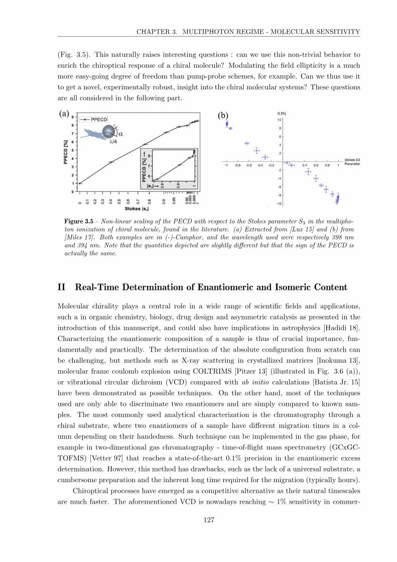
CHAPTER 3. MULTIPHOTON REGIME - MOLECULAR SENSITIVITY
(Fig. 3.5). This naturally raises interesting questions : can we use this non-trivial behavior to
enrich the chiroptical response of a chiral molecule? Modulating the field ellipticity is a much
more easy-going degree of freedom than pump-probe schemes, for example. Can we thus use it
to get a novel, experimentally robust, insight into the chiral molecular systems? These questions
are all considered in the following part.
Figure 3.5 – Non-linear scaling of the PECD with respect to the Stokes parameter S3 in the multipho-ton ionization of chiral molecule, found in the literature. (a) Extracted from [Lux 15] and (b) from[Miles 17]. Both examples are in (-)-Camphor, and the wavelength used were respectively 398 nmand 394 nm. Note that the quantities depicted are slightly different but that the sign of the PECD isactually the same.
II Real-Time Determination of Enantiomeric and Isomeric Content
Molecular chirality plays a central role in a wide range of scientific fields and applications,
such a in organic chemistry, biology, drug design and asymmetric catalysis as presented in the
introduction of this manuscript, and could also have implications in astrophysics [Hadidi 18].
Characterizing the enantiomeric composition of a sample is thus of crucial importance, fun-
damentally and practically. The determination of the absolute configuration from scratch can
be challenging, but methods such as X-ray scattering in crystallized matrices [Inokuma 13],
molecular frame coulomb explosion using COLTRIMS [Pitzer 13] (illustrated in Fig. 3.6 (a)),
or vibrational circular dichroism (VCD) compared with ab initio calculations [Batista Jr. 15]
have been demonstrated as possible techniques. On the other hand, most of the techniques
used are only able to discriminate two enantiomers and are simply compared to known sam-
ples. The most commonly used analytical characterization is the chromatography through a
chiral substrate, where two enantiomers of a sample have different migration times in a col-
umn depending on their handedness. Such technique can be implemented in the gas phase, for
example in two-dimentional gas chromatography - time-of-flight mass spectrometry (GCxGC-
TOFMS) [Vetter 97] that reaches a state-of-the-art 0.1% precision in the enantiomeric excess
determination. However, this method has drawbacks, such as the lack of a universal substrate, a
cumbersome preparation and the inherent long time required for the migration (typically hours).
Chiroptical processes have emerged as a competitive alternative as their natural timescales
are much faster. The aforementioned VCD is nowadays reaching ∼ 1% sensitivity in commer-
127

CHAPTER 3. MULTIPHOTON REGIME - MOLECULAR SENSITIVITY
cial instruments, able to monitor the enantiomeric excess in real time [Guo 04, Mower 18] by
simply recording the variation of vibrational absorption depending on the light helicity. This
technique, however, relies on electric quadrupolar and magnetic dipolar effects, and is thus only
implementable in liquid samples, requiring a significant amount of molecules and introducing
difficulties related to the solvatation effects. This is the case more generally for the histor-
ical absorption circular dichroism and optical rotation experiments (linked together with the
Kramers-Kronig relation). In the gas phase, microwave three-wave mixing, based on a combi-
nation of two fields to selectively excite rotational transitions, inducing a chiral-sensitive free
induction decay, yields a ∼ 1% precision [Patterson 13a, Patterson 13b, Shubert 14] (depicted
in Fig. 3.6 (b)). High-order harmonic generation has also been proved to be chiral-sensitive
[Cireasa 15, Baykusheva 19] but still remains a weak effect, even if recent theoretical develop-
ments on locally and globally chiral fields hold the promise of strongly increasing this sensitivity
[Ayuso 19].
Figure 3.6 – Illustrations found in the literature of chirality-sensitive observables. (a) Coulombexplosion imaging of the two enantiomers of the CHBrClF molecule, extracted from [Pitzer 13]. (b)(left) Microwave three-wave mixing scheme, in which the initial phase of the emitting dipole dependson the handedness of the enantiomer and thus the enantiomeric excess. (middle) Orientation of thetransition dipoles involved. The last one reverses with the enantiomer handedness. (right) Resultingrotational free induction decay, measured in the two enantiomers of 1,3-butanediol (right). Extractedfrom [Patterson 13a].
Finally, photoelectron circular dichroism, discussed at length in this manuscript, has been
applied to retrieve the enantiomeric purity of various samples in the gas phase. Precision of
128

CHAPTER 3. MULTIPHOTON REGIME - MOLECULAR SENSITIVITY
≤ 1% has been reached in a few hours in single-photon ionization using XUV synchrotron
radiation [Nahon 16]. Similar precision was achieved in REMPI-PECD in about 10 mn with a
1 kHz repetition rate laser [Kastner 16] and 5% in 1 min at higher repetition rate [Miles 17].
Interestingly, multi-component enantiomeric determination was demonstrated using PECD and
photoelectron-photoion coincidence detection, distinguishing compounds and yielding ∼ 20%
accuracy in the enantiomeric excess in 18 h [Rafiee Fanood 15]. We will see in this section how
these performances can be significantly improved by employing elliptical polarizations in REMPI
processes, combined with a high repetition rate table-top laser. It can provide a better precision,
within a shorter acquisition time, and even resolve multicomponent mixtures without the need
of mass spectrometry.
II. 1 Photoelectron ELliptical Dichroism (PEELD)
This experiment has been done in Bordeaux in collaboration with Jason Greenwood and Caiomhe
Bond from the Queen’s University of Belfast. As mentioned in the introduction of this chapter,
the photoelectron angular distribution does not have a cylindrical symmetry if the polarization
of the laser field is neither linear nor circular. In particular, this is the case with elliptical polar-
izations. Consequently, a typical VMI projection does not contain all the information encoded
in the distribution in this case. Two methods can be used to access the full 3D distribution :
either tomographic reconstruction from several VMI images projected along different axis, or
direct 3D measurement using delay lines detector, as discussed in the previous chapter. These
two possibilities will be compared in the next section.
Fig. 3.7 illustrates the 3D photoelectron distribution retrieved using tomographic technique,
for several chiral molecules (left column) with several field ellipticities (top row) measured in a
[3+1] REMPI scheme at 515 nm. The field intensity used was 5 ×10¹³ W.cm−2 and the repetition
rate of the laser was set to 2 MHz. For each molecular target (row), 36 VMI projections were
recorded. For each projection, the ellipticity of the field was continuously varied and the axis
of the field ellipse were kept fixed. The ellipse was rotated by steps of 10 degrees between the
projections in order to perform the tomographic reconstruction. Thanks to the high repetition
rate of the laser source, each projection took about 200 s to record, for a total of 120 min for each
row. The analysis method will be more extensively presented in the next section. Essentially, a
lock-in detection technique enabled an efficient filtering of the noise. The distributions presented
above in each panel are the 3D reconstructed photoelectron distributions at a given ellipticity.
The lower distributions in each panel are the corresponding dichroic signals, corresponding to the
part of the distribution that reverses with the handedness of the field (at the same ellipticity).
They can also be obtained by selecting the forward/backward antisymmetric part along the laser
propagation axis for a given polarization, or by subtracting the signal obtained between the two
enantiomers. These three methods are in principle redundant for PECD. In practice, the two
first ones were applied to the data in order to cancel experimental artifacts, and the comparison
with the opposite enantiomer is only used for sanity check, as it is more cumbersome to change
the sample handedness than the light helicity. We will see that this turns out to be more subtle
than PECD in the present case.
129

CHAPTER 3. MULTIPHOTON REGIME - MOLECULAR SENSITIVITY
Figure 3.7 – 3D photoelectron momentum distributions retrieved using tomographic reconstructionfrom VMI projections in (+)-Fenchone (a), (-)-Fenchone (b), (+)-Camphor (c) and (+)-Limonene(d). The laser field used was at a wavelength of 515 nm ([3+1] REMPI in all the cases) at 5 ×10¹³
W.cm−2, and the columns correspond to a Stokes parameter S3 = 1 (left), 0.9 (center) and 0.6(right). In each caption, the total distribution is depicted above and the corresponding dichroic part(defined in the text) is depicted below. z is the laser propagation axis (towards positive values), andalso the axis around which the projections are rotated for the tomographic reconstruction, in order toreconstruct the ’blind’ y axis. 36 projections were recorded for each row, with 10° steps, for a totalof 120 min of acquisition per row.
130

CHAPTER 3. MULTIPHOTON REGIME - MOLECULAR SENSITIVITY
Each panel displays isosurface contours of the complete and dichroic part of the measured
distributions, and several important features are visible. At first sight, one can notice that
both the total and the chiral-specific distributions are very sensitive to the target. One can see
that the distributions obtained with the circularly polarized field (S3 = 1) do have a cylindrical
symmetry around z, corresponding to the PECD. But when introducing ellipticity (S3 = 0.9
and 0.6), the symmetry is broken, the distribution starts to be peaked along the main axis
of the field ellipse and finer structures in the dichroic signal appear. The more ellipticity is
introduced, the more prominent this effect is, especially in Camphor (c). We named this effect
Photoelectron ELliptical Dichroism (PEELD). This typically reveals the anisotropy of excitation
induced by the non-circular field, preferentially exciting the molecules transition dipole along
the main axis of the field. As the excited state manifold involved greatly depends on the
molecular structure, the PEELD signal is intrinsically very sensitive to it. Especially, Fenchone
and Camphor have very distinguishable distributions even if these two molecules are isomers
that can not be resolved in a mass spectrum. Even with a small ellitpicity (S3 = 0.9), the
dichroic signal globally changes sign in Fenchone for example. Finally, the comparison between
(+) and (-)-Fenchone confirms the enantiomeric sensitivity of the experimental measurements.
Note that an intriguing whirl shape is visible in the dichroic parts with elliptical polariza-
tions, in particular in Camphor (c) at S3 = 0.9. This reflects an additional symmetry breaking
: while the inversion of the S3 parameter only inverts the signs of the features, the inversion
of the enantiomer handedness also reverses the rotation of the whirl. This is confirmed by
the comparison of the central features in Fenchone (a) and (b), at S3 = 0.9 and 0.6. In the
strong field ionization regime, this could be understood as a chiral attoclock effect, but in the
present multiphoton regime, the interpretation is more indirect and not fully understood so far.
In any case, this indicates that elliptical fields break the cylindrical symmetry by introducing
preferential axis. As a consequence, one must be careful with the quantities defined. In the
present case, the dichroic signal is forward/backward antisymmetric and reverses sign with the
ellipticity, but sustains a spatial inversion with the reversal of the enantiomer handedness. This
is the reason why the dichroic signal can not be directly obtained from the subtraction of the
signal obtained with the two enantiomers in this case. Interestingly, the photoelectron angular
distributions are thus defined absolutely by the set of field and enantiomer here, and not only
relatively. This type of effects will also be described with strong tailored laser fields in the last
chapter of this manuscript.
Asymmetry Factor G
Despite containing all the accessible information, the complete distribution is not neces-
sarily the best observable. Primarily because acquiring enough statistics for a 3D measurement
necessarily takes time. Furthermore, it makes the estimation of the overall forward/backward
asymmetry quite difficult. For this purpose, similarly to the PECD, we define an asymmetry
factor G as :
131

CHAPTER 3. MULTIPHOTON REGIME - MOLECULAR SENSITIVITY
G =4(F −B)
(F +B)(3.5)
where F and B are respectively the integrated signal on the forward and backward hemi-
spheres. The evolution of G with respect to the Stokes parameter S3 measured in (+)-Fenchone,
(+)-Camphor and (+)-Limonene measured at a field intensity of I515nm = 5 · 1012 W.cm−2 is
presented in Fig. 3.8. Interesting features appear more clearly here. Firstly, the asymmetry
factor G has a linear dependency with S3 at low ellipticity, depicted with the dotted lines. Sec-
ondly, one can observe a drastic nonlinear behavior for |S3| ≥ 0.6, even leading to a sign change
of G around |S3| = 0.9. Thirdly, the observable shows a strong molecular dependency, especially
between Fenchone and Camphor/Limonene, as G is maximized in the first case in circular polar-
ization while it almost vanishes for the other ones. Note that reducing the whole evolution with
respect to a single factor can be a little bit too simplistic : one can see here that Camphor and
Limonene are hardly distinguishable with G only. We will address this issue in the next sections.
Figure 3.8 – Evolution of the the forward/backward asymmetry G as a function of S3, in (+)-Fenchone (red squares), (+)-Camphor (green diamonds) and (+)-Limonene (purple circles), at5×1012 W.cm−2. The dotted lines are a linear extrapolation of the low-S3 behavior.
Interpretation
With the 515 nm laser wavelength used here, the ionization occurs in a [3+1] REMPI
scheme, where the intermediate states lie in the Rydberg state manifold at 3 × 2.41 = 7.22
eV , just below the ionization threshold as depicted in Fig. 3.9 for Fenchone, whose Ip = 8.72
eV (HOMO). When circular polarization is used, the excitation preferentially occurs in the
randomly aligned sample for the molecules whose transition dipole moment is in the polarization
plane (right panel). If lower ellipticity is introduced, the excitation will start to be also due to
the linear polarization component of the field. In this case, the excitation will preferentially
occur along the polarization axis (left panel). The key point here is that this multiphoton
excitation is more efficient for the linear photons than for the circular ones. Indeed, within
a perturbative approach, the efficiency of a three-photon process scales with the cube of the
laser electric field, and for a given beam energy flux, a linear field has a greater amplitude than
a circular one (by a factor√
2). This non-linearity makes the anisotropy of excitation very
132

CHAPTER 3. MULTIPHOTON REGIME - MOLECULAR SENSITIVITY
sensitive even to a small linear component. On the other hand, it is thus not very sensitive to
the circular component at low S3 parameters. This competition between circular and linear
components does not take place in the ionization step as we mainly focus on the dichroic part
of the photoelectron distribution : only the circular ones will produce PEELD signal. This
part can thus be considered as a single-photon ionization process from the excited states, that
scales linearly with S3. Overall, despite the fact that the ”pump” and the ”probe” are not
independently controlled here, the whole enrichment of the PEELD is related to this preferential
excitation. It yields a sharp evolution of the asymmetry at high S3, and can be considered as
linearly evolving with S3 at low ellipticities, when the linear component completely dominates
the excitation.
Figure 3.9 – PEELD effect in the REMPI scheme of the Fenchone at a wavelength of 515 nm. (left)At low field ellipticity, the excitation to the intermediate states is preferentially performed by thelinearly polarized photons. This induces an anisotropy of excitation in the randomly aligned sample,as the molecules having a transition dipole along the polarization axis are preferentially excited. Thedichroic response only comes from the part ionized from the excited states with circularly polarizedphotons. (right) At high ellipticity, the excitation is performed mainly by circularly polarized photons,selecting all the molecules in the polarization plane.
Evolution with the Field Intensity
From the comparison of the two studies of the evolution of the asymmetry in the photoelec-
tron distributions carried in Camphor, at 398 nm [Lux 15] and 394 nm [Miles 17], presented in
the Fig. 3.5 in the introduction of this chapter, an intriguing discrepancy appears. Even if the
evolution of the asymmetry with S3 is monotonous in both cases, their exact evolution slightly
differ. This might be either caused by a slightly different central wavelength, or by a different
intensity used. In both cases, this indicates that the nonlinearity can be very sensitive to the
exact levels at play.
In order to gain an additional hint into the role of the intermediate resonances, we
have investigated the evolution of the PEELD with the laser intensity. Fig. 3.10 (a) and
(b) show the 3D-PEELD projection in the VMI plane (px, pz), where x corresponds to the
133

CHAPTER 3. MULTIPHOTON REGIME - MOLECULAR SENSITIVITY
linear polarization axis and z is the laser propagation axis, respectively using laser intensities
of I515nm = 5 ×10¹² W.cm−2 and I515nm = 1.7 ×10¹³ W.cm−2, for several S3 values, in
(+)-Fenchone. The py-integrations are normalized to the maximum of the symmetric signal
value as 2(L-R)/max(L+R), where L and R and respectively the signal of the left and right
hemispheres (forward/backward). Since the resonances at play in the REMPI process lie in the
Rydberg manifold close to the ionization threshold, they are likely to be subject to Stark-shift
from the laser field. Consequently, increasing the intensity will shift the energy levels resonant
with the excitation, modifying the PEELD response. This is consistent with the data recorded
with the OPA presented in Section 2.I, where the tunability of the source enables to scan across
the resonances. Indeed, we have seen that consecutive excited states can have an opposite sign
of PECD. One can thus expect a similar behavior on the PEELD response in the present case
where the levels are shifted, for a fixed wavelength. However, the resonant energy shift range
was quite great with the tunable source, but the ionization was performed in a [2+1] REMPI
scheme while it is at [3+1] in the current study. The excited states involved are thus closer
to the continuum and are more sensitive to Stark shift. In addition, we have seen that the
nonlinearity of the PEELD could have a higher sensitivity than PECD to the intermediate
levels. The analysis of the data recorded with the tunable source is still ongoing, but we can
already expect that the Stark shift of the intermediate states could strongly affect the PEELD
response in the present case, for a fixed wavelength. The intensity-dependent evolution of the
PEELD presented in Fig. 3.10 (a) and (b) is mostly visible for the low energy structures,
corresponding to the [3+1] ionization. The relative weight of the outer ring, corresponding to
the 5-photons process, also increases but remains quite independent on the ellipticity. This
suggests that this latter feature does not build on the resonances. The reduction of the global
evolution to the G factor is displayed on Fig. 3.10 (c). At low intensity, the asymmetry
maximizes at |S3| ∼ 0.6, while it is dominated in circular polarization between a few 1012− 1013
W.cm−2. The process will tend to the strong field regime when further increasing the intensity,
in which case the chiral molecular potential plays a less prominent role in the scattering process,
yielding a weaker dichroic response.
In summary, the nonlinear dependency on S3 appears even more drastically here than in
the previously mentioned literature. Varying this Stokes parameter significantly expands the
molecular and enantiomeric specificity of the photoelectron distribution. The PEELD effect
seems to be a universal effect of REMPI schemes in chiral molecules and brings the perspective
to use its non-monotonic behavior to enrich the molecular signatures for analytical purposes.
II. 2 Lock-in Detection : Continuous Modulation of S3
The most straightforward manner to measure a PEELD experimentally is to simply set a po-
larization, then record the signal, then fix a new polarization and so on. However, this type of
incremental recording is very exposed to fluctuations (laser power, alignment, target density...).
The longer the acquisition, the more at risk it is. A common but fastidious manner to mitigate
the fluctuations is to repeat the experiment several times in a row and average the result. Addi-
134

CHAPTER 3. MULTIPHOTON REGIME - MOLECULAR SENSITIVITY
Figure 3.10 – (a-b) Projections of the 3D-PEELD from (+)-Fenchone in the (x,z) plane, at 5×10¹²
W.cm−2 (a) and 1.7×10¹³ W.cm−2 (b). The z axis is the laser propagation direction (towards positivevalues) and the x axis is the main axis of the laser ellipse, and the VMI detector lies in the (x,z) plane.The (x,z) projection are integration over the time-of-flight (y) axis of the VMI. (c) Evolution of theellipticity dependence of the forward/backward asymmetry G with laser intensity in (+)-Fenchone.The measurements took about 10 minutes at each intensity, with a laser repetition rate of 2 MHz, byrotating a quarter waveplate at 45°/s in front of the VMI and using the lock-in detection presentedin the next paragraph.
tionally in our case, the use of a high repetition rate laser renders the exposure time necessary
to record a decent VMI image very short (down to 50 ms). It means that even with an advanced
motorized stage, the acquisition duty cycle is severely limited by the time it takes to rotate the
waveplate to the next ellipticity. It is not necessarily related to its angular velocity, but more
to the acceleration/deceleration and the inherent deadtimes of the softwave synchronizing the
camera and the stage.
In order to overcome these two inconveniences, we implemented a continuous ellipticity
modulation scheme. A quarter-waveplate is rotated at a constant angular velocity, so that the
S3 parameter of the laser beam is continuously and periodically modulated, combined with a
continuous acquisition of the PEELD (c-PEELD) in the VMI device. The temporal evolution
of the polarization state is depicted on Fig. 3.11. The polarization goes from a given circular
to the opposite one every 90°, from circular to linear or conversely every 45° and the whole
evolution has a 180° periodicity. In between, the polarization continuously evolves through all
the elliptical intermediates. Note that the axis of the ellipse also rotates, so the projection
135

CHAPTER 3. MULTIPHOTON REGIME - MOLECULAR SENSITIVITY
angle relatively to the ellipse varies with the ellipticity. This can be circumvented by rotating
a half-waveplate in front of a fixed quarter-waveplate, which was necessary in the tomographic
reconstruction presented in Fig. 3.7. However, the rotation of the ellipse does not affect the
implementation that will be presented in the rest of the section. Since the VMI records pro-
jections and is insensitive to the momentum along the spectrometer axis py, the only difference
that could happen would be a slight displacement of the features along the px axis (the main
axis of the polarization ellipse) and would not induce any significant change. The goal here is to
Fourier-transform the periodically modulated signal to isolate every frequency of the total signal
and the antisymmetric part, as we will see. The Fourier transform acts as a lock-in detection,
filtering out the experimental fluctuations that are very unlikely to match the relevant frequen-
cies. Additionally, the fluctuations of the signal level are also canceled by the normalization of
the asymmetry parameter.
Figure 3.11 – Principle of the continuous ellipticity modulation scheme. (a) Laser polarization as afunction of the quarter waveplate rotation. (b) Evolution of the Stokes parameter S3 and ellipticityε of the laser as a function of the waveplate rotation. Note that ε, which is by definition a positivequantity, has been modulated by a positive sign for right polarizations and a minus sign for leftpolarizations for clearer comparison with S3. (c) Schematic evolution of the total signal and theantisymmetric part of the signal of the VMI images, in the case where the dichroic response scaleslinearly with S3. (d) Corresponding Fourier transform of the periodic symmetric and antisymmetricsignal.
Except for the Belfast’s measurements, we used in this experiment the BlastBeat laser
system in CELIA which is a Yb-doped fiber laser delivering 50 W of 130 fs pulses at a repetition
rate between 166 kHz and 2 MHz (Tangerine SP, Amplitude). Second harmonic generation was
performed from the output wavelength 1030 nm to 515 nm with a type-I β-Barium Borate (BBO)
crystal, and isolated from the fundamental frequency with two dichroic mirrors. The quarter-
waveplate modulating the polarization was mounted on a fast direct-drive rotation stage capable
of rotations up to 720 °/s (RGV100BL, Newport). The acquisition of the VMI images (apparatus
136

CHAPTER 3. MULTIPHOTON REGIME - MOLECULAR SENSITIVITY
described in Section 2.II) was done using a S-CMOS camera (Orca Flash 4.0, Hamamatsu)
without deadtime between images. The camera was also triggered by the rotation so that the
ellipticity is calibrated, meaning that the initial phase is known.
The high repetition rate of the laser enabled a camera exposure time of τexp = 50 ms. We
set the waveplate angular velocity at ωλ/4 = 45 °/s, so that the full 180° periodicity (which is
the one of the asymmetry) is described in 80 points, which is decent for a Fourier transform, in
T0 = 4 s. As the rotation still goes during the exposure, each image is an average over 2.25°, on
which the PEELD does not evolve too much.
II. 3 Accurate Measurement of the Enantiomeric Excess
We will present in this section the application of the c-PEELD to determine the enantiomeric
excess (ee) of a pure chemical compound. The signal from the VMI images was numerically
integrated to reduce it to the asymmetry factor Graw(t), as defined in Eq. 3.5 for each image.
The possible asymmetry artifact induced by the spatial inhomogeneity of the detector gain was
corrected by averaging the signal between the opposite ellipticities as :
G(t) =1
2(Graw(t)−Graw(t+ T0/2)) (3.6)
as T0/2 is the time taken for a 90° rotation of the quarter waveplate. G(t) recorded in the
two pure enantiomers of Fenchone is presented in Fig. 3.12 (a). A 2 MHz repetition rate was
used with the exposure and rotation parameters indicated above, so that each point is a sum
over 100k laser shots. The initial position corresponds to the linear polarization, and the 24 s
displayed correspond to 3 full rotations, i.e. 6 · T0. The sinusoidal shaded area represents the
evolution of the total photoelectron yield (or ’total signal’), and shows that it maximizes in linear
polarization, every 90° (T0/2). The evolution of the G(t) factor of the (+) and (-)-Fenchone are
plotted in red and blue, respectively. It periodically follows the one presented in Fig. 3.8 (a),
as the S3 parameter is continuously scanned (cf Fig. 3.11). As expected, the asymmetry is
clearly inverted between the two enantiomers. The Fourier transform of the total signal and
the asymmetry factor G(t) are depicted in Fig. 3.12 (b), respectively in black and red. The
T0/2 modulation of the total signal shows an isolated peak at 2Ω0, where Ω0 = 2πT0
= 0.25 Hz.
Other frequencies could appear at 2kΩ0, k ∈ N∗ (as the total signal has a T0/2 periodicity),
corresponding to the non-linearity of the signal variation with the polarization. Note as well
that in this Fourier decomposition, a circular dichroism of the ionization yield [Boesl 13] would
appear as a Ω0 component of the in the total signal with a phase depending on the enantiomer.
The Fourier transform of the asymmetry parameter F [G(t)] = G(Ω) (in red) presents a rich
structure that can be used as a molecular fingerprint. Indeed, the non-linear dependency of G
with respect to S3 (seen in Fig. 3.8) appears as a frequency comb here, and is molecular-sensitive.
This aspect will be discussed more in detail at the end of this section. The frequency comb of
the Fourier transform of G(t) is made of odd Ω0 orders (2k + 1)Ω0, k ∈ N∗. This structure
comes from the fact that the dichroic signal has a 180° (= Ω0) periodicity, but is necessarily
symmetric around |S3| = 1 and antisymmetric around S3 = 0, excluding the even orders. This
non-overlap between the total and the dichroic frequency components makes the separation very
137

CHAPTER 3. MULTIPHOTON REGIME - MOLECULAR SENSITIVITY
robust. Typically, if the inhomogeneity correction (Eq. 3.6) is not applied, artifacts will clearly
be indicated by odd orders in the total signal spectrum.
Figure 3.12 – (a) Unfiltered temporal evolution of the forward/backward asymmetry G(t) in (+)-Fenchone (red) and (-)-Fenchone (blue) at 5×10¹² W.cm−2 as the ellipticity is continuously scannedby rotating a quarter waveplate. The total photoelectron yield from (+)-Fenchone is depicted in gray.(b) Oscillation spectrum of the forward/backward asymmetry (red) and of the total signal (black)obtained by Fourier transforming the temporal signals. The fundamental frequency is Ω0 = 0.25 Hz.
The relative amplitudes and phases of the components of G((2k + 1)Ω0) are molecular-
specific. Additionally, since G is a normalized quantity, their absolute amplitude is only pro-
portional to the enantiomeric excess in the analyzed sample. If we focus on the stronger peak
G(3Ω0), which is the less subject to noise, the calibration from a known sample of enantiomeric
excess eeref directly provides :
ee = ± |G(3Ω0)||Gref (3Ω0)|
· eeref (3.7)
while the ± sign is given by the 0 or π phase of the 3Ω0 component relatively to the
reference. We used an enantiopure (+)-Fenchone sample as a reference here (Sigma Aldrich),
as it provides the less noisy reference, but in principle the calibration can be done with any
known enantiomeric excess eeref . The fact that the G(3Ω0) component dominates the G(Ω0)
one indicates that the nonlinearity induced by the anisotropy of excitation is the main driver of
the evolution of G with respect to S3 in this case.
This procedure has been tested in several samples of known ee, with an acquisition time of
10 minutes each. The first one is (-)-Fenchone (Sigma Aldrich) specified at 84.2% ± 4%. The
two other ones are mixtures of the two commercial enantiomers, determined with the precision
138

CHAPTER 3. MULTIPHOTON REGIME - MOLECULAR SENSITIVITY
of a microbalance. The results of the measurements are presented in Table 3.1.
Mixture Expected ee ee measured by c-PEELD
(−)-Fenchone −84.2± 4% * −84.0± 0.4%
Mix 1 63.1± 4% 62.7± 0.5%
Mix 2 25.1± 4% 24.9± 0.4%
Table 3.1 – Measurement of the enantiomeric excess of three mixtures of Fenchone using (+)-Fenchone as a reference with eeref = 1. Each measurement corresponds to a 10 minute acquisition.The error bars of the c-PEELD measurements are 95% confidence intervals. * = values from thesupplier (Sigma Aldrich).
Note that the errorbar of the c-PEELD is much smaller and consistent with the one of the
supplier.
Error Estimation
Error estimation is crucial in analytical applications. We first assess the statistical error
by slicing the 10 minutes measurements in the (+)-Fenchone into slices by applying a Gaussian
filter of variable duration τ FWHM. A statistical analysis is then applied to the enantiomeric
excess estimated for each slice. The 95% confidence interval is depicted on Figure 3.13 (a). As
one can see, the Fourier transform is not optimally precise if the window is too short and does
not cover enough oscillations, providing about 5% precision in 3 s (only 4/3 oscillations in G(t)).
On the other hand, the errorbar quickly diminishes to its minimum value around τ = 30 s.
From this point, increasing the number of oscillations is not the bottleneck anymore, yielding a
constant ∼ 2% precision. This means that the uncertainty can then only be improved by adding
more measurements, by simply repeating the process several times and averaging the results.
This procedure has been implemented on a 10 minute measurement. While keeping the total
acquisition duration constant (10 min), the number of slices has been increased by decreasing
the slice duration τ . The resulting Student’s statistical analysis is shown in Figure 3.13 (b),
and display a 95% confidence interval kept relatively constant under 0.5% over the whole range.
Notably, using a high number of subsets diminishes the error down to 0.3%.
Beyond statistical error, the estimation of the systematic error is also important. Obvi-
ously, as the c-PEELD is a method based on the comparison with a reference, the enantiomeric
purity of the reference can induce a systematic error, affecting the accuracy of the measure-
ment. Moreover, the measurement of the reference can present an error, but this one can be
minimized by affording a long enough measurement. In addition, as the technique relies on a
signal modulation, the linearity of the detector has to be verified. In order to estimate it, a 10
minute acquisition in (+)-Fenchone has been recorded while increasing the micro-channel plates
voltage by 20 V every 30 s, then decreasing it again (Figure 3.13 (c)). The variation of global
signal covered here was about two orders of magnitudes. A Gabor analysis of the signal has been
performed using a Gaussian window of 3 s FWHM. It constitutes a way to get the instantaneous
variation of G(3Ω0) (more details in the next paragraph). The resulting estimation of the ee is
shown on panel (d). One can see that the retrieved ee is systematically lower than the expected
value (ee = +1 for (+)-Fenchone) during the first 3 minutes by ∼ 5%. Despite being within
139

CHAPTER 3. MULTIPHOTON REGIME - MOLECULAR SENSITIVITY
Figure 3.13 – Statistical analysis of the enantiomeric excess measurement by PEELD. (a) 95% con-fidence interval of the enantiomeric excess of a pure (+)-Fenchone sample, as a function of theduration of the measurement. (b) Results of a 10 min ee measurement by statistical analysis of setsof submeasurements, as a function of the number and duration of the submeasurements. (c-d) Totalsignal and enantiomeric excess measured while increasing the gain of the microchannel plates detectorevery 30 s.
the range of the statistical error, this indicates that a new calibration could be useful at low
MCP gain. But importantly, the data presented between 3 and 10 minutes demonstrates that
the ee estimation is robust over an order of magnitude of signal variation. This is significant
compared to the sources of fluctuations such the molecular gas jet density or laser power. This
last parameter must be stable enough however, since the PEELD can depend on the laser inten-
sity, as shown in Fig. 3.10. This is a considerable advantage of the fiber laser sources, with the
drawback of handling adequately the high average power to avoid pointing and beam quality
fluctuations, due to thermal effects.
140

CHAPTER 3. MULTIPHOTON REGIME - MOLECULAR SENSITIVITY
II. 4 Continuous Measurement of the Enantiomeric Excess
Since c-PEELD technique provides measurements of the enantiomeric excess of a sample within
a few seconds, we will demonstrate that it can be used to track it in real-time. In order to
mimic the temporal evolution of the ee during a chemical reaction, for instance, we connected
the tubes containing the pure (+), (-) and the two mixtures of Fenchone determined in Table
3.1 to the gas pipe supplying the VMI jet. We then consecutively opened them while closing the
other ones to vary the sample composition. The c-PEELD signal recorded on-the-fly is shown in
Figure 3.14. The total signal, plotted in panel (a), presents a quite constant level except when
a new tube is open, as the pressure built with the sample evaporation goes back to equilibrium
in a few tens of seconds. Nevertheless, we have seen that this does not have consequences on
the measured ee.
Figure 3.14 – Continuous monitoring of enantiomeric excess by c-PEELD. (a) Total photoelectronsignal as a function of time, as different samples are successively connected to the jet. (b) Measuredenantiomeric excess (black dots) and 95% confidence error bars (gray). The horizontal lines are thetheoretical values of the enantiomeric excesses of the different mixtures.
The Gabor analysis of the asymmetry parameter G(t) has been performed with Gaussian
envelopes of 5 s FWHM. This time-frequency analysis consists in multiplying the time-domain
signal G(t) with a sliding (Gaussian) window centered on a variable time τ , and perform its
Fourier transform :
G(Ω, τ) =
∫ +∞
−∞G(t)e−
(t−τ)2
2σ2 eiΩtdt (3.8)
141

CHAPTER 3. MULTIPHOTON REGIME - MOLECULAR SENSITIVITY
which basically quantifies the spectral components as a function of time. Of course, like
any time-frequency analysis, the larger the time resolution, the worse the frequency resolution
and vice versa. In our case, it means that σ is a trade-off between temporal responsiveness and
the retrieved ee precision. Note that other kernel functions, i.e. different than the Gaussian,
can be interesting as discussed in [Volpato 19] but less straightforward to interpret. The
evolution of the enantiomeric excess and its sign, respectively extracted from the amplitude and
phase of G(3Ω0, τ), are presented on Figure 3.14 (b). Every time the supplying flask is changed,
a transient occurring on 2-3 minutes is observed. This corresponds to the inertia of the gas
dynamics in the pipe towards the VMI, and particularly of the long 200 µm-diameter capillary
that creates the jet. After this transient, the signal converges to the expected ee, depicted with
the lines colored lines respectively to the labels in panel (a), within the 0.4% errorbar determined
in the previous section for this Gabor window. The slight offset of the measurement compared
to the expected value for some mixtures is probably due to a change of laser duration, identified
as resulting from the room temperature oscillations in the laboratory with a ∼ 20 minute period.
This change of pulse duration modifies the intensity of the frequency-doubled beam, and thus
the PEELD calibration. This means that further improvement can be done by more efficiently
locking the laser parameters, for instance by setting a feedback loop on the 515 nm beam energy.
In any case, the compromise between the ee precision and the temporal resolution demon-
strated in this experiments constitutes a major breakthrough for chiral analysis in the gas phase.
Alternative Detection Setup
The results presented so far were obtained using a Velocity Map Imaging device. Although
being a quite standard instrument in Physics laboratories, it remains quite expensive and its
multidimensional angular resolution of the photoelectron distribution is not fully necessary when
the only chiral observable is the asymmetry factor G. For this reason, the group of Jason Green-
wood in the Queen’s University of Belfast has developed a much more simple device presented in
Figure 3.15, designed to directly collect the electrons emitted forward and backward, regardless
of their kinetic energy [Miles 17]. They have performed the measurements presented here in
Belfast, and sent us the results to integrate them to our analysis.
This device, called CERSEI (Chiral Electron Removal and Separation for Enantiomer
Identification), relies on an homogeneous magnetic field (∼ 30 Gauss) generated by two coils
collinearly to the laser axis to guide the photoelectrons out of the interaction chamber. Once the
forward- and backward-emitted electrons are separated, they are deflected from the laser axis by
adding a homogeneous electric field and collected on two separate Channel Electron Multipliers
(CEM). The laser pulses used here were 1.8 µJ of the second harmonic (520 nm) from the
300 fs pulses generated at a repetition rate of 1 MHz (Spirit HE, Spectra Physics). A 20 cm
focal length lens was used to focus the beam in the effusive gas jet, produced from a capillary,
reaching an intensity of 1012 W.cm−2. The rather small chamber was solely pumped by a 200
L.s−1 turbomolecular pump to about 10−6 mbar with the jet and around 10−7 mbar without.
Under these conditions, the data were acquired sequentially for 30 s every 10° of the wave plate
angle. The counting rate used here was below 0.1 ionization per short to avoid saturation, but
this could be significantly improved by replacing the CEM with MCPs.
142

CHAPTER 3. MULTIPHOTON REGIME - MOLECULAR SENSITIVITY
Figure 3.15 – Schematic of the Belfast instrument used to directly measure PEELD, detailed in thetext. The electrodes and simulated trajectories were produced by SIMION 8.0 charge particle opticssoftware.
The evolution of G with respect to S3 measured with this device in (+)-Fenchone is shown
in Figure 3.16 (a). It behavior is in good agreement with what has been measured in the VMI.
An emulation of the c-PEELD technique is shown on panel (b), where the pure (+)-Fenchone
(red) is compared to a mixture of ee = −66% Fenchone (blue). We do observe the sign inversion
of the G(t) function along with its amplitude modulation, that provided a measurement of
ee = −63± 5%.
Figure 3.16 – Temporal evolution of the forward/backward asymmetry G in (+)-Fenchone (red) anda Fenchone mixture with ee = 63% using 520 nm pulses at ∼ 1×10¹² W.cm−2, as the ellipticityis continuously scanned by rotating a quarter waveplate. These measurements were taken with theCERSEI instrument in Belfast.
This measurement can readily be improved by using a higher laser intensity that would
increase the signal and the nonlinearity of G with respect to S3. But more importantly, this
demonstrates the possibility to implement the PEELD and c-PEELD with a very simple and
compact instrument.
II. 5 High-Dimensional Molecular Fingerprint : Multi-Component Analysis
2D Fingerprints
As mentioned in the introduction of this section, the enantiomeric analysis of a multi-
component mixture can be challenging. For instance, measuring the PECD in coincidence with
143
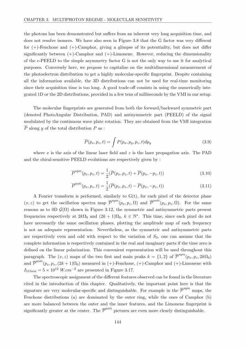
CHAPTER 3. MULTIPHOTON REGIME - MOLECULAR SENSITIVITY
the photons has been demonstrated but suffers from an inherent very long acquisition time, and
does not resolve isomers. We have also seen in Figure 3.8 that the G factor was very different
for (+)-Fenchone and (+)-Camphor, giving a glimpse of its potentiality, but does not differ
significantly between (+)-Camphor and (+)-Limonene. However, reducing the dimensionality
of the c-PEELD to the simple asymmetry factor G is not the only way to use it for analytical
purposes. Conversely here, we propose to capitalize on the multidimensional measurement of
the photoelectron distribution to get a highly molecular-specific fingerprint. Despite containing
all the information available, the 3D distributions can not be used for real-time monitoring
since their acquisition time is too long. A good trade-off consists in using the numerically inte-
grated 1D or the 2D distributions, provided in a few tens of milliseconds by the VMI in our setup.
The molecular fingerprints are generated from both the forward/backward symmetric part
(denoted PhotoAngular Distribution, PAD) and antisymmetric part (PEELD) of the signal
modulated by the continuous wave plate rotation. They are obtained from the VMI integration
P along y of the total distribution P as :
P (px, pz, t) =
∫P (px, py, pz, t)dpy (3.9)
where x is the axis of the linear laser field and z is the laser propagation axis. The PAD
and the chiral-sensitive PEELD evolutions are respectively given by :
Psym
(px, pz, t) =1
2(P (px, pz, t) + P (px,−pz, t)) (3.10)
Panti
(px, pz, t) =1
2(P (px, pz, t)− P (px,−pz, t)) (3.11)
A Fourier transform is performed, similarly to G(t), for each pixel of the detector plane
(x, z) to get the oscillation spectra map Psym(px, pz,Ω) and Panti(px, pz,Ω). For the same
reasons as to 0D G(Ω) shown in Figure 3.12, the symmetric and antisymmetric parts present
frequencies respectively at 2kΩ0 and (2k + 1)Ω0, k ∈ N∗. This time, since each pixel do not
have necessarily the same oscillation phases, plotting the amplitude map of each frequency
is not an adequate representation. Nevertheless, as the symmetric and antisymmetric parts
are respectively even and odd with respect to the variation of S3, one can assume that the
complete information is respectively contained in the real and imaginary parts if the time zero is
defined on the linear polarization. This convenient representation will be used throughout this
paragraph. The (x, z) maps of the two first and main peaks k = 1, 2 of Psym(px, pz, 2kΩ0)
and Panti(px, pz, (2k + 1)Ω0) measured in (+)-Fenchone, (+)-Camphor and (+)-Limonene with
I515nm = 5× 10¹² W.cm−2 are presented in Figure 3.17.
The spectroscopic assignment of the different features observed can be found in the literature
cited in the introduction of this chapter. Qualitatively, the important point here is that the
signature are very molecular-specific and distinguishable. For example in the Psym maps, the
Fenchone distributions (a) are dominated by the outer ring, while the ones of Camphor (b)
are more balanced between the outer and the inner features, and the Limonene fingerprint is
significantly greater at the center. The Panti pictures are even more clearly distinguishable.
144

CHAPTER 3. MULTIPHOTON REGIME - MOLECULAR SENSITIVITY
Figure 3.17 – Fourier decomposition of the oscillations of the VMI images with ellipticity in (+)-Fenchone (top), (+)-Camphor (mid) and (+)-Limonene (bottom), using 515 nm pulses at 5×10¹²
W.cm−2. (a-c) Symmetric components of the image Psym(px, pz, 2kΩ0). (d-f) Antisymmetric com-
ponents of the images Panti(px, pz, (2k + 1)Ω0). All values are normalized to the maximum of
Psym(px, pz, 2Ω0). The z axis is the laser propagation direction and the x axis is the main axis
of the laser polarization ellipse.
The 2Ω0 map of Psym dominates the symmetric signal and thus maximizes in linear
polarization for all the (px, pz) points. The 4Ω0 component can be more complex since it
reflects the non-linearity with respect to S3. However, the negative central part is probably
related to the rotation of the field ellipse axis relatively to the projection axis, and is not
physically meaningful. The spectral maps of the antisymmetric parts present even richer
structures. The sign change of the low energy PEELD can be due to vibrational excitation of
the ion, as observed in the PECD, or also to the longer scattering process of the low kinetic
energy electrons. Note that two areas of opposite sign in the same half of the detector can
cancel out in the integration giving G(t) (or G(Ω)), reducing its sensitivity. For instance in
Fenchone, we understand through these 2D maps why the integrated G(3Ω0) is stronger than
G(Ω0), as seen in Fig. 3.12 (b) : the multitude of nodes in the Panti(px, pz,Ω0) map reduces
significantly its integrated value. In any case, one can see that this enriched 2D fingerprint
succeeds in discriminating Camphor and Limonene, which was not the case with the 0D quantity.
1D Fingerprints
High-dimensional measurements provides a high fingerprint selectivity, but increases the
acquisition time. One can expect the 2D maps shown in Fig. 3.17 to be adapted for highly
complex mixtures analysis but in the context of continuous measurements, we found that 1D
fingerprints were a good compromise. These latter are generated by numerically integrating the
145

CHAPTER 3. MULTIPHOTON REGIME - MOLECULAR SENSITIVITY
VMI images along the polarization axis x and keep the laser propagation axis z as the remaining
dimension :
P (pz, t) =
∫P (px, pz, t)dpx (3.12)
We then performed a Fourier analysis in the same manner as previously to get the reference
spectral component Psym
(pz, 2kΩ0) and Panti
(pz, (2k + 1)Ω0) of (+)-Fenchone (compound A)
and (+)-Camphor (compound B). The time-resolved composition and ee is then retrieved with
a Gabor analysis of the signal from the evolving sample, with a 30 s Gaussian filter. In a general
manner, the composition of a mixture of two species A and B is retrieved using the c-PEELD
signal as follows. The absolute composition at every time t is determined from the symmetric
parts Psym
by minimizing the function f with a least-square algorithm :
f = |Psym
mix(pz, 2Ω0, t)− a(t)Psym
A (pz, 2Ω0)− (1− a(t))Psym
B (pz, 2Ω0)|2
+ α4|Psym
mix(pz, 4Ω0, t)− a(t)Psym
A (pz, 4Ω0)− (1− a(t))Psym
B (pz, 4Ω0)|2
+ α6|Psym
mix(pz, 6Ω0, t)− a(t)Psym
A (pz, 6Ω0)− (1− a(t))Psym
B (pz, 6Ω0)|2
+ ...
(3.13)
The minimization parameter a(t) and (1− a(t)) then gives the relative proportion of signal
coming from the species A or B respectively, independently of their ee. The conversion into
absolute concentration in the sample can be simply done in principle by taking into account the
absolute photoionization cross sections and partial pressures of each compound, but is beyond
the scope of this study. The α2k coefficients can be used to adjust the weight of the different
spectral components, which can be relevant if one or several of them are much more compound-
specific than others.
The second step consists in retrieving the respective enantiomeric excess eeA and eeB from
the antisymmetric components of the c-PEELD Panti
by minimizing the function g :
g = |Panti
mix(pz,Ω0, t)− a(t)eeA(t)Panti
A (pz,Ω0)− (1− a(t))eeB(t)Panti
B (pz,Ω0)|2
+ β3|Panti
mix(pz, 3Ω0, t)− a(t)eeA(t)Panti
A (pz, 3Ω0)− (1− a(t))eeB(t)Panti
B (pz, 3Ω0)|2
+ β5|Panti
mix(pz, 5Ω0, t)− a(t)eeA(t)Panti
A (pz, 5Ω0)− (1− a(t))eeB(t)Panti
B (pz, 5Ω0)|2
+ ...
(3.14)
Here the parameters β2k+1 plays the same role of tunable balancing coefficients. The op-
timization of f and g can be either done sequentially or globally, but led to the same result in
this case.
The calibrations 1D maps of pure (+)-Fenchone (orange) and (+)-Camphor (blue) are
depicted on the left panels in Figure 3.18, respectively (b), (c) and (d). The Psym
(pz, 2Ω0)
components are sufficient to make the distinction between the two compounds, so all the other
α2k were set to zero. On the contrary, one can see that Panti
(pz, 3Ω0) adds a lot of sensitivity
146

CHAPTER 3. MULTIPHOTON REGIME - MOLECULAR SENSITIVITY
compared to Panti
(pz,Ω0) to retrieve the respective ee. For this reason, we set β3 = 10 so that
the 3Ω0 weight gets comparable with the Ω0 component in the minimization, and all other β2k+1
to zero.
Figure 3.18 shows the tracking of (b) Psym
mix(pz, 2Ω0, t), (c) Panti
mix(pz,Ω0, t) and (d)
Panti
mix(pz, 3Ω0, t) of an evolving sample. The absolute composition obtained from a(t) and
(1−a(t)) is plotted in (e) and the retrieved ee of the two species is plotted in (f). The sample evo-
lution sequence started from t = 0 to t ≈ 2′30′′ with partially connected flasks of (-)-Fenchone
and (-)-Camphor. As one can see in Figure 3.18 (a), the total signal level decreases at first.
Panel (e) reveals that it comes from a transient in the signal of Fenchone, while the Camphor
one remains stable. At t ≈ 2′30′′, we open more the (-)-Fenchone valve and we slightly close
the (-)-Camphor valve. This is clearly detected and visible in (e). Note that meanwhile, the
ee found remain completely independent on the relative signal level, at eefenchone = −82 ± 5%
and eecamphor = 94 ± 2% in a 95% confidence interval. At t = 5′, the (-)-Fenchone sample was
swapped with the (+) enantiomer. Once again, this change is clearly visible, without affecting
eecamphor, and shows a ∼ 3′ transient, converging to eefenchone = 91±8% from t ≈ 8′ to the end.
The ee found remains stable, even while the partial pressure of Fenchone decreases gradually in
time. At t = 10′, the (-)-Camphor flask is closed while opening the (+) one. Once again, we
keep track of the evolution without affecting the measurement of the other compound.
This experiment thus demonstrates the capacity of the c-PEELD technique to track the
absolute and enantiomeric composition of a mixture with a remarkable precision and temporal
resolution. The next step in the retrieval of the fast evolution of ee is to fit the evolving 2D maps
P(px, pz,Ω, t) instead of the integrated 1D P(pz, 2Ω, t). The main question is how to be efficient
in the fitting procedure to provide the evolution in real time for the users. For this purpose, An-
toine Comby and Baptiste Fabre are developing strategies based on neural network optimization.
The fast ee tracking technique developed here could be interesting for industrial purposes.
At this stage, it can be used for instance for monitoring in live the quality of a product in a
production line. Another exciting application would be the resolution of complex unknown sam-
ples. Typically, natural extracts, that are sometimes very important for obtaining enantiopure
compounds, are often challenging to characterize. Our method could be very competitive in this
context, but several challenges remain to be faced. Firstly, a calibration on known pure samples
is required, meaning that one needs prior knowledge on the analyzed samples. Secondly, we still
have to determine the sensitivity of the detection for species in large minority, and the ability
to identify the different molecules in a more complex mixture (more that two species). Finally,
we still have to establish whether or not the PEELD effect is universal and applies for a wide
spectrum of molecules. These questions are currently being investigated in our group. Of course,
the effect lies in the intermediate excited states in the REMPI process. But one could wonder if
their sole presence is necessary, or if the effect also depends on their nature. This question will
be addressed in the next section.
147

CHAPTER 3. MULTIPHOTON REGIME - MOLECULAR SENSITIVITY
Figure 3.18 – Real-time analysis of a dynamical Camphor-Fenchone mixture. The fingerprints
Psym
(pz, 2Ω0), Panti
(pz,Ω0) and Panti
(pz, 3Ω0) from pure (+)-Fenchone (orange) and (+)-Camphor(blue) were recorded using pure samples before the dynamical measurement and are presented in theleft column. See the text for the sample evolution sequence. (a) Total signal from the gas mixtureduring the c-PEELD measurement. (b) Temporal evolution of the 1D symmetric component at 2Ω0,extracted from a Gabor analysis with a 30 s window. (c) 1D antisymmetric component at Ω0. (d)1D antisymmetric component at Ω0. (e) Contribution to the total signal and (f) enantiomeric ex-cess of Fenchone (orange) and Camphor (blue) retrieved by fitting the symmetric and antisymmetriccomponents.
148

CHAPTER 3. MULTIPHOTON REGIME - MOLECULAR SENSITIVITY
III Elliptical Dichroism Studied in the COLTRIMS
We have seen in Section 3.II that the PhotoElectron Elliptical Dichroism (PEELD) effect could
enrich the usual PhotoElectron Circular Dichroism (PECD) in the REMPI regime. We have
demonstrated that this effect could be used for analytic purposes, in particular yielding enough
signal-to-noise ratio to extract the enantiomeric and isomeric content of a sample, either very
precisely or in real time. In this context, the velocity map imaging spectrometer (VMI) is the
detection instrument of choice, as it can afford a high level of signal. In particular, the complete
resolution of the 3D photoelectron angular distribution is not required in this case.
The situation differs if the goal is the complete resolution of the phenomenon, and with-
out such a constrain on the duration of the acquisitions. Firstly, the measurement of the 3D
distributions can be either performed using the VMI or the COLTRIMS, and knowing which
one is the most suited is not trivial. We will thus compare these two techniques. Secondly, we
will compare the response of two closely-structured chiral molecules, Ethyl-Lactate and Methyl-
Lactate, to further investigate the mechanism of anisotropy of excitation. Finally, one of the
main experimental goal and challenge of this thesis, namely the measurement of dichroic signals
in coincidence with different ions an fragments, will be addressed.
III. 1 Direct COLTRIMS Measurement and VMI Tomography
Two techniques, presented in Chapter 2, are at our disposal to measure arbitrary 3D photoelec-
tron angular distributions.
On the one hand, the tomographic reconstruction dwells on the reconstruction from a
set of 2D (VMI) projections, projected along different axis relatively to the laser polarization.
The technique benefits from the fast acquisition of each projection, but several are required.
The more complex the structure is, the more projections are needed to correctly reconstruct it.
Roughly, details that are finer than the angular step between the projections can not be resolved,
but additional issues can be encountered. The noise can affect the reconstructed distributions,
especially in the fine structures. Moreover, the slow fluctuations of the laser (e.g. power and
pointing) can slightly change the ionization conditions between the beginning and the end of
the measurement, and can affect drastically the reconstruction. The main signal limitation here
is the saturation of the detector (in particular the camera) and avoiding the creation of space
charge (where too many electrons are produced and repel each other, inducing a distortion of
the image). These issues can be tempered by respectively reducing the camera exposure time
and increasing the laser repetition rate at constant signal level.
On the other hand, the direct measurement of the distributions using the delay line detector
of the COLTRIMS takes a lot of time compared to a VMI image, but is done in one time. If
only the electron distributions are needed, the ion detector can be switched off, the coincidence
condition is not applied and all the electrons are collected. In this case, the only signal acquisition
limitation is the one of the detector. This time, as the MCPs are operated at high gain, the time
between two consecutive electrons in each channel can be too short to let the channel fully recover
its gain (in typically 1 ms). The other detection limitation can occur if too many electrons are
149

CHAPTER 3. MULTIPHOTON REGIME - MOLECULAR SENSITIVITY
produced at each laser shot, as the delay lines are not suited for many multi-hit events. This last
problem can, again, be limited by increasing the laser repetition rate, and happens well before
the space charge encountered in the VMI. At the end, the maximum counting rate is about
100 kHz, but the equivalent quantity is hard to define in the VMI. Technically speaking, the
COLTRIMS also uses a reconstruction algorithm to retrieve the full electron distribution, but
it is different from the tomographic one. Indeed, it uses only explicit equations from the delay
lines timings that do not use any assumption on the signal structure and complexity, but the
COLTRIMS also has a given resolution (discussed in the previous chapter). The technique is,
however, less sensitive to the laser fluctuations, as they are averaged in the measurement and do
not confuse the reconstruction. Finally, the measurement performed with the COLTRIMS can
be monitored live, and possibly divided in subsets and corrected relatively to the fluctuations,
while the tomography needs the complete set to be recorded in a row.
At the end, the comparison of the direct COLTRIMS measurement and the VMI tomo-
graphic reconstruction is not trivial. We will thus assess the respective pros and cons based on
two experimental examples where the laser electric field has no cylindrical symmetry.
Elliptically Polarized Field
The first case presented is the one of interest in this chapter, namely the ionization of
chiral molecules with elliptically polarized light in the multiphoton regime. The photoionization
of (+)-Fenchone has been performed at 515 nm for Stokes parameters S3 = 1, 0.9 and 0.6
in the VMI at an intensity of 5 × 10¹³ W.cm−2 and the COLTRIMS at 6 × 10¹³ W.cm−2.
In the VMI measurement, the laser repetition rate was 2 MHz to maximize the signal at a
reasonable peak intensity. 36 projections have been recorded by rotating the laser field ellipse
by steps of 10 degrees. Each time, a continuous PEELD measurement has been performed
by continuously varying the ellipticity and keeping the axis of the electric field ellipse fixed.
The symmetric and antisymmetric parts at different S3 values are then reconstructed from the
oscillating components, as explained in the previous section. Each projection took 200 s to
be recorded, for a total duration of 120 min for the whole measurement. In the COLTRIMS
measurement, the laser repetition rate was set to 1 MHz (S3=1), 750 kHz (S3=0.9) and 400 kHz
(S3=0.6) to get a fixed 100 kHz of electron counting rate at the same intensity. This time, each
of the three distributions at various S3 was recorded independently, at fixed |S3|, where the sign
of the ellipticity has been inverted several times to remove the experimental artifacts. For each
distribution, 300 M counts have been recorded, for a total duration of 150 min for the whole
dataset.
The reconstructed 3D distributions (PES) and the corresponding dichroic signal (PEELD)
(forward/backward antisymmetric part along the laser axis) are presented in Fig. 3.19. The first
observation is that the global shapes of both the PES and the PEELD show a good agreement
between the two methods. Another substantiating information is that the distributions show
a cylindrical symmetry when the field is circularly polarized. At this time, these observations
constituted the first validation of the COLTRIMS capacity, but also confirmed the foundation
of the photoelectron elliptical dichroism effect. A further comparison confirms that only minor
details differ, such as the inner part of the PEELD at S3 = 0.6. However, the amplitude of the
150

CHAPTER 3. MULTIPHOTON REGIME - MOLECULAR SENSITIVITY
dichroic signal is greater in the COLTRIMS measurements. This might be caused to the way the
normalization is performed, as the continuous PEELD measurements are normalized respectively
to Fourier frequency G(2Ω0) whereas it is done relatively to the pixel with the highest level of
signal in the direct COLTRIMS measurement.
Figure 3.19 – Complete photoelectron angular distributions, measured in (+)-Fenchone at 515 nm,retrieved by tomographic reconstruction in the VMI at 5 × 10¹³ W.cm−2 (a-c) and directly measuredin the COLTRIMS at 6 × 10¹³ W.cm−2 (d-f). The laser Stokes parameter was S3 = 1 in the firstcolumn, 0.9 in the second and 0.6 in the third one. In each panel, the normalized total distributionis depicted above and the corresponding dichroic signal (forward/backward antisymmetric along thelaser axis) is shown below.
In this example, the ellipticity of the field breaks the cylindrical symmetry of the distri-
butions and make the 3D reconstruction necessary. The duration of the acquisitions is also
151

CHAPTER 3. MULTIPHOTON REGIME - MOLECULAR SENSITIVITY
relatively similar, and the tunability of the laser repetition rate is a great asset to maximize the
signal in any case. The structures to resolve are not very complex and both methods succeed
in measuring them, but this is not always the case.
Orthogonal Two-Color Field
This second example is based on the 3D measurement of the ESCARGOT effect, presented
in Section 4.III, again in (+)-Fenchone. It is the chirosensitive response obtained in the pho-
toelectron angular distribution of chiral molecules ionized with an orthogonal two-color field,
produced by combining beams at 1030 nm and 515 nm, orthogonally and linearly polarized. We
will focus on two cases here, where the field follows a ”C”-shape and an ”8”-shape. The estimated
laser conditions used in the VMI were I1030nm = 1.6 × 10¹³ W.cm−2 and I515nm = 3.4 × 10¹²
W.cm−2, at a repetition rate of 750 kHz. 25 projections were recorded at an angular step of 15
degrees, for a acquisition of about 1 min per projection. For each image, the two-color phase
was scanned in order to extract the oscillating components, as explained in the corresponding
chapter. The whole acquisition thus took 25 min. For the COLTRIMS measurements, the in-
tensities were estimated about I1030nm = 4.6 × 10¹² W.cm−2 and I515nm = 2.5 × 10¹² W.cm−2,
at a laser repetition rate of 166 kHz, for an electron acquisition rate of about 100 kHz. The
continuous variation of the field shape was not possible, so each image was recorded at a fixed
two-color phase. The 2π periodicity of the signal was sampled in 9 steps. At each point, 100 M
counts were recorded in about 17 min, for a complete duration of 150 min.
The comparison is presented in Fig. 3.20, where the result of the tomographic reconstruc-
tion is depicted in panels (a) and (b) and the COLTRIMS measurement in (c) and (d). The
distributions are in qualitative agreement in terms of global shape. In particular, the PES is
driven along the 2w axis (py) depending on the two-color phase, and the dichroic signal appears
with the same sign. However, several discrepancies can be pointed out. Firstly, the laser intensity
is supposed to be higher in the VMI measurement but the ATI peak, present in the COLTRIMS
measurement (like the four corners of a square), does not appear in the VMI. Secondly, the total
signal is much more noisy in the VMI, whereas its dichroic part looks smoother than in the
direct measurement. Since the 3D structures observed in the COLTRIMS symmetric parts are
well reproduced by TDSE calculations, this would indicate that the tomography hardly manage
to grasp the fine details in this case. Finally, the amplitude of the dichroic signal is greater
in the VMI than in the COLTRIMS, which goes against the observation done in the previous
example. This could be explained by a wrong estimation of the intensity, since its magnitude
should decrease at stronger fields, or by an overestimation in the reconstruction.
The direct measurement provided by the COLTRIMS appears to be better than the
tomographic reconstruction to resolve fine 3D angular structures. Nevertheless, one should keep
in mind that this latter has been recorded with 6 times less statistics. On an equal footing, the
VMI measurement could thus be done with more signal to get a better signal-to-noise ratio, or
with more projections in order to resolve finer structures. We can then expect the performance
of the tomography to be closer to the one of the direct measurement.
In term of pure performances, the two methods seem to be relatively similar, at least in
152

CHAPTER 3. MULTIPHOTON REGIME - MOLECULAR SENSITIVITY
Figure 3.20 – Complete photoelectron angular distributions, measured in (+)-Fenchone using orthog-onal two-color fields, retrieved by tomographic reconstruction in the VMI(a-b) and directly measuredin the COLTRIMS (c-d). The tailored field was ”8”-shaped in the left column and ”C”-shaped in theright one. In each panel, the normalized total distribution is depicted above and the correspondingdichroic signal (forward/backward antisymmetric along the laser axis) is shown below.
the same order of magnitude. Yet, what comes out from this comparison is a gap in robustness
and ease of implementation. In particular, as the tomographic reconstruction requires an offline
analysis, the outcome of an experiment can only be known afterwards. If the result lacks
153

CHAPTER 3. MULTIPHOTON REGIME - MOLECULAR SENSITIVITY
statistics or angular resolution, which is hard to know in advance, extending the dataset might
be difficult. Also, determining if a reconstruction is reliable or not can also be complex without
external reference. Conversely, the direct measurement can be monitored online, and if an
interesting feature starts to show up, one can just let the acquisition run until the result is
satisfactory. Moreover, the algorithm performing the reconstruction of the angular distributions
in the COLTRIMS is explicit, and its behavior and reliability can be more easily checked. Finally,
the VMI is a rather simple apparatus which is used here in one of its most advanced manner.
Contrarily, the capacity of the COLTRIMS is only partially used here, and the goal is of course
to go towards its complete use. We will thus dwell on COLTRIMS measurements for the rest of
this section.
III. 2 Elliptical Dichroism in Ethyl- and Methyl-Lactate
Historically, most of the studies on chiral molecules were carried out in our group on Fenchone,
and sometimes in one of its isomer, Camphor, or in Limonene, for several reasons. As mentioned
in the introduction of this chapter, many pioneering studies on PECD were conducted in these
molecules that have become a good benchmark, showing large dichroic response to circular fields.
Indeed, terpenes are rigid molecules without distribution of conformers, each of them having a
specific PECD. In addition, their study in the gas phase is simplified by their high volatility.
Meanwhile, one of the initial aims of this thesis was the investigation of the chiral recognition,
which is the ensemble of mechanisms involved in the way chiral molecules interact with each
other, for example in enantioselective chemical reactions. In this perspective, the time-resolved
photodissociation of heterodimers of chiral molecules can be interesting to give, for instance,
a varying chiral response depending on the point at which the dissociation is. For efficiently
creating heterodimers, similarly-structured chiral molecules with a high permanent dipole must
be used. For this purpose, we decided to investigate Methyl-Lactate and Ethyl-Lactate, that are
shown in Fig. 3.21.
Figure 3.21 – Molecular structures of the Ethyl-Lactate and Methyl-Lacate.
Prior to any time-resolved or PEELD experiment, these new systems must be characterized.
This has been done almost from scratch, as the energy levels of these molecules and their
REMPI schemes were not found in the literature. We will firstly focus on the photoelectron
distributions. The analysis of the mass spectra will be presented in further section of this part.
154

CHAPTER 3. MULTIPHOTON REGIME - MOLECULAR SENSITIVITY
Synchrotron Absorption Spetrum
The first stage of the characterization is the absorption spectrum. Below 6 eV, this was
done using different solvents at the Institut des Sciences Moleculaires at the University of Bor-
deaux, but no absorption bands were found in this UV range. Synchrotron sources are ideal
above 6 eV, as their wavelength is precisely tunable and calibrated. We had the chance to obtain
absorption spectra recorded and analyzed by Nelson De Oliveira, specialist of the VUV Fourier
transform spectroscopy, one of the experimental branch of the DESIRS beamline of the syn-
chrotron SOLEIL, France. The Fourier transform can be performed on this beamline between 5
eV and 40 eV [de Oliveira 09], but our range of interest is up to the ionization threshold of the
molecules, which we determined experimentally at 10.29 eV, as will be shown in this section.
The absorption spectrum of Ethyl- and Methyl-Lactate at a 1 mbar pressure are presented in
Fig. 3.22. The photon energy resolution is 0.45 meV. One can see that the spectrum of the two
molecules are very similar, which makes sense given their similar structures. However, small
differences can be noticed, caused by the ethyl- or methyl- groups.
Figure 3.22 – One-photon absorption spectrum of Ethyl-Lactate (left) and Methyl-Lactate (right),measured at the DESIRS beamline at the synchrotron SOLEIL.
Even if these spectra correspond to the one-photon process, and are thus not quantitatively
usable as is in multiphoton ionization, they present two major interests. Firstly, they give the
position of the broad level manifolds present in the molecules. As these manifolds of molecular
excited states always show a high density of states of different symmetries, they are still likely
to be involved in any REMPI scheme. Secondly, these spectra are essential for the calibration
and the assessment of the reliability of theoretical calculations. This enables, for instance, to
check that the calculation basis is large enough to reproduce the high-lying states. Additionally,
calculated levels often show a systematic offset, that can thus be corrected. This will be used
in further section of this manuscript.
Power Scaling Law
Another important step consists in identifying the resonances at play in the multiphoton
ionization of the two molecules at the two wavelengths of interest, 515 nm and 343 nm. The
155

CHAPTER 3. MULTIPHOTON REGIME - MOLECULAR SENSITIVITY
easiest way to determine it experimentally is the variation of the ionization yield S as a function
on the laser intensity I. In the nonresonant multiphoton regime, is should scale as S ∝ In
where n is the number of photons required for the photoionization. However, if an intermediate
resonance is involved in the process, the excitation step can become the bottleneck and drive
the yield. As a result, one can fit the scaling law in two ways :
S = A · In∗
S =n∑
m=1
Am · Im(3.15)
where either an effective n∗ ∈ R+ is fitted, or alternatively where the weight of the integer
polynomial orders Am are determined. This procedure is only applicable, of course, below any
saturation. We have performed the second type of fit to directly retrieve the relative contri-
butions of the resonances in the REMPI process, on the measurement of the counting rate of
photoelectrons in coincidence with the ions. The results are presented in Fig. 3.23. Interestingly,
the branching ratio significantly differ between the two molecules. In the 3-photon ionization
at 343 nm, the process in Ethyl-Lactate is mostly driven by the excitation at 7.2 eV (95 %),
while only 5 % scales as the non-resonant ionization. In contrast, they are more balanced in
Methyl-Lactate (respectively 45 % and 55 %). By comparison with the absorption spectrum in
Fig. 3.22, the excitation occurs in the tail of the first manifold of states peaking around 8 eV.
In the 5-photon ionization by the 515 nm wavelength, resonances at 4.8 eV (70 %) and 7.2 eV
(30 %) are dominant in Ethyl-Lactate. In liquid phase, we did not observe any absorption band
around 5 eV. Anyway, the density of state at this energy is probably much lower, with a lower
oscillator strength, and since this excitation is performed with two photons, this particular level
could be less visible at one photon for symmetry reasons. Another explanation would be the
saturation of the transitions, leading to an irrelevant scaling, but this is unlikely to be the case
at the energy per pulse used, as less than one molecule was ionized per laser shot in average.
In contrast in Methyl-Lactate, the power scaling law indicates the prominence of
the intermediates levels at 7.2 eV (75 %) and 9.6 eV (25 %), just below the ionization
threshold. These results suggest that even if the two molecular systems only differ by a sub-
stituent group, their REMPI processes are strongly dissimilar. They can thus constitute a good
benchmark for investigating the role of the intermediate resonances at play in the PEELD effect.
Photoelectron Spectra
The photoelectron kinetic energy spectra of Ethyl-Lactate and Methyl-Lactate were
recorded at 343 nm and 515 nm, with linearly polarized field. The results are presented in
Fig. 3.24.
The spectra of Ethyl- and Methyl-Lactate are qualitatively similar, even if their Ip were
found respectively at 10.1 eV and 10.3 eV in coincidence with the parent ion. The ionization
energy is reached with a 343 nm wavelength (3.61 eV) in 4-photon absorption at 10.8 eV (up to
respectively 0.7 eV and 0.5 eV kinetic energy in EL and ML), or 5-photon at 14.4 eV (up to 4.3
156

CHAPTER 3. MULTIPHOTON REGIME - MOLECULAR SENSITIVITY
Figure 3.23 – Power scaling law of Ethyl-Lactate (EL) at 343 nm (a) and 515 nm (b), and Methyl-Lactate (ML) at 343 nm (c) and 515 nm (d). The experimental data, the fit and the 50 % confidenceinterval are depicted. The resulting resonant contributions are depicted below. The experiment wasperformed at a laser repetition rate of 500 kHz.
eV and 4.1 eV). At 515 nm (2.41 eV), the 5-photon process reaches 12.0 eV (up to 1.9 eV and
1.7 eV of kinetic energy). The first ATI of the 0.8 eV peak is visible at 3.2 eV.
The direct assignment of the spectra is challenging since the system is highly dissociative
upon ionization, as we will see in this section. As a result, part of the energy is kept in the
ionic system and the photoelectron spectra tend to peak at low kinetic energy. In addition, the
peaks are relatively broad, probably due to the resolution of our spectrometer as discussed in
the previous chapter. Nevertheless, the study of the angular dependency of the photoelectrons
distribution will show interesting results.
Wavelength- and Molecule- Dependency of the PEELD
Experimental measurements of the PhotoElectron Elliptical Dichroism has been carried
out in the COLTRIMS in both (-)-Ethyl-Lactate and (-)-Methyl-Lactate (carried by 2 bars of
N2 as seeded gas), at 343 nm and 515 nm. In each case, distributions were recorded at field
ellipticities of 100 % (|S3| = 1), 64 % (|S3| = 0.90) and 36 % (|S3| = 0.63). Each acquisition
was performed by periodically rotating a half waveplate in front of a fixed quarter waveplate
in order to reverse the sign of the helicity while keeping the axis of the field ellipse fixed. The
photoelectron distributions discussed here were not recorded in coincidence with the ions, in
157

CHAPTER 3. MULTIPHOTON REGIME - MOLECULAR SENSITIVITY
Figure 3.24 – Photoelectron kinetic energy spectra of (a) Ethyl-Lactate at 343 nm, (b) Ethyl-Lactateat 515 nm, (c) Methyl-Lactate at 343 nm and (d) Methyl-Lactate at 515 nm, recorded with a linearlypolarized field. The conditions were (a) 2 µJ/pulse at a repetition rate of 166 kHz, (b) 6µJ/pulse,166 kHz, (c) 1.6 µJ/pulse, 166 kHz, (d) 4.3 µJ/pulse, 250 kHz. The chiral molecules were carriedby 2 bars of N2 and the nozzle heated at 90°C.
order to use a high counting rate and get a good statistics rapidly and identify the interesting
cases. A summary of the experimental conditions used is given in Table 3.2. The repetition
rate of the laser is tuned to maximize the counting rate at a given energy per pulse. Note that
the multiphoton ionization efficiency is larger in linear polarization than in circular at a fixed
power. This could also have been compensated with the repetition rate, but we preferred to do
the measurements in a row for a better comparison.
The photoelectron distributions were fully measured, but representing them in 3D does not
necessarily provide the most quantitative comparison. Conversely to the distributions obtained
with the previous systems (as in Fig. 3.19), the PES maximizes at zero kinetic energy, which
can be related to the dissociative aspect of the ionization, but the PEELD response is spread at
higher energy. In the present discussion, we will focus on 2D distributions in the plane containing
the main axis of the ellipse (vertical) and the laser propagation axis (horizontal). Compared to
the VMI-like projections, we can here select central cuts of the distributions between -50×10−3
and +50×10−3 a.u. (in momentum) to get a better contrast. The results are presented in
Fig. 3.25. The columns display, from left to right, the dichroic responses obtained with a field
ellipticity of 100%, 64% and 36% and the corresponding cut of the total signal. The sign of the
dichroic signal is presented with the same convention as for PECD, i.e. for a left rotating field
(negative values of S3). The rows (a-e) correspond to the conditions given in Table 3.2. The white
circles indicate the main signal peak found in the PES and are reported in the corresponding
PEELD distributions. The PES and PEELD are defined here in polar coordinates (r, θ) where
the radius is r ∝√Ekin and the angle θ is defined from the forward direction of the laser
158

CHAPTER 3. MULTIPHOTON REGIME - MOLECULAR SENSITIVITY
Molecule Wavelength Energy Repetition Rate Ellipticity Counting Rate Counts(nm) (µJ/pulse) (kHz) % (kHz) (M)
100 93 620(-)-EL 343 4.3 166 64 97 640
36 105 675
100 70 510(-)-EL 515 15 166 64 80 550
36 110 560
100 70 400(-)-EL 515 9.5 900 64 100 610
36 150 665
100 140 750(-)-ML 343 3.4 500 64 150 700
36 155 870
100 45 590(-)-ML 515 10 500 64 125 750
36 130 770
Table 3.2 – Overview of the experimental conditions used in the measurement of the PEELD in Ethyl-and Methyl-Lactate at 343 nm and 515 nm.
(horizontal, right). From the raw signal Sraw(r, θ), the PES is obtained with an up/down and
left/right symmetrization, to remove the experimental artifacts :
Su/d(r, θ) =1
2(Sraw(r, θ) + Sraw(r,−θ))
PES(r, θ) =1
2
(Su/d(r, θ + π/2) + Su/d(r,−θ + π/2)
) (3.16)
and the PEELD is obtained from the left/right antisymmetric part (i.e. along the laser
axis) of the the up/down symmetric signal Su/d, normalized radius by radius relatively to the
PES, as :
PEELDunnorm(r, θ) =1
2
(Su/d(r, θ + π/2)− Su/d(r,−θ + π/2)
)PEELD(r, θ) = 2× (PEELDunnorm(r, θ)/PES(r, θ))
(3.17)
The order of magnitude of the dichroic signal is in the few percents range. Overall, on the
contrary to rigid molecules such as Fenchone or Camphor, Ethyl- and Methyl-Lactate are floppy
systems, such that the amplitude of their PECD is relatively smaller. Note that in the presented
figure, a threshold has been applied to put at zero the dichroic signal where the total signal is
less than 10% of its maximum, since the noise in this region can become dominant.
As one can see in Fig. 3.25, the PEELD measured at 343 nm, in both (-)-Ethyl- and (-
)-Methyl-Lactate (rows (a) and (d)) show a typical one-photon behavior (described previously
in this chapter). The distributions have a low-order symmetry and the amplitude decreases at
lower ellipticity, as expected for a [2+1] ionization (supported by the power law of Fig. 3.23). In
159

CHAPTER 3. MULTIPHOTON REGIME - MOLECULAR SENSITIVITY
addition, the PEELD amplitude linearly scales with S3, even if only three points are compared
here, and the shape of the patterns does not evolve with the ellipticity. These features suggest
that the anisotropy breaking in the photoelectron elliptical dichroism plays a minor role in these
cases. The effects of anisotropy of excitation are not visible, and the process is certainly driven
by the last photon absorbed from the intermediate resonance.
In Ethyl-Lactate at 515 nm (rows (b) and (c)), the dichroic observable seems to be more
typical of a REMPI scheme. Contributions of higher-orders Legendre polynomials are visible,
with a sign flip around the laser axis. Again, the amplitude slightly decreases at low ellipticity
but the pattern remains largely unaffected. Several features appear at different energies, slightly
above and below the white ring depicted, but also at very low energy. When reducing the
intensity (from (b) to (c)), the relative contribution of the inner features increases. We will
investigate these energy structures in further detail in the next section, but in any case the
PEELD effect remains weak here. These observations are consistent with the REMPI scheme
found in Fig. 3.23 (b). Since the anisotropy breaking does not seem to take place here, the
presence of the high-orders of polynomials simply comes from the fact that several photons are
involved in the ionization step.
These situations contrast with the observations made in (-)-Methyl-Lactate at 515 nm (e).
Similarly to the Ethyl-Lactate, several energy structures appear in the dichroic signal, yet with
a less visible contribution of high-order symmetries. This goes along with the corresponding
REMPI scheme found with the power scaling law, where less photons are involved in the ioniza-
tion step. Conversely to the other cases, the amplitude of the forward/backward antisymmetric
part is not maximized in circular polarization, which is a typical sign of the PEELD effect, as
pointed out in the previous section of this chapter. In addition, one can note the evolution of
the pattern with the field ellipticity. In particular, the features above the 0.8 eV circle change
sign near the horizontal axis and at the center and is very similar to what has been noticed in
Fenchone, Camphor and Limonene in Fig. 3.7. Meanwhile, the low kinetic energy feature move
from a multiphoton (presence of b3) to a single photon (only b1) aspect when reducing ε.
This comparison points out that the anisotropy of excitation yielding the PEELD effect is
not systematic. One has to keep in mind that the PECD is a quantity that is averaged over
randomly aligned samples, and that the contribution of all the orientations can greatly vary.
The photoexcitation process can preferentially select the molecules for which the transition
dipole is in the polarization plane with circular polarizations, along the polarization axis with
linear polarizations, or in between depending on the field ellipticity. In some cases, the dichroic
response of the molecules in a plane are very similar than along an axis, in such a way that the
response do not vary from the linear ellipticity dependency. In some other cases, the preferential
excitation is very noticeable in the signal. From the example given here, it does not seem like
some general rule can be easily drawn, from the molecular structure, the number of states or
the number of photons involved. Unfortunately, this can set a limitation to the enrichment of
the PEELD response compared to the PECD in some cases, and the evolution of the PECD
depending on the molecular orientation is not trivial to predict theoretically. Also, when several
excited states come into play in the REMPI, some of them can evolve while others do not. We
will see in the next section that an additional effect can also come into play.
160

CHAPTER 3. MULTIPHOTON REGIME - MOLECULAR SENSITIVITY
Figure 3.25 – Central cuts of the photoelectron angular distributions of the total signal (far right)and the corresponding dichroic parts for field ellipticites of 100%, 64% and 36% (from left to right).The measurements were performed in (-)-Ethyl-Lactate at 343 nm (a) and 515 nm (b-c), and in (-)-Methyl-Lactate at 343 nm (d) and 515 nm (e) in the conditions indicated in Table 3.2. The verticalaxis corresponds to the main field ellipse axis and the horizontal one to the laser propagation axis(from left to right). The cuts were obtained by integrating over ± 0.05 a.u. (momentum) along thesmall ellipse axis, centered around zero. The white circles indicate the main peak in the PES andare reported in the corresponding rows. The sign of the dichroic signal is presented with the sameconvention as for PECD, i.e. for a left rotating field (negative values of S3).
III. 3 Coincidence Measurement : Dependency to the Fragmentation
The main appeal of the COLTRIMS is of course its coincidence capacity. It is also challenging
in term of acquisition time, and renders a systematic study difficult. We will thus focus here
on the photoionization process of the (-)-Methyl-Lactate at a 515 nm wavelength as this case
displays a noticeable PEELD effect. The acquisition of the angular distributions at three field
ellipticities presented in Fig. 3.25 (e) took about 6 hours (at one compound and one wavelength),
at an electron counting rate of the order of 100 kHz. As discussed in the previous chapter, the
counting rate when the coincidence is needed is in the 10-15 kHz range (for a laser repetition rate
of typically 166 kHz) due to some limitations, and only a fraction of this can be used because,
161

CHAPTER 3. MULTIPHOTON REGIME - MOLECULAR SENSITIVITY
among others, of the detection efficiency. Furthermore, since the contributions of the different
ionic species can be more or less prominent in the mass spectrum, the effective counting rate of
each species of interest can be very low.
Not all the observables take the same amount of data to be satisfactorily resolved. The
1D quantities, such as the photoion mass spectrum and the photoelectron kinetic energy
distribution can usually be determined in a few minutes. The VMI-like 2D projections of the
electron take more statistics (typically ten times more), and the complete 3D distributions
needs another order of magnitude of duration. The challenge comes when one wants to obtain
the dichroic signals, that are of the order of a few percents of the total signal, and when
ions in minority are studied, each of these conditions adding an additional temporal order of
magnitude. We will see in this part a preliminary study in coincidence to define the current
capacities.
Fragment-Dependent PECD
Upon ionization, molecules can fragment into different ionic species depending on several
factors. Firstly, the fragmentation depends on the molecular orbital ionized. This can be
qualitatively understood for the localized orbitals [Backx 75, Tan 78], as removing an electron
from a bonding orbital can weaken the bond. However in general, several fragmentation pathways
can happen with different branching ratios, increasing the complexity and rendering a one-to-one
assignment difficult. Secondly, the cation can be left in an excited state upon ionization, some
of these states being unstable (dissociative). In REMPI processes, the dissociation can even
happen from the excited states if they lie above the dissociative limit, and thus depend on these
excited states. Finally, since all these parameters depend on the molecular orientation relatively
to the laser field, the fragmentation can also depend on this parameter.
As already discussed in this chapter, the PECD also depends on all these factors. The
consequences on the PECD and its link with the fragmentation channel can thus be of high
interest. For instance, can we assign the ionized orbitals in a molecular system that is highly
dissociative upon ionization as the Methyl-Lactate? Does the dissociative nature of this ioniza-
tion prohibits the appearance of a PECD? The first fragmentation channels of the ionisation
continuum are often correlated to the appearance of excited states of the cation. This corre-
lation have been used for instance in CRATI (channel-resolved ATI) to reveal the energy shift
induced by a strong field [Boguslavskiy 12]. This has also been used in single-photon PECD
to disentangle the contributions from different orbitals ionized [Garcia 14]. However, systems
for which the fragmentation diagrams are pure enough to directly assign the features are rare,
and the situation is more complex in most cases. Nevertheless, we will use this approach in the
context of multiphoton PEELD.
The photoelectron circular dichroism (PECD) is known to be potentially correlated to
the fragmentation pathway. In the one-photon ionization regime in Methyl-Oxyrane, the
PECD can vary depending on the molecular orbital ionized, as well as the fragmentation
[Garcia 13, Garcia 14] as discussed just above. In the strong field ionization regime, again
in Methyl-Oxyrane, a dependency has also been found [Fehre 19], even if the electrons are
mostly ionized from the HOMO in this regime. It has been interpreted as an alignment effect,
162

CHAPTER 3. MULTIPHOTON REGIME - MOLECULAR SENSITIVITY
as both the PECD [Tia 17] and the fragmentation [Litvinyuk 03, Hansen 12] are sensitive
to it. In this case since the initial orbital is fixed, the alignment effect involves preferential
transitions to excited states. In the multiphoton regime, two studies (respectively in Camphor
and Limonene) showed that the kinetic energy spectra and their angular dependency were not
sensitive to the correlated ion [Lehmann 13, Rafiee Fanood 16]. This was interpreted as typical
of the post-ionization fragmentation, meaning for instance in the second reference that the
photoelectrons were emitted at 3 photons and the fourth photon was used to dissociate the
ion (post-ionization absorption). Another study demonstrated that in Methyl-Oxyrane, the
electron kinetic energy distribution shows a different amplitude of the PES depending on the
fragment. This modulates the amplitude of the final PECD figure, but the sign of the PECD
at a given energy was not affected by itself [Rafiee Fanood 14].
At 12.0 eV, reached by 5-photon ionization at 515 nm, Methyl-Lactate shows already a rich
fragmentation behavior, as shown in Fig. 3.26 (a). Unfortunately, the ionization continuum
with the energy of appearance of the fragments have not been studied with a tunable VUV
source. The relative contributions will be presented in Table 3.3 and the assignment of the mass
spectrum, as well as the fragmentation mechanisms will be discussed in the next section. We
will here concentrate on the three main fragments, detected in a broad peak around 31-32 amu,
a narrow one at 32 amu and the dominant, broad one at 45 amu. The width of the features
correspond to the recoil acquired during the fragmentation process. An unfragmented ion is
very narrow while the fragments are typically much broader. The distributions of photoelectrons
depicted in Fig. 3.26 (b) and (c) are obtained by filtering the corresponding ion masses. Note
that the broad peak around 31-32 amu is only selected on the left side of the 32 amu narrow
signal here. The row (b) shows the central cuts of the total distributions in the plane containing
the laser axis, normalized relatively to the signal without coincidence (right). The row (c)
depicts the corresponding dichroic signal obtained in circular polarization, of the order of 2%
relatively to their respective PES. These images were reconstructed from a total of 680 Mcounts
recorded at 11 kHz, for an acquisition duration of about 17 hours, split between two days. The
laser repetition rate used was 166 kHz, at an intensity I515nm = 17 µJ/pulse. Methyl-Lactate
was carried by 1 bar of helium, and the jet nozzle was heated at 110°C. Note that the statistics
without coincidence is not only the sum of all the coincidences, but also accounts for the electron
counted without ions.
All the PES associated with the different fragments show a component at zero kinetic energy,
which can be related to the dissociation, but they also present different signal distributions
at higher kinetic energies. This will also be detailed later in this section. Let us, for now,
concentrate on the dichroic response measured, Fig. 3.26 (c). On one hand, the PECD obtained
from the sum of the signal over all the species (right) is clearly comparable to the one presented
in Fig. 3.25 (e). In addition, the PECD associated with the dominant mass at 45 amu (70%
of the signal) looks very similar to the one without coincidence, which makes sense. On the
other hand, the signal from the less abundant species clearly suffers from the lack of statistics.
The PECD in coincidence with the 32 amu fragment could suggest that the very different PES
indeed induces a change in the PECD, similarly to what was found in [Rafiee Fanood 14]. In
163

CHAPTER 3. MULTIPHOTON REGIME - MOLECULAR SENSITIVITY
Figure 3.26 – Photoelectron and photoion coincidence measurement in (-)-Methyl-Lactate obtainedwith a 515 nm wavelength, at I515nm = 17 µJ/pulse and a laser repetition rate of 166 kHz. (a)Mass spectrum, where the parent unfragmented ion is visible at 104 amu. Methyl-Lactate was carriedby 1 bar of helium, and the jet nozzle was heated at 110°C. b) Central cuts of the photoelectrondistributions in coincidence with the ion masses at 31 amu, 32 amu and 45 amu indicated by thearrow in (a), and the total counts without condition on the ions. The vertical axis is the mainaxis of the field ellipse and the horizontal is the laser axis. (c) Corresponding forward/backwardantisymmetric signal, normalized energy by energy, obtained using circular polarization.
particular, the prominence of the outer ring compared to the inner feature changes their relative
contributions in the PECD. Interestingly in the distribution associated with the mass 31 amu,
the dichroic signature would indicate globally an opposite sign compared to the unfiltered one,
but more signal would be required to confirm this statement.
The capacity to acquire PECD and PEELD in coincidence is thus technically feasible and
demonstrated here. Generally speaking, based on the Fig. 3.25 and 3.26, we can assume that
about 750 M electron counts are necessary to get a good statistics in 2D projections or cuts.
With the current limitations, this takes about 2 hours of acquisition without coincidence and
20 hours with the coincidence condition. These numbers are of course multiplied for fragments
in minority, which means having a stable acquisition during a few days, and this number can
be multiplied if the study requires several points, for instance in ellipticity for the PEELD or in
delay for time-resolved pump-probe experiments. For this purpose, work is currently in progress
to implement further active stabilizations to the laser source, automatic safety measures and
164

CHAPTER 3. MULTIPHOTON REGIME - MOLECULAR SENSITIVITY
remote control and monitoring of the experiment to leave it run continuously over days. We
also aim at increasing the acquisition rate, by moving from a window to continuous coincidence
assignment scheme.
Kinetic Energy Distributions
Even if the measurement of the dichroic signal directly in coincidence with the ionic species
would require an additional experiment, further information can already be found in the analysis
of the kinetic energy distributions. A radial cut in the PECD figure along the laser propagation
axis (forward), without coincidence filter, is depicted in Fig. 3.27 (a). The features of alternating
sign are located at 0.1 eV, 0.7 eV, 1.1 eV and 1.45 eV. From the comparison with the Fig. 3.25
(e), the ellipticity dependent-feature is mostly visible in the outer rings. Its origin can be
investigated by comparing it to the distributions of the total signal in coincidence obtained in
circular polarization, that are shown in Fig. 3.27 (b).
Firstly, it is interesting to note that the distributions greatly differ between the species.
The electrons in coincidence with the unfragmented ion (104 amu) have the highest kinetic
energy since no energy is taken by the fragmentation. Using this particular signal is a good
way to determine the vertical Ip of the molecule, estimated at 10.29 eV here. The distributions
associated with the fragments are made of three peaks in variable proportion, appearing at 0.1
eV, 0.8 eV and 1.3 eV. These peaks can be associated to different photofragmentation channels,
and their relative ratio in the signal in coincidence with each fragment as well as the ratio between
the fragments can give access to the different branching ratios. This gives the perspective to not
only study the dependency of the PECD or PEELD to the final fragment, but more specifically
to the fragmentation pathway.
Secondly, except for the lowest energy peak, the location of the PECD is shifted compared
to the PES, and the sign flips occur around the PES maxima. This effect is also quite typical of
many other systems, but a competition can take place here between the dichroic signal from the
PES lines at 0.8 eV and 1.3 eV as they are close enough, and this is where the PEELD effect
is located in Fig. 3.25 (e). The coincidence capacity gives again some interesting information.
Even if the contribution of the 45 amu fragment is dominant, the other ones are not negligible
in the signal without coincidence. However, the electrons at a kinetic energy of about 1.5 eV,
where the PEELD is located, mainly originate from the 45 amu fragment.
The same distributions as a function of the associated ion, obtained in linear polarization
is presented in Fig. 3.27 (c). Two major differences appear. The first one is that the high
energy shoulder at 1.3 eV in the total signal and only in the dominant 45 amu fragment has
largely decreased in proportion. We have measured that the transition appears continuously and
smoothly as a function of the field ellipticity (not shown here). The PEELD effect could thus
be caused either by an actual change of the dichroic response, or by a variation of the relative
contribution of two overlapping ionization channels, leading both to the mass 45 amu. The
second interesting difference in circular polarization is in the relative ratio of the total signal
between the different fragments, indicated by the scaling factors in the figure. The PEELD
could then be potentially linked to a variation in the relative proportions of the ion yields as a
function of the ellipticity.
165

CHAPTER 3. MULTIPHOTON REGIME - MOLECULAR SENSITIVITY
Figure 3.27 – (a) Radial cut forward along the laser axis in the PECD figure obtained without coinci-dence filter in (-)-Methyl-Lactate ionized at 515 nm. (b) Angularly integrated kinetic energy spectrumof the total photoelectron signal without coincidence and in coincidence with the fragments at 31 amu,32 amu, 45 amu, the parent ion at 104 amu, obtained with a circular light polarization. The scalingfactor are indicated in each panel. (c) Same as (b), obtained with a linearly polarized field.
This latter effect can also be monitored in the ellipticity-dependent mass spectrum. The
effect if small and hard to read directly on the mass spectrum. In particular, the normalization
can be either performed relatively to the integrated spectrum or to the maximum. Neither
cases are fully satisfactory, and artifacts related to the exact acquisition rate (replica) can
affect the result. Let us then simply mention that the ratio between the amplitudes of the 32
amu and 45 amu peaks can vary by 75% depending on the light ellipticity, where the 32 amu
fragment is relatively maximized in linear polarization. Interestingly, the results suggest that
the dependency does not linearly scale with S3. However, the results analyzed so far are not
reliable enough and one must stay cautious with them. If this variation was to be confirmed, it
166

CHAPTER 3. MULTIPHOTON REGIME - MOLECULAR SENSITIVITY
could be related to the PEELD, since in particular the 32 amu and 45 amu masses take part in
the photoelectron features in the 0.8-1.5 eV range.
The dependency to the field ellipticity of the electron kinetic energy spectrum (and possibly
of the mass spectrum) can be interpreted as a variation of the ionization and fragmentation
pathways. While the anisotropy of excitation in a randomly aligned sample can occur within
a single pathway, the ionization of Methyl-Lactate at 515 nm turns out to show a particularly
rich behavior as several processes are at play. The effect observed in the fragmentation can be
caused by two things, as referenced above in this section. The first one is a dependency of the
ionic state to the ellipticity, meaning that the weight of different molecular orbitals involved can
vary. In this case, one can expect the transition dipoles to the excited states to be affected. The
second one would be a direct orientation effect, since the fragmentation is sensitive to it, even
from a single orbital, at least in the strong field regime [Fehre 19]. In both cases, this would be
linked to the anisotropy of excitation at the origin of the PEELD.
Note that we have planed to investigate if the photoelectron distributions were sensitive to
the associated fragment momentum. For instance in the dominant 45 amu mass, the large TOF
distribution corresponds to the recoil of the fragments upon fragmentation. A decent statistics
should be achievable even for subsets of the mass distribution, and this might unravel additional
information about the anisotropy of the process.
III. 4 Fragmentation Mechanisms
In order to more precisely determine the molecular effects involved in the present system, it can
be interesting to assign the features presented so far, in particular the different fragments. The
comparison between Methyl- and Ethyl-Lactate helps doing so. Fig. 3.28. shows the two mass
spectrum obtained in the photoionization of these two species with a circularly polarized 515
nm field.
A summary of the main masses detected in Methyl-Lactate is given in Table 3.3. Note
that a few false masses can appear (not highlighted in red), because of the laser shot replica
discussed in the previous chapter. The Methyl-Lactate mass spectrum presented in Fig. 3.26 (a)
will be used as a reference in the table, since this was the one corresponding to the coincidence
measurements. Fig. 3.28 is just used for comparison between Methyl- and Ethyl-Lactate and
fragment assignment, since they were not recorded in exactly the same jet conditions. A very
small pollution of water is neglected, as well as the peaks corresponding to the 13C isotopes.
Mass (amu) 15 19 31-32 32 45 61 89 96 102 104
Peak Area (norm.) 3% / 14% 3% 70% 5% 2% 0.05% 0.2% 0.5%
Table 3.3 – Area of the ionic species in the Methyl-Lactate mass spectrum of reference shown in 3.26(a), ionized at 515 nm at an energy of 17 µJ/pulse and a repetition rate of 166 kHz, in circularpolarization. The target was carried by 1 bar of helium, and the nozzle was heated at 110°C. Thiscorresponds to the measurements performed in coincidence presented.
The fragmentation of Methyl-Lactate can be compared to a study found in the literature
that determined several plausible fragmentation mechanism by electron impact [Tajima 95],
167

CHAPTER 3. MULTIPHOTON REGIME - MOLECULAR SENSITIVITY
Figure 3.28 – Mass spectrum of (a) Methyl-Lactate and (b) Ethyl-Lactate, ionized with a circularlypolarized 515 nm field. The laser conditions were (a) 10 µJ/pulse and 166 kHz repetition rate and(b) 4.2 µJ/pulse, 500 kHz. In both cases, the chiral molecules were carried by 2 bars of N2, andthe nozzle heated at 90°C. The masses found in ML (a) in the reference spectrum (3.26 (a)) arehighlighted in red, and the other ones are false masses caused by the replica, or water (18 amu). Themasses that also appear in EL (b) are in red, while the ones that are shifted relatively to ML areindicated in green.
adapted in Fig. 3.29. The masses of the fragments measured in our case in Methyl-Lactate
(in red in Fig. 3.28 (a)) are highlighted in bold. They were also found in Ethyl-Lactate (in
red in Fig. 3.28 (b)), except for the shifted masses indicated by the mark ’EL’ (in green in
Fig. 3.28 (b)). The fragments at 19 amu, 45 amu and 89 amu are relatively simple to explain,
while the one at 61 amu comes from a so-called McLaffertie rearrangement. This assignment is
confirmed by the fact that the 61 amu mass appear at 75 amu in Ethyl-Lactate. The 32 amu
mass corresponds to the detachment of the methanol group, since this peak is shifted to 46 amu
in Ethyl-Lactate. The 31 amu mass probably comes from the deprotonation of the methanol
group, while the 15 amu fragment is probably CH+3 and the one at 102 amu subsequent to a
deprotonation of the parent molecule (104 amu) (respectively at 116 amu and 118 amu in Ethyl-
Lactate). The only unexplained signal is at 96 amu but is only found in very small quantity.
Interestingly, some fragments conserve the chirality of the parent molecule while others do not.
This brings the perspective to carry out time-resolved pump-probe experiments, where the loss
or the modification of the chirality would be tracked during the fragmentation process using a
circular or elliptical probe pulse. Note that the degeneracy of the mass associated with some
fragments, in particular at 15 amu and 89 amu, can be lifted by comparing the mass spectra with
168

CHAPTER 3. MULTIPHOTON REGIME - MOLECULAR SENSITIVITY
the one of Ethyl-Lactate, even if the branching ratios are not necessarily equals. The 89 amu
peak is completely shifted to 103 amu, meaning that the second mechanism in Fig. 3.29 would
dominate over the first one. Nevertheless, the 15 amu peak does not appear in the Ethyl-Lactate
mass spectrum but species are found at 29, indicating that the first mechanism actually appear
but is likely to leave the charge on the ethyl or methyl fragment.
Note that complementary measurements of the Methyl-Lactate mass spectrum, performed
on another beamline at other wavelengths, will be presented in the next section, in Fig. 3.38.
Figure 3.29 – Plausible fragmentation mechanisms of the Methyl-Lactate, adapted from [Tajima 95].The masses indicated in bold are the one observed in our conditions. The mass shifts that are visibleby replacing the methyl by an ethyl group (in Ethyl-Lactate, EL) are indicated.
The fragmentation mechanisms in the ion continuum can be of great interest since they
give a hint into the localization, or the orbital from which the photoelectron has been ionized.
This can be compared, in particular, to theoretical calculations, as we will see in the following
part.
169

CHAPTER 3. MULTIPHOTON REGIME - MOLECULAR SENSITIVITY
III. 5 TDDFT Calculations
In this context, the energy diagram of the molecule is also a central information. We had the
chance to get it calculated by Nadia Ben Amor and Marie-Catherine Heitz from the Laboratoire
de Chimie et Physique Quantique (Toulouse, France), and Bernard Pons from our group. The
task is quite challenging in this molecule, especially since a good description of the Rydberg
states requires many states in the basis to grasp the proper electronic overview in the 7-9 eV
range, i.e. 3-1 eV below the Ip. Moreover this molecule does not have a high degree of symmetry,
and the ab initio calculations are challenging in their assignment. Different levels of calculation
have been compared, depending on the compromise between the number of and the precision on
each one required. So far, the best results have been obtained using Time-Dependent Density
Functional Theory (TDDFT), using the CAM-B3LYP functional, and two basis can be used
depending on the needs. The first one is the Aug-cc-pVTZ, where the triple zeta provides a
good description at a high computational cost. As a consequence, this basis is used to finely
describe the excitations up to a certain energy, and the transitions beyond this point are missing.
Up to 57 excited states can be calculated within a decent time (of the order of a few days or
weeks) here. This means that the high-lying Rydberg states are partially missing. To overcome
this issue, an alternative consists in using a Dunning-Hay VDZPD basis (valence double zeta,
polarization and diffuse orbitals) for each atom, with a double basis of Rydberg 2s-2p-2d states
and a f function centered on the center of mass of the cation. This choice is made in order to
reduce the computational cost while still having a basis that should be suited for the remote
Rydberg states, as up to 100 levels are calculated with this basis. The diagram of the calculated
excited states obtained with the two basis is depicted in the upper panel of Fig. 3.30, where the
y axis is the one-photon oscillator strength. In the lower panel, the levels are convoluted with
a Gaussian function of width 0.2 eV to reproduce the broadening of the lines. The one-photon
absorption spectrum measured with the synchrotron source is also depicted for comparison and
calibration of a small energy offset, which is typical in DFT calculation.
One can see from the figure that the triple zeta calculations are in remarkably good agree-
ment with the synchrotron reference. In particular, the three main peaks are quantitatively
reproduced. However, an additional peak is found a 6.9 eV and some levels are obviously lack-
ing above 10 eV. The results from the double zeta also looks in good agreement at high energy,
but do not match below 8.5 eV. Nevertheless, they reproduce more accurately the high-energy
end of the spectrum.
The TDDFT calculations also provide the structures of the excited states at play in the
different REMPI schemes, and in particular the nature of the transition and the localization of
the wavefunction [Harvey 14, Derbali 19]. To illustrate the idea, the isodensity surfaces of the
electron density of the HOMO, HOMO-1 and HOMO-2 are depicted in Fig. 3.31. The orbital
energies calculated are respectively -9.43 eV, -9.98 eV and -10.69 eV. The vertical ionization
potential, obtained from the energy difference between the neutral and cationic fundamental
states at the equilibrium geometry of the neutral, were calculated for the HOMO at 10.51
eV and the HOMO-1 at 10.67 eV, in relatively good agreement with the 10.29 eV measured
experimentally. This study is still in progress, but we aims at establishing the correlation between
170

CHAPTER 3. MULTIPHOTON REGIME - MOLECULAR SENSITIVITY
Figure 3.30 – (Upper panel) Diagram of the excited states of Methyl-Lactate obtained with TDDFTcalculations up to the ionization threshold at 10.29 eV, where the y axis is the one-photon oscillatorstrength. The blue lines are obtained with the double zeta basis and the black lines with the triplezeta basis. (Lower panel) Convolution of the levels calculated with a Gaussian of width 0.2 eV. Theone-photon absorption spectrum measured with a synchrotron source is also depicted for comparison.Note that the double zeta curve is shifted by +50 meV and the one of the triple zeta by -50 meV tomatch the synchrotron calibration at best.
Figure 3.31 – Isodensity surfaces of the electron density of the HOMO, HOMO-1 and HOMO-2,calculated using TDDFT in Methyl-Lactate.
fragmentation mechanisms to the excitation. For instance, the charge creation on the -OH group
at the origin of the 89 amu, 45 amu and 19 amu fragments (second and third rows in Fig. 3.29)
are likely to originate from the ionization of the HOMO. Conversely, the first row yielding a
89 amu mass would be more related to the HOMO-2. In the same fashion, the ionization of
the carbonyl oxygen and the bond breaking that initiate the McLaffertie rearrangement (last
row) would be due to the electron removal in the HOMO-1. This is a simplistic vision, and
the transitions often involve several states in various proportion, but this information could be
potentially accessible from the inversion of the branching ratios detected in photoelectron kinetic
energy spectrum in coincidence with the fragments.
We will see in the next section that these calculations are also at the basis of cutting-edge
171

CHAPTER 3. MULTIPHOTON REGIME - MOLECULAR SENSITIVITY
modeling of the time-resolved response of the excited wavepacket.
III. 6 Perspectives
The COLTRIMS device coupled with the table-top high repetition rate source has been devel-
oped in order to go beyond the limitations of the VMI spectrometer. The elements presented in
this section were the first implementation of the COLTRIMS that had an interest beyond purely
technical purposes, and used both the photoelectron 3D angular resolution and the coincidence
capacity. We have demonstrated that although the full capacities are not yet available at the
same time, each of them individually works, and the objective to combine them seems at reach.
At the moment, one can already state that the underlying molecular effects involved in the pho-
toelectron elliptical dichroism leave traces in both the photoelectron and the photoion signals,
even if this study is still under progress. In this perspective, new molecular systems have been
characterized from scratch and showed interesting effects.
The initial goal was the time-resolved study of the dissociation of heterodimers of chiral
species. In addition to the challenging acquisition time that it will require, we did not manage
to produce a significant dimer signal so far, and this can be due to two reasons. The first one
is that the molecular jet conditions were not suited for their production. The second possibility
is that we actually produced dimers, but the high disposition of the system to fragment breaks
almost all of them before detection at the total energy investigated. The main solution would
be to get a tunable UV source to reach a total energy lying above the Ip of the complex but
below the Ip of the respective fragments. This dissociation is however not necessarily prohibitive,
and we have planned to try with smoother ionization conditions, for example in single-photon
processes from the HHG source. From the presented study, it also turns out that the concept
could be transposed to the fragmentation of the monomer into chiral of achiral fragments. The
easiest way would be to perform the ionization on some neutral fragment, if the fragmentation
can occur from a pump pulse below ionization threshold. Conversely, double ionization schemes
could also be of interest, but more challenging.
IV Time-Resolved PhotoElectron Circular Dichroism
The resonance-enhanced multiphoton ionization of molecules presented in this chapter is
particularly suited for time-resolved studies. In particular, the electronic dynamics of the
excited intermediate states can be investigated by the well-known pump-probe scheme, where
the excitation and the ionization steps are decoupled and performed by different laser pulses.
Circular Pump - Linear Probe : TR-PXECD
On the one hand, one can use a circularly polarized pump photon and a linear probe.
The dichroic effect involved is the photoexcitation-induced photoelectron circular dichroism
(PXECD), as already mentioned in the introduction of this chapter, and depicted in Fig. 3.4.
In this study [Beaulieu 18b], our group has shown that in the [1+1’] ionization of Fenchone and
Camphor with a pump around 200 nm and a 405 nm probe, the dynamical evolution of the
172

CHAPTER 3. MULTIPHOTON REGIME - MOLECULAR SENSITIVITY
dichroic part of the signal could give informations complementary to the PES. Fig. 3.32 shows
the total signal (zeroth order), first order b1 and third order b3 coefficients of the decomposition
of the angular distributions on a basis of Legendre polynomials, for (+)-Fenchone excited at
201 nm and (+)-Camphor excited at 202 nm and 200 nm, as a function of the pump-probe
delay and the photoelectron energy. Note that the definition of the decomposition is given
in Eq. 3.1 and that the aspect of the first and third orders are displayed in Fig. 3.2 (b).
In Fenchone (left column), the exponential decrease of the PES, fitted with a time constant
of 3.3 ps, simply describes the vibronic relaxation of the excited states towards lower states.
Conversely, the dynamics of the dichroic signal occurs over a few hundreds of femtoseconds, and
reveals the decoherence of the excited wavepacket. In addition, b1 shows a smooth decay in the
low energy region while an oscillatory behavior is found in the higher energies. The opposite
can be found in the b3. This time-dependent and electron-energy-dependent behavior has been
attributed to be characteristic of internal vibrational torsional motion and may indicate the
change of the chiral structure of the molecule induced by such motion. In Camphor (center and
right columns), the PES dynamics is quite similar, while the one of the PXECD is drastically
shorter despite a similar Rydberg state lifetime. This shows that this latter effect is very
sensitive to the exact structure of the molecule. Finally, varying the excitation wavelength
from 202 nm to 200 nm also modifies the dichroic dynamics, showing that this observable is
very sensitive, in this example to the vibrational excitation. Further discussion can be found in
the paper. Broadly speaking, this example illustrates the enhanced sensitivity provided by the
angle-resolved photoelectron spectra, in particular in the dichroic response in chiral molecules.
Linear Pump - Circular Probe : Excited-State TR-PECD
On the other hand, the pump pulse can remain linear, and thus not induce any dichroic
interaction. The excited wavepacket can then be ionized using a circularly polarized probe, in
order to isolate the PECD from the excited state. This type of study has already been performed
in our group [Comby 16], again without my personal contribution, in a similar [1+1’] scheme
in Fenchone. The linearly polarized pump centered around 201 nm (6.17 eV) performed the
excitation to the 3s Rydberg state while the circular probe at 403 nm performed the ionization
with a single photon, as schematized in Fig. 3.33 (a). Firstly, the pump pulse can not initiate
any dichroic interaction here, yet a significant PECD has been measured. This showed that
PECD can originate from such a loosely bounded state, whose electronic density is depicted in
the figure. In particular, it is very similar in sign and amplitude to the one from the one-photon
ionization from the HOMO using VUV photons [Nahon 16]. Secondly, the evolution of both the
PES and PECD could be tracked independently and occurred typically over a few ps, as shown
in Fig. 3.33 (b).
Even if the distribution does not have a cylindrical symmetry, indicated by the tilde over
the quantities, the decomposition on a basis of Legendre polynomials has been performed to
quantitatively monitor the pump-probe delay dependency. Their temporal evolution is depicted
in Fig. 3.34 (a) and (b), and the time constants extracted from the exponential fits are given
in the panel (c). Interestingly, not all the coefficients show the same dynamics. Simply put,
the 3.28 ps decay of the total ionization yield (∼B0) reflects the lifetime of the 3s Rydberg state
173

CHAPTER 3. MULTIPHOTON REGIME - MOLECULAR SENSITIVITY
Figure 3.32 – Evolution of the PES and PXECD Legendre coefficients as a function of the pump–probedelay and the photoelectron kinetic energy, in (+)-Fenchone with a 201 nm pump, and in (+)-Camphor with a 202 nm pump or with a 200 nm pump. The black dotted lines represent the kineticenergy of the photoelectron corresponding to the maximum of PES. The decay times of the main PEScomponent are 3.28±0.05 and 2.36±0.07 ps for Fenchone and Camphor, respectively. Extracted from[Beaulieu 18b].
and its decay through internal conversion processes to lower valence states. The evolution of∼b1 is driven by the Rydberg-continuum transition dipole, while
∼b2 and
∼b3 are sensitive to the
anisotropy of excitation induced by the linearly polarized pump. The faster decay time of these
latter has been interpreted as a signature of the loss of anisotropy due to the rotational motion
of the molecules [Blokhin 03], and supported by calculations.
Finally, a 400 fs transient can be noticed on the rising edge of∼b1. It has been interpreted as
a signature of the intramolecular vibrational relaxation. In the early stage after the excitation,
the redistribution of the population into the vibrational states of the 3s Rydberg state, each of
them potentially having a different dichroic response, would blur the averaged signal and lead
to this decrease. As only some of them can relax efficiently, the recovery of the∼b1 amplitude
corresponds to the survival of a few states only with a high sensitivity to the overall chirality of
the molecule.
Temporal Resolution
The two studies presented above were carried out with the Ti:Sa laser source Aurore at
CELIA operating at 1 kHz, and the detector used was the VMI presented in the previous chapter.
The pulse duration was of the order of 75 fs, enabling a sub-100 fs dynamical resolution. This
was enough for the processes described, but remains restrictive for faster processes. Indeed,
since PECD is a powerful and sensitive probe of molecular chirality, we anticipate the ultrafast
174

CHAPTER 3. MULTIPHOTON REGIME - MOLECULAR SENSITIVITY
Figure 3.33 – (a) Schematic of the excitation scheme used to measure time-resolved PECD from the3s Rydberg state of Fenchone. The HOMO and the 3s orbitals are drawn to illustrate the differencein the initial wave function of the outgoing electron. (b) The photoelectron images recorded in (-)-Fenchone. Each probe helicity are subtracted one from the other to extract the unnormalized oddLegendre polynomial coefficients, while the sum of these images provides the photoelectron spectrum(PES). Extracted from [Comby 16].
resolution of chiral dynamics to bring additional informations at the few femtosecond timescale,
which remains unexplored so far. Our new fiber laser system does not help in this way, since
its pulse duration is even longer, about 135 fs. For this reason, we found interesting to initiate
a collaboration with a group disposing of a much shorter source. This section presents the
preliminary results obtained from an experiment I performed with Vincent Wanie, Erik Mansson
and Andrea Trabattoni, directed by Francesca Calegari at the Deutsches Elektronen-Synchrotron
(DESY) in Hamburg, Germany.
IV. 1 Few-Optical Cycle UV-IR Beamline
Overview of the Beamline
The beamline in Hamburg at which the Time-Resolved PECD experiment was conducted
has been newly built and specifically designed for few-femtoseconds and attosecond experiments,
and is described in [Galli 19]. The commercial source (Coherent) is a Ti:Sa laser delivering 20 fs
pulses at 800 nm, at a repetition rate of 1 kHz and an energy of 10 mJ/pulse after a double stage
amplification. It is also CEP-stable. The pulses are compressed in a 1 meter-long hollow-core
fiber postcompression stage, filled with argon (∼ 0.15 mbar). The spectrum can be broaden up to
500-1000 nm, for a duration of 4-5 fs at an energy of 2.5 mJ/pulse (from 6 mJ/pulse). The beam
is then sent under vacuum for the rest of the beamline in order to remain optimally compressed.
This defines a high standard in terms of automation and remote control of the setup. The beam
can then be split into three arms. In the first one, it is kept as is, while the second one can
be used to perform high-order harmonics generation in the XUV range. Noticeably, the last
175

CHAPTER 3. MULTIPHOTON REGIME - MOLECULAR SENSITIVITY
Figure 3.34 – Temporal evolution of the Legendre polynomials coefficients extracted from the measure-ment on (−)-Fenchone (empty markers) and (+)-Fenchone (filled markers, with a sign inversion).(a) Even orders, corresponding to the PES. (b) Odd orders, corresponding to the PECD. Note thatwhen the population in the 3s state starts to be less than 10% (delay ≥ 7 ps), the normalization by
a small∼B0 increases the dispersion of the normalized coefficients. (c) Table of the time constants
extracted from the exponential fit of the coefficients evolution. Adapted from [Comby 16].
arm is used to perform third harmonic generation in rare gas (argon here, at 1 bar) in a glass
cell. The material of the cell has been chosen for its high ablation threshold. It is placed in
a differential pumping stage, so that the residual pressure in the rest of the beamline remains
low, and the gas can be collected and reused. This THG stage has been designed in order to
keep the duration very short and avoid propagation through a dense medium. As a result, the
266 nm pulses produced can have a duration in the sub-2 fs range (2-3 optical cycles). The
energy in optimal conditions is about 215 nJ/pulse at the source and 150 nJ/pulse on target.
The arms are then recombined in a slightly non-collinear geometry in the detection apparatus
to perform pump-probe experiments. This latter consists in a VMI for the electrons, while
the other side is made of a deflectron in order to measure the ion mass spectrum with a high
resolution ∆mm for heavy masses. Note that their VMI has a more complex field geometry than
ours, especially because it must be adapted to the drilled repeller plate used for the ion detection.
The photoelectron/photoion detector has been designed to perform covariance measurements,
even if this capacity has not been fully implemented yet. An XUV spectrometer is also placed
176

CHAPTER 3. MULTIPHOTON REGIME - MOLECULAR SENSITIVITY
at the end of the beamline for high-order harmonics spectroscopy experiments. A scheme of the
setup is presented in Fig. 3.35. Note that the system is also designed for a high stability, in
particular relatively to the vibrations and the delay drift.
Figure 3.35 – Simplified scheme of the ultrashort IR-UV-XUV beamline used in our collaborationin Hamburg. AS = active stabilization, HCF = hollow-core fiber, CM = chirped mirror, BS =beamsplitter, FL = focusing lens, TM = toroidal mirror, DP = differential pumping, DM = dichroicmirror, G = grating.
Originally, this beamline has been developed in order to provide multiple pump-probe
schemes in the IR, UV and XUV range. The main novelty lies in the generation of the few-
optical cycle UV wavelength, which is of particular interest for the study of biologically-relevant
molecules as many of them present excited states in this range. While pulse duration should
enable the resolution of ultrafast processes, such as charge migration, the repetition rate
prevents the coincidence measurement. This typically illustrates the compromises that have to
be made in the current state of the laser science and technology, and in this case the covariance
measurements was preferred. This beamline is thus very complementary to the one developed
at CELIA in Bordeaux.
Experimental Scheme and Characterization of the Pulses
The third harmonics generated is centered at 260 nm and, given its bandwidth, overlaps
spectrally with the fourth harmonics of our ytterbium laser at 257 nm. In this sense, an excitation
of a molecular system with a two-photon transition of the THG (centered at 9.3 eV) would end
in the same energy region as a four-photon absorption of the 515 nm photons (9.6 eV), with a
broader spectral bandwidth. We have thus chosen Methyl-Lactate as a chiral target, since this
energy lies in the Rydberg states manifold just below the ionization threshold, as characterized
in the previous section. In addition, this can potentially provide a point of comparison between
different REMPI schemes with different wavelengths and bandwidths but similar central energy,
which is inaccessible in Bordeaux so far as the fourth harmonic of the 1030 nm still remains
challenging to couple in the COLTRIMS.
We then use a [2+1’] REMPI scheme with wavelengths respectively centered at 260 nm
and 700 nm, as schematized in Fig. 3.36 (a). Problematically for PECD studies, the frequency
conversion process in the THG is only efficient in linear polarization because of the central
177

CHAPTER 3. MULTIPHOTON REGIME - MOLECULAR SENSITIVITY
symmetry of the medium. Moreover, with such a duration, we could not insert a quarter
waveplate in the UV beam. The only arm for which the polarization can be modulated is
thus the infrared one. In this case, the dispersion induced by the waveplate is pre-compensated
in the chirped mirrors of the postcompression, which is not possible in the UV arm since this
would decrease the THG efficiency.
Figure 3.36 – (a) Pump-probe scheme used in the TR-PECD experiment, in Methyl-Lacate. Theabsorption spectrum is depicted along the energy axis, and the blue shaded area represents the two-photon spectral width of the pump only. We see that some photoelectron background can be expected atlow kinetic energy from the pump alone. (b) Characterization of the probe pulse centered at 700 nm,with the spectrum (left) and its SHG-FROG trace (right), retrieving a duration of 5.7 fs FWHM. (c)Characterization of the pump pulse, with the spectrum (left) and the cross-correlation trace recordedby photoionization of krypton. Its fit yields a 9.5-13 fs UV pulse duration.
The spectra of the 700 nm and 260 nm beams is presented in the panels (b) and (c) of Fig.
3.36, as well as the corresponding pulse duration measurement. In the first case, it has been
directly retrieved using a SHG-FROG device. The duration of the pump has been estimated
from a cross-correlation ionization trace with the probe pulse in krypton, where the trace has
been fitted with a function :
Ae−(t−t0)
2
2σ2 +B
[1 + erf(
t− t0√2σ− σ√
2τ)
]e−(t−t0)
τ + y0 (3.18)
where the first term accounts for the pulses durations and the second for potentially excited
states of krypton, of lifetime τ . From the number of photons involved nIR = 3 and nUV = 2,
the measurement of σ from the cross correlation and the knowledge of the duration of the IR
pulse σIR, one can retrieve the UV duration σUV with :
σ2 =
√σ2IR
nIR+σ2UV
nUV(3.19)
At the end, the IR pulse FWHM is estimated to be 5.7 fs (for a Fourier limited duration
178

CHAPTER 3. MULTIPHOTON REGIME - MOLECULAR SENSITIVITY
of 4.3 fs), with small pre- or post-pulses at 50 fs from the center (as visible in the FROG
trace in Fig. 3.36 (b), with an amplitude of about 30%), that are relatively far enough to not
play a role in the dynamics. The UV duration has been determined to be reasonably in the
9.5-13 fs range in our conditions, probably due to the fact that the conditions in which the
conversion efficiency is the best are not necessarily exactly the one giving the shortest duration
on target. In the [2+1’] scheme used, we can reasonably assume a sub-10 fs dynamical resolution.
The spectral support of the short pulses (9.4±1.0 eV for the excitation and 1.8±0.4 eV
for the ionization) can be in fact problematic for the energy resolution of the processes. In
particular, the tail of the UV spectrum can directly ionize the Methyl-Lactate (Ip = 10.3 eV)
without probe, inducing a background at low photoelectron kinetic energy. Moreover, a lot of
states can be excited, inducing a complex dynamics. Finally, the bandwidth of the probe can
also blur the resolution in the kinetic energy spectrum, and yield broad features instead of clearly
defined ones.
IV. 2 Characterization and Analysis of the Measurements
A pump-probe experiment is always more challenging than with a single-pulse, and one must
maximize the part of the signal that actually comes from the desired REMPI scheme. In our
case, the edge of the pump spectrum could directly ionize the molecule, leaving a constant
background in the low photoelectron kinetic energy region. This part can be removed in the
analysis, but it constituted a limitation of the dynamical range of the detector in order to
avoid saturation by the localized background. Accounting in addition for the repetition rate
of 1 kHz, the signal-to-noise ratio was a central concern in the experiment. A common way to
improve it is to simply repeat the measurements several times N and average the data, for a
signal-to-noise ratio increasing as ∝√N . This can not be done infinitely, however, as the laser
stability becomes an issue at some point. The analysis of the experimental data must then be
performed carefully in order to assess the credibility of the observations, as proposed in this part.
Pump-Probe Signal
The best pump-probe conditions were found in an empirical manner, as the estimation of
the pump intensity is quite hard because of the weak average power. The UV intensity was
simply maximized (while keeping a stable spectrum), as we were not able to produce three-
photon features from the pump only anyway. When doing this, the zero kinetic energy features
indicated a decent two-photon excitation. The intensity of the probe pulse was more tricky to
set, as we wanted a good pump-probe signal but avoid multiphoton absorption from the excited
states a much as possible. We have thus performed a power scaling law to identify the regimes
at reach. The data is fitted with a function y = y0 + Axn where y0, A and n are adjusted,
and the results are presented in Fig. 3.37. The fit performed up to high power presented in
panel (a) shows a strong nonlinear evolution n = 4.1. This indicates the prevalence of the non-
resonant [1+4’] process here. However, when focusing only on the low powers (panel (b)), the
scaling n = 1.6 is much closer to the linear behavior expected for the desired [2+1’] scheme,
179

CHAPTER 3. MULTIPHOTON REGIME - MOLECULAR SENSITIVITY
yet with the presence of the [2+2’]. Even if the results presented are integrated over the whole
photoelectron kinetic energy spectrum and could be energetically selected, the bandwidth of the
pulses prevents from a complete disentanglement of the [2+1’] and [2+2’] processes. This issue
will be discussed further in this section. Interestingly, in the case where the pump and probe do
not overlap temporally (panel (c)), the non-resonant processes are eliminated and the yield scales
with n = 1.1. This indeed indicates that part of the signal comes from cross-correlation effects
while a non-negligible part comes from the actual [2+1’] pump-probe scheme we are interested
in. Note that the [2+2’] process is not uninteresting by itself, but the features overlap renders
the assignment of the processes more difficult.
Figure 3.37 – Power scaling law of the IR probe in the 260 nm + 700 nm REMPI of Methyl-Lactate.(a) At pump-probe overlap on a wide power range, (b) At pump-probe overlap, at low power, (c) Atpump probe delay of +20 fs, at low power.
We thus chose the optimal IR power as 8 mW, corresponding to a 8 µJ/pulse energy and
a 1.9×10¹² W.cm−2 power on target.
Kinetic Energy Distribution and Mass Spectrum
The mass spectrum obtained in Methyl-Lactate with a zero delay between the pump and
the probe is presented in Fig. 3.38, and is compared to the one obtained in Bordeaux at 515 nm.
Note that the jet conditions are completely different, but no dimers were found in any case. As
will be discussed later, the pump-probe contrast is close to x2 in the Hamburg measurements.
This means that about half of the ion signal comes from the ionization from the tail of the pump
spectrum for a total energy of about 10.3 eV, and half of it from the [2+1’] process, for a total
energy brought to the system centered around 11.3 eV. In comparison, the 5-photon absorption
at 515 nm was at 12.0 eV.
Interestingly, most of the masses are common to the two cases, as indicated in green (15
amu, 18 amu, 19 amu, 33 amu, 45 amu, 61 amu, 76 amu, 89 amu, 102 amu and 104 amu for
the parent molecule). These peaks have mostly been already discussed in the previous Section
3.III. This confirms that Methyl-Lactate is highly dissociative upon ionization. Two processes
overlap in the Hamburg measurements, but importantly, the mass spectrum recorded with the
pump alone is exactly the same. This indicates that the appearance of these fragments indeed
occurs below the ionization threshold at 10.3 eV. This is confirmed by the fact that only a small
fraction of the masses detected here are at 104 amu, i.e. the parent ion. In addition, half of the
signal also comes from the [2+1’] REMPI and no additional fragments can be observed with the
180

CHAPTER 3. MULTIPHOTON REGIME - MOLECULAR SENSITIVITY
probe at a total energy centered at 11.3 eV.
Contrarily, the peaks at 31 amu and 32 amu visible at 515 nm (in blue) do not appear in
the Hamburg measurements, meaning that these fragments appear between 11.3 eV and 12.0
eV. Note that the two unassigned peaks at 56 amu and 59 amu on the blue curve do not appear
in the reference spectra of Methyl-Lactate used in coincidence.
Interestingly, the mass resolution of the deflectron is greater than the one of the COLTRIMS,
and enables to unveil small peaks, indicated in red (27 amu, 29 amu, 43 amu, 44 amu, 59 amu).
They have probably not enough statistics to be studied in coincidence anyway, but this remains
interesting since this is the first mass spectrum comparison in Methyl-Lactate. Note that the
peaks measured by the deflectron are slightly asymmetric, so there is no species for instance at
46 amu.
We will not discuss the pump-probe delay dependency of the mass spectra extensively
in this manuscript, as the analysis is not complete yet. Let us simply mention that the total
photoion yield follows the one of the photoelectrons, and that the mass-dependent signal level
is very small and is hardly reliable. We will thus focus on the photoelectron distributions for
the rest of this section.
Figure 3.38 – Mass spectrum of Methyl-Lactate obtained in Hamburg at 260 nm + 700 nm (red) andin Bordeaux at 515 nm (blue). In the first case, 50% of the signal comes from the 2-photon ionizationfrom the pump for a total energy around 10.3 eV, and 50% from the [2+1’] REMPI centered at 11.3eV. In the second case, the ionization is performed with 5 photons, at 12.0 eV. The masses that matchare indicated in green, the ones specific to the ionization at 12.0 eV in blue and the ones resolvedonly in Hamburg in red. Note that the mass resolution of the deflectron is greater than the one of theCOLTRIMS. The maximum of the two curves are normalized to 1, and zoomed in the 0-0.3 region.The red curve is also multiplied by a factor of x3 and a -0.01 offset is applied to improve visibility.
The corresponding photoelectron kinetic energy spectrum obtained in Methyl-Lactate with
a zero delay between the pump and the probe is depicted in Fig. 3.39 (a). It is very monotonous
and no peaks are visibly present. This illustrates the spectroscopic challenge of using such
short pulses, as already discussed. The strong signal around zero kinetic energy comes from the
181

CHAPTER 3. MULTIPHOTON REGIME - MOLECULAR SENSITIVITY
ionization from the probe alone. Additionally, most of the signal is within 1 eV. This is in good
agreement with the [2+1’] process, where 11.3 eV are brought in a system with an ionization
threshold of 10.3 eV, and its monotonic decrease is typical of a dissociative ionization.
First Tests and Raw PECD
The present experiment was the first real one on the new beamline in Hamburg, and thus
involved an important work of characterization. Firstly, we had to make sure that the mono-
tonic photoelectron kinetic energy distributions did not come from a issue with the VMI. The
comparison between the VMI photoelectron distributions obtained using short pulses and 20
fs-long pulses that did not undergo the postcompression, in Fenchone and using the IR only at
a high intensity to generate ATI peaks is presented in Fig. 3.39 (b) and (c). The ATI peaks are
clearly defined with the long pulses, and the resolution of the VMI is thus not an issue. Note
that the long pulses can be used for calibration and comparison of the PECD from a reference
(not shown here). The broad features visible in the PECD measured with the short pulses can
thus not be directly assigned, but ranges of kinetic energy can be defined. From this point, the
results presented in the rest of the section were obtained with the short pulses.
Figure 3.39 – (a) Photoelectron kinetic energy distribution acquired in Methyl-Lactate using shortpulses, at the pump-probe overlap in the conditions indicated above. (b) VMI projections of thephotoelectron distributions obtained in Fenchone using the IR pulses only, showing several ATI peaks.The left panel shows the case obtained with pulses of 20 fs (narrow spectrum, no postcompression)and the right one with 5.6 fs pulses. The IR power is 2.5 W for the long pulses and 1.6 W for theshort ones, because of the losses in the postcompression. All the other parameters are the same.
Secondly, we had to make sure that the PECD images obtained did not present experimental
artifacts. In particular, we have noticed that the complex field configuration of this VMI induced
a high sensitivity to the centering of the interaction volume in the spectrometer, which is not
supposed to be the case in a simple VMI. The distortion induced could create a false PECD
signal of several tens of percents and completely cover the actual dichoic signal. We could fully
solve this issue by precisely positioning the VMI (with a precision of the order of 1 mm) with
182

CHAPTER 3. MULTIPHOTON REGIME - MOLECULAR SENSITIVITY
respect to the laser focii by monitoring the symmetry of the distributions obtained in rare gas.
Once this issue was fixed, the second milestone consisted in verifying that the PECD measured in
Methyl-Lactate reverses with the enantiomer handedness, shown in Fig. 3.40. The PECD in this
figure is calculated from the raw distributions, without performing the projection on a Legendre
polynomial basis. It is obtained from the difference of the raw distributions obtained with a
right circular polarization and a left circular polarization, forward/backward antisymmetrized.
It is also normalized relatively to the PES pixel by pixel, and a threshold of 1.5% is used to cut
the PECD that comes from a too weak PES. The results appears quite noisy and not structured,
but the sign flip between the two enantiomers is clearly visible. In addition, the amplitude of the
PECD found in the two cases is about 2.2-2.4%. Note the presence of a reproducible evolution
of the central feature with the pump-probe delay, indicating a probable dynamics accessible.
Figure 3.40 – Raw PECD figures measured in (+)- (upper row) and (-)-Methyl-Lactate (lower row),at a pump-probe delay τ of 0 fs (left column) and +9 fs (right column). The PECD is normalized herepixel by pixel to the PES and is cut at 1.5% of the PES. The horizontal axis is the laser propagationaxis and the vertical one corresponds to the pump polarization.
In order to more quantitatively describe the evolution of the PECD with respect to the
pump-probe delay, further analysis of the raw PES and PECD distributions was performed, as
we will see in the next paragraph.
Analysis Scheme and Statistical Error
For a given dataset acquired, the delays are scanned 22 times (denoted cycles here, 11 in
the forward delay direction and 11 backwards) in order to enhance the signal-to-noise ratio.
Instead of directly averaging them, we have chosen to perform a Student’s statistical analysis in
order to quantify the credibility of the observations, in which the level of noise was significant.
For a quantitative analysis, the photoelectron angular distribution at each delay for each cycle
undergo a projection on a basis of Legendre polynomials using the pBASEX algorithm discussed
in the previous chapter. For this, the VMI projections are converted into polar coordinates and
183

CHAPTER 3. MULTIPHOTON REGIME - MOLECULAR SENSITIVITY
the angular distribution of each momentum (or energy) radius is fitted by Legendre polynomials,
up to the fourth order. The momentum range used was from 0.02 a.u. (5 meV) to 0.44 a.u.
(2.6 eV) by steps of 5 ×10⁻³ a.u., and the convergence of the fit with respect to the number
of polynomial orders has been checked. At this point, the data is relatively noisy and a slight
2D Gaussian filter is applied along the delay and energy dimensions (σ = 1 pixel in energy and
time). This is justified by the fact that narrow energy structures should not appear because of
the spectral width as mentioned above, and that features appearing at the scale of the delay
steps can not be resolved anyway. A variable number of cycles (1 to 22) are then grouped into
subsets of data (respectively 22 to 1), on which the statistical analysis is performed.
Similarly to what has been already presented in this chapter in Fig. 3.13, this procedure
enables one to determine if the statistical error of the final averaged curve is the best with many
noisy measurements of a few cleaner measurements (for a given total number of cycles), and
determines the final best confidence interval. The evolution of the final error of the coefficient
of the Legendre polynomials orders b0, 2b1/b0, 0.5b3/b0 and the MPPECD (2b1 − 0.5b3)/b0 as
a function of the number of cycles in a subgroup (for a total of 22 cycles) is presented in Fig.
3.41. The Student’s statistics used to obtain these curves can be understood as, on the one
hand, the confidence decreases if too few subgroups are averaged and, on the other hand, if each
subgroup is too noisy. It appears clear from it that the best statistical uncertainty is obtained
by grouping the cycles 4-by-4 or 5-by-5 in 5 subgroups. Note that the error on b0 (a) suffers less
from the division into many subgroups as its signal-to-noise ratio is much higher than for the
other parameters. Furthermore, this implies that the normalized quantities are not too much
affected by the noise of the denominator. This procedure is used for the rest of the presented
results to evaluate the errorbars of the observables b0, b1 and b2.
IV. 3 Experimental Results
First Observations
The evolution of the measured b0 and b1/b0 as a function of the pump probe delay, integrated
over the kinetic energy, is presented in Fig. 3.42. The delay is scanned here from -20 fs to 61
fs with steps of 3 fs. The total yield (b0, in panel (a)) shows a clear pump-probe signal with
a contrast of x2, where the baseline is due to the tail of the pump spectrum (the probe can
not ionize by itself). The rising edge is about 20 fs-long and after the pump-probe overlap, the
signal decreases more slowly, with a time parameter of the order of several tens of femtoseconds.
Clearly, we see here that the lifetime of the excited states of Methyl-Lactate around 9.3 eV is
very short. In addition to this, an oscillatory component in the falling edge can be noticed
and is relatively safely above the errorbars. This type of pump-probe signal is typical of cases
where the pump performs the excitation and the probe ionizes the excited states whose lifetime
is visible in the decay here.
The first order of the Legendre polynomials (panel (b)) also presents a rich behavior.
At large negative delays (-20 fs), the PECD found is close to zero. This makes sense, as the
pump is linearly polarized. Around the temporal overlap, the PECD increases to about +1%.
After this transient, the dichroic signal changes sign to maximize about -1% around +20 fs.
184

CHAPTER 3. MULTIPHOTON REGIME - MOLECULAR SENSITIVITY
Figure 3.41 – Evolution of the final error of the coefficient of the Legendre polynomials orders b0 (a),2b1/b0 (b), 0.5b3/b0 (c) and the MPPECD (2b1− 0.5b3)/b0 (d) as a function of the number of cyclesin a subgroup (for a total of 22 cycles). The errors here are averaged over the energy and the delaysand calculated relatively to the final average of all the subgroups. Note that the percents in the panels(b), (c) and (d) are expressed relatively to b0.
Figure 3.42 – Evolution of the kinetic energy-integrated b0 and b1/b0 as a function of the pump probedelay. The errorbars indicated are estimated from the statistical analysis.
Interestingly, b1 also shows an oscillatory component from this point to the end of the scan at
+61 fs. Importantly, these oscillations appear reasonably beyond the uncertainty.
Fit and Extraction of the Components
Beyond the qualitative description of the features observed in both b0 and b1, a fitting
procedure is performed to extract them more quantitatively. The fit function is the same as the
one used in the cross-correlation measurement :
Ae−(t−t0)
2
2σ2 +B
[1 + erf(
t− t0√2σ− σ√
2τ)
]e−(t−t0)
τ + y0 (3.20)
185

CHAPTER 3. MULTIPHOTON REGIME - MOLECULAR SENSITIVITY
and contains two terms. The first one is a Gaussian, describing the cross-correlation effects,
i.e. possible non-resonant effects, of width σ. The second one, described by the error function
(erf) and the exponential term accounts for the pump-probe signal from the excited states, with a
lifetime τ . It originates from the convolution of the Gaussian pulse profile (for the instantaneous
probability of excitation) with the exponential decay of the states. The fit is performed to
optimize the amplitudes A and B, the baseline y0, the width of the cross-correlation σ and the
decay τ , and such for each polynomial order. The result is depicted in Fig. 3.43, for b0 (a),
2b1/b0 (b), b2 (c) and the MPPECD (d). This latter is defined in Eq. 3.2 in the introduction
of this chapter, and quantifies the number of electrons emitted forward compared to backward,
normalized by the total yield.
Figure 3.43 – Fit of the energy-integrated Legendre polynomials coefficients b0 (a), 2b1/b0 (b), b2 (c)and the TRPECD (d), with the function of Eq. 3.18. In each panel, the data is indicated with theblue circles, the complete fit with the red line, the two terms in the fit are depicted in dotted line forinformation and the rest, in light blue, is the difference between the the experimental data and the fit.The normalization is performed relatively to the maximum value of b0 in (a) and (c) and relativelyto b0 at each point in (b) and (d).
In all the cases, the non-oscillatory components of the curves are nicely fitted by the func-
tion. The oscillatory part is isolated by subtracting the fit to the experimental data. The 0 fs
reference of the delays is just an experimental approximation here. The fitted parameters are
summarized in the Table 3.4. Note that the fit of the MPPECD suggests an irrelevant negative
baseline, and one should be cautious with it.
We have not completely concluded the interpretation of these results so far, but several
observations can be made. The narrower distribution found in b2 (panel (c)) compared to b0
(panel (a)) reflects the nonlinearity of the anisotropy of excitation. Alternatively, this could
also be explained by the presence of higher nonlinear non-resonant processes at the temporal
overlap. Also, the shorter decay parameter could be a sign of the loss of anisotropy. In any
186

CHAPTER 3. MULTIPHOTON REGIME - MOLECULAR SENSITIVITY
y0 (arb.u.) A (arb.u.) B (arb.u.) t0 (fs) σ (fs) τ (fs)
b0 875 ±18 451 ±47 455 ±31 5.9 ±0.7 8.9 ±0.5 58 ±6.0
2b1/b0 -0.5 ±1.5 7.8 ±1.8 -2.4 ±1.9 3.4 ±1.9 10.1 ±2.1 45 ±63
b2 -56 ±0.6 -14 ±7.4 -31 ±5.2 2.8 ±1.3 5.8 ±0.6 17 ±1.4
MPPECD -5.7 ±4.1 10 ±6 3 ±8 -2.2 ±1.7 12.0 ±3.3 29 ±113
Table 3.4 – Overview of the parameters retrieved in the evolution of b0, 2b1/b0, b2 and theMPPECD = (2b1 − 0.5b3)/b0, fitted by the Eq. 3.20, as shown in Fig. 3.43. The errors givenare the one sigma, i.e. 63% confidence.
case, the fits present significant resonant and a non-resonant components. We have, in addition,
measured that this latter increases in proportion at higher intensities, which is in agreement
with the [1+4’] process suggested by the power scaling law at high intensity at the overlap. In
the moderate field conditions used here, the relative contributions are balanced, and give a hint
on the evolution found in b1 (panel (b)). Indeed, the strong positive sign found at the temporal
overlap can be associated with these non-resonant transitions, while the dichroic signal from
the excited states, with a negative sign, prevails after the cross-correlation. The decay of the
b1 is also fitted as shorter than the one of the b0 and could also indicate some underlying process.
One of the main interest of the procedure is, of course, the extraction of the oscillatory
component, displayed in Fig. 3.44. We will focus on the b0 and b1/b0 orders, but the results
are qualitatively similar for b2 and the MPPECD (repectively following b0 and b1). The
two components oscillate with a ≈ 22 fs period. Its amplitude could follow the part of
the fit corresponding to the resonant features, i.e. maximizing around 20-30 fs. The two
curves oscillate almost perfectly in phase opposition, but importantly, the mirroring is not
perfect, in such a way that a normalization artifact is unlikely to be at the origin of the b1/b0
oscillation. To the best of our knowledge, the observation of such femtosecond oscillations in the
PECD has not been reported so far and their potential origin will be discussed in the next section.
Figure 3.44 – Oscillatory components of b0 and b1/b0, extracted from the fit presented in Fig. 3.43.The two curves are normalized and shifted vertically for a clearer comparison.
187

CHAPTER 3. MULTIPHOTON REGIME - MOLECULAR SENSITIVITY
Kinetic Energy Dependency
The results presented so far are averaged over the whole 0.05-2.6 eV kinetic energy range.
As the PECD is known to be sensitive to the intermediate excited state, its resolution in energy
would be of high interest. While the spectral ∼2 eV bandwith of the pump creates a wide
wavepacket over the excited states, the ∼ 0.8 eV bandwidth of the probe broadens the features
in the photoelectron spectrum. The photoelectron kinetic energy spectrum is thus completely
unstructured. However, the different components of the spectrum can still preferentially origi-
nate from different states, located one probe photon below in energy. We will thus see in this
paragraph a preliminary energy resolution of the PECD. As previously mentioned, the noise
level in the experiment prevents from a fine energy resolution, and the spectrum can only be
integrated over wide radius ranges. The delay-averaged photoelectron kinetic energy spectrum
is presented in Fig. 3.45 (a), and is split into three areas of relatively similar integrated level
of signal. The corresponding temporal evolution of the b0 and b1/b0 parameters, for energies of
0-75 meV, 75-210 meV and 210-750 meV are depicted respectively in panel (b), (c) and (d). At
first sight, it appears that the evolution in the 0-75 meV range mostly follows the one of the
full radius-integrated quantities in Fig. 3.44, as expected since it is the largest contribution.
The polynomial coefficients follow the same trend in the 210-750 meV region, namely presenting
oscillations of about 22 fs in phase opposition. Surprisingly, the evolution in the 75-210 meV
differs from the others. While the b1 remains almost identical, the b1/b0 component oscillates
this time in phase. Note that the effect does not come from a simple sign inversion, from an
offset of the fitted baseline for example, but seems to be actual. Overall, the oscillation period
remains similar. Interestingly enough, this observation suggests that the time-resolved measure-
ment of the PECD yielded in chiral molecules at this timescale provides additional information
compared to the time-resolved PES.
Figure 3.45 – (a) Delay-integrated photoelectron kinetic energy spectrum, obtained using short pulses.The corresponding temporal evolution of the b0 and b1/b0 parameters, for energies of 0-75 meV,75-210 meV and 210-750 meV is depicted respectively in panel (b), (c) and (d). In each panel, thetwo curves are normalized and shifted vertically for a clearer comparison.
188

CHAPTER 3. MULTIPHOTON REGIME - MOLECULAR SENSITIVITY
The choice of the energy ranges used is not completely fixed yet. The example taken
here simply aims a showing that the relative phase of the oscillations between the different
Legendre polynomials can be evolving along the kinetic energies. The substantial singularity of
the intermediate energies is however relatively robust. This is also related to the question of
the statistical error. The assessment of the errorbar is indeed crucial to determine what radial
selection is affordable.
In the perspective of identifying the excited state involved, understanding the processes at
play and determining relevant kinetic energy integration ranges, theoretical support can be of
high interest.
IV. 4 Interpretation and Theoretical Modeling
While the interpretation of the fitted curves in term of resonant and non-resonant contributions
is relatively clear, the origin of the oscillations is more intricate. We have been investigating two
interpretations so far. On the one hand, the ∼ 22 fs period could be associated with the C=O
vibration. Its appearance in the PECD is plausible, since this observable is very sensitive to the
molecular potential, but in this case its effect on the b0 is not obvious. Generally, small changes
in the molecular structure should not affect the total yield significantly, except in specific cases
such as the presence of a shape resonance [Piancastelli 99]. This case would be very interesting
and fortunate, yet quite unlikely to apply. On the other hand, the oscillatory behavior could be
explained straightforwardly by quantum beats between several electronic excited states, whose
energy difference would match 22 fs (≈ 200 meV). This type of effect is quite clear in the case
of simple systems where only a few states are involved, but in such a molecule, the density of
state is quite large and the oscillations are likely to be blurred. In order to answer this question,
advanced theoretical modeling is currently being developed by Nadia Ben Amor and Marie-
Catherine Heitz from the Laboratoire de Chimie et Physique Quantique (Toulouse, France) and
Bernard Pons from our group. The TDDFT calculations presented at the end of the previous
section are used here in particular to obtain the two-photon excitation cross-section of the
excited states. In the present case, the description of the Rydberg states is important and
the double zeta basis is used. The cross-section can then be convoluted with the two-photon
spectral intensity of the pump to obtain quantitatively the excited wavepacket. This procedure
is depicted in Fig. 3.46 (a), and the resulting wavepacket is show in panel (b). In this latter
plot, the transitions from a dominant HOMO character are depicted in red, with a dominant
HOMO-1 character in green, and the transitions without a dominant character in black circles.
It is interesting to note that except for a few points, most of the significant levels above 9.4 eV
have a dominant HOMO-1 character while the one below this value are mostly HOMO. This
is typically a criterion on which a relevant energy selection on the experimental kinetic energy
spectrum could be defined. As always in a molecular system, many states are at play, yet the ∼200 meV difference could be associated with the dominant levels around 9.33 eV and 9.49 eV,
or between 9.41 eV and 9.61 eV.
In order to go beyond these initial guesses, the theoreticians are currently working on
developing and implementing a model fully grasping the pump-probe dynamics. To that end,
189

CHAPTER 3. MULTIPHOTON REGIME - MOLECULAR SENSITIVITY
Figure 3.46 – Modeling of the excited wavepacket created in the Methyl-Lactate, computed by TDDFT.(a) Two-photon excitation cross-section of the excited states in the region of interest. The spectralintensity of the pump is depicted in red. (b) Convolution of the cross-section with the spectral in-tensity. The transitions from a dominant HOMO character are depicted in red, with a dominantHOMO-1 character in green, and more mixed transitions in black circles.
the ionization from the excited wavepacket is described with a semi-analytic expression (Fermi’s
golden rule) of the transition to molecular scattering states. This remains in the single active
electron approximation with a fixed molecular geometry. More details can be found in the
PhD thesis of Alex Clergerie. Simply, this type of calculations should provide quantitatively the
time-dependent, angularly resolved photoelectron distribution and will account for the electronic
beatings. If the vibrational dynamics happened to be involved, this calculation could be repeated
for several molecular geometry.
V Conclusion and Perspectives
Several milestones have been presented in this chapter, based on the high sensitivity of photo-
electron circular dichroism in Resonance-Enhanced Multiphoton Ionization.
Firstly, the high-repetition rate beamline has been implemented with the VMI in order
to get a cutting-edge signal-to-noise ratio. The use of a lock-in ellipticity modulation scheme
provides an enrichment of the dichroic response of chiral molecules, and has been implemented
for continuous isomeric and enantiomeric content monitoring. We believe that the state-of-the-
art performances obtained can be used beyond the scope of an academic laboratory. In this
190

CHAPTER 3. MULTIPHOTON REGIME - MOLECULAR SENSITIVITY
perspective, Antoine Comby, a former PhD student of the group, has started a spin-off project
and has been designing and building a commercial-grade system aiming at providing continuous
enantiomeric excess measurement, with a compact fiber laser source and integrated VMI.
Secondly, the broad characterizations from scratch of two chiral systems, Ethyl- and Methyl-
Lactate, have been presented. This enables us to extend the scope of REMPI chiral studies to
new systems, whose strong fragmentation could reveal interesting characteristics. Furthermore,
these molecules should efficiently form dimers (permanent dipole of 3.48 D for Ethyl-Lactate,
3.23 D for Methyl-Lactate, calculated with DFT). They are thus systems of choice for the
investigation of the mechanisms involved in the chiral recognition process. Preliminary results
have been obtained with the new photoelectron-photoion coincidence detection device, and give
a hint of the wide variety of the observables provided. In particular, the most complete yet
challenging experiments, namely time-resolved PECD measurements in coincidence, seem at
reach and various setup improvements to reach this level have been discussed.
In the meantime, the characteristics of our setup have been complemented by using an
external ultrashort IR-UV source to perform pump-probe resolution of the chiral dynamics at
an unprecedented timescale. It appears that PECD is indeed able to reveal processes of the
order of tens of femtoseconds, and its interpretation in terms of underlying chiral dynamics is
still under investigation.
191

CHAPTER 3. MULTIPHOTON REGIME - MOLECULAR SENSITIVITY
192

Chapter 4
Strong Field Regime
. 1 Context
We have seen in the general introduction of this thesis that PECD was originally observed and
described in the single-photon ionization regime, already bringing a strong chiral sensitivity to
many molecular aspects : orbital ionized, vibrational level, isomerism, conformerism, etc. The
multiphoton regime has then been developed in Chapter 3, and presents wide perspectives. In
particular in resonance-enhanced multiphoton ionization, the excitation of intermediate bound
states has great implications in the PECD observed and provides an additional sensitivity. As
we have seen, their effects can be isolated by decoupling the excitation and the ionization steps.
This is also of high interest as it brings the possibility of time-resolved pump-probe experi-
ments. Nevertheless, the complexity of the PECD signal, originating from its wide spectrum of
sensitivity, increases in the multiphoton regime.
If the field intensity is further increased, one can reach the strong field ionization regime.
One might expect that in this case the observable is all the more complex. Oppositely, it turns
out that one can reach a semi-classical regime where the interaction is significantly simplified.
Furthermore, the ionization is largely reduced to the sole HOMO. We will see in the introduction
of this chapter that many interesting manipulations can be performed in this regime, such as
attosecond metrology or electron trajectories control. However, structural effects are usually
negligible in strong field conditions. Can molecular chirality be encoded in such a regime?
Can we use the broad toolbox provided by strong field interaction to resolve chirality at an
unprecedented timescale?
. 2 From the Perturbative Description
The entire physical description of the phenomena presented so far in this manuscript relies on
a critical hypothesis : it stands only if the interaction force of the electronic system with the
laser field is small compared to the molecular interactions. Namely, the field is perturbative.
Quantum-mechanically speaking, the electronic Hamiltonian can be written :
193

CHAPTER 4. STRONG FIELD REGIME
H = H0 + V(t) (4.1)
where H0 is the field-free (unperturbed) Hamiltonian and V is the perturbation. We assume
here that the eigenstates and eigenvalues of H0 are known. In our case, as the laser wavelength
that we use is always much larger than the size of a molecule (respectively hundreds of nanome-
ters compared to hundreds of picometers), one can apply the electric dipole approximation,
writing :
V(t) = V0cos(ωt) (4.2)
where ω is the angular frequency of the laser field. Assuming V0 H0, one can apply the
time-dependent perturbation theory (see [Cohen-Tannoudji 77] Chap. XIII for a comprehensive
description of the method). In this description, the field slightly affects the energy of the
eigenstates of H0 (Stark-shift), and most importantly, it induces couplings between them. These
two quantities can be calculated at different order of the perturbation and a general formula
can be derived, yielding the well-know Fermi’s golden rule. The transition probability from an
initial state |ϕi〉 to a final state |ϕf 〉 can be written at the first order as :
Γ(1)i→f ∝ | 〈ϕf | V0 |ϕi〉 |2δ(Ef − Ei − ~ω) (4.3)
This formula can be generalized at any order n ∈ N∗ as :
Γ(n)i→f ∝
∑k1,...,kn−1
| 〈ϕf | V0 |ϕk1〉 〈ϕk1 | V0 |ϕk2〉 ... 〈ϕkn−2 | V0 |ϕkn−1〉 〈ϕkn−1 | V0 |ϕi〉 |2
× δ(Ef − Ek1 − ~ω)δ(Ek1 − Ek2 − ~ω)...δ(Ekn−1 − Ei − ~ω)
(4.4)
where k1, k2...kn−2, kn−1... are all the possible intermediate (real or virtual) states.
The order in the perturbative development, i.e. the number of 〈ϕ| V0 |ϕ〉 terms in Eq.
(4.4) corresponds to the number of photons involved in the transition. This result contains very
fundamental properties : the field couples states separated by ~ω with each other, the electron
density can ”jump” several times with multiphoton processes though intermediate states, and
so on. Also, as V0 scales linearly with the electric field, a n-photon process efficiency scales as
Γ(n) ∝ E2n0 ∝ In with E0 the electric field amplitude and I the laser intensity. Interestingly, the
notion of photon clearly appears here even though the field is not explicitly quantified.
This description does not stand anymore if V0 . H0, as the effect of the field becomes comparable
with that of the molecular potential. The energy levels are strongly modified, and not even well-
defined anymore. We will see in this chapter how deeply this affects the understanding of the
underlying physics, and how complementary the nonperturbative regime can be in terms of
insight provided.
To give an order of magnitude of the interactions, the electric field felt by an electron on the
Bohr orbit is about 5 ×10¹¹ V.m−1 (= 1 a.u.). This field corresponds, for an electromagnetic
wave, to an energy flux of 3.5 ×10¹⁶ W.cm−2. However, this constitute an upper bound for
194

CHAPTER 4. STRONG FIELD REGIME
valence electrons, and strong field effects can arise at a fraction of this intensity.
I Introduction of the Strong Field Regime
I. 1 Strong Field Approximation (SFA)
With the advent of ultrashort pulsed laser has come the ability to generate extremely high field
intensities, way above 1014 W.cm−2. Around this value, the perturbative description begins to
fail and the potential energy surface on which the electron density evolves becomes drastically
affected. In one dimension x, the field term V(t) in Eq. (4.1) can be written as :
V(t) = V0cos(ωt) = V0Xcos(ωt) (4.5)
with X the position operator. This simply describes a linear function added to the potential,
alternatively modulated in time. The simple case of a 1D Coulombian atomic potential affected
by this field term is depicted in Fig. 4.1.
Figure 4.1 – One dimensional view of the bending of a Coulomb potential by a strong laser field.
A comprehensive model, the Strong Field Approximation (SFA), starts here by considering
that only the ground state of the molecular (or atomic) potential is taken into account (namely
the HOMO). Secondly, one can consider that the potential is bent enough so that the electronic
density can tunnel out of the well at a rate Γ, expressed in atomic units for simplicity :
Γ = Γ0e−2(2Ip)
3/2
3|E0| (4.6)
with Ip the ionization threshold of the ground state, E0 the electric field amplitude and Γ0
a pre-factor that depends on the molecular structure [Haessler 11]. Because of this exponential
decrease of the tunneling rate with the ionization potential, the ionization is largely dominated
by the highest occupied orbital. Developed initially in the 1960’s by Keldysh [Keldysh 65,
195

CHAPTER 4. STRONG FIELD REGIME
Perelomov 66], this description is valid providing the field does not evolve too quickly compared
to the electronic density, i.e. the tunneling process remains adiabatic. An important indicator
of the adiabaticity is the well-known Keldysh parameter γ, which compares the tunneling time
with the laser frequency. Note that the concept of tunneling time is slightly tricky : it is
defined relatively to a classical particle even if the tunneling process is intrinsically quantum,
and puzzling quantities, such as imaginary times, can arise. The Keldysh parameter γ is defined
as :
γ = ω
√2meIp
eE0(4.7)
and gives a qualitative estimation of the tunneling regime. The aforementioned quasi-static
condition is valid if γ 1, i.e. for high field intensities and low field frequencies. On the
other hand, if γ 1, the perturbative description previously mentioned prevails. The transition
between these two clearly-defined regimes around γ ' 1 can be more subtle as we will see at the
end of this chapter. Note also that if the field is strong enough to completely erase the barrier,
the tunneling description does not stand, but this case (the barrier suppression ionization) is of
limited interest in this manuscript.
The tunneled-out electronic wavefunction then evolves under the influence of the electric
field, and the SFA neglects the influence of the ionic atomic or molecular potential on this evo-
lution. In a first approximation, the electron dynamics can be treated classically by integrating
the classical equations of motion, correctly reproducing some observed features. In the SFA
model itself, the propagation in the continuum of an electron that tunneled out at a time ti can
be expressed in terms of semi-classical action :
S(~p, ti, t) = −∫ t
ti
[(~p+ ~A(t′))2
2+ Ip]dt
′ (4.8)
where ~A = −∫ t−∞
~E(t′)dt′ is the vector potential of the electromagnetic field. The solutions
can be found by solving the saddle-point equation :
∂S
∂t=
(~p+ ~A(t))2
2+ Ip = 0 (4.9)
Within this description of the light-matter interaction, the atomic or molecular potential
only influences the tunneling rate Γ0 through the ionization potential Ip. In spite of its simplic-
ity, this model has been remarkably successful in describing important features of strong-field
physics. We will illustrate this by a few examples in this introduction.
I. 2 Variety of Processes
What happens to the electrons driven by the laser field after the tunnel ionization? Several types
of processes can follow, depending on the exact field configuration and the ionization time within
the optical cycle, as depicted in Fig. 4.2. Firstly, the photoelectrons can simply directly leave
the vicinity of the ionic core (b), namely the direct trajectories, which dominate the ionization
in the rising edge of the electric field. These electrons can also undergo additional acceleration
196

CHAPTER 4. STRONG FIELD REGIME
by the field, leading to the above-threshold ionization (ATI). This can also be understood as an
absorption of photons above the threshold. Even if the field is not quantified here, the additional
kinetic energy is an integer value of ~ω. In any case, several trajectories, ionized at different
times within an optical cycle, can end up with the same final momenta . As a result, trajectories
can interfere and yield an interference pattern. This can reveal information about the relative
phase accumulated by the trajectories, and is referred to as photoelectron interferometry.
Secondly, if the electrons are tunneled out in the falling edge of the laser electric field, their
initial acceleration can be compensated by the electric field at the following half-optical cycle,
whose force points towards the opposite direction. As a result, the electrons can go back to the
ionic core, and induce rescattering processes. The trajectories can then keep the same direction
(forward recattering, as depicted in (c)) or ’bounce back’ on the core (backward rescattering
, (d)), and lead to more complex interference patterns. For instance, elastic rescattering is
used in photoelectron holography and laser-induced electron diffraction. These effects are of
particular interest, since they can reveal some of the ion’s structural information. Inelastic
rescattering, where part of the photoelectron energy is given back to the ion, underlies for
instance nonsequential double ionization processes.
Figure 4.2 – Schematic of few different processes that can occur after the removal of an electronthrough strong-field ionization. (a) Gaussian-shaped few-cycle electric field. The white dot representsthe time at which the electron is emitted in the continuum. (b) The electrons that are born in thecontinuum just before the maximum of the field are directly accelerated away from the ionic core.The ATI spectra arise from this type of trajectories. (c) The electrons which are born significantlyafter the maximum of the electric field can experience forward rescattering. (d) the electrons whichare born later after the maximum of the electric field can experience backward rescattering. (e)The electrons which are born just after the maximum of the electric field can experience radiativerecombination. Note that more complicated trajectories have been ignored here, such as multiplerescattering trajectories. Reproduced from the PhD thesis of Samuel Beaulieu.
Finally, the trajectories that can come back close to the ionic core and overlap spatially
with the initial wavefunction can sustain radiative recombination (Fig. 4.2 (e)). In this case,
the kinetic energy accumulated by the electron is converted into the emission of high-energy
photons, and is commonly known as high-order harmonics generation (HHG).
These effects can be fostered or tempered relatively to each other with the field conditions
but are usually closely linked and intricate. A few examples of processes we are interested in in
197

CHAPTER 4. STRONG FIELD REGIME
this thesis are further detailed in this introduction.
I. 3 High-order Harmonics Generation (HHG)
One of the great successes of the strong field physics has been the ability to produce high-order
harmonics of a laser field. As more extensively discussed in Section 2.I, the generated radiation
has very interesting properties. Firstly, it is a coherent source of photons in the energy range from
the XUV to the X-ray domains. Secondly, HHG can be used to obtain extremely short pulses,
at an unprecedented duration down to a few dozens of attoseconds, and is thus of particular
interest for pump-probe time-resolved experiments. Thirdly, the process is very sensitive to the
generation medium, and can be used to directly probe the latter.
We will see in this section how the mechanism of the high-order harmonics generation can
be described in a typical strong-field framework.
The High-order Harmonics Generation Process
The theoretical description widely used today to understand the HHG process is based on
the three-step model [Corkum 93, Schafer 93], as schematized in Fig. 4.3 (a). (1) The laser
field bends the atomic or molecular potential so that part of the ground state wavefunction can
tunnel out in the continuum in one direction. This must be done in a controlled manner so
that this process occurs efficiently but not all the density must be ionized. This is typically
the case with intensities about 1014 W.cm−2 = 2.8× 10⁻³ a.u., where E0 = 53× 10−3 a.u. and
Ip are comparable in Eq. (4.6) (typically Ip ≈ 10 eV = 370 × 10−3 a.u.). (2) The outgoing
wavepacket is driven and accelerated in the continuum by the field. As this latter oscillates in
time, it changes sign half an optical cycle after the tunneling. The wavepacket is thus driven
back towards the ionic core. (3) The electron wavepacket can radiatively recombine from the
continuum to the ground state, yielding the emission of a high-energy photon.
This model can seem simplistic, but it is surprisingly efficient at describing many properties
of the HHG :
i) The process is periodic in time as it is repeated every half-optical cycle. This manifests
itself as a comb-like emission spectrum in the energy domain, and can be understood as spectral
interference (Fig. 4.3 (b)). Only odd harmonics of the driving field show up as the process is
repeated twice per optical cycle. This somehow re-introduces the notion of photon quantification.
Note that even harmonics can be generated by breaking the temporal symmetry of the process,
for example by adding the second harmonic of the driving field [Mauritsson 09].
ii) Electrons in the continuum accumulate kinetic energy before recombining. This can be
calculated classically using the so-called Simpleman model [Corkum 93, Schafer 93]. The classi-
cal equations of motion are just integrated for the ejected electrons, starting with zero velocity.
Important features then appear. The maximum kinetic energy that can be gained by an electron
in the continuum determines the position of the cut-off of the harmonic spectrum. Furthermore,
two distinct electron trajectories, with different ionization and recombination times, lead to the
same final kinetic energy, i.e. to the same emitted photon energy (see Fig. 4.3 (c)). These two
198
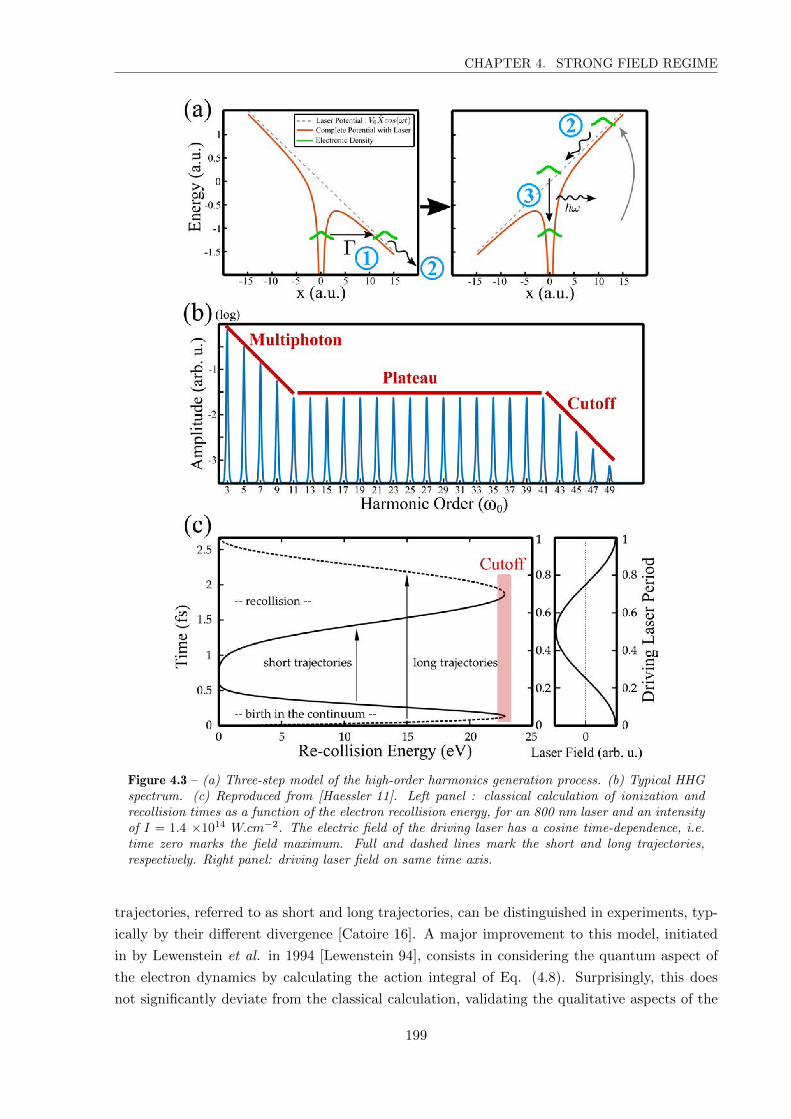
CHAPTER 4. STRONG FIELD REGIME
Figure 4.3 – (a) Three-step model of the high-order harmonics generation process. (b) Typical HHGspectrum. (c) Reproduced from [Haessler 11]. Left panel : classical calculation of ionization andrecollision times as a function of the electron recollision energy, for an 800 nm laser and an intensityof I = 1.4 ×10¹⁴ W.cm−2. The electric field of the driving laser has a cosine time-dependence, i.e.time zero marks the field maximum. Full and dashed lines mark the short and long trajectories,respectively. Right panel: driving laser field on same time axis.
trajectories, referred to as short and long trajectories, can be distinguished in experiments, typ-
ically by their different divergence [Catoire 16]. A major improvement to this model, initiated
in by Lewenstein et al. in 1994 [Lewenstein 94], consists in considering the quantum aspect of
the electron dynamics by calculating the action integral of Eq. (4.8). Surprisingly, this does
not significantly deviate from the classical calculation, validating the qualitative aspects of the
199

CHAPTER 4. STRONG FIELD REGIME
latter, but provides of course finer description of the quantum effect, such as the trajectories
interferences. Right from the classical model, the spectral cut-off of the emission appears around
Ip+3.17Up, where Up = e2<~E2>2meω2 is the ponderomotive energy, corresponding to the mean kinetic
energy of the electrons in the electric field. This is of crucial interest for generating high energy
photons, as one should thus induce the highest possible Up for this purpose. However, one should
still keep in mind that this can also influence the ionization rate and the Keldysh parameter.
iii) The emission results from the recombination of a wavepacket with its own source. As
a result, the emitted radiation conserves the coherence of the driving field. The coherence of
the process is highlighted and exploited for example in interferometric techniques, such as the
RABBITT (Reconstruction of Attosecond Burst By Interference of Two-photon Transitions)
[Veniard 96]. For doing this, sidebands of the harmonics generated by a field with the same
frequency as the driving field are created in a photoelectron spectrum where two quantum
path can interfere. This gives access to the relative phase between the harmonics. The spatial
coherence can also be used for instance in two-sources interferometry [Smirnova 09].
iv) Temporally, the launching of the trajectories does not spread uniformly across the driving
laser pulse. Indeed, the ionization maximizes around the high field intensities. As a result, the
emission of a given harmonic is confined around the corresponding trajectories recombination.
Since the driving field is periodic, the harmonic emission is also periodic, and forms a train
of pulses, emitted every half optical cycle. Being temporally confined within half an optical
cycle, each pulse has a duration in the sub-femtosecond, or attosecond range. Furthermore,
the trajectories corresponding to different emission wavelengths do not recombine at the same
time. As a results, the attosecond emission is chirped, alternatively positively and negatively
along every driving half optical cycle (Fig. 4.4). As the process efficiency is also modulated
with the driving field, the HHG emission temporally appears as a train of attosecond pulses
[Paul 01, Mairesse 03]. Recent techniques can be implemented to reduce this train to a single,
isolated attosecond pulse. For example, as a strong field is required here, one can use few-
cycles laser pulse to confine the generation to a single half-optical cycle [Hentschel 01], namely
amplitude gating. Another way around can be found by noticing that, as the wavepacket must
be driven back to the ionic core, the process declines drastically with the driving field ellipticity
[Chang 04, Strelkov 04]. By combining two delayed, counter-rotating circular polarization, a
field can be obtained with only half an optical cycle being linear. This polarization gating
confines the HHG to a single attosecond pulse. Even more efficient combinations of gating, such
as double-optical gating, have been developed since then [Chang 07]. Note also that for the
isolated attosecond pulse to be as short as possible, the intrinsic chirp between the harmonics
needs to be compensated, for instance by inserting metallic foils to compress the pulse down to
53 as [Li 17].
v) The efficiency of the whole process in inherently low, up to the 10−5 range in the best cases
[Comby 20a]. Studies converged to an efficiency scaling as λ4−8 [Tate 07, Shiner 09, Comby 20a].
Three factors determine the global efficiency. Firstly, the ionization rate must be maintained
at a reasonable level to avoid complete ionization of the system. Secondly, due to its quantum
nature, the propagating wavepacket always spreads perpendicularly to the laser field. As a
result, a significant fraction of the accelerated electrons never overlaps spatially with the ground
200

CHAPTER 4. STRONG FIELD REGIME
Figure 4.4 – Electron trajectories, for a 800 nm field at I = 1 ×10¹⁴ W.cm−2. The color representsthe final accumulated kinetic energy, i.e. the HHG photon energy. Reproduced from the PhD thesisof Julien Higuet.
state. Thirdly, the recombination efficiency, which is linked to the transition dipole between the
ground state and the continuum, is by itself limited. This dipole is the complex conjugate of
the one-photon ionization dipole, and is known to decrease drastically with the photoelectron
kinetic energy. Note that it also encodes the spatial information of the source, for instance the
symmetry of the orbitals, the geometry of a molecular system etc., and is the term of interest
in high-order harmonics spectroscopy.
This description at the atomic or molecular scale misses an essential point : the macroscopic
response. The process always occurs coherently between many centers in the gas target, driven
by the same laser field. All the single-center responses must thus constructively add up along the
interaction volume for the process to be efficient. This primarily leads to the collimation of the
HHG emission along the laser field, but it is also of crucial interest for the conversion efficiency
of the process. Indeed, for it to be maximized, one should consider the so-called phase-matching
conditions [Gaarde 08] : the dispersion of the HHG along the target must be controlled. Also,
re-absorption of the HHG must be kept low [Constant 99]. This typically implies avoiding too
much ionization and avoiding too high gas density. This is of course in contradiction with
the initial proclivity to use higher intensity and higher gas density to increase the efficiency.
It means that the process is fundamentally limited as a compromise must be found. At the
end, the length-density product of the generating media is the relevant parameter to consider
[Rothhardt 14, Comby 18].
As we now understand, the high-order harmonics generation process has strong-field
specific characteristics. Several parameters are to be considered simultaneously to optimize the
process, depending on the goal. In any case, the process can be kept efficient by scaling the
201

CHAPTER 4. STRONG FIELD REGIME
experiment while keeping some parameters constant [Heyl 16]. High-enough HHG intensity to
induce non-linear processes has recently become available [Takahashi 13, Senfftleben 20], using
long focal length. Long wavelengths can be used to generate photons at very high frequency,
up to the keV range [Popmintchev 12]. On the one hand, if only a high average photon flux is
required, high-repetition rate sources have been shown to be of great interest [Klas 16]. Our
group recently reached the mW range at 18 eV at a repetition rate of 166 kHz [Comby 19].
Other very good results have also been obtained with a different technology, generating the
harmonics in a cavity [Porat 18b]. HHG has been widely used as a secondary radiation source
in the XUV and x-ray domain, but it can also be used to resolve the dynamics in the generating
medium itself, as we will see in the next paragraph.
High Harmonic Spectroscopy
As we have seen in Section 2.I, the high-order harmonic generation process has been widely
used as a secondary radiation source in the XUV and x-ray domain. We will see here that
it can also be used to self-probe the generating medium itself. On the one hand, one can
use HHG in such a way by manipulating the generating medium. For instance, the process
is sensitive to many molecular effects, such as molecular alignment [Kanai 05], vibrational
wavepacket [Lein 05, Baker 06, Miller 16], and vibronic excitation [Ferre 15a], among others.
The excited wavepacket can be used to perform tomographic reconstruction of the molecular
orbitals [Itatani 04, Haessler 10, Vozzi 11, Peng 19].
An alternative approach also exists. As we have seen above, HHG can be understood with
a simple, yet efficient three-step model. From this model, it appears clear that the electron
trajectories can also be manipulated with more complex field configurations. This is typically
achieved by using two-color fields that are harmonic to each other, such as a fundamental field
and its second harmonic. For instance, adding a second perpendicular generation field can
enhance the control on the trajectories of the scattering electrons and modulate the recollision
angle, which can help decoupling nuclear and electronic degrees of freedom [Ferre 16]. This
configuration can also be used to allow or forbid the recombination of chosen trajectories,
i.e. harmonics, and reveal the exit time of the electrons [Shafir 12] (see Fig. 4.5 (a)). Even
more complex vectorial fields can be employed, such as counter-rotating bicircular bichromatic
driving fields (see Fig. 4.5 (b) and (c)). These latter enable for an effective return of the
wavepacket in the vicinity of the ionic core despite rotating [Fleischer 14, Kfir 16]. We will
see that the manipulation of the electron trajectories in this same fashion can also be of high
interest in photoelectron spectroscopy, and will be at the core of this chapter.
I. 4 Strong Field Photoelectron Spectroscopy
We have seen in the previous section that the photons emitted during strong field processes
can be used as an observable. However, the electrons tunneled out of the atomic or molecular
potential do not necessarily recombine, and are actually very often emitted. The perspective
of collecting and measuring them is exciting, in order to get a complementary insight in the
202

CHAPTER 4. STRONG FIELD REGIME
Figure 4.5 – (a) Principle of the displacement gate, with two linearly polarized fields : one which isstrong (red) and the other one which is orthogonally polarized, weaker in intensity and modulatedtwice as fast (second harmonic, blue). The orthogonal field forbids or allows the recombinationdepending on the trajectory, i.e. the harmonic order. Adapted from [Shafir 12]. (b) HHG spectrumof the 16th harmonics of a two-color field, as a function of the driving fields polarizations. Theslight wavelength incommensurate ratio λ2 = 0.51λ1 enables to distinguish energetically the differentphoton combinations leading to this harmonic order, as indicated on the right. The different angularmomentum combinations allowed are scanned with the fields ellipticities, as indicated below. Extractedfrom [Kfir 16]. (c) Exotic laser fields that can be obtained experimentally, providing a control on theelectron trajectories. Reproduced from [Fleischer 14].
electronic attosecond dynamics. In a first place neglecting the interaction of the tunneled out
electron with the ionic potential, the classical kinematic momentum ~p = m~v of an electron
freely oscillating in a field is ~p(t) = ~p(t′)− ~A(t′) + ~A(t) for any times t and t′. This ensures the
conservation of the canonical momentum of the photoelectrons ~p − ~A = ~Ct at all time in the
scattering. Assuming that the electrons have zero kinetic energy right after being tunneled out
(at ti), this imposes the final momentum ~pf when the laser field has passed ( ~Af = ~0) to be :
~pf = − ~A(ti) (4.10)
This directly links the detected photoelectron momentum distribution with the vector
potential of the field at the ionization time, and obviously the ionization time itself, and can be
203

CHAPTER 4. STRONG FIELD REGIME
used in various ways. We will thoroughly use this property in this manuscript. For now, let us
simply describe the shape of the distributions that can be observed.
Photoelectron Interferometry
The most simple scheme is performed by ionizing targets with a single linearly polarized
strong laser field. In this case, several distinct ionization times can correspond to the same
final momentum, but their phases accumulated during the scattering process differ. As a result,
interferences can appear, and are commonly referred to as photoelectron interferometric patterns.
We invite the reader unfamiliar with photoelectron interferometry to check the Simpolator
[Lein : Simpolator 0] to get a didactic feeling of the different patterns. This tool enables one
to visualize the different trajectories contributions, depending on their ionization times (which
quarter-optical cycle) and their type (direct or rescattered). An illustration of the different
interference patterns is proposed in Fig. 4.6, calculated for a single 800 nm field at 2 ×10¹⁴
W.cm−2, linearly horizontally polarized. The trajectories included are indicated in the lower
caption of each panel. Let us define the time zero at a positive maximum of the field. The direct
trajectories launched during the first quarter-optical cycle are shown in (a). They all end up
with a positive momentum along the laser axis pz because the vector potential is negative during
this part of the cycle (− ~A is depicted in red dotted line in the caption), with a certain transverse
distribution along py (and px, not calculated here). The photoelectron momentum cutoff appears
around 2Up (in our case Up = 0.44 a.u., for a cutoff in momentum at 1.3 a.u.). Interestingly, the
photoelectrons tunneling out during the second quarter-optical cycle (b) appear with the same
final momentum distribution on the same half of the detector. As a result, including the direct
trajectories of both the first and second quarters leads to an interference pattern on one half of
the detector (c), called intracycle interferences. This pattern will be discussed more extensively
in the next paragraph.
The direct trajectories from the two subsequent quarters will have an exactly symmetric
behavior on the negative pz part of the final momentum. Including all the direct trajectories
from a complete optical cycle thus lead to the figure shown in Fig. 4.6 (d). Importantly,
photoelectrons tunneling out during consecutive optical cycles can also overlap and interfere.
For instance, the pattern obtained from the first quarter of two consecutive optical cycles of
shown in panel (e). This concentric ring pattern, or intercycle interferences, corresponds to
the ATI rings. By taking into account all the direct trajectories of two optical cycles, the final
distribution (f) is simply obtained by overlapping the intracycle (d) and intercycle (e) patterns.
Finally, everything can become significantly more complex if the rescattered trajectories
are taken into account. The rescattered trajectories from the first optical quarter are depicted
in (g). This time, their final momentum distributions spread much more and on both sides.
In here, the direct trajectory can be seen as a phase reference that can be used to access
the phase accumulated during the rescattering process. For instance, their interference with
the direct trajectories from the same quarter cycle is shown in panel (h). Panel (i) shows
the photoelectron momentum distribution obtained by taking into account all the direct and
rescattered trajectories from two full optical cycles. The interferences might appear very
intricate. However, the pattern of the direct trajectories (shown in (f)) globally dominates in
204

CHAPTER 4. STRONG FIELD REGIME
Figure 4.6 – Photoelectron distributions for ionization times in different quarter-optical cycles anddifferent types of trajectories, calculated with the Simpolator [Lein : Simpolator 0]. Laser is linearlypolarized here along the z axis. The simulations are performed at 800 nm and 2 ×10¹⁴ W.cm−2. (a)Direct trajectories from the first quarter. (b) Direct trajectories from the second quarter, ending in thesame half of the detector. (c) Interference pattern obtained by including the direct trajectories fromthe first and second quarter-optical cycles, namely intracycle interferences. (d) Pattern obtained withall the direct trajectories of a single optical cycle. (e) Interference pattern obtained from the overlapof the first quarters of two consecutive optical cycles, namely intercycle interferences or ATI. (f)Distribution obtained from all the direct trajectories over two optical cycles, which is a combinationof the intercycle and intracycle intereferences. (g) Rescattered trajectories from the first quarter.(h) Interferences between the direct and rescattered trajectories from the first quarter. (i) Completepattern obtained with all the trajectories in two optical cycles.
the low momentum values, at least at the field intensity used.
Advanced Patterns
Other more complicated patterns can be found in the literature. One can cite the spider
(see Fig. 4.7 (1-a)), identified as interference between two forward-scattered electrons from
the same cycle [Huismans 11, Hickstein 12] or the fishbone, from direct and backscattered
trajectories [Bian 12, Li 15, Haertelt 16]. Rescattered electrons are of course very sensitive
to the ionic core and more advanced theoretical tools start to be necessary to correctly
reproduce their behavior, among which can be cited Coulomb-corrected SFA (CCSFA) where
the Coulomb potential of the ion is perturbatively taken into account in the SFA action. Many
other advanced methods have recently flourished, grasping for instance the physics of the fan
structure, involving intermediate bound states [Rudenko 04, Maharjan 06]. These advances are
205

CHAPTER 4. STRONG FIELD REGIME
comprehensively summarized in [Faria 20].
Figure 4.7 – (1) Two-color photoelectron interferometry. The spider pattern (a) can be modulated bythe second weak, collinear field. The phase of the resulting oscillation (b) is used to reveal attosecondionization times differences. Reproduced from [Porat 18a]. (2) Co-rotating and counter-rotating bi-circular bichromatic electric fields (green dashed lines) for different field ratios, and the correspondingvector potentials (solid blue lines). (3) Corresponding calculated photoelectron momentum distribu-tions in the polarization plane, where the trajectories are driven by the tailored vector potential. (2)and (3) are adapted from [Mancuso 16].
The resolution of the complex interference patterns can be challenging, in particular
experimentally since they always overlap. Recent progresses in photoelectron interferometry
have emerged with the use of more subtle field configurations. For instance, adding a weak,
second harmonic along the driving field can affect the tunnel barrier, modulating the spider
structures (see Fig. 4.7 (1-b)) and revealing differences in ionization times of the order of tens of
attoseconds [Porat 18a]. A linear second harmonic field can also be added orthogonally in order
to streak the distribution depending on their ionization times. This gives the possibility to
relieve the degeneracy between some trajectories [Zhang 14a, Richter 15], identify for instance
different types of trajectories [Li 15, Li 16, Richter 16] and unraveling fundamental properties
of the tunnel ionization [Han 17]. Similarly to HHG, more exotic laser fields can be employed
to manipulate the photoelectron trajectories [Mancuso 16] as shown in Fig. 4.7 (2) and (3) with
circularly polarized fields where the two main parameters are the relative helicities and field
ratio. For example, counter-rotating two-color fields can be used, where the vector potential
follows a clover shape. Cusp-like distributions of photoelectrons along the laser propagation
axis, revealing the Coulomb focusing contribution [Dimitriou 04], can be detected, in opposition
with the Gaussian-distributed direct trajectories [Eckart 18]. This effect comes from the
electrostatic field created by the ionic core, acting as a lens on the scattering trajectories, and
206

CHAPTER 4. STRONG FIELD REGIME
will be discussed more extensively in this chapter.
Direct Trajectories
We will be, in this manuscript, mainly interested in the most simple interferometric patterns
originating from the direct scattering trajectories, isolated in Fig. 4.8 (a). As we have seen,
these trajectories dominate at moderate field intensity. Let us describe them more quantitatively
here. They can be expressed from the SFA analytically [Maxwell 17], and split into intercycle
and intracycle interferences, as already discussed. Similarly to the harmonic comb generated in
HHG mentioned in the previous section, this intercycle interference (paths 1 and 1’ in Fig. 4.8
(a)) arises as modulations in the frequency domain, here corresponding to the kinetic energy of
the photoelectrons. As a result, constructive interferences in the distribution occurs at :
Ekin =p2x + p2
y + p2z
2= nω − Ip − Up (4.11)
for n ∈ N∗, nω−Ip−Up > 0. This corresponds to the well-know Above-Threshold Ionization
(ATI) rings, that can also be understood as an electronic density ionized from the absorption of
n photons, depicted in Fig. 4.8 (b). In this figure, the white rings indicate the solutions of Eq.
4.11.
The second family, intracycle, arises from the interference between electrons born within
the same optical cycle (for instance paths 1 and 2 in Fig. 4.8 (a)). [Maxwell 17] proposed to split
them in two types, A and B, respectively within a half optical cycle and between two consecutive
halves optical cycles. Similarly, their analytical expression can be derived, for an electric field
along z, as :
(pz −
4√Up
π
)2
+ p2x + p2
y = 2nω − 2Ip − 2Up +
(4√Up
π
)2
(4.12)
where n ∈ N∗, 2nω − 2Ip − 2Up + (4√
(Up)/π)2 > 0. One again, the patterns appears as a
concentric ring pattern, but this time off-centered by 4√
(Up)/π, as seen on Fig. 4.8 (c). The
white dotted circles highlight the solutions of Eq. 4.12, and are a good approximation with the
calculated distributions (full circles) along the pz axis corresponding to the laser polarization.
Calculation gives the possibility to isolate each of these patterns, but of course the ”actual”
physical distribution is obtained by overlapping them, as presented in panel (d).
These patterns are relatively simple and well understood. Can we use them to reveal
information about molecular chirality in the strong field interaction regime? Can we use the sub-
optical cycle sensitivity to the photoelectron interferometry to get access to chiral information
at an attosecond timescale? Can the description in terms of photoelectron trajectories be used
to understand how chirality is encoded into the photoelectrons individually?
207

CHAPTER 4. STRONG FIELD REGIME
Figure 4.8 – (a) Scheme of the direct photoelectron trajectories with the same final momentum, ionizedat different times. The ionization time of the three trajectory examples, with a final momentumupwards, are reported on the temporal panel. The interference can occur between two optical cycles(e.g. between trajectories 1 and 1’), yielding the ATI pattern presented in (b). It can also originatefrom ionization times within half an optical cycle (1 and 2), yielding the pattern on (c). The whitelines in (b) and (c) correspond respectively to the solutions of the analytical expression 4.11 and4.12. The combination of the two effects gives the modulation shown in (d). (b,c,d) are adapted from[Maxwell 17].
I. 5 Chirality in the Strong Field Regime
The details of the molecular potential are neglected in the strong field approximation. However,
as we have seen in the examples above, the potential can play a significant role in the strong field
physics, raising numerous questions. Are strong field processes sensitive to molecular chirality?
Does the asymmetric interaction of the electrons with the chiral potential and chiral field reveal
the same information as the non-chiral part of the interaction? Can sub-cycle tailored laser
fields be used to probe molecular chirality?
High harmonics generation in chiral molecules has been proved to be sensitive to the chirality
of the target, through laser-induced magnetic transitions in the ion, occurring between ionization
and recombination [Cireasa 15]. However, the HHG process loses its efficiency as the ellipticity
increases because the electron can hardly be driven back to the ionic core. HHG is thus not
possible with circularly polarized light. To circumvent that issue, advanced field shapes can
208

CHAPTER 4. STRONG FIELD REGIME
be used, offering both a rotation of the electric field and the possibility to produce recolliding
electron trajectories [Kfir 15, Fleischer 14, Neufeld 18]. The chiral effect remains weak, but this
scheme was recently used for time-resolved studies of the chiral response using transient HHG
gratings [Baykusheva 19]. The main limitation of these chiral HHG experiments is that they
rely on magnetic dipole interactions. Very recently, innovative schemes have been proposed
to design high-harmonic generation experiments that would be chiral-sensitive in the electric
dipole approximation [Ayuso 19, Neufeld 19], by relying on complex 3D driving laser fields. One
of these schemes is currently being implemented in our team by Sandra Beauvarlet.
Within this thesis, we have focused on using PhotoElectron Circular Dichroism as an
electric-dipole sensitive observable of molecular chirality. As we have seen, PECD is well-suited
in the single-photon and multiphoton regime. We have mentioned in the introduction of this
thesis that PECD had been shown to persist in the tunnel ionization regime in a measurement
performed in Fenchone, providing a rather uniform, low PECD signal over a broad electron
kinetic energy range [Beaulieu 16b, Beaulieu 16a]. The existence of PECD is not allowed within
the strong field approximation, as shown in [Dreissigacker 14]. However, Classical Trajectory
Monte-Carlo (CTMC) simulations performed in our group showed that the emergence of strong
field PECD could be understood semi-classically. The trajectories of electrons scattering in a
chiral molecular potential under the influence of a circularly polarized laser field were calculated
and averaged over molecular orientations. The resulting photoelectron angular distributions
showed a forward-backward asymmetry, even in a strong laser field, as depicted in Fig. 4.9.
Figure 4.9 – (a) Typical ionizing CTMC electron trajectory in fenchone embedded in a circularlypolarized laser pulse at a 800 nm wavelength and I = 1014 W.cm−2. (b) PAD (bottom half) andPECD (top half) from CTMC calculations in the tunneling ionization regimes. The light propagationaxis is horizontal and the radius extends up to 10 eV. Reproduced from [Beaulieu 16a].
The possibility to measure PECD in strong fields opens many perspectives of transferring
the tools used to manipulate and measure the underlying attosecond dynamics. A first step in
this direction was taken with the measurement of the attosecond dynamics of chiral photoion-
ization [Beaulieu 17]. In this study, a self-referenced attosecond photoelectron interferometric
measurement has been performed to measure the temporal profile of the forward and backward
electron wavepackets with a few-attoseconds resolution. An angle-dependent delay has been
measured between the electrons ejected forward and backward, which reaches 24 attoseconds.
Furthermore, the temporal shape of the electron wavepacket has also been reconstructed from
autoionizing states.
209

CHAPTER 4. STRONG FIELD REGIME
Within this thesis, we have taken a step forward by using tailored laser fields to address
fundamental questions : Does the instantaneous rotation of the field matter in chiral light-matter
interaction? Is PECD a quantity that builds up over the optical cycles or, conversely, does it
reflect an instantaneous interaction with the field? What is the timescale of the chiral response
in the electron ejection? Is tunnel ionization sensitive to the chirality of the molecular potential?
II Enantioselective Sub-Cycle Antisymmetric Response Gated by
electric-field rOTation (ESCARGOT)
The first investigation of sub-optical cycle chiral photoionization was performed in collaboration
with Shaked Rozen and Nirit Dudovich from the Weizmann Institute of Science (Israel), and
published in Physical Review X [Rozen 19].
Dichroic effects arise from the asymmetric interplay between a chiral potential and a chiral
field. Chiroptical processes generally rely on the use of circularly polarized radiation. We
have seen in Section 3.II that using elliptical polarizations could significantly enrich the chiral
photoionization phenomenon in the resonance-enhanced multiphoton regime. Here, we aim at
using more complex fields, resulting from the combination of multiple laser pulses with different
frequencies and polarizations. The very definition of the polarization state of such field raises a
challenge. Polarization is usually defined as a constant quantity in time. To take into account
the slow variations of the polarization, on can define the instantaneous ellipticity of a light pulse
as [Boge 14] :
ε(t) = tan
[1
2arcsin
(2Ez(t)Ey(t)sin(φzy)
E2z (t) + E2
y(t)
)](4.13)
where ~uz and ~uy are the two components of the polarization plane and φzy is their relative
phase. This quantity ε(t) reflects the temporal evolution of the ellipticity. To describe more
complex electric fields, a new quantity can be introduced. Lipkin defined a quantity in the
1960’s, the ”zilch” [Lipkin 64], later renamed optical chirality in the 2010’s [Tang 10]. The
optical chirality C is given by :
C =ε02~E · ~∇× ~E +
1
2µ0
~B · ~∇× ~B (4.14)
and is a geometric picture that quantifies the chirality of any arbitrary shape of electric
field. Interestingly enough, this idea has been used to shape fields with greater optical chirality
than circular polarization [Tang 11].
By neglecting the transverse derivatives and assuming that the field has a slowly varying
envelope, in such a way that the remaining x derivatives (along the propagation axis) can be
replaced by temporal derivatives, the geometric definition of the optical chirality given in Eq.
(4.14) can be transformed into a temporal quantity [Neufeld 18] that we will call instantaneous
chirality IC throughout the manuscript. As the electric dipole approximation prevails over the
other contributions and describes PECD, the magnetic field can be neglected, leading to :
210

CHAPTER 4. STRONG FIELD REGIME
IC(t) =ε02c0
[Ez(t)∂tEy(t)− Ey(t)∂tEz(t)] (4.15)
where c0 is the speed of light. We assume here that the field propagates along the ~ux axis.
The instantaneous chirality quantifies the rotational velocity of the electromagnetic field. We will
use it normalized relatively to a right circular polarization, meaning that |IC| = 1 corresponds to
an evolution of the field ∂ ~E/∂t orthogonal to the field ~E, with a positive (respectively negative)
sign for clockwise (anticlockwise) rotations, from the target point of view.
We will see in this chapter how these instantaneous quantities become relevant with tailored
laser fields and how we can use them to monitor the chiral dynamics of the photoelectrons at a
sub-optical cycle timescale.
II. 1 Orthogonal Bilinear Bichromatic Field
Orthogonal Bilinear Bichromatic electric fields can be easily generated by combining two linearly,
orthogonally polarized pulses with respective frequencies ω and 2ω. It can can be expressed,
assuming the fundamental frequency is along ~uz and its second harmonic along ~uy, as :
~E(t) = E0[cos(ωt) ~uz + rcos(2ωt+ ϕω/2ω) ~uy] (4.16)
where r = E2ω/Eω is the field ratio and ϕω/2ω is the relative phase between them. The
parameter ϕω/2ω has a great impact on the field shape, depicted in Fig. 4.10 (a). It can
range from a ”C”- (ϕω/2ω = 0, π) to an ”8”-shape (ϕω/2ω = π/2, 3π/2), through some less
symmetric ”bent-8”-shape (e.g. ϕω/2ω = 3π/4). This OTC (orthogonal two-color) field is of
great interest in our case as its instantaneous chirality alternates sign within one optical cycle
(define as the ω frequency cycle), as the colorscale in Fig. 4.10 (a) indicates. Fig. 4.10 (b-c)
respectively show the evolution of the instantaneous ellipticity and the instantaneous chirality
over the laser period depending on ϕω/2ω, as defined in Eq. (4.13) and (4.15).
Noticeably, the ε(t) or IC are not equal to zero most of the time but as they change sign,
these quantities integrated over a laser cycle vanish to zero. One can thus wonder : can we
induce and detect a dichroic response when ionizing a chiral molecule with such a field? In
other words, the question is to know whether the instantaneous or the average chirality of the
field matter in chiroptical processes.
Semi-classical Picture
Following the semi-classical interpretation of the PECD mentioned in (I. 5), one can quali-
tatively think about two limit cases, summarized in Fig. 4.11 with the point of view of a typical
velocity map imaging PECD experiment. The characteristic time τ it takes for the ejected elec-
tron to scatter into the chiral molecular potential under the influence of the chiral field while
escaping will be the relevant factor here. On one hand, if τ 2π/ω (∼ 3.4 fs in our experiment),
the dynamics will be alternatively driven by positive and negative IC, resulting in no dichroic
effect in average. On the other hand, if τ . 2π/ω, one can expect some dichroic signal to survive.
In the VMI configuration proposed, the photoelectron distribution is projected on the de-
211

CHAPTER 4. STRONG FIELD REGIME
Figure 4.10 – Schematic description of the sub-cycle instantaneous ellipticity and optical chiralityof the pulse. (a) 2D and 3D representations of the shape of a composite electric field obtained bycombining a fundamental component at ω polarized along z and a 2ω component along y, with 10%intensity ratio, for different relative phases ϕω/2ω between the two components. The color indicatesthe instantaneous chirality at each instant in the cycle. Note that in 2D representation of the 0 andπ phases, we can only see the first half cycle of the laser field. The second half cycle is not visiblesince it traces exactly the same route as the first half, only in the reverse direction, which causes thechirality of the second half to be opposite. (b) Instantaneous ellipticity (defined in Eq. 4.13) and (c)Instantaneous chirality (Eq. 4.15) of the tailored field along a laser optical cycle, as a function ofϕω/2ω.
tector, resolving the ~ux and ~uz dimensions, respectively being the laser propagation axis and the
ω field axis. The key ingredient here is the fact that in the strong field regime, the relationship
between the final momentum of the photoelectron and the vector potential at the ionization
time given in Eq. (4.10) imposes the upper half of the distribution to come from one half-optical
cycle and the lower half of the distribution to come from the other half cycle. The observable
of interest is the part of the distribution antisymmetric along the propagation axis, as we look
for the chirosensitive part of the signal, but also antisymmetric along the ω polarization axis, as
the instantaneous chirality of the field is inverted between the upper and the lower halves along
this axis. We named this effect Enantioselective Sub-Cycle Antisymmetric Response Gated by
electric-field rOTation (ESCARGOT, ”snail” in French). Note that it is not properly speaking
a dichroic effect, since it does not result from the subtraction of two opposite field helicities.
Interestingly, in parallel to our study, a similar effect has been predicted to occur in the few
photon ionization regime [Demekhin 18], with a different interpretation involving quantum path
interferences in a coherent control fashion.
212

CHAPTER 4. STRONG FIELD REGIME
Figure 4.11 – Scheme of the two limit cases presented in the text. (left) If the photoelectron scattersin the chiral potential under the influence of the tailored field for a duration much greater than theoptical cycle, the instantaneous chirality of field should cancel out. (right) If this duration is smallerthan half an optical cycle, one can expect a non-vanishing imprinting of the instantaneous chiralityin the photoelectron angular distribution.
II. 2 Velocity Map Imaging Experiment
Experimental Setup
Photoionization of (+)-Fenchone and (+)-Camphor molecules has been conducted in a VMI
using a single arm of the Blast Beat fiber laser system at CELIA, described in Section 2.I of this
manuscript. The 50 W output of one amplifier, delivering 130 fs pulses at 1030 nm (ω in this
case) at a repetition rate of 750 kHz, was split into two arms in a Mach-Zehnder interferometer
using a half-waveplate combined with a polarizing beamsplitter to control the field ratio r in Eq.
(4.16), as presented in Fig. 4.12. The first arm remained at the fundamental frequency, while
the second one was frequency-doubled in a 1 mm thick type-I beta barium borate (BBO) crystal
to generate the second harmonic (2ω = 515 nm). The polarization axis of the second harmonic
was rotated using a half-waveplate to be into the orthogonal two-color field configuration. The
arms were recombined using a dichroic mirror, while the relative delay was coarsely controlled
with a pair of mirrors on a translation stage and finely adjusted by a pair of fused silica wedges
in the 1030 nm arm. A 1 mm calcite plate was put in the recombined beam to ensure a perfect
cross-polarization. Indeed, small imperfections in the orthogonality could induce experimental
artifacts, in particular the 2ω components along the ω axis could modulate the tunneling rate.
The birefringent character of the calcite plate enables to temporally separate the main (perfectly
orthogonal) component of the 2ω field from its collinear imperfections. As a result, this latter
is temporally shifted away from the strong laser pulse, and is not intense enough anymore to
induce any effect by itself. Finally, a f = 30 cm lens was used to focus the two-color pulses in
the VMI. The chromatism of the lens was compensated by using a slightly detuned telescope in
the ω arm to ensure the overlap of the ω and 2ω focii.
Usually in attosecond physics, a very high level mechanical stability of the setup must
be reached. In particular, vibrations must be avoided. We have dealt with this issue, but
213

CHAPTER 4. STRONG FIELD REGIME
Figure 4.12 – Scheme of the optical setup used to generate the orthogonal two-color (OTC) field. PH= pinhole, λ/2 = half waveplate, PBS = polarizing beamsplitter, BBO = beta-barium borate crystal,DM = dichroic mirror, BD = beam dump, BC = beam combiner.
non-negligible thermal drifts could not be avoided. Indeed, despite enabling for very short
acquisitions, the high-repetition rate source suffers from a high average power and deleterious
thermal effects. As a result, we have noticed that the two-color phase could evolve within the
acquisition time. In order to overcome this issue, a Fourier filter procedure was employed to
isolate the relevant signal. The two-color delay was continuously scanned with the wedges in the
fundamental arm over 270 fs, corresponding to a ∼ 980 rad (≈ 80 times ω) scan in ϕω/2ω. They
were moved with a motorized stage at a speed of 16 µm/s. With a wedge angle θ = 2.9° and an
optical index of nSiO2,1030nm = 1.4627, an optical cycle is scanned in 48 µm, so the whole scan
duration was ∼ 240 s. The VMI camera exposure time was 50 ms, for a total of ∼ 5000 images,
meaning an optical cycle was resolved in about 60 points. The thermal drifts were completely
filtered-out by the procedure described in the next paragraph since they do not match any of
the frequencies of interest.
An alternative setup using an active two-color phase stabilization is presented in Section
4.III, in the case the detection system requires more acquisition time.
Fourier Filter Analysis
The periodic modulation of the up/down and forward/backward antisymmetrized part of
the signal was isolated, for each pixel, at twice the fundamental frequency, in the same fashion
as the PEELD experiment presented in Section 3.II. This enabled us to reconstruct the ES-
CARGOT signal at every two-color phase ϕω/2ω by applying an inverse Fourier transform on
the filtered component. This procedure reveals the quite weak relevant quantity, whose order
of magnitude is about 1%, and get over the experimental imperfections in the measurement.
This issue is usually solved in PECD experiments by doing a differential measurement between
left and right circular polarization, but using a Fourier analysis provides a much more reliable
way to do in our tailored field configuration. The absolute phase is not directly accessible with
214

CHAPTER 4. STRONG FIELD REGIME
the optical setup used. However, it can be retrieved in the Fourier analysis : the ionization
probability also oscillates with ϕω/2ω, and we assumed that it maximizes when the electric field
maximizes (at 0, π...). This yields a 4ω oscillating component in the total signal, as shown in
Fig. 4.13, which is used as a reference for the 2ω oscillation of the antisymmetric image. This
method of absolute phase calibration is nevertheless not fully trustworthy. It turns out that we
have noticed afterwards that this was not fully accurate at all intensities. We will not extensively
discuss this aspect in this section since it does not affect the interpretations presented. A more
reliable absolute phase calibration will be provided in the next section, using the complete 3D
measurements of the photoelectron angular distributions, which are not accessed here.
Figure 4.13 – Calibration of the two-color phase using 4ω oscillations. (a) Total photoelectron yieldof a typical (+)-Fenchone scan as a function of two-color delay, normalized to the maximal totalsignal in the scan. (b) Fourier transform amplitude of the signal in (a), in units of the fundamentalfrequency ω0 = 291 THz, the frequency of the 1030 nm field, showing a clear peak at the 4ω frequency.(c) The phase of the antisymmetric signal as function of momentum P, for three (+)-Fenchone scans.The phases were extracted by averaging over all the pixels with the same total signal momentum in onequarter of the detector, for each image in the scan, and calculating the Fourier transform of the timeevolution of this averaged signal. Then the phase of the 2ω Fourier component was extracted, andcalibrated according to the 4ω oscillation phase of the total signal. The calibration is tested only formomentum higher than 0.25 a.u. since one can see in Fig. 4.14 in lower momenta, the asymmetricsignal changes sign many times within each quarter of the detector, and therefore averaging over eachquarter is meaningless. (d) An example for the Fourier transform amplitude of the antisymmetricsignal for momentum 0.4 a.u., in units of ω0.
Note that a π uncertainty remains on ϕω/2ω, simply corresponding to a sign change of
the instantaneous chirality, meaning that we only access here the shape of the field and not
which way it is rotating. This only yields a sign uncertainty in the chiral signal, which is not
such a relevant feature. Again, the method presented in the next section enables to lift off this
ambiguity.
Experimental Results
215

CHAPTER 4. STRONG FIELD REGIME
Fig. 4.14 shows the ESCARGOT measurement performed in (+)-Fenchone at Iω = 2 ×10¹³ W.cm−2 and 7 × 10¹³ W.cm−2, and in (+)-Camphor at 3 × 10¹³ W.cm−2, respectively in
the first, second and third row. The intensity ratio was kept at I2ω/Iω = 0.1, corresponding to
a field ratio of r = 0.3. Note that the electric field shape is included in each caption, but the
polarization plane is not the one detected in this VMI configuration, the laser propagation axis
being the horizontal axis here. The left column depicts the total distribution, while the other ones
show the ESCARGOT signal for ϕω/2ω = 0, π/4, π/2, 3π/4, π. The rest of the range between
π and 2π is just the same panel with an opposite sign. One can observe in panel (a) and (m)
that the total distributions at low intensities show characteristic energy structures. The rings
up to 0.2 a.u. correspond to the ionization of different orbitals in a 8-photon absorption scheme
of the dominating fundamental ω field, for both Fenchone and Camphor. In Fenchone, the first
ATI of the dominant component around 0.15 a.u. is visible at 0.35 a.u., a well as a very weak
second ATI around 0.45 a.u.. In Camphor, the dominant feature appears around 0.1 a.u., and
the corresponding ATI appear around 0.3 and 0.4 a.u.. This is a typical behavior of the strong
field regime, which is close to be reached here : since the tunnel ionization drastically decreases
with the energy of the orbital ionized, most of the signal originates from the HOMO. On the
other hand, the distribution at higher intensity (g) goes towards a well-established strong field
regime : it is much more continuous because of the broadening induced by the ponderomotive
shift, the energy of the ATI cutoff increases and the distribution gets narrower along the vertical
axis (the ω polarization axis).
Figure 4.14 – Experimental data from the Fourier analysis of the VMI images. (a,g,m) Normalizedprojections in the VMI plane of the the photoelectron angular distribution for (a) (+)-Fenchonewith a fundamental field of 2 ×10¹³ W.cm−2 (g) (+)-Fenchone at 7 ×10¹³ W.cm−2 and (m) (+)-Camphor at 3 ×10¹³ W.cm−2. (b-f),(h-l),(n-r) Evolution of the ESCARGOT signal as a function ofthe relative phase ϕω/2ω between the two components of the ionizing field (ϕω/2ω = 0, π/4, π/2, 3π/4and π from left to right). The shape of the two-color field, colored according to the instantaneouschirality, is shown next to each image. The ESCARGOT signal is normalized to the maximum ofthe photoelectron spectrum in (a,g,m). The data is presented after up-down antisymmetrization.
The first and main feature of these results is of course the presence of a forward/backward
216

CHAPTER 4. STRONG FIELD REGIME
asymmetric ESCARGOT signal in the order of 0.1− 0.5% of the total signal, with an up/down
sign inversion expected from the change of instantaneous chirality along the optical cycle.
This confirms experimentally that the dynamics of the photoelectron in the vicinity of the
chiral potential occurs at the sub-optical cycle scale, i.e. in the sub-3.4 fs range. Noticeably,
this occurs at all two-color phases, even for the ”C”-shaped OTC field. Secondly, one can
see that the distributions are strongly dependent on ϕω/2ω, and can range at low intensity in
(+)-Fenchone (b-f) from a quite continuous fourfold pattern like in Fig. 4.14 (d) to a much
more structured pattern involving sign change between electrons with the same kinetic energy
(e.g. (b)). Interestingly, at higher intensity (h-l), the structure becomes less dependent to the
two-color phase and only shows a global sign change between (j) and (k). This behavior is also
reproduced in (+)-Camphor, an isomer of Fenchone, at lower intensity (n-r) between panels
(q) and (r). By comparing the results obtained in Fenchone and Camphor at low intensity
(first and third rows), it appears that the distribution at this intensity range depends strongly
on the molecular potential. Moreover, the amplitude of the ESCARGOT signal decreases at
higher intensity. Qualitatively, this can be understood as the molecular potential plays a less
important role towards strong field regime.
At first sight, one could expect that the electric field configuration used in (c) and (e)
should give the same ESCARGOT signal, since the fields shapes are just mirror imaged along a
dimension which is summed in the VMI projections. This is not the case at all, and reflects the
dynamical origin of the ESCARGOT signal : while the shape of the fields are indeed mirrored,
the rotation of the field vector along these shapes is inverted. This can be visualized with the
colorscale of the field shape in the caption of each panel, as a positive instantaneous chirality
(in red) corresponds to a clockwise rotation and a negative IC (in blue) corresponds to a anti-
clockwise rotation. This means that not only the shape, but also the dynamical evolution of the
optical cycle matters here.
Another dynamical aspect of the process lies in the fact that a significant amplitude of
ESCARGOT signal can be measured at every two-color phase. Demekhin et. al. claimed that
this was not possible, for a purely geometric argument [Demekhin 18] : in particular with a
”C”-shaped field (ϕω/2ω = 0 or π), the instantaneous chirality of the clockwise and anticlockwise
components should cancel out. We thus see here that not only the geometric, but also the
dynamical aspects of the driving field play a role. This latter breaks the perfect reversal
between the two components and as a result, one of them can overcome the other. A further
discussion will be proposed later in this manuscript.
Robustness and Validity of the Measurements
The error margin of the measurement has been estimated by splitting the 270 fs scan in 10
scans of 27 fs each. The 95% confidence interval has been calculated by statistical analysis (such
as detailed in Section 3.II). This yielded a maximum 0.5± 0.1% dichroic signal for Fenchone at
low intensity, while it reaches a lower value of 0.10± 0.03% at high intensity. The ESCARGOT
signal is thus decently above the errorbar.
A common practice in chiroptical measurements consists in comparing the signal obtained
217

CHAPTER 4. STRONG FIELD REGIME
from opposite enantiomers. Unfortunately, this procedure is not possible here, because of the
absolute sign ambiguity in the instantaneous chirality of the laser field. To circumvent this
issue, we performed the ESCARGOT measurements in a racemic mixture of Fenchone, which
contains both enantiomers in equal proportions. The results are presented in Fig. 4.15, and
compared to those obtained in a pure enantiomer, with the same colorscale. The signal in the
racemic mixture completely vanishes in the low intensity case, validating the chiral sensitivity of
the measurement. At high intensity, a non-zero ESCARGOT signal is detected, showing sharp
structures. This signal originates from artifacts in the photoelectron imaging. It is however
clearly lower and more localized than the signal obtained in the pure enantiomer, ensuring that
the ESCARGOT signal in (+)-Fenchone is also genuine at high intensity.
Figure 4.15 – Comparison of the ESCARGOT signal obtained in (+)-Fenchone (first and third rows)and a racemic mixture (second and forth rows), at 2 ×10¹³ W.cm−2 and 7 ×10¹³ W.cm−2.
Data presented up to now were up/down antisymmetrized, to follow the expected symmetry
of the ESCARGOT signal. The results obtained without the antisymmetrization procedure are
shown in Fig. 4.16. These raw results are mostly up/down antisymmetric, which justifies the
numerical antisymmetrization of the ESCARGOT.
In order to confirm and get a better insight of the features shown by the experimental
results, we will compare them to numerical simulation.
II. 3 Numerical Time-Dependent Schrodinger Equation Resolution
The following modeling has been mainly performed by Bernard Pons from our group. Time-
Dependent Schrodinger Equation (TDSE) calculations consists in numerically propagating the
wavefunction with a discrete iteration timestep, on a discrete spatial grid. In principle, it does
not neglect any effect (such as the influence of the potential), works at any regime and is only
218

CHAPTER 4. STRONG FIELD REGIME
Figure 4.16 – Experimental data without up-down antisymmetrization. (a) Normalized projection inthe (x, z) plane of the the photoelectron angular distribution for (+)-Fenchone with a fundamentalfield of 2 ×10¹³ W.cm−2. (b-f) Evolution of the ESCARGOT signal as a function of the relativephase ϕω/2ω between the two components of the ionizing field. The shape of the two-color field, coloredaccording to the instantaneous chirality, is shown next to each image. The ESCARGOT signal isnormalized to the maximum of the photoelectron spectrum in (a).
limited by the numerical precision of the grid. However, as this type of calculation can become
extremely demanding in processing power, the grid can not be arbitrarily large and arbitrarily
finely discretized, and numerical tricks are often required (see paragraph below for more details).
The calculations presented here have been performed in a toy-model chiral molecule, where the
nuclei are frozen in a chiral geometry , as it is the simplest chiral potential that can be engineered.
This system, also known as Bernardine (in honor of its creator Pr. Bernard Pons) is built with
four nuclei located at ~R0 = ~0, ~R1 = ~x, ~R2 = 2~y and ~R3 = 3~z, in atomic units, with respective
charges Z0 = −1.9 a.u. and Z1−3 = 0.9 a.u.. The field-free Hamiltonian that will apply to the
single-electron wavefunction is then H0 = −12∇
2 −∑3
i=0Zi|~r−~Ri|
where ~r is the position of the
electron. The calculation then consists in numerically solving the Schrodinger equation :(−i ∂∂t
+H0 + V(~r, t)
)Ψ(~R,~r, t) = 0 (4.17)
where V is the oscillating field potential in the electric dipole approximation as written in
Eq. (4.5). The goal of using such a simple toy-model molecule is of course not to grasp the
fine structures of the molecular potential but to see what general features can be identified. It
has been designed here so that its fundamental state, depicted in Fig. 4.17, has an ionization
potential Ip = 8.98 eV , in the range of the ones of Fenchone and Camphor. Note that the
standard one-photon PECD in this toy-model molecule is about 2% with circularly polarized
field.
Numerical Results
The calculated 3D photoelectron distributions have been integrated along the 2ω polar-
ization axis to be comparable with the 2D VMI projection. The calculations, performed for
three intensities Iω = 5 × 10¹² W.cm−2, 2 × 10¹³ W.cm−2 and 5 × 10¹³ W.cm−2 with an field
intensity ratio of I2ω/Iω = 0.1 are presented in Fig. 4.18 in the same way as the experimental
results. One can see in the total signal distribution (a,g,m) that the intensities used here cover
the transition between the multiphoton and the strong field regime, with many ATI rings.
The calculations also display a remarkable ESCARGOT signal, for all two-color phases.
Interestingly, some remarkable elements found in the experiment are nicely reproduced here.
At low intensity, the sign modulations along the low-energy ring (e.g. with the ”C”-shaped laser
219

CHAPTER 4. STRONG FIELD REGIME
Figure 4.17 – Skeleton and isosurface representation of the fundamental state of the toy model chiralmolecule employed in the TDSE calculations.
Figure 4.18 – TDSE calculations of photoionization of a toy model chiral molecule by the tailoredorthogonal two-color field. (a,g,m) Projections in the (x, z) plane of the symmetric part of the pho-toelectron spectrum, at 5 × 10¹² W.cm−2 (a), 2 × 10¹³ W.cm−2 (g) and 5 × 10¹³ W.cm−2 (m) .(b-f),(h-l),(n-r) Corresponding projections of the ESCARGOT signal, defined as the antisymmetricpart of the photoelectron distribution with respect to the propagation axis z and fundamental laserpolarization axis x. The relative phase between the two components of the laser field are ϕω/2ω = 0,π/4, π/2, 3π/4 and π from left to right. The shape of the two-color field, colored according to theinstantaneous chirality, is shown next to each calculation.
field in (b)) also disappear for a different two-color phase (e). While increasing the intensity
to the intermediate value (second row), one can see that these modulations tend to reduce
as the field becomes more prominent compared to the molecular potential. The amplitude of
the asymmetric part of the signal also diminishes with intensity, (respectively from 1.5% to
1.0% to 0.5%) in a way that when the strong field regime is well established (third row), the
signal coming from the ATI rings dominates and the distribution sharpens along the field axis.
In-depth comparison will be detailed in further section.
220

CHAPTER 4. STRONG FIELD REGIME
Method of the Calculation
Details about the calculation itself can be found in [Rozen 19]. One way to perform the
spatial discretization for the TDSE calculations is to define a cartesian grid on which each unit is
affected by the surrounding ones at each timestep, using a numerical propagator function derived
from the analytical Schrodinger equation. An alternative, used here, consists in expressing the
wavefunctions spatially on a basis of physically meaningful functions. The basis of functions used
are the jl(klr)Ysin,coslm (Ωr) with 0 ≤ l ≤ lmax and −l ≤ m ≤ l, where l and m are the angular and
magnetic quantum numbers respectively. Ysin,coslm are sine and cosine real spherical harmonics,
describing the angular dependency, and jl(klr) are spherical Bessel functions, describing the
radial part of the functions. As the basis is necessarily finite, the parameters were bounded to
rmax = 200 a.u., lmax = 10 and kmax = 7 a.u.. It is important in this situation to verify whether
the results are affected by these boundaries or not. Indeed, if the grid is too small, i.e. a non-
negligible electronic density reaches the boundaries within the temporal range of the calculation,
the end of the grid (a purely numerical limitation) will act as a ”wall” on which the wavefunction
can bounce back. To make sure this is not the case, a convergence check was performed, which
consists in doing the calculation on a larger grid and see if it influences the results. This is
especially sensitive at high intensity, as the wavefunction can be excited to high l (this is the
mathematical equivalent of saying that the distribution get peaked along the field) and that large
r can be reached because of the numerous ATI peaks. The convergence check in l is presented
in Fig. 4.19, where the same calculations using lmax = 10 and lmax = 14 are depicted. The
total signals (a) and (c) can not be distinguished from each other, while the ESCARGOT signal
(b) and (d) is also in good agreement. The only noticeable difference in the high momentum
values along the vertical (ω polarization) axis, but is not significant. This type of comparison
can be done for all the parameters, but typical signs can also indicate a convergence issue. In
particular, the wave structures at the high momentum values along the vertical axis are typical
of a reflection of the wavefunction on the boundaries of the spatial box. Since these effects
remain localized on the outer features and do not affect the results qualitatively, especially at
lower intensities, we assumed that the convergence is verified.
Moreover, as the ESCARGOT signal comes from a randomly oriented target, the calculation
must be performed and summed over many molecular orientations. Once again, only a discrete
set of orientation can be calculated. In our case, an angular Euler spacing of ∆α = ∆β = ∆γ =
π/4 was used, corresponding to a total of 256 orientations. This convergence has also been
verified, as displayed in Fig. 4.20.
The calculation is also necessarily discretized and limited in the time domain. This is
the reason why the fundamental frequency used here was 800 nm, with the second harmonic
field at 400 nm. Compared to the 1030-515 nm used in the experiment, this represents a
reduction of about 30% of the laser period, reducing the cost of the calculations. In order to
keep the computational load affordable, the calculation has been performed over four optical
cycles, corresponding to ∼ 11 fs. The envelope of the pulse was designed to be a linear rising
slope during the first cycle, flat during the two central cycles and a falling linear slope for the
last cycle. The main effect of using such a short pulse appears as a carrier-envelope phase (CEP)
221

CHAPTER 4. STRONG FIELD REGIME
Figure 4.19 – Convergence check with respect to the maximum angular momentum included in theTDSE calculations : Symmetric (a) and antisymmetric (b) parts of the photoelectron momentumdistribution obtained with lmax = 10. (c) and (d) are the counterparts of (a) and (b), respectively,obtained with lmax = 14. All other TDSE parameters are the same in both calculations: rmax = 200a.u., kmax = 7 a.u.,∆α = ∆β = ∆γ = π/4 with a two-color phase of ϕω/2ω = 0.
Figure 4.20 – Convergence check with respect to the number of random molecular orientations in-cluded in the TDSE calculations : Symmetric (a) and antisymmetric (b) parts of the photoelectronmomentum distribution obtained with an angular Euler spacing ∆α = ∆β = ∆γ = π/4. (c) and(d) are the counterparts respectively of (a) and (b), obtained with ∆α = ∆β = ∆γ = π/5. All otherTDSE parameters are the same in both calculations: rmax = 200 a.u., lmac = 10 and kmax = 7 a.u.,with two-color phase of ϕω/2ω = 0.
dependency, i.e. the relative phase between the electric field oscillation and its envelope. Indeed,
depending on the CEP, the symmetry of the field and the asymmetry of the ESCARGOT signal
along the ω axis can be broken, as shown in Fig. 4.21. The upper panels of this figure represent
the electric fields for CEP values of 0, π/2 and π, depicted for a two-color phase ϕω/2ω = 0
for clarity. The worst CEP effect in the photoelectron distributions calculated was found at
222

CHAPTER 4. STRONG FIELD REGIME
ϕω/2ω = 3π/4, and is depicted on the lower panels for a CEP of 0 (a), π/2 (b) and π (c).
However, the effect can be canceled by antisymmetrizing the distribution along the fundamental
field axis. The ESCARGOT signal becomes independent of the CEP, as shown in panels (d),
(e) and (f). Note that in the experiment, as the laser pulse duration was much longer, this
effect was completely negligible and this operation was performed to get rid of the experimental
artifacts.
Figure 4.21 – (Upper panels) Visualization of the CEP on the shape of the orthogonal two-colorelectric field, for CEP phases of 0, π/2 and π, depicted for a two-color phase ϕω/2ω = 0 for clarity.(Lower panels) Influence of the carrier-envelop phase φCEP in the TDSE calculations at 5 ×10¹²
W.cm−2 and for a two-color phase ϕω/2ω = 3π/4. (a-c) Projections of the ESCARGOT signal,defined as the antisymmetric part of the photoelectron distribution with respect to the propagationaxis x. (d-f) Corresponding signal, antisymmetrized along the fundamental laser polarization axis z.The carrier-envelop phase is φCEP = 0 in (a,c), φCEP = π/2 in (b,e), and φCEP = π in (c,f).
II. 4 Interpretation in Terms of Electron Trajectories
Both experiment and TDSE simulations show characteristic features that have to be understood.
To do so, a simple model based on a typical strong field picture has been developed. It consists
223

CHAPTER 4. STRONG FIELD REGIME
in calculating the classical trajectories, starting with zero momentum at the exit of the tunnel
barrier, under the influence of the OTC field only. The influence of the ionic core is neglected in
the calculation of the trajectories, but it is of course of crucial importance for the chiral response.
This aspect is artificially added to the model by considering an effective asymmetric interaction
between the chiral potential and the chiral field. More precisely, this means weighting every
trajectory calculated by the instantaneous chirality of the field while the electron is within a
certain range. Here we model this range with a Gaussian function with a FWHM of r0 = 1
nm centered at zero. In other words, the asymmetric interaction fades out with the distance,
and the integrated value of the IC along each trajectory reflects the ESCARGOT signal. This
model is very qualitative, and we developed it in 1D along the ω polarization axis as this field
dominates the dynamics of the photoelectrons (I2ω/Iω = 0.1 throughout this study).
Results are shown in Fig. 4.22 for photoelectrons ionized during an optical cycle. The red
line in the first panel (a) depicts the ω electric field and the shaded area corresponds to the
final kinetic energy of the electrons along this field axis, born at the corresponding time. The
final kinetic energy is maximized for the electrons born when the field is minimal and vice-versa.
They end up in the negative z range when they are emitted in a falling slope of the field and in
the positive z range if emitted in a rising slope. A few typical electron trajectories are shown
in (b) and (c), respectively in the cases ϕω/2ω = π/2 and 0. Note that only the IC differs from
between these two panels. The value of the instantaneous chirality is encoded in the color of the
lines.
As the kinetic energy curves in (b) show, two electron trajectories lead to the same final
energy on each side (up and down) of the detector : e1 and e2 for the lower part and e3 and
e4 for the upper part. The instantaneous chiralities experienced by the electrons 1 and 2 are
exactly opposite at their time of birth. However, the chiral response is not expected to be
instantaneous, but to be accumulated during the departure of the electrons from the region of
influence of the ionic potential, typically 1 nm from the core. In the case of the ”8”-shaped
electric field (b), trajectory e2 (born at ti = 0.3T0 where T0 = 3.44 fs corresponding to 1030 nm)
escapes the core quite rapidly and experiences only a given sign of IC in the vicinity of the core.
Electrons e1, born at ti = 0.2T0, sees a small opposite IC for a short time until 0.25T0 (hardly
visible in the color scale), but is mostly affected by the negative IC for the rest of its trajectory.
This means that these two trajectories, both ending on the lower part, will have a very similar
integrated IC, yielding one given sign of ESCARGOT signal. A symmetric situation is found
0.5T0 (∼ 1.7 fs) later with electrons e4 and e5, that will be imprinted with the opposite chirality
and will end up on the other side. This entanglement between pz and the IC sign explains
the up/down antisymmetry of the ESCARGOT. This picture is slightly more complex for low
kinetic energy electrons such as e3, as they spend more time in the vicinity of the core and get
alternatively affected by opposite IC. This could induce a drop in the signal for the trajectories
ending with low momentum along z, that we can observe in the experiment (Fig. 4.14 (j)) and
in the calculations as we go towards the strong field regime (Fig. 4.18 second and third row).
The situation is slightly different with the ”C”-shaped electric field (Fig. 4.22 (c)). Both e1
and e2 experience a sign change of the chirality of the field during their escape. This can mitigate
the accumulated value but except for very specific kinetic energy electrons at specific two-color
224

CHAPTER 4. STRONG FIELD REGIME
Figure 4.22 – Sub-cycle control over the instantaneous chirality of the field. (a) Oscillation of thefundamental electric field (red) and final kinetic energy of the electrons as a function of their ion-ization time (gray). The kinetic energy is plotted as a positive value for electrons with an upwardsfinal velocity and as negative for electrons with a final downwards velocity, in order to differentiatebetween electrons reaching each half of the detector. (b-c) Two pairs of electron trajectories (e1,2 ande4,5), each pair leading to the same final kinetic energy, and a trajectory of a low energy electron(e3). The trajectories are plotted for ϕω/2ω = π/2 (b) and ϕω/2ω = π (c). The colormap depicts theinstantaneous chirality of the field. (d) Instantaneous chirality integrated over the time duration inwhich each electron is closer than 1 nm to the molecular core, as a function of the two-color phaseand final kinetic energy of the electron. The quantity is averaged over the trajectories contributingto each final photoelectron kinetic energy.
phases, it remains not equal to zero. The rest of the predictions made for the ”8”-shaped field
remains valid.
The value of the instantaneous chirality integrated over a 1 nm gaussian range experienced
by photoelectrons within 5 eV kinetic energy as function of the two-color phase is shown on
Fig. 4.22 (d). The quantity displayed is averaged over the trajectories contributing to each final
photoelectron kinetic energy, in order to mimic the final signal. The two cases presented above
correspond to the dashed lines. Overall, the model emphasizes the sensitivity of the ESCARGOT
signal to the electron trajectories in the vicinity of the chiral potential, under the influence of
the chiral field.
225

CHAPTER 4. STRONG FIELD REGIME
II. 5 Discussion and Perspective
We have seen that in the strong field regime, the trajectories of the photoelectrons were driven
by the laser electric field and vector potential. Tailored fields can be generated to finely drive
the dynamics of the photoelectrons at the attosecond and molecular level. In the domain of
molecular chirality, this study demonstrates experimentally and theoretically that the concept
of instantaneous rotation, or instantaneous chirality of the field can be relevant for chiroptical
measurements. Indeed, beyond the cycle-averaged definition of the polarization of light, sub-
optical cycle instantaneous chirality can be imprinted to the dynamics of the electrons emitted
from a chiral molecule, yielding an asymmetric signal typical of the dichroic interaction at the
basis of the PhotoElectron Circular Dichroism. We have seen that in the case of bilinear bichro-
matic fields that this response can be observed at any two-color phase, from the multiphoton
to the strong field regime. When going toward strong fields, the signal becomes less complex
and less prominent as the field starts to overcome the chiral molecular potential. A strong field
picture of classical electron trajectories helps understanding the qualitative features of the ES-
CARGOT signal, such as antisymmetry along the ω axis, sensitivity to the two-color phase and
globally grasps the dynamical buildup of the process.
However, beyond this qualitative description, several features remain unclear. Firstly, fine
details of the molecular potential can drastically affect the interaction, as we see from the
comparison between two isomers, Fenchone and Camphor (Fig. 4.14). Secondly, structures in
the ESCARGOT patterns such as sign inversion or modulations of the signal along a radius of
constant kinetic energy (especially at low kinetic energy) are measured and calculated. One can
suspect quantum interference to be at the origin of this. Indeed, as we have seen, several electron
trajectories born at different times, that have experienced different instantaneous chirality, can
end up with the same final momentum. This is known to produce interference patterns, as we
have seen in previous section with photoelectron interferometry. Although this effect should
arise in the polarization plane, which is not accessed here, this might be revealed in a Velocity
Map Imaging configuration by the asymmetry of the interaction, along the laser propagation
axis x. This perspective gives strong motivations for extending this study with a device capable
of 3D photoelectron angular distribution measurement, such as a COLTRIMS, as we will see in
the next section.
III Three-Dimensional Chiral Photoelectron Interferometry
The study presented in this chapter has also been carried out in collaboration with Shaked Rozen
and Nirit Dudovich from the Weizmann Institute of Science, Israel. It is currently in preparation
for publication.
III. 1 Mapping of the Vector Potential
As mentioned in the introduction of this chapter, orthogonal bilinear bichromatic (or orthogonal
two-color, OTC) fields have already been proved to be interesting in the strong field ionization of
achiral targets [Zhang 14a, Richter 15, Richter 16]. In a the Strong Field Approximation (SFA)
226

CHAPTER 4. STRONG FIELD REGIME
presented in the introduction of this chapter, the conservation of the canonical momentum can
be derived and a simple mapping relates the final photoelectron momentum ~pf with the vector
potential at the ionization time ~A(ti), where ~E = −∂ ~A∂t , as :
~pf = − ~A(ti) (4.18)
with a certain distribution. The relevant quantity here is thus not the electric field but its
corresponding vector potential. The qualitative principle of the photoelectron interferometry is
depicted in Fig. 4.23 (1). The two limit shapes of the orthogonal bilinear bichromatic field are
displayed here. In panel (1-a), the ”8”-shaped electric field has a corresponding ”C”-shaped vector
potential, and in (1-b) the ”C”-shaped electric field has an ”8”-shaped vector potential. Note that
the colorbars used for both the field and the vector potential correspond to the instantaneous
chirality of the field, and can be used to visualize the temporal mapping. In each case, the
projection of the photoelectron distribution in the polarization plane calculated with the SFA
model is presented, and several features stand out.
Firstly, the photoelectrons can be ionized at different times within the optical cycle, and
the tunneling rate given in Eq. 4.6 associates the high probability to the maxima of the field,
depicted in full arrows in the figure. Conversely, the low probabilities are shown in dotted arrows
and originate from low field amplitudes. As a consequence, the majority of the signal yielded
appears in the low kinetic energy region. Note that the concentric ring pattern originates
from the repetition of the optical cycle over time, and corresponds to the Above-Threshold
Ionization (ATI) peaks. Secondly, the 2ω component of the field (along y) clearly distorts the
vector potential, either in a ”C”- or ”8”-shaped depending on the two-color phase (respectively
ϕω/2ω = −π/2 and ϕω/2ω = 0). This clearly affects the distribution and dresses the trajectories
along the y axis, creating a strong asymmetry in panel (1-a) which follows − ~A while leaving the
pattern symmetric in (1-b).
The distortion of the vector potential can be used to control the photoelectron trajectories.
The photoelectron angular distributions experimentally obtained in argon in [Richter 15] for
the single-color and the two-color cases are compared in Fig. 4.23 (2-a) and (2-b). They
firstly show that the photoelectron trajectories can indeed be dressed by the second harmonic
field, in particular toward one half of the detector. Furthermore, with the ”C”-shaped vector
potential used here, two photoelectron trajectories tunneled out at different times within the
optical cycle (either during the clockwise or the anticlockwise half-cycles) can end up with the
same momentum. As a result, a strong modulation is visible across the whole distribution,
corresponding to the intracycle interferences described in the introduction of this chapter. The
authors have also shown that this modulation could be controlled with the two-color phase,
as displayed in the panels (3). Depending on the shape of the vector potential, photoelectron
trajectories can indeed either end up in one or the other half of the detector, when inverting
the ”C” shape. Additionally, tailoring an ”8”-shaped vector potential spatially splits the two
solutions. As a result, the interferences vanish.
The orthogonal two-color field is thus very interesting for controlling and disentangling
227

CHAPTER 4. STRONG FIELD REGIME
Figure 4.23 – (1) Schematic representation of the photoelectron interferometry using a tailored field.The mapping of the final photoelectron momentum is given by the vector potential at the ionizationtime. High ionization probabilities are depicted with the full green arrows while the low probabilitiesare shown with dotted arrows. (1-a) ”8”-shaped electric field, with a corresponding ”C”-shaped vectorpotential. (1-b) ”C”-shaped electric field, with a corresponding ”8”-shaped vector potential. The colorsused for both the field and the vector potential correspond to the instantaneous chirality of the field,and can be used to visualize the temporal mapping. (2) Photoelectron distributions obtained in argonwith I780nm = 1.4 × 10¹⁴ W.cm−2 (2-a) and with an additional orthogonal second harmonic withan intensity ratio of I390nm/I780nm = 0.09 and a ”C”-shaped vector potential (2-b). The orientationof the fields are depicted in each panel and the vector potential is indicated by the dashed line. (3)Evolution of the interferences on one half of the detector as a function of the two-color phase. (3-a)Dependence of the spatially-integrated pattern with the two-color phase and pz/ptotal. (3-b) Lineoutsof the photoelectron signal for different two-color phases. The corresponding shape of the vectorpotential is depicted in (3-c). (2) and (3) are adapted from [Richter 15].
the different contributions of the photoelectron trajectories. The patterns obtained reveal
the phase of the emitted photoelectron wavepacket. This phase can be related to two terms
: the initial phase and the phase individually accumulated during the scattering, and such
for each interfering trajectory. In [Han 17], it has been demonstrated that these controlled
interference patterns can reveal the sub-barrier phase acquired by the wavepackets upon
tunneling. These studies were performed in achiral targets, so the instantaneous chirality of the
228

CHAPTER 4. STRONG FIELD REGIME
field was not playing a role. Can we use this interferometric scheme to access these quantities
that were missing in the ESCARGOT study? Can we expect such quantities to be affected by
the chiral nature of the interaction? Can different trajectory reveal different aspects of this
interaction? The distinction of the trajectories is particularly hard in the VMI projections, and
the resolution is obtained here in the polarization plane of the laser field. Does the resolution
of this third dimension explain the origin of the VMI projections presented in the previous study?
The interferences we will be interested in correspond to the direct trajectories [Li 16,
Maxwell 17] discussed in the introduction of the chapter, and their pattern in the one-color
case has been given in Eq. 4.12. Qualitatively, we do not expect the second harmonic field
to drastically modify the pattern itself, since the fundamental field still is dominant and the
mapping still scans the projection plane up and down along an optical cycle. We rather expect
modulations of its amplitude according to the overlap of the trajectories, as just explained, and
potentially of its phase depending on the different effects at play.
III. 2 Chirality in the Photoelectron Interferometry : TDSE Support
Three-Dimensional Picture
On the one hand, the photoelectron interferometry is accessible in the polarization plane
and the mapping associated enables the sub-optical cycle assignment of the ionization time. On
the other hand, the dichroic signal in which the chiral interaction between the chiral potential
and the instantaneous chirality of the field is encoded along the laser propagation axis. The
complete 3D resolution of the photoelectron distributions is thus necessary, in order to combine
these two aspects of the strong field ionization by the tailored laser field.
The distributions have been calculated by numerically solving the Time-Dependent
Schrodinger Equation (TDSE) in a toy-model chiral molecule. The method is presented in
the previous section. The results obtained at a field intensity of I800nm = 2 ×10¹³ W.cm−2 and
I400nm = 2 ×10¹² W.cm−2, for a two-color phase ϕω/2ω = −π/2 (”8”-shaped electric field and
”C”-shaped vector potential) are presented in Fig. 4.24. Isosurfaces of the symmetric part of the
distribution (along the laser propagation axis) are depicted in the panel (a). Note that only an
up/down symmetrization (along the ω axis z) of the signal is performed here in order to cancel
the CEP artifact of the calculations, as already discussed. Its projection in the polarization
plane is highlighted in panel (b). In this plane, the distribution clearly follows the ”C”-shape of
the vector potential. In addition, the interference pattern associated with the direct trajectories
is evident. Thus, even though TDSE does not provide a direct way to investigate the details of
the electron trajectories, their signature remains clear in the signal. A striking difference can
be noted in the projection of the distribution along the 2ω axis, in panel (c). This projection
plane corresponds to the one accessible in a standard VMI configuration, as presented in the
previous section. This projection appears hardly affected by the dressing field compared to the
one-color case, and the ATI rings are the only clear structure. This indicates that the weaker
second harmonic field indeed only dresses the photoelectron trajectories along its axis.
The situation greatly differs in the ESCARGOT part of the signal, depicted in panel (d).
229

CHAPTER 4. STRONG FIELD REGIME
Figure 4.24 – Isosurface representation of the complete (a) and chirosensitive part (d) of the 3Dphotoelectron momentum distributions calculated by TDSE resolution on a toy model chiral molecule.The x,y and z axis are respectively the laser propagation axis, the 2ω polarization axis and the ωpolarization axis. The calculations were done with ϕω/2ω = −π/2, I800nm = 2 ×10¹³ W.cm−2 andI400nm = 2 ×10¹² W.cm−2. Panels (b) and (e) highlight the respective projections in the polarizationplane from the target point of view. Panels (c) and (f) show the projections along the 2ω polarizationaxis, denoted ’VMI’ plane here. (d) results from the integration over the positive px half of thedistribution and the other panels from the integration over the whole respective axis.
230

CHAPTER 4. STRONG FIELD REGIME
It is obtained by taking the forward/backward antisymmetric part (along the laser propagation
axis x) of the raw results. As expected, an additional up/down antisymmetry along the ω axis
z is visible, and originates from the mirror symmetry of the field (and vector potential) along
this axis. Small imperfections of this up/down sign inversion (CEP artifacts) are canceled by
forcing the antisymmetry. The projection in the polarization plane of the ESCARGOT signal,
performed over the forward half (target point of view) is presented in panel (e). Qualitatively,
this projection follows the modulations of the total signal visible in (b), with a relatively low
amplitude along the 2ω (horizontal) axis and a strong amplitude along the ω (vertical) axis.
Interestingly, in addition to the up/down antisymmetry, a sign flip between different fringes of
the pattern is visible at the tips of the ”C” shape. Finally, the dressing of the second harmonic
also induces an asymmetry of the dichroic signal along the 2ω axis. These informations were
not accessible in the previous VMI experiment as this axis was integrated. The corresponding
projection is shown in panel (f). The most striking feature is that conversely to the total
distribution, the VMI projection of the forward/backward antisymmetric signal appears
strongly modulated by the trajectories interference. This suggests that the interferometric
pattern, originally only visible in the polarization plane, is encoded and revealed along the
laser propagation axis by the asymmetric interaction of the field with a chiral potential. The
chirosensitive ESCARGOT signal thus adds an important observable to investigate complex
photoelectron scattering processes in polyatomic molecules, if these latter are chiral.
Complementarity of the Observables
Let us focus here on a simple example to illustrate the complementarity of the observables.
With a ”C”-shaped vector potential (ϕω/2ω = −π/2), a given set of final photoelectron momen-
tum in the polarization plane (py, pz) can be associated with two distinct trajectories, or two
ionization times within an optical cycle, depicted by the red and blue points in Fig. 4.25 (a).
The location of their contribution in the total and dichroic part of the signal in the projection
is depicted in panels (b) and (c), respectively. Scanning the location along the vector potential
scans the ionization time difference, and thus the difference of accumulated phase between the
trajectories, giving rise to the interference pattern.
In this configuration, the instantaneous chirality of the electric field (IC, defined in Eq.
4.15) at the ionization times of the two interfering photoelectron trajectories is exactly opposite.
This statement remains valid at any place of the plane. The origin of the two trajectories within
the optical cycle of the laser field is depicted in panel (d). If the chirosensitive signal was only
originating from the initial instantaneous response at the time of ionization, the contributions
of the two trajectories would cancel out and the chiral signal would globally vanish. However,
in the semi-classical interpretation of the PECD in the strong field regime, depicted in panel
(e), the photoelectron driven by the field takes a certain time τ to escape the chiral molecular
potential. As simplistically modeled in Fig. 4.22, the instantaneous chirality of the field is
thus not only imprinted to the electron at its ionization time but also during its scattering in
the vicinity of the ionic core. In Fig. 4.25 (d), even if the two trajectories have an opposite
instantaneous chirality at the origin, they have the same positive gradient of IC in such a way
that the subsequent IC is maximized in the positive values in the first case while it tends to
231

CHAPTER 4. STRONG FIELD REGIME
lower negative values in the second. Consequently, the chiral signal from the first trajectory
prevails in the final observable.
Figure 4.25 – Location of an arbitrary set of two photoelectron trajectories associated with the samefinal momentum py, pz in the polarization plane, in the case of ϕω/2ω = −π/2. (a) ”C”shaped vectorpotential. (b) Projection of the photoelectrons in the polarization plane, calculated using TDSE inthe same conditions as the Fig. 4.24. (c) Corresponding dichroic signal. (d) ”8”-shaped electric field.The origin of the same trajectories in the optical cycle are displayed, and the subsequent instantaneouschirality during a time τ is highlighted in the two cases. The arrows indicate the direction of rotation.(e) Schematic representation of a photoelectron trajectory scattering in the chiral molecular potentialunder the influence of a chiral field during a certain duration τ .
This constitutes a significant observation for the interpretation of chiral scattering pro-
cesses and PECD in general. On one side, it draws the link between the chirality experienced
individually by the trajectories and the final dichroic signal. On the other side, this suggests
that such a dichroic effect can give further and complementary insight compared to achiral
photoelectron interferometry. Indeed, while the mapping of the vector potential only gives
information about the ionization time in a first approximation, the chiral interaction adds a
perspective into the dynamics of the scattering, namely after the ionization.
Evolution with the Two-Color Phase
As already presented in Fig. 4.10, the shape of the electric field can be tailored from a ”C”
to an ”8” or any intermediate form, by controlling the two-color phase ϕω/2ω. The corresponding
vector potential is of course affected, and the distribution evolves with it. The projections of the
3D TDSE calculations in the polarization plane using I800nm = 2 ×10¹³ W.cm−2 and I400nm = 2
×1012 W.cm−2 are shown in Fig. 4.26, for ϕω/2ω = −π/2 (a,f), −π/4 (b,g), 0 (c,h), +π/4 (d,i)
and +π/2 (e,j). The corresponding fields and vector potentials are indicated above with the
232

CHAPTER 4. STRONG FIELD REGIME
target point of view, and the colorbar corresponds to the field instantaneous chirality.
Figure 4.26 – 2D projections, from the target point of view, of the total (a-e) and forward/backwardantisymmetric part (f-j) of the 3D photoelectrons angular distribution from TDSE calculation on atoy model chiral molecule. Columns : ϕω/2ω = −π/2 (a,f), −π/4 (b,g), 0 (c,h), +π/4 (d,i) and+π/2 (e,j)) with respect to Eq. 4.16. The total signals are integrated along the whole distributionswhile the antisymmetric parts are along the forward half. The fields used were I800nm = 2 ×10¹³
W.cm−2 and I400nm = 2 ×10¹² W.cm−2.
The TDSE calculations at this moderate intensity nicely display the dressing effect of the 2ω
field, where the total distributions (a-e)continuously follow the mapping of the vector potential
from the ”C” to the inverted ”C” shape. The contrast of the interference fringes also appear
very contrasted in these two cases. The amplitude of the modulations is weaker with the ”8”-
shaped vector potential, as fewer trajectories overlap. The chirosensitive responses (f-j) reach
1% of the total signal, and also follow the shape and modulations of driven by the mapping of
the photoelectron distribution. Furthermore, the modulation of the two-color phase not only
influences the final distribution but also the instantaneous chirality of the field in the early times
of the scattering. A first approach to understand the structures of the ESCARGOT signal can
consist in extending the reasoning presented just above in Fig. 4.25. At ϕω/2ω = −π/2 or
+π/2 (Fig. 4.26 (f,j)), several trajectories imprinted with an opposite sign of IC can overlap at
the same location. The balance between the respective chirosensitive signals evolves along the
”C” shape and could yield the sign flip observed. Contrarily, the upper (or lower) half of the
distribution obtained with the ”8”-shaped vector potential (h) are mainly driven by a given sign
of IC. As a result, the ESCARGOT signal is dominated by this given IC.
The resulting structures are thus constituted over several overlapping effects. The next
section will focus on the experimental measurements of the complete 3D distributions. In order
to describe them more quantitatively, and in particular the effect of the sub-optical cycle chirality
233

CHAPTER 4. STRONG FIELD REGIME
of the field, another section will present a second modeling based on SFA.
III. 3 Experimental Measurements
Experimental Setup
The description of the setup used to generate the bilinear bichromatic field can be found in
the previous chapter, and adapted in the present case in Fig. 4.27. The intensities were tuned to
9.5 W at 1030 nm (ω) with 0.8 W of 515 nm (2ω), with orthogonal linear polarizations, at a laser
repetition rate of 166 kHz. A sub-cycle stabilization was actively performed using a piezoelectric
stage. The feedback loop was locked on a photodiode monitoring fringes between 1030 nm beams
from the two arms picked up from the recombination dichroic mirror, while most of the power
was reflected or transmitted for the collinear recombination. The relative sub-optical cycle phase
was finely tuned using a pair of fused silica wedges placed after the recombination. A telescope
with x3 magnification and a f=60 cm effective focal length was used to focalize the two collinear
beams. A slightly detuned telescope was placed in the ω arm to compensate the chromatic
aberration of the lenses so that the focii of the ω and 2ω beams overlap in the detector.
Figure 4.27 – Scheme of the optical setup used to generate the orthogonal two-color (OTC) field. PH= pinhole, λ/2 = half waveplate, PBD = polzarizing beamsplitter, P = polarizer, BBO = beta-bariumborate crystal, DM = dichroic mirror, BD = beam dump, BC = beam combiner, PD = photodiode,AS = active delay stabilization.
The signal has been measured using the COLTRIMS apparatus described in Sections 2.III-
2.IV. The shaped laser beam was focused under vacuum on a supersonic molecular jet made
by injecting 2 bars of carrier gas (N2) in a heated bubbler of (+)-Fenchone (≥98 % purity,
Sigma Aldrich) and carried by gradually heated pipes, to avoid condensation, to the nozzle. The
photoelectrons produced were carried on the detector using an homogeneous electric field (8.2
V.cm−1 over 29.1 cm) and confined with a magnetic field (8.25 Gauss) from the main Helmholtz
coils. The geomagnetic field was compensated using smaller transverse coils. The experiment
234

CHAPTER 4. STRONG FIELD REGIME
does not directly capitalize on the coincidence capacity of the COLTRIMS, as the ion side has
been used only for alignment and characterization purposes. The so-called coincidence condition,
imposing much less than one ionization per laser shot to avoid fake coincidence, is relaxed here.
The only count rate limitation was the dynamical response of the MCPs and delay lines, enabling
a 3D reconstruction in affordable times. The event counting rate was about 100 kHz and 100M
counts were recorded for each phase.
Contrary to the VMI detection, the acquisition takes much more time and the Fourier
filtering can not be performed. A direct measurement of the signal for selected two-color phases
has thus been preferred. The 2π periodicity of the signal was sampled in 9 steps, spaced by
π/4. The acquisition at each point took about 17 min, for a complete duration of 150 min. In
the experiment, the absolute two-color phase can not be accessed directly, and only the relative
phase is stabilized and scanned. The phase calibration has been achieved by comparing the
asymmetry induced along the 2ω field axis in the complete distributions. This py axis was
not resolved in the VMI measurements and must provide the phase without the modulo π
uncertainty left in the Fourier analysis used in the previous study. Note that the projections
along the 2ω axis (not depicted here) are in good agreement with the VMI measurements,
but indicate that the previous calibration using the oscillation of the total photoelectron yield
might not be accurate at low intensity.
Results
The projections of the 3D photoelectron momentum distributions measured experimen-
tally are presented in Fig. 4.28 in a similar way than the TDSE results. The field intensities
(I1030nm = 4.6 ×10¹² W.cm−2 and I515nm = 2.5 ×10¹² W.cm−2) are relatively low compared to
the calculations but the longer wavelength partially attenuates the difference in the ionization
regime. Measurements were also performed at higher intensity but a damage on the detector
prevents us from correctly isolating the dichroic signal, unfortunately. Nevertheless, the data
presented here can be compared with the theory.
The projections of the total distributions displayed in panels (a) to (e) indeed follow the
shape of the vector potential. In particular the center of mass of the distribution in the polar-
ization plane clearly moves from left to right here. The interferences are also less contrasted
than in the calculation since the detection setup and phase stabilization have a given resolution.
With the fields and wavelength used and the approximate formula of the pattern given in Eq.
4.12, one can expect the fringe spacing to be greater than in the TDSE calculations (shown in
Fig. 4.26). With this in mind, the observed pattern seems plausible.
The projections of the forward/backward antisymmetric parts of the signal reach here 0.3
% in amplitude (while it was about 1% in the TDSE). Their evolution also seems similar to
the TDSE calculations, in particular their continuous evolution from −π/2 to +π/2 with a
global sign flip appearing at +π/4. The images obtained with the ”C”-shaped vector potential
also display a sign change at the tips of the C, and the one associated with the ”8”-shaped
vector potential has a dominant contribution. Note that photoelectrons are detected in the low
kinetic energy region, which is not the case in the calculation. As these trajectories are likely
to spend more time in the vicinity of the potential, we do not expect this part of the signal
235

CHAPTER 4. STRONG FIELD REGIME
Figure 4.28 – 2D projections, from the target point of view, of the total (a-e) and forward/backwardantisymmetric part (f-j) of the 3D photoelectrons momentum distributions experimentally measuredin the COLTRIMS in (+)-Fenchone, for two-color phases ϕω/2ω = −π/2 (a,f), −π/4 (b,g), 0 (c,h),+π/4 (d,i) and +π/2 (e,j)) with respect to Eq. 4.16. The total signals are integrated along the wholepx while the antisymmetric parts are along the forward half. The field intensity was estimated atI1030nm = 4.6 ×10¹² W.cm−2 and I515nm = 2.5 ×10¹² W.cm−2.
to be comparable with the TDSE. Some quantitative discrepancies can be obviously pointed
out, but the calculations and the experiment are not done in the same system and a perfect
match would be surprising. Still, the experiment globally confirms that the dichroic response
can be tailored with the electric field in the polarization plane. The relatively good qualitative
agreement suggests that the process is not so much driven by the fine details of the molecular
potential, but rather by the instantaneous chirality of the field.
III. 4 Explicit Description of the Trajectories : SFA Calculations
The TDSE calculations provide a quantitative simulation of the photoionization with a few
assumptions (in particular without conditions on the ionization regime or on the interaction
with the potential) and constitutes a reliable point of comparison. However, it does not
provide a intuitive picture in term of photoelectron trajectories, which is at the root of our
interpretation. For this purpose, the SFA model presented in the introduction of this chapter
is more suited and associates explicitly ionization time with final momentum. Nevertheless, its
main downside is the complete omission of the interaction between the electron and the ionic
core during the scattering process. This constitutes an issue in some cases already presented,
but specifically in our case, this means that the chiral interaction can not be described as is.
For this reason, we propose the following phenomenological add-on to the SFA model. Note
236

CHAPTER 4. STRONG FIELD REGIME
that most of the SFA calculations were performed by Shaked Rozen.
Identification of the Trajectories
The standard calculation of the photoelectron ejection is firstly performed using the Eq.
4.9. The final 2D distributions a(~p, t0) in the polarization plane ~p = (py, pz) are thus expressed
from the action integral S(~p, t0) defined in Eq. 4.8, where t0 is the ionization time, as :
a(~p, t0) = |∑traj
eiS(~p,t0)|2 (4.19)
The calculation is performed over three optical cycles and the signal is obtained by coher-
ently summing over the continuum of trajectories. The result is presented in Fig. 4.29 (a) in the
case of a ”C”-shaped vector potential, but the following reasoning stands for all phases. While
two solutions per set (py, pz) per optical cycle are obtained in the one-color case, four distinct
ones are found with the orthogonal bilinear bichromatic field. They can be split in four families
that are depicted in Fig. 4.29 (b) to (e). The radial modulation comes from the repetition of
the ionization at each optical cycle. It can be interesting in addition to represent the map of the
ionization time within an optical cycle for each family, as a function of the final photoelectron
momentum (panels (f-i)). The colorscale of these panels indicates the ionization time t0 of the
solutions, with a threshold at 20% of the signal. The radial modulations were suppressed here
for visibility by selecting the trajectories within a single cycle. Fortunately, the first two families
dominate the signal for most of the final momenta, in such a way that we can still consider the
interference of the direct trajectories as a two-source inteferometry. If this was not the case, the
fringes would have been much more complex to interpret straightforwardly. The optical cycle is
indicated on the vector potential depicted and starts from the upper tip. The family 1 (panel
(b)) originates from the first half optical cycle, when the vector potential rotates anticlockwise.
Its upper half is emitted during the first quarter of the optical cycle, and the lower part during
the second quarter. The situation is symmetric for the family 2, which corresponds to the pho-
toelectrons ionized during the second half of the optical cycle, when the vector potential rotates
clockwise.
Several types of interference can thus be distinguished. The first one results from two
photoelectrons originating from two consecutive quarter cycles (for example 0.25-0.5 T0 and
0.5-0.75 T0, or -0.25-0 T0 and 0 − 0.25T0, where T0 is the fundamental optical period). The
second type comes from electron from the same optical cycle but not from consecutive quarters
(for instance 0-0.25 T0 and 0.75-1 T0). These two types are commonly refereed to as intracycle
interferences, and their pattern can be derived analytically in the one-color case as presented in
Eq. 4.12 [Maxwell 17]. In addition, intercycle inteferences can arise from trajectories ionized at
different optical cycles (such as -0.25-0 and 0.75-1 T0) and correspond to the ATI concentric
rings, given in Eq. 4.11. The final signal (in panel (a)) is thus simply a product of all these
patterns.
Embedding the Chiral Interaction in SFA
In order to introduce chirality in the SFA signal, we implement a phenomenological pertur-
237

CHAPTER 4. STRONG FIELD REGIME
Figure 4.29 – Decomposition of the solutions of the SFA in the polarization plane in trajectories,in the case where the vector potential is ”C”-shaped. (a) Total distribution obtained by coherentlysumming all the contributions. (b-e) Four distinct types of solutions found at each optical cycle.The radial modulation comes from the repetition of the ionization at each optical cycle. (f-i) Map ofthe ionization time within an optical cycle for each family, as a function of the final photoelectronmomentum. The colorbar indicates the ionization time, with a threshold at 20% of the single-cyclesignal, i.e. without radial modulations, for clarity. The quarter optical cycles are depicted on thevector potential above.
bation of the solutions found. This is based on a simple assumption, which consists in considering
that the chiral interaction can have two effects on the complex photoelectron signal : a phase
and/or an amplitude modulation. The PECD originates from a phase difference between the
scattering partial waves [Powis 08] (see Fig. 4.30 (a)). In a typical PECD experiment, only the
amplitude asymmetry of the photoelectron wavepacket can be accessed, through the detection
of the number of electrons ejected forward and backward. Phase-resolved chiral photoionization
has recently revealed that the forward and backward wavepackets also carry chirosensitive phase
shifts [Beaulieu 17]. In the SFA picture, each trajectory results from a set of interfering partial
waves (see Fig. 4.30 (b)). The chiroptical interaction thus modulates both the amplitude and
phase of each trajectory. Comparing the interference patterns produced by these trajectories
in the forward and backward hemispheres thus directly gives access to the chiral-induced phase
shift between the two trajectories.
To phenomenologically introduce the chiral-induced phase and amplitude modulations, we
propose to express the forward/backward antisymmetric signal in the polarization plane as :
238

CHAPTER 4. STRONG FIELD REGIME
Figure 4.30 – Origin of the PECD in term of partial waves forward/backward phase offset induced bythe chirality. (a) A phase difference ∆ϕF or ∆ϕB between the partial waves results in a the variationof the angular yield, namely PECD. (b) In the case where several trajectories interfere, the phasebetween the partial waves in each trajectory ∆ϕF1
and ∆ϕF2induces the amplitude modulation. The
phase between the partial waves among the trajectories due to the ionization time offset ∆ϕt0(F )
induces the term denoted as ”phase effect” in the text. Note that this latter can also be affected bythe relative phase between the partials waves ∆ϕF1
and ∆ϕF2. The backward part was omitted here
for clarity.
aF/B(~p, t0) = |∑traj
ei(S(~p,t0)+δ)(1 + δ′)|2 − |∑traj
ei(S(~p,t0)−δ)(1− δ′)|2 (4.20)
where
δ = α
∫ +∞
t0
IC(t)R(t0 − t)dt
δ′ = β
∫ +∞
t0
IC(t)R(t0 − t)dt(4.21)
are respectively the phase and amplitude perturbations for each trajectory ionized at t0,
induced by its interaction with the subsequent instantaneous chirality of the field IC(t) and the
chiral ionic potential, that has a certain range R. This range is actually expressed in space, and
we presently use a simple Gaussian function to describe it :
R(t0 − t) = e− r(t−t0)
2
2r20 (4.22)
where r(t − t0) is the distance from the ionic center to the electron at a time t − t0 and
r0 is a range parameter. In this model, α and β are respectively quantifying the phase and
amplitude perturbations of the action. This model is pretty simplistic and does not aim at
precisely grasping the details of the chiral interaction. However, it has the advantage of explicitly
describing the different terms in a phenomenological manner. Three parameters are adjusted in
order to reproduce the chiral-sensitive signal, namely the amplitude (β), the phase (α) and the
range (r0). Their respective effects can be decomposed in distinct features, as presented in Fig.
239

CHAPTER 4. STRONG FIELD REGIME
4.31.
Figure 4.31 – Effect of the phase (α), the amplitude (β) and the integration range r0 in the dichroicsignal obtained in the polarization plane with the simple chirality-embedded SFA model presentedin the text. The columns correspond to the field and vector potential depicted above, and the fieldconditions used were I800nm = 2 ×10¹³ W.cm−2 and I400nm = 2 ×10¹² W.cm−2. ’No integration’refers to the case where we only take into account the IC at the exit time IC(t0), by using R = δ(r).
Let us first consider the case where the chiral response is supposed to be instantaneous (’no
integration’). When the vector potential is ”C”-shaped, a pure amplitude chiral response leads
to no ESCARGOT signal. This is due to the fact that the two families of trajectories ending
up in the same place of the detector have experienced opposite instantaneous chiralities. The
difference in amplitude then cancel out each other, leading to a zero net asymmetry. On the other
hand, an instantaneous phase response can lead to a significant ESCARGOT signal. Indeed, the
phase difference between the interfering trajectories is cumulative since it represents opposite
forward/backward pattern offsets. Even small shifts can be magnified in the forward/backward
difference. Conversely with an ”8”-shaped vector potential, the amplitude effects of each half
of the detector add up and yield a strong ESCARGOT signal, while the chiral phase difference
240

CHAPTER 4. STRONG FIELD REGIME
tends to reduce. The different patterns are also very distinguishable, and such for any two-color
phase. The amplitude effect (β = 1) tends to yield a homogeneous ESCARGOT response over
the upper and lower halves of the distributions, while the phase effect (α = 1) always induces a
strongly oscillating pattern at twice the frequency of the total signal.
The modulation of the magnitude of the different effects with the two-color phase is
almost opposite when a 1 nm integration range is applied. In any case, the phase- and
amplitude-related ESCARGOT signals do not maximize at the same two-color phase, regardless
of the integration. The optimization of the parameters is thus based on three observables, to
be compared with the TDSE and experimental results. The first one is the relative steadiness
of the dichroic signal amplitude with ϕω/2ω. The second one is the qualitative structure of the
signal, in particular the sign flip a certain phases. Finally, the global amplitude is taken into
account. A more quantitative manner to determine the parameters is still being investigated,
but the results obtained so far can be a good basis of discussion.
The patterns resulting from the SFA calculations are very different from those observed in
the TDSE, in which the forward/backward asymmetry is mainly localized around the vertical
direction, i.e. around the polarization axis of the fundamental laser. This is due to the fact
that one key element is missing from out interpretation : Coulomb focusing, which will be now
discussed.
III. 5 Coulomb Focusing and Yukawa Screened Potential
Discrepancy Between TDSE and SFA
The photoelectron distributions obtained from the TDSE (Fig. 4.26) and the SFA model
(Fig. 4.31) show a puzzling discrepancy. While the total signal is homogeneously distributed
along the ”C” shape of the vector potential and the chiral parts prominently appear along the
vertical (ω) axis in the TDSE case, they are both dominant along the horizontal (2ω) axis in
the SFA. We were initially suspecting an issue in the theoretical descriptions, but very recent
developments indicate that it might actually be meaningful.
The SFA model is relatively simple and neglects the interaction of the photoelectron
and the ionic core during the scattering process. Still, a smoking-gun trace of the influence
of this latter has been experimentally detected in the orthogonal bilinear bichromatic field
configuration [Richter 16]. In this study, performed at I780nm = 1.4 ×10¹⁴ W.cm−2 and
I390nm = 1.3 ×10¹³ W.cm−2, two distinct features in the photoelectron signal in the polarization
plane have been identified, as shown in Fig. 4.32 (a-c). The first one corresponds to the features
described so far, which follow the dressing of the vector potential. The authors called it the
”streakable” part, as the 2ω polarization acts as a streaking field (isolated in Fig. 4.32 (b)). In
addition to this, an ”unstreakable” component can be noticed. Interestingly, the unstreakable
part completely vanishes if the Coulomb interaction is removed from calculations. It thus
corresponds to the trajectories that have undergone Coulomb focusing from the ionic core,
meaning that the electrons that have spent enough time in the vicinity of the cation have been
attracted to it and their momentum ends up being affected. This effect was already known
241

CHAPTER 4. STRONG FIELD REGIME
for leaving typical traces, for example, by turning Gaussian distributions into cusp-like profiles
in the photoelectron distributions along the laser axis. This has been demonstrated with
linear one-color fields [Dimitriou 04] and counter-rotating circularly polarized two-color fields
[Eckart 18]. In the present case of an orthogonal bilinear bichromatic field, the focusing effect
almost completely cancels the dressing effect of the second harmonic in the polarization plane
and the corresponding trajectories end up along the py = 0 axis, regardless of the two-color phase.
Figure 4.32 – (a-c) Adapted from [Richter 16] : evolution of the photoelectron distribution producedwith an orthogonal two-color field along the 2ω axis as a function of the two-color phase. (a) Exper-imental distributions measured in argon at at I780nm = 1.4 ×10¹⁴ W.cm−2 and I390nm = 1.3 ×10¹³
W.cm−2. (b) CTMC simulations neglecting the Coulomb potential. (c) CTMC simulations includingthe Coulomb potential. (d-f) TDSE calculations from our team at I800nm = 5 ×10¹³ W.cm−2 andI400nm = 5 ×10¹² W.cm−2. (d) Photoelectron momentum distribution in the polarization plane ofthe laser, integrated over px, where the ω field is along the z axis and the 2ω field along the y axis.(e) Evolution along the 2ω axis of the central part of the distribution (red box in (d)), as a functionof the two-color phase. (f) Same as (e), for the ATI peaks (green box in (d)). Note that the phaseunits of π are defined relatively to the fundamental field.
TDSE at High Field Intensity
The discrepancy between our SFA and TDSE results might also be due to the low intensity
used in the calculations (I800nm = 2 ×10¹³ W.cm−2 and I400nm = 2 ×10¹² W.cm−2). Indeed, the
strong field approximation is well-suited to describe the processes occurring at high intensity.
We thus increased the intensity to I800nm = 5 ×10¹³ W.cm−2 and I400nm = 5 ×10¹² W.cm−2.
The results of the TDSE calculations are compared to the ones of [Richter 16] in Fig. 4.32 (d-f).
The simulated 3D photoelectron distribution were integrated over two different regions. The
242

CHAPTER 4. STRONG FIELD REGIME
evolution of the central part (red box in (d)) along the 2ω axis as a function of the two-color
phase is shown in panel (e), while the one of the high energy features (green box in (d)) are
depicted in (f). Interestingly, these two components show a completely different behavior. The
central part seems to follow the curve of the ”streakable part”, i.e. the vector potential, meaning
that this part of the signal could be associated with direct trajectories. Conversely, the ATI
peaks oscillate much less with the dressing of the vector potential (and even in opposition to
it). They could then be associated with the Coulomb-focused trajectories.
In order to see how these different types of photoelectron trajectories are affected by the
dressing of the 2ω field, the projection in the polarization plane of the total distributions and
their respective forward/backward antisymmetric parts are presented in Fig. 4.33 for different
phases. Comparatively to the calculations at lower fields, the higher field conditions directly
impact the distributions, in particular several ATI peaks are visible in the total signal (a-e). It
appears clear from the evolution of the complete distributions that the central part (first ring)
is shaped and dressed by the vector potential, smoothly evolving here from the ”C” (a) to the
inverted ”C” shape (e). This is another way to visualize the fact that this part of the signal is
”streakable”. Oppositely, the signal along the vertical axis is almost unaffected by the two-color
phase. As just mentioned, this could be the signature of Coulomb-focused trajectories.
Figure 4.33 – 2D projections, from the target point of view, of the total (a-e) and forward/backwardantisymmetric part (f-j) of the 3D photoelectrons angular distribution from TDSE calculation on atoy model chiral molecule. Columns : ϕω/2ω = −π/2 (a,f), −π/4 (b,g), 0 (c,h), +π/4 (d,i) and+π/2 (e,j)) with respect to Eq. 4.16. The total signals are integrated along the whole distributionswhile the antisymmetric parts are along the forward half. The fields used were I800nm = 5 ×10¹³
W.cm−2 and I400nm = 5 ×10¹² W.cm−2.
243

CHAPTER 4. STRONG FIELD REGIME
Such features could be of high interest in this study. As these trajectories do not interact
with the ionic potential in the same way (they spend more time in its vicinity), one can expect
them to be differently imprinted with the chirality of the potential. A particularly interesting
behavior, displayed in the present case, is that the ESCARGOT signal is indeed mainly located
along the vertical axis on the ATI signal (f-j). One can have the following interpretation. In
this regime, the amplitude of the ESCARGOT signal typically decreases since the molecular
potential is less prominent compared to the field [Beaulieu 16a]. The direct trajectories are thus
less imprinted with the chiral interaction. Conversely, the Coulomb-focused trajectories recover
part of this sensitivity. Determining the qualitative influence of the ionic potential on the 3D
photoelectron angular distributions produced by a tailored laser field is not an easy task. The
interpretation can be simplified by taking a different look at the results, within the framework
of the attoclock technique.
Origin of the ESCARGOT Signal
The attoclock effect is described in the introduction of the next section. Simply put, when
performing ionization with a short circularly or elliptically polarized pulse, the ionization can be
confined to the peak of the field. Since the field rotates, any angular offset of the distribution
compared to the vector potential can be read as a temporal offset, called attoclock delay, as
shown in Fig. 4.34 (a). Interestingly, the attoclock idea can also be implemented with more
exotic fields [Han 18]. In our case, the rotation of the field (and vector potential) is inverted
between the upper and lower halves (see panel (b)). As a result, the angular offset is opposite
between these two halves.
Figure 4.34 – (a) Principle of the attoclock effect on a circularly polarized short pulse. The tunneling isconfined at the peak (black) dot. Since the vector potential rotates, an angular offset of the distribution(grey dot) can be read as a delay in the ionization ∆T . (b) Same principle applied with the orthogonaltwo-color field with ϕω/2ω = 0, for an achiral target. (c) Same as (b), with a chiral target. The chiralinteraction can induce a chiral attoclock effect, meaning that the delay can be slightly different forthe photoelectrons emitted forward (∆T±F ) and backward (∆T±B ), depending on the instantaneouschirality of the field (±). The example is depicted for ∆T+
F > ∆T+B (positive values of instantaneous
chirality (+), in red). Since it is a dichroic effect, it reverses with the IC. This leads to the up/downasymmetry of the ESCARGOT signal. (d) Same as (c), with ϕω/2ω = π. The instantaneous chiralityof the field is reversed here. However, this also means that the rotation is mirrored compared to (c),in such a way that the relative position between the forward and backward parts of the signal is thesame as in (c).
244

CHAPTER 4. STRONG FIELD REGIME
We propose here to extent the concept to chiral interaction, which consists in assuming
that the attoclock delay ∆T could be slightly different between the forward and the backward
parts of the photoelectron distribution. Since it is a dichroic effect, the effect would reverse if
the sign of the field instantaneous chirality is inverted. The consequences on the dichroic signal
is qualitatively depicted in Fig. 4.34 (c). Let us assume for instance that ∆T+F > ∆T+
B (with
a positive sign of IC). In this example (ϕω/2ω = 0), this means that the forward signal will be
located on the left of the backward signal on the upper half. The effect is of course mirrored on
the lower half, since the IC is inverted. This can be compared to the case of ϕω/2ω = π, depicted
in the panel (d). The instantaneous chirality of the field is reversed here. However, this also
means that the rotation is mirrored compared to (c), in such a way that the relative position
between the forward and backward parts of the signal is the same as in (c) (i.e. forward signal
on the left of the backward signal in the upper half in our example). Since the chirosensitive
signal adds up regardless of the sign of the instantaneous chirality of the field, this means that
this effect remains qualitatively identical for all two-color phases, and in particular even for the
”C”-shaped vector potential. This reproduces the behavior observed in the unstreakable part of
the ESCARGOT signal calculated with TDSE at high intensity (Fig. 4.33 (f-j)). Surprisingly,
this means that the ESCARGOT signal does not sustain a simple sign flip when inverting
the field chirality. The only way to invert the sign of the features is to swap the enantiomer
handedness. The 3D ESCARGOT signal is thus singularly defined by the absolute set of field
and enantiomer (oppositely to PECD, where for instance, the signal from a (+) enantiomer and
RCP can not be distinguished from the one of the (-) one with a LCP). Note that monitoring
only the projection along the 2ω axis removes this resolution, in such a way that the VMI
projections of the ESCARGOT signal does simply flip sign while inverting the IC, as we have
seen in the previous section.
The SFA model presented above predicts interferometric effects to be involved in the ES-
CARGOT signal. However, they are covered by the Coulomb-focusing effect that refocuses all
the patterns along the ω axis. Can we still access the ionization phases? For this purpose, it is
possible to remove the effect of the Coulomb potential in the calculations. Instead of performing
them with a standard Coulomb potential (V (r) = −1/r), a screened Yukawa potential has been
used here. This latter aims at mimicking the Coulomb potential at short distances but cuts its
long-range tail, expressed by adding a e−(r−r0) cutoff term. The complete study is still being
carried out, but the first results are promising. The comparison between the TDSE calculations
using a Coulomb or a Yukawa potential, at I800nm = 5 ×10¹³ W.cm−2 and I400nm = 5 ×10¹²
W.cm−2 and for the ”8”-shaped vector potential (ϕω/2ω = 0) is given in Fig. 4.35. The first
striking result is that the features associated with the Coulomb-focused trajectories (along the
vertical axis in (a)) completely disappear with the Yukawa potential (b), confirming the initial
assignment. Furthermore, the ESCARGOT signal in this region also cancels (d), indicating that
the latter indeed originates from long range effects. Conversely, the central features associated
with the direct trajectories remains significant in the complete distribution (b), which is in good
agreement with our interpretation.
Nevertheless, the Coulomb focusing can not be completely switched off with the Yukawa
245

CHAPTER 4. STRONG FIELD REGIME
potential. Since the corresponding features lie along the ω polarization axis, it is possible to
avoid their residual contribution by looking away from the polarization plane. The result is
depicted in Fig. 4.35, for ϕω/2ω = 0 (e) and π/2 (f), for the ESCARGOT signal integrated
between px = [0.18 - 0.27] a.u. along the laser propagation axis. The patterns obtained look
very modulated in this case. They can be compared to SFA calculations performed with a chiral
phase effect only (α = 0.01 and β = 0 in Eq. 4.21), and with a very short integration time of
the instantaneous chirality of 50 as, shown in panels (g) and (h). We see that the patterns
are in good qualitative agreement. We have not concluded on this particular comparison yet,
but this already strongly suggests that the chiral phase effects indeed play a role in the direct
photoelectron trajectories. Furthermore, the very short integration time required to reproduce
the features at both two-color phases indicates that the effect corresponds to a chiral phase
imposed at the onset of the wavepacket, i.e. the tunnel ionization.
Figure 4.35 – (a-d) 2D projections in the polarization plane calculated by TDSE at I800nm = 5 ×10¹³
W.cm−2 and I400nm = 5 ×10¹² W.cm−2 and for the ”8”-shaped vector potential (ϕω/2ω = 0). Thetotal distributions (upper panels) and ESCARGOT parts (lower panels) are presented, for Coulomb(a,c) and Yukawa screened potential (b,d). (c) and (d) are displayed with the same colorbar forcomparison. (e-f) Slice of the ESCARGOT signal obtained with the Yukawa potential in TDSE inthe field polarization plane (py, pz), integrated away from the center between 0.18 a.u. and 0.27 a.u. inpx, the laser propagation axis. (e) and (f) correspond respectively to the two-color phases ϕω/2ω = 0and π/2. (g-h) ESCARGOT signal from the extended SFA model presented in the text, performedwith a chiral phase effect only (α = 0.01, β = 0), and with an integration of the instantaneouschirality of 50 as, in the same field conditions, for two-color phases of ϕω/2ω = 0 (g) and π/2 (h).
Finally, this is to be compared to the experimental ESCARGOT measurements, shown in
Fig. 4.28. Even if is was performed in moderate field conditions, the features corresponding to
the chiral attoclock seems to be distinguishable. It is not evident, however, to know if the absence
of fast modulations are related to the resolution of the COLTRIMS, or the longer wavelength
used for instance. As we see, the complete distribution is itself less modulated. In any case,
246

CHAPTER 4. STRONG FIELD REGIME
it would be interesting to reproduce the measurements in stronger field conditions. It might
enable to measure the tunneling phase shifts, if we manage to isolate the interference structures
from the Coulomb-focused features. In the meantime, we have used another way to tackle the
question of the sensitivity of the tunnel-ionization to chirality. For this, we have used the chiral
attoclock with a different field configuration, as we will see in the last section.
III. 6 Perspectives
The high density of information contained in the 3D photoelectron momentum distribution leads
to many results in the presented study. We have demonstrated that the combination of the pho-
toelectron interferometry with the sub-optical cycle gating of the instantaneous chirality of the
laser field shows substantial increase of the information provided individually by each technique.
In particular, the chiral interaction adds dynamical informations to the vector potential map-
ping, and inversely the mapping relates the PECD to the interaction individually experienced by
the photoelectron trajectories. Beyond the experimental feasibility, the complementarity of the
TDSE in terms of completeness and the SFA in terms of explicit trajectory description is shown.
Recent developments indicate that different types of trajectories can be identified depending on
the field condition used. While they have already been investigated using the interferometry, the
chirality adds a fundamental insight into the picture. The nature of the interaction at the origin
of this photoelectron dichroism can be finally unraveled by using a screened Yukawa potential
in the modeling. The final investigations and structuration of the concepts presented are still
being carried out, but will undoubtedly be of high interest.
We will see in the next section that these concepts are not specific to the orthogonal two-
color fields and can be tackled from another point of view with different shapes of tailored laser
fields.
IV Chiral Attoclock
As seen throughout this chapter, tailored laser fields can be extensively used in the strong field
regime to unravel the different processes at play. In this last section, we will briefly describe a
study conducted in our group, where counter-rotating bicircular bichromatic (CBCBC) fields
have been employed in the strong field ionization of chiral molecules. The discussion will remain
concise since I have not personally participated in the experiment and the calculations. Yet, I
got involved in the analysis and the discussions, and the outcomes give a particularly relevant
perspective in this chapter. The results are currently under reviewing for publication.
The Attoclock Principle
When performing strong field ionization with a short circularly or elliptically polarized pulse,
the ionization can be confined to the peak of the field because of the exponential ionization rate
(given in Eq. 4.6). And as the field rotates, any angular offset of the distribution compared to the
vector potential can be understood as a temporal offset, called attoclock [Eckle 08, Torlina 15].
It gives a dynamical resolution at the attosecond timescale without using typical pump-probe
247

CHAPTER 4. STRONG FIELD REGIME
schemes and is of particular interest for investigating fundamental questions such as tunneling
time. Indeed, even if simple models and experiments assume that the time it takes for the electron
to ”go through” the tunnel is equal to zero, the veracity of this assumption remains uncertain.
Some studies concluded to a finite time [Pfeiffer 12, Landsman 14, Camus 17]. However, some
other claim that it could be due to other effects [Kheifets 20], such as the Wigner time-delay,
corresponding to a phase offset of a wavefunction escaping a potential compared to the free
wave. In addition, non-zero momentum at the exit of the tunnel barrier has also been proposed
[Camus 17]. In fact, the same result can be either interpreted as resulting from zero tunneling
delay and zero longitudinal momentum [Ni 18], or from nonzero value of both these quantities
whose effects cancel out each other [Han 19, Kheifets 20]. Interestingly, the attoclock idea can
also be implemented with more exotic field configurations [Han 18].
Can the very high sensitivity of the attoclock be used to retrieve the interplay between
the field and the chiral molecular potential? In particular, can it be affected, similarly to
PECD, differently for the photoelectron emitted forward and backward? Can different types
of photoelectron trajectories be affected differently depending on their interplay with the chiral
ionic core?
IV. 1 Counter-Rotating Bicircular Bichromatic Field
The combination of two counter-rotating laser circularly polarized laser fields at ω and 2ω yields
a threefold field shape. The field amplitude ratio changes the shape, in between a triangle and
a clover, as depicted in Fig. 4.36 (a) for Eω//E2ω = 2 (left), 1 (center) and 0.5 (right). The
two-color phase does not determine the shape, but only induces a global rotation. Conversely
to the orthogonal bilinear bichromatic field, the ”leaves” are identical and the final distribution
has the same threefold symmetry, without inversion of the chiral response.
The 3D photoelectron momentum distribution from such a field has been measured ex-
perimentally using the tomographic reconstruction of VMI images. For each distribution, 31
projections have been recorded, each of them accumulated over 104 laser shots (10 seconds at a
repetition rate of 1 kHz, on the Ti:Sa source Aurore at CELIA). The results obtained in (+)-
Camphor and (+)-Fenchone are depicted in Fig. 4.36 (2). The complete distributions (a) and
(c) reflect the threefold symmetry of the field and several ATI are visible. Interestingly, since the
field has a non-zero instantaneous chirality, a chiral-sensitive signal can be isolated by selecting
the forward/backward antisymmetric part along the laser propagation axis (b) and (d).
IV. 2 Families of Trajectories
Once again, the distributions obtained can be understood with the semi-classical framework in
terms of photoelectron trajectories. In this study, Classical Trajectory Monte Carlo (CTMC)
calculations have been performed in order to get an intuitive picture. This method consists
in classically propagating statistical ensembles of electronic trajectories, under the molecular
potential and laser field. 107 non-interacting trajectories have been propagated in the phase
space, and the ionized ones can be selected and analyzed individually. The electrons can be
considered as freed when they escape the sphere of radius 5 a.u. . Slices of the 3D distribution
248

CHAPTER 4. STRONG FIELD REGIME
Figure 4.36 – (1) Threefold clover shape of the counter-rotating bicircular bichromatic laser field, fora field ratio Eω//E2ω = 2 (left), 1 (center) and 0.5 (right). (2) Experimental measurements, usingtomographic reconstruction of VMI projections, of the 3D photoelectron angular distribution (a,c) andforward/backward asymmetry (b,d) obtained by photoionizing (+)-Camphor (a,b) and (+)-Fenchone(c,d) by a CBCBC field with I800nm = I400nm = 8 ×10¹² W.cm−2. The laser propagates along the zaxis.
calculated in an atomic target are presented is given in Fig. 4.37 (a). The mapping of the
final momentum given by the vector potential at the ionization time ~pf = − ~A(ti) still holds in
principle and explains the threefold shape of the distributions. Nevertheless, it appears here that
the slice of the distribution in the polarization plane has more of a fan shape, while it resembles
a clover then an inverted fan when looking towards the high values of |pz| (along the laser axis).
It turns out that this evolution can be explained by the interplay between different types
of trajectories. Two families have been identified, and are compared in the Fig. 4.37. Family
1, in blue, is made of the photoelectrons emitted during approximately the first half of each
”leaf” (0-650 as), and are positively chirped (low energies first), as visible in panel (b). The
second family depicted in red exits the atom during the next half (695-950 as), is more confined
temporally and is negatively chirped. Their ionization dynamics also differ. Initially bounded
in the 2.5 a.u. sphere in their classical ground state, the electrons of family 1 escape the 5 a.u.
249

CHAPTER 4. STRONG FIELD REGIME
Figure 4.37 – CTMC simulations of atomic photoionization by a CBCBC field at ~ω = 1.55 eV,Iω = 1.6 ×10¹⁴ W.cm−2 and r = I2ω/Iω = 4. (a) 3D electron momentum distribution, and cuts
parallel to the laser polarization plane. The dotted white line corresponds to the shape of − ~A(t), where~A(t) is vector potential associated to the CBCBC field. (b) Final energy of the freed electrons as afunction of the time at which they exit the atom, discriminating the direct (blue) and delayed (red)families, that are repeated within each leaf of the vector potential clover. (c) Average trajectories ofdirect (blue) and delayed (red) electrons leaving their initial confinement region (dark shaded area)
and the atom (light shaded area) within one leaf of ~A(t). The dashed green line is − ~E(t), where~E(t) is the CBCBC field, the arrow corresponding to the release time interval of the electrons. (d)Temporal evolution of the radial distance from the origin for direct (blue) and delayed (red) electronsending up with 6.8 eV kinetic energy.
radius relatively quick upon excitation (c). Conversely the electrons from family 2 spend more
time in the vicinity of the potential before escaping it. Panel (d) shows the temporal evolution
of the radius of the photoelectrons as a function of time, for trajectories ending at 6.8 eV. The
first bunch escapes the atom around 360 as, while the second one remains within ∼ 4 a.u. for
about 600 as before being ionized.
This soft rescattering experienced by the second family of electron trajectories prior to the
ionization induces a broadening of the momentum distribution along the laser axis, compared
to the first family. As a result, while the first family dominates the signal in the polarization
plane, the second one gradually overcomes as |pz| increases. This statement is corroborated by
250

CHAPTER 4. STRONG FIELD REGIME
quantum calculations, and remains valid at lower intensities and different field ratios.
Trajectory-Sensitive Attoclock
In the SFA framework, the tunnel ionization is instantaneous and the photoelectron exits
with no momentum, and the final momentum is directly given by the vector potential. However,
as mentioned in the introduction of the chapter, these hypothesis are not necessarily always valid
and deviations from this model have been reported. In addition, these effects can not really be
distinguished from each other experimentally and the interpretation depends on the point of
view. In any case, the attoclock technique is particularly suited to investigate these questions,
where an angular offset of the distribution can be read as a delay.
Figure 4.38 – Photoionization of argon atoms by a 800-400 nm CBCBC field at Iω = 1.4 ×10¹⁴
W.cm−2 and r = I2ω/Iω ≈ 1. (a-c) Attoclock polar plots of the signal of the first ATI peak at 1.3eV, for electrons ejected at θ = 3°(a), θ = 13° (b), and θ = 45° (c). (d) Photoelectron signal asfunction of the electron ejection angle θ and streaking angle ϕ. The signal is normalized at each θby its ϕ-averaged value. The blue vertical lines correspond to the slices shown in (a-c).
The experimental measurement of the photoelectron produced with a CBCBC field in argon
at Iω = 1.4 ×10¹⁴ W.cm−2 and r = I2ω/Iω ≈ 1 is presented in Fig. 4.38. The evolution of the
distribution as a function of the streaking angle ϕ and the ejection angle θ (see Fig. 4.37 (a)
for the parametrization) is shown in Fig. 4.38. It appears that the clover-shaped distribution
is found in the polarization plane (low θ values) (a). While increasing θ, six peaks appear (b)
and beyond ∼ 35°, only three remain (c). This confirms the features identified in the CTMC
calculations, as the two families of trajectories appear distinctively here at low and high θ, and
overlap and interfere at intermediate values. Interestingly, the evolution of the attoclock as a
function of the ejection angle θ can be clearly read here, and evolves from one family to the
251

CHAPTER 4. STRONG FIELD REGIME
other (panel (d)).
IV. 3 Sensitivity to Chirality
Experimental Measurements
The forward/backward asymmetry (FBA) in the distribution measured in chiral molecules
presented in Fig. 4.36 will not be discussed extensively here. Let us simply mention that the
interference between the different families of trajectories enhances the contrast of the dichroic
response at the location where they overlap. The field parameters can then be tuned to balance
the relative contributions of the families. The FBA can be maximized beyond 100 % (the
normalization used enables a maximum of 200 %), due to destructive interferences between the
families backward but not forward. This high value is obtained at an intensity where the strong
field ionization regime is not well established. In order to discuss the sensitivity of the attoclock
effect to chirality, we will thus use higher intensities.
The evolution of the streaking angle ϕ with the ejection angle θ recorded in (+)-Camphor
and (+)-Fenchone at Iω = 5 ×10¹³ W.cm−2 and r = I2ω/Iω ≈ 0.1 is presented in Fig. 4.39,
respectively (a) and (b). The signal is normalized at each θ by its ϕ-averaged value to increase
visibility. Similarly to the argon measurements, the threefold pattern is clearly visible here and
shifts according to the ejection angle, i.e. to the dominating family of trajectories. The streaking
phase of the angular oscillation ϕ0(θ) is extracted by Fourier analysis and highlighted in the upper
panels. The difference between the phase measured forward (positive θ) and backward (negative
θ) is calculated and converted into attoseconds, from the knowledge of the laser wavelength.
The chiral attoclock is depicted in the middle row, while the forward/backward asymmetry is
presented on the lower one.
In both chiral molecules, the chiral attoclock effect is weak at low values of θ. This means
that the attoclock effect of the photoelectron trajectories belonging to the family 1 are hardly
affected by the chirality of the potential. Interestingly, in the region where the family 2 become
comparable in amplitude with the first one (around ± 40°), the chiral attoclock suddenly
increases up to dozens of attoseconds, indicating that the second family is much more sensitive
to this effect. This effect remains similar on the higher ATI peaks, where the effect become
even more located at the transition. Note that the effect is similar, yet distinguishable in the
two system presented. This suggests that the fine details of the molecular potential play a role
here. Finally, note that a significant forward/backward asymmetry can be seen (lower row) for
all trajectories, even if the values obtained for the direct electrons are generally lower than for
the delayed electrons, especially in Fenchone.
Short- and Long-Range Effects
Time-Dependent Schrodinger Equation (TDSE) calculations have been performed with the
CBCBC field, in a toy-model chiral molecule similarly to what have been already presented
in this chapter. Briefly, they nicely reproduce the features described so far, in particular the
different families of trajectories and the attoclock effect. In the perspective of unraveling the
contribution of the short- and long-range effects of the potential, the comparison between the
252

CHAPTER 4. STRONG FIELD REGIME
Figure 4.39 – Attoclock measurements in (+)-Camphor (a) and (+)-Fenchone (b) at Iω = 5 ×10¹³
W.cm−2 and r = I2ω/Iω ≈ 0.1 and right circular polarization of the fundamental. Top row : Photo-electron signal of the two first ATI peaks as a function of the electron ejection angle θ and streakingangle ϕ. The signal is normalized at each θ by its ϕ-averaged value. The lines represent the streak-ing phase ϕ0(θ) extracted by Fourier analysis. Middle row : Differential attoclock delay ∆tf/b(θ)between electrons ejected forward and backward. The scale is linear between -10 as and +10 as, andlogarithmic beyond. Bottom row : Forward/Backward asymmetry (FBA).
Coulomb and screened Yukawa potentials has been performed. Noticeably, the jump in of the
streaking phase between the two families of trajectories is still visible with the screened potential,
indicating that both families still exist. Importantly, the chiral attoclock and forward/backward
asymmetry remain visible for the second family. This corroborates the vision given by the
CTMC calculations in Fig. 4.37, namely that the delayed photoelectrons are imprinted by the
chirality of the potential while they spend hundreds of attoseconds in its vicinity. Conversely,
the chiral attoclock effect almost completely vanishes for the direct trajectories. This shows
that these photoelectrons are affected by the chirality of the potential at long ranges, which
is consistent with previous studies [Torlina 15, Sainadh 19]. Notably, the forward/backward
asymmetry remains significant for the direct trajectories. This means that in this case, this very
simple observable can have a superior sensitivity to the molecular potential. This is due to the
quantum nature of the photoionization process, which encodes the subtle influence of scattering
phase-shifts in the photoelectron circular dichroism [Powis 08].
IV. 4 Discussion
The present study show both theoretically and experimentally that the chiral potential can play
a significant role in strong field ionization. Its effect emerges not only in the forward/backward
asymmetry of the signal similarly to PECD, but also here in the angular streaking performed by
the CBCBC field. This contradicts the picture of adiabatic tunneling, where the photoelectrons
instantaneously tunnel out of the potential barrier at a large enough distance to scatter almost
253

CHAPTER 4. STRONG FIELD REGIME
only under the influence of the field. From the parameters used here, the Keldysh parameter is
indeed about 1.5, meaning that the tunneling regime is rather non-adiabatic. The consequences
are typically transverse momentum shift at the tunnel exit, a delayed appearance in the contin-
uum, or an increase of electron energy leading to a shift of the tunneling exit distance towards
the ionic core [Klaiber 15].
Figure 4.40 – Illustration of the under-the-barrier motion of the electron during the tunneling process.The adiabatic picture is represented by the black arrow. The non-adiabatic picture is depicted bythe blue dotted line. The non-adiabatic process can be described as an excitation followed by anadiabatic ionization (red arrows). The tunneling and multiphoton ionization channels are representedby respectively the horizontal and vertical green arrows. Inspired from [Klaiber 15].
The latter effect is particularly crucial in the case of chiral interaction, since the closer the
electrons emerge from the core, the stronger the influence of the chiral ionic potential will be.
The non-adiabatic tunneling regime can be decomposed into two steps. The electron gets excited
in a first place, and then tunnels out adiabatically from the excited states [Klaiber 15, Ni 18].
This vision is close to the one presented here with the semi-classical analysis of the delayed
family of photoelectrons, and is corroborated with quantum calculations (not shown here).
The presented work demonstrates that the short range potential can strongly influence the
electron wavepacket before it gets tunneled out, which is unveiled here by the asymmetric part of
the interaction. It could explain the reminiscence of PECD even close to the adiabatic tunneling
regime [Beaulieu 16a]. Additionally, evidences also indicate a vanishing influence of these short
range effects on the outcome of the attoclock measurements.
V Conclusion and Perspectives
We have seen in this chapter that the strong field ionization regime was providing a partic-
ularly rich insight into the molecular chirality. Indeed, the semi-classical picture in terms of
photoelectron trajectories enables us to rationalize the chirality experienced individually by the
254

CHAPTER 4. STRONG FIELD REGIME
photoelectrons. Their interference is a central observable here, and provide a very sensitive
probe. In particular, tailored laser fields allow for their fine control and can be used in differ-
ent configurations, to reveal complementary points of views on the same global process. The
sub-optical nature of the chiral interaction of the photoelectron driven by the field under the
influence of the molecular potential opens a broad doorway to dynamics occurring at a timescale
hardly accessible in a pump-probe scheme. Beyond this, the spatio-temporal mapping of the
final momenta unveils the different interactions that the scattering electrons underwent. Not
only this gives a deeper understanding of the processes at the origin of the photoelectron circu-
lar dichroism. The use of the chirality turns out to particularly enrich the observables already
widely used in the strong field Physics community. Paradoxically, the complexification of the
light-matter interaction scheme (using polyatomic molecules and complex field shapes) leads
to the simplification of the interpretation. Indeed, the forward/backward asymmetries in the
angular distribution isolates specifically the crossed interaction with the field and the potential.
255

CHAPTER 4. STRONG FIELD REGIME
256

Chapter 5
General Conclusion
and Perspectives
We will here briefly summarize the results presented throughout this manuscript and discuss
the perspectives of improvements and future studies.
Experimental Developments
The development of a high repetition rate laser beamline based on a commercial-grade fiber laser
technology has been presented. It shows great advantages in terms of day-to-day ease of use,
and enables one to carry out molecular physics experiments with an unprecedented acquisition
time. A broad range of light-matter interaction regimes can be reached : the fundamental
near-infrared wavelength can be used in strong field interaction or sustain frequency conversion
to perform multiphoton ionization. We have seen that XUV photons could also be produced
by (cascaded) high-order harmonics generation. The fluxes obtained with this technique are
highly competitive compared to the other technologies currently available. In order to use
it in our field of interest, the monochromatization and production of circularly or elliptically
polarized harmonics have been discussed. An optical parametric amplification stage has also
been presented. The wavelength tunability is indeed a great asset, in particular so that the
photon energy matches certain resonant processes. We are currently examining the possibilities
to implement it permanently to our setup.
This technology also has drawbacks, which we have dealt with. Firstly, the high repetition
rate goes along with a high average power which has to be handled to avoid in particular
thermal drifts. We have seen that they could cause trouble during experiments, but could be
circumvented by using lock-in detection schemes. We also foresee to implement further active
stabilizations to the beamline so that it can be used in a more reliable manner. In a similar
fashion, we have seen that a sub-optical cycle delay stabilization has also been achieved in an
interferometer to generate tailored laser fields. Secondly, the duration of the pulses provided
are relatively long, compared to other laser technologies. Hollow-core capillary postcompression
has been employed to reduce it. While we are still working on implementing it on a daily
257

CHAPTER 5. GENERAL CONCLUSION AND PERSPECTIVES
basis, other recent technologies such as multipath cells [Lavenu 18] or solitonic compression
[Travers 19] are being considered.
The tunability of the repetition rate offers an important degree of freedom for the investi-
gation of molecular processes : the pulse energy can be kept constant while the signal level is
maximized. With this high repetition rate source, photoionization experiments were carried out
in our velocity map imaging spectrometer with an unprecedented statistics acquisition. This
allows either to monitor much finer effects, or to investigate additional degrees of freedom by
increasing the dimensionality of the measurement.
It also breaks an important limitation of table-top sources : coincidence measurements,
which set a limitation in terms of events per shot. A significant part of this thesis was dedicated
to building, implementing, characterizing and optimizing a photoelectron/photoion coincidence
spectrometer (COLTRIMS). Despite being a relatively mature technique, this constitutes a
new field of expertise in our laboratory. Even if the unmounted apparatus and acquisition
software were acquired from a company, the development of the device remains challenging.
In particular, continuous progress has been made for the optimization of its counting rate,
which is the cornerstone of advanced experiments. Several perspectives to further improve it are
still being investigated, and especially reconsidering the numerical coincidence acquisition and
tagging.
Coincidence detection requires long acquisitions. For this purpose, the stabilization of the
beamline mentioned just above, as well as its automation and remote control are crucial.
Multiphoton Regime
PEELD
Photoelectron circuclar dichroism (PECD) is a powerful observable of molecular chirality, which
has multiple sensitivities. We have here investigated the role of the anisotropy of excitation
that can take place in resonance-enhanced multiphoton ionization or chiral organic compounds.
In particular, they can be revealed by the non-trivial dependency of the asymmetries in the
photoelectron angular distributions to the laser field ellipticity, in simple one-color experiments
(photoelectron elliptical dichroism, or PEELD). We have seen that the informations encoded are
highly enantiomer- and molecular-specific, and can be used for analytical purposes. Combined
with the high repetition rate source, a technique of measurement of the enantiomeric excess
of a sample has been developed. It presents highly competitive performances, either in terms
of accuracy or in terms of reactivity, enabling for continuous monitoring. Furthermore, the
ellipticity-dependent distributions can constitute molecular fingerprints, and be used to track
the composition of multicomponent mixtures. A spin-off project has been initiated to implement
the process at an industrial-grade level. In this context, the systematic investigation of the
robustness of the measurement is crucial. In particular, the generalization of the observations
to a wide range of chiral compounds is important, as well as its repeatability in various laser
conditions.
258

CHAPTER 5. GENERAL CONCLUSION AND PERSPECTIVES
Generally speaking, the multiphoton regime enables a great variety of configurations. The
first PEELD results obtained with the tunable wavelength source are under analysis. Fig. 5.1
shows the primary results. It shows the interesting potential of selecting the different excitations,
as well as non-trivial behavior such as the sign flip of b1 or b3 around 2 eV depending on the
laser wavelength and ellipticity.
Figure 5.1 – Photoelectron elliptical dichroism with a tunable wavelength source. The columns cor-respond to Stokes parameters S3 = 0.1, 0.4, 0.6 and 1.0, from left to right. (Top row) Photoelecronkinetic energy spectra (b0) as a function of the laser wavelength. The white lines indicate the ion-ization from the 3s, 3p and π* excited states. (Middle row) Corresponding first order of Lengendrepolynomials b1. (Bottom row) Corresponding b3.
Furthermore, the investigation of the PEELD effect as a function of the pulse duration and
259

CHAPTER 5. GENERAL CONCLUSION AND PERSPECTIVES
spectrum width, using the postcompression, has been initiated.
Time-Resolved Chiral Dynamics
Few-femtosecond photorelaxation of (M)Ethyl-Lactate
A time-resolved PECD experiment has been performed on an external ultrashort UV-IR
beamline in a VMI. This constitutes the first investigation of the process at the few-femtosecond
timescale. The first conclusions indicate that interesting dynamics can be revealed at this
timescale. The broad spectral support of the short pulses can however mix different processes
and theoretical modeling is currently being performed to clarify the interpretation.
The developments carried out in this thesis open the way to perform time-resolved pump-
probe measurements, enabled by resonance-enhanced multiphoton ionization, in coincidence
experiments. In this fashion, one could for instance use a pump pulse to initiate the breaking of
a chiral molecule into achiral fragments. A circular probe could then reveal molecular chirality
at various delays, i.e. different stages of the fragmentation.
Light-Induced Chirality
A collaboration with Jason Greenwood and Caiomhe Bond has also taken place to study
transient chirality : in molecules such as Stilbene or Azobenzene, sterical hindrance can strain
the molecule into a chiral isomer. We hoped that the photoisomerization induced by a circular
pump could have preferentially induced the transient formation of a given enantiomer, which
would have been tracked by a circular probe. Unfortunately, the effect is expected to be
very weak (magnetic dipole effect) in such a way that we have not managed to identify it
experimentally so far.
Towards Time-Resolved Chiral Recognition
Two chiral molecules that have a good tendency to form dimers, Ethyl- and Methyl-Lactate,
have been characterized in the perspective of investigating the dynamics of the chiral recognition
processes. It turns out that their particularly rich fragmentation can also be a good support
in this context. The investigation of the fragment-dependent photoelectron distributions has
been presented, and preliminary results indicate that they can be used to disentangle different
contributions in the photofragmentation and photoionization processes, which is the goal of
using coincidence detection here. The opening toward fragment-resolved PECD measurements
is clear, and recent improvements of the beamline should undoubtedly enable us to reach this
milestone.
Apart from this, double ionization experiments would be of high interest to investigate for
instance PECD in cationic species. Yet, the process is usually minority and remains technically
challenging in coincidence detection. Finally, XUV-VIS pump-probe experiments would also
constitute a very good support. The ionization could for instance be induced by the XUV pho-
tons and dressed by the visible ones, or conversely. For this purpose, the coherent combination
of our two amplifiers and the complete stabilization of the beamline are crucial.
260

CHAPTER 5. GENERAL CONCLUSION AND PERSPECTIVES
Strong Field Regime
We have seen that investigating molecular chirality by using the tools of the strong field interac-
tion regime can bring interesting insights into both domains. On the one hand, the semi-classical
interpretation of photoionization in terms of electron trajectories enables to describe the chi-
rality experienced individually by the photoelectrons. On the other hand, chirosensitive effects
add a dynamical observable of the effect of the molecular potential. Despite the fact that this
latter is neglected in a first approximation in strong fields, it indeed plays an important role
in photoionization. By introducing chirality in this context, the effect of the molecular poten-
tial can be isolated by monitoring specifically the forward/backward antisymmetric part of the
photoelectron angular distributions.
The sensitivity of the photoelectron trajectories to the vectorial properties of the laser field
has been investigated using two types of tailored field : orthogonal bilinear bichromatic and
counter-rotating bicircular bichromatic fields. The first configuration has been used to show
that chirosensitive processes could be induced by the instantaneous chirality of the electric field
at the sub-optical timescale. This constitutes an important observation, since it opens the
investigation of chirality to an unprecedented timescale of processes. Beyond this, the shape
of the electric field has been used to manipulate the different photoelectron trajectories as well
as their experienced chirality. The interference pattern observed is a very sensitive observable,
and can be controlled in order to reveal different interactions affecting different trajectories. By
combining experimental measurements and several types of theoretical models, we have seen
that some trajectories can directly escape the molecular potential while some other spend more
time in its vicinity. As a result, they end up being affected differently by its chirality.
Depending on the field configuration, complementary observations can be made. We have in
particular isolated chiral phase effects and chiral attoclock effects. These quantities are typically
used to reveal very fine strong field effects at the attosecond timescale : the tunneling phase, the
scattering of the wavepacket, the rescattering onto the ionic core, and other processes related to
the diabaticity of the process, such as the initial velocity, the tunneling time and distance, the
interplay with intermediate bound states and so on. These effects are often intricate and hard to
distinguish, in such a way that the interpretations can be sometimes controversial and disputed.
Adding chirality can offer a new angle of view into these processes, which are of fundamental
interest.
Furthermore, photoionization is not the only process of interest in strong field physics. The
manipulation of the field chirality and the electron trajectories could also be related for instance
to the high-order harmonics generation process. Again, this could be used either to access further
information about the generating medium, or to control the properties of the emitted radiation.
Conclusion
The work described in this manuscript has covered a broad spectral range of ionizing sources,
from the IR to the XUV, associated with different ionization mechanisms, from tunnel ionization
to single-photon absorption. In the view of this diversity, can we draw conclusions on the ideal
261

CHAPTER 5. GENERAL CONCLUSION AND PERSPECTIVES
light source, regime, and observable to investigate ultrafast chirality?
XUV/Single-Photon Ionization : In this regime, PECD has the great advantage of being a
universal probe and offering a broad range of sensitivities. Furthermore, its theoretical descrip-
tion, based on the perturbative approach, starts to be quantitative and enables one to isolate
each of these sensitivities. Nevertheless, the production of circularly polarized ultrashort XUV
pulses remains experimentally challenging. The single-photon ionization also often opens many
photoionization channels, whose contributions overlap in the photoelectron spectra. This issue
worsens with the broad bandwidth supporting ultrashort pulses. Good perspectives are pro-
vided by photoelectron-photoion coincidence spectroscopy, which enables partial deciphering of
the spectra in this sense.
REMPI : Resonance-enhanced multiphoton ionization is much easier to perform experi-
mentally speaking. The signal yielded is strong, and very fast acquisitions can be performed, for
instance using VMI. It is more selective in the ionization channels than single-photon processes,
and tends to present less congested photoelectron spectra. The strong influence of the inter-
mediate resonances can be interesting, but significantly complicate its description. Still, theory
starts to be semi-quantitative [Goetz 17, Demekhin 18, Goetz 19]. Experimentally, the PEELD
effect can be used to increase the dimensionality of the measurement, and COLTRIMS can help
identifying orientation dependency.
Strong Fields : This framework presents an intrinsic attosecond resolution, and allows
for a simplified semi-classical description. It has a high versatility in terms of trajectory
manipulation. In addition, single (or few) ionization channels/orbitals are naturally selected
by tunnel ionization. However, the probe can significantly perturb the system. A quantitative
description for real systems is thus difficult. Interestingly, advanced optical schemes can be
applied to isolate background-free signatures of the chiral potential. Moreover, this can be
investigated using Coulomb-corrected theoretical strong-field approaches.
PECD is thus an observable of choice of molecular chirality, as it is strong, relatively easy
to access, highly versatile and allows for multiple angles of view. These studies are conducted in
the gas phase and present the advantage of being carried out in isolated systems, where hopefully
all the processes can be grasped explicitly. With the recent technological advances, in particular
in liquid jet techniques for photoelectron ultrafast spectroscopy [Jordan 20], I look forward to
the extension of PECD towards the world of liquid phase. I believe that the ultrafast resolution
of the chiral interactions occurring in this phase could be of high interest for the understanding
of many chemical processes, involved in particular in living systems.
262

CHAPTER 5. GENERAL CONCLUSION AND PERSPECTIVES
Figure 5.2 – Table summarizing some perspectives presented in this thesis manuscript.
263

CHAPTER 5. GENERAL CONCLUSION AND PERSPECTIVES
264

Bibliography
[Ashfold 06] M. N. R. Ashfold, N. H. Nahler, A. J. Orr-Ewing, O. P. J. Vieuxmaire,
R. L. Toomes, T. N. Kitsopoulos, I. A. Garcia, D. A. Chestakov, S.-M.
Wu & D. H. Parker. Imaging the dynamics of gas phase reactions. Phys.
Chem. Chem. Phys., 8, 1, pages 26–53, (2006). [Cited on page 66.]
[Ayuso 19] D. Ayuso, O. Neufeld, A. F. Ordonez, P. Decleva, G. Lerner, O. Cohen,
M. Ivanov & O. Smirnova. Synthetic chiral light for efficient control of
chiral light–matter interaction. Nature Photonics, 13, 12, pages 866–871,
(2019). [Cited on pages 128 and 209.]
[Backx 75] C. Backx & M. J. V. d. Wiel. Electron-ion coincidence measurements of
CH4. Journal of Physics B: Atomic and Molecular Physics, 8, 18, pages
3020–3033, (1975). [Cited on page 162.]
[Baker 06] S. Baker, J. S. Robinson, C. A. Haworth, H. Teng, R. A. Smith, C. C.
Chirila, M. Lein, J. W. G. Tisch & J. P. Marangos. Probing Proton
Dynamics in Molecules on an Attosecond Time Scale. Science, 312, 5772,
pages 424–427, (2006). [Cited on pages 54 and 202.]
[Barreau 18] L. Barreau, K. Veyrinas, V. Gruson, S. J. Weber, T. Auguste, J.-F. Her-
gott, F. Lepetit, B. Carre, J.-C. Houver, D. Dowek & P. Salieres. Evidence
of depolarization and ellipticity of high harmonics driven by ultrashort
bichromatic circularly polarized fields. Nature Communications, 9, 4727,
(2018). [Cited on page 59.]
[Barreau 20] L. Barreau, A. D. Ross, S. Garg, P. M. Kraus, D. M. Neumark & S. R.
Leone. Efficient table-top dual-wavelength beamline for ultrafast transient
absorption spectroscopy in the soft X-ray region. Scientific Reports, 10,
5773, (2020). [Cited on pages 53 and 54.]
[Batista Jr. 15] J. M. Batista Jr., E. W. Blanch & V. d. S. Bolzani. Recent advances in
the use of vibrational chiroptical spectroscopic methods for stereochemical
characterization of natural products. Natural Product Reports, 32, 9,
pages 1280–1302, (2015). [Cited on page 127.]
[Baykusheva 19] D. Baykusheva, D. Zindel, V. Svoboda, E. Bommeli, M. Ochsner,
A. Tehlar & H. J. Worner. Real-time probing of chirality during a chem-
265

BIBLIOGRAPHY
ical reaction. Proceedings of the National Academy of Sciences, 116, 48,
pages 23923–23929, (2019). [Cited on pages 128 and 209.]
[Beaulieu 16a] S. Beaulieu, A. Ferre, R. Geneaux, R. Canonge, D. Descamps, B. Fabre,
N. Fedorov, F. Legare, S. Petit, T. Ruchon, V. Blanchet, Y. Mairesse &
B. Pons. Universality of photoelectron circular dichroism in the photoion-
ization of chiral molecules. New Journal of Physics, 18, 10, page 102002,
(2016). [Cited on pages 41, 42, 121, 209, 244, and 254.]
[Beaulieu 16b] S. Beaulieu, A. Comby, B. Fabre, D. Descamps, A. Ferre, G. Gar-
cia, R. Geneaux, F. Legare, L. Nahon, S. Petit, T. Ruchon, B. Pons,
V. Blanchet & Y. Mairesse. Probing ultrafast dynamics of chiral molecules
using time-resolved photoelectron circular dichroism. Faraday Discus-
sions, 194, pages 325–348, (2016). [Cited on pages 119, 121, and 209.]
[Beaulieu 17] S. Beaulieu, A. Comby, A. Clergerie, J. Caillat, D. Descamps, N. Du-
dovich, B. Fabre, R. Geneaux, F. Legare, S. Petit, B. Pons, G. Porat,
T. Ruchon, R. Taıeb, V. Blanchet & Y. Mairesse. Attosecond-resolved
photoionization of chiral molecules. Science, 358, pages 1288––1294,
(2017). [Cited on pages 209 and 238.]
[Beaulieu 18a] S. Beaulieu, A. Comby, D. Descamps, B. Fabre, G. A. Garcia,
R. Geneaux, A. G. Harvey, F. Legare, Z. Masın, L. Nahon, A. F. Ordonez,
S. Petit, B. Pons, Y. Mairesse, O. Smirnova & V. Blanchet. Photoexcita-
tion circular dichroism in chiral molecules. Nature Physics, 14, 5, pages
484–489, (2018). [Cited on pages 121, 123, and 124.]
[Beaulieu 18b] S. Beaulieu, A. Comby, D. Descamps, S. Petit, F. Legare, B. Fabre,
V. Blanchet & Y. Mairesse. Multiphoton photoelectron circular dichro-
ism of limonene with independent polarization state control of the bound-
bound and bound-continuum transitions. The Journal of Chemical
Physics, 149, 13, page 134301, (2018). [Cited on pages 124, 125, 126,
172, and 174.]
[Berthod 06] A. Berthod. Chiral recognition mechanisms. Analytical Chemistry, 78, 7,
pages 2093–2099, (2006). [Cited on pages 30 and 31.]
[Bian 12] X.-B. Bian & A. D. Bandrauk. Attosecond Time-Resolved Imaging of
Molecular Structure by Photoelectron Holography. Physical Review Let-
ters, 108, 263003, (2012). [Cited on page 205.]
[Billaud 12] P. Billaud, M. Geleoc, Y. J. Picard, K. Veyrinas, J. F. Hergott,
S. Marggi Poullain, P. Breger, T. Ruchon, M. Roulliay, F. Delmotte,
F. Lepetit, A. Huetz, B. Carre & D. Dowek. Molecular frame photoe-
mission in dissociative ionization of H2 and D2 induced by high har-
monic generation femtosecond XUV pulses. Journal of Physics B: Atomic,
266

BIBLIOGRAPHY
Molecular and Optical Physics, 45, 194013, (2012). [Cited on pages 43
and 44.]
[Blokhin 03] A. P. Blokhin, M. F. Gelin, E. V. Khoroshilov, I. V. Kryukov & A. V.
Sharkov. Dynamics of optically induced anisotropy in an ensemble of
asymmetric top molecules in the gas phase. Optics and Spectroscopy, 95,
3, pages 346–352, (2003). [Cited on page 174.]
[Boesl 13] U. Boesl, A. Bornschlegl, C. Loge & K. Titze. Resonance-enhanced mul-
tiphoton ionization with circularly polarized light: chiral carbonyls. Ana-
lytical and Bioanalytical Chemistry, 405, pages 6913–6924, (2013). [Cited
on page 137.]
[Boge 14] R. Boge, S. Heuser, M. Sabbar, M. Lucchini, L. Gallmann, C. Cirelli &
U. Keller. Revealing the time-dependent polarization of ultrashort pulses
with sub-cycle resolution. Optics Express, 22, 22, page 26967, (2014).
[Cited on page 210.]
[Boguslavskiy 12] A. E. Boguslavskiy, J. Mikosch, A. Gijsbertsen, M. Spanner,
S. Patchkovskii, N. Gador, M. J. J. Vrakking & A. Stolow. The Multielec-
tron Ionization Dynamics Underlying Attosecond Strong-Field Spectro-
scopies. Science, 335, 6074, pages 1336–1340, (2012). [Cited on page 162.]
[Bordas 96] C. Bordas, F. Paulig, H. Helm & D. L. Huestis. Photoelectron imag-
ing spectrometry: Principle and inversion method. Review of Scientific
Instruments, 67, 6, pages 2257–2268, (1996). [Cited on page 66.]
[Bourgalais 20] J. Bourgalais, N. Carrasco, L. Vettier, T. Gautier, V. Blanchet, S. Pe-
tit, D. Descamps, N. Fedorov, R. Delos & J. Gaudin. On an EUV At-
mospheric Simulation Chamber to Study the Photochemical Processes of
Titan’s Atmosphere. Scientific Reports, 10, 10009, (2020). [Cited on
page 58.]
[Bowering 01] N. Bowering, T. Lischke, B. Schmidtke, N. Muller, T. Khalil & U. Heinz-
mann. Asymmetry in Photoelectron Emission from Chiral Molecules In-
duced by Circularly Polarized Light. Physical Review Letters, 86, 7, pages
1187–1190, (2001). [Cited on page 34.]
[Calegari 16] F. Calegari, A. Trabattoni, A. Palacios, D. Ayuso, M. C. Castrovilli,
J. B. Greenwood, P. Decleva, F. Martın & M. Nisoli. Charge migration
induced by attosecond pulses in bio-relevant molecules. Journal of Physics
B: Atomic, Molecular and Optical Physics, 49, 142001, (2016). [Cited on
page 54.]
[Camus 17] N. Camus, E. Yakaboylu, L. Fechner, M. Klaiber, M. Laux, Y. Mi, K. Z.
Hatsagortsyan, T. Pfeifer, C. H. Keitel & R. Moshammer. Experimental
267

BIBLIOGRAPHY
Evidence for Quantum Tunneling Time. Physical Review Letters, 119,
023201, (2017). [Cited on page 248.]
[Catoire 16] F. Catoire, A. Ferre, O. Hort, A. Dubrouil, L. Quintard, D. Descamps,
S. Petit, F. Burgy, E. Mevel, Y. Mairesse & E. Constant. Complex struc-
ture of spatially resolved high-order-harmonic spectra. Physical Review
A, 94, 063401, (2016). [Cited on page 199.]
[Chandler 87] D. W. Chandler & P. L. Houston. Two-dimensional imaging of state-
selected photodissociation products detected by multiphoton ionization.
The Journal of Chemical Physics, 87, 2, pages 1445–1447, (1987). [Cited
on page 66.]
[Chang 04] Z. Chang. Single attosecond pulse and XUV supercontinuum in the high-
order harmonic plateau. Physical Review A, 70, 043802, (2004). [Cited
on page 200.]
[Chang 07] Z. Chang. Controlling attosecond pulse generation with a double optical
gating. Physical Review A, 76, 051403(R), (2007). [Cited on page 200.]
[Chen 10] M.-C. Chen, P. Arpin, T. Popmintchev, M. Gerrity, B. Zhang,
M. Seaberg, D. Popmintchev, M. M. Murnane & H. C. Kapteyn. Bright,
Coherent, Ultrafast Soft X-Ray Harmonics Spanning the Water Window
from a Tabletop Light Source. Physical Review Letters, 105, 173901,
(2010). [Cited on page 53.]
[Cireasa 15] R. Cireasa, A. E. Boguslavskiy, B. Pons, M. C. H. Wong, D. Descamps,
S. Petit, H. Ruf, N. Thire, A. Ferre, J. Suarez, J. Higuet, B. E.
Schmidt, A. F. Alharbi, F. Legare, V. Blanchet, B. Fabre, S. Patchkovskii,
O. Smirnova, Y. Mairesse & V. R. Bhardwaj. Probing molecular chirality
on a sub-femtosecond timescale. Nature Physics, 11, 8, pages 654–658,
(2015). [Cited on pages 128 and 208.]
[Cohen-Tannoudji 77] C. Cohen-Tannoudji, B. Diu & F. Laloe. Quantum mechanics, volume 2.
Hermann and John Wiley and Sons, Inc., (1977). [Cited on page 194.]
[Comby 16] A. Comby, S. Beaulieu, M. Boggio-Pasqua, D. Descamps, F. Legare,
L. Nahon, S. Petit, B. Pons, B. Fabre, Y. Mairesse & V. Blanchet. Re-
laxation Dynamics in Photoexcited Chiral Molecules Studied by Time-
Resolved Photoelectron Circular Dichroism: Toward Chiral Femtochem-
istry. The Journal of Physical Chemistry Letters, 7, 22, pages 4514–4519,
(2016). [Cited on pages 41, 173, 175, and 176.]
[Comby 18] A. Comby, S. Beaulieu, E. Constant, D. Descamps & Y. Mairesse. Ab-
solute gas density profiling in high-order harmonic generation. Optics
Express, 26, 15, page 6001, (2018). [Cited on pages 55 and 201.]
268

BIBLIOGRAPHY
[Comby 19] A. Comby, D. Descamps, S. Beauvarlet, A. Gonzalez, F. Guichard, S. Pe-
tit, Y. Zaouter & Y. Mairesse. Cascaded harmonic generation from a
fiber laser: a milliwatt XUV source. Optics Express, 27, 15, page 20383,
(2019). [Cited on pages 55, 56, 57, and 202.]
[Comby 20a] A. Comby, E. Bloch, S. Beauvarlet, D. Rajak, S. Beaulieu, D. Descamps,
A. Gonzalez, F. Guichard, S. Petit, Y. Zaouter, V. Blanchet & M. Y.
Bright, polarization-tunable high repetition rate extreme ultraviolet beam-
line for coincidence electron-ion imaging. arXiv:2006.06297, (2020).
[Cited on pages 49, 55, 58, 59, and 200.]
[Comby 20b] A. Comby, C. M. Bond, E. Bloch, D. Descamps, B. Fabre, S. Petit,
Y. Mairesse, J. B. Greenwood & V. Blanchet. Using photoelectron ellipti-
cal dichroism (PEELD) to determine real-time variation of enantiomeric
excess. Chirality, 1–9, (2020). [Cited on page 121.]
[Constant 99] E. Constant, D. Garzella, P. Breger, E. Mevel, C. Dorrer, C. Le Blanc,
F. Salin & P. Agostini. Optimizing High Harmonic Generation in Ab-
sorbing Gases: Model and Experiment. Physical Review Letters, 82, 8,
pages 1668–1671, (1999). [Cited on page 201.]
[Corkum 93] P. B. Corkum. Plasma perspective on strong field multiphoton ionization.
Physical Review Letters, 71, 13, pages 1994–1997, (1993). [Cited on
page 198.]
[Cousin 17] S. L. Cousin, N. Di Palo, B. Buades, S. M. Teichmann, M. Reduzzi,
M. Devetta, A. Kheifets, G. Sansone & J. Biegert. Attosecond Streaking in
the Water Window: A New Regime of Attosecond Pulse Characterization.
Physical Review X, 7, 041030, (2017). [Cited on page 53.]
[Dasch 92] C. J. Dasch. One-dimensional tomography: a comparison of Abel, onion-
peeling, and filtered backprojection methods. Applied Optics, 31, 8, page
1146, (1992). [Cited on page 69.]
[de Oliveira 09] N. de Oliveira, D. Joyeux, D. Phalippou, J. C. Rodier, F. Polack,
M. Vervloet & L. Nahon. A Fourier transform spectrometer without a
beam splitter for the vacuum ultraviolet range: From the optical design
to the first UV spectrum. Review of Scientific Instruments, 80, 043101,
(2009). [Cited on page 155.]
[Demekhin 18] P. V. Demekhin, A. N. Artemyev, A. Kastner & T. Baumert. Photoelec-
tron Circular Dichroism with Two Overlapping Laser Pulses of Carrier
Frequencies ω and 2ω Linearly Polarized in Two Mutually Orthogonal Di-
rections. Physical Review Letters, 121, 253201, (2018). [Cited on pages
121, 126, 212, 217, and 262.]
269

BIBLIOGRAPHY
[Derbali 19] I. Derbali, H. R. Hrodmarsson, Z. Gouid, M. Schwell, M.-C. Gazeau, J.-
C. Guillemin, M. Hochlaf, M. E. Alikhani & E.-L. Zins. Photoionization
and dissociative photoionization of propynal in the gas phase: theory and
experiment. Physical Chemistry Chemical Physics, 21, 26, pages 14053–
14062, (2019). [Cited on page 170.]
[Dimitriou 04] K. I. Dimitriou, D. G. Arbo, S. Yoshida, E. Persson & J. Burgdorfer.
Origin of the double-peak structure in the momentum distribution of ion-
ization of hydrogen atoms driven by strong laser fields. Physical Review
A, 70, 061401(R), (2004). [Cited on pages 206 and 242.]
[Dorner 00] R. Dorner, V. Mergel, O. Jagutzki, L. Spielberger, J. Ullrich, R. Mosham-
mer & H. Schmidt-Bocking. Cold Target Recoil Ion Momentum Spec-
troscopy: a ‘momentum microscope’ to view atomic collision dynamics.
Physics Reports, 330, 2-3, pages 95–192, (2000). [Cited on page 73.]
[Dowek 07] D. Dowek, M. Lebech, J. Houver & R. Lucchese. Circular dichroism
in molecular frame photoemission. Molecular Physics, 105, 11-12, pages
1757–1768, (2007). [Cited on page 39.]
[Dowek 09] D. Dowek, A. Haouas, R. Guillemin, C. Elkharrat, J.-C. Houver, W. B. Li,
F. Catoire, L. Journel, M. Simon & R. R. Lucchese. Recoil frame photoe-
mission in inner-shell photoionization of small polyatomic molecules. The
European Physical Journal Special Topics, 169, 1, pages 85–93, (2009).
[Cited on page 43.]
[Dreissigacker 14] I. Dreissigacker & M. Lein. Photoelectron circular dichroism of chiral
molecules studied with a continuum-state-corrected strong-field approxi-
mation. Physical Review A, 89, 053406, (2014). [Cited on page 209.]
[Dribinski 02] V. Dribinski, A. Ossadtchi, V. A. Mandelshtam & H. Reisler. Reconstruc-
tion of Abel-transformable images: The Gaussian basis-set expansion Abel
transform method. Review of Scientific Instruments, 73, 7, pages 2634–
2642, (2002). [Cited on page 70.]
[Dubietis 17] A. Dubietis, G. Tamosauskas, R. Suminas, V. Jukna & A. Couairon. Ul-
trafast supercontinuum generation in bulk condensed media (Invited Re-
view). arXiv:1706.04356 [physics], (2017). [Cited on page 61.]
[Eckart 16] S. Eckart, M. Richter, M. Kunitski, A. Hartung, J. Rist, K. Henrichs,
N. Schlott, H. Kang, T. Bauer, H. Sann, L. Schmidt, M. Schoffler,
T. Jahnke & R. Dorner. Nonsequential Double Ionization by Counter-
rotating Circularly Polarized Two-Color Laser Fields. Physical Review
Letters, 117, 133202, (2016). [Cited on page 44.]
270

BIBLIOGRAPHY
[Eckart 18] S. Eckart, M. Kunitski, M. Richter, A. Hartung, J. Rist, F. Trinter,
K. Fehre, N. Schlott, K. Henrichs, L. P. H. Schmidt, T. Jahnke, M. Schof-
fler, K. Liu, I. Barth, J. Kaushal, F. Morales, M. Ivanov, O. Smirnova &
R. Dorner. Ultrafast preparation and detection of ring currents in single
atoms. Nature Physics, 14, pages 701–704, (2018). [Cited on pages 206
and 242.]
[Eckle 08] P. Eckle, M. Smolarski, P. Schlup, J. Biegert, A. Staudte, M. Schoffler,
H. G. Muller, R. Dorner & U. Keller. Attosecond angular streaking. Na-
ture Physics, 4, pages 565–570, (2008). [Cited on page 247.]
[Eppink 97] A. T. J. B. Eppink & D. H. Parker. Velocity map imaging of ions
and electrons using electrostatic lenses: Application in photoelectron and
photofragment ion imaging of molecular oxygen. Review of Scientific In-
struments, 68, 9, pages 3477–3484, (1997). [Cited on page 66.]
[Evans 12] A. C. Evans, C. Meinert, C. Giri, F. Goesmann & U. J. Meierhenrich.
Chirality, photochemistry and the detection of amino acids in interstellar
ice analogues and comets. Chemical Society Reviews, 41, 16, page 5447,
(2012). [Cited on page 27.]
[Faria 20] C. F. d. M. Faria & A. S. Maxwell. It is all about phases: ultrafast
holographic photoelectron imaging. Reports on Progress in Physics, 83, 3,
page 034401, (2020). arXiv: 1906.11781. [Cited on page 206.]
[Fehre 19] K. Fehre, S. Eckart, M. Kunitski, C. Janke, D. Trabert, J. Rist, M. Weller,
A. Hartung, L. P. H. Schmidt, T. Jahnke, R. Dorner & M. Schoffler. Link
between Photoelectron Circular Dichroism and Fragmentation Channel in
Strong Field Ionization. The Journal of Physical Chemistry A, 123, 30,
pages 6491–6495, (2019). [Cited on pages 45, 162, and 167.]
[Ferray 88] M. Ferray, A. L’Huillier, X. F. Li, L. A. Lompre, G. Mainfray & C. Manus.
Multiple-harmonic conversion of 1064 nm radiation in rare gases. Journal
of Physics B: Atomic, Molecular and Optical Physics, 21, 3, pages L31–
L35, (1988). [Cited on pages 53 and 54.]
[Ferre 15a] A. Ferre, A. E. Boguslavskiy, M. Dagan, V. Blanchet, B. D. Bruner,
F. Burgy, A. Camper, D. Descamps, B. Fabre, N. Fedorov, J. Gaudin,
G. Geoffroy, J. Mikosch, S. Patchkovskii, S. Petit, T. Ruchon, H. Soifer,
D. Staedter, I. Wilkinson, A. Stolow, N. Dudovich & Y. Mairesse. Multi-
channel electronic and vibrational dynamics in polyatomic resonant high-
order harmonic generation. Nature Communications, 6, 5952, (2015).
[Cited on page 202.]
[Ferre 15b] A. Ferre, C. Handschin, M. Dumergue, F. Burgy, A. Comby, D. Descamps,
B. Fabre, G. A. Garcia, R. Geneaux, L. Merceron, E. Mevel, L. Nahon,
271

BIBLIOGRAPHY
S. Petit, B. Pons, D. Staedter, S. Weber, T. Ruchon, V. Blanchet &
Y. Mairesse. A table-top ultrashort light source in the extreme ultraviolet
for circular dichroism experiments. Nature Photonics, 9, pages 93–98,
(2015). [Cited on pages 39 and 59.]
[Ferre 16] A. Ferre, H. Soifer, O. Pedatzur, C. Bourassin-Bouchet, B. Bruner,
R. Canonge, F. Catoire, D. Descamps, B. Fabre, E. Mevel, S. Petit,
N. Dudovich & Y. Mairesse. Two-Dimensional Frequency Resolved Opto-
molecular Gating of High-Order Harmonic Generation. Physical Review
Letters, 116, 053002, (2016). [Cited on page 202.]
[Fleischer 14] A. Fleischer, O. Kfir, T. Diskin, P. Sidorenko & O. Cohen. Spin angular
momentum and tunable polarization in high-harmonic generation. Nature
Photonics, 8, 7, pages 543–549, (2014). [Cited on pages 59, 202, 203,
and 209.]
[Gaarde 08] M. B. Gaarde, J. L. Tate & K. J. Schafer. Macroscopic aspects of at-
tosecond pulse generation. Journal of Physics B: Atomic, Molecular and
Optical Physics, 41, 13, page 132001, (2008). [Cited on page 201.]
[Galli 19] M. Galli, V. Wanie, D. P. Lopes, E. P. Ma nsson, A. Trabattoni, L. Co-
laizzi, K. Saraswathula, A. Cartella, F. Frassetto, L. Poletto, F. Legare,
S. Stagira, M. Nisoli, R. Martınez Vazquez, R. Osellame & F. Calegari.
Generation of deep ultraviolet sub-2-fs pulses. Optics Letters, 44, 6, page
1308, (2019). [Cited on page 175.]
[Ganjitabar 18] H. Ganjitabar, R. Hadidi, G. A. Garcia, L. Nahon & I. Powis.
Vibrationally-resolved photoelectron spectroscopy and photoelectron circu-
lar dichroism of bicyclic monoterpene enantiomers. Journal of Molecular
Spectroscopy, 353, pages 11–19, (2018). [Cited on pages 39 and 120.]
[Ganjitabar 20] H. Ganjitabar, G. A. Garcia, L. Nahon & I. Powis. Decoupling vibration
and electron energy dependencies in the photoelectron circular dichroism
of a terpene, 3-carene. The Journal of Chemical Physics, 153, 3, page
034302, (2020). [Cited on pages 37, 39, and 120.]
[Garcia 04] G. A. Garcia, L. Nahon & I. Powis. Two-dimensional charged particle
image inversion using a polar basis function expansion. Review of Sci-
entific Instruments, 75, 11, pages 4989–4996, (2004). [Cited on pages 35
and 70.]
[Garcia 13] G. A. Garcia, L. Nahon, S. Daly & I. Powis. Vibrationally induced in-
version of photoelectron forward-backward asymmetry in chiral molecule
photoionization by circularly polarized light. Nature Communications, 4,
2132, (2013). [Cited on pages 38, 120, and 162.]
272

BIBLIOGRAPHY
[Garcia 14] G. A. Garcia, H. Dossmann, L. Nahon, S. Daly & I. Powis. Photoelec-
tron circular dichroism and spectroscopy of trifluoromethyl- and methyl-
oxirane: a comparative study. Physical Chemistry Chemical Physics, 16,
page 16214, (2014). [Cited on pages 37, 45, and 162.]
[Gardner 17] D. F. Gardner, M. Tanksalvala, E. R. Shanblatt, X. Zhang, B. R. Gal-
loway, C. L. Porter, R. Karl Jr, C. Bevis, D. E. Adams, H. C. Kapteyn,
M. M. Murnane & G. F. Mancini. Subwavelength coherent imaging of
periodic samples using a 13.5 nm tabletop high-harmonic light source.
Nature Photonics, 11, pages 259–263, (2017). [Cited on page 53.]
[Gaumnitz 17] T. Gaumnitz, A. Jain, Y. Pertot, M. Huppert, I. Jordan, F. Ardana-
Lamas & H. J. Worner. Streaking of 43-attosecond soft-X-ray pulses gen-
erated by a passively CEP-stable mid-infrared driver. Optics Express, 25,
22, page 27506, (2017). [Cited on page 53.]
[Gethyn Timothy 16] J. Gethyn Timothy. Review of multianode microchannel array detector
systems. Journal of Astronomical Telescopes, Instruments, and Systems,
2, 030901, (2016). [Cited on page 77.]
[Goetz 17] R. E. Goetz, T. A. Isaev, B. Nikoobakht, R. Berger & C. P. Koch. Theo-
retical description of circular dichroism in photoelectron angular distribu-
tions of randomly oriented chiral molecules after multi-photon photoion-
ization. The Journal of Chemical Physics, 146, 2, page 024306, (2017).
[Cited on pages 121, 124, and 262.]
[Goetz 19] R. E. Goetz, C. P. Koch & L. Greenman. Quantum Control of Photoelec-
tron Circular Dichroism. Physical Review Letters, 122, 1, (2019). [Cited
on pages 121, 126, and 262.]
[Goulielmakis 10] E. Goulielmakis, Z.-H. Loh, A. Wirth, R. Santra, N. Rohringer, V. S.
Yakovlev, S. Zherebtsov, T. Pfeifer, A. M. Azzeer, M. F. Kling, S. R.
Leone & F. Krausz. Real-time observation of valence electron motion.
Nature, 466, pages 739–743, (2010). [Cited on page 54.]
[Guo 04] C. Guo, R. D. Shah, R. K. Dukor, X. Cao, T. B. Freedman & L. A. Nafie.
Determination of Enantiomeric Excess in Samples of Chiral Molecules
Using Fourier Transform Vibrational Circular Dichroism Spectroscopy:
Simulation of Real-Time Reaction Monitoring. Analytical Chemistry, 76,
23, pages 6956–6966, (2004). [Cited on page 128.]
[Hadidi 18] R. Hadidi, D. K. Bozanic, G. A. Garcia & L. Nahon. Electron asym-
metries in the photoionization of chiral molecules: possible astrophysical
implications. Advances in Physics: X, 3, 1, page 1477530, (2018). [Cited
on pages 26, 39, and 127.]
273

BIBLIOGRAPHY
[Haertelt 16] M. Haertelt, X.-B. Bian, M. Spanner, A. Staudte & P. B. Corkum.
Probing Molecular Dynamics by Laser-Induced Backscattering Hologra-
phy. Physical Review Letters, 116, 133001, (2016). [Cited on page 205.]
[Haessler 10] S. Haessler, J. Caillat, W. Boutu, C. Giovanetti-Teixeira, T. Ruchon,
T. Auguste, Z. Diveki, P. Breger, A. Maquet, B. Carre, R. Taıeb & P. Sal-
ieres. Attosecond imaging of molecular electronic wavepackets. Nature
Physics, 6, 3, pages 200–206, (2010). [Cited on page 202.]
[Haessler 11] S. Haessler, J. Caillat & P. Salieres. Self-probing of molecules with high
harmonic generation. Journal of Physics B: Atomic, Molecular and Op-
tical Physics, 44, 20, page 203001, (2011). [Cited on pages 195 and 199.]
[Han 17] M. Han, P. Ge, Y. Shao, M.-M. Liu, Y. Deng, C. Wu, Q. Gong & Y. Liu.
Revealing the Sub-Barrier Phase using a Spatiotemporal Interferometer
with Orthogonal Two-Color Laser Fields of Comparable Intensity. Phys-
ical Review Letters, 119, 073201, (2017). [Cited on pages 206 and 228.]
[Han 18] M. Han, P. Ge, Y. Shao, Q. Gong & Y. Liu. Attoclock Photoelectron
Interferometry with Two-Color Corotating Circular Fields to Probe the
Phase and the Amplitude of Emitting Wave Packets. Physical Review
Letters, 120, 073202, (2018). [Cited on pages 244 and 248.]
[Han 19] M. Han, P. Ge, Y. Fang, X. Yu, Z. Guo, X. Ma, Y. Deng, Q. Gong &
Y. Liu. Unifying Tunneling Pictures of Strong-Field Ionization with an
Improved Attoclock. Physical Review Letters, 123, 073201, (2019). [Cited
on page 248.]
[Hansen 12] J. L. Hansen, L. Holmegaard, J. H. Nielsen, H. Stapelfeldt, D. Dimitrovski
& L. B. Madsen. Orientation-dependent ionization yields from strong-field
ionization of fixed-in-space linear and asymmetric top molecules. Journal
of Physics B: Atomic, Molecular and Optical Physics, 45, 1, page 015101,
(2012). [Cited on page 163.]
[Hartmann 19] G. Hartmann, M. Ilchen, P. Schmidt, C. Kustner-Wetekam, C. Ozga,
F. Scholz, J. Buck, F. Trinter, J. Viefhaus, A. Ehresmann, M. Schoffler,
A. Knie & P. Demekhin. Recovery of High-Energy Photoelectron Circu-
lar Dichroism through Fano Interference. Physical Review Letters, 123,
043202, (2019). [Cited on page 37.]
[Harvey 14] J. Harvey, R. P. Tuckett & A. Bodi. Shining new light on the mul-
tifaceted dissociative photoionisation dynamics of CCl4. Phys. Chem.
Chem. Phys., 16, 38, pages 20492–20499, (2014). [Cited on page 170.]
[Hadrich 16] S. Hadrich, M. Kienel, M. Muller, A. Klenke, J. Rothhardt, R. Klas,
T. Gottschall, T. Eidam, A. Drozdy, P. Jojart, Z. Varallyay, E. Cormier,
274

BIBLIOGRAPHY
K. Osvay, A. Tunnermann & J. Limpert. Energetic sub-2-cycle laser with
216 W average power. Optics Letters, 41, 18, page 4332, (2016). [Cited
on page 60.]
[Heck 95] A. J. R. Heck & D. W. Chandler. Imaging Techniques for the Study of
Chemical Reaction Dynamics. Annual Review of Physical Chemistry, 46,
335–72, (1995). [Cited on page 69.]
[Helm 93] H. Helm, N. Bjerre, M. J. Dyer, D. L. Huestis & M. Saeed. Images of
photoelectrons formed in intense laser fields. Physical Review Letters, 70,
21, pages 3221–3224, (1993). [Cited on page 66.]
[Hemmers 04] O. Hemmers, R. Guillemin & D. Lindle. Nondipole effects in soft X-
ray photoemission. Radiation Physics and Chemistry, 70, pages 123–147,
(2004). [Cited on page 33.]
[Hentschel 01] M. Hentschel, R. Kienberger, C. Spielmann, G. A. Reider, N. Milosevic,
T. Brabec, P. Corkum, U. Heinzmann, D. M. & F. Krausz. Attosec-
ond metrology. Nature, 414, pages 509–513, (2001). [Cited on pages 53
and 200.]
[Hergenhahn 04] U. Hergenhahn, E. E. Rennie, O. Kugeler, S. Marburger, T. Lischke,
I. Powis & G. Garcia. Photoelectron circular dichroism in core level ion-
ization of randomly oriented pure enantiomers of the chiral molecule cam-
phor. The Journal of Chemical Physics, 120, 10, pages 4553–4556, (2004).
[Cited on page 35.]
[Hergott 02] J.-F. Hergott, M. Kovacev, H. Merdji, C. Hubert, Y. Mairesse, E. Jean,
P. Breger, P. Agostini, B. Carre & P. Salieres. Extreme-ultraviolet high-
order harmonic pulses in the microjoule range. Physical Review A, 66,
021801(R), (2002). [Cited on page 54.]
[Heyl 16] C. M. Heyl, H. Coudert-Alteirac, M. Miranda, M. Louisy, K. Kovacs,
V. Tosa, E. Balogh, K. Varju, A. L´ Huillier, A. Couairon & C. L. Arnold.
Scale-invariant nonlinear optics in gases. Optica, 3, 1, page 75, (2016).
[Cited on page 202.]
[Hickstein 12] D. D. Hickstein, P. Ranitovic, S. Witte, X.-M. Tong, Y. Huismans,
P. Arpin, X. Zhou, K. E. Keister, C. W. Hogle, B. Zhang, C. Ding,
P. Johnsson, N. Toshima, M. J. J. Vrakking, M. M. Murnane & H. C.
Kapteyn. Direct Visualization of Laser-Driven Electron Multiple Scatter-
ing and Tunneling Distance in Strong-Field Ionization. Physical Review
Letters, 109, 073004, (2012). [Cited on page 205.]
[Huismans 11] Y. Huismans, A. Rouzee, A. Gijsbertsen, J. H. Jungmann, A. S.
Smolkowska, P. S. W. M. Logman, F. Lepine, C. Cauchy, S. Zamith,
275

BIBLIOGRAPHY
T. Marchenko, J. M. Bakker, G. Berden, B. Redlich, A. F. G. van der
Meer, H. G. Muller, W. Vermin, K. J. Schafer, M. Spanner, M. Y. Ivanov,
O. Smirnova, D. Bauer, S. V. Popruzhenko & M. J. J. Vrakking. Time-
Resolved Holography with Photoelectrons. Science, 331, 6013, pages 61–64,
(2011). [Cited on page 205.]
[Inokuma 13] Y. Inokuma, S. Yoshioka, J. Ariyoshi, T. Arai, Y. Hitora, K. Takada,
S. Matsunaga, K. Rissanen & M. Fujita. X-ray analysis on the nanogram
to microgram scale using porous complexes. Nature, 495, 7442, pages
461–466, (2013). [Cited on page 127.]
[Itatani 04] J. Itatani, J. Levesque, D. Zeidler, H. Niikura, H. Pepin, J. C. Kieffer,
P. B. Corkum & D. M. Villeneuve. Tomographic imaging of molecular
orbitals. Nature, 432, 7019, pages 867–871, (2004). [Cited on page 202.]
[Itatani 05] J. Itatani, D. Zeidler, J. Levesque, M. Spanner, D. M. Villeneuve & P. B.
Corkum. Controlling High Harmonic Generation with Molecular Wave
Packets. Physical Review Letters, 94, 123902, (2005). [Cited on page 54.]
[Jagutzki 02] O. Jagutzki, V. Mergel, K. Ullmann-Pfleger, L. Spielberger, U. Spillmann,
R. Dorner & H. Schmidt-Bocking. A broad-application microchannel-plate
detector system for advanced particle or photon detection tasks: large area
imaging, precise multi-hit timing information and high detection rate.
Nuclear Instruments and Methods in Physics Research Section A: Accel-
erators, Spectrometers, Detectors and Associated Equipment, 477, 1-3,
pages 244–249, (2002). [Cited on page 75.]
[Jahnke 04] T. Jahnke, T. Weber, T. Osipov, A. Landers, O. Jagutzki, L. Schmidt,
C. Cocke, M. Prior, H. Schmidt-Bocking & R. Dorner. Multicoincidence
studies of photo and Auger electrons from fixed-in-space molecules using
the COLTRIMS technique. Journal of Electron Spectroscopy and Related
Phenomena, 141, 2-3, pages 229–238, (2004). [Cited on page 43.]
[Johnson 18] A. S. Johnson, D. R. Austin, D. A. Wood, C. Brahms, A. Gregory, K. B.
Holzner, S. Jarosch, E. W. Larsen, S. Parker, C. S. Struber, P. Ye,
J. W. G. Tisch & J. P. Marangos. High-flux soft x-ray harmonic gen-
eration from ionization-shaped few-cycle laser pulses. Science Advances,
4, eaar3761, (2018). [Cited on page 53.]
[Jordan 20] I. Jordan, M. Huppert, D. Rattenbacher, M. Peper, D. Jelovina, C. Perry,
A. von Conta, A. Schild & H. J. Worner. Attosecond spectroscopy of liquid
water. Science, 369, pages 974–979, (2020). [Cited on page 262.]
[Jorissen 02] A. Jorissen & C. Cerf. Asymmetric Photoreactions as the Origin of
Biomolecular Homochirality: A Critical Review. Origins of Life and Evo-
lution of the Biosphere, 32, pages 129–142, (2002). [Cited on page 27.]
276

BIBLIOGRAPHY
[Kanai 05] T. Kanai, S. Minemoto & H. Sakai. Quantum interference during high-
order harmonic generation from aligned molecules. Nature, 435, 7041,
pages 470–474, (2005). [Cited on page 202.]
[Kastner 16] A. Kastner, C. Lux, T. Ring, S. Zullighoven, C. Sarpe, A. Senftleben &
T. Baumert. Enantiomeric Excess Sensitivity to Below One Percent by
Using Femtosecond Photoelectron Circular Dichroism. ChemPhysChem,
17, 8, pages 1119–1122, (2016). [Cited on pages 41 and 129.]
[Kastner 17] A. Kastner, T. Ring, B. C. Kruger, G. B. Park, T. Schafer, A. Senftleben
& T. Baumert. Intermediate state dependence of the photoelectron circu-
lar dichroism of fenchone observed via femtosecond resonance-enhanced
multi-photon ionization. The Journal of Chemical Physics, 147, 1, page
013926, (2017). [Cited on pages 41, 64, 121, and 122.]
[Kastner 19] A. Kastner, T. Ring, H. Braun, A. Senftleben & T. Baumert. Obser-
vation of Photoelectron Circular Dichroism Using a Nanosecond Laser.
ChemPhysChem, 20, pages 1416–1419, (2019). [Cited on page 121.]
[Kastner 20] A. Kastner, G. Koumarianou, P. Glodic, P. C. Samartzis, N. Ladda, S. T.
Ranecky, T. Ring, S. Vasudevan, C. Witte, H. Braun, H.-G. Lee, A. Sen-
ftleben, R. Berger, G. B. Park, T. Schafer & T. Baumert. High-resolution
resonance-enhanced multiphoton photoelectron circular dichroism. Physi-
cal Chemistry Chemical Physics, 22, 14, pages 7404–7411, (2020). [Cited
on pages 61 and 121.]
[Keldysh 65] L. V. Keldysh. Ionization in the field of a strong electromagnetic wave. So-
viet Physics, Journal of Experimental and Theoretical Physics, 47, pages
1945–1957, (1965). [Cited on page 196.]
[Keller 03] U. Keller. Recent developments in compact ultrafast lasers. Nature, 424,
6950, pages 831–838, (2003). [Cited on page 48.]
[Kfir 15] O. Kfir, P. Grychtol, E. Turgut, R. Knut, D. Zusin, D. Popmintchev,
T. Popmintchev, H. Nembach, J. M. Shaw, A. Fleischer, H. Kapteyn,
M. Murnane & O. Cohen. Generation of bright phase-matched circularly-
polarized extreme ultraviolet high harmonics. Nature Photonics, 9, 2,
pages 99–105, (2015). [Cited on pages 59 and 209.]
[Kfir 16] O. Kfir, E. Bordo, G. Ilan Haham, O. Lahav, A. Fleischer & O. Cohen. In-
line production of a bi-circular field for generation of helically polarized
high-order harmonics. Applied Physics Letters, 108, 21, page 211106,
(2016). [Cited on pages 59, 202, and 203.]
[Kheifets 20] A. S. Kheifets. The attoclock and the tunnelling time debate. Journal of
Physics B: Atomic, Molecular and Optical Physics, 53, 7, page 072001,
(2020). arXiv: 1910.08891. [Cited on page 248.]
277

BIBLIOGRAPHY
[Klaiber 15] M. Klaiber, K. Z. Hatsagortsyan & C. H. Keitel. Tunneling Dynamics
in Multiphoton Ionization and Attoclock Calibration. Physical Review
Letters, 114, 083001, (2015). [Cited on page 254.]
[Klas 16] R. Klas, S. Demmler, M. Tschernajew, S. Hadrich, Y. Shamir, A. Tun-
nermann, J. Rothhardt & J. Limpert. Table-top milliwatt-class extreme
ultraviolet high harmonic light source. Optica, 3, 11, page 1167, (2016).
[Cited on pages 56 and 202.]
[Koide 91] T. Koide, T. Shidara, M. Yuri, N. Kandaka & H. Fukutani. Production
and direct measurement of circularly polarized vacuum-ultraviolet light
with multireflection optics. Applied Physics Letters, 58, 23, pages 2592–
2594, (1991). [Cited on page 59.]
[Krausz 09] F. Krausz & M. Ivanov. Attosecond physics. Reviews of Modern Physics,
81, 1, pages 163–234, (2009). [Cited on page 54.]
[Landsman 14] A. S. Landsman, M. Weger, J. Maurer, R. Boge, A. Ludwig, S. Heuser,
C. Cirelli, L. Gallmann & U. Keller. Ultrafast resolution of tunneling
delay time. Optica, 1, 5, page 343, (2014). [Cited on page 248.]
[Lavenu 17] L. Lavenu, M. Natile, F. Guichard, Y. Zaouter, M. Hanna, E. Mottay &
P. Georges. High-energy few-cycle Yb-doped fiber amplifier source based
on a single nonlinear compression stage. Optics Express, 25, 7, page 7530,
(2017). [Cited on page 60.]
[Lavenu 18] L. Lavenu, M. Natile, F. Guichard, Y. Zaouter, X. Delen, M. Hanna,
E. Mottay & P. Georges. Nonlinear pulse compression based on a gas-
filled multipass cell. Optics Letters, 43, 10, page 2252, (2018). [Cited on
pages 60 and 258.]
[Lehmann 13] C. S. Lehmann, N. B. Ram, I. Powis & M. H. M. Janssen. Imaging
photoelectron circular dichroism of chiral molecules by femtosecond mul-
tiphoton coincidence detection. The Journal of Chemical Physics, 139,
23, page 234307, (2013). [Cited on pages 40, 45, 120, 121, and 163.]
[Lein : Simpolator 0] M. Lein : Simpolator. https://lein.itp.uni-hannover.de/simpolator.html,
(0). [Cited on pages 204 and 205.]
[Lein 05] M. Lein. Attosecond Probing of Vibrational Dynamics with High-
Harmonic Generation. Physical Review Letters, 94, 053004, (2005).
[Cited on page 202.]
[Lepine 14] F. Lepine, M. Y. Ivanov & M. J. J. Vrakking. Attosecond molecular
dynamics: fact or fiction? Nature Photonics, 8, 3, pages 195–204, (2014).
[Cited on page 54.]
278

BIBLIOGRAPHY
[Lewenstein 94] M. Lewenstein, P. Balcou, M. Y. Ivanov, A. L’Huillier & P. B. Corkum.
Theory of high-harmonic generation by low-frequency laser fields. Physical
Review A, 49, 3, pages 2117–2132, (1994). [Cited on page 199.]
[L’Huillier 03] A. L’Huillier, D. Descamps, A. Johansson, J. Norin, J. Mauritsson &
C.-G. Wahlstrom. Applications of high-order harmonics. The European
Physical Journal D - Atomic, Molecular and Optical Physics, 26, 1, pages
91–98, (2003). [Cited on page 54.]
[Li 15] M. Li, X. Sun, X. Xie, Y. Shao, Y. Deng, C. Wu, Q. Gong & Y. Liu.
Revealing backward rescattering photoelectron interference of molecules
in strong infrared laser fields. Scientific Reports, 5, 8519, (2015). [Cited
on pages 205 and 206.]
[Li 16] Y. Li, Y. Zhou, M. He, M. Li & P. Lu. Identifying backward-rescattering
photoelectron hologram with orthogonal two-color laser fields. Optics Ex-
press, 24, 21, page 23697, (2016). [Cited on pages 206 and 229.]
[Li 17] J. Li, X. Ren, Y. Yin, K. Zhao, A. Chew, Y. Cheng, E. Cunningham,
Y. Wang, S. Hu, Y. Wu, M. Chini & Z. Chang. 53-attosecond X-ray
pulses reach the carbon K-edge. Nature Communications, 8, 186, (2017).
[Cited on pages 53 and 200.]
[Lipkin 64] D. M. Lipkin. Existence of a New Conservation Law in Electromagnetic
Theory. Journal of Mathematical Physics, 5, 5, pages 696–700, (1964).
[Cited on page 210.]
[Litvinyuk 03] I. V. Litvinyuk, K. F. Lee, P. W. Dooley, D. M. Rayner, D. M. Vil-
leneuve & P. B. Corkum. Alignment-Dependent Strong Field Ionization
of Molecules. Physical Review Letters, 90, 23, page 233003, (2003). [Cited
on page 163.]
[Lux 12] C. Lux, M. Wollenhaupt, T. Bolze, Q. Liang, J. Kohler, C. Sarpe &
T. Baumert. Circular Dichroism in the Photoelectron Angular Distribu-
tions of Camphor and Fenchone from Multiphoton Ionization with Fem-
tosecond Laser Pulses. Angewandte Chemie International Edition, 51,
20, pages 5001–5005, (2012). [Cited on pages 40, 41, and 120.]
[Lux 15] C. Lux, M. Wollenhaupt, C. Sarpe & T. Baumert. Photoelectron Circular
Dichroism of Bicyclic Ketones from Multiphoton Ionization with Fem-
tosecond Laser Pulses. ChemPhysChem, 16, 1, pages 115–137, (2015).
[Cited on pages 41, 121, 126, 127, and 133.]
[Maharjan 06] C. M. Maharjan, A. S. Alnaser, I. Litvinyuk, P. Ranitovic & C. L. Cocke.
Wavelength dependence of momentum-space images of low-energy elec-
trons generated by short intense laser pulses at high intensities. Journal
279

BIBLIOGRAPHY
of Physics B: Atomic, Molecular and Optical Physics, 39, 8, pages 1955–
1964, (2006). [Cited on page 205.]
[Mairesse 03] Y. Mairesse, A. de Bohan, L. J. Frasinski, H. Merdji, L. C. Dinu,
P. Monchicourt, P. Breger, M. Kovacˇev, R. Taıeb, B. Carre, H. G.
Muller, P. Agostini & P. Salie res. Attosecond Synchronization of High-
Harmonic Soft X-rays. Science, 302, 5650, pages 1540–1543, (2003).
[Cited on page 200.]
[Mancuso 16] C. A. Mancuso, D. D. Hickstein, K. M. Dorney, J. L. Ellis, E. Hasovic,
R. Knut, P. Grychtol, C. Gentry, M. Gopalakrishnan, D. Zusin, F. J.
Dollar, X.-M. Tong, D. B. Milosevic, W. Becker, H. C. Kapteyn & M. M.
Murnane. Controlling electron-ion rescattering in two-color circularly po-
larized femtosecond laser fields. Physical Review A, 93, 053406, (2016).
[Cited on page 206.]
[Manzhos 03] S. Manzhos & H.-P. Loock. Photofragment image analysis using the
Onion-Peeling Algorithm. Computer Physics Communications, 154, 1,
pages 76–87, (2003). [Cited on page 69.]
[Marangos 16] J. P. Marangos. Development of high harmonic generation spectroscopy
of organic molecules and biomolecules. Journal of Physics B: Atomic,
Molecular and Optical Physics, 49, 13, page 132001, (2016). [Cited on
page 54.]
[Mauritsson 09] J. Mauritsson, J. M. Dahlstrom, E. Mansten & T. Fordell. Sub-cycle
control of attosecond pulse generation using two-colour laser fields. Jour-
nal of Physics B: Atomic, Molecular and Optical Physics, 42, 13, page
134003, (2009). [Cited on page 198.]
[Maxwell 17] A. S. Maxwell, A. Al-Jawahiry, T. Das & C. F. d. M. Faria. Coulomb-
corrected quantum interference in above-threshold ionization: Working to-
wards multitrajectory electron holography. Physical Review A, 96, 023420,
(2017). [Cited on pages 207, 208, 229, and 237.]
[McPherson 87] A. McPherson, G. Gibson, H. Jara, U. Johann, T. S. Luk, I. A. McIntyre,
K. Boyer & C. K. Rhodes. Studies of multiphoton production of vacuum-
ultraviolet radiation in the rare gases. Journal of the Optical Society of
America B, 4, 2, pages 595–601, (1987). [Cited on pages 53 and 54.]
[Meckel 08] M. Meckel, D. Comtois, D. Zeidler, A. Staudte, D. Pavicic, H. C. Band-
ulet, H. Pepin, J. C. Kieffer, R. Dorner, D. M. Villeneuve & P. B. Corkum.
Laser-Induced Electron Tunneling and Diffraction. Science, 320, 5882,
pages 1478–1482, (2008). [Cited on pages 43 and 44.]
280

BIBLIOGRAPHY
[Menssen 16] A. Menssen, C. S. Trevisan, M. S. Schoffler, T. Jahnke, I. Bocharova,
F. Sturm, N. Gehrken, B. Gaire, H. Gassert, S. Zeller, J. Voigtsberger,
A. Kuhlins, F. Trinter, A. Gatton, J. Sartor, D. Reedy, C. Nook, B. Berry,
M. Zohrabi, A. Kalinin, I. Ben-Itzhak, A. Belkacem, R. Dorner, T. We-
ber, A. L. Landers, T. N. Rescigno, C. W. McCurdy & J. B. Williams.
Molecular frame photoelectron angular distributions for core ionization of
ethane, carbon tetrafluoride and 1,1-difluoroethylene. Journal of Physics
B: Atomic, Molecular and Optical Physics, 49, 5, page 055203, (2016).
[Cited on page 43.]
[Miles 17] J. Miles, D. Fernandes, A. Young, C. Bond, S. Crane, O. Ghafur,
D. Townsend, J. Sa & J. Greenwood. A new technique for probing chi-
rality via photoelectron circular dichroism. Analytica Chimica Acta, 984,
pages 134–139, (2017). [Cited on pages 41, 126, 127, 129, 133, and 142.]
[Miller 16] M. R. Miller, A. Jaron-Becker & A. Becker. High-harmonic spectroscopy
of laser-driven nonadiabatic electron dynamics in the hydrogen molecular
ion. Physical Review A, 93, 013406, (2016). [Cited on page 202.]
[Miron 08] C. Miron, P. Morin, D. Ceolin, L. Journel & M. Simon. Multipathway
dissociation dynamics of core-excited methyl chloride probed by high res-
olution electron spectroscopy and Auger-electron–ion coincidences. The
Journal of Chemical Physics, 128, 15, page 154314, (2008). [Cited on
page 43.]
[Moshammer 94] R. Moshammer, J. Ullrich, M. Unverzagt, W. Schmidt, P. Jardin, R. E.
Olson, R. Mann, R. Dorner, V. Mergel, U. Buck & H. Schmidt-Bocking.
Low-Energy Electrons and Their Dynamical Correlation with Recoil Ions
for Single Ionization of Helium by Fast, Heavy-Ion Impact. Physical Re-
view Letters, 73, 25, pages 3371–3374, (1994). [Cited on page 73.]
[Moshammer 96] R. Moshammer, M. Unverzagt, W. Schmitt, J. Ullrich & H. Schmidt-
Bocking. A 4pi recoil-ion electron momentum analyzer: a high-resolution
“microscope” for the investigation of the dynamics of atomic, molecular
and nuclear reactions. Nuclear Instruments and Methods in Physics Re-
search Section B: Beam Interactions with Materials and Atoms, 108, 4,
pages 425–445, (1996). [Cited on page 73.]
[Mower 18] M. P. Mower & D. G. Blackmond. In-Situ Monitoring of Enantiomeric
Excess During a Catalytic Kinetic Resolution. ACS Catalysis, 8, 7, pages
5977–5982, (2018). [Cited on page 128.]
[Nahon 04] L. Nahon & C. Alcaraz. SU5: a calibrated variable-polarization syn-
chrotron radiation beam line in the vacuum-ultraviolet range. Applied
Optics, 43, 5, page 1024, (2004). [Cited on page 59.]
281

BIBLIOGRAPHY
[Nahon 06] L. Nahon, G. A. Garcia, C. J. Harding, E. Mikajlo & I. Powis. Determi-
nation of chiral asymmetries in the valence photoionization of camphor
enantiomers by photoelectron imaging using tunable circularly polarized
light. The Journal of Chemical Physics, 125, 11, page 114309, (2006).
[Cited on pages 35, 36, 120, and 126.]
[Nahon 16] L. Nahon, L. Nag, G. A. Garcia, I. Myrgorodska, U. Meierhenrich,
S. Beaulieu, V. Wanie, V. Blanchet, R. Geneaux & I. Powis. Deter-
mination of accurate electron chiral asymmetries in fenchone and cam-
phor in the VUV range: sensitivity to isomerism and enantiomeric purity.
Physical Chemistry Chemical Physics, 18, 18, pages 12696–12706, (2016).
[Cited on pages 35, 37, 120, 129, and 173.]
[Nayak 18] A. Nayak, I. Orfanos, I. Makos, M. Dumergue, S. Kuhn, E. Skantzakis,
B. Bodi, K. Varju, C. Kalpouzos, H. I. B. Banks, A. Emmanouilidou,
D. Charalambidis & P. Tzallas. Multiple ionization of argon via multi-
XUV-photon absorption induced by 20-GW high-order harmonic laser
pulses. Physical Review A, 98, 023426, (2018). [Cited on page 54.]
[Neufeld 18] O. Neufeld & O. Cohen. Optical Chirality in Nonlinear Optics: Applica-
tion to High Harmonic Generation. Physical Review Letters, 120, 133206,
(2018). [Cited on pages 209 and 210.]
[Neufeld 19] O. Neufeld, D. Ayuso, P. Decleva, M. Y. Ivanov, O. Smirnova & O. Cohen.
Ultrasensitive Chiral Spectroscopy by Dynamical Symmetry Breaking in
High Harmonic Generation. Physical Review X, 9, 031002, (2019). [Cited
on page 209.]
[Ni 18] H. Ni, U. Saalmann & J.-M. Rost. Tunneling exit characteristics from
classical backpropagation of an ionized electron wave packet. Physical
Review A, 97, 013426, (2018). [Cited on pages 248 and 254.]
[Nisoli 96] M. Nisoli, S. De Silvestri & O. Svelto. Generation of high energy 10 fs
pulses by a new pulse compression technique. Applied Physics Letters,
68, 20, pages 2793–2795, (1996). [Cited on page 60.]
[Nisoli 17] M. Nisoli, P. Decleva, F. Calegari, A. Palacios & F. Martın. Attosec-
ond Electron Dynamics in Molecules. Chemical Reviews, 117, 16, pages
10760–10825, (2017). [Cited on page 54.]
[Oberheide 97] J. Oberheide, P. Wilhelms & M. Zimmer. New results on the absolute ion
detection efficiencies of a microchannel plate. Measurement Science and
Technology, 8, 4, pages 351–354, (1997). [Cited on page 81.]
[Oppermann 19] M. Oppermann, B. Bauer, T. Rossi, F. Zinna, J. Helbing, J. Lacour &
M. Chergui. Ultrafast broadband circular dichroism in the deep ultraviolet.
Optica, 6, 1, page 56, (2019). [Cited on page 33.]
282

BIBLIOGRAPHY
[Osborn 16] D. L. Osborn, C. C. Hayden, P. Hemberger, A. Bodi, K. Voronova &
B. Sztaray. Breaking through the false coincidence barrier in electron–ion
coincidence experiments. The Journal of Chemical Physics, 145, 16, page
164202, (2016). [Cited on page 96.]
[Pasteur 48] L. Pasteur. Recherches sur les relations qui peuvent exister entre la forme
cristalline, la composition chimique et le sens de la polarisation rotatoire.
Annales de Chimie et de Physique, 24, 3, pages 442–459, (1848). [Cited
on page 28.]
[Patterson 13a] D. Patterson & J. M. Doyle. Sensitive Chiral Analysis via Microwave
Three-Wave Mixing. Physical Review Letters, 111, 023008, (2013). [Cited
on page 128.]
[Patterson 13b] D. Patterson, M. Schnell & J. M. Doyle. Enantiomer-specific detection
of chiral molecules via microwave spectroscopy. Nature, 497, 7450, pages
475–477, (2013). [Cited on page 128.]
[Paul 01] P. M. Paul, E. S. Toma, P. Breger, G. Mullot, F. Auge, P. Balcou, H. G.
Muller & P. Agostini. Observation of a Train of Attosecond Pulses from
High Harmonic Generation. Science, 292, 5522, pages 1689–1692, (2001).
[Cited on pages 53 and 200.]
[Peng 19] P. Peng, C. Marceau & D. M. Villeneuve. Attosecond imaging of molecules
using high harmonic spectroscopy. Nature Reviews Physics, 1, 2, pages
144–155, (2019). [Cited on page 202.]
[Perelomov 66] A. M. Perelomov, V. S. Popov & M. V. Terent’Ev. Ionization of Atoms
in an Alternating Electric Field. Soviet Physics, Journal of Experimen-
tal and Theoretical Physics, 23, 5, pages 1393–1409, (1966). [Cited on
page 196.]
[Pertot 17] Y. Pertot, C. Schmidt, M. Matthews, A. Chauvet, M. Huppert, V. Svo-
boda, A. von Conta, A. Tehlar, D. Baykusheva, J.-P. Wolf & H. J.
Worner. Time-resolved x-ray absorption spectroscopy with a water win-
dow high-harmonic source. Science, 355, pages 264–267, (2017). [Cited
on page 54.]
[Pfeiffer 12] A. N. Pfeiffer, C. Cirelli, M. Smolarski, D. Dimitrovski, M. Abu-samha,
L. B. Madsen & U. Keller. Attoclock reveals natural coordinates of the
laser-induced tunnelling current flow in atoms. Nature Physics, 8, 1,
pages 76–80, (2012). [Cited on page 248.]
[Piancastelli 99] M. Piancastelli. The neverending story of shape resonances. Journal of
Electron Spectroscopy and Related Phenomena, 100, 1-3, pages 167–190,
(1999). [Cited on pages 39 and 189.]
283

BIBLIOGRAPHY
[Pitzer 13] M. Pitzer, M. Kunitski, A. S. Johnson, T. Jahnke, H. Sann, F. Sturm,
L. P. H. Schmidt, H. Schmidt-Bocking, R. Dorner, J. Stohner,
J. Kiedrowski, M. Reggelin, S. Marquardt, A. Schiesser, R. Berger &
M. S. Schoffler. Direct Determination of Absolute Molecular Stereochem-
istry in Gas Phase by Coulomb Explosion Imaging. Science, 341, 6150,
pages 1096–1100, (2013). [Cited on pages 43, 127, and 128.]
[Popmintchev 12] T. Popmintchev, M.-C. Chen, D. Popmintchev, P. Arpin, S. Brown, S. Al-
isauskas, G. Andriukaitis, T. Balciunas, O. D. Mucke, A. Pugzlys, A. Bal-
tuska, B. Shim, S. E. Schrauth, A. Gaeta, C. Hernandez-Garcia, L. Plaja,
A. Becker, A. Jaron-Becker, M. M. Murnane & H. C. Kapteyn. Bright Co-
herent Ultrahigh Harmonics in the keV X-ray Regime from Mid-Infrared
Femtosecond Lasers. Science, 336, 6086, pages 1287–1291, (2012). [Cited
on pages 53 and 202.]
[Porat 18a] G. Porat, G. Alon, S. Rozen, O. Pedatzur, M. Kruger, D. Azoury,
A. Natan, G. Orenstein, B. D. Bruner, M. J. J. Vrakking & N. Dudovich.
Attosecond time-resolved photoelectron holography. Nature Communica-
tions, 9, 2805, (2018). [Cited on page 206.]
[Porat 18b] G. Porat, C. M. Heyl, S. B. Schoun, C. Benko, N. Dorre, K. L. Corwin &
J. Ye. Phase-matched extreme-ultraviolet frequency-comb generation. Na-
ture Photonics, 12, 7, pages 387–391, (2018). [Cited on pages 56 and 202.]
[Powis 00] I. Powis. Photoelectron circular dichroism of the randomly oriented chi-
ral molecules glyceraldehyde and lactic acid. The Journal of Chemical
Physics, 112, 1, pages 301–310, (2000). [Cited on page 34.]
[Powis 08] I. Powis, C. J. Harding, G. A. Garcia & L. Nahon. A Valence Photoelec-
tron Imaging Investigation of Chiral Asymmetry in the Photoionization
of Fenchone and Camphor. ChemPhysChem, 9, 3, pages 475–483, (2008).
[Cited on pages 34, 37, 120, 238, and 253.]
[Powis 14] I. Powis. Communication: The influence of vibrational parity in chiral
photoionization dynamics. The Journal of Chemical Physics, 140, 11,
page 111103, (2014). [Cited on page 38.]
[Rafiee Fanood 14] M. M. Rafiee Fanood, I. Powis & M. H. M. Janssen. Chiral Asymmetry
in the Multiphoton Ionization of Methyloxirane Using Femtosecond Elec-
tron–Ion Coincidence Imaging. The Journal of Physical Chemistry A,
118, 49, pages 11541–11546, (2014). [Cited on pages 41, 45, and 163.]
[Rafiee Fanood 15] M. M. Rafiee Fanood, N. B. Ram, C. S. Lehmann, I. Powis & M. H. M.
Janssen. Enantiomer-specific analysis of multi-component mixtures by
correlated electron imaging–ion mass spectrometry. Nature Communica-
tions, 6, 7511, (2015). [Cited on pages 41, 121, 122, and 129.]
284

BIBLIOGRAPHY
[Rafiee Fanood 16] M. M. Rafiee Fanood, M. H. M. Janssen & I. Powis. Wavelength depen-
dent photoelectron circular dichroism of limonene studied by femtosecond
multiphoton laser ionization and electron-ion coincidence imaging. The
Journal of Chemical Physics, 145, 12, page 124320, (2016). [Cited on
page 163.]
[Reid 12] K. L. Reid. Photoelectron angular distributions: developments in appli-
cations to isolated molecular systems. Molecular Physics, 110, 3, pages
131–147, (2012). [Cited on page 122.]
[Ren 18] X. Ren, J. Li, Y. Yin, K. Zhao, A. Chew, Y. Wang, S. Hu, Y. Cheng,
E. Cunningham, Y. Wu, M. Chini & Z. Chang. Attosecond light sources
in the water window. Journal of Optics, 20, 2, page 023001, (2018). [Cited
on pages 53 and 54.]
[Richter 15] M. Richter, M. Kunitski, M. Schoffler, T. Jahnke, L. P. Schmidt, M. Li,
Y. Liu & R. Dorner. Streaking Temporal Double-Slit Interference by an
Orthogonal Two-Color Laser Field. Physical Review Letters, 114, 143001,
(2015). [Cited on pages 206, 226, 227, and 228.]
[Richter 16] M. Richter, M. Kunitski, M. Schoffler, T. Jahnke, L. P. H. Schmidt &
R. Dorner. Ionization in orthogonal two-color laser fields: Origin and
phase dependences of trajectory-resolved Coulomb effects. Physical Re-
view A, 94, 033416, (2016). [Cited on pages 206, 226, 241, and 242.]
[Ritchie 76] B. Ritchie. Theory of the angular distribution of photoelectrons ejected
from optically active molecules and molecular negative ions. Physical
Review A, 13, 4, pages 1411–1415, (1976). [Cited on page 34.]
[Rothhardt 14] J. Rothhardt, M. Krebs, S. Hadrich, S. Demmler, J. Limpert & A. Tun-
nermann. Absorption-limited and phase-matched high harmonic genera-
tion in the tight focusing regime. New Journal of Physics, 16, 3, page
033022, (2014). [Cited on page 201.]
[Rozen 19] S. Rozen, A. Comby, E. Bloch, S. Beauvarlet, D. Descamps, B. Fabre,
S. Petit, V. Blanchet, B. Pons, N. Dudovich & Y. Mairesse. Control-
ling Subcycle Optical Chirality in the Photoionization of Chiral Molecules.
Physical Review X, 9, 031004, (2019). [Cited on pages 210 and 221.]
[Rudenko 04] A. Rudenko, K. Zrost, C. D. Schroter, V. L. B. d. Jesus, B. Feuerstein,
R. Moshammer & J. Ullrich. Resonant structures in the low-energy elec-
tron continuum for single ionization of atoms in the tunnelling regime.
Journal of Physics B: Atomic, Molecular and Optical Physics, 37, 24,
pages L407–L413, (2004). [Cited on page 205.]
285

BIBLIOGRAPHY
[Sainadh 19] U. S. Sainadh, H. Xu, X. Wang, A. Atia-Tul-Noor, W. C. Wallace,
N. Douguet, A. Bray, I. Ivanov, K. Bartschat, A. Kheifets, R. T. Sang
& I. V. Litvinyuk. Attosecond angular streaking and tunnelling time in
atomic hydrogen. Nature, 568, 7750, pages 75–77, (2019). [Cited on
page 253.]
[Sann 16] H. Sann, T. Havermeier, C. Muller, H.-K. Kim, F. Trinter, M. Waitz,
J. Voigtsberger, F. Sturm, T. Bauer, R. Wallauer, D. Schneider,
M. Weller, C. Goihl, J. Tross, K. Cole, J. Wu, M. Schoffler, H. Schmidt-
Bocking, T. Jahnke, M. Simon & R. Dorner. Imaging the Temporal Evolu-
tion of Molecular Orbitals during Ultrafast Dissociation. Physical Review
Letters, 117, 243002, (2016). [Cited on page 44.]
[Schafer 93] K. J. Schafer, B. Yang, L. F. DiMauro & K. C. Kulander. Above threshold
ionization beyond the high harmonic cutoff. Physical Review Letters, 70,
11, pages 1599–1602, (1993). [Cited on page 198.]
[Schafers 99] F. Schafers, H.-C. Mertins, A. Gaupp, W. Gudat, M. Mertin, I. Packe,
F. Schmolla, S. Di Fonzo, G. Soullie, W. Jark, R. Walker, X. Le Cann,
R. Nyholm & M. Eriksson. Soft-x-ray polarimeter with multilayer optics:
complete analysis of the polarization state of light. Applied Optics, 38,
19, page 4074, (1999). [Cited on page 59.]
[Scharge 07] T. Scharge, C. Cezard, P. Zielke, A. Schutz, C. Emmeluth & M. A.
Suhm. A peptide co-solvent under scrutiny: self-aggregation of 2,2,2-
trifluoroethanol. Physical Chemistry Chemical Physics, 9, 32, page 4472,
(2007). [Cited on page 31.]
[Scoles 88] G. Scoles. Atomic and molecular beam methods, volume 1. Oxford
University Press, (1988). [Cited on page 85.]
[Scuderi 11] D. Scuderi, K. Le Barbu-Debus & A. Zehnacker. The role of weak hy-
drogen bonds in chiral recognition. Physical Chemistry Chemical Physics,
13, 40, page 17916, (2011). [Cited on page 30.]
[Senfftleben 20] B. Senfftleben, M. Kretschmar, A. Hoffmann, M. Sauppe, J. Tummler,
I. Will, T. Nagy, M. J. J. Vrakking, D. Rupp & B. Schutte. Highly
non-linear ionization of atoms induced by intense high-harmonic pulses.
Journal of Physics: Photonics, 2, 3, page 034001, (2020). [Cited on pages
54 and 202.]
[Shafir 12] D. Shafir, H. Soifer, B. D. Bruner, M. Dagan, Y. Mairesse,
S. Patchkovskii, M. Y. Ivanov, O. Smirnova & N. Dudovich. Resolv-
ing the time when an electron exits a tunnelling barrier. Nature, 485,
7398, pages 343–346, (2012). [Cited on pages 202 and 203.]
286

BIBLIOGRAPHY
[Shiner 09] A. D. Shiner, C. Trallero-Herrero, N. Kajumba, H.-C. Bandulet, D. Com-
tois, F. Legare, M. Giguere, J.-C. Kieffer, P. B. Corkum & D. M. Vil-
leneuve. Wavelength Scaling of High Harmonic Generation Efficiency.
Physical Review Letters, 103, 073902, (2009). [Cited on page 200.]
[Shubert 14] V. A. Shubert, D. Schmitz, D. Patterson, J. M. Doyle & M. Schnell.
Identifying Enantiomers in Mixtures of Chiral Molecules with Broadband
Microwave Spectroscopy. Angewandte Chemie International Edition, 53,
4, pages 1152–1155, (2014). [Cited on page 128.]
[Smeenk 09] C. Smeenk, L. Arissian, A. Staudte, D. M. Villeneuve & P. B. Corkum.
Momentum space tomographic imaging of photoelectrons. Journal of
Physics B: Atomic, Molecular and Optical Physics, 42, 18, page 185402,
(2009). [Cited on page 71.]
[Smirnova 09] O. Smirnova, Y. Mairesse, S. Patchkovskii, N. Dudovich, D. Villeneuve,
P. Corkum & M. Y. Ivanov. High harmonic interferometry of multi-
electron dynamics in molecules. Nature, 460, 7258, pages 972–977, (2009).
[Cited on page 200.]
[Soai 00] K. Soai, T. Shibata & I. Sato. Enantioselective Automultiplication of
Chiral Molecules by Asymmetric Autocatalysis. Accounts of Chemical
Research, 33, 6, pages 382–390, (2000). [Cited on page 27.]
[Stener 04] M. Stener, G. Fronzoni, D. Di Tommaso & P. Decleva. Density functional
study on the circular dichroism of photoelectron angular distribution from
chiral derivatives of oxirane. Journal of Chemical Physics, 120, 7, pages
3284–3296, (2004). [Cited on page 35.]
[Strelkov 04] V. Strelkov, A. Zair, O. Tcherbakoff, R. Lopez-Martens, E. Cormier,
E. Mevel & E. Constant. Generation of attosecond pulses with ellipticity-
modulated fundamental. Applied Physics B: Lasers and Optics, 78, 7-8,
pages 879–884, (2004). [Cited on page 200.]
[Sturm 17] F. P. Sturm, X. M. Tong, A. Palacios, T. W. Wright, I. Zalyubovskaya,
D. Ray, N. Shivaram, F. Martın, A. Belkacem, P. Ranitovic & T. We-
ber. Mapping and controlling ultrafast dynamics of highly excited H
2 molecules by VUV-IR pump-probe schemes. Physical Review A, 95,
012501, (2017). [Cited on page 43.]
[Tajima 95] S. Tajima, Y. Nagai, O. Sekiguchi, M. Fujishige & N. Uchida. Fragmenta-
tion of the metastable molecular ion of methyl lactate: The formation of
oxygen-protonated methanol [CH3OH2]+ involving double hydrogen atom
transfers. Journal of the American Society for Mass Spectrometry, 6, 3,
pages 202–206, (1995). [Cited on pages 167 and 169.]
287

BIBLIOGRAPHY
[Takahashi 02] E. Takahashi, Y. Nabekawa & K. Midorikawa. Generation of 10-mJ co-
herent extreme-ultraviolet light by use of high-order harmonics. Optics
Letters, 27, 21, pages 1920–1922, (2002). [Cited on page 54.]
[Takahashi 13] E. J. Takahashi, P. Lan, O. D. Mucke, Y. Nabekawa & K. Midorikawa. At-
tosecond nonlinear optics using gigawatt-scale isolated attosecond pulses.
Nature Communications, 4, 2691, (2013). [Cited on pages 54 and 202.]
[Tan 78] K. H. Tan, C. E. Brion, P. E. van der Leeuv & M. J. van der Wiel. Absolute
oscillator strengths (10-60 eV) for the photoabsorption, photoionisation
and fragmentation of H2O. Chemical Physics, 29, pages 299–309, (1978).
[Cited on page 162.]
[Tang 10] Y. Tang & A. E. Cohen. Optical Chirality and Its Interaction with Matter.
Physical Review Letters, 104, 163901, (2010). [Cited on page 210.]
[Tang 11] Y. Tang & A. E. Cohen. Enhanced Enantioselectivity in Excitation of
Chiral Molecules by Superchiral Light. Science, 332, 6027, pages 333–336,
(2011). [Cited on page 210.]
[Tao 16] Z. Tao, C. Chen, T. Szilvasi, M. Keller, M. Mavrikakis, H. Kapteyn &
M. Murnane. Direct time-domain observation of attosecond final-state
lifetimes in photoemission from solids. Science, 353, 6294, pages 62–67,
(2016). [Cited on page 54.]
[Tate 07] J. Tate, T. Auguste, H. G. Muller, P. Salieres, P. Agostini & L. F. Di-
Mauro. Scaling of Wave-Packet Dynamics in an Intense Midinfrared
Field. Physical Review Letters, 98, 013901, (2007). [Cited on page 200.]
[Tia 17] M. Tia, M. Pitzer, G. Kastirke, J. Gatzke, H.-K. Kim, F. Trinter, J. Rist,
A. Hartung, D. Trabert, J. Siebert, K. Henrichs, J. Becht, S. Zeller,
H. Gassert, F. Wiegandt, R. Wallauer, A. Kuhlins, C. Schober, T. Bauer,
N. Wechselberger, P. Burzynski, J. Neff, M. Weller, D. Metz, M. Kircher,
M. Waitz, J. B. Williams, L. P. H. Schmidt, A. D. Muller, A. Knie,
A. Hans, L. Ben Ltaief, A. Ehresmann, R. Berger, H. Fukuzawa, K. Ueda,
H. Schmidt-Bocking, R. Dorner, T. Jahnke, P. V. Demekhin & M. Schof-
fler. Observation of Enhanced Chiral Asymmetries in the Inner-Shell
Photoionization of Uniaxially Oriented Methyloxirane Enantiomers. The
Journal of Physical Chemistry Letters, 8, 13, pages 2780–2786, (2017).
[Cited on pages 39, 40, 120, 123, and 163.]
[Torlina 15] L. Torlina, F. Morales, J. Kaushal, I. Ivanov, A. Kheifets, A. Zielinski,
A. Scrinzi, H. G. Muller, S. Sukiasyan, M. Ivanov & O. Smirnova. Inter-
preting attoclock measurements of tunnelling times. Nature Physics, 11,
6, pages 503–508, (2015). [Cited on pages 247 and 253.]
288

BIBLIOGRAPHY
[Travers 19] J. C. Travers, T. F. Grigorova, C. Brahms & F. Belli. High-energy pulse
self-compression and ultraviolet generation through soliton dynamics in
hollow capillary fibres. Nature Photonics, 13, 8, pages 547–554, (2019).
[Cited on pages 60 and 258.]
[Trinter 13] F. Trinter, J. B. Williams, M. Weller, M. Waitz, M. Pitzer, J. Voigts-
berger, C. Schober, G. Kastirke, C. Muller, C. Goihl, P. Burzynski,
F. Wiegandt, T. Bauer, R. Wallauer, H. Sann, A. Kalinin, L. P. H.
Schmidt, M. Schoffler, N. Sisourat & T. Jahnke. Evolution of Inter-
atomic Coulombic Decay in the Time Domain. Physical Review Letters,
111, 093401, (2013). [Cited on page 44.]
[Turchini 04] S. Turchini, N. Zema, G. Contini, G. Alberti, M. Alagia, S. Stranges,
G. Fronzoni, M. Stener, P. Decleva & T. Prosperi. Circular dichroism
in photoelectron spectroscopy of free chiral molecules: Experiment and
theory on methyl-oxirane. Physical Review A, 70, 014502, (2004). [Cited
on pages 35 and 120.]
[Turchini 09] S. Turchini, D. Catone, G. Contini, N. Zema, S. Irrera, M. Stener,
D. Di Tommaso, P. Decleva & T. Prosperi. Conformational Effects in
Photoelectron Circular Dichroism of Alaninol. ChemPhysChem, 10, 11,
pages 1839–1846, (2009). [Cited on pages 35 and 120.]
[Turchini 13] S. Turchini, D. Catone, N. Zema, G. Contini, T. Prosperi, P. Decleva,
M. Stener, F. Rondino, S. Piccirillo, K. C. Prince & M. Speranza.
Conformational Sensitivity in Photoelectron Circular Dichroism of 3-
Methylcyclopentanone. ChemPhysChem, 14, 8, pages 1723–1732, (2013).
[Cited on pages 35, 38, 120, and 121.]
[Tzallas 03] P. Tzallas, D. Charalambidis, N. A. Papadogiannis, K. Witte & G. D.
Tsakiris. Direct observation of attosecond light bunching. Nature, 426,
6964, pages 267–271, (2003). [Cited on page 54.]
[Ullrich 87] J. Ullrich & H. Schmidt-Bocking. Time-of-flight spectrometer for the
determination of microradian projectile scattering angles in atomic col-
lisions. Physics Letters A, 125, 4, pages 193–196, (1987). [Cited on
page 73.]
[Ullrich 88] J. Ullrich, M. Horbatsch, V. Dangendorf, S. Kelbch & H. Schmidt-
Bocking. Scattering-angle-dependent multiple ionisation cross sections
in high-energy heavy-ion-atom collisions. Journal of Physics B: Atomic,
Molecular and Optical Physics, 21, 4, pages 611–624, (1988). [Cited on
page 73.]
[Ullrich 95] J. Ullrich, R. Moshammer, M. Unverzagt, W. Schmidt, P. Jardin,
R. Dorner, V. Merge & H. Schmidt-Boking. Ionization collision dynamics
289

BIBLIOGRAPHY
in 3.6 MeV/u Ni24+ on He encounters. Nuclear Instruments and Methods
in Physics Research B, 98, pages 375–379, (1995). [Cited on page 73.]
[Ullrich 03] J. Ullrich, R. Moshammer, A. Dorn, R. Dorner, L. P. H. Schmidt &
H. Schmidt-Bocking. Recoil-ion and electron momentum spectroscopy:
reaction-microscopes. Reports on Progress in Physics, 66, 9, pages 1463–
1545, (2003). [Cited on page 73.]
[Veniard 96] V. Veniard, R. Taıeb & A. Maquet. Phase dependence of (N+1)-color
(N>1) IR-UV photoionization of atoms with higher harmonics. Physical
Review A, 54, 1, pages 721–728, (1996). [Cited on page 200.]
[Vetter 97] W. Vetter & V. Schurig. Enantioselective determination of chiral
organochlorine compounds in biota by gas chromatography on modified
cyclodextrins. Journal of Chromatography A, 774, 1-2, pages 143–175,
(1997). [Cited on page 127.]
[Veyrinas 13] K. Veyrinas, C. Elkharrat, S. Marggi Poullain, N. Saquet, D. Dowek,
R. R. Lucchese, G. A. Garcia & L. Nahon. Complete determination of
the state of elliptically polarized light by electron-ion vector correlations.
Physical Review A, 88, 063411, (2013). [Cited on page 59.]
[Volpato 19] A. Volpato & E. Collini. Optimization and selection of time-frequency
transforms for wave-packet analysis in ultrafast spectroscopy. Optics Ex-
press, 27, 3, page 2975, (2019). [Cited on page 142.]
[Vozzi 11] C. Vozzi, M. Negro, F. Calegari, G. Sansone, M. Nisoli, S. De Silvestri &
S. Stagira. Generalized molecular orbital tomography. Nature Physics, 7,
10, pages 822–826, (2011). [Cited on page 202.]
[Warrick 17] E. R. Warrick, J. E. Bækhøj, W. Cao, A. P. Fidler, F. Jensen, L. B.
Madsen, S. R. Leone & D. M. Neumark. Attosecond transient absorption
spectroscopy of molecular nitrogen: Vibrational coherences in the b′1Σ+u
state. Chemical Physics Letters, 683, pages 408–415, (2017). [Cited on
page 54.]
[Westphal 89] C. Westphal, J. Bansmann, M. Getzlaff & G. Schonhense. Circular
Dichroism in the Angular Distribution of Photoelectrons from Oriented
CO Molecules. Physical Reveiw Letters, 63, 2, pages 151–154, (1989).
[Cited on page 39.]
[Whitaker 03] B. Whitaker. Imaging in molecular dynamics : technology and applica-
tions. Cambridge University Press, (2003). [Cited on page 66.]
[Wiley 55] W. C. Wiley & I. H. McLaren. Time-of-Flight Mass Spectrometer with
Improved Resolution. Review of Scientific Instruments, 26, 12, pages
1150–1157, (1955). [Cited on page 66.]
290

BIBLIOGRAPHY
[Wollenhaupt 09] M. Wollenhaupt, M. Krug, J. Kohler, T. Bayer, C. Sarpe-Tudoran &
T. Baumert. Three-dimensional tomographic reconstruction of ultrashort
free electron wave packets. Applied Physics B, 95, 4, pages 647–651,
(2009). [Cited on page 71.]
[Zehnacker 08] A. Zehnacker & M. Suhm. Chirality Recognition between Neutral
Molecules in the Gas Phase. Angewandte Chemie International Edition,
47, 37, pages 6970–6992, (2008). [Cited on pages 30 and 31.]
[Zhang 14a] L. Zhang, X. Xie, S. Roither, D. Kartashov, Y. Wang, C. Wang, M. Schof-
fler, D. Shafir, P. B. Corkum, A. Baltuska, I. Ivanov, A. Kheifets, X. Liu,
A. Staudte & M. Kitzler. Laser-sub-cycle two-dimensional electron-
momentum mapping using orthogonal two-color fields. Physical Review
A, 90, 061401(R), (2014). [Cited on pages 206 and 226.]
[Zhang 14b] L. Zhang, X. Xie, S. Roither, Y. Zhou, P. Lu, D. Kartashov, M. Schoffler,
D. Shafir, P. B. Corkum, A. Baltuska, A. Staudte & M. Kitzler. Subcycle
Control of Electron-Electron Correlation in Double Ionization. Physical
Review Letters, 112, 193002, (2014). [Cited on page 43.]
[Zhao 20] X. Zhao, S.-J. Wang, W.-W. Yu, H. Wei, C. Wei, B. Wang, J. Chen &
C. D. Lin. Metrology of Time-Domain Soft X-Ray Attosecond Pulses and
Reevaluation of Pulse Durations of Three Recent Experiments. Physical
Review Applied, 13, 034043, (2020). [Cited on page 53.]
291


Etude des dynamiques chirales femtosecondes et attosecondes par imagerie de vecteur vitesse
et spectroscopie de photoelectrons et photoions en coıncidence
Resume : L’absence de symetrie miroir dans la structure d’une molecule, ou chiralite, est
d’importance fondamentale dans de nombreux domaines, de la biologie a la chimie, la synthese de medica-
ments ou encore la physique. Elle est etudiee ici a son echelle de temps naturelle, de la femtoseconde
(10−15 s) a l’attoseconde (10−18 s), en utilisant des impulsions laser ultrabreves. Quand une molecule
chirale est ionisee par un champ laser polarise circulairement, de fortes asymetries chirosensitives peuvent
apparaıtre dans la distribution angulaire de photoelectrons, a savoir le dichroısme circulaire de photo-
electrons.
Nous verrons comment une source laser a haute cadence de nouvelle generation peut etre utilisee
avec un spectrometre imageur de vecteur vitesse ou un spectrometre de photoelectrons-photoions en coın-
cidence pour acceder a ces asymetries. L’interaction lumiere-matiere sera exploree dans deux regimes.
D’une part, l’ionisation multiphotonique montre une grande sensibilite moleculaire. Des champs polarises
elliptiquement seront en particuler utilises pour etudier les mecanismes d’anisotropie d’excitation. Des
processus dependants de la fragmentation seront resolus avec la detection en coıncidence, et nous ac-
cederons a des dynamiques femtoseconde avec des schemas pompe-sonde resolus en temps. D’autre part,
l’ionisation en champs forts nous fait disposer d’un cadre semi-classique simplifie. Il sera utilise pour
decoder l’interaction lumiere-matiere a l’echelle d’une fraction de cycle optique, a l’origine des processus
chiroptiques, en utilisant des champs laser vectoriels complexes. Cela nous permettra de comprendre com-
ment les trajectoires individuelles de photoelectrons sont impregnees par la chiralite, tout en enrichissant
la boıte a outils des champs forts d’une observable hautement sensible.
Mots-cles : Chiralite - Laser a haute cadence - Spectroscopie de coıncidence - Dichroisme circulaire de
photoelectrons - Dynamiques Femtoseconde et Attoseconde
Femtosecond and attosecond chiral dynamics investigated by velocity map imaging
and photoelectron photoion coincidence spectroscopy
Abstract : The absence of mirror symmetry in the structure of a molecule, or chirality, is of
fundamental importance in a broad range of fields, from biology, chemistry, drug synthesis, and physics.
It is investigated here at its natural timescale, from femtosecond (10−15 s) to attosecond (10−18 s), by the
use of ultrashort laser pulses. When a chiral molecule is ionized by a circularly polarized laser field, strong
chirosensitive asymmetries can appear in the photoelectron angular distribution, namely photoelectron
circular dichroism.
We will see here how new generation high repetition rate laser beamline can be employed with
a velocity map imaging spectrometer or a photoelectron-photoion coincidence spectrometer in order to
access these asymmetries. The light-matter interaction will be investigated in two regimes. One the
one hand, multiphoton ionization shows a high molecular sensitivity. Elliptically polarized fields will
be used in particular to study the mechanisms of anisotropy of excitation. Fragmentation-dependent
processes will be resolved with the coincidence detection, and femtosecond dynamics will be accessed by
using time-resolved pump-probe schemes. On the other hand, strong field ionization provides a simplified
semi-classical framework. It will be used to unravel the sub-optical cycle light-matter interaction at the
origin of chiroptical processes by the use of tailored vectorial laser fields. This will enable us to understand
how the individual photoelectron trajectories are imprinted with chirality, while enriching the strong-field
toolbox with a highly sensitive observable.
Key-words : Chirality - High repetition rate laser - Coincidence spectroscopy - Photoelectron circular
dichroism - Femtosecond and Attosecond Dyncamics