Set-up analysis and Optimization of CFD Simulations for Radial Turbines

Engineering Applications of Computational Fluid Mechanics Vol. 7, No. 4, pp. 441–460 (2013)

Received: 29 Oct. 2012; Revised: 8 Jul. 2013; Accepted: 11 Jul. 2013

441

SET-UP ANALYSIS AND OPTIMIZATION OF CFD SIMULATIONS FOR

RADIAL TURBINES

J. Galindo #, S. Hoyas #, P. Fajardo *# and R. Navarro #

* Bioingeniería e Ingeniería Aeroespacial, Universidad Carlos III de Madrid, 28911 Leganés, Spain.

E-Mail: [email protected] (Corresponding Author) # CMT - Motores Térmicos, Universitat Politècnica de València, Camino de Vera S/N,

46022 Valencia, Spain

ABSTRACT: This paper proposes a CFD method for simulating radial turbocharger turbine flows. A review is

presented of the computational model in terms of meshing, mesh movement strategy, and computational algorithm in

turbomachinery CFD simulations. A novel local mesh independence analysis is developed for this purpose. This

procedure is aimed at distributing the cells more efficiently by selecting suitable cell sizes for the different regions of

the domain to optimize the use of the available computational resources. Pressure- and density-based solvers are

compared. The influence of the moving-mesh strategy was analyzed, and small differences were observed in the

region near the maximum efficiency point, while these differences increased when off-design conditions were

considered. Finally, a comparison of the results with data from an experimental test bench shows that the proposed

computational methodology can be used to characterize radial turbomachinery. The objective of the analysis and the

optimization of the case configuration was to establish some general guidelines for CFD turbomachinery

simulations.

Keywords: CFD simulation, turbocharging, radial turbine, local mesh independence

1. INTRODUCTION

The energy of the exhaust gases from an internal

combustion engine (ICE) is approximately 30-40

% of the chemical energy released by the

combustion. These gases can be expanded in the

turbocharger turbine to drive the compressor. The

compressor’s task is to increase the density of the

air admitted to the cylinder, thereby increasing the

engine power output or allowing the engine size

to be reduced without decreasing the power

output. The latter technique is known as

downsizing.

There is therefore a strong interest in optimizing

the performance of turbomachines. To this end,

researchers in the field have focused on

understanding the fluid dynamic processes

involved in a turbomachine (Japikse and Baines,

1997 and Baines, 2005) using either experimental

or computational methods. Experimental research

is carried out by testing the turbo in a test rig, as

in Galindo et al. (2006), Spence et al. (2007), and

Rajoo and Martinez-Botas (2008). Alternatively,

researchers such as Hiereth and Prenninger (2007)

and Decombes et al. (2010) have used CFD to

analyze the internal turbine flow. The use of CFD

is becoming more widespread due to advances in

the development of numerical methods and an

increase in achievable computational power.

Some papers in the literature have reported a good

agreement between CFD computations and

experimental results, including those of Kreuz-

Ihli et al. (2000), Dai et al. (2004), Thakker and

Hourigan (2005), and Su et al. (2012). Most of the

computational studies on turbomachinery employ

steady boundary conditions and assume steady

flow, as in Simpson et al. (2009). Blanco-

Marigorta et al. (2000) used ANSYS-FLUENT to

study the influence of the volute geometry and the

relative positions of the impeller and volute

casing using unsteady simulations but with

constant boundary conditions.

However, when the turbine is working under

engine-like conditions, the flow at the turbine

inlet is far from constant due to the pulses

generated in the cylinders (Baines, 2010). Galindo

et al. (2013) analyzed the flow in a radial turbine

under sinusoidal pulses and Hellström and Fuchs

(2008) studied the effect of inlet flow on turbine

performance.

The objective of this paper is to analyze and

optimize the set-up of 3D CFD turbocharger

turbine simulations to maximize their

computational efficiency, i.e., to achieve the

highest possible resolution with the computational

resources available. The second objective is to

present some good working practices or

guidelines for CFD simulations in

Engineering Applications of Computational Fluid Mechanics Vol. 7, No. 4 (2013)

442

turbomachinery for the industry. To achieve these

objectives, an introduction to turbomachinery

modeling is given in this section. In Section 2, the

experimental methodology is described and a

reference set-up for the simulations is defined. In

Section 3, a novel procedure for establishing the

mesh independence analysis is proposed, in which

mesh independence is analyzed locally instead of

considering the whole computational domain.

Section 4 provides a comparison of the different

set-up options, focusing on the solver type and

wheel rotation strategy. The results of these

analyses are used in Section 5 to obtain the

characteristic curves of the turbine, which are

compared to the experimental results. The main

conclusions of the paper are presented in Section

6.

2. REVIEW OF COMPUTATIONAL

APPROACH AND DEFINITION OF

REFERENCE SET-UP

3D CFD simulations were performed for the

study using the real geometry of a variable

geometry radial turbine (VGT), which provides

better performance over a wider flow range

(Hiereth and Prenninger, 2007) by changing the

stator vanes angle. All the computations were

carried out using ANSYS-FLUENT code. The

experimental measurements were performed on a

turbocharger test rig similar to that used by Luján

et al. (2002). The experimental facility is briefly

described in Section 2.1. The measurements

obtained were used to validate the simulation

results.

The existence of turbine vanes influences the

operating conditions of the turbine; in particular,

the interaction between stator and rotor can affect

the simulation set-up. This issue will be dealt with

later on. The ability to change vane angles

introduces a new uncertainty into the simulation

because there is no clear method for determining

the actual aperture of the stator nozzles once the

turbine is assembled in the test rig at either high

or low temperatures. While there is some

uncertainty due to play in the different elements

of the mechanism at low temperatures, the

deformation of the elements at high temperatures

is unknown.

In the process of setting up the case, many

different parameters must be considered.

Therefore, it seems reasonable to analyze their

effects one at a time. A reference case was

therefore chosen and used as a baseline to analyze

different configuration parameters. All the

computations were performed using the ideal gas

law with variable thermal properties.

2.1 Experimental method

Experimental measurements were obtained on a

continuous flow bench to characterize the turbine.

This facility is formed by two separate flow lines:

one feeds the turbine under controlled pressure

and temperature, while the second feeds the

compressor. The facility includes distinct

instruments to independently measure the mass

flow at each line. The flow pressure and

temperature of the ducts at the inlet and outlet of

both the compressor and turbine were also

measured (SAE, 1995). Because the simulations

were performed assuming adiabatic walls, the

turbocharger had to be insulated to minimize heat

loss through the walls during the experiments.

Only overall measurements are generally

available for automotive turbines, as their size

makes it difficult to measure the flow properties

in the flow field of vaned turbines such as the one

under study. In practical terms, this means that

only the pressure ratio, corrected mass flow rate,

rotational speed, and enthalpy drop can be

obtained for validation.

2.1.1 Angular position

It is also worth mentioning that there is an

additional uncertainty when comparing

experimental results with simulations due to the

position of the VGT nozzle vanes. The variation

in the positioning system of the vanes due to the

looseness, or play, of the joint introduces

uncertainty in the real position being tested. The

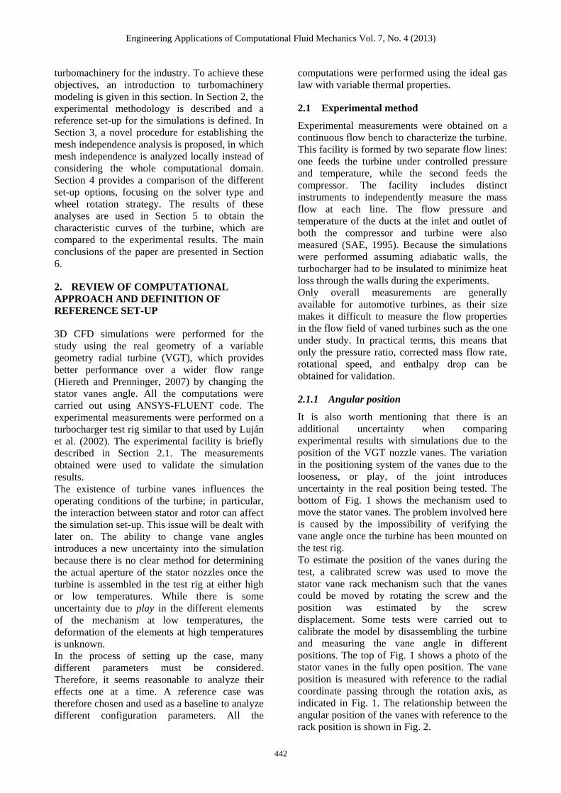
bottom of Fig. 1 shows the mechanism used to

move the stator vanes. The problem involved here

is caused by the impossibility of verifying the

vane angle once the turbine has been mounted on

the test rig.

To estimate the position of the vanes during the

test, a calibrated screw was used to move the

stator vane rack mechanism such that the vanes

could be moved by rotating the screw and the

position was estimated by the screw

displacement. Some tests were carried out to

calibrate the model by disassembling the turbine

and measuring the vane angle in different

positions. The top of Fig. 1 shows a photo of the

stator vanes in the fully open position. The vane

position is measured with reference to the radial

coordinate passing through the rotation axis, as

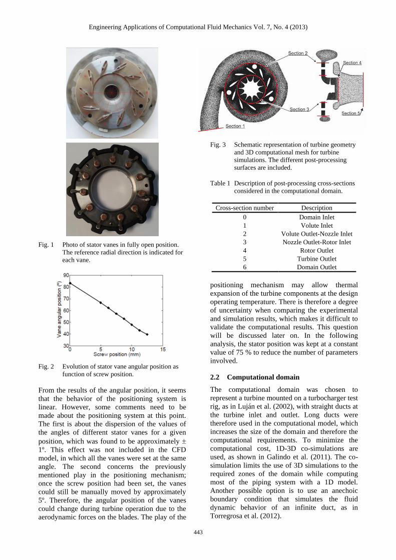
indicated in Fig. 1. The relationship between the

angular position of the vanes with reference to the

rack position is shown in Fig. 2.


443

Fig. 1 Photo of stator vanes in fully open position.

The reference radial direction is indicated for

each vane.

Fig. 2 Evolution of stator vane angular position as

function of screw position.

From the results of the angular position, it seems

that the behavior of the positioning system is

linear. However, some comments need to be

made about the positioning system at this point.

The first is about the dispersion of the values of

the angles of different stator vanes for a given

position, which was found to be approximately

1º. This effect was not included in the CFD

model, in which all the vanes were set at the same

angle. The second concerns the previously

mentioned play in the positioning mechanism;

once the screw position had been set, the vanes

could still be manually moved by approximately

5º. Therefore, the angular position of the vanes

could change during turbine operation due to the

aerodynamic forces on the blades. The play of the

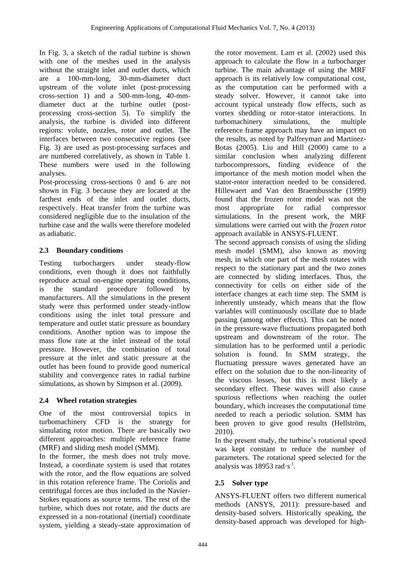
Fig. 3 Schematic representation of turbine geometry

and 3D computational mesh for turbine

simulations. The different post-processing

surfaces are included.

Table 1 Description of post-processing cross-sections

considered in the computational domain.

Cross-section number Description

0 Domain Inlet

1 Volute Inlet

2 Volute Outlet-Nozzle Inlet

3 Nozzle Outlet-Rotor Inlet

4 Rotor Outlet

5 Turbine Outlet

6 Domain Outlet

positioning mechanism may allow thermal

expansion of the turbine components at the design

operating temperature. There is therefore a degree

of uncertainty when comparing the experimental

and simulation results, which makes it difficult to

validate the computational results. This question

will be discussed later on. In the following

analysis, the stator position was kept at a constant

value of 75 % to reduce the number of parameters

involved.

2.2 Computational domain

The computational domain was chosen to

represent a turbine mounted on a turbocharger test

rig, as in Luján et al. (2002), with straight ducts at

the turbine inlet and outlet. Long ducts were

therefore used in the computational model, which

increases the size of the domain and therefore the

computational requirements. To minimize the

computational cost, 1D-3D co-simulations are

used, as shown in Galindo et al. (2011). The co-

simulation limits the use of 3D simulations to the

required zones of the domain while computing

most of the piping system with a 1D model.

Another possible option is to use an anechoic

boundary condition that simulates the fluid

dynamic behavior of an infinite duct, as in

Torregrosa et al. (2012).


444

In Fig. 3, a sketch of the radial turbine is shown

with one of the meshes used in the analysis

without the straight inlet and outlet ducts, which

are a 100-mm-long, 30-mm-diameter duct

upstream of the volute inlet (post-processing

cross-section 1) and a 500-mm-long, 40-mm-

diameter duct at the turbine outlet (post-

processing cross-section 5). To simplify the

analysis, the turbine is divided into different

regions: volute, nozzles, rotor and outlet. The

interfaces between two consecutive regions (see

Fig. 3) are used as post-processing surfaces and

are numbered correlatively, as shown in Table 1.

These numbers were used in the following

analyses.

Post-processing cross-sections 0 and 6 are not

shown in Fig. 3 because they are located at the

farthest ends of the inlet and outlet ducts,

respectively. Heat transfer from the turbine was

considered negligible due to the insulation of the

turbine case and the walls were therefore modeled

as adiabatic.

2.3 Boundary conditions

Testing turbochargers under steady-flow

conditions, even though it does not faithfully

reproduce actual on-engine operating conditions,

is the standard procedure followed by

manufacturers. All the simulations in the present

study were thus performed under steady-inflow

conditions using the inlet total pressure and

temperature and outlet static pressure as boundary

conditions. Another option was to impose the

mass flow rate at the inlet instead of the total

pressure. However, the combination of total

pressure at the inlet and static pressure at the

outlet has been found to provide good numerical

stability and convergence rates in radial turbine

simulations, as shown by Simpson et al. (2009).

2.4 Wheel rotation strategies

One of the most controversial topics in

turbomachinery CFD is the strategy for

simulating rotor motion. There are basically two

different approaches: multiple reference frame

(MRF) and sliding mesh model (SMM).

In the former, the mesh does not truly move.

Instead, a coordinate system is used that rotates

with the rotor, and the flow equations are solved

in this rotation reference frame. The Coriolis and

centrifugal forces are thus included in the Navier-

Stokes equations as source terms. The rest of the

turbine, which does not rotate, and the ducts are

expressed in a non-rotational (inertial) coordinate

system, yielding a steady-state approximation of

the rotor movement. Lam et al. (2002) used this

approach to calculate the flow in a turbocharger

turbine. The main advantage of using the MRF

approach is its relatively low computational cost,

as the computation can be performed with a

steady solver. However, it cannot take into

account typical unsteady flow effects, such as

vortex shedding or rotor-stator interactions. In

turbomachinery simulations, the multiple

reference frame approach may have an impact on

the results, as noted by Palfreyman and Martinez-

Botas (2005). Liu and Hill (2000) came to a

similar conclusion when analyzing different

turbocompressors, finding evidence of the

importance of the mesh motion model when the

stator-rotor interaction needed to be considered.

Hillewaert and Van den Braembussche (1999)

found that the frozen rotor model was not the

most appropriate for radial compressor

simulations. In the present work, the MRF

simulations were carried out with the frozen rotor

approach available in ANSYS-FLUENT.

The second approach consists of using the sliding

mesh model (SMM), also known as moving

mesh, in which one part of the mesh rotates with

respect to the stationary part and the two zones

are connected by sliding interfaces. Thus, the

connectivity for cells on either side of the

interface changes at each time step. The SMM is

inherently unsteady, which means that the flow

variables will continuously oscillate due to blade

passing (among other effects). This can be noted

in the pressure-wave fluctuations propagated both

upstream and downstream of the rotor. The

simulation has to be performed until a periodic

solution is found. In SMM strategy, the

fluctuating pressure waves generated have an

effect on the solution due to the non-linearity of

the viscous losses, but this is most likely a

secondary effect. These waves will also cause

spurious reflections when reaching the outlet

boundary, which increases the computational time

needed to reach a periodic solution. SMM has

been proven to give good results (Hellström,

2010).

In the present study, the turbine’s rotational speed

was kept constant to reduce the number of

parameters. The rotational speed selected for the

analysis was 18953 rad·s.1.

2.5 Solver type

ANSYS-FLUENT offers two different numerical

methods (ANSYS, 2011): pressure-based and

density-based solvers. Historically speaking, the

density-based approach was developed for high-


445

speed compressible flows, while the pressure-

based approach was used for incompressible and

mildly compressible flow. However, both

methods have now been extended to solve a wide

range of flow conditions beyond their initial

intent.

In both methods, momentum equations are used

to obtain the velocity field. In the pressure-based

approach, a pressure equation is derived by

combining the continuity and momentum

equations, while the density is calculated using

the equation of state. In the density-based solver,

the continuity equation is solved to obtain the

density field, while the pressure field is

determined from the equation of state. The two

numerical methods are based on a finite-volume

discretization procedure, but the linearization and

the approach to solving the discretized equations

are different. In general, the density-based method

is considered to be more accurate than the

pressure-based solver in terms of shock

resolution.

2.5.1 Pressure-based solver

As stated above, in the pressure-based solver, a

pressure equation is obtained from a combination

of the continuity and momentum equations. In

this way, the obtained velocity field satisfies the

continuity. Due to the nonlinearity and coupled

behavior of the flow equations, the solution

process involves iterations. Thus, the entire set of

governing equations (continuity for the velocity

field and pressure equation) is solved repeatedly

until the solution converges.

Segregated and coupled pressure-based

algorithms are available in ANSYS-FLUENT

(ANSYS, 2011). In the segregated algorithm,

each of the governing equations is solved

independently. In the coupled algorithm, the

momentum equations and the pressure-based

continuity equation are solved simultaneously. As

a general rule, the coupled algorithm has a higher

convergence speed than the segregated algorithm.

However, the memory requirement for the

coupled algorithm is also higher.

2.5.2 Density-based solver

In the same way, two formulations exist under the

density-based solver: implicit and explicit

methods (ANSYS, 2011). The implicit and

explicit density-based formulations differ in the

way that they linearize the coupled equations. In

the implicit formulation, the unknown value of a

given variable in each cell is computed using a

relationship that includes both existing and

unknown values from neighboring cells. The

system of equations for the unknowns is therefore

coupled, and these equations must be solved

simultaneously. On the other hand, in the explicit

formulation, the unknown value for a given

variable in each cell is computed using a

relationship that includes only the existing values.

The equations for the unknown values in each cell

can thus be solved one at a time to calculate the

unknown quantities.

In summary, the density-based explicit approach

solves for all variables cell by cell, while the

implicit approach solves for all flow variables in

all cells at the same time. Choosing an implicit or

explicit solver only applies to the coupled set of

flow equations. Transport equations for additional

scalars, e.g., turbulence, are solved segregated

from the coupled set. The greater stability of the

implicit formulation provides a converged steady-

state solution much faster than the explicit

formulation, although its memory requirements

are greater.

When a density-based numerical method is used

to obtain steady-state flow solutions, the temporal

terms are maintained in the equation. The

transient solution is thus computed until a steady-

state is reached. This procedure differs from that

for pressure-based methods, in which the terms

dealing with temporal variation are not included

in the discretized equations.

2.5.3 Spatial discretization

A second-order scheme for spatial discretization

is adopted for all flow equations. This scheme

computes the face values from the discrete values

stored in the cell centers for the evaluation of flux

terms.

2.6 Turbulence model

With the current computational capacities, a direct

numerical simulation in which the whole Navier-

Stokes equations are computed is only affordable

in simple cases (flat plate, pipes, channels, etc.).

In more complex cases, the turbulence needs to be

modeled, which constitutes a critical issue in CFD

simulations. Different approaches can be

followed: Reynolds averaged (RANS) or

unsteady Reynolds averaged (URANS) methods

in transient simulations or a detached-eddy

simulation (DES) (Strelets, 2001) or even a large-

eddy simulation (LES) (Smagorinsky, 1963).

Turbomachines are complex fluid dynamic

systems in which adverse pressure gradients and

flow separation can occur. Many works have been

published on the analysis of turbulence models in


446

turbomachinery simulations. Su et al. (2012)

compared RANS and LES for an incompressible

case. DES and LES models are considered to be

more accurate than RANS because they resolve a

part of the turbulence spectrum. However, they

have an unaffordable computational cost for the

purpose of the current work and other difficulties

arise, such as the appropriate definition of the

inlet boundary conditions (Tabor and Baba-

Ahmadi, 2010). The RANS approach was

therefore selected for this work. Aghaei-Tog et al.

(2008) analyzed different RANS turbulence

models in CFD radial turbomachinery

computations. The most commonly used RANS

models for internal flow problems are those

defined by two equations. Their main advantage

is their good trade-off between computational cost

and accuracy, such as in Menter’s SST turbulence

model (Menter, 1994). The SST model blends the

robust and accurate formulation of the k- model

(Wilcox, 1988) in the near-wall region with the

free-stream independence of the k- model in the

far field (Menter, 1992). In the SST turbulence

model, the transport of the principal turbulent

shear stress is taken into account, which allows

the correct response to adverse pressure gradients

to be obtained.

The SST model has been used in most of the

turbomachinery applications found in the

literature. Menter et al. (2004) applied the SST

model to turbomachinery simulations and found

good agreement between the computations and

the experimental data for all cases considered.

Another of its applications in turbomachinery

simulations can be found in the work by Pecnik et

al. (2001), in which the uncertainty of transition

prediction is analyzed. Simpson et al. (2009) used

the SST in CFD simulations of vaned and

vaneless radial turbines, obtaining good results.

These examples testify to the model’s ability to

capture the effects of Reynolds number variations

and flow separation over a wide range of

conditions. Based on the number of cases in the

literature in which the k- SST model has

provided good results, this model was adopted for

the computations in the present study.

2.7 Reference set-up

In the following section, the effect of the mesh

size on the results is evaluated to identify the

most suitable mesh for the computations. To

perform this mesh independence analysis, a

reference case must be defined. Apart from the

configuration decisions already mentioned in this

section, such as the domain geometry and

turbulence model, there are other model set-up

choices that have to be made. For computational

reasons, the analysis is performed using a

pressure-based solver and an MRF strategy for

rotor motion. In Section 4, the effect of the case

configuration will also be evaluated.

3. LOCAL MESH INDEPENDENCE

ANALYSIS

The first thing that must be analyzed when

dealing with 3D simulations is the geometry

considered, especially the mesh. The mesh should

be fine enough to faithfully reproduce the

geometry, which is usually achieved by searching

for the independence of the solution in terms of

the number of cells. The meshes used for the

computations in this work are similar to that

shown in Fig. 3.

The main difficulty in dealing with real

geometries is achieving the appropriate mesh. In

this work, a mixed polyhedral and extruded-

polygonal non-conformal mesh was used.

ANSYS-FLUENT makes it possible to generate a

polyhedral mesh from a tetrahedral mesh using

the algorithm described in the ANSYS (2009).

The greatest advantage of polyhedral meshes is

that they are more accurate than the equivalent

tetrahedral mesh. In other words, it is possible to

achieve the same resolution with fewer cells

(FLUENT, 2006). Polyhedral meshes have been

used to solve computational problems in

engineering, as in Tritthart and Gutknecht (2007),

who developed a method for solving Reynolds

equations with polyhedral cells, which showed

better behavior than quadrilateral cells in certain

problems. Baris and Mendonça (2011) used a

polyhedral mesh for turbocharger computations

and cited less numerical diffusion and a more

accurate gradient calculation as the benefits of

this type of mesh.

Once the mesh type is chosen, mesh

independence analysis should be performed.

Mesh independence analysis is usually conducted

by considering that finer meshes produce better

results due to the discretization error, which

decreases with cell size. The usual procedure

when dealing with turbomachinery simulations

consists of using different meshes with

increasingly small cell sizes, as used by Li (2009).

This procedure may seem straightforward in the

case of a simple system, particularly if the cells

are more or less uniformly distributed. However,

for a more complex system and if the real

geometry is considered, it may not be the most

appropriate because not all the subdomains of the


447

system require the same number of cells. This is

the case for the turbine, in which a smaller cell

size is preferable in the rotor region, where the

momentum interchange occurs, relative to that in

the ducts, which can be computed with a one-

dimensional approach. The procedure shown here

aims to optimize the resources in terms of cell

distribution.

It is worth mentioning at this point that even

though smaller cells theoretically produce better

results, there are other issues that have not been

taken into account. One is that if cell refinement

has not been properly carried out, it may increase

the cell aspect ratio, and the use of distorted cells

can introduce convergence errors and even

spurious solutions. The other issue is that RANS

turbulence models are usually applied in

combination with wall functions, which model

flow behavior near the wall. Although the k-

turbulence model was chosen and its automatic

wall treatment (Esch and Menter, 2003) has the

advantage of ensuring a high degree of grid

independence, the y+ values of the cells at the

walls must be within the range of application of

the wall function, as explained in the ANSYS

(2009). A thorough mesh refinement should

therefore be performed to prevent cells next to the

walls from having y+ values too low to accurately

use the wall functions or too high to resolve the

viscous sublayer.

As previously stated, the turbine was divided into

four different regions: the volute, stator, rotor, and

outlet regions. The local mesh independence

analysis proceeds as follows. First, a reference

case was defined in terms of the mesh. Each

turbine zone was analyzed independently. The

influence of mesh size on each region was

investigated by changing the grid in this zone

only, using the rest of the mesh from the reference

case. Simulations were performed with a

progressively finer mesh until the variation of the

solution of two consecutive cases was sufficiently

small, as is the usual procedure in standard mesh

independence analysis. At this point, the increase

in the computational cost of additional

refinements is not justified by the increase in

resolution. The process continues with the

analysis of the following turbine zone. When all

the subdomains have been evaluated, the

information obtained can be used to determine the

regions most worth refining to obtain a better cell

distribution. The numerical set-up described in

the previous section is used throughout the mesh

independence analysis.

To study the mesh refinement effect, two

parameters are analyzed at every refinement level:

mass flow through the current element and total

turbine torque. In the following subsections, the

meshing procedure and the local mesh

independence analysis of each turbine region are

described.

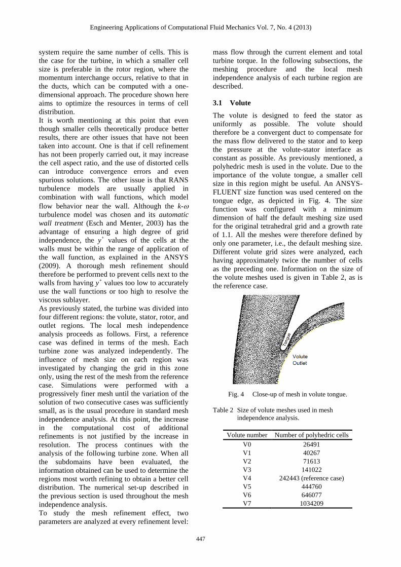
3.1 Volute

The volute is designed to feed the stator as

uniformly as possible. The volute should

therefore be a convergent duct to compensate for

the mass flow delivered to the stator and to keep

the pressure at the volute-stator interface as

constant as possible. As previously mentioned, a

polyhedric mesh is used in the volute. Due to the

importance of the volute tongue, a smaller cell

size in this region might be useful. An ANSYS-

FLUENT size function was used centered on the

tongue edge, as depicted in Fig. 4. The size

function was configured with a minimum

dimension of half the default meshing size used

for the original tetrahedral grid and a growth rate

of 1.1. All the meshes were therefore defined by

only one parameter, i.e., the default meshing size.

Different volute grid sizes were analyzed, each

having approximately twice the number of cells

as the preceding one. Information on the size of

the volute meshes used is given in Table 2, as is

the reference case.

Fig. 4 Close-up of mesh in volute tongue.

Table 2 Size of volute meshes used in mesh


Volute number Number of polyhedric cells

V0 26491

V1 40267

V2 71613

V3 141022

V4 242443 (reference case)

V5 444760

V6 646077

V7 1034209


448

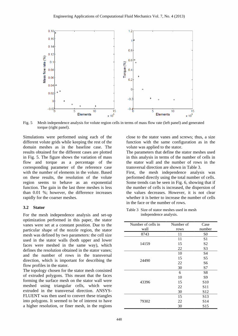
Fig. 5 Mesh independence analysis for volute region cells in terms of mass flow rate (left panel) and generated

torque (right panel).

Simulations were performed using each of the

different volute grids while keeping the rest of the

domain meshes as in the baseline case. The

results obtained for the different cases are plotted

in Fig. 5. The figure shows the variation of mass

flow and torque as a percentage of the

corresponding parameter of the reference case

with the number of elements in the volute. Based

on these results, the resolution of the volute

region seems to behave as an exponential

function. The gain in the last three meshes is less

than 0.01 %; however, the difference increases

rapidly for the coarser meshes.

3.2 Stator

For the mesh independence analysis and set-up

optimization performed in this paper, the stator

vanes were set at a constant position. Due to the

particular shape of the nozzle region, the stator

mesh was defined by two parameters: the cell size

used in the stator walls (both upper and lower

faces were meshed in the same way), which

defines the resolution obtained in the stator vanes;

and the number of rows in the transversal

direction, which is important for describing the

flow profiles in the stator.

The topology chosen for the stator mesh consisted

of extruded polygons. This meant that the faces

forming the surface mesh on the stator wall were

meshed using triangular cells, which were

extruded in the transversal direction. ANSYS-

FLUENT was then used to convert these triangles

into polygons. It seemed to be of interest to have

a higher resolution, or finer mesh, in the regions

close to the stator vanes and screws; thus, a size

function with the same configuration as in the

volute was applied to the stator.

The parameters that define the stator meshes used

in this analysis in terms of the number of cells in

the stator wall and the number of rows in the

transversal direction are shown in Table 3.

First, the mesh independence analysis was

performed directly using the total number of cells.

Some trends can be seen in Fig. 6, showing that if

the number of cells is increased, the dispersion of

the values decreases. However, it is not clear

whether it is better to increase the number of cells

in the face or the number of rows.

Table 3 Size of stator meshes used in mesh


Number of cells in

wall

Number of

rows

Case

number

8743 11 S0

14159

11 S1

15 S2

22 S3

24490

10 S4

15 S5

22 S6

30 S7

43396

6 S8

10 S9

15 S10

22 S11

30 S12

79302

15 S13

22 S14

30 S15


449

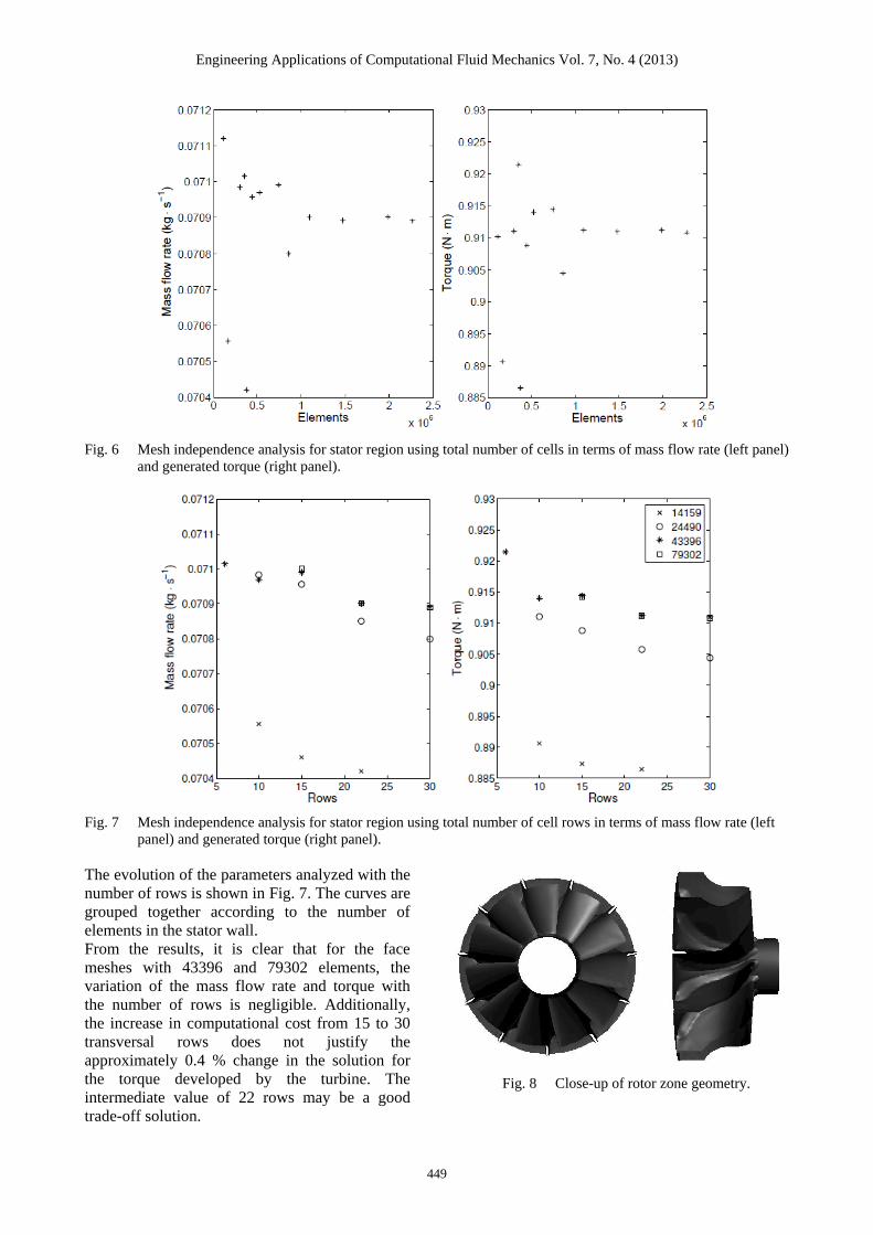
Fig. 6 Mesh independence analysis for stator region using total number of cells in terms of mass flow rate (left panel)

and generated torque (right panel).

Fig. 7 Mesh independence analysis for stator region using total number of cell rows in terms of mass flow rate (left

panel) and generated torque (right panel).

The evolution of the parameters analyzed with the

number of rows is shown in Fig. 7. The curves are

grouped together according to the number of

elements in the stator wall.

From the results, it is clear that for the face

meshes with 43396 and 79302 elements, the

variation of the mass flow rate and torque with

the number of rows is negligible. Additionally,

the increase in computational cost from 15 to 30

transversal rows does not justify the

approximately 0.4 % change in the solution for

the torque developed by the turbine. The

intermediate value of 22 rows may be a good

trade-off solution.

Fig. 8 Close-up of rotor zone geometry.


450

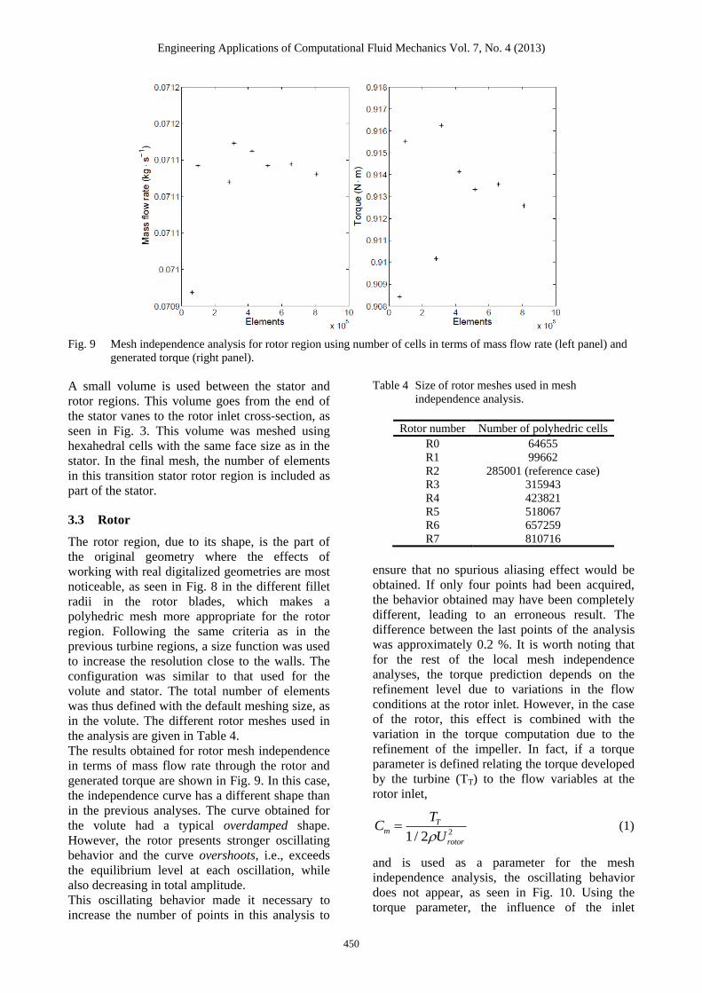
Fig. 9 Mesh independence analysis for rotor region using number of cells in terms of mass flow rate (left panel) and

generated torque (right panel).

A small volume is used between the stator and

rotor regions. This volume goes from the end of

the stator vanes to the rotor inlet cross-section, as

seen in Fig. 3. This volume was meshed using

hexahedral cells with the same face size as in the

stator. In the final mesh, the number of elements

in this transition stator rotor region is included as

part of the stator.

3.3 Rotor

The rotor region, due to its shape, is the part of

the original geometry where the effects of

working with real digitalized geometries are most

noticeable, as seen in Fig. 8 in the different fillet

radii in the rotor blades, which makes a

polyhedric mesh more appropriate for the rotor

region. Following the same criteria as in the

previous turbine regions, a size function was used

to increase the resolution close to the walls. The

configuration was similar to that used for the

volute and stator. The total number of elements

was thus defined with the default meshing size, as

in the volute. The different rotor meshes used in

the analysis are given in Table 4.

The results obtained for rotor mesh independence

in terms of mass flow rate through the rotor and

generated torque are shown in Fig. 9. In this case,

the independence curve has a different shape than

in the previous analyses. The curve obtained for

the volute had a typical overdamped shape.

However, the rotor presents stronger oscillating

behavior and the curve overshoots, i.e., exceeds

the equilibrium level at each oscillation, while

also decreasing in total amplitude.

This oscillating behavior made it necessary to

increase the number of points in this analysis to

Table 4 Size of rotor meshes used in mesh


Rotor number Number of polyhedric cells

R0 64655

R1 99662

R2 285001 (reference case)

R3 315943

R4 423821

R5 518067

R6 657259

R7 810716

ensure that no spurious aliasing effect would be

obtained. If only four points had been acquired,

the behavior obtained may have been completely

different, leading to an erroneous result. The

difference between the last points of the analysis

was approximately 0.2 %. It is worth noting that

for the rest of the local mesh independence

analyses, the torque prediction depends on the

refinement level due to variations in the flow

conditions at the rotor inlet. However, in the case

of the rotor, this effect is combined with the

variation in the torque computation due to the

refinement of the impeller. In fact, if a torque

parameter is defined relating the torque developed

by the turbine (TT) to the flow variables at the

rotor inlet,

21/ 2

Tm

rotor

TC

U (1)

and is used as a parameter for the mesh

independence analysis, the oscillating behavior

does not appear, as seen in Fig. 10. Using the

torque parameter, the influence of the inlet


451

Fig. 10 Evolution of torque coefficient with number of cells in turbine rotor region.

Fig. 11 Mesh independence analysis for outlet region using total number of cells in terms of mass flow rate (left

panel) and generated torque (right panel).

conditions on the calculated torque is reduced;

thus, the torque accuracy is only determined by

the accuracy of predicting the exchange of

momentum with the rotor walls.

3.4 Outlet region

The turbine outlet region lies between the rotor

outlet and the turbine outlet (Sections 4 and 5 in

Fig. 3). As in previous cases, different mesh sizes

were used in the outlet region, and a uniform

tetrahedral mesh was used for the subsequent

conversion to polyhedra. The various meshes are

described in Table 5.

The results obtained for the outlet region mesh

independence in terms of the mass flow rate

through the cross-section and the torque generated

by the turbine are shown in Fig. 11, which shows

Table 5 Size of outlet region meshes used in mesh


Outlet region number Number of polyhedric cells

O0 29281

O1 56392

O2 128671 (reference case)

O3 207451

O4 432179

a very pronounced trend. In the meshes with more

than 105 elements, the parameters change little.

However, the meshes with fewer elements do

show large variations.

3.5 Final considerations and selected mesh

The local mesh independence of the different

turbine components was analyzed in the previous


452

subsections. From these results, it is possible to

establish the best cell distribution between the

different turbine zones according to the

computational resources available. However, a

number of points should be made before

proceeding.

First, the current analysis was performed by

separating the influence of the different

components. If a final mesh resolution of

approximately 1 % accuracy is sought, the

relative error in each of the components should be

lower (a limit of approximately 0.2 % was

considered in this work) to remain on the

conservative side.

The analysis was performed by assuming that the

behavior of the different components was

independent to justify the procedure used, in

which the local mesh independence of each

component was studied by replacing only that

region of the mesh in a reference case and thus all

the variations between the different simulations

were attributed to the replaced zone. However, it

is not clear that if mesh independence has been

achieved using the rest of the regions in the

reference case, it will also be independent once all

the regions have been changed to the refined

mesh. To ensure the independence of the final

mesh, some additional simulations were

performed, substituting each of the mesh

components for the finest one used in the previous

analysis. The effect of the reference case was

assessed in this way. In the simulations performed

after refining the different zones in the selected

mesh, the solution varied by less than 0.2 % in

terms of mass flow and torque, thus ensuring

mesh independence.

Finally, the inlet and outlet ducts were not

included in the mesh independence analysis. The

inlet and outlet were meshed using a cell size

similar to that used in the volute, and an extruded

scheme was used to mesh the volume.

3.5.1 Final mesh

From the results of the mesh independence

analysis, the following meshes were chosen for

each of the components:

It is important to emphasize here that the mesh

selected for the stator was the one with 43396

cells in the stator wall and 22 rows in the

transversal direction. The number of elements in

the ducts is not included in Table 6, but the cells

are counted in the total number of elements. The

inlet duct contains approximately 1.2 % of the

total cells, while the outlet duct contains

approximately 4.9 %. The total number of cells

Table 6 Number of elements in mesh of different

turbine components for mesh selected using

mesh independence analysis.

Zone Number of

polyhedric cells (%)

Average cell

volume

(mm3/cell)

Volute 646077 (23.3 %) 0.21

Stator 1094812 (39.5 %) 0.017

Rotor 657259 (23.6 %) 0.017

Outlet region 207451 (7.5 %) 0.40

Total number

of elements 2777122 0.090

for the turbine alone is 2605599. The last column

in Table 6 provides the average cell volume

(mm3/cell) in each turbine zone. As expected, the

cell size required in the volute is larger than that

obtained for the stator and rotor.

4. SET-UP COMPARISON

After selecting the appropriate mesh, the

computational cases must be configured.

Different parameters must be considered in this

procedure. The most important of these

parameters for the case of turbomachinery

simulations are the moving mesh strategy, the

solver used in the simulations, and the temporal

discretization. This section compares the effect of

the different configurations.

4.1 Type of solver

Simulations were carried out with different mesh

sizes to compare the behavior of pressure- and

density-based numerical methods. These

calculations were performed using the multiple

reference frame approach to simulate rotor

motion. The results were compared in terms of

the corrected mass flow and the power developed

by the turbine. The turbine corrected mass flow is

defined as

0*

0

t

t

Tm

Tm

p

p

(2)

Hereinafter, the corrected mass flow is based on a

pressure (p0) of 101325 Pa and a temperature (T0)

of 288.15 K. The results of the different

simulations are shown in Fig. 12.

Certain conclusions can be drawn from the

results. First, although the ANSYS-FLUENT

user’s manual maintains that both solvers are


453

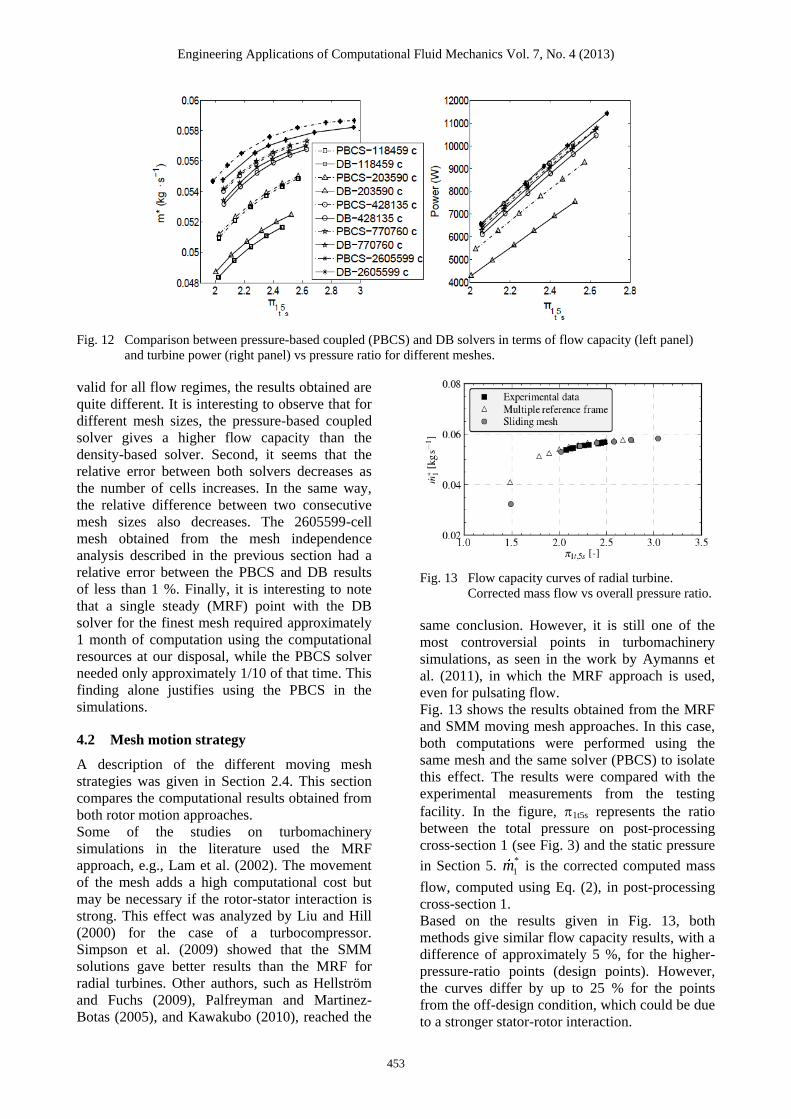
Fig. 12 Comparison between pressure-based coupled (PBCS) and DB solvers in terms of flow capacity (left panel)

and turbine power (right panel) vs pressure ratio for different meshes.

valid for all flow regimes, the results obtained are

quite different. It is interesting to observe that for

different mesh sizes, the pressure-based coupled

solver gives a higher flow capacity than the

density-based solver. Second, it seems that the

relative error between both solvers decreases as

the number of cells increases. In the same way,

the relative difference between two consecutive

mesh sizes also decreases. The 2605599-cell

mesh obtained from the mesh independence

analysis described in the previous section had a

relative error between the PBCS and DB results

of less than 1 %. Finally, it is interesting to note

that a single steady (MRF) point with the DB

solver for the finest mesh required approximately

1 month of computation using the computational

resources at our disposal, while the PBCS solver

needed only approximately 1/10 of that time. This

finding alone justifies using the PBCS in the

simulations.

4.2 Mesh motion strategy

A description of the different moving mesh

strategies was given in Section 2.4. This section

compares the computational results obtained from

both rotor motion approaches.

Some of the studies on turbomachinery

simulations in the literature used the MRF

approach, e.g., Lam et al. (2002). The movement

of the mesh adds a high computational cost but

may be necessary if the rotor-stator interaction is

strong. This effect was analyzed by Liu and Hill

(2000) for the case of a turbocompressor.

Simpson et al. (2009) showed that the SMM

solutions gave better results than the MRF for

radial turbines. Other authors, such as Hellström

and Fuchs (2009), Palfreyman and Martinez-

Botas (2005), and Kawakubo (2010), reached the

Fig. 13 Flow capacity curves of radial turbine.

Corrected mass flow vs overall pressure ratio.

same conclusion. However, it is still one of the

most controversial points in turbomachinery

simulations, as seen in the work by Aymanns et

al. (2011), in which the MRF approach is used,

even for pulsating flow.

Fig. 13 shows the results obtained from the MRF

and SMM moving mesh approaches. In this case,

both computations were performed using the

same mesh and the same solver (PBCS) to isolate

this effect. The results were compared with the

experimental measurements from the testing

facility. In the figure, 1t5s represents the ratio

between the total pressure on post-processing

cross-section 1 (see Fig. 3) and the static pressure

in Section 5. *

1m is the corrected computed mass

flow, computed using Eq. (2), in post-processing

cross-section 1.

Based on the results given in Fig. 13, both

methods give similar flow capacity results, with a

difference of approximately 5 %, for the higher-

pressure-ratio points (design points). However,

the curves differ by up to 25 % for the points

from the off-design condition, which could be due

to a stronger stator-rotor interaction.


454

As previously stated, there is an uncertainty in

positioning the stator at the desired aperture,

which made it difficult to acquire experimental

data to validate the computations. The procedure

applied to compare the experimental points was

as follows: the turbine installed in the test rig was

set at a given pressure ratio, and the stator

aperture was changed by adjusting the rack of the

positioning system until the corrected mass flow

matched the previously computed value. Once the

stator position had been set, a complete curve was

obtained for the rotational speed considered. The

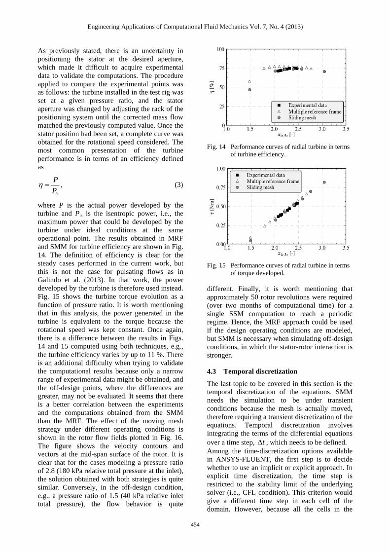
most common presentation of the turbine

performance is in terms of an efficiency defined

as

,is

P

P (3)

where P is the actual power developed by the

turbine and Pis is the isentropic power, i.e., the

maximum power that could be developed by the

turbine under ideal conditions at the same

operational point. The results obtained in MRF

and SMM for turbine efficiency are shown in Fig.

14. The definition of efficiency is clear for the

steady cases performed in the current work, but

this is not the case for pulsating flows as in

Galindo et al. (2013). In that work, the power

developed by the turbine is therefore used instead.

Fig. 15 shows the turbine torque evolution as a

function of pressure ratio. It is worth mentioning

that in this analysis, the power generated in the

turbine is equivalent to the torque because the

rotational speed was kept constant. Once again,

there is a difference between the results in Figs.

14 and 15 computed using both techniques, e.g.,

the turbine efficiency varies by up to 11 %. There

is an additional difficulty when trying to validate

the computational results because only a narrow

range of experimental data might be obtained, and

the off-design points, where the differences are

greater, may not be evaluated. It seems that there

is a better correlation between the experiments

and the computations obtained from the SMM

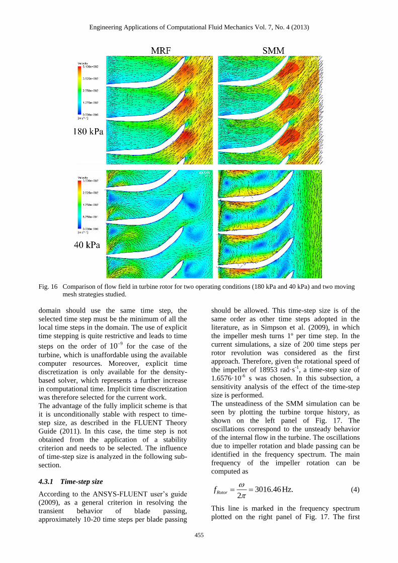
than the MRF. The effect of the moving mesh

strategy under different operating conditions is

shown in the rotor flow fields plotted in Fig. 16.

The figure shows the velocity contours and

vectors at the mid-span surface of the rotor. It is

clear that for the cases modeling a pressure ratio

of 2.8 (180 kPa relative total pressure at the inlet),

the solution obtained with both strategies is quite

similar. Conversely, in the off-design condition,

e.g., a pressure ratio of 1.5 (40 kPa relative inlet

total pressure), the flow behavior is quite

Fig. 14 Performance curves of radial turbine in terms

of turbine efficiency.

Fig. 15 Performance curves of radial turbine in terms

of torque developed.

different. Finally, it is worth mentioning that

approximately 50 rotor revolutions were required

(over two months of computational time) for a

single SSM computation to reach a periodic

regime. Hence, the MRF approach could be used

if the design operating conditions are modeled,

but SMM is necessary when simulating off-design

conditions, in which the stator-rotor interaction is

stronger.

4.3 Temporal discretization

The last topic to be covered in this section is the

temporal discretization of the equations. SMM

needs the simulation to be under transient

conditions because the mesh is actually moved,

therefore requiring a transient discretization of the

equations. Temporal discretization involves

integrating the terms of the differential equations

over a time step, t , which needs to be defined.

Among the time-discretization options available

in ANSYS-FLUENT, the first step is to decide

whether to use an implicit or explicit approach. In

explicit time discretization, the time step is

restricted to the stability limit of the underlying

solver (i.e., CFL condition). This criterion would

give a different time step in each cell of the

domain. However, because all the cells in the


455

Fig. 16 Comparison of flow field in turbine rotor for two operating conditions (180 kPa and 40 kPa) and two moving

mesh strategies studied.

domain should use the same time step, the

selected time step must be the minimum of all the

local time steps in the domain. The use of explicit

time stepping is quite restrictive and leads to time

steps on the order of 910

for the case of the

turbine, which is unaffordable using the available

computer resources. Moreover, explicit time

discretization is only available for the density-

based solver, which represents a further increase

in computational time. Implicit time discretization

was therefore selected for the current work.

The advantage of the fully implicit scheme is that

it is unconditionally stable with respect to time-

step size, as described in the FLUENT Theory

Guide (2011). In this case, the time step is not

obtained from the application of a stability

criterion and needs to be selected. The influence

of time-step size is analyzed in the following sub-

section.

4.3.1 Time-step size

According to the ANSYS-FLUENT user’s guide

(2009), as a general criterion in resolving the

transient behavior of blade passing,

approximately 10-20 time steps per blade passing

should be allowed. This time-step size is of the

same order as other time steps adopted in the

literature, as in Simpson et al. (2009), in which

the impeller mesh turns 1º per time step. In the

current simulations, a size of 200 time steps per

rotor revolution was considered as the first

approach. Therefore, given the rotational speed of

the impeller of 18953 rad·s-1, a time-step size of

1.6576·10-6 s was chosen. In this subsection, a

sensitivity analysis of the effect of the time-step

size is performed.

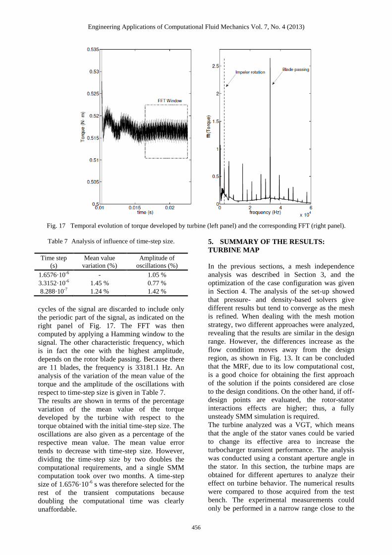
The unsteadiness of the SMM simulation can be

seen by plotting the turbine torque history, as

shown on the left panel of Fig. 17. The

oscillations correspond to the unsteady behavior

of the internal flow in the turbine. The oscillations

due to impeller rotation and blade passing can be

identified in the frequency spectrum. The main

frequency of the impeller rotation can be

computed as

3016.46Hz.2

Rotorf

(4)

This line is marked in the frequency spectrum

plotted on the right panel of Fig. 17. The first


456

Fig. 17 Temporal evolution of torque developed by turbine (left panel) and the corresponding FFT (right panel).

Table 7 Analysis of influence of time-step size.

Time step

(s)

Mean value

variation (%)

Amplitude of

oscillations (%)

1.6576·10-6 - 1.05 %

3.3152·10-6 1.45 % 0.77 %

8.288·10-7 1.24 % 1.42 %

cycles of the signal are discarded to include only

the periodic part of the signal, as indicated on the

right panel of Fig. 17. The FFT was then

computed by applying a Hamming window to the

signal. The other characteristic frequency, which

is in fact the one with the highest amplitude,

depends on the rotor blade passing. Because there

are 11 blades, the frequency is 33181.1 Hz. An

analysis of the variation of the mean value of the

torque and the amplitude of the oscillations with

respect to time-step size is given in Table 7.

The results are shown in terms of the percentage

variation of the mean value of the torque

developed by the turbine with respect to the

torque obtained with the initial time-step size. The

oscillations are also given as a percentage of the

respective mean value. The mean value error

tends to decrease with time-step size. However,

dividing the time-step size by two doubles the

computational requirements, and a single SMM

computation took over two months. A time-step

size of 1.6576·10-6 s was therefore selected for the

rest of the transient computations because

doubling the computational time was clearly

unaffordable.

5. SUMMARY OF THE RESULTS:

TURBINE MAP

In the previous sections, a mesh independence

analysis was described in Section 3, and the

optimization of the case configuration was given

in Section 4. The analysis of the set-up showed

that pressure- and density-based solvers give

different results but tend to converge as the mesh

is refined. When dealing with the mesh motion

strategy, two different approaches were analyzed,

revealing that the results are similar in the design

range. However, the differences increase as the

flow condition moves away from the design

region, as shown in Fig. 13. It can be concluded

that the MRF, due to its low computational cost,

is a good choice for obtaining the first approach

of the solution if the points considered are close

to the design conditions. On the other hand, if off-

design points are evaluated, the rotor-stator

interactions effects are higher; thus, a fully

unsteady SMM simulation is required.

The turbine analyzed was a VGT, which means

that the angle of the stator vanes could be varied

to change its effective area to increase the

turbocharger transient performance. The analysis

was conducted using a constant aperture angle in

the stator. In this section, the turbine maps are

obtained for different apertures to analyze their

effect on turbine behavior. The numerical results

were compared to those acquired from the test

bench. The experimental measurements could

only be performed in a narrow range close to the


457

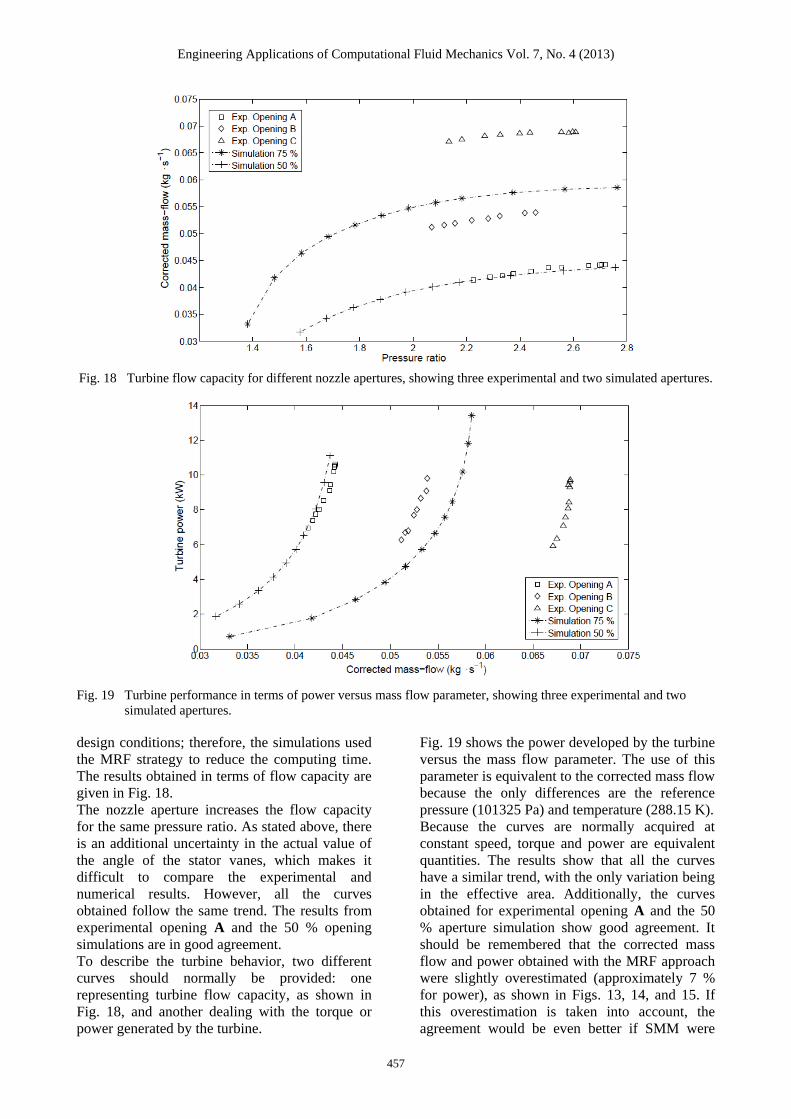
Fig. 18 Turbine flow capacity for different nozzle apertures, showing three experimental and two simulated apertures.

Fig. 19 Turbine performance in terms of power versus mass flow parameter, showing three experimental and two

simulated apertures.

design conditions; therefore, the simulations used

the MRF strategy to reduce the computing time.

The results obtained in terms of flow capacity are

given in Fig. 18.

The nozzle aperture increases the flow capacity

for the same pressure ratio. As stated above, there

is an additional uncertainty in the actual value of

the angle of the stator vanes, which makes it

difficult to compare the experimental and

numerical results. However, all the curves

obtained follow the same trend. The results from

experimental opening A and the 50 % opening

simulations are in good agreement.

To describe the turbine behavior, two different

curves should normally be provided: one

representing turbine flow capacity, as shown in

Fig. 18, and another dealing with the torque or

power generated by the turbine.

Fig. 19 shows the power developed by the turbine

versus the mass flow parameter. The use of this

parameter is equivalent to the corrected mass flow

because the only differences are the reference

pressure (101325 Pa) and temperature (288.15 K).

Because the curves are normally acquired at

constant speed, torque and power are equivalent

quantities. The results show that all the curves

have a similar trend, with the only variation being

in the effective area. Additionally, the curves

obtained for experimental opening A and the 50

% aperture simulation show good agreement. It

should be remembered that the corrected mass

flow and power obtained with the MRF approach

were slightly overestimated (approximately 7 %

for power), as shown in Figs. 13, 14, and 15. If

this overestimation is taken into account, the

agreement would be even better if SMM were


458

used. Due to the similarity between the

experimental and numerical results, the method

developed for the simulations can be considered

satisfactory.

6. CONCLUSIONS

This paper describes a CFD turbine simulation

method. First, an assessment was made of the

different CFD modeling options, focusing on a

description of the turbine used, boundary

conditions and turbulence model. The selection of

the turbulence model was based on several works

in the literature that successfully applied the

SST model to turbomachinery simulations.

As boundary conditions, total pressure and

temperature were imposed in the inlet cross-

section and static pressure at the domain outlet

throughout the work. A description of the

experimental facility and the measuring sensors

used to acquire the validation data was also given.

To optimize the distribution of cells in the mesh, a

new procedure was developed to analyze mesh

independence. The general mesh independence

procedure is based on analyzing the total number

of cells in the mesh. In this work, the analysis was

performed by dividing the turbine into zones: the

volute, stator, rotor, and outlet regions. The cell

size of each zone was varied and replaced in a

reference case until the independence of the

current region was achieved. The same procedure

was repeated for the different regions. Using this

new strategy, a more appropriate cell distribution

can be obtained than that provided by a standard

mesh independence analysis. One possible

limitation of this procedure is that it assumes that

the mesh independence analysis of each

subdomain does not depend on the mesh in the

other regions. This problem was addressed in the

paper, and the defined mesh was found to fulfill

the requirements. It is also important to

emphasize that the mesh independence was

evaluated under certain operating conditions, and

the mesh obtained could vary if these conditions

were to change, particularly when working under

off-design conditions. However, analyzing the

mesh for multiple operating points involves an

unacceptable computational cost. This novel

procedure has been applied to the case of a radial

turbine. However, the methodology could be used

for the mesh independence analysis of any

complex system.

Next, the different options available in ANSYS-

FLUENT for the case configuration were

analyzed. These options address solver type,

moving mesh strategy and time-step size.

Density- and pressure-based solvers give different

results. However, the relative error decreases as

the number of cells in the mesh increases. Two

different approaches were considered for rotor

motion strategy: multiple reference frame and the

sliding mesh model. The first approach has a

much lower computational cost and gives a good

approximation (approximately 7 % error in

torque) if the operating point is close to the design

conditions and was thus applied to obtain the

characteristic curves of the turbine. However,

when off-design points are considered, the error

increases because the transient effects due to

rotor-stator interaction increase, and it is therefore

necessary to perform a fully transient simulation

and actually rotate the mesh to capture this

behavior.

Finally, because a VGT turbine was analyzed, the

effect of nozzle aperture on turbine flow capacity

and the performance curve was studied. The

results were compared with experimental

measurements taken from a turbocharger test rig.

The agreement between both sets of results

validates the computational method developed.

ACKNOWLEDGEMENTS

The authors are indebted to the Spanish

Ministerio de Economía y Competitividad through

Project TRA 2010-16205.

REFERENCES

1. Aghaei tog R, Tousi AM, Tourani A (2008).

Comparison of turbulence methods in CFD

analysis of compressible flows in radial

turbomachines. Aircraft Engineering and

Aerospace Technology: An International

Journal 80(6):657-665.

2. ANSYS (2009). Ansys Fluent 12.0 User's

Guide. Canonsburg, PA: ANSYS Inc.

3. ANSYS (2011). ANSYS FLUENT Theory

Guide. ANSYS Inc.

4. Aymanns R, Scharf J, Uhlmann T, Lückmann

D (2011). A revision of quasi steady

modelling of turbocharger turbines in the

simulation of pulse charged engines. 16th

Supercharging Conference.

5. Baines NC (2005). Fundamentals of

Turbocharging. Concepts NREC.

6. Baines NC (2010), Turbocharger turbine

pulse flow performance and modeling - 25

years on. 9th Int. Conf. Turbochargers and

Turbocharging, 347-362.


459

7. Baris O, Mendonça F (2011). Automotive

turbocharger compressor CFD and extension

towards incorporating installation effects.

Proceedings of the ASME Turbo Expo 2011:

Power for Land, Sea and Air, GT2011-46796.

8. Blanco-Marigorta E, Fernández-Francos J,

González-Pérez J, Santolaria-Morros C

(2000). Numerical flow simulation in a

centrifugal pump with impeller-volute

interaction. ASME 2000 Fluids Engineering

Division Summer Meeting.

9. Dai J, Ijichi N, Tange H, Shibata H, Tamaki

H, Yamaguchi S (2004). Comparison of

internal flow field between experiment and

computation in a radial turbine impeller.

JSME International Journal Series B

47(1):48-56.

10. Decombes G, Pichouron JF, Maroteaux F,

Moreno N, Jullien J (2010). Simulation of the

performance of a variable geometry

turbocharger for diesel engine road

propulsion. International Journal of

Thermodynamics 5(3):139-149.

11. Esch T, Menter FR (2003). Heat transfer

predictions based on two-equation turbulence

models with advanced wall treatment.

Proceedings of the 4th International

Symposium on Turbulence, Heat & Mass

Transfer, Antalya, Turkey, 614-621.

12. FLUENT (2006). FLUENT 6.3 Validation

Guide.

13. Galindo J, Serrano JR, Guardiola C, Cervelló

C (2006). Surge limit definition in a specific

test bench for the characterization of

automotive turbochargers. Experimental

Thermal and Fluid Science 30(5):449-462.

14. Galindo J, Tiseira A, Fajardo P, Navarro R

(2011). Coupling methodology of 1D finite

difference and 3D finite volume CFD codes

based on the method of characteristics.

Mathematical and Computer Modelling 54(7-

8):1738-1746.

15. Galindo J, Fajardo P, Navarro R, García-

Cuevas LM (2013). Characterization of a

radial turbocharger turbine in pulsating flow

by means of CFD and its application to

engine modeling. Applied Energy 103:116-

127.

16. Hellström F, Fuchs L (2008). Effects of inlet

conditions on the turbine performance of a

radial turbine. Proceedings of the ASME

Turbo Expo 2008: Power for Land, Sea and

Air (6).

17. Hellström F, Fuchs L (2009). Numerical

computation of the pulsatile flow in a

turbocharger with realistic inflow conditions

from an exhaust manifold. Proceedings of

ASME Turbo Expo 2009: Power for Land,

Sea and Air, GT2009-5961.

18. Hellström F (2010). Numerical Computations

of the Unsteady Flow in Turbochargers. PhD

thesis, Royal Institute of Technology KTH

Fluid Physics.

19. Hiereth H, Prenninger P (2007). Charging the

Internal Combustion Engine. Springer

Verlag.

20. Hillewaert K, Van den Braembussche RA

(1998). Numerical Simulation of Impeller-

Volute Interaction in Centrifugal

Compressors. ASME Paper No. 98-GT-244.

21. Japikse D, Baines NC (1997). Introduction to

Turbomachinery. Oxford University Press.

22. Kawakubo T (2010). Unsteady rotor-stator

interaction of a radial-inflow turbine with

variable nozzle vanes. Proc. of ASME Turbo

Expo 2010: Power for Land, Sea and Air,

GT2010-23677.

23. Kreuz-Ihli T, Filsinger D, Schulz A, Wittig S

(2000). Numerical and experimental study of

unsteady flow field and vibration in radial in

flow turbines. Journal of Turbomachinery

122:247-254.

24. Lam JKW, Roberts QDH, McDonnell GT

(2002). Flow modelling of a turbocharger

turbine under pulsating flow. ImechE

Conference Transactions from 7th

International Conference on Turbochargers

and Turbocharging, 14-15.

25. Li H (2009). Fluid flow analysis of a single-

stage centrifugal fan with a ported diffuser.

Engineering Applications of Computational

Fluid Mechanics 3:147-163.

26. Liu Z, Hill DL (2000). Issues surrounding

multiple frames of reference models for turbo

compressor applications. Fifteenth

International Compressor Engineering

Conference, Purdue University, USA.

27. Luján JM, Bermúdez V, Serrano JR, Cervelló

C (2002). Test Bench for Turbocharger

Groups Characterization. SAE Paper 2002-

01-0163.

28. Menter FR (1992). Influence of freestream

values on k-omega turbulence model

predictions. AIAA journal 30:1657-1659.

29. Menter FR (1994). Two-equation eddy-

viscosity turbulence models for engineering

applications. AIAA journal 32(8):1598-1605.

30. Menter FR, Langtry R, Hansen T (2004).

CFD simulation of turbomachinery flows

verification, validation and modeling.

European Congress on Computational


460

Methods in Applied Sciences and

Engineering, ECCOMAS.

31. Palfreyman D, Martinez-Botas RF (2005).

The pulsating flow field in a mixed flow

turbocharger turbine: An experimental and

computational study. Journal of

Turbomachinery 127(1):144-155.

32. Pecnik R, Witteveen JAS, Iaccarino G (2011).

Uncertainty quantification for laminar-

turbulent transition prediction in RANS

turbomachinery applications. 49th AIAA

Aerospace Sciences Meeting including the

New Horizons Forum and Aerospace

Exposition.

33. Rajoo S, Botas RM (2008). Variable

geometry mixed flow turbine for

turbochargers: An experimental study.

International Journal of Fluid Machinery and

Systems 1(1):155-168.

34. SAE (1995). Supercharching Testing

Standards.

35. Simpson AT, Spence SWT, Watterson JK

(2009). A comparison of the flowstructures

and losses within vaned and vaneless stators

for radial turbines. Journal of

Turbomachinery 131(3), 031010.

36. Smagorinsky J (1963). General circulation

experiments with the primitive equations.

Monthly Weather Review 91(3):99-164.

37. Spence SWT, Rosborough RSE, Artt D,

McCullough G (2007). A direct performance

comparison of vaned and vaneless stators for

radial turbines. Journal of Turbomachinery

129(1):53-61.

38. Strelets M (2001). Detached eddy simulation

of massively separated flows. 39th AIAA

Aerospace Sciences Meeting and Exhibit.

39. Su WT, Li FC, Li XB, Wei XZ, Zhao Y

(2012). Assessment of LES performance in

simulating complex 3D flows in

turbomachines. Engineering Applications of

Computational Fluid Mechanics 6(3):356-

365.

40. Tabor GR, Baba-Ahmadi MH (2010). Inlet

conditions for large eddy simulation: A

review. Computers and Fluids 39:553-567.

41. Thakker A, Hourigan F (2005).

Computational fluid dynamics analysis of a

0.6 m, 0.6 hub-to-tip ratio impulse turbine

with fixed guide vanes. Renewable Energy

30(9):1387-1399.

42. Torregrosa AJ, Fajardo P, Gil A, Navarro R

(2012). Development of a non-reflecting

boundary condition for its application in 3D

computational fluid dynamic codes.

Engineering Applications of Computational

Fluid Mechanics 6(3):447-460.

43. Tritthart M, Gutknecht D (2007). Three-

dimensional simulation of free-surface flows

using polyhedral finite volumes. Engineering

Applications of Computational Fluid

Mechanics 1(1):1-14.

44. Wilcox DC (1988). Reassessment of the

scale-determining equation for advanced

turbulence models. AIAA Journal

26(11):1299-1310.

Set-up analysis and Optimization of CFD Simulations for Radial Turbines

Documents

Transcript of Set-up analysis and Optimization of CFD Simulations for Radial Turbines