water

Article

Efficiency Assessment for Rehabilitated Francis Turbines UsingURANS Simulations

Philippe Martineau Rousseau, Azzeddine Soulaïmani * and Michel Sabourin

Citation: Martineau Rousseau, P.;

Soulaïmani, A.; Sabourin, M.

Efficiency Assessment for

Rehabilitated Francis Turbines Using

URANS Simulations. Water 2021, 13,

1883. https://doi.org/10.3390/

w13141883

Academic Editor: Jochen Aberle

Received: 16 May 2021

Accepted: 30 June 2021

Published: 7 July 2021

Publisher’s Note: MDPI stays neutral

with regard to jurisdictional claims in

published maps and institutional affil-

iations.

Copyright: © 2021 by the authors.

Licensee MDPI, Basel, Switzerland.

This article is an open access article

distributed under the terms and

conditions of the Creative Commons

Attribution (CC BY) license (https://

creativecommons.org/licenses/by/

4.0/).

Département de Génie Mécanique, École de Technologie Supérieure, Montréal, 1100 rue Notre Dame Ouest,Montreal, QC H3C 1K3, Canada; phil.mart.rous@gmail.com (P.M.R.); cc-Michel.Sabourin@etsmtl.ca (M.S.)* Correspondence: azzeddine.soulaimani@etsmtl.ca

Abstract: Due to the large number of aging hydraulic turbines in North America, rehabilitation is agrowing market as these turbines have low efficiency compared to modern ones. ComputationalFluid Dynamics identifies components with poor hydraulic performance. The models often usedin industry are based on individually analyzing the sub-components of a turbine instead of fullturbine simulations due to computational and time limitations. An industrial case has shown thatsuch analyses may lead to underestimating the efficiency increases by modifying the stay vane. Theunsteady full turbine simulation proposes to simulate all components simultaneously to assess thisefficiency augmentation due to stay vane rehabilitation. The developed simulation methodology isused to evaluate the efficiency increase and the flow of two rehabilitated turbines with stay vanemodifications. Comparison with model tests shows the accuracy of the simulations. However, themethodology used shows imprecision in predicting the efficiency increase compared to model tests.Further works should consider the use of more complex flow modeling methods to measure theefficiency increase by the stay vane modifications.

Keywords: Computational Fluid Dynamics; hydraulic turbine; Francis turbine; hydraulic rehabilita-tion; efficiency

1. Introduction

Hydroelectricity provides approximately 16.2% of the total energy consumed world-wide [1]. With more than 100 years of existence in North America, hydropower produces60% of the electricity consumed in Canada and approximately 10% of the needs of theUnited States [2]. A large number of plants provide this electricity, and many of them mustbe rehabilitated to assure continued operation. Major maintenance of a turbine-generatoroften involves the replacement of the runner as well as hydraulic modifications and is anexcellent opportunity to increase performance.

In the rehabilitation process of large hydro-plants, Computational Fluid Dynamics(CFD) is often used to assess the turbine efficiency of existing installations and to identifyproblematic components [3–6]. The most common methods use a domain decompositionapproach where simulations are run individually for each component, due to limitedcomputing resources [7–11]. However, assumptions and simplifications of the flow aremade when transmitting boundary conditions from one component to the other. Completeturbine simulation could assess efficiency more accurately, as it represents the flow withfewer assumptions and simplifications [12].

This large-scale computational approach has been made more accessible in researchstudies and has been used more and more frequently in industry, thanks to the increases incomputing power [12–14]. A literature review shows that complete turbine simulations inmodern geometries, without flow separations in the stay vanes (SVs), assess performanceadequately at the best operating point (BEP) with the steady and unsteady ReynoldsAveraged Navier-Stokes equations [11,15–20]. Outside the BEP, unsteady simulationsare required to improve efficiency prediction, but they are more often used to measure

Water 2021, 13, 1883. https://doi.org/10.3390/w13141883 https://www.mdpi.com/journal/water

Water 2021, 13, 1883 2 of 23

pressure fluctuations in the distributor, the runner, and the draft tube to evaluate dynamicloads [15,17,20,21]. Many standard two-equation turbulence closure models are used, buttheir influence seems to be negligible, as shown by detailed analyses [22]. Recent worksreveal that efficiency evaluation outside the BEP remains very difficult to assess, as flowseparations in the runner and draft tube are under-predicted [18].

Few studies have focused on hydraulic turbine rehabilitation with case studies ofboundary layer separation at the SVs. Most works focus on increasing efficiency by runnermodifications or the replacement of guide vanes (GVs) [3–5]. One rehabilitation study withcomplete turbine simulations achieved efficiency augmentation by minor modifications tothe SVs and the GVs [11]. The study of the draft tube flow is usually the main topic devotedto turbine rehabilitation, as complex turbulent phenomena in the flow could significantlydecrease efficiency near the BEP [23,24].

This paper pushes the CFD capabilities to the analysis of full-scale hydraulic turbinesby the study of SV modifications on the efficiency augmentation of rehabilitated Francishydraulic turbines using URANS simulations. Two rehabilitated hydraulic turbines ofsimilar specific speeds (Nsq of 64.4 RPM and 69.2 RPM) are studied. The first objectiveis to compare the efficiency predictions of full-turbine Unsteady Reynold Navier-Stokes(URANS) simulations with experimental data. The second objective is to analyze in moredetail the influence of SV efficiency increase on the distributor, the runner, and the drafttube flow.

The numerical methodology is presented in the next section. The main numericalingredients for the CFD code are briefly outlined along with the computational domain andthe boundary conditions. Grid scaling tests are performed on the spiral case and tandemcascade, runner, and draft tube sub-domains. A brief presentation of the model test’sdevelopment along with the main experimental results are given in Section 2. The resultsof the unsteady full turbine simulations are presented in Section 3, where the efficiencyincreases are compared with the experimental data.

2. Numerical Methodology

The numerical methodology of full turbine simulations is based on a comparativeapproach to assess the efficiency losses in all components, and the increase of turbineefficiency with SV modifications, as indicated in Figure 1, in the rehabilitation process oftwo hydraulic turbines. Modifications to the first case (case 1) and the extension in thesecond case (case 2) mainly reduce the boundary layer separation at the leading edges ofthe SVs.

Figure 1. Modifications to the SV of case 1 (left) and 2 (right).

Numerical simulations are performed on both cases at the model test geometry di-mensions (DRunner = 350 mm). The full turbine computational domain is composed of threesubdomains corresponding to the spiral case, the runner, and the draft tube. Two interfacesare used to connect the fixed and rotating subdomains, as shown in Figure 2.

Water 2021, 13, 1883 3 of 23

Figure 2. Computational domain of full turbine simulation.

The spiral case domain includes 24 SVs and 24 GVs. The runner domain includesa 17-blade Francis runner with a shroud and a hub. The draft tube domain consists ofan elbow diffuser and begins at the runner outlet. A rectangular extension is added atits exit to promote solution convergence and to reduce the domain size [25]. Interface 1,between the spiral case and the runner, is positioned approximately halfway between theGV’s trailing edge and the runner blade’s leading edge. Interface 2, between the runnerand the draft tube, is positioned at a fixed distance to the blade’s trailing edge. This givesthe interface a conical configuration, designed to reduce the numerical diffusion on thedraft tube vortex. Figure 3 provides a 3D view of the full turbine simulation domain.

Figure 3. Example of full turbine simulation domain geometry.

2.1. Numerical Parameters

The Reynolds number of the flow is 5.1 × 106 in case 1 and 4.8 × 106 in case 2, atmodel test dimension. The turbulent flow is computed using the ANSYS CFX solver [26].Unsteady Reynolds-Averaged Navier-Stokes (URANS) equations, the k-ω SST turbulencemodel, and transient rotor-stator interfaces are used to conduct complete turbine sim-ulations [26–28]. This interface type actualizes flow information between rotating andstationary domains at each time step without averaging flow quantities, which allows thewakes of older SV geometries to be well-resolved at the runner inlet. URANS simulationsalso improve the modeling of vortex phenomena in the draft tube flow [25].

Reynolds-Averaged Navier-Stokes (RANS) equations and the k-ω SST turbulencemodel are utilized to model the flow in spiral case simulations in the absence of rotatingcomponents. In every simulation, k-ω SST equations are used to capture the boundarylayer separation at the SV and in draft tubes ([8,18]). This turbulence model is commonlyused in hydraulic turbines, as it is good for capturing flow separation [29].

Water 2021, 13, 1883 4 of 23

Numerical errors and their propagation in the flow are limited with the use of thesecond-order temporal Euler scheme, spatial discretization and advection schemes. Inaddition, mesh refinements in areas of high flow gradient help to reduce numerical errors.The ANSYS CFX advection scheme is used with β = 1. This coefficient adds an anti-diffusive correction to the Upwind Difference scheme for a fully second-order advectiondiscretization.

In unsteady simulations, the time step is selected to achieve a statistical convergenceto model the interactions between SV wakes and the runner blades and to reduce numericalerrors. Seven rotations at 2 per time step (~4.2 × 10−4 s) are performed, followed by oneat 0.5 (~1.05 × 10−4 s) to obtain the final solution. This unsteady strategy obtains goodstatistical convergence of the main hydraulic turbine quantities relative to their averagevalue. The initial solution to these simulations is obtained from a steady computationusing frozen rotor interfaces and the high-resolution advection scheme. The time step ofthe last rotation is comparable to the value used for the numerical analysis of rotor-statorinteraction and draft tube pressure fluctuations in Francis turbines ([18,28,30]).

The Courant-Friedrichs-Levy (CFL) number quantifies the stability of the discretiza-tion scheme and the reduction of numerical errors. ANSYS CFX defines the CFL numberfor a one-dimensional grid as Equation (1). The average CFL number ~0.23 measured atthe runner outlet, a high-velocity area in the turbine, at the smallest time step 0.5 suggestssatisfactory stability as well as a satisfactory reduction of numerical errors [26]. The averageCFL number for the turbine components at this time step is always less than one, with amaximum of 0.88 in the runner sub-domain.

CFL = u∆t∆x

(1)

Refer to the notation section for the definition of variables in Equation (1). Threeiterations are generally required so that the residual’s maximum is less than 10−4 ateach time step. However, in some simulations, there may be very few cells (0.003% ofthe runner’s sub-domain volume) near the blade’s inlet, where convergence is not fullyachieved even after three iterations. This is mostly due to the lack of control over tetrahedralcell quality, combined with the high-velocity gradients in this area.

2.2. Boundary Conditions

In all of the simulations, the turbine discharge was imposed at the inlet with a fullydeveloped analytical turbulent velocity profile pipe flow [31]. An average zero staticpressure condition is imposed at the outlet. These boundary conditions are numericallystable and commonly used in hydraulic turbine simulations ([18,26]). Turbulence intensityof 5% is imposed at the spiral case inlet. The imposed discharge corresponds to the valuesmeasured in the model tests. For the two cases studied, a GV opening (γ) sets the operatingpoint, Table 1, with a corresponding discharge coefficient.

Table 1. Operating points of hydraulic turbines studied.

Title Case 1 Case 2

Geometry Old New Old New

γ() 25 25 24 24ϕ/ϕopt 0.998 1.002 1.002 1.001

2.3. Evaluation of Turbine Parameters

The numerical hydraulic turbine head (Hn) was evaluated according to IEC 60193 [32],Equation (2), where static pressure is the average value measured by pressure probes at aspiral case inlet (P1) or at a draft tube outlet (P2). The kinetic energy was computed using

Water 2021, 13, 1883 5 of 23

the turbine discharge amount Q and the flow area at a spiral case inlet A1 or at a draft tubeoutlet A2.

Hn =

(P1

ρg+

(Q/A1)2

2g+ z1

)−(

P2

ρg+

(Q/A2)2

2g+ z2

)(2)

Figure 4 shows the pressure probes and surface positions for turbine head evaluation.

Figure 4. Surfaces and pressure tap locations to evaluate turbine head and components efficiency losses.

The head loss of each component was computed using inlet and outlet control surfaces,as shown in Figure 4. The energy at the spiral case inlet and the draft tube outlet wasevaluated by following the IEC method. For the other control surfaces, the energy wasevaluated as the flow average defined in Equation (3) with the local mass flow.

E =∑

.mpTotal

∑.

mρg(3)

The efficiency loss coefficient (∆ψ/ϕ2) is used to express the energy loss in eachcomponent of the turbine. Equations (4) and (5) show this coefficient by the difference ofthe energy coefficient between the inlet and the outlet components and the flow coefficient.

∆ψ =E Outlet − E Inlet

Ω2D2(4)

ϕ =Q

ΩD3 (5)

The energy head is compute, Equation (6), with the mechanical runner torque fromthe numerical simulations.

Hi =2πΩT

Qg(6)

In unsteady simulation, the results are an arithmetic average of all of the flow com-ponents at each time step of the 0.5 runner rotation. Refer to the notation section for thedefinition of variables in Equations (2)–(6).

2.4. Mesh Generation

Hybrid tetrahedral meshes generated with Pointwise 17.0 R2 [33] are used for thespatial discretization of full turbine and spiral case simulation domains. Mesh quality,construction turnaround time, and the quality of the results support the use of this meshtype rather than hexahedral structured meshes [34].

Water 2021, 13, 1883 6 of 23

For the full turbine simulation, the spiral case, runner, and draft tube subdomains weremeshed independently and then glued to impose flux continuities at the non-matchinginterfaces, using the General Grid Interface Module (GGI).

To model boundary layer separation at the SVs of old geometries, the Y+ in all of themeshes was set to approximately 2.5 to take advantage of the wall-flow resolution of thek-ω SST turbulence model [29]. With this Y+, only a few cells are in the viscous sub-layerand a minimum of 20 cells are in the turbulent boundary layer when using a 1.2 expansionfactor. The Y+ on the SVs of case 2 is ~1 due to their rounded leading edges. Indeed, theSV chamfered edge of case 1 sets the boundary layer separation point position. Meshingparameters impose a minimum of 20 and a maximum of 60 prismatic tetrahedral cell layerson the walls to provide a smooth transition to tetrahedral cells. The hydraulic profile’sthin edges, the draft tube pier noses, and the runner’s cone are all spatially discretizedwith ordered tetrahedral cells. The volume mesh size was controlled by approximating thesurface-to-volume cell size factor. According to these criteria, the spiral case meshes andfull turbine simulations are similar to those shown in Figure 5 in the SV and GV zones.

Figure 5. Transition between prismatic and tetrahedral volume cells.

Figure 6 shows a sectional view in the meridian plane of the runner mesh. Meshdensity in the runner is principally dictated by numerical stability. High flow gradientsneed a sufficient mesh density on the blade’s leading and trailing edges.

Figure 6. Cut view in volume runner mesh.

Figure 7 shows the mesh in the draft tube slightly upstream of the pier.

Water 2021, 13, 1883 7 of 23

Figure 7. Draft tube fine mesh upstream pier nose.

2.5. Grid Scaling Test

The grid convergence index (GCI) method was followed to assess numerical errors andgrid convergence [35]. The analysis of grid independence with the grid convergence index(GCI) method in full turbine simulations is complex and requires significant computationalresources. For this reason, the GCI method uses three smaller sub-domains (spiral case andtandem cascade, runner, and draft tube) of the full turbine simulation (Tables 2 and 3).

Table 2. Nodes (106) in meshes used for case 1 and 2 spiral case simulations.

Title Case 1 Case 2

Geometry Old New Old New

Coarse 24.6 15.1 9.7 10.8Medium 28.8 20.5 16.2 20.9

Fine 68.4 22.9 25.7 27.9

Table 3. Nodes (106) in meshes used for runner and draft tube simulations.

Simulation Runner Draft Tube

Coarse 0.46 2.67Medium 0.72 4.77

Fine 1.12 6.59

Grid density variation is accomplished with refinements on the SV, GV, and flangesurfaces. Cells are also added in the volumes around SVs and GVs. The Y+ is the same forall grids of the spiral case and tandem cascade; it provides a similar flow resolution onwalls. Three different grid densities (1 for fine, 2 for medium, and 3 for coarse density) foreach case and geometry are used in the spiral case. Fine mesh of case 1 old geometry spiralcase use significantly more nodes than new geometry to capture the velocity gradient onthe sharp edge of the SVs.

The domain utilized for the runner simulation is a periodic passage with one runnerblade and one GV. The outlet of this domain is about 0.56RRunner below the runner. Theflow imposed at the GV inlet is an average uniform flow with the SV’s outlet orientation.

The draft tube simulation uses a limited domain with an inlet about 0.56RRunner belowthe runner and the same outlet as the complete turbine simulation domain. The velocityand turbulence fields imposed at the inlet come from an average flow of one runner rotationof a complete turbine simulation of case 1’s new geometry.

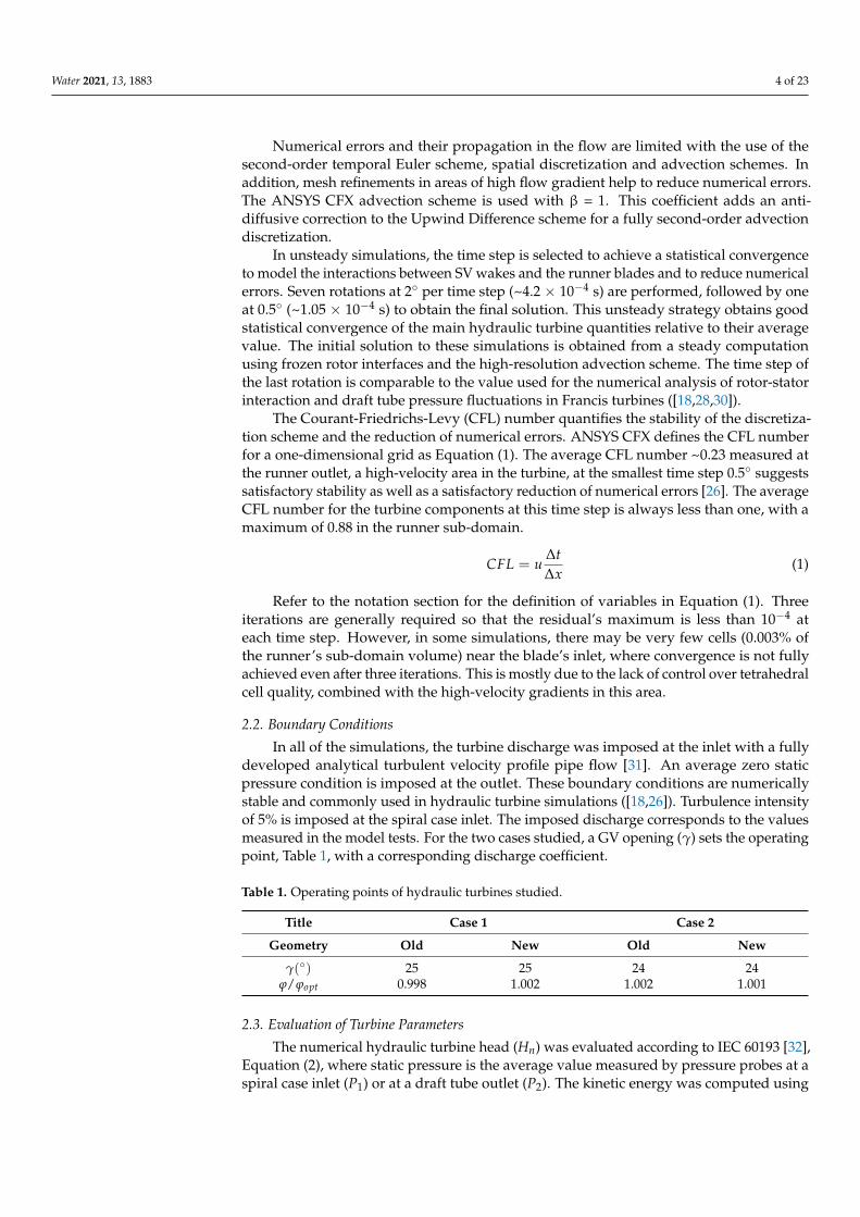
Table 4 shows the uncertainties and the extrapolated values of the efficiency loss inthe spiral case domain obtained by the GCI method.

Water 2021, 13, 1883 8 of 23

Table 4. Spatial discretization error and numerical uncertainties in spiral case and tandem cascade.

Title Case 1 Case 2

Geometry Old New Old New

c21 1.36 1.04 1.17 1.10c32 1.05 1.11 1.19 1.25

φ1 (m) 0.818 0.474 0.487 0.446φ2 (m) 0.798 0.474 0.492 0.435φ3 (m) 0.783 0.471 0.491 0.437

ε32 0.0198 −0.00291 0.00023 0.00222ε21 0.0244 −0.00033 0.00435 −0.0112e21

a 0.0244 0.000702 0.00892 0.0252

GCI21f ine 0.000943 0.000859 0.000429 -

This method begins by evaluating the ratio (c21 et ε21) between the representative sizeof the two mesh densities members (h) and the efficiency loss in the spiral case domain (φ)evaluated by simulation, Equations (7) and (8), to obtain the approximate relative error,Equation (9), and the numerical uncertainty, Equation (10). The calculation of numericaluncertainty using the apparent order of the simulations (p), evaluated by an iterativemethod, allows extrapolating the results of simulations with a size of cells near zero.

c21 =h2

h1(7)

ε21 =φ1

φ2(8)

e21a =

∣∣∣∣φ1 − φ2

φ1

∣∣∣∣ (9)

GDC21f ine =

1.25e21a

cp21 − 1

(10)

Refer to the notation section for the definition of variables in Equations (7)–(10).Numerical uncertainty (GCIfine

21) is relatively small, with a maximum value of 0.1% anda minimum of 0.04% with finer meshes. The apparent order of the simulations variesbetween 11.4 and 21.2, with no possible values for case 2’s new SVs. Negative values ofε32/ε21 reveal oscillatory convergence in three cases. These are due to the small differencein the efficiency loss between each mesh density. Oscillatory convergence could indicatea level of the mesh-independence of the efficiency losses, as mesh densities appear to besufficient to model boundary layer separations and recirculation zones at SVs, or in theirabsence, in the new geometries. These results allow the use of the medium mesh density inthe spiral case for the complete turbine simulation.

Table 5 presents the results obtained by the GCI method in the runner and the drafttube sub-domains. The finer mesh allows a flow resolution up to the viscous sub-layeron the wall of those components. The efficiency losses in the runner are evaluated with anumerical error of 3.6%, the energy head with an error of 6.3%, and the efficiency losses inthe draft tube with an error of 6.3%. These GCI method results indicate the achievement ofa stable convergence. Medium-density meshes are used in the runner and in the draft tubefor the complete turbine simulation (Table 6).

Water 2021, 13, 1883 9 of 23

Table 5. Spatial discretization error and numerical uncertainties in runner and draft tube meshes.

Sub-Domain Runner Draft Tube

c31 1.159 1.114c32 1.161 1.213

φ1 (m) 12.31 4.03φ2 (m) 12.83 3.58φ3 (m) 11.54 3.13

ε32 −1.290 −0.450ε21 0.520 −0.450e21

a 0.042 0.112GCI21

f ine 0.036 0.063

Table 6. Nodes (106) in meshes used for case 1 and 2 full turbine simulations.

Case 1 Case 2

Sub Domain Old New Old New

Spiral case 39.7 28.2 24.9 28.5Runner 22 17.8

Draft tube 6.7 5.6

These simulations have required approximately 200 h with 120 CPUs for their resolution.

2.6. Model Tests

Experimental tests of two cases were carried out in previous studies (unpublishedfor proprietary reasons). They provide experimental efficiency values for cases 1 and 2.The tests were made according to IEC 60193 [36] and IEC 60995 [32] standards. The testsshowed that SV modifications lead to efficiency increases of 2.2% and 1.0% in cases 1 and 2,respectively, at the BEP (Figure 8).

Figure 8. Hydraulic turbine efficiency of case 1 and 2 with and without SV modifications. Efficiencyis relative to the maximal efficiency of the new geometry for each case.

The model tests evaluated efficiency with systematic and random uncertainties stem-ming from the accuracy of the equipment and the measurement methods. According to the

Water 2021, 13, 1883 10 of 23

IEC 60193 methodology, the efficiency uncertainty is ±0.0013 for case 1 and ±0.0014 forcase 2 for the BEP at maximal efficiency.

3. Results

The numerical results of full turbine simulations are used to assess efficiency increase,in each component, due to SV modification compared to that measured in model tests inboth cases studied.

3.1. Efficiency Increase

The results of numerical simulations for the case 1 and 2 turbines are presented inTable 7.

Table 7. Efficiency losses coefficient reduction evaluate by complete turbine simulation. Model testsvalues are show as reference.

Title ∆ψ/ϕ2Old−∆ψ/ϕ2

New(∆ψ/ϕ2

Old−∆ψ/ϕ2New)CFD

(∆ψ/ϕ2Old−∆ψ/ϕ2New)CFD Total

(%)

Case 1 2 1 2

Spiral case 0.001 −0.002 ~0 −4Stay vanes 0.137 0.032 57 72

Guide vanes 0.081 0.017 34 39Runner 0.025 −0.001 11 −3

Draft tube −0.004 −0.002 −2 −4Total 0.240 0.044 100 100

Model tests 0.367 0.111 - -

Full turbine simulations determine a total reduction of the efficiency loss coefficientof 0.240 in case 1. This is 65% of the total efficiency loss coefficient reduction measured inmodel tests. In case 2, the simulations indicate a total efficiency loss coefficient reduction of0.044 or 40% of that measured in model tests. In both cases, the main source of efficiencyincrease is from the SV. The GVs are the second-largest source of the reduction of theefficiency loss coefficient. The efficiency loss coefficient in the case 1 runner counts for10.6% of the total while a slight increase is calculated in case 2. The magnitude of theefficiency loss variations in the spiral case and the draft tube is very low, as they appearto be within the range of numerical uncertainty for both cases. The absence of variationin the efficiency losses in the spiral case is normal, as there are no modifications to thiscomponent. The efficiency losses in the spiral case come from the wall friction and thesecondary flows, and these phenomena are not affected by the flow modification in theSVs. The variation of the efficiency losses in the draft tube is very small compared to thetotal increase measured in the model tests.

3.2. Tandem Cascade

Figure 9 shows the efficiency loss coefficient as a function of the tandem cascade radiusfor the two cases studied. The comparison of the slope of the efficiency loss coefficientbetween the old and new geometries shows that in case 1, the main source of efficiencyloss is located at the leading edge of the SVs. The other major efficiency losses are locatedat the exit of the old SVs in case 1. In the absence of new efficiency losses in the GVs, theslope is very similar between the two geometries for both cases.

Water 2021, 13, 1883 11 of 23

Figure 9. Efficiency loss coefficient in the tandem cascade in cases 1 and 2. Flow direction is from theright to the left in the figure. SV and GV position are marked with the vertical dashed lines.

In case 2, the difference in the slope of the efficiency loss coefficient between the twogeometries is reduced relative to that of case 1. The slopes of the efficiency losses at the SVsof the old geometry are generally constant. They are only somewhat greater than thoseof the new SVs, and almost identical in the GVs. Similar to case 1, the increase is mostlygenerated in the SVs for both geometries.

According to the observation of the efficiency loss coefficient in the tandem cascade,the significant reduction of efficiency losses is due to the elimination of the boundarylayer separation at the SVs due to their modifications. The velocity at the SVs of the twogeometries, Figures 10 and 11, indicate the large boundary layer separation caused bythe misalignment of their leading edges with the flow, as shown by the position of thestagnation point where the velocity is zero.

Figure 10. Velocity at the tandem cascade horizontal plane in case 1 hydraulic turbine functions ofthe inlet area of the spiral case and the turbine discharge.

Water 2021, 13, 1883 12 of 23

Figure 11. Velocity at the tandem cascade horizontal plane in case 2 hydraulic turbine functions ofthe inlet area of the spiral case and the turbine discharge.

The flow misalignment is much more significant in the old geometry than in the newone, as the modification of the SVs significantly reduced the misalignment of their leadingedges with the flow (see Table 8). This is the main cause of the recirculation zones and ofthe large efficiency losses in the old geometries of the two cases studied.

Table 8. Flow orientation misalignment at the leading edge of the stay vanes of case 1 and 2.

Geometry Old New

Case 1 14.2 6.1

Case 2 23.8 4.2

Added to the misalignment of the SVs to the flow, the velocity contours highlightthe difficulty of a chamfer leading edge to keep the flow attached to the wall, as in case 1.Indeed, the velocity at the leading edge of the SVs reveals that the flow detaches from thewall on sharp chamfer angles due to the strong adverse pressure gradient created there.This is the boundary layer separation point and the beginning of the recirculation zone atthe SVs. A boundary layer separation is also observed very locally on the SVs’ intrados.This separation shows the main weakness of chamfer geometry, as it creates efficiencylosses even if the flow is properly oriented with the hydraulic profile. The modification tothe SV’s geometry with a rounded leading edge attenuates this problem and reduces theincidence of flow misalignment, as evidenced by the velocity contour.

In case 2’s old geometry, the leading edges are appropriate to limit the boundarylayer separation; however, the velocity contour shows the important misalignment ofapproximately 24 of the flow with the SVs. The increase in the adverse pressure gradientis due to the rapid change in direction of the SV’s leading edges. Indeed, this is thepoint of the boundary layer separation. By reducing the misalignment with the flow, theextension added to the new geometry attenuates the rapid change in direction of the SVsand therefore the magnitude of the adverse pressure gradient. However, the effect of along application of adverse pressure gradient is observed on the upper surface of the SVsin the form of the flow slowing in the boundary layer. This slowing reveals the work of theSVs done on the flow to obtain an adequate orientation with the GVs.

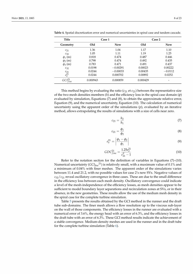
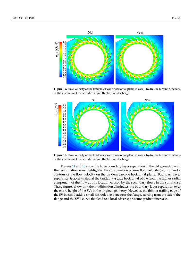
Flow observations at the tandem cascade show that the modification of the SVseliminates all the recirculation zones (flow velocity almost zero) in the tandem cascadein both cases studied, as indicated in Figures 12 and 13. In case 1, modification of thetrailing edge of the SV also reduces its prominent wake. At the SVs located at the end of thespiral case with the small recirculation zone, a much larger wake is observed in the originalgeometry compared to the wake in the modified one. In both cases, the recirculation zonesare closed in the GVs due to the flow restriction caused by the significant reduction of theflow section. This effect on the flow is visible through the zones of higher flow velocity atthe entrance of the GVs.

Water 2021, 13, 1883 13 of 23

Figure 12. Flow velocity at the tandem cascade horizontal plane in case 1 hydraulic turbine functionsof the inlet area of the spiral case and the turbine discharge.

Figure 13. Flow velocity at the tandem cascade horizontal plane in case 2 hydraulic turbine functionsof the inlet area of the spiral case and the turbine discharge.

Figures 14 and 15 show the large boundary layer separation in the old geometry withthe recirculation zone highlighted by an isosurface of zero flow velocity (um = 0) and acontour of the flow velocity on the tandem cascade horizontal plane. Boundary layerseparation is accentuated at the tandem cascade horizontal plane from the higher radialcomponent of the flow at this location caused by the secondary flows in the spiral case.These figures show that the modification eliminates the boundary layer separation overthe entire height of the SVs in the original geometry. However, the thinner trailing edge ofthe SV in case 1 adds a small recirculation zone near the flange, starting from the exit of theflange and the SV’s curve that lead to a local adverse pressure gradient increase.

Water 2021, 13, 1883 14 of 23

Figure 14. Flow velocity at the tandem cascade horizontal plane functions of the inlet area of thespiral case and the turbine discharge and um = 0 isosurface in case 1 hydraulic turbine.

Figure 15. Flow velocity at the tandem cascade horizontal plane functions of the inlet area of thespiral case and the turbine discharge and um = 0 isosurface in case 2 hydraulic turbine.

The azimuthal variation of the recirculation zones shows the variation of the flowdirection at the leading edge of the SV. The spiral case imposes a more radial flow at itsbeginning and end while imposing a tangential direction to the flow in the middle, asshown in Figure 16. In both cases, the evolution of the azimuthal flow in the spiral caseindicates this is a deceleration flow type; a result of the configuration of the spiral case [37].This figure also shows, by its comparison between the old and new geometries, the absenceof any influence of the recirculation zones on the flow direction at the SV’s leading edges.

Recirculation zones in the tandem cascade affect the components of the mean flow atthe exit of the GVs in the old geometry of case 1, as shown in Figure 17, with the angularmomentum as a function of the radius. They have no effect on the angular momentum inthe old geometry in case 2. Indeed, the recirculation zones in the original geometry increasethe angular momentum provided to the GV’s outlet.

Water 2021, 13, 1883 15 of 23

Figure 16. Flow orientation at SV leading edge of the two studied hydraulic turbines.

Figure 17. Angular momentum in function of the tandem cascade radius.

The effect of the recirculation zone can be noted at the boundary layer separation pointon the leading edge of the SVs by a fast decrease in the angular momentum. The flow areareduction by the flow recirculation zones then increases the tangential component of theflow in the SVs. This result of a tangential flow at the exit of the SVs is significantly higherin the original geometry of case 1. For the old geometry, a similar effect is found in case 2as the flow gains in angular momentum at the SV’s exit. In this case, it also appears that therecirculation zone partially blocks the radial component of the flow, thereby increasing thetangential flow. The comparison of the angular momentum at the exit of the GVs betweenthe two geometries of case 2 shows that they restored the flow. However, in case 1, theold geometry maintains a higher angular momentum than the new one. This difference

Water 2021, 13, 1883 16 of 23

between the two geometries is due to the position of the SVs relative to the position of theguide vanes. The alignment of the GVs with the SVs in case 2 closes the recirculation zonesand promotes the restoration of flow through the strong attenuation of the wake. On thecontrary, in case 1, the position of the SVs between two GVs leads to the large wake of therecirculation zones at the exit of the GVs. This large wake creates a deficit of radial velocitywith the effect of increasing the tangential flow, as at the exit of the SVs.

3.3. Runner

The efficiency loss variation between the old and new geometries in the case 1 runneris affected by the variation of the average flow component at the GV’s outlet. It is observedthat the modification of the flow’s angular momentum by the recirculation zone in the oldgeometry implies a greater flow misalignment on the blade’s leading edge, as shown inFigure 18. In case 2, the absence of efficiency loss variation is the consequence of the verysimilar average flow component between the two geometries at the GV’s outlet.

Figure 18. Streamlines at a runner blade of case 1 old and new geometries.

Using the average velocity components, the hydraulic angle difference at a bladeleading edge between the two geometries is about 0.35. In contrast, the variation ofthe angle between the partial and the high load operation points is about 3. If the flowmisalignment is greater than that of the old geometry, it remains attached to the wall ofthe blade as shown by the streamline, with an increase of the energy runner head andefficiency losses.

The observation of the efficiency loss coefficient as a function of the relative positionin the runner, Figure 19, confirms the greater efficiency losses at the runner inlet in the oldgeometry of case 1. In comparison, case 2 shows no variation in runner efficiency lossesbetween the two geometries.

Water 2021, 13, 1883 17 of 23

Figure 19. Efficiency loss coefficient as function of relative position in the runner of the case 1 and 2.

As a comparison of the mass of flow distribution at the GV outlet, Figure 20, showsthe absence of differences due to recirculation zones between the old and new geometries.According to this figure, the mass flow distribution is very similar for the two geometriesin each case study. The mass flow distribution at the GV outlet is rather a function of thespiral case geometry than of the SV. Thus, since the mass flow distribution is similar in bothgeometries of the two cases, it does not influence the efficiency losses in the runner. Therunner energy head is considered as the main head loss source in the hydraulic turbine andas a factor that has a major effect on the flow uniformity and distribution at the GV outlet.

Figure 20. Azimuthal mass flow variation at GV outlet of case 1 and 2 hydraulic turbines.

3.4. Draft Tube

Figures 21 and 22 show the velocity flow obtained with the full turbine simulationsat different planes in a draft tube. Some differences are observed between the old andnew geometries of the two cases, such as the recirculation zones, characterized by zero

Water 2021, 13, 1883 18 of 23

flow velocity at the outlet of the draft tube. It is observed that the flow at the beginningof the sluice is quite similar in both geometries, and then small differences appear in thedevelopment of recirculation zones. However, the overall topology of the flow is verysimilar for the draft tube of both the old and new geometries. Indeed, the total area blockedby the recirculation zones at the exit of the draft tube appears to be substantially the samein both geometries, which is why the low-efficiency loss coefficient reduction is evaluatedin the new geometry according to the IEC method.

Figure 21. Flow velocity in the draft tube of old and new geometries of case 1 functions of the inlet area of the draft tubeand the turbine discharge.

Figure 22. Flow velocity in the draft tube of old and new geometries of case 2 functions of the inlet area of the draft tubeand the turbine discharge.

Comparison of the flow at the runner outlet between the old and new geometries ofcase 1 gives some clues about the slight difference observed in the flow in the draft tube,as exposed in Figure 23, with circumferential, radial, and axial velocities. There are largerdifferences between the two geometries in the axial and circumferential velocities, dueto the mass flow variation imposed at the turbine inlet. In fact, the simulation uses theoperating point determined in a test model for each geometry. This implies that there ismore circumferential velocity at the runner output in the new geometry, made visible by alarger recirculation zone at the center of the draft tube.

Water 2021, 13, 1883 19 of 23

Figure 23. Axial, circumferential and radial flows at runner outlet of case 1 hydraulic turbine. Axialvelocity is function of the inlet area of the draft tube and the turbine discharge.

Figure 24 shows that SV modifications bring no significant changes in the velocityfields at the case 2 runner outlet. Note that the significant imbalance of the radial velocity,and to a lesser extent, the axial velocity, is the consequence of the oblong shape of the drafttube cone. In fact, the radial velocity at the wall is mainly led by the divergence angle ofthe draft tube cone [23]. Due to its particular shape, the divergence angle varies alongthe perimeter of the tube cone and increases the radial velocity at each side of the oblong.The effect on the axial velocity is similar; where the divergence angle is larger, the more itdecelerates the flow.

Water 2021, 13, 1883 20 of 23

Figure 24. Axial, circumferential and radial flows at runner outlet of case 2 hydraulic turbine. Axialvelocity is function of the inlet area of the draft tube and the turbine discharge.

In both cases, the full turbine simulations do not capture the effect of eliminating therecirculation zones in the tandem cascade at the runner outlet. The change of the meanflow comes from the flow rate imposed at the turbine inlet, as measured in the model testsfor the same GVs’ opening. The mean flow at the runner outlet is mainly a function ofthe flow rate, the runner blade shape, and the rotational speed, according to the velocitytriangle [38]. As expected, the numerical simulation shows lower circumferential velocityfor the new geometry’s runner outlet, as the flow rate is higher.

4. Conclusions

The full turbine simulation methodology developed is used to model the flow inall of the components of two rehabilitated hydraulic turbines to evaluate their ability toaccurately quantify the efficiency increase caused by the SV modification and its effectthroughout the turbine in comparison to model tests. The application of this methodologyevaluated up to 65% of the model tests’ efficiency increases in case 1 and 40% in case 2.Comparing component-to-component in case 1, the simulation found 57% of the totalmodel tests’ efficiency increases in the SV, 34% in the GV, 11% in the runner, and an

Water 2021, 13, 1883 21 of 23

insignificant variation in the draft tube. In case 2, 72% of efficiency loss was computed tobe in the SV, 39% in the GV, and an insignificant variation in the runner and the draft tube.

In both cases, the elimination of the recirculation zones by the SV modification wasdetermined to be the main cause of the significant efficiency increase in that component. Theefficiency increase in the GVs of the new geometry comes from the elimination of the wakedue to the recirculation zones at the SV. For both cases, the effect of the SV’s modificationis very similar, except for the variation of angular momentum at the GV’s outlet in case1, where this angular momentum variation between the old and new geometries leads tothe efficiency increase in the runner. In the second case, the absence of modification to theaverage flow at the runner inlet results in the absence of efficiency loss variation in thiscomponent. The local disturbances in the flow due to the recirculation zones at the exitof the GVs are reduced by the runner. The absence of efficiency loss variation in the drafttube is explained by the small difference in the flow at the runner outlet.

The methodology of the full turbine simulation developed with URANS equationsand the k-ω SST turbulence model appears to reach its limits to accurately assess the overallefficiency losses in the hydraulic turbines studied. The mesh-independence study in eachcomponent of the turbine shows the low probability of obtaining a significant efficiencyloss change with finer meshes. Finally, it is proposed that further works could use a morecomplex flow modeling approach to observe if the wake of the boundary layer separationof the SVs and its turbulent structures can influence the flow and efficiency loss in therunner and the draft tube.

Author Contributions: Conceptualization, M.S.; methodology, P.M.R.; software, P.M.R.; validation,P.M.R., A.S. and M.S.; formal analysis, P.M.R. abs A.S.; investigation, P.M.R.; resources, A.S. and M.S.;data curation, P.M.R.; writing—original draft preparation, P.M.R.; writing—review and editing, A.S.and P.M.R.; visualization, P.M.R.; supervision, A.S. and M.S.; project administration, A.S. and M.S.;funding acquisition, A.S. and M.S. All authors have read and agreed to the published version ofthe manuscript.

Funding: An Industrial Innovation Scholarship provided by the Natural Sciences and EngineeringResearch Council of Canada (NSERC) and Research Fund of Quebec Nature and Technology (FRQNT)has allowed the realization of this work through its financial support.

Institutional Review Board Statement: Not applicable.

Informed Consent Statement: Not applicable.

Acknowledgments: The permission to use the geometries as well technical and financial supportis granted by Alstom Energy & Transport Canada Inc. The simulations were performed on thesupercomputers of Compute Canada.

Conflicts of Interest: The authors declare no conflict of interest.

Nomenclature

NotationA area (m2)c grid refinement factorea approximate relative erroreext extrapolated relative errorE energy head (m)g gravitational acceleration (ms−2)GCIfine fine-grid convergence indexHi runner internal head (m)Hn turbine hydraulic head (m)h representative cell size (m)

Water 2021, 13, 1883 22 of 23

Nsq hydraulic turbine specific speed (s−1).

m mass flow (kgs−1)P pressure (kgm−1s−2)p GCI method apparent orderQ discharge (m3s−1)r radius (m)T torque (Nm)t unit of time (s)u velocity (ms−1)um flow velocity (ms−1)uθ circumferential velocity (ms−1)ur radial velocity (ms−1)x length (m)Y+ dimensionless distancez elevation (m)γ guide vanes opening ()ε critical value differenceη efficiencyϕ discharge coefficientφ critical valueφext extrapolated valueψ energy coefficientΩ rotational speed (s−1)

References1. Canadian Hydropower Association. Hydropower in Canada: Past, Present and Future. Available online: http://www.

renewableenergyworld.com/rea/news/article/2009/10/hydropowerin-canada-past-present-and-future (accessed on1 July 2021).

2. International Energy Agency. Key World Energy Statistics; International Energy Agency: Paris, France, 2008.3. Eberle, P.; Couston, M.; Sabourin, M. The refurbishment of low head Francis turbines. Int. J. Hydropower Dams 2003, 10, 45–48.4. Michel, B.; Vuillerod, G.; Francois, M.; Kunz, T. Efficient rehabilitation of hydro generating units. Int. J. Hydropower Dams 2007, 14,

140–146.5. Michel, B.; Couston, M.; Sabourin, M.; Francois, M. Hydro Turbines Rehabilitation; IMechE Event Publications, 2004; pp. 3–12.

Available online: https://www.encyclopedie-energie.org/wp-content/uploads/2018/09/art083_Michel-Bernard-Couston-Michel-et-al_Hydro-turbines-rehabilitation.pdf (accessed on 1 July 2021).

6. Morris, D.; Froehlich, D.; Hartmann, O. Guides for hydroplant modernization. In Proceedings of the American Power Conference,Chicago, IL, USA, 18–20 April 1988; Volume 50, pp. 1067–1076.

7. Drtina, P.; Sallaberger, M. Hydraulic turbines—Basic principles and state-of-the-art computational fluid dynamics applications.Proc. Inst. Mech. Eng. Part C J. Mech. Eng. Sci. 1999, 213, 85–102. [CrossRef]

8. Suzuki, T.; Nagafuji, T.; Komiya, H.; Shimada, T.; Kobayashi, T.; Taniguchi, N. Flow behavior around stay vanes and guide vanesof a Francis turbine. ASME J. Fluids Eng. 1996, 118, 110–115. [CrossRef]

9. Vu, T.C.; Shyy, W. Performance Prediction by Viscous Flow Analysis for Francis Turbine Runner. J. Fluids Eng. 1994, 116, 116–120.[CrossRef]

10. Vu, T.C.; Shyy, W. Navier-Stokes Flow Analysis for Hydraulic Turbine Draft Tubes. J. Fluids Eng. 1990, 112, 199–204. [CrossRef]11. Wu, J.; Shimmei, K.; Tani, K.; Niikura, K.; Sato, J. CFD-Based Design Optimization for Hydro Turbines. J. Fluids Eng. 2007,

129, 159. [CrossRef]12. Keck, H.; Drtina, P.; Sick, M. Numerical Hill Chart Prediction by Means of CFD Stage Simulation for a Complete Francis Turbine.

In Hydraulic Machinery and Cavitation; Springer Science and Business Media LLC: Berlin, Germany, 1996; pp. 170–179.13. Dörlfer, P. Observer-based control of a low-head Pelton plant equipped with a long penstock. In Proceedings of the 2nd

Conference on Modeliling, Testing & Monitoring for Hydro Poweplants, Lausanne, Switzerland, 8–11 July 1996.14. Ruprecht, A. Unsteady flow simulation in hydraulic machinery. Task Q. 2002, 6, 187–208.15. Kurosawa, S.; Lim, S.M.; Enomoto, Y. Virtual model test for a Francis turbine. In IOP Conference Series: Earth and Environmental

Science; IOP Publishing: Philadelphia, PA, USA, 2010; Volume 12.16. Lain, S.; Garcia, M.; Quintero, B.; Orrego, S. CFD Numerical simulations of Francis turbines Simulación numérica (CFD) de

turbinas Francis. Rev. Fac. Ing. Univ. Antioq. 2010, 51, 24–33.17. Magnoli, M.; Schilling, R. Increase of the annual energy output in hydraulic powerplants through active flow control. Renew.

Energy Power Qual. J. 2011, 1148–1153. [CrossRef]18. Trivedi, C.; Cervantes, M.J.; Gandhi, B.K.; Dahlhaug, O.G. Experimental and Numerical Studies for a High Head Francis Turbine

at Several Operating Points. J. Fluids Eng. 2013, 135, 111102. [CrossRef]

Water 2021, 13, 1883 23 of 23

19. Wu, Y.; Liu, S.; Wu, X.; Dou, H.; Zhang, L.; Tao, X. Turbulent flow computation through a model Francis turbine and itsperformance prediction. In IOP Conference Series: Earth and Environmental Science; IOP Publishing: Philadelphia, PA, USA, 2010;Volume 12.

20. Yexiang, X.; Zhengwei, W.; Zongguo, Y.; Mingan, L.; Ming, X.; Dingyou, L. Numerical analysis of unsteady flow under high-headoperating conditions in Francis turbine. Eng. Comput. 2010, 27, 365–386. [CrossRef]

21. Zobeiri, A.; Kueny, J.L.; Farhat, M.; Avellan, F. Pump-Turbine Rotor-Stator Interactions in Generating Mode: Pressure Fluctuationin Distributor Channel. In Proceedings of the 23rd IAHR Symposium on Hydraulic Machinery and Systems, Yokohama, Japan,17–21 October 2006.

22. Maruzewski, P.; Hayashi, H.; Münch, C.; Yamaishi, K.; Hashii, T.; Mombelli, H.P.; Sugow, Y.; Avellan, F. Turbulence modeling forFrancis turbine water passages simulation. In IOP Conference Series: Earth and Environmental Science; IOP Publishing: Philadelphia,PA, USA, 2010; Volume 12.

23. Mauri, S.; Kueny, J.-L.; Avellan, F. Werle´-Legendre Separation in a Hydraulic Machine Draft Tube. In Proceedings of the ASME2002 Joint U.S.-European Fluids Engineering Division Conference, Montreal, QC, Canada, 14–18 July 2002; Volume 1, Fora, PartsA and B. pp. 885–891. [CrossRef]

24. Tridon, S.; Barre, S.; Ciocan, G.; Ségoufin, C.; Leroy, P. Discharge Imbalance Mitigation in Francis Turbine Draft-Tube Bays. J.Fluids Eng. 2012, 134, 041102. [CrossRef]

25. Beaubien, C.A. Simulations Numériques de L’écoulement Turbulent dans un Aspirateur de Turbine Hydraulique; Université Laval:Québec, QC, Canada, 2013.

26. ANSYS, Inc. Release 13.0, ANSYS CFX-Solver Theory Guide; Southpointe: Canonsburg, PA, USA, 2010.27. Gagnon, J.M.; Deschênes, C. Numerical Simulation with flow feature extraction of a propeller turbine unsteady rotor-stator

interaction. In WIT Transactions on Modelling and Simulation; WIT Press: Southampton, England, 2007; Volume 46. [CrossRef]28. Nennemann, B.; Vu, T.C.; Farhat, M. CFD prediction of Unsteady Wicket Gate-Runner Interaction in Francis Turbines: A New

Standard Hydraulic Design Procedure. In Proceedings of the HYDRO 2005 International Conference and Exhibition, Villach,Austria, 17–20 October 2005.

29. Menter, F.; Kuntz, M.; Langtry, R. Ten years of industrial experience with the SST turbulence model. Turbul. Heat Mass Transf.2003, 4, 625–632.

30. Ciocan, G.D.; Iliescu, M.S.; Vu, T.C.; Nennemann, B.; Avellan, F. Experimental Study and Numerical Simulation of the FLINDTDraft Tube Rotating Vortex. J. Fluids Eng. 2006, 129, 146–158. [CrossRef]

31. Munson, B.R.; Okiishi, T.H.; Huesbsch, W.W.; Rothmayer, A.P. Fundamentals of Fluid Mechanics; John Wile & Sons: Hoboken, NJ,USA, 2013.

32. International Electrotechnical Commission. Determination of the Prototype Performance from Model Acceptance Tests of HydraulicMachines with Consideration of Scale Effects; IEC TC4, 4, 1987–1981; International Electrotechnical Commission: Geneva,Switzerland, 1991.

33. Pointwise. Pointwise V17. 2013. Available online: http://www.pointwise.com/ (accessed on 1 July 2021).34. Rousseau, P.M.; Sabourin, M. Comparison between structured hexahedral and hybrid tetrahedral meshes generated by commercial

software for CFD hydraulic turbine analysis. In Proceedings of the 21st Annual Conference of the CFD Society of Canada,Sherbrooke, QC, Canada, 6–9 May 2013.

35. Celik, B.; Ghia, U.; Roache, P.J. Procedure for estimation and reporting of uncertainty due to discretization in CFD applications.ASME J. Fluids Eng. 2008, 130, 078001.

36. International Electrotechnical Commission. Hydraulic Turbines, Storage Pumps and Pump-Turbines-Model Acceptance Tests; Interna-tional Electrotechnical Commission: Geneva, Switzerland, 1999.

37. Kurokawa, J.; Nagahara, H. Flow Characteristics in Spiral Casings of Water Turbines. In Proceedings of the 13th InternationalAssociation for Hydraulic Research Symposium on Hydraulic Machinery and Cavitation, Montreal, QC, Canada, 1 June 1986.

38. Logan, E., Jr. Handbook of Turbomachinery; CRC Press: New York, NY, USA, 2003.