IN DEGREE PROJECT MECHANICAL ENGINEERING,SECOND CYCLE, 30 CREDITS

, STOCKHOLM SWEDEN 2018

Impact from flexible operation on High Head Francis turbines

ANDREAS NILSSEN SKORPEN

KTH ROYAL INSTITUTE OF TECHNOLOGY

SCHOOL OF ENGINEERING SCIENCES

i

Preface This master’s thesis was written at the Waterpower Laboratory, Department of Energy and Process Engineering at the Norwegian University of Science and Technology (NTNU) during the spring of 2018. The thesis marks the end of my master’s degree in Engineering Mechanics at The Royal Institute of Technology (KTH) and my exchange semester to NTNU.

I would like to thank my supervisor Professor Ole Gunnar Dahlhaug for providing me with a lot of information regarding Francis turbines and great discussions about the future perspectives for hydropower in Norway. In addition, I would like to thank him for his hospitality at the Waterpower Laboratory and the great and including environment at the laboratory.

I would especially like to thank my supervisor Dr. Bjarne Børresen at Multiconsult Norge AS for providing the thesis, excellent and regular feedback, encouragement, and for allowing me to ask him and get answers to all my questions.

I would also like to thank Erik Os Tengs and Live Salvesen Fevåg at EDR Medeso AS for assistance with the numerical structural model, Igor Illev at the Waterpower Laboratory for measurement data and Chirag Trivedi at the Waterpower Laboratory for the numerical fluid model.

Andreas N. Skorpen Oslo, Norway. June 2018

ii

Abstract Today the European energy grid contains more renewable energy sources than ever before, yet there is little to no research on how the increased amount affects the cost structure of the remaining energy sources of the grid. A consequence of phasing more renewable energy sources into the power grid, is a reduction of the overall balancing capacity of the grid. Thus, the demand for balancing services from the remaining dispatchable energy sources increases. Hydropower is currently frequently used to balance the grid, and thus, the increased demand for balancing services offers a large opportunity for the hydropower segment. Furthermore, as the operating patterns become increasingly aggressive, the structural integrity is reduced, and the maintenance costs are increased. This thesis finds and elucidates the magnitude of the reduced lifetime and increased maintenance costs.

This master’s thesis finds that the reduction of the structural integrity comes at a large cost, and greatly impacts the overall financial feasibility. In that regard, it is presented market solutions that further incentives balancing services. Balancing services are in markets sold as system services, which includes frequency response, black start capacity, reactive power, and reserve capacity. The thesis presents operating patterns for Francis turbines that seek to fulfill the various system services.

The thesis predicts the lifetime of five unique operating patterns, one is assumingly the status

quo of operations today, and another is an analogy of operating the turbine like a battery. The results show that low part load and startup are the most damaging operating points, and that the lifetime is lower for flexible operations, than the currently expected lifetime.

Despite greatly reducing the lifetime of the turbine, the evaluated cases are financially feasible if they are adequately rewarded. The exact power price that provides adequate rewards differs for all five cases. Financially feasible power prices are in the interval 0.257 to 0.0533 NOK/kWh, where the lowest price refer to current operations and the highest price refers to the aggressive extreme case.

The analyses conducted in this thesis are utilizing the numerical software ANSYS mechanical to predict the stress state, the Palmgren-Miner method to predict the lifetime, the rothalpy relationship to predict the pressure in the runner and net present value calculations to evaluate the financial feasibility. In addition, the thesis utilizes, and post-processes previously conducted numerical fluid analyses and pressure measurements from the Waterpower Laboratory at NTNU.

iii

Sammendrag Europas energisystem består i dag av mer fornybare energikilder enn noen gang før og trenden er økende. Denne oppgaven undersøker endringer i kostnadsstrukturen til vannkraft, når flere fornybare energikilder fases inn i nettet. Konsekvensen av at flere fornybare energikilder fases inn i kraftnettet, er at fleksibiliteten til nettet reduseres. Dette vil føre til økt etterspørsel av balansetjenester fra gjenværende energikilder i kraftnettet. Ettersom vannkraft allerede brukes for å balansere kraftnettet, vil økt etterspørsel føre til store fremtidige muligheter for vannkraftnæringen. Denne oppgaven viser at vannkraftturbiners strukturelle integritet reduseres og at vedlikeholdskostnaden øker ved aggressive driftsmønstre, de antatte driftsmønstrene er nødvendig for å kunne tilby balansetjenester til nettet, og samtidig ha et bærekraftig energisystem.

Gjennom denne masteroppgaven blir det vist at kostnadene av å tilby balanseringstjenester er store, og vil påvirke de finansielle resultatene. Denne oppgaven presenterer markedsløsninger, som gir finansielle insentiver for balanseringstjenester. Disse tjenestene selges som systemtjenester, som blant annet inkluderer frekvensrespons, gjenoppstartkapasitet, reaktiv kraft og reservekapasitet. Denne oppgaven presenterer også driftsmønstre for Francis-turbiner, som antas å oppfylle nåværende og fremtidige systemtjenester.

Oppgaven predikerer levetiden til fem unike driftsmønstre, der et av de fem driftsmønsteret er slik turbiner antas å driftes i dag og et annet er en analogi for å drifte en turbin som et batteri. Resultatene viser at lav dellast og oppstart er de mest skadelige driftspunktene, og videre at levetiden reduseres ved å innføre mer aggressive driftsmønstre.

Selv om levetiden reduseres ved aggressive driftsmønstre, er det økonomisk gunstig å tilby balanseringstjenester dersom belønningen er tilstrekkelig. Kraftprisen som bestemmer lønnsomheten varierer som en funksjon av redusert levetid. Ettersom at levetiden reduseres mest av antall oppstarter og dellasteroperasjoner av systemet, er dette avgjørende lønnsomhets parametere. Kraftprisen som gir finansielt gunstige scenarioer er i intervallet 0.0553 til 0.257 NOK/kWh, hvor den laveste prisen gir lønnsomhet ved dagens drift og den høyeste er for det mest aggressive driftsmønsteret.

Analysene som gjennomføres i denne oppgaven benytter det numeriske programmet ANSYS for å predikere spenningstilstanden, Palmgren-Miner-metoden for å predikere levetiden, Rothalpy-forholdet for å predikere trykket i løpehjulet og netto nåverdi-metoden for å evaluere lønnsomhet. Tidligere utførte numeriske strømmingsanalyser og trykkmålinger fra Vannkraftlaboratoriet ved NTNU er prosessert og benyttet i oppgaven.

iv

Table of content

Preface ............................................................................................................................................................. i

Abstract .......................................................................................................................................................... ii

Sammendrag .................................................................................................................................................. iii

Abbreviations ................................................................................................................................................ vii

1 Introduction ........................................................................................................................................... 1

1.1 Objective ........................................................................................................................................ 1

1.2 The Thesis ...................................................................................................................................... 2

2 Flexible Generation ............................................................................................................................... 3

2.1 Flexibility ....................................................................................................................................... 3

2.2 Hydropower Turbines’ Flexibility ................................................................................................... 3

2.3 Integration of Renewable Energy Sources ....................................................................................... 3

2.4 Frequency Control ......................................................................................................................... 4

2.5 Markets for Flexible Generation ..................................................................................................... 6

2.6 System services ............................................................................................................................... 6

2.7 Current Markets for System Services ............................................................................................... 7

2.8 The Nordic Balancing Concept ..................................................................................................... 13

2.9 Integration of Hydropower ........................................................................................................... 13

3 Hydropower Turbines ......................................................................................................................... 14

3.1 Francis Turbines .......................................................................................................................... 14

3.2 Flow Patterns in Francis Runners ................................................................................................. 15

3.3 Hill Chart ..................................................................................................................................... 16

3.4 Rothalpy ....................................................................................................................................... 17

3.5 The Waterpower Laboratory ......................................................................................................... 18

3.6 Cost Estimations for Francis Runners ........................................................................................... 19

3.7 Cost Estimations for Operations ................................................................................................... 20

4 Operating Pattern of Francis Turbines ............................................................................................... 21

4.1 Dynamic Effects ........................................................................................................................... 21

4.2 Startup ......................................................................................................................................... 22

4.3 Speed No Load ............................................................................................................................. 26

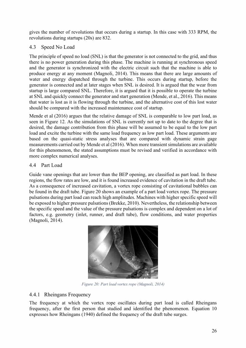
4.4 Part Load ..................................................................................................................................... 26

4.5 Best Efficiency Point and High load .............................................................................................. 27

5 Impact of Flexible Operations ............................................................................................................. 29

5.1 System Effectiveness and Reliability Engineering .......................................................................... 29

5.2 Reliability of Network Systems ...................................................................................................... 31

5.3 Quantification of System Effectiveness .......................................................................................... 31

v

5.4 Design Adequacy .......................................................................................................................... 32

5.5 Cost Model ................................................................................................................................... 34

5.6 Net Present Value ......................................................................................................................... 34

5.7 Impact on Hydropower ................................................................................................................. 35

6 Mechanical Engineering Definitions ................................................................................................... 36

6.1 Stress and Constitutive Relations .................................................................................................. 36

6.2 Dynamic Stresses.......................................................................................................................... 37

7 Damage and Lifetime Model ............................................................................................................... 39

7.1 Fatigue and Lifetime Model .......................................................................................................... 39

7.2 Material Parameters .................................................................................................................... 40

7.3 Stress History in Francis Runners ................................................................................................. 42

7.4 Simplified Analytical Stress Solutions ........................................................................................... 44

8 Previous Studies ................................................................................................................................... 47

8.1 Voith Hydro’s Study ..................................................................................................................... 47

8.2 SINTEF ........................................................................................................................................ 48

8.3 Fatigue Analyses of Prototype Francis Runners ............................................................................ 49

8.4 Predicted Operating Patterns ....................................................................................................... 50

9 Experiments and Previous Simulations ............................................................................................... 51

9.1 Recorded Data ............................................................................................................................. 51

9.2 Khoj ............................................................................................................................................. 53

9.3 Numerical Fluid Analyses ............................................................................................................. 54

9.4 Method 1 – Curve Fit.................................................................................................................... 55

9.5 Method 2 - Pressure based on Experimental Data ......................................................................... 58

9.6 Method 3 – Extracted pressure values ........................................................................................... 58

9.7 Peak to Peak Pressure .................................................................................................................. 58

10 Numerical Structural Analysis Model ................................................................................................. 60

10.1 Geometry ..................................................................................................................................... 61

10.2 Symmetry Conditions .................................................................................................................... 61

10.3 Mesh ............................................................................................................................................ 61

10.4 Boundary Conditions .................................................................................................................... 62

10.5 Loads ........................................................................................................................................... 63

10.6 Rotational Velocity ....................................................................................................................... 64

10.7 Mesh Independence Studies .......................................................................................................... 64

11 Results .................................................................................................................................................. 65

11.1 Pressure Calculations ................................................................................................................... 65

11.2 Analytical Solution ....................................................................................................................... 70

11.3 Numerical Structural Analyses ...................................................................................................... 70

11.4 Damage calculations .................................................................................................................... 77

vi

11.5 Financial Results .......................................................................................................................... 80

11.6 NPV of project .............................................................................................................................. 81

12 Discussion ............................................................................................................................................ 84

12.1 Pressure Calculations ................................................................................................................... 84

12.2 Numerical Structural Analysis ...................................................................................................... 85

12.3 Operating Patterns ....................................................................................................................... 86

12.4 Damage Calculations ................................................................................................................... 87

12.5 Cost and Financial Results ........................................................................................................... 89

12.6 Future Perspectives ...................................................................................................................... 90

13 Conclusion ........................................................................................................................................... 92

14 Further work ....................................................................................................................................... 93

15 Bibliography ........................................................................................................................................... i

Appendix A – Pressure and Results from Numerical Fluid Analysis and post-processing ............................ i

Appendix B – Von Mises and bending stress contribution ............................................................................. i

Appendix C – Location of Sensors................................................................................................................... i

Appendix D – Thickness and Length Parameters ........................................................................................... i

Appendix E – Cost Estimates from NVE......................................................................................................... i

Appendix F – Mean Stress Mesh Convergence ............................................................................................... i

Appendix G – Amplitude Stress Mesh Convergence ...................................................................................... i

Appendix H – Mean Stress at Sharp Corner................................................................................................... i

Appendix I – Mesh Quality.............................................................................................................................. i

Appendix J – MATLAB Code ......................................................................................................................... i

vii

Abbreviations BEP – Best efficiency point

TSO – Transmission system operator

CO2 – Carbon dioxide

RES – Renewable energy sources

RoCoF – Rate of change of frequency

PFC – Primary frequency control

SFC – Secondary frequency control

TFC – Tertiary frequency control

DSM – Demand side management

DS3 – Delivering a secure, sustainable electricity system

SNSP – System non-synchronous penetration

RSI – Rotor stator interaction

MTTF – Mean time to failure

OPEX – operational expenditures

ROI – Return on investment

CAPEX – Capital expenditures

HCF – High-cycle fatigue

LCF – Low-cycle fatigue

UTS – Ultimate tensile strength

NPV – Net present value

NOK – Norwegian kroner

NTNU – Norwegian University of Science and Technology

KTH – The Royal Institute of Technology

RPM – Revolutions per minute

ISO – International Organization for Standardization

CI – Confidence interval

SNL – Speed no-load

FSI – Fluid Structure Interaction

1

1 Introduction

Today the European energy grid contains more renewable energy sources than ever before, and the portion is increasing (EEA, 2017). This is a consequence of the European Commission’s goal of a low-carbon economy by 2050 (also called Energy Roadmap 2050) and is in accordance with the Kyoto Protocol (European Union, 2012). Specifically, it expresses a goal of reducing the equivalent of eighty to ninety-five per cent of total emissions in 1990, by 2050. This implies an eighty-five per cent decrease of carbon dioxide (CO2) emission. To achieve this goal, renewable energy sources must replace current fossil sources. It is expected that solar and wind generation are likely to make up fifty per cent of all renewables in Europe by the year 2020 (Eurelectric, 2014). In addition to dramatically shifting the production portfolio of the energy market, there are new and unfamiliar demands imposed on the transmission system operators (TSO) and power producers. Consequently, uncertainties around pricing, cost, and operations emerge in the energy supply chain.

Generated energy is a momentary product, which means that consumption takes place at the same time as production (Ommedal, 2015). A stable supply of high quality energy is in high demand, and current trends suggest that wind and solar offer little to no help in stabilizing generation, nor are they capable of storing energy. The generation from wind and solar power is dependent on wind currents and sun light, respectively. This means that the European Commission’s goal of 2050 low-carbo economy would be highly dependent on metrological factors, if the decrease of greenhouse gases is a product from merely solar and wind solutions. However, energy from solar and wind combined with dispatchable energy sources could be a possible solution to stabilize the electrical output. Dispatchable energy sources can quickly be switched on and off and are thus able to adjust its output in accordance with the current market’s demand (Donev, et al., u.d.). Typical dispatchable energy sources are natural gas, other combustive energy sources, and hydropower. With an increasing environmental focus, hydropower is by far the more environmental friendly alternative within this category.

Successfully managing stability, predictability, and regulation is a prerequisite to sustainably achieve the environmental goals. Seasonal and historical data can to a certain degree predict variations in the supply of energy, however unpredictable supply requires spare capacity in the power grid and momentarily reactions. Hydropower is capable of both balancing the grid and providing flexibility, thus, it is a viable solution – though currently at an unknown cost. The relationship between the responsiveness of the turbine, operational cost, wear, and damage of the hydropower plant are topics of interest, both in general and in this thesis. It is a general observation in the Nordic energy markets that the liberalization of the energy markets in the 1990s led to changes in the operating patterns (Ommedal, 2015). It is inferred that the changes led to increased mechanical loading and wear on the hydropower units, however there exist little or no systematic documentation of this (B. Børresen, personal communication, May 4th, 2018). The wear of the turbines is expected to accelerate as the operating patterns are becoming increasingly aggressive. Thus, it is of great interest to map the structural integrity of the turbine and the corresponding cost of operations within an aggressive market.

1.1 Objective

The objective of this thesis is to investigate the relation between flexible operating patterns, mechanical loading, and predict its maintenance costs. The following tasks are to be considered:

1. Review and describe current markets for system services 2. Based on the DS3 market in Ireland, investigate how the operating pattern of a typical

Norwegian power plant may change if integrated into such a market

2

3. Based on the Francis 99 model, including existing measurements and computations, evaluate the impact of operating pattern on the turbine’s lifetime

4. Develop a future market scenario for flexible operations of hydropower plants a. Describe how participating in these markets will impact the operating pattern

5. Develop a simplified cost model for choosing how to operate the unit or plant under different market considerations

6. If there is time available, a model for balancing various operating regimes will be developed

1.2 The Thesis

This thesis is divided into eight parts. The parts are:

1. Chapter 2 – 7 presents relevant theoretical background information. 2. Chapter 8 presents relevant previous studies that highlights important aspects around

the impact of flexible operations. 3. Chapter 9 presents relevant experiments and previously conducted numerical

simulations. 4. Chapter 10 presents the numerical models made and utilized during the work with this

thesis. 5. Chapter 11 presents the results obtained from the numerical simulations and the post-

processing of pressure measurements from the Waterpower Laboratory. 6. Chapter 12 presents the discussion, which presents limitations and assumptions present

in the results. Furthermore, the section also presents potential issues with the results, and offers solutions to these.

7. Chapter 13 presents the conclusions that can be drawn, through the results and discussions presented in this thesis.

8. Chapter 14 presents recommendations for further work, which could increase the quality of the results.

The thesis is constructed as an eye opener for the hydropower industry regarding the cost of operating turbines at various operating points. The thesis is also containing extensive amounts of literature studies, to highlight what flexible generation actually is. The thesis deliberately contains theoretical background of hydropower turbines and some mechanical engineering definitions that some readers might consider trivial. Nevertheless, these, and the appendices are included to ensure the efficiency of the thesis and that it can be read as a stand-alone paper. In addition, the knowledge of Francis turbines at NTNU and KTH diverges and the author wants to ensure that the thesis is read with approximately the same background at both universities. The MATLAB scripts and custom-made functions are attached in the appendices to allow future students to continue the work conducted in this thesis.

3

2 Flexible Generation

Flexible generation is a wide-reaching term denoted and named differently in the literature. In sources from Germany, the term is commonly denoted as control power markets, which encompasses both the generation and the market in which the services are sold (Böttger, 2018). In the United Kingdom, flexibility co-exists with system operability and balancing services (Energy UK, 2017). In the Nordics the term is co-existing with energy balancing (Statnett, 2017). In this thesis both the terms flexible generation and energy balancing are used to explain the principles of flexibility and the markets that provide balancing services.

2.1 Flexibility

Flexibility is the ability of a system to abruptly adjust its output. Energy markets define the term flexibility as quickly dispatchable generation (Eurelectric, 2014) and energy storage capacity (ofgem, 2017). Flexibility is in this thesis defined in accordance with its definition in energy markets and focused on dispatchable generation.

Today, hydropower and natural gas (open cycle gas turbines) are responsible for a large portion of the flexibility provided in the European energy market (Fraunhofer IWES, 2015). These are highly dispatchable and able to balance the energy market. Nevertheless, natural gas technologies are out of scope for this thesis and not discussed further. The following values determines the flexibility of a power plant (Hell, 2017):

1. Power capacity [MW]: The dispatchable range of generated output power of the

particular unit.

2. Power ramp rate [MW/min]: The rate at which the particular plant is capable of

increasing and decreasing the range of generated output power.

3. Storage energy [MWh]: The required energy stored in the reservoir for power area

balancing.

2.2 Hydropower Turbines’ Flexibility

The values that decide the flexibility of the hydropower plant can be further broken down into what specifically makes hydropower flexible, and that is the alterable operating patterns of the turbines. With an increasing demand of balancing power in future energy markets, expectations are that, the operating patterns of hydropower turbines are becoming increasingly more aggressive (Solvang, et al., 2011). Aggressive operating patterns are by Welte & Solvang (2011) defined as:

1. The plant is started and stopped more frequently than previously.

2. The plant is experiencing large and frequent load variations.

3. The plant is more frequently operated at part load and overload.

Projections are that the demand for balancing services rises as a consequence of integration of non-dispatchable renewable energy sources in the power grid (Statnett, 2017).

2.3 Integration of Renewable Energy Sources

A specific issue when phasing non-dispatchable renewable energy sources into the grid are the challenges to meet requirements for quality of supply, e.g. maintaining system frequency. This issue is the center around the sustainability of current and future system services. The wind and solar energy distributed to the energy system varies constantly as the sources are dependent on externally uncontrollable factors (Statnett, 2017). In addition to the uncontrollable nature of wind and solar energy sources, they do not provide the grid with reserve capacity nor system

4

inertia. The power grid’s system inertia is one of the fundamental perquisites of the grid (Tielens & hertem, 2012). The kinetic energy of rotating masses of synchronous generators and turbines, defines the system’s inertia. The inertia determines the immediate frequency response due to unforeseen demand spikes in the desired output power, either increases or decreases. Power grids with high system inertia are capable of easily adjusting to changes in demand.

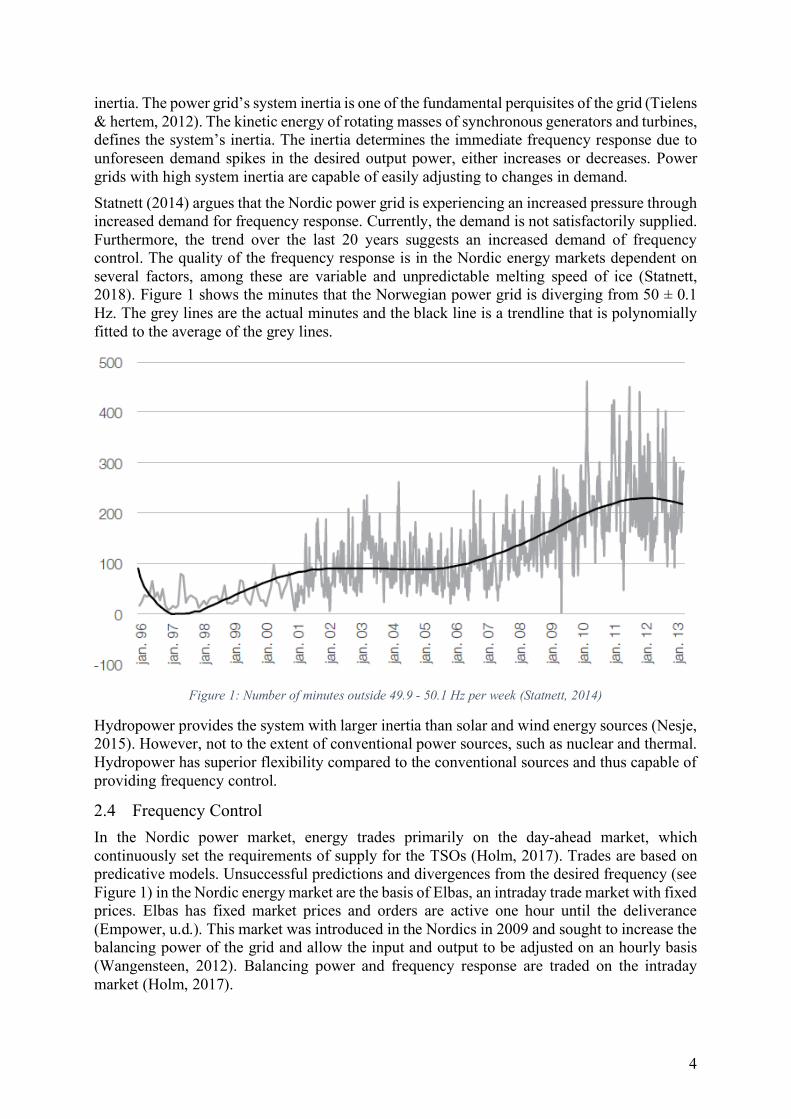
Statnett (2014) argues that the Nordic power grid is experiencing an increased pressure through increased demand for frequency response. Currently, the demand is not satisfactorily supplied. Furthermore, the trend over the last 20 years suggests an increased demand of frequency control. The quality of the frequency response is in the Nordic energy markets dependent on several factors, among these are variable and unpredictable melting speed of ice (Statnett, 2018). Figure 1 shows the minutes that the Norwegian power grid is diverging from 50 ± 0.1 Hz. The grey lines are the actual minutes and the black line is a trendline that is polynomially fitted to the average of the grey lines.

Figure 1: Number of minutes outside 49.9 - 50.1 Hz per week (Statnett, 2014)

Hydropower provides the system with larger inertia than solar and wind energy sources (Nesje, 2015). However, not to the extent of conventional power sources, such as nuclear and thermal. Hydropower has superior flexibility compared to the conventional sources and thus capable of providing frequency control.

2.4 Frequency Control

In the Nordic power market, energy trades primarily on the day-ahead market, which continuously set the requirements of supply for the TSOs (Holm, 2017). Trades are based on predicative models. Unsuccessful predictions and divergences from the desired frequency (see Figure 1) in the Nordic energy market are the basis of Elbas, an intraday trade market with fixed prices. Elbas has fixed market prices and orders are active one hour until the deliverance (Empower, u.d.). This market was introduced in the Nordics in 2009 and sought to increase the balancing power of the grid and allow the input and output to be adjusted on an hourly basis (Wangensteen, 2012). Balancing power and frequency response are traded on the intraday market (Holm, 2017).

5

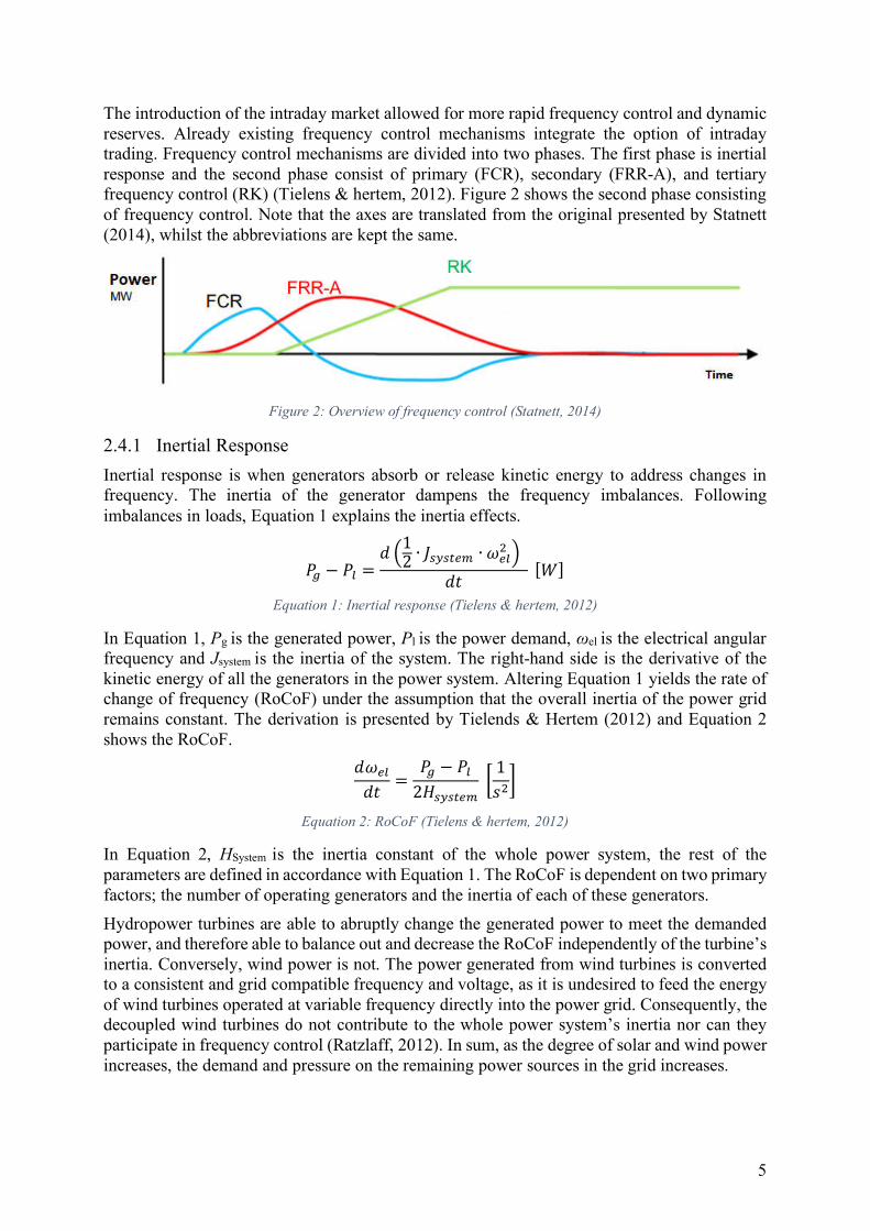
The introduction of the intraday market allowed for more rapid frequency control and dynamic reserves. Already existing frequency control mechanisms integrate the option of intraday trading. Frequency control mechanisms are divided into two phases. The first phase is inertial response and the second phase consist of primary (FCR), secondary (FRR-A), and tertiary frequency control (RK) (Tielens & hertem, 2012). Figure 2 shows the second phase consisting of frequency control. Note that the axes are translated from the original presented by Statnett (2014), whilst the abbreviations are kept the same.

Figure 2: Overview of frequency control (Statnett, 2014)

2.4.1 Inertial Response

Inertial response is when generators absorb or release kinetic energy to address changes in frequency. The inertia of the generator dampens the frequency imbalances. Following imbalances in loads, Equation 1 explains the inertia effects.

𝑃" − 𝑃$ = 𝑑 '12 ∙ 𝐽,-,./0 ∙ 𝜔/$2 3𝑑𝑡 [𝑊] Equation 1: Inertial response (Tielens & hertem, 2012)

In Equation 1, Pg is the generated power, Pl is the power demand, ωel is the electrical angular frequency and Jsystem is the inertia of the system. The right-hand side is the derivative of the kinetic energy of all the generators in the power system. Altering Equation 1 yields the rate of change of frequency (RoCoF) under the assumption that the overall inertia of the power grid remains constant. The derivation is presented by Tielends & Hertem (2012) and Equation 2 shows the RoCoF. 𝑑𝜔/$𝑑𝑡 = 𝑃" − 𝑃$2𝐻,-,./0 : 1𝑠2<

Equation 2: RoCoF (Tielens & hertem, 2012)

In Equation 2, HSystem is the inertia constant of the whole power system, the rest of the parameters are defined in accordance with Equation 1. The RoCoF is dependent on two primary factors; the number of operating generators and the inertia of each of these generators.

Hydropower turbines are able to abruptly change the generated power to meet the demanded power, and therefore able to balance out and decrease the RoCoF independently of the turbine’s inertia. Conversely, wind power is not. The power generated from wind turbines is converted to a consistent and grid compatible frequency and voltage, as it is undesired to feed the energy of wind turbines operated at variable frequency directly into the power grid. Consequently, the decoupled wind turbines do not contribute to the whole power system’s inertia nor can they participate in frequency control (Ratzlaff, 2012). In sum, as the degree of solar and wind power increases, the demand and pressure on the remaining power sources in the grid increases.

6

2.4.2 Primary Frequency Control

Primary frequency control (PCF) is the fastest developed type of frequency control. It is deployed within few seconds (<30s) of a load imbalance and is activated for the first half minute after the imbalance. Equation 3 explains the speed drop that PFC balances.

𝑆> = −Δ𝑓 𝑓ABΔ𝑃C 𝑃CDB [−]

Equation 3: Speed drop (Pierre, et al., 2015)

In Equation 3, f0 is the target frequency (50 Hz), Δ𝑓 = 𝑓 − 𝑓A is the difference between the actual frequency and the target frequency, PGn is the rated active power output and Δ𝑃C = 𝑃C −𝑃CD is the difference between the actual power output and the rated power output. A device called the governor automatically regulates the power input in accordance with the rotational velocity to balance the frequency after the speed drop (Valkvæ, 2016). In addition, it seeks to find the amount of energy required to counter the speed drop and return the system to equilibrium. PFC determines the amount of energy required to balance Equation 3 and secondary frequency control feeds the energy into the system (Pierre, et al., 2015).

2.4.3 Secondary Frequency Control

After the PFC has balanced the frequency, secondary frequency control (SFC) adjusts utilization of load to increase the energy fed into the system and to restore the frequency to 50 Hz and the system to equilibrium. This occurs automatically during and after the phase of PFC has ended (15s to 15min) (Statnett, 2014).

2.4.4 Tertiary Frequency Control

Following PFC and SFC is the tertiary frequency control (TFC), which occurs during the minutes and hours after the load imbalance and frequency has been restored (>15min). It is a manual process that seeks to optimize energy production and minimizes costs, while the power demand in the market is saturating. The TFC restores a series of plants to its initial state following load imbalances. In other words, it prepares for future imbalances (Statnett, 2014).

2.5 Markets for Flexible Generation

Flexible generation is, in itself, not a sustainable revenue source that the TSO’s and power generating companies should strive for. Without regulation and a market that complement and incentivize these services, it is a loss project because flexibility requires reserve capacity (Energy UK, 2017). This is an issue that Statnett in collaboration with Svenska Kraftnät are currently addressing in the Nordic region. Their view on the topic is that existing market solutions are not providing sufficiently clear and precise pricing signals. Currently, there are not enough financial incentives to ensure that TSOs are keeping sufficient balancing reserves at hand (Statnett, 2017). Thus, more market solutions that facilitates for flexible generation are required.

2.6 System services

System services is an umbrella term that encompasses all balancing services, system services is also called ancillary services (entsoe, 2017). Both terms are valid for the balancing services and flexible generation. The definition of system services are all services that help grid operators maintain a consistent energy system. The three values, previously defined by Welte & Solvang (2011) that expressed the hydropower plants flexibility, can provide all types of

7

system services. System services are split into under categories that can and will be sold on the open market. There are currently several system services provided. However, if the demand and regularity of these services increase, the market must reward the TSOs accordingly. Current system services are (entsoe, 2017):

1. Black start capability

Is the ability of the TSOs to restart the grid following a blackout. This requires fast auxiliary energy sources that complement the slow energy sources during the blackout.

2. Frequency response

Is the ability to adjust for abnormalities in frequency as a result of imbalance of supply and demand of energy production. A surplus of energy generation increases the frequency of the grid, and vice versa, a shortage of energy generation will lead to a decrease of the frequency (Greenwood, et al., 2017). This is explained by Equation 2.

3. Fast reserve

Is the ability of the TSOs to rapidly increase or decrease the supply of energy to match the current demand for energy. This is a parameter that is dependent on the power ramp rate, power capacity, and the storage energy of the generating source. Fast reserve and frequency response are two services that cannot be provided independently as both are highly dependent of the current state of demand and supply of energy (National Grid UK, 2018).

4. Reactive power

Is the ability to maintain the voltage level within acceptable levels. It allows the system to respond to unpredicted incidents and shifts in supply and demand.

2.7 Current Markets for System Services

There are currently markets all over Europe that either co-exists within countries, regional boundaries, or collaborates across these to provide system services to the European market. This thesis presents an overview of global initiatives and markets predictions, which the Nordic market can integrate further incentives flexible generation. Presented initiatives and markets are the DS3 market in Ireland, national grid markets in the United Kingdom, current and future predicted markets in Netherlands and Germany, and a short overview of how the Nordic TSOs are planning to participate and utilize these future markets.

2.7.1 United Kingdom –National grid

The United Kingdom is tendering several different system services to smart grid companies, which are rewarded market prices for their services. In their approach to introduce large scale system services, they have introduced four basic principles that the system service market should uphold (Energy UK, 2017):

1. Competitive and market based

The procurement and market for ancillary services must be market based in order to achieve inclusiveness and to ensure that the services are being provided at the least possible cost for the TSO’s customers. It is further sought that bilateral contracts are avoided to ensure competitiveness of the market and fair pricing.

8

2. Transparent

The markets where the services are sold and bought should be transparent and the future

demand requirements quantified. This aims to allow developers to account for revenue

generated through ancillary services.

3. Level playing field

It should be sought to minimize barriers to entry in the ancillary service market.

Furthermore, it aims to create competition across different procurement methods,

independent of size and type.

4. Fit for the future

The ancillary service market should facilitate for evolution of the energy system and

new technologies must be possible to implement in the current system.

All of national grid’s services seek to follow these principles, realized through tender periods that includes the generators, storage providers, and aggregated demand side participants, which places their tenders during a given tender period. System services that are up for tender by the national grid are (Energy UK, 2017):

• Frequency response services

• Reserve services

• Reactive power services

• Demand side response

2.7.1.1 Enhanced Market Frequency Response Tenders

One service that has recently undergone tendering is the frequency response service. The service is split into two parts, service 1 and service 2. Service 1 is classified as a wide deadband service, and service 2 as a narrow deadband service (National grid, 2016). Deadband is the acceptable variance in the system before the service actives. Service 1 has a deadband of ± 0.05 Hz and service 2 has a deadband of ± 0.015Hz. Service 2 places a larger toll on the supplier, as smaller frequency variations will trigger the service.

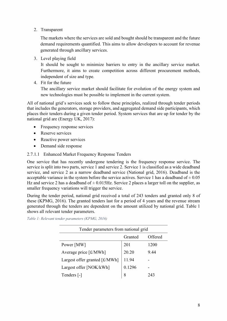
During the tender period, national grid received a total of 243 tenders and granted only 8 of these (KPMG, 2016). The granted tenders last for a period of 4 years and the revenue stream generated through the tenders are dependent on the amount utilized by national grid. Table 1 shows all relevant tender parameters.

Table 1: Relevant tender parameters (KPMG, 2016)

Tender parameters from national grid

Granted Offered

Power [MW] 201 1200

Average price [£/MWh] 20.20 9.44

Largest offer granted [£/MWh] 11.94 -

Largest offer [NOK/kWh] 0.1296 -

Tenders [-] 8 243

9

2.7.1.2 Tendering the Supply Curve

All tenders are collected and summarized as a mutually exclusive supply curve in Figure 3 (Overlapping and more than 1 tender by each company has been omitted in the curve). The y-axis of the curve is the tendered price per MWh and the x-axis is the total MW. The black line expresses the upper limit of power demanded by national grid. Note that the NOK value in Table 1 is the conversion between £ and NOK at 24.05.2018.

Figure 3: Supply curve for EFR (KPMG, 2016)

KPMG (2016) argues that the accepted auction prices were far lower than expected prior to the tenders, by both the participants and the market. Strategic bidding explains some of the low prices, with early market entry as a motivational factor. In addition, it is argued that certain suppliers are expecting aggressive energy pricing in the near future (KPMG, 2016). In addition, Pratt (2016) argues that the low tenders are a consequence of low-cost battery storage solutions. Both Pratt (2016) and KPMG (2016) argue that certain producer are willing to accept lower prices to hedge future revenue and financing, which can be used to build out more balancing services in the future. Eighty-seven per cent of the offered capacity was bid at a higher price than the most expensive contract awarded.

Similar tenders have been carried out for all four of national grid’s ancillary services. These tenders are not explained in depth in this thesis, and more information is found online at national grid’s homepage. The ERF tender offer is included to show the potential of ancillary services and how these services are acquired through competitive markets. The tender offer highlights the potential and willingness to provide these service, at a fair price for the consumer, TSO, and provider.

10

2.7.2 Control Power Markets in Germany

The control power markets in Germany, and potential improvements and integration of prices for effectiveness was presented at the PRIBAS Project Workshop the 8th of February 2018 at NTNU, Trondheim. Dr. Diana Böttger held the presentation about the German power market.

2.7.2.1 Overview of Power Markets in Germany

The German power market is split into three categories (Böttger, 2018):

1. Long-term trading

Forward and future contracts are traded

2. Short-term trading

Spot market trading. Including day-ahead and intraday

3. Real-time balancing

Control power markets

The short-term trading market is similar to the Nordic short-term market traded on Nord pool spot and Elbas, presented in section 2.4. The control power market (integrated part of intraday trading, where only frequency response is traded) efficiently trades PFC, SFC, and TFC. Reserve capacity trades as pay-as-bid. This means that there are continuously tendered offers from energy producers. Consequently, the taken tenders are those with lowest price for the spare capacity, which meet the instantaneous demand. The price of the energy required for SFC and TFC utilizes a similar pay-as-bid method. International cooperation between Germany, Netherlands, and Switzerland allow automatic netting of SFC across control area borders. The participants in the control power market have to prequalify their asses in advance similarly as for the United Kingdom markets, explained in section 2.7.1. Currently the prequalified assets exceed the control power demand by a factor of 20. Indicating that the supply far outweighs the demand.

2.7.2.2 Fundamental Control Power Market

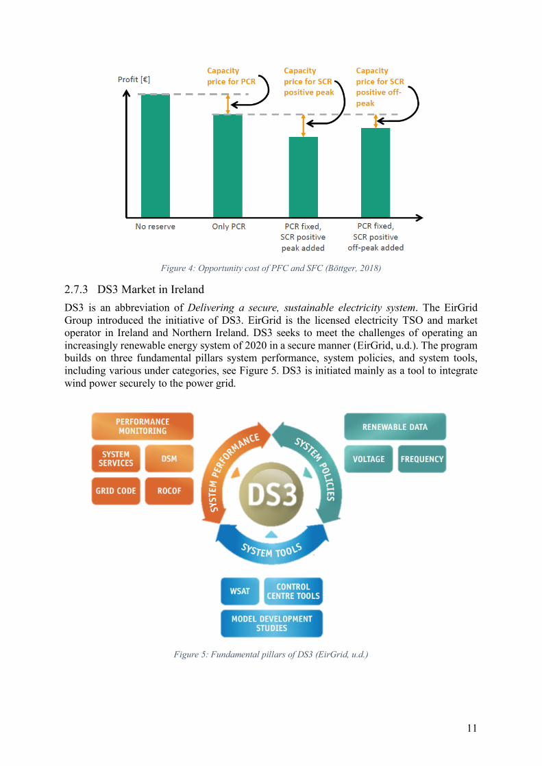
Dr. Böttger suggests implementing a new fundamental control power market model, which offer prices based on the opportunity costs of the service provided. The inputs of the model are power plant fleet, current spot market prices and demanded control power. The model seeks to return profit-maximal control power, at the least opportunity cost by all the units in the grid collected. The largest difference with the suggest model and the current model is that the suggested model pools several assets based on utility instead of bids from separate units. Thus, the services grant an efficient market optimal price, which incorporates the opportunity cost of various alternative usages. Figure 4 illustrates the profit difference and the opportunity cost, hence the price offered for the services.

11

Figure 4: Opportunity cost of PFC and SFC (Böttger, 2018)

2.7.3 DS3 Market in Ireland

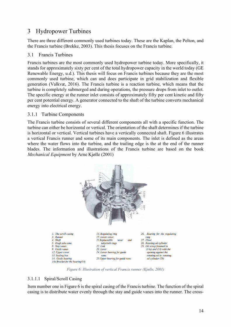
DS3 is an abbreviation of Delivering a secure, sustainable electricity system. The EirGrid Group introduced the initiative of DS3. EirGrid is the licensed electricity TSO and market operator in Ireland and Northern Ireland. DS3 seeks to meet the challenges of operating an increasingly renewable energy system of 2020 in a secure manner (EirGrid, u.d.). The program builds on three fundamental pillars system performance, system policies, and system tools, including various under categories, see Figure 5. DS3 is initiated mainly as a tool to integrate wind power securely to the power grid.

Figure 5: Fundamental pillars of DS3 (EirGrid, u.d.)

12

2.7.3.1 System Performance

The system performance refers to the performance of all energy sources jointly connected to the power system. The main aim of the pillar is to:

1. Gain information about future performance of specific plants and the jointly connected plants.

2. Ensure development of a portfolio of plants aligned with the long-term operational needs of the power system.

3. Identify and incentivize necessary system services required to operate a secure and sustainable electricity system.

RoCoF is a crucial component in developing a sustainable and secure energy system. In particularly in Ireland, they are faced with a problem of reduced system inertia. This is because the overall energy portfolio is experiencing an increased portion of wind energy. Performance monitoring, demand side management (DSM), and grid code monitoring seek to predict future energy demand with high accuracy, to balance out difference between generated and demanded energy (EirGrid, u.d.). In mathematical terms, the performance monitoring pillar of DS3 means to control and balance the right-hand side numerator of Equation 2.

2.7.3.2 System Policies

As renewable energy generation increases, the TSOs are required to update and develop new operational policies that maintains a sustainable power grid. In particular, new methodologies concerning the issue of handling control of frequency and voltage. Coupling of wind turbines to the system inertia and high wind speed shutdown are current research topics that would greatly impact the system. The success of the system policies is highly dependent on new technology and methodologies (EirGrid, u.d.). The main goal of the policies is to increase the amount of system non-synchronous penetration (SNSP) from fifty to seventy-five per cent. SNSP is the percentage of generation that comes from non-dispatchable energy sources. This can only be achieved through better monitoring and overall performance of the energy system.

2.7.3.3 System Tools

The goal of an evolved and refined power system, requires new tools to handle and operate it. In particular, the accuracy of current wind forecasting models is too low to successfully estimate production over the coming hours and days (EirGrid, u.d.). EirGrid successfully developed a tool to manage and monitor system inertia, RoCoF, and SNSP. The monitoring tool in connection with a technology to turn wind energy into a dispatchable source, increases the sustainability and reliability of energy portfolios that contain larger degrees of renewable non-dispatchable energy sources.

13

2.8 The Nordic Balancing Concept

The Nordic balancing concept encompasses technical, financial, and political issues. It seeks to provide adequate incentives to the market participants that provides system services. In contrast with the studies conducted in United Kingdom, Netherlands, and Ireland. Statnett (2017) values flexibility as a three-dimensional market concept. The dimensions are:

1. What – Type and amount The TSO is responsible for providing a product portfolio of system services that answers the demands of the power system. In addition, the services provided by the TSO must account for the current and future market’s ability to deliver these services. Scarcity of supply of system services must inevitably be reflected in the current market price of these services.

2. When – in time The price of the services offered should follow the general market trends at all times. During times with abundance of energy generation, the price is set accordingly. Likewise, when generation is scarce the price will increase. Energy and imbalance prices should not be capped nor floored to ensure that market participants are granted adequate prices.

3. Where – Should the system service be located The location of the system service in the grid topology is also an important factor to the quality of the services. The Nordic market utilizes a bidding zone structure that seeks to address all bottlenecks in the grid. Market participants that provide system services in less developed zones must be rewarded accordingly.

Markets that provide flexibility must account for the opportunity cost of integrating these three parameters in any power plant. The balancing concept is fundamentally based on two layers, which are security of supply and economic efficiency. Successful implementation of the three-dimensional market concepts should fulfill both layers. It is an underlying assumption of the three layers that TSOs that offer sustainable supply must be financially rewarded for the economical effectiveness that their services provide.

Tara Botnen Holm (2017) evaluated the importance of the short-term markets in the Nordic energy markets during her master’s thesis. Her thesis provides supplementary information about Elbas. She extracted prices from Nord Pool for system services with a price interval of 2 to 45 €/MWh (0.004 to 0.429 NOK/kWh with conversion rate of 27.05.2018) in December 2015. The full price chart can be seen in her master’s thesis The future importance of short term

markets: An analyse of intraday prices in the Nordic intraday market; Elbas.

2.9 Integration of Hydropower

The ideas discussed in this section gives a holistic overview of how an efficient market for system services operates. Currently, there is too much uncertainty regarding the actual cost of operating within the boundaries of this market. Thus, what is an adequate price for these services is still up for discussion. If the TSOs forces hydropower companies to operate their turbines aggressively, the undesired externalities to their facilities must be rewarded fair returns. In addition, the tender offers from national grid are below the average energy price during the first quarter of 2018 in Norway, and the relevance is questionable. Nevertheless, it does show that the system service market is gaining increased attention from energy providers.

14

3 Hydropower Turbines

There are three different commonly used turbines today. These are the Kaplan, the Pelton, and the Francis turbine (Brekke, 2003). This thesis focuses on the Francis turbine.

3.1 Francis Turbines

Francis turbines are the most commonly used hydropower turbine today. More specifically, it stands for approximately sixty per cent of the total hydropower capacity in the world today (GE Renewable Energy, u.d.). This thesis will focus on Francis turbines because they are the most commonly used turbine, which can and does participate in grid stabilization and flexible generation (Valkvæ, 2016). The Francis turbine is a reaction turbine, which means that the turbine is completely submerged and during operations, the pressure drops from inlet to outlet. The specific energy at the runner inlet consists of approximately fifty per cent kinetic and fifty per cent potential energy. A generator connected to the shaft of the turbine converts mechanical energy into electrical energy.

3.1.1 Turbine Components

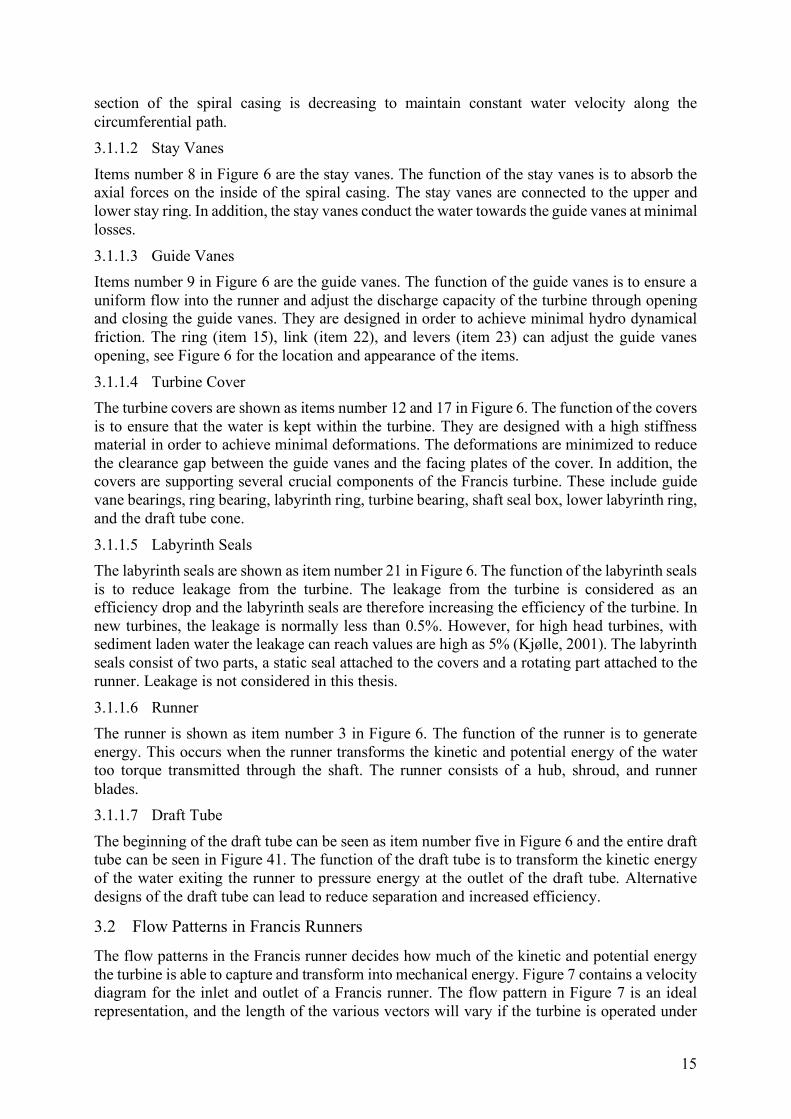
The Francis turbine consists of several different components all with a specific function. The turbine can either be horizontal or vertical. The orientation of the shaft determines if the turbine is horizontal or vertical. Vertical turbines have a vertically connected shaft. Figure 6 illustrates a vertical Francis runner and some of its main components. The inlet is defined as the areas where the water flows into the turbine, and the trailing edge is the at the end of the runner blades. The information and illustrations of the Francis turbine are based on the book Mechanical Equipment by Arne Kjølle (2001)

Figure 6: Illustration of vertical Francis runner (Kjølle, 2001)

3.1.1.1 Spiral/Scroll Casing

Item number one in Figure 6 is the spiral casing of the Francis turbine. The function of the spiral casing is to distribute water evenly through the stay and guide vanes into the runner. The cross-

15

section of the spiral casing is decreasing to maintain constant water velocity along the circumferential path.

3.1.1.2 Stay Vanes

Items number 8 in Figure 6 are the stay vanes. The function of the stay vanes is to absorb the axial forces on the inside of the spiral casing. The stay vanes are connected to the upper and lower stay ring. In addition, the stay vanes conduct the water towards the guide vanes at minimal losses.

3.1.1.3 Guide Vanes

Items number 9 in Figure 6 are the guide vanes. The function of the guide vanes is to ensure a uniform flow into the runner and adjust the discharge capacity of the turbine through opening and closing the guide vanes. They are designed in order to achieve minimal hydro dynamical friction. The ring (item 15), link (item 22), and levers (item 23) can adjust the guide vanes opening, see Figure 6 for the location and appearance of the items.

3.1.1.4 Turbine Cover

The turbine covers are shown as items number 12 and 17 in Figure 6. The function of the covers is to ensure that the water is kept within the turbine. They are designed with a high stiffness material in order to achieve minimal deformations. The deformations are minimized to reduce the clearance gap between the guide vanes and the facing plates of the cover. In addition, the covers are supporting several crucial components of the Francis turbine. These include guide vane bearings, ring bearing, labyrinth ring, turbine bearing, shaft seal box, lower labyrinth ring, and the draft tube cone.

3.1.1.5 Labyrinth Seals

The labyrinth seals are shown as item number 21 in Figure 6. The function of the labyrinth seals is to reduce leakage from the turbine. The leakage from the turbine is considered as an efficiency drop and the labyrinth seals are therefore increasing the efficiency of the turbine. In new turbines, the leakage is normally less than 0.5%. However, for high head turbines, with sediment laden water the leakage can reach values are high as 5% (Kjølle, 2001). The labyrinth seals consist of two parts, a static seal attached to the covers and a rotating part attached to the runner. Leakage is not considered in this thesis.

3.1.1.6 Runner

The runner is shown as item number 3 in Figure 6. The function of the runner is to generate energy. This occurs when the runner transforms the kinetic and potential energy of the water too torque transmitted through the shaft. The runner consists of a hub, shroud, and runner blades.

3.1.1.7 Draft Tube

The beginning of the draft tube can be seen as item number five in Figure 6 and the entire draft tube can be seen in Figure 41. The function of the draft tube is to transform the kinetic energy of the water exiting the runner to pressure energy at the outlet of the draft tube. Alternative designs of the draft tube can lead to reduce separation and increased efficiency.

3.2 Flow Patterns in Francis Runners

The flow patterns in the Francis runner decides how much of the kinetic and potential energy the turbine is able to capture and transform into mechanical energy. Figure 7 contains a velocity diagram for the inlet and outlet of a Francis runner. The flow pattern in Figure 7 is an ideal representation, and the length of the various vectors will vary if the turbine is operated under

16

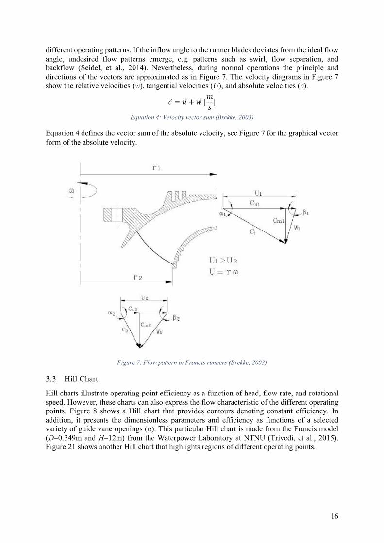
different operating patterns. If the inflow angle to the runner blades deviates from the ideal flow angle, undesired flow patterns emerge, e.g. patterns such as swirl, flow separation, and backflow (Seidel, et al., 2014). Nevertheless, during normal operations the principle and directions of the vectors are approximated as in Figure 7. The velocity diagrams in Figure 7 show the relative velocities (w), tangential velocities (U), and absolute velocities (c).

𝑐 = 𝑢H⃗ + 𝑤HH⃗ [𝑚𝑠 ] Equation 4: Velocity vector sum (Brekke, 2003)

Equation 4 defines the vector sum of the absolute velocity, see Figure 7 for the graphical vector form of the absolute velocity.

Figure 7: Flow pattern in Francis runners (Brekke, 2003)

3.3 Hill Chart

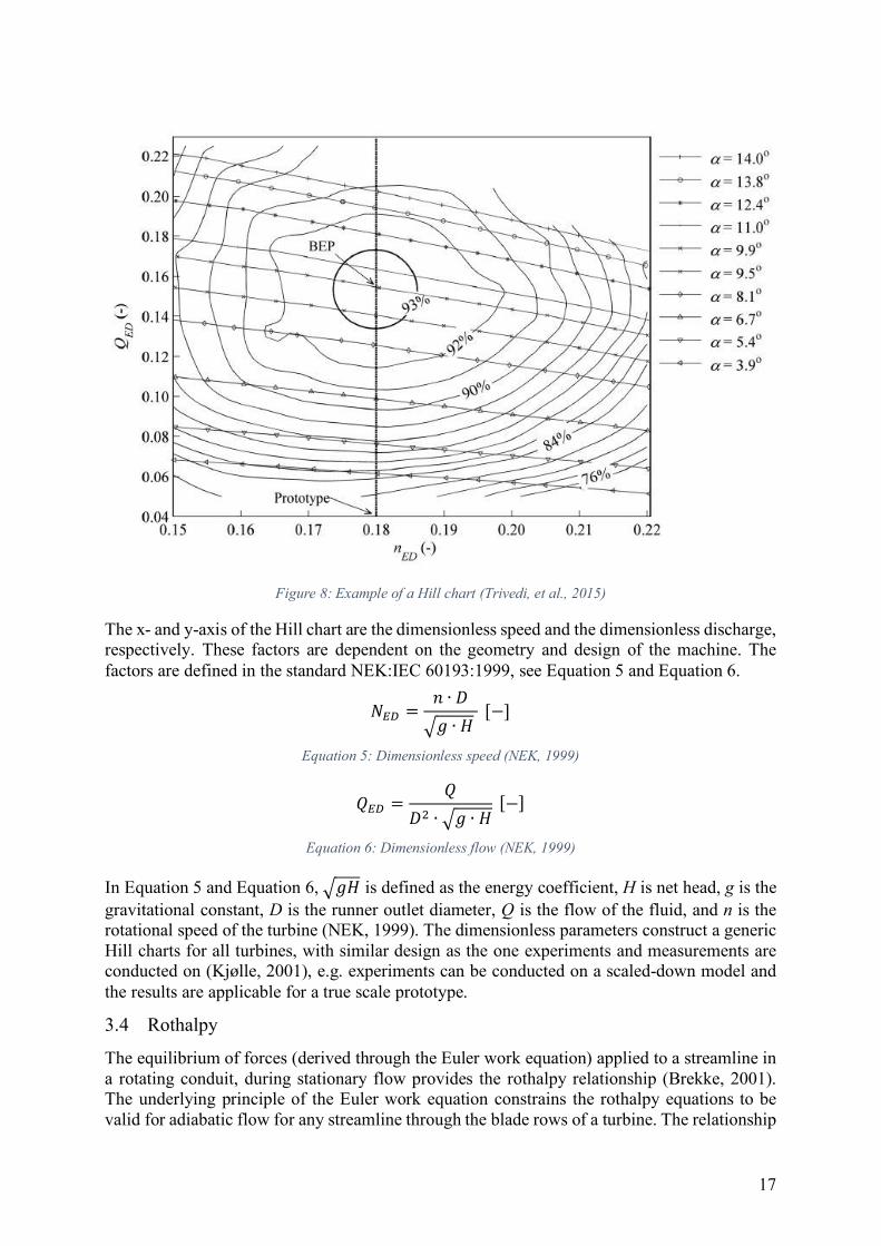
Hill charts illustrate operating point efficiency as a function of head, flow rate, and rotational speed. However, these charts can also express the flow characteristic of the different operating points. Figure 8 shows a Hill chart that provides contours denoting constant efficiency. In addition, it presents the dimensionless parameters and efficiency as functions of a selected variety of guide vane openings (α). This particular Hill chart is made from the Francis model (D=0.349m and H=12m) from the Waterpower Laboratory at NTNU (Trivedi, et al., 2015). Figure 21 shows another Hill chart that highlights regions of different operating points.

17

Figure 8: Example of a Hill chart (Trivedi, et al., 2015)

The x- and y-axis of the Hill chart are the dimensionless speed and the dimensionless discharge, respectively. These factors are dependent on the geometry and design of the machine. The factors are defined in the standard NEK:IEC 60193:1999, see Equation 5 and Equation 6.

𝑁M> = 𝑛 ∙ 𝐷P𝑔 ∙ 𝐻[−]

Equation 5: Dimensionless speed (NEK, 1999)

𝑄M> = 𝑄𝐷2 ∙ P𝑔 ∙ 𝐻[−] Equation 6: Dimensionless flow (NEK, 1999)

In Equation 5 and Equation 6, P𝑔𝐻 is defined as the energy coefficient, H is net head, g is the gravitational constant, D is the runner outlet diameter, Q is the flow of the fluid, and n is the rotational speed of the turbine (NEK, 1999). The dimensionless parameters construct a generic Hill charts for all turbines, with similar design as the one experiments and measurements are conducted on (Kjølle, 2001), e.g. experiments can be conducted on a scaled-down model and the results are applicable for a true scale prototype.

3.4 Rothalpy

The equilibrium of forces (derived through the Euler work equation) applied to a streamline in a rotating conduit, during stationary flow provides the rothalpy relationship (Brekke, 2001). The underlying principle of the Euler work equation constrains the rothalpy equations to be valid for adiabatic flow for any streamline through the blade rows of a turbine. The relationship

18

holds for viscous and inviscid flow. Despite assuming steady flow, it is applicable for the time-average of unsteady flow, provided that the averaging is over a long enough time period. In deriving the rothalpy equation, the friction between the fluid and the turbo machine is neglected. Thus, local changes in angular momentum are not accounted for (Dixon & Hall, 2014). Rothalpy is in some literature denoted as the relative specific stagnation energy, e.g. in the book Fluid mechanics and Thermodynamic of Turbomachinery. Brekke (2001) defines rothalpy according to Equation 7.

𝑃𝜌 + 𝑤22 − 𝑢22 = 𝐶𝑜𝑛𝑠𝑡𝑎𝑛𝑡 W𝑚2

𝑠2 X Equation 7: Rothalpy relation (Brekke, 2001)

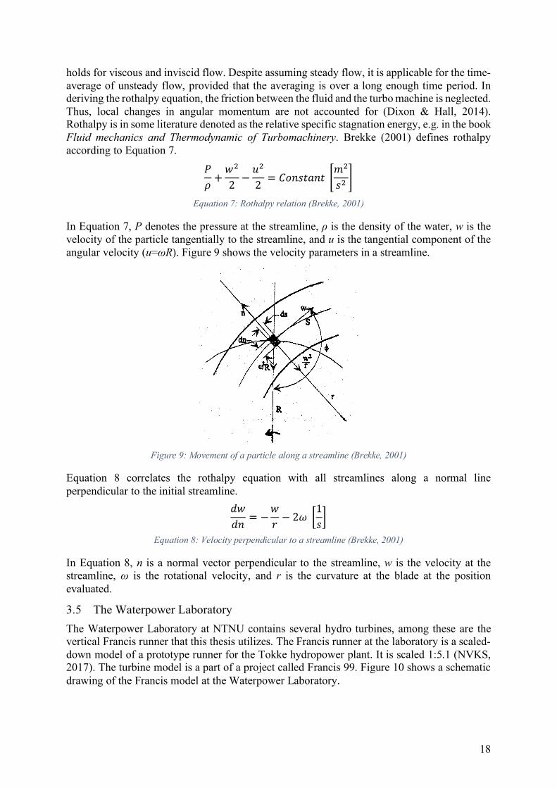
In Equation 7, P denotes the pressure at the streamline, ρ is the density of the water, w is the velocity of the particle tangentially to the streamline, and u is the tangential component of the angular velocity (u=ωR). Figure 9 shows the velocity parameters in a streamline.

Figure 9: Movement of a particle along a streamline (Brekke, 2001)

Equation 8 correlates the rothalpy equation with all streamlines along a normal line perpendicular to the initial streamline. 𝑑𝑤𝑑𝑛 = −𝑤𝑟 − 2𝜔 :1𝑠<

Equation 8: Velocity perpendicular to a streamline (Brekke, 2001)

In Equation 8, n is a normal vector perpendicular to the streamline, w is the velocity at the streamline, ω is the rotational velocity, and r is the curvature at the blade at the position evaluated.

3.5 The Waterpower Laboratory

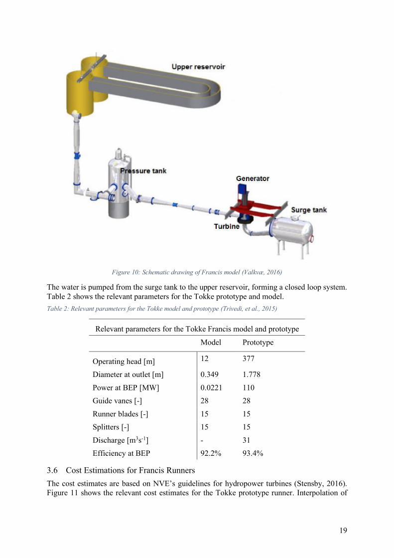
The Waterpower Laboratory at NTNU contains several hydro turbines, among these are the vertical Francis runner that this thesis utilizes. The Francis runner at the laboratory is a scaled-down model of a prototype runner for the Tokke hydropower plant. It is scaled 1:5.1 (NVKS, 2017). The turbine model is a part of a project called Francis 99. Figure 10 shows a schematic drawing of the Francis model at the Waterpower Laboratory.

19

Figure 10: Schematic drawing of Francis model (Valkvæ, 2016)

The water is pumped from the surge tank to the upper reservoir, forming a closed loop system. Table 2 shows the relevant parameters for the Tokke prototype and model.

Table 2: Relevant parameters for the Tokke model and prototype (Trivedi, et al., 2015)

Relevant parameters for the Tokke Francis model and prototype

Model Prototype

Operating head [m] 12 377

Diameter at outlet [m] 0.349 1.778

Power at BEP [MW] 0.0221 110

Guide vanes [-] 28 28

Runner blades [-] 15 15

Splitters [-] 15 15

Discharge [m3s-1] - 31

Efficiency at BEP 92.2% 93.4%

3.6 Cost Estimations for Francis Runners

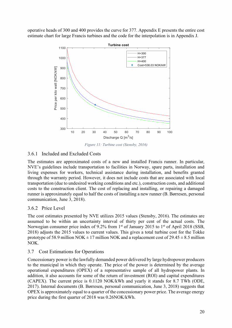
The cost estimates are based on NVE’s guidelines for hydropower turbines (Stensby, 2016). Figure 11 shows the relevant cost estimates for the Tokke prototype runner. Interpolation of

20

operative heads of 300 and 400 provides the curve for 377. Appendix E presents the entire cost estimate chart for large Francis turbines and the code for the interpolation is in Appendix J.

Figure 11: Turbine cost (Stensby, 2016)

3.6.1 Included and Excluded Costs

The estimates are approximated costs of a new and installed Francis runner. In particular, NVE’s guidelines include transportation to facilities in Norway, spare parts, installation and living expenses for workers, technical assistance during installation, and benefits granted through the warranty period. However, it does not include costs that are associated with local transportation (due to undesired working conditions and etc.), construction costs, and additional costs to the construction client. The cost of replacing and installing, or repairing a damaged runner is approximately equal to half the costs of installing a new runner (B. Børresen, personal communication, June 3, 2018).

3.6.2 Price Level

The cost estimates presented by NVE utilizes 2015 values (Stensby, 2016). The estimates are assumed to be within an uncertainty interval of thirty per cent of the actual costs. The Norwegian consumer price index of 9.2% from 1st of January 2015 to 1st of April 2018 (SSB, 2018) adjusts the 2015 values to current values. This gives a total turbine cost for the Tokke prototype of 58.9 million NOK ± 17 million NOK and a replacement cost of 29.45 ± 8.5 million NOK.

3.7 Cost Estimations for Operations

Concessionary power is the lawfully demanded power delivered by large hydropower producers to the municipal in which they operate. The price of the power is determined by the average operational expenditures (OPEX) of a representative sample of all hydropower plants. In addition, it also accounts for some of the return of investment (ROI) and capital expenditures (CAPEX). The current price is 0.1120 NOK/kWh and yearly it stands for 8.7 TWh (ODE, 2017). Internal documents (B. Børresen, personal communication, June 3, 2018) suggests that OPEX is approximately equal to a quarter of the concessionary power price. The average energy price during the first quarter of 2018 was 0.26NOK/kWh.

21

4 Operating Pattern of Francis Turbines

Operating patterns are in this thesis defined as a set of operating points. Voith Hydro splits the operating regimes of Francis turbines into six different operational modes (Seidel, et al., 2014).

1. Startup [cycle/day]

2. Speed no-load (SNL) [%]

3. Low part load [%]

4. Part load [%]

5. Around best efficiency point (BEP) [%]

6. High load [%]

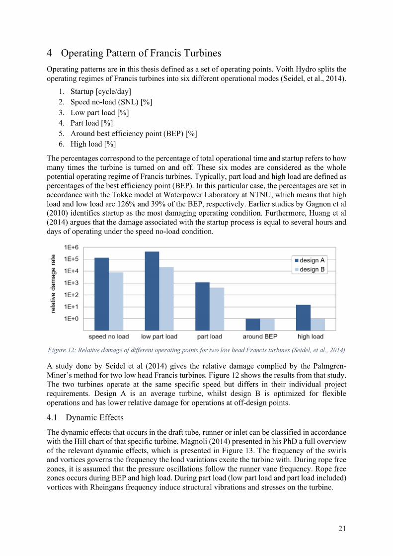
The percentages correspond to the percentage of total operational time and startup refers to how many times the turbine is turned on and off. These six modes are considered as the whole potential operating regime of Francis turbines. Typically, part load and high load are defined as percentages of the best efficiency point (BEP). In this particular case, the percentages are set in accordance with the Tokke model at Waterpower Laboratory at NTNU, which means that high load and low load are 126% and 39% of the BEP, respectively. Earlier studies by Gagnon et al (2010) identifies startup as the most damaging operating condition. Furthermore, Huang et al (2014) argues that the damage associated with the startup process is equal to several hours and days of operating under the speed no-load condition.

Figure 12: Relative damage of different operating points for two low head Francis turbines (Seidel, et al., 2014)

A study done by Seidel et al (2014) gives the relative damage complied by the Palmgren-Miner’s method for two low head Francis turbines. Figure 12 shows the results from that study. The two turbines operate at the same specific speed but differs in their individual project requirements. Design A is an average turbine, whilst design B is optimized for flexible operations and has lower relative damage for operations at off-design points.

4.1 Dynamic Effects

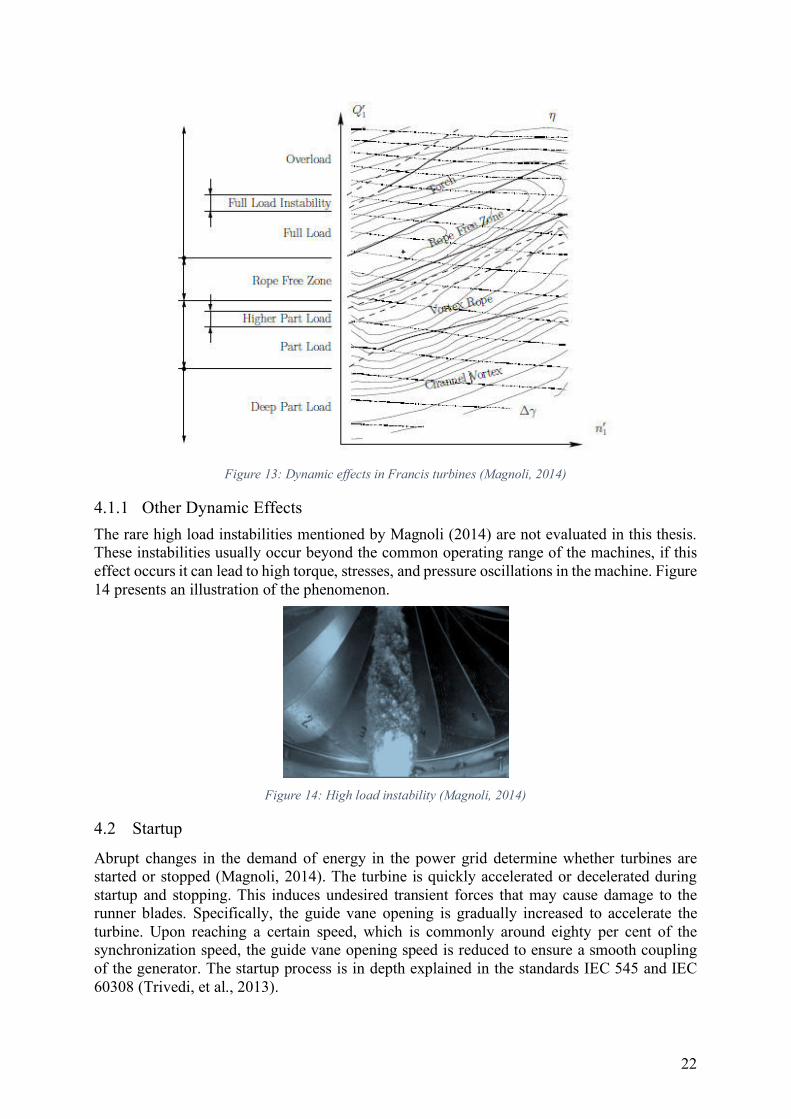
The dynamic effects that occurs in the draft tube, runner or inlet can be classified in accordance with the Hill chart of that specific turbine. Magnoli (2014) presented in his PhD a full overview of the relevant dynamic effects, which is presented in Figure 13. The frequency of the swirls and vortices governs the frequency the load variations excite the turbine with. During rope free zones, it is assumed that the pressure oscillations follow the runner vane frequency. Rope free zones occurs during BEP and high load. During part load (low part load and part load included) vortices with Rheingans frequency induce structural vibrations and stresses on the turbine.

22

Figure 13: Dynamic effects in Francis turbines (Magnoli, 2014)

4.1.1 Other Dynamic Effects

The rare high load instabilities mentioned by Magnoli (2014) are not evaluated in this thesis. These instabilities usually occur beyond the common operating range of the machines, if this effect occurs it can lead to high torque, stresses, and pressure oscillations in the machine. Figure 14 presents an illustration of the phenomenon.

Figure 14: High load instability (Magnoli, 2014)

4.2 Startup

Abrupt changes in the demand of energy in the power grid determine whether turbines are started or stopped (Magnoli, 2014). The turbine is quickly accelerated or decelerated during startup and stopping. This induces undesired transient forces that may cause damage to the runner blades. Specifically, the guide vane opening is gradually increased to accelerate the turbine. Upon reaching a certain speed, which is commonly around eighty per cent of the synchronization speed, the guide vane opening speed is reduced to ensure a smooth coupling of the generator. The startup process is in depth explained in the standards IEC 545 and IEC 60308 (Trivedi, et al., 2013).

23

Figure 15: Startup and synchronization of the turbine (Trivedi, et al., 2013)

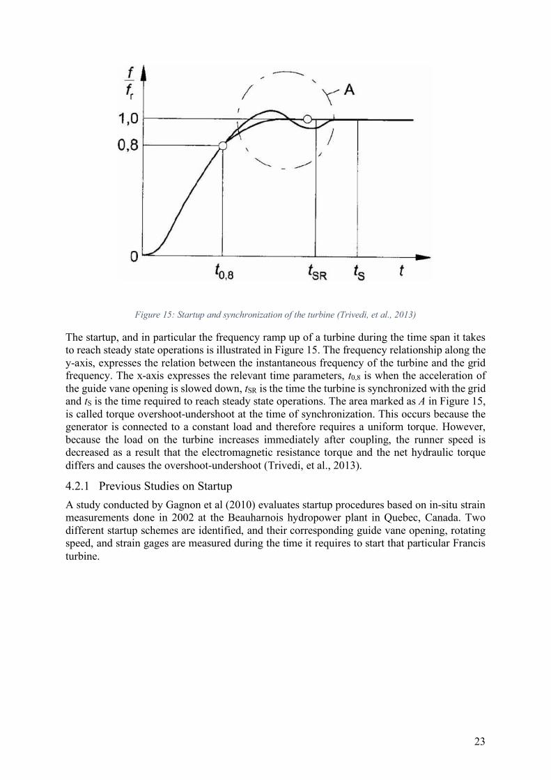
The startup, and in particular the frequency ramp up of a turbine during the time span it takes to reach steady state operations is illustrated in Figure 15. The frequency relationship along the y-axis, expresses the relation between the instantaneous frequency of the turbine and the grid frequency. The x-axis expresses the relevant time parameters, t0,8 is when the acceleration of the guide vane opening is slowed down, tSR is the time the turbine is synchronized with the grid and tS is the time required to reach steady state operations. The area marked as A in Figure 15, is called torque overshoot-undershoot at the time of synchronization. This occurs because the generator is connected to a constant load and therefore requires a uniform torque. However, because the load on the turbine increases immediately after coupling, the runner speed is decreased as a result that the electromagnetic resistance torque and the net hydraulic torque differs and causes the overshoot-undershoot (Trivedi, et al., 2013).

4.2.1 Previous Studies on Startup

A study conducted by Gagnon et al (2010) evaluates startup procedures based on in-situ strain measurements done in 2002 at the Beauharnois hydropower plant in Quebec, Canada. Two different startup schemes are identified, and their corresponding guide vane opening, rotating speed, and strain gages are measured during the time it requires to start that particular Francis turbine.

24

Figure 16: Guide vane opening during a startup

(Gagnon, et al., 2010)

Figure 17: Rotating speed during a startup (Gagnon,

et al., 2010)

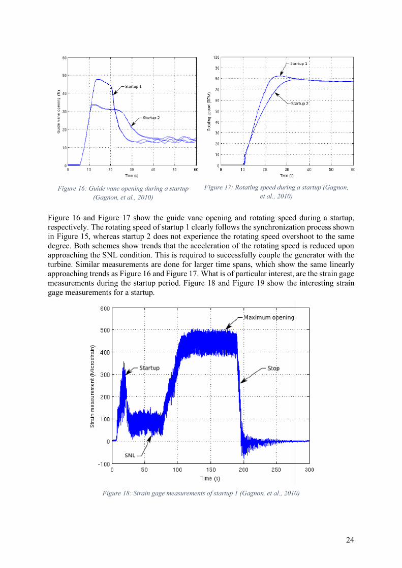
Figure 16 and Figure 17 show the guide vane opening and rotating speed during a startup, respectively. The rotating speed of startup 1 clearly follows the synchronization process shown in Figure 15, whereas startup 2 does not experience the rotating speed overshoot to the same degree. Both schemes show trends that the acceleration of the rotating speed is reduced upon approaching the SNL condition. This is required to successfully couple the generator with the turbine. Similar measurements are done for larger time spans, which show the same linearly approaching trends as Figure 16 and Figure 17. What is of particular interest, are the strain gage measurements during the startup period. Figure 18 and Figure 19 show the interesting strain gage measurements for a startup.

Figure 18: Strain gage measurements of startup 1 (Gagnon, et al., 2010)

25

As a result of the larger guide vane opening during the startup, startup 1 experiences increased strain during the first 50 seconds of the startup, compared to startup 2.

Figure 19: Strain gage measurements of startup 2 (Gagnon, et al., 2010)

Figure 18 and Figure 19 are assemblies of three independent recordings that aim to illustrate a simplified operating sequence, going from startup to complete stop. The section recordings that are assembled are:

1. Startup that ends at SNL

2. SNL ending at maximum guide vane opening

3. Maximum guide vane opening ending at a complete stop

4.2.2 Revolutions and Strain During Startup

The startup scheme lasts for the time interval it takes the turbine to reach synchronization speed. Thus, at t0.8 the number of load cycles during this interval are decided by integrating the guide vane passing frequency over the time it takes to accelerate the turbine. It is further assumed that the pressure pulsations follow this frequency.

𝑛,.Z[. = \ 𝑡A.^22 𝑑𝛼C` = \ 𝑡A.^2 𝑑𝑅𝑃𝑀C`cdefgA = 832jfg

A [𝑅𝑒𝑣] 𝛼C` = 𝑅𝑃𝑀C`,.n.o − 𝑅𝑃𝑀C`,.pA𝑡A.^ − 0 = 𝑅𝑃𝑀C`,.n.o𝑡A.^ :𝑅𝑒𝑣𝑠2 <

Equation 9: Revolutions during startup

The time required for a startup is defined in accordance with the studies conducted by Huang et al (2014) and Gagnon et al (2010). These studies indicate that the acceleration of a turbine takes approximately 20 seconds, shown in figures Figure 17, Figure 18 and Figure 19. Strain that occurs during startup is assumed to be proportional with the guide vane opening. In Figure 16 the guide vanes are opened 2.5 – 3 times more at startup than at BEP. Thus, the strains are approximated to be 2.5 times the strain that results from mean pressure at BEP. Equation 9

26

gives the number of revolutions that occurs during a startup. In this case with 333 RPM, the revolutions during startups (20s) are 832.

4.3 Speed No Load

The principle of speed no load (SNL) is that the generator is not connected to the grid, and thus there is no power generation during this phase. The machine is running at synchronous speed and the generator is synchronized with the electric circuit such that the machine is able to produce energy at any moment (Magnoli, 2014). This means that there are large amounts of water and energy dispatched through the turbine. This occurs during startup, before the generator is connected and at later stages when SNL is desired. It is argued that the wear from startup is large compared SNL. Therefore, it is argued that it is possible to operate the turbine at SNL and quickly connect the generator and start generation (Mende, et al., 2016). This means that water is lost as it is flowing through the turbine, and the alternative cost of this lost water should be compared with the increased maintenance cost of startup.

Mende et al (2016) argues that the relative damage of SNL is comparable to low part load, as seen in Figure 12. As the simulations of SNL is currently not up to date to the degree that is desired, the damage contribution from this phase will be assumed to be equal to the low part load and excite the turbine with the same load frequency as low part load. These arguments are based on the quasi-static stress analyses that are compared with dynamic strain gage measurements carried out by Mende et al (2016). When more transient simulations are available for this phenomenon, the stated assumptions must be revised and verified in accordance with more complex numerical analyses.

4.4 Part Load

Guide vane openings that are lower than the BEP opening, are classified as part load. In these regions, the flow rates are low, and it is found increased evidence of cavitation in the draft tube. As a consequence of increased cavitation, a vortex rope consisting of cavitational bubbles can be found in the draft tube. Figure 20 shows an example of a part load vortex rope. The pressure pulsations during part load can reach high amplitudes. Machines with higher specific speed will be exposed to higher pressure pulsations (Brekke, 2010). Nevertheless, the relationship between the specific speed and the value of the pressure pulsations is complex and dependent on a lot of factors, e.g. geometry (inlet, runner, and draft tube), flow conditions, and water properties (Magnoli, 2014).

Figure 20: Part load vortex rope (Magnoli, 2014)

4.4.1 Rheingans Frequency

The frequency at which the vortex rope oscillates during part load is called Rheingans frequency, after the first person that studied and identified the phenomenon. Equation 10 expresses how Rheingans (1940) defined the frequency of the draft tube surges.

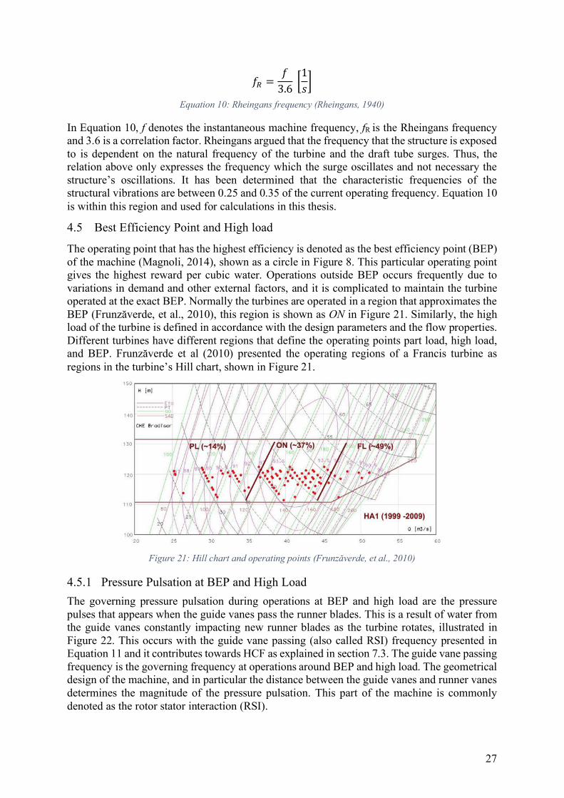
27

𝑓c = 𝑓3.6:1𝑠< Equation 10: Rheingans frequency (Rheingans, 1940)

In Equation 10, f denotes the instantaneous machine frequency, fR is the Rheingans frequency and 3.6 is a correlation factor. Rheingans argued that the frequency that the structure is exposed to is dependent on the natural frequency of the turbine and the draft tube surges. Thus, the relation above only expresses the frequency which the surge oscillates and not necessary the structure’s oscillations. It has been determined that the characteristic frequencies of the structural vibrations are between 0.25 and 0.35 of the current operating frequency. Equation 10 is within this region and used for calculations in this thesis.

4.5 Best Efficiency Point and High load

The operating point that has the highest efficiency is denoted as the best efficiency point (BEP) of the machine (Magnoli, 2014), shown as a circle in Figure 8. This particular operating point gives the highest reward per cubic water. Operations outside BEP occurs frequently due to variations in demand and other external factors, and it is complicated to maintain the turbine operated at the exact BEP. Normally the turbines are operated in a region that approximates the BEP (Frunzăverde, et al., 2010), this region is shown as ON in Figure 21. Similarly, the high load of the turbine is defined in accordance with the design parameters and the flow properties. Different turbines have different regions that define the operating points part load, high load, and BEP. Frunzăverde et al (2010) presented the operating regions of a Francis turbine as regions in the turbine’s Hill chart, shown in Figure 21.

Figure 21: Hill chart and operating points (Frunzăverde, et al., 2010)

4.5.1 Pressure Pulsation at BEP and High Load

The governing pressure pulsation during operations at BEP and high load are the pressure pulses that appears when the guide vanes pass the runner blades. This is a result of water from the guide vanes constantly impacting new runner blades as the turbine rotates, illustrated in Figure 22. This occurs with the guide vane passing (also called RSI) frequency presented in Equation 11 and it contributes towards HCF as explained in section 7.3. The guide vane passing frequency is the governing frequency at operations around BEP and high load. The geometrical design of the machine, and in particular the distance between the guide vanes and runner vanes determines the magnitude of the pressure pulsation. This part of the machine is commonly denoted as the rotor stator interaction (RSI).

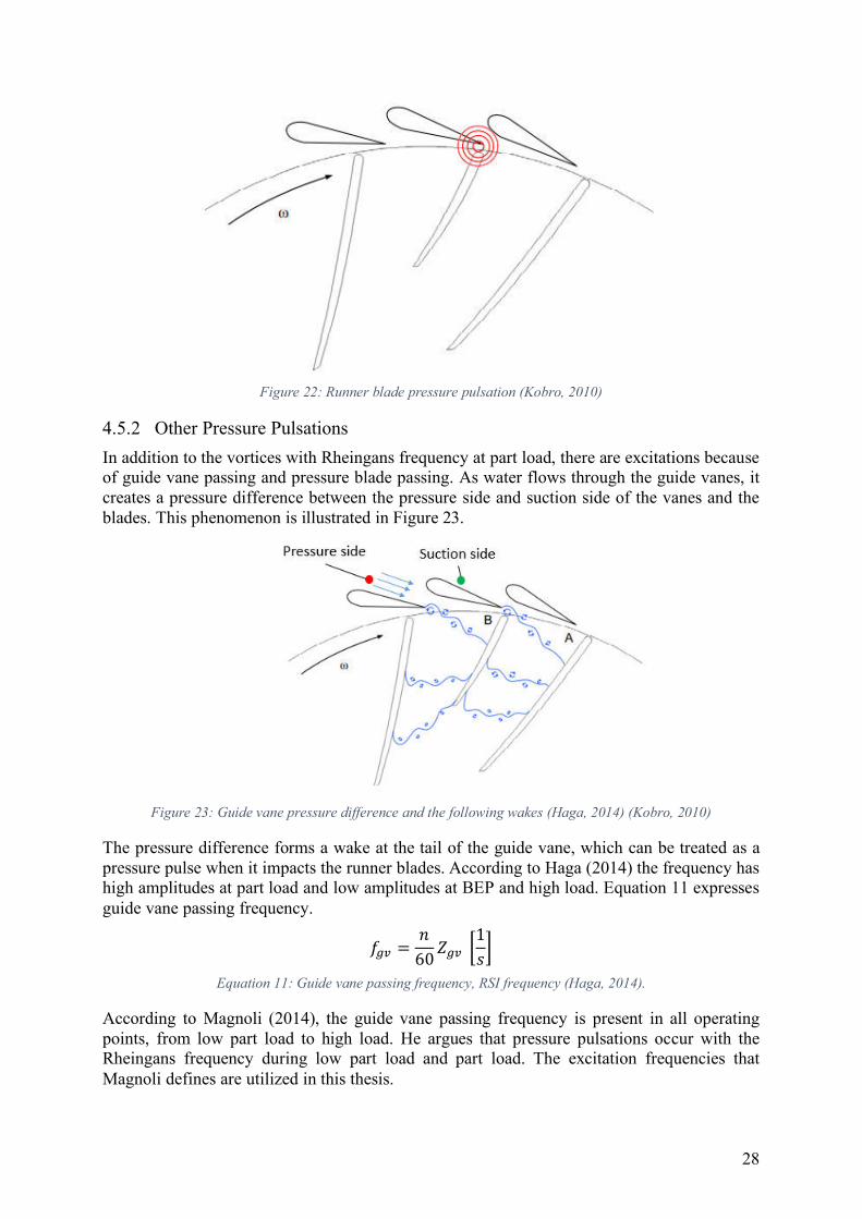
28

Figure 22: Runner blade pressure pulsation (Kobro, 2010)

4.5.2 Other Pressure Pulsations

In addition to the vortices with Rheingans frequency at part load, there are excitations because of guide vane passing and pressure blade passing. As water flows through the guide vanes, it creates a pressure difference between the pressure side and suction side of the vanes and the blades. This phenomenon is illustrated in Figure 23.

Figure 23: Guide vane pressure difference and the following wakes (Haga, 2014) (Kobro, 2010)

The pressure difference forms a wake at the tail of the guide vane, which can be treated as a pressure pulse when it impacts the runner blades. According to Haga (2014) the frequency has high amplitudes at part load and low amplitudes at BEP and high load. Equation 11 expresses guide vane passing frequency.

𝑓"s = 𝑛60𝑍"s :1𝑠< Equation 11: Guide vane passing frequency, RSI frequency (Haga, 2014).

According to Magnoli (2014), the guide vane passing frequency is present in all operating points, from low part load to high load. He argues that pressure pulsations occur with the Rheingans frequency during low part load and part load. The excitation frequencies that Magnoli defines are utilized in this thesis.

29

5 Impact of Flexible Operations

The chart in Figure 24 presents the generic approach to evaluate the impact of flexible operations. The chart is only for illustrative purposes, and the ordering of the components are less important than the boundaries they set for the overall purpose of evaluating the impact. This section covers the fundamental links and assumptions utilized to find the impact of flexible operations. The chart is made by the author of this thesis to highlight the thought process during the evaluation of flexible operations.

Figure 24: Generic process of evaluating impact of flexible operations impact

5.1 System Effectiveness and Reliability Engineering

System effectiveness seeks to address the availability, dependability, capability, and reliability of a system. Reliability is comparable to the active operating time of the system and is therefore a component of the availability of the system. Availability is the probability that the system is operating satisfactory at a given point in time, found by evaluating the ratio between operations and downtime (maintenance, repairs, idle time, and etc.) (Kececioglu, 2003).

5.1.1 Reliability and Availability

Reliability is a probabilistic term, which implies that the term is a number between 0 and 1. It is the conditional probability that the system will successfully operate within:

1. A given confidence interval.

2. Without failure and at a specified performance level according to its age.

3. For a given time span when used according to its purpose and intended use.

Equation 12 is the mathematical model that describes reliability (Kececioglu, 2003).

𝑅(𝑡) = 𝑁w(𝑡)𝑁x(𝑡) = 𝑁x(𝑡) − 𝑁y(𝑡)𝑁x(𝑡) [−] Equation 12: Reliability (Kececioglu, 2003)

In Equation 12, Ns, NF, and NT denote successful, unsuccessful, and total operations over a given time span, respectively. For energy production, Ns, NF, and NT are active time, unplanned outage time, and total time (B. Børresen, personal communication, June 3, 2018), respectively. By altering Equation 12, it is possible to find the failure distribution. Reliability is the complementary product of the failure distribution, see Equation 13.

𝑅(𝑡) = 1 − 𝑁y(𝑡)𝑁.(𝑡) = 1 − 𝑄(𝑡)[−] Equation 13: Failure distribution (Kececioglu, 2003)

Equation 14 gives the statistical failure distribution.

Operating Patterns

Reliability and System

EffectivenessDamage Model Cost Model

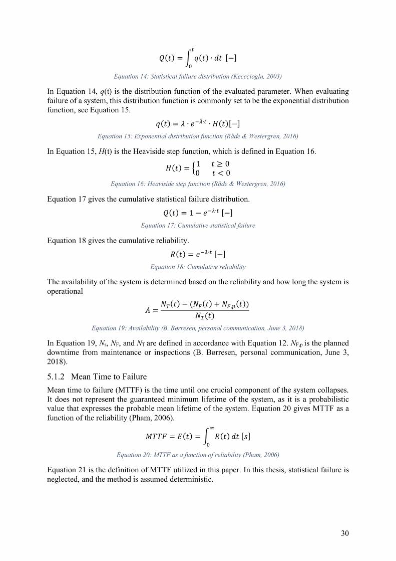
30

𝑄(𝑡) = \ 𝑞(𝑡) ∙ 𝑑𝑡.A [−]

Equation 14: Statistical failure distribution (Kececioglu, 2003)

In Equation 14, q(t) is the distribution function of the evaluated parameter. When evaluating failure of a system, this distribution function is commonly set to be the exponential distribution function, see Equation 15.

𝑞(𝑡) = 𝜆 ∙ 𝑒|}∙. ∙ 𝐻(𝑡)[−] Equation 15: Exponential distribution function (Råde & Westergren, 2016)

In Equation 15, H(t) is the Heaviside step function, which is defined in Equation 16.

𝐻(𝑡) = ~1𝑡 ≥ 00𝑡 < 0

Equation 16: Heaviside step function (Råde & Westergren, 2016)

Equation 17 gives the cumulative statistical failure distribution.

𝑄(𝑡) = 1 − 𝑒|}∙. [−] Equation 17: Cumulative statistical failure

Equation 18 gives the cumulative reliability.

𝑅(𝑡) = 𝑒|}∙.[−] Equation 18: Cumulative reliability

The availability of the system is determined based on the reliability and how long the system is operational

𝐴 = 𝑁x(𝑡) − (𝑁y(𝑡) + 𝑁y,�(𝑡))𝑁x(𝑡) Equation 19: Availability (B. Børresen, personal communication, June 3, 2018)

In Equation 19, Ns, NF, and NT are defined in accordance with Equation 12. NF,p is the planned downtime from maintenance or inspections (B. Børresen, personal communication, June 3, 2018).

5.1.2 Mean Time to Failure

Mean time to failure (MTTF) is the time until one crucial component of the system collapses. It does not represent the guaranteed minimum lifetime of the system, as it is a probabilistic value that expresses the probable mean lifetime of the system. Equation 20 gives MTTF as a function of the reliability (Pham, 2006).

𝑀𝑇𝑇𝐹 = 𝐸(𝑡) = \ 𝑅(𝑡)�A 𝑑𝑡[𝑠]

Equation 20: MTTF as a function of reliability (Pham, 2006)

Equation 21 is the definition of MTTF utilized in this paper. In this thesis, statistical failure is neglected, and the method is assumed deterministic.

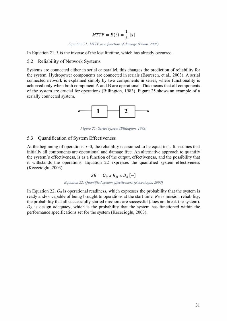
31

𝑀𝑇𝑇𝐹 = 𝐸(𝑡) = 1𝜆[𝑠] Equation 21: MTTF as a function of damage (Pham, 2006)

In Equation 21, λ is the inverse of the lost lifetime, which has already occurred.

5.2 Reliability of Network Systems

Systems are connected either in serial or parallel, this changes the prediction of reliability for the system. Hydropower components are connected in serials (Børresen, et al., 2003). A serial connected network is explained simply by two components in series, where functionality is achieved only when both component A and B are operational. This means that all components of the system are crucial for operations (Billington, 1983). Figure 25 shows an example of a serially connected system.

Figure 25: Series system (Billington, 1983)

5.3 Quantification of System Effectiveness

At the beginning of operations, t=0, the reliability is assumed to be equal to 1. It assumes that initially all components are operational and damage free. An alternative approach to quantify the system’s effectiveness, is as a function of the output, effectiveness, and the possibility that it withstands the operations. Equation 22 expresses the quantified system effectiveness (Kececioglu, 2003).

𝑆𝐸 = 𝑂c𝑥𝑅e𝑥𝐷�[−] Equation 22: Quantified system effectiveness (Kececioglu, 2003)

In Equation 22, OR is operational readiness, which expresses the probability that the system is ready and/or capable of being brought to operations at the start time. RM is mission reliability, the probability that all successfully started missions are successful (does not break the system). DA is design adequacy, which is the probability that the system has functioned within the performance specifications set for the system (Kececioglu, 2003).

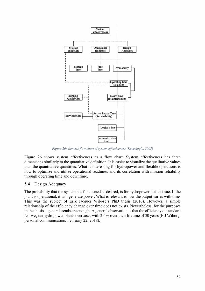
32

Figure 26: Generic flow chart of system effectiveness (Kececioglu, 2003)

Figure 26 shows system effectiveness as a flow chart. System effectiveness has three dimensions similarly to the quantitative definition. It is easier to visualize the qualitative values than the quantitative quantities. What is interesting for hydropower and flexible operations is how to optimize and utilize operational readiness and its correlation with mission reliability through operating time and downtime.

5.4 Design Adequacy

The probability that the system has functioned as desired, is for hydropower not an issue. If the plant is operational, it will generate power. What is relevant is how the output varies with time. This was the subject of Erik Jacques Wiborg’s PhD thesis (2016). However, a simple relationship of the efficiency change over time does not exists. Nevertheless, for the purposes in the thesis – general trends are enough. A general observation is that the efficiency of standard Norwegian hydropower plants decreases with 2-4% over their lifetime of 30 years (E.J Wiborg, personal communication, February 22, 2018).

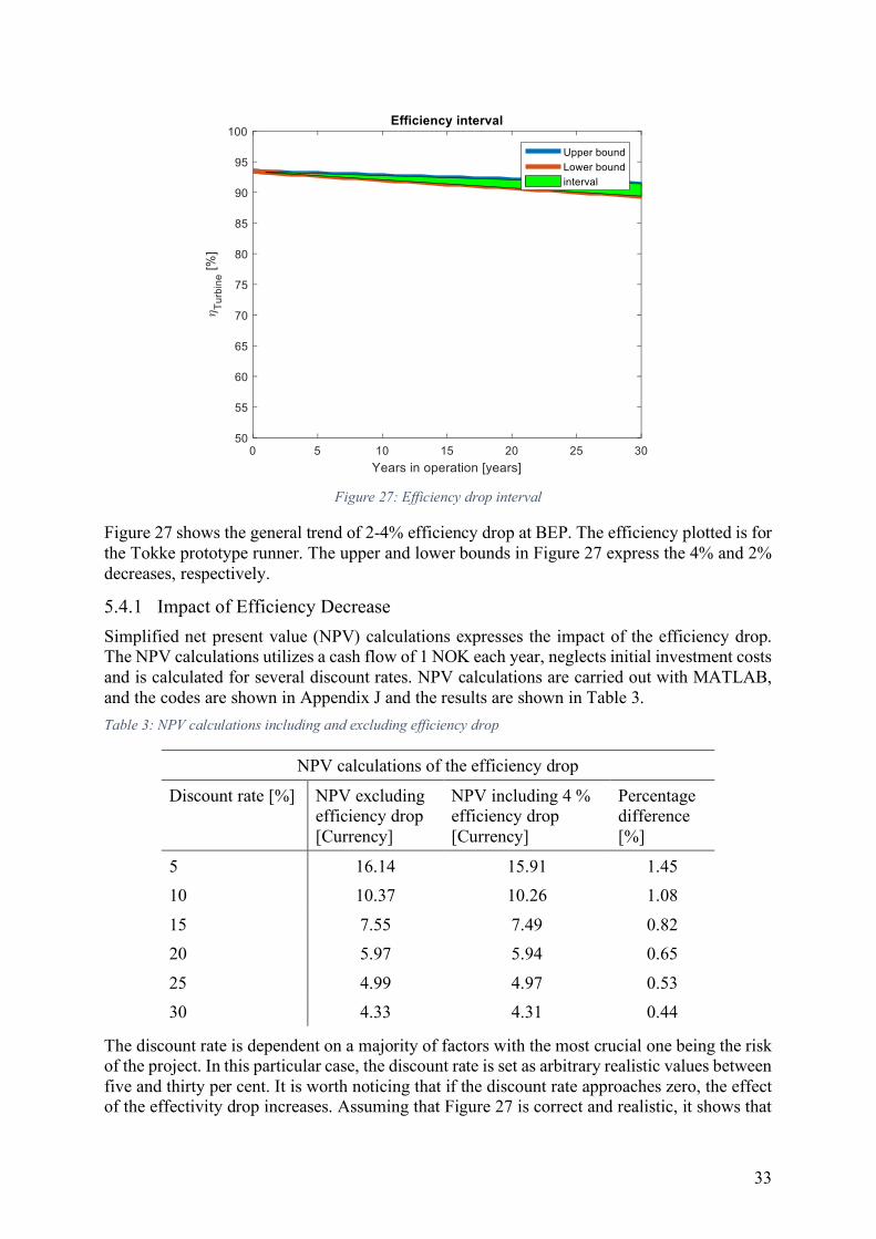
33

Figure 27: Efficiency drop interval

Figure 27 shows the general trend of 2-4% efficiency drop at BEP. The efficiency plotted is for the Tokke prototype runner. The upper and lower bounds in Figure 27 express the 4% and 2% decreases, respectively.

5.4.1 Impact of Efficiency Decrease

Simplified net present value (NPV) calculations expresses the impact of the efficiency drop. The NPV calculations utilizes a cash flow of 1 NOK each year, neglects initial investment costs and is calculated for several discount rates. NPV calculations are carried out with MATLAB, and the codes are shown in Appendix J and the results are shown in Table 3.

Table 3: NPV calculations including and excluding efficiency drop

NPV calculations of the efficiency drop

Discount rate [%] NPV excluding efficiency drop [Currency]

NPV including 4 % efficiency drop [Currency]

Percentage difference [%]

5 16.14 15.91 1.45

10 10.37 10.26 1.08

15 7.55 7.49 0.82

20 5.97 5.94 0.65

25 4.99 4.97 0.53

30 4.33 4.31 0.44

The discount rate is dependent on a majority of factors with the most crucial one being the risk of the project. In this particular case, the discount rate is set as arbitrary realistic values between five and thirty per cent. It is worth noticing that if the discount rate approaches zero, the effect of the effectivity drop increases. Assuming that Figure 27 is correct and realistic, it shows that

34

the reduction of efficiency over the lifetime of the turbine does not impact the generated cash flows to a noticeable degree. The difference in NPV when including the efficiency drop is very small, see Table 3. As a matter of fact, it is expected that the NPV of the efficiency drop will be much smaller than the uncertainty of future energy prices (Böttger, 2018), unscheduled maintenance, uncertainty in construction, and rehabilitation costs (Norconsult AS, 2016). However, as predictions of future energy prices is out of scope for this thesis, the efficiency drop is included. The design adequacy of the hydropower plant is the relationship between the current efficiency and the initial efficiency.

5.5 Cost Model

This thesis utilizes a simple generic cost model, presented in Equation 23.

𝐶x�.Z$ = 𝑃��,, + 𝐶eZ�D./DZD�/ + 𝐶c/�Ds/,.0/D. [𝑁𝑂𝐾] Equation 23: Generic cost model

In Equation 23, CMaintenance is the maintenance cost, CReinvestment is the reinvestment cost, and Ploss

are the operational losses. The operational losses have two dimensions, losses due to downtime and efficiency drop.

𝑃��,, = 𝑃>��D.�0/ + 𝑃��/[Z.��DZ$$�,,= \ 𝑃(𝑡)

>��D.�0/∙ 𝑝(𝑡) ∙ 𝑑𝑡 + \ Δ𝜂 ∙ 𝑔 ∙ 𝜌 ∙ 𝑄 ∙ 𝐻 ∙ 𝑝(𝑡)𝑑𝑡

��/[Z.��D,[𝑁𝑂𝐾]

Equation 24: Operational losses

In Equation 24, the downtime component consists of the lost production while repairing the turbine and the associated lost income during the downtime. Operational losses are losses associated with the efficiency drop that continuously increases, see Figure 27.

𝐶eZ�D./DZD�/ = 𝐶d$ZDD/� + 𝐶�D�$ZDD/� + 𝐶M����0//D. [𝑁𝑂𝐾] Equation 25: Maintenance cost

Equation 25 shows all the under categories of the maintenance cost. It is assumed that there is a linear relationship with the maintenance cost and the lifetime of the turbine. The maintenance cost (planned, unplanned, and equipment) is set equal to a quarter of the concessionary power price (see section 3.7), thus, maintenance cost represents the OPEX. The impact of the operating patterns is evaluated based on the change of cost, expressed as NPV for the different patterns.

The reinvestment cost is the costs associated with replacement and repairs of the turbine, discounted to present values. Furthermore, turbines that has not yet collapsed includes a fraction of the total replacement costs. The replacement cost is given in section 3.6.

5.6 Net Present Value

Net present value (NPV) is a method used to find the current value of future cash flows (positive or negative). The NPV calculations assumes that there is a linear relationship between the energy produced and the income generated. Thus, it is here neglected variations in the energy prices. Equation 26 expresses the effect of a hydropower plant (NVE, 2015).

𝑃 = 𝑄𝐻𝑔𝜌𝜂[W] Equation 26: Effect (NVE, 2015)

35

In Equation 26, Q is the flow rate, H is the net head, g is the gravitational constant, ρ is the density of the water, and η is the effectivity of the hydropower plant. If the effect (Equation 26) is multiplied by operational time, it gives energy. Equation 27 expresses the equation for NPV (Inverstorpedia, 2018).

𝑁𝑃𝑉 =� 𝐶.(1 + 𝑟). − 𝐶Ax.p�

[𝑁𝑂𝐾] Equation 27: Net present value (NPV) (Inverstorpedia, 2018)

In Equation 27, Ct is the cash flow during the period t, r is the discount rate, t is the evaluated time period, T is the total time evaluated, and C0 is the total initial investment cost. For hydropower, the base discount rate is set equal to ten per cent (IRENA, 2012).

5.7 Impact on Hydropower

System effectiveness, lifetime, reliability, downtime, and maintenance for general and typical operating patterns are well-documented and there is a lot of data to draw conclusions from. What is interesting is how system effectiveness changes with aggressive operating patterns, as a result of an increased demand for flexible generation. This is achieved by evaluating aggressive operating patterns, its associated costs and current value. It is sought to find a relationship between the three characteristics presented by Welte and Solvang (2011) (see section 2.2) and system effectiveness.

The impact of flexible operations follows the generic model presented in Figure 24. A set of operating patterns are assumed, the reliability is a function of the design adequacy and MTTF and a fatigue damage model is utilized. Operational and maintenance costs are found under those underlying assumptions.

36

6 Mechanical Engineering Definitions

During operations of any machine, forces impacts the machine. In order to evaluate if these forces are within acceptable limits without fracturing the machine, it is important to have knowledge of the material and the external forces. This section contains an overview of stress and strain, a generic damage model, and a lifetime model. The model works for all machines operating under varying (and constant) load conditions.

6.1 Stress and Constitutive Relations

The constitutive relations address the correlation between force and deformation. More specifically, they correlate stresses and strains (Sundström, 2010). Equation 28 defines stress for a uniaxial bar exposed to force.

𝜎 = 𝐹𝐴[𝑃𝑎] Equation 28: Stress (Sundström, 2010)

In Equation 28, F is the applied force, A is the force exposed area, and s is the stress. Equation 29 defines elongation, commonly called strain.

𝜖 = 𝑙� − 𝑙A𝑙A = Δ𝑙𝑙A [−] Equation 29: Strain (Sundström, 2010)

In Equation 29, the subscripts denote the length at the initial state (0) and deformed state (i). The simplest constitutive relationship between strain and stress is the 1-D expression of Hooke’s law, expressed in Equation 30.

𝜎 = 𝐸𝜖[𝑃𝑎] Equation 30: Hooke's law (Sundström, 2010)

In Equation 30, E is the modulus of elasticity, commonly called Young’s modulus in a 1-D case. Multi axial stress states have similar equations, where the Young’s modulus is considered as the stiffness of the material and expressed as a matrix. In multi axial stress states, the stress is a stress tensor that contains all stress dimensions and it is likewise for the strains. Equation 31 expresses a multiaxial stress state.

σ = 𝐶𝜖[𝑃𝑎] Equation 31: Multi axial stress state (Gudmundson, 2010)

In Equation 31, s is a six-dimensional column stress vector, the strain is a six-dimensional column vector and C is a six by six stiffness matrix. The stiffness matrix can be very complex and defined in accordance with the specific material model utilized. Matrices for different material models can be found in various mechanical engineering handbooks and course literature, e.g. in Material Mechanics by Peter Gudmundson (2010). Equation 32 expresses the stress (similar for strain) as a transposed column vector in Voigt notation.

σx = �𝜎  , 𝜎-, 𝜎¡ , 𝜏 -, 𝜏 ¡ , 𝜏-¡£[𝑃𝑎] Equation 32: Transposed stress column vector (Gudmundson, 2010)

In Equation 32, the column stress vector is transposed to a row vector. In most engineering applications, a six-dimensional stress state does not explicitly say anything about the potential

37

for failure. Equivalent stress states are better suited to address this. There exist several equivalent stress states, but the most popular are the Von Mises and Tresca criterions (Gudmundson, 2010). Von Mises stress is a method to find an equivalent 1-D stress when there is a multi-axial stress state. It incorporates all the stress components in Equation 32. Equation 33 is the definition of Von Mises stress (Sundström, 2010).

𝜎`e2 = 𝜎 2 + 𝜎-2 + 𝜎¡2 − 𝜎 𝜎- − 𝜎 𝜎¡−𝜎-𝜎¡ + 3𝜏 -2 + 3𝜏 ¡2 + 3𝜏-¡2 [𝑃𝑎2] Equation 33: Von Mises stress (Sundström, 2010)

6.2 Dynamic Stresses

Stress can occur statically or dynamically. In dynamic stress states, the static and mean stresses are of less importance, as these are often not the reason the structure collapses. The frequency at which the stresses oscillates and at what magnitude are what governs fatigue fractures. Equation 34 expresses the amplitude stress.

𝜎� = Δ𝜎2 = 𝜎eZ  − 𝜎e�D2 = 𝜎eZ (1 − 𝑅)2 [𝑃𝑎] Equation 34: Amplitude stress (Nilsson, 2001)

In Equation 34, s is the stress and R is the stress ratio, which is the difference between the minimum stress and maximum stress, expressed in Equation 35.

𝑅 = σe�D𝜎eZ  [−] Equation 35: Stress ratio (Nilsson, 2001)

Equation 36 expresses the mean stress in dynamic stress states.

𝜎0 = 𝜎eZ  + 𝜎e�D2 [−] Equation 36: Mean stress (Nilsson, 2001)

6.2.1 Goodman’s Criteria

To further evaluate the stress state, the amplitude stresses are adjusted in accordance with the mean stresses. The adjustment seeks to find an equivalent effective stress that encompasses all stress states and material properties. The effective stress parameter is used for fatigue assessment. There are several different methods and principles that accomplishes this. Nevertheless, this thesis uses Goodman’s criterion to find an effective stress state. Equation 37 expresses Goodman’s criterion. 𝜎�𝜎/ + ¤ 𝜎0𝜎�xw¥

Z = 1[−] Equation 37: Goodman's criterion (Ferreira, et al., 2005)

In Equation 37, σA is the stress amplitude, σe is the endurance limit, σm is the mean stress, σUTS

is the ultimate tensile strength, and a is a factor that is set equal to 1 for the linear Goodman criterion and 2 for the parabolic Gerber expression (Ferreira, et al., 2005). Figure 28 graphically expresses the Goodman and Gerber adjustments.

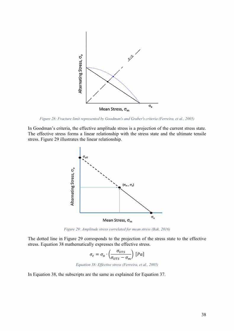
38

Figure 28: Fracture limit represented by Goodman's and Graber's criteria (Ferreira, et al., 2005)

In Goodman’s criteria, the effective amplitude stress is a projection of the current stress state. The effective stress forms a linear relationship with the stress state and the ultimate tensile stress. Figure 29 illustrates the linear relationship.

Figure 29: Amplitude stress correlated for mean stress (Bak, 2016)

The dotted line in Figure 29 corresponds to the projection of the stress state to the effective stress. Equation 38 mathematically expresses the effective stress.

𝜎/ = 𝜎Z ∙ ¤ 𝜎�xw𝜎�xw − 𝜎0¥[𝑃𝑎] Equation 38: Effective stress (Ferreira, et al., 2005)

In Equation 38, the subscripts are the same as explained for Equation 37.

39

7 Damage and Lifetime Model

The damage in turbines are results of both dynamic and static stresses in the materials. A generic fatigue model can assess the lifetime of a turbine. This paper utilizes the Palmgren-Miner model, which attempts to predict the existing lifetime of the component. For serially connected components, it is sufficient to only evaluate the critical part. The critical part is in this paper assumed to be the turbine, because it experiences the largest stresses. Failure occurs at the area with the largest stresses, therefore, it is sufficient to only analyze the runner. The fatigue analyses give the remaining lifetime of the turbine. MTTF expresses the average remaining lifetime and is in this setting similar to the remaining lifetime found through fatigue analyses. Commonly, MTTF is defined as a statistical term (Råde & Westergren, 2004), whilst these analyses provide a deterministic value. However, the applications of MTTF explained in section 5.1 are still valid.

7.1 Fatigue and Lifetime Model

The Palmgren-Miner model evaluates the fatigue damage of the turbine, which is a cumulative damage model. The model is also known as the linear damage accumulation rule (Santecchia, et al., 2016).

𝐷 =�𝐷�¦�p�

=� 𝑛�𝑁�(Δ𝜎)¦�p�

[−] Equation 39: Palmgren-Miner model (Santecchia, et al., 2016)

In Equation 39, D is defined as the cumulative linear summarized damage that results from each load cycle, ni is the number of load cycles at a given stress level, and Ni is the maximum number of load cycles given by the S-N curve at that particular load (given by the x-axis of Figure 31). The principle of the model is that when the D reaches one, the component will collapse.

The goal of introducing a damage model is to find the impact of cyclic stresses on the functional lifetime of the component. In order to this, a generalized Palmgren-Miner model is utilized. The generalization of the model assumes that both fatigue and static wear is cumulatively summarized. This is a generalization of the model presented in ISO (International Organization for Standardization) 19902, which includes previous damage. Equation 40 expresses the current remaining fatigue damage.

𝐷2 = 1 − 𝐷�[−] Equation 40: Remaining lifetime (ISO, 2007)

In Equation 40, the subscripts 1 and 2 denote damage at times 1 and 2, respectively. By generalizing the model, Equation 41 defines the instantaneous remaining life of the system.

𝐷.�.(𝑡) = 1 −�𝐷�,yZ.�"�/¦�p�

−�𝐷�,w.Z.��D�p�

[−] Equation 41: Total lifetime (ISO, 2007)

In Equation 41, the remaining lifetime is decomposed into fatigue and static damage contribution. Accordingly, Equation 42 estimates the fatigue life of the component (ISO, 2007).

𝐷�(𝑡) = 𝑇𝐿 [−] Equation 42: Fatigue life (ISO, 2007)

40

In Equation 42, T is the time over which the Palmgren-Miner sum is determined, D(T) is the calculated damage during time T, and L is the total lifetime of the component. The fatigue life estimated through this model is based on the S-N curve. Respectively, the cumulative time span can be found by solving Equation 41. Figure 30 shows the generalized model, graphically illustrated by simple linear damage curves.

Figure 30: Cumulative damage methodology (March, 2003)

In Figure 30, the total damage is divided into three components that are the result of either dynamic or static damage of the hydropower plant. By combining the fatigue and static damage of the component, it is possible to find a lifetime model that bases itself on holistic damage perspectives of the turbines – and not two separate models. Nevertheless, the cumulative model is a conservative approach and will in many cases underestimate the total lifetime of the system (Schoenborna, et al., 2015).

7.2 Material Parameters

Typical Francis runners are made of martensitic-austenitic-ferritic stainless cast steels (Huth, 2005). Commonly used materials have chemical composition of 13-17% Cr & 4% Ni (Brekke, 2001).

7.2.1 Wöhler Curves

There are scarce resources available that accurately addresses the fatigue limits of Francis runners. In addition, there are no international standards to generate the Wöhler curves for Francis runners (commonly called S-N curves). Previous studies indicate that ASME 5.110-3 can be used (Børresen, et al., 2003), however the author of this thesis has been unsuccessful in obtaining this standard. Nevertheless, there has been conducted experimental tests that has provided the industry with relevant S-N curves. This thesis will utilize a combination of the curves presented by Huth (2005) and ISO 19902 for the fatigue assessment of Francis runners. The S-N curves from both ISO 19902 and Huth are shown in Figure 31 and Figure 32, respectively. The ISO curves are extrapolated under the assumption that there exists no endurance limit for materials exposed to corrosive environments (Pfennig, et al., 2013).

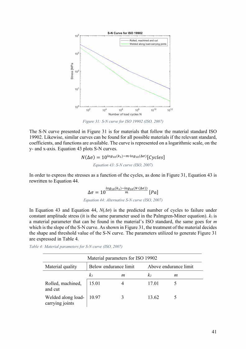
41

Figure 31: S-N curve for ISO 19902 (ISO, 2007)

The S-N curve presented in Figure 31 is for materials that follow the material standard ISO 19902. Likewise, similar curves can be found for all possible materials if the relevant standard, coefficients, and functions are available. The curve is represented on a logarithmic scale, on the y- and x-axis. Equation 43 plots S-N curves.

𝑁(Δ𝜎) = 10$�"¨n(¦¨)|0∙$�"¨n(©ª)[𝐶𝑦𝑐𝑙𝑒𝑠] Equation 43: S-N curve (ISO, 2007)

In order to express the stresses as a function of the cycles, as done in Figure 31, Equation 43 is rewritten to Equation 44.

Δ𝜎 = 10$�"¨n(¦¨)|$�"¨n(¬∙(©ª))0 [𝑃𝑎] Equation 44: Alternative S-N curve (ISO, 2007)

In Equation 43 and Equation 44, N(Δσ) is the predicted number of cycles to failure under constant amplitude stress (it is the same parameter used in the Palmgren-Miner equation). k1 is a material parameter that can be found in the material’s ISO standard, the same goes for m which is the slope of the S-N curve. As shown in Figure 31, the treatment of the material decides the shape and threshold value of the S-N curve. The parameters utilized to generate Figure 31 are expressed in Table 4.

Table 4: Material parameters for S-N curve (ISO, 2007)

Material parameters for ISO 19902

Material quality Below endurance limit Above endurance limit

k1 m k1 m

Rolled, machined, and cut

15.01 4 17.01 5

Welded along load-carrying joints

10.97 3 13.62 5

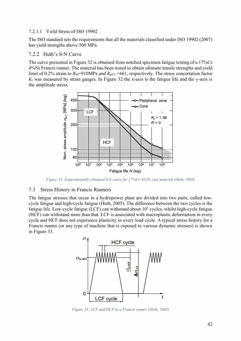
42

7.2.1.1 Yield Stress of ISO 19902

The ISO standard sets the requirements that all the materials classified under ISO 19902 (2007) has yield strengths above 500 MPa.

7.2.2 Huth’s S-N Curve

The curve presented in Figure 32 is obtained from notched specimen fatigue testing of a 17%Cr 4%Ni Francis runner. The material has been tested to obtain ultimate tensile strengths and yield limit of 0.2% strain to RM=910MPa and Rp0.2 =661, respectively. The stress concertation factor Kt was measured by strain gauges. In Figure 32 the x-axis is the fatigue life and the y-axis is the amplitude stress.

Figure 32: Experimentally obtained S-N curve for 17%Cr-4%Ni cast material (Huth, 2005)

7.3 Stress History in Francis Runners

The fatigue stresses that occur in a hydropower plant are divided into two parts, called low-cycle fatigue and high-cycle fatigue (Huth, 2005). The difference between the two cycles is the fatigue life. Low-cycle fatigue (LCF) can withstand about 105 cycles, whilst high-cycle fatigue (HCF) can withstand more than that. LCF is associated with macroplastic deformation in every cycle and HCF does not experience plasticity in every load cycle. A typical stress history for a Francis runner (or any type of machine that is exposed to various dynamic stresses) is shown in Figure 33.

Figure 33: LCF and HCF in a Francis runner (Huth, 2005)

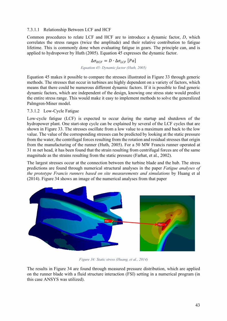
43

7.3.1.1 Relationship Between LCF and HCF

Common procedures to relate LCF and HCF are to introduce a dynamic factor, D, which correlates the stress ranges (twice the amplitude) and their relative contribution to fatigue lifetime. This is commonly done when evaluating fatigue in gears. The principle can, and is applied to hydropower by Huth (2005). Equation 45 expresses the dynamic factor.

Δ𝜎­®y = 𝐷 ∙ Δ𝜎�®y [𝑃𝑎] Equation 45: Dynamic factor (Huth, 2005)

Equation 45 makes it possible to compare the stresses illustrated in Figure 33 through generic methods. The stresses that occur in turbines are highly dependent on a variety of factors, which means that there could be numerous different dynamic factors. If it is possible to find generic dynamic factors, which are independent of the design, knowing one stress state would predict the entire stress range. This would make it easy to implement methods to solve the generalized Palmgren-Miner model.

7.3.1.2 Low-Cycle Fatigue

Low-cycle fatigue (LCF) is expected to occur during the startup and shutdown of the hydropower plant. One start-stop cycle can be explained by several of the LCF cycles that are shown in Figure 33. The stresses oscillate from a low value to a maximum and back to the low value. The value of the corresponding stresses can be predicted by looking at the static pressure from the water, the centrifugal forces resulting from the rotation and residual stresses that origin from the manufacturing of the runner (Huth, 2005). For a 50 MW Francis runner operated at 31 m net head, it has been found that the strain resulting from centrifugal forces are of the same magnitude as the strains resulting from the static pressure (Farhat, et al., 2002).

The largest stresses occur at the connection between the turbine blade and the hub. The stress predictions are found through numerical structural analyses in the paper Fatigue analyses of

the prototype Francis runners based on site measurements and simulations by Huang et al (2014). Figure 34 shows an image of the numerical analyses from that paper

Figure 34: Static stress (Huang, et al., 2014)

The results in Figure 34 are found through measured pressure distribution, which are applied on the runner blade with a fluid structure interaction (FSI) setting in a numerical program (in this case ANSYS was utilized).

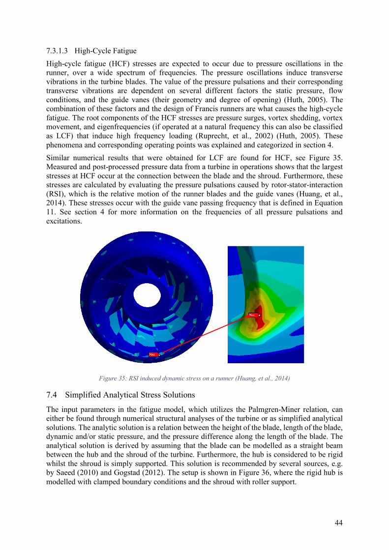
44

7.3.1.3 High-Cycle Fatigue

High-cycle fatigue (HCF) stresses are expected to occur due to pressure oscillations in the runner, over a wide spectrum of frequencies. The pressure oscillations induce transverse vibrations in the turbine blades. The value of the pressure pulsations and their corresponding transverse vibrations are dependent on several different factors the static pressure, flow conditions, and the guide vanes (their geometry and degree of opening) (Huth, 2005). The combination of these factors and the design of Francis runners are what causes the high-cycle fatigue. The root components of the HCF stresses are pressure surges, vortex shedding, vortex movement, and eigenfrequencies (if operated at a natural frequency this can also be classified as LCF) that induce high frequency loading (Ruprecht, et al., 2002) (Huth, 2005). These phenomena and corresponding operating points was explained and categorized in section 4.

Similar numerical results that were obtained for LCF are found for HCF, see Figure 35. Measured and post-processed pressure data from a turbine in operations shows that the largest stresses at HCF occur at the connection between the blade and the shroud. Furthermore, these stresses are calculated by evaluating the pressure pulsations caused by rotor-stator-interaction (RSI), which is the relative motion of the runner blades and the guide vanes (Huang, et al., 2014). These stresses occur with the guide vane passing frequency that is defined in Equation 11. See section 4 for more information on the frequencies of all pressure pulsations and excitations.

Figure 35: RSI induced dynamic stress on a runner (Huang, et al., 2014)

7.4 Simplified Analytical Stress Solutions

The input parameters in the fatigue model, which utilizes the Palmgren-Miner relation, can either be found through numerical structural analyses of the turbine or as simplified analytical solutions. The analytic solution is a relation between the height of the blade, length of the blade, dynamic and/or static pressure, and the pressure difference along the length of the blade. The analytical solution is derived by assuming that the blade can be modelled as a straight beam between the hub and the shroud of the turbine. Furthermore, the hub is considered to be rigid whilst the shroud is simply supported. This solution is recommended by several sources, e.g. by Saeed (2010) and Gogstad (2012). The setup is shown in Figure 36, where the rigid hub is modelled with clamped boundary conditions and the shroud with roller support.

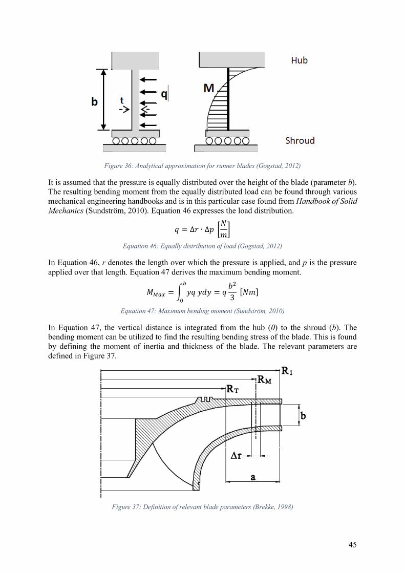
45

Figure 36: Analytical approximation for runner blades (Gogstad, 2012)

It is assumed that the pressure is equally distributed over the height of the blade (parameter b). The resulting bending moment from the equally distributed load can be found through various mechanical engineering handbooks and is in this particular case found from Handbook of Solid

Mechanics (Sundström, 2010). Equation 46 expresses the load distribution.

𝑞 = Δ𝑟 ∙ Δ𝑝 :𝑁𝑚< Equation 46: Equally distribution of load (Gogstad, 2012)

In Equation 46, r denotes the length over which the pressure is applied, and p is the pressure applied over that length. Equation 47 derives the maximum bending moment.

𝑀eZ  = \ 𝑦𝑞𝑦𝑑𝑦¯A = 𝑞 𝑏23 [𝑁𝑚]

Equation 47: Maximum bending moment (Sundström, 2010)

In Equation 47, the vertical distance is integrated from the hub (0) to the shroud (b). The bending moment can be utilized to find the resulting bending stress of the blade. This is found by defining the moment of inertia and thickness of the blade. The relevant parameters are defined in Figure 37.

Figure 37: Definition of relevant blade parameters (Brekke, 1998)

46

Equation 48 defines the maximum bending stress.

𝜎0Z  = 𝑀eZ  ∙ 𝑡2 ∙ 𝐼 [𝑃𝑎] Equation 48: Maximum bending stress (Sundström, 2010)

In Equation 48, t is the thickness of the blade and I is the moment of inertia. Equation 49 defines the moment of inertia.

𝐼 = Δ𝑟 ∙ 𝑡²12 [𝑚2] Equation 49: Moment of inertia (Sundström, 2010)

Equation 50 defines the relationship between the pressure difference, torque on the runner shaft and power of the turbine (Brekke, 1998).

𝑀[�DD/[ = 𝑃𝜔 = 𝑍 ∙ 𝑎 ∙ 𝑏 ∙ 𝑅0 ∙ Δ𝑝[𝑁𝑚] Equation 50: Relationship between torque and power (Brekke, 1998)

In Equation 50, P is the power of the turbine, ω is the rotational velocity, Z is the number of runner blades, a is a design parameter, b is the width of the blade, RM is the middle radius, and p is the pressure over the evaluated area. Equation 51 expresses the maximum bending stresses in each runner blade.

𝜎0Z  = 2 ∙ 𝑏2 ∙ Δ𝑝𝑡2 [𝑃𝑎] Equation 51: Derived expression for maximum bending stress

In Equation 51, it is assumed that all torque is transferred from the water to the turbine in in the region between RT and R1. The parameters in Equation 50 and their relationship are dependent on the design of the turbine. Brekke (1998) argues that in general the results for Francis turbines are relevant and good approximations when a is equal to 1.5 b. With the underlying assumptions and these equations, the bending stresses can be roughly approximated. All the same, it is worth noticing that this approximation assumes that the dominating stress state is bending and neglecting all other principal stress components. The results from the analytical approximation is shown in the results section. Furthermore, Appendix D presents the height (b) and thickness (t) parameters.

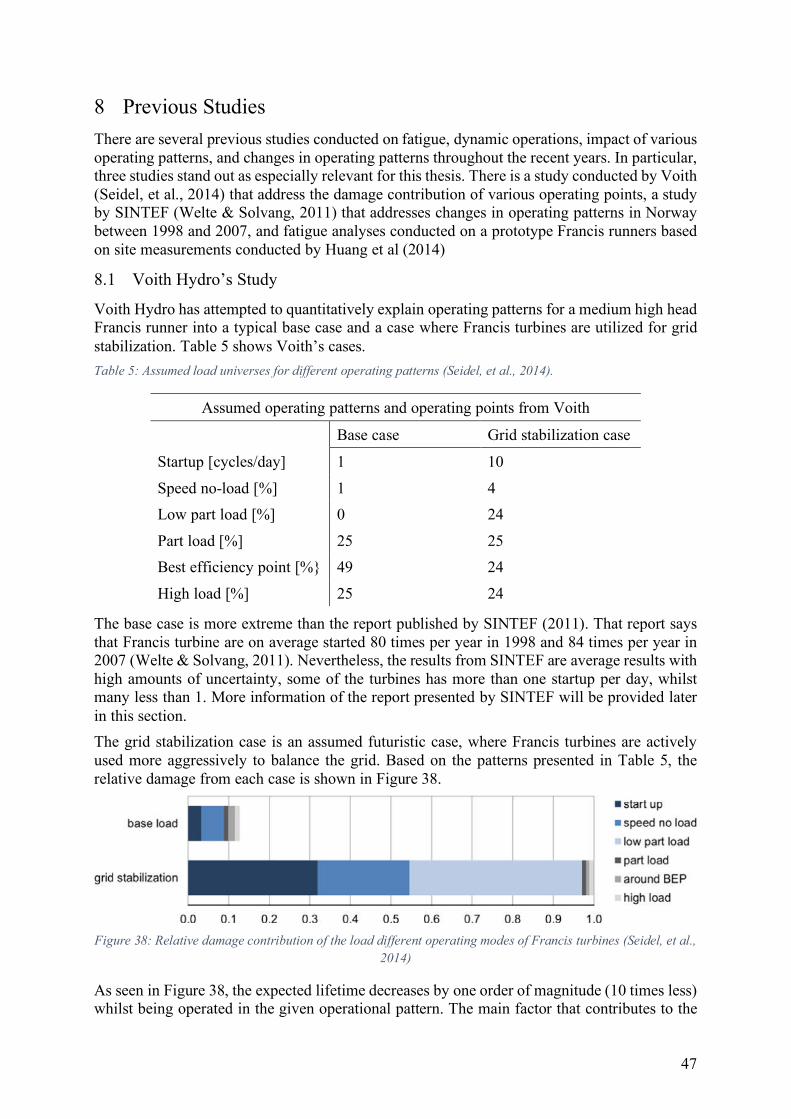
47

8 Previous Studies

There are several previous studies conducted on fatigue, dynamic operations, impact of various operating patterns, and changes in operating patterns throughout the recent years. In particular, three studies stand out as especially relevant for this thesis. There is a study conducted by Voith (Seidel, et al., 2014) that address the damage contribution of various operating points, a study by SINTEF (Welte & Solvang, 2011) that addresses changes in operating patterns in Norway between 1998 and 2007, and fatigue analyses conducted on a prototype Francis runners based on site measurements conducted by Huang et al (2014)

8.1 Voith Hydro’s Study

Voith Hydro has attempted to quantitatively explain operating patterns for a medium high head Francis runner into a typical base case and a case where Francis turbines are utilized for grid stabilization. Table 5 shows Voith’s cases.

Table 5: Assumed load universes for different operating patterns (Seidel, et al., 2014).

Assumed operating patterns and operating points from Voith

Base case Grid stabilization case

Startup [cycles/day] 1 10

Speed no-load [%] 1 4

Low part load [%] 0 24

Part load [%] 25 25

Best efficiency point [%} 49 24

High load [%] 25 24

The base case is more extreme than the report published by SINTEF (2011). That report says that Francis turbine are on average started 80 times per year in 1998 and 84 times per year in 2007 (Welte & Solvang, 2011). Nevertheless, the results from SINTEF are average results with high amounts of uncertainty, some of the turbines has more than one startup per day, whilst many less than 1. More information of the report presented by SINTEF will be provided later in this section.

The grid stabilization case is an assumed futuristic case, where Francis turbines are actively used more aggressively to balance the grid. Based on the patterns presented in Table 5, the relative damage from each case is shown in Figure 38.

Figure 38: Relative damage contribution of the load different operating modes of Francis turbines (Seidel, et al.,

2014)

As seen in Figure 38, the expected lifetime decreases by one order of magnitude (10 times less) whilst being operated in the given operational pattern. The main factor that contributes to the

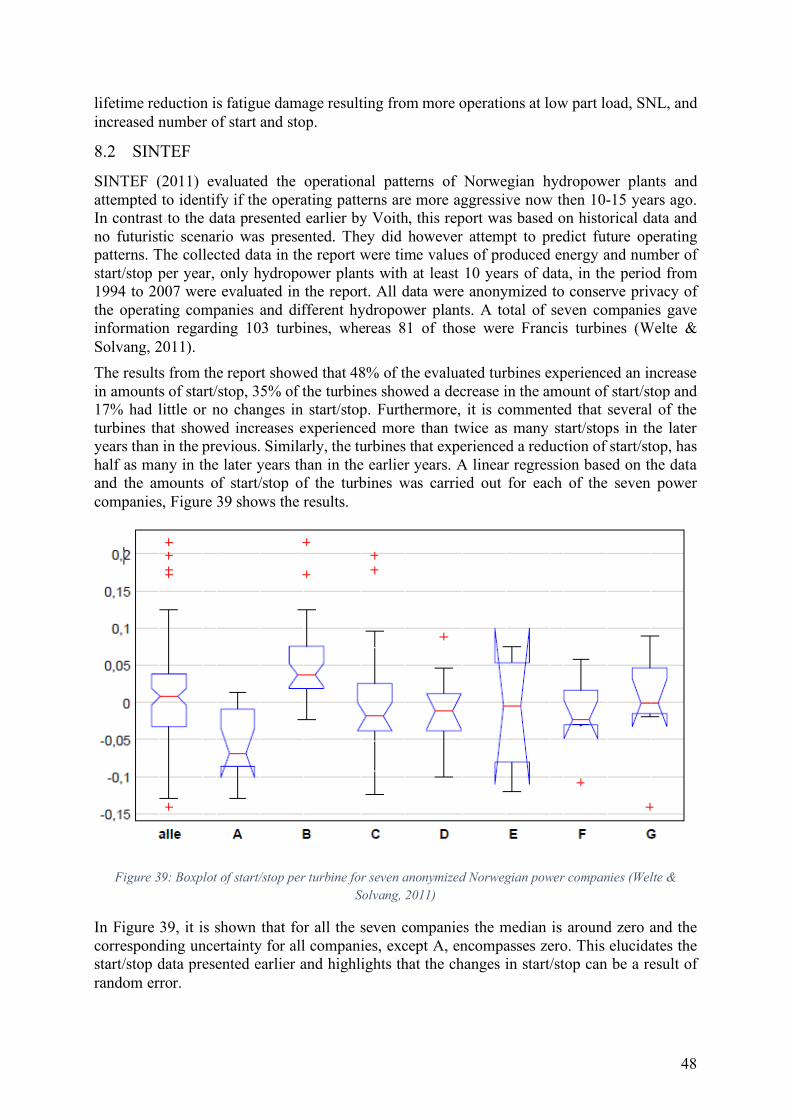
48

lifetime reduction is fatigue damage resulting from more operations at low part load, SNL, and increased number of start and stop.

8.2 SINTEF

SINTEF (2011) evaluated the operational patterns of Norwegian hydropower plants and attempted to identify if the operating patterns are more aggressive now then 10-15 years ago. In contrast to the data presented earlier by Voith, this report was based on historical data and no futuristic scenario was presented. They did however attempt to predict future operating patterns. The collected data in the report were time values of produced energy and number of start/stop per year, only hydropower plants with at least 10 years of data, in the period from 1994 to 2007 were evaluated in the report. All data were anonymized to conserve privacy of the operating companies and different hydropower plants. A total of seven companies gave information regarding 103 turbines, whereas 81 of those were Francis turbines (Welte & Solvang, 2011).

The results from the report showed that 48% of the evaluated turbines experienced an increase in amounts of start/stop, 35% of the turbines showed a decrease in the amount of start/stop and 17% had little or no changes in start/stop. Furthermore, it is commented that several of the turbines that showed increases experienced more than twice as many start/stops in the later years than in the previous. Similarly, the turbines that experienced a reduction of start/stop, has half as many in the later years than in the earlier years. A linear regression based on the data and the amounts of start/stop of the turbines was carried out for each of the seven power companies, Figure 39 shows the results.

Figure 39: Boxplot of start/stop per turbine for seven anonymized Norwegian power companies (Welte &

Solvang, 2011)

In Figure 39, it is shown that for all the seven companies the median is around zero and the corresponding uncertainty for all companies, except A, encompasses zero. This elucidates the start/stop data presented earlier and highlights that the changes in start/stop can be a result of random error.

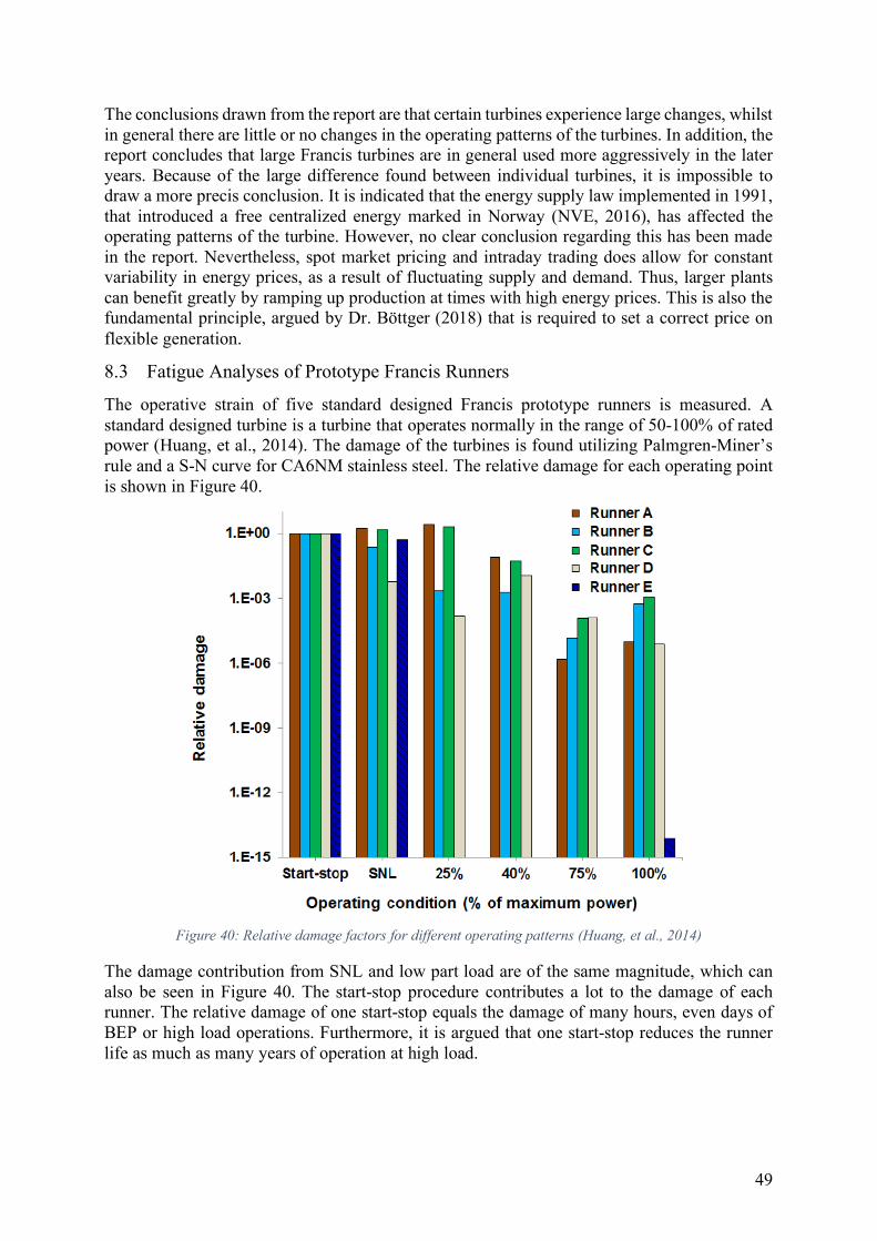
49

The conclusions drawn from the report are that certain turbines experience large changes, whilst in general there are little or no changes in the operating patterns of the turbines. In addition, the report concludes that large Francis turbines are in general used more aggressively in the later years. Because of the large difference found between individual turbines, it is impossible to draw a more precis conclusion. It is indicated that the energy supply law implemented in 1991, that introduced a free centralized energy marked in Norway (NVE, 2016), has affected the operating patterns of the turbine. However, no clear conclusion regarding this has been made in the report. Nevertheless, spot market pricing and intraday trading does allow for constant variability in energy prices, as a result of fluctuating supply and demand. Thus, larger plants can benefit greatly by ramping up production at times with high energy prices. This is also the fundamental principle, argued by Dr. Böttger (2018) that is required to set a correct price on flexible generation.

8.3 Fatigue Analyses of Prototype Francis Runners

The operative strain of five standard designed Francis prototype runners is measured. A standard designed turbine is a turbine that operates normally in the range of 50-100% of rated power (Huang, et al., 2014). The damage of the turbines is found utilizing Palmgren-Miner’s rule and a S-N curve for CA6NM stainless steel. The relative damage for each operating point is shown in Figure 40.

Figure 40: Relative damage factors for different operating patterns (Huang, et al., 2014)

The damage contribution from SNL and low part load are of the same magnitude, which can also be seen in Figure 40. The start-stop procedure contributes a lot to the damage of each runner. The relative damage of one start-stop equals the damage of many hours, even days of BEP or high load operations. Furthermore, it is argued that one start-stop reduces the runner life as much as many years of operation at high load.

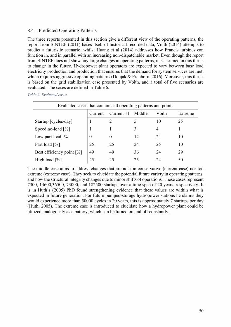
50

8.4 Predicted Operating Patterns

The three reports presented in this section give a different view of the operating patterns, the report from SINTEF (2011) bases itself of historical recorded data, Voith (2014) attempts to predict a futuristic scenario, whilst Huang et al (2014) addresses how Francis turbines can function in, and in parallel with an increasing non-dispatchable market. Even though the report from SINTEF does not show any large changes in operating patterns, it is assumed in this thesis to change in the future. Hydropower plant operators are expected to vary between base load electricity production and production that ensures that the demand for system services are met, which requires aggressive operating patterns (Doujak & Eichhorn, 2016). Moreover, this thesis is based on the grid stabilization case presented by Voith, and a total of five scenarios are evaluated. The cases are defined in Table 6.

Table 6: Evaluated cases

Evaluated cases that contains all operating patterns and points

Current Current +1 Middle Voith Extreme

Startup [cycles/day] 1 2 5 10 25

Speed no-load [%] 1 1 3 4 1

Low part load [%] 0 0 12 24 10

Part load [%] 25 25 24 25 10

Best efficiency point [%] 49 49 36 24 29

High load [%] 25 25 25 24 50

The middle case aims to address changes that are not too conservative (current case) nor too extreme (extreme case). They seek to elucidate the potential future variety in operating patterns, and how the structural integrity changes due to minor shifts of operations. These cases represent 7300, 14600,36500, 73000, and 182500 startups over a time span of 20 years, respectively. It is in Huth’s (2005) PhD found strengthening evidence that these values are within what is expected in future generation. For future pumped-storage hydropower stations he claims they would experience more than 50000 cycles in 20 years, this is approximately 7 startups per day (Huth, 2005). The extreme case is introduced to elucidate how a hydropower plant could be utilized analogously as a battery, which can be turned on and off constantly.

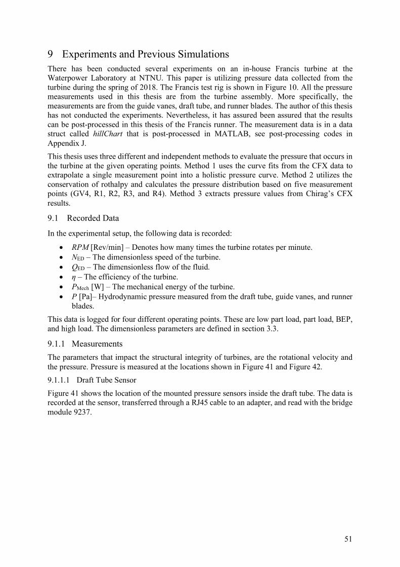
51

9 Experiments and Previous Simulations There has been conducted several experiments on an in-house Francis turbine at the Waterpower Laboratory at NTNU. This paper is utilizing pressure data collected from the turbine during the spring of 2018. The Francis test rig is shown in Figure 10. All the pressure measurements used in this thesis are from the turbine assembly. More specifically, the measurements are from the guide vanes, draft tube, and runner blades. The author of this thesis has not conducted the experiments. Nevertheless, it has assured been assured that the results can be post-processed in this thesis of the Francis runner. The measurement data is in a data struct called hillChart that is post-processed in MATLAB, see post-processing codes in Appendix J.

This thesis uses three different and independent methods to evaluate the pressure that occurs in the turbine at the given operating points. Method 1 uses the curve fits from the CFX data to extrapolate a single measurement point into a holistic pressure curve. Method 2 utilizes the conservation of rothalpy and calculates the pressure distribution based on five measurement points (GV4, R1, R2, R3, and R4). Method 3 extracts pressure values from Chirag’s CFX results.

9.1 Recorded Data

In the experimental setup, the following data is recorded:

• RPM [Rev/min] – Denotes how many times the turbine rotates per minute. • NED – The dimensionless speed of the turbine. • QED – The dimensionless flow of the fluid. • η – The efficiency of the turbine. • PMech [W] – The mechanical energy of the turbine. • P [Pa]– Hydrodynamic pressure measured from the draft tube, guide vanes, and runner

blades.

This data is logged for four different operating points. These are low part load, part load, BEP, and high load. The dimensionless parameters are defined in section 3.3.

9.1.1 Measurements

The parameters that impact the structural integrity of turbines, are the rotational velocity and the pressure. Pressure is measured at the locations shown in Figure 41 and Figure 42.

9.1.1.1 Draft Tube Sensor

Figure 41 shows the location of the mounted pressure sensors inside the draft tube. The data is recorded at the sensor, transferred through a RJ45 cable to an adapter, and read with the bridge module 9237.

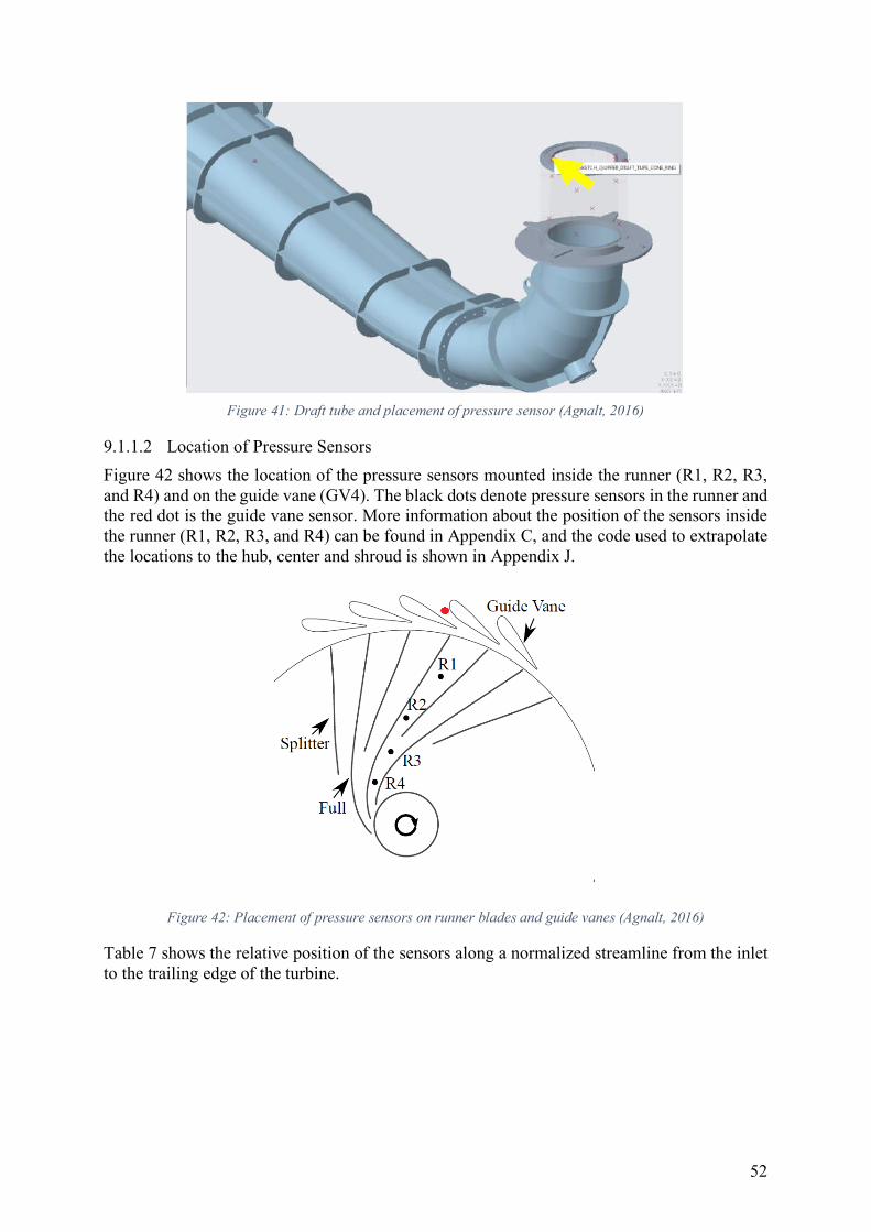
52

Figure 41: Draft tube and placement of pressure sensor (Agnalt, 2016)

9.1.1.2 Location of Pressure Sensors

Figure 42 shows the location of the pressure sensors mounted inside the runner (R1, R2, R3, and R4) and on the guide vane (GV4). The black dots denote pressure sensors in the runner and the red dot is the guide vane sensor. More information about the position of the sensors inside the runner (R1, R2, R3, and R4) can be found in Appendix C, and the code used to extrapolate the locations to the hub, center and shroud is shown in Appendix J.

Figure 42: Placement of pressure sensors on runner blades and guide vanes (Agnalt, 2016)

Table 7 shows the relative position of the sensors along a normalized streamline from the inlet to the trailing edge of the turbine.

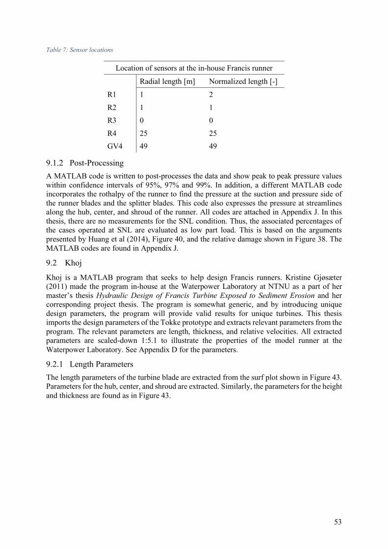
53

Table 7: Sensor locations

Location of sensors at the in-house Francis runner

Radial length [m] Normalized length [-]

R1 1 2

R2 1 1

R3 0 0

R4 25 25

GV4 49 49

9.1.2 Post-Processing

A MATLAB code is written to post-processes the data and show peak to peak pressure values within confidence intervals of 95%, 97% and 99%. In addition, a different MATLAB code incorporates the rothalpy of the runner to find the pressure at the suction and pressure side of the runner blades and the splitter blades. This code also expresses the pressure at streamlines along the hub, center, and shroud of the runner. All codes are attached in Appendix J. In this thesis, there are no measurements for the SNL condition. Thus, the associated percentages of the cases operated at SNL are evaluated as low part load. This is based on the arguments presented by Huang et al (2014), Figure 40, and the relative damage shown in Figure 38. The MATLAB codes are found in Appendix J.

9.2 Khoj

Khoj is a MATLAB program that seeks to help design Francis runners. Kristine Gjøsæter (2011) made the program in-house at the Waterpower Laboratory at NTNU as a part of her master’s thesis Hydraulic Design of Francis Turbine Exposed to Sediment Erosion and her corresponding project thesis. The program is somewhat generic, and by introducing unique design parameters, the program will provide valid results for unique turbines. This thesis imports the design parameters of the Tokke prototype and extracts relevant parameters from the program. The relevant parameters are length, thickness, and relative velocities. All extracted parameters are scaled-down 1:5.1 to illustrate the properties of the model runner at the Waterpower Laboratory. See Appendix D for the parameters.

9.2.1 Length Parameters

The length parameters of the turbine blade are extracted from the surf plot shown in Figure 43. Parameters for the hub, center, and shroud are extracted. Similarly, the parameters for the height and thickness are found as in Figure 43.

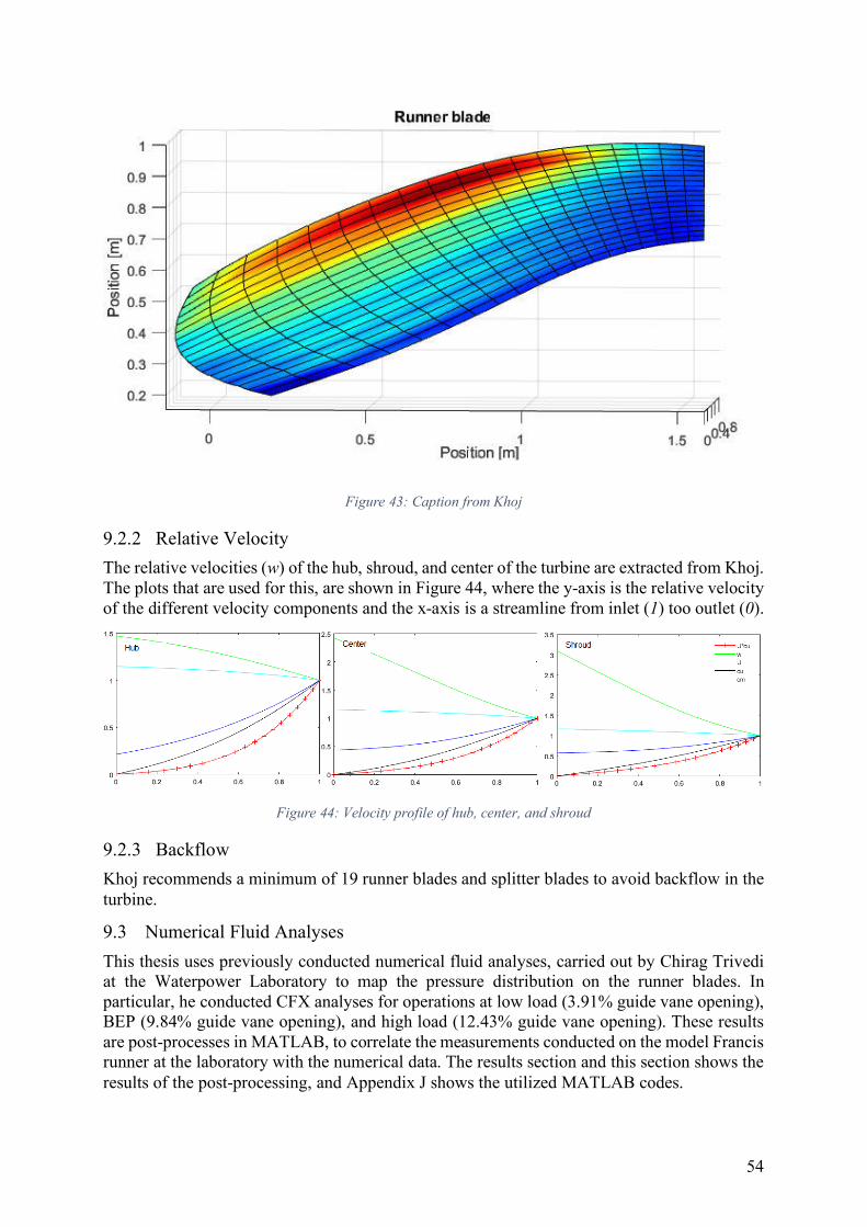
54

Figure 43: Caption from Khoj

9.2.2 Relative Velocity

The relative velocities (w) of the hub, shroud, and center of the turbine are extracted from Khoj. The plots that are used for this, are shown in Figure 44, where the y-axis is the relative velocity of the different velocity components and the x-axis is a streamline from inlet (1) too outlet (0).

Figure 44: Velocity profile of hub, center, and shroud

9.2.3 Backflow

Khoj recommends a minimum of 19 runner blades and splitter blades to avoid backflow in the turbine.

9.3 Numerical Fluid Analyses

This thesis uses previously conducted numerical fluid analyses, carried out by Chirag Trivedi at the Waterpower Laboratory to map the pressure distribution on the runner blades. In particular, he conducted CFX analyses for operations at low load (3.91% guide vane opening), BEP (9.84% guide vane opening), and high load (12.43% guide vane opening). These results are post-processes in MATLAB, to correlate the measurements conducted on the model Francis runner at the laboratory with the numerical data. The results section and this section shows the results of the post-processing, and Appendix J shows the utilized MATLAB codes.

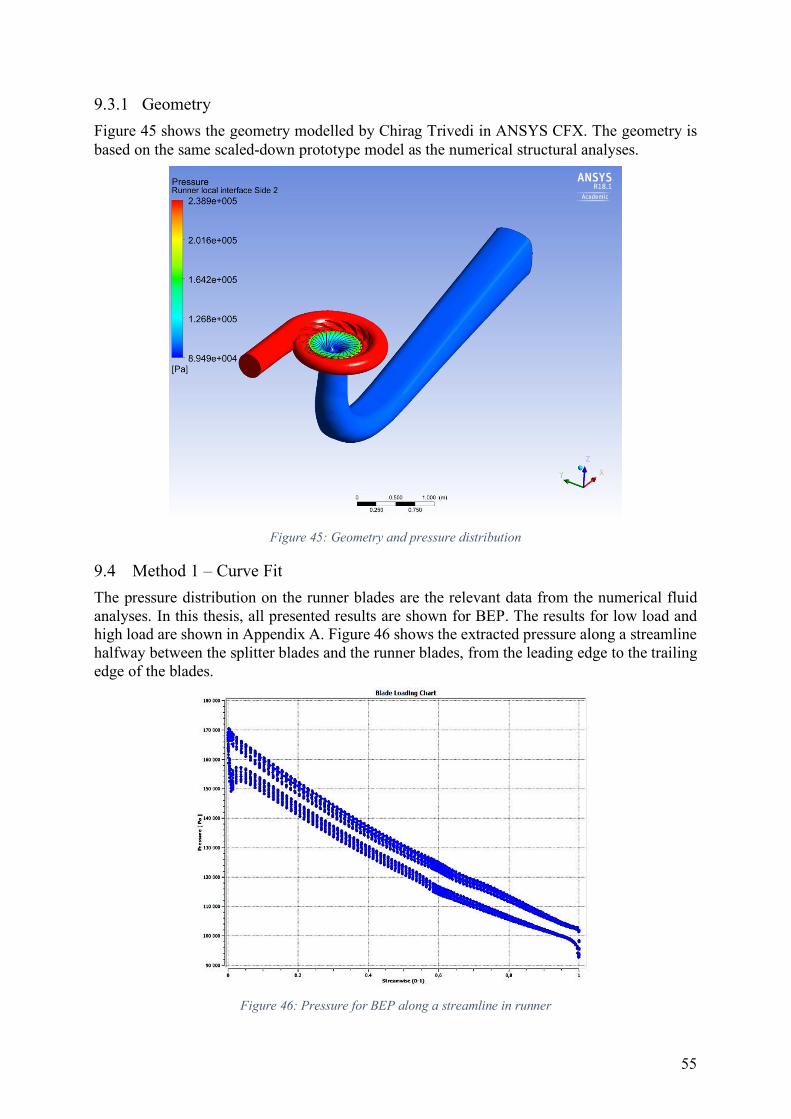
55

9.3.1 Geometry

Figure 45 shows the geometry modelled by Chirag Trivedi in ANSYS CFX. The geometry is based on the same scaled-down prototype model as the numerical structural analyses.

Figure 45: Geometry and pressure distribution

9.4 Method 1 – Curve Fit

The pressure distribution on the runner blades are the relevant data from the numerical fluid analyses. In this thesis, all presented results are shown for BEP. The results for low load and high load are shown in Appendix A. Figure 46 shows the extracted pressure along a streamline halfway between the splitter blades and the runner blades, from the leading edge to the trailing edge of the blades.

Figure 46: Pressure for BEP along a streamline in runner

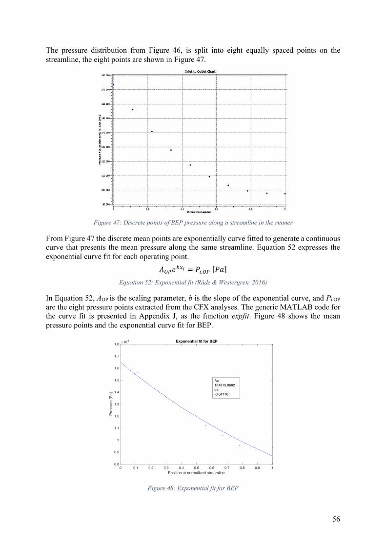
56

The pressure distribution from Figure 46, is split into eight equally spaced points on the streamline, the eight points are shown in Figure 47.

Figure 47: Discrete points of BEP pressure along a streamline in the runner

From Figure 47 the discrete mean points are exponentially curve fitted to generate a continuous curve that presents the mean pressure along the same streamline. Equation 52 expresses the exponential curve fit for each operating point.

𝐴�d𝑒¯ ³ = 𝑃�,�d [𝑃𝑎] Equation 52: Exponential fit (Råde & Westergren, 2016)

In Equation 52, AOP is the scaling parameter, b is the slope of the exponential curve, and Pi,OP

are the eight pressure points extracted from the CFX analyses. The generic MATLAB code for the curve fit is presented in Appendix J, as the function expfit. Figure 48 shows the mean pressure points and the exponential curve fit for BEP.

Figure 48: Exponential fit for BEP

0 0.1 0.2 0.3 0.4 0.5 0.6 0.7 0.8 0.9 1

Position at normalized streamline

0.8

0.9

1

1.1

1.2

1.3

1.4

1.5

1.6

1.7

1.8

Pre

ssure

[P

a]

105 Exponential fit for BEP

A=

164815.8682

b=

-0.64116

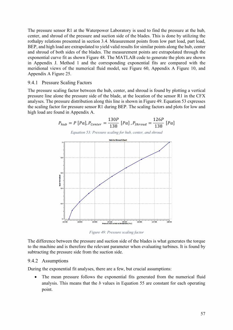
57

The pressure sensor R1 at the Waterpower Laboratory is used to find the pressure at the hub, center, and shroud of the pressure and suction side of the blades. This is done by utilizing the rothalpy relations presented in section 3.4. Measurement points from low part load, part load, BEP, and high load are extrapolated to yield valid results for similar points along the hub, center and shroud of both sides of the blades. The measurement points are extrapolated through the exponential curve fit as shown Figure 48. The MATLAB code to generate the plots are shown in Appendix J. Method 1 and the corresponding exponential fits are compared with the meridional views of the numerical fluid model, see Figure 60, Appendix A Figure 10, and Appendix A Figure 25.

9.4.1 Pressure Scaling Factors

The pressure scaling factor between the hub, center, and shroud is found by plotting a vertical pressure line alone the pressure side of the blade, at the location of the sensor R1 in the CFX analyses. The pressure distribution along this line is shown in Figure 49. Equation 53 expresses the scaling factor for pressure sensor R1 during BEP. The scaling factors and plots for low and high load are found in Appendix A.

𝑃 �¯ = 𝑃[𝑃𝑎], 𝑃®/D./[ = 130𝑃138 [𝑃𝑎], 𝑃w´[��� = 126𝑃138 [𝑃𝑎] Equation 53: Pressure scaling for hub, center, and shroud

Figure 49: Pressure scaling factor

The difference between the pressure and suction side of the blades is what generates the torque to the machine and is therefore the relevant parameter when evaluating turbines. It is found by subtracting the pressure side from the suction side.

9.4.2 Assumptions

During the exponential fit analyses, there are a few, but crucial assumptions:

• The mean pressure follows the exponential fits generated from the numerical fluid

analysis. This means that the b values in Equation 55 are constant for each operating

point.

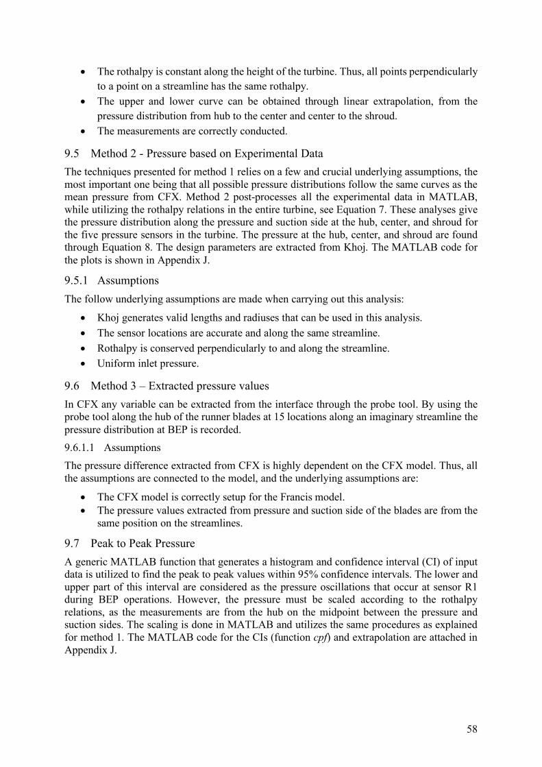
58

• The rothalpy is constant along the height of the turbine. Thus, all points perpendicularly

to a point on a streamline has the same rothalpy.

• The upper and lower curve can be obtained through linear extrapolation, from the

pressure distribution from hub to the center and center to the shroud.

• The measurements are correctly conducted.

9.5 Method 2 - Pressure based on Experimental Data

The techniques presented for method 1 relies on a few and crucial underlying assumptions, the most important one being that all possible pressure distributions follow the same curves as the mean pressure from CFX. Method 2 post-processes all the experimental data in MATLAB, while utilizing the rothalpy relations in the entire turbine, see Equation 7. These analyses give the pressure distribution along the pressure and suction side at the hub, center, and shroud for the five pressure sensors in the turbine. The pressure at the hub, center, and shroud are found through Equation 8. The design parameters are extracted from Khoj. The MATLAB code for the plots is shown in Appendix J.

9.5.1 Assumptions

The follow underlying assumptions are made when carrying out this analysis:

• Khoj generates valid lengths and radiuses that can be used in this analysis.

• The sensor locations are accurate and along the same streamline.

• Rothalpy is conserved perpendicularly to and along the streamline.

• Uniform inlet pressure.

9.6 Method 3 – Extracted pressure values

In CFX any variable can be extracted from the interface through the probe tool. By using the probe tool along the hub of the runner blades at 15 locations along an imaginary streamline the pressure distribution at BEP is recorded.

9.6.1.1 Assumptions

The pressure difference extracted from CFX is highly dependent on the CFX model. Thus, all the assumptions are connected to the model, and the underlying assumptions are:

• The CFX model is correctly setup for the Francis model. • The pressure values extracted from pressure and suction side of the blades are from the

same position on the streamlines.

9.7 Peak to Peak Pressure

A generic MATLAB function that generates a histogram and confidence interval (CI) of input data is utilized to find the peak to peak values within 95% confidence intervals. The lower and upper part of this interval are considered as the pressure oscillations that occur at sensor R1 during BEP operations. However, the pressure must be scaled according to the rothalpy relations, as the measurements are from the hub on the midpoint between the pressure and suction sides. The scaling is done in MATLAB and utilizes the same procedures as explained for method 1. The MATLAB code for the CIs (function cpf) and extrapolation are attached in Appendix J.

59

9.7.1.1 Application of peak to peak values

The peak to peak values are assumed to capture the entire relevant range of pressures that can occur in the turbine during the various operating points. Thus, the lower part of the CI is the pressure on the suction side and the upper part on the pressure side. Method 1 is utilized to extrapolate the peak to peak values to a continuous pressure distribution in the turbine.

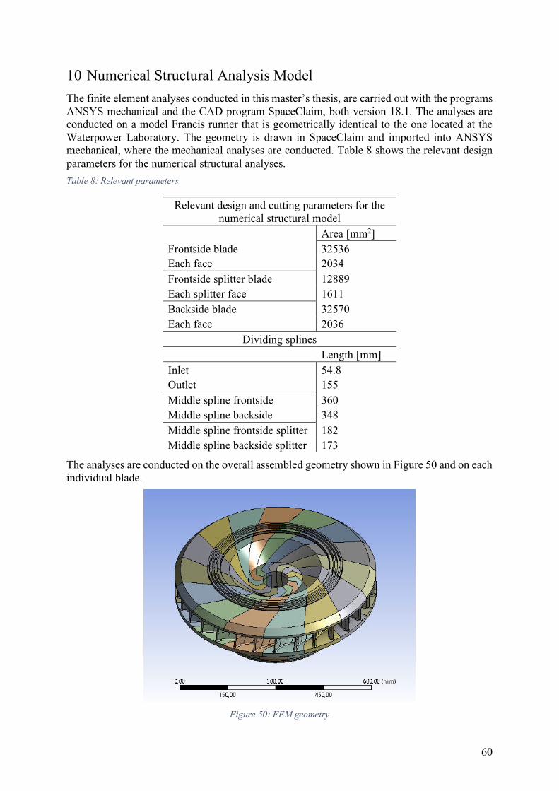
60

10 Numerical Structural Analysis Model

The finite element analyses conducted in this master’s thesis, are carried out with the programs ANSYS mechanical and the CAD program SpaceClaim, both version 18.1. The analyses are conducted on a model Francis runner that is geometrically identical to the one located at the Waterpower Laboratory. The geometry is drawn in SpaceClaim and imported into ANSYS mechanical, where the mechanical analyses are conducted. Table 8 shows the relevant design parameters for the numerical structural analyses.

Table 8: Relevant parameters

Relevant design and cutting parameters for the numerical structural model

Area [mm2]

Frontside blade 32536 Each face 2034

Frontside splitter blade 12889

Each splitter face 1611

Backside blade 32570

Each face 2036

Dividing splines

Length [mm]

Inlet 54.8 Outlet 155

Middle spline frontside 360

Middle spline backside 348

Middle spline frontside splitter 182

Middle spline backside splitter 173

The analyses are conducted on the overall assembled geometry shown in Figure 50 and on each individual blade.

Figure 50: FEM geometry

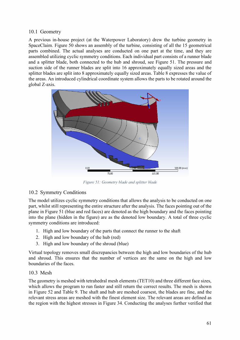
61

10.1 Geometry

A previous in-house project (at the Waterpower Laboratory) drew the turbine geometry in SpaceClaim. Figure 50 shows an assembly of the turbine, consisting of all the 15 geometrical parts combined. The actual analyses are conducted on one part at the time, and they are assembled utilizing cyclic symmetry conditions. Each individual part consists of a runner blade and a splitter blade, both connected to the hub and shroud, see Figure 51. The pressure and suction side of the runner blades are split into 16 approximately equally sized areas and the splitter blades are split into 8 approximately equally sized areas. Table 8 expresses the value of the areas. An introduced cylindrical coordinate system allows the parts to be rotated around the global Z-axis.

Figure 51: Geometry blade and splitter blade

10.2 Symmetry Conditions

The model utilizes cyclic symmetry conditions that allows the analysis to be conducted on one part, whilst still representing the entire structure after the analysis. The faces pointing out of the plane in Figure 51 (blue and red faces) are denoted as the high boundary and the faces pointing into the plane (hidden in the figure) are as the denoted low boundary. A total of three cyclic symmetry conditions are introduced:

1. High and low boundary of the parts that connect the runner to the shaft

2. High and low boundary of the hub (red)

3. High and low boundary of the shroud (blue)

Virtual topology removes small discrepancies between the high and low boundaries of the hub and shroud. This ensures that the number of vertices are the same on the high and low boundaries of the faces.

10.3 Mesh

The geometry is meshed with tetrahedral mesh elements (TET10) and three different face sizes, which allows the program to run faster and still return the correct results. The mesh is shown in Figure 52 and Table 9. The shaft and hub are meshed coarsest, the blades are fine, and the relevant stress areas are meshed with the finest element size. The relevant areas are defined as the region with the highest stresses in Figure 34. Conducting the analyses further verified that

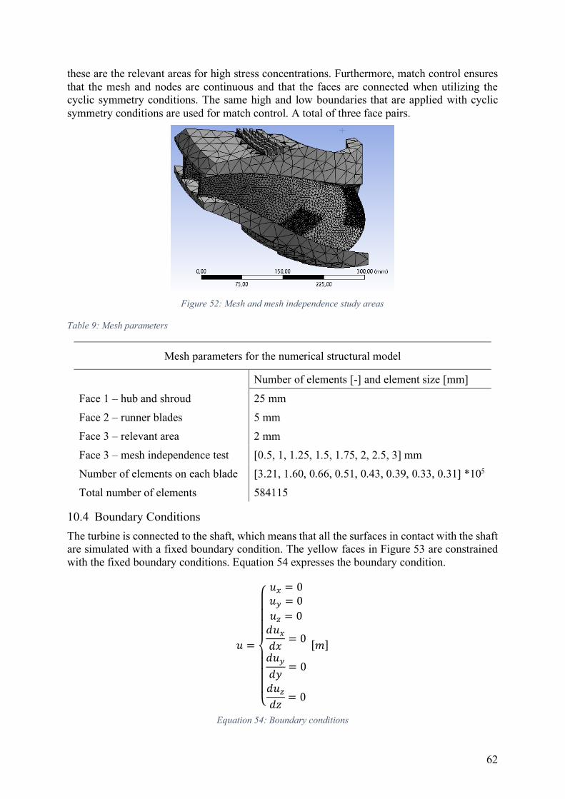
62

these are the relevant areas for high stress concentrations. Furthermore, match control ensures that the mesh and nodes are continuous and that the faces are connected when utilizing the cyclic symmetry conditions. The same high and low boundaries that are applied with cyclic symmetry conditions are used for match control. A total of three face pairs.

Figure 52: Mesh and mesh independence study areas

Table 9: Mesh parameters

Mesh parameters for the numerical structural model

Number of elements [-] and element size [mm]

Face 1 – hub and shroud 25 mm

Face 2 – runner blades 5 mm

Face 3 – relevant area 2 mm

Face 3 – mesh independence test [0.5, 1, 1.25, 1.5, 1.75, 2, 2.5, 3] mm

Number of elements on each blade [3.21, 1.60, 0.66, 0.51, 0.43, 0.39, 0.33, 0.31] *105

Total number of elements 584115

10.4 Boundary Conditions

The turbine is connected to the shaft, which means that all the surfaces in contact with the shaft are simulated with a fixed boundary condition. The yellow faces in Figure 53 are constrained with the fixed boundary conditions. Equation 54 expresses the boundary condition.

𝑢 =

⎩⎪⎪⎪⎨⎪⎪⎪⎧𝑢  = 0𝑢- = 0𝑢¡ = 0𝑑𝑢 𝑑𝑥 = 0𝑑𝑢-𝑑𝑦 = 0𝑑𝑢¡𝑑𝑧 = 0

[𝑚]

Equation 54: Boundary conditions

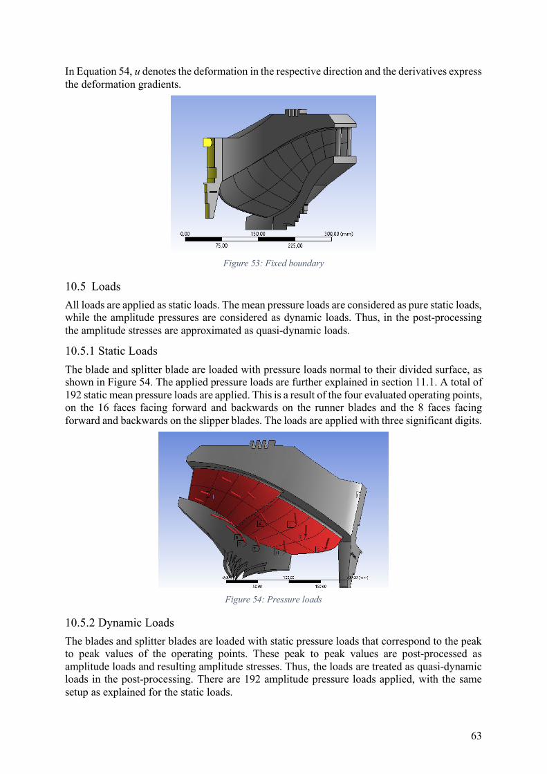
63

In Equation 54, u denotes the deformation in the respective direction and the derivatives express the deformation gradients.

Figure 53: Fixed boundary

10.5 Loads

All loads are applied as static loads. The mean pressure loads are considered as pure static loads, while the amplitude pressures are considered as dynamic loads. Thus, in the post-processing the amplitude stresses are approximated as quasi-dynamic loads.

10.5.1 Static Loads

The blade and splitter blade are loaded with pressure loads normal to their divided surface, as shown in Figure 54. The applied pressure loads are further explained in section 11.1. A total of 192 static mean pressure loads are applied. This is a result of the four evaluated operating points, on the 16 faces facing forward and backwards on the runner blades and the 8 faces facing forward and backwards on the slipper blades. The loads are applied with three significant digits.

Figure 54: Pressure loads

10.5.2 Dynamic Loads

The blades and splitter blades are loaded with static pressure loads that correspond to the peak to peak values of the operating points. These peak to peak values are post-processed as amplitude loads and resulting amplitude stresses. Thus, the loads are treated as quasi-dynamic loads in the post-processing. There are 192 amplitude pressure loads applied, with the same setup as explained for the static loads.

64

10.6 Rotational Velocity

The static and the quasi-dynamic models includes a rotational velocity component. The value of the rotational velocity is decided by the experiments conducted at the Waterpower Laboratory, and defined in Table 10.

Table 10: Rotational velocities

Measured rotational velocity at four operating points

Rotational velocity [RPM]

Low part load 340

Part load 337.3

Best efficiency point 333.5

High load 335

The rotational velocity is applied on the structure as seen in Figure 55, which is a view of the top side of the hub.

Figure 55: Rotational velocity

10.7 Mesh Independence Studies

Two mesh independence studies are conducted to ensure that the solution converges towards a constant stress value. This goes in parallel with the regions meshed with finer mesh, and only those parts of the mesh are refined in the studies. Table 9 shows the relevant parameters for the mesh independence study. Figure 52 shows the relevant areas and section 11.3.7 show the results from the mesh independence studies. In addition, Appendix F, Appendix G, Appendix H, and Appendix I show the images from the mean stresses, amplitude stresses, mean stress at the sharp corner, and mesh quality the numerical analyses, respectively.

In addition to the mesh independence studies, the averaged and unaveraged stresses are evaluated. The average results are the average of the six stress components from Equation 32, and then solving for the equivalent stress component (Sharcnet, u.d.). The unaveraged stresses are found by finding the equivalent stress component of the six components from Equation 32, and then solving the average of the six equivalent stress components.

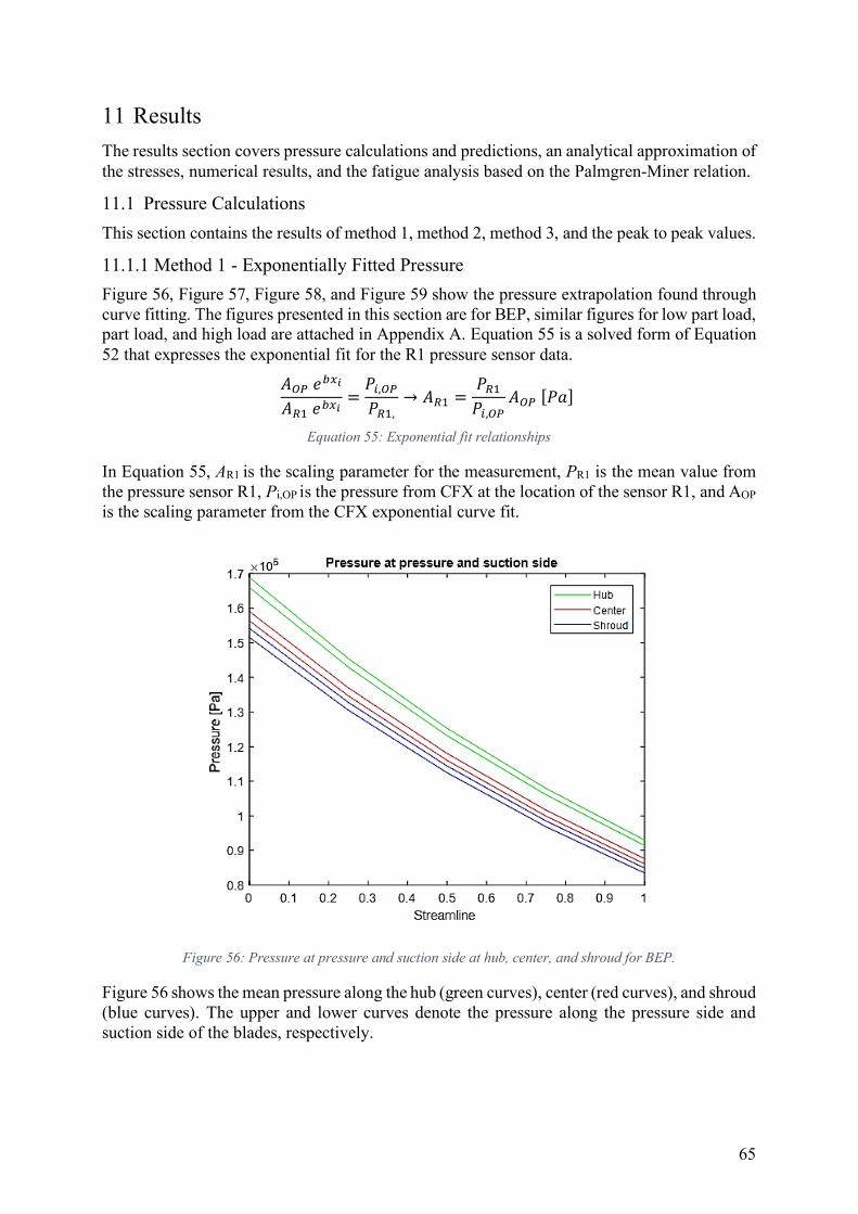
65

11 Results

The results section covers pressure calculations and predictions, an analytical approximation of the stresses, numerical results, and the fatigue analysis based on the Palmgren-Miner relation.

11.1 Pressure Calculations

This section contains the results of method 1, method 2, method 3, and the peak to peak values.

11.1.1 Method 1 - Exponentially Fitted Pressure

Figure 56, Figure 57, Figure 58, and Figure 59 show the pressure extrapolation found through curve fitting. The figures presented in this section are for BEP, similar figures for low part load, part load, and high load are attached in Appendix A. Equation 55 is a solved form of Equation 52 that expresses the exponential fit for the R1 pressure sensor data.

𝐴�d 𝑒¯ ³𝐴c�𝑒¯ ³ = 𝑃�,�d𝑃c�, → 𝐴c� = 𝑃c�𝑃�,�d 𝐴�d [𝑃𝑎] Equation 55: Exponential fit relationships

In Equation 55, AR1 is the scaling parameter for the measurement, PR1 is the mean value from the pressure sensor R1, Pi,OP is the pressure from CFX at the location of the sensor R1, and AOP is the scaling parameter from the CFX exponential curve fit.

Figure 56: Pressure at pressure and suction side at hub, center, and shroud for BEP.

Figure 56 shows the mean pressure along the hub (green curves), center (red curves), and shroud (blue curves). The upper and lower curves denote the pressure along the pressure side and suction side of the blades, respectively.

66

Figure 57: Mean pressure on pressure side at BEP

Figure 58: Mean pressure on suction side at BEP

Figure 57 and Figure 58 show the mean pressure of the hub and center, and center and shroud, respectively. The difference between the pressure and suction side (torque generating pressure) is shown in Figure 59.

Figure 59: Pressure difference between pressure and suction side of blade at BEP

11.1.1.1 Meridional View

Figure 60 shows the meridional view extracted from the numerical fluid model.

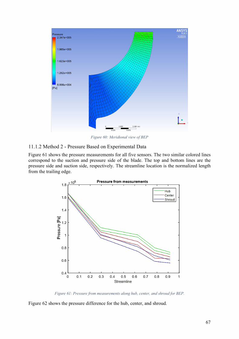
67

Figure 60: Meridional view of BEP

11.1.2 Method 2 - Pressure Based on Experimental Data

Figure 61 shows the pressure measurements for all five sensors. The two similar colored lines correspond to the suction and pressure side of the blade. The top and bottom lines are the pressure side and suction side, respectively. The streamline location is the normalized length from the trailing edge.

Figure 61: Pressure from measurements along hub, center, and shroud for BEP.

Figure 62 shows the pressure difference for the hub, center, and shroud.

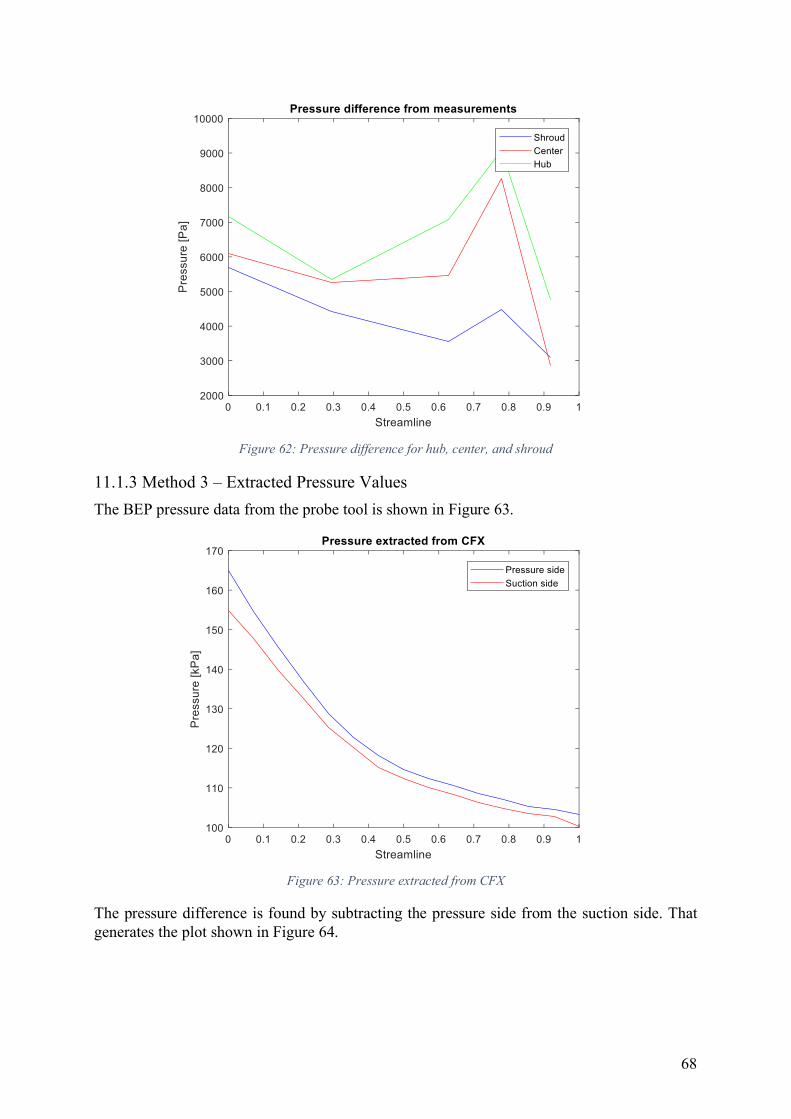
68

Figure 62: Pressure difference for hub, center, and shroud

11.1.3 Method 3 – Extracted Pressure Values

The BEP pressure data from the probe tool is shown in Figure 63.

Figure 63: Pressure extracted from CFX

The pressure difference is found by subtracting the pressure side from the suction side. That generates the plot shown in Figure 64.

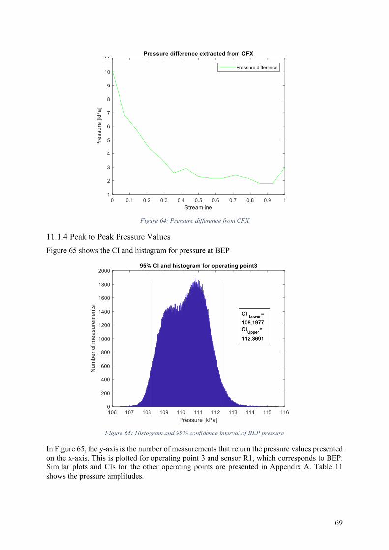
69

Figure 64: Pressure difference from CFX

11.1.4 Peak to Peak Pressure Values

Figure 65 shows the CI and histogram for pressure at BEP

Figure 65: Histogram and 95% confidence interval of BEP pressure

In Figure 65, the y-axis is the number of measurements that return the pressure values presented on the x-axis. This is plotted for operating point 3 and sensor R1, which corresponds to BEP. Similar plots and CIs for the other operating points are presented in Appendix A. Table 11 shows the pressure amplitudes.

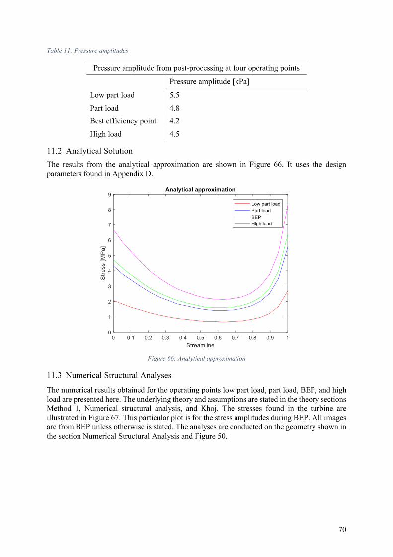
70

Table 11: Pressure amplitudes

Pressure amplitude from post-processing at four operating points

Pressure amplitude [kPa]

Low part load 5.5

Part load 4.8

Best efficiency point 4.2

High load 4.5

11.2 Analytical Solution

The results from the analytical approximation are shown in Figure 66. It uses the design parameters found in Appendix D.

Figure 66: Analytical approximation

11.3 Numerical Structural Analyses

The numerical results obtained for the operating points low part load, part load, BEP, and high load are presented here. The underlying theory and assumptions are stated in the theory sections Method 1, Numerical structural analysis, and Khoj. The stresses found in the turbine are illustrated in Figure 67. This particular plot is for the stress amplitudes during BEP. All images are from BEP unless otherwise is stated. The analyses are conducted on the geometry shown in the section Numerical Structural Analysis and Figure 50.

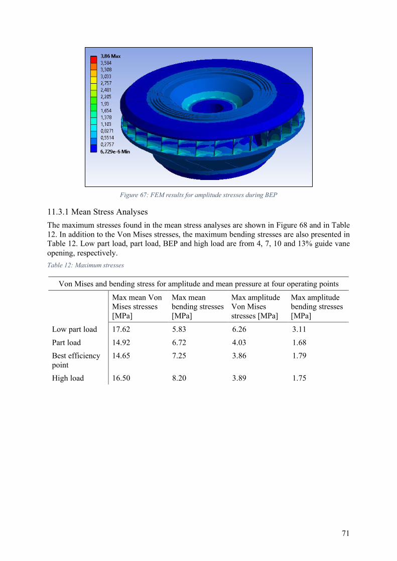
71

Figure 67: FEM results for amplitude stresses during BEP

11.3.1 Mean Stress Analyses

The maximum stresses found in the mean stress analyses are shown in Figure 68 and in Table 12. In addition to the Von Mises stresses, the maximum bending stresses are also presented in Table 12. Low part load, part load, BEP and high load are from 4, 7, 10 and 13% guide vane opening, respectively.

Table 12: Maximum stresses

Von Mises and bending stress for amplitude and mean pressure at four operating points

Max mean Von Mises stresses [MPa]

Max mean bending stresses [MPa]

Max amplitude Von Mises stresses [MPa]

Max amplitude bending stresses [MPa]

Low part load 17.62 5.83 6.26 3.11

Part load 14.92 6.72 4.03 1.68

Best efficiency point

14.65 7.25 3.86 1.79

High load 16.50 8.20 3.89 1.75

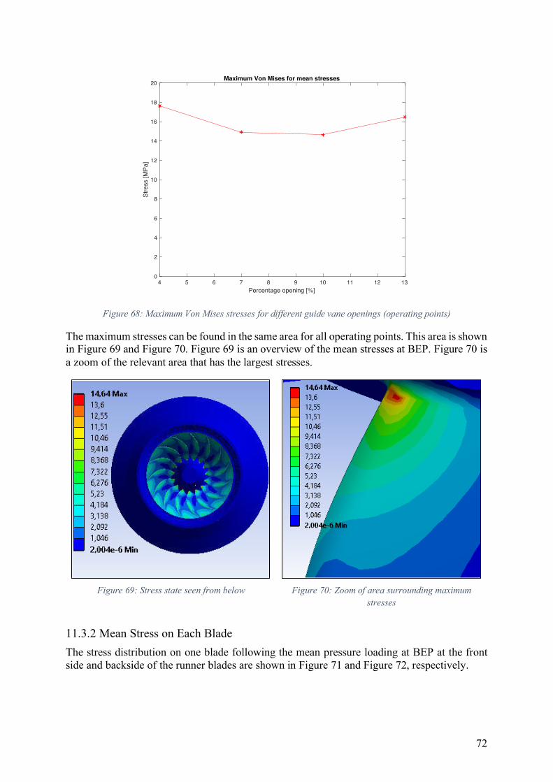
72

Figure 68: Maximum Von Mises stresses for different guide vane openings (operating points)

The maximum stresses can be found in the same area for all operating points. This area is shown in Figure 69 and Figure 70. Figure 69 is an overview of the mean stresses at BEP. Figure 70 is a zoom of the relevant area that has the largest stresses.

Figure 69: Stress state seen from below

Figure 70: Zoom of area surrounding maximum

stresses

11.3.2 Mean Stress on Each Blade

The stress distribution on one blade following the mean pressure loading at BEP at the front side and backside of the runner blades are shown in Figure 71 and Figure 72, respectively.

4 5 6 7 8 9 10 11 12 13

Percentage opening [%]

0

2

4

6

8

10

12

14

16

18

20

Str

ess [M

Pa]

Maximum Von Mises for mean stresses

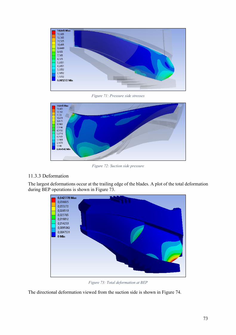
73

Figure 71: Pressure side stresses

Figure 72: Suction side pressure

11.3.3 Deformation

The largest deformations occur at the trailing edge of the blades. A plot of the total deformation during BEP operations is shown in Figure 73.

Figure 73: Total deformation at BEP

The directional deformation viewed from the suction side is shown in Figure 74.

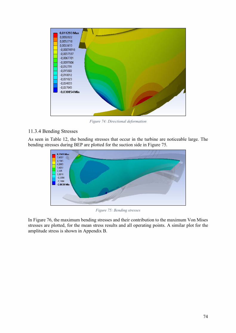
74

Figure 74: Directional deformation

11.3.4 Bending Stresses

As seen in Table 12, the bending stresses that occur in the turbine are noticeable large. The bending stresses during BEP are plotted for the suction side in Figure 75.

Figure 75: Bending stresses

In Figure 76, the maximum bending stresses and their contribution to the maximum Von Mises stresses are plotted, for the mean stress results and all operating points. A similar plot for the amplitude stress is shown in Appendix B.

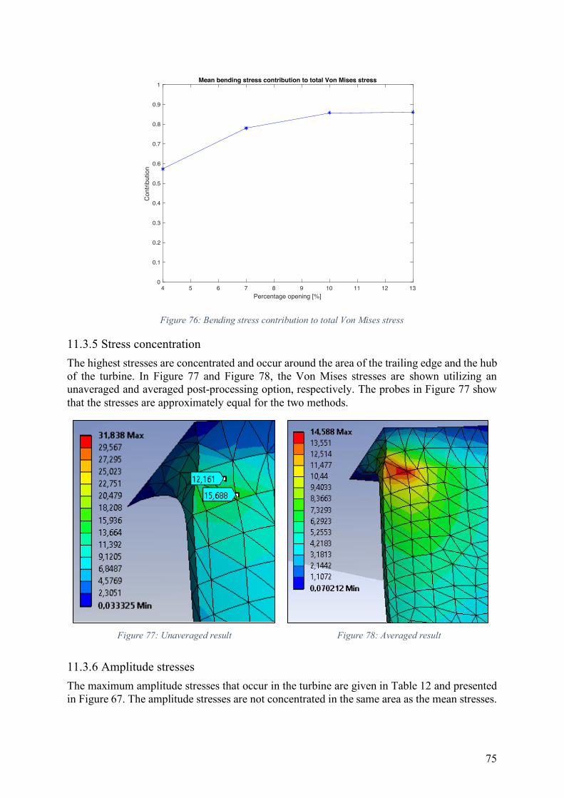
75

Figure 76: Bending stress contribution to total Von Mises stress

11.3.5 Stress concentration

The highest stresses are concentrated and occur around the area of the trailing edge and the hub of the turbine. In Figure 77 and Figure 78, the Von Mises stresses are shown utilizing an unaveraged and averaged post-processing option, respectively. The probes in Figure 77 show that the stresses are approximately equal for the two methods.

Figure 77: Unaveraged result

Figure 78: Averaged result

11.3.6 Amplitude stresses

The maximum amplitude stresses that occur in the turbine are given in Table 12 and presented in Figure 67. The amplitude stresses are not concentrated in the same area as the mean stresses.

4 5 6 7 8 9 10 11 12 13

Percentage opening [%]

0

0.1

0.2

0.3

0.4

0.5

0.6

0.7

0.8

0.9

1

Contr

ibution

Mean bending stress contribution to total Von Mises stress

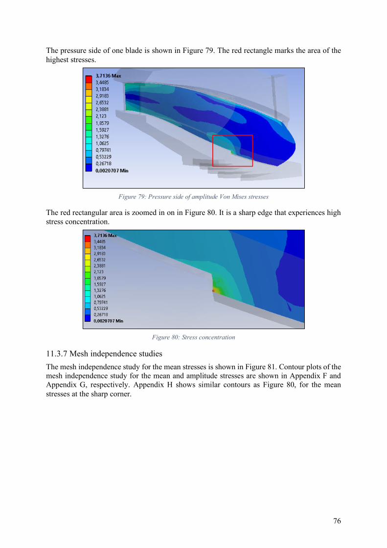
76

The pressure side of one blade is shown in Figure 79. The red rectangle marks the area of the highest stresses.

Figure 79: Pressure side of amplitude Von Mises stresses

The red rectangular area is zoomed in on in Figure 80. It is a sharp edge that experiences high stress concentration.

Figure 80: Stress concentration

11.3.7 Mesh independence studies

The mesh independence study for the mean stresses is shown in Figure 81. Contour plots of the mesh independence study for the mean and amplitude stresses are shown in Appendix F and Appendix G, respectively. Appendix H shows similar contours as Figure 80, for the mean stresses at the sharp corner.

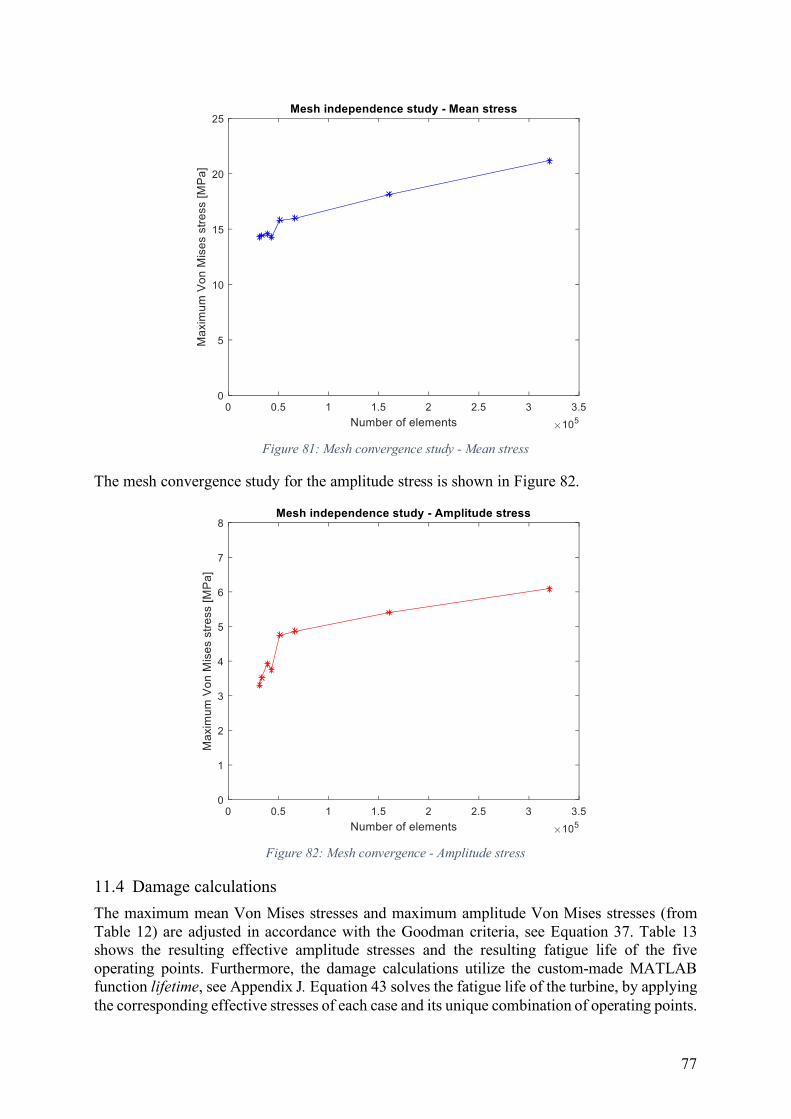
77

Figure 81: Mesh convergence study - Mean stress

The mesh convergence study for the amplitude stress is shown in Figure 82.

Figure 82: Mesh convergence - Amplitude stress

11.4 Damage calculations

The maximum mean Von Mises stresses and maximum amplitude Von Mises stresses (from Table 12) are adjusted in accordance with the Goodman criteria, see Equation 37. Table 13 shows the resulting effective amplitude stresses and the resulting fatigue life of the five operating points. Furthermore, the damage calculations utilize the custom-made MATLAB function lifetime, see Appendix J. Equation 43 solves the fatigue life of the turbine, by applying the corresponding effective stresses of each case and its unique combination of operating points.

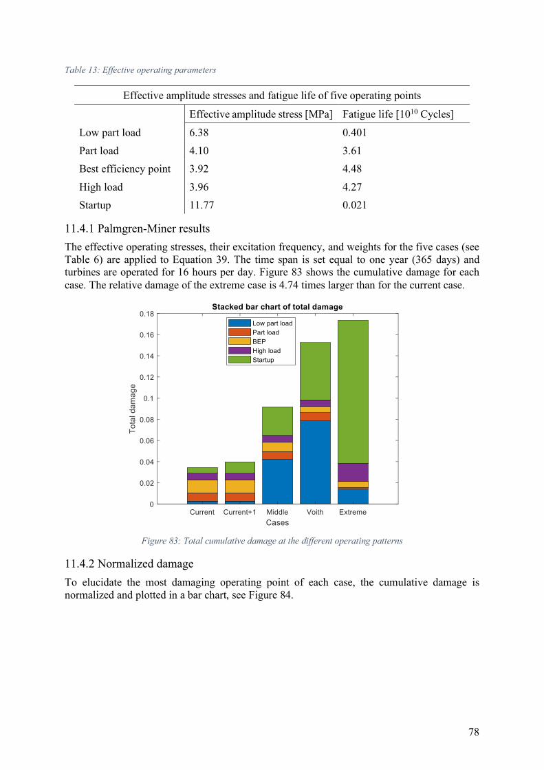
78

Table 13: Effective operating parameters

Effective amplitude stresses and fatigue life of five operating points

Effective amplitude stress [MPa] Fatigue life [1010 Cycles]

Low part load 6.38 0.401

Part load 4.10 3.61

Best efficiency point 3.92 4.48

High load 3.96 4.27

Startup 11.77 0.021

11.4.1 Palmgren-Miner results

The effective operating stresses, their excitation frequency, and weights for the five cases (see Table 6) are applied to Equation 39. The time span is set equal to one year (365 days) and turbines are operated for 16 hours per day. Figure 83 shows the cumulative damage for each case. The relative damage of the extreme case is 4.74 times larger than for the current case.

Figure 83: Total cumulative damage at the different operating patterns

11.4.2 Normalized damage

To elucidate the most damaging operating point of each case, the cumulative damage is normalized and plotted in a bar chart, see Figure 84.

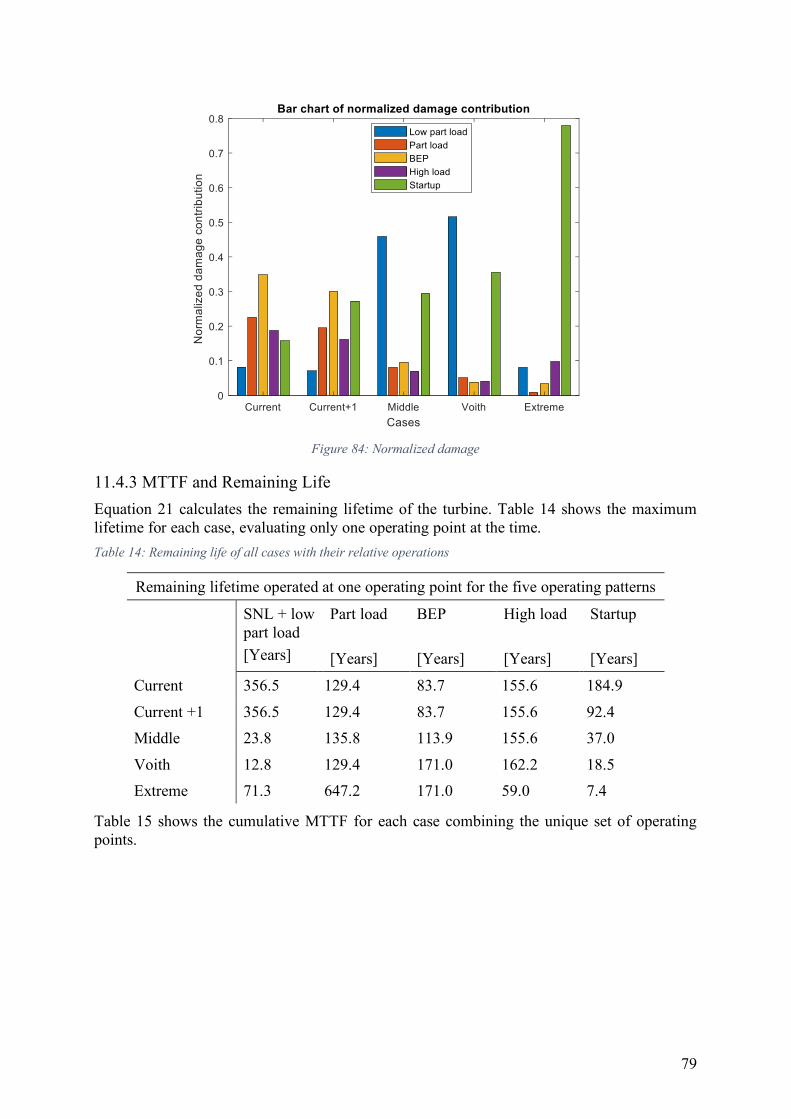
79

Figure 84: Normalized damage

11.4.3 MTTF and Remaining Life

Equation 21 calculates the remaining lifetime of the turbine. Table 14 shows the maximum lifetime for each case, evaluating only one operating point at the time.

Table 14: Remaining life of all cases with their relative operations

Remaining lifetime operated at one operating point for the five operating patterns

SNL + low part load

[Years]

Part load

[Years]

BEP

[Years]

High load

[Years]

Startup

[Years]

Current 356.5 129.4 83.7 155.6 184.9

Current +1 356.5 129.4 83.7 155.6 92.4

Middle 23.8 135.8 113.9 155.6 37.0

Voith 12.8 129.4 171.0 162.2 18.5

Extreme 71.3 647.2 171.0 59.0 7.4

Table 15 shows the cumulative MTTF for each case combining the unique set of operating points.

80

Table 15: Cumulative MTTF

Cumulative mean time to failure for the five operating patterns

MTTF [Years]

Current 30.1

Current +1 26.2

Middle 11.9

Voith 7.6

Extreme 6.8

11.4.4 Damage as Function of Startup

Table 16 shows the operational number of days for each operating point compared to one startup.

Table 16: Operational damage equal to one startup

Operations at four operating points, which damage equals one startup

Low part load Part load BEP High load

Equals one startup [days]

7.04 64.1 80.4 76.0

11.5 Financial Results

This section presents the financial results due to changing to flexible operations. As a base case, the concessionary energy price is set equal to 0.028 NOK/kWh, the average energy price is 0.26 NOK/kWh, and the discount rate is 10%.

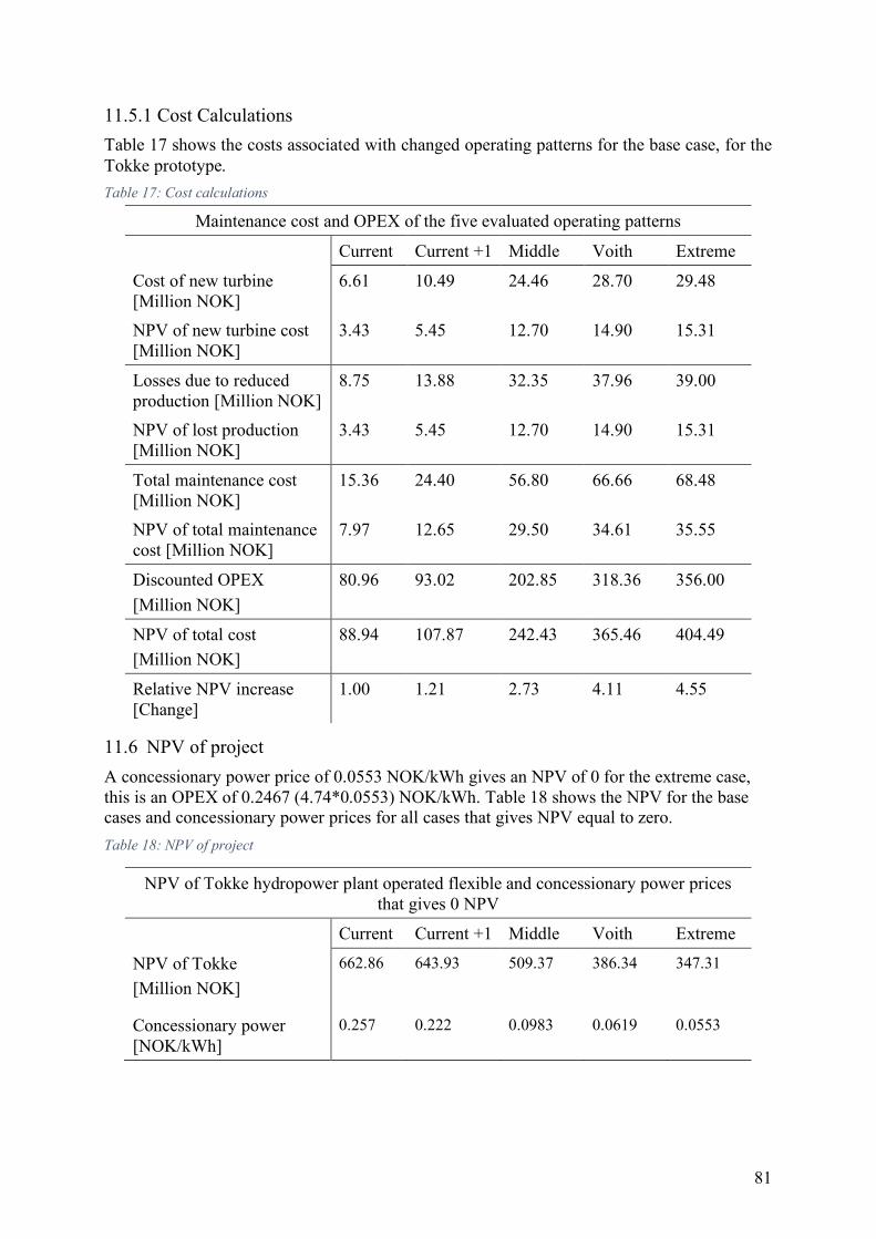
81

11.5.1 Cost Calculations

Table 17 shows the costs associated with changed operating patterns for the base case, for the Tokke prototype.

Table 17: Cost calculations

Maintenance cost and OPEX of the five evaluated operating patterns

Current Current +1 Middle Voith Extreme

Cost of new turbine [Million NOK]

6.61 10.49 24.46 28.70 29.48

NPV of new turbine cost [Million NOK]

3.43 5.45 12.70 14.90 15.31

Losses due to reduced production [Million NOK]

8.75 13.88 32.35 37.96 39.00

NPV of lost production [Million NOK]

3.43 5.45 12.70 14.90 15.31

Total maintenance cost [Million NOK]

15.36 24.40 56.80 66.66 68.48

NPV of total maintenance cost [Million NOK]

7.97 12.65 29.50 34.61 35.55

Discounted OPEX

[Million NOK]

80.96 93.02 202.85 318.36 356.00

NPV of total cost

[Million NOK]

88.94 107.87 242.43 365.46 404.49

Relative NPV increase [Change]

1.00 1.21 2.73 4.11 4.55

11.6 NPV of project

A concessionary power price of 0.0553 NOK/kWh gives an NPV of 0 for the extreme case, this is an OPEX of 0.2467 (4.74*0.0553) NOK/kWh. Table 18 shows the NPV for the base cases and concessionary power prices for all cases that gives NPV equal to zero.

Table 18: NPV of project

NPV of Tokke hydropower plant operated flexible and concessionary power prices that gives 0 NPV

Current Current +1 Middle Voith Extreme

NPV of Tokke

[Million NOK]

662.86 643.93 509.37 386.34 347.31

Concessionary power [NOK/kWh]

0.257 0.222 0.0983 0.0619 0.0553

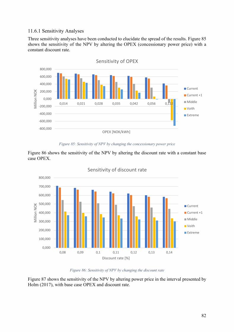
82

11.6.1 Sensitivity Analyses

Three sensitivity analyses have been conducted to elucidate the spread of the results. Figure 85 shows the sensitivity of the NPV by altering the OPEX (concessionary power price) with a constant discount rate.

Figure 85: Sensitivity of NPV by changing the concessionary power price

Figure 86 shows the sensitivity of the NPV by altering the discount rate with a constant base case OPEX.

Figure 86: Sensitivity of NPV by changing the discount rate

Figure 87 shows the sensitivity of the NPV by altering power price in the interval presented by Holm (2017), with base case OPEX and discount rate.

-800,000

-600,000

-400,000

-200,000

0,000

200,000

400,000

600,000

800,000

0,014 0,021 0,028 0,035 0,042 0,056 0,112

Mil

lio

n N

OK

OPEX [NOK/kWh]

Sensitivity of OPEX

Current

Current +1

Middle

Voith

Extreme

0,000

100,000

200,000

300,000

400,000

500,000

600,000

700,000

800,000

0,08 0,09 0,1 0,11 0,12 0,13 0,14

Mil

lio

n N

OK

Discount rate [%]

Sensitivity of discount rate

Current

Current +1

Middle

Voith

Extreme

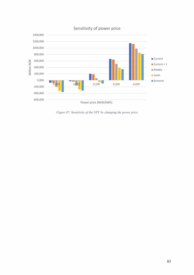
83

Figure 87: Sensitivity of the NPV by changing the power price

-600,000

-400,000

-200,000

0,000

200,000

400,000

600,000

800,000

1000,000

1200,000

1400,000

0,004 0,020 0,100 0,260 0,429

Mil

lio

n N

OK

Power price [NOK/kWh]

Sensitivity of power price

Current

Current + 1

Middle

Voith

Extreme

84

12 Discussion The discussion section covers the uncertainty of selected assumptions and the validity of these. It also attempts to draw conclusions from the results and elucidate certain parts of the results that requires an explanation.

12.1 Pressure Calculations

The results presented in this thesis, are dependent on correct evaluation of the pressure in the turbine runner, see section 11.1 that presents the results of the three pressure methods. The choice of preceding with method 1 is based on several factors, primarily it is a result of elimination of lesser alternatives.

12.1.1 Pressure Method 2

Method 2 utilizes the extracted design parameters from Khoj and measurement data from the Waterpower Laboratory. The MATLAB codes from Appendix J creates the plots shown in Figure 61 and Figure 62. Inconsistency of the model is the primary issue, which could origin from the underlying assumptions and theory of the rothalpy relations.

The measurements from R1, R2, R3, and R4 are assumed to follow the same streamline in the turbine, nevertheless, it is impossible to confirm this. Conservation of rothalpy is a fundamental assumption to calculate the pressure at the suction and pressure side of the runner blades. As explained in section 3.4, the rothalpy relationship is valid only for steady state flow and conservation of momentum (no friction), this is rarely the case in measurements. It is also possible that the time averaging is not evaluating a long enough time series to be valid for the rothalpy relation. Thus, it is invalid to apply such a constrained theory to real measurements, which evidently takes everything into account. The pressure measurements at every location are not one hundred per cent correlated through the rothalpy relationships. In particular, Figure 62 shows that the pressure difference does not follow the expected exponential relationship, instead the difference seems to increase towards the trailing edge. The increase is expected if there is friction that is higher at the inlet than at the trailing edge. The rothalpy relationship is capable of predicting the mean pressure, which is shown in Figure 61. Khoj suggests that it could occur backflow in the turbine. This would, similarly as for friction, greatly impact the measurements and induce flaws in calculated pressure differences. In sum, method 2 is able to predict the mean pressure in the runner and to a certain degree elucidate the magnitude of the pressure difference.

12.1.2 Pressure Method 3

Method 3 comes from the probe function (a point and click function in CFX) applied to Chirag Trivedi’s CFX program. This particular method yields valid results, which are applicable for the model runner in the Waterpower Laboratory. Nevertheless, it is not transparent, generic, certain, nor academic enough for this thesis. The exact location of the probed results is impossible to double-check. It would be possible to find a correlation factor between the model runner and the prototype and utilize this method. On the other hand, it is uncertain if these results would be generic and applicable for all Francis runners. Furthermore, this thesis seeks to provide general objective methodology that can be reproduced for new and unique hydropower plants, from the MATLAB scripts in Appendix J. Thus, method 3 is discarded.

12.1.3 Pressure Method 1

The con arguments presented in section 12.1.1 and 12.1.2 eliminated method 2 and 3. Method 1 requires few input parameters to be generalized for new unique turbines. The pressure difference is found by a pressure measurement (P), the relative position (r) of the measurement

85

at the guide vanes, runner or draft tube, the operational speed (RPM), net head (H), and flow rate (QED). This is assuming that the relative pressure difference between hub, center, and shroud are generic and follow the same patterns as the model runner. This assumption is somewhat questionable, as all hydropower turbines are custom-made with their own pressure characteristics. The actual distribution can be different for turbines that utilizes unique design parameters. Accordingly, if this is the case, valid results can be obtained if the pressure scaling factors are updated in the MATLAB function trykkblad. Furthermore, the method is not valid for turbines operated outside normal operating conditions that induce undesired flow conditions. More information on how to update the MATLAB codes is found in Appendix J. The meridional views further validates that the stresses extrapolated from a single measurement point give reasonable results.

12.2 Numerical Structural Analysis

The results of the numerical analyses are valid under certain conditions and the results must be read in accordance with the limitations presented in this section.

12.2.1 Mesh Convergence

The mesh convergence study (see Figure 81 and Figure 82) and mesh quality study for 2 mm elements (Appendix I) further validates the stresses. The mean stress concentration disappears from the sharp corner (see Figure 80) with element sizes above 1.5mm. The similarity between the stresses presented by the unaveraged and averaged results concludes that the mesh quality is sufficient. Thus, the utilized element size of 2 mm at the relevant areas are adequate.

12.2.2 Average vs. Unaverage

Comparison of average and unaveraged elements further strengthens the results of the analyses. Figure 77 and Figure 78 show the unaveraged and averaged results, respectively. The area of stress concentration is at the connection between the splitter blades and the shroud for the unaveraged methods. However, the magnitude of the stresses along the runner blades and the hub at the trailing edge are approximately identical for both methods, see the results of the probes in Figure 77. As expected, there are small numerical discrepancies between averaging the results of the 10 node elements and the unaveraged results. In conclusion, these discrepancies are too small to make the results invalid and instead improves the integrity of the model.

12.2.3 Deformation

The blades bend along the yellow contour in Figure 74. The deformation is both into the plane and out of the plane. This is because the turbine has a unique weld design, the weld connecting the blade and shroud is shorter than usually. The unique design causes the turbine to bend around a point on the lower part of the blade, see the area where the deformation shifts from positive to negative in Figure 74.

12.2.4 Bending Stresses

Bending stress is the governing stress state is the blades. In reality there are additional principal stresses present. Figure 76 shows that maximum stresses at BEP and high load are subjected to relatively more bending stress than the low part load and part load. As expected, the current state of the deformation does induce large bending stresses. Figure 76 shows that more principal stress components are present in the blades. The unique weld design is partly responsible for the complex stress state at the trailing edge of the blades.

86

12.2.5 Comparison with the Analytical Solution

Figure 76 gives indications that the analytical approximation, which only evaluates bending stress is somewhat applicable. The values obtained from the analytical solution are a tad lower than the numerical stresses. This is a result of a more complex stress state in the numerical simulations, potential numerical errors (even though it is unlikely with the utilized mesh quality) and simplifications of the applied pressure in the analytical solution. The principal stress components that are not included in the analytical solution, are the largest sources of difference. Nevertheless, the magnitude of the stresses from the analytical and numerical solutions are within the same region. Thus, the analytical solution can provide quick, but less accurate results than numerical simulations of the maximum stresses. It is worth noticing that the analytical solution is better suited to estimate the stress state for BEP and high load, as the Von Mises stresses at these operating points contains larger portions of bending stress.

12.2.6 Comparisons with Previous Studies

The location of the maximum stresses matches the location found in previous studies, see the location of the mean stresses in Figure 34 and amplitude RSI induced stresses in Figure 35. Figure 35 has concentrations at the trailing edge around the connection between the shroud and runner blade. Even though the amplitude stresses concentrate at a different area in this study, the relative location is the same. Both are located at the end of the weld between the shroud and blade, see Figure 69, Figure 72, and Figure 79. The shorter weld on the Francis model used in the numerical simulations is the reason that the maximum amplitude stresses occur at a different location. The magnitudes of the effective stresses are comparable, both in magnitude and location, with the stresses obtained by Ingebjørg Valkvæ (2016) in her master’s thesis Dynamic

loads on Francis turbines.

12.2.7 Assumptions

The studies conducted in this thesis does not account for harmonic responses. Thus, it is crucial, in particular for the quasi-dynamic amplitude studies, that the analyses are not conducted at the eigenfrequencies of the system. It is assumed that regular operating patterns do not induce vibrations at the eigenfrequency of the system, thus the results in this thesis are valid for regular operations.

12.2.8 Unsuccessful One-Way FSI.

Several unsuccessful attempts were made to incorporate the numerical fluid analyses in the structural analyses. Valkvæ (2016) was successful in implementing this in her master’s thesis. This was not possible in this thesis, even though EDR Medeso gave their best assistance on the matter. There were several unsuccessful attempts to import the pressure directly into ANSYS mechanical and importing it utilizing an acoustic extension. The issue appeared to be mismatching of nodes on the structural and fluid model. However, the results obtained through interpolation of the pressure measurements and applying these on the numerical structural model are comparable with the results obtained by Valkvæ (2016). It is recommended to carry out two-way FSI analyses to gain results that could pin point the increased wear, the analyses would strengthen the validity or discard some of the results presented in this thesis.

12.3 Operating Patterns

There exists limited research on prospective future operating patterns. The author of this thesis has in collaboration with the supervisors and inspirations from Voith (Seidel, et al., 2014), suggested potential patterns. The recommended operating patterns presented in this thesis are aligned with the three key characteristics presented by Welte & Solvang (2011).

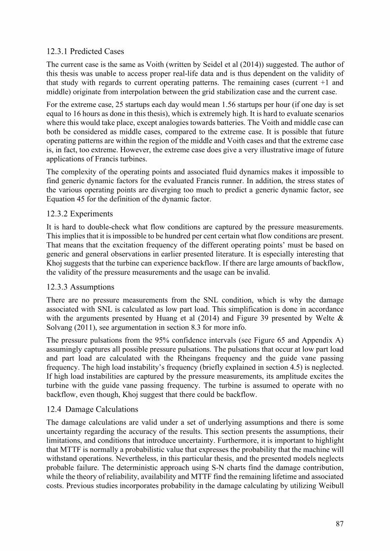
87

12.3.1 Predicted Cases

The current case is the same as Voith (written by Seidel et al (2014)) suggested. The author of this thesis was unable to access proper real-life data and is thus dependent on the validity of that study with regards to current operating patterns. The remaining cases (current +1 and middle) originate from interpolation between the grid stabilization case and the current case.

For the extreme case, 25 startups each day would mean 1.56 startups per hour (if one day is set equal to 16 hours as done in this thesis), which is extremely high. It is hard to evaluate scenarios where this would take place, except analogies towards batteries. The Voith and middle case can both be considered as middle cases, compared to the extreme case. It is possible that future operating patterns are within the region of the middle and Voith cases and that the extreme case is, in fact, too extreme. However, the extreme case does give a very illustrative image of future applications of Francis turbines.

The complexity of the operating points and associated fluid dynamics makes it impossible to find generic dynamic factors for the evaluated Francis runner. In addition, the stress states of the various operating points are diverging too much to predict a generic dynamic factor, see Equation 45 for the definition of the dynamic factor.

12.3.2 Experiments

It is hard to double-check what flow conditions are captured by the pressure measurements. This implies that it is impossible to be hundred per cent certain what flow conditions are present. That means that the excitation frequency of the different operating points’ must be based on generic and general observations in earlier presented literature. It is especially interesting that Khoj suggests that the turbine can experience backflow. If there are large amounts of backflow, the validity of the pressure measurements and the usage can be invalid.

12.3.3 Assumptions

There are no pressure measurements from the SNL condition, which is why the damage associated with SNL is calculated as low part load. This simplification is done in accordance with the arguments presented by Huang et al (2014) and Figure 39 presented by Welte & Solvang (2011), see argumentation in section 8.3 for more info.

The pressure pulsations from the 95% confidence intervals (see Figure 65 and Appendix A) assumingly captures all possible pressure pulsations. The pulsations that occur at low part load and part load are calculated with the Rheingans frequency and the guide vane passing frequency. The high load instability’s frequency (briefly explained in section 4.5) is neglected. If high load instabilities are captured by the pressure measurements, its amplitude excites the turbine with the guide vane passing frequency. The turbine is assumed to operate with no backflow, even though, Khoj suggest that there could be backflow.

12.4 Damage Calculations

The damage calculations are valid under a set of underlying assumptions and there is some uncertainty regarding the accuracy of the results. This section presents the assumptions, their limitations, and conditions that introduce uncertainty. Furthermore, it is important to highlight that MTTF is normally a probabilistic value that expresses the probability that the machine will withstand operations. Nevertheless, in this particular thesis, and the presented models neglects probable failure. The deterministic approach using S-N charts find the damage contribution, while the theory of reliability, availability and MTTF find the remaining lifetime and associated costs. Previous studies incorporates probability in the damage calculating by utilizing Weibull

88

distributed curve in the S-N charts to address MTTF (Qvale, 2016), this is not done in this thesis.

12.4.1 Fracturing Runner

All analyses are based on the assumption that the runner fractures first, because it experiences the largest stresses. However, it is likely that other components experience increased wear during flexible operations. Nevertheless, if operations are increasingly aggressive, ceteris

paribus, the wear of the runner increases the most.

12.4.2 Low Part Load and SNL

Damage from low part load dominates the middle and Voith cases. Table 16 shows that low part load is by far the most damaging operating point, in addition to startup. Trends in operating patterns suggest that turbines are operated more at SNL than previously, see cases by Voith (2014). If the assumptions regarding the similarities between SNL and low part load are false, it would exaggerate or understate the overall damage. In addition, the results of the damage calculations show that the operator should refrain from operations at low part load as much as possible. Low part load produces the least amount of energy, at a higher cost than the BEP.

12.4.3 Startup

The theoretical background of the startup process is primarily based on the study conducted by Gagnon et al (2010), thus this paper is dependent on the quality of that study. Equation 9 decides how many revolutions that occurs during startup of the turbine. The guide vane passing frequency is assumed to increase linearly until synchronization. In reality the acceleration is approximately linear, and thus, the speed increases more like a quadratic function. This linearization does not impact the results to a large degree. Furthermore, the number of startups is a vital parameter – as startup significantly impacts the damage of the runner. If an actual startup is faster than what evaluated here, the structural impact of startup is exaggerated. Likewise, for strain, if the actual strain is lower than presented in Figure 18 and Figure 19 the structural impact of startup is exaggerated. It should be noted that the relative damage from startup is higher in this thesis, than seen in Figure 40.

12.4.4 Time Span

The author of this thesis has not been able to access real-life data regarding operating time and downtime of typical Francis runners. The turbines assumingly operate 16 hours every day, until collapse. Conversely, if the ratio between downtime and operating time is different than what was presented in this thesis, the relative and normalized results are still valid.

12.4.5 Crack Growth

This thesis does not contain analyses of crack growth. This is a result of lacking experimental data, which made crack growth experiments impossible. Moreover, this implies that all analyses are conducted on initially crack free turbines. In that case, the S-N curve methodology utilized in this thesis is adequate for such fatigue assessments.

12.4.6 Assumptions

The S-N chart is extrapolated to be valid for HCF and ultra-HCF. To allow this, it is essential that it is valid to extrapolate S-N curves in corrosive environments. On the other hand, if this is invalid, the lifetime of the turbine, at all operating points would be infinite. The endurance limits presented by Huth (2005) would then never induce fatigue damage, unless the S-N charts are extrapolated.

89

Francis turbines has no clearly defined material standards. Which is why this thesis uses a combination of the presented literature. The S-N chart is from NS-EN 19902:2007, while yield stress and UTS are from Huth’s PhD (2005). The validity of this, in particular the link between the material parameters and the S-N curve are essential for the results.

12.5 Cost and Financial Results

The cost and financial analyses are conducted until failure (6.76 years) including repair of the extreme case (3 months). All NPV calculations assumes that changing to flexible operations does not require any initial investments.

12.5.1 Sensitivity Analyses

The concessionary power price is a combination of OPEX and CAPEX. Initially, OPEX is set equal to 25% of the concessionary power price. The OPEX is assumed to be proportional with the change of lifetime. A reduction of the lifetime by 4, increases the OPEX by 4. Figure 85 shows how the NPV changes when adjusting the OPEX to 50%, 75%, 100%, 125% 150%, 200%, and 400% (400% is equal to the total concessionary power price). The sensitivity analysis proves that the NPV is very dependent on the OPEX. Practical deductions of the sensitivity analyses, are that lower percentages of the concessionary power price means turbines that are optimized for flexible operations. Optimization in the form of reduced wear, easier and cheaper maintenance, or potentially a more robust turbine. The sensitivity analyses for varying concessionary prices shows that the extreme case has a positive NPV for concessionary power prices (OPEX 0.2467) below 0.0553 NOK/kWh.

KPGM and national grid (2016) found that the highest tender was 0.1296 NOK/kWh. The base OPEX for the extreme case is 96% of this (0.028*4.74 / 0.1296). This indicates that the base case with OPEX equal to 25% of the concessionary power price, is too high or that the services are not adequately rewarded by national grid. Another possibility is that the tenders granted by national grid are too low. The offers can be too low to a variety of reasons, potential reasons are presented in section 2.7.1.2. The comparison is under the assumption that the energy provides in United Kingdom are operating under the same cost conditions as the Nordic hydropower plants.

The NPV is less sensitive to changes in the discount rate. As expected, the relative difference between the different cases goes towards a constant value when the discount rate increases. This is a consequence of the importance of the first year’s cash flow, which is seen in Equation 27 that very large discount rates make future cash flows go towards zero.

Holm (2017) presented in her master’s thesis, that energy prices vary between 0.004 and 0.429 NOK/kWh for system services in the Nordic intraday market. If prices are below 0.26NOK/kWh, the operators should be careful with operating the turbines aggressively, see the sensitivity analysis of variable power price in Figure 87. The intraday market Elbas is very rewarding, for all cases, when the power price spikes, seen in the two curves on the right side of Figure 87. These prices are more appropriate for Nordic power producers, than the ones presented by national grid.

12.5.2 Alternative Cost

The method of rewarding flexible operations with the alternative cost, suggested by Dr. Böttger (2018), are easily applicable for all cases. The price of the different operating patterns, is the difference in NPV from the current case. This can either be payed upfront or with raised power prices that after discounting future cash flows fill the NPV gap. The alternative to flexible operations, is simply speaking to continue with regular operations, thus, the current case.

90

12.5.3 Adjustments

The cost of a reinstalled turbine is set equal to half the cost on the new turbine, the value origins from discussions with the supervisors of the thesis. If the cost is set equal to hundred per cent of a new turbine, the total NPV only experiences minor changes. The impact is very low because the cost is discounted with a ten percent rate over 6.9 years, and the relative cost of a new turbine is small compared to the discounted maintenances costs and OPEX.

All cases that are still operational after 6.9 years (all cases except extreme) includes a fraction of the turbine cost and production losses due to downtime. The cost is proportional with the relative difference in lifetime. Thus, the current case contains 1/4.74 of the discounted replacement cost, likewise, for the loss of production. The current case includes discounted downtime of 3/4.74 months. In addition, all cases include a relative efficiency drop. The efficiency drop also incorporates the relative change of lifetime, under the assumption that all turbines experience a four percent efficiency drop throughout their lifetime, e.g. the current case has an efficiency drop of 4%/4.74 after 6.9 years.

12.5.4 Time span Issues

The energy price of the next six years is initially set equal to the average energy price of the first quarter of 2018, in Norway. It is possible that the energy price would rise or fall in the coming six years. Incorporation of variable energy prices is in this thesis out of scope, as there would be too much uncertainty regarding it. Figure 87 shows a sensitivity analysis that utilizes price intervals, which were granted on Elbas in 2015. The analyses are conducted with constant prices of the entire time span. The NPV is as expected very dependent on the power price.

The NPV calculations neglects initial investments and all revenue sources are from operations at BEP (110 MW). The cash flows follow Equation 26 multiplied by total time of operations and the power price or the OPEX, depending on if it is a revenue or cost source, respectively. This is an exaggeration of the actual income and cost. This simplification is valid as both factors are equally exaggerated. Furthermore, this implies that the million NOK values are uncertain, while the relative difference and normalized results are more accurate representations of the cases. Nor are the actual sizes of the cash flows hundred per cent certain, because all cases have unique sets of operating points. Nevertheless, these simplifications are justified by assuming that the average of all operations are approximately at BEP. Meaning that 33% at low load, 33% at BEP and 33% at high load gives 100% at BEP.

12.5.5 Reliability and Availability

The financial analyses do not accurately incorporate reliability and availability of the system. Instead, they approximate average operational time to 16 hours per day for 365 days per year, with planned downtime of 3 months upon collapse of the turbine. The unplanned outage time is neglected in all analyses, and assumingly captured by the proportionality between the lifetime and the OPEX. On the other hand, it is possible that aggressive operating patterns invokes more unplanned maintenance, thus, the OPEX is not necessary hundred per cent proportional with the lifetime.

12.6 Future Perspectives

Are the operating patterns presented in this thesis feasible? Can these patterns be implemented in real-life and what are the alternatives? These are some of the loose ends that are addressed in this section.

91

12.6.1 Feasibility

Operating all cases for the same time span is questionable and seems unfeasible. It is unlikely that a turbine operated like a battery (extreme case) is active for 16 hours per day. More likely, are unique solutions for each particular plant, which seeks to follow the principles of profit maximal solutions expressed by Dr. Böttger (2018). In particular, this is a great opportunity for the Nordic hydropower companies. They have the unique position to closely monitor the alternative cost of all their plants and create holistic solutions that follow the grid mentality of DS3.

A feasible solution is to spread out the number of startups to more than one turbine. Making the overall portfolio mimic the current +1 case, instead of having one aggressively operated turbine. Clustering 13 turbines at the current +1 yields the same balancing capacity as a single turbine operated extremely. Introducing the principles of performance monitoring from DS3 provides adequate techniques to operate a cluster of turbines in such a way.

Alternative suggestions are to change the design of a few turbines, to reduce either the wear, the replacement costs, or the OPEX during flexible generation. A robust turbine will experience less wear (e.g. thicker turbine blades). The robustness comes at an increased manufacturing cost and/or reduced efficiency. The manufacturing cost rises with more expensive materials and/or more material as a consequence of increased thickness. It is likely that the efficiency drops if the weight or thickness of the turbine are increased. Especially, as current designs assumingly yield efficiency close to the maximal theoretical efficiency. The end goal of the design changes are to reduce the OPEX for turbines providing flexible generation and that actively sell system services.

12.6.2 Frequency Control

Flexible hydropower is an excellent alterative for increased frequency control, despite individually providing relative low system inertia. The structural impacts on operating the turbine like a battery are large, but the cost is relative small compared to similar solutions, e.g. batteries. The 100 MW batteries installed in Australia by Tesla, Inc. is rumored to cost at least 115 million USD (Guess, 2017). This is larger than the cost of operating the turbine extremely, for the entire OPEX interval evaluated in Figure 85. Hydropower is a renewable, relatively cheap, and feasible alternative compared to other equally effective balancing sources. Whether hydropower is the most environmentally and efficiency balancing sources or not, must be revised if research is successful in coupling wind turbines with the grid. Nevertheless, with the current status quo, hydropower is the preferred alternative.

12.6.3 Parallel Integrated Design

A design that could solve many of the problems with reduced lifetime and high stress concentrations would be a matrix of parallel and serially connected small turbines, similar to a grid of turbines. Such a system of turbines provides the same balancing capacity as current turbines if sufficiently many turbines are jointly connected. This design is by the author called parallel integrated design, which is a proximity of how Google’s servers are made up of several cheap jointly connected machines (Taylor, 2003). A system of smaller turbines can co-exist with current hydropower solutions and offer increased balancing capacity at critical times. The design and feasibility of such a system is not evaluated in this thesis, but they are interesting topics for further studies in the field of flexible generation.

92

13 Conclusion This thesis evaluates the impact of flexible operations on the structural integrity and the associated increased maintenance cost. Through the work, the following conclusions can be drawn under the assumptions presented in the discussion section:

1. Flexible operations induce large stresses and reduce the lifetime of Francis runners. Startup and low part load are the most damaging operating points. One startup is equal to 7 days, 64 days, 80 days, and 76 days at low part load, part load, BEP, and high load, respectively.

2. The maximum effective stresses that occur during low part load, part load, BEP, high load, and startup are 6.38, 4.10, 3.92, 3.96, and 11.77 MPa, respectively.

3. The total lifetime of the current, current +1, middle, Voith, and the extreme cases are 30.1, 26.2,11.9, 7.6, and 6.8 years, respectively.

4. Analytical solutions are able to predict the maximum stresses in a Francis runner with some certainty. The analytical solution underestimates the stress state compared to numerical solutions, as the analytical solution assumes that the stress state is purely bending.

5. The flexible generation cases current, current +1, middle, Voith and extreme has total costs of 88.9, 107.9, 242.4, 365.5 and 404.5 million NOK.

6. Flexible generation have lower NPV than the current cases due to increased OPEX. The flexible scenarios are very sensitive to OPEX. The initial estimate of OPEX is set equal to 25% of the concessionary power price (0.028 NOK/kWh), it gives positive NPV for the five evaluated cases. A base concessionary power price of 0.257, 0.222, 0.0983, 0.0619, and 0.0553 NOK/kWh gives 0 NPV for the current, current+1, middle, Voith, and extreme cases, respectively. When the power price is below 0.26NOK/kWh, the operators should be careful with flexible generation and operating patterns.

7. Hydropower is well suited for integration to the current, and prospective market solutions for balancing services. In addition, it is the cheaper alternative compared to batteries, and the more renewable alternative to conventional balancing sources.

93

14 Further work The author of this thesis has found aspects of the thesis that would benefit from more research. The following aspects are listed in prioritized order (in the author’s opinion), which would increase the accuracy and robustness of the results presented in this thesis:

1. Further investigations with regards to how the operating patterns of hydropower turbines will change when integrated and utilized for intraday trading. It is necessary to pin point exact number of startups and the corresponding percentages associated with each operating point.

2. Increased data and knowledge of the OPEX. The assumption of OPEX equal to twenty-five per cent of the concessionary power price is specific and not necessarily applicable for unique turbines.

3. Pressure measurements from SNL and startup. This would remove the assumption regarding the strain at startup and the simplification that SNL is treated as low part load.

4. Documentation of real fatigue data from the Francis runner at the Waterpower Laboratory at NTNU. Preferably documentation of the impact ultra-HCF has on the endurance limit in corrosive environments. In addition, real S-N charts found through fatigue testing would increase the robustness of the results.

5. Assessment of the damage that occurs during flexible generation to other components than just the turbine runner.

6. More accurate prediction of dynamic stresses using two-way FSI numerical analyses. 7. Incorporate real-life data of reliability and availability to further asses the active

operational time in the models. To successfully do this, it is necessary to get real-life information regarding the planned and unplanned maintenance of Francis turbines.

8. A financial model that incorporates variable energy prices, both on the Elbas and Nord Pool markets. This mean variable market set operating revenue and costs, which are set in accordance with the current market prices. In addition, differentiation of the operating patterns that are hundred per cent accurate.

9. Attempt to design a parallel integrated design utilizing Francis turbines, to see if this solution has lower maintenance cost than regular turbines.

i

15 Bibliography

Agnalt, E. (2016). Design of experiment WP 1.3 Onboard pressure measurements Second

Iteration. Trondheim: The Norwegian University of Science and Technology Faculty of Engineering Science and Technology Department of Energy and Process Engineering.

Bak, M. (2016, 02 12). Mean Stress Corrections in Fatigue. Retrieved 04 10, 2018, from Computer Aided Engineering Associates: https://caeai.com/blog/mean-stress-corrections-fatigue

Böttger, D. (2018, 02 8). Combined modeling of spot and control power markets in Germany. Combined modeling of spot and control power markets in Germany. Trondheim: Fraunhofer IEE.

Børresen, B., Faanes, S., Moltubakk, T., & Rangnes, G. (2003). Driftsrelatert

Kostnadsfunksjon. Oslo: GE Energy (Norway) AS.

Billington, R. (1983). Reliability Evaluation of Engineering Systems. New York: Springer US.

Brekke, H. (1998). Konstruksjon av pumper og turbiner. Trondheim: Vannkraftlaboratoriet NTNU.

Brekke, H. (2001). Hydraulic Turbines - Design, Erection and Operation. Trondheim: Norwegian university of science and technology.

Brekke, H. (2003). Pumper & Turbiner. Trondheim: Vannkraftlaboratoriet NTNU.

Brekke, H. (2010). Performance and safety of hydraulic turbines. IOP Conf. Series: Earth and

Environmental Science 12. Timisoara: Editura Politehnica.

Dixon, S. L., & Hall, C. A. (2014). Fluid Mechanics and Thermodynamic of Turbomachinery

7th edition. Oxford, UK: Elsevier Inc.

Donev, J., Hanania, J., & Stenhouse, K. (n.d.). Energy Education. Retrieved from http://energyeducation.ca/encyclopedia/Dispatchable_source_of_electricity

Doujak, E., & Eichhorn, M. (2016, 04). An Approach to Evaluate the Lifetime of a High Head

Francis Runner. Honolulu: 16th International Symposium on Transport Phenomena and Dynamics of Rotating Machinery (ISROMAC 2016).

EEA. (2017). Renewable energy in Europe – 2017 Update - Recent growth and knock-on effects

. Luxembourg: Publications Office of the European Union,.

EirGrid. (n.d.). The DS3 Programme. Retrieved 05 12, 2018, from EirGrid Group: http://www.eirgridgroup.com/site-files/library/EirGrid/DS3-Programme-Brochure.pdf

Empower. (n.d.). Empower. Retrieved 05 11, 2011, from Information management services: https://www.empower.eu/elbas_trading

Energy UK. (2017, 04). Ancillary services report 2017. Retrieved 02 20, 2018, from Energy UK: https://www.energy-uk.org.uk/publication.html?task=file.download&id=6138

entsoe. (2017, 03 10). Survey on Ancillary Services Procurement, Balancing Market Design

2016. Retrieved from European network of tranmission system operators for electicity: https://www.entsoe.eu/about-entso-e/market/balancing-and-ancillary-services-markets/Pages/default.aspx

ii

Eurelectric. (2014). Flexibel gas markets for variable reneweable generation. Brussels, Belgum: Union of the Electricity Industry.

European Union. (2012). Energy Roadmap 2050. Luxemburg: Publications Office of the European Union.

Farhat, M., Natal, S., Avellan, F., Paquet, F., Lowys, P., & Couston, M. (2002). Onboard

Measurements of Pressure and Stain Fluctations in a Model of Low Head Francis

Turbine . Lausanne: Swiss Federal Institute of Technology, LHM.

Ferreira, J. L., Araújo, J. A., Lima, P., Mourão, T. M., & Menin, E. C. (2005). Assesment of

fatigue properties and S-N curves for DIN EN 10283 Alloy steel. Brasília: University of Brasília – Mechanical Engineering Departament – Stress Analysis Laboratory – GaMMa Research Group.

Fraunhofer IWES. (2015). The European Power System in 2030: Flexibility Challenges and

Integration Benefits. München: Fraunhofer IWES.

Frunzăverde, D., Muntean, S., Mărginean, G., Câmpian, V., Marşavina, L., Terzi, R., & Şerban, V. (2010). Failure analysis of a Francis turbine. IOP Conf. Ser.: Earth Environ. Sci. 12

012115.

Gagnon, M., Tahan, A., Bocher, P., & Thibault, D. (2010, May). Impact of startup scheme on Francis runnner life expectancy. Conference Series Earth and Environmental Science.

GE Renewable Energy. (n.d.). GE Renewable Energy. Retrieved 03 05, 2018, from Francis Hydro Turbine: https://www.gerenewableenergy.com/hydro-power/large-hydropower-solutions/hydro-turbines/francis-turbine

Gjøsæter, K. (2011). Hydraulic Design of Francis Turbine Exposed to Sediment Erosion. Trondheim: Norwegian University of Science and Technology Department of Energy and Process Engineering.

Gogstad, P. J. (2012). Hydraulic design of Francis turbine exposed to sediment erosion. Trondheim: Norwegian University of Science and Technology Department of Energy and process Engineering.

Greenwood, D., Lim, K., Patsios, C., Lyons, P., Lim, Y., & Taylor, P. (2017, 06 17). Frequency response services designed for energy storage. Applied energy, 115-127.

Gudmundson, P. (2010). Material Mechanics 3rd edition. Stockholm: Department of Solid Mechanics KTH Engineering Sciences.

Guess, M. (2017, 01 12). ars technica. Retrieved from Tesla beats deadline, switches on gigantic Australian battery array: https://arstechnica.com/cars/2017/12/tesla-beats-deadline-switches-on-gigantic-australian-battery-array/

Haga, S. T. (2014). Dynamic load on High Head Francis turbines during start/stop. Trondheim: Norwegian University of Science and Technolog Department of Energy and Process Engineering.

Hell, J. (2017). High flexible Hydropower Generation concepts for future grids. Vienna, Austria: Andritz Hydro GmbH.

Holm, T. B. (2017). The future importance of short term markets: An analyse of intraday prices

in the Nordic intraday market; Elbas. Ås: NMBU - Faculty of Environmental Sciences and Natural Resource Management (INA).

iii

Huang, X., Chamberland-Lauzon, J., Oram, C., Klopfer, A., & Ruchonnet, N. (2014). Fatigue

analyses of the prototype Francis runners based on site measurements and simulations. Zürich: Andritz Hydro.

Huth, H.-J. (2005). Fatigue Design of Hydraulic Turbine Runners. Trondheim: NTNU Trykk.

Inverstorpedia. (2018, 04 10). Net Present Value - NPV. Retrieved 04 10, 2018, from Inverstorpedia: https://www.investopedia.com/terms/n/npv.asp

IRENA. (2012). Renewable Energy Technologies: Cost Analysis Series. Bonn, Germany: The International Renewable Energy Agency (IRENA).

ISO. (2007). NS-EN ISO19902:2007. Brussels: European Standard.

Kececioglu, D. (2003). Maintainability, Availability, and Operational Readiness Engineering

Handbook. Lancaster, Pennsylvania: DEStech publications.

Kjølle, A. (2001). Hydropower in Norway - Mechanical equipment. Trondheim: Norwegian University of Science and Technology.

Kobro, E. (2010). Measurement of Pressure Pulsations in Francis turbines. Trondheim: Faculty of Engineering Science and Technology Department of Energy and Process Engineering.

KPMG. (2016, 09). KPMG Energy Advisory. Retrieved 03 05, 2018, from EFR tender results: https://home.kpmg.com/content/dam/kpmg/uk/pdf/2016/10/kpmg-efr-tender-market-briefing-updated.pdf

Magnoli, M. V. (2014). Numerical simulation of pressure oscillations in large Francis turbines

at partial and full load operating conditions and their effects on the runner structural

behaviour and fatigue life. München: Technischen universität München.

March, P. A. (2003). Quantifying the Maintenance Costs Associated with Variable Operating

Conditions . Hydro Resource Solutions LLC.

Mende, C., Weber, W., & Seidel, U. (2016). Progress in load prediction for speed-no-load

operation in Francis turbines. Heidenheim: Voith Hydro Holding GmbH & Co.

National grid. (2016, 08 26). Nationalgrid UK. Retrieved 05 03, 2018, from Enhanced Frequency Response Market Information Report: https://www.nationalgrid.com/sites/default/files/documents/EFR%20Market%20Information%20Report%20v1.pdf

National Grid UK. (2018). Fast reserve. Retrieved 02 20, 2018, from nationalgrid UK: https://www.nationalgrid.com/uk/electricity/balancing-services/reserve-services/fast-reserve?overview

NEK. (1999). Hydraulic turbines, storage pumps and pump-turbines (NEK IEC 60193:1999). Geneva: IEC - International Electrotechnical Commission.

Nesje, B. (2015). The need for Inertia in the Nordic Power System. Trondheim: Norwegian University of Science and Technology Department of Electric Power Engineering.

Nilsson, F. (2001). Fracutre Mechanics - From Theory to Applications. Stockholm: Department of Solid Mechanics KTH (Royal Institute of Technology).

Norconsult AS. (2016). Kostnadsgrunnlag for vannkraft - Kostnadsnivå januar 2015. Oslo: NVEs hustrykkeri.

iv

NVE. (2015). Kostnader i energisektoren - Kraft, varme og effektivisering . Oslo: Norges vassdrags- og energidirektorat .

NVE. (2016, 02 10). www.nve.no. (NVE, Editor) Retrieved from Norges vassdrags- og energidirektorat: https://www.nve.no/om-nve/vassdrags-og-energihistorie/nves-historie/1991-den-nye-energiloven-fra-forvaltning-til-forretning/

NVKS. (2017, 09 18). Norwegian Hydropower Centre. Retrieved from Francis 99: https://www.ntnu.edu/nvks/francis-99

ODE. (2017, 02 19). Regjeringen.no. Retrieved 05 21, 2018, from Konsesjonskraftprisen for 2018: https://www.regjeringen.no/no/aktuelt/konsesjonskraftprisen-for-2018/id2582488/

ofgem. (2017). Upgrading Our Energy System - Smart Systems and Flexibility Plan. London: Office of Gas and Electricity Markets.

Ommedal, H. K. (2015). Cost of flexibility in the future European power system. Trondheim: Norwegian University of Science and Technology Department of Electric Power Engineering.

Pfennig, A., Wolf, M., & Kranzmann, A. (2013). Corrosion Fatigue Behavior and S-N-curve

of X46Cr13 Exposed to CCSenvironment environment Obtained from Laboratory in-

situ-experiments. Berlin: Elsevier Ltd.

Pham, H. (2006). System Software Reliability. London: Springer-Verlag London.

Pierre, J., Vogler-Finck, & Früh, W.-G. (2015). Evolution of primary frequency control

requirements in Great Britain with increasing wind generation. Edinburgh: Elsevier.

Pratt, D. (2016, 08 26). Energy Storage. Retrieved 06 11, 2018, from Battery storage dominates National Grid EFR tender results: https://www.energy-storage.news/news/battery-storage-dominates-national-grid-efr-tender-results

Qvale, P. (2016). Utmattingsanalyse av løpehjul til vannturbiner utsatt for

spektrumsbelastning. Trondheim: Norges teknisk-naturvitenskapelige universitet Institutt for produktutvikling og materialer.

Ratzlaff, T. (2012). Effects Future Renewable Installations Will Have on System Synchronous

and Synthetic Inertia. Delft: TU Delft Electrical Sustainable Energy Electrical Power Systems.

Råde, L., & Westergren, B. (2004). Mathmematics Handbook for Science and Engineering. Lund: Studentlitteratur AB.

Rheingans, W. J. (1940). Power Swings in Hydroelectric Power Plants. Milwaukee: ASME - The American Society of Mechanical Engineering.

Ruprecht, A., Maihöfer, M., Heitele, M., & Helmrich, T. (2002). Massivley parallel

computation of the flow in hydro turbines. Lausanne: Proceedings of the Hydraulic Machinery and Systems 21st IAHR Symposium.

Saeed, R., Galybin, A., & Popov, V. (2010). Modelling of flow-induced stresses in a Francis turbine runner. Advances in Engineering Software, 1245-1255.

Santecchia, E., Hamouda, A. M., Musharavati, F., Zalnezhad, E., Cabibbo, M., Mehtedi, M. E., & Spigarelli, S. (2016). A Review on Fatigue Life Prediction Methods for Metals. Kairo: Hindawi Publishing Corporation. Retrieved from https://www.hindawi.com/journals/amse/2016/9573524/

v

Schoenborna, S., Kaufmanna, H., Sonsinoa, C., & Heima, R. (2015). Cumulative damage of

high-strength cast iron alloys for automotive applications. Darmstadt: Elsevier Ltd.

Seidel, U., Mende, C., Hübner, B., Weber, W., & Otto, A. (2014). Dynamic loads in Francis

runners and their impact on fatigue life. Voith Hydro Holding GmbH & Co. KG. Heidenheim: IAHR Symposium on Hydraulic Machinery and Systems.

Sharcnet. (n.d.). Sharcnet. Retrieved 06 14, 2018, from Averaged vs. Unaveraged Contour Results: https://www.sharcnet.ca/Software/Ansys/16.2.3/en-us/help/wb_sim/ds_Unaveraged_Results.html

Solvang, E., Harby, A., & Killingtveit, Å. (2011). Økt balansekraftkapasitet i norske

vannkraftverk. Trondheim: SINTEF.

SSB. (2018, 05 09). Statistisk sentralbyrå. Retrieved 05 14, 2018, from Konsumprisindeks: https://www.ssb.no/kpi

Statnett. (2014). Systemdrifts- og markedsutviklingsplan. Oslo: Statnett.

Statnett. (2017, 06). The Nordic Balancing Concept. Retrieved 02 20, 2018, from Statnett: http://www.statnett.no/Global/Dokumenter/Kraftsystemet/Markedsinformasjon/Landssentralen/The%20Nordic%20Balancing%20Concept.pdf

Statnett. (2018, 09 29). Statnett. Retrieved 06 04, 2018, from Systemdrifts- og markedsutviklingsplan 2017-2021: http://www.statnett.no/Global/Dokumenter/Kraftsystemet/Systemansvar/Hoved_Systemdrift_N_lores_enkeltsider.pdf

Stensby, K. E. (2016). Kostnadsgrunnlag for vannkraft - Kostnadsnivå januar 2015. Oslo: Norges vassdrags- og energidirektorat (NVE).

Sundström, B. (2010). Handbook of Solid Mechnics. Stockholm: Department of Solid Mechanics KTH.

Taylor, A. (2003, 10 10). Google's Secret: 'Cheap and Fast' Hardware. Retrieved 06 24, 2018, from PCWorld: https://www.pcworld.com/article/112891/article.html

Tielens, P., & hertem, D. V. (2012). Grid Inertia and Frequency Control in Power Systems with

High Penetration of Renewables. Heverlee: Electrical Engineering Department, KU Leuven.

Trivedi, C., Cervantes, M. J., Dahlhaug, O. G., & Gandhi, B. K. (2015). Experimental Investigation of a High Head Francis Turbine During Spin-No-Load Operations. Journal of Fluids Engineering.

Trivedi, C., Gandhi, B., & Michel, C. J. (2013, March 07). Effect of transients on Francis turbine runner life: A review. Journal of Hydraulic Research, 121-132.

Valkvæ, I. (2016). Dynamic loads on Francis turbines. Trondheim: Norwegian University of Science and Technology Department of Energy and Process Engineering.

Wangensteen, I. (2012). Power System Economics: the Nordic Electricty Market. Trondheim: Norwegian University of Science and Technology.

Welte, T., & Solvang, E. (2011). Endring av kjøremønster i norske vannkraftverk. Trondheim: SINTEF.

Wiborg, E. J. (2016). Continuous Efficiecy Measurements on Hydro Power Plants. Trondheim: Faculty of Engineering Science and Technology, Department of Energy and Process Engineering.

vi

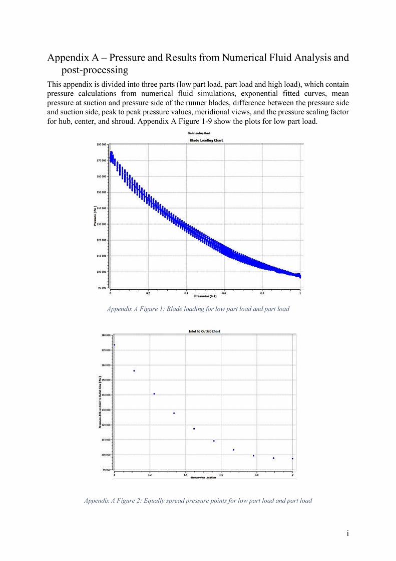
i

Appendix A – Pressure and Results from Numerical Fluid Analysis and post-processing

This appendix is divided into three parts (low part load, part load and high load), which contain pressure calculations from numerical fluid simulations, exponential fitted curves, mean pressure at suction and pressure side of the runner blades, difference between the pressure side and suction side, peak to peak pressure values, meridional views, and the pressure scaling factor for hub, center, and shroud. Appendix A Figure 1-9 show the plots for low part load.

Appendix A Figure 1: Blade loading for low part load and part load

Appendix A Figure 2: Equally spread pressure points for low part load and part load

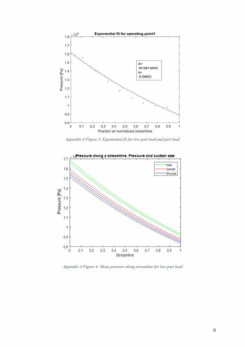
ii

Appendix A Figure 3: Exponential fit for low part load and part load

Appendix A Figure 4: Mean pressure along streamline for low part load

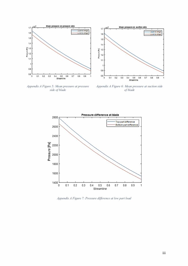
iii

Appendix A Figure 5: Mean pressure at pressure

side of blade

Appendix A Figure 6: Mean pressure at suction side

of blade

Appendix A Figure 7: Pressure difference at low part load

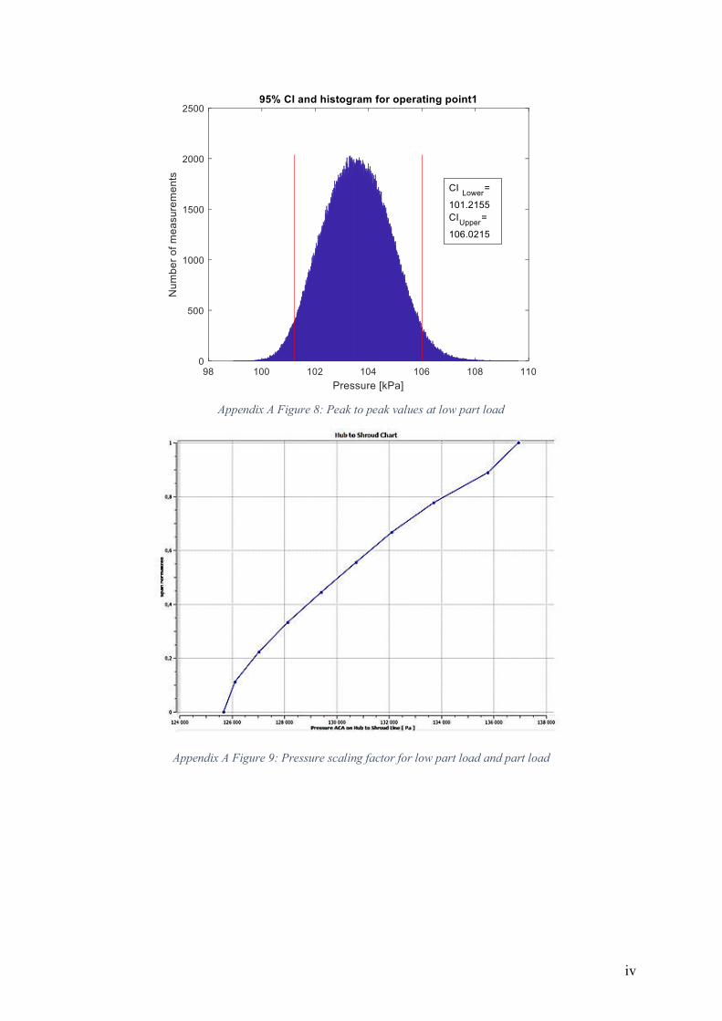
iv

Appendix A Figure 8: Peak to peak values at low part load

Appendix A Figure 9: Pressure scaling factor for low part load and part load

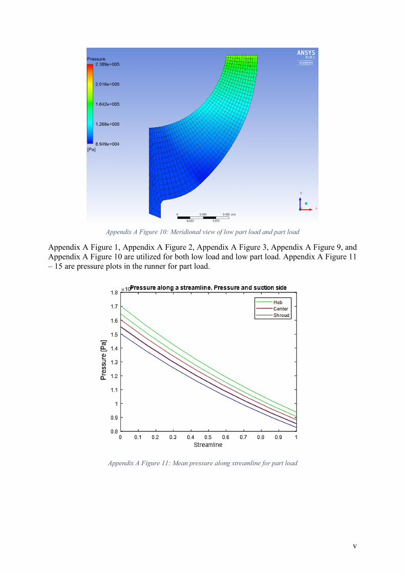
v

Appendix A Figure 10: Meridional view of low part load and part load

Appendix A Figure 1, Appendix A Figure 2, Appendix A Figure 3, Appendix A Figure 9, and Appendix A Figure 10 are utilized for both low load and low part load. Appendix A Figure 11 – 15 are pressure plots in the runner for part load.

Appendix A Figure 11: Mean pressure along streamline for part load

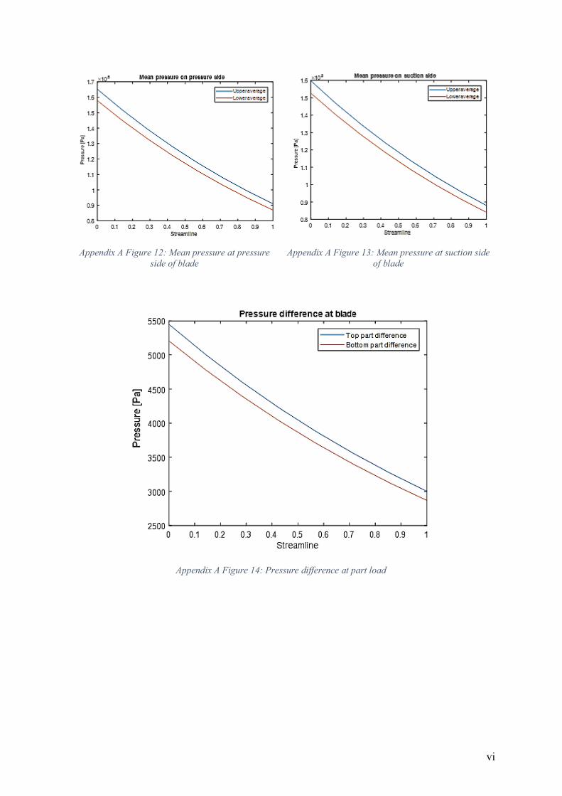
vi

Appendix A Figure 12: Mean pressure at pressure

side of blade

Appendix A Figure 13: Mean pressure at suction side

of blade

Appendix A Figure 14: Pressure difference at part load

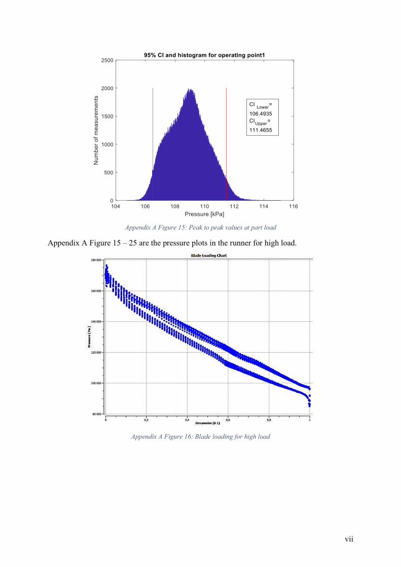
vii

Appendix A Figure 15: Peak to peak values at part load

Appendix A Figure 15 – 25 are the pressure plots in the runner for high load.

Appendix A Figure 16: Blade loading for high load

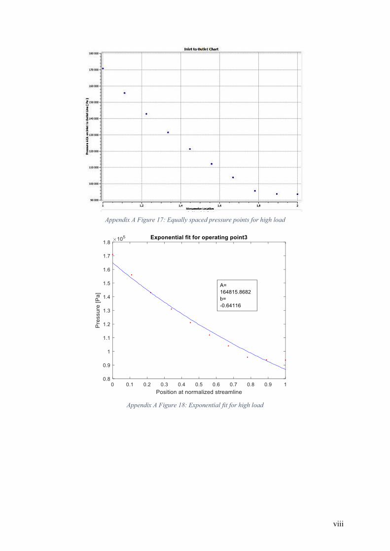
viii

Appendix A Figure 17: Equally spaced pressure points for high load

Appendix A Figure 18: Exponential fit for high load

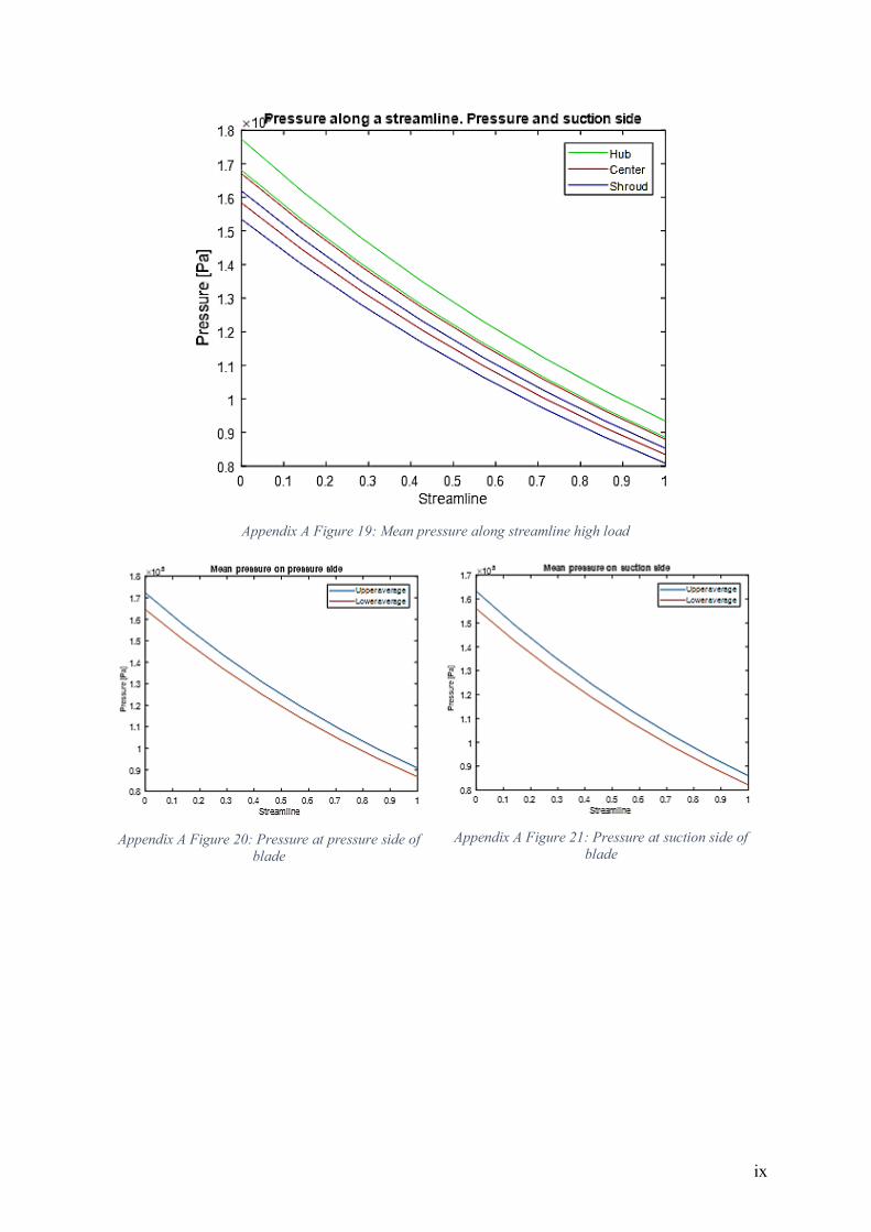
ix

Appendix A Figure 19: Mean pressure along streamline high load

Appendix A Figure 20: Pressure at pressure side of

blade

Appendix A Figure 21: Pressure at suction side of

blade

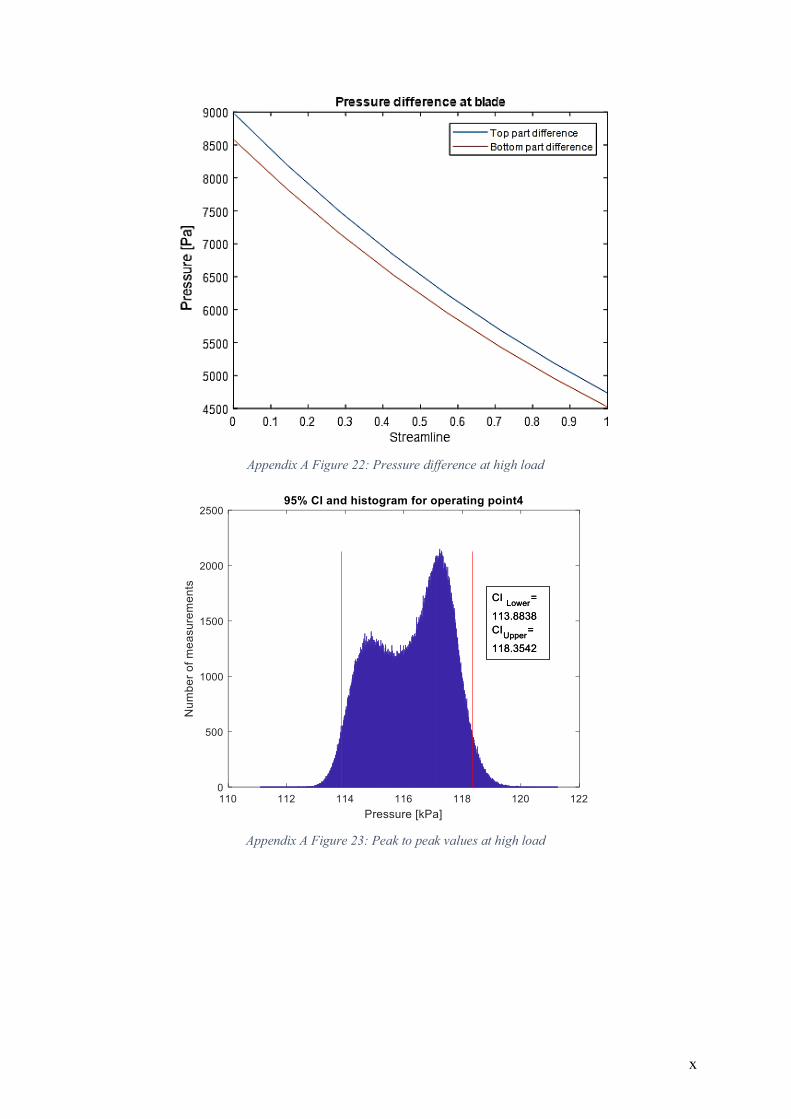
x

Appendix A Figure 22: Pressure difference at high load

Appendix A Figure 23: Peak to peak values at high load

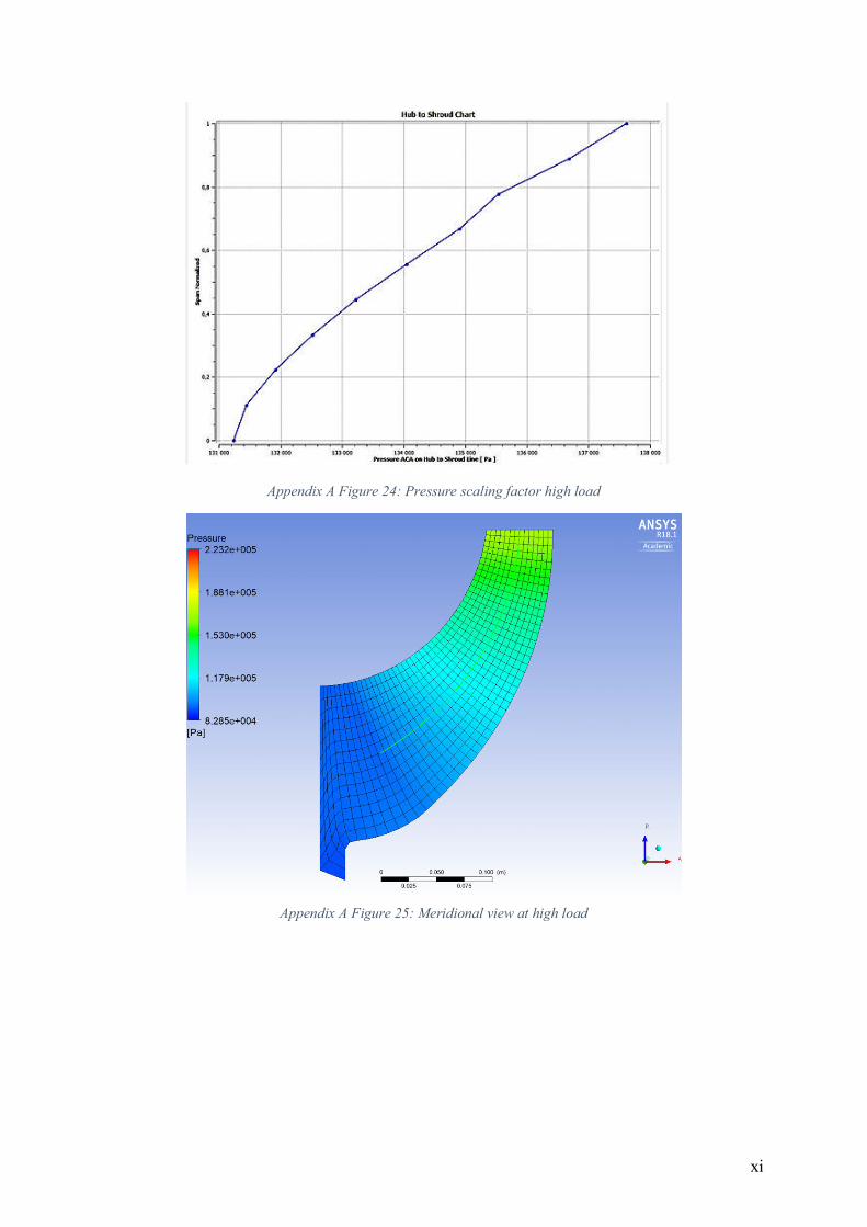
xi

Appendix A Figure 24: Pressure scaling factor high load

Appendix A Figure 25: Meridional view at high load

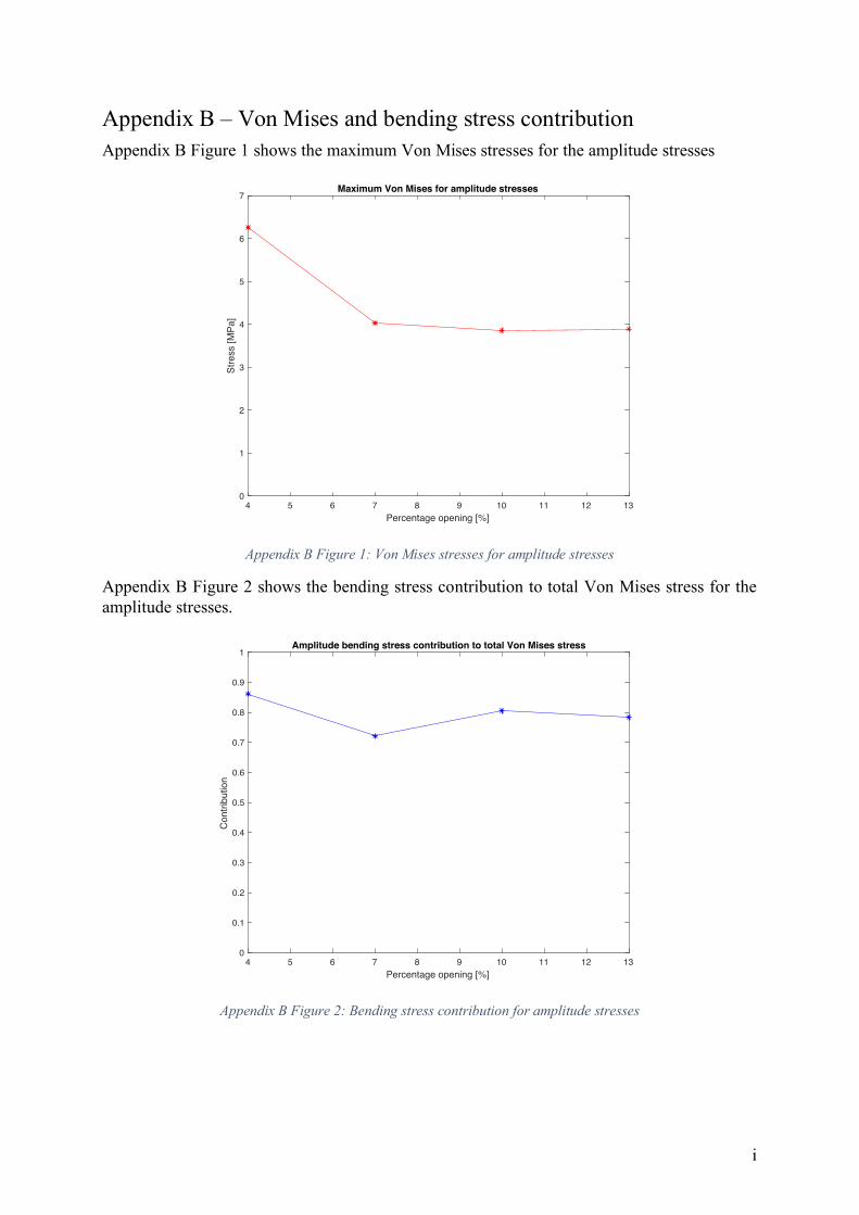
i

Appendix B – Von Mises and bending stress contribution Appendix B Figure 1 shows the maximum Von Mises stresses for the amplitude stresses

Appendix B Figure 1: Von Mises stresses for amplitude stresses

Appendix B Figure 2 shows the bending stress contribution to total Von Mises stress for the amplitude stresses.

Appendix B Figure 2: Bending stress contribution for amplitude stresses

4 5 6 7 8 9 10 11 12 13

Percentage opening [%]

0

1

2

3

4

5

6

7

Str

ess [M

Pa]

Maximum Von Mises for amplitude stresses

4 5 6 7 8 9 10 11 12 13

Percentage opening [%]

0

0.1

0.2

0.3

0.4

0.5

0.6

0.7

0.8

0.9

1

Contr

ibution

Amplitude bending stress contribution to total Von Mises stress

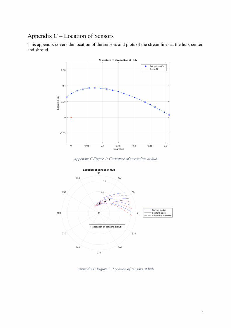
i

Appendix C – Location of Sensors This appendix covers the location of the sensors and plots of the streamlines at the hub, center, and shroud.

Appendix C Figure 1: Curvature of streamline at hub

Appendix C Figure 2: Location of sensors at hub

0 0.05 0.1 0.15 0.2 0.25 0.3

Streamline

-0.05

0

0.05

0.1

0.15

Location [m

]Curvature of streamline at Hub

Points from Khoj

Curve fit

0

30

60

90

120

150

180

210

240

270

300

330

0

0.1

0.2

0.3

Location of sensor at Hub

Runner blades

Splitter blades

Streamline in middle

* is location of sensors at Hub

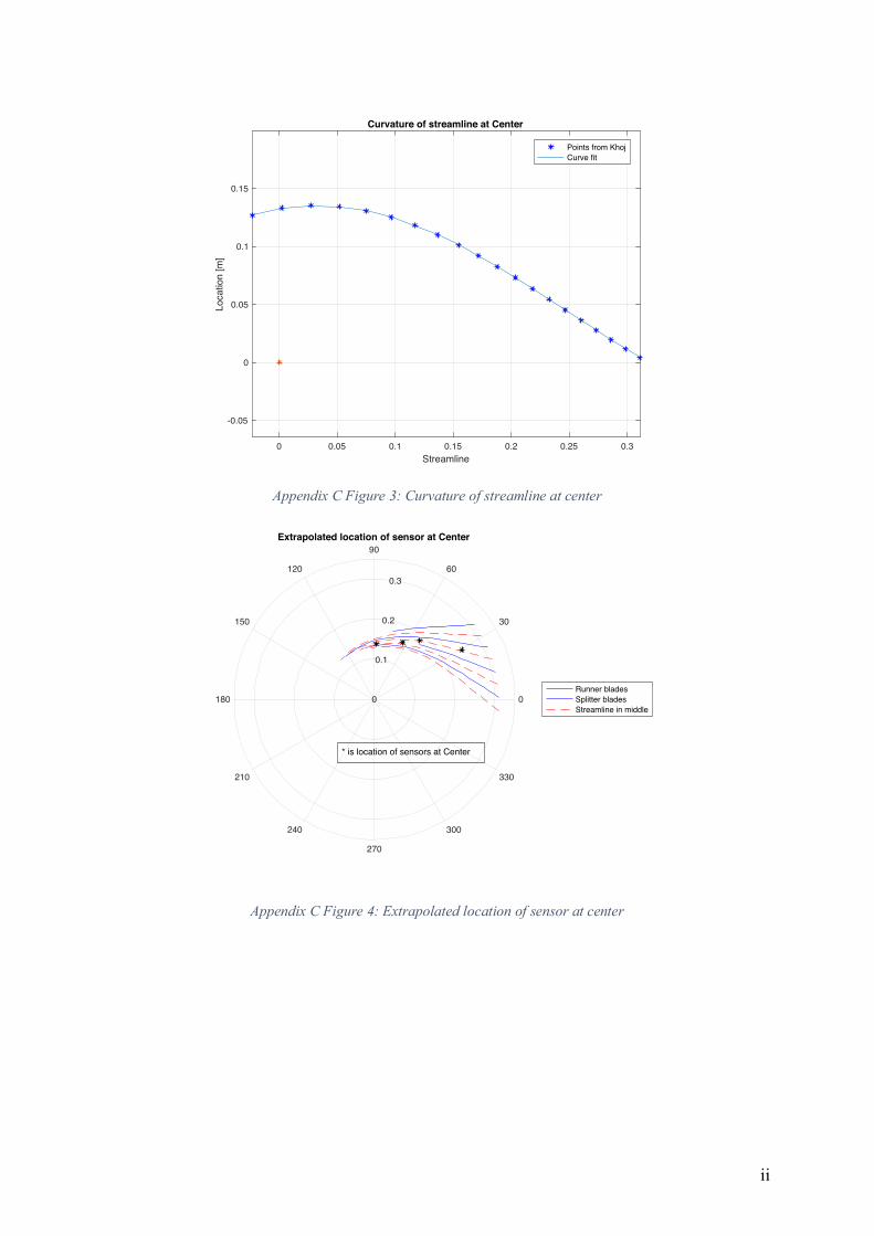
ii

Appendix C Figure 3: Curvature of streamline at center

Appendix C Figure 4: Extrapolated location of sensor at center

0 0.05 0.1 0.15 0.2 0.25 0.3

Streamline

-0.05

0

0.05

0.1

0.15

Location [m

]

Curvature of streamline at Center

Points from Khoj

Curve fit

0

30

60

90

120

150

180

210

240

270

300

330

0

0.1

0.2

0.3

Extrapolated location of sensor at Center

Runner blades

Splitter blades

Streamline in middle

* is location of sensors at Center

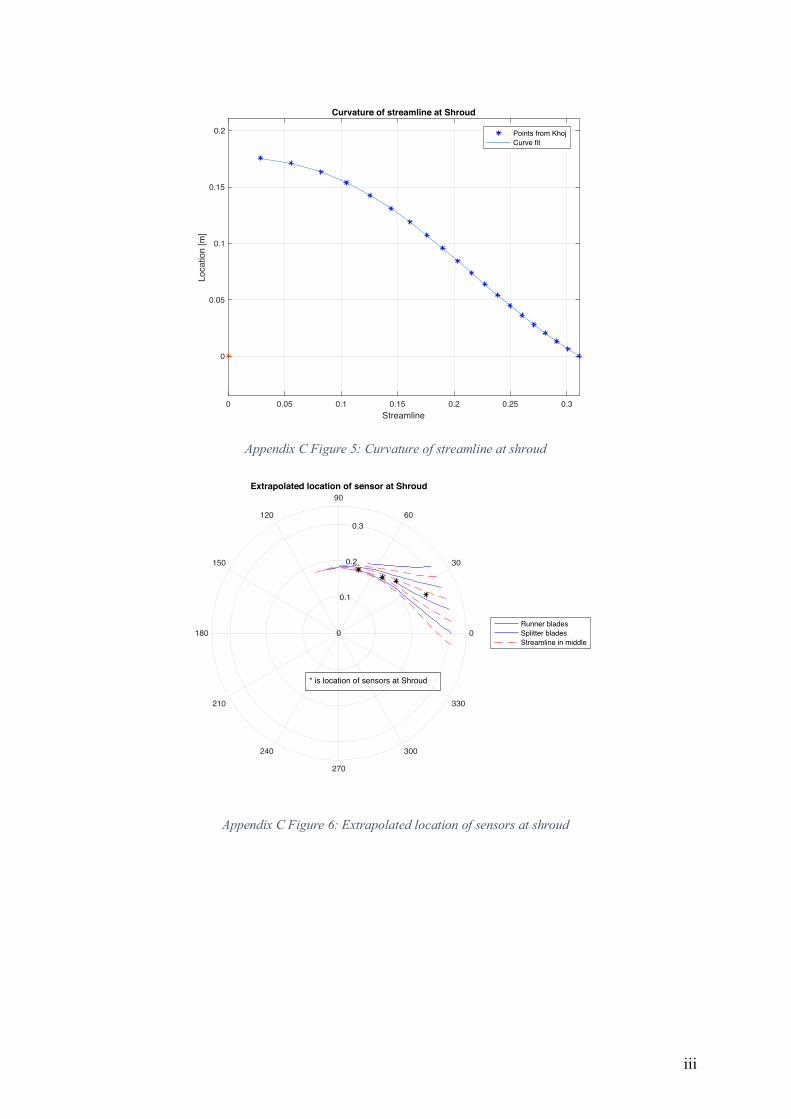
iii

Appendix C Figure 5: Curvature of streamline at shroud

Appendix C Figure 6: Extrapolated location of sensors at shroud

0 0.05 0.1 0.15 0.2 0.25 0.3

Streamline

0

0.05

0.1

0.15

0.2

Location [m

]

Curvature of streamline at Shroud

Points from Khoj

Curve fit

0

30

60

90

120

150

180

210

240

270

300

330

0

0.1

0.2

0.3

Extrapolated location of sensor at Shroud

Runner blades

Splitter blades

Streamline in middle

* is location of sensors at Shroud

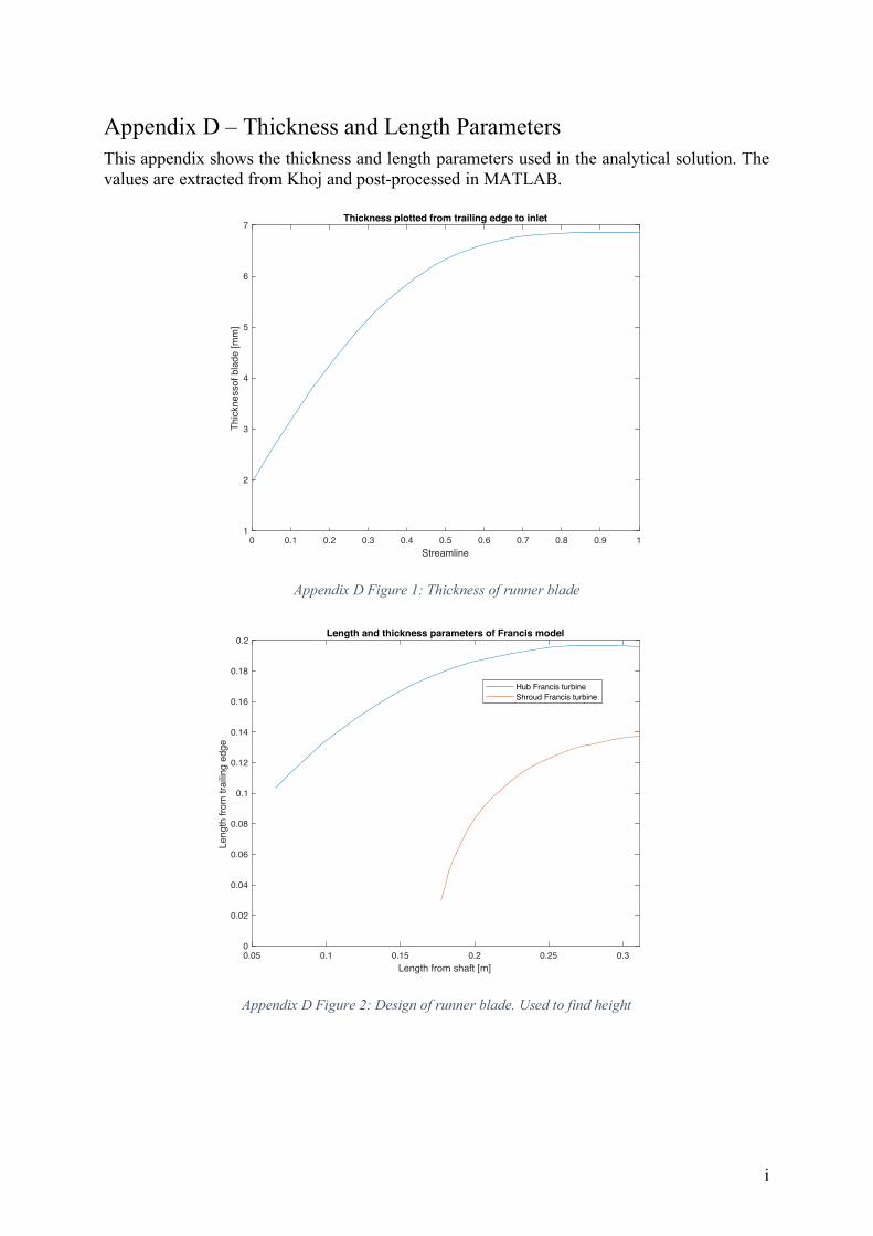
i

Appendix D – Thickness and Length Parameters This appendix shows the thickness and length parameters used in the analytical solution. The values are extracted from Khoj and post-processed in MATLAB.

Appendix D Figure 1: Thickness of runner blade

Appendix D Figure 2: Design of runner blade. Used to find height

0 0.1 0.2 0.3 0.4 0.5 0.6 0.7 0.8 0.9 1

Streamline

1

2

3

4

5

6

7T

hic

knessof bla

de [m

m]

Thickness plotted from trailing edge to inlet

0.05 0.1 0.15 0.2 0.25 0.3

Length from shaft [m]

0

0.02

0.04

0.06

0.08

0.1

0.12

0.14

0.16

0.18

0.2

Length

fro

m tra

iling e

dge

Length and thickness parameters of Francis model

Hub Francis turbine

Shroud Francis turbine

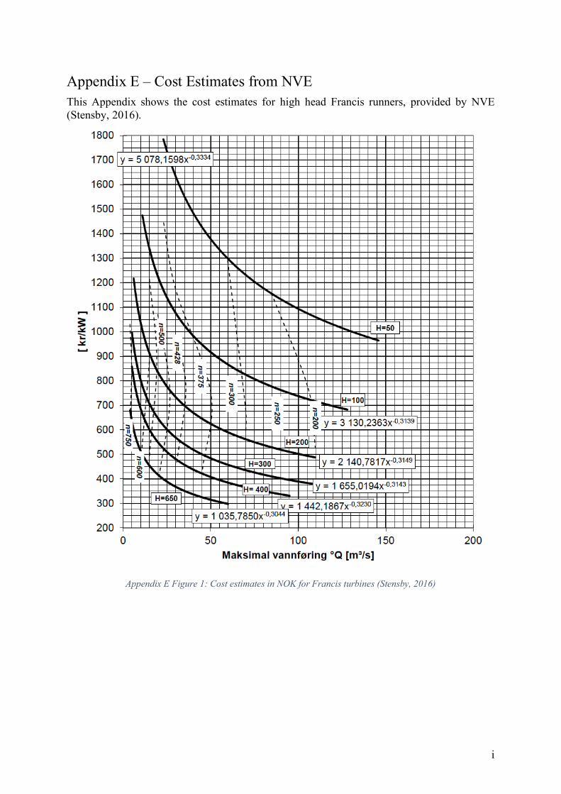
i

Appendix E – Cost Estimates from NVE This Appendix shows the cost estimates for high head Francis runners, provided by NVE (Stensby, 2016).

Appendix E Figure 1: Cost estimates in NOK for Francis turbines (Stensby, 2016)

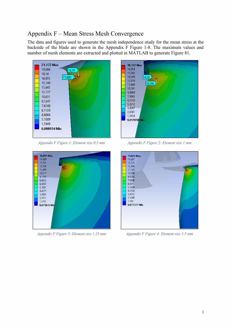
i

Appendix F – Mean Stress Mesh Convergence The data and figures used to generate the mesh independence study for the mean stress at the backside of the blade are shown in the Appendix F Figure 1-8. The maximum values and number of mesh elements are extracted and plotted in MATLAB to generate Figure 81.

Appendix F Figure 1: Element size 0.5 mm

Appendix F Figure 2: Element size 1 mm

Appendix F Figure 3: Element size 1.25 mm

Appendix F Figure 4: Element size 1.5 mm

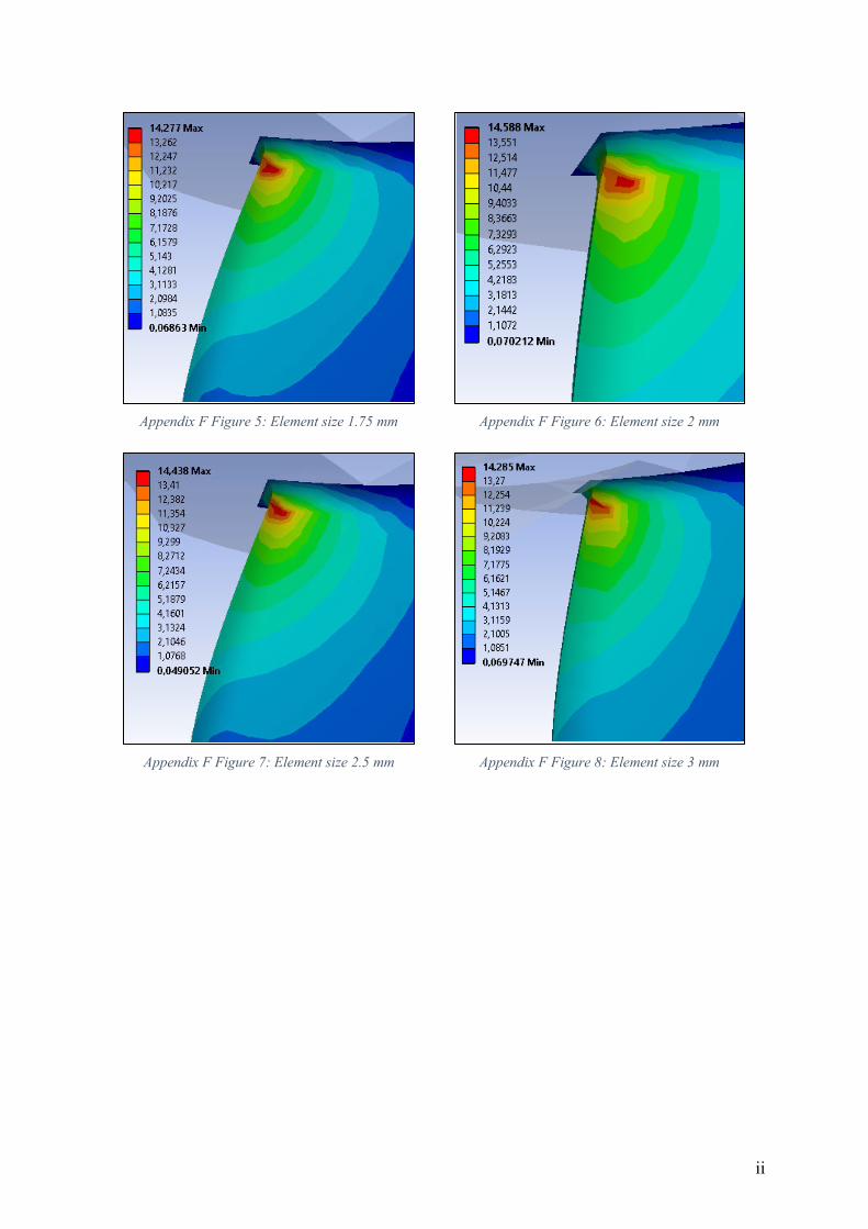
ii

Appendix F Figure 5: Element size 1.75 mm

Appendix F Figure 6: Element size 2 mm

Appendix F Figure 7: Element size 2.5 mm

Appendix F Figure 8: Element size 3 mm

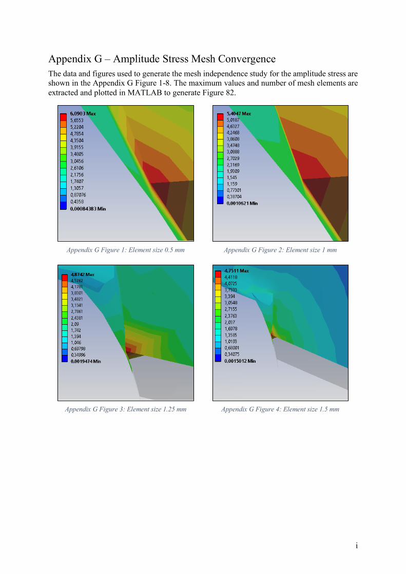
i

Appendix G – Amplitude Stress Mesh Convergence The data and figures used to generate the mesh independence study for the amplitude stress are shown in the Appendix G Figure 1-8. The maximum values and number of mesh elements are extracted and plotted in MATLAB to generate Figure 82.

Appendix G Figure 1: Element size 0.5 mm

Appendix G Figure 2: Element size 1 mm

Appendix G Figure 3: Element size 1.25 mm

Appendix G Figure 4: Element size 1.5 mm

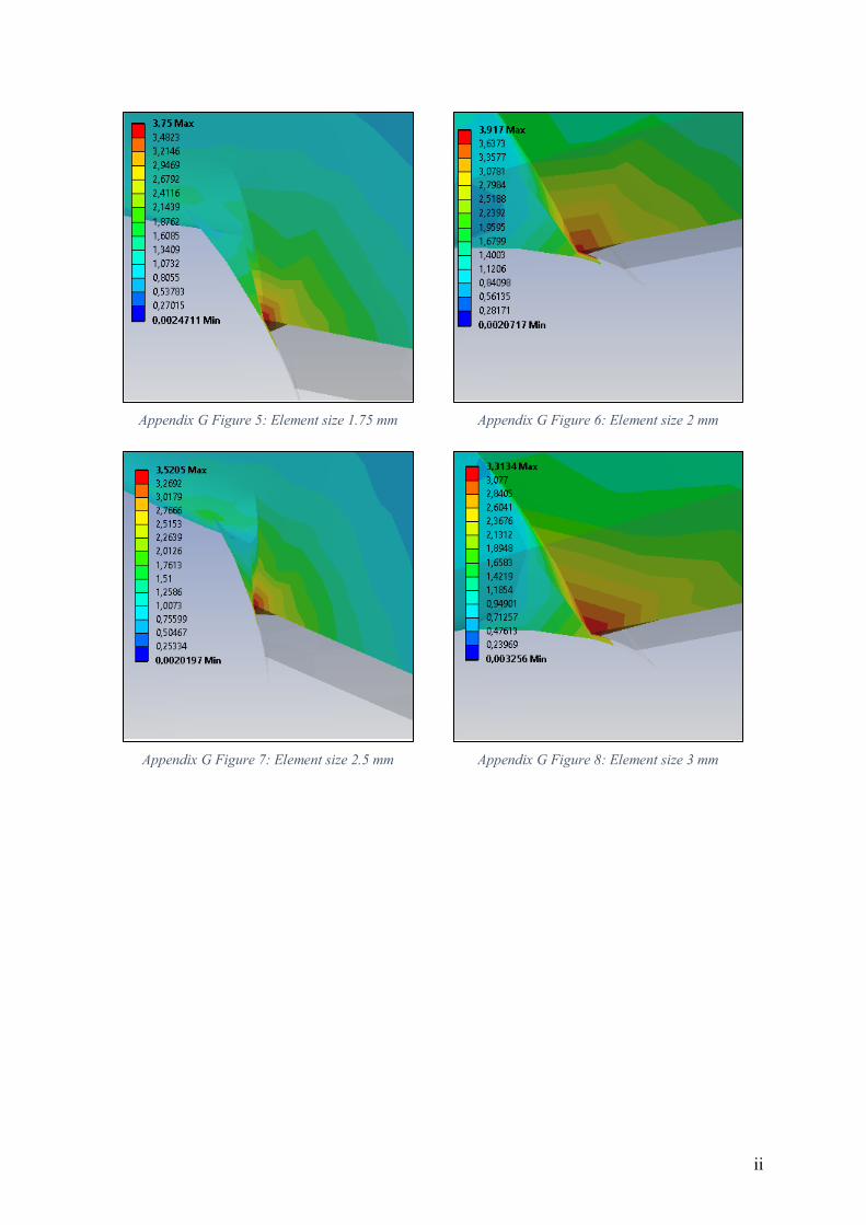
ii

Appendix G Figure 5: Element size 1.75 mm

Appendix G Figure 6: Element size 2 mm

Appendix G Figure 7: Element size 2.5 mm

Appendix G Figure 8: Element size 3 mm

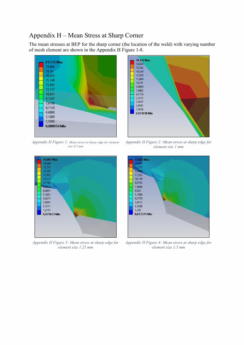
Appendix H – Mean Stress at Sharp Corner The mean stresses at BEP for the sharp corner (the location of the weld) with varying number of mesh element are shown in the Appendix H Figure 1-8.

Appendix H Figure 1: Mean stress at sharp edge for element

size 0.5 mm

Appendix H Figure 2: Mean stress at sharp edge for

element size 1 mm

Appendix H Figure 3: Mean stress at sharp edge for

element size 1.25 mm

Appendix H Figure 4: Mean stress at sharp edge for

element size 1.5 mm

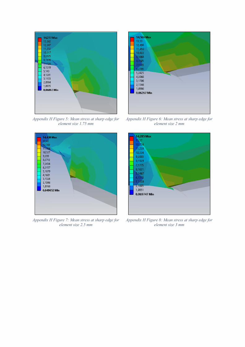
Appendix H Figure 5: Mean stress at sharp edge for

element size 1.75 mm

Appendix H Figure 6: Mean stress at sharp edge for

element size 2 mm

Appendix H Figure 7: Mean stress at sharp edge for

element size 2.5 mm

Appendix H Figure 8: Mean stress at sharp edge for

element size 3 mm

i

Appendix I – Mesh Quality The mesh quality with 2 mm element size is shown in Appendix I Figure 1. The x-axis defines the mesh quality. Mesh elements with quality equal to one are the best fitting elements.

Appendix I Figure 1: Mesh Quality

i

Appendix J – MATLAB Code This appendix contains all the MATLAB codes and functions. In addition, it presents a short overview on how to update the codes to be valid for new turbines.

To update the code, the following parameters are required:

1. A pressure measurement a. The location of the sensor b. Pressure measurements over a relevant time period, e.g., 60seconds. c. The average rotational speed d. The dimensionless flow e. The Head

2. That pressure measurement must be stored as: 𝑜𝑃 = [𝑃𝑟𝑒𝑠𝑠𝑢𝑟𝑒, 𝑅𝑃𝑀, 𝑄M> , 𝐻] In this particular case, it is stored as: 𝑜𝑃 = [𝑚𝑒𝑎𝑛�𝑑𝑎𝑡𝑎𝑠𝑒𝑡. 𝑝𝑟𝑒𝑠𝑠𝑢𝑟𝑒(𝑛𝑢𝑚𝑏𝑒𝑟, : )£, 𝑑𝑎𝑡𝑎𝑠𝑒𝑡. 𝑅𝑃𝑀(1, 𝑛𝑢𝑚𝑏𝑒𝑟), 𝑑𝑎𝑡𝑎𝑠𝑒𝑡. 𝑄𝑒𝑑(𝑛𝑢𝑚𝑏𝑒𝑟), 𝑑𝑎𝑡𝑎𝑠𝑒𝑡. ℎ𝑒𝑎𝑑(1, 𝑛𝑢𝑚𝑏𝑒𝑟)]

3. Solve the MATLAB function trykkblad with sensor location and the stored measurement. That gives the pressure at the pressure and suction side of the blade at the location of the sensor.

4. Change the function ansysP, and parameter P_calc to the output of step 3. That will call the function expfit to exponentially fit the pressure at suction and pressure side from step 3.

5. Export the pressure plots from MATLAB to ANSYS and solve a mechanical model. 6. Export the resulting Von Mises stresses from ANSYS to MATLAB. 7. Update the smean and f variables in the MATLAB function lifetime. 8. Select your operating patterns through the function lifetime.

For examples 25% at low part load, part load, BEP, and high load with 1 startup per day is expressed as: [D, D¾¿¾ÀÁ] = lifetime(0.25,0.25,0.25,0.25,1)

Below are all the MATLAB functions and scripts utilized in this thesis and required to reproduce the results obtained in this thesis.

Exponential fit function function [A,b]=expfit(operatingpoint) %Generic matlab function to exponentially fit streamlines for low load, %BEP, and high load. Operating point 1 is low load, 2 is BEP, and %3 high load. The initial parameters are based on the CFX analyses. %[A,b]=expfit(operatingpoint) will return the exponent b %(slope of the curve) and the scaling parameter A, and a plot of the %exponential fit. y9_84 = [1.68E+05,1.54E+05,1.42E+05,1.32E+05,1.23E+05,1.15E+05,... 1.08E+05,101000,9.97E+04,9.96E+04]; %Pessure extracted from CFX - BEP str9_84 = [1.00E+00,1.11E+00,1.22E+00,1.34E+00,1.45E+00,1.56E+00, ... 1.67E+00,1.78E+00,1.89E+00,2.00E+00]-1; %Streamline location y3_91 = [173486.5,1.56E+05,1.41E+05,1.28E+05,1.17E+05,1.09E+05, ... 1.03E+05,9.94E+04,9.78E+04,9.74E+04]; %Pressure extracted from CFX - low part load and part load str3_91 = [1.00,1.11,1.22,1.34,1.45,1.56,1.67,1.78,1.89,2.00]-1; %Streamline location y12_43 = [1.71E+05,1.56E+05,1.43E+05,1.31E+05,1.21E+05,1.12E+05, ... 1.04E+05,9.57E+04,9.38E+04,9.36E+04]; %Pressure extracted from CFX - High load str12_43 = [1, 1.11, 1.22, 1.34, 1.45, 1.56, 1.67, 1.78, 1.89, 2]-1; %Streamline location y = []; y(1,:) = y3_91; y(2,:) = y9_84;

ii

y(3,:) = y12_43; %Pressure matrix x = []; x(1,:) = str3_91; x(2,:) = str9_84; x(3,:) = str12_43; %Streamline matrix M = [ones(length(x(operatingpoint,:)),1),x(operatingpoint,:)']; % Ensures that x is a column vector lny = log(y(operatingpoint,:)); % Ensure that y is a column vector and takes the logarithm of the column lny = lny'; X = M\lny; % Solve for parameters A = exp(X(1)); % Solve for A b = X(2); % Solve for b xval = linspace(min(x(operatingpoint,:)),... max(x(operatingpoint,:))); yval = A*exp(b*xval); figure(); plot(x(operatingpoint,:),y(operatingpoint,:),'r.',xval,yval,'b'); title(['Exponential fit for operating point',num2str(operatingpoint)]) ylabel('Pressure [Pa]') xlabel('Position at normalized streamline') dim = [.6 .5 .3 .2]; str= {'A=',num2str(A), 'b=',num2str(b)}; annotation('textbox',dim,'String',str,'FitBoxToText','on') end

Pressure at blades function [P,P_pside, P_sside, delta]=trykkblad(sensor,loc,oP) %This function is used to find the pressure at pressure side and suction %side of the runner blades. %Sensors are 1,2,3,4 respectively R1 R2 R3 R4. Loc: 1(hub) 2 (center) %3 (shroud). The operation point (oP) is the data struct hillChart. %The following oPs are utilized in this report: %low part load - 56 - 4% %oP=[mean(hillChart.PTR1(56,:)),hillChart.RPM(1,56),hillChart.Qed(56),... % hillChart.Head(1,56)] %Part load - 133 - 7% %oP=[mean(hillChart.PTR1(133,:)),hillChart.RPM(1,133),hillChart.Qed(133),.. % hillChart.Head(1,133)] %BEP 175 - 10.02% %oP=[mean(hillChart.PTR1(175,:)),hillChart.RPM(1,175),hillChart.Qed(175),.. % hillChart.Head(1,175)] %Max load 259 - 13% %oP=[mean(hillChart.PTR1(259,:)),hillChart.RPM(1,259),hillChart.Qed(259),.. % hillChart.Head(1,259)] D1=0.63; D2=0.349; B1=0.06; beta_1=69; rho=998; %Design and fluid parameters. P=oP(1)*10^3; rpm=oP(2); Qed=oP(3); H=oP(4); Q = Qed*(D2^2)*sqrt(H*9.82146516); omega = pi*rpm/30; u1 = omega*(D1/2); cm1 = Q/(3.14*D1*B1); cm2 = cm1*1.1; cu1 = u1-cm1/(tand(beta_1)); w1 = sqrt((u1-cu1)^2+cm1^2); %Velocity parameters if loc == 2 && sensor==1 P=P*130/138; elseif loc==3 && sensor == 1 P=P*126/138; elseif loc == 2 && sensor == 2 P=P*104/113; elseif loc==3 && sensor == 2 P=P*97/113; elseif loc==2 && sensor== 3 P=P*97.6/104.5; elseif loc==3 && sensor == 3 P=P*97/104.5; elseif loc==2 && sensor == 4 P=P*97.100/99.150; elseif loc==3 && sensor == 4 P=P*97.100/99.150; end %Pressure adjustment of sensors to take into account difference inlet %pressure at hub, center, and shroud. Based on CFX data X_hub = [1.585 1.51 1.434 1.356 1.277 1.195 1.113 1.028 0.9425 0.8537...

iii

0.7634 0.6715 0.5778 0.4823 0.3852 0.2894 0.1907 0.09639 ... 0.008712 -0.07069]./5.1; Y_hub = [0.03907 0.08165 0.124 0.1659 0.2071 0.2474 0.2857 0.3225 .... 0.3567 0.3885 0.4167 0.4405 0.4592 0.4717 0.4766 0.4725 0.4572 ... 0.4292 0.3874 0.3293]./5.1; X_shroud = [1.585,1.535,1.484,1.433,1.381,1.328,1.273, 1.217,1.159,... 1.099,1.036,0.9684,0.897,0.8195,0.735,0.6411,0.533,... 0.4172,0.284,0.145]./5.1; Y_shroud = [0,0.033,0.067,0.104,0.143,0.185,0.229,0.276,0.326,0.377... ,0.431,0.4889,0.548 ,0.607,0.668,0.727,0.785,0.833,... 0.873,0.896]./5.1; X_center = [1.585,1.522,1.458,1.393,1.326,1.257,1.187,1.114,1.038,... 0.959,0.875,0.789,0.696,0.597,0.492,0.382,0.264,... 0.139,0.012,-0.118]./5.1; Y_center = [0.021,0.06,0.1,0.142,0.186,0.231,0.277,0.324,0.373,... 0.421,0.4697, 0.516,0.561,0.603,0.639,0.667,0.685,0.69,... 0.679,0.647]./5.1; %Streamline locations at hub, center and shroud %Relative velocity and curvature. Curvature is found from the generic %matlab function LineCurvature w_hub = [1.17 1.3455 1.41 1.449 1]; %Relative velocity at hub Vert_hub(:,1)=X_hub; Vert_hub(:,2)=Y_hub; temp=LineCurvature2D(Vert_hub); %Radius of the curvature at the hub. Linecurvature2D is a generic matlab %function found online at mathworks. k_hub=1./temp; %Curvature at hub w_center = [1.384 1.978 2.196 2.35 1]; %Relative velocity at center Vert_center(:,1)=X_center; Vert_center(:,2)=Y_center; temp=LineCurvature2D(Vert_center); %Radius of the curvature at center k_center=1./temp; %Curvature of center w_shroud = [1.55 2.4 2.72 3 1]; %Relative velocity at the shroud Vert_shroud(:,1)=X_shroud; Vert_shroud(:,2)=Y_shroud; temp=LineCurvature2D(Vert_shroud); %Radius of the curvature at shroud k_shroud=1./temp; %Curvature at the shroud w=[]; w(:,1)=w_hub; w(:,2)=w_center; w(:,3)=w_shroud; %Relative velocity matrix k=[]; k(:,1)=k_hub([6 12 15 18 1]); k(:,2)=k_center([6 12 15 18 1]); k(:,3)=k_shroud([6 12 15 18 1]); %Relevant curvature at the location of the sensors. %Radial position of sensors (R1, R2, R3,and R4) r = [0.24042 0.15734 0.12164 0.08695 0.2965; 0.2506 0.1849 0.1581 ... 0.1380 0.3108; 0.2629 0.2127 0.1947 0.1827 0.301]; %Radius locations extracted from Khoj r=r'; %Transposed locations %Delta n. The length between the sensors and their respective suction and %pressure sides. Obtained from Khoj. delta_n=[((33.21-26.4)*pi/180)*0.24042, ((57.26-50.48)*pi/180)*0.15734,... ((68.36-58.51)*pi/180)*0.12164,((91.36-83)*pi/180)*0.08695,... ((25.41-16.94)*pi/180)*0.2965; ((31.98-25.14)*pi/180)*0.2506, 0.0194, 0.0242,... ((92-88.99)*pi/180)*0.1380,((24.76-15.92)*pi/180)*0.3108;... ((28.15-22.2)*pi/180)*0.2629, 0.0217,0.0214,0.0095,... ((24-13.23)*pi/180)*0.301]./2; delta_n=delta_n'; %Rothalpy relations. dwdn = -2*omega - (w1*w(sensor,loc))/k(sensor,loc); %Velocity perpendicular to the streamline w_pressure = w1*w(sensor,loc)+delta_n(sensor,loc)*dwdn; %Velocity at pressure side w_suction = w1*w(sensor,loc)-delta_n(sensor,loc)*dwdn; %velocity at suction side I =P/rho+((w1*w(1,1))^2)/2-((omega*r(sensor,loc))^2)/2; %Rothaply - values is 65.7529 for BEP P_pside=(I-(w_pressure^2)/2+((omega*r(sensor,loc))^2)/2)*rho; %I is constant along and perpendicular to a streamline

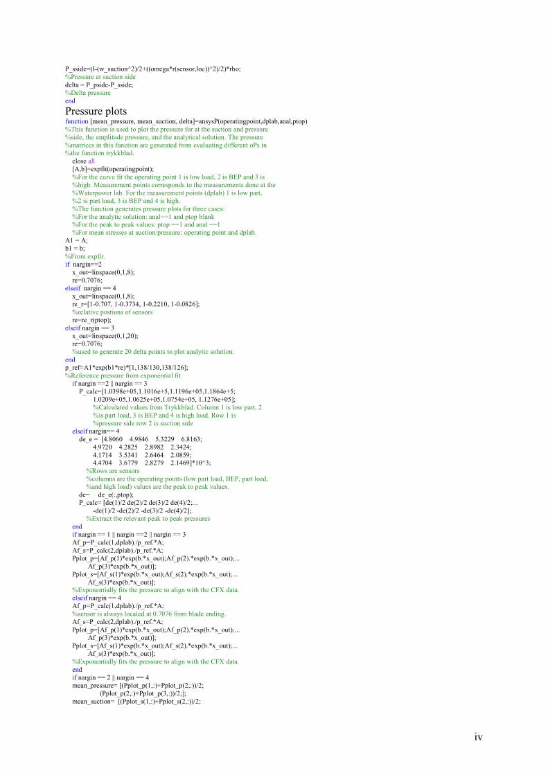
iv

P_sside=(I-(w_suction^2)/2+((omega*r(sensor,loc))^2)/2)*rho; %Pressure at suction side delta = P_pside-P_sside; %Delta pressure end

Pressure plots function [mean_pressure, mean_suction, delta]=ansysP(operatingpoint,dplab,anal,ptop) %This function is used to plot the pressure for at the suction and pressure %side, the amplitude pressure, and the analytical solution. The pressure %matrices in this function are generated from evaluating different oPs in %the function trykkblad. close all [A,b]=expfit(operatingpoint); %For the curve fit the operating point 1 is low load, 2 is BEP and 3 is %high. Measurement points corresponds to the measurements done at the %Waterpower lab. For the measurement points (dplab) 1 is low part, %2 is part load, 3 is BEP and 4 is high. %The function generates pressure plots for three cases: %For the analytic solution: anal==1 and ptop blank %For the peak to peak values: ptop ==1 and anal ==1 %For mean stresses at suction/pressure: operating point and dplab. A1 = A; b1 = b; %From expfit. if nargin==2 x_out=linspace(0,1,8); re=0.7076; elseif nargin == 4 x_out=linspace(0,1,8); re_r=[1-0.707, 1-0.3734, 1-0.2210, 1-0.0826]; %relative postions of sensors re=re_r(ptop); elseif nargin == 3 x_out=linspace(0,1,20); re=0.7076; %used to generate 20 delta points to plot analytic solution. end p_ref=A1*exp(b1*re)*[1,138/130,138/126]; %Reference pressure from exponential fit if nargin ==2 || nargin == 3 P_calc=[1.0398e+05,1.1016e+5,1.1196e+05,1.1864e+5; 1.0209e+05,1.0625e+05,1.0754e+05, 1.1276e+05]; %Calculated values from Trykkblad. Column 1 is low part, 2 %is part load, 3 is BEP and 4 is high load. Row 1 is %pressure side row 2 is suction side elseif nargin== 4 de_e = [4.8060 4.9846 5.3229 6.8163; 4.9720 4.2825 2.8982 2.3424; 4.1714 3.5341 2.6464 2.0859; 4.4704 3.6779 2.8279 2.1469]*10^3; %Rows are sensors %columns are the operating points (low part load, BEP, part load, %and high load) values are the peak to peak values. de= de_e(:,ptop); P_calc= [de(1)/2 de(2)/2 de(3)/2 de(4)/2;... -de(1)/2 -de(2)/2 -de(3)/2 -de(4)/2]; %Extract the relevant peak to peak pressures end if nargin == 1 || nargin ==2 || nargin == 3 Af_p=P_calc(1,dplab)./p_ref.*A; Af_s=P_calc(2,dplab)./p_ref.*A; Pplot_p=[Af_p(1)*exp(b.*x_out);Af_p(2).*exp(b.*x_out);... Af_p(3)*exp(b.*x_out)]; Pplot_s=[Af_s(1)*exp(b.*x_out);Af_s(2).*exp(b.*x_out);... Af_s(3)*exp(b.*x_out)]; %Exponentially fits the pressure to align with the CFX data. elseif nargin == 4 Af_p=P_calc(1,dplab)./p_ref.*A; %sensor is always located at 0.7076 from blade ending. Af_s=P_calc(2,dplab)./p_ref.*A; Pplot_p=[Af_p(1)*exp(b.*x_out);Af_p(2).*exp(b.*x_out);... Af_p(3)*exp(b.*x_out)]; Pplot_s=[Af_s(1)*exp(b.*x_out);Af_s(2).*exp(b.*x_out);... Af_s(3)*exp(b.*x_out)]; %Exponentially fits the pressure to align with the CFX data. end if nargin == 2 || nargin == 4 mean_pressure= [(Pplot_p(1,:)+Pplot_p(2,:))/2; (Pplot_p(2,:)+Pplot_p(3,:))/2;]; mean_suction= [(Pplot_s(1,:)+Pplot_s(2,:))/2;

v

(Pplot_s(2,:)+Pplot_s(3,:))/2]; %Calculated values to be used as input parameters in ANSYS end if nargin == 2 figure() plot(x_out,Pplot_p(1,:),'g',x_out,Pplot_p(2,:),'r',x_out,Pplot_p(3,:),'b') hold on plot(x_out,Pplot_s(1,:),'g',x_out,Pplot_s(2,:),'r',x_out,Pplot_s(3,:),'b') legend('Hub','Center','Shroud') title('Pressure at pressure and suction side') xlabel('Streamline') ylabel('Pressure [Pa]') figure() plot(x_out,mean_pressure(1,:),x_out,mean_pressure(2,:)); legend('Upper average','Lower average') title('Mean pressure on pressure side') xlabel('Streamline') ylabel('Pressure [Pa]') figure() plot(x_out,mean_suction(1,:),x_out,mean_suction(2,:)); legend('Upper average','Lower average') title('Mean pressure on suction side') xlabel('Streamline') ylabel('Pascal [Pa]') end if nargin == 2 || nargin == 4 deltaa=[(mean_pressure(1,:)-mean_suction(1,:));... (mean_pressure(2,:)-mean_suction(2,:))]; figure() plot(x_out, deltaa(1,:),x_out, deltaa(2,:)); title('Pressure difference at blade') legend('Top part difference','Bottom part difference') xlabel('Streamline') ylabel('Pressure [Pa]') elseif nargin ==3 mean_suction = [(Pplot_s(1,:)+Pplot_s(2,:)+Pplot_s(3,:))]./3; mean_pressure =[(Pplot_p(1,:)+Pplot_p(2,:)+Pplot_p(3,:))]./3; delta=[mean_pressure(:)-mean_suction(:)]; %Same as explained above. figure() plot(x_out, delta); title('Pressure difference between pressure and suction side') legend('Delta') xlabel('Streamline') ylabel('Pressure [Pa]') end end

Histogram and confidence intervals function [lower,upper,delta] = cpf(dataset,level,plotting,measurementpoint) %Function used to generate confidence intervals and histograms. %Confidence level can be set from 0.95 to 0.99. %Plotting is a toggle off/on setting. plotting==1 will plot the diagrams. %Measurement point is a graphical parameter, which will adjust the title %of the histogram. The following values from hillChart correspond to their %respective operating points: %56 = low part load = measurement point 1 %133 = Part load = measurement point 2 %175 = BEP = measurement point 3 %259 = high load = measurement point 4 %Example of a histogram for BEP[a,b,d]=cpf(hillChart.PTR1(175,:),0.95,1,3) [N,e] = histcounts(dataset,1000); Me = mean(dataset); NumberOfPoints = sum(N); temp = 0; for i = 1:length(N) temp = temp+N(i); value = temp/NumberOfPoints; if value >= (1-level)/2 lower = e(i); break; end end temp=0; for j = 1:length(N) temp = temp+N(j); value = temp/NumberOfPoints; if value >= level+(1-level)/2 upper = e(j); break; end

vi

end if plotting == 1 time = [0:1/10240:60-1/10240]; figure(1) plot(time,dataset,'b') hold on plot([0, 60-1/10240],[lower, lower],'r') plot([0, 60-1/10240],[upper, upper],'r') hold off figure(2) hist(dataset,1000) hold on plot([lower, lower],[0, max(N)],'r') plot([upper, upper], [0, max(N)],'r') hold off xlabel('Pressure [kPa]') ylabel('Number of measurements') if nargin == 4 title(['95% CI and histogram for operating point',num2str(measurementpoint)]) else title('95% CI and histogram') end dim = [.7 .5 .3 .2]; str= {'CI _{Lower}=',num2str(lower), 'CI_{Upper}=',num2str(upper)}; annotation('textbox',dim,'String',str,'FitBoxToText','on') end delta=upper-lower; end

Analytical solution function [sigma]=stress(operatingpoint,dplab) %This function is used to solve the analytical solution. It has extracted %values from Khoj, which can be found in appendix C and D. x_norm = linspace(0,1,20); ts = [[0.336 0.528];[0.387 0.577];[0.439 0.626];[0.495 0.673];... [0.554 0.719];[0.612 0.761];[0.675 0.799];[0.738 0.836];... [0.803 0.869];[0.869 0.897];[0.938 0.924];[1.008 0.946];... [1.078 0.964];[1.149 0.978];[1.220 0.989];[1.293 0.997];... [1.366 1.002];[1.439 1.003];[1.512 1.002];[1.585 0.999]]; %Top side location extracted from Khoj bs = [[0.903 0.152];[0.919 0.204];[0.932 0.247];[0.947 0.287];... [0.974 0.349];[0.996 0.389];[1.021 0.426];[1.048 0.461];... [1.078 0.494];[1.111 0.525];[1.164 0.566];[1.202 0.589];... [1.241 0.611];[1.302 0.638];[1.341 0.652];[1.387 0.665];... [1.430 0.676];[1.496 0.689];[1.541 0.695];[1.585 0.700]]; %Bottom side locations extracted from Khoj. b = sqrt(((ts(:,1)./5.1)-(bs(:,1)./5.1)).^2 +... ((ts(:,2)./5.1)-(bs(:,2)./5.1)).^2); %Height of blade form Pythagoras. t_vector = [[1 17.500];[0.947 17.499];[0.895 17.496];[0.842 17.482];... [0.789 17.446];[0.737 17.374];[0.684 17.248];[0.632 17.052];... [0.579 16.766];[0.526 16.374];[0.474 15.859];[0.421 15.209];... [0.368 14.412];[0.316 13.463];[0.263 12.361];[0.211 11.111];... [0.158 9.725];[0.105 8.224];[0.053 6.636];[0 5]]./5.1; %Thickness vector. x = t_vector(:,1)*5.1; x = x'; t = t_vector(:,2)*2*10^-3; t = t'; [mp,ms,delta]=ansysP(operatingpoint,dplab,1); %Generate reference pressure m = mp; %Pressure at pressure side delta_p = delta; %Delta pressure sigma = []; for i=1:length(b); sigma(i)=((2.*b(i).^2).*delta_p(i))./(t(i).^2).*10^-6; %Finds the different stresses at various operating patterns. end plot(x_norm,sigma) xlabel('Streamline') ylabel('Stress [MPa]') end

Damage and lifetime model function [D,D_all]=lifetime(lpl,pl,bep,hl,start) %This function is used to find the damage of the different operating cases %and to find how many days 1 startup is equivalent to in operations. N1 = linspace(10,10^7,10000); %LCF cycles

vii

N2 = linspace(10^7,10^12,10000); %HCF cycles k1 = 10.97; k2 = 13.62; m1 = 3; m2 = 5; %Parameters used for the S-N curves from ISO 19902 s1 = -1*(log10(N1)-k1)/m1; s2 = 10.^s1; s12 = -1*(log10(N2)-k2)/m2; s22 = 10.^s12; %Stresses N3 = [N1 N2]; s2t = [s2 s22]; %Cycle and amplitude stress vectors. %Damage model smean = [17.62 14.92 14.65 16.50]*10^6; %Mean stress from ansys f = [340 337.3 333.5 335]/60; %Frequency from measurements. samp = [6.26 4.03 3.86 3.89]*10^6; %Amplitude stress from ansys gv = 28; %Number of guide vanes flpl = f(1)/3.6+f(1)*gv; fpl = f(2)/3.6+f(2)*gv; fbep = f(3)*gv; fhl = f(4)*gv; %Excitation frequnecies ys = 661*10^6; %Yield strength from Huth UTS = 910*10^6; %Utimate tensile strength from Huth sef = [samp.*(UTS./(UTS-smean)).*10^-6]; %Goodman correlation seff = [sef sef(3)*3]; %Goodman correlation and startup i1 = find(((s2t>(seff(1)-0.025)) & (s2t<(seff(1)+0.025)))); i2 = find(((s2t>(seff(2)-0.0025)) & (s2t<(seff(2)+0.0025)))); i3 = find(((s2t>(seff(3)-0.0025)) & (s2t<(seff(3)+0.0025)))); i4 = find(((s2t>(seff(4)-0.0025)) & (s2t<(seff(4)+0.0025)))); i5 = find(((s2t>(seff(5)-0.55)) & (s2t<(seff(5)+0.55)))); i_m = [i1(2), i2(2), i3(2), i4(2) i5(1)]; %Positions of effective stress in SN curve N_seff = N3(i_m); %The fatigue life of the effective stresses t_l = 60*60*37.5*52; %Total time over 1 year. R_start = 20*fbep; %Revolutions during startup Dlpl = lpl*t_l*flpl/N_seff(1); Dpl = pl*t_l*fpl/N_seff(2); Dbep = bep*t_l*fbep/N_seff(3); Dhl = hl*t_l*fhl/N_seff(4); Dst = start*R_start*365/N_seff(5); %Damage D_all = [Dlpl Dpl Dbep Dhl Dst]; %Damage vector D = Dlpl + Dpl + Dbep + Dhl + Dst; %Cumulative damage end

Function for curvature function k=LineCurvature2D(Vertices,Lines) % This function calculates the curvature of a 2D line. It first fits % polygons to the points. Then calculates the analytical curvature from % the polygons; % % k = LineCurvature2D(Vertices,Lines) % % inputs, % Vertices : A M x 2 list of line points. % (optional) % Lines : A N x 2 list of line pieces, by indices of the vertices % (if not set assume Lines=[1 2; 2 3 ; ... ; M-1 M]) % outputs, % k : M x 1 Curvature values % Example, Circle % r=sort(rand(15,1))*2*pi; % Vertices=[sin(r) cos(r)]*10; % Lines=[(1:size(Vertices,1))' (2:size(Vertices,1)+1)']; Lines(end,2)=1;

viii

% k=LineCurvature2D(Vertices,Lines); % figure, hold on; % N=LineNormals2D(Vertices,Lines); % k=k*100; % plot([Vertices(:,1) Vertices(:,1)+k.*N(:,1)]',[Vertices(:,2) Vertices(:,2)+k.*N(:,2)]','g'); % plot([Vertices(Lines(:,1),1) Vertices(Lines(:,2),1)]',[Vertices(Lines(:,1),2) Vertices(Lines(:,2),2)]','b'); % plot(sin(0:0.01:2*pi)*10,cos(0:0.01:2*pi)*10,'r.'); % axis equal; % Example, Hand % load('testdata'); % k=LineCurvature2D(Vertices,Lines); % figure, hold on; % N=LineNormals2D(Vertices,Lines); % k=k*100; % plot([Vertices(:,1) Vertices(:,1)+k.*N(:,1)]',[Vertices(:,2) Vertices(:,2)+k.*N(:,2)]','g'); % plot([Vertices(Lines(:,1),1) Vertices(Lines(:,2),1)]',[Vertices(Lines(:,1),2) Vertices(Lines(:,2),2)]','b'); % plot(Vertices(:,1),Vertices(:,2),'r.'); % axis equal; % Function is written by D.Kroon University of Twente (August 2011) % If no line-indices, assume a x(1) connected with x(2), x(3) with x(4) ... if(nargin<2) Lines=[(1:(size(Vertices,1)-1))' (2:size(Vertices,1))']; end % Get left and right neighbor of each points Na=zeros(size(Vertices,1),1); Nb=zeros(size(Vertices,1),1); Na(Lines(:,1))=Lines(:,2); Nb(Lines(:,2))=Lines(:,1); % Check for end of line points, without a left or right neighbor checkNa=Na==0; checkNb=Nb==0; Naa=Na; Nbb=Nb; Naa(checkNa)=find(checkNa); Nbb(checkNb)=find(checkNb); % If no left neighbor use two right neighbors, and the same for right... Na(checkNa)=Nbb(Nbb(checkNa)); Nb(checkNb)=Naa(Naa(checkNb)); % Correct for sampeling differences Ta=-sqrt(sum((Vertices-Vertices(Na,:)).^2,2)); Tb=sqrt(sum((Vertices-Vertices(Nb,:)).^2,2)); % If no left neighbor use two right neighbors, and the same for right... Ta(checkNa)=-Ta(checkNa); Tb(checkNb)=-Tb(checkNb); % Fit a polygons to the vertices % x=a(3)*t^2 + a(2)*t + a(1) % y=b(3)*t^2 + b(2)*t + b(1) % we know the x,y of every vertice and set t=0 for the vertices, and % t=Ta for left vertices, and t=Tb for right vertices, x = [Vertices(Na,1) Vertices(:,1) Vertices(Nb,1)]; y = [Vertices(Na,2) Vertices(:,2) Vertices(Nb,2)]; M = [ones(size(Tb)) -Ta Ta.^2 ones(size(Tb)) zeros(size(Tb)) zeros(size(Tb)) ones(size(Tb)) -Tb Tb.^2]; invM=inverse3(M); a(:,1)=invM(:,1,1).*x(:,1)+invM(:,2,1).*x(:,2)+invM(:,3,1).*x(:,3); a(:,2)=invM(:,1,2).*x(:,1)+invM(:,2,2).*x(:,2)+invM(:,3,2).*x(:,3); a(:,3)=invM(:,1,3).*x(:,1)+invM(:,2,3).*x(:,2)+invM(:,3,3).*x(:,3); b(:,1)=invM(:,1,1).*y(:,1)+invM(:,2,1).*y(:,2)+invM(:,3,1).*y(:,3); b(:,2)=invM(:,1,2).*y(:,1)+invM(:,2,2).*y(:,2)+invM(:,3,2).*y(:,3); b(:,3)=invM(:,1,3).*y(:,1)+invM(:,2,3).*y(:,2)+invM(:,3,3).*y(:,3); % Calculate the curvature from the fitted polygon k = 2*(a(:,2).*b(:,3)-a(:,3).*b(:,2)) ./ ((a(:,2).^2+b(:,2).^2).^(3/2)); function Minv = inverse3(M) % This function does inv(M) , but then for an array of 3x3 matrices adjM(:,1,1)= M(:,5).*M(:,9)-M(:,8).*M(:,6); adjM(:,1,2)= -(M(:,4).*M(:,9)-M(:,7).*M(:,6)); adjM(:,1,3)= M(:,4).*M(:,8)-M(:,7).*M(:,5); adjM(:,2,1)= -(M(:,2).*M(:,9)-M(:,8).*M(:,3)); adjM(:,2,2)= M(:,1).*M(:,9)-M(:,7).*M(:,3); adjM(:,2,3)= -(M(:,1).*M(:,8)-M(:,7).*M(:,2)); adjM(:,3,1)= M(:,2).*M(:,6)-M(:,5).*M(:,3); adjM(:,3,2)= -(M(:,1).*M(:,6)-M(:,4).*M(:,3)); adjM(:,3,3)= M(:,1).*M(:,5)-M(:,4).*M(:,2); detM=M(:,1).*M(:,5).*M(:,9)-M(:,1).*M(:,8).*M(:,6)-M(:,4).*M(:,2).*M(:,9)+M(:,4).*M(:,8).*M(:,3)+M(:,7).*M(:,2).*M(:,6)-M(:,7).*M(:,5).*M(:,3); Minv=bsxfun(@rdivide,adjM,detM);

Scripts used for all plots %%

%Pressure plots from method 2 pp = []; pps = []; oP = [mean(hillChart.PTR1(175,:)),hillChart.RPM(1,175),... hillChart.Qed(175),hillChart.Head(1,175)]; %Used to get correct RPM, Qed and head oP(1) = mean(hillChart.PTGV4(175,:)) - 7; %Pressure from operating point BEP, at guide vanes. [pi,ps,pss,delta] = trykkblad(5,1,oP); pp(1,1) = ps;

ix

pps(1,1) = pss; [pi,ps,pss,delta] = trykkblad(5,2,oP); pp(1,2) = ps; pps(1,2) = pss; [pi,ps,pss,delta] = trykkblad(5,3,oP); pp(1,3) = ps; pps(1,3) = pss; oP(1) = mean(hillChart.PTR1(175,:)); %Pressure from operating point BEP, at R1. [pi,ps,pss,delta] = trykkblad(1,1,oP); pp(2,1) = ps; pps(2,1) = pss; [pi,ps,pss,delta] = trykkblad(1,2,oP); pp(2,2) = ps; pps(2,2) = pss; [pi,ps,pss,delta] = trykkblad(1,3,oP); pp(2,3) = ps; pps(2,3) = pss; %Pressure from operating point BEP, at R2. oP(1) = mean(hillChart.PTR2(175,:)); [pi,ps,pss,delta] = trykkblad(2,1,oP); pp(3,1) = ps; pps(3,1) = pss; [pi,ps,pss,delta] = trykkblad(2,2,oP); pp(3,2) = ps; pps(3,2) = pss; [pi,ps,pss,delta] = trykkblad(2,3,oP); pp(3,3) = ps; pps(3,3) = pss; %Pressure from operating point BEP, at R3 oP(1) = mean(hillChart.PTR3(175,:)); [pi,ps,pss,delta] = trykkblad(3,1,oP); pp(4,1) = ps; pps(4,1) = pss; [pi,ps,pss,delta] = trykkblad(3,2,oP); pp(4,2) = ps; pps(4,2) = pss; [pi,ps,pss,delta] = trykkblad(3,3,oP); pp(4,3) = ps; pps(4,3) = pss; %Pressure from operating point BEP, at R4. oP(1) = mean(hillChart.PTR4(175,:)); [pi,ps,pss,delta] = trykkblad(4,1,oP); pp(5,1) = ps; pps(5,1) = pss; [pi,ps,pss,delta] = trykkblad(4,2,oP); pp(5,2) = ps; pps(5,2) = pss; [pi,ps,pss,delta] = trykkblad(4,3,oP); pp(5,3) = ps; pps(5,3) = pss; x_ref = [1-1, 1-0.707, 1-0.3734, 1-0.2210, 1-0.0826]; %Reference locations of the pressure sensors. pp; %Pressure at pressure side pps; %Pressure at suction side l1 = [pp(1,1),pp(2,1),pp(3,1),pp(4,1),pp(5,1)]; l2 = [pp(1,2),pp(2,2),pp(3,2),pp(4,2),pp(5,2)]; l3 = [pp(1,3),pp(2,3),pp(3,3),pp(4,3),pp(5,3)]; ls1 = [pps(1,1),pps(2,1),pps(3,1),pps(4,1),pps(5,1)]; ls2 = [pps(1,2),pps(2,2),pps(3,2),pps(4,2),pps(5,2)]; ls3 = [pps(1,3),pps(2,3),pps(3,3),pps(4,3),pps(5,3)]; %Extracted values r1 = [0.2965 0.24042 0.15734 0.12164 0.08695] r2 = [0.3108 0.2506 0.1849 0.1581 0.1380]; r3 = [0.301 0.2629 0.2127 0.1947 0.1827]; %Extrapolated locations of the pressure sensors figure() plot(x_ref,l1,'g') hold on plot(x_ref,l2,'r') hold on plot(x_ref,l3,'b') hold on plot(x_ref,ls1,'g') hold on plot(x_ref,ls2,'r') hold on plot(x_ref,ls3,'b')

x

legend('Hub','Center', 'Shroud') title('Pressure from measurements') ylabel('Pressure [Pa]') xlabel('Streamline') hold off %%

%Delta pressure from method 2 delta = [pp-pps]; %Delta pressure figure() plot(x_ref,delta(:,1),'b',x_ref,delta(:,2),'r',x_ref,delta(:,3),'g') legend('Shroud','Center', 'Hub') ylabel('Pressure [Pa]') xlabel('Streamline') title('Pressure difference from measurements') %%

%Peak to peak values %peak to peak used in the function ansysP. And to generate all the %histograms in the report and the appendices. de = []; [a,b,d] = cpf(hillChart.PTGV4(56,:),0.95,0); de(1,1) = d; [a,b,d] = cpf(hillChart.PTGV4(133,:),0.95,0); de(2,1) = d; [a,b,d] = cpf(hillChart.PTGV4(175,:),0.95,0); de(3,1) = d; [a,b,d] = cpf(hillChart.PTGV4(259,:),0.95,0); de(4,1) = d; [a,b,d] = cpf(hillChart.PTR1(56,:),0.95,0); de(1,2) = d; [a,b,d] = cpf(hillChart.PTR1(133,:),0.95,0); de(2,2) = d; [a,b,d] = cpf(hillChart.PTR1(175,:),0.95,0); de(3,2) = d; [a,b,d] = cpf(hillChart.PTR1(259,:),0.95,0); de(4,2) = d; [a,b,d] = cpf(hillChart.PTR2(56,:),0.95,0); de(1,3) = d; [a,b,d] = cpf(hillChart.PTR2(133,:),0.95,0); de(2,3) = d; [a,b,d] = cpf(hillChart.PTR2(175,:),0.95,0); de(3,3) = d; [a,b,d] = cpf(hillChart.PTR2(259,:),0.95,0); de(4,3) = d; [a,b,d] = cpf(hillChart.PTR3(56,:),0.95,0); de(1,4) = d; [a,b,d] = cpf(hillChart.PTR3(133,:),0.95,0); de(2,4) = d; [a,b,d] = cpf(hillChart.PTR3(175,:),0.95,0); de(3,4) = d; [a,b,d] = cpf(hillChart.PTR3(259,:),0.95,0); de(4,4) = d; [a,b,d] = cpf(hillChart.PTR4(56,:),0.95,0); de(1,5) = d; [a,b,d] = cpf(hillChart.PTR4(133,:),0.95,0); de(2,5) = d; [a,b,d] = cpf(hillChart.PTR4(175,:),0.95,0); de(3,5) = d; [a,b,d] = cpf(hillChart.PTR4(259,:),0.95,0); de(4,5) = d; %Row 1 is low part load %Row 2 is part load %row 3 is BEP %row 4 is high load. %col 1 is gv, 2 R1, 3 R2, 4 R3 and 5 R4 re_r = [1 ,0.707, 0.3734, 0.2210, 0.0826]; %Reference locations of the pressure sensors. %%

%analytical solution s = []; [sigma] = stress(1,1); s(1,:) = sigma; [sigma] = stress(1,2); s(2,:) = sigma; [sigma] = stress(2,3); s(3,:) = sigma; [sigma] = stress(3,4); s(4,:) = sigma; %Stress for the analytical solutions at the four operating points.

xi

close all x_n = linspace(0,1,20); %Streamline divided into 20 equally spaced points plot(x_n,s(1,:),'r',x_n,s(2,:),'b',x_n,s(3,:),'g',x_n,s(4,:),'m') ylabel('Stress [MPa]') xlabel('Streamline') title('Analytical approximation') legend('Low part load','Part load','BEP','High load') %%

%exponentially fitted peak to peak. %These values are inserted into the %ANSYS program as pressure loads. [mean_pressure, mean_suction] = ansysP(1,1,1,3); ms_lpl = mean_suction; mp_lpl = mean_pressure; [mean_pressure, mean_suction] = ansysP(1,2,1,3); ms_pl = mean_suction; mp_pl = mean_pressure; [mean_pressure, mean_suction] = ansysP(2,3,1,3); ms_bep = mean_suction; mp_bep = mean_pressure; [mean_pressure, mean_suction] = ansysP(3,4,1,3); ms_hl = mean_suction; mp_hl = mean_pressure; %Pressure at all operating points for amplitude stresses [mean_pressure, mean_suction] = ansysP(1,1); mms_lpl = mean_suction; mmp_lpl = mean_pressure; [mean_pressure, mean_suction] = ansysP(1,2); mms_pl = mean_suction; mmp_pl = mean_pressure; [mean_pressure, mean_suction] = ansysP(2,3); mms_bep = mean_suction; mmp_bep = mean_pressure; [mean_pressure, mean_suction] = ansysP(3,4); mms_hl = mean_suction; mmp_hl = mean_pressure; %Pressure at all operating points for mean stresses close all %Pressure is applied to areas in ANSYS. %Odd rows are top side of blade %Even rows are bottom p_matrix_s=[ms_lpl;ms_pl;ms_bep;ms_hl;mms_lpl;mms_pl;mms_bep;mms_hl]*10^-6 p_matrix_P=[mp_lpl;mp_pl;mp_bep;mp_hl;mmp_lpl;mmp_pl;mmp_bep;mmp_hl]*10^-6 %Pressure at suction and pressure side in MPa. These values are inserted %into ANSYS %%

%Bending stress contribution sigmax = [17.622,14.921,14.645,16.495]; %Max mean stress sigsh = [5.8312, 6.7206,7.2547,8.1989]; %Max bending stress for mean stress sigAmax = [6.2594, 4.0327 ,3.8596, 3.891]; %Max amplitude stress sigsA = [3.1129, 1.6807 , 1.7946 ,1.7607]; %Max amplitude bending stress sA2 = sqrt(3*sigsA.^2); %Von Mises of mean bending s2 = sqrt(3*sigsh.^2); %Von Mises of amplitude bending precop = [4, 7, 10, 13]; %Guide vane opening figure() plot(precop, sigmax,'-*r') ylabel('Stress [MPa]') xlabel('Percentage opening [%]') title('Maximum Von Mises for mean stresses') ylim([0 20]) figure() plot(precop, s2./sigmax,'-*b') ylabel('Contribution') xlabel('Percentage opening [%]') title('Mean bending stress contribution to total Von Mises stress') ylim([0 1]) figure() plot(precop, sigAmax,'-*r') ylabel('Stress [MPa]') xlabel('Percentage opening [%]') title('Maximum Von Mises for amplitude stresses') ylim([0 7])

xii

figure() plot(precop, sA2./sigAmax,'-*b') ylabel('Contribution') xlabel('Percentage opening [%]') title('Amplitude bending stress contribution to total Von Mises stress') ylim([0 1]) %%

%S-N Curve parameters N1 = linspace(10,10^7,10000); %LCF cycles N2 = linspace(10^7,10^12,10000); %HCF cycles k1 = 15.01; k2 = 17.01; k12 = 10.97; k22 = 13.62; %k1 parameters. 1 subscript is pre-endurance limit and 2 are post-endurance %limit. 1 denotes rolled and cut material quality and 2 denotes welded m1 = 4; m2 = 5; m12 = 3; m22 = 5; %m parameters pre- and post-endurance limit. 1 and 2 are the same as for k1 s11 = -1*(log10(N1)-k1)/m1; s1 = 10.^s11; s22 = -1*(log10(N2)-k2)/m2; s2 = 10.^s22; s21 = -1*(log10(N1)-k12)/m12; s12 = 10.^s21; s212 = -1*(log10(N2)-k22)/m22; s2222 = 10.^s212; %y-axis of S-N chart N3 = [N1 N2]; %Cycle vector (x-axis) s2t = [s12 s2222]; %Stress vector (y-axis) figure() loglog(N1,s1,'b',N2,s2,'b') legend('Rolled, machined and cut') hold on loglog(N3,s2t,'g','DisplayName','Welded along load-carrying joints') xlim([10 10^12]) title('S-N Curve for ISO 19902') ylabel('Stress [MPa') xlabel('Number of load cycles N') %%

%damage model d = []; t_d = []; norm = []; %Components of damage for each operating point. Column 1 is low part load. %2 is part load, 3 is BEP, 4 is high load and 5 is startup. [D,ted] = lifetime(0.01,0.25,0.49,0.25,1); d(1) = D; t_d(1,:) = ted; sum1 = sum(t_d(1,:)); norm(1,:) = t_d(1,:)/sum1; [D,ted] = lifetime(0.01,0.25,0.49,0.25,2); d(2) = D; t_d(2,:) = ted; sum2 = sum(t_d(2,:)); norm(2,:) = t_d(2,:)/sum2; [D,ted] = lifetime(0.15,0.24,0.36,0.25,5); d(3) = D; t_d(3,:) = ted; sum3 = sum(t_d(3,:)); norm(3,:) = t_d(3,:)/sum3; [D,ted] = lifetime(0.28,0.25,0.24,0.24,10); d(4) = D; t_d(4,:) = ted; sum4 = sum(t_d(4,:)); norm(4,:) = t_d(4,:)/sum4; [D,ted] = lifetime(0.05,0.05 ,0.24,0.66,25); d(5) = D; t_d(5,:) = ted; sum5 = sum(t_d(5,:)); norm(5,:) = t_d(5,:)/sum5; y = [t_d(1,:);t_d(2,:); t_d(3,:); t_d(4,:);t_d(5,:)]; %Sort total damage ynorm = [norm(1,:);norm(2,:); norm(3,:);norm(4,:);norm(5,:)];

xiii

%Sort normalized damage diff1_4 = t_d(5)/t_d(1); %Relative difference MTTF_OP = 1./t_d; %MTTF for each operating point MTTF_TOT = 1./d; %MTTF for each operating pattern names = {'Current'; 'Current+1'; 'Middle'; 'Voith'; 'Extreme'}; x = 1:5; figure() bar(x,y,'stacked') set(gca,'xticklabel',names) legend('Low part load','Part load','BEP','High load','Startup') ylabel('Total damage') xlabel('Cases') title('Stacked bar chart of total damage') figure() bar(x,ynorm) set(gca,'xticklabel',names) legend('Low part load','Part load','BEP','High load','Startup') ylabel('Normalized damage contribution ') xlabel('Cases') title('Bar chart of normalized damage contribution') %%

%Mesh independence study enum= [320542 160411 66293 51394 43171 38941 33392 31033]; %Number of elements maxst= [21.172 18.15 16.00 15.822 14.28 14.57 14.44 14.3]; maxampst= [6.09 5.41 4.87 4.75 3.75 3.92 3.52 3.31]; %Maximum Von Mises stress figure() plot(enum,maxst,'*-b') ylim([0, 25]) title('Mesh independence study - Mean stress') ylabel('Maximum Von Mises stress [MPa]') xlabel('Number of elements') figure() plot(enum,maxampst,'*-r') ylim([0,8]) title('Mesh independence study - Amplitude stress') ylabel('Maximum Von Mises stress [MPa]') xlabel('Number of elements') %%

%Efficiency drop x = 0:1:30; %Years y2 = 93.4-2/30.*x; %Linear 2% overall loss y1 = 93.4-4/30.*x; %Linear 4% overall loss plot(x,y2) hold on plot(x,y1) hold off title('Efficiency interval') xlabel('Years in operation [years]') ylabel('\eta_{Turbine} [%]') ylim([50 100]) mask = y2 > y1; fx = [x(mask), fliplr(x(mask))]; fy = [y1(mask), fliplr(y2(mask))]; %Plots a filled plot with green. hold on fill_color = [.929 .694 .125]; fh = fill(fx,fy,'g'); legend('Upper bound','Lower bound','interval') set(findobj(gca,'Type','line'),'LineWidth',4); hold off %%

%Pressure difference from CFX - Method 3. %Extracted CFX DATA y1 = [1548,1478,1397,1325,1253,1201,1152,1123 ... 1101,1083,1063,1048,1036,1027,1003,]*0.1; %Suction side pressure data from CFX y2 = [1649,1546,1454,1369,1289,1227,1181,1146 ... 1123,1105,1087,1070,1054,1045,1033,]*0.1; %Pressure side pressure data from CFX x = linspace(0,1,15); %Streamline

xiv

delta = y2-y1; %Delta figure() plot(x,y2,'b',x,y1,'r') legend('Pressure side','Suction side') ylabel('Pressure [kPa]') xlabel('Streamline') title('Pressure extracted from CFX') figure() plot(x,delta,'g') legend('Pressure difference') ylabel('Pressure [kPa]') xlabel('Streamline') title('Pressure difference extracted from CFX') %%

%NPV calculations for CF of 1 NOK. CF_0 = ones(1,30); CF_2 = []; CF_2(1) = 1; L_2 = 0.02; %Efficiency drop of 2% CF_4 = []; CF_4(1) = 1; L_4 = 0.04; %Efficiency drop of 4% for i=1:(length(CF_0)-1) CF_2(i+1)=CF_2(i)*(1-L_2/30); CF_4(i+1)=CF_4(i)*(1-L_4/30); end rate = linspace(0.05,0.3,6); pr_val0 = []; pr_val2 = []; pr_val4 = []; for k=1:length(rate) pr_val0(k)=pvvar(CF_0,rate(k)); pr_val2(k)=pvvar(CF_2,rate(k)); pr_val4(k)=pvvar(CF_4,rate(k)); end pr_val_all = [pr_val0;pr_val2;pr_val4]; perc_diff = (pr_val_all(1,:)-pr_val_all(3,:))./pr_val_all(1,:)*100; %Percentage difference %%

%Cost estimates %H=300 from NVE x = 0:100; %Discharge y300 = 1655.0194.*x.^-0.3143*1.092; %H=400 from NVE y400 = 1422.1867.*x.^-0.3230*1.092; %9.2% consumer price index e377 = -0.3143+(377-300)*(-0.3230+0.3149)/(100); r377 = 1655.0194 +(377-300)*(1422.1867-1655.0194)/100; %Interpolation y377 = r377.*x.^e377*1.092; %Function for Tokke runner x31 = 31; %Cost of Tokke runner y377_31 = r377*x31^e377*1.092; %Cost value MW = 110*10^6; t_c = y377_31*MW*10^-3; figure() plot(x,y300,'r',x,y377,'b',x,y400,'g',x31,y377_31,'*') legend('H=300','H=377','H=400','Cost=536.03 NOK/kW') xlim([5,100]) xlabel('Discharge Q [m^3/s]') ylabel('Price per kilo watt [NOK/kW]') title('Turbine cost') %%

%Location of sensors in streamline X_hub = [1.585 1.51 1.434 1.356 1.277 1.195 1.113 1.028 0.9425 0.8537... 0.7634 0.6715 0.5778 0.4823 0.3852 0.2894 0.1907 0.09639, ... 0.008712 -0.07069]./5.1; Y_hub = [0.03907 0.08165 0.124 0.1659 0.2071 0.2474 0.2857 0.3225, ... 0.3567 0.3885 0.4167 0.4405 0.4592 0.4717 0.4766 0.4725, ... 0.4572 0.4292 0.3874 0.3293]./5.1; rad_hub = sqrt(X_hub.^2+Y_hub.^2); %Radian location theta_hub= atan(Y_hub./X_hub);

xv

%Angular position theta_hub(end)= pi+theta_hub(end); %Last angular position figure(1) plot(X_hub,Y_hub,'b*') axis equal hold on plot(X_hub,Y_hub) plot(0,0,'*') grid on xlabel('Streamline') ylabel('Location [m]') title('Curvature of streamline at Hub') legend('Points from Khoj','Curve fit') hold off figure(2) dt=0; r1=0.24042;%Radius of r1. r2=0.15734;%-.- r2 r3=0.12164;% r4=0.08695;% %note that radiuses are adjusted to the polar plots with their respective %adjustment factors presented in the two equations below. for i = 1:1:2 polarplot(theta_hub+dt,rad_hub,'b'); hold on off = ((2*pi)/15)/2; polarplot(theta_hub(1:13)+dt+off,rad_hub(1:13),'b') polarplot(theta_hub+dt/2-off/2,rad_hub,'--r') polarplot(theta_hub+dt/2-off/2+2*off,rad_hub,'--r') dt=dt+(2*pi)/15; end polarplot(theta_hub(11)+0.02,r1,'*k') polarplot(theta_hub(15),r2,'*k') polarplot(theta_hub(16)+0.1-0.04,r3,'*k') polarplot(theta_hub(18)+0.085+0.08,0.08695,'*k') title('Location of sensor at Hub') dim = [.3 .1 .3 .3]; str = '* is location of sensors at Hub'; annotation('textbox',dim,'String',str,'FitBoxToText','on') legend('Runner blades','Splitter blades','Streamline in middle') hold off normalizedR = (rad_hub-rad_hub(end))/(rad_hub(1)-rad_hub(end)); %SHROUD X_shroud = [1.585,1.535,1.484,1.433,1.381,1.328,1.273, 1.217,1.159,... 1.099,1.036,0.9684,0.897,0.8195,0.735,0.6411,0.533,0.4172,... 0.284,0.145]./5.1; Y_shroud = [0,0.033,0.067,0.104,0.143,0.185,0.229,0.276,0.326,0.377,... 0.431,0.4889,0.548 ,0.607,0.668,0.727,0.785,0.833,... 0.873,0.896]./5.1; rad_shroud = sqrt(X_shroud.^2+Y_shroud.^2); theta_shroud = atan(Y_shroud./X_shroud); figure(3) plot(X_shroud,Y_shroud,'b*') axis equal hold on plot(X_shroud,Y_shroud) plot(0,0,'*') grid on xlabel('Streamline') ylabel('Location [m]') title('Curvature of streamline at Shroud') legend('Points from Khoj','Curve fit') figure(4) dt=0; for i = 1:1:2 polarplot(theta_shroud+dt,rad_shroud,'b'); hold on %off = ((2*pi)/15)/2; polarplot(theta_shroud(1:13)+dt+off,rad_shroud(1:13),'b') polarplot(theta_shroud+dt/2-off/2,rad_shroud,'--r') polarplot(theta_shroud+dt/2-off/2+2*off,rad_shroud,'--r') dt=dt+(2*pi)/15; end polarplot(theta_shroud(11)+0.02,0.2629,'*k') polarplot(theta_shroud(15),0.2127,'*k') polarplot(theta_shroud(16)+0.1-0.04,0.1947,'*k') polarplot(theta_shroud(18)+0.085+0.08,0.1827,'*k') title('Extrapolated location of sensor at Shroud') dim = [.3 .1 .3 .3];

xvi

str = '* is location of sensors at Shroud'; annotation('textbox',dim,'String',str,'FitBoxToText','on') legend('Runner blades','Splitter blades','Streamline in middle') normalizedR_shroud = (rad_shroud-rad_shroud(end))/(rad_shroud(1)-rad_shroud(end)); % CENTER X_center = [1.585,1.522,1.458,1.393,1.326,1.257,1.187,1.114,1.038, ... 0.959,0.875,0.789,0.696,0.597,0.492,0.382,0.264,0.139, ... 0.012,-0.118]./5.1; Y_center = [0.021,0.06,0.1,0.142,0.186,0.231,0.277,0.324,0.373, ... 0.421,0.4697,0.516,0.561,0.603,0.639,0.667,0.685,0.69,... 0.679,0.647]./5.1; rad_center = sqrt(X_center.^2+Y_center.^2); theta_center = atan(Y_center./X_center); theta_center(end)= pi+theta_center(end); figure(5) plot(X_center,Y_center,'b*') axis equal hold on plot(X_center,Y_center) plot(0,0,'*') grid on xlabel('Streamline') ylabel('Location [m]') title('Curvature of streamline at Center') legend('Points from Khoj','Curve fit') figure(6) dt=0; for i = 1:1:2 polarplot(theta_center+dt,rad_center,'b'); hold on off = ((2*pi)/15)/2; polarplot(theta_center(1:13)+dt+off,rad_center(1:13),'b') polarplot(theta_center+dt/2-off/2,rad_center,'--r') polarplot(theta_center+dt/2-off/2+2*off,rad_center,'--r') dt=dt+(2*pi)/15; end polarplot(theta_center(11)+0.02,0.2506,'*k') polarplot(theta_center(15),0.1849,'*k') polarplot(theta_center(16)+0.1-0.04,0.1581,'*k') polarplot(theta_center(18)+0.085+0.08,0.1380,'*k') title('Extrapolated location of sensor at Center') dim = [.3 .1 .3 .3]; str = '* is location of sensors at Center'; annotation('textbox',dim,'String',str,'FitBoxToText','on') legend('Runner blades','Splitter blades','Streamline in middle') normalizedR_center = (rad_center-rad_center(end))/(rad_center(1)-rad_center(end)); %%

%Thickness and length parameters l_turb= [[1 17.500];[0.9473 17.4997];[0.8947 17.49640];[0.8421 17.482];... [0.7894 17.446];[0.7368 17.37];[0.684 17.248];[0.6315 17.0515];... [0.5789 16.766];[0.526 16.3738];[0.4736 15.8593];[0.421 15.208];... [0.3684 14.412];[0.315 13.4628];[0.263 12.3607];[0.2105 11.111];... [0.1579 9.7252];[0.105 8.2240];[0.0526 6.6361];[0 5]]./5.1; %Length values from Khoj t_vector = [[1 17.500];[0.947 17.499];[0.895 17.496];[0.842 17.482];... [0.789 17.446];[0.737 17.374];[0.684 17.248];[0.632 17.052];... [0.579 16.766];[0.526 16.374];[0.474 15.859];[0.421 15.209];... [0.368 14.412];[0.316 13.463];[0.263 12.361];[0.211 11.111];... [0.158 9.725];[0.105 8.224];[0.053 6.636];[0 5]]./5.1; %Thickness values from Khoj. x=l_turb(:,1)*5.1; x=x'; y=t_vector(:,2)*2; y=y'; figure(); plot(x,y); xlabel('Streamline') ylabel('Thicknessof blade [mm]') title('Thickness plotted from trailing edge to inlet') ts =[[0.3361 0.5282];[0.3875 0.5772];[0.4399 0.6261];[0.4954 0.6734];... [0.5541 0.7191];[0.6128 0.7607];[0.6746 0.7999];[0.7381 0.8360];... [0.8031 0.8687];[0.8697 0.8979];[0.9379 0.9236];[1.0077 0.9456];... [1.0775 0.9638];[1.1489 0.9784];[1.2203 0.9894];[1.2932 0.9972];... [1.3662 1.0017];[1.4391 1.0034];[1.5121 1.0025];[1.5851 0.9990]]./5.1; %Top side locations of turbine extracted from Khoj bs =[[0.9038 0.1522];[0.9192 0.2036];[0.9317 0.2465];[0.9467 0.2886];... [0.9742 0.3497];[0.9961 0.3887];[1.0207 0.4259];[1.0482 0.4612];... [1.0783 0.4942];[1.1108 0.5248];[1.1639 0.5658];[1.2016 0.5897];... [1.2409 0.6110];[1.3022 0.6380];[1.3408 0.6518];[1.3872 0.6656];...

xvii

[1.4306 0.6762];[1.4964 0.6886];[1.5407 0.6949];[1.5851 0.7000]]./5.1; %Bottom side locations of turbine extracted from Khoj. b= sqrt(((ts(:,1))-(bs(:,1))).^2+... +((ts(:,2))-(bs(:,2))).^2) %Height of blade calculated from pythagoras figure() plot(ts(:,1),ts(:,2),bs(:,1),bs(:,2)) legend('Hub Francis turbine','Shroud Francis turbine','location','best') xlabel('Length from shaft [m]') ylabel('Length from trailing edge') title('Length and thickness parameters of Francis model') ylim([0 0.2]) xlim([0.05 0.3108]) %%

%days of operating points equal to one startup. lifetime(0,0,0,0,1); %Damage from startup n = linspace(0.001, 0.04, 50); %Parameter used to find startup equivalent in damage vector. n2 = linspace(0.05,0.2,50); %Parameter used to find startup equivalent in damage vector. n3 = linspace(0.2,0.4,50); %Parameter used to find startup equivalent in damage vector. d = []; for i=1:length(n) [dl]=lifetime(n,0,0,0,0); [dpl]=lifetime(0,n2,0,0,0); [dbep]=lifetime(0,0,n3,0,0); [dhl]=lifetime(0,0,0,n3,0); end %n(24) n(24)*365 %7 days low part load is 1 startup n2(42)*365 %64 days at part load n3(6)*365 %80 days at BEP n3(3)*365 %75 days at high load

This page has intentionally been left blank

TRITA SCI GRU 2018:295

www.kth.se