Sensitivity Analysis of Coexistence in EcologicalCommunities: Theory and Application

György Barabás, Liz Pásztor, Géza Meszéna & Annette Ostling

Ecology Letters (2014), 17:1479-1494

Abstract

Sensitivity analysis, the study of how ecological variables of interest respond to changes inexternal conditions, is a theoretically well-developed and widely applied approach in populationecology. Though the application of sensitivity analysis to predicting the response of species-richcommunities to disturbances also has a long history, derivation of a mathematical framework forunderstanding the factors leading to robust coexistence has only been a recent undertaking. Herewe suggest that this new development opens up a new perspective, providing advances rangingfrom the applied to the theoretical. First, it yields a framework to be applied in specific casesfor assessing the extinction risk of community modules in the face of environmental change.Second, it can be used to determine trait combinations allowing for coexistence that is robustto environmental variation, and limits to diversity in the presence of environmental variation,for specific community types. Third, it offers general insights into the nature of communitiesthat are robust to environmental variation. We apply recent community-level extensions ofmathematical sensitivity analysis to example models for illustration. We discuss the advantagesand limitations of the method, and some of the empirical questions the theoretical frameworkcould help answer.

Keywords: coexistence; model analysis; niche theory; robustness

1 Introduction

A key approach to understanding the processes shaping communities in nature is to consider themin the context of the conditions needed for long-term species coexistence. Most often considered iswhen coexistence of a set of species is dynamically stable, meaning that small perturbations of thepopulation densities are damped and the system returns to some attractor (Armstrong & McGehee1980). Similar, useful dynamical concepts include resilience and reactivity (Neubert & Caswell1997), which quantify the rate of return to equilibrium and the initial amplification of perturbations,respectively.

Here we focus instead on the property of robustness of coexistence (Abrams 2001, Meszéna et al.2006). Robustness refers to the response of a system’s equilibrium state to altering model parameters:

1

if the equilibrium state does not change much even for relatively large parameter perturbations, thesystem is robust, otherwise it is unrobust. Note that “equilibrium states” may include fixed points,limit cycles, or any other long-term behavior. Robustness takes a different focus than stability andrelated concepts mentioned above. It considers the response of variables (e.g. population densities)to changes in parameters (intrinsic death rates, predator conversion efficiencies, etc.) governingthe system, rather than the response of variables to perturbations of the variables themselves withparameters fixed.

Within population ecology, the study of robustness has had a long and distinguished history,though the approach is better known as sensitivity analysis (Caswell 2001, chapter 9). Sensitivityanalysis focuses on how a variable of interest (such as population growth rate or density) is expectedto change in response to parameter perturbations. Sensitivity and robustness express the sameinformation, but are inversely related: a population growth rate or density is sensitive to parameterchanges if it is not robust to them, and vice versa. Sensitivity analysis in population ecology hasled to deep insights both in an applied context, for population viability analyses, conservation, andmanagement (Crouse et al. 1987, Hochberg et al. 1992, Silvertown et al. 1993, Noon & McKelvey1996, Seamans et al. 1999, Fujiwara & Caswell 2001, Hunter et al. 2010), and in a theoreticalcontext, especially in life history theory (Hamilton 1966, Charlesworth & Leon 1976, Michod 1979,Caswell 1982, 1984, Gleeson 1984, Pásztor et al. 1996, Caswell 2011).

The application of sensitivity analysis to communities also began early, with several differentapproaches emerging. First, the concept of robust coexistence and coexistence region (bandwidth)was introduced by Armstrong (1976) as the range of parameters allowing for stable coexistence(see also Vandermeer 1975). Abrams and co-workers later followed up with this perspective, usingsimulations to determine coexistence regions in various resource consumption (Abrams 1984) andpredator-prey (Abrams et al. 2003) models, including competition and resource fluctuations (Abrams& Holt 2002, Abrams 2004), and mutualistic interactions (Abrams & Nakajima 2007).

In a parallel development, Levins (1974) introduced loop analysis to predict the effects of smallperturbations of model parameters on the equilibrium state of large communities characterized onlyby the sign structure of the interactions between its members. Bender et al. (1984) establishedthe use of the inverse community matrix (Levins 1968, May 1973) in calculating the sensitivityof equilibrium population sizes to press perturbations of abundances (corresponding to a constantrate of influx/outflow of individuals in time). Several studies have built on this approach (Yodzis1988, 2000, Dambacher et al. 2002, Novak et al. 2011), finding very high sensitivities to pressperturbations in large ecological systems, hampering predictability due to imperfect knowledge ofparameters. Using the technique of generalized modeling (Yeakel et al. 2011), Aufderheide et al.(2013) developed a numerical method for estimating the importance of each species in a communityand thus identifying parameters the community is especially sensitive to.

Recently, the influence of the presence or absence of species on communities has also beenexplored (community viability analysis; Ebenman & Jonsson 2005), which specifically considersthe sensitivity of community composition to species removal in terms of the number of resultingsecondary extinctions (Ebenman et al. 2004, Allesina & Pascual 2009). Finally, the study of thesensitivity of model predictions to altering the form of their ingredient functions has also been an

2

important approach—for instance, the effect of replacing the Holling type-II functional responsewith an Ivlev function in predator-prey models (Gross et al. 2009, Cordoleani et al. 2011, Adamson& Morozov 2012).

Despite this lively area of research over a number of decades, a mathematical framework forunderstanding the factors resulting in robust coexistence did not emerge, until recently. In relationto the problem of competitive exclusion and limiting similarity, Meszéna et al. (2006) presented anew approach for studying the robustness of coexistence and offered a theoretical framework forthe construction of community-wide sensitivity formulas which explicitly quantify the response ofpopulation abundances to perturbations of arbitrary model parameters. Recently, a series of suchformulas have been worked out for nonequilibrium communities and communities of structuredpopulations within this framework (Szilágyi & Meszéna 2009a,b, 2010, Barabás et al. 2012a,b,2013, Barabás & Ostling 2013, Barabás et al. 2014).

Here we suggest that this new mathematical framework opens up a perspective providing bothapplied and theoretical advances. Our dual purpose is to show how one can use the frameworkin practice, and to demonstrate these advances and the emerging insights by applying it to modelexamples. In particular, we suggest the framework provides: 1) a mathematical framework forassessing the extinction risk of interacting populations in the face of environmental perturbations; 2)a tool for determining expected trait distribution in and limits to the diversity of specific communitytypes; and 3) general insights into the nature of robust communities.

This article is structured as follows. First we provide a guide to the mathematical frameworkof calculating sensitivities of stationary abundances to parameter perturbations, and demonstrateits use on a simple pedagogical example. We then go on to discuss three further examples, eachsignificantly more complicated than the previous toy model. These both demonstrate the power ofthe framework to handle a variety of complex dynamics (including nonequilibrium behavior andpopulation structure), and illustrate its use for assessing extinction risk and as a tool for determiningexpected trait diversity and limits to similarity. Next, we point out some of the generalities thatemerge from the framework. Irrespective of model details or the particular mechanisms maintainingdiversity, a biologically easily interpretable geometric picture emerges for describing communityrobustness. It can be used to draw general conclusions about the coexistence of similar species:beyond some level of similarity, coexistence gets more sensitive as species get more similar. Weclose by pointing out limitations of the framework, and outlining some of the empirical questionswe believe its use could help answer.

2 Community-wide sensitivity analysis of population abundance: afield guide

We start out from a general model of S interacting species:

1Ni

dNi

dt= ri

(Rµ (N j, t) ,E, t)

(i = 1 . . .S), (1)

3

where Ni is the density of species i, and ri is its per capita growth rate—the “species fitness” ofChesson (2000)—which is a function of:

• t, time. Any variability in the external environment (the vagaries of the weather) will result inan explicit time dependence of the ri.

• E, the collection of model parameters. Parameters are characteristics of the system governingspecies dynamics: they may include environmental variables (like temperature), heritabletraits (bill depth in birds), or phenomenological characteristics possibly containing the effectsof both (intrinsic death rates). We use the convention that parameters are never time-dependent.For instance, if the community is subjected to regularly oscillating weather described byacos(ωt), then E will include the amplitude a and the frequency ω , but the time dependencewill be treated as an explicit dependence of the ri on t.

• R, the collection of variables mediating density-dependent effects—which are thereforefunctions of the species abundances N j. Rµ refers to the µth component of this vector.We call Rµ the regulating factors (Levin 1970, Meszéna et al. 2006); Rµ measures thequantity/concentration of the µ th factor. Regulating factors may include resources, predators,pathogens, refuge availability, or any other thing involved in the feedback between populationdensities and growth rates. The important point is that all interactions in the community haveto be mediated by the Rµ . See Box 1 for a more in-depth look at regulating factors.

Let us assume Eq. (1) has a fixed point. Our central question is how the position of this fixedpoint is expected to change in phase space after perturbing the parameters E. At equilibrium allgrowth rates are zero: ri

(Rµ (N j(E)) ,E)= 0. Since these equations are inherently nonlinear, there

is no general way of solving them for the equilibrium densities Ni(E). It is however possible todetermine the response of the fixed point to small perturbations of E via linearization. This formulareads

σi =−S

∑j=1

a−1i j z j (2)

(Meszéna et al. 2006). Here σi is the sensitivity of the equilibrium abundance of species i toperturbations of the parameter E, the community matrix ai j describes species interactions, a−1

i j refersto the (i, j)th entry of the inverse of this matrix (and not to the inverse of the (i, j)th entry), and z j

gives the response of species j’s growth rate to E:

σi =dNi

dE, ai j = ∑

µ

∂ ri

∂Rµ

∂Rµ

∂N j, z j =

∂ r j

∂E, (3)

where all quantities are evaluated at the unperturbed equilibrium. Here E refers to a single modelparameter (it is therefore a scalar); Ni, σi, z j, and r j are the ith ( jth) entries of vectors of lengthS; Rµ is the µth entry of a vector whose length is the number of regulating factors; and ai j is the(i, j)th entry of an S×S matrix.

4

Box 1: Regulating factors

In this work we stick to the convention that all interactions between individuals within thecommunity are parametrized via regulating factors. The two major groups of regulating factorsare resources and natural enemies, as these not only influence population growth but are alsoaffected by them. Population regulation may arise from direct or indirect interactions betweenindividuals. For instance, if the frequency of density-dependent aggressive interactions dependson the average level of stress hormones in individuals, then its distribution within the populationmay function as a regulating factor. Also, regulating factors may be spatiotemporally structured.If two bird species are regulated by the number of available nesting sites and use the exact samesites but in alternative seasons, then we have effectively two separate factors. Similarly, thesame type of resource in different spatial locations may function to regulate two populationsindependently, becoming two factors instead of one.

The concept of regulating factors might appear confusing at first because, importantly, thereis no unique way of choosing them. As long as all interactions are mediated by some set ofregulating factors, the choice is valid. A simple procedure to see if indeed all feedbacks havebeen considered is this: 1) pretend that all potential regulating factors have fixed values thatdo not change; 2) check if now each species in the community is undergoing simple density-independent exponential growth/decline. Fixing the quantities of the regulating factors amountsto lifting the burden of the checks and balances of nature from the species: food always getsreplenished, predators and parasites are kept at bay. In fact, ever since the influential studiesof Birch (1953), such removal of the feedbacks between population densities and growth rateshas been the standard practice in experimental studies determining species’ tolerance curves toenvironmental factors (such as temperature or pH).

Importantly, the final sensitivities do not depend on the particular choice of regulatingfactors. The impact and sensitivity vectors do change, but the generalized community matrixai j is unaffected, as can be seen from any of the equations in Box 3.

What strategy should one follow in choosing the regulating factors for specific models?There are always two “trivial” choices to go by that always work: 1) choose the populationdensities themselves; 2) choose the per capita growth rates. The first choice makes the impactvectors trivial, the second makes the sensitivity vectors trivial, putting all the complications inthe other vector (see Section 2). In implicit, phenomenological models where the underlyingmechanisms are not considered (e.g., Lotka–Volterra models), often this is the only way to go.In this case, nothing is really gained by using regulating factors.

Often however, and especially in more mechanistic, process-based models, it is better toinclude other regulating variables and consider the impact and sensitivity vectors separately.To take a very simple example, consider piscivorous fish which will consume any species ofprey as long as the prey’s body size falls within some given range. Let us also assume thatnone of the prey exhibit any behavioral patterns that would differentiate them in the eyes of the

5

predator. How should we choose the regulating variables? One could go by the obvious choiceof assigning all prey population densities as separate regulating factors and end up with a verycomplicated model. However, if we realize that from the point of view of the predators all preyspecies are the same, we can make the (weighted) sum of all prey densities a single regulatingfactor, thus reducing the number of variables and simplifying the problem considerably.

In fact, it is a good general principle to try finding the minimal set of regulating factors forany problem. Not only does this reduce the number of variables, it also constrains the maximumnumber of robustly coexisting species, which cannot exceed the number of regulating factors(see Sections 2 and 5.1).

In summary, there is no “right” way of choosing regulating factors, only more or lessuseful ways of doing so. As long as all feedbacks between growth rates and densities are takeninto account, the formalism will work. At worst, nothing is gained; at best, one can analyzemodels via a good choice of regulating factors that otherwise would be impossible to treat. SeeSection 4.3 (and the corresponding section in the Supporting Information) for an example wherechoosing regulating factors well makes the difference in whether the model can be analyzed.

Note that Eq. (2) is interpreted differently from the classic, Lotka–Volterra-based formulation ofthe Levins school (Levins 1974, Yodzis 1988, Dambacher et al. 2002, Novak et al. 2011): we usethe per capita instead of the total population growth rates to calculate ai j, and since all interactionsbetween individuals are mediated through the regulating factors, we assume an explicit formulationof the model in question. Though using a slightly different approach and notation, this formula wasalso derived by Verdy & Caswell (2008, Eqs. 29, 30).

The determinant of ai j is the key measure of community robustness against parameter per-turbations: small/large values of det(ai j) imply low/high robustness (high/low sensitivity). Fora set of species coexisting at a stable fixed point, small det(ai j) implies that the position of thepoint undergoes large shifts even for small changes in E, possibly moving it out of the all-positiveregion of phase space, causing extinctions. See Box 2 for more details on the relationship betweensensitivity, dynamical stability, and det(ai j).

In contrast to earlier approaches to sensitivity analysis in the community context, Meszéna et al.(2006) connected det(ai j) to quantities that are both generally defined and biologically meaningful:

• The effect of species j’s density on the µth regulating factor. This is the impact vector I j,µ .

• The effect of the µ th regulating factor on species i’s growth rate. This is the sensitivity vector1

Si,µ .

1There is an unfortunate clash of terminology here: the “sensitivity vector” has nothing to do with sensitivities asin the response of variables to parameter perturbations. To avoid confusion, we will consistently refer to Si,µ as the“sensitivity vector”.

6

Species 1's abundance N1

Spec

ies

2's

abundan

ceN

2A: Isoclines and equilibria of a two-species system

Species 1's abundance N1

Spec

ies

2's

abundan

ceN

2

B: Isoclines and equilibria with perturbations

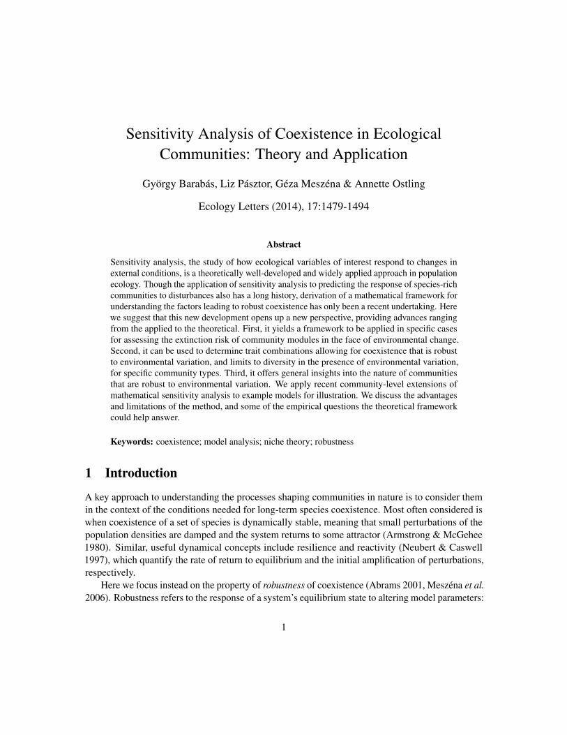
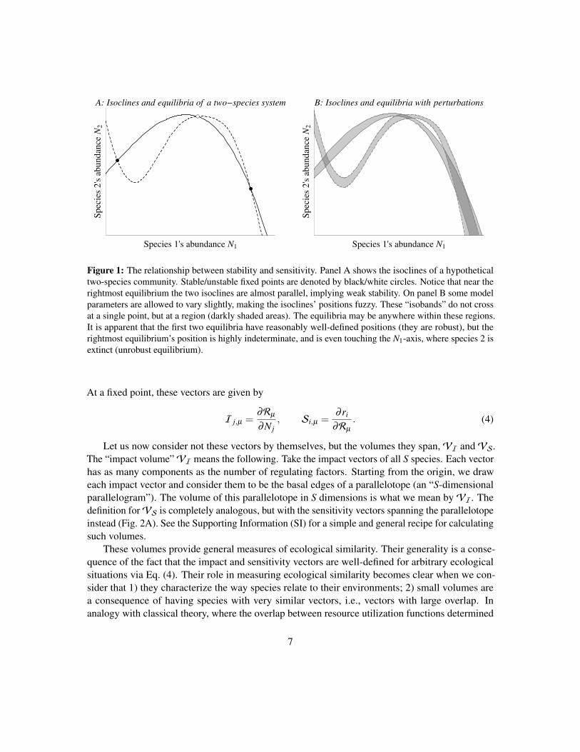
Figure 1: The relationship between stability and sensitivity. Panel A shows the isoclines of a hypotheticaltwo-species community. Stable/unstable fixed points are denoted by black/white circles. Notice that near therightmost equilibrium the two isoclines are almost parallel, implying weak stability. On panel B some modelparameters are allowed to vary slightly, making the isoclines’ positions fuzzy. These “isobands” do not crossat a single point, but at a region (darkly shaded areas). The equilibria may be anywhere within these regions.It is apparent that the first two equilibria have reasonably well-defined positions (they are robust), but therightmost equilibrium’s position is highly indeterminate, and is even touching the N1-axis, where species 2 isextinct (unrobust equilibrium).

At a fixed point, these vectors are given by

I j,µ =∂Rµ

∂N j, Si,µ =

∂ ri

∂Rµ. (4)

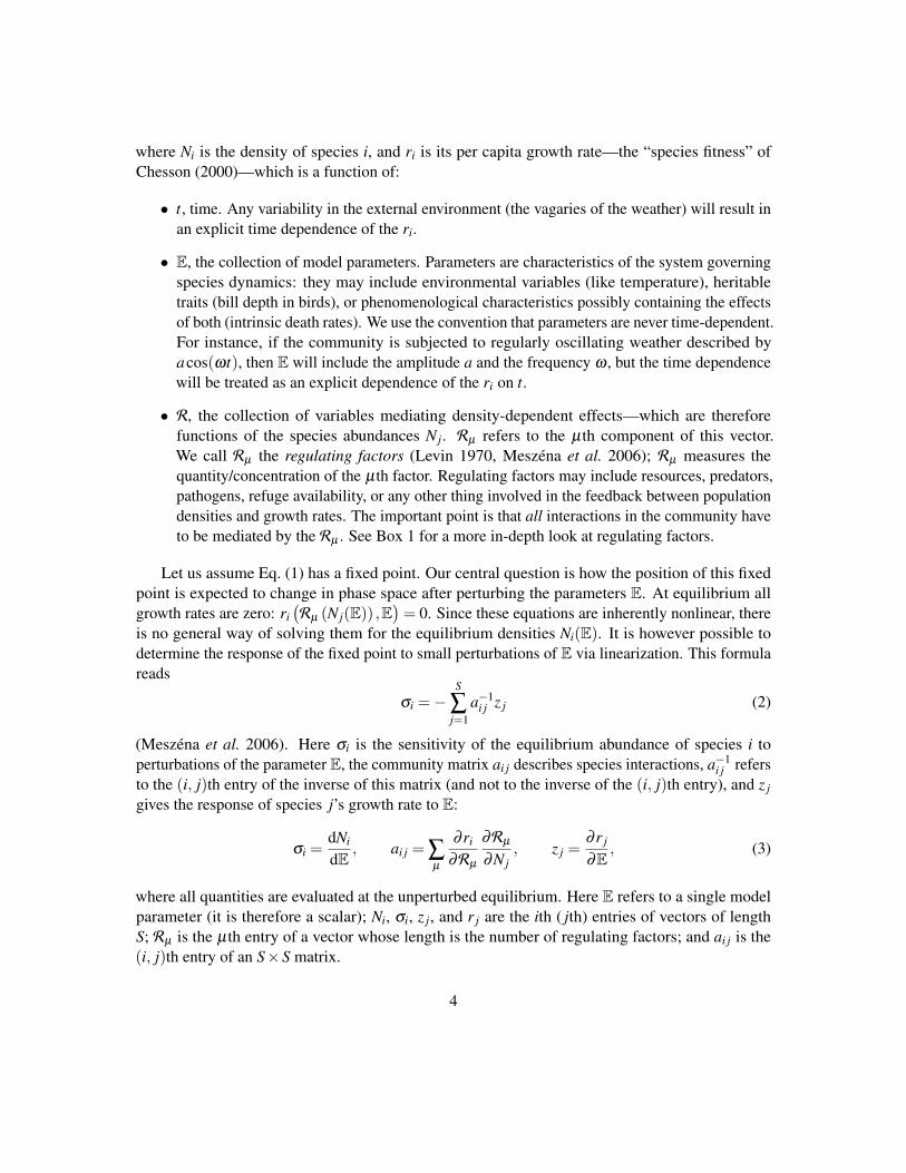
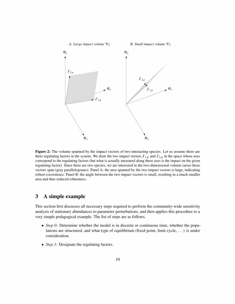
Let us now consider not these vectors by themselves, but the volumes they span,VI andVS.The “impact volume”VI means the following. Take the impact vectors of all S species. Each vectorhas as many components as the number of regulating factors. Starting from the origin, we draweach impact vector and consider them to be the basal edges of a parallelotope (an “S-dimensionalparallelogram”). The volume of this parallelotope in S dimensions is what we mean byVI. Thedefinition forVS is completely analogous, but with the sensitivity vectors spanning the parallelotopeinstead (Fig. 2A). See the Supporting Information (SI) for a simple and general recipe for calculatingsuch volumes.

These volumes provide general measures of ecological similarity. Their generality is a conse-quence of the fact that the impact and sensitivity vectors are well-defined for arbitrary ecologicalsituations via Eq. (4). Their role in measuring ecological similarity becomes clear when we con-sider that 1) they characterize the way species relate to their environments; 2) small volumes area consequence of having species with very similar vectors, i.e., vectors with large overlap. Inanalogy with classical theory, where the overlap between resource utilization functions determined

7

interaction coefficients (MacArthur & Levins 1967), the volumes are a measure of the aggregateoverlap between several species (Fig. 2).

Box 2: Sensitivity and dynamical stability

Fig. 1 illustrates the basic idea behind the community-wide sensitivity analysis of coex-istence and its relationship with conventional dynamical stability. Panel A shows the phasespace of a two-species community. The isoclines of the two species are shown; stable/unstableequilibria are indicated by black/white circles (we ignore the “trivial” unstable equilibrium atthe origin where both species are absent).

Panel B shows what happens when certain model parameters are slightly altered. In responseto the perturbations, the isoclines’ positions change. The two thick bands represent the possiblepositions of the isoclines after all possible (small) parameter perturbations, which is relevantbecause in nature parameters are expected to be continuously perturbed by extrinsic factors.The width of these “isobands” is not uniform: there is no reason to expect model parametersto influence all parts of the isoclines equally. Importantly, the equilibria now cease to havewell-defined locations: they may be anywhere within the area where the “isobands” cross(shaded regions of overlap). It is apparent that the positions of the two equilibria to the left arenot very sensitive to parameter perturbations. On the other hand, the rightmost equilibrium maybe located in a much wider region—and, since this region touches the horizontal axis, certainparameter changes may even result in the extinction of the second species. The size of theshaded area measures the sensitivity (robustness) of the equilibrium to parameter perturbations,with the two terms inversely related: a sensitive equilibrium (large area of overlap) is unrobust,while an insensitive one (small overlap) is robust.

Note that it makes perfect sense to measure the sensitivity of the unstable equilibrium(which in this case is quite robust). Sensitivity and stability are therefore separate properties:stability/instability means that small perturbations of the densities will decay/amplify, whilesensitivity measures how much the position of the equilibrium changes in phase space aftersmall perturbations of the parameters—regardless of whether the equilibrium is stable or not.Though an unstable equilibrium does not describe coexistence per se, its sensitivity may stillprovide useful information about the system. For instance, in classic predator-prey models anunstable equilibrium is often surrounded by a stable limit cycle. If the unstable equilibriumpoint is sensitive enough that it may actually cross one of the coordinate axes, then so will thecycle, meaning that the species are at risk of extinction.

Observe on Fig. 1 that the isoclines at the rightmost equilibrium point intersect at a verysmall angle. It is known (Kuznetsov 2004) that the smaller the angle of intersection, the smallerthe Jacobian’s determinant at the equilibrium; in the limit of tangentially touching isoclines, thedeterminant is zero. Since the determinant is the product of the eigenvalues, such an equilibriummust have at least one eigenvalue very close to zero, signaling weak stability/instability. These

8

weakly stable/unstable equilibria are also the most sensitive to parameter perturbations, becausenear-parallel isoclines mean that even a slight thickening of the isoclines into “isobands” willcreate large areas of overlap, as seen on Fig. 1. Conversely, strongly stable/unstable equilibriaare robust to parameter perturbations. Note that this is only a tendency: if the isoclines donot thicken appreciably after perturbation, then even near-parallel isoclines will not translateinto high sensitivity. For instance, the angle of intersection for the unstable equilibrium in themiddle is not particularly high, and yet it is quite robust because the thickness of the isobands isvery small near that point. Eq. (2) formalizes this intuitive relationship between stability andsensitivity, and extends it to an arbitrary number of species: ai j measures the angle betweenisoclines, and z j measures the “thickening” of the isoclines into isobands near the equilibriumpoint.

Finally, note that for simplicity we have considered fixed point equilibria of unstructuredpopulations, but the exact same conclusions turn out to be valid for limit cycles and/or structuredpopulations (Box 3). Though for these more complicated scenarios the matrix ai j in Eq. (2)cannot be interpreted as a simple Jacobian anymore, the result that a small det(ai j) signals anoversensitive system still holds, irrespective of model details.

Armed with these concepts, it turns out the determinant of ai j may always be approximated as∣∣det(ai j)

∣∣≤VIVS (5)

(Meszéna et al. 2006). In words, the product of the volumes spanned by the impact and sensitivityvectors puts an upper bound on the magnitude of ai j’s determinant. This implies that wheneverVIVS is small, all other things being equal, robustness will also be small. Knowing these volumestherefore opens up a possible shortcut to exploring community robustness, a property we will use inSections 4.2 and 4.3.

So far we have only discussed the sensitivity analysis of fixed point equilibria in continuous time,for communities of unstructured populations. However, the same methodology may be extended tomore complex dynamical states, like limit cycles (Barabás et al. 2012a, Barabás & Ostling 2013) oraperiodic stationary oscillations (Szilágyi & Meszéna 2010), both in discrete and continuous time.One may also consider communities where the species have complex life cycles, requiring structuredpopulation models (Szilágyi & Meszéna 2009a, Barabás et al. 2014). All this extra complexity canbe incorporated into the framework described above. Importantly, though the particular expressionsfor σi, ai j, and z j do change, the general form of the sensitivity formulas, Eqs. (2) and (5), remainthe same for all these scenarios, revealing a unified structure underneath all such calculations.Importantly, impact and sensitivity vectors can be identified in each. Box 3 summarizes theseformulas and gives the proper interpretation of Eq. (2) when various complexities are incorporated.Due to this common structure, we refer to ai j as the “generalized community matrix”, which reducesto the classical community matrix for point equilibria of unstructured communities, but may alsoaccount for additional complexities such as temporal fluctuations and population structure.

9

R 1

R 2

R 3

A: Large impact volume V I

I 1,Μ

I 2,Μ

R 1

R 2

R 3

B: Small impact volume V I

I 1,Μ

I 2,Μ

Figure 2: The volume spanned by the impact vectors of two interacting species. Let us assume there arethree regulating factors in the system. We draw the two impact vectors I1,µ and I2,µ in the space whose axescorrespond to the regulating factors (but what is actually measured along these axes is the impact on the givenregulating factor). Since there are two species, we are interested in the two-dimensional volume (area) thesevectors span (gray parallelograms). Panel A: the area spanned by the two impact vectors is large, indicatingrobust coexistence. Panel B: the angle between the two impact vectors is small, resulting in a much smallerarea and thus reduced robustness.

3 A simple example

This section first discusses all necessary steps required to perform the community-wide sensitivityanalysis of stationary abundances to parameter perturbations, and then applies this procedure to avery simple pedagogical example. The list of steps are as follows.

• Step 0: Determine whether the model is in discrete or continuous time, whether the popu-lations are structured, and what type of equilibrium (fixed point, limit cycle, . . . ) is underconsideration.

• Step 1: Designate the regulating factors.

10

• Step 2: Based on Step 0, look up the necessary formulas in Box 3 and calculate the impactand sensitivity vectors of each species.

• Step 3: Calculate the volumesVI andVS. A small productVIVS signals an oversensitivesystem. For more precise quantitative estimates, move on to Step 4.

• Step 4: Calculate ai j using the appropriate formula.

• Step 5: Pick an arbitrary model parameter E of interest and obtain the vector z j.

• Step 6: Calculate the sensitivities from the general equation Eq. (2).

The toy example we look at here is a simple consumer-resource model with two species and twononinteracting abiotic resources. The dynamics of the consumers is given by

ri =1Ni

dNi

dt= bi1G1 +bi2G2−mi, (6)

where ri, Ni, and mi are the per capita growth rate, population density, and mortality rate of speciesi, respectively; Gµ represents the available concentration of resource µ; and biµ is the amount ofpopulation growth species i can achieve on one unit of resource µ . The resource dynamics is in turngiven by

dGµ

dt= kµ

(Dµ −Gµ

)− cµ1N1− cµ2N2, (7)

where Dµ , kµ , and cµi are respectively the saturation concentration, turnover rate, and species i’s percapita consumption rate of resource µ . We assume kµ = 1.

Let us designate specific values for the entries of biµ and cµi:

biµ =

(1 00 1

), cµi =

(1 ρρ 1

). (8)

The above choice for biµ means each consumer can achieve population growth on only one of theresources. They might still consume the indigestible resource: this cross-consumption is measuredby the parameter ρ .

Let us now perform the steps of the analysis outlined above.Step 0. We know (Tilman 1982) that this type of consumer-resource model has a fixed point

equilibrium. We can solve for this equilibrium: due to dGµ/dt = 0 the resources satisfy

Gµ = Dµ − cµ1N1− cµ2N2 (9)

(we used kµ = 1), and the equilibrium densities are calculated from Eq. (6) by setting ri = 0 andusing Eqs. (8) and (9):

N1 =D1−ρD2

1−ρ2 , N2 =D2−ρD1

1−ρ2 . (10)

11

Here we introduced the quantities Di = Di−mi. Note that mi is the threshold value for Di abovewhich the ith consumer can survive in monoculture; Di denotes the excess above this minimum.These expressions are singular when ρ = 1, yielding meaningful equilibrium densities only whenD1 is exactly equal to D2.

For ρ < 1 the conditions for N1,N2 > 0 read

D1 > ρD2, D2 > ρD1, (11)

orρD1 < D2 <

1ρ

D1. (12)

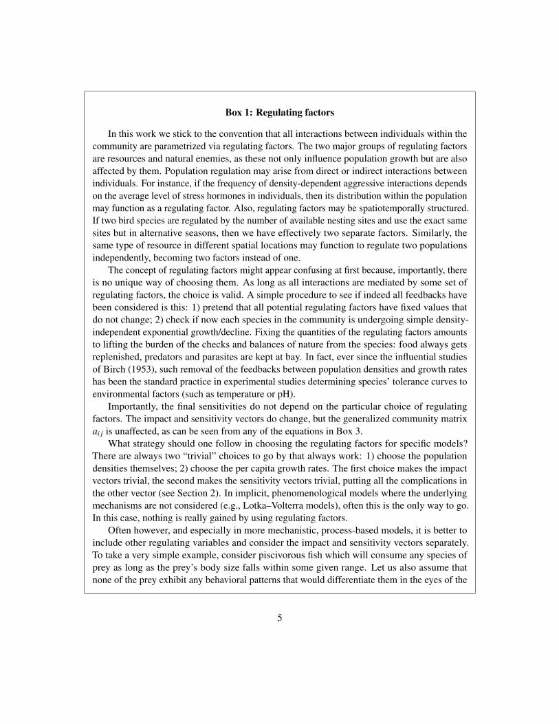
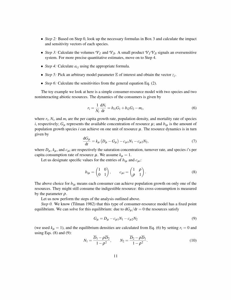
These can only be simultaneously satisfied for 0 < ρ < 1. Observe that, for D1 fixed, the range ofvalues of D2 allowing for coexistence shrinks with increasing ρ (Fig. 3A). One could also derivea similar condition for positive equilibrium densities when ρ > 1; however, these solutions aredynamically unstable and therefore of no interest to us.

0 0.2 0.4 0.6 0.8 10

1

2

3

4

5

Overlap in consumption Ρ

D2

A: Region of coexistence

D1

0 0.2 0.4 0.6 0.8 1-10

-5

0

5

10

Overlap in consumption Ρ

Sen

siti

vit

ies

Σi

B: Sensitivity of equilibrium to D2

Figure 3: Coexistence regions and sensitivities in the toy model of Section 3. Panel A: coexistence regionfor the parameter D2 as a function of ρ , based on Eq. (12). The value of D1 is fixed at 1 (dashed line).The shaded area represents the D2 values allowing for coexistence. Notice that this region shrinks to apoint at ρ = 1: here coexistence is only possible by fine-tuning D2 to be exactly equal to D1. Panel B:sensitivities of species 1 (solid curve) and 2 (dashed curve) to perturbing D2, given by Eq. (23); units are[abundance/resource concentration]. The curves diverge to minus/plus infinity as ρ → 1, signaling that anarbitrarily small perturbation could knock the species to extinction—in line with the result on panel A.

In this model we have the benefit of knowing the precise dependence of the equilibrium densitieson the parameters via Eq. (10), therefore sensitivity analysis is, strictly speaking, not even necessary.However, our purpose here is to show how the method works in an example where we can compare

12

the results with the exact solution. The same procedure will then work for problems where wecannot solve for the equilibrium state explicitly—see Section 4 for particular examples.

The model is at a fixed point in continuous time, and the populations are unstructured. Thereforethe ingredients needed for the analysis are given by Eq. (33) in Box 3:

σi =dNi

dE, ai j = ∑

µ

∂ ri

∂Rµ︸︷︷︸Si,µ

∂Rµ

∂N j︸︷︷︸I j,µ

, z j =∂ r j

∂E. (13)

Step 1. We choose the regulating factors for Eq. (6). Remember that the only criterion for thischoice is that the regulating variables have to mediate all density-dependent interactions (see Box 1).Here we go with Rµ = Gµ .

Step 2. Calculate the impact and sensitivity vectors of each species based on the definitions inEq. (13):

I j,µ =∂Rµ

∂N j=

∂∂N j

(Dµ − cµ1N1− cµ2N2

)=−cµ j, (14)

Si,µ =∂ ri

∂Rµ=

∂∂Rµ

(bi1R1 +bi2R2−mi

)= biµ . (15)

Observe, using Eq. (8), that the sensitivity vectors of the two species, (1, 0) and (0, 1), are markedlydifferent. In contrast, the impact vectors (−1, −ρ) and (−ρ, −1) are identical for ρ = 1 andbecome increasingly different as ρ departs from the value 1.

We could also calculate these vectors for different choices of the regulating variables. Asmentioned in Box 1, different choices of the regulating factors can change the impact and sensitivityvectors, but will leave ai j unchanged. For instance, we could make the resource depletion levelsthe regulating factors instead of the resources themselves: Rµ = ∑i cµiNi = Dµ −Gµ (the hatdistinguishing this alternative choice from our original one). Expressing the growth rates ri asfunctions of these factors:

ri = bi1(D1− R1

)+bi2

(D2− R2

)−mi. (16)

We can now calculate the alternative vectors:

I j,µ =∂ Rµ

∂N j=

∂∂N j

(cµ1N1 + cµ2N2

)= cµ j, (17)

Si,µ =∂ ri

∂ Rµ=

∂∂ Rµ

(bi1(D1− R1

)+bi2

(D2− R2

)−mi

)=−biµ . (18)

This alternative choice reverses the direction of the impact and sensitivity vectors.Step 3. We calculate the volumesVI andVS, which carry valuable information on robustness

(Section 2). In our case, as I j,µ and Si,µ happen to form square matrices, the volume is given bythe absolute values of their determinants (see the Supporting Information):

VI =∣∣det

(−cµ j

)∣∣=∣∣∣∣det

(−1 −ρ−ρ −1

)∣∣∣∣= 1−ρ2, VS =∣∣det

(biµ)∣∣=

∣∣∣∣det(

1 00 1

)∣∣∣∣= 1. (19)

13

Using Eq. (5),VIVS = 1−ρ2, so without any further calculations we know that coexistence willget more and more sensitive to parameter perturbations as ρ approaches 1. At the point where ρ isprecisely equal to 1,VIVS = 0 and coexistence has infinite sensitivity (zero robustness). This isconsistent with Eq. (12) and Fig. 3A: the parameter region allowing for coexistence shrinks withincreasing ρ , and at ρ = 1 becomes a single point.

Step 4. We calculate the matrix ai j from Eq. (13):

ai j =2

∑µ=1

∂ ri

∂Rµ

∂Rµ

∂N j=

2

∑µ=1Si,µI j,µ =−

2

∑µ=1

biµcµ j =−(

1 00 1

)(1 ρρ 1

)=

(−1 −ρ−ρ −1

). (20)

We get the exact same result using Rµ , or any other choice of the regulating factors. Since ai j

depends on Rµ only through the chain rule, this dependence must ultimately cancel from the finalexpression.

Step 5. We pick a model parameter E. Let us choose E = D2: we are interested in theconsequences of increasing the excess resource supply for Species 2 while keeping it constant forSpecies 1. Since the original equations are expressed in terms of Di instead of Di, we rewrite thegrowth rates at equilibrium as functions of Di = Di−mi. Substituting Eq. (9) into Eq. (6):

0 = r j =2

∑k=1

b jkDk−m j−2

∑µ=1

2

∑k=1

b jµcµkNk =2

∑k=1

b jkDk+2

∑k=1

b jkmk−m j−2

∑µ=1

2

∑k=1

b jµcµkNk, (21)

and now we can calculate z j:

z j =∂ r j

∂D2=

∂∂D2

(2

∑k=1

b jkDk +2

∑k=1

b jkmk−m j−2

∑µ=1

2

∑k=1

b jµcµkNk

)= b j2 =

(01

). (22)

Step 6. Determine the sensitivities σi of the equilibrium abundances to perturbing D2 using thegeneral formula Eq. (2):

σi =dNi

dD2=−

S

∑j=1

a−1i j z j =−

(−1 −ρ−ρ −1

)−1(01

)

=1

1−ρ2

(1 −ρ−ρ 1

)(01

)=

11−ρ2

(−ρ1

).

(23)

If all went well, we should have gotten the same result as if we had directly taken the derivative ofEq. (10) with respect to D2—which is indeed the case. Fig. 3B shows these sensitivities.

As a side note, observe that the σi are meaningful even for −1 < ρ < 0. A negative ρ means theith consumer facilitates the resource it cannot digest. A stable equilibrium still ensues in this case,but species 1, instead of responding negatively to an increase in D2, will respond positively due tothis facilitation. This is not apparent from looking only atVIVS = 1−ρ2, which is independent ofthe sign of ρ . The volumes do give general information about robustness, but the numerical detailsare only given by the full sensitivity formula.

14

In summary, the key quantity determining the sensitivity of equilibrium abundances to D2 in thisexample is ρ , measuring the segregation between the two impact vectors. As ρ approaches 1 frombelow, the impact vectors become similar and therefore sensitivity towards parameter perturbationsbecomes large. Also, the range of D2 values allowing for coexistence shrinks to zero gradually asρ increases, as shown by Eq. (12) and Fig. 3. For ρ ≈ 1, it becomes very hard to fine-tune D2 tosupport coexistence.

4 Applications

This section applies the community-wide sensitivity framework to three different model studies inorder to demonstrate how the machinery outlined above can handle situations that are significantlymore complicated than the previous toy example, and to demonstrate uses of the framework forassessing extinction risk and determining species traits predicted by a species interaction model. Inparticular, there are three complicating factors we consider. The first is temporal fluctuations in theenvironment (Section 4.1), where we also show how coexistence regions and extinction risk canbe estimated from sensitivities. The second is spatial heterogeneity (Section 4.2), where we deriveeffective limits to species similarity using sensitivities. The third are noncompetitive interactions(Section 4.3) in a model where stability criteria do not put a bound on the number of potentiallycoexisting species, but sensitivities do.

The details of our calculations are found in the Supporting Information. Importantly, we presenteach model with regulating factors already assigned. This is not to say other choices are notpossible (see Box 1), but the details of how and why we choose them are relegated to the SupportingInformation.

4.1 Handling temporal fluctuations: assessing extinction risk in a model of forb-grass competition

Here we perform community-wide sensitivity analysis on a competition model, proposed by Levine& Rees (2004), to describe a mechanism of persistence of rare native forbs with exotic grasseson a California grassland. They proposed that environmental fluctuations are key for generatingcoexistence, with the otherwise rare forbs benefiting from occasional good years while beingbuffered against bad years due to their superior seed banks (storage effect; Chesson & Warner 1981,Chesson 1994, 2000). Their annual plant model can be written

Ni(t +1) =((1−gi(t))(1−di)+

λi(t)gi(t)1+αiR(t)

)Ni(t), (24)

where i may be 1 (forb) or 2 (grass), Ni(t) is the density of species i’s seeds in the seedbank at timet, αi = (α, 1), and the time-dependent regulating factor is a linear function of the densities:

R(t) = g1(t)N1(t)α

+g2(t)N2(t). (25)

15

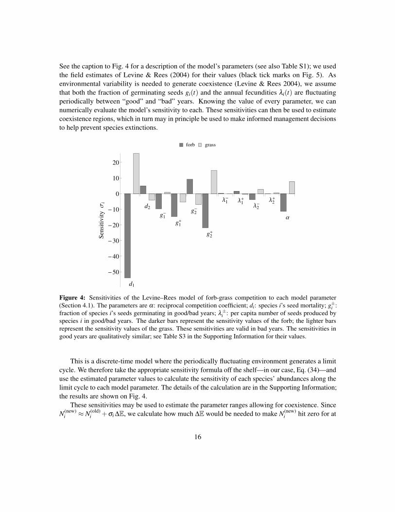
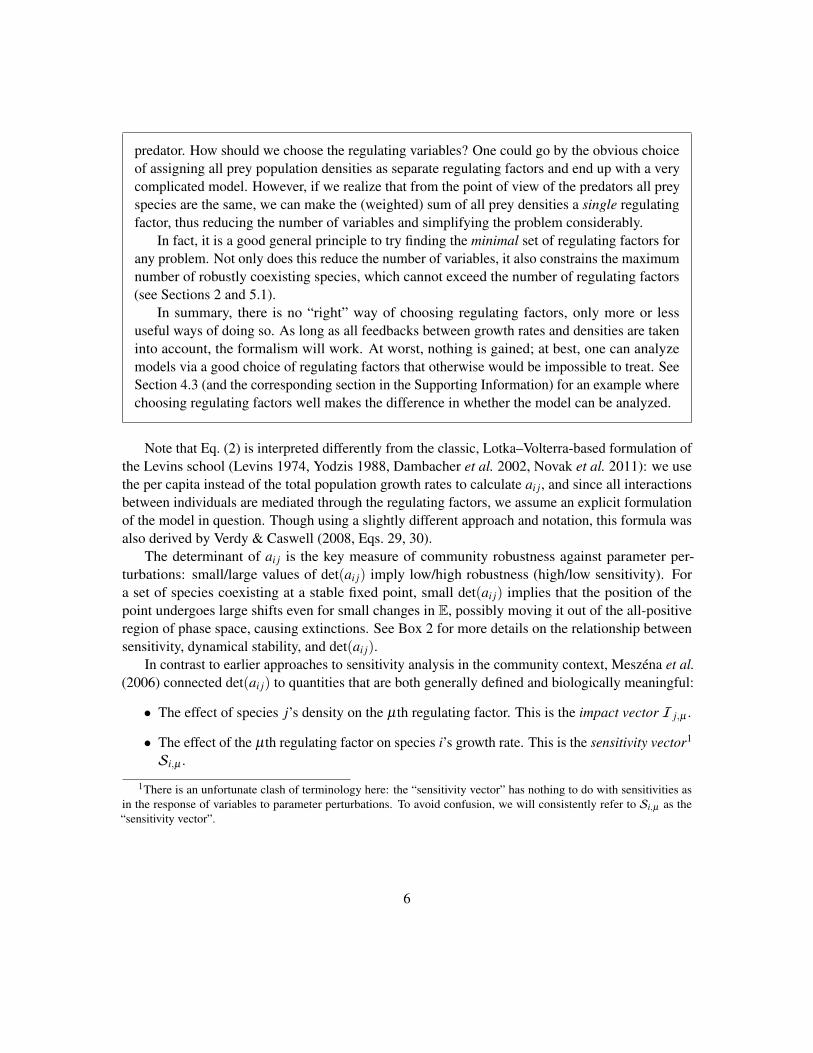
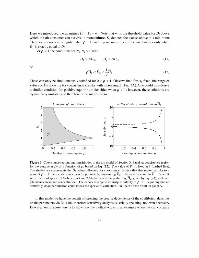
See the caption to Fig. 4 for a description of the model’s parameters (see also Table S1); we usedthe field estimates of Levine & Rees (2004) for their values (black tick marks on Fig. 5). Asenvironmental variability is needed to generate coexistence (Levine & Rees 2004), we assumethat both the fraction of germinating seeds gi(t) and the annual fecundities λi(t) are fluctuatingperiodically between “good” and “bad” years. Knowing the value of every parameter, we cannumerically evaluate the model’s sensitivity to each. These sensitivities can then be used to estimatecoexistence regions, which in turn may in principle be used to make informed management decisionsto help prevent species extinctions.

forb grass

d1

d2

g1

-

g1

+

g2

-

g2

+

Λ1

-Λ

1

+

Λ2

-Λ

2

+

Α

-50

-40

-30

-20

-10

0

10

20

Sen

sit

ivit

yΣ

i

Figure 4: Sensitivities of the Levine–Rees model of forb-grass competition to each model parameter(Section 4.1). The parameters are α: reciprocal competition coefficient; di: species i’s seed mortality; g±i :fraction of species i’s seeds germinating in good/bad years; λ±i : per capita number of seeds produced byspecies i in good/bad years. The darker bars represent the sensitivity values of the forb; the lighter barsrepresent the sensitivity values of the grass. These sensitivities are valid in bad years. The sensitivities ingood years are qualitatively similar; see Table S3 in the Supporting Information for their values.

This is a discrete-time model where the periodically fluctuating environment generates a limitcycle. We therefore take the appropriate sensitivity formula off the shelf—in our case, Eq. (34)—anduse the estimated parameter values to calculate the sensitivity of each species’ abundances along thelimit cycle to each model parameter. The details of the calculation are in the Supporting Information;the results are shown on Fig. 4.

These sensitivities may be used to estimate the parameter ranges allowing for coexistence. SinceN(new)

i ≈ N(old)i +σi ∆E, we calculate how much ∆E would be needed to make N(new)

i hit zero for at

16

d1 d2 g1

-g

1

+g

2

-g

2

+

0.0

0.2

0.4

0.6

0.8

1.0

Param

ete

rv

alu

eHd

i,g

i±L

Λ1

- Λ1

+ Λ2

- Λ2

+ Α

0

10

20

30

40

50

Param

ete

rv

alu

eHΛ

i±,

ΑL

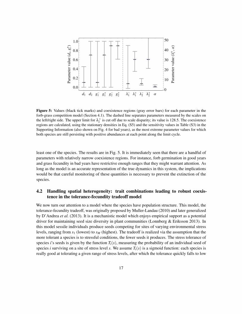
Figure 5: Values (black tick marks) and coexistence regions (gray error bars) for each parameter in theforb-grass competition model (Section 4.1). The dashed line separates parameters measured by the scales onthe left/right side. The upper limit for λ+

2 is cut off due to scale disparity; its value is 128.5. The coexistenceregions are calculated, using the stationary densities in Eq. (S5) and the sensitivity values in Table (S3) in theSupporting Information (also shown on Fig. 4 for bad years), as the most extreme parameter values for whichboth species are still persisting with positive abundances at each point along the limit cycle.

least one of the species. The results are in Fig. 5. It is immediately seen that there are a handful ofparameters with relatively narrow coexistence regions. For instance, forb germination in good yearsand grass fecundity in bad years have restrictive enough ranges that they might warrant attention. Aslong as the model is an accurate representation of the true dynamics in this system, the implicationswould be that careful monitoring of these quantities is necessary to prevent the extinction of thespecies.

4.2 Handling spatial heterogeneity: trait combinations leading to robust coexis-tence in the tolerance-fecundity tradeoff model

We now turn our attention to a model where the species have population structure. This model, thetolerance-fecundity tradeoff, was originally proposed by Muller-Landau (2010) and later generalizedby D’Andrea et al. (2013). It is a mechanistic model which enjoys empirical support as a potentialdriver for maintaining seed size diversity in plant communities (Lonnberg & Eriksson 2013). Inthis model sessile individuals produce seeds competing for sites of varying environmental stresslevels, ranging from s1 (lowest) to sM (highest). The tradeoff is realized via the assumption that themore tolerant a species is to stressful conditions, the fewer seeds it produces. The stress tolerance ofspecies i’s seeds is given by the function Ti(s), measuring the probability of an individual seed ofspecies i surviving on a site of stress level s. We assume Ti(s) is a sigmoid function: each species isreally good at tolerating a given range of stress levels, after which the tolerance quickly falls to low

17

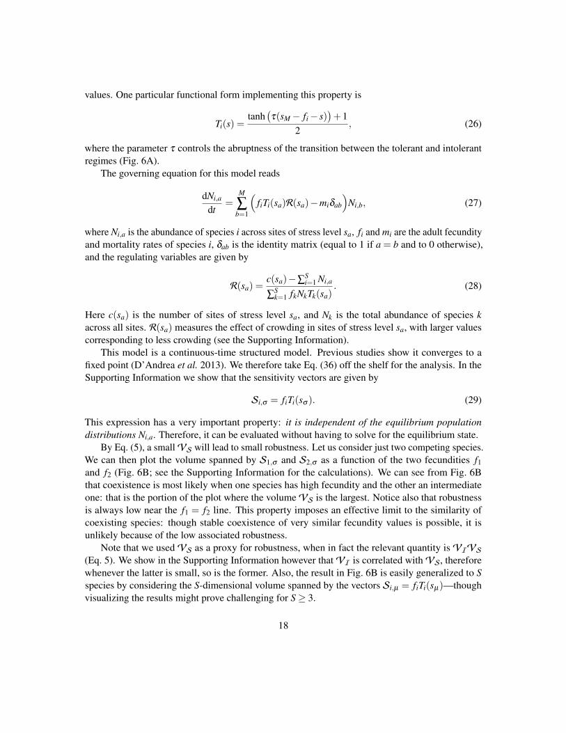
values. One particular functional form implementing this property is

Ti(s) =tanh

(τ(sM− fi− s)

)+1

2, (26)

where the parameter τ controls the abruptness of the transition between the tolerant and intolerantregimes (Fig. 6A).

The governing equation for this model reads

dNi,a

dt=

M

∑b=1

(fiTi(sa)R(sa)−miδab

)Ni,b, (27)

where Ni,a is the abundance of species i across sites of stress level sa, fi and mi are the adult fecundityand mortality rates of species i, δab is the identity matrix (equal to 1 if a = b and to 0 otherwise),and the regulating variables are given by

R(sa) =c(sa)−∑S

i=1 Ni,a

∑Sk=1 fkNkTk(sa)

. (28)

Here c(sa) is the number of sites of stress level sa, and Nk is the total abundance of species kacross all sites. R(sa) measures the effect of crowding in sites of stress level sa, with larger valuescorresponding to less crowding (see the Supporting Information).

This model is a continuous-time structured model. Previous studies show it converges to afixed point (D’Andrea et al. 2013). We therefore take Eq. (36) off the shelf for the analysis. In theSupporting Information we show that the sensitivity vectors are given by

Si,σ = fiTi(sσ ). (29)

This expression has a very important property: it is independent of the equilibrium populationdistributions Ni,a. Therefore, it can be evaluated without having to solve for the equilibrium state.

By Eq. (5), a smallVS will lead to small robustness. Let us consider just two competing species.We can then plot the volume spanned by S1,σ and S2,σ as a function of the two fecundities f1and f2 (Fig. 6B; see the Supporting Information for the calculations). We can see from Fig. 6Bthat coexistence is most likely when one species has high fecundity and the other an intermediateone: that is the portion of the plot where the volumeVS is the largest. Notice also that robustnessis always low near the f1 = f2 line. This property imposes an effective limit to the similarity ofcoexisting species: though stable coexistence of very similar fecundity values is possible, it isunlikely because of the low associated robustness.

Note that we usedVS as a proxy for robustness, when in fact the relevant quantity isVIVS(Eq. 5). We show in the Supporting Information however thatVI is correlated withVS, thereforewhenever the latter is small, so is the former. Also, the result in Fig. 6B is easily generalized to Sspecies by considering the S-dimensional volume spanned by the vectors Si,µ = fiTi(sµ)—thoughvisualizing the results might prove challenging for S≥ 3.

18

s1 sM

0

1

Environmental stress level s

To

lera

nce

fun

ctio

nT

HsLA: Tolerance functions of two species

Species 1

Hhigh f LSpecies 2

Hlow f L

0 5 100

5

10

Fecundity f1

Fec

un

dit

yf 2

B: Robustness of coexistence V S

0

20

40

60

0

0

5

10

Figure 6: The tolerance-fecundity tradeoff model (Section 4.2). Panel A: tolerance functions of two species(solid and dashed curves). The abscissa represents stress, ranging from s1 to sM . The ordinate is the probabilitythat a seed survives the given stress level. The tolerance functions are sigmoid curves with a relatively abrupttransition from the tolerant to the intolerant regime. The tradeoff is implemented by making the specieswith the higher fecundity f less tolerant. Panel B: The volumeVS spanned by the sensitivity vectors of twospecies, as a function of their fecundities; units are [1/time2]. The volume is largest where one species hashigh fecundity and the other an intermediate one. Both species possessing similar fecundities leads to smallvolumes. We know from Eq. (5) that a small volume is sufficient for making coexistence oversensitive andtherefore unrealistic; only in the high-volume regions is coexistence even a possibility.

4.3 Handling noncompetitive interactions: stability vs. robustness of coexistence inthe Gross model of interspecific facilitation

For our final example we analyze a model of interspecific facilitation proposed by Gross (2008).There have been ongoing efforts to incorporate facilitation into ecological theory in a general wayfor more than a decade now (Bruno et al. 2003), and the model of Gross (2008) is an important stepin this direction. This example demonstrates how large a difference it makes to shift the emphasisfrom the stability of coexistence to its robustness against varying parameters. If one only considersstability, expected diversity is in fact unlimited. Taking sensitivities into account, the maximumnumber of species turns out to be strongly limited.

The Gross model is one of intraguild mutualism (Crowley & Cox 2011), where several consumerspecies compete for a single resource. Facilitation is included via the assumption that an increasein the abundance of one competitor reduces the death rate of another. Empirical examples includeplant species providing cushion for others (Cerfonteyn et al. 2011, McIntire & Fajardo 2013), andMüllerian mimicry rings in butterflies (Elias et al. 2008) or catfish (Alexandrou et al. 2011), where

19

joining the ring confers an advantage to otherwise competing species by reducing nonregulatorypredation pressure.

In the simplest version of the model only two species compete: in this case, the coexistencecondition is that the mutualistic effects must confer enough advantage on the species to turn theirinvasion growth rates positive when the other species is resident. When generalizing the modelto several species, the facilitation network may in principle be arbitrarily complicated, but Gross(2008) made a simplifying assumption to keep the model tractable: facilitation was assumed tobe hierarchical. This means species 1 is not facilitated by anyone, species 2 is facilitated only byspecies 1, species 3 is facilitated by species 1 and 2, and so on. This assumption actually allows formore coexistence on average than random facilitation networks (Gross 2008). The equations for thismodel read

1Ni

dNi

dt= fi(R)−m0

i +di

(1− exp

(−θ ∑

k<iNk

))(i = 1 . . .S) (30)

for the consumers, anddRdt

= g(R)−S

∑i=1

ci fi(R)Ni (31)

for the resource (SI). Here S is the total number of consumer species, Ni is the density of species i,fi(R) is its per capita resource-dependent growth rate, m0

i its baseline mortality, di the maximumadvantage it can gain from facilitation (we assume di ≤ m0

i ), θ measures the facilitative advantageconferred by a single species, R is the resource, g(R) the resource supply rate, and ci the species’consumption rates.

The consequences of this facilitation on coexistence are drastic: Gross (2008) has proven that anarbitrary number of species may coexist on the single resource. His proof relies on demonstratingthat, given a community of S species, one can always choose parameters such that an (S+ 1)thspecies can be added without causing any extinctions. In dynamical terms: if there was a stableequilibrium point for S species, there will also be one for S+1 species as well.

Stable coexistence of an arbitrary number of species is therefore possible. However, one canalso ask how sensitive this nontrivial stable fixed point is to altering parameters. As proven in theSupporting Information, increasing the number of species will make the community ever moresensitive to parameter changes. The asymptotic robustness of the community, for large S, is shownto be

S√VIVS ∼ Nθ exp(−NθS/2) , (32)

where N is the smallest of the equilibrium densities of the consumer species. Taking the Sth root ofVIVS makes robustness comparable across different values of S; see the Supporting Informationfor details.

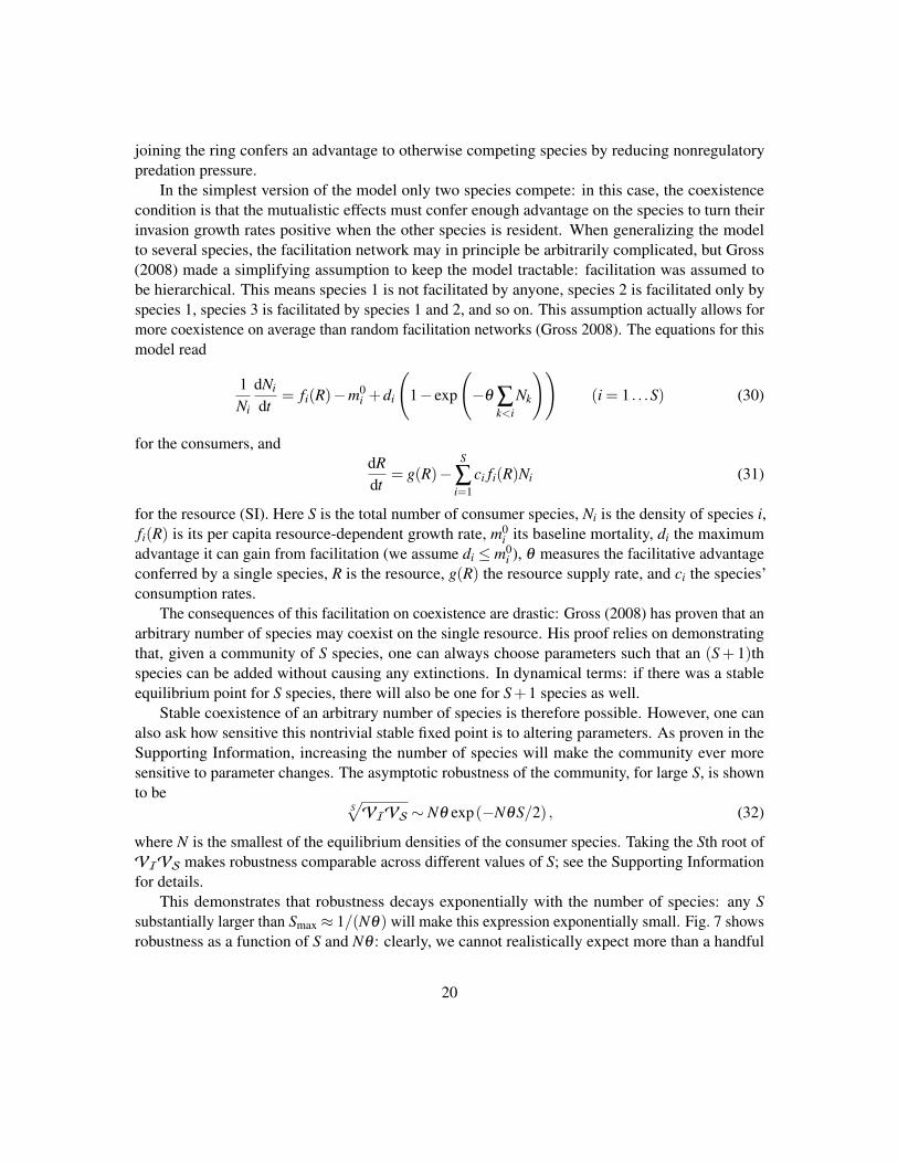
This demonstrates that robustness decays exponentially with the number of species: any Ssubstantially larger than Smax ≈ 1/(Nθ) will make this expression exponentially small. Fig. 7 showsrobustness as a function of S and Nθ : clearly, we cannot realistically expect more than a handful

20

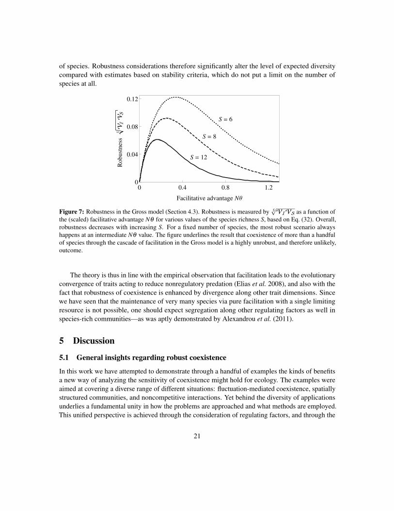
of species. Robustness considerations therefore significantly alter the level of expected diversitycompared with estimates based on stability criteria, which do not put a limit on the number ofspecies at all.

0 0.4 0.8 1.20

0.04

0.08

0.12

Facilitative advantage NΘ

Robust

nes

sV

IV

S

SS = 6

S = 8

S = 12

Figure 7: Robustness in the Gross model (Section 4.3). Robustness is measured by S√VIVS as a function of

the (scaled) facilitative advantage Nθ for various values of the species richness S, based on Eq. (32). Overall,robustness decreases with increasing S. For a fixed number of species, the most robust scenario alwayshappens at an intermediate Nθ value. The figure underlines the result that coexistence of more than a handfulof species through the cascade of facilitation in the Gross model is a highly unrobust, and therefore unlikely,outcome.

The theory is thus in line with the empirical observation that facilitation leads to the evolutionaryconvergence of traits acting to reduce nonregulatory predation (Elias et al. 2008), and also with thefact that robustness of coexistence is enhanced by divergence along other trait dimensions. Sincewe have seen that the maintenance of very many species via pure facilitation with a single limitingresource is not possible, one should expect segregation along other regulating factors as well inspecies-rich communities—as was aptly demonstrated by Alexandrou et al. (2011).

5 Discussion

5.1 General insights regarding robust coexistence

In this work we have attempted to demonstrate through a handful of examples the kinds of benefitsa new way of analyzing the sensitivity of coexistence might hold for ecology. The examples wereaimed at covering a diverse range of different situations: fluctuation-mediated coexistence, spatiallystructured communities, and noncompetitive interactions. Yet behind the diversity of applicationsunderlies a fundamental unity in how the problems are approached and what methods are employed.This unified perspective is achieved through the consideration of regulating factors, and through the

21

introduction of impact and sensitivity vectors describing species’ interactions with these factors. Justas in the context of population-level sensitivity analyses (Caswell 2008), having explicit sensitivityformulas means one can gain general insights not accessible via purely simulation-based approaches.

The generality and flexibility of the concept of regulating factors allows for the commontreatment of seemingly very different types of interactions. Traditional resource competition,predator-mediated effects (such as apparent competition), facilitation, spatial effects, and temporalsegregation are all handled on the same footing: the details do change (Box 3), but both theirunderlying mathematical structure and their basic biological interpretation remains the same.

The mathematical framework presented here further shows that species’ impact and sensitivityvectors characterize the system’s sensitivity to environmental perturbations, regardless of whether thesystem is at equilibrium or not, or whether there is spatial structure, or noncompetitive interactions.Specifically, the volumes spanned by these vectors are key in determining sensitivity via Eq. (5):large volumes imply low sensitivity, while small volumes imply high sensitivity. Hence, highenvironmental variability coupled with small volumes is expected to lead to extinctions, making itless likely that such communities would be observed. This provides a general understanding of thedistribution of species traits expected in robust communities, and reveals constraints that robustnessrequirements may put on communities, beyond those imposed by stability.

What causes impact and sensitivity vectors to span small volumes? There are two options. First,volumes will be small if the vectors are short, i.e., the regulating interactions of the populations areweak. Second, volumes will be small if the vectors spanning them are nearly collinear or, moregenerally, linearly dependent (Fig. 2): that is, when the regulating interactions of the differentspecies are not differentiated sufficiently.

This second possibility is nothing else than the classical idea of limiting similarity, formulated ina precise way. Sensitivity analysis adds precision in three ways. First, it clarifies that coexistence ofsimilar species it is not impossible, just unlikely, requiring a narrow set of environmental parameters.Second, it yields a quantitative estimate of this parameter range. Third, it clarifies that the propertyin which species must differ for robust coexistence is their way of being regulated, described by theimpact and sensitivity vectors.

When the number of regulating factors is smaller than the number of species, the frameworkshows that not only is it impossible for all of the species to coexist stably (Levin 1970), it is alsoimpossible for them to coexist robustly, sinceVI (orVS) will be zero. Moreover, even when thenumber of regulating factors is infinite (Section 4.2) or unbounded (Section 4.3), in which caseconsideration of stability alone would suggest that coexistence of infinitely many species is at leastpossible, sensitivity analysis shows infinite diversity is not expected, because too much coexistenceleads to overly similar impact and sensitivity vectors. We saw this explicitly in the results of ouranalysis of the tolerance-fecundity tradeoff model (Fig. 6B): robustness is zero along the line ofidentical fecundities f1 = f2. This is because the sensitivity vectors of identical species are the same,so they point in the same direction, leading to VS = 0. Robustness is still very small if the twofecundities are nearly equal. Importantly, what we see on Fig. 6B reflects a property we will observein all cases, because VI and VS are continuous functions of the impact and sensitivity vectors.Therefore, near-identical species will always have near-zero robustness.

22

In this way, the community-wide sensitivity analysis of coexistence essentially recreates whatusually goes under the umbrella of “niche theory” (Case 2000, p. 368): avoiding competitiveexclusion requires limited niche overlap as measured by impact and sensitivity vectors. Thoughthe expectation of strict limits to similarity is mathematically and biologically naive, sensitivityanalysis leads to the conclusion that effective limits to similarity are still the expected rule of thumb(Section 4.2, Szabó & Meszéna 2006, Barabás & Meszéna 2009, Barabás et al. 2012b).

The robustness perspective naturally leads to the empirical question of how robust naturalcommunities tend to be. As we have seen, sensitivities, coupled with a knowledge of the size oftypical environmental perturbations, yield viable parameter regions. How wide do these regions tendto be in natural communities compared to what is strictly required for the community’s persistence?Put another way, does the regime of environmental variation have a big influence on communitystructure, or do other forces governing community structure (e.g., selection for trait differencesamong species) act to generate communities even more robust than required? One study by Adleret al. (2010) in a perennial plant community suggests the stabilization of coexistence is quite strong(much stronger than strictly necessary to compensate for fitness differences between the species),suggesting it should also be quite robust. However, the parameter region allowing for coexistencemust be compared with the range of environmental fluctuations in this system if we are to get adefinitive answer.

In fact, one may wonder whether community robustness tends to vary systematically alongenvironmental gradients. Certain environments are relatively constant; some are more variable,which in general means more perturbed. More perturbed communities require, ceteris paribus, awider coexistence region. Does this actually play out in nature? And if so, what consequencesdoes it have for expected community and diversity patterns? We believe that the community-widesensitivity framework will help answer these and similar empirical questions.

5.2 Limitations of the framework

Though the presented method does provide the applied and theoretical advantages outlined above,it also comes with its inevitable drawbacks and caveats. The most important drawback is thatthe method is based on linearization: sensitivity values are accurate only for small parameterperturbations. Therefore, extrapolations to large parameter changes should be treated with care,which will only be accurate if the sensitivities themselves are not very sensitive. If they are heavilyconvex/concave functions, or if the analyzed equilibria undergo saddle-node bifurcations betweentheir current locations and zero (signaling a potential catastrophic shift), the linear extrapolationswill be unreliable. Then, the method’s safest domain of application is looking at the responseof systems strictly to small parameter changes. This is an important point in the context of theLevine–Rees model (Section 4.1), where the coexistence regions of Fig. 5 are all derived usinglinear extrapolation.

Fortunately, a common experience in performing sensitivity analyses is that extrapolations basedon sensitivities yield surprisingly accurate results even for large perturbations, both in a population(de Kroon et al. 2000) and a community-wide (Barabás & Ostling 2013, Barabás et al. 2014) context.

23

Under what circumstances we may expect such accuracy is an open question. However, use of thelinear approximation means our methods are ill-suited for studying the effects of species removal oncommunities (Ebenman et al. 2004, Ebenman & Jonsson 2005, Allesina & Pascual 2009), becausesuch perturbations involve very large changes in the system.

Another issue is that all parameter estimates possess a level of uncertainty. How can we knowthe degree to which measurement errors affect sensitivity results? There are two aspects to thisproblem. First, as mentioned above, if the linear approximation is not very good, sensitivity valuesmight themselves sensitively depend on measured parameter values. Second, even if sensitivitiesare accurate for a wide range of parameters, predictive power may be hampered if their values arevery large: then, even a small error in measurement would mean a large error in prediction.

How can one deal with this problem in practice? First, it can be approached in the same wayas any other kind of uncertainty: by considering the confidence intervals of parameter estimates,and repeating the sensitivity calculations for various randomly chosen parameter values within theparameters’ confidence intervals. This way, one obtains a distribution of sensitivities instead of asingle sensitivity value. See Barabás & Ostling (2013) and Barabás et al. (2014) for how this is donein practice. The same procedure could then be applied, for instance, to the Levine–Rees model if wehad data on parameter error estimates.

Second, note that, in contrast to experience with smaller communities (Barabás & Ostling 2013,Barabás et al. 2014), several studies (Yodzis 1988, Dambacher et al. 2002, Novak et al. 2011)have found very high sensitivities of equilibrium abundances to press perturbations when analyzinglarge ensembles of species. Systematic application of our methods to large systems is work inprogress, but if we believe these results to be general (i.e., large communities are more sensitive),then one possibility for avoiding the problem of overly high sensitivities is to concentrate on smallercommunity compartments which can be thought of as independent mesocosms consisting of just ahandful of species (Krause et al. 2003, Guimerà et al. 2010, Stouffer & Bascompte 2011).

Yet another caveat comes with using the volumetric approach, based onVI andVS, to gaininsight into the robustness of coexistence. As we have seen, these volumes can provide a shortcut torobustness calculations. They are, however, only part of the story because in Eq. (2) the vector z j

also plays a role. Though the volumes may be small, the vector z j may also be small and thereforerobustness may not be as weak as it appears based on the volumes alone (or vice versa). In anextreme case, imagine that the growth rates are at a local maximum or minimum with respect toE; then z j = ∂ r j/∂E = 0, so sensitivity is zero regardless of VIVS. In Section 3 for instance,VIVS was insensitive to the sign of ρ , but the sensitivities were not. The volumes do reveal generalinformation, but not the numerical details.

Moreover, though the presented framework can already treat a variety of dynamics, the list isfar from complete. We do not yet have formulas for the sensitivity of general, aperiodic stationaryoscillations (with or without population structure), or formulas for the sensitivity of transients insteadof stationary states. Transient sensitivities would enable us to assess the short-term consequences ofparameter changes, an endeavor just as important as being able to calculate long-term consequences.

Finally, a note about the procedure outlined in Section 3 for performing sensitivity analyses(which we consistently follow in the main text and the Supporting Information as well). Although it

24

looks straightforward, this does not mean all case studies will look the same. To take an analogy,consider conventional sensitivity analysis of structured populations. One could say it is verysimple: 1) construct the life cycle graph; 2) estimate the transition probabilities and fecundities; 3)calculate the leading eigenvalue; 4) calculate the corresponding left and right eigenvectors; 5) createtheir tensor product to obtain the sensitivity matrix. But, as Caswell himself pointed out: “Everypopulation analysis that I have been involved with has required some unique methodological twistsand turns” (Caswell 2001, p. 107). What we provided is merely an outline, which does not implythat particular models can have no “special needs” in their analyses.

6 Conclusions

The recently developed mathematical framework for the sensitivity analysis of stationary abun-dances of interacting species to parameter perturbations provides an important new perspective incommunity ecology. It opens up the possibility of an analytical approach to estimating extinctionrisk. It provides a tool for understanding how diversity and community patterns may be influencedby environmental variation, in addition to stability constraints. Finally, it yields insight into thenature of the interaction between robustly coexisting species, in terms of species’ interactions withregulating factors. These insights apply fairly generally, even to models with complex dynamics,and provide a new perspective on the concept of niche differentiation in ecology. Here we haveguided the reader on the use of this new mathematical framework and illustrated its potential throughapplication to a variety of models. Although the framework has limitations—most notably in that itis based on a linear approximation—its application could help answer a set of empirical questionsin community ecology regarding the degree to which environmental fluctuations and robustnessconstraints determine the structure of communities.

25

Box 3: Community-wide sensitivity formulas

Below we give a catalog list of the sensitivity formulas for various dynamical scenarios.The general structure of each equation is given by Eq. (2):

σi =−S

∑j=1

a−1i j z j,

where a−1i j is the (i, j)th entry of the inverse matrix, not the inverse of the (i, j)th entry. For each

case we state the applicability of the given formula, reference where it was originally derived,give the interpretation of σi along with the formulas for ai j and z j, and indicate the impact andsensitivity vectors I j,µ and Si,µ .

1. Fixed point dynamics, in either discrete or continuous time, for communities of unstruc-tured populations (Meszéna et al. 2006):

σi =dNi

dE, ai j = ∑

µ

∂ ri

∂Rµ︸︷︷︸Si,µ

∂Rµ

∂N j︸︷︷︸I j,µ

, z j =∂ r j

∂E. (33)

In discrete time, ri is the natural log of species i’s discrete geometric rate of growth from time tto t +1: ri = log(Ni(t +1)/Ni(t)). In continuous time, ri is the per capita growth rate of speciesi: ri = dNi/(Nidt).

2. Limit cycle of fixed period length T in discrete time, for communities of unstructuredpopulations (Barabás & Ostling 2013):

σi =1

Ni(0)dNi(0)

dE, ai j =−δi j +

0

∏t=T−1

(δi j +∑

µ

∂ ri(t)∂Rµ(t)︸ ︷︷ ︸Si,µ (t)

∂Rµ(t)∂N j(t)

N j(t)︸ ︷︷ ︸

I j,µ (t)

), z j =

T−1

∑t=0

∂ r j(t)∂E

,

(34)where ri(t) = log(Ni(t + 1)/Ni(t)), and δi j is the identity matrix (equal to 1 if i = j and to 0otherwise). The product from t = T − 1 to 0 above refers to the (i, j)th entry of a productof matrices (taken in decreasing order in time), not to the product of the (i, j)th entries—seeEqs. (S12) and (S13) in the Supporting Information for the special case of T = 2. Note thatthe regulating factors are functions of t within the cycle, so each regulating variable at eachmoment in time can potentially serve as a separate regulating factor.

3. Limit cycle of fixed period length T in continuous time, for communities of unstructuredpopulations (Barabás et al. 2012a): this is obtained simply from Eq. (34) in the limit of infinitely

26

many infinitesimally small discrete time steps ∆t (Barabás & Ostling 2013):

σi =1

Ni(0)dNi(0)

dE, ai j =−δi j+TExp

(∫ T

0∑µ

∂ ri(t)∂Rµ(t)︸ ︷︷ ︸Si,µ (t)

∂Rµ(t)∂N j(t)

N j(t)︸ ︷︷ ︸

I j,µ (t)

dt), z j =

∫ T

0

∂ r j(t)∂E

dt,

(35)where Exp means matrix exponential (obtained by substituting the matrix in the argument intothe usual Taylor series of the exponential function), and T is the time-ordering operator thatrearranges a product of matrices to decreasing order in time (Barabás et al. 2012a).

4. Fixed point dynamics in either discrete or continuous time, for communities of structuredpopulations (Szilágyi & Meszéna 2009a, Barabás et al. 2014):

σi =dNi

dE, ai j = ∑

µ

(∑a,b

vi,a∂Ai,ab

∂Rµwi,b

)

︸ ︷︷ ︸Si,µ

∑ν

(δµν −

∂Gµ

∂Rν

)−1(∑c

∂Rν

∂N j,cw j,c

)

︸ ︷︷ ︸I j,µ

,

z j = ∑a,b

v j,a∂A j,ab

∂Ew j,b +∑

µ,ν

(∑a,b

vi,a∂Ai,ab

∂Rµwi,b

)(δµν −

∂Gµ

∂Rν

)−1 ∂Gν

∂E,

(36)

where Ai,ab is the (a,b)th entry of species i’s projection matrix evaluated at equilibrium; Ni

is the weighted total abundance of species i; δµν is the identity matrix; vi,a, wi,a, and Ni,a arethe ath component of species i’s leading left and right eigenvectors and population abundancevector, respectively; the inverses always refer to the (µ,ν)th entries of the inverse matrix asopposed to the inverse of the (µ,ν)th entries; and

Gµ (Rν ,E) =∑j

∑a,b,c

(n j

∑d q j,dw j,d

∂Rµ

∂n j,a

s j

∑k=2

1λ j−λ k

j

(wk

j,a−∑e q j,ewk

j,e

∑ f q j, f w j, fw j,a

)vk

j,b

)

×A j,bc (Rν ,E)w j,c

(37)

describes the effect of perturbing the species’ population structures on the regulation of thecommunity (the dependence of Gµ on Rν and E comes strictly from A j,bc; all other quantitiesare evaluated at the unperturbed equilibrium). Here q j,a is a positive vector giving the weightof the ath stage class in the weighted total abundance of species j, λ j is species j’s leadingeigenvalue, s j is the number of stage classes of species j, and the superscript k means we areconsidering the kth (non-leading) eigenvalue/eigenvector. The eigenvectors are normalized sothat ∑a wi,a = 1 and ∑a vk

i,awli,a = δkl for every species i. Though the nature of the population

structure can be arbitrary (age, stage, physiological, spatial,. . . ), in the special case of spatialstructure a single regulating factor R can be thought of as splitting up into as many differentfactors as the number of distinct spatial locations.

27

Acknowledgements

We would like to thank Stefano Allesina, Rafael D’Andrea, Aaron King, Mercedes Pascual, andIstván Scheuring for discussions, and Hal Caswell and two anonymous reviewers for their helpfulcomments on the manuscript. LP and GM were supported by the Hungarian Scientific ResearchFund (grant OTKA K81628).

References

Abrams, P. A. (1984). Variability in resource consumption rates and the coexistence of competingspecies. Theoretical Population Biology, 25, 106–124.

Abrams, P. A. (2001). The effect of density-independent mortality on the coexistence of exploitativecompetitors for renewing resources. American Naturalist, 158, 459–470.

Abrams, P. A. & Holt, R. D. (2002). The impact of consumer-resource cycles on the coexistence ofcompeting consumers. Theoretical Population Biology, 62, 281–295.

Abrams, P. A., Brassil, C. E. & Holt, R. D. (2003). Dynamics and responses to mortality ratesofcompeting predators undergoing predator–prey cycles. Theoretical Population Biology, 64,163–176.

Abrams, P. A. (2004). When does periodic variation in resource growth allow robust coexistence ofcompeting consumer species? Ecology, 85, 372–382.

Abrams, P. A. & Nakajima, M. (2007). Does competition between resources change the competitionbetween their consumers to mutualism? variations on two themes by vandermeer. AmericanNaturalist, 170, 744–757.

Adamson, M. W. & Morozov, A. (2012). When can we trust our model predictions? Unearthingstructural sensitivity in biological systems. Proceedings of the Royal Society A.

Adler, P. B., Ellner, S. P. & Levine, J. M. (2010). Coexistence of perennial plants: an embarrassmentof niches. Ecology Letters, 13, 1019–1029.

Alexandrou, M. A., Oliveira, C., Maillard, M., McGill, R. A. R., Newton, J., Creer, S. & Taylor,M. I. (2011). Competition and phylogeny determine community structure in Müllerian co-mimics.Nature, 469, 84–88.

Allesina, S. & Pascual, M. (2009). Googling food webs: can an eigenvector measure species’importance for coextinctions? PLoS Computational Biology, 5, e10000494.

Armstrong, R. (1976). Fugitive species: Experiments with fungi and some theoretical considerations.Ecology, 57, 953–963.

28

Armstrong, R. & McGehee, R. (1980). Competitive exclusion. American Naturalist, 15, 151–170.

Aufderheide, H., Rudolf, L., Gross, T. & Lafferty, K. D. (2013). How to predict community responsesto perturbations in the face of imperfect knowledge and network complexity. Proceedings of theRoyal Society of London Series B, 280, 20132355.

Barabás, G. & Meszéna, G. (2009). When the exception becomes the rule: the disappearance oflimiting similarity in the Lotka–Volterra model. Journal of Theoretical Biology, 258, 89–94.

Barabás, G., Meszéna, G. & Ostling, A. (2012a). Community robustness and limiting similarity inperiodic environments. Theoretical Ecology, 5, 265–282.

Barabás, G., Pigolotti, S., Gyllenberg, M., Dieckmann, U. & Meszéna, G. (2012b). Continuouscoexistence or discrete species? A new review of an old question. Evolutionary Ecology Research,14, 523–554.

Barabás, G., D’Andrea, R. & Ostling, A. (2013). Species packing in nonsmooth competition models.Theoretical Ecology, 6, 1–19.

Barabás, G. & Ostling, A. (2013). Community robustness in discrete-time periodic environments.Ecological Complexity, 15, 122–130.

Barabás, G., Meszéna, G. & Ostling, A. (2014). Fixed point sensitivity analysis of interactingstructured populations. Theoretical Population Biology, 92, 97–106.

Bender, E. A., Case, T. J. & Gilpin, M. E. (1984). Perturbation experiments in community ecology:Theory and practice. Ecology, 65, 1–13.

Birch, L. C. (1953). Experimental background to the study of the distribution and abundance ofinsects. I. The influence of temperature, moisture, and food on the innate capacity for increase ofthree grain beetles. Ecology, 34, 698–711.

Bruno, J. F., Stachowitz, J. J. & Bertness, M. D. (2003). Inclusion of facilitation into ecologicaltheory. Trends in Ecology and Evolution, 18, 119–125.

Case, T. J. (2000). An Illustrated Guide to Theoretical Ecology. Oxford University Press, New York.

Caswell, H. (1982). Optimal life histories and the age-specific costs of reproduction. Journal ofTheoretical Biology, 98, 519–529.

Caswell, H. (1984). Optimal life histories and age-specific costs of reproduction: two extensions.Journal of Theoretical Biology, 107, 169–172.

Caswell, H. (2001). Matrix population models: Construction, analysis and interpretation. 2ndedition. Sinauer Associates.

29

Caswell, H. (2008). Perturbation analysis of nonlinear matrix population models. DemographicResearch, 18, 59–115.

Caswell, H. (2011). Matrix models and sensitivity analysis of populations classified by age andstage: a vec-permutation matrix approach. Theoretical Ecology.

Cerfonteyn, M. E., Le Roux, P. C., Van Vuuren, B. J. & Born, C. (2011). Cryptic spatial aggregationof the cushion plant Azorella selago (Apiaceae) revealed by a multilocus molecular approachsuggests frequent intraspecific facilitation under sub-Antarctic conditions. American Journal ofBotany, 98, 909–914.

Charlesworth, B. & Leon, J. A. (1976). The relation of reproductive effort to age. AmericanNaturalist, 110, 449–459.

Chesson, P. & Warner, R. R. (1981). Environmental variability promotes coexistence in lotterycompetitive systems. American Naturalist, 117, 923–943.

Chesson, P. (1994). Multispecies competition in variable environments. Theoretical PopulationBiology, 45, 227–276.

Chesson, P. (2000). Mechanisms of maintenance of species diversity. Annual Review of Ecologyand Systematics, 31, 343–366.

Cordoleani, F., Nerini, D., Gauduchon, M., Morozov, A. & Poggiale, J-C. (2011). Structuralsensitivity of biological models revisited. Journal of Theoretical Biology, 283, 82–91.

Crouse, D. T., Crowder, L. B. & Caswell, H. (1987). A stage-based population model for loggerheadsea turtles and implications for conservation. Ecology, 68, 1412–1423.

Crowley, P. H. & Cox, J. J. (2011). Intraguild mutualism. Trends in Ecology and Evolution, 26,627–633.

Dambacher, J. M., Li, H. W. & Rossignol, P. A. (2002). Relevance of community structure inassessing indeterminacy of ecological predictions. Ecology, 83, 1372–1385.

D’Andrea, R., Barabás, G. & Ostling, A. (2013). Revising the tolerance-fecundity trade-off; or, onthe consequences of discontinuous resource use for limiting similarity, species diversity, and traitdispersion. American Naturalist, 181, E91–101.

Ebenman, B., Law, R. & Borrvall, C. (2004). Community viability analysis: The response ofecological communities to species loss. Ecology, 85, 2591–2600.

Ebenman, B. & Jonsson, T. (2005). Using community viability analysis to identify fragile systemsand keystone species. Trends in Ecology and Evolution, 20, 568–575.

30

Elias, M., Gompert, Z., Jiggins, C. & Willmott, K. (2008). Mutualistic interactions drive ecologicalniche convergence in a diverse butterfly community. PLOS Biology.

Fujiwara, M. & Caswell, H. (2001). Demography of the endangered North Atlantic right whale.Nature, 414, 537–541.

Gleeson, S. K. (1984). Medawar’s theory of senescence. Journal of Theoretical Biology, 108,475–479.

Gross, K. (2008). Positive interactions among competitors can produce species-rich communities.Ecology Letters, 11, 929–936.

Gross, T., Edwards, A. M. & Feudel, U. (2009). The invisible niche: weakly density-dependentmortality and the coexistence of species. Journal of Theoretical Biology, 258, 148–155.

Guimerà, R., Stouffer, D. B., Sales-Pardo, M., Leicht, E. A., Newman, M. E. J. & Amaral, L. A. N.(2010). Origin of compartmentalization in food webs. Ecology, 91, 2941–2951.

Hamilton, W. D. (1966). The moulding of senescence by natural selection. Journal of TheoreticalBiology, 12, 12–45.

Hochberg, M. E., Thomas, J. A. & Elmes, G. W. (1992). A modelling study of the populationdynamics of a large blue butterfly, Maculinea rebeli, a parasite of red ant nests. Journal of AnimalEcology, 61, 397–409.

Hunter, C. M., Caswell, H., Runge, M. C., Regehr, E. V., Amstrup, S. C. & Stirling, I. (2010).Climate change threatens polar bear populations: a stochastic demographic analysis. Ecology, 91,2883–2898.

Krause, A. E., Frank, K. A., Mason, D. M., Ulanowicz, R. E. & Taylor, W. W. (2003). Compartmentsrevealed in food-web structure. Nature, 426, 282–285.

de Kroon, H., van Groenendael, J. & Ehrlén, J. (2000). Elasticities: a review of methods and modellimitations. Ecology, 81, 607–618.

Kuznetsov, Y. (2004). Elements of applied bifurcation theory, 3rd edition. Springer Verlag, Berlin.

Levin, S. A. (1970). Community equilibria and stability, and an extension of the competitiveexclusion principle. American Naturalist, 104, 413–423.

Levine, J. M. & Rees, M. (2004). Effects of temporal variability on rare plant persistence in annualsystems. American Naturalist, 164, 350–363.

Levins, R. (1968). Evolution in changing environments. Princeton University Press, Princeton.

Levins, R. (1974). Qualitative analysis of partially specified systems. Ann. NY Acad. Sci., 231,123–138.

31

Lonnberg, K. & Eriksson, O. (2013). Rules of the seed size game: contests between large-seededand small-seeded species. Oikos, 122, 1080–1084.

MacArthur, R. H. & Levins, R. (1967). Limiting similarity, convergence, and divergence ofcoexisting species. American Naturalist, 101, 377–385.

May, R. M. (1973). Stability and Complexity in Model Ecosystems. Princeton University Press,Princeton.

McIntire, E. J. B. & Fajardo, A (2013). Facilitation as a ubiquitous driver of biodiversity. NewPhytologist.

Meszéna, G., Gyllenberg, M., Pásztor, L. & Metz, J. A. J. (2006). Competitive exclusion andlimiting similarity: a unified theory. Theoretical Population Biology, 69, 68–87.

Michod, R. (1979). Evolution of life histories in response to age-specific mortality factors. AmericanNaturalist, 113, 531–550.

Muller-Landau, H. C. (2010). The tolerance-fecundity trade-off and the maintenance of diversity inseed size. Proceedings of the National Academy of Sciences of the USA, 107, 4242–4247.

Neubert, M. G. & Caswell, H. (1997). Alternatives to resilience for measuring the responses ofecological systems to perturbations. Ecology, 78, 653–665.

Noon, B. R. & McKelvey, K. S. (1996). Management of the spotted owl: a case history inconservation biology. Annual Review of Ecology and Systematics, 27, 135–162.

Novak, M., Wootton, J. T., Doak, D. F., Emmerson, M., Estes, J. A. & Tinker, M. T. (2011).Predicting community responses to perturbations in the face of imperfect knowledge and networkcomplexity. Ecology, 92, 836–846.

Pásztor, L., Meszéna, G. & Kisdi, É. (1996). R0 or r: a matter of taste? Journal of EvolutionaryBiology, 9, 511–518.

Seamans, M. E., Gutiérrez, R. J., May, C. A. & Peery, M. Z. (1999). Demography of two Mexicanspotted owl populations. Conservation Biology, 13, 744–754.

Silvertown, J., Franco, M. & Menges, E. (1993). Interpretation of elasticity matrices as an aid tomanagement of plant populations of conservation. Conservation Biology, 10, 591–597.

Stouffer, D. B. & Bascompte, J. (2011). Compartmentalization increases food-web persistence.Proceedings of the National Academy of Sciences USA, 108, 3648–3652.

Szabó, P. & Meszéna, G. (2006). Limiting similarity revisited. Oikos, 112, 612–619.

Szilágyi, A. & Meszéna, G. (2009a). Limiting similarity and niche theory for structured populations.Journal of Theoretical Biology, 258, 27–37.

32

Szilágyi, A. & Meszéna, G. (2009b). Two-patch model of spatial niche segregation. EvolutionaryEcology, 23, 187–205.

Szilágyi, A. & Meszéna, G. (2010). Coexistence in a fluctuating environment by the effect of relativenonlinearity: a minimal model. Journal of Theoretical Biology, 267, 502–512.

Tilman, D. (1982). Resource Competition and Community Structure. Princeton, New York.

Vandermeer, J. H. (1975). Interspecific competition: A new approach to the classical theory. Science,188, 253–255.

Verdy, A. & Caswell, H. (2008). Sensitivity analysis of reactive ecological dynamics. Bulletin ofMathematical Biology, 70, 1634–1659.

Yeakel, J. D., Stiefs, D., Novak, M. & Gross, T. (2011). Generalized modeling of ecologicalpopulation dynamics. Theoretical Ecology, 4, 179–194.

Yodzis, P. (1988). The indeterminacy of ecological interactions as perceived through perturbationexperiments. Ecology, 69, 508–515.

Yodzis, P. (2000). Diffuse effects in food webs. Ecology, 81, 261–266.

33

Sensitivity Analysis of Coexistence in EcologicalCommunities: Theory and Application

Supporting Information

György Barabás, Liz Pásztor, Géza Meszéna & Annette Ostling

Contents

Sensitivity analysis of forb-grass competition 2Model description . . . . . . . . . . . . . . . . . . . . . . . . . . . . . . . . . . . . . . 2Sensitivity analysis . . . . . . . . . . . . . . . . . . . . . . . . . . . . . . . . . . . . . 2

The tolerance-fecundity tradeoff model 8Model description . . . . . . . . . . . . . . . . . . . . . . . . . . . . . . . . . . . . . . 8Sensitivity analysis . . . . . . . . . . . . . . . . . . . . . . . . . . . . . . . . . . . . . 9

The Gross model 16Model description . . . . . . . . . . . . . . . . . . . . . . . . . . . . . . . . . . . . . . 16Sensitivity analysis . . . . . . . . . . . . . . . . . . . . . . . . . . . . . . . . . . . . . 16The bound on the number of coexisting species . . . . . . . . . . . . . . . . . . . . . . 19

Appendix: the volume spanned by a set of vectors 21

1

Sensitivity analysis of forb-grass competition

Model description

The model of Levine & Rees (2004) is a discrete-time annual plant model. The equations read

Ni(t +1) =((1−gi(t))(1−di)+

λi(t)gi(t)1+αi (g1(t)N1(t)/α +g2(t)N2(t))

)Ni(t), (S1)

where the species index i may be 1 (forb) or 2 (grass), and Ni(t) is the number of seeds of species iin the seed bank in year t prior to germination. The vector αi = (α, 1) is shorthand for α when i = 1and 1 when i = 2. The description and numerical value of each parameter are given in Table S1.In this model we assume that the fecundities and germination rates fluctuate periodically between“good” and “bad” years.

E Description Valued1 Forb death rate in the seed bank 0.1d2 Grass death rate in the seed bank 0.7g−1 Fraction of forb seeds germinating in a bad year 0.1g+1 Fraction of forb seeds germinating in a good year 0.7g−2 Fraction of grass seeds germinating in a bad year 0.9g+2 Fraction of grass seeds germinating in a good year 0.9λ−1 Number of forb seeds/individual in a bad year 5λ+

1 Number of forb seeds/individual in a good year 30λ−2 Number of grass seeds/individual in a bad year 5λ+

2 Number of grass seeds/individual in a good year 30α Reciprocal interspecific competition coefficient 2

Table S1: Numerical value and description of each parameter in the Levine–Rees model. The environment isassumed to oscillate between good (+) and bad (−) years, as shown by the variation in the fecundities andgermination probabilities. The symbol E stands for any one model parameter.

The expression in parentheses in Eq. (S1) is the annual geometric growth rate of species i; itsnatural log is the growth rate ri(t):

ri(t) = log((1−gi(t))(1−di)+

λi(t)gi(t)1+αi (g1(t)N1(t)/α +g2(t)N2(t))

). (S2)

Sensitivity analysis

Here we go through all the steps of calculating the sensitivity of the stationary state to each modelparameter. The steps required for the analysis are outlined in the Box.

2

Box: The steps of community-wide sensitivity analysis

• Step 0: Determine whether the model is in discrete or continuous time, whether thepopulations are structured, and what type of equilibrium (fixed point, limit cycle, . . . ) isunder consideration.

• Step 1: Designate the regulating factors.

• Step 2: Based on Step 0, look up the necessary formulas for the impact and sensitivityvectors, and calculate them for each species.

• Step 3: Calculate the volumesVI andVS. A small productVIVS signals an oversensi-tive system. For more precise quantitative estimates, move on to Step 4.

• Step 4: Calculate ai j using the formula appropriate for the particular dynamical scenariounder consideration.

• Step 5: Pick an arbitrary model parameter E of interest and obtain the vector z j from theappropriate formula.

• Step 6: Calculate the sensitivities σi from the general equation

σi =−S

∑j=1

a−1i j z j,

where a−1i j refers to the (i, j)th entry of the inverse matrix, as opposed to the inverse of its

(i, j)th entry.

Step 0. As mentioned before, we assume the environment alternates regularly between goodand bad years. This will generate a stationary two-cycle. If the model has a two-cycle, the twice-compounded model has a fixed point. Solving for the fixed point yields two possible solutions,corresponding to the two distinct points within the cycle. Using Eq. (S2), the total population growthover two time steps is zero:

log((1−gi(0))(1−di)+

λi(0)gi(0)1+αi (g1(0)N1(0)/α +g2(0)N2(0))

)

+ log((1−gi(1))(1−di)+

λi(1)gi(1)1+αi (g1(1)N1(1)/α +g2(1)N2(1))

)= 0.

(S3)

3

Expressing Ni(1) through Ni(0) by setting t = 0 in Eq. (S1), and substituting the result into Eq. (S3),we get

log((1−gi(0))(1−di)+

λi(0)gi(0)1+αi (g1(0)N1(0)/α +g2(0)N2(0))

)

+ log

((1−gi(1))(1−di)+λi(1)gi(1)

×[

1+αig1(1)

α

((1−g1(0))(1−d1)+

λ1(0)g1(0)1+g1(0)N1(0)+αg2(0)N2(0)

)

+αig2(1)((1−g2(0))(1−d2)+

λ2(0)g2(0)1+g1(0)N1(0)/α +g2(0)N2(0)

)]−1)= 0.

(S4)

This constitutes one equation for N1(0) and N2(0) each, giving the fixed point of the twice-compounded model (i.e., the limit cycle of the original one). With the parameters given in Table S1,the solution can be obtained numerically via any reputable algorithm for solving systems of nonlinearalgebraic equations. The two pairs of solutions are

(N−1 = 23.636; N−2 = 10.044

),(

N+1 = 19.697; N+

2 = 4.329),

(S5)

as is easily verified by substituting these values back into Eq. (S4) along with the parameter values inTable S1 (naturally, there will be some rounding error involved). The N−i and N+

i are the populationdensities along the two-cycle. Though the literal calculation we performed was for obtaining thedensities in year t = 0, we got two different results because it is completely arbitrary whether wedesignate t = 0 to be a bad or a good year. This means that we can interpret N−i as the densities in abad year, and N+

i as the densities in a good year.As this is a discrete-time model with unstructured populations, and since the attractor under

consideration is a limit cycle, the formulas needed for the analysis are

σi =1

Ni(0)dNi(0)

dE, ai j =−δi j +

0

∏t=T−1

(δi j +∑

µ

∂ ri(t)∂Rµ(t)︸ ︷︷ ︸Si,µ

∂Rµ(t)∂N j(t)

N j(t)︸ ︷︷ ︸

I j,µ

), z j =

∂∂E

T−1

∑t=0

r j(t)

(S6)(Barabás & Ostling 2013), where δi j is the identity matrix, equal to 1 if i = j and to 0 otherwise.These quantities are connected through the general sensitivity formula

σi =−S

∑j=1

a−1i j z j, (S7)

where a−1i j is the (i, j)th entry of the inverse matrix, not the inverse of its (i, j)th entry.

4

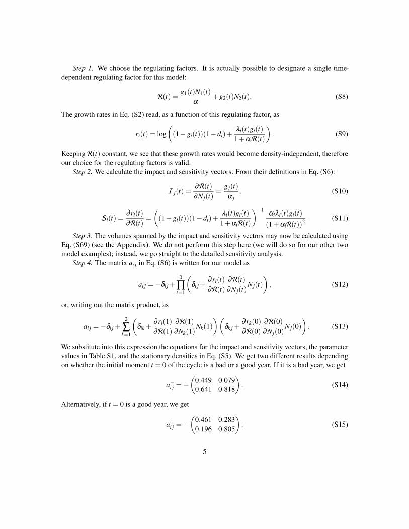
Step 1. We choose the regulating factors. It is actually possible to designate a single time-dependent regulating factor for this model:

R(t) = g1(t)N1(t)α

+g2(t)N2(t). (S8)

The growth rates in Eq. (S2) read, as a function of this regulating factor, as

ri(t) = log((1−gi(t))(1−di)+

λi(t)gi(t)1+αiR(t)

). (S9)

Keeping R(t) constant, we see that these growth rates would become density-independent, thereforeour choice for the regulating factors is valid.

Step 2. We calculate the impact and sensitivity vectors. From their definitions in Eq. (S6):

I j(t) =∂R(t)∂N j(t)

=g j(t)α j

, (S10)

Si(t) =∂ ri(t)∂R(t) =

((1−gi(t))(1−di)+

λi(t)gi(t)1+αiR(t)

)−1 αiλi(t)gi(t)

(1+αiR(t))2 . (S11)

Step 3. The volumes spanned by the impact and sensitivity vectors may now be calculated usingEq. (S69) (see the Appendix). We do not perform this step here (we will do so for our other twomodel examples); instead, we go straight to the detailed sensitivity analysis.

Step 4. The matrix ai j in Eq. (S6) is written for our model as

ai j =−δi j +0

∏t=1

(δi j +

∂ ri(t)∂R(t)

∂R(t)∂N j(t)

N j(t)), (S12)

or, writing out the matrix product, as

ai j =−δi j +2

∑k=1

(δik +

∂ ri(1)∂R(1)

∂R(1)∂Nk(1)

Nk(1))(

δk j +∂ rk(0)∂R(0)

∂R(0)∂N j(0)

N j(0)). (S13)

We substitute into this expression the equations for the impact and sensitivity vectors, the parametervalues in Table S1, and the stationary densities in Eq. (S5). We get two different results dependingon whether the initial moment t = 0 of the cycle is a bad or a good year. If it is a bad year, we get

a−i j =−(

0.449 0.0790.641 0.818

). (S14)

Alternatively, if t = 0 is a good year, we get

a+i j =−(

0.461 0.2830.196 0.805

). (S15)

5

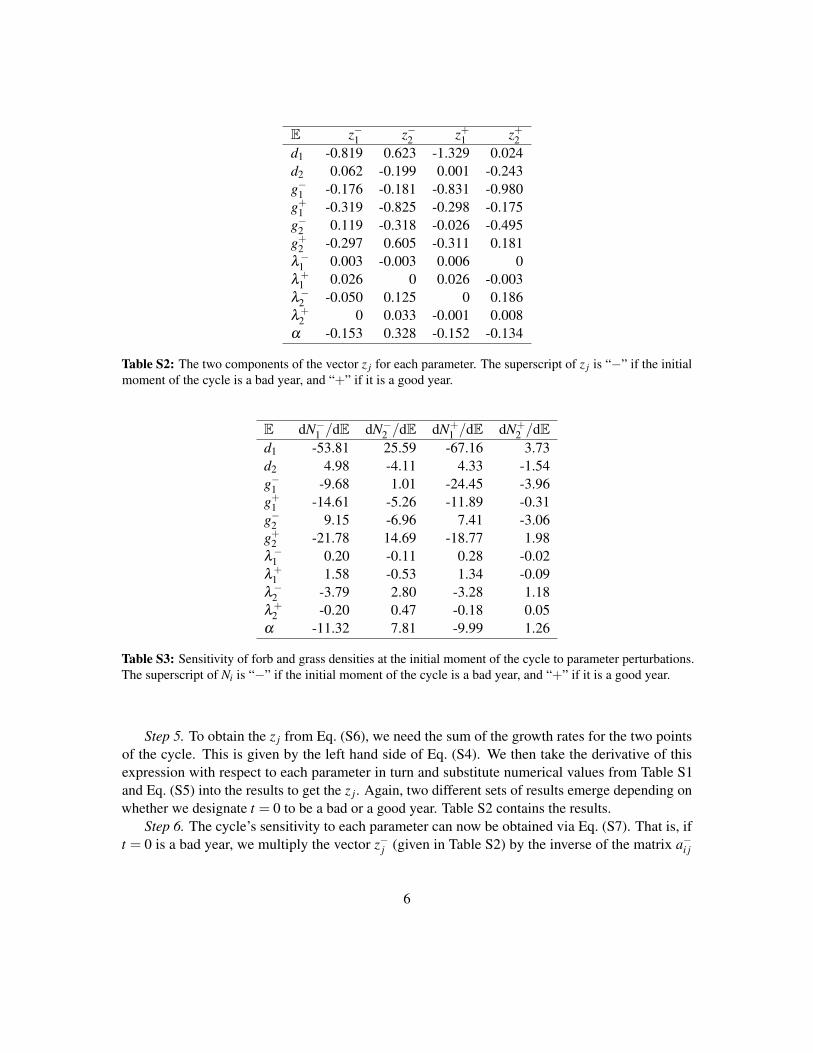
E z−1 z−2 z+1 z+2d1 -0.819 0.623 -1.329 0.024d2 0.062 -0.199 0.001 -0.243g−1 -0.176 -0.181 -0.831 -0.980g+1 -0.319 -0.825 -0.298 -0.175g−2 0.119 -0.318 -0.026 -0.495g+2 -0.297 0.605 -0.311 0.181λ−1 0.003 -0.003 0.006 0λ+

1 0.026 0 0.026 -0.003λ−2 -0.050 0.125 0 0.186λ+

2 0 0.033 -0.001 0.008α -0.153 0.328 -0.152 -0.134

Table S2: The two components of the vector z j for each parameter. The superscript of z j is “−” if the initialmoment of the cycle is a bad year, and “+” if it is a good year.

E dN−1 /dE dN−2 /dE dN+1 /dE dN+

2 /dEd1 -53.81 25.59 -67.16 3.73d2 4.98 -4.11 4.33 -1.54g−1 -9.68 1.01 -24.45 -3.96g+1 -14.61 -5.26 -11.89 -0.31g−2 9.15 -6.96 7.41 -3.06g+2 -21.78 14.69 -18.77 1.98λ−1 0.20 -0.11 0.28 -0.02λ+

1 1.58 -0.53 1.34 -0.09λ−2 -3.79 2.80 -3.28 1.18λ+

2 -0.20 0.47 -0.18 0.05α -11.32 7.81 -9.99 1.26

Table S3: Sensitivity of forb and grass densities at the initial moment of the cycle to parameter perturbations.The superscript of Ni is “−” if the initial moment of the cycle is a bad year, and “+” if it is a good year.

Step 5. To obtain the z j from Eq. (S6), we need the sum of the growth rates for the two pointsof the cycle. This is given by the left hand side of Eq. (S4). We then take the derivative of thisexpression with respect to each parameter in turn and substitute numerical values from Table S1and Eq. (S5) into the results to get the z j. Again, two different sets of results emerge depending onwhether we designate t = 0 to be a bad or a good year. Table S2 contains the results.

Step 6. The cycle’s sensitivity to each parameter can now be obtained via Eq. (S7). That is, ift = 0 is a bad year, we multiply the vector z−j (given in Table S2) by the inverse of the matrix a−i j

6

times minus one. Since the sensitivity σi is given by the derivative of the densities divided by thedensities (Eq. S6), we multiply the result by N−i (given in Eq. S5) to obtain dNi(0)/dE. If t = 0 is agood year, then we multiply z+j by the inverse of a+i j and then multiply by minus one times N+

i . SeeTable S3 for all sensitivity values.

As a final remark, we emphasize again that coexistence in this model is maintained purelyby environmental fluctuations. Using the framework and terminology of Chesson, coexistenceis maintained by pure storage effect (Chesson & Warner 1981, Chesson 1994, 2000). Relativenonlinearity is not operating because R(t) is a linear function of the population densities (Eq. S8),and fluctuation-independent mechanisms are also not operating because in the absence of fluctuationsthere is just a single regulating factor and therefore no coexistence.∗ Therefore the only stabilizingmechanism is the temporal storage effect. We highlight that our sensitivity approach to understandingcoexistence differs from Chesson’s in that Chesson uses the invader’s long-term growth rate to seewhether coexistence is possible via mutual invasibility, while the sensitivity approach quantifiescoexistence via the range of parameters that will allow for it. See Barabás et al. (2012, Appendix 3)and Barabás & Ostling (2013, Section 4) for the precise mathematical relationship between the twoframeworks.

∗A single regulating factor means the impact and sensitivity vectors are confined to a one-dimensional space. Thevolume spanned by the vectors of more than one species is therefore necessarily zero, leading to loss of robustness andthe breakdown of coexistence.

7

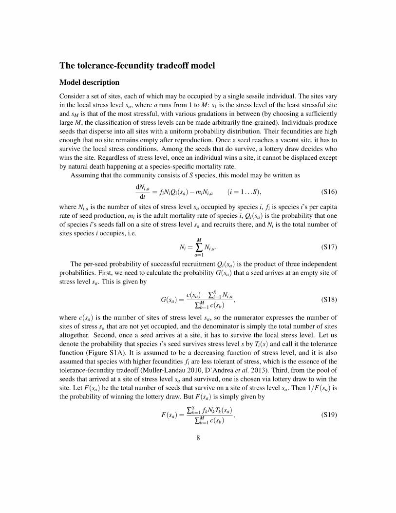
The tolerance-fecundity tradeoff model

Model description

Consider a set of sites, each of which may be occupied by a single sessile individual. The sites varyin the local stress level sa, where a runs from 1 to M: s1 is the stress level of the least stressful siteand sM is that of the most stressful, with various gradations in between (by choosing a sufficientlylarge M, the classification of stress levels can be made arbitrarily fine-grained). Individuals produceseeds that disperse into all sites with a uniform probability distribution. Their fecundities are highenough that no site remains empty after reproduction. Once a seed reaches a vacant site, it has tosurvive the local stress conditions. Among the seeds that do survive, a lottery draw decides whowins the site. Regardless of stress level, once an individual wins a site, it cannot be displaced exceptby natural death happening at a species-specific mortality rate.

Assuming that the community consists of S species, this model may be written as

dNi,a

dt= fiNiQi(sa)−miNi,a (i = 1 . . .S), (S16)

where Ni,a is the number of sites of stress level sa occupied by species i, fi is species i’s per capitarate of seed production, mi is the adult mortality rate of species i, Qi(sa) is the probability that oneof species i’s seeds fall on a site of stress level sa and recruits there, and Ni is the total number ofsites species i occupies, i.e.

Ni =M

∑a=1

Ni,a. (S17)

The per-seed probability of successful recruitment Qi(sa) is the product of three independentprobabilities. First, we need to calculate the probability G(sa) that a seed arrives at an empty site ofstress level sa. This is given by

G(sa) =c(sa)−∑S

i=1 Ni,a

∑Mb=1 c(sb)

, (S18)

where c(sa) is the number of sites of stress level sa, so the numerator expresses the number ofsites of stress sa that are not yet occupied, and the denominator is simply the total number of sitesaltogether. Second, once a seed arrives at a site, it has to survive the local stress level. Let usdenote the probability that species i’s seed survives stress level s by Ti(s) and call it the tolerancefunction (Figure S1A). It is assumed to be a decreasing function of stress level, and it is alsoassumed that species with higher fecundities fi are less tolerant of stress, which is the essence of thetolerance-fecundity tradeoff (Muller-Landau 2010, D’Andrea et al. 2013). Third, from the pool ofseeds that arrived at a site of stress level sa and survived, one is chosen via lottery draw to win thesite. Let F(sa) be the total number of seeds that survive on a site of stress level sa. Then 1/F(sa) isthe probability of winning the lottery draw. But F(sa) is simply given by

F(sa) =∑S

k=1 fkNkTk(sa)

∑Mb=1 c(sb)

, (S19)

8

the total number of surviving seeds divided by the total number of sites. Therefore, Qi(sa) may bewritten

Qi(sa) = G(sa)Ti(sa)1

F(sa)= Ti(sa)

c(sa)−∑Si=1 Ni,a

∑Sk=1 fkNkTk(sa)

. (S20)

Substituting this expression into Eq. (S16) yields

dNi,a

dt= fiNiTi(sa)

c(sa)−∑Si=1 Ni,a

∑Sk=1 fkNkTk(sa)

−miNi,a. (S21)

Let us cast this model equation in the form of traditional structured population models:

dNi,a

dt=

M

∑b=1

(fiTi(sa)

c(sa)−∑Si=1 Ni,a

∑Sk=1 fkNkTk(sa)

−miδab

)Ni,b, (S22)

where we used Eq. (S17) in the first term on the right hand side, and the δab in the second termis the identity matrix, equal to 1 if a = b and to 0 otherwise. The expression in parentheses is theprojection matrix Ai,ab of species i, multiplying the stage distribution vector Ni,b:

Ai,ab = fiTi(sa)c(sa)−∑S

i=1 Ni,a

∑Sk=1 fkNkTk(sa)

−miδab. (S23)

The model therefore describes a community of interacting structured populations in continuous time,where the ath stage class of species i measures the number of sites of stress level sa that species ioccupies.

Sensitivity analysis

For the tolerance-fecundity tradeoff model we are only performing qualitative sensitivity analysis,i.e., we calculate the impact and sensitivity vectors and the volumes they span but do not evaluatethe full sensitivity formula.

Step 0. As demonstrated elsewhere numerically (D’Andrea et al. 2013), this model converges toa stable equilibrium state. We therefore wish to analyze the sensitivity of this fixed point, generatedby the model which is in continuous time and involves population structure. The appropriatesensitivity formulas are therefore given by

σi =dNi

dE, ai j = ∑

µ

(∑a,b

vi,a∂Ai,ab

∂Rµwi,b

)

︸ ︷︷ ︸Si,µ

(∑c

∂Rµ

∂N j,cw j,c

)

︸ ︷︷ ︸I j,µ

, z j = ∑a,b

v j,a∂A j,ab

∂Ew j,b (S24)

(Szilágyi & Meszéna 2009, Barabás et al. 2014), where vi,a and wi,a are the ath component of theleft and right leading eigenvectors of Ai,ab, respectively. Note that these are simplified expressions;

9

the fully general form (which we do not need here) is found in Box 3 of the main text or in Barabáset al. (2014, Eq. 29). For these formulas to hold, the normalization conditions

M

∑a=1

wi,a = 1,M

∑a=1

vi,awi,a = 1 (S25)

have to be observed for all i. Biologically, since Eq. (S24) is evaluated at equilibrium, the leftleading eigenvector is the reproductive value vector while the right leading eigenvector is the stablestage distribution.

In general we would need to solve the model for the equilibrium state. This model is complicatedenough that this would only be possible using numerical simulations. However, as we will see,explicit knowledge of the equilibrium state is not needed to draw useful qualitative conclusionsabout the behavior of this system.

Step 1. We choose the regulating factors. Notice that the Ai,ab depend on the densities onlythrough the fraction in the first term of Eq. (S23). Therefore a natural choice for the regulatingfactors is

R(sa) =c(sa)−∑S

i=1 Ni,a

∑Sk=1 fkNkTk(sa)

=G(sa)

F(sa), (S26)

which is the density-dependent factor in Qi(sa). The projection matrices then read

Ai,ab = fiTi(sa)R(sa)−miδab, (S27)

which is density-independent if we keep R(sa) artificially fixed for all a, i.e., this is indeed a properchoice for the regulating factors.

In this model, space is the only limiting resource. However, space is not homogeneous, as sitesdiffer in stress level. One therefore has to measure crowding for each stress level separately, resultingin M different regulating factors, the R(sa) for every a. If the gradation of various stress levels isinfinitely fine-grained (i.e., we have a smooth stress gradient), M→ ∞ and we have infinitely manyregulating factors, in perfect analogy with a resource continuum.

Step 2a. We first calculate the sensitivity vectors, and then the impact vectors (Step 2b). FromEq. (S24), the sensitivity of the ith species to the µth regulating factor reads

Si,µ =M

∑a=1

M

∑b=1

vi,a∂Ai,ab

∂R(sµ)wi,b. (S28)

The derivative can be calculated directly using Eq. (S27):

∂Ai,ab

∂R(sµ)=

∂∂R(sµ)

(fiTi(sa)R(sa)−miδab

)= fiTi(sa)δaµ . (S29)

To evaluate the eigenvectors of Ai,ab, notice first that the second term on the right hand side ofEq. (S27) is proportional to the identity matrix and does not influence the eigenvectors. Therefore,

10

only the first term (let us denote it by Uab) needs to be considered for calculating eigenvectors. Thisfirst term can also be written Uab = gahb, where ga = fiTi(sa)R(sa) and hb = 1 (each component ofhb is equal to 1). Such a matrix has only one right and corresponding left eigenvector (given by ga

and hb themselves) such that their corresponding eigenvalue is nonzero. Indeed, for any vector xa,

M

∑b=1

Uabxb =M

∑b=1

gahbxb = ga

(M

∑b=1

hbxb

), (S30)

therefore xa = ga is the only right eigenvector with a nonzero eigenvalue. Similarly, ha is the onlyleft eigenvector with a nonzero eigenvalue, because for any vector xa,

M

∑b=1

xbUba =M

∑b=1

xbgbha = ha

(M

∑b=1

gbxb

). (S31)

From this it is also clear that the nonzero eigenvalue itself is given by ∑Ma=1 gaha. As both ga

and ha are, in our case, vectors with positive components, this eigenvalue must be some positivenumber. This means that, since all the other eigenvalues are zero, this eigenvalue is the leading one.Therefore, its left and right eigenvectors must correspond to the reproductive value and the stablestage distribution, respectively.

The stable stage distribution is then proportional to ga = fiTi(sa)R(sa):

wi,a = qi fiTi(sa)R(sa), (S32)

where

qi =

(M

∑a=1

fiTi(sa)R(sa)

)−1

(S33)

ensures proper normalization. Similarly, since ha = 1, the properly normalized left eigenvector is

vi,a = 1 (S34)

for all species. Using Eqs. (S29), (S32), and (S34), the sensitivity vectors can now be calculatedfrom the definition Eq. (S28):

Si,µ =M

∑a=1

M

∑b=1

vi,a∂Ai,ab

∂R(sµ)wi,b =

M

∑a=1

M

∑b=1

fiTi(sa)δaµqi fiTi(sb)R(sb)

=M

∑a=1

fiTi(sa)δaµqi

(M

∑b=1

fiTi(sb)R(sb)

)

︸ ︷︷ ︸1/qi

=M

∑a=1

fiTi(sa)δaµ = fiTi(sµ).(S35)

In words, the sensitivity vector of species i is its tolerance function weighted by its fecundity. Thiscan be evaluated without any knowledge of the system’s dynamics or current state.

11

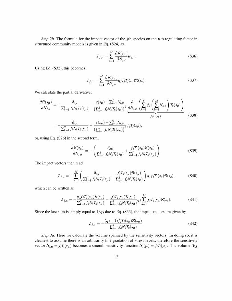
Step 2b. The formula for the impact vector of the jth species on the µth regulating factor instructured community models is given in Eq. (S24) as

I j,µ =M

∑a=1

∂R(sµ)

∂N j,aw j,a. (S36)

Using Eq. (S32), this becomes

I j,µ =M

∑a=1

∂R(sµ)

∂N j,aq j f jTj(sa)R(sa). (S37)

We calculate the partial derivative:

∂R(sµ)

∂N j,a=− δaµ

∑Sk=1 fkNkTk(sµ)

− c(sµ)−∑Si=1 Ni,µ(

∑Sk=1 fkNkTk(sµ)

)2∂

∂N j,a

(S

∑k=1

fk

(M

∑b=1

Nk,b

)Tk(sµ)

)

︸ ︷︷ ︸f jTj(sµ )

=− δaµ

∑Sk=1 fkNkTk(sµ)

− c(sµ)−∑Si=1 Ni,µ(

∑Sk=1 fkNkTk(sµ)

)2 f jTj(sµ),

(S38)

or, using Eq. (S26) in the second term,

∂R(sµ)

∂N j,a=−

(δaµ

∑Sk=1 fkNkTk(sµ)

+f jTj(sµ)R(sµ)

∑Sk=1 fkNkTk(sµ)

). (S39)

The impact vectors then read

I j,µ =−M

∑a=1

(δaµ

∑Sk=1 fkNkTk(sµ)

+f jTj(sµ)R(sµ)

∑Sk=1 fkNkTk(sµ)

)q j f jTj(sa)R(sa), (S40)

which can be written as

I j,µ =−q j f jTj(sµ)R(sµ)

∑Sk=1 fkNkTk(sµ)

− f jTj(sµ)R(sµ)

∑Sk=1 fkNkTk(sµ)

q j

M

∑a=1

f jTj(sa)R(sa). (S41)

Since the last sum is simply equal to 1/q j due to Eq. (S33), the impact vectors are given by

I j,µ =−(q j +1) f jTj(sµ)R(sµ)

∑Sk=1 fkNkTk(sµ)

. (S42)

Step 3a. Here we calculate the volume spanned by the sensitivity vectors. In doing so, it iscleanest to assume there is an arbitrarily fine gradation of stress levels, therefore the sensitivityvector Si,µ = fiTi(sµ) becomes a smooth sensitivity function Si(µ) = fiTi(µ). The volume VS

12

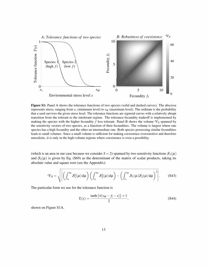
s1 sM

0

1

Environmental stress level s

Tole

rance

funct

ion

THsL

A: Tolerance functions of two species

Species 1

Hhigh f LSpecies 2

Hlow f L

0 5 100

5

10

Fecundity f1

Fec

undit

yf 2

B: Robustness of coexistence V S

0

20

40

60

0

0

5

10

Figure S1: Panel A shows the tolerance functions of two species (solid and dashed curves). The abscissarepresents stress, ranging from s1 (minimum level) to sM (maximum level). The ordinate is the probabilitythat a seed survives the given stress level. The tolerance functions are sigmoid curves with a relatively abrupttransition from the tolerant to the intolerant regime. The tolerance-fecundity tradeoff is implemented bymaking the species with the higher fecundity f less tolerant. Panel B shows the volume VS spanned bythe sensitivity vectors of two species, as a function of their fecundities. The volume is largest where onespecies has a high fecundity and the other an intermediate one. Both species possessing similar fecunditiesleads to small volumes. Since a small volume is sufficient for making coexistence oversensitive and thereforeunrealistic, it is only in the high-volume regions where coexistence is even a possibility.

(which is an area in our case because we consider S = 2) spanned by two sensitivity functions S1(µ)and S2(µ) is given by Eq. (S69) as the determinant of the matrix of scalar products, taking itsabsolute value and square root (see the Appendix):

VS =√√√√∣∣∣∣∣

(∫ sM

s1

S21(µ)dµ

)(∫ sM

s1

S22(µ)dµ

)−(∫ sM

s1

S1(µ)S2(µ)dµ)2∣∣∣∣∣. (S43)

The particular form we use for the tolerance function is

Ti(s) =tanh

(τ(sM− fi− s)

)+1

2, (S44)

shown on Figure S1A.

13

We can evaluate the integrals. The indefinite integral of S2i (µ) is

∫S2

i (µ)dµ = f 2i

∫T 2

i (µ)dµ =f 2i

4

∫ (tanh

(τ(sM− fi−µ)

)+1)2 dµ

=− f 2i

4τ(tanh(τ ( fi +µ− sM))+2log(cosh(τ ( fi +µ− sM)))−2aµ)+ const,

(S45)

as is easily verified by taking the expression’s derivative with respect to µ . The definite integral thenreads

∫ sM

s1

S2i (µ)dµ =

f 2i

4τ(− tanh(τ ( fi))−2log(cosh(τ ( fi)))

+ tanh(τ ( fi + s1− sM))+2log(cosh(τ ( fi + s1− sM)))+2τsM−2s1τ).

(S46)

The other integral is∫S1(µ)S2(µ)dµ =

f1 f2

4τ(− log(cosh(τ ( f1 +µ− sM)))− log(cosh(τ ( f2 +µ− sM)))

+coth(( f1− f2)τ)(log(cosh(τ ( f2 +µ− sM)))− log(cosh(τ ( f1 +µ− sM))))+2µτ)

+const.

(S47)

Its definite integral is then∫ sM

s1

S1(µ)S2(µ)dµ =f1 f2

4τ(− log(cosh(τ ( f1 + sM− sM)))− log(cosh(τ ( f2)))

−coth(( f1− f2)τ) log(cosh(τ ( f1)))+ coth(( f1− f2)τ) log(cosh(τ ( f2)))

+ log(cosh(τ ( f1 + s1− sM)))+ log(cosh(τ ( f2 + s1− sM)))

+coth(( f1− f2)τ) log(cosh(τ ( f1 + s1− sM)))

−coth(( f1− f2)τ) log(cosh(τ ( f2 + s1− sM)))

+2τsM−2s1τ).

(S48)

Substituting Eqs. (S46) and (S48) into Eq. (S43), we get an explicit expression forVS as a functionof the two fecundities f1 and f2:

VS = f1 f2

4τ

∣∣∣∣(− tanh(τ( f1 + s1− sM))+2(− log(cosh(τ( f1 + s1− sM)))

+ log(cosh( f1τ))+ s1τ− sMτ)+ tanh( f1τ))(− tanh(τ( f2 + s1− sM))

+2(− log(cosh(τ( f2 + s1− sM)))+ log(cosh( f2τ))+ s1τ− sMτ)+ tanh( f2τ))−(− log(cosh(τ( f1 + s1− sM)))− log(cosh(τ( f2 + s1− sM)))

+coth(( f1− f2)τ)(− log(cosh(τ( f1 + s1− sM)))+ log(cosh(τ( f2 + s1− sM)))

+ log(cosh( f1τ))− log(cosh( f2τ)))+ log(cosh( f1τ))+ log(cosh( f2τ))

+2s1τ−2sMτ)2∣∣∣∣1/2

.

(S49)

14

This is the function plotted on Figure S1B, with s1 = 0, sM = 10, and τ = 1.Step 3b. The volume spanned by the impact vectors. As Eq. (S42) depends on the stationary

densities Nk, the volumeVI cannot be evaluated without knowing these quantities. However, thisvolume is not needed for drawing qualitative conclusions based on the sensitivity vectors only, forthe following reason.

In Eq. (S42), Tj(sµ) and R(sµ) in the numerator are are quantities whose values fall between0 and 1. The denominator expresses the seed rain, and since we have made the assumption at theoutset that the seed rain contains at least one seed per empty site, the denominator cannot be smallerthan 1. The magnitude of any one component of the jth sensitivity vector therefore cannot exceed(q j +1) f j. There is no reason why this factor should be very large: f j is a rate and so proportionalto the log of the annual seed production, while q j is simply a normalizing constant. This means thatevery component of each impact vector is bounded in magnitude. Therefore, the volume spanned bythese vectors will also be bounded.

Since robustness is determined byVIVS, this observation means that whenever the volumespanned by the sensitivity vectors is small, robustness will also necessarily be small, becauseVI isbounded from above and so cannot compensate for a smallVS.

Moreover, we can see from Eq. (S42) that I j,µ is actually proportional to S j,µ = f jTj(sµ),thereforeVI will be large/small whereverVS is large/small.

This means that the volumes spanned by the sensitivity vectors are sufficient to determine therobustness of coexistence in the sense that wherever the sensitivity volume is small, coexistencecannot be expected to hold.

15

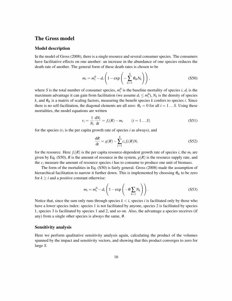
The Gross model

Model description

In the model of Gross (2008), there is a single resource and several consumer species. The consumershave facilitative effects on one another: an increase in the abundance of one species reduces thedeath rate of another. The general form of these death rates is chosen to be

mi = m0i −di

(1− exp

(−

S

∑k=1

θikNk

)), (S50)

where S is the total number of consumer species, m0i is the baseline mortality of species i, di is the

maximum advantage it can gain from facilitation (we assume di ≤ m0i ), Nk is the density of species

k, and θik is a matrix of scaling factors, measuring the benefit species k confers to species i. Sincethere is no self-facilitation, the diagonal elements are all zero: θii = 0 for all i = 1 . . .S. Using thesemortalities, the model equations are written

ri =1Ni

dNi

dt= fi(R)−mi (i = 1 . . .S) (S51)

for the species (ri is the per capita growth rate of species i as always), and

dRdt

= g(R)−S

∑i=1

ci fi(R)Ni (S52)

for the resource. Here fi(R) is the per capita resource-dependent growth rate of species i, the mi aregiven by Eq. (S50), R is the amount of resource in the system, g(R) is the resource supply rate, andthe ci measure the amount of resource species i has to consume to produce one unit of biomass.

The form of the mortalities in Eq. (S50) is fairly general. Gross (2008) made the assumption ofhierarchical facilitation to narrow it further down. This is implemented by choosing θik to be zerofor k ≥ i and a positive constant otherwise:

mi = m0i −di

(1− exp

(−θ ∑

k<iNk

)). (S53)

Notice that, since the sum only runs through species k < i, species i is facilitated only by those whohave a lower species index: species 1 is not facilitated by anyone, species 2 is facilitated by species1, species 3 is facilitated by species 1 and 2, and so on. Also, the advantage a species receives (ifany) from a single other species is always the same, θ .

Sensitivity analysis

Here we perform qualitative sensitivity analysis again, calculating the product of the volumesspanned by the impact and sensitivity vectors, and showing that this product converges to zero forlarge S.

16

Step 0. It was already proved by Gross (2008) that this system has a stable all-positive fixedpoint. In the two-species case, limit cycles were also observed. While they cannot be ruled out forS > 2, they have not been observed in numerical simulations. Even if there happen to be alternativeattractors in phase space, we will concentrate on the sensitivity of the nontrivial fixed point only.Fortunately, as we will see, an explicit knowledge of this equilibrium state will not be needed forour analysis.

Since the model is unstructured, continuous time, and we are analyzing the sensitivity of a fixedpoint, the appropriate sensitivity formulas are given by

σi =dNi

dE, ai j = ∑

µ

∂ ri

∂Rµ︸︷︷︸Si,µ

∂Rµ

∂N j︸︷︷︸I j,µ

, z j =∂ r j

∂E(S54)

(Meszéna et al. 2006).Step 1. We need to designate the regulating factors. We make the following choice:

R1 = R,

Rµ = exp

(−θ ∑

k<µNk

)(µ = 2 . . .S).

(S55)

Note that we could have made other choices as well—we could have made Rµ>1 = ∑k<µ Nk oreven just Rµ>1 = Nµ , as all these choices satisfy the criterion that keeping their values artificiallyfixed leads to the density-independence of the growth rates ri. However, performing the necessarycalculations may be easy with some choices and hard or even impossible with others. In our case, itturns out that Eq. (S55) lends itself to analytical treatment much better than the other choices (seebelow). The model equations, rewritten in terms of the regulating factors, are

r1 = f1(R1)−m01,

ri = fi(R1)−m0i +di (1−Ri) (i = 2 . . .S).

(S56)

We can see that our choice of regulating factors is valid, because fixing their values would make theper capita growth rates density-independent.

Step 2. The impact vectors I j,µ and sensitivity vectors Si,µ are calculated using Eq. (S54):

I j,µ =∂Rµ

∂N j=

(∂R1

∂N j,0, . . . ,0,−θR j+1︸ ︷︷ ︸

µ= j+1

,−θR j+2, . . . ,−θRS

), (S57)

Si,µ =∂ ri

∂Rµ=

(∂ fi

∂R1,0, . . . ,0, −di︸︷︷︸

µ=i

,0, . . . ,0), (S58)

where all quantities are evaluated at equilibrium.

17

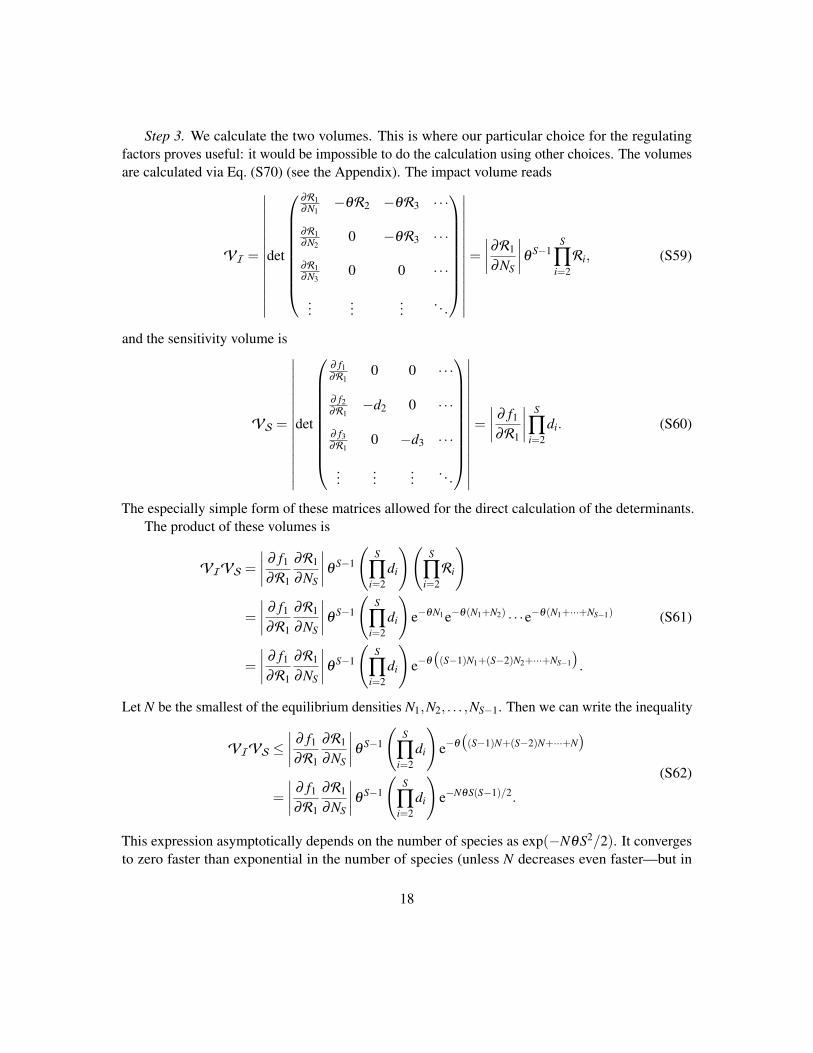
Step 3. We calculate the two volumes. This is where our particular choice for the regulatingfactors proves useful: it would be impossible to do the calculation using other choices. The volumesare calculated via Eq. (S70) (see the Appendix). The impact volume reads

VI =

∣∣∣∣∣∣∣∣∣∣∣∣∣∣

det

∂R1∂N1

−θR2 −θR3 · · ·∂R1∂N2

0 −θR3 · · ·∂R1∂N3

0 0 · · ·

......

.... . .

∣∣∣∣∣∣∣∣∣∣∣∣∣∣

=

∣∣∣∣∂R1

∂NS

∣∣∣∣θ S−1S

∏i=2Ri, (S59)

and the sensitivity volume is

VS =

∣∣∣∣∣∣∣∣∣∣∣∣∣∣∣

det

∂ f1∂R1

0 0 · · ·∂ f2∂R1

−d2 0 · · ·∂ f3∂R1

0 −d3 · · ·

......

.... . .

∣∣∣∣∣∣∣∣∣∣∣∣∣∣∣

=

∣∣∣∣∂ f1

∂R1

∣∣∣∣S

∏i=2

di. (S60)

The especially simple form of these matrices allowed for the direct calculation of the determinants.The product of these volumes is

VIVS =∣∣∣∣

∂ f1

∂R1

∂R1

∂NS

∣∣∣∣θ S−1

(S

∏i=2

di

)(S

∏i=2Ri

)

=

∣∣∣∣∂ f1

∂R1

∂R1

∂NS

∣∣∣∣θ S−1

(S

∏i=2

di

)e−θN1e−θ(N1+N2) · · ·e−θ(N1+···+NS−1)

=

∣∣∣∣∂ f1

∂R1

∂R1

∂NS

∣∣∣∣θ S−1

(S

∏i=2

di

)e−θ((S−1)N1+(S−2)N2+···+NS−1

).

(S61)

Let N be the smallest of the equilibrium densities N1,N2, . . . ,NS−1. Then we can write the inequality

VIVS ≤∣∣∣∣

∂ f1

∂R1

∂R1

∂NS

∣∣∣∣θ S−1

(S

∏i=2

di

)e−θ((S−1)N+(S−2)N+···+N

)

=

∣∣∣∣∂ f1

∂R1

∂R1

∂NS

∣∣∣∣θ S−1

(S

∏i=2

di

)e−NθS(S−1)/2.

(S62)

This expression asymptotically depends on the number of species as exp(−NθS2/2). It convergesto zero faster than exponential in the number of species (unless N decreases even faster—but in

18

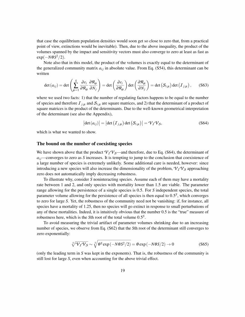
that case the equilibrium population densities would soon get so close to zero that, from a practicalpoint of view, extinctions would be inevitable). Then, due to the above inequality, the product of thevolumes spanned by the impact and sensitivity vectors must also converge to zero at least as fast asexp(−NθS2/2).

Note also that in this model, the product of the volumes is exactly equal to the determinant ofthe generalized community matrix ai j in absolute value. From Eq. (S54), this determinant can bewritten

det(ai j) = det

(S

∑µ=1

∂ ri

∂Rµ

∂Rµ

∂N j

)= det

(∂ ri

∂Rµ

)det(

∂Rµ

∂N j

)= det

(Si,µ)

det(I j,µ

), (S63)

where we used two facts: 1) that the number of regulating factors happens to be equal to the numberof species and therefore I j,µ and Si,µ are square matrices, and 2) that the determinant of a product ofsquare matrices is the product of the determinants. Due to the well-known geometrical interpretationof the determinant (see also the Appendix),

∣∣det(ai j)∣∣=∣∣det

(I j,µ)

det(Si,µ

)∣∣=VIVS, (S64)

which is what we wanted to show.

The bound on the number of coexisting species

We have shown above that the productVIVS—and therefore, due to Eq. (S64), the determinant ofai j—converges to zero as S increases. It is tempting to jump to the conclusion that coexistence ofa large number of species is extremely unlikely. Some additional care is needed, however: sinceintroducing a new species will also increase the dimensionality of the problem,VIVS approachingzero does not automatically imply decreasing robustness.

To illustrate why, consider S noninteracting species. Assume each of them may have a mortalityrate between 1 and 2, and only species with mortality lower than 1.5 are viable. The parameterrange allowing for the persistence of a single species is 0.5. For S independent species, the totalparameter volume allowing for the persistence of all species is then equal to 0.5S, which convergesto zero for large S. Yet, the robustness of the community need not be vanishing: if, for instance, allspecies have a mortality of 1.25, then no species will go extinct in response to small perturbations ofany of these mortalities. Indeed, it is intuitively obvious that the number 0.5 is the “true” measure ofrobustness here, which is the Sth root of the total volume 0.5S.

To avoid measuring the trivial artifact of parameter volumes shrinking due to an increasingnumber of species, we observe from Eq. (S62) that the Sth root of the determinant still converges tozero exponentially:

S√VIVS ∼ S

√θ S exp(−NθS2/2) = θ exp(−NθS/2)→ 0 (S65)

(only the leading term in S was kept in the exponents). That is, the robustness of the community isstill lost for large S, even when accounting for the above trivial effect.

19

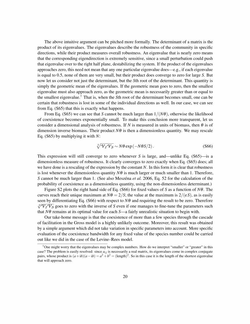
The above intuitive argument can be pitched more formally. The determinant of a matrix is theproduct of its eigenvalues. The eigenvalues describe the robustness of the community in specificdirections, while their product measures overall robustness. An eigenvalue that is nearly zero meansthat the corresponding eigendirection is extremely sensitive, since a small perturbation could pushthat eigenvalue over to the right half plane, destabilizing the system. If the product of the eigenvaluesapproaches zero, this need not mean that any one particular eigenvalue does—e.g., if each eigenvalueis equal to 0.5, none of them are very small, but their product does converge to zero for large S. Butnow let us consider not just the determinant, but the Sth root of the determinant. This quantity issimply the geometric mean of the eigenvalues. If the geometric mean goes to zero, then the smallesteigenvalue must also approach zero, as the geometric mean is necessarily greater than or equal tothe smallest eigenvalue.† That is, when the Sth root of the determinant becomes small, one can becertain that robustness is lost in some of the individual directions as well. In our case, we can seefrom Eq. (S65) that this is exactly what happens.

From Eq. (S65) we can see that S cannot be much larger than 1/(Nθ), otherwise the likelihoodof coexistence becomes exponentially small. To make this conclusion more transparent, let usconsider a dimensional analysis of robustness. If N is measured in units of biomass, then θ is ofdimension inverse biomass. Their product Nθ is then a dimensionless quantity. We may rescaleEq. (S65) by multiplying it with N:

S√VIVS ∼ Nθ exp(−NθS/2) . (S66)

This expression will still converge to zero whenever S is large, and—unlike Eq. (S65)—is adimensionless measure of robustness. It clearly converges to zero exactly when Eq. (S65) does; allwe have done is a rescaling of the expression by the constant N. In this form it is clear that robustnessis lost whenever the dimensionless quantity Nθ is much larger or much smaller than 1. Therefore,S cannot be much larger than 1. (See also Meszéna et al. 2006, Eq. 52 for the calculation of theprobability of coexistence as a dimensionless quantity, using the non-dimensionless determinant.)

Figure S2 plots the right hand side of Eq. (S66) for fixed values of S as a function of Nθ . Thecurves reach their unique maximum at Nθ = 2/S; the value at the maximum is 2/(eS), as is easilyseen by differentiating Eq. (S66) with respect to Nθ and requiring the result to be zero. Therefore

S√VIVS goes to zero with the inverse of S even if one manages to fine-tune the parameters suchthat Nθ remains at its optimal value for each S—a fairly unrealistic situation to begin with.

Our take-home message is that the coexistence of more than a few species through the cascadeof facilitation in the Gross model is a highly unlikely outcome. Moreover, this result was obtainedby a simple argument which did not take variation in specific parameters into account. More specificevaluation of the coexistence bandwidth for any fixed value of the species number could be carriedout like we did in the case of the Levine–Rees model.

†One might worry that the eigenvalues may be complex numbers. How do we interpret “smaller” or “greater” in thiscase? The problem is easily resolved: since ai j is necessarily a real matrix, its eigenvalues come in complex conjugatepairs, whose product is (a+ ib)(a− ib) = a2 +b2 = (length)2. So in this case it is the length of the shortest eigenvaluethat will approach zero.

20

0 0.4 0.8 1.20

0.04

0.08

0.12

Facilitative advantage NΘ

Robust

nes

sV

IV

S

S

S = 6

S = 8

S = 12

Figure S2: The robustness S√VIVS as a function of the (scaled) facilitative advantage Nθ for various values

of S, based on Eq. (S66). The most robust scenario always happens at an intermediate Nθ value.

Appendix: the volume spanned by a set of vectors

Suppose we are given a set of S vectors, with Wi,µ referring to the µth entry of the ith vector(i = 1 . . .S). We assume without loss of generality that µ = 1 . . .L, i.e., each vector has L entries (Lis not necessarily equal to S). To calculate the volumeVW of the parallelotope spanned by thesevectors, define the following matrix of scalar products:

Wi j =L

∑µ=1Wi,µW j,µ . (S67)

Note that, in case µ is a continuous as opposed to a discrete index (i.e., when we have functionsWi(µ) instead of vectorsWi,µ ), the summation above becomes integration with respect to µ:

Wi j =∫ µ1

µ0

Wi(µ)W j(µ)dµ, (S68)

where µ0 and µ1 are the appropriate limits of integration. Using Wi j, the volumeVW may now becalculated with the help of the so-called Gram determinant det(Wi j) (Gantmacher 1959):

VW =√∣∣det(Wi j)

∣∣. (S69)

There are two special cases for which this expression can be simplified. First,VW = 0 wheneverL < S. Second, for L = S, the formula simplifies to

VW =∣∣det

(Wi,µ)∣∣ (S70)

(Meszéna et al. 2006, Appendix C), whereWi,µ is treated as a (square) matrix with row index i andcolumn index µ .

21

References

Barabás, G., Meszéna, G. & Ostling, A. (2012). Community robustness and limiting similarity inperiodic environments. Theoretical Ecology, 5, 265–282.

Barabás, G. & Ostling, A. (2013). Community robustness in discrete-time periodic environments.Ecological Complexity, 15, 122–130.

Barabás, G., Meszéna, G. & Ostling, A. (2014). Fixed point sensitivity analysis of interactingstructured populations. Theoretical Population Biology, 92, 97–106.

Chesson, P. & Warner, R. R. (1981). Environmental variability promotes coexistence in lotterycompetitive systems. American Naturalist, 117, 923–943.

Chesson, P. (1994). Multispecies competition in variable environments. Theoretical PopulationBiology, 45, 227–276.

Chesson, P. (2000). Mechanisms of maintenance of species diversity. Annual Review of Ecologyand Systematics, 31, 343–366.

D’Andrea, R., Barabás, G. & Ostling, A. (2013). Revising the tolerance-fecundity trade-off; or, onthe consequences of discontinuous resource use for limiting similarity, species diversity, and traitdispersion. American Naturalist, 181, E91–101.

Gantmacher, F. R. (1959). Matrix theory. Chelsea Publishing, New York.

Gross, K. (2008). Positive interactions among competitors can produce species-rich communities.Ecology Letters, 11, 929–936.

Levine, J. M. & Rees, M. (2004). Effects of temporal variability on rare plant persistence in annualsystems. American Naturalist, 164, 350–363.

Meszéna, G., Gyllenberg, M., Pásztor, L. & Metz, J. A. J. (2006). Competitive exclusion andlimiting similarity: a unified theory. Theoretical Population Biology, 69, 68–87.

Muller-Landau, H. C. (2010). The tolerance-fecundity trade-off and the maintenance of diversity inseed size. Proceedings of the National Academy of Sciences of the USA, 107, 4242–4247.

Szilágyi, A. & Meszéna, G. (2009). Limiting similarity and niche theory for structured populations.Journal of Theoretical Biology, 258, 27–37.

22