Selection and Genome Plasticity as the Key Factors in the Evolution of Bacteria

Itamar Sela,* Yuri I. Wolf, and Eugene V. Koonin†

National Center for Biotechnology Information, National Library of Medicine,National Institutes of Health, Bethesda, Maryland 20894, USA

(Received 10 December 2018; revised manuscript received 6 June 2019; published 5 August 2019)

In prokaryotes, the number of genes in different functional classes shows apparent universal scaling withthe total number of genes that can be approximated by a power law, with a sublinear, near-linear, orsuperlinear scaling exponent. These dependences are gene class specific but hold across the entire diversityof bacteria and archaea. Several models have been proposed to explain these universal scaling laws,primarily based on the specifics of the respective biological functions. However, a population-genetictheory of universal scaling is lacking. We employ a simple mathematical model for prokaryotic genomeevolution, which, together with the analysis of 34 clusters of closely related bacterial genomes, allows us toidentify the underlying factors that govern the evolution of the genome content. Evolution of the genecontent is dominated by two functional class-specific parameters: selection coefficient and genomeplasticity. The selection coefficient quantifies the fitness cost associated with deletion of a gene in a givenfunctional class or the advantage of successful incorporation of an additional gene. Genome plasticityreflects both the availability of the genes of a given class in the external gene pool that is accessible to theevolving population and the ability of microbes to accommodate these genes in the short term, that is, theclass-specific horizontal gene transfer barrier. The selection coefficient determines the gene loss rate,whereas genome plasticity is the principal determinant of the gene gain rate.

DOI: 10.1103/PhysRevX.9.031018 Subject Areas: Biological Physics,Interdisciplinary Physics

I. INTRODUCTION

Comparative analyses of prokaryotic genomes show thatthe number of genes in different functional classes scalesdifferentially with the genome size [1–6]. The scaling lawsare robust under various statistical tests [5], across differentdatabases, and for different gene classifications [2–6]. Inthe seminal analysis of scaling, van Nimwegen fitted thescaling to a power law of the form [2]

x1 ¼ ηxγ; ð1Þ

where x1 denotes the number of genes that belong to aspecific functional class, and x is the total number of genes.Power laws are the simplest functions that give good fits tothe gene scaling data [2,5]. Analysis of the scalingexponents γ has shown that such exponents are (nearly)universal for each functional class across a broad range of

microbes (notwithstanding some debate on the validity ofthe exact universality [5,7]), suggesting that differences inscaling reflect important not yet understood features ofcellular organization and its evolution. In attempts toexplain the empirical observation that power-law scalingis a good fit to the genomic data, several theoretical modelshave been proposed, as outlined below.In the first, now classic analysis of scaling laws, van

Nimwegen grouped the functional classes of genes alongthree integer exponents 0,1,2, arguing that deviations fromthe integers, as demonstrated in the dataset analyzed here(Fig. 1 and Table I), most likely reflected gene classifica-tion ambiguities [2]. The gene classes with the 0 exponentinclude information processing systems (translation, basaltranscription, and replication), those with the exponent of 1are primarily genes for metabolic enzymes and transporters,whereas those with the exponent of 2 encode variousregulatory proteins. The essential information processingsystems are universally conserved and remain nearly thesame in all microbes regardless of genome size; metabolicnetworks expand proportionally to the genome growth, andthe complexity of regulatory circuits increases quadrati-cally with the total number of genes (i.e., linearly with thenumber of potential interactions between gene products).To put this conceptual thinking on quantitative ground, thetoolbox model has been proposed to explain the quadratic

*itamar.sela@nih.gov†koonin@ncbi.nlm.nih.gov

Published by the American Physical Society under the terms ofthe Creative Commons Attribution 4.0 International license.Further distribution of this work must maintain attribution tothe author(s) and the published article’s title, journal citation,and DOI.

PHYSICAL REVIEW X 9, 031018 (2019)

2160-3308=19=9(3)=031018(19) 031018-1 Published by the American Physical Society

scaling, whereby the number of regulators grows faster thanthe number of metabolic enzymes thanks to the frequentreuse of the latter enzymes in new pathways [8,9].Subsequently, the toolbox model has been extended toassume that the gene composition of prokaryotic genomesis determined by selection for fixed proportions of genesfrom different functional classes; under this assumption, themodel recapitulates both the scaling laws and the distri-bution of gene family sizes within each functional class[10]. The linear scaling was also obtained under a theo-retical model with two classes of genes, internal (house-keeping) and external (ecological), and a reproductive rateset to be independent of the genome size [11]. Finally,given that prokaryotic genome evolution is dominated by

extensive gene loss and horizontal gene transfer (HGT)[12–16], it has been hypothesized that the universalexponents are determined by distinct gene gain and lossrates for different classes of genes and reflect the innovationpotential of these classes [17]. Clearly, regulatory geneshave the highest innovation potential, whereas informationprocessing systems have next to none.Although the power laws provide good fits to the

genomic data, the origin of the observed scaling remainsobscure. Given that genome sizes barely span 2 orders ofmagnitude (Fig. 1), the power-law fits should be treated asapproximations rather than firmly established quantitativelaws. More importantly, although the models surveyedabove account for the power-law fit to the genomic data,

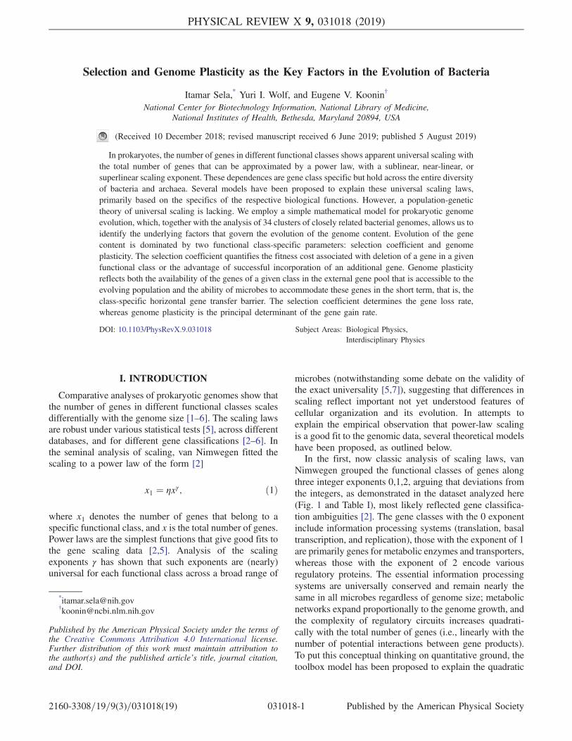
FIG. 1. The scaling laws for all functional classes of the COGs. The number of genes in each functional class scales with the totalnumber of genes, and the scaling exponents substantially differ between the classes. The number of genes in a given COG category isplotted against the total number of genes, together with a power-law fit and model fit, as given by Eq. (2). Each gray point represents onegenome from the analyzed set of 1490 genomes. The scaling is fitted to a power law which is indicated by a solid gray line. The fittedscaling exponent is indicated in parentheses. Red points correspond to the mean values for each ATGC in the dataset, and the model fit ofEq. (2) is shown by the solid red line.

SELA, WOLF, and KOONIN PHYS. REV. X 9, 031018 (2019)

031018-2

they stop short of a general theory of genome evolutionrooted in population genetics that would yield power lawsor even account for the observed scaling.Here, we analyze a simple population genetics model for

prokaryotic genome evolution [18]. Genome evolution ismodeled as a stochastic process of gene gains and losses,and we formulate an explicit model for the gene gainand loss rates within the theory of population genetics.In previous studies, this modeling framework was devel-oped and utilized to analyze the evolution of prokaryoticgenome size [18,19], i.e., the number of genes. Here, wepresent two substantial extensions to the model that enableus to analyze the scaling laws and extract the underlyingevolutionary factors. First, within the same modelingframework, we analyze the evolution of distinct functionalclasses of genes. Second, we analyze, also in a class-specific manner, the divergent evolution of genome contentwhich is measured by the number of orthologs shared by apair of genomes [20]. The scaling we obtain under thismodel does not follow a power law and does not yieldinteger exponents. Extraction of model parameters from thegenomic data engenders two major challenges. First, itis essential to extract independently the factors thatdictate gain and loss rates. This is achieved by accountingfor the divergence of genome content which depends on theloss rate only. Second, to infer the dependence of theevolutionary factors on the genome size, it is essential tocompare different groups of microbes that evolve underspecific local influences [19]. To filter out such influences,

class-specific quantities are normalized by genomic means,and the ratios are used to extract model parameters.The analyses presented here show that prokaryotic

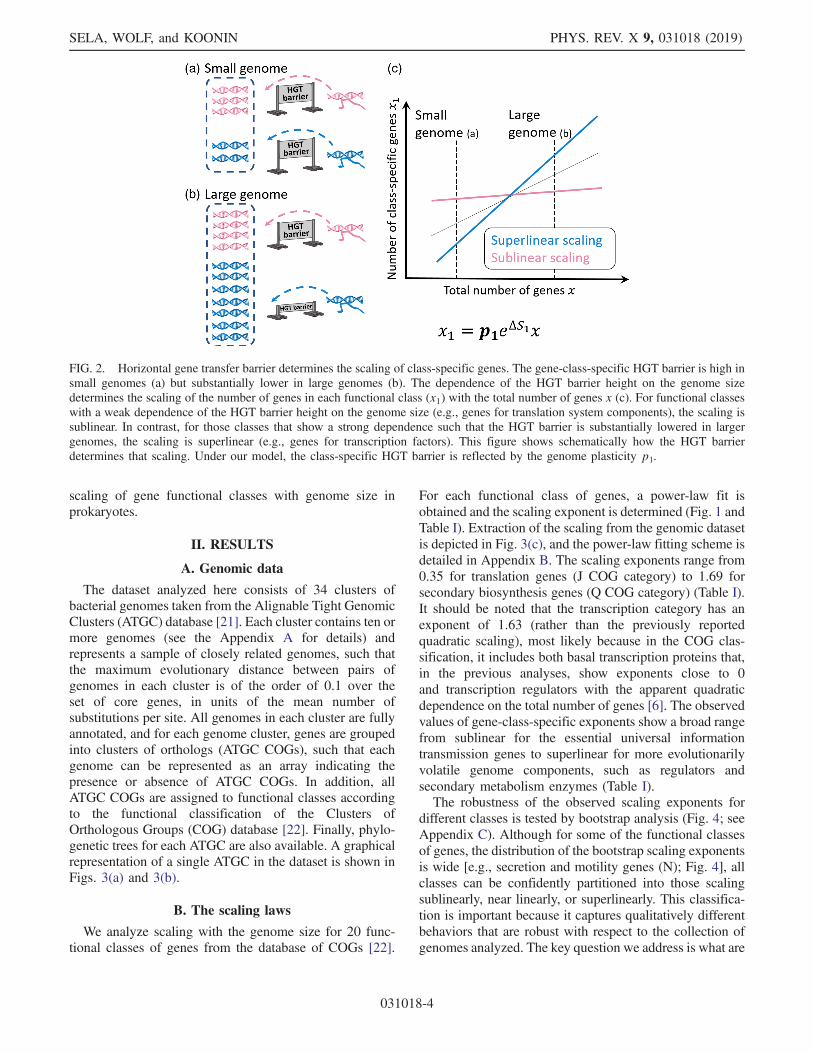
evolution is dominated by two underlying factors: selectioncoefficient and genome plasticity. While the selectioncoefficient is a standard quantity in population genetics,genome plasticity is an evolutionary factor that emergedfrom the analysis presented here, and it is the principledeterminant of the gene gain rate. The class-specificgenome plasticity reflects both the abundance of the genesof a given functional class in the external gene pool fromwhich genes can be captured by the evolving microbialpopulation, and the class-specific HGT barrier, i.e., theability of genomes to absorb new genes from the givenclass. The HGT barrier not only decreases with the numberof genes, but the reduction in the barrier height is classspecific and dictates the scaling. To illustrate these findings,two representative genomes of different sizes are illustratedin Fig. 2 as collections of genes [Figs. 2(a) and 2(b)]. Thereduction in the HGT-barrier height is modest in functionalclasses that scale sublinearly and comprise a similarfraction of the genome across different groups of microbes,largely, independent of the genome size [Fig. 2(c)]. Incontrast, in the classes that scale superlinearly with thegenome size, the reduction in the HGT-barrier height isdramatic, allowing for frequent acquisition and fast turn-over rate of the respective genes. Thus, in this work, wepresent a simple population-genetic theory that uncoversthe evolutionary factors underlying the observed universal

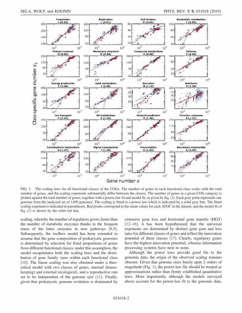
TABLE I. Scaling, selection, and plasticity in different functional classes of microbial genes.

Class FunctionsScaling

exponent γΔS1

slope −qAverage selectioncoefficient hΔS1i

Averageplasticity hp1i

Plasticityslope b

J Translation 0.35 −1.10 × 10−2 2.68 0.005 1.54 × 10−5L Replication and repair 0.51 −1.35 × 10−3 0.98 0.013 −9.18 × 10−5D Cell division 0.64 −1.58 × 10−5 1.83 0.002 −3.21 × 10−5F Nucleotide metabolism and transport 0.69 −1.75 × 10−2 2.15 0.003 3.65 × 10−5O Post-translational modification,

protein turnover, and chaperone functions0.83 −5.42 × 10−3 1.38 0.010 4.88 × 10−5

M Membrane and cell wall structure and biogenesis 0.88 −1.05 × 10−3 0.65 0.029 4.57 × 10−5H Coenzyme metabolism 0.88 −4.68 × 10−3 1.51 0.011 4.62 × 10−5V Defense 0.94 −3.72 × 10−7 −0.44 0.034 −6.68 × 10−5C Energy production and conversion 1.00 −4.52 × 10−3 1.19 0.017 8.92 × 10−5I Lipid metabolism 1.08 −4.86 × 10−3 0.92 0.016 1.24 × 10−4N Secretion and motility 1.18 −7.13 × 10−8 0.27 0.014 1.07 × 10−4X Mobilome: prophages, transposons 1.24 −2.06 × 10−4 −4.76 1.021 1.12 × 10−2P Inorganic ion transport and metabolism 1.24 −3.76 × 10−3 0.75 0.026 1.15 × 10−4E Amino acid metabolism and transport 1.24 −1.90 × 10−3 1.12 0.028 8.15 × 10−5R General functional prediction only 1.26 −1.05 × 10−3 0.37 0.051 1.15 × 10−4S Function unknown 1.27 −5.92 × 10−7 0.55 0.025 3.35 × 10−5G Carbohydrate metabolism and transport 1.47 −1.86 × 10−3 0.46 0.041 1.65 × 10−4T Signal transduction 1.49 −1.28 × 10−3 0.57 0.030 1.25 × 10−4K Transcription 1.63 −1.67 × 10−3 0.27 0.058 1.81 × 10−4Q Biosynthesis, transport, and catabolism

of secondary metabolites1.69 −5.77 × 10−3 0.06 0.021 2.54 × 10−4

SELECTION AND GENOME PLASTICITY AS THE KEY FACTORS … PHYS. REV. X 9, 031018 (2019)

031018-3

scaling of gene functional classes with genome size inprokaryotes.

II. RESULTS

A. Genomic data

The dataset analyzed here consists of 34 clusters ofbacterial genomes taken from the Alignable Tight GenomicClusters (ATGC) database [21]. Each cluster contains ten ormore genomes (see the Appendix A for details) andrepresents a sample of closely related genomes, such thatthe maximum evolutionary distance between pairs ofgenomes in each cluster is of the order of 0.1 over theset of core genes, in units of the mean number ofsubstitutions per site. All genomes in each cluster are fullyannotated, and for each genome cluster, genes are groupedinto clusters of orthologs (ATGC COGs), such that eachgenome can be represented as an array indicating thepresence or absence of ATGC COGs. In addition, allATGC COGs are assigned to functional classes accordingto the functional classification of the Clusters ofOrthologous Groups (COG) database [22]. Finally, phylo-genetic trees for each ATGC are also available. A graphicalrepresentation of a single ATGC in the dataset is shown inFigs. 3(a) and 3(b).

B. The scaling laws

We analyze scaling with the genome size for 20 func-tional classes of genes from the database of COGs [22].

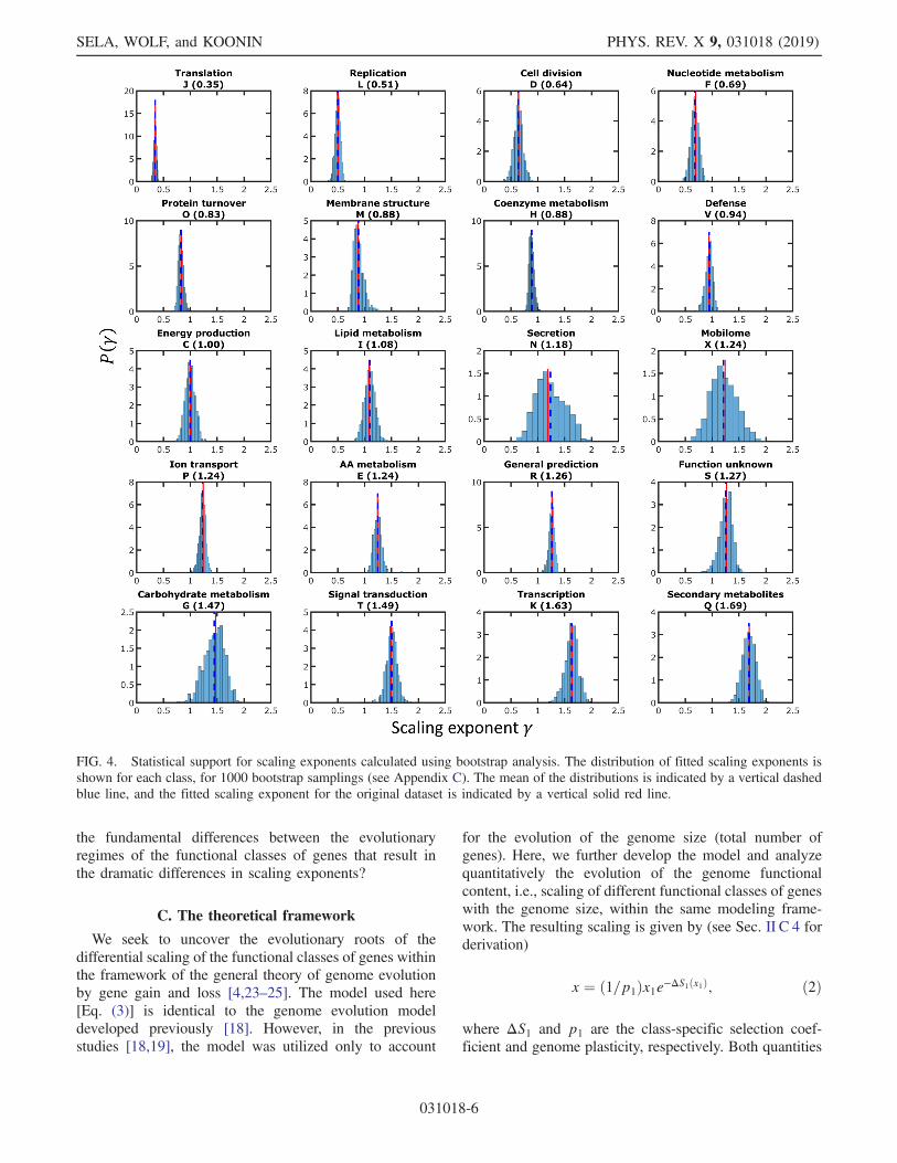
For each functional class of genes, a power-law fit isobtained and the scaling exponent is determined (Fig. 1 andTable I). Extraction of the scaling from the genomic datasetis depicted in Fig. 3(c), and the power-law fitting scheme isdetailed in Appendix B. The scaling exponents range from0.35 for translation genes (J COG category) to 1.69 forsecondary biosynthesis genes (Q COG category) (Table I).It should be noted that the transcription category has anexponent of 1.63 (rather than the previously reportedquadratic scaling), most likely because in the COG clas-sification, it includes both basal transcription proteins that,in the previous analyses, show exponents close to 0and transcription regulators with the apparent quadraticdependence on the total number of genes [6]. The observedvalues of gene-class-specific exponents show a broad rangefrom sublinear for the essential universal informationtransmission genes to superlinear for more evolutionarilyvolatile genome components, such as regulators andsecondary metabolism enzymes (Table I).The robustness of the observed scaling exponents for

different classes is tested by bootstrap analysis (Fig. 4; seeAppendix C). Although for some of the functional classesof genes, the distribution of the bootstrap scaling exponentsis wide [e.g., secretion and motility genes (N); Fig. 4], allclasses can be confidently partitioned into those scalingsublinearly, near linearly, or superlinearly. This classifica-tion is important because it captures qualitatively differentbehaviors that are robust with respect to the collection ofgenomes analyzed. The key question we address is what are

FIG. 2. Horizontal gene transfer barrier determines the scaling of class-specific genes. The gene-class-specific HGT barrier is high insmall genomes (a) but substantially lower in large genomes (b). The dependence of the HGT barrier height on the genome sizedetermines the scaling of the number of genes in each functional class (x1) with the total number of genes x (c). For functional classeswith a weak dependence of the HGT barrier height on the genome size (e.g., genes for translation system components), the scaling issublinear. In contrast, for those classes that show a strong dependence such that the HGT barrier is substantially lowered in largergenomes, the scaling is superlinear (e.g., genes for transcription factors). This figure shows schematically how the HGT barrierdetermines that scaling. Under our model, the class-specific HGT barrier is reflected by the genome plasticity p1.

SELA, WOLF, and KOONIN PHYS. REV. X 9, 031018 (2019)

031018-4

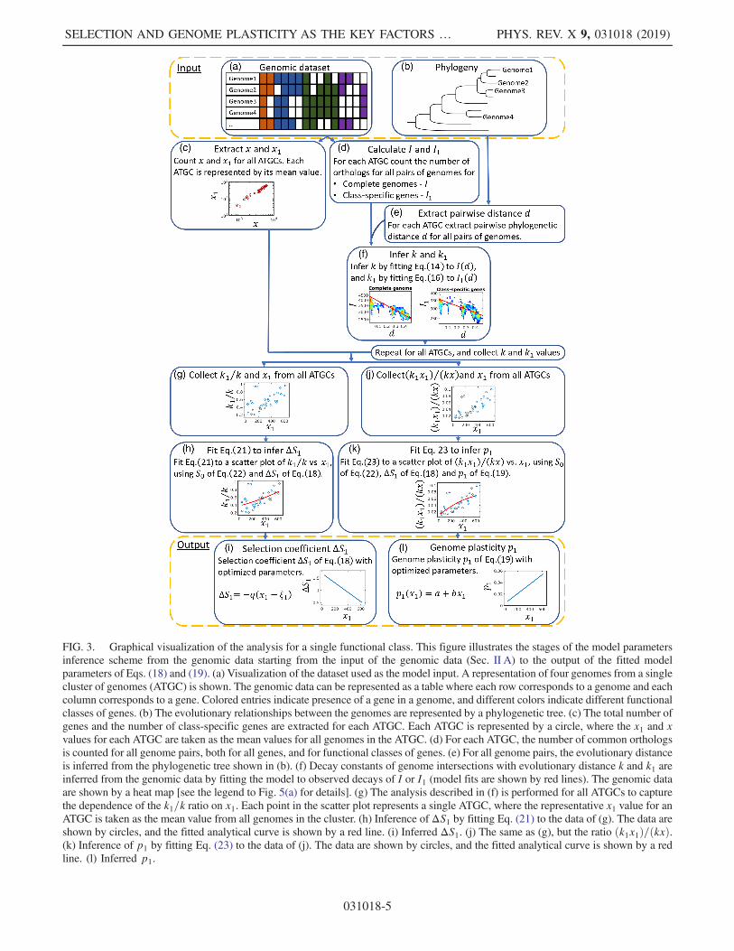
FIG. 3. Graphical visualization of the analysis for a single functional class. This figure illustrates the stages of the model parametersinference scheme from the genomic data starting from the input of the genomic data (Sec. II A) to the output of the fitted modelparameters of Eqs. (18) and (19). (a) Visualization of the dataset used as the model input. A representation of four genomes from a singlecluster of genomes (ATGC) is shown. The genomic data can be represented as a table where each row corresponds to a genome and eachcolumn corresponds to a gene. Colored entries indicate presence of a gene in a genome, and different colors indicate different functionalclasses of genes. (b) The evolutionary relationships between the genomes are represented by a phylogenetic tree. (c) The total number ofgenes and the number of class-specific genes are extracted for each ATGC. Each ATGC is represented by a circle, where the x1 and xvalues for each ATGC are taken as the mean values for all genomes in the ATGC. (d) For each ATGC, the number of common orthologsis counted for all genome pairs, both for all genes, and for functional classes of genes. (e) For all genome pairs, the evolutionary distanceis inferred from the phylogenetic tree shown in (b). (f) Decay constants of genome intersections with evolutionary distance k and k1 areinferred from the genomic data by fitting the model to observed decays of I or I1 (model fits are shown by red lines). The genomic dataare shown by a heat map [see the legend to Fig. 5(a) for details]. (g) The analysis described in (f) is performed for all ATGCs to capturethe dependence of the k1=k ratio on x1. Each point in the scatter plot represents a single ATGC, where the representative x1 value for anATGC is taken as the mean value from all genomes in the cluster. (h) Inference of ΔS1 by fitting Eq. (21) to the data of (g). The data areshown by circles, and the fitted analytical curve is shown by a red line. (i) Inferred ΔS1. (j) The same as (g), but the ratio ðk1x1Þ=ðkxÞ.(k) Inference of p1 by fitting Eq. (23) to the data of (j). The data are shown by circles, and the fitted analytical curve is shown by a redline. (l) Inferred p1.

SELECTION AND GENOME PLASTICITY AS THE KEY FACTORS … PHYS. REV. X 9, 031018 (2019)

031018-5

the fundamental differences between the evolutionaryregimes of the functional classes of genes that result inthe dramatic differences in scaling exponents?

C. The theoretical framework

We seek to uncover the evolutionary roots of thedifferential scaling of the functional classes of genes withinthe framework of the general theory of genome evolutionby gene gain and loss [4,23–25]. The model used here[Eq. (3)] is identical to the genome evolution modeldeveloped previously [18]. However, in the previousstudies [18,19], the model was utilized only to account

for the evolution of the genome size (total number ofgenes). Here, we further develop the model and analyzequantitatively the evolution of the genome functionalcontent, i.e., scaling of different functional classes of geneswith the genome size, within the same modeling frame-work. The resulting scaling is given by (see Sec. II C 4 forderivation)

x ¼ ð1=p1Þx1e−ΔS1ðx1Þ; ð2Þ

where ΔS1 and p1 are the class-specific selection coef-ficient and genome plasticity, respectively. Both quantities

FIG. 4. Statistical support for scaling exponents calculated using bootstrap analysis. The distribution of fitted scaling exponents isshown for each class, for 1000 bootstrap samplings (see Appendix C). The mean of the distributions is indicated by a vertical dashedblue line, and the fitted scaling exponent for the original dataset is indicated by a vertical solid red line.

SELA, WOLF, and KOONIN PHYS. REV. X 9, 031018 (2019)

031018-6

(ΔS1 and p1) are approximated by the first-order expansionand are extracted from the genomic data as detailed inSec. II D.In addition, the modeling framework is extended to

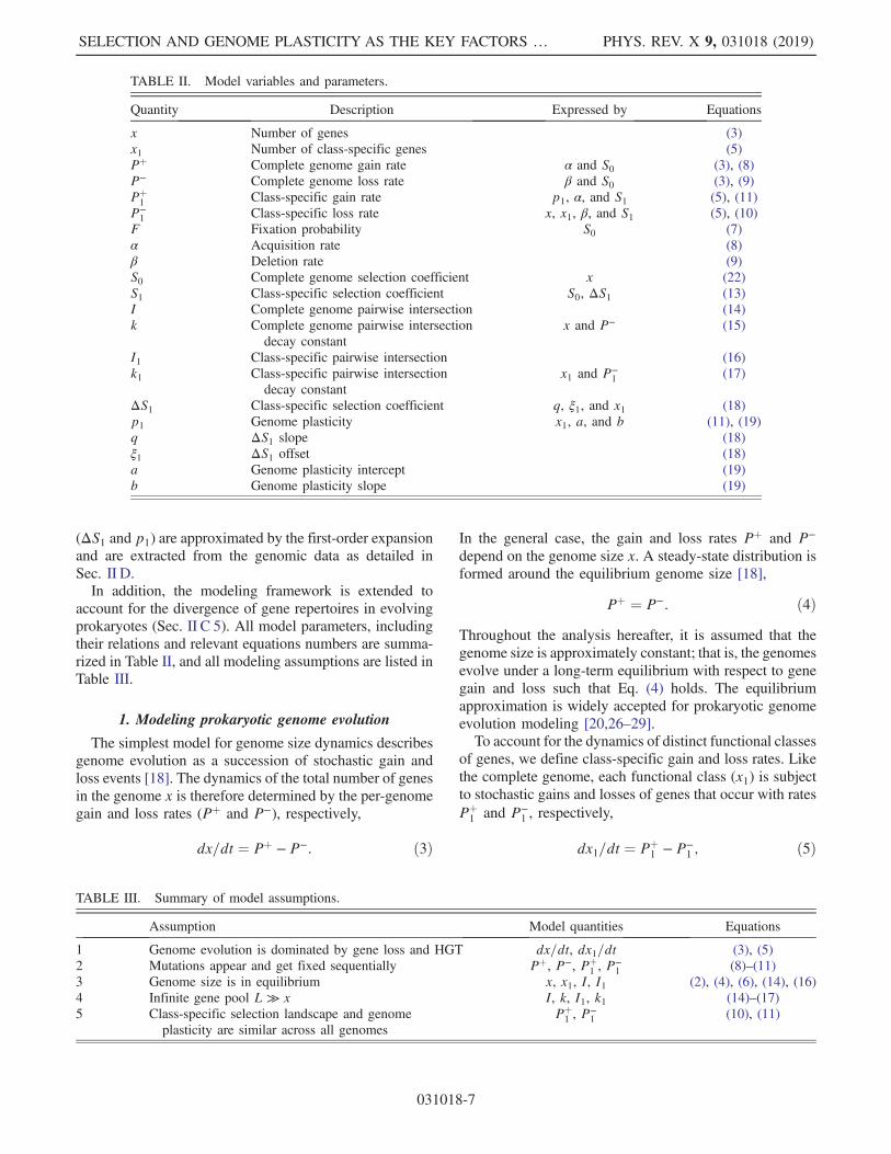
account for the divergence of gene repertoires in evolvingprokaryotes (Sec. II C 5). All model parameters, includingtheir relations and relevant equations numbers are summa-rized in Table II, and all modeling assumptions are listed inTable III.

1. Modeling prokaryotic genome evolution

The simplest model for genome size dynamics describesgenome evolution as a succession of stochastic gain andloss events [18]. The dynamics of the total number of genesin the genome x is therefore determined by the per-genomegain and loss rates (Pþ and P−), respectively,

dx=dt ¼ Pþ − P−: ð3Þ

In the general case, the gain and loss rates Pþ and P−

depend on the genome size x. A steady-state distribution isformed around the equilibrium genome size [18],

Pþ ¼ P−: ð4ÞThroughout the analysis hereafter, it is assumed that thegenome size is approximately constant; that is, the genomesevolve under a long-term equilibrium with respect to genegain and loss such that Eq. (4) holds. The equilibriumapproximation is widely accepted for prokaryotic genomeevolution modeling [20,26–29].To account for the dynamics of distinct functional classes

of genes, we define class-specific gain and loss rates. Likethe complete genome, each functional class (x1) is subjectto stochastic gains and losses of genes that occur with ratesPþ1 and P−

1 , respectively,

dx1=dt ¼ Pþ1 − P−

1 ; ð5Þ

TABLE II. Model variables and parameters.

Quantity Description Expressed by Equations

x Number of genes (3)x1 Number of class-specific genes (5)Pþ Complete genome gain rate α and S0 (3), (8)P− Complete genome loss rate β and S0 (3), (9)Pþ1 Class-specific gain rate p1, α, and S1 (5), (11)

P−1 Class-specific loss rate x, x1, β, and S1 (5), (10)

F Fixation probability S0 (7)α Acquisition rate (8)β Deletion rate (9)S0 Complete genome selection coefficient x (22)S1 Class-specific selection coefficient S0, ΔS1 (13)I Complete genome pairwise intersection (14)k Complete genome pairwise intersection

decay constantx and P− (15)

I1 Class-specific pairwise intersection (16)k1 Class-specific pairwise intersection

decay constantx1 and P−

1 (17)

ΔS1 Class-specific selection coefficient q, ξ1, and x1 (18)p1 Genome plasticity x1, a, and b (11), (19)q ΔS1 slope (18)ξ1 ΔS1 offset (18)a Genome plasticity intercept (19)b Genome plasticity slope (19)

TABLE III. Summary of model assumptions.

Assumption Model quantities Equations

1 Genome evolution is dominated by gene loss and HGT dx=dt, dx1=dt (3), (5)2 Mutations appear and get fixed sequentially Pþ, P−, Pþ

1 , P−1 (8)–(11)

3 Genome size is in equilibrium x, x1, I, I1 (2), (4), (6), (14), (16)4 Infinite gene pool L ≫ x I, k, I1, k1 (14)–(17)5 Class-specific selection landscape and genome

plasticity are similar across all genomesPþ1 , P

−1 (10), (11)

SELECTION AND GENOME PLASTICITY AS THE KEY FACTORS … PHYS. REV. X 9, 031018 (2019)

031018-7

with an equilibrium value x1 that satisfies

Pþ1 ¼ P−

1 : ð6Þ

In the next subsection, we express gain and loss ratesexplicitly and show how class-specific rates are related tothe overall genome gain and loss rates.

2. Explicit formulation for gene gainand loss rates for finite population

Assuming a finite effective population size under theweak genome dynamics limit (acquisition and deletionrates are low enough such that acquisitions and deletionsoccur and get fixed sequentially), the gene gain and lossrates can be expressed as the product of the mutation rateand the probability for the mutation to get fixed in thepopulation F [18]. The fixation probability depends on S0,the genomic mean of the selection coefficient normalizedby effective population size [30] (see Appendix D)

FðS0Þ ¼S0

1 − e−S0: ð7Þ

Following the seminal genome size analyses by Lynch andConery [31], we further assume that the organisms’ fitnesscan be expressed as a function of the number of genes. Thisassumption implies symmetry of the selective effects withrespect to gain and loss of a single gene: The benefit (orcost) is of equal magnitude for gain and loss events but withopposite signs [18,19]. Formally, if acquisition of a gene isassociated with a selection coefficient S0, deletion of thesame gene is associated with a selection coefficient −S0.Denoting acquisition and deletion rates by α and β,respectively, the gain and loss rates are

Pþ ¼ αðxÞFðS0Þ; ð8Þ

P− ¼ βðxÞFð−S0Þ: ð9Þ

The S0 value can be regarded as the mean selectivebenefit (or cost) associated with the acquisition or loss of arandom gene. In principle, the mean value of S0 could beobtained by measuring the selective effect that is associatedwith a deletion of one gene at a time and averaged over allgene deletions in all genomes and their respective envi-ronments. As we explain above, there is symmetry betweengain and loss events with respect to the selective effect.However, a closer examination of the gene acquisitionprocess reveals a more complicated picture that involvestwo distinct timescales. Even genetic material that isbeneficial on a large timescale appears to be measurablydeleterious initially so that fitness is recovered only after atransient time period of several hundred generations [32].In contrast, the coefficient S0 is inferred from extantgenomes and thus reflects the average cost (or benefit)

of gene deletion, and accordingly, the long-term averagebenefit (or cost) carried by a gene already incorporated inthe genome. Within this framework, the short timescale,that is, the transient phase of gene acquisition, is incorpo-rated into the gain rate of Eq. (8) through the acquisitionrate α. Specifically, α represents the combined effect of theDNA insertion rate and HGT barrier, that is, the probabilitythat the acquired gene is not eliminated from the populationwithin the short timescale.Gain and loss rates for genes that belong to a specific

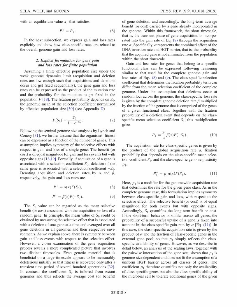
functional class can be expressed following reasoningsimilar to that used for the complete genome gain andloss rates of Eqs. (8) and (9). The class-specific selectioncoefficient that determines the fixation probability term candiffer from the mean selection coefficient of the completegenome. Under the assumption that deletions occur atrandom loci across the genome, the class-specific loss rateis given by the complete genome deletion rate β multipliedby the fraction of the genome that is comprised of the genesof a given functional class. Together with the fixationprobability of a deletion event that depends on the class-specific mean selection coefficient S1, this multiplicationgives

P−1 ¼ x1

xβðxÞFð−S1Þ: ð10Þ

The acquisition rate for class-specific genes is given bythe product of the global acquisition rate α, fixationprobability that depends on the class-specific mean selec-tion coefficient S1, and the class-specific genome plasticityp1,

Pþ1 ¼ p1αðxÞFðS1Þ: ð11Þ

Here, p1 is a modifier for the genomewide acquisition ratethat determines the rate for the given gene class. As in thecomplete genome case, this formulation implies symmetrybetween class-specific gain and loss, with respect to theselective effect: The selective benefit (or cost) is of equalmagnitude for both events but with opposite signs.Accordingly, S1 quantifies the long-term benefit or cost.If the short-term behavior is similar across all genes, theprobability of a successful uptake of a gene is taken intoaccount in the class-specific gain rate by α [Eq. (11)]. Inthis case, the class-specific acquisition rate is given by theproduct of α and the fraction of class-specific genes in theexternal gene pool, so that p1 simply reflects the class-specific availability of genes. However, as we describe indetail below, an analysis of the scaling laws, together withthe pairwise intersection of the gene sets, shows that p1 isgenome-size dependent and does not fit the assumption of auniform HGT barrier across all classes of genes. Thecoefficient p1 therefore quantifies not only the availabilityof class-specific genes but also the class-specific ability ofthe microbial cell to tolerate additional genes of the given

SELA, WOLF, and KOONIN PHYS. REV. X 9, 031018 (2019)

031018-8

functional class within the short timescale. Hence, wedenote p1 as class-specific genome plasticity.

3. Selection-drift balance in the evolution of genome size

The relation between the selection coefficient S0 and thedeletion bias β=α under the assumption of a steady state canbe obtained by substituting the explicit expressions for Pþand P− of Eqs. (8) and (9) into Eq. (4)

eS0 ¼ βðxÞ=αðxÞ: ð12Þ

Equation (12) quantifies the selection-drift balance withrespect to the evolution of the genome size. When genegain is beneficial and is associated with a positive selectioncoefficient S0, equilibrium is possible only when genedeletion is more frequent than acquisition ðβ > αÞ, suchthat the selective pressure towards genome growth isbalanced by the intrinsic deletion bias. Similarly, equilib-rium in the case when genome growth is counterselected,i.e., S0 < 0, is only possible when acquisitions occur morefrequently than deletions (β < α). Finally, in the specialcase when acquisition and deletion rates are equal (β ¼ α),equilibrium is possible only in the strictly neutral caseðS0 ¼ 0Þ. As demonstrated by our previous analysis, onaverage, S0 > 0, which requires a deletion bias to reachequilibrium in genome evolution [18,19]. Indeed, intrinsicdeletion bias had been consistently detected for diversegenomes [33–35]. As we show in the following subsection,the relation of Eq. (12) is also useful to relate x and x1, thatis, to obtain the model formulation for the scaling laws.

4. Model prediction for scaling of class-specificgenes with genome size

The relation between the number of class-specific genesx1 and the genome size x [Fig. 5(a)] of Eq. (2) can beobtained by substituting the explicit expressions for Pþ

1 andP−1 of Eqs. (10) and (11) into Eq. (6), together with the

relation for S0 and β=α of Eq. (12). The coefficient ΔS1 inEq. (2) is the mean selective (dis)advantage of a gene in thegiven functional class with respect to a random gene

ΔS1 ¼ S1 − S0: ð13Þ

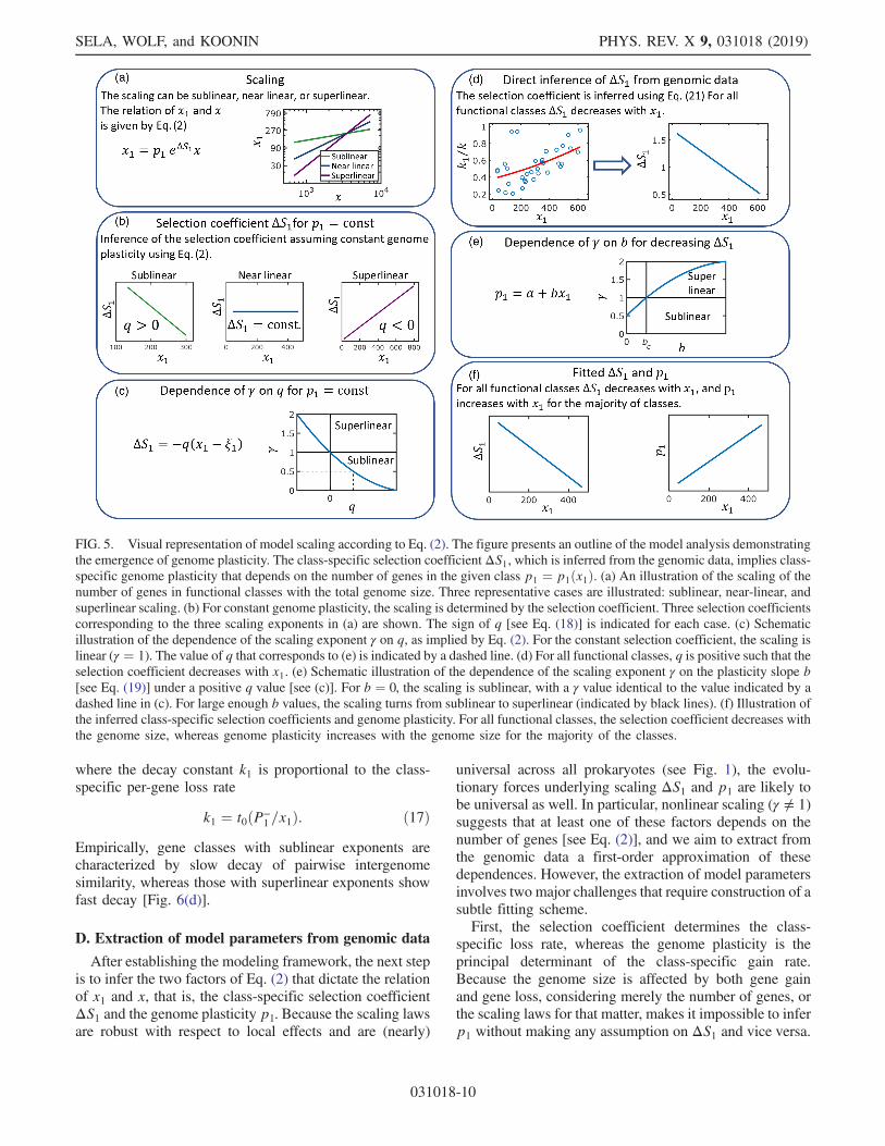
The scaling depends on two factors, class-specific genomeplasticity p1 and class-specific selection coefficient ΔS1,and can be interpreted as follows. If p1 is constant, thescaling is determined by ΔS1 [Fig. 5(b)]. For a constant(that is, independent of the number of genes in the class)ΔS1, the scaling is linear. Sublinear or superlinear scalingemerges when ΔS1 depends on the number of genesΔS1 ¼ ΔS1ðx1Þ. Specifically, the scaling is sublinear whenΔS1 decreases with x1 and superlinear when ΔS1 increaseswith x1 [Fig. 5(c)].

5. Model of genome content evolution

One of the key observable measures of microbialgenome evolution is the pairwise intersection betweengenomes (I), that is, the number of orthologous genesshared by a pair of genomes. Importantly, in this study weextend the modeling framework to account for the evolu-tion of the genome content, and not only the number ofgenes. As we show below, the model analysis demonstratesthat the pairwise intersection decays exponentially withthe evolutionary distances, which is incorporated into themodeling framework. Accounting for the evolution of thegenome content is a crucial extension of the model withrespect to previous studies [18,19] that allows inference ofthe class-specific selection coefficient from the genomicdata, as we explain in detail in the next section.Both the number of genes in a genome and the pairwise

intersections between gene complements result from thesame evolutionary processes of stochastic gene gain andloss events. A complete theoretical description of genomeevolution should therefore account for both of thesequantities. The stochastic gain and loss of genes entail adecay in pairwise genomes similarity through the course ofevolution, even when the total number of genes remainsapproximately constant. As a first-order approximation,given an infinite external gene pool [26], the pairwisegenome intersections decay exponentially with the treedistance d (see Appendix E for derivation)

IðdÞ ¼ xe−kd: ð14Þ

The rate of pairwise genome similarity decay is determinedsolely by the gene loss rate, with the decay constant kproportional to the per-gene loss rate

k ¼ t0ðP−=xÞ; ð15Þ

where t0 is a conversion constant from tree distance units totime units. This model fits comparative genomic observa-tions on the pairwise genome similarity decay with evolu-tionary distance in archaea, bacteria, and bacteriophages[20,36,37]. We test these observations on the ATGC setanalyzed in the present work and confirm the closeagreement of the model with the data [Fig. 6(a)].Extraction of the decay constants from the genomic datasetis depicted in Figs. 3(d)–3(f), and the fitting scheme isdetailed in Appendix B.With respect to the genome content, all quantities can be

defined for genomic subsets that include only genes from aspecific functional class. Similar to its complete genomeanalog, the class-specific pairwise intersection I1 (i.e., thenumber of genes of class 1 shared between the pair ofgenomes) decays exponentially with evolutionary distance[Figs. 6(b) and 6(c)]

I1ðdÞ ¼ x1e−k1d; ð16Þ

SELECTION AND GENOME PLASTICITY AS THE KEY FACTORS … PHYS. REV. X 9, 031018 (2019)

031018-9

where the decay constant k1 is proportional to the class-specific per-gene loss rate

k1 ¼ t0ðP−1 =x1Þ: ð17Þ

Empirically, gene classes with sublinear exponents arecharacterized by slow decay of pairwise intergenomesimilarity, whereas those with superlinear exponents showfast decay [Fig. 6(d)].

D. Extraction of model parameters from genomic data

After establishing the modeling framework, the next stepis to infer the two factors of Eq. (2) that dictate the relationof x1 and x, that is, the class-specific selection coefficientΔS1 and the genome plasticity p1. Because the scaling lawsare robust with respect to local effects and are (nearly)

universal across all prokaryotes (see Fig. 1), the evolu-tionary forces underlying scaling ΔS1 and p1 are likely tobe universal as well. In particular, nonlinear scaling (γ ≠ 1)suggests that at least one of these factors depends on thenumber of genes [see Eq. (2)], and we aim to extract fromthe genomic data a first-order approximation of thesedependences. However, the extraction of model parametersinvolves two major challenges that require construction of asubtle fitting scheme.First, the selection coefficient determines the class-

specific loss rate, whereas the genome plasticity is theprincipal determinant of the class-specific gain rate.Because the genome size is affected by both gene gainand gene loss, considering merely the number of genes, orthe scaling laws for that matter, makes it impossible to inferp1 without making any assumption on ΔS1 and vice versa.

FIG. 5. Visual representation of model scaling according to Eq. (2). The figure presents an outline of the model analysis demonstratingthe emergence of genome plasticity. The class-specific selection coefficient ΔS1, which is inferred from the genomic data, implies class-specific genome plasticity that depends on the number of genes in the given class p1 ¼ p1ðx1Þ. (a) An illustration of the scaling of thenumber of genes in functional classes with the total genome size. Three representative cases are illustrated: sublinear, near-linear, andsuperlinear scaling. (b) For constant genome plasticity, the scaling is determined by the selection coefficient. Three selection coefficientscorresponding to the three scaling exponents in (a) are shown. The sign of q [see Eq. (18)] is indicated for each case. (c) Schematicillustration of the dependence of the scaling exponent γ on q, as implied by Eq. (2). For the constant selection coefficient, the scaling islinear (γ ¼ 1). The value of q that corresponds to (e) is indicated by a dashed line. (d) For all functional classes, q is positive such that theselection coefficient decreases with x1. (e) Schematic illustration of the dependence of the scaling exponent γ on the plasticity slope b[see Eq. (19)] under a positive q value [see (c)]. For b ¼ 0, the scaling is sublinear, with a γ value identical to the value indicated by adashed line in (c). For large enough b values, the scaling turns from sublinear to superlinear (indicated by black lines). (f) Illustration ofthe inferred class-specific selection coefficients and genome plasticity. For all functional classes, the selection coefficient decreases withthe genome size, whereas genome plasticity increases with the genome size for the majority of the classes.

SELA, WOLF, and KOONIN PHYS. REV. X 9, 031018 (2019)

031018-10

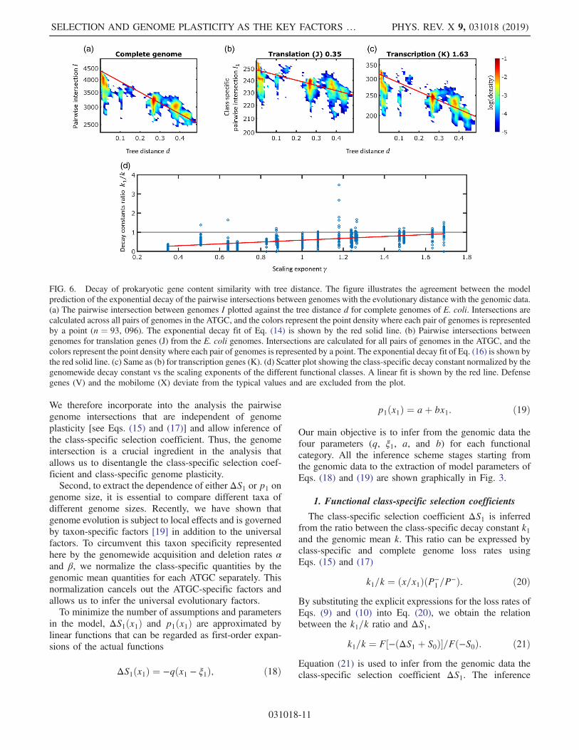
We therefore incorporate into the analysis the pairwisegenome intersections that are independent of genomeplasticity [see Eqs. (15) and (17)] and allow inference ofthe class-specific selection coefficient. Thus, the genomeintersection is a crucial ingredient in the analysis thatallows us to disentangle the class-specific selection coef-ficient and class-specific genome plasticity.Second, to extract the dependence of either ΔS1 or p1 on

genome size, it is essential to compare different taxa ofdifferent genome sizes. Recently, we have shown thatgenome evolution is subject to local effects and is governedby taxon-specific factors [19] in addition to the universalfactors. To circumvent this taxon specificity representedhere by the genomewide acquisition and deletion rates αand β, we normalize the class-specific quantities by thegenomic mean quantities for each ATGC separately. Thisnormalization cancels out the ATGC-specific factors andallows us to infer the universal evolutionary factors.To minimize the number of assumptions and parameters

in the model, ΔS1ðx1Þ and p1ðx1Þ are approximated bylinear functions that can be regarded as first-order expan-sions of the actual functions

ΔS1ðx1Þ ¼ −qðx1 − ξ1Þ; ð18Þ

p1ðx1Þ ¼ aþ bx1: ð19Þ

Our main objective is to infer from the genomic data thefour parameters (q, ξ1, a, and b) for each functionalcategory. All the inference scheme stages starting fromthe genomic data to the extraction of model parameters ofEqs. (18) and (19) are shown graphically in Fig. 3.

1. Functional class-specific selection coefficients

The class-specific selection coefficient ΔS1 is inferredfrom the ratio between the class-specific decay constant k1and the genomic mean k. This ratio can be expressed byclass-specific and complete genome loss rates usingEqs. (15) and (17)

k1=k ¼ ðx=x1ÞðP−1 =P

−Þ: ð20ÞBy substituting the explicit expressions for the loss rates ofEqs. (9) and (10) into Eq. (20), we obtain the relationbetween the k1=k ratio and ΔS1,

k1=k ¼ F½−ðΔS1 þ S0Þ�=Fð−S0Þ: ð21ÞEquation (21) is used to infer from the genomic data theclass-specific selection coefficient ΔS1. The inference

FIG. 6. Decay of prokaryotic gene content similarity with tree distance. The figure illustrates the agreement between the modelprediction of the exponential decay of the pairwise intersections between genomes with the evolutionary distance with the genomic data.(a) The pairwise intersection between genomes I plotted against the tree distance d for complete genomes of E. coli. Intersections arecalculated across all pairs of genomes in the ATGC, and the colors represent the point density where each pair of genomes is representedby a point (n ¼ 93, 096). The exponential decay fit of Eq. (14) is shown by the red solid line. (b) Pairwise intersections betweengenomes for translation genes (J) from the E. coli genomes. Intersections are calculated for all pairs of genomes in the ATGC, and thecolors represent the point density where each pair of genomes is represented by a point. The exponential decay fit of Eq. (16) is shown bythe red solid line. (c) Same as (b) for transcription genes (K). (d) Scatter plot showing the class-specific decay constant normalized by thegenomewide decay constant vs the scaling exponents of the different functional classes. A linear fit is shown by the red line. Defensegenes (V) and the mobilome (X) deviate from the typical values and are excluded from the plot.

SELECTION AND GENOME PLASTICITY AS THE KEY FACTORS … PHYS. REV. X 9, 031018 (2019)

031018-11

stages are depicted in Figs. 3(g)–3(i), and technical detailsof the optimization procedure are given in Appendix F. Thegenomewide selection coefficient S0 is determined basedon our previous results [19], where we found that thecomplete genome selection coefficient S0 is related to thetotal number of genes x by

S0 ¼ ln ð0.7x0.06Þ: ð22Þ

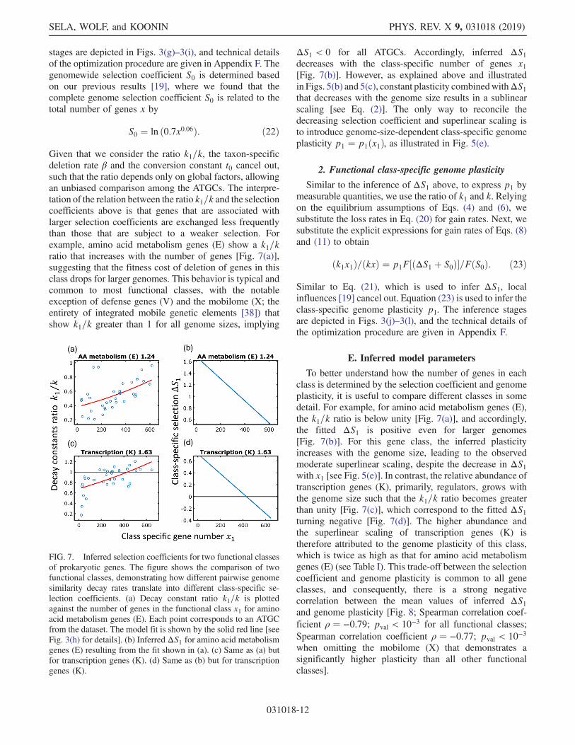
Given that we consider the ratio k1=k, the taxon-specificdeletion rate β and the conversion constant t0 cancel out,such that the ratio depends only on global factors, allowingan unbiased comparison among the ATGCs. The interpre-tation of the relation between the ratio k1=k and the selectioncoefficients above is that genes that are associated withlarger selection coefficients are exchanged less frequentlythan those that are subject to a weaker selection. Forexample, amino acid metabolism genes (E) show a k1=kratio that increases with the number of genes [Fig. 7(a)],suggesting that the fitness cost of deletion of genes in thisclass drops for larger genomes. This behavior is typical andcommon to most functional classes, with the notableexception of defense genes (V) and the mobilome (X; theentirety of integrated mobile genetic elements [38]) thatshow k1=k greater than 1 for all genome sizes, implying

ΔS1 < 0 for all ATGCs. Accordingly, inferred ΔS1decreases with the class-specific number of genes x1[Fig. 7(b)]. However, as explained above and illustratedin Figs. 5(b) and 5(c), constant plasticity combinedwithΔS1that decreases with the genome size results in a sublinearscaling [see Eq. (2)]. The only way to reconcile thedecreasing selection coefficient and superlinear scaling isto introduce genome-size-dependent class-specific genomeplasticity p1 ¼ p1ðx1Þ, as illustrated in Fig. 5(e).

2. Functional class-specific genome plasticity

Similar to the inference of ΔS1 above, to express p1 bymeasurable quantities, we use the ratio of k1 and k. Relyingon the equilibrium assumptions of Eqs. (4) and (6), wesubstitute the loss rates in Eq. (20) for gain rates. Next, wesubstitute the explicit expressions for gain rates of Eqs. (8)and (11) to obtain

ðk1x1Þ=ðkxÞ ¼ p1F½ðΔS1 þ S0Þ�=FðS0Þ: ð23Þ

Similar to Eq. (21), which is used to infer ΔS1, localinfluences [19] cancel out. Equation (23) is used to infer theclass-specific genome plasticity p1. The inference stagesare depicted in Figs. 3(j)–3(l), and the technical details ofthe optimization procedure are given in Appendix F.

E. Inferred model parameters

To better understand how the number of genes in eachclass is determined by the selection coefficient and genomeplasticity, it is useful to compare different classes in somedetail. For example, for amino acid metabolism genes (E),the k1=k ratio is below unity [Fig. 7(a)], and accordingly,the fitted ΔS1 is positive even for larger genomes[Fig. 7(b)]. For this gene class, the inferred plasticityincreases with the genome size, leading to the observedmoderate superlinear scaling, despite the decrease in ΔS1with x1 [see Fig. 5(e)]. In contrast, the relative abundance oftranscription genes (K), primarily, regulators, grows withthe genome size such that the k1=k ratio becomes greaterthan unity [Fig. 7(c)], which correspond to the fitted ΔS1turning negative [Fig. 7(d)]. The higher abundance andthe superlinear scaling of transcription genes (K) istherefore attributed to the genome plasticity of this class,which is twice as high as that for amino acid metabolismgenes (E) (see Table I). This trade-off between the selectioncoefficient and genome plasticity is common to all geneclasses, and consequently, there is a strong negativecorrelation between the mean values of inferred ΔS1and genome plasticity [Fig. 8; Spearman correlation coef-ficient ρ ¼ −0.79; pval < 10−3 for all functional classes;Spearman correlation coefficient ρ ¼ −0.77; pval < 10−3

when omitting the mobilome (X) that demonstrates asignificantly higher plasticity than all other functionalclasses].

FIG. 7. Inferred selection coefficients for two functional classesof prokaryotic genes. The figure shows the comparison of twofunctional classes, demonstrating how different pairwise genomesimilarity decay rates translate into different class-specific se-lection coefficients. (a) Decay constant ratio k1=k is plottedagainst the number of genes in the functional class x1 for aminoacid metabolism genes (E). Each point corresponds to an ATGCfrom the dataset. The model fit is shown by the solid red line [seeFig. 3(h) for details]. (b) Inferred ΔS1 for amino acid metabolismgenes (E) resulting from the fit shown in (a). (c) Same as (a) butfor transcription genes (K). (d) Same as (b) but for transcriptiongenes (K).

SELA, WOLF, and KOONIN PHYS. REV. X 9, 031018 (2019)

031018-12

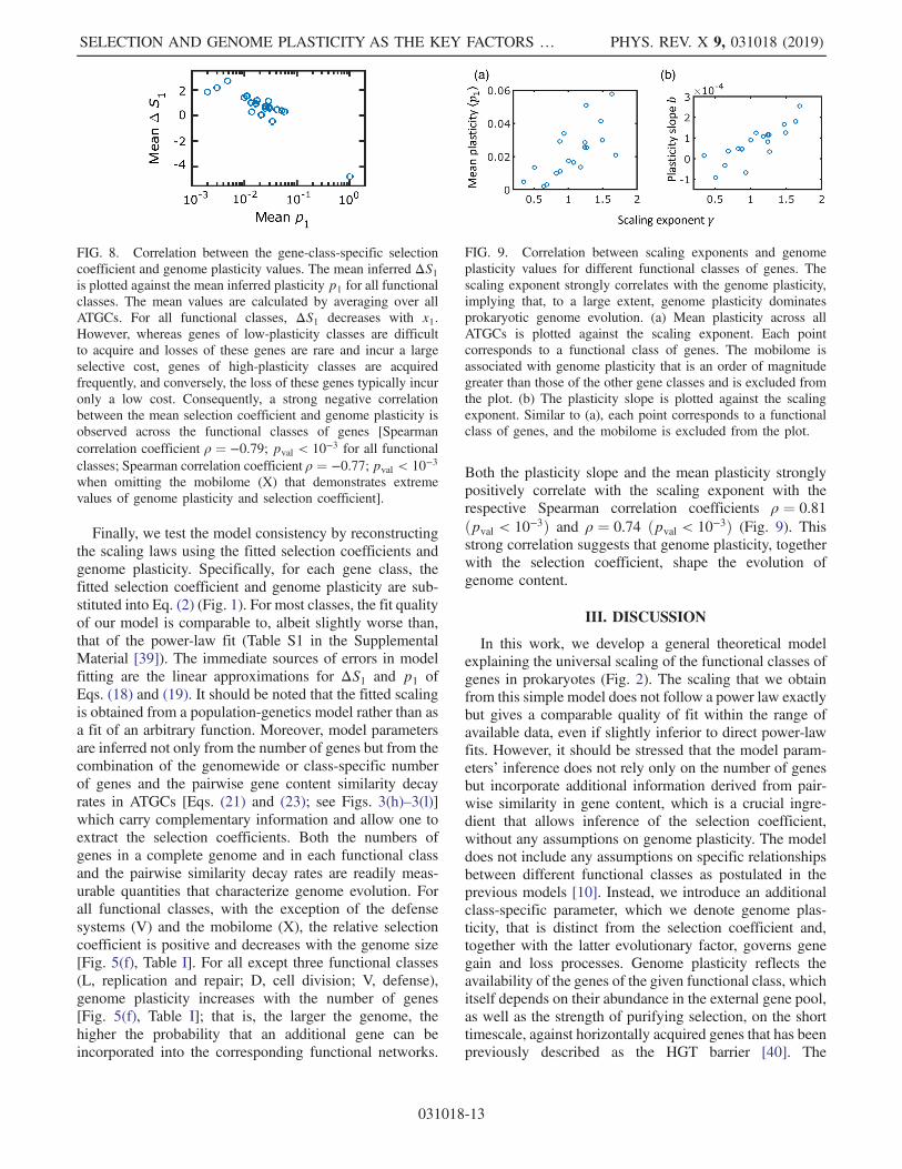
Finally, we test the model consistency by reconstructingthe scaling laws using the fitted selection coefficients andgenome plasticity. Specifically, for each gene class, thefitted selection coefficient and genome plasticity are sub-stituted into Eq. (2) (Fig. 1). For most classes, the fit qualityof our model is comparable to, albeit slightly worse than,that of the power-law fit (Table S1 in the SupplementalMaterial [39]). The immediate sources of errors in modelfitting are the linear approximations for ΔS1 and p1 ofEqs. (18) and (19). It should be noted that the fitted scalingis obtained from a population-genetics model rather than asa fit of an arbitrary function. Moreover, model parametersare inferred not only from the number of genes but from thecombination of the genomewide or class-specific numberof genes and the pairwise gene content similarity decayrates in ATGCs [Eqs. (21) and (23); see Figs. 3(h)–3(l)]which carry complementary information and allow one toextract the selection coefficients. Both the numbers ofgenes in a complete genome and in each functional classand the pairwise similarity decay rates are readily meas-urable quantities that characterize genome evolution. Forall functional classes, with the exception of the defensesystems (V) and the mobilome (X), the relative selectioncoefficient is positive and decreases with the genome size[Fig. 5(f), Table I]. For all except three functional classes(L, replication and repair; D, cell division; V, defense),genome plasticity increases with the number of genes[Fig. 5(f), Table I]; that is, the larger the genome, thehigher the probability that an additional gene can beincorporated into the corresponding functional networks.

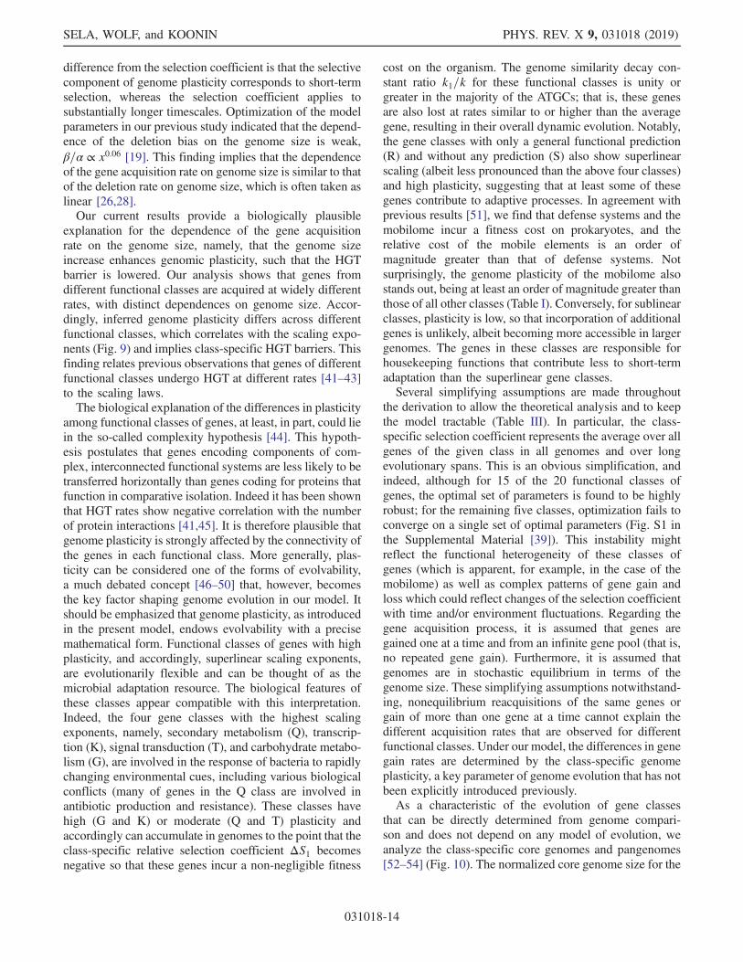
Both the plasticity slope and the mean plasticity stronglypositively correlate with the scaling exponent with therespective Spearman correlation coefficients ρ ¼ 0.81ðpval < 10−3Þ and ρ ¼ 0.74 ðpval < 10−3Þ (Fig. 9). Thisstrong correlation suggests that genome plasticity, togetherwith the selection coefficient, shape the evolution ofgenome content.

III. DISCUSSION

In this work, we develop a general theoretical modelexplaining the universal scaling of the functional classes ofgenes in prokaryotes (Fig. 2). The scaling that we obtainfrom this simple model does not follow a power law exactlybut gives a comparable quality of fit within the range ofavailable data, even if slightly inferior to direct power-lawfits. However, it should be stressed that the model param-eters’ inference does not rely only on the number of genesbut incorporate additional information derived from pair-wise similarity in gene content, which is a crucial ingre-dient that allows inference of the selection coefficient,without any assumptions on genome plasticity. The modeldoes not include any assumptions on specific relationshipsbetween different functional classes as postulated in theprevious models [10]. Instead, we introduce an additionalclass-specific parameter, which we denote genome plas-ticity, that is distinct from the selection coefficient and,together with the latter evolutionary factor, governs genegain and loss processes. Genome plasticity reflects theavailability of the genes of the given functional class, whichitself depends on their abundance in the external gene pool,as well as the strength of purifying selection, on the shorttimescale, against horizontally acquired genes that has beenpreviously described as the HGT barrier [40]. The

FIG. 8. Correlation between the gene-class-specific selectioncoefficient and genome plasticity values. The mean inferred ΔS1is plotted against the mean inferred plasticity p1 for all functionalclasses. The mean values are calculated by averaging over allATGCs. For all functional classes, ΔS1 decreases with x1.However, whereas genes of low-plasticity classes are difficultto acquire and losses of these genes are rare and incur a largeselective cost, genes of high-plasticity classes are acquiredfrequently, and conversely, the loss of these genes typically incuronly a low cost. Consequently, a strong negative correlationbetween the mean selection coefficient and genome plasticity isobserved across the functional classes of genes [Spearmancorrelation coefficient ρ ¼ −0.79; pval < 10−3 for all functionalclasses; Spearman correlation coefficient ρ ¼ −0.77; pval < 10−3

when omitting the mobilome (X) that demonstrates extremevalues of genome plasticity and selection coefficient].

FIG. 9. Correlation between scaling exponents and genomeplasticity values for different functional classes of genes. Thescaling exponent strongly correlates with the genome plasticity,implying that, to a large extent, genome plasticity dominatesprokaryotic genome evolution. (a) Mean plasticity across allATGCs is plotted against the scaling exponent. Each pointcorresponds to a functional class of genes. The mobilome isassociated with genome plasticity that is an order of magnitudegreater than those of the other gene classes and is excluded fromthe plot. (b) The plasticity slope is plotted against the scalingexponent. Similar to (a), each point corresponds to a functionalclass of genes, and the mobilome is excluded from the plot.

SELECTION AND GENOME PLASTICITY AS THE KEY FACTORS … PHYS. REV. X 9, 031018 (2019)

031018-13

difference from the selection coefficient is that the selectivecomponent of genome plasticity corresponds to short-termselection, whereas the selection coefficient applies tosubstantially longer timescales. Optimization of the modelparameters in our previous study indicated that the depend-ence of the deletion bias on the genome size is weak,β=α ∝ x0.06 [19]. This finding implies that the dependenceof the gene acquisition rate on genome size is similar to thatof the deletion rate on genome size, which is often taken aslinear [26,28].Our current results provide a biologically plausible

explanation for the dependence of the gene acquisitionrate on the genome size, namely, that the genome sizeincrease enhances genomic plasticity, such that the HGTbarrier is lowered. Our analysis shows that genes fromdifferent functional classes are acquired at widely differentrates, with distinct dependences on genome size. Accor-dingly, inferred genome plasticity differs across differentfunctional classes, which correlates with the scaling expo-nents (Fig. 9) and implies class-specific HGT barriers. Thisfinding relates previous observations that genes of differentfunctional classes undergo HGT at different rates [41–43]to the scaling laws.The biological explanation of the differences in plasticity

among functional classes of genes, at least, in part, could liein the so-called complexity hypothesis [44]. This hypoth-esis postulates that genes encoding components of com-plex, interconnected functional systems are less likely to betransferred horizontally than genes coding for proteins thatfunction in comparative isolation. Indeed it has been shownthat HGT rates show negative correlation with the numberof protein interactions [41,45]. It is therefore plausible thatgenome plasticity is strongly affected by the connectivity ofthe genes in each functional class. More generally, plas-ticity can be considered one of the forms of evolvability,a much debated concept [46–50] that, however, becomesthe key factor shaping genome evolution in our model. Itshould be emphasized that genome plasticity, as introducedin the present model, endows evolvability with a precisemathematical form. Functional classes of genes with highplasticity, and accordingly, superlinear scaling exponents,are evolutionarily flexible and can be thought of as themicrobial adaptation resource. The biological features ofthese classes appear compatible with this interpretation.Indeed, the four gene classes with the highest scalingexponents, namely, secondary metabolism (Q), transcrip-tion (K), signal transduction (T), and carbohydrate metabo-lism (G), are involved in the response of bacteria to rapidlychanging environmental cues, including various biologicalconflicts (many of genes in the Q class are involved inantibiotic production and resistance). These classes havehigh (G and K) or moderate (Q and T) plasticity andaccordingly can accumulate in genomes to the point that theclass-specific relative selection coefficient ΔS1 becomesnegative so that these genes incur a non-negligible fitness

cost on the organism. The genome similarity decay con-stant ratio k1=k for these functional classes is unity orgreater in the majority of the ATGCs; that is, these genesare also lost at rates similar to or higher than the averagegene, resulting in their overall dynamic evolution. Notably,the gene classes with only a general functional prediction(R) and without any prediction (S) also show superlinearscaling (albeit less pronounced than the above four classes)and high plasticity, suggesting that at least some of thesegenes contribute to adaptive processes. In agreement withprevious results [51], we find that defense systems and themobilome incur a fitness cost on prokaryotes, and therelative cost of the mobile elements is an order ofmagnitude greater than that of defense systems. Notsurprisingly, the genome plasticity of the mobilome alsostands out, being at least an order of magnitude greater thanthose of all other classes (Table I). Conversely, for sublinearclasses, plasticity is low, so that incorporation of additionalgenes is unlikely, albeit becoming more accessible in largergenomes. The genes in these classes are responsible forhousekeeping functions that contribute less to short-termadaptation than the superlinear gene classes.Several simplifying assumptions are made throughout

the derivation to allow the theoretical analysis and to keepthe model tractable (Table III). In particular, the class-specific selection coefficient represents the average over allgenes of the given class in all genomes and over longevolutionary spans. This is an obvious simplification, andindeed, although for 15 of the 20 functional classes ofgenes, the optimal set of parameters is found to be highlyrobust; for the remaining five classes, optimization fails toconverge on a single set of optimal parameters (Fig. S1 inthe Supplemental Material [39]). This instability mightreflect the functional heterogeneity of these classes ofgenes (which is apparent, for example, in the case of themobilome) as well as complex patterns of gene gain andloss which could reflect changes of the selection coefficientwith time and/or environment fluctuations. Regarding thegene acquisition process, it is assumed that genes aregained one at a time and from an infinite gene pool (that is,no repeated gene gain). Furthermore, it is assumed thatgenomes are in stochastic equilibrium in terms of thegenome size. These simplifying assumptions notwithstand-ing, nonequilibrium reacquisitions of the same genes orgain of more than one gene at a time cannot explain thedifferent acquisition rates that are observed for differentfunctional classes. Under our model, the differences in genegain rates are determined by the class-specific genomeplasticity, a key parameter of genome evolution that has notbeen explicitly introduced previously.As a characteristic of the evolution of gene classes

that can be directly determined from genome compari-son and does not depend on any model of evolution, weanalyze the class-specific core genomes and pangenomes[52–54] (Fig. 10). The normalized core genome size for the

SELA, WOLF, and KOONIN PHYS. REV. X 9, 031018 (2019)

031018-14

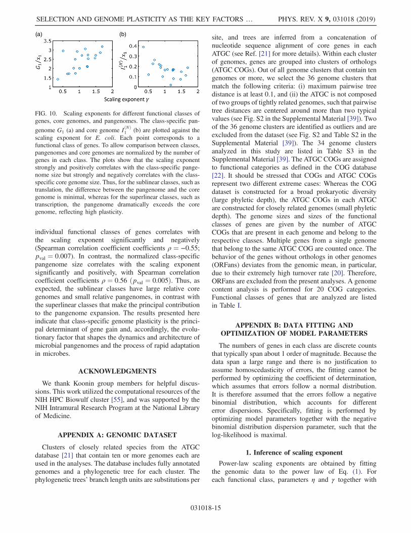
individual functional classes of genes correlates withthe scaling exponent significantly and negatively(Spearman correlation coefficient coefficients ρ ¼ −0.55;pval ¼ 0.007). In contrast, the normalized class-specificpangenome size correlates with the scaling exponentsignificantly and positively, with Spearman correlationcoefficient coefficients ρ ¼ 0.56 ðpval ¼ 0.005Þ. Thus, asexpected, the sublinear classes have large relative coregenomes and small relative pangenomes, in contrast withthe superlinear classes that make the principal contributionto the pangenome expansion. The results presented hereindicate that class-specific genome plasticity is the princi-pal determinant of gene gain and, accordingly, the evolu-tionary factor that shapes the dynamics and architecture ofmicrobial pangenomes and the process of rapid adaptationin microbes.

ACKNOWLEDGMENTS

We thank Koonin group members for helpful discus-sions. This work utilized the computational resources of theNIH HPC Biowulf cluster [55], and was supported by theNIH Intramural Research Program at the National Libraryof Medicine.

APPENDIX A: GENOMIC DATASET

Clusters of closely related species from the ATGCdatabase [21] that contain ten or more genomes each areused in the analyses. The database includes fully annotatedgenomes and a phylogenetic tree for each cluster. Thephylogenetic trees’ branch length units are substitutions per

site, and trees are inferred from a concatenation ofnucleotide sequence alignment of core genes in eachATGC (see Ref. [21] for more details). Within each clusterof genomes, genes are grouped into clusters of orthologs(ATGC COGs). Out of all genome clusters that contain tengenomes or more, we select the 36 genome clusters thatmatch the following criteria: (i) maximum pairwise treedistance is at least 0.1, and (ii) the ATGC is not composedof two groups of tightly related genomes, such that pairwisetree distances are centered around more than two typicalvalues (see Fig. S2 in the Supplemental Material [39]). Twoof the 36 genome clusters are identified as outliers and areexcluded from the dataset (see Fig. S2 and Table S2 in theSupplemental Material [39]). The 34 genome clustersanalyzed in this study are listed in Table S3 in theSupplemental Material [39]. The ATGC COGs are assignedto functional categories as defined in the COG database[22]. It should be stressed that COGs and ATGC COGsrepresent two different extreme cases: Whereas the COGdataset is constructed for a broad prokaryotic diversity(large phyletic depth), the ATGC COGs in each ATGCare constructed for closely related genomes (small phyleticdepth). The genome sizes and sizes of the functionalclasses of genes are given by the number of ATGCCOGs that are present in each genome and belong to therespective classes. Multiple genes from a single genomethat belong to the same ATGC COG are counted once. Thebehavior of the genes without orthologs in other genomes(ORFans) deviates from the genomic mean, in particular,due to their extremely high turnover rate [20]. Therefore,ORFans are excluded from the present analyses. A genomecontent analysis is performed for 20 COG categories.Functional classes of genes that are analyzed are listedin Table I.

APPENDIX B: DATA FITTING ANDOPTIMIZATION OF MODEL PARAMETERS

The numbers of genes in each class are discrete countsthat typically span about 1 order of magnitude. Because thedata span a large range and there is no justification toassume homoscedasticity of errors, the fitting cannot beperformed by optimizing the coefficient of determination,which assumes that errors follow a normal distribution.It is therefore assumed that the errors follow a negativebinomial distribution, which accounts for differenterror dispersions. Specifically, fitting is performed byoptimizing model parameters together with the negativebinomial distribution dispersion parameter, such that thelog-likelihood is maximal.

1. Inference of scaling exponent

Power-law scaling exponents are obtained by fittingthe genomic data to the power law of Eq. (1). Foreach functional class, parameters η and γ together with

FIG. 10. Scaling exponents for different functional classes ofgenes, core genomes, and pangenomes. The class-specific pan-

genome G1 (a) and core genome IðNÞ1 (b) are plotted against the

scaling exponent for E. coli. Each point corresponds to afunctional class of genes. To allow comparison between classes,pangenomes and core genomes are normalized by the number ofgenes in each class. The plots show that the scaling exponentstrongly and positively correlates with the class-specific pange-nome size but strongly and negatively correlates with the class-specific core genome size. Thus, for the sublinear classes, such astranslation, the difference between the pangenome and the coregenome is minimal, whereas for the superlinear classes, such astranscription, the pangenome dramatically exceeds the coregenome, reflecting high plasticity.

SELECTION AND GENOME PLASTICITY AS THE KEY FACTORS … PHYS. REV. X 9, 031018 (2019)

031018-15

the negative binomial distribution dispersion parameter areoptimized by maximizing the log-likelihood for allgenomes in the dataset. Genomes that do not contain genesthat belong to the respective class are excluded from theanalysis. The resulting fits are shown in Fig. 1, and the fitAkaike information criterion values are listed in Table S1 ofthe Supplemental Material [39].

2. Inference of pairwise intersection decay constants

The pairwise intersections decay constants k and k1 areinferred by fitting Eqs. (14) and (16) separately for eachATGC to the genomic data. Since ORFans are omitted fromthe dataset, the intercept is set to the mean number of genes(x for complete genomes and x1 for class-specific genes),such that the decay constant and the negative binomialdispersion parameter are optimized by maximizing the log-likelihood. Genomes that do not contain genes that belongto the respective class are excluded from the analysis.

APPENDIX C: STATISTICAL ANALYSIS OFSCALING EXPONENTS

For each functional class, a power law is fitted to acollection of genes generated by bootstrapping the originaldataset. Specifically, the sampled dataset is generated bysampling with replacement the ATGCs and collecting allgenomes in sampled ATGCs. Sampling is performed overATGCs and not directly at the level of genomes in order toavoid sampling bias due to the different number ofgenomes in each ATGC. The distribution of the fittedscaling exponents is shown for each class for 1000 boot-strap samplings in Fig. 4. For each pair of classes, thedistribution overlap C is calculated and shown in Table S4of the Supplemental Material [39]. Specifically, for cat-egories X and Y, with scaling exponents γX ≤ γY for theoriginal dataset and bootstrap exponents γXi and γYj , theoverlap is given by

CXY ¼�X1000

i¼1

X1000j¼1

cXYij

�=10002 ðC1Þ

with

cXYij ¼�1 for γXi > γYj ;

0 else:ðC2Þ

Given that, for the original dataset, the scaling exponent ofclass X is smaller than that of class Y, the overlap CXYindicates the probability of a bootstrap exponent of class Xto be greater than the bootstrap exponent of class Y.Accordingly, CXX ¼ 1=2.

APPENDIX D: POPULATION-SIZE-NORMALIZED SELECTION COEFFICIENT

Scaling the time by the effective population size Neallows us to express gain and loss rates through S0 ¼ Nes0,where s0 is the genomewide average of the selectioncoefficient. Substituting into the genome size dynamicsof Eq. (3) the gain and loss rates of Eqs. (8) and (9), we getthe explicit form

dx=dt ¼ αðxÞFðS0Þ − βðxÞFð−S0Þ; ðD1Þ

where F denotes the fixation probability of Eq. (7).

APPENDIX E: PAIRWISE GENOMEINTERSECTIONS

To account for the genome content similarity, eachgenome is represented by a vector X with elements thatassume values of 1 or 0. Each entry represents an ATGCCOG, where 1 or 0 indicate the presence or absence,respectively, of that ATGC COG in the genome. Genomesize x is then given by the sum of all elements in X. Thenumber of common genes I is defined as

IðtÞ ¼ hX · Yi; ðE1Þ

where X and Y are two vectors that represent the twogenomes, the angled brackets indicate averaging over allpossible pairs of genomes, and the dot operation standsfor a scalar product. The pairwise genomes intersectiondynamic is given by

dI=dt ¼ 2hðdX=dtÞ · Yi; ðE2Þ

where we use the fact that both averages are equalhðdX=dtÞ · Yi ¼ hX · ðdY=dtÞi. For a finite gene pool ofsize L (the limit of an infinite gene pool, which is used inthe Results section, is calculated below), we have

ðdX=dtÞ · Yi ¼ −P− LL − x

IðtÞ=xþ P− xL − x

; ðE3Þ

where the last approximation relies on the steady-stateassumption Pþ ≈ P−. Substituting the relation above intothe equation for the pairwise genome similarity timederivative of Eq. (E2) and solving the differential equation,we obtain the exponential decay of the pairwise genomeintersection to an asymptote x2=L,

IðtÞ ¼ ½Ið0Þ − x2=L�e−νt þ x2=L ðE4Þ

with decay constant

ν ¼ 2P−

xL

L − x: ðE5Þ

SELA, WOLF, and KOONIN PHYS. REV. X 9, 031018 (2019)

031018-16

The asymptote x2=L can be obtained using a simpleintuitive derivation. The two intersecting genomes areregarded as two independent random samples of x genesfrom a pool of L genes. The probability that a sample fromthe second genome includes a gene that was alreadysampled in the first genome is x=L. To obtain the numberof intersecting genes, this probability is multiplied by thenumber of trials, that is, the number of genes x, giving theintersection asymptote x2=L. Assuming a clock withrespect to loss events, the time t can be translated intothe tree pairwise distance as d ¼ 2t=t0. Further assumingthat the gene pool is much larger than the mean genomesize L ≫ x (formally equivalent to the assumption of aninfinite gene pool [26]), we get for I the exponential decayof Eq. (14), with the decay constant of Eq. (15).Finally, it is possible to consider pairwise genome

intersections with respect to a subset of genes. Thederivation presented in Eqs. (E1)–(E5) can be repeatedfor genes that belong to a specific functional class, resultingin an exponential decay of the class-specific pairwiseintersections I1 of Eq. (16), with the decay constant k1of Eq. (17).

APPENDIX F: OPTIMIZATION OF MODELPARAMETERS

For each functional class, four model parameters q, ξ1, a,and b of Eqs. (18) and (19) are optimized using the meannumbers of genes and decay constants for each ATGC x, x1,k, and k1. Specifically, all four model parameters areoptimized simultaneously using Eqs. (20) and (22),together with S0 of Eq. (21), by maximizing the goodnessof fit R2 for both equations. The model parameters areoptimized by maximizing a goal function that is given bythe sum of goodness-of-fit values for both equations. Inprinciple, four-dimensional optimization can converge at alocal minimum or else it could have substantially differentnearly optimal solutions. To ensure that optimal parametersare picked and to demonstrate the robustness of the optimalsolution, the following procedure is applied. In the firststage, optimization is performed for each functional classstarting from an arbitrary point in the parameter space

a ¼ meanðx1=xÞ;b ¼ 0;

q ¼ 0.01;

ξ1 ¼ maxðx1Þ: ðF1Þ

The outcome of this optimization, including both theoptimized parameters and the goal function values, is setas a benchmark, where each functional class is associatedwith different values. Further optimizations are performedstarting from random points in the parameter space, and wekeep the results of 100 optimizations with goal function

values equal to or greater than the benchmark valueG0. Foreach functional class, the differences in the parameters’values in each of the 100 optimizations and the benchmarkoptimization are calculated. The difference D is calculatedfor each model parameter as

D ¼���� z0 − zi

z0

����; ðF2Þ

where z0 denotes the benchmark value of a model param-eter, and zi is an optimal model parameter value obtainedwhen starting the optimization from a random point in theparameter space. For all but five functional classes (celldivision D, defense V, secretion N, mobilome X, andfunction unknown S), optimizations converge consistently,with negligible D, as shown in Fig. S1 of the SupplementalMaterial [39]. The large differences observed for fiveclasses imply that there are two or more local maximawith goal function values equal to or larger than G0.In the next stage, we find the global maximum.

A procedure similar to the one described above is applied,but instead of setting the benchmark based on an arbitrarystarting point, the benchmark goal function value is takenas the maximum value of 100 optimizations that start fromrandom points in the parameter space. Optimizations arethen performed starting from random points in the param-eter space until 100 solutions with the goal function valueequal to or greater than the benchmark value are obtained.In this case, each of the 20 functional classes converge to asingle-class-specific point in the parameter space, as shownin Fig. S3 of the Supplemental Material [39]. All fivecategories (D, V, N, X, and S) that previously showed largedifferences between the optimal and near-optimal param-eter values converge to a solution with a negative q[positive slope of the class-specific selection coefficient;see Eq. (18)]. For these five classes, we apply the constraintq > 0 and repeat the search. The differences for the optimaland near-optimal solutions with q > 0 are shown in Fig. S4of the Supplemental Material [39]. The genome plasticitycan be determined, but different starting points converge atdifferent selection coefficients. The solution with thelargest goal function value is taken as the optimal solution,and comparison of the selection coefficients and genomeplasticities for optimal solutions with q > 0 and q < 0 areshown in Fig. S5 of the Supplemental Material [39].

[1] C. K. Stover et al., Complete Genome Sequence of Pseu-domonas aeruginosa PAO1, an Opportunistic Pathogen,Nature (London) 406, 959 (2000).

[2] E. van Nimwegen, Scaling Laws in the Functional Contentof Genomes, Trends Genet. 19, 479 (2003).

[3] K. T. Konstantinidis and J. M. Tiedje, Trends between GeneContent and Genome Size in Prokaryotic Species with

SELECTION AND GENOME PLASTICITY AS THE KEY FACTORS … PHYS. REV. X 9, 031018 (2019)

031018-17

Larger Genomes, Proc. Natl. Acad. Sci. U.S.A. 101, 3160(2004).

[4] E. V. Koonin and Y. I. Wolf, Genomics of Bacteria andArchaea: The Emerging Dynamic View of the ProkaryoticWorld, Nucleic Acids Res. 36, 6688 (2008).

[5] N. Molina and E. van Nimwegen, Scaling Laws in Func-tional Genome Content across Prokaryotic Clades andLifestyles, Trends Genet. 25, 243 (2009).

[6] E. De Lazzari, J. Grilli, S. Maslov, and M. C. Lagomarsino,Family-Specific Scaling Laws in Bacterial Genomes, Nu-cleic Acids Res. 45, 7615 (2017).

[7] O. X. Cordero and P. Hogeweg, Regulome Size in Prokar-yotes: Universality and Lineage-Specific Variations, TrendsGenet. 25, 285 (2009).

[8] S. Maslov, S. Krishna, T. Y. Pang, and K. Sneppen, ToolboxModel of Evolution of Prokaryotic Metabolic Networks andTheir Regulation, Proc. Natl. Acad. Sci. U.S.A. 106, 9743(2009).

[9] T. Y. Pang and S. Maslov, A Toolbox Model of Evolution ofMetabolic Pathways on Networks of Arbitrary Topology,PLoS Comput. Biol. 7, e1001137 (2011).

[10] J. Grilli, B. Bassetti, S. Maslov, and M. C. Lagomarsino,Joint Scaling Laws in Functional and Evolutionary Cat-egories in Prokaryotic Genomes, Nucleic Acids Res. 40,530 (2012).

[11] B. O. Bengtsson, Modelling the Evolution of Genomes withIntegrated External and Internal Functions, J. Theor. Biol.231, 271 (2004).

[12] E. V. Koonin, K. S. Makarova, and L. Aravind, HorizontalGene Transfer in Prokaryotes: Quantification and Classi-fication, Annu. Rev. Microbiol. 55, 709 (2001).

[13] C. Pal, B. Papp, and M. J. Lercher, Adaptive Evolution ofBacterial Metabolic Networks by Horizontal Gene Transfer,Nat. Genet. 37, 1372 (2005).

[14] T. J. Treangen and E. P. Rocha, Horizontal Transfer, NotDuplication, Drives the Expansion of Protein Families inProkaryotes, PLoS Genet. 7, e1001284 (2011).

[15] P. Puigbo, A. E. Lobkovsky, D. M. Kristensen, Y. I. Wolf,and E. V. Koonin, Genomes in Turmoil: Quantification ofGenome Dynamics in Prokaryote Supergenomes, BMCBiol. 12, 66 (2014).

[16] W. F. Doolittle, Lateral Genomics, Trends Cell Biol. 9, M5(1999).

[17] N. Molina and E. van Nimwegen, The Evolution ofDomain-Content in Bacterial Genomes, Biol. Direct 3,51 (2008).

[18] I. Sela, Y. I. Wolf, and E. V. Koonin, Theory of ProkaryoticGenome Evolution, Proc. Natl. Acad. Sci. U.S.A. 113,11399 (2016).

[19] I. Sela, Y. I. Wolf, and E. V. Koonin, Estimation of Universaland Taxon-Specific Parameters of Prokaryotic GenomeEvolution, PLoS One 13, e0195571 (2018).

[20] Y. I. Wolf, K. S. Makarova, A. E. Lobkovsky, and E. V.Koonin, Two Fundamentally Different Classes of MicrobialGenes, Nat. Microbiol. 2, 16208 (2016).

[21] D. M. Kristensen, Y. I. Wolf, and E. V. Koonin, ATGCDatabase and ATGC-COGs: An Updated Resource forMicro- and Macro-Evolutionary Studies of ProkaryoticGenomes and Protein Family Annotation, Nucleic AcidsRes. 45, D210 (2017).

[22] M. Y. Galperin, K. S. Makarova, Y. I. Wolf, and E. V.Koonin, Expanded Microbial Genome Coverage and Im-proved Protein Family Annotation in the COG Satabase,Nucleic Acids Res. 43, D261 (2015).

[23] A. R. Mushegian and E. V. Koonin, A Minimal Gene Set forCellular Life Derived by Comparison of Complete BacterialGenomes, Proc. Natl. Acad. Sci. U.S.A. 93, 10268 (1996).

[24] A. B. Kolsto, Dynamic Bacterial Genome Organization,Mol. Microbiol. 24, 241 (1997).

[25] E. V. Koonin, Comparative Genomics, Minimal Gene-Setsand the Last Universal Common Ancestor, Nat. Rev.Microbiol. 1, 127 (2003).

[26] F. Baumdicker, W. R. Hess, and P. Pfaffelhuber, TheInfinitely Many Genes Model for the Distributed Genomeof Bacteria, Genome Biol. Evol. 4, 443 (2012).

[27] D. H. Huson and M. Steel, Phylogenetic Trees Based onGene Content, Bioinformatics 20, 2044 (2004).

[28] R. E. Collins and P. G. Higgs, Testing the Infinitely ManyGenes Model for the Evolution of the Bacterial CoreGenome and Pangenome, Mol. Biol. Evol. 29, 3413 (2012).

[29] P. Marttinen and W. P. Hanage, Speciation Trajectories inRecombining Bacterial Species, PLoS Comput. Biol. 13,e1005640 (2017).

[30] D. M. McCandlish, C. L. Epstein, and J. B. Plotkin, FormalProperties of the Probability of Fixation: Identities,Inequalities and Approximations, Theor. Popul. Biol. 99,98 (2015).

[31] M. Lynch and J. S. Conery, The Origins of GenomeComplexity, Science 302, 1401 (2003).

[32] S. Bershtein, A. W. Serohijos, S. Bhattacharyya, M.Manhart, J. M. Choi, W.Mu, J. Zhou, and E. I. Shakhnovich,Protein Homeostasis Imposes a Barrier on FunctionalIntegration of Horizontally Transferred Genes in Bacteria,PLoS Genet. 11, e1005612 (2015).

[33] D. A. Petrov, T. A. Sangster, J. S. Johnston, D. L. Hartl, andK. L. Shaw, Evidence for DNA Loss as a Determinant ofGenome Size, Science 287, 1060 (2000).

[34] D. A. Petrov, DNA Loss and Evolution of Genome Size inDrosophila, Genetica 115, 81 (2002).

[35] C. H. Kuo and H. Ochman,Deletional Bias across the ThreeDomains of Life, Genome Biol. Evol. 1, 145 (2009).

[36] G. Plata, C. S. Henry, and D. Vitkup, Long-Term Pheno-typic Evolution of Bacteria, Nature (London) 517, 369 (2015).

[37] T. N. Mavrich and G. F. Hatfull, Bacteriophage EvolutionDiffers by Host, Lifestyle and Genome, Nat. Microbiol. 2,17112 (2017).

[38] L. S. Frost, R. Leplae, A. O. Summers, and A. Toussaint,Mobile Genetic Elements: The Agents of Open SourceEvolution, Nat. Rev. Microbiol. 3, 722 (2005).

[39] See Supplemental Material at http://link.aps.org/supplemental/10.1103/PhysRevX.9.031018 for Supplemen-tal figures and tables.

[40] R. Sorek, Y. Zhu, C. J. Creevey, M. P. Francino, P. Bork, andE. M. Rubin, Genome-Wide Experimental Determination ofBarriers to Horizontal Gene Transfer, Science 318, 1449(2007).

[41] O. Cohen, U. Gophna, and T. Pupko, The ComplexityHypothesis Revisited: Connectivity Rather Than FunctionConstitutes a Barrier to Horizontal Gene Transfer, Mol.Biol. Evol. 28, 1481 (2011).

SELA, WOLF, and KOONIN PHYS. REV. X 9, 031018 (2019)

031018-18

[42] Y. Nakamura, T. Itoh, H. Matsuda, and T. Gojobori, BiasedBiological Functions of Horizontally Transferred Genes inProkaryotic Genomes, Nat. Genet. 36, 760 (2004).

[43] R. Merkl, A Comparative Categorization of Protein Func-tion Encoded in Bacterial or Archeal Genomic Islands,J. Mol. Evol. 62, 1 (2006).

[44] R. Jain, M. C. Rivera, and J. A. Lake, Horizontal GeneTransfer among Genomes: The Complexity Hypothesis,Proc. Natl. Acad. Sci. U.S.A. 96, 3801 (1999).

[45] A. Wellner, M. N. Lurie, and U. Gophna, Complexity,Connectivity, and Duplicability as Barriers to Lateral GeneTransfer, Genome Biol. 8, R156 (2007).

[46] A. Wagner, Robustness, Evolvability, and Neutrality, FEBSLett. 579, 1772 (2005).

[47] A. Crombach and P. Hogeweg, Evolution of Evolvability inGene Regulatory Networks, PLoS Comput. Biol. 4,e1000112 (2008).

[48] M. Pigliucci, Is Evolvability Evolvable?, Nat. Rev. Genetics9, 75 (2008).

[49] J. Masel and M. V. Trotter, Robustness and Evolvability,Trends Genet. 26, 406 (2010).

[50] J. Lehman and K. O. Stanley, Evolvability is Inevitable:Increasing Evolvability without the Pressure to Adapt,PLoS One 8, e62186 (2013).

[51] J. Iranzo, J. A. Cuesta, S. Manrubia, M. I. Katsnelson, andE. V. Koonin, Disentangling the Effects of Selection andLoss Bias on Gene Dynamics, Proc. Natl. Acad. Sci. U.S.A.114, E5616 (2017).

[52] D. Medini, C. Donati, H. Tettelin, V. Masignani, and R.Rappuoli, The Microbial Pan-Genome, Curr. Opin. Genet.Dev. 15, 589 (2005).

[53] G. Vernikos, D. Medini, D. R. Riley, and H. Tettelin, TenYears of Pan-Genome Analyses, Curr. Opin. Microbiol. 23,148 (2015).

[54] J. O. McInerney, A. McNally, and M. J. O’Connell, WhyProkaryotes Have Pangenomes, Nat. Microbiol. 2, 17040(2017).

[55] http://hpc.nih.gov.

SELECTION AND GENOME PLASTICITY AS THE KEY FACTORS … PHYS. REV. X 9, 031018 (2019)

031018-19