The Stability of Strategic Plasticity

Rory SmeadUniversity of California, Irvine

Kevin J.S. ZollmanCarnegie Mellon University

April 30, 2009

Abstract

Recent research into the evolution of higher cognition has piquedan interest in the effect of natural selection on the ability of creaturesto respond to their environment (behavioral plasticity). It is believedthat environmental variation is required for plasticity to evolve in caseswhere the ability to be plastic is costly. We investigate one form ofenvironmental variation: frequency dependent selection. Using toolsin game theory, we investigate a few models of plasticity and outlinethe cases where selection would be expected to maintain it. Ultimatelywe conclude that frequency dependent selection is likely insufficient tomaintain plasticity given reasonable assumptions about its costs. Thisresult is very similar to one aspect of the well-discussed Baldwin effect,where plasticity is first selected for and then later selected against. Weshow how in these models one would expect plasticity to grow in thepopulation and then be later reduced. Ultimately we conclude that ifone is to account for the evolution of behavioral plasticity in this way,one must appeal to a very particular sort of external environmentalvariation.

Keywords: Game theory, Evolutionarily stable strategy, Behav-ioral plasticity

1 Introduction

Humans and many other animals are behaviorally adaptive – they mod-ify their behavior in response to the environment. This flexibility is often

1

placed in contrast to more rigidly specified behaviors which are not capa-ble of changing across environmental circumstances.1 It is generally believedthat behavioral plasticity will be selectively advantageous when there is en-vironmental variation. Environmental variation, very broadly conceived, cancome in many forms. It may come from a source external to the population,such as seasonal or ecological change. Or, it may be due to changes in thepopulation itself as in frequency-dependent selection. Variation of the firstkind has been discussed in some detail (Ancel, 1999; Godfrey-Smith, 1996,2002; Sterelny, 2003) and it can be shown that behavioral plasticity can beadvantageous when there is such external variation.

It is difficult to determine what counts as an “external” environmentfor the purpose of predicting the benefits of variability. In particular docases of game-theoretic interaction, where an individual’s fitness dependson the type with whom it is interacting, count? One might suppose thatcases of frequency dependent selection like this might be sufficient to selectfor behavioral plasticity. Different interactions over time represent differentlocal environments for an individual and will thus appear similar to changesin weather or predatory threats (classic examples of “external” variation).Furthermore for populations out of equilibrium, the proportion of differenttypes will change over time thus benefiting different behaviors across severalgenerations. These considerations might lead one to suppose that frequencydependent selection represents an extreme version of external environmentalvariation.

This paper investigates this possibility using evolutionary game theory.2

We find that populations of plastic individuals will not be maintained byevolution, and often plasticity will be eliminated entirely. This result sug-gests that a particular sort of environmental variation is necessary to sustainplasticity – not any sort of variation will do. More specifically, the varia-tion caused by frequency dependent selection is often insufficient to result inplasticity in strategic situations that can be modeled as games. Furthermore,when we examine the evolutionary dynamics in these settings, we find thatplasticity is often initially selected for only to be reduced in later generations.This is similar to one aspect of the Baldwin effect, where acquired charac-

1Behavioral plasticity can be distinguished from developmental plasticity where theway an organism develops varies with its environment. For the purposes of this paper, wewill focus on behavioral plasticity.

2The evolution of plasticity in games has been investigated already in different contextsby Harley (1981); Suzuki and Arita (2004).

2

teristics (in this case, social behaviors) are replaced by similar hereditarycharacteristics.3

We begin by providing the necessary background in game theory in sec-tion 2. After these preliminaries, we present three models that include aplastic phenotype (an adaptive strategy). While all these models include aplastic strategy, they differ in the method by which costs are associated withthat phenotype. We analyze these models and present our primary resultsin sections 3 and 4. Finally section 5 concludes.

2 Game Theory

A game is a mathematical object which specifies a set of players P ={1, . . . , n}, a set of strategies for each player Si (where i ∈ P ), and a payofffunction for each player, πi : S1 × S2 × · · · × Sn → Rn. In keeping with bio-logical game theory, we will here treat the payoff as representing a strategy’sfitness.

Here we will restrict ourselves to considering one class of games, thefinite symmetric two-player game. A game is symmetric just in case eachplayer has the same set of strategies (Si = Sj for all i, j) and the payofffunction depends only on the strategy chosen not the identity of the player.We can then represent the payoff function as a single function π(x, y) whichrepresents the fitness of playing strategy x against strategy y.

Since we are restricting ourselves to considering only finite games, S hasonly finitely many members. We can, however, extend the strategy space toinclude mixed strategies (strategies which involve choosing different elementsof S with some probability). Now an agent’s strategy is represented by aprobability distribution over S and we can then consider the expected fitnessfrom each strategy played against another, represented by u(x, y).

Given any game, we can construct a best response correspondence forthat game. For some (possibly mixed) strategy, x, B(x) represents the set ofstrategies which do best against x. Formally,

B(x) = {y|u(y, x) ≥ u(y′, x)∀y′} (1)

3Ancel (1999) refers to this as the “Simpson-Baldwin effect” from the formulation ofthe Baldwin effect by Simpson (1953). We will follow Ancel and use the phrase “Simpson-Baldwin effect” when discussing the relationship between our results and the Baldwineffect in section 4.

3

A set of strategies s∗ is a Nash equilibrium if and only if each strategy inthat set is a best response to the others. Formally, s∗ is a Nash equilibriumwhen s∗i ∈ B(s∗−i) for all players i (where s∗i represents player i’s strategy ins∗ and s∗−i represents the other player’s strategy). We will represent the setof all Nash equilibria in a game by NE.

From an evolutionary perspective Nash equilibria are insufficient to rep-resent stable states of populations since there are some Nash equilibria whichone would expect to be invaded by mutation. As a result, a slightly morelimiting solution concept was devised for this purpose, the EvolutionarilyStable Strategy (Maynard Smith and Price, 1973; Maynard Smith, 1982).

Definition 1. A strategy set s∗ is an evolutionarily stable strategy (ESS) ifand only the following two conditions are met

• u(s∗, s∗) ≥ u(s, s∗) for all alternative strategies s and

• If u(s∗, s∗) = u(s, s∗), then u(s∗, s) > u(s, s).

This more restrictive solution concept captures the idea that a populationis stable to invasion by mutation. Evolutionarily stable strategies can beeither pure or mixed strategies. Traditionally a mixed strategy representsdirectly the strategy of an individual who randomizes their behavior, butthis interpretation can be implausible in some contexts. Instead one caninterpret a mixed strategy as a population state, where a certain proportionof a population is playing each strategy. Here uninvadability represents a sortof asymptotic stability of the population under mutation (Weibull, 1995).

It is important to note that in any mixed strategy equilibrium s∗, if twopure strategies, s and s′, are both played with positive probability it mustbe the case that u(s, s∗) = u(s′, s∗). (Otherwise one would have an incentiveto play the better of the two.) As a result, a mixed strategy equilibrium isan ESS only if u(s∗, s) > u(s, s) for all s that are present in the mixture.

There are two features of equilibria which will be of use in the discus-sion. A Nash equilibrium is symmetric when both players are playing thesame strategy. Only symmetric Nash equilibria can be evolutionarily sta-ble (although not all are). Second, a Nash equilibrium (or ESS), N , ispareto superior to another Nash equilibrium, O, if u(N1, N2) > u(O1, O2)and u(N2, N1) > u(O2, O1) – e.g. both players do better in N than in O.

Although somewhat limited, games with only two strategies (so called2 × 2 games) are often used to capture many different types of behavior.

4

When possible we try to present general results, but for some propositionswe must restrict ourselves to 2× 2 games. While there are four payoffs in asymmetric 2× 2 game, we can represent all such games with two parameterswithout losing best response and dominance relations (Weibull, 1995). Thischaracterization leaves us with only three classes of games, each of whichis characterized by different equilibria. Coordination games have two purestrategy Nash equilibria which are symmetric. Hawk-Dove games have twoasymmetric pure strategy Nash equilibria, and Dominance Solvable games(e.g. the Prisoner’s Dilemma) have only one Nash equilibrium.

3 The reduction of strategic plasticity

With these preliminaries in hand we can return to strategic plasticity. Sup-pose there is a population of players and who are randomly paired to play arepeated game against one another. There are phenotypes which correspondto each of the pure strategies in the underlying game and one phenotypewhich corresponds to “learning” (our plastic strategy). The learning pheno-type is capable of adapting itself to do well against the individual with whichit is paired. But this phenotype can only determine the type of its opponentthrough observation of the opponent’s behavior in the game, there are noexternal cues on which the learner can rely.

Traditionally it is assumed that plasticity is costly. Perhaps maintainingor developing the ability to adapt is costly or alternatively there is an intrinsiccost associated with making errors in the process of learning.4 Our first twomodels follow this first suggestion that learning has some exogenous cost,there is some basic fitness cost to being able to adapt which is not a featureof the game or the learning process. In the third model we will capture thesuggestion that the cost of learning is the result of errors in the learningprocess where learners occasionally fail to play the best response.

Ultimately we find that populations of learners can only rarely be main-tained by evolution, and that in many cases, learning will be totally elimi-nated by the evolutionary process.

4Ancel (1999) describes the following examples “In bacteria, for example, plasticity re-quires genetic machinery whose costs are in terms of increased replication time. Learning-based plasticity may entail energetic costs of searching RNA molecules with multiple con-figurations may trade accuracy for the potential for variable binding” (199).

5

3.1 Exogenous cost

Our model will take a base game whose strategies represent phenotypes in apopulation and extend it by including a new phenotype L, which representsthe plastic individual. We will assume that the plastic individual, or learner,is capable of learning the best response against others and learns to play aNash equilibrium against itself.5 We will pick members of a population toplay the game repeatedly against each other, and assume that the game isrepeated sufficiently often that the errors generated by the process of learningare removed (an assumption that will be relaxed in section 3.2). However,we will assume that there is some fixed fitness cost which represents the costsimposed by developing, maintaining, or implementing an adaptive strategy.These costs are taken to be fixed regardless of the underlying game beingplayed.

Formally, we will represent these assumptions by constructing a newgame, GL by defining the utility function uL based on an underlying gameG. We will restrict ourselves to considering cases where every strategy in Ghas a unique best response.6 The payoff function uL(·) is defined as follows:

1. uL(x, y) = πG(x, y) if x, y ∈ S

2. uL(L, y) = πG(B(y), y)− c

3. uL(x,L) = πG(x,B(x)) if x ∈ S

4. uL(L,L) =∑

s∈NE α(s)(

12uG(s1, s2) + 1

2uG(s2, s1)− c

)c > 0 represents the cost of learning. So that the cost of learning does not

effect the results too substantially, we will restrict c to be smaller than thedifference between any two payoffs in the game. In condition 4, we assumethat there is a probability distribution, α over the possible Nash equilibria ofthe game which represents the probability that learning will converge to thatequilibrium. The remainder of that function represents the idea that, givenone converges to a Nash equilibrium, it is arbitrary which role one plays.

5This has already excluded a set of possible learning rules which do not necessarilyconverge to Nash equilibria. Extending this model to those cases, while interesting, isbeyond the scope of this paper.

6While this may seem a substantive assumption, we are only excluding an very small setof games. Any game that features a strategy which does not have a unique best responseis not robust to epsilon perturbations of the payoffs.

6

uL has not been fully specified at this point. We have not defined uL(s,L)for a mixed strategy s. If there is a unique best response to the mixture wewill let uL(s,L) = uG(s, B(s)); the plastic individual finds the best response.But if s is a part of a mixed strategy Nash equilibrium then any mixture overthe pure strategies in s is a best response to s. This is a more complicatedsituation that is discussed in more detail below. For the time being we willleave this case underspecified.7

With this in hand we can now investigate the stability properties of ourlearning type L. Our first proposition shows that in many games, learningcannot be an ESS.

Proposition 1. For all games G without a pareto dominant mixed strategyNash equilibrium, L is not an ESS of the game GL.

Proof. We will show that L is not an ESS by finding a strategy s such thatuL(s,L) > uL(L,L). Let s = maxs′ u

G(s′, B(s′)), i.e. the strategy whichdoes best against its best response among all strategies in G. Consider theNash equilibrium N of G which has the highest payoff to one of the players.uG(s, B(s)) ≥ uG(Ni, N−i), by definition of s. By hypothesis, s is not amixed strategy. By condition 4, uG(Ni, N−i) > uL(L,L). So, as a resultuL(s,L) > uL(L,L).

No symmetric 2×2 game can have a pareto dominant mixed strategy Nashequilibrium and so L cannot be an ESS for any 2 × 2 base game. However,there are larger games that fall outside the scope of this proposition. Asan example consider Rock-Paper-Scissors, pictured in figure 1. In this gamethe unique Nash equilibrium is a mixed equilibrium where each strategy isplayed with equal probability. In this equilibrium the payoff to both playersis 0. Consider the extension of this game to include L. The payoff to apopulation of learners is −c. But any invading pure strategy receives −1,since this is the payoff of that strategy against its best response. So, no purestrategy can invade. However, the mixed strategy which plays Rock, Paper,and Scissors with equal probability does better against the population (0)than the population does against itself, (−c).

7The extended game GL has a an odd feature: for some mixed strategies m of GL,uL(m,L) will not be a weighted average of uL(s,L) for each s inm. This occurs because L’sresponse to a mixture is different than its response to a pure type. It becomes important,then, that we be careful to distinguish a monomorphic population of mixing types and apolymorphic population of non-mixing types. When necessary mention will be made ofthe intended interpretation.

7

Rock Paper ScissorsRock 0, 0 −1, 1 1,−1Paper 1,−1 0, 0 −1, 1

Scissors −1, 1 1,−1 0, 0

Figure 1: Rock-Paper-Scissors

Whether proposition 1 holds in these cases depends critically on whatlearning does when it encounters a mixture that constitutes a mixed strat-egy Nash equilibrium. It is a feature of such mixtures that they make theopponent indifferent between several pure strategies, and by extension indif-ferent between all mixtures over those pure strategies. Different plausiblelearning rules will behave in different ways, and thus may effect the stabilityof L.

Rock Paper ScissorsRock 0, 0 −1, 2 1,−1Paper 2,−1 0, 0 −1, 1

Scissors −1, 1 1,−1 0, 0

Figure 2: Modified Rock-Paper-Scissors

For example consider the modified Rock-Paper-Scissor game in figure 2.Suppose one player uses the strategy to play Rock with probability 1

4, Paper

with probability 13, and Scissors with probability 5

12. This renders any strat-

egy by the opponent a best response. We have not specified what a learnerwill do in this circumstance. Suppose the learner plays Scissors with prob-ability one. This yields an expected payoff of − 1

12for the mixed player.

The learners are able to coordinate on the mixed strategy equilibrium withthemselves, and so as a result achieve a higher payoff than the mixed playersachieve against the learners. This renders L an ESS.

Of course, this would be a rather bizarre learning rule: when indifferentbetween several strategies it chooses the one which harms its opponent themost. Suppose instead that learners randomly chose a strategy from thoseavailable.8 Now, in the modified Rock-Paper-Scissors game, the mixture caninvade a population of learners.

8For instance this would be the case for Herrnstein reinforcement learning (cf. Rothand Erev, 1995).

8

Ultimately this shows that in games of this sort, where there are paretodominant mixed strategy Nash equilibria, the choices we make for the learn-ing rule will have important effects on the stability of learning. It is possibleto make learning stable, but it does require some specific choices about theresponse of the learning rule when all strategies are of equal value.

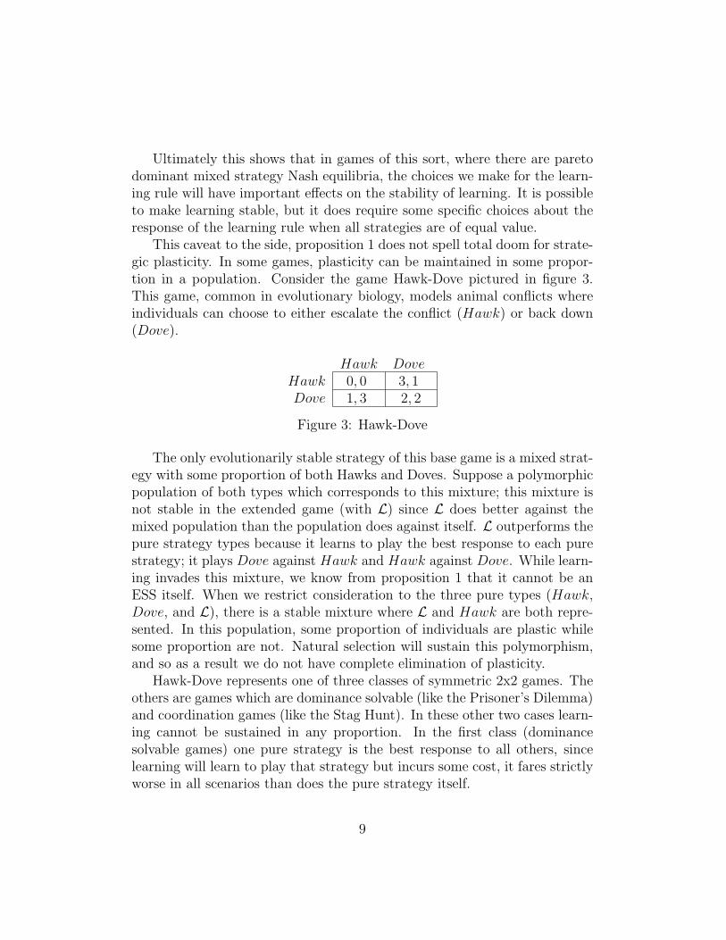
This caveat to the side, proposition 1 does not spell total doom for strate-gic plasticity. In some games, plasticity can be maintained in some propor-tion in a population. Consider the game Hawk-Dove pictured in figure 3.This game, common in evolutionary biology, models animal conflicts whereindividuals can choose to either escalate the conflict (Hawk) or back down(Dove).

Hawk DoveHawk 0, 0 3, 1Dove 1, 3 2, 2

Figure 3: Hawk-Dove

The only evolutionarily stable strategy of this base game is a mixed strat-egy with some proportion of both Hawks and Doves. Suppose a polymorphicpopulation of both types which corresponds to this mixture; this mixture isnot stable in the extended game (with L) since L does better against themixed population than the population does against itself. L outperforms thepure strategy types because it learns to play the best response to each purestrategy; it plays Dove against Hawk and Hawk against Dove. While learn-ing invades this mixture, we know from proposition 1 that it cannot be anESS itself. When we restrict consideration to the three pure types (Hawk,Dove, and L), there is a stable mixture where L and Hawk are both repre-sented. In this population, some proportion of individuals are plastic whilesome proportion are not. Natural selection will sustain this polymorphism,and so as a result we do not have complete elimination of plasticity.

Hawk-Dove represents one of three classes of symmetric 2x2 games. Theothers are games which are dominance solvable (like the Prisoner’s Dilemma)and coordination games (like the Stag Hunt). In these other two cases learn-ing cannot be sustained in any proportion. In the first class (dominancesolvable games) one pure strategy is the best response to all others, sincelearning will learn to play that strategy but incurs some cost, it fares strictlyworse in all scenarios than does the pure strategy itself.

9

In coordination games the situation is rather more complex, but we canagain show that learning cannot be sustained. These games feature two purestrategies, both of which are best responses to themselves. We can show thatthere cannot be a mixed strategy ESS which contains both learning and anystrategy which is a best response to itself.

Proposition 2. Suppose a symmetric two player game G, a strategy s of Gsuch that s is a best response to itself, and mixed strategy Nash equilibriums∗ of GL which includes s and L. s∗ is not an ESS.

Proof. Suppose s is a best response to itself, s is played with non-zero prob-ability in s∗, and that s∗ is an ESS. Since s∗ is a mixed strategy Nash equi-librium in which s is represented u(s, s∗) = u(s∗, s∗). By hypothesis s∗ is anESS, so it must be the case that u(s∗, s) > u(s, s). Expanded this says,∑

i∈S−{L,s}

piπ(i, s) + psπ(s, s) + pL[π(s, s)− c] > π(s, s) (2)

Where pi represents the probability i is played in s∗. Reducing this equationgives us, ∑

i∈S−{L,s}

piπ(i, s)− pLc > (1− ps − pL)π(s, s) (3)

Which is equivalent to,∑i∈S−{L,s}

pi1− ps − pL

(π(i, s)− π(s, s))− pLc

1− ps − pL> 0 (4)

Since s is a best response to itself, π(i, s) − π(s, s) ≤ 0, and as a resultequation 4 cannot be satisfied.

This shows that Hawk-Dove like games represent a sort of special casefor sustaining learning. In any game where a strategy is a best response toitself, learning can only be sustained in populations where that strategy isabsent.

So far we have assumed that the only costs imposed by learners wason themselves. This coincides with understanding costs as being caused bymaintenance or development of the ability to learn. However, we might openthe door for L as an ESS by dropping this assumption. We will generalizethe notion of cost by allowing the costs to be imposed on all interactions.

10

We will introduce cost function c : S × S → R which will represent the costfor one strategy against another.

We are now generating a different game with the following payoff function:

1. uL(x, y) = πG(x, y)− c(x, y) if x, y ∈ S

2. uL(L, y) = πG(B(y), y)− c(L, y)

3. uL(x,L) = πG(x,B(x))− c(x,L) if x ∈ S

4. uL(L,L) =∑

s∈NE α(s)(

12uG(s1, s2) + 1

2uG(s2, s1)− c(L,L)

)Given this generic representations of costs, we may ask: what is required

to make L an ESS? We will first consider cases where the cost imposed isrelatively constant across all strategies.

The following two propositions demonstrate that learners must learn toplay the socially optimal and equitable Nash equilibrium (if one exists), inorder for L to be an ESS.9

Proposition 3. Suppose there is no pareto dominant mixed strategy Nashequilibrium in G. If c is such that |c(x, y)− c(w, z)| is sufficiently small forall w, x, y, z and L is an ESS, then α(N) ≈ 1 for the socially optimal Nashequilibrium N .

Proof. Let N ∈ NE be the Nash equilibrium that is best for one of itsplayers, that is for Ni, u(Ni, N−i) ≥ u(N ′j, N

′−j) for all N ′ ∈ NE. By the

definition of ESS, uL(L,L) ≥ uL(Ni,L). Since N is a Nash equilibrium N−iis a best response to Ni, so uL(Ni,L) = uG(Ni, N−i) − c(Ni,L) ≤ uL(L,L).Substituting this yields,∑s∈NE

α(s)

(1

2uG(s1, s2) +

1

2uG(s2, s1)− c(L,L)

)≥ uG(Ni, N−i)− c(Ni,L)

(5)Since we are assuming that costs are relatively constant, we will assume theyare equal. As a result the average on the left side of 5 must be greater thanor equal to the payoff to the best possible payoff in a Nash equilibrium. Thiscan only be obtained when the socially optimal Nash equilibrium is the bestpossible payoff for any strategy in equilibrium and α assigns the sociallyoptimal Nash equilibrium sufficiently high probability.

9A Nash equilibrium is socially optimal if the sum of payoff to both players is larger(or as large) in that Nash equilibrium than in any other.

11

When costs are relatively uniform, this proposition entails that the func-tion α assigns near probability 1 to one Nash equilibrium. In particular, itmust assign probability 1 to the socially optimal Nash equilibrium – i.e., theequilibrium which is best for both players considered together. This restrictsthe class of possible learning rules which are ESS to a very small set. Inaddition to this restriction on learning rules there is also a restriction on theunderlying game.

Proposition 4. Suppose there is no pareto dominant mixed strategy Nashequilibrium in G. If c is such that |c(x, y)−c(w, z)| is sufficiently small for allw, x, y, z and L is an ESS, then the Nash equilibrium N played by L againstitself is such that uG(N1, N2) ≈ uG(N2, N1).

Proof. By proposition 3, uL(L,L) = 12uG(N1, N2) + 1

2uG(N2, N1) − c(L,L).

Let uG(N1, N2) ≥ uG(N2, N1). Since L is an ESS, it must be the case that:

1

2uG(N1, N2) +

1

2uG(N2, N1)− c(L,L) ≥ uG(N1, N2)− c(N1,L) (6)

Again, ignoring c, this can only be satisfied when uG(N1, N2) = uG(N2, N1).

These two propositions together entail significant restrictions both on thegame and on the types of learning that may be stable. The game must featurea symmetric, socially optimal Nash equilibrium and the learning phenotypemust learn to play that equilibrium almost all of the time.

But what if the costs imposed are not uniform? Could learning be sus-tained in all games? The following proposition follows immediately from thedefinition of ESS.

Proposition 5. Suppose there is no pareto dominant mixed strategy Nashequilibrium in G and let s be a strategy of G which does the best against its bestresponse. If L is an ESS, then either c(L,L) < c(s,L) or c(L,L) = c(s,L)and c(L, s) < c(s, s).

For L to be an ESS it must be more costly to be a non-learner than alearner in a world of learners. The key to the evolutionary stability of learningis the cost of not being a learner when interacting with learners. (This isnot to say, however, that it is intrinsically more costly to be a non-learnerthan a learner – although such a case would satisfy the definition.) There

12

are reasons one may think this may be the case (i.e. that c(L,L) ≤ c(s,L)).For instance, the cost to learners may come from the time spent playing non-best-responses while exploring the game. But, this exploration does not onlyaffect the learner, but also the learner’s opponent. Thus, depending on thespecifics of the game this exploration may be more costly to those interactingwith learners than the learners themselves.10 In section 3.2, we will consideran idealized version of these “endogenous” costs.

3.2 Endogenous Costs of Learning

If we imagine that the cost function, c(x, y), is generated endogenously by Lplaying other possible strategies while learning, we can incorporate it directlyinto the utility function of the players. We will express the cost function asthe result of this exploration by L. This means that c(s, s′) = 0 for anys, s′ ∈ S since neither player will be changing strategies and will simplyreceive the payoff uL(s, s′). As a result, we will only consider cases where Lis involved.

For sake of tractability, we will focus on symmetric 2 × 2 games and re-strict ourselves to pure-strategies and learners that always learn to play purestrategy Nash equilibria (this is because it is not clear how how “deviations”from mixed strategies ought to be calculated). We will ask the followingquestion: can L be an ESS when we express c(x, y) endogenously? Let ε bethe total proportion of stage-game plays where L deviates from their normalbehavior s∗i .

11 Let 0 < ε < 0.5. The endogenous cost can now be expressedas part of the utility functions:

1. uL(L, s) = (1− ε)πG(s∗i , s) + επG(−s∗i , s)

2. uL(s,L) = (1− ε)πG(s, s∗i ) + επG(s,−s∗i )

3. uL(L,L) = (1−ε)22

(πG(s∗i , s∗j) + πG(s∗j , s

∗i )) + (ε − ε2)πG(s∗i ,−s∗j) + (ε −

ε2)πG(−s∗i , s∗j) + ε2

2(πG(−s∗i ,−s∗j) + πG(−s∗j ,−s∗i ))

10Another reason might be that several different games are being played and it is difficultto distinguish them. This would be a form of “external” variation similar to a change inpayoff structure.

11For tractability reasons, we assuming that ε is the same regardless of the opponent,which is not necessarily true of all learning rules. For instance, Herrnstein reinforcementlearning may have a higher ε against itself than against pure strategies. A detailed lookat Herrnstein reinforcement learning in this evolutionary setting is explored in (Zollmanand Smead, 2008).

13

When costs to learning are made endogenous in this way, there is anexample of a 2× 2 game where L is an ESS: a subset of coordination games(figure 4). To see this, let a = 2, x = 2−δ and b = 1 where δ < ε and each areclose to 0. Further, let (L,L) result in “attempting” to play socially optimalNE (A,A). To see L is an ESS, we need only consider u(L,L) and u(s,L)for s = A,B. With these values, letting δ → 0: uL(L,L) ≈ (2 − 2ε) + ε2;uL(A,L) ≈ 2− 2ε; uL(B,L) ≈ 1 + ε. Thus, uL(L,L) > uL(A,L) > uL(B,L)and hence L is an ESS.

A BA a 0B x b

Figure 4: A coordination game (a > x, a > b > 0).

We can vary a, b, x, and ε to create a class of examples. L will be an ESSin this class whenever the following condition is satisfied:

a− x < bε

1− ε(7)

There is an usual thing about this set of examples where L is an ESS,however. L is not really playing a best response to itself. The mixed strategyNash Equilibrium is where each player plays A with probability b

a−x+b . So,if p(A) is less than this, the best response to that mixed strategy is thepure strategy B. Note that for L to be an ESS, we need (1 − ε) < b

a−x+bwhich means that the exploration rate of L must be high enough that thebest response to the actual behavior of L is B not A as the learners are“attempting” to play. Thus, there is a sense in which for L to be an ESS inthis case, learners need to best respond to what other learners are “trying”to do and not their actual behavior.

This class of examples represents the only cases where L is an ESS. Thisis expressed the fallowing proposition proved in the appendix.

Proposition 6. If G is a 2×2 symmetric game of a form other than the coor-dination game above and we consider only pure strategies (and pure strategyequilibria) then L is not an ESS of GL.

Proof in appendix A.

14

3.3 Summary

We have shown that plasticity can be sustained in only very rare circum-stances. When there is an exogenous cost to learning that is higher thanother strategies, a limited type of learning can only be an ESS in a veryrestricted set of games. When the exogenous costs are approximately equalto learners and those interacting with them, only specific learners in specificgames can be ESS. The only case where learning can generally be an ESS isif the costs are greater to non-learners than to learners. While this is not im-possible, it would require some argument to demonstrate this is a widespreadphenomenon.

With respect to endogenous costs modeled as errors in the game we foundthat learning cannot be sustained except in a very narrow class of 2×2 gamesand only then for learners of a peculiar sort. Overall there are not many caseswhere learning can be sustained, and we should not expect to find stable pop-ulations of all plastic types. However, thus far we have only been consideringthe equilibria of these games, not the evolutionary dynamics. One mightwonder if plasticity is ever favored by natural selection – should we expectthe frequency of plasticity to increase in a population out of equilibrium?We will now turn to this second consideration.

4 The Simpson-Baldwin effect

This history of the growth and later reduction of plasticity is one aspectof what is known as the Baldwin effect (Baldwin, 1896).12 This aspect hascome to be called the Simpson-Baldwin effect, following its later explicationby Simpson (1953).

So far we have only discussed how evolution would eliminate or reducethe number of adaptive individuals – the second component of the Simpson-Baldwin effect. The first component, that natural selection would first selectfor plasticity, is not uniformly common to our models.

Since learning plays the best response to every other strategy, it will oftenbe the case that it initially does better than some arbitrary mixture. This

12Discussions of the Baldwin effect often involve looking at how evolution affects anorganism’s norm of reaction and admit of a wide range of plasticity. Because we arefocusing on behavioral plasticity in simple games, our discussion here will differ from thetradition and we will continue to assume individuals are either plastic (using the adaptivestrategy L from above) or not.

15

Figure 5: The dynamics of a coordination game

Figure 6: The dynamics of a Hawk-Dove game

16

Figure 7: The dynamics of a prisoner’s dilemma game

is not assured because for some mixtures that are sufficiently close to anequilibrium the impact of the cost to learning, c, will be sufficient to makelearning worse than the population. However, in many cases of interest itwill be the case that learning is initially rewarded and then later harmed.

Figures 5-7 show the three simplices which result from considering thethree classes of symmetric 2x2 games.13 In each of these cases we find thatlearning is initially better than average at most starting points – this isrepresented by moving toward the top of the figure. In all three cases we seethat once learning represents a significant portion of the population, anotherstrategy can invade.

Figure 5 (a coordination game) and figure 7 (a prisoner’s dilemma) bothrepresent striking examples of the Simpson-Baldwin effect. Many trajectoriesfollow a path that initially provides substantial gains for learning, but oncethere the population is then invaded by a superior pure strategy. As learningbecomes more frequent its presence changes the fitness of the other strategiessuch that one of them is superior. In these cases we have a circumstance

13Lines in these simplices represent the trajectory of the discrete time replicator dynam-ics for one of three canonical games: a pure coordination game with a pareto dominantequilibrium, a prisoner’s dilemma, and a Hawk-Dove game. In these three cases the payoffsrange from 0 to 3 and the cost of learning is 0.1.

17

which conforms exactly to the process described by Baldwin.14

5 Conclusion

We have shown that frequency dependent selection, conceived of as gametheoretic interaction, often cannot sustain populations totally composed ofbehaviorally plastic individuals. Furthermore, mixed populations containingplastic types can be sustained only under specific conditions.15 This demon-strates an important limitation to the sort of environmental complexity thatcan provide the selective pressure for the evolution of complex traits suchas cognition: for the evolution of such traits, we will need more than simplesocial interaction.

Instead, we assert that the explanation for the evolution of these traits islikely to be found outside of strategic interaction and is instead found in ex-ternal environmental variation. This variation can effect strategic situations– a game whose payoff function changes over time, for instance – but thesource of the variation must be external to features of the population itself.This has significantly limited the types of environmental variation that canbe appealed to in order to explain plasticity. In addition, our results demon-strate that the Simpson-Baldwin effect may be more widespread in strategicsituations than previously supposed.

6 Acknowledgements

The authors would like to thank Kevin Kelly for providing the central in-sights which led to the development of several of the proofs. Helpful com-ments were also provided by Brian Skyrms, Bruce Glymour, Santiago Amaya,Teddy Siedenfeld, Steve Frank, Kyle Stanford, and the participants of theSkyrmsfest Workshop in Laguna Beach.

14Further discussion of the relationship between these results and the different aspectsof the Baldwin effect occurs in (Zollman and Smead, 2008).

15Like all such modeling, we are limited by our assumptions. We are aware of a circum-stance where learning subject only to endogenous cost is stable in a Prisoner’s dilemmagame. But this case violates the assumptions of section 3.2. The basin of attraction inthis case is small, and it will be eliminated by the introduction of very small exogenouscosts. While we cannot demonstrate the case is unique, we suspect such counter-exampleswill be similarly fragile.

18

A Proof of proposition 6

Proof. Since G is a 2 × 2 game we know that there is only one possibledeviation from any NE. Thus, we only need to consider pure strategies NEin 3 cases (see figure 8).

A BA a yB x b

Figure 8: Generic 2× 2 Game.

1. Strictly Dominance Solvable: If G is strictly dominance solvable, thenlet s be the strictly dominant strategy. Without loss of generality, letx = 0 and A be the strictly dominant strategy (a > 0 and y > b). Weneed to show that u(A,L) > u(L,L) or:

(1− ε)a+ εy > (1− ε)2a+ (ε− ε2)x+ ε2b (8)

And, since y > b and ε < 0.5 this is necessarily satisfied.

2. Hawk Dove: Without loss of generality, let a = 0, b ≥ 0, x > a andy > b. We need to show that either A or B can invade L.

(i) If x ≥ y, then let s = B:

u(L,L) =1

2[(1− ε)2x+ ε2y + (1− ε)2y + ε2x] + (ε− ε2)b (9)

andu(B,L) = (1− ε)x+ εb (10)

Hence, u(L,L) < u(B,L) and L is not an ESS.

(ii) If y > x then L will resist invasion of B only if u(L,L) ≥ u(B,L),expanded these are:

u(B,L) = (1− ε)2x+ (ε− ε2)x+ (ε− ε2)b+ ε2b (11)

19

and

u(L,L) = (1− ε)2 (y + x)

2+ (ε− ε2)b+ (ε− ε2)0 + ε2

(y + x)

2(12)

which gives us that L will be an ESS only if:

b ≤ y − x2ε2

− y

ε+ x+ y (13)

Considering strategy A, we can state that will resist invasion of A onlyif u(L,L) ≥ u(A,L), expanded u(A,L) is:

u(A,L) = (1− ε)2y + (ε− ε2)y + (ε− ε2)0 + ε20 (14)

When this is taken in conjunction with u(L,L) gives us that L will bean ESS only if:

b ≥y−x2ε

+ x− ε(y + x)

1− ε(15)

These two inequalities cannot be satisfied when y > x > 0 and ε < 0.5.

3. Coordination: Without loss of generality, let y = 0, a > x > 0, andb ≥ a, (coordination games other than those discussed above). We justneed to show that u(B,L) > u(L,L). Expanding these gives us:

u(B,L) = (1− ε)2b+ (ε− ε2)b+ (ε− ε2)x+ ε2x (16)

and if (L,L) “attempts” to play the superior pure-strategy Nash equi-librium (B,B) (their highest possible payoff) then we have:

u(L,L) = (1− ε)2b+ (ε− ε2)x+ (ε− ε2)0 + ε2a (17)

Thus, we need (ε − ε2)b + ε2x > ε2a which is satisfied due to ε < 0.5and b ≥ a and hence, L is not an ESS.

20

References

Ancel, L. W. (1999). A quantitative model of the Simpson-Baldwin effect.Journal of Theoretical Biology 196, 197–209.

Baldwin, J. (1896). A new factor in evolution. The American Naturalist 30,441–445.

Godfrey-Smith, P. (1996). Complexity and the Function of Mind in Nature.Cambridge University Press.

Godfrey-Smith, P. (2002). Environmental complexity, signal detection, andthe evolution of cognition. In G. M. Bekoff and C. Allen (Eds.), TheCognitive Animal, Chapter 18, pp. 135–141.

Harley, C. B. (1981). Learning the evolutionarility stable strategy. Journalof Theoretical Biology 89, 611–633.

Maynard Smith, J. (1982). Evolution and the Theory of Games. Cambridge:Cambridge University Press.

Maynard Smith, J. and G. Price (1973). The logic of animal conflict. Na-ture 146, 15–18.

Roth, A. E. and I. Erev (1995). Learning in extensive-form games: Experi-mental data and simple dynamics models in the intermediate term. Gamesand Economic Behavior 8, 164–212.

Simpson, G. G. (1953, June). The Baldwin effect. Evolution 7 (2), 110–117.

Sterelny, K. (2003). Thought in a Hostile World: The Evolution of HumanCognition. Blackwell.

Suzuki, R. and T. Arita (2004). Interactions between learning and evolution:The outstanding strategy generated by the Baldwin effect. BioSystems 77,57–71.

Weibull, J. (1995). Evolutionary Game Theory. Cambridge: MIT Press.

Zollman, K. and R. Smead (2008). Plasticity and language: an example ofthe Baldwin effect? Philosophical Studies forthcomming.

21