applied sciences

Article

Seismic Control of SDOF Systems with NonlinearEddy Current Dampers

Longteng Liang 1, Zhouquan Feng 1,2,3,* and Zhengqing Chen 1,2,3

1 College of Civil Engineering, Hunan University, Changsha 410082, China2 Key Laboratory of Wind and Bridge Engineering of Hunan Province, Hunan University, Changsha 410082, China3 State Key Laboratory of Advanced Design and Manufacturing for Vehicle Body, Hunan University,

Changsha 410082, China* Correspondence: zqfeng@hnu.edu.cn

Received: 1 July 2019; Accepted: 16 August 2019; Published: 20 August 2019�����������������

Featured Application: This work deals with the dynamic response calculation and energy dissipationanalysis of a linear elastic single-degree-of-freedom (SDOF) system with a supplemental nonlineareddy current damper (ECD) subjected to base excitation, in preparation for optimum design andperformance evaluation for structural vibration control with ECDs.

Abstract: The nonlinear model and energy dissipation of a rotary axial eddy current damper (ECD)and the dynamic responses to harmonic and seismic base excitations of a linear elastic SDOF systemwith the nonlinear ECD (SDOF-ECD) are investigated. Firstly, the nonlinear force-velocity relationshipof the ECD is studied using finite element simulation, experimental testing and mathematical modelfitting. Secondly, the energy dissipated by the nonlinear ECD under a cycle of harmonic motion isderived analytically and its optimal critical velocity is determined such that the energy dissipationis maximized. Finally, the responses of the SDOF-ECDs subjected to harmonic and seismic baseexcitations are calculated using numerical algorithm, where the displacement and accelerationcontrol performance and the energy dissipation capacity of the ECD are compared with those of theconventional fluid viscous dampers (FVDs). The results indicate that the seismic control performanceof ECDs outperforms that of FVDs in most cases and it is anticipated that the ECDs can be used asgood alternative devices to conventional FVDs for seismic control applications.

Keywords: eddy current damper; passive vibration control; nonlinear damper; seismic responsemitigation; energy dissipation

1. Introduction

Structural vibration control has been widely applied in civil engineering, such as wind-inducedvibration reduction and seismic protection of high-rise buildings [1–5], seismic response mitigation oflong span bridges [6–8], human-induced vibration control of footbridges and floor decks [9,10], vibrationcontrol of stay cables [11–13], vibration control of wind turbines [14–16] and vibration control ofmarine structures [16,17], etc. Energy dissipation devices, such as fluid viscous dampers (FVDs) [6,18],magnetorheological (MR) dampers [7,11,12], pounding dampers [17,19–21] and electromagneticdampers [2,9,22–25], can suppress structural vibration effectively. In recent years, an innovative controldevice named eddy current damper (ECD) has gained more and more attention in the field of structuralvibration control. The eddy current damping is a kind of magnetic damping, which is contactlessbetween the movable members. Therefore, wear and fatigue are minimized in the ECDs, minimummaintenance is required and lifetime is maximized, gently outperforming that of contact-type dampers.Compared to conventional FVDs, there is no working fluid and no fluid degradation and leakage

Appl. Sci. 2019, 9, 3427; doi:10.3390/app9163427 www.mdpi.com/journal/applsci

Appl. Sci. 2019, 9, 3427 2 of 18

problems exist in the ECDs. The ECDs can be made tube-like and produce an axial force [26], or coupledwith a ball screw to form a rotary axial eddy current damper [27]. The eddy current damping unit can bealso integrated with a mass and a spring to form an eddy current tuned mass damper (EC-TMD) [2,22].

In its simplest form, an ECD device consists of a conductive plate and a pair of magnets. When theconductive plate moves through a magnetic field, the movement induces an eddy current in theconductive plate. The interaction of the eddy currents and the applied magnetic field induces a dragforce that resists the relative motion between the conductive plate and the magnets. The drag forceis also called the eddy current damping force. However, the energy dissipation density of such aneddy current damping system is usually very low, and this disadvantage does restrict its industrialapplications [26]. In recent years, significant improvements have been made by either enhancingmagnetic strength or increasing the speed of relative movement. For example, the use of back ironsin the ECDs is shown to increase the damping coefficients by a factor of up to five [22]. The relativespeed between the conductive plate and magnets can be amplified using a ball screw [27] or a linearmagnetic gear [28]. A ball screw can transform low speed linear motion into high speed rotary motionand a linear magnetic gear can amplify the linear speed by several times.

For the ECDs without velocity amplification, the relative velocity between the conductive plateand magnets is not very high if the external excitations are in the low frequency band. In such cases,the constitutive behavior of eddy current damping is linear for the relationship between the dampingforce and relative velocity [22]. When the external excitations are in very high frequency band such asearthquakes and impact loads, or the ECDs are enhanced with amplification mechanisms such as theball screw or magnetic gear, the relative velocity between the conductive plate and magnets becomesmuch higher. In such cases, the constitutive behavior of eddy current damping is nonlinear due to theinfluence of the reaction field of the eddy current in the conductive plate [29].

It is common in both design and retrofit of structures to approximate the real multi-degree-of-freedom (MDOF) system with an equivalent single-degree-of-freedom (SDOF) system such thatthe latter represents the most relevant characteristics of the former for a particular motion mode.In this way, any preliminary attempt to design a supplemental damping system for a structure can besimplified allowing the designer to use an equivalent SDOF model instead. In view of the nonlinearproperties of ECDs, the governing equation for an SDOF-ECD system becomes nonlinear, which isdifficult to calculate the system response analytically. On the other hand, as structural engineers aremost familiar with classical viscous damping, it is essential to compare the performance of ECDs withFVDs, which are nonlinear in nature as well.

This investigation aims to demonstrate how nonlinear ECDs affect the dynamic responses ofSDOF systems and evaluate the seismic control performance compared with FVDs. Presented firstare the nonlinear characteristics of a rotary axial ECD, where we demonstrate that its force-velocityrelationship can be characterized by the Wouterse’s model [29]. Secondly, the energy dissipationcapacity of the nonlinear ECD is derived analytically when subjected to harmonic motion and itsoptimal critical velocity for energy dissipation are obtained, where its energy dissipation characteristicsare compared with FVDs. Thirdly, steady-state responses of the SDOF-ECD systems under harmonicexcitations are calculated using numerical simulations, their displacement and acceleration responsesare compared with those of the SDOF-FVD systems. Fourthly, the seismic response control performanceand energy dissipation capacity of the SDOF-ECD systems under real earthquakes are analyzed andcompared with the SDOF-FVD systems. Some conclusion remarks are drawn in the final part.

2. Nonlinear Constitutive Behavior of an Eddy Current Damper

Generally speaking, the mathematical models for supplemental damping devices are quitecomplicated. The most widely used energy dispassion devices are FVDs. Experimental evidence [30]reveals that the constitutive behavior of FVDs for the force-velocity relationship can be described by afractional velocity power law as follows

Appl. Sci. 2019, 9, 3427 3 of 18

FFVD = cdvα (1)

where cd is a damping coefficient, α is a velocity exponent, and v is the relative velocity between twoends of the damper. The exponent α is responsible for the nonlinear damping of FVDs and dependsupon the hydraulic circuit employed. Typically, α ranges from 0.35 to 1.00 for seismic mitigationapplications [18].

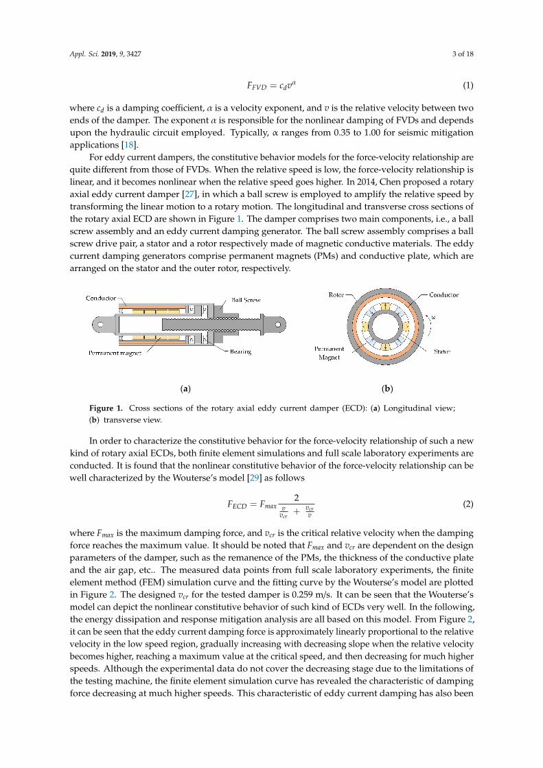
For eddy current dampers, the constitutive behavior models for the force-velocity relationship arequite different from those of FVDs. When the relative speed is low, the force-velocity relationship islinear, and it becomes nonlinear when the relative speed goes higher. In 2014, Chen proposed a rotaryaxial eddy current damper [27], in which a ball screw is employed to amplify the relative speed bytransforming the linear motion to a rotary motion. The longitudinal and transverse cross sections ofthe rotary axial ECD are shown in Figure 1. The damper comprises two main components, i.e., a ballscrew assembly and an eddy current damping generator. The ball screw assembly comprises a ballscrew drive pair, a stator and a rotor respectively made of magnetic conductive materials. The eddycurrent damping generators comprise permanent magnets (PMs) and conductive plate, which arearranged on the stator and the outer rotor, respectively.

1

(a)

(b)

Figure 1. Cross sections of the rotary axial eddy current damper (ECD): (a) Longitudinal view; (b) transverse view.

Figure 1. Cross sections of the rotary axial eddy current damper (ECD): (a) Longitudinal view;(b) transverse view.

In order to characterize the constitutive behavior for the force-velocity relationship of such a newkind of rotary axial ECDs, both finite element simulations and full scale laboratory experiments areconducted. It is found that the nonlinear constitutive behavior of the force-velocity relationship can bewell characterized by the Wouterse’s model [29] as follows

FECD = Fmax2

vvcr

+ vcrv

(2)

where Fmax is the maximum damping force, and vcr is the critical relative velocity when the dampingforce reaches the maximum value. It should be noted that Fmax and vcr are dependent on the designparameters of the damper, such as the remanence of the PMs, the thickness of the conductive plateand the air gap, etc.. The measured data points from full scale laboratory experiments, the finiteelement method (FEM) simulation curve and the fitting curve by the Wouterse’s model are plottedin Figure 2. The designed vcr for the tested damper is 0.259 m/s. It can be seen that the Wouterse’smodel can depict the nonlinear constitutive behavior of such kind of ECDs very well. In the following,the energy dissipation and response mitigation analysis are all based on this model. From Figure 2,it can be seen that the eddy current damping force is approximately linearly proportional to the relativevelocity in the low speed region, gradually increasing with decreasing slope when the relative velocitybecomes higher, reaching a maximum value at the critical speed, and then decreasing for much higherspeeds. Although the experimental data do not cover the decreasing stage due to the limitations ofthe testing machine, the finite element simulation curve has revealed the characteristic of dampingforce decreasing at much higher speeds. This characteristic of eddy current damping has also been

Appl. Sci. 2019, 9, 3427 4 of 18

reported in other literatures [29,31–33]. This unique characteristic can protect the damper and theconnection part between the damper and structure from damage when an over-load is exerted on thedamper. For example, when a huge impact load is exerted on the damper, the damping force willdecrease at much higher speeds for ECDs, but for conventional FVDs without unloading mechanisms,the damping force will go up again and consequently the damper and the connection part will bedamaged due to relatively great local stress.

2

Figure 2. Comparison of fitting curve with measured points and FEM curve for ECDs.

Figure 2. Comparison of fitting curve with measured points and FEM curve for ECDs.

3. Energy Dissipation Analysis

3.1. Energy Dissipation Capacity Under Harmonic Motion

Compared with FVDs, the ECDs have quite different constitutive behavior for the force-velocityrelationship. In view of these differences, we have to analyze their energy dissipation capacities ascompared with FVDs. The dampers are assumed to be subjected to harmonic motion u = u0 sin (ωt).Here, we assumed the maximum damping force Fmax in the ECD is the same as the maximum dampingforce in the FVD under the same harmonic motion. It should be noted that the maximum dampingforce of ECDs will occur at the critical velocity which is not necessary the same as the maximumvelocity, while the maximum damping force of FVDs happens at the maximum velocity. Under theconditions of the same harmonic motion and the same maximum damping force, we will compare theenergy dissipation capacities of ECDs and FVDs.

For FVDs which is governed by Equation (1), the energy dissipated by the damper during a cycleof harmonic motion u = u0 sin (ωt) is [18]

EFVD = 4∫ u0

0FFVDdu =

2Cd√πuα + 1

0 ωαΓ(α2 + 1)

Γ(α+32 )

(3)

where Γ(x) is the gamma function.For ECDs which is governed by Equation (2), the energy dissipated by the damper during a cycle

of the same harmonic motion u = u0 sin (ωt) is

EECD = 4∫ u0

0

2Fmaxv

vcr+ vcr

vdu =

4vcrFmaxπω

(1−vcr√

v2cr + u2

0ω2) (4)

Appl. Sci. 2019, 9, 3427 5 of 18

The detailed formula derivation is shown in Appendix A. It can be seen that EECD is a function ofvcr when Fmax, u0 and ω are specified. In the following section, we will derive the optimal vcr when theenergy dissipation capacity EECD is maximized.

3.2. Optimal Critical Velocity Under Harmonic Motion

In order to determine the maximum energy dissipation capacity of ECDs, here we use FVDs asthe reference, and take the dimensionless energy ratio EECD/EFVD as the objective function. It shouldbe noted that the maximum velocity of the harmonic motion u = u0 sin (ωt) is u0ω. Here, we take thedimensionless velocity ratio X = vcr/u0ω as the dependent variable. From the governing Equation (1)of FVDs, the maximum damping force is

Fmax = cd(u0ω)α (5)

From Equations (3)–(5), the dimensionless energy ratio can be obtained as

EECD

EFVD=

2√πΓ(α + 3

2 )

Γ(α2 + 1)X(1−

1√1 + 1

X2

) (6)

Through observing the mathematical structure of Equation (6), it can be seen that the term2√πΓ(α + 3

2 )

Γ(α2 + 1) is determined by the velocity exponent α of the FVDs, and the other term X(1 − 1√1 + 1

X2

)

is determined by the dimensionless velocity ratio X of ECDs.For a certain design of FVD, the velocity exponent α is specified. Here, we use the dimensionless

velocity ratio X as the dependent variable to find an optimal design of ECD such that the energydissipation of ECD is maximized as compared to that of the FVD. Let’s denote Y = X(1− 1√

1 + 1X2

),

and take its derivatives, we can know that when X =√

12 (−1 +

√5) ≈ 0.786, the energy dissipation

ratio EECDEFVD

reaches the maximum (See Appendix B). It can be seen that when the ratio of the criticalvelocity to the maximum velocity is 0.786, the energy dissipation capacity of ECD reaches its maximum.It should be noted that the energy dissipation ratio is also dependent on the velocity exponent α ofFVDs. The energy dissipation ratio versus the velocity ratio is plotted in Figure 3.

3

Figure 3. The energy dissipation ratio versus the velocity ratio.

Appl. Sci. 2019, 9, 3427 6 of 18

From Figure 3, it can be seen that it always can find a better design of ECD when the velocityexponent α of FVD is larger than 0.2 such that the energy dissipation capacity of ECD is larger thanthat of FVD under the same harmonic motion. As we know, the velocity exponent α of FVDs rangesfrom 0.35 to one for seismic applications, and therefore the ECDs can be used as good alternativedevices for seismic response mitigation. It is particularly worth pointing out that the critical velocitycorresponding to the maximum damping force is not the designed maximum velocity of the damperand the damping force will fall down when the velocity is larger than the critical velocity. This uniquecharacteristic guarantees that the failure risk of dampers and mounting supports can be reduced incase of an over-limit earthquake.

4. SDOF Systems with Nonlinear Eddy Current Dampers

In order to further analyze the response mitigation performance and energy dissipation capacity ofnonlinear ECDs, we consider a linear elastic SDOF system supplemented with an ECD. The governingequation of the SDOF-ECD coupling system, the steady state response to the harmonic excitation,and the dynamic response and energy dissipation to seismic excitation are analyzed in detail in thefollowing sessions.

4.1. Equations of Motion and System Paramerts

The schematic model of the SDOF system with a supplemental damper subjected to groundmotion is shown in Figure 4. The equation governing the motion of the SDOF system with massm, elastic stiffness k, linear viscous damping coefficient c, and a nonlinear FVD subjected to groundacceleration

..ug(t) is

m..u + c

.u + ku + cd

.uα = −m

..ug (7)

while for the SDOF-ECD coupling system, the equation governing the motion is

m..u + c

.u + ku + Fmax

2.u.

ucr+

.ucr.u

= −m..ug (8)

4

Figure 4. The schematic model of the SDOF system with a supplemental damper subjected toground motion.

The system parameters are selected from a longitudinal motion mode of a long span suspensionbridge as follows: The mass m = 1.4 × 107 kg; the natural frequency f = 0.124 Hz; the structuraldamping ratio ζ = 0.02; the peak ground acceleration

..ugo = 1.5247 m/s2. In order to compare the

response mitigation performance of ECDs and FVDs, here we set the damping coefficient of the FVDcd = 1.2× 107N/(m/s)α, the critical velocity of the ECD vcr = 0.786vmax, and the maximum dampingforce for ECD is the same as that of FVD Fmax = cdvαmax.

Appl. Sci. 2019, 9, 3427 7 of 18

4.2. Response to Harmonic Excitations

Before analysis of seismic responses, the steady-state responses to harmonic excitations are studied,in which two key response quantities, i.e., the displacement response and acceleration response areselected. The harmonic excitation is assumed to be

..ug =

..ugosinωt. The responses are calculated using

the Runge-Kutta algorithm.

4.2.1. Displacement Response

Define the displacement response factor to be the ratio of the displacement response amplitudeto the maximum value of static displacement Rd = uo/usto, and the frequency ratio to be the ratio ofthe external excitation frequency to the system natural frequency ω/ωn. The displacement responsefactors are first calculated for FVDs when the velocity exponent α = 0.2, 0.4, 0.6, 0.8, 1, and theirresults are plotted against the frequency ratio in Figure 5 using dotted lines. Then, the displacementresponse factors are calculated for ECDs and their results are plotted against the frequency ratio inFigure 5 using solid lines. These results indicate that for the frequency ratio in the vicinity of one, i.e.,in the resonance frequency band, the displacement responses of SDOF-ECDs are smaller than those ofSDOF-FVDs. As the velocity exponent α of the FVD increases, the control performance of the ECDsget better and better compared with that of FVDs. It should be pointed out that the displacementresponses of SDOF-ECDs are almost the same as or even slightly worse than those of SDOF-FVDs inthe far from the resonance frequency band.

5

Figure 5. Comparison of displacement response factors for SDOF-ECDs and SDOF-FVDs.

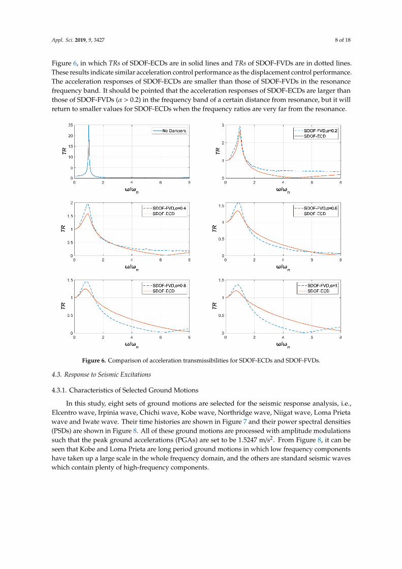
4.2.2. Acceleration Response

Define the transmissibility (TR) as the ratio of the total acceleration amplitude of the structuralmass to the peak ground acceleration TR =

..ut

o/..ugo. The TRs are plotted against the frequency ratio in

Appl. Sci. 2019, 9, 3427 8 of 18

Figure 6, in which TRs of SDOF-ECDs are in solid lines and TRs of SDOF-FVDs are in dotted lines.These results indicate similar acceleration control performance as the displacement control performance.The acceleration responses of SDOF-ECDs are smaller than those of SDOF-FVDs in the resonancefrequency band. It should be pointed that the acceleration responses of SDOF-ECDs are larger thanthose of SDOF-FVDs (α > 0.2) in the frequency band of a certain distance from resonance, but it willreturn to smaller values for SDOF-ECDs when the frequency ratios are very far from the resonance.

6

Figure 6. Comparison of acceleration transmissibilities for SDOF-ECDs and SDOF-FVDs.

4.3. Response to Seismic Excitations

4.3.1. Characteristics of Selected Ground Motions

In this study, eight sets of ground motions are selected for the seismic response analysis, i.e.,Elcentro wave, Irpinia wave, Chichi wave, Kobe wave, Northridge wave, Niigat wave, Loma Prietawave and Iwate wave. Their time histories are shown in Figure 7 and their power spectral densities(PSDs) are shown in Figure 8. All of these ground motions are processed with amplitude modulationssuch that the peak ground accelerations (PGAs) are set to be 1.5247 m/s2. From Figure 8, it can beseen that Kobe and Loma Prieta are long period ground motions in which low frequency componentshave taken up a large scale in the whole frequency domain, and the others are standard seismic waveswhich contain plenty of high-frequency components.

Appl. Sci. 2019, 9, 3427 9 of 18

7

Figure 7. Time histories of ground motions.

8

Figure 8. Power spectral densities of ground motions.

Appl. Sci. 2019, 9, 3427 10 of 18

4.3.2. Displacement and Acceleration Responses to Real Earthquakes

The system parameters are the same as before, and the responses to different ground motions arecalculated using the Runge-Kutta algorithm. The peak displacement responses (PDRs) and the peakacceleration responses (PARs) are shown in Tables 1 and 2, respectively. Here, we define the responsereduction ratio ρ as follows

ρ =Ao − Ad

Ao(9)

where Ao is the peak displacement or acceleration response without a damper and Ad is the peakdisplacement or acceleration response with a damper. The larger the reduction ratio, the better theresponse control performance of supplemental devices. The reduction ratios of displacement andacceleration are compared for ECDs and FVDs in Figures 9 and 10, respectively. The points abovethe zero line indicate that the control performance of ECD is better than that of FVD, and vice versa.From Figures 9 and 10, it is found that the displacement and acceleration reduction ratios of ECDs arelarger than those of FVDs in most cases, and the displacement reduction ratios are generally greaterthan the acceleration reduction ratios for both ECDs and FVDs. It should also be pointed out thatthere are still some cases where ECDs do not work better than FVDs for Kobe and Loma Prieta seismicwaves. In the previous Section 4.2, it is found that although the control performance of the ECDs arebetter than that of FVDs in the resonance frequency band, in the frequency band of a certain distancefrom the resonance or far from the resonance, the control performance of the ECDs are slightly worse insome cases. That is the reason why ECDs do not work better than FVDs when the dominant frequencyband of the seismic excitation is far from the resonance.

Table 1. Peak displacement responses (PDRs) of SDOF-ECDs and SDOF-FVDs.

SeismicWave

WithoutDamper (m)

FVD-SDOF ECD-SDOF

α PDR (m) ρ PDR (m) ρ

Elcentro 0.1553

0.2 0.0097 93.75% 0.0158 89.81%0.4 0.0200 87.12% 0.0186 88.04%0.6 0.0324 79.12% 0.0273 82.43%0.8 0.0404 73.96% 0.0333 78.56%1 0.0498 67.91% 0.0441 71.63%

Irpinia 0.1977

0.2 0.0399 79.82% 0.0416 78.97%0.4 0.0634 67.92% 0.0579 70.69%0.6 0.0846 57.22% 0.0724 63.39%0.8 0.1033 47.75% 0.0890 54.95%1 0.1155 41.54% 0.1049 46.94%

ChiChi 1.0532

0.2 0.0225 97.86% 0.0225 97.86%0.4 0.0321 96.95% 0.0316 97.00%0.6 0.0460 95.63% 0.0417 96.04%0.8 0.0967 90.81% 0.0561 94.67%1 0.1640 84.43% 0.0787 92.53%

Kobe 0.1271

0.2 0.0817 35.67% 0.0778 38.80%0.4 0.0883 30.48% 0.0802 36.89%0.6 0.0950 25.24% 0.0863 32.11%0.8 0.0963 24.19% 0.0936 26.37%1 0.0969 23.76% 0.0981 22.80%

Northridge 0.1441

0.2 0.0178 87.68% 0.0161 88.82%0.4 0.0300 79.18% 0.0248 82.76%0.6 0.0373 74.13% 0.0329 77.15%0.8 0.0458 68.23% 0.0396 72.50%1 0.0578 59.92% 0.0447 68.97%

Niigat 0.4533

0.2 0.0220 95.14% 0.0252 94.43%0.4 0.0426 90.59% 0.0384 91.52%0.6 0.0721 84.10% 0.0554 87.77%0.8 0.1208 73.34% 0.0795 82.47%1 0.1733 61.77% 0.1023 77.44%

Appl. Sci. 2019, 9, 3427 11 of 18

Table 1. Cont.

SeismicWave

WithoutDamper (m)

FVD-SDOF ECD-SDOF

α PDR (m) ρ PDR (m) ρ

LomaPrieta

0.1475

0.2 0.0749 49.21% 0.0636 56.84%0.4 0.0652 55.80% 0.0669 54.62%0.6 0.0646 56.17% 0.0687 53.43%0.8 0.0636 56.86% 0.0695 52.89%1 0.0684 53.59% 0.0673 54.34%

Iwate 0.6960

0.2 0.0466 93.30% 0.0362 94.81%0.4 0.0629 90.96% 0.0511 92.66%0.6 0.0830 88.07% 0.0726 89.57%0.8 0.1304 81.26% 0.0931 86.62%1 0.1767 74.61% 0.1150 83.48%

Table 2. Peak acceleration responses (PARs) of SDOF-ECDs and SDOF-FVDs.

SeismicWave

WithoutDamper (m/s2)

SDOF-FVD SDOF-ECD

α PAR (m/s2) ρ PAR (m/s2) ρ

Elcentro 2.98

0.2 2.57 13.60% 2.55 14.43%0.4 2.69 9.58% 2.59 13.09%0.6 2.72 8.68% 2.75 7.54%0.8 2.88 3.13% 2.81 5.54%1 2.93 1.59% 2.86 3.99%

Irpinia 3.08

0.2 2.96 3.92% 3.05 0.89%0.4 2.84 7.80% 2.84 7.77%0.6 2.98 3.29% 2.92 5.16%0.8 2.98 3.12% 2.94 4.40%1 3.01 2.20% 2.97 3.39%

ChiChi 3.26

0.2 2.57 21.14% 2.56 21.54%0.4 2.78 14.67% 2.74 15.78%0.6 2.91 10.83% 2.85 12.70%0.8 2.97 8.72% 2.92 10.51%1 3.05 6.49% 2.95 9.47%

Kobe 3.13

0.2 2.54 18.77% 2.54 18.71%0.4 2.81 10.21% 2.78 11.26%0.6 3.02 3.48% 2.92 6.75%0.8 3.11 0.71% 3.02 3.45%1 3.12 0.42% 3.08 1.70%

Northridge 2.99

0.2 2.55 14.65% 2.51 15.96%0.4 2.71 9.43% 2.66 11.00%0.6 2.85 4.72% 2.75 7.91%0.8 2.92 2.14% 2.87 4.07%1 2.98 0.26% 2.90 2.88%

Niigat 3.10

0.2 2.79 10.10% 2.78 10.52%0.4 2.94 5.22% 2.88 6.99%0.6 2.96 4.48% 2.94 5.16%0.8 3.01 3.03% 2.97 4.17%1 3.01 2.85% 2.99 3.45%

LomaPrieta

3.11

0.2 3.14 −1.16% 2.96 4.63%0.4 3.06 1.49% 3.03 2.35%0.6 2.97 4.51% 3.03 2.46%0.8 2.96 4.77% 2.97 4.34%1 3.02 2.80% 2.94 5.34%

Iwate 3.18

0.2 2.61 17.77% 2.82 11.19%0.4 2.98 6.15% 2.96 6.75%0.6 3.03 4.49% 3.03 4.62%0.8 3.12 1.88% 3.07 3.47%1 3.09 2.73% 3.09 2.58%

Appl. Sci. 2019, 9, 3427 12 of 18

9

Figure 9. Displacement reduction ratios under different earthquakes.

10

Figure 10. Acceleration reduction ratios under different earthquakes.

4.3.3. Energy Dissipation Analysis Under Seismic Excitations

For elastic SDOF systems, the input energy of seismic excitations will be finally dissipated by thestructural inherent damping and supplemental damping devices. In this paper, the energy dissipatedby the inherent damping is expressed as

Ein =

∫ Tt

0c

.u

.udt =

∫ Tt

02ζmωn

.u

.udt (10)

where Tt is the duration of the ground motions. The energy dissipated by the supplemental dampingdevices (ECDs or FVDs) is

EECD(FVD) =

∫ Tt

0FECD(FVD)(

.u)

.udt (11)

Appl. Sci. 2019, 9, 3427 13 of 18

The total dissipated energy is

Etotal = Ein + EECD(FVD) (12)

The time history results of the normalized dissipated energy of FVD and ECD subjected to theElcentro ground motion are shown in Figure 11. As shown in Figure 11a, the normalized energydissipated by the FVD (α = 1) is 0.9648, which is 27.38 times of that dissipated by the correspondinginherent damping (0.0352), indicating that the FVD improves the energy dissipation capability ofuncontrolled systems by 27.38 times. As a contrast, it is clear that in Figure 11b, the energy dissipatedby the ECD is larger than the energy dissipated by the FVD. Specifically, the normalized energydissipated by the ECD in Figure 11b is 0.9808, which is about 50.98 times of the energy dissipated bythe corresponding inherent damping (0.0192). These results indicate that the ECD could improve theenergy dissipation capability of uncontrolled systems by about 50.98 times.

11

Figure 11. Dissipated energy of SDOF systems (ζ = 2%) with FVD and ECD subjected to theElcentro earthquake.

As indicated by Equation (10), if the inherent damping is prescribed, the energy dissipated bythe inherent damping depends on the response amplitude. To protect the structure, the supplementaldamping devices are required to dissipate the majority of the input seismic energy. Here, we define anew criterion named as the energy dissipation ratio (ER) to represent the energy dissipation capacityof supplemental damping devices. The larger the energy dissipative ratio, the larger the energydissipation capability of supplemental devices.

ERECD(FVD) =EECD(FVD)

Ein(13)

The energy dissipation ratios of the SDOF systems (ζ = 2%) with FVDs and ECDs subjected todifferent ground motions are compared in Table 3 and Figure 12. From Figure 12, the points above thezero line indicate that the energy dissipation capacity of ECD is better than that of FVD, and vice versa.It is found that the energy dissipation capacity of ECDs are larger than those of FVDs in most cases.

Appl. Sci. 2019, 9, 3427 14 of 18

Table 3. Energy dissipation ratios (ERs) of SDOF-ECDs and SDOF-FVDs.

SeismicWave

SDOF-FVD SDOF-ECD

α Normalized Energy ER Normalized Energy ER

Elcentro

0.2 0.9974 383.51 0.9967 302.270.4 0.9946 183.40 0.9946 185.370.6 0.9892 91.83 0.9915 117.220.8 0.9801 49.14 0.9870 75.771 0.9648 27.38 0.9808 50.98

Irpinia

0.2 0.9955 219.02 0.9950 199.280.4 0.9914 114.72 0.9920 123.240.6 0.9857 68.99 0.9881 83.020.8 0.9771 42.62 0.9837 60.251 0.9649 27.50 0.9783 45.18

ChiChi

0.2 0.9976 424.25 0.9973 372.160.4 0.9947 187.15 0.9950 200.180.6 0.9894 92.95 0.9919 122.120.8 0.9798 48.40 0.9877 80.031 0.9649 27.50 0.9822 55.29

Kobe

0.2 0.9919 122.42 0.9926 133.270.4 0.9892 91.89 0.9898 97.120.6 0.9839 60.99 0.9868 74.520.8 0.9759 40.58 0.9833 58.781 0.9649 27.50 0.9792 47.06

Northridge

0.2 0.9974 383.35 0.9974 381.090.4 0.9943 173.06 0.9946 185.420.6 0.9889 89.46 0.9912 113.200.8 0.9799 48.71 0.9871 76.301 0.9649 27.50 0.9818 54.08

Niigat

0.2 0.9968 315.39 0.9969 322.720.4 0.9944 178.90 0.9947 189.160.6 0.9889 89.25 0.9917 119.900.8 0.9789 46.43 0.9874 78.531 0.9649 27.50 0.9824 55.89

Loma Prieta

0.2 0.9910 110.46 0.9930 140.990.4 0.9895 94.66 0.9902 101.010.6 0.9843 62.67 0.9871 76.570.8 0.9763 41.12 0.9835 59.721 0.9649 27.47 0.9794 47.57

Iwate

0.2 0.9966 296.45 0.9963 267.730.4 0.9942 171.17 0.9939 162.510.6 0.9882 83.77 0.9909 108.470.8 0.9785 45.54 0.9869 75.481 0.9649 27.50 0.9824 55.78

12

Figure 12. Energy dissipation ratios under different earthquakes.

Appl. Sci. 2019, 9, 3427 15 of 18

5. Conclusions

This paper investigates the dynamic characteristics of a rotary axial ECD and its seismic reductionperformance when applied in a linear elastic SDOF system. The nonlinear force-velocity relationshipof the ECD is expressed using the Wouterse’s model which are validated by Finite element simulationand experimental testing. The energy dissipation capacity of the ECD is obtained analytically and itsoptimal parameters for maximum energy dissipation are also derived. The control performance ofECDs is investigated and evaluated under harmonic excitations and real earthquake ground motions.The most important findings are summarized below:

(1) The force-velocity constitutive behavior of the ECD can be well depicted by the Wouterse’smodel. The eddy current damping force is linearly proportional to the velocity for low speedregion, gradually increasing with decreasing slope when the velocity become higher, reachinga maximum at the critical speed, and then decreasing for much higher speeds. These uniquecharacteristics can protect the damper and structure from damage when an over-load is exertedon the damper.

(2) When the ratio of the critical velocity of the ECD to the maximum velocity is 0.786, the energydissipation capacity of ECD reaches its maximum under harmonic motions. It always can find abetter design of ECD when the velocity exponent α of FVD is larger than 0.2 such that the energydissipation capacity of ECD is larger than that of FVD under the same harmonic motion.

(3) In the resonance frequency band, both the displacement and acceleration responses of SDOF-ECDsare smaller than those of SDOF-FVDs under the same harmonic excitation. As the velocityexponent α of the FVD increases, the control performance of the corresponding ECD gets betterand better compared with that of FVD.

(4) The displacement and acceleration reduction ratios of ECDs are larger than those of FVDs in mostof the cases under real earthquake excitations, and the displacement reduction ratios are generallygreater than the acceleration reduction ratios for both ECDs and FVDs. The energy dissipationcapacity of ECDs outperforms that of FVDs in most of the cases under real earthquake excitations.

Currently, this paper is limited to the numerical evaluation of ECDs for elastic SDOF systems.The conclusions summarized above are based on the limited data presented in this paper. To furtherextrapolate the findings, the next step is to experimentally test the performance of ECDs with structures.Meanwhile, the further studies on applying ECDs in MDOF systems will also be developed in the future.

Author Contributions: All authors made scientific contributions: L.L. derived the formulas and made thecalculations, Z.F. conceived the idea of this research and wrote the manuscript, and Z.C. revised the manuscript.

Funding: This work was supported in part by the National Natural Science Foundation of China under grantNo. 51708203, the Fundamental Research Funds for the Central Universities under grant No. 531118010047,the Open Research Fund Program of Guangdong Key Laboratory of Earthquake Engineering and ApplicationTechnology under grant No. 2014B030301075-02, the Open Research Fund Program for innovation platforms ofuniversities in the Hunan province from the Education Department of Hunan Province under grant No. 17K022,and the independent research project funds from the State Key Laboratory of Advanced Design and Manufacturingfor Vehicle Body in Hunan University under grant No. 71860006.

Conflicts of Interest: The authors declare no conflict of interest.

Appendix A

The mathematic proofs of Equation (4) are shown in this appendix section. The energy dissipationof ECD under a cycle of harmonic excitation is

EECD = 4∫ u0

02Fmaxv

vcr +vcrv

du = 4∫ π

2ω0

2vcrFmax

1+v2

cr(u0ω cos (ωt))2

dt

= 8vcrFmax∫ π

2ω0

1

1+v2

cr(u0ω cos (ωt))2

dt(A1)

Appl. Sci. 2019, 9, 3427 16 of 18

The indefinite integral in Equation (A1) can be rewritten as∫1

1 + v2cr

(u0ω cos (ωt))2

dt =∫

1

1 + v2cr(sec (ωt))2

(u0ω))2

dt (A2)

Substitute s = ωt and ds = ωdt into Equation (A2), it becomes∫1

1 +v2cr

(u0ω cos (ωt))2

dt = 1ω

∫1

v2crsec2 (s)

u02ω2 +1

ds = 1ω

∫ sec2 (s)v2

crsec4 (s)

u02ω2 +sec2 (s)

ds

= 1ω

∫ sec2 (s)

(1+tan2(s))(1+v2cr(1+tan2(s))

u02ω2 )

ds(A3)

Substitute p = tan (s) and dp = sec2 (s)ds into Equation (A3), it becomes∫1

1 +v2cr

(u0ω cos (ωt))2

dt = 1ω

∫1

(p2+1)(v2

cr(p2+1)

u02ω2 +1)

dp

= 1ω

∫( 1

p2+1 −v2

crv2

crp2+v2cr+u02ω2 )dp

= −v2

crω

∫1

v2crp2+v2

cr+u02ω2 dp + 1ω

∫1

p2+1 dp

= −v2

crω

∫1

(v2cr+u02ω2)(

v2crp2

v2cr+u0

2ω2 +1)dp + 1

ω

∫1

p2+1 dp

= −v2

crω(v2

cr+u02ω2)

∫1

v2crp2

v2cr+u0

2ω2 + 1dp + 1

ω

∫1

p2+1 dp

(A4)

Substitute v =vcrp

√v2

cr + u02ω2and dv = vcr√

v2cr + u02ω2

dp into Equation (A4), it becomes

∫1

1+v2cr

(u0ω cos (ωt))2

dt = − vcr

ω√

v2cr+u02ω2

∫1

v2+1 dv + 1ω

∫1

p2+1 dp

=tan−1 (p)

ω −vcr tan−1 (v)

ω√

v2cr+u02ω2

= t−vcrtan−1(

vcr tan (ωt)√

v2cr+u0

2ω2)

ω√

v2cr+u02ω2

(A5)

According to Equations (A1) and (A5)

EECD = 8vcrFmax∫ π

2ω0

1

1 +v2

cr(u0ω cos (ωt))2

dt

= 8vcrFmax( limt→ π

2ω

(t−vcr tan−1 (

vcr tan (ωt)√

v2cr+u0

2ω2)

ω√

v2cr+u02ω2

) − 0)

= 8vcrFmax(π

2ω −πvcr

2ω√

v2cr+u02ω2

)

= 4vcrFmaxπω (1− vcr√

v2cr+u02ω2

)

(A6)

Appendix B

The mathematic proofs of optimal value for critical velocity of ECDs are shown in this appendixsection. Firstly, obtaining the derivative and second derivative of Y = X(1− 1√

1 + 1X2

)

Y′ = 1−1√

1 + 1X2

−1

(1 + 1X2 )

3/2X2

(A7)

Y′′ =3

(1 + 1X2 )

5/2X5−

1

(1 + 1X2 )

3/2X3

(A8)

Appl. Sci. 2019, 9, 3427 17 of 18

Let Y′ = 0, Equation (A7) can be rewritten as

1− 1√1+ 1

X2

−1

(1+ 1X2 )

3/2X2

= 0

(1 + 1X2 )

3/2X2 +

√1 + 1

X2 = (1 + 1X2 )

2X2

(A9)

Denote a =√

1 + 1X2 , (a > 0 & a , 1, X , ∞) and substitute it into Equation (A9), it becomes

a3

a2−1 + a = a4

a2−1a4−2a3 + a

a2−1 = 0a(a−1)(a2

−a−1)a2−1 = 0

(A10)

Since a > 0 & a , 1, Solve (a2− a− 1) = 0 and it gets

a =12(1 +

√

5) (A11)

Substitute this value back into a =√

1 + 1X2 and it gets

X =

√12(−1 +

√

5) ≈ 0.786 (X > 0) (A12)

Substitute X = 0.786 to Equation (A8)

Y′′ =3

(1 + 1X2 )

5/2X5−

1

(1 + 1X2 )

3/2X3≈ −0.415 < 0 (A13)

Therefore, when X = 0.786, Y reaches its maximum, and then the energy dissipation ratio EECDEVD

reaches its maximum.

References

1. Lu, X.; Chen, J. Mitigation of wind-induced response of Shanghai Center Tower by tuned mass damper.Struct. Des. Tall Spec. Build. 2011, 20, 435–452. [CrossRef]

2. Lu, X.; Zhang, Q.; Weng, D.; Zhou, Z.; Wang, S.; Mahin, S.A.; Ding, S.; Qian, F. Improving performanceof a super tall building using a new eddy-current tuned mass damper. Struct. Control Health Monit. 2017,24, e1882. [CrossRef]

3. Ji, X.; Liu, D.; Hutt, C.M. Seismic performance evaluation of a high-rise building with novel hybrid coupledwalls. Eng. Struct. 2018, 169, 216–225. [CrossRef]

4. Qian, H.; Li, H.; Song, G. Experimental investigations of building structure with a superelastic shape memoryalloy friction damper subject to seismic loads. Smart Mater. Struct. 2016, 25, 125056. [CrossRef]

5. Li, L.; Song, G.; Ou, J. Hybrid active mass damper (AMD) vibration suppression of nonlinear high-risestructure using fuzzy logic control algorithm under earthquake excitations. Struct. Control Health Monit.2011, 18, 698–709. [CrossRef]

6. Guo, T.; Liu, J.; Zhang, Y.; Pan, S. Displacement Monitoring and Analysis of Expansion Joints of Long-SpanSteel Bridges with Viscous Dampers. J. Bridge Eng. 2015, 20, 04014099. [CrossRef]

7. Yang, M.-G.; Chen, Z.-Q.; Hua, X.-G. An experimental study on using MR damper to mitigate longitudinalseismic response of a suspension bridge. Soil Dyn. Earthq. Eng. 2011, 31, 1171–1181. [CrossRef]

8. Li, C.; Li, H.-N.; Hao, H.; Bi, K.; Chen, B. Seismic fragility analyses of sea-crossing cable-stayed bridgessubjected to multi-support ground motions on offshore sites. Eng. Struct. 2018, 165, 441–456. [CrossRef]

9. Wen, Q.; Hua, X.G.; Chen, Z.Q.; Yang, Y.; Niu, H.W. Control of Human-Induced Vibrations of a CurvedCable-Stayed Bridge: Design, Implementation, and Field Validation. J. Bridge Eng. 2016, 21, 04016028. [CrossRef]

10. Varela, W.D.; Battista, R.C. Control of vibrations induced by people walking on large span composite floordecks. Eng. Struct. 2011, 33, 2485–2494. [CrossRef]

Appl. Sci. 2019, 9, 3427 18 of 18

11. Li, H.; Liu, M.; Li, J.; Guan, X.; Ou, J. Vibration Control of Stay Cables of the Shandong Binzhou Yellow RiverHighway Bridge Using Magnetorheological Fluid Dampers. J. Bridge Eng. 2007, 12, 401–409. [CrossRef]

12. Chen, Z.Q.; Wang, X.Y.; Ko, J.M.; Ni, Y.Q.; Spencer, B.F.; Yang, G.; Hu, J.H. MR damping system formitigating wind-rain induced vibration on Dongting Lake Cable-Stayed Bridge. Wind Struct. 2004, 7, 293–304.[CrossRef]

13. Shi, X.; Zhu, S.; Li, J.-Y.; Spencer, B.F., Jr. Dynamic behavior of stay cables with passive negative stiffnessdampers. Smart Mater. Struct. 2016, 25, 075044. [CrossRef]

14. Zhang, Z.; Staino, A.; Basu, B.; Nielsen, S.R.K. Performance evaluation of full-scale tuned liquid dampers(TLDs) for vibration control of large wind turbines using real-time hybrid testing. Eng. Struct. 2016, 126,417–431. [CrossRef]

15. Zhang, Z.; Nielsen, S.R.K.; Basu, B.; Li, J. Nonlinear modeling of tuned liquid dampers (TLDs) in rotatingwind turbine blades for damping edgewise vibrations. J. Fluids Struct. 2015, 59, 252–269. [CrossRef]

16. Zuo, H.; Bi, K.; Hao, H. Using multiple tuned mass dampers to control offshore wind turbine vibrationsunder multiple hazards. Eng. Struct. 2017, 141, 303–315. [CrossRef]

17. Song, G.B.; Zhang, P.; Li, L.Y.; Singla, M.; Patil, D.; Li, H.N.; Mo, Y.L. Vibration Control of a Pipeline StructureUsing Pounding Tuned Mass Damper. J. Eng. Mech. 2016, 142, 04016031. [CrossRef]

18. Lin, W.-H.; Chopra, A.K. Earthquake response of elastic SDF systems with non-linear fluid viscous dampers.Earthq. Eng. Struct. Dyn. 2002, 31, 1623–1642. [CrossRef]

19. Wang, W.; Wang, X.; Hua, X.; Song, G.; Chen, Z. Vibration control of vortex-induced vibrations of a bridgedeck by a single-side pounding tuned mass damper. Eng. Struct. 2018, 173, 61–75. [CrossRef]

20. Lin, W.; Song, G.; Chen, S. PTMD Control on a Benchmark TV Tower under Earthquake and Wind LoadExcitations. Appl. Sci. 2017, 7, 425. [CrossRef]

21. Zhang, P.; Song, G.; Li, H.-N.; Lin, Y.-X. Seismic Control of Power Transmission Tower Using Pounding TMD.J. Eng. Mech. 2013, 139, 1395–1406. [CrossRef]

22. Huang, Z.W.; Hua, X.G.; Chen, Z.Q.; Niu, H.W. Modeling, Testing, and Validation of an Eddy CurrentDamper for Structural Vibration Control. J. Aerosp. Eng. 2018, 31, 04018063. [CrossRef]

23. Shen, W.; Zhu, S.; Xu, Y. An experimental study on self-powered vibration control and monitoring systemusing electromagnetic TMD and wireless sensors. Sens. Actuators A Phys. 2012, 180, 166–176. [CrossRef]

24. Shen, W.; Zhu, S.; Zhu, H.; Xu, Y. Electromagnetic energy harvesting from structural vibrations duringearthquakes. Smart Struct. Syst. 2016, 18, 449–470. [CrossRef]

25. Shen, W.; Zhu, S.; Zhu, H. Unify Energy Harvesting and Vibration Control Functions in Randomly ExcitedStructures with Electromagnetic Devices. J. Eng. Mech. 2019, 145, 04018115. [CrossRef]

26. Zuo, L.; Chen, X.; Nayfeh, S. Design and Analysis of a New Type of Electromagnetic Damper With IncreasedEnergy Density. J. Vib. Acoust. 2011, 133, 041006. [CrossRef]

27. Chen, Z. Outer Cup Rotary Axial Eddy Current Damper. 15 September 2014.28. Pérez-Díaz, J.; Valiente-Blanco, I.; Cristache, C. Z-Damper: A New Paradigm for Attenuation of Vibrations.

Machines 2016, 4, 12. [CrossRef]29. Wouterse, J.H. Critical torque and speed of eddy current brake with widely separated soft iron poles. IEE Proc.

B (Electr. Power Appl.) 1991, 138, 153. [CrossRef]30. Constantinou, M.C.; Soong, T.T.; Dargush, G.F. Passive Energy Dissipation Systems for Structural Design and

Retrofit; MCEER Monograph No. MCEER-98-MN01, SUNY; UBIR: Buffalo, NY, USA, 1998.31. Nehl, T.W.; Lequesne, B.; Gangla, V.; Gutkowski, S.A.; Robinson, M.J.; Sebastian, T. Nonlinear two-dimensional

finite element modeling of permanent magnet eddy current couplings and brakes. IEEE Trans. Magn. 1994,30, 3000–3003. [CrossRef]

32. Canova, A.; Vusini, B. Analytical modeling of rotating eddy-current couplers. IEEE Trans. Magn. 2005, 41,24–35. [CrossRef]

33. Sharif, S.; Faiz, J.; Sharif, K. Performance analysis of a cylindrical eddy current brake. IET Electr. Power Appl.2012, 6, 661. [CrossRef]

© 2019 by the authors. Licensee MDPI, Basel, Switzerland. This article is an open accessarticle distributed under the terms and conditions of the Creative Commons Attribution(CC BY) license (http://creativecommons.org/licenses/by/4.0/).