Nonlinear Analysis Methods for Evaluating Seismic ...
104
Nonlinear Analysis Methods for Evaluating Seismic Performance of Multi-Story RC Buildings Saeid Moussavi Tayyebi Submitted to the Institute of Graduate Studies and Research in the partial fulfillment of the requirements for the Degree of Master of Science in Civil Engineering Eastern Mediterranean University October 2014 Gazimağusa, North Cyprus
-
Upload
khangminh22 -
Category
Documents
-
view
3 -
download
0
Transcript of Nonlinear Analysis Methods for Evaluating Seismic ...

Nonlinear Analysis Methods for Evaluating Seismic
Performance of Multi-Story RC Buildings
Saeid Moussavi Tayyebi
Submitted to the
Institute of Graduate Studies and Research
in the partial fulfillment of the requirements for the Degree of
Master of Science
in Civil Engineering
Eastern Mediterranean University
October 2014
Gazimağusa, North Cyprus

Approval of the Institute of Graduate Studies and Research
Prof. Dr. Elvan Yılmaz
Director
I certify that this thesis satisfies the requirements of thesis for the degree of Master of
Science in Civil Engineering.
Prof. Dr. Özgür Eren
Chair, Department of Civil Engineering
We certify that we have read this thesis and that in our opinion it is fully adequate in
scope and quality as a thesis for the degree of Master of Science in Civil Engineering.
Asst. Prof. Dr. Serhan Şensoy
Supervisor
Examining Committee
1. Asst. Prof. Dr. Mürüde Çelikağ
2. Asst. Prof. Dr. Giray Ozay
3. Asst. Prof. Dr. Serhan Şensoy

iii
ABSTRACT
A major challenge in performance-based earthquake engineering is to develop simple
and practical methods for estimating capacity level and seismic demand on structures
by taking into account their inelastic behavior. Researchers and engineers certainly
prefer to use nonlinear static methods over complicated nonlinear time-history
methods. However, in Nonlinear Static procedure both predetermined target
displacement and force distribution pattern are based on a false assumption that the
structural behavior and its responses are dominated by the fundamental vibration
modes. Therefore, over the past decades, there have been a great number of studies on
considering higher mode contribution in nonlinear static results. However, their major
drawback is that these approaches are inevitably more complex and time consuming
compared to a single-run pushover analysis.
The primary aim of this work is to perform and compare different nonlinear analysis
methods for evaluating the seismic performances of structures. For these purposes,
three models are considered to represent low-rise, medium-rise and high-rise
structures. This consist of a moment resisting reinforced concrete structures with no
shear walls, located in a high-seismicity region of Turkey. They are designed
according to Turkish Earthquake Code 2007 and TS 500-2000 codes, considering both
seismic and gravity loads.
The Displacement-based Adaptive Pushover Analysis (DAP), which was proposed by
Antoniou and Pinho (2004), is one of the performance assessments tool for improving
the accuracy of the obtained results of nonlinear static analysis in estimating the

iv
seismic demands of the structures. In this thesis, reliability of the DAP in estimating
the seismic response of 3, 8 and 12-story moment resisting reinforced concrete frames
responding in the inelastic range is demonstrated. Therefore, Incremental Dynamics
Analysis (IDA), by applying a large set of natural records, and FEMA 440 static
pushover procedure are performed for comparison. The capacity curves of the
structures, as derived by both DAP and FEMA440 pushover curves are compared with
the IDA envelopes by using SeismoStruct software. Performance levels of structures
are also estimated and compared by performing DAP and Incremental Dynamic
Analysis using SeismoStruct software and, FEMA440 pushover analysis using
SAP2000 program. Results are presented and discussed for advantage and
disadvantage of procedures.
It is demonstrated that Displacement-based Adaptive Pushover Analysis is adequate
for estimating seismic response of reinforce concrete frame and represents an
alternative simpler procedure compared to IDA. The DAP method not only automates
the pushover analysis, but also improves the accuracy of its results in estimating the
seismic demands of the structure.
Keywords: Multi-Mode Pushover Analysis, Incremental Dynamic Analysis,
Displacement-based Adaptive Pushover Analysis, and Nonlinear Static Analysis

v
ÖZ
Performansa dayalı deprem mühendisliğinin en önemli tartışmalarından biri de basit
ve uygulanabilir metodların hayata geçirilip yapı deprem kapasitesinin ve talebinin
belirlenmesi amacı ile doğrusal ve elastik olamayan modellerin analizene olanak
sağlamaktır. Araştırmacılar ve mühendisler daha basit doğrusal olamayan statik
yöntemleri daha karm aşık zaman-tanım alanındaki çözümlere tercih etmektedirler.
Öte yandan doğrusal olmayan statik analiz yöntemlerinde yapıya uygulanan kuvvetler
yapı periyodu ve kuvvet dağılımı sabit tutularak yapıldığında hasar gören ve elastic
ötesi davranan yapıların analizinde gerçekci çözümler üretemeyebilir. Bu nedenle
özellikle son dönemlerde birden fazla modal etkiyi dikkate Alana ve yük dağılımını
sabiit kabul etmeyen yöntemler üzerinde çalışmalar yapılmıştır. Nevar ki bu yöntemler
yinede kaçınılmaz olarak karmaşık olabilmektedir.
Bu çalışmanın ana amacı yapıların deprem performanslarının belirlenmesinde farklı
yöntemlerin karşılaştırılamsıdır. Bu amaç doğrultusunda alçak katlı, orta katlı ve
yüksek katlı çerçeve sistemler yapılar tasarlanıp değerlendirilmiştir. Modeller Türk
Deprem Yönetmeliğinde belirtilen birinci derece deprem bölgesinde ve Türk Deprem
Yönetmeliği,2007 ve TS500-2000 yönetmelikleri kullanılarak düşey ve deprem
yüklerine göre tasarlanmıştır.
Deplasmana bağlı Değişken İtme Analizi (DAP) yöntemi, deprem performasının daha
sağlıklı belirlenmesi için geliştirilen yöntemlerden biridir. Bu tezde DAP yönteminin
güvenli bir şekilde uygulanıp uygulanmayacağının belirlenmesi amacı ile 3, 8 ve 12
katlı yapılar Analiz edilmiştir. Bununla birlikte Artımsal Dinamik Analiz (IDA)

vi
yöntemi, toplamda 12 deprem kayıdı kullanılarak çalışılmış ve DAP, FEMA 440 ve
IDA yöntemleri karşılaştırılmıştır. Bu amaç için SeismoStruct yazılımı kullanılmış ve
elede edilen performans eğrileri ve IDA eğrileri karşılaştırılmıştır. Ayrıca FEMA 440
yöntemine göre performans seviyelerinin belirlenmesinde SAP2000 kullanılmıştır.
Bu çalışmada gösterilmiştir ki DAP yöntemi betonarme yapıların performans
değerlendirmelerinde IDA yöntemine alternative olarak daha basit bir yöntem olarak
kullanılabilir. DAP yönteminin geleneksel itma analizi yöntemine göre sistematik bir
yöntem olamsının yanında daha doğru sonuçlar verdiği ayrıca gözlemlenmiştir.
Anahtar Kelimeler: Çok Modlu İtme Analizini, Artımsal Dinamik Analiz,
Deplasmana bağlı Değişken İtme Analizi, ve Statik İtme Analizi.

vii
Dedicated
To my Lovely Father and Mother
To my dearest Brother

viii
ACKNOWLEDGMENT
I would like to thank Dr. Serhan Şensoy for his valuable suggestions and guidance, I
sincerely appreciate all the time he spent on this research work. I would also like to
extend my thanks to all the members of the Civil Engineering Department for their
kindnesses and supports.
I wish to thank my parents for their love and encouragement throughout my life. My
father, Mahdi, who is the one of the best civil engineer for me. He encouraged me to
concentrate on my study especially when I encountered difficulties. My mother, Souri,
who helped me concentrate on completing my study and supporting mentally. Her
encouragement are too numerous to mention. Also, I appreciate my brother and my
best friend, Ali, who gives encouragement in his particular way. I appreciate all of the
times you visited, called, chatted and e-mailed with words of faith, encouragement and
wisdom that carried me through every day of this process. Finally. I would like to
express my appreciation to everyone who made these years in Cyprus a wonderful
experience.

ix
TABLE OF CONTENTS
ABSTRACT ................................................................................................................ iii
ÖZ ................................................................................................................................ v
DEDICATION ........................................................................................................... vii
ACKNOWLEDGMENT ........................................................................................... viii
LIST OF TABLES .................................................................................................... xiii
LIST OF FIGURES .................................................................................................. xiv
LIST OF ABBREVIATIONS ................................................................................... xvi
.................................................................................................... 1
1.1 Objective ............................................................................................................ 1
1.2 Performance-Based Seismic Evaluation............................................................. 2
1.3 Seismic Performance Assessment Methods ....................................................... 3
1.3.1 Linear Static Procedure ................................................................................ 3
1.3.2 Linear Dynamic Procedure .......................................................................... 4
1.3.3 Nonlinear Static Procedure (NSP): .............................................................. 4
1.3.4 Advantages and Disadvantages of Nonlinear Static Procedures ................. 5
1.3.5 Multi-Mode Pushover Analysis ................................................................... 6
1.3.5.1 Adaptive Pushover Procedures ............................................................. 7
1.3.5.2 Modal Pushover Analysis (MPA) ......................................................... 9
1.3.5.3 Incremental Response Spectrum Analysis (IRSA) ............................. 10
1.3.6 Nonlinear Dynamic Analysis ..................................................................... 15
1.3.6.1 Nonlinear Time History Dynamic Analysis Method .......................... 15
1.3.6.2 Incremental Dynamic Analysis ........................................................... 16
1.3.6.3 Advantages and Disadvantages of Dynamic Procedures .................... 17
1.3.7 Why nonlinear dynamics analysis cannot be in codes? ............................. 18

x
1.4 Thesis Outline ................................................................................................... 19
................................................................. 20
2.1 Modeling .......................................................................................................... 20
2.1.1 Description of structures ............................................................................ 20
2.2 Sections Design ................................................................................................ 24
2.2.1 3-story structure ......................................................................................... 24
2.2.2 8-story structure ......................................................................................... 26
2.2.3 12-story structure ....................................................................................... 28
.................................................................................................. 30
3.1 Target Displacement ......................................................................................... 30
3.2 Computing and defining inelastic frame elements ........................................... 33
3.2.1 Defining inelastic frame elements in SeismoStruct Software ................... 33
3.2.2 Defining inelastic frame elements in SAP2000 ......................................... 35
3.3 Structural Performance limits states ................................................................. 37
3.3.1 Immediate occupancy (IO) ........................................................................ 37
3.3.2 Life Safety (LS) ......................................................................................... 37
3.3.3 Collapse Prevention (CP)........................................................................... 37
3.3.4 Collapse (C) ............................................................................................... 38
3.3.5 Drift Levels ................................................................................................ 38
3.4 Nonlinear Static Procedures ............................................................................. 39
3.4.1 Introduction ................................................................................................ 39
3.4.2 Methodology .............................................................................................. 40
3.4.2.1 Nonlinear Static Analysis Procedures ................................................. 40
3.4.2.2 Conventional Nonlinear Static Analysis Based on FEMA 356 .......... 40
3.4.2.3 Idealizing force-displacement curve ................................................... 41

xi
3.5 Displacement-based Adaptive Pushover .......................................................... 42
3.5.1 Introduction ................................................................................................ 42
3.5.2 Methodology .............................................................................................. 43
3.5.3 Choice of the Software for Computer Analysis (SeismoStruct software) . 44
3.6 Incremental Dynamic Analysis (IDA).............................................................. 45
3.6.1 Introduction ................................................................................................ 45
3.6.2 Methodology .............................................................................................. 46
3.6.3 Selected Ground Motions .......................................................................... 47
3.6.4 SeismoStruct Software ............................................................................... 48
3.6.5 Summarizing the IDA Curves.................................................................... 50
........................................................................... 51
4.1 3-Story Frame ................................................................................................... 51
4.1.1 Target displacement of 3-Story Frame ...................................................... 51
4.1.2 Performance limit states of 3-Story Frame ................................................ 52
4.2 8-Story Frame ................................................................................................... 54
4.2.1 Target displacement of 8-Story Frame ...................................................... 54
4.2.2 Performance limit states of 8-Story Frame ................................................ 55
4.3 12-Story Frame ................................................................................................. 57
4.3.1 Target displacement of 12-Story Frame .................................................... 57
4.3.2 Performance limit states of 12-Story Frame .............................................. 58
4.4 Capacity curve of conventional pushover analysis .......................................... 60
4.5 Incremental Dynamic analysis (IDA) ............................................................... 62
4.5.1 Post processing and Generating IDA Curves ............................................ 62
4.5.2 Summarizing the IDA Curves.................................................................... 64
4.5.2.1 Defining of Limit States ...................................................................... 66

xii
4.5.3 Probabilistic fragility curves ...................................................................... 67
4.6 Inter-Story Drift Profiles derived by DAP Method .......................................... 71
4.7 Comparison between Nonlinear Dynamic and Static Analyses ....................... 73
4.7.1 Base Shear vs. Top Displacement Curves (Capacity Curve) ..................... 73
4.7.2 Performance Limit States of Nonlinear Dynamic and Static Analyses ..... 79
........................................................................ 80
5.1 Summary .......................................................................................................... 80
5.2 Conclusion ........................................................................................................ 82
5.3 Recommendations ............................................................................................ 83
REFERENCES ........................................................................................................... 84

xiii
LIST OF TABLES
Table 2.1. Columns section characterizations. ........................................................... 25
Table 3.1. Structural Performance Levels (FEMA356, 2000). ................................. 38
Table 3.2. List of earthquake ground motions (PEER, 2010) .................................... 49
Table 4.1. FEMA440 parameters for 3-story frame model. ....................................... 51
Table 4.2. Pushover steps for 3-story frame model ................................................... 52
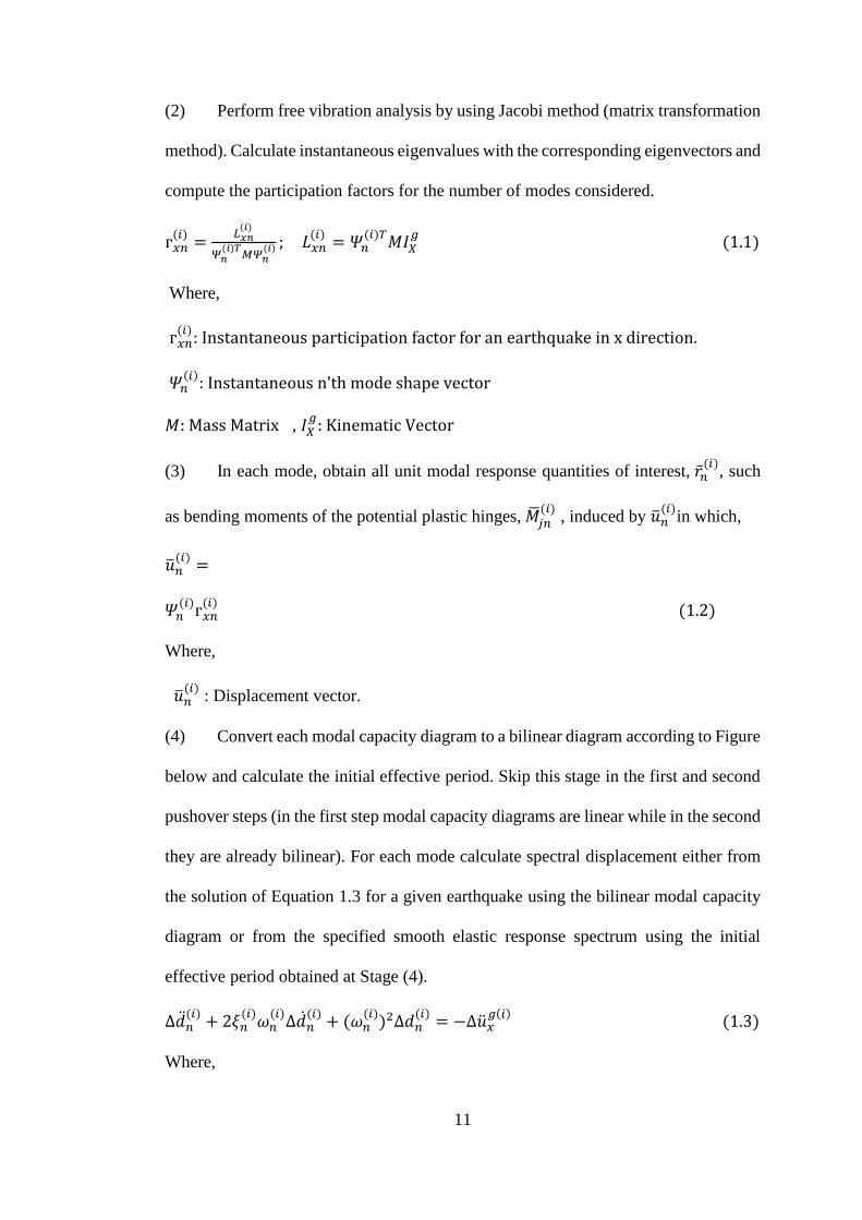
Table 4.3. The performance levels of 3-Story Frame ................................................ 53
Table 4.4. FEMA440 parameters for 8-story frame model. ....................................... 54
Table 4.5. Pushover steps for 8-story frame model ................................................... 55
Table 4.6. The performance levels of 8-Story Frame ................................................ 56
Table 4.7. FEMA440 parameters for 12-story frame model. ..................................... 57
Table 4.8. Pushover steps for 12-story frame model ................................................. 58
Table 4.9. The performance levels of 12-Story Frame .............................................. 59
Table 4.10. Summarized capacities for each limit-states for (a) 3-story (b) 8-story (c)
12-story RC Frame. ............................................................................................ 66
Table 4.11. Seismic performance levels of Structures by performing Incremental
Dynamics Analysis using SeismoStruct software. ............................................. 68
Table 4.12. Seismic performances of Structures by performing DAP and Pushover
Analyses and IDA Methods. .............................................................................. 79

xiv
LIST OF FIGURES
Figure 1.1. Modal capacity diagram Bi-linearization ................................................ 12
Figure 1.2. Scaling procedure for a modal displacement increment. ......................... 13
Figure 1.3. ID1A Envelope curves study done by Vamvatsikos & Cornell (2002)
used thirty ground motion records. .................................................................... 17
Figure 2.1. 3D models of symmetric-plan 3-story, 8-story and 12-story structure. ... 22
Figure 2.2. 3-story RC structure are 12 m by 12m in plan, 8-story RC structure are
27.5 m by 27.5m in plan and 12-story RC structure are 39 m by 39m in plan. . 23
Figure 2.3. Longitudinal beam and column reinforcement amount (𝒄𝒎𝟐). .............. 24
Figure 2.4. Longitudinal beam and column reinforcement amount (𝒄𝒎𝟐). .............. 26
Figure 2.5. Longitudinal beam and column reinforcement amount (𝒄𝒎𝟐). .............. 28
Figure 3.1. Global and local sources of geometric nonlinearities (SeismoStruct,
2007) .................................................................................................................. 33
Figure 3.2. Material inelasticity (SeismoStruct, 2007) .............................................. 34
Figure 3.3. The relationship of Force-deformation of a typical plastic hinge............ 36
Figure 3.4. Idealized force-displacement curve for NSA (FEMA440, 2005) ............ 41
Figure 3.5. Shape of updated loading vector at each analysis step in Adaptive
pushover. (Pietra, Pinho, & Antonio, 2006). ..................................................... 43
Figure 3.6. IDA envelopes has been summarized into their 16%, median and 84%
fractiles (Vamvatsikos & Cornell, 2002). ......................................................... 50
Figure 4.1. Static Pushover Curve and its Idealized force-displacement for (a) 3-story
(b) 8-story (c) 12-story RC frame ...................................................................... 61
Figure 4.2. IDA curves of twenty earthquakes for (a) 3-story (b) 8-story (c) 12-story
RC Frame. .......................................................................................................... 63

xv
Figure 4.3. The Summary of the IDA Curve for (a) 3-story (b) 8-story (c) 12-story
RC Frame. .......................................................................................................... 65
Figure 4.4. The fraction-based probabilistic fragility curves in terms of PGA (a) 3-
story (b) 8-story (c) 12-story RC Frame. ........................................................... 68
Figure 4.5. The fraction-based probabilistic fragility curves in terms of top drift (m)
(a) 3-story (b) 8-story (c) 12-story RC Frame. ................................................... 69
Figure 4.6. Inter-story drift profiles of (a) 3-Story (b) 8-Story (c) 12-Story RC Frame.
............................................................................................................................ 72
Figure 4.7. Capacity curves of (a) 3-story (b) 8-story (c) 12-story RC frame,
determined by performing conventional pushover and DAP, compared against
IDA envelopes. ................................................................................................... 76

xvi
LIST OF ABBREVIATIONS
SDOF Single Degree of Freedom
MDOF Multi Degree of Freedom
IDA Incremental Dynamic Analysis
DAP Displacement-based Adaptive Analysis
FAP Force-based Adaptive Analysis
NSP Nonlinear Static Procedure
NDP Nonlinear Dynamics Procedure
RC Reinforced Concrete
GM Ground Motion
FEM Finite Element Method
THA Time History Analysis
FEMA Federal Emergency Management Agency
PBEE Performance Based Earthquake Engineering
USGS U.S. Geological Survey
NEHRP National Earthquake Hazards Reduction Program
PGA Peak Ground Acceleration
PGV Peak Ground Velocity
PGD Peak Ground Displacement
TEC Turkish Earthquake Code
SRSS Square root of sum of squares
CQC Complete Quadratic Combination

1
INTRODUCTION
1.1 Objective
Over the decades, researchers in performance-based earthquake engineering try to
develop simple and precise approaches for predicting seismic capacity and demand on
structures by taking into account their inelastic behavior. (Chopra A. K., August 2004).
The nonlinear static procedure (NSP) has become a popular tool for design verification
and performance assessment of structural systems. The usage of NSP method is
certainly going to be preferred, among engineers, instead of complicated and
impractical methods of nonlinear time-history analysis (NTH) (Pinho R., 2005). The
NSP is limited to single-mode response; for that reason, NSP is appropriate for regular
low-rise structures where higher mode contributions is not significant. The
conventional NSP greatly underestimate the upper stories seismic demands of
irregular-plan and high-rise structures because the procedures do not take into account
higher modes contributions to the response (Poursha, 2008).
This thesis evaluates a multi-mode nonlinear static analysis method that have proposed
by Antoniou and Pinho (2004), which is able to consider higher-modes contributions
on structure response. The procedure, which has been named the Displacement-based
Adaptive Pushover Analysis (DAP), is applied to three RC frames with different
elevations. Therefore, the main objectives of the present work will be to evaluate and
compare performances of proposed Adaptive Pushover Analysis (Pinho & Antoniou,

2
2004b). The accuracy of Adaptive Pushover Analysis methods will be assessed in
predicting the global response, through a comparison of Adaptive Pushover Analysis
curves with Incremental Dynamic Analysis (IDA) envelopes, as well as limit states
capacity of structures. The results indicate that; Adaptive Pushover Analysis has the
capacity to efficiently overcome the restrictions of conventional pushover analysis and
estimate the limit state capacity and seismic demand of high-rise structures with
acceptable accuracy.
1.2 Performance-Based Seismic Evaluation
Earthquake is one of the greatest natural disasters on this planet, which is capable of
causing immense loss of life or property damage. Early failure has been observed in
buildings that were designed according to modern principles of earthquake designs.
The main reasons are because of difficulty in prediction of post-elastic seismic
response of structures and lack of information regarding regional seismic hazard due
to random nature of earthquakes and accordingly we do not have enough knowledge
about structural behavior that subjected to dynamic loads. As a result, the adequacy of
seismic codes to inhibit a total or partial collapse of buildings during earthquakes has
been questioned. Eventually it has been concluded that the structural behavior and
damageability of structures during strong earthquakes is essentially controlled by the
inelastic deformation capacities of the ductile structural elements. Accordingly, this
means that structural design and seismic assessment should be based on nonlinear
deformation, not on the stresses derived by the assumed equivalent lateral loads
(Aydınoğlu & Önem, 2010). Regardless of this recognition, many earthquake design
codes are still governed on the force-based design. However, researchers attempt to
incorporate the displacement-based evaluation and design concept into the seismic
engineering practice.

3
Ghobarah (2001) states that Future seismic design practice will be based on explicit
performance criteria that can be quantified, considering multiple performance and
hazard levels. Performance-based earthquake engineering is the powerful methods
aiming direct design of new buildings and dealing with the seismic performance
assessment of pre-designed or existing buildings. Performance-based design has many
different interpretations, and according to Applied Technology Council ATC 40
document, performance-based design refers to the methodology in which structural
criteria are expressed in terms of achieving a performance objective.
1.3 Seismic Performance Assessment Methods
Seismic performance assessment methods are mainly linear or nonlinear and static or
dynamic. As a result, for evaluating seismic demand and capacity of the existing
structures four main kinds of analysis methods are available:
Linear static
Linear dynamic (Time-history and Response spectrum)
Non-linear static (Adaptive Pushover analysis)
Non-linear dynamic (nonlinear time-history and Incremental dynamic
analysis)
1.3.1 Linear Static Procedure
Linear Static Procedure (LSP) utilized for force-based evaluation methodology and is
the simplest structural analysis method. Seismic structural performance can be
assessed by equivalent static analysis. However, the analysis procedures are
appropriate for short, regular-plan buildings when higher mode effects are not
significant. According to FEMA 356 (2000), while using this method, structures are
analyzed and evaluated with linearly elastic damping and stiffness values, at or near

4
yield level. Accordingly, the methods are restricted to 8-story structures without
torsional irregularities and total height should not exceeding 25 m.
1.3.2 Linear Dynamic Procedure
When contribution of higher modes on structure response are significant, Linear
Dynamic Procedures are appropriate methods and their results are more accurate than
linear static procedures. According to FEMA 356 (2000), linear method should be used
when buildings modeled with equivalent viscous damping values and linearly elastic
stiffness, at or near yield level for this method. FEMA 356 (2000) gives the two
methods of Response Spectrum and Time History for LDP but in these methods, linear
elastic analysis is utilized to obtain the displacements and internal forces of the system.
1.3.3 Nonlinear Static Procedure (NSP):
Nonlinear static procedure is an approximate structural analysis method in which the
structures subjected to ground shaking in a monotonically increasing pattern of lateral
forces with a fixed height-wise distribution until the control node reaches to
predetermine target displacement (FEMA356, 2000). NSA is a proper method for
symmetric-plan low to mid-rise structures for which higher modes contributions are
likely to be minimal.
Based on FEMA 356 (FEMA356, 2000), NSP is not just an appropriate method for
low-rise structures and is not limited with a single mode response. In fact, FEMA 356
indicates that NSP is an appropriate estimator of capacity demand of high-rise
buildings. This is not possible, because the invariant or adaptive lateral load patterns,
except SRSS of modal story loads pattern, specified in FEMA 356 are all associated
with a single-mode response.
The major drawbacks in this method are (Aydinoglu, 2003),

5
Defining the seismic loads through elastic spectral accelerations has no
theoretical basis, as they are not consistent with the inelastic deformation of
the structure during the pushover process.
The peak response quantities corresponded with the multi-mode contributions
are not able to be properly estimated with a conversion technique based on a
single-mode response.
1.3.4 Advantages and Disadvantages of Nonlinear Static Procedures
According to FEMA 440 (2005), Nonlinear static procedures are a reliable assessments
tool for estimating of maximum floor and roof displacements but their capability to
predict the maximum inter-story drifts of structures are unreliable, particularly for
structures that higher modes effects are more significant on them. However, results of
inter-story drifts obtained by multi-mode pushover analyses, such as DAP, are more
accurate and reliable particularly in high-rise structures. NSPs are also very poor
estimators of other response quantities, includes overturning moments and shear forces
in structures that higher modes control the structural response.
Mwafey and Elnashai (2000), state that the main usage of the NSP is to predict the
seismic capacity of structures and less applicable for prediction of seismic demands
particularly when a special ground motion is applied to the structure.

6
1.3.5 Multi-Mode Pushover Analysis
Single-mode nonlinear static analysis is based on the assumption that the structural
response is dominated by fundamental mode and changes of the mode shapes are not
considered after structure yields. According to this, the structure subjected to
monotonically increasing lateral loads with a fixed height-wise distribution until the
control node reaches to predetermine target displacement. But, it has been proved that
after yielding occurs; the results of this procedure are not reliable (Rovithakis, Pinho,
& Antoniou, 2002). Therefore, the fixed lateral load patterns cannot consider higher
modes effect and are not able to redistribute inertia loads due to yielding of the
structure. Thus, various multi-mode pushover analysis approaches have been proposed
by many researchers to take into account the structural responses in several modes.
In multi-mode pushover analyses, which are described by various investigators, the
results are obtained for each mode independently, by applying invariant lateral load
distributions that represent structural response in each modes. In each modal pushover
analysis, predetermined target displacement is computed from obtained structural
response values. Then for each modal pushover analysis, modal structural response
quantities are determined separately. Finally, they are combined by applying statistical
combination methods (SRSS or CQC). This approach is based on assumption that the
lateral load distributions and mode shapes are fixed, although structural response in
each mode should be consider as nonlinear. Target displacement values can be
calculated by using equivalent linearization approaches (FEMA440, 2005). There
have been a great number of studies on this issue and only the ones with the greatest
importance are chosen to be referred to in this study.

7
1.3.5.1 Adaptive Pushover Procedures
Adaptive pushover analysis, proposed by Gupta and Kunnath (2000), is based on an
elastic demand spectrum. Accordingly in the proposed method, equivalent seismic
loads are computed at each pushover step using the instantaneous mode shapes. The
associated elastic spectral accelerations are used for scaling of the seismic loads.
Lateral loads are applied to the structure in each mode independently and after scaling
the incremental modal responses, finally they combined with statistical rules (SRSS).
The two major drawbacks regarding multi-mode adaptive pushover analysis proposed
by Gupta and Kunnath (2000) are:
Loading characteristics based on elastic instantaneous spectral
accelerations, associated with the instantaneous free vibration periods, are
not compatible with the structural inelastic behavior.
Conventional pushover curve, obtained by combining multi-mode pushover
analyses results, is not able to estimate the peak response quantities
properly. (Aydinoglu, 2003).
Alternative pushover procedures [(Elnashai,2001), (Rovithakis, Pinho, & Antoniou,
2002)] have been proposed based on adaptive load patterns after recognizing the fact
that conventional pushover methods suffer from some limitations due to
implementation of fixed load distributions, that are not consistent with the progressive
structural yielding of the elements, and neglecting effects of higher and torsional
modes. In adaptive pushover procedure, the story forces are obtained at each modal
pushover step applying the interested mode shapes according to the instantaneous
stiffness matrix and corresponding elastic spectral Pseudo accelerations. Then lateral
force distribution is computed by combing the story forces with a modal combination
8
statistical rule and applied through a single-run pushover analysis. Two critical
conclusions can be drawn in this procedure (Aydinoglu, 2003),
Adaptive load pattern represents the inelastic behavior in a more reliable way
compared to fixed load pattern; however it suffers from the same problems that
elastic spectral accelerations are not consistent with the instantaneous inelastic
response.
The application of the modal combination in defining the equivalent seismic
loads instead of combining the response quantities induced by those loads in
individual modes.
Displacement-based Adaptive Pushover (DAP) technique has been proposed by
Antoniou and Pinho (2004a, b), in which a set of lateral displacements (rather than
forces) is monotonically applied to the structure. The displacement pattern is updated
at each step of the analysis, based on the current dynamic characteristics of the
structure. The DAP approach represents better performance than the force-based
adaptive pushover and has been further investigated that the performance of the DAP
method shows significantly improvement in estimation of seismic demand of the
structure. (Pinho & Antoniou, 2004b). In chapter 3, represents detailed Displacement-
based Adaptive Pushover and its fundamental methodology.

9
1.3.5.2 Modal Pushover Analysis (MPA)
MPA method proposed by Chopra and Goel (2001) to take to the account higher modes
effects in NSA and achieve a notable contribution to the multi-mode pushover
analysis. MPA method for estimating peak inelastic structural response to earthquake
excitation, summarized in sequence of steps:
(1) Run pushover analysis and plot pushover curves independently for each mode with
invariant lateral load patterns associated with the linear (initial) mode shapes,
(2) Convert the pushover curve in each mode to a capacity spectrum of the
corresponding equivalent SDOF system using the modal conversion parameters based
on the same linear (initial) mode shapes,
(3) Calculate peak inelastic displacement of the equivalent SDOF system in each mode
for a given earthquake using the bilinear form of the capacity diagram as a backbone
curve (alternatively calculate inelastic spectral displacement using smooth response
spectrum – FEMA, 2000),
(5) Calculate peak inelastic response quantities of interest, include story drifts
independently in each mode,
(6) Apply SSRS rule to estimate the combined peak response quantities.
The weakest point of MPA procedure is performing the pushover analysis
independently in each mode without considering the effect of other modes in the
plastic hinge formation. In fact in a frame analysis, different sets of plastic hinges are
developed at different locations independently in each mode and generally linear
behavior governs even in high-rise structures except in the first few modes (Aydinoglu,
2003). For this reason, MPA provide unacceptable accuracy in plastic hinge rotations,
however errors are found relatively smaller in story drifts, because of the participation

10
of the elastic higher modes. This finding led to a questionable suggestion that story
drifts could be considered in lieu of the plastic hinge rotations as the representative
demand parameter in the acceptance criteria of NSP (Chopra & Goel, 2001). Since the
inelastic behavior in higher modes is poorly estimated, a modified version of MPA
developed in 2004 in which structural seismic demands were determined by
combination of the inelastic response of first-mode pushover analysis with the elastic
response of higher modes (Chopra, Goel, & Chintanapakdee, 2004)
1.3.5.3 Incremental Response Spectrum Analysis (IRSA)
Aydinoglu developed a multi-modal IRSA method in 2003. He describes the
procedure, in which by performing an incremental pushover analysis, effects of
multiple modes are taking into the account. The incremental nature of the analysis
allows the effects of softening due to inelasticity in one mode to be reflected in the
properties of the other modes. Aydinoglu applied the analysis to a generic 9-story
frame model of the SAC building to estimate seismic demand of structure while the
gravity loads and P-Δ effects were neglected. After comparing the results with modal
pushover analysis (four modes) and nonlinear dynamic analysis, there was a very good
agreement for inter-story drift, story shear, floor displacement, floor overturning
moment and beam plastic hinge rotation. Despite the good results obtained by this
method FEMA 440 (2005) states that Further study is required to establish the
generality of the finding and potential limitations of the approach.
The basic steps to be performed at each IRSA stage are described below:
(1) Condense out massless degrees of freedom from the instantaneous (tangent)
stiffness matrix modified at the end of the previous pushover step.
11
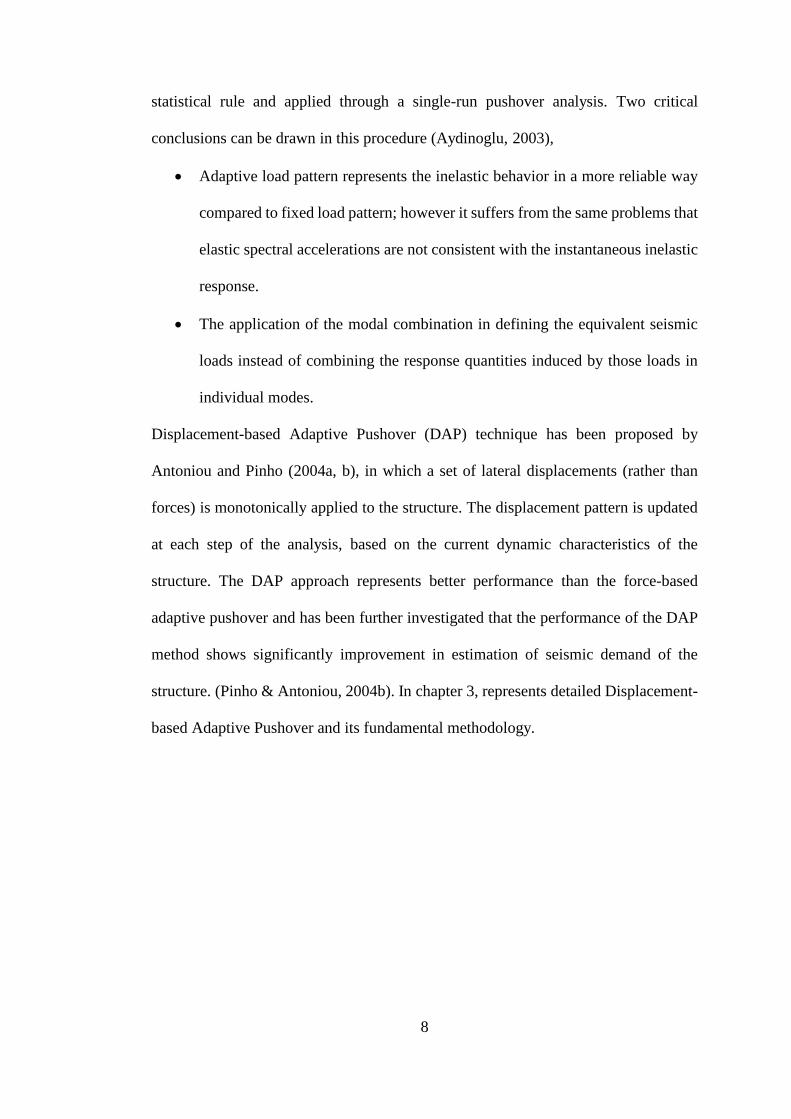
(2) Perform free vibration analysis by using Jacobi method (matrix transformation
method). Calculate instantaneous eigenvalues with the corresponding eigenvectors and
compute the participation factors for the number of modes considered.
г𝑥𝑛(𝑖)
=𝐿𝑥𝑛
(𝑖)
𝛹𝑛(𝑖)𝑇
𝑀𝛹𝑛(𝑖) ; 𝐿𝑥𝑛
(𝑖)= 𝛹𝑛
(𝑖)𝑇𝑀𝐼𝑋
𝑔 (1.1)
Where,
г𝑥𝑛(𝑖)
: Instantaneous participation factor for an earthquake in x direction.
𝛹𝑛(𝑖)
: Instantaneous n’th mode shape vector
𝑀: Mass Matrix , 𝐼𝑋𝑔
: Kinematic Vector
(3) In each mode, obtain all unit modal response quantities of interest, �̅�𝑛(𝑖)
, such
as bending moments of the potential plastic hinges, �̅�𝑗𝑛(𝑖)
, induced by �̅�𝑛(𝑖)
in which,
�̅�𝑛(𝑖)
=
𝛹𝑛(𝑖)
г𝑥𝑛(𝑖)
(1.2)
Where,
�̅�𝑛(𝑖)
: Displacement vector.
(4) Convert each modal capacity diagram to a bilinear diagram according to Figure
below and calculate the initial effective period. Skip this stage in the first and second
pushover steps (in the first step modal capacity diagrams are linear while in the second
they are already bilinear). For each mode calculate spectral displacement either from
the solution of Equation 1.3 for a given earthquake using the bilinear modal capacity
diagram or from the specified smooth elastic response spectrum using the initial
effective period obtained at Stage (4).
∆�̈�𝑛(𝑖)
+ 2𝜉𝑛(𝑖)
𝜔𝑛(𝑖)
∆�̇�𝑛(𝑖)
+ (𝜔𝑛(𝑖)
)2∆𝑑𝑛(𝑖)
= −∆�̈�𝑥𝑔(𝑖)
(1.3)
Where,

12
∆�̈�𝑥𝑔(𝑖)
: Ground acceleration increment.
𝜉𝑛(𝑖)
: Instantaneous modal damping ratio.
𝜔𝑛(𝑖)
: Instantaneous natural frequency
∆𝑑𝑛(𝑖)
: Modal displacement increment at the (i)’th incremental step is expressed as,
𝑑𝑛(𝑖)
= 𝑑𝑛(𝑡) − 𝑑𝑛(𝑡𝑖 − 1)
In which, 𝑑𝑛(𝑡): Modal displacement in the n’th mode.
Figure 1.1. Modal capacity diagram Bi-linearization (Aydinoglu, 2003).
(5) Calculate inter-modal scale factors for all modes considered from Equations
1.4 as appropriate. In the practical version of IRSA with initial elastic periods, inter-
modal scale factors are calculated from Equation 1.5 only once at the first pushover
step and thereafter constantly used in all steps.
𝜆𝑛(𝑖)
=𝑆𝑑𝑖𝑛
(𝑖)− 𝑑𝑛
(𝑖−1)
𝑆𝑑𝑖𝑙(𝑖)
− 𝑑1(𝑖−1)
(1.4)
Where,

13
𝜆𝑛(𝑖)
: Intermodal scale factor
𝑆𝑑𝑖𝑛(𝑖)
: Peak inelastic modal displacement
𝜆𝑛(𝑖)
=𝑆𝑑𝑒𝑛
(𝑖)−𝑑𝑛
(𝑖−1)
𝑆𝑑𝑒𝑙(𝑖)
−𝑑1(𝑖−1) (1.5)
Where,
𝑆𝑑𝑒𝑛(𝑖)
: Elastic spectral displacement of the n’th mode.
𝜆𝑛(𝑖)
= 𝜆𝑛(1)
=𝑆𝑑𝑒𝑛
(𝑖)
𝑆𝑑𝑒𝑙(𝑖) (𝑖 =
2,3, … ) (1.6)
Figure 1.2. Scaling procedure for a modal displacement increment (Aydinoglu,
2003).
(6) Using the information obtained at Stage (3) and (6) calculate combined unit
response quantities of interest,�̅�(𝑖), such as bending moments of the potential plastic
hinges �̅�𝑗(𝑖)
from Equations1.7-9, respectively, or from the specified smooth elastic
response spectrum using the initial effective period obtained at Stage (4).

14
�̅�(𝑖) = √∑ (�̅�𝑛(𝑖)
𝜆𝑛(𝑖)
)2𝑁𝑠𝑛=1 (1.7)
�̅�𝑗(𝑖)
= √∑ (�̅�𝑗𝑛(𝑖)
𝜆𝑛(𝑖)
)2𝑁𝑠𝑛=1 (1.8)
�̅�(𝑖) = √∑ ∑ (�̅�𝑚(𝑖)
𝜌𝑚𝑛(𝑖)
�̅�𝑛(𝑖)
)𝑁𝑠𝑛=1
𝑁𝑠𝑚=1 (1.9)
(7) Calculate the first modal displacement increment from Equation 1.10 and
locate the plastic hinge yielded at the end of this pushover step. Then, obtain the
response quantities of interest from Equation 1.11 and the new coordinates of modal
capacity diagram(s) from Equation 1.12-13,
∆𝑑1(𝑖)
=𝑀𝑗
(𝑦)−𝑀𝑗
(𝑖−1)
�̅�𝑗(𝑖) (1.10)
𝑟(𝑖) = 𝑟(𝑖−1) + �̅�(𝑖)∆𝑑1(𝑖)
(1.11)
𝑑𝑛(𝑖)
= 𝑑𝑛(𝑖−1)
+ ∆𝑑𝑛(𝑖)
= 𝑑𝑛(𝑖−1)
+ 𝜆𝑛(𝑖)
∆𝑑1(𝑖)
(1.12)
𝑎𝑛(𝑖)
= 𝑎𝑛(𝑖−1)
+ ∆𝑎𝑛(𝑖)
= 𝑎𝑛(𝑖−1)
+ 𝜆𝑛(𝑖)
(𝜔𝑛(𝑖)
)2∆𝑑1(𝑖)
(1.13)
(8) Check if the first modal displacement exceeded the first-mode spectral
displacement obtained at Stage (5). If exceeded, calculate the peak response quantities
from Equations 1.15-16 and terminate the analysis. If not, continue with the next step.
∆𝑑𝑛(𝑝)
= 𝑆𝑑𝑖𝑛(𝑝)
− 𝑑𝑛(𝑝−1)
(1.15)
𝑟(𝑖) = 𝑟(𝑖−1) + �̅�(𝑖)∆𝑑1(𝑖)
(1.16)
(9) Considering the last yielded hinge determined at Stage (8), modify the current
stiffness matrix and return to Stage (1) for the next pushover step.

15
1.3.6 Nonlinear Dynamic Analysis
Nonlinear dynamic analyses are able to generating results with high accuracy and also
relatively low uncertainty by using the combination of ground motion acceleration
(FEMA440, 2005). When the NDP is applied for seismic performance assessment of
the structure, a mathematical model directly incorporating the nonlinear load
deformation characteristics of individual components and then ground motion time
histories, in which represent the severity of earthquake, are applied to the elements of
the structure. (FEMA356, 2000). NDA is the most accurate and reliable approach of
seismic analysis which in practice it takes too much time and computational efforts.
The method has usually been applied only by researchers in the past and the obtained
result cannot be used easily in the design practice.
1.3.6.1 Nonlinear Time History Dynamic Analysis Method
This method evaluates structural seismic performance by applying series of ground
motions acceleration to structure. In this procedure, ground motion acceleration apply
to structure for evaluating the displacement of each frame to estimate the performance
limit states possibility for each frame. Three steps are required for selecting the
Earthquake records. Firstly, earthquake design response spectrum should be specified
according to seismic code related to the location of construction building, then several
earthquake ground motion records are selected corresponding to site characteristics
and seismic design spectrum. Finally, selected earthquake records are uploaded and
then by considering a load case, selected acceleration series are applied to the structure
to assess the Seismic Performance of structure (Mezgeen, 2014).

16
1.3.6.2 Incremental Dynamic Analysis
IDA is a method that estimates the seismic behavior of structure by specifying
performance limit-states for a specified structure at a selected site. It fundamentally
takes the old concept of scaling accelerogram records and use it in such a way that
estimate precisely the full range of structural behavior, from elasticity to collapse. In
IDA procedure, a set of chosen ground motion records is applied to a structural model,
each of those scaled to multiple levels of intensity (Vamvatsikos & Cornell, 2002).
Finally, by summarizing IDA envelops, defining limit-states on them and obtaining
the results with fragility curves of probabilistic structural damage, the aims of
performance-based earthquake engineering can be reached. In chapter 3, represents
detailed incremental dynamic analysis and its fundamental methodology. The main
objectives of IDA method are summarized below,
Better understanding of the structural behavior under strong ground motion
levels.
Predicting the seismic structural capacity level of the structure.
Comprehensive understanding the range of response or demands against the
range of potential levels of a ground motion record.
Illustrate the dispersion of the structural response nature within increasing of
seismic ground motion intensity.
Derive a multi-record IDA curve to demonstrate stability and variability of
different seismic ground motion records.

17
1.3.6.3 Advantages and Disadvantages of Dynamic Procedures
According to FEMA 440 (2005), great dispersion in engineering demand parameters
is resulted by the ground motion variability. FEMA440 illustrate this problem by
showing Figure 1.3. The figure demonstrates the results obtained from the research
work done by Vamvatsikos & Cornell (2002) in which a series of nonlinear time
history analyses perform by setting selected ground shaking that scaled to multiple
levels of intensity.
According to FEMA 356, Calculated response can be highly sensitive to characteristics
of individual ground motions for nonlinear dynamic procedures.
Figure 1.3. IDA Envelope curves study done by Vamvatsikos & Cornell (2002) used
thirty ground motion records.

18
1.3.7 Why nonlinear dynamics analysis cannot be in codes?
It is undeniable that NDA is the most accurate and reliable technique in evaluating
structural seismic performance. Instead, static analyses always have major drawbacks
such as absence of time-dependent effects. The main reasons that nonlinear dynamics
analysis cannot be in codes are described below (Pietra, Antoniou, & Pinho, 2006),
Earthquake design codes are not a proper guidance on approaches to
simulate a set of site-specific acceleration time-series consistent with given
code standard response spectrum.
Despite the improvements in computer processing power, NDA still takes
too much time and computational efforts for 3D irregular models with
thousands of elements. There are some modelling errors faced by the
researcher while evaluation process evolves therefore designers should
consider that the dynamics analysis will require to be repeated several times.
In dynamic analysis output, It is not easy to detect errors in finite elements
model, instead errors in pushover analysis tend to be relatively apparent,
that is the reason for a first model checking, preliminary simpler analysis,
such as pushover analysis, are run.
Therefore, it is concluded that development of nonlinear static analysis approaches
need to be continue, so that these analysis methods will become as reliable and accurate
as nonlinear dynamics analysis.

19
1.4 Thesis Outline
This study consists of five chapters and is organized according to the following outline,
Chapter 2 presents an overall summary of the modeling assumptions. Modeling
considerations includes structures geometry, sections properties and material
characteristics ae also described.
In chapter 3, nonlinear analyses includes Pushover, DAP and IDA has been discussed
in detail. The reasons for choosing of the selected Software and codes are also
explained. This chapter describes the ways of selecting Ground Motion records and
how to generate pushover, IDA and fragility curves for seismic performance
assessment of structures.
Chapter 4 concentrates on the analytical results of nonlinear analyses based on
methodology described in Chapter 3. Pushover curves obtained by each nonlinear
static method are compared with IDA envelopes and their seismic performance
assessed.
Chapter 5 presents summary, conclusions and recommendations of the present study.

20
DESIGN OF SAMPLE STRUCTURES
2.1 Modeling
2.1.1 Description of structures
Three RC structures, with different elevation, are considered to represent high-rise,
medium-rise and low-rise RC structures for this work. The structures have a moment
resisting RC elements without any shear walls and are supposed to be located in a high-
seismicity region of Turkey. Structures are designed according to TS 500-2000 and
Turkish Earthruake Code (2007), taking into account seismic and gravity loads. The
sample structures considered in this study are discribed as follows,
All the floors are the same height of 3 m in elevation.
The dimensions of structures (width/elevation) used in this study are the
same ratio.
A typical RC structures with high ductility level is considered.
In order to design structures, Equivalent static analysis, defined by a
TEC2007 response spectrum, and fully rigid design method are used.
The Response Modification Factor for Systems of high Ductility level
according to TEC2007 is 8 (Table 5.2, (TEC, 2007)).
𝑅𝑥=𝑅𝑦=8

21
Seismic evaluation has been applied according to the Turkish Seismic Code
(2007) with Ground Motion Acceleration of 0.4 in zone 1 and soil type Z4
has been used.
Purpose of occupancy Considered Residential, so Importance Factors is
equal to 1 (I=1) according to table 2.3 of TSC2007.
Consider the limitation of relative story drift according to TSC2007.
(𝛿𝑖)𝑚𝑎𝑥
ℎ𝑖≤ 0.02 (2.1)
The participating live load (30% of live load) and dead load on the structure
are 2 𝐾𝑁
𝑚2 and 5
𝐾𝑁
𝑚2, respectively.
Yield strength of the both longitudinal and transverse reinforcements was
assumed to be 420 MPa and the characteristic compressive strength of
concrete is equal to 25 MPa. In the potential plastic hinge regions, Three
layouts with 0.1m, 0.15m, and 0.2m spacings are used for transverse
reinforcement. Mechanical properties of used steel in the analyses were
selected according to Turkish standard Code (TS500, 2000).
Figure 2.1 represents 3D of the sample models and, plan view of 3-, 8- and 12-story
structures are shown in Figure 2.2 .

22
Figure 2.1. 3D models of symmetric-plan 3-story, 8-story and 12-story structure.

23
Figure 2.2. 3-story RC structure are 12 m by 12m in plan, 8-story RC structure are
27.5 m by 27.5m in plan and 12-story RC structure are 39 m by 39m in plan.

24
2.2 Sections Design
2.2.1 3-story structure
The 3-story RC frame is 9 m in elevation and all the floors are the same height of 3
meter. The frame has three bays with 4 meter span length. Longitudinal beam and
column reinforcement amount and, column dimensions are demonstrated in Figure 2.3
and Table 2.1, respectively. The section area of all beams are 0.2m×0.5m. The amounts
of top and bottom reinforcement (in 𝑐𝑚2) and beam section characterizations are
displayed in the elevation view in Figure 2.3 and Table 2.2, respectively.
Figure 2.3. Longitudinal beam and column reinforcement amount (𝑐𝑚2).

25
Table 2.1. Columns section characterizations.
Dimension(cm) REINFORCEMENT Stirrup
Story1 50x25 10∅20 ∅8/20
Story2 50x25,40x25 10∅20, 8∅18 ∅8/20
Story3 40x25 8∅18, 8∅16 ∅8/10
Table 2.2. Beam section characterizations.
Dimension(cm) Top Bottom Stirrup
3-story 50x20 3∅18 3∅18 ∅8/15

26
2.2.2 8-story structure
The 8-story RC frame is 24 meter in elevation and all the floors are the same height of
3 meter. The frame has five bays with 5.5 meter span length. Longitudinal beam and
column reinforcement amount and, column dimensions are demonstrated in Figure 2.4
and Table 2.3, respectively. The section area of all beams are 0.2m×0.6m. The amounts
of top and bottom reinforcement (in 𝑐𝑚2) and beam section characterizations are
displayed in the elevation view in Figure 2.4 and Table 2.4, respectively.
Figure 2.4. Longitudinal beam and column reinforcement amount (𝑐𝑚2).

27
Table 2.3. Columns section characterizations.
Dimension(cm) REINFORCEMENT Stirrup
Story1 75x35,80x40 10∅28, 14∅28 ∅8/15
Story2 70x35 10∅28 ∅8/15
Story3 70x35 10∅28 ∅8/15
Story4 70x30 10∅28 ∅8/15
Story5 70x30 10∅28 ∅8/15
Story6 70x30, 50x30 10∅28, 10∅25 ∅8/15
Story7 50x25 10∅22 ∅8/12.5
Story8 50x25, 40x20 10∅25,8∅18 ∅8/12.5
Table 2.4. Beam section characterizations.
Dimension(cm) Top Bottom Stirrup
8-story 60x20 3∅18+2∅20 6∅18 ∅8/15

28
2.2.3 12-story structure
The 12-story RC frame is 36 meter in elevation and all the floors are the same height
of 3 meter. The frame has six bays with 6.5 meter span length. Longitudinal beam and
column reinforcement amount and, column dimensions are demonstrated in Figure 2.5
and Table 2.5, respectively. The section area of all beams are 0.2m×0.7m. The amounts
of top and bottom reinforcement (in 𝑐𝑚2) and beam section characterizations are
displayed in the elevation view in Figure 2.5 and Table 2.6, respectively.
Figure 2.5. Longitudinal beam and column reinforcement amount (𝑐𝑚2).

29
Table 2.5. Columns section characterizations.
Dimension(cm) REINFORCEMENT Stirrup
Story1 80x40,95x60, 100x60 14∅28,18∅32, 18∅32 ∅8/15
Story2 80x45, 90x60, 95x60 14∅25,12∅25, 12∅25 ∅8/15
Story3 80x40, 90x55, 90x55 14∅25,12∅25, 12∅25 ∅8/15
Story4 75x40, 85x50, 90x50 14∅28,12∅22, 12∅22 ∅8/15
Story5 75x40, 80x45, 90x45 14∅28,12∅22, 12∅22 ∅8/15
Story6 75x35, 80x45, 85x45 14∅28,12∅22, 12∅22 ∅8/15
Story7 75x35, 70x40, 70x45 12∅28,12∅25, 12∅22 ∅8/15
Story8 75x35, 70x35, 70x35 12∅28,12∅28, 12∅25 ∅8/15
Story9 75x35, 65x30, 70x30 12∅28,12∅28, 12∅28 ∅8/15
Story10 70x30, 60x30, 60x30 10∅28,10∅28, 12∅25 ∅8/15
Story11 70x30, 45x30, 45x30 10∅28, 8∅28, 10∅22 ∅8/15
Story12 70x30, 40x20, 35x20 10∅28, 8∅20, 8∅18 ∅8/15
Table 2.6. Beam section characterizations.
Dimension(cm) Top Bottom Stirrup
12-story 70x20 8φ20 2∅20 ∅8/15

30
METHODOLOGY
3.1 Target Displacement
According to FEMA356, The target displacement is intended to represent the
maximum displacement likely to be experienced during the design earthquake. The
appropriate estimation of target displacement point is a very important task in the
seismic performance assessment of structures. Equation 3.1 represents a basic relation
that is used to calculate the target displacement, 𝛿𝑡 , at each story level (FEMA440,
2005),
𝛿𝑡 = 𝐶0𝐶1𝐶2𝐶3𝑆𝑎𝑇𝑒
2
4𝜋2 (3.1)
Where,
𝑪𝟎 is Modification factor used to relate spectral displacement of an equivalent SDOF
system to the roof displacement of the structure MDOF system obtained applying one
of the following methods,
The easiest way is using Table 3-2 of FEMA 356 to determine the
appropriate value of the modification factor.
The first modal participation factor obtained at the level of the control node.
A shape vector consistent to the deflected shape of the structure at the target
displacement can be used.

31
According to FEMA 356, 𝑪𝟏 is modification factor to relate expected maximum
inelastic displacements to displacements obtained for linear elastic response.
FEMA440 states that the modification factor estimates maximum displacements with
unacceptable accuracy. FEMA 440 improved the simplified equation 3.2 that can be
used for most structures.
𝐶1 = 1 +𝑅 − 1
𝑎𝑇𝑒2
(3.2)
Where;
𝑇𝑒: Effective fundamental period of the structure.
𝑎: Constant parameter for different site classes, for instant, a is equal to 60 in site class
D.
R: Ratio of elastic strength demand.
𝑅 =𝑆𝑎
𝑉𝑦
𝑊
(3.3)
Where,
𝑆𝑎: Response spectrum acceleration, g,
𝑉𝑦: Yield strength obtained by performing NSP
𝑊: Effective seismic weight of the structure
𝐶𝑚: Effective mass factor using Table 3-1 in FEMA356.
According to FEMA 356, 𝑪𝟐 is modification factor to represent the effect of pinched
hysteretic shape, stiffness degradation and strength deterioration on maximum
displace-ment response. FEMA 440 states that this modification factor has limitation
in considering the effects of strength degradation and recommend that the
𝐶2 coefficient be as equation 3.4.

32
𝐶2 = 1 +1
800(
𝑅 − 1
𝑇)
2
(3.4)
{𝑇 < 0.2𝑠 → 𝐶2 = 0.2𝑇 > 0.7𝑠 → 𝐶2 = 1
(3.5)
According to FEMA 356, 𝑪𝟑 is modification factor to represent increased
displacements due to dynamic P-∆ effects. Values of 𝐶3 shall be calculated using
Equation 3.6-7.
𝐶3 = 1 +|𝛼|(𝑅−1)
𝑇𝑒, For structures with negative post yield stiffness (3.6)
𝛼: Ratio of post-yield stiffness to effective elastic stiffness, as shown in Figure 3.4.
C3 = 1
For structures with positive post yield stiffness (3.7)
FEMA 440 eliminate the FEMA 356 coefficient 𝑪𝟑. Ratio of elastic strength demand
(R), instead of 𝑪𝟑, has been suggested by FEMA 440 code for avoiding dynamic
instability.

33
3.2 Computing and defining inelastic frame elements
In this study, for performing nonlinear analysis two different finite element software,
SeismoStruct and SAP2000, are selected. Modeling of structure and, defining
geometric and material nonlinearities are the main differences between the two
selected programs.
3.2.1 Defining inelastic frame elements in SeismoStruct Software
SeismoStruct software is capable of considering both global and local sources of
geometric and material nonlinearities. The current unknown deformation of the
elements have been described by attaching local chord system to each finite element
as shown in Figure 3.1 and it rotates and translates with the element. (SeismoStruct,
2007). Geometric nonlinearities are also available in SAP2000 software for nonlinear
time-history analysis and P-delta plus large displacements effects are taken into
account by the program.
Figure 3.1. Global and local sources of geometric nonlinearities (SeismoStruct,
2007)
For characterizing of the nonlinear response of the system, defining of material
elasticity to elements is very important task and it can be defined in elements through
distributed and concentrated plasticity. In SeismoStruct software, material inelasticity
of the elements is made of so called fiber modeling approach in which the element has
been subdivided into many segments. The section is discretized in sufficient quantity

34
of fibres and the response of sections are obtained through the integration single fiber’s
response of individual fibres (typically 100-150) (SeismoStruct, 2007). SAP2000
software do not take into account the material nonlinearity of the elements.
Figure 3.2. Material inelasticity (SeismoStruct, 2007)
In SeismoStruct software, many various material types are available while in SAP2000
program, only elastic material such as orthotropic and isotropic can be used.

35
3.2.2 Defining inelastic frame elements in SAP2000
In nonlinear analysis, to consider nonlinear structural behavior of each element, plastic
hinges are assigned at the both ends of beam–column elements. FEMA (2000c) has
given information about nonlinear plastic hinge properties of all of the structural
elements in its Tables 6-7 through 6-9 which researchers widely use them.
SAP2000 implements the plastic hinge properties and computes it automatically from
section and material properties based on given criteria in ATC-40 or FEMA-356. In
SAP2000, three kinds of hinge properties are available. They are User-Defined hinge
properties, Auto Hinge Properties, and Program Generated Hinge properties. Inverse
of User-Defined hinge properties, Auto hinge properties cannot be modified and
viewed because the default properties are section dependent. In user-defined hinge
properties, it is required to define moment curvature data for each element and moment
rotation relationship for each section.
In program Generated Hinge Properties, the software combines its built-in criteria with
the defined section properties for each object to generate the final hinge properties
which means that you do considerably less work defining the hinge properties because
you do not need to define every hinge. CSI SAP2000 program is able to displays the
plastic hinges behavior at each step of the change process (SAP2000, 2006).
Inel and Ozmen (2006) state that for RC buildings, the difference between the results
of pushover analysis by using Auto hinge and User-Defined properties is very little for
new buildings and more for old ones (more appropriate for rehabilitation objectives).
Since the aim of this study is assessing the nonlinear behavior of RC buildings that
designed according new design code. M3 and P-M2-M3 interaction hinges were used

36
for defining hinges at the beginning and ending points of the beams and columns,
respectively. Therefore, Auto-hinge properties are assigned to the frame elements
based on FEMA-356 generalized force-deformation relation model as shown in Figure
3.3.
Figure 3.3. The relationship of Force-deformation of a typical plastic hinge
(FEMA356, 2000).

37
3.3 Structural Performance limits states
According to FEMA 356, the discrete Structural Performance Levels, that is going to
be studied, are Collapse Prevention (CP), Life Safety (LS) and Immediate Occupancy
(IO).
3.3.1 Immediate occupancy (IO)
In this level, the post-earthquake damage should be in the level that the structure
remains safe to occupy and stays harmless to inhabit. The basic seismic and vertical
force-resisting systems of the structure retain the pre-earthquake design stiffness and
strength of the construction. Therefore, Slight damage to the structure has occurred,
that can be easily repaired, is observed.
3.3.2 Life Safety (LS)
In this level, the post-earthquake damage should be in the level that the structure has
suffered considerable damage, nevertheless retains a margin opposing onset of partial
or total collapse. Some elements and components of structure are severely damaged
and there is risk of injury to life. It should be possible to repair the structure and
repairing may be less economical when compared to complete reconstruction.
3.3.3 Collapse Prevention (CP)
In this level, the post-earthquake damage should be in the level that the building is on
the verge of experiencing partial or total collapse. The structure has suffered
Comprehensive damage, as well as encompassing momentous degradation in the
strength and stiffness of the seismic load resisting system. The construction is not safe
for re-occupancy and could not be technically practical to repair.

38
3.3.4 Collapse (C)
In this level, the post-earthquake damage should be in the level that the structure is at
the total collapse and fails to satisfy any criteria that mentioned above, thus this means
that re-occupancy of the structure should not permitted because the structure is at the
collapse level.
3.3.5 Drift Levels
Inter-story drift profiles were used to achieve valuable results data on the failure
mechanism and illustrate influence of yielding derived from the inelastic procedures
that is directly correlated to non-structural and structural damage (FEMA440, 2005).
In this work, according to FEMA 356, three limit states including collapse prevention
(CP), life safety (LS) and immediate occupancy (IQ) will be defined. For a RC frame
without any shear walls, the IQ is defined when inter-story drift ratio reaches 1% of
the floor height. Similarly for LS is defined at 𝜃𝑚𝑎𝑥= 0.02 and finally CP is considered
for 𝜃𝑚𝑎𝑥 = 0.04, as shown in Table 3.1 (FEMA356, 2000).
Table 3.1. Structural Performance Levels (FEMA356, 2000).
Elements Type CP LS IQ
Concrete Frames Drift 4% transient 2% transient 1% transient

39
3.4 Nonlinear Static Procedures
3.4.1 Introduction
The Nonlinear Static Procedures (NSP) is nowadays generally recognized as
appropriate seismic performance and the assessment of existing buildings. The aim of
NSP is to estimate seismic demand and capacity of a structure with acceptable
accuracy. In the procedure, the structure subjected to ground shaking in a
monotonically increasing pattern of lateral forces with a fixed height-wise
distribution until a target displacement is reached (FEMA440, 2005). The stages of
performing NSA method was summarized by following steps,
1. Model the structures includes of the elements established by computer.
2. Define section material of the elements and their characteristics.
3. Assign beams and columns of the frame, then identify cross sections of
elements.
4. Define and assign live and dead forces as a vertical load pattern according to
TS500 code. Different types of lateral load pattern distribution, according to
Fema356, are applied to the frames.
5. Define plastic hinge properties. Auto-hinge properties are assigned to the frame
elements based on FEMA-356.
6. Define the pushover load cases and identify nonlinear static analysis (P-Δ
effects are considered by the program).
7. Run the analysis, then the results information is derived and the capacity curve
is achieved to assess the seismic performance of the building.
After running traditional pushover analysis, the capacity curve achieved and then the
determined target displacement for choses performance level has to be obtain based
on FEMA 440.

40
3.4.2 Methodology
3.4.2.1 Nonlinear Static Analysis Procedures
The procedures could be an appropriate method for performance assessment of
buildings that does not have significant higher mode effects, such as short symmetric
buildings. Therefore, first a modal response spectrum analysis is executed to capture
90% mass participation by using sufficient modes for evaluating the efficiency of
higher modes. A second RSA should also be executed and only the first mode
participation shall be considered. If the maximum shear story, obtained by modal RSA,
exceeds 130% of the story shear, obtained by RSA in which taking into account only
the first mode response, the effects of higher modes in that structure will be significant.
3.4.2.2 Conventional Nonlinear Static Analysis Based on FEMA 356
In FEMA 356, two separate NSA are required to be applied. Different load vectors
should be applied in each analysis. The larger value of response quantity of the two
analyses will be selected to determine acceptability criteria (FEMA356, 2000).
1. First load vector shall be chosen from the below options,
First mode: Limited to the structures that their mass participates in first mode
are not less than 75 percent.
Code distribution: Limited to the structures that their mass participates in
first mode are not less than 75 percent, and it is suggested that uniform
distribution should be the second load vector.
SRSS of modal story loads: If 𝑇𝑒 > 1𝑠, this option should be applied.
2. A second load vector shall be chosen from the below lists,
Adaptive load distribution
Uniform distribution

41
3.4.2.3 Idealizing force-displacement curve
In NSA, the calculated relationship between displacement of a control node and base
shear should be idealized to the bilinear curve in order to calculate effective yield
strength,𝑉𝑦 the effective lateral stiffness, 𝐾𝑒, and the yield slop, α, , of the structure as
illustrated in Figure 3.4. At the origin is starting point of initial linear portion of the
idealized force-displacement curve and maximum base shear is the last point of the
second linear portion. The effective lateral stiffness, 𝐾𝑒 should be considered as the
secant stiffness obtained a base shear force equal to 60% of the effective yield strength
of the building. The post-yield slope, α, should be identified by a line segment which
passes through the substantial curve at the obtained target displacement (FEMA440,
2005).
Figure 3.4. Idealized force-displacement curve for NSA (FEMA440, 2005)

42
3.5 Displacement-based Adaptive Pushover
3.5.1 Introduction
Antoniou and Pinho have proposed a displacement-based adaptive pushover analysis
(DAP) in 2004 to take into account the updated loading vector at each analysis step
according to current dynamic characteristics of the building. The aim of adaptive
pushover analysis is to evaluate the seismic performance of the structure by predicting
seismic demands and capacity of a building and considering its dynamic response
characteristics includes the effect of the frequency content and deformation of input
motion. (Pinho & Antoniou, 2004b).
The lateral load distribution in the adaptive pushover method, continuously updated
during the analysis, depending to modal shapes and participation factors obtained by
performing eigenvalue analysis at each step of analysis. DAP is fully multi-modal
method that take into account the modification of the inertia forces, the structural
stiffness softening, and its period elongation due to spectral amplification (Antoniou
& Pinho, 2004a).
DAP has the capability to update and change the horizontal load distributions based
on the constantly changing modal properties of the structure and solves the drawback
of fixed-load pattern of the pushover analysis, providing a more accurate tool for
assessing structural performance and better response estimator than conventional
pushover methods, particularly, in structures that the effects of higher modes play a
major role in its dynamic structural response.

43
Figure 3.5. Shape of updated loading vector at each analysis step in Adaptive
pushover. (Pietra, Pinho, & Antonio, 2006).
3.5.2 Methodology
The analysis stages of the Displacement-base Adaptive Pushover method, described
in greater detail in the study of Pinho and Antoniou [2004], are as follows,
1. Perform eigenvalue analysis taking into account the structural stiffness
softening at the end of the last load step without applying any additional force.
Then, compute eigenvectors and periods of the system. Preferably use Lanczos
method for this purpose (Hughes, 1987).
2. According to the participation factors and the modal shapes of the
Eigensolution, the patterns of the displacements are obtained for each mode
separately. For considering corresponding value for each vibration mode in the
calculation of the load pattern, a particular spectral shape should be defined.
3. Using statistical rules method (SRSS or CQC) to combine the lateral load
profiles of the modes. The absolute values of story forces are obtained by the
nominal loads and the load factor λ, because only the relative story loads values

44
are interested. Horizontal loads are normalized according to the maximum
value for DAP.
4. Increase the load factor λ to scaled-up story loads. The story forces are obtained
by the nominal load at that story, updated load factor and the displacement
pattern calculated above (typically, the nominal loads are equivalent at all
stories). Incremental scaling can also be employed, whereby only the load
increment is updated and added to the load already applied to structure
throughout the last increments.
5. Apply the new obtained loads to the structure and then determine the response
of the structure by solving the system of equations at the new equilibrium state.
6. Update and compute the matrix of tangent stiffness of the system and return to
the first stage of the algorithm, for the next increment of the DAP.
3.5.3 Choice of the Software for Computer Analysis (SeismoStruct software)
SeismoStruct software is a fiber-based Finite Elements program for seismic analysis
of the buildings. The software is able to evaluate structural performance under
dynamic or static loading, taking into the account geometric nonlinearities as well as
material inelasticity (SeismoStruct, 2007). The accuracy of the program in assessment
structural performance has been proved by comparing its results with experimental
results obtained by pseudo-dynamic tests [ (Casarotti & Pinho, 2006), (Elnashai &
Pinho, 2000)]. Moreover, the algorithm in section 3.5.2 is available in the software and
has been implemented effectively that will be used to perform the DAP method.
Antoniou and Pinho (2002), state that The main advantage of the proposed algorithm
is that it permits the application of the exact force profiles calculated by modal analysis
at every step, without stability or performance problems.

45
3.6 Incremental Dynamic Analysis (IDA)
3.6.1 Introduction
Incremental Dynamic Analysis (IDA) is a parametric structural analysis approach that
has proposed to predict seismic behavior of structures under strong ground motion.
IDA is able to estimate limit-state capacity and seismic demand by executing a series
of nonlinear time history analyses under a suite of multiple scaled ground motion
records. Selected ground motion intensity, for evaluating seismic capacity, is
incrementally increased until structural capacity reach to the global collapse.
Vamvatsikos (2002) states that IDA has significant potential and is not just a solution
for performance based earthquake engineering. In other words, it has the capability to
extend far beyond that and give more accurate prediction about structural behavior
under seismic load to researchers. IDA method basically takes the old concept of
scaling ground motion records and develops it into a way to accurately describe the
full range of structural behavior, from elasticity to collapse. IDA is widely applicable
method and a multi-purpose tool for assessing structural performance which can
accurately predict the responses of structures under a wide range of intensities.
IDA is one of the well-known approaches to evaluate the structural performance level
under a suite of seismic ground motions. IDA is able to estimate limit-state capacity
and seismic demand by performing a series of nonlinear time history analyses under a
suite of multiple scaled accelerogram records of earthquake ground motion
acceleration. In IDA method, the intensity of selected ground motion is incrementally
increased until the intended limit state seismic capacity of the global structural system
is achieved. Besides, it contains plotting an intensity measure (i.e. first mode spectral
acceleration,𝑆𝑎) versus a damage measure (maximum inter-story drift ratio).

46
Moreover, fragility curves have been also derived by IDA method in which
demonstrate expected damage in terms of Collapse Prevention, Life Safety and
immediate occupancy as a function of the chosen ground motion intensity. The multi-
record IDA curves have been summarized into their 16%, median and 84% fragility
curves and then limit states capacity at each performance capacity level have been
obtained. Based on obtained result, probabilistic structural damage (fragility curves)
are estimated in terms of maximum inter-story drift ratio and PGA for predefined limit
states at each performance capacity level. SeismoStruct software program was used in
order to run IDA.
3.6.2 Methodology
In this study, IDA method has been performed on 3, 8 and 12-story RC frame building
which is designed according to the TS500-2000 design code. Then, twenty earthquake
ground motion records have been selected and subjected to RC frames. Accordingly,
Nonlinear Dynamic Time History Analysis has been applied under a set of ground
motions scaled to a specific level of intensity and then IDA curves for each dynamic
analysis have been derived. Consequently, by summarizing the multi record IDA into
their 16%, median and 84% percentiles, fractile values are obtained. In this work, the
maximum inter-story drift ratio of the structure has been considered as a damage
measure (DM) and 5% damped first mode spectral acceleration as an intensity measure
(IM).

47
3.6.3 Selected Ground Motions
For performing IDA, a series of nonlinear dynamic time history analysis has applied
to structure under a suite of multiple scaled ground motion records. The task of
selecting and scaling a proper real set of ground motion is very important for seismic
design and analysis and also this is a complex task because each of them has
differences in their characteristics and accordingly their effects on structural response
will be different.
Moreover, the accuracy of IDA results are depends on the number of chosen
accelerogram records. According to research performed by Shome and Cornell (1999),
it is usually enough to select ten to twenty accelerogram records to estimate limit-state
capacity and seismic demand of structures with sufficient accuracy. All the twenty
selected ground motion records data were taken from NGA STRONG MOTION
RECORD database of Pacific Earthquake Engineering Research (PEER) center,
(PEER, 2010).
Some limitations in selecting of ground motion records were imposed to balance
selection of large motions and to insure that they are strong enough to cause structural
damage and collapse. The limitations in selecting of ground motion records are
described as follows,
Lowest moment magnitude of earthquake should be 6.5.
AGA and PGV should be greater than 0.2g and15 cm/sec, respectively.
Source to site Distance should be at least 10 km.

48
The recommended lowest usable frequency for the record should be less than
0.25Hz, to ensure that the low frequency content was not removed by the
ground motion filtering process
All NEHRP soil type of selected ground motion records happened to be on C
and D sites categories. Soil shear wave velocity should be greater than 180m/s
in upper 30m of soil.
Spectral shape is not considered in selecting of records
Ground motion records were chosen to be free-field without any consideration
of station housing.
Selected Fault Mechanism in all records are Strike-slip to be in consistent with
Turkey.
Twenty ground motions records were selected by considering the restrictions described
above. The next step is to apply these records to the RC Frames in order to determine
maximum inter-story drift ratio of the systems and finally drawing IDA envelopes.
3.6.4 SeismoStruct Software
One type of analysis that can be run directly in Seismostruct program is incremental
Dynamics analysis. For performing IDA, the user is asked to enter the Incremental
Scaling Factors in the first step and then requires to define the time history curve
(usually a natural or artificial accelerogram) and corresponding curve multiplier
(scaling factor) (SeismoStruct, 2007).

Table 3.2. List of earthquake ground motions (PEER, 2010)
Even Information Site Information Record Information
EQ Index
Peer NGA Rec.
Num.
Event Year Fault Type
Mag. Station Name
Vs-30 (m/s)
Fault Distance
NEHRP Soil
Type
Lowest Usable Freq. (Hz)
PGV PGA
1 1602 Duzce, Turkey 1999 Strike-Slip 7.14 Bolu 326 12.2 D 0.06 56.4 0.728 2 1787 Hector Mine 1999 Strike-Slip 7.13 Hector 684.9 11.2 C 0.04 28.6 0.266
3 169 Imperial Valley 1979 Strike-Slip 6.53 Delta 274.5 22.285 D 0.06 26.0 0.238
4 174 Imperial Valley 1979 Strike-Slip 6.53 El Centro Array #11 196.2 13 D 0.25 34.5 0.364
5 177 Imperial Valley 1979 Strike-Slip 6.53 El Centro Array #2 188.8 14.33 D 0.125 31.5 0.315
6 189 Imperial Valley 1979 Strike-Slip 6.53 SAHOP Casa Flores 338.6 10.215 C 0.25 19.6 0.287
7 162 Imperial Valley 1979 Strike-Slip 6.53 Calexico Fire Statio 231.2 11 D 0.25 21.2 0.275
8 1111 Kobe, Japan 1995 Strike-Slip 6.9 Nishi-Akashi 609 16.15 C 0.12 37.3 0.509
9 1116 Kobe, Japan 1995 Strike-Slip 6.9 Shin-Osaka 256 23.8 D 0.12 37.8 0.243
10 1158 Kocaeli, Turkey 1999 Strike-Slip 7.51 Duzce 276 14.5 D 0.24 58.8 0.312
11 1148 Kocaeli, Turkey 1999 Strike-Slip 7.51 Arcelik 523 12.05 C 0.09 17.7 0.218
12 900 Landers 1992 Strike-Slip 7.28 Yermo Fire Station 353.6 23.7 D 0.07 51.5 0.245
13 848 Landers 1992 Strike-Slip 7.3 Coolwater 271 19.85 D 0.13 25.6 0.283
14 752 Loma Prieta 1989 Strike-Slip 6.93 Capitola 288.6 22.1 D 0.25 36.5 0.529
15 767 Loma Prieta 1989 Strike-Slip 6.9 Gilroy Array #3 349.9 12.5 D 0.12 35.7 0.555
16 778 Loma Prieta 1989 Strike-Slip 6.9 Hollister Diff. Array 215.5 24.67 D 0.125 43.9 0.269
17 1634 Manjil, Iran 1990 Strike-Slip 7.37 Abbar 724.5 12.8 C 0.25 55.3 0.209
18 721 Superstition Hills 1987 Strike-Slip 6.54 El Centro Imp. Co. 192.1 18.35 D 0.125 40.9 0.258
19 721 Superstition Hills 1987 Strike-Slip 6.54 El Centro Imp. Co. 192.1 18.35 D 0.125 46.4 0.358
20 725 Superstition Hills 1987 Strike-Slip 6.54 Poe Road (temp) 207.5 11.45 D 0.25 35.7 0.446

50
3.6.5 Summarizing the IDA Curves
It is essential to summarize generated IDA Curves for defining limit states on them
since each IDA curve contains large variability of records, a huge amount of data and
a wide range of behavior. Therefore, it is needed to utilize a proper summarization
method to reduce this huge amount of data. IDA envelope curve can be summarized,
by many easy techniques, a measure of dispersion (e.g., the difference between two
fractiles, or the standard deviation) and into central value (median). Vamvatsikos
(2002) has chosen the cross sectional fractiles technique to summarize IDA curves in
his study. Based on above discussion, I have summarized IDA curves based on
calculation the 84%, median and 16% fractile values of IM (IM84% , IM50% ,IM16%
respectively) and DM (DM84%, DM50%,DM16% , respectively) for each limit-state,
as shown in Table 4.10.
Figure 3.6. IDA envelopes has been summarized into their 16%, median and 84%
fractiles (Vamvatsikos & Cornell, 2002).

51
RESULTS AND DISCUSSIONS
4.1 3-Story Frame
4.1.1 Target displacement of 3-Story Frame
Table 4.1. FEMA440 parameters for 3-story frame model.
The target displacement,𝛿𝑡, of 3-story RC frame are calculated in accordance with
Equation 3.1 and obtained parameter shown in Table 4.1, as specified in section 3.1.
𝛿𝑡 = 𝐶0𝐶1𝐶2𝐶3𝑆𝑎
𝑇𝑒2
4𝜋2= 0.071 𝑚
Item Value Item Value Item Value
𝐶0 1.298 𝑇𝑖 0.412 𝑉𝑦 145.118
𝐶1 1.202 𝐾𝑖 6660.229 𝐷𝑦 0.023
𝐶2 1.033 𝐾𝑒 6308.367 Weight 460.066
𝑆𝑎 1.000 Alpha 0.224 𝐶𝑚 1.000
𝑇𝑒 0.423 R 3.171

52
4.1.2 Performance limit states of 3-Story Frame
Table 4.2. Pushover steps for 3-story frame model.
Step Displacement Base Force Drift Ratio
m kN %
1 0.012 77.638 0.13
2 0.028 147.614 0.315
3 0.047 188.359 0.53
4 0.071 215.708 0.79
5 0.106 249.517 1.176
6 0.115 255.212 1.281
7 0.151 263.41 1.681
8 0.173 268.299 1.92
9 0.173 268.299 1.92
Pushover analysis steps are shown in Table 4.2 applying 1st mode lateral load for the
3-story frame model via CSI SAP2000. The obtained results demonstrate that the 3-
story RC frame starts to yield at 0.023 m top displacement. At step 4, Plastic hinges
for beams change their performance level to immediate occupancy and at this level the
structure has 0.071 m top displacement. According to FEMA 356, the post-earthquake
damage should be in the level that the structure remains safe to occupy and stays
harmless to inhabit, and slight damage to the structure has occurred, that can be easily
repaired. In the next step, top displacement is reached to 0.151m and the performance
level of beams raise and change to life safety. In this level, some structural components
and elements has suffered comprehensive damage and there is risk of injury to life.
Structure collapse at step 8 where top displacement is equal to 0.172m. Table 4.3
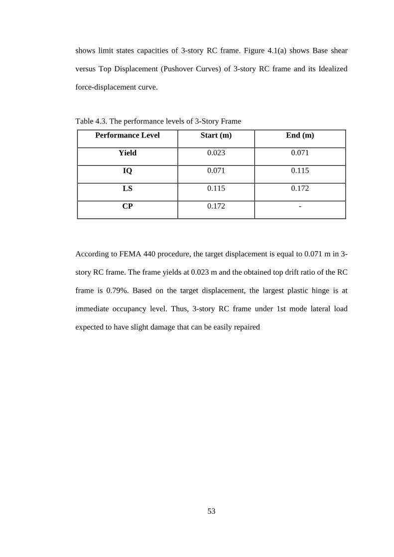
53
shows limit states capacities of 3-story RC frame. Figure 4.1(a) shows Base shear
versus Top Displacement (Pushover Curves) of 3-story RC frame and its Idealized
force-displacement curve.
Table 4.3. The performance levels of 3-Story Frame
According to FEMA 440 procedure, the target displacement is equal to 0.071 m in 3-
story RC frame. The frame yields at 0.023 m and the obtained top drift ratio of the RC
frame is 0.79%. Based on the target displacement, the largest plastic hinge is at
immediate occupancy level. Thus, 3-story RC frame under 1st mode lateral load
expected to have slight damage that can be easily repaired
Performance Level Start (m) End (m)
Yield 0.023 0.071
IQ 0.071 0.115
LS 0.115 0.172
CP 0.172 -

54
4.2 8-Story Frame
4.2.1 Target displacement of 8-Story Frame
Table 4.4. FEMA440 parameters for 8-story frame model.
The target displacement, 𝛿𝑡, 8-Story Frame are calculated in accordance with Equation
3.1 and obtained parameter shown in Table 4.4, as specified in section 3.1.
𝛿𝑡 = 𝐶0𝐶1𝐶2𝐶3𝑆𝑎
𝑇𝑒2
4𝜋2= 0.318 𝑚
Item Value Item Value Item Value
𝐶0 1.332 𝑇𝑖 0.993 𝑉𝑦 743.092
𝐶1 1.060 𝐾𝑖 8506.897 𝐷𝑦 0.087
𝐶2 1.000 𝐾𝑒 8506.897 Weight 3639.137
𝑆𝑎 0.926 Alpha 0.116 𝐶𝑚 1.000
𝑇𝑒 0.993 R 4.533

55
4.2.2 Performance limit states of 8-Story Frame
Table 4.5. Pushover steps for 8-story frame model
Step Displacement Base Force Drift Ratio
m kN %
1 0.057 485.194 0
2 0.082 654.187 0.238
3 0.115 769.869 0.341
4 0.216 887.837 0.481
5 0.318 970.292 0.9
6 0.32 971.753 1.325
7 0.404 1024.907 1.332
8 0.449 1040.195 1.684
9 0.449 1040.197 1.872
Pushover analysis steps are shown in Table 4.5 applying uniform lateral load for the
8-story frame model via CSI SAP2000. The obtained results demonstrate that the 8-
story RC frame starts to yield at 0.087 m top displacement. At step 4, Plastic hinges
for beams change their performance level to immediate occupancy and at this level the
structure has 0.26 m top displacement. According to FEMA 356, the post-earthquake
damage should be in the level that the structure remains safe to occupy and stays
harmless to inhabit, and slight damage to the structure has occurred, that can be easily
repaired. In the next step, top displacement is reached to 0.404m and the performance
level of beams raise and change to life safety. In this level, some structural components
and elements has suffered comprehensive damage and there is risk of injury to life.

56
Structure collapse at step 8 where top displacement is equal to 0.44 m. Table 4.6 shows
limit states capacities of 3-story RC frame. Figure 4.1(b) shows Base shear versus Top
Displacement (Pushover Curves) of 3-story RC frame and its Idealized force-
displacement curve.
Table 4.6. The performance levels of 8-Story Frame
According to FEMA 440 procedure, the target displacement is equal to 0.318 m in 8-
story RC frame. The frame yields at 0.0874 m and the obtained top drift ratio of the
RC frame is 0.9%. Based on the target displacement, the largest plastic hinge is at
immediate occupancy level. Thus, 8-story RC frame under uniform lateral load
expected to have slight damage that can be easily repaired.
Performance Level Start (m) End (m)
Yield 0.087 0.264
IQ 0.264 0.404
LS 0.404 0.438
CP 0.438 -

57
4.3 12-Story Frame
4.3.1 Target displacement of 12-Story Frame
Table 4.7. FEMA440 parameters for 12-story frame model.
The target displacement, 𝛿𝑡 , 12-Story Frame are calculated in accordance with
Equation 3.1 and obtained parameter shown in Table 4.7, as specified in section 3.1.
𝛿𝑡 = 𝐶0𝐶1𝐶2𝐶3𝑆𝑎𝑇𝑒
2
4𝜋2 = 0.47
Item Value Item Value Item Value
𝐶0 1.296 𝑇𝑖 1.450 𝑉𝑦 872.411
𝐶1 1.000 𝐾𝑖 9889.537 𝐷𝑦 0.091
𝐶2 1.000 𝐾𝑒 9609.151 Weight 9306.740
𝑆𝑎 0.680 Alpha 0.094 𝐶𝑚 1.000
𝑇𝑒 1.471 R 7.254

58
4.3.2 Performance limit states of 12-Story Frame
Table 4.8. Pushover steps for 12-story frame model
Pushover analysis steps are shown in Table 4.8 applying uniform lateral load for the
12-story frame model via CSI SAP2000. The obtained results demonstrate that the 12-
story RC frame starts to yield at 0.091 m top displacement. At step 4, Plastic hinges
for columns change their performance level to immediate occupancy and at this level
the structure has 0.24 m top displacement. According to FEMA 356, the post-
earthquake damage should be in the level that the structure remains safe to occupy and
stays harmless to inhabit, and slight damage to the structure has occurred, that can be
easily repaired. In the next step, top displacement is reached to 0.44m and the
performance level of columns raise and change to life safety. In this level, some
structural components and elements has suffered comprehensive damage and there is
risk of injury to life. Structure collapse at step 6 where top displacement is equal to
0.53m. Table 4.9 shows limit states capacities of 3-story RC frame. Figure 4.1(c)
Step Displacement Base Force Drift Ratio
m kN %
0 0 0 0
1 0.0429 424.175 0.119
2 0.0683 640.993 0.189
3 0.123 866.542 0.341
4 0.241 1038.191 0.668
5 0.440 1198.216 1.222
6 0.529 1242.221 1.470

59
shows Base shear versus Top Displacement (Pushover Curves) of 3-story RC frame
and its Idealized force-displacement curve.
Table 4.9. The performance levels of 12-Story Frame
According to FEMA 440 procedure, the target displacement is equal to 0.47 m in 8-
story RC frame. The frame yields at 0.091 m and the obtained top drift ratio of the RC
frame is 0.9%. Based on the target displacement, the largest plastic hinge is at life
safety level. Thus, 8-story RC frame under uniform lateral load expected to have
comprehensive damage and there is risk of injury to life.
Performance Level Start (m) End (m)
Yield 0.091 0.241
IQ 0.241 0.440
LS 0.440 0.529
CP 0.529 -

60
4.4 Capacity curve of conventional pushover analysis
Figure 4.3(a-c) shows structure's pushover capacity curve with bilinear system
behavior derived by performing pushover analysis, in accordance with FEMA 440,
using SAP2000 program.
(a)
0
50
100
150
200
250
300
0 0.05 0.1 0.15 0.2 0.25 0.3 0.35 0.4
Bas
e S
he
ar (
KN
)
Displacement (m)
CapacityCurve
Bi-linearsystembehavior

61
(b)
(c)
Figure 4.1. Static Pushover Curve and its Idealized force-displacement for (a) 3-story
(b) 8-story (c) 12-story RC frame
0
200
400
600
800
1000
1200
0 0.1 0.2 0.3 0.4 0.5 0.6 0.7 0.8
Bas
e S
he
ar (
KN
)
Displacement (m)
CapacityCurve
Bi-linearsystembehavior
0
200
400
600
800
1000
1200
1400
0 0.2 0.4 0.6 0.8 1 1.2 1.4 1.6
Bas
e S
he
ar (
KN
)
Displacement (m)
CapacityCurve
Bi-linearsystembehavior

62
4.5 Incremental Dynamic analysis (IDA)
4.5.1 Post-processing and Generating IDA Curves
It is important to choose a proper IM and DM to obtain appropriate post-processing
results. It has been proven by Luco and Cornell (2004) that first mode pseudospectral
acceleration for damping equal to 5%,𝑆𝑎(𝑇1, 5%) is a sufficient and efficient IM
choice for the medium-rise structures since it provides a proper estimate of seismic
demand and capacity of the building, and minimizes the scatter in the results.
(a)
0
2
4
6
8
10
0 1 2 3 4 5 6 7
Sa(T
1,5%
) (g
)
Maximum Inter-Story Drift Ratio (%)
NGA1602
NGA1787
NGA169
NGA174
NGA177
NGA189
NGA162
NGA1111
NGA1116
NGA1158
NGA1148
NGA900
NGA848
NGA752
NGA767
NGA778
NGA1634
NGA721-FP
NGA721-FN
NGA725

63
(b)
(c)
Figure 4.2. IDA curves of twenty earthquakes for (a) 3-story (b) 8-story (c) 12-story
RC Frame.
0
0.5
1
1.5
2
2.5
3
3.5
4
4.5
0 1 2 3 4 5 6 7 8
Sa(T
1,5%
) (g
)
Maximum Inter-Story Drift Ratio (%)
NGA1602
NGA1787
NGA169
NGA174
NGA177
NGA189
NGA162
NGA1111
NGA1116
NGA1158
NGA1148
NGA900
NGA848
NGA752
NGA767
NGA778
NGA1634
NGA721-FP
NGA721-FN
NGA725
0
0.5
1
1.5
2
2.5
0 1 2 3 4 5 6
Sa(T
1,5%
) (g
)
Maximum Inter-Story Drift Ratio (%)
NGA1602
NGA1787
NGA169
NGA174
NGA177
NGA189
NGA162
NGA1111
NGA1116
NGA1158
NGA1148
NGA900
NGA848
NGA752
NGA767
NGA778
NGA1634
NGA721-FP
NGA721-FN
NGA725

64
4.5.2 Summarizing the IDA Curves
16%, median and 84% IDA curves were achieved by summarizing the multi-record
IDA envelopes for each of the three case studies as explained in detail in section 3.6.5.
Then, limit states have been defined at each performance level, as shown in Table
4.10(a-c). Figures 4.3(a-c) show multi-record IDA envelope (84%, median and 16%
fragility curves) of each time period.
(a)
0
1
2
3
4
5
6
7
8
9
0 1 2 3 4 5 6 7
Sa(T
1,5
%)
(g)
Maximum Inter-Story Drift Ratio (%)
16%
50%
84%

65
(b)
(c)
Figure 4.3. The Summary of the IDA Curve for (a) 3-story (b) 8-story (c) 12-story
RC Frame.
0
0.5
1
1.5
2
2.5
3
3.5
4
0 1 2 3 4 5 6 7 8
Sa(T
1,5
%)(
g)
Maximum Inter-Story Drift Ratio (%)
16%
50%
84%
0
0.2
0.4
0.6
0.8
1
1.2
1.4
1.6
1.8
0 1 2 3 4 5 6
Sa(T
1,5
%)(
g)
Maximum Inter-Story Drift Ratio (%)
16%
50%
84%

66
4.5.2.1 Defining of Limit States
Table 4.10. Summarized capacities for each limit-states for (a) 3-story (b) 8-story (c)
12-story RC Frame.
(a)
𝑺𝒂(𝑻𝟏,5%)(g) 𝜽𝒎𝒂𝒙
16% 50% 84% 16% 50% 84%
Immediate Occupancy 0.644 0.851 1.210 0.01 0.01 0.01
Life Safety 1.430 1.903 2.880 0.02 0.02 0.02
Collapse Prevention 2.648 3.920 7.060 0.04 0.04 0.04
(b)
𝑺𝒂 (𝑻𝟏,5%)(g) 𝜽𝒎𝒂𝒙
16% 50% 84% 16% 50% 84%
Immediate Occupancy 0.361 0.446 0.651 0.01 0.01 0.01
Life Safety 0.616 1.084 1.569 0.02 0.02 0.02
Collapse Prevention 1.345 2.380 3.338 0.04 0.04 0.04
(c)
𝑺𝒂 (𝑻𝟏,5%)(g) 𝜽𝒎𝒂𝒙
16% 50% 84% 16% 50% 84%
Immediate Occupancy 0.178 0.261 0.353 0.01 0.01 0.01
Life Safety 0.366 0.673 0.791 0.02 0.02 0.02
Collapse Prevention 0.988 1.255 1.5039 0.04 0.04 0.04

67
4.5.3 Probabilistic Fragility Curves
Fragility curves are useful tools for estimating potential and probability of structural
damage due to earthquake as a function of peak ground acceleration and top
displacement. Fragility curve can be determined based on standard probability
distribution (assume to be lognormal). The normal distribution fragility curves in terms
of first-mode spectral acceleration and top drift (m) at the predefined limit states are
displayed in Figure 4.4(a-c) and Figure 4.4(a-c), respectively. Probability of each
performance level for different earthquake zones are provided in Table 4.11.
(a)
(b)
0
0.1
0.2
0.3
0.4
0.5
0.6
0.7
0.8
0.9
1
0 1 2 3 4 5 6 7 8 9 10
Pro
bab
ility
(%
)
First-Mode Spectral Acceleration, Sa(T1,5%) (g)
ImmediateOccupancy
Life Safetly
CollapsePrevention
0
0.1
0.2
0.3
0.4
0.5
0.6
0.7
0.8
0.9
1
0 0.3 0.6 0.9 1.2 1.5 1.8 2.1 2.4 2.7 3 3.3 3.6 3.9 4.2
Pro
bab
ility
(%
)
First-Mode Spectral Acceleration, Sa(T1,5%) (g)
ImmediateOccupancy
Life Safetly
CollapsePrevention

68
(c)
Figure 4.4. The normal distribution probabilistic fragility curves in terms of PGA (a)
3-story (b) 8-story (c) 12-story RC Frame.
Table 4.11. Seismic performance levels of Structures by performing Incremental
Dynamics Analysis using SeismoStruct software.
0
0.1
0.2
0.3
0.4
0.5
0.6
0.7
0.8
0.9
1
0 0.2 0.4 0.6 0.8 1 1.2 1.4 1.6 1.8
Pro
bab
ility
(%
)
First-Mode Spectral Acceleration, Sa(T1,5%) (g)
ImmediateOccupancy
Life Safetly
CollapsePrevention
Structure
Frame
Limit
state
Seismic Zone- First-Mode Spectral
Accelaration (g)
𝑺𝒂=0.7 𝑺𝒂=0.9 𝑺𝒂=1.1
Probability of Exceeding %
3-Story
IQ 22 49 76
LS 0 0 13
CP 0 0 0
8-Story
IQ 88 100 100
LS 18 32 49
CP 0 0 9
12-Story
IQ 100 100 100
LS 58 82 95
CP 0 15 35

69
(a)
(b)
(c)
Figure 4.5. The normal distribution probabilistic fragility curves in terms of top drift
(m) (a) 3-story (b) 8-story (c) 12-story RC Frame.
0
0.1
0.2
0.3
0.4
0.5
0.6
0.7
0.8
0.9
1
0.066 0.067 0.068 0.069 0.07 0.071 0.072 0.073 0.074 0.075
Pro
bab
ility
(%
)
Top Drift (m)
ImmediateOccupancy
Life Safetly
CollapsePrevention
0
0.1
0.2
0.3
0.4
0.5
0.6
0.7
0.8
0.9
1
0 0.06 0.12 0.18 0.24 0.3 0.36 0.42 0.48 0.54 0.6 0.66 0.72 0.78
Pro
bab
ility
(%
)
Top Drift (m)
ImmediateOccupancy
Life Safetly
CollapsePrevention
0
0.1
0.2
0.3
0.4
0.5
0.6
0.7
0.8
0.9
1
0 0.05 0.1 0.15 0.2 0.25 0.3 0.35 0.4 0.45 0.5 0.55 0.6 0.65 0.7 0.75 0.8 0.85
Pro
bab
ility
(%
)
Top Drift (m)
ImmediateOccupancy
Life Safetly
CollapsePrevention

70
Target displacement for 3-story RC frame is equal to 0.071 meter, as calculated in
section 4.1.1. At this point, the frame has the probability of 64% to be in IO level and
no probability exist that the performance level of structure be in LS level and CP level,
as derived from the Figure 4.5(a), according to IDA results using SeismoStruct
software.
Target displacement for 8-story RC frame is equal to 0.318 meter, as calculated in
section 4.2.1. At this point, the frame has the probability of 100% and 40% to be in IO
and LS level, respectively and, no probability exist that the performance level of
structure be in CP level, as derived from the Figure 4.5(b).
Target displacement for 12-story RC frame is equal to 0.47 meter, as calculated in
section 4.3.1. At this point, the frame has the probability of 100% and 94% to be in IO
and LS level, respectively and, no probability exist that the performance level of
structure be in CP level, as derived from the Figure 4.5(c).

71
4.6 Inter-Story Drift Profiles derived by DAP Method
Dario (2008) states that the DAP characteristic is positive and encouraging in the
estimating of the drift profiles shape of high-rise RC structures. In Figure 4.6(a-c), the
obtained inter-story drift profiles of the three RC frames are demonstrated by
performing DAP method using SeismoStruct software.
(a)
(b)
0
1
2
3
0 0.25 0.5 0.75 1 1.25
Sto
ry L
eve
l
Maximum Inter-Story Drift Ratio %
AdaptivePushoveranalysis
ImmediateOccupancy
0
1
2
3
4
5
6
7
8
0 0.25 0.5 0.75 1 1.25 1.5 1.75 2 2.25
Sto
ry L
eve
l
Maximum Inter-Story Drift Ratio %
AdaptivePushoveranalysis
ImmediateOccupancy
Life Safety

72
(c)
Figure 4.6. Inter-story drift profiles of (a) 3-Story (b) 8-Story (c) 12-Story RC Frame.
As shown in Figures 4.6(a-c), the maximum inter-story drift ratio of 3-story frame has
reached to 1% and the limit state criteria at this level is immediate occupancy
according to FEMA 356. In 8-story frame, the maximum inter-story drift ratio has not
exceeded 2% and it still remain in immediate occupancy level and at this level,
structure expected to have slight damage that can be easily repaired. The maximum
inter-story drift ratio in 12-story frame has reached to 2% and the limit state criteria at
this level is life safety the building is expected to have comprehensive damage and
there is risk of injury to life.
0123456789
101112
0 0.5 1 1.5 2 2.5
Sto
ry L
eve
l
Maximum Inter-Story Drift Ratio %
AdaptivePushoveranalysis
ImmediateOccupancy
Life Safety

73
4.7 Comparison between Nonlinear Dynamic and Static Analyses
4.7.1 Base Shear vs. Top Displacement Curves (Capacity Curve)
One of the most important steps in post-processing of nonlinear structural analysis is
to achieve the capacity curve (base shear versus top displacement). The capacity curve
can reveal important features of structural response, includes yield displacement, total
strength and initial stiffness estimation of the structure. Thus, it is important and
crucial to compare the new approaches of pushover analysis to nonlinear dynamic
analysis envelopes in terms of the base shear vs. top displacement curve. The aim of
comparing different analyses method is to identify and understand the differences in
the results achieved by different approaches, and verify their accuracy compared to
dynamic and static analyses, applying variable or fixed load distributions (Rovithakis,
Pinho, & Antoniou, 2002). The results of capacity curves obtained by different
nonlinear analyses are shown in Figure 4.7(a-c). All the nonlinear analysis performed
by using SeimoStruct software for reducing errors.

(a)
0
100
200
300
400
500
600
700
0 0.05 0.1 0.15 0.2 0.25 0.3 0.35 0.4
Bas
e S
he
ar(K
N)
Top Displacement(m)
Conventioal PushoverAnalysis
Adaptive Pushover analysis
NGA1602
NGA1787
NGA169
NGA174
NGA177
NGA189
NGA162
NGA1111
NGA1116
NGA1158
NGA1148
NGA900
NGA848
NGA752
NGA767
NGA778
NGA1634
NGA721-FP
NGA721-FN
NGA725

(b)
0
500
1000
1500
2000
2500
3000
0 0.1 0.2 0.3 0.4 0.5 0.6 0.7 0.8 0.9 1
Bas
e S
he
ar(K
N)
Top Displacement (m)
Conventioal PushoveranalysisAdaptive PushoveranalysisNGA1602
NGA1787
NGA169
NGA174
NGA177
NGA189
NGA162
NGA1111
NGA1116
NGA1158
NGA1148
NGA900
NGA848
NGA752
NGA767
NGA778
NGA1634
NGA721-FP
NGA721-FN
NGA725

(c)
Figure 4.7. Capacity curves of (a) 3-story (b) 8-story (c) 12-story RC frame, determined by performing conventional pushover and DAP,
compared against IDA envelopes.
0.00E+00
5.00E+02
1.00E+03
1.50E+03
2.00E+03
2.50E+03
3.00E+03
3.50E+03
4.00E+03
4.50E+03
5.00E+03
0 0.1 0.2 0.3 0.4 0.5 0.6 0.7 0.8
Bas
e S
he
ar (
KN
)
Top Displacement (m)
Conventioal PushoveranalysisAdaptive PushoveranalysisNGA1602
NGA1787
NGA169
NGA174
NGA177
NGA189
NGA162
NGA1111
NGA1116
NGA1158
NGA1148
NGA900
NGA848
NGA752
NGA767
NGA778
NGA1634
NGA721-FP
NGA721-FN
NGA725

77
The capacity curves for 3-story building are shown in Figure 4.7(a). Study result of 3-
Story RC frame reveals that adaptive and conventional pushover analyses are
appropriate procedures when the fundamental modes dominate the response. The figure
demonstrate that the accuracy of the conventional pushover and DAP approaches seems
to be satisfying up to the displacement equal to 1.4 percent of the total height. After that
negative post-yielding stiffness can be observed in DAP method due to decreasing the
post yielding stiffness of the structure and the methods cannot trace the exact behavior
of the structure up to the collapse point.
In Figure 4.7(b), the curves for 8-story structural system are presented. The result of
DAP method are acceptable until the roof displacement reaches to 1.25% of the total
height and after that negative post-yielding stiffness can be observed. It can be seen
from the results that the conventional pushover method was inadequate to capture the
characteristics of the dynamic behavior, but the adaptive curves provided an
approximate fit to the dynamic envelopes.
The capacity curves of the 12-story structure are shown in Figure 4.7(c). The curves
are derived by conventional pushover analysis and DAP method, then are compared
with the IDA envelopes. The curve clearly demonstrates the advantages of using DAP
analysis over non-adaptive pushover analysis. Nevertheless, both the DAP and
conventional pushover analyses could not reproduce the dynamic envelope results.
According to Antoniou and Pinho (2002), there are two main factors that a dynamic
behavior may be attributed. Firstly, the sensitivity of the structural response to the
peculiarities of each earthquake record, which can cause irregular, erratic-shaped
dynamic envelopes. Secondly, and most importantly, the difficulties faced by static

78
procedures, even by the more sophisticated adaptive schemes, to describe complex
dynamic phenomena.
Static analyses, in terms of its pushover curve, have the ability to assess the response
of structure under seismic load with acceptable accuracy in the case of structures where
the structural response is dominated by first mode, as in the case of the 3-Story RC
frame. Instead in 8-Story structure, estimation of seismic demand became less accurate
at high stages of structural deformations, associated with the response contributions of
higher modes. In particular, the conventional pushover curve only in the case of the 3-
Story frame provides a pushover curve closer to the IDA envelope but DAP
demonstrates higher consistency in leading to less erroneous estimations.

79
4.7.2 Performance Limit States of Nonlinear Dynamic and Static Analyses
The acceptance limits and actual damage level that obtained by different nonlinear
procedures are shown in Tables 4.12. By comparing the Structural seismic
performances achieved with damage predicted performing DAP (obtained in section
4.6), IDA (obtained in section 4.5.3) using SeimoStruct software and conventional
pushover analysis (obtained in section 4.3.2) using SAP2000 software , in 3, 8 and 12-
story frame, all the procedures were found to have approximately the same level of
performance.
Table 4.12. Seismic performances of Structures by performing DAP and Pushover
Analyses and IDA Methods.
Structure
Frame
𝜹𝒕 (FEMA440)
(m)
DAP
Pushover
Analysis
Incremental Dynamic
Analysis
Limit State
Criteria
Limit State
Criteria
Limit
state
Probability of
Exceeding (%)
3-Story 0.071
Immediate
Occupancy
(IQ)
Immediate
Occupancy
(IQ)
IQ 64
LS 0
CP 0
8-Story 0.318
Immediate
Occupancy
(IQ)
Immediate
Occupancy
(IQ)
IQ 100
LS 40
CP 0
12-Story 0.47 Life Safety
(LS)
Life Safety
(LS)
IQ 100
LS 94
CP 0

80
SUMMARY AND CONCLUSION
5.1 Summary
The general description of structures is as follows; Three RC structures, with different
height, are considered to represent high-rise, medium-rise and low-rise RC structures
for this work. The structures have a typical RC elements without any shear walls and
are supposed to be located in a high-seismicity region of Turkey. Structures are
designed according to TS 500-2000 and Turkish Earthruake Code (2007), taking into
account seismic and gravity loads. Three reinforced concrete structures, is assessed by
employing various nonlinear analysis procedures in this study.
The nonlinear static analysis, in accordance with FEMA440, has been explained and
used. The conventional nonlinear static analysis method is a relatively simple method
for assessing seismic capacity and demand of RC structures as described in chapter 3.
However, further study is still needed to determine limitations of the approach and
prove the accuracy and reliability of the method. The method has been performed by
using CSI SAP2000 finite element software.
The performance of the Displacement-based Adaptive Pushover (DAP), proposed by
Antoniou and Pinho (2004(b)), has been evaluated and compared with conventional
pushover analysis and IDA in the cases of 3, 8 and 12-story RC frames by using
SeismoStruct software.

81
Through this study, detailed and fundamental methodology of Incremental Dynamic
Analysis has been discussed. Twenty ground motion records have been applied on the
considered frames and then nonlinear time history analysis have been executed for
different levels of scaling of each ground motion record by using SeismoStruct
software. Finally, IDA envelope curves have been derived from the analysis and then
damage levels of structures have been demonstrated in accordance with FEMA356 for
different level of limit states. Consequently, probabilistic fragility curves are also
achieved in terms of top drift and PGA for each considered levels of damaged and
probability of each performance level for different drift ratio and earthquake zones
given in the code calculated.
The main objectives of this study were to assess and compare performances of
traditional pushover and dynamic analysis (IDA) with those obtained with the more
recently proposed multi-mode nonlinear static analysis (DAP) and verify reliability of
the procedures for RC-frame structures. In detail, in the first part of study the attention
has been focused on the performance of static and dynamic methods, in estimating
global response of the structures by comparing pushover curves with IDA envelopes.
The second study concentrates on the evaluation of the performance of static and
dynamic procedures in limit state predictions of RC frames.

82
5.2 Conclusion
In current engineering design practice, the conventional pushover analysis represents
an easier and more practical method with respect to nonlinear dynamic analyses. The
procedure avoid the major pitfalls in time-history analyses, which require simulation of
time history ground motions records compatible with target response spectrum and they
remain computationally demanding particularly in evaluating a 3D structure model that
has thousands of elements.
According to the results of the study, displacement-based adaptive pushover analysis
represents an improvement regarding to other static procedure, although the method
couldn not provide the optimal solution. In fact, the capacity curves clearly demonstrate
that DAP provides better estimates particularly for high-rise structures in which the
effects of vibration higher modes are significant. In other words, results obtained in
present study clearly demonstrates the advantages of using DAP analysis over non-
adaptive methods in estimating of the seismic response evaluation of high-rise structure
responding in the inelastic range of behavior. Hence, DAP represents simplify and
practical procedure that able to predict the response shape of high-rise RC structures
with appropriate accuracy, although it cannot estimate completely satisfactory
compared with dynamic procedures.

83
5.3 Recommendations
In this work, the number of analyzed models is not enough to make any definite
conclusion, therefore, further and profound study of adaptive and conventional
pushover analyses have to be carried out to determine limitations of the methods and
establish the generality of the results.
Furthermore, all the tests have been performed on 2D regular plan models which may
not clearly highlight the high-mode effects. Thus, more case studies is required
particularly for taller irregular plan building structures
Various multi-mode pushover analysis approaches have been proposed and developed
over decades by many researchers to take to account the structural responses in several
modes and these approaches can be compared to each other to find the best practical
multi-mode pushover analysis approaches. The simplest procedure that is as close to
reality as possible is usually the best one.

84
REFERENCES
Ahmed, G. (2001). Performance-based design in earthquake engineering: state of
development. Engineering Structures 23 (2001) , 878–884.
Antoniou, S., & Pinho, R. (2004a). Advantages and limitations of adaptive and non
adaptive force-based . Journal of Earthquake Engineering, Vol. 8, No 4, pp.
497-522.
Aydınoğlu, M. (2004). An improved pushover procedure for engineering
practice:Incremental Response Spectrum Analysis (IRSA). International
Workshop on Performance-based Seismic Design: Concepts and
Implementation, Bled, Slovenia, PEER Report 2004/05: 345-356.
Aydınoğlu, M., & Önem, G. (2010). Evaluation of Analysis Procedures for Seismic
Assessment and Retrofit Design. Earthquake Engineering in Europe,
Geotechnical, Geological, and Earthquake Engineering Volume 17, 2010, pp
171-198.
Aydinoglu, N. (2003). An incremental response spectrum analysis procedure based on
inelastic spectral displacements. Bulletin of Earthquake Engineering, 1:3–36.
Casarotti, C., & Pinho, R. (2006). Seismic response of continuous span bridges through
fibre-based finite element analysis. Earthquake Engineering and Engineering
Vibrations.

85
Chopra, A. K. (August 2004). Estimating Seismic Demands for Performance-Based
Engineering of Buildings. 13th World Conference Earthquake Engineering.
Vancouver, Canada: Keynote Paper No. 5007.
Chopra, A., & Goel, R. (2001). A Modal Pushover Analysis Procedure to Estimate
Seismic Demands for Buildings: Theory and Preliminary Evaluation. Report
No. PEER 2001/03, Pacific Earthquake Engineering Research Center,
University of California, Berkeley.
Chopra, A., Goel, R., & Chintanapakdee, C. (2004). Evaluation of a modified MPA
procedure assuming higher modes as elastic to estimate seismic demands.
Earthquake Spectra, Vol. 20, No. 3, Earthquake Engineering Research Institute,
Oakland, California, pp. 757-778.
Dario, P. (2008). Evaluation of Pushover Procedures for the Seismic Design of
Buildings. Rose School, University of Pravia.
Elnashai, A. (2001). advanced inelastic static (pushover) analysis for earthquake
applications. Structural Engineering and Mechanics,Vol. 12, No.1 , 51-69.
Elnashai, A., & Pinho, R. (2000). Dynamic collapse testing of a full-scale four storey
RC frame. ISET Journal of Earthquake Engineering, Special Issue on
Experimental Techniques, Vol. 37, No. 4, pp. 143-164.
FEMA356. (2000). Prestandard and Commentary . Washington DC: Federal
Emergency Management Agency.

86
FEMA440. (2005). Improvement of Nonlinear Static Seismic Analysis Procedures.
Washington DC: Federal Emergency Management Agency.
Gupta, B., & Kunnath, S. (2000). Adaptive spectra-based pushover procedure for
seismic evaluation of structures. Earthquake Spectra , 367-392.
Hughes, T. (1987). The Finite Element Method, Linear Static and Dynamic Finite
Element. Prentice-Hall.
Mezgeen, R. (2014). Seismic Performance Assessment and Strengthening of a Multi-
Story RC Building through a CaseStudy of Seaside Hotel. Gazimağusa, North
Cyprus: Eastern Mediterranean University.
Mwafy, A., & Elnashai, A. (2000). Static pushover versus dynamic collapse analysis of
RC buildings. ENG STRUCT, 23(5), pp. 407-424.
PEER. (2010). Technical Report for the Ground Motion Database web . California
Pacific Earthquake Engineering Research Center:
http://peer.berkeley.edu/peer_ground_motion_database. .
Pietra, D., Antoniou, S., & Pinho, R. (2006). A Displacement-based Adaptive Pushover
for Seismic Assessment of Steel and Reinforced Concrete Buildings. 8th US
National Conference in Earthquake Engineering, (p. No. 1701). San Francisco,
US.

87
Pietra, D., Pinho, R., & Antonio, S. (2006). A displacement-based adaptive pushover
for seismic assessment of steel and reinforced concrete buildings. Proceedings
of the Eighth US National Conference on Earthquake Engineering, San
Francisco, USA, Paper no. 1701.
Pinho R., A. S. (2005). A displacement-based adaptive pushover algorithm for
assessment of vertically irregular frames. Proceedings of the Fourth European
Workshop on the Seismic Behaviour of Irregular and Complex Structures.
Thessaloniki, Greece.
Pinho, R., & Antoniou, S. (2004b). Development and verification of a displacement-
based adaptive. Journal of Earthquake Engineering8(5), 643–661.
Poursha, M. K. (2008). A consecutive modal pushover procedure for estimating the
seismic demands of tall buildings. Engineering Structures 31 (2009) 591–599.
Rovithakis, A., Pinho, R., & Antoniou, S. (2002). Development and verification of a
fully adaptive pushover procedure. Proceeding of twelfth European Conference
on Earthquake Engineering (p. Paper Reference 822). London: Published by
Elsevier Science Ltd.
SAP2000. (2006). Integrated software for structural analysis and design. Berkeley,
California: Computer s a nd S tr uctur es Inc.
SeismoStruct. (2007). A computer program for static and dynamic nonlinear analysis
of . available from URL: http://www.seismosoft.com: SeismoSoft.

88
Shome, N., & Cornell, C. A. (1999). Probabilistic seismic demand analysis of nonlinear
structures. Report No. RMS-35 , RMS Program, Stanford University, Stanford,
URL http://pitch.stanford.edu/rmsweb/Thesis/NileshShome.pdf.
TEC. (2007). Specification for structures to be built in disaster areas– earthquake
disaster prevention. Ministry of Public Works and Settlement, Government of
the Republic of Turkey.
TS500. (2000). Requirementsfor design and construction of reinforced concrete
structures. Ankara, Turkey: Turkish Standards Institute.
Vamvatsikos, D., & Cornell, C. (2002). Incremental dynamic analysis. submitted to
Earthquake Engineering and Structural Dynamics, John Wiley & Sons, Ltd.