UNIVERSITÉ DE MONTRÉAL

SEGMENTATION AND CHARACTERIZATION OF SMALL RETINAL VESSELS INFUNDUS IMAGES USING THE TENSOR VOTING APPROACH

ARGYRIOS CHRISTODOULIDISDÉPARTEMENT DE GÉNIE INFORMATIQUE ET GÉNIE LOGICIEL

ÉCOLE POLYTECHNIQUE DE MONTRÉAL

THÈSE PRÉSENTÉE EN VUE DE L’OBTENTIONDU DIPLÔME DE PHILOSOPHIÆ DOCTOR

(GÉNIE INFORMATIQUE)MAI 2017

c© Argyrios Christodoulidis, 2017.

UNIVERSITÉ DE MONTRÉAL

ÉCOLE POLYTECHNIQUE DE MONTRÉAL

Cette thèse intitulée :

SEGMENTATION AND CHARACTERIZATION OF SMALL RETINAL VESSELS INFUNDUS IMAGES USING THE TENSOR VOTING APPROACH

présentée par : CHRISTODOULIDIS Argyriosen vue de l’obtention du diplôme de : Philosophiæ Doctora été dûment acceptée par le jury d’examen constitué de :

M. PESANT Gilles, Ph. D., présidentMme CHERIET Farida, Ph. D., membre et directrice de rechercheM. HURTUT Thomas, Ph. D., membre et codirecteur de rechercheM. FAUCON Timothée, Doctorat, membreM. DAI BUI Tien, Ph. D., membre externe

iii

DEDICATION

To my family, friends, and teachers

iv

Oculus animus index(The eyes are the window of the soul)

-Latin proverb

v

ACKNOWLEDGMENTS

I could not finish this thesis without acknowledging the help and support of severalpeople. First of all, I would like to thank the members of my doctoral committee, ProfessorGiles Pesant, Professor Tien Dai Bui, and Timothée Faucon (Ph.D.), for taking the time toread and evaluate this thesis.

I would like to thank my advisors for trusting me and letting me pursue this excitingproject. I am grateful to my main supervisor Professor Farida Cheriet for her guidance at allthe phases of this project, for her patience, motivation, as well as her immense knowledge.For the last four years, she inspired me and helped me to navigate through new intellec-tual avenues and challenges. Additionally, I want to thank Professor Thomas Hurtut for hiscosupervision throughout my doctoral studies. His scientific inquiries were always on pointhelping me to turn my thoughts and ideas into concrete results ; the challenging questionsincented me to think my research from different perspectives. Besides my advisors, I want tothank the chair of the department, Professor Pierre Langlois.

The research carried out in this thesis was funded in part by Diagnos Inc. and NSERC.I would like to thank the former and the current members of Diagnos team that helped meto facilitate important aspects of this project. Dr. Hadi Chakor for his help regarding themedical and clinical features of this thesis, Houssen Ben Tahar, Lama Seoud (Ph.D.), andQifeng Gan (Ph.D.) for the feedback and technical support on various stages of the project.

I would also like to thank the following former and current members of the Laboratoryof Imaging and Vision 4D. Among them are Philippe Debanné, Sébastien Grenier, CosminLuduşan (Ph.D.), Mahnaz Fasih, Cédric Meurée, Mickaël Garnier (Ph.D.), Maya Alsheh-Ali (Ph.D.), Jérémy Chambon, Hamza Bendaoudi (Ph.D.), Kondo Claude Assi (Ph.D.),Nesrine Zaglam (Ph.D.), Pascale Béliveau (Ph.D.), Rola Harmouche (Ph.D.), Fantin Girard,Mitchel Benovoy (Ph.D.), Pierre-André Brousseau, Thanh-Vân Phan, Mathieu Tournier,Florian Berton, Bilal Khomri, Rana Farah (Ph.D.), Ahmed Abdelsalam, Ola Ahmad (Ph.D.),and Maxime Schmitt.

I would like to close these acknowledgments by expressing gratitude to my parents,friends, and teachers. My parents for supporting me from distant, and letting me pursuemy goals, dreams, and interests. My friends in Greece and here in Montréal for the endlessdiscussions on the various matters of this project, on my life, on my experiences, and mydiscoveries. Finally, the teachers at all stages of my education that had sparked my interestin research.

vi

RÉSUMÉ

La rétine permet de visualiser facilement une partie du réseau vasculaire humain. Elle offreainsi un aperçu direct sur le développement et le résultat de certaines maladies liées au réseauvasculaire dans son entier. Chaque complication visible sur la rétine peut avoir un impact surla capacité visuelle du patient. Les plus petits vaisseaux sanguins sont parmi les premièresstructures anatomiques affectées par la progression d’une maladie, être capable de les analyserest donc crucial. Les changements dans l’état, l’aspect, la morphologie, la fonctionnalité, oumême la croissance des petits vaisseaux indiquent la gravité des maladies.

Le diabète est une maladie métabolique qui affecte des millions de personnes autourdu monde. Cette maladie affecte le taux de glucose dans le sang et cause des changementspathologiques dans différents organes du corps humain. La rétinopathie diabétique décrit l’en-semble des conditions et conséquences du diabète au niveau de la rétine. Les petits vaisseauxjouent un rôle dans le déclenchement, le développement et les conséquences de la rétinopa-thie. Dans les dernières étapes de cette maladie, la croissance des nouveaux petits vaisseaux,appelée néovascularisation, présente un risque important de provoquer la cécité. Il est donccrucial de détecter tous les changements qui ont lieu dans les petits vaisseaux de la rétinedans le but de caractériser les vaisseaux sains et les vaisseaux anormaux. La caractérisationen elle-même peut faciliter la détection locale d’une rétinopathie spécifique.

La segmentation automatique des structures anatomiques comme le réseau vasculaire estune étape cruciale. Ces informations peuvent être fournies à un médecin pour qu’elles soientconsidérées lors de son diagnostic. Dans les systèmes automatiques d’aide au diagnostic, lerôle des petits vaisseaux est significatif. Ne pas réussir à les détecter automatiquement peutconduire à une sur-segmentation du taux de faux positifs des lésions rouges dans les étapesultérieures. Les efforts de recherche se sont concentrés jusqu’à présent sur la localisationprécise des vaisseaux de taille moyenne. Les modèles existants ont beaucoup plus de difficultésà extraire les petits vaisseaux sanguins. Les modèles existants ne sont pas robustes à la grandevariance d’apparence des vaisseaux ainsi qu’à l’interférence avec l’arrière-plan. Les modèles dela littérature existante supposent une forme générale qui n’est pas suffisante pour s’adapterà la largeur étroite et la courbure qui caractérisent les petits vaisseaux sanguins. De plus, lecontraste avec l’arrière-plan dans les régions des petits vaisseaux est très faible. Les méthodesde segmentation ou de suivi produisent des résultats fragmentés ou discontinus. Par ailleurs,la segmentation des petits vaisseaux est généralement faite aux dépends de l’amplificationdu bruit. Les modèles déformables sont inadéquats pour segmenter les petits vaisseaux. Lesforces utilisées ne sont pas assez flexibles pour compenser le faible contraste, la largeur, et

vii

la variance des vaisseaux. Enfin, les approches de type apprentissage machine nécessitent unentraînement avec une base de données étiquetée. Il est très difficile d’obtenir ces bases dedonnées dans le cas des petits vaisseaux.

Cette thèse étend les travaux de recherche antérieurs en fournissant une nouvelle mé-thode de segmentation des petits vaisseaux rétiniens. La détection de ligne à échelles multiples(MSLD) est une méthode récente qui démontre une bonne performance de segmentation dansles images de la rétine, tandis que le vote tensoriel est une méthode proposée pour reconnecterles pixels. Une approche combinant un algorithme de détection de ligne et de vote tensoriel estproposée. L’application des détecteurs de lignes a prouvé son efficacité à segmenter les vais-seaux de tailles moyennes. De plus, les approches d’organisation perceptuelle comme le votetensoriel ont démontré une meilleure robustesse en combinant les informations voisines d’unemanière hiérarchique. La méthode de vote tensoriel est plus proche de la perception humainque d’autres modèles standards. Comme démontré dans ce manuscrit, c’est un outil poursegmenter les petits vaisseaux plus puissant que les méthodes existantes. Cette combinaisonspécifique nous permet de surmonter les défis de fragmentation éprouvés par les méthodes detype modèle déformable au niveau des petits vaisseaux. Nous proposons également d’utiliserun seuil adaptatif sur la réponse de l’algorithme de détection de ligne pour être plus robusteaux images non-uniformes. Nous illustrons également comment une combinaison des deuxméthodes individuelles, à plusieurs échelles, est capable de reconnecter les vaisseaux sur desdistances variables. Un algorithme de reconstruction des vaisseaux est également proposé.Cette dernière étape est nécessaire car l’information géométrique complète est requise pourpouvoir utiliser la segmentation dans un système d’aide au diagnostic.

La segmentation a été validée sur une base de données d’images de fond d’oeil à hauterésolution. Cette base contient des images manifestant une rétinopathie diabétique. La seg-mentation emploie des mesures de désaccord standards et aussi des mesures basées sur laperception. En considérant juste les petits vaisseaux dans les images de la base de données,l’amélioration dans le taux de sensibilité que notre méthode apporte par rapport à la méthodestandard de détection multi-niveaux de lignes est de 6.47%. En utilisant les mesures baséessur la perception, l’amélioration est de 7.8%.

Dans une seconde partie du manuscrit, nous proposons également une méthode pourcaractériser les rétines saines ou anormales. Certaines images contiennent de la néovascula-risation. La caractérisation des vaisseaux en bonne santé ou anormale constitue une étapeessentielle pour le développement d’un système d’aide au diagnostic. En plus des défis queposent les petits vaisseaux sains, les néovaisseaux démontrent eux un degré de complexitéencore plus élevé. Ceux-ci forment en effet des réseaux de vaisseaux à la morphologie com-plexe et inhabituelle, souvent minces et à fortes courbures. Les travaux existants se limitent

viii

à l’utilisation de caractéristiques de premier ordre extraites des petits vaisseaux segmentés.Notre contribution est d’utiliser le vote tensoriel pour isoler les jonctions vasculaires et d’uti-liser ces jonctions comme points d’intérêts. Nous utilisons ensuite une statistique spatialede second ordre calculée sur les jonctions pour caractériser les vaisseaux comme étant sainsou pathologiques. Notre méthode améliore la sensibilité de la caractérisation de 9.09% parrapport à une méthode de l’état de l’art.

La méthode développée s’est révélée efficace pour la segmentation des vaisseaux réti-niens. Des tenseurs d’ordre supérieur ainsi que la mise en œuvre d’un vote par tenseur viaun filtrage orientable pourraient être étudiés pour réduire davantage le temps d’exécution etrésoudre les défis encore présents au niveau des jonctions vasculaires. De plus, la caractéri-sation pourrait être améliorée pour la détection de la rétinopathie proliférative en utilisantun apprentissage supervisé incluant des cas de rétinopathie diabétique non proliférative oud’autres pathologies. Finalement, l’incorporation des méthodes proposées dans des systèmesd’aide au diagnostic pourrait favoriser le dépistage régulier pour une détection précoce desrétinopathies et d’autres pathologies oculaires dans le but de réduire la cessité au sein de lapopulation.

ix

ABSTRACT

As an easily accessible site for the direct observation of the circulation system, human retinacan offer a unique insight into diseases development or outcome. Retinal vessels are repre-sentative of the general condition of the whole systematic circulation, and thus can act asa "window" to the status of the vascular network in the whole body. Each complication onthe retina can have an adverse impact on the patient’s sight. In this direction, small vessels’relevance is very high as they are among the first anatomical structures that get affectedas diseases progress. Moreover, changes in the small vessels’ state, appearance, morphology,functionality, or even growth indicate the severity of the diseases.

This thesis will focus on the retinal lesions due to diabetes, a serious metabolic diseaseaffecting millions of people around the world. This disorder disturbs the natural blood glucoselevels causing various pathophysiological changes in different systems across the human body.Diabetic retinopathy is the medical term that describes the condition when the fundus andthe retinal vessels are affected by diabetes. As in other diseases, small vessels play a crucialrole in the onset, the development, and the outcome of the retinopathy. More importantly,at the latest stage, new small vessels, or neovascularizations, growth constitutes a factor ofsignificant risk for blindness. Therefore, there is a need to detect all the changes that occurin the small retinal vessels with the aim of characterizing the vessels to healthy or abnormal.The characterization, in turn, can facilitate the detection of a specific retinopathy locally,like the sight-threatening proliferative diabetic retinopathy.

Segmentation techniques can automatically isolate important anatomical structures likethe vessels, and provide this information to the physician to assist him in the final decision. Incomprehensive systems for the automatization of DR detection, small vessels role is significantas missing them early in a CAD pipeline might lead to an increase in the false positive rateof red lesions in subsequent steps. So far, the efforts have been concentrated mostly on theaccurate localization of the medium range vessels. In contrast, the existing models are weakin case of the small vessels. The required generalization to adapt an existing model does notallow the approaches to be flexible, yet robust to compensate for the increased variability inthe appearance as well as the interference with the background. So far, the current templatemodels (matched filtering, line detection, and morphological processing) assume a generalshape for the vessels that is not enough to approximate the narrow, curved, characteristicsof the small vessels. Additionally, due to the weak contrast in the small vessel regions,the current segmentation and the tracking methods produce fragmented or discontinuedresults. Alternatively, the small vessel segmentation can be accomplished at the expense of

x

background noise magnification, in the case of using thresholding or the image derivativesmethods. Furthermore, the proposed deformable models are not able to propagate a contourto the full extent of the vasculature in order to enclose all the small vessels. The deformablemodel external forces are ineffective to compensate for the low contrast, the low width, thehigh variability in the small vessel appearance, as well as the discontinuities. Internal forces,also, are not able to impose a global shape constraint to the contour that could be able toapproximate the variability in the appearance of the vasculature in different categories ofvessels. Finally, machine learning approaches require the training of a classifier on a labelledset. Those sets are difficult to be obtained, especially in the case of the smallest vessels. Inthe case of the unsupervised methods, the user has to predefine the number of clusters andperform an effective initialization of the cluster centers in order to converge to the globalminimum.

This dissertation expanded the previous research work and provides a new segmentationmethod for the smallest retinal vessels. Multi-scale line detection (MSLD) is a recent methodthat demonstrates good segmentation performance in the retinal images, while tensor votingis a method first proposed for reconnecting pixels. For the first time, we combined theline detection with the tensor voting framework. The application of the line detectors hasbeen proved an effective way to segment medium-sized vessels. Additionally, perceptualorganization approaches like tensor voting, demonstrate increased robustness by combininginformation coming from the neighborhood in a hierarchical way. Tensor voting is closer thanstandard models to the way human perception functions. As we show, it is a more powerfultool to segment small vessels than the existing methods. This specific combination allows usto overcome the apparent fragmentation challenge of the template methods at the smallestvessels. Moreover, we thresholded the line detection response adaptively to compensate fornon-uniform images. We also combined the two individual methods in a multi-scale schemein order to reconnect vessels at variable distances. Finally, we reconstructed the vesselsfrom their extracted centerlines based on pixel painting as complete geometric informationis required to be able to utilize the segmentation in a CAD system.

The segmentation was validated on a high-resolution fundus image database that in-cludes diabetic retinopathy images of varying stages, using standard discrepancy as well asperceptual-based measures. When only the smallest vessels are considered, the improve-ments in the sensitivity rate for the database against the standard multi-scale line detectionmethod is 6.47%. For the perceptual-based measure, the improvement is 7.8% against thebasic method.

The second objective of the thesis was to implement a method for the characterization ofisolated retinal areas into healthy or abnormal cases. Some of the original images, from which

xi

these patches are extracted, contain neovascularizations. Investigation of image featuresfor the vessels characterization to healthy or abnormal constitutes an essential step in thedirection of developing CAD system for the automatization of DR screening. Given that theamount of data will significantly increase under CAD systems, the focus on this category ofvessels can facilitate the referral of sight-threatening cases to early treatment. In additionto the challenges that small healthy vessels pose, neovessels demonstrate an even higherdegree of complexity as they form networks of convolved, twisted, looped thin vessels. Theexisting work is limited to the use of first-order characteristics extracted from the smallsegmented vessels that limits the study of patterns. Our contribution is in using the tensorvoting framework to isolate the retinal vascular junctions and in turn using those junctionsas points of interests. Second, we exploited second-order statistics computed on the junctionspatial distribution to characterize the vessels as healthy or neovascularizations. In fact, thesecond-order spatial statistics extracted from the junction distribution are combined withwidely used features to improve the characterization sensitivity by 9.09% over the state ofart.

The developed method proved effective for the segmentation of the retinal vessels. Higherorder tensors along with the implementation of tensor voting via steerable filtering couldbe employed to further reduce the execution time, and resolve the challenges at vascularjunctions. Moreover, the characterization could be advanced to the detection of prolifera-tive retinopathy by extending the supervised learning to include non-proliferative diabeticretinopathy cases or other pathologies. Ultimately, the incorporation of the methods intoCAD systems could facilitate screening for the effective reduction of the vision-threateningdiabetic retinopathy rates, or the early detection of other than ocular pathologies.

xii

TABLE OF CONTENTS

DEDICATION . . . . . . . . . . . . . . . . . . . . . . . . . . . . . . . . . . . . . . . iii

ACKNOWLEDGMENTS . . . . . . . . . . . . . . . . . . . . . . . . . . . . . . . . . v

RÉSUMÉ . . . . . . . . . . . . . . . . . . . . . . . . . . . . . . . . . . . . . . . . . . vi

ABSTRACT . . . . . . . . . . . . . . . . . . . . . . . . . . . . . . . . . . . . . . . . ix

TABLE OF CONTENTS . . . . . . . . . . . . . . . . . . . . . . . . . . . . . . . . . xii

LIST OF TABLES . . . . . . . . . . . . . . . . . . . . . . . . . . . . . . . . . . . . . xvi

LIST OF FIGURES . . . . . . . . . . . . . . . . . . . . . . . . . . . . . . . . . . . . xvii

LIST OF ACRONYMS AND ABBREVIATIONS . . . . . . . . . . . . . . . . . . . . xx

CHAPTER 1 INTRODUCTION . . . . . . . . . . . . . . . . . . . . . . . . . . . . 11.1 Motivation . . . . . . . . . . . . . . . . . . . . . . . . . . . . . . . . . . . . . 11.2 The role of small retinal vessels in diabetic retinopathy . . . . . . . . . . . . 21.3 Fundus imaging . . . . . . . . . . . . . . . . . . . . . . . . . . . . . . . . . . 21.4 Research contributions . . . . . . . . . . . . . . . . . . . . . . . . . . . . . . 31.5 Thesis outline . . . . . . . . . . . . . . . . . . . . . . . . . . . . . . . . . . . 5

CHAPTER 2 LITERATURE REVIEW . . . . . . . . . . . . . . . . . . . . . . . . . 62.1 Background . . . . . . . . . . . . . . . . . . . . . . . . . . . . . . . . . . . . 6

2.1.1 Eye anatomy . . . . . . . . . . . . . . . . . . . . . . . . . . . . . . . 62.1.2 Retina anatomy and physiology . . . . . . . . . . . . . . . . . . . . . 72.1.3 Retinal vessels . . . . . . . . . . . . . . . . . . . . . . . . . . . . . . . 82.1.4 Retinal vessel pathologies . . . . . . . . . . . . . . . . . . . . . . . . 92.1.5 Diabetic retinopathy diagnosis and screening . . . . . . . . . . . . . . 102.1.6 Neovascularizations (NVs) . . . . . . . . . . . . . . . . . . . . . . . . 13

2.2 Healthy retinal vessel segmentation algorithms . . . . . . . . . . . . . . . . . 132.2.1 Intensity-based methods . . . . . . . . . . . . . . . . . . . . . . . . . 14

2.2.1.1 Matched filtering . . . . . . . . . . . . . . . . . . . . . . . . 152.2.1.2 Morphological processing . . . . . . . . . . . . . . . . . . . 162.2.1.3 Line detection . . . . . . . . . . . . . . . . . . . . . . . . . . 19

xiii

2.2.1.4 Derivative methods . . . . . . . . . . . . . . . . . . . . . . . 212.2.1.5 Active contours . . . . . . . . . . . . . . . . . . . . . . . . . 242.2.1.6 Level sets . . . . . . . . . . . . . . . . . . . . . . . . . . . . 252.2.1.7 Tracking . . . . . . . . . . . . . . . . . . . . . . . . . . . . . 272.2.1.8 Minimum-cost path . . . . . . . . . . . . . . . . . . . . . . 30

2.2.2 Machine learning algorithms . . . . . . . . . . . . . . . . . . . . . . . 312.2.2.1 Supervised . . . . . . . . . . . . . . . . . . . . . . . . . . . 312.2.2.2 Unsupervised . . . . . . . . . . . . . . . . . . . . . . . . . . 342.2.2.3 Deep learning . . . . . . . . . . . . . . . . . . . . . . . . . . 36

2.2.3 Tensor voting . . . . . . . . . . . . . . . . . . . . . . . . . . . . . . . 372.2.3.1 Tensor representation . . . . . . . . . . . . . . . . . . . . . 382.2.3.2 Voting process . . . . . . . . . . . . . . . . . . . . . . . . . 392.2.3.3 Tensor voting as an inference technique . . . . . . . . . . . 412.2.3.4 Tensor voting applications and specifications . . . . . . . . . 42

2.3 Neovascularization segmentation and characterization . . . . . . . . . . . . . 432.3.1 Neovascularization segmentation . . . . . . . . . . . . . . . . . . . . . 432.3.2 Neovascularization characterization . . . . . . . . . . . . . . . . . . . 44

2.4 Retinal vessel segmentation metrics . . . . . . . . . . . . . . . . . . . . . . . 472.4.1 Discrepancy measures . . . . . . . . . . . . . . . . . . . . . . . . . . 472.4.2 Perceptual metrics . . . . . . . . . . . . . . . . . . . . . . . . . . . . 49

2.5 General discussion on the limits of the existing methods . . . . . . . . . . . . 502.5.1 Vessel segmentation methods . . . . . . . . . . . . . . . . . . . . . . 502.5.2 Neovascularization segmentation and characterization methods . . . . 52

2.6 Thesis objectives . . . . . . . . . . . . . . . . . . . . . . . . . . . . . . . . . 53

CHAPTER 3 SMALL RETINAL VESSEL SEGMENTATION . . . . . . . . . . . . 553.1 Methodology . . . . . . . . . . . . . . . . . . . . . . . . . . . . . . . . . . . 55

3.1.1 Preprocessing . . . . . . . . . . . . . . . . . . . . . . . . . . . . . . . 563.1.2 Large to medium caliber vessel segmentation . . . . . . . . . . . . . . 563.1.3 Adaptive thresholding . . . . . . . . . . . . . . . . . . . . . . . . . . 583.1.4 Small vessel centerline extraction . . . . . . . . . . . . . . . . . . . . 583.1.5 Small vessel reconstruction . . . . . . . . . . . . . . . . . . . . . . . . 61

3.1.5.1 Large vessel tracking . . . . . . . . . . . . . . . . . . . . . . 623.1.5.2 Small vessel tracking . . . . . . . . . . . . . . . . . . . . . . 633.1.5.3 Small vessel reconstruction . . . . . . . . . . . . . . . . . . 63

3.1.6 Postprocessing . . . . . . . . . . . . . . . . . . . . . . . . . . . . . . 64

xiv

3.2 Experiments . . . . . . . . . . . . . . . . . . . . . . . . . . . . . . . . . . . . 653.2.1 Image database . . . . . . . . . . . . . . . . . . . . . . . . . . . . . . 653.2.2 Parameter setting . . . . . . . . . . . . . . . . . . . . . . . . . . . . . 66

3.3 Vessel segmentation performance . . . . . . . . . . . . . . . . . . . . . . . . 693.3.1 Full vasculature performance . . . . . . . . . . . . . . . . . . . . . . . 693.3.2 Small vessels analysis . . . . . . . . . . . . . . . . . . . . . . . . . . . 73

3.3.2.1 Group differences between healthy and diabetic performance 783.4 Discussion . . . . . . . . . . . . . . . . . . . . . . . . . . . . . . . . . . . . . 783.5 Conclusion . . . . . . . . . . . . . . . . . . . . . . . . . . . . . . . . . . . . . 80

CHAPTER 4 SMALL RETINAL VESSEL CHARACTERIZATION . . . . . . . . . 824.1 Methodology . . . . . . . . . . . . . . . . . . . . . . . . . . . . . . . . . . . 82

4.1.1 Junction center detection . . . . . . . . . . . . . . . . . . . . . . . . . 824.1.1.1 Vessel extraction . . . . . . . . . . . . . . . . . . . . . . . . 824.1.1.2 Postprocessing . . . . . . . . . . . . . . . . . . . . . . . . . 834.1.1.3 Tensor voting . . . . . . . . . . . . . . . . . . . . . . . . . . 834.1.1.4 Junction centers isolation . . . . . . . . . . . . . . . . . . . 83

4.1.2 Features extraction . . . . . . . . . . . . . . . . . . . . . . . . . . . . 854.1.2.1 Spatial distribution measures . . . . . . . . . . . . . . . . . 85

4.1.3 Classification Protocol . . . . . . . . . . . . . . . . . . . . . . . . . . 854.2 Results and Discussion . . . . . . . . . . . . . . . . . . . . . . . . . . . . . . 86

4.2.1 Anatomically Corresponding Regions . . . . . . . . . . . . . . . . . . 864.2.2 Result on First-order Measure . . . . . . . . . . . . . . . . . . . . . . 864.2.3 Dispersion Indices . . . . . . . . . . . . . . . . . . . . . . . . . . . . . 864.2.4 Kth-Order Nearest Neighbor Indices . . . . . . . . . . . . . . . . . . . 874.2.5 Classification . . . . . . . . . . . . . . . . . . . . . . . . . . . . . . . 88

4.3 Conclusion . . . . . . . . . . . . . . . . . . . . . . . . . . . . . . . . . . . . . 89

CHAPTER 5 GENERAL DISCUSSION . . . . . . . . . . . . . . . . . . . . . . . . 905.1 Work summary . . . . . . . . . . . . . . . . . . . . . . . . . . . . . . . . . . 905.2 Limitations of the proposed solution and future perspectives . . . . . . . . . 91

5.2.1 Vessel segmentation limits . . . . . . . . . . . . . . . . . . . . . . . . 915.2.2 Vessel characterization limits . . . . . . . . . . . . . . . . . . . . . . 925.2.3 Future developments . . . . . . . . . . . . . . . . . . . . . . . . . . . 93

CHAPTER 6 CONCLUSION . . . . . . . . . . . . . . . . . . . . . . . . . . . . . . 956.1 Future research work . . . . . . . . . . . . . . . . . . . . . . . . . . . . . . . 95

xv

6.1.1 Tensor voting . . . . . . . . . . . . . . . . . . . . . . . . . . . . . . . 956.1.2 Discrepancy measures . . . . . . . . . . . . . . . . . . . . . . . . . . 966.1.3 Spatial point processes and neovascularizations . . . . . . . . . . . . 976.1.4 Other applications . . . . . . . . . . . . . . . . . . . . . . . . . . . . 98

REFERENCES . . . . . . . . . . . . . . . . . . . . . . . . . . . . . . . . . . . . . . . 99

xvi

LIST OF TABLES

Table 2.1 Confusion matrix together with the standard discrepancy metrics . . 48Table 2.2 Cases of images with neovascularizations in different studies . . . . . 53Table 2.3 Images with PDR per database . . . . . . . . . . . . . . . . . . . . . 54Table 3.1 Parameters of the proposed approach and the selected values . . . . . 68Table 3.2 Full vasculature performance evaluation on test set in terms of sensiti-

vity specificity accuracy . . . . . . . . . . . . . . . . . . . . . . . . . 70Table 3.3 Full vasculature performance evaluation on test set in terms of CAL

metric . . . . . . . . . . . . . . . . . . . . . . . . . . . . . . . . . . . 72Table 3.4 Performance comparison of different methods on test set in terms of

sensitivity specificity accuracy . . . . . . . . . . . . . . . . . . . . . 72Table 3.5 Smallest vessel (D < 8) segmentation evaluation on test set in terms

of sensitivity specificity and accuracy . . . . . . . . . . . . . . . . . . 74Table 3.6 Smallest vessel (D < 8) segmentation evaluation on test set in terms

of CAL metric . . . . . . . . . . . . . . . . . . . . . . . . . . . . . . 74Table 3.7 Full Vasculature performance evaluation on test set in terms of sensi-

tivity specificity accuracy . . . . . . . . . . . . . . . . . . . . . . . . 78Table 3.8 Smallest vessel (D < 8) segmentation evaluation on test set in terms

of sensitivity specificity accuracy . . . . . . . . . . . . . . . . . . . . 78Table 4.1 Dispersion indices across the different cases . . . . . . . . . . . . . . . 89Table 4.2 Classification performance per feature set case . . . . . . . . . . . . . 89

xvii

LIST OF FIGURES

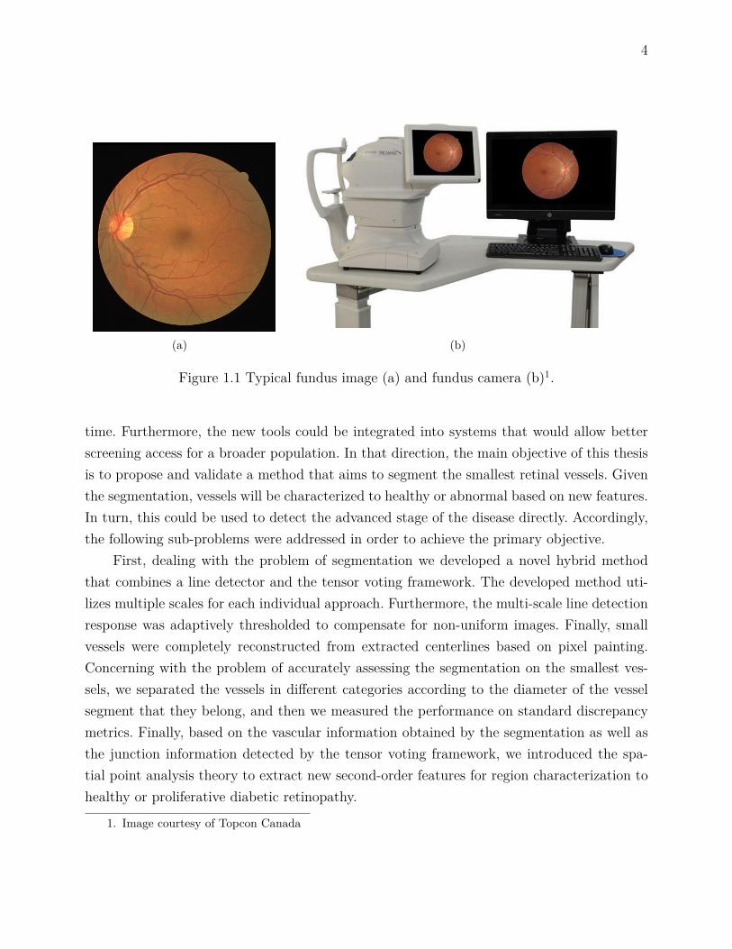
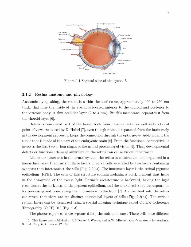
Figure 1.1 Typical fundus image (a) and fundus camera (b) . . . . . . . . . . . . 4Figure 2.1 Sagittal slice of the eyeball . . . . . . . . . . . . . . . . . . . . . . . . 7Figure 2.2 The retinal layers at two different resolutions . . . . . . . . . . . . . . 8Figure 2.3 Illustration of the retinal layers in OCT . . . . . . . . . . . . . . . . . 9Figure 2.4 Graphical demonstration of the vessel network and supply in the retina 10Figure 2.5 Example of the differences in the apperance of the vessels between a

healthy and a PDR case . . . . . . . . . . . . . . . . . . . . . . . . . 14Figure 2.6 Categories of the retinal vessels segmentation methods. . . . . . . . . 14Figure 2.7 Example on the construction of kernels for multi-scale matched filtering 17Figure 2.8 Application of standard matched filtering in a non-proliferative diabetic

retinopathy image . . . . . . . . . . . . . . . . . . . . . . . . . . . . . 17Figure 2.9 Schematic diagram of path opening . . . . . . . . . . . . . . . . . . . 19Figure 2.10 Example of path opening applied on a fundus image . . . . . . . . . . 19Figure 2.11 Radon transform . . . . . . . . . . . . . . . . . . . . . . . . . . . . . 20Figure 2.12 Example of the multi-scale line (MSLD) detection approach applied on

a high resolution retinal image . . . . . . . . . . . . . . . . . . . . . . 21Figure 2.13 Example of the application of the new vesselness measure proposed by

T. Jerman et al. on a high resolution fundus image . . . . . . . . . . 23Figure 2.14 Example of T-snake vessel segmentation . . . . . . . . . . . . . . . . 26Figure 2.15 Example of the evolution of level sets . . . . . . . . . . . . . . . . . . 26Figure 2.16 Example of the application of Sobolev active contour for vessel seg-

mentation . . . . . . . . . . . . . . . . . . . . . . . . . . . . . . . . . 28Figure 2.17 Example of tracking . . . . . . . . . . . . . . . . . . . . . . . . . . . 29Figure 2.18 Example of the application of anisotropic fast marching proposed by

Da Chen et al. for full retinal vessel segmentation . . . . . . . . . . . 31Figure 2.19 Example of the application of multi-scale regression for centerline de-

tection . . . . . . . . . . . . . . . . . . . . . . . . . . . . . . . . . . . 34Figure 2.20 Example of a basic convolutional neural network (CNN) architecture 37Figure 2.21 Components of tensor voting . . . . . . . . . . . . . . . . . . . . . . . 38Figure 2.22 Encoding of point and line structures as tensors . . . . . . . . . . . . 40Figure 2.23 The result of the application of the tensor voting approach in a frag-

mented input line and a fragmented junction . . . . . . . . . . . . . . 41

xviii

Figure 2.24 Examples of segmentation of neovascularizations on the disk and el-sewhere . . . . . . . . . . . . . . . . . . . . . . . . . . . . . . . . . . 45

Figure 2.25 Categorization of available features for vessel characterization. In thedifferent measures subscripts V and A denote the extraction of infor-mation at the vessel pixels or at the whole area, respectively. . . . . . 46

Figure 3.1 Block diagram of the proposed pipeline for retinal vessel segmentation. 55Figure 3.2 Effect of the preprocessing steps on the final segmentation result in

Image_01_h . . . . . . . . . . . . . . . . . . . . . . . . . . . . . . . 57Figure 3.3 Example of applying fixed thresholding versus adaptive thresholding

in two images of healthy subjects from HRF database . . . . . . . . . 59Figure 3.4 Small vessel reconnection example . . . . . . . . . . . . . . . . . . . . 61Figure 3.5 Small vessel tracking example . . . . . . . . . . . . . . . . . . . . . . 64Figure 3.6 Small vessel reconstruction example . . . . . . . . . . . . . . . . . . . 65Figure 3.7 Postprocessing example . . . . . . . . . . . . . . . . . . . . . . . . . . 66Figure 3.8 Single (blue line) and multi (red line) scale tensor voting execution

time for a typical retinal image across scales σTV F = 5 : 5 : 50. . . . . 68Figure 3.9 Analysis of parameter settings . . . . . . . . . . . . . . . . . . . . . . 69Figure 3.10 Full vessel segmentation examples in Image_01_healthy (first row) and

Image_04_diabetic (second row) . . . . . . . . . . . . . . . . . . . . 71Figure 3.11 Differences in the discrepancy metrics across the available segmentation

methods. . . . . . . . . . . . . . . . . . . . . . . . . . . . . . . . . . . 73Figure 3.12 Small vessel segmentation example in Image_15_healthy . . . . . . . 75Figure 3.13 Small vessel segmentation example in Image_10_healthy . . . . . . . 76Figure 3.14 Small vessel segmentation example in Image_06_diabetic . . . . . . 77Figure 3.15 Small vessel segmentation at different stages in proposed pipeline, for

Image_06_diabetic . . . . . . . . . . . . . . . . . . . . . . . . . . . . 77Figure 3.16 Missing small vessels in the reference segmentation of Image_15_healthy 80Figure 4.1 Junction center detection pipeline. . . . . . . . . . . . . . . . . . . . 82Figure 4.2 The orientation uncertainty in junctions of varying degrees of complexity 84Figure 4.3 Algorithmic steps for the junction center isolation. (a) PDR region,

(b) vessel extraction after MSLD, (c) postprocessed result, (d) tensorvoting ballness measure, and (e) final detected junction centers. . . . 84

Figure 4.4 Isolated areas and junctions for analysis in HRF and Messidor database 87Figure 4.5 Boxplot of junction counts, and Nearest neighbor measurements . . . 88Figure 6.1 Second order versus higher order tensors on resolving a 3D crossing . 96Figure 6.2 Duits et al. pipeline for curve extraction . . . . . . . . . . . . . . . . 97

xix

Figure 6.3 Example of the Gestalt principles for grouping . . . . . . . . . . . . . 97

xx

LIST OF ACRONYMS AND ABBREVIATIONS

DR Diabetic RetinopathyPDR Proliferative Diabetic RetinopathyNPDR Non-Proliferative Diabetic RetinopathyCAD Computer Aided DetectionWHO World Health OrganizationMA MicroaneurysmFOV Field Of ViewRPE Retinal Pigment EpitheliumOCT Optical Coherence TomographyRNFL Retinal Nerve Fiber LayerGCL Ganglion Cell LayerIPL Inner Plexiform LayerINL Inner Nuclear LayerONL Outer Nuclear LayerIS Inner SegmentsT Temporal sideN Nasal sideIRMA Intra-Retinal Microvascular AnomaliesNV NeovascularizationNVD Neovascularization on the optic DiscNVE Neovascularization ElsewhereVEGF Vascular Endothelial Growing FactorETDRS Early Treatment Diabetic Retinopathy StudySVL Severe Visual LossUK United KingdomCOS Canadian Ophthalmological Society2D 2-Dimensional3D 3-DimensionalMSLD Multi-Scale Line DetectorGVF Gradient Vector FlowVFC Vector Field ConvolutionOOF Optimally Oriented FluxT-snake Topology snakes

xxi

MHT Multiple Hypothesis TestingCT Computed TomographyANN Artificial Neural NetworkK-NN K-Nearest NeighborGMM Gaussian Mixture ModelSVM Support Vector MachineEM Expectation-MaximizationGA Genetic AlgorithmFCM Fuzzy C-MeansSOM Self-Organizing MapCNN Convolutional Neural NetworkTVF Tensor Voting FrameworkGLCM Gray-Level Co-Occurence MatrixHOS Higher Order SpectraSTAPLE Simultaneous Truth And Performance Level EstimationMTVF Multi-Scale Tensor Voting FrameworkDT-CWT Dual-Tree Complex Wavelet TransformDWT Discrete Wavelet TransformCAL Connectivity Area LengthSens. SensitivitySpecif. SpecificityH HealthyG GlaucomatousM MeanSD Standard DeviationVMR Variance Mean RatioRBF Radial Base FunctionKth-NN Kth-order Nearest NeighborMRI Magnetic Resonance Imaging

1

CHAPTER 1 INTRODUCTION

This chapter will motivate the reader about the segmentation and characterization problemon the small retinal vessels. To do so, we will introduce the necessary details about the impactof diabetic retinopathy on the society and the patient’s vision. Moreover, the importance ofsmall vessels in the diagnosis, and the progress of the disease into sight-threatening retinopa-thy. The scientific challenges for the existing methods will also be introduced. Additionally,we will provide the general context of the fundus imaging field and its challenges. Finally, wewill give the objectives along with the general outline of the thesis.

1.1 Motivation

Vision is one of the five fundamental senses of the human body and probably the mostimportant. The majority of the information that is received daily is visual cues from theoutside world. Possible complications in the vision, therefore, can lead to incapacity fornormal everyday function. Consequently, there is a fundamental need to study and eliminatethe factors that might have an adverse impact on vision.

One important factor is diabetes. This disease affects the eyes indirectly, and it canlead to blindness if it is neglected. The diabetic eye disease or diabetic retinopathy, whichis preventable, is the result of changes in the microvascular circulation system of the eye.According to the world health organization (WHO) [1] diabetic retinopathy is a significantcause of new-onset blindness cases in many developed countries. It was estimated that theprevalence of blindness, due to diabetic retinopathy, is 4.8% of 37 million cases throughoutthe world. The organization has also included it in VISION2020, a global initiative for thecomplete eradication of avoidable blindness by the year 2020.

The standard way to inspect the retina for detection is through the ophthalmoscope.Although ophthalmoscopy is considered a gold standard, digital fundus images along withimaging have been replacing the standard way of retina examination. In both cases, thephysician searches for specific patterns of abnormalities in the small or large vessels as wellas on the retina surface. The procedure is manually performed which is a very tedious workthat takes time. Concurrently, the introduction of screening programs of the population willsignificantly increase the volume of data to be processed. Therefore, methods for computerizedand precise quantification of the disease can be useful for the reduction of the investedresources.

An important tool that can be utilized in the computerized screening is the segmentationof the anatomical structures of the retina. Segmentation algorithms can highlight the most

2

important retinal structures like the vessels, or help the physicians to identify abnormalfeatures that are related to the disease quickly. Due to the nature of the images, thesealgorithms need to perform under challenging imaging conditions. Furthermore, small vesselsappear in the center or the periphery of the image varying in appearance with complex shapeconfigurations and fade boundaries. Finally, pathology alters important image features.

1.2 The role of small retinal vessels in diabetic retinopathy

At a high-level, the classification of the disease is dichotomous indicating the presence ornot of new vessels. This type of classification allows the separation of cases to diabeticretinopathy that is not sight-threatening against cases where there is very high probabilityof sight-threatening complications to the patients. At a more fundamental level, the diseasealters the functionality of the small vessels that is reflected in changes in their appearance.Initially, vascular capillaries are occluded causing the appearance of microaneurysms (MAs),these mark the first stage of the disease. The more severe stages include the appearance ofbright, or dark lesions caused by further complications at the small vessels level. Accumulatedchanges that occur as the disease progresses lead to the growth, or the proliferation, of newvessels that are similar in appearance to the small healthy vasculature. The presence of thenew small vessels is critical for the outcome of the diagnosis as this category of vessels areprone to collapsing, hemorrhaging, and subsequently sight-threatening complications. In suchcases, robust segmentation and subsequently characterization of the small vessels to neovesselsor healthy becomes essential. The next step is the identification of the pathological regionsthat might directly indicate the presence of advanced diabetic retinopathy. Characterizationof the regions to healthy or abnormal is the first step in the detection process.

1.3 Fundus imaging

The predecessor of today’s fundus imaging devices was the direct ophthalmoscope which wasfirst invented by Herman von Helmholtz in the 1850s [2]. Even though the eye is a semi-transparent organ, its optical properties do not allow inspecting it without direct externalillumination. The working principle of ophthalmoscopy is based on the alignment of an illu-mination beam of light and an observing point. In order to achieve this, specially designedlens or mirrors are placed between the patient’s and the physician’s eye. If we substituteobserver’s eye with a digital photographic camera, we can have fundus imaging [3].

There is a standard acquisition protocol. The subject is seated in front of the camera, andthen its head is positioned comfortably to the imaging apparatus. Under complete darkroomconditions, light is emitted by a flash lamp that is directed into the eye. Finally, the reflected

3

light is captured by the camera.Different camera specifications can exist. The field of view (FOV) ranges from 35 to 60

degrees, which also depends if pupil dilation (mydriasis) is utilized. The latter is achieved bytopical application of medication (tropicamide), and it is recommended when there is a needof inspecting the periphery areas of the retina. However, dilation can induce discomfort tothe patient, and it is not disconnected from medical complications, so undilated inspection isusually preferred. The image resolution of a camera can range from low to high, e.g. 768x584to 3504x2336 pixels. Higher resolution cameras are preferred as the vessels as well as otherstructures can appear in more detail. The next figure (Fig 1.1) shows a fundus camera alongwith a typically acquired image.

This imaging modality is of particular interest for our application. Fundus imaging isa widely accepted method for inspecting the retina and diagnosing diabetic retinopathy [4].The advantages of using this modality are that it can produce digital images, which canbe processed quantitatively. Furthermore, it is a non-invasive way to image the retina withminimal discomfort for the patient. It is also relatively cheap technology, which makes itattractive for screening programs. Finally, it is easy to transfer the data through a networkto a data server.

Even though the acquisition protocol is standardized, the images suffer from artefactsthat make the segmentation, and characterization of the small vessels challenging. In fact,the obtained images can suffer from non-uniform illumination problems. Vessels closer tothe optic disc are more prominent, while vessels at the periphery more obscure. Due to theillumination, image contrast could substantially vary causing the smallest vessels to appearvery faint relatively to the adjacent background region. Moreover, the quality of the imagesis not unrelated to the age of the subject, the coexistence of anterior or posterior retinalpathologies, and from the appearance of the retina.

1.4 Research contributions

The ultimate goal of the thesis is to propose new tools to facilitate the screening of diabeticretinopathy. Screening tries to sort cases to healthy, or cases deemed for further action.Moreover, according to the severity of the identified DR case, screening can refer the subjectto the appropriate medical intervention. For example, an emergency treatment in case of aNV detection, or better management for a NPDR case. CAD could augment screening byusing automatic methods for image analysis. In this context, small vessels play an importantrole as missing them could lead to increased false positive rates in dark lesion CAD systems orincreased false negatives in sight-threatening CAD systems. As the number of available datascales up, computerized methods could be proved beneficial to exploit better the physician’s

4

(a) (b)

Figure 1.1 Typical fundus image (a) and fundus camera (b)1.

time. Furthermore, the new tools could be integrated into systems that would allow betterscreening access for a broader population. In that direction, the main objective of this thesisis to propose and validate a method that aims to segment the smallest retinal vessels. Giventhe segmentation, vessels will be characterized to healthy or abnormal based on new features.In turn, this could be used to detect the advanced stage of the disease directly. Accordingly,the following sub-problems were addressed in order to achieve the primary objective.

First, dealing with the problem of segmentation we developed a novel hybrid methodthat combines a line detector and the tensor voting framework. The developed method uti-lizes multiple scales for each individual approach. Furthermore, the multi-scale line detectionresponse was adaptively thresholded to compensate for non-uniform images. Finally, smallvessels were completely reconstructed from extracted centerlines based on pixel painting.Concerning with the problem of accurately assessing the segmentation on the smallest ves-sels, we separated the vessels in different categories according to the diameter of the vesselsegment that they belong, and then we measured the performance on standard discrepancymetrics. Finally, based on the vascular information obtained by the segmentation as well asthe junction information detected by the tensor voting framework, we introduced the spa-tial point analysis theory to extract new second-order features for region characterization tohealthy or proliferative diabetic retinopathy.

1. Image courtesy of Topcon Canada

5

1.5 Thesis outline

This thesis proposes the segmentation of the small retinal vessels as well as their characteri-zation to healthy or abnormal. This chapter gave the general motivation for the problem. Todo so, we briefly introduced the different stages of the diabetic retinopathy, how these stagesare related to the smallest retinal vessels, as well as how the fundus imaging is used in theclinical practice. We also presented the scientific challenges for both the segmentation of thesmallest vessels and imaging of the retina using fundus cameras. Finally, the research goal andthe research contributions were highlighted. The following chapter will present the necessarybackground and the literature review that will provide the state-of-the-art of segmentationtechniques in healthy vessels. Additionally, the segmentation and characterization methodsfor the abnormal vasculature, as well as the evaluation metrics for assessing the performanceof the methods are presented. Furthermore, Chapter 3 and Chapter 4 will present the pro-posed methodology for the segmentation and characterization of the vessels along with theresults. Chapter 5 will provide a general discussion of the work together with the limitations,and possible future research developments. Finally, Chapter 6 will conclude the thesis bysummarizing the work and providing possible future work.

6

CHAPTER 2 LITERATURE REVIEW

This chapter will begin by providing the necessary background about important concepts ofthe general anatomy and physiology of the retina under physiological, or under pathologicaldiabetic retinopathy. Details will be provided on the diagnosis of the disease, the manage-ment, as well as how diabetic retinopathy is related to changes in the small vessels. This willbe followed by the state-of-the-art of segmentation techniques in the healthy retinal vessels.Furthermore, this chapter will describe the available techniques for the abnormal retinal ves-sel segmentation and characterization problem. Moreover, different performance evaluationmethods of the segmentation algorithms will be presented. Finally, a general discussion onthe limits of the methods with respect to the problem of the smallest vessel will be provided.The chapter will close with the definition of the thesis objectives.

2.1 Background

Computerized techniques are becoming more prevalent in the retinal imaging field. There-fore, it is important to understand how the different methods, such as the segmentationand characterization of the small retinal vessel, could be used to facilitate the diagnosis andmanagement of diabetic retinopathy. This section will describe the general anatomy of thestructures that are affected by diabetic retinopathy : the eye, the retina, and the retinal ves-sels. How the disease is diagnosed and managed. Finally, the importance of neovascularizationin the outcome of the retinopathy.

2.1.1 Eye anatomy

The eye consists of two compartments, as figure 2.1 shows, the anterior and the posteriorchamber. The posterior chamber, or vitreous, which is located between the lens and the retina,is filled with a transparent non-renewable gel substance, the vitreous humor [5]. Additionally,two groups of fibrous layers can be found in the eye, the external and the internal. The externalincludes the sclera, the cornea, and the choroid, while the internal entails the retina. Thelatter, which is the most important for our application, is further divided into two layers, theposteromedial retina, which is the visual part where the light rays are concentrated, and theanterior, which is the non-visual part. Visual retina begins from the fovea centralis or maculaand extends until the ora serrata.

7

Figure 2.1 Sagittal slice of the eyeball2.

2.1.2 Retina anatomy and physiology

Anatomically speaking, the retina is a thin sheet of tissue, approximately 100 to 250 µmthick, that lines the inside of the eye. It is located anterior to the choroid and posterior tothe vitreous body. A thin acellular layer (2 to 4 µm), Bruch’s membrane, separates it fromthe choroid layer [6].

Retina is considered part of the brain, both from developmental as well as functionalpoint of view. As stated by D. Hubel [7], even though retina is separated from the brain earlyin the development process, it keeps the connection through the optic nerve. Additionally, thetissue that is made of is a part of the embryonic brain [8]. From the functional perspective, itinvolves the first two or four stages of the neural processing of vision [9]. Thus, developmentaldefects or functional damage anywhere on the retina can cause vision impairment.

Like other structures in the neural system, the retina is constructed, and organized in ahierarchical way. It consists of three layers of nerve cells separated by two layers containingsynapses that interconnect the cells (Fig. 2.2(a)). The innermost layer is the retinal pigmentepithelium (RPE). The cells of this structure contain melanin, a black pigment that helpsin the absorption of the excess light. Retina’s architecture is backward, having the lightreceptors at the back close to the pigment epithelium, and the neural cells that are responsiblefor processing and transferring the information to the front [7]. A closer look into the retinacan reveal that there are ten distinct anatomical layers of cells (Fig. 2.2(b)). The variousretinal layers can be visualized using a special imaging technique called Optical CoherenceTomography (OCT) [10] (Fig. 2.3).

The photoreceptor cells are separated into the rods and cones. These cells have different

2. This figure was published in R.L.Drake, A.Wayne, and A.W. Mitchell, Gray’s anatomy for students,3rd ed. Copyright Elsevier (2013).

8

(a) (b)

Figure 2.2 The retinal layers at two different resolutions. (a) The front ganglion, the middlelayer of the neural cells, and the back where photoreceptors are located3. (b) A sketch of thecellular retinal layers, at a more microscopic scale4.

physiological characteristics. Rods are more sensitive in low light conditions (scotopic vision)than cones ; while cones, even though they are not very light sensitive (photopic vision), areresponsible for our color recognition, and our ability to see fine details. The number of rodsand cones vary significantly along the retina. Cones are concentrated at the fovea, where wecan perceive the object with fine details. Rods, in contrary, are more scattered and they areabsent in the fovea.

2.1.3 Retinal vessels

Retina blood supply comes from the central retinal artery, which is a branch of the ophthalmicartery. It enters the eye from the optic disc and follows a fairly standard pattern at theganglion cell level. Just before entering the eye, it is divided into two secondary branches, theinferior and the superior. Each secondary branch is further divided to nasal and temporalarteries. The bifurcations continue through the periphery, where there is a gradual reductionin the vessels’ diameter. This gradual change leads to the bifurcation of the large vessels intocapillaries. Some temporal branches form arches around the fovea. The venous network alsofollows a similar pattern [12].

On the base, around the optic nerve, the major arteries measure approximately 100 µmin diameter having 18 µm thick walls. In higher order branches the diameter decreases untilit ends up to only 15 µm [12]. The composition of the vessels also changes according tothe vessel diameter. Large vessels are composed of five to seven muscle layers, while small

3. Adapted by permission from Macmillan Publisher Ltd : Nature Reviews Drug Discovery [11], copyright(2015)

4. Courtesy of American Scientist [8]

9

(a) (b) (c)

Figure 2.3 Illustration of the retinal layers in OCT. The first image (a) is the acquired OCTvolume. The second image (b) is the segmentation result that reveals the different cellularlayers, namely the retinal nerve fiber layer (RNFL), the ganglion cell layer (GCL), the innerplexiform layer (IPL), the inner nuclear layer (INL), the outer nuclear layer (ONL) + innersegments (IS), the outer segments (OS), and the retinal pigment epithelium (RPE+). Thefinal image (c) is the segmented surfaces around the fovea (T : temporal side, N : nasal side)[14] ( c©[2010], IEEE).

arterioles include a single cell layer. The retinal vessel network does not communicate withany other network, so if there is any vessel obstruction, it can lead to impaired visual function[12, 13].

The vessel network is organized in such a way, to optimize the blood supply in all thecritical areas of the retina. Furthermore, it has been observed that the normal vasculatureis guided by pre-existing neuronal cells that act as scaffolds for the vessel growth [15]. Thenet effect is the appearance of the retinal vasculature as a tree-like structure (Fig. 2.4).However, there are two avascular regions, where vessels do not exist. Firstly, surface vesselscannot reach the fovea and a 0.5 mm circular region around it. Secondly, vessels cannot resideposterior to the boundary of the non-visual part of the retina called the ora seratta [12, 13].

2.1.4 Retinal vessel pathologies

Under diabetes, the glucose levels in the blood are higher than normal cases. This metabolicchange has an adverse impact on the retinal circulation that triggers many pathophysiolo-gical changes [16, 17], of which the most important are related to the smallest vessels [18].The previous changes lead to the disruption of the local blood flow in the retina tissue. Inorder to compensate for that, vessel growth factors are secreted causing angiogenesis andneovascularization [19]. These new vessels have poor prognostic value for vision because theygrow at the vitreo-retinal interface, an interactive environment, that causes inflammation,and ultimately collapse of the fragile neovascularizations. Consequently, vitreous or preretinal

10

Figure 2.4 Graphical demonstration of the vessel network and supply in the retina. Retinalvessels belong to the central retinal artery/vein ; they cover the retina in a tree-line architec-ture, and they are superficial to the retina5.

haemorrhages are induced followed by retinal detachment, and partial, or total vision loss[16].

2.1.5 Diabetic retinopathy diagnosis and screening

Diabetic retinopathy is a progressive disease that includes five main stages. The differentstages document the severity of retinopathy based on the visible signs, observed by theretina specialists. Different distinguishable signs characterize the disease as it involves fromthe early to the later stages. The evolution of the retinopathy among the five stages, accordingto the Early Treatment Diabetic Retinopathy Study (ETDRS) [20], is :

1. No retinopathy : No sign is apparent that can indicate retinopathy.

2. Mild Non-Proliferative Diabetic Retinopathy(NPDR) : The first clinical sign is a limitednumber (>3) of microaneurysms (MAs). In this stage, only MAs can be observed.

3. Moderate to severe NPDR : Additional MAs are present on the eyes at these stagesand other more complex manifestations lead to the appearance of noticeable dark orbright lesions. When a group of deep capillaries has been occluded, blot haemmorrhagesappear in the retina. Another sign in the moderate NPDR is the emergence of hardexudates as well as the cotton wool spots. The former are lipid depositions leaked fromthe MAs ; while the latter are caused by the swollen neural axons on the nerve fiberlayer. In parallel, intra-retinal microvascular anomalies (IRMAs) and venous beadingscan be present in an extensive retinal area. As the disease progresses, extensive intra-vascular areas are occluded. Remodeling of the unobstructed vasculature thus takes

5. This figure was published in C.V.Network, Developmental anatomy of the retinal and choroidal vas-culature, Copyright Elsevier (2011).

11

place, which leads to morphological as well as functional adaptations of the unaffectedvessels. IRMAs are leaky tortuous capillaries in the areas of capillary occlusion ; whilevenous beadings are localized dilations of the venous wall, which represents the effortof the body to grow new vessels on the non-perfused tissue. As the disease advances,the appearance of lesions is more frequent.

4. PDR : At this point, vascular endothelial growing factors (VEGFs) are secreted thatlead to the formation of new small, fragile vessels, the neovascularizations.

The five-level staging does not reflect visual function, but only the condition of theretina observed via ophthalmoscope or fundus photography. Maculopathy, the swelling of themacula, is another potential factor for visual complication thus for full range classificationthe presence or absence of maculopathy is reported separately from the retinopathy [21].

The disease can be unnoticed by the patient until its late stages, where the symp-toms involve reduced visual acuity or even blindness. Thus, early cost-effective diagnosis andmanagement are required. Diabetic retinopathy can be effectively assessed, based on the ins-pection of the retina through a direct or indirect ophthalmoscope as well as fundus imaging.Besides this, historically, prevention had been limited to the monitor, and tight control ofthe modifiable risk factors, like the blood glucose/lipid/pressure levels. The aforementionedestablished means of prevention together with the publishing of the ETDRS report aboutthe effectiveness of laser therapy helped in the general reduction of the rates of progressionto sight-threatening diabetic retinopathy [22].

As a second line of measure, screening was introduced to the public. According to WHO,[23] screening is defined as "the presumptive identification of unrecognized disease or defectby the application of test, examinations or other procedures which can be applied rapidly.Screening tests sort out apparently well persons who probably have a disease from those whoprobably not. A screening test is not intended to be diagnostic. Persons with positive orsuspicious findings must be referred to their physicians for diagnosis and necessary treatment".Screening for diabetic retinopathy is a broad public health practice, as it is highlightedin [21], that aims to identify patients with early signs of the disease, to provide effectivemanagement and treatment. Evidence for the effectiveness of screening for sight threateningdiabetic retinopathy as part of national policies was given in [24].

In practice, screening programs designed on a national level have been proven adequatein further reducing visual complications. In parallel, the acceptance of fundus imaging asan equivalent to ophthalmoscopy [25] further facilitated the implementation of a range ofnational screening programs that ultimately helped diabetic patients. For example, Icelandhad implemented a national screening program and achieved to reduce the blindness amongdiabetic patient from 2.4% in 1980 to 0.5% in 2005 [24]. Furthermore, in a metanalysis [22],

12

where a range of studies from two consecutive decades are examined, it was reported that after10-years the incidence rate of proliferative diabetic retinopathy (PDR) and severe visual loss(SVL), has been reduced by 4.9% and 3.4%, respectively. In another cost-effectiveness study[26], conducted in isolated communities of Ontario in Canada, screening with fundus imagingwas proved cost-effective versus no screening. Moreover, screening with fundus imaging wasproved superior to ophthalmoscopy on site as the latter requires the manual inspection of theretina through a hand-held tool, as well as, more intensive employment of trained personnel.

Different screening schemes have been implemented around the world. These can betailored to the specific needs of a country, in order to maximize the efficiency, and ultima-tely increase the coverage. In UK [21, 27] for example, fundus imaging is embedded in thesecondary care level, with either centralized or decentralized grading by specialists in mobileunits (technicians or trained physicians). Then the patients are referred to an ophthalmo-logist for further diagnosis or therapy if it is necessary. In a recent study published by agroup in Australia [28], the burden of grading is proposed to be shifted towards the pri-mary care ; in this way, there will be advantages in the impact and speed of the outcome.In Canada, Canadian Ophthalmological Society (COS) is responsible for publishing clinicalpractice guidelines for screening, and management of the diabetic retinopathy [29]. As canbe seen, manual screening has been proven effective in reducing the progression rates of dia-betic retinopathy. However, the screening rates are still lagging behind the expected influxof diabetic patients in the healthcare systems in the near future. Currently, in the US, 50%of type 2 diabetic patients do not have access to any type of eye examination [30]. Whilethe corresponding non-attendance rates are 22% and 20-30% for Australia [28] and for theUK [30], respectively. The goal of the possible new policies would be to increase the scree-ning coverage. These new policies will eventually lead to a dramatic increase in the size ofprocessed data, and thus computerized approaches might play a major role. For example,RetinaCheck project [31] was launched which is a sino-dutch collaboration between an ex-tensive network of hospitals and universities with the aim to screen the entire populationof a Chinese province for sight threatening retinopathies, including diabetic. Accounting forapproximately 24 million people, this large-scale retina screening program will be realized byCAD systems that will automatically analyze the retinal images. Additionally, it has beennoticed that screening rates are analogous to the socioeconomic level. Hence, new meansof access, like teleophthalmology, should be considered. In parallel, with the advent of newtechnologies, automatization of screening is cost-effective and in some cases, it is even en-couraged [21]. In Scotland, for example, it has been estimated that the cost per patient forautomated detection is approximate $0.25 [30], sufficiently low for subsidized programs. Fi-nally, computerized-based screening is flexible, and it can be integrated into many models

13

for the effective management of the diabetic retinopathy.

2.1.6 Neovascularizations (NVs)

The appearance of a patient with proliferative diabetic retinopathy is considered an emer-gency and immediate therapy should be administrated, usually via lasers, VEGF inhibitors,or even vitrectomy [32]. Neovascularizations are particularly interesting for our project. In thecomprehensive classification schemes, PDR stage is further divided in three subcategories :1) mild, 2) moderate, and 3) severe. The following factors determine the severity. Firstly, thelocation of the neovascularizations, namely on the disc (NVD), or elsewhere on the retina(NVE). Secondly, the size of the neovascularizations area with respect to the area of the opticdisc. Finally, the presence of vitreous or preretinal haemorrhages.

Neovascularizations, usually grow from the post-capillary venules in an abnormal patternthat does not obey the fractals’ law properties of healthy vessel development. Neovesselslack a standard self-similar hierarchical pattern, branching in random directions. NVs canbe mistaken with small healthy or IRMAs vessels, but not with other dark lesions like themicroaneurysms. Neovascularizations demonstrate greater variability than the MAs both inshape as well as in size, and thus they pose extra challenges and requirements. Furthermore,NVs demonstrate special functional as well as morphological properties. New vessels lackthe tight cellular junctions that are apparent in existing vessels, so they leak throughouttheir length. Additionally, neovascularizations occur along the border between healthy andischemic retina, while IRMAs occur within areas of capillary occlusion. Individually, they areas tortuous as IRMAs, forming chaotic networks in groups that cover a large retinal area.They usually loop back to the optic disc (NVD) and have wider vessel diameter on the tipthan the base. IRMAs on the other hand, never form loops. Furthermore, slightly differentappearance regarding brightness and sharpness, of their edges, can be attributed to the factthat IRMAs grow deeper than neovascularizations. Figure 2.5 shows examples of isolatedregions with neovascularizations on the optic disc and elsewhere from an image with PDR.

2.2 Healthy retinal vessel segmentation algorithms

Generally speaking, there has been a constant effort to classify the retinal vessel segmentationmethods in a systematic way according to the methodology that is followed. Early segmen-tation methods were either categorized into contour-based or region-based approaches [33].Since the establishment of the field of retinal vessel segmentation, several new methods havebeen presented that extend and utilize new knowledge, so several subcategories were startedto emerge. Lately, scientists started combining algorithms together in hybrid schemes, andso blurred boundaries between the methods exist. A good point for someone to start is the

14

(a) (b) (c)

Figure 2.5 Example of the differences in the apperance of the vessels between a healthy and aPDR case. (a) Healthy retinal image, (b) PDR retinal image, (c) zoomed regions containingneovascularizations on the disc or elsewhere corresponding to the green, red, and blue insetin (b).

review of a series of surveys that have been published in the literature [34, 35, 36, 37].The categorization that is followed in this thesis can be seen in the next figure (Fig.

2.6). To begin with, for each subcategory the working principles and the assumptions willbe given. Then a critical analysis of the advantages and the disadvantages in the context ofthe retinal vessel segmentation will follow. Finally, similar work and contributions in otherapplications will be provided.

Retinal vesselsegmentation algorithms

Intensity-basedmethods

Machine learningmethods

Contour-basedmethods

Region-basedmethods

Template DerivativeDeformable

model

Figure 2.6 Categories of the retinal vessels segmentation methods.

2.2.1 Intensity-based methods

Intensity-based is the largest and broadest of all the categories of methods. The algorithmshere segment the images by searching mainly for specific intensity patterns in the images.In turn, Intensity-based algorithms are divided between the region and the contour-basedmethods.

15

Contour-based methods are trying to include and group in the same contour, edge, orcurve the pixels that satisfy a certain criterion that depends on an applied template. Pixelswhich are not separated by an edge are allocated to the same category. Additionally, in thiscategory an initial curve can be defined that deforms according to some constraints or forcesin order to fit a contour.

Region-based methods operate iteratively by grouping neighbor pixels which have similarintensity values into the same region or by splitting regions of pixels which have dissimilarvalues. A fundamental algorithm that applies the aforementioned principles is the regiongrowing [38]. All subsequent methods in this category are an extension of the basic model.Additionally, representing the data using graphs facilitates the application of minimum-costpath approaches. Contour and Region-based methods are further separated in subcategoriesthat we will analyze.

2.2.1.1 Matched filtering

One of the earliest introduced segmentation methods for retinal vessels was the matched fil-tering. This approach, which was first proposed in the 1980s, is based on template matchingof a small representative vessel segment along the whole image in the spatial domain. Mat-ched filtering has been widely used for retinal vessel segmentation [39] as well as for coronaryarterial tree detection from X-ray angiography [40] and neuron tracing from 3D confocal bio-microscopy [41]. In the case of retinal vessels, the template is constructed as a 2D convolutionkernel that filters the image and enhances the vessels. The design of the filter is based onfour assumptions for the vasculature. Firstly, the large vessels demonstrate small curvaturesso the filter can be approximated by a piecewise straight kernel. Secondly, the cross-sectionalintensity profile of the vessels can be approximated by a Gaussian, so the profile of the filtershould be a Gaussian too. Thirdly, vessels can appear in different orientations and scales, sothe filter should be adapted accordingly. Finally, vessels are darker than their background sothe sides of the filters should be at higher intensity level than the central region.

When matched filtering is applied, the effect is the enhancement of the vessels againsttheir background. Subsequently, thresholding can take place as a final step in order to segmentthe vessels. Since the Gaussian is a very general representation, there are cases where it cannotapproximate adequately vessels’ shapes. For example, when the curvature is very high in shortdistance. Additionally, this method has a problem of over-segmenting irrelevant structuresthat resemble vessels. Indeed, physiological structures like the optic disc as well as pathologiessuch as microaneurysms and bright lesions can be falsely recognised as a vessel structure. Forthe smallest vessels in particular (∼3 pixels in diameter), there may be not enough samplesto model the profile with a Gaussian or any other model.

16

Efforts have been placed in the direction of improving several aspects of the basic mat-ched filtering approach or introducing novel variations by applying more complex models. Forexample, multi-scale sensitivity can be achieved by varying the width of the kernel (Fig. 2.7)and then retaining the maximum response across all the scales [42]. A curved-support Gaus-sian model has recently been proposed to model non-straight structures [43]. Furthermore,in order to suppress the false positive detections some authors proposed the combinationof matched filters with the first order derivative of the Gaussian [44] ; while others exploitfeatures in the thresholding phase [45]. In another case [46], the authors used self-matchedfiltering, where the selected template is a 180◦ rotated version of the local neighborhood.In another study, the authors optimized exhaustively the Gaussian parameters before theapplication to the retinal images in order to reduce the computational time [47].

There have been efforts to include more information to cover all the available cases andovercome the possible limitation of the basic model. One problem is the central reflection thatoccurs on the large vessels and which appears as an elevation at the center of the Gaussian[48]. The central reflection can be modeled by utilizing a double Gaussian profile [49, 50], adifference of Gaussians [51], a Laplacian kernel [52], or a multiscale Hermite approximation[53]. The last model together with a method based on the superposition of Gaussian functions[54] in a local area, has been proposed to model the healthy vessel bifurcations. A moreskewed model than the standard Gaussian was proposed in [55]. Some authors, moreover,introduced constrains to distinguish vessels from the pathologies. L. Zhang et al. [56], forexample, reduced the false positives from non-line edges (Fig. 2.8) by incorporating a double-sided thresholding in the Gaussian matched filtering. This model reduces the probability ofpositive responses from non-vascular pathologies or the optic disc. Transforming the intensityprofile in the frequency domain using phase congruency [57] offers a scale as well as intensityinvariant representation of the vessel cross-section, that it can also compensate for the blurredboundaries. Finally, modeling of the dark or bright lesions was made possible using multi-concavity modeling [58] or by examining the divergence of the gradient vector field in theimage [59]. This information was in turn incorporated into processes that distinguish vesselsfrom pathologies on diabetic retinopathy images.

Detecting the object of interest by directly modeling it has been proved an effective, yeta straightforward way to filter most of the vasculature from the background. Besides matchedfiltering, other template-based methods have been proposed in the literature.

2.2.1.2 Morphological processing

A more general vessel representation that does not take into account the cross section in-formation is the morphological processing. This category of algorithms tries to segment the

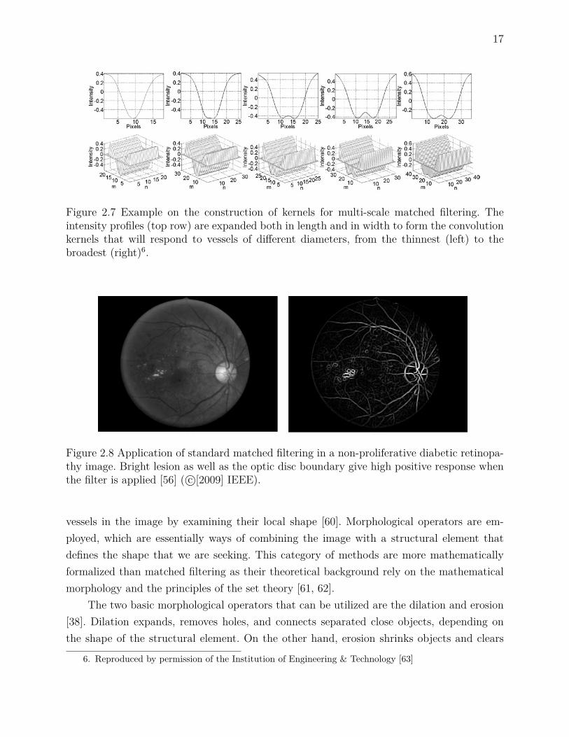
17

Figure 2.7 Example on the construction of kernels for multi-scale matched filtering. Theintensity profiles (top row) are expanded both in length and in width to form the convolutionkernels that will respond to vessels of different diameters, from the thinnest (left) to thebroadest (right)6.

Figure 2.8 Application of standard matched filtering in a non-proliferative diabetic retinopa-thy image. Bright lesion as well as the optic disc boundary give high positive response whenthe filter is applied [56] ( c©[2009] IEEE).

vessels in the image by examining their local shape [60]. Morphological operators are em-ployed, which are essentially ways of combining the image with a structural element thatdefines the shape that we are seeking. This category of methods are more mathematicallyformalized than matched filtering as their theoretical background rely on the mathematicalmorphology and the principles of the set theory [61, 62].

The two basic morphological operators that can be utilized are the dilation and erosion[38]. Dilation expands, removes holes, and connects separated close objects, depending onthe shape of the structural element. On the other hand, erosion shrinks objects and clears

6. Reproduced by permission of the Institution of Engineering & Technology [63]

18

the image from isolated small island in the background, again based on the structural ele-ment. All subsequent advanced morphological operators, like opening, closing or top-hat arecombinations of dilations or erosions in different orders.

The basic assumptions that are considered to segment the vessels include the fact thatthe vessels are piecewise, locally linear, elongated structures, thus similarly shaped structuralelements can isolate them. Vessels, furthermore, can appear in different orientations andscales so the structural elements should be varied accordingly. Finally, vessels have uniformand higher grayscale intensity than the background.

The advantages of these algorithms against other available methods include their ro-bustness to noise and reduced computational cost. Moreover, morphology has been utilizedin pre/post-processing processes [64]. However, the basic algorithm does not employ thecross section information of the vessels. Additionally, morphological processing is inaccuratein term of localizing the vessels’ boundary. The basic working principles, also, are not ap-plicable in the thinnest or the most tortuous of the vessels ; and finally, over-segmentationis frequent from similar to vessel physiological structures. More particularly, for the narrowvessels, the size and shape of the structural element is inadequate to approximate the vessels,so there is low sensitivity in that cases.

Several studies exist that employ morphological processing either for enhancing or seg-menting retinal vessels. In an early paper [65], vessels were enhanced by applying a multi-directional linear structural element ; while recently A.M. Mendoca et al. [66] employedmultiscale circular structural elements in successive top-hat operations to enhance the ves-sels. Furthermore, M.S. Miri and A. Mahloojifar [67] proposed a new scheme where multi-structural elements of different orientations and scales are used in the same window area tosegment the vessels. In another series of similar methods [68, 69, 70], the authors investigatedthe Gaussian cross-sectional profile of the vessels. Firstly, they computed the local curvatureusing Laplacian filtering, and after that, they isolated the vessels by applying an alternatingfilter with a linear structuring element and morphological reconstruction. The authors in[71] tried to overcome the problem of over-segmentation of the optic disc, by first employingmorphology to localize the optic disc, and then a series of morphological processes for theretinal vessels. Lately, morphological definition of paths (see Fig. 2.9, 2.10) has been proposedthat can reconnect vessel pixels to non-straight paths [72, 73]. In other applications, a recentadvance includes the introduction of the spatially variant morphology [74], where Hessianbased vesselness controls the size and orientation of the structural element.

Processing the images by means of morphology offers a more mathematically formalizedway to detect the vasculature as all the operations are a combination of basic functions. Aneven simpler template-based method has been proposed to isolate the vessels.

19

Figure 2.9 Schematic diagram of path opening. Given a specific binary adjacency relation,horizontal in (a) and the most prominent pixels (red), path opening connects neighbors toform three different paths (b)7.

Figure 2.10 Example of path opening applied on a fundus image. Given the vessel enhancedimage at the left column path opening reconnects the most prominent, with respect to thefilter response, pixels to form paths at the right column8.

2.2.1.3 Line detection

The simplest of all the template-based methods that do not include any width informationis the line detection. The fundamental assumption that is being made in this subcategory ofalgorithms is that vessels are piecewise elongated line-like structures with lower intensity thanthe background. In the basic working scenario of a single-scale approach, a straight samplingline is utilized that computes the mean intensities along different orientations across the wholeimage in the spatial domain. When the line is parallel to the vessels, the mean responseis maximum. The methodology here is closely related to the Radon and discrete Hough

7. Reprinted from B.Yin et al., Vessel extraction from nonfluorescein fundus images using orientationaware detector, vol. 26, Pages. 232-242, Copyright (2015), with permission from Elsevier [73].

8. Reprinted from B.Yin et al., Vessel extraction from nonfluorescein fundus images using orientationaware detector, vol. 26, Pages. 232-242, Copyright (2015), with permission from Elsevier [73].

20

Figure 2.11 Radon transform 9.

transform [75], (see Fig. 2.11). Radon transform computes a series of parallel line integralsin different offsets from the center of the object that are projected in a certain distance in ananother projection line (x). The projection line, in turn, is rotated to accommodate differentangles (θ). The final value that is registered, in another parametric space, is the sum of allthe projections. Equally, the basic line detector is a special case of this transform. This istrue if we substitute the basic integral functional with the computation of the mean value ;if we only allow the central line to be projected ; and if we finally assume that the responseis the maximum along the available orientations.

This method was first utilized to identify linear structures in mammographic [77] aswell as ultrasound [78] data. However, it was recently being applied to retinal images [79](Fig. 2.12). Lately, it was adapted to multi-scale schemes to cover all the available vessels’diameters by varying the length of the sampling line [80]. Additionally, line-based approachesare computationally inexpensive, embarrassingly parallel, and can be combined in hybridschemes [73]. One drawback of the basic line detector is that it produces high responsesin pathologies like microaneurysms and bright lesions because these structures have similarcharacteristics to the vessels. The former has been effectively tackled by examining morecarefully the results derived by the line detectors. More precisely, it could be assumed thatin case of the vessel there will be a peak in the response of the filter in a specific direction,parallel to the direction of the vessel, while in small microaneurysms the response will be highin all the examined directions [81, 82]. Another limitation is in the detection of the vessels’bifurcations. This problem was tried to be solved by representing the local image around theexamined central point into polar coordinates [83] ; another possible way is to use the analysisof the orientation space [84] to identify multiple response peaks that indicate the existence ofa junction or a crossing. Based on the line detectors other authors extended the method to be

9. Courtesy of Mathworks : [76]

21

applied in the optic disc localization [85]. A different configuration of multiple parallel lines,or measuring the contrast instead of the intensity, was implemented in order to facilitatethe detection of the smallest vessels [86, 87, 88]. Finally, local orientation selection by theapplication of the Hessian followed by line detection was proposed for X-ray angiography, aswell as for retinal images, in [89].

The previous template-based methods try to detect the vessels in the spatial domain.Instead, we can investigate the vascular properties differently by examining the images inanother space, the variational domain.

Figure 2.12 Example of the multi-scale line (MSLD) detection approach applied on a highresolution retinal image. (a) input image, (b) MSLD response, and (c) segmented vesselsbased on thresholding.

2.2.1.4 Derivative methods

In this category of algorithms it is assumed that the images are two-dimensional functionsf(x, y) where the vessels appear as local maxima or minima [90]. The vessel detection is thenperformed by examining the image derivatives properties.

One of the earliest adopted methods for vessel segmentation was edge detection viafirst-order derivatives or gradients. Gradient-based edge detectors (Sobel, Prewitt, Robert,Canny) had been utilized in many studies [91, 92, 93]. The process is based on low levelprimitives, and the implementation requires less computation. The method tries to identifythe local gradient direction together with its response. However, the kernels cannot easilyhandle non-straight vessels, fragmenting the result. Secondly, the kernels are of single-scaleand thus they do not take into account any information about the intensity variation. Thirdly,the method can only detect the boundary of the large vessels ; while its response is low if theline deviates from an ideal step edge.

A methodological extension is the combination of the local gradient into a matrix, thestructural tensor. By decomposing the tensor, neighbor information can be considered impro-

22

ving the response of the vessels against other irrelevant structures. This approach has beeneffectively implemented in [94] for differentiating vessels, from bifurcations, and nodules inchest computed tomography (CT).

Different groups tried to tackle some problems related to the gradient-based methodsby taking into account the fact that vessels’ cross-sectional profile is a Gaussian. To do so,they utilized the first-order derivative of the Gaussian function [66, 95]. The first-order im-proves the performance of the basic gradient-based edge detectors ; however, it only extractsfragmented centerlines. Post-processing hence is required to connect the fragmented detectedcenterlines. Additionally, the convolution with a Gaussian filter is equivalent to the applica-tion of filtering in all the image directions (isotropic diffusion) [96] ; where the direction ofthe gradient determines the orientation of the filtering. When isotropic filtering is appliedto images it removes the excess background noise ; however at the expense of filtering thevessel boundary, merging close vessels, and filtering out small vessels. Anisotropic diffusionwas proposed to overcome the problem by filtering the image in an orthogonal direction tothe detected gradient [97, 98, 99]. For the problem of merging close vessels, alternative me-thods that have been proposed utilize the gradient vector flow (GVF) [100] or the optimallyoriented flux (OOF) [101].

An extension to the previous methodology is the exploitation of the second-order de-rivative properties. Similarly to tensor, the higher order representation offers additional in-formation from the neighborhood, like the curvature, which has different values dependingif the object is tubular or blob-like. One appealing implementation is the Hessian matrixcomputation in every pixel Is of the image (2.1) :

Hessian(Is) =∂2Is

∂x2∂2Is∂xy

∂2Is∂yx

∂2Is∂y2

(2.1)

The image derivatives can be approximated numerically by convolving the image withthe partial second-order Gaussian derivatives. This is a practical way also for scale spacerepresentation of the image because by varying the width of the Gaussian function we canexamine vessels of different diameters. Eigen decomposition of the Hessian matrix follows,where the principal directions of the underlying structure are computed. The extracted prin-cipal directions are very important features because the vessels are parallel to the eigenvectorthat corresponds to the maximum eigenvalue [90]. The vessel enhancement is then performedby combining the eigenvalues in appropriate quantities or models. Examples include : Lo-renz’s [102], Sato’s [103], and Frangi’s [104] vesselness models. Vascular centerlines can alsobe detected by decomposing the Hessian matrix as it was presented in C. Steger paper [90].

Since Gaussians are used to approximate the derivatives, Hessian matrix representation

23

also suffers from the same problems as the isotropic diffusion filtering. In this case, the si-tuation is even worse because the second derivatives’ effects are magnified. Additionally, themethod is insensitive to noise, which is connected to the detected vessels. Also, the methodis insensitive to inhomogeneous regions, and the approach has a problem at bifurcations. Ne-vertheless, it has been extensively utilized in many contemporary applications [105, 106]. In[107] T. Linderberg introduced γ variable to weight the scale response. To further improve themethod in another study, a vessel diameter depending on an equalization factor d was usedto weight retina vessels of different diameters [108]. For the problem of merging close vessels,a new second-order derivative was proposed in [109] that is based on a bi-Gaussian operator.M. Sofka et al. [110], in another study, proposed a hybrid scheme where the responses frommatched filtering and Hessian matrix were combined to better detect the retinal vessels. Ina similar fashion, a general multi-scale method for centerlines detection was proposed thatcombines the second and the first-order derivatives together on a dimensionless ratio, over-coming their disadvantages [111]. In two very recent studies, the response of Frangi’s modelis improved by redefining the contribution of each eigenvalue in the final vesselness measure[112] (Fig. 2.13), or by applying the model in another parametric space, the orientation scoredomain [113].

Derivative-based methods are a category that has received considerable attention fromthe community. Derivative methods have been also incorporated in more sophisticated and

Figure 2.13 Example of the application of the new vesselness measure proposed by T. Jermanet al. [112] on a high resolution fundus image. The figures along the columns show the inputimage, the response of the standard Frangi filter, the second eigenvalue of the decomposedHessian matrix, and the simple thresholded response of the new vesselness measure, respec-tively. The second row shows the responses and segmentation corresponding to the orangeinset in the first figure. Finally, the arrows point to bifurcations and small vessels that arefaint in Frangi’s method ( c©[2016] IEEE).

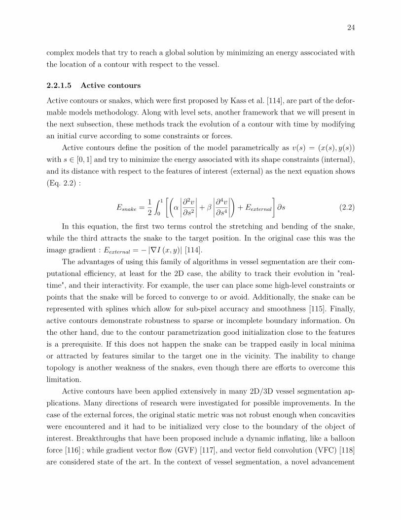
24

complex models that try to reach a global solution by minimizing an energy asscociated withthe location of a contour with respect to the vessel.

2.2.1.5 Active contours

Active contours or snakes, which were first proposed by Kass et al. [114], are part of the defor-mable models methodology. Along with level sets, another framework that we will present inthe next subsection, these methods track the evolution of a contour with time by modifyingan initial curve according to some constraints or forces.

Active contours define the position of the model parametrically as v(s) = (x(s), y(s))with s ∈ [0, 1] and try to minimize the energy associated with its shape constraints (internal),and its distance with respect to the features of interest (external) as the next equation shows(Eq. 2.2) :

Esnake = 12

∫ 1

0

[(α

∣∣∣∣∣∂2v

∂s2

∣∣∣∣∣+ β

∣∣∣∣∣∂4v

∂s4

∣∣∣∣∣)

+ Eexternal

]∂s (2.2)

In this equation, the first two terms control the stretching and bending of the snake,while the third attracts the snake to the target position. In the original case this was theimage gradient : Eexternal = − |∇I (x, y)| [114].

The advantages of using this family of algorithms in vessel segmentation are their com-putational efficiency, at least for the 2D case, the ability to track their evolution in "real-time", and their interactivity. For example, the user can place some high-level constraints orpoints that the snake will be forced to converge to or avoid. Additionally, the snake can berepresented with splines which allow for sub-pixel accuracy and smoothness [115]. Finally,active contours demonstrate robustness to sparse or incomplete boundary information. Onthe other hand, due to the contour parametrization good initialization close to the featuresis a prerequisite. If this does not happen the snake can be trapped easily in local minimaor attracted by features similar to the target one in the vicinity. The inability to changetopology is another weakness of the snakes, even though there are efforts to overcome thislimitation.

Active contours have been applied extensively in many 2D/3D vessel segmentation ap-plications. Many directions of research were investigated for possible improvements. In thecase of the external forces, the original static metric was not robust enough when concavitieswere encountered and it had to be initialized very close to the boundary of the object ofinterest. Breakthroughs that have been proposed include a dynamic inflating, like a balloonforce [116] ; while gradient vector flow (GVF) [117], and vector field convolution (VFC) [118]are considered state of the art. In the context of vessel segmentation, a novel advancement

25

is the eigen-snake proposed by R. Toledo et al. [119]. The external force, here, learns to re-cognise, by classification, the vessels features by filtering the image at multiple scales in thedirection of the principal eigenvector of the structural tensor.

Higher-order geometrical constraints are utilized in the ribbon snakes [120, 121]. It isassumed that elongated linear structures, like the vessels, consist of two parallel edges with avarying diameter. Thus, two parallel snakes can be fitted on the boundary of the lines. Simi-larly, Bashir Al-Diri et al. [122] utilized the ribbon snake approach for the segmentation, butto facilitate the initialization of the model they firstly identified the centerlines by tramlinefiltering.

Another drawback of the original active contour methodology is the inability to changeits topology, namely to split and merge during its evolution. This problem has been addressedby topology adaptive t-snakes [123] and more recently by the extended topological active nets[124]. Figure 2.14 shows an example of T-snakes applied on the retinal image. Multiple T-snakes are initialized across the vessels that merge to segment the vessels.

Active contours represent the deformable model explicitly on the image plane. A metho-dological extension is to represent the evolving model implicitly, as the interface between anhyper-surface and the image plane.

2.2.1.6 Level sets

Level sets, which were first proposed by S. Osher and J.A. Sethian [125], define the problemone dimension higher than the dimensionality of the data. Thus, for the 2D segmentationcase, it is assumed that the model is embedded in a 3-dimensional surface, usually initializedas a signed distance function. In this scheme, the model is defined as the zero level-set ofthe 3D function (z = 0). Formally, if Ψ : <2 → < is the level-set function, the segmentationcontour is given by the following equation :

C ={p ∈ <2|Ψ (p) = 0

}(2.3)

The evolution phase now concerns the motion of the hypersurface and not the 2D modelitself. In the original work [125, 126], the evolution of the surface over time t is the solutionto the next equation :

∂Ψ∂t

+ v ‖∇Ψ‖ = 0 (2.4)

where v is a velocity term normal to the contour direction that guarantees convergence. Theincorporation of different external forces can drive the level-set closer to the boundary ofthe object of interest. Figure 2.15 demonstrates the principle of hyper-surface evolution as afunction of time in level sets. The final contour is the intersection between the image plane

26

Figure 2.14 Example of T-snake vessel segmentation. Several active contours are initializedon the vessels that subsequently merge into a single contour as the algorithm iterates10.

and the specific instance of the hyper-surface at time t.The basic advantages of the level sets are that they do not suffer from the parametrization

issues of the snakes. Additionally, the topology can change very easily ; so the zero level-setcan break into more than one contours during its evolution to capture multiple objects. Onedrawback of the level-sets is their increased computational cost.

Figure 2.15 Example of the evolution of level sets. The first row shows the initialization ofthe curve (a) and hyper-surface (b) at t = 0, while the second row shows the evolution of thecurve (c) and its corresponding hyper-surface (d) at time t [127] ( c©[2002] IEEE).

Extension to the original framework is the implicit geometric active contour proposed byM. Malladi et al. [127]. An internal curvature-based force together with a ballon-like externalforce guides the level-set towards the object boundary. Other available external forces arethe mean curvature motion [128], and the gradient vector flow [129] applied on a geodesic

10. Reprinted from T. McInernry and D. Terzopoulos, T-snakes : Topology adaptive snakes, vol. 4, no. 2,Pages. 73-91, Copyright (2000), with permission from Elsevier [123]

27

active contour. In [130] a flux-based external force was constructed based on the Hessianvesselness measure. Similarly, Y. Zhao et al. [131] incorporated the vesselness into an infiniteperimeter active contour model in order to improve the propagation of the curve at the thinand elongated vessels. T. Chan and L. Vese [132], moreover, modified the external force todemonstrate no dependency on the image gradient but only on the regional information ;which is an extension to the original D. Mumford and J. Shah method [133]. Althoughthe method can be trapped into local minima, its multi-scale and noise robustness made itappealing for vessel segmentation applications [134]. A new method was proposed in [135] thataccelerates the minimization of the Mumford-Shah model. The new method was combinedwith Gabor wavelets to overcome the non-uniform illumination problem. In the context ofsmall vessel segmentation, Chan Vese model [136] is outperformed by a newer method, theSobolev active contours [137] (Fig 2.16). This can be accounted to the fact that Sobolev-basedmethod contains a length increasing term that is better suited for approximating elongatedstructures like the vessels. Other algorithms that utilize prior shape information include theone proposed in [138]. Here, the method allows fitting a ball measure during the level-setevolution, which can constrain the contour expansion to approximate the tubular shape,penalizing possible leakage phenomena. Furthermore, P. Yan and A.A. Kassim [139] wereinspired by the capillary force associated with thin tubes to propose a new model. In theiralgorithm, the small diameter of a tube can facilitate the level-set to evolve deeper into thevery narrow vessels.

Level sets, as well as the previous subcategories represent the most diverse group ofthe intensity-based approaches. The second major category of methods is the region-basedmethods which consists of tracking and minimum-cost techniques.

2.2.1.7 Tracking

One major drawback of the basic region growing method is that it does not constrain thegrowth of the region to a specific shape locally, which leads to leakage phenomena in lowcontrast areas. We can overcome this limitation by assuming that the region growing shouldinclude a shape constraint. Under that consideration, tracking is an iterative process, where avessel model is compared to a local image segment to get the vessel’s parameters of centerlineand width. This is followed by the prediction of the direction from the current position viaoptimization.

The advantages of tracking over other methods include the low computational burdensince the image is processed locally. Connectivity is also preserved because the method isbased on a region growing algorithm. Furthermore, the use of an explicit model can extractthe local information of centerline position and diameter. On the other hand, limitations

28

Figure 2.16 Example of the application of Sobolev active contour for vessel segmentation.The figures from left to right demonstrate how the initialized contour of the level set expandsto segment the vessels11.

of the method include the inadequacy to continue the tracking process when challengingareas are encountered. In our context, the challenging regions are those that demonstratereduction on the vessel/background contrast and diameter, bifurcations, vessel crossings, orencountered adjacent vessels.

Several numbers of vessel models descriptions exist in the literature. For example, itcan be assumed that the boundary of the vessels coincides with the ridges computed bythe gradient magnitude [140] or the Hessian matrix [141] in a preprocessing step. Templatematching is another option [142]. Finally, a cross-sectional model compared or fitted locally tothe corresponding perpendicular vessel profile has been proposed [143, 144] ; the model can besimilar to the searching pattern namely, a double Gaussian, or a more general ellipsoid cross-section [145]. Tubular tracking, as proposed in [144] that utilizes a generalized circular cross-section template for localizing the vessel, is considered more appropriate for our application.Since it is a general vessel representation, it can approximate not only medium to largescale vessels, but also small vessels that have a different, more circular cross-sectional profile.Independent of the considered application, other models or methods that have been proposedare the spheres [146] and the flexible super-ellipsoids [147].

The optimization step tries to find the possible location or direction of the vessel in thenext step. The correct prediction of the local direction can be achieved by looking in thedirection indicated in a previously tracking step. Then in the next iteration, the model isrecentered by employing different measures. Fuzzy C-mean clustering [148], Kalman filtering[149, 150], particle filtering [151, 152], and Bayesian-based tracking [153, Fig. 2.17] have beenemployed. Fuzzy C-mean clustering is an unsupervised classification approach. Kalman filte-ring identifies the possible direction by taking into account all the previous predictions in a

11. New possibilities with Sobolev active contours, International Journal of Computer Vision, vol. 84, no.2, pp. 113-129, G. Sundaramoorthi et al., With permission of Springer [137]

29

(a) (b)

Figure 2.17 Example of tracking. (a) tracking iterations along a straight vessel. (b) trackingresult on a high resolution fundus image12.

probabilistic way ; however, it is a single hypothesis method that does not take into accountalternative paths in low contrast or branching cases. An extension to the former metho-dology is the particle filtering, a multiple hypothesis approach, which employs a number ofparticles each one representing an alternative state. The net effect is to overcome the previouslimitations at the expense of increased computational cost, at least for three-dimensional pro-blems. Optimization based on maximizing the a posteriori criterion of Bayes theory in orderto identify the vessel edges has been also proposed. In a purely deterministic way, multiplehypothesis testing (MHT) [144], which has been applied only on 3D applications, finds thebest direction by testing all the available branching options up to a predefined depth in thesearching space. This allows the method to decide about the local vessel direction using in-formation from subsequent steps overcoming challenging areas. Another approach that hasbeen proposed, is the prediction based on the geometrical image moments, that was appliedto a CT angiography application [154].

Bifurcations are taken into account in the vessel modeling level, or dealt by seekingactively in a depth first search fashion ; namely, after a single branch has been detected thetracking process is reinitialized in the first identified candidate. Tracking has been combinedwith deformable models to augment the process [155, 156]. Automatic initialization, also, hasbeen achieved by employing a preprocessing step where probable vessel points are identifiedby applying filtering (vesselness [90, 157], simple Gaussian [158]), or by considering the endingpoints of pre-identified large vessels as the tracking seeds in hybrid schemes.

Region-based methods are further subdivided to algorithms according to the used datarepresentation. Tracking methods are directly applied on the image space while representing

12. Reprinted from J.Zhang et al., A retinal vessel boundary tracking method based on bayesian theoryand multi-scale line detection, vol. 38, no. 6, Pages. 517-525, Copyright (2014), with permission from Elsevier[153]

30

the images as graphs allow us to use minimum-cost techniques.

2.2.1.8 Minimum-cost path

In the semi-automatic case, given a starting and an ending point inside a vessel, we canutilize a minimum-cost approach to identify the centerline. Generally speaking, minimum-costmethods try to minimize a cost function associated with the path that connects two points.Representing the data as a weighted undirected graph with vertices as the image pixels andedge weights as the intensities can help in the direction of applying the shortest path methodproposed by Dijkstra [159]. Fast marching [160] is another numerical optimization scheme,related to the level set approach, which tries to find the shortest path by solving the Eikonalequation.

The method is robust against possible discontinuities or low contrast areas [161] ; howe-ver, the second point is required, and only a single centerline is defined between two pointsat a time. Another potential problem is that there are cases of local minima paths extractedby the algorithm that are shortcuts, especially in low contrast areas. This can be solved byselecting an appropriate cost, the cost aggregation rule, and a penalizing term for deviatingaway from the desired course. For example, in [162] the authors used the Hessian vesselnessinstead of the grayscale intensity to increase the probability of constraining the path intothe vessel. In [163] also, the authors penalized the great changes in the mean intensity le-vel around a neighborhood that might denote the jumping of the path to an adjacent closevessel (shortcut). Additionally, they penalised differently the diagonal from the vertical orhorizontal transitions. A curvature regularization term independent of the vessel length wasintroduced that deals with the problem of shortcuts in retinal images [164]. Lately, the com-bination of curvature penalization and a new metric defined on the orientation space wasproposed to deal with the same problem [165]. However, it has only been applied for closedcontour detection in natural images.

Furthermore, the extraction of a single centerline requires the exhaustive explorationof the searching space greatly increasing the computational time. Methods that have beenproposed to speed up the searching process includes, the bidirectional propagation [166],where the searching is initiated from both the source and the target point. Eventually, thesearch trees that begin from the two points meet in an image pixel, and the optimal pathis extracted. In another approach, a freezing scheme is introduced that acts as a stoppingcriterion for further searching branches with very high costs [167].

Minimum-cost path techniques’ aim is to extract centerlines ; however, we might be in-terested in extracting whole vessels. One way to overcome this problem is to incorporate anadditional dimension that corresponds to the vessel width. In [168], the authors modified

31

the fast marching algorithm to include the aforementioned characteristic, and applied it toseveral applications, including to images coming from ophthalmological data.

Finally, the algorithms require the user intervention ; however, recently an exploratoryapproach has been proposed to overcome the problem. R. Estrada et al. [169] developed analgorithm based on forest representation, which applies an iterative procedure until conver-gence is achieved and the whole retinal vessel network is segmented without user intervention.Lately, Da Chen et al. [170] used an anisotropic fast marching scheme applied on vessel key-points detected by vesselness to extract the full retinal vasculature from a single retinal image.Figure 2.18 gives an example.

Figure 2.18 Example of the application of anisotropic fast marching proposed by Da Chen etal. [170] for full retinal vessel segmentation ((c) D. Chen et al., 2016).

2.2.2 Machine learning algorithms

The algorithms based on machine learning techniques deal with the automatic determinationof the class of a pixel that is examined. In our case we usually have a two class problem :1) vessel and 2) non-vessel or background. The methods here are divided into two mainsubcategories : supervised and unsupervised. Lately, a third subcategory of methods startedto emerge that try to model the way the human visual perception system functions at afundamental or a more abstract level.

The learning process is performed after vessel descriptors are extracted. The descriptorsare based on feature extraction. For that, a set of N-dimensional image feature of each pixelis required. A large variety of feature descriptors has been proposed in the literature spanningfrom the existing segmentation to filtering methods.

2.2.2.1 Supervised

Supervised algorithms usually consist of two stages, the designing stage and the applicationphase. The sequence of actions is the following : A special classifier is firstly employed, and

32

then a rule for vessel detection is statistically learned by employing a characteristic labeledtraining set. Usually, the latter is a subset of the available data that acts as a validation set forthe classifier. Then, the trained classifier is applied to a new image, which belongs to the testset, in which case it categorises its pixels as vessels or non-vessels. The resulting categorizationcan be either hard, explicitly assigning the examined pixel in one of the available class orsoft where the examined pixel is assigned a probability belonging to a specific class.

There are some advantages and disadvantages related to this category of algorithms.Firstly, the performance of the algorithms depends on the careful tuning of its components.The existence of a ground truth or a manually labeled set, additionally, is prerequisite sinceit is used to train the classifiers. This set should be representative of the test set that will beused to evaluate the algorithm. For the smallest vessels, more particularly, the labeling canbe performed with little consensus on their exact position among experts leading to extrachallenges for the classifier. The selection of the features, additionally, should be appropriatefor the application and should give good discrimination power. Over-fitting can also be ob-served. Finally, the classifier should be robust enough to be able to handle the problem.Neovascularizations more particularly can demonstrate high variability on their shape andlocation ; these together with the fact that NVs are rare can make the construction of arepresentative training/feature set challenging. If the previous conditions are satisfied thensupervised, methods are usually better than other available approaches. Another advantageis that they can be perceived as a black box ; hence after the training/testing phase the usersimply inputs the image, without being concerned about tuning any parameters. The nextsection will present some examples where supervised algorithms were employed to segmentthe retinal vessel. The analysis will focus mostly on the analysis of the existence of differentcategories of classifiers.

Usually the methods are categorized according to the classifier that they utilize, so wecan have the following methods based on : 1) Artificial neural networks (ANNs) [171, 172,173, 174], 2) K-nearest classifiers (K-NNs) [175, 176], 3) Support vector machines (SVMs)[79, 177, 178, 83], 4) Statistical [179, 180, 181, 182], and 5) Ensemble techniques [183, 184,185].

Inspired by the basic biological processing unit, or the neuron, ANNs were proposed.An artifical neuron is a mathematical representation, as a function, of the transformationsthat occur on an input in a biological neuron. Based on the fundamental unit, ANNs wereproposed as an early effort to model the human visual perception system. The artificial systemis a layered network of interconnected nodes, where the input is transformed according to acharacteristic function and some adaptive weights. The input is the feature vector and theoutput is the decision about the input vector. The learning phase involves the adjustment of

33

the weight. ANNs is a non-linear classification method. D. Marín et al. [172], utilized ANNand a 7-D vector composed of gray-level and moment invariant-based features for vessel/non-vessel discrimination.

The general principle behind the second category, KNNs, is that the values in the featurespace are similar for pixels that belong to the same class and so in a sense, they are clusteredin a close distance. Thus, the goal is to find the decision boundary that separates the clusters[176]. In order to find this boundary, the training set is utilized. One special characteristicof this classifier is that it can produce soft classification, namely a probability for a pixel tobelong to a certain class.

Similarly, SVMs, try to find a boundary that separates the features. The goal of thisclassifier is to find an hyperplane in the N-dimensional feature space that maximizes thefunctional margin, namely the distance between the hyperplane and the closest point of anyclass. Then in the testing phase, every input feature vector will be assigned in a class withrespect to their position from the trained hyperplane function. There are different algorithmsthat have been proposed in the literature that use SVMs. For example, Ricci and R. Perfetti[79] proposed a scheme, where firstly a single-scale line detector is used to obtain the featuresand then SVM for pixel classification, the performance is very good in the public database.

Bayesian approaches are probabilistic methods. If we assume that y = (y (s))s∈S is theobserved image and y = (x (s))s∈S the groundtruth where x (s) denotes the true (unknown)segment or region which pixel s belongs to. The observed y (s) is interpreted as a realizationof a random variable whose parameter is a function of x (s). The probability distribution ofthe observed image y has a density f (y/x). This density describes the "forward problem"of image formation, including both the stochastic noise in observing y and the deterministicinfluence of x on y. Given a prior distribution π (x) of x, the posterior distribution of x giveny is

P

(x

y

)∝ f

(y

x

)π (x) (2.5)

and the segmentation x is usually estimated by choosing an estimator that maximises theposterior probability [179].

A recent new approach is to combine different classifier to increase the discriminationpower. This ensemble scheme is used to improve the classification by weighting the "opinion"of each individually employed classifier.

Additional supervised methods that have been proposed for segmenting vascular struc-tures are the reinforcement learning and the regression. Reinforcement learning algorithmstry to find the optimum solution by interacting with their environment. The concept of rewar-ding or punishment in the learning phase is introduced, where feedback is obtained through

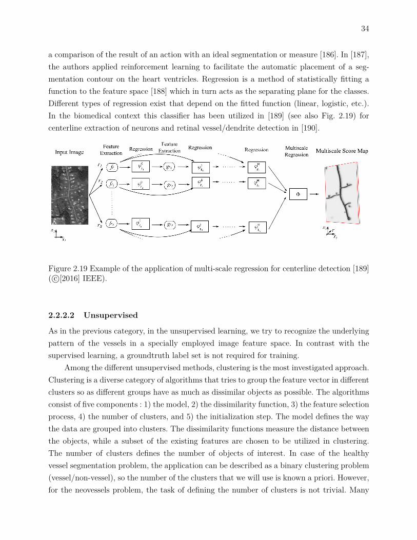
34

a comparison of the result of an action with an ideal segmentation or measure [186]. In [187],the authors applied reinforcement learning to facilitate the automatic placement of a seg-mentation contour on the heart ventricles. Regression is a method of statistically fitting afunction to the feature space [188] which in turn acts as the separating plane for the classes.Different types of regression exist that depend on the fitted function (linear, logistic, etc.).In the biomedical context this classifier has been utilized in [189] (see also Fig. 2.19) forcenterline extraction of neurons and retinal vessel/dendrite detection in [190].

Figure 2.19 Example of the application of multi-scale regression for centerline detection [189]( c©[2016] IEEE).

2.2.2.2 Unsupervised

As in the previous category, in the unsupervised learning, we try to recognize the underlyingpattern of the vessels in a specially employed image feature space. In contrast with thesupervised learning, a groundtruth label set is not required for training.

Among the different unsupervised methods, clustering is the most investigated approach.Clustering is a diverse category of algorithms that tries to group the feature vector in differentclusters so as different groups have as much as dissimilar objects as possible. The algorithmsconsist of five components : 1) the model, 2) the dissimilarity function, 3) the feature selectionprocess, 4) the number of clusters, and 5) the initialization step. The model defines the waythe data are grouped into clusters. The dissimilarity functions measure the distance betweenthe objects, while a subset of the existing features are chosen to be utilized in clustering.The number of clusters defines the number of objects of interest. In case of the healthyvessel segmentation problem, the application can be described as a binary clustering problem(vessel/non-vessel), so the number of the clusters that we will use is known a priori. However,for the neovessels problem, the task of defining the number of clusters is not trivial. Many

35

definitions of what cluster is, exist in the literature. Additionally, the use of different similarityfunctions gives rise to the total number of available algorithms [191, 192]. Initialization ofthe cluster centers in the feature space is also challenging in the small vessel segmentationproblem as the optimization step does not guarantee the convergence of the cluster centers tothe global minimum. To begin with, clustering can be distinguished into hard or soft/fuzzy.In the former case, the algorithm assigns the features as belonging to a single cluster ; whilein the later case a function is utilized to show the likelihood of membership of the featuresin all the available clusters.

The simplest clustering algorithm is the K-means which aims to group the features intothe clusters that are in the minimum distance. The process is iterative that includes theassignment step, where the features are assigned to the closest clusters, and the updatingstep where the clusters’ location is recomputed. Examples of the previous are the K-NN [176,193] and Fuzzy C-Means [194, 195]. Another approach is to assume that the features comefrom a Gaussian mixed distribution. In order to find the parameters of each distribution(mean, standard deviation, weight) expectation-maximization (EM) can be utilized [196].This technique has also been applied outside of the context of clustering [197]. Anothersubcategory of algorithms is the hierarchical clustering. Here, a dendrogram is constructedthat represents the grouping of the features in clusters and their corresponding similarityat every iteration. This method was applied in the following study [198] to find the bestthreshold in an image histogram, which was further utilized for vessel segmentation. Recently,evolutionary approaches were considered for clustering. The working principle is drawn frombiological evolution, and so the notation is the same (mutation, gene, generation, parents,daughters, selection, crossover, etc.). Genetic algorithms perform global searching, in contrastto other algorithms so they can overcome local minimums. In [199] GA and FCM werecombined in a hybrid scheme to segment the retinal vessels.

The unsupervised classification method equivalent to the ANNs is the self-organizingmaps or SOMs. This technique, which was first proposed by T. Kohonen [200], is based on theneurobiological principles of visual perception and how the biosignal is processed early in theneural-retina using competitive learning [201]. In this technique, neurons are interconnectedforming local clusters within the same layer. Later, in the training phase, the neurons competein a given stimulus, which is a random sample of the training set. The winner is determined bythe distance between the input and the output of the neurons modified by some preselectedweights. The activity of the winning neuron then is spread in a short distance mutuallyreinforcing the weights of the neighbor cells. After many training cycles, testing takes placewhere SOMs are applied to a new set of images. SOMs and clustering have been combinedto segment the retinal vessels in [202].

36

Insipired by the principles of human visual perception and relying on the ANNs newunsupervised learning methods have emerged. In parallel, there has been an effort to modeloriginal theories proposed by cognitive scientists about the visual perception into a commoncomputational framework .

2.2.2.3 Deep learning

Deep learning has emerged as an alternative to the ANNs method for image analysis tasksgiving very promising results [203]. Significant advances allowed deep learning to outperformtraditional ANNs as well as other supervised methods [204]. These include the use of a simplecharacteristic function to speed up the training phase. The non-handcraft feature extractionstep realized via convolving the input image with trainable kernels (CNN). Additionally,the introduction of deep architectures with many interconnected layers that are able torepresent complex compositional hierarchies of features, namely high order features thatrely on lower level features such as shapes constructed by lines. The use of max poolingand dropout to accelerate the training phase and increase the robustness to overfitting,respectively. Additionally, graphical processing units are used for the acceleration of trainingand testing.

However, deep architectures and more particularly CNNs require a lot of resources inorder to be effectively applied. The basic parameters that are learned during the trainingphase are the weights of the convolution kernels. Depending on the size of the kernels andthe depth of the architecture, the number of parameters that has to be learned is in the orderof hundreds of millions. This can place a computational strain to the task of finding the opti-mal values. Furthermore, initialization of the weights is very important. Lately, initializationof the convolution weights with specially designed filters [43] has been proposed that can ac-celerate the training phase by approximately 82% [205]. Furthermore, the number of trainingsamples play a crucial role in the effective training of a CNN. A large number of examples,together with their labels, should be provided in order for the network to construct the mostrepresentative features. In a recent work, for example, P. Liskowksi and K. Krawiec [206]trained their CNN (Fig. 2.20) on 400000 healthy vascular regions achieving high accuracy.However, this is inadequate in the neovascularization segmentation case. As it was showedthat the vascular proliferations are rare among the screened population. On top of that, theydemonstrate very high variability in their appearance, and pixel-level labeling by an expertis not provided.

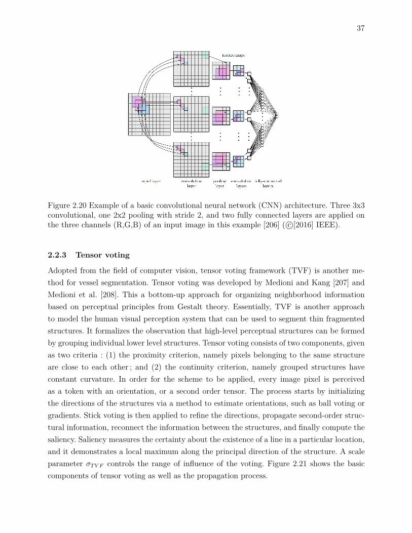
37

Figure 2.20 Example of a basic convolutional neural network (CNN) architecture. Three 3x3convolutional, one 2x2 pooling with stride 2, and two fully connected layers are applied onthe three channels (R,G,B) of an input image in this example [206] ( c©[2016] IEEE).

2.2.3 Tensor voting

Adopted from the field of computer vision, tensor voting framework (TVF) is another me-thod for vessel segmentation. Tensor voting was developed by Medioni and Kang [207] andMedioni et al. [208]. This a bottom-up approach for organizing neighborhood informationbased on perceptual principles from Gestalt theory. Essentially, TVF is another approachto model the human visual perception system that can be used to segment thin fragmentedstructures. It formalizes the observation that high-level perceptual structures can be formedby grouping individual lower level structures. Tensor voting consists of two components, givenas two criteria : (1) the proximity criterion, namely pixels belonging to the same structureare close to each other ; and (2) the continuity criterion, namely grouped structures haveconstant curvature. In order for the scheme to be applied, every image pixel is perceivedas a token with an orientation, or a second order tensor. The process starts by initializingthe directions of the structures via a method to estimate orientations, such as ball voting orgradients. Stick voting is then applied to refine the directions, propagate second-order struc-tural information, reconnect the information between the structures, and finally compute thesaliency. Saliency measures the certainty about the existence of a line in a particular location,and it demonstrates a local maximum along the principal direction of the structure. A scaleparameter σTV F controls the range of influence of the voting. Figure 2.21 shows the basiccomponents of tensor voting as well as the propagation process.

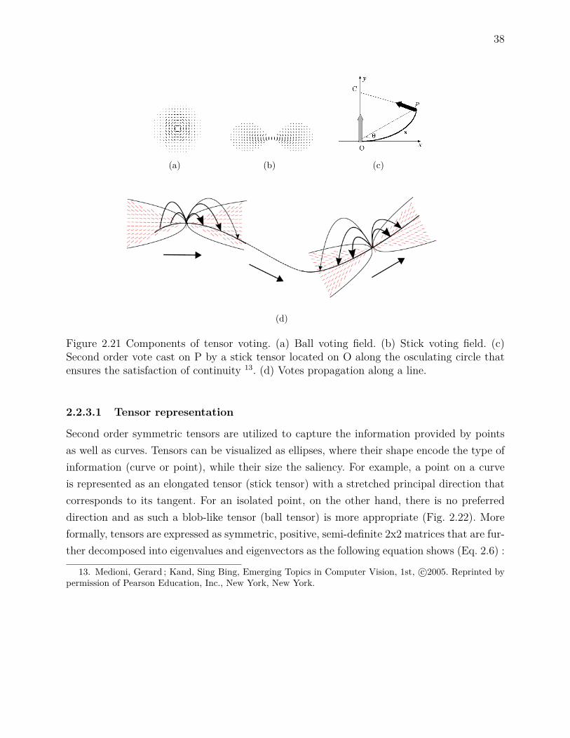
38

(a) (b) (c)

(d)

Figure 2.21 Components of tensor voting. (a) Ball voting field. (b) Stick voting field. (c)Second order vote cast on P by a stick tensor located on O along the osculating circle thatensures the satisfaction of continuity 13. (d) Votes propagation along a line.

2.2.3.1 Tensor representation

Second order symmetric tensors are utilized to capture the information provided by pointsas well as curves. Tensors can be visualized as ellipses, where their shape encode the type ofinformation (curve or point), while their size the saliency. For example, a point on a curveis represented as an elongated tensor (stick tensor) with a stretched principal direction thatcorresponds to its tangent. For an isolated point, on the other hand, there is no preferreddirection and as such a blob-like tensor (ball tensor) is more appropriate (Fig. 2.22). Moreformally, tensors are expressed as symmetric, positive, semi-definite 2x2 matrices that are fur-ther decomposed into eigenvalues and eigenvectors as the following equation shows (Eq. 2.6) :

13. Medioni, Gerard ; Kand, Sing Bing, Emerging Topics in Computer Vision, 1st, c©2005. Reprinted bypermission of Pearson Education, Inc., New York, New York.

39

T =axx axy

axy ayy

,= λ1e1eT1 + λ2e2eT2 ,

= (λ1 − λ2) e1eT1 + λ2(e1eT1 + e2eT2

),

(2.6)

where λ1 is the largest eigenvalue, λ2 the smallest eigenvalue, and ei the correspondingorthogonal eigenvectors. According to the previous, a point or ball tensor will have verysimilar eigenvalues λ1 ≈ λ2, while a curve or stick tensor a predominant direction with λ1 > λ2

(Fig. 2.22). Subsequently, every tensor can be defined as a function of three parametersT (β, s, b) (Eq. 2.7), namely the ballness/stickness plus the orientation. After the tensorrepresentation, sparse and dense voting is applied to determine the final saliency at everylocation.

T (β) = arccos(e1e

Tx

),

T (s) = λ1 − λ2,

T (b) = λ2

(2.7)

2.2.3.2 Voting process

As it is mentioned in the original work, a vote describes the estimation of the existence ofa geometric structure that passes from both the voter’s and the receiver’s location, and theassociated certainty of the estimation is expressed with the saliency. Since vector informationis propagated through voting, the estimated direction of the structure is also included. Thenthe "opinion" or votes of all the tensors are combined by adding the accumulated votes.There are two types of voting that are applied consecutively following the tensor encoding,sparse and dense voting. Sparse voting, involves the communication of votes between onlytensors, while dense voting the communication of information at every possible location orpixel adjacent to the examined tensor. To facilitate the previous, a vote generation functionis used.

Assuming an osculating circle 16 that passes from the voting token (O) to the receivingtoken (P) (Fig. 2.21(c)) the strength or magnitude of the vote depends on the arc length OPs, the curvature factor k, the degree of decay with curvature c, and the scale of voting σ :(Eq. 2.8) :

16. The osculating circle of a curve C at a given point O is the circle that has the same tangent as C atpoint O as well as the same curvature.

40

ShapeEigenvalues/vectors

of the shapesEllipsoid

Covariance matrixrepresentationof the ellipsoid

Point

λ1 = λ2 = 1

Ball

I =

[1 00 1

]

t

Curve

λ1 = 1, λ2 = 0e1 = t t

Stick[t2x tytxtxty t2y

]

Figure 2.22 Encoding of point and line structures as tensors15.

DF (s, κ, σ) = e−s2+ck2σ2 (2.8)

where c = −16log(0.1)×(σ−1)π2 , and σ is a modifiable scale parameter that controls the range of

influence of the tokens.A voting field centered and aligned with the principal direction of the voter can be used

to compute the orientation and magnitude of the vote in the neighborhood of the voter.Two possible voting fields can exist : 1) stick (Fig. 2.21(b)) and 2) ball (Fig. 2.21(a)). Voteinterpretation follows where at each pixel the sum of all votes is analyzed. This is performedby eigenvalue/vector decomposition of the accumulated votes in matrix T. Then, the saliency(T (s)) and the orientation uncertainty (T (b)) are returned by the eigenvalues of the finaltensor.

T =[e1 e2

] λ1 00 λ2

eT1eT2

(2.9)

The final algorithmic step is the extraction of a centerline, via non-maximal suppression,from the saliency map as the measure is locally maximum perpendicularly to the directionof the curve.

15. Reprint from G. Medioni et al., A computational framework for segmentation and grouping, Copyright(2000), with permission from Elsevier [208]

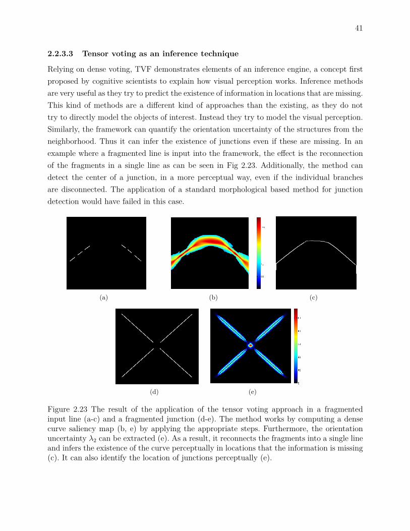
41

2.2.3.3 Tensor voting as an inference technique

Relying on dense voting, TVF demonstrates elements of an inference engine, a concept firstproposed by cognitive scientists to explain how visual perception works. Inference methodsare very useful as they try to predict the existence of information in locations that are missing.This kind of methods are a different kind of approaches than the existing, as they do nottry to directly model the objects of interest. Instead they try to model the visual perception.Similarly, the framework can quantify the orientation uncertainty of the structures from theneighborhood. Thus it can infer the existence of junctions even if these are missing. In anexample where a fragmented line is input into the framework, the effect is the reconnectionof the fragments in a single line as can be seen in Fig 2.23. Additionally, the method candetect the center of a junction, in a more perceptual way, even if the individual branchesare disconnected. The application of a standard morphological based method for junctiondetection would have failed in this case.

(a) (b) (c)

(d) (e)

Figure 2.23 The result of the application of the tensor voting approach in a fragmentedinput line (a-c) and a fragmented junction (d-e). The method works by computing a densecurve saliency map (b, e) by applying the appropriate steps. Furthermore, the orientationuncertainty λ2 can be extracted (e). As a result, it reconnects the fragments into a single lineand infers the existence of the curve perceptually in locations that the information is missing(c). It can also identify the location of junctions perceptually (e).

42

2.2.3.4 Tensor voting applications and specifications

The method is closely related to the structural tensors, however in the latter case the tensorsare constructed exclusively by using the image gradient information. The tensor voting fra-mework, on the other hand, is flexible and there is no restriction on the type of informationthat it could be considered as a tensor. Another difference is that here a tensorial voting fieldis applied instead of a scalar field. In the original framework, also, the method was proposedto be applied only in binary images. This is a constraint posed by the algorithm, howeverthis limitation can be overcome by assuming that the gray-scale responses are weights to thepixels as it was applied in [209]. Moreover, in contrast with other perceptual based approaches[210], it can work in open curves so it can directly be applied to vessel segmentation.

As it was explicitly mentioned in [211] there are many ways to generate the tensor fieldfrom the image : "The way to generate is application specific. As an example, a tensor fieldcould be obtained by creating features images of the orientation and stickness by applying anytype of orientation-sensitive filter with 180 degrees symmetry on the image data and taking theorientation with the maximum filter response. The ballness could be obtained by any isotropicfilter on the image data". Indeed, in the following paper [209], where tensor voting is appliedfor retinal vessel segmentation (centerline detection), image gradients are used to encode thedirection information [209, Eq. 7]. Furthermore, in another study [212] the Hessian matrix isapplied to obtain the tensor.

Finally, the approach is time consuming, having an asymptotic computational complexityof O (s2k2) that depends on the image (s) and the voting kernel (k) size. The authors in [211],implemented a method based on steerable filters and managed to drop the complexity to alogarithmic scale O (s2logs).

This method has been successfully applied to a range of biomedical imaging applica-tions [213, 214, 215, 216, 217]. These include filling microvascular discontinuities [213] basedon interpolating the width between reconnected segments, and detecting important cellularstructures [214] by iterating a TVF along a range of scales. A variety of algorithmic impro-vements to the basic framework was proposed in the literature that were comprehensivelyreviewed by Maggiori et al. [217]. In the same context, R. Duits et al. [218] proposed a moregeneralized definition of the tensor voting as part of a formalized set theory, namely the Liegroup using variational methods, where exponential curves fit in another parametric space,the roto-translational group SE (d). In the d = 2 case, the osculating circles that define thetensor voting field are used for fitting in the new parametric space. The method was recentlyadopted in a hybrid scheme for retinal vessel segmentation [113].

In retinal imaging applications, single scale TVF has been applied to either extractfull vessels [219] or segment centerlines [209]. No particular care was given to the problem

43

of full small vessel segmentation in either of these studies. The work in Park et al. [219]focused on identifying the optic disc as the converging point of the largest vessels and used adirect thresholding of the saliency map. In this manner, disconnected curvilinear structuresbelonging to lesions or irrelevant structures can get high saliency values, so thresholding islikely to remove small vessels without suppressing the false positives. The authors in Leng etal. [209] extracted the centerlines based on steerable tensor voting [211]. Rather than applyingthe framework for extracting the saliency of the structures globally, they used the method tolink pre-identified edges. Moreover, in a preliminary phase, edge points were discarded basedon the global length criterion. But the setting of a non-adaptive global length parameter isnot effective for retaining the smallest vessels and causes a translation in the final centerlinelocation.

2.3 Neovascularization segmentation and characterization

A recently identified problem is the precise segmentation and characterization of neovascula-rizations. As far as fundus imaging is concerned, some of the efforts have been placed towardsthe localization of the neovascularization within the the optic disc only (NVDs) [220, 221,222, 223], while lately some of the studies shifted towards both NVE and NVD cases [56,224, 225, 226, 227, 228, 229, 230, 231, 232, 233]. NVDs are well contrasted against the back-ground owing to the fact that the optic disc is the brightest retinal structure. Moreover, theseverity of the proliferative diabetic retinopathy can be directly determined by the locationof the new vessels. Pathophysiologically speaking, neovascularizations first grow in locationsaway from the optic disk and then elsewhere. On the later stages, NVDs are classified asmore severe since there is a higher impact in the retinal detachment following haemorrhages.Nevertheless, it is preferred to detect neovascularization early rather than in late stages atmore critical locations. A patient with PDR requires immediate medical intervention, andhence we have to focus detecting the NVs in all possible locations.

2.3.1 Neovascularization segmentation

Some authors relied on pre-existing algorithms such as matched filtering to segment thevessels, while others further improved the segmentation process via pre-processing and en-hancement before incorporating the characterization step. As we will show, some methodsdo not require the segmentation to initiate the neovascularization detection process.

Preprocessing and vessel enhancement of the retinal images was proposed as a mean ofmitigating the effect of artifacts during the acquisition process and the influence of otherstructures or pathologies. The latter is reasonable because at the PDR stage several brightor dark lesions can coexist. For the preprocessing the operations that are utilized involve :

44

median filtering [226, 229], adaptive histogram equalization [226, 233], contrast enhancement[225, 229, 230], morphology [229], and wavelets [229, 230]. For the vessel enhancement stepwavelets [227, 228], matched filtering [56, 225], Gabor filtering [231], vesselness based onHessian [231], multi-scale line detection [230], morphology [225, 226], and non-linear diffusion[231] has been proposed.

Subsequently, segmentation on the preprocessed or vessel enhanced image is performed.To begin with, fuzzy clustering was proposed in [226]. Moreover, a heuristic approach wasutilized in two studies [227, 228] that segments the image by applying multi-layered thre-sholding. Zhang et al. [56], also, designed a method based on matched filtering that cansegment neovascularizations, by effectively suppressing false positives edges that originatefrom non-linear structures. However, they did not extend their research towards the vesselscharacterization. Welikala et al. [230] applied the same principles on MSLD [80] as well asthresholding [230], while Gupta et al. [231] isolated the thin vessels by thresholding the com-bination of different vesselness features. Finally, morphology [229] coupled with Gaussianmatched filtering [225] was utilized in order to identify the vessels. Figure 2.24 shows anexample of NV segmentation on the disc and elsewhere.

One problem with the existing studies is that the segmentation performance is not clearlyreported. Besides the work of three research groups [56, 227, 228, 230] the methods do notprovide clear evidence about the segmentation in the normal as well as abnormal cases. Apartfrom some limited cases, this can be accounted for the fact that manual neovascularizationsegmentation is not provided in the available databases. Subsequently, the characterizationstep is confined at the region level. Furthermore, the amount of available images with NVs islimited therefore very high success rate is reported, especially from the supervised approaches.

2.3.2 Neovascularization characterization

The next step is the characterization of the identified vessels [224, 225, 226, 227, 228, 229,230, 231, 232, 233]. The majority of the previous work is based on the application of machinelearning techniques, and more specifically supervised, to characterize the healthy from theabnormal small vessels based on some extracted features. These include grayscale as well asbinary measurements on individual vessels’ appearance, morphometry, geometry, and texture.In this work, we categorized the features (Figure 2.25) according to the measured quantity,as well as the study that they were introduced and applied.

The available features are either extracted from the grayscale region or based on measu-rements on the segmented vessels. The main advantage of the grayscale based features is thatthey do not rely on pre-segmenting the vessels, mitigating the impact of possible over-undersegmentation performance on subsequent steps. Furthermore, second-order information is ta-

45

(a) (b)

Figure 2.24 Examples of segmentations of neovascularizations on the disk and elsewhere(NVE/D) using a) [228]17 and b) [230]18 methods. (a) The neovascularizations on the leftmostcolumn are compared with a groundtruth segmentation and colored according to the classthat they belong. Green vessels are the true positives ; red are the false positives ; while bluecorrespond to the false negatives. The central column illustrates how the system annotatesthe abnormal vessels on the retina. (b) neovascularizations segmentation using MSLD.

ken into account, when for example textures are used. However, the appearance or geometryof the vessels such as the tortuosity or orientation cannot be directly extracted from thegrayscale region.

On the other hand, features extracted from binarized regions are straightforward tocompute. Furthermore, they are based on quantities that have a more natural meaning.The last point is very important because it is easier to interpret the results. For example,it has been assumed that vascularization is denser at the proliferative stage [225], or thatvessels grow in random directions at that stage [220, 230], we can easily study the previousassumptions using binary based features. However, in that family of features, the performancedepends on the quality of the segmentation. Additionally, the existing work is limited to first-order statistics, such as counting the total number of junctions, and their density in an image,or the region. Therefore, the relative spatial arrangement of the segmented vessels is not takeninto account.

17. Reprint from M. Usman Akram et al., Detection of neovascularization in retinal images using multi-variate m-Mediods based classifier, Copyright (2013), with permission from Elsevier [228]

18. Reprint from R. Welikala et al., Genetic algorithm based feature selection combined with dual classi-fication for the automated detection of proliferative diabetic retinopathy, Copyright (2015), with permissionfrom Elsevier [230]

46

In another direction, a new classifier, the m-Mediods, was proposed by M.U. Akram etal. [228]. Without relying on specialized features, as the previous studies did, it achieves thehighest performance against traditionally exploited classifiers (SVMs, kNNs, and GMMs).An example of the application of the algorithm can be seen in figure 2.24.

Feature

Grayscale

Texture

GLCM [229,231, 232, 233]RLM [229, 233]LBP [231, 232]

AM-FM [224, 231, 232]Color correl-ogram [231]

Spectrum anal-ysis [229, 231]

Filtering

Gabor [231, 232]Contourlet [232]Vesselness [231]Non-linear dif-fusion [231]Fourier frac-tal dim. [229]

Gradient

µV [226, 227, 228, 230]σV [226, 227, 228]

σA [230]µV/CVV (wall) [230]

CVV [230]

Statistical

µV [226, 227, 228, 230]µA [230]

maxA, σA [230]CVV [226, 227, 230]∑

I2V [227, 228]MSLDV [230]Moments

[226, 227, 231]

Binary

Geometry

Connectivity [230]Compacteness [230]Width [228, 230]Length [230]

Direction [229, 230]

Statistical

∑V [225, 228, 230]ρV [230],

ρV (segments) [228]∑V (segments)

[225, 228, 230]∑J [230]

Morphometry

Vessel tortuositsy[226, 230, 231]

Fractal dim. [229]

Figure 2.25 Categorization of available features for vessel characterization. In the differentmeasures subscripts V and A denote the extraction of information at the vessel pixels or atthe whole area, respectively.

Unsupervised algorithms were utilized to a limited degree in the context of NVs charac-terization. S.S.A. Hassan et al. [225] tackled the problem by applying simple morphologicalrules in a local window area on the pre-segmented image. The method is not automatic.Instead of detecting the abnormalities on the vessels’ location the algorithm works on a localwindow ; while the parameters for the rules are empirically set. There are also false positivesfrom other lesions (bright, dark) that are not suppressed during the segmentation processand they might contribute toward false positives.

Finally, in [229] an unsupervised statistical learning method is applied for the characteri-zation of the vessels. The following features were selected : 1) statistical textures (GLCM andrun-length matrix) ; 2) higher order spectra (HOS) analysis ; and 3) fractal analysis. Fractalshave been extensively used for neovascularization characterization in diabetic retinopathy.Those features were extracted from the binary as well as directly from the grayscale image.

47

2.4 Retinal vessel segmentation metrics

Generally speaking, the lack of a segmentation algorithm that could perform equally goodin all sorts of scenarios had raised the need of effectively evaluating the segmentation per-formance. For this reason, different evaluation metrics has been developed that assess andrank the performance of different algorithms applied to the same problem, namely the vesselsegmentation.

Various schemes that classify the segmentation metrics in a range of categories has beenproposed in the literature. According to Y.J. Zhang et al. [234], the segmentation evaluationmethods can be divided into four categories : 1) the analytical methods, 2) the empiricalgoodness, 3) the empirical discrepancy and 4) the perceptual metrics. In another study [235],the empirical methods are further separated into standalone and relative methods. Finally,perceptual metrics were analyzed in [236].

Quantitative evaluation of empirical approaches is much elaborated and can extract anobjective metric about the applied segmentation algorithm. The decision is made independentof the human factor and based only on the relative comparison with a reference manualsegmentation, in the empirical discrepancy case. Alternatively, the a priori knowledge abouta good segmentation can be utilized to infer about the performance, as it is applied in theempirical goodness case.

First, we will analyze the discrepancy measures that are commonly utilized for theperformance evaluation of the retinal vessels segmentation algorithms. After that, we willcontinue with a new category of measures, the perceptual measures.

2.4.1 Discrepancy measures

A very well documented family of measures is based on the discrepancy metrics that count thenumber of miss-segmented pixels between the estimated and groundtruth segmentation. Theconfusion matrix (Table 2.1) as well as the derived measures (see Eq. 2.10, 2.11, 2.12) [237]are considered as very reliable for assessing the segmentation performance on the healthyand diseased retinal vessels. Usually, a percentage is computed for all three metrics for eachselected image. Higher values are preferred. For example, 100% sensitivity demonstrates thatthe algorithm can perfectly recognize as vessels pixels that are truly vessels pixels from thereference image. Specificity, moreover, works on the non-vessels class, while accuracy reportsabout both categories.

Sensitivity = number of True Positivesnumber of True Positives + number of False Negatives (2.10)

48

Specificity = number of True Negativesnumber of True Negatives + number of False Positivies (2.11)

Accuracy = number of True Positives + number of True Negativesnumber of Positives + number of Negatives (2.12)

Table 2.1 Confusion matrix together with the standard discrepancy metrics

Groundtruth

Estimated(Algorithm)

Vessel No vessel

Vessel TruePositive

FalsePositve

No vessel FalseNegative

TrueNegative

↓Sensitivity

↓Specificity

Despite their extensive use, as the next studies show [108, 79, 151, 122, 229], there areseveral disadvantages related to these metrics that we will analyze. First and foremost, thediscrepancy methods require a manual segmentation from an expert in order to work. Thisis very tedious work and sometimes the result is subjective ; general public repositories ofretinal images were introduced to the community to address the problem.

Examples of these databases are the DRIVE, STARE, MESSIDOR, DIARETDB andmore recently HRF. Some of the databases include one or more manual segmentation from anexpert of the vascular tree, while others only the diagnosis about the examined image. Thesegmentation algorithms, depending on the popularity of the database, can be tested across arange of methodologies. Sometimes around 20 different algorithms can be assessed at the sametime, and get a comprehensive opinion about their performance. However, these databases aregeneral, and apart from some cases, they do not include delineations of abnormal vessels suchas neovascularizations ; thus in occurrences of a special problem either an ophthalmologisthas to spend some of his valuable time to segment the regions or validate a segmentationproduced by trained staff.

Furthermore, these metrics work on a pixel-by-pixel basis comparing corresponding pixelsbetween the estimated and the manual segmentation. This is a particularly undesirable fea-ture since the measures cannot account for slight variations on vessel detections. Especiallyfor the smallest vessels, the centerline, the bifurcations, and the vessels’ boundary the pro-bability of locating the positives away from their true location is very high reducing the

49

performance rates. Some efforts have been placed in the direction of penalizing the distancebetween the detected and true vessels [238], while more recently a measure has been propo-sed that among other things tolerates for possible deviations by morphologically dilating thesegmentation result [239].

Additionally, as has already been pointed out by M.Niemeijer et al. [175] the globalbinary classification metrics do not take into account the heterogeneity of the pixel populationof segments of the vasculature with a different diameter. In fact, the smallest vessels representapproximately 10% of the total surface area of the vessel network, while the whole vasculaturecovers 10% of the available field of view. Applying the aforementioned metrics give highsuccess rates even when the narrow vessels are missed. Finally, they do not correlate wellwith the human perception of a good segmentation.

2.4.2 Perceptual metrics

The ultimate goal of the metrics is to objectively simulate the evaluation that a humanobserver or expert would perform if he was asked to assess the quality of segmentation on animage [235]. To achieve this, one proposed way is to incorporate the information about howdifferent errors in the segmentation are perceived by the human. Since different kinds of errorsare not visually equally important, up to some degree, weighting according to the humanperception can be applied to facilitate the process. This can be achieved by incorporatingsubjective experiments [240]. The subjective evaluation offers a way to study and characterizethe different categories of artifacts that can exist and weight according to the human or amore expert opinion. Then perceptually driven objective metrics can be derived by findingthe mathematical relation or psychometric function [236], between the perceptual as well as apredefined objective metric. Alternatively, discrepancy metrics can be statistically correlateddirectly with the subjective quality evaluation results to indicate their degree of similarity[239].

Perceptual metrics offer a better way to evaluate the segmentation methods than simplediscrepancy measures. They produce results that are consistent with the human opinionabout a good segmentation as the next studies have shown [240, 239]. Additionally, theycan effectively model complex artifacts that under discrepancy measures are difficult to deal.For example, the "annoyance" of false positive ranges perceptually with its location, size,shape and so weighting should be applied that depends on these factors. Moreover, artifactscan be perceived differently according to the context or their importance. Finally, subjectiveexperiments allow the perceptual metric to be tailored for a specific application, for example,the identification of the small healthy or unhealthy retinal vessels.

Several studies have been published for the subjective evaluation step for images [239,

50

241, 242] and video applications [240, 243, 244]. Besides the next study [236], where a com-prehensive designing scheme is presented, the task is informal, and there is no standardizedway to study and characterize the impact of different kind of artifacts. Moreover, it requiresmuch-elaborated designing from the researcher side and the experiments are not easily repli-cable. Usually, non-expert subjects participate in the study under conditions that are fixedby the researcher. Some of the studies [235, 245] have utilized empirical weighting for theartifact which is not adequate to characterize the metric as perceptual. Finally, like other dis-crepancy methods, they still require a groundtruth in order to be able to apply the objectivemetric not only in the designing but also in the application phase. In a different direction,when there is a lack of a single representative reference this can be estimated by comparingseveral manual segmentations on the same data using various techniques [246] amongst ofwhich STAPLES is the most popular [247].

As far as the retinal vessels are concerned, in [239] individual metrics that characte-rize important vasculature features were utilized to build a new metric. Then the authorscombined the individual quantities with subjective experiments and statistically concluded[248] that their approach correlates better than other examined discrepancy metrics with thehuman perception. However, in their study, the authors did not examine the performance ondiseased retinas. Additionally, they assumed equal weights for all the individual metrics wi-thout first considering the effect that each quantity measured by the individual metric has onthe human perception. Finally, even though the proposed metric can tolerate for deviationsin the detection of the vessel pixels by including morphological dilation and erosion, this isdone at the expense of invariance on the diameter detection.

2.5 General discussion on the limits of the existing methods

The preceding sections presented the state-of-the-art of algorithms for the segmentation ofthe retinal vessels, and the characterization of neovascularizations. This section will discussthe limitations of the existing methods for our problem.

2.5.1 Vessel segmentation methods

The current literature is limited to the problem of segmenting the medium-to-large retinalvessels. The authors of the existing work were mainly focused on the scope of demonstratingthat the various proposed methods were sufficient to tackle the problem of global retinalvessel segmentation using standard discrepancy measures. The different methods were eva-luated on the segmentation task using all the available vessels calibers which are not suitableas fundus images contain predominantly medium-to-large vessels. Subsequently, algorithmicimprovements of the methods against already existing one were carried out with respect to

51

the problem of general retinal vessel segmentation. One reason might be that CAD systemsalong with the automatization of screening were not prevalent enough to justify the invest-ment of resources into the problem of small retinal vessels segmentation. Furthermore, smallvessels demonstrate challenges that make it a difficult problem to be addressed. As new deve-lopments require comprehensive CAD systems with several steps that could be able to assistand detect all the possible stages of the sight-threatening diabetic retinopathy, small vesselsimportance is becoming more relevant.

The existing methods are limited by challenges posed by the small vessels. Machinelearning techniques require the existence of an already established model, in the form of adescriptor, to be effectively applied. The work is done on a highly abstract level where oneor multiple algorithms can be combined forming a feature vector. Additionally, training on alabeled set containing the small vessels is a prerequisite. This set is difficult to be isolated fromexisting databases, or extracted by an expert. Additionally, unsupervised methods require thecorrect initialization of a predefined number of clusters to avoid the trapping of the clustercenter into a local minimum, or the assignment of pixels coming from irrelevant structuresinto the wrong class.

In the intensity-based approaches, on the other hand, the work is done on a more fun-damental level. Here, a model should be constructed that based on some assumptions itwill approximate the problem. Scientifically speaking, this kind of approaches are more ap-propriate since new knowledge can be acquired that can improve our understanding of thegeneral nature of the problem. Subsequently, if the model is adequate, it can be incorporatedin a descriptor as part of a machine learning approach.

However, the construction of a model is not a trivial issue, and this can be the subjectof our work. For the model to be sufficiently robust, assumptions must be formulated thatwill hold under different cases. As has been seen in the previous review, a variety of methodshave been presented but their assumptions are weak for the small vessels. Template-basedmethods, for example, assume a very general representation that is not flexible enough toaccommodate the curvature variability in the small vessels, resulting in the fragmentationof the result. Furthermore, derivatives are usually approximated using Gaussians, so there iscertainly filtering of important information. This causes the derivative-based method not tobe sensitive enough to the presence of small vessels at low contrasted areas, magnifying oreven reconnecting the background noise to the vessel. Moreover, deformable models have tobe initialized close to the fade boundary of the small vessels, and even if level-sets are usedtheir external forces are not sensitive enough to get attracted to the full extent of the retinalvessels. The areas around the small vessels demonstrate increased intensity inhomogeneity,background noise, lower contrast, and at the same time, the appearance of the vessels is

52

thin, variable, and curved. Region-based methods are either semi-automatic, or they are notable to merge small vessels into a single region with the medium-to-large vessels as they canstop their evolution at the first encountered difficulty. In addition to the previous challenges,the contrast of the fine vessels against the background is so low that essentially the smallvessels can appear as disconnected. Eventually, tracking can stop at the first fragmentation.Finally, the application of tensor voting in retinal field is limited as it was only used forretinal centerline detection. It does not produce a fully reconstructed vasculature, and it wasapplied on a single scale only, namely it considers a particular distance between structuresfor perceptual reconnection. Therefore, to tackle the problem of small vessel segmentationwe have to propose a new method.

2.5.2 Neovascularization segmentation and characterization methods

Limited work has been done on the domain of effective segmentation and characterizationof neovascularizations. This can be attributed to the fact that this kind of dark lesion israre among the total screening population. Epidemiologically speaking, during the precedingyears with the increased awareness about the impact of diabetic retinopathy, the prevalence ofPDR has been reduced. Additionally, accurate segmentation and characterization of the NVsare not trivial, so the efforts are limited only to the healthy blood vessels. Nevertheless, theirdetection is crucial, because it is the predominant sign of proliferative diabetic retinopathy,and possible missing can immediately lead to visual impairment.

Intensity-based methods, as well as machine learning, coupled with preprocessing, havebeen proposed to isolate the neovascularizations. These methods include template, derivative,as well as unsupervised methods. The aim is to detect as many abnormal vessels as possibleand then perform characterization, at the region level, in order to identify case with abnormalvessels. However, this is achieved at the expense of missing vascular junctions that are noteasily recoverable.

Features that measure first or second order characteristics are computed directly fromthe grayscale version of the selected regions, while only first order information are computedfrom the binarized version of the selected region. Second order information can be extractedfrom the grayscale regions via textures. However, the extracted quantities are not easily in-terpreteable and require several steps of further processing. At the same time, the currentmethods cannot extract second order information from the segmented vessels of the regions asit is not trivial to incorporate the distance information between the vessels, without first de-fining a relevant anatomical landmark. Thus, for the binary case, only first order informationis currently used.

Many methods depend on the number of available data, especially the supervised me-

53

thods. Another problem is the shortage of images with neovascularizations on the availabledatasets. For example, the authors in [220] covering approximately 30.000 people with dia-betes managed only to obtain and examine 38 cases of PDR, while the freely available data-bases, combined, do not offer more than that. Table 2.2 illustrates the number of neovascu-lariazation cases per database across the various studies. As a result, the algorithms are notrigorously tested or trained in many examples. Consequently, in the testing phase, in caseof a new previously difficult unencountered configuration, the algorithm might produce anerror. Our aim is to apply our system for screening in a range of populations, which meansthat the algorithm should be tested in a wide range of images. In this direction, the lackof data was tried to be addressed in the literature by developing algorithms for computersimulated neovascularizations on the retina based on fractal modeling [249].

Table 2.2 Cases of images with neovascularizations in different studies

Type of Study Num. of Type of Study Num. ofPDR images/total PDR images/total

NVD only : [56] 4/35 NVD & NVE : [224] 20 (regions)/120[220] 38/109 [225] 11/313[221] 27/57 [226] 20/50[222] 9/23 [227] 1097(segments)[223] 100/300 [228] 52/1440

[229] 27/110[230] 20/60[231] 100/779[232] 31/43[233] 50/180

2.6 Thesis objectives

An important tool that can facilitate the computerized detection of diabetic retinopathy is thesegmentation of retinal vessels. Segmentation algorithms can highlight the most importantretinal structures like the healthy vessels, or help the physicians to quickly identify abnormalfeatures that are related to the disease. Due to the nature of the images, these algorithms needto perform under challenging conditions. Small vessels appear in the center or the peripheryof the image varying in appearance with complex shape configurations and fade boundaries.Also, the disease may alter the appearance of the vessels or lead to the growth of lesions that

54

Table 2.3 Images with PDR per database [228]

Database No. of Images Normal With PDR NVD NVE

DRIVE [175] 40 19 3 0 3STARE [45] 81 30 5 3 4DIARETDB [250] 89 5 7 3 5MESSIDOR [251] 1200 397 37 27 18HRF [63] 45 30 7 - -

are similar to the small vasculature. In such cases, robust segmentation and subsequentlycharacterization become essential.

As it was presented in this chapter, several algorithms have been proposed to isolatethe vasculature. However, they are incapable of correctly identifying the smallest vessels, orthey are not tested in datasets containing the smallest vessels exclusively. Therefore, the firstobjective of the thesis is the vessel segmentation.

Given the small retinal vessel segmentation, the next step is the identification of thepathological regions that might directly indicate the presence of proliferative diabetic retino-pathy. Characterization of the regions to healthy or abnormal is the first step in the detectionprocess. Several supervised approaches have been proposed to characterize regions to healthyor abnormal. However, they use a standard set of features based on the various measurementon the already segmented vasculature. Therefore, the second objective of the thesis is thevessel characterization.

This thesis will try to address the previous two objectives by proposing new methodsfor the segmentation of the smallest retinal vessels as well as the characterization of regionsto healthy or abnormal. Achieving the previous would help in the direction of constructingCAD systems that could be used for the early detection of sight-threatening diabetic reti-nopathy. For both tasks, we propose methods that examine how the retinal structures areperceptually or spatially organized using the neighborhood information. To assess the seg-mentation performance on the smallest vessels, we will separate the vasculature in differentcategories according to their caliber. Then we will apply standard discrepancy measures. Thenext section will analyze the proposed methodology that was used to achieve the objectives.

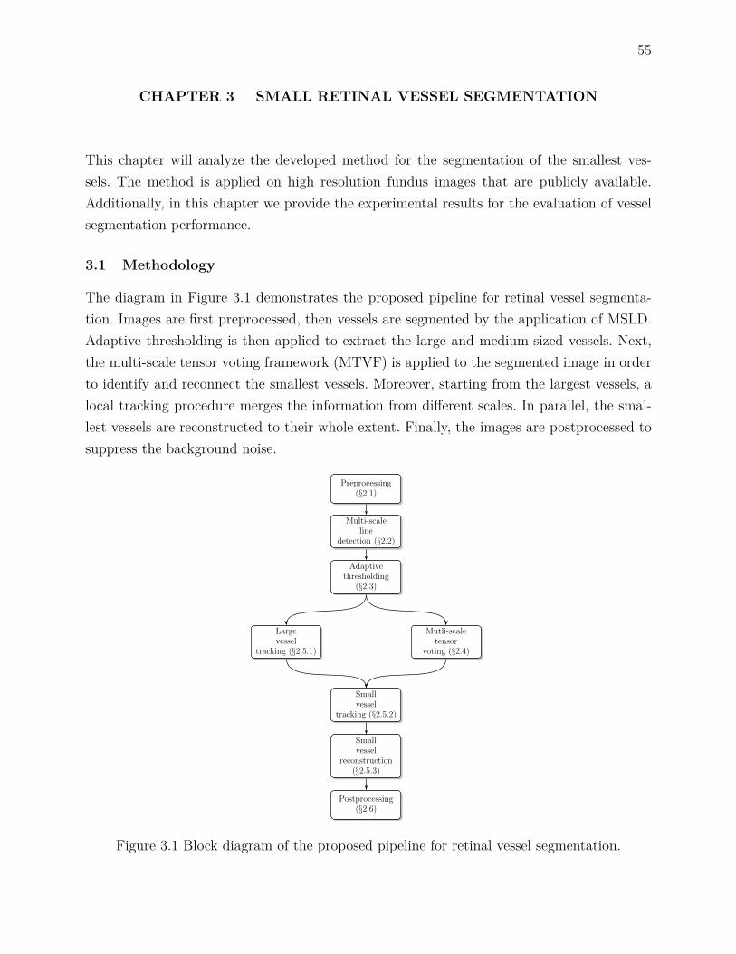
55

CHAPTER 3 SMALL RETINAL VESSEL SEGMENTATION

This chapter will analyze the developed method for the segmentation of the smallest ves-sels. The method is applied on high resolution fundus images that are publicly available.Additionally, in this chapter we provide the experimental results for the evaluation of vesselsegmentation performance.

3.1 Methodology

The diagram in Figure 3.1 demonstrates the proposed pipeline for retinal vessel segmenta-tion. Images are first preprocessed, then vessels are segmented by the application of MSLD.Adaptive thresholding is then applied to extract the large and medium-sized vessels. Next,the multi-scale tensor voting framework (MTVF) is applied to the segmented image in orderto identify and reconnect the smallest vessels. Moreover, starting from the largest vessels, alocal tracking procedure merges the information from different scales. In parallel, the smal-lest vessels are reconstructed to their whole extent. Finally, the images are postprocessed tosuppress the background noise.

Preprocessing(§2.1)

Multi-scaleline

detection (§2.2)

Adaptivethresholding

(§2.3)

Largevessel

tracking (§2.5.1)

Mutli-scaletensor

voting (§2.4)

Smallvessel

tracking (§2.5.2)

Smallvessel

reconstruction(§2.5.3)

Postprocessing(§2.6)

Figure 3.1 Block diagram of the proposed pipeline for retinal vessel segmentation.

56

3.1.1 Preprocessing

The retinal images are preprocessed to correct for non-uniform lighting, to normalize theimage contrast, and to suppress the background noise. Even though the full color rangeis used by a human observer to recognize the vessels, simultaneously processing the threeimage channels require significant computational resources. Instead, we use a single channelfor preprocessing. The green channel of the input image Igreen is used as it provides thehighest contrast between the vessels and the background.

Several approaches have been proposed for contrast enhancement and illumination cor-rection, however each one focuses on a specific task. Locally adaptive contrast ehnancementis a standard method achieving good results, but illumination variations are not corrected.Conversely, illumination correction methods like high-pass filtering, large sized median filte-ring, or mathematical approximation do not improve the contrast. M. Foracchia et al. haveachieved simultaneous local illumination and contrast correction [252]. This method was spe-cifically designed for retinal images. In our work, the method is applied on the images to getIenhanced.

Moreover, the dual-tree complex wavelet transform (DT-CWT) [253] is applied to Ienhancedin order to filter out the background noise. The applied DT-CWT, which is an extension of thediscrete wavelet transform (DWT), is widely used in retinal images. The applied method ismulti-scale, it approximates shift-invariance, and it increases the directional sensitivity of thediscrete wavelets. Although other wavelet families (Gabor, ridgelets, curvelets, or contourlets)are more directionally sensitive and thus more tailored for vessel enhancement than back-ground noise suppression, they are more computationally expensive. Since the focus of ourwork was to filter out the background impulse noise, we considered DT-CWT for filtering.Filtering is applied [254] with the parameter t experimentally selected as described in Section3.2.2 to suppress the background noise without distorting the information on the smallestvessels. High values not only can remove the noise, but they can also filter out the smallestvessels. For example, Figure 3.2 shows the effect of filtering on the final segmentation resultusing three different filtering levels t = 0, t = 0.015 and t = 2. In this example, the regionis first preprocessed, MSLD is then applied to enhance the vessels, and simple thresholdingisolates the vessels from the background. The preprocessing step allows us to remove most ofthe background noise ; however, the filtering parameters must be carefully selected to avoidremoving the smallest vessels.

3.1.2 Large to medium caliber vessel segmentation

Following the preprocessing step, we aim to isolate the large to medium caliber vessels, andat the same time detect fragmented the smallest caliber vessels. Since the prerequisite is

57

(a) Igreen (b) Ienhanced

(c) Groundtruth (d) t = 0 (e) t = 0.015 (f) t = 2

Figure 3.2 Effect of the preprocessing steps on the final segmentation result in Image_01_h.(a) input image Igreen, (b) lighting-corrected and contrast-enhanced image Ienhanced, (c)groundtruth segmentation corresponding to the green square inset in (b), and (d)-(f) ef-fect of wavelet filtering on the final segmentation result at three different levels : t = 0,t = 0.015, t = 2.

to detect small vessel fragments, multi-scale vesselness or tracking pipelines are inadequate.Multi-scale vesselsness methods, approximate the Hessian matrix by Gaussian filtering thathas the effect of filtering out the small vessels, magnifying the background noise or evenreconnecting it to the detected vessels. Moreover, tracking methods, halt in the first encoun-tered fragmentation. For this reason, MSLD is applied to the images as proposed in [80].In contrast to matched filtering and morphological processing, MSLD eliminates the widthparameter from the model. Therefore, the model is simpler, depends on a single modifiableparameter, and it can better approximate vessels of smaller caliber. Moreover, the approachis simple to implement, fast, achieving similar segmentation performance to matched filteringin the large to medium sized vessels. MSLD was proposed as an extension to the single-scaleline detector and is contemporary to other standard template-based approaches. The lengthof the rotating line W , which implements the multi-scale component of the approach, variesfrom a minimum to a maximum value and the unweighted average response across the scalesis computed in order to enhance the vessels. The response is thresholded to distinguish thevessels from the background. In our case, we adjust parameterW according to the vessel reso-lution (Section 3.2.2). Figure 2.12 shows an example of applying the original MSLD methodon an image.

58

3.1.3 Adaptive thresholding

The resulting line response is then fed into an adaptive thresholding step to isolate thevessels. In the original MSLD approach, simple thresholding with a fixed value for all theimages in the database was proposed [80]. But since there is variability in the acquisitionprocess, the background of the retinal images does not show a uniform distribution acrossour database. Thus, the choice of a single fixed threshold is inadequate when the wholedatabase is processed. Figure 3.3 shows an example where simple thresholding with a fixedvalue (T = 120) is used to segment two healthy images in the database. The given globalthreshold only partially segments the vessels in the second case (Figure 3.3(d)). Therefore,we apply adaptive thresholding in order to extract the vessels more reliably. The proposedstep is faster than if a more locally adaptive thresholding method has been used.

The histogram of the MSLD responses has a specific form, resembling a normal distribu-tion with a distinguishable peak corresponding to the largest anatomical structure, namelythe fundus background (Figure 3.3(a), 3.3(c)). In addition, there is an elevated region ora valley to the right of the peak which corresponds to the foreground. In order to choosean optimal global threshold we can follow the rule of thumb proposed in [255]. This worksuggests finding the central location of the background distribution, i.e. its mean, and addingto that the full width of the background at half height. In order to apply this, we fit a simpleGaussian to the histogram. To obtain the adaptive thresholding value, we modify the rule ofthumb slightly by varying the distance from the mean (µGaussian). Thus, the threshold value(T ) is given by Equation 3.1 :

T = bµGaussianc+ αbσGaussianc, (3.1)

where µGaussian and σGaussian are the mean and standard deviation of the fitted Gaussian,respectively. The value for weighting factor α is experimentally determined as in Section 3.2.2.Figures 3.3(e) and 3.3(f) demonstrate the adaptive thresholding result for the two healthyimages. For the second image, the method is much more effective at segmenting the vesselsthan non-adaptive thresholding.

3.1.4 Small vessel centerline extraction

Following the thresholding step, many smaller vessels remain fragmented, and a MTVF isused to reconnect them. Besides deep learning, tensor voting is an interesting method as itis closer to the way human visual perception functions than other existing models. As aninference engine, it propagates rich information in the gaps between the small vessels thatare useful for subsequent steps of our algorithm. The existence of a curve, the direction, as

59

0 50 100 150 200 250 3000

1

2

3

4

5x 10

5

X: 120Y: 5.077e+004

Intensity level

Cou

nts

Image valuesFitted curve

(a) (b)

0 50 100 150 200 250 3000

1

2

3

4

5

6x 10

5

X: 120Y: 6538

Intensity level

Cou

nts

Image valuesFitted curve

(c) (d)

(e) (f)

Figure 3.3 Example of applying fixed thresholding versus adaptive thresholding in two imagesof healthy subjects from HRF database. (a) histogram of the normalized line response values(X-axis) against the number of counts (Y-axis) of the 2nd healthy subject (blue line) togetherwith the fitted Gaussian (red dashed line), (b) segmentation result of the 2nd healthy subjectusing a fixed threshold value at T = 120, (c) histogram of the normalized line response valuesof the 10th healthy subject (blue line) together with the fitted Gaussian (red dashed line), (d)segmentation result of the 10th healthy subject using a fixed threshold value at T = 120, and(e)-(f) segmentation result of the 2nd and 10th healthy subjects using adaptive thresholding.

well as the orientation uncertainty can be extracted from TVF. Morphological processing,on the other hand can only reconnect aligned fragments that are not very distant from eachother.

The basic component of single scale tensor voting, namely the second order symmetrictensor, is used to capture the information provided by points as well as curves according tothe following expression :

T =[axxayx

axyayy

]= λ1e1eT1 + λ2e2eT2 = (λ1 − λ2) e1eT1 + λ2

(e1eT1 + e2eT2

), (3.2)

where entries a represent the a priori information about the orientation of the tensor. In ourcase, we do not assume any specific direction thus we initialize the tensor with the identitymatrix. Additionally, λ1 (resp. λ2) is the largest (resp. smallest) eigenvalue, and e1 (resp.e2) is the corresponding eigenvector that is normal (resp. parallel) to the local structure.If we set λ2 = 0 and λ1 = λ2 we get the measures of saliency and ballness, respectively.Ball voting is used to initialize the direction of the structures among the tensors. Since theorientation information is not available for the ball voting step, the points are encoded with

60

the second order identity tensor T. Stick voting follows, where a symmetric fan-shaped votingfield centered and aligned with the principal direction of the voter propagates information toevery neighboring pixel around the tensor. The voting distance depends on the scale factorσTV F according to the following equation [207, Eq. 5.2] :

c = −16log (0.1) (σTV F − 1)π2 , (3.3)

Interpretation follows voting ; at each pixel, the sum of all votes is analyzed by eigen-decomposition of matrix T. The saliency measure gives a maximum perpendicular to thelocal stickness direction, so centerlines can be extracted by non-maximum suppression.

We use MTVF to group the fragmented smallest vessels into single longer vessels. Thisis justifiable if we consider that the gap between the vessels can vary, that higher votingscales can capture neighborhood information at a greater distance, while smaller scale cancapture neighborhood information at a smaller distance. The tensor voting scale σTV F isvaried between a maximum and a minimum value with a predefined step which is determinedexperimentally (Section 3.2.2). The same adaptive thresholded image is used as input acrossall the scales. Here we apply the voting separately for each scale, and then we fuse theinformation by computing the union of the centerlines across all the scales during tracking.Iterative voting [214], where the output centerline under a given scale is the input to a higherscale has been proposed, however we wanted to keep the centerlines from all the scales fortracking as multiple centerlines can better support the existence of a curve at a given location.

The framework is applied without saliency thresholding [219] or vote weighting [209].Indeed, directly thresholding the saliency map can lead to suppression of important infor-mation from the small vessels. Therefore, we instead extract the local maximum from thesaliency map without thresholding. Moreover, the grayscale contrast as well as the MSLDresponse between the smallest vessels and the background is very low. Additionally, there arecases where the background has a higher response than the structure of interest, so weightingthe votes can lead to amplifying the saliency on the false positives.

The framework as it was originally proposed by G. Medioni et al. [207, 208] is appliedhere. In this framework, ball voting takes into account directional information at a greaterdistance than local gradient [209], and the extent of influence is directly determined by theselected scale in the framework. Even though the implementation based on steerable filteringis superior, in terms of computational time, it is an approximation to the original framework[217]. Figure 3.4 shows an example of how the method is applied at scales σMTV F = 5 : 50 toreconnect small fragmented vessels in a challenging isolated image region, in the periphery.The same adaptive thresholded input image (Figure 3.4(a)) is used for each voting scale.

61

Non-maximum suppression on the saliency map (Figure 3.4(b), 3.4(c), 3.4(d)) extracts thecenterlines that, combined into a single map, are used at the reconstruction phase (Figure3.4(h)). In this example, higher voting scales manage to reconnect the fragmented vessels(Figure 3.4(e), 3.4(f), 3.4(g)).

(a)

(b) (e)

(h)(c) (f)

.(d) (g)

Figure 3.4 Small vessel reconnection example. (a) input image, (b)-(d) saliency maps obtainedby small (σTV F = 5), medium (σTV F = 25) and large (σTV F = 50) voting scales, (e)-(g)centerline maps corresponding to each tensor voting scale, and (h) centerlines union acrossσTV F = 5 : 50 where each color represents a different voting scale.

3.1.5 Small vessel reconstruction

The result of the previous step includes the reconnection of the small vessels into single cen-terlines, and in turn their connection to the larger caliber vessels. Still, the small vessels donot have full width, multiple centerlines represent the location of a single vessel, and back-ground noise is present. We choose a tracking approach to combine the previously segmentedlarge vessels with the small vessel centerlines obtained by the MTVF. The advantage of thisapproach is that we can examine individual vessels as we proceed and obtain useful informa-

62

tion that can facilitate their reconstruction. Furthermore, as we track the smallest vessels,we can combine the fused multi-scale centerlines to reconstruct single centerlines. Methodsbased on morphology, on the other hand, would be inadequate as they do not fully utilizethe rich information that TVF can provide, namely the direction and the connection of smallvessel centerlines to the large vessels. Unless a more complicated morphological method isimplemented, they are global as they apply the same operator everywhere, vessels and back-ground. The proposed method uses two centerline maps : (1) the skeletonized image of thelarge vessels (Section 3.1.3), and (2) the fused small vessels centerline map (Section 3.1.4).

3.1.5.1 Large vessel tracking

The process is initialized by identifying vascular seed points around the optic disc. Vessels arehighly interconnected there, forming a tree-like structure that emerges from the optic disc.Therefore, the chance of missing a larger vessel by following all the branches from their root islow. If for example we start the tracking from a distant large vessel that is fragmented, we willstop when we reach a gap, thus stopping the process before reaching any other vessels. On theother hand, by starting at the optic disc we are able to continue tracking by selecting a largevessel that is next to the one that we stopped tracking. Furthermore, initiating tracking fromthe optic disc allows us to only keep small vessel centerlines and not reconnect backgroundnoise. The seeds are the intersection points between a circle with a center at coordinatesC (x, y) and radius R with the skeletonized image of the large vessels. The circle parametersare directly dependent on the optic disc size and location ; they were manually identified byan expert for all the images in the database.

A depth first based tracking approach is applied on the large vessel skeleton where in-dividual vessels are tracked down to their terminal points. In this way, tracking prioritizesreaching the vascular terminal points, and subsequent initiation of the small vessel tracking,over exploring distant branched vessels. Sequential thinning is applied to obtain the skele-ton, thereby suppressing small and noisy branched vessels caused by incomplete and noisysegmentation at the vessel tip.

From there, the next step is the local searching around the endpoints reached by tracking,in a 3-by-3 neighborhood A, for a small vessel seed that corresponds to a TVF centerlinepoint. This centerline point will initiate the small vessel tracking process. In that way, weconfine our analysis to areas of interest around the large vessel end-points without tryingto reconnect background noise. The neighborhood size is crucial for the initialization of thesecond tracking phase, because it links the large and small vessel segmentation processes. Asearch neighborhood larger than three pixels risks tracking disconnected noise.

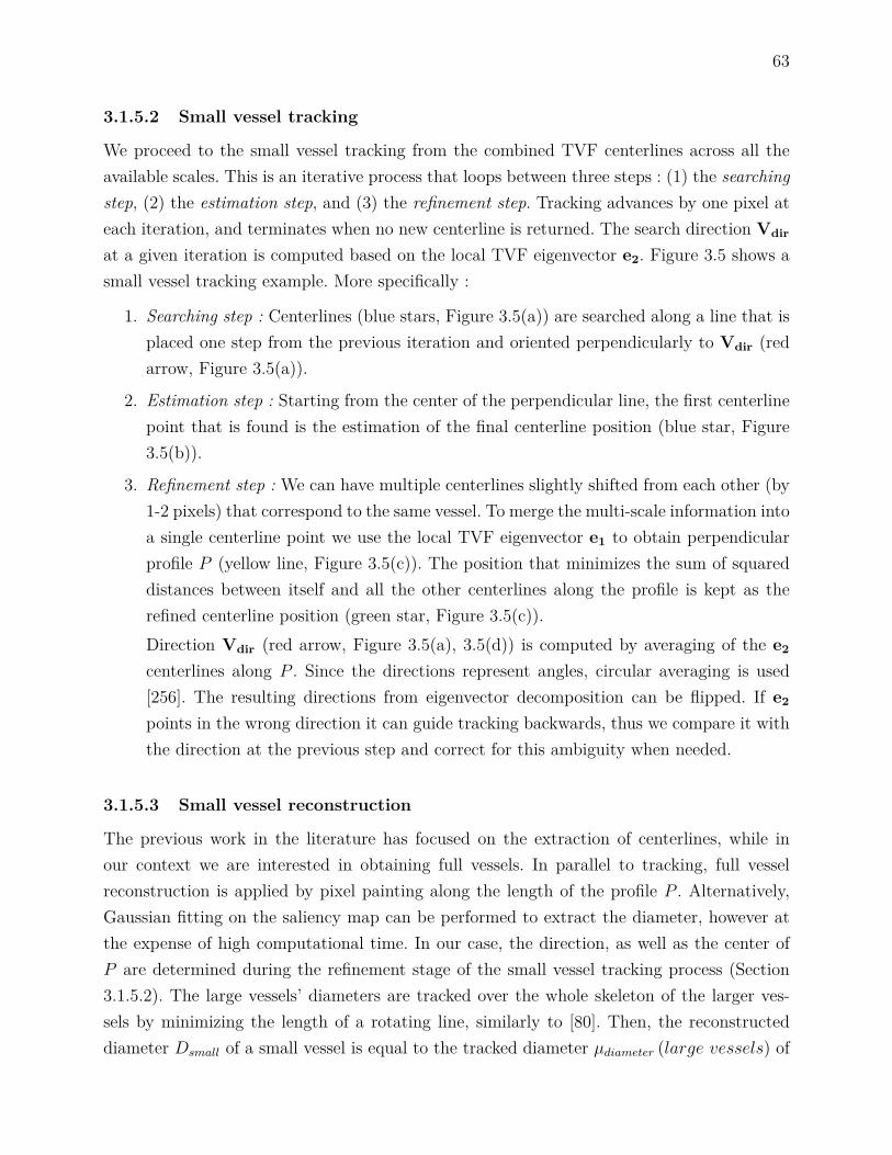
63

3.1.5.2 Small vessel tracking

We proceed to the small vessel tracking from the combined TVF centerlines across all theavailable scales. This is an iterative process that loops between three steps : (1) the searchingstep, (2) the estimation step, and (3) the refinement step. Tracking advances by one pixel ateach iteration, and terminates when no new centerline is returned. The search direction Vdir

at a given iteration is computed based on the local TVF eigenvector e2. Figure 3.5 shows asmall vessel tracking example. More specifically :

1. Searching step : Centerlines (blue stars, Figure 3.5(a)) are searched along a line that isplaced one step from the previous iteration and oriented perpendicularly to Vdir (redarrow, Figure 3.5(a)).

2. Estimation step : Starting from the center of the perpendicular line, the first centerlinepoint that is found is the estimation of the final centerline position (blue star, Figure3.5(b)).

3. Refinement step : We can have multiple centerlines slightly shifted from each other (by1-2 pixels) that correspond to the same vessel. To merge the multi-scale information intoa single centerline point we use the local TVF eigenvector e1 to obtain perpendicularprofile P (yellow line, Figure 3.5(c)). The position that minimizes the sum of squareddistances between itself and all the other centerlines along the profile is kept as therefined centerline position (green star, Figure 3.5(c)).Direction Vdir (red arrow, Figure 3.5(a), 3.5(d)) is computed by averaging of the e2

centerlines along P . Since the directions represent angles, circular averaging is used[256]. The resulting directions from eigenvector decomposition can be flipped. If e2

points in the wrong direction it can guide tracking backwards, thus we compare it withthe direction at the previous step and correct for this ambiguity when needed.

3.1.5.3 Small vessel reconstruction

The previous work in the literature has focused on the extraction of centerlines, while inour context we are interested in obtaining full vessels. In parallel to tracking, full vesselreconstruction is applied by pixel painting along the length of the profile P . Alternatively,Gaussian fitting on the saliency map can be performed to extract the diameter, however atthe expense of high computational time. In our case, the direction, as well as the center ofP are determined during the refinement stage of the small vessel tracking process (Section3.1.5.2). The large vessels’ diameters are tracked over the whole skeleton of the larger ves-sels by minimizing the length of a rotating line, similarly to [80]. Then, the reconstructeddiameter Dsmall of a small vessel is equal to the tracked diameter µdiameter (large vessels) of

64

Vdir

(a) (b)

e1

(c)

Vdir

(d)

Figure 3.5 Small vessel tracking example. (a) Searching of centerlines (blue stars) perpen-dicularly to Vdir (red arrow), (b) estimation of the final centerline position (blue star), (c)refinement of the final centerline position (green star) by searching along profile P (yellowline), and (d) Vdir search direction for next tracking iteration.

the preceding large vessel, averaged over several skeleton points at the end of that vessel.Averaging of the diameter is necessary because the large vessel gradually narrows towards itstip, so we have to normalize µdiameter (large vessels) by considering a number N of prece-ding points, N being experimentally determined (Section 3.2.2). The reconstruction processis restricted to the smallest vessels, i.e. those of diameter D < 8 pixels (see section 3.2.1). Asa final step, morphological closing with a small circular element is applied to fill holes in thereconstructed vessel caused by the inpainting of curved vessels along straight lines. Figureprovides an example of small vessel reconstruction.

3.1.6 Postprocessing

The MSLD response is sensitive to background lesions and artifacts, so non-vascular dis-connected components remain after the adaptive thresholding stage. Additionally, branchedvessels may remain disconnected after tracking. Junctions are high order morphological fea-tures that represent the separation of a main vessel into smaller branches. Both MSLD andTVF are inadequate to approximate the bifurcation pattern when it comes to enhancing orsegmenting vascular regions at less prominent junctions. MSLD applies a straight line tem-

65

plate, while there is a high degree of directional uncertainty that cannot be estimated bysecond order tensors in the TVF.

The final step in our pipeline is the morphological cleaning of background artifacts fromthe image, together with the inclusion of disconnected vessels. The choice of morphology wasbased on the algorithimic and computational requirements of the step. According to our me-thod, all the connected components (CC) that are disconnected from the main vasculatureare sequentially analyzed. If they are larger than a specific size (AreaCC > Areavalue), elon-gated enough (ElongationCC > X) and not very solid (SolidityCC < X), then they belongto vessels and thus they are retained from the thresholded image. Elongation or eccentricityof an ellipse (ε) is defined as :

ε=2

√(LengthMajorAxis

2

)2−(LengthMinorAxis

2

)2

LengthMinorAxis

, (3.4)

where LengthMajorAxis and LengthMinorAxis are the major and minor axis lengths of an el-lipse, respectively [257]. Solidity is defined as the ratio of the area over the convex hull area.Conservative values for the parameters used at this step were experimentally determined asdescribed in Section 3.2.2. This allowed us to clean the images while retaining important vas-cular structures. Figure 3.7 shows an example where the postprocessing step for backgroundnoise suppression is applied in a highlighted area of an image.

3.2 Experiments

3.2.1 Image database

Our approach was evaluated on high resolution fundus images from the HRF database [63].The database contains three categories of images : healthy subjects (H), diabetic retinopathypatients (DR),and glaucomatous patients (G). Each category comprises 15 images acquired

(a) (b) (c) (d) (e)

Figure 3.6 Small vessel reconstruction example. (a) Input grayscale image, (b) simple thre-sholded image, (c) centerline union, (d) reconstructed vessels, and (r) reference.

66

using a CANON CF-60UVi camera [258] with fixed resolution of 3504 x 2336 pixels andpixel size of 6.05 x 6.46 µm. Manual segmentations of the vessels are provided for the wholedatabase. In this study, all the vessels of small width were considered as small vessels. Thisdefinition of size is invariant to location and branching order, however it depends on theacquisition process, the field of view and the image resolution. For this particular high reso-lution database, we qualitatively selected the vessel diameter value that isolates most of theterminal, non-fragmented vessels, without including vessels that might belong to the largervascular structures, such as the major arcades. Everything below 8 pixels in diameter wasthus considered as a small vessel. This value yielded a good compromise between the aimsof identifying complete terminal vessels and excluding larger vessels. The rest of the vascu-lature, with diameter above the 8-pixel threshold, was considered as belonging to the largeand medium-sized categories of vessels.

3.2.2 Parameter setting

The vessel segmentation performance was evaluated at two levels : (1) using the fullvasculature, and (2) restricting the analysis to the smallest vessels. The glaucomatous casesin our database were not severe, so they show deterioration on the optic disc but none for the

(a) (b)

(c)

Figure 3.7 Postprocessing example. (a) Adaptive thresholded input image, (b) zoomed areacorresponding to inset in (a), and (c) same image area after postprocessing (cleaning).

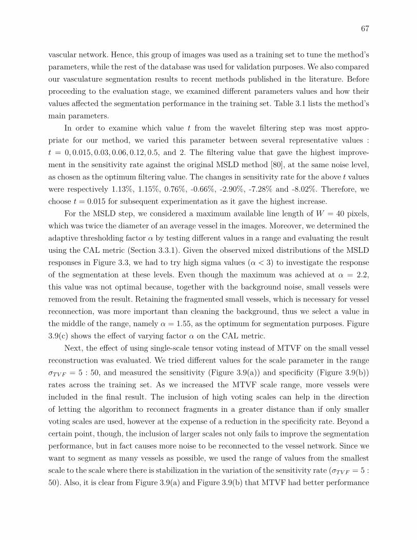
67

vascular network. Hence, this group of images was used as a training set to tune the method’sparameters, while the rest of the database was used for validation purposes. We also comparedour vasculature segmentation results to recent methods published in the literature. Beforeproceeding to the evaluation stage, we examined different parameters values and how theirvalues affected the segmentation performance in the training set. Table 3.1 lists the method’smain parameters.

In order to examine which value t from the wavelet filtering step was most appro-priate for our method, we varied this parameter between several representative values :t = 0, 0.015, 0.03, 0.06, 0.12, 0.5, and 2. The filtering value that gave the highest improve-ment in the sensitivity rate against the original MSLD method [80], at the same noise level,as chosen as the optimum filtering value. The changes in sensitivity rate for the above t valueswere respectively 1.13%, 1.15%, 0.76%, -0.66%, -2.90%, -7.28% and -8.02%. Therefore, wechoose t = 0.015 for subsequent experimentation as it gave the highest increase.

For the MSLD step, we considered a maximum available line length of W = 40 pixels,which was twice the diameter of an average vessel in the images. Moreover, we determined theadaptive thresholding factor α by testing different values in a range and evaluating the resultusing the CAL metric (Section 3.3.1). Given the observed mixed distributions of the MSLDresponses in Figure 3.3, we had to try high sigma values (α < 3) to investigate the responseof the segmentation at these levels. Even though the maximum was achieved at α = 2.2,this value was not optimal because, together with the background noise, small vessels wereremoved from the result. Retaining the fragmented small vessels, which is necessary for vesselreconnection, was more important than cleaning the background, thus we select a value inthe middle of the range, namely α = 1.55, as the optimum for segmentation purposes. Figure3.9(c) shows the effect of varying factor α on the CAL metric.

Next, the effect of using single-scale tensor voting instead of MTVF on the small vesselreconstruction was evaluated. We tried different values for the scale parameter in the rangeσTV F = 5 : 50, and measured the sensitivity (Figure 3.9(a)) and specificity (Figure 3.9(b))rates across the training set. As we increased the MTVF scale range, more vessels wereincluded in the final result. The inclusion of high voting scales can help in the directionof letting the algorithm to reconnect fragments in a greater distance than if only smallervoting scales are used, however at the expense of a reduction in the specificity rate. Beyond acertain point, though, the inclusion of larger scales not only fails to improve the segmentationperformance, but in fact causes more noise to be reconnected to the vessel network. Since wewant to segment as many vessels as possible, we used the range of values from the smallestscale to the scale where there is stabilization in the variation of the sensitivity rate (σTV F = 5 :50). Also, it is clear from Figure 3.9(a) and Figure 3.9(b) that MTVF had better performance

68

measures than single scale TVF.We then evaluated the small vessel reconstruction parameter N to determine the value

giving the best improvement in sensitivity rate against the original MSLD method [80] at thesame noise level. The changes in sensitivity rate, as we increased N from 1 to 8 (by steps of 1),were respectively 1.13%, 1.14%, 1.14%, 1.15%, 1.12%, 1.13%, 1.12%, and 1.12%. Therefore,we choose N = 4 for the rest of the experiments. Finally, the postprocessing parametervalues were selected by examining the CAL performance metric. As described in section3.1.6, these parameters establish the morphological limits between real vessel segments (tobe reconnected) and artifacts (to be removed). We varied Areavalue from 200 to 600 andX from 0.2 to 0.9. Values of Areavalue = 500, or 10 times the largest vessel diameter, andX = 0.5, gave the maximum perceptual response (Figure 3.9(d)). Table 3.1 summarizes theresults of the parameter setting process. The computational time across the different scalesin MTVF for a typical image is given in Figure 3.8.

Table 3.1 Parameters of the proposed approach and the selected values

.

Parameter (Section) Function Selected valuet (§3.1) Wavelet filtering t = 0.015W (§3.2) MSLD (80) W = 40α (§3.3) Adaptive thresholding factor α = 1.55

σTV F (§3.4) Multi-scale tensor voting range σTV F = 5 : 5 : 50N (§3.5) Large vessel skeleton pixels for reconstruction N = 4

Areavalue, X (§3.6) Postprocessing Areavalue > 500, X = 0.5

5 10 15 20 25 30 35 40 45 500

200

400

600

800

1000

1200

Scale range

Exe

cutio

n tim

e (s

ec.)

Multi−scale Tensor VotingSinge−scale Tensor Voting

Figure 3.8 Single (blue line) and multi (red line) scale tensor voting execution time for atypical retinal image across scales σTV F = 5 : 5 : 50.

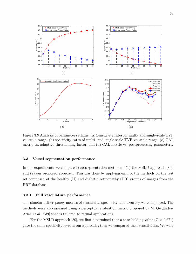
69

5 10 15 20 25 30 35 40 45 5086.4

86.5

86.6

86.7

86.8

86.9

87

87.1

87.2

87.3

Scale range

Sen

sitiv

ity (

%)

Multi−scale Tensor VotingSingle−scale Tensor Voting

(a)

5 10 15 20 25 30 35 40 45 5094.9

95

95.1

95.2

95.3

95.4

95.5

95.6

95.7

95.8

Scale range

Spe

cific

ity (

%)

Multi−scale Tensor VotingSingle−scale Tensor Voting

(b)

0 0.5 1 1.5 2 2.5 30.1

0.2

0.3

0.4

0.5

0.6

0.7

0.8

0.9

α factor

CA

L m

etric

val

ue

Adaptive simple thresholding

(c)

0.2 0.3 0.4 0.5 0.6 0.7 0.8 0.9 10.774

0.776

0.778

0.78

0.782

0.784

0.786

0.788

0.79

0.792

0.794

Elongation>X & Solidity<X

CA

L m

etric

val

ue

Area>200Area>300Area>400Area>500Area>600

(d)

Figure 3.9 Analysis of parameter settings. (a) Sensitivity rates for multi- and single-scale TVFvs. scale range, (b) specificity rates of multi- and single-scale TVF vs. scale range, (c) CALmetric vs. adaptive thresholding factor, and (d) CAL metric vs. postprocessing parameters.

3.3 Vessel segmentation performance

In our experiments we compared two segmentation methods : (1) the MSLD approach [80],and (2) our proposed approach. This was done by applying each of the methods on the testset composed of the healthy (H) and diabetic retinopathy (DR) groups of images from theHRF database.

3.3.1 Full vasculature performance

The standard discrepancy metrics of sensitivity, specificity and accuracy were employed. Themethods were also assessed using a perceptual evaluation metric proposed by M. Gegúndez-Arias et al. [239] that is tailored to retinal applications.

For the MSLD approach [80], we first determined that a thresholding value (T > 0.671)gave the same specificity level as our approach ; then we compared their sensitivities. We were

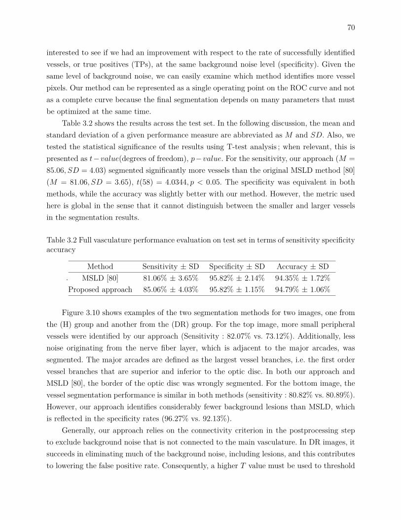
70

interested to see if we had an improvement with respect to the rate of successfully identifiedvessels, or true positives (TPs), at the same background noise level (specificity). Given thesame level of background noise, we can easily examine which method identifies more vesselpixels. Our method can be represented as a single operating point on the ROC curve and notas a complete curve because the final segmentation depends on many parameters that mustbe optimized at the same time.

Table 3.2 shows the results across the test set. In the following discussion, the mean andstandard deviation of a given performance measure are abbreviated as M and SD. Also, wetested the statistical significance of the results using T-test analysis ; when relevant, this ispresented as t−value(degrees of freedom), p−value. For the sensitivity, our approach (M =85.06, SD = 4.03) segmented significantly more vessels than the original MSLD method [80](M = 81.06, SD = 3.65), t(58) = 4.0344, p < 0.05. The specificity was equivalent in bothmethods, while the accuracy was slightly better with our method. However, the metric usedhere is global in the sense that it cannot distinguish between the smaller and larger vesselsin the segmentation results.

Table 3.2 Full vasculature performance evaluation on test set in terms of sensitivity specificityaccuracy

.Method Sensitivity ± SD Specificity ± SD Accuracy ± SD

MSLD [80] 81.06% ± 3.65% 95.82% ± 2.14% 94.35% ± 1.72%Proposed approach 85.06% ± 4.03% 95.82% ± 1.15% 94.79% ± 1.06%

Figure 3.10 shows examples of the two segmentation methods for two images, one fromthe (H) group and another from the (DR) group. For the top image, more small peripheralvessels were identified by our approach (Sensitivity : 82.07% vs. 73.12%). Additionally, lessnoise originating from the nerve fiber layer, which is adjacent to the major arcades, wassegmented. The major arcades are defined as the largest vessel branches, i.e. the first ordervessel branches that are superior and inferior to the optic disc. In both our approach andMSLD [80], the border of the optic disc was wrongly segmented. For the bottom image, thevessel segmentation performance is similar in both methods (sensitivity : 80.82% vs. 80.89%).However, our approach identifies considerably fewer background lesions than MSLD, whichis reflected in the specificity rates (96.27% vs. 92.13%).

Generally, our approach relies on the connectivity criterion in the postprocessing stepto exclude background noise that is not connected to the main vasculature. In DR images, itsucceeds in eliminating much of the background noise, including lesions, and this contributesto lowering the false positive rate. Consequently, a higher T value must be used to threshold

71

(a) (b) (c)

(d) (e) (f)

Figure 3.10 Full vessel segmentation examples in Image_01_healthy (first row) andImage_04_diabetic (second row). (a) and (d) original image, (b) and (e) segmentation resultof our approach, (c) and (f) segmentation result of MSLD method. In the segmentation maps(b, c and e, f), blue pixels represent the true positives, red pixels are the false negatives,yellow pixels are the false positives, and black pixels are the true negatives.

the MSLD response to achieve the same specificity rate as our approach for pathological cases.For healthy cases, the difference in sensitivity between the two methods is even greater, asexemplified in Figure 3.10.

Table 3.3 shows the results in terms of the perceptual performance metric (CAL, orConnectivity Area Length). This measure is the product of three individual metrics : connec-tivity, area and length. The connectivity criterion penalizes any deviation from the numberof connected components in the reference image. Meanwhile, the length (resp. area) crite-rion measures the degree of coincidence, in terms of total skeleton length (resp. vessel area),between the groundtruth and tested segmentations (239). Length is an important individualmetric because it shows to what extend each method can identify vessels. This criterion eva-luates the skeletonized vasculature, thereby disregarding the influence of the pixel areas ofthe different categories of vessels.

Our approach (M = 0.779, SD = 0.060) achieves significantly higher CAL performancethan the original MSLD method [80] (M = 0.701, SD = 0.127), t(58) = 3.0203, p < 0.05.The proposed method seeks to maximize resulting vascular connectivity, thus that particularcriterion is very close to 1 (or perfectly preserved connectivity compared to the reference

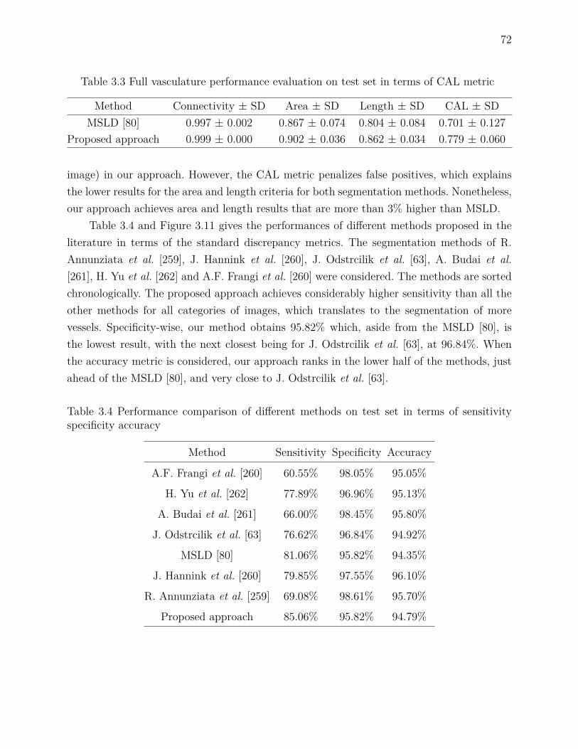
72

Table 3.3 Full vasculature performance evaluation on test set in terms of CAL metric

Method Connectivity ± SD Area ± SD Length ± SD CAL ± SDMSLD [80] 0.997 ± 0.002 0.867 ± 0.074 0.804 ± 0.084 0.701 ± 0.127

Proposed approach 0.999 ± 0.000 0.902 ± 0.036 0.862 ± 0.034 0.779 ± 0.060

image) in our approach. However, the CAL metric penalizes false positives, which explainsthe lower results for the area and length criteria for both segmentation methods. Nonetheless,our approach achieves area and length results that are more than 3% higher than MSLD.

Table 3.4 and Figure 3.11 gives the performances of different methods proposed in theliterature in terms of the standard discrepancy metrics. The segmentation methods of R.Annunziata et al. [259], J. Hannink et al. [260], J. Odstrcilik et al. [63], A. Budai et al.[261], H. Yu et al. [262] and A.F. Frangi et al. [260] were considered. The methods are sortedchronologically. The proposed approach achieves considerably higher sensitivity than all theother methods for all categories of images, which translates to the segmentation of morevessels. Specificity-wise, our method obtains 95.82% which, aside from the MSLD [80], isthe lowest result, with the next closest being for J. Odstrcilik et al. [63], at 96.84%. Whenthe accuracy metric is considered, our approach ranks in the lower half of the methods, justahead of the MSLD [80], and very close to J. Odstrcilik et al. [63].

Table 3.4 Performance comparison of different methods on test set in terms of sensitivityspecificity accuracy

Method Sensitivity Specificity Accuracy

A.F. Frangi et al. [260] 60.55% 98.05% 95.05%

H. Yu et al. [262] 77.89% 96.96% 95.13%

A. Budai et al. [261] 66.00% 98.45% 95.80%

J. Odstrcilik et al. [63] 76.62% 96.84% 94.92%

MSLD [80] 81.06% 95.82% 94.35%

J. Hannink et al. [260] 79.85% 97.55% 96.10%

R. Annunziata et al. [259] 69.08% 98.61% 95.70%

Proposed approach 85.06% 95.82% 94.79%

73

Frangi Yu Budai Odstrcilik MSLD Hannink Annunziata Proposed 55

60

65

70

75

80

85

90

95

100

105

Se

Sp

Acc

Se

SpAcc

Se

SpAcc

Se

SpAcc

Se

SpAcc

Se

SpAcc

Se

Sp

Acc

Se

SpAcc

Figure 3.11 Differences in the discrepancy metrics across the available segmentation methods.

3.3.2 Small vessels analysis

The standard discrepancy measures cannot account for the heterogeneity in the pixel areasof vessel segments of different diameters [175]. Thus, we confined the following part of ouranalysis to the smallest vessels. The smallest vessels of the groundtruth images were firstisolated from the rest of the vessel network. To achieve this, the minimization of a rotatingline on the pixels belonging to the skeletonized reference image was applied as in Section3.1.5.3. Next, the diameter value at each skeleton point is assigned to all vessel pixels alongthe normal direction at that point. Then, the pixels belonging to vessels of diameter lessthan 8 pixels were isolated, and the final result of this operation was subtracted from therest of the reference image. The segmentation algorithms were assessed by computing thesame discrepancy measures as those used for the full vasculature analysis (Section 3.3.1),and by assigning the large vessel pixels from the reference to the true negative class. Thesegmentation maps of A.F. Frangi [260] and J. Hannink [260] were also available, so ouranalysis included these methods.

Table 3.5 shows the performance of the four methods on the smallest vessels when thepixel-based discrepancy measures were considered. Our approach (M = 68.64, SD = 6.78)achieved significantly higher sensitivity than MSLD [80] (M = 62.17, SD = 8.51, t(58) =3.225, p < 0.05), J. Hannink [260] (M = 54.08, SD = 12.36, t(58) = 5.6580, p < 0.05), andA.F. Frangi [260] (M = 49.01, SD = 11.11, t(58) = 8.2576, p < 0.05) methods. In fact, thedifference between our method and the available ones is greater than when all the vesselswere considered. Our approach detected approximately 6% more small vessels than the MSLD[80]. Moreover, this increase doubles and triples when our approach is compared with the J.Hannink [260] and A.F. Frangi methods [260], respectively. In our analysis we remove thedetected medium to large-sized vessels, however the oversegmentation of the vessels boundaryis not taken into account which explains the differences in the specificity and accuracy metrics

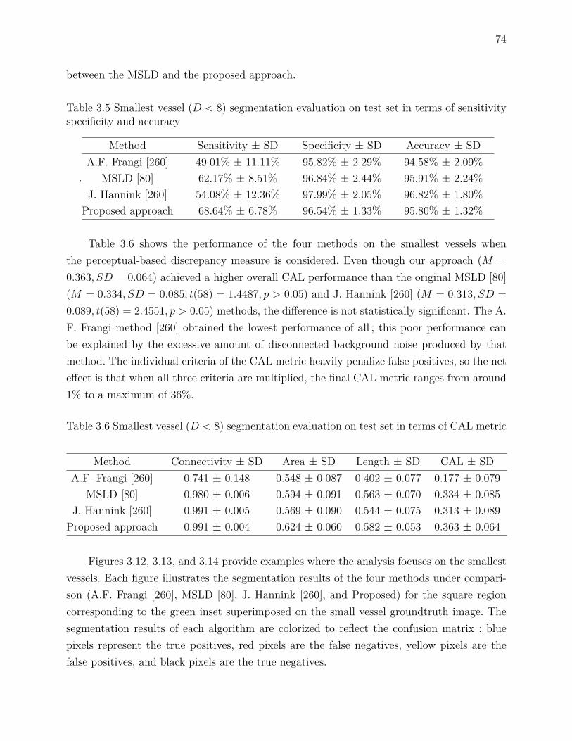
74

between the MSLD and the proposed approach.

Table 3.5 Smallest vessel (D < 8) segmentation evaluation on test set in terms of sensitivityspecificity and accuracy

.

Method Sensitivity ± SD Specificity ± SD Accuracy ± SDA.F. Frangi [260] 49.01% ± 11.11% 95.82% ± 2.29% 94.58% ± 2.09%

MSLD [80] 62.17% ± 8.51% 96.84% ± 2.44% 95.91% ± 2.24%J. Hannink [260] 54.08% ± 12.36% 97.99% ± 2.05% 96.82% ± 1.80%

Proposed approach 68.64% ± 6.78% 96.54% ± 1.33% 95.80% ± 1.32%

Table 3.6 shows the performance of the four methods on the smallest vessels whenthe perceptual-based discrepancy measure is considered. Even though our approach (M =0.363, SD = 0.064) achieved a higher overall CAL performance than the original MSLD [80](M = 0.334, SD = 0.085, t(58) = 1.4487, p > 0.05) and J. Hannink [260] (M = 0.313, SD =0.089, t(58) = 2.4551, p > 0.05) methods, the difference is not statistically significant. The A.F. Frangi method [260] obtained the lowest performance of all ; this poor performance canbe explained by the excessive amount of disconnected background noise produced by thatmethod. The individual criteria of the CAL metric heavily penalize false positives, so the neteffect is that when all three criteria are multiplied, the final CAL metric ranges from around1% to a maximum of 36%.

Table 3.6 Smallest vessel (D < 8) segmentation evaluation on test set in terms of CAL metric

Method Connectivity ± SD Area ± SD Length ± SD CAL ± SDA.F. Frangi [260] 0.741 ± 0.148 0.548 ± 0.087 0.402 ± 0.077 0.177 ± 0.079

MSLD [80] 0.980 ± 0.006 0.594 ± 0.091 0.563 ± 0.070 0.334 ± 0.085J. Hannink [260] 0.991 ± 0.005 0.569 ± 0.090 0.544 ± 0.075 0.313 ± 0.089

Proposed approach 0.991 ± 0.004 0.624 ± 0.060 0.582 ± 0.053 0.363 ± 0.064

Figures 3.12, 3.13, and 3.14 provide examples where the analysis focuses on the smallestvessels. Each figure illustrates the segmentation results of the four methods under compari-son (A.F. Frangi [260], MSLD [80], J. Hannink [260], and Proposed) for the square regioncorresponding to the green inset superimposed on the small vessel groundtruth image. Thesegmentation results of each algorithm are colorized to reflect the confusion matrix : bluepixels represent the true positives, red pixels are the false negatives, yellow pixels are thefalse positives, and black pixels are the true negatives.

75

Figure 3.12 (Image_15_healthy), presents the best performance of the proposed ap-proach for both the large and small vessel categories. Qualitatively, our approach segmentsmost of the vessels without retaining any disconnected background noise, however the ter-minal vessels and the boundary of the large vessels are overestimated in terms of length andwidth. Also, some false positive vessels are reconnected to the main vasculature. Quantitati-vely, our approach achieves the highest sensitivity but the lowest specificity.

(a) Image_15_healthy (b) Reference (c) Isolated smallest vessels

(d) A. F. Frangi (e) MSLD (f) J. Hannink (g) Proposed approach

Figure 3.12 Small vessel segmentation example in Image_15_healthy. (a) Grayscale in-put image, (b) manual segmentation of the whole vasculature, (c) isolated smallest ves-sels, (d) A. F. Frangi [260] segmentation result :(Sens.full = 70.97%, Specif.full =98.44%, Sens.smallest = 40.36%, Specif.smallest = 99.34%), (e) MSLD [80] segmentation re-sult :(Sens.full = 87.28%, Specif.full = 97.14%, Sens.smallest = 72.41%, Specif.smallest =97.85%), (f) J. Hannink [260] segmentation result :(Sens.full = 86.27%, Specif.full =97.80%, Sens.smallest = 66.30%, Specif.smallest = 98.47%), and (g) Proposed ap-proach segmentation result :(Sens.full = 92.91%, Specif.full = 95.99%, Sens.smallest =83.83%, Specif.smallest = 96.36%)

Figure 3.13 (Image_10_healthy), presents the worst performance of the proposed ap-proach for the small vessel category. Our method has the same qualitative behavior as in thebest case ; it segments most of the vessels without retaining any disconnected backgroundnoise. But this is achieved at the expense of overestimating the vessel diameters/endpointsand reconnecting vessel-like false positives components. Even though this image representsthe worst-case performance, our method still reaches the highest sensitivity rate among the

76

considered methods.

(a) Image_10_healthy (b) Reference (c) Isolated smallest vessels

(d) A. F. Frangi (e) MSLD (f) J. Hannink (g) Proposed approach

Figure 3.13 Small vessel segmentation example in Image_10_healthy. (a) grayscale inputimage, (b) manual segmentation of the whole vasculature, (c) isolated smallest vessels(D < 8), (d) A. F. Frangi [260] segmentation result :(Sens.full = 70.97%, Specif.full =98.44%, Sens.smallest = 39.47%, Specif.smallest = 97.58%), (e) MSLD [80] segmentation re-sult :(Sens.full = 79.37%, Specif.full = 97.58%, Sens.smallest = 53.15%, Specif.smallest =98.45%), (f) J. Hannink [260] segmentation result :(Sens.full = 74.94%, Specif.full =98.53%, Sens.smallest = 35.01%, Specif.smallest = 99.32%), and (g) Proposed ap-proach segmentation result :(Sens.full = 82.54%, Specif.full = 96.96%, Sens.smallest =57.08%, Specif.smallest = 97.59%)

Finally, Figure 3.14 (Image_06_diabetic) presents the worst performance of the propo-sed approach in terms of full vascular network segmentation. An interesting feature of thisimage is that it includes many convoluted vessels that could be neovessels. Our approachmanaged to segment most of these vessels. The majority of them were segmented earlier inour pipeline (at the adaptive thresholding stage), while the MTVF partially completed thenetwork (Figure 3.15). We note as well that the the vessel widths were over-estimated. At thesame time, the other three methods failed to segment many vessels in this region of interest.This is reflected in their sensitivity rates, which are lower than for our approach.

77

(a) Image_06_diabetic (b) Reference (c) Isolated smallest vessels

(d) A. F. Frangi (e) MSLD (f) J. Hannink (g) Proposed approach

Figure 3.14 Small vessel segmentation example in Image_06_diabetic. (a) grayscale in-put image, (b) manual segmentation of the whole vasculature, (c) isolated smallest vessels(D < 8), (d) A. F. Frangi [260] segmentation result :(Sens.full = 71.26%, Specif.full =92.94%, Sens.smallest = 54.19%, Specif.smallest = 92.44%), (e) MSLD [80] segmentation re-sult :(Sens.full = 72.59%, Specif.full = 93.90%, Sens.smallest = 55.35%, Specif.smallest =94.79%), (f) J. Hannink [260] segmentation result :(Sens.full = 68.25%, Specif.full =95.85%, Sens.smallest = 42.56%, Specif.smallest = 96.66%), and (g) Proposed ap-proach segmentation result :(Sens.full = 74.43%, Specif.full = 93.62%, Sens.smallest =58.62%, Specif.smallest = 94.47%)

(a) (b) (c)

Figure 3.15 Small vessel segmentation at different stages in proposed pipeline, forImage_06_diabetic. (a) adaptive thresholding result, (b) small vessel reconnection result,and (c) postprocessed result.

78

3.3.2.1 Group differences between healthy and diabetic performance

We divided the entire test set into the healthy (H) and diabetic (DR) images in order toassess how the proposed method performed on the separate groups as compared to theoverall case. For the healthy group, the improvement in sensitivity over the original MSLDmethod [80] widened : our method detected 11% more small vessels than MSLD. However,this was accomplished at the expense of more false positives, probably due to overestimationof the vessel endpoints and widths or from false positive reconnections. The opposite trendwas observed for the DR group. The gain in sensitivity over MSLD [80] dropped, but in termsof specificity the proposed method segmented less noise. This can be accounted for by theinherent connectivity criterion that removes isolated background noise and artifacts. Whenthe two image groups are merged, the performances are averaged so the specificity is thesame across the database and the sensitivity is reduced compared to the healthy case. Tables3.7 and 3.8 give the results for the standard discrepancy metrics separately in each imagegroup.

Table 3.7 Full Vasculature performance evaluation on test set in terms of sensitivity specificityaccuracy

.

Category Method Sensitivity ± SD Specificity ± SD Accuracy ± SD

H MSLD [80] 80.50% ± 4.04% 97.66% ± 0.55% 95.74% ± 0.63%Proposed approach 86.60% ± 3.40% 96.67% ± 0.43% 95.54% ± 0.43%

DR MSLD [80] 81.62% ± 3.26% 93.99% ± 1.41% 92.95% ± 1.23%Proposed approach 83.53% ± 4.13% 94.97% ± 1.02% 94.05% ± 0.98%

Table 3.8 Smallest vessel (D < 8) segmentation evaluation on test set in terms of sensitivityspecificity accuracy

.

Category Method Sensitivity ± SD Specificity ± SD Accuracy ± SD

H MSLD [80] 58.10% ± 8.64% 97.86% ± 0.51% 96.90% ± 0.46%Proposed approach 69.90% ± 7.15% 96.96% ± 0.42% 96.30% 0.39%

DR MSLD [80] 66.25% ± 6.31% 94.33% ± 1.36% 93.61% ± 1.21%Proposed approach 67.38% ± 6.39% 95.55% ± 1.06% 94.81% ± 1.06%

3.4 Discussion

Segmenting the smallest retinal vessels is still a challenging problem. The MSLD method[80] is based on straight line segments, which is inadequate in this context. Using tensor

79

voting can help by retaining only the information that is perceptually significant to extendingthe segmentation to the smallest vessels. In this chapter, we have proposed a novel hybridapproach that combines the two methods. Multi-scale information from the TVF is combinedin a new way that allows us to reconnect vessels at greater distances than single scale tensorvoting. Besides, our approach can fully reconstruct the vessels, which enables the use of theframework for lesion detection in CAD systems.

Even though the proposed method achieved higher performance than MSLD [80] in themajority of full and small vessel experiments, several challenges remain to be addressed. Inthe final result, the segmented small vessels can be slightly translated from their groundtruthcounterparts. Similarly, their reconstructed widths do not exactly coincide in some locationswith the corresponding vessels in the manually segmented image. Moreover, small vesselterminal points are over-estimated. Additionally, the TVF can reconnect vessel-like falsepositive structures to the main vasculature, while conversely it can miss real vessels lyingafter junctions.

The errors in the reconstructed width of a small vessel can be attributed to the pixelpainting process. The diameter obtained from the larger vessel is used without taking into ac-count local information such as the local saliency from TVF. This gives rise to false positivesand to an equivalent reduction in the true positive counts. The issue of vessel over-extensionwas also raised by Z. Leng et al. [209], however their solution was based on simple post-processing, taking into account the information from an initial centerline map extracted bya Canny edge detector. The vessel over-extension problem, together with the false positivereconnection problem, is related to the quality of the available reference. Precise manual seg-mentation of the smallest vessels is not obvious in high resolution images, even for an expert.Therefore, the use of multiple experts who manually segment the same images would allowa consensus groundtruth to be constructed. With such a reference, there would be higherconfidence about the smallest vessels’ positions and extents. In our case, there were instanceswhere the expert did not identify small vessels or did not extend them until their endpoints.Figure 3.16 highlights examples where small vessels of weaker contrast are missing or theywere not completed in the manual segmentation. Our approach, on the other hand, managedto identify and/or complete these vessels.

Furthermore, there is significant difficulty in reconnecting vessel segments that are lo-cated beyond junctions. As was highlighted in Section 3.1.6, the high level of orientationuncertainty causes the TVF to fragment the vessels at junctions, even if these structures arewell defined. In the proposed method, we try to retain branched vessels via morphologicalprocessing, but alternatives could be considered. The ballness measure (λ2) reaches localmaxima at junctions. Using it directly via concurrent tracking and searching for branched

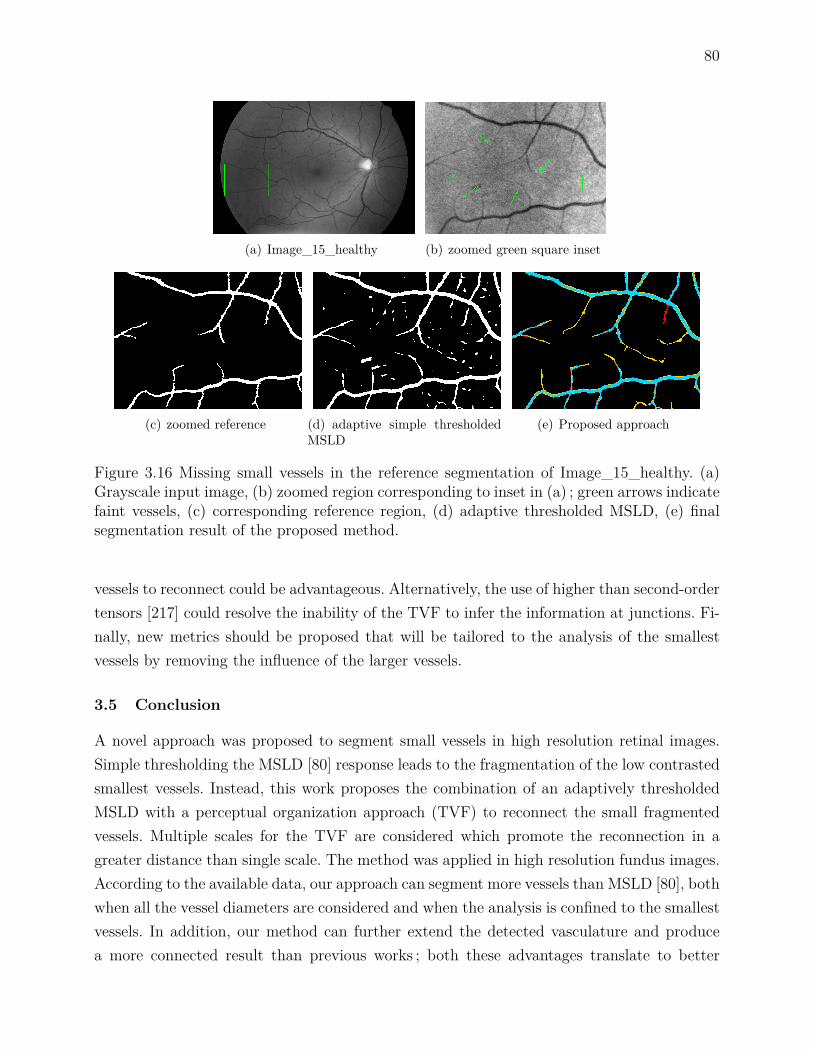
80

(a) Image_15_healthy (b) zoomed green square inset

(c) zoomed reference (d) adaptive simple thresholdedMSLD

(e) Proposed approach

Figure 3.16 Missing small vessels in the reference segmentation of Image_15_healthy. (a)Grayscale input image, (b) zoomed region corresponding to inset in (a) ; green arrows indicatefaint vessels, (c) corresponding reference region, (d) adaptive thresholded MSLD, (e) finalsegmentation result of the proposed method.

vessels to reconnect could be advantageous. Alternatively, the use of higher than second-ordertensors [217] could resolve the inability of the TVF to infer the information at junctions. Fi-nally, new metrics should be proposed that will be tailored to the analysis of the smallestvessels by removing the influence of the larger vessels.

3.5 Conclusion

A novel approach was proposed to segment small vessels in high resolution retinal images.Simple thresholding the MSLD [80] response leads to the fragmentation of the low contrastedsmallest vessels. Instead, this work proposes the combination of an adaptively thresholdedMSLD with a perceptual organization approach (TVF) to reconnect the small fragmentedvessels. Multiple scales for the TVF are considered which promote the reconnection in agreater distance than single scale. The method was applied in high resolution fundus images.According to the available data, our approach can segment more vessels than MSLD [80], bothwhen all the vessel diameters are considered and when the analysis is confined to the smallestvessels. In addition, our method can further extend the detected vasculature and producea more connected result than previous works ; both these advantages translate to better

81

perceptual performance. Compared to other published methods, our approach segments morevessels at the expense of slightly higher background noise. However, the proposed algorithmshould be validated in datasets containing images with different pixel resolutions.

Methods relying on a connectivity criterion for segmenting the vessels are well suited forpreprocessing the retinal vasculature in CAD systems. On the other hand, simple thresholdingdoes not set any restriction on the background responses, which can result in false negatives ata subsequent lesion detection step, i.e. failure to detect potentially vision-threatening lesions.

Future work will focus on utilizing the ballness measure (λ2) computed in the tensorvoting framework for neovascularization detection. This category of vessels is even more chal-lenging to detect because neovessels are very fine and tortuous structures with low contrastthat form chaotic networks around the optic disc or in other areas of the retina. Their pre-sence in the fundus image signals the transition to the final stage of diabetic retinopathy andthus their accurate detection is essential.

82

CHAPTER 4 SMALL RETINAL VESSEL CHARACTERIZATION

This chapter will present the developed method for the characterization problem of healthyor proliferative diabetic retinopathy regions (PDR). Besides, it will provide the experimentalresults.

4.1 Methodology

The methodology consists of three steps, each one separated in individual basic steps : (1) thejunction center detection step, (2) the feature extraction step, and (3) the classification step.Diagram in Figure 4.1 demonstrates the proposed pipeline for the junction center detectionstage. Vessels are firstly extracted based on the method presented in Chapter 4. Postproces-sing is then applied to remove backgroun noise. Next, the TVF is applied at a single scaleto detect the junctions. Finally, noisy or very close junctions are suppressed. Following thejunction center detection steps, features are selected from manually identified regions, whileclassification is applied to examine the performance of the selected features.

Vessel Extraction Postprocessing Tensor Voting JunctionCenter Isolation

Figure 4.1 Junction center detection pipeline.

4.1.1 Junction center detection

4.1.1.1 Vessel extraction

We apply the MSLD [80] on the green channel of the retinal images whose illumination is cor-rected and background noise is filtered, as in Chapter 3. We apply the line detector, adjustingthe line length parameter W according to the image resolution. The overall distribution ofline response values varies according to the considered image and database, so we determinethe simple threshold value adaptively by fitting a Gaussian function on the distribution ofeach image. We use the same threshold value T = bµGaussianc+bσGaussianc for all the availableimages, where µGaussian is the mean value and σGaussian is the standard deviation of the fittedfunction, respectively.

83

4.1.1.2 Postprocessing

Simple thresholding the line response leads to the retention of disconnected background struc-tures that are either small in size or irregular in shape. In order to remove this type of noise weperform a conservative morphological analysis. We suppress all the disconnected componentsthat have 400 < AreaCC < 1000 and that are not elongated enough (ElongationCC < 0.99).Smaller components are completely removed, while larger components are kept regardless oftheir shape. The values of these parameters are chosen empirically aiming for backgroundnoise suppression, and at the same time retention of NV regions that are identified as PDR.

4.1.1.3 Tensor voting

We detect the junctions by decomposing the second order tensor T into its eigenvalues(λ1, λ2), and measuring the ballness measure (λ2) there :

T = λ1e1eT1 + λ2e2eT2 = (λ1 − λ2) e1eT1 + λ2(e1eT1 + e2eT2

),

where e1,2 are orthogonal eigenvectors that hold the direction of the inferred lines at eachpixel location. Furthermore, scale parameter σTVF defines the extend of the voting field andsubsequently controls the distance in which the neighbor information is taken into account.The ballness measure of the tensor quantifies the local orientation uncertainty of the seg-mented vessels and it exhibits local maximum there. Since we are interested in extractinginformation from cluttered vessels low scale value should be used (σTVF = 20). One advan-tage of using TVF for junction detection is that it can infer the information based on theperceptual organization of the neighbor structures. Morphological processing, on the otherhand, is inadequate to detect the junctions if the information is missing.

4.1.1.4 Junction centers isolation

The result of the previous step is a map with junctions as the local maxima on the image.Directly thresholding the map might be efficient, but not as effective as morphological proces-sing. The orientation uncertainty for junctions varies significantly across the image becauseits value depends on how clutter the neighbor structures of a junction are. Figure 4.2 showsan example where the orientation uncertainty is computed across junctions with ascendingclutterness. Thresholding can suppress junctions that have low values. In our method, wefirst identify the regional maxima by applying the height-domes [263] algorithm. We thenisolate the maximum values inside these domes. We morphologically reconstruct the originalgrayscale image I from I − h1, and then we subtract the result from the input image. Thisway, whole regions, unlike single pixels that demonstrate local maxima, can be identified.

84

Additionally, we select the most prominent domes, namely the regions that have height overh2. The values for the parameters are empirically set to h1 = 2600 and h2 = 1400 and dependon the value of the scale σTVF. Finally, we merge closely identified junctions that belong tothe same region by finding the barycenter in an 11x11 window. Figure 4.3 shows an exampleof the previous algorithmic steps in an image with NVDs.

(a) (b) (c) (d)

(e) (f) (g) (h)

Figure 4.2 The orientation uncertainty in junctions of varying degrees of complexity. Thefirst row (a-d) shows input junctions to TVF that have three (a), four (b), six (c), or eight(d) branches. The second row (e-h) shows the orientation uncertainty value for each junction.Generally, higher order junctions have higher uncertainty.

(a) (b) (c) (d) (e)

Figure 4.3 Algorithmic steps for the junction center isolation. (a) PDR region, (b) vesselextraction after MSLD, (c) postprocessed result, (d) tensor voting ballness measure, and (e)final detected junction centers.

85

4.1.2 Features extraction

4.1.2.1 Spatial distribution measures

We compute the following spatial statistics. Two versions of the dispersion index definedas : i) the variance over the mean number of junctions (VMR) across the healthy and the PDRgroup of images, and ii) the mean distance from the center of mass of junctions (VMR (µd)).Additionally, we compute two versions of the Kth-Nearest Neighbor index. The first isthe index described in [264], that in turn is based on the aggregation index R proposed byP.J. Clark [265], and defined as :

Kth-NN (K) = D(observed) (K)D(random) (K) =

∑K

i=1 µ(di)N

K(2K)!(2K !)2√ρ

,

where µ (di) is the mean nearest Kth-order neighbor distance between all the junctions, Nis the number of points, and ρ is the density. The second version of the measure is just thenumerator of the index, without the comparison against the random distribution which isalso a second-order statistic that can quantify the spatial arrangement.

The first measure can quantify if the arrangement of points, or the area pattern, is moreclustered or ordered than if it have been randomly arranged in the same region. The secondmeasure summarizes, in pixels, the inter-junction distances. Both measures are straight-forward to compute, and in contrast with the first-order measures they take into accountdistances. By applying these measures we can study the relative aggregation of the patternsin the two considered cases, the healthy and the PDR. Therefore, we can investigate if theassumption that the vessel junctions are denser in PDR holds. It also allow us to studythe spatial interactions between the junctions that give rise to the formation of the specificpattern in each case. Finally, Kth-order neighbor index is a second-order characteristic.

4.1.3 Classification Protocol

We assess the benefit of "incorporating" the newly proposed measures for classifying regionsto PDR. For that reason, we extract 21 features from each region, that were first proposedin the literature [220, 230]. Furthermore, we include the following that were also proposed in[229] : local entropy, measurements on the gray-level co-occurrence matrix (GLCM), and theproposed spatial distribution measures up to the 20th order for the Kth-NN case. Additionally,we compute the mean, median, minimum, maximum values of the new measures, as well asthe slope of a linear function fitted on the proposed measures in Section 4.1.2.1. In total, 88features thus are considered. We use a wrapper method for forward feature selection using a

86

support vector machine (SVM) with an RBF kernel, as in [220, 230]. We dedicate 2/3 of thewhole set for training and validation, and the rest for testing.

4.2 Results and Discussion

We perform our analysis in images collected from 5 databases (Diaretdb [266], HRF [63],Messidor [251], Kaggle [267], and a private one). In order to compare the healthy and theabnormal junctions we confine our analysis at a region-level.

4.2.1 Anatomically Corresponding Regions

We apply the spatial point pattern analysis in anatomically corresponding circular regions.Confining the analysis on anatomically corresponding regions removes the user influence fromthe healthy region selection process. It also allows, up to a degree, an introduction of naturalvariance in the collected data. Generally, two regions from different images are correspondingif they are in approximately similar locations in the available field of view (FOV). A trainedmember isolated 114 regions with NVs from the 5 databases, each region originating froma single image. Then we transform the NV center into polar coordinates (R, φ). With R

being the distance, in optic disc (OD) radius, between the OD center and the NV center,while φ is the angle. In the healthy images we select the regions that are at R distance andφ angle with respect to the OD, manually adjusting if the center is found outside of theFOV. Thus, each NV region is compared to a set of healthy regions. The area of the selectedregions was set to one fifth of the total FOV area of each image. The healthy group of imagescontained 99 images. Overall, 5688 regions from the healthy group are compared with 114abnormal regions. We perform the spatial analysis using the measures described in Section4.1.3. Figure 4.4 shows an isolated region with NVDs along with the corresponding regionsfrom the healthy cases. For each region we provide the segmented vessels with superimposedthe junctions.

4.2.2 Result on First-order Measure

The boxplot in Figure 4.5(a) shows the results on the number of junctions for the two cases.Generally, there is an overlap between the healthy and the diabetic groups. Even though wehave a denser pattern in the PDR cases, just counting the number of junctions is not enoughto highlight any differences between the healthy and the PDR group.

4.2.3 Dispersion Indices

The value for the dispersion is different for the two groups for both measures (Table 4.1).Both the healthy and the PDR regions are over-dispersed with respect to the mean number

87

(a) (b) (c)

(d) (e) (f)

Figure 4.4 Isolated areas and junctions for analysis in HRF and Messidor database. (a)PDR region, (b-f) anatomically corresponding healthy areas together with superimposedtheir isolated junctions (red stars).

of junctions. According to this measure, there are many instances where the count of junc-tions is higher or lower than the mean value of the corresponding group. Furthermore, thejunctions are approximately 3 pixels closer to the center of mass of junctions, an artificiallygenerated reference point, when a PDR case is encountered. These measure are not sensitiveto the spatial arrangement of junctions in each region so they are invariant to changes in theunderlying pattern, namely they cannot distinguish between a dense or a scattered pattern.

4.2.4 Kth-Order Nearest Neighbor Indices

The two measures based on Kth-NN (K) take into account the inter-junction distances. TheKth-order index includes the K = 1 case which only examines the nearest neighbor. Higherorder nearest neighbors better highlight the differences between the two considered groups.The graphs in Figures 4.5(b) and 4.5(c) show the results. For the first case, values under oneshow that the arrangement of points, or the area pattern, is more clustered than the randomdistribution. In PDR, we have a generally more clustered pattern than the healthy regions(20th-order Mann-Whitney U-test : p<0.05). Furthermore, we show that the mean inter-junction distance, when it is not compared against the random distribution, is considerable

88

lower for the diabetic than the healthy group (20th-order Mann-Whitney U-test : p<0.05).

0

20

40

60

80

100

120

Healthy Images Diabetic Group

Number of Junctions

(a)

0 5 10 15 200.7

0.75

0.8

0.85

0.9

0.95

1

1.05

1.1Kth−order index

Kth order neighbor

inde

x va

lue

HealthyDiabetic

(b)

0 5 10 15 2020

40

60

80

100

120

140

160

180

200Kth−order distance

Kth order neighbor

inde

x va

lue

HealthyDiabetic

(c)

Figure 4.5 (a) Boxplot of junction counts. (b) Kth-order index measurements over the expectedrandom distribution of the junctions. (c) Kth-order distance of the junctions for each group.

4.2.5 Classification

We apply a 10-fold feature selection process on two different feature sets : (a) including 39features proposed in the literature, and (b) including 88 features, with 49 newly proposed.In both cases the following features are selected : mean vessel wall gradient (Wall (µ∇)),number of junctions obtained by skeletonizing the segmented vessels (Skel (J)), mean graylevel (Seg (µI)), mean local gray level (µI), and local entropy (E). Additionally, in the (a)case the number of vessel orientations (DirN) is included, while in the (b) case the Kth-NN (2)without the random comparison is added. Replacing the number of vessel orientations withthe proposed second-order feature improves the classification sensitivity by approximately9%, and slightly the accuracy (Table 4.2).

89

Table 4.1 Dispersion indices across the different cases

Category VMR VMR (µd)Healthy 8.95 11.13PDR 7.14 8.26

Table 4.2 Classification performance per feature set case

Selected Features Sensitivity Specificity Accuracy Precision(a) feature set 75.76% 99.94% 99.48% 96.15%(b) feature set 84.85% 99.94% 99.66% 96.55%

4.3 Conclusion

In this chapter we proposed a new method for the characterization of the retinal blood vessels.This is important in the direction of assisting the physician in the effective detection of thiscategory of vessels. For the first time, TVF is applied for the vessel characterization problemas well as the distribution analysis of junctions with measures that originate from the spatialpoint pattern analysis theory. We observe significant differences between healthy and regionswith PDR when we apply our analysis. Finally, including the Kth-NN (K) distance measureimproves the classification performance.

Accurate a priori information about the vessel location is crucial for the junction detec-tion step. TVF infers the information from the neighborhood so it can partially compensatefor missed segmentation at junctions which is not the case for junction detection from theskeleton. In parallel, the postprocessing and the center isolation step ensure the suppressionof irrelevant junctions. However, their parameter values are empirically set. Future work willfocus towards the application of the proposed methodology for accomplishing the detectiontask. This could be achieved by training the features on non-proliferative diabetic retinopa-thy cases and then testing on whole images. Moreover, higher order tensors could be used toresolve the orientation uncertainty problem, and thus distinguish junctions from crossings.This could allow to further study the differences in the distribution of different kinds of vesseljunctions under healthy or abnormal cases.

90

CHAPTER 5 GENERAL DISCUSSION

This chapter will summarize the scientific contributions with respect to the state-of-the art.It will also highlight the limits of the methodology, and discuss possible future developments.

5.1 Work summary

The main objective of the research was to propose and validate a method targeted towardsthe realization of a CAD system for diabetic retinopathy. This system could, in turn, assistthe physician in the detection and diagnosis of sight-threatening diabetic retinopathy underdifferent scenarios. This thesis focused on the earliest stages of the pipeline of a potentiallyusable system, namely the segmentation and the characterization step of the vessels. Bothsteps are crucial for the success of most of the systems. The previous chapters presented twocontributions to the scientific community.

Firstly, we proposed a new methodology for the retinal vessel segmentation problem. Alocal linearity criterion is considered for the vessels by several existing methods, including themulti-scale line detector. We eliminated the assumption that the vessels have to be piecewisestraight to be detected by combining the MSLD with the tensor voting framework. Tensorvoting works as an inference engine, propagating structural, directional, and orientation un-certainty information. Moreover, the method models the visual perception and not directlythe vessels. Therefore it offers better generalization than other methods that try to model aspecific object of interest. For the first objective, we utilized the structural and directionalinformation provided by tensor voting to reconnect fragmented small vessels. While tensorvoting scale parameter can reconnect curves at a specific distance, vessels appear fragmentedat variable distances closer or more distant than the response from a specific value of theparameter. Therefore, we proposed multiple scales for the structural reconnection. In our me-thod, we use all the centerlines from the scales to better support the existence of a centerlineat a specific location. Then, we fuse the multiple centerlines into a single more representa-tive one using local tracking, and the direction information provided by TVF. The existingalgorithms stop when the centerline is segmented, however, subsequent steps in CAD sys-tems require full vasculature to perform detection. Therefore, in parallel to the local trackingsmall vessels’ width is reconstructed by pixel painting perpendicularly to the curve direction.Finally, the multi-scale line detector threshold value is computed using a globally adaptivemethod which is faster than if a more locally adaptive method has been used. The result ofour method is a fully connected vasculature without fragmented vessels, and with reducedbackground noise.

91

The existing methods are validated globally using the standard discrepancy measures,however the major vessels contribute more than the minor to the performance results. Instead,the validation of the new methodology was tested not only globally, but also on isolated smallvessels from high-resolution fundus images. Therefore, our protocol is more comprehensiveon validating new retinal vessel segmentation methods.

The second contribution concerns the characterization of regions to healthy or prolifera-tive. Building on the multi-scale line segmentor, and relying on the orientation uncertaintyinformation provided by TVF we extract features that facilitate the characterization of ves-sels to healthy or proliferative. The existing methods detect junctions using mathematicalmorphology, which is an unreliable way when information is missing. Instead, we use a percep-tual way, via single-scale TVF, to compensate for the missed segmentation information, anddetect the junctions. Then, a new category of features is applied that measure second-orderinformation. Computing the inter-junction distances is a reliable way to incorporate second-order information, as junctions is a more stable anatomical landmark than other vascularfeatures like the center of the vessels. Employing the new features into a standard classifica-tion protocol improves the recognition performance of neovascularizations, compared to thecase when already existing features are used.

5.2 Limitations of the proposed solution and future perspectives

This thesis introduced two main contributions to the scientific community, however the workis far from complete. Based on the presented developments, we will highlight the limitationsof our method, and possible directions of research to further advance the retinal imagingfield.

5.2.1 Vessel segmentation limits

The most important shortcoming is that the segmentation methodology developed for thefirst contribution is not extended to the neovascularization segmentation problem. The pro-posed segmentation method does not actively exploit all the available information providedby the tensor voting framework. Finally, it is not fully automatic and demonstrates highcomputational cost.

The local tracking process stops or tracks a single branch if it encounters a junction.This is caused by the high orientation uncertainty at junctions that is not actively takeninto account, and thus centerline fragments under non-maximal suppression, consequentlystopping the tracking process. Neovascularizations are lesions with an increased number ofjunctions, so the current approach does not improve the segmentation of the MSLD stepthere. During tracking, we do not consider the high orientation uncertainty, or λ2, to track

92

multiple branches, the framework is also limited by the utilization of second-order tensorsthat are insufficient at directly detecting junctions. Moreover, the small vessel reconstructionfrom the local tracking step is not optimal. The propagated width is just the diameter of thepreceding large vessel bounded by the definition of the small vessels, which is not adaptiveenough to compensate for different caliber of small vessels. Initially, we were using a moreadaptive approach where Gaussian fitting on the saliency profile along all the TVF scales,averaging the acquired estimation of vessel diameter. However, this was abandoned becauseit was approximately 200 times slower than the current approach, and hard to motivate thesteps. Finally, advanced pathology can affect the large vessels, so an unreliable medium-to-large vessel segmentation result could be obtained from MSLD, further hampering the smallvessel reconnection and tracking steps.

The vessel tracking method is not fully automatic. It requires the detection of the opticdisc and the initiation of the tracking step from there. Additionally, the whole pipeline isnot free of tunable parameters. For the first two steps, the preprocessing and the MSLD,the values depend on the utilized acquisition of the data. In the second contribution, wemanage to automate the adaptive thresholding stage. Still, many more steps have to beoptimized in order for our algorithm to become fully automatic. The vessel segmentationmethod was validated only on high-resolution images. Even though high-resolution data aremore relevant, as more advanced cameras are common in the clinical setting, we have tovalidate the method on standard lower resolution databases (DRIVE, STARE) to have abetter comparison against other available methods. However, in order to achieve that wehave to first tune the parameter of the method for the specifications of these databases.

The proposed approach could be deployed into a comprehensive CAD system wherevessels are firstly segmented, and then lesion analysis is performed to detect diabetic retino-pathy at different stages. However, the required computational resources are very high for theutilized tensor voting framework, in term of execution speed, and this limits its applicability.Even though the execution is done on the graphical processing unit the expended time ishigh, in the order of hundreds of seconds per scale, and not constant. Namely, it depends onthe size of the voting field (σTV F ). Additionally, other components of the algorithm furtherhinder the execution time.

5.2.2 Vessel characterization limits

For the second contribution, our method heavily relies on the vessels segmentation per-formance. The proposed segmentation approach inherits the non-robusteness of the MSLDmethod to lesions. The postprocessing step partially compensates this. Then the method pro-ceeds to the feature extraction from the extracted vessels. Besides all the problems related to

93

the segmentation, there are additional parameters for the junction center detection, some ofwhich are tuned empirically. Finally, we do not examine the robustness of the classificationmethod to non-proliferative diabetic retinopathy cases.

Another limitation that is not covered by the current as well as the existing studiesis the discrimination between similar categories of abnormal vessels. As diabetic retinopa-thy progresses from non-proliferative to proliferative stage two categories of tortuous vesselscan exist : 1) Intra-retinal microvascular abnormalities (IRMAs) and 2) neovascularizations(NVs). Although both have similar appearance, their similarities are limited, up to somedegree, only to their morphological characteristics. Each one has different functional charac-teristics, visible under angiography, and their appearance reflects the different severity of thedisease. As far as we are concerned, the issue of distinguishing between IRMAs, NVs, andhealthy vessels has not been investigated in the literature.

5.2.3 Future developments

The aforementioned limitations can lead to new developments that are necessary for thedirection of realizing a comprehensive CAD system for sight-threatening diabetic retinopathy.We could further exploit the utilized information provided by the tensor voting framework,modify certain algorithmic as well as computational aspects at the MTVF, the local tracking,and the vessel reconnection steps. Finally, improve the vessel characterization step.

For example, a possible extension of the method would be to actively search for highorientation uncertainty, or λ2, during tracking to reconnect fragmented branches. However,there are two main issues that should be first addressed. Firstly, the maximum response oforientation uncertainty is not located on an exact vessel location, and thus a large searchingarea is needed, potentially risking tracking noise. Secondly, the local tracking has to examinewhat is reconnected not only from the segmented structures point of view, e.g. linear struc-tures that gave high MSLD responses, but also from another feature perspective to avoidreconnecting lesions, or irrelevant background noise. A different approach is to use higherthan second order tensors that can compensate for the orientation uncertainty, and thereforeminimize the centerline fragmentation around junctions. For the computational resources is-sue, another possible direction is to use the tensor voting implemented via steerable filteringas it was proposed in [211]. This method is an approximation of the original TVF that has avery low constant execution time of 8 seconds regardless of the scale for images of the HRFdatabase. However, the alternative implementation is an approximation to the original TVF[217], and thus a comprehensive assessment of the centerline extraction performance shouldbe first performed before it is being applied to our problem. Finally, for the small vesselreconstruction, a different approach is to infer the small vessel diameter information from

94

the neighborhood of already segmented vessels, namely to reconstruct the width using thebinary information before and/or after possible gaps.

The second stage is the characterization stage. We could incorporate regions with NPDRinto the characterization step and perform the classification protocol to measure the robust-ness of the newly proposed features of this thesis. Then, based on the learned descriptors andassuming that the features are robust we could construct a proliferative diabetic retinopathydetector that could work at the region level.

95

CHAPTER 6 CONCLUSION

This thesis proposed and validated a new algorithm for the segmentation of the smallest re-tinal vessels. The method combines a standard retinal vessel segmentation method (Section3.1.2) with a new method adopted from the computer vision field, into a hybrid scheme,for the perceptual reconnection of curves. Besides the combination, which is novel, impor-tant algorithmic aspects were incorporated into the method. Firstly, to achieve better initialsegmentation for the vessels global adaptive thresholding is applied (Section 3.1.3). The per-ceptual reconnection of curves at variable distances is achieved by multiple scales (Section3.1.4). Finally, for the width reconstruction of the small vessels pixel painting is applied(Section 3.1.5).

The new algorithm was compared against the standard vessel segmentation methodimproving the sensitivity by 4%. Moreover, we confined the analysis on the small vessels,which is a new way to examine the limits of the segmentation algorithms. The new methodimproved the sensitivity difference even further to a difference of 6.47%.

This thesis also proposed a new approach for characterizing regions with already seg-mented vessels to healthy or proliferative. The method achieves the junction extraction ina perceptual way by exploiting the TVF orientation uncertainty (Section 4.1.1). Then, weextracted new features that when they are incorporated into existing one can improve theclassification of regions to healthy or proliferative by approximately 9%. The new featuresare adopted from the spatial statistics field. They measure second-order information by in-corporating the inter-junction distance information (Section 4.1.2).

6.1 Future research work

6.1.1 Tensor voting

There are several directions for future work. In the tensor voting framework, and consequentlyin our work, second order tensors are used for curve segmentation and orientation uncertaintyestimation. Three research directions could be investigated.

Higher order tensor can be used to resolve the orientation uncertainty at junctions,distinguish between junctions and crossings, or even facilitate the local tracking. The studyin [268] applied higher order tensor voting for resolving fiber crossings in brain MRI data.Figure 6.1 shows an example, in 3D, of how second-order tensors are unable to give directioninformation, instead sixth-order tensors can resolve the different directions.

In connection to the previous, several important concepts are introduced and applied inthe TVF method, such as second-order tensors for data representation, tensor addition for

96

Figure 6.1 Second order versus higher order tensors on resolving a 3D crossing. (a) Second-order tensors have no directional information. (b) Instead, sixth-order tensors can give highlocal values perpendicularly to their direction 19.

vote accumulation, and spectral analysis for saliency and orientation uncertainty extraction.These concepts are part of a recent branch of mathematics, the tensor calculus that couldinspire us to use new tools to analyze even further the vector field data with different forma-lized ways adopted from this branch of mathematics. In the same direction, R. Duits et al.[218] defined tensor voting as part of the Lie group, a mathematical set theory. Figure 6.2shows an example of their method for extracting curves. Tensors are also used to representthe data in machine learning, and more particularly deep learning, so probably there mightbe a link between tensor voting and machine learning.

Tensor voting is an effort to model the human visual perception by formalizing theGestalt theory. Currently, the framework incorporates three basic rules for the perceptualgrouping, namely the proximity, the similarity, and the good continuation criteria. Therefore,another direction of research is to incorporate into the model the rest of the rules as well asglobal gestalt principles such as their interactions, conflicts, and masking effects between thelaws [269]. These will lead to a more complete model for visual perception. Figure 6.3 showsexamples of series where gestalt principles for grouping are applied.

6.1.2 Discrepancy measures

The segmentation algorithms are assessed using standard discrepancy measures. New bettermeasures could be proposed that take into account the differences between the large, thesmall, as well as other categories of lesions (neovascularizations). These new measures couldweight a pixel, from the reference image, according to the vessel caliber. Another direction isto develop perceptual measures that utilize special psychometric functions [236] for differentkind of lesions or artifacts.

19. New Developments in the Visualization and Processing of Tensor Fields, Towards resolving fibercrossings with higher order tensor inpainting, 2012, page 253-265, T. Schultz, With permission of Springer,[268]

97

Figure 6.2 Duits et al. pipeline for curve extraction. The curves are described in a newdomain, the roto-translation frame, where curves are defined as series of simpler functions[218] ((c) R. Duits et al., 2016).

Figure 6.3 Example of the Gestalt principles for grouping. From top left to right : co-lor constancy and proximity, similarity of shape and texture, good continuation, closure,convexity, parallelism, amodal completion, color constancy, good continuation, closure andcontinuation, and modal completion 20.

6.1.3 Spatial point processes and neovascularizations

The second-order metrics applied in this thesis are adopted from the spatial point processfield, a recognized scientific field for the statistical investigation of spatial patterns. There aremany more features that could be investigated that have been proposed for other applications[270, 271]. Besides measuring second order information, we can infer the process that gives riseto an examined spatial pattern, and even model it. For example, it has been observed that thehealthy angiogenesis, as well as the unhealthy neovascularization, is guided by interactions

20. From gestalt theory to image analysis : a probabilistic approach, 2007, vol. 34, A. Desolneux et al.,With permission of Springer [269]

98

between neurons and vessels that are biochemically regulated [15]. In our experiments inChapter 4 we proved that the process that gives rise to the junctions not only is not randomfor the healthy and proliferative regions, but it is also different for the two process, whichis supported by the literature [272]. Therefore, we can use the tools from the spatial pointprocess field to analyze the data from a different perspective.

There is a lack of proliferative diabetic retinopathy data because the sign is at the lateststage and therefore rare. We can try to overcome this problem by simulating the neovascu-larization. Even though there has been a study [249] where the authors generated artificialneovascularizations based on random walk, the developed model is very simple incorpora-ting only a single parameter. However, we can be inspired by other studies where they tryto model the growth of neovascularizations in other systems and diseases [273] by takinginto account more parameters, such as the remodelling of the diameters, the ageing of thenetwork, the chemical response to the VEGF, and the branching/bifurcations. The artificialneovascularization generation method could also be combined with a learned spatial pointprocess model constructed on real data, to select only the NVs that satisfy some conditions.Another completely different approach is to utilize deep learning to simulate more data [274].

6.1.4 Other applications

The work described in this thesis can lay the foundations for new CAD systems for thedetection of sight-threatening diabetic retinopathy. The segmentation of smaller vessels caneventually lead to a reduction of false positives, as misrecognized vessels can be falsely detec-ted as lesions in the latest stages of a CAD pipeline. Other retinopathies, equally significantto diabetic complications like hypertension, glaucoma, or cataract that might affect the ac-quisition as well as the appearance of the vessels co-exist. An effective CAD system shouldtake into account these too. Finally, our approach is tailored to fundus images, and diabeticretinopathy pathologies. The proposed methods could be tested to other 2D/3D imagingmodalities (e.g. MRI/X-ray/CT angiography), pathologies, as well as ocular OCT, interven-tional OCT for retinal microsurgery, hyperspectral imaging, retinal fluoroscopy, and for thedetection of other similar to the vessels anatomical structures like neurons from microscopy.

99

REFERENCES

[1] World Health Organisation, “Prevention of blindness from diabetes mellitus : report ofwho consulation in gevena, switzerland 9-11 november 2005,” November 2005.

[2] C. Keeler, “The ophthalmoscope in the lifetime of hermann von helmholtz,”Archives of Ophthalmology, vol. 120, no. 2, pp. 194–201, 2002. [Online]. Available :+http://dx.doi.org/10.1001/archopht.120.2.194

[3] T. Duane, W. Tasman, and E. Jaeger, Duane’s Ophthalmology 2006. LippincottWilliams & Wilkins, 2006.

[4] G. A. Williams, I. U. Scott, J. A. Haller, A. M. Maguire, D. Marcus, and H. McDonald,“Single-field fundus photography for diabetic retinopathy screening : A report by theamerican academy of ophthalmology,” Ophthalmology, vol. 111, no. 5, pp. 1055–1062,2004.

[5] R. L. Drake, A. Wayne, and A. W. Mitchell, Gray’s anatomy for students, 3rd ed.Churchill Livingstone, February 2013.

[6] E. D. Hilton, Retina, 5th ed. Elsevier, 2012.

[7] D. Hubel, Eye, Brain, and Vision, ser. Scientific American Library Series. HenryHolt and Company, 1995. [Online]. Available : http://books.google.ca/books?id=2Id9QgAACAAJ

[8] H. Kolb, “How the retina works,” Amer. Scientist, vol. 91, no. 1, pp. 28–35, 2003.

[9] J. Werner and L. Chalupa, The Visual Neurosciences. MIT Press, 2004.

[10] D. Huang, E. Swanson, C. Lin, J. Schuman, W. Stinson, W. Chang, M. Hee, T. Flotte,K. Gregory, C. A. Puliafito et al., “Optical coherence tomography,” Science, vol. 254,no. 5035, pp. 1178–1181, 1991.

[11] E. A. Kimbrel and R. Lanza, “Current status of pluripotent stem cells : moving thefirst therapies to the clinic,” Nature Reviews Drug Discovery, 2015.

[12] C. V. Network, “Developmental anatomy of the retinal and choroidal vasculature,” TheRetina and Its Disorders, p. 179, 2011.

[13] S. S. Hayreh, M. Zimmerman, A. Kimura, and A. Sanon, “Central retinal artery occlu-sion. : Retinal survival time,” Experimental Eye Research, vol. 78, no. 3, pp. 723–736,2004.

[14] M. D. Abràmoff, M. K. Garvin, and M. Sonka, “Retinal imaging and image analysis,”Biomedical Engineering, IEEE Reviews in, vol. 3, pp. 169–208, 2010.

100

[15] R. F. Gariano and T. W. Gardner, “Retinal angiogenesis in development and disease,”Nature, vol. 438, no. 7070, pp. 960–966, 2004.

[16] D. B. Archer, “Diabetic retinopathy : some cellular, molecular and therapeutic consi-derations,” Eye, vol. 13, no. 4, pp. 497–523, 1999.

[17] H. F. Jelinek and M. J. Cree, Automated image detection of retinal pathology. CRCPress, 2010.

[18] S. Melmed, K. S. Polonsky, P. R. Larsen, and H. M. Kronenberg, Williams Textbook ofEndocrinology : Expert Consult. Elsevier Health Sciences, 2011.

[19] J. W. Miller, A. P. Adamis, and L. P. Aiello, “Vascular endothelial growth factor inocular neovascularization and proliferative diabetic retinopathy,” Diabetes/metabolismreviews, vol. 13, no. 1, pp. 37–50, 1997.

[20] M. D. Davis, M. R. Fisher, R. E. Gangnon, F. Barton, L. M. Aiello, E. Y. Chew,F. Ferris, G. L. Knatterud et al., “Risk factors for high-risk proliferative diabetic re-tinopathy and severe visual loss : Early treatment diabetic retinopathy study report#18.” Investigative ophthalmology & visual science, vol. 39, no. 2, pp. 233–252, 1998.

[21] Diabetic Retinopathy Guidelines. Royal College of Ophthalmologists, December 2012.

[22] T. Y. Wong, M. Mwamburi, R. Klein, M. Larsen, H. Flynn, M. Hernandez-Medina,G. Ranganathan, B. Wirostko, A. Pleil, and P. Mitchell, “Rates of progression in dia-betic retinopathy during different time periods a systematic review and meta-analysis,”Diabetes Care, vol. 32, no. 12, pp. 2307–2313, 2009.

[23] J. Wilson and G. Jungner, “Principles and practice of screening,” WHO : Geneva, 1968.

[24] P. Scanlon, “The english national screening programme for sight-threatening diabeticretinopathy,” Journal of Medical Screening, vol. 15, no. 1, pp. 1–4, 2008.

[25] D. Y. Lin, M. S. Blumenkranz, R. J. Brothers, and D. M. Grosvenor, “The sensitivityand specificity of single-field nonmydriatic monochromatic digital fundus photographywith remote image interpretation for diabetic retinopathy screening : a comparison withophthalmoscopy and standardized mydriatic color photography,” American journal ofophthalmology, vol. 134, no. 2, pp. 204–213, 2002.

[26] D. Maberley, H. Walker, A. Koushik, and A. Cruess, “Screening for diabetic retinopathyin James Bay, Ontario : a cost-effectiveness analysis,” Canadian Medical AssociationJournal, vol. 168, no. 2, pp. 160–164, 2003.

[27] DRSSW, “Diabetic Retinopathy Screening Service for Wales,” http://www.cardiffandvaleuhb.wales.nhs.uk/page/42582, 2013, [Online ; accessed 17-March-2013].

101

[28] D. A. Askew, L. Crossland, R. S. Ware, S. Begg, P. Cranstoun, P. Mitchell, and C. L.Jackson, “Diabetic retinopathy screening and monitoring of early stage disease in gene-ral practice : Design and methods,” Contemporary Clinical Trials, vol. 33, pp. 969–975,2012.

[29] M. Philip Hooper, M. C. Boucher, M. Alan Cruess, K. G. Dawson, M. Walter Delpero,M. Mark Greve, M. Vladimir Kozousek, M. Wai-Ching Lam, and D. A. Maberley,“Canadian ophthalmological society evidence-based clinical practice guidelines for themanagement of diabetic retinopathy,” Can J Ophthalmol, vol. 47, pp. 1–30, 2012.

[30] M. D. Abramoff, M. Niemeijer, and S. R. Russell, “Automated detection of diabeticretinopathy : barriers to translation into clinical practice,” Expert review of medicaldevices, vol. 7, no. 2, pp. 287–296, 2010.

[31] Retinacheck project. Accessed : 2016-11-10. [Online]. Available : http://www.retinacheck.org/research

[32] P. Hooper, M.-C. Boucher, K. Colleaux, A. Cruess, M. Greve, W.-C. Lam, S. Shortt,and E. Tourville, “Contemporary management of diabetic retinopathy in Canada : fromguidelines to algorithms guidance,” Opthalmologica, vol. 231, no. 1, pp. 1–14, 2013.

[33] C. A. Glasbey and G. W. Horgan, Image analysis for the biological sciences. JohnWiley & Sons New York, 1995.

[34] M. R. K. Mookiah, U. R. Acharya, C. K. Chua, C. M. Lim, E. Ng, and A. Laude,“Computer-aided diagnosis of diabetic retinopathy : A review,” Computers in biologyand medicine, vol. 43, no. 12, pp. 2136–2155, 2013.

[35] M. M. Fraz, P. Remagnino, A. Hoppe, B. Uyyanonvara, A. R. Rudnicka, C. G. Owen,and S. A. Barman, “Blood vessel segmentation methodologies in retinal images–a sur-vey,” Computer methods and programs in biomedicine, vol. 108, no. 1, pp. 407–433,2012.

[36] D. Lesage, E. D. Angelini, I. Bloch, and G. Funka-Lea, “A review of 3d vessel lumensegmentation techniques : Models, features and extraction schemes,” Medical imageanalysis, vol. 13, no. 6, pp. 819–845, 2009.

[37] K. Bühler, P. Felkel, and A. La Cruz, Geometric methods for vessel visualization andquantification-a survey. Springer, 2004.

[38] W. K. Pratt, Digital image processing. New York, London : John Wiley & Sons, Inc.,2001.

[39] S. Chaudhuri, S. Chatterjee, N. Katz, M. Nelson, and M. Goldbaum, “Detection ofblood vessels in retinal images using two-dimensional matched filters,”Medical Imaging,IEEE Transactions on, vol. 8, no. 3, pp. 263–269, 1989.

102

[40] C.-Y. Lin and Y.-T. Ching, “Extraction of coronary arterial tree using cine x-ray an-giograms,” Biomedical Engineering : Applications, Basis and Communications, vol. 17,no. 03, pp. 111–120, 2005.

[41] K. A. Al-Kofahi, S. Lasek, D. H. Szarowski, C. J. Pace, G. Nagy, J. N. Turner, andB. Roysam, “Rapid automated three-dimensional tracing of neurons from confocalimage stacks,” Information Technology in Biomedicine, IEEE Transactions on, vol. 6,no. 2, pp. 171–187, 2002.

[42] J. Jan, J. Odstrcilik, J. Gazarek, and R. Kolár, “Retinal image analysis aimed at bloodvessel tree segmentation and early detection of neural-layer deterioration,” Computeri-zed Medical Imaging and Graphics, vol. 36, no. 6, pp. 431–441, 2012.

[43] R. Annunziata, A. Kheirkhah, S. Aggarwal, P. Hamrah, and E. Trucco, “A fully au-tomated tortuosity quantification system with application to corneal nerve fibres inconfocal microscopy images,” Medical image analysis, vol. 32, pp. 216–232, 2016.

[44] B. Zhang, L. Zhang, L. Zhang, and F. Karray, “Retinal vessel extraction by matched fil-ter with first-order derivative of Gaussian,” Computers in biology and medicine, vol. 40,no. 4, pp. 438–445, 2010.

[45] A. Hoover, V. Kouznetsova, and M. Goldbaum, “Locating blood vessels in retinalimages by piecewise threshold probing of a matched filter response,” Medical Imaging,IEEE Transactions on, vol. 19, no. 3, pp. 203–210, 2000.

[46] N.-X. Lion, V. Zagorodnov, and Y.-P. Tan, “Retinal vessel detection using self-matchedfiltering,” in Image Processing, 2007. ICIP 2007. IEEE International Conference on,vol. 6. IEEE, 2007, pp. VI–33.

[47] M. Al-Rawi, M. Qutaishat, and M. Arrar, “An improved matched filter for blood vesseldetection of digital retinal images,” Computers in Biology and Medicine, vol. 37, no. 2,pp. 262–267, 2007.

[48] D. A. Roberts, “Analysis of vessel absorption profiles in retinal oximetry,” Medicalphysics, vol. 14, p. 124, 1987.

[49] L. Gang, O. Chutatape, and S. M. Krishnan, “Detection and measurement of reti-nal vessels in fundus images using amplitude modified second-order Gaussian filter,”Biomedical Engineering, IEEE Transactions on, vol. 49, no. 2, pp. 168–172, 2002.

[50] H. Narasimha-Iyer, J. M. Beach, B. Khoobehi, and B. Roysam, “Automatic identifi-cation of retinal arteries and veins from dual-wavelength images using structural andfunctional features,” Biomedical Engineering, IEEE Transactions on, vol. 54, no. 8, pp.1427–1435, 2007.

103

[51] J. Lowell, A. Hunter, D. Steel, A. Basu, R. Ryder, and R. L. Kennedy, “Measurementof retinal vessel widths from fundus images based on 2-d modeling,” Medical Imaging,IEEE Transactions on, vol. 23, no. 10, pp. 1196–1204, 2004.

[52] K. A. Vermeer, F. M. Vos, H. Lemij, and A. M. Vossepoel, “A model based method forretinal blood vessel detection,” Computers in Biology and Medicine, vol. 34, no. 3, pp.209–219, 2004.

[53] L. Wang, A. Bhalerao, and R. Wilson, “Analysis of retinal vasculature using a multi-resolution hermite model,” Medical Imaging, IEEE Transactions on, vol. 26, no. 2, pp.137–152, 2007.

[54] L. Wang and A. Bhalerao, “Detecting branching structures using local gaussian mo-dels,” in Biomedical Imaging, 2002. Proceedings. 2002 IEEE International Symposiumon. IEEE, 2002, pp. 161–164.

[55] N. P. Singh and R. Srivastava, “Retinal blood vessels segmentation by using gumbelprobability distribution function based matched filter,” Computer methods and pro-grams in biomedicine, vol. 129, pp. 40–50, 2016.

[56] D. Zhang, Q. Li, and J. You, “A modified matched filter with double-sided thresholdingfor screening proliferative diabetic retinopathy,” Information Technology in Biomedi-cine, IEEE Transactions on, vol. 13, no. 4, pp. 528–534, 2009.

[57] T. Zhu, “Fourier cross-sectional profile for vessel detection on retinal images,” Compu-terized Medical Imaging and Graphics, vol. 34, no. 3, pp. 203–212, 2010.

[58] B. S. Lam, Y. Gao, and A.-C. Liew, “General retinal vessel segmentation usingregularization-based multiconcavity modeling,” Medical Imaging, IEEE Transactionson, vol. 29, no. 7, pp. 1369–1381, 2010.

[59] B. S. Lam and H. Yan, “A novel vessel segmentation algorithm for pathological retinaimages based on the divergence of vector fields,” Medical Imaging, IEEE Transactionson, vol. 27, no. 2, pp. 237–246, 2008.

[60] R. M. Haralick, S. R. Sternberg, and X. Zhuang, “Image analysis using mathematicalmorphology,” Pattern Analysis and Machine Intelligence, IEEE Transactions on, no. 4,pp. 532–550, 1987.

[61] G. G. Matheron, Random sets and integral geometry. New York, London : Wiley,1975. [Online]. Available : http://opac.inria.fr/record=b1086458

[62] J. Serra, Image Analysis and Mathematical Morphology, 1st ed. Academic Press, 1982.

[63] J. Odstrcilik, R. Kolar, A. Budai, J. Hornegger, J. Jan, J. Gazarek, T. Kubena, P. Cer-nosek, O. Svoboda, and E. Angelopoulou, “Retinal vessel segmentation by improved

104

matched filtering : evaluation on a new high-resolution fundus image database,” IETImage Processing, vol. 7, no. 4, pp. 373–383, 2013.

[64] M. E. Martínez-Pérez, A. D. Hughes, A. V. Stanton, S. A. Thom, N. Chapman,A. A. Bharath, and K. H. Parker, “Geometrical and morphological analysis of vascularbranches from fundus retinal images,” in Medical Image Computing and Computer-Assisted Intervention–MICCAI 2000. Springer, 2000, pp. 756–765.

[65] B. D. Thackray and A. C. Nelson, “Semi-automatic segmentation of vascular networkimages using a rotating structuring element (ROSE) with mathematical morphologyand dual feature thresholding,” Medical Imaging, IEEE Transactions on, vol. 12, no. 3,pp. 385–392, 1993.

[66] A. M. Mendonca and A. Campilho, “Segmentation of retinal blood vessels by combiningthe detection of centerlines and morphological reconstruction,” Medical Imaging, IEEETransactions on, vol. 25, no. 9, pp. 1200–1213, 2006.

[67] M. S. Miri and A. Mahloojifar, “Retinal image analysis using curvelet transform andmultistructure elements morphology by reconstruction,” Biomedical Engineering, IEEETransactions on, vol. 58, no. 5, pp. 1183–1192, 2011.

[68] F. Zana and J.-C. Klein, “A multimodal registration algorithm of eye fundus imagesusing vessels detection and hough transform,” Medical Imaging, IEEE Transactions on,vol. 18, no. 5, pp. 419–428, 1999.

[69] ——, “Segmentation of vessel-like patterns using mathematical morphology and cur-vature evaluation,” Image Processing, IEEE Transactions on, vol. 10, no. 7, pp. 1010–1019, 2001.

[70] C. Heneghan, J. Flynn, M. Ó Keefe, and M. Cahill, “Characterization of changes inblood vessel width and tortuosity in retinopathy of prematurity using image analysis,”Medical Image Analysis, vol. 6, no. 4, pp. 407–429, 2002.

[71] T. Walter and J.-C. Klein, “Segmentation of color fundus images of the human retina :Detection of the optic disc and the vascular tree using morphological techniques,” inMedical Data Analysis. Springer, 2001, pp. 282–287.

[72] E. M. Sigurðsson, S. Valero, J. A. Benediktsson, J. Chanussot, H. Talbot, andE. Stefánsson, “Automatic retinal vessel extraction based on directional mathematicalmorphology and fuzzy classification,” Pattern Recognition Letters, vol. 47, pp. 164–171,2014.

[73] B. Yin, H. Li, B. Sheng, X. Hou, Y. Chen, W. Wu, P. Li, R. Shen, Y. Bao, andW. Jia, “Vessel extraction from non-fluorescein fundus images using orientation-awaredetector,” Medical image analysis, vol. 26, no. 1, pp. 232–242, 2015.

105

[74] A. Dufour, O. Tankyevych, B. Naegel, H. Talbot, C. Ronse, J. Baruthio, P. Dokládal,and N. Passat, “Filtering and segmentation of 3d angiographic data : Advances basedon mathematical morphology,” Medical Image Analysis, vol. 17, no. 2, pp. 147–164,2013.

[75] S. R. Deans, “Hough transform from the radon transform,” Pattern Analysis and Ma-chine Intelligence, IEEE Transactions on, no. 2, pp. 185–188, 1981.

[76] Mathworks documentation : Inverse radon transform definition. Acces-sed : 2017-02-17. [Online]. Available : https://www.mathworks.com/help/images/the-inverse-radon-transformation.html

[77] R. Zwiggelaar, S. M. Astley, C. R. Boggis, and C. J. Taylor, “Linear structures in mam-mographic images : detection and classification,” Medical Imaging, IEEE Transactionson, vol. 23, no. 9, pp. 1077–1086, 2004.

[78] R. N. Czerwinski, D. L. Jones, and W. D. O’Brien Jr, “Detection of lines and boun-daries in speckle images-application to medical ultrasound,” Medical Imaging, IEEETransactions on, vol. 18, no. 2, pp. 126–136, 1999.

[79] E. Ricci and R. Perfetti, “Retinal blood vessel segmentation using line operators andsupport vector classification,” Medical Imaging, IEEE Transactions on, vol. 26, no. 10,pp. 1357–1365, 2007.

[80] U. T. Nguyen, A. Bhuiyan, L. A. Park, and K. Ramamohanarao, “An effective retinalblood vessel segmentation method using multi-scale line detection,” Pattern Recogni-tion, 2013.

[81] I. Lazar and A. Hajdu, “Retinal microaneurysm detection through local rotating cross-section profile analysis,” Medical Imaging, IEEE Transactions on, 2013.

[82] L. Giancardo, F. Meriaudeau, T. Karnowski, Y. Li, K. Tobin, and E. Chaum, “Mi-croaneurysm detection with radon transform-based classification on retina images,”in Engineering in Medicine and Biology Society, EMBC, 2011 Annual InternationalConference of the IEEE. IEEE, 2011, pp. 5939–5942.

[83] X. You, Q. Peng, Y. Yuan, Y.-m. Cheung, and J. Lei, “Segmentation of retinal bloodvessels using the radial projection and semi-supervised approach,” Pattern Recognition,vol. 44, no. 10, pp. 2314–2324, 2011.

[84] J. Chen, Y. Sato, and S. Tamura, “Orientation space filtering for multiple orientationline segmentation,” Pattern Analysis and Machine Intelligence, IEEE Transactions on,vol. 22, no. 5, pp. 417–429, 2000.

106

[85] S. Lu and J. H. Lim, “Automatic optic disc detection from retinal images by a lineoperator,” Biomedical Engineering, IEEE Transactions on, vol. 58, no. 1, pp. 88–94,2011.

[86] M. M. Orkisz, C. Bresson, I. E. Magnin, O. Champin, and P. C. Douek, “Improvedvessel visualization in MR angiography by nonlinear anisotropic filtering,” MagneticResonance in Medicine, vol. 37, no. 6, pp. 914–919, 1997.

[87] K. Allen, N. Joshi, and J. A. Noble, “Tramline and np windows estimation for enhan-ced unsupervised retinal vessel segmentation,” in Biomedical Imaging : From Nano toMacro, 2011 IEEE International Symposium on. IEEE, 2011, pp. 1387–1390.

[88] M. Zhang and J.-C. Liu, “Directional local contrast based blood vessel detection inretinal images,” in Image Processing, 2007. ICIP 2007. IEEE International Conferenceon, vol. 4. IEEE, 2007, pp. IV–317.

[89] P. T. Truc, M. A. Khan, Y.-K. Lee, S. Lee, and T.-S. Kim, “Vessel enhancement filterusing directional filter bank,” Computer Vision and Image Understanding, vol. 113,no. 1, pp. 101–112, 2009.

[90] C. Steger, “An unbiased detector of curvilinear structures,” Pattern Analysis and Ma-chine Intelligence, IEEE Transactions on, vol. 20, no. 2, pp. 113–125, 1998.

[91] Y.-J. Jeong, S. Ley, R. Dillmann, and R. Unterhinninghofen, “Vessel centerline ex-traction in phase-contrast MR images using vector flow information,” in SPIE MedicalImaging. International Society for Optics and Photonics, 2012, pp. 83 143H–83 143H.

[92] L. Sukkaew, B. Uyyanonvara, and S. Barman, “Comparison of edge detection tech-niques on vessel detection of infant’s retinal image,” Proceeding of ICIM2005, pp. 6–1,2005.

[93] F. Oloumi, R. M. Rangayyan, P. Casti, and A. L. Ells, “Computer-aided diagnosis ofplus disease via measurement of vessel thickness in retinal fundus images of preterminfants,” Computers in biology and medicine, vol. 66, pp. 316–329, 2015.

[94] G. Agam, S. G. Armato III, and C. Wu, “Vessel tree reconstruction in thoracic CTscans with application to nodule detection,” Medical Imaging, IEEE Transactions on,vol. 24, no. 4, pp. 486–499, 2005.

[95] M. Fraz, S. Barman, P. Remagnino, A. Hoppe, A. Basit, B. Uyyanonvara, A. R. Rudni-cka, and C. G. Owen, “An approach to localize the retinal blood vessels using bit planesand centerline detection,” Computer methods and programs in biomedicine, 2011.

[96] V. Mahadevan, H. Narasimha-Iyer, B. Roysam, and H. L. Tanenbaum, “Robust model-based vasculature detection in noisy biomedical images,” Information Technology inBiomedicine, IEEE Transactions on, vol. 8, no. 3, pp. 360–376, 2004.

107

[97] P. Perona and J. Malik, “Scale-space and edge detection using anisotropic diffusion,”Pattern Analysis and Machine Intelligence, IEEE Transactions on, vol. 12, no. 7, pp.629–639, 1990.

[98] H. L. Manh, A. Moelker, C. Klink, A. Mendrik, W. Niessen, and T. van Walsum,“Evaluation of diffusion filters for 3D CTA liver vessel enhancement,” in Medical ImageComputing and Computer-Assisted Intervention–MICCAI 2012. Springer, 2012, pp.168–172.

[99] M. Ben Abdallah, J. Malek, R. Tourki, and K. Krissian, “Restoration of retinal imagesusing anisotropic diffusion like algorithms,” in Computer Vision in Remote Sensing(CVRS), 2012 International Conference on. IEEE, 2012, pp. 116–121.

[100] C. Bauer and H. Bischof, “A novel approach for detection of tubular objects and itsapplication to medical image analysis,” in Pattern Recognition. Springer, 2008, pp.163–172.

[101] F. Benmansour and L. D. Cohen, “Tubular structure segmentation based on minimalpath method and anisotropic enhancement,” International Journal of Computer Vision,vol. 92, no. 2, pp. 192–210, 2011.

[102] C. Lorenz, I.-C. Carlsen, T. M. Buzug, C. Fassnacht, and J. Weese, “Multi-scale linesegmentation with automatic estimation of width, contrast and tangential direction in2D and 3D medical images,” in CVRMed-MRCAS’97. Springer, 1997, pp. 233–242.

[103] Y. Sato, S. Nakajima, H. Atsumi, T. Koller, G. Gerig, S. Yoshida, and R. Kikinis,“3D multi-scale line filter for segmentation and visualization of curvilinear structuresin medical images,” in CVRMed-MRCAS’97. Springer, 1997, pp. 213–222.

[104] A. F. Frangi, W. J. Niessen, K. L. Vincken, and M. A. Viergever, “Multiscalevessel enhancement filtering,” in Medical Image Computing and Computer-AssistedInterventation-MICCAI-98. Springer, 1998, pp. 130–137.

[105] W. Zhang, J. Liu, J. Yao, A. Louie, T. Nguyen, S. Wank, W. Nowinski, and R. Sum-mers, “Mesenteric vasculature-guided small bowel segmentation on 3-D CT,” MedicalImaging, IEEE Transactions on, vol. 32, no. 11, pp. 2006–2021, 2013.

[106] R. D. Rudyanto, S. Kerkstra, E. M. Van Rikxoort, C. Fetita, P.-Y. Brillet, C. Lefevre,W. Xue, X. Zhu, J. Liang, İ. Öksüz et al., “Comparing algorithms for automated vesselsegmentation in computed tomography scans of the lung : the vessel12 study,” Medicalimage analysis, vol. 18, no. 7, pp. 1217–1232, 2014.

[107] T. Lindeberg, “Edge detection and ridge detection with automatic scale selection,”International Journal of Computer Vision, vol. 30, no. 2, pp. 117–156, 1998.

108

[108] M. E. Martinez-Perez, A. D. Hughes, S. A. Thom, A. A. Bharath, and K. H. Parker,“Segmentation of blood vessels from red-free and fluorescein retinal images,” MedicalImage Analysis, vol. 11, no. 1, pp. 47–61, 2007.

[109] C. Xiao, M. Staring, Y. Wang, D. Shamonin, and B. Stoel, “A multiscale bi-Gaussian fil-ter for adjacent curvilinear structures detection with application to vasculature images,”Image Processing, IEEE Transactions on, vol. 22, no. 1, pp. 174–188, 2013.

[110] M. Sofka and C. V. Stewart, “Retinal vessel centerline extraction using multiscalematched filters, confidence and edge measures,” Medical Imaging, IEEE Transactionson, vol. 25, no. 12, pp. 1531–1546, 2006.

[111] F. Isikdogan, A. Bovik, and P. Passalacqua, “Automatic channel network extractionfrom remotely sensed images by singularity analysis,” IEEE Geoscience and RemoteSensing Letters, vol. 12, no. 11, pp. 2218–2221, 2015.

[112] T. Jerman, F. Pernus, B. Likar, and Z. Spiclin, “Enhancement of vascular structuresin 3d and 2d angiographic images,” Medical Imaging, IEEE Transactions on, vol. 35,no. 9, pp. 2107–2118, 2016.

[113] J. Zhang, B. Dashtbozorg, E. Bekkers, J. Pluim, R. Duits, and B. ter Haar Romeny,“Robust retinal vessel segmentation via locally adaptive derivative frames in orientationscores,” Medical Imaging, IEEE Transactions on, 2016.

[114] M. Kass, A. Witkin, and D. Terzopoulos, “Snakes : Active contour models,” Interna-tional journal of computer vision, vol. 1, no. 4, pp. 321–331, 1988.

[115] V. Uhlmann, J. Fageot, and M. Unser, “Hermite snakes with control of tangents,” IEEETransactions on Image Processing, vol. 25, no. 6, pp. 2803–2816, 2016.

[116] H. Tek and B. B. Kimia, “Image segmentation by reaction-diffusion bubbles,” in Com-puter Vision, 1995. Proceedings., Fifth International Conference on. IEEE, 1995, pp.156–162.

[117] C. Xu and J. L. Prince, “Snakes, shapes, and gradient vector flow,” Image Processing,IEEE Transactions on, vol. 7, no. 3, pp. 359–369, 1998.

[118] B. Li and S. T. Acton, “Active contour external force using vector field convolutionfor image segmentation,” Image Processing, IEEE Transactions on, vol. 16, no. 8, pp.2096–2106, 2007.

[119] R. Toledo, X. Orriols, P. Radeva, X. Binefa, J. Vitria, C. Canero, and J. Villanuev,“Eigensnakes for vessel segmentation in angiography,” in Pattern Recognition, 2000.Proceedings. 15th International Conference on, vol. 4. IEEE, 2000, pp. 340–343.

[120] H. Mayer, I. Laptev, and A. Baumgartner, “Multi-scale and snakes for automatic roadextraction,” in Computer Vision-ECCV’98. Springer, 1998, pp. 720–733.

109

[121] B. Al-Diri, A. Hunter et al., “A ribbon of twins for extracting vessel boundaries,” inMedical and Biological Engineering, 2000. Proceedings. The 3rd European Conferenceon. Society for the organization of the european medical and biological engineeringconference, 2005.

[122] B. Al-Diri, A. Hunter, and D. Steel, “An active contour model for segmenting andmeasuring retinal vessels,” Medical Imaging, IEEE Transactions on, vol. 28, no. 9, pp.1488–1497, 2009.

[123] T. McInerney and D. Terzopoulos, “T-snakes : Topology adaptive snakes,” Medicalimage analysis, vol. 4, no. 2, pp. 73–91, 2000.

[124] N. Bova, Ó. Ibáñez, and Ó. Cordón, “Extended topological active nets,” Image andVision Computing, vol. 31, no. 12, pp. 905–920, 2013.

[125] S. Osher and J. A. Sethian, “Fronts propagating with curvature-dependent speed :algorithms based on Hamilton-Jacobi formulations,” Journal of computational physics,vol. 79, no. 1, pp. 12–49, 1988.

[126] J. A. Sethian, “Fast marching methods and level set methods for propagating inter-faces,” in von Karman Institute Lecture Series, Computational Fluid Mechanics, 1998.

[127] R. Malladi, J. A. Sethian, and B. C. Vemuri, “Shape modeling with front propagation :A level set approach,” Pattern Analysis and Machine Intelligence, IEEE Transactionson, vol. 17, no. 2, pp. 158–175, 1995.

[128] V. Caselles, “Geometric models for active contours,” in Image Processing, 1995. Pro-ceedings., International Conference on, vol. 3. IEEE, 1995, pp. 9–12.

[129] N. Paragios, O. Mellina-Gottardo, and V. Ramesh, “Gradient vector flow fast geodesicactive contours,” in Computer Vision, 2001. ICCV 2001. Proceedings. Eighth IEEEInternational Conference on, vol. 1. IEEE, 2001, pp. 67–73.

[130] M. Descoteaux, D. L. Collins, and K. Siddiqi, “A geometric flow for segmenting vas-culature in proton-density weighted mri,” Medical image analysis, vol. 12, no. 4, pp.497–513, 2008.

[131] Y. Zhao, L. Rada, K. Chen, S. P. Harding, and Y. Zheng, “Automated vessel segmenta-tion using infinite perimeter active contour model with hybrid region information withapplication to retinal images,” IEEE transactions on medical imaging, vol. 34, no. 9,pp. 1797–1807, 2015.

[132] T. F. Chan and L. A. Vese, “Active contours without edges,” Image Processing, IEEETransactions on, vol. 10, no. 2, pp. 266–277, 2001.

110

[133] D. Mumford and J. Shah, “Optimal approximations by piecewise smooth functions andassociated variational problems,” Communications on pure and applied mathematics,vol. 42, no. 5, pp. 577–685, 1989.

[134] K. Sum and P. Y. Cheung, “Vessel extraction under non-uniform illumination : a levelset approach,” Biomedical Engineering, IEEE Transactions on, vol. 55, no. 1, pp. 358–360, 2008.

[135] X. Du and T. D. Bui, “Retinal image segmentation based on mumford-shah model andgabor wavelet filter,” in Pattern Recognition (ICPR), 2010 20th International Confe-rence on. IEEE, 2010, pp. 3384–3387.

[136] D. Rivest-Heénault, M. Cheriet, S. Deschenes, and C. Lapierre, “Length increasingactive contour for the segmentation of small blood vessels,” in Pattern Recognition(ICPR), 2010 20th International Conference on. IEEE, 2010, pp. 2796–2799.

[137] G. Sundaramoorthi, A. Yezzi, A. C. Mennucci, and G. Sapiro, “New possibilities withSobolev active contours,” International Journal of Computer Vision, vol. 84, no. 2, pp.113–129, 2009.

[138] D. Nain, A. Yezzi, and G. Turk, “Vessel segmentation using a shape driven flow,” inMe-dical Image Computing and Computer-Assisted Intervention–MICCAI 2004. Springer,2004, pp. 51–59.

[139] P. Yan and A. A. Kassim, “MRA image segmentation with capillary active contour,” inMedical Image Computing and Computer-Assisted Intervention–MICCAI 2005. Sprin-ger, 2005, pp. 51–58.

[140] O. Wink, W. J. Niessen, and M. A. Viergever, “Fast delineation and visualization ofvessels in 3-d angiographic images,” Medical Imaging, IEEE Transactions on, vol. 19,no. 4, pp. 337–346, 2000.

[141] S. R. Rao, S. E. Shelton, and P. A. Dayton, “The “fingerprint” of cancer extends beyondsolid tumor boundaries : Assessment with a novel ultrasound imaging approach,” IEEETransactions on Biomedical Engineering, vol. 63, no. 5, pp. 1082–1086, 2016.

[142] O. Chutatape, L. Zheng, and S. Krishnan, “Retinal blood vessel detection and trackingby matched Gaussian and Kalman filters,” in Engineering in Medicine and BiologySociety, 1998. Proceedings of the 20th Annual International Conference of the IEEE,vol. 6. IEEE, 1998, pp. 3144–3149.

[143] A. La Cruz, M. Straka, A. Kochl, M. Sramek, E. Groller, and D. Fleischmann, “Non-linear model fitting to parameterize diseased blood vessels,” in Proceedings of the confe-rence on Visualization’04. IEEE Computer Society, 2004, pp. 393–400.

111

[144] O. Friman, M. Hindennach, C. Kühnel, and H.-O. Peitgen, “Multiple hypothesis tem-plate tracking of small 3D vessel structures,” Medical Image Analysis, vol. 14, no. 2,pp. 160–171, 2010.

[145] H. Shim, D. Kwon, I. D. Yun, and S. U. Lee, “Robust segmentation of cerebral arterialsegments by a sequential monte carlo method : Particle filtering,” Computer methodsand programs in biomedicine, vol. 84, no. 2, pp. 135–145, 2006.

[146] B. Whited, J. Rossignac, G. Slabaugh, T. Fang, and G. Unal, “Pearling : 3D interactiveextraction of tubular structures from volumetric images,” Interaction in Medical ImageAnalysis and Visualization, held in conjunction with MICCAI, 2007.

[147] J. A. Tyrrell, E. di Tomaso, D. Fuja, R. Tong, K. Kozak, R. K. Jain, and B. Roysam,“Robust 3-D modeling of vasculature imagery using superellipsoids,” Medical Imaging,IEEE Transactions on, vol. 26, no. 2, pp. 223–237, 2007.

[148] Y. A. Tolias and S. M. Panas, “A fuzzy vessel tracking algorithm for retinal imagesbased on fuzzy clustering,” IEEE Transactions on Medical Imaging, vol. 17, no. 2, pp.263–273, 1998.

[149] S. Worz and K. Rohr, “Segmentation and quantification of human vessels using a 3-dcylindrical intensity model,” Image Processing, IEEE Transactions on, vol. 16, no. 8,pp. 1994–2004, 2007.

[150] K.-S. Lin, C.-L. Tsai, C.-H. Tsai, M. Sofka, S.-J. Chen, and W.-Y. Lin, “Retinal vas-cular tree reconstruction with anatomical realism,” IEEE Transactions on BiomedicalEngineering, vol. 59, no. 12, pp. 3337–3347, 2012.

[151] B. Nayebifar and H. Abrishami Moghaddam, “A novel method for retinal vessel trackingusing particle filtering,” Computers in Biology and Medicine, vol. 43, pp. 541–548, 2013.

[152] D. Lesage, E. D. Angelini, G. Funka-Lea, and I. Bloch, “Adaptive particle filtering forcoronary artery segmentation from 3d ct angiograms,” Computer Vision and ImageUnderstanding, vol. 151, pp. 29–46, 2016.

[153] J. Zhang, H. Li, Q. Nie, and L. Cheng, “A retinal vessel boundary tracking method ba-sed on bayesian theory and multi-scale line detection,” Computerized Medical Imagingand Graphics, vol. 38, no. 6, pp. 517–525, 2014.

[154] C. Bołdak, Y. Rolland, C. Toumoulin, and J. Coatrieux, “An improved model-basedvessel tracking algorithm with application to computed tomography angiography,”Journal of Biocybernetics and Biomedical Engineering, vol. 3, no. 1, pp. 41–64, 2003.

[155] D. Rueckert, P. Burger, S. Forbat, R. Mohiaddin, and G.-Z. Yang, “Automatic trackingof the aorta in cardiovascular MR images using deformable models,” Medical Imaging,IEEE Transactions on, vol. 16, no. 5, pp. 581–590, 1997.

112

[156] N. H. Solouma, A. Youssef, Y. A. Badr, and Y. M. Kadah, “A new real-time reti-nal tracking system for image-guided laser treatment,” Biomedical Engineering, IEEETransactions on, vol. 49, no. 9, pp. 1059–1067, 2002.

[157] K. K. Delibasis, A. I. Kechriniotis, C. Tsonos, and N. Assimakis, “Automatic model-based tracing algorithm for vessel segmentation and diameter estimation,” Computermethods and programs in biomedicine, vol. 100, no. 2, pp. 108–122, 2010.

[158] A. Can, H. Shen, J. N. Turner, H. L. Tanenbaum, and B. Roysam, “Rapid automatedtracing and feature extraction from retinal fundus images using direct exploratoryalgorithms,” Information Technology in Biomedicine, IEEE Transactions on, vol. 3,no. 2, pp. 125–138, 1999.

[159] E. Dijkstra, “A note on two problems in connexion with graphs,” Numerische Mathe-matik, vol. 11, pp. 269–271, 1959.

[160] L. D. Cohen and R. Kimmel, “Global minimum for active contour models : A minimalpath approach,” International journal of computer vision, vol. 24, no. 1, pp. 57–78,1997.

[161] V. S. Joshi, M. K. Garvin, J. M. Reinhardt, and M. D. Abràmoff, “Identification andreconnection of interrupted vessels in retinal vessel segmentation,” in Biomedical Ima-ging : From Nano to Macro, 2011 IEEE International Symposium on. IEEE, 2011,pp. 1416–1420.

[162] O. Wink, A. F. Frangi, B. Verdonck, M. A. Viergever, and W. J. Niessen, “3d mra co-ronary axis determination using a minimum cost path approach,” Magnetic Resonancein Medicine, vol. 47, no. 6, pp. 1169–1175, 2002.

[163] L. Pedersen, M. Grunkin, B. Ersbøll, K. Madsen, M. Larsen, N. Christoffersen, andU. Skands, “Quantitative measurement of changes in retinal vessel diameter in ocularfundus images,” Pattern Recognition Letters, vol. 21, no. 13, pp. 1215–1223, 2000.

[164] W. Liao, K. Rohr, and S. Wörz, “Globally optimal curvature-regularized fast mar-ching for vessel segmentation,” in Medical Image Computing and Computer-AssistedIntervention–MICCAI 2013. Springer, 2013, pp. 550–557.

[165] D. Chen, J.-M. Mirebeau, and L. D. Cohen, “A new finsler minimal path model withcurvature penalization for image segmentation and closed contour detection,” in Pro-ceedings of the IEEE Conference on Computer Vision and Pattern Recognition, 2016,pp. 355–363.

[166] O. Wink, W. J. Niessen, and M. A. Viergever, “Minimum cost path determinationusing a simple heuristic function,” in Pattern Recognition, 2000. Proceedings. 15th In-ternational Conference on, vol. 3. IEEE, 2000, pp. 998–1001.

113

[167] T. Deschamps and L. D. Cohen, “Fast extraction of tubular and tree 3D surfaces withfront propagation methods,” in Pattern Recognition, 2002. Proceedings. 16th Interna-tional Conference on, vol. 1. IEEE, 2002, pp. 731–734.

[168] H. Li and A. Yezzi, “Vessels as 4-D curves : Global minimal 4-D paths to extract 3-D tubular surfaces and centerlines,” Medical Imaging, IEEE Transactions on, vol. 26,no. 9, pp. 1213–1223, 2007.

[169] R. Estrada, C. Tomasi, M. T. Cabrera, D. K. Wallace, S. F. Freedman, and S. Farsiu,“Exploratory dijkstra forest based automatic vessel segmentation : applications in videoindirect ophthalmoscopy (vio),” Biomedical optics express, vol. 3, no. 2, pp. 327–339,2012.

[170] D. Chen, J.-M. Mirebeau, and L. D. Cohen, “Vessel tree extraction using radius-liftedkeypoints searching scheme and anisotropic fast marching method,” Journal of Algo-rithms & Computational Technology, p. 1748301816656289, 2016.

[171] G. G. Gardner, D. Keating, T. H. Williamson, and A. T. Elliott, “Automatic detectionof diabetic retinopathy using an artificial neural network : a screening tool,” BritishJournal of Opthalomology, vol. 80, no. 11, pp. 940–944, 1996.

[172] D. Marín, A. Aquino, M. E. Gegúndez-Arias, and J. M. Bravo, “A new supervisedmethod for blood vessel segmentation in retinal images by using gray-level and momentinvariants-based features,” Medical Imaging, IEEE Transactions on, vol. 30, no. 1, pp.146–158, 2011.

[173] S. W. Franklin and S. E. Rajan, “Retinal vessel segmentation employing ann techniqueby gabor and moment invariants-based features,” Applied Soft Computing, vol. 22, pp.94–100, 2014.

[174] C. Zhu, B. Zou, R. Zhao, J. Cui, X. Duan, Z. Chen, and Y. Liang, “Retinal vesselsegmentation in colour fundus images using extreme learning machine,” ComputerizedMedical Imaging and Graphics, 2016.

[175] M. Niemeijer, J. Staal, B. van Ginneken, M. Loog, and M. D. Abramoff, “Comparativestudy of retinal vessel segmentation methods on a new publicly available database,”in Medical Imaging 2004. International Society for Optics and Photonics, 2004, pp.648–656.

[176] J. Staal, M. D. Abràmoff, M. Niemeijer, M. A. Viergever, and B. van Ginneken, “Ridge-based vessel segmentation in color images of the retina,” Medical Imaging, IEEE Tran-sactions on, vol. 23, no. 4, pp. 501–509, 2004.

114

[177] A. Osareh and B. Shadgar, “Automatic blood vessel segmentation in color images ofretina,” Iran. J. Sci. Technol. Trans. B : Engineering, vol. 33, no. B2, pp. 191–206,2009.

[178] L. Xu and S. Luo, “A novel method for blood vessel detection from retinal images,”Biomedical engineering online, vol. 9, no. 1, p. 14, 2010.

[179] A. Simó and E. de Ves, “Segmentation of macular fluorescein angiographies. a statisticalapproach,” Pattern Recognition, vol. 34, no. 4, pp. 795–809, 2001.

[180] J. V. Soares, J. J. Leandro, R. M. Cesar, H. F. Jelinek, and M. J. Cree, “Retinalvessel segmentation using the 2-D Gabor wavelet and supervised classification,”MedicalImaging, IEEE Transactions on, vol. 25, no. 9, pp. 1214–1222, 2006.

[181] A. Pourmorteza, S. H. R. Tofighi, A. Roodaki, A. Yazdani, and H. Soltanian-Zadeh,“Context-dependent segmentation of retinal blood vessels using hidden markov mo-dels,” in Advances in Computer Science and Engineering. Springer, 2009, pp. 348–355.

[182] K. Basak, G. Dey, D. Sheet, M. Mahadevappa, M. Mandal, and P. K. Dutta, “Pro-babilistic graphical modeling of speckle statistics in laser speckle contrast imagingfor noninvasive and label-free retinal angiography,” in 2015 37th Annual Internatio-nal Conference of the IEEE Engineering in Medicine and Biology Society (EMBC).IEEE, 2015, pp. 6244–6247.

[183] M. M. Fraz, P. Remagnino, A. Hoppe, B. Uyyanonvara, A. R. Rudnicka, C. G. Owen,and S. A. Barman, “An ensemble classification-based approach applied to retinal bloodvessel segmentation,” Biomedical Engineering, IEEE Transactions on, vol. 59, no. 9,pp. 2538–2548, 2012.

[184] M. M. Fraz, A. R. Rudnicka, C. G. Owen, and S. A. Barman, “Delineation of bloodvessels in pediatric retinal images using decision trees-based ensemble classification,”International journal of computer assisted radiology and surgery, vol. 9, no. 5, pp. 795–811, 2014.

[185] C. Lupaşcu, D. Tegolo, and E. Trucco, “FABC : Retinal vessel segmentation usingadaboost,” Information Technology in Biomedicine, IEEE Transactions on, vol. 14,no. 5, pp. 1267–1274, 2010.

[186] F. Sahba, H. R. Tizhoosh, and M. M. Salama, “Increasing object recognition rate usingreinforced segmentation,” in Image Processing, 2006 IEEE International Conferenceon. IEEE, 2006, pp. 781–784.

[187] L. Wang, K. Lekadir, S.-L. Lee, R. Merrifield, and G.-Z. Yang, “A general framework forcontext-specific image segmentation using reinforcement learning,” IEEE transactionson medical imaging, vol. 32, no. 5, pp. 943–956, 2013.

115

[188] P. Komarek, “Logistic regression for data mining and high-dimensional classification,”Robotics Institute, p. 222, 2004.

[189] A. Sironi, E. Türetken, V. Lepetit, and P. Fua, “Multiscale centerline detection,” IEEETransactions on Pattern Analysis and Machine Intelligence, vol. 38, no. 7, pp. 1327–1341, 2016.

[190] R. Rigamonti and V. Lepetit, “Accurate and efficient linear structure segmentationby leveraging ad hoc features with learned filters,” in Medical Image Computing andComputer-Assisted Intervention–MICCAI 2012. Springer, 2012, pp. 189–197.

[191] V. Estivill-Castro, “Why so many clustering algorithms : a position paper,” ACMSIGKDD Explorations Newsletter, vol. 4, no. 1, pp. 65–75, 2002.

[192] A. K. Jain, M. N. Murty, and P. J. Flynn, “Data clustering : a review,” ACM computingsurveys (CSUR), vol. 31, no. 3, pp. 264–323, 1999.

[193] M. Niemeijer, X. Xu, A. V. Dumitrescu, P. Gupta, B. van Ginneken, J. C. Folk, andM. D. Abramoff, “Automated measurement of the arteriolar-to-venular width ratio indigital color fundus photographs,” IEEE Transactions on medical imaging, vol. 30,no. 11, pp. 1941–1950, 2011.

[194] E. Emary, H. M. Zawbaa, A. E. Hassanien, G. Schaefer, and A. T. Azar, “Retinal vesselsegmentation based on possibilistic fuzzy c-means clustering optimised with cuckoosearch,” in 2014 International Joint Conference on Neural Networks (IJCNN). IEEE,2014, pp. 1792–1796.

[195] S. S. Kar and S. P. Maity, “Blood vessel extraction and optic disc removal using curvelettransform and kernel fuzzy c-means,” Computers in biology and medicine, vol. 70, pp.174–189, 2016.

[196] D. Relan, T. MacGillivray, L. Ballerini, and E. Trucco, “Retinal vessel classification :sorting arteries and veins,” in 35th Annual International Conference of the IEEE EMBSEngineering in Medicine and Biology Society (EMBC), Osaka, Japan, 2013, pp. 7396–7399.

[197] D. Kaba, A. G. Salazar-Gonzalez, Y. Li, X. Liu, and A. Serag, “Segmentation of retinalblood vessels using Gaussian mixture models and expectation maximisation,” in HealthInformation Science. Springer, 2013, pp. 105–112.

[198] M. Tagore, G. B. Kande, E. Rao, and B. P. Rao, “Segmentation of retinal vasculatureusing phase congruency and hierarchical clustering,” in Advances in Computing, Com-munications and Informatics (ICACCI), 2013 International Conference on. IEEE,2013, pp. 361–366.

116

[199] S. Xie and H. Nie, “Retinal vascular image segmentation using genetic algorithm plusFCM clustering,” in Intelligent System Design and Engineering Applications (ISDEA),2013 Third International Conference on. IEEE, 2013, pp. 1225–1228.

[200] T. Kohonen, “Self-organization and associative memory,” Self-Organization and Asso-ciative Memory, 100 figs. XV, 312 pages.. Springer-Verlag Berlin Heidelberg New York.Also Springer Series in Information Sciences, volume 8, vol. 1, 1988.

[201] H. Yin, “The self-organizing maps : Background, theories, extensions and applications,”in Computational intelligence : a compendium. Springer, 2008, pp. 715–762.

[202] J. Zhang, Y. Cui, W. Jiang, and L. Wang, “Blood vessel segmentation of retinal imagesbased on neural network,” in International Conference on Image and Graphics. Sprin-ger, 2015, pp. 11–17.

[203] Q. Li, B. Feng, L. Xie, P. Liang, H. Zhang, and T. Wang, “A cross-modality learningapproach for vessel segmentation in retinal images,” IEEE transactions on medicalimaging, vol. 35, no. 1, pp. 109–118, 2016.

[204] Y. LeCun, Y. Bengio, and G. Hinton, “Deep learning,” Nature, vol. 521, no. 7553, pp.436–444, 2015.

[205] R. Annunziata and E. Trucco, “Accelerating convolutional sparse coding for curvilinearstructures segmentation by refining scird-ts filter banks,” IEEE transactions on medicalimaging, 2016.

[206] P. Liskowski and K. Krawiec, “Segmenting retinal blood vessels with deep neural net-works,” IEEE transactions on medical imaging, 2016.

[207] G. Medioni and S. B. Kang, Emerging topics in computer vision. Prentice Hall PTR,2004.

[208] G. Medioni, M.-S. Lee, and C.-K. Tang, A computational framework for segmentationand grouping. Elsevier, 2000.

[209] Z. Leng, J. R. Korenberg, B. Roysam, and T. Tasdizen, “A rapid 2-d centerline ex-traction method based on tensor voting,” in 2011 IEEE international symposium onbiomedical imaging : From nano to macro. IEEE, 2011, pp. 1000–1003.

[210] L. R. Williams and K. K. Thornber, “A comparison of measures for detecting naturalshapes in cluttered backgrounds,” International Journal of Computer Vision, vol. 34,no. 2-3, pp. 81–96, 1999.

[211] E. Franken, M. van Almsick, P. Rongen, L. Florack, and B. ter Haar Romeny, “Anefficient method for tensor voting using steerable filters,” in European Conference onComputer Vision. Springer, 2006, pp. 228–240.

117

[212] E. Franken, P. Rongen, M. van Almsick, and B. ter Haar Romeny, “Detection of elec-trophysiology catheters in noisy fluoroscopy images,” in International Conference onMedical Image Computing and Computer-Assisted Intervention. Springer, 2006, pp.25–32.

[213] L. Risser, F. Plouraboué, and X. Descombes, “Gap filling of 3-d microvascular networksby tensor voting,” IEEE transactions on medical imaging, vol. 27, no. 5, pp. 674–687,2008.

[214] L. A. Loss, G. Bebis, and B. Parvin, “Iterative tensor voting for perceptual groupingof ill-defined curvilinear structures,” IEEE transactions on medical imaging, vol. 30,no. 8, pp. 1503–1513, 2011.

[215] M. Yigitsoy and N. Navab, “Structure propagation for image registration,” IEEE tran-sactions on medical imaging, vol. 32, no. 9, pp. 1657–1670, 2013.

[216] M. A. Zuluaga, R. Rodionov, M. Nowell, S. Achhala, G. Zombori, A. F. Mendelson,M. J. Cardoso, A. Miserocchi, A. W. McEvoy, J. S. Duncan et al., “Stability, structureand scale : improvements in multi-modal vessel extraction for seeg trajectory planning,”International journal of computer assisted radiology and surgery, vol. 10, no. 8, pp.1227–1237, 2015.

[217] E. Maggiori, H. L. Manterola, and M. del Fresno, “Perceptual grouping by tensorvoting : a comparative survey of recent approaches,” IET Computer Vision, vol. 9,no. 2, pp. 259–277, 2014.

[218] R. Duits, M. Janssen, J. Hannink, and G. Sanguinetti, “Locally adaptive frames in theroto-translation group and their applications in medical imaging,” Journal of Mathe-matical Imaging and Vision, pp. 1–36, 2016.

[219] J. Park, N. T. Kien, and G. Lee, “Optic disc detection in retinal images using tensorvoting and adaptive mean-shift,” in 2007 IEEE International Conference on IntelligentComputer Communication and Processing. IEEE, 2007, pp. 237–241.

[220] K. A. Goatman, A. D. Fleming, S. Philip, G. J. Williams, J. A. Olson, and P. F.Sharp, “Detection of new vessels on the optic disc using retinal photographs,” MedicalImaging, IEEE Transactions on, vol. 30, no. 4, pp. 972–979, 2011.

[221] C. Agurto, H. Yu, V. Murray, M. Pattichis, S. Barriga, W. Bauman, and P. Soliz,“Detection of neovascularization in the optic disc using an AM-FM representation,granulometry, and vessel segmentation,” in Engineering in Medicine and Biology Society(EMBC), 2012 Annual International Conference of the IEEE. IEEE, 2012, pp. 4946–4949.

118

[222] G. Tamil Pavai and S. Tamil Selvi, “Identification of proliferative diabetic retinopathyusing texture segmentation,” Journal of Computer Science, vol. 9, no. 3, 2013.

[223] C. Agurto, H. Yu, V. Murray, M. S. Pattichis, S. Nemeth, S. Barriga, and P. Soliz, “Amultiscale decomposition approach to detect abnormal vasculature in the optic disc,”Computerized Medical Imaging and Graphics, vol. 43, pp. 137–149, 2015.

[224] C. Agurto, V. Murray, E. Barriga, S. Murillo, M. Pattichis, H. Davis, S. Russell,M. Abràmoff, and P. Soliz, “Multiscale am-fm methods for diabetic retinopathy le-sion detection,” IEEE Transactions on Medical Imaging, vol. 29, no. 2, pp. 502–512,2010.

[225] S. S. A. Hassan, D. B. Bong, and M. Premsenthil, “Detection of neovascularization indiabetic retinopathy,” Journal of digital imaging, vol. 25, no. 3, pp. 437–444, 2012.

[226] K. Saranya, B. Ramasubramanian, and S. Kaja Mohideen, “A novel approach for thedetection of new vessels in the retinal images for screening Diabetic Retinopathy,” inCommunications and Signal Processing (ICCSP), 2012 International Conference on.IEEE, 2012, pp. 57–61.

[227] M. U. Akram, A. Tariq, and S. A. Khan, “Detection of neovascularization for screeningof proliferative diabetic retinopathy,” in Image Analysis and Recognition. Springer,2012, pp. 372–379.

[228] M. Usman Akram, S. Khalid, A. Tariq, and M. Younus Javed, “Detection of neovascula-rization in retinal images using multivariate m-Mediods based classifier,” ComputerizedMedical Imaging and Graphics, vol. 37, no. 5, pp. 346–357, 2013.

[229] J. Lee, B. C. Y. Zee, and Q. Li, “Detection of neovascularization based on fractaland texture analysis with interaction effects in diabetic retinopathy,” PloS one, vol. 8,no. 12, p. e75699, 2013.

[230] R. Welikala, M. Fraz, J. Dehmeshki, A. Hoppe, V. Tah, S. Mann, T. Williamson, andS. Barman, “Genetic algorithm based feature selection combined with dual classifica-tion for the automated detection of proliferative diabetic retinopathy,” ComputerizedMedical Imaging and Graphics, vol. 43, pp. 64–77, 2015.

[231] G. Gupta, S. Kulasekaran, K. Ram, N. Joshi, M. Sivaprakasam, and R. Gandhi, “Localcharacterization of neovascularization and identification of proliferative diabetic reti-nopathy in retinal fundus images,” Computerized Medical Imaging and Graphics, 2016.

[232] M. Vatanparast and A. Harati, “A feasibility study on detection of neovascularization inretinal color images using texture,” in Computer and Knowledge Engineering (ICCKE),2012 2nd International eConference on. IEEE, 2012, pp. 221–226.

119

[233] U. R. Acharya, E. Ng, J.-H. Tan, S. V. Sree, and K.-H. Ng, “An integrated index forthe identification of diabetic retinopathy stages using texture parameters,” Journal ofmedical systems, vol. 36, no. 3, pp. 2011–2020, 2012.

[234] Y. J. Zhang, “A survey on evaluation methods for image segmentation,” Pattern recog-nition, vol. 29, no. 8, pp. 1335–1346, 1996.

[235] P. L. Correia and F. Pereira, “Objective evaluation of video segmentation quality,”Image Processing, IEEE Transactions on, vol. 12, no. 2, pp. 186–200, 2003.

[236] E. D. Gelasca, “Full-reference objective quality metrics for video watermarking, videosegmentation and 3D model watermarking,” Ph.D. dissertation, Department of Electi-cal and Electronic Engineering, Ecole Polytechnique Federal de Lausanne, 2005.

[237] T. Fawcett, “An introduction to ROC analysis,” Pattern recognition letters, vol. 27,no. 8, pp. 861–874, 2006.

[238] U. T. Nguyen, K. Ramamohanarao, L. A. Park, L. Wang, A. Bhuiyan, and I. Ahmed,“A quantitative measure for retinal blood vessel segmentation evaluation,” IJCVSP,vol. 1, no. 1, pp. 1–8, 2012.

[239] M. E. Gegúndez-Arias, A. Aquino, J. M. Bravo, and D. Marin, “A function for qualityevaluation of retinal vessel segmentations,” Medical Imaging, IEEE Transactions on,vol. 31, no. 2, pp. 231–239, 2012.

[240] E. D. Gelasca and T. Ebrahimi, “On evaluating video object segmentation quality :a perceptually driven objective metric,” Selected Topics in Signal Processing, IEEEJournal of, vol. 3, no. 2, pp. 319–335, 2009.

[241] M. D. Heath, S. Sarkar, T. Sanocki, and K. W. Bowyer, “A robust visual method forassessing the relative performance of edge-detection algorithms,” Pattern Analysis andMachine Intelligence, IEEE Transactions on, vol. 19, no. 12, pp. 1338–1359, 1997.

[242] C. W. Shaffrey, I. H. Jermyn, and N. G. Kingsbury, “Psychovisual evaluation of imagesegmentation algorithms,” in Proc. Advanced Concepts for Intelligent Vision Systems2002, 2002.

[243] P. Villegas, X. Marichal, and A. Salcedo, “Objective evaluation of segmentation masksin video sequences,” in Proc. Workshop Image Analysis for Multimedia Interactive Ser-vices, vol. 99, 1999, pp. 85–88.

[244] K. McKoen, R. Navarro-Prieto, B. Duc, E. Durucan, F. Ziliani, and T. Ebrahimi, “Eva-luation of video segmentation methods for surveillance applications,” in Proc. EuropeanSignal Processing Conference 2000, 2000.

120

[245] P. Villegas and X. Marichal, “Perceptually-weighted evaluation criteria for segmenta-tion masks in video sequences,” Image Processing, IEEE Transactions on, vol. 13, no. 8,pp. 1092–1103, 2004.

[246] T. A. Lampert, A. Stumpf, and P. Gançarski, “An empirical study into annotatoragreement, ground truth estimation, and algorithm evaluation,” IEEE Transactions onImage Processing, vol. 25, no. 6, pp. 2557–2572, 2016.

[247] J. Jomier, V. LeDigarcher, and S. R. Aylward, “Comparison of vessel segmentationsusing STAPLE,” in Medical Image Computing and Computer-Assisted Intervention–MICCAI 2005. Springer, 2005, pp. 523–530.

[248] D. W. Paglieroni, “Design considerations for image segmentation quality assessmentmeasures,” Pattern Recognition, vol. 37, no. 8, pp. 1607–1617, 2004.

[249] X. Xu, B. Li, J. F. Florez, and H. K. Li, “Simulation of diabetic retinopathy neovascu-larization in color digital fundus images,” in Advances in Visual Computing. Springer,2006, pp. 421–433.

[250] T. Kauppi, V. Kalesnykiene, J.-K. Kamarainen, L. Lensu, I. Sorri, H. Uusitalo, H. Käl-viäinen, and J. Pietilä, “Diaretdb0 : Evaluation database and methodology for diabeticretinopathy algorithms.”

[251] E. Decencière, X. Zhang, G. Cazuguel, B. Laÿ, B. Cochener et al., “Feedback on apublicly distributed image database : the messidor database,” Image Analysis and Ste-reology, vol. 33, no. 3, pp. 231–234, 2014.

[252] M. Foracchia, E. Grisan, and A. Ruggeri, “Luminosity and contrast normalization inretinal images,” Medical Image Analysis, vol. 9, no. 3, pp. 179–190, 2005.

[253] N. G. Kingsbury, “The dual-tree complex wavelet transform : a new technique for shiftinvariance and directional filters,” in IEEE Digital Signal Processing Workshop, vol. 86.Citeseer, 1998, pp. 120–131.

[254] D. L. Donoho, “De-noising by soft-thresholding,” IEEE transactions on informationtheory, vol. 41, no. 3, pp. 613–627, 1995.

[255] G. van Antwerpen, P. Verbeek, and F. Groen, “Automatic counting of asbestos fibres,”in Signal Processing Conference (EUSIPCO), 1986 Proceedings of the 3rd European.Elsevier, 1986, pp. 891–896.

[256] P. Berens et al., “Circstat : a matlab toolbox for circular statistics,” J Stat Softw,vol. 31, no. 10, pp. 1–21, 2009.

[257] R. M. Haralick and L. G. Shapiro, Computer and robot vision. Addison-Wesley Long-man Publishing Co., Inc., 1991.

121

[258] A. Budai, J. Odstrcilik, R. Kolar, J. Hornegger, J. Jan, T. Kubena, and G. Michel-son, “A public database for the evaluation of fundus image segmentation algorithms,”Investigative Ophthalmology & Visual Science, vol. 52, no. 14, pp. 1345–1345, 2011.

[259] R. Annunziata, A. Garzelli, L. Ballerini, A. Mecocci, and E. Trucco, “Leveraging multis-cale hessian-based enhancement with a novel exudate inpainting technique for retinalvessel segmentation,” Biomedical and Health Informatics, IEEE Journal of, vol. PP,no. 99, pp. 1–1, 2015.

[260] J. Hannink, R. Duits, and E. Bekkers, “Crossing-preserving multi-scale vesselness,” inMedical Image Computing and Computer-Assisted Intervention–MICCAI 2014. Sprin-ger, 2014, pp. 603–610.

[261] A. Budai, R. Bock, A. Maier, J. Hornegger, and G. Michelson, “Robust vessel seg-mentation in fundus images,” International journal of biomedical imaging, vol. 2013,2013.

[262] H. Yu, S. Barriga, C. Agurto, G. Zamora, W. Bauman, and P. Soliz, “Fast vesselsegmentation in retinal images using multiscale enhancement and second-order localentropy,” in SPIE medical imaging. International Society for Optics and Photonics,2012, pp. 83 151B–83 151B.

[263] L. Vincent, “Morphological grayscale reconstruction in image analysis : applicationsand efficient algorithms,” IEEE transactions on image processing, vol. 2, no. 2, pp.176–201, 1993.

[264] H. Thompson, “Distribution of distance to nth neighbour in a population of randomlydistributed individuals,” Ecology, vol. 37, no. 2, pp. 391–394, 1956.

[265] P. J. Clark and F. C. Evans, “Distance to nearest neighbor as a measure of spatialrelationships in populations,” Ecology, vol. 35, no. 4, pp. 445–453, 1954.

[266] T. Kauppi, V. Kalesnykiene, J.-K. Kamarainen, L. Lensu, I. Sorri et al., “The diaretdb1diabetic retinopathy database and evaluation protocol.” in BMVC, 2007, pp. 1–10.

[267] https ://www.kaggle.com/c/diabetic-retinopathy-detection/data. Accessed : 2016-11-03. [Online]. Available : https://www.kaggle.com/c/diabetic-retinopathy-detection/data

[268] T. Schultz, “Towards resolving fiber crossings with higher order tensor inpainting,” inNew Developments in the Visualization and Processing of Tensor Fields. Springer,2012, pp. 253–265.

[269] A. Desolneux, L. Moisan, and J.-M. Morel, From gestalt theory to image analysis : aprobabilistic approach. Springer Science & Business Media, 2007, vol. 34.

122

[270] E. Velázquez, I. Martínez, S. Getzin, K. A. Moloney, and T. Wiegand, “An evaluationof the state of spatial point pattern analysis in ecology,” Ecography, 2016.

[271] R. A. Krasnoperov and D. Stoyan, “Spatial correlation analysis of isotropic micro-vessels : methodology and application to thyroid capillaries,” Annals of biomedicalengineering, vol. 34, no. 5, pp. 810–822, 2006.

[272] A. Weidemann, T. U. Krohne, E. Aguilar, T. Kurihara, N. Takeda, M. I. Dorrell, M. C.Simon, V. H. Haase, M. Friedlander, and R. S. Johnson, “Astrocyte hypoxic responseis essential for pathological but not developmental angiogenesis of the retina,” Glia,vol. 58, no. 10, pp. 1177–1185, 2010.

[273] G. Landini and G. Misson, “Simulation of corneal neovascularization by inverted diffu-sion limited aggregation.” Investigative ophthalmology & visual science, vol. 34, no. 5,pp. 1872–1875, 1993.

[274] A. Radford, L. Metz, and S. Chintala, “Unsupervised representation learning with deepconvolutional generative adversarial networks,” arXiv preprint arXiv :1511.06434, 2015.