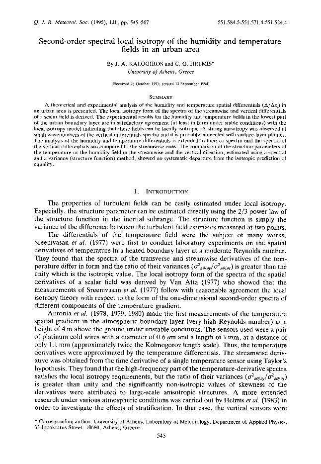
Q. J . R. Meteorol. Soc. (1995), 121, pp. 545-567 55 1.584.5 :55 1.571.4: 55 1 ,524.4

Second-order spectral local isotropy of the humidity and temperature fields in an urban area

By J. A. KALOGIROS and C. G . HELMIS* University of Athens, Greece

(Received 28 October 1993; revised 13 September 1994)

S u M M A R Y

A theoretical and experimental analysis of the humidity and temperature spatial differentials (A/Ax,) in an urban area is presented. The local isotropy form of the spectra of the streamwise and vertical differentials of a scalar field is derived. The experimental results for the humidity and temperature fields in the lowest part of the urban boundary layer are in satisfactory agreement (at least in form under stable conditions) with the local isotropy model indicating that these fields can be locally isotropic. A strong anisotropy was observed at small wavenumbers of the vertical differentials spectra and it is probably connected with surface-layer plumes. The analysis of the humidity and temperature differentials is extended to their co-spectra and the spectra of the vertical differentials are compared to the streamwise ones. The comparison of the structure parameters of the temperature or the humidity field in the streamwise and the vertical direction, estimated using a spectral and a variance (structure function) method, showed no systematic departure from the isotropic prediction of equality.

1. INTRODUCTION

The properties of turbulent fields can be easily estimated under local isotropy. Especially, the structure parameter can be estimated directly using the 2/3 power law of the structure function in the inertial subrange. The structure function is simply the variance of the difference between the turbulent field estimates measured at two points.

The differentials of the temperature field were the subject of many works. Sreenivasan et al. (1977) were first to conduct laboratory experiments on the spatial derivatives of temperature in a heated boundary layer at a moderate Reynolds number. They found that the spectra of the transverse and streamwise derivatives of the tem- perature differ in form and the ratio of their variances (02&/&,/a2&+/&) is greater than the unity which is the isotropic value. The local isotropy form of the spectra of the spatial derivatives of a scalar field was derived by Van Atta (1977) who showed that the measurements of Sreenivasan et al. (1977) follow with reasonable agreement the local isotropy theory with respect to the form of the one-dimensional second-order spectra of different components of the temperature gradient.

Antonia et al. (1978, 1979, 1980) made the first measurements of the temperature spatial gradient in the atmospheric boundary layer (very high Reynolds number) at a height of 4 m above the ground under unstable conditions. The sensors used were a pair of platinum cold wires with a diameter of 0.6 pm and a length of 1 mm, at a distance of only 1.1 mm (approximately twice the Kolmogorov length scale). Thus, the temperature derivatives were approximated by the temperature differentials. The streamwise deriv- ative was obtained from the time derivative of a single temperature sensor using Taylor’s hypothesis. They found that the high-frequency part of the temperature-derivative spectra satisfies the local isotropy requirements, but the ratio of their variances ( a 2 d @ / d y / 0 2 , @ / & )

is greater than unity and the significantly non-isotropic values of skewness of the derivatives were attributed to large-scale anisotropic structures. A more extended research under various atmospheric conditions was carried out by Helmis et al. (1983) in order to investigate the effects of stratification. In that case, the vertical sensors were

* Corresponding author: University of Athens, Laboratory of Meteorology, Department of Applied Physics, 33 Ippokratus Street, 10680, Athens, Greece.

545

546 J. A. KALOGIROS and C. G. HELMIS

pairs of 12.5 ,um diameter platinum wires of 40 cm length each, wound around a plexiglass former, and separated by a distance of 32 cm. The temperature-derivative spectra were shown to follow the theoretical isotropic relations under convective and near-neutral conditions and the ratio of the variances ( 0 2 d e / @ / a 2 d e / & ) was found to be greater than unity under stable conditions.

In a more recent laboratory study Mestayer (1982), using boundary-layer data with a high Reynolds number, questioned the local isotropy assumption in the inertial subrange for the velocity and temperature fields (and even in the dissipative subrange for the latter field) based on various statistics of the derivatives of these fields. Particularly, the odd order structure functions showed significant departure from the local isotropy relations, while the -5/3 power laws of spectra did not seem to be closely connected with the existence of local isotropy. The anisotropy was attributed to large-scale anisotropy conserved through the eddy cascade down to the very small scales. Similar results were obtained from Antonia er al. (1986) using turbulent plane jet data with a moderate Reynolds number. They also reproduced the previous result that the ratios of the mean- square values of the transverse and streamwise derivatives of the temperature ( d d o / & , /

a 2 d O / d x ) and the longitudinal velocity ( a2&/+/d&/&) are greater than the isotropic Values (1 and 2, respectively). The quasi-organized large-scale anisotropy in the velocity and temperature fields was associated with mean gradients of these fields and was shown to be more significant for the temperature statistics.

While many works have tested the local isotropy of the temperature field, second- order spectral tests for the local isotropy of the humidity field, e.g. through the spectrum of its streamwise and vertical differential, have not been considered in previous works. The spatial gradient vector of humidity is more difficult to measure since the small and fast sensors that are needed are not easily constructed. In this work the humidity differentials were measured with the psychrometric method using platinum wires and bead thermistors to measure dry- and wet-bulb temperature, respectively. Since the time response of the wet sensors was limited due to wicking, their output was corrected using the method proposed by Kalogiros and Helmis (1993) applied to differentials instead of scalar quantities. In this way it was possible to recover a rapidly varying signal at frequencies one order of magnitude higher than the cut-off frequency of the sensor.

In this paper the local isotropy form of the spectrum of the spatial differentials of a scalar field is derived in order to compare with the experimental results. Also, exper- imental indications of the local isotropy of the humidity differentials in an urban area are presented, and the temperature field and its correlation with the humidity field are examined. The structure parameters of temperature and humidity in the streamwise and the vertical direction, obtained with various methods, are used to test the local isotropy prediction of equality.

2. EXPERIMENTAL DETAILS

A turbulence probe was used, mounted on a fixed support of height 4 m on the roof- top of the seven-storey building of the Laboratory of Meteorology (25m high with a horizontal dimension of about 15 m at its top) in the centre of Athens, Greece. The full details of the probe are given by Asimakopoulos et af. (1980) and Helmis et al. (1983). The building is much higher (10 to 15 m) than the surrounding buildings and thus their wake or blocking effects are estimated to be low. Still, the experimental site is not entirely free of the aerodynamical influences of the building itself, even though the wind speed during the experiments is low (0.5-3 m s - ' ) . These influences are definitely reduced

SECOND-ORDER SPECTRAL LOCAL ISOTROPY 547

at a height of 4 m above the roof-top of the building especially for the higher wavenumbers (or frequencies) of the measured spectra. The effect of the experimental location on the measurements and the dynamic field is discussed in more detail, along with the measurement errors, in section 4.

The quantities measured were the horizontal wind velocity (miniature cup anem- ometer), the temperature (fine platinum wire of 12.5 pm diameter), and the wet-bulb temperature (bead thermistor) 15 cm upwind from the temperature sensor. The instru- ments face the wind by use of a wind vane on the probe. Also, the temperature difference in the vertical direction was measured using a pair of platinum wire sensors (12.5 pm) separated by a distance of 25 cm. The spatial streamwise difference of temperature (and similarly the corresponding difference of wet-bulb temperature) was obtained using the difference between consecutive measurements of the single temperature sensor and Taylor's hypothesis:

AT/Ax = {T(t) - T(t + At)}/(UAt) (1)

where U is the mean wind speed during the run, and At is the sampling period. The difference of wet-bulb temperature in the vertical direction was measured using a pair of wet thermistors separated by a distance of 11 or 25cm in the same experimental arrangement as the temperature sensors (interlaced with them for the 25 cm separation arrangement). Their output was corrected because of their limited time response (about 0.2 Hz for a wind speed of 3 m s-') according to Kalogiros and Helmis (1993).

The vapour pressure differentials Ae/Ax, were calculated by the dry- and wet-bulb temperature differentials (A T/Ax, and A T,/Ax,, respectively) using the derivative of the psychometric equation (Iribarne and Godson 1973) :

AelAx, = A AT,/Ax, + B AT/Ax, (2)

where A = 2354 (In 10){es(Twa)/T$a} - B , B = - y P , T,, is the average value of the wet- bulb temperature T, during the run, log {e,( T,)} = 9.4051 - 2354/T,, y = 0.66 x lop3 K-l is the psychrometric constant, and P the atmospheric pressure in mi lk bars. e is in millibars, and T and T, in kelvins. In the case of the streamwise differential Axl = Ax and for the vertical direction Ax2 = Az. The temperature (strictly speaking the potential temperature) is a conservative passive scalar, since enthalpy is a transportable quantity, and so is the humidity mixing ratio (or equivalently the vapour pressure e neglecting the pressure fluctuations, since the humidity mixing ratio r = 0.622e/P) accord- ing to mass conservation if there are no processes like chemical reactions or phase changes. Thus, according to the psychrometric equation the wet-bulb temperature is a transportable passive scalar and the isotropic relations should also apply to this scalar.

Ten runs of 20-minute period each were recorded on 14 February and 5 June 1991 with fair weather, under convective, near-neutral and stable conditions, with low winds (up to 3 m s-l). The sampling frequency was 10 Hz and the instrument outputs were filtered with analog low-pass filters (5 Hz) to avoid aliasing.

For each run the mean values of wind velocity, temperature, wet-bulb temperature, vapour pressure and the differentials of the temperature and vapour pressure and their variances were calculated. The power spectra of the measured physical quantities and the corresponding cross-spectra, phase and coherence spectra were also computed using a 1024-point Fast Fourier Transform (FFT) with segment averaging and logarithmic frequency smoothing for every 20-minute run. Finally, the structure parameters of temperature and vapour pressure were computed using the inertial subrange relation for the computed spectra or the structure functions.

548 J. A. KALOGIROS and C . G. HELMIS

3. THEORY

The separation distance between the sensors has a major impact on the spectra of the spatial differentials of a turbulent scalar field. A first approach to this problem was carried out by Browne et al. (1983) for a separation distance between the sensors of the order of the Kolmogorov microscale (a few millimetres). For such small distances the differentials can approximate the corresponding derivatives, but this is not usually the case. In the following paragraphs we derive the general form of the one-dimensional spectrum of the differential AB/Axj of a scalar field, 19, e.g. the temperature or the humidity field, under the local isotropy hypothesis. First, we review the isotropic spectral relations for the corresponding derivatives.

Let the three-dimensional scalar field 8 be represented by a Fourier-Stieltjes integral (Lumley and Panofsky 1964):

B(r) = eiK.r dZg(K) -I0

(3)

where dZO(K) is the Fourier transform coefficient, and K = (q, K ~ , K,) is the wavevector. Following Van Atta (1977) the one-dimensional spectra of the derivatives dB/dx and

under local isotropy are:

vJO/dx(Kx> = dvO(Kx) (4a) and, since K,VO(Kx) -+ 0 for K~ += according to the discussion below Eq. ( 5 )

or using Eq. (4a)

VdO/dx(Kx) = -Kx dVdO/dz(Kx)/dKx. (4c)

In the inertial subrange, where Eq. ( 5 ) below holds true, using Eqs. (4a) and (4c) we get:

vdO/&(Kx) = v J O / d z ( K i ) - 3{VJO/27(Kx) - vJO/Jx(Ki)) ( 4 4

where V(K,) is the one-dimensional spectrum of the quantity in the subscript at the wavenumber K~ (the along wind or x-component of the wavevector K), and K; is a wavenumber in the inertial subrange. The one-dimensional spectrum of 8 in the inertial subrange under local isotropy has the well known form of the -5/3 power law (Kaimal et al. 1972):

V ~ K , ) = 0.25C&5/3 ( 5 )

where Ciis the structure parameter of Band we restrict ourselves to positive wavenumbers K ~ . Equation (4a) leads to a 1/3 power law for vJO/&(Kx) while, according to Eq. (4d), vJO/Jz(Kx) does not follow a power law, but falls much slower than the -5/3 law of Ve(K,) in the inertial subrange. In the dissipation subrange there is an exponential fall-off of all these spectra (Tatarskii 1971; Tennekes and Lumley 1972). In the case of the one- dimensional spectrum of temperature this rapid fall-off is described by Eqs. (8) and (12) below. Thus, the integral in Eq. (4b) is convergent.

Since in practice the measurements are made in the time domain, Taylor’s hypothesis is used to convert the one-dimensional spectrum in the wavenumbers space to the measurable one-dimensional spectrum S(f) in the frequency domain f:

SECOND-ORDER SPECTRAL LOCAL ISOTROPY 549

The former analysis holds for the gradient of a scalar field 8: A8/Axj+ dO/dx j , for Axj+ 0. In practice, the measurements refer to the differential AO/Axj with Axj # 0. The differential of Eq. (3) is:

A8(r)/Axj = 1JJ-z ieiK"{sin(~jAxj/2)/( Axj/2)}dZO(~).

The previous relation implies that:

dZA O/Ax, ( K, = i{sin(K,Ax,/2) /( Ax,/2)}dZO( K)

and the three-dimensional spectrum is:

@A 6'/Axj ( K, = {sin(qk,/2> /( Ax]/2) }'@ O( K,

where @ ) 8 ( ~ ) is the three-dimensional spectrum of 0. The one-dimensional spectrum that is measured is:

+W

vAO/Axj(Kx) = 11 @AO/AX,X,(~) dKy dKz -m

= J1-1 {S~~(+X,/~)/(AX,/~)}~@,(K) dK, dK,.

For an isotropic field the three-dimensional spectrum depends only on the amplitude of the wavevector, QO ( K ) = QO (K), and is related to the one-dimensional spectrum VO(~ , ) with the relation (Tatarskii 1971):

@@ (K) = -(1/24 dVO (K)/dK. (8) Thus, the streamwise differential of an isotropic scalar field is:

vA @/Ax = {sin (KxAx/2)/( Ax/2) }2 Cmr QO (K)A d@ dA

= {sin(Kxhx/2)/(A.x/2))2VB (K,) (9) where A2 = K; + K:. This is the relation that was derived and tested by Browne et al. (1983).

For the vertical differential the approximation of Browne et al. (1983)-their Eq. (17)--cannot be used for our case of Az = 25 cm. A more precise analysis gives:

t m 2n VAO/A~(K,) = ( ~ / A z ) ~ 1 I sin2(A sin @Az/2) QO ( K ) A d@ dA

0 0

= (l/AZ)' /+m{l - Jo(AA.Z)}~JG@~(K) KdK

vAO:Az(Kx) = I {2J1(AAZ)/(AA2)}KV0 (K) dK.

(104 Kx

where Jo(x) is the Bessel fuhction of the first kind and zero order. Using the properties of the Bessel functions: Jo(0) = 1, Jo(w) = 0 and dJo(x)/dx = -Jl(x), where Jl(x) is the Bessel function of the first kind and first order, and Eqs. (8) and (loa) we get:

+m

(lob) KX

550 J. A. KALOGIROS and C. G. HELMIS

Equations (9) and (lob) tend to Eqs. (4a) and (4b) for the spectra of the spatial derivatives when Ax and Az tend to zero. In practice, this can be achieved when the separation distances are of the order of the Kolmogorov microscale, where the dissipation subrange begins. Equation (loa) or (lob) can be used for the cakulation of VA(f/A,(K,)

by numerical integration. Thus, the effect of the separation distance between the sensors on the spectrum of their difference can be examined.

In the case of the streamwise differential, combining Eqs. (9) and (4a) we get:

v A o / A x ( ~ x ) = {sin(~xA~/2)/(~,A~/2)}~Vd6r/dx(K,) (11) which means that for small wavenumbers K* < l/Ax--or frequencies f < U/(2nAx)-the effect (fall-off) of finite separation Ax on the measured spectrum v A e / A x is less than 10%. The correction factor tends to 1 for f + 0. The measured spectrum of the streamwise differential presents a maximum at f - 0.695 U/(nAx), assuming a 1/3 power law for Vde,h(~x) in the inertial subrange and that Ax is substantially larger than the Kolmogorov microscale. In our case, Ax = UAt = U/ f s , where fs = 10 Hz is the sampling frequency, and the maximum of the spectrum is at f = 2 Hz.

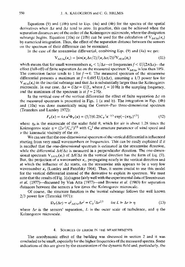
In the vertical case of the vertical differential the effect of finite separation Az on the measured spectrum is presented in Figs. 1 (a and b). The integration in Eqs. (4b) and (10a) was done numerically using the Corrsin-Pao three-dimensional spectrum (Tennekes and Lumley 1972):

F @ ( K ) = 4 n 2 i D o ( ~ ) = (5/3)0.25C02~-5/3 e x p { - ( ~ q ~ ) ~ / ~ ) (12) where qe is the microscale of the scalar field 8, which for air is about 1.28 times the Kolmogorov scale q = (Zv2/C,Z)3/8 with C: the structure parameter of wind speed and v the kinematic viscosity of the air.

We can see that the one-dimensional spectrum of the vertical differential is influenced starting from very small wavenumbers or frequencies. This can be easily explained if it is recalled that the one-dimensional spectrum is estimated in the streamwise direction, while the differential A8/Az is measured in a perpendicular direction. The one-dimen- sional spectrum VAo,Az(~,) of Ae/Az in the vertical direction has the form of Eq. (9). But, the projection of a wavenumber K,, propagating nearly in the vertical direction and at which the influence of Az starts, on the streamwise axis appears to be a very low wavenumber ivX (Lumley and Panofsky 1964). Thus, it seems crucial to use this model for the vertical differential instead of the derivative to explain its spectrum. We must note that the results of Fig. l(a) agree fairly well with the experimental data of Sreenivasan et al. (1977)-discussed by Van Atta (1977)-and Browne et al. (1983) for separation distances between the sensors a few times the Kolmogorov microscale.

Of course, the structure function in the inertial subrange follows the well known 2/3 power law (Tatarskii 1971):

Do ( A r ) = d A @ / A r A ? = ce for L 2+ Ar 2+ q (13) where Ar is the sensors’ separation, L is the outer scale of turbulence, and q the Kolmogorov microscale.

4. SOURCES OF ERROR IN THE MEASUREMENTS

The aerodynamic effect of the building was discussed in section 2 and it was concluded to be small, especially for the higher frequencies of the measured spectra. Some indications of this are given by the examination of the dynamic field and, particularly, the

SECOND-ORDER SPECTRAL LOCAL ISOTROPY 55 1

1

t 10 - 7 4

? O -’4

1 .o

2.0

5.0

20.0

100.0

500.0 \

nz+o

5 cm

10 cm

15 cm

20 cm

25 cm

30 cm

10- ’ f I 1 1 1 1 1 1 1 1 I I 1 1 1 1 1 1 1 I 1 1 1 1 1 1 1 1 I I 1

KO= 10 -’ 10 -’ 1 10

Kx (m-7 Figure 1. (a) The ratio of the one-dimensional spectra of the vertical differential Afl/Az and the vertical derivative do/& of a scalar field fl versus wavenumber rrx normalized with Az. (b) The ratio of the one- dimensional spectra of AB/Az at wavenumber rrX and a@/dz at wavenumber K~ = 10-3m-k for different values

of Az. The microscale qs was taken to be 1.0 mm.

552 J. A. KALOGIROS and C. G. HELMIS

power spectrum of the streamwise wind velocity using the measurements of the miniature cup anemometer with a frequency response up to 1 Hz for the low wind speed of our experiment (Figs. 3 and 6). The distortion of the fine structure of the dynamic field by an obstacle in a turbulent flow is highly variable in magnitude and sign, depending on the ratio of the integral scale of turbulence and the dimension of the obstacle perpendicular to the flow, the wavenumber range (low or high wavenumbers), and the position relative to the obstacle (Britter et al. 1979). Outside the boundary layer of the obstacle (i.e. not very close to its surface), this distortion is caused by the blocking mechanism (more significant near the obstacle surface) and the mean flow (vorticity) distortion by the obstacle. The wake-induced velocity fluctuations (vortex shedding) contribute to this distortion, too. The form of the wind velocity spectrum is modified depending on the degree of flow distortion and does not follow the isotropic -5/3 power law in the inertial subrange. No evident modification of the wind velocity spectrum was observed in our measurements, which indicate the existence of an inertial subrange (suggesting local equilibrium and no wake effects) in the same frequency range with the T and e measure- ments under unstable conditions, and probably under stable conditions (Figs. 3 and 6, respectively). Thus, the experimental site (4 m above the roof-top of that particular building) is presumably representative of the lowest part of the urban surface layer under the low wind speed conditions during our experiment.

The instrument that was used was designed to limit the measurement errors. Small currents (80 PA) were passed through the temperature sensors to avoid wind velocity sensitivity (Wyngaard 1971a). The effect of the configuration and the dimensions of the sensors were restricted at frequencies higher than 1 Hz (Wyngaard 1971b; Andreas 1981; Smedman and Lundin 1987). The differential sensors were matched to avoid the corruption of the temperature differences by their mean temperature (Mestayer and Chambaud 1979; Antonia et al. 1979). This error was limited by the relatively large separation distance between the differential sensors, too.

Two significant sources of error may be the frequency response of the sensors (especially the wet sensors) and the application of Taylor’s hypothesis. Taylor’s hypothesis is used for the calculation of the streamwise differences and the transfer of the theoretical results of section 3 to the frequency domain, according to Eq. (6).

(a) The effect of the frequency response of the sensors According to local isotropy, Eq. (ll), the spectrum of the streamwise differential,

which is measured using a single sensor, increases with frequency until a maximum is reached when Ax is in the inertial subrange. Thus, the measured variance may be seriously restricted by the cut-off frequency of the sensor and the low-pass filtering to avoid aliasing or noise. That depends on the position of the cut-off frequency relatively to the frequency of the maximum of the true spectrum of the streamwise differential. The first error, which is significant for the streamwise differential of wet-bulb temperature, is corrected applying the method presented by Kalogiros and Helmis (1993) to the measurements of the single wet sensor. The effect of the anti-aliasing filter is discussed in the experimental results (section 5(c)).

The error due to the mean cut-off frequency of the two vertical differential wet sensors was greatly corrected using the method described by Kalogiros and Helmis (1993) applied to the differential dry and wet sensors. But, because a differential amplifier was used at the output of the pair of wet thermistors, unlike the case of a single wet thermistor, the effect of the different frequency responses of the two sensors remains. The frequency response of each sensor depends on the quantity of the water on the wicking that covers the sensor. Thus, a difference between the frequency responses of the two sensors is

SECOND-ORDER SPECTRAL LOCAL ISOTROPY 553

inevitable. If the two wet sensors have cut-off frequencies fcl and fc2, respectively, the difference of the first-order linear approximation of their heat transfer equation, which is presented in Kalogiros and Helmis (1993), gives:

A T + (1/2nfcm)a(AT)/dt + (1/2nfc,)dTm/at = AT, (14a)

where f c m = 2fclfc2/(fc~ + fed, fcd = fclfC2/(fcl - f c 2 ) , A T is the measured temperature difference, Tm = (TI + T2)/2 is the mean value of the sensors measurements, and AT, is the ambient temperature difference. By Fourier transforming Eq. (14a) we get for the Fourier transforms:

XAT + i(f/fcm)XAT + i(f/fcd)xTm = xATa- (14b)

The third term on the left side is due to the difference in the cut-off frequency of the sensors introducing the Fourier transform of their mean temperature. Since the spectrum (proportional to the square magnitude of the corresponding Fourier transform) of the temperature follows the -5/3 power law in the inertial subrange, this term is more significant at the higher frequencies. Also, the effect of the difference in the cut-off frequency of the two sensors is proportional to this difference. This effect was observed experimentally when the correction for the mean cut-off frequency fcm was applied to the pair of differential sensors of the wet-bulb temperature. The spectrum of ATW/Az presented a fall-off compared to the theoretical form at frequencies higher than 0.5 Hz. This was attributed to the difference in the cut-off frequency of the wet sensors.

(b) The error due to the application of Taylor’s hypothesis The application of Taylor’s hypothesis, involving Eq. (6), leads to an energy transfer

from the lower frequencies to the higher ones because of the fluctuations of the convection velocity (Wyngaard and Clifford 1977). The power spectra in the inertial subrange are not especially overestimated.

But, the application of Taylor’s hypothesis in the calculation of the streamwise differential, using Eq. (l) , may introduce a serious effect on its total variance. According to Wyngaard and Clifford (1977) and Antonia et al. (1980) the error introduced in the true total variance of ae/ax is:

&/axm = a2,9/ax (1 + 6 d / ( 2 U 2 ) ) (15) where a 6/dxm is the measured streamwise derivative using Taylor’s hypothesis. This correction is quite important for the correct estimation of the variance of the streamwise derivative. We must note that Eq. (15) refers to the total variance of the streamwise derivative. The case of the streamwise differential leads to a correction that depends on Ax. According to Wyngaard and Clifford (1977), the measured one-dimensional spectrum of the scalar field 0 is:

Vgm(Kx) = Vo (K,) + ( O ~ , / ~ U ~ ) ( K ; ~ ~ V O / ~ K , ~ + 2~,dVg/d~,). (16)

Using Eqs. (16) and (9), we can calculate the one-dimensional spectrum of AO/Axm = -A6/( UAt). The integral of VAo/k,m over the whole range of K~ gives the total variance of AO/Axm, i.e. the streamwise differential using Taylor’s hypothesis (Eq. (1)). We used the Corrsin-Pao three-dimensional spectrum, Eq. (12), to evaluate numerically the error in &g,Axm in the form of Eq. (15):

&/,m = a2Ao/Ax{1 + A(u2,/2U2)I. (17)

554 J. A. KALOGIROS and C . G. HELMIS

0.0 10 -' 1 10 10

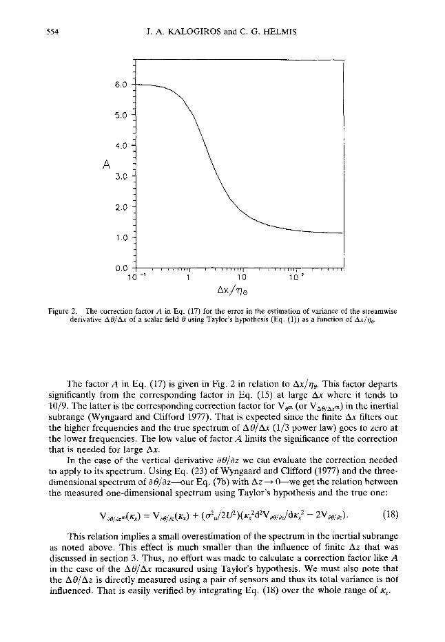
Figure 2. The correction factor A in Eq. (17) for the error in the estimation of variance of the streamwise derivative AO/Ax of a scalar field O using Taylor's hypothesis (Eq. (1)) as a function of Ax/qe .

The factor A in Eq. (17) is given in Fig. 2 in relation to A.x/qO. This factor departs significantly from the corresponding factor in Eq. (15) at large Ax where it tends to 10/9. The latter is the corresponding correction factor for Vem (or Vholhxm) in the inertial subrange (Wyngaard and Clifford 1977). That is expected since the finite Ax filters out the higher frequencies and the true spectrum of AO/Ax (1/3 power law) goes to zero at the lower frequencies. The low value of factor A limits the significance of the correction that is needed for large Ax.

In the case of the vertical derivative dO/az we can evaluate the correction needed to apply to its spectrum. Using Eq. (23) of Wyngaard and Clifford (1977) and the three- dimensional spectrum of dO/az-our Eq. (7b) with Az + &we get the relation between the measured one-dimensional spectrum using Taylor's hypothesis and the true one:

This relation implies a small overestimation of the spectrum in the inertial subrange as noted above. This effect is much smaller than the influence of finite Az that was discussed in section 3. Thus, no effort was made to calculate a correction factor like A in the case of the AO/Ax measured using Taylor's hypothesis. We must also note that the AB/hz is directly measured using a pair of sensors and thus its total variance is not influenced. That is easily verified by integrating Eq. (18) over the whole range of K ~ .

SECOND-ORDER SPECTRAL LOCAL ISOTROPY 555

5. EXPERIMENTAL RESULTS

In this section we present the experimental results of two 20-minute runs under unstable and stable conditions, respectively. For each run the mean values and the variances of wind speed U , temperature T , and vapour pressure e are given. The Reynolds number Re and the Kolmogorov microscale q determined from the structure parameter of wind speed for each run are also given. The lower scale of the inertial subrange is of the order of the height z above ground (29 m in our case) under unstable conditions and a fraction (1110) of the Monin-Obukhov length (not measured in our experiment) under stable conditions in the surface layer (Kaimal et al. 1972). Thus, the outer scale of turbulence L was approximated by the height above ground (Re = Uz/v), and the lower frequency f o and the higher frequency f K of the inertial subrange were approximated by U / z and U/(2~cq), respectively. Furthermore, the spectra of T , e, AT/Axj , AT,/Axi, and AelAx,, and the coherence and phase spectra of AelAx, - AT/Axi in the frequency range 9.8 x to 4.7 Hz are presented and discussed. Finally, the structure parameters of T and e in the streamwise and the vertical direction, calculated for the ten processed runs, using the inertial subrange form of the spectra and the structure functions, are compared as an additional check of local isotropy.

(a) Unstable conditions The run presented here started at 1204 LST -1004 GMT (near noon) on 5 June 1991

(sunset at 2030 LST) and the sky was clear. The mean values and variances of U , T , and e are shown in Table 1. The relative humidity was 34%. The separation distance for the streamwise and the vertical differential was Ax = UAt = U/fs = 20 cm, and Az = 25 cm, respectively ( f s = 10 Hz is the sampling frequency). The turbulent parameters are Re = 3.97 X lo6, r/ = 0.64 mm, and an inertial subrange is expected between the frequencies f, = 6.9 X lop2 Hz and f K = 497 Hz.

TABLE 1. THE AVERAGE VALUES AND VARIANCES OF WIND SPEED (rr), DRY-BULB TEM- PERATURE (13, AND VAPOUR PRESSURE (e) FOR THE TWO 20-MINUTE RUNS PRESENTED IN THE

EXPERIMENTAL RESULTS

Time (LST) U 02” T (JZT e a2e Date Stability (ms-I) (m’s-’) (“C) (“C’) (mb) (mb’)

5 Jun. 1991 1204 2.0 0.78 28.2 0.29 13.2 0.13

14 Feb. 1991 2040 0.6 0.12 13.2 0.02 11.7 0.06 convective

stable

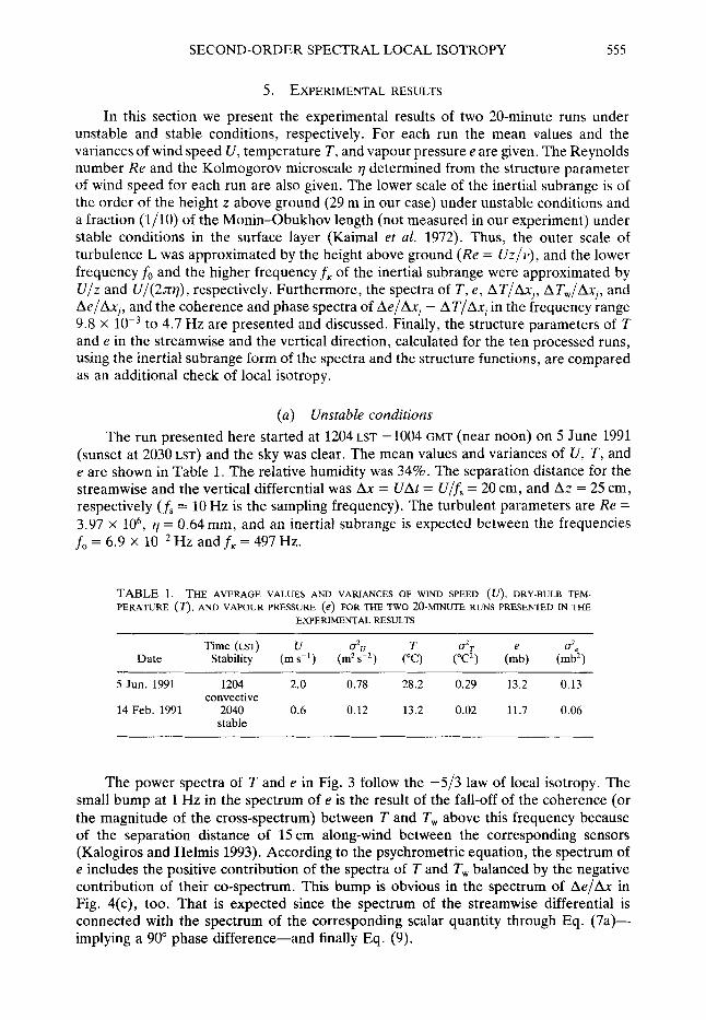
The power spectra of T and e in Fig. 3 follow the -513 law of local isotropy. The small bump at 1 Hz in the spectrum of e is the result of the fall-off of the coherence (or the magnitude of the cross-spectrum) between T and T, above this frequency because of the separation distance of 15 cm along-wind between the corresponding sensors (Kalogiros and Helmis 1993). According to the psychrometric equation, the spectrum of e includes the positive contribution of the spectra of T and T, balanced by the negative contribution of their co-spectrum. This bump is obvious in the spectrum of Ae/Ax in Fig. 4(c), too. That is expected since the spectrum of the streamwise differential is connected with the spectrum of the corresponding scalar quantity through Eq. (7a)- implying a 90” phase difference-and finally Eq. (9).

556

10 -5

J. A. KALOGIROS and C. G. HELMIS

0 .

0.

0

' 4 A

5/3

A A A A A s, ..... ST

0 0 0 0 0 s,

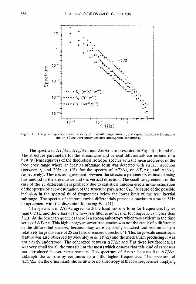
The spectra of ATlAx,, ATw/Axl, and AelAx, are presented in Figs. 4(a, b and c). The structure parameters for the streamwise and vertical differentials correspond to a best fit (least squares) of the theoretical isotropic spectra with the measured ones in the frequency range where an inertial subrange form was detected with visual inspection (between fo and 2 Hz or 1 Hz for the spectra of AT/Ax, or ATwAx,, and AelAx,, respectively). There is an agreement between the structure parameters estimated using this method in the streamwise and the vertical direction. The small disagreement in the case of the T, differentials is probably due to statistical random errors in the estimation of the spectra or a low estimation of the structure parameter CTw$ because of the possible inclusion in the spectral fit of frequencies below the lower limit of the true inertial subrange. The spectra of the streamwise differentials present a maximum around 2 Hz in agreement with the discussion following Eq. (11).

The spectrum of AT/Az agrees with the local isotropy form for frequencies higher than 0.2 Hz and the effect of the low-pass filter is noticeable for frequencies higher than 3 Hz. At the lower frequencies there is a strong anisotropy which was evident in the time series of ATlAz. This high energy at lower frequencies was not the result of a difference in the differential sensors, because they were especially matched and separated by a relatively large distance of 25 cm (also discussed in section 4). This large-scale anisotropic feature was also observed by Moulsley et al. (1982) and the mechanism producing it was not clearly understood. The coherence between AT/Az and T at these low frequencies was very small for all the runs (0.1 at the most) which ensures that this kind of error was not introduced in our measurements. The spectrum of Ae/Az behaves like AT/Az , although the anisotropy continues to a little higher frequencies. The spectrum of ATw/Az, on the other hand, shows little or no anisotropy at the low frequencies, implying

SECOND-ORDER SPECTRAL LOCAL ISOTROPY

10 - l ?

10 -2y

10 -3z

n

I N

c

I N I

€ N

0

4 W

._ \ 3 I- cn"

J 0

10 - l =

10 -*= 0

0 0

0

0

10 -2 10 - l 1 f (Hz)

0

= = . 10 - 4 4

cTW,2=o. 1 1 XI 0-' 0~2m-2'3

CTw:=O. 1 6 x 1 0-' 0C2m-2'3 10 - 5 1

0 0

0

0

0

0

0

557

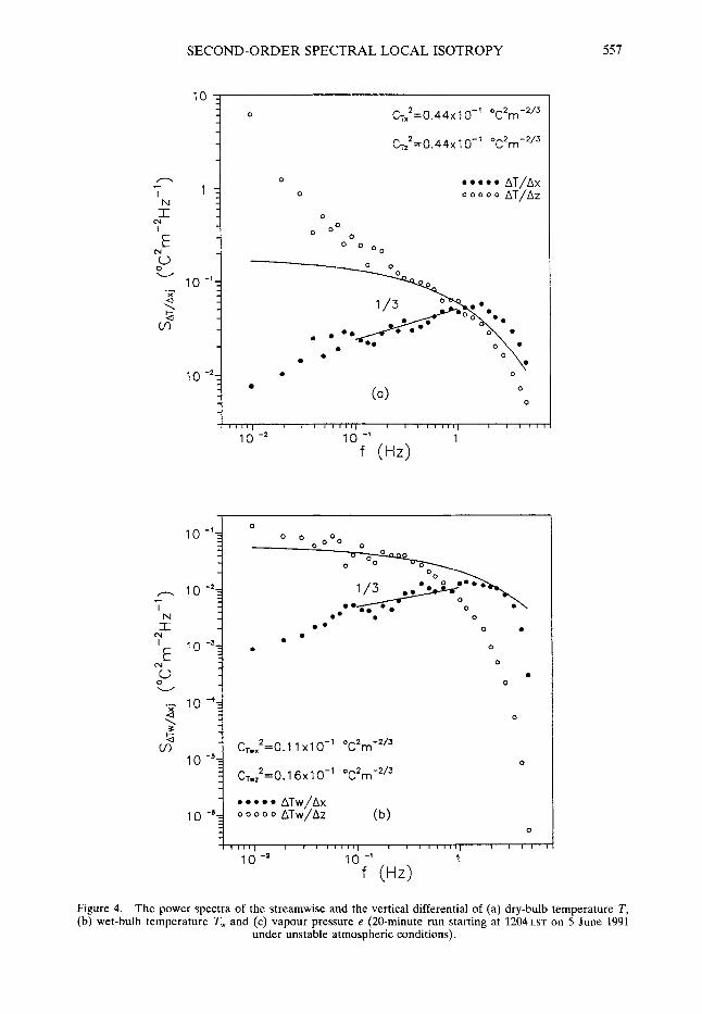
Figure 4. The power spectra of the streamwise and the vertical differential of (a) dry-bulb temperature T, (b) wet-bulb temperature T, and (c) vapour pressure e (20-minute run starting at 1204 LST on 5 June 1991

under unstable atmospheric conditions).

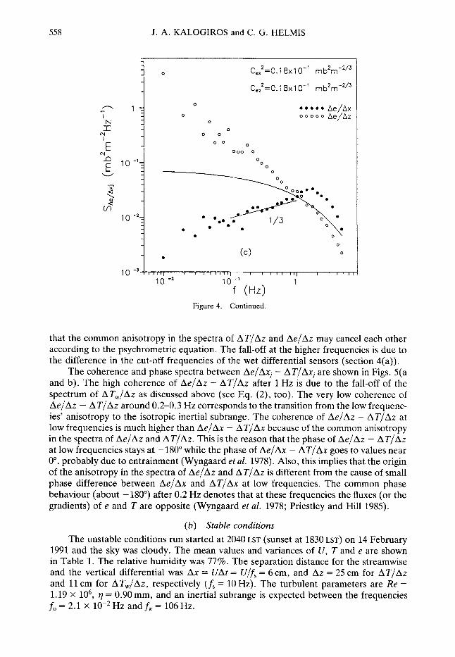
558 J. A. KALOGIROS and C. G. HELMIS

l o Ce:=O. 1 8 x 1 0-' M b2rn-2'3

Ce,*=O.18x1 0-' rnb2rn-2'3

0

0

10 -?

Figure 4. Continued.

that the common anisotropy in the spectra of A T / A z and Ae/Az may cancel each other according to the psychrometric equation. The fall-off at the higher frequencies is due to the difference in the cut-off frequencies of the wet differential sensors (section 4(a)).

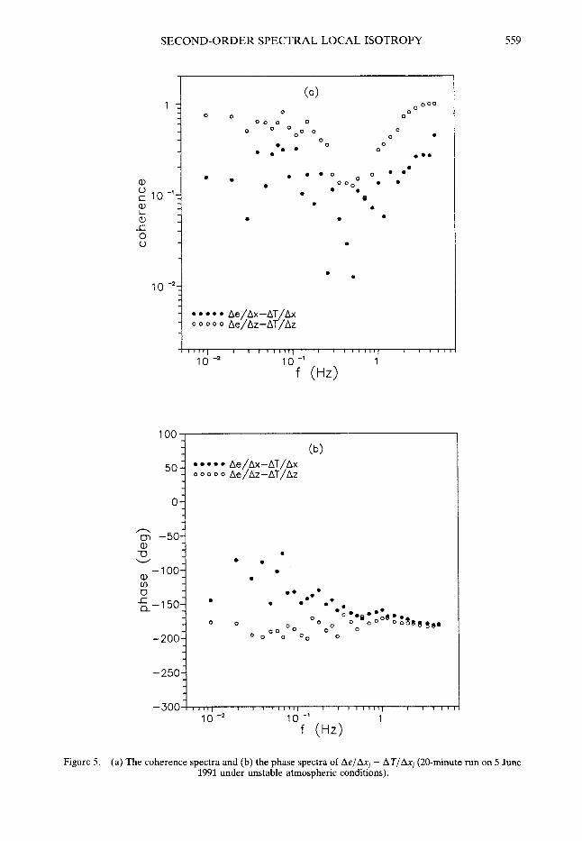
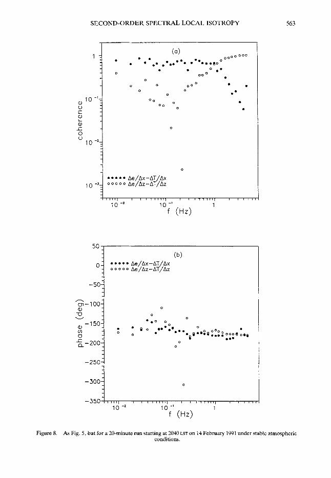
The coherence and phase spectra between Ae/Axi - AT/Axi are shown in Figs. 5(a and b). The high coherence of Ae/Az - A T / A z after 1 Hz is due to the fall-off of the spectrum of AT,/Az as discussed above (see Eq. (2), too). The very low coherence of Ae/Az - A T / A z around 0.2-0.3 Hz corresponds to the transition from the low frequenc- ies' anisotropy to the isotropic inertial subrange. The coherence of Ae/Az - A T / A z at low frequencies is much higher than Ae/Ax - AT/Ax because of the common anisotropy in the spectra of A e / A z and A T / A z . This is the reason that the phase of Ae/Az - A T / A z at low frequencies stays at -180" while the phase of Ae/Ax - AT/Ax goes to values near Oo, probably due to entrainment (Wyngaard et al. 1978). Also, this implies that the origin of the anisotropy in the spectra of Ae/Az and A T / A z is different from the cause of small phase difference between Ae/Ax and AT/Ax at low frequencies. The common phase behaviour (about -180") after 0.2 Hz denotes that at these frequencies the fluxes (or the gradients) of e and T are opposite (Wyngaard et al. 1978; Priestley and Hill 1985).

( b ) Stable conditions The unstable conditions run started at 2040 LST (sunset at 1830 LST) on 14 February

1991 and the sky was cloudy. The mean values and variances of U , T and e are shown in Table 1. The relative humidity was 77%. The separation distance for the streamwise and the vertical differential was Ax = UAt = U/fs = 6 cm, and Az = 25 cm for A T / A z and 11 cm for AT,/Az, respectively (fs = 10 Hz). The turbulent parameters are Re = 1.19 x lo6, q = 0.90 mm, and an inertial subrange is expected between the frequencies fo = 2.1 x lo-* Hz and f K = 106 Hz.

SECOND-ORDER SPECTRAL LOCAL ISOTROPY 559

100 J 1

Figure 5. (a) The coherence spectra and (b) the phase spectra of Ae/Ax, - AT/Ax, (20-minute run on 5 June 1991 under unstable atmospheric conditions).

560 J. A. KALOGIROS and C. G. HELMIS

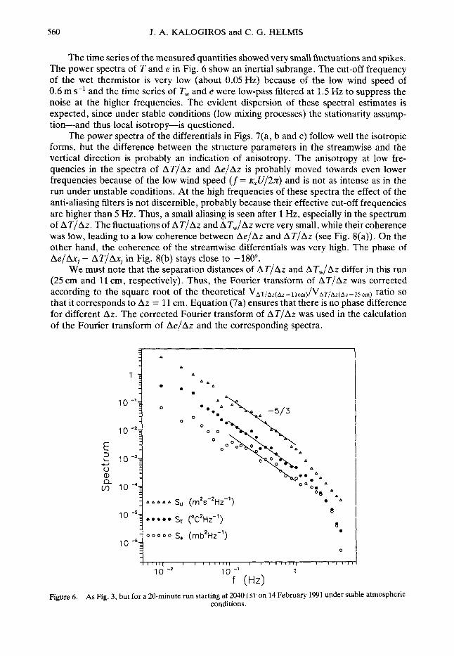
The time series of the measured quantities showed very small fluctuations and spikes. The power spectra of T and e in Fig. 6 show an inertial subrange. The cut-off frequency of the wet thermistor is very low (about 0.05Hz) because of the low wind speed of 0.6 m s-l and the time series of T, and e were low-pass filtered at 1.5 Hz to suppress the noise at the higher frequencies. The evident dispersion of these spectral estimates is expected, since under stable conditions (low mixing processes) the stationarity assump- tion-and thus local isotropy-is questioned.

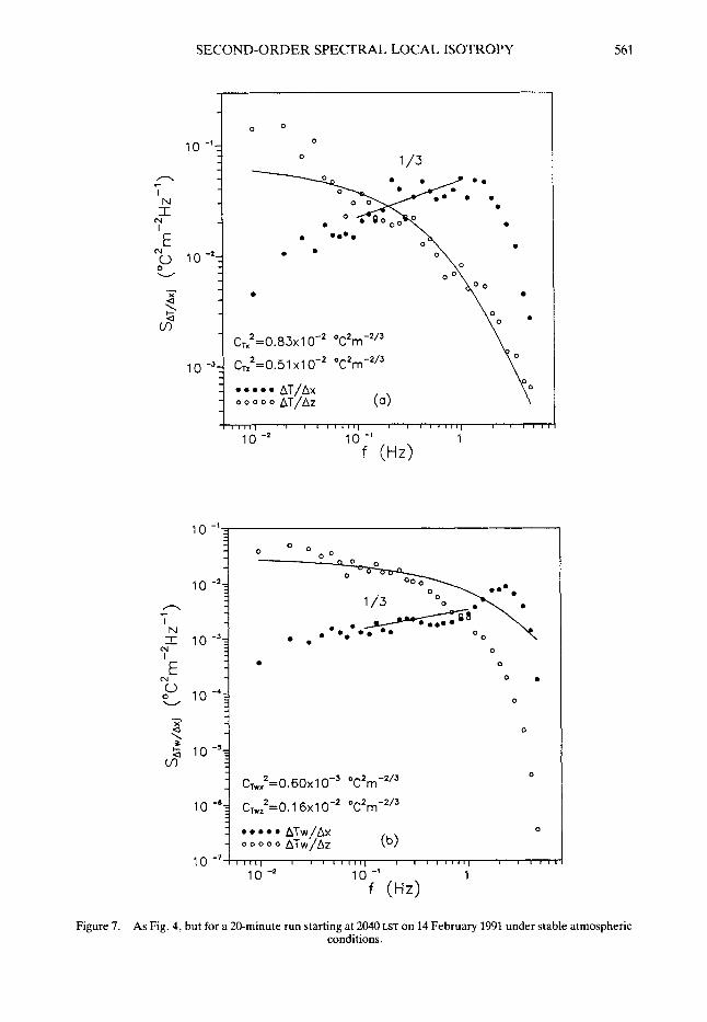
The power spectra of the differentials in Figs. 7(a, b and c) follow well the isotropic forms, but the difference between the structure parameters in the streamwise and the vertical direction is probably an indication of anisotropy. The anisotropy at low fre- quencies in the spectra of AT1A.z and Ae/Az is probably moved towards even lower frequencies because of the low wind speed ( f = K , U / ~ J G ) and is not as intense as in the run under unstable conditions. At the high frequencies of these spectra the effect of the anti-aliasing filters is not discernible, probably because their effective cut-off frequencies are higher than 5 Hz. Thus, a small aliasing is seen after 1 Hz, especially in the spectrum of AT/Az. The fluctuations of AT/Az and ATw/Az were very small, while their coherence was low, leading to a low coherence between Ae/Az and AT/Az (see Fig. 8(a)). On the other hand, the coherence of the streamwise differentials was very high. The phase of he/&, - AT/Axj in Fig. 8(b) stays close to -180".

We must note that the separation distances of AT/Az and hTw/Az differ in this run (25 cm and 11 cm, respectively). Thus, the Fourier transform of AT/Az was corrected according to the square root of the theoretical VAT/At (Ar= IlCm)/VAT/Ar(Az=25 cm) ratio so that it corresponds to Az = 11 cm. Equation (7a) ensures that there is no phase difference for different Az. The corrected Fourier transform of AT/Az was used in the calculation of the Fourier transform of Ae/Az and the corresponding spectra.

A

.'HZ-') * A

8

8

0

-II I I , 1 1 1 1 1 1 , I , I I I I , , , I ! ( 1 1

I d -2 10 -' 1 f (Hz)

Figure 6. As Fig. 3, but for a 20-minute run starting at 2040 LST on 14 February 1991 under stable atmospheric conditions.

SECOND-ORDER SPECTRAL LOCAL ISOTROPY

I

E ,O W 10-4 N

561

0

0

0 .

0

O - i

O\ 0 .

0-2 O ~ 2 ~ - 2 / 3

o-2 0cZm-2/3

C~,,2=0.60~1 0-3 0C2rn-2’3

CTw;=O. 1 6x 1 O-’ 0C2m-2’3

* * * * * ATw/Ax o o o o o ATw/Az (b)

0

0

0

Figure 7. As Fig. 4, but for a 20-minute run starting at 2040 LST on 14 February 1991 under stable atmospheric conditions.

562 J. A. KALOGIROS and C. G. HELMIS

n 7

I N r

N I E n N

E W

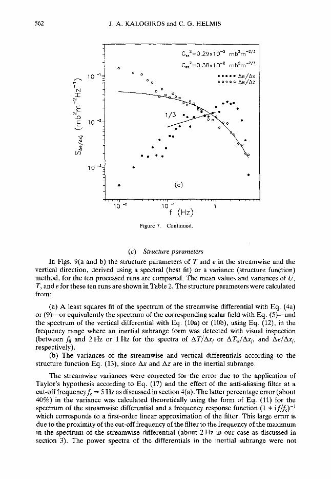
Ce,2=0.29x1 O-’ rr~b’rn-~’~

0 Ce,2=O.38x1 O-’ rr~b~rn-~/’ 0 0

0 0

. am

a

* . .. * .

Figure 7. Continued

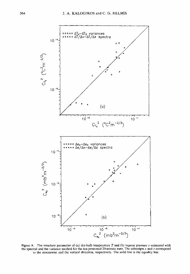
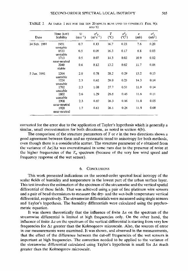
(c ) Structure parameters In Figs. 9(a and b) the structure parameters of T and e in the streamwise and the

vertical direction, derived using a spectral (best fit) or a variance (structure function) method, for the ten processed runs are compared. The mean values and variances of U , T , and e for these ten runs are shown in Table 2. The structure parameters were calculated from:

(a) A least squares fit of the spectrum of the streamwise differential with Eq. (4a) or (9)--or equivalently the spectrum of the corresponding scalar field with Eq. (5)-and the spectrum of the vertical differential with Eq. (loa) or (lob), using Eq. (12), in the frequency range where an inertial subrange form was detected with visual inspection (between fo and 2 Hz or 1 Hz for the spectra of ATIAxi or ATW/Axi, and Ae/Axi, respectively).

(b) The variances of the streamwise and vertical differentials according to the structure function Eq. (13), since Ax and Az are in the inertial subrange.

The streamwise variances were corrected for the error due to the application of Taylor’s hypothesis according to Eq. (17) and the effect of the anti-aliasing filter at a cut-off frequencyf, = 5 Hz as discussed in section 4(a). The latter percentage error (about 40%) in the variance was calculated theoretically using the form of Eq. (11) for the spectrum of the streamwise differential and a frequency response function (1 + if/fc)-I which corresponds to a first-order linear approximation of the filter. This large error is due to the proximity of the cut-off frequency of the filter to the frequency of the maximum in the spectrum of the streamwise differential (about 2Hz in our case as discussed in section 3). The power spectra of the differentials in the inertial subrange were not

SECOND-ORDER SPECTRAL LOCAL ISOTROPY 563

50 I I

-3001 0

-350 1 10 -z

Figure 8. As Fig. 5, but for a 20-minute run starting at 2040 LST on 14 February 1991 under stable atmospheric conditions.

564 J. A. KALOGIROS and C. G . HELMIS

n

3 I

E N 0 W

N c 0

n rl

‘E: I

E

E N a v

N c 0

10

10

10

0

10

0 0 0 0 0 ATx-ATZ variances A A A A A AT/AX-AT/AZ spectra

-2-

I I I , I I I , 10 -2 10 -‘

0 0 0 0 0 Aex-Aez variances 6 A 6 6 A Ae/Ax-Ae/Az spectra 3 -1

0 0 0 0 0 Aex-Aez variances 6 A 6 6 A Ae/Ax-Ae/Az spectra

-1 -

-2 -

-3-

I , , , I

10 -’ 10 -2 10 -l Id -l 1 0 -’ CeX2 (m b2m-2’3)

Figure 9. The structure parameter of (a) dry-bulb temperature T and (b) vapour pressure e estimated with the spectral and the variance method for the ten processed 20-minute runs. The subscripts x and z correspond

to the streamwise and the vertical direction, respectively. The solid line is the equality line.

SECOND-ORDER SPECTRAL LOCAL ISOTROPY 565

TABLE 2. AS TABLE 1 BUT FOR THE TEN 20-MINUTE RUNS USED TO CONSTRUCT FIGS. 9(a AND b)

Time (LST) U U2” T f f 2 T e U2e

Date Stability (ms-’) (m’s-’) (“C) (“C’) (mb) (mb’)

14 Feb. 1991

5 Jun. 1991

1451 unstable

1533 unstable

1713 near-neutral

2040 stable

1204 unstable

1224 unstable

1702 unstable

1802 unstable

1908 near-neutral

1928 near-neutral

0.7 0.13 16.7

0.5 0.09 16.3

0.5 0.07 14.3

0.6 0.12 13.2

2.0 0.78 28.2

2.3 0.82 28.0

2.3 1.08 27.7

2.6 1.29 26.8

2.3 0.87 26.3

1.7 0.61 26.1

0.23 7.6

0.17 8.8

0.02 10.9

0.02 11.7

0.29 13.2

0.25 14.3

0.51 11.9

0.45 11.6

0.16 11.8

0.26 11.9

0.20

0.03

0.02

0.06

0.13

0.14

0.14

0.11

0.05

0.08

corrected for the error due to the application of Taylor’s hypothesis which is generally a similar, small overestimation for both directions, as noted in section 4(b).

The comparison of the structure parameters of Tor e in the two directions shows a good agreement between them and no systematic trend to anisotropy for both methods, even though there is a considerable scatter. The structure parameter of e obtained from the variance of Ae/Ax was overestimated in some runs due to the presence of noise at the higher frequencies of the T, spectrum (because of the very low wind speed and frequency response of the wet sensor).

6 . CONCLUSIONS

This work presented indications on the second-order spectral local isotropy of the scalar fields of humidity and temperature in the lowest part of the urban surface layer. This test involves the estimation of the spectmm of the streamwise and the vertical spatial differential of these fields. That was achieved using a pair of fine platinum wire sensors and a pair of bead thermistors to measure the dry- and the wet-bulb temperature vertical differential, respectively. The streamwise differentials were measured using single sensors and Taylor’s hypothesis. The humidity differentials were calculated using the psychro- metric equation.

It was shown theoretically that the influence of finite Ax on the spectrum of the streamwise differential is limited at high frequencies only. On the other hand, the influence of finite Az on the spectrum of the vertical differential is starting from very low frequencies for Az greater than the Kolmogorov microscale. Also, the sources of error in our measurements were examined. It was shown, and observed in the measurements, that the effect of the difference between the cut-off frequencies of the wet sensors is important at high frequencies. The correction needed to be applied to the variance of the streamwise differential calculated using Taylor’s hypothesis is small for Ax much greater than the Kolmogorov microscale.

566 J. A. KALOGIROS and C . G. HELMIS

The measured spectra of the humidity and temperature differentials under unstable and stable conditions were compared to the theoretically derived ones and a good agreement was noticed (at least in form under stable conditions). A common strong anisotropy was observed at the lower frequencies of the spectra of the vertical differentials of the humidity and temperature fields. This anisotropy produced a difference between the frequency behaviour of the coherence and the phase spectra of Ae/Az - AT/Az and Ae/Ax - AT/Ax. This anisotropy is probably connected with the horizontal inhomogeneities (buildings alternating with parks and streets) of the urban area that can trigger, even under stable atmospheric conditions, surface-layer plumes having diameters of the order of 100m (Stull 1988). These plumes are anisotropic vertical structures transported by the wind, with most of their energy in the vertical direction, producing ramp-like shapes in the temperature and wind velocity traces that were observed in the time series of our measurements, too. On the other hand, these structures are charac- terized by strong vertical temperature (superadiabatic) and humidity gradients, while the air between them is almost neutrally stratified, and, thus, they contribute significantly to the lower frequencies of the spectra of the vertical differentials of the temperature and humidity fields. Finally, the structure parameters of the humidity or the temperature field in the streamwise and the vertical direction, estimated using the spectral or the variance method, were compared and no systematic departure from the local isotropy prediction of equality was observed, even though there was some dispersion in the data.

Andreas, E. L.

Antonia, R. A. M., Anselmet, F.

Antonia, R. A. and

Antonia, R. A., Chambers, A. J.,

and Chambers, A. J .

Chambers, A. J.

Phong-Anant, D. and Rajagopalan, S.

Antonia, R. A . , Chambers, A. J. and Phan-Thien, N.

Asimakopoulos, D. N., Lalas, D. P., Helmis, C. G . and Caroubalos, C. A.

Mumford, J. C.

Chambers, A. J.

Britter, R. E., Hunt, J. C. R. and

Browne, L. W., Antonia, R. A. and

Helmis, C. G . , Asimakopoulos, D. N., Lalas, D. P. and Moulsley, T. J.

Iribarne, J . V. and Godson, W. L.

Kaimal, J . C., Wyngaard, J. C., Izumi, Y. and Cote, 0. R.

Kalogiros, J. A. and Helmis, C. G.

Lumley, J. L. and Panofsky, H. A. Mestayer, P.

1981

1986

1978

1979

1980

1980

1979

1983

1983

1973

1972

1993

1964 1982

REFERENCES The effects of volume averaging on spectra measured with a

Lyman-alpha hygrometer. J . Appl. Meteorol., 20, 467- 475

Assessment of local isotropy using measurements in a turbulent plane jet. J . Fluid Mech., 163, 365-391

Spectra of temperature derivatives in the atmospheric surface layer. Boundary-Layer Meteorol., 15, 341-345

Properties of spatial temperature derivatives in the atmospheric surface layer. Boundary-Layer Meteorol.,

Taylor’s hypothesis and spectra of velocity and temperature derivatives in a turbulent shear flow. Boundary-Layer Meteorol., 19, 19-29

An atmospheric turbulence probe. IEEE Trans. Geosci. Remote Sensing, GE-18, 347-353

17, 101-118

The distortion of turbulence by a circular cylinder. J . Fluid Mech., 92, 269-301

Effect of the separation between cold wires on the spatial derivatives of temperature in a turbulent flow. Boundary- Layer Meteorol., 27, 129-139

On the local isotropy of the temperature field in an urban area. J. Appl. Meteorol., 22, 1594-1601

Atmospheric thermodynamics. Geophysics and Astrophysics

Spectral characteristics of surface-layer turbulence. Q. J . R.

Fast-response humidity measurements with the physchrometric

The structure of atmospheric turbulence. Interscience, Wiley Local isotropy and anisotropy in a high-Reynolds-number

turbulent boundary layer. J . Fluid Mech., 125, 475-503

Monographs, Vol. 6. D. Reidel Publishing Company

Meteorol. SOC., 98, 56S589

method. J . Appl. Meteorol., 32, 1499-1507

SECOND-ORDER SPECTRAL LOCAL ISOTROPY 567

Mestayer, P. and Chambaud, P.

Moulsley, T. J . , Asimakopoulos, D. N., Cole, R. S. , Caughey, S. J and Crease, B. A.

Priestley, J . T. and Hill, R. J.

Sreenivasan, K. R., Antonia, R. A.

Smedman, A . and Lundin, K. and Danh, H. Q.

Stull. R. B.

Tatarskii, V. I.

Tennekes, H. and Lumley, J. L. Van Atta, C. W.

Wyngaard, J. C

Wyngaard, J . C. and Clifford, S. F.

Wyngaard, J. C., Penel, W. T., Lenschow, D . H. and Lemone, M. A .

1979

1982

1985

1977

1987

1988

1971

1972 1977

1971a

1971b

1977

1978

Some limitations to measurements of turbulence micro-struc- ture with hot and cold wires. Boundary-Layer Meteorol.,

Temperature structure parameter measurements using dif- ferential temperature sensors. Boundary-Layer Meteorol., 23, 307-315

16, 311-329

Measuring high-frequency humidity, temperature and radio refractive index in the surface layer. J . Atmos. Ocean. Technol., 2, 233-251

Temperature dissipation fluctuations in a turbulent boundary layer. Phys. Fluids, 20, 1238-1249

Influence of sensor configuration on measurements of dry and wet-bulb temperature fluctuations. J . Atmos. Ocean. Technol., 4, 668-673

An Introduction to boundary layer meteorology. Kluwer Academic Publishers, Dordrecht/Boston/London

The effects of the turbulent atmosphere on wave propagation. Israel Program for Scientific Translations, Jerusalem

A first course in turbulence. MIT Press, Cambridge, Mass Second-order spectral local isotropy in turbulent scalar fields.

J . Fluid. Mech., 80, 609-615 The effect of velocity sensitivity on temperature derivative

statistics in isotropic turbulence. J . Fluid Mech., 48,763- 769

Spatial resolution of a resistance wire temperature sensor. Phys. Fluids., 14, 2052-2054

Taylor’s hypothesis and high-frequency turbulence spectra. J . Atmos. Sci., 34, 922-929

The temperature-humidity covariance budget in the convective boundary layer. J . Atmos. Sci., 35, 47-58