15 APRIL 2003 1041L U E T A L .

q 2003 American Meteorological Society

Analysis of Humidity Halos around Trade Wind Cumulus Clouds

MIAO-LING LU,* JIAN WANG,*,@ ANDREW FREEDMAN,1 HAFLIDI H. JONSSON,# RICHARD C. FLAGAN,*ROBERT A. MCCLATCHEY,1 AND JOHN H. SEINFELD*

*California Institute of Technology, Pasadena, California1Aerodyne Research, Inc., Billerica, Massachusetts#Naval Postgraduate School, Monterey, California

(Manuscript received 17 June 2002, in final form 12 November 2002)

ABSTRACT

Regions of enhanced humidity in the vicinity of cumulus clouds, so-called cloud halos, reflect features ofcloud evolution, exert radiative effects, and may serve as a locus for new particle formation. Reported here arethe results of an aircraft sampling campaign carried out near Oahu, Hawaii, from 31 July through 10 August2001, aimed at characterizing the properties of trade wind cumulus cloud halos. An Aerodyne Research, Inc.,fast spectroscopic water vapor sensor, flown for the first time in this campaign, allowed characterization ofhumidity properties at 10-m spatial resolution. Statistical properties of 60 traverses through cloud halos overthe campaign were in general agreement with measurements reported by Perry and Hobbs. One particularlylong-lived cloud is analyzed in detail, through both airborne measurement and numerical simulation, to trackevolution of the cloud halos over the cloud’s lifetime. Results of both observation and the simulation show thatcloud halos tend to be broad at lower levels and narrow at upper levels, and broader on the downshear sidethan on the upshear side, broadening with time particularly in the downshear direction. The high correlation ofclear-air turbulence distribution with the halo distribution temporally and spatially suggests that the halo forms,in part, due to turbulent mixing at the cloud boundary. Radiative calculations carried out on the simulated cloudand halo field indicate that the halo radiative effect is largest near cloud top during mature and dissipationstages. The halo-enhanced atmospheric shortwave absorption, averaged over this period, is about 1.3% of totalsolar absorption in the column.

1. Introduction

Cloud halos, which are regions of enhanced humidityin the vicinity of isolated cumulus clouds, are intimatelyassociated with atmospheric dynamics, as they reflectfeatures of cloud formation and dissipation, and mightalso serve as the predominant region of cloud-associatednew particle formation. Moreover, halos exert radiativeeffects, in addition to those of the clouds themselves,which have an impact on the energy balance of theatmosphere. Halos have been identified in aircraft stud-ies (Malkus 1949; Ackerman 1958; Telford and Wagner1980; Radke and Hobbs 1991; Hobbs and Radke 1992;Perry and Hobbs 1996), ground-based measurements(Platt and Gambling 1971; Kollias et al. 2001), mod-eling studies of detrainment (Raymond and Blyth 1986;Bretherton and Smolarkiewicz 1989; Raga et al. 1990;Taylor and Baker 1991), and numerical simulations (Lu

@ Current affiliation: Environmental Sciences Department, Brook-haven National Laboratory, Upton, New York.

Corresponding author address: Dr. John H. Seinfeld, CaliforniaInstitute of Technology, 210-41, Pasadena, CA 91125.E-mail: seinfeld@caltech.edu

et al. 2002). Such regions have been also reported as-sociated with frontal clouds (Weber et al. 2001) andmountain thunderstorms (Raymond et al. 1991). Sum-maries of these airborne and ground-based measure-ments of cloud halos are given in Table 1.

From aircraft measurements of 31 small to mediumsized, isolated marine cumulus clouds off the coast ofWashington and Oregon, Perry and Hobbs (1996) iden-tified three factors dominant in determining the exis-tence and extent of halos—cloud age, wind shear, andpresence of a stable atmospheric layer. The halo regionwas found to broaden with increasing cloud age, withthe region being most significant in the downshear di-rection from the cloud (see section 3a for definition ofupshear and downshear).

Lu et al. (2002) utilized the three-dimensional (3D)Regional Atmospheric Modeling System (RAMS) mod-el to simulate the spatial and temporal development ofcloud halos for isolated, small to medium sized cumulusboth in the presence and absence of wind shear. Thesimulated temporal and spatial patterns were in reason-able quantitative agreement with reported observations.They further calculated the radiative effect of the hu-midity halo using a 3D radiative transfer model.Through case studies, Lu et al. (2002) found that halos

1042 VOLUME 60J O U R N A L O F T H E A T M O S P H E R I C S C I E N C E S

TABLE 1. Airborne and ground-based measurements of cloud halos.

Cloud Location Halo observations

Malkus (1949) Trade cumulus Caribbean Sea Clear-air disturbance wasfound generally in thedownshear from the cloud,broader on the downshearthan the upshear side. Thisclear-air disturbance was lat-er related to the humidityhalo by Ackerman

Ackerman (1958) Trade cumulus Caribbean Sea The major regions of clear-airdisturbance (e.g., water va-por field) was found on thedownshear side of the cloudand broadens as cloud ages

Telford and Wagner(1980)

Small cumulus Off the northeast shoreline ofChesapeake Bay

Clear-air disturbance in watervapor mixing ratio was onlyon the dissipating (down-shear) side of the cloud

Radke and Hobbs(1991)

Small cumulus East of the Cascade Mts.,Washington

High humidity and Aitken nu-cleus concentration in clear-air regions near cloud ex-tended out to distances ofseveral cloud radii

Raymond et al. (1991) Moutain thunderstorm New Mexico Layers of elevated humiditywere visible as detrainingstratus clouds

Hobbs and Radke(1992)

Small cumulus East of the Cascade Mts.,Washington

Elevated humidity and Aitkennuclei in the vicinity ofcloud at the cross-shear di-rection

Perry and Hobbs(1996)

Small–medium sized cumulus Off the coast of Washingtonand Oregon

First statistical analysis ofcloud halos

Kollias et al. (2001) Marine fair weather cumuli Virginia Key, Miami, Florida Large moisture gradients wereobserved at the cloud later-als by radar wind profiler

Weber et al. (2001) Frontal clouds Remote South Pacific Ocean(478S, 1538E)

Gradual decrease in RH (3%km21) beyond the cloudboundary was identified

exert their greatest radiative effect for more convectiveclouds with vertical wind shear in the dissipation stageof cloud lifetime.

A number of investigators (e.g., Weber et al. 2001;Clarke and Kapustin 2002) have reported new particleformation in the vicinity of clouds. Kerminen and Wex-ler (1994) showed that atmospheric nucleation is mostfavored when there is a rapid transition from moderateto high humidity. Perry and Hobbs (1994) observedelevated ambient condensation nuclei (CN) levels as-sociated with conditions of high humidity, low totalaerosol surface area, low temperature, high SO2, andenhanced actinic flux. Their observations indicate thatclear air above cloud top and downwind of the cloudin the outflow anvil are possible loci for new particleformation.

We report here on an aircraft sampling campaign,termed ‘‘Cloud Halo,’’ conducted between 31 July and10 August 2001 in the vicinity of Oahu, Hawaii. Ourgoals are to investigate cloud halos using a new, fast-response water vapor sensor as a follow-on to earlierstudies, to evaluate the ability to simulate halo devel-opment with a 3D dynamical model (RAMS), and to

evaluate the radiative effects of cloud halos. The mea-surements from this campaign add to the existing bodyof information on cloud halos, their frequency of oc-currence, spatial extent, and meteorological character-istics. These data will aid in assessing the shortwave(SW) radiative impact of halo regions and the extent towhich halo regions are of importance in the SW energybalance of the atmosphere. Radiative flux measurementsin the vicinity of cloud edges are difficult to interpret.When numerical simulation of cloud development canbe demonstrated to agree qualitatively with observa-tions, then numerically simulated halo fields can be usedas a basis to assess radiative impacts.

In section 2 the sampling campaign and the airborneinstruments employed are described. We then select fordetailed analysis one cloud sampled during the cam-paign for which an extraordinary degree of observationwas achieved (section 3). A numerical simulation of thedevelopment of that particular cloud is presented in sec-tion 4. In section 5, we simulate the radiative propertiesof halos and the extent to which halos influence overallatmospheric SW absorption.

15 APRIL 2003 1043L U E T A L .

2. Cloud Halo field experiment andinstrumentation

In the Cloud Halo campaign, the Center for Interdis-ciplinary Remotely-Piloted Aircraft Studies (CIRPAS)Twin Otter aircraft flew nine missions out of MarineCorps Base Hawaii at Kaneohe, Oahu, Hawaii (21.448N,157.778W) from 31 July through 10 August 2001. Am-bient conditions northeast of Kaneohe Bay, Hawaii, aretypical of those giving rise to trade wind cumulus (Aus-tin et al. 1996). Forty-four isolated cumulus clouds weresampled over the nine missions. The Twin Otter aircraftexecuted a similar flight pattern for each cloud, samplingat a near constant aircraft velocity of 50 m s21, startingover the cloud top, followed by horizontal traversesthrough the cloud at ever decreasing altitudes, endingwith a traverse just below the cloud. The horizontalpasses through a given cloud, chosen to be in the upwindand downwind directions, commenced at least 3 kmfrom the visible cloud boundary. Ambient soundings inclear air were usually taken each day at the beginningand the end of the mission.

The meteorological instrument package on the TwinOtter consisted of a Rosemount E102AL total temper-ature probe, Setra 270 static pressure transducer, andSetra 239 differential pressure transducers for measure-ments of dynamic pressure, side slip, and angle of at-tack. The Rosemount total temperature probe uses asensing element in the airstream to measure the tem-perature. The accuracy of this instrument has been re-ported in Lawson and Cooper (1990) to be 0.38C inclear sky and 218C at a liquid water content (LWC) of2 g m23. A NovAtel Propack GPS system reported lo-cation as well as ground speed, track, and vertical speed.The Trimble Advanced Navigation System (TANS) vec-tor provided the aircraft attitude in addition to a redun-dant measurement of location. Humidity measurementswere carried out by a new high-speed (10-Hz band-width) spectroscopic water vapor concentration monitordeveloped by Aerodyne Research, Inc. (described inmore detail below) and an Edgetech 137-C3 chilled mir-ror dewpoint probe.

Cloud LWC was measured by the cloud/aerosol pre-cipitation spectrometer (CAPS) probe manufactured byDroplet Measurement Technologies, Inc. It contains acloud and aerosol spectrometer (CAS; measuring par-ticle diameters from 0.5–50 mm) and a cloud imagingprobe (CIP; measuring particle diameters from 25–1550mm). The CAS collects both forward (28–128) and back-ward (1688–1788) scattered light from particles passingthrough a focused laser beam and sorts the measuredpulse heights into 20 channels, each of which corre-sponds to a particle diameter. The CIP measures particleimages by capturing the shadow of the particles thatpass through a focused laser. The collimated beam il-luminates a linear array of 64 photodiodes. The arrayis scanned at a rate corresponding to 25 mm of distance

traveled, which thus determines the resolution of theprobe.

A differential mobility analyzer (DMA) system in themain cabin was used to measure aerosol size distribu-tions from 10 to 350-nm diameter. The aerosol samplewas drawn from the community inlet that was sharedby other instruments in the main cabin. For the particlesize range measured by the DMA system, the trans-mission efficiency of aerosol through the communityinlet has been established to be essentially 100%. Theaerosol sample flowed first to a Nafion drier (Perma-Pure PD07018T-12SS), in which the relative humidityof the sample was reduced to below 27%. The chargingdistribution of the dried aerosol was then brought to aknown steady state by a 210Po charger. Nearly mono-disperse aerosols were selected by a cylindrical differ-ential mobility analyzer (CDMA; TSI Inc., model 3081)and counted by a condensation nucleus counter (CNC;TSI Inc., model 3010), which has a 50% counting ef-ficiency at 10-nm diameter. The CDMA was operatedwith an aerosol to sheath flow ratio of 0.604 L min21

to 6.04 L min21. All flows were monitored and main-tained by feedback controllers to compensate for en-vironmental changes during airborne measurement. Us-ing the scanning mobility technique (Wang and Flagan1990), the DMA system generates a complete size dis-tribution over the range of 10- to 350-nm diameter every50 s. The DMA system was calibrated prior to the CloudHalo experiment and accurately recovered both the peaksize and number concentration of monodisperse cali-bration aerosols down to 15-nm diameter. Data from theDMA system were analyzed using the data inversionprocedure described by Collins et al. (2002).

In addition to the DMA system, a Particle MeasuringSystems, Inc. (PMS) passive cavity aerosol spectrometerprobe (PCASP)-100X and a PMS forward scatteringspectrometer probe (FSSP)-100 were deployed. The twoPMS optical probes were mounted under the left wingof the Twin Otter aircraft. Since a heater on the inlet ofthe PCASP reduced the relative humidity to below 30%,the PCASP provided measurements of dry aerosol sizedistributions. The PCASP has a measurement range of0.1–3.5 mm in diameter and was calibrated using poly-styrene latex spheres of known sizes. Since the PCASPinfers particle size from light scattered by the particle,the bin size of the PCASP was adjusted for measurementof dry marine aerosol, using the procedure of Liu andDaum (2000). The FSSP provided cloud droplet sizedistributions from 2.9- to 40-mm diameter during theexperiment. The FSSP was calibrated with sphericalglass beads, and the bin sizes were adjusted for therefractive index of cloud droplets through Mie calcu-lations. Three condensation nucleus counters were op-erated in parallel. One of them is an ultrafine conden-sation nucleus counter (UCNC, TSI model 3025), whichmeasures the total concentration of particles larger than3-nm diameter. The other two are condensation nucleuscounters (TSI model 3010) that report the total concen-

1044 VOLUME 60J O U R N A L O F T H E A T M O S P H E R I C S C I E N C E S

FIG. 1. Schematic of the Aerodyne Research, Inc., spectroscopic water vapor sensor. Also shownare the relative intensities of the frequency components produced by the Zeeman (magnetic) splittingof the lamp output. The lower frequency component n1 is absorbed by the water vapor in the absorptioncell, producing a net AC signal at the detector. See text for a full explanation.

trations of particles larger than 6- and 10-nm diameter,respectively.

The Aerodyne Research, Inc., fast spectroscopic wa-ter vapor sensor (Kebabian et al. 2002) was employedfor the first time in field measurements in the presentstudy. The instrument operates by measuring the dif-ferential absorption of emission lines emanating from asimple argon gas discharge lamp in a water vapor ab-sorption band in the near infrared (;935 nm; Kebabian1998; Kebabian et al. 1998, 2002). The lamp emissionof interest is the neutral argon line at a frequency of 10687.43 cm21 (Moore 1971; Kaufman and Edlen 1974).This line is close to, but not coincident with, a strongwater vapor absorption line at 10 687.36 cm21 (Rothmanet al. 1998). A longitudinal magnetic field of the properstrength (the Zeeman effect; Jenkins and White 1957),is used to divide the lamp emission into one frequencycomponent (at lower energy n1) that is strongly ab-sorbed by the water vapor line, and a second frequencycomponent (at higher energy n2) that is only weaklyabsorbed. This fact forms the basis for a differentialabsorption measurement.

Referring to a schematic diagram of the sensor shownin Fig. 1, the argon discharge lamp, in the presence ofthe magnetic field, produces two components with equalintensity, but orthogonal circular polarizations. Discrim-ination between the two frequency components is ac-complished by using polarization selection. The polari-zation selector produces a linearly polarized light beam

of half the intensity and comprising alternate frequencycomponents. When this light passes through an multipassabsorption cell of off-axis astigmatic design (McManuset al. 1995) containing air with finite humidity, the lowerfrequency component n1 is more strongly absorbed thanthe other component. The resulting modulated signal (DI5 In2 2 In1) can be measured using synchronous detec-tion techniques and compared to the average DC signallevel [I0 5 (In1 1 In2)/2] to provide an absorbance mea-surement (DI/I0). A full description of the sensor and acomparison of its performance to a chilled mirror hy-grometer and capacitance-based polymer sensor duringthe flight are presented in Kebabian et al. (2002).

As shown in Fig. 1, air was drawn into the sensorthrough a stainless steel tube (2.5 cm outside diameter)that extended past the boundary layer of the aircraft andwas positioned so that clean air was being sampled. Inorder to minimize water droplet intake, the tube inletfaced backward and had a protective lip welded onto itin order to prevent intake of liquid water that had con-densed on the outside of the intake tube. No discernibleuptake of liquid water was noted in approximately 40h of flight time. Upon entry into the fuselage cabin, theair flowed through a resistive heater in order to preventany condensation in the polyethylene tubing that trans-ported the air to the sensor. A 15 L s21 blower, locatedat the exit of the sensor, was used to maintain the airvolume flow at ;10 L s21. The air was then exhaustedinto the cabin. The sensor was operated at an electronic

15 APRIL 2003 1045L U E T A L .

TABLE 2. Characteristics of nine trade wind cumulus clouds studied

Cloud no. Cloud Top (m) Base (m) Depth (m)Average

width* (km) Traverses

12345

3 Aug cloud 36 Aug cloud 16 Aug cloud 67 Aug cloud 17 Aug cloud 5

19251731178220261970

457488594453568

14681243118815731402

1.156.771.534.662.05

45766

6789

7 Aug cloud 69 Aug cloud 29 Aug cloud 39 Aug cloud 4

2327**

16811676

534690486742

1793**

1195934

2.44**

7.292.62

14684

Average 1890 557 1350 3.56 Total 5 60

* Average cloud width is obtained by averaging the cloud width throughout the cloud depth.** Cloud-top altitude is not available for this cloud.

bandwidth and sample rate, which provided a spatialresolution of 10 m at the 50 m s21 flight speed of theTwin Otter aircraft.

3. Halo observations

Nine missions were flown over the period 31 July–10 August 2001, during which 44 individual cumulusclouds were sampled. Because of typically short cloudlifetimes, most of the sampled clouds were characterizedby only a few (e.g., three) aircraft traverses. Subse-quently we will present statistical data on the sampledclouds, in terms of frequency of halo occurrence andthe spatial distribution. At 0047 UTC 8 August 2001,a particularly long-lived cumulus cloud (cloud 6 in Table2) was encountered and sampled extensively. This cloudconstitutes an ideal test case of a trade wind cumulus.For this reason, we devote considerable attention tomeasurements made on this cloud. We also focus on theability to numerically simulate the development of thisparticular cloud because it provides an opportunity tostudy the development of the cloud halo and its radiativeimpact in some detail. As noted, for each traverse, theaircraft was at least 3 km away from the cloud lateralboundary at the beginning and end of the traverse. Theaircraft made two complete cycles of penetrations fromabove cloud top to below cloud base; observation 1consists of traverses 1 through 8, and observation 2corresponds to traverses 9 through 14 (Fig. 2). The totalelapsed time of the 14 traverses through the cloud was78 min.

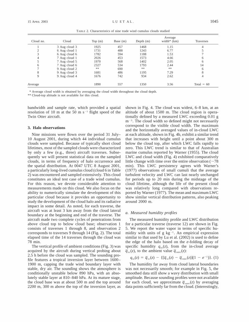
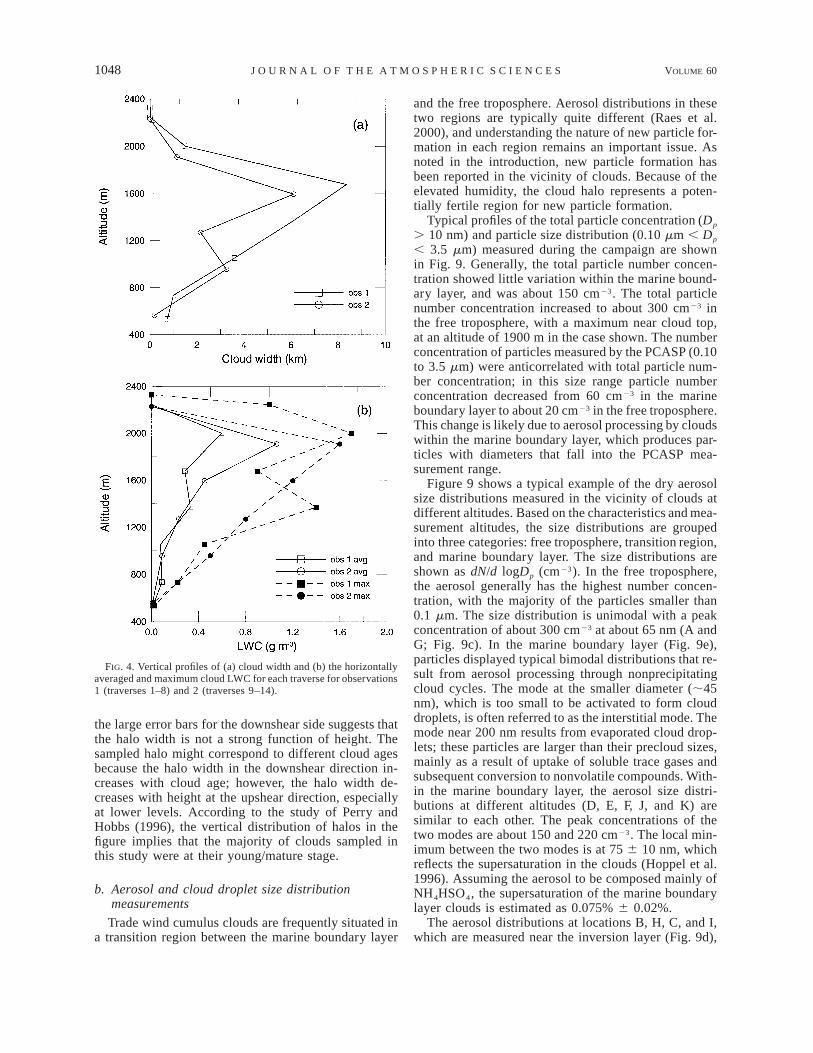
The vertical profile of ambient conditions (Fig. 3) wasacquired by the aircraft during vertical probing about2.5 h before the cloud was sampled. The sounding pro-file features a tropical inversion layer between 1600–1900 m, capping the trade wind boundary layer withstable, dry air. The sounding shows the atmosphere isconditionally unstable below 890 hPa, with an abso-lutely stable layer at 810–840 hPa. At its mature stage,the cloud base was at about 500 m and the top around2200 m, 300 m above the top of the inversion layer, as

shown in Fig. 4. The cloud was widest, 6–8 km, at analtitude of about 1500 m. The cloud region is opera-tionally defined by a measured LWC exceeding 0.01 gm23. The cloud width so defined might not necessarilycorrespond to the visible cloud width. The maximumand the horizontally averaged values of in-cloud LWCat each altitude, shown in Fig. 4b, exhibit a similar trendthat increases with height until a point about 300 mbelow the cloud top, after which LWC falls rapidly tozero. This LWC trend is similar to that of Australianmarine cumulus reported by Warner (1955). The cloudLWC and cloud width (Fig. 4) exhibited comparativelylittle change with time over the entire observation (;78min). This LWC persistency agrees with Warner’s(1977) observations of small cumuli that the averageturbulent velocity and LWC can last nearly unchangedfor periods up to 20 min during the midstage of thecloud lifetime, although the life of the present cloudwas relatively long compared with observations re-ported by Warner (1977). The mean and maximum LWCshow similar vertical distribution patterns, also peakingaround 2000 m.

a. Measured humidity profiles

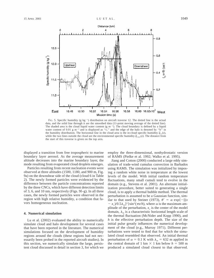
The measured humidity profile and LWC distributionfor a particular traverse (traverse 12) are shown in Fig.5. We report the water vapor in terms of specific hu-midity with units of g kg21. An empirical expressionsimilar to that used by Lu et al. (2002) is used to definethe edge of the halo based on the e-folding decay ofspecific humidity qve(z), from the in-cloud average

vc(z), to the ambient value venv(z):q q21q (z) 5 q (z) 2 {[q (z) 2 q (z)](1 2 e )}.ve vc vc venv (1)

The humidity far away from cloud lateral boundarieswas not necessarily smooth; for example in Fig. 5, thesmoothed data still show a wavy distribution with smallamplitude. Because sounding profiles were not availablefor each cloud, we approximate venv(z) by averagingqdata points sufficiently far from the cloud. (Interestingly,

1046 VOLUME 60J O U R N A L O F T H E A T M O S P H E R I C S C I E N C E S

FIG. 2. Flight path for the cumulus cloud at 0047 UTC 8 Aug 2001. A total of 14 traverses (green) are shown. Observation 1 representstraverses 1 through 8; observation 2 represents traverses 9 through 14. Red circles denote the cloud boundary.

the ambient values are not necessarily the same on bothsides of the cloud.) From the smoothed data shown inFig. 5, it can be seen that the measured humidity profileoutside the cloud, beginning from the mark ‘‘c’’ to thetwo lower horizontal lines, can be approximated by anexponential decay. For some traverses, for example tra-verse 4 (Fig. 6), the aircraft did not fly far enough fromthe cloud to reach a constant ambient humidity. In thiscase, the humidities at the start and the end of the tra-verse are used to define the far-ambient humidities. Re-turning to Fig. 5, the humidity halo at the downshearside of the cloud is about four times broader than thatat the upshear side.

The wind vector u is defined as positive in the positivex direction for Cartesian coordinates (x 2 z) in the east–west and vertical directions. For example, an easterlywind is defined as negative. The vertical wind shearvector is defined as du/dz. The direction of the shearvector is positive if du/dz . 0, and vice versa. Thedownshear and upshear directions are defined by thedirection of the shear vector; in that sense, the shearvector always points in the downshear direction. Thecloud morphology is tilted and stretched by the verticalshear, and the cloud is basically tilted to the downshear

direction. Consider an easterly wind (u , 0), the ve-locity of which decreases as z increases; in this case,the shear vector is positive (du/dz . 0) and points inthe positive x direction. Then for a cloud, the downsheardirection is in the positive x direction, which is on theeast side of the cloud. A westerly wind (u . 0), thevelocity of which increases with height, has the samedirection of the shear vector as the previous case. There-fore, the downshear and upshear directions are the samein these two cases.

The vertical distribution of the humidity halo on bothsides of the cloud was determined (Fig. 7). Perry andHobbs (1996) found that the presence of a stable layercan limit the vertical distribution of the halo. In Fig. 7,in accord with this observation, we note that the cloudhalo is distributed mainly below the inversion layer onboth sides of the cloud. The vertical east–west windprofile shows a weak wind shear with the easterly windincreasing with height roughly below the inversion basewhere most of the halo is present; therefore, the down-shear side is on the west side relative to the cloud. Thevertical distribution of halo shows that halo width islargest at the lowest altitudes, decreasing with heightbelow the inversion base, also in both of the downshear

15 APRIL 2003 1047L U E T A L .

FIG. 3. Skew T–logp diagram of the ambient sounding profile on 8 Aug 2001 taken for the extensivelystudied cloud (see sections 3 and 4) at 0047 UTC, 21.578N, 156.828W. Temperature and dewpoint temperatureprofiles are represented by thick lines. The skewed abscissa is temperature (8C), and the ordinate is pressure(hPa). Dotted lines (K) represent dry adiabats. Curved dashed lines (8C) are pseudoadiabats. Straight dashedlines (g kg21) are isopleths of the saturation water vapor mixing ratio. The north–south wind is not shown.

and upshear directions. This trend is similar to the ob-servations of Perry and Hobbs (1996) that when theinversion layer lies in the middle of the cloud, the halotends to be broader at the lower levels. The figure alsoshows the halo is wider in the downshear than the up-shear direction. The peak of the halo width above theinversion base for observation 1 could be due to a holein the cloud as shown in the simulation later. The halobecomes much broader at later times (e.g., observation2) at the lower cloud levels in the downshear direction,but the halo at the upshear side stays relatively un-changed with time.

From the 44 individual clouds sampled over the two-week period, we select nine clouds for which four ormore traverses were made for statistical analysis (Table2). Humidity halos were identified approximately 54%of the time during the total of 60 traverses. All haloswere less than two cloud radii in horizontal extent. Ingeneral, as indicated in Table 3, humidity halos are more

frequent and broader at the downshear side (55% and0.67 cloud radii) than the upshear side (44% and 0.41cloud radii). The frequency of occurrence and width ofthe cloud halo on the upshear side observed in the pre-sent study are close to those of the cumulus clouds offthe coasts of Oregon and Washington reported by Perryand Hobbs (1996); however, the frequency of occur-rence and width at the downshear side in the presentstudy are less than reported by Perry and Hobbs (1996).One possible explanation is that the clouds sampled inthe present study consist of a higher fraction of young/mature clouds.

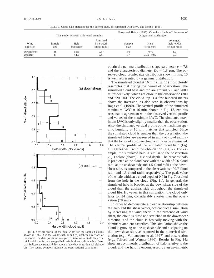
The vertical distribution of these sampled halos isshown in Fig. 8. The data points are categorized intofive altitude bins. The mean of the data for each altitudebin represents the halo width at that altitude range withthe standard deviation as its error bar. The figure showsthat the halo basically is broad at the lower levels ofthe cloud and narrow around cloud top. In this figure,

1048 VOLUME 60J O U R N A L O F T H E A T M O S P H E R I C S C I E N C E S

FIG. 4. Vertical profiles of (a) cloud width and (b) the horizontallyaveraged and maximum cloud LWC for each traverse for observations1 (traverses 1–8) and 2 (traverses 9–14).

the large error bars for the downshear side suggests thatthe halo width is not a strong function of height. Thesampled halo might correspond to different cloud agesbecause the halo width in the downshear direction in-creases with cloud age; however, the halo width de-creases with height at the upshear direction, especiallyat lower levels. According to the study of Perry andHobbs (1996), the vertical distribution of halos in thefigure implies that the majority of clouds sampled inthis study were at their young/mature stage.

b. Aerosol and cloud droplet size distributionmeasurements

Trade wind cumulus clouds are frequently situated ina transition region between the marine boundary layer

and the free troposphere. Aerosol distributions in thesetwo regions are typically quite different (Raes et al.2000), and understanding the nature of new particle for-mation in each region remains an important issue. Asnoted in the introduction, new particle formation hasbeen reported in the vicinity of clouds. Because of theelevated humidity, the cloud halo represents a poten-tially fertile region for new particle formation.

Typical profiles of the total particle concentration (Dp

. 10 nm) and particle size distribution (0.10 mm , Dp

, 3.5 mm) measured during the campaign are shownin Fig. 9. Generally, the total particle number concen-tration showed little variation within the marine bound-ary layer, and was about 150 cm23. The total particlenumber concentration increased to about 300 cm23 inthe free troposphere, with a maximum near cloud top,at an altitude of 1900 m in the case shown. The numberconcentration of particles measured by the PCASP (0.10to 3.5 mm) were anticorrelated with total particle num-ber concentration; in this size range particle numberconcentration decreased from 60 cm23 in the marineboundary layer to about 20 cm23 in the free troposphere.This change is likely due to aerosol processing by cloudswithin the marine boundary layer, which produces par-ticles with diameters that fall into the PCASP mea-surement range.

Figure 9 shows a typical example of the dry aerosolsize distributions measured in the vicinity of clouds atdifferent altitudes. Based on the characteristics and mea-surement altitudes, the size distributions are groupedinto three categories: free troposphere, transition region,and marine boundary layer. The size distributions areshown as dN/d logDp (cm23). In the free troposphere,the aerosol generally has the highest number concen-tration, with the majority of the particles smaller than0.1 mm. The size distribution is unimodal with a peakconcentration of about 300 cm23 at about 65 nm (A andG; Fig. 9c). In the marine boundary layer (Fig. 9e),particles displayed typical bimodal distributions that re-sult from aerosol processing through nonprecipitatingcloud cycles. The mode at the smaller diameter (;45nm), which is too small to be activated to form clouddroplets, is often referred to as the interstitial mode. Themode near 200 nm results from evaporated cloud drop-lets; these particles are larger than their precloud sizes,mainly as a result of uptake of soluble trace gases andsubsequent conversion to nonvolatile compounds. With-in the marine boundary layer, the aerosol size distri-butions at different altitudes (D, E, F, J, and K) aresimilar to each other. The peak concentrations of thetwo modes are about 150 and 220 cm23. The local min-imum between the two modes is at 75 6 10 nm, whichreflects the supersaturation in the clouds (Hoppel et al.1996). Assuming the aerosol to be composed mainly ofNH4HSO4, the supersaturation of the marine boundarylayer clouds is estimated as 0.075% 6 0.02%.

The aerosol distributions at locations B, H, C, and I,which are measured near the inversion layer (Fig. 9d),

15 APRIL 2003 1049L U E T A L .

FIG. 5. Specific humidity (g kg21) distribution on aircraft traverse 12. The dotted line is the actualdata, and the solid line through it are the smoothed data (11-point moving average of the dotted line).The shaded area is the cloud liquid water content (g m23). The cloud boundary is defined by a liquidwater content of 0.01 g m23 and is displayed as ‘‘c,’’ and the edge of the halo is denoted by ‘‘h’’ inthe humidity distribution. The horizontal line in the cloud area is the in-cloud specific humidity vc(z),qwhile the two lines outside the cloud are the environmental specific humidity venv(z). The distance fromqthe start of this traverse is given on the top axis.

displayed a transition from free tropospheric to marineboundary layer aerosol. As the average measurementaltitude decreases into the marine boundary layer, themode resulting from evaporated cloud droplets emerges.

Particles resulting from recent nucleation events wereobserved at three altitudes (1500, 1180, and 900 m, Fig.9a) on the downshear side of the cloud (cloud 6 in Table2). The newly formed particles were evidenced by thedifference between the particle concentrations reportedby the three CNCs, which have different detection limitsof 3, 6, and 10 nm, respectively (Figs. 9f–g). In all threecases, the newly formed particles were observed in theregion with high relative humidity, a condition that fa-vors homogeneous nucleation.

4. Numerical simulation

Lu et al. (2002) evaluated the ability to numericallysimulate cloud and halo development for several casesthat have been reported in the literature. The numericalsimulations focused on the development of humidityregions around the clouds (these regions had not nec-essarily been probed in the reported aircraft studies). Inthis section, we numerically simulate the large, persis-tent cloud discussed in detail in section 3, for which we

employ the three-dimensional, nonhydrostatic versionof RAMS (Pielke et al. 1992; Walko et al. 1995).

Jiang and Cotton (2000) conducted a large eddy sim-ulation of trade-wind cumulus convection in Barbadosusing RAMS. The simulation was initialized by impos-ing a random white noise in temperature at the lowestlevels of the model. With initial random temperaturefluctuations, many small cumuli tend to evolve in thedomain (e.g., Stevens et al. 2001). An alternate initial-ization procedure, better suited to generating a singlecloud, is to apply a thermal bubble method. The thermalperturbation is assumed to be a Gaussian function, sim-ilar to that used by Steiner (1973), u9 5 a exp{2[(x2 xc)/0.5lm]2}sin2(pz/h), where a is the maximum am-plitude of the perturbation, xc is the center of the modeldomain, lm is a characteristic horizontal length scale ofthe thermal fluctuation (McNider and Kopp 1990), andh is the effective perturbation depth. The size of theinitial pulse greatly influences the numerical develop-ment of the cloud (e.g., Murray 1971). Different per-turbations were tested to find that for which the simu-lated cloud resembled that observed. An initial thermalperturbation of a 5 0.1 K with lm 5 632 m applied inthe central domain of 1 km 3 1 km below h 5 500 mproduced a simulated cloud closest to that observed.

1050 VOLUME 60J O U R N A L O F T H E A T M O S P H E R I C S C I E N C E S

FIG. 6. Same as Fig. 5 but for traverse 4. The ambient specific humidity is defined as that at the startand end of the traverse.

FIG. 7. Vertical profile of cloud halo width at the west and eastsides of the cloud vs the altitude normalized with the cloud depthfor observations 1 and 2. The normalized altitudes of 0 and 1 referto cloud base and cloud top, respectively. Below the inversion base,the west side relative to the cloud is the downshear direction.

(Although cases were tried with lm 5 4 km, close tothe observed averaged cloud width, this perturbation didnot produce a cloud similar to that observed.) Our ex-perience shows that a humidity perturbation saturating

the lower levels (e.g., below 214 m) of the model, con-fined in the central region, is required. We have arbi-trarily set the y component of wind to be zero, so thatthe cloud movement can be followed easily.

The simulation domain has a horizontal resolution of100 m, equivalent to a 2-s measurement resolution (at 50m s21 flight speed), and vertical resolution of 40 m at thelowest altitude with a vertical stretching ratio of 1.1. Thesimulation domain is thus 6 km 3 6 km 3 11 km, thehorizontal domain size being large enough to cover thecloud and the associated cloud halo. The sea surface tem-perature (SST) was prescribed using the National Centersfor Environmental Prediction (NCEP) Reynolds averageSST of 300 K (see Web site http://podaac.jpl.nasa.gov/reynolds/reynoldspbrowse.html) in the vicinity of Hawaiiin August 2001. The lateral boundary condition is periodic,and the upper and lower boundaries are rigid lids. Theaveraged cloud droplet size distribution (Fig. 10) observedduring traverse 7 by the FSSP-100, was integrated overthe droplet spectrum to give a cloud droplet number con-centration (Nt) of 76 cm23. By fitting the data with amodified gamma distribution used in RAMS (Walko et al.1995),

n21N D 1 Dtn(D) 5 exp 2 ; (2)1 2 1 2G(n) D D Dn n n

with this cloud droplet number concentration value, we

15 APRIL 2003 1051L U E T A L .

TABLE 3. Cloud halo statistics for the current study as compared with Perry and Hobbs (1996).

Winddirection

This study: Hawaii trade wind cumulus

Samplesize

Halofrequency

Averagedhalo width

(cloud radii)

Perry and Hobbs (1996): Cumulus clouds off the coast ofOregon and Washington

Samplesize

Halofrequency

Averagedhalo width

(cloud radii)

DownshearUpshear

3839

55%44%

0.670.41

5657

75%35%–40%

1.30.3

FIG. 8. Vertical profile of the halo width for the sampled cloudsshown in Table 2 in the (a) downshear and (b) upshear directions ofthe cloud. The data points are categorized into five altitude bins. Thethick solid line is the averaged halo width of each altitude bin. Errorbars indicate the standard deviations of the data points in each altitudebin. The square symbols indicate the observational data points.

obtain the gamma distribution shape parameter n 5 7.8and the characteristic diameter Dn 5 1.8 mm. The ob-served cloud droplet size distribution shown in Fig. 10is well represented by a gamma distribution.

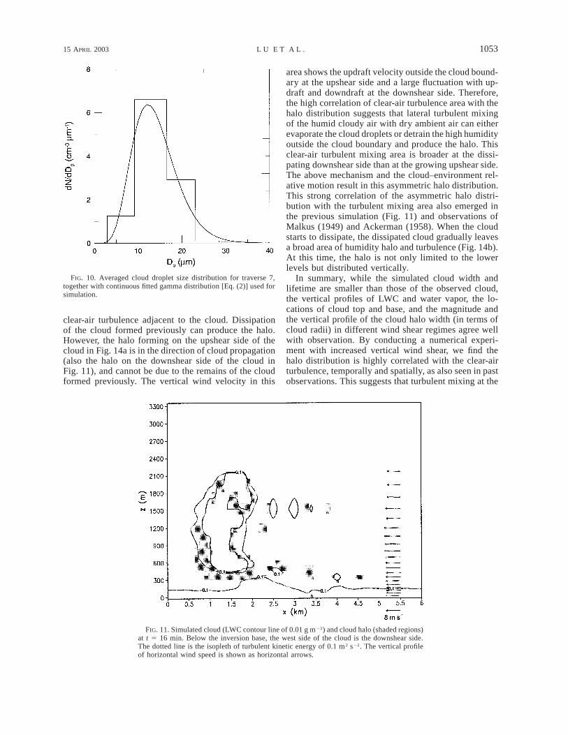
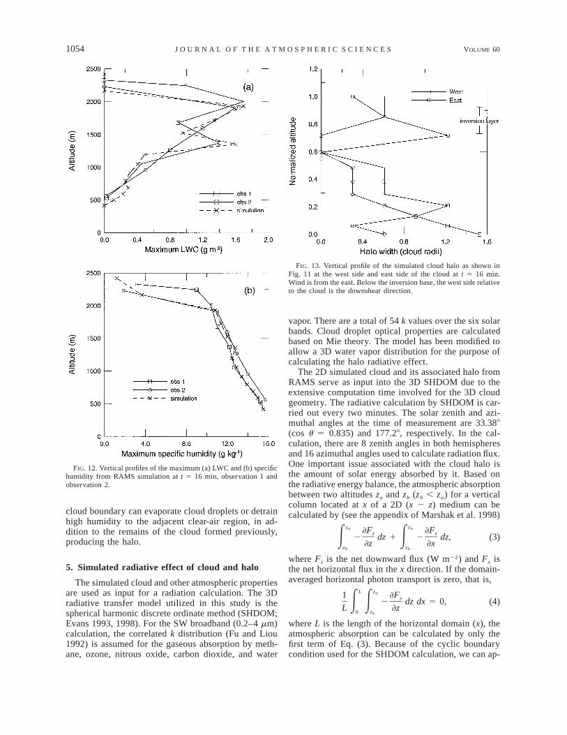
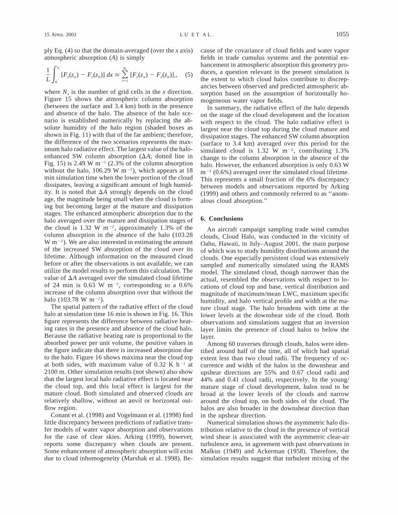
The simulated cloud at 16 min (Fig. 11) most closelyresembles that during the period of observation. Thesimulated cloud base and top are around 500 and 2000m, respectively, which are close to the observation (300and 2200 m). The cloud top is a few hundred metersabove the inversion, as also seen in observations byRaga et al. (1990). The vertical profile of the simulatedmaximum LWC at 16 min, shown in Fig. 12, exhibitsreasonable agreement with the observed vertical profileand values of the maximum LWC. The simulated max-imum LWC is only slightly smaller than the observation.Also, the simulated vertical profile of the maximum spe-cific humidity at 16 min matches that sampled. Sincethe simulated cloud is smaller than the observation, thesimulated halos are expressed in units of cloud radii sothat the factor of absolute cloud width can be eliminated.The vertical profile of the simulated cloud halo (Fig.13) agrees well with the observation (Fig. 7). For ex-ample, the simulated halo is similar to the observation2 (1) below (above) 0.6 cloud depth. The broadest halois predicted at the cloud base with the width of 0.6 cloudradii at the upshear side and 1.5 cloud radii at the down-shear side, as compared to the observations of 0.7 cloudradii and 1.3 cloud radii, respectively. The peak valueof the halo width at a cloud depth of 0.7 in Fig. 7 resultedfrom the hole in the cloud (Fig. 11). In general, thesimulated halo is broader at the downshear side of thecloud than the upshear side throughout the simulatedcloud life. However, in this simulation, the cloud onlylasts for 24 min, considerably shorter than the obser-vation (78 min).

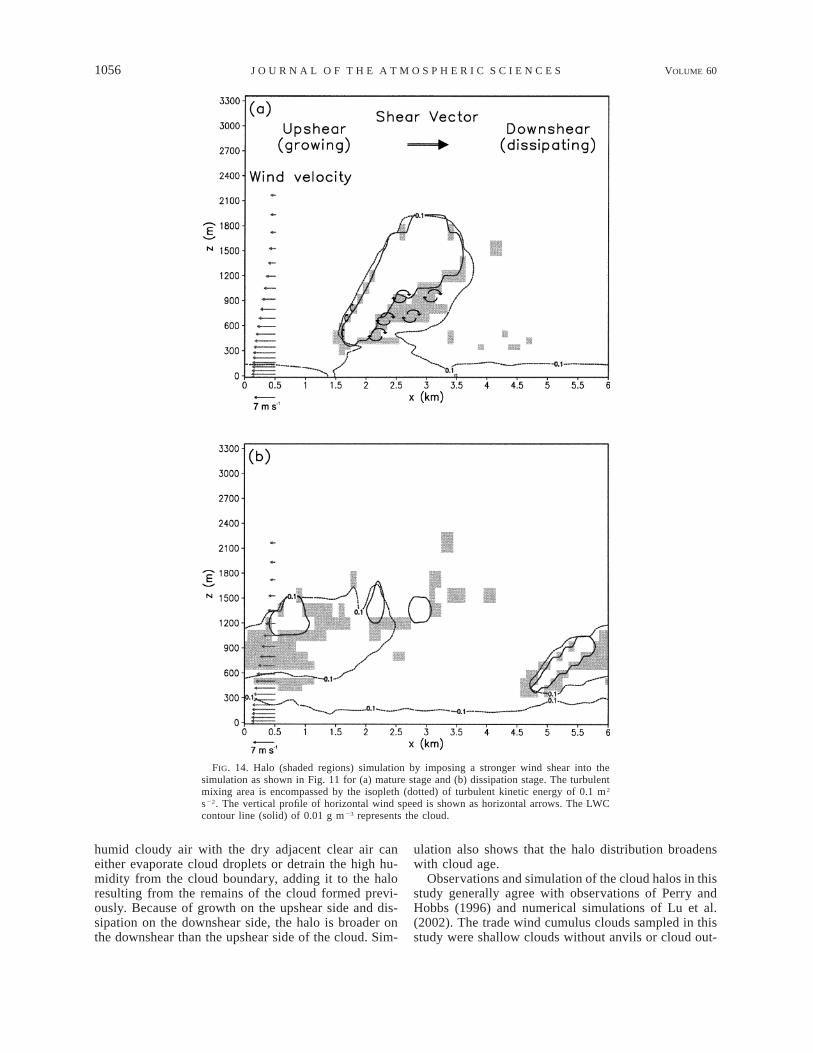
In order to demonstrate a clear relationship betweenthe halo and the shear vector, we conduct a simulationby increasing the wind shear. In the presence of windshear, the cloud is tilted and stretched in the downsheardirection, and the cloud is basically moving with thedominant ambient easterlies. This simulation shows thecloud is growing on the upshear side and dissipating onthe downshear side, as reported in the numerical sim-ulation (e.g., Vaillancourt et al. 1997) and observation(e.g., Telford and Wagner 1980). Results in Fig. 14ashow an asymmetric distribution of halo relative to thecloud, and the halo is encompassed by an asymmetric

1052 VOLUME 60J O U R N A L O F T H E A T M O S P H E R I C S C I E N C E S

FIG. 9. (a) Flight track during sampling of a convective cumulus cloud from 0050 to 0204 UTC 6 Aug 2001,with different altitudes labelled A–K; (b) vertical profile of total particle concentration and particle concentrationin the size range 0.1 to 3.5 mm diameter; (c)–(e) dry aerosol size distributions in free troposphere, transitionregion, and marine boundary layer; (f )–(g) particle concentrations measured by three CNCs when newly formedparticles were detected.

15 APRIL 2003 1053L U E T A L .

FIG. 10. Averaged cloud droplet size distribution for traverse 7,together with continuous fitted gamma distribution [Eq. (2)] used forsimulation.

FIG. 11. Simulated cloud (LWC contour line of 0.01 g m23) and cloud halo (shaded regions)at t 5 16 min. Below the inversion base, the west side of the cloud is the downshear side.The dotted line is the isopleth of turbulent kinetic energy of 0.1 m2 s22. The vertical profileof horizontal wind speed is shown as horizontal arrows.

clear-air turbulence adjacent to the cloud. Dissipationof the cloud formed previously can produce the halo.However, the halo forming on the upshear side of thecloud in Fig. 14a is in the direction of cloud propagation(also the halo on the downshear side of the cloud inFig. 11), and cannot be due to the remains of the cloudformed previously. The vertical wind velocity in this

area shows the updraft velocity outside the cloud bound-ary at the upshear side and a large fluctuation with up-draft and downdraft at the downshear side. Therefore,the high correlation of clear-air turbulence area with thehalo distribution suggests that lateral turbulent mixingof the humid cloudy air with dry ambient air can eitherevaporate the cloud droplets or detrain the high humidityoutside the cloud boundary and produce the halo. Thisclear-air turbulent mixing area is broader at the dissi-pating downshear side than at the growing upshear side.The above mechanism and the cloud–environment rel-ative motion result in this asymmetric halo distribution.This strong correlation of the asymmetric halo distri-bution with the turbulent mixing area also emerged inthe previous simulation (Fig. 11) and observations ofMalkus (1949) and Ackerman (1958). When the cloudstarts to dissipate, the dissipated cloud gradually leavesa broad area of humidity halo and turbulence (Fig. 14b).At this time, the halo is not only limited to the lowerlevels but distributed vertically.

In summary, while the simulated cloud width andlifetime are smaller than those of the observed cloud,the vertical profiles of LWC and water vapor, the lo-cations of cloud top and base, and the magnitude andthe vertical profile of the cloud halo width (in terms ofcloud radii) in different wind shear regimes agree wellwith observation. By conducting a numerical experi-ment with increased vertical wind shear, we find thehalo distribution is highly correlated with the clear-airturbulence, temporally and spatially, as also seen in pastobservations. This suggests that turbulent mixing at the

1054 VOLUME 60J O U R N A L O F T H E A T M O S P H E R I C S C I E N C E S

FIG. 12. Vertical profiles of the maximum (a) LWC and (b) specifichumidity from RAMS simulation at t 5 16 min, observation 1 andobservation 2.

FIG. 13. Vertical profile of the simulated cloud halo as shown inFig. 11 at the west side and east side of the cloud at t 5 16 min.Wind is from the east. Below the inversion base, the west side relativeto the cloud is the downshear direction.

cloud boundary can evaporate cloud droplets or detrainhigh humidity to the adjacent clear-air region, in ad-dition to the remains of the cloud formed previously,producing the halo.

5. Simulated radiative effect of cloud and halo

The simulated cloud and other atmospheric propertiesare used as input for a radiation calculation. The 3Dradiative transfer model utilized in this study is thespherical harmonic discrete ordinate method (SHDOM;Evans 1993, 1998). For the SW broadband (0.2–4 mm)calculation, the correlated k distribution (Fu and Liou1992) is assumed for the gaseous absorption by meth-ane, ozone, nitrous oxide, carbon dioxide, and water

vapor. There are a total of 54 k values over the six solarbands. Cloud droplet optical properties are calculatedbased on Mie theory. The model has been modified toallow a 3D water vapor distribution for the purpose ofcalculating the halo radiative effect.

The 2D simulated cloud and its associated halo fromRAMS serve as input into the 3D SHDOM due to theextensive computation time involved for the 3D cloudgeometry. The radiative calculation by SHDOM is car-ried out every two minutes. The solar zenith and azi-muthal angles at the time of measurement are 33.388(cos u 5 0.835) and 177.28, respectively. In the cal-culation, there are 8 zenith angles in both hemispheresand 16 azimuthal angles used to calculate radiation flux.One important issue associated with the cloud halo isthe amount of solar energy absorbed by it. Based onthe radiative energy balance, the atmospheric absorptionbetween two altitudes za and zb (zb , za) for a verticalcolumn located at x of a 2D (x 2 z) medium can becalculated by (see the appendix of Marshak et al. 1998)

z za a]F ]Fz x2 dz 1 2 dz, (3)E E]z ]xz zb b

where Fz is the net downward flux (W m22) and Fx isthe net horizontal flux in the x direction. If the domain-averaged horizontal photon transport is zero, that is,

L za1 ]Fx2 dz dx 5 0, (4)E EL ]z0 zb

where L is the length of the horizontal domain (x), theatmospheric absorption can be calculated by only thefirst term of Eq. (3). Because of the cyclic boundarycondition used for the SHDOM calculation, we can ap-

15 APRIL 2003 1055L U E T A L .

ply Eq. (4) so that the domain-averaged (over the x axis)atmospheric absorption (A) is simply

L Nx1[F (z ) 2 F (z )] dx ù [F (z ) 2 F (z )] , (5)OE z a z b z a z b iL i510

where Nx is the number of grid cells in the x direction.Figure 15 shows the atmospheric column absorption(between the surface and 3.4 km) both in the presenceand absence of the halo. The absence of the halo sce-nario is established numerically by replacing the ab-solute humidity of the halo region (shaded boxes asshown in Fig. 11) with that of the far ambient; therefore,the difference of the two scenarios represents the max-imum halo radiative effect. The largest value of the halo-enhanced SW column absorption (DA; dotted line inFig. 15) is 2.49 W m22 (2.3% of the column absorptionwithout the halo, 106.29 W m22), which appears at 18min simulation time when the lower portion of the clouddissipates, leaving a significant amount of high humid-ity. It is noted that DA strongly depends on the cloudage, the magnitude being small when the cloud is form-ing but becoming larger at the mature and dissipationstages. The enhanced atmospheric absorption due to thehalo averaged over the mature and dissipation stages ofthe cloud is 1.32 W m22, approximately 1.3% of thecolumn absorption in the absence of the halo (103.28W m22). We are also interested in estimating the amountof the increased SW absorption of the cloud over itslifetime. Although information on the measured cloudbefore or after the observations is not available, we canutilize the model results to perform this calculation. Thevalue of DA averaged over the simulated cloud lifetimeof 24 min is 0.63 W m22, corresponding to a 0.6%increase of the column absorption over that without thehalo (103.78 W m22).

The spatial pattern of the radiative effect of the cloudhalo at simulation time 16 min is shown in Fig. 16. Thisfigure represents the difference between radiative heat-ing rates in the presence and absence of the cloud halo.Because the radiative heating rate is proportional to theabsorbed power per unit volume, the positive values inthe figure indicate that there is increased absorption dueto the halo. Figure 16 shows maxima near the cloud topat both sides, with maximum value of 0.32 K h21 at2100 m. Other simulation results (not shown) also showthat the largest local halo radiative effect is located nearthe cloud top, and this local effect is largest for themature cloud. Both simulated and observed clouds arerelatively shallow, without an anvil or horizontal out-flow region.

Conant et al. (1998) and Vogelmann et al. (1998) findlittle discrepancy between predictions of radiative trans-fer models of water vapor absorption and observationsfor the case of clear skies. Arking (1999), however,reports some discrepancy when clouds are present.Some enhancement of atmospheric absorption will existdue to cloud inhomogeneity (Marshak et al. 1998). Be-

cause of the covariance of cloud fields and water vaporfields in trade cumulus systems and the potential en-hancement in atmospheric absorption this geometry pro-duces, a question relevant in the present simulation isthe extent to which cloud halos contribute to discrep-ancies between observed and predicted atmospheric ab-sorption based on the assumption of horizontally ho-mogeneous water vapor fields.

In summary, the radiative effect of the halo dependson the stage of the cloud development and the locationwith respect to the cloud. The halo radiative effect islargest near the cloud top during the cloud mature anddissipation stages. The enhanced SW column absorption(surface to 3.4 km) averaged over this period for thesimulated cloud is 1.32 W m22, contributing 1.3%change to the column absorption in the absence of thehalo. However, the enhanced absorption is only 0.63 Wm22 (0.6%) averaged over the simulated cloud lifetime.This represents a small fraction of the 6% discrepancybetween models and observations reported by Arking(1999) and others and commonly referred to as ‘‘anom-alous cloud absorption.’’

6. Conclusions

An aircraft campaign sampling trade wind cumulusclouds, Cloud Halo, was conducted in the vicinity ofOahu, Hawaii, in July–August 2001, the main purposeof which was to study humidity distributions around theclouds. One especially persistent cloud was extensivelysampled and numerically simulated using the RAMSmodel. The simulated cloud, though narrower than theactual, resembled the observations with respect to lo-cations of cloud top and base, vertical distribution andmagnitude of maximum/mean LWC, maximum specifichumidity, and halo vertical profile and width at the ma-ture cloud stage. The halo broadens with time at thelower levels at the downshear side of the cloud. Bothobservations and simulations suggest that an inversionlayer limits the presence of cloud halos to below thelayer.

Among 60 traverses through clouds, halos were iden-tified around half of the time, all of which had spatialextent less than two cloud radii. The frequency of oc-currence and width of the halos in the downshear andupshear directions are 55% and 0.67 cloud radii and44% and 0.41 cloud radii, respectively. In the young/mature stage of cloud development, halos tend to bebroad at the lower levels of the clouds and narrowaround the cloud top, on both sides of the cloud. Thehalos are also broader in the downshear direction thanin the upshear direction.

Numerical simulation shows the asymmetric halo dis-tribution relative to the cloud in the presence of verticalwind shear is associated with the asymmetric clear-airturbulence area, in agreement with past observations inMalkus (1949) and Ackerman (1958). Therefore, thesimulation results suggest that turbulent mixing of the

1056 VOLUME 60J O U R N A L O F T H E A T M O S P H E R I C S C I E N C E S

FIG. 14. Halo (shaded regions) simulation by imposing a stronger wind shear into thesimulation as shown in Fig. 11 for (a) mature stage and (b) dissipation stage. The turbulentmixing area is encompassed by the isopleth (dotted) of turbulent kinetic energy of 0.1 m2

s22. The vertical profile of horizontal wind speed is shown as horizontal arrows. The LWCcontour line (solid) of 0.01 g m23 represents the cloud.

humid cloudy air with the dry adjacent clear air caneither evaporate cloud droplets or detrain the high hu-midity from the cloud boundary, adding it to the haloresulting from the remains of the cloud formed previ-ously. Because of growth on the upshear side and dis-sipation on the downshear side, the halo is broader onthe downshear than the upshear side of the cloud. Sim-

ulation also shows that the halo distribution broadenswith cloud age.

Observations and simulation of the cloud halos in thisstudy generally agree with observations of Perry andHobbs (1996) and numerical simulations of Lu et al.(2002). The trade wind cumulus clouds sampled in thisstudy were shallow clouds without anvils or cloud out-

15 APRIL 2003 1057L U E T A L .

FIG. 15. Domain-averaged (over the x axis) SW atmospheric col-umn (surface to 3.4 km) absorption (A) as a function of simulationtime in the presence and absence of humidity halo. The dotted lineis the halo-enhanced atmospheric absorption (DA).

FIG. 16. Increase of the atmospheric heating rate in the presence of a cloud halo over that in the absenceof a halo for the simulation shown in Fig. 11. Contour lines (green dashed) are 0.01, 0.03, 0.06, 0.12, 0.15,0.2, and 0.3 K h21. The LWC contour line (purple solid) of 0.01 g m23 is the cloud, and shaded regions(yellow) are the halo. Two shaded contour plots provide an expanded view of the enhanced heating ratenear the cloud top.

flows. We can expect that more convective clouds, suchas thunderstorms or clouds in the ITCZ, with cloudoutflow regions near cloud tops, will exhibit broaderhalos.

Regions in the vicinity of clouds are favorable fornew particle formation. Aerosols measured in the vi-cinity of the trade wind cumulus clouds reflected threeregimes: free troposphere, transition zone, and marineboundary layer. In the free troposphere, the aerosol sizedistribution was found to be unimodal with a peak sizeat about 65 nm, while being bimodal in the marineboundary layer with peaks at about 45 and 185 nm.These observations are consistent with prior measure-ments reported in the literature. Particles resulting fromrecent nucleation events, when observed, occurred onthe downshear side of the cloud, coincident with theregion of largest halo.

Radiative absorption of the simulated halo has beenestimated using the radiative transfer model SHDOM.Results show that the halo radiative effect is largest atthe cloud mature and dissipating stages. A peak columnabsorption (surface to 3.4 km) due to the halo of 2.49W m22 (2.3%) is noted early in the cloud dissipationstage. The temporally and spatially averaged SW col-umn absorption during this period for the simulatedcloud is 1.32 W m22, a 1.3% increase of the column

1058 VOLUME 60J O U R N A L O F T H E A T M O S P H E R I C S C I E N C E S

absorption over that in the absence of a halo. However,the increased absorption is only 0.63 W m22 (0.6%)when averaged over the simulated cloud lifetime. Thisrepresents a small fraction of the 6% discrepancy be-tween models and observations reported by Arking(1999) and others and commonly referred to as anom-alous cloud absorption. The spatial distribution of thehalo radiative effect is largest near cloud top, which, inaddition to the humidity halo, results in conditions fa-vorable to homogenous nucleation.

Acknowledgments. This work was supported by Na-tional Science Foundation Grants ATM-9907010 andATM-9910744. This work was also supported in partby the Office of Naval Research. The authors wish toacknowledge Dr. William C. Conant for helpful com-ments. We also thank anonymous reviewers for theirvaluable comments on this work.

REFERENCES

Ackerman, B., 1958: Turbulence around tropical cumuli. J. Meteor.,15, 69–74.

Arking, A., 1999: The influence of clouds and water vapor on at-mospheric absorption. Geophys. Res. Lett., 26, 2729–2732.

Austin, G. R., R. M. Rauber, H. T. Ochs III, and L. J. Miller, 1996:Trade-wind clouds and Hawaiian rainbands. Mon. Wea. Rev.,124, 2126–2151.

Bretherton, C. S., and P. K. Smolarkiewicz, 1989: Gravity waves,compensating subsidence and detrainment around cumulusclouds. J. Atmos. Sci., 46, 740–759.

Clarke, A. D., and V. N. Kapustin, 2002: A Pacific aerosol survey.Part I: A decade of data on particle production, transport, evo-lution, and mixing in the troposphere. J. Atmos. Sci., 59, 363–382.

Collins, D. R., R. C. Flagan, and J. H. Seinfeld, 2002: Improved in-version of scanning DMA data. Aerosol. Sci. Technol., 36, 1–9.

Conant, W. C., A. M. Vogelmann, and V. Ramanathan, 1998: Theunexplained solar absorption and atmospheric H2O: A direct testusing clear-sky data. Tellus, 50, 525–533.

Evans, K. F., 1993: Two-dimensional radiative transfer in cloudyatmospheres: The spherical harmonic spatial grid method. J. At-mos. Sci., 50, 3111–3124.

——, 1998: The spherical harmonic discrete ordinate method forthree-dimensional atmospheric radiative transfer. J. Atmos. Sci.,55, 429–446.

Fu, Q., and K. N. Liou, 1992: On the correlated k-distribution methodfor radiative transfer in nonhomogeneous atmospheres. J. Atmos.Sci., 49, 2139–2156.

Hobbs, P. V., and L. F. Radke, 1992: Reply. J. Atmos. Sci., 49, 1516–1517.

Hoppel, W. A., G. M. Frick, and J. W. Fitzgerald, 1996: Deducingdroplet concentration and supersaturation in marine boundarylayer clouds from surface aerosol measurements. J. Geophys.Res., 101, 26 553–26 565.

Jenkins, F., and H. White, 1957: Fundamentals of Optics. McGrawHill, 637 pp.

Jiang, H., and W. R. Cotton, 2000: Large eddy simulation of shallowcumulus convection during BOMEX: Sensitivity to microphysicsand radiation. J. Atmos. Sci., 57, 582–594.

Kaufman, V., and B. Edlen, 1974: Reference wavelengths from atomicspectra in the range 15 A to 25000 A. J. Phys. Chem. Ref. Data,3, 825–896.

Kebabian, P. L., cited 1998: Optical monitor for water vapor con-centration. U.S. Patent 5,760,895. [Available online at http://patft.uspto.gov/netahtml/srchnum.htm.]

——, T. Berkoff, and A. Freedman, 1998: Water vapour sensing usingpolarization selection of a Zeeman-split argon discharge lampemission line. Meas. Sci. Technol., 9, 1793–1796.

——, C. E. Kolb, and A. Freedman, 2002: Spectroscopic water vaporsensor for rapid response measurements of humidity in the tropo-sphere. J. Geophys. Res., 107, 4670, doi:10.1029/2001JD002003.

Kerminen, V.-M., and A. S. Wexler, 1994: Particle formation due toSO2 oxidation and high relative humidity in the remote marineboundary layer. J. Geophys. Res., 99, 25 607–25 614.

Kollias, P., B. A. Albrecht, R. Lhermitte, and A. Savtchenko, 2001:Radar observations of updrafts, downdrafts, and turbulence infair-weather cumuli. J. Atmos. Sci., 58, 1750–1766.

Lawson, R. P., and W. A. Cooper, 1990: Performance of some airbornethermometers in clouds. J. Atmos. Oceanic Technol., 7, 480–494.

Liu, Y. G., and P. H. Daum, 2000: The effect of refractive index onsize distributions and light scattering coefficients derived fromoptical particle counters. J. Aerosol Sci., 31, 945–957.

Lu, M.-L., R. A. McClatchey, and J. H. Seinfeld, 2002: Cloud halos:Numerical simulation of dynamical structure and radiative im-pact. J. Appl. Meteor, 41, 832–848.

Malkus, J. S., 1949: Effects of wind shear on some aspects of con-vection. Trans. Amer. Geophys. Union, 30, 19–25.

Marshak, A., A. Davis, W. Wiscombe, W. Ridgway, and R. Cahalan,1998: Biases in shortwave column absorption in the presence offractal clouds. J. Climate, 11, 431–446.

McManus, J. B., P. L. Kebabian, and M. Zahniser, 1995: Astigmaticmirror multipass absorption cell for long path length spectros-copy. Appl. Opt., 34, 3336–3338.

McNider, R. T., and F. J. Kopp, 1990: Specification of the scale andmagnitude of thermals used to initiate convection in cloud mod-els. J. Appl. Meteor., 29, 99–104.

Moore, C., 1971: Atomic energy levels. NBS Circular 467, U.S. Gov-ernment Printing Office, 309 pp.

Murray, F. W., 1971: Humidity augmentation as the initial pulse ina numerical cloud model. Mon. Wea. Rev., 99, 37–48.

Perry, K. D., and P. V. Hobbs, 1994: Further evidence for particlenucleation in clear air adjacent to marine cumulus clouds. J.Geophy. Res., 99, 22 803–22 818.

——, 1996: Influences of isolated cumulus clouds on the humidityof their surroundings. J. Atmos. Sci., 53, 159–174.

Pielke, R. A., and Coauthors, 1992: A comprehensive meteorologicalmodeling system—RAMS. Meteor. Atmos. Phys., 49, 69–91.

Platt, C. M. R., and D. J. Gambling, 1971: Laser radar reflexions anddownward infrared flux enhancement near small cumulus. Na-ture, 232, 182–185.

Radke, L. F., and P. V. Hobbs, 1991: Humidity and particle fieldsaround some small cumulus clouds. J. Atmos. Sci., 48, 1190–1193.

Raes, F., R. Van Dingenen, E. Vignati, J. Wilson, J. P. Putaud, J. H.Seinfeld, and P. Adams, 2000: Formation and cycling of aerosolsin the global troposphere. Atmos. Environ., 34, 4215–4240.

Raga, G. B., J. B. Jensen, and M. B. Baker, 1990: Characteristics ofcumulus band clouds off the coast of Hawaii. J. Atmos. Sci., 47,338–355.

Raymond, D. J., and A. M. Blyth, 1986: A stochastic mixing modelfor nonprecipitating cumulus clouds. J. Atmos. Sci., 43, 2708–2718.

——, R. Solomon, and A. M. Blyth, 1991: Mass fluxes in NewMexico mountain thunderstorm from radar and aircraft mea-surements. Quart. J. Roy. Meteor. Soc., 117, 587–621.

Rothman, L. S., and Coauthors, 1998: The HITRAN molecular spec-troscopic database and HAWKS (HITRAN atmospheric work-station): 1996 edition. J. Quant. Spectrosc. Radiat. Transfer, 60,665–710.

Steiner, J. T., 1973: A three-dimensional model of cumulus clouddevelopment. J. Atmos. Sci., 30, 414–435.

Stevens, B., and Coauthors, 2001: Simulations of trade wind cumuliunder a strong inversion. J. Atmos. Sci., 58, 1870–1891.

15 APRIL 2003 1059L U E T A L .

Taylor, G. R., and M. B. Baker, 1991: Entrainment and detrainmentin cumulus clouds. J. Atmos. Sci., 48, 112–121.

Telford, J. W., and P. B. Wagner, 1980: The dynamical and liquidwater structure of the small cumulus as determined from itsenvironment. Pure Appl. Geophys., 118, 935–952.

Vaillancourt, P. A., M. K. Yau, and W. W. Grabowski, 1997: Upshearand downshear evolution of cloud structure and spectral prop-erties. J. Atmos. Sci., 54, 1203–1217.

Vogelmann, A. M., V. Ramanathan, W. C. Conant, and W. E. Hunter,1998: Observational constraints on non-Lorentzian continuumeffects in the near-infrared solar spectrum using ARM ARESEdata. J. Quant. Spectrosc. Radiat. Transfer, 60, 231–246.

Walko, R. L., W. R. Cotton, M. P. Meyers, and J. Y. Harrington, 1995:New RAMS cloud microphysics parameterization. Part I: Thesingle-moment scheme. Atmos. Res., 38, 29–62.

Wang, S., and R. C. Flagan, 1990: Scanning electrical mobility spec-trometer. Aerosol. Sci. Technol., 13, 230–240.

Warner, J., 1955: The water content of cumuliform cloud. Tellus, 7,449–457.

——, 1977: Time variation of updraft and water content in smallcumulus clouds. J. Atmos. Sci., 34, 1306–1312.

Weber, R. J., and Coauthors, 2001: Measurements of enhanced H2SO4

and 2–4 nm particles near a frontal cloud during the First AerosolCharacterization Experiment (ACE1). J. Geophy. Res., 106, 24107–24 117.