The diurnal cycle of shallow Cumulus clouds

over land: A single column model

intercomparison study

�

Geert Lenderink�, A. Pier Siebesma

�, Sylvain Cheinet

�, Sarah Irons

�, Colin G. Jones

�,

Pascal Marquet�, Frank Muller

�, Dolores Olmeda

�, Javier Calvo

�, Enrique Sanchez

�,

and Pedro M. M. Soares� �

�Royal Netherlands Meteorological Institute, De Bilt, The Netherlands

�Laboratoire de Meteorologie Dynamique, Paris, France�

Met Office, Bracknell, Berkshire, United Kingdom�

Rossby Center, SMHI, Norrkoping, Sweden�

Meteo France (CNRM/GMGEC), Toulouse, France�

Max-Planck Institur fur Meteorologie, Hanburg, Germany�

Instituto Nacional de Meteorologia, Madrid Spain�

DECivil do Instituto Superior de Engenharia de Lisboa, Portugal�

Centro de Geofisica da Universidade de Lisboa, Portugal

July 21, 2003

�Corresponding author address: Geert Lenderink, KNMI, 3730 AE De Bilt, P.O. Box

201, The Netherlands. E-mail: lenderin@knmi.nl

Summary

An intercomparison study for single column models (SCMs) of the diurnal cycle

of shallow cumulus convection is reported. The case, based on measurements at

the ARM Southern Great Plain site on 21���

June 1997, has been used in an LES

intercomparison study before. Results of the SCMs reveal the following general

deficiencies: too large values of cloud cover and cloud liquid water, unrealistic

thermodynamic profiles, and high amounts of noise. These results are analyzed in

terms of the behavior of different parameterization schemes involved: the convec-

tion scheme, the turbulence scheme, and the cloud scheme. In general the behavior

of the SCMs can be grouped in two different classes: one class with too strong

mixing by the turbulence scheme, the other class with too strong activity by the

convection scheme. In both classes high values of cloud cover and cloud liquid

water content occur. Many of the SCMs suffer from a numerical instability in the

cloud layer mainly due to the turbulence scheme. Results are also strongly depen-

dent on vertical resolution, in particular caused by resolution dependencies in the

mass flux scheme. The coupling between subcloud turbulence and the convection

scheme plays a crucial role in determining the thermodynamic profiles. Finally,

(in part) motivated by these results several models have been successfully updated

with new parameterization schemes and/or their present schemes have been suc-

cessfully modified.

QJRMS 1

1. Introduction

The representation of clouds in present Atmospheric General Circulation Models

(AGCMs) used in climate research and in numerical weather prediction (NWP) is

relatively poor, thereby limiting the predictability of cloud feedbacks in a chang-

ing climate. In particular, the representation of shallow cumulus (Cu) convection

is an important issue. Shallow cumulus clouds are an integral part of the Hadley

circulation, increasing the near surface transport of moisture to the ITCZ, thereby

intensifying deep convection (Tiedtke 1989). Over land, shallow cumulus convec-

tion also plays an important role in the preconditioning for deep convection.

For these reasons shallow cumulus convection has been the subject of many

studies. A number of these have been performed in GCSS WG1 [GEWEX (Global

Energy Water cycle EXperiment) Clouds System Study Working Group 1 (Brown-

ing 1993)]. In the 4th GCSS WG-1 intercomparison case (“BOMEX”) a typical

tradewind shallow Cumulus cloud with low cloud fraction was studied (Siebesma

et al. 2003). The next case (“ATEX”) concentrated on cumulus clouds rising into

stratocumulus (Stevens et al. 2001), which is a cloud regime which commonly oc-

curs in the tradewind area near the transition area from stratocumulus clouds to

cumulus clouds (de Roode and Duynkerke 1997). Over land the much stronger

and non-stationary surface forcing, in particular the sensible and latent heat fluxes,

might change the dynamics of the cumulus convection (compared to the weakly

forced, stationary situation over sea). For this reason the 6th GCSS WG-1 case

(“ARM”) was focused on the diurnal cycle of cumulus clouds over land. This case

was compiled by Andy Brown based on measurements at the ARM site on the

Southern Great Plains (USA) on 21st June 1997 (Brown et al. 2002).

In all these intercomparisons, the main emphasis was on the comparison of

LES results with observations, and the intercomparison of the different LES re-

sults. This has been extremely helpful in evaluating the different LES models,

giving confidence that LES can be used for these cases as a “substitute” (but no

replacement) of reality providing us with a full 3D picture of the turbulent motions

where measurements are sparse. This also opens a way to critically evaluate the

different parameterizations involved with the representation of convective clouds,

like e.g. mass flux schemes and cloud schemes. In particular, the BOMEX case

has been very popular in this respect (e.g., Siebesma and Cuijpers 1995; Siebesma

and Holtslag 1996; Grant and Brown 1999; Bechtold et al. 2001; van Salzen and

McFarlane 2002; Neggers et al. 2002).

QJRMS 2

Despite this, relatively little attention has been paid to the critical evaluation

and documentation of results from single column models (SCMs) derived from

(semi-) operational NWP or climate models. In the last few years, however, it has

become clear that this step is essential, and that the whole cycle of intercompar-

ing observations, LES and SCMs (and full 3D AGCM simulations) is critical to

actually improve parameterizations in operational models.

This paper studies the representation of the diurnal cycle of cumulus convec-

tion in several SCM versions of (semi-)operational models. This comparison is

part of the EU-funded EUROCS (European Cloud Systems) project, which aims at

improving the representation of stratiform and convective clouds in climate mod-

els. We use the GCSS WG-1 6���

case studying the diurnal cycle of Cumulus clouds

(Brown et al. 2002) for the following reason. This case is rather demanding be-

cause all the parameterizations in the SCM have to work together in the different

regimes capturing the diurnal cycle. What might work well in the mature stage

of Cu clouds might not work properly in other stages of the diurnal cycle. Many

of the parameterizations recently developed have been tuned to the stationary ma-

rine BOMEX case, and it is not clear how well they work for this nonstationary

continental case.

The first objective of the paper is to show how realistic cumulus clouds are rep-

resented by state-of-the-art, operational climate/NWP models. The models consid-

ered are: ARPEGE (CLIMAT), ECHAM4, the ECMWF model (hereafter shortly

denoted ECMWF), HIRLAM, MESO-NH, RACMO and the UK Met Office model

(hereafter METO). These models are described in the Appendix (see also table 1).

The second objective is to analyze the behavior of the different parameterization

schemes involved. These are the turbulence scheme, the convection scheme and

the cloud/condensation scheme. We will keep this analysis as general as possible,

not focusing too much into the behavior of one particular model, but attempting to

identify typical behavior in classes of models/or parameterizations. In this respect,

it should be noted that this intercomparison should not be considered as a “beauty

contest” giving a rank among the models participating nor among the different pa-

rameterization schemes. Sometimes, one assumption might ruin the solution in an

otherwise good model. For example, an apparently small change in the closure

assumption of the convection scheme may easily turn a “good” model into a “bad”

one (or vice versa). On the other hand, models that produce reasonable results are

not necessarily based on the realistic physics, but sometimes benefit from canceling

QJRMS 3

errors or diffusive numerics. As part of the analysis we will also show some results

of research models, that are not (yet) in operational use, in order to further illumi-

nate our findings. Finally, (in part) motivated by these results several models have

been successfully updated with new parameterization schemes and/or their present

schemes have been successfully modified. The outcome of these improvements is

also documented here.

2. Case

a. Case Description

The case is based on an idealization of observations made at the Southern Great

Plains (SGP) on 21� �

June 1997. During that day cumulus clouds developed on top

of a clear convective boundary layer. The case was compiled by Andy Brown of

the UK Met Office and is described in detail in Brown et al. (2002). Figure 2

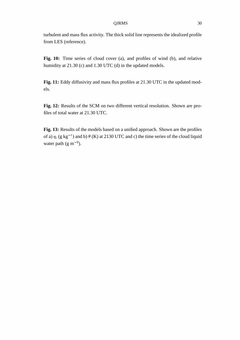
The initial profiles are shown in Fig. 1. The surface latent and sensible heat

fluxes are prescribed, with values close to zero in early morning and the evening,

and a maximum at midday of 500 W m �

�and 140 W m �

�, respectively. This

implies a Bowen ratio of approximately 0.3, whereas typical values in marine Cu

are much lower (e.g, 0.06 in BOMEX). The surface roughness is 0.035 m. Small

tendencies representing the effect of large-scale advection and shortwave radiation

are prescribed [for details see Brown et al. (2002)].

b. Summary of LES results

In Brown et al. (2002) the results of 8 LES models are discussed. The spread be-

tween these different LES results was relatively small, in particular in comparison

with the spread in the SCM results presented here. For convenience, we will there-

fore only present LES results of the KNMI LES model (Cuijpers and Duynkerke

1993).

In Fig. 2 the evolution of the potential temperature and the cloud liquid water

are shown. The evolution of the potential temperature shows the growth of the

inversion from near the surface to 800 m at 15 UTC (9 LT) when clouds appear.

At that time clouds are shallow with the highest cloud tops at 1000-1500 m, but

gradually the cloud layer deepens with the highest cloud tops at 2500-2800 m after

19 UTC (13 LT). At the same time cloud base rises from 800 m to 1300 m. Values

QJRMS 4

of cloud liquid water (domain averaged) are relatively low with values of 0.01-0.04

g kg �

�. Figure 3

Other LES results are shown in concert with the SCM results. We will con-

centrate on time series of vertically integrated quantities, like Liquid Water Path

(LWP) and cloud fraction. In addition, we will focus on the profiles at two differ-

ent stages: at 17.30 UTC with a shallow cloud layer forced from the subcloud and

at 21.30 UTC with well developed, active clouds.

3. Results of the (semi-) operational versions

We intercompare results of 7 different models: ARPEGE (CLIMAT), ECHAM4,

ECMWF, HIRLAM, METO and MESO-NH and RACMO. For METO only the mean

profiles and the timeseries were available. These models and their physics pack-

ages are shortly described in the appendix. Some relevant model aspects are also

described in concert with the analysis of the results.

Most participants have run their model on two different vertical resolutions,� � � and

� ��� with respectively 19 and 40 levels in the lowest 4 km of the atmo-

sphere. Resolution� � � equals (in the lowest 4 km) the L60 resolution presently

operational in ECMWF (Teixeira 1999).� � � has a vertical grid spacing of 200-400

m in the cloud layer (and higher near the surface). Even though� � � is a high oper-

ational resolution, the cloud layer is only resolved by 3 or 4 points, and numerical

errors are relative large. Therefore,� ��� has a grid spacing of 150-200 m in the

cloud layer. If available, we show results on� ��� since at that resolution numerical

errors are smaller. For ECMWF and HIRLAM results on� ��� were not available;

for these models we will show results on� � � . It is noted here that in ECHAM4 and

METO results on� ��� are rather different from results on the lower vertical resolu-

tion at which the model is run operationally. Sensitivity to vertical resolution will

be shown in section 5c.

a. Timeseries

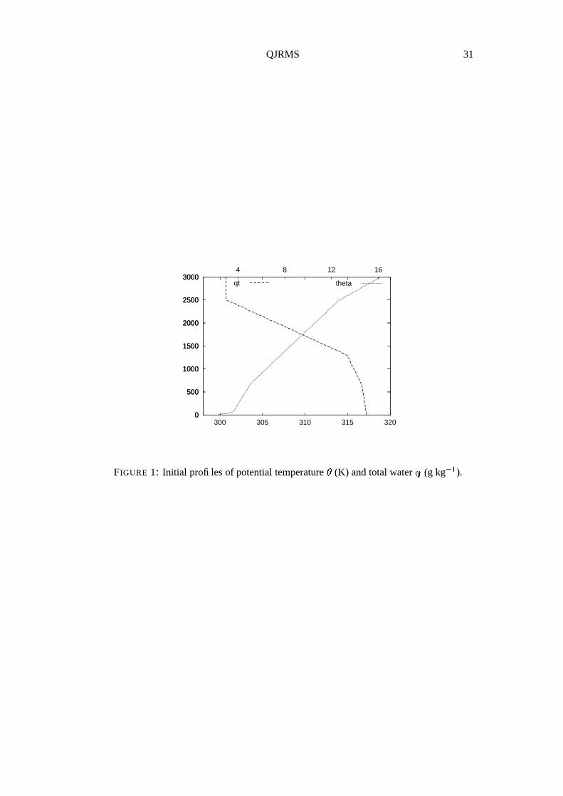
In Fig. 3 the time evolution of the total (projected) cloud cover is shown. Most

models have too high cloud cover in the mid-afternoon, over 50 % in ECMWF,

ECHAM4, ARPEGE and HIRLAM. In addition, in most models clouds do not

dissolve at the end of the day (HIRLAM, RACMO, ECMWF, ECHAM4), or even

peak in cloud fraction after sunset (RACMO and HIRLAM). ECHAM4 already has

QJRMS 5

a rather high cloud cover in the early hours of the simulation.

It is not entirely trivial to compare total projected cloud cover in the SCMs

and in the LES. How the horizontally slab average cloud fraction as a function of

height projects onto the total cloud cover is strongly dependent on the vertical ge-

ometry of the clouds. In LES results of BOMEX (Siebesma et al. 2003) the ratio

between total cloud cover and the maximum of the layer cloud fraction is on av-

erage 2.2, but ranges between 1.3 and 3.7 (with the major uncertainty in the total

cloud cover). For this case, the KNMI LES model gives a ratio of about 2 (see

Fig. 3). In the SCMs this effect is reflected by the cloud overlap assumption. Most

SCMs use a maximum random overlap assumption. Using this overlap assump-

tion for the cloud fraction profile simulated by LES in Fig. 5 the total maximum

overlap cloud cover equals the maximum of the layer cloud fraction. In that case

it would be better to compare SCM results of total cloud cover to the maximum of

the layer cloud fraction of the LES results. On the other extreme, some SCM mod-

els produce clouds with almost no vertical coherent structure, resulting in a total

cloud cover far exceeding the maximum of the layer cloud fraction. For instance,

ARPEGE has a maximum of the layer cloud fraction hardly exceeding 30 %, but

computes a total projected cloud cover of over 70 % (see also Fig. 5).

The cloud liquid water path (vertical integral of the mean liquid water content)

shows similar behavior. Most SCMs have LWPs that are a factor 2-5 times higher

than in the LES model, most outspoken in ARPEGE and METO with values over

300 g m �

�, and in ECMWF reaching 150 g m �

�. In both LWP as in cloud cover

most SCMs show a high level of intermittency. Note that the intermittency in the

LES results is caused by sampling of a relatively small amount of clouds in the

LES domain of 6.4 � 6.4 km. Most SCMs, however, are representative for (much)

larger domain sizes, and the parameterizations do not represent the lifecycle of one

single cloud and should therefore not contain this type of intermittency.

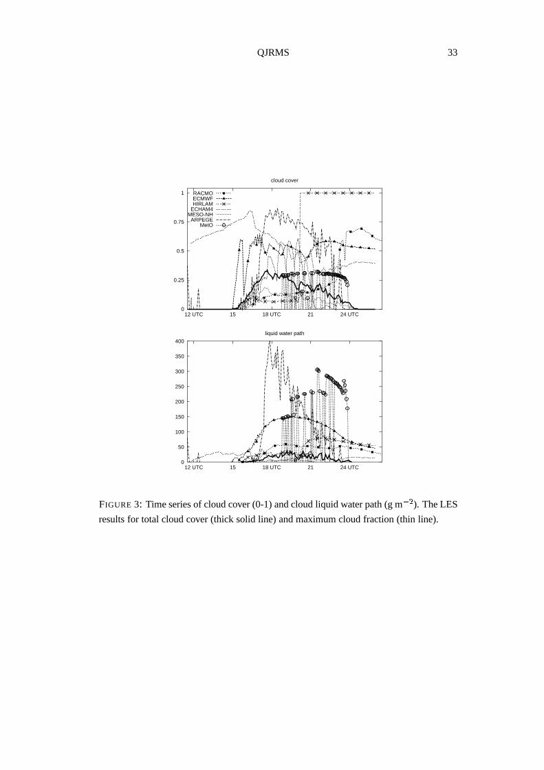
b. ProfilesFigure 4

We focus on two different phases of the diurnal cycle of cumulus convection: first

just after the onset of clouds at 17.30 UTC (11.30 local time), and next at the active

phase with well developed clouds at 21.30 UTC (15.30 local time). Figure 5

Profiles at 17.30 UTC are shown in Fig. 4. In the LES model there is a shallow

cloud layer with cloud base at 800 m and highest cloud tops at 1500 m. There is

no well developed conditionally unstable profile yet as can be seen in profiles of

QJRMS 6

total water � � and the potential temperature � (which in this case is close to the

moist conserved liquid water potential temperature ��� ). In this phase, the clouds

are mainly forced from the subcloud layer. The profiles of � and � � in the SCMs are

reasonably close to the LES results. Some SCMs, however, already developed a

considerable amount of grid point noise, in particular in ECHAM4 (see e.g. results

for � � , relative humidity and � ). At this early stage of cloud formation, the cloud

fraction and cloud liquid water already show rather high values in most SCMs

(except in HIRLAM and METO which have no clouds at this time). In the LES

model the shape of profiles of liquid water and cloud fraction is similar, but in the

SCMs they are often rather dissimilar. For example, ECHAM4 has clouds reaching

the surface, but no correspond liquid water, and in ECMWF liquid water strongly

peaks at one layer in the inversion, but the cloud layer extends over more layers.

MESO-NH has a rather high cloud fraction (45 %) but almost no corresponding

liquid water. RACMO shows the opposite behavior, with somewhat low cloud

fractions, but too much cloud liquid water. The horizontal wind component �shows two models (ECHAM4 and RACMO) with weak winds in the cloud layer,

but too strong winds in the subcloud layer, and a large gradient near cloud base.

ECMWF bas too strong winds in the sub-cloud layer.

The profiles in the mid-afternoon at 21.30 UTC (15.30 local time) are shown in

Fig. 5. The differences between the LES model and the SCMs, and among the dif-

ferent SCMs have increased significantly. Three models (ECMWF, ARPEGE, and

ECHAM4) have high moisture contents in the inversion above 2000 m, whereas

the cloud layer, in particular near cloud base, is too dry. Except ARPEGE, these

models are also too warm in the cloud layer. HIRLAM, on the other hand, is char-

acterized by a very shallow boundary layer, which is too moist and covered with

thick stratiform clouds. The temperature and moisture profiles in RACMO and

MESO-NH are reasonably close to the LES results (see e.g. the profile of relative

humidity), but the cloud fraction in MESO-NH is too small and the cloud liquid

water in RACMO too large. ECMWF has a remarkable peak in cloud fraction in

the inversion, despite that the relative humidity at that height is below 80 %. A

peak in cloud fraction in ARPEGE at 2500 m corresponds to a maximum in rela-

tive humidity (90 %) at that height. RACMO and ECHAM4 have unrealistic wind

profiles, and noise is apparent in the profiles of ECHAM4 and to a lesser extent

in ARPEGE. [Note that e.g. ECHAM4 seems to have problems with conserving

heat or did not apply the correct forcing since they are to warm (compared to LES)

QJRMS 7

everywhere.] Figure 6

In four models the clouds did not dissolve at the end of the day. Fig. 6 shows the

relative humidity and cloud fraction in the evening 19.30 local time at a time when

the cloud should have disappeared. RACMO and HIRLAM are close to saturation

just below the inversion, and accordingly predict high cloud fractions. In ECMWF

the cloud fraction peaks close to the inversion at a higher level. In ECHAM4 some

thin clouds remain, despite the comparatively low relative humidity,

4. Analysis of the results

The results are analyzed in terms of the individual behavior of the different param-

eterization schemes and their mutual interaction. As discussed in the introduction,

three parameterizations play a major role: i) the turbulence scheme, ii) the convec-

tion scheme, and iii) the cloud/condensation scheme.

a. Turbulence

All models use diffusion to represent subcloud turbulent mixing; that is, the turbu-

lence scheme computes fluxes from

������������ �������

� ������ (1)

where � ��� � ����� � � � � etc � . Here, and in the following, � denotes the grid box

mean value. Commonly used closures to compute the eddy diffusivity � are the

TKE- � closure, the Louis (1979) closure, or the � -profile method (Troen and Mahrt

1986).

The TKE- � scheme employs a prognostic equation for Turbulent Kinetic En-

ergy (TKE or � ) (see e.g., Stull 1988) combined with a diagnostic length scale:

��� � ��� �!#" � (2)

Different TKE- � schemes use rather different rules to prescribe the length scale

� ����� in terms of local and/or nonlocal stability measures: e.g. based on a parcel

method in MESO-NH (Bougeault and Lacarrere 1989) and based on the local Ri in

ECHAM4 (Roeckner et al. 1996). The Louis (1979) closure uses

�$� � ������%%%%�'&(�)�

%%%% (3)

QJRMS 8

with � ����� depending on the Richardson number, chosen such that near the surface

the scheme matches to surface flux profile relations. The � � profile method (Troen

and Mahrt 1986) uses prescribed, approximately quadratic profiles, from the sur-

face to the top of the convective boundary layer. In such a scheme, the entrainment

flux at the boundary layer top is often prescribed.

ECMWF and METO use a � -profile method with prescribed entrainment rate,

and ARPEGE the 2���

order Mellor and Yamada (1974) scheme based on diag-

nostic (instead of prognostic) TKE. For stable conditions ECMWF uses the Louis

(1979) closure. The other models use a TKE- � scheme, but with rather different

formulations of the length scale.

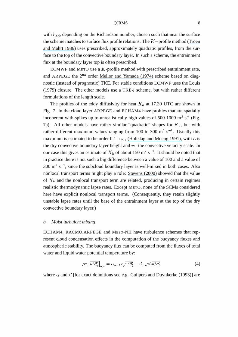
The profiles of the eddy diffusivity for heat � � at 17.30 UTC are shown in

Fig. 7. In the cloud layer ARPEGE and ECHAM4 have profiles that are spatially

incoherent with spikes up to unrealistically high values of 500-1000 m�

s �

�(Fig.

7a). All other models have rather similar “quadratic” shapes for � � , but with

rather different maximum values ranging from 100 to 300 m�

s �

�. Usually this

maximum is estimated to be order 0.1 h � � (Holtslag and Moeng 1991), with�

is

the dry convective boundary layer height and � � the convective velocity scale. In

our case this gives an estimate of � � of about 150 m�

s �

�. It should be noted that

in practice there is not such a big difference between a value of 100 and a value of

300 m�

s �

�, since the subcloud boundary layer is well-mixed in both cases. Also

nonlocal transport terms might play a role: Stevens (2000) showed that the value

of � � and the nonlocal transport term are related, producing in certain regimes

realistic thermodynamic lapse rates. Except METO, none of the SCMs considered

here have explicit nonlocal transport terms. (Consequently, they retain slightly

unstable lapse rates until the base of the entrainment layer at the top of the dry

convective boundary layer.)

b. Moist turbulent mixing

ECHAM4, RACMO,ARPEGE and MESO-NH have turbulence schemes that rep-

resent cloud condensation effects in the computation of the buoyancy fluxes and

atmospheric stability. The buoyancy flux can be computed from the fluxes of total

water and liquid water potential temperature by:

���� � � � � %% � � ��� � � ��� � � � � ������ � � ��� � � � �� � (4)

where � and � [for exact definitions see e.g. Cuijpers and Duynkerke (1993)] are

QJRMS 9

dependent on whether the atmosphere is unsaturated with no cloud water (subscript

u) or saturated (subscript s). In dry conditions, � � ��� and � ��������� . With a latent

heat flux of 500 W m �

�and a sensible heat flux of 140 W m �

�the moisture flux

amounts to about 30 % of the buoyancy flux. In the saturated conditions, however,� ������� � and � ��������� , which, in this case, means that the moisture flux dominates

the buoyancy flux for saturated conditions. The vertical stability is computed from

the gradients of � � and � � in a similar way. In partly cloudy conditions, the buoyancy

flux is obtained by a linear interpolation in cloud fraction � of the dry and moist

contributions: ��� � � � � � ����� � ��� ���� � � � � %% � � � ���� � � � � %% � (5)

For skewed motions Eq. (5) can be extended to include the non-Gaussian part

(Cuijpers and Bechtold 1995). This is done in MESO-NH and will be done in next

version of ARPEGE. This may however induce overlap with the convection scheme

(“double counting”).

In addition, these models (except ARPEGE) use mixing in moist conserved

quantities (e.g, in � � and � � ) or add seperate mixing of cloud liquid water. Although

the use of diffusion for cloud liquid water might be questioned, the procedure of

mixing liquid and water vapor sepately can lead to realistic fluxes of conserved

variables – diffusion is a linear operator – in cloudy boundary layers (for a discus-

sion on this subject see e.g. Lenderink and van Meijgaard 2001).

Because the formulation of buoyancy flux given by Eq. (5) is strongly depen-

dent on the cloud fraction, small changes in cloud fraction have a large impact on

the atmospheric stability and the buoyancy flux. The dependency in moist turbu-

lence scheme may give rise to instability (in ARPEGE and MESO-NH) and cloud

regime transitions from Cu to more stratiform clouds (or vice-versa). In ECHAM4

the instability is related to the limit behavior of the Louis (1979) stability func-

tions for small wind shear in combination with a moist formulation for stability

(Lenderink and van Meijgaard 2001; Lenderink et al. 2000). In that case, small

local variations in cloud fraction strongly impact on the length scale, and thus

on turbulent mixing. The turbulent fluxes again feed back onto cloud fraction by

changing humidity and temperature profiles. The instability in ECHAM4 is visible

from the timeseries and profiles of � � in the cloud layer in Fig. 7. Potentially,

this is a very strong destabilizing feedback circle combining the impact of cloud

condensation on stability and therefore mixing, on one hand, and turbulent mixing

on cloud formation, on the other hand. In RACMO a similar feedback gives rise to

QJRMS 10

increasing cloud cover with time . More active mixing in the cloud layer tends to

straighten the profiles, giving rise to a shallow but well mixed boundary layer rep-

resentative for stratiform clouds. This positive feedback is e.g. visible in the time

series of � � in the cloud layer (Fig. 7). In stratiform clouds long wave cooling

is an important source of turbulence, but in the case setup it is neglected. Taking

longwave cooling into account, we might expect this feedback to have a stronger

effect, resulting in still higher cloud fractions. Figure 7

c. Convection

All models except ARPEGE run with an explicit parameterization of convective

transports in the cloud. HIRLAM uses an adapted version of the Kuo (1974)

scheme; all other models use a bulk mass flux approach: RACMO, ECHAM4,

ECMWF based on Tiedtke (1989); MESO-NH based on Kain and Fritsch (1990)

and in METO based on Gregory and Rowntree (1990).

In the following analysis we will concentrate on the mass flux closures, mainly

because most recent developments in parameterizations of convection have been

achieved in these type of schemes. The bulk mass flux approach computes the

convective fluxes from � ��� ����� � � � � � � � � � � (6)

with the equation for the cloud updraft � � �� � � ���� ��� � � � � � � � (7)

and the mass flux� � �

�)� ����� �� � � (8)

Here, � and � govern the amount of updraft mass due to entrainment and detrain-

ment, respectively. Mass flux schemes mainly differ in how the values at cloud

base, and the fractional entrainment and detrainment coefficients, � and � , are pre-

scribed. In the inversion, the updraft becomes negatively buoyant, and above that

zero-buoyancy level the mass flux detrains massively .

In Fig. 8 we plotted the flux produced by the mass flux scheme [as defined by

Eq. (6)] for � � and � � . These fluxes represent a warming and drying near cloud base,

and a moistening and cooling close to the inversion. In ECHAM4 and ECMWF this

effect is very strong. To analyze this behavior we focus first on the mass flux�

in

Fig. 8c. In the cloud layer, the mass flux in two models (ECMWF and ECHAM4) is

QJRMS 11

constant with height, with massive detrainment in a shallow layer in the inversion.

In ECHAM4 it is assumed that 80 % of the detrainment takes place in the first layer

above the zero buoyancy level and 20 % in the next level. At this high vertical

resolution this causes an extremely rapid detrainment. In MESO-NH the mass flux

above cloud base first strongly increases, followed by a rapid decrease. RACMO

has a gradual decrease in the mass flux fixed by the entrainment and detrainment

coefficients in Siebesma and Holtslag (1996).

It should be noted that all model have a linear profile of the fluxes of total

water and liquid water potential temperature from the surface to cloud base. This

represent transport by the organized flow in the subcloud layer connected to the

cumulus cloud, drawing moisture and heat from the subcloud layer. This is part

of the closure assumption used in the models. The massflux�

is not used in the

subcloud layer, and its shape in the subcloud layer is therefore irrelevant. Figure 8

In general, the difference between the updraft and the mean field (not shown)

increases with height above cloud base. We illustrate this for moisture by writing

Eq. (7) as ��� ���� � � � � ����� � (9)

with� ��� � � � � � and ��� � �� �

�� . If we assume ��� and � constant, just for sake

of the argument, this equation can solved easily (see also Eq. A3 in Siebesma and

Holtslag 1996)� � � ���

� � � � � � ��� � ���� ��� ����� � ���������� (10)

with� � � ��� is

� � at cloud base, and� � ��� the cloud base height. The first term is

the asymptotic behavior, and the second term the behavior near cloud base. Taking

typical values of� � � ��� � 1 g kg �

�, ��� ��� � � �

�g kg �

�m �

�and � �! � � �

�,

the second term is negative, so� � increases with height above cloud base. Given

that in general the mass flux in the SCMs is rather constant or sometimes even

increases with height, the flux of the total water increases with height. This reflects

that the mass flux scheme takes away moisture from the lowest part of the cloud

and deposits this in or close to the inversion. In ECHAM4 and ECMWF this effect

is very pronounced (see Fig. 8), being at odds with LES results and common sense.

Hence, the mass flux should decrease with height in order to obtain moisture fluxes

that also decrease with height. Similar arguments hold for the flux of liquid water

potential temperature.

The increase in the convective flux of total water with height is responsible

QJRMS 12

for the large gradient just above cloud base. In the subcloud layer this gradient

does not occur due to the intense mixing by the turbulence scheme. In terms of

potential temperature an inversion is created just above the well-mixed subcloud

layer. This is clearly visible in the profiles of especially relative humidity in Fig.

5 (ECMWF, and ECHAM4). There is a positive feedback because the difference

between updraft and mean field increases during this process.

The high moisture content above 2300 m in ECHAM4 and ECMWF are caused

by too strong activity of the mass flux scheme, depositing too much moisture in/or

just above the inversion. In ECMWF, time series of the mass flux at cloud base

revealed that in the first few hours after the onset of the clouds, the mass flux

obtained very high values of 0.2 kg m �

�s �

�. This confirms results of Neggers

et al. (2003), where it was shown that the mass flux closure based on moist static

energy convergence strongly overpredicts the cloud base mass flux.

In HIRLAM a switch turns convection smoothly off when the horizontal grid

spacing gets finer. This switch is mainly developed with deep convection in mind,

but acts for shallow convection also. The results presented here are for a horizontal

resolution of 4 km, which is the typical resolution the HIRLAM aims at in the near

future. Results at a resolution of 20 km (not shown) are better with much deeper

clouds, extending to 2500 m during the mid afternoon. But also at this horizontal

resolution a rather thick, low-level cloud develops at the end of the day after 23

UTC.

d. Interaction of turbulence and convection

The interaction between the convection scheme and the turbulence scheme plays an

important role. The turbulence and the mass flux scheme determine how the pro-

files of temperature and humidity evolve. The resulting profiles, in particular near

cloud base, again influence mass flux activity and/or turbulent activity, potentially

giving rise to strong feedback loops.

In some models, the role of the turbulence scheme is crucial to prevent unre-

alistically strong drying of the lower part of the cloud layer due to the mass flux

scheme. However, the inversion above cloud base caused by the mass flux scheme,

may limit turbulent transports. In this case a run-away process may occur. Dry

turbulence schemes are slightly more susceptible to this feedback, but it may also

occur in moist turbulence schemes. In ECHAM4, the stability functions in terms

of the local Ri number, and the limit behavior for small wind shear (Lenderink and

QJRMS 13

van Meijgaard 2001) are responsible for a cessation of turbulent transports across

cloud base.

On the other hand, a feedback between the cloud base closure of the mass

flux scheme and the turbulence scheme might lead to a reduction of convective

activity. This type of feedback may occur with closures based on the assumption

of subcloud equilibrium, or more precisely, based on subcloud convergence of

moisture (ECHAM4 and RACMO) or moist static energy (ECMWF). In that case,

the mass flux at subcloud is adjusted so that the total moisture (or moist static

energy) content of the subcloud layer remains constant:

� � ��� �� � � ���� � � � � � ���� � ���� � � � � � � � ��� (11)

with ��� � �� � � the surface latent heat flux and ��� � �� � � ��� the moisture flux through cloud

base generated in the turbulence scheme. In this closure the following feedback

may occur. If the stability at cloud base weakens, the turbulence fluxes at cloud

base will increase. In effect, the closure will reduce the mass flux activity. This

process will erode the inversion at cloud base further (due to combined effects of

more active diffusion and less mass flux activity). Schemes with moist turbulence

schemes are more susceptible to this feedback (e.g. in RACMO). Obviously, this

feedback is strongly dependent on the type of closure; for example, it does not

occur with closures based on the subcloud turbulent velocity scale (Grant 2001),

such as e.g. used in METO.

Since mass flux schemes are basically advection schemes, the way the advec-

tion operator is implemented plays an important role. Many of the present-day

operational mass flux schemes use implementations that are close to upwind dif-

ferencing (Tiedtke 1989). They introduce considerable amounts of numerical dif-

fusion (order M � ��� � � � � � m�

s �

�with � �

the grid spacing). In fact, using

the non-diffusive central differencing in ECMWF, large gradients at cloud base oc-

curred. Since at high resolution numerical diffusion becomes insignificant, these

models tend to become more unstable with increased vertical resolution. In com-

bination with turbulence schemes based on local stability measures (like e.g. the

Richardson number) this may give rise to high levels of noise. This plays a role in

at least results of ECHAM4, RACMO, and ECMWF.

QJRMS 14

e. cloud schemes

There is a large spread in how models treat cloud fraction, cloud liquid water, and

evaporation and condensation. The range spans from statistical schemes, which

diagnose cloud liquid water and cloud fraction based on mean values of � � and � �and estimates of their subgrid variability (in MESO-NH and ARPEGE), to process-

based schemes with prognostic equations for both cloud liquid water and cloud

fraction (e.g. ECMWF). Other models combine a diagnostic cloud cover, based

on relative humidity (HIRLAM, ECHAM4) or total water (RACMO), with a prog-

nostic equation for cloud condensate based on Sundqvist et al. (1989). Due to this

variety in cloud schemes used, it is hard to draw general conclusion from the re-

sults. In addition, the fact that most models drift away from realistic temperature

and humidity profiles rather quickly (as is shown in Fig. 5) complicates the analy-

sis. A perfect model approach in which cloud schemes are fed with realistic mean

profiles would be more revealing, but this approach was not exercised here. An

example of such an approach is discussed in Siebesma et al. (2003).

One rather general conclusion one might draw from the results is that in the

prognostic schemes cloud fraction and cloud liquid water are (often) strongly tied

to the convective activity. For example, in these models the detrainment of liquid

water by the mass flux scheme is used as a source term for the liquid water, given

by: � � � ������ � � ��� � �� ������ � � � � � �

��� � (12)

In several models (ECHAM4, RACMO, and ECMWF) this leads to a peak in cloud

liquid water content close to the inversion, where massive detrainment takes place.

In ECMWF a similar term is also used in the prognostic equation for the cloud

fraction leading to high cloud fractions in the inversion. These high values of the

cloud related parameters occur despite the relatively low relative humidity, which

does not appear to be a very realistic feature.

5. ProgressFigure 9

a. Synthesis of previous resultsFigure 10

The activity of both mass flux and turbulence schemes, and their relative strengths,

are major issues. To summarize, we plotted in Fig. 9 three different profiles of total

water that are characteristics corresponding to three typical cases of the SCM re-

QJRMS 15

sults. The “active diffusion” case represents a model with strong diffusive activity

(and corresponding weak or normal mass flux activity). In the cloud layer profiles

are too close to the moist adiabat (too straight). Cloud fraction is accordingly too

high. The turbulence scheme tends to produce a sharp inversion at the cloud top.

The “active mass flux” case corresponds to a model with too strong mass flux ac-

tivity. In this model too much moisture is taken out of the lower part of the cloud

and deposited near the inversion. In this case cloud fraction tends to peak near the

inversion. In both cases we assumed that the flux at cloud base is correct, resulting

in a correct subcloud layer moisture content. Finally, if in addition to the “active

mass flux” case the turbulence scheme transports more moisture across cloud base,

the gradients at cloud base tend to weaken. In this “active mass flux and diffusion”

case the subcloud tends to dry and cloud layer tends to moisten, resulting in even

higher cloud fractions near the inversion.

b. Results of updated models

Based on the findings described above, many participants updated their models

with new physics schemes and/or modified their present schemes. Results of some

successful updates are shortly described below. It is not our goal to describe and

analyze these changes extensively. Merely, we would like to illustrate which type

of modifications potentially lead to improved results. In four models significant im-

provements were obtained. These updated models, referenced by ECMWF-WST,

RACMO-WST, ARPEGE-TKE, are described below.

ECMWF-WST uses a new closure of the cloud base mass flux based on the

convective velocity scale (Grant 2001)

� � ��� � � � � (13)

with � � ������� . The closure based on subcloud moist static energy convergence

employed in the reference version gave unrealistically high values of the cloud

base mass flux in the early hours of cloud formation. This is prevented by using

Eq. (13). Also the boundary layer scheme for convective conditions was replaced

(Siebesma and Teixeira 2000) and the updraft properties at cloud base were com-

puted from a new parcel method (Jacob and Siebesma 2002).

RACMO-WST also employs the convective velocity scale closure by Eq. (13),

but with slightly higher value � � ����� � . The main reason for this change is that the

used moisture convergence closure gave rise to a regime transition to higher cloud

QJRMS 16

fractions at the end of the simulation period. In addition, mixing of momentum in

the mass flux scheme was turned off, but at the same time vertical diffusion was

added by����� � � ��� � (14)

with � ��� ��� �� m. The length scale � ��� chosen so that about 20-30 % of the total

flux of � � and � � in the cloud is due to diffusion and the other part due to the mass

flux as supported by LES results in Siebesma et al. (2003). One may consider this

additional diffusion as representing mixing by the smaller eddies in the cloud; it is

done for heat, moisture and momentum.

In ARPEGE-TKE the diagnostic turbulence closure was replaced by a prognos-

tic TKE- � scheme with the Bougeault and Lacarrere (1989) length scale to improve

numerical stability of the scheme. In Bougeault and Lacarrere (1989) length scales

are determined by the distance which an adiabatic parcel can rise/sink before being

stopped by buoyancy effects. The moist turbulence scheme has been extended with

mixing in moist conserved variables, and a nonlocal term (skewed) is added to Eq.

(5). A mass flux scheme has been added based on the ideas of Kain and Fritsch

(1990) and described in Bechtold et al. (2001). Chaboureau and Bechtold (2002)

and Lopez (2002) describe the new cloud and condensation scheme.

Finally, in the HIRLAM-CLIM the main change was a replacement of the

cloud and convection scheme STRACO by a package developed by the SMHI

Rossby climate modeling center consisting of the Kain and Fritsch (1990) con-

vection scheme and Rasch and Kristjansson (1998) cloud/condensation scheme

(Unden et al. 2002).

Results of these updated schemes are shown in Fig. 10. The time series of

the cloud cover show lower, more realistic values below 40 % in the models, ex-

cept in ECMWF-WST. The latter is caused by the prognostic cloud scheme in

which cloud cover is too strongly tied to the (massive) detrainment of the mass

flux scheme. The thermodynamical profiles are significantly improved in all mod-

els as can be seen from the relative humidity profiles, though HIRLAM-CLIM

shows the footprint of a slightly too strong mass flux activity. The wind profiles in

RACMO-WST are vastly improved due to deactivation of momentum transport by

the mass flux scheme and the inclusion of additional diffusive momentum trans-

port. In HIRLAM-CLIM there is a trace of instability left.

To illustrate both the activity of the diffusion and the mass flux scheme, we

plotted � � and�

at 21.30 UTC in Fig. 11. The mass fluxes are of the same order

QJRMS 17

of magnitude, but the different models have rather different shapes; ranging from

constant with height (ECMWF-WST), uniformly decreasing with height (RACMO-

WST), to first increasing and then decreasing with height in the two Kain and

Fritsch (1990) based models (ARPEGE-TKE and HIRLAM-CLIM). All models

have similar quadratic shape profiles of � � in the subcloud layer with small values

in the cloud layer.

Finally, in ECHAM (results not shown) the change of the cloud cover scheme

from a relative humidity based scheme (Sundqvist et al. 1989) to a statistical cloud

cover scheme (Tompkins 2002) vastly improved the onset of cloud formation.

However, the convective and turbulent transport still caused a significant moist

bias close to the inversion, causing high cloud amounts. Figure 11

c. Resolution dependency

The results of most models depend strongly on vertical resolution. To illustrate

typical model resolution dependencies we present results of ECHAM4, METO,

RACMO-WST, ARPEGE-TKE at� � � and

� ��� resolution in Fig. 12. In ECHAM4,

results of the high resolution are much more contaminated by gridpoint noise. The

results on� � � are reasonable, but the

� ��� results are unacceptable due to instabili-

ties related to the turbulence scheme. In RACMO the results on� � � are character-

ized by a more shallow and moist cloud layer. Analysis showed that, on this res-

olution, the mass flux is not able to penetrate high enough, and already massively

detrains moisture in the upper part of the cloud layer, instead of in the inversion.

This is related to the fact that the detrainment layer is diagnosed as the whole layer

immediately below the first (half or flux) level where the cloud updraft is negatively

buoyant. It does not take into account that part of this layer may be in the active

buoyant cloud where there should be no massive detrainment. In particular, on low

resolution too much moisture is therefore deposited in the active cloud. Results of

RACMO-WST obtained with a 50 m grid spacing are almost identical to the� ���

results, showing that this effect becomes insignificant at� ��� resolution.

The results of METO and ARPEGE-TKE show rather large sensitivities to ver-

tical resolution. The low resolution results are considerable more moist in the

subcloud layer (1-2 g kg �

�), and gradients at cloud base are (much) larger. The

latter reflects the weak activity of the turbulence scheme across cloud base (unable

to moisten the lower part of the cloud layer sufficiently) and/or the strong activity

of the mass flux scheme.

QJRMS 18

It is noted that METO and ECHAM4 perform (somewhat) better on� � � reso-

lution. In ECHAM4 the amount of gridpoint noise is significantly lower on� � �

compared to the high resolution results. In METO the properties of the subcloud

layer are close to the LES, but the cloud layer shows in imprint of a too active

mass flux scheme. Results of METO on� � � are rather close to the results of the

resolution the model is run operationally. Figure 12

d. Unified approaches

Considering the dependency of the results on the relative importance of mass flux

and turbulent activity, and the rather ad-hoc formulation of closures of mass flux

scheme, it seems advantageous to use unified approaches to represent fluxes in

cloud and subcloud layer. In addition to the results of the operational models,

results of three research models based on such an approach were analysed.

Two models, MESO-DIF [described in Sanchez and Cuxart (2003)] and CHEIN-

DIF [described in Cheinet and Teixeira (2003)], employ a unified approach based

on diffusion using a moist TKE- � closure. This approach is motivated by the ob-

servation that a unique and rather constant eddy diffusivity in the cloud layer can

be diagnosed (flux divided by gradient) from the LES results in e.g. BOMEX in-

tercomparison (Siebesma et al. 2003). CHEIN-MF uses a multi-parcel mass flux

approach (Cheinet 2003). Results of these three models are shown in Fig. 13. Figure 13

Results of the models based on moist diffusion show a reasonable skill to pre-

dict the temperature and moisture profile, in particular when compared to the re-

sults of the operational SCMs (see Fig. 5). On the downside, however, the results

are characterized by a rather high level of intermittency in the cloud layer. Also

these models tend to create a too sharp inversion, reflecting that a local diffusion

scheme is not able to represent the overshoots of the strongest updrafts in the in-

version.

As shown in Fig. 13, the temperature and humidity profiles predicted by

CHEIN-MF are very close to the LES results, both in the cloud layer and in the

sub-cloud layer. The fact that the same entraining plume model is used for the un-

saturated and the saturated updrafts is thought to explain the consistent treatment

of the sub-cloud and cloud layer mixing. Timing of the convective activity is very

good (see the liquid water path in fig 13c). Since this model is purely diagnostic

with respect to the turbulence variables, this suggests that the cloud layer adjusts

very rapidly to the surface forcing in our case. Also, the model results turn out to

QJRMS 19

be much less sensitive to vertical resolution compared to bulk mass-flux approach

(with only one updraft), as results with 70 levels and 14 levels (up to 4000m) are

virtually the same (not shown).

6. Discussion

An intercomparison of the diurnal cycle of cumulus convection in different SCMs

derived from (semi-) operational models is presented. The SCM results revealed

several deficiencies. In general, results are characterized by: too large values of

cloud liquid water and cloud cover, strong intermittent behavior, and unrealistic

profiles of temperature and humidity (and wind) in the cloud layer.

The results are analyzed in terms of the behavior of the different parameteri-

zation schemes involved: the turbulence scheme, the cumulus convection scheme,

and the cloud/condensation scheme. The different models have different causes for

their deficiencies. The main causes are (not applying all to one model):

� Too strong activity of the turbulence scheme, giving rise to too strongly

mixed, too shallow and too moist boundary layers.

� Strong intermittency mainly caused by the interaction of the (moist) turbu-

lence scheme with the cloud scheme and the convection scheme [e.g., see

Eq. (5) ].

� Too strong activity of the mass flux scheme causing a too dry (warm) lower

part of the cloud, and a too moist (cold) upper part. Often a strong inversion

at cloud base results, prohibiting any turbulent transport across cloud base.

� Unrealistic transport of momentum in the mass flux scheme

� Too strong dependency of the cloud/condensation scheme on the (massive)

detrainment by the mass flux scheme.

� Strong dependency on vertical resolution.

In general, the SCM results could be divided into two different classes. In

one class, turbulent activity was too strong and in the other class the mass flux

activity was too strong. Typical, idealized profiles obtained in these classes are

shown in Fig. 9. Paradoxically, in both classes too high values of cloud cover

and liquid water content occur: in the first class being a realistic consequence

QJRMS 20

of the shallow, moist boundary layer, in the second class mainly caused by the

(unrealistically) strong dependency of cloud liquid water and/or cloud fraction on

the detrainment from the mass flux scheme. Results are strongly dependent on

vertical resolution. In particular, results of the mass flux scheme close to cloud

base and close to the zero-buoyancy level at cloud top are very sensitive. A grid

spacing of approximately 200 m in the cloud layer is needed to resolve mass flux

profiles sufficiently.

Based on these findings, several SCMs have been updated with new physics

packages and/or their present packages have been revised. These new model per-

form significantly better on this case, though there are some remaining deficiencies.

All updated models use a bulk mass flux approach combined with diffusion in the

subcloud layer. For this combination, the following specific recommendations are

made:

� use a turbulence scheme based (predominantly) on nonlocal stability charac-

teristic (e.g., Bougeault and Lacarrere 1989; Lenderink and Holtslag 2003).

� use a mass flux closure based on the convective velocity scale of the subcloud

layer (e.g., Grant 2001).

� use either local diffusion for transport of momentum in the cloud layer, or a

mass flux approach with weak nonlocal characteristics; that is, with updraft

properties which relax strongly to environmental profiles [see also Brown

(1999) for more on this issue]

� use a statistically based cloud scheme, or a prognostic scheme with a weaker

(than presently used in many models) dependency on the massive detrain-

ment by the mass flux scheme.

It should be noted that we do not argue that with other (type of) schemes realistic

results cannot be obtained; we argue that SCMs that satisfy these points perform

reasonably well in the present case.

Results of several research models based on a unified approach, either based

on a mass flux approach or on diffusion, discussed in Section 5 are considered to

be promising. In particular the results for the multiple mass flux approach promote

further developments in order to use this approach in an operational model (see

also Cheinet, 2003a,b).

QJRMS 21

Finally, we would like to emphasize the importance of the “triggering function”

of convection, even though this matter is almost neglected in this paper. But the

case considered here is so strongly forced by the surface fluxes that all SCMs

trigger convection at about the right time, and timing of the triggering of convection

is therefore not a crucial issue here. However, experience with a simulation of the

diurnal cycle of Stratocumulus clouds also performed in the EUROCS project,

showed that some of the SCMs did also trigger the mass flux scheme in that case,

which causes a significant reduction of the cloud cover (Duynkerke et al. 2003).

Moreover, results shown in Jacob and Siebesma (2002) showed that the triggering

function is extremely important in AGCM simulations of ECMWF.

Acknowledgments This work benefited greatly from discussions during EUROCS

workshops in Reading, Lissabon, De Bilt and Madrid. This study has been made

with financial support of the European Union (Contract number EVK2-CT-1999-

00051).

QJRMS 22

TABLE 1: Key Characteristics of the SCMs. Between brackets the revised models.

Scientists Model a Diffusion b Convection c Cloud d

Marquet ARPEGE�

TKEd [TKE] / d [m] no [KF] Dc / Dl [Pl]

Siebesma ECMWF PRO / d T Pc / Pl

Mueller (Chlond) ECHAM4�

TKE / m T Dc / Pl

Lenderink RACMO�

TKE / m T Dc / Pl

Irons METO PRO / m GR Dc / Dl

Soares (Miranda) MESO-NH�

TKE / m KF Dc / Dl

Olmeda/Calvo HIRLAM�

TKE / d KUO Dc / Pl

Jones HIRLAM-CLIM�

TKE / d KF Dc / Pl

Sanchez (Cuxart) MESO-DIF TKE / m no Dc / Dl

Cheinet CHEIN-DIF TKE /m no Dc / Dl

Cheinet CHEIN-MF no MulMF Dc / Dl

aMain model reference:�

Gibelin and Deque (2003),�

Roeckner et al. (1996),�

Lenderink et al.

(2000),�

Lafore et al. (1998),�

Unden et al. (2002)bDry (d) stands mixing in dry variables only;(m) stand for mixing in moist variables and/or

computation stability in moist variables. TKE stands for a prognostic TKE, TKEd for diagnostic

TKE, PRO for a K-profile methodcKF stand for Kain and Fritsch (1990); T stands for Tiedtke (1989), KUO for Kuo (1974); GR

for Gregory and Rowntree (1990); and MulMF for Multiple Massflux (Cheinet 2003)dPc stand for prognostic cloud cover, Dc diagnostic cloud cover, Pl prognostic cloud liquid

water, and Dl diagnostic cloud liquid water.

APPENDIX A

SCM description

The physics packages of the (semi-) operational model are summarized in Table

1. Below follows some more detailed information.

ARPEGE employs a 2� �

order Mellor and Yamada (1974) turbulence closure

with diagnostic value of TKE. Mixing is done in dry static energy and water vapor

only, though the scheme uses a moist formulation for stability (Bougeault 1982).

For shallow convection the mass flux scheme is inactivated. A statistical cloud

scheme (Ricard and Royer 1993) with diagnostic cloud liquid water and cloud

fraction is used.

ECHAM4 Roeckner et al. (1996) uses a moist turbulence scheme based on

prognostic TKE, with the length scale formulation based on Louis (1979). The

convection scheme is the bulk mass flux scheme by Tiedtke (1989). The Sundqvist

QJRMS 23

et al. (1989) scheme is used for cloud condensation and evaporation. Cloud frac-

tion is based on relative humidity.

RACMO is based on ECHAM4 physics. The the length scale in ECHAM4 tur-

bulence scheme has been replaced in order to improve the behavior for (moist)

convective conditions as discussed in Lenderink and Holtslag (2003). The cloud

fraction is computed by a simple statistical scheme with a link between mass flux

activity and the variance of total water used in the cloud scheme (Lenderink and

Siebesma 2000). RACMO uses the Tiedtke (1989) mass flux scheme, but with

modified (increased) entrainment and detrainment coefficients for shallow convec-

tion (Siebesma and Holtslag 1996).

ECMWF uses the Louis (1979) scheme for stable and a K-profile method (Troen

and Mahrt 1986) for unstable conditions with a prescribed top entrainment rate.

The scheme mixes “dry” variables only (water vapor and dry static energy) and is

based on dry formulation for stability. The convection scheme is the Tiedtke (1989)

mass flux scheme. ECMWF uses a fully prognostic cloud scheme with prognostic

equations for both cloud fraction and cloud condensate (Tiedtke 1993).

HIRLAM uses a “dry” TKE- � scheme with the Bougeault and Lacarrere (1989)

parcel length scale formulation (Cuxart et al. 2000). The convection and cloud

scheme is STRACO (Soft Transition Condensation), which combines a modified

Kuo (1974) convection scheme with clouds and condensation based on Sundqvist

et al. (1989). A switch has been introduced to smoothly turn off convection in

the full 3D model for horizontal resolutions below 10km. The present SCM sim-

ulations used a 4 km resolution which means that the convective tendencies are

significantly reduced.

METO uses a K-profile method combined with prescribed entrainment rates

to compute turbulent fluxes. It is uses a nonlocal transport term in convective

conditions (Holtslag and Boville 1993). It mixes conserved variables and is based

on a moist formulation of stability. The Gregory and Rowntree (1990) convection

scheme is used, together with a closure bases on � � (Grant 2001). The entrainment

rates are as Grant and Brown (1999). The cloud scheme is diagnostic based on

relative humidity.

MESO-NH uses a moist turbulence scheme (Cuxart et al. 2000) based on the

Bougeault and Lacarrere (1989) length scale. The mass flux used is the Kain and

Fritsch (1990) mass flux scheme. It uses a statistical cloud scheme based on total

water and liquid water potential temperature.

QJRMS 24

REFERENCES

Bechtold, P., E. Bazile, F. Guichard, P. Mascart, and E. Richard, 2001: A mass

flux convection scheme for regional and global models. Quart. J. Roy. Me-

teor. Soc., 127, 869–886.

Bougeault, Ph., 1982: Cloud-ensemble relations based on the gamma probability

distribution for the higher-order models of the planetary boundary layer. J.

Atmos. Sci., 39, 2691–2700.

Bougeault, Ph. and P. Lacarrere, 1989: Parameterization of orography-induced

turbulence in a mesobeta-scale model. Mon. Wea. Rev, 117, 1872–1890.

Brown, A.R., 1999: Large-eddy simulation and parametrization of the effects

of shear on shallow cumulus convection. Boundary-Layer Meteorology, 91,

65–80.

Brown, A.R., R.T. Cederwall, A. Chlond, P.G. Duynkerke, J.-C Golaz, J. M.

Khairoutdinov, D.C. Lewellen, A.P. Lock, M.K. Macvean, C.-H. Moeng,

R.A.J. Neggers, A.P. Siebesma, and B. Stevens, 2002: Large-eddy simula-

tion of the diurnal cycle of shallow cumulus convection over land. Quart. J.

Roy. Met. Soc., 128(B), 1075–1094.

Browning, K.A., 1993: The GEWEX cloud system study (GCSS). Bull. of the

Amer. Met. Soc., 74, 387–399.

Chaboureau, J-P and P. Bechtold, 2002: A simple cloud parameterization derived

from cloud resolving model data: Diagnostic and prognostic applications. J.

Atmos. Sci., 59, 2362–2372.

Cheinet, S., 2003: A multiple mass-flux parameterization for the surface-

generated convection. part 2: Cloudy cores. Accepted pending minor re-

visions, JAS,, page 18.

Cheinet, S. and J. Teixeira, 2003: A simple formulation for the eddy-diffusivity

parameterization of cloudy boundary layers. In press, Geophy. Res. Letters,

page 4.

Cuijpers, J.W.M. and P. Bechtold, 1995: A simple parameterization of cloud

related variables for use in boundary layer models. J. Atmos. Sci., 52, 2486–

2490.

QJRMS 25

Cuijpers, J.W.M. and P.G. Duynkerke, 1993: Large-eddy simulation of trade-

wind cumulus clouds. J. Atmos. Sci., 50, 3894–3908.

Cuxart, J., P. Bougeault, and J-L Redelsperger, 2000: A turbulence scheme al-

lowing for mesoscale and large-eddy simulations. Quart. J. Roy. Met. Soc.,

126, 1–30.

de Roode, S.R. and P.G. Duynkerke, 1997: Observed lagrangian transition of stra-

tocumulus into cumulus during astex: mean state and turbulence structure. J.

Atmos. Sci., 54, 2157–2173.

Duynkerke, P.G., S.R. de Roode, and 17 coathors, 2003: Observations and nu-

merical simulation of the diurnal cycle of the eurocs stratocumulus case. sub-

mitted to QJRMS (this special issue).

Gibelin, A.-L. and M. Deque, 2003: Anthropogenic climate change over the

mediterranean region simulation by a global veriable resolution model. Cli-

mate Dynamics, 20, 327–339.

Grant, A.L.M., 2001: Cloud-base fluxes in the cumulus-capped boundary layer.

Quart. J. Roy. Met. Soc., 127, 407–422.

Grant, A.L.M. and A.R. Brown, 1999: A simililarity hypothesis for shallow

cumulus transports. Quart. J. Roy. Met. Soc., 125, 1913–1936.

Gregory, D. and P.R. Rowntree, 1990: A mass flux convection scheme with repre-

sentation of cloud ensemble characteristics and stability- dependent closure.

Mon. Wea. Rev, 118, 1483–1506.

Holtslag, A.A.M. and B.A. Boville, 1993: Local versus nonlocal boundary-layer

diffusion in a global climate model. J. Climate, 6, 1825–1842.

Holtslag, A.A.M. and C-H. Moeng, 1991: Eddy diffusivity and countergradient

transport in the convective atmospheric boundary layer. J. Atmos. Sci., 48,

1690–1698.

Jacob, C. and A.P. Siebesma, 2002: A new subcloud model for mass-flux convec-

tion schemes: Influence on triggering, updraft properties and model climate.

accepted by Mon. Wea. Rev.

Kain, J.S. and J.M. Fritsch, 1990: A one-dimensional entraining/detraining plume

model and its application in convective parameterization. J. Atmos. Sci., 47,

2784–2802.

QJRMS 26

Kuo, H. L., 1974: Further studies of the parameterization of the influence of

cumulus convection on large-scale flow. J. Atmos. Sci., 31, 1232–1240.

Lafore, J.-P., J. Stein, N. Asensio, P. Bougeault, V. Ducrocq, J. Duron, C. Fischer,

P. Hereil, P. Marcart, J.-P. Pinty, J.-L. Redelsperger, E. Richard, and J. Vila-

Guerau de Arellano, 1998: The Meso-NH atmospheric simulation system.

part 1: Adiabatic formulation and control simulations. Annales Geophysicae,

16, 90–109.

Lenderink, G. and A.A.M. Holtslag, 2003: A new length scale formulation for

turbulent mixing in clear and cloudy boundary layers. submitted to QJRMS

(this special issue).

Lenderink, G. and A.P. Siebesma, 2000: Combining the massflux approach with

a statistical cloud schemes. In Proceedings of 14th Symposium on Boundary

Layers and Turbulence, Aspen, USA, pages 66–69. Americal Meteorological

Society.

Lenderink, G. and E. van Meijgaard, 2001: Impacts of cloud and turbulence

schemes on integrated water vapor: Comparison between model predictions

and gps measurements. Meteor. Atm. Phys., 77, 131–144.

Lenderink, G., E. van Meijgaard, and A.A.M. Holtslag, 2000: Evaluation of the

ECHAM4 cloud-turbulence scheme for stratocumulus. Meteor. Zeitschrift,

9, 41–47.

Lopez, Ph., 2002: Implementation and validation of a new prognostic large-scale

cloud and precipitation scheme for climate and data-assimilation purposes.

Quart. J. Roy. Met. Soc., 128(A), 229–258.

Louis, J.F., 1979: A parametric model of vertical fluxes in the atmosphere.

Boundary-Layer Meteorology, 17, 187–202.

Mellor, G. L. and T. Yamada, 1974: A hierarchy of turbulence closure models for

planetary boundary layers. J. Atmos. Sci., 31, 1791–1806.

Neggers, R.A.J., A.P. Siebesma, and H.J.J. Jonker, 2002: A multiparcel model

for shallow cumulus convection. J. Atmos. Sci., 59, 1655–1668.

Neggers, R.A.J., A.P. Siebesma, G. Lenderink, and A.A.M. Holtslag, 2003: An

evaluation of mass flux closures for diurnal cycles of shallow cumulus. ac-

cepted by Mon. Wea. Rev.

QJRMS 27

Rasch, P J and J E Kristjansson, 1998: A comparison of the CCM3 model climate

using diagnosed and predicted condensate parameterizations. J. Climatol.,

11, 1587–1614.

Ricard, J.L. and J.F. Royer, 1993: A statistical cloud scheme for use in an agcm.

Ann. Geophysicae, 11, 1095–1115.

Roeckner, E., L. Bengtsson, M. Christoph, M. Claussen, L. Dumenil, M. Esch,

M. Giorgetta, U. Schlese, and U. Schulzweida, 1996: The atmospheric

general circulation model ECHAM-4: Model description and simulation of

present-day climate. Technical Report 218, Max-Planck-Institut fur Meteo-

rologie.

Sanchez, E. and J. Cuxart, 2003: A bouyancy-based mixing length proposal for

cloudy boundary layers. QJRMS (EUROCS special issue).

Siebesma, A.P., C.S. Bretherton, A. Brown, A. Chlond, J. Cuxart, P.G.

Duynkerke, H. Jiang, M. Khairoutdinov, D. Lewellen, C-H Moeng,

E. Sanchez, B. Stevens, and D. E. Stevens, 2003: A large eddy simula-

tion intercomparison study of shallow cumulus convection. J. Atmos. Sci.,

60, 1201–1219.

Siebesma, A.P. and J.W.M. Cuijpers, 1995: Evaluation of parametric assumptions

for shallow cumulus convection. J. Atmos. Sci., 52, 650–666.

Siebesma, A.P. and A.A.M. Holtslag, 1996: Model impacts of entrainment and

detrainment rates in shallow cumulus convection. J. Atmos. Sci., 53, 2354–

2364.

Siebesma, A.P. and J. Teixeira, 2000: An advection-diffusion scheme for the

convective boundary layer, description and 1d-results. In Proceedings of

14th Symposium on Boundary Layers and Turbulence, Aspen, USA, pages

133–136. Americal Meteorological Society.

Stevens, B., 2000: Quasi-steady analysis of a pbl model with an eddy-diffusivity

profile and non-local fluxes. Mon. Wea. Rev, 128, 824–836.

Stevens, B., A.S. Ackerman, B.A. Albrecht, A.R. Brown, A. Chlond,

J. Cuxart, P.G. Duynkerke, D.C. Lewellen, M.K. Macvean, R.A.J. Neggers,

E. Sanchez, A.P. Siebesma, and D.E. Stevens, 2001: Simulations of trade-

wind cumuli under a strong inversion. J. Atmos. Sci., 58, 1870–1891.

QJRMS 28

Stull, R.B., 1988: An introduction to boundary layer meteorology. Kluwer Aca-

demic Publishers.

Sundqvist, H., E. Berge, and J.E. Kristjansson, 1989: Condensation and cloud

parameterization studies with a mesoscale numerical prediction model. Mon.

Wea. Rev, 117, 1641–1657.

Teixeira, J., 1999: The impact of increased boundary layer vertical resolution on

the ECMWF forecast system. Technical Report 268, ECMWF.

Tiedtke, M., 1989: A comprehensive mass flux scheme for cumulus parameteri-

zation in large-scale models. Mon. Wea. Rev, 177, 1779–1800.

Tiedtke, M., 1993: Representation of clouds in large-scale models. Mon. Wea.

Rev, 121, 3040–3061.

Tompkins, A., 2002: A prognostic parameterization for the subgrid-scale vari-

ability of water vapor and clouds in large-scale models and its use to diagnose

cloud cover. J. Atmos. Sci., 59, 1917–1942.

Troen, I. and L. Mahrt, 1986: A simple model of the atmospheric boundary

layer: sensitivity to surface evaporation. Boundary-Layer Meteorology, 37,

129–148.

Unden, P.and L. Rontu, H. Jarvinen, P. Lynch, J. Calvo, G. Cats, J. Cuxart,

K.Eerola, C. Fortelius, J. A. Garcia-Moya, C. Jones, G. Lenderink, A. Mc-

Donald, R. McGrath, B. Navascues, N. W. Nielsen, V. Odegaard, E. Ro-

driguez, M. Rummukainen, R. Room, K. Sattler, H. Savijarvi B. H. Sass and,

B. W. Schreur, H. The, and S. Tijm, 2002: Hirlam-5 scientific documenta-

tion. Technical report, SMHI.

van Salzen, K. and N.A. McFarlane, 2002: Parameterization of the bulk effects

of lateral and cloud-top entrainment in transient shallow cumulus clouds. J.

Atmos. Sci., 59, 1405–1430.

QJRMS 29

Figure captions

Fig. 1: Initial profiles of potential temperature � (K) and total water � � (g kg �

�).

Fig. 2: Time evolution of the potential temperature and cloud liquid water in the

KNMI LES model. Contour interval 1 K and 0.05 g kg �

�, with additional contours

at 0.001 and 0.025 g kg �

�.

Fig. 3: Time series of cloud cover (0-1) and cloud liquid water path (g m �

�). The

LES results for total cloud cover (thick solid line) and maximum cloud fraction

(thin line).

Fig. 4: Profiles of potential temperature � (K), total water � � (g kg �

�), relative

humidity (%), horizontal velocity � (ms �

� � , cloud fraction and cloud liquid water

� � (g kg �

�) at 17.30 UTC (11.30 LT). LES results are hourly averages; SCM results

are instantaneous values.

Fig. 5: As Fig. 4 but now at 21.30 UTC (15.30 LT). Note that these are instantanu-

ous values. In models with intermittent behavior this may be rather different from

the time averaged results. For example, METO has no cloud at this time, whereas

from the time series it is clear that there are clouds in the time mean values.

Fig. 6: Profiles of relative humidity and cloud fraction at 1.30 UTC (19.30 LT)

Fig. 7: Profiles of � � at 17.30 UTC for a) ECHAM4 and ARPEGE, b) RACMO,

ECMWF, HIRLAM, and MESO-NH, and c) timeseries of � � in the cloud layer at

1500 m (all in m�s �

�)

Fig. 8: Fluxes of a) � � and b) � � from the mass flux scheme (in W m �

�), and c) the

mass flux�

(m s �

�)

Fig. 9: Typical idealized profiles of moisture resulting from models characterized

by (too) strong turbulent mixing, (too) strong mass flux activity, and both strong

QJRMS 30

turbulent and mass flux activity. The thick solid line represents the idealized profile

from LES (reference).

Fig. 10: Time series of cloud cover (a), and profiles of wind (b), and relative

humidity at 21.30 (c) and 1.30 UTC (d) in the updated models.

Fig. 11: Eddy diffusivity and mass flux profiles at 21.30 UTC in the updated mod-

els.

Fig. 12: Results of the SCM on two different vertical resolution. Shown are pro-

files of total water at 21.30 UTC.

Fig. 13: Results of the models based on a unified approach. Shown are the profiles

of a) � � (g kg �

�) and b) � (K) at 2130 UTC and c) the time series of the cloud liquid

water path (g m �

�).

QJRMS 31

0

500

1000

1500

2000

2500

3000

300 305 310 315 320

theta

0

500

1000

1500

2000

2500

30004 8 12 16

qt

FIGURE 1: Initial profiles of potential temperature�

(K) and total water � � (g kg �

�).

QJRMS 32

FIGURE 2: Time evolution of the potential temperature and cloud liquid water in the KNMI

LES model. Contour interval 1 K and 0.05 g kg �

�, with additional contours at 0.001 and

0.025 g kg �

�.

QJRMS 33

0

0.25

0.5

0.75

1

12 UTC 15 18 UTC 21 24 UTC

cloud cover

RACMOECMWFHIRLAM

ECHAM4MESO-NHARPEGE

MetO

0

50

100

150

200

250

300

350

400

12 UTC 15 18 UTC 21 24 UTC

liquid water path

FIGURE 3: Time series of cloud cover (0-1) and cloud liquid water path (g m �

�). The LES

results for total cloud cover (thick solid line) and maximum cloud fraction (thin line).

QJRMS 34

0

500

1000

1500

2000

2500

3000

302 304 306 308 310 312

theta (K)

initialLES

RACMOECMWFHIRLAM

ECHAM4MESO-NHARPEGE

METO

0

500

1000

1500

2000

2500

3000

2 4 6 8 10 12 14 16 18

qt (g/kg)

initialLES

RACMOECMWFHIRLAM

ECHAM4MESO-NHARPEGE

METO

0

500

1000

1500

2000

2500

3000

0 20 40 60 80 100

relative humidity (%)

LESRACMOECMWFHIRLAM

ECHAM4MESO-NHARPEGE

METO0

500

1000

1500

2000

2500

3000

4 5 6 7 8 9 10 11 12

u (m/s)

initialLES

RACMOECMWFHIRLAM

ECHAM4MESO-NHARPEGE

METO

0

500

1000

1500

2000

2500

3000

0 0.2 0.4 0.6 0.8 1

cloud fraction (0-1)

initialLES

RACMOECMWFHIRLAM

ECHAM4MESO-NHARPEGE

METO

0

500

1000

1500

2000

2500

3000

0 0.1 0.2 0.3 0.4

cloud liquid water (g/kg)

initialLES

RACMOECMWFHIRLAM

ECHAM4MESO-NHARPEGE

METO

FIGURE 4: Profiles of potential temperature�

(K), total water � � (g kg �

�), relative humid-

ity (%), horizontal velocity � (ms �

���, cloud fraction and cloud liquid water � � (g kg �

�)

at 17.30 UTC (11.30 LT). LES results are hourly averages; SCM results are instantaneous

values.

QJRMS 35

0

500

1000

1500

2000

2500

3000

306 308 310 312 314

theta (K)

initialLES

RACMOECMWFHIRLAM

ECHAM4MESO-NHARPEGE

METO

0

500

1000

1500

2000

2500

3000

2 4 6 8 10 12 14 16 18

qt (g/kg)

initialLES

RACMOECMWFHIRLAM

ECHAM4MESO-NHARPEGE

METO

0

500

1000

1500

2000

2500

3000

0 20 40 60 80 100

relative humidity (%)

LESRACMOECMWFHIRLAM

ECHAM4MESO-NHARPEGE

METO0

500

1000

1500

2000

2500

3000

4 5 6 7 8 9 10 11 12

u (m/s)

initialLES

RACMOECMWFHIRLAM

ECHAM4MESO-NHARPEGE

METO

0

500

1000

1500

2000

2500

3000

0 0.2 0.4 0.6 0.8 1

cloud fraction (0-1)

initialLES

RACMOECMWFHIRLAM

ECHAM4MESO-NHARPEGE

METO

0

500

1000

1500

2000

2500

3000

0 0.1 0.2 0.3 0.4

cloud liquid water (g/kg)

initialLES

RACMOECMWFHIRLAM

ECHAM4MESO-NHARPEGE

METO

FIGURE 5: As Fig. 4 but now at 21.30 UTC (15.30 LT). Note that these are instantanuous

values. In models with intermittent behavior this may be rather different from the time

averaged results. For example, METO has no cloud at this time, whereas from the time

series it is clear that there are clouds in the time mean values.

QJRMS 36

0

500

1000

1500

2000

2500

3000

0 20 40 60 80 100

relative humidity (%)

LESRACMOECMWFHIRLAM

ECHAM4MESO-NHARPEGE

METO0

500

1000

1500

2000

2500

3000

0 0.2 0.4 0.6 0.8 1

cloud fraction (0-1)

initialLES

RACMOECMWFHIRLAM

ECHAM4MESO-NHARPEGE

METO

FIGURE 6: Profiles of relative humidity and cloud fraction at 1.30 UTC (19.30 LT)

QJRMS 37

a) b)

0

500

1000

1500

2000

2500

0 200 400 600 800

Kh (m2/s)

ECHAM4ARPEGE

0

500

1000

1500

2000

2500

0 100 200 300

Kh (m2/s)

RACMOECMWFHIRLAM

MESO-NH

c)

10

20

30

40

50

60

70

12 UTC 15 18 UTC 21 24 UTC

Eddy diffusivity Kh (m2/s) at 1500 m

RACMOECMWFHIRLAM

ECHAM4MESO-NH

FIGURE 7: Profiles of � � at 17.30 UTC for a) ECHAM4 and ARPEGE, b) RACMO,

ECMWF, HIRLAM, and MESO-NH, and c) timeseries of � � in the cloud layer at 1500

m (all in m�s �

�)

QJRMS 38

a) b)

0

500

1000

1500

2000

2500

3000

-250 -200 -150 -100 -50 0 50

ρ cp M (θlup - θl ) (W m-2)

RACMOECMWF

ECHAM40

500

1000

1500

2000

2500

3000

-200 0 200 400 600 800

ρ L M (qtup - qt ) (W m-2)

RACMOECMWF

ECHAM4

c)0

500

1000

1500

2000

2500

3000

0 0.02 0.04 0.06 0.08 0.1 0.12

M (m s-1)

LESRACMOECMWF

ECHAM4MESO-NH

FIGURE 8: Fluxes of a)� � and b) � � from the mass flux scheme (in W m �

�), and c) the

mass flux � (m s �

�)

QJRMS 39

active diffusion

active mass flux

active diffusion andmass flux

.

.

FIGURE 9: Typical idealized profiles of moisture resulting from models characterized by

(too) strong turbulent mixing, (too) strong mass flux activity, and both strong turbulent and

mass flux activity. The thick solid line represents the idealized profile from LES (refer-

ence).

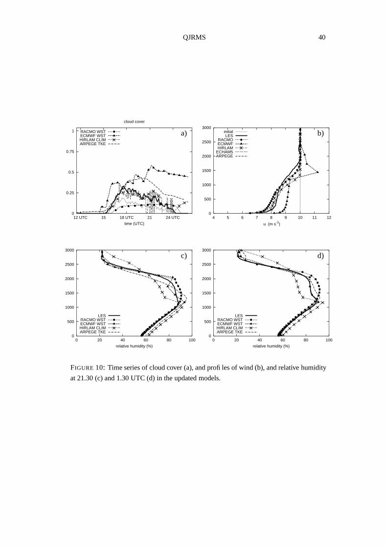
QJRMS 40

a) b)

0

0.25

0.5

0.75

1

12 UTC 15 18 UTC 21 24 UTC

time (UTC)

cloud cover

RACMO WSTECMWF WSTHIRLAM CLIMARPEGE TKE

0

500

1000

1500

2000

2500

3000

4 5 6 7 8 9 10 11 12

u (m s-1)

initialLES

RACMOECMWFHIRLAM

ECHAM5ARPEGE

c) d)

0

500

1000

1500

2000

2500

3000

0 20 40 60 80 100

relative humidity (%)

LESRACMO WSTECMWF WSTHIRLAM CLIMARPEGE TKE

0

500

1000

1500

2000

2500

3000

0 20 40 60 80 100

relative humidity (%)

LESRACMO WSTECMWF WSTHIRLAM CLIMARPEGE TKE

FIGURE 10: Time series of cloud cover (a), and profiles of wind (b), and relative humidity

at 21.30 (c) and 1.30 UTC (d) in the updated models.

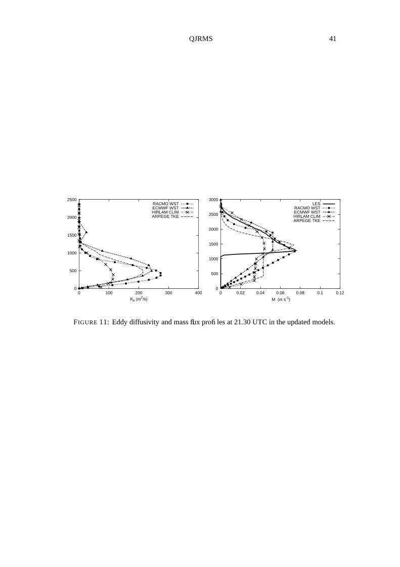
QJRMS 41

0

500

1000

1500

2000

2500

0 100 200 300 400

Kh (m2/s)

RACMO WSTECMWF WSTHIRLAM CLIMARPEGE TKE

0

500

1000

1500

2000

2500

3000

0 0.02 0.04 0.06 0.08 0.1 0.12

M (m s-1)

LESRACMO WSTECMWF WSTHIRLAM CLIMARPEGE TKE

FIGURE 11: Eddy diffusivity and mass flux profiles at 21.30 UTC in the updated models.

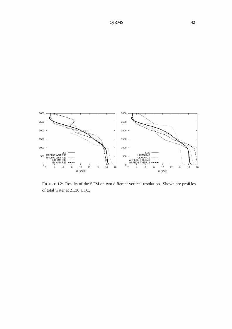
QJRMS 42

0

500

1000

1500

2000

2500

3000

2 4 6 8 10 12 14 16 18

qt (g/kg)

LESRACMO WST R40RACMO WST R19

ECHAM R40ECHAM R19

0

500

1000

1500

2000

2500

3000

2 4 6 8 10 12 14 16 18

qt (g/kg)

LESUKMO R40UKMO R19

ARPEGE TKE R40ARPEGE TKE R19

FIGURE 12: Results of the SCM on two different vertical resolution. Shown are profiles

of total water at 21.30 UTC.

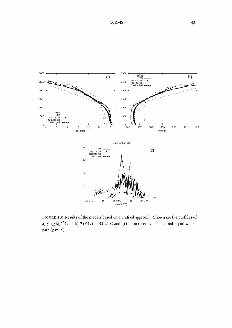
QJRMS 43

a) b)

0

500

1000

1500

2000

2500

3000

4 6 8 10 12 14 16

qt (g/kg)

initialLES

MESO-DIFCHEIN-DIFCHEIN-MF

0

500

1000

1500

2000

2500

3000

306 307 308 309 310 311 312

theta (K)

initialLES

MESO-DIFCHEIN-DIFCHEIN-MF

c)

20

40

60

80

12 UTC 15 18 UTC 21 24 UTC

time (UTC)

liquid water path

LESMESO-DIFCHEIN-DIFCHEIN-MF

FIGURE 13: Results of the models based on a unified approach. Shown are the profiles of

a) � � (g kg �

�) and b)

�(K) at 2130 UTC and c) the time series of the cloud liquid water

path (g m �

�).