Seasonal Variations in Terrestrial Water Storage for Major Midlatitude River Basins

Seasonal Variations in Terrestrial Water Storage for Major Midlatitude River Basins

MARTIN HIRSCHI

Institute for Atmospheric and Climate Science, Swiss Federal Institute of Technology (ETH), Zürich, Switzerland

SONIA I. SENEVIRATNE*Goddard Earth Science and Technology Center, NASA Goddard Space Flight Center, Greenbelt, Maryland

CHRISTOPH SCHÄR

Institute for Atmospheric and Climate Science, Swiss Federal Institute of Technology (ETH), Zürich, Switzerland

(Manuscript received 23 November 2004, in final form 22 August 2005)

ABSTRACT

This paper presents a new diagnostic dataset of monthly variations in terrestrial water storage for 37midlatitude river basins in Europe, Asia, North America, and Australia. Terrestrial water storage is the sumof all forms of water storage on land surfaces, and its seasonal and interannual variations are in principledetermined by soil moisture, groundwater, snow cover, and surface water. The dataset is derived with thecombined atmospheric and terrestrial water-balance approach using conventional streamflow measure-ments and atmospheric moisture convergence data from the ECMWF 40-yr Re-Analysis (ERA-40). Arecent study for the Mississippi River basin (Seneviratne et al. 2004) has demonstrated the validity of thisdiagnostic approach and found that it agreed well with in situ observations in Illinois. The present studyextends this previous analysis to other regions of the midlatitudes.

A systematic analysis is presented of the slow drift that occurs with the water-balance approach. It isshown that the drift not only depends on the size of the catchment under consideration, but also on thegeographical region and the underlying topography. The drift is in general not constant in time, but artificialinhomogeneities may result from changes in the global observing system used in the 44 yr of the reanalysis.To remove this time-dependent drift, a simple high-pass filter is applied. Validation of the results isconducted for several catchments with an appreciable coverage of in situ soil moisture and snow cover depthobservations in the former Soviet Union, Mongolia, and China. Although the groundwater component isnot accounted for in these observations, encouraging correlations are found between diagnostic and in situestimates of terrestrial water storage, both for seasonal and interannual variations. Comparisons conductedagainst simulated ERA-40 terrestrial water storage variations suggest that the reanalysis substantiallyunderestimates the amplitude of the seasonal cycle.

The basin-scale water-balance (BSWB) dataset is available for download over the Internet. It constitutesa useful tool for the validation of climate models, large-scale land surface data assimilation systems, andindirect observations of terrestrial water storage variations.

1. Introduction

The water stored on land surfaces, referred to as ter-restrial water storage (TWS), plays a key role in the

hydrological cycle. In particular, soil moisture is an es-sential element contributing to land–atmosphere cou-pling (e.g., Koster et al. 2004) and is known to be im-portant for numerical weather prediction (e.g., Beljaarset al. 1996) and seasonal forecasting (e.g., Koster et al.2000), as well as climate modeling in general (e.g.,Shukla and Mintz 1982; Milly and Dunne 1994). Thesoil moisture–precipitation feedback (e.g., Betts et al.1996; Eltahir 1998; Schär et al. 1999) also demonstratesits relevance for local and regional climate. An accurateunderstanding of such processes, as well as the ability tosimulate present-day soil moisture evolution on conti-nental to subcontinental scales, is an important pre-

* Current affiliation: Institute for Atmospheric and ClimateScience, Swiss Federal Institute of Technology (ETH), Zürich,Switzerland.

Corresponding author address: Martin Hirschi, Institute for At-mospheric and Climate Science, ETH Zürich, Universitätsstrasse16, 8092 Zürich, Switzerland.E-mail: [email protected]

FEBRUARY 2006 H I R S C H I E T A L . 39

© 2006 American Meteorological Society

JHM480

requisite for predicting future changes in soil moistureand related impacts on the occurrence of floods (e.g.,Milly et al. 2002; Kleinn et al. 2005) or droughts (e.g.,Wetherald and Manabe 1999; Seneviratne et al. 2002;Schär et al. 2004b).

Reliable datasets of TWS and its components (mostlysoil moisture, snow, groundwater, and surface water)are extremely scarce, however. Soil moisture is mea-sured routinely only on a few spots around the world,mostly in the former Soviet Union, Mongolia, China,India, and Illinois (Robock et al. 2000). Model-derivedestimates (e.g., Mintz and Serafini 1992; Dirmeyer et al.1999, 2002) are available, but the uncertainty associatedwith these products is relatively large (e.g., Entin et al.1999). Snow and groundwater measurements tend fortheir part to be even more limited (e.g., Rodell andFamiglietti 2001; Seneviratne et al. 2004). Remote sens-ing holds quite some promise in this area, in particularthe recently launched Gravity Recovery and ClimateExperiment, which appears capable of successfully cap-turing large-scale variations in TWS (Tapley et al. 2004;Wahr et al. 2004). However, this mission has only re-cently started and cannot provide any information onpast values of TWS. In general, large-scale soil moistureestimates from different sources substantially disagree(Reichle et al. 2004).

In a recent paper, Seneviratne et al. (2004, hereafterreferred to as S04) have demonstrated that retrospec-tive basin-scale estimates of TWS can be successfullyderived from combined atmospheric and terrestrial wa-ter-balance computations, using streamflow measure-ments and reanalysis data. Their study focused on theMississippi River basin for the time period 1987–96 andused European Centre for Medium-Range WeatherForecasts (ECMWF) 40-yr Re-Analysis (ERA-40) datain combination with U.S. Geological Survey (USGS)streamflow measurements. In particular, estimates de-rived with this approach for Illinois (�2 � 105 km2)were found to agree very well with in situ observationsof soil moisture, groundwater, and snow.

The present study extends this previous analysis to 37river basins in Europe, Asia, North America, and Aus-tralia and has as its main aim the creation of a basin-scale dataset of monthly TWS variations covering up to40 yr. The described dataset is freely available on theInternet (see section 6) and is expected to be of par-ticular use for climate applications in regions wherelarge-scale observational data are not available.

The paper is structured as follows. Section 2 gives anoverview of the methodology and describes the riverbasins investigated as well as the datasets employed.Section 3 presents the main results of this study, that is,the climatologies of the derived estimates for the con-

sidered river basins. In section 4, the ERA-40 moistureflux convergence and the derived water-balance esti-mates are compared against historical data, soil mois-ture and snow depth observations, and the simulatedERA-40 TWS. Section 5 presents a possible applicationof the computed dataset for climate model validation,followed by information for data download (section 6).Finally, the last section provides a summary of the re-sults as well as the main conclusions of this study.

2. Computation of the water-balance estimates

a. The water-balance equations

This section presents a short overview of the terres-trial, atmospheric, and combined water-balance equa-tions [for a more detailed description, see Peixoto andOort (1992) and S04]. For a given river basin, the waterbalance at the surface can be expressed as

��S

�t� � ��R� � �P � E�, �1

where S represents the terrestrial water storage (here-after referred to as TWS) of the given area, R the mea-sured streamflow (assumed to include both the surfaceand the groundwater runoff of the area), P the areaprecipitation, and E the area evapotranspiration. Theoverbar denotes a temporal average (i.e., monthlymeans) and {} a space average over the region.

Neglecting the contribution of the liquid and solidwater in clouds, the atmospheric water balance for thesame area can be expressed as

��W

�t � � ��H · Q� � �P � E�, �2

where W represents the column storage of water vaporand Q the vertically integrated two-dimensional watervapor flux. The operator (H ·) represents the horizon-tal divergence. The term {P � E} can be eliminatedbetween (1) and (2) to give

��S

�t� � ��W

�t � � ��H · Q� � �R�. �3

In this combined equation, the monthly variations inTWS of the studied region can be expressed as the sumof three terms only: the change in atmospheric watervapor content, the water vapor flux convergence, andthe measured river streamflow. The term {�W/�t} is usu-ally negligible for annual means, but not for monthlymeans, particularly during the spring and fall (Rasmus-son 1968; S04). Here we use ERA-40 atmospheric re-analysis data for the terms {�W/�t} and {H · Q}, andconventional runoff data for the term {R}.

40 J O U R N A L O F H Y D R O M E T E O R O L O G Y VOLUME 7

b. Investigated river basins

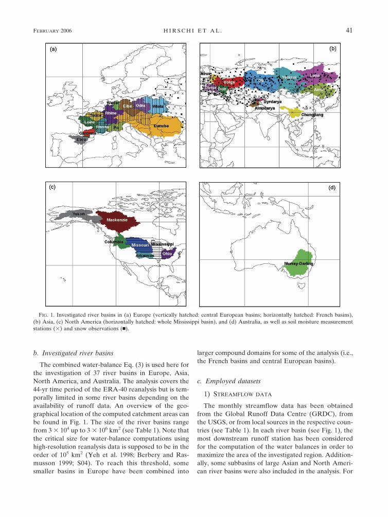
The combined water-balance Eq. (3) is used here forthe investigation of 37 river basins in Europe, Asia,North America, and Australia. The analysis covers the44-yr time period of the ERA-40 reanalysis but is tem-porally limited in some river basins depending on theavailability of runoff data. An overview of the geo-graphical location of the computed catchment areas canbe found in Fig. 1. The size of the river basins rangefrom 3 � 104 up to 3 � 106 km2 (see Table 1). Note thatthe critical size for water-balance computations usinghigh-resolution reanalysis data is supposed to be in theorder of 105 km2 (Yeh et al. 1998; Berbery and Ras-musson 1999; S04). To reach this threshold, somesmaller basins in Europe have been combined into

larger compound domains for some of the analysis (i.e.,the French basins and central European basins).

c. Employed datasets

1) STREAMFLOW DATA

The monthly streamflow data has been obtainedfrom the Global Runoff Data Centre (GRDC), fromthe USGS, or from local sources in the respective coun-tries (see Table 1). In each river basin (see Fig. 1), themost downstream runoff station has been consideredfor the computation of the water balances in order tomaximize the area of the investigated region. Addition-ally, some subbasins of large Asian and North Ameri-can river basins were also included in the analysis. For

FIG. 1. Investigated river basins in (a) Europe (vertically hatched: central European basins; horizontally hatched: French basins),(b) Asia, (c) North America (horizontally hatched: whole Mississippi basin), and (d) Australia, as well as soil moisture measurementstations (�) and snow observations (�).


Fig 1 live 4/C

TABLE 1. Characteristics of the analyzed river basins.

Basin name Runoff stationStreamflowdata source

Station coordinateslat/lon

Catchmentarea (km2)

Consideredyearsa

Smax � Sminb

(mm)

Northern AsiaAmur Komsomolsk GRDCc 50.63/137.12 1 921 624 1958–90 43Lena Stolb GRDC 72.37/126.80 2 351 052 1958–94 107Lena subbasin

Vitim Bodaibo GRDC 57.82/114.17 176 837 1958–88 58Yenisei Igarka GRDC 67.48/86.5 2 513 361 1958–95 104Yenisei subbasins

Podkamennaya Tunguska Kuzmovka GRDC 62.32/92.12 209 591 1958–89 175Selenga Mostovoy GRDC 52.03/107.48 438 715 1958–99 63

Ob Salekhard GRDC 66.57/66.53 2 859 889 1958–94 143Ob subbasins

Tom Tomsk GRDC 56.5/84.92 62 830 1958–99 345Tura Tiumen GRDC 57.15/65.53 57 973 1958–90 163Irtish Omsk GRDC 55.02/73.21 403 309 1958–90 104

Central and east AsiaAmudarya Kerki GRDC, l.s.d 37.83/65.25 321 599 1959–92 246Syrdarya Chinaz l.s.d 40.91/68.72 166 381 1987–92 182Changjiang Yichang l.s.e 30.7/111.3 965 180 1958–2000 112

Western RussiaNeva Novosaratovka GRDC, l.s.f 59.8/30.72 233 423 1958–90 161Volga Volgograd GRDC 48.77/44.72 1 333 747 1958–90 158Don Razdorskaya GRDC 47.5/40.67 420 740 1958–90 170Dnepr Dnepr Power Plant GRDC 47.92/35.15 451 778 1958–84 145

EuropeDanube Ceatal Izmail GRDC 45.22/28.73 772 220 1958–99 131Wisla Tczew GRDC 54.1/18.82 193 500 1958–93 96Odra Gozdowice GRDC 52.77/14.32 107 992 1958–93 88Elbe Neu-Darchau GRDC 53.23/10.89 132 014 1958–2001 103Weser Intschede GRDC 52.96/9.13 35 888 1958–2001 130Rhine Rees GRDC 51.76/6.4 160 704 1958–2001 113Rhone Beaucaire GRDC, l.s.g 43.92/4.67 94 836 1958–99 120Po Pontelagoscuro GRDC, l.s.h 44.88/11.65 85 223 1958–90 51Seine Poses GRDC, l.s.i 49.3/1.25 84 144 1971–95 190Loire Montjean GRDC, l.s.j 47.38/�0.83 107 646 1958–92 147Garonne Mas-D’Agenais/Tonneins GRDC, l.s.k 44.42/0.23 49 381 1958–99 132Ebro Tortosa GRDC 40.82/0.52 83 930 1958–83 157

North AmericaMississippi Vicksburg USGSl 32.3/�90.9 2 868 901 1958–97 99Mississippi subbasins

Missouri Kansas City USGS 39.1/�94.58 1 201 513 1958–99 90Arkansas Van Buren USGS 35.33/�94.28 382 423 1958–2000 77Ohio Metropolis USGS 37.13/�88.73 503 558 1958–2000 100

Columbia The Dalles USGS 45.6/�121.17 600 730 1958–2000 269Yukon Pilot Station USGS 61.93/�162.86 779 081 1976–95 116Mackenzie Arctic Red River GRDC 67.46/�133.74 1 587 878 1973–96 96

AustraliaMurray–Darling Blanchetown l.s.m �34.35/139.62 1 006 173 1967–2001 60

a Longest continuous period between 1958 and 2001 (ERA-40 period) with runoff data.b Amplitude of seasonal cycle of TWS inferred from drift-corrected {�S/�t}.c Global Runoff Data Centre, Koblenz, Germany; Thomas Lüllwitz.d Local source (l.s.): Hydrometeorological Survey of Uzbekistan (Uzgidromet), Tashkent (for details see Schär et al. 2004a).e Changjiang Water Resource Commission (CWRC), Wuhan, China; Min Yawou.f State Hydrological Institute, St. Petersburg, Russia.g Compagnie Nationale du Rhône, Lyon, France; Luc Levasseur (for 1980–99).h Ufficio Idrografico e Mareografico di Parma, Italy; Dr. Ing. Luigi Ciarmatori (for 1986–90).i Direction régionale de l’environnement, Ile-de-France, Paris, France; Frédéric Raout (for 1978–95).j Direction régionale de l’environnement, Pays-de-la-Loire, Nantes, France; Simon Lery (for 1980–92).k Direction régionale de l’environnement, Midi-Pyrénées, Toulouse, France; Michel Bouziges (for 1980–99).l U.S. Geological Survey (for data download, see http://waterdata.usgs.gov/nwis/sw).m Gauging station AW426903: Department of Water, Land and Biodiversity Conservation, Government of South Australia, Australia

(K. Ellett, University of Melbourne, Australia, 2004, personal communication).


many rivers (especially in Russia), it was difficult oreven impossible to get more recent runoff data (after1990).

2) ERA-40 MOISTURE FLUX DIVERGENCE AND

CHANGES IN ATMOSPHERIC MOISTURE CONTENT

The vertically integrated moisture fluxes and changesin atmospheric moisture content are taken from theERA-40 reanalysis product (Simmons and Gibson2000; Simmons et al. 2004) of the ECMWF. The ERA-40 reanalysis covers the period from mid-1957 to mid-2002; here we use data for the years 1958–2001, that is,44 yr altogether.

For a detailed description of the fields used fromERA-40 as well as the computation of the moisture fluxdivergence, the reader is referred to S04. The ERA-40model has a T159 spherical harmonic representation forthe atmospheric dynamic and thermodynamic fields,and uses a reduced Gaussian grid (Hortal and Simmons1991) with grid spacing of 112 km. There are 60 levelsin the vertical, with a particular high resolution in thelower troposphere: The lowest model level is at 10 mabove the surface and there are 8, 11, 15, 17 and 22levels below 500, 1000, 2000, 3000, and 5000 m, respec-tively. The reanalysis uses a three-dimensional varia-tional assimilation system (Courtier et al. 1998) with a6-h analysis cycle. Additional documentation on ERA-40 can be found at http://www.ecmwf.int/research/era/.

The two ERA-40 fields used in the water-balancecomputations (i.e., moisture flux divergence andchanges in atmospheric moisture content) contain as-similated humidity and wind observations. These fieldsare averaged over the basins using the fractional cov-erage of the catchments in each ERA-40 grid box as aweighting factor [following Schär et al. (2004a),adapted for the reduced Gaussian grid].

3) TOPOGRAPHICAL DATA

Seneviratne et al. (2004) used simple quadrilateralsto define the area of the river basins for the computa-tion of the terms in (3). Here, the catchments’ defini-tions are derived from the HYDRO1k topographicaldataset (for data download, see http://edc.usgs.gov/products/elevation/gtopo30/hydro/index.html).HYDRO1k, developed at the USGS Earth ResourcesObservation Systems (EROS) Data Center, is a geo-graphic database providing a comprehensive and con-sistent global coverage. The basis of all data layersavailable in the HYDRO1k database is the hydrologi-cally corrected digital elevation model (DEM), which isbased on the GTOPO30 dataset, a 30 arc s DEM of theworld. To ensure that the DEM is able to reproduce the

correct movement of water across its surface, the DEMwas processed to remove elevation anomalies that caninterfere with hydrologically correct flow.

For the Murray–Darling basin in Australia, the glob-al Simulated Topological Network at 30-min spatialresolution (STN-30; Vörösmarty et al. 2000) is used todefine the catchment, since there is no coverage of theHYDRO1k dataset on this continent. STN-30 repre-sents rivers as a set of spatial and tabular data layersderived from a 30-min flow-direction grid (for datadownload, see http://www.watsys.sr.unh.edu/Stn-30/stn-30.html).

3. Results

a. Introductory examples and drift correction

This section exemplifies the analysis of the diagnosedmonthly variations in TWS for the Ob and the RhineRiver basins.

Figures 2a and 2b display the mean annual cycleof the moisture flux convergence, surface runoff,and the diagnosed monthly variations in TWS (raw anddrift-corrected values; see below) for the Ob and theRhine River basins. Not shown in these panels arethe monthly changes in atmospheric moisture content{�W/�t}, because the contribution of this term to thewhole coupled water balance is only small in all inves-tigated river basins. The mean annual cycle of the at-mospheric moisture content has its maximum usually inmidsummer. For comparison, the panels also includethe simulated ERA-40 TWS variations (i.e., as modeledby the ERA-40 land surface scheme), which include soilmoisture (all levels) and snow water equivalent (to bediscussed in section 4d).

The Ob basin displays a runoff peak in June, which isproduced by snowmelt (Fig. 2a). The Rhine runoff (Fig.2b) does not exhibit a pronounced seasonal cycle, dueto compensating characteristics in the upper and lowerreaches during winter and summer (winter with highdischarge in low regions and storage of water in moun-tains as snow; spring/summer with low discharge inlower regions and increased runoff in elevated areasdue to snowmelt). For both basins, there is atmosphericmoisture convergence in the cold season and moisturedivergence in summer.

The temporal integration of the estimated monthlyvariations in TWS, that is,

S�t � S0 � �t0

t ��S

�t� dt with S0 � 0 mm, �4

shows a drift in TWS (Figs. 2c,d). This drift results fromsmall violations of the long-term water-balance compo-


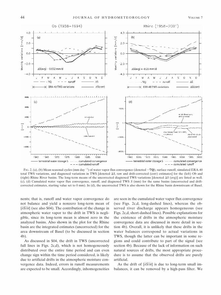
nents; that is, runoff and water vapor convergence donot balance and yield a nonzero long-term mean of{�S/�t} (see also S04). The contribution of the change inatmospheric water vapor to the drift in TWS is negli-gible, since its long-term mean is almost zero in theanalyzed basins. Also shown in the plot for the Rhinebasin are the integrated estimates (uncorrected) for thearea downstream of Basel (to be discussed in section4b).

As discussed in S04, the drift in TWS (uncorrectedfull lines in Figs. 2c,d), which is not homogeneouslydistributed over the entire time period and can evenchange sign within the time period considered, is likelydue to artificial drifts in the atmospheric moisture con-vergence data. Indeed, errors in runoff measurementsare expected to be small. Accordingly, inhomogeneities

are seen in the cumulated water vapor flux convergence(see Figs. 2c,d, long-dashed lines), whereas the ob-served river discharge appears homogeneous (seeFigs. 2c,d, short-dashed lines). Possible explanations forthe existence of drifts in the atmospheric moistureconvergence data are discussed in more detail in sec-tion 4b). Overall, it is unlikely that these drifts in thewater balances correspond to actual variations inTWS, though the latter can be important in some re-gions and could contribute to part of the signal (seesection 4b). Because of the lack of information on suchnatural sources of drifts, the most appropriate proce-dure is to assume that the observed drifts are purelyartificial.

As the drift of {�S/�t} is due to long-term small im-balances, it can be removed by a high-pass filter. We

FIG. 2. (a), (b) Mean seasonal cycles (mm day�1) of water vapor flux convergence (denoted �Q), surface runoff, simulated ERA-40total TWS variations, and diagnosed variations in TWS [denoted �S, raw and drift-corrected (corr) estimates] for the (left) Ob and(right) Rhine River basins. The long-term means of the uncorrected diagnosed TWS variations [denoted �S (avg)] are listed as well.(c), (d) Cumulated water vapor flux convergence, runoff, and diagnosed TWS S (mm) for the same basins (uncorrected and drift-corrected estimates, starting value set to 0 mm). In (d), the uncorrected TWS is also shown for the Rhine basin downstream of Basel.


have selected a particularly simple approach and sub-tract a running mean with a 3-yr window from theoriginal estimates of TWS variations. This proce-dure successfully removes the artificial drift withoutlosing the short-term variability (van den Hurk et al.2005) and forces the long-term average of {�S/�t} tozero (see drift-corrected full lines in Figs. 2c,d). Theapplication of more sophisticated filters has also beentested, but the adopted procedure is sufficient for ourpurpose.

The impact of the drift correction is shown in Figs. 2aand 2b by the thin (uncorrected) and bold (corrected)solid lines. In the case of the Ob basin, the correctionsare small and the two lines coincide. In the case of theRhine, the corrections are substantial and amount to�0.15 mm day�1.

b. Regional climatologies

Figures 3–5 display the mean annual cycle of the wa-ter-balance quantities for most considered European,Asian, North American, and Australian river basins inthe same format as Figs. 2a and 2b, averaged over thedenoted years. Some smaller basins in Europe havebeen combined into one larger compound basin. Forinstance, the French basins refer to the Seine, Loire,Garonne, and Rhone (see Fig. 1).

Beside the monthly variations in TWS, we have alsocomputed “absolute” values of TWS for all basins using(4) with drift-corrected {�S/�t}. The amplitudes of themean seasonal cycles, that is, Smax – Smin, are tabulatedin Table 1.

1) EUROPEAN RIVER BASINS

Most of the European rivers (central European andFrench basins, Danube, Wisla, Odra, Rhone, Seine) donot exhibit a pronounced seasonal cycle of runoff. Nor-mally, runoff is lowest in summer and highest in (late)winter. The Po basin shows two runoff maxima associ-ated with the two precipitation maxima in spring andlate autumn (Frei and Schär 1998). The two precipita-tion maxima are also evident in the atmospheric mois-ture convergence. In most other basins of Europe, thereis atmospheric moisture convergence in the cold seasonand moisture divergence in summer.

2) ASIAN RIVER BASINS

The Lena, Yenisei (not displayed), and Volga Riverbasins in northern Asia show a seasonal cycle that ishighly dependent on the runoff peak in May or June,which is generated by snowmelt (e.g., Dettinger andDiaz 2000). The Volga basin displays moisture diver-

gence in summer, which contributes to the TWS deple-tion. The Lena and Yenisei River basins display mois-ture convergence during the whole year with maximumvalues in spring and fall, and the TWS depletion inthese basins is mostly determined by snowmelt and run-off.

The two central Asian river basins Amudarya andSyrdarya (not shown) display a similar but less pro-nounced snowmelt peak in runoff in June and July, butthe TWS variations are more affected by moisture con-vergence in winter and divergence in summer, as is typi-cal for a semiarid region.

The Amur and the Changjiang basins exhibit a strongmoisture convergence in summer associated with themonsoon occurring in these regions. This is also influ-encing river runoff, which shows an increasing tendencyuntil the end of the summer.

The Don, Dnepr, and Neva basins show smallmonthly variations in runoff. Streamflow values of theDon are very low and the variations in TWS followclosely the moisture convergence. In the case of theNeva, runoff is relatively large, but without a snowmeltpeak similar to the other higher-latitude river basins(Volga, Ob, Lena, and Yenisei). This is partly explainedby lakes that are damping the effect of spring snowmelt(Pardé 1947).

3) NORTH AMERICAN AND AUSTRALIAN RIVER

BASINS

The seasonal cycles of the Columbia, Yukon, andMackenzie River basins in North America show a run-off peak in June, which is generated by snowmelt. TheYukon and Mackenzie basins exhibit moisture conver-gence during the whole year and the water storagedepletion in this region is mostly driven by changes insnow cover (same pattern as in the Lena and YeniseiRiver basins). The variations in TWS in the Columbiaregion is strongly dependent on the seasonal develop-ment of the moisture convergence, which displays highvalues in autumn/winter, and large divergence in sum-mer. The western Mississippi subbasins (Missouri andArkansas) show small and constant runoff valuesthroughout the year, whereas the eastern subbasin(Ohio) displays a runoff peak in March. All subbasinsof the Mississippi exhibit moisture divergence in sum-mer.

The Murray–Darling basin in Australia displays onlyvery small runoff values throughout the year (note thediffering scale of the y axis). Thus the variation in TWSis defined by the atmospheric moisture flux, whichshows convergence in austral winter and divergence insummer.


FIG. 3. As in Figs. 2a and 2b but for other European basins.


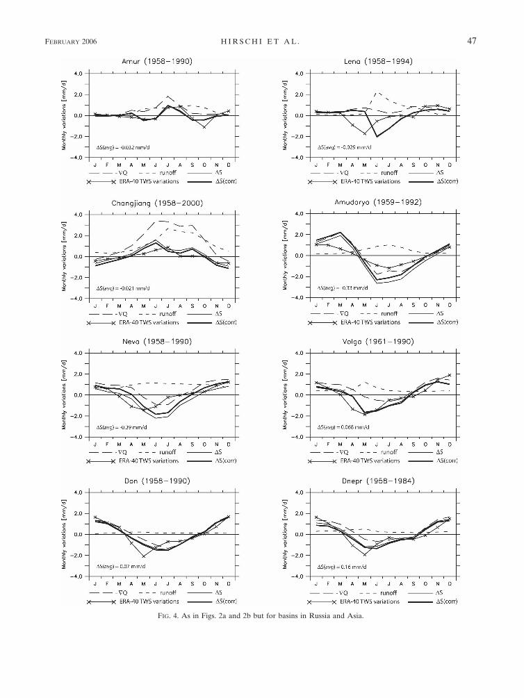
FIG. 4. As in Figs. 2a and 2b but for basins in Russia and Asia.


FIG. 5. As in Figs. 2a and 2b but for basins in North America and Australia.


4. Discussion and comparison with other datasets

The combined water-balance method used here forthe diagnosis of monthly variations in TWS has beenvalidated by S04 for the fraction of Mississippi basincovering Illinois for the time frame 1987–96. The analy-sis showed excellent agreement with observational dataof soil moisture, groundwater, and snow from the Illi-nois State Water Survey (ISWS) and the Midwest Re-gional Climate Center (MRCC).

Here we provide some additional validation andcomparisons against other datasets. For all the analysis,the employed runoff data can be assumed to be accu-rate within a few percent for long-term averages. Errorsin runoff observations should thus not contaminate theresults of the water-balance computations. Observa-tional runoff errors range from less than 5% to 5%–10% and depend on the instrumentation and the meth-ods used to distribute discharge data both in time andspace (Winter 1981; Rantz 1982a,b). When analyzingmodel-derived TWS variations against our estimates,one should take into account that the measured river

discharge may be anthropogenically influenced as a re-sult of water management procedures (Hagemann andDümenil 1998).

a. Comparison with historical values of P � E inEurope

The ERA-40 water vapor flux convergence is com-pared here with water-balance estimates from severalhistorical studies. Alestalo (1983) calculated verticallyintegrated, annual, and monthly averaged divergencesof the horizontal water vapor flux directly from aero-logical observations for two European domains. Thecorners of his domains were defined by World Meteo-rological Organization (WMO) aerological stations(see Fig. 6). Korzun (1974) as well as Baumgartner andReichel (1975) mapped the world water balances andestimated precipitation (P), evaporation (E), and run-off by using long-term control relationships (e.g., P – E� runoff). In his investigations on the heat balance ofthe earth, Budyko (1963) drew conclusions on theevapotranspiration in various regions. Combining these

FIG. 6. Regions A (vertically hatched) and M (horizontally hatched) from Alestalo (1983), used for comparisons with ERA-40water vapor convergence.


estimates with precipitation and runoff data, he com-piled a picture of the global water cycle. Alestalo (1983)used the aforementioned three studies to estimate thewater-balance components for the above-mentionedEuropean domains (see Table 2).

According to (2), � {H · Q} is essentially balancedby {P � E} for annual means. The mean annual valuesfor the large European domain A (see Fig. 6) displayedin Alestalo (1983) range from 230 (Budyko 1963) to 275mm yr�1 (Baumgartner and Reichel 1975). The meanERA-40 values of 184 mm yr�1 for the same region andthe period 1974–76, and 211 mm yr�1 for the period1958–2001 are close to these historical estimates (seeTable 2).

For the smaller central European region [region M inAlestalo (1983); see Fig. 6], however, ERA-40 under-estimates the moisture convergence by up to 50% com-pared to the other estimates. This is a striking result,since the same observations used in Alestalo (1983) arealso assimilated in ERA-40. It is likely that this under-estimation is very dependent on the definition of theregion M, and in particular its southern border that runsparallel to the Alpine ridgeline. When extending thearea slightly to the south, the ERA-40 convergence in-creases significantly and agrees much better with thehistorical estimates. This indicates the difficulty whenaveraging the ERA-40 fields over small areas in thevicinity of complex topography. Although each gridbox is included in the computation of the estimatesaccording to its fractional coverage of the domain [seesection 2c(2)], sub-grid-scale meteorological features,which are especially strong in a topographically com-plex region such as central Europe, are not fully repre-sented, leading to unclosed water budgets. The use ofphysical catchments as the basis for the domain defini-tions, as done in our study, is here of some advantage.

Nevertheless, Table 2 suggests that ERA-40 has atendency to underestimate atmospheric water vaporconvergence, and this can at least partly explain thediagnosed negative long-term drifts in water storage(see Fig. 2d and next subsection) in many smaller river

basins of this region (Danube, Wisla, Odra, Elbe,Weser, Rhine, Rhone, Loire, Garonne, Ebro).

b. Long-term balance of the moisture fluxconvergence and runoff

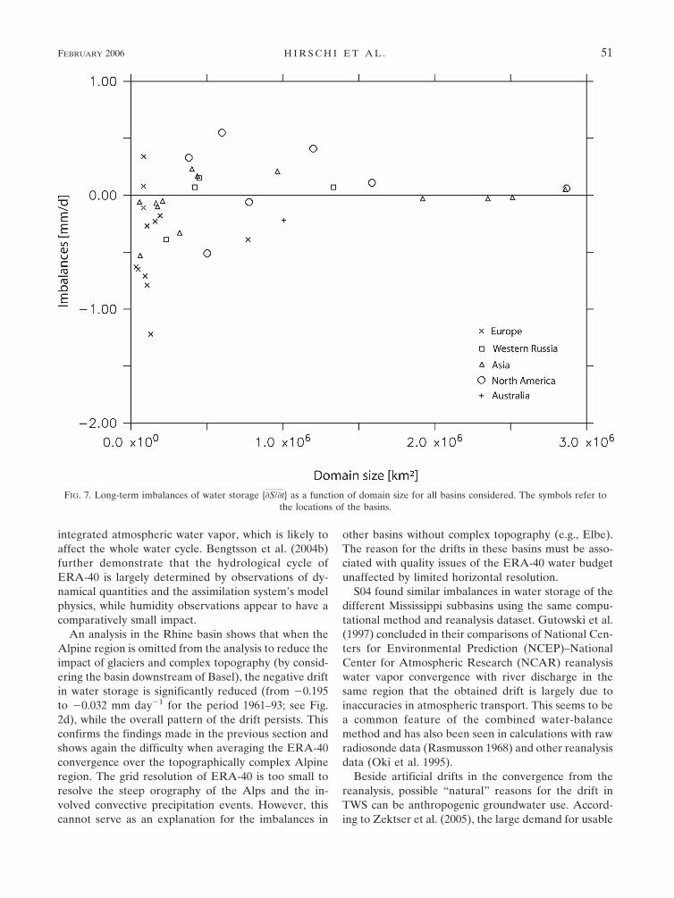
To validate the long-term moisture flux convergencewith runoff data (note that the contribution of thechange in atmospheric water vapor to the drift in TWSis negligible, since its long-term mean is almost zero;see previous section), Fig. 7 shows the averages of thedrift in water storage over the computed years {�S/�t} asa function of domain size for the various river basins.The critical domain size for water-balance computa-tions using high-resolution reanalysis data is supposedto be in the order of 105 km2 (Yeh et al. 1998; Berberyand Rasmusson 1999; S04). Our results roughly confirmthis threshold.

However, the water storage in the basins of westernRussia and northern and central Asia is quite well bal-anced not only for the large regions, but also for mostsmall basins (Don, Dnepr, Syrdarya, subbasins of theOb, Yenisei, and Lena), whereas many, even large cen-tral and western European basins, exhibit a pro-nounced (mostly negative) drift in long-term waterstorage (Danube, Wisla, Odra, Elbe, Weser, Rhine,Rhone, Loire, Garonne, Ebro). In North America, thewater balance is stable for the large river basins (Mis-sissippi and Mackenzie), whereas most small domainsare not well balanced (with the exception of the Yukonbasin). This analysis suggests that the magnitude of theimbalances is not only dependent on the size of theriver basins but also on the geographical region underconsideration (i.e., climatological and topographicalproperties, e.g., Seneviratne 2003).

As previously discussed in S04 (see also Figs. 2c,d),the drift in the integrated TWS is often not homoge-neously distributed over time and can even change signwithin the analysis period. This is likely due to changesin the quality and quantity of observations entering theERA-40 data assimilation system (Betts et al. 2003b),for instance, the introduction of satellite data in the late1970s, the diminution of the radiosonde network in the1990s in the countries of the former Soviet Union, Af-rica, and South America, and the increasing number ofsatellite observations in the same period. More detailedstudies on the influence of changes in the global ob-serving system on the ERA-40 hydrological cycle andon trends in this dataset have been published recently.Bengtsson et al. (2004a) conclude that changes in theobserving systems, which have taken place in the last 40yr, have introduced artificial climate trends of similarmagnitude as the real ones in the reanalysis data. Inparticular, they find an overestimation of the trend in

TABLE 2. Comparison of annual mean values of � {H · Q} and{P � E} for the European region A (see Fig. 6, after Alestalo1983) in mm yr�1.

Period � {H · Q} {P � E}

Region A (central and east Europe)Alestalo (1983) 1974–76 235Budyko (1963) Not specified 230Baumgartner and

Reichel (1975)Not specified 275

ERA-40 (this paper) 1974–76 184ERA-40 (this paper) 1958–2001 211


integrated atmospheric water vapor, which is likely toaffect the whole water cycle. Bengtsson et al. (2004b)further demonstrate that the hydrological cycle ofERA-40 is largely determined by observations of dy-namical quantities and the assimilation system’s modelphysics, while humidity observations appear to have acomparatively small impact.

An analysis in the Rhine basin shows that when theAlpine region is omitted from the analysis to reduce theimpact of glaciers and complex topography (by consid-ering the basin downstream of Basel), the negative driftin water storage is significantly reduced (from �0.195to �0.032 mm day�1 for the period 1961–93; see Fig.2d), while the overall pattern of the drift persists. Thisconfirms the findings made in the previous section andshows again the difficulty when averaging the ERA-40convergence over the topographically complex Alpineregion. The grid resolution of ERA-40 is too small toresolve the steep orography of the Alps and the in-volved convective precipitation events. However, thiscannot serve as an explanation for the imbalances in

other basins without complex topography (e.g., Elbe).The reason for the drifts in these basins must be asso-ciated with quality issues of the ERA-40 water budgetunaffected by limited horizontal resolution.

S04 found similar imbalances in water storage of thedifferent Mississippi subbasins using the same compu-tational method and reanalysis dataset. Gutowski et al.(1997) concluded in their comparisons of National Cen-ters for Environmental Prediction (NCEP)–NationalCenter for Atmospheric Research (NCAR) reanalysiswater vapor convergence with river discharge in thesame region that the obtained drift is largely due toinaccuracies in atmospheric transport. This seems to bea common feature of the combined water-balancemethod and has also been seen in calculations with rawradiosonde data (Rasmusson 1968) and other reanalysisdata (Oki et al. 1995).

Beside artificial drifts in the convergence from thereanalysis, possible “natural” reasons for the drift inTWS can be anthropogenic groundwater use. Accord-ing to Zektser et al. (2005), the large demand for usable

FIG. 7. Long-term imbalances of water storage {�S/�t} as a function of domain size for all basins considered. The symbols refer tothe locations of the basins.


water in combination with the semiarid climate has ledto groundwater overdraft in the southwestern UnitedStates. This produced declining trends in aquifer stor-age and hydraulic height in this region. This decline canbe seen also in some groundwater level records fromthe USGS (e.g., see, http://nwis.waterdata.usgs.gov/nwis/gwlevels/?site_no�393403101575901; a station inthe Arkansas River basin with an average groundwaterlevel decrease of 0.5 mm day�1 over the last 30 yr).Since this anthropogenic removal of water is not ac-counted for in the water-balance calculations, it possi-bly can explain the occurring positive drift in computedTWS in river basins of this region (i.e., Missouri, Ar-kansas). Other neglected factors possibly contributingto a drift in the calculation are direct groundwater dis-charge to the ocean (which is not included in runoff andrepresents approximatively 6% of the total annualglobal water gain by the oceans with highly variablespatial distribution; Zektser and Loaiciga 1993) and in-terbasin groundwater flow.

As described in the previous section, we correct theestimates of TWS variations by high-pass filtering (seeFigs. 3–5). This approach provides more realistic esti-mates than the raw diagnostic values, but some openquestions remain. In particular, high-pass filteringwould be of limited value if the drift of the assimilationsystem should have a strong seasonal cycle.

c. Correlation with soil moisture and snow depthobservations

Soil moisture measurements from the Global SoilMoisture Data Bank (Robock et al. 2000) available for

the former Soviet Union, China, and Mongolia are usedfor comparison with the diagnosed estimates of TWSvariations. The datasets entail gravimetric measure-ments of the plant available soil water in different typesof agricultural areas. An overview of the consideredsoil moisture datasets and of their temporal and verticalresolution is presented in Table 3. Snow depth mea-surements for the former Soviet Union spanning a pe-riod from 1881 to 1995 are also included in the com-parisons. They are based on observations made by per-sonnel at 284 WMO stations and are available on aCD-ROM (NSIDC 1999). The snow depths are con-verted in water equivalent using a snow density value of100 kg m�2 (value for fresh snow, e.g., Brasnett 1999).Also larger values for the snow density representingolder snow were tested. However, the resulting changein the results of the comparisons discussed below wasonly minor.

All available station measurements (see Fig. 1) areaveraged over the corresponding basins assuming equalweight. Despite the known problems when averagingpoint measurements over an area, this procedure is ap-plicable in regions with a reasonably homogeneous dis-tribution of the stations and can give there an indicationof the quality of the diagnosed TWS variations.

Besides soil moisture and snow water, TWS also in-cludes mainly groundwater and surface water, whichcan significantly contribute to the total TWS variations(e.g., S04). In the regions investigated here, there are toour knowledge no comprehensive, large-scale observa-tional datasets of groundwater and surface water.Therefore the comparison of the computed estimates

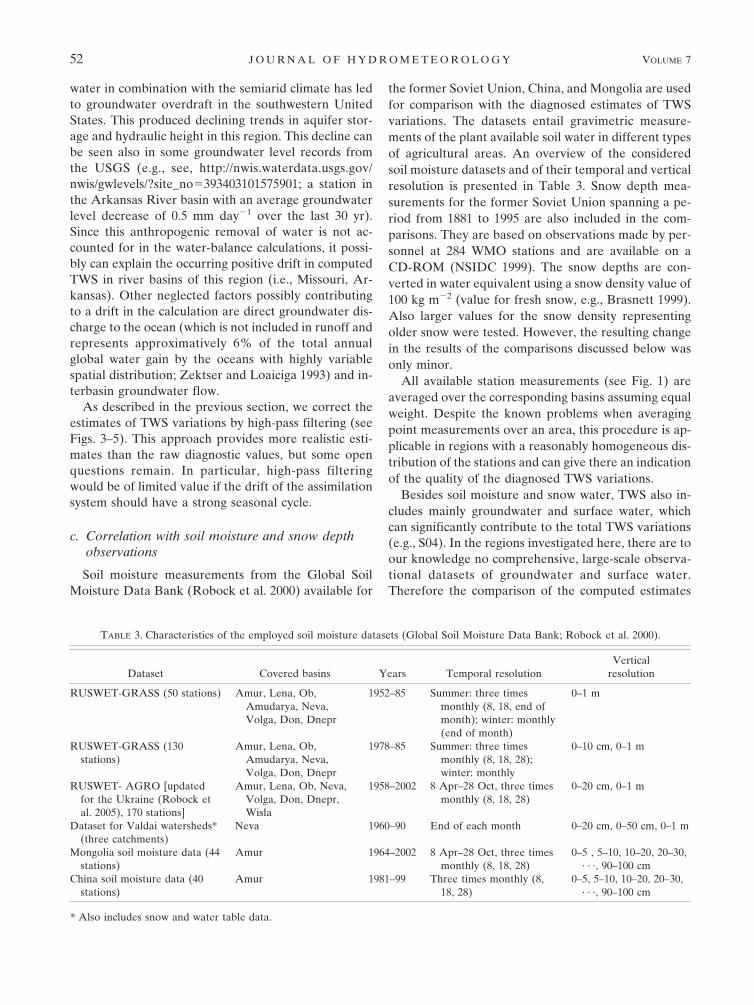
TABLE 3. Characteristics of the employed soil moisture datasets (Global Soil Moisture Data Bank; Robock et al. 2000).

Dataset Covered basins Years Temporal resolutionVertical

resolution

RUSWET-GRASS (50 stations) Amur, Lena, Ob,Amudarya, Neva,Volga, Don, Dnepr

1952–85 Summer: three timesmonthly (8, 18, end ofmonth); winter: monthly(end of month)

0–1 m

RUSWET-GRASS (130stations)

Amur, Lena, Ob,Amudarya, Neva,Volga, Don, Dnepr

1978–85 Summer: three timesmonthly (8, 18, 28);winter: monthly

0–10 cm, 0–1 m

RUSWET- AGRO [updatedfor the Ukraine (Robock etal. 2005), 170 stations]

Amur, Lena, Ob, Neva,Volga, Don, Dnepr,Wisla

1958–2002 8 Apr–28 Oct, three timesmonthly (8, 18, 28)

0–20 cm, 0–1 m

Dataset for Valdai watersheds*(three catchments)

Neva 1960–90 End of each month 0–20 cm, 0–50 cm, 0–1 m

Mongolia soil moisture data (44stations)

Amur 1964–2002 8 Apr–28 Oct, three timesmonthly (8, 18, 28)

0–5 , 5–10, 10–20, 20–30,· · ·, 90–100 cm

China soil moisture data (40stations)

Amur 1981–99 Three times monthly (8,18, 28)

0–5, 5–10, 10–20, 20–30,· · ·, 90–100 cm

* Also includes snow and water table data.


with soil moisture and snow depth observations hasonly a reduced significance in regions where seasonalchanges in groundwater and surface water play an im-portant role in the water cycle. However, together withthe findings of S04, they can give further evidence ofthe applicability of the water-balance method in differ-ent regions.

In Figs. 8 and 9, the diagnosed monthly variations inTWS (drift corrected) are compared against soil mois-ture and snow depth observations for the Volga, Ob,Dnepr, and Don River basins. Correlation between ob-served and diagnosed monthly variations amount to be-tween 0.59 and 0.75. The agreement is also reasonablein terms of anomalies (i.e., deviation from the climatol-ogy) for these basins (not shown). In some other re-gions (e.g., Amur), the correlation is quite poor, likelydue to the nonrepresentative distribution of the soilmoisture and snow measurement stations in the basins(see Fig. 1) and due to the lack of groundwater andsurface water data. The amplitudes of the observationsoften seem to be smaller than the estimates. Especiallyin summer, the decrease in water storage is less pro-nounced in the observations (e.g., Ob). The water-balance estimates also seem to slightly lag behind theobservations. Both effects are likely associated withgroundwater and surface water (wetlands, lakes, reser-voirs, rivers) storage, which are not accounted for in theobservations available. The west Siberian region, forexample, is known to be one of the world largest wet-lands (Fraser and Keddy 2005), and western and centralRussia is an area of considerable groundwater recharge(up to 300 mm yr�1, estimated by the hydrologicalmodel WaterGAP Global Hydrological Model; Döll etal. 2003; Struckmeier et al. 2004). To account for themissing observations of temporarily stored groundwa-ter and surface water in these comparisons, we alsoperformed additional comparisons applying a time de-lay of one month for the runoff in the water-balancecalculations for the large Ob and Volga River basins.As a consequence, the resulting correlations betweenthe estimates and soil moisture and snow observationsincreased slightly (Ob: from 0.75 to 0.79; Volga: from0.74 to 0.76), showing the importance of groundwaterand surface water storage in these regions.

d. Comparison against ERA-40 soil moisture andsnow

For comparison, simulated ERA-40 total TWS varia-tions (see section 3a) are also included in the seasonalmean displays (see Figs. 2a,b and 3–5). The ERA-40data include soil moisture from all levels (0–7, 7–28,28–100, and 100–289 cm), as well as snow water equiva-lent. As there is no groundwater in the ERA-40 model;

soil moisture and snow represent the ERA-40 model’stotal TWS.

Compared to the computed estimates, the simulatedERA-40 TWS shows an earlier and stronger depletionin spring (March, April, May) for almost all investi-gated river basins, whereas its winter values are oftenhigher than the estimated TWS variations (e.g., Odra,Dnepr, Mackenzie). The ERA-40 snow analysis (vanden Hurk et al. 2000) uses snow depth observations,and in addition a nudging toward climatology in areaswhere observations are inadequate to correct the mod-eled snow depth. Analyses of the ERA-40 surface wa-ter budgets in the Mississippi (Betts et al. 2003a) andthe Mackenzie (Betts et al. 2003b) River basins haveshown that positive snow water analysis increments arecomparable to snowfall. Being a significant source termin the frozen water budget, this addition of water inwinter likely leads to the observed higher values ofTWS variations in ERA-40. The early and strong de-crease of TWS in ERA-40 is presumably associatedwith the fact that melted snow in the model is immedi-ately removed as runoff, whereas in reality it mightrefreeze deeper in the snowpack (Betts et al. 2003b).

In summer, the ERA-40 TWS often shows a less pro-nounced decrease (e.g., Rhine, Ob, Mississippi). Thisbehavior is likely related to the soil moisture nudgingscheme used in ERA-40, which corrects soil moisture inthe first three layers (0–7, 7–28, and 28–100 cm) basedon the 6-h atmospheric analysis increments of specifichumidity at the lowest model level (Douville et al.2000). The idea behind this scheme is that a too dry (ortoo wet) soil will lead to a too dry (or too wet) bound-ary layer in the first-guess 6-h forecast compared to theatmospheric analysis (which includes information fromhumidity observations). The nudging is effective in pre-venting the model to drift. However, the resulting soilmoisture increments during summer predominantlyadd water to the soil, leading to a damping of the sea-sonal cycle (Betts et al. 1998, 1999, 2003a; S04).

Overall, the diagnosed estimates of monthly TWSvariations show a much more realistic seasonal cyclethan the simulated ERA-40 values. Similar conclusionswere reached in S04, showing in particular that the di-agnosed water-balance estimates for Illinois agree bet-ter with in situ observations than the ERA-40 soil mois-ture.

5. Application to model validation

An important motivation of the current study is theuse of diagnosed TWS variations for the validation ofclimate models. All current climate models containsome description of surface hydrology, but there is an


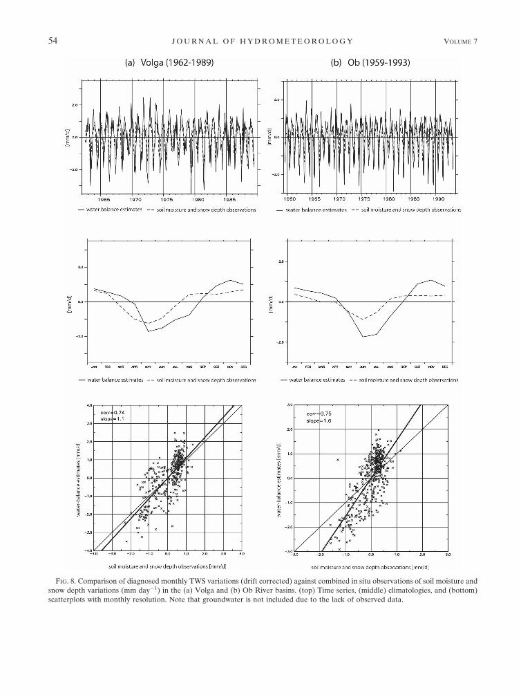
FIG. 8. Comparison of diagnosed monthly TWS variations (drift corrected) against combined in situ observations of soil moisture andsnow depth variations (mm day�1) in the (a) Volga and (b) Ob River basins. (top) Time series, (middle) climatologies, and (bottom)scatterplots with monthly resolution. Note that groundwater is not included due to the lack of observed data.


apparent lack of validation data. For illustration of theenvisioned approach, we here present some prelimi-nary results on the validation of regional climate mod-els over Europe.

The diagnosed estimates of monthly TWS variationsin European river basins is used for the validation ofregional climate models involved in the EU-projectPrediction of Regional Scenarios and Uncertainties for

FIG. 9. As in Fig. 8 but for the (a) Dnepr and (b) Don basins.


Defining European Climate Change Risks and Effects(PRUDENCE; see http://prudence.dmi.dk/). The proj-ect is geared toward reducing deficiencies and quanti-fying uncertainties in projections of future climatechange (Christensen et al. 2002). The models differ withrespect to the physical and dynamical formulations,land-use characteristics, and computational domains(see Table 4). All models cover the major part of Eu-rope at a resolution of approximately 50 km. Theysimulate a control climate (1961–90), as well as an A2-scenario time slice (2071–2100), and are driven by theHadley Centre HadAM3H simulations [except theCentre National de Recherches Meteorologiques(CNRM) control run driven by observed sea surfacetemperatures]. Here attention is restricted to the con-trol integration.

Figure 10 shows a comparison of the drift-correcteddiagnosed monthly variations in TWS against controlruns of various PRUDENCE models (see Table 4) andsimulated ERA-40 TWS variations (see also section 4d)for the Danube basin. The total TWS of the modelsincludes soil water and snow water equivalent. Thesefirst preliminary results display substantial differences

between the models. Several models, as well as theERA-40 reanalysis (as already mentioned in section 4d)underestimate the decrease in TWS during summercompared to the diagnosed water-balance estimates.The differences during summer are particularly largeand amount to more than 1 mm day�1. Some modelsunderestimate the summer drying by more than a factor2. There are also considerable deficiencies in winter(likely relating to the representation of snow).

As a next step, a systematic analysis of the PRUDENCEmodels in the many European river basins will be con-ducted using the produced dataset of drift-correctedTWS variations. Another preliminary application canbe found in van den Hurk et al. (2005; analysis of re-gional climate models in the Rhine basin). This illus-trates the promising potential of the new dataset formodel validation purposes.

6. Data download

The diagnosed basin-scale water-balance (BSWB)data of the various river basins described in this papercan be downloaded from the Web (at http://www.iac.ethz.ch/data/water_balance/).

FIG. 10. Comparison of drift-corrected estimates of variations in TWS against PRUDENCEmodel runs and simulated ERA-40 data (mm day�1) for the Danube basin (772 220 km2). Thediagnosed water-balance estimates are based on the period 1961–90, and the simulations arerepresentative for the same period but employ the forcing of an AGCM run (HadAM3H)driven by observed sea surface temperature variations.


7. Summary and conclusions

The combined terrestrial and atmospheric water-balance approach has been applied for the diagnosis ofmonthly terrestrial water storage variations in 37 riverbasins of Europe, Asia, North America, and Australia,following an earlier study over the Mississippi region(Seneviratne et al. 2004). The latter study showed ex-cellent agreement with observational data of soil mois-ture, snow, and groundwater in a domain covering Illi-nois. The present paper extends this analysis to otherregions of the midlatitudes and also performs some ad-ditional validation.

The long-term balance of the moisture flux conver-gence and the runoff shows negative imbalances in thecomputed water storage in many basins of Europe.Comparisons of the ERA-40 water vapor flux conver-gence with estimates from former water-balance studiesfor Europe point out the difficulty of averaging theERA-40 grid fields over small areas affected by topog-raphy. A source of artificial drift is changes of the glob-

al observing system used in the 44 yr of the reanalysis.By applying a simple drift correction, these artificialimbalances can be corrected. Yet there remains someuncertainty as the drift correction may lead to errors ifthe underlying bias is associated with a strong seasonalcycle. The comparisons of the diagnosed terrestrial wa-ter storage variations against soil moisture observationsin the former Soviet Union, Mongolia, and China, aswell as with snow depth measurements in the formerSoviet Union, display reasonably good correlations inbasins with a representative distribution of soil mois-ture measurement stations (Volga, Ob, Don, andDnepr), though the contribution of groundwater is gen-erally difficult to assess on these large scales. The ac-curacy of the diagnosed water balances is contrasted forthe various regions investigated and appears to be high-est for large river basins with little topographic andclimatic variations. Comparison with simulated ERA-40 terrestrial water storage variations showed that thediagnostic water balances have a much more realisticseasonal cycle.

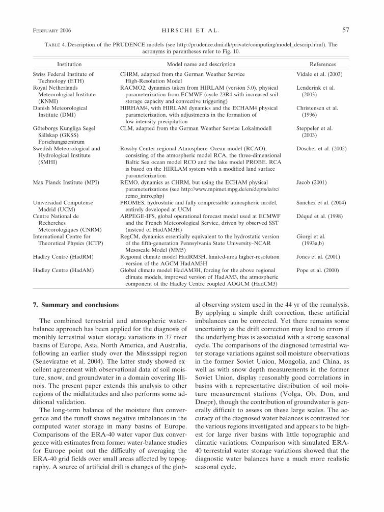
TABLE 4. Description of the PRUDENCE models (see http://prudence.dmi.dk/private/computing/model_descrip.html). Theacronyms in parentheses refer to Fig. 10.

Institution Model name and description References

Swiss Federal Institute ofTechnology (ETH)

CHRM, adapted from the German Weather ServiceHigh-Resolution Model

Vidale et al. (2003)

Royal NetherlandsMeteorological Institute(KNMI)

RACMO2, dynamics taken from HIRLAM (version 5.0), physicalparameterization from ECMWF (cycle 23R4 with increased soilstorage capacity and convective triggering)

Lenderink et al.(2003)

Danish MeteorologicalInstitute (DMI)

HIRHAM4, with HIRLAM dynamics and the ECHAM4 physicalparameterization, with adjustments in the formation oflow-intensity precipitation

Christensen et al.(1996)

Göteborgs Kungliga SegelSällskap (GKSS)Forschungszentrum

CLM, adapted from the German Weather Service Lokalmodell Steppeler et al.(2003)

Swedish Meteorological andHydrological Institute(SMHI)

Rossby Center regional Atmosphere–Ocean model (RCAO),consisting of the atmospheric model RCA, the three-dimensionalBaltic Sea ocean model RCO and the lake model PROBE. RCAis based on the HIRLAM system with a modified land surfaceparameterization.

Döscher et al. (2002)

Max Planck Institute (MPI) REMO, dynamics as CHRM, but using the ECHAM physicalparameterizations (see http://www.mpimet.mpg.de/en/depts/ia/rc/remo_intro.php)

Jacob (2001)

Universidad ComputenseMadrid (UCM)

PROMES, hydrostatic and fully compressible atmospheric model,entirely developed at UCM

Sanchez et al. (2004)

Centre National deRecherchesMeteorologiques (CNRM)

ARPEGE-IFS, global operational forecast model used at ECMWFand the French Meteorological Service, driven by observed SST(instead of HadAM3H)

Déqué et al. (1998)

International Centre forTheoretical Physics (ICTP)

RegCM, dynamics essentially equivalent to the hydrostatic versionof the fifth-generation Pennsylvania State University–NCARMesoscale Model (MM5)

Giorgi et al.(1993a,b)

Hadley Centre (HadRM) Regional climate model HadRM3H, limited-area higher-resolutionversion of the AGCM HadAM3H

Jones et al. (2001)

Hadley Centre (HadAM) Global climate model HadAM3H, forcing for the above regionalclimate models, improved version of HadAM3, the atmosphericcomponent of the Hadley Centre coupled AOGCM (HadCM3)

Pope et al. (2000)


The possible applications of the newly deriveddataset are numerous, as has been shown by an exem-plary application to model validation (section 5), aswell as in the study of van den Hurk et al. (2005). It isexpected that the new dataset (see previous section fordata download) will find further climate applications inthe future, in particular for inferring information onterrestrial water storage variations in regions withoutlarge-scale observations.

Acknowledgments. We thank Pedro Viterbo (ECMWF)for making available the ERA-40 data. Many thanks tothe respective teams of the Global Soil Moisture DataBank, the Global Runoff Data Centre (Koblenz, Ger-many; Thomas Lüllwitz) and the U.S. Geological Sur-vey (USGS). We wish to thank also the local providersof runoff data (Michel Bouziges, Luigi Ciarmatori,Kevin Ellett, Simon Lery, Luc Levasseur, FrédéricRaout, Min Yawou; for affiliations see Table 1), as wellas Joachim Gurtz, Massimiliano Zappa, and J. C.Scherer (Ministère de l’aménagement du territoire etde l’environnement, Bureau des données sur l’eau,Paris, France) for the help in collecting this data. Sin-cere thanks to Dietmar Grebner, Andreas Güntner,Bart van den Hurk, Simon Jaun, Thomas Peter, RetoStöckli, and Pier Luigi Vidale for many useful com-ments and discussions, to Daniel Lüthi for computa-tional support, and to Pia Eugster for the digitalizationof runoff data. Comments from three anonymous re-viewers are also gratefully acknowledged. This researchwas supported by the Fifth Framework Programme ofthe European Union (project PRUDENCE, ContractEVK2-2000-00132), by the Swiss Ministry for Educa-tion and Research (BBW Contract 01.0305-1), and bythe Swiss National Science Foundation (NCCR Cli-mate).

REFERENCES

Alestalo, M., 1983: The atmospheric water vapour budget overEurope. Variations in the Global Water Budget, A. Street-Perrott, Ed., D. Reidel, 67–79.

Baumgartner, A., and E. Reichel, 1975: The World Water Bal-ance—Mean Annual Global, Continental and Maritime Pre-cipitation, Evaporation and Runoff. Elsevier, 179 pp.

Beljaars, A. C. M., P. Viterbo, M. J. Miller, and A. K. Betts, 1996:The anomalous rainfall over the United States during July1993: Sensitivity to land surface parameterization and soilmoisture anomalies. Mon. Wea. Rev., 124, 362–383.

Bengtsson, L., S. Hagemann, and K. I. Hodges, 2004a: Can cli-mate trends be calculated from reanalysis data? J. Geophys.Res., 109, D11111, doi:10.1029/2004JD004536.

——, K. I. Hodges, and S. Hagemann, 2004b: Sensitivity of large-scale atmospheric analyses to humidity observations and itsimpact on the global water cycle and tropical and extratro-pical weather systems in ERA-40. Tellus, 56A, 202–217.

Berbery, E. H., and E. M. Rasmusson, 1999: Mississippi moisturebudgets on regional scales. Mon. Wea. Rev., 127, 2654–2673.

Betts, A. K., J. H. Ball, A. C. M. Beljaars, M. J. Miller, and P. A.Viterbo, 1996: The land–surface atmosphere interaction: Areview based on observational and global modeling perspec-tives. J. Geophys. Res., 101, 7209–7225.

——, P. Viterbo, and E. Wood, 1998: Surface energy and waterbalance for the Arkansas–Red River basin from the ECMWFreanalysis. J. Climate, 11, 2881–2897.

——, J. H. Ball, and P. Viterbo, 1999: Basin-scale surface waterand energy budgets for the Mississippi from the ECMWFreanalysis. J. Geophys. Res., 104, 19 293–19 306.

——, ——, M. Bosilovich, P. Viterbo, Y. Zhang, and W. B. Ros-sow, 2003a: Intercomparison of water and energy budgets forfive Mississippi subbasins between ECMWF reanalysis(ERA-40) and NASA Data Assimilation Office fvGCM for1990–1999. J. Geophys. Res., 108, 8618, doi:10.1029/2002JD003127.

——, ——, and P. Viterbo, 2003b: Evaluation of the ERA-40surface water budget and surface temperature for the Mac-kenzie River basin. J. Hydrometeor., 4, 1194–1211.

Brasnett, B., 1999: A global analysis of snow depth for numericalweather prediction. J. Appl. Meteor., 38, 726–740.

Budyko, M. I., Ed., 1963: Atlas of the Heat Balance of the Earth.Glavnaia Geofizica Obsercatoriia, 69 pp.

Christensen, J. H., O. B. Christensen, P. Lopez, E. van Meijgaard,and M. Botzet, 1996: The HIRHAM4 regional atmosphericclimate model. Scientific Rep. 96-4, Danish MeteorologicalInstitute, 51 pp.

——, T. R. Carter, and F. Giorgi, 2002: PRUDENCE employsnew methods to assess European climate change. Eos, Trans.Amer. Geophys. Union, 83, 147.

Courtier, P., and Coauthors, 1998: The ECMWF implementationof three dimensional variational assimilation (3D-Var). PartI: Formulation. Quart. J. Roy. Meteor. Soc., 124, 1783–1808.

Déqué, M., P. Marquet, and R. G. Jones, 1998: Simulation ofclimate change over Europe using a global variable resolu-tion general circulation model. Climate Dyn., 14, 173–189.

Dettinger, M. D., and H. F. Diaz, 2000: Global characteristics ofstream flow seasonality and variability. J. Hydrometeor., 1,289–309.

Dirmeyer, P. A., A. J. Dolman, and N. Sato, 1999: The pilot phaseof the Global Soil Wetness Project. Bull. Amer. Meteor. Soc.,80, 851–875.

——, X. Gao, and T. Oki, 2002: GSWP-2: The Second Global SoilWetness Project Science and Implementation Plan. IGPOPublication Series 37, International GEWEX Project Office,65 pp.

Döll, P., F. Kaspar, and B. Lehner, 2003: A global hydrologicalmodel for deriving water availability indicators: Model tuningand validation. J. Hydrol., 270, 105–134.

Döscher, R., U. Willen, C. Jones, A. Rutgersson, H. E. M. Meier,U. Hansson, and L. P. Graham, 2002: The development ofthe coupled regional ocean–atmosphere model RCAO. Bo-real Environ. Res., 7, 183–192.

Douville, H., P. Viterbo, J.-F. Mahfouf, and A. C. M. Beljaars,2000: Evaluation of the optimum interpolation and nudgingtechniques for soil moisture analysis using FIFE data. Mon.Wea. Rev., 128, 1733–1756.

Eltahir, E. A. B., 1998: A soil moisture–rainfall feedback mecha-nism. 1. Theory and observations. Water Resour. Res., 34,765–776.

Entin, J. K., A. Robock, K. Y. Vinnikov, V. Zabelin, S. Liu, A.


Namkhai, and T. Adysasuren, 1999: Evaluation of GlobalSoil Wetness Project soil moisture simulations. J. Meteor.Soc. Japan, 77, 183–197.

Fraser, L. H., and P. A. Keddy, Eds., 2005: The World’s LargestWetlands: Ecology and Conservation. Cambridge UniversityPress, 488 pp.

Frei, C., and C. Schär, 1998: A precipitation climatology of theAlps from high-resolution rain-gauge observations. Int. J. Cli-matol., 18, 873–900.

Giorgi, F., M. R. Marinucci, and G. T. Bates, 1993a: Developmentof a second generation regional climate model (RegCM2).Part I: Boundary layer and radiative transfer processes. Mon.Wea. Rev., 121, 2794–2813.

——, ——, ——, and G. D. Canio, 1993b: Development of a sec-ond generation regional climate model (REGCM2). Part II:Convective processes and assimilation of lateral boundaryconditions. Mon. Wea. Rev., 121, 2814–2832.

Gutowski, W. J. J., Y. Chen, and Z. Ötles, 1997: Atmosphericwater vapor transport in NCEP–NCAR reanalyses: Compari-son with river discharge in the central United States. Bull.Amer. Meteor. Soc., 78, 1957–1969.

Hagemann, S., and L. Dümenil, 1998: A parametrization of thelateral waterflow for the global scale. Climate Dyn., 14, 17–31.

Hortal, M., and A. J. Simmons, 1991: Use of reduced Gaussiangrids in spectral models. Mon. Wea. Rev., 119, 1057–1074.

Jacob, D., 2001: A note to the simulation of the annual and inter-annual variability of the water budget over the Baltic Seadrainage basin. Meteor. Atmos. Phys., 77, 61–73.

Jones, R., J. Murphy, D. Hassell, and R. Taylor, 2001: Ensemblemean changes in a simulation of the European climate of2071–2100, using the new Hadley Centre regional climatemodelling system HadAM3H/HadRM3H. Hadley CentreRep., Met Office, 19 pp. [Avaliable online at http://prudence.dmi.dk/public/publications/hadley_200208.pdf.]

Kleinn, J., C. Frei, J. Gurtz, D. Lüthi, P. L. Vidale, and C. Schär,2005: Hydrologic simulations in the Rhine basin driven by aregional climate model. J. Geophys. Res., 110, doi:10.1029/2004JD005143.

Korzun, V. I., 1974: World water balance and water resources of theearth. Report of the USSR Committee for the IHD, 663 pp.

Koster, R. D., M. J. Suarez, and M. Heiser, 2000: Variance andpredictability of precipitation at seasonal-to-interannual ti-mescales. J. Hydrometeor., 1, 26–46.

——, and Coauthors, 2004: Regions of strong coupling betweensoil moisture and precipitation. Science, 305, 1138–1140.

Lenderink, G., B. van den Hurk, E. van Meijgaard, A. van Ulden,and H. Cuijpers, 2003: Simulation of present-day climate inRACMO2: First results and model developments. KNMITech. Rep. 252, 24 pp.

Milly, P. C. D., and K. A. Dunne, 1994: Sensitivity of the globalwater cycle to the water-holding capacity of the land. J. Cli-mate, 7, 506–526.

——, R. T. Wetherald, K. A. Dunne, and T. L. Delworth, 2002:Increasing risks of great floods in a changing climate. Nature,415, 514–517.

Mintz, Y., and Y. V. Serafini, 1992: A global monthly climatologyof soil moisture and water balance. Climate Dyn., 8, 13–27.

NSIDC, 1999: Historical Soviet Daily Snow Depth. Version 2.0.National Snow and Ice Data Center, Boulder, CO, CD-ROM.

Oki, T., K. Musiake, J. Matsuyama, and K. Masuda, 1995: Globalatmospheric water balance and runoff from large river basins.Hydrol. Processes, 9, 655–678.

Pardé, M., 1947: Fleuves et Rivières. 2d ed. Librairie ArmandColin, 224 pp.

Peixoto, J. P., and A. H. Oort, 1992: Physics of Climate. AIPPress, 520 pp.

Pope, D. V., M. Gallani, R. Rowntree, and A. Stratton, 2000: Theimpact of new physical parameterizations in the Hadley Cen-tre climate model: HadAM3. Climate Dyn., 16, 123–146.

Rantz, S. E., 1982a: Measurement of stage and discharge. Vol. 1,Measurement and Computation of Streamflow, Water-supply Paper 2175, U.S. Geological Survey, 284 pp.

——, 1982b: Computation of discharge. Vol. 2, Measurement andComputation of Streamflow, Water-supply Paper 2175, U.S.Geological Survey, 631 pp.

Rasmusson, E. M., 1968: Atmospheric water vapor transport andthe water balance of North America. Mon. Wea. Rev., 96,720–734.

Reichle, R. H., R. D. Koster, J. Dong, and A. A. Berg, 2004:Global soil moisture from satellite observations, land surfacemodels, and ground data: Implications for data assimilation.J. Hydrometeor., 5, 430–442.

Robock, A., K. Y. Vinnikov, G. Srinivasan, J. K. Entin, S. E.Hollinger, N. A. Speranskaya, S. Liu, and A. Namkhai, 2000:The Global Soil Moisture Data Bank. Bull. Amer. Meteor.Soc., 81, 1281–1299.

——, M. Mu, K. Vinnikov, I. V. Trofimova, and T. I. Adamenko,2005: Forty five years of observed soil moisture in theUkraine: No summer desiccation (yet). Geophys. Res. Lett.,32, doi:10.1029/2004GL021914.

Rodell, M., and J. S. Famiglietti, 2001: An analysis of terrestrialwater storage variations in Illinois with implications for theGravity Recovery and Climate Experiment (GRACE). Wa-ter Resour. Res., 37, 1327–1339.

Sanchez, E., C. Gallardo, M. A. Gaertner, A. Arribas, and M.Castro, 2004: Future climate extreme events in the Mediter-ranean simulated by a regional climate model: First ap-proach. Global Planet. Change, 44, 163–180.

Schär, C., D. Lüthi, U. Beyerle, and E. Heise, 1999: The soil–precipitation feedback: A process study with a regional cli-mate model. J. Climate, 12, 722–741.

——, L. Vasilina, F. Pertziger, and S. Dirren, 2004a: Seasonalrunoff forecasting using precipitation from meteorologicaldata assimilation systems. J. Hydrometeor., 5, 959–973.

——, P. L. Vidale, D. Lüthi, C. Frei, C. Häberli, M. A. Liniger,and C. Appenzeller, 2004b: The role of increasing tempera-ture variability in European summer heatwaves. Nature, 427,332–336.

Seneviratne, S. I., 2003: Terrestrial water storage: A critical vari-able for midlatitude climate and climate change. Ph.D. thesis,Atmospheric and Climate Science ETH Zürich, ETH No.14944, 155 pp.

——, J. S. Pal, E. A. B. Eltahir, and C. Schär, 2002: Summerdryness in a warmer climate: A process study with a regionalclimate model. Climate Dyn., 20, 69–85.

——, P. Viterbo, D. Lüthi, and C. Schär, 2004: Inferring changesin terrestrial water storage using ERA-40 reanalysis data:The Mississippi River basin. J. Climate, 17, 2039–2057.

Shukla, J., and Y. Mintz, 1982: Influence of land-surface evapo-ration on the earth’s climate. Science, 215, 1498–1501.

Simmons, A. J., and J. K. Gibson, 2000: The ERA-40 Project Plan.ERA-40 Project Report Series 1, ECMWF, Shinfield Park,Reading, United Kingdom, 62 pp.

——, and Coauthors, 2004: Comparison of trends and low-frequency variability in CRU, ERA-40 and NCEP/NCAR


analyses of surface air temperature. J. Geophys. Res., 109,D24115, doi:10.1029/2004JD005306.

Steppeler, J., G. Doms, U. Schättler, H. W. Bitzer, A. Gassmann,U. Damrath, and G. Gregoric, 2003: Meso-gamma scale fore-casts using the nonhydrostatic model LM. Meteor. Atmos.Phys., 82, 75–96.

Struckmeier, W. F., W. H. Gilbrich, A. Richts, and M. Zaepke,2004: WHYMAP and the groundwater resources map of theworld at the scale of 1:50 000 000: Special Edition for the32nd International Geological Congress, Florence/Italy, 20–28 August 2004. BGR. [Available online at http://www.bgr.de/b1hydro/fachbeitraege/a200401/expl_note.pdf.]

Tapley, B. D., S. Bettadpur, J. C. Ries, P. F. Thompson, andM. M. Watkins, 2004: GRACE measurements of mass vari-ability in the earth system. Science, 305, 503–505.

van den Hurk, B. J. J. M., P. Viterbo, A. C. M. Beljaars, and A. K.Betts, 2000: Offline validation of the ERA40 surface scheme.Tech. Memo. 295, ECMWF, Reading, United Kingdom, 43pp.

——, and Coauthors, 2005: Soil control on runoff response toclimate change in regional climate model simulations. J. Cli-mate, 18, 3536–3551.

Vidale, P. L., D. Lüthi, C. Frei, S. Seneviratne, and C. Schär, 2003:

Predictability and uncertainty in a regional climate model. J.Geophys. Res., 108, 4586, doi:10.1029/2002JD002810.

Vörösmarty, C. J., B. M. Fekete, M. Meybeck, and R. Lammers,2000: A simulated topological network representing the glob-al system of rivers at 30-minute spatial resolution (STN-30).Global Biogeochem. Cycles, 14, 599–621.

Wahr, J., S. Swenson, V. Zlotnicki, and I. Velicogna, 2004: Time-variable gravity from GRACE: First results. Geophys. Res.Lett., 31, L11501, doi:10.1029/2004GL019779.

Wetherald, R. T., and S. Manabe, 1999: Detectability of summerdryness caused by greenhouse warming. Climatic Change, 43,495–511.

Winter, T. C., 1981: Uncertainties in estimating the water balanceof lakes. Water Resour. Bull., 17, 82–115.

Yeh, P. J.-F., M. Irizarry, and E. A. B. Eltahir, 1998: Hydrocli-matology of Illinois: A comparison of monthly evaporationestimates based on atmospheric water balance and soil waterbalance. J. Geophys. Res., 103, 19 823–19 837.

Zektser, I. S., and H. A. Loaiciga, 1993: Groundwater fluxes in theglobal hydrologic cycle: Past, present and future. J. Hydrol.,144, 405–427.

——, ——, and J. T. Wolf, 2005: Environmental impacts ofgroundwater overdraft: Selected case studies in the south-western United States. Environ. Geol., 47, 396–404.


Seasonal Variations in Terrestrial Water Storage for Major Midlatitude River Basins

Documents

Transcript of Seasonal Variations in Terrestrial Water Storage for Major Midlatitude River Basins