1

Seasonal variation of the mesospheric inversion layer, thunderstorms and 1

mesospheric ozone over India 2

S. Fadnavis1, Devendraa Siingh1,2, G. Beig1 and R. P. Singh3 3

4

1Indian Institute of Tropical Meteorology, Pune-411 008, India 5

2Current affiliation: University of Tartu, Institute of Environmental Physics, 18 Ulikooli 6

Street, Tartu-50090, Estonia 7

3Vice-Chancellor, Veer Kunwar Singh University, ARA (Bihar)-80230, India 8

9

Abstract 10

11

Temperature and ozone volume mixing ratio profiles obtained from the Halogen 12

Occultation Experiment (HALOE) aboard the Upper Atmospheric Research Satellite 13

(UARS) over India and over the open ocean to the south during the period 1991-2001 are 14

analyzed to study the characteristic features of the Mesospheric Inversion Layer (MIL) at 15

70 to 85 km altitude and its relation with the ozone mixing ratio at this altitude. We have 16

also analyzed both the number of lightning flashes measured by the Optical Transient 17

Detector (OTD) onboard the MicroLab-1 satellite for the period April 1995 - March 2000 18

and ground-based thunderstorm data collected from 78 widespread Indian observatories 19

for the same period to show that the MIL amplitude and thunderstorm activity are 20

correlated. All the data sets examined exhibit a semiannual variation. The seasonal 21

variation of MIL amplitude and the frequency of occurrence of the temperature inversion 22

indicate a fairly good correlation with the seasonal variation of thunderstorms and the 23

2

average ozone volume mixing ratio across the inversion layer. The observed correlation 1

between local thunderstorm activity, MIL amplitude and mesospheric ozone volume 2

mixing ratio are explained by the generation, upward propagation and mesospheric 3

absorption of gravity waves produced by thunderstorms. 4

5

3

1. Introduction 1

2

One of the spectacular transient phenomena observed on certain days at 3

mesospheric altitudes is the Mesospheric Inversion Layer (MIL) or thermal inversion 4

layer at altitudes between 70 to 85 km. This was first reported by Schmidlin (1976) and 5

later on by various workers into the measured temperature at low and mid latitudes by 6

different techniques such as a Rayleigh lidar (Hauchecorne et al., 1987; Jenkins et al., 7

1987; Meriwether et al., 1998; Thomas et al., 2001; Kumar et al., 2001), a sodium lidar 8

(She et al., 1995; States and Gardner, 1998; Chen et al., 2000) and satellite photometry 9

(Clancy and Rush, 1989; Clancy et al.,1994; Leblanc and Hauchecorne, 1997). Various 10

characteristics of the MIL at low latitude (Kumar et al., 2001; Nee et al., 2002; Ratnam et 11

al., 2003; Fadnavis and Beig, 2004) and mid latitudes (Leblanc and Hauchecorne 1997; 12

Meriwether et al., 1998; States and Gardner 1998; Thomas et al., 2001) have been studied 13

by exploring variations of the amplitude, frequency of occurrence, height and width of 14

the MIL. 15

The physical mechanism producing and sustaining the inversion layer is not well 16

understood; different mechanisms have been proposed from time to time to explain the 17

observed characteristics. States and Gardner (1998) attributed the MIL to diurnal tides. 18

Chu et al. (2005), using night time lidar measurements from the Starfire Optical Range 19

(SOR) of New Mexico and Maui (Hawaii), attributed the MIL observed between 85-101 20

km to diurnal or semidiurnal tides. Further, the coupling of gravity waves (GWs) and the 21

mesopause tidal structure was also proposed as the cause of MIL (Meriwether et al., 22

1998; Liu and Hagan, 1998; Liu et al., 2000). Mlynczak and Solomon (1991, 1993) and 23

4

Meriwether and Mlynczak (1995) explored the possibility of chemical heating of the 1

mesosphere by exothermic reactions. Hauchecorne et al. (1987), Senft and Gardner 2

(1991), Meriwether et al. (1994), Whiteway et al. (1995), Thomas et al. (1996), Sica and 3

Thorslay (1996), Gardner and Yang (1998) and Meriwether et al. (1998) indicated that 4

GW breaking plays an important role in the development of MIL. Various processes such 5

as tidal disturbances, chemical heating, tides/gravity waves-mean flow interactions, 6

semiannual oscillations and inertial instabilities may either singly or collectively be 7

operative in the production of the MIL. 8

Two-dimensional modeling studies reveal that GWs play a significant role in 9

amplifying the temperature amplitude of the tidal structure and thus contribute to strong 10

MILs (Hauchecorne and Maillard, 1990; Leblanc et al., 1995). Hauchecorne et al. (1987) 11

described a model in which a succession of breaking GWs would generate a MIL through 12

the gradual accumulation of heat. The breaking and dissipation of gravity waves provide 13

a feedback mechanism causing turbulent heating which maintains the MIL (Meriwether 14

and Gardner, 2000). Upward propagating gravity waves produce turbulence and turbulent 15

viscous type mixing becomes important for tidal dissipation in the mesosphere and lower 16

thermosphere (Akmaev, 2001 a, b). Akmaev (2001b) simulated the large-scale dynamics 17

of the mesosphere and lower thermosphere with parameterized gravity waves and 18

produced realistic simulations of the zonal mean thermal structure and winds and their 19

seasonal variations in the mesosphere and lower thermosphere. The simulation results 20

show that the diurnal tidal variation is a leading contributor to the semi-diurnal variation 21

in the occurrence of inversion layers at low latitudes (Akmaev, 2001a,b, and references 22

therein). However, Fadnavis and Beig (2004) emphasized that chemical heating involving 23

5

ozone reactions may be a possible contributor to the production of MIL. Detailed 1

discussions on the possible mechanisms for MIL production are given by Meriwether and 2

Gardner (2000). 3

In the real atmosphere, thunderstorm updrafts and tropospheric convection cause 4

the generation of internal gravity waves which penetrate up into the middle atmosphere. 5

The dissipation of gravity waves may result either in heating or cooling depending upon 6

the prevailing conditions in the atmosphere. In the upper middle atmosphere these waves 7

may dissipate due to a local convective instability and may produce heating near 70 km 8

altitude (Goya and Miyahara, 1999). Several papers report evidence of the relationship 9

between observed gravity waves and strong convective activity (Erickson et al., 1973, 10

Allen and Vincent, 1995; Walterscheid et al., 2001; Alexander et al., 2005,). The 11

propagation of gravity waves from the troposphere to the mesosphere is strongly 12

influenced by the zonal wind which in turn is related to the global zonal and meridional 13

circulation in the middle atmosphere ( Delisi and Dunkerton , 1988). Thus the semi – 14

annual oscillation in gravity wave activity may be related with zonal wind profile. Garcia 15

and Solomon (1985) explained the semi-annual oscillations in mesospheric ozone due to 16

filtering of gravity waves by the equatorial wind profile , modulating the transport of 17

H2O and the associated destruction of ozone 18

In this paper we study a possible relationship between thunderstorms and 19

mesospheric heating near 70-85 km (as evaluated by MIL). For this purpose, we have 20

analyzed the height profile of temperature, and mesospheric ozone volume mixing ratio, 21

for the period October 1991- September 2001 and the thunderstorm occurrence rate for 22

the period April 1995-March 2000. The sources of the data used and its analysis are 23

6

described in the next section-2. The results are discussed in section 3. The proposed 1

mechanism and its interpretation are discussed in section 4. Although, due to the 2

limitation of the availability of data, we have limited our analysis to different regions of 3

India, the results of the analysis should be applicable to other regions as well. Finally, 4

some conclusions are given in section 5. 5

6

7

2. Data and Analysis 1

2

The vertical structure of the middle atmospheric temperature and ozone volume 3

mixing ratio along with other parameters have been regularly measured by the Halogen 4

Occultation Experiment (HALOE) aboard the Upper Atmospheric Research Satellite 5

(UARS) since October 1991. These profiles are interpolated onto a standard set of 6

pressure levels in the altitude range between 10 and 130 km, with a vertical resolution of 7

about 2.3 km between pressure levels. Since HALOE is a solar occultation instrument, 8

solar infrared measurements are only made during UARS orbit sunrises and sunsets. 9

Latitudinal coverage is from 80oS to 80oN over the course of a year. The UARS orbit has 10

an inclination of 570 and a period of about 96 minutes. This results in the measurement of 11

thirty profiles per day at two quasi-fixed latitudes, that is 15 at one latitude, 12

corresponding to sunrise, and 15 at another corresponding to sunset. 13

The HALOE (Version 19, level 3AT) temperature results are for the period 14

October 1991 to September 2001 over the altitude range of 34-86 km; above 86 km, 15

HALOE uses MSISE-90 model results, which are used in the present study. The error in 16

the temperature varies from 1K at 30 km to ~20 K at 90 km (10 K at 75 km). When daily 17

temperature profiles from 50 km to 100 km were plotted, the most notable feature in the 18

temperature structure of mesosphere, the inversions, could be observed. Standard vertical 19

temperature profiles show a decrease in temperature above the stratopause with 20

increasing altitude, up to the mesopause, above which the temperature increases with 21

altitude. These are non inversion days, as shown in figure 1(a). Figure 1(b) shows that the 22

temperature decreases above the stratopause as usual, but at about 75 km it starts to 23

8

increase up to 77-83 km and then it again decreases to ~90km; these specific days are 1

called mesospheric inversion days. The altitude range ~75-85 km in the mesosphere 2

where temperature reversal takes place is known as the inversion layer. The difference 3

between the maximum temperature and minimum temperature in this range is known as 4

the amplitude of inversion layer. The altitude where the temperature becomes a minimum 5

and then starts increasing is known as the bottom of the inversion layer. The altitude 6

where the temperature becomes a maximum and then again decreases is known as the top 7

(peak) of the inversion layer. The thickness is the difference between the altitude at the 8

top and the bottom of the inversion layer. 9

Details of the calculation of the amplitude and occurrence rate of the MIL are 10

given by Fadnavis and Beig (2004). We have considered four geographic regions: (1) 11

Indian region (0-300N, 60-1000E), which is further subdivided into two latitudinal bands 12

(2) Band-1 (0-150N, 60-1000E) and (3) Band-2 (16-300N, 60-1000E), and (4) the oceanic 13

region (17.50S-2.60S; 56.50E-71.50E). Daily temperature profiles are analyzed for these 14

regions to study the frequency of occurrence and amplitude of the MIL. The amplitude of 15

the inversion layer, if present, is obtained on a daily basis; these values are averaged to 16

obtain monthly mean values. These monthly means are further averaged for each month 17

over 10 year period to study seasonal variations over all the regions. Because errors in 18

temperature estimates near the altitudes of the MIL are about 10K, inversions of 10K 19

amplitude or more can be considered as being significant. The amplitude of the inversion 20

varies between ~4 and 24K, with an average amplitude of around 12K being observed 21

over all the three regions (1) to (3). 22

Ozone volume mixing ratios (VMRs) obtained from HALOE are extracted over 23

9

these Indian regions for October 1991-September 2001 and over the ocean region for 1

April 1995-March 2000. The ozone VMRs are averaged over the altitude range from 60-2

70 km near the bottom of the MIL, from 70-85 km where the MIL occurs, and from 85-3

90 km near the warm top of the MIL, in order to study the characteristic variations of 4

ozone below, within and on top of the MIL. 5

Thunderstorm related information is derived from Optical Transient Detector 6

(OTD) data, which is a scientific payload on the MicroLab-1 satellite, launched in April 7

1995. The spatial resolution of the instrument is 10 km and the temporal resolution is 2 8

ms. The OTD instrument detects both intra-cloud and cloud-to-ground discharges during 9

day and night conditions, with a high detection efficiency. The orbital trajectory of the 10

MicroLab-1 satellite allows the OTD to circle the Earth once every 100 minutes at an 11

altitude of 740 km. Using its 128 x 128 pixel photo-diode array and wide field-of-view 12

lens, the OTD instrument views an area of 1300 km x 1300 km. Given the field-of-view 13

and the orbital trajectory, the OTD can monitor individual storms and storm systems for 14

about 4 minutes (Christian et al., 2003). OTD data is available till March 2000. The 15

number of flashes recorded by OTD over the period April 1995 - March 2000 is obtained 16

over the Indian region (0-300N, 60-1000E), the band-1 (0-150N, 60-1000E), the band-2 17

(16-300N, 60-1000E) and over the ocean (17.50S to 2.60S; 56.50E to 71.50E) from the 18

website: 19

http://thunder.nsstc.nasa.gov/lightning-cgi-bin/otd/OTDSearch.pl 20

The total number of flashes for a month is summed over the 5 year period to 21

obtain the monthly distributions for the geographic regions. 22

Ground based thunderstorm data for the period April 1995 – March 2000 are 23

10

obtained from 78 Indian observatories spread over the Indian region (0-300 N, 60-1000E), 1

the band-1(0-150N, 60-1000E) and the band-2(16-300N, 60-1000E). These data have been 2

extracted from summaries published by the Indian Meteorological Department (IMD, 3

1995-2000). 4

To study the possible linkage between the MIL and the lightning/thunderstorm 5

occurrence, the monthly amplitude of the MIL and the frequency of occurrence are also 6

considered for the operational period of the OTD. 7

8

11

3. Results and Discussions 1

2

Figure 1(a) and 1(b) exhibit typical vertical temperature structures for randomly 3

selected non-inversion days (28 April, 21 July, 22 July 1995) and inversion days (9 May, 4

2 November and 4 November 1995), respectively; successive temperature profiles are 5

shifted by 20K. On 9 May 1995, a minimum temperature of 186K is observed at an 6

altitude of 72 km above which it does not follow the usual fall in temperature as per the 7

lapse rate. Instead it increases with height and reaches a maximum of 209 K at an altitude 8

of 80 km, above which it again decreases. The amplitude of the inversion for this layer is 9

thus found to be ~23 K the inversion layer can be seen in other profiles, which are 10

marked by double-pointed arrows in Figure 1. All the profiles are examined for the entire 11

10 years and the amplitude, and occurrence, of the mesospheric inversion layer are 12

obtained for each day. These results clearly indicate that on inversion days the 13

temperature increases by ~20 K within 70-85 km altitude range. 14

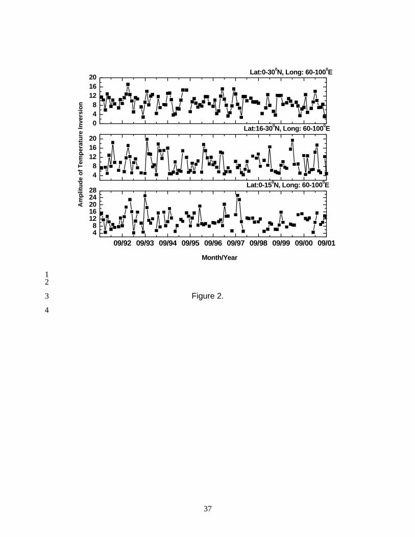
The monthly mean amplitude of the inversion temperature is obtained over all 15

three continental regions. Figure 2 displays the time series of the monthly mean variation 16

of the amplitude of the inversion over the Indian region, the band-1 and the band-2. The 17

amplitude of the inversion varies from 4 to 16K over the Indian region, from 4 to 24 K 18

over the band-1 and from 4 to 20 K over the band-2. The amplitude of the inversion is on 19

average, ~12 K over all three regions. Amplitude of inversion has been calculated from 20

the data extracted over the Indian region (0-300N, 60-1000E), the band-1 (0-150N, 60-21

1000E) and the band-2 (16-300N, 60-1000E) separately on a daily basis. Temperature 22

profiles over the Indian regions include daily profiles of band-1 as well as those of band-23

12

2. Amplitudes obtained from these profiles are then averaged for a month for all the years 1

for the Indian region. Hence amplitude gets averaged. This averaged amplitude appears 2

over the Indian region. For example in October 1992 amplitude of inversion over the 3

band-1 was 12.58K and over the band-2 was 9.73K. If we average these amplitudes we 4

get ((12.58+9.73)/2.0)= 11.15K, which is close to observed amplitude over the Indian 5

region (~10.5K). Hence amplitude of two individual Indian sub-regions reaches higher 6

values (4 K to 24 K over the band-1 and 4 to 20 K over the band-2) than the Indian region 7

(4K to 16K). 8

To study seasonal variations the amplitude of the inversions for each month is 9

averaged for the entire 10 year period. Figure 3(a) and 3(b) exhibit the seasonal variation 10

of frequency of occurrence and amplitude of the MIL along with two sigma error bars for 11

the three regions. Both the amplitude and the frequency of occurrence show a semiannual 12

variation over all regions. Over the band-1, the maxima occur in April (just after spring 13

equinox) and November (just after fall equinox). The amplitude of the temperature 14

inversion shows maxima in the months of April or May and October or November. The 15

monthly mean amplitude varies from 7 to 12 K over the Indian region, from 8 to 16 K 16

over the band-1, and from 5 to 13K over the band-2, in good agreement with values 17

reported by Leblanc and Hauchecorne (1997), who obtained the seasonal mean amplitude 18

of the temperature inversion for the period September 1991-August 1995 to vary from 2 19

K to 10K. The strong semiannual variation with maxima one month after the equinoxes 20

has also been reported by Fadnavis and Beig, (2004, and references therein). 21

In order to study the relationship between both the frequency of occurrence and 22

the amplitude of the MIL and thunderstorm activity, data are analyzed for the period 23

13

April 1995-March 2000, when OTD data were available. Figure 4(a) and 4(b) exhibit the 1

seasonal variation of frequency of occurrence and MIL amplitude along with two sigma 2

error bars for 5 year period. They are rather similar to results shown in Figure 3. Figure 3

5(a) shows the seasonal variation of frequency of occurrence and (b) the MIL amplitude 4

with the number of lightning flashes as obtained from OTD over the respective regions 5

for the same periods. The annual variations for the two parameters are the same, with 6

maxima during the equinoxes and minima during summer and winter for all three 7

regions. In all the figures we have shown the correlation coefficient between the variables 8

(left and right vertical axes), which lies between 0.50 and 0.72. 9

Figure 6 (a) and 6(b) shows seasonal variation of frequency of occurrence and 10

MIL amplitude versus the number of thunderstorm days obtained from widely spread 11

stations over the respective regions. It is interesting to note that the annual variation of 12

the number of thunderstorm days shows characteristic variation with variation of latitude. 13

Closest to the equator (0-150N, 60-1000E) the maximum is observed during May and 14

October, with the May maximum being stronger than the October maximum. For the 15

Band-2 (16-300N, 60-1000E) the maximum number of thunderstorm days occurs during 16

May and September, with the September maximum being stronger. Manohar et al. (1999) 17

have reported the latitudinal distribution of thunderstorm-activity over the Indian region 18

using these station data for the period 1970-1980. The latitudinal variation of the mean 19

number of thunderstorm days indicates systematic changes in the semiannual oscillation, 20

which are consistent with the migration of the Inter-Tropical Convergence Zone (ITCZ) 21

over different latitudinal belts. Over the band-1 the first maximum occurs in April-May 22

and the second in October-November; the first maximum is stronger than the second. In 23

14

the case of the band-2, the first maximum is in May whereas the second is in September, 1

and is stronger than the May one (Manohar et al., 1999). Our results show similar 2

variations. Frequency of occurrence and amplitude of inversion, exhibit fairly good 3

correlation, with the number of thunderstorm days over the Indian region. The correlation 4

is poorer over the band-1 and the band-2. The reason for this may be that numbers of land 5

stations are smaller there. Over the entire tropical region (uppermost panels) the 6

frequency of occurrence and the MIL amplitude exhibit fairly good correlations (>0.5) as 7

there are larger number of stations. 8

The number of lightning flashes as obtained from OTD data shows a better 9

correlation with the frequency of occurrence and the MIL amplitude over all three 10

regions (Figure 5) than with the number of thunder storm day (Figure 6). The reason may 11

be that both HALOE and OTD view the sky from above and cover both land and ocean 12

regions. Lightning flashes and number of thunderstorms days show better correlation 13

with frequency of occurrence than the MIL amplitude. This indicates that inversion may 14

be occurring with thunderstorm activity but its amplitude may not be varying 15

proportionately. 16

Figure 7 (a) shows the seasonal variation of frequency of occurrence of the 17

mesospheric temperature inversion and the number of lightning flashes recorded by OTD 18

satellite for the period April 1995 -March 2000 over the open ocean South of India (2.50S 19

- 17.50S; 56.50E - 71.50E). Figure 7(b) shows the seasonal distribution of amplitude of 20

temperature inversion versus the number of lightning flashes recorded by the OTD 21

satellite for the same period and over the same area. It is evident that the number of 22

lightning flashes and the frequency of MIL occurrence (%) are considerably less over the 23

15

ocean than over to land, but the amplitude of the temperature inversions are of the same 1

magnitude (see Figure 5). Both the frequency of occurrence (r = 0.53) and the amplitude 2

of the mesospheric temperature inversion (r = 0.65) show fairly good correlation with the 3

number of lightning flashes, and both have a strong semiannual variation. 4

To study the characteristic variation of ozone near the cold bottom of the MIL, 5

within the MIL and near the warm top of the MIL, ozone volume mixing ratios over the 6

Indian tropical region for the period October 1991- September 2001 have been averaged 7

over 65-70 km, 70-85 km and 85-90 km, respectively. To smooth the time series, six-8

point running averages were obtained. Figure 8 indicates the time series of the average 9

ozone volume mixing ratio (scatter plot) and the six-point running averages (thick line), 10

near the bottom of the MIL (65-70 km), within the MIL region (70-85 km) and at the top 11

of the MIL (85-90 km) region. Semiannual oscillations in ozone content are quite evident 12

for all three altitudes, but with a strong annual oscillation at 65-70km. It is interesting to 13

note that the ozone content reverses its phase in region of 70-85 km, where the MIL is 14

most frequently observed. The ozone volume mixing ratio at 70 – 85km is ~0.4 times its 15

value observed at 65-70 km. 16

To study the relation between the frequency of occurrence and the amplitude of 17

the temperature inversion with the variation of ozone content, the frequency of 18

occurrence and the amplitude of the temperature inversion calculated for the period 19

October 1991-September 2001 are averaged for each month. Ozone volume mixing ratios 20

are averaged over the altitude range (70-85 km) where the MIL is most frequently 21

observed for each month. Figure 9 (a) and 9(b) show the seasonal variation of frequency 22

of occurrence and the MIL amplitude together with the average ozone volume mixing 23

16

ratio (Part per billon by volume). Ozone amounts show a semiannual variation. Both the 1

frequency of occurrence and the amplitude of the MIL show a good correlation with the 2

seasonal variation of ozone. 3

Over the ocean region the inversions are observed in the 70-80 km altitude range; 4

hence, the ozone volume mixing ratios are averaged over 70-80 km. Figure 10 indicates 5

the seasonal variation of frequency of occurrence and MIL amplitude with the average 6

ozone volume mixing ratios (ppb) over the oceanic region for the period April 1995 - 7

March 2000. Again ozone amounts show a semiannual variation. The frequency of 8

occurrence and the amplitude of the mesospheric temperature inversion show correlation 9

coefficients of 0.31 and 0.12 respectively; these are statistically insignificant at the 99% 10

level. Because the ozone concentrations are somewhat less over the ocean region than 11

over the land, the chemical heating in the mesosphere will be less. This may be a reason 12

for the insignificant correlation between the variation of ozone and the frequency of 13

occurrence and the MIL amplitude over this oceanic region. 14

The semiannual oscillation in ozone amounts for the altitude range 70-90 Km 15

over the tropics was reported from satellite data (Richard et al., 1990; Thomas, 1990). 16

The ozone volume mixing ratios show the maximum values during April and November 17

over all three Indian regions. From Solar Mesosphere Explorer (SME) satellite 18

measurements for the period 1982-1983, Thomas and Barth (1984) reported that the 19

ozone density near 80 km shows large seasonal changes. During the equinoxes the ozone 20

densities are about 2-3 times those observed at the solstices, as is also evident in the 21

present study. Thomas and Barth (1984) proposed that seasonal variability in ozone may 22

be understood in terms of transport by gravity waves in the mesosphere, which in turn 23

17

result from the seasonal modulation of the propagation and breaking of small scale 1

gravity waves there. 2

3

18

4. Mechanism and Interpretations 1

2

In the above figures, we have shown that over India, semiannual variation in the 3

frequency of occurrence of mesospheric temperature inversion layer has a fairly good 4

correlation with semiannual variations in thunderstorm activity and averaged ozone 5

volume mixing ratios. Both the frequency of occurrence and the amplitude of the 6

temperature inversion layer show maximum values during April-May (in the pre 7

monsoon season) and October-November, when thunderstorm activity is also high. 8

Thunderstorm activity over India shows both a latitudinal and a seasonal variation in the 9

pre-monsoon season (Manohar et al., 1999). The seasonal variation is related to the 10

migration of the monsoon trough or Inter-Tropical Conversion Zone (ITCZ) from the 11

band-1 (0-150N, 60-1000E) to band - 2 (16-300N, 60-1000E). The band-1 shows 12

maximum thunderstorm activity during April, as the monsoon trough marches northward; 13

the band-2 shows maximum thunderstorm activity during May. During June- July the 14

monsoon spreads all over India and therefore, the number of thunderstorms observed is 15

less at this time. The withdrawal of monsoon starts in the northern India and progresses 16

towards the South, thunderstorm activity increases; during September thunderstorm 17

activity is high over band-2 and during October over band-1. 18

The formation of the MIL has been simulated in numerical models of the 19

atmosphere, including the local drag on the zonal wind associated with gravity wave 20

breaking capable of creating local adiabatic circulation and hence adiabatic heating and 21

cooling (Hauchecorne and Maillard, 1990; Leblanc et al., 1995). Liu and Gardner (2005) 22

tried to explain the observed weaker MIL at Maui than at SOR, New Mexico in terms of 23

19

weaker gravity wave dissipation and therefore a weaker downward flux of atomic 1

oxygen, which is associated with several chemical reactions in this region that converts 2

solar energy to the chemical heating leading to the MIL. This shows that gravity wave 3

breaking and dissipation play significant roles in the formation/existence of MIL. 4

HALOE and OTD being polar orbiting satellites, their simultaneous passes over a 5

specific region are very few. Table 1 and Table 2 indicate typical days where 6

simultaneous HALOE, OTD and ground based station data are available over a common 7

region. Table 1 indicates typical non inversion days when neither thunderstorm activity 8

was reported at nearby ground stations nor lightning flashes recorded by OTD in a 30 x 30 9

grid centered at the position of HALOE. Table 2 shows typical inversion days when 10

thunderstorm activity was reported at nearby ground stations and lightning flashes were 11

recorded by OTD. 12

The rapid and deep convection associated with thunder storm generated gravity 13

waves which propagate upwards and may get amplified. The gravity waves become 14

unstable at the height where the zonal wind velocity becomes equal to the wave phase 15

velocity. Usually in mesosphere this condition is satisfied and breaking of gravity waves 16

takes place (Sica and Thorsley, 1996: Thomas et al., 1996). The turbulent heating, arising 17

from the breaking of waves, provides a feedback mechanism that then may maintain the 18

observed MIL. A strong seasonal dependence of mesospheric GW activity is observed, 19

with a peak in the summer months and much reduced activity during the winter months 20

over a mid-latitudinal station in Michigan, U.S. A. (42.30 N, 83.7 0W) (Wu and Killeen, 21

1996). 22

Temperature profiles obtained from ground based MST radars and Lidars show 23

20

fluctuations in nighttime temperatures with characteristic scales resembling those of 1

large-scale gravity waves (Parameswaran et al., 2000). The dynamics of dissipating GWs 2

will transport heat downward. Thus, the transport of heat below 80 km by dissipating 3

GWs may contribute to the formation of the MIL near 70 km (Meriwether and Gardner, 4

2000). A two dimensional model simulation of gravity wave-tidal coupling points 5

strongly points to the conclusion that the breaking of gravity waves may play a 6

significant role by amplifying the temperature amplitude of the tidal structure and 7

producing a large MIL (Liu and Hagan, 1998; Liu et al., 2000). Although it is known that 8

the tidal variation is the significant contributor to the semidiurnal variation in the 9

occurrence of inversion layers at low latitudes, we could not evaluate the contribution of 10

tides from the HALOE data, due to its poor sampling in local time. 11

Heating due to several exothermic chemical reactions (implying ozone) could also 12

promote temperature inversions (Meriwether and Mlynczak, 1995; Mlynczak and 13

Solomon, 1993; Fadnavis and Beig, 2004). The seasonal modulation of the propagation 14

and breaking of small-scale gravity waves leads to the variation of gravity-wave-induced 15

transport in the mesosphere, which produces seasonal variability in ozone (Thomas and 16

Barth, 1984). Garcia and Solomon (1985) have discussed that the filtering of gravity 17

waves by the equatorial wind profile is responsible for modulating the transport of H2O 18

and associated destruction of ozone. The gravity waves produced during thunderstorms 19

may contribute to the production of MIL, and may perturb the semiannual oscillation 20

(reverse phases observed in the MIL). Gravity waves may also lead to the transport of 21

atomic oxygen and through the route of chemical heating may contribute to the 22

production of ozone. This established correlation between thunderstorm, MIL and ozone 23

21

transport. 1

Sentman et al. (2003) reported the simultaneous observation of coincident gravity 2

waves and sprites in the mesosphere, emanating from the same underlying thunderstorm. 3

Sprites are the results of atmospheric heating by the electromagnetic pulse generated by a 4

powerful lightning stroke (Füllekrug et al., 2006, Barrington-Leigh and Inan, 1999, 5

Siingh et al., 2005, 2007, and references therein). Sprites may also change the 6

concentration of NOx and HOx in the mesosphere (Hiraki et al., 2002). These chemical 7

changes may have an impact on the observed cooling/heating in the middle atmosphere, 8

which may influence MIL. This aspect has not yet been explored. Attempt should be 9

made to find out if there is any relation between MILs and sprites. 10

11

22

5. Conclusions 1

2

The seasonal variation of the frequency of occurrence and the amplitude of the 3

mesospheric inversion layer obtained from HALOE temperature profiles over the entire 4

Indian region (0-300 N, 60-1000E), the band-1(0-150N, 60-1000E), the band-2 (16-300N, 5

60-1000E) and the oceanic region (17.50S - 2.50S; 56.50E - 71.50E) show strong 6

semiannual variations. Both the frequency of occurrence and the amplitude of the 7

temperature inversion exhibit a maximum and minimum in the same month over the 8

respective regions except for the Indian region. The semiannual oscillation in ozone 9

below the cold bottom of the MIL reverses its phase within the MIL region. Above the 10

warm top of the MIL, the phase of the semiannual oscillation does not show such a 11

reversal but its amplitude increases. The Seasonal variation of the frequency of 12

occurrence and amplitude of the inversion exhibit a fairly good correlation with the 13

seasonal variation of the number of lightning flashes and of thunderstorm days. The 14

seasonal variation of frequency of the occurrence and the amplitude of the inversion also 15

exhibits a fairly good correlation with the seasonal variation of ozone over these regions. 16

The frequency of occurrence of the MIL and thunderstorm activity are less over the 17

oceanic region than over the land. Thunderstorm activity is observed by OTD and nearby 18

ground station data on strong inversion days, and no thunderstorm activity is observed by 19

OTD and nearby ground station data on non inversion days. This all indicates that gravity 20

waves produced during thunderstorms, together with chemical heating due to ozone, may 21

contribute significantly in the production of the mesospheric inversion layer. 22

23

23

Acknowledgements 1

We (S.F. and G.B.) acknowledge the Climate And Weather of Sun Earth System–2

India (CAWSES) program of the Indian Space Research Organization for financial 3

assistance to this project. D. Siingh would like to acknowledge the DST, under the 4

BOYSCAST programme (reference SR/BY/A-19/05). We are also grateful to anonymous 5

reviewers for their valuable suggestions. We thank reviewer II for his help in English 6

language corrections. 7

8

24

References 1

2

Akmaev, R. A. (2001 a), Simulation of large-scale dynamics in the mesosphere and lower 3

thermosphere with the Doppler-spread parameterization of gravity waves, 1 4

Implementation and zonal mean climatologies. J. Geophys. Res., 106, 1193-1204. 5

Akmaev, R. A. (2001 b), Simulation of large-scale dynamics in the mesosphere and 6

lower thermosphere with the Doppler-spread parameterization of gravity waves, 2 7

Eddy mixing and the diurnal tide. J. Geophys. Res., 106, 1205-1213. 8

Alexander, M. Joan, H. Richter Jadwiga, and R. Bruce (2005), Sutherland generation and 9

trapping of gravity waves from convection with comparison to parameterization. 10

J. Atmos. Sci., 62, 1- 26. 11

Allen S. J., and R. A. Vincent (1995), Gravity wave activity in the lower atmosphere: 12

seasonal and latitudinal variations. J. Geophys. Res., 100, 1327-1350. 13

Barrington-Leigh C.P., and U. S. Inan (1999), Elves triggered by positive and negative 14

lightning dischargs. Geophys. Res. Lett., 26, 683-686. 15

Chen S., H. Zhilin, M.A. White, H. Chen, D.A. Krueger, and C.Y. She (2000), Lidar 16

observations of seasonal variation of diurnal mean temperature in the mesopause 17

region over Fort Collins. J. Geophys. Res., 105, 12371-12380. 18

Christian, H. J., R. J. Blakeslee, D. J. Boccippio, W. L. Boeck, D. E. Buechler, K. T. 19

Drescoll, S. J. Goodman, J. M. Hall, W. J. Koshak, D. M. Mach, and M. F. 20

Stewart (2003), Global frequency and distribution of lightning as observed by the 21

Optical Transient Detector. J. Geophys. Res., 108, doi:10.1029/2002JD002347. 22

Chu, X., C.S. Gardner, and S. J. Franke (2005), Nocturnal thermal structure of the 23

25

mesosphere and lower thermosphere region at Maui, Hawali (20.70 N), and 1

Starfire optical range, New Mexico (350). J. Geophys. Res., 110, D09S03, doi: 2

1029/2004JD004891. 3

Clancy, R.T., and Rush, D. W. (1989), Climatology and trends of mesospheric (58-90 4

km) temperatures based upon 1982-1986 SME limb scattering profiles. J. 5

Geophys. Res., 94, 3377-3393. 6

Clancy, R.T., D.W. Rush, and M.T. Callan (1994), Temperature minima in the average 7

thermal structure of the middle atmosphere (70-80 km) from analysis of 40- to 92-8

km SME global temperature profiles. J. Geophys. Res., 99, 19001-19020. 9

Delise, D.P. and Dunkerton, T.J.(1988), seasonal variation of semi-annual oscillations, J. 10

Atmos. Science, 45, 2772-2787, 11

Erickson, Carl O., F. Linwood, and Jr. Whitney (1973), Picture of the month: gravity 12

waves following severe thunderstorms. Mon. Wea. Rev., 101, doi: 10.1175/1520 13

0493, 101, 708 – 711. 14

Fadnavis, S and G. Beig (2004), Mesospheric temperature inversions over the Indian 15

tropical region. Ann. Geophysiae. 22, 3375-3383. 16

Fullekrug, M., E .A. Mareev, and M. J. Rycroft (2006), Sprites, Elves and Intense 17

Lightning Discharges, Kluwer Academic Publishers, Boston/Dordrecht/London, 18

2006. 19

Gardner, C. S., and W. Yang (1998), Measurement of the dynamical cooling rate 20

associated with the vertical transport of heat by dissipating gravity waves in the 21

mesopause region at the starfire Optical range, New Mexico. J. Geophys. Res., 22

103, 16 909-16,926. 23

26

Gracia, R.R and Solomon, S., (1985), The effect of breaking gravity waves on the 1

dynamics and the chemical composition of mesosphere and lower thermosphere J. 2

Geophys. Res., 90, 3850-3868. 3

Goya, K., and S. Miyahara (1999), Non-hydrostatic nonlinear 2-D model simulations of 4

internal gravity waves in realistic zonal winds. Adv. Space Res., issue no. 11, 24, 5

1523-1526. 6

Hauchecorne, A., M. L. Chanin, and R. Wilson (1987), Mesospheric temperature 7

inversion and gravity wave breaking. Geophys. Res. Lett., 14, 933-936. 8

Hauchecorne, A., and A. Maillard (1990), A 2-D dynamical model of mesospheric 9

temperature inversions in winter. Geophys. Res. Lett., 17, 2197-2200. 10

Hiraki, Y., T. Lizhu, H. Fukunishi, K. Nanbu, and H. Fujiwara,( 2002), Development of 11

a new numerical model for investigating the energetics of Sprites. American 12

Geophysical Union, Fall Meeting 2002, abstract #A11C-0105. 13

India Meteorological Department, 1995-2000: All India weather summaries of Indian 14

Weather Review, Pune, 1995-2000. 15

Jenkins, D.B., D. P. Wareing, L. Thomas, and G. Vaughan (1987), Upper stratospheric 16

and mesospheric temperatures derived from lidar observations at Aberystwyth. J. 17

Atmos. Terr. Phys., 49, 287-298. 18

Kumar, V. S., Y. B. Kumar, K. Raghunath, P. B. Rao, M. Krishnaiah, K. Mizutani, A. 19

Aoki, M. Yasui, and T. Itabe (2001), Lidar measurements of mesospheric 20

temperature inversion at low latitude. Ann. Geophys., 19, 1039-1044. 21

Leblanc, T., and A. Hauchecorne (1997), Recent observations of mesospheric 22

temperature inversions. J. Geophys. Res., 102, 19471-19482. 23

27

Leblanc, T., A. Hauchecorne, M. L. Chanin, F. W. Taylor, C. D. Rodgers, and N. Livesey 1

(1995), Mesospheric inversions as seen by ISAMS (UARS). Geophys. Res. Lett., 2

22, 1485-1488. 3

Liu, A. Z., and C. S. Gardner (2005), Vertical heat and constituent transport in the 4

mesopause region by dissipating gravity waves at Maui, Hawaii (20.7°N), and 5

Starfire Optical Range, New Mexico (35°N). J. Geophys. Res., 110, D09S13, doi: 6

10.1029/2004JD004965. 7

Liu, H. L., and M.E. Hagan (1998), Local heating/cooling of the mesosphere due to 8

gravity wave and tidal coupling. Geophys. Res. Lett., 25, 941-944. 9

Liu, H. L., M. E. Hagan and R. G. Roble (2000), Local mean state changes due to gravity 10

wave breaking modulated by the diurnal tide. J. Geophys. Res., 105, 12,381-11

12,396. 12

Manohar, G. K., S. S. Kandalgaonkar, and M. I. R. Tinmaker (1999), Thunderstorm 13

activity over India and the Indian southwest monsoon. J. Geophys. Res., 104, 14

4169-4188. 15

Meriwether, J. W., and C. S. Gardner (2000), A review of the mesospheric inversion 16

layer phenomenon. J. Geophys.. Res., 105, 12405- 12416. 17

Meriwether, J. W., X. Gao, V. Wickwar, T. Wilkerson, K. Beissner, S. Collins, and M. 18

Hagan (1998), Observed coupling of the mesospheric inversion layer to the 19

thermal tidal structure. Geophys. Res. Lett., 25, 1479-1482. 20

Meriwether, J. W., and M. G. Mlynczak (1995), Is chemical heating a major cause of the 21

mesosphere inversion layer? J. Geophys. Res., 100, 1379-1387. 22

Meriwether, J. W., P. D. Dao, R. T. McNutt, W. Klemetti, W. Moskowitz, and G. 23

28

Davidson (1994), Raleigh lidar observations of mesosphere temperature structure. 1

J. Geophys. Res., 99, 16973-16987. 2

Mlynczak, M. G., and S. Solomon (1991), Middle atmosphere heating by exothermic 3

chemical reactions involving odd hydrogen species. Geophys. Res. Lett., 18, 37-4

40. 5

Mlynczak, M. G., and S. Solomon (1993), A detailed evaluation of the heating efficiency 6

in the middle atmosphere. J. Geophys. Res., 98, 10517-10541. 7

Nee, J. B., S. Thulasiram, W. N. Chen, M. V. Ratnam and D. N. Rao (2002), Middle 8

atmospheric temperature structure over two tropical locations, Chung Li (250N, 9

1210E) and Gadanki (13.50N, 79.20E). J. Atmos. Solar-Terr. Phys., 64, 1311-10

1319. 11

Parameswaran, K., M. N. Sasi, G. Ramkumar, P. R. Nair, V. Deepa, B. V. 12

Krishnamurthy, S. R. Prabhakaran Nayar, K. Revathy, G. Mrudula, K. Satheesan, 13

Y. Bhavanikumar, V. Sivkumar, T. Raghunath, Rajendraprsad, and M. Krishnaiah 14

(2000), Atitude profile of temperature from 4 to 80 km over the tropics from MST 15

radar and lidar, J. Atmos. Solar-Terr. Phys., 62, 1327-1337. 16

Ratnam, M., Venkat, J. B. Nee, W. N. Chen, V. Siva Kumar and P. B. Rao (2003), 17

Recent observations of mesospheric temperature inversions over a tropical station 18

(13.5°N,79.2°E), J. Atmos. Solar-Terr. Phys., 65, 323-334. 19

Richard, M. B., D. F. Strobel, M. E. Summers, J. J. Olivero, and M. Allen (1990), The 20

seasonal variation of water vapor and ozone in the upper mesosphere: Implication 21

for vertical transport and ozone photochemistry. J. Geophys. Res., 95, 883-893. 22

Schmidlin, F.J (1976), Temperature inversion near 75 km, Geophys. Res. Lett., 3,173-23

29

3,176. 1

Senft, D. C., and C. S. Gardner (1991), Seasonal variability of gravity waves activity and 2

spectra in the mesopause region at Urbana. J. Geophys. Res., 96, 17229-17264. 3

Sentman, D.D., E.M. Wescott, R.H. Picard, J.R. Winick, H.C. Stenbaek-Nielsen, E.M. 4

Dewan, D.R. Moudry, F.T. São Sabbas, M.J. Heavner, and J. Morrill (2003), 5

Simultaneous Observations of Mesospheric Gravity Waves and Sprites Generated 6

by a Midwestern Thunderstorm. J. Atmos. Solar-Terr. Phys., 65, 537-550. 7

She, C.Y., D. A. Kruger, R. Roble, P. Keckhut, P., A. Hauchecorne, and M. L. Chanin, 8

(1995), Vertical structure of mid-latitude temperature from stratosphere to 9

mesosphere (30-105 km). Geophys. Res. Lett., 22, 377-380. 10

Siingh, Devendraa, R. P. Singh, A. K. Kamra, P. N. Gupta, R. Singh, V. Gopalkrishnan, 11

and A. K. Singh (2005), Review of electromagnetic coupling between Earth’s 12

atmosphere and space environment. J. Atmos. Solar-Terr. Phys., 67, 637-658. 13

Siingh, Devendraa, V. Gopalkrishnan, R. P. Singh, A. K. Kamra, Shubha Singh, V. Pant, 14

R. Singh, and A. K. Singh (2007), The atmospheric global electric circuit: An 15

overview. Atmos. Res., 84, 91-110. 16

Sica, R.J., and M. D. Thorsley (1996), Measurements of superadibatic lapse rates in the 17

middle atmosphere. Geophys. Res. Lett., 23, 2797-2800. 18

States, R. J., and C. S. Gardner (1998), Influence of the diurnal tide and thermospheric 19

heat sources on the formation of mesospheric temperature inversion layers. 20

Geophys. Res. Lett., 25, 1483-1487. 21

Thomas, J. D., D. P. Sipler, and J. E. Salah (2001), Raleigh lidar observations of a 22

mesospheric inversion layer during night and day. Geophys. Res. Lett., 28, 3597-23

30

3600. 1

Thomas, L., A. K. P. Marsh, D. P. Wareing, I. Astin, and H. Changra (1996), VHF 2

echoes from the middle mesosphere and the thermal structure observed by lidar. J. 3

Geophys. Res., 101, 12867-12877. 4

Thomas, R. J. ( 1990), Seasonal Ozone Variations in the Upper Mesosphere. J. Geophys. 5

Res., 95, 7395-7401. 6

Thomas, R.J., and C. A. Barth (1984), Seasonal variation of ozone in the upper 7

mesosphere gravity waves, Geophys. Res. Lett.,11, 673-676. 8

Walterscheid, R. L., G. Schubert, and D. G. Brinkman (2001), Small-scale gravity waves 9

in the upper mesosphere and lower thermosphere generated by deep tropical 10

convection. J. Geophys. Res., 106, 31,825-31,832. 11

Whiteway, J., A. I. Carlswell, and W. E. Ward (1995), Mesospheric temperature 12

inversions with overlying nearly adiabatic lapse rate: An indication of well mixed 13

turbulent layer. Geophys. Res. Lett., 22, 1201-1204. 14

Wu, O., and T. L. Killeen (1996), Seasonal dependence of mesospheric gravity waves 15

(<100km) at Peach Mountain observatory, Michigan. Geophys. Res. Lett., 23, 16

2211-2214. 17

18

31

Table and Figure Captions: 1

Table 1: Non inversion days observed in the HALOE temperature profile and no 2

thunderstorm activity reported at a nearby station and no lightning flashes 3

recorded by the OTD in this vicinity on the same day. 4

Table 2: Inversion days observed in the HALOE temperature profile and 5

thunderstorm activity reported at a nearby station and the number of lightning 6

flashes recorded by the OTD on the same day. 7

Figure1: Vertical temperature structure for the three randomly selected typical (a) non 8

inversion days (28 April, 21 July, 22 July 1995) and (b) inversion days (9 May, 2 9

November, 4 November, 1995) within the Indian tropical belt recorded by 10

HALOE. The interval between the double-pointed arrows represents the width of 11

the inversion layer. 12

Figure 2. Monthly variation of the amplitude of the temperature inversion derived 13

from the HALOE temperature series over the Indian region (0 -300 N, 60 -1000 14

E), the band-1(0 - 150N, 60 - 1000E) and the band-2 (16-300 N, 60-1000 E) for the 15

period 1991- 2001. 16

Figure 3. Seasonal variations of (a) Frequency of occurrence of MIL, (b) Amplitude 17

of MIL derived from the HALOE temperature series over the Indian region (0-300 18

N, 60-1000 E) for the period 1991- 2001. The error bars show ±2 sigma values. 19

Figure 4. Seasonal variation of (a) Frequency of occurrence of MIL, (b) Amplitude 20

of MIL using the HALOE temperature series over the Indian region (0-300 N, 60-21

1000 E) for the period April 1995 - March 2000. The error bars show ±2 sigma 22

values. 23

Figure 5. Seasonal variation of the (a) Frequency of occurrence of temperature 24

32

inversion (%) obtained from the HALOE temperature data and number of 1

lightning flashes as obtained from OTD data for the period April 1995 - March 2

2000, over the Indian region (0 - 300 N, Long. 60 -1000 E), the band-1 (0-150 N, 3

60-1000 E) and the band-2 (16 - 300N, 60 - 1000 E). (b) Amplitude of MIL as 4

obtained from the HALOE temperature data and number of lightning flashes as 5

obtained from OTD data. 6

Figure 6. Seasonal variation of the (a) Frequency of occurrence of the temperature 7

inversion (HALOE data) and the number of thunderstorm days as obtained from 8

different stations also for the period April 1995 -March 2000, over the Indian 9

region (0-300 N, 60-1000 E), the band-1 (0-150 N, 60-1000 E) and the band-2 (16-10

300 N, 60-1000 E). (b) Amplitude of MIL and number of thunderstorm days as 11

obtained from ground stations for the same period and locations. 12

Figure 7. Seasonal variation of the (a) Frequency of occurrence of the temperature 13

inversion (HALOE data) and the number of lightning flashes as obtained from the 14

OTD satellite, for the period April 1995 -March 2000, over the ocean are (17.5 - 15

2.50S; 56.5 - 71.50E). (b) Amplitude of MIL and the number of lightning flashes 16

(OTD data), for the same period and over the same ocean region. 17

Figure 8. Seasonal variation in averaged ozone concentration (ppb) at 65 -70 km, 70 18

– 85 km and 85 – 90 km over the Indian region (0 -300 N, 60 -1000 E) for the 19

period October 1991-September 2001 (scatter plot); the six points running 20

average is also plotted (thick line). 21

Figure 9. Seasonal variation of the (a) Frequency of occurrence of the temperature 22

inversion and the averaged ozone concentration at 70 – 85 km, both obtained from 23

33

HALOE data for the period October 1991-September 2001, over the three Indian 1

regions considered. (b) Amplitude of MIL and the averaged ozone concentration 2

at 70 - 85 km, for the same period and location. 3

Figure 10. Seasonal variation of the (a) Frequency of occurrence of the temperature 4

inversion and the averaged ozone concentration at 70 – 85 km from HALOE data 5

for the period April 1995 -March 2000, over the ocean region (17.5 - 2.50S; 56.5 6

- 71.50E). (b) Amplitude of the MIL and the averaged ozone concentration at 70 - 7

85 km for the same period and location. 8

9

34

Table 1 1

2 Non inversion day

as observed in HALOE

temperature profile (Day /Month/Year)

HALOE Position

No thunderstorm activity reported at nearby ground station

No lighting flashes recorded by OTD within 30 x 30 grid centered at

21/07/95 12.830 N, 83.560 E

Vellore - 12.550 N, 79.090 E Madras – 13.030 N, 80.150 E

(120 N, 80.50 E)

22/07/95 17.80 N, 80.530 E

Solapur – 17.40 N, 75.540 E Hyderabad – 17.270 N, 78.280 E

(170 N, 78.50 E)

08/03/99 25.260 N, 72.670 E

Udaipur- 24.350 N, 73.420 E Neemuch- 24.280N, 74.540E -

( 250 N, 720 E)

22/12/99 20.690 N, 83.570 E

Jagdalpur- 19.050 N, 82.020 E Gopalpur- 19.160 N, 84.530 E

(190 N , 820 E)

3 4 5 6 7

8

35

1 Table 2 2

3 4

Temperature inversion observed

in HALOE temperature profile

on (Day /Month/Year)

HALOE Position

Thunderstorm activity reported at ground station

Number of lighting flashes recorded by OTD within 30 x 30 grid centered at

29/5/95 10.160 N, 88.640 E

Cuddalore- 11.460 N, 79.450 E Nagapattinam-10.460

N, 79.50 E

30 (100 N , 860 E)

27/7/97 22.660 N, 71.050 E

Ahemedabad- 23.040

N, 72.380 E Ambikapur- 23.150 N, 83.150 E

41 (220 N, 720 E)

15/9/99 26.920 N, 76.260 E

Dubrugarh–27.290 N, 94.50 E

7 (260 N 760 E)

5/2/2000 29.040 N, 76.210 E

New Delhi- 28.350

N,77.120 E Dubrugarh– 27.290 N, 94.50 E

16 (270 N, 770 E)

5 6

7

36

1

50

60

70

80

90

100

180 200 220 240 260 280 300 320 340

(b) Inversion DaysNon-Inversion Days

Temperature (K)

28 April 1995 21 July 1195 22 July 1995

Temperature (K)

Alti

tude

(km

)(a)

50

60

70

80

90

100

160 180 200 220 240 260 280 300

9 May 1995 2 November 1995 4 November 1995

2 Figure 1. 3

4

5

37

09/92 09/93 09/94 09/95 09/96 09/97 09/98 09/99 09/00 09/0148

1216202428

Lat:16-300N, Long: 60-1000E

Lat:0-150N, Long: 60-1000E

Lat:0-300N, Long: 60-1000E

Month/Year

Am

plitu

de o

f Tem

pera

ture

Inve

rsio

n

48

121620

048

121620

1 2

Figure 2. 3

4

38

1

Figure 3. 2

3

J F M A M J J A S O N D0

20

40

60

80

Lat: 0-150N, Long:60-1000E

Lat: 16-300N, Long 60-1000E

Fre

quen

cy o

f Occ

urre

nce

(%)

Month

0

20

40

60

80

(a)

20

40

60

80

100 Lat: 0-300N, Long: 60-1000E

J F M A M J J A S O N D -4

8

12

16

20

Month

4

8

12

16

20

Am

plitu

de o

f Tem

pera

ture

Inve

rsio

n

4

8

12

Lat:16-300 N, Long:60-1000E

Lat:0-150N, Long:60-1000E

Lat:0-300N, Long:60-1000E(b)

39

1

2

3

4

5

6

7

8

9

10

11

Figure 4. 12

13

14

15

16

17

18

19

20

21

22

23

24

25

26

27

J F M A M J J A S O N D0

20406080

100 Lat: 0-150N, Long:60-1000E

Month

J F M A M J J A S O N D0

20

40

60

80

100

Fre

quen

cy o

f Occ

urre

nce

(%)

Lat: 16-300N, Long:60-1000E

J F M A M J J A S O N D0

20

4060

80100 (a) Lat: 0-300N, Long:60-1000E

J F M A M J J A S O N D4

8

12

16

20

Month

048

121620

Lat: 16-300N, Long:60-1000E

Lat: 0-150N, Long:60-1000E

Lat: 0-300N, Long:60-1000E

Am

plitu

de o

f Tem

pera

ture

Inve

rsio

n

(b)

048

121620

40

1

2

3

4

Figure 5. 5

6

J F M A M J J A S O N D

810121416

r = 0.5

No.

of

Ligh

tnin

g Fl

ashe

s

Month

468

101214

r = 0.52

Lat: 16-300N, Long:60-1000E

Lat: 0-150N, Long:60-1000E

Lat: 0-300N, Long: 60-1000E

Am

plitu

de o

f Tem

pera

ture

Inve

rsio

n

6

8

10

12

14r = 0.62

Amplitude of Temperature Inversion

(b)

010k20k30k40k

No. of Lightning Flashes obtained from OTD Satellite

0

10k

20k

30k

0.0

5.0k

10.0k

15.0k

20.0k

J F M A M J J A S O N D

40

60

80

100

r = 0.51N

o. o

f Li

ghtn

ing

Flas

hes

Month

020406080

100

r = 0.61

Lat: 16-300N, Long: 60-1000E

Lat: 0-150N, Long: 60-1000E

Lat: 0-300N, Long: 60-1000E

Freq

uenc

y of

Occ

urre

nce

(%) 40

50607080

r = 0.72

Frequency of Temperature Inversion

010k20k30k40k

No. of Lightning Flashes obtained from OTD Satellite

0

10k

20k

30k

(a)

0

10k

20k

41

1 2

Figure 6. 3 4

J F M A M J J A S O N D

810121416

r = 0.02

No.

of T

hund

erst

orm

Day

s

Month

468

101214

r = 0.03

Lat: 16-300N, Long: 60-1000E

Lat: 0-150N, Long: 60-1000E

Lat: 0-300N, Long: 60-1000E

Am

plitu

de o

f Tem

pera

ture

Inve

rsio

n

(b)

6

8

10

12

14r = 0.51

Amplitude of Temperature Inversion

0.0500.01.0k1.5k2.0k2.5k3.0k

No. of Thunderstorm Days

0

1k

2k

0.0

500.0

1.0k

1.5k

J F M A M J J A S O N D3044587286

100

r = 0.48

No.

of

Thun

ders

orm

Day

s

Month

020406080

100

r = 0.23

Lat: 16-300N, Long: 60-1000E

Lat: 0-150N, Long: 60-1000E

Lat: 0-300N, Long: 60-1000E

Freq

uenc

y of

Occ

urre

nce

(%)

(a)

4050607080 r = 0.65

Frequency of Temperature Inversion

0.0500.01.0k1.5k2.0k2.5k3.0k3.5k

No. of Thunderstorm Days

0.0

500.0

1.0k

1.5k

2.0k

0.0

500.0

1.0k

1.5k

42

1 2

3

4

5

6

7

8

9

10

11

12

13

14

15

16

17

Figure 7. 18

19

J F M A M J J A S O N D

10

20

30

40

50

0

10

20

30

40

50

60

70

80

Frequency of Occurrence

Month

Over the ocean ( Lat:17.50S to 2.50S; Long 56.50E to 71.50E)

r = 0.53

Freq

uenc

y of

Occ

urre

nce

(%)

(a)

Num

ber o

f Lig

htni

ng F

lash

es (O

TD)

Number of Lightning Flashes

J F M A M J J A S O N D10

12

14

16

18

20

0

10

20

30

40

50

60

Num

ber o

f Lig

htni

ng F

lash

es (O

TD)

Amplitude of Temperature Inversion Month

Over the ocean ( Lat:17.50S to 2.50S; Long: 56.50E to 71.50E)

r = 0.65

Am

plitu

de o

f Te

mpe

ratu

re In

vers

ion

(K)

(b)

Number of Lightning Flashes

43

1

,,

12/92 12/93 12/94 12/95 12/96 12/97 12/98 12/99 12/00240

280

320

360

Month/Year

80

120

160

65-70 km

70-85 km

80120160200

Ave

rage

Ozo

ne C

once

ntra

tion

(ppb

)85-90 km

2

3

Figure 8. 4

5

6

7

44

1

2

3

4

5

6

7

8

9

10

11

12

13

14

15

16

17

18

Figure 9. 19

20 21

J F M A M J J A S O N D

50

60

70

80

90

r = 0.58

Ave

rage

Ozo

ne C

once

ntra

tion

(ppb

)

Month

30405060708090

Frequency of Temperature Inversion

r = 0.65

Freq

uenc

y of

Occ

urre

nce

(%) 40

5060708090

r = 0.77

Lat:16-300N, Long: 60-1000E

Lat:0-150N, Long: 60-1000E

Lat:0-300N, Long: 60-1000E(a)

150165180195210

7590105120135150165

80

100

120

140

160

Average Ozone Concentration

J F M A M J J A S O N D8

10

12

14

16

Amplitude of Temperature Inversion

r = 0.66

Ave

rage

Ozo

ne C

once

ntra

tion

(ppb

)

Month

56789

1011

r = 0.62Am

plitu

de o

f Tem

pera

ture

Inve

rsio

n

7.07.58.08.59.09.5

10.010.511.0

r = 0.64

Lat:16-300N, Long: 60-1000E

Lat:0-15 N, Long: 60-1000E

Lat:0-300, Long: 60-1000E(b)

150165180195210

7590105120135150165

80

100

120

140

160

Average Ozone Concentration

45

1 2 3 4 5 6 7 8 9 10 11 12 13 14 15 16 17 18 19 20 21 22 23 24 25 26 27

28 Figure 10 29

J F M A M J J A S O N D

10

20

30

40

50

60

70

80

90

100

110

120

Frequency of OccurrenceMonth

Over the ocean ( Lat:17.50S to 2.50S; Long: 56.50E to 71.50E)

r = 0.31

Freq

uenc

y of

Occ

urre

nce

(%)

(a)

Ave

rage

Ozo

ne C

once

ntra

tion

(ppb

)

Average Ozone Concentration

J F M A M J J A S O N D10

12

14

16

18

20

60

70

80

90

100

110

120

Ave

rage

Ozo

ne C

once

ntra

tion

(ppb

)

Amplitude of Temperature Inversion

Month

Over the ocean ( Lat:17.50S to 2.50S; Long: 56.50E to 71.50E)

r = 0.12

Am

plitu

de o

f Te

mpe

ratu

re In

vers

ion

(K)

(b)

Average Ozone Concentration

All in-text references underlined in blue are linked to publications on ResearchGate, letting you access and read them immediately.