Bayesian model selection applied to self-noise geoacoustic inversion

Bayesian model selection applied to self-noisegeoacoustic inversion

David J. Battle,a) Peter Gerstoft, William S. Hodgkiss, and W. A. KupermanMarine Physical Laboratory, Scripps Institution of Oceanography, La Jolla, California 92093-0238

Peter L. NielsenNATO Undersea Research Centre, 19138 La Spezia, Italy

~Received 15 March 2004; revised 25 June 2004; accepted 28 June 2004!

Self-noise geoacoustic inversion involves the estimation of bottom parameters such as sound speedsand densities by analyzing towed-array signals whose origin is the tow platform itself. As well asforming inputs to more detailed assessments of seabed geology, these parameters enableperformance predictions for sonar systems operating in shallow-water environments. In this paper,Gibbs sampling is used to obtain joint and marginal posterior probability distributions for seabedparameters. The advantages of viewing parameter estimation problems from such a probabilisticperspective include better quantified uncertainties for inverted parameters as well as the ability tocompute Bayesian evidence for a range of competing geoacoustic models in order to judge whichmodel explains the data most efficiently. ©2004 Acoustical Society of America.@DOI: 10.1121/1.1785671#

PACS numbers: 43.30.Pc, 43.60.Pt@AIT # Pages: 2043–2056

dyf iroity

tic

t

derwsses

mt-

zea-e

ar

a

oritevfir

ilityterling.a-

ted

toing

ural

ob-te-tionsele-s inofndhtses-enaler-tingthe

ingith

nglu-lyticthodareec

I. INTRODUCTION

In self-noise geoacoustic inversion, plant and hydronamic noise generated by the tow ship as a by-product onormal operation is used to interrogate the ocean enviment. Because of its inherent mobility, reduced complexand low environmental impact, self-noise inversion usingtowed array is a very promising modality of geoacousexploration.1

In our previous paper,2 data acquired during the joinNATO/Marine Physical Laboratory experiment—MAPEX2000—was analyzed using maximum-likelihoo~ML ! methods to evaluate the feasibility of self-noise invsion from towed-array data. The major conclusion drafrom this preliminary work was that matched-field proceing ~MFP!, in conjunction with global search procedursuch as genetic algorithms~GA!, was sufficiently sensitive inthe near field to permit robust first-order inversion of paraeters such asp-wave velocity for a range-independent botom environment known to be reasonably well characterias a fluid half-space. This was despite low to modersignal-to-noise ratios~SNR! during the experiment and considerable uncertainty in relation to several important geomric parameters, such as water depth, source range, andshape.

In this paper, we again direct our attention to the nefield inversion problem using towed-array data, applyingdifferent paradigm to its solution and addressing two imptant questions: First, can we better quantify the sensitivlimits of near-field inversion? Second, is there a consistway of ranking our success in modeling an unknown enronment using multiple parametrizations? To address the

a!Now with the Ocean Engineering Dept., Massachusetts Institute of Tnology, Cambridge, MA. Electronic mail: [email protected]

J. Acoust. Soc. Am. 116 (4), Pt. 1, October 2004 0001-4966/2004/116(4

-tsn-,a

-n-

-

dte

t-ray

r-a-ynti-st

question, we focus on characterizing the posterior probabdensities ~PPDs! associated with ensembles of paramesamples generated by a procedure known as Gibbs sampAssuming that the model is correct, the PPD then summrizes our complete state of knowledge about the estimaparameters including their mean~expected! values, maxi-muma posteriori~MAP! values, and variances. In answerthe second question, we find as a consequence of knowthe PPD that Bayesian probability theory embodies a natranking for competing models, known asevidence. In Sec. II,we briefly reiterate a few salient aspects of Bayesian prability theory relevant to the current analysis. For compleness, we restate Bayes’ rule and underline the interpretaof likelihoods, priors, and evidence in the context of inverproblems. In Sec. III, we describe in some detail our impmentation of the Gibbs sampler used to obtain the resultlater sections. While our development parallels thatDosso3–5 as recently applied to the analysis of synthetic aexperimental geoacoustic data, we offer our own insiginto the workings of the algorithm and some further suggtions for improving its efficiency. In Sec. IV we revisit thMAPEX2000 experiment and various aspects of the sigprocessing and modeling requirements of near-field invsion. Whereas in Ref. 2 we concentrated on demonstrainversion consistency throughout an extensive portion ofdataset, in Sec. V we focus on themethodologyof Bayesianmodel selection—analyzing a single 10-s frame and derivPPDs corresponding to a variety of geoacoustic models wincreasing levels of complexity. In addition to presentimarginal distributions for the inverted parameters, we evaate the Bayesian evidence for each model using both anaGaussian approximations and a more accurate meknown as reverse importance sampling. Our conclusionsgiven in Sec. VI.

h-

2043)/2043/14/$20.00 © 2004 Acoustical Society of America

ese

id-l

reis

-graa

tio

seo

th

l-iliiniot

rkw

ilit

the

ond

od

nkstheata

-ful,

t-

re-

atr-ethe

nevi-

ed-is-

eby

e-

h

II. BAYESIAN INFERENCE

The single aspect that most popularly distinguishBayesian probability and its application in inverproblems—Bayesianinference—from its so-calledorthodoxor frequentistalternatives is the use of prior~before-data!probabilities to modulate posterior~after-data! probabilitiesaccording to Bayes’ rule

p~mud,Mk!5p~dum,Mk!p~muMk!

p~duMk!, ~1!

wherem is a vector of model parametersmi ( i 51,...,P), d isa vector of measured datadn (n51,...,N), and themodelsMk (k51,...,M ) embody various parametrizations consered plausible in explainingd. p(aub) denotes conditionaprobability, meaning the probability of some outcomeagiven a previous outcomeb. In words, Eq.~1! reads

posterior5likelihood3prior

evidence.

Specializing to the geoacoustic problem at hand, wegard themi as representing acoustic quantities that we wto infer from datadf acquired at discrete frequenciesv f ( f51,...,F) from an array ofN hydrophones. The likelihoodp(dum,Mk) quantifies the error in matching thedf with rep-lica fields generated by a continuous wave~cw! propagationmodel, while the priorp(muMk) defines and weights plausible ranges for the parametersmi . The evidence appearinin the denominator can, at first, be thought of as an ovenormalization for the PPD, which is independent of the prameter vectorm.

A. First level of inference

As defined by MacKay,6 the first of the two levels ofBayesian inference is concerned with parameter estimaproblems in which each proposed model is assumed tocorrect, i.e., all conceivable possibilities are encompaswithin its prior parameter space. This assumption is respsible for the aforementioned normalization

E p~mud,Mk!dm51. ~2!

Aside from this technicality, it is theshapeof the PPD, andhence only the likelihood and prior terms, that influencefirst level of inference.

It is often a criticism of Bayesian probability that, athough it offers clear guidance on how to use prior probabties through Eq.~1!, it is neutral as to how they are derivedthe first place. As is the case with inference in general, prhave an inescapable subjective element, which highlightsfact that all inference is subjective to a point. In this woflat priors have been assumed for all parameters, with lobounds l i and upper boundsui , such that the normalizedprior density for each parametermi is given by

p~mi uMk!51

~ui2 l i !5

1

wi. ~3!

In such cases, provided the bulk of the posterior probabis bounded within the assumedwi , the prior is said to be

2044 J. Acoust. Soc. Am., Vol. 116, No. 4, Pt. 1, October 2004

s

-h

ll-

nbed

n-

e

-

rshe,er

y

diffuseand does not significantly influence the shape ofPPD. Even diffuse priors, however, can impact therelativeprobabilities of proposed models, thus influencing the seclevel of inference, as described next.

B. Second level of inference

Whereas at the first level of inference only the likelihoand ~usually to a lesser extent! the prior are important, thesecond level involves the denominator, orevidenceterm,which is the normalizing constant for the PPD,viz.

p~duMk!5E p~dum,Mk!p~muMk!dm. ~4!

At the second level of inference, the intention is to raeach modelMk in terms of its ability to explain the data. Ais well known, such a ranking cannot be based solely onlikelihood, as arbitrarily complex models can match the darbitrarily closely. Paralleling Eq.~1!, a posterior probabilitycan also be attributed to eachMk , independent of its parameters. However, in this case, normalization is not meaningleaving the proportionality

p~Mkud!}p~duMk!p~Mk!. ~5!

The reason that Eq.~5! cannot be normalized is simply thathe universe of modelsMk is subjective and infinite. Usually, the best that can be done is to enumerateM models forcomparison, and—assuming no initial preference—thesulting prior probabilities are given by

p~Mk!51/M . ~6!

It then follows, for the purposes of model comparison, ththe posterior probability of each model is simply propotional to its evidence, which for reasons that will becomapparent later in this section is sometimes referred to asmarginal or integrated likelihood. According to Bayesiatheory, the model associated with the highest numericaldence as given by Eq.~4! is to be preferred.

What may not be immediately apparent from the precing discussion is how Bayesian evidence automatically dcriminates against models that are overly complex, therexpressing a preference forparsimoniousparametrizations.7

This preference is also known as Occam’s razor6 and be-comes more visible after assuming ahypotheticalGaussianform for the parameter likelihood around the maximum liklihood ~ML ! point m @with an ML valuep(dum,Mk) and aparameter covariance matrixCm]

p~dum,Mk!5p~dum,Mk!expS 2DmTCm

21Dm

2 D . ~7!

In Secs. V B and V C, it will be shown that Eq.~7! is oftennot a good approximation to real likelihood functions, whicrequire numerical integration~Sec. III F!. However, such ap-proximations are common in probability theory,8,6 princi-pally because the integral orhypervolumeof a Gaussian like-lihood function inP dimensions has the analytic form

E p~dum,Mk!dm5p~dum,Mk!~2p!P/2AdetCm. ~8!

Battle et al.: Bayesian model selection

is

odeigli-

itIne

er

atwt

o

bte

s.

v

oaghireb

ri

dehesi

ateiandpea

rsziis

ters

ar-illndm

litysti-bs

bu-Inpos-lly

.s

an,tionpli-

rlyinal

re,ataustsso-

theer-

tonc-n-ical

uc-trn

the

or-

Making the further simplifying assumptions that the priorflat and that the integral in Eq.~4! is not strongly affected byincluding the tails ofp(dum,Mk) which lie outside the priorrangesui and l i , Eq. ~4! can be rewritten

~9!

from which it can be seen that the maximum likelihoachieved by a particular model does, as expected, wpositively toward its ranking. Weighing against the likehood, however, is the so-calledOccam factor,6,7,9 which canbe interpreted as an integral of the prior probability densweighted according to the distribution of the likelihood.other words, the Occam factor is a measure of the conctration of prior probability within the high-likelihood regionof a parameter space, and it displays the following genproperties:6–9

~i! The Occam factor penalizes models that incorporlarge numbers of free parameters through the groof the prior hypervolumeP i 51

P wi .~ii ! For the same reason, the Occam factor penalizes m

els with widea priori parameter boundswi .~iii ! The Occam factor penalizes models that have to

finely tuned to fit the data, as these have concentraPPDs and correspondingly small posterior volume

In geophysical theory, the first to describe Bayesian edence in model selection was Jeffreys in 1939.10 Only veryrecently, however, new applications have been reported.7,9,11

The reasons for this no doubt stem from the complexityreal-world problems and the difficulties in deriving and mnipulating the necessary probability distributions. AlthouEq. ~4! is a simple prescription, such integrations requspecialized numerical methods that have only recentlycome practical.

Whereas alternative concepts such as minimum desctive lengths~MDL !, Akaike information criteria~AIC!, andlikelihood ratio tests have also been applied to moselection,12 proponents of Bayesian inference point to tfact that the concept of evidence flows naturally and contently from the basicdesiderataof probability theory. In fact,most other methods can be viewed as being closely relto, or approximations of the full Bayesian framework dscribed here.6 Recent analyses have indicated that Bayesmodel selection, which has higher computational demathan other approximate methods, is capable of superiorformance, particularly in cases of low SNR and/or smamounts of data.13

C. Marginal inference

As discussed above, the calculation of~usually nonana-lytic! PPDs is central to numerical applications of the fiand second levels of Bayesian inference. When summaria posteriori knowledge of parameter values, however, it

J. Acoust. Soc. Am., Vol. 116, No. 4, Pt. 1, October 2004

h

y

n-

al

eh

d-

ed

i-

f-

e-

p-

l

s-

ed-nsr-

ll

tng

desirable to treat eachmi ~or perhaps pairs ofmi in the 2Dmarginal probability distribution case! separately, while inte-grating over the range of influence of the other paramemiÞ j , giving marginal probability distributions of the form

p~mj ud,Mk!5E p~mj ,miÞ j ud,Mk!dmiÞ j . ~10!

Parameter estimation based on the properties of mginal distributions is known as marginal inference, and wbe applied extensively in Sec. V, in which both one- atwo-dimensional marginal distributions are computed frosamples drawn from the joint parameter PPD.

III. GIBBS SAMPLING

The basic inputs to Bayesian analysis are probabidistributions, and in practice, these can be difficult to emate given the dimensionality of real-world problems. Gibsampling is an iterative Markov chain Monte Carlo~MCMC!procedure designed to sample from joint posterior distritions using only samples from conditional distributions.the case of large-scale problems with many parameterssessing unknown correlations, joint distributions are usuanot available, whereas conditional distributions often are

The origins of the Gibbs sampler date back to Hasting14

in statistical analysis and subsequently Geman and Gem15

who applied the idea to large-scale image reconstrucproblems. Comprehensive accounts of the theory and apcation of Gibbs sampling to inverse problems—particulathose in geophysics—as well as references to the origliterature include Gelfand and Smith,16 Smith and Roberts,17

Sen and Stoffa,18 and Mosegaard and Sambridge.11 In rela-tion to ocean-acoustic problems of the type of interest heDosso3–5 recently analyzed synthetic and experimental dand concluded that Gibbs sampling is a powerful and robmeans of estimating geoacoustic parameters and their aciated errors.

In this section, we briefly discuss issues relevant tointegration of high-dimensional PPDs in geoacoustic invsion. These include the Metropolis–Hastings approachsample generation, definition of a matched-field energy fution, Gibbs sampler initialization, coordinate rotation, covergence criteria, and finally, one approach to the numerestimation of Bayesian evidence.

A. Sample generation

In essence, Gibbs sampling consists of generating scessive samples fromP conditional distributions, such that athe completion of theqth iteration, the parameter vecto(m1

q ,m2q ,m3

q ,...,mP21q ,mP

q ) can be considered to have beedrawn from the joint PPD. For clarity, it will be implicitlyassumed that posterior probabilities are conditional ondatad and modelMk from this point. Starting with the ini-tial parameter vector (m1

0,m20,m3

0,...,mP210 ,mP

0 ) and denot-ing the conditional distribution of parameterm1 with respectto parameters m2→P in the first iteration asp(m1um2

0,m30,...,mP21

0 ,mP0 ), the sampling proceeds with

each successive conditional distribution immediately inc

2045Battle et al.: Bayesian model selection

ths

leibs-ec

,is

.eas

anther

rao

i-

oId

ri-

oci-veruntoream-elud-

isdnd

di-c-

u-

cycean,

nbefor

telyn ofte thevetheofe

porating the previously selected parameter value. Using‘‘ ←’’ symbol to denote the drawing of a sample, the firiteration can be illustrated as8

m11←p~m1um2

0,m30,...,mP21

0 ,mP0 !

m21←p~m2um3

0,m40,...,mP

0 ,m11!

m31←p~m3um4

0,m50,...,m1

1,m21!

] ] ]

mP1←p~mPum1

1,m21,...,mP22

1 ,mP211 !,

with the qth iteration given by

m1q←p~m1um2

q21,m3q21,...,mP21

q21 ,mPq21!

m2q←p~m2um3

q21,m4q21,...,mP

q21,m1q!

m3q←p~m3um4

q21,m5q21,...,m1

q ,m2q!

] ] ]

mPq←p~mPum1

q ,m2q ,...,mP22

q ,mP21q !.

In the Metropolis–Hastings variant of the Gibbs sampused here, samples are drawn from each conditional distrtion according to the Metropolis rule, wherein uniformly ditributed perturbations, resulting in modified parameter vtors m8, are accepted with probability

paccept5H p~m8!

p~m!for p~m8!<p~m!,

1 for p~m8!.p~m!.

~11!

As in Eq. ~1!, the p(m) are posterior probabilities whichgiven simplifying Gaussian assumptions regarding the noand modeling errors, take the exponential form

p~m!5exp@2E~m!#, ~12!

whereE(m) is an energy functionto be discussed shortlyThe above combination of sequential perturbation, acctance, and rejection establishes a Markov chain whose spling density can be shown to converge to the GibbBoltzmann distribution from thermodynamics11,18

p~m!51

ZexpF2

E~m!

T G , ~13!

with the normalization orpartition functionZ ignored, and aparticular choice of unity for the temperatureT. This is thesame equilibrium distribution associated with simulatednealing~SA! algorithms, and hence Gibbs sampling hasinterpretation of being SA conducted at a constant tempture of T51.19,20

When evaluating the multidimensional integrals@Eq.~10!# with importance sampling, the variance of the integestimates is reduced if the generating distribution is proptional to the integrand, and this is actually obtained withGibbs sampler.3,8,18 Generally, when evaluating the multidmensional integrals@Eq. ~10!# with importance sampling, thesampling distribution should be concentrated in regionsthe parameter space where the PPD is most significant.ally, if the PPD is perfectly mirrored by the sampling dist


et

ru-

-

e

p-m-–

-ea-

lr-a

fe-

bution, then the error in estimating the PPD and its assated marginal integrals tends to zero—a situation neachieved in practice, but approximated with a given amoof computation such that Gibbs sampling is usually far mattractive than either less adaptive or more exhaustive spling techniques.3,8,18 While other methods of importancsampling have also been applied to PPD estimation, incing, for example, GA in ocean acoustics,21–26 the great ad-vantage of Gibbs sampling is that the sampling distributionknownto be given by Eq.~13!. In the case of GA and relatemethods, the sampling distribution is usually not known aconsequently the results may be difficult to interpret.4

B. Energy function

In Ref. 2, parameter estimation was carried out byrectly maximizing normalized Bartlett power objective funtions of the form

Bf~m!5Fwf†~m!Rfwf~m!

tr@Rf #iwf~m!i2G , ~14!

where thewf were replica vectors calculated from a continous wave acoustic propagation model and theRf ( f51,...,F) were cross-spectral density matrices~CSDMs! av-eraged fromNs snapshot vectorsdn, f of the array data atfrequenciesv f according to

Rf51

Ns(n51

Ns

dn, fdn, f† . ~15!

To formulate the energy functionE(m) required by Eq.~12!, Eq. ~14! can be transformed into themismatchor errorfunction27

f f~m!512Bf~m!, ~16!

following which3,25

E~m!5(f 51

Ff f~m!udf u2

s f2

, ~17!

whereudf u2 is the total power seen by the array in frequenband f and s f

2 is a corresponding estimate of the varianassociated with the combination of model mismatch, oceand instrumental noise.

To estimates f2, two simplifying assumptions have bee

made here. First, considering the single frame of data todiscussed in Sec. IV, and the three frequencies selectedinversion, it is reasonable to take the SNR as approximaconstant across frequency. Second, the spatial distributionoise along the array has been assumed constant despishort range of the experiment which, in reality, would haresulted in higher SNRs at the end of the array nearersource. Following the maximum-likelihood argumentsGerstoft and Mecklenbra¨uker in relation to the noise variancexpected after averagingNs snapshots, as in Eq.~15!, theaverage variance can be estimated as3,25,27

save2 5

fave~m!udaveu2

Ne, ~18!


ch

th

toaledta

-

s

u

tt-

dghnim

om

-eb

bil-a-nce

andep-eters arey

is-

re-

wherefave(m) is the average normalized Bartlett mismatobtained using a global search~at the first level of inference!,udaveu2 is the average measured power, andNe is an estimateof the number of degrees of freedom associated withnoise.

As discussed by Gerstoft and Mecklenbra¨uker25,27 andDosso,3,4 the selection of appropriate values forNe ~andhencesave

2 ) in geoacoustic inversion is problematic duethe fact that the structure of the true model and hencethat of the true signal are generally unknowable. Becausthis, modelingerrors actually tend to dominate even at moerate SNR values—in most cases swamping the impacnoise completely. Faced with this difficulty, we adoptedheuristic approach and choseNe55 ~Refs. 28, 25, 3, 4! not-ing that: ~1! This was approximately the number~six! ofindependent snapshots used, and~2! from experience, acceptance ratios~proportions of accepted Metropolis moves! onthe order of 25% to 50% are typically indicative of Gibbsampler algorithms performing correctly.11,13 Too large anestimate ofNe leads to artificially narrow PPDsrelative tothe prior boundsthrough the exponentiation in Eq.~12!, andcorrespondingly poor acceptance ratios.

To summarize, the final energy function used in oGibbs sampler had the form

E~m!5S(f 51

F

f f~m!, ~19!

with S5Ne /fave(m). Given that the highest average Bartlepower~correlation coefficient squared! obtained here was approximately 0.8, the overall energy scaling factorS was

S5Ne

fave~m!'

5

0.2525. ~20!

C. Initialization

As Gibbs samplers essentially sample around the moof PPDs, they must be correctly initialized to regions of hiposterior probability. In many reported applications, an itialization orburn-in phase has preceded to the equilibriu(T51) sampling phase such that an initial quenching frsome high temperature takes place.8,3,4 In this work, wefound that SA initialization did perform satisfactorily provided the starting temperature and annealing schedule wcorrectly chosen—usually by trial and error. However, su

FIG. 1. The configuration of theALLIANCE and theMANNING during theMAPEX2000 self-noise experiment.


e

soof-of

r

es

-

re-

stituting a genetic algorithm~GA! in place of SA ultimatelyproved faster in locating the main concentrations of probaity. This was probably due to the insensitivity of GA to prameter correlations that can seriously affect the acceptaratios obtained during conventional SA.

D. Coordinate rotation

As noted by Collins and Fishman,29 algorithms that gen-erate univariate parameter perturbations, such as SAGibbs sampling, are particularly susceptible to poor acctance ratios when sampling strongly correlated paramspaces. In ocean acoustics, such parameter correlationfrequently encountered,30 and coordinate rotation, wherebthe parameter covariance matrixC, or alternatively, a cova-riance matrix computed from field derivatives29 is effectivelyorthogonalized, is a standard solution that will not be dcussed here in detail. Following Dosso,3 our Gibbs sampler

FIG. 2. The tracks of the NRVALLIANCE and MANNING during theMAPEX2000 self-noise experiment. All times are UTC. Each frame repsents a 30-s increment.


teti

-o

r-p

io

hat

tionto

lity.ght

wecep-g

axi-eterile

eriapsbleIV

dasha

,th

xity

t.

face

ers

originally included a covariance estimation phase conducat T51 following which the parameter covariance was esmated from sampled vectorsm as

Cm'^mm†&2^m&^m&†. ~21!

Collins and Fishman29 originally suggested using the covariance matrix of the derivatives of the field. Insteadsampling the covariance matrixCm , the Cramer–Rao lowebound matrixCCRLB which contains information about parameter coupling, can be used to estimate the requiredrameter rotations. In this work the Cramer–Rao formulatdue to Baggeroeret al.extended to the multifrequency case31

is used

FIG. 3. Normalized power spectral density computed from time-seriesbeamformed in the approximate direct-path direction of the supportMANNING. The three frequencies used for inversion were 131.47, 262.94,306.88 Hz, as indicated by the top markers.

FIG. 4. Towed-array shape models.~a! Simple parabolic model with depthbow and tilt. ~b! Cubic spline model fitting a variable number of deppoints—in this caseza1 , za2 , za3 , andza4 .


d-

f

a-n

@CCRLB21 # i j 5(

f 51

F

TrFK f21 ]K f

]mjK f

21 ]K f

]miG , ~22!

where theK f are outer products of replica fieldswf calcu-lated at the ML pointm and loaded uniformly on their di-agonals to approximate the estimated SNR of the data. TEq. ~22! can be used in this wayindependently of the dataisless surprising when it is considered that coordinate rotais simply another kind of importance sampling designedconcentrate samples in regions of high posterior probabiWhile it is conceivable that a proposed ocean model mibe sufficiently far from reality for Eq.~22! to fail as the basisof such a sampling distribution, in all cases reported hereobserved substantial improvements in Gibbs sampler actance ratios whenC was estimated semianalytically usinEq. ~22! ~up to 50%! as opposed to Eq.~21! ~'25%!.

E. Convergence criteria

As we were mainly interested inmarginal PPDs, webased our Gibbs sampler convergence criteria on the mmum fractional change undergone by any 50-bin paramhistogram in 100 cycles through the Gibbs sampler. Whnot as rigorous as the dual-population convergence critused by others,3 we checked for convergence every 100 steand found that histogram changes below 10% were a reliasign of convergence. All results presented in Sec.achieved this criterion.

taipnd

FIG. 5. Six acoustic waveguide models with varying degrees of compleand their associated parameters.~a! Iso-velocity water over half-space.~b!Sound-speed gradient over half-space.~c! Iso-velocity water over sedimenand half-space.~d! Sound-speed gradient over sediment and half-space~e!Iso-velocity water over two-layer sediment and half-space.~f! Sound-speedgradient over two-layer sediment and half-space. Note the distinct surand bottom water column velocitiesCw1 andCw2 in models~b!, ~d!, and~f!.Also note that while the two sediment layer velocitiesCs1 and Cs1 aredistinct in models~e! and ~f!, the densities and attenuations of these lay(rs andas) have been assumed equal for simplicity.


opmxanl sr

hinf.

ratedofin-

elf,ythe

nce-

g.

tedrinee-

ingac-stoffgthpthal-

the

esval,per

oiseed.

ed

-s ahilegertionthe

or

g

F. Reverse importance sampling

In Sec. II B, Bayesian evidence was defined in termsan integral that, given a Gaussian approximation to therameter likelihood and flat priors, had a simple analytic forUnfortunately, as will be apparent in Sec. V, such appromations can result in errors of many orders of magnitudesometimes compromise the outcome of Bayesian modelection. More accurate calculation of evidence calls fonumerical integration approach.

O Ruanaidh and Fitzgerald8 describe such an approacthat is closely related to the concept of importance samplbut works in reverse to extract the probabilistic evidence omodel from samplesmq already available from its joint PPD

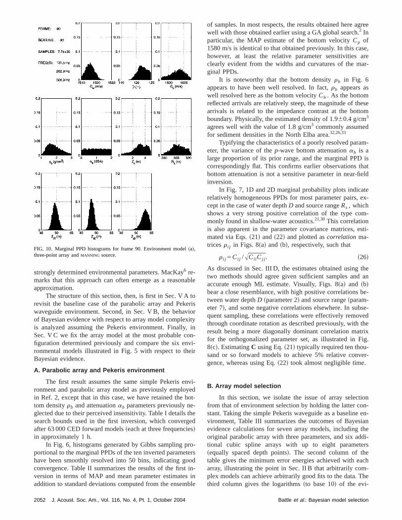
FIG. 6. Marginal PPD histograms for frame 90. Environment model~a!,parabolic array andMANNING source.

TABLE I. Parameters and inversion bounds for the first case involvinparabolic array and Pekeris environment.

Parameter Symbol Unit Min Max

Water sound speed Cw m/s 1510 1530Water depth D m 115 125Bottom sound speed Cb m/s 1450 1650Bottom density rb g/cm3 1 3Bottom attenuation ab dB/l 0 2Source depth Zs m 0 5Source range Rs m 275 325Array depth Za m 45 55Array tilt f degrees 22 2Array bow B m 25 5


fa-.i-de-

a

g,a

In the present case, these samples will have been geneat the first level of inference, i.e., in estimating the PPDthe parameters via Gibbs sampling. The task then is tovoke a Gaussian approximation, not for the integral itsbut to bereverse sampledby the existing ensemble, therebcalibrating the unknown evidence integral against that ofGaussian, which is known. Takingg(m) as a normalizedGaussian

E g~m!dm51, ~23!

andE as the unknown evidence integral

E5E f ~m!dm, ~24!

E can be shown to be approximated by8

1

E '1

Q (q51

Qg~mq!

f ~mq!. ~25!

Calculating Bayesian evidence by reverse importasampling~RIS! is straightforward, requiring negligible further computation once the PPD samplesmq and their func-tional valuesf (mq) have been generated by Gibbs samplin

IV. SELF-NOISE INVERSION

A. MAPEX2000

The 90-min experiment discussed here was conducby the NATO Undersea Research Center and the MaPhysical Laboratory as part of MAPEX2000, which was spcifically directed at validating a range of array processand geoacoustic inversion techniques. The data werequired north of the island of Elba, off the Italian west coaon the 29th of November, 2000 between the times07:17:30 and 08:45:00 UTC.2 The array used consisted o128 hydrophones evenly spaced at 2 m. Half-wavelensampling therefore occurred at approximately 375 Hz. Decontrol with this array proved less accurate than hoped,though this turned out to be of little consequence, asarray shape was included in the vectorm along with theother parameters to be optimized.

The self-noise inversion dataset comprised 175 framsampled at 30-s intervals. Only the first 10 s of each interor 60 000 samples at a sampling rate of 6000 samplessecond, were recorded. One novel aspect of this self-nexperiment was that two research vessels were involvFrom about frame 60 to frame 107, the NRVALLIANCE , withits array towed approximately 330 m behind, was followby a smaller vessel, theMANNING, at a range of approxi-mately 900 m. The horizontal distance of theMANNING fromthe tail of the array was therefore approximately 300 m.

As in our earlier analysis,2 we have made the assumption here that the source ship was well approximated apoint source over the range of frequencies considered. Wrealizing that this may not generally be the case with larvessels or at higher frequencies, the point-source assumpseems to have been borne out at least in the case ofMANNING by consistently sharp matched-field process~MFP! peaks.

a


that

s

b

hetra

ndc0e

ir

ndis

stic

eent

nifi-lba

werewaveinmue

in-0%ities

ia-

.47,topmath

ng

a

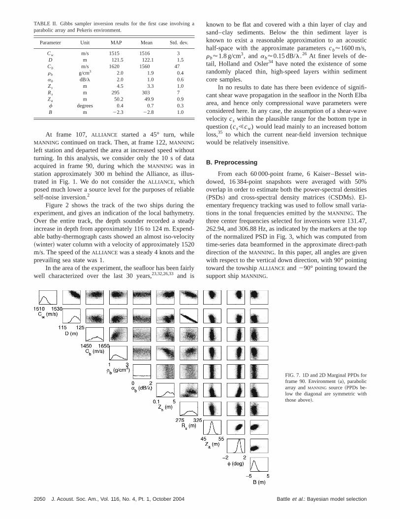
At frame 107, ALLIANCE started a 45° turn, whileMANNING continued on track. Then, at frame 122,MANNING

left station and departed the area at increased speed witurning. In this analysis, we consider only the 10 s of dacquired in frame 90, during which theMANNING was instation approximately 300 m behind the Alliance, as illutrated in Fig. 1. We do not consider theALLIANCE , whichposed much lower a source level for the purposes of reliaself-noise inversion.2

Figure 2 shows the track of the two ships during texperiment, and gives an indication of the local bathymeOver the entire track, the depth sounder recorded a steincrease in depth from approximately 116 to 124 m. Expeable bathy-thermograph casts showed an almost iso-velo~winter! water column with a velocity of approximately 152m/s. The speed of theALLIANCE was a steady 4 knots and thprevailing sea state was 1.

In the area of the experiment, the seafloor has been fawell characterized over the last 30 years,23,32,26,33 and is

TABLE II. Gibbs sampler inversion results for the first case involvingparabolic array and Pekeris environment.

Parameter Unit MAP Mean Std. dev.

Cw m/s 1515 1516 3D m 121.5 122.1 1.5Cb m/s 1620 1560 47rb g/cm3 2.0 1.9 0.4ab dB/l 2.0 1.0 0.6Zs m 4.5 3.3 1.0Rs m 295 303 7Za m 50.2 49.9 0.9f degrees 0.4 0.7 0.3B m 22.3 22.8 1.0


outa

-

le

y.dy-

ity

ly

known to be flat and covered with a thin layer of clay asand–clay sediments. Below the thin sediment layerknown to exist a reasonable approximation to an acouhalf-space with the approximate parameterscb'1600 m/s,rb'1.8 g/cm3, andab'0.15 dB/l.26 At finer levels of de-tail, Holland and Osler34 have noted the existence of somrandomly placed thin, high-speed layers within sedimcore samples.

In no results to date has there been evidence of sigcant shear wave propagation in the seafloor in the North Earea, and hence only compressional wave parametersconsidered here. In any case, the assumption of a shear-velocity cs within the plausible range for the bottom typequestion (cs!cw) would lead mainly to an increased bottoloss,35 to which the current near-field inversion techniqwould be relatively insensitive.

B. Preprocessing

From each 60 000-point frame, 6 Kaiser–Bessel wdowed, 16 384-point snapshots were averaged with 5overlap in order to estimate both the power-spectral dens~PSDs! and cross-spectral density matrices~CSDMs!. El-ementary frequency tracking was used to follow small vartions in the tonal frequencies emitted by theMANNING. Thethree center frequencies selected for inversions were 131262.94, and 306.88 Hz, as indicated by the markers at theof the normalized PSD in Fig. 3, which was computed frotime-series data beamformed in the approximate direct-pdirection of theMANNING. In this paper, all angles are givewith respect to the vertical down direction, with 90° pointintoward the towshipALLIANCE and290° pointing toward thesupport shipMANNING.

FIG. 7. 1D and 2D Marginal PPDs forframe 90. Environment~a!, parabolicarray andMANNING source~PPDs be-low the diagonal are symmetric withthose above!.


byafoo

ngmthlelti

c-

onth

retht-a-erad

o0

are

. B

thengidethele

ttledents,ins

stora-

ntalwe

ionedli-tionreing

for

etri-en-tly;

e as-by

less

a

et

ble

isenm

Given the level of interference originating from nearshipping traffic, it was found useful to incorporate additionspatial filtering of the snapshot data. Preprocessing thereentailed temporal windowing and 2D FFT transformationeach snapshot, frequency masking to exclude certain raof spatial frequencies, and then inverse 1D FFT transfortion back into phone-frequency space. In this analysis,spatial frequency cutoff was set to include arrival angwithin 60° of endfire to capture most of the expected mupath arrivals from theMANNING. To retain the normalizationof Eq. ~14!, identical filtering was applied to the replica vetors wf .

C. Propagation modeling

Accurately modeling the response of acoustic envirments is a principal aspect of geoacoustic inversion. Inpresent case of self-noise inversion, particular attentionrequired to aspects of short-range propagation that diffetiate it from long-range waveguide propagation—namelyleaky or virtual modesthat result from steep angles of botom incidence.1 In view of this, two approaches to propagtion modeling capable of accuracy in the near field wused, the first of which—wave number integration—hasready been detailed in Ref. 2. The second approach, basethe complex effective depth~CED! ideas of Zhang andTindle,36 was motivated by the modeling requirementsGibbs sampling, which can easily run to the order of 15

models for a single inversion.The first great advantage of CED models is that they

based on normal modes, which are characteristic of thevironment and independent of source–receiver geometry

FIG. 8. Parameter correlation matrices for the Pekeris environmentparabolic array~parameter order as per Tables I and II!: ~a! Gibbs samplerestimate;~b! Estimate via Eq.~22!; ~c! Estimate via Eq.~21! after samplingin rotated coordinates. The parameter indices now relate to a new sorthogonal coordinates.

TABLE III. Results for the array model selection. The three-point splineseen to give the highest evidence. Note that the table displays log evidand the probability of a model is based on just the evidence; thus, the sdifferences for each model are important.

Model Min E

Log evidence

RIS Gaussian

Parabola 20.1 214.4 214.3Spline 3 19.4 214.2 213.8Spline 4 19.1 214.4 213.8Spline 5 18.9 214.8 214.1Spline 6 17.9 215.3 214.4Spline 7 17.7 215.5 214.6Spline 8 17.3 215.7 215.5


lrefes

a-es-

-eisn-e

el-on

f

en-y

keeping environmental parameters at the beginning ofGibbs chain, it is possible to improve efficiency by reusithe mode functions to evaluate the array field for a wvariety of geometric variations. Second, by replacingsingle-interface reflection coefficient of Zhang and Tindwith an invariant embedding scheme,37 the capability of ourCED code was extended to arbitrary bottom layering at liadditional cost. The disadvantage of our existing CED cois that it cannot handle water column sound-speed gradiewhich were instead modeled by wave number integrationthis work. Modifications of our CED code along the linedescribed by Westwoodet al.38 are expected to remedy thiproblem, enabling Gibbs sampling to be applied efficientlymore complex environments for which wave number integtion is currently slower by a factor of about 20.

D. Array modeling

From the standpoint of real data analysis, it is importato allow for geometric distortion of the array from its idehorizontal and straight configuration. Whereas in Ref. 2modeled the array as a parabolic curve with bowB metersand tilt f degrees, in this work we extended the descriptto a cubic spline passing through multiple equally spacpoints. Each point has freedom in depth, allowing compcated array shapes to be modeled. Figure 4 is an illustraof both models, as it is our intention in Sec. V to compaeach with respect to Bayesian evidence, thereby quantifythe level of complexity most appropriate.

V. RESULTS

In this section, we present inversion results obtainedframe 90 of the MAPEX2000 dataset using theMANNING asa source, and a variety of geoacoustic and array paramzations. Strictly speaking, the selection of the array andvironmental models should have been made concurrenhowever, we undertook these analyses separately on thsumption that the array parameters were well determinedthe data and hence hierarchically separable from the

nd

of

FIG. 9. Normalized probabilities for the towed-array models listed in TaIII based on Bayesian evidence.

ceall


a

toe

vioxit,onv

ei

nyebo-thge

roteoin

sb

gree

se,arear-

esetom

m-

ishateld

teex-

m-

esti-

thean

be-

se-vedtherixig.

er-

ionn-en-

ianthedi-rs

ach-he

strongly determined environmental parameters. MacKay6 re-marks that this approach can often emerge as a reasonapproximation.

The structure of this section, then, is first in Sec. V Arevisit the baseline case of the parabolic array and Pekwaveguide environment. Second, in Sec. V B, the behaof Bayesian evidence with respect to array model compleis analyzed assuming the Pekeris environment. FinallySec. V C we fix the array model at the most probable cfiguration determined previously and compare the six enronmental models illustrated in Fig. 5 with respect to thBayesian evidence.

A. Parabolic array and Pekeris environment

The first result assumes the same simple Pekeris eronment and parabolic array model as previously emploin Ref. 2, except that in this case, we have retained thetom densityrb and attenuationab parameters previously neglected due to their perceived insensitivity. Table I detailssearch bounds used in the first inversion, which converafter 63 000 CED forward models~each at three frequencies!in approximately 1 h.

In Fig. 6, histograms generated by Gibbs sampling pportional to the marginal PPDs of the ten inverted paramehave been smoothly resolved into 50 bins, indicating goconvergence. Table II summarizes the results of the firstversion in terms of MAP and mean parameter estimateaddition to standard deviations computed from the ensem

FIG. 10. Marginal PPD histograms for frame 90. Environment model~a!,three-point array andMANNING source.


ble

risr

yin-i-r

vi-dt-

ed

-rsd-

inle

of samples. In most respects, the results obtained here awell with those obtained earlier using a GA global search.2 Inparticular, the MAP estimate of the bottom velocityCp of1580 m/s is identical to that obtained previously. In this cahowever, at least the relative parameter sensitivitiesclearly evident from the widths and curvatures of the mginal PPDs.

It is noteworthy that the bottom densityrb in Fig. 6appears to have been well resolved. In fact,rb appears aswell resolved here as the bottom velocityCb . As the bottomreflected arrivals are relatively steep, the magnitude of tharrivals is related to the impedance contrast at the botboundary. Physically, the estimated density of 1.960.4 g/cm3

agrees well with the value of 1.8 g/cm3 commonly assumedfor sediment densities in the North Elba area.32,26,33

Typifying the characteristics of a poorly resolved paraeter, the variance of thep-wave bottom attenuationab is alarge proportion of its prior range, and the marginal PPDcorrespondingly flat. This confirms earlier observations tbottom attenuation is not a sensitive parameter in near-fiinversion.

In Fig. 7, 1D and 2D marginal probability plots indicarelatively homogeneous PPDs for most parameter pairs,cept in the case of water depthD and source rangeRs , whichshows a very strong positive correlation of the type comonly found in shallow-water acoustics.21,30This correlationis also apparent in the parameter covariance matrices,mated via Eqs.~21! and ~22! and plotted ascorrelation ma-tricesr i j in Figs. 8~a! and ~b!, respectively, such that

r i j 5Ci j /ACii Cj j . ~26!

As discussed in Sec. III D, the estimates obtained usingtwo methods should agree given sufficient samples andaccurate enough ML estimate. Visually, Figs. 8~a! and ~b!bear a close resemblance, with high positive correlationstween water depthD ~parameter 2! and source range~param-eter 7!, and some negative correlations elsewhere. In subquent sampling, these correlations were effectively remothrough coordinate rotation as described previously, withresult being a more diagonally dominant correlation matfor the orthogonalized parameter set, as illustrated in F8~c!. EstimatingC using Eq.~21! typically required ten thou-sand or so forward models to achieve 5% relative convgence, whereas using Eq.~22! took almost negligible time.

B. Array model selection

In this section, we isolate the issue of array selectfrom that of environment selection by holding the latter costant. Taking the simple Pekeris waveguide as a baselinevironment, Table III summarizes the outcomes of Bayesevidence calculations for seven array models, includingoriginal parabolic array with three parameters, and six adtional cubic spline arrays with up to eight paramete~equally spaced depth points!. The second column of thetable gives the minimum error energies achieved with earray, illustrating the point in Sec. II B that arbitrarily complex models can achieve arbitrarily good fits to the data. Tthird column gives the logarithms~to base 10! of the evi-


ngv

ict

e

emin

insi

inoma

adab

rwa

tha

ous

theove.selba

ghtique.mn,cityent,eeds.

ofrraye ofinthepre-e

esed

r

-ef.

k

dence values as calculated by reverse importance samplithe most accurate method used here. These log-evidenceues can be compared with those in the fourth column, whwere calculated by a fast approximate method based onGaussian assumption of Eq.~9!. As discussed in Sec. II B, inthe absence of prior preferences toward particular modthat with the highest evidence~or log evidence! is preferred,and the array model with the highest evidence in this casthe three-point spline. While array models of higher coplexity achieved lower energies, the Occam factor implicitthe evidence formulation automatically discriminated agathem, leading to a monotonic decrease in probability, aslustrated by the normalized probability plot of Fig. 9.

Interestingly, both the parabola and three-point splpossess the same number of parameters, though the geric mapping of these parameters into the misfit function wdifferent for each case. While an argument could be mthat the particular prior bounds used weighed unreasonagainst the parabolic array~or vice versa!, these bounds werebelieved to be reasonably representative of the state of puncertainty. For this reason, the three-point spline arrayselected here as the basis for subsequent inversions.

C. Environment model selection

Having established that the three-point spline hadhighest Bayesian evidence of the seven array models evated, we now turn to evaluating evidence values for varienvironmental models. Figure 5 depicts schematically the

FIG. 11. Marginal PPD histograms for frame 90. Environment model~b!,three-point array andMANNING source.


—al-hhe

ls,

is-

tl-

eet-

sely

iors

elu-six

ocean-acoustic environments considered, includingsimple Pekeris waveguide used as the baseline case abAgain, the choice of models was subjective—in this cabased on previous geoacoustic inversions in the North Eregion23,32,26,33and also recent high-resolution surveys,34,39

which have indicated near-surface stratification that mireasonably be detected by the present self-noise technThe addition of sound-speed gradients to the water coluwhile seemingly unnecessary given the almost iso-veloprofile measured at sparse locations during the experimwas of interest here because the impact of such profiles nto be better understood in relation to near-field inversion

Marginal PPDs generated by Gibbs sampling for eachthe six environments—assuming the three-point spline apreviously selected—appear in Figs. 10 to 15. In the casmodel ~a! in Fig. 10, it can be observed that the changearray parametrization has not significantly affected eithershapes of the PPDs or the parameter estimates obtainedviously using a parabolic array. Similarly to Fig. 6, thsource depthZs is observed to be multimodal, but becomless so following the addition of a water column sound-spegradient. For model~b! in Fig. 11, the velocity estimate fothe lower water column was 151266 m/s relative to the sur-face velocity estimate of 151864 m/s, suggesting a significant deviation from the iso-velocity assumption made in R2.

Model ~c! is again an iso-velocity model, with the bulwater sound-speed estimateCw being 151663 m/s. How-

FIG. 12. Marginal PPD histograms for frame 90. Environment model~c!,three-point array andMANNING source.


itisyin

enser

rast

eade

ethen

tilo

ort

ocyua

coc-

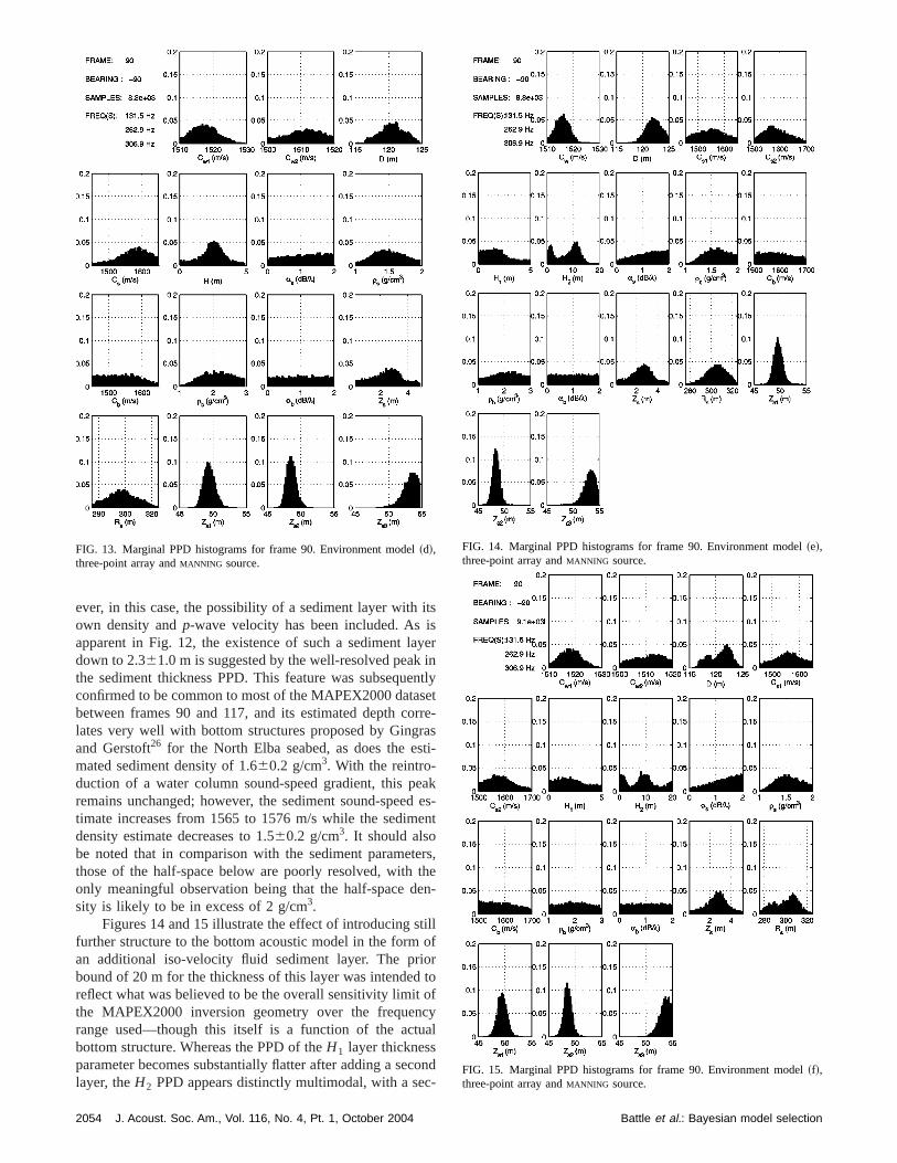
ever, in this case, the possibility of a sediment layer withown density andp-wave velocity has been included. Asapparent in Fig. 12, the existence of such a sediment ladown to 2.361.0 m is suggested by the well-resolved peakthe sediment thickness PPD. This feature was subsequconfirmed to be common to most of the MAPEX2000 databetween frames 90 and 117, and its estimated depth colates very well with bottom structures proposed by Gingand Gerstoft26 for the North Elba seabed, as does the emated sediment density of 1.660.2 g/cm3. With the reintro-duction of a water column sound-speed gradient, this premains unchanged; however, the sediment sound-speetimate increases from 1565 to 1576 m/s while the sedimdensity estimate decreases to 1.560.2 g/cm3. It should alsobe noted that in comparison with the sediment parametthose of the half-space below are poorly resolved, withonly meaningful observation being that the half-space dsity is likely to be in excess of 2 g/cm3.

Figures 14 and 15 illustrate the effect of introducing sfurther structure to the bottom acoustic model in the forman additional iso-velocity fluid sediment layer. The pribound of 20 m for the thickness of this layer was intendedreflect what was believed to be the overall sensitivity limitthe MAPEX2000 inversion geometry over the frequenrange used—though this itself is a function of the actbottom structure. Whereas the PPD of theH1 layer thicknessparameter becomes substantially flatter after adding a selayer, theH2 PPD appears distinctly multimodal, with a se

FIG. 13. Marginal PPD histograms for frame 90. Environment model~d!,three-point array andMANNING source.


s

er

tlyt

re-si-

kes-nt

rs,e-

lf

of

l

nd

FIG. 14. Marginal PPD histograms for frame 90. Environment model~e!,three-point array andMANNING source.

FIG. 15. Marginal PPD histograms for frame 90. Environment model~f!,three-point array andMANNING source.


uibitynais

voraom

dethca

hheethoursim

eub-

entterand

ble

therth-st a

inularpat-

nyperr

sis-set

ly a

onnsis-velin-

PDa

lerg,tion

ign,ta-ved.

.dffe

in

ond peak at approximately 10 m. This is possibly on accoof two actual sediment layers in the bottom, or also possjust a resonant condition for the bottom interface reflectiv

As done in Sec. V B for array model selection, the quatitative results of environment model selection are summrized in Table IV and Fig. 16. Unlike the previous case, itdifficult to rank competing environmental modelsa priori inrelation to their parametric complexity, and hence the edence does not behave monotonically either side of thetimal selection—model~d!. The MAP and mean parameteestimates for this model, along with their associated standdeviations, represent the final output of the two levelsBayesian inference employed in this paper, and are sumrized in Table V.

Also unlike the previous case, the environment mofound to have the highest Bayesian evidence was alsowhich achieved the best overall fit. Given the hierarchirelationship between models~d! and ~f!, it is at first surpris-ing that the latter could not achieve a lower energy, thougis possible that the initial GA search simply failed to find tglobally optimal solution. This is testimony to why it is mordesirable to characterize PPDs in inverse problems rathan just search for the best fit. Further, it can be noted frEq. ~25! that the reverse importance sampling procedused for accurate evidence estimation—unlike the Gausapproximation of Eq.~9!—does not depend on the maximu

TABLE IV. Results for environment model selection. Model~d! is seen togive the highest evidence. Note that the table displays log evidence anprobability of a model is based on just the evidence; thus, the small diences for each model are important.

Model Min E

Log evidence

RIS Gaussian

~a! 19.4 214.2 213.8~b! 19.1 214.1 213.7~c! 19.7 215.2 214.7~d! 14.7 213.6 212.7~e! 15.0 213.9 213.1~f! 14.9 213.7 213.1

FIG. 16. Normalized probabilities for the environment models listedTable IV based on Bayesian evidence.


ntly.--

i-p-

rdfa-

latl

it

ermean

likelihood estimatep(duMk). The evidence values in thsecond column of Table IV, therefore, are unbiased by soptimal ML solutions, unlike those in the third column—although in any case, both methods identified model~d! asthe most probable.

In relation to Fig. 16, there appears to be a consistdemarcation between environments with iso-velocity wacolumns as opposed to sound-speed gradients—the leftright columns of Fig. 5. The latter are always more probathan the former, with the difference between models~c! and~d! being almost anomalous. This suggests that even atshort ranges necessary for self-noise inversion, it is wowhile modeling the water column as possessing at leafirst-order sound-speed gradient.

Finally, on the basis of histogram plots such as thoseFigs. 10 to 15, it is not easy to see the reasons for particmodel preferences, but in numerous reruns, the essentialtern of Fig. 16 was fairly consistently reproduced. In acase, we stated in the Introduction that the focus of this pawas on themethodologyof Bayesian model selection rathethan exhaustive demonstration, which would need contency checks across a more extensive portion of our datathan the single frame analyzed here, and also possibwider range of realistic ocean models.

VI. CONCLUSIONS

A Bayesian approach to solving self-noise inversiproblems has been presented. This approach provides cotent methods for both parameter estimation at the first leof inference, and model selection at the second level ofference.

To implement the calculations necessary—namely Pestimation, marginalization, and integration—we usedMetropolis–Hastings variant of the popular Gibbs sampalgorithm, which, combined with fast acoustic modelinmade the tasks of parameter estimation and model selectractable. Variations on conventional Gibbs sampler dessuch as an initial fast GA optimization, and coordinate rotion according to semianalytic covariance estimates prosuccessful in accelerating overall algorithm performance

TABLE V. Results of final geoacoustic inversion.

Parameter Unit MAP Mean Std. dev

Cw1 m/s 1518 1518 4Cw2 m/s 1512 1511 5D m 121 121 1.8Cs m/s 1598 1577 45H m 2.7 2.5 1as dB/l 2.0 1.1 0.6rs g/cm3 1.5 1.5 0.2Cb m/s 1539 1540 51rb g/cm3 2.5 2.2 0.5ab dB/l 1.4 1.0 0.6Zs m 2.0 2.5 1Rs m 301 300 10za1 m 49.6 49.7 0.9za2 m 48.7 48.8 0.7za3 m 53.8 53.4 1.0

ther-


deesiatdpa

ran

m

ided

as

stist

a

in-

ob

th-tio

aal

ins

anch

lcu

bso

n

alion

s-

ms

tic

ncy.

sticng.

.

sticm.

nst.

e,p://

d-

W.st.

o-eter

llowode

,

mation

inst.

n

an

de

il

The second level of inference is concerned with moselection, i.e., the problem of selecting a model that bexplains a data set at a given signal to noise ratio. Bayemodel selection, as discussed here, is based on calculevidence, which is the integral of the product of likelihooand prior probability over all model parameters. This aproach penalizes models that are more complex than wranted by the data by virtue of the Occam factor.

ACKNOWLEDGMENTS

This work was supported by NAVSEA/ASTO undeContract N00014-01-D-0043-D003 and by ONR under GrN00014-03-1-0393.

1W. A. Kuperman, M. F. Werby, K. E. Gilbert, and G. J. Tango, ‘‘Beaforming on bottom-interacting tow-ship noise,’’ IEEE J. Ocean. Eng.OE-10~3!, 290–298~1985!.

2D. J. Battle, P. Gerstoft, W. A. Kuperman, W. S. Hodgkiss, and M. Serius, ‘‘Geoacoustic inversion of tow-ship noise via near-field-matchfield processing,’’ IEEE J. Ocean. Eng.OE-28~3!, 454–467~2003!.

3S. E. Dosso, ‘‘Quantifying uncertainty in geoacoustic inversion. I. A fGibbs sampler approach,’’ J. Acoust. Soc. Am.111, 129–142~2002!.

4S. E. Dosso and P. L. Nielsen, ‘‘Quantifying uncertainty in geoacouinversion. II. Application to broadband, shallow-water data,’’ J. AcouSoc. Am.111, 143–159~2002!.

5S. E. Dosso, ‘‘Environmental uncertainty in environmental source locization,’’ Inverse Probl.19, 419–431~2003!.

6D. J. C. MacKay, ‘‘Bayesian interpolation,’’ Neural Comput.4, 415–447~1992!.

7A. Malinverno, ‘‘Parsimonious Bayesian Markov chain Monte Carloversion in a nonlinear geophysical problem,’’ Geophys. J. Int.151, 675–688 ~2002!.

8J. J. K. ORuanaidh and W. J. Fitzgerald,Numerical Bayesian MethodsApplied to Signal Processing~Springer, New York, 1996!.

9A. Malinverno, ‘‘A Bayesian criterion for simplicity in inverse problemparametrization,’’ Geophys. J. Int.140, 267–285~2000!.

10H. Jeffreys, Theory of Probability ~Oxford University Press, Oxford,1939!.

11K. Mosegaard and M. Sambridge, ‘‘Monte Carlo analysis of inverse prlems,’’ Inverse Probl.18, 29–54~2002!.

12C. F. Mecklenbraüker, P. Gerstoft, J. F. Bohme, and P. Chung, ‘‘Hypoesis testing for geoacoustic environmental models using likelihood raJ. Acoust. Soc. Am.105, 1738–1748~1999!.

13C. Andrieu and A. Doucet, ‘‘Joint Bayesian model selection and estimtion of noisy sinusoids via reversible jump MCMC,’’ IEEE Trans. SignProcess.47~10!, 2667–2676~1999!.

14W. K. Hastings, ‘‘Monte Carlo sampling methods using Markov chaand their applications,’’ Biometrika87, 97–109~1970!.

15S. Geman and D. Geman, ‘‘Stochastic relaxation, Gibbs distributionsthe Bayesian restoration of images,’’ IEEE Trans. Pattern Anal. MaIntell. 6, 721–741~1984!.

16A. E. Gelfand and A. F. M. Smith, ‘‘Sampling-based approaches to calating marginal densities,’’ J. Am. Stat. Assoc.85, 398–409~1990!.

17A. F. M. Smith and G. O. Roberts, ‘‘Bayesian computation via the gibsampler and related Markov chain Monte Carlo methods,’’ J. R. Stat. SSer. B. Methodol.55, 3–23~1993!.

18M. K. Sen and P. L. Stoffa, ‘‘Bayesian inference, Gibbs sampler auncertainty estimation in geophysical inversion,’’ Geophys. Prospect.44,313–350~1996!.


lstaning

-r-

t

--

t

c.

l-

-

,’’

-

d.

-

c.

d

19W. A. Kuperman, M. D. Colins, J. S. Perkins, and N. R. Davis, ‘‘Optimtime-domain beamforming with simulated annealing including applicatof a priori information,’’ J. Acoust. Soc. Am.88~4!, 1802–1810~1990!.

20M. D. Collins and W. A. Kuperman, ‘‘Focalization: Environmental focuing and source localization,’’ J. Acoust. Soc. Am.90, 1410–1422~1991!.

21P. Gerstoft, ‘‘Inversion of seismoacoustic data using genetic algorithanda posterioriprobability distributions,’’ J. Acoust. Soc. Am.95, 770–782 ~1994!.

22P. Gerstoft, ‘‘ Inversion of acoustic data using a combination of genealgorithms and the Gauss-Newton approach,’’ J. Acoust. Soc. Am.97,2181–2191~1995!.

23P. Gerstoft and D. F. Gingras, ‘‘Parameter estimation using multifrequerange-dependent acoustic data in shallow water,’’ J. Acoust. Soc. Am99,2839–2850~1996!.

24J. Hermand and P. Gerstoft, ‘‘Inversion of broadband multitone acoudata from the Yellow Shark summer experiments,’’ IEEE J. Ocean. EOE-21~4!, 324–346~1996!.

25P. Gerstoft and C. F. Mecklenbraüker, ‘‘Ocean acoustic inversion withestimation ofa posterioriprobability distributions,’’ J. Acoust. Soc. Am104, 808–819~1998!.

26D. F. Gingras and P. Gerstoft, ‘‘Inversion for geometric and geoacouparameters in shallow water: Experimental results,’’ J. Acoust. Soc. A97, 3589–3598~1995!.

27C. F. Mecklenbraüker and P. Gerstoft, ‘‘Objective functions for oceaacoustic inversion derived by likelihood methods,’’ J. Comput. Acou8~2!, 259–270~2000!.

28P. Gerstoft, SAGA Users guide 2.0, an inversion software packagSACLANT Undersea Research Centre, SM-333, 1997. httwww.mpl.ucsd.edu/people/gerstoft/saga

29M. D. Collins and L. Fishman, ‘‘Efficient navigation of parameter lanscapes,’’ J. Acoust. Soc. Am.98, 1637–1644~1995!.

30G. L. D’Spain, J. J. Murray, W. S. Hodgkiss, N. O. Booth, and P.Schey, ‘‘Mirages in shallow water matched field processing,’’ J. AcouSoc. Am.105, 3245–3265~1999!.

31A. B. Baggeroer, W. A. Kuperman, and H. Schmidt, ‘‘Matched field prcessing: Source localization in correlated noise as an optimum paramestimation problem,’’ J. Acoust. Soc. Am.83, 571–587~1988!.

32F. B. Jensen, ‘‘Comparison of transmission loss data for different shawater areas with theoretical results provided by a three-fluid normal-mpropagation model,’’ inSound Propagation in Shallow Water, edited by O.F. Hastrup and O. V. Olesen, CP-14~SACLANT ASW Research CentreLa Spezia Italy, 1974!, pp. 79–92.

33D. D. Ellis and P. Gerstoft, ‘‘Using inversion techniques to extract bottoscattering strengths and sound speeds from shallow-water reverberdata,’’ in Proc. ECUA96, 1996, pp. 557–562.

34C. W. Holland and J. Osler, ‘‘High-resolution geoacoustic inversionshallow water: A joint time- and frequency-domain technique,’’ J. AcouSoc. Am.107, 1263–1279~2000!.

35D. D. Ellis and D. M. F. Chapman, ‘‘A simple shallow water propagatiomodel including shear wave effects,’’ J. Acoust. Soc. Am.78, 2087–2095~1985!.

36Z. Y. Zhang and C. T. Tindle, ‘‘Complex effective depth of the ocewaveguide,’’ J. Acoust. Soc. Am.93, 205–213~1993!.

37F. B. Jensen, W. A. Kuperman, M. B. Porter, and H. Schmidt,Computa-tional Ocean Acoustics~AIP, New York, 1994!.

38E. K. Westwood, C. T. Tindle, and N. R. Chapman, ‘‘A normal momodel for acoustoelastic ocean environments,’’ J. Acoust. Soc. Am.100,3631–3645~1996!.

39C. W. Holland, ‘‘Regional extension of geoacoustic data,’’ in 5thEurop.Conf. Underwater Acoustics, edited by Zakharia, Chevret, and Duba~European Commission, Luxembourg! 2000, pp. 793–796.


Bayesian model selection applied to self-noise geoacoustic inversion

Documents

Transcript of Bayesian model selection applied to self-noise geoacoustic inversion