CRP TIME MIGRATION - Wave Inversion Technology (WIT)

231

CRP TIME MIGRATION

T. A. Coimbra, J. H. Faccipieri, and M. Tygel

email: [email protected], [email protected], [email protected]: Common Reflection Point (CRP), Common Reflection Surface (CRS), time migration

ABSTRACT

Since the early days of seismic processing, time migration has proven to be a valuable tool for a num-ber of imaging purposes. Main motivations for its widespread use include robustness with respect tovelocity errors, as well as fast turnovers and low computation costs. In areas of complex geology, inwhich it has well-known limitations, time migration can still be value by providing first images andalso attributes, which can be of much help in further, comprehensive depth migration. Time migra-tion is a very close process to the zero-offset common-reflection-surface (ZO CRS) stacking method,in fact, Kirchhoff time migration operators can be readily formulated in terms of CRS parameters.In the nineties, several studies have shown appealing advantages in the use of common-reflection-point (CRP) traveltimes to replace conventional common-midpoint (CMP) traveltimes for a numberof stacking and migration purposes. In this paper, we follow that trend and introduce a Kirchhoff-typeprestack time migration algorithm, referred to as CRP time migration. The algorithm is based on aCRP operator together with optimal apertures, both computed with the help of CRS parameters. Fielddata example indicate the good potential of the proposed technique.

INTRODUCTION

Time migration is routinely applied in seismic processing to obtain first, time-domain, images in a fastand inexpensive way. In many situations, typically mild to moderate laterally velocity variations, timemigration can yield satisfactory imaging solutions. Advantages of time migration include robustness (lesssensitivity to velocity errors), fast turnovers and low computational costs. Losses in image accuracy andinterpretation power (mainly associated with geological complexity and strong lateral velocity variations)are well-known limitations of time migration, as compared to comprehensive depth migration (see, e.g.,Hubral and Krey, 1980; Yilmaz, 2001; Robein, 2003). Because of noise reduction, collapse of diffractionsand triplications, time-migrated images can be of help in event picking, seismic tomography (Dell et al.,2014), as well as time-to-depth conversion (Cameron et al., 2007; Iversen and Tygel, 2008).

The good properties of time migration motivates the search of more accurate algorithms to overcomelimitations and enlarge the applicability of time migration. As shown in the literature (Bancroft et al.,1994; Perroud et al., 1999; Spinner and Mann, 2006; Coimbra et al., 2013), it is advantageous to replacethe conventional NMO (for CMP stacking) or diffraction (for time migration) operators by appropriatecommon-reflection-point (CRP) operators, the latter being constructed, typically with common-reflection-surface (CRS) parameters. Moreover, additional accuracy is also obtained by considering minimal, so-called projected Fresnel Zone (PFZ), apertures (Schleicher et al., 1997), such apertures also being estimatedusing CRS parameters.

In this paper, we follow the trend of performing Kirchhoff-type, time migration under the use of aCRP operator and optimal apertures, both computed with the help of CRS parameters. The approach iscalled CRP time migration. Besides describing the proposed technique, we briefly discuss the relatedapproaches, already available in the literature. A field data example confirm the good potential of theproposed technique for accurate time migration.

232 Annual WIT report 2014

FORMULATION

The CRP time migration technique envisaged here is formulated as a Kirchhoff-type algorithm, in whichthe migration operator is a CRP traveltime defined in terms of CRS parameters estimated from the prestackdata. Furthermore, the same CRS parameters also define a minimal aperture in which the Kirchhoff sum-mation is optimally carried out.

The construction of the proposed CRP time migration is based on the relationships between the trav-eltime operators of stacking (here represented by the ZO CRS diffraction traveltime) and time migration(here represented by the double-square root (DSR) traveltime), in which both operators refer to the same(unknown) target reflector. For simplicity, we assume that the acquisition surface is planar horizontal.

Notation: Both operators are defined on a same prestack data volume, with traces specified as (m,h), inwhich m = (m

1

,m2

)T and h = (h1

, h2

)T represent midpoint and half-offset coordinates. As usual prac-tice, we assume that the application of the stacking operator produces a data volume that well approximatesthe one obtained when the subsurface is illuminated by a ZO acquisition. In the same way, the applicationof the time migration operator produces a prestack Kirchhoff time-migrated image of that subsurface.

The central point of the stacking operator (i.e., the point where the stacking output is assigned) isdenoted by (m

0

, t0

), in which m

0

represents trace location and t0

the traveltime in the ZO (stacked)domain. More specifically, t

0

represents the two-way traveltime of the ZO reflection ray (assumed non-converted primary) from the surface point specified by m

0

to the target reflector. That ZO ray is called thecentral normal ray and supposed to be uniquely determined by m

0

. The point where the ZO central rayhits the target reflector is referred to as the normal-incidence point (NIP).

In the same way, the central point of the time migration operator (i.e., the point where the time migrationoutput is assigned) is denoted by (x

0

, ⌧0

), in which x

0

= (x1

, x2

)T represents trace location and ⌧0

is thetwo-way traveltime in the time migrated domain. The point at the surface specified by x

0

is determinedfrom the central image ray, which is the one that starts at NIP on the target reflector and hits the surfacewith slowness vector perpendicular to that surface.

Stacking and time migration operators: With the notations described above, we are ready to write thestacking and time migration operators under consideration. We recall that such operators are linked tothe same (unknown) target reflector. More specifically, the central ZO points (m

0

, t0

) and (x0

, ⌧0

) of thestacked and time migration operators relates to the same NIP at the target reflector by means of the centralZO and image rays, respectively. We have

(a) Stacking operator: That is given by the ZO CRS diffraction moveout, defined in the prestack domainand central point, (m

0

, t0

) at the ZO (stacked) volume.

tDCRS(m,h) =q

[t0

+ a

T (m�m

0

)]2

+ (m�m

0

)TC(m�m

0

) + h

TCh, (1)

(b) Time-migration operator: That is given by the double-square-root (DSR) moveout, defined in theprestack domain and of central point (x

0

, ⌧0

) in the time-migrated domain

tM (m,h) = (1/2)q

⌧20

+ (m� h� x

0

)TS(m� h� x

0

)

+ (1/2)q

⌧20

+ (m+ h� x

0

)TS(m+ h� x

0

) . (2)

In the literature, the time-migration quantity, S, is referred to as the sloth parameter. For later use, it isconvenient to write down the above traveltimes in the ZO configuration, namely tDZO(m) = tDCRS(m,0)and tMZO(m) = tM (m,0). After a little algebra, we find

[tDZO(m)]2 = t20

+ 2t0

a

T (m�m

0

) + (m�m

0

)T (aaT +C)(m�m

0

) , (3)

[tMZO(m)]2 = ⌧20

+ (m� x

0

)TS(m� x

0

) . (4)

Annual WIT report 2014 233

Relationships between coefficients of stacking and time migration operators: We now investigatethe link between the coefficients of the stacking and time migration operators related to the same targetreflector. For that, we consider stacking and time-migration ZO operators of Equations (3) and (4) in themain text.

We suppose that the the central point (m0

, t0

) of the stacking operator is a reflection point in the ZO(stacked) domain and, moreover, that point mapped to (x

0

, ⌧0

) after time migration. Following, e. g., Mannet al. (2000) (in the 2D situation) and Gelius and Tygel (2015) (in 3D case), we recall that the time-migratedpoint, (x

0

, ⌧0

), that corresponds to the ZO point (m0

, t0

), is the minimum (apex) of the stacking operator,tDZO(m). As such, that apex, m = x

0

, is determined by the condition

@[tDZO]2

@m

�

�

�

�

m=x0

= 2tDZO(x0

)@tDZO

@m

�

�

�

�

m=x0

= 2[t0

a+ (aaT +C)(x0

�m

0

)] = 0 . (5)

Solving for m0

and substituting into Equation (3), leads to the expressions

x

0

= m

0

� t0

(aaT +C)�1

a , (6)

⌧0

= tDZO(x0

) = t0

q

1� a

T (aaT +C)�1

a . (7)

Moreover, we also find

tDZO(m)2 = ⌧20

+ (m� x

0

)T�

aa

T +C

�

(m� x

0

) , (8)

so that, comparison with the ZO time-migration operator tMZO(m) of Equation (4) leads to the additionalrelations

S = aa

T +C , (9)

t20

= [tMZO(m0

)]2 = ⌧20

+ (m0

� x

0

)TS(m0

� x

0

) . (10)

We also observe thatC = 4V�2

NMO, and S = 4V�2

M , (11)

where VNMO and VM are the so-called NMO and time migration velocity ellipses, evaluated at (m0

, t0

)and (x

0

, ⌧0

), respectively. We note that, in the 2D situation, VNMO and VM represent the NMO and timemigration velocities, respectively.

CRP curve and CRP surface: In what follows, we assume that the quantities {m0

, t0

,a,C} are given.That differs from the usual practice with the CRS method, in which the central point, (m

0

, t0

) is given andthe CRS parameters a and C are estimated from the data and attached to that central point. Here, we thefour parameters {m

0

, t0

,a,C} are all freely given. At a later stage, these four parameters will be estimatedregarding their relationship to a given central point (x

0

, ⌧0

) in the time-migrated domain.We recall that the CRP gather that pertains to a given central point, (m

0

, t0

), assumed to be a reflectionpoint in the ZO (stacked) volume, consists of the source-receiver pairs, (SCRP (h), GCRP (h)) which, forvarying half offsets, h, share the same reflection point at the target reflector as the one (NIP) determinedby (m

0

, t0

). As shown in Appendix A, the quantities {m0

, t0

,a,C}, determine the source SCRP (h) =mCRP (h)� h and receiver GCRP (h) = mCRP (h) + h, in which the midpoints mCRP (h), is given by

mCRP (h) = m

0

+2(hT

a)h

t0

+p

t20

+ 4(hTa)2

. (12)

In the following, the CRP traveltime curve, tCRP (h) (see Figure 1) that refers to the quantities{m

0

, t0

,a,C} is chosen to be the one that results from the DSR traveltime applied to the CRP gatherthat corresponds to such quantities. In symbols

tCRP (h) = tM (mCRP (h),h) . (13)


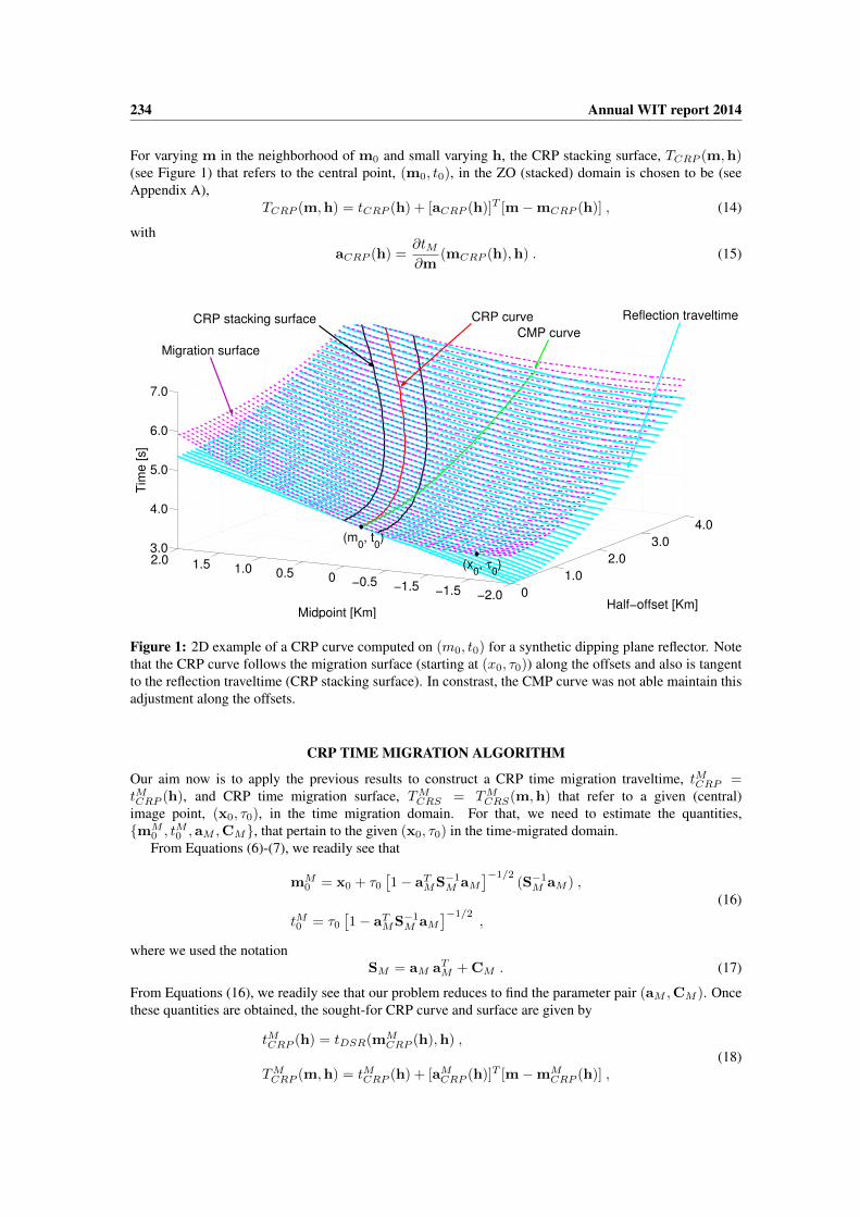
For varying m in the neighborhood of m0

and small varying h, the CRP stacking surface, TCRP (m,h)(see Figure 1) that refers to the central point, (m

0

, t0

), in the ZO (stacked) domain is chosen to be (seeAppendix A),

TCRP (m,h) = tCRP (h) + [aCRP (h)]T [m�mCRP (h)] , (14)

withaCRP (h) =

@tM@m

(mCRP (h),h) . (15)

0

1.0

2.0

3.0

4.0

!2.0!1.5!1.5!0.500.51.01.52.03.0

4.0

5.0

6.0

7.0

Half!offset [Km]Midpoint [Km]

Tim

e [s]

CRP curve Reflection traveltime

CMP curve

(x0, !

0)

(m0, t

0)

Migration surface

CRP stacking surface

Figure 1: 2D example of a CRP curve computed on (m0

, t0

) for a synthetic dipping plane reflector. Notethat the CRP curve follows the migration surface (starting at (x

0

, ⌧0

)) along the offsets and also is tangentto the reflection traveltime (CRP stacking surface). In constrast, the CMP curve was not able maintain thisadjustment along the offsets.

CRP TIME MIGRATION ALGORITHM

Our aim now is to apply the previous results to construct a CRP time migration traveltime, tMCRP =tMCRP (h), and CRP time migration surface, TM

CRS = TMCRS(m,h) that refer to a given (central)

image point, (x0

, ⌧0

), in the time migration domain. For that, we need to estimate the quantities,{mM

0

, tM0

,aM ,CM}, that pertain to the given (x0

, ⌧0

) in the time-migrated domain.From Equations (6)-(7), we readily see that

m

M0

= x

0

+ ⌧0

⇥

1� a

TMS

�1

M aM

⇤�1/2(S�1

M aM ) ,

tM0

= ⌧0

⇥

1� a

TMS

�1

M aM

⇤�1/2,

(16)

where we used the notationSM = aM a

TM +CM . (17)

From Equations (16), we readily see that our problem reduces to find the parameter pair (aM ,CM ). Oncethese quantities are obtained, the sought-for CRP curve and surface are given by

tMCRP (h) = tDSR(mMCRP (h),h) ,

TMCRP (m,h) = tMCRP (h) + [aMCRP (h)]

T [m�m

MCRP (h)] ,

(18)


where m

MCRP and a

MCRP are the same functions as their counterparts mCRP and aCRP , computed, how-

ever, with the quantities {mM0

, tM0

,aM ,CM}.

Time migration parameter estimation: We are now ready to address the problem of estimating theparameters aM and CM , from which the central point, (mM

0

, tM0

), as well as the CRP curve, tMCRP (h),and CRP surface, TM

CRP (m,h), are obtained. That is simply done as follows: For a user-selected ensembleof trial parameters {a,C}, construct for each of them the CRP surface, TCRP (m,h) and compute thestacking energy (semblance) along that surface. The parameter pair for which the maximum energy isattained is the one to be selected.

The estimations indicated above require proper apertures in midpoint and half-offset directions. Theaperture in midpoint direction is attached to the estimation of the midpoint inclination, aMCRP , of the CRPsurface for varying offsets. Since a is the first derivative in midpoint, only a small aperture is needed andexperiments. In our 2D experiments, we found that aperture sizes of five traces for each offset are enough.Based on these results, in the 3D case, we recommend the same aperture size in inline and crosslinedirections (i.e., totaling 25 traces in regular grid for each offset). In offset direction, the aperture should bethe same as in any prestack time migration. Thus, in the 3D case, the number of traces considered on eachestimation of aM and CM is the number of midpoint traces times the number of offsets.

Computation of CRP time migration: As earlier indicated, we propose Kirchhoff-type time migrationsuch that, for each output image point, stacks the prestack data along the CRP surface that corresponds tothat output point. as stacking migration using the CRP surface that refers to the image point. In analogy ofthe well-established Kirchhoff depth migration (see, e.g., Schleicher et al., 1993), the CRP time migrationis computed by an expression that has the form

DMCRP (x0

, ⌧0

) = � 1

2⇡

Z

A

WMCRP [@tD]t=tMCRP

dmdh . (19)

Here, DMCRP (x0

, ⌧0

) is the time migration output at the image point, (x0

, ⌧0

), D = D(m,h, t) is theprestack data. As well known (see, e.g., Schleicher et al., 1993), the partial derivative of the data,@tD(m,h, t) with respect to time is applied to preserve the original time shape of the seismic signal.Moreover, tMCRP = tMCRP (m,h) represents the CRP surface that refers to the (output) image point.

The quantity WMCRP represents the weight function that aims in recovering of the amplitudes. Based

on Zhang et al. (2000), we use the true-amplitude weight for a locally homogeneous medium of matrixmigration velocity determined by the matrix S (see Equation (11)),

WMCRP =

⌧0

pdetS

4(�h)2

✓

1

tS+

1

tG

◆✓

tStG

+tGtS

◆

, (20)

to measure the amplitudes stacked along of the diffraction manifold in Equation (19). The values tS andtG are defined in (A-2) and (A-3), respectively.

The migration aperture, denoted A represents the region over which the migration integral is performed.Based on the concept of Projected Fresnel Zone (PFZ) (Schleicher et al., 1997), the aperture A is proposedto consist of points (m,h) which simultaneously satisfy the conditions

km�mCRP (h)k < �m and khk < �h , (21)

where, �m and �h are midpoint and half-offset aperture bounds. Here, the aperture bound in half-offsetdirection, �h, is taken as the one used in any prestack time migration. Following the same lines as inFaccipieri et al. (2015), the aperture bound in midpoint direction, �m can be given by

�m = ↵

s

wtM0

�C, (22)

where, |�C | = max{|�C1

|, |�C2

|}, in which �C1

and �C2

are the eigenvalues of the 2⇥2 symmetric matrixC, w is the length of the seismic pulse. Moreover, t0M is the ZO traveltime that is given by Equation (16), interms of the CRS parameters, {aM ,CM}, that pertain to the (output) image point (x

0

, ⌧0

). Finally, ↵ > 1is a user-selected adjustment parameter.


2.5D situation: In the case of 2D dataset, the above-described time-migrated algorithm needs to be mod-ified so as to yield 3D meaningful amplitudes after integration on a single seismic line. To overcome thissituation, we adopt the so-called 2.5D assumption, which considers that the geological properties of themedium do not vary in the out-of-plane direction of the seismic line, at the same time maintaining the 3Dcharacter of a point source and point receiver. In this case, the out-of-plane influence to the amplitudes canbe accounted for from in-plane information only. More information on 2.5D media can be found in, e.g.,Bleistein (1986). In 2D seismic data, the parameters a and C become the scalars, having the form

a = a

Tu✓ and C = u

T✓ Cu✓ (23)

withu✓ = (cos ✓, sin ✓)T , (24)

where ✓ is the acquisition azimuth. The midpoint and offsets coordinates also changes with the azimuthand are given by

m = mu✓ and h = hu✓. (25)

In the 2.5D situation, the CRP time migration integral, Equation (19), becomes

DMCRP (x0

, ⌧0

) =1p2⇡

Z

A

WM2.5D

h

@1/2t D

i

t=tMCRP

dmdh (26)

where the operator @1/2t represents the anti-causal half-derivative in time (see. e.g., Bleistein, 1986). For

the weight function, Equation (20), we use the expression derived on Zhang et al. (2000), namely

WM2.5D =

⌧0

2�h

r

1

tS+

1

tG

✓

tStG

+tGtS

◆

. (27)

The aperture bound in midpoint is now given by (compare with Equation (22) for the 3D case)

�2.5Dm = ↵

r

wtM0

C. (28)

The aperture bound in half-offset, �h is, once more, the one used in any time-migration algorithm.

EXAMPLES

The proposed CRP time migration was applied to a 2D real dataset acquired offshore in Brazil at Jequit-inhonha basin. The dataset has 4 ms time sampling, 12.5 m between Common Midpoint (CMP) gathers,25 m between hydrophones with minimum and maximum offsets of 150 m and 3125 m, respectively. Forcomparison purposes, Figure 2 (left) shows a CRS stacked section obtained with global estimation of pa-rameters with the following apertures: (i) Midpoint: 30 m from zero to 1.3 s, increasing linearly until150 m at 3.5 s and constant until the maximum time sample. (ii) Offset: 650 m from 0 to 1.3 s, increasinglinearly until 1050 m at 3.5 s and constant until the final time, 6.0 s. A conventional post-stack Kirchhofftime-migrated section constructed with that dataset is shown at Figure 2 (right). The migration aperturethat has been used was ten times greater than the minimum aperture proposed, ↵ = 10 in Equation (28).We observe that, under that conventional procedure, smaller apertures were not able to image some ofthe dips present in the data. To carry out the CRP time migration, the CRS parameters a and C must beestimated using TM

CRP from Equation (18). In the present example, the estimations were performed us-ing constant midpoint and half-offset apertures of 50 m and 1000 m, respectively. Once these parameterswere estimated, for each (x

0

, ⌧0

), the dataset was migrated, considering the 2.5D case formulation, givenby Equations (26)-(27). The obtained time-migration section is shown in Figure 3 (left). The migrationapertures were calculated using Equation (28) for each (mM

0

, tM0

) with ↵ = 1 and w = 40 ms which leadsto different values of apertures depending of CM and tM

0

. Figure 3 (right) shows the semblance values forthe estimated parameters. It is possible to identify and quantify the regions where the CRP surface adjustedthe events properly. The semblance panel can be seen as valuable tool for the purposes of evaluation andquality control of the CRP time migration.


Midpoint [km]

Tim

e [s]

CRS stacked section

!18 !17 !16 !15 !14

1.8

2

2.2

2.4

2.6

2.8

3

3.2

3.4

3.6

Coordinate [km]

Tim

e [

s]

CRS section migrated (Post!stack)

!18 !17 !16 !15 !14

1.8

2

2.2

2.4

2.6

2.8

3

3.2

3.4

3.6

Figure 2: Stacked section obtained with CRS method (left) and its post-stack Kirchhoff migration withaperture ten times greater (↵ = 10) than the proposed minimum aperture in midpoints (right). Remark:The velocity model used to migrate the dataset was obtained by the CRP time migration.

Coordinate [km]

Tim

e [s]

CRP migrated section

!18 !17 !16 !15 !14

1.8

2

2.2

2.4

2.6

2.8

3

3.2

3.4

3.6

Coordinate [km]

Tim

e [s]

Semblance panel

!18 !17 !16 !15 !14

1.8

2

2.2

2.4

2.6

2.8

3

3.2

3.4

3.6

0.1

0.2

0.3

0.4

0.5

0.6

0.7

Figure 3: Left: Prestack time-migrated section obtained with the proposed CRP algorithm using the mini-mum apertures in midpoint. Right: Semblance obtained on the estimation of parameters for each (x

0

, ⌧0

).

Using the same velocity model estimated before, two conventional prestack Kirchhoff time migrationwere perfomed varying only the migration apertures aiming to examinate their influence on final result.Figure 4 shows theses migrated sections with ↵ = 1 (left) and with ↵ = 10 (right). For the minimummigration aperture, ↵ = 1, some of the dips were not imaged and the reflections appear unfocused. Thisis expected since the conventional time migration is not able to indentify the region where the constructiveinterference occurs. In practice, larger migration apertures are used to avoid this limitation. Figure 4 (right)shows an example where the migration aperture was ten times greater and it is possible to observe that thefeatures present on Figure 3 (left) were imaged. However, the noise levels between these two results areconsiderable which justifies the application of the proposed method.


Coordinate [km]

Tim

e [

s]Conventional migrated section (min aperture)

!18 !17 !16 !15 !14

1.8

2

2.2

2.4

2.6

2.8

3

3.2

3.4

3.6

Coordinate [km]

Tim

e [s]

Conventional migrated section (max aperture)

!18 !17 !16 !15 !14

1.8

2

2.2

2.4

2.6

2.8

3

3.2

3.4

3.6

Figure 4: Left: Prestack migrated section obtained with conventional Kirchhoff time migration using theminimum aperture in midpoints, ↵ = 1. Right: Same procedure using ↵ = 10.

CONCLUSIONS

A Kirchhoff-type, time migration algorithm is proposed that is optimal in two respects. First, the sum-mation is performed along the common-reflection-point (CRP) curve (as opposed to the conventionaldiffraction-time hyperbola). Second, a small aperture, associated to the projected Fresnel zone (PFZ),is employed that is able to restrict the summation to that part of the CRP curve where constructive interfer-ence occurs. A key feature of the algorithm is a transformation function that maps each given image pointinto a corresponding point in the ZO (stacked) volume and also computes the zero-offset (ZO) common-reflection-surface (CRS) parameters there. Such quantities are used to construct the CRP curve and thesummation aperture at each image point. First field-data examples confirm the good potential of the newtechnique for high-quality, time migration results.

ACKNOWLEDGMENTS

We acknowledge support from the National Council for Scientific and Technological Development (CNPq-Brazil), the National Institute of Science and Technology of Petroleum Geophysics (ICTP-GP-Brazil) andthe Center for Computational Engineering and Sciences (Fapesp/Cepid # 2013/08293-7-Brazil). We alsoacknowledge support of the sponsors of the Wave Inversion Technology (WIT) Consortium.

REFERENCES

Bancroft, J. C., Geiger, H. D., Foltinek, D., and Wang, S. (1994). Prestack migration by equivalent offsetsand CSP gathers. In CREWES Research Report, volume 6.

Bleistein, N. (1986). Two-and-one-half dimensinal in-plane wavepropagation. Geophysical Prspecting,34:686–703.

Cameron, M. K., Fomel, S. B., and Sethian, J. A. (2007). Seismic velocity estimation from time migration.Inverse Problems, 23:1329–1369.

Coimbra, T. A., Novais, A., and Schleicher, J. (2013). Theory of offset-continuation trajectory stack. In13th International Congress of the Brazilian Geophysical Society & EXPOGEF, Rio de Janeiro, Brazil,26–29 August 2013. Society of Exploration Geophysicists and Brazilian Geophysical Society.

Dell, S., Gajewski, D., and Tygel, M. (2014). Image ray tomography. Geophysical Prospecting, 62(3):413–426.


Faccipieri, J. H., Coimbra, T. A., Gelius, L.-J., and Tygel, M. (2015). Stacking apertures and estimationstrategies for reflection and diffraction enhancement. Wave Inversion Technology (WIT) Report, 18.

Gelius, L.-J. and Tygel, M. (2015). Migration-velocity building in time and depth from 3D (2D) common-reflection-surface (CRS) stacking - theoretical framework. Studia Geophysica et Geodaetica: Acceptedfor publication.

Hubral, P. and Krey, T. (1980). Interval Velocities from Seismic Reflection Time Measurements. SEG.

Iversen, E. and Tygel, M. (2008). Image-ray tracing for joint 3D seismic velocity estimation and time-to-depth conversion. Geophysics, 73(3):S99–S114.

Mann, J., Hubral, P., Traub, B., Gerst, A., and Meyer, H. (2000). Macro-model independent approximativeprestack time migration. 62nd Mtg. Eur. Assn. Geosci. Eng. EAGE, Expanded Abstracts.

Perroud, M., Hbral, P., and Höcht, G. (1999). Common-reflection-point stacking in laterally inhomoge-neous media. Geophysical Prospecting, 47:1–24.

Robein, E. (2003). Velocities, time-imaging and depth-imaging in reflection seismics: Principles andmethods. EAGE.

Schleicher, J., Hubral, P., Tygel, M., and Jaya, M. S. (1997). Minimum apertures and Fresnel zones inmigration and demigration. Geophysics, 62(1):183–194.

Schleicher, J., Tygel, M., and Hubral, P. (1993). 3-D true-amplitude finite-offset migration. Geophysics,58(8):1112–1126.

Spinner, M. and Mann, J. (2006). True-amplitude based Kirchhoff time migration for AVO/AVA analysis.Geophysics, 15:133–152.

Yilmaz, O. (2001). Seismic Data Analysis: Processing, Inversion and Interpretation of Seismic Data (2ndedition). Society of Exploration Geophysicists (SEG), Oklahoma, Tulsa, USA.

Zhang, Y., Gray, S., and Young, J. (2000). Exact and approximate weights for Kirchhoff migration. In SEGTechnical Program Expanded Abstracts 2000. Society of Exploration Geophysicists.

APPENDIX A

EXPRESSION OF CRP TRAJECTORY

We now focus our attention on the construction of the CRP operator that refers to a given time-migrationsloth parameter, S and time-migration central point, (x

0

, ⌧0

). For that, start with the time migration opera-tor of Equation (2) for a fixed half-offset, which we recast in the more convenient form

tM (m,h;x0

, ⌧0

) = tS(m,h;x0

, ⌧0

) + tG(m,h;x0

, ⌧0

) , (A-1)

with tS = tS(m,h;x0

, ⌧0

) and tG = tG(m,h;x0

, ⌧0

) given by

t2S =⌧20

4+

1

4(m� h� x

0

)TS(m� h� x

0

) , (A-2)

t2G =⌧20

4+

1

4(m+ h� x

0

)TS(m+ h� x

0

) . (A-3)

Note the change in notation in the above expressions, in which the dependence on the time-migrationcentral point, (x

0

, ⌧0

), is made explicitly. Introducing the notation �m = m � m

0

and also usingEquation (10) to replace ⌧2

0

in Equations (A-2) and (A-3), we can recast the time-migration traveltime,tM (m,h;x

0

, ⌧0

), of Equation (A-1) into the modified form, more convenient to our purposes,

t(m0,t0)M (m,h;x

0

) = t(m0,t0)S (m,h;x

0

) + t(m0,t0)G (m,h;x

0

) , (A-4)


where

4[t(m0,t0)S ]2(m,h;x

0

) = t20

+ (�m� h)TS(�m� h) + 2(m0

� x

0

)TS(�m� h) , (A-5)

4[t(m0,t0)G ]2(m,h;x

0

) = t20

+ (�m+ h)TS(�m+ h) + 2(m0

� x

0

)TS(�m+ h) . (A-6)

Geometrical interpretation of t(m0,t0)M (m,h;x

0

): The time-migration traveltime of Equations (A-4)-(A-6) admit the following appealing interpretation: Consider the isochrone in depth domain specified bythe central point (m

0

, t0

). That isochrone is taken only conceptually because we do not have a depth-velocity model. For any point, P , on that isochrone, specified by the lateral coordinate, x

0

, and for everyfixed half-offset, h, Equation (A-4) represents the (DSR) traveltime that refers to the point diffractor the Punder common-offset configuration of half-offset, h.

For varying point diffractors along the isochrone (as specified by correspondingly varying coordinatevectors, x

0

, an ensemble of diffraction surfaces are obtained. Such ensemble has, as an envelope, thereflection response of the isochrone, taken as a reflector, also under the same common-offset configurationspecified by h. In order to determine the envelope of the ensemble of diffraction surfaces parameterized byx

0

, We apply the so-called envelope condition

@tM@x

0

(m,h) = 0 . (A-7)

In view of the expressions

@t2S@x

0

= 2tS@tS@x

0

= �S(�m� h) ,

(A-8)@t2G@x

0

= 2tG@tG@x

0

= �S(�m+ h) .

Using Equation (A-8) in Equation (A-7), leads to

1

tSS(�m� h) +

1

tGS(�m+ h) = 0 , (A-9)

which transforms intotG(�m+ h) = �tS(�m� h) . (A-10)

Squaring both sides of the above equation and after a little algebra, we obtain

x

0

= m

0

+4t2

0

S

�1�m

h

Th��m

T�m

. (A-11)

Substitution of Equation (A-11) into Equations (A-5) and (A-6), we find the expression

[tRISO(m,h;m0

, t0

)]2 = h

TSh+

t20

h

Th

h

Th��m

T�m

. (A-12)

Geometrical interpretation of tRISO(m,h): Consider a fixed half-offset, h. Equation (A-12) representsthe reflection traveltime of the ZO isochrone that refers to the central point, (m

0

, t0

), taken as a depthreflector, under the common-offset configuration of that fixed half-offset. Let us suppose now that the ZOreflection traveltime of the target reflector is given by the expression t

0

= t0

(m0

). For varying points(m

0

, t0

(m0

)) on that reflection curve, the traveltime functions of Equation (A-12) constitute an ensembleof reflection traveltimes of isochrones, parameterized by the midpoints, m

0

. The envelope of that ensembleis obtained by the condition

@tRISO

@m0

(m,h;m0

, t0

) = 0 . (A-13)


Under the consideration that@tRISO

@m0

=1

2tRISO

@[tRISO]2

@m0

, (A-14)

we find2a(hT

h��m

T�m) + t0

�m = 0. (A-15)

The above quadratic equation in �m = �mCRP = mCRP �m

0

, which mCRP is given by Equation (12)in the main text.

CRP TIME MIGRATION - Wave Inversion Technology (WIT)

Documents

Transcript of CRP TIME MIGRATION - Wave Inversion Technology (WIT)