applied sciences

Article

3D Gravity Inversion on Unstructured Grids

Siyuan Sun 1,2, Changchun Yin 2,* and Xiuhe Gao 1,3,*

�����������������

Citation: Sun, S.; Yin, C.; Gao, X. 3D

Gravity Inversion on Unstructured

Grids. Appl. Sci. 2021, 11, 722.

https://doi.org/10.3390/app11020722

Received: 6 December 2020

Accepted: 10 January 2021

Published: 13 January 2021

Publisher’s Note: MDPI stays neu-

tral with regard to jurisdictional clai-

ms in published maps and institutio-

nal affiliations.

Copyright: © 2021 by the authors. Li-

censee MDPI, Basel, Switzerland.

This article is an open access article

distributed under the terms and con-

ditions of the Creative Commons At-

tribution (CC BY) license (https://

creativecommons.org/licenses/by/

4.0/).

1 China Aero Geophysical Survey & Remote Sensing Center for Natural Resources,Comprehensive Department of Aero Geophysical Survey, Beijing 100083, China; sunsyagrs@gmail.com

2 College of Geo-Exploration Sciences and Technology, Jilin University, Changchun 130026, China3 Key Laboratory of Airborne Geophysics and Remote Sensing Geology, Ministry of Nature and Resources,

Beijing 100083, China* Correspondence: yinchangchun@jlu.edu.cn (C.Y.); gaoxhagrs@gmail.com (X.G.);

Tel.: +86-0431-8850-2426 (C.Y.); +86-010-6206-0135 (X.G.)

Abstract: Compared with structured grids, unstructured grids are more flexible to model arbitrarilyshaped structures. However, based on unstructured grids, gravity inversion results would bediscontinuous and hollow because of cell volume and depth variations. To solve this problem,we first analyzed the gradient of objective function in gradient-based inversion methods, and anew gradient scheme of objective function is developed, which is a derivative with respect toweighted model parameters. The new gradient scheme can more effectively solve the problemwith lacking depth resolution than the traditional inversions, and the improvement is not affectedby the regularization parameters. Besides, an improved fuzzy c-means clustering combined withspatial constraints is developed to measure property distribution of inverted models in both spatialdomain and parameter domain simultaneously. The new inversion method can yield a more internalcontinuous model, as it encourages cells and their adjacent cells to tend to the same property value.At last, the smooth constraint inversion, the focusing inversion, and the improved fuzzy c-meansclustering inversion on unstructured grids are tested on synthetic and measured gravity data tocompare and demonstrate the algorithms proposed in this paper.

Keywords: gravity; unstructured grids; depth resolution; inversion

1. Introduction

Conventionally, gravity forward modeling is implemented by dividing the subsurfaceinto a large number of rectangular prisms, and the gravity anomaly is calculated byintegrating the gravitational effect due to each prism. However, structured grids havelimited capability when modeling structures with complex shapes (such as topographicsurfaces), and a staircased configuration from structured grids results in a loss of accuracy.In comparison, unstructured grids can easily be designed to conform to arbitrary straight-edged boundaries, topography, and subsurfaces. On the other hand, the local refinementor coarsening of the mesh, in regions where higher accuracy is required or lower accuracyis acceptable, can be performed without affecting the grids outside these regions. Theseproperties can ultimately result in higher accuracy and lower computational cost.

For gravity forward modeling with unstructured grids, several methods have beendeveloped. Talwani and Ewing [1], and Talwani [2] used numerical integration techniquesby dividing models of arbitrary shape into polygonal prisms or laminas. Barnett [3] andOkabe [4] developed techniques for gravity and magnetic modeling due to homogeneouspolyhedral bodies. Zhang et al. [5] and Cai and Wang [6] used the finite-element methodto calculate the gravitational response of 3D rectangular grids, while May and Knepley [7]used the fast multipole method to tackle the same problem. Jahandari and Farquharson [8]used finite-volume and finite-element methods to gravity forward modeling and theirresults showed that the quadratic finite-element scheme is more accurate but also morecomputationally demanding scheme. The flexibility of unstructured tetrahedral meshes

Appl. Sci. 2021, 11, 722. https://doi.org/10.3390/app11020722 https://www.mdpi.com/journal/applsci

Appl. Sci. 2021, 11, 722 2 of 15

has been proved to be advantageous when complex model geometries have to be modeled.However, the numerical schemes (such as finite-volume and finite-element methods)handling such tetrahedral meshes can lead to less-accurate results in comparison with thestructured, regular grids.

Three-dimensional (3D) regularized inversion has been a popular approach in rightrectangular prisms [9–12]. In regularization inversion, a regularization term enables usto incorporate more information so that a smooth or sharp model can be yielded [13].Li and Oldenburg [9,14] used an objective function that penalize both the deviation of therecovered model from a reference model and the structural complexity in three spatialdirections. A focusing method is developed to reconstruct a compact and sharper image ofthe subsurface [11,15,16]. A fuzzy c-means clustering algorithm [17–20] is applied to inducethe recovered physical properties to gather around clusters determined by some prioriinformation. In addition, a depth weighting function is vital to recovering the model at aproper depth on structured grids. Li and Oldenburg [9] firstly introduce a depth weightingfunction in the Tikhonov formulation. Portniaguine and Zhdanov [16] have introduceda nonlinear depth weighting that equalizes the sensitivity of the observed data to cellslocated at different depths and horizontal positions. In a mathematically less rigorous way,Commer [21] directly applied a weighting function to the gradient of data misfit functionaland the results revealed a great improvement in depth resolution. However, when thesemethods are directly used to gravity inversion on unstructured grids, a discontinuousand hollow model is more likely to be yielded. This arises because volume distinctionof unstructured grids also has a considerable effect on model distribution besides depthvariation of grids. This is more pronounced when the local refinement or coarsening of theunstructured mesh is used.

In this paper, by analyzing the gradient of objective functional, we find that thedistribution of density is related to the conventional gradient formulation of objectivefunctional. Subsequently, two mechanisms of depth weighting are compared and analyzedin detail: (1) a regularization-based strategy: applying a depth weighting to the regular-ization term [9,11,14,16]; and (2) gradient-based strategy: applying a depth weighting tothe gradient of data misfit [21,22]. The comparative analysis indicates that the secondmethod would improve gravity depth resolution more directly and effectively, and thisimprovement is less influenced by regularization parameters. Moreover, the regularizationterms will have a restraining effect at all depths. Besides, we develop an improved fuzzyc-means clustering method combined with spatial constraints. Compared with previousworks [17–20], it measures property distribution of inverted models in both the spatialdomain and parameter domain, and it can provide a more continuous distribution ofproperties on unstructured grids.

To demonstrate the effectiveness of our algorithm, we tested both on a synthetic anda field dataset from the Vinton salt dome by Bell Geospace. The forward modeling isaccomplished with the algorithm of Okabe [4] based on unstructured grids, which hasbeen used in gravity researches [17,23,24]. We use TetGen [25] to generate tetrahedral grids.TetGen is an open-source software that generates the tetrahedral and Voronoï grids asrequired. The algorithms of TetGen are Delaunay-based, which ensures high quality for thewhole grids by maximizing the minimum dihedral angle in the grids. The results show thatthe problem in gravity inversion with the anomaly concentration to the surface is largelysolved. The inverted models show sharp boundaries and true positions.

2. Methods

The technical methods of this paper mainly include three issues: forward modelingalgorithm on tetrahedral grids, Fuzzy c-means clustering constraints, and depth weighting.In this chapter, we will introduce a forward modeling algorithm on tetrahedral grids andFuzzy c-means clustering constraints only, and the depth weighting will be described andanalyzed in Section 3.

Appl. Sci. 2021, 11, 722 3 of 15

2.1. Gravity Forward Modeling Based on Tetrahedral Grids

In the right-handed Cartesian coordinate system, as shown in Figure 1, based onBarnett [3] and Okabe [4], by successively imposing thrice coordinate rotations on everyedge of the polyhedral body, the gravity anomalies g of a homogeneous polyhedral bodycan be converted to the sum of the contributions from all edges, which can be expressed as

g = Gρn

∑i

[cos ψi

m

∑j

Jj(i)

](1)

Appl. Sci. 2021, 11, x FOR PEER REVIEW 3 of 17

2.1. Gravity Forward Modeling Based on Tetrahedral Grids In the right-handed Cartesian coordinate system, as shown in Figure 1, based on Bar-

nett [3] and Okabe [4], by successively imposing thrice coordinate rotations on every edge of the polyhedral body, the gravity anomalies g of a homogeneous polyhedral body can be converted to the sum of the contributions from all edges, which can be expressed as

=

n

i

m

jji iJψρGg )(cos (1)

Figure 1. A tetrahedral cell in coordinate system.

In Equation (1), G is Newton’s gravitational constant, and ρ is the density of the cell. n is the facet number of the polyhedral body. m is the edge number of the ith facet. For tetrahedral grids, n = 4 and m = 3. ψi is a rotation angle of the ith facet, while Jj(i) is the contribution of jth edge in the ith facet, which is expressed as

( ) ( )),(

),(

111

coscos))(sin1(

tan2sincoslncossin)(++

+++−++−= −

jj

jj

YX

YXj

jjjjjjj θZ

θXRYθZRθYθXθYθXiJ (2)

where

−′−′−′

•

−•

−=

obs

obs

obs

1000cossin0sincos

cos0sin010sin0cos

zzyyxx

φφφφ

ψψ

ψψ

ZYX

(3)

2/1222 )( ZYXR ++= (4)

In the above equations, φ, ψ, and θ are respectively three rotation angles for the jth edge, and can be calculated as follows [4],

( ) 2/122cos

zxyz

yz

SS

Sφ

+−= (5)

( ) 2/122sin

zxyz

zx

SS

Sφ+

−= (6)

( ) 2/1222cos

xyzxyz

xy

SSS

Sψ

++−= (7)

Figure 1. A tetrahedral cell in coordinate system.

In Equation (1), G is Newton’s gravitational constant, and ρ is the density of the cell.n is the facet number of the polyhedral body. m is the edge number of the ith facet. Fortetrahedral grids, n = 4 and m = 3. ψi is a rotation angle of the ith facet, while Jj(i) is thecontribution of jth edge in the ith facet, which is expressed as

Jj(i) =

[(X sin θj −Y cos θj

)ln(X cos θj + Y sin θj + R

)− 2Z tan−1 (1 + sin θj)(Y + R) + X cos θj

Z cos θj

](Xj+1,Yj+1)

(Xj ,Yj)

(2)

where XYZ

=

cos ψ 0 − sin ψ0 1 0

sin ψ 0 cos ψ

• cos ϕ sin ϕ 0− sin ϕ cos ϕ 0

0 0 1

• x′ − xobs

y′ − yobsz′ − zobs

(3)

R = (X2 + Y2 + Z2)1/2

(4)

In the above equations, ϕ, ψ, and θ are respectively three rotation angles for the jthedge, and can be calculated as follows [4],

cos ϕ = −Syz(

S2yz + S2

zx

)1/2 (5)

sinϕ = − Szx(S2

yz + S2zx

)1/2 (6)

cosψ = −Sxy(

S2yz + S2

zx + S2xy

)1/2 (7)

Appl. Sci. 2021, 11, 722 4 of 15

sin ψ =S2

yz + S2zx(

S2yz + S2

zx + S2xy

)1/2 (8)

cos θ =Xj+1 − Xj[

(Xj+1 − Xj)2 + (Yj+1 −Yj)

2]1/2 (9)

sin θ =Yj+1 −Yj[

(Xj+1 − Xj)2 + (Yj+1 −Yj)

2]1/2 (10)

In the above Equations (5)–(8), Syz, Sxz, and Sxy are the projected areas of the ith facetrespectively onto the y-z-, z-x-, and x-y- planes. It should be pointed out that the verticesof the facet must be arranged clockwise in the X-Y-plane before Equation (3) is calculated.However, the generation of tetrahedral meshes is automatic and vertices are arranged andstored randomly. Therefore, we introduce a judgment and rearrangement of vertices beforethe gravity contribution of each facet is calculated. For more details about the rotationsand judgment, please see Appendix A.

2.2. Fuzzy C-Means Clustering Inversion with Spatial Constraints

The inverse problem is solved by minimizing the Tikhonov parametric functional [13].Fuzzy c-means clustering method (FCM) is used as the regularization term [18,19]. Theobjective function of gravity inversion is formulated as follows:

Φ = Φd + λΦm = ‖Fm− dobs‖2 + λp

∑k‖W f /2

Ck(m− Ck)‖

2(11)

where F is a forward modeling operator. m are density parameters of all cells. dobs areobserved data. Φd is a data misfitting term, and Φm is a regularization term to constrain

model structure. λ is a trade-off parameter. Φm =p∑k‖W f /2

Ck(m− Ck)‖

2is the clustering

term to classify the physical property values into distinct clusters C = {Ck|k = 1, 2, · · · , p}.In this paper, we assume that p and C are determined from a priori information. Theparameter f, known as fuzzification parameter, is generally set to 2.0 [26]. Here, WCk is adiagonal matrix that measures the degree of the physical property values belonging to thekth cluster,

WCk = diag

(m− Ck)− 2/( f − 1)

p∑k(m− Ck)

− 2/( f − 1)

(12)

Φm can effectively classify the physical property values into distinct clusters in theparameter domain, however, it has no effect on the spatial distribution of density. Asa result, the property spatial distributions may be discontinuous and discrete. So, onstructured grids, Sun and Li [18,19] added the smoothness regularization term to promotecontinuous in the spatial domain. However, it is difficult to balance the smoothness andclustering term and reconstruct a continuous model on unstructured grids.

Thus, we combine spatial constraints into the FCM term to help recover spatialcontinuity of physical property. We reset component wise of m as follows:

m′ j =

(mj +

qj

∑l

ml

)/(qj + 1

)(13)

where qj is set to be the adjacent cells number of jth cell, and it is usually equal to 4 exceptfor the cells at boundaries. m′ j denotes the average of properties in the jth cell and itsadjacent cells. The new Φm can measure the inverted model in both spatial domain and

Appl. Sci. 2021, 11, 722 5 of 15

parameter domain. When the new Φm is minimized, it induces the properties of the jth celland its adjacent cells to gather a certain cluster Ck. So, a continuous property distribution inspatial domain and a focused property distribution in parameter domain can be obtained.

In Equation (11), depth weighting function is not involved as it does in gravityinversion based on structured grids. Compared with structured grids, cell volumes areno longer the same as a constant. The dual effects of volume and depth difference ofgrids would result in a discontinuous and hollow model. While, the local refinementor coarsening of the mesh is an important advantage of unstructured grids, which willinevitably lead to different mesh volumes. So, it’s crucial to solve this problem beforegravity inversion based on unstructured grids used widely in field data. We will discussthe depth weighting in the next section.

3. Analysis of Depth Weighting on Unstructured Grids

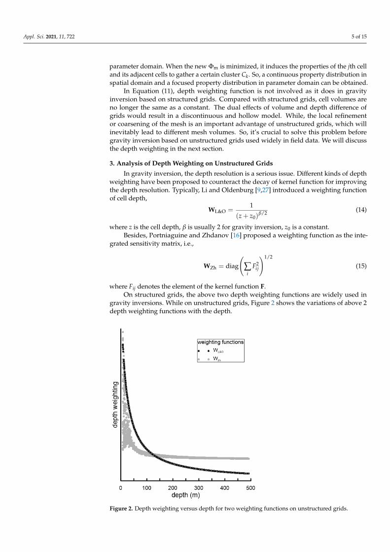
In gravity inversion, the depth resolution is a serious issue. Different kinds of depthweighting have been proposed to counteract the decay of kernel function for improvingthe depth resolution. Typically, Li and Oldenburg [9,27] introduced a weighting functionof cell depth,

WL&O =1

(z + z0)β/2 (14)

where z is the cell depth, β is usually 2 for gravity inversion, z0 is a constant.Besides, Portniaguine and Zhdanov [16] proposed a weighting function as the inte-

grated sensitivity matrix, i.e.,

WZh = diag

(∑

iF2

ij

)1/2

(15)

where Fij denotes the element of the kernel function F.On structured grids, the above two depth weighting functions are widely used in

gravity inversions. While on unstructured grids, Figure 2 shows the variations of above 2depth weighting functions with the depth.

Appl. Sci. 2021, 11, x FOR PEER REVIEW 6 of 17

Figure 2. Depth weighting versus depth for two weighting functions on unstructured grids.

Results in Figure 2 are calculated over an area of 500 m × 500 m × 500 m composed of tetrahedral grids. z0 is chosen to be 20 in Equation (14). As volume of grids are different for tetrahedral meshes, the depth weighting ZhW is normalized by cell volumes. In Figure 2, similar tendencies can be seen from two weightings. L&OW is only related to depth, and all cells at the same depth have the same weightings. However, ZhW are different for cells at the same depth, especially near the surface, which is caused by difference of cell volume. On unstructured grids, if cells at the same depth have the same weightings, it will result in that the cells with larger volumes have the priority to change their densities first to fit the observed data. So based on unstructured grids, ZhW is better than L&OW to improve resolution of gravity inversion.

Stabilized gradient-based inversion methods prove to be efficient for 3D imaging problems with highly parameterized models. Based on the principle of gradient-based inversion methods, setting the gradient to near zero can minimize the objective function efficiently [21]. The gradient of Equation (11) can be expressed as

Td m obs( ) ( )

pf

z Ci ii

Cλ λ∇Φ = ∇Φ + ∇Φ = − + −F Fm d W W m (16)

Firstly, let’s focus on the gradient of data misfit

)(Φ obsT

d dFmF −=∇ (17)

It is well known that the gravity forward modeling operator F decays quickly as depth increases [9,28]. Therefore, when multiplying FT with the data misfit Fm–dobs, dΦ∇ will be less sensitive to depth, so densities of shallow cells will first change to fit dobs. As a result, the inverse model will more easily concentrate to the surface in the traditional gra-dient-based inversions. So, from this perspective, the key to improve the depth resolution is how to counteract the decay of FT in dΦ∇ .

In a conventional way, imposing depth weighting into Φm can improve depth reso-lution [9,14,16]. Then the gradient of the objective function can be expressed as

Figure 2. Depth weighting versus depth for two weighting functions on unstructured grids.

Appl. Sci. 2021, 11, 722 6 of 15

Results in Figure 2 are calculated over an area of 500 m × 500 m × 500 m composed oftetrahedral grids. z0 is chosen to be 20 in Equation (14). As volume of grids are different fortetrahedral meshes, the depth weighting WZh is normalized by cell volumes. In Figure 2,similar tendencies can be seen from two weightings. WL&O is only related to depth, and allcells at the same depth have the same weightings. However, WZh are different for cells atthe same depth, especially near the surface, which is caused by difference of cell volume.On unstructured grids, if cells at the same depth have the same weightings, it will resultin that the cells with larger volumes have the priority to change their densities first to fitthe observed data. So based on unstructured grids, WZh is better than WL&O to improveresolution of gravity inversion.

Stabilized gradient-based inversion methods prove to be efficient for 3D imagingproblems with highly parameterized models. Based on the principle of gradient-basedinversion methods, setting the gradient to near zero can minimize the objective functionefficiently [21]. The gradient of Equation (11) can be expressed as

∇Φ = ∇Φd + λ∇Φm = FT(Fm− dobs) + λp

∑i

WzW fCi(m− Ci) (16)

Firstly, let’s focus on the gradient of data misfit

∇Φd = FT(Fm− dobs) (17)

It is well known that the gravity forward modeling operator F decays quickly as depthincreases [9,28]. Therefore, when multiplying FT with the data misfit Fm–dobs,∇Φd will beless sensitive to depth, so densities of shallow cells will first change to fit dobs. As a result,the inverse model will more easily concentrate to the surface in the traditional gradient-based inversions. So, from this perspective, the key to improve the depth resolution is howto counteract the decay of FT in ∇Φd.

In a conventional way, imposing depth weighting into Φm can improve depth resolu-tion [9,14,16]. Then the gradient of the objective function can be expressed as

∇Φ = ∇Φd + λ∇Φ′m (18)

where Φ′m denotes the regularization term after depth weighting imposed.Then the weighted ∇Φ′m decays quickly and becomes less sensitive to depth as

∇Φd does. It encourages that properties of shallow cells will first satisfy the constraintof Φ′m, such that the property differences of shallow cells in smooth inversion or therelative properties of shallow cells in focus inversion tends to zero. As a result, thisfeature encourages the properties of shallow cells to remain unchanged and counteracts theinfluence of FT on shallow cells. So the depth resolution can be improved to some extent,but the improvement is affected by the balance of∇Φd and∇Φ′m, i.e., trade-off parameterλ. With a small λ, ∇Φ′m is not powerful enough to offset the decay of FT in ∇Φd, sothe recovered model may be shallower than the true model. While with an overlarge λ,the recovered model may be deeper than the true model. What’s worse, as ∇Φ′m decaysquickly with increasing depth, its effect on deep cells is weakened.

Another solving method is to directly apply a depth weighting function to ∇Φdinstead of Φm in a mathematically less rigorous way [21]. In this way, the gradient ofobjective function can be expressed as

∇Φ = ∇Φ′d + λ∇Φm = WzFT(Fm− dobs) + λ∇Φm (19)

where Wz is a depth weighting function that increases quickly as depth increases, which isjust adverse to the decay of FT in ∇Φd. Compared with Equation (18), ∇Φd is multipliedby Wz in Equation (19) instead of a depth weighted Φ′m. Therefore, Wz can counteractthe effect of FT in ∇Φd directly and effectively. Besides, different with ∇Φ′m, ∇Φm is not

Appl. Sci. 2021, 11, 722 7 of 15

related to depth, which means that λ would have less effect on the improvement of depthresolution as it does in Equation (18).

From the perspective of objective function gradient, above analyses indicate that thegradient-based strategy in Equation (19) is more effective to improve depth resolution thanthe method shown in Equation (18).

4. Results

To demonstrate the effectiveness of our algorithm, we tested both on a synthetic and afield dataset from the Vinton salt dome by Bell Geospace [29] and compared the improvedFCM clustering inversion with focusing inversion and conventional FCM clustering inver-sion in the examples. In the following examples, the open-source software TetGen [25] isused to generate tetrahedral grids. The conjugate gradient method is implemented to solvethe gravity inverse problems.

4.1. Inversions of Simulation Data

The synthetic gravity data were generated for a 3D homogeneous structure with arelative density of 1 g/cm3, as shown in Figure 3. The top bury depth is 100 m. The gravitydata were calculated at the Earth’s surface on a grid with 50 m spacing and a total of 320locations. We discretized the survey area (1000 m× 800 m× 600 m) into 237,298 tetrahedralgrids with maximum cell volume of 5000 m3 when using the program TetGen [25]. Twodepth weighting strategies with different inversion methods were respectively applied torecover the synclinal structure. A uniform relative density model of 0 g/cm3 was used asthe initial model. A constraint on the upper-lower limit of density [0 g/cm3, 1.0 g/cm3]was used in these experiments. We carried out the FCM clustering gravity inversion withC = {0 g/cm3, 1 g/cm3} and p = 2. The inversion was taken as converged when the datamisfit or relative model norm update was below their respective predetermined thresholds.

Appl. Sci. 2021, 11, x FOR PEER REVIEW 8 of 17

Figure 3. A V-shaped structure with a relative density of 1 g/cm3 on unstructured grids.

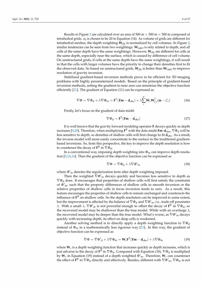
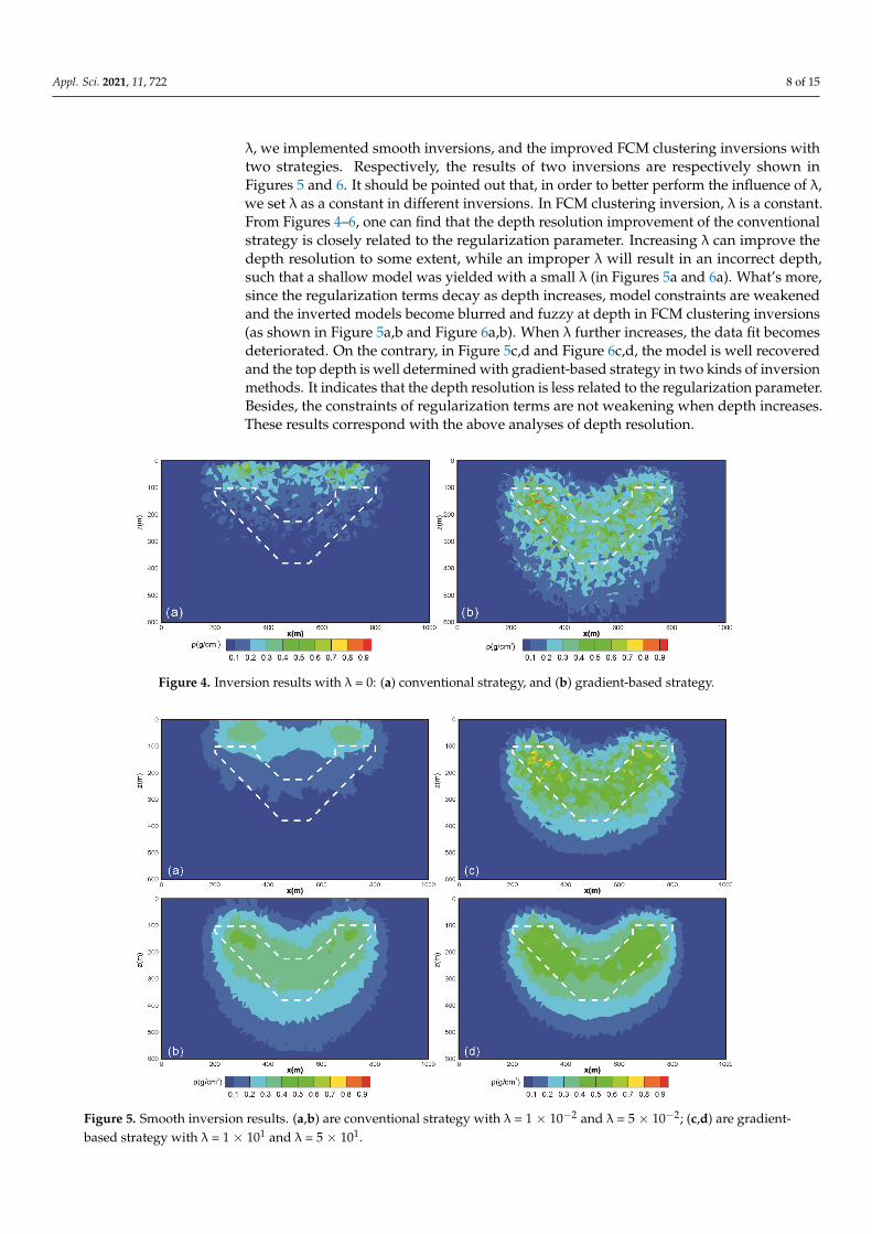
The inversion results of two weighting strategies without regularization terms (λ = 0) are shown in Figure 4, where the section passing the center in y-direction is shown only. The dashed boxes in the figure outline the true boundaries of the anomalous body. With no model structure constraints, the result with a conventional strategy in Equation (16) (as shown in Figure 4a) demonstrates a concentration near the surface, while it is im-proved by using gradient-based strategy in Equation (17) (as shown in Figure 4b). Then using different λ, we implemented smooth inversions, and the improved FCM clustering inversions with two strategies. Respectively, the results of two inversions are respectively shown in Figures 5 and 6. It should be pointed out that, in order to better perform the influence of λ, we set λ as a constant in different inversions. In FCM clustering inversion, λ is a constant. From Figures 4–6, one can find that the depth resolution improvement of the conventional strategy is closely related to the regularization parameter. Increasing λ can improve the depth resolution to some extent, while an improper λ will result in an in-correct depth, such that a shallow model was yielded with a small λ (in Figures 5a and 6a). What’s more, since the regularization terms decay as depth increases, model constraints are weakened and the inverted models become blurred and fuzzy at depth in FCM clus-tering inversions (as shown in Figures 5a,b and 6a,b). When λ further increases, the data fit becomes deteriorated. On the contrary, in Figures 5c,d and 6c,d, the model is well re-covered and the top depth is well determined with gradient-based strategy in two kinds of inversion methods. It indicates that the depth resolution is less related to the regulari-zation parameter. Besides, the constraints of regularization terms are not weakening when depth increases. These results correspond with the above analyses of depth resolution.

In Figure 7, focusing inversion and conventional FCM clustering inversion are im-plemented with gradient-based strategy to compare with the improved FCM clustering inversion. We set a large initial λ, and then used the c to gradually reduce it. One can find that all these three methods can reconstruct a compact model. However, from Figure 7a,b, it is shown that focusing inversion and conventional FCM clustering inversion yield the inverted models into segments or with holes on unstructured grids. Focusing inversion is to reconstruct the model with minimum volume, and it has no constraint in spatial do-main. In conventional FCM clustering inversion, one may increase smooth constraint to yield a continuous model, while the constraint of FCM clustering is weakened and the

Figure 3. A V-shaped structure with a relative density of 1 g/cm3 on unstructured grids.

The inversion results of two weighting strategies without regularization terms (λ = 0)are shown in Figure 4, where the section passing the center in y-direction is shown only.The dashed boxes in the figure outline the true boundaries of the anomalous body. With nomodel structure constraints, the result with a conventional strategy in Equation (16) (asshown in Figure 4a) demonstrates a concentration near the surface, while it is improved byusing gradient-based strategy in Equation (17) (as shown in Figure 4b). Then using different

Appl. Sci. 2021, 11, 722 8 of 15

λ, we implemented smooth inversions, and the improved FCM clustering inversions withtwo strategies. Respectively, the results of two inversions are respectively shown inFigures 5 and 6. It should be pointed out that, in order to better perform the influence of λ,we set λ as a constant in different inversions. In FCM clustering inversion, λ is a constant.From Figures 4–6, one can find that the depth resolution improvement of the conventionalstrategy is closely related to the regularization parameter. Increasing λ can improve thedepth resolution to some extent, while an improper λ will result in an incorrect depth,such that a shallow model was yielded with a small λ (in Figures 5a and 6a). What’s more,since the regularization terms decay as depth increases, model constraints are weakenedand the inverted models become blurred and fuzzy at depth in FCM clustering inversions(as shown in Figure 5a,b and Figure 6a,b). When λ further increases, the data fit becomesdeteriorated. On the contrary, in Figure 5c,d and Figure 6c,d, the model is well recoveredand the top depth is well determined with gradient-based strategy in two kinds of inversionmethods. It indicates that the depth resolution is less related to the regularization parameter.Besides, the constraints of regularization terms are not weakening when depth increases.These results correspond with the above analyses of depth resolution.

Appl. Sci. 2021, 11, x FOR PEER REVIEW 9 of 17

inverted model will not be focusing and compact. But in Figure 6, the models are more compact and no holes inside with the improved FCM clustering method. That is because the new method induces cells and their adjacent cells to tend to the same value except for the constraint of smooth regularization term.

Table 1 shows a clear perspective of inversion results with different methods, strate-gies, and trade-off parameters. The comparative analysis indicates that the second method would improve gravity depth resolution more directly and effectively, and this improve-ment is less influenced by regularization parameters. Moreover, the regularization terms will have a restraining effect at all depths.

Table 1. Inversion result list with different methods, strategies, and parameters.

Result Inversion Method Strategy Trade-Off Parameter Figure 4a NaN Conventional strategy 0

Figure 4b NaN Gradient-based strat-egy 0

Figure 5a Smooth inversion Conventional strategy 1 × 10−2 Figure 5b Smooth inversion Conventional strategy 5 × 10−2

Figure 5c Smooth inversion Gradient-based strat-egy

1 × 101

Figure 5d Smooth inversion Gradient-based strat-egy 5 × 101

Figure 6a New FCM inversion Conventional strategy 1 × 10−3 Figure 6b New FCM inversion Conventional strategy 3 × 10−3

Figure 6c New FCM inversion Gradient-based strat-egy

3 × 100

Figure 6d New FCM inversion Gradient-based strat-egy

5 × 100

Figure 7a Focusing inversion Gradient-based strat-

egy method of Lelièvre et

al. [17]

Figure 7b Conventional FCM

inversion Gradient-based strat-

egy method of Lelièvre et

al. [17]

Figure 4. Inversion results with λ = 0: (a) conventional strategy, and (b) gradient-based strategy. Figure 4. Inversion results with λ = 0: (a) conventional strategy, and (b) gradient-based strategy.

Appl. Sci. 2021, 11, x FOR PEER REVIEW 10 of 17

Figure 5. Smooth inversion results. (a,b) are conventional strategy with λ = 1 × 10−2 and λ = 5 × 10−2; (c,d) are gradient-based strategy with λ = 1 × 101 and λ = 5 × 101.

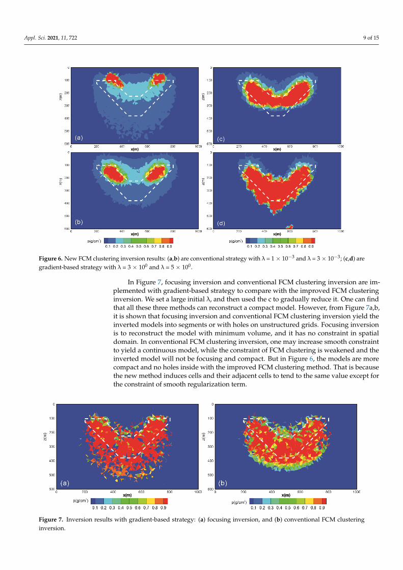
Figure 6. New FCM clustering inversion results: (a,b) are conventional strategy with λ = 1 × 10−3 and λ = 3 × 10−3; (c,d) are gradient-based strategy with λ = 3 × 100 and λ = 5 × 100.

Figure 5. Smooth inversion results. (a,b) are conventional strategy with λ = 1 × 10−2 and λ = 5 × 10−2; (c,d) are gradient-based strategy with λ = 1 × 101 and λ = 5 × 101.

Appl. Sci. 2021, 11, 722 9 of 15

Appl. Sci. 2021, 11, x FOR PEER REVIEW 10 of 17

Figure 5. Smooth inversion results. (a,b) are conventional strategy with λ = 1 × 10−2 and λ = 5 × 10−2; (c,d) are gradient-based strategy with λ = 1 × 101 and λ = 5 × 101.

Figure 6. New FCM clustering inversion results: (a,b) are conventional strategy with λ = 1 × 10−3 and λ = 3 × 10−3; (c,d) are gradient-based strategy with λ = 3 × 100 and λ = 5 × 100. Figure 6. New FCM clustering inversion results: (a,b) are conventional strategy with λ = 1× 10−3 and λ = 3× 10−3; (c,d) are

gradient-based strategy with λ = 3 × 100 and λ = 5 × 100.

In Figure 7, focusing inversion and conventional FCM clustering inversion are im-plemented with gradient-based strategy to compare with the improved FCM clusteringinversion. We set a large initial λ, and then used the c to gradually reduce it. One can findthat all these three methods can reconstruct a compact model. However, from Figure 7a,b,it is shown that focusing inversion and conventional FCM clustering inversion yield theinverted models into segments or with holes on unstructured grids. Focusing inversionis to reconstruct the model with minimum volume, and it has no constraint in spatialdomain. In conventional FCM clustering inversion, one may increase smooth constraintto yield a continuous model, while the constraint of FCM clustering is weakened and theinverted model will not be focusing and compact. But in Figure 6, the models are morecompact and no holes inside with the improved FCM clustering method. That is becausethe new method induces cells and their adjacent cells to tend to the same value except forthe constraint of smooth regularization term.

Appl. Sci. 2021, 11, x FOR PEER REVIEW 11 of 17

Figure 7. Inversion results with gradient-based strategy: (a) focusing inversion, and (b) conventional FCM clustering in-version.

4.2. Field Data Inversion The survey area Vinton Dome is located in southwestern Louisiana, USA. We used a

subset of the survey area for this study that covers approximately 16 km2 in the middle of the survey area, which was acquired and processed by Bell Geospace in 2008 [29]. Before we inverted the data, a second-order trend surface was removed to get rid of background, and an upward continuation of 100 m was done to eliminate the shallow local anomalies. The processed gravity data is displayed in Figure 8.

Figure 8. Field data subset from Vinton Dome area after trend surface removing and upward con-tinuation (data courtesy of Scott Hammond from Bell Geospace).

Inversion area is 4 km × 4 km × 1 km with 169,949 cells and 1681 survey stations. The station interval was 100 m. The upper-lower limit of density was assumed to be [0 g/cm3, 0.55 g/cm3] and clusters C = {0 g/cm3, 0.55 g/cm3} was used in our inversions. Smooth in-version, conventional and improved FCM clustering inversion are implemented with a gradient-based strategy. We specifically point the x-, y-and z-axis to the East, North, and vertically downwards. Figures 9–11 show the slices of the recovered model on x-y-, x-z-, and y-z-planes of different inversion methods.

Figure 7. Inversion results with gradient-based strategy: (a) focusing inversion, and (b) conventional FCM clusteringinversion.

Appl. Sci. 2021, 11, 722 10 of 15

Table 1 shows a clear perspective of inversion results with different methods, strate-gies, and trade-off parameters. The comparative analysis indicates that the second methodwould improve gravity depth resolution more directly and effectively, and this improve-ment is less influenced by regularization parameters. Moreover, the regularization termswill have a restraining effect at all depths.

Table 1. Inversion result list with different methods, strategies, and parameters.

Result Inversion Method Strategy Trade-Off Parameter

Figure 4a NaN Conventional strategy 0Figure 4b NaN Gradient-based strategy 0Figure 5a Smooth inversion Conventional strategy 1 × 10−2

Figure 5b Smooth inversion Conventional strategy 5 × 10−2

Figure 5c Smooth inversion Gradient-based strategy 1 × 101

Figure 5d Smooth inversion Gradient-based strategy 5 × 101

Figure 6a New FCM inversion Conventional strategy 1 × 10−3

Figure 6b New FCM inversion Conventional strategy 3 × 10−3

Figure 6c New FCM inversion Gradient-based strategy 3 × 100

Figure 6d New FCM inversion Gradient-based strategy 5 × 100

Figure 7a Focusing inversion Gradient-based strategy method of Lelièvre et al. [17]Figure 7b Conventional FCM inversion Gradient-based strategy method of Lelièvre et al. [17]

4.2. Field Data Inversion

The survey area Vinton Dome is located in southwestern Louisiana, USA. We used asubset of the survey area for this study that covers approximately 16 km2 in the middle ofthe survey area, which was acquired and processed by Bell Geospace in 2008 [29]. Beforewe inverted the data, a second-order trend surface was removed to get rid of background,and an upward continuation of 100 m was done to eliminate the shallow local anomalies.The processed gravity data is displayed in Figure 8.

Appl. Sci. 2021, 11, x FOR PEER REVIEW 11 of 17

Figure 7. Inversion results with gradient-based strategy: (a) focusing inversion, and (b) conventional FCM clustering inversion.

4.2. Field Data Inversion The survey area Vinton Dome is located in southwestern Louisiana, USA. We used a

subset of the survey area for this study that covers approximately 16 km2 in the middle of the survey area, which was acquired and processed by Bell Geospace in 2008 [29]. Before we inverted the data, a second-order trend surface was removed to get rid of background, and an upward continuation of 100 m was done to eliminate the shallow local anomalies. The processed gravity data is displayed in Figure 8.

Figure 8. Field data subset from Vinton Dome area after trend surface removing and upward continuation (data courtesy of Scott Hammond from Bell Geospace).

Inversion area is 4 km × 4 km × 1 km with 169,949 cells and 1681 survey stations. The station interval was 100 m. The upper-lower limit of density was assumed to be [0 g/cm3, 0.55 g/cm3] and clusters C = {0 g/cm3, 0.55 g/cm3} was used in our inversions. Smooth inversion, conventional and improved FCM clustering inversion are implemented with a gradient-based strategy. We specifically point the x-, y-and z-axis to the East, North, and vertically downwards. Figures 9–11 show the slices of the recovered model on x-y-, x-z-, and y-z-planes of different inversion methods.

Figure 8. Field data subset from Vinton Dome area after trend surface removing and upwardcontinuation (data courtesy of Scott Hammond from Bell Geospace).

Inversion area is 4 km × 4 km × 1 km with 169,949 cells and 1681 survey stations. Thestation interval was 100 m. The upper-lower limit of density was assumed to be [0 g/cm3,0.55 g/cm3] and clusters C = {0 g/cm3, 0.55 g/cm3} was used in our inversions. Smoothinversion, conventional and improved FCM clustering inversion are implemented with agradient-based strategy. We specifically point the x-, y-and z-axis to the East, North, and

Appl. Sci. 2021, 11, 722 11 of 15

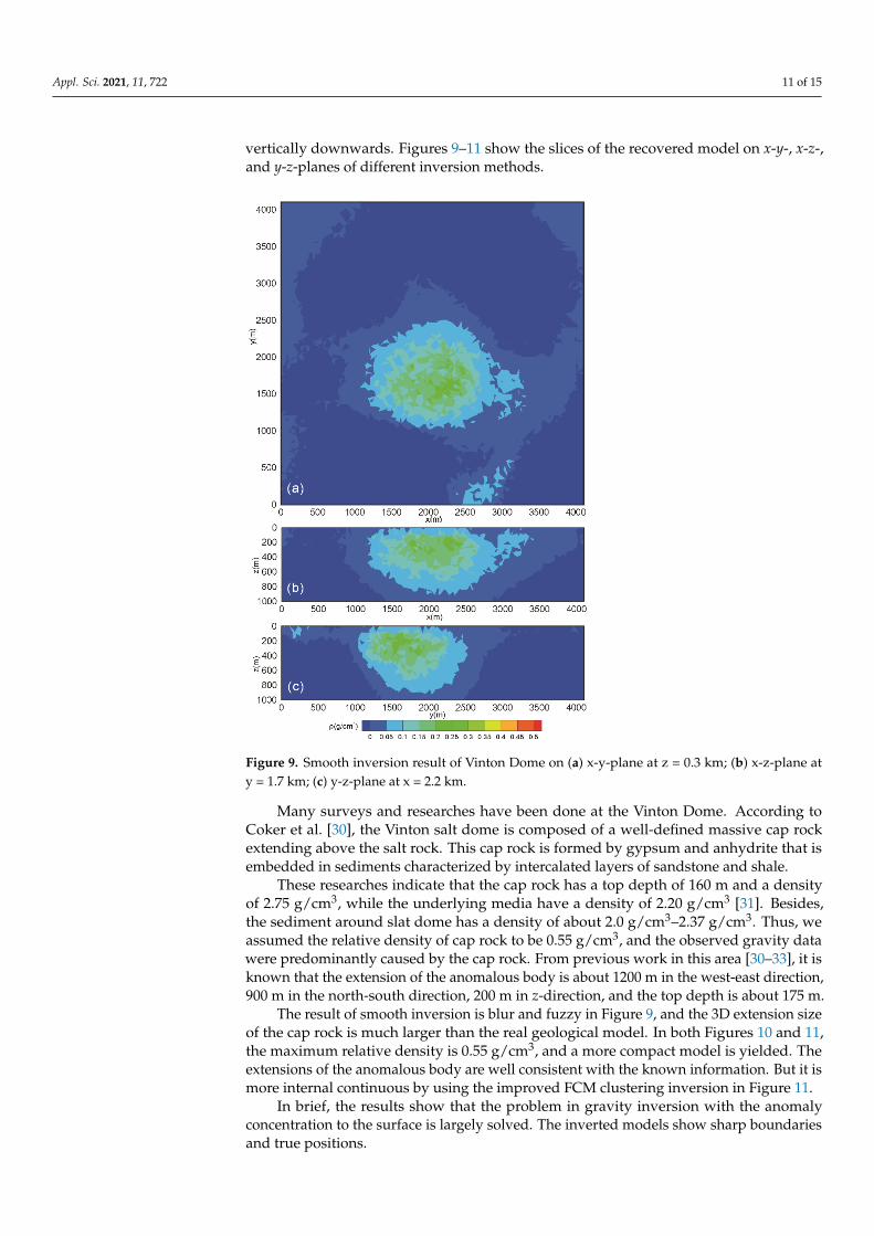
vertically downwards. Figures 9–11 show the slices of the recovered model on x-y-, x-z-,and y-z-planes of different inversion methods.

Appl. Sci. 2021, 11, x FOR PEER REVIEW 12 of 17

Figure 9. Smooth inversion result of Vinton Dome on (a) x-y-plane at z = 0.3 km; (b) x-z-plane at y = 1.7 km; (c) y-z-plane at x = 2.2 km. Figure 9. Smooth inversion result of Vinton Dome on (a) x-y-plane at z = 0.3 km; (b) x-z-plane aty = 1.7 km; (c) y-z-plane at x = 2.2 km.

Many surveys and researches have been done at the Vinton Dome. According toCoker et al. [30], the Vinton salt dome is composed of a well-defined massive cap rockextending above the salt rock. This cap rock is formed by gypsum and anhydrite that isembedded in sediments characterized by intercalated layers of sandstone and shale.

These researches indicate that the cap rock has a top depth of 160 m and a densityof 2.75 g/cm3, while the underlying media have a density of 2.20 g/cm3 [31]. Besides,the sediment around slat dome has a density of about 2.0 g/cm3–2.37 g/cm3. Thus, weassumed the relative density of cap rock to be 0.55 g/cm3, and the observed gravity datawere predominantly caused by the cap rock. From previous work in this area [30–33], it isknown that the extension of the anomalous body is about 1200 m in the west-east direction,900 m in the north-south direction, 200 m in z-direction, and the top depth is about 175 m.

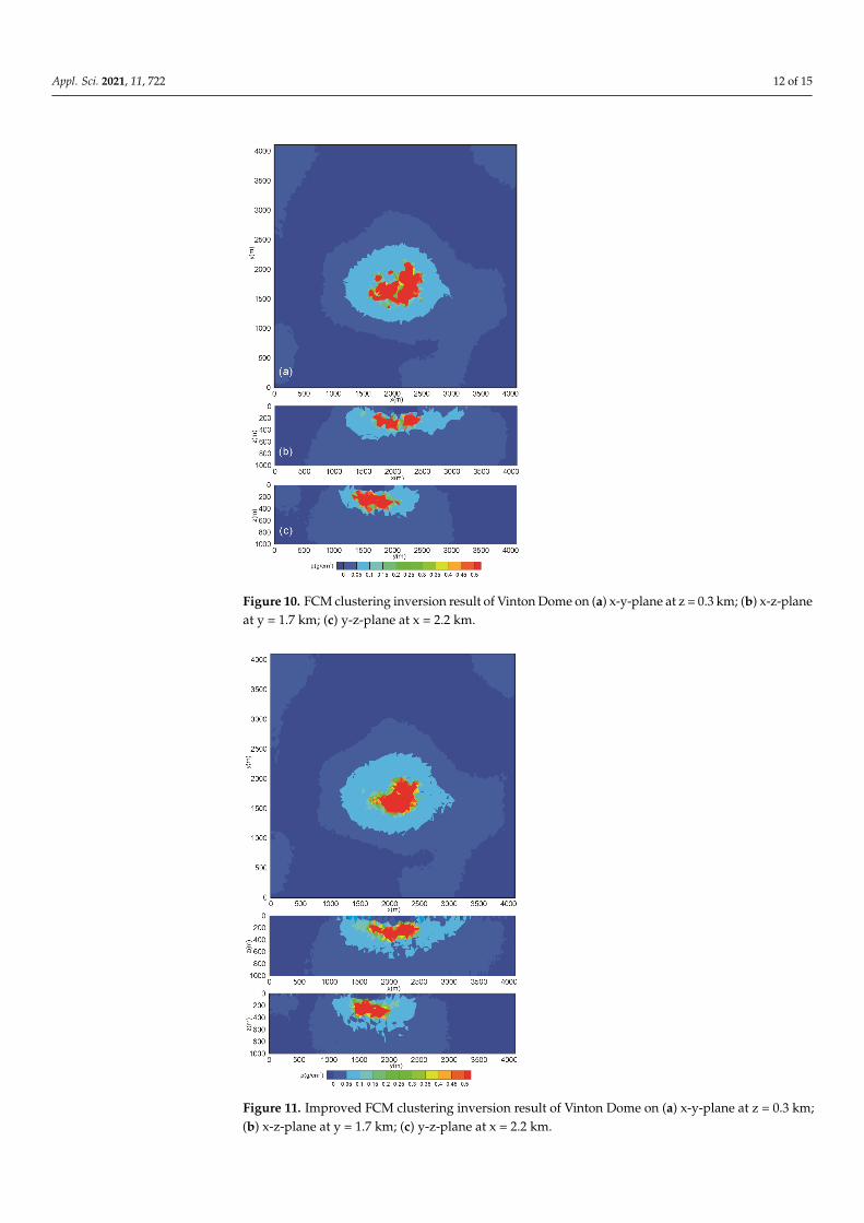
The result of smooth inversion is blur and fuzzy in Figure 9, and the 3D extension sizeof the cap rock is much larger than the real geological model. In both Figures 10 and 11,the maximum relative density is 0.55 g/cm3, and a more compact model is yielded. Theextensions of the anomalous body are well consistent with the known information. But it ismore internal continuous by using the improved FCM clustering inversion in Figure 11.

In brief, the results show that the problem in gravity inversion with the anomalyconcentration to the surface is largely solved. The inverted models show sharp boundariesand true positions.

Appl. Sci. 2021, 11, 722 12 of 15

Appl. Sci. 2021, 11, x FOR PEER REVIEW 13 of 17

Figure 10. FCM clustering inversion result of Vinton Dome on (a) x-y-plane at z = 0.3 km; (b) x-z-plane at y = 1.7 km; (c) y-z-plane at x = 2.2 km.

Many surveys and researches have been done at the Vinton Dome. According to Coker et al. [30], the Vinton salt dome is composed of a well-defined massive cap rock extending above the salt rock. This cap rock is formed by gypsum and anhydrite that is embedded in sediments characterized by intercalated layers of sandstone and shale.

These researches indicate that the cap rock has a top depth of 160 m and a density of 2.75 g/cm3, while the underlying media have a density of 2.20 g/cm3 [31]. Besides, the sed-iment around slat dome has a density of about 2.0 g/cm3–2.37 g/cm3. Thus, we assumed the relative density of cap rock to be 0.55 g/cm3, and the observed gravity data were pre-dominantly caused by the cap rock. From previous work in this area [30–33], it is known that the extension of the anomalous body is about 1200 m in the west-east direction, 900 m in the north-south direction, 200 m in z-direction, and the top depth is about 175 m.

The result of smooth inversion is blur and fuzzy in Figure 9, and the 3D extension size of the cap rock is much larger than the real geological model. In both Figures 10 and 11, the maximum relative density is 0.55 g/cm3, and a more compact model is yielded. The exten-sions of the anomalous body are well consistent with the known information. But it is more internal continuous by using the improved FCM clustering inversion in Figure 11.

Figure 10. FCM clustering inversion result of Vinton Dome on (a) x-y-plane at z = 0.3 km; (b) x-z-planeat y = 1.7 km; (c) y-z-plane at x = 2.2 km.

Appl. Sci. 2021, 11, x FOR PEER REVIEW 14 of 17

Figure 11. Improved FCM clustering inversion result of Vinton Dome on (a) x-y-plane at z = 0.3 km; (b) x-z-plane at y = 1.7 km; (c) y-z-plane at x = 2.2 km.

In brief, the results show that the problem in gravity inversion with the anomaly con-centration to the surface is largely solved. The inverted models show sharp boundaries and true positions.

5. Conclusions In gravity inversion based on unstructured grids, the dual effects of volume and

depth difference of grids would result in a discontinuous and hollow model. However, the local refinement or coarsening of the mesh, an important advantage of unstructured grids, will inevitably lead to different mesh volumes. So, it’s crucial to solve this problem before gravity inversion based on unstructured grids used widely in field data.

From the view of the objective function gradient, we analyzed the cause of poor depth resolution and two strategies of depth weighting in gradient-based inversion meth-ods. It indicated that the key to improve the depth resolution is how to counteract the decay of kernels in the data misfit gradient. The data-based strategy can improve the depth resolution more directly and effectively than the conventional strategy.

Besides an improved FCM clustering combined with spatial constraints is developed to obtain a continuous density distribution in the spatial domain and a focused property distribution in the parameter domain. It will reconstruct a more continuous inverted model on unstructured grids. With different regularization parameters, two weighting strategies are compared by applying smooth and the new FCM clustering inversions on synthetic data sets. The results show that the depth resolution of the gradient-based strat-egy is independent of regularization parameters and regularization terms does not

Figure 11. Improved FCM clustering inversion result of Vinton Dome on (a) x-y-plane at z = 0.3 km;(b) x-z-plane at y = 1.7 km; (c) y-z-plane at x = 2.2 km.

Appl. Sci. 2021, 11, 722 13 of 15

5. Conclusions

In gravity inversion based on unstructured grids, the dual effects of volume and depthdifference of grids would result in a discontinuous and hollow model. However, the localrefinement or coarsening of the mesh, an important advantage of unstructured grids, willinevitably lead to different mesh volumes. So, it’s crucial to solve this problem beforegravity inversion based on unstructured grids used widely in field data.

From the view of the objective function gradient, we analyzed the cause of poor depthresolution and two strategies of depth weighting in gradient-based inversion methods.It indicated that the key to improve the depth resolution is how to counteract the decayof kernels in the data misfit gradient. The data-based strategy can improve the depthresolution more directly and effectively than the conventional strategy.

Besides an improved FCM clustering combined with spatial constraints is developedto obtain a continuous density distribution in the spatial domain and a focused propertydistribution in the parameter domain. It will reconstruct a more continuous inverted modelon unstructured grids. With different regularization parameters, two weighting strategiesare compared by applying smooth and the new FCM clustering inversions on syntheticdata sets. The results show that the depth resolution of the gradient-based strategy isindependent of regularization parameters and regularization terms does not weaken withdepth increases. Compared with focusing inversion and conventional FCM clusteringinversion, the improved FCM clustering inversion can provide a more continuous model.

At last, we implemented the gradient-based strategy and the improved FCM clusteringinversion on field data sets. The results show that a compact model can be better consistentwith the known information than smooth inversion. But it is more internal continuous byusing the improved FCM clustering inversion.

Author Contributions: Conceptualization, S.S. and C.Y.; methodology, validation, and visualizationS.S. and X.G.; writing—original draft preparation, S.S.; writing—review and editing, C.Y. and X.G.;supervision, C.Y.; project administration, C.Y. All authors have read and agreed to the publishedversion of the manuscript.

Funding: This research was financially supported by China Postdoctoral Science Foundation(2020M670601), the China Geological Survey Project (DD20189143) and the Basic Scientific ResearchFunds of the key Laboratory of Aero Geophysics and Remote Sensing Geology, Ministry of NaturalResources (2020YFL11).

Institutional Review Board Statement: Not applicable.

Informed Consent Statement: Not applicable.

Data Availability Statement: Restrictions apply to the availability of field data. Data was obtainedfrom Bell Geospace and are available from Siyuan Sun with the permission of Scott Hammond fromBell Geospace.

Acknowledgments: We would like to thank Scott Hammond from Bell Geospace for providing theirfield data from Vinton salt dome.

Conflicts of Interest: The authors declare no conflict of interest.

Appendix A

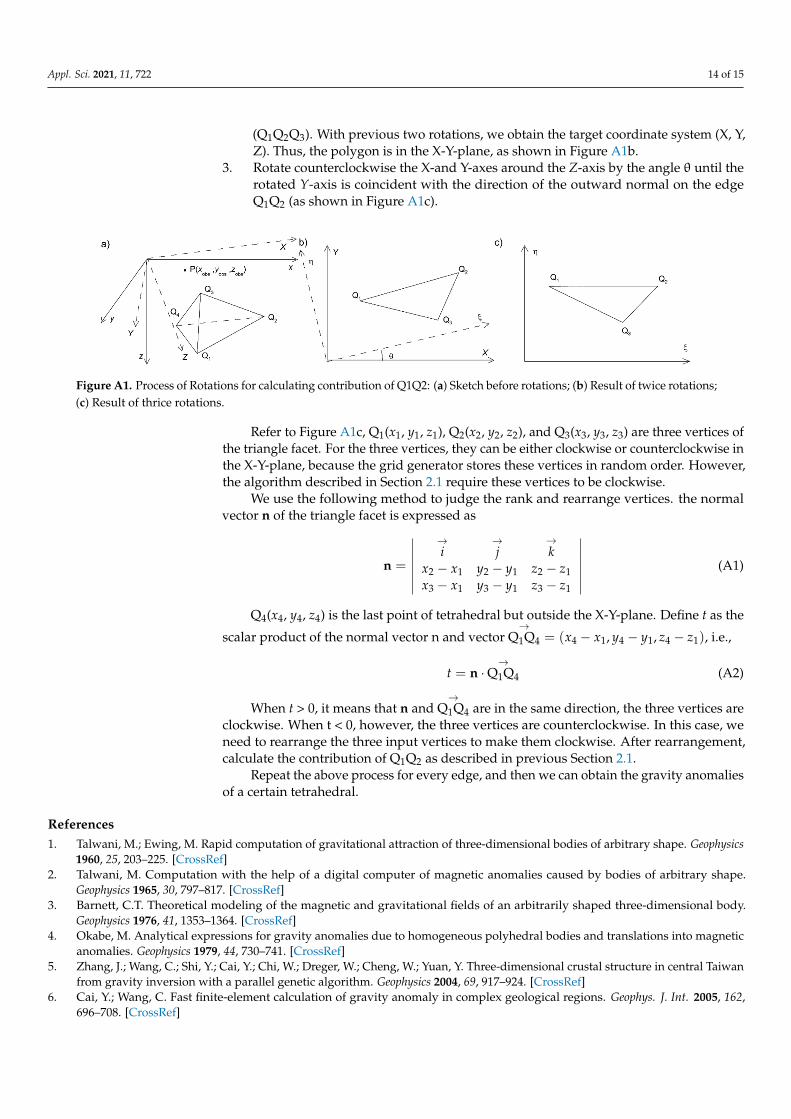
As shown in Equation (1), the gravity anomalies cause by a tetrahedral is equal to thesum of the contributions from six edges. Taking the edge Q1Q2 in Figure 1 for example, wecan describe thrice rotations as follows:

1. Rotate counterclockwise the x- and y-axes around the z-axis in Figure A1a by theangle ϕ until the rotated x-axis is coincident with the direction of the outward normalonto the x-y-plane.

2. Rotate counterclockwise the z- and x-axes around the y-axis by the angle ψ until therotated z-axis is coincident with the outward normal direction of the triangle facet

Appl. Sci. 2021, 11, 722 14 of 15

(Q1Q2Q3). With previous two rotations, we obtain the target coordinate system (X, Y,Z). Thus, the polygon is in the X-Y-plane, as shown in Figure A1b.

3. Rotate counterclockwise the X-and Y-axes around the Z-axis by the angle θ until therotated Y-axis is coincident with the direction of the outward normal on the edgeQ1Q2 (as shown in Figure A1c).

Appl. Sci. 2021, 11, x FOR PEER REVIEW 15 of 17

weaken with depth increases. Compared with focusing inversion and conventional FCM clustering inversion, the improved FCM clustering inversion can provide a more contin-uous model.

At last, we implemented the gradient-based strategy and the improved FCM cluster-ing inversion on field data sets. The results show that a compact model can be better con-sistent with the known information than smooth inversion. But it is more internal contin-uous by using the improved FCM clustering inversion.

Author Contributions: Conceptualization, S.S. and C.Y.; methodology, validation, and visualiza-tion S.S. and X.G.; writing—original draft preparation, S.S.; writing—review and editing, C.Y. and X.G.; supervision, C.Y.; project administration, C.Y. All authors have read and agreed to the pub-lished version of the manuscript.

Funding: This research was financially supported by China Postdoctoral Science Foundation (2020M670601), the China Geological Survey Project (DD20189143) and the Basic Scientific Re-search Funds of the key Laboratory of Aero Geophysics and Remote Sensing Geology, Ministry of Natural Resources (2020YFL11).

Institutional Review Board Statement: Not applicable.

Informed Consent Statement: Not applicable.

Data Availability Statement: Restrictions apply to the availability of field data. Data was obtained from Bell Geospace and are available from Siyuan Sun with the permission of Scott Hammond from Bell Geospace.

Acknowledgments: We would like to thank Scott Hammond from Bell Geospace for providing their field data from Vinton salt dome.

Conflicts of Interest: The authors declare no conflict of interest.

Appendix A As shown in Equation (1), the gravity anomalies cause by a tetrahedral is equal to the

sum of the contributions from six edges. Taking the edge Q1Q2 in Figure 1 for example, we can describe thrice rotations as follows: 1. Rotate counterclockwise the x- and y-axes around the z-axis in Figure A1a by the angle

φ until the rotated x-axis is coincident with the direction of the outward normal onto the x-y-plane.

2. Rotate counterclockwise the z- and x-axes around the y-axis by the angle ψ until the rotated z-axis is coincident with the outward normal direction of the triangle facet (Q1Q2Q3). With previous two rotations, we obtain the target coordinate system (X, Y, Z). Thus, the polygon is in the X-Y-plane, as shown in Figure A1b.

3. Rotate counterclockwise the X-and Y-axes around the Z-axis by the angle θ until the rotated Y-axis is coincident with the direction of the outward normal on the edge Q1Q2 (as shown in Figure A1c).

Figure A1. Process of Rotations for calculating contribution of Q1Q2: (a) Sketch before rotations; (b) Result of twice rota-tions; (c) Result of thrice rotations. Figure A1. Process of Rotations for calculating contribution of Q1Q2: (a) Sketch before rotations; (b) Result of twice rotations;(c) Result of thrice rotations.

Refer to Figure A1c, Q1(x1, y1, z1), Q2(x2, y2, z2), and Q3(x3, y3, z3) are three vertices ofthe triangle facet. For the three vertices, they can be either clockwise or counterclockwise inthe X-Y-plane, because the grid generator stores these vertices in random order. However,the algorithm described in Section 2.1 require these vertices to be clockwise.

We use the following method to judge the rank and rearrange vertices. the normalvector n of the triangle facet is expressed as

n =

∣∣∣∣∣∣∣→i

→j

→k

x2 − x1 y2 − y1 z2 − z1x3 − x1 y3 − y1 z3 − z1

∣∣∣∣∣∣∣ (A1)

Q4(x4, y4, z4) is the last point of tetrahedral but outside the X-Y-plane. Define t as the

scalar product of the normal vector n and vector→

Q1Q4 = (x4 − x1, y4 − y1, z4 − z1), i.e.,

t = n ·→

Q1Q4 (A2)

When t > 0, it means that n and→

Q1Q4 are in the same direction, the three vertices areclockwise. When t < 0, however, the three vertices are counterclockwise. In this case, weneed to rearrange the three input vertices to make them clockwise. After rearrangement,calculate the contribution of Q1Q2 as described in previous Section 2.1.

Repeat the above process for every edge, and then we can obtain the gravity anomaliesof a certain tetrahedral.

References1. Talwani, M.; Ewing, M. Rapid computation of gravitational attraction of three-dimensional bodies of arbitrary shape. Geophysics

1960, 25, 203–225. [CrossRef]2. Talwani, M. Computation with the help of a digital computer of magnetic anomalies caused by bodies of arbitrary shape.

Geophysics 1965, 30, 797–817. [CrossRef]3. Barnett, C.T. Theoretical modeling of the magnetic and gravitational fields of an arbitrarily shaped three-dimensional body.

Geophysics 1976, 41, 1353–1364. [CrossRef]4. Okabe, M. Analytical expressions for gravity anomalies due to homogeneous polyhedral bodies and translations into magnetic

anomalies. Geophysics 1979, 44, 730–741. [CrossRef]5. Zhang, J.; Wang, C.; Shi, Y.; Cai, Y.; Chi, W.; Dreger, W.; Cheng, W.; Yuan, Y. Three-dimensional crustal structure in central Taiwan

from gravity inversion with a parallel genetic algorithm. Geophysics 2004, 69, 917–924. [CrossRef]6. Cai, Y.; Wang, C. Fast finite-element calculation of gravity anomaly in complex geological regions. Geophys. J. Int. 2005, 162,

696–708. [CrossRef]

Appl. Sci. 2021, 11, 722 15 of 15

7. May, D.A.; Knepley, M.G. Optimal, scalable forward models for computing gravity anomalies. Geophys. J. Int. 2011, 187, 161–177.[CrossRef]

8. Jahandari, H.; Farquharson, C.G. Forward modeling of gravity data using finite-volume and finite-element methods on unstruc-tured grids. Geophysics 2013, 78, G69–G80. [CrossRef]

9. Li, Y.; Oldenburg, D.W. 3-D inversion of gravity data. Geophysics 1998, 63, 109–119. [CrossRef]10. Boulanger, O.; Chouteau, M. Constraints in 3D gravity inversion. Geophys. Prospect. 2001, 49, 265–280. [CrossRef]11. Zhdanov, M.S.; Ellis, R.; Mukherjee, S. Three-dimensional regularized focusing inversion of gravity gradient tensor component

data. Geophysics 2004, 69, 925–937. [CrossRef]12. Silva, D.F.J.; Barbosa, V.C.; Silva, J.B. 3D gravity inversion through an adaptive-learning procedure. Geophysics 2009, 7, I9–I21.

[CrossRef]13. Tikhonov, A.N.; Arsenin, V.Y. Solution of Ill-Posed Problems; Wiley: New York, NY, USA, 1977; p. 258.14. Li, Y.; Oldenburg, D.W. 3-D inversion of magnetic data. Geophysics 1996, 61, 394–408. [CrossRef]15. Last, B.J.; Kubik, K. Compact gravity inversion. Geophysics 1983, 48, 713–721. [CrossRef]16. Portniaguine, O.; Zhdanov, M.S. 3-D magnetic inversion with data compression and image focusing. Geophysics 2002, 67,

1532–1541. [CrossRef]17. Lelièvre, P.G.; Farquharson, C.G.; Hurich, C.A. Joint inversion of seismic traveltimes and gravity data on unstructured grids with

application to mineral exploration. Geophysics 2012, 77, K1–K15. [CrossRef]18. Sun, J.; Li, Y. Multidomain petrophysically constrained inversion and geology differentiation using guided fuzzy c-means

clustering. Geophysics 2015, 80, ID1–ID18. [CrossRef]19. Sun, J.; Li, Y. joint inversion of multiple geophysical data using guided fuzzy c-means clustering. Geophysics 2016, 81, ID37–ID57.

[CrossRef]20. Singh, A.; Sharma, S. Modified Zonal Cooperative Inversion of Gravity Data-a Case Study from Uranium Mineralization; SEG Technical

Program Expanded Abstracts: Houston, TX, USA, 2017; pp. 1744–1749.21. Commer, M. Three-dimensional gravity modelling and focusing inversion using rectangular meshes. Geophys. Prospect. 2011, 59,

966–979. [CrossRef]22. Liu, Y.P.; Wang, Z.W.; Du, X.J.; Liu, J.H.; Xu, J.S. 3D constrained inversion of gravity data based on the Extrapolation Tikhonov

regularization algorithm. Chin. J. Geophys. 2013, 56, 1650–1659. (In Chinese)23. Ren, Z.; Chen, C.; Pan, K.; Kalscheuer, T.; Maurer, H.; Tang, J. Gravity Anomalies of Arbitrary 3D Polyhedral Bodies with

Horizontal and Vertical Mass Contrasts. Surv. Geophys. 2017, 38, 479–502. [CrossRef]24. Zhao, G.; Chen, B.; Chen, L.; Liu, J.; Ren, Z. High-accuracy 2D and 3D Fourier forward modeling of gravity field based on the

Gauss-FFT method. J. Appl. Geophys. 2018, 150, 294–303. [CrossRef]25. Si, H. Tetgen: A Quality Tetrahedral Mesh Generator and a 3D Delaunay Triangulator. 2009. Available online: http://wias-berlin.

de/software/index.jsp?id=TetGen&lang=1 (accessed on 25 September 2017).26. Hathaway, R.J.; Bezdek, J.C. Fuzzy c-means clustering of incomplete data: IEEE Transactions on Systems, Man, and Cybernetics,

Part B. Cybernetics 2001, 31, 735–744. [PubMed]27. Fedi, M.; Rapolla, A. 3-D inversion of gravity and magnetic data with depth resolution. Geophysics 1999, 64, 452–460. [CrossRef]28. Li, Y.; Oldenburg, D.W. Joint inversion of surface and three-component borehole magnetic data. Geophysics 2000, 65, 540–552.

[CrossRef]29. Dickinson, J.L.; Brewster, J.R.; Robinson, J.W.; Murphy, C.A. Imaging techniques for full tensor gravity gradiometry data. In

Proceedings of the 11th SAGA Biennial Technical Meeting and Exhibition, Swaziland, South Africa, 16–18 September 2009.cp-241-00019.

30. Coker, M.O.; Bhattacharya, J.P.; Marfurt, K.J. Fracture patterns within mudstones on the flanks o f a salt dome: Syneresis orslumping? Gulf Coast Assoc. Geol. Soc. 2007, 57, 125–137.

31. Ennen, C. Mapping Gas-Charged Fault Blocks around the Vinton Salt Dome, Louisiana Using Gravity Gradiometry Data. Master’sThesis, University of Houston, Houston, TX, USA, 2012.

32. Salem, A.; Masterton, S.; Campbell, S.; Dickinson, J.D.; Murphy, C. Interpretation of tensor gravity data using an adaptive tiltangle method. Geophys. Prospect. 2013, 61, 1065–1076. [CrossRef]

33. Thompson, S.A.; Eichelberger, O.H. Vinton salt dome, Calcasieu Parish, Louisiana. AAPG Bull. 1928, 12, 385–394.