Seasonal Predictability of Daily Rainfall Characteristics in Central NorthernChile for Dry-Land Management

KOEN VERBIST

International Centre for Eremology, Department of Soil Management, Ghent University, Ghent, Belgium, and Water Centre

for Arid Zones in Latin America and the Caribbean (CAZALAC), La Serena, Chile

ANDREW W. ROBERTSON

International Research Institute for Climate and Society, Columbia University, Palisades, New York

WIM M. CORNELIS AND DONALD GABRIELS

International Centre for Eremology, Department of Soil Management, Ghent University, Ghent, Belgium

(Manuscript received 18 August 2009, in final form 23 April 2010)

ABSTRACT

The seasonal predictability of daily winter rainfall characteristics relevant to dry-land management was

investigated in the Coquimbo region of central northern Chile, with focus on the seasonal rainfall total, daily

rainfall frequency, and mean daily rainfall intensity on wet days at the station scale. Three approaches of

increasing complexity were tested. First, an index of the simultaneous El Nino–Southern Oscillation (ENSO)

was regressed onto May–August (MJJA) observed precipitation; this explained 32% of station-averaged

rainfall-amount variability, but performed poorly in a forecasting setting. The second approach used retro-

spective seasonal forecasts made with three general circulation models (GCMs) to produce downscaled

seasonal rainfall statistics by means of canonical correlation analysis (CCA). In the third approach, a non-

homogeneous hidden Markov model (nHMM) driven by the GCM’s seasonal forecasts was used to model

stochastic daily rainfall sequences. While the CCA is used as a downscaling method for the seasonal rainfall

characteristics themselves, the nHMM has the ability to simulate a large ensemble of daily rainfall sequences

at each station from which the rainfall statistics were calculated. Similar cross-validated skill estimates were

obtained using both the CCA and nHMM, with the highest correlations with observations found for seasonal

rainfall amount and rainfall frequency (up to 0.9 at individual stations). These findings were interpreted using

analyses of observed rainfall spatial coherence, and by means of synoptic rainfall states derived from the

HMM. The downscaled hindcasts were then tailored to meteorological drought prediction, using the stan-

dardized precipitation index (SPI) based on seasonal values, the frequency of substantial rainfall days (.15 mm;

FREQ15) and the daily accumulated precipitation deficit. Deterministic hindcasts of SPI showed high hit rates,

with high ranked probability skill score for probabilistic hindcasts of FREQ15 obtained via the nHMM.

1. Introduction

Climate variability can have serious social impacts in

semiarid regions, especially for farmers who depend on

rain-fed agriculture and on livestock production based

on natural vegetation. In the Coquimbo region in central

northern Chile, where rainfall amounts often drop under

the limit for crop growth, a lack of rainfall results in

a crisis situation for society. Over US$2.6 million were

spent during the severe drought of 2007 to support af-

fected families and farmers in the Coquimbo region,

repair damage, recover degraded soils, and increase

irrigation programs (MINAGRI 2008). Although these

measures reduced the negative effects of the 2007

drought, they did not address all affected families because

of budget limitations, nor did they increase preparedness

and resilience to future droughts. Of the 16 307 rural

families in Chile seeking monetary aid to overcome the

negative aspects of the 2007 drought, more than 75%

indicated suffering a lack of sufficient water for irrigation

Corresponding author address: Koen Verbist, Dept. of Soil Man-

agement, Coupure Links 653, 9000 Ghent, Belgium.

E-mail: Koen.Verbist@UGent.be

1938 J O U R N A L O F A P P L I E D M E T E O R O L O G Y A N D C L I M A T O L O G Y VOLUME 49

DOI: 10.1175/2010JAMC2372.1

� 2010 American Meteorological Society

and domestic use, and they observed harvest losses for

the crops grown for their own consumption [J. Castillo,

Fondo de Solidaridad e Inversion Social (FOSIS), 2008,

personal communication]. A typical problem here is the

lack of preparedness prior to these natural events, mak-

ing any governmental action afterward less cost effective.

Despite the need, the current Drought Alleviation Plan

formulated by the Chilean government for the region

(FOSIS 2008) does not include strategies for drought

early warning, and the feasibility of such a system has yet

to be demonstrated.

The El Nino–Southern Oscillation (ENSO) is known

to have a strong impact on winter rainfall over central

northern Chile, with positive rainfall anomalies during

El Nino events, and below-normal rainfall mostly asso-

ciated with La Nina conditions (Aceituno 1988; Aceituno

et al. 2009; Falvey and Garreaud 2007; Montecinos and

Aceituno 2003; Pittock 1980; Quinn and Neal 1983;

Rubin 1955; Rutllant and Fuenzalida 1991; Garreaud

et al. 2009). However, the associated seasonal predict-

ability and forecast skill levels from current dynamical

seasonal prediction models (e.g., Goddard et al. 2003)

have not yet been assessed in detail for the statistics of

local daily weather that are likely to be most pertinent to

meteorological drought.

In this paper we document the characteristics of

daily winter rainfall from station observations over the

Coquimbo region, and assess their seasonal predictabil-

ity from three current seasonal prediction general circu-

lation models (GCMs), together with statistical techniques

to ‘‘downscale’’ and tailor the output from these rela-

tively course resolution models to the station scale.

While GCMs typically misrepresent the characteristics

of local daily rainfall, statistical downscaling can often

correct such biases and provide probabilistic rainfall

simulations that are well calibrated against local station

data (Hughes and Guttorp 1994; Robertson et al. 2009).

Our analysis of the station rainfall data begins with

a decomposition of seasonal rainfall amounts into rain-

fall frequency and the mean rainfall amount falling on

wet days; that is, the rainfall intensity. The correlation

between rainfall data from stations separated by in-

creasing distances; that is, the spatial ‘‘coherence,’’ for

each of the seasonal anomaly types (rainfall amount,

intensity, and frequency) across the region is then in-

vestigated. Spatial coherence provides a measure of the

potential seasonal predictability, because there is no

a priori reason for the seasonal anomalies to differ be-

tween locations, except due to local-scale processes;

Moron et al. (2007) argued that these are dominated by

unpredictable noise over homogeneous regions. From

such analyses of seasonal anomalies, rainfall frequency at

local scale has been shown to be generally more spatially

coherent in the tropics, and thus potentially more pre-

dictable on seasonal time scales (Moron et al. 2007), but it

has not heretofore been investigated for the midlatitudes

such as is done in this study. For a climatically homoge-

neous region, even in regions of complex terrain like

Coquimbo, high spatial coherence would be an indicator

of potential predictability, although the reverse is not

necessarily the case.

To gain insight into the nature of the daily rainfall

variability and its year-to-year modulations in more de-

tail, we model the sequences of station rainfall in terms of

different daily rainfall patterns, or rainfall states, as de-

termined by a hidden Markov model (HMM). The HMM

can simulate stochastic daily sequences of rainfall oc-

currence with a specific rainfall intensity, by estimating

the transition probabilities between daily weather pat-

terns or states. The Markov property requires that the

probability of occurrence of a particular state on a given

day only depends on the previous day’s state. The set of

states needed to describe the local daily rainfall char-

acteristics are determined from observed rainfall re-

cords; the states are not directly observed and are as

such hidden. In the homogeneous HMM, the transition

probabilities from one state to the other are not allowed

to vary in time. In its nonhomogeneous form (nHMM),

the transition probability between states can vary in

time, allowing external inputs to influence the rainfall

characteristics between one year and another. Seasonal

GCM predictions can be used to determine these inputs,

creating an effective method to downscale them to most

probable daily rainfall sequences at the station scale,

training the nHMM on each year for which GCM sea-

sonal hindcasts are available (Charles et al. 1999;

Robertson et al. 2004, 2006, 2009). Encouraging results

were reported by Bellone et al. (2000), who used a

combined climate index, including wind, temperature

and relative humidity fields, together with an nHMM to

construct a model for daily rainfall amounts. In addition

to probabilistic downscaling using the nHMM, we apply

a simpler method based on canonical correlation anal-

ysis (CCA) to the seasonally averaged statistics them-

selves (seasonal amount, daily rainfall frequency, and

mean daily intensity), in order to obtain downscaled

estimates of their seasonal predictability.

The work in this paper aims to lay the foundations for

constructing (meteorological) drought early warning sys-

tems, through analyses of daily rainfall and by estimating

seasonal predictability. The rainfall data and GCMs are

described in section 2, with the statistical methods out-

lined in section 3. The results of the station rainfall

analyses and retrospective forecasts of drought indices

are presented in section 4, with the concluding remarks

in section 5.

SEPTEMBER 2010 V E R B I S T E T A L . 1939

2. Data

a. Observed rainfall data

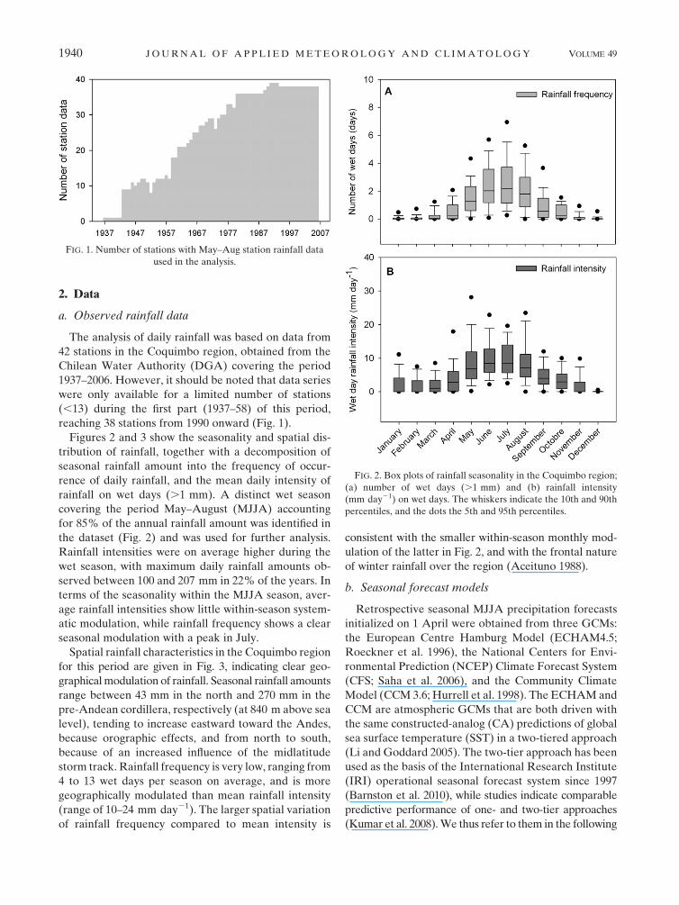
The analysis of daily rainfall was based on data from

42 stations in the Coquimbo region, obtained from the

Chilean Water Authority (DGA) covering the period

1937–2006. However, it should be noted that data series

were only available for a limited number of stations

(,13) during the first part (1937–58) of this period,

reaching 38 stations from 1990 onward (Fig. 1).

Figures 2 and 3 show the seasonality and spatial dis-

tribution of rainfall, together with a decomposition of

seasonal rainfall amount into the frequency of occur-

rence of daily rainfall, and the mean daily intensity of

rainfall on wet days (.1 mm). A distinct wet season

covering the period May–August (MJJA) accounting

for 85% of the annual rainfall amount was identified in

the dataset (Fig. 2) and was used for further analysis.

Rainfall intensities were on average higher during the

wet season, with maximum daily rainfall amounts ob-

served between 100 and 207 mm in 22% of the years. In

terms of the seasonality within the MJJA season, aver-

age rainfall intensities show little within-season system-

atic modulation, while rainfall frequency shows a clear

seasonal modulation with a peak in July.

Spatial rainfall characteristics in the Coquimbo region

for this period are given in Fig. 3, indicating clear geo-

graphical modulation of rainfall. Seasonal rainfall amounts

range between 43 mm in the north and 270 mm in the

pre-Andean cordillera, respectively (at 840 m above sea

level), tending to increase eastward toward the Andes,

because orographic effects, and from north to south,

because of an increased influence of the midlatitude

storm track. Rainfall frequency is very low, ranging from

4 to 13 wet days per season on average, and is more

geographically modulated than mean rainfall intensity

(range of 10–24 mm day21). The larger spatial variation

of rainfall frequency compared to mean intensity is

consistent with the smaller within-season monthly mod-

ulation of the latter in Fig. 2, and with the frontal nature

of winter rainfall over the region (Aceituno 1988).

b. Seasonal forecast models

Retrospective seasonal MJJA precipitation forecasts

initialized on 1 April were obtained from three GCMs:

the European Centre Hamburg Model (ECHAM4.5;

Roeckner et al. 1996), the National Centers for Envi-

ronmental Prediction (NCEP) Climate Forecast System

(CFS; Saha et al. 2006), and the Community Climate

Model (CCM 3.6; Hurrell et al. 1998). The ECHAM and

CCM are atmospheric GCMs that are both driven with

the same constructed-analog (CA) predictions of global

sea surface temperature (SST) in a two-tiered approach

(Li and Goddard 2005). The two-tier approach has been

used as the basis of the International Research Institute

(IRI) operational seasonal forecast system since 1997

(Barnston et al. 2010), while studies indicate comparable

predictive performance of one- and two-tier approaches

(Kumar et al. 2008). We thus refer to them in the following

FIG. 1. Number of stations with May–Aug station rainfall data

used in the analysis.

FIG. 2. Box plots of rainfall seasonality in the Coquimbo region;

(a) number of wet days (.1 mm) and (b) rainfall intensity

(mm day21) on wet days. The whiskers indicate the 10th and 90th

percentiles, and the dots the 5th and 95th percentiles.

1940 J O U R N A L O F A P P L I E D M E T E O R O L O G Y A N D C L I M A T O L O G Y VOLUME 49

as ECHAM-CA and CCM-CA, respectively. The CFS is

a coupled ocean–atmosphere GCM with initialization

of the atmosphere, ocean, and land surface conditions

through data assimilation. For all models, the ensemble

mean (over 24 members for ECHAM and CCM and

15 members for CFS) gridded precipitation was used at

a resolution of T62 (;1.98) for CFS and T42 (;2.88) for

ECHAM-CA and CCM-CA, over the domain 208–408S

and 658–858W. Seasonal MJJA precipitation hindcasts

were available for the 1981–2002 period for CCM-CA

and ECHAM-CA, and for the 1981–2005 period in the

case of CFS.

3. Statistical methods

a. Spatial coherence analysis

Estimates of spatial coherence of interannual rainfall

station anomalies are used as indicators of potential

seasonal predictability following Moron et al. (2007).

The number of spatial degrees of freedom (DOF) gives

an empirical estimate of the spatial coherence in terms

of empirical orthogonal functions (EOFs), with higher

values denoting lower spatial coherence:

DOF 5M2 �M

j51e2

j

,, (1)

where ej are the eigenvalues of the correlation matrix

formed from the station seasonal-mean time series and

M is the number of stations.

A second measure of the spatial coherence of inter-

annual anomalies is given by the interannual variance of

the standardized precipitation anomaly index, var(SAI),

which is constructed from the station average of the

standardized rainfall anomalies (Katz and Glantz 1986):

var(SAIi) 5 var

1

M�M

j51

(xij� x

j)

sj

24

35, (2)

where xj is the long-term time mean over i 5 1, . . . , N

years and sj is the interannual standard deviation for

station j. The var(SAI) is a maximum when all stations

are perfectly correlated, var(SAI) 5 1, and a minimum

when the stations are uncorrelated, resulting in a

var(SAI) 5 1/M.

b. Hidden Markov model

A state-based Markovian model was used to model

daily rainfall sequences at the 42 stations, in order to

gain insight into the daily rainfall process, and as a

means to downscale daily rainfall sequences (downscal-

ing in space and time). We use the approach developed

by Hughes and Guttorp (1994) for rainfall occurrence,

FIG. 3. Average rainfall characteristics during the wet season (May–Aug): (a) seasonal rainfall amount; (b) rainfall frequency; (c) mean

daily rainfall intensity for the period 1937–2006. A locator map indicates the position of the Coquimbo region within Chile and South

America.

SEPTEMBER 2010 V E R B I S T E T A L . 1941

while additionally modeling rainfall amounts. The hid-

den Markov model used here is described fully in

Robertson et al. (2004, 2006). In brief, the time sequence

of daily rainfall measurements on the network of sta-

tions is assumed to be generated by first-order Markov

chain of a few discrete hidden (i.e., unobserved) rainfall

states. For each state, the daily rainfall amount at each

station is modeled by a zero-amount delta function for

dry days and an exponential for days with nonzero rain-

fall. To apply the HMM to downscaling, rainfall state

transition probabilities were allowed to vary with time,

resulting in the nonhomogeneous HMM (nHMM). In

this study, transition probabilities between states are

modeled as functions of predictor variables, in our case

GCM predictions of MJJA seasonal-averaged precip-

itation over the region (58–408S, 1008–508W). For data

compression, a conventional principal components (PC)

analysis was first applied to the gridded seasonal-averaged

GCM (CFS) precipitation fields, with each gridded pre-

cipitation value standardized by its interannual standard

deviation at that gridpoint, selecting here the leading PC

as the input variable to the nHMM. The leading PC rep-

resented 36% of the model variance and showed a corre-

lation coefficient of 0.72 with the observed average rainfall

in the region (period 1980–2005). The nHMM was trained

under leave-three-years-out cross-validation, using the

CFS 15-member ensemble mean. To make downscaled

simulations, we used each CFS ensemble member in turn,

and generated 10 stochastic realizations for each one,

yielding an ensemble prediction of 150 daily rainfall se-

quences for each MJJA season, providing a probabilistic

forecast (Robertson et al. 2009).

The seasonal statistics of interest (seasonal amount,

daily rainfall frequency, and mean daily intensity on wet

days) were then computed from these simulated rainfall

sequences and compared to their observed counterparts

at each station.

c. Downscaling of seasonal forecasts usingcanonical correlation analysis

In addition to the nHMM, downscaling was also carried

out by applying canonical correlation analysis (CCA) di-

rectly to the seasonal rainfall statistics of interest. The

CCA regularizes the high-dimensional regression problem

between a spatial field of predictors and predictands by

reducing the spatial dimensionality via principal compo-

nent analysis and thus minimizes problems of overfitting

and multicolinearity (Tippett et al. 2003). Cross validation

was used to determine the truncation points of the PC and

CCA time series, via the Climate Predictability Tool

(CPT) software toolbox (more information available

online at http://iri.columbia.edu/outreach/software/). As

predictor datasets the retrospective seasonal MJJA

precipitation forecasts by the three GCMs discussed in

section 2b were used in conjunction with the MJJA

seasonal rainfall at the 42 stations of the Coquimbo re-

gion. The three CCA models were trained and tested

over the 1981–2000 period, with a cross-correlation

window of five years (i.e., leaving out two years on either

side of the verification value). As employed here, the

CCA provides a deterministic mean forecast value, in

contrast to the nHMM probabilistic ensemble.

4. Results

a. Spatial coherence of rainfall anomalies

As a first step toward assessing the seasonal predict-

ability of rainfall at local scale, we begin with an analysis

of spatial coherence for each of the three rainfall char-

acteristics: seasonal amount, rainfall frequency, and mean

daily intensity. Based on Fig. 3, spatial coherence esti-

mates were made separately for the three provinces

(from north to south: Elqui, Limari, and Choapa) and

for three altitude classes (from west to east: 0–500 m,

500–1500 m and .1500m; Fig. 3). Table 1 shows both the

degrees of freedom and the variance of the standardized

anomaly index for these sub datasets. The highest DOF

and lowest var(SAI) was observed for the Elqui province

in the north, indicating lowest spatial coherence of sea-

sonal anomalies, consistent with its more arid nature

and more sporadic rainfall. A similar tendency was found

when looking at altitude influences, with lowest spatial

coherence at highest altitudes (.1500 m), caused by

orographic influences on rainfall variability.

The dependence of spatial coherence characteristics

was analyzed as a function of time scale using station

autocorrelation. Figure 4 shows the averaged Pearson

correlation between each station pair plotted against

distance, for rainfall amount, intensity, and frequency

TABLE 1. DOF and var(SAI)] for seasonal rainfall amount

(RAm), rainfall intensity (RI), and rainfall frequency (RF) for

each province and altitude class in the Coquimbo region.

DOF Var(SAI)

N* RAm RI RF RAm RI RF

Province

Elqui 12 9.14 17.26 11.85 0.30 0.20 0.26

Limari 24 4.07 7.13 5.10 0.44 0.31 0.40

Choapa 8 5.14 7.17 6.18 0.41 0.34 0.37

Altitude class

0–500 m 13 5.05 8.91 6.33 0.40 0.28 0.36

500–1500 m 25 5.10 7.86 6.38 0.40 0.31 0.35

.1500 m 6 13.57 21.01 15.09 0.23 0.161 0.21

* Number of stations used.1 Minimum var(SAI) value (mean correlation equals zero).

1942 J O U R N A L O F A P P L I E D M E T E O R O L O G Y A N D C L I M A T O L O G Y VOLUME 49

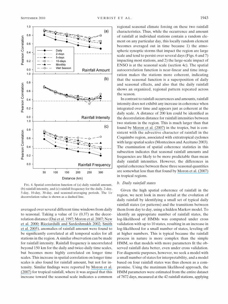
averaged over several different time windows from daily

to seasonal. Taking a value of 1/e (0.37) as the decor-

relation distance (Dai et al. 1997; Moron et al. 2007; New

et al. 2000; Ricciardulli and Sardeshmukh 2002; Smith

et al. 2005), anomalies of rainfall amount were found to

be significantly correlated at all temporal scales for all

stations in the region. A similar observation can be made

for rainfall intensity. Rainfall frequency is uncorrelated

beyond 150 km for the daily and twice-daily time scales,

but becomes more highly correlated on longer time

scales. This increase in spatial correlation on longer time

scales is also found for rainfall amount, but not for in-

tensity. Similar findings were reported by Moron et al.

(2007) for tropical rainfall, where it was argued that this

increase toward the seasonal scale indicates a common

regional seasonal climate forcing on these two rainfall

characteristics. Thus, while the occurrence and amount

of rainfall at individual stations contain a random ele-

ment on any particular day, this locally random element

becomes averaged out in time because 1) the atmo-

spheric synoptic storms that impact the region are large

scale and tend to persist over several days (Figs. 6 and 7)

impacting most stations, and 2) the large-scale impact of

ENSO is at the seasonal scale (section 4c). The spatial

autocorrelation function is near-linear and time integ-

ration makes the stations more coherent, indicating

that the seasonal function is a superposition of daily

and seasonal effects, and also that the daily rainfall

shows an organized, regional pattern repeated across

the season.

In contrast to rainfall occurrences and amounts, rainfall

intensity does not exhibit any increase in coherence when

integrated over time and appears just as coherent at the

daily scale. A distance of 200 km could be identified as

the decorrelation distance for rainfall intensities between

two stations in the region. This is much larger than that

found by Moron et al. (2007) in the tropics, but is con-

sistent with the advective character of rainfall in the

Coquimbo region, associated with extratropical cyclones

with large spatial scales (Montecinos and Aceituno 2003).

The examination of spatial coherence statistics in this

subsection indicates that seasonal rainfall amounts and

frequencies are likely to be more predictable than mean

daily rainfall intensities. However, the differences in

spatial coherence between these three seasonal quantities

are somewhat less than that found by Moron et al. (2007)

in tropical regions.

b. Daily rainfall states

Given the high spatial coherence of rainfall in the

region, we next look in more detail at the evolution of

daily rainfall by identifying a small set of typical daily

rainfall states (or patterns) and the transitions between

them from day to day, using a hidden Markov model. To

identify an appropriate number of rainfall states, the

log-likelihood of HMMs was computed under cross

validation with up to 10 states, resulting in an increase in

log-likelihood for a small number of states, leveling off

at higher numbers. This is typical because the rainfall

process in nature is more complex than the simple

HMM, so that models with more parameters fit the ob-

served rainfall data better, even under cross validation.

For diagnostic purposes, however, we seek a model with

a small number of states for interpretability, and a model

based on four rainfall states was thus chosen as a com-

promise. Using the maximum likelihood approach, the

HMM parameters were estimated from the entire dataset

of 7872 days, measured at the 42 rainfall stations, applying

FIG. 4. Spatial correlation function of (a) daily rainfall amount,

(b) rainfall intensity, and (c) rainfall frequency for the daily, 2-day,

5-day, 10-day, 30-day, and seasonal-averaging periods. The 1/e

decorrelation value is shown as a dashed line.

SEPTEMBER 2010 V E R B I S T E T A L . 1943

the iterative expectation-maximization (EM) algorithm

(Dempster et al. 1977; Ghahramani 2001). The algo-

rithm was initialized 10 times from random seeds, se-

lecting the run with the highest log-likelihood.

The four rainfall states thus obtained are shown in

Fig. 5 in terms of their rainfall characteristics, showing

the probability of rainfall occurrence at each station

(Figs. 5a–d), and the average rainfall intensity on wet

days (Figs. 5e–h). States were ordered from overall driest

to wettest. This ordering shows a dry state 1 with rainfall

probabilities near zero at all stations and three states with

increasing probabilities for rainfall and generally larger

rainfall amounts on wet days. The spatial pattern of state

2 resembles that of the mean characteristics seen in Fig. 3,

with more-frequent rainfall in the south and at higher

altitudes. State 3 represents the rainfall events where

rainfall is probable at most locations excluding the most

northern ones, while rainfall intensities remain relatively

small. State 4 can be interpreted as the very wet state,

with high rainfall probabilities over the whole region and

large rainfall intensities.

When looking at the matrix of day-to-day transition

probabilities between the four states (Table 2), it can

quickly be seen that state 1 is the most persistent state,

but it is also the state to which the wetter states 2 and 3

are most likely to evolve. State 4, the very wet state, has

an almost equal probability for each of the states to

follow it, indicating that states 2 and 3 tend to be in-

termediate in the transitions from a wet period to a dry

period.

A visual interpretation of the temporal evolution

is given in Fig. 6, showing the most probable daily

sequence of the four states that occurred over the

70-winter record (1937–2006) of daily rainfall, obtained

using the dynamical programming Viterbi algorithm

(Forney 1978). Once the parameters of the HMM have

been estimated from the rainfall data, the Viterbi al-

gorithm uses the HMM state parameters in conjunc-

tion with the rainfall data to assign each day of the

historical record to a particular state. This resulted

on average in 105 days per season of state 1 (85.4%),

10 days of state 2 (7.7%), and 5 days of state 3 (4.2%).

FIG. 5. Four-state HMM rainfall parameters. (a)–(d) Probabilities of rainfall occurrence and (e)–(h) mean rainfall intensities

(i.e., wet-day amounts).

1944 J O U R N A L O F A P P L I E D M E T E O R O L O G Y A N D C L I M A T O L O G Y VOLUME 49

The very wet state 4 occurred on only 3 days (2.7%) on

average during each MJJA season of the 70-year pe-

riod, but on average 56% of total seasonal rainfall was

observed on these very wet days. The horizontal traces

in Fig. 6 illustrate graphically the high intermittency of

rainfall over the region, with individual rainfall events

often lasting several days and being made up of days

from several of the wetter states. On average, no ob-

vious seasonality is apparent across the season.

Figure 7 shows composite sea level pressure (SLP)

fields from the NCEP–National Center for Atmospheric

Research (NCAR) reanalysis data (Kalnay et al. 1996),

obtained by averaging over the days falling into each

state and plotting them as an anomaly from the long-

term MJJA average. The state SLP anomaly patterns

demonstrate the well-known relationship between rainfall

in central Chile and synoptic-wave disturbances (Falvey

and Garreaud 2007). The wet states 2–4 are associated

with a similar wave pattern with an anomalous trough

over the Chilean coast extending east of the Andes, but

with increasing trough intensity as a function of rainfall,

while the dry state 1 (note finer contour interval in Fig. 7a)

has the opposite footprint of anomalous anticyclonic con-

ditions over central Chile. The tendency seen in the state

sequence for multiday persistent rainfall events made up

of several states (Fig. 6) shows that this anomalous low

pressure pattern, once established, often remains approx-

imately stationary while growing and decaying in situ;

the partitioning of the associated rainfall events into

states 2–4 demonstrates the strong dependence of rainfall

probability and intensity on the amplitude of this synoptic

weather pattern.

c. ENSO influence on seasonal rainfallcharacteristics

The interannual variability over the Coquimbo region

can be interpreted in terms of the HMM’s state se-

quence, with more instances of the wetter states during

wet winters. Before proceeding with that analysis, we

first summarize the well-known ENSO influence on the

seasonal statistics of rainfall (MJJA amount, rainfall

frequency, and mean daily intensity) averaged over all

42 stations. The relationship between seasonal rainfall

amounts and ENSO is plotted in Fig. 8 in terms of the

Nino-3.4 index. All but one (the year 1984) of the very

wet winters (.100 mm above average rainfall) have

been associated with the warm ENSO phase, with all of

these ENSO events in their developing phase over the

MJJA season. The cold ENSO phase has almost always

been associated with below-normal rainfall, although

several years have less than normal rainfall without

strong La Nina characteristics. The Pearson correlation

between Nino-3.4 and MJJA rainfall amount for the

entire period 1937–2006 is 0.57, which is statistically

TABLE 2. Transition matrix for the 4-state HMM. ‘‘From’’ states

occupy the rows; ‘‘to’’ states occupy the columns. Thus, the prob-

ability of a transition from state 2 to state 1 is 0.56.

To state

From state 1 2 3 4

1 0.92 0.05 0.02 0.01

2 0.56 0.22 0.12 0.09

3 0.47 0.25 0.19 0.09

4 0.23 0.28 0.22 0.27

FIG. 6. The most probable HMM state sequence obtained using the Viterbi algorithm. Rainfall

states are indicated from driest (state 1) to wettest (state 4) on the color bar.

SEPTEMBER 2010 V E R B I S T E T A L . 1945

significant at the 99% level according to a two-sided

Student test. The Spearman correlation coefficient, which

is less sensitive than the Pearson correlation to strong

outliers, was lower (0.45), but still significant. When only

ENSO years are included, as defined by those years

where positive or negative anomalies of one standard

deviation (60.68C) were observed for the Nino-3.4 in-

dex, the Pearson correlation increases to 0.83, which is

indicative for the strength of the ENSO signal in extreme

wet or dry years. The Spearman correlation coefficient

was 0.80, suggesting only a limited influence of outliers.

Table 3 shows the correlations between the observed

station-averaged MJJA rainfall amount, frequency, and

intensity and the cross-validated hindcasts from multi-

ple linear regressions with the Nino-3.4 index averaged

over different time periods as a predictor. Correlations

are strongest when the Nino-3.4 index is contempora-

neous or follows the MJJA season, consistent with the

so-called ENSO spring predictability barrier around

May; once established during boreal summer, ENSO

events tend to persist into the following boreal fall. The

hindcasts with the February–May (FMAM)-averaged

FIG. 7. Composites of sea level pressure anomalies (hPa) for each rainfall state. A finer contour interval is used in (a) for clarity.

FIG. 8. Station-averaged MJJA rainfall amount, colored according to the sign and magnitude of

the Nino-3.4 SST index for the period 1937–2005.

1946 J O U R N A L O F A P P L I E D M E T E O R O L O G Y A N D C L I M A T O L O G Y VOLUME 49

Nino-3.4 index or even for individual months March,

April, and May, were only weakly correlated with the

MJJA total rainfall data, with Pearson correlations of

0.26, 0.15, 0.32, and 0.44 respectively, limiting the pre-

diction potential of the Nino-3.4 index. Similar behavior

was found for rainfall frequency, with highest Pearson

correlation for the contemporaneous period, whereas

rainfall intensity was weakly correlated when using the

Nino-3.4 index as a predictor for all periods considered

(Table 3).

d. ENSO influence on rainfall states

Year-to-year variations in the frequency of the four

rainfall states were correlated with the MJJA-averaged

Nino-3.4 index, resulting in Pearson correlation co-

efficients of 20.44, 0.27, 0.18, and 0.52, respectively (all

are significant at the 95% level, except for state 3).

Thus the ENSO relationship discussed above is mostly

expressed in terms of the frequency of occurrences of

states 1 and 4. This is remarkable, given the small number

of days falling into state 4 and its association with the

most-intense storms, and demonstrates the strong re-

lationship between El Nino and intense storms in central

Chile.

El Nino events tend to weaken the subtropical anti-

cyclone and to displace the frontal storms to more

northern locations than normal with a blocking of their

usual path further to the south (Garreaud and Battisti

1999; Rutllant and Fuenzalida 1991). This is consistent

with our finding of a positive correlation between the

occurrence of the three wet states and the ENSO index.

When evaluating wet years, Rutllant and Fuenzalida

(1991) found that a low-pressure zone becomes estab-

lished over central Chile and northwestern Argentina,

separating the Pacific anticyclone from the Atlantic high

pressure area, which is consistent with the observed at-

mospheric circulation patterns observed for states 2 to 4

that exhibit an anomalous synoptic trough between 308

and 408S, and a ridge to the south (Fig. 7).

e. Seasonal prediction of daily rainfall aggregates

Given the impact of ENSO on Coquimbo region

rainfall documented in the previous subsections, we next

explore the seasonal predictability of the observed rain-

fall based on GCM retrospective forecasts. In this sub-

section, we consider the seasonal aggregate scale, using

the canonical correlation analysis described in section 3c

to regress the GCM seasonal-averaged rainfall predic-

tions onto the observed station seasonal rainfall statistics

presented in section 4a. Scatterplots of the cross-validated

seasonal rainfall deterministic forecasts are shown in Fig. 9

over the hindcast period (1981–2000) for each of the

three GCMs, where each circle represents the forecast

mean of the seasonal rainfall amount for each station

year. A clear deviation from the 1:1 line is observed for

the ECHAM-CA model, indicating clear underestima-

tion of the higher rainfall amounts observed during wet

years. The CCM-CA model shows an overestimation at

the lower rainfall amounts, while failing to predict the

more extreme rainfall values. The CFS model performs

best, showing the least scatter as well as quite success-

ful predictions in the higher range of rainfall amounts.

This is confirmed by Table 4, which gives the station-

averaged root-mean-square error (RMSE), mean error

TABLE 3. Pearson correlation coefficients between the observed

station-averaged seasonal RAm, RF, and RI, and the cross-validated

hindcasts using the average Nino-3.4 index (1937–2006) for different

months and multimonth periods as a predictor. NDJF represents

November–February.

Avg Nino-3.4 index

FMAM March April May MJJA NDJF

RAm 0.26 0.15 0.32 0.44 0.57 0.39

RF 0.33 0.23 0.36 0.49 0.59 0.39

RI 20.29 20.42 20.09 0.03 0.20 0.19

FIG. 9. Cross-validated hindcasts vs observed precipitation amounts using CCA for the three GCMs for

the period 1981–2000, where each circle represents the value for each station, for each year. Thus, there

are 42 3 20 circles in each panel.

SEPTEMBER 2010 V E R B I S T E T A L . 1947

or bias (ME), and Pearson correlation coefficients (r)

for each of the model (cross validated) retrospective

forecasts of station precipitation. The CCM-CA gave

the lowest correlation and the highest RMSE, but was

the least biased, with a low ME. Correlation was higher

for the ECHAM-CA, but ME and RMSE indicated

an important bias in comparison to the other models.

The CFS model showed the highest correlation coeff-

icient and a low RMSE, but with a negative ME, un-

derestimating the observed rainfall amounts at the highest

observed rainfall amounts (e.g., 36% at 500 mm). Nev-

ertheless, the CFS model was selected for further pro-

cessing because of its superior correlation statistics.

Since seasonal MJJA hindcasts for the period 1981–2005

were available for the CFS model, this period was used

for further analysis.

The Pearson correlation skill map from CFS for all

stations (Fig. 10) shows a good correlation between

observed and hindcast precipitation for almost all sta-

tions, with individual correlations between 0.57 and 0.80.

This could be expected, because of the high Pearson

correlation skill (r was 0.76) of the CFS to predict Nino-

3.4 SST, when initialized on 1 April, and a high corre-

lation (r of 0.82) between the leading PC of the gridded

CFS rainfall and Nino-3.4 SST, which explains large part

of the variability in rainfall amounts observed (see Fig. 8).

A similar picture emerges for rainfall frequency, with

slightly lower Pearson skill (0.20–0.63), while the cor-

relation coefficients for rainfall intensity are generally

much lower (from 20.15 to 0.64).

f. Seasonal prediction of stochastic daily rainfallsequences

Having addressed the seasonal predictability of daily

rainfall aggregates (seasonal amount, rainfall frequency,

and mean daily intensity) in the previous subsection, we

next use the nHMM as described in section 3b to derive

seasonal forecasts of daily rainfall sequences at each of

the stations. The nHMM used here builds on the HMM

results presented in sections 4b and 4d, but with the in-

clusion of CFS forecasts of MJJA seasonal-averaged

precipitation, as described in section 3b. This is the same

TABLE 4. The r, ME, and RMSE for cross-validated CCA hind-

casts of seasonal rainfall amount with the ECHAM-CA, CFS, and

CCM-CA models for the period 1981–2000.

r ME (mm) RMSE (mm)

ECHAM-CA 0.41* 29.74 133.54

CFS 0.69* 28.45 99.92

CCM-CA 0.17* 22.24 137.73

* Correlation is significant at significance level a 5 0.05.

FIG. 10. Pearson correlation between CFS hindcasts downscaled using CCA and observed rainfall for (a) seasonal rainfall amount,

(b) rainfall frequency, and (c) mean rainfall intensity for the period 1981–2005.

1948 J O U R N A L O F A P P L I E D M E T E O R O L O G Y A N D C L I M A T O L O G Y VOLUME 49

CFS predictor field used via CCA in the previous sub-

section.

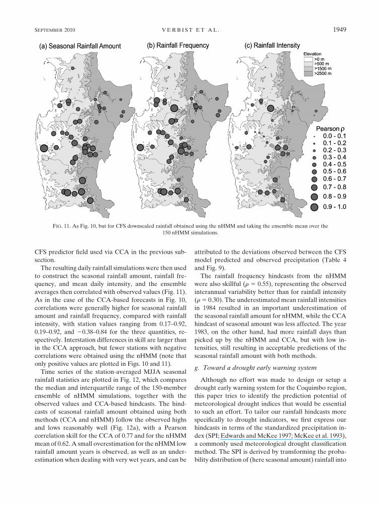
The resulting daily rainfall simulations were then used

to construct the seasonal rainfall amount, rainfall fre-

quency, and mean daily intensity, and the ensemble

averages then correlated with observed values (Fig. 11).

As in the case of the CCA-based forecasts in Fig. 10,

correlations were generally higher for seasonal rainfall

amount and rainfall frequency, compared with rainfall

intensity, with station values ranging from 0.17–0.92,

0.19–0.92, and 20.38–0.84 for the three quantities, re-

spectively. Interstation differences in skill are larger than

in the CCA approach, but fewer stations with negative

correlations were obtained using the nHMM (note that

only positive values are plotted in Figs. 10 and 11).

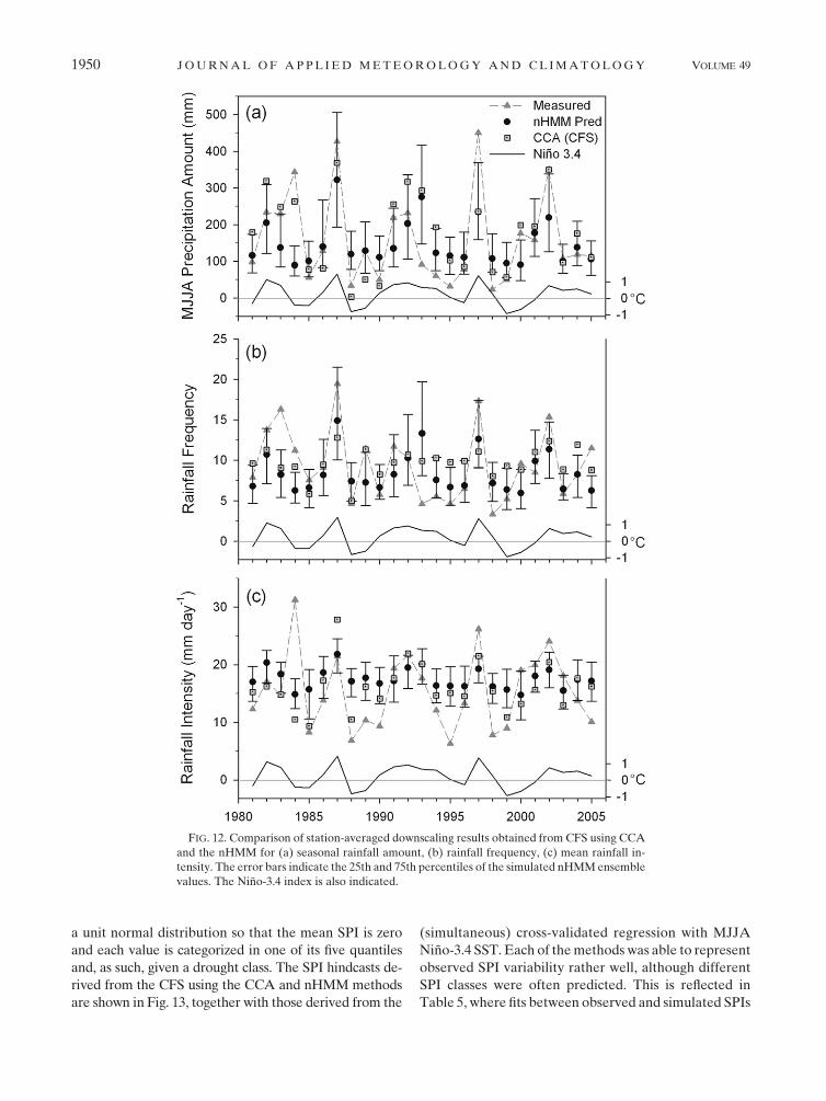
Time series of the station-averaged MJJA seasonal

rainfall statistics are plotted in Fig. 12, which compares

the median and interquartile range of the 150-member

ensemble of nHMM simulations, together with the

observed values and CCA-based hindcasts. The hind-

casts of seasonal rainfall amount obtained using both

methods (CCA and nHMM) follow the observed highs

and lows reasonably well (Fig. 12a), with a Pearson

correlation skill for the CCA of 0.77 and for the nHMM

mean of 0.62. A small overestimation for the nHMM low

rainfall amount years is observed, as well as an under-

estimation when dealing with very wet years, and can be

attributed to the deviations observed between the CFS

model predicted and observed precipitation (Table 4

and Fig. 9).

The rainfall frequency hindcasts from the nHMM

were also skillful (r 5 0.55), representing the observed

interannual variability better than for rainfall intensity

(r 5 0.30). The underestimated mean rainfall intensities

in 1984 resulted in an important underestimation of

the seasonal rainfall amount for nHMM, while the CCA

hindcast of seasonal amount was less affected. The year

1983, on the other hand, had more rainfall days than

picked up by the nHMM and CCA, but with low in-

tensities, still resulting in acceptable predictions of the

seasonal rainfall amount with both methods.

g. Toward a drought early warning system

Although no effort was made to design or setup a

drought early warning system for the Coquimbo region,

this paper tries to identify the prediction potential of

meteorological drought indices that would be essential

to such an effort. To tailor our rainfall hindcasts more

specifically to drought indicators, we first express our

hindcasts in terms of the standardized precipitation in-

dex (SPI; Edwards and McKee 1997; McKee et al. 1993),

a commonly used meteorological drought classification

method. The SPI is derived by transforming the proba-

bility distribution of (here seasonal amount) rainfall into

FIG. 11. As Fig. 10, but for CFS downscaled rainfall obtained using the nHMM and taking the ensemble mean over the

150 nHMM simulations.

SEPTEMBER 2010 V E R B I S T E T A L . 1949

a unit normal distribution so that the mean SPI is zero

and each value is categorized in one of its five quantiles

and, as such, given a drought class. The SPI hindcasts de-

rived from the CFS using the CCA and nHMM methods

are shown in Fig. 13, together with those derived from the

(simultaneous) cross-validated regression with MJJA

Nino-3.4 SST. Each of the methods was able to represent

observed SPI variability rather well, although different

SPI classes were often predicted. This is reflected in

Table 5, where fits between observed and simulated SPIs

FIG. 12. Comparison of station-averaged downscaling results obtained from CFS using CCA

and the nHMM for (a) seasonal rainfall amount, (b) rainfall frequency, (c) mean rainfall in-

tensity. The error bars indicate the 25th and 75th percentiles of the simulated nHMM ensemble

values. The Nino-3.4 index is also indicated.

1950 J O U R N A L O F A P P L I E D M E T E O R O L O G Y A N D C L I M A T O L O G Y VOLUME 49

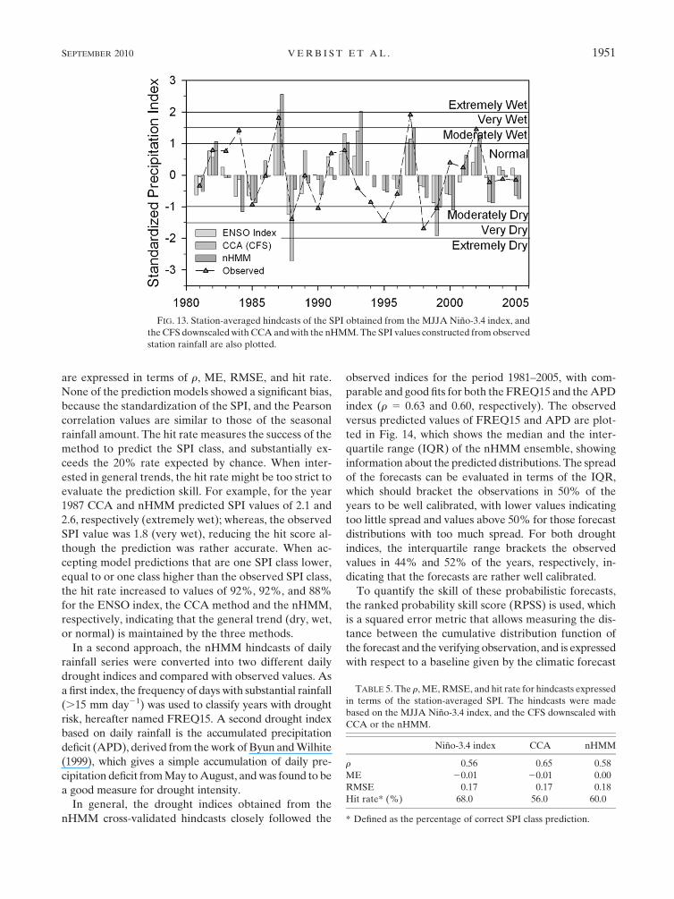
are expressed in terms of r, ME, RMSE, and hit rate.

None of the prediction models showed a significant bias,

because the standardization of the SPI, and the Pearson

correlation values are similar to those of the seasonal

rainfall amount. The hit rate measures the success of the

method to predict the SPI class, and substantially ex-

ceeds the 20% rate expected by chance. When inter-

ested in general trends, the hit rate might be too strict to

evaluate the prediction skill. For example, for the year

1987 CCA and nHMM predicted SPI values of 2.1 and

2.6, respectively (extremely wet); whereas, the observed

SPI value was 1.8 (very wet), reducing the hit score al-

though the prediction was rather accurate. When ac-

cepting model predictions that are one SPI class lower,

equal to or one class higher than the observed SPI class,

the hit rate increased to values of 92%, 92%, and 88%

for the ENSO index, the CCA method and the nHMM,

respectively, indicating that the general trend (dry, wet,

or normal) is maintained by the three methods.

In a second approach, the nHMM hindcasts of daily

rainfall series were converted into two different daily

drought indices and compared with observed values. As

a first index, the frequency of days with substantial rainfall

(.15 mm day21) was used to classify years with drought

risk, hereafter named FREQ15. A second drought index

based on daily rainfall is the accumulated precipitation

deficit (APD), derived from the work of Byun and Wilhite

(1999), which gives a simple accumulation of daily pre-

cipitation deficit from May to August, and was found to be

a good measure for drought intensity.

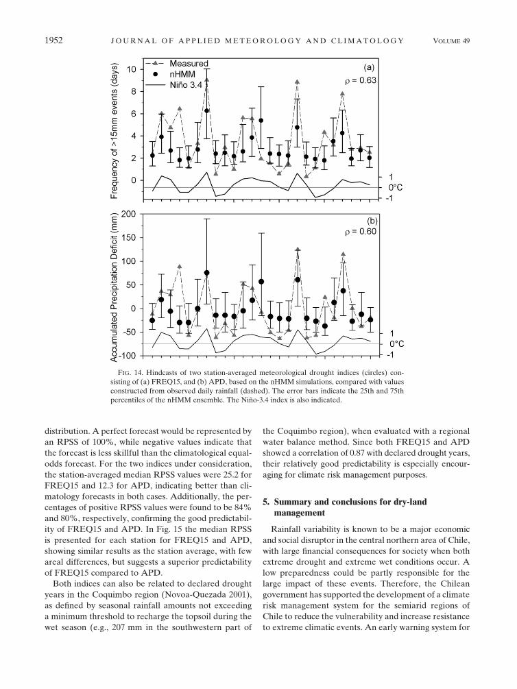
In general, the drought indices obtained from the

nHMM cross-validated hindcasts closely followed the

observed indices for the period 1981–2005, with com-

parable and good fits for both the FREQ15 and the APD

index (r 5 0.63 and 0.60, respectively). The observed

versus predicted values of FREQ15 and APD are plot-

ted in Fig. 14, which shows the median and the inter-

quartile range (IQR) of the nHMM ensemble, showing

information about the predicted distributions. The spread

of the forecasts can be evaluated in terms of the IQR,

which should bracket the observations in 50% of the

years to be well calibrated, with lower values indicating

too little spread and values above 50% for those forecast

distributions with too much spread. For both drought

indices, the interquartile range brackets the observed

values in 44% and 52% of the years, respectively, in-

dicating that the forecasts are rather well calibrated.

To quantify the skill of these probabilistic forecasts,

the ranked probability skill score (RPSS) is used, which

is a squared error metric that allows measuring the dis-

tance between the cumulative distribution function of

the forecast and the verifying observation, and is expressed

with respect to a baseline given by the climatic forecast

FIG. 13. Station-averaged hindcasts of the SPI obtained from the MJJA Nino-3.4 index, and

the CFS downscaled with CCA and with the nHMM. The SPI values constructed from observed

station rainfall are also plotted.

TABLE 5. The r, ME, RMSE, and hit rate for hindcasts expressed

in terms of the station-averaged SPI. The hindcasts were made

based on the MJJA Nino-3.4 index, and the CFS downscaled with

CCA or the nHMM.

Nino-3.4 index CCA nHMM

r 0.56 0.65 0.58

ME 20.01 20.01 0.00

RMSE 0.17 0.17 0.18

Hit rate* (%) 68.0 56.0 60.0

* Defined as the percentage of correct SPI class prediction.

SEPTEMBER 2010 V E R B I S T E T A L . 1951

distribution. A perfect forecast would be represented by

an RPSS of 100%, while negative values indicate that

the forecast is less skillful than the climatological equal-

odds forecast. For the two indices under consideration,

the station-averaged median RPSS values were 25.2 for

FREQ15 and 12.3 for APD, indicating better than cli-

matology forecasts in both cases. Additionally, the per-

centages of positive RPSS values were found to be 84%

and 80%, respectively, confirming the good predictabil-

ity of FREQ15 and APD. In Fig. 15 the median RPSS

is presented for each station for FREQ15 and APD,

showing similar results as the station average, with few

areal differences, but suggests a superior predictability

of FREQ15 compared to APD.

Both indices can also be related to declared drought

years in the Coquimbo region (Novoa-Quezada 2001),

as defined by seasonal rainfall amounts not exceeding

a minimum threshold to recharge the topsoil during the

wet season (e.g., 207 mm in the southwestern part of

the Coquimbo region), when evaluated with a regional

water balance method. Since both FREQ15 and APD

showed a correlation of 0.87 with declared drought years,

their relatively good predictability is especially encour-

aging for climate risk management purposes.

5. Summary and conclusions for dry-landmanagement

Rainfall variability is known to be a major economic

and social disruptor in the central northern area of Chile,

with large financial consequences for society when both

extreme drought and extreme wet conditions occur. A

low preparedness could be partly responsible for the

large impact of these events. Therefore, the Chilean

government has supported the development of a climate

risk management system for the semiarid regions of

Chile to reduce the vulnerability and increase resistance

to extreme climatic events. An early warning system for

FIG. 14. Hindcasts of two station-averaged meteorological drought indices (circles) con-

sisting of (a) FREQ15, and (b) APD, based on the nHMM simulations, compared with values

constructed from observed daily rainfall (dashed). The error bars indicate the 25th and 75th

percentiles of the nHMM ensemble. The Nino-3.4 index is also indicated.

1952 J O U R N A L O F A P P L I E D M E T E O R O L O G Y A N D C L I M A T O L O G Y VOLUME 49

droughts and floods would be an essential component of

such an approach, which requires estimation and pre-

diction of the rainfall characteristics relevant to drought

as a first step.

Winter rainfall characteristics in the Coquimbo region

of Chile were first investigated using daily rainfall re-

cords at 42 stations, with special attention to spatial and

temporal characteristics and the relationship with ENSO.

Seasonal rainfall amounts, daily rainfall frequencies,

and mean daily rainfall intensities all generally increase

southward and eastward toward the Andes (Fig. 3). An

analysis of the spatial correlations between stations

(Fig. 4) indicated large interstation correlations at the

daily time scale, particularly for rainfall amount. The

spatial coherence of rainfall amount and frequency was

found to increase substantially with temporal averaging,

suggesting the role of ENSO forcing at the seasonal scale.

Seasonal anomalies of mean daily rainfall intensity were

found to be less spatially coherent (Table 1), though their

coherence was larger than found by Moron et al. (2007)

for tropical rainfall, because of the frontal character of

rainfall in the region.

The spatiotemporal evolution of daily rainfall pat-

terns across the region was further elucidated in terms of

four rainfall states identified using a hidden Markov

model; these states consisted of dry and increasingly wet

conditions (Fig. 5), the latter associated with near-sta-

tionary trough in sea level pressure, centered to the

south and east of the region (Fig. 7). The daily sequences

of these states showed sporadic rainfall events with little

seasonality within the winter season (Fig. 6), while the

likelihood of an intense storm across the region (state 4)

was found to be strongly correlated with ENSO, thus

providing an interpretation in terms of daily weather for

the well-established seasonal rainfall relationship with

ENSO (Fig. 8).

FIG. 15. Median RPSS for hindcasts of (a) FREQ15 and (b) APD constructed from the nHMM simulations.

SEPTEMBER 2010 V E R B I S T E T A L . 1953

Seasonal predictability of rainfall characteristics was

explored firstly using a simple univariate index of ENSO;

this proved only to be well correlated for simultaneous

(May or MJJA) values of the index, and thus not useful

for prediction since lead times are insufficient for drought

prediction. Rainfall intensities were found not to be well

correlated. Predictability was further explored using a

GCM to forecast MJJA rainfall amounts. In our ap-

proach, the GCMs were initialized with 1 April climate

and/or oceanic conditions of each year 1981–2005, pre-

senting as such a real prediction with lead times up to four

months. Of three the GCMs considered (ECHAM-CA,

CCM-CA, and CFS), the highest skill and lowest bias was

obtained for the CFS model (Fig. 9; Table 4). The CFS

was then downscaled to represent local variability in sta-

tion data, using two different techniques. First, a canonical

correlation analysis (CCA) approach was developed

to map GCM forecasts of seasonal precipitation to sea-

sonal rainfall characteristics (seasonal rainfall amount,

daily rainfall frequency, mean daily rainfall intensity on

wet days) at each rainfall station. Second, a nonhomo-

geneous HMM was used to derive ensembles of sto-

chastic daily rainfall sequences at each station as a

function of GCM seasonally averaged rainfall; the sea-

sonal rainfall characteristics were then calculated from

these simulated daily sequences. For both downscaling

methods the skill for seasonal rainfall amount, fre-

quency, and mean daily intensity examined at the sta-

tion scale (Figs. 10–12) produced similar results. The

highest correlations with observations were found for

seasonal rainfall amount and rainfall frequency for

most measuring stations in the region, but low or neg-

ative correlations for rainfall intensity. These differ-

ences in skill are consistent with differences in the

spatial coherence of station-scale seasonal rainfall

anomalies (Table 1), with mean daily rainfall intensity

being less spatially coherent and thus less predictable

than seasonal amount and daily frequency (Moron et al.

2007).

Since the objective of the work is oriented toward

the development of a drought early warning system for

dry-land management, the (retrospective) forecasts of

rainfall were then tailored for drought prediction. Fol-

lowing the recommendations of the World Meteoro-

logical Organization (Declaration on Drought Indices,

11 December 2009, available online at http://www.unccd.

int/publicinfo/wmo/docs/LincolnDeclaration.pdf), the

standardized precipitation index, which was calculated

from seasonal rainfall amounts, was used as a proxy for

meteorological drought. The SPI was forecast with both

the CFS-CCA and CFS-nHMM approach and compared

with observed values, showing that the SPI was quite well

forecast by both methods (Fig. 13).

For some end-user applications, the seasonal-averaged

SPI may be too coarse, and drought indices based on daily

weather statistics may be more appropriate. Motivated

by the potential needs for dry-land management, the

nHMM was used to forecast two additional drought in-

dices based on daily rainfall statistics, showing high cor-

relations with observations and positive prediction skill

for all stations when using the frequency of occurrence of

days exceeding 15 mm day21 (FREQ15) and the accu-

mulated daily precipitation deficit (APD). While the

CCA could also be applied to these statistics, calculating

the appropriate predictand from daily observed data, the

daily rainfall sequences simulated by the nHMM have the

potential to be used in pasture and crop models that re-

quire daily weather sequences (e.g., Robertson et al. 2007).

Downscaled seasonal predictions of seasonal and daily

rainfall characteristics and related meteorological drought

indices have been shown feasible for the Coquimbo re-

gion. This could be regarded as an important step in the

development of a tailored climate risk management

system that should contribute to reduce climate uncer-

tainty in a region that is affected by high rainfall vari-

ability. The approach presented in this paper could

eventually be extended to forecast agricultural and/or

hydrological drought conditions, for which high spatial

and temporal resolution of downscaled predictions is

required, such as provided by the nHMM approach. The

methodology for predicting the nature of within-season

daily rainfall variability presented in this paper is also

likely to be successful in other regions where daily rainfall

variability can be linked to predictable large-scale cli-

matic patterns.

Acknowledgments. The authors thank the Chilean

Water Authority (Direccion General de Aguas) for pro-

viding the daily rainfall series of the Coquimbo region and

the three anonymous reviewers for their helpful com-

ments to improve the manuscript. This research was fun-

ded by the Flemish Government, Department of Sciences

and Innovation/Foreign Policy, the UNESCO Regional

Office for Science and Technology in Latin America and

the Caribbean, and by National Oceanic and Atmospheric

Administration Grant NA050AR4311004 and the U.S.

Department of Energy’s Climate Change Prediction Pro-

gram Grant DE-FG02-02ER63413.

REFERENCES

Aceituno, P., 1988: On the functioning of the Southern Oscillation

in the South American sector. Part I: Surface climate. Mon.

Wea. Rev., 116, 505–524.

——, M. Prieto, M. Solari, A. Martınez, G. Poveda, and M. Falvey,

2009: The 1877–1878 El Nino episode: associated impacts in

South America. Climatic Change, 92, 389–416.

1954 J O U R N A L O F A P P L I E D M E T E O R O L O G Y A N D C L I M A T O L O G Y VOLUME 49

Barnston, A. G., S. Li, S. J. Mason, D. G. DeWitt, L. Goddard, and

X. Gong, 2010: Verification of the first 11 years of IRI’s

seasonal climate forecasts. J. Appl. Meteor. Climatol., 49,

493–520.

Bellone, E., J. P. Hughes, and P. Guttorp, 2000: A hidden Markov

model for downscaling synoptic atmospheric patterns to pre-

cipitation amounts. Climate Res., 15, 1–12.

Byun, H.-R., and D. A. Wilhite, 1999: Objective quantification of

drought severity and duration. J. Climate, 12, 2747–2756.

Charles, S. P., B. C. Bates, P. H. Whetton, and J. P. Hughes, 1999:

Validation of downscaling models for changed climate con-

ditions: case study of southwestern Australia. Climate Res.,

12, 1–14.

Dai, A., I. Y. Fung, and A. D. del Genio, 1997: Surface global

observed land precipitations variations: 1900–1988. J. Climate,

10, 2943–2962.

Dempster, A. P., N. M. Laird, and D. R. Rubin, 1977: Maximum

likelihood from incomplete data via the EM algorithm. J. Roy.

Stat. Soc., 39B, 1–38.

Edwards, D. C., and T. B. McKee, 1997: Characteristics of 20th

century drought in the United States at multiple time scales.

Climatology Rep. 97–2, Department of Atmospheric Science,

Colorado State University, 155 pp.

Falvey, M., and R. Garreaud, 2007: Wintertime precipitation epi-

sodes in central Chile: Associated meteorological conditions

and orographic influences. J. Hydrometeor., 8, 171–193.

Forney, G. D., 1978: The Viterbi algorithm. Proc. IEEE, 61,

268–278.

FOSIS, 2008: Superando la sequıa. Plan especial para familias vul-

nerables de zonas rurales afectadas por la sequıa (Overcoming

the drought. Special plan for vulnerable families in rural areas

affected by drought). Fondo de Solidaridad e Inversion Social,

11 pp.

Garreaud, R. D., and D. S. Battisti, 1999: Interannual (ENSO)

and interdecadal (ENSO-like) variability in the Southern

Hemisphere tropospheric circulation. J. Climate, 12, 2113–

2122.

——, M. Vuille, R. Compagnucci, and J. Marengo, 2009: Present-

day South American climate. Palaeogeogr. Palaeoclimatol.

Palaeoecol., 281, 180–195.

Ghahramani, Z., 2001: An introduction to hidden Markov models

and Bayesian networks. Int. J. Pattern Recognit. Artif. Intell.,

15, 9–42.

Goddard, L., A. G. Barnston, and S. J. Mason, 2003: Evaluation of

the IRI’s ‘‘Net Assessment’’ seasonal climate forecasts: 1997–

2001. Bull. Amer. Meteor. Soc., 84, 1761–1781.

Hughes, J. P., and P. Guttorp, 1994: A class of stochastic models for

relating synoptic atmospheric patterns to regional hydrologic

phenomena. Water Resour. Res., 30, 1535–1546.

Hurrell, J. W., J. J. Hack, B. A. Boville, D. L. Williamson, and

J. T. Kiehl, 1998: The dynamical simulation of the NCAR

Community Climate Model version 3 (CCM3). J. Climate, 11,1207–1236.

Kalnay, E., and Coauthors, 1996: The NCEP/NCAR 40-Year Re-

analysis Project. Bull. Amer. Meteor. Soc., 77, 437–471.

Katz, R. W., and M. H. Glantz, 1986: Anatomy of a rainfall index.

Mon. Wea. Rev., 114, 764–771.

Kumar, A., Q. Zhang, J.-K. E. Schemm, M. Heureux, and K.-H. Seo,

2008: An Assessment of errors in the simulation of atmospheric

interannual variability in uncoupled AGCM simulations. J. Cli-

mate, 21, 2204–2217.

Li, S., and L. Goddard, 2005: Retrospective forecasts with the

ECHAM4.5 AGCM. IRI Tech. Rep. 05-02. IRI, 16 pp.

McKee, T. B., N. J. Doesken, and J. Kliest, 1993: The relationship

of drought frequency and duration to time scales. Proc. Eighth

Conf. on Applied Climatology, Anaheim, CA, Amer. Meteor.

Soc., 179–184.

MINAGRI, 2008: Advances in the execution of agricultural

emergencies: June 16, 2008 (in Spanish). Chilean Ministry of

Agriculture Rep., 42 pp.

Montecinos, A., and P. Aceituno, 2003: Seasonality of the ENSO-

related rainfall variability in central Chile and associated cir-

culation anomalies. J. Climate, 16, 281–296.

Moron, V., A. W. Robertson, M. N. Ward, and P. Camberlin, 2007:

Spatial coherence of tropical rainfall at the regional scale.

J. Climate, 20, 5244–5263.

New, M., M. Hulme, and P. Jones, 2000: Representing twentieth-

century space–time climate variability. Part II: Development

of 1901–96 monthly grids of terrestrial surface climate. J. Cli-

mate, 13, 2217–2238.

Novoa-Quezada, P., 2001: Determinacion de condicion de sequıa

por analisis de la variacion de humedad del horizonte radicular

usando el modelo de simulacion Hidrosuelo (Determining the

drought condition by analyzing the moisture variation in the

root zone using the Hidrosuelo simulation model). CONAF,

Vina del Mar, Chile, 44 pp.

Pittock, A. B., 1980: Patterns of climatic variation in Argentina and

Chile. Part I: Precipitation, 1931–1960. Mon. Wea. Rev., 108,

1347–1361.

Quinn, W., and V. Neal, 1983: Long-term variations in the South-

ern Oscillation, El Nino and the Chilean subtropical rainfall.

Fish Bull., 81, 363–374.

Ricciardulli, L., and P. D. Sardeshmukh, 2002: Local time- and

space scales of organized tropical deep convection. J. Climate,

15, 2775–2790.

Robertson, A. W., S. Kirshner, and P. J. Smyth, 2004: Downscaling

of daily rainfall occurrence over northeast Brazil using a hid-

den Markov model. J. Climate, 17, 4407–4424.

——, ——, P. C. Smyth, S. P. Charles, and B. C. Bates, 2006:

Subseasonal-to-interdecadal variability of the Australian mon-

soon over North Queensland. Quart. J. Roy. Meteor. Soc., 132,

519–542.

——, A. V. M. Ines, and J. W. Hansen, 2007: Downscaling of

seasonal precipitation for crop simulation. J. Appl. Meteor.

Climatol., 46, 677–693.

——, V. Moron, and Y. Swarinoto, 2009: Seasonal predictability of

daily rainfall statistics over Indramayu district, Indonesia. Int.

J. Climatol., 29, 1449–1462.

Roeckner, E., and Coauthors, 1996: The atmospheric general cir-

culation model ECHAM-4: Model description and simulation

of present-day climate. Max-Planck-Institut fur Meteorologie

Rep., 90 pp.

Rubin, M. J., 1955: An analysis of pressure anomalies in the

Southern Hemisphere. Notos, 4, 11–16.

Rutllant, J., and H. Fuenzalida, 1991: Synoptic aspects of the cen-

tral Chile rainfall variability associated with the Southern

Oscillation. Int. J. Climatol., 11, 63–76.

Saha, S., and Coauthors, 2006: The NCEP Climate Forecast Sys-

tem. J. Climate, 19, 3483–3517.

Smith, D. F., A. J. Gasiewski, D. L. Jackson, and G. A. Wick, 2005:

Spatial scales of tropical precipitation inferred from TRMM

microwave imager data. IEEE Trans. Geophys. Remote Sens.,

43, 1542–1551.

Tippett, M. K., M. Barlow, and B. Lyon, 2003: Statistical correction

of central southwest Asia winter precipitation simulations. Int.

J. Climatol., 23, 1421–1433.

SEPTEMBER 2010 V E R B I S T E T A L . 1955

Copyright of Journal of Applied Meteorology & Climatology is the property of American Meteorological

Society and its content may not be copied or emailed to multiple sites or posted to a listserv without the

copyright holder's express written permission. However, users may print, download, or email articles for

individual use.