Near-term Climate Change: Projections and Predictability - IPCC

953

11

This chapter should be cited as:Kirtman, B., S.B. Power, J.A. Adedoyin, G.J. Boer, R. Bojariu, I. Camilloni, F.J. Doblas-Reyes, A.M. Fiore, M. Kimoto, G.A. Meehl, M. Prather, A. Sarr, C. Schär, R. Sutton, G.J. van Oldenborgh, G. Vecchi and H.J. Wang, 2013: Near-term Climate Change: Projections and Predictability. In: Climate Change 2013: The Physical Science Basis. Contribution of Working Group I to the Fifth Assessment Report of the Intergovernmental Panel on Climate Change [Stocker, T.F., D. Qin, G.-K. Plattner, M. Tignor, S.K. Allen, J. Boschung, A. Nauels, Y. Xia, V. Bex and P.M. Midgley (eds.)]. Cambridge University Press, Cambridge, United Kingdom and New York, NY, USA.

Coordinating Lead Authors:Ben Kirtman (USA), Scott B. Power (Australia)

Lead Authors:Akintayo John Adedoyin (Botswana), George J. Boer (Canada), Roxana Bojariu (Romania), Ines Camilloni (Argentina), Francisco Doblas-Reyes (Spain), Arlene M. Fiore (USA), Masahide Kimoto (Japan), Gerald Meehl (USA), Michael Prather (USA), Abdoulaye Sarr (Senegal), Christoph Schär (Switzerland), Rowan Sutton (UK), Geert Jan van Oldenborgh (Netherlands), Gabriel Vecchi (USA), Hui-Jun Wang (China)

Contributing Authors:Nathaniel L. Bindoff (Australia), Philip Cameron-Smith (USA/New Zealand), Yoshimitsu Chikamoto (USA/Japan), Olivia Clifton (USA), Susanna Corti (Italy), Paul J. Durack (USA/Australia), Thierry Fichefet (Belgium), Javier García-Serrano (Spain), Paul Ginoux (USA), Lesley Gray (UK), Virginie Guemas (Spain/France), Ed Hawkins (UK), Marika Holland (USA), Christopher Holmes (USA), Johnna Infanti (USA), Masayoshi Ishii (Japan), Daniel Jacob (USA), Jasmin John (USA), Zbigniew Klimont (Austria/Poland), Thomas Knutson (USA), Gerhard Krinner (France), David Lawrence (USA), Jian Lu (USA/Canada), Daniel Murphy (USA), Vaishali Naik (USA/India), Alan Robock (USA), Luis Rodrigues (Spain/Brazil), Jan Sedláček (Switzerland), Andrew Slater (USA/Australia), Doug Smith (UK), David S. Stevenson (UK), Bart van den Hurk (Netherlands), Twan van Noije (Netherlands), Steve Vavrus (USA), Apostolos Voulgarakis (UK/Greece), Antje Weisheimer (UK/Germany), Oliver Wild (UK), Tim Woollings (UK), Paul Young (UK)

Review Editors:Pascale Delecluse (France), Tim Palmer (UK), Theodore Shepherd (Canada), Francis Zwiers (Canada)

Near-term Climate Change:Projections and Predictability

954

11

Table of Contents

Executive Summary ..................................................................... 955

11.1 Introduction ...................................................................... 958

Box 11.1: Climate Simulation, Projection, Predictability and Prediction ..................................................................... 959

11.2 Near-term Predictions .................................................... 962

11.2.1 Introduction .............................................................. 962

11.2.2 Climate Prediction on Decadal Time Scales ............... 965

11.2.3 Prediction Quality ..................................................... 966

11.3 Near-term Projections .................................................... 978

11.3.1 Introduction .............................................................. 978

11.3.2 Near-term Projected Changes in the Atmosphere and Land Surface ...................................................... 980

11.3.3 Near-term Projected Changes in the Ocean .............. 993

11.3.4 Near-term Projected Changes in the Cryosphere ....... 995

11.3.5 Projections for Atmospheric Composition and Air Quality to 2100 ................................................... 996

11.3.6 Additional Uncertainties in Projections of Near-term Climate................................................... 1004

Box 11.2: Ability of Climate Models to Simulate Observed Regional Trends ............................................... 1013

References ................................................................................ 1015

Frequently Asked Questions

FAQ 11.1 If You Cannot Predict the Weather Next Month, How Can You Predict Climate for the Coming Decade? .................................................... 964

FAQ 11.2 How Do Volcanic Eruptions Affect Climate and Our Ability to Predict Climate? .......................... 1008

955

Near-term Climate Change: Projections and Predictability Chapter 11

11

1 In this Report, the following summary terms are used to describe the available evidence: limited, medium, or robust; and for the degree of agreement: low, medium, or high. A level of confidence is expressed using five qualifiers: very low, low, medium, high, and very high, and typeset in italics, e.g., medium confidence. For a given evidence and agreement statement, different confidence levels can be assigned, but increasing levels of evidence and degrees of agreement are correlated with increasing confidence (see Section 1.4 and Box TS.1 for more details).

2 In this Report, the following terms have been used to indicate the assessed likelihood of an outcome or a result: Virtually certain 99–100% probability, Very likely 90–100%, Likely 66–100%, About as likely as not 33–66%, Unlikely 0–33%, Very unlikely 0–10%, Exceptionally unlikely 0–1%. Additional terms (Extremely likely: 95–100%, More likely than not >50–10 0%, and Extremely unlikely 0–5%) may also be used when appropriate. Assessed likelihood is typeset in italics, e.g., very likely (see Section 1.4 and Box TS.1 for more details).

Executive Summary

This chapter assesses the scientific literature describing expectations for near-term climate (present through mid-century). Unless otherwise stated, ‘near-term’ change and the projected changes below are for the period 2016–2035 relative to the reference period 1986–2005. Atmos-pheric composition (apart from CO2; see Chapter 12) and air quality projections through to 2100 are also assessed.

Decadal Prediction

The nonlinear and chaotic nature of the climate system imposes natu-ral limits on the extent to which skilful predictions of climate statistics may be made. Model-based ‘predictability’ studies, which probe these limits and investigate the physical mechanisms involved, support the potential for the skilful prediction of annual to decadal average tem-perature and, to a lesser extent precipitation.

Predictions for averages of temperature, over large regions of the planet and for the global mean, exhibit positive skill when verified against observations for forecast periods up to ten years (high confidence1). Predictions of precipitation over some land areas also exhibit positive skill. Decadal prediction is a new endeavour in climate science. The level of quality for climate predictions of annual to decadal average quantities is assessed from the past performance of initialized predictions and non-initialized simulations. {11.2.3, Figures 11.3 and 11.4}

In current results, observation-based initialization is the dominant con-tributor to the skill of predictions of annual mean temperature for the first few years and to the skill of predictions of the global mean surface temperature and the temperature over the North Atlantic, regions of the South Pacific and the tropical Indian Ocean for longer periods (high confidence). Beyond the first few years the skill for annual and multi-annual averages of temperature and precipitation is due mainly to the specified radiative forcing (high confidence). {Section 11.2.3, Figures 11.3 to 11.5}

Projected Changes in Radiative Forcing of Climate

For greenhouse gas (GHG) forcing, the new Representative Con-centration Pathway (RCP) scenarios are similar in magnitude and range to the AR4 Special Report on Emission Scenarios (SRES) scenarios in the near term, but for aerosol and ozone precursor emissions the RCPs are much lower than SRES by factors of 1.2 to 3. For these emissions the spread across RCPs by 2030 is much nar-rower than between scenarios that considered current legislation and

maximum technically feasible emission reductions (factors of 2). In the near term, the SRES Coupled Model Intercomparison Project Phase 3 (CMIP3) results, which did not incorporate current legislation on air pollutants, include up to three times more anthropogenic aerosols than RCP CMIP5 results (high confidence), and thus the CMIP5 global mean temperatures may be up to 0.2°C warmer than if forced with SRES aerosol scenarios (medium confidence). {10.3.1.1.3, Figure 10.4, 11.3.1.1, 11.3.5.1, 11.3.6.1, Figure 11.25, Tables AII.2.16 to AII.2.22 and AII.6.8}

Including uncertainties for the chemically reactive GHG meth-ane gives a range in concentration that is 30% wider than the spread in RCP concentrations used in CMIP5 models (likely2). By 2100 this range extends 520 ppb above RCP8.5 and 230 ppb below RCP2.6 (likely), reflecting uncertainties in emissions from agricultural, forestry and land use sources, in atmospheric lifetimes, and in chemical feedbacks, but not in natural emissions. {11.3.5}

Emission reductions aimed at decreasing local air pollution could have a near-term impact on climate (high confidence). Short-lived air pollutants have opposing effects: cooling from sulphate and nitrate; warming from black carbon (BC) aerosol, carbon monox-ide (CO) and methane (CH4). Anthropogenic CH4 emission reductions (25%) phased in by 2030 would decrease surface ozone and reduce warming averaged over 2036–2045 by about 0.2°C (medium confi-dence). Combined reductions of BC and co-emitted species (78%) on top of methane reductions (24%) would further reduce warming (low confidence), but uncertainties increase. {Section 7.6, Chapter 8, 11.3.6.1, Figure 11.24a, 8.7.2.2.2, Table AII.7.5a}

Projected Changes in Near-term Climate

Projections of near-term climate show modest sensitivity to alternative RCP scenarios on global scales, but aerosols are an important source of uncertainty on both global and regional scales. {11.3.1, 11.3.6.1}

Projected Changes in Near-term Temperature

The projected change in global mean surface air temperature will likely be in the range 0.3 to 0.7°C (medium confidence). This projection is valid for the four RCP scenarios and assumes there will be no major volcanic eruptions or secular changes in total solar irradiance before 2035. A future volcanic eruption similar to the 1991 eruption of Mt Pinatubo would cause a rapid drop in global mean surface air temperature of several tenths °C in the following year, with recovery over the next few years. Possible future changes in solar irradiance

956

Chapter 11 Near-term Climate Change: Projections and Predictability

11

could influence the rate at which global mean surface air temperature increases, but there is high confidence that this influence will be small in comparison to the influence of increasing concentrations of GHGs in the atmosphere. {11.3.6, Figure 11.25}

It is more likely than not that the mean global mean surface air temperature for the period 2016–2035 will be more than 1°C above the mean for 1850–1900, and very unlikely that it will be more than 1.5°C above the 1850–1900 mean (medium confidence). {11.3.6.3}

In the near term, differences in global mean surface air temper-ature change across RCP scenarios for a single climate model are typically smaller than differences between climate models under a single RCP scenario. In 2030, the CMIP5 ensemble median values differ by at most 0.2ºC between RCP scenarios, whereas the model spread (17 to 83% range) for each RCP is about 0.4ºC. The inter-scenario spread increases in time: by 2050 it is 0.8ºC, whereas the model spread for each scenario is only 0.6ºC. Regionally, the largest differences in surface air temperature between RCP2.6 and RCP8.5 are found in the Arctic. {11.3.2.1.1, 11.3.6.1, 11.3.6.3, Figure 11.24a,b, Table AII.7.5}

It is very likely that anthropogenic warming of surface air tem-perature will proceed more rapidly over land areas than over oceans, and that anthropogenic warming over the Arctic in winter will be greater than the global mean warming over the same period, consistent with the AR4. Relative to natural internal variability, near-term increases in seasonal mean and annual mean temperatures are expected to be larger in the tropics and subtropics than in mid-latitudes (high confidence). {11.3.2, Figures 11.10 and 11.11}

Projected Changes in the Water Cycle and Atmospheric Circulation

Zonal mean precipitation will very likely increase in high and some of the mid latitudes, and will more likely than not decrease in the subtropics. At more regional scales precipitation changes may be influenced by anthropogenic aerosol emissions and will be strongly influenced by natural internal variability. {11.3.2, Figures 11.12 and 11.13}

Increases in near-surface specific humidity over land are very likely. Increases in evaporation over land are likely in many regions. There is low confidence in projected changes in soil moisture and surface run off. {11.3.2, Figure 11.14}

It is likely that the descending branch of the Hadley Circulation and the Southern Hemisphere (SH) mid-latitude westerlies will shift poleward. It is likely that in austral summer the projected recov-ery of stratospheric ozone and increases in GHG concentrations will have counteracting impacts on the width of the Hadley Circulation and the meridional position of the SH storm track. Therefore, it is likely that in the near term the poleward expansion of the descending southern branch of the Hadley Circulation and the SH mid- latitude westerlies in austral summer will be less rapid than in recent decades. {11.3.2}

There is medium confidence in near-term projections of a north-ward shift of Northern Hemisphere storm tracks and westerlies. {11.3.2}

Projected Changes in the Ocean and Cryosphere

It is very likely that globally averaged surface and vertically averaged ocean temperatures will increase in the near term. It is likely that there will be increases in salinity in the tropical and (especially) subtropical Atlantic, and decreases in the western tropical Pacific over the next few decades. The Atlantic Meridional Overturning Circulation is likely to decline by 2050 (medium confidence). However, the rate and magnitude of weakening is very uncertain and, due to large internal variability, there may be decades when increases occur. {11.3.3}

It is very likely that there will be further shrinking and thinning of Arctic sea ice cover, and decreases of northern high-latitude spring time snow cover and near surface permafrost (see glos-sary) as global mean surface temperature rises. For high GHG emissions such as those corresponding to RCP8.5, a nearly ice-free Arctic Ocean (sea ice extent less than 1 × 106 km2 for at least 5 con-secutive years) in September is likely before mid-century (medium con-fidence). This assessment is based on a subset of models that most closely reproduce the climatological mean state and 1979 to 2012 trend of Arctic sea ice cover. There is low confidence in projected near-term decreases in the Antarctic sea ice extent and volume. {11.3.4}

Projected Changes in Extremes

In most land regions the frequency of warm days and warm nights will likely increase in the next decades, while that of cold days and cold nights will decrease. Models project near-term increases in the duration, intensity and spatial extent of heat waves and warm spells. These changes may proceed at a different rate than the mean warming. For example, several studies project that European high-percentile summer temperatures warm faster than mean temper-atures. {11.3.2.5.1, Figures 11.17 and 11.18}

The frequency and intensity of heavy precipitation events over land will likely increase on average in the near term. However, this trend will not be apparent in all regions because of natural vari-ability and possible influences of anthropogenic aerosols. {11.3.2.5.2, Figures 11.17 and 11.18}

There is low confidence in basin-scale projections of changes in the intensity and frequency of tropical cyclones (TCs) in all basins to the mid-21st century. This low confidence reflects the small number of studies exploring near-term TC activity, the differences across published projections of TC activity, and the large role for nat-ural variability and non-GHG forcing of TC activity up to the mid-21st century. There is low confidence in near-term projections for increased TC intensity in the North Atlantic, which is in part due to projected reductions in North Atlantic aerosols loading. {11.3.2.5.3}

957


11

Projected Changes in Air Quality

The range in projections of air quality (O3 and PM2.5 in near-surface air) is driven primarily by emissions (including CH4), rather than by physical climate change (medium confidence). The response of air quality to climate-driven changes is more uncertain than the response to emission-driven changes (high confidence). Globally, warming decreases background surface O3 (high confidence). High CH4 levels (RCP8.5, SRES A2) can offset this decrease, raising 2100 background surface O3 on average by about 8 ppb (25% of current levels) relative to scenarios with small CH4 chang-es (RCP4.5, RCP6.0) (high confidence). On a continental scale, pro-jected air pollution levels are lower under the new RCP scenarios than under the SRES scenarios because the SRES did not incorporate air quality legislation (high confidence). {11.3.5, 11.3.5.2; Figures 11.22 and 11.23ab, AII.4.2, AII.7.1–AII.7.4}

Observational and modelling evidence indicates that, all else being equal, locally higher surface temperatures in polluted regions will trigger regional feedbacks in chemistry and local emissions that will increase peak levels of O3 and PM2.5 (medium confidence). Local emissions combined with background levels and with meteorological conditions conducive to the formation and accu-mulation of pollution are known to produce extreme pollution epi-sodes on local and regional scales. There is low confidence in project-ing changes in meteorological blocking associated with these extreme episodes. For PM2.5, climate change may alter natural aerosol sources (wildfires, wind-lofted dust, biogenic precursors) as well as precipi-tation scavenging, but no confidence level is attached to the overall impact of climate change on PM2.5 distributions. {11.3.5, 11.3.5.2, Box 14.2}

958


11

11.1 Introduction

This chapter describes current scientific expectations for ‘near-term’ cli-mate. Here ‘near term’ refers to the period from the present to mid-cen-tury, during which the climate response to different emissions scenar-ios is generally similar. Greatest emphasis in this chapter is given to the period 2016–2035, though some information on projected changes before and after this period (up to mid-century) is also assessed. An assessment of the scientific literature relating to atmospheric compo-sition (except carbon dioxide (CO2), which is addressed in Chapter 12) and air quality for the near-term and beyond to 2100 is also provided.

This emphasis on near-term climate arises from (1) a recognition of its importance to decision makers in government and industry; (2) an increase in the international research effort aimed at improving our understanding of near-term climate; and (3) a recognition that near-term projections are generally less sensitive to differences between future emissions scenarios than are long-term projections. Climate prediction on seasonal to multi-annual time scales require accurate estimates of the initial climate state with less dependence on chang-es in external forcing3 over the period. On longer time scales climate projections rely on projections of external forcing with little reliance on the initial state of internal variability. Estimates of near-term climate depend partly on the committed change (caused by the inertia of the oceans as they respond to historical external forcing), the time evo-lution of internally generated climate variability and the future path of external forcing. Near-term climate is sensitive to rapid changes in some short-lived climate forcing agents (Jacobson and Streets, 2009; Wigley et al., 2009; UNEP and WMO, 2011; Shindell et al., 2012b).

The need for near-term climate information has spawned a new field of climate science: decadal climate prediction (Smith et al., 2007; Meehl et al., 2009b, 2013d). The Coupled Model Intercomparison Project Phase 5 (CMIP5) experimental protocol includes a sequence of near-term predictions (1 to 10 years) where observation-based information is used to initialize the models used to produce the forecasts. The goal is to exploit the predictability of internally generated climate variability as well as that of the externally forced component. The result depends on the ability of current models to reproduce the observed variability as well as on the accurate depiction of the initial state (see Box 11.1). Skilful multi-annual to decadal climate predictions (in the technical sense of ‘skilful’ as outlined in 11.2.3.2 and FAQ 11.1) are being pro-duced although technical challenges remain that need to be overcome in order to improve skill. These challenges are now being addressed by the scientific community.

Climate change experiments with models that do not depend on initial condition but on the history and projection of climate forcings (often referred to as ‘uninitialized’ or ‘non-initialized’ projections or simply as ‘projections’) are another component of CMIP5. Such projections have been the main focus of assessments of future climate in previ-ous IPCC assessments and are considered in Chapters 12 to 14. The main focus of attention in past assessments has been on the properties of projections for the late 21st century and beyond. Projections also

3 Seasonal-to-interannual predictions typically include the impact of external forcing.

provide valuable information on externally forced changes to near-term climate, however, and are an important source of information that complements information from the predictions. Projections are also assessed in this chapter.

The objectives of this chapter are to assess the state of the science con-cerning both near-term predictions and near-term projections. CMIP5 results are considered for the near term as are other published near-term predictions and projections. The chapter consists of four major assessments:

1. The scientific basis for near-term prediction as reflected in esti-mates of predictability (see Box 11.1), and the dynamical and physical mechanisms underpinning predictability, and the process-es that limit predictability (see Section 11.2).

2. The current state of knowledge in near-term prediction (see Sec-tion 11.2). Here the emphasis is placed on the results from the decadal (10-year) multi-model prediction experiments in the CMIP5 database.

3. The current state of knowledge in near-term projection (see Sec-tion 11.3). Here the emphasis is on what the climate in next few decades may look like relative to 1986–2005, based on near-term projections (i.e., the forced climatic response). The focus is on the ‘core’ near-term period (2016–2035), but some information prior to this period and out to mid-century is also discussed. A key issue is when, where and how the signal of externally forced climate change is expected to emerge from the background of natural cli-mate variability.

4. Projected changes in atmospheric composition and air quality, and their interactions with climate change during the near term and beyond, including new findings from the Atmospheric Chemistry and Climate Model Intercomparison (ACCMIP) initiative.

959


11

Box 11.1 | Climate Simulation, Projection, Predictability and Prediction

This section outlines some of the ideas and the terminology used in this chapter.

Internally generated and externally forced climate variabilityIt is useful for purposes of analysis and description to consider the pre-industrial climate system as being in a state of climatic equilib-rium with a fixed atmospheric composition and an unchanging Sun. In this idealized state, naturally occurring processes and interac-tions within the climate system give rise to ‘internally generated’ climate variability on many time scales (as discussed in Chapter 1). Variations in climate may also result due to features ‘external’ to this idealized system. Forcing factors, such as volcanic eruptions, solar variations, anthropogenic changes in the composition of the atmosphere, land use change etc., give rise to ‘externally forced’ climate variations. In this sense climate system variables such as annual mean temperatures (as in Box 11.1, Figure 1 for instance) may be characterized as a combination of externally forced and internally generated components with T(t) = Tf(t) + Ti(t). This separation of T, and other climate variables, into components is useful when analysing climate behaviour but does not, of course, mean that the climate system is linear or that externally forced and internally generated components do not interact.

Climate simulationA climate simulation is a model-based representation of the temporal behaviour of the climate system under specified external forcing and boundary conditions. The result is the modelled response to the imposed external forcing combined with internally generated var-iability. The thin yellow lines in Box 11.1, Figure 1 represent an ensemble of climate simulations begun from pre-industrial conditions with imposed historical external forcing. The imposed external conditions are the same for each ensemble member and differences among the simulations reflect differences in the evolutions of the internally generated component. Simulations are not intended to be forecasts of the observed evolution of the system (the black line in Box 11.1, Figure 1) but to be possible evolutions that are consistent with the external forcings.

In practice, and in Box 11.1, Figure 1, the forced component of the temperature variation is estimated by averaging over the different simulations of T(t) with Tf(t) the component that survives ensemble averaging (the red curve) while Ti(t) averages to near zero for a large enough ensemble. The spread among individual ensemble members (from these or pre-industrial simulations) and their behaviour with time provides some information on the statistics of the internally generated variability. (continued on next page)

Global mean temperatureIndividualforecasts

Forecaststart time

Ensemble mean simulation

Individualsimulations

Observed

Ensemble mean forecast

1960 1970 1980 1990 2000 2010

−0.5

0.0

0.5

1.0

Year

Tem

pera

ture

anom

aly

(°C

)

Box 11.1, Figure 1 | The evolution of observation-based global mean temperature T (the black line) as the difference from the 1986–2005 average together with an ensemble of externally forced simulations to 2005 and projections based on the RCP4.5 scenario thereafter (the yellow lines). The model-based estimate of the externally forced component Tf (the red line) is the average over the ensemble of simulations. To the extent that the red line correctly estimates the forced component, the difference between the black and red lines is the internally generated component Ti for global mean temperature. An ensemble of forecasts of global annual mean temperature, initialized in 1998, is plotted as thin purple lines and their average, the ensemble mean forecast, as the thick green line. The grey areas along the axis indicate the presence of external forcing associated with volcanoes.

960


11

Climate projectionA climate projection is a climate simulation that extends into the future based on a scenario of future external forcing. The simulations in Box 11.1, Figure 1 become climate projections for the period beyond 2005 where the results are based on the RCP4.5 forcing scenario (see Chapters 1 and 8 for a discussion of forcing scenarios).

Climate prediction, climate forecastA climate prediction or climate forecast is a statement about the future evolution of some aspect of the climate system encompassing both forced and internally generated components. Climate predictions do not attempt to forecast the actual day-to-day progression of the system but instead the evolution of some climate statistic such as seasonal, annual or decadal averages or extremes, which may be for a particular location, or a regional or global average. Climate predictions are often made with models that are the same as, or similar to, those used to produce climate simulations and projections (assessed in Chapter 9). A climate prediction typically proceeds by integrating the governing equations forward in time from observation-based initial conditions. A decadal climate prediction com-bines aspects of both a forced and an initial condition problem as illustrated in Box 11.1, Figure 2. At short time scales the evolution is largely dominated by the initial state while at longer time scales the influence of the initial conditions decreases and the importance of the forcing increases as illustrated in Box 11.1, Figure 4. Climate predictions may also be made using statistical methods which relate current to future conditions using statistical relationships derived from past system behaviour.

Because of the chaotic and nonlinear nature of the climate system small differences, in initial conditions or in the formulation of the forecast model, result in different evolutions of forecasts with time. This is illustrated in Box 11.1, Figure 1, which displays an ensemble of forecasts of global annual mean temperature (the thin purple lines) initiated in 1998. The individual forecasts are begun from slightly different initial conditions, which are observation-based estimates of the state of the climate system. The thick green line is the average of these forecasts and is an attempt to predict the most probable outcome and to maximize forecast skill. In this schematic example, the 1998 initial conditions for the forecasts are warmer than the average of the simulations. The individual and ensemble mean forecasts exhibit a decline in global temperature before beginning to rise again. In this case, initialization has resulted in more realistic values for the forecasts than for the corresponding simulation, at least for short lead times in the forecast. As the individual forecasts evolve they diverge from one another and begin to resemble the projection results.

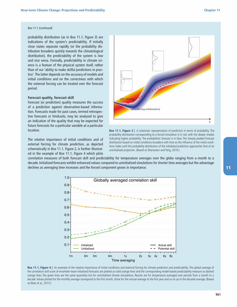
A probabilistic view of forecast behaviour is depicted schematically in Box 11.1, Figure 3. The probability distribution associated with the climate simulation of temperature evolves in response to external forcing. By contrast, the probability distribution associated with a climate forecast has a sharply peaked initial distribution representing the comparatively small uncertainty in the observation-based initial state. The forecast probability distribution broadens with time until, ultimately, it becomes indistinguishable from that of an uninitialized climate projection.

Climate predictabilityThe term ‘predictability’, as used here, indicates the extent to which even minor imperfections in the knowledge of the current state or of the representation of the system limits knowledge of subsequent states. The rate of separation or divergence of initially close states of the climate system with time (as for the light purple lines in Box 11.1, Figure 1), or the rate of displacement and broadening of its

Box 11.1 (continued)

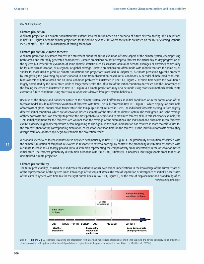
Box 11.1, Figure 2 | A schematic illustrating the progression from an initial-value based prediction at short time scales to the forced boundary-value problem of climate projection at long time scales. Decadal prediction occupies the middle ground between the two. (Based on Meehl et al., 2009b.)

(continued on next page)

961


11

probability distribution (as in Box 11.1, Figure 3) are indications of the system’s predictability. If initially close states separate rapidly (or the probability dis-tribution broadens quickly towards the climatological distribution), the predictability of the system is low and vice versa. Formally, predictability in climate sci-ence is a feature of the physical system itself, rather than of our ‘ability to make skilful predictions in prac-tice’. The latter depends on the accuracy of models and initial conditions and on the correctness with which the external forcing can be treated over the forecast period.

Forecast quality, forecast skillForecast (or prediction) quality measures the success of a prediction against observation-based informa-tion. Forecasts made for past cases, termed retrospec-tive forecasts or hindcasts, may be analysed to give an indication of the quality that may be expected for future forecasts for a particular variable at a particular location.

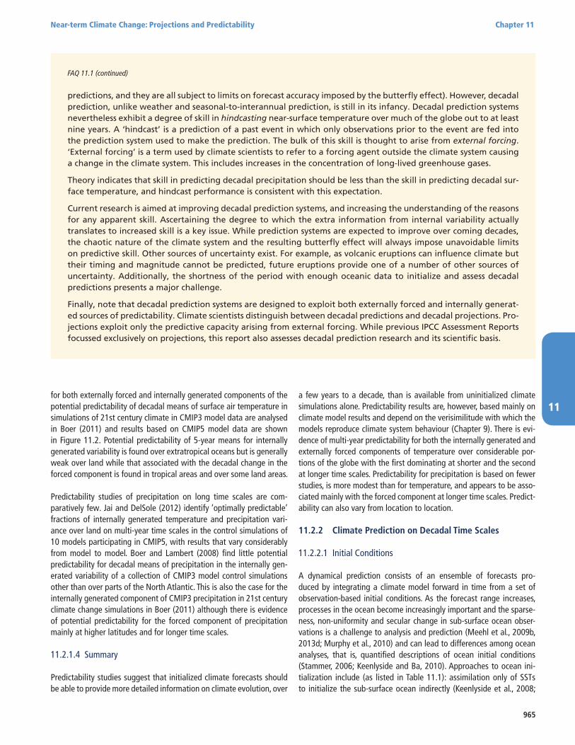
The relative importance of initial conditions and of external forcing for climate prediction, as depicted schematically in Box 11.1, Figure 2, is further illustrat-ed in the example of Box 11.1, Figure 4 which plots correlation measures of both forecast skill and predictability for temperature averages over the globe ranging from a month to a decade. Initialized forecasts exhibit enhanced values compared to uninitialized simulations for shorter time averages but the advantage declines as averaging time increases and the forced component grows in importance.


t

p[X | forcing,initialization]

p[X | forcing]

Box 11.1, Figure 3 | A schematic representation of prediction in terms of probability. The probability distribution corresponding to a forced simulation is in red, with the deeper shades indicating higher probability. The probabilistic forecast is in blue. The sharply peaked forecast distribution based on initial conditions broadens with time as the influence of the initial condi-tions fades until the probability distribution of the initialized prediction approaches that of an uninitialized projection. (Based on Branstator and Teng, 2010.)

Time averaging

Globally averaged correlation skill

1m 2m 3m 6m 1y 2y 3y 4y 6y 8y

0.1

0.2

0.3

0.4

0.5

0.6

0.7

0.8

0.9

1.0

InitializedUnitialized

Actual skillPotential skill

Box 11.1, Figure 4 | An example of the relative importance of initial conditions and external forcing for climate prediction and predictability. The global average of the correlation skill score of ensemble mean initialized forecasts are plotted as solid orange lines and the corresponding model-based predictability measure as dashed orange lines. The green lines are the same quantities but for uninitialized climate simulations. Results are for temperature averaged over periods from a month to a decade. Values plotted for the monthly average correspond to the first month, those for the annual average to the first year and so on up to the decadal average. (Based on Boer et al., 2013.)

962


11

11.2 Near-term Predictions

11.2.1 Introduction

11.2.1.1 Predictability Studies

The innate behaviour of the climate system imposes limits on the abil-ity to predict its evolution. Small differences in initial conditions, exter-nal forcing and/or in the representation of the behaviour of the system produce differences in results that limit useful prediction. Predictability studies estimate predictability limits for different variables and regions.

11.2.1.2 Prognostic Predictability Studies

Prognostic predictability studies analyse the behaviour of models inte-grated forward in time from perturbed initial conditions. The study of Griffies and Bryan (1997) is one of the earliest studies of the predict-ability of internally generated decadal variability in a coupled atmos-phere–ocean climate model. The study concentrates on the North Atlantic and the subsurface ocean temperature while the subsequent studies of Boer (2000) and Collins (2002) deal mainly with surface temperature. Long time scale temperature variability in the North Atlantic has received considerable attention together with its possible connection to the variability of the Atlantic Meridional Overturn-ing Circulation (AMOC) in predictability studies by Collins and Sinha (2003), Collins et al. (2006), Dunstone and Smith (2010), Dunstone et al. (2011), Grotzner et al. (1999), Hawkins and Sutton (2009), Latif et al. (2006, 2007), )Msadek et al. (2010), Persechino et al. (2012), Pohlmann et al. (2004, 2013), Swingedouw et al. (2013), and Teng et al. (2011). The predictability of the AMOC varies among models and, to some extent, with initial model states, ranging from several to 10 or more years. The predictability values are model-based and the realism of the simulated AMOC in the models cannot be easily judged in the absence of a sufficiently long record of observation-based AMOC values. Many predictability studies are based on perturbations to surface quantities but Sevellec and A. Fedorov (2012) and Zanna (2012) note that small perturbations to deep ocean quantities may also affect upper ocean values. The predictability of the North Atlantic sea surface temperature (SST) is typically weaker than that of the AMOC and the connection between the predictability of the AMOC, and the SST is inconsistent among models.

Prognostic predictability studies of the Pacific are less plentiful although Pacific Decadal Variability (PDV) mechanisms (including the Pacific Decadal Oscillation (PDO) and the Inter-decadal Pacific Oscilla-tion (IPO) have received considerable study (see Chapters 2 and 12). Power and Colman (2006) find predictability on multi-year time scales in SST and on decadal time-scales in the sub-surface ocean temper-ature in the off-equatorial South Pacific in their model. Power et al. (2006) find no evidence for the predictability of inter-decadal changes in the nature of El Niño-Southern Oscillation (ENSO) impacts on Aus-tralian rainfall. Sun and Wang (2006) suggest that some of the tem-perature variability linked to PDV can be predicted approximately 7 years in advance. Teng et al. (2011) investigate the predictability of the first two Empirical Orthogonal Functions (EOFs) of annual mean SST and upper ocean temperature identified with PDV and find predict-ability of the order of 6 to 10 years. Meehl et al. (2010) consider the

predictability of 19-year filtered Pacific SSTs in terms of low order EOFs and find predictability on these long time scales.

Hermanson and Sutton (2010) report that predictable signals in dif-ferent regions and for different variables may arise from differing ini-tial conditions and that ocean heat content is more predictable than atmospheric and surface variables. Branstator and Teng (2010) ana-lyse upper ocean temperatures, and some SSTs, for averages over the North Atlantic, North Pacific and the tropical Atlantic and Pacific in the National Center for Atmospheric Research (NCAR) model. Predictabil-ity associated with the initial state of the system decreases whereas that due to external forcing increases with time. The ‘cross-over’ time, when the two contributions are equal, is longer in extratropical (7 to 11 years) compared to tropical (2 years) regions and in the North Atlantic compared to the North Pacific. Boer et al. (2013) estimate surface air (rather than upper ocean) temperature predictability in the Canadian Centre for Climate Modelling and Analysis (CCCma) model and find a cross-over time (using a different measure) on the order of 3 years when averaged over the globe.

11.2.1.3 Diagnostic Predictability Studies

Diagnostic predictability studies are based on analyses of the observed record or the output of climate models. Because long data records are needed, diagnostic multi-annual to decadal predictability studies based on observational data are comparatively few. Newman (2007) and Alexander et al. (2008) develop multivariate empirical Linear Inverse Models (LIMs) from observation-based SSTs and find predictability for ENSO and PDV type patterns that are generally limited to the order of a year although exceeding this in some areas. Zanna (2012) develops a LIM based on Atlantic SSTs and infers the possibility of decadal scale predictability. Hoerling et al. (2011) appeal to forced climate change relative to the 1971–2000 period together with the statistics of natural variability to infer the potential for the prediction of temperature over North America for 2011–2020.

Tziperman et al. (2008) apply LIM-based methods to Geophysical Fluid Dynamics Laboratory (GFDL) model output, as do Hawkins and Sutton (2009) and Hawkins et al. (2011) to Hadley Centre model output and find predictability up to a decade or more for the AMOC and North Atlantic SST. Branstator et al. (2012) use analog and multivariate linear regression methods to quantify the predictability of the internally gen-erated component of upper ocean temperature in results from six cou-pled models. Results differ considerably across models but offer some areas of commonality. Basin-average estimates indicate predictability for up to a decade in the North Atlantic and somewhat less in the North Pacific. Branstator and Teng (2012) assess the predictability of both the internally generated and forced component of upper ocean temperature in results from 12 coupled models participating in CMIP5. They infer potential predictability from initializing the internally generated com-ponent for 5 years in the North Pacific and 9 years in the North Atlantic while the forced component dominates after 6.5 and 8 years in the two basins. Results vary among models, although with some agreement for internal component predictability in subpolar gyre regions.

Studies of ‘potential predictability’ take a number of forms but broad-ly assume that overall variability may be separated into a long time

963


11

scale component of interest and shorter time scale components that are unpredictable on these long time scales, written symbolically as s2

X = s2v + s2

e. The fraction p = s2v / s2

X is a measure of potentially predictable variance provided that hypothesis that s2

v is zero may be rejected. Small p indicates either a lack of long time scale variability or its smallness as a fraction of the total. Predictability is ‘potential’ in the sense that the existence of appreciable long time scale variability is not a direct indication that it may be skilfully predicted. There are

a number of approaches to estimating potential predictability each with its statistical difficulties (e.g., DelSole and Feng, 2013). At mul-ti-annual time scales the potential predictability of the internally gen-erated component of temperature is studied in Boer (2000), Collins (2002), Pohlmann et al. (2004), Power and Colman (2006) and, in a multi-model context, in Boer (2004) and Boer and Lambert (2008). Power and Colman (2006) report that potential predictability in the ocean tends to increase with latitude and depth. Multi-model results

Figure 11.1 | The potential predictability of 5-year means of temperature (lower), the contribution from the forced component (middle) and from the internally generated compo-nent (upper). These are multi-model results from CMIP5 RCP4.5 scenario simulations from 17 coupled climate models following the methodology of Boer (2011). The results apply to the early 21st century.

964


11


FAQ 11.1 | If You Cannot Predict the Weather Next Month, How Can You Predict Climate for the Coming Decade?

Although weather and climate are intertwined, they are in fact different things. Weather is defined as the state of the atmosphere at a given time and place, and can change from hour to hour and day to day. Climate, on the other hand, generally refers to the statistics of weather conditions over a decade or more.

An ability to predict future climate without the need to accurately predict weather is more commonplace that it might first seem. For example, at the end of spring, it can be accurately predicted that the average air temperature over the coming summer in Melbourne (for example) will very likely be higher than the average temperature during the most recent spring—even though the day-to-day weather during the coming summer cannot be predicted with accuracy beyond a week or so. This simple example illustrates that factors exist—in this case the seasonal cycle in solar radiation reaching the Southern Hemisphere—that can underpin skill in predicting changes in climate over a coming period that does not depend on accuracy in predicting weather over the same period.

The statistics of weather conditions used to define climate include long-term averages of air temperature and rainfall, as well as statistics of their variability, such as the standard deviation of year-to-year rainfall variability from the long-term average, or the frequency of days below 5°C. Averages of climate variables over long periods of time are called climatological averages. They can apply to individual months, seasons or the year as a whole. A climate prediction will address questions like: ‘How likely will it be that the average temperature during the coming summer will be higher than the long-term average of past summers?’ or: ‘How likely will it be that the next decade will be warmer than past decades?’ More specifically, a climate prediction might provide an answer to the question: ‘What is the probability that temperature (in China, for instance) averaged over the next ten years will exceed the temperature in China averaged over the past 30 years?’ Climate predictions do not provide forecasts of the detailed day-to-day evolution of future weather. Instead, they provide probabilities of long-term changes to the statistics of future climatic variables.

Weather forecasts, on the other hand, provide predictions of day-to-day weather for specific times in the future. They help to address questions like: ‘Will it rain tomorrow?’ Sometimes, weather forecasts are given in terms of prob-abilities. For example, the weather forecast might state that: ‘the likelihood of rainfall in Apia tomorrow is 75%’.

To make accurate weather predictions, forecasters need highly detailed information about the current state of the atmosphere. The chaotic nature of the atmosphere means that even the tiniest error in the depiction of ‘initial con-ditions’ typically leads to inaccurate forecasts beyond a week or so. This is the so-called ‘butterfly effect’.

Climate scientists do not attempt or claim to predict the detailed future evolution of the weather over coming seasons, years or decades. There is, on the other hand, a sound scientific basis for supposing that aspects of climate can be predicted, albeit imprecisely, despite the butterfly effect. For example, increases in long-lived atmospheric greenhouse gas concentrations tend to increase surface temperature in future decades. Thus, information from the past can and does help predict future climate.

Some types of naturally occurring so-called ‘internal’ variability can—in theory at least—extend the capacity to predict future climate. Internal climatic variability arises from natural instabilities in the climate system. If such variability includes or causes extensive, long-lived, upper ocean temperature anomalies, this will drive changes in the overlying atmosphere, both locally and remotely. The El Niño-Southern Oscillation phenomenon is probably the most famous example of this kind of internal variability. Variability linked to the El Niño-Southern Oscillation unfolds in a partially predictable fashion. The butterfly effect is present, but it takes longer to strongly influence some of the variability linked to the El Nino-Southern Oscillation.

Meteorological services and other agencies have exploited this. They have developed seasonal-to-interannual pre-diction systems that enable them to routinely predict seasonal climate anomalies with demonstrable predictive skill. The skill varies markedly from place to place and variable to variable. Skill tends to diminish the further the predic-tion delves into the future and in some locations there is no skill at all. ‘Skill’ is used here in its technical sense: it is a measure of how much greater the accuracy of a prediction is, compared with the accuracy of some typically simple prediction method like assuming that recent anomalies will persist during the period being predicted.

Weather, seasonal-to-interannual and decadal prediction systems are similar in many ways (e.g., they all incorpo-rate the same mathematical equations for the atmosphere, they all need to specify initial conditions to kick-start


965


11for both externally forced and internally generated components of the potential predictability of decadal means of surface air temperature in simulations of 21st century climate in CMIP3 model data are analysed in Boer (2011) and results based on CMIP5 model data are shown in Figure 11.2. Potential predictability of 5-year means for internally generated variability is found over extratropical oceans but is generally weak over land while that associated with the decadal change in the forced component is found in tropical areas and over some land areas.

Predictability studies of precipitation on long time scales are com-paratively few. Jai and DelSole (2012) identify ‘optimally predictable’ fractions of internally generated temperature and precipitation vari-ance over land on multi-year time scales in the control simulations of 10 models participating in CMIP5, with results that vary considerably from model to model. Boer and Lambert (2008) find little potential predictability for decadal means of precipitation in the internally gen-erated variability of a collection of CMIP3 model control simulations other than over parts of the North Atlantic. This is also the case for the internally generated component of CMIP3 precipitation in 21st century climate change simulations in Boer (2011) although there is evidence of potential predictability for the forced component of precipitation mainly at higher latitudes and for longer time scales.

11.2.1.4 Summary

Predictability studies suggest that initialized climate forecasts should be able to provide more detailed information on climate evolution, over

a few years to a decade, than is available from uninitialized climate simulations alone. Predictability results are, however, based mainly on climate model results and depend on the verisimilitude with which the models reproduce climate system behaviour (Chapter 9). There is evi-dence of multi-year predictability for both the internally generated and externally forced components of temperature over considerable por-tions of the globe with the first dominating at shorter and the second at longer time scales. Predictability for precipitation is based on fewer studies, is more modest than for temperature, and appears to be asso-ciated mainly with the forced component at longer time scales. Predict-ability can also vary from location to location.

11.2.2 Climate Prediction on Decadal Time Scales

11.2.2.1 Initial Conditions

A dynamical prediction consists of an ensemble of forecasts pro-duced by integrating a climate model forward in time from a set of observation-based initial conditions. As the forecast range increases, processes in the ocean become increasingly important and the sparse-ness, non-uniformity and secular change in sub-surface ocean obser-vations is a challenge to analysis and prediction (Meehl et al., 2009b, 2013d; Murphy et al., 2010) and can lead to differences among ocean analyses, that is, quantified descriptions of ocean initial conditions (Stammer, 2006; Keenlyside and Ba, 2010). Approaches to ocean ini-tialization include (as listed in Table 11.1): assimilation only of SSTs to initialize the sub-surface ocean indirectly (Keenlyside et al., 2008;

FAQ 11.1 (continued)

predictions, and they are all subject to limits on forecast accuracy imposed by the butterfly effect). However, decadal prediction, unlike weather and seasonal-to-interannual prediction, is still in its infancy. Decadal prediction systems nevertheless exhibit a degree of skill in hindcasting near-surface temperature over much of the globe out to at least nine years. A ‘hindcast’ is a prediction of a past event in which only observations prior to the event are fed into the prediction system used to make the prediction. The bulk of this skill is thought to arise from external forcing. ‘External forcing’ is a term used by climate scientists to refer to a forcing agent outside the climate system causing a change in the climate system. This includes increases in the concentration of long-lived greenhouse gases.

Theory indicates that skill in predicting decadal precipitation should be less than the skill in predicting decadal sur-face temperature, and hindcast performance is consistent with this expectation.

Current research is aimed at improving decadal prediction systems, and increasing the understanding of the reasons for any apparent skill. Ascertaining the degree to which the extra information from internal variability actually translates to increased skill is a key issue. While prediction systems are expected to improve over coming decades, the chaotic nature of the climate system and the resulting butterfly effect will always impose unavoidable limits on predictive skill. Other sources of uncertainty exist. For example, as volcanic eruptions can influence climate but their timing and magnitude cannot be predicted, future eruptions provide one of a number of other sources of uncertainty. Additionally, the shortness of the period with enough oceanic data to initialize and assess decadal predictions presents a major challenge.

Finally, note that decadal prediction systems are designed to exploit both externally forced and internally generat-ed sources of predictability. Climate scientists distinguish between decadal predictions and decadal projections. Pro-jections exploit only the predictive capacity arising from external forcing. While previous IPCC Assessment Reports focussed exclusively on projections, this report also assesses decadal prediction research and its scientific basis.

966


11

Dunstone, 2010; Swingedouw et al., 2013); the forcing of the ocean model with atmospheric observations (e.g., Du et al., 2012; Matei et al., 2012b; Yeager et al., 2012) and more sophisticated alternatives based on fully coupled data assimilation schemes (e.g., Zhang et al., 2007a; Sugiura et al., 2009).

Dunstone and Smith (2010) and Zhang et al. (2010a) found an expected improvement in skill when sub-surface information was used as part of the initialization. Assimilation of atmospheric data, on the other hand, is expected to have little impact after the first few months (Balmaseda and Anderson, 2009). The initialization of sea ice, snow cover, frozen soil and soil moisture can potentially contribute to seasonal and sub-seasonal skill (e.g., Koster et al., 2010; Toyoda et al., 2011; Chevallier and Salas-Melia, 2012; Paolino et al., 2012), although an assessment of their benefit at longer time scales has not yet been determined.

11.2.2.2 Ensemble Generation

An ensemble can be generated in many different ways and a wide range of methods have been explored in seasonal prediction (e.g., Stockdale et al., 1998; Stan and Kirtman, 2008) but not yet fully investigated for decadal prediction (Corti et al., 2012). Methods being investigated include adding random perturbations to initial conditions, using atmos-pheric states displaced in time, using parallel assimilation runs (Doblas-Reyes et al., 2011; Du et al., 2012) and perturbing ocean initial condi-tions (Zhang et al., 2007a; Mochizuki et al., 2010). Perturbations leading to rapidly growing modes, common in weather forecasting, have also been investigated (Kleeman et al., 2003; Vikhliaev et al., 2007; Hawkins and Sutton, 2009, 2011; Du et al., 2012). The uncertainty associated with the limitations of a model’s representation of the climate system may be partially represented by perturbed physics (Stainforth et al., 2005; Murphy et al., 2007) or stochastic physics (Berner et al., 2008), and applied to multi-annual and decadal predictions (Doblas-Reyes et al., 2009; Smith et al., 2010). Weisheimer et al. (2011) compare these three approaches in a seasonal prediction context.

The multi-model approach, which is used widely and most common-ly, combines ensembles of predictions from a collection of models, thereby increasing the sampling of both initial conditions and model properties. Multi-model approaches are used across time scales rang-ing from seasonal–interannual (e.g., DEMETER; Palmer et al. (2004), to seasonal-decadal (e.g., Weisheimer et al., 2011; van Oldenborgh et al., 2012), in climate change simulation (e.g., IPCC, 2007, Chapter 10; Meehl et al., 2007b) and in the ENSEMBLES and CMIP5-based decadal predictions assessed in Section 11.2.3. A problem with the multi-model approach is tha inter-dependence of the climate models used in current forecast systems (Power et al. 2012; Knutti et al. 2013) is expected to lead to co-dependence of forecast error.

11.2.3 Prediction Quality

11.2.3.1 Decadal Prediction Experiments

Decadal predictions for specific variables can be made by exploiting empirical relationships based on past observations and expected phys-ical relationships. Predictions of North Pacific Ocean temperatures have been achieved using prior wind stress observations (Schneider

and Miller, 2001). Both global and regional predictions of surface temperature have been made based on projected changes in external forcing and the observed state of the natural variability at the start date (Lean and Rind, 2009; Krueger and von Storch, 2011; Ho et al., 2012a; Newman, 2013). Some of these forecast systems are also used as benchmarks to compare with the dynamical systems under devel-opment. Comparisons (Newman (2013) have shown that there is simi-larity in the temperature skill between a linear inverse method and the CMIP5 hindcasts, pointing at a similarity in their sources of skill. In the future, the combination of information from empirical and dynamical predictions might be explored to provide a unified and more skilful source of information.

Evidence for skilful interannual to decadal temperatures using dynam-ical models forced only by previous and projected changes in anthro-pogenic greenhouse gases (GHGs) and aerosols and natural varia-tions in volcanic aerosols and solar irradiance is reported by Lee et al. (2006b), Räisänen and Ruokolainen (2006) and Laepple et al. (2008). Some attempts to predict the 10-year climate over regions have been done using this approach, and include assessments of the role of the internal decadal variability (Hoerling et al., 2011). To be clear, in the context of this report these studies are viewed as projections because no attempt is made to use observational estimates for the initial con-ditions. Essentially, an uninitialized prediction is synonymous with a projection. These projections or uninitialized predictions are referred to synonymously in the literature as ‘NoInit,’ or ‘NoAssim’, referring to the fact that no assimilated observations are used for the specification of the initial conditions.

Additional skill can be realized by initializing the models with obser-vations in order to predict the evolution of the internally generated component and to correct the model’s response to previously imposed forcing (Smith et al., 2010; Fyfe et al., 2011; Kharin et al., 2012; Smith et al., 2012). Again, to be clear, the assessment provided here distin-guishes between predictions in which attempts are made to initialize the models with observations, and projections. See Box 11.1 and FAQ 11.1 for further details.

The ENSEMBLES project (van Oldenborgh et al., 2012), for example, has conducted a multi-model decadal retrospective prediction study, and the Coupled Model Intercomparison Project phase 5 (CMIP5) pro-posed a coordinated experiment that focuses on decadal, or near-term, climate prediction (Meehl et al., 2009b; Taylor et al., 2012). Prior to these initiatives, several pioneering attempts at initialized decadal pre-diction were made (Pierce et al., 2004; Smith et al., 2007; Troccoli and Palmer, 2007; Keenlyside et al., 2008; Pohlmann et al., 2009; Mochizuki et al., 2010). Results from the CMIP5 coordinated experiment (Taylor et al., 2012) are the basis for the assessment reported here.

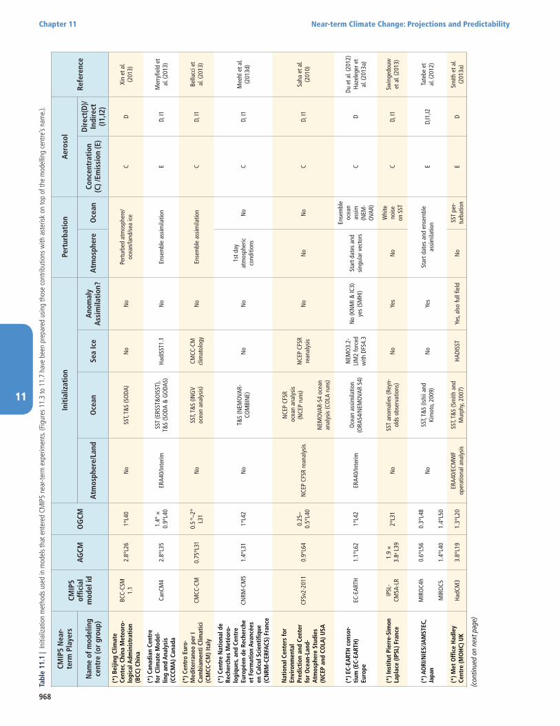
Because the practice of decadal prediction is in its infancy, details of how to initialize the models included in the CMIP5 near-term exper-iment were left to the discretion of the modelling groups and are described in Meehl et al. (2013d) and Table 11.1. In CMIP5 experi-ments, volcanic aerosol and solar cycle variability are prescribed along the integration using observation-based values up to 2005, and assuming a climatological 11-year solar cycle and a background vol-canic aerosol load in the future. These forcings are shared with CMIP5

967


11

1960 1970 1980 1990 2000 2010

1918

2021

(ºC

)

SST 60ºS-60ºN CMIP5 Init / rm=12months

MRI-CGCM3MIROC4hMIROC5 CMCC-CM

EC-Earth2.3HadCM3 CNRM-CM5

IPSL-CM5GFDL-CM2

CanCM4MPI-M

1960 1970 1980 1990 2000 2010

Ano

mal

y (°

C)

MRI-CGCM3MIROC4hMIROC5 CMCC-CM

EC-Earth2.3HadCM3 CNRM-CM5

IPSL-CM5GFDL-CM2

CanCM4MPI-M

-0.5

0.5

0.0

ERSSTHadISST

ERSSTHadISST

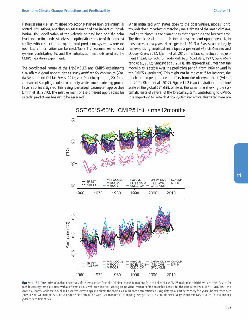
Figure 11.2 | Time series of global mean sea surface temperature from the (a) direct model output and (b) anomalies of the CMIP5 multi-model initialized hindcasts. Results for each forecast system are plotted with a different colour, with each line representing an individual member of the ensemble. Results for the start dates 1961, 1971, 1981, 1991 and 2001 are shown, while the model and observed climatologies to obtain the anomalies in (b) have been estimated using data from start dates every five years. The reference data (ERSST) is drawn in black. All time series have been smoothed with a 24-month centred moving average that filters out the seasonal cycle and removes data for the first and last years of each time series.

historical runs (i.e., unintialized projections) started from pre-industrial control simulations, enabling an assessment of the impact of initial-ization. The specification of the volcanic aerosol load and the solar irradiance in the hindcasts gives an optimistic estimate of the forecast quality with respect to an operational prediction system, where no such future information can be used. Table 11.1 summarizes forecast systems contributing to, and the initialization methods used in, the CMIP5 near-term experiment.

The coordinated nature of the ENSEMBLES and CMIP5 experiments also offers a good opportunity to study multi-model ensembles (Gar-cia-Serrano and Doblas-Reyes, 2012; van Oldenborgh et al., 2012) as a means of sampling model uncertainty while some modelling groups have also investigated this using perturbed parameter approaches (Smith et al., 2010). The relative merit of the different approaches for decadal predictions has yet to be assessed.

When initialized with states close to the observations, models ‘drift’ towards their imperfect climatology (an estimate of the mean climate), leading to biases in the simulations that depend on the forecast time. The time scale of the drift in the atmosphere and upper ocean is, in most cases, a few years (Hazeleger et al., 2013a). Biases can be largely removed using empirical techniques a posteriori (Garcia-Serrano and Doblas-Reyes, 2012; Kharin et al., 2012). The bias correction or adjust-ment linearly corrects for model drift (e.g., Stockdale, 1997; Garcia-Ser-rano et al., 2012; Gangstø et al., 2013). The approach assumes that the model bias is stable over the prediction period (from 1960 onward in the CMIP5 experiment). This might not be the case if, for instance, the predicted temperature trend differs from the observed trend (Fyfe et al., 2011; Kharin et al., 2012). Figure 11.2 is an illustration of the time scale of the global SST drift, while at the same time showing the sys-tematic error of several of the forecast systems contributing to CMIP5. It is important to note that the systematic errors illustrated here are

968


11

Tabl

e 11

.1 |

Initi

aliza

tion

met

hods

use

d in

mod

els

that

ent

ered

CM

IP5

near

-term

exp

erim

ents

. (Fi

gure

s 11

.3 to

11.

7 ha

ve b

een

prep

ared

usin

g th

ose

cont

ribut

ions

with

ast

erisk

on

top

of th

e m

odel

ling

cent

re’s

nam

e.).

(con

tinue

d on

nex

t pag

e)

CMIP

5 N

ear-

term

Pla

yers

CMIP

5 of

ficia

l m

odel

idAG

CMO

GCM

Init

ializ

atio

nPe

rtur

bati

onA

eros

ol

Refe

renc

eN

ame

of m

odel

ing

cent

re (o

r gr

oup)

Atm

osph

ere/

Land

Oce

anSe

a Ic

eA

nom

aly

Ass

imila

tion

?A

tmos

pher

eO

cean

Conc

entr

atio

n (C

) /Em

issi

on (E

)

Dir

ect(

D)/

Indi

rect

(I1,I2

)

(*) B

eijin

g Cl

imat

e Ce

nter

, Chi

na M

eteo

ro-

logi

cal A

dmin

istr

atio

n(B

CC) C

hina

BCC-

CSM

1.1

2.8°

L26

1°L4

0N

oSS

T, T&

S (S

ODA

)N

oN

oPe

rtur

bed

atm

osph

ere/

ocea

n/la

nd/s

ea ic

eC

DXi

n et

al.

(201

3)

(*) C

anad

ian

Cent

re

for

Clim

ate

Mod

el-

ling

and

Ana

lysi

s(C

CCM

A) C

anad

a

CanC

M4

2.8°

L35

1.4°

×

0.9°

L40

ERA4

0/In

terim

SST

(ERS

ST&

OIS

ST),

T&S

(SO

DA &

GO

DAS)

HadI

SST1

.1N

oEn

sem

ble

assi

mila

tion

ED,

I1M

erry

field

et

al. (

2013

)

(*) C

entr

o Eu

ro-

Med

iter

rane

o pe

r I

Cam

biam

enti

Clim

atic

i(C

MCC

-CM

) Ita

ly

CMCC

-CM

0.75

°L31

0.5 °–

2°L3

1N

oSS

T, T&

S (IN

GV

ocea

n an

alys

is)

CMCC

-CM

cl

imat

olog

yN

oEn

sem

ble

assi

mila

tion

CD,

I1Be

llucc

i et

al. (

2013

)

(*) C

entr

e N

atio

nal d

e Re

cher

ches

Met

éoro

-lo

giqu

es, a

nd C

entr

e Eu

ropé

en d

e Re

cher

che

et F

orm

atio

n Av

ancé

es

en C

alcu

l Sci

enti

fique

(C

NRM

-CER

FACS

) Fra

nce

CNRM

-CM

51.

4°L3

11°

L42

No

T&S

(NEM

OVA

R-CO

MBI

NE)

No

No

1st d

ay

atm

osph

eric

co

nditi

ons

No

CD,

I1M

eehl

et a

l. (2

013d

)

Nat

iona

l Cen

ters

for

Envi

ronm

enta

lPr

edic

tion

and

Cen

ter

for

Oce

an-L

and-

Atm

osph

ere

Stud

ies

(NCE

P an

d CO

LA) U

SA

CFSv

2-20

110.

9°L6

40.

25–

0.5°

L40

NCE

P CF

SR re

anal

ysis

NCE

P CF

SR o

cean

ana

lysi

s (N

CEP

runs

)N

CEP

CFSR

re

anal

ysis

No

No

No

CD,

I1Sa

ha e

t al.

(201

0)

NEM

OVA

R-S4

oce

an

anal

ysis

(CO

LA ru

ns)

(*) E

C-EA

RTH

con

sor-

tium

(EC-

EART

H)

Euro

peEC

-EAR

TH1.

1°L6

21°

L42

ERA4

0/In

terim

Oce

an a

ssim

ilatio

n(O

RAS4

/NEM

OVA

R S4

)

NEM

O3.

2-LI

M2

forc

ed

with

DFS

4.3

No

(KN

MI &

IC3)

ye

s (S

MHI

)St

art d

ates

and

si

ngul

ar v

ecto

rs

Ense

mbl

e oc

ean

assi

m

(NEM

-O

VAR)

CD

Du e

t al.

(201

2)Ha

zele

ger e

t al

. (20

13a)

(*) I

nsti

tut

Pier

re-S

imon

La

plac

e (IP

SL) F

ranc

eIP

SL-

CM5A

-LR

1.9

×

3.8o L

392°

L31

No

SST

anom

alie

s (R

eyn-

olds

obs

erva

tions

)N

oYe

sN

oW

hite

no

ise

on S

STC

D, I1

Swin

gedo

uw

et a

l. (2

013)

(*) A

ORI

/NIE

S/JA

MST

EC,

Japa

n

MIR

OC4

h0.

6°L5

60.

3°L4

8N

oSS

T, T&

S (Is

hii a

nd

Kim

oto,

200

9)N

oYe

sSt

art d

ates

and

ens

embl

e as

sim

ilatio

nE

D,I1

,I2Ta

tebe

et

al. (

2012

)

MIR

OC5

1.4°

L40

1.4°

L50

(*) M

et O

ffice

Had

ley

Ce

ntre

(MO

HC)

UK

HadC

M3

3.8°

L19

1.3°

L20

ERA4

0/EC

MW

F op

erat

iona

l ana

lysi

sSS

T, T&

S (S

mith

and

M

urph

y, 2

007)

HADI

SST

Yes,

also

full

field

No

SST

per-

turb

atio

nE

DSm

ith e

t al.

(201

3a)

969


11

CMIP

5 N

ear-

term

Pla

yers

CMIP

5 O

ffici

al

Mod

el ID

AGCM

OG

CM

Init

ializ

atio

nPe

rtur

bati

onA

eros

ol

Refe

renc

eN

ame

of M

odel

ing

Cent

re (o

r gr

oup)

Atm

osph

ere/

Land

Oce

anSe

a Ic

eA

nom

aly

Ass

imila

tion

?A

tmos

pher

eO

cean

Conc

entr

atio

n (C

) /Em

issi

on (E

)

Dir

ect(

D)/

Indi

rect

(I1,I2

)

(*) M

ax P

lanc

k In

stit

ute

for

Met

eoro

logy

(M

PI-M

) Ger

man

y

MPI

-ESM

-LR

1.9°

L47

1.5°

L40

No

T&S

from

forc

ed O

GCM

No

Yes

1-da

y la

gged

CD

Mat

ei e

t al.

(201

2b)

MPI

-ESM

-MR

1.9°

L95

0.4°

L40

(*) M

eteo

rolo

gica

l Re

sear

ch In

stit

ute

(MRI

) Jap

anM

RI-C

GCM

31.

1°L4

81°

L51

No

SST,

T&S

(Ishi

i and

Ki

mot

o, 2

009)

No

Yes

Star

t dat

es a

nd e

nsem

ble

assi

mila

tion

ED,

I1,I2

Tate

be e

t al

. (20

12)

Glo

bal M

odel

ing

and

Ass

imila

tion

O

ffice

, (N

ASA

) USA

GEO

S-5

2.5 °×

2o

L72

1°L5

0M

ERRA

T&S

from

oce

an a

ssim

i-la

tion

(GEO

S iO

DAS)

GEO

S iO

DAS

rean

alys

isN

oTw

o-si

ded

bree

ding

met

hod

ED

(*) N

atio

nal C

ente

r fo

r Atm

osph

eric

Re

sear

ch (N

CAR)

USA

CCSM

41.

3°L2

61.

0°L6

0N

o

Oce

an a

ssim

ila-

tion

(PO

PDAR

T)

Ice

stat

e fro

m fo

rced

oc

ean-

ice

GCM

(str

ong

salin

ity

rest

orin

g fo

r PO

PDAR

T)

No

Sing

le a

tm fr

om

AMIP

run

Ense

mbl

e as

sim

ila-

tion

ED

Oce

an s

tate

from

fo

rced

oce

an-ic

e G

CM

Stag

gere

d at

m

star

t dat

es fr

om

unin

itial

ized

run

Sing

le

mem

ber

ocea

n

Yeag

er e

t al

. (20

12)

(*) G

eoph

ysic

al F

luid

D

ynam

ics

Labo

ra-

tory

(GFD

L) U

SA

GFD

L-CM

2.1

2.5°

L24

1°L5

0N

CEP

rean

alys

isO

cean

obs

erva

tions

of 3

-D T

& S

& S

STN

oN

oCo

uple

d En

KFC

DYa

ng e

t al.

(201

3)

LASG

, Ins

titu

te o

f Atm

o-sp

heri

c Ph

ysic

s, Ch

ines

e A

cade

my

of S

cien

ces;

an

d CE

SS, T

sing

hua

Uni

vers

ity

Chin

a

FGO

ALS-

g22.

8°L2

61°

L30

No

SST,

T&S

(Ishi

i et

al.,

200

6)N

oN

oA

sim

plifi

ed s

chem

e of

3DV

arC

D, I1

Wan

g et

al.

(201

3)

LASG

, Ins

titu

te o

f Atm

o-sp

heri

c Ph

ysic

s, Ch

ines

e A

cade

my

of S

cien

ces

Chin

a, T

sing

hua

Uni

vers

ity

Chin

a

FGO

ALS-

s22.

8°L2

61°

L30

No

T&S

(EN

3_v2

a)N

oYe

sIn

crem

enta

l Ana

lysi

s U

pdat

es (I

AU) s

chem

eC

DW

u an

d Zh

ou

(201

2)

(Tab

le 1

1.1

cont

inue

d)

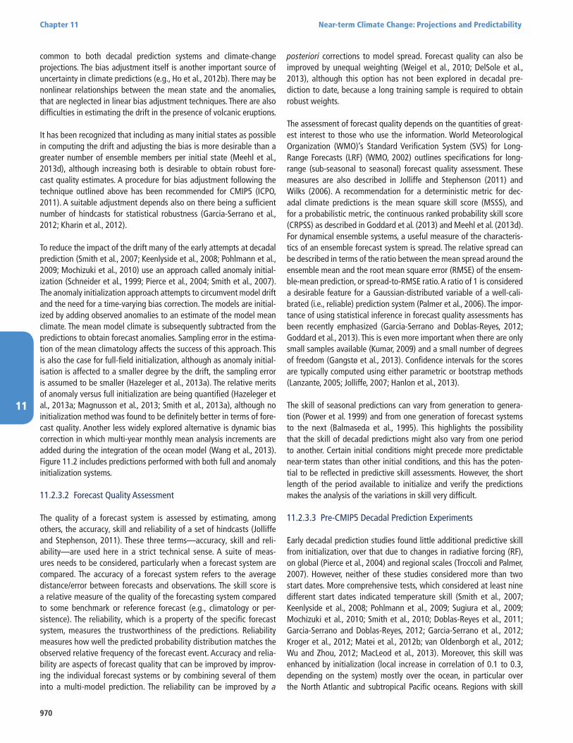
970


11

common to both decadal prediction systems and climate-change projections. The bias adjustment itself is another important source of uncertainty in climate predictions (e.g., Ho et al., 2012b). There may be nonlinear relationships between the mean state and the anomalies, that are neglected in linear bias adjustment techniques. There are also difficulties in estimating the drift in the presence of volcanic eruptions.

It has been recognized that including as many initial states as possible in computing the drift and adjusting the bias is more desirable than a greater number of ensemble members per initial state (Meehl et al., 2013d), although increasing both is desirable to obtain robust fore-cast quality estimates. A procedure for bias adjustment following the technique outlined above has been recommended for CMIP5 (ICPO, 2011). A suitable adjustment depends also on there being a sufficient number of hindcasts for statistical robustness (Garcia-Serrano et al., 2012; Kharin et al., 2012).

To reduce the impact of the drift many of the early attempts at decadal prediction (Smith et al., 2007; Keenlyside et al., 2008; Pohlmann et al., 2009; Mochizuki et al., 2010) use an approach called anomaly initial-ization (Schneider et al., 1999; Pierce et al., 2004; Smith et al., 2007). The anomaly initialization approach attempts to circumvent model drift and the need for a time-varying bias correction. The models are initial-ized by adding observed anomalies to an estimate of the model mean climate. The mean model climate is subsequently subtracted from the predictions to obtain forecast anomalies. Sampling error in the estima-tion of the mean climatology affects the success of this approach. This is also the case for full-field initialization, although as anomaly initial-isation is affected to a smaller degree by the drift, the sampling error is assumed to be smaller (Hazeleger et al., 2013a). The relative merits of anomaly versus full initialization are being quantified (Hazeleger et al., 2013a; Magnusson et al., 2013; Smith et al., 2013a), although no initialization method was found to be definitely better in terms of fore-cast quality. Another less widely explored alternative is dynamic bias correction in which multi-year monthly mean analysis increments are added during the integration of the ocean model (Wang et al., 2013). Figure 11.2 includes predictions performed with both full and anomaly initialization systems.

11.2.3.2 Forecast Quality Assessment

The quality of a forecast system is assessed by estimating, among others, the accuracy, skill and reliability of a set of hindcasts (Jolliffe and Stephenson, 2011). These three terms—accuracy, skill and reli-ability—are used here in a strict technical sense. A suite of meas-ures needs to be considered, particularly when a forecast system are compared. The accuracy of a forecast system refers to the average distance/error between forecasts and observations. The skill score is a relative measure of the quality of the forecasting system compared to some benchmark or reference forecast (e.g., climatology or per-sistence). The reliability, which is a property of the specific forecast system, measures the trustworthiness of the predictions. Reliability measures how well the predicted probability distribution matches the observed relative frequency of the forecast event. Accuracy and relia-bility are aspects of forecast quality that can be improved by improv-ing the individual forecast systems or by combining several of them into a multi-model prediction. The reliability can be improved by a

posteriori corrections to model spread. Forecast quality can also be improved by unequal weighting (Weigel et al., 2010; DelSole et al., 2013), although this option has not been explored in decadal pre-diction to date, because a long training sample is required to obtain robust weights.

The assessment of forecast quality depends on the quantities of great-est interest to those who use the information. World Meteorological Organization (WMO)’s Standard Verification System (SVS) for Long- Range Forecasts (LRF) (WMO, 2002) outlines specifications for long-range (sub-seasonal to seasonal) forecast quality assessment. These measures are also described in Jolliffe and Stephenson (2011) and Wilks (2006). A recommendation for a deterministic metric for dec-adal climate predictions is the mean square skill score (MSSS), and for a probabilistic metric, the continuous ranked probability skill score (CRPSS) as described in Goddard et al. (2013) and Meehl et al. (2013d). For dynamical ensemble systems, a useful measure of the characteris-tics of an ensemble forecast system is spread. The relative spread can be described in terms of the ratio between the mean spread around the ensemble mean and the root mean square error (RMSE) of the ensem-ble-mean prediction, or spread-to-RMSE ratio. A ratio of 1 is considered a desirable feature for a Gaussian-distributed variable of a well-cali-brated (i.e., reliable) prediction system (Palmer et al., 2006). The impor-tance of using statistical inference in forecast quality assessments has been recently emphasized (Garcia-Serrano and Doblas-Reyes, 2012; Goddard et al., 2013). This is even more important when there are only small samples available (Kumar, 2009) and a small number of degrees of freedom (Gangstø et al., 2013). Confidence intervals for the scores are typically computed using either parametric or bootstrap methods (Lanzante, 2005; Jolliffe, 2007; Hanlon et al., 2013).

The skill of seasonal predictions can vary from generation to genera-tion (Power et al. 1999) and from one generation of forecast systems to the next (Balmaseda et al., 1995). This highlights the possibility that the skill of decadal predictions might also vary from one period to another. Certain initial conditions might precede more predictable near-term states than other initial conditions, and this has the poten-tial to be reflected in predictive skill assessments. However, the short length of the period available to initialize and verify the predictions makes the analysis of the variations in skill very difficult.

11.2.3.3 Pre-CMIP5 Decadal Prediction Experiments

Early decadal prediction studies found little additional predictive skill from initialization, over that due to changes in radiative forcing (RF), on global (Pierce et al., 2004) and regional scales (Troccoli and Palmer, 2007). However, neither of these studies considered more than two start dates. More comprehensive tests, which considered at least nine different start dates indicated temperature skill (Smith et al., 2007; Keenlyside et al., 2008; Pohlmann et al., 2009; Sugiura et al., 2009; Mochizuki et al., 2010; Smith et al., 2010; Doblas-Reyes et al., 2011; Garcia-Serrano and Doblas-Reyes, 2012; Garcia-Serrano et al., 2012; Kroger et al., 2012; Matei et al., 2012b; van Oldenborgh et al., 2012; Wu and Zhou, 2012; MacLeod et al., 2013). Moreover, this skill was enhanced by initialization (local increase in correlation of 0.1 to 0.3, depending on the system) mostly over the ocean, in particular over the North Atlantic and subtropical Pacific oceans. Regions with skill

971


11

improvements from initialization for precipitation are small and rarely statistically significant (Goddard et al., 2013).

11.2.3.4 Coupled Model Intercomparison Project Phase 5 Decadal Prediction Experiments

Indices of global mean temperature, the Atlantic Multi-decadal Varia-bility (AMV; (Trenberth and Shea, 2006)) and the Inter-decadal Pacific Oscillation (IPO; Power et al., 1999) or Pacific Decadal Oscillation (PDO) are used as benchmarks to assess the ability of decadal forecast sys-tems to predict multi-annual averages of climate variability (Kim et al., 2012; van Oldenborgh et al., 2012; Doblas-Reyes et al., 2013; Goddard et al., 2013; see also Figure 11.3). Initialized predictions of global mean surface air temperature (GMST) for the following year are now being performed in almost-real time (Folland et al., 2013).

Non-initialized predictions (or projections) of the global mean tem-perature are statistically significantly skilful for most of the forecast ranges considered (high confidence), due to the almost monotonic increase in temperature, pointing to the importance of the time-var-ying RF (Murphy et al., 2010; Kim et al., 2012). This leads to a high (above 0.9) correlation of the ensemble mean prediction that varies very as a function of forecast lead time. This holds whether the changes in the external forcing (i.e., changes in natural and/or anthropogenic atmospheric composition) are specified (i.e., CMIP5) or are projected (ENSEMBLES). The skill of the multi-annual global mean surface tem-perature improves with initialization, although this is mainly evidenced when the accuracy is measured in terms of the RMSE (Doblas-Reyes et al., 2013). An improved prediction of global mean surface temperature is evidenced by the closer fit of the initialized predictions during the 21st century (Figure 11.3; Meehl and Teng, 2012; Doblas-Reyes et al., 2013; Guemas et al., 2013; Box 9.2). The impact of initialization is seen as a better representation of the phase of the internal variability, in particular in increasing the upper ocean heat content (Meehl et al., 2011) and in terms of a correction of the model’s forced response.

The AMV (Chapter 14) has important impacts on temperature and pre-cipitation over land (Li and Bates, 2007; Li et al., 2008; Semenov et al., 2010). The AMV index shows a large fraction of its variability on dec-adal time scales and has multi-year predictability (Murphy et al., 2010; Garcia-Serrano and Doblas-Reyes, 2012). The AMV has been connected to multi-decadal variability of Atlantic tropical cyclones (Goldenberg et al., 2001; Zhang and Delworth, 2006; Smith et al., 2010; Dunstone et al., 2011). Figure 11.3 shows that the CMIP5 multi-model ensemble mean has skill on multi-annual time scales, the skill being generally larger than for the single-model forecast systems (Garcia-Serrano and Doblas-Reyes, 2012; Kim et al., 2012). The skill of the AMV index improves with initialization (high confidence) for the early forecast ranges. In particu-lar, the RMSE is substantially reduced (indicating improved skill) with initialization for the AMV. The positive correlation of the non-initialized AMV predictions is consistent with the view that part of the recent variability is due to external forcings (Evan et al., 2009; Ottera et al., 2010; Chang et al., 2011; Booth et al., 2012; Garcia-Serrano et al., 2012; Terray, 2012; Villarini and Vecchi, 2012; Doblas-Reyes et al., 2013).

Pacific decadal variability is associated with potentially important climate impacts, including rainfall over America, Asia, Africa and Aus-

tralia (Power et al., 1999; Deser et al., 2004; Seager et al., 2008; Zhu et al., 2011; Li et al., 2012). The combination of Pacific and Atlantic variability and climate change is an important driver of multi-decadal USA drought (McCabe et al., 2004; Burgman et al., 2010) including key events like the American dustbowl of the 1930s (Schubert et al., 2004). van Oldenborgh et al. (2012) reported weak skill in hindcasting the IPO in the ENSEMBLES multi-model. Doblas-Reyes et al. (2013) show that the ensemble-mean skill of the ENSEMBLES multi-model IPO is not statistically significant at the 95% level and shows no clear impact of the initialization, in agreement with the predictability study of Meehl et al. (2010). On the other hand, case studies suggest that there might be some initial states that can produce skill in predicting IPO-related decadal variability for some time periods (e.g., Chikamoto et al., 2012b; Meehl and Arblaster, 2012; Meehl et al., 2013a).

The higher AMV and global mean temperature skill of the CMIP5 pre-dictions with respect to the ENSEMBLES hindcasts (van Oldenborgh et al., 2012; Goddard et al., 2013) might be partly due to the CMIP5 multi-model using specified instead of projected aerosol loading (espe-cially the volcanic aerosol) and solar irradiance variations during the simulations. As these forcings cannot be specified in a real forecast set-ting, ENSEMBLES offers an estimate of the skill closer to what could be expected from a real-time forecast system such as the one described in (Smith et al., 2013a). The use of correct forcings nevertheless allows a more powerful test of the effect of initialization on the ability of models to reproduce past observations.

Near-term prediction systems have significant skill for temperature over large regions (Figure 11.4), especially over the oceans (Smith et al., 2010; Doblas-Reyes et al., 2011; Kim et al., 2012; Matei et al., 2012b; van Oldenborgh et al., 2012; Hanlon et al., 2013). It has been shown that a large part of the skill corresponds to the correct representation of the long-term trend (high confidence) as the skill decreases substan-tially after an estimate of the long-term trend is removed from both the predictions and the observations (e.g., Corti et al., 2012; van Old-enborgh et al., 2012; MacLeod et al., 2013). Robust skill increase due to initialization (Figure 11.4) is limited to areas of the North Atlantic, the Indian Ocean and the southeast Pacific (high confidence) (Doblas-Reyes et al., 2013), in agreement with previous results (Pohlmann et al., 2009; Smith et al., 2010; Mochizuki et al., 2012) and predictability estimates (Branstator and Teng, 2012). Similar results have been found in several individual forecast systems (e.g., Muller et al., 2012; Bel-lucci et al., 2013). However, the impact of initialization on the skill in those regions, though robust (as shown by the agreement between the different CMIP5 systems) is small and not statistically significant with 90% confidence.

The improvement in retrospective North Atlantic variability predictions from initialization (Smith et al., 2010; Dunstone et al., 2011; Garcia-Serrano et al., 2012; Hazeleger et al., 2013b) suggests that internal var-iability was important to North Atlantic variability during the past few decades. However, the interpretation of the results is complicated by the fact that the impact on skill varies slightly with the forecast quality measure used (Figure 11.3; Doblas-Reyes et al., 2013). This has been attributed to, among other things, the different impact of the predicted local trends on the scores used (Goddard et al., 2013). Skill in hindcasts of subpolar Atlantic temperature, which is evident in Figure 11.4, is

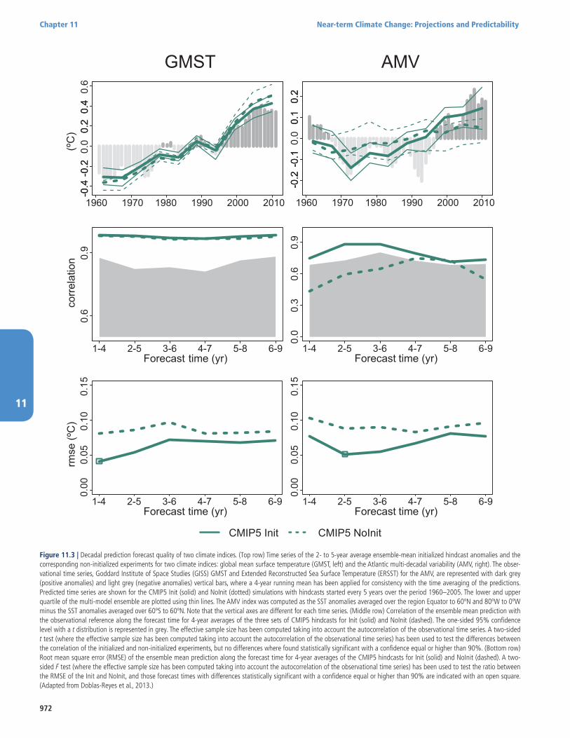
972


11

GMST AMV

CMIP5 Init CMIP5 NoInit

1960 1970 1980 1990 2000 2010

(ºC

)-0

.4-0

.4-0

.2-0

.20.

20.

20.

40.

4

1960 1970 1980 1990 2000 2010

-0.2

-0.1

0.1

0.2

-0.2

-0.1

0.1

0.2

0.0

Forecast time (yr)1-4 2-5 3-6 4-7 5-8 6-9

corr

elat

ion

0.6

0.9

rmse

(ºC

)

Forecast time (yr)

0.00

1-4 2-5 3-6 4-7 5-8 6-9

0.15

0.10

0.05

Forecast time (yr)

0.0

0.3

0.6

0.9

1-4 2-5 3-6 4-7 5-8 6-9

Forecast time (yr)

0.00

1-4 2-5 3-6 4-7 5-8 6-9

0.15

0.10

0.05

0.0

0.6

Figure 11.3 | Decadal prediction forecast quality of two climate indices. (Top row) Time series of the 2- to 5-year average ensemble-mean initialized hindcast anomalies and the corresponding non-initialized experiments for two climate indices: global mean surface temperature (GMST, left) and the Atlantic multi-decadal variability (AMV, right). The obser-vational time series, Goddard Institute of Space Studies (GISS) GMST and Extended Reconstructed Sea Surface Temperature (ERSST) for the AMV, are represented with dark grey (positive anomalies) and light grey (negative anomalies) vertical bars, where a 4-year running mean has been applied for consistency with the time averaging of the predictions. Predicted time series are shown for the CMIP5 Init (solid) and NoInit (dotted) simulations with hindcasts started every 5 years over the period 1960–2005. The lower and upper quartile of the multi-model ensemble are plotted using thin lines. The AMV index was computed as the SST anomalies averaged over the region Equator to 60ºN and 80ºW to 0ºW minus the SST anomalies averaged over 60ºS to 60ºN. Note that the vertical axes are different for each time series. (Middle row) Correlation of the ensemble mean prediction with the observational reference along the forecast time for 4-year averages of the three sets of CMIP5 hindcasts for Init (solid) and NoInit (dashed). The one-sided 95% confidence level with a t distribution is represented in grey. The effective sample size has been computed taking into account the autocorrelation of the observational time series. A two-sided t test (where the effective sample size has been computed taking into account the autocorrelation of the observational time series) has been used to test the differences between the correlation of the initialized and non-initialized experiments, but no differences where found statistically significant with a confidence equal or higher than 90%. (Bottom row) Root mean square error (RMSE) of the ensemble mean prediction along the forecast time for 4-year averages of the CMIP5 hindcasts for Init (solid) and NoInit (dashed). A two-sided F test (where the effective sample size has been computed taking into account the autocorrelation of the observational time series) has been used to test the ratio between the RMSE of the Init and NoInit, and those forecast times with differences statistically significant with a confidence equal or higher than 90% are indicated with an open square. (Adapted from Doblas-Reyes et al., 2013.)

973


11

improved more by initialization than is skill in hindcasting sub-tropical Atlantic temperature (Garcia-Serrano et al., 2012; Robson et al., 2012; Hazeleger et al., 2013b). This is relevant because the sub-polar branch of the AMV is a source of skill for multi-year North Atlantic tropical storm frequency predictions (Smith et al., 2010). Vecchi et al. (2013) argued that the nominal improvement in multi-year forecasts of North Atlantic hurricane frequency was mainly due to persistence.

Sugiura et al. (2009) reported on skill in hindcasting the Pacific Decadal Oscillation (PDO) in their forecast system. They ascribed the skill to the interplay between Rossby waves and a clockwise propagation of ocean heat content anomalies along the Kuroshio–Oyashio extension and subtropical subduction pathway. However, as Figure 11.4 shows, the Pacific Ocean has the lowest temperature skill overall, with no con-sistent impact from initialization. The central North Pacific has zero or negative skill, which may be due to the relatively large amplitude of the interannual variability when compared to the long-term trend; the overall failure to predict the largest warming events (Guémas et al., 2012) beyond a few months; and differences (compared to AMV) in how surface temperature and upper ocean heat content interact for the PDO (Mochizuki et al., 2010; Chikamoto et al., 2012a; Mochizuki et al., 2012). There is a robust loss of skill due to initialization in the CMIP5 predictions over the equatorial Pacific (Doblas-Reyes et al., 2013) that has not been adequately explained.

The AMV is thought to be related to the AMOC (Knight et al., 2005). An assessment of the impact of observing systems on AMOC predictability indicates that the recent dense observations of oceanic temperature and salinity are crucial to constraining the AMOC in one model Zhang et al. (2007a). The observing system representative of the pre-2000s was not as effective, indicating that inadequate observations in the past might also limit the impact of initialization on the predictions. This has been confirmed by Pohlmann et al. (2013) using decadal pre-dictions, where they also find a positive impact from initialization that agrees with Hazeleger et al. (2013b). Assessments of the skill of pre-diction systems to hindcast past variability in the AMOC have been attempted (Pohlmann et al., 2013; Swingedouw et al., 2013) although direct measures of the AMOC are far too short to underpin a relia-ble estimate of skill, and longer histories are poorly known (Matei et al., 2012a; Vecchi et al., 2012). There is very low confidence in current estimates of the skill of the AMOC hindcasts. Sustained ocean observa-tions, such as Argo, a broad global array of temperature/salinity profil-ing floats, and Rapid Climate Change-Meridional Overturning Circula-tion and Heatflux Array (RAPID-MOCHA), will be needed to build a capability to reliably predict the AMOC (Srokosz et al., 2012).

Climate prediction is, by nature, probabilistic. Probabilistic predictions are expected to be skilful, but also reliable. Decadal predictions should be evaluated on the basis of whether they give an accurate estimation of the relative frequency of the predicted outcome. This question can be addressed using, among other tools, attributes diagrams (Mason, 2004). They measure how closely the forecast probabilities of an event correspond to the mean probability of observing the event. They are based on a discrete binning of many forecast probabilities taken over a given geographical region. Figure 11.5 illustrates the CMIP5 mul-ti-model Init and NoInit attributes diagrams for predictions of both the global and North Atlantic SSTs to be in the lower tercile (where the

tercile threshold has been estimated separately for the predictions and the observations). The diagrams are constructed using predictions for each grid point over the corresponding area. For perfect reliability the forecast probability and the frequency of occurrence should be equal, and the plotted points should lie on the diagonal (solid black line in the figure). When the line joining the bullets (the reliability curve) has positive slope it indicates that as the forecast probability of the event increases, so does the chance of observing the event. The predictions therefore can be considered as moderately reliable. However, if the slope of the curve is less than the slope of the diagonal, then the fore-cast system is overconfident. If the reliability curve is mainly horizontal, then the frequency of occurrence of the event does not depend on the forecast probabilities and the predictions contain no more information than a random guess. An ideal forecast should have a good resolution whilst retaining reliability, that is, probability forecasts should be both sharp and reliable.

In agreement with Corti et al. (2012), CMIP5 multi-model surface tem-perature predictions are more reliable for the North Atlantic than when considered over the global oceans, and have a tendency to be over-confident particularly for the global oceans (medium confidence). This means that the multi-model ensemble spread should not be considered as a robust measure of the actual uncertainty, at least for multi-an-nual averages. The attributes diagrams already take into account the systematic error in the simulated variability by estimating separately the event thresholds for the predictions and the observational refer-ence. For the North Atlantic, initialization improves the reliability of the predictions, which translates into an increase of the Brier skill score, the probabilistic skill measure with respect to a naïve climatological pre-diction (which is reliable, but not skilful) used to aggregate the infor-mation in the attributes diagram. However, the uncertainty associated with these estimates is not negligible. This is due mainly to the small sample of start dates, which has the consequence that the number of predictions with a given probability is small to give a robust estimate of the observed relative frequency (Brocker and Smith, 2007). In addi-tion to this, there are biases in the reliability diagram itself (Ferro and Fricker, 2012). These results suggest that the multi-model ensemble should be used with care when estimating probability forecasts or the uncertainty of the mean predictions. Given that the models used for the dynamical predictions are the same as those used for the projections, this verification also provides useful information for the assessment of the projections (cf. Box 11.2).

The skill in hindcasting precipitation over land (Figure 11.6) is much lower than the skill in hindcasting temperature over land. This is con-sistent with predictability studies discussed previously (e.g., Box 11.1) (high confidence). Several regions, especially in the Northern Hemi-sphere (NH) and West Africa (Gaetani and Mohino, 2013), have skill but these regions are not statistically significant with a 95% confi-dence level. The positive skill in hindcasting precipitation can be attrib-uted mostly to variable RF (high confidence) as initialization improves the skill very little (Goddard et al., 2013). The areas with positive skill agree with those where the precipitation trends of multi-annual aver-ages are the largest (Doblas-Reyes et al., 2013). The skill in areas like West Africa might be associated with the positive AMV skill, as the AMV drives interannual variability in precipitation over this region (van Oldenborgh et al., 2012).

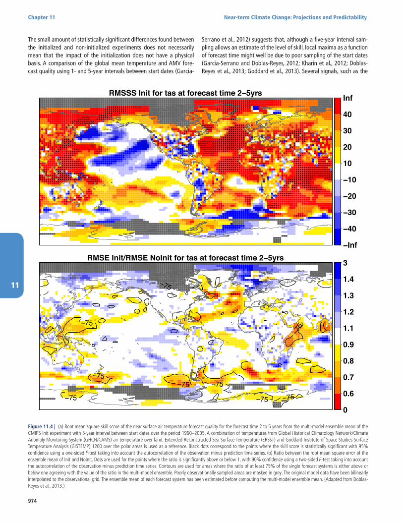
974


11

RMSSS Init for tas at forecast time 2−5yrs.

.......

.

.....

.

......

......

.

.

.

.

..

.

.

...

.

.

.

....

.

....

.

.

.........

...

.

.

.

.

.

...

.

....

...

..

...

..

..

.

...

..

...

...

..

.

.

.

....

......

...

......

.....

............

.

......

.............

.

...

.

..........

.

....

.

..........

.

....

...........

.

...........

...........

.

..........

.

......

..

..

.

.....

..

..

....

...

.

.........

..

.

.

.........

.

...

..........

.

............

.

..........

.

..........

.

.

.....

..

..

...

..

...

...

...........

...

...

...

...

...

....

.

......

.

.

.

..

..

.

.......

.

..

..

.......

..

...........

.....

.............

.

.............

...

.

.

....

............

...........

..

...

.........

.

.

...

......

.

..

..

......

...

..

......

..

...

...

..

.

....

....

....

..

....

.

.

.....

.

..

.

..

.

...

..

..

......

.

..

..

...

..

...

..

....................................................

..... ... .

..

.

.

.

..

....

..

.

.

.....

..

.......

.

...

......

...

.....

.

..

..............

.

......

.

......

.

.

......

....

.

.

......

......

..

.

......

........

......

......

........

......

......

..........

......

.....

...........

......

.......

............

......

........

............

.......

......

.....................

......

.............

.......

......

............

.....

.....

............

.

.....

..........

....

...

.

.

..

.

....

..

.

.

.

....

....

..

.

.

...

−Inf

−40

−30

−20

−10

10

20

30

40

Inf

RMSE Init/RMSE NoInit for tas at forecast time 2−5yrs

−75

−75

−75

−75

−75 −75

−75 −75

−75

...

..

.

. ....

...

0

0.6

0.7

0.8

0.9

1.1

1.2

1.3

1.4

3

Figure 11.4 | (a) Root mean square skill score of the near surface air temperature forecast quality for the forecast time 2 to 5 years from the multi-model ensemble mean of the CMIP5 Init experiment with 5-year interval between start dates over the period 1960–2005. A combination of temperatures from Global Historical Climatology Network/Climate Anomaly Monitoring System (GHCN/CAMS) air temperature over land, Extended Reconstructed Sea Surface Temperature (ERSST) and Goddard Institute of Space Studies Surface Temperature Analysis (GISTEMP) 1200 over the polar areas is used as a reference. Black dots correspond to the points where the skill score is statistically significant with 95% confidence using a one-sided F-test taking into account the autocorrelation of the observation minus prediction time series. (b) Ratio between the root mean square error of the ensemble mean of Init and NoInit. Dots are used for the points where the ratio is significantly above or below 1, with 90% confidence using a two-sided F-test taking into account the autocorrelation of the observation minus prediction time series. Contours are used for areas where the ratio of at least 75% of the single forecast systems is either above or below one agreeing with the value of the ratio in the multi-model ensemble. Poorly observationally sampled areas are masked in grey. The original model data have been bilinearly interpolated to the observational grid. The ensemble mean of each forecast system has been estimated before computing the multi-model ensemble mean. (Adapted from Doblas-Reyes et al., 2013.)

The small amount of statistically significant differences found between the initialized and non-initialized experiments does not necessarily mean that the impact of the initialization does not have a physical basis. A comparison of the global mean temperature and AMV fore-cast quality using 1- and 5-year intervals between start dates (Garcia-

Serrano et al., 2012) suggests that, although a five-year interval sam-pling allows an estimate of the level of skill, local maxima as a function of forecast time might well be due to poor sampling of the start dates (Garcia-Serrano and Doblas-Reyes, 2012; Kharin et al., 2012; Doblas-Reyes et al., 2013; Goddard et al., 2013). Several signals, such as the

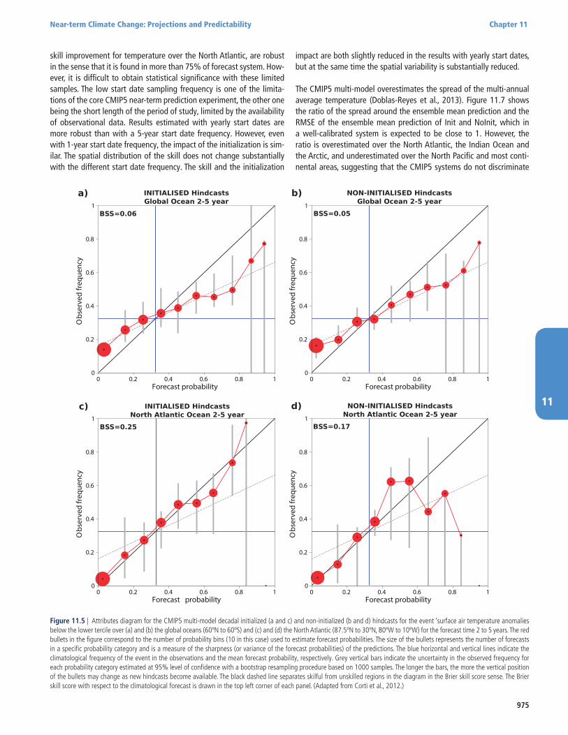
975


11

skill improvement for temperature over the North Atlantic, are robust in the sense that it is found in more than 75% of forecast system. How-ever, it is difficult to obtain statistical significance with these limited samples. The low start date sampling frequency is one of the limita-tions of the core CMIP5 near-term prediction experiment, the other one being the short length of the period of study, limited by the availability of observational data. Results estimated with yearly start dates are more robust than with a 5-year start date frequency. However, even with 1-year start date frequency, the impact of the initialization is sim-ilar. The spatial distribution of the skill does not change substantially with the different start date frequency. The skill and the initialization

impact are both slightly reduced in the results with yearly start dates, but at the same time the spatial variability is substantially reduced.

The CMIP5 multi-model overestimates the spread of the multi-annual average temperature (Doblas-Reyes et al., 2013). Figure 11.7 shows the ratio of the spread around the ensemble mean prediction and the RMSE of the ensemble mean prediction of Init and NoInit, which in a well-calibrated system is expected to be close to 1. However, the ratio is overestimated over the North Atlantic, the Indian Ocean and the Arctic, and underestimated over the North Pacific and most conti-nental areas, suggesting that the CMIP5 systems do not discriminate

0 0.2 0.4 0.6 0.8 1Forecast probability

0

0.2

0.4

0.6

0.8

1

Obs

erve

d fr

eque

ncy


0

0.2

0.4

0.6

0.8

1

Obs

erve

d fr

eque

ncy


0

0.2

0.4

0.6

0.8

1

Obs

erve

d fr

eque

ncy


0

0.2

0.4

0.6

0.8

1

Obs

erve

d fr

eque

ncy

Figure 11.5 | Attributes diagram for the CMIP5 multi-model decadal initialized (a and c) and non-initialized (b and d) hindcasts for the event ‘surface air temperature anomalies below the lower tercile over (a) and (b) the global oceans (60ºN to 60ºS) and (c) and (d) the North Atlantic (87.5ºN to 30ºN, 80ºW to 10ºW) for the forecast time 2 to 5 years. The red bullets in the figure correspond to the number of probability bins (10 in this case) used to estimate forecast probabilities. The size of the bullets represents the number of forecasts in a specific probability category and is a measure of the sharpness (or variance of the forecast probabilities) of the predictions. The blue horizontal and vertical lines indicate the climatological frequency of the event in the observations and the mean forecast probability, respectively. Grey vertical bars indicate the uncertainty in the observed frequency for each probability category estimated at 95% level of confidence with a bootstrap resampling procedure based on 1000 samples. The longer the bars, the more the vertical position of the bullets may change as new hindcasts become available. The black dashed line separates skilful from unskilled regions in the diagram in the Brier skill score sense. The Brier skill score with respect to the climatological forecast is drawn in the top left corner of each panel. (Adapted from Corti et al., 2012.)

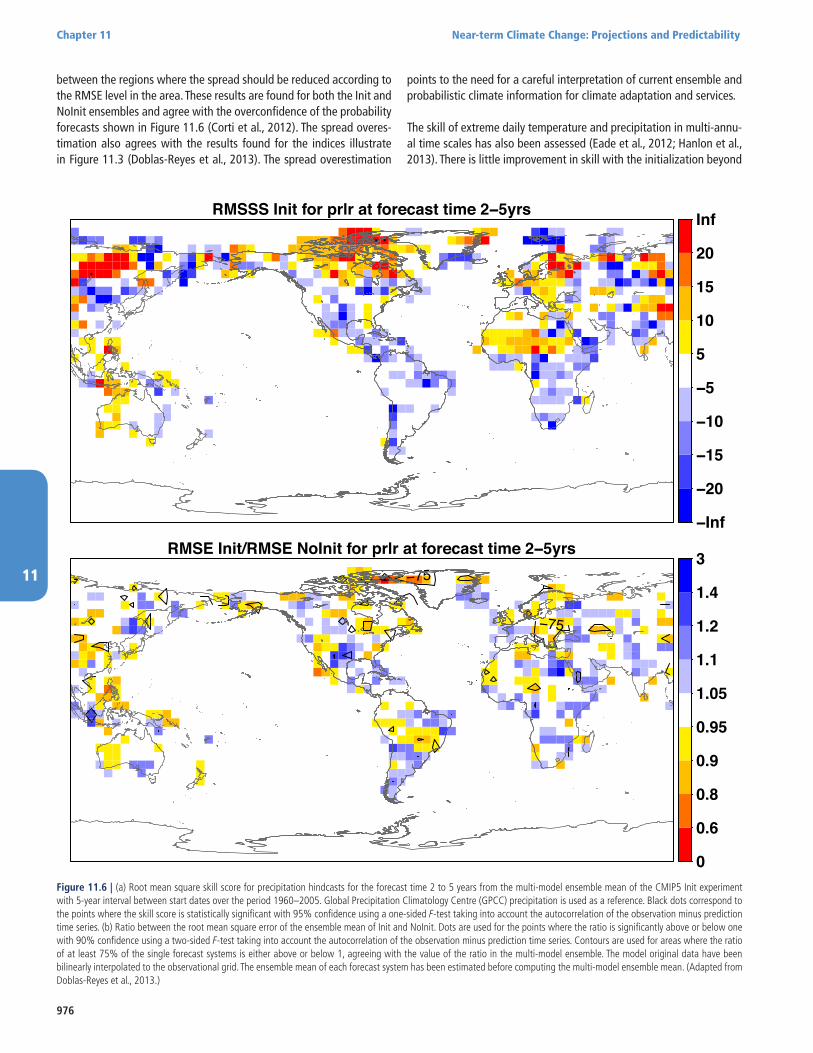
976


11

RMSSS Init for prlr at forecast time 2−5yrs

.

. .

−Inf

−20

−15

−10

−5

5

10

15

20

Inf

RMSE Init/RMSE NoInit for prlr at forecast time 2−5yrs −75

−75

.

0

0.6

0.8

0.9

0.95

1.05

1.1

1.2

1.4

3

Figure 11.6 | (a) Root mean square skill score for precipitation hindcasts for the forecast time 2 to 5 years from the multi-model ensemble mean of the CMIP5 Init experiment with 5-year interval between start dates over the period 1960–2005. Global Precipitation Climatology Centre (GPCC) precipitation is used as a reference. Black dots correspond to the points where the skill score is statistically significant with 95% confidence using a one-sided F-test taking into account the autocorrelation of the observation minus prediction time series. (b) Ratio between the root mean square error of the ensemble mean of Init and NoInit. Dots are used for the points where the ratio is significantly above or below one with 90% confidence using a two-sided F-test taking into account the autocorrelation of the observation minus prediction time series. Contours are used for areas where the ratio of at least 75% of the single forecast systems is either above or below 1, agreeing with the value of the ratio in the multi-model ensemble. The model original data have been bilinearly interpolated to the observational grid. The ensemble mean of each forecast system has been estimated before computing the multi-model ensemble mean. (Adapted from Doblas-Reyes et al., 2013.)

between the regions where the spread should be reduced according to the RMSE level in the area. These results are found for both the Init and NoInit ensembles and agree with the overconfidence of the probability forecasts shown in Figure 11.6 (Corti et al., 2012). The spread overes-timation also agrees with the results found for the indices illustrate in Figure 11.3 (Doblas-Reyes et al., 2013). The spread overestimation

points to the need for a careful interpretation of current ensemble and probabilistic climate information for climate adaptation and services.

The skill of extreme daily temperature and precipitation in multi-annu-al time scales has also been assessed (Eade et al., 2012; Hanlon et al., 2013). There is little improvement in skill with the initialization beyond

977


11

Spread/RMSE Init for tas at forecast time 2−5yrs

0

0.3

0.6

0.8

0.9

1.2

1.5

2

4

6

Figure 11.7 | Ratio between the surface temperature spread around the ensemble mean and the root mean square error (RMSE) of the ensemble-mean prediction of Init and NoInit for the forecast time 2 to 5 years with 5-year interval between start dates over the period 1960–2005. A combination of temperatures from Global Historical Climatology Network/Climate Anomaly Monitoring System (GHCN/CAMS) air temperature over land, Extended Reconstructed Sea Surface Temperature (ERSST) v3b over sea and Goddard Insti-tute of Space Studies Surface Temperature Analysis (GISTEMP) 1200 over the polar areas is used as a reference to compute the RMSE. (Adapted from Doblas-Reyes et al., 2013.)

the first year, suggesting that skill then arises largely from the varying external forcing. The skill for extremes is generally similar to, but slight-ly lower than, that for the mean.

Responding to the increases in decadal skill in certain regions due to initialization, a coordinated quasi-operational decadal prediction ini-tiative has been organized (Smith et al., 2013b). The forecast systems participating in the initiative are based on those of CMIP5 and have been evaluated for forecast quality. Statistical predictions are also included in the initiative. The most recent forecast shows (compared to the projections) substantial warming of the north Atlantic subpo-lar gyre, cooling of the north Pacific throughout the next decade and cooling over most land and ocean regions and in the global average out to several years ahead. However, in the absence of explosive or frequent volcanic eruptions, global surface temperature is predicted to continue to rise and, to a certain degree, recover from the reduced rate of warming (see Box 9.2).

11.2.3.5 Realizing Potential

Although idealized model experiments show considerable promise for predicting internal variability, realizing this potential is a challenging task. There are three main hurdles: (1) the limited availability of data to initialize and verify predictions, (2) limited progress in initialization techniques for decadal predictions and (3) dynamical model shortcom-ings that require validating how the simulated variance compares with the observed variance.

It is expected that the availability of temperature and salinity data in the top 2 km of the ocean through the enhanced global deployment of Argo floats will give a step change in our ability to initialize and pre-

dict ocean heat and density anomalies (Zhang et al., 2007a; Dunstone and Smith, 2010). Another important advancement is the availabili-ty of highly accurate altimetry data, made especially useful after the launching of TOPography EXperiment (TOPEX)/Poseidon in 1992. Argo and altimeter data became available only in 2000 and 1992 respec-tively, so an accurate estimate of their impact on real forecasts has to wait (Dunstone and Smith, 2010). In all cases, both the length of the observational data sets and the reduced coverage of the data avail-able, especially before 2000, are serious limitations to obtain robust estimates of forecast quality.

Improved initialization of other aspects such as sea ice, snow cover, frozen soil and soil moisture, may also have potential to contribute to predictive skill beyond the seasonal time scale. This could be investi-gated, for example by using measurements of soil moisture from the Soil Moisture and Ocean Salinity (SMOS) satellite launched in 2009, or by initializing sea ice thickness with observations from the CryoSat-2 satellite launched in 2010. Along the same line, understanding the links between the initialization and the correct prediction of both the internal and external variability should help improving forecast quality (Solomon et al., 2011).

Many of the current decadal prediction systems use relatively simple initialization schemes and do not adopt fully coupled initialization/ensemble generation schemes. Assimilation schemes offer opportuni-ties for fully coupled initialization including assimilation of variables such as sea ice, snow cover and soil moisture, although they present technically and scientifically challenging problems. This approach has been tested in schemes like four-dimensional variational data assim-ilation (4DVAR; Sugiura et al., 2008) and the ensemble Kalman filter (Keppenne et al., 2005; Zhang et al., 2007a).

978


11

Bias correction is used to reduce the effects of model drift, but the nonlinearity in the climate system (e.g., Power (1995) might limit the effectiveness of bias correction and thereby reduce forecast quality. Understanding and reducing both drift and systematic errors is impor-tant (Palmer and Weisheimer, 2011), as it is also for seasonal-to-inter-annual climate prediction and for climate change projections. While improving models is the highest priority, efforts to quantify the degree of interference between model bias and predictive signals should not be overlooked.

11.3 Near-term Projections

11.3.1 Introduction

In this section the outlook for global and regional climate up to mid-century is assessed, based on climate model projections. In con-trast to the predictions discussed in Section 11.2, these projections are not initialized using observations; instead, they are initialized from historical simulations of the evolution of climate from pre-industrial conditions up to the present. The historical simulations are forced by estimates of past anthropogenic and natural climate forcing agents, and the projections are obtained by forcing the models with scenari-os for future climate forcing agents. Major use is made of the CMIP5 model experiments forced by the Representative Concentration Path-way (RCP) scenarios discussed in Chapters 1 and 8. Projections of cli-mate change in this and subsequent chapters are expressed relative to the reference period: 1986–2005. In this chapter most emphasis is given to the period 2016–2035, but some information on changes pro-jected before and after this period (up to mid-century) is also provided. Longer-term projections are assessed in Chapters 12 and 13.

Key assessment questions addressed in this section are: What is the externally forced signal of near-term climate change, and how large is it compared to natural internal variability? From the point of view of climate impacts, the absolute magnitude of climate change may in some instances be less important than the magnitude relative to the local level of natural internal variability. Because many systems are naturally adapted to a background level of variability, it may be changes that move outside of this range that are most likely to trigger impacts that are unprecedented in the recent past (e.g., Lobell and Burke (2008) for crops).

An important conclusion of the AR4 (Section 10.3.1) was that near-term climate projections are not very sensitive to plausible alternative non-mitigation scenarios for GHG concentrations (specifically the Spe-cial Report on Emission Scenarios (SRES) scenarios; comparison with RCP scenarios is discussed in Chapter 1), that is, in the near term, dif-ferent scenarios give rise to similar magnitudes and patterns of climate change. (Note, however, that some impacts may be more sensitive.) For this reason, most of the projections presented in this chapter are based on one specific RCP scenario, RCP4.5. RCP4.5 was chosen because of its intermediate GHG forcing. However, there is greater sensitivity to other forcing agents, in particular anthropogenic aerosols (e.g., Chalm-ers et al., 2012). Consequently, a further question addressed in this section (especially in Section 11.3.6.1) is: To what extent are near-term climate projections sensitive to alternative scenarios for anthropogenic

forcing? Note finally that a great deal of additional information on near-term projections is provided in Annex I.

11.3.1.1 Uncertainty in Near-term Climate Projections

As discussed in Chapters 1 (Section 1.4) and 12 (Section 12.2), climate projections are subject to several sources of uncertainty. Here three main sources are distinguished. The first arises from natural internal variability, which is intrinsic to the climate system, and includes phe-nomena such as variability in the mid-latitude storm tracks and the ENSO. The existence of internal variability places fundamental limits on the precision with which future climate variables can be project-ed. The second is uncertainty concerning the past, present and future forcing of the climate system by natural and anthropogenic forcing agents such as GHGs, aerosols, solar forcing and land use change. Forc-ing agents may be specified in various ways, for example, as emissions or as concentrations (see Section 12.2). The third is uncertainty related to the response of the climate system to the specified forcing agents.

Quantifying the uncertainty that arises from each of the three sources is an important challenge. For projections, no attempt is made to predict the evolution of the internal variability. Instead, the statistics of this variability are included as a component of the uncertainty associated with a projection. The magnitude of internal variability can be estimat-ed from observations (Chapters 2, 3 and 4) or from climate models (Chapter 9). Challenges arise in estimating the variability on decadal and longer time scales, and for rare events such as extremes, as obser-vational records are often too short to provide robust estimates.

Uncertainty concerning the past forcing of the climate system arises from a lack of direct or proxy observations, and from observational errors. This uncertainty can influence future projections of some vari-ables (particularly large-scale ocean variables) for years or even dec-ades ahead (e.g., Meehl and Hu, 2006; Stenchikov et al., 2009; Gregory, 2010). Uncertainty about future forcing arises from the inability to pre-dict future anthropogenic emissions and land use change, and natural forcings (e.g., volcanoes), and from uncertainties concerning carbon cycle and other biogeochemical feedbacks (Chapters 6, 12 and Annex II.4.1). The uncertainties in future anthropogenic forcing are typically investigated through the development of specific scenarios (e.g., for emissions or concentrations), such as the RCP scenarios (Chapters 1 and 8). Different scenarios give rise to different climate projections, and the spread of such projections is commonly described as scenario uncertainty. The sensitivity of climate projections to alternative sce-narios for future anthropogenic emissions is discussed especially in Section 11.3.6.1

To project the climate response to specified forcing agents, climate models are required. The term model uncertainty describes uncertainty about the extent to which any particular climate model provides an accurate representation of the real climate system. This uncertainty arises from approximations required in the development of models. Such approximations affect the representation of all aspects of the climate including natural internal variability and the response to exter-nal forcings. As discussed in Chapter 1 (Section 1.4.2), the term model uncertainty is sometimes used in a narrower sense to describe the spread between projections generated using different models or model

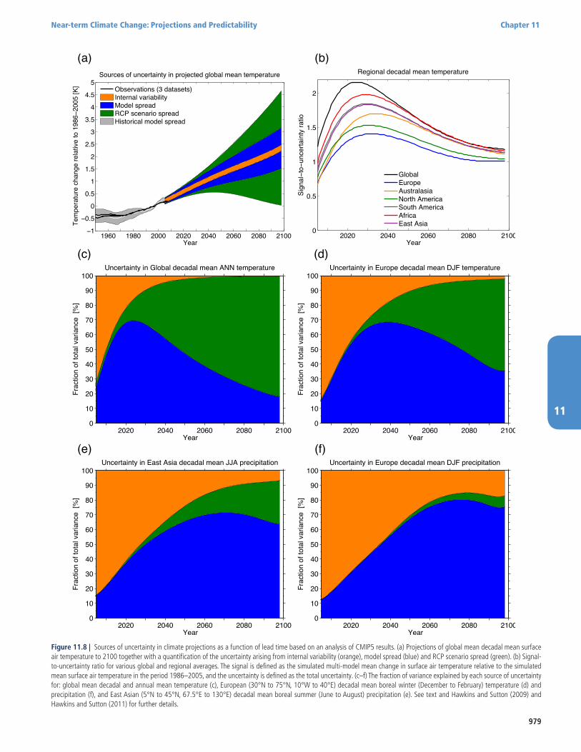
979


11

(a) (b)Te

mpe

ratu

re c

hang

e re

lativ

e to

198

620

05 [K

]

Year

Sources of uncertainty in projected global mean temperature

1960 1980 2000 2020 2040 2060 2080 210010.5

00.5

11.5

22.5

33.5

44.5

5Observations (3 datasets)Internal variabilityModel spreadRCP scenario spreadHistorical model spread

2020 2040 2060 2080 21000

0.5

1

1.5

2

Sign

alto

unce

rtain

ty ra

tio

Regional decadal mean temperature

Year

GlobalEuropeAustralasiaNorth AmericaSouth AmericaAfricaEast Asia

(c) (d)

Year

Frac

tion

of to

tal v

aria

nce

[%]

Uncertainty in Global decadal mean ANN temperature

2020 2040 2060 2080 21000

10

20

30

40

50

60

70

80

90

100

Year

Frac

tion

of to

tal v

aria

nce

[%]

Uncertainty in Europe decadal mean DJF temperature

2020 2040 2060 2080 21000

10

20

30

40

50

60

70

80

90

100

(e) (f)

Year

Frac

tion

of to

tal v

aria

nce

[%]

Uncertainty in East Asia decadal mean JJA precipitation

2020 2040 2060 2080 21000

10

20

30

40

50

60

70

80

90

100

Year

Frac

tion

of to

tal v

aria

nce

[%]

Uncertainty in Europe decadal mean DJF precipitation

2020 2040 2060 2080 21000

10

20

30

40

50

60

70

80

90

100

Figure 11.8 | Sources of uncertainty in climate projections as a function of lead time based on an analysis of CMIP5 results. (a) Projections of global mean decadal mean surface air temperature to 2100 together with a quantification of the uncertainty arising from internal variability (orange), model spread (blue) and RCP scenario spread (green). (b) Signal-to-uncertainty ratio for various global and regional averages. The signal is defined as the simulated multi-model mean change in surface air temperature relative to the simulated mean surface air temperature in the period 1986–2005, and the uncertainty is defined as the total uncertainty. (c–f) The fraction of variance explained by each source of uncertainty for: global mean decadal and annual mean temperature (c), European (30°N to 75°N, 10°W to 40°E) decadal mean boreal winter (December to February) temperature (d) and precipitation (f), and East Asian (5°N to 45°N, 67.5°E to 130°E) decadal mean boreal summer (June to August) precipitation (e). See text and Hawkins and Sutton (2009) and Hawkins and Sutton (2011) for further details.

980


11

versions; however, such a measure is crude as it takes no account of factors such as model quality (Chapter 9) or model independence. The term model response uncertainty is used here to describe the dimen-sion of model uncertainty that is directly related to the response to external forcings. To obtain projections of extreme events such as trop-ical cyclones, or regional phenomena such as orographic rainfall, it is sometimes necessary to employ a dynamical or statistical downscaling procedure. Such downscaling introduces an additional dimension of model uncertainty (e.g., Alexandru et al., 2007).

The relative importance of the different sources of uncertainty depends on the variable of interest, the space and time scales involved (Sec-tion 10.5.4.3 of Meehl et al. (2007b)), and the lead-time of the projec-tion. Figure 11.8 provides an illustration of these dependencies based on an analysis of CMIP5 projections (following Hawkins and Sutton, 2009, 2011;Yip et al., 2011). In this example, the forcing-related uncer-tainty is estimated using the spread of projections for different RCP scenarios (i.e., scenario uncertainty), while the spread among differ-ent models for individual RCP scenarios is used as a measure of the model response uncertainty. Internal variability is estimated from the models as in Hawkins and Sutton (2009). Key points are: (1) the uncer-tainty in near-term projections is dominated by internal variability and model spread. This finding provides some of the rationale for consid-ering near-term projections separately from long-term projections. Note, however, that the RCP scenarios do not sample the full range of uncertainty in future anthropogenic forcing, and that uncertainty in aerosol forcings in particular may be more important than is suggested by Figure 11.8 (see Section 11.3.6.1); (2) internal variability becomes increasingly important on smaller space and time scales; (3) for pro-jections of precipitation, scenario uncertainty is less important and (on regional scales) internal variability is generally more important than for projections of surface air temperature; (4) the full model uncertainty may well be larger or smaller than the model spread due to common errors or unrealistic models.

A key quantity for any climate projection is the signal-to-noise (S/N) ratio (Christensen et al., 2007), where the ‘signal’ is a measure of the amplitude of the projected climate change, and the noise is a measure of the uncertainty in the projection. Higher S/N ratios indicate more robust projections of change and/or changes that are large relative to background levels of variability. Depending on the purpose, it may be useful to identify the noise with the total uncertainty, or with a specific component such as the internal variability. The evolution of the S/N ratio with lead time depends on whether the signal grows more rapidly than the noise, or vice versa. Figure 11.8 (top right) shows that, when the noise is identified with the total uncertainty, the S/N ratio for surface air temperature is typically higher at lower latitudes and has a maximum at a lead time of a few decades (Cox and Stephenson, 2007; Hawkins and Sutton, 2009). The former feature is primarily a consequence of the greater amplitude of internal variability in mid-lat-itudes. The latter feature arises because over the first few decades, when scenario uncertainty is small, the signal grows most rapidly, but subsequently, the contribution from scenario uncertainty grows more rapidly than does the signal, so the S/N ratio falls. See Hawkins and Sutton (2009, 2011) for further details.

11.3.2 Near-term Projected Changes in the Atmosphere and Land Surface

11.3.2.1 Surface Temperature

11.3.2.1.1 Global mean surface air temperature

Figure 11.9 (a) and (b) show CMIP5 projections of global mean surface air temperature under RCP4.5. The 5 to 95% range for the projected anomaly for the period 2016–2035, relative to the reference period 1986–2005, is 0.47°C to 1.00°C (see also Table 12.2). However, as discussed in Section 11.3.1.1, this range provides only a very crude measure of uncertainty, and there is no guarantee that the real world must lie within this range. Obtaining better estimates is an important challenge. One approach involves initializing climate models using observations, as discussed in Section 11.2. Figure 11.9 (b) compares multi-model initialized climate predictions (8 models from Smith et al., 2013b), initialized in 2011; 14 CMIP5 decadal prediction experiment models following the methodology of Meehl and Teng (2012), initial-ized in 2006 with the ‘raw’ uninitialized CMIP5 projections. The 5 to 95% range for both sets of initialized predictions is cooler (by about 15% for the median values) than the corresponding range for the raw projections, particularly at the upper end. The differences are partly a consequence of initializing the models in a state that is cool (in com-parison to the median of the raw projections) as a result of the recent hiatus in global mean surface temperature rise (see Box 9.2). However, it is not yet possible to attribute all of the reasons with confidence because the raw projections are based on a different, and larger, set of models than the initialized predictions, and because of uncertainties related to the bias adjustment of the initialized predictions (Goddard et al., 2013; Meehl et al., 2013d)

Another approach to making projections involves weighting models according to some measure of their quality (see Chapter 9). A specific approach of this type, known as Allen, Stott and Kettleborough (ASK) (Allen et al., 2000; Stott and Kettleborough, 2002), is based on the use of results from detection and attribution studies (Chapter 10), in which the fit between observations and model simulations of the past is used to scale projections of the future. ASK requires specific simulations to be carried out with individual forcings (e.g., anthropogenic GHG forc-ing alone), and only some of the centres participating in CMIP5 have carried out the necessary integrations. Biases in ASK-derived projec-tions may arise from errors in the specified forcings, or in the simulated patterns of response, and/or from nonlinearities in the responses to forcings.

Figure 11.9c shows the projected range of global mean surface air tem-perature change derived using the ASK approach for RCP4.5 (Stott and G. Jones, 2012; Stott et al., 2013) applied to six models and compares this with the range derived from the 42 CMIP5 models. In this case decadal means are shown. The 5 to 95% confidence interval for the projected temperature anomaly for the period 2016–2035, based on the ASK method, is 0.39°C to 0.87°C. As for the initialized predictions shown in Figure 11.9b, both the lower and upper values are below the corresponding values obtained from the raw CMIP5 results, although there is substantial overlap between the two ranges. The relative cooling of the ASK results is directly related to evidence presented in

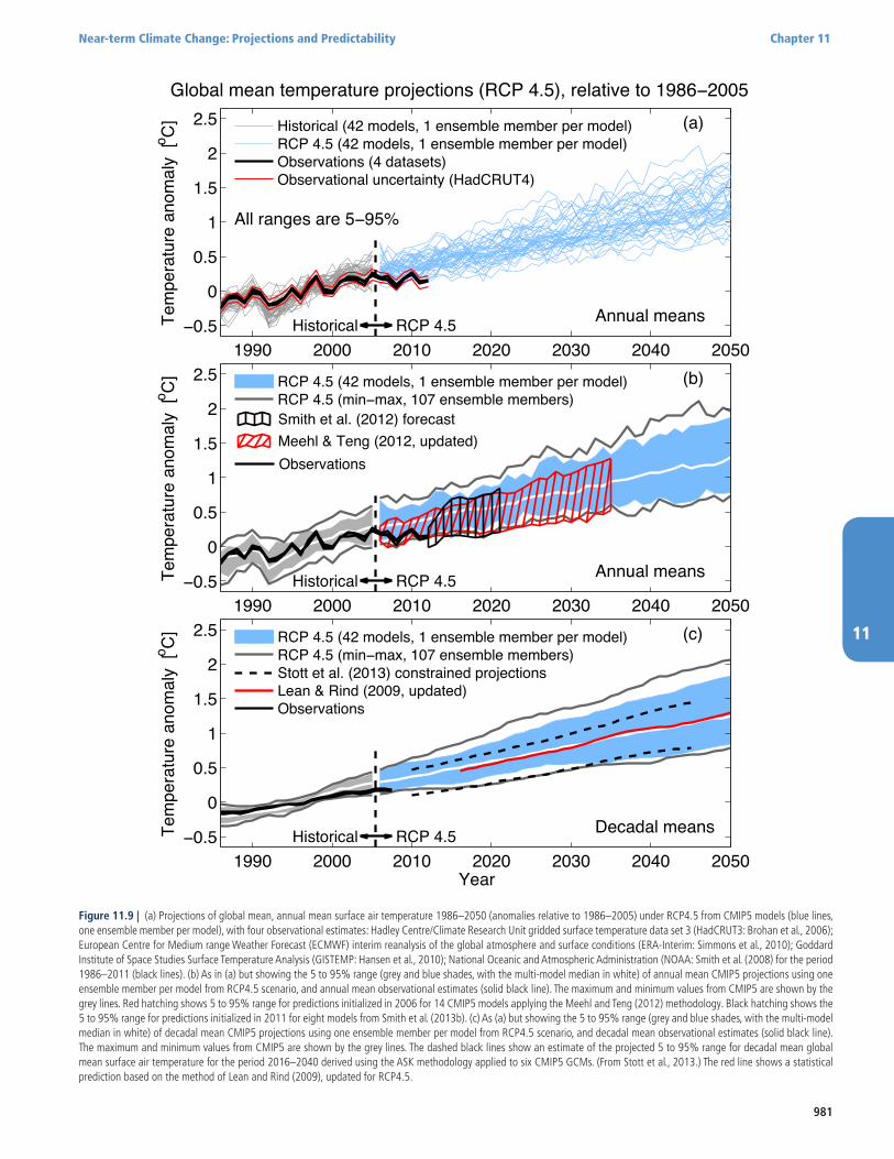
981


11

Figure 11.9 | (a) Projections of global mean, annual mean surface air temperature 1986–2050 (anomalies relative to 1986–2005) under RCP4.5 from CMIP5 models (blue lines, one ensemble member per model), with four observational estimates: Hadley Centre/Climate Research Unit gridded surface temperature data set 3 (HadCRUT3: Brohan et al., 2006); European Centre for Medium range Weather Forecast (ECMWF) interim reanalysis of the global atmosphere and surface conditions (ERA-Interim: Simmons et al., 2010); Goddard Institute of Space Studies Surface Temperature Analysis (GISTEMP: Hansen et al., 2010); National Oceanic and Atmospheric Administration (NOAA: Smith et al. (2008) for the period 1986–2011 (black lines). (b) As in (a) but showing the 5 to 95% range (grey and blue shades, with the multi-model median in white) of annual mean CMIP5 projections using one ensemble member per model from RCP4.5 scenario, and annual mean observational estimates (solid black line). The maximum and minimum values from CMIP5 are shown by the grey lines. Red hatching shows 5 to 95% range for predictions initialized in 2006 for 14 CMIP5 models applying the Meehl and Teng (2012) methodology. Black hatching shows the 5 to 95% range for predictions initialized in 2011 for eight models from Smith et al. (2013b). (c) As (a) but showing the 5 to 95% range (grey and blue shades, with the multi-model median in white) of decadal mean CMIP5 projections using one ensemble member per model from RCP4.5 scenario, and decadal mean observational estimates (solid black line). The maximum and minimum values from CMIP5 are shown by the grey lines. The dashed black lines show an estimate of the projected 5 to 95% range for decadal mean global mean surface air temperature for the period 2016–2040 derived using the ASK methodology applied to six CMIP5 GCMs. (From Stott et al., 2013.) The red line shows a statistical prediction based on the method of Lean and Rind (2009), updated for RCP4.5.

1990 2000 2010 2020 2030 2040 2050−0.5

0

0.5

1

1.5

2

2.5

Tem

pera

ture

ano

mal

y [o C]

Global mean temperature projections (RCP 4.5), relative to 1986−2005

All ranges are 5−95%

Annual meansRCP 4.5Historical

(a)Historical (42 models, 1 ensemble member per model)RCP 4.5 (42 models, 1 ensemble member per model)Observations (4 datasets)Observational uncertainty (HadCRUT4)

Meehl & Teng (2012, updated)Observations

Smith et al. (2012) forecast

RCP 4.5HistoricalTem

pera

ture

ano

mal

y [o C]

(b)

Annual means

1990 2000 2010 2020 2030 2040 2050−0.5

0

0.5

1

1.5

2

2.5 RCP 4.5 (42 models, 1 ensemble member per model)RCP 4.5 (min−max, 107 ensemble members)

RCP 4.5Historical

(c)

Year

Tem

pera

ture

ano

mal

y [o C]

Decadal means

1990 2000 2010 2020 2030 2040 2050−0.5

0

0.5

1

1.5

2

2.5 RCP 4.5 (42 models, 1 ensemble member per model)RCP 4.5 (min−max, 107 ensemble members)Stott et al. (2013) constrained projectionsLean & Rind (2009, updated)Observations

982


11

Seasonal mean air temperature change (RCP4.5: 2016-2035)

Figure 11.10 | CMIP5 multi-model ensemble mean of projected changes in December, January and February and June, July and August surface air temperature for the period 2016–2035 relative to 1986–2005 under RCP4.5 scenario (left panels). The right panels show an estimate of the model-estimated internal variability (standard deviation of 20-year means). Hatching in left-hand panels indicates areas where projected changes are small compared to the internal variability (i.e., smaller than one standard deviation of estimated internal variability), and stippling indicates regions where the multi-model mean projections deviate significantly from the simulated 1986–2005 period (by at least two standard deviations of internal variability) and where at least 90% of the models agree on the sign of change. The number of models considered in the analysis is listed in the top-right portion of the panels; from each model one ensemble member is used. See Box 12.1 in Chapter 12 for further details and discussion. Technical details are in Annex I.

Chapter 10 (Section 10.3.1) that ‘This provides evidence that some CMIP5 models have a higher transient response to GHGs and a larger response to other anthropogenic forcings (dominated by the effects of aerosols) than the real world (medium confidence).’ The ASK results and the initialised predictions both suggest that those CMIP5 models that warm most rapidly over the period (1986–2005) to (2016–2035) may be inconsistent with the observations. This possibility is also sug-gested by comparing the models with the observed rate of warming since 1986—see Box 9.2 for a full discussion of this comparison. Lastly, Figure 11.9 also shows a statistical prediction for global mean surface air temperature, using the method of Lean and Rind (2009), which uses multiple linear regression to decompose observed temperature vari-ations into distinct components. This prediction is very similar to the CMIP5 multi-model median.

The projections shown in Figure 11.9 assume the RCP4.5 scenario and use the 1986–2005 reference period. In Section 11.3.6 addition-al uncertainties associated with future forcing, climate responses and sensitivity to the choice of reference period, are discussed. An overall assessment of the likely range for future global mean surface air tem-perature is provided in Section 11.3.6.3.

For the remaining projections in this chapter the spread among the CMIP5 models is used as a simple, but crude, measure of uncertainty.

The extent of agreement between the CMIP5 projections provides rough guidance about the likelihood of a particular outcome. But—as partly illustrated by the discussion above—it must be kept firmly in mind that the real world could fall outside of the range spanned by these particular models. See Section 11.3.6 for further discussion.

11.3.2.1.2 Regional and seasonal patterns of surface warming

The geographical pattern of near-term surface warming simulated by the CMIP5 models (Figure 11.10) is consistent with previous IPCC reports in a number of key aspects, although weaknesses in the ability of current models to capture observed regional trends (Box 11.2) must be kept in mind. First, temperatures over land increase more rapidly than over sea (e.g., Manabe et al., 1991; Sutton et al., 2007). Process-es that contribute to this land–sea warming contrast include differ-ent local feedbacks over ocean and land and changes in atmospheric energy transport from ocean to land regions (e.g., Lambert and Chiang, 2007; Vidale et al., 2007; Shimpo and Kanamitsu, 2009; Fasullo, 2010; Boer, 2011; Joshi et al., 2011).

Second, the projected warming in wintertime shows a pronounced polar amplification in the NH (see Box 5.1). This feature is found in virtually all coupled model projections, but the CMIP3 simulations generally appeared to underestimate this effect in comparison to

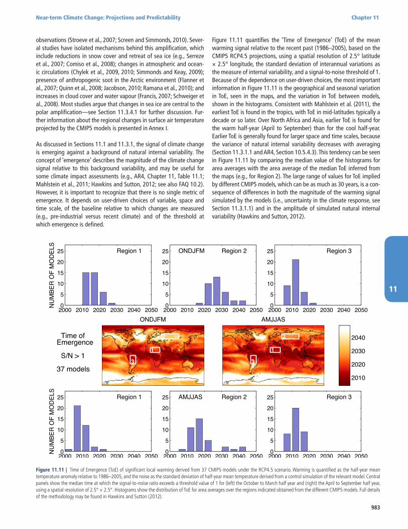
983


11

observations (Stroeve et al., 2007; Screen and Simmonds, 2010). Sever-al studies have isolated mechanisms behind this amplification, which include reductions in snow cover and retreat of sea ice (e.g., Serreze et al., 2007; Comiso et al., 2008); changes in atmospheric and ocean-ic circulations (Chylek et al., 2009, 2010; Simmonds and Keay, 2009); presence of anthropogenic soot in the Arctic environment (Flanner et al., 2007; Quinn et al., 2008; Jacobson, 2010; Ramana et al., 2010); and increases in cloud cover and water vapour (Francis, 2007; Schweiger et al., 2008). Most studies argue that changes in sea ice are central to the polar amplification—see Section 11.3.4.1 for further discussion. Fur-ther information about the regional changes in surface air temperature projected by the CMIP5 models is presented in Annex I.

As discussed in Sections 11.1 and 11.3.1, the signal of climate change is emerging against a background of natural internal variability. The concept of ‘emergence’ describes the magnitude of the climate change signal relative to this background variability, and may be useful for some climate impact assessments (e.g., AR4, Chapter 11, Table 11.1; Mahlstein et al., 2011; Hawkins and Sutton, 2012; see also FAQ 10.2). However, it is important to recognize that there is no single metric of emergence. It depends on user-driven choices of variable, space and time scale, of the baseline relative to which changes are measured (e.g., pre-industrial versus recent climate) and of the threshold at which emergence is defined.

Figure 11.11 quantifies the ‘Time of Emergence’ (ToE) of the mean warming signal relative to the recent past (1986–2005), based on the CMIP5 RCP4.5 projections, using a spatial resolution of 2.5° latitude × 2.5° longitude, the standard deviation of interannual variations as the measure of internal variability, and a signal-to-noise threshold of 1. Because of the dependence on user-driven choices, the most important information in Figure 11.11 is the geographical and seasonal variation in ToE, seen in the maps, and the variation in ToE between models, shown in the histograms. Consistent with Mahlstein et al. (2011), the earliest ToE is found in the tropics, with ToE in mid-latitudes typically a decade or so later. Over North Africa and Asia, earlier ToE is found for the warm half-year (April to September) than for the cool half-year. Earlier ToE is generally found for larger space and time scales, because the variance of natural internal variability decreases with averaging (Section 11.3.1.1 and AR4, Section 10.5.4.3). This tendency can be seen in Figure 11.11 by comparing the median value of the histograms for area averages with the area average of the median ToE inferred from the maps (e.g., for Region 2). The large range of values for ToE implied by different CMIP5 models, which can be as much as 30 years, is a con-sequence of differences in both the magnitude of the warming signal simulated by the models (i.e., uncertainty in the climate response, see Section 11.3.1.1) and in the amplitude of simulated natural internal variability (Hawkins and Sutton, 2012).

Figure 11.11 | Time of Emergence (ToE) of significant local warming derived from 37 CMIP5 models under the RCP4.5 scenario. Warming is quantified as the half-year mean temperature anomaly relative to 1986–2005, and the noise as the standard deviation of half-year mean temperature derived from a control simulation of the relevant model. Central panels show the median time at which the signal-to-noise ratio exceeds a threshold value of 1 for (left) the October to March half year and (right) the April to September half year, using a spatial resolution of 2.5° × 2.5°. Histograms show the distribution of ToE for area averages over the regions indicated obtained from the different CMIP5 models. Full details of the methodology may be found in Hawkins and Sutton (2012).

ONDJFM

Time ofEmergence

S/N > 1

37 models

1

2

3

2000 2010 2020 2030 2040 20500

5

10

15

20

25 Region 1

NU

MBE

R O

F M

OD

ELS

2000 2010 2020 2030 2040 20500

5

10

15

20

25 Region 2ONDJFM

2000 2010 2020 2030 2040 20500

5

10

15

20

25 Region 3

AMJJAS

1

2

3

2010

2020

2030

2040

2000 2010 2020 2030 2040 20500

5

10

15

20

25 Region 1

NU

MBE

R O

F M

OD

ELS

2000 2010 2020 2030 2040 20500

5

10

15

20

25 Region 2AMJJAS

2000 2010 2020 2030 2040 20500

5

10

15

20

25 Region 3

984


11

In summary, it is very likely that anthropogenic warming of surface air temperature over the next few decades will proceed more rapidly over land areas than over oceans, and that the warming over the Arctic in winter will be greater than the global mean warming over the same period. Relative to background levels of natural internal variability, near-term increases in seasonal mean and annual mean temperatures are expected to occur more rapidly in the tropics and subtropics than in mid-latitudes (high confidence).

11.3.2.2 Free Atmospheric Temperature

Changes in zonal mean temperature for the near-term period (2016–2035 compared to the base period 1986–2005) for the multi-model CMIP5 ensemble show a pattern similar to that in the CMIP3, with warming in the troposphere and cooling in the stratosphere of a couple of degrees that is significant even in the near term period. There is relatively greater warming in the tropical upper troposphere and northern high latitudes. A more detailed assessment of observed and simulated changes in free atmospheric temperatures can be found in Sections 10.3.1.2.1 and 12.4.3.2.

11.3.2.3 The Water Cycle

As discussed in the AR4 (Section 10.3.6; Meehl et al., 2007b), the IPCC Technical Paper on Climate Change and Water (Bates et al., 2008) and the Special Report on Managing the Risks of Extreme Events and Disasters to Advance Climate Change Adaptation (Seneviratne et al., 2012), a general intensification of the global hydrological cycle, and of precipitation extremes, are expected for a future warmer climate (e.g., (Huntington, 2006; Williams et al., 2007; Wild et al., 2008; Chou et al., 2009; Dery et al., 2009; O’Gorman and Schneider, 2009; Lu and Fu, 2010; Seager et al., 2010; Wu et al., 2010; Kao and Ganguly, 2011; Muller et al., 2011; Durack et al., 2012). In this section, projected changes in the time-mean hydrological cycle are discussed; changes in extremes, are presented in Section 11.3.2.5 while processes underlying precipitation changes are treated in Chapter 7.

11.3.2.3.1 Changes in precipitation

AR4 projections of the spatial patterns of precipitation change in response to GHG forcing (Chapter 10, Section 10.3.2) showed consist-ency between models on the largest scales (i.e., zonal means) but large uncertainty on smaller scales. The consistent pattern was characterized by increases at high latitudes and in wet regions (including the maxima in mean precipitation found in the tropics), and decreases in dry regions (including large parts of the subtropics). Large uncertainties in the sign of projected change were seen especially in regions located on the borders between regions of increases and regions of decreases. More recent research has highlighted the fact that if models agree that the projected change is small in some sense relative to internal variability, then agreement on the sign of the change is not expected (Tebaldi et al., 2011; Power et al., 2012). This recognition led to the identifica-tion of subregions within the border regions, where models agree that projected changes are either zero or small (Power et al., 2012). This, and other considerations, also led to the realization that the consensus among models on precipitation projections is more widespread than might have been inferred on the basis of the projections described in

the AR4 (Power et al., 2012). Information on the reliability of near-term projections can also be obtained from verification of past regional trends (Räisänen (2007); Box 11.2)

Since the AR4 there has also been considerable progress in under-standing the factors that govern the spatial pattern of change in pre-cipitation (P), precipitation minus evaporation (P – E), and inter-model differences in these patterns. The general pattern of wet-get-wetter (also referred to as ‘rich-get-richer’, e.g., Held and Soden, 2006; Chou et al., 2009; Allan et al., 2010) and dry-get-drier has been confirmed, although with deviations in some dry regions at present that are pro-jected to become wetter by some models, e.g., Northeast Brazil in austral summer and East Africa (see Annex I). It has been demon-strated that the wet-get-wetter pattern implies an enhanced season-al precipitation range between wet and dry seasons in the tropics, and enhanced inter-hemispheric precipitation gradients (Chou et al., 2007).

It has recently been proposed that analysis of the energy budget, pre-viously applied only to the global mean, may provide further insights into the controls on regional changes in precipitation (Levermann et al., 2009; Muller and O’Gorman, 2011; O’Gorman et al., 2012). Muller and O’Gorman (2011) argue in particular that changes in radiative and surface sensible heat fluxes provide a guide to the local precipitation response over land. Projected and observed patterns of oceanic pre-cipitation change in the tropics tend to follow patterns of SST change because of local changes in atmospheric stability, such that regions warming more than the tropics as a whole tend to exhibit an increase in local precipitation, while regions warming less tend to exhibit reduced precipitation (Johnson and Xie, 2010; Xie et al., 2010).

AR4 (Section 10.3.2 and Chapter 11) showed that, especially in the near term, and on regional or smaller scales, the magnitude of projected changes in mean precipitation was small compared to the magnitude of natural internal variability (Christensen et al., 2007). Recent work has confirmed this result, and provided more quantifi-cation (e.g., Hawkins and Sutton, 2011; Hoerling et al., 2011; Rowell, 2011; Deser et al., 2012; Power et al., 2012). Hawkins and Sutton (2011) presented further analysis of CMIP3 results and found that, on spatial scales of the order of 1000 km, internal variability contributes 50 to 90% of the total uncertainty in all regions for projections of dec-adal and seasonal mean precipitation change for the next decade, and is the most important source of uncertainty for many regions for lead times up to three decades ahead (Figure 11.8). Thereafter, response uncertainty is generally dominant. Forcing uncertainty (except for that relating to aerosols, see Section 11.4.7) is generally negligible for near-term projections. The S/N ratio for projected changes in seasonal mean precipitation is highest in the subtropics and at high latitudes. Rowell (2011) found that the contribution of response uncertainty to the total uncertainty (response plus internal variability) in local precipitation change is highest in the deep tropics, particularly over South Amer-ica, Africa, the east and central Pacific, and the Atlantic. Over trop-ical land and summer mid-latitude continents the representation of SST changes, atmospheric processes, land surface processes, and the terrestrial carbon cycle all contribute to the uncertainty in projected changes in rainfall.

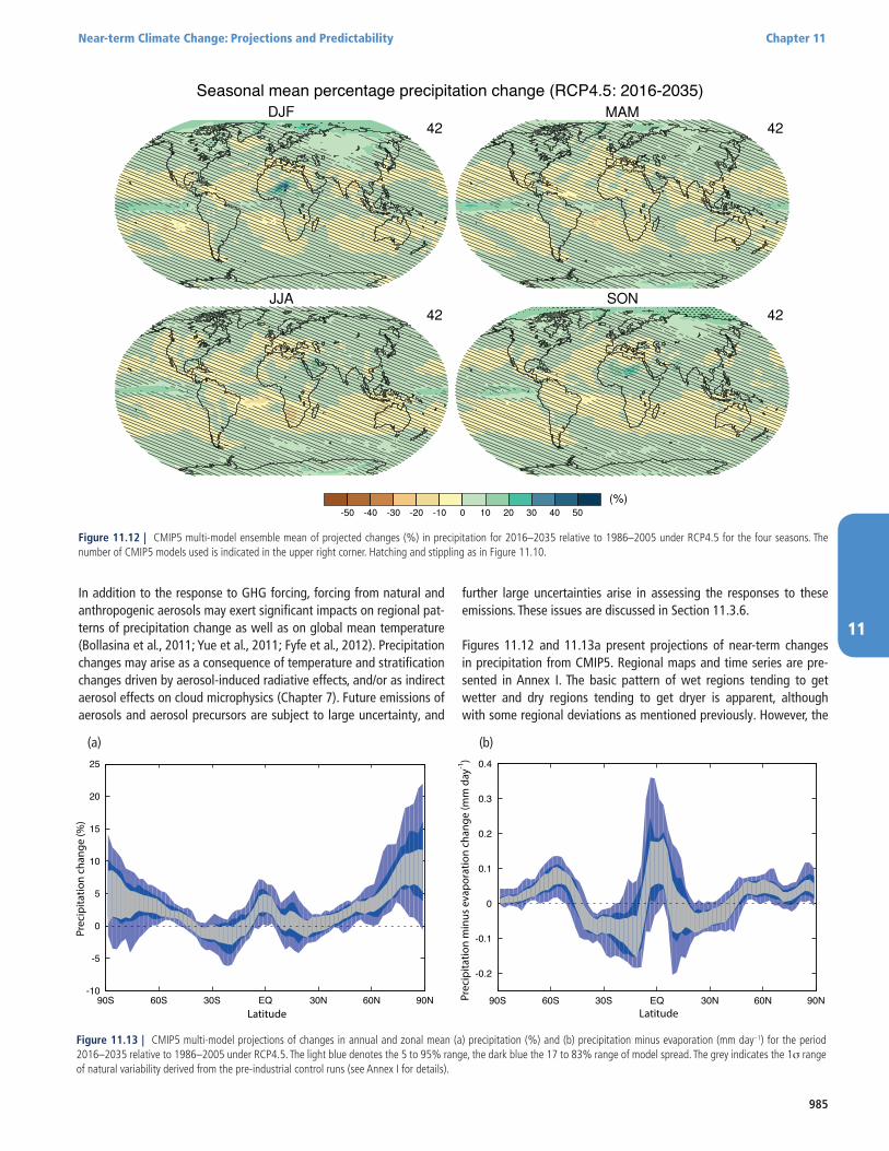
985


11

In addition to the response to GHG forcing, forcing from natural and anthropogenic aerosols may exert significant impacts on regional pat-terns of precipitation change as well as on global mean temperature (Bollasina et al., 2011; Yue et al., 2011; Fyfe et al., 2012). Precipitation changes may arise as a consequence of temperature and stratification changes driven by aerosol-induced radiative effects, and/or as indirect aerosol effects on cloud microphysics (Chapter 7). Future emissions of aerosols and aerosol precursors are subject to large uncertainty, and

Seasonal mean percentage precipitation change (RCP4.5: 2016-2035)

further large uncertainties arise in assessing the responses to these emissions. These issues are discussed in Section 11.3.6.

Figures 11.12 and 11.13a present projections of near-term changes in precipitation from CMIP5. Regional maps and time series are pre-sented in Annex I. The basic pattern of wet regions tending to get wetter and dry regions tending to get dryer is apparent, although with some regional deviations as mentioned previously. However, the

Figure 11.12 | CMIP5 multi-model ensemble mean of projected changes (%) in precipitation for 2016–2035 relative to 1986–2005 under RCP4.5 for the four seasons. The number of CMIP5 models used is indicated in the upper right corner. Hatching and stippling as in Figure 11.10.

-10

-5

0

5

10

15

20

25

90S 60S 30S EQ 30N 60N 90N

Prec

ipita

tion

chan

ge (%

)

Latitude

-0.2

-0.1

0

0.1

0.2

0.3

0.4

90S 60S 30S EQ 30N 60N 90NPrec

ipita

tion

min

us e

vapo

ratio

n ch

ange

(mm

day

-1)

Latitude

Figure 11.13 | CMIP5 multi-model projections of changes in annual and zonal mean (a) precipitation (%) and (b) precipitation minus evaporation (mm day–1) for the period 2016–2035 relative to 1986–2005 under RCP4.5. The light blue denotes the 5 to 95% range, the dark blue the 17 to 83% range of model spread. The grey indicates the 1s range of natural variability derived from the pre-industrial control runs (see Annex I for details).

(a) (b)

986


11

large response uncertainty is evident in the substantial spread in the magnitude of projected change simulated by different climate models (Figure 11.13a). In addition, it is important to recognize—as discussed in previous sections—that models may agree and still be in error (e.g., Power et al. 2012). In particular, there is some evidence from com-paring observations with simulations of the recent past that climate models might be underestimating the magnitude of changes in precip-itation in many regions (Pincus et al., 2008; Liepert and Previdi, 2009; Schaller et al., 2011; Joetzjer et al., 2012) This evidence is discussed in detail in Chapter 9 (Section 9.4.1) and Box 11.2, and could imply that projected changes in precipitation are underestimated by current models. However, the magnitude of any underestimation has yet to be quantified, and is subject to considerable uncertainty.

Figures 11.12 and 11.13a also highlight the large amplitude of the nat-ural internal variability of mean precipitation. On regional scales, mean projected changes are almost everywhere smaller than the estimated standard deviation of natural internal variability. The only exceptions are the northern high latitudes and the equatorial Pacific Ocean (Figure 11.12). For zonal means (Figure 11.13a) and at high latitudes only, the projected changes relative to the recent past exceed the estimated standard deviation of internal variability.

Overall, zonal mean precipitation will very likely increase in high and some of the mid latitudes, and will more likely than not decrease in the subtropics. At more regional scales precipitation changes may be influenced by anthropogenic aerosol emissions and will be strongly influenced by natural internal variability.

11.3.2.3.2 Changes in evaporation, evaporation minus precipitation, runoff, soil moisture, relative humidity and specific humidity

Because the variability of the atmospheric moisture storage is negli-gible, global mean increases in evaporation are required to balance increases in precipitation in response to anthropogenic forcing (Meehl et al., 2007a; Trenberth et al., 2007; Bates et al., 2008; Lu and M. Cai, 2009). The global atmospheric water content is constrained by the Clausius–Clapeyron equation to increase at around 7% K–1; howev-er, both the global precipitation and evaporation in global warming simulations increase at 1 to 3% K–1 (Lambert and Webb, 2008; Lu and M.Cai, 2009).

Changes in evapotranspiration over land are influenced not only by the response to RF, but also by the vegetation response to elevated CO2 concentrations. Physiological effects of CO2 may involve both the sto-matal response, which acts to restrict transpiration (Field et al., 1995; Hungate et al., 2002; Cao et al., 2009, 2010; Lammertsma et al., 2011), and an increase in plant growth and leaf area, which acts to increase evapotranspiration (El Nadi, 1974; Bounoua et al., 2010). Simulation of the latter process requires the inclusion of vegetation models that allow spatial and temporal variability in the amount of active biomass, either by changes in the phenological cycle or changes in the biome structure.

In response to GHG forcing, dry land areas tend to show a reduction of evaporation and often precipitation, accompanied by a drying of the soil and an increase of surface temperature, in response to decreases

in latent heat fluxes from the surface (e.g., Fischer et al., 2007; Sen-eviratne et al., 2010). Jung et al. (2010) use a mixture of observations and models to illustrate a recent global mean decline in land surface evaporation due to soil-moisture limitations. Accompanying precipita-tion effects are more subtle, as there are significant uncertainties and large geographical variations regarding the soil-moisture precipitation feedback (Hohenegger et al., 2009; Taylor et al., 2011). AR4 projec-tions (Meehl et al. (2007b) of annual mean soil moisture changes for the 21st century showed a tendency for decreases in the subtropics, southern South America and the Mediterranean region, and increases in limited areas of east Africa and central Asia. Changes seen in other regions were mostly not consistent or statistically significant.

AR4 projections of 21st century runoff changes (Meehl et al., 2007b) showed consistency in sign among models indicating annual mean reductions in southern Europe and increases in Southeast Asia and at high northern latitudes. Projected changes in global mean runoff asso-ciated with the physiological effects of doubled CO2 concentrations show increases of 6 to 8% relative to pre-industrial levels, an increase that is comparable to that simulated in response to RF changes (11% ± 6%) (Betts et al., 2007; Cao et al., 2010). Gosling et al. (2011) assess the projected impacts of climate change on river runoff from global and basin-scale hydrological models obtaining increased runoff with global warming in the Liard (Canada), Rio Grande (Brazil) and Xiangxi (China) basins and decrease for the Okavango (southwest Africa).

Consideration of hydrological drought conditions employs a range of different dryness indicators, such as soil moisture or other drought indi-ces that integrate precipitation and evaporation effects (Seneviratne et al., 2012). There are large uncertainties in regional drought projections (Burke and Brown, 2008), and very few studies have addressed the near-term future (Sheffield and Wood, 2008; Dai, 2011). In order to provide an indication of future changes of water availability, Figure 11.13b presents zonal mean changes in precipitation minus evapora-tion (P – E) from CMIP5. As in the case of precipitation (Figure 11.13a), the uncertainty is dominated by model differences as opposed to natural variability (compare blue versus grey shading). The results are consistent with the wet-get-wetter and dry-get-drier pattern (e.g., Held and Soden 2006): In the high latitudes and the tropics, most of the models project zonal-mean increases in P – E, which over land would need to be compensated by increases in runoff (see next paragraph). In contrast, zonal mean projected changes in the subtropics are nega-tive, indicating decreases in water availability. Although this pattern is evident in most or all of the models, and although several studies project drought increases in the near term future (Sheffield and Wood, 2008; Dai, 2011), the assessment is debated in the literature based on discrepancies in the recent past and due to natural variability (Senevi-ratne et al., 2012; Sheffield et al., 2012).

The global distribution of the 2016–2035 changes in annual mean evaporation, evaporation minus precipitation (E – P), surface runoff, soil moisture, relative humidity and surface-level specific humidity from the CMIP5 multi-model ensemble under RCP4.5 are shown in Figure 11.14. Changes in evaporation over land (Figure11.14a), are mostly positive with the largest values at northern high latitudes, in agreement with projected temperature increases (Figure 11.10). Over the oceans, evap-oration is also projected to increase in most regions. Projected changes

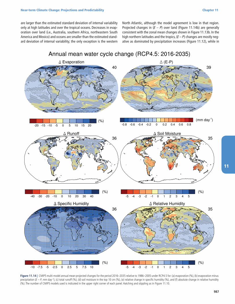
987


11

are larger than the estimated standard deviation of internal variability only at high latitudes and over the tropical oceans. Decreases in evap-oration over land (i.e., Australia, southern Africa, northeastern South America and Mexico) and oceans are smaller than the estimated stand-ard deviation of internal variability; the only exception is the western

North Atlantic, although the model agreement is low in that region. Projected changes in (E – P) over land (Figure 11.14b) are generally consistent with the zonal mean changes shown in Figure 11.13b. In the high northern latitudes and the tropics, (E – P) changes are mostly neg-ative as dominated by precipitation increases (Figure 11.12), while in

Figure 11.14 | CMIP5 multi-model annual mean projected changes for the period 2016–2035 relative to 1986–2005 under RCP4.5 for: (a) evaporation (%), (b) evaporation minus precipitation (E – P, mm day–1), (c) total runoff (%), (d) soil moisture in the top 10 cm (%), (e) relative change in specific humidity (%), and (f) absolute change in relative humidity (%). The number of CMIP5 models used is indicated in the upper right corner of each panel. Hatching and stippling as in Figure 11.10.

988


11

the subtropics several areas exhibit increases in (E – P), in particular in Europe, western Australia and central-western USA. However, in most locations changes are smaller than internal variability.

Annual mean shallow soil moisture (Figure 11.14d) shows decreases in most subtropical regions (except La Plata basin in South America) and in central Europe, and increases in northern mid-to-high latitudes. Pro-jected changes are larger than the estimated internal variability only in southern Africa, the Amazon region and Europe. Projected changes in runoff (Figure 11.14c) show decreases in northern Africa, western Australia, southern Europe and southwestern USA and increases larger than the internal variability in northwestern Africa, southern Arabia and southeastern South America associated to the projected changes in precipitation (Figure 11.12). Owing to the simplified hydrological models in many CMIP5 climate models, the projections of soil moisture and runoff have large model uncertainties.

Changes in near-surface specific humidity are positive, with the larg-est values at northern high latitudes when expressed in percentage terms (Figure 11.14e). This is consistent with the projected increases in temperature when assuming constant relative humidity. These changes are larger than the estimated standard deviation of internal variabil-ity almost everywhere: the only exceptions are oceanic regions such as the northern North Atlantic and around Antarctica. In comparison, absolute changes in near-surface relative humidity (Figure 11.14f) are much smaller, on the order of a few percent, with general decreases over most land areas, and small increases over the oceans. Significant decreases relative to natural variability are projected in the Amazonia, southern Africa and Europe, although the model agreement in these regions is low.

Over the next few decades projected increases in near-surface specific humidity are very likely, and projected increases in evaporation are likely in many land regions. There is low confidence in projected chang-es in soil moisture and surface runoff.

11.3.2.4 Atmospheric Circulation

11.3.2.4.1 Northern Hemisphere extratropical circulation

In the NH extratropics, some Atmosphere–Ocean General Circulation Models (AOGCMs) indicate changes to atmospheric circulation from anthropogenic forcing by the mid-21st century, including a pole-ward shift of the jet streams and associated zonal mean storm tracks (Miller et al., 2006; Pinto et al., 2007; Paeth and Pollinger, 2010) and a strengthening of the Atlantic storm track (Pinto et al., 2007), Figure 11.15. Consistent with this, the CMIP5 AOGCMs exhibit an ensemble mean increase in the North Atlantic Oscillation (NAO) and Northern Annular Model (NAM) indices by 2050, especially in autumn and winter (Gillett et al., 2013).

However, there are reasons to be cautious over these near-term projec-tions. Although models simulate the broad features of the large-scale circulation well, there remain quite significant biases in many models (see Sections 9.4.1.4.3 and 9.5.3.2). The response of the NH circulation can be sensitive to small changes in model formulation (Sigmond et al., 2007), and to features that are known to be poorly simulated in many

climate models. These features include high- and low-latitude physics (Rind, 2008; Woollings, 2010), ocean circulation (Woollings and Black-burn, 2012), tropical circulation (Haarsma and Selten, 2012) and strat-ospheric dynamics (Huebener et al., 2007; Morgenstern et al., 2010; Scaife et al., 2012). As a result, there is considerable model uncertainty in the response of the NH storm track position (Ulbrich et al., 2008), stationary waves (Brandefelt and Kornich, 2008) and the jet streams (Miller et al., 2006; Ihara and Kushnir, 2009; Woollings and Blackburn, 2012). Further, CMIP5 models show that the response of NH extratrop-ical circulation to even strong GHG forcing remains weak compared to recent multidecadal variability and a recent detection and attribution study suggests that tropospheric ozone and aerosol changes may have been a key driver to NH extratropical circulation changes (Gillett et al., 2013). Some AOGCMs simulate multi-decadal NAO variability as large as that recently observed with no external forcing (Selten et al., 2004; Semenov et al., 2008). This suggests that internal variability could dom-inate the anthropogenically forced response in the near term (Deser et al., 2012).

Some studies have predicted a shift to the negative phase of the Atlan-tic Multi-decadal Oscillation (AMO) over the coming few decades, with potential impacts on atmospheric circulation around the Atlantic sector (Knight et al., 2005; Sutton and Hodson, 2005; Folland et al., 2009). It has also been suggested that there may be significant changes in solar forcing over the next few decades, which could have an influence on NAO-related atmospheric circulation (Lockwood et al., 2011), although these predictions are highly uncertain (see Section 11.3.6.2.2).

There is only medium confidence in near-term projections of a north-ward shift of NH storm track and westerlies, and an increase of the NAO/NAM because of the large response uncertainty and the poten-tially large influence of internal variability.

11.3.2.4.2 Southern Hemisphere extratropical circulation

Increases in GHGs, and related dynamical processes, are projected to lead to poleward shifts in the annual mean position of Southern Hemisphere (SH) extratropical storm tracks and winds (Figure 11.17; Chapters 10 and 12). A key issue in projections of near-term SH extra-tropical circulation change is the extent to which changes driven by stratospheric ozone recovery will counteract changes driven by increas-ing GHGs. Several observational and modeling studies (Gillett and Thompson, 2003; Shindell and Schmidt, 2004; Arblaster and Meehl, 2006; Roscoe and Haigh, 2007; Fogt et al., 2009; Polvani et al., 2011a; Gillett et al., 2013) indicate that, over the late 20th and early 21st cen-turies, the observed summertime poleward shift of the westerly jet (a positive Southern Annular Mode (SAM)) has been caused primarily by the depletion of stratospheric ozone, with increasing GHGs contributing only a smaller fraction to the observed trends. The latest generation of climate models project substantially smaller poleward trends in SH atmospheric circulation in austral summer over the coming half century compared to those over the late 20th century, as the recovery of strat-ospheric ozone will oppose the effects of continually increasing GHGs (Arblaster et al., 2011; McLandress et al., 2011; Polvani et al., 2011a; Eyring et al., 2013). Locally, internal variability may be a dominant con-tributor to near-term changes in lower-tropospheric zonal winds (Figure 11.17). The average 2016–2035 SH extratropical storm tracks and zonal

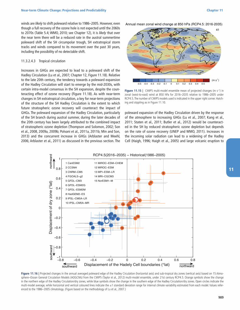
989


11

winds are likely to shift poleward relative to 1986–2005. However, even though a full recovery of the ozone hole is not expected until the 2060s to 2070s (Table 5.4; WMO, 2010; see Chapter 12), it is likely that over the near term there will be a reduced rate in the austral summertime poleward shift of the SH circumpolar trough, SH extratropical storm tracks and winds compared to its movement over the past 30 years, including the possibility of no detectable shift.

11.3.2.4.3 Tropical circulation

Increases in GHGs are expected to lead to a poleward shift of the Hadley Circulation (Lu et al., 2007; Chapter 12, Figure 11.18). Relative to the late 20th century, the tendency towards a poleward expansion of the Hadley Circulation will start to emerge by the mid-2030s, with certain intra-model consensus in the SH expansion, despite the coun-teracting effect of ozone recovery (Figure 11.18). As with near-term changes in SH extratropical circulation, a key for near-term projections of the structure of the SH Hadley Circulation is the extent to which future stratospheric ozone recovery will counteract the impact of GHGs. The poleward expansion of the Hadley Circulation, particularly of the SH branch during austral summer, during the later decades of the 20th century has been largely attributed to the combined impact of stratospheric ozone depletion (Thompson and Solomon, 2002; Son et al., 2008, 2009a, 2009b; Polvani et al., 2011a, 2011b; Min and Son, 2013) and the concurrent increase in GHGs (Arblaster and Meehl, 2006; Arblaster et al., 2011) as discussed in the previous section. The

poleward expansion of the Hadley Circulation driven by the response of the atmosphere to increasing GHGs (Lu et al., 2007; Kang et al., 2011; Staten et al., 2011; Butler et al., 2012) would be counteract-ed in the SH by reduced stratospheric ozone depletion but depends on the rate of ozone recovery (UNEP and WMO, 2011). Increases in the incoming solar radiation can lead to a widening of the Hadley Cell (Haigh, 1996; Haigh et al., 2005) and large volcanic eruption to

Figure 11.15 | CMIP5 multi-model ensemble mean of projected changes (m s–1) in zonal (west-to-east) wind at 850 hPa for 2016–2035 relative to 1986–2005 under RCP4.5. The number of CMIP5 models used is indicated in the upper right corner. Hatch-ing and stippling as in Figure 11.10.

−0.8 −0.6 −0.4 −0.2 0 0.2 0.4 0.6 0.8−1

−0.8

−0.6

−0.4

−0.2

0

0.2

0.4

0.6

0.8

1

1

1

1 CanESM2

Displacement of the Hadely Cell boundaries (°lat)

Dis

plac

emen

t of d

ry z

one

(°la

t)

2

2

2 CCSM4

3

3

3 CNRM−CM5

4

4

4 FGOALS−g25

5

5 GFDL−CM36

6

6 GFDL−ESM2G

7

7

7 GFDL−ESM2M

8

8

8 HadGEM2−ES

9

9

9 IPSL−CM5A−LR

10

10

10 IPSL−CM5A−MR

11

11

11 MIROC−ESM−CHEM

12

12

12 MIROC−ESM

13

13

13 MPI−ESM−LR

1414

14 MRI−CGCM3

15

15

15 NorESM1−M

RCP4.5(2016−2035) − Historical(1986−2005)

north

war

dso

uthw

ard

northwardsouthward

Figure 11.16 | Projected changes in the annual averaged poleward edge of the Hadley Circulation (horizontal axis) and sub-tropical dry zones (vertical axis) based on 15 Atmo-sphere–Ocean General Circulation Models (AOGCMs) from the CMIP5 (Taylor et al., 2012) multi-model ensemble, under 21st century RCP4.5. Orange symbols show the change in the northern edge of the Hadley Circulation/dry zones, while blue symbols show the change in the southern edge of the Hadley Circulation/dry zones. Open circles indicate the multi-model average, while horizontal and vertical coloured lines indicate the ±1 standard deviation range for internal climate variability estimated from each model. Values refer-enced to the 1986–2005 climatology. (Figure based on the methodology of Lu et al., 2007.)

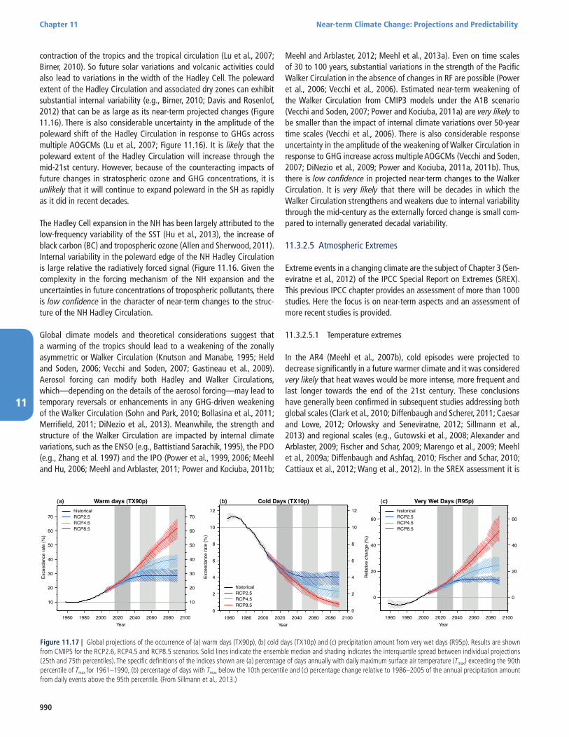
990


11

Figure 11.17 | Global projections of the occurrence of (a) warm days (TX90p), (b) cold days (TX10p) and (c) precipitation amount from very wet days (R95p). Results are shown from CMIP5 for the RCP2.6, RCP4.5 and RCP8.5 scenarios. Solid lines indicate the ensemble median and shading indicates the interquartile spread between individual projections (25th and 75th percentiles). The specific definitions of the indices shown are (a) percentage of days annually with daily maximum surface air temperature (Tmax) exceeding the 90th percentile of Tmax for 1961–1990, (b) percentage of days with Tmax below the 10th percentile and (c) percentage change relative to 1986–2005 of the annual precipitation amount from daily events above the 95th percentile. (From Sillmann et al., 2013.)

contraction of the tropics and the tropical circulation (Lu et al., 2007; Birner, 2010). So future solar variations and volcanic activities could also lead to variations in the width of the Hadley Cell. The poleward extent of the Hadley Circulation and associated dry zones can exhibit substantial internal variability (e.g., Birner, 2010; Davis and Rosenlof, 2012) that can be as large as its near-term projected changes (Figure 11.16). There is also considerable uncertainty in the amplitude of the poleward shift of the Hadley Circulation in response to GHGs across multiple AOGCMs (Lu et al., 2007; Figure 11.16). It is likely that the poleward extent of the Hadley Circulation will increase through the mid-21st century. However, because of the counteracting impacts of future changes in stratospheric ozone and GHG concentrations, it is unlikely that it will continue to expand poleward in the SH as rapidly as it did in recent decades.

The Hadley Cell expansion in the NH has been largely attributed to the low-frequency variability of the SST (Hu et al., 2013), the increase of black carbon (BC) and tropospheric ozone (Allen and Sherwood, 2011). Internal variability in the poleward edge of the NH Hadley Circulation is large relative the radiatively forced signal (Figure 11.16. Given the complexity in the forcing mechanism of the NH expansion and the uncertainties in future concentrations of tropospheric pollutants, there is low confidence in the character of near-term changes to the struc-ture of the NH Hadley Circulation.

Global climate models and theoretical considerations suggest that a warming of the tropics should lead to a weakening of the zonally asymmetric or Walker Circulation (Knutson and Manabe, 1995; Held and Soden, 2006; Vecchi and Soden, 2007; Gastineau et al., 2009). Aerosol forcing can modify both Hadley and Walker Circulations, which—depending on the details of the aerosol forcing—may lead to temporary reversals or enhancements in any GHG-driven weakening of the Walker Circulation (Sohn and Park, 2010; Bollasina et al., 2011; Merrifield, 2011; DiNezio et al., 2013). Meanwhile, the strength and structure of the Walker Circulation are impacted by internal climate variations, such as the ENSO (e.g., Battistiand Sarachik, 1995), the PDO (e.g., Zhang et al. 1997) and the IPO (Power et al., 1999, 2006; Meehl and Hu, 2006; Meehl and Arblaster, 2011; Power and Kociuba, 2011b;

Meehl and Arblaster, 2012; Meehl et al., 2013a). Even on time scales of 30 to 100 years, substantial variations in the strength of the Pacific Walker Circulation in the absence of changes in RF are possible (Power et al., 2006; Vecchi et al., 2006). Estimated near-term weakening of the Walker Circulation from CMIP3 models under the A1B scenario (Vecchi and Soden, 2007; Power and Kociuba, 2011a) are very likely to be smaller than the impact of internal climate variations over 50-year time scales (Vecchi et al., 2006). There is also considerable response uncertainty in the amplitude of the weakening of Walker Circulation in response to GHG increase across multiple AOGCMs (Vecchi and Soden, 2007; DiNezio et al., 2009; Power and Kociuba, 2011a, 2011b). Thus, there is low confidence in projected near-term changes to the Walker Circulation. It is very likely that there will be decades in which the Walker Circulation strengthens and weakens due to internal variability through the mid-century as the externally forced change is small com-pared to internally generated decadal variability.

11.3.2.5 Atmospheric Extremes

Extreme events in a changing climate are the subject of Chapter 3 (Sen-eviratne et al., 2012) of the IPCC Special Report on Extremes (SREX). This previous IPCC chapter provides an assessment of more than 1000 studies. Here the focus is on near-term aspects and an assessment of more recent studies is provided.

11.3.2.5.1 Temperature extremes

In the AR4 (Meehl et al., 2007b), cold episodes were projected to decrease significantly in a future warmer climate and it was considered very likely that heat waves would be more intense, more frequent and last longer towards the end of the 21st century. These conclusions have generally been confirmed in subsequent studies addressing both global scales (Clark et al., 2010; Diffenbaugh and Scherer, 2011; Caesar and Lowe, 2012; Orlowsky and Seneviratne, 2012; Sillmann et al., 2013) and regional scales (e.g., Gutowski et al., 2008; Alexander and Arblaster, 2009; Fischer and Schar, 2009; Marengo et al., 2009; Meehl et al., 2009a; Diffenbaugh and Ashfaq, 2010; Fischer and Schar, 2010; Cattiaux et al., 2012; Wang et al., 2012). In the SREX assessment it is

1960 1980 2000 2020 2040 2060 2080 2100

10

20

30

40

50

60

70

Year

Exce

edan

ce ra

te (%

)

10

20

30

40

50

60

70historicalRCP2.5RCP4.5RCP8.5

Warm days (TX90p)(a)

1960 1980 2000 2020 2040 2060 2080 21000

2

4

6

8

10

12

Year

Exce

edan

ce ra

te (%

)

0

2

4

6

8

10

12

Cold Days (TX10p)

1960 1980 2000 2020 2040 2060 2080 2100

0

20

40

60

Year

Rel

ativ

e ch

ange

(%)

0

20

40

60

Very Wet Days (R95p)(b) (c)

historicalRCP2.5RCP4.5RCP8.5

historicalRCP2.5RCP4.5RCP8.5

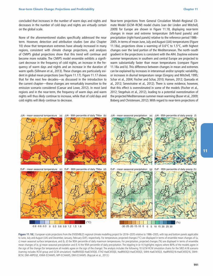
991


11

concluded that increases in the number of warm days and nights and decreases in the number of cold days and nights are virtually certain on the global scale.

None of the aforementioned studies specifically addressed the near term. However, detection and attribution studies (see also Chapter 10) show that temperature extremes have already increased in many regions, consistent with climate change projections, and analyses of CMIP5 global projections show that this trend will continue and become more notable. The CMIP5 model ensemble exhibits a signifi-cant decrease in the frequency of cold nights, an increase in the fre-quency of warm days and nights and an increase in the duration of warm spells (Sillmann et al., 2013). These changes are particularly evi-dent in global mean projections (see Figure 11.17). Figure 11.17 shows that for the next few decades—as discussed in the introduction to the current chapter—these changes are remarkably insensitive to the emission scenario considered (Caesar and Lowe, 2012). In most land regions and in the near-term, the frequency of warm days and warm nights will thus likely continue to increase, while that of cold days and cold nights will likely continue to decrease.

Near-term projections from General Circulation Model–Regional Cli-mate Model (GCM–RCM) model chains (van der Linden and Mitchell, 2009) for Europe are shown in Figure 11.18, displaying near-term changes in mean and extreme temperature (left-hand panels) and precipitation (right-hand panels) relative to the reference period 1986–2005. In terms of mean June, July and August (JJA) temperatures (Figure 11.18a), projections show a warming of 0.6°C to 1.5°C, with highest changes over the land portion of the Mediterranean. The north–south gradient in the projections is consistent with the AR4. Daytime extreme summer temperatures in southern and central Europe are projected to warm substantially faster than mean temperatures (compare Figure 11.18a and b). This difference between changes in mean and extremes can be explained by increases in interannual and/or synoptic variability, or increases in diurnal temperature range (Gregory and Mitchell, 1995; Schar et al., 2004; Fischer and Schar, 2010; Hansen, 2012; Quesada et al., 2012; Seneviratne et al., 2012). There is some evidence, however, that this effect is overestimated in some of the models (Fischer et al., 2012; Stegehuis et al., 2012), leading to a potential overestimation of the projected Mediterranean summer mean warming (Buser et al., 2009; Boberg and Christensen, 2012). With regard to near-term projections of

(°C) (%)

Figure 11.18 | European-scale projections from the ENSEMBLES regional climate modelling project for 2016–2035 relative to 1986–2005, with top and bottom panels applicable to June, July and August (JJA) and December, January, February (DJF), respectively. For temperature, projected changes (°C) are displayed in terms of ensemble mean changes of (a, c) mean seasonal surface temperature, and (b, d) the 90th percentile of daily maximum temperatures. For precipitation, projected changes (%) are displayed in terms of ensemble mean changes of (e, g) mean seasonal precipitation and (f, h) the 95th percentile of daily precipitation. The stippling in (e–h) highlights regions where 80% of the models agree in the sign of the change (for temperature all models agree on the sign of the change). The analysis includes the following 10 GCM-RCM simulation chains for the SRES A1B scenario (naming includes RCM group and GCM simulation): HadRM3Q0-HadCM3Q0, ETHZ-HadCM3Q0, HadRM3Q3-HadCM3Q3, SMHI-HadCM3Q3, HadRM3Q16-HadCM3Q16, SMHI-BCM, DMI-ARPEGE, KNMI-ECHAM5, MPI-ECHAM5, DMI-ECHAM5. (Rajczak et al., 2013.)

992


11

record heat compared to record cold (Meehl et al., 2009b) show, for one model, that over the USA the ratio of daily record high temperatures to daily record low temperatures could increase from an early 2000s value of roughly 2 to 1 to a mid-century value of about 20 to 1.

In terms of December, January and February (DJF) temperatures (Figure 11.18c), projections show a warming of 0.3°C to 1.8°C, with the larg-est changes in the N–NE part of Europe. This characteristic pattern of changes tends to persist to the end of century (van der Linden and Mitchell, 2009). In contrast to JJA temperatures, daytime high-percen-tile (i.e., warm) winter temperatures are projected to warm slower than mean temperatures (compare Figure 11.18c and Figure 11.18d), while low-percentile (i.e., cold) winter temperatures warm faster than the mean. This behaviour is indicative of reductions in internal variability, which may be linked to changes in storm track activity, reductions in diurnal temperature range and changes in snow cover (e.g., Colle et al. 2013; Dutra et al., 2011).

11.3.2.5.2 Heavy precipitation events

For the 21st century, the AR4 and the SREX concluded that heavy pre-cipitation events were likely to increase in many areas of the globe (IPCC, 2007). Since AR4, a larger number of additional studies have been published using global and regional climate models (Fowler et al., 2007; Gutowski et al., 2007; Sun et al., 2007; Im et al., 2008; O’Gorman and Schneider, 2009; Xu et al., 2009; Hanel and Buishand, 2011; Hein-rich and Gobiet, 2011; Meehl et al., 2012b). For the near term, CMIP5 global projections (Figure 11.17c) confirm a clear tendency for increas-es in heavy precipitation events in the global mean, but there are sig-nificant variations across regions (Sillmann et al., 2013). Past observa-tions have also shown that interannual and decadal variability in mean and heavy precipitation are large, and are in addition strongly affected by internal variability (e.g., El Niño), volcanic forcing and anthropogen-ic aerosol loads (see Section 2.3.1). In general models have difficulties in representing these variations, particularly in the tropics (see Section 9.5.4.2). Thus the frequency and intensity of heavy precipitation events will likely increase over many land areas in the near term, but this trend will not be apparent in all regions, because of natural variability and possible influences of anthropogenic aerosols.

Simulations with regional climate models demonstrate that the response in terms of heavy precipitation events to anthropogenic cli-mate change may become evident in some but not all regions in the near term. For instance, ENSEMBLES projections for Europe (see Figure 11.18e–h) confirm the previous IPCC results that changes in mean precipitation as well as heavy precipitation events are characterized by a pronounced north–south gradient in the extratropics, especially in the winter season, with precipitation increases in the higher lati-tudes and decreases in the subtropics. Although this pattern starts to emerge in the near term, the projected changes are statistically signif-icant only in a fraction of the domain. The results are affected by both changes in water vapour content as induced by large-scale warming and large-scale circulation changes. Figure 11.18e–h also shows that mid- and high-latitude projections for changes in DJF extremes and means are qualitatively similar in the near term, at least for the event size considered.

Previous work reviewed in AR4 has established that extreme precipitation events may increase substantially stronger than mean precipitation amounts. More specifically, extreme events may increase with the atmospheric water vapour content, that is, up to the rate of the Clausius–Clapeyron (CC) relationship (e.g., Allen and Ingram, 2002). More recent work suggests that increases beyond this threshold may occur for short-term events associated with thunderstorms (Len-derink and Van Meijgaard, 2008; Lenderink and Meijgaard, 2010) and tropical convection (O’Gorman, 2012). A number of studies showed strong dependencies on location and season, but confirm the exist-ence of significant deviations from the CC scaling (e.g., Lenderink et al., 2011; Mishra et al., 2012; Berg et al., 2013). Studies with cloud-re-solving models generally support the existence of temperature-precip-itation relations that are close to or above (up to about twice) the CC relation (Muller et al., 2011; Singleton and Toumi, 2012).

11.3.2.5.3 Tropical cyclones

The projected response of tropical cyclones (TCs) at the end of the 21st century is summarized in Section 14.6.1 and the IPCC Special Report on Extremes (SREX) (Seneviratne et al., 2012). Relative to the number of studies focussing on projections of TC activity at the end of the 21st century (Section 14.6.1; Knutson et al., 2010; Seneviratne et al., 2012 there are fewer studies that have explored near-term projections of TC activity (Table 11.2); the North Atlantic (NA) stands out as the basin with most studies. In the NA, there are mixed projections for basin-wide TC frequency, suggesting significant decreases (Knutson et al., 2013a) or non-significant changes (Villarini et al., 2011; Villarini and Vecchi, 2012). Multi-model mean projected NA TC frequency chang-es based on CMIP3 and CMIP5 over the first half of the 21st century were smaller than the overall uncertainty estimated from the Coupled General Circulation Models (CGCMs), with internal climate variability being a leading source of uncertainty through the mid-21st century (Villarini et al., 2011; Villarini and Vecchi, 2012). Therefore, based on the limited literature available, the conflicting near-term projections in basins with more than one study, the large influence of internal variability, the lack of confidently detected/attributed changes in TC activity (Chapter 10) and the conflicting projections for basin-wide TC frequency even at the end of the 21st century (Chapter 14), there is currently low confidence in basin-scale and global projections of trends in tropical cyclone frequency to the mid-21st century.

Exploring different hurricane intensity measures, two studies project near-term increases of NA hurricane intensity (Knutson et al., 2013a; Villarini and Vecchi, 2013), driven in large part by projected reductions in NA tropospheric aerosols in CMIP5 future forcing scenarios. Studies project near-term increases in the frequency Category 4–5 TCs in the NA (Knutson et al., 2013a) and southwest Pacific (Leslie et al., 2007). Published studies agree in the sign of projected mid-century intensity change (intensification), but the only basin with more than one study exploring intensity is the NA. For the NA, an estimate of the time scale of emergence of projected changes in intense TC frequency exceeds 60 years (Bender et al., 2010), although that estimate depends crucially on the amplitude of internal climate variations of intense hurricane fre-quency (e.g., Emanuel, 2011), which remains poorly constrained at the moment. Therefore, there is low confidence in near-term TC intensity projections in all TC basins.

993


11

Modes of climate variability that in the past have led to variations in the intensity, frequency and structure of tropical cyclones across the globe—such as the ENSO (e.g., Zhang and Delworth, 2006; Wang et al., 2007; Callaghan and Power, 2011; Chapter 14)—are very likely to continue influencing TC activity through the mid-21st century. There-fore, it is very likely that over the next few decades tropical cyclone frequency, intensity and spatial distribution globally, and in individual basins, will vary from year to year and decade to decade.

11.3.3 Near-term Projected Changes in the Ocean

11.3.3.1 Temperature

Globally averaged surface and near-surface ocean temperatures are projected by AOGCMs to warm over the early 21st century, in response to both present day atmospheric concentrations of GHGs (‘committed warming’; e.g., Meehl et al., 2006) and projected future changes in RF (Figure 11.19). Globally averaged SST shows substantial year-to-year and decade-to-decade variability (e.g., Knutson et al., 2006; Meehl et al., 2011), whereas the variability of depth-averaged ocean tempera-tures is much less (e.g., Meehl et al., 2011; Palmer et al., 2011). The rate at which globally averaged surface and depth-averaged temperatures rise in response to a given scenario for RF shows a considerable spread between models (an example of response uncertainty; see Section 11.2), due to differences in climate sensitivity and ocean heat uptake (e.g., Gregory and Forster, 2008). In the CMIP5 models under all RCP forcing scenarios, globally averaged SSTs are projected to be warmer over the near term relative to 1986–2005 (Figure 11.20).

A key uncertainty in the future evolution of globally averaged oceanic temperature are possible future large volcanic eruptions, which could

impact the radiative balance of the planet for 2 to 3 years after their eruption and act to reduce oceanic temperature for decades into the future (Delworth et al., 2005; Stenchikov et al., 2009; Gregory, 2010). An estimate using the GFDL-CM2.1 coupled AOGCM (Stenchikov et al., 2009) suggests that a single Tambora (1815)-like volcano could erase the projected global ocean depth-averaged temperature increase for many years to a decade. A Pinatubo (1991)-like volcano could erase the projected increase for 2 to 10 years. See Section 11.3.6 for further discussion.

TC Basin Explored Projected Change in TC Activity Reported Notes Reference

GlobalReduced global, Northern Hemisphere and Southern Hemisphere frequency 2016–2035 relative to 1986–2005.

High-resolution atmospheric model forced by CMIP3 SRES A1B multi-model SST change 2004–2099.

Sugi and Yoshimura (2012)

N.W. PacificOver first half of 21st century: Reduced Activity over South China Sea, Increased Activity near subtropical Asia

Statistical downscale of five CMIP3 models under SRES A1B.

Wang et al. (2011)

N.W. PacificOver 2001–2040, a decrease in TC frequency in the East China Sea, and a frequen-cy decrease and increase in intensity of Yangze River Basin landfalling typhoons.

Statistical downscaling of CGCM forced by CMIP3 SRES A1B scenario.

Orlowsky and Seneviratne (2012)

S.W. Pacific Differences of 2000–2050 with 1970–2000. Negligible change in overall frequency. Significant (~15%) increase in number of Category 4–5 TCs.

Dynamical regional downscale of coupled AOGCM forced with IPCC IS92a increasing CO2 scenario.

Leslie et al. (2007)

N. AtlanticLinear trend in TC frequency 2001–2050: Ensemble-mean non-significant decrease in TC frequency (–5%). Ensemble range of –50% to +30%.

Statistical downscaling of CMIP3 models under A1B scenario.

Villarini et al. (2011)

N. AtlanticTC frequency averaged 2016–2035 minus 1986–2005: Ensemble-mean non-significant increase for RCP2.6 (4%), non-significant decrease for RCP4.5 (–2%) and RCP8.5 (–1%). Ensemble range of –30% to 27% across all scenarios/models.

Statistical downscaling of CMIP5 RCP2.6, RCP4.5 and RCP8.5

Villarini and Vecchi (2012)

N. AtlanticPower Dissipation Index averaged 2016–2035 minus 1986–2005: Ensemble mean significant increase for RCP2.6 (23%) and RCP8.5 (17%), non-significant increase for RCP4.5 (10%). Ensemble range of –43% to 78% across all scenarios/models.

Statistical downscaling of CMIP5 RCP2.6, RCP4.5 and RCP4.5

Villarini and Vecchi (2013)

N. Atlantic

Difference 2016–2035 minus 1986–2005 averages: Significant decrease (–20%) to overall TC and hurricane frequency. Significant increase (+45%) in number of Category 4–5 TCs. Significant increase in pre-cipitation of hurricanes (11%) and tropical storms (18%).

Double dynamical refinement of CMIP5 RCP4.5 multi-model ensemble projections.

Knutson et al. (2013a)

Table 11.2 | Summary of studies exploring near-term projections of tropical cyclone (TC) activity. First column lists the TC basin explored, the second column summarizes the changes in TC activity reported in each study, the third column presents notes on the methodology and the fourth column provides a reference to the study.

Global sea surface temperature change

(°C

)

Figure 11.19 | Projected changes in annual averaged, globally averaged, surface ocean temperature based on 12 Atmosphere–Ocean General Circulation Models (AOGCMs) from the CMIP5 (Meehl et al., 2007b) multi-model ensemble, under 21st century scenarios RCP2.6, RCP4.5, RCP6.0 and RCP8.5. Shading indicates the 90% range of projected annual global mean surface temperature anomalies. Anomalies com-puted against the 1986–2005 average from the historical simulations of each model.

994


11

In the absence of multiple major volcanic eruptions (see Section 11.3.6.2), it is very likely that globally averaged surface and depth-av-eraged temperatures averaged 2016–2035 will be warmer than those averaged over 1986–2005.

There are regional variations in the projected amplitude of ocean tem-perature change (Figure 11.20) which are influenced by ocean circula-tion as well as surface heating (Timmermann et al., 2007; Vecchi and Soden, 2007; DiNezio et al., 2009; Yin et al., 2009; Xie et al., 2010; Yin et al., 2010), including changes in tropospheric aerosol concentrations (e.g., Booth et al., 2012; Villarini and Vecchi, 2012). Inter-decadal vari-ability of upper ocean temperatures is larger in mid-latitudes, particu-larly in the NH, than in the tropics. A consequence of this contrast is that it will take longer in the mid-latitudes than in the tropics for the anthropogenic warming signal to emerge from the noise of internal variability (Wang et al., 2010).

Projected changes to thermal structure of the tropical Indo-Pacific are strongly dependent on the future behaviour of the Walker Circu-lation (Vecchi and Soden, 2007; DiNezio et al., 2009; Timmermann et al., 2010), in addition to changes in heat transport and changes in surface heat fluxes. It is likely that internal climate variability will be a dominant contributor to changes in the depth and tilt of the equatorial thermocline, and the strength of the east–west gradient of SST across the Pacific through the mid-21st century; thus it is likely there will be multi-year periods with increases or decreases in these measures.

11.3.3.2 Salinity

Changes in sea surface salinity are expected in response to changes in precipitation, evaporation and runoff (see Section 11.3.2.3), as well as ocean circulation; in general (but not in every region), salty regions are expected to become saltier and fresh regions fresher (e.g., Durack et al. 2012; Terray et al. 2012; Figure 11.20). As discussed in Chapter 10 (Section 10.4.2), observation-based and attribution studies have found some evidence of an emerging anthropogenic signal in salin-ity change (Section 10.4.2), in particular increases in surface salinity

in the subtropical North Atlantic, and decreases in the west Pacific warm pool region (Stott et al., 2008; Cravatte et al., 2009; Durack and Wijffels, 2010; Durack et al., 2012; Pierce et al., 2012; Terray et al., 2012). Models generally predict increases in salinity in the tropical and (especially) subtropical Atlantic, and decreases in the western tropical Pacific over the next few decades (Figure 11.20) (Durack et al., 2012; Terray et al., 2012). These projected decreases in the Atlantic and in the western tropical Pacific are considered likely.

Projected near-term increases in freshwater flux into the Arctic Ocean produce a fresher surface layer and increased transport of fresh water into the North Atlantic (Holland et al., 2006; Holland et al., 2007; Vavrus et al., 2012). Such contributions to decreased density of the ocean sur-face layer in the North Atlantic could act to reduce deep ocean con-vection there and contribute to a near-term reduction of strength of Atlantic Meridional Ocean Circulation (AMOC). However, the strength of the AMOC can also be modulated by changes in temperature, such as those from changing RF (Delworth and Dixon, 2006).

11.3.3.3 Circulation

As discussed in previous assessment reports, the AMOC is generally projected to weaken over the next century in response to increase in atmospheric GHG. However, the rate and magnitude of weakening is very uncertain. Response uncertainty is a major contributor in the near term, but the influence of anthropogenic aerosols and natural RFs (solar, volcanic) cannot be neglected, and could be as important as the influence of GHGs (e.g., Delworth and Dixon, 2006; Stenchikov et al., 2009). For example, the rate of weakening of the AMOC in two models with different climate sensitivities is quite different, with the less sensitive model (CCSM4) showing less weakening and a more rapid recovery than the more sensitive model (Community Earth System Model 1/Community Atmosphere Model 5 (CESM1/CAM5; Meehl et al., 2013c). In addition, the natural variability of the AMOC on dec-adal time scales is poorly known and poorly understood, and could dominate any anthropogenic response in the near term (Drijfhout and Hazeleger, 2007). The AMOC is known to play an important role in the

Figure 11.20 | CMIP5 multi-model ensemble mean of projected changes in sea surface temperature (right panel; °C) and sea surface salinity (left panel; practical salinity units) for 2016–2035 relative to 1986–2005 under RCP4.5. The number of CMIP5 models used is indicated in the upper right corner. Hatching and stippling as in Figure 11.10.

995


11

decadal variability of the North Atlantic Ocean, but climate models show large differences in their simulation of both the amplitude and spectrum of AMOC variability (e.g., Bryan et al., 2006; Msadek et al., 2010). In some AOGCMs changes in SH surface winds influence the evolution of the AMOC on time scales of many decades (Delworth and Zeng, 2008), so the delayed response to SH wind changes, driven by the historical reduction in stratospheric ozone along with its projected recovery, could be an additional confounding issue (Section 11.3.2.3). Overall, it is likely that there will be some decline in the AMOC by 2050, but decades during which the AMOC increases are also to be expect-ed. There is low confidence in projections of when an anthropogenic influence on the AMOC might be detected (Baehr et al., 2008; Roberts and Palmer, 2012).

Projected changes to oceanic circulation in the Indo-Pacific are strongly dependent on future response of the Walker Circulation (Vecchi and Soden, 2007; DiNezio et al., 2009), the near-term projected weaken-ing of which is smaller than the expected variability on time scales of decades to years (Section 11.3.2.4.3). Taking variability into account, there is medium confidence in a weakening of equatorial Pacific cir-culation, including equatorial upwelling and the shallow subtropical overturning in the Pacific, and the Indonesian Throughflow over the coming decades.

11.3.4 Near-term Projected Changes in the Cryosphere

This section assesses projected near-term changes of elements of the cryosphere. These consist of sea ice, snow cover and near-surface per-mafrost (frozen ground), changes to the Arctic Ocean and possible abrupt changes involving the cryosphere. Glaciers and ice sheets are addressed in Chapter 13. Here near-term changes in the geographi-cal coverage of sea ice, snow cover and near-surface permafrost are assessed.

Trends due to changes in external forcing exist alongside consider-able interannual and decadal variability. This complicates our ability to make specific, precise short-term projections, and delays the emer-gence of a forced signal above the noise.

11.3.4.1 Sea Ice

Though most of the CMIP5 models project a nearly ice-free Arctic (sea ice extent less than 1 × 106 km2 for at least 5 consecutive years) at the end of summer by 2100 in the RCP8.5 scenario (see Section 12.4.6.1), some show large changes in the near term as well. Some previous models project an ice-free summer period in the Arctic Ocean by 2040 (Holland et al., 2006), and even as early as the late 2030s using a criterion of 80% sea ice area loss (e.g., Zhang, 2010). By scaling six CMIP3 models to recent observed September sea ice changes, a nearly ice-free Arctic in September is projected to occur by 2037, reaching the first quartile of the distribution for timing of September sea ice loss by 2028 (Wang and Overland, 2009). However, a number of models that have fairly thick Arctic sea ice produce a slower near-term decrease in sea ice extent compared to observations (Stroeve et al., 2007). Based on a linear extrapolation into the future of the recent sea ice volume trend from a hindcast simulation conducted with a regional model of the Arctic sea ice–ocean system (Maslowski et al., 2012) projected that

it would take only until about 2016 to reach a nearly ice-free Arctic Ocean in summer. However, such an approach not only neglects the effect of year-to-year or longer-term variability (Overland and Wang, 2013) but also ignores the negative feedbacks that can occur when the sea ice cover becomes thin (Notz, 2009). Mahlstein and Knutti (2012) estimated the annual mean global surface warming threshold for nearly ice-free Arctic conditions in September to be ~2°C above the present derived from both CMIP3 models and observations.

An analysis of CMIP3 model simulations indicates that for near-term predictions the dominant factor for decreasing sea ice is increased ice melt, and reductions in ice growth play a secondary role (Holland et al., 2010). Arctic sea ice has larger volume loss when there is thicker ice initially across the CMIP3 models, with a projected accumulated mass loss of about 0.5 m by 2020, and roughly 1.0 m by 2050, with considerable model spread (Holland et al., 2010). The CMIP3 models tended to under-estimate the observed rapid decline of summer Arctic sea ice during the satellite era, but these recent trends are more accu-rately simulated in the CMIP5 models (see Section 12.4.6.1). For CMIP3 models, results indicate that the changes in Arctic sea ice mass budget over the 21st century are related to the late 20th century mean sea ice thickness distribution (Holland et al., 2010), average sea ice thick-ness (Bitz, 2008; Hodson et al., 2012), fraction of thin ice cover (Boe et al., 2009) and oceanic heat transport to the Arctic (Mahlstein et al., 2011). Acceleration of sea ice drift observed over the last three dec-ades, underestimated in CMIP3 projections (Rampal et al., 2011), and the presence of fossil-fuel and biofuel soot in the Arctic environment (Jacobson, 2010), could also contribute to ice-free late summer condi-tions over the Arctic in the near term. Details on the transition to an ice-free summer over the Arctic are presented in Chapter 12 (Sections 12.4.6.1 and 12.5.5.7).

The discussion in Section 12.4.6.1 makes the case for assessing near-term projections of Arctic sea ice by weighting/recalibrating the models based on their present-day Arctic sea ice simulations, with a credible underlying physical basis in order to increase confidence in the results, and accounting for the potentially large imprint of natural variabili-ty on both observations and model simulations (see Section 9.8.3). A subselection of a set of CMIP5 models that fits those criteria, following the methodology proposed by Massonnet et al. (2012), is applied in Chapter 12 (Section 12.4.6.1) to the full set of models that provid-ed the CMIP5 database with sea ice output. Among the five selected models, four project a nearly ice-free Arctic Ocean in September (sea ice extent less than 1 × 106 km2 for at least 5 consecutive years) before 2050 for RCP8.5, the earliest and latest years of near disappearance of the sea ice pack being about 2040 and about 2060, respectively. The potential irreversibility of the Arctic sea ice loss and the possibility of an abrupt transition toward an ice-free Arctic Ocean are discussed in Section 12.5.5.7.

In light of all these results and others discussed in greater detail in Sec-tion 12.4.6.1, it is very likely that the Arctic sea ice cover will continue to shrink and thin all year round during the 21st century as the annual mean global surface temperature rises. It is also likely that the Arctic Ocean will become nearly ice-free in September before the middle of the century for high GHG emissions such as those corresponding to RCP8.5 (medium confidence).

996


11

In early 21st century simulations, Antarctic sea ice cover is projected to decrease in the CMIP5 models, though CMIP3 and CMIP5 models simulate recent decreases in Antarctic sea ice extent compared to slight increases in the observations (Section 12.4.6.1). However, there is the possibility that melting of the Antarctic ice sheet could be chang-ing the vertical ocean temperature stratification around Antarctica and encourage sea ice growth (Bintanja et al., 2013). This and other evidence discussed in Section 12.4.6.1 leads to the assessment that there is low confidence in Antarctic sea ice model projections that show near-term decreases of sea ice cover because of the wide range of model responses and the inability of almost all of the models to reproduce the mean seasonal cycle, interannual variability and overall increase of the Antarctic sea ice areal coverage observed during the satellite era (see Section 9.4.3).

11.3.4.2 Snow Cover

Decreases of snow cover extent (SCE, defined over ice-free land areas) are strongly connected to a shortening of seasonal snow cover dura-tion (Brown and Mote, 2009) and are related to both precipitation and temperature changes (see Section 12.4.6.2). This has implications for snow on sea ice where loss of sea ice area in autumn delays snowfall accumulation, with CMIP5 multi-model mean values of snow depth in April north of 70°N reduced from about 28 cm to roughly 18 cm for the 2031–2050 period compared to the 1981–2000 average (Hezel et al., 2012). The snow accumulation season by mid-century in one model is projected to begin later in autumn, with the melt season initiated earlier in the spring (Lawrence and Slater, 2010). As discussed in great-er detail in Section 12.4.6.2, projected increases in snowfall across much of the northern high latitudes act to increase snow amounts, but warming reduces the fraction of precipitation that falls as snow. In addition, the reduction of Arctic sea ice also provides an increased moisture source for snowfall (Liu et al., 2012). Whether the average SCE decreases or increases by mid-century depends on the balance between these competing factors. The dividing line where models tran-sition from simulating increasing or decreasing maximum snow water equivalent roughly coincides with the –20°C isotherm in the mid-20th century November to March mean surface air temperature (Raisanen, 2008). The projected change of SCE over some regions is inconsistent with that of extreme snowfall, a major contributor to SCE. For instance, SCE is projected to decrease over northern China by the mid-21st century (Shi et al., 2011), while the extreme snowfall events over the region are projected to increase (Sun et al., 2010).

Time series of projected changes in relative SCE (for NH ice-free land areas) are shown in Figure 12.32. Multi-model averages from the CMIP5 archive (Brutel-Vuilmet et al., 2013) show percentage decreas-es of NH SCE ± 1 standard deviation for the 2016–2035 time period for a March to April average using a 15% extent threshold for the four RCP scenarios as follows: RCP2.6: –5.2% ± 1.9% (21 models); RCP4.5: –5.3% ± 1.5% (24 models); RCP6.0: –4.5% ± 1.2% (16 models); RCP8.5: –6.0% ± 2.0% (24 models).

11.3.4.3 Near Surface Permafrost

Virtually all near-term projections indicate a substantial amount of near-surface permafrost degradation (typically taking place in the upper

2 to 3 m; see Callaghan et al. (2011) and see glossary for detailed defi-nition), and thaw depth deepening over much of the permafrost area (Sushama et al., 2006; Lawrence et al., 2008; Guo and Wang, 2012).As discussed in more detail in Section 12.4.6.2, these projections have increased credibility compared to the previous generation of models assessed in the AR4 because current climate models represent perma-frost more accurately (Alexeev et al., 2007; Nicolsky et al., 2007; Law-rence et al., 2008). The reduction in annual mean near-surface perma-frost area for the 2016–2035 time period compared to the 1986–2005 reference period for the CMIP5 models (Slater and Lawrence, 2013) for the NH for the four RCP scenarios is 21% ± 5% (RCP2.6), 18% ± 6% (RCP4.5), 18% ± 3% (RCP6.0) and 20% ± 5% (RCP8.5).

11.3.5 Projections for Atmospheric Composition and Air Quality to 2100

The future evolution of atmospheric composition is determined by the chemical–physical processes in the atmosphere, forced primarily by anthropogenic and natural emissions and by interactions with the biosphere and ocean (Chapters 2, 6, 7, 8 and 12). Twenty-first century projections of the chemically reactive GHGs, including methane (CH4), nitrous oxide (N2O) and ozone (O3), as well as aerosols, are assessed here (Section 11.3.5.1). Future air pollution, specifically ground-level O3 and PM2.5 (particulate matter with a diameter of less than 2.5 μm, a measure of aerosol concentration), is also assessed here (Section 11.3.5.2). The impact of changes in natural emissions and deposition through altered land use (Heald et al., 2008; Chen et al., 2009a; Cook et al., 2009; Wu et al., 2012) and production of food or biofuels (Chap-ter 6) on atmospheric composition and air quality are not assessed here. Projected CO2 abundances are discussed in Chapters 6 and 12.

Projections for the 21st century are based predominantly on the CMIP5 models that included atmospheric chemistry and the related ACCMIP (Atmospheric Chemistry and Climate Model Intercomparison Project) models, driven by the RCP emission and climate scenarios. These and the earlier SRES scenarios include only direct anthropogenic emis-sions. Natural emissions may also change with biosphere feedbacks in response to climate or land use change (Chapters 6, 8). Emphasis is placed on evaluating the 21st-century RCP scenarios from emissions to abundance, summarized in tables in Annex II. For the well-mixed greenhouse gases (WMGHGs), the effective radiative forcing (ERF) in both RCP and SRES scenarios increases similarly before 2040 with little spread (±16% in ERF; see Tables AII.6.1 to AII.6.10), but by 2050 the RCP2.6 scenario diverges, falling well below the envelope containing both the SRES and other RCP scenarios.

National and regional regulations implemented on emissions con-tributing to ground-level ozone and PM2.5 pollution influence global atmospheric chemistry and climate (NRC, 2009; HTAP, 2010a), as was recognized in the TAR (Jacob et al., 1993; Penner et al., 1993; Johnson et al., 1999; Prather et al., 2001). Ozone and aerosols are radiatively active species (Chapters 7 and 8) and many of their precursors serve as indirect GHGs (e.g., nitrogen oxides (NOx), carbon monoxide (CO), Non Methane Volatile Organic Compounds (NMVOC)) by changing the atmospheric oxidative capacity, and thereby the lifetimes and abun-dances of CH4, hydrofluorocarbons (HFCs) and tropospheric O3 (Chap-ter 8). Consequently their evolution can influence near-term climate

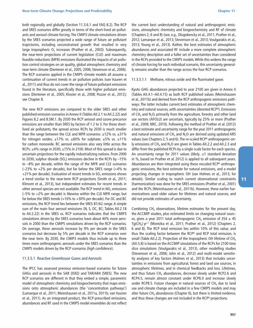
997


11

both regionally and globally (Section 11.3.6.1 and FAQ 8.2). The RCP and SRES scenarios differ greatly in terms of the short-lived air pollut-ants and aerosol climate forcing. The CMIP3 climate simulations driven by the SRES scenarios projected a wide range of future air pollutant trajectories, including unconstrained growth that resulted in very large tropospheric O3 increases (Prather et al., 2003). Subsequently, the near-term projections of current legislation (CLE) and maximum feasible reductions (MFR) emissions illustrated the impacts of air pollu-tion control strategies on air quality, global atmospheric chemistry and near-term climate (Dentener et al., 2005, 2006; Stevenson et al., 2006). The RCP scenarios applied in the CMIP5 climate models all assume a continuation of current trends in air pollution policies (van Vuuren et al., 2011) and thus do not cover the range of future pollutant emissions found in the literature, specifically those with higher pollutant emis-sions (Dentener et al., 2005; Kloster et al., 2008; Pozzer et al., 2012); see Chapter 8.

The new RCP emissions are compared to the older SRES and other published emission scenarios in Annex II (Tables AII.2.1 to AII.2.22) and Figures 8.2 and 8.SM.1. By 2030 the RCP aerosol and ozone precursor emissions are smaller than SRES by factors of 1.2 to 3. For these short-lived air pollutants, the spread across RCPs by 2030 is much smaller than the range between the CLE and MFR scenarios: ±12% vs. ±31% for nitrogen oxides; ±17% vs. ±60% for sulphate; ±5% vs. ±11% for carbon monoxide. BC aerosol emissions also vary little across the RCPs: ±4% range in 2030; ±15% in 2100. Most of this spread is due to uncertain projections for the rapidly industrializing nations. From 2000 to 2030, sulphur dioxide (SO2) emissions decline in the RCPs by –15% to –8% per decade, within the range of the MFR and CLE scenarios (–23% to +2% per decade), but far below the SRES range (+4% to +21% per decade). Evaluation of recent trends in SO2 emissions shows a trend similar to the near-term RCP projections (Smith et al., 2011; Klimont et al., 2013), but independent estimates for recent trends in other aerosol species are not available. The RCP trend in NOx emissions (–5% to +2% per decade) is likewise within the CLE-MFR range, but far below the SRES trends (+10% to +30% per decade). For OC and BC emissions, the RCP trend lies between the SRES B1/A2 range. A simple sum of the main four aerosol emissions (N, S, OC, BC; Tables AII.2.18 to AII.2.22) in the SRES vs. RCP scenarios indicates that the CMIP3 simulations driven by the SRES scenarios have about 40% more aero-sols in 2000 than the CMIP5 simulations driven by the RCP scenarios. On average, these aerosols increase by 9% per decade in the SRES scenarios but decrease by 5% per decade in the RCP scenarios over the near term. By 2030, the CMIP3 models thus include up to three times more anthropogenic aerosols under the SRES scenarios than the CMIP5 models driven by the RCP scenarios (high confidence).

11.3.5.1 Reactive Greenhouse Gases and Aerosols

The IPCC has assessed previous emission-based scenarios for future GHGs and aerosols in the SAR (IS92) and TAR/AR4 (SRES). The new RCP scenarios are different in that they embed a simple, parametric model of atmospheric chemistry and biogeochemistry that maps emis-sions onto atmospheric abundances (the ‘concentration pathways’) (Lamarque et al., 2011; Meinshausen et al., 2011a, 2011b; van Vuuren et al., 2011). As an integrated product, the RCP-prescribed emissions, abundances and RF used in the CMIP5 model ensembles do not reflect

the current best understanding of natural and anthropogenic emis-sions, atmospheric chemistry and biogeochemistry and RF of climate (Chapters 2, 6 and 8) (see, e.g., Dlugokencky et al., 2011; Prather et al., 2012; Lamarque et al., 2013; Stevenson et al., 2013; Voulgarakis et al., 2013; Young et al., 2013). Rather, the best estimates of atmospheric abundances and associated RF include a more complete atmospheric chemistry description and a fuller set of uncertainties than considered in the RCPs provided to the CMIP5 models. While this widens the range of climate forcing for each individual scenario, this uncertainty general-ly remains smaller than the range across the four RCP scenarios.

11.3.5.1.1 Methane, nitrous oxide and the fluorinated gases

Kyoto GHG abundances projected to year 2100 are given in Annex II (Tables AII.4.1–AII.4.15) as both RCP published values (Meinshausen et al., 2011b) and derived from the RCP anthropogenic emissions path-ways. The latter includes current best estimates of atmospheric chem-istry and natural sources, with uncertainties (denoted RCP&). Emissions of CH4 and N2O, primarily from the agriculture, forestry and other land use sectors (AFOLU) are uncertain, typically by 25% or more (Prather et al., 2009; NRC, 2010). Following the method of Prather et al. (2012) a best estimate and uncertainty range for the year 2011 anthropogenic and natural emissions of CH4 and N2O are derived using updated AR5 values (see Chapters 2, 5 and 6). The re-scaled RCP& anthropogenic-on-ly emissions of CH4 and N2O are given in Tables AII.2.2 and AII.2.3 and differ from the published RCPs by a single scale factor for each species. An uncertainty range for 2011 values (likely, ±1 standard deviation in %, based on Prather et al. 2012) is applied to all subsequent years. Abundances are then integrated using these rescaled RCP& anthropo-genic emissions, the best estimate for natural emissions, and a model projecting changes in tropospheric OH (see Holmes et al., 2013; for details). Similar scaling to match current observational constraints (harmonization) was done for the SRES emissions (Prather et al., 2001) and the RCPs (Meinshausen et al., 2011b). However, these earlier har-monizations used older values for lifetimes and natural sources, and did not provide estimates of uncertainty.

Combining CH4 observations, lifetime estimates for the present day, the ACCMIP studies, plus estimated limits on changing natural sourc-es, gives a year 2011 total anthropogenic CH4 emission of 354 ± 45 Tg(CH4) yr–1 (Montzka et al., 2011; Prather et al., 2012) (Chapters 2, 6 and 8). The RCP total emission lies within 10% of this value, and thus the scaling factor between the RCP& and RCP total emission, is small (Table AII.2.2). Projection of the tropospheric OH lifetime of CH4 (AII.5.8) is based on the ACCMIP simulations of the RCPs for 2100 time slice simulations (Voulgarakis et al., 2013), other modelling studies (Stevenson et al., 2006; John et al., 2012) and multi-model sensitiv-ity analyses of key factors (Holmes et al., 2013) that includes uncer-tainties in emissions from agricultural, forest and land use sources, in atmospheric lifetimes, and in chemical feedbacks and loss. Lifetimes, and thus future CH4 abundances, decrease slowly under RCP2.6 and RCP4.5, remain almost constant under RCP6.0 and increase slowly under RCP8.5. Future changes in natural sources of CH4 due to land use and climate change are included in a few CMIP5 models and may alter future CH4 abundances (Chapter 6), but there is limited evidence, and thus these changes are not included in the RCP& projections.

998


11

The resulting best estimates of total CH4 anthropogenic emissions and abundances (RCP&) are compared with RCP values in Figure 11.21. For RCP2.6, the CH4 abundance is projected to decline continuously over the century by about 30%, whereas in RCP 4.5 and 6.0 it peaks mid-century and then declines to below the year 2011 abundance by the end of the century. Throughout the century, the uncertainty in CH4 abundance for an individual scenario is less than range from RCP2.6 to RCP8.5. For example, by year 2020 the spread in CH4 abundance across the RCPs is already large, 1720 to 1920 ppb, with uncertainty in each scenario estimated at only ±20 ppb. The likely range for RCP& CH4 is 30% wider than that in the RCP CH4 abundances used to force the CMIP5 models (Figure 11.21): by year 2100 the likely range of RCP8.5& CH4 abundance extends 520 ppb above the single-valued RCP8.5 CH4 abundance, and RCP2.6& CH4 extends 230 ppb below RCP2.6 CH4.

Substantial effort has gone into identifying and quantifying individual sources of N2O (see Chapter 6) but less into evaluating its lifetime and chemical feedbacks. Recent multi-model, chemistry–climate studies

(CCMVal) project a more vigorous stratospheric overturning by 2100 that is expected to shorten the N2O lifetime (Oman et al., 2010; Strahan et al., 2011), but no evaluation of the lifetime is reported. Here we com-bine observations of N2O (pre-industrial, present, and present trends; Chapter 2), with two modern studies of the lifetime (Hsu and Prather, 2010; Fleming et al., 2011), and a Monte Carlo method (Prather et al., 2012) to estimate a year 2011 total anthropogenic emission of 6.7 ± 1.3 TgN(N2O) yr–1 (Table AII.2.3). All RCP N2O (anthropogenic) emis-sions are reduced by 20% so that year 2011 values are consistent with an observationally constrained budget using a longer lifetime than adopted by the RCPs (Table AII.2.3). The N2O lifetime (Table AII.5.9) is projected to decrease by 2 to 4% by year 2100, due to changing circulation and chemistry in the stratosphere (Fleming et al., 2011) and to the negative chemical feedback on its own lifetime (Prather and Hsu, 2010). In the near term, the spread in N2O across RCP&s is small: 330 to 332 ± 4 ppb in year 2020; 346 to 365 ± 11 ppb in year 2050. By year 2100, the range of best-estimate N2O concentrations across the RCP&s (354–425 ppb) is 20% smaller than that across the RCPs (344–435 ppb), but the likely range in RCP&s encompasses the RCP range.

Recent measurements show some discrepancies with bottom-up inventories of the industrially produced, synthetic fluorinated (F) gases (AII.2.4 to AII.2.15). European HFC-23 emissions are greatly under-re-ported (Keller et al., 2011) while HFC-125 and 152a are roughly con-sistent with emissions inventories (Brunner et al., 2012). Globally, HFC-365mfc and HFC-245fa emissions are overestimated (Vollmer et al., 2011) while SF6 appears to be under-reported (Levin et al., 2010). For HFC-134a, combining current measurements and lifetimes (Table 2.1, Chapter 8; WMO, 2010; Prather et al., 2012) gives an estimate of 2010 emissions (~150 Gg yr–1) that is consistent with the RCP range (139 to 153 Gg yr–1). Without clear guidance on how to correct or place uncer-tainty on the RCP F-gas emissions, the RCP emissions are reported without uncertainty estimates in Annex II Tables AII.2.4 to AII.2.15. For the very long-lived SF6 and perfluorocarbons (CF4, C2F6, C6F10) uncer-tainty in lifetimes does not significantly affect the projected abundanc-es over the 21st century (AII.4.4 to AII.4.7). Projected HFC abundances depend on the changes in tropospheric OH, which determines their atmospheric lifetime (Chapter 8). The relative change in hydroxyl rad-ical (OH), as indicated by the projected OH lifetime of CH4 (AII.5.8), is used to project HFCs including uncertainties (likely range) (AII.4.8 to AII.4.15) (Prather et al., 2012).

Scenarios for the ozone-depleting GHG under control of the Montreal Protocol (chlorofluorocarbons (CFCs), HCFCs, halons in AII.4.16) follow scenario A1 of the 2010 WMO Ozone Assessment (WMO, 2010; Table 5-A3). All CFC abundances decline throughout the century, but some HCFC abundances increase to 2030 before their phase-out and decline. The summed ERF of all these F-gases is approximately constant (0.35 to 0.39 W m–2) up to year 2040 for all RCPs but declines thereafter. In RCP8.5, the drop in ERF from the Montreal Protocol gases is nearly made up by the growth in HFCs (Tables AII.6.4 to AII.6.6, Chapter 8).

11.3.5.1.2 Tropospheric and stratospheric O3

Projected O3 changes are broken into tropospheric and stratospheric columns (Dobson Unit (DU); see AII.5.1 and AII.5.2) because each has different driving factors and RF efficiencies (Chapter 8). Tropospheric

Figure 11.21 | Projections for CH4 (a) anthropogenic emissions (MtCH4 yr–1) and (b) atmospheric abundances (ppb) for the four RCP scenarios (2010–2100). Natural emis-sions in 2010 are estimated to be 202 ± 35 MtCH4 yr–1 (see Chapter 8). The thick solid lines show the published RCP2.6 (light blue), RCP4.5 (dark blue), RCP6.0 (orange) and RCP8.5 (red) values. Thin lines with markers show values from this assessment (denot-ed as RCPn.n&, following methods of Prather et al. (2012) and Holmes et al. (2013): red plus, RCP8.5; orange square, RCP6.0; light blue circle, RCP4.5; dark blue asterisk, RCP2.6. The shaded region shows the likely range from the Monte Carlo calculations that consider uncertainties, including in current anthropogenic emissions.

2010 2020 2030 2040 2050 2060 2070 2080 2090 2100100

200

300

400

500

600

700

800

900

1000

1100C

H4 a

nthr

opog

enic

em

issi

ons

(Mt C

H4 y

r-1)

2010 2020 2030 2040 2050 2060 2070 2080 2090 2100500

1000

1500

2000

2500

3000

3500

4000

4500

CH

4 abu

ndan

ce (p

pb)

RCP2.0RCP4.5RCP6.0RCP8.5

(b)

(a)

RCP2.6&RCP4.5&RCP6.0&RCP8.5&

999


11

O3 changes are driven by anthropogenic emissions of CH4, NOx, CO, NMVOC (AII.2.2.16 to AII.2.2.18). Small changes (<10%) are project-ed over the next few decades. By 2100 tropospheric O3 decreases in RCP2.6, 4.5 and 6.0 but increases in RCP8.5 due to CH4 increases. Higher tropospheric temperatures and humidity drive a decline in trop-ospheric O3, but stratospheric O3 recovery and increased stratosphere–troposphere exchange can counter that (Shindell et al., 2006; Zeng et al., 2008, 2010; Kawase et al., 2011; Lamarque et al., 2011). The latter effect is difficult to quantify but it is included in some of the ACCMIP and CMIP5 models used to project tropospheric O3. Changes in natu-ral emissions of NOx, particularly soil and lightning NOx, and biogenic NMVOC may also alter tropospheric O3 abundances (Wild, 2007; Wu et al., 2007). However, global estimates of their change with climate (e.g., Kesik et al., 2006; Monson et al., 2007; Butterbach-Bahl et al., 2009; Price, 2013) remain highly uncertain.

Best estimates for projected tropospheric O3 change following the RCP scenarios (Table AII.5.2) are based on ACCMIP time slice simulations for 2030 and 2100 with chemistry–climate models (Young et al., 2013) and the CMIP5 simulations (Eyring et al., 2013). There is high confi-dence in these results because similar estimates are obtained when projections are made using the response of tropospheric O3 to key forcing factors that vary across scenarios (Prather et al., 2001; Steven-son et al., 2006; Oman et al., 2010; Wild et al., 2012). The ACCMIP models show a wide range in tropospheric O3 burden changes from 2000 to 2100: –5 DU (–15%) in RCP2.6 to +5 DU in RCP8.5. The CMIP5 results are similar but not identical: –3 DU (–9%) to +10 DU (+30%). The 2030 and 2100 multi-model mean estimates are more robust for ACCMIP which includes 5 to 11 models (range depends on time slice and scenario) than for CMIP5 (4 models). Tropospheric O3 changes in the near term (2030–2040) are small (±2 DU), except for RCP8.5 (>3 DU), which shows continued growth through to 2100 driven primarily by CH4 increases. The ERF from tropospheric O3 changes (AII.6.7b) par-allels the O3 burden change (Stevenson et al., 2013).

Stratospheric O3 is being driven by declining chlorine levels, changing N2O and CH4, cooler temperatures from increased CO2, and a more vigorous overturning circulation in the stratosphere driven by more wave propagation under climate change (Butchart et al., 2006; Eyring et al., 2010; Oman et al., 2010). Overall stratospheric O3 is expected to increase in the coming decades, reversing the majority of the loss that occurred between 1980 and 2000. Best estimates for global mean stratospheric O3 change under the RCP scenarios (Table AII.5.1) are taken from the CMIP5 results (Eyring et al., 2013). By 2100 stratospher-ic O3 columns show a 5 to 7% increase above 2000 levels for all RCPs, recovering to within 1% of the pre-ozone hole 1980 levels by 2050, but with latitudinal differences.

11.3.5.1.3 Aerosols

Aerosol species can be emitted directly (mineral dust, sea salt, BC and some organic carbon (OC)) or indirectly through precursor gases (SO2, ammonia, nitrogen oxides, hydrocarbons); see Chapter 7. CMIP5 models (Lamarque et al., 2011; Shindell et al., 2013) have projected changes in aerosol burden (Tg) and aerosol optical depth (AOD) to year 2100 using RCP emissions for anthropogenic source (Tables AII.5.3 to AII.5.8). Total AOD is dominated by dust and sea salt, but absorbing

aerosol optical depth (AAOD) is primarily of anthropogenic origin (Chapter 7). Uniformly, anthropogenic aerosols decrease under RCPs as expected from the declining emissions (11.3.5, Figure 8.2, AII.2.17 to AII.2.22). From years 2010 to 2030 the aerosol burdens decrease across the RCPs but at varied rates: for sulphate from 6% (RCP8.5) to 23% (RCP2.6); for BC from 5% (RCP4.5) to 15% (RCP2.6), and for OC from 0% (RCP6.0) to 11% (RCP4.5). The summed aerosol load-ing of these three anthropogenic components drop from year 2010 to year 2030 by 5% to 12% (across RCPs), and by year 2100 this drop is 24% to 39% (Tables AII.5.5 to AII.5.7). These evolving aerosol loadings reduce the magnitude of the negative aerosol forcing (Chapter 8; Table AII.6.9) even in the near term (11.3.6.1).

11.3.5.2 Projections of Air Quality for the 21st Century

Future air quality depends on anthropogenic emissions (local, regional and global), natural biogenic emissions and the physical climate (e.g., Steiner et al., 2006, 2010; Meleux et al., 2007; Tao et al., 2007; Wu et al., 2008; Doherty et al., 2009; Carlton et al., 2010; Tai et al., 2010; Hoyle et al., 2011). This assessment focuses on O3 and PM2.5 in surface air, reflecting the preponderance of published literature and multi-model assessments for these air pollutants (e.g., HTAP, 2010a) plus the chem-istry–climate CMIP5 and ACCMIP model simulations. Nitrogen and acid deposition is addressed in Chapter 6. Toxic atmospheric species such as mercury and persistent organic pollutants are outside this assessment (Jacob and Winner, 2009; NRC, 2009; HTAP, 2010b, 2010c).

The global and continental-scale surface O3 and PM2.5 changes assessed here include (1) the impact of climate change (Section 11.3.5.2.1), and (2) the impact of changing global and regional anthropogenic emis-sions (Section 11.3.5.2.2). Changes in local emissions within a met-ropolitan region or surrounding air basin on local air quality projec-tions are not assessed here. Anthropogenic emissions of O3 precursors include NOx, CH4, CO, and NMVOC; PM2.5 is both directly emitted (OC, BC) and produced photochemically from precursor emissions (NOx, NH3, SO2, NMVOC) (see Tables AII.2.2,16-22). Recent reviews describe the impact of temperature-driven processes on O3 and PM2.5 air qual-ity from observational and modelling evidence (Isaksen et al., 2009; Jacob and Winner, 2009; Fiore et al., 2012). Projecting future air quality empirically from a mean surface warming using the observed correla-tion with temperature is problematic, as there is little evidence that future pollution episodes can be simply modelled as all else being equal except for a uniform temperature shift. Air quality relationships with synoptic conditions may be more robust (e.g., Dharshana et al., 2010; Appelhans et al., 2012; Tai et al., 2012a, 2012b), but require the ability to project changes in key conditions such as blocking and stag-nation episodes. The response of blocking frequency to global warming is complex, with summertime increases possible over some regions, but models are generally biased compared to observed blocking sta-tistics, and indicate even larger uncertainty in projecting changes in blocking intensity and persistence (Box 14.2).

11.3.5.2.1 Climate-driven changes

Projecting regional air quality faces the challenge of simulating first the changes in regional climate and then the feedbacks from atmospheric chemistry and the biosphere. The air pollution response

1000


11

to climate-driven changes in the biosphere is uncertain as to sign because of competing effects: for example, plants currently emit more NMVOC with warmer temperatures; with higher CO2 and water stress plants may emit less; with a warmer climate the vegetation types may shift to emit either more or less NMVOC; shifting vegetation types may also alter surface uptake of ozone and aerosols; and our under-standing of chemical oxidation pathways for biogenic emissions is incomplete (e.g., Monson et al., 2007; Carlton et al., 2009; Hallquist et al., 2009; Ito et al., 2009; Pacifico et al., 2009, 2012; Paulot et al., 2009). Although studies have split the cause of air quality changes into climate versus emissions, these attributions are difficult to assess for several reasons: the global-to-regional down-scaling of meteorol-ogy that is model dependent (see Chapters 9 and 14; also Manders et al., 2012), the brief simulations that preclude clear separation of climate change from climate variability (Nolte et al., 2008; Fiore et al., 2012; Langner et al., 2012a), and the lack of systematically explored standard scenarios for local anthropogenic emissions, land use change and biogenic emissions.

OzoneGlobally, a warming climate decreases baseline surface O3 almost every-where but increases O3 levels in some polluted regions and seasons. The surface ozone response to climate change alone between 2000 and 2030 is shown in Figure 11.22 (CLIMATE), where the ranges reflect multi-model differences in spatial averages (solid green lines) and spa-tial variability within a single model (dashed green lines). There is high confidence that in unpolluted regions, higher water vapour abundances and temperatures enhance O3 destruction, leading to lower baseline O3 levels in a warmer climate (e.g., global average in Figure 11.22). Higher CH4 levels such as in RCP8.5 can offset this climate-driven decrease in baseline O3. Other large-scale factors that could increase baseline O3 in a warming climate include increased lightning NOx and stratospheric influx of O3 (see Section 11.3.5.1). Evidence and agreement are lim-ited regarding the impact of climate change on long-range transport of pollutants (Wu et al., 2008; HTAP, 2010a; Doherty et al., 2013). The global chemistry-climate models assessed here (Figures 11.22, 11.23ab) include most of these feedback processes, but a systematic evaluation of their relative impacts is lacking. In polluted regions, observations show that high-O3 episodes correlate with high temperatures (e.g., Lin et al., 2001; Bloomer et al., 2009; Ras-mussen et al., 2012), but these episodes also coincide with cloud-free enhanced photochemistry and with air stagnation that concentrates pollution near the surface (e.g., AR4 Box 7.4). Other temperature-re-lated factors, such as biogenic emissions from vegetation and soils, volatilization of NMVOC, thermal decomposition of organic nitrates to NOx and wildfire frequency may increase with a warming climate and are expected to increase surface O3

(e.g., Doherty et al., 2013; Skjøth and Geels, 2013; and as reviewed by Isaksen et al. (2009), Jacob and Winner (2009) and Fiore et al. (2012)), although some of these process-es are known to have optimal temperature ranges (e.g., Sillman and Samson, 1995; Guenther et al., 2006; Steiner et al., 2010). Overall, the integrated effect of these processes on O3 remains poorly understood, and they have been implemented with varying levels of complexity in the models assessed here.

Models show that a warmer atmosphere can lead to local O3 increas-es during the peak pollution season (e.g., by 2 to 6 ppb within Cen-

tral Europe by 2030; green dashed line for Europe in Figure 11.22). Regional models projecting summer daytime statistics tend to simu-late a wider range of climate-driven changes (e.g., Zhang et al., 2008; Avise et al., 2012; Kelly et al., 2012), with most studies focusing on 2050 (Fiore et al., 2012) or beyond. For example, summer tempera-ture extremes over parts of Europe are projected to warm more than the corresponding mean local temperatures due to enhanced variabil-ity at interannual to intraseasonal time scales (see Section 12.4.3.3). Several modelling studies note a longer season for O3 pollution in a warmer world (Nolte et al., 2008; Racherla and Adams, 2008). For some regions, models agree on the sign of the O3 response to a warming climate (e.g., increases in northeastern USA and southern Europe; decreases in northern Europe), but they often disagree (e.g., the mid-west, southeast, and western USA (Jacob and Winner, 2009; Weaver et al., 2009; Langner et al., 2012a; Langner et al., 2012b; Manders et al., 2012)). Several studies have suggested a role for changing synoptic meteorology on future air pollution levels (Leibensperger et al., 2008; Jacob and Winner, 2009; Weaver et al., 2009; Lang and Waugh, 2011; Tai et al., 2012a, 2012b; Turner et al., 2013), but projected regional changes in synoptic conditions are uncertain (see Sections 11.3.2.4, 12.4.3.3 and Box 14.2). Observational and modelling evidence togeth-er indicate that, all else being equal, a warming climate is expected to increase surface O3 in polluted regions (medium confidence), although a systematic evaluation of all the factors driving extreme pollution epi-sodes is lacking.

AerosolsEvaluations as to whether climate change will worsen or improve aerosol pollution are model-dependent. Assessments are confound-ed by opposing influences on the individual species contributing to total PM2.5 and large interannual variability caused by the small-scale meteorology (e.g., convection and precipitation) that controls aerosol concentrations (Mahmud et al., 2010). For a full discussion, see Chap-ter 7. Higher temperatures generally decrease nitrate aerosol through enhanced volatility but increase sulphate aerosol through faster pro-duction, although observed PM2.5–temperature correlations also reflect humidity and synoptic meteorology (e.g., Aw and Kleeman, 2003; Liao et al., 2006; Racherla and Adams, 2006; Unger et al., 2006a; Hedegaard et al., 2008; Jacobson, 2008; Kleeman, 2008; Pye et al., 2009; Tai et al., 2012b). Natural aerosols may increase with temperature, particu-larly carbonaceous aerosol from wildfires, mineral dust, and biogenic secondary organic aerosol (SOA; Section 7.3.5; Mahowald and Luo, 2003; Tegen et al., 2004; Jickells et al., 2005; Woodward et al., 2005; Mahowald et al., 2006; Liao et al., 2007; Mahowald, 2007; Tagaris et al., 2007; Heald et al., 2008; Spracklen et al., 2009; Jiang et al., 2010; Yue et al., 2010; Carvalho et al., 2011; Fiore et al., 2012). SOA formation also depends on anthropogenic emissions and atmospheric oxidizing capacity (Carlton et al., 2010; Jiang et al., 2010).

Aerosols are scavenged from the atmosphere by precipitation and direct deposition (see Chapter 7). Hence most components of PM2.5 are anti-correlated with precipitation (Tai et al., 2010), and aerosol bur-dens are expected to decrease on average where precipitation increas-es (Racherla and Adams, 2006; Liao et al., 2007; Tagaris et al., 2007; Zhang et al., 2008; Avise et al., 2009; Pye et al., 2009). However, a shift in the frequency and type of precipitation may be as important as the change in mean precipitation (see Chapter 7). Seasonal and regional

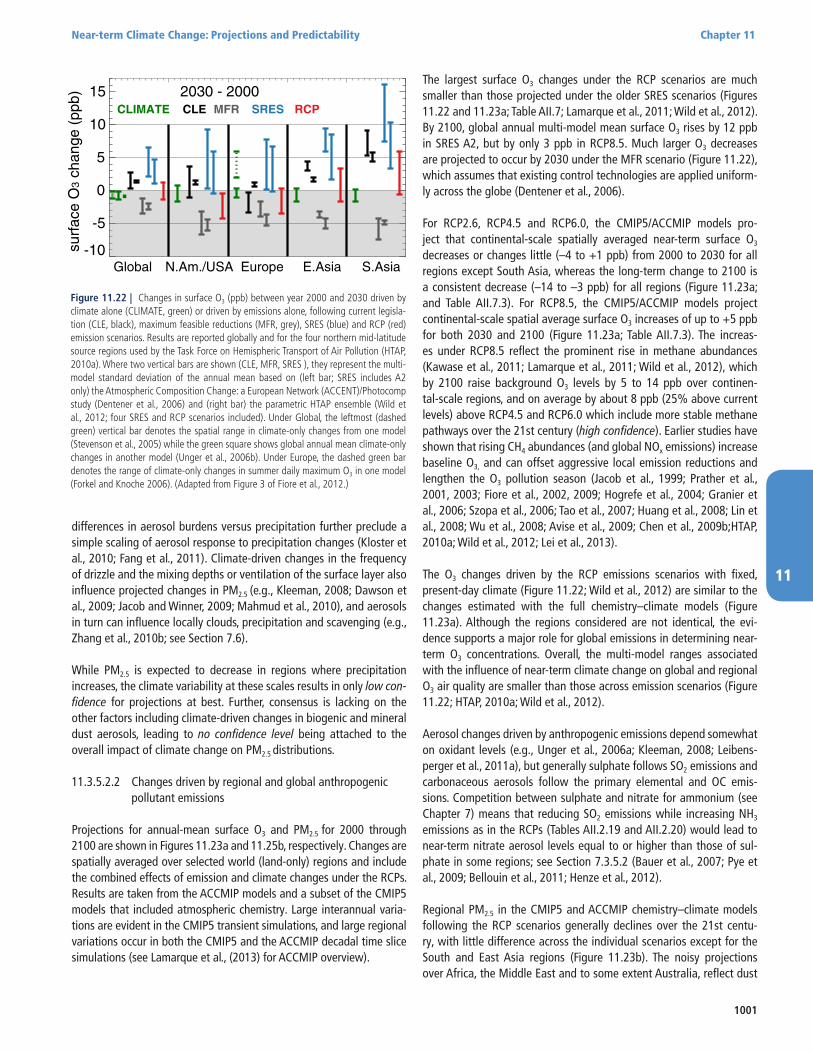
1001


11

differences in aerosol burdens versus precipitation further preclude a simple scaling of aerosol response to precipitation changes (Kloster et al., 2010; Fang et al., 2011). Climate-driven changes in the frequency of drizzle and the mixing depths or ventilation of the surface layer also influence projected changes in PM2.5 (e.g., Kleeman, 2008; Dawson et al., 2009; Jacob and Winner, 2009; Mahmud et al., 2010), and aerosols in turn can influence locally clouds, precipitation and scavenging (e.g., Zhang et al., 2010b; see Section 7.6).

While PM2.5 is expected to decrease in regions where precipitation increases, the climate variability at these scales results in only low con-fidence for projections at best. Further, consensus is lacking on the other factors including climate-driven changes in biogenic and mineral dust aerosols, leading to no confidence level being attached to the overall impact of climate change on PM2.5 distributions.

11.3.5.2.2 Changes driven by regional and global anthropogenic pollutant emissions

Projections for annual-mean surface O3 and PM2.5 for 2000 through 2100 are shown in Figures 11.23a and 11.25b, respectively. Changes are spatially averaged over selected world (land-only) regions and include the combined effects of emission and climate changes under the RCPs. Results are taken from the ACCMIP models and a subset of the CMIP5 models that included atmospheric chemistry. Large interannual varia-tions are evident in the CMIP5 transient simulations, and large regional variations occur in both the CMIP5 and the ACCMIP decadal time slice simulations (see Lamarque et al., (2013) for ACCMIP overview).

The largest surface O3 changes under the RCP scenarios are much smaller than those projected under the older SRES scenarios (Figures 11.22 and 11.23a; Table AII.7; Lamarque et al., 2011; Wild et al., 2012). By 2100, global annual multi-model mean surface O3 rises by 12 ppb in SRES A2, but by only 3 ppb in RCP8.5. Much larger O3 decreases are projected to occur by 2030 under the MFR scenario (Figure 11.22), which assumes that existing control technologies are applied uniform-ly across the globe (Dentener et al., 2006).

For RCP2.6, RCP4.5 and RCP6.0, the CMIP5/ACCMIP models pro-ject that continental-scale spatially averaged near-term surface O3 decreases or changes little (–4 to +1 ppb) from 2000 to 2030 for all regions except South Asia, whereas the long-term change to 2100 is a consistent decrease (–14 to –3 ppb) for all regions (Figure 11.23a; and Table AII.7.3). For RCP8.5, the CMIP5/ACCMIP models project continental-scale spatial average surface O3 increases of up to +5 ppb for both 2030 and 2100 (Figure 11.23a; Table AII.7.3). The increas-es under RCP8.5 reflect the prominent rise in methane abundances (Kawase et al., 2011; Lamarque et al., 2011; Wild et al., 2012), which by 2100 raise background O3 levels by 5 to 14 ppb over continen-tal-scale regions, and on average by about 8 ppb (25% above current levels) above RCP4.5 and RCP6.0 which include more stable methane pathways over the 21st century (high confidence). Earlier studies have shown that rising CH4 abundances (and global NOx emissions) increase baseline O3, and can offset aggressive local emission reductions and lengthen the O3 pollution season (Jacob et al., 1999; Prather et al., 2001, 2003; Fiore et al., 2002, 2009; Hogrefe et al., 2004; Granier et al., 2006; Szopa et al., 2006; Tao et al., 2007; Huang et al., 2008; Lin et al., 2008; Wu et al., 2008; Avise et al., 2009; Chen et al., 2009b;HTAP, 2010a; Wild et al., 2012; Lei et al., 2013).

The O3 changes driven by the RCP emissions scenarios with fixed, present-day climate (Figure 11.22; Wild et al., 2012) are similar to the changes estimated with the full chemistry–climate models (Figure 11.23a). Although the regions considered are not identical, the evi-dence supports a major role for global emissions in determining near-term O3 concentrations. Overall, the multi-model ranges associated with the influence of near-term climate change on global and regional O3 air quality are smaller than those across emission scenarios (Figure 11.22; HTAP, 2010a; Wild et al., 2012).

Aerosol changes driven by anthropogenic emissions depend somewhat on oxidant levels (e.g., Unger et al., 2006a; Kleeman, 2008; Leibens-perger et al., 2011a), but generally sulphate follows SO2 emissions and carbonaceous aerosols follow the primary elemental and OC emis-sions. Competition between sulphate and nitrate for ammonium (see Chapter 7) means that reducing SO2 emissions while increasing NH3 emissions as in the RCPs (Tables AII.2.19 and AII.2.20) would lead to near-term nitrate aerosol levels equal to or higher than those of sul-phate in some regions; see Section 7.3.5.2 (Bauer et al., 2007; Pye et al., 2009; Bellouin et al., 2011; Henze et al., 2012).

Regional PM2.5 in the CMIP5 and ACCMIP chemistry–climate models following the RCP scenarios generally declines over the 21st centu-ry, with little difference across the individual scenarios except for the South and East Asia regions (Figure 11.23b). The noisy projections over Africa, the Middle East and to some extent Australia, reflect dust

Figure 11.22 | Changes in surface O3 (ppb) between year 2000 and 2030 driven by climate alone (CLIMATE, green) or driven by emissions alone, following current legisla-tion (CLE, black), maximum feasible reductions (MFR, grey), SRES (blue) and RCP (red) emission scenarios. Results are reported globally and for the four northern mid-latitude source regions used by the Task Force on Hemispheric Transport of Air Pollution (HTAP, 2010a). Where two vertical bars are shown (CLE, MFR, SRES ), they represent the multi-model standard deviation of the annual mean based on (left bar; SRES includes A2 only) the Atmospheric Composition Change: a European Network (ACCENT)/Photocomp study (Dentener et al., 2006) and (right bar) the parametric HTAP ensemble (Wild et al., 2012; four SRES and RCP scenarios included). Under Global, the leftmost (dashed green) vertical bar denotes the spatial range in climate-only changes from one model (Stevenson et al., 2005) while the green square shows global annual mean climate-only changes in another model (Unger et al., 2006b). Under Europe, the dashed green bar denotes the range of climate-only changes in summer daily maximum O3 in one model (Forkel and Knoche 2006). (Adapted from Figure 3 of Fiore et al., 2012.)

-10

-5

0

5

10

15su

rfac

e O

3 ch

ange

(pp

b) 2030 - 2000CLIMATE SRES RCPCLE MFR

Global N.Am./USA Europe E.Asia S.Asia

1002


11

sources and their strong dependence on interannual meteorological variability. Over the two Asian regions, different PM2.5 levels between the RCPs are due to (1) OC emission trajectories over South Asia and (2) combined changes in carbonaceous aerosol and SO2 over East Asia (Fiore et al., 2012) (Figure 8.SM.1).

Global emissions of aerosols and precursors can contribute to high-PM events. For example, dust trans-oceanic transport events are observed to increase aerosols in downwind regions (Prospero, 1999; Grousset et al., 2003; Chin et al., 2007; Fairlie et al., 2007; Huang et al., 2008; Liu et al., 2009; Ramanathan and Feng, 2009; HTAP, 2010a). The bal-ance between regional and global anthropogenic emissions versus

climate-driven changes for PM2.5 will vary regionally with future chang-es in precipitation, wildfires, dust and biogenic emissions.

In summary, lower air pollution levels are projected following the RCP emissions as compared to the SRES emissions in the TAR and AR4, reflecting implementation of air pollution control measures (high confidence). The range in projections of air quality is driven primarily by emissions (including CH4) rather than by physical climate change (medium confidence). The total emission-driven range in air quality—including the CLE and MFR scenarios—is larger than that spanned by the RCPs (see Section 11.3.5.1 for comparison of RCPs and SRES).

Figure 11.23a | Projected changes in annual mean surface O3 (ppb mole fraction) from 2000 to 2100 following the RCP scenarios (8.5, red; 6.0, orange; 4.5, light blue; 2.6, dark blue). Results in each box are averaged over the designated coloured land regions. Continuous coloured lines and shading denote the average and full range of four chemistry–cli-mate models (GFDL-CM3, GISS-E2-R, and NCAR-CAM3.5 from CMIP5 plus LMDz-ORINCA). Coloured dots and vertical black bars denote the average and full range of the ACCMIP models (CESM-CAM-superfast, CICERO-OsloCTM2, CMAM, EMAC-DLR, GEOSCCM, GFDL-AM3, HadGEM2, MIROC-CHEM, MOCAGE, NCAR-CAM3.5, STOC-HadAM3, UM-CAM) for decadal time slices centred on 2010, 2030, 2050 and 2100. Participation in the decadal slices ranges from 2 to 12 models (see (Lamarque et al., 2013)). Changes are relative to the 1986–2005 reference period for the CMIP5 transient simulations, and relative to the average of the 1980 and 2000 decadal time slices for the ACCMIP ensemble. The average value and model standard deviation for the reference period is shown in the top of each panel for CMIP5 models (left) and ACCMIP models (right). In cases where multiple ensemble members are available from a single model, they are averaged prior to inclusion in the multi-model mean. (Adapted from Fiore et al., 2012.)

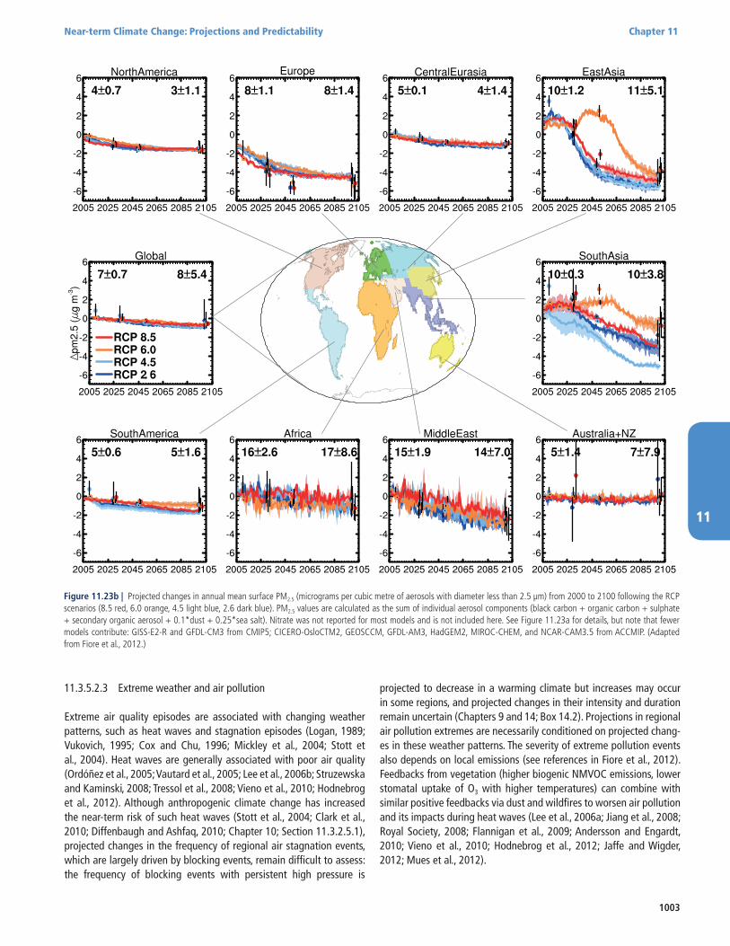
1003


11

11.3.5.2.3 Extreme weather and air pollution

Extreme air quality episodes are associated with changing weather patterns, such as heat waves and stagnation episodes (Logan, 1989; Vukovich, 1995; Cox and Chu, 1996; Mickley et al., 2004; Stott et al., 2004). Heat waves are generally associated with poor air quality (Ordóñez et al., 2005; Vautard et al., 2005; Lee et al., 2006b; Struzewska and Kaminski, 2008; Tressol et al., 2008; Vieno et al., 2010; Hodnebrog et al., 2012). Although anthropogenic climate change has increased the near-term risk of such heat waves (Stott et al., 2004; Clark et al., 2010; Diffenbaugh and Ashfaq, 2010; Chapter 10; Section 11.3.2.5.1), projected changes in the frequency of regional air stagnation events, which are largely driven by blocking events, remain difficult to assess: the frequency of blocking events with persistent high pressure is

projected to decrease in a warming climate but increases may occur in some regions, and projected changes in their intensity and duration remain uncertain (Chapters 9 and 14; Box 14.2). Projections in regional air pollution extremes are necessarily conditioned on projected chang-es in these weather patterns. The severity of extreme pollution events also depends on local emissions (see references in Fiore et al., 2012). Feedbacks from vegetation (higher biogenic NMVOC emissions, lower stomatal uptake of O3 with higher temperatures) can combine with similar positive feedbacks via dust and wildfires to worsen air pollution and its impacts during heat waves (Lee et al., 2006a; Jiang et al., 2008; Royal Society, 2008; Flannigan et al., 2009; Andersson and Engardt, 2010; Vieno et al., 2010; Hodnebrog et al., 2012; Jaffe and Wigder, 2012; Mues et al., 2012).

Figure 11.23b | Projected changes in annual mean surface PM2.5 (micrograms per cubic metre of aerosols with diameter less than 2.5 μm) from 2000 to 2100 following the RCP scenarios (8.5 red, 6.0 orange, 4.5 light blue, 2.6 dark blue). PM2.5 values are calculated as the sum of individual aerosol components (black carbon + organic carbon + sulphate + secondary organic aerosol + 0.1*dust + 0.25*sea salt). Nitrate was not reported for most models and is not included here. See Figure 11.23a for details, but note that fewer models contribute: GISS-E2-R and GFDL-CM3 from CMIP5; CICERO-OsloCTM2, GEOSCCM, GFDL-AM3, HadGEM2, MIROC-CHEM, and NCAR-CAM3.5 from ACCMIP. (Adapted from Fiore et al., 2012.)

1004


11

There is high agreement across numerous modelling studies projecting increases in extreme O3 pollution events over the USA and Europe, but the projections do not consistently agree at the regional level (Kleeman, 2008; Jacob and Winner, 2009; Jacobson and Streets, 2009; Weaver et al., 2009; Huszar et al., 2011; Katragkou et al., 2011; Langner et al., 2012b) because they depend on accurate projections of local emissions, regional climate and poorly understood biospheric feed-backs. Although observational evidence clearly demonstrates a strong statistical correlation between extreme temperatures (heat waves) and pollution events, this temperature correlation reflects in part the coin-cident occurrence of stagnation events and clear skies that also drive extreme pollution. Mechanistic understanding of biogenic emissions, deposition and atmospheric chemistry is consistent with a tempera-ture-driven increase in pollution extremes in already polluted regions, although these processes may not scale simply with mean tempera-ture under a changing climate (see Section 11.3.5.2.1), and better pro-jections of the changing meteorology at regional scales are needed. Assuming all else is equal (e.g., local anthropogenic emissions) this collective evidence indicates that uniformly higher temperatures in polluted environments will trigger regional feedbacks during air stag-nation episodes that will increase peak pollution (medium confidence).

11.3.6 Additional Uncertainties in Projections of Near-term Climate

As discussed in Section 11.3.1, most of the projections presented in Sections 11.3.2 to 11.3.4 are based on the RCP4.5 scenario and rely on the spread among the CMIP5 ensemble of opportunity as an ad hoc measure of uncertainty. It is possible that the real world might follow a path outside (above or below) the range projected by the CMIP5 models. Such an eventuality could arise if there are processes operating in the real world that are missing from, or inadequately represented in, the models. Two main possibilities must be considered: (1) Future radi-ative and other forcings may diverge from the RCP4.5 scenario and, more generally, could fall outside the range of all the RCP scenarios; (2) The response of the real climate system to radiative and other forcing may differ from that projected by the CMIP5 models. A third possibility is that internal fluctuations in the real climate system are inadequately simulated in the models. The fidelity of the CMIP5 models in simulating internal climate variability is discussed in Chapter 9.

Future changes in RF will be caused by anthropogenic and natural processes. The consequences for near-term climate of uncertainties in anthropogenic emissions and land use are discussed in Section 11.3.6.1. The uncertainties in natural RF that are most important for near-term climate are those associated with future volcanic eruptions and variations in the radiation received from the Sun (solar output), and are discussed in Section 11.3.6.2. In addition, carbon cycle and other biogeochemical feedbacks in a warming climate could poten-tially lead to abundances of CO2 and CH4 (and hence RF) outside the range of the RCP scenarios, but these feedbacks are not expected to play a major role in near term climate—see Chapters 6 and 12 for further discussion.

The response of the climate system to radiative and other forcing is influenced by a very wide range of processes, not all of which are adequately simulated in the CMIP5 models (Chapter 9). Of particular

concern for projections are mechanisms that could lead to major ‘sur-prises’ such as an abrupt or rapid change that affects global-to-con-tinental scale climate. Several such mechanisms are discussed in this assessment report; these include: rapid changes in the Arctic (Section 11.3.4 and Chapter 12), rapid changes in the ocean’s overturning cir-culation (Chapter 12), rapid change of ice sheets (Chapter 13) and rapid changes in regional monsoon systems and hydrological climate (Chapter 14). Additional mechanisms may also exist as synthesized in Chapter 12. These mechanisms have the potential to influence climate in the near term as well as in the long term, albeit the likelihood of substantial impacts increases with global warming and is generally lower for the near term. Section 11.3.6.3 provides an overall assess-ment of projections for global mean surface air temperature, taking into account all known quantifiable uncertainties.

11.3.6.1 Uncertainties in Future Anthropogenic Forcing and the Consequences for Near-term Climate

Climate projections for periods prior to year 2050 are not very sensi-tive to available alternative scenarios for anthropogenic CO2 emissions (see Section 11.3.2.1.1; Stott and Kettleborough, 2002; Meehl et al., 2007b). Near-term projections, however, may be sensitive to changes in emissions of climate forcing agents with lifetimes shorter than CO2, particularly the GHGs CH4 (lifetime of a decade), tropospheric O3 (life-time of weeks), and tropospheric aerosols (lifetime of days). Although the RCPs and SRES scenarios span a similar range of total effective radiative forcing (ERF, see Section 7.5, Figure 7.3, Chapter 8), they include different ranges of ERF from aerosol, CH4, and tropospheric O3 (see Section 11.3.5.1, Tables AII.6.2 and AII.6.7 to AII.6.10). From years 2000 to 2030 the change in ERF across the RCPs ranges from –0.05 to +0.14 W m–2 for CH4 and from –0.04 to +0.08 W m–2 for tropospheric O3 (Tables AII.6.2 and AII.6.7; Stevenson et al., 2013). From years 2000 to 2030 the total aerosol ERF becomes less negative, increasing by +0.26 W m–2 for RCP8.5 (only RCP evaluated; for ACCMIP results see Table AII.6.9; Shindell et al., 2013). Total ERF change across scenarios derived from the CMIP5 ensemble can be compared only beginning in 2010. For the period 2010 to 2030, total ERF in the CMIP5 decadal averages increases by +0.5 to +1.0 W m–2 (RCP2.6 and RCP6.0 to RCP8.5; Table AII.6.10) while total ERF from the published RCPs increases by +0.7 to +1.1 W m–2 (RCP2.6 and RCP6.0 to RCP8.5, Table AII.6.8). Here we re-examine the near-term temperature increases projected from the RCPs (see Section 11.3.2.1.1) and assess the potential for changes in near-term anthropogenic forcing to induce climate responses that fall outside these scenarios.

For the different RCP pathways the increase in global mean surface temperature by 2026–2035 relative to the reference period 1986-2005 ranges from 0.74°C (RCP2.6 and RCP6.0) to 0.94°C (RCP8.5) (median of CMIP5 models, see Figure 11.24, Table AII.7.5). This inter-scenario range of 0.20°C is smaller than the inter-model spread for an indi-vidual scenario: 0.33°C to 0.52°C (defined as the 17 to 83% range of the decadal means of the models). This RCP inter-scenario spread may be too narrow as discussed in Section 11.3.5.1. The temperature increase of the most rapidly warming scenario (RCP8.5) emerges from inter-model spread (i.e., becomes greater than two times the 17 to 83% range) by about 2040, due primarily to increasing CH4 and CO2. By 2050 the inter-scenario spread is 0.8ºC whereas the model spread

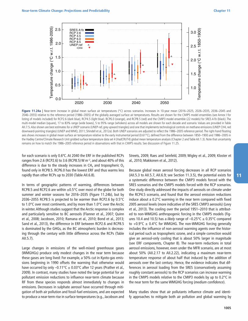
1005


11

for each scenario is only 0.6ºC. At 2040 the ERF in the published RCPs ranges from 2.6 (RCP2.6) to 3.6 (RCP8.5) W m–2, and about 40% of this difference is due to the steady increases in CH4 and tropospheric O3 found only in RCP8.5. RCP6.0 has the lowest ERF and thus warms less rapidly than other RCPs up to 2030 (Table AII.6.8).

In terms of geographic patterns of warming, differences between RCP8.5 and RCP2.6 are within ±0.5°C over most of the globe for both summer and winter seasons for 2016–2035 (Figure 11.24b), but by 2036–2055 RCP8.5 is projected to be warmer than RCP2.6 by 0.5°C to 1.0°C over most continents, and by more than 1.0°C over the Arctic in winter. Although studies suggest that the Arctic response is complex and particularly sensitive to BC aerosols (Flanner et al., 2007; Quinn et al., 2008; Jacobson, 2010; Ramana et al., 2010; Bond et al., 2013; Sand et al., 2013), the difference in ERF between RCP2.6 and RCP8.5 is dominated by the GHGs, as the BC atmospheric burden is decreas-ing through the century with little difference across the RCPs (Table AII.5.7).

Large changes in emissions of the well-mixed greenhouse gases (WMGHGs) produce only modest changes in the near term because these gases are long lived: For example, a 50% cut in Kyoto-gas emis-sions beginning in 1990 offsets the warming that otherwise would have occurred by only –0.11°C ± 0.03°C after 12 years (Prather et al., 2009). In contrast, many studies have noted the large potential for air pollutant emission reductions to influence near-term climate because RF from these species responds almost immediately to changes in emissions. Decreases in sulphate aerosol have occurred through miti-gation of both air pollution and fossil-fuel emissions, and are expected to produce a near-term rise in surface temperatures (e.g., Jacobson and

Streets, 2009; Raes and Seinfeld, 2009; Wigley et al., 2009; Kloster et al., 2010; Makkonen et al., 2012).

Because global mean aerosol forcing decreases in all RCP scenarios (AII.5.3 to AII.5.7, AII.6.9; see Section 11.3.5), the potential exists for a systematic difference between the CMIP3 models forced with the SRES scenarios and the CMIP5 models forced with the RCP scenarios. One study directly addressed the impacts of aerosols on climate under the RCP4.5 scenario, and found that the aerosol emission reductions induce about a 0.2°C warming in the near term compared with fixed 2005 aerosol levels (more indicative of the SRES CMIP3 aerosols) (Levy et al., 2013). The cooling over the period 1951–2010 that is attribut-ed to non-WMGHG anthropogenic forcing in the CMIP5 models (Fig-ures 10.4 and 10.5) has a likely range of –0.25°C ± 0.35°C compared to +0.9°C ± 0.4°C for WMGHG. The non-WMGHG forcing generally includes the influence of non-aerosol warming agents over the histor-ical period such as tropospheric ozone, and a simple correction would give an aerosol-only cooling that is about 50% larger in magnitude (see ERF components, Chapter 8). The near-term reductions in total aerosol emissions, however, even under the MFR scenario, are at most about 50% (AII.2.17 to AII.2.22), indicating a maximum near-term temperature response of about half that induced by the addition of aerosols over the last century. Hence, the evidence indicates that dif-ferences in aerosol loading from the SRES (conservatively assuming roughly constant aerosols) to the RCP scenarios can increase warming in the CMIP5 models relative to the CMIP3 models by up to 0.2°C in the near term for the same WMGHG forcing (medium confidence).

Many studies show that air pollutants influence climate and identi-fy approaches to mitigate both air pollution and global warming by

0.0

0.5

1.0

1.5

2.0

2.5

2020 2030 2040 2050

Tem

pera

ture

cha

nge

(°C

w.r

.t. 1

986-

2005

)

SRES A1bRCP 2.6RCP 4.5RCP 6.0RCP 8.5UNEP-ref

-CH4

1.0

1.5

2.0

2.5

3.0

Tem

pera

ture

cha

nge

(°C

w.r

.t. 1

850-

1900

)

Figure 11.24a | Near-term increase in global mean surface air temperatures (°C) across scenarios. Increases in 10-year mean (2016–2025, 2026–2035, 2036–2045 and 2046–2055) relative to the reference period (1986–2005) of the globally averaged surface air temperatures. Results are shown for the CMIP5 model ensembles (see Annex I for listing of models included) for RCP2.6 (dark blue), RCP4.5 (light blue), RCP6.0 (orange), and RCP8.5 (red) and the CMIP3 model ensemble (22 models) for SRES A1b (black). The multi-model median (square), 17 to 83% range (wide boxes), 5 to 95% range (whiskers) across all models are shown for each decade and scenario. Values are provided in Table AII.7.5. Also shown are best estimates for a UNEP scenario (UNEP-ref, grey upward triangles) and one that implements technological controls on methane emissions (UNEP CH4, red downward-pointing triangles) (UNEP and WMO, 2011; Shindell et al., 2012a). Both UNEP scenarios are adjusted to reflect the 1986–2005 reference period. The right-hand floating axis shows increases in global mean surface air temperature relative to the early instrumental period (0.61°C), defined from the difference between 1850–1900 and 1986–2005 in the Hadley Centre/Climate Research Unit gridded surface temperature data set 4 (HadCRUT4) global mean temperature analysis (Chapter 2 and Table AII.1.3). Note that uncertainty remains on how to match the 1986–2005 reference period in observations with that in CMIP5 results. See discussion of Figure 11.25.

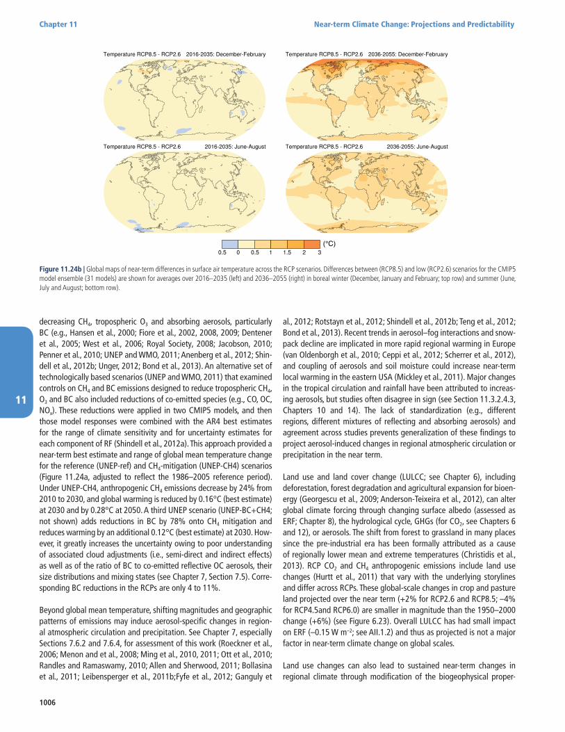
1006


11

decreasing CH4, tropospheric O3 and absorbing aerosols, particularly BC (e.g., Hansen et al., 2000; Fiore et al., 2002, 2008, 2009; Dentener et al., 2005; West et al., 2006; Royal Society, 2008; Jacobson, 2010; Penner et al., 2010; UNEP and WMO, 2011; Anenberg et al., 2012; Shin-dell et al., 2012b; Unger, 2012; Bond et al., 2013). An alternative set of technologically based scenarios (UNEP and WMO, 2011) that examined controls on CH4 and BC emissions designed to reduce tropospheric CH4, O3 and BC also included reductions of co-emitted species (e.g., CO, OC, NOx). These reductions were applied in two CMIP5 models, and then those model responses were combined with the AR4 best estimates for the range of climate sensitivity and for uncertainty estimates for each component of RF (Shindell et al., 2012a). This approach provided a near-term best estimate and range of global mean temperature change for the reference (UNEP-ref) and CH4-mitigation (UNEP-CH4) scenarios (Figure 11.24a, adjusted to reflect the 1986–2005 reference period). Under UNEP-CH4, anthropogenic CH4 emissions decrease by 24% from 2010 to 2030, and global warming is reduced by 0.16°C (best estimate) at 2030 and by 0.28°C at 2050. A third UNEP scenario (UNEP-BC+CH4; not shown) adds reductions in BC by 78% onto CH4 mitigation and reduces warming by an additional 0.12°C (best estimate) at 2030. How-ever, it greatly increases the uncertainty owing to poor understanding of associated cloud adjustments (i.e., semi-direct and indirect effects) as well as of the ratio of BC to co-emitted reflective OC aerosols, their size distributions and mixing states (see Chapter 7, Section 7.5). Corre-sponding BC reductions in the RCPs are only 4 to 11%.

Beyond global mean temperature, shifting magnitudes and geographic patterns of emissions may induce aerosol-specific changes in region-al atmospheric circulation and precipitation. See Chapter 7, especially Sections 7.6.2 and 7.6.4, for assessment of this work (Roeckner et al., 2006; Menon and et al., 2008; Ming et al., 2010, 2011; Ott et al., 2010; Randles and Ramaswamy, 2010; Allen and Sherwood, 2011; Bollasina et al., 2011; Leibensperger et al., 2011b;Fyfe et al., 2012; Ganguly et

(°C)

al., 2012; Rotstayn et al., 2012; Shindell et al., 2012b; Teng et al., 2012; Bond et al., 2013). Recent trends in aerosol–fog interactions and snow-pack decline are implicated in more rapid regional warming in Europe (van Oldenborgh et al., 2010; Ceppi et al., 2012; Scherrer et al., 2012), and coupling of aerosols and soil moisture could increase near-term local warming in the eastern USA (Mickley et al., 2011). Major changes in the tropical circulation and rainfall have been attributed to increas-ing aerosols, but studies often disagree in sign (see Section 11.3.2.4.3, Chapters 10 and 14). The lack of standardization (e.g., different regions, different mixtures of reflecting and absorbing aerosols) and agreement across studies prevents generalization of these findings to project aerosol-induced changes in regional atmospheric circulation or precipitation in the near term.

Land use and land cover change (LULCC; see Chapter 6), including deforestation, forest degradation and agricultural expansion for bioen-ergy (Georgescu et al., 2009; Anderson-Teixeira et al., 2012), can alter global climate forcing through changing surface albedo (assessed as ERF; Chapter 8), the hydrological cycle, GHGs (for CO2, see Chapters 6 and 12), or aerosols. The shift from forest to grassland in many places since the pre-industrial era has been formally attributed as a cause of regionally lower mean and extreme temperatures (Christidis et al., 2013). RCP CO2 and CH4 anthropogenic emissions include land use changes (Hurtt et al., 2011) that vary with the underlying storylines and differ across RCPs. These global-scale changes in crop and pasture land projected over the near term (+2% for RCP2.6 and RCP8.5; –4% for RCP4.5and RCP6.0) are smaller in magnitude than the 1950–2000 change (+6%) (see Figure 6.23). Overall LULCC has had small impact on ERF (–0.15 W m–2; see AII.1.2) and thus as projected is not a major factor in near-term climate change on global scales.

Land use changes can also lead to sustained near-term changes in regional climate through modification of the biogeophysical proper-

Figure 11.24b | Global maps of near-term differences in surface air temperature across the RCP scenarios. Differences between (RCP8.5) and low (RCP2.6) scenarios for the CMIP5 model ensemble (31 models) are shown for averages over 2016–2035 (left) and 2036–2055 (right) in boreal winter (December, January and February; top row) and summer (June, July and August; bottom row).

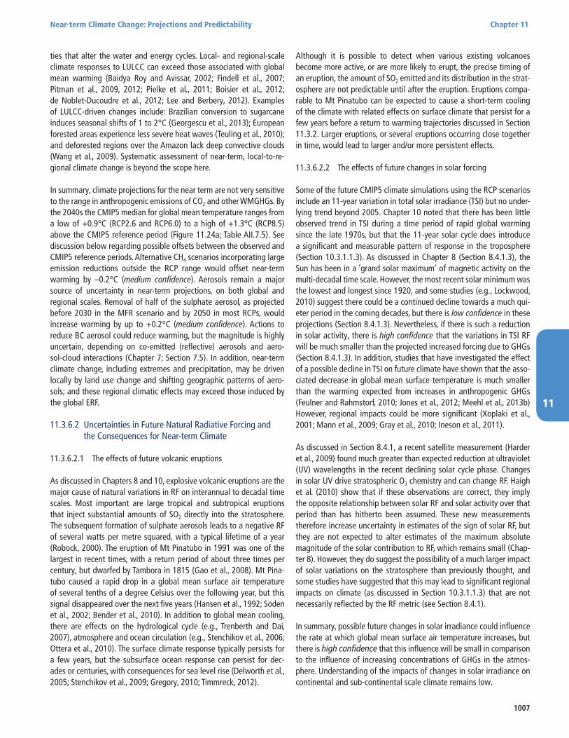
1007


11

ties that alter the water and energy cycles. Local- and regional-scale climate responses to LULCC can exceed those associated with global mean warming (Baidya Roy and Avissar, 2002; Findell et al., 2007; Pitman et al., 2009, 2012; Pielke et al., 2011; Boisier et al., 2012; de Noblet-Ducoudre et al., 2012; Lee and Berbery, 2012). Examples of LULCC-driven changes include: Brazilian conversion to sugarcane induces seasonal shifts of 1 to 2°C (Georgescu et al., 2013); European forested areas experience less severe heat waves (Teuling et al., 2010); and deforested regions over the Amazon lack deep convective clouds (Wang et al., 2009). Systematic assessment of near-term, local-to-re-gional climate change is beyond the scope here.

In summary, climate projections for the near term are not very sensitive to the range in anthropogenic emissions of CO2 and other WMGHGs. By the 2040s the CMIP5 median for global mean temperature ranges from a low of +0.9°C (RCP2.6 and RCP6.0) to a high of +1.3°C (RCP8.5) above the CMIP5 reference period (Figure 11.24a; Table AII.7.5). See discussion below regarding possible offsets between the observed and CMIP5 reference periods. Alternative CH4 scenarios incorporating large emission reductions outside the RCP range would offset near-term warming by –0.2°C (medium confidence). Aerosols remain a major source of uncertainty in near-term projections, on both global and regional scales. Removal of half of the sulphate aerosol, as projected before 2030 in the MFR scenario and by 2050 in most RCPs, would increase warming by up to +0.2°C (medium confidence). Actions to reduce BC aerosol could reduce warming, but the magnitude is highly uncertain, depending on co-emitted (reflective) aerosols and aero-sol-cloud interactions (Chapter 7; Section 7.5). In addition, near-term climate change, including extremes and precipitation, may be driven locally by land use change and shifting geographic patterns of aero-sols; and these regional climatic effects may exceed those induced by the global ERF.

11.3.6.2 Uncertainties in Future Natural Radiative Forcing and the Consequences for Near-term Climate

11.3.6.2.1 The effects of future volcanic eruptions

As discussed in Chapters 8 and 10, explosive volcanic eruptions are the major cause of natural variations in RF on interannual to decadal time scales. Most important are large tropical and subtropical eruptions that inject substantial amounts of SO2 directly into the stratosphere. The subsequent formation of sulphate aerosols leads to a negative RF of several watts per metre squared, with a typical lifetime of a year (Robock, 2000). The eruption of Mt Pinatubo in 1991 was one of the largest in recent times, with a return period of about three times per century, but dwarfed by Tambora in 1815 (Gao et al., 2008). Mt Pina-tubo caused a rapid drop in a global mean surface air temperature of several tenths of a degree Celsius over the following year, but this signal disappeared over the next five years (Hansen et al., 1992; Soden et al., 2002; Bender et al., 2010). In addition to global mean cooling, there are effects on the hydrological cycle (e.g., Trenberth and Dai, 2007), atmosphere and ocean circulation (e.g., Stenchikov et al., 2006; Ottera et al., 2010). The surface climate response typically persists for a few years, but the subsurface ocean response can persist for dec-ades or centuries, with consequences for sea level rise (Delworth et al., 2005; Stenchikov et al., 2009; Gregory, 2010; Timmreck, 2012).

Although it is possible to detect when various existing volcanoes become more active, or are more likely to erupt, the precise timing of an eruption, the amount of SO2 emitted and its distribution in the strat-osphere are not predictable until after the eruption. Eruptions compa-rable to Mt Pinatubo can be expected to cause a short-term cooling of the climate with related effects on surface climate that persist for a few years before a return to warming trajectories discussed in Section 11.3.2. Larger eruptions, or several eruptions occurring close together in time, would lead to larger and/or more persistent effects.

11.3.6.2.2 The effects of future changes in solar forcing

Some of the future CMIP5 climate simulations using the RCP scenarios include an 11-year variation in total solar irradiance (TSI) but no under-lying trend beyond 2005. Chapter 10 noted that there has been little observed trend in TSI during a time period of rapid global warming since the late 1970s, but that the 11-year solar cycle does introduce a significant and measurable pattern of response in the troposphere (Section 10.3.1.1.3). As discussed in Chapter 8 (Section 8.4.1.3), the Sun has been in a ‘grand solar maximum’ of magnetic activity on the multi-decadal time scale. However, the most recent solar minimum was the lowest and longest since 1920, and some studies (e.g., Lockwood, 2010) suggest there could be a continued decline towards a much qui-eter period in the coming decades, but there is low confidence in these projections (Section 8.4.1.3). Nevertheless, if there is such a reduction in solar activity, there is high confidence that the variations in TSI RF will be much smaller than the projected increased forcing due to GHGs (Section 8.4.1.3). In addition, studies that have investigated the effect of a possible decline in TSI on future climate have shown that the asso-ciated decrease in global mean surface temperature is much smaller than the warming expected from increases in anthropogenic GHGs (Feulner and Rahmstorf, 2010; Jones et al., 2012; Meehl et al., 2013b) However, regional impacts could be more significant (Xoplaki et al., 2001; Mann et al., 2009; Gray et al., 2010; Ineson et al., 2011).

As discussed in Section 8.4.1, a recent satellite measurement (Harder et al., 2009) found much greater than expected reduction at ultraviolet (UV) wavelengths in the recent declining solar cycle phase. Changes in solar UV drive stratospheric O3 chemistry and can change RF. Haigh et al. (2010) show that if these observations are correct, they imply the opposite relationship between solar RF and solar activity over that period than has hitherto been assumed. These new measurements therefore increase uncertainty in estimates of the sign of solar RF, but they are not expected to alter estimates of the maximum absolute magnitude of the solar contribution to RF, which remains small (Chap-ter 8). However, they do suggest the possibility of a much larger impact of solar variations on the stratosphere than previously thought, and some studies have suggested that this may lead to significant regional impacts on climate (as discussed in Section 10.3.1.1.3) that are not necessarily reflected by the RF metric (see Section 8.4.1).

In summary, possible future changes in solar irradiance could influence the rate at which global mean surface air temperature increases, but there is high confidence that this influence will be small in comparison to the influence of increasing concentrations of GHGs in the atmos-phere. Understanding of the impacts of changes in solar irradiance on continental and sub-continental scale climate remains low.

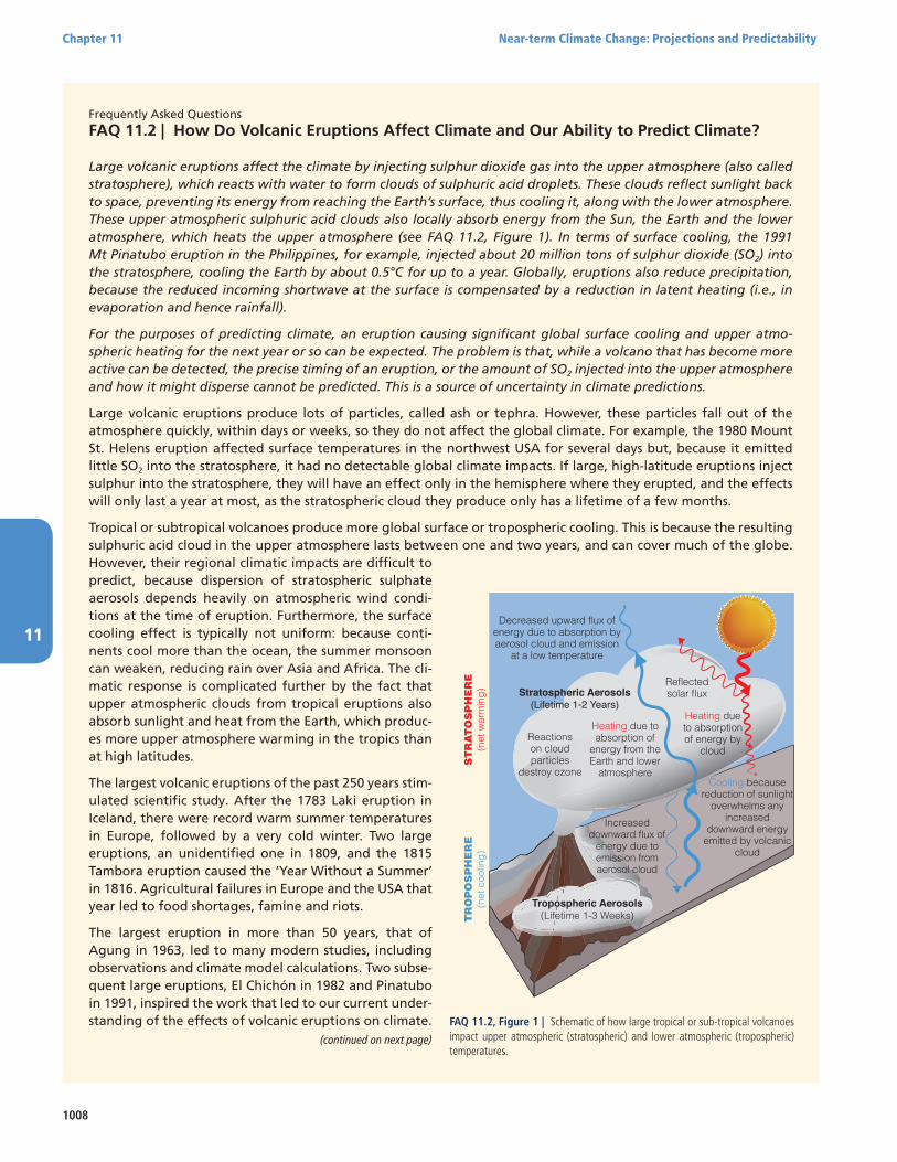
1008


11


FAQ 11.2 | How Do Volcanic Eruptions Affect Climate and Our Ability to Predict Climate?

Large volcanic eruptions affect the climate by injecting sulphur dioxide gas into the upper atmosphere (also called stratosphere), which reacts with water to form clouds of sulphuric acid droplets. These clouds reflect sunlight back to space, preventing its energy from reaching the Earth’s surface, thus cooling it, along with the lower atmosphere. These upper atmospheric sulphuric acid clouds also locally absorb energy from the Sun, the Earth and the lower atmosphere, which heats the upper atmosphere (see FAQ 11.2, Figure 1). In terms of surface cooling, the 1991 Mt Pinatubo eruption in the Philippines, for example, injected about 20 million tons of sulphur dioxide (SO2) into the stratosphere, cooling the Earth by about 0.5°C for up to a year. Globally, eruptions also reduce precipitation, because the reduced incoming shortwave at the surface is compensated by a reduction in latent heating (i.e., in evaporation and hence rainfall).

For the purposes of predicting climate, an eruption causing significant global surface cooling and upper atmo-spheric heating for the next year or so can be expected. The problem is that, while a volcano that has become more active can be detected, the precise timing of an eruption, or the amount of SO2 injected into the upper atmosphere and how it might disperse cannot be predicted. This is a source of uncertainty in climate predictions.

Large volcanic eruptions produce lots of particles, called ash or tephra. However, these particles fall out of the atmosphere quickly, within days or weeks, so they do not affect the global climate. For example, the 1980 Mount St. Helens eruption affected surface temperatures in the northwest USA for several days but, because it emitted little SO2 into the stratosphere, it had no detectable global climate impacts. If large, high-latitude eruptions inject sulphur into the stratosphere, they will have an effect only in the hemisphere where they erupted, and the effects will only last a year at most, as the stratospheric cloud they produce only has a lifetime of a few months.

Tropical or subtropical volcanoes produce more global surface or tropospheric cooling. This is because the resulting sulphuric acid cloud in the upper atmosphere lasts between one and two years, and can cover much of the globe. However, their regional climatic impacts are difficult to predict, because dispersion of stratospheric sulphate aerosols depends heavily on atmospheric wind condi-tions at the time of eruption. Furthermore, the surface cooling effect is typically not uniform: because conti-nents cool more than the ocean, the summer monsoon can weaken, reducing rain over Asia and Africa. The cli-matic response is complicated further by the fact that upper atmospheric clouds from tropical eruptions also absorb sunlight and heat from the Earth, which produc-es more upper atmosphere warming in the tropics than at high latitudes.

The largest volcanic eruptions of the past 250 years stim-ulated scientific study. After the 1783 Laki eruption in Iceland, there were record warm summer temperatures in Europe, followed by a very cold winter. Two large eruptions, an unidentified one in 1809, and the 1815 Tambora eruption caused the ‘Year Without a Summer’ in 1816. Agricultural failures in Europe and the USA that year led to food shortages, famine and riots.

The largest eruption in more than 50 years, that of Agung in 1963, led to many modern studies, including observations and climate model calculations. Two subse-quent large eruptions, El Chichón in 1982 and Pinatubo in 1991, inspired the work that led to our current under-standing of the effects of volcanic eruptions on climate. FAQ 11.2, Figure 1 | Schematic of how large tropical or sub-tropical volcanoes

impact upper atmospheric (stratospheric) and lower atmospheric (tropospheric) temperatures.

Decreased upward flux of energy due to absorption by aerosol cloud and emission

at a low temperature

Reflected solar flux

Cooling because reduction of sunlight

overwhelms any increased

downward energy emitted by volcanic

cloud

Increased downward flux of

energy due to emission from aerosol cloud

Reactions on cloud particles

destroy ozone

Heating due to absorption of

energy from the Earth and lower

atmosphere

Heating due to absorption of energy by

cloud

Tropospheric Aerosols(Lifetime 1-3 Weeks)

Stratospheric Aerosols(Lifetime 1-2 Years)


1009


11

11.3.6.3 Synthesis of Near-term Projections of Global Mean Surface Air Temperature

Figure 11.25 provides a synthesis of near-term projections of global mean surface air temperature (GMST) from CMIP5, CMIP3 and studies that have attempted to use observations to quantify projection uncer-tainty (see Section 11.3.2.1). On the basis of this evidence, an attempt is made here to assess a likely range for GMST in the period 2016–2035. Such an overall assessment is not straightforward. The following points must be taken into account:

1. No likelihoods are associated with the different RCP scenarios. For this reason, previous IPCC Assessment Reports have only present-ed projections that are conditional on specific scenarios. Here we attempt a broader assessment across all four RCP scenarios. This is possible only because, as discussed in Section 11.3.6.1, near-term projections of GMST are not especially sensitive to these different scenarios.

2. In the near term it is expected that increases in GMST will be driven by past and future increases in GHG concentrations and future decreases in anthropogenic aerosols, as found in all the RCP scenarios. Figure 11.25c shows that in the near term the CMIP3 projections based on the SRES scenarios are generally cooler than

the CMIP5 projections based on the RCP scenarios. This difference is at least partly attributable to higher aerosol concentrations in the SRES scenarios (see Section 11.3.6.1).

3. The CMIP3 and CMIP5 projections are ensembles of opportunity, and it is explicitly recognized that there are sources of uncertain-ty not simulated by the models. Evidence of this can be seen by comparing the Rowlands et al. (2012) projections for the A1B sce-nario, which were obtained using a very large ensemble in which the physics parameterizations were perturbed in a single climate model, with the corresponding raw multi-model CMIP3 projec-tions. The former exhibit a substantially larger likely range than the latter. A pragmatic approach to addressing this issue, which was used in the AR4 and is also used in Chapter 12, is to consider the 5 to 95% CMIP3/5 range as a ‘likely’ rather than ‘very likely’ range.

4. As discussed in Section 11.3.6.2, the RCP scenarios assume no underlying trend in total solar irradiance and no future volcanic eruptions. Future volcanic eruptions cannot be predicted and there is low confidence in projected changes in solar irradiance (Chapter 8). Consequently the possible effects of future changes in natural forcings are excluded from the assessment here.

FAQ 11.2 (continued)

Volcanic clouds remain in the stratosphere only for a couple of years, so their impact on climate is correspondingly short. But the impacts of consecutive large eruptions can last longer: for example, at the end of the 13th century there were four large eruptions—one every ten years. The first, in 1258 CE, was the largest in 1000 years. That sequence of eruptions cooled the North Atlantic Ocean and Arctic sea ice. Another period of interest is the three large, and several lesser, volcanic events during 1963–1991 (see Chapter 8 for how these eruptions affected atmo-spheric composition and reduced shortwave radiation at the ground.

Volcanologists can detect when a volcano becomes more active, but they cannot predict whether it will erupt, or if it does, how much sulphur it might inject into the stratosphere. Nevertheless, volcanoes affect the ability to predict climate in three distinct ways. First, if a violent eruption injects significant volumes of sulphur dioxide into the stratosphere, this effect can be included in climate predictions. There are substantial challenges and sources of uncertainty involved, such as collecting good observations of the volcanic cloud, and calculating how it will move and change during its lifetime. But, based on observations, and successful modelling of recent eruptions, some of the effects of large eruptions can be included in predictions.

The second effect is that volcanic eruptions are a potential source of uncertainty in our predictions. Eruptions cannot be predicted in advance, but they will occur, causing short-term climatic impacts on both local and global scales. In principle, this potential uncertainty can be accounted for by including random eruptions, or eruptions based on some scenario in our near-term ensemble climate predictions. This area of research needs further explora-tion. The future projections in this report do not include future volcanic eruptions.

Third, the historical climate record can be used, along with estimates of observed sulphate aerosols, to test the fidelity of our climate simulations. While the climatic response to explosive volcanic eruptions is a useful analogue for some other climatic forcings, there are limitations. For example, successfully simulating the impact of one erup-tion can help validate models used for seasonal and interannual predictions. But in this way not all the mechanisms involved in global warming over the next century can be validated, because these involve long term oceanic feed-backs, which have a longer time scale than the response to individual volcanic eruptions.

1010


11

5. As discussed in Section 11.3.2.1.1 observationally constrained ‘ASK’ projections (Gillett et al., 2013; Stott et al., 2013) are 10 to 15% cooler (median values for RCP4.5; 6–10% cooler for RCP8.5), and have a narrower range, than the corresponding ‘raw’ (unini-tialized) CMIP5 projections. The reduced rate of warming in the ASK projections is related to evidence from Chapter 10 (Section 10.3.1) that ‘some CMIP5 models have a higher transient response to GHGs and a larger response to other anthropogenic forc-ings (dominated by the effects of aerosols) than the real world (medium confidence).’ These models may warm too rapidly as GHGs increase and aerosols decline.

6. Over the last two decades the observed rate of increase in GMST has been at the lower end of rates simulated by CMIP5 models (Figure 11.25a). This hiatus in GMST rise is discussed in detail in Box 9.2 (Chapter 9), where it is concluded that the hiatus is attributable, in roughly equal measure, to a decline in the rate of increase in ERF and a cooling contribution from internal variability (expert judgment, medium confidence). The decline in the rate of increase in ERF is attributed primarily to natural (solar and vol-canic) forcing but there is low confidence in quantifying the role of forcing trend in causing the hiatus, because of uncertainty in the magnitude of the volcanic forcing trend and low confidence in the aerosol forcing trend. Concerning the higher rate of warming in CMIP5 simulations it is concluded that there is a substantial contribution from internal variability but that errors in ERF and in model responses may also contribute. There is low confidence in this assessment because of uncertainties in aerosol forcing in particular.

The observed hiatus has important implications for near-term pro-jections of GMST. A basic issue concerns the sensitivity of projec-tions to the choice of reference period. Figure 11.25b and c shows the 5 to 95% ranges for CMIP5 projections using a 1986–2005 reference period (light grey), and the same projections using a 2006–2012 reference period (dark grey). The latter projections are cooler, and the effect of using a more recent reference period appears similar to the effect of initialization (discussed in Section 11.3.2.1.1 and shown in Figure 11.25c for RCP4.5). Using this more recent reference period, the 5 to 95% range for the mean GMST in 2016–2035 relative to 1986–2005 is 0.36°C to 0.79°C (using all RCP scenarios, weighted to ensure equal weights per model and using an estimate of the observed GMST anomaly for (2006–2012)–(1986–2005) of 0.16°C). This range may be compared with the range of 0.48°C to 1.15°C obtained from the CMIP5 models using the original 1986–2005 reference period.

7. In view of the sensitivity of projections to the reference period it is helpful to consider the possible rate of change of GMST in the near term. The CMIP5 5 to 95% ranges for GMST trends in the period 2012–2035 are 0.11°C to 0.41°C per decade. This range is similar to, though slightly narrower than, the range found by Easterling and Wehner (2009) for the CMIP3 SRES A2 scenario over the longer period 2000–2050. It may also be compared with recent rates in the observational record (e.g., ~0.26°C per decade for 1984–1998 and ~0.04°C per decade for hiatus period 1998–2012; See Box 9.2). The RCP scenarios project that ERF will increase more

rapidly in the near term than occurred over the hiatus period (see Box 9.2 and Annex II), which is consistent with more rapid warm-ing. In addition, Box 9.2 includes an assessment that internal vari-ability is more likely than not to make a positive contribution to the increase in GMST in the near term. Internal variability is included in the CMIP5 projections, but because most of the CMIP5 simu-lations do not reproduce the observed reduction in global mean surface warming over the last 10 to 15 years, the distribution of CMIP5 near-term trends will not reflect this assessment and might, as a result, be biased low. This uncertainty, however, is somewhat counter balanced by the evidence of point 5, which suggests a high bias in the distribution of near-term trends. A further projection of GMST for the period 2016–2035 may be obtained by starting from the observed GMST for 2012 (0.14°C relative to 1986–2005) and projecting increases at rates between the 5 to 95% CMIP5 range of 0.11°C to 0.41°C per decade. The resulting range of 0.29°C to 0.69°C, relative to 1986–2005, is shown on Figure 11.25(c).

Overall, in the absence of major volcanic eruptions—which would cause significant but temporary cooling—and, assuming no significant future long term changes in solar irradiance, it is likely (>66% prob-ability) that the GMST anomaly for the period 2016–2035, relative to the reference period of 1986–2005 will be in the range 0.3°C to 0.7°C (expert assessment, to one significant figure; medium confidence). This range is consistent, to one significant figure, with the range obtained by using CMIP5 5 to 95% model trends for 2012–2035. It is also con-sistent with the CMIP5 5 to 95% range for all four RCP scenarios of 0.36°C to 0.79°C, using the 2006–2012 reference period, after the upper and lower bounds are reduced by 10% to take into account the evidence noted under point 5 that some models may be too sensitive to anthropogenic forcing. The 0.3°C to 0.7°C range includes the likely range of the ASK projections and initialized predictions for RCP4.5. It corresponds to a rate of change of GMST between 2012 and 2035 in the range 0.12°C to 0.42°C per decade. The higher rates of change can be associated with a significant positive contribution from internal variability (Box 9.2) and/or high rates of increase in ERF (e.g., as found in RCP8.5). Note that an upper limit of 0.8°C on the 2016–2035 GMST corresponds to a rate of change over the period 2012–2035 of 0.49°C per decade, which is considered unlikely. The assessed rates of change are consistent with the AR4 SPM statement that ‘For the next two dec-ades, a warming of about 0.2°C per decade is projected for a range of SRES emission scenarios’. However, the implied rates of warming over the period from 1986–2005 to 2016–2035 are lower as a result of the hiatus: 0.10°C to 0.23°C per decade, suggesting the AR4 assessment was near the upper end of current expectations for this specific time interval.

The assessment here provides only a likely range for GMST. Possible reasons why the real world might depart from this range include: RF departs significantly from the RCP scenarios, due to either natural (e.g., major volcanic eruptions, changes in solar irradiance) or anthropogenic (e.g., aerosol or GHG emissions) causes; processes that are poorly sim-ulated in the CMIP5 models exert a significant influence on GMST. The latter class includes: a possible strong ‘recovery’ from the recent hiatus in GMST; the possibility that models might underestimate decadal vari-ability (but see Section 9.5.3.1); the possibility that model sensitivity to anthropogenic forcing may differ from that of the real world (see point

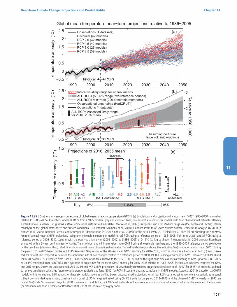
1011


11

Tem

pera

ture

ano

mal

y (°

C)

Global mean temperature near−term projections relative to 1986−2005

RCPsHistorical

(a)

1990 2000 2010 2020 2030 2040 2050−0.5

0

0.5

1

1.5

2

2.5 Observations (4 datasets)Historical (42 models)RCP 2.6 (32 models)RCP 4.5 (42 models)RCP 6.0 (25 models)RCP 8.5 (39 models)

0

1

2

3

Relative to 1850−1900

RCPsHistorical

(b)

Tem

pera

ture

ano

mal

y (°

C)

ALL RCPs Assessed likely rangefor 2016−2035 mean

Assuming no futurelarge volcanic eruptions

1990 2000 2010 2020 2030 2040 2050−0.5

0

0.5

1

1.5

2

2.5 Indicative likely range for annual meansALL RCPs (5−95% range, two reference periods)ALL RCPs min−max (299 ensemble members)Observational uncertainty (HadCRUT4)Observations (4 datasets)

B1 A1B A2SRES CMIP3

2.6 4.5 6.0 8.5 ALLRCPs CMIP5

Key: %59%5 17−83%

Obs. Constrained

Meehl &

Teng

4.5 4.5 8.5

Stott et al.

Row

lands et al.

A1B

Using trends

AssessedALL

(c)

Tem

pera

ture

ano

mal

y (°

C) Projections of 2016−2035 mean

0

0.5

1

1.5

Figure 11.25 | Synthesis of near-term projections of global mean surface air temperature (GMST). (a) Simulations and projections of annual mean GMST 1986–2050 (anomalies relative to 1986–2005). Projections under all RCPs from CMIP5 models (grey and coloured lines, one ensemble member per model), with four observational estimates (Hadley Centre/Climate Research Unit gridded surface temperature data set 4 (HadCRUT4): Morice et al., 2012); European Centre for Medium range Weather Forecast (ECMWF) interim reanalysis of the global atmosphere and surface conditions (ERA-Interim): Simmons et al., 2010); Goddard Institute of Space Studies Surface Temperature Analysis (GISTEMP): Hansen et al., 2010); National Oceanic and Atmospheric Administration (NOAA): Smith et al., 2008)) for the period 1986–2012 (black lines). (b) As (a) but showing the 5 to 95% range of annual mean CMIP5 projections (using one ensemble member per model) for all RCPs using a reference period of 1986–2005 (light grey shade) and all RCPs using a reference period of 2006–2012, together with the observed anomaly for (2006–2012) to (1986–2005) of 0.16°C (dark grey shade). The percentiles for 2006 onwards have been smoothed with a 5-year running mean for clarity. The maximum and minimum values from CMIP5 using all ensemble members and the 1986–2005 reference period are shown by the grey lines (also smoothed). Black lines show annual mean observational estimates. The red hatched region shows the indicative likely range for annual mean GMST during the period 2016–2035 based on the ‘ALL RCPs Assessed’ likely range for the 20-year mean GMST anomaly for 2016–2035, which is shown as a black bar in both (b) and (c) (see text for details). The temperature scale on the right hand side shows changes relative to a reference period of 1850-1900, assuming a warming of GMST between 1850-1900 and 1986-2005 of 0.61°C estimated from HadCRUT4.The temperature scale relative to the 1850-1900 period on the right-hand side assumes a warming of GMST prior to 1986–2005 of 0.61°C estimated from HadCRUT4. (c) A synthesis of projections for the mean GMST anomaly for 2016–2035 relative to 1986–2005. The box and whiskers represent the 66% and 90% ranges. Shown are unconstrained SRES CMIP3 and RCP CMIP5 projections; observationally constrained projections: Rowlands et al. (2012) for SRES A1B scenario, updated to remove simulations with large future volcanic eruptions; Meehl and Teng (2012) for RCP4.5 scenario, updated to include 14 CMIP5 models; Stott et al. (2013), based on six CMIP5 models with unconstrained 66% ranges for these six models shown as unfilled boxes; unconstrained projections for all four RCP scenarios using two reference periods as in panel b (light grey and dark grey shades, consistent with panel b); 90% range estimated using CMIP5 trends for the period 2012–2035 and the observed GMST anomaly for 2012; an overall likely (>66%) assessed range for all RCP scenarios. The dots for the CMIP5 estimates show the maximum and minimum values using all ensemble members. The medians (or maximum likelihood estimate for Rowlands et al. 2012) are indicated by a grey band.

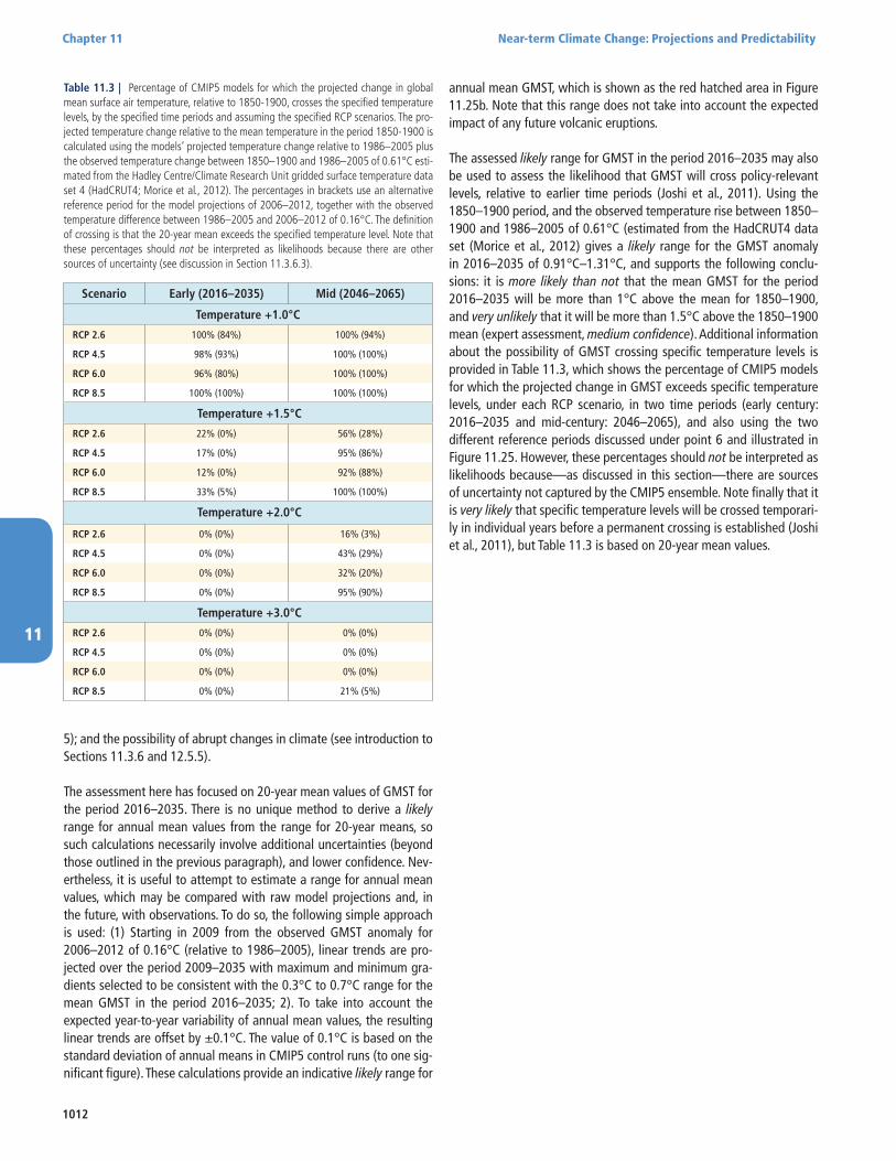
1012


11

5); and the possibility of abrupt changes in climate (see introduction to Sections 11.3.6 and 12.5.5).

The assessment here has focused on 20-year mean values of GMST for the period 2016–2035. There is no unique method to derive a likely range for annual mean values from the range for 20-year means, so such calculations necessarily involve additional uncertainties (beyond those outlined in the previous paragraph), and lower confidence. Nev-ertheless, it is useful to attempt to estimate a range for annual mean values, which may be compared with raw model projections and, in the future, with observations. To do so, the following simple approach is used: (1) Starting in 2009 from the observed GMST anomaly for 2006–2012 of 0.16°C (relative to 1986–2005), linear trends are pro-jected over the period 2009–2035 with maximum and minimum gra-dients selected to be consistent with the 0.3°C to 0.7°C range for the mean GMST in the period 2016–2035; 2). To take into account the expected year-to-year variability of annual mean values, the resulting linear trends are offset by ±0.1°C. The value of 0.1°C is based on the standard deviation of annual means in CMIP5 control runs (to one sig-nificant figure). These calculations provide an indicative likely range for

annual mean GMST, which is shown as the red hatched area in Figure 11.25b. Note that this range does not take into account the expected impact of any future volcanic eruptions.

The assessed likely range for GMST in the period 2016–2035 may also be used to assess the likelihood that GMST will cross policy-relevant levels, relative to earlier time periods (Joshi et al., 2011). Using the 1850–1900 period, and the observed temperature rise between 1850–1900 and 1986–2005 of 0.61°C (estimated from the HadCRUT4 data set (Morice et al., 2012) gives a likely range for the GMST anomaly in 2016–2035 of 0.91°C–1.31°C, and supports the following conclu-sions: it is more likely than not that the mean GMST for the period 2016–2035 will be more than 1°C above the mean for 1850–1900, and very unlikely that it will be more than 1.5°C above the 1850–1900 mean (expert assessment, medium confidence). Additional information about the possibility of GMST crossing specific temperature levels is provided in Table 11.3, which shows the percentage of CMIP5 models for which the projected change in GMST exceeds specific temperature levels, under each RCP scenario, in two time periods (early century: 2016–2035 and mid-century: 2046–2065), and also using the two different reference periods discussed under point 6 and illustrated in Figure 11.25. However, these percentages should not be interpreted as likelihoods because—as discussed in this section—there are sources of uncertainty not captured by the CMIP5 ensemble. Note finally that it is very likely that specific temperature levels will be crossed temporari-ly in individual years before a permanent crossing is established (Joshi et al., 2011), but Table 11.3 is based on 20-year mean values.

Scenario Early (2016–2035) Mid (2046–2065)

Temperature +1.0°C

RCP 2.6 100% (84%) 100% (94%)

RCP 4.5 98% (93%) 100% (100%)

RCP 6.0 96% (80%) 100% (100%)

RCP 8.5 100% (100%) 100% (100%)

Temperature +1.5°C

RCP 2.6 22% (0%) 56% (28%)

RCP 4.5 17% (0%) 95% (86%)

RCP 6.0 12% (0%) 92% (88%)

RCP 8.5 33% (5%) 100% (100%)

Temperature +2.0°C

RCP 2.6 0% (0%) 16% (3%)

RCP 4.5 0% (0%) 43% (29%)

RCP 6.0 0% (0%) 32% (20%)

RCP 8.5 0% (0%) 95% (90%)

Temperature +3.0°C

RCP 2.6 0% (0%) 0% (0%)

RCP 4.5 0% (0%) 0% (0%)

RCP 6.0 0% (0%) 0% (0%)

RCP 8.5 0% (0%) 21% (5%)

Table 11.3 | Percentage of CMIP5 models for which the projected change in global mean surface air temperature, relative to 1850-1900, crosses the specified temperature levels, by the specified time periods and assuming the specified RCP scenarios. The pro-jected temperature change relative to the mean temperature in the period 1850-1900 is calculated using the models’ projected temperature change relative to 1986–2005 plus the observed temperature change between 1850–1900 and 1986–2005 of 0.61°C esti-mated from the Hadley Centre/Climate Research Unit gridded surface temperature data set 4 (HadCRUT4; Morice et al., 2012). The percentages in brackets use an alternative reference period for the model projections of 2006–2012, together with the observed temperature difference between 1986–2005 and 2006–2012 of 0.16°C. The definition of crossing is that the 20-year mean exceeds the specified temperature level. Note that these percentages should not be interpreted as likelihoods because there are other sources of uncertainty (see discussion in Section 11.3.6.3).

1013


11

Box 11.2 | Ability of Climate Models to Simulate Observed Regional Trends

The ability of models to simulate past climate change on regional scales can be used to investigate whether the multi-model ensemble spread covers the forcing and model uncertainties. Agreement between observed and simulated regional trends, taking natural variabil-ity and model spread into account, would build confidence in near-term projections. Although large-scale features are simulated well (see Chapter 10), on sub-continental and smaller scales the observed trends are, in general, more often in the tails of the distribution of modelled trends than would be expected by chance fluctuations (Bhend and Whetton, 2012; Knutson et al., 2013b; van Oldenborgh et al., 2013). Natural variability and model spread are larger at smaller scales (Stott et al., 2010), but this is not enough to bridge the gap between models and observations. Downscaling with Regional Climate Models (RCMs) does not affect seasonal mean trends except near mountains or coastlines in Europe (van Oldenborgh et al., 2009; van Haren et al., 2012). These results hold for both observed and modelled estimates of natural variability and for various analyses of the observations. Given the statistical nature of the comparisons, it is currently not possible to say in which regions observed discrepancies are due to coincidental natural variability and in which regions they are due to forcing or model deficiencies. These results show that in general the Coupled Model Intercomparison Project Phase 5 (CMIP5) ensemble cannot be taken as a reliable regional probability forecast, but that the true uncertainty can be larger than the model spread indicated in the maps in this chapter and Annex I.

Temperature Räisänen (2007) and Yokohata et al. (2012) compared regional linear temperature trends during 1955–2005 (1961–2000) with cor-responding trends in the CMIP3 ensemble. They found that the range of simulated trends captured the observed trend in nearly all locations. Using another metric, Knutson et al., (2013b) found that CMIP5 models did slightly better than CMIP3 in reproducing linear trends (see also Figure 10.2, Section 10.3.1.1.2). The linear CMIP5 temperature trends are compared with the observed trends in Box 11.2, Figure 1a–h. The rank histograms show the warm bias in global mean temperature (see Chapter 10) and some overconfidence, but within the inter-model spread. However, the apparent agreement appears to be for the wrong reason. Many of the models that appear to correctly simulate observed high regional trends do so because they have a high climate response (i.e., the global temperature rises quickly) and do not simulate the observed spatial pattern of trends (Kumar et al., 2013). To address this, Bhend and Whetton (2012) and van Oldenborgh et al. (2013) use another definition of the local trend: the regression of the local temperature on the (low-pass filtered) global mean temperature. This definition separates the local temperature response pattern from the global mean climate response. They find highly significant discrepancies between the CMIP3 and CMIP5 trend patterns and a variety of estimates of observed trend estimates. These discrepancies are defined relative to an error model that includes the (modelled or observed) natural variability, model spread and spatial autocorrelations. In the following, areas where the observed and modelled trends show marked differences are noted. Areas of agreement are covered in Section 10.3.1.1.4.

In December to February the observed Arctic amplification extends further south than modelled in Central Asia and northwestern North America. In June to August southern Europe and North Africa have warmed significantly faster than both CMIP3 and CMIP5 models simulated (van Oldenborgh et al., 2009); this also holds for the Middle East. The observed Indo-Pacific warm pool trend is significantly higher than the modelled trend year-round (Shin and Sardeshmukh, 2011; Williams and Funk, 2011), and the North Pacific and the southeastern USA and adjoining ocean trends were lower. Direct causes for many of these discrepancies are known (e.g., December to February circulation trends that differ between the observation and the models (Gillett et al., 2005; Gillett and Stott, 2009; van Olden-borgh et al., 2009; Bhend and Whetton, 2012) or teleconnections from other areas with trend biases (Deser and Phillips, 2009; Meehl et al., 2012a), but the causes of the underlying discrepancies are often unknown. Possibilities include observational uncertainties (note, however, that the areas where the observations warm more than the models do not correspond to areas of increased urbanization or irrigation; cf. Section 2.4.1.3), an underestimation of the low-frequency variability (Knutson et al. (2013b) show evidence that this is probably not the case for temperature outside the tropics), unrealistic local forcing (e.g., aerosols (Ruckstuhl and Norris, 2009)), or missing or misrepresented processes in models (e.g., fog (Vautard et al., 2009; Ceppi et al., 2012)).

Precipitation In spite of the larger variability relative to the trends and observational uncertainties (cf. Section 2.5.1.2), annual mean regional linear precipitation trends have been found to differ significantly between observations and CMIP3 models, both in the zonal mean (Allan and Soden, 2007; Zhang et al., 2007b) and regionally (Räisänen, 2007). The comparison is shown in Box 11.2, Figure 1i–p for the CMIP5 half-year seasons used in Annex I, following van Oldenborgh et al. (2013). In both half years the observations fall more often in the highest and lowest 5% than expected by chance fluctuations within the ensemble (grey area). The differences larger than the difference between the CRU and GPCC analyses (cf. Figure 2.29) are noted below. (continued on next page)

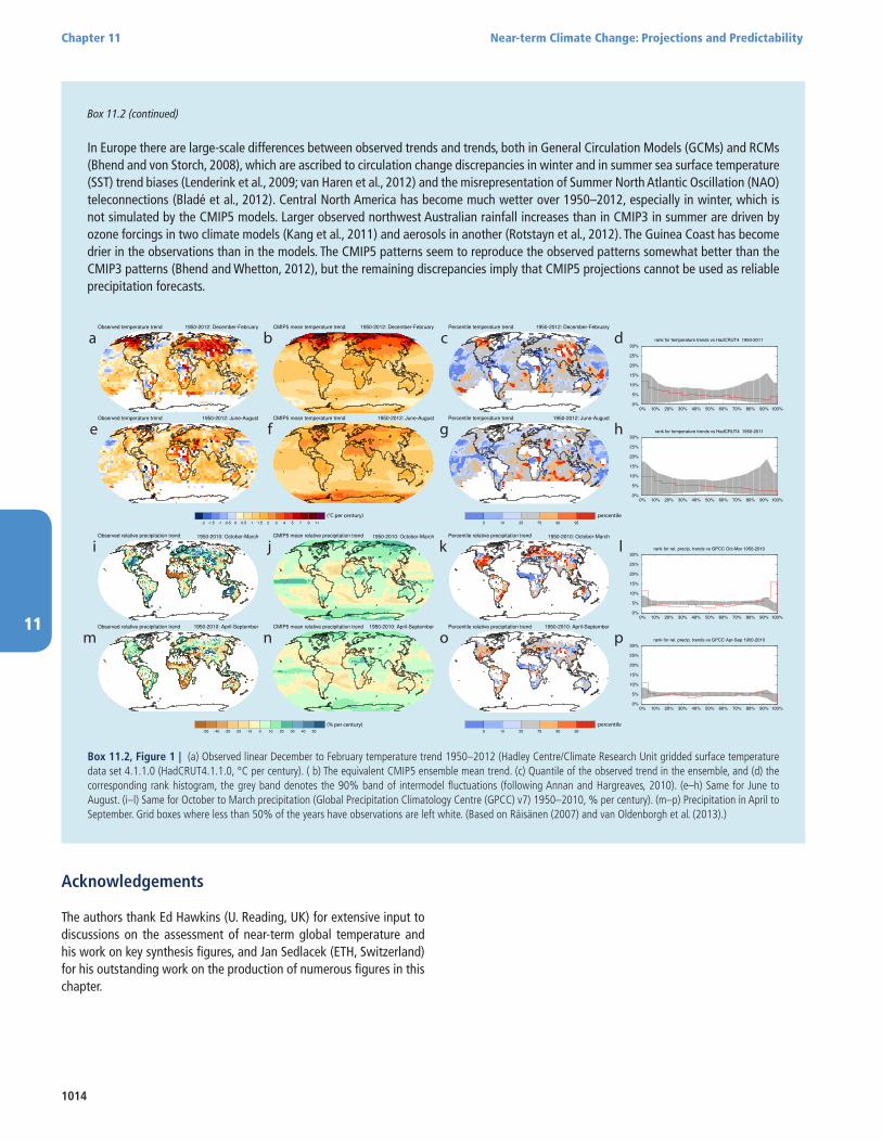
1014


11


In Europe there are large-scale differences between observed trends and trends, both in General Circulation Models (GCMs) and RCMs (Bhend and von Storch, 2008), which are ascribed to circulation change discrepancies in winter and in summer sea surface temperature (SST) trend biases (Lenderink et al., 2009; van Haren et al., 2012) and the misrepresentation of Summer North Atlantic Oscillation (NAO) teleconnections (Bladé et al., 2012). Central North America has become much wetter over 1950–2012, especially in winter, which is not simulated by the CMIP5 models. Larger observed northwest Australian rainfall increases than in CMIP3 in summer are driven by ozone forcings in two climate models (Kang et al., 2011) and aerosols in another (Rotstayn et al., 2012). The Guinea Coast has become drier in the observations than in the models. The CMIP5 patterns seem to reproduce the observed patterns somewhat better than the CMIP3 patterns (Bhend and Whetton, 2012), but the remaining discrepancies imply that CMIP5 projections cannot be used as reliable precipitation forecasts.

Box 11.2, Figure 1 | (a) Observed linear December to February temperature trend 1950–2012 (Hadley Centre/Climate Research Unit gridded surface temperature data set 4.1.1.0 (HadCRUT4.1.1.0, °C per century). ( b) The equivalent CMIP5 ensemble mean trend. (c) Quantile of the observed trend in the ensemble, and (d) the corresponding rank histogram, the grey band denotes the 90% band of intermodel fluctuations (following Annan and Hargreaves, 2010). (e–h) Same for June to August. (i–l) Same for October to March precipitation (Global Precipitation Climatology Centre (GPCC) v7) 1950–2010, % per century). (m–p) Precipitation in April to September. Grid boxes where less than 50% of the years have observations are left white. (Based on Räisänen (2007) and van Oldenborgh et al. (2013).)

a b c d

0%

5%

10%

15%

20%

25%

30%

0% 10% 20% 30% 40% 50% 60% 70% 80% 90% 100%

rank for temperature trends vs HadCRUT4 1950-2011

e f g h

0%

5%

10%

15%

20%

25%

30%

0% 10% 20% 30% 40% 50% 60% 70% 80% 90% 100%

rank for temperature trends vs HadCRUT4 1950-2011

(°C per century) percentile

percentile(% per century)

i j k l

0%

5%

10%

15%

20%

25%

30%

0% 10% 20% 30% 40% 50% 60% 70% 80% 90% 100%

rank for rel. precip. trends vs GPCC Oct-Mar 1950-2010

m n o p

0%

5%

10%

15%

20%

25%

30%

0% 10% 20% 30% 40% 50% 60% 70% 80% 90% 100%

rank for rel. precip. trends vs GPCC Apr-Sep 1950-2010

Acknowledgements

The authors thank Ed Hawkins (U. Reading, UK) for extensive input to discussions on the assessment of near-term global temperature and his work on key synthesis figures, and Jan Sedlacek (ETH, Switzerland) for his outstanding work on the production of numerous figures in this chapter.

1015


11

References

Alexander, L. V., and J. M. Arblaster, 2009: Assessing trends in observed and modelled climate extremes over Australia in relation to future projections. Int. J. Climatol., 29, 417–435.

Alexander, M. A., L. Matrosova, C. Penland, J. D. Scott, and P. Chang, 2008: Forecasting Pacific SSTs: Linear inverse model predictions of the PDO. J. Clim., 21, 385–402.

Alexandru, A., R. de Elia, and R. Laprise, 2007: Internal variability in regional climate downscaling at the seasonal scale. Mon. Weather Rev., 135, 3221–3238.

Alexeev, V. A., D. J. Nicolsky, V. E. Romanovsky, and D. M. Lawrence, 2007: An evaluation of deep soil configurations in the CLM3 for improved representation of permafrost. Geophys. Res. Lett., 34, L09502.

Allan, R. P., and B. J. Soden, 2007: Large discrepancy between observed and simulated precipitation trends in the ascending and descending branches of the tropical circulation. Geophys. Res. Lett., 34, L18705.

Allan, R. P., B. J. Soden, V. O. John, W. Ingram, and P. Good, 2010: Current changes in tropical precipitation. Environ. Res. Lett., 5, 025205.

Allen, M. R., and W. J. Ingram, 2002: Constraints on future changes in climate and the hydrologic cycle. Nature, 419, 224–232.

Allen, M. R., P. A. Stott, J. F. B. Mitchell, R. Schnur, and T. L. Delworth, 2000: Quantifying the uncertainty in forecasts of anthropogenic climate change. Nature, 407, 617–620.

Allen, R., and S. Sherwood, 2011: The impact of natural versus anthropogenic aerosols on atmospheric circulation in the Community Atmosphere Model. Clim. Dyn., 36, 1959–1978.

Anderson-Teixeira, K., P. Snyder, T. Twine, S. Cuadra, M. Costa, and E. DeLucia, 2012: Climate-regulation services of natural and agricultural ecoregions of the Americas. Nature Clim. Change, doi:10.1038/nclimate1346.

Andersson, C., and M. Engardt, 2010: European ozone in a future climate: Importance of changes in dry deposition and isoprene emissions. J. Geophys. Res., 115, D02303.

Anenberg, S. C., et al., 2012: Global air quality and health co-benefits of mitigating near-term climate change through methane and black carbon emission controls. Environ. Health Perspect., 120, 831–839.

Annan, J. D., and J. C. Hargreaves, 2010: Reliability of the CMIP3 ensemble. Geophys. Res. Lett., 37, L02703.

Appelhans, T., A. Sturman, and P. Zawar-Reza, 2012: Synoptic and climatological controls of particulate matter pollution in a Southern Hemisphere coastal city. Int. J. Climatol., 33, 463-479.

Arblaster, J. M., and G. A. Meehl, 2006: Contributions of external forcings to southern annular mode trends. J. Clim., 19, 2896–2905.

Arblaster, J. M., G. A. Meehl, and D. J. Karoly, 2011: Future climate change in the Southern Hemisphere: Competing effects of ozone and greenhouse gases. Geophys. Res. Lett., 38, L02701.

Avise, J., R. G. Abraham, S. H. Chung, J. Chen, and B. Lamb, 2012: Evaluating the effects of climate change on summertime ozone using a relative response factor approach for policymakers. J. Air Waste Manage. Assoc., 62, 1061–1074.

Avise, J., J. Chen, B. Lamb, C. Wiedinmyer, A. Guenther, E. Salathé©, and C. Mass, 2009: Attribution of projected changes in summertime US ozone and PM2.5 concentrations to global changes. Atmos. Chem. Phys., 9, 1111–1124.

Aw, J., and M. J. Kleeman, 2003: Evaluating the first-order effect of intraannual temperature variability on urban air pollution. J. Geophys. Res., 108, 4365.

Baehr, J., K. Keller, and J. Marotzke, 2008: Detecting potential changes in the meridional overturning circulation at 26°N in the Atlantic. Clim. Change, 91, 11–27.

Baidya Roy, S., and R. Avissar, 2002: Impact of land use/land cover change on regional hydrometeorology in Amazonia,. J. Geophys. Res., 107(D20), LBA 4-1-LBA 4-12. DOI: 10.1029/2000JD000266.

Balmaseda, M., and D. Anderson, 2009: Impact of initialization strategies and observations on seasonal forecast skill. Geophys. Res. Lett., 36, L01701.

Balmaseda, M. A., M. K. Davey, and D. L. T. Anderson, 1995: Decadal and seasonal dependence of ENSO prediction skill. J. Clim., 8, 2705–2715.

Bates, B. C., Z. W. Kundzewicz, S. Wu, and J. P. Palutikof, 2008: Climate Change and Water. Technical Paper of the Intergovernmental Panel on Climate Change. IPCC, 210 pp.

Battisti, D., and E. Sarachik, 1995: Understanding and predicting ENSO. Rev. Geophys., 1367–1376.

Bauer, S. E., D. Koch, N. Unger, S. M. Metzger, D. T. Shindell, and D. G. Streets, 2007: Nitrate aerosols today and in 2030: A global simulation including aerosols and tropospheric ozone. Atmos. Chem. Phys., 7, 5043–5059.

Bellouin, N., J. G. L. Rae, A. Jones, C. E. Johnson, J. M. Haywood, and O. Boucher, 2011: Aerosol forcing in the CMIP5 simulations by Hadgem2-ES and the role of ammonium nitrate. J. Geophys. Res. Atmos., doi:10.1029/2011JD016074.

Bellucci, A., et al., 2013: Decadal climate predictions with a coupled OAGCM initialized with oceanic reanalyses. Clim. Dyn., 40, 1483–1497.

Bender, F. A. M., A. M. L. Ekman, and H. Rodhe, 2010: Response to the eruption of Mount Pinatubo in relation to climate sensitivity in the CMIP3 models. Clim. Dyn., 35, 875–886.

Berg, P., C. Moseley, and J.O. Haerter, 2013: Strong increase in convective precipitation in response to higher temperatures. Nature Geosci., 6, 181-185, DOI: 10.1038/ngeo1731.

Berner, J., F. J. Doblas-Reyes, T. N. Palmer, G. Shutts, and A. Weisheimer, 2008: Impact of a quasi-stochastic cellular automaton backscatter scheme on the systematic error and seasonal prediction skill of a global climate model. Philos. Trans. R. Soc. London A, 366, 2561–2579.

Betts, R. A., et al., 2007: Projected increase in continental runoff due to plant responses to increasing carbon dioxide. Nature, 448, 1037–1041, DOI 10.1038/nature06045.

Bhend, J., and H. von Storch, 2008: Consistency of observed winter precipitation trends in northern Europe with regional climate change projections. Clim. Dyn., 31, 17–28.

Bhend, J., and P. Whetton, 2012: Consistency of simulated and observed regional changes in temperature, sea level pressure and precipitation. Clim. Change, doi:10.1007/s10584-012-0691-2.

Bintanja, R., G.J. van Oldenborgh, S.S. Drijfhout, B. Wouters, and C. A. Katsman, 2013: Important role for ocean warming and increased ice-shelf melt in Antarctic sea-ice expansion. Nature Geosci, 6, 376–379.

Birner, T., 2010: Recent widening of the tropical belt from global tropopause statistics: Sensitivities. J. Geophys. Res. Atmos., 115, DOI:10.1029/2010JD014664.

Bitz, C., 2008: Some aspects of uncertainty in predicting sea ice thinning. In: Arctic Sea Ice Decline: Observations, Projections, Mechanisms, and Implications. Geophysical Monographs, 180. American Geophysical Union, Washington, DC, pp. 63–76.

Bladé, I., D. Fortuny, G. J. van Oldenborgh, and B. Liebmann, 2012: The summer North Atlantic Oscillation in CMIP3 models and related uncertainties in projected summer drying in Europe. J. Geophys. Res., 116, D16104.

Bloomer, B. J., J. W. Stehr, C. A. Piety, R. J. Salawitch, and R. R. Dickerson, 2009: Observed relationships of ozone air pollution with temperature and emissions. Geophys. Res. Lett., 36, L09803.

Boberg, F., and J. H. Christensen, 2012: Overestimation of Mediterranean summer temperature projections due to model deficiencies. Nature Clim. Change, 2(6), 433–436.

Boe, J. L., A. Hall, and X. Qu, 2009: September sea-ice cover in the Arctic Ocean projected to vanish by 2100. Nature Geosci., 2, 341–343.

Boer, G. J., 2000: A study of atmosphere-ocean predictability on long time scales. Clim. Dyn., 16, 469–477.

Boer, G. J., 2004: Long time-scale potential predictability in an ensemble of coupled climate models. Clim. Dyn., 23, 29–44.

Boer, G. J., 2011: Decadal potential predictability of twenty-first century climate. Clim. Dyn., 36, 1119–1133.

Boer, G. J., and S. J. Lambert, 2008: Multi-model decadal potential predictability of precipitation and temperature. Geophys. Res. Lett., 35, L05706.

Boer, G. J., V. V. Kharin, and W. J. Merryfield, 2013: Decadal predictability and forecast skill. Clim. Dyn., doi:10.1007/s00382-013-1705-0.

Boisier, J. P., et al., 2012: Attributing the impacts of land-cover changes in temperate regions on surface temperature and heat fluxes to specific causes: Results from the first LUCID set of simulations. J. Geophys. Res. Atmos., 117.

Bollasina, M. A., Y. Ming, and V. Ramaswamy, 2011: Anthropogenic aerosols and the weakening of the South Asian summer monsoon. Science, doi:10.1126/science.1204994.

Bond, T. C., et al., 2013: Bounding the role of black carbon in the climate system: A scientific assessment. J. Geophys. Res., doi:10.1002/jgrd.50171.

1016


11

Booth, B. B. B., N. J. Dunstone, P. R. Halloran, T. Andrews, and N. Bellouin, 2012: Aerosols implicated as a prime driver of twentieth-century North Atlantic climate variability. Nature, 485, 534–534.

Bounoua, L., F. G. Hall, P. J. Sellers, A. Kumar, G. J. Collatz, C. J. Tucker, and M. L. Imhoff, 2010: Quantifying the negative feedback of vegetation to greenhouse warming: A modeling approach. Geophys. Res. Lett., 27, L23701.

Brandefelt, J., and H. Kornich, 2008: Northern Hemisphere stationary waves in future climate projections. J. Clim., doi: 10.1175/2008JCLI2373.1, 6341-6353.

Branstator, G., and H. Y. Teng, 2010: Two limits of initial-value decadal predictability in a CGCM. J. Clim., 23, 6292–6311.

Branstator, G., and H. Y. Teng, 2012: Potential impact of initialization on decadal predictions as assessed for CMIP5 models. Geophys. Res. Lett., 39, L12703.

Branstator, G., H. Y. Teng, G. A. Meehl, M. Kimoto, J. R. Knight, M. Latif, and A. Rosati, 2012: Systematic estimates of initial-value decadal predictability for six AOGCMs. J. Clim., 25, 1827–1846.

Brocker, J., and L. A. Smith, 2007: Increasing the reliability of reliability diagrams. Weather Forecast., 22, 651–661.

Brohan, P., J. J. Kennedy, I. Harris, S. F. B. Tett, and P. D. Jones, 2006: Uncertainty estimates in regional and global observed temperature changes: A new data set from 1850. J. Geophys. Res. Atmos., 111, DOI 10.1029/2005JD006548.

Brown, R. D., and P. W. Mote, 2009: The response of Northern Hemisphere snow cover to a changing climate. J. Clim., 22, 2124–2145.

Brunner, D., S. Henne, C. A. Keller, S. Reimann, M. K. Vollmer, S. O’Doherty, and M. Maione, 2012: An extended Kalman-filter for regional scale inverse emission estimation. Atmos. Chem. Phys., 12, 3455–3478.

Brutel-Vuilmet, C., M. Menegoz, and G. Krinner, 2013: An analysis of present and future seasonal Northern Hemisphere land snow cover simulated by CMIP5 coupled climate models. Cryosphere, 7, 67–80.

Bryan, F. O., G. Danabasoglu, N. Nakashiki, Y. Yoshida, D. H. Kim, J. Tsutsui, and S. C. Doney, 2006: Response of the North Atlantic thermohaline circulation and ventilation to increasing carbon dioxide in CCSM3. J. Clim., 19, 2382–2397.

Burgman, R., R. Seager, A. Clement, and C. Herweijer, 2010: Role of tropical Pacific SSTs in global medieval hydroclimate: A modeling study. Geophys. Res. Lett., 37, L06705.

Burke, E., and S. Brown, 2008: Evaluating uncertainties in the projection of future drought. J. Hydrometeor, 9, 292–299.

Buser, C. M., H.R. Künsch, D. Lüthi, M. Wild, and C. Schär, 2009: Bayesian multi-model projection of climate: Bias assumptions and interannual variability. Clim. Dyn., 33(6), 849-868, DOI:10.1007/s00382-009-0588-6.

Butchart, N., et al., 2006: Simulations of anthropogenic change in the strength of the Brewer-Dobson circulation. Clim. Dyn., 27, 727–741.

Butler, T. M., Z. S. Stock, M. R. Russo, H. A. C. Denier van der Gon, and M. G. Lawrence, 2012: Megacity ozone air quality under four alternative future scenarios. Atmos. Chem. Phys., 12, 4413–4428.

Butterbach-Bahl, K., M. Kahl, L. Mykhayliv, C. Werner, R. Kiese, and C. Li, 2009: A European-wide inventory of soil NO emissions using the biogeochemical models DNDC/Forest-DNDC. Atmos. Environ., 43, 1392–1402.

Caesar, J., and J. A. Lowe, 2012: Comparing the impacts of mitigation versus non-intervention scenarios on future temperature and precipitation extremes in the HadGEM2 climate model. J. Geophys. Res., 117, D15109.

Callaghan, J., and S. B. Power, 2011: Variability and decline in the number of severe tropical cyclones making land-fall over eastern Australia since the late nineteenth century. Clim. Dyn., 37, 647–662.

Callaghan, T. V., M. Johansson, O. Anisimov, H. H. Christiansen, A. Instanes, V. Romanovsky, and S. Smith, 2011: Changing permafrost and its impacts. In: Snow, Water, Ice and Permafrost in the Arctic (SWIPA). Arctic Monitoring and Assessment Program (AMAP).

Cao, L., G. Bala, K. Caldeira, R. Nemani, and G. Ban-Weiss, 2009: Climate response to physiological forcing of carbon dioxide simulated by the coupled Community Atmosphere Model (CAM3.1) and Community Land Model (CLM3.0). Geophys. Res. Lett., 36, L10402.

Cao, L., G. Bala, K. Caldeira, R. Nemani, and G. Ban-Weiss, 2010: Importance of carbon dioxide physiological forcing to future climate change. Proc. Natl. Acad. Sci. U.S.A., 107, 9513–9518.

Carlton, A. G., C. Wiedinmyer, and J. H. Kroll, 2009: A review of Secondary Organic Aerosol (SOA) formation from isoprene. Atmos. Chem. Phys., 9, 4987–5005.

Carlton, A. G., R. W. Pinder, P. V. Bhave, and G. A. Pouliot, 2010: To what extent can biogenic SOA be controlled? Environ. Sci. Technol., 44, 3376–3380.

Carvalho, A., A. Monteiro, M. Flannigan, S. Solman, A. I. Miranda, and C. Borrego, 2011: Forest fires in a changing climate and their impacts on air quality. Atmos. Environ., 45, 5545–5553.

Cattiaux, J., P. Yiou, and R. Vautard, 2012: Dynamics of future seasonal temperature trends and extremes in Europe: A multi-model analysis from CMIP. Clim. Dyn., 38(9–10), 1949-1964, DOI: 10.1007/s00382-001-1211-1.

Ceppi, P., S. C. Scherrer, A. M. Fischer, and C. Appenzeller, 2012: Revisiting Swiss temperature trends 1959–2008. Int. J. Climatol., 32, 203–213.

Chalmers, N., E. J. Highwood, E. Hawkins, R. Sutton, and L. J. Wilcox, 2012: Aerosol contribution to the rapid warming of near-term climate under RCP 2.6. Geophys. Res. Lett., 39, L18709.

Chang, C. Y., J. C. H. Chiang, M. F. Wehner, A. R. Friedman, and R. Ruedy, 2011: Sulfate aerosol control of tropical Atlantic climate over the twentieth century. J. Clim., 24, 2540–2555.

Chen, J., J. Avise, A. Guenther, C. Wiedinmyer, E. Salathe, R. B. Jackson, and B. Lamb, 2009a: Future land use and land cover influences on regional biogenic emissions and air quality in the United States. Atmos. Environ., 43, 5771–5780.

Chen, J., et al., 2009b: The effects of global changes upon regional ozone pollution in the United States. Atmos. Chem. Phys., 9, 1125–1141.

Chevallier, M., and D. Salas-Melia, 2012: The role of sea ice thickness distribution in the Arctic sea ice potential predictability: A diagnostic approach with a coupled GCM. J. Clim., 25, 3025–3038.

Chikamoto, Y., M. Kimoto, M. Watanabe, M. Ishii, and T. Mochizuki, 2012a: Relationship between the Pacifc and Atlantic stepwise climate change during the 1990s. Geophys. Res. Lett., 39, L21710.

Chikamoto, Y., et al., 2012b: Predictability of a stepwise shift in Pacific climate during the late 1990s in hindcast experiments using MIROC. J. Meteorol. Soc. Jpn., 90A, 1–21.

Chin, M., T. Diehl, P. Ginoux, and W. Malm, 2007: Intercontinental transport of pollution and dust aerosols: Implications for regional air quality. Atmos. Chem. Phys., 7, 5501–5517.

Chou, C., J. Y. Tu, and P. H. Tan, 2007: Asymmetry of tropical precipitation change under global warming. Geophys. Res. Lett., 34, L17708.

Chou, C., J. D. Neelin, C. A. Chen, and J. Y. Tu, 2009: Evaluating the “rich-get-richer’’ mechanism in tropical precipitation change under global warming. J. Clim., 22, 1982–2005.

Christensen, J. H., et al., 2007: Regional climate projections. In: Climate Change 2007: The Physical Science Basis. Contribution of Working Group I to the Fourth Assessment Report of the Intergovernmental Panel on Climate Change [Solomon, S., D. Qin, M. Manning, Z. Chen, M. Marquis, K. B. Averyt, M. Tignor and H. L. Miller (eds.)] Cambridge University Press, Cambridge, United Kingdom and New York, NY, USA, pp. 847–940.

Christidis, N., P. A. Stott, G. C. Hegerl, and R. A. Betts, 2013: The role of land use change in the recent warming of daily extreme temperatures. Geophys. Res. Lett., 40, 589–594.

Chylek, P., C. K. Folland, G. Lesins, and M. K. Dubey, 2010: Twentieth century bipolar seesaw of the Arctic and Antarctic surface air temperatures. Geophys. Res. Lett., 37, L08703.

Chylek, P., C. K. Folland, G. Lesins, M. K. Dubey, and M. Y. Wang, 2009: Arctic air temperature change amplification and the Atlantic Multidecadal Oscillation. Geophys. Res. Lett., 36, L14801.

Clark, R. T., J. M. Murphy, and S. J. Brown, 2010: Do global warming targets limit heatwave risk? Geophys. Res. Lett., 37, L17703.

Colle, B. A., Z. Zhang, K.A. Lombardo, E. Chang, P. Liu, M. Zhang, and S. Hameed, 2013: Historical and future predictions of eastern North America and western Atlantic extratropical cyclones in CMIP5 during the cool Season. J. Clim., doi:10.1175/JCLI-D-12-00498.1.

Collins, M., 2002: Climate predictability on interannual to decadal time scales: The initial value problem. Clim. Dyn., 19, 671–692.

Collins, M., and B. Sinha, 2003: Predictability of decadal variations in the thermohaline circulation and climate. Geophys. Res. Lett., 30, 1306.

Collins, M., et al., 2006: Interannual to decadal climate predictability in the North Atlantic: A multimodel-ensemble study. J. Clim., 19, 1195–1203.

Comiso, J. C., C. L. Parkinson, R. Gersten, and L. Stock, 2008: Accelerated decline in the Arctic Sea ice cover. Geophys. Res. Lett., 35, L01703.

Cook, B. I., R. L. Miller, and R. Seager, 2009: Amplification of the North American “Dust Bowl” drought through human-induced land degradation. Proc. Natl Acad. Sci. U.S.A., 106, 4997–5001.

1017


11

Corti, S., A. Weisheimer, T.N. Palmer, F. J. Doblas-Reyes, and L. Magnusson, 2012: Reliability of decadal predictions. Geophys. Res. Lett., doi:10.1029/2012GL053354.

Cox, P., and D. Stephenson, 2007: Climate change - A changing climate for prediction. Science, 317, 207–208.

Cox, W., and S. Chu, 1996: Assessment of interannual ozone variation in urban areas from a climatological perspective. Atmos. Environ., 30, 2615–2625.

Cravatte, S., T. Delcroix, D. Zhang, M. McPhaden, and J. Leloup, 2009: Observed freshening and warming of the western Pacific Warm Pool. Clim. Dyn., 33, 565–589.

Dai, A., 2011: Drought under global warming: A review. WIREs Clim. Change, 2, 45–65.

Davis, S. M., and K. H. Rosenlof, 2012: A Multidiagnostic intercomparison of tropical-width time series using reanalyses and satellite observations. J. Clim., 25, 1061–1078.

Dawson, J. P., P. N. Racherla, B. H. Lynn, P. J. Adams, and S. N. Pandis, 2009: Impacts of climate change on regional and urban air quality in the eastern United States: Role of meteorology. J. Geophys. Res., 114, D05308.

de Noblet-Ducoudre, N., et al., 2012: Determining robust impacts of land-use-induced land cover changes on surface climate over North America and Eurasia: Results from the first set of LUCID experiments. J. Clim., 25, 3261–3281.

DelSole, T., and X. Feng, 2013: The ‘‘Shukla–Gutzler’’ method for estimating potential seasonal predictability. Mon. Weather Rev., 141, 822–832.

DelSole, T., X. S. Yang, and M. K. Tippett, 2013: Is unequal weighting significantly better than equal weighting for multi-model forecasting? Q. J. R. Meteorol. Soc., 139, 176–183.

Delworth, T., and K. Dixon, 2006: Have anthropogenic aerosols delayed a greenhouse gas-induced weakening of the North Atlantic thermohaline circulation? Geophys. Res. Lett., doi:10.1029/2005GL024980, L02606.

Delworth, T., V. Ramaswamy, and G. Stenchikov, 2005: The impact of aerosols on simulated ocean temperature and heat content in the 20th century. Geophys. Res. Lett., 32, L24709, doi: 10.1029/2005GL024457.

Delworth, T. L., and F. Zeng, 2008: Simulated impact of altered Southern Hemisphere winds on the Atlantic Meridional Overturning Circulation. Geophys. Res. Lett., 35, L20708, doi: 10.1029/2008GL035166.

Dentener, F., et al., 2005: The impact of air pollutant and methane emission controls on tropospheric ozone and radiative forcing: CTM calculations for the period 1990–2030. Atmos. Chem. Phys., 5, 1731–1755.

Dentener, F., et al., 2006: The global atmospheric environment for the next generation. Environ. Sci. Technol., 40, 3586–3594.

Dery, S. J., M. A. Hernandez-Henriquez, J. E. Burford, and E. F. Wood, 2009: Observational evidence of an intensifying hydrological cycle in northern Canada. Geophys. Res. Lett., 36, L13402.

Deser, C., and A. S. Phillips, 2009: Atmospheric circulation trends, 1950–2000: The relative roles of sea surface temperature forcing and direct atmospheric radiative forcing. J. Clim., 22, 396–413.

Deser, C., A. S. Phillips, and J. W. Hurrell, 2004: Pacific interdecadal climate variability: Linkages between the tropics and the North Pacific during boreal winter since 1900. J. Clim., 17, 3109–3124.

Deser, C., A. Phillips, V. Bourdette, and H. Y. Teng, 2012: Uncertainty in climate change projections: The role of internal variability. Clim. Dyn., 38, 527–546.

Dharshana, K. G. T., S. Kravtsov, and J. D. W. Kahl, 2010: Relationship between synoptic weather disturbances and particulate matter air pollution over the United States. J. Geophys. Res. Atmos., 115, D24219, doi:10.1029/2010JD014852.

Diffenbaugh, N. S., and M. Ashfaq, 2010: Intensification of hot extremes in the United States. Geophys. Res. Lett., 37, L15701.

Diffenbaugh, N. S., and M. Scherer, 2011: Observational and model evidence of global emergence of permanent, unprecedented heat in the 20th and 21st centuries. Clim. Change, 107(3–4), 615–624.

DiNezio, P., G. A. Vecchi, and A. Clement, 2013: Detectability of changes in the Walker Circulation in response to global warming. J. Clim., doi:10.1175/JCLI-D-12-00531.1.

DiNezio, P., A. Clement, G. Vecchi, B. Soden, and B. Kirtman, 2009: Climate response of the equatorial Pacific to global warming. J. Clim., doi: 10.1175/2009JCLI2982.1, 4873–4892.

Dlugokencky, E. J., E. G. Nisbet, R. Fisher, and D. Lowry, 2011: Global atmospheric methane: Budget, changes and dangers. Philos. Trans. R. Soc. London A, 369, 2058–2072.

Doblas-Reyes, F. J., M. A. Balmaseda, A. Weisheimer, and T. N. Palmer, 2011: Decadal climate prediction with the ECMWF coupled forecast system: Impact of ocean observations. J. Geophys. Res. Atmos, 116, D19111.

Doblas-Reyes, F. J., et al., 2009: Addressing model uncertainty in seasonal and annual dynamical ensemble forecasts. Q. J. R. Meteorol. Soc., 135, 1538–1559.

Doblas-Reyes, F. J., et al., 2013: Initialized near-term regional climate change prediction. Nature Commun., 4, 1715.

Doherty, R., et al., 2009: Current and future climate- and air pollution-mediated impacts on human health. Environ. Health, 8, doi: 10.1186/1476-069X-8-S1-S8.

Doherty, R. M., et al., 2013: Impacts of climate change on surface ozone and intercontinental ozone pollution: A multi-model study. J. Geophys. Res. Atmos., doi:10.1002/jgrd.50266.

Drijfhout, S. S., and W. Hazeleger, 2007: Detecting Atlantic MOC changes in an ensemble of climate change simulations. J. Clim., 20, 1571–1582.

Du, H., F. J. Doblas-Reyes, J. Garcia-Serrano, V. Guemas, Y. Soufflet, and B. Wouters, 2012: Sensitivity of decadal predictions to the initial atmospheric and oceanic perturbations. Clim. Dyn., 39, 2013–2023.

Dunstone, N. J., and D. M. Smith, 2010: Impact of atmosphere and sub-surface ocean data on decadal climate prediction. Geophys. Res. Lett., 37, L02709.

Dunstone, N. J., D. M. Smith, and R. Eade, 2011: Multi-year predictability of the tropical Atlantic atmosphere driven by the high latitude North Atlantic Ocean. Geophys. Res. Lett., 38, L14701.

Durack, P. J., and S. E. Wijffels, 2010: Fifty-year trends in global ocean salinities and their relationship to broad-scale warming. J. Clim., 23, 4342–4362.

Durack, P. J., S. E. Wijffels, and R. J. Matear, 2012: Ocean salinities reveal strong global water cycle intensification during 1950 to 2000. Science, 336, 455-458, doi: 10.1126/science.1212222.

Dutra, E., C. Schar, P. Viterbo, and P. M. A. Miranda, 2011: Land-atmosphere coupling associated with snow cover. Geophys. Res. Lett., 38, L15707.

Eade, R., E. Hamilton, D. M. Smith, R. J. Graham, and A. A. Scaife, 2012: Forecasting the number of extreme daily events out to a decade ahead. J. Geophys. Res., 117, D21110, doi:10.1029/2012JD018015.

Easterling, D. R., and M. F. Wehner, 2009: Is the climate warming or cooling? Geophys. Res. Lett., 36, L08706.

El Nadi, A. H., 1974: The significance of leaf area in evapotranspiration. Ann. Bot, 38(3), 607–611.

Emanuel, K., 2011: Global warming effects on U.S. hurricane damage. Weather Clim. Soc., 3, 261–268.

Evan, A. T., D. J. Vimont, A. K. Heidinger, J. P. Kossin, and R. Bennartz, 2009: The role of aerosols in the evolution of tropical North Atlantic Ocean Temperature anomalies. Science, 324, 778–781.

Eyring, V., et al., 2013: Long-term changes in tropospheric and stratospheric ozone and associated climate impacts in CMIP5 simulations. J. Geophys., Res., 118. 5029-5060, doi:10.1002/jgrd.50316.

Eyring, V., et al., 2010: Multi-model assessment of stratospheric ozone return dates and ozone recovery in CCMVal-2 models. Atmos. Chem. Phys., 10, 9451–9472.

Fairlie, T. D., D. J. Jacob, and R. J. Park, 2007: The impact of transpacific transport of mineral dust in the United States. Atmos. Environ., 41, 1251–1266.

Fang, Y., et al., 2011: The impacts of changing transport and precipitation on pollutant distributions in a future climate. J. Geophys. Res., 116, D18303.

Fasullo, J. T., 2010: Robust land-ocean contrasts in energy and water cycle feedbacks. J. Clim., 23, 4677–4693.

Ferro, C. A. T., and T. E. Fricker, 2012: A bias-corrected decomposition of the Brier score. Q. J. R. Meteorol. Soc., 138, 1954–1960.

Feulner, G., and S. Rahmstorf, 2010: On the effect of a new grand minimum of solar activity on the future climate on Earth. Geophys. Res. Lett., 37, L05707, doi: 10.1029/2010GL042710.

Field, C. B., R. B. Jackson, and H. A. Mooney, 1995: Stomatal responses to increased CO2—Implications from the plant to the global-scale. Plant Cell Environ., 18, 1214–1225.

Findell, K. L., E. Shevliakova, P. C. D. Milly, and R. J. Stouffer, 2007: Modeled impact of anthropogenic land cover change on climate. J. Clim., 20, 3621–3634.

Fiore, A. M., J. J. West, L. W. Horowitz, V. Naik, and M. D. Schwarzkopf, 2008: Characterizing the tropospheric ozone response to methane emission controls and the benefits to climate and air quality. J. Geophys. Res., 113, D08307.

Fiore, A. M., D. J. Jacob, B. D. Field, D. G. Streets, S. D. Fernandes, and C. Jang, 2002: Linking ozone pollution and climate change: The case for controlling methane. Geophys. Res. Lett., 29, 1919.

1018


11

Fiore, A. M., et al., 2012: Global air quality and climate. Chem. Soc. Rev., 41, 6663–6683.

Fiore, A. M., et al., 2009: Multimodel estimates of intercontinental source-receptor relationships for ozone pollution. J. Geophys. Res., 114, D04301.

Fischer, E. M., and C. Schar, 2009: Future changes in daily summer temperature variability: Driving processes and role for temperature extremes. Clim. Dyn., 33, 917–935.

Fischer, E. M., and C. Schar, 2010: Consistent geographical patterns of changes in high-impact European heatwaves. Nature Geosci., 3, 398–403.

Fischer, E. M., J. Rajczak, and C. Schär, 2012: Changes in European summer temperature variability revisited. Geophys. Res. Lett., 6, L19702.

Fischer, E. M., S. I. Seneviratne, P. L. Vidale, D. Luthi, and C. Schar, 2007: Soil moisture–atmosphere interactions during the 2003 European summer heat wave. J. Clim., 20, 5081–5099.

Flanner, M. G., C. S. Zender, J. T. Randerson, and P. J. Rasch, 2007: Present-day climate forcing and response from black carbon in snow. J. Geophys. Res., 112, D11202, doi: 10.1029/2006JD008003.

Flannigan, M. D., M. A. Krawchuk, W. J. de Groot, B. M. Wotton, and L. M. Gowman, 2009: Implications of changing climate for global wildland fire. Int. J. Wildland Fire, 18, 483–507.

Fleming, E., C. Jackman, R. Stolarski, and A. Douglass, 2011: A model study of the impact of source gas changes on the stratosphere for 1850–2100. Atmos. Chem. Phys., 11, 8515–8541.

Fogt, R. L., J. Perlwitz, A. J. Monaghan, D. H. Bromwich, J. M. Jones, and G. J. Marshall, 2009: Historical SAM variability. Part II: Twentieth-century variability and trends from reconstructions, observations, and the IPCC AR4 Models. J. Clim., 22, 5346–5365.

Folland, C., J. Knight, H. Linderholm, D. Fereday, S. Ineson, and J. Hurrell, 2009: The summer North Atlantic Oscillation: Past, present, and future. J. Clim., doi: 10.1175/2008JCLI2459.1, 1082–1103.

Folland, C. K., A.W. Colman, D.M. Smith, O. Boucher, D. E. Parker, and J.-P. Vernier, 2013: High predictive skill of global surface temperature a year ahead. Geophys. Res. Lett., 40, 761–767.

Forkel, R. and R. Knoche, 2006: Regional climate change and its impact on photooxidant concentrations in

southern Germany: Simulations with a coupled regional climate-chemistry model. J. Geophys. Res., 2006, 111, D12302.

Fowler, H. J., M. Ekstrom, S. Blenkinsop, and A. P. Smith, 2007: Estimating change in extreme European precipitation using a multimodel ensemble. J. Geophys. Res. Atmos., 112, D18104, doi: 10.1029/2007JD008619.

Francis, J. A. H., E, 2007: Changes in the fabric of the Arctic’s greenhouse blanket. Environ. Res. Lett., doi:10.1088/1748-9326/2/4/045011.

Fyfe, J. C., N. P. Gillett, and G. J. Marshall, 2012: Human influence on extratropical Southern Hemisphere summer precipitation. Geophys. Res. Lett., 39, L23711.

Fyfe, J. C., W. J. Merryfield, V. Kharin, G. J. Boer, W. S. Lee, and K. von Salzen, 2011: Skillful predictions of decadal trends in global mean surface temperature. Geophys. Res. Lett., 38, L22801.

Gaetani, M., and E. Mohino, 2013: Decadal prediction of the Sahelian precipitation in CMIP5 simulations. J. Clim., doi:10.1175/JCLI-D-12-00635.1.

Gangstø, R., A. P. Weigel, M. A. Liniger, and C. Appenzeller, 2013: Comments on the evaluation of decadal predictions. Clim. Res., 55, 181–200.

Ganguly, D., P. J. Rasch, H. Wang, and J.-H. Yoon, 2012: Climate response of the South Asian monsoon system to anthropogenic aerosols. J. Geophys. Res., 117, D13209.

Gao, C. C., A. Robock, and C. Ammann, 2008: Volcanic forcing of climate over the past 1500 years: An improved ice core-based index for climate models. J. Geophys. Res. Atmos., 113, D23111, doi: 10.1029/2008JD010239.

Garcia-Serrano, J., and F. J. Doblas-Reyes, 2012: On the assessment of near-surface global temperature and North Atlantic multi-decadal variability in the ENSEMBLES decadal hindcast. Clim. Dyn., 39, 2025–2040.

Garcia-Serrano, J., F. J. Doblas-Reyes, and C. A. S. Coelho, 2012: Understanding Atlantic multi-decadal variability prediction skill. Geophys. Res. Lett., 39, L18708, doi:10.1029/2012GL053283.

Gastineau, G., L. Li, and H. Le Treut, 2009: The Hadley and Walker Circulation changes in global warming conditions described by idealized atmospheric simulations. J. Clim., 22, 3993–4013.

Georgescu, M., D. B. Lobell, and C. B. Field, 2009: Potential impact of U.S. biofuels on regional climate. Geophys. Res. Lett., 36, L21806.

Georgescu, M., D. B. Lobell, C. B. Field, and A. Mahalov, 2013: Simulated hydroclimatic impacts of projected Brazilian sugarcane expansion. Geophys. Res. Lett., 40, 972-977, doi:10.1002/grl,50206.

Gillett, N., R. Allan, and T. Ansell, 2005: Detection of external influence on sea level pressure with a multi-model ensemble. Geophys. Res. Lett., 32, L19714, doi: 10.1029/2005GL023640.

Gillett, N., V. Arora, D. Matthews, and M. Allen, 2013: Constraining the ratio of global warming to cumulative CO2 emissions using CMIP5 simulations. J. Clim., doi:10.1175/JCLI-D-12-00476.1.

Gillett, N. P., and D. W. J. Thompson, 2003: Simulation of recent Southern Hemisphere climate change. Science, 302, 273–275.

Gillett, N. P., and P. A. Stott, 2009: Attribution of anthropogenic influence on seasonal sea level pressure. Geophys. Res. Lett., 36, L23709.

Goddard, L., et al., 2013: A verification framework for interannual-to-decadal predictions experiments. Clim. Dyn., 40, 245–272.

Goldenberg, S. B., C. W. Landsea, A. M. Mestas-Nunez, and W. M. Gray, 2001: The recent increase in Atlantic hurricane activity: Causes and implications. Science, 293, 474–479.

Gosling, S. N., R. G. Taylor, N. W. Arnell, and M. C. Todd, 2011: A comparative analysis of projected impacts of climate change on river runoff from global and catchment-scale hydrological models. Hydrol. Earth Syst. Sci., 15, 279–294.

Granier, C., et al., 2006: Ozone pollution from future ship traffic in the Arctic northern passages. Geophys. Res. Lett., 33, L13807.

Gray, L., et al., 2010: Solar Influences on climate. Rev. Geophys., 48, RG4001, doi: 10.1029/2009/RG000282.

Gregory, J., 2010: Long-term effect of volcanic forcing on ocean heat content. Geophys. Res. Lett., doi:10.1029/2010GL045507, L22701.

Gregory, J. M., and J. F. B. Mitchell, 1995: Simulation of daily variability of surface-temperature and precipitation over Europe in the current and 2xco(2) climates using the Ukmo Climate Model. Q. J. R. Meteorol. Soc., 121, 1451–1476.

Gregory, J. M., and P. M. Forster, 2008: Transient climate response estimated from radiative forcing and observed temperature change. J. Geophys. Res. Atmos., 113, D23105, doi:10.1029/2008JD010405.

Griffies, S. M., and K. Bryan, 1997: A predictability study of simulated North Atlantic multidecadal variability. Clim. Dyn., 13, 459–487.

Grotzner, A., M. Latif, A. Timmermann, and R. Voss, 1999: Interannual to decadal predictability in a coupled ocean-atmosphere general circulation model. J. Clim., 12, 2607–2624.

Grousset, F. E., P. Ginoux, A. Bory, and P. E. Biscaye, 2003: Case study of a Chinese dust plume reaching the French Alps. Geophys. Res. Lett., 30, L22701.

Guemas, V., F. J. Doblas-Reyes, I. Andreu-Burillo, and M. Asif, 2013: Retrospective prediction of the global warming slowdown in the last decade. Nature Clim. Change, doi:10.1038/nclimate1863.

Guémas, V., F.J. Doblas-Reyes, F. Lienert, Y. Soufflet, and H. Du, 2012: Identifying the causes of the poor decadal climate prediction skill over the North Pacific. J. Geophys. Res., 117, D20111.

Guenther, A., T. Karl, P. Harley, C. Wiedinmyer, P. I. Palmer, and C. Geron, 2006: Estimates of global terrestrial isoprene emissions using MEGAN (Model of Emissions of Gases and Aerosols from Nature). Atmos. Chem. Phys., 6, 3181–3210.

Guo, D. L., and H. Wang, 2012: A projection of permafrost degradation on the Tibetan Plateau during the 21st century. J. Geophys. Res., 117, D05106, doi:10.1029/2011JD016545.

Gutowski, W. J., K. A. Kozak, R. W. Arritt, J. H. Christensen, J. C. Patton, and E. S. Takle, 2007: A possible constraint on regional precipitation intensity changes under global warming. J. Hydrometeorol., 8, 1382–1396.

Gutowski, W. J., et al., 2008: Causes of observed changes in extremes and projections of future changes. In: Weather and Climate Extremes in a Changing Climate. Regions of Focus: North America, Hawaii, Caribbean, and U.S. Pacific Islands [T. R. Karl, G. A. Meehl, D. M. Christopher, S. J. Hassol, A. M. Waple and W. L. Murray (eds.)]. U.S. Climate Change Science Program and the Subcommittee on Global Change Research.

Haarsma, R. J., and F. M. Selten, 2012: Anthropogenic changes in the Walker Circulation and their impact on the extra-tropical planetary wave structure in the Northern Hemisphere. Clim. Dyn., doi: 10.1007/s00382-012-1308-1.

Haigh, J., A. Winning, R. Toumi, and J. Harder, 2010: An influence of solar spectral variations on radiative forcing of climate. Nature, 467, 696–699.

Haigh, J. D., 1996: The impact of solar variability on climate. Science, 272, 981–984.

1019


11

Haigh, J. D., M. Blackburn, and R. Day, 2005: The response of tropospheric circulation to perturbations in lower-stratospheric temperature. J. Clim., 18, 3672–3685.

Hallquist, M., et al., 2009: The formation, properties and impact of secondary organic aerosol: Current and emerging issues. Atmos. Chem. Phys., 9, 5155–5236.

Hanel, M., and T. A. Buishand, 2011: Analysis of precipitation extremes in an ensemble of transient regional climate model simulations for the Rhine basin. Clim. Dyn., 36, 1135–1153.

Hanlon, H. M., G. C. Hegerl, S. F. B. Tett, and D. M. Smith, 2013: Can a decadal forecasting system predict temperature extreme indices? J. Clim., doi:10.1175/JCLI-D-12-00512.1.

Hansen, J., A. Lacis, R. Ruedy, and M. Sato, 1992: Potential climate impact of Mount-Pinatubo eruption. Geophys. Res. Lett., 19, 215–218.

Hansen, J., R. Ruedy, M. Sato, and K. Lo, 2010: Global surface temperature change. Rev. Geophys., 48.

Hansen, J., M. Sato, R. Ruedy, A. Lacis, and V. Oinas, 2000: Global warming in the twenty-first century: An alternative scenario. Proc. Natl. Acad. Sci. U.S.A., 97, 9875–9880.

Hansen, J., M. Sato and R. Ruedy, 2012: Perception of climate change. Proc. Natl. Acad. Sci. U.S.A., 109(37), E2415–E2423.

Harder, J., J. Fontenla, P. Pilewskie, E. Richard, and T. Woods, 2009: Trends in solar spectral irradiance variability in the visible and infrared. Geophys. Res. Lett., 36, L07801, doi: 10.1029/2008GL036797.

Hawkins, E., and R. Sutton, 2009: The potential to narrow uncertainty in regional climate predictions. Bull. Am. Meteorol. Soc., 90, 1095-1107, doi: 10.1175/2009BAMS2607.1.

Hawkins, E., and R. Sutton, 2011: The potential to narrow uncertainty in projections of regional precipitation change. Clim. Dyn., 37, 407–418.

Hawkins, E., and R. Sutton, 2012: Time of emergence of climate signals. Geophys. Res. Lett., doi:10.1029/2011GL050087.

Hawkins, E., J. Robson, R. Sutton, D. Smith, and N. Keenlyside, 2011: Evaluating the potential for statistical decadal predictions of SSTs with a perfect model approach. Clim. Dyn., 37, 2495.

Hazeleger, W., et al., 2013a: Multiyear climate predictions using two initialisation strategies. Geophys. Res. Lett., doi::10.1002/grl.50355.

Hazeleger, W., et al., 2013b: Predicting multi-year North Atlantic Ocean variability. J. Geophys. Res., doi:10.1002/grl.50355.

Heald, C. L., et al., 2008: Predicted change in global secondary organic aerosol concentrations in response to future climate, emissions, and land use change. J. Geophys. Res., 113, D05211.

Hedegaard, G. B., J. Brandt, J. H. Christensen, L. M. Frohn, C. Geels, K. M. Hansen, and M. Stendel, 2008: Impacts of climate change on air pollution levels in the Northern Hemisphere with special focus on Europe and the Arctic. Atmos. Chem. Phys., 8, 3337–3367.

Heinrich, G., and A. Gobiet, 2011: The future of dry and wet spells in Europe: A comprehensive study based on the ENSEMBLES regional climate models. Int. J. Climatol, doi:658 10.1002/joc.2421.

Held, I., and B. Soden, 2006: Robust responses of the hydrological cycle to global warming. J. Clim., 5686–5699.

Henze, D. K., et al., 2012: Spatially Refined Aerosol Direct Radiative Forcing Efficiencies. Environ. Sci. Technol., 46, 9511–9518.

Hermanson, L., and R. T. Sutton, 2010: Case studies in interannual to decadal climate predictability. Clim. Dyn., 35, 1169–1189.

Hezel, P. j., X. Zhang, C.M. Bitz, and B. P. Kelly, 2012: Projected decline in snow depth on Arctic sea ice casued by progressively later autumn open ocean freeze-up this century. Geophys. Res. Lett., 39, L17505, doi:10.1029/2012GL052794.

Ho, C. K., Hawkins, Shaffrey, and Underwood, 2012a: Statistical decadal predictions for sea surface temperatures: A benchmark for dynamical GCM predictions. Clim. Dyn., doi:10.1007/s00382-012-1531-9.

Ho, C. K., D. B. Stephenson, M. Collins, C. A. T. Ferro, and S. J. Brown, 2012b: Calibration strategies: A source of additional uncertainty in climate change projections. Bull. Am. Meteorol. Soc., 93, 21–26.

Hodnebrog, Ø., et al., 2012: Impact of forest fires, biogenic emissions and high temperatures on the elevated Eastern Mediterranean ozone levels during the hot summer of 2007. Atmos. Chem. Phys., 12, 8727–8750.

Hodson, D. L. R., S.P.E. Keeley, A. West, J. Ridley, E. Hawkins, and H. T. Hewitt, 2012: Identifying uncertainties in Arctic climate change projections. Clim. Dyn., doi:10.1007/s00382-012-1512-z.

Hoerling, M., et al., 2011: On North American decadal climate for 2011–20. J. Clim., 24, 4519–4528.

Hogrefe, C., et al., 2004: Simulating changes in regional air pollution over the eastern United States due to changes in global and regional climate and emissions. J. Geophys. Res., 109, D22301.

Hohenegger, C., P. Brockhaus, C. S. Bretherton, and C. Schar, 2009: The soil moisture-precipitation feedback in simulations with explicit and parameterized convection. J. Clim., 22, 5003–5020.

Holland, M. M., J. Finnis, and M. C. Serreze, 2006: Simulated Arctic Ocean freshwater budgets in the twentieth and twenty-first centuries. J. Clim., 19, 6221–6242.

Holland, M. M., M.C. Serreze, and J. Stroeve, 2010: The sea ice mass budget of the Arctic and its future change as simulated by coupled climate models. Clim. Dyn., 34, 185-200, doi: 10.1007/s00382-008-0493-4.

Holland, M. M., J. Finnis, A. P. Barrett, and M. C. Serreze, 2007: Projected changes in arctic ocean freshwater budgets. J. Geophys. Res., 112, G04S55, doi: 10.1029/2006/JG000354.

Holmes, C. D., M. J. Prather, O. A. Søvde, and G. Myhre, 2013: Future methane, hydroxyl, and their uncertainties: Key climate and emission parameters for future predictions. Atmos Chem Phys, 13, 285–302.

Hoyle, C. R., et al., 2011: A review of the anthropogenic influence on biogenic secondary organic aerosol. Atmos. Chem. Phys., 11, 321–343.

Hsu, J., and M. Prather, 2010: Global long-lived chemical modes excited in a 3-D chemistry transport model: Stratospheric N2O, NOy, O3 and CH4 chemistry. Geophys. Res. Lett., 37, L07805.

HTAP, 2010a: Hemispheric Transport of Air Pollution 2010, Part A: Ozone and Particulate Matter. Air Pollution Studies No. 17. United Nations, New York, NY, USA, and Geneva, Swtzerland, 278 pp.

HTAP, 2010a, 2010b: Hemispheric Transport of Air Pollution 2010, Part C: Persistent Organic Pollutants. Air Pollution Studies No. 19. United Nations, New York, NY, USA, and Geneva, Switzerland, 278 pp.

HTAP, 2010a, 2010c: Hemispheric Transport of Air Pollution 2010, Part B: Mercury. Air Pollution Studies No. 18. United Nations, New York, NY, USA, and Geneva, Switzerland, 278 pp.

Hu, Y., L. Tao, and J. Liu, 2013: Poleward expansion of the Hadley Circulation in CMIP5 simulations. Adv. Atmos. Sci., 30, 790–795.

Huang, H.-C., et al., 2008: Impacts of long-range transport of global pollutants and precursor gases on U.S. air quality under future climatic conditions. J. Geophys. Res., 113, D19307.

Huebener, H., U. Cubasch, U. Langematz, T. Spangehl, F. Niehorster, I. Fast, and M. Kunze, 2007: Ensemble climate simulations using a fully coupled ocean-troposphere-stratosphere general circulation model. Philos. Trans. R. Soc. London A, doi: 10.1098/rsta.2007.2078, 2089-2101.

Hungate, B. A., et al., 2002: Evapotranspiration and soil water content in a scrub-oak woodland under carbon dioxide enrichment. Global Change Biol., 8, 289–298.

Huntington, T. G., 2006: Evidence for intensification of the global water cycle: Review and synthesis. J. Hydrol., 319, 83–95.

Hurtt, G. C., et al., 2011: Harmonization of land-use scenarios for the period 1500–2100: 600 years of global gridded annual land-use transitions, wood harvest, and resulting secondary lands. Clim. Change, 109, 117–161.

Huszar, P., et al., 2011: Effects of climate change on ozone and particulate matter over Central and Eastern Europe. Clim. Res., 50, 51–68.

Ihara, C., and Y. Kushnir, 2009: Change of mean midlatitude westerlies in 21st century climate simulations. Geophys. Res. Lett., doi:10.1029/2009GL037674, L13701.

Im, E. S., W. J. Gutowski, and F. Giorgi, 2008: Consistent changes in twenty-first century daily precipitation from regional climate simulations for Korea using two convection parameterizations. Geophys. Res. Lett., 35, L14706.

Ineson, S., A. Scaife, J. Knight, J. Manners, N. Dunstone, L. Gray, and J. Haigh, 2011: Solar forcing of winter climate variability in the Northern Hemisphere. Nature Geosci., 4, 753–757.

ICPO, 2011: Decadal and Bias Correction for Decadal Climate Predictions. CLIVAR Publication Series No.150, International CLIVAR Project Office. 6 pp.

IPCC, 2007: Climate Change 2007: The Physical Science Basis. Contribution of Working Group I to the Fourth Assessment Report of the Intergovernmental Panel on Climate Change [Solomon, S., D. Qin, M. Manning, Z. Chen, M. Marquis, K. B. Averyt, M. Tignor and H. L. Miller (eds.)] Cambridge University Press, Cambridge, United Kingdom and New York, NY, USA, 996 pp.

1020


11

Isaksen, I. S. A., et al., 2009: Atmospheric composition change: Climate-chemistry interactions. Atmos. Environ., 43, 5138–5192.

Ishii, M., and M. Kimoto, 2009: Reevaluation of historical ocean heat content variations with an XBT depth bias correction. J. Oceanogr., 65, 287–299.

Ishii, M., M. Kimoto, K. Sakamoto, and S. Iwasaki, 2006: Steric sea level changes estimated from historical ocean subsurface temperature and salinity analyses. J. Oceanogr., 62, 155–170.

Ito, A., S. Sillman, and J. E. Penner, 2009: Global chemical transport model study of ozone response to changes in chemical kinetics and biogenic volatile organic compounds emissions due to increasing temperatures: Sensitivities to isoprene nitrate chemistry and grid resolution. J. Geophys. Res., 114, D09301.

Jacob, D. J., and D. A. Winner, 2009: Effect of climate change on air quality. Atmos. Environ., 43, 51–63.

Jacob, D. J., J. A. Logan, and P. P. Murti, 1999: Effect of rising Asian emissions on surface ozone in the United States. Geophys. Res. Lett., 26, 2175–2178.

Jacob, D. J., et al., 1993: Factors regulating ozone over the United-States and its export to the global atmosphere. J. Geophys. Res. Atmos., 98, 14817–14826.

Jacobson, M., 2008: Effects of wind-powered hydrogen fuel cell vehicles on stratospheric ozone and global climate. Geophys. Res. Lett., doi:10.1029/2008GL035102, L14706.

Jacobson, M., 2010: Short-term effects of controlling fossil-fuel soot, biofuel soot and gases, and methane on climate, Arctic ice, and air pollution health. J. Geophys. Res., D14209, doi:10.1029/2009JD013795.

Jacobson, M., and D. Streets, 2009: Influence of future anthropogenic emissions on climate, natural emissions, and air quality. J. Geophys. Res., D08118, doi:10.1029/2008JD011476.

Jaffe, D. A., and N. L. Wigder, 2012: Ozone production from wildfires: A critical review. Atmos. Environ., 51, 1–10.

Jai, L., and T. DelSole, 2012: Multi-year predictability of temperature and precipitation in multiple climate models. Geophys. Res. Lett., 39, L17705.

Jiang, X., Z.-L. Yang, H. Liao, and C. Wiedinmyer, 2010: Sensitivity of biogenic secondary organic aerosols to future climate change at regional scales: An online coupled simulation. Atmos. Environ., 44, 4891–4907.

Jiang, X., C. Wiedinmyer, F. Chen, Z.-L. Yang, and J. C.-F. Lo, 2008: Predicted impacts of climate and land use change on surface ozone in the Houston, Texas, area. J. Geophys. Res., 113, D20312.

Jickells, T. D., et al., 2005: Global iron connections between desert dust, ocean biogeochemistry, and climate. Science, 308, 67–71.

Joetzjer, E., H. Douville, C. Delire, and P. Ciais, 2012: Present-day and future Amazonian precipitation in global climate models: CMIP5 versus CMIP3. Clim. Dyn., doi:10.1007/s00382-012-1644-1.

John, J. G., A. M. Fiore, V. Naik, L. W. Horowitz, and J. P. Dunne, 2012: Climate versus emission drivers of methane lifetime from 1860–2100. Atmos. Chem. Phys., 12, 12021-12036, doi: 10.5194/acp-12-12021-2012.

Johnson, C. E., W. J. Collins, D. S. Stevenson, and R. G. Derwent, 1999: Relative roles of climate and emissions changes on future tropospheric oxidant concentrations. J. Geophys. Res., 104, 18631–18645.

Johnson, N. C., and S. P. Xie, 2010: Changes in the sea surface temperature threshold for tropical convection. Nature Geosci., 3, 842–845.

Jolliffe, I. T., 2007: Uncertainty and inference for verification measures. Weather Forecast., 22, 637–650.

Jolliffe, I. T., and D. B. Stephenson, 2011: Forecast Verification: A Practitioner’s Guide in Atmospheric Science, 2nd ed. John Wiley & Sons, Hoboken, NJ, USA.

Jones, G., M. Lockwood, and P. Stott, 2012: What influence will future solar activity changes over the 21st century have on projected global near-surface temperature changes? J. Geophys. Res., 117, D05103, doi.1029/2011JD17013.

Joshi, M., E. Hawkins, R. Sutton, J. Lowe, and D. Frame, 2011: Projections of when temperature change will exceed 2 degrees C above pre-industrial levels. Nature Clim. Change, 1, 407–412.

Jung, M., et al., 2010: Recent decline in the global land evapotranspiration trend due to limited moisture supply. Nature, 467, 951–954.

Kang, S. M., L. M. Polvani, J. C. Fyfe, and M. Sigmond, 2011: Impact of polar ozone depletion on subtropical precipitation. Science, 332, 951–954.

Kao, S. C., and A. R. Ganguly, 2011: Intensity, duration, and frequency of precipitation extremes under 21st-century warming scenarios. J. Geophys. Res., 116, D16119, doi:10.1029/2010JD015529.

Katragkou, E., P. Zanis, I. Kioutsioukis, I. Tegoulias, D. Melas, B. C. Kruger, and E. Coppola, 2011: Future climate change impacts on summer surface ozone from regional climate-air quality simulations over Europe. J. Geophys. Res., 116, D22307, doi:10.1029/2011JD015899.

Kawase, H., T. Nagashima, K. Sudo, and T. Nozawa, 2011: Future changes in tropospheric ozone under Representative Concentration Pathways (RCPs). Geophys. Res. Lett., 38, L05801.

Keenlyside, N. S., and J. Ba, 2010: Prospects for decadal climate prediction. WIREs Clim. Change, 1, 627–635.

Keenlyside, N. S., M. Latif, J. Jungclaus, L. Kornblueh, and E. Roeckner, 2008: Advancing decadal-scale climate prediction in the North Atlantic sector. Nature, 453, 84–88.

Keller, C. A., D. Brunner, S. Henne, M. K. Vollmer, S. O’Doherty, and S. Reimann, 2011: Evidence for under-reported western European emissions of the potent greenhouse gas HFC-23. Geophys. Res. Lett., 38, L15808.

Kelly, J., P. A. Makar, and D. A. Plummer, 2012: Projections of mid-century summer air-quality for North America: Effects of changes in climate and precursor emissions. Atmos Chem Phys, 12, 5367–5390.

Keppenne, C. L., M. M. Rienecker, N. P. Kurkowski, and D. A. Adamec, 2005: Ensemble Kalman filter assimilation of temperature and altimeter data with bias correction and application to seasonal prediction. Nonlin. Process. Geophys., 12, 491–503.

Kesik, M., et al., 2006: Future scenarios of N2O and NO emissions from European forest soils. J. Geophys., Res., 111, G02018.

Kharin, V. V., G. J. Boer, W. J. Merryfield, J. F. Scinocca, and W. S. Lee, 2012: Statistical adjustment of decadal predictions in a changing climate. Geophys. Res. Lett., 39, L19705.

Kim, H. M., P. J. Webster, and J. A. Curry, 2012: Evaluation of short-term climate change prediction in multi-model CMIP5 decadal hindcasts. Geophys. Res. Lett., 39, L10701.

Kleeman, M. J., 2008: A preliminary assessment of the sensitivity of air quality in California to global change. Clim. Change, 87(Suppl 1), S273–S292.

Kleeman, R., Y. M. Tang, and A. M. Moore, 2003: The calculation of climatically relevant singular vectors in the presence of weather noise as applied to the ENSO problem. J. Atmos. Sci., 60, 2856–2868.

Klimont, Z., S. J. Smith, and J. Cofala, 2013: The last decade of global anthropogenic sulfur dioxide: 2000–2011 emissions. Environ. Res. Lett., 8, 014003, doi:10.1088/1748-9326/8/1/014003.

Kloster, S., F. Dentener, J. Feichter, F. Raes, U. Lohmann, E. Roeckner, and I. Fischer-Bruns, 2010: A GCM study of future climate response to aerosol pollution reductions. Clim. Dyn., 34, 1177–1194.

Kloster, S., et al., 2008: Influence of future air pollution mitigation strategies on total aerosol radiative forcing. Atmos. Chem. Phys., 8, 6405–6437.

Knight, J., R. Allan, C. Folland, M. Vellinga, and M. Mann, 2005: A signature of persistent natural thermohaline circulation cycles in observed climate. Geophys. Res. Lett., doi:10.1029/2005GL024233, L20708.

Knutson, T., and S. Manabe, 1995: Time-mean response over the tropical Pacific to increased CO2 in a coupled ocean-atmosphere model. J. Clim., 8, 2181–2199.

Knutson, T.R., and coauthors, 2013a: Dynamical Downscaling Projections of Late 21st Century Atlantic Hurricane Activity CMIP3 and CMIP5 Model-based Scenarios. J. Climate, doi:10.1175/JCLI-D-12-00539.1

Knutson, T. R., F. Zeng, and A. T. Wittenberg 2013b: Multimodel Assessment of Regional Surface Temperature Trends: CMIP3 and CMIP5 Twentieth-Century Simulations. J. Clim., 26, 4168–4185.

Knutson, T. R., et al., 2006: Assessment of Twentieth-Century regional surface temperature trends using the GFDL CM2 coupled models. J. Clim., 19, 1624-1651, doi: 10.1175/JCLI3709.1.

Knutson, T. R., et al., 2010: Tropical cyclones and climate change. Nature Geosci, 3, 157–163.

Knutti, R., D. Masson, and A. Gettelman, 2013: Climate model genealogy: Generation CMIP5 and how we got there. Geophys. Res. Lett., doi:10.1002/grl.50256.

Koster, R. D., et al., 2010: Contribution of land surface initialization to subseasonal forecast skill: First results from a multi-model experiment. Geophys. Res. Lett., 37, L02402.

Kroger, J., W. A. Muller, and J. S. von Storch, 2012: Impact of different ocean reanalyses on decadal climate prediction. Clim. Dyn., 39, 795–810.

Krueger, O., and J.-S. von Storch, 2011: A simple empirical model for decadal climate prediction. J. Clim., 24, 1276–1283.

Kumar, A., 2009: Finite samples and uncertainty estimates for skill measures for seasonal prediction. Mon. Weather Rev., 137, 2622–2631.

1021


11

Kumar, S., V. Merwade, D. Niyogi, and J. L. Kinter III, 2013: Evaluation of temperature and precipitation trends and long-term persistence in CMIP5 20th century climate simulations. J. Clim., doi:10.1175/JCLI-D-12-00259.1.

Laepple, T., S. Jewson, and K. Coughlin, 2008: Interannual temperature predictions using the CMIP3 multi-model ensemble mean. Geophys. Res. Lett., 35, L10701.

Lamarque, J.-F., et al., 2011: Global and regional evolution of short-lived radiatively-active gases and aerosols in the Representative Concentration Pathways. Clim. Change, doi:10.1007/s10584-011-0155-0, 1–22.

Lamarque, J. F., et al., 2013: The Atmospheric Chemistry and Climate Model Intercomparison Project (ACCMIP): Overview and description of models, simulations and climate diagnostics. Geosci. Model Dev., 6, 179-206, doi 10.5194/gmf-6-179-2013.

Lambert, F. H., and J. C. H. Chiang, 2007: Control of land-ocean temperature contrast by ocean heat uptake. Geophys. Res. Lett., 34, L13704, doi: 10.1029/2007GL029755.

Lambert, F. H., and M. J. Webb, 2008: Dependency of global mean precipitation on surface temperature. Geophys. Res. Lett., 35, L23803.

Lammertsma, E. I., H. J. de Boer, S. C. Dekker, D. L. Dilcher, A. F. Lotter, and F. Wagner-Cremer, 2011: Global CO2 rise leads to reduced maximum stomatal conductance in Florida vegetation. Proc. Acad. Sci. U.S.A., 108, 4035–4040.

Lang, C., and D. W. Waugh, 2011: Impact of climate change on the frequency of Northern Hemisphere summer cyclones. J. Geophys. Res., 116, D04103, doi: 10.1029/2010JD014300.

Langner, J., M. Engardt, and C. Andersson, 2012a: European summer surface ozone 1990–2100. Atmos. Chem. Phys.,12, 10097–10105.

Langner, J., M. Engardt, A. Baklanov, J. H. Christensen, M. Gauss, C. Geels, G. B. Hedegaard, R. Nuterman, D. Simpson, J. Soares, M. Sofiev, P. Wind, and A. Zakey, 2012b: A multi-model study of impacts of climate change on surface ozone in Europe. Atmos. Chem. Phys., 12, 10423-10440.

Lanzante, J. R., 2005: A cautionary note on the use of error bars. J. Clim., 18, 3699–3703.

Latif, M., M. Collins, H. Pohlmann, and N. Keenlyside, 2006: A review of predictability studies of Atlantic sector climate on decadal time scales. J. Clim., 19, 5971–5987.

Latif, M., C. W. Boning, J. Willebrand, A. Biastoch, A. Alvarez-Garcia, N. Keenlyside, and H. Pohlmann, 2007: Decadal to multidecadal variability of the Atlantic MOC: Mechanisms and predictability. In: Ocean Circulation: Mechanisms and Impacts - Past and Future Changes of Meridional Overturning. AGU Monograph 173. [A. Schmittner, J. C. H. Chiang and S. R. Hemming (eds.)]. American Geophysical Union, Washington, DC, pp. 149–166.

Lawrence, D. M., and A. G. Slater, 2010: The contribution of snow condition trends to future ground climate. Clim. Dyn., 34, 969–981.

Lawrence, D. M., A. G. Slater, V. E. Romanovsky, and D. J. Nicolsky, 2008: Sensitivity of a model projection of near-surface permafrost degradation to soil column depth and representation of soil organic matter. J. Geophys. Res., 113, F02011, doi:10.1029/2007JF000883/

Lean, J. L., and D. H. Rind, 2009: How will Earth’s surface temperature change in future decades? Geophys. Res. Lett., 36, L15708.

Lee, J. D., et al., 2006a: Ozone photochemistry and elevated isoprene during the UK heatwave of august 2003. Atmos. Environ., 40, 7598-7613.

Lee, S.-J., and E. H. Berbery, 2012: Land cover change effects on the climate of the La Plata Basin. J. Hydrometeorol., 13, 84–102.

Lee, T. C. K., F. W. Zwiers, X. B. Zhang, and M. Tsao, 2006b: Evidence of decadal climate prediction skill resulting from changes in anthropogenic forcing. J. Clim., 19, 5305–5318.

Lei, H., D. J. Wuebbles, X.-Z. Liang, and S. Olsen, 2013: Domestic versus international contributions on 2050 ozone air quality: How much is convertible by regional control? Atmos. Environ., 68, 315–325.

Leibensperger, E. M., L. J. Mickley, and D. J. Jacob, 2008: Sensitivity of US air quality to mid-latitude cyclone frequency and implications of 1980–2006 climate change. Atmos. Chem. Phys., 8, 7075–7086.

Leibensperger, E. M., L. J. Mickley, D. J. Jacob, and S. R. H. Barrett, 2011a: Intercontinental influence of NOx and CO emissions on particulate matter air quality. Atmos. Environ., 45, 3318–3324.

Leibensperger, E. M., L. J. Mickley, D. J. Jacob, W.-T. Chen, J. H. Seinfeld, A. Nenes, P. J. Adams, D. G. Streets, N. Kumar, and D. Rind, 2012: Climatic effects of 1950–2050 changes in US anthropogenic aerosols – Part 2: Climate response. Atmos. Chem. Phys., 12, 3349-3362.

Lenderink, G., and E. Van Meijgaard, 2008: Increase in hourly precipitation extremes beyond expectations from temperature changes. Nature Geosci., 1, 511–514.

Lenderink, G., and E. v. Meijgaard, 2010: Linking increases in hourly precipitation extremes to atmospheric temperature and moisture changes. Environ. Res. Lett., 5(2), 025208.

Lenderink, G., E. van Meijgaard, and F. Selten, 2009: Intense coastal rainfall in the Netherlands in response to high sea surface temperatures: Analysis of the event of August 2006 from the perspective of a changing climate. Clim. Dyn., 32, 19–33.

Lenderink, G., H.Y. Mok, T.C. Lee, and G. J. v. Oldenborgh, 2011: Scaling and trends of hourly precipitation extremes in two different climate zones—Hong Kong and the Netherlands. Hydrol. Earth Syst. Sci., 15(9), 3033–3041.

Leslie, L. M., D. J. Karoly, M. Leplastrier, and B. W. Buckley, 2007: Variability of tropical cyclones over the southwest Pacific Ocean using a high-resolution climate model. Meteorol. Atmos. Phys., 97, 171–180.

Levermann, A., J. Schewe, V. Petoukhov, and H. Held, 2009: Basic mechanism for abrupt monsoon transitions. Proc. Natl. Acad. Sci. U.S.A., 106, 20572–20577.

Levin, I., et al., 2010: The global SF6 source inferred from long-term high precision atmospheric measurements and its comparison with emission inventories. Atmos. Chem. Phys., 10, 2655–2662.

Levy, H., L. W. Horowitz, Daniel Schwarzkopf, M. M., G. Y., N. J.-C., and V. Ramaswamy, 2013: The roles of aerosol direct and indirect effects in past and future climate change. J. Geophys. Res., doi:10.1002/jgrd.50192.

Li, H. L., H. J. Wang, and Y. Z. Yin, 2012: Interdecadal variation of the West African summer monsoon during 1979–2010 and associated variability. Clim. Dyn., doi:10.1007/s00382-012-1426-9.

Li, S. L., and G. T. Bates, 2007: Influence of the Atlantic multidecadal oscillation on the winter climate of East China. Adv. Atmos. Sci., 24, 126–135.

Li, S. L., J. Perlwitz, X. W. Quan, and M. P. Hoerling, 2008: Modelling the influence of North Atlantic multidecadal warmth on the Indian summer rainfall. Geophys. Res. Lett., 35, L05804.

Liao, H., W.-T. Chen, and J. H. Seinfeld, 2006: Role of climate change in global predictions of future tropospheric ozone and aerosols. J. Geophys. Res., 111, D12304.

Liao, K.-J., et al., 2007: Sensitivities of ozone and fine Particulate matter formation to emissions under the impact of potential future climate change. Environ. Sci. Technol., 41, 8355–8361.

Liepert, B. G., and M. Previdi, 2009: Do models and observations disagree on the rainfall response to global warming? J. Clim., 22, 3156–3166.

Lin, C. Y. C., D. J. Jacob, and A. M. Fiore, 2001: Trends in exceedances of the ozone air quality standard in the continental United States, 1980–1998. Atmos. Environ., 35, 3217–3228.

Lin, J.-T., D. J. Wuebbles, and X.-Z. Liang, 2008: Effects of intercontinental transport on surface ozone over the United States: Present and future assessment with a global model. Geophys. Res. Lett., 35, L02805.

Liu, J., D. L. Mauzerall, L. W. Horowitz, P. Ginoux, and A. M. Fiore, 2009: Evaluating inter-continental transport of fine aerosols: (1) Methodology, global aerosol distribution and optical depth. Atmos. Environ., 43, 4327–4338.

Liu, J., J. A. Curry, H. Wang, M. Song, and R. M. Horton, 2012: Impact of declining Arctic sea ice on winter snowfall. Proc. Natl. Acad. Sci. U.S.A., 109, 4074–4079.

Lobell, D. B., and M. B. Burke, 2008: Why are agricultural impacts of climate change so uncertain? The importance of temperature relative to precipitation. Environ. Res. Lett., 3, L05804.

Lockwood, M., 2010: Solar change and climate: An update in the light of the current exceptional solar minimum. Proc. R. Soc. London A, 466, 303–329.

Lockwood, M., R. G. Harrison, M. J. Owens, L. Barnard, T. Woollings, and F. Steinhilber, 2011: The solar influence on the probability of relatively cold UK winters in the future. Environ. Res. Lett., 6, 034004, doi:10.1088/1748-9326/6/3/034004.

Logan, J. A., 1989: Ozone in rural areas of the United States. J. Geophys. Res., 94, 8511–8532.

Lu, J., and M.Cai, 2009: Stabilization of the atmospheric boundary layer and the muted global hydrological cycle response to global warming. J. Hydrometeor, 10, 347-352, doi: 10.1175/2008JHM1058.1.

Lu, J., G. Vecchi, and T. Reichler, 2007: Expansion of the Hadley Cell under global warming. Geophys. Res. Lett., doi:10.1029/2006GL028443, L06805.

Lu, R. Y., and Y. H. Fu, 2010: Intensification of East Asian summer rainfall interannual variability in the twenty-first century simulated by 12 CMIP3 coupled models. J. Clim., 23, 3316–3331.

MacLeod, D. A., C Caminade, and A. P. Morse, 2013: Useful decadal climate prediction at regional scales? A look at the ENSEMBLES stream 2 decadal hindcasts. Environ. Res. Lett., 7, 044012.

1022


11

Magnusson, L., M. Balmaseda, S. Corti, F. Molteni, and T. Stockdale, 2013: Evaluation of forecast strategies for seasonal and decadal forecasts in presence of systematic model errors. Clim. Dyn., doi:10.1007/s00382-012-1599-2.

Mahlstein, I., and R. Knutti, 2012: September Arctic sea ice predicted to disappear near 2C global warming above present. J. Geophys. Res., 117, D06104.

Mahlstein, I., R. Knutti, S. Solomon, and R. W. Portmann, 2011: Early onset of significant local warming in low latitude countries. Environ. Res. Lett., 6, L06805.

Mahmud, A., M. Hixson, J. Hu, Z. Zhao, S. H. Chen, and M. J. Kleeman, 2010: Climate impact on airborne particulate matter concentrations in California using seven year analysis periods. Atmos. Chem. Phys., 10, 11097–11114.

Mahowald, N. M., 2007: Anthropocene changes in desert area: Sensitivity to climate model predictions. Geophys. Res. Lett., 34, L18817.

Mahowald, N. M., and C. Luo, 2003: A less dusty future? Geophys. Res. Lett., 30, 1903.

Mahowald, N. M., D. R. Muhs, S. Levis, P. J. Rasch, M. Yoshioka, C. S. Zender, and C. Luo, 2006: Change in atmospheric mineral aerosols in response to climate: Last glacial period, preindustrial, modern, and doubled carbon dioxide climates. J. Geophys. Res., 111, D10202.

Makkonen, R., A. Asmi, V. M. Kerminen, M. Boy, A. Arneth, P. Hari, and M. Kulmala, 2012: Air pollution control and decreasing new particle formation lead to strong climate warming. Atmos. Chem. Phys., 12, 1515–1524.

Manabe, S., R. J. Stouffer, M. J. Spelman, and K. Bryan, 1991: Transient responses of a coupled Ocean Atmosphere Model to gradual changes of atmospheric CO2 .1. Annual mean response. J. Clim., 4, 785–818.

Manders, A. M. M., E. van Meijgaard, A. C. Mues, R. Kranenburg, L. H. van Ulft, and M. Schaap, 2012: The impact of differences in large-scale circulation output from climate models on the regional modeling of ozone and PM. Atmos Chem Phys, 12, 9441–9458.

Mann, M., et al., 2009: Global signatures and dynamical origins of the Little Ice Age and Medieval Climate Anomaly. Science, 326, 1256–1260.

Marengo, J. A., R. Jones, L. M. Alves, and M. C. Valverde, 2009: Future change of temperature and precipitation extremes in South America as derived from the PRECIS regional climate modeling system. Int. J. Climatol., 29, 2241–2255.

Maslowski, W., J. C. Kinney, M. Higgens, and A. Roberts, 2012: The future of Arctic sea ice. Annu. Rev. Earth Planet. Sci., 40, 625–654.

Mason, S. J., 2004: On using “climatology” as a reference strategy in the Brier and ranked probability skill scores. Mon. Weather Rev., 132, 1891–1895.

Massonnet, T. Fichefet, H. Goosse, C. M. Bitz, G. Philippon-Berthier, M. M. Holland, and P.-Y. Barriat, 2012: Constraining projections of summer Arctic sea ice. Cryosphere, 6, 1383–1394.

Matei, D., J. Baehr, J. H. Jungclaus, H. Haak, W. A. Muller, and J. Marotzke, 2012a: Multiyear prediction of monthly mean Atlantic Meridional Overturning Circulation at 26.5 degrees N. Science, 335, 76–79.

Matei, D., H. Pohlmann, J. Jungclaus, W. Muller, H. Haak, and J. Marotzke, 2012b: Two tales of initializing decadal climate prediction experiments with the ECHAM5/MPI-OM Model. J. Clim., 25, 8502–8523.

McCabe, G. J., M. A. Palecki, and J. L. Betancourt, 2004: Pacific and Atlantic Ocean influences on multidecadal drought frequency in the United States. Proc. Natl.Acad.Sci. U.S.A., 101, 4136 – 4141.

McLandress, C., T. G. Shepherd, J. F. Scinocca, D. A. Plummer, M. Sigmond, A. I. Jonsson, and M. C. Reader, 2011: Separating the dynamical effects of climate change and ozone depletion. Part II. Southern Hemisphere troposphere. J. Clim., 24, 1850–1868.

Meehl, G., et al., 2006: Climate change projections for the twenty-first century and climate change commitment in the CCSM3. J. Clim., 2597–2616.

Meehl, G. A., and A. X. Hu, 2006: Megadroughts in the Indian monsoon region and southwest North America and a mechanism for associated multidecadal Pacific sea surface temperature anomalies. J. Clim., 19, 1605–1623.

Meehl, G. A., and J. M. Arblaster, 2011: Decadal variability of Asian-Australian monsoon-ENSO-TBO relationships. J. Clim., 24, 4925–4940.

Meehl, G. A., and J. M. Arblaster, 2012: Relating the strength of the tropospheric biennial oscillation (TBO) to the phase of the Interdecadal Pacific Oscillation (IPO). Geophys. Res. Lett., 39, L20716.

Meehl, G. A., and H. Y. Teng, 2012: Case studies for initialized decadal hindcasts and predictions for the Pacific region. Geophys. Res. Lett., 39, L22705.

Meehl, G. A., A. X. Hu, and C. Tebaldi, 2010: Decadal prediction in the Pacific region. J. Clim., 23, 2959–2973.

Meehl, G. A., J. M. Arblaster, and G. Branstator, 2012a: Mechanisms contributing to the warming hole and the consequent U.S. east-west differential of heat extremes. J. Clim., 25, 6394–6408.

Meehl, G.A., A. Hu, J.M. Arblaster, J. Fasullo, and K.E. Trenberth, 2013a: Externally forced and internally generated decadal climate variability associated with the Interdecadal Pacific Oscillation, J. Climate, 26, 7298-7310, doi: http://dx.doi.org/10.1175/JCLI-D-12-00548.1

Meehl, G. A., J.M. Arblaster, and D. R. Marsh, 2013b: Could a future “Grand Solar Minimum” like the Maunder Minimum stop global warming? Geophys. Res. Lett., doi: 10.1002/grl.50361.

Meehl, G. A., C. Tebaldi, G. Walton, D. Easterling, and L. McDaniel, 2009a: Relative increase of record high maximum temperatures compared to record low minimum temperatures in the U. S. Geophys. Res. Lett., 36, L08703.

Meehl, G. A., J. M. Arblaster, J. T. Fasullo, A. Hu, and K. E. Trenberth, 2011: Model-based evidence of deep-ocean heat uptake during surface-temperature hiatus periods. Nature Clim. Change, 1, 360–364.

Meehl, G. A., et al., 2007a: The WCRP CMIP3 multimodel dataset - A new era in climate change research. Bull. Am. Meteorol. Soc., 88, 1383-1394.

Meehl, G. A., et al., 2013c: Climate change projections in CESM1(CAM5) compared to CCSM4. J. Clim., doi:10.1175/JCLI-D-12-00572.1.

Meehl, G. A., et al., 2012b: Climate system response to external forcings and climate change projections in CCSM4. J. Clim., 25, 3661–3683.

Meehl, G. A., et al., 2007b: Global climate projections. In: Climate Change 2007: The Physical Science Basis. Contribution of Working Group I to the Fourth Assessment Report of the Intergovernmental Panel on Climate Change [Solomon, S., D. Qin, M. Manning, Z. Chen, M. Marquis, K. B. Averyt, M. Tignor and H. L. Miller (eds.)] Cambridge University Press, Cambridge, United Kingdom and New York, NY, USA, pp. 747–846.

Meehl, G. A., et al., 2009b: Decadal prediction: Can it be skillful? Bull. Am. Meteorol. Soc., 90, 1467–1485.

Meehl, G. A., et al., 2013d: Decadal climate prediction: An update from the trenches. Bull. Am. Meteorol. Soc., doi:10.1175/BAMS-D-12-00241.1.

Meinshausen, M., T. M. L. Wigley, and S. C. B. Raper, 2011a: Emulating atmosphere-ocean and carbon cycle models with a simpler model, MAGICC6—Part 2: Applications. Atmos Chem Phys, 11, 1457–1471.

Meinshausen, M., S. J. Smith, K. Calvin, and J. Daniel, 2011b: The RCP greenhouse gas concentrations and their extensions from 1765 to 2300. Clim. Change, doi: 10.1007/s10584-011-0156–z.

Meleux, F., F. Solmon, and F. Giorgi, 2007: Increase in summer European ozone amounts due to climate change. Atmos. Environ., 41, 7577–7587.

Menon, S., and et al., 2008: Aerosol climate effects and air quality impacts from 1980 to 2030. Environ. Res. Lett., 3, 024004.

Merrifield, M. A., 2011: A shift in western tropical Pacific sea level trends during the 1990s. J. Clim., 24, 4126–4138.

Merryfield, W. J., et al., 2013: The Canadian Seasonal to Interannual Prediction System. Part I: Models and initialization. Mon. Weather Rev., doi:10.1175/MWR-D-12-00216.1.

Mickley, L. J., D. J. Jacob, B. D. Field, and D. Rind, 2004: Effects of future climate change on regional air pollution episodes in the United States. Geophys. Res. Lett., 31, L24103.

Mickley, L. J., E. M. Leibensperger, D. J. Jacob, and D. Rind, 2011: Regional warming from aerosol removal over the United States: Results from a transient 2010–2050 climate simulation. Atmos. Environ., doi:10.1016/j.atmosenv.2011.07.030.

Miller, R., G. Schmidt, and D. Shindell, 2006: Forced annular variations in the 20th century intergovernmental panel on climate change fourth assessment report models. J. Geophys. Res.,D18101, doi:10.1029/2005JD006323.

Min, S.-K., and S.-K. Son, 2013: Multi-model attribution of the Southern Hemisphere Hadley Cell widening: Major role of ozone depletion. J. Geophys. Res., 118, 3007–3015.

Ming, Y., V. Ramaswamy, and G. Persad, 2010: Two opposing effects of absorbing aerosols on global-mean precipitation. Geophys. Res. Lett., 37, L13701.

Ming, Y., V. Ramaswamy, and G. Chen, 2011: A model investigation of aerosol-induced changes in boreal winter extratropical circulation. J. Clim., doi:10.1175/2011jcli4111.1.

Mishra, V., J. M. Wallace, and D. P. Lettenmaier, 2012: Relationship between hourly extreme precipitation and local air temperature in the United States. Geophys. Res. Lett., 39, L16403.

Mochizuki, T., et al., 2012: Decadal prediction using a recent series of MIROC global climate models. J. Meteorol. Soc. Jpn., 90A, 373–383.

1023


11

Mochizuki, T., et al., 2010: Pacific decadal oscillation hindcasts relevant to near-term climate prediction. Proc, Natl. Acad. Sci. U.S.A., 107, 1833–1837.

Monson, R. K., et al., 2007: Isoprene emission from terrestrial ecosystems in response to global change: Minding the gap between models and observations. Philos. Trans.R. Soc. A, 365, 1677–1695.

Montzka, S., M. Krol, E. Dlugokencky, B. Hall, P. Jockel, and J. Lelieveld, 2011: Small interannual variability of global atmospheric hydroxyl. Science, 331, 67–69.

Morgenstern, O., et al., 2010: Anthropogenic forcing of the Northern Annular Mode in CCMVal-2 models. J. Geophys. Res., D00M03, doi:10.1029/2009JD013347.

Morice, C. P., J. J. Kennedy, N. A. Rayner, and P. D. Jones, 2012: Quantifying uncertainties in global and regional temperature change using an ensemble of observational estimates: The HadCRUT4 data set. J. Geophys. Res., 117, D08101, doi: 10.1029/2011JD017187.

Msadek, R., K. Dixon, T. Delworth, and W. Hurlin, 2010: Assessing the predictability of the Atlantic meridional overturning circulation and associated fingerprints. Geophys. Res. Lett., doi:10.1029/2010GL044517, L19608.

Mues, A., A. Manders, M. Schaap, A. Kerschbaumer, R. Stern, and P. Builtjes, 2012: Impact of the extreme meteorological conditions during the summer 2003 in Europe on particulate matter concentrations. Atmos. Environ., 55, 377–391.

Muller, C. J., and P. A. O’Gorman, 2011: An energetic perspective on the regional response of precipitation to climate change. Nature Clim. Change, 1, 266–271.

Muller, C. J., P. A. O’Gorman, and L. E. Back, 2011: Intensification of precipitation extremes with warming in a cloud-resolving model. J. Clim., 24, 2784–2800.

Muller, W. A., et al., 2012: Forecast skill of multi-year seasonal means in the decadal prediction system of the Max Planck Institute for Meteorology. Geophys. Res. Lett., 39, L22707.

Murphy, J., et al., 2010: Towards prediction of decadal climate variability and change. Proced. Environ. Sci., 1, 287–304.

Murphy, J. M., B. B. B. Booth, M. Collins, G. R. Harris, D. M. H. Sexton, and M. J. Webb, 2007: A methodology for probabilistic predictions of regional climate change from perturbed physics ensembles. Philos. Trans. R. Soc. A, 365, 1993–2028.

Newman, M., 2007: Interannual to decadal predictability of tropical and North Pacific sea surface temperatures. J. Clim., 20, 2333–2356.

Newman, M., 2013: An empirical benchmark for decadal forecasts of global surface temperature anomalies. J. Clim., doi:10.1175/JCLI-D-12-00590.1.

Nicolsky, D. J., V. E. Romanovsky, V. A. Alexeev, and D. M. Lawrence, 2007: Improved modeling of permafrost dynamics in a GCM land-surface scheme. Geophys. Res. Lett., 34, L08501.

Nolte, C. G., A. B. Gilliland, C. Hogrefe, and L. J. Mickley, 2008: Linking global to regional models to assess future climate impacts on surface ozone levels in the United States. J. Geophys. Res., 113, D14307.

Notz, D., 2009: The future of ice sheets and sea ice: Between reversible retreat and unstoppable loss. Proc. Natl. Acad. Sci. U.S.A., 106, 20590–20595.

NRC, 2009: Global Sources of Local Pollution:An Assessment of Long-Range Transport of Key Air Pollutants to and from the United States. The National Academies Press, Washington, DC.

NRC, 2010: Greenhouse Gas Emissions: Methods to Support International Climate Agreements. National Research Council, Washington, DC.

O’Gorman, P. A., 2012: Sensitivity of tropical precipitation extremes to climate change. Nature Geosci., 5(10), 697–700.

O’Gorman, P. A., and T. Schneider, 2009: The physical basis for increases in precipitation extremes in simulations of 21st-century climate change. Proc. Natl. Acad. Sci. U.S.A., 106, 14773–14777.

O’Gorman, P. A., R. P. Allan, M. P. Byrne, and M. Previdi, 2012: Energetic constraints on precipitation under climate change. Surv. Geophys., 33, 585–608.

Oman, L., et al., 2010: Multimodel assessment of the factors driving stratospheric ozone evolution over the 21st century. J. Geophys. Res., 115, D24306, doi: 10.1029/2010JD014362.

Ordóñez, C., H. Mathis, M. Furger, S. Henne, C. Hüglin, J. Staehelin, and A. S. H. Prévôt, 2005: Changes of daily surface ozone maxima in Switzerland in all seasons from 1992 to 2002 and discussion of summer 2003. Atmos. Chem. Phys., 5, 1187–1203.

Orlowsky, B., and S. I. Seneviratne, 2012: Global changes in extremes events: Regional and seasonal dimension. Climatic Change. Climate Change, 110(3–4), 669–696.

Ott, L., et al., 2010: Influence of the 2006 Indonesian biomass burning aerosols on tropical dynamics studied with the GEOS-5 AGCM. J. Geophys. Res., 115, D14121.

Ottera, O. H., M. Bentsen, H. Drange, and L. L. Suo, 2010: External forcing as a metronome for Atlantic multidecadal variability. Nature Geosci., 3, 688–694.

Overland, J. E., and M. Wang, 2013: When will the summer Arctic be nearly ice free? Geophys. Res. Lett., doi:10.1002/grl.50316.

Pacifico, F., S. P. Harrison, C. D. Jones, and S. Sitch, 2009: Isoprene emissions and climate. Atmos. Environ., 43, 6121–6135.

Pacifico, F., G. A. Folberth, C. D. Jones, S. P. Harrison, and W. J. Collins, 2012: Sensitivity of biogenic isoprene emissions to past, present, and future environmental conditions and implications for atmospheric chemistry. J. Geophys. Res. Atmos., 117, D22302.

Paeth, H., and F. Pollinger, 2010: Enhanced evidence in climate models for changes in extratropical atmospheric circulation. Tellus A, 62, 647–660.

Palmer, M. D., D. J. McNeall, and N. J. Dunstone, 2011: Importance of the deep ocean for estimating decadal changes in Earth’s radiation balance. Geophys. Res. Lett., 38, L13707.

Palmer, T. N., and A. Weisheimer, 2011: Diagnosing the causes of bias in climate models—why is it so hard? Geophys. Astrophys. Fluid Dyn., 105, 351–365.

Palmer, T. N., R. Buizza, R. Hagedon, A. Lawrence, M. Leutbecher, and L. Smith, 2006: Ensemble prediction: A pedagogical perspective. ECMWF Newslett., 106, 10–17.

Palmer, T. N., et al., 2004: Development of a European multimodel ensemble system for seasonal-to-interannual prediction (DEMETER). Bull. Am. Meteorol. Soc., 85, 853-872.

Paolino, D. A., J. L. Kinter, B. P. Kirtman, D. H. Min, and D. M. Straus, 2012: The Impact of Land Surface and Atmospheric Initialization on Seasonal Forecasts with CCSM. J. Clim., 25, 1007–1021.

Paulot, F., J. D. Crounse, H. G. Kjaergaard, J. H. Kroll, J. H. Seinfeld, and P. O. Wennberg, 2009: Isoprene photooxidation: New insights into the production of acids and organic nitrates. Atmos. Chem. Phys., 9, 1479–1501.

Penner, J. E., H. Eddleman, and T. Novakov, 1993: Towards the development of a global inventory for black carbon emissions. Atmos. Environ. A, 27, 1277–1295.

Penner, J. E., M. J. Prather, I. S. A. Isaksen, J. S. Fuglestvedt, Z. Klimont, and D. S. Stevenson, 2010: Short-lived uncertainty? Nature Geosci, 3(9), 587–588.

Persechino, A., J. Mignot, D. Swingedouw, S. Labetoulle, and E. Guilyardi, 2012: Decadal predictability of the Atlantic Meridional Overturning Circulation and climate in the IPSL-CM5A-LR model. Clim. Dyn, doi: 10.1007/s00382-012-1466-1.

Pielke, R. A., et al., 2011: Land use/land cover changes and climate: Modeling analysis and observational evidence. WIREs Clim. Change, 2, 828–850.

Pierce, D. W., P. J. Gleckler, T. P. Barnett, B. D. Santer, and P. J. Durack, 2012: The fingerprint of human-induced changes in the ocean’s salinity and temperature fields. Geophys. Res. Lett., 39, L21704, doi:10.1029/2012GL053389.

Pierce, D. W., T. P. Barnett, R. Tokmakian, A. Semtner, M. Maltrud, J. A. Lysne, and A. Craig, 2004: The ACPI Project, Element 1: Initializing a coupled climate model from observed conditions. Clim. Change, 62, 13–28.

Pincus, R., C. P. Batstone, R. J. P. Hofmann, K. E. Taylor, and P. J. Glecker, 2008: Evaluating the present day simulation of clouds, precipitation, and radiation in climate models. J. Geophys. Res., 113, D14209.

Pinto, J., U. Ulbrich, G. Leckebusch, T. Spangehl, M. Reyers, and S. Zacharias, 2007: Changes in storm track and cyclone activity in three SRES ensemble experiments with the ECHAM5/MPI-OM1 GCM. Clim. Dyn., doi: 10.1007/s00382-007-0230-4, 195–210.

Pitman, A. J., et al., 2012: Effects of land cover change on temperature and rainfall extremes in multi-model ensemble simulations. Earth Syst. Dyn., 3, 213–231.

Pitman, A. J., et al., 2009: Uncertainties in climate responses to past land cover change: First results from the LUCID intercomparison study. Geophys. Res. Lett., 36, L14814.

Pohlmann, H., J. H. Jungclaus, A. Köhl, D. Stammer, and J. Marotzke, 2009: Initializing decadal climate predictions with the GECCO oceanic synthesis: Effects on the North Atlantic. J. Clim., 22, 3926–3938.

Pohlmann, H., M. Botzet, M. Latif, A. Roesch, M. Wild, and P. Tschuck, 2004: Estimating the decadal predictability of a coupled AOGCM. J. Clim., 17, 4463–4472.

Pohlmann, H., et al., 2013: Predictability of the mid-latitude Atlantic meridional overturning circulation in a multi-model system. Clim. Dyn., doi:10.1007/s00382-013-1663-6.

Polvani, L. M., M. Previdi, and C. Deser, 2011a: Large cancellation, due to ozone recovery, of future Southern Hemisphere atmospheric circulation trends. Geophys. Res. Lett., 38, L04707.

1024


11

Polvani, L. M., D. W. Waugh, G. J. P. Correa, and S.-W. Son, 2011b: Stratospheric ozone depletion: The main driver of twentieth-century atmospheric circulation changes in the Southern Hemisphere. J. Clim., 24, 795–812.

Power, S., and R. Colman, 2006: Multi-year predictability in a coupled general circulation model. Clim. Dyn., 26, 247–272.

Power, S., T. Casey, C. Folland, A. Colman, and V. Mehta, 1999: Inter-decadal modulation of the impact of ENSO on Australia. Clim. Dyn., 15, 319–324.

Power, S. B., 1995: Climate drift in a global ocean General-Circulation Model. J. Phys. Oceanogr., 25, 1025–1036.

Power, S. B., and G. Kociuba, 2011a: The impact of global warming on the Southern Oscillation Index. Clim. Dyn., 37, 1745–1754.

Power, S. B., and G. Kociuba, 2011b: What caused the observed twentieth-century weakening of the Walker Circulation? J. Clim., 24, 6501–6514.

Power, S. B., M. Haylock, R. Colman, and X. Wang, 2006: The predictability of interdecadal changes in ENSO and ENSO teleconnections. J. Clim., 19, 4755–4771.

Power, S. B., F. Delage, R. Colman, and A. Moise, 2012: Consensus on 21st century rainfall projections in climate models more widespread than previously thought. J. Clim., doi::10.1175/JCLI-D-11-00354.1.

Pozzer, A., et al., 2012: Effects of business-as-usual anthropogenic emissions on air quality. Atmos Chem Phys, 12, 6915–6937.

Prather, M., et al., 2001: Atmospheric chemistry and greenhouse gases. In: Climate Change 2001: The Scientific Basis. Contribution of Working Group I to the Third Assessment Report of the Intergovernmental Panel on Climate Change [J. T. Houghton, Y. Ding, D. J. Griggs, M. Noquer, P. J. van der Linden, X. Dai, K. Maskell and C. A. Johnson (eds.)]. Cambridge University Press, Cambridge, United Kingdom and New York, NY, USA, pp. 239–287.

Prather, M., et al., 2003: Fresh air in the 21st century? Geophys. Res. Lett., 30, 1100.Prather, M. J., and J. Hsu, 2010: Coupling of nitrous oxide and methane by global

atmospheric chemistry. Science, 330, 952–954.Prather, M. J., C. D. Holmes, and J. Hsu, 2012: Reactive greenhouse gas scenarios:

Systematic exploration of uncertainties and the role of atmospheric chemistry. Geophys. Res. Lett., 39, L09803.

Prather, M. J., et al., 2009: Tracking uncertainties in the causal chain from human activities to climate. Geophys. Res. Lett., 36, L05707.

Price, C., 2013: Lightning applications in weather and climate. Surv. Geophys., doi: 10.1007/s10712–012-9218-7.

Prospero, J. M., 1999: Long-term measurements of the transport of African mineral dust to the southeastern United States: Implications for regional air quality. J. Geophys. Res. Atmos., 104, 15917–15927.

Pye, H. O. T., H. Liao, S. Wu, L. J. Mickley, D. J. Jacob, D. K. Henze, and J. H. Seinfeld, 2009: Effect of changes in climate and emissions on future sulfate-nitrate-ammonium aerosol levels in the United States. J. Geophys. Res., 114, D01205.

Quesada, B., R. Vautard, P. Yiou, M. Hirschi, and S. Seneviratne, 2012: Asymmetric European summer heat predictability from wet and dry southern winters and springs. Nature Clim. Change, 2 (10), 736–741.

Quinn, P. K., et al., 2008: Short-lived pollutants in the Arctic: Their climate impact and possible mitigation strategies. Atmos. Chem. Phys., 8, 1723–1735.

Racherla, P. N., and P. J. Adams, 2006: Sensitivity of global tropospheric ozone and fine particulate matter concentrations to climate change. J. Geophys. Res., 111, D24103.

Racherla, P. N., and P. J. Adams, 2008: The response of surface ozone to climate change over the eastern United States. Atmos. Chem. Phys., 8, 871–885.

Raes, F., and J. H. Seinfeld, 2009: New directions: Climate change and air pollution abatement: A bumpy road. Atmos. Environ., 43, 5132–5133.

Räisänen, J., 2008: Warmer climate: Less or more snow? Clim. Dyn., 30, 307–319.Räisänen, J., 2007: How reliable are climate models? Tellus A, 59, 2–29.Räisänen, J., and L. Ruokolainen, 2006: Probabilistic forecasts of near-term climate

change based on a resampling ensemble technique. Tellus A, 58, 461–472.Rajczak, J., P. Pall, and C. Schär, 2013: Projections of extreme precipitation events in

regional climate simulations for the European and Alpine regions. J. Geophys. Res., doi:10.1002/jgrd.50297.

Ramana, M. V., V. Ramanathan, Y. Feng, S. C. Yoon, S. W. Kim, G. R. Carmichael, and J. J. Schauer, 2010: Warming influenced by the ratio of black carbon to sulphate and the black-carbon source. Nature Geosci, 3, 542–545.

Ramanathan, V., and Y. Feng, 2009: Air pollution, greenhouse gases and climate change: Global and regional perspectives. Atmos. Environ., 43, 37–50.

Rampal, P., J. Weiss, C. Dubois, and J. M. Campin, 2011: IPCC climate models do not capture Arctic sea ice drift acceleration: Consequences in terms of projected sea ice thinning and decline. J. Geophys. Res., 116, C00D07, doi: 10.1029/2011JC007110.

Randles, C. A., and V. Ramaswamy, 2010: Direct and semi-direct impacts of absorbing biomass burning aerosol on the climate of southern Africa: A Geophysical Fluid Dynamics Laboratory GCM sensitivity study. Atmos. Chem. Phys., 10, 9819–9831.

Rasmussen, D. J., A. M. Fiore, V. Naik, L. W. Horowitz, S. J. McGinnis, and M. G. Schultz, 2012: Surface ozone-temperature relationships in the eastern US: A monthly climatology for evaluating chemistry-climate models. Atmos. Environ., doi:10.1016/j.atmosenv.2011.11.021.

Rind, D., 2008: The consequences of not knowing low-and high-latitude climate sensitivity. Bull. Am. Meteorol. Soc., doi: 10.1175/2007BAMS2520.1, 855–864.

Roberts, C. D., and M. D. Palmer, 2012: Detectability of changes to the Atlantic meridional overturning circulation in the Hadley Centre Climate Models. Clim. Dyn., 39, 2533-2546, doi: 10.1007/s00382-012-1306-3.

Robock, A., 2000: Volcanic eruptions and climate. Rev. Geophys., 38, 191–219.Robson, J. I., R. T. Sutton, and D. M. Smith, 2012: Initialized decadal predictions of the

rapid warming of the North Atlantic ocean in the mid 1990s. Geophys. Res. Lett., 39, L19713, doi: 10.1029/2012GL053370.

Roeckner, E., P. Stier, J. Feichter, S. Kloster, M. Esch, and I. Fischer-Bruns, 2006: Impact of carbonaceous aerosol emissions on regional climate change. Clim. Dyn., 27, 553–571.

Roscoe, H. K., and J. D. Haigh, 2007: Influences of ozone depletion, the solar cycle and the QBO on the Southern Annular Mode. Q. J. R. Meteorol. Soc., 133, 1855–1864.

Rotstayn, L. D., S. J. Jeffrey, M. A. Collier, S. M. Dravitzki, A. C. Hirst, J. I. Syktus, and K. K. Wong, 2012: Aerosol- and greenhouse gas-induced changes in summer rainfall and circulation in the Australasian region: A study using single-forcing climate simulations. Atmos. Chem. Phys., 12, 6377–6404.

Rowell, D. P., 2011: Sources of uncertainty in future change in local precipitation. Clim. Dyn., doi:10.1007/s00382-011-1210-2.

Rowlands, D. J., et al., 2012: Broad range of 2050 warming from an observationally constrained large climate model ensemble. Nature Geosci., 5, 256–260.

Royal Society, 2008: Ground-Level Ozone in the 21st Century: Future Trends, Impacts and Policy Implications.The Royal Society, London, United Kingdom.

Ruckstuhl, C., and J. R. Norris, 2009: How do aerosol histories affect solar “dimming” and “brightening” over Europe?: IPCC-AR4 models versus observations. J. Geophys. Res. Atmos., 114, D00D04, doi: 1029/2008JD011066.

Saha, S., et al., 2010: The NCEP Climate Forecast System Reanalysis. Bull. Am. Meteorol. Soc., 91, 1015–1057.

Sand, T., K. Berntsen, J. E. Kay, J. F. Lamarque, Ø. Seland, and A. Kirkevåg, 2013: The Arctic response to remote and local forcing of black carbon. Atmos Chem Phys, 13, 211–224.

Scaife, A. A., et al., 2012: Climate change projections and stratosphere-troposphere interaction. Clim. Dyn., 38, 2089–2097.

Schaller, N., I. Mahlstein, J. Cermak, and R. Knutti, 2011: Analyzing precipitation projections: A comparison of different approaches to climate model evaluation. J. Geophys. Res., 116, D10118.

Schar, C., P. L. Vidale, D. Luthi, C. Frei, C. Haberli, M. A. Liniger, and C. Appenzeller, 2004: The role of increasing temperature variability in European summer heatwaves. Nature, 427, 332–336.

Scherrer, S. C., P. Ceppi, M. Croci-Maspoli, and C. Appenzeller, 2012: Snow-albedo feedback and Swiss spring temperature trends. Theor. Appl. Climatol., 110, 509–516.

Schneider, E. K., B. Huang, Z. Zhu, D. G. DeWitt, J. L. Kinter, K. B.P., and J. Shukla, 1999: Ocean data assimilation, initialization and predictions of ENSO with a coupled GCM. Mon. Weather Rev., 127, 1187–1207.

Schneider, N., and A. J. Miller, 2001: Predicting western North Pacific Ocean climate. J. Clim., 14, 3997–4002.

Schubert, S., M. J. Suarez, P. J. Pegion, R. D. Koster, and J. T. Bacmeister, 2004: On the cause of the 1930s Dust Bowl. Science, 303, 1855–1859.

Schweiger, A. J., R. W. Lindsay, S. Vavrus, and J. A. Francis, 2008: Relationships between Arctic sea ice and clouds during autumn. J. Clim., 21, 4799–4810.

Screen, J. A., and I. Simmonds, 2010: The central role of diminishing sea ice in recent Arctic temperature amplification. Nature, 464, 1334–1337.

1025


11

Seager, R., Y. Kushnir, M. Ting, M. Cane, N. Naik, and J. Miller, 2008: Would advance knowledge of 1930s SSTs have allowed prediction of the dust bowl drought? J. Clim., 21, 3261–3281.

Seager, R., N. Naik, W. Baethgen, A. Robertson, Y. Kushnir, J. Nakamura, and S. Jurburg, 2010: Tropical oceanic causes of interannual to multidecadal precipitation variability in southeast South America over the past century. J. Clim., 23, 5517–5539.

Selten, F., G. Branstator, H. Dijkstra, and M. Kliphuis, 2004: Tropical origins for recent and future Northern Hemisphere climate change. Geophys. Res. Lett., doi:10.1029/2004GL020739, L21205.

Semenov, V., M. Latif, J. Jungclaus, and W. Park, 2008: Is the observed NAO variability during the instrumental record unusual? Geophys. Res. Lett., doi:10.1029/2008GL033273, L11701.

Semenov, V. A., M. Latif, D. Dommenget, N. S. Keenlyside, A. Strehz, T. Martin, and W. Park, 2010: The impact of North Atlantic-Arctic multidecadal variability on Northern Hemisphere surface air temperature. J. Clim., 23, 5668–5677.

Seneviratne, S. I., et al., 2010: Investigating soil moisture-climate interactions in a changing climate: A review. Earth Sci. Rev., 99, 125–161.

Seneviratne, S. I., et al., 2012: Changes in climate extremes and their impacts on the natural physical environment. In: IPCC Special Report on Extreme Events and Disasters (SREX). World Meteorological Organization, Geneva, Switzerland, pp.

Serreze, M. C., A. P. Barrett, A. G. Slater, M. Steele, J. L. Zhang, and K. E. Trenberth, 2007: The large-scale energy budget of the Arctic. J. Geophys. Res., 112, D11122, doi: 10.1029/2006JD008230.

Sevellec, F., and A. Fedorov, 2012: Model bias reduction and the limits of oceanic decadal predictability: Importance of the deep ocean. J. Clim., doi:10.1175/JCLI-D-12-00199.1.

Sheffield, J., and E. F. Wood, 2008: Projected changes in drought occurrence under future global warming from multi-model, multi-scenario, IPCC AR4 simulations. Clim. Dyn., 31, 79–105.

Sheffield, J., E. F. Wood, and M. L. Roderick, 2012: Little change in global drought over the past 60 years. Nature, 491, 435–440.

Shi, Y., X. J. Gao, J. Wu, and F. Giorgi, 2011: Changes in snow cover over China in the 21st century as simulated by a high resolution regional climate model. Environ. Res. Lett., 6, 045401, doi: 10.1088/1748-9326/6/4/045401.

Shimpo, A., and M. Kanamitsu, 2009: Planetary scale land-ocean contrast of near-surface air temperature and precipitation forced by present and future SSTs. J. Meteorol. Soc. Jpn., 87, 877–894.

Shin, S.-I., and P. D. Sardeshmukh, 2011: Critical influence of the pattern of tropical ocean warming on remote climate trends. Clim. Dyn., 36, 1577–1591.

Shindell, D., et al., 2013: Radiative forcing in the ACCMIP historical and future climate simulations. Atmos. Chem. Phys., 13, 2939-2974.

Shindell, D., et al., 2012a: Simultaneously mitigating near-term climate change and improving human health and food security. Science, 335, 183–189.

Shindell, D. T., and G. A. Schmidt, 2004: Southern Hemisphere climate response to ozone changes and greenhouse gas increases. Geophys. Res. Lett., 31, L18209, doi:10.1029/2004GL020724.

Shindell, D. T., A. Voulgarakis, G. Faluvegi, and G. Milly, 2012: Precipitation response to regional radiative forcing. Atmos. Chem. Phys., 12, 6969–6982.

Shindell, D. T., et al., 2006: Simulations of preindustrial, present-day, and 2100 conditions in the NASA GISS composition and climate model G-PUCCINI. Atmos. Chem. Phys., 6, 4427–4459.

Sigmond, M., P. Kushner, and J. Scinocca, 2007: Discriminating robust and non-robust atmospheric circulation responses to global warming. J. Geophys. Res., D20121, doi:10.1029/2006JD008270.

Sillman, S., and P. J. Samson, 1995: Impact of temperature on oxidant photochemistry in urban, polluted rural and remote environments. J. Geophys. Res., 100, 11497–11508.

Sillmann, J., V.V. Kharin, F. W. Zwiers, and X. Zhang, 2013: Climate extreme indices in the CMIP5 multi-model ensemble. Part 2: Future climate projections. J. Geophys. Res., 118, 1–21.

Simmonds, I., and K. Keay, 2009: Extraordinary September Arctic sea ice reductions and their relationships with storm behavior over 1979–2008. Geophys. Res. Lett., 36, L19715.

Simmons, A. J., K. M. Willett, P. D. Jones, P. W. Thorne, and D. P. Dee, 2010: Low-frequency variations in surface atmospheric humidity, temperature, and precipitation: Inferences from reanalyses and monthly gridded observational data sets. J. Geophys. Res. Atmos., 115, D01110, doi:10.1029/2009JD012442.

Singleton, A., and R. Toumi, 2012: Super-Clausius-Clapeyron scaling of rainfall in a model squall line. Q. J. R. Meteorol. Soc., 139, 334–339.

Skjøth, C. A., and C. Geels, 2013: The effect of climate and climate change on ammonia emissions in Europe. Atmos Chem Phys, 13, 117–128.

Slater, A. G., and D. M. Lawrence, 2013: Diagnosing present and future permafrost from climate models. J. Clim., doi:10.1175/JCLI-D-12-00341.1.

Smith, D. M., and J. M. Murphy, 2007: An objective ocean temperature and salinity analysis using covariances from a global climate model. J. Geophys. Res., 112, C02022.

Smith, D. M., A. A. Scaife, and B. P. Kirtman, 2012: What is the current state of scientific knowledge with regard to seasonal and decadal forecasting? Environ. Res. Lett., 7, 015602.

Smith, D. M., R. Eade, and H. Pohlmann, 2013a: A comparison of full-field and anomaly initialization for seasonal to decadal climate prediction. Clim. Dyn., doi:10.1007/s00382-013-1683-2.

Smith, D. M., S. Cusack, A. W. Colman, C. K. Folland, G. R. Harris, and J. M. Murphy, 2007: Improved surface temperature prediction for the coming decade from a global climate model. Science, 317, 796–799.

Smith, D. M., R. Eade, N. J. Dunstone, D. Fereday, J. M. Murphy, H. Pohlmann, and A. A. Scaife, 2010: Skilful multi-year predictions of Atlantic hurricane frequency. Nature Geosci., 3, 846–849.

Smith, D. M., et al., 2013b: Real-time multi-model decadal climate predictions. Clim. Dyn., doi:10.1007/s00382-012-1600–0.

Smith, S. J., J. van Aardenne, Z. Klimont, R. J. Andres, A. Volke, and S. Delgado Arias, 2011: Anthropogenic sulfur dioxide emissions: 1850–2005. Atmos Chem Phys, 11, 1101–1116.

Smith, T. M., R. W. Reynolds, T. C. Peterson, and J. Lawrimore, 2008: Improvements to NOAA’s historical merged land-ocean surface temperature analysis (1880–2006). J. Clim., 21, 2283–2296.

Soden, B. J., R. T. Wetherald, G. L. Stenchikov, and A. Robock, 2002: Global cooling after the eruption of Mount Pinatubo: A test of climate feedback by water vapor. Science, 296, 727–730.

Sohn, B. J., and S.-C. Park, 2010: Strengthened tropical circulations in past three decades inferred from water vapor transport. J. Geophys. Res., 115, D15112.

Solomon, A., et al., 2011: Distinguishing the roles of natural and anthropogenically forced decadal climate variability. Bull. Am. Meteorol. Soc., 92, 141–156.

Son, S., N. Tandon, L. Polvani, and D. Waugh, 2009a: Ozone hole and Southern Hemisphere climate change. Geophys. Res. Lett., doi:10.1029/2009GL038671, L15705.

Son, S., et al., 2009b: The impact of stratospheric ozone recovery on tropopause height trends. J. Clim., doi: 10.1175/2008JCLI2215.1, 429–445.

Son, S. W., et al., 2008: The impact of stratospheric ozone recovery on the Southern Hemisphere westerly jet. Science, 320, 1486–1489.

Spracklen, D. V., L. J. Mickley, J. A. Logan, R. C. Hudman, R. Yevich, M. D. Flannigan, and A. L. Westerling, 2009: Impacts of climate change from 2000 to 2050 on wildfire activity and carbonaceous aerosol concentrations in the western United States. J. Geophys. Res., 114, D20301.

Srokosz, M., et al., 2012: Past, present, and future changes in the Atlantic Meridional Overturning Circulation. Bull. Am. Meteorol. Soc., 93, 1663–1676.

Stainforth, D. A., et al., 2005: Uncertainty in predictions of the climate response to rising levels of greenhouse gases. Nature, 433, 403–406.

Stammer, D., 2006: Report of the First CLIVAR Workshop on Ocean Reanalysis. WCRP Informal Publication No. 9/2006. ICPO Publication Series No. 93. World Climate Research Programme, World Meteorological Organization, Geneva, Switzerland.

Stan, C., and B. P. Kirtman, 2008: The influence of atmospheric noise and uncertainty in ocean initial conditions on the limit of predictability in a coupled GCM. J. Clim., 21, 3487–3503.

Staten, P. W., J. J. Rutz, T. Reichler, and J. Lu, 2011: Breaking down the tropospheric circulation response by forcing. Clim. Dyn., doi:10.1007/s00382-011-1267-y.

Stegehuis, A. I., R. Vautard, P. Ciais, R. Teuling, M. Jung, and P. Yiou, 2012: Summer temperatures in Europe and land heat fluxes in observation-based data and regional climate model simulations. Clim. Dyn., doi:10.1007/s00382-012-1559-x.

Steiner, A. L., S. Tonse, R. C. Cohen, A. H. Goldstein, and R. A. Harley, 2006: Influence of future climate and emissions on regional air quality in California. J. Geophys. Res., 111, D18303.

1026


11

Steiner, A. L., A. J. Davis, S. Sillman, R. C. Owen, A. M. Michalak, and A. M. Fiore, 2010: Observed suppression of ozone formation at extremely high temperatures due to chemical and biophysical feedbacks. Proc. Natl. Acad. Sci. U.S.A., doi:10.1073/pnas.1008336107.

Stenchikov, G., T. Delworth, V. Ramaswamy, R. Stouffer, A. Wittenberg, and F. Zeng, 2009: Volcanic signals in oceans. J. Geophys. Res. Atmos., doi:ARTN D16104, 10.1029/2008JD011673, -.

Stenchikov, G., K. Hamilton, R. Stouffer, A. Robock, V. Ramaswamy, B. Santer, and H. Graf, 2006: Arctic Oscillation response to volcanic eruptions in the IPCC AR4 climate models. J. Geophys. Res., 111, D07107, doi.1029/2005JD006286.

Stevenson, D., R. Doherty, M. Sanderson, C. Johnson, B. Collins, and D. Derwent, 2005: Impacts of climate change and variability on tropospheric ozone and its precursors. Faraday Discuss., 130, 41–57.

Stevenson, D. S., et al., 2013: Tropospheric ozone changes, radiative forcing and attribution to emissions in the Atmospheric Chemistry and Climate Model Intercomparison Project (ACCMIP). Atmos. Chem. Phys., 13, 3063-2085. doi:10.5194/acp-13-3063-2013.

Stevenson, D. S., et al., 2006: Multimodel ensemble simulations of present-day and near-future tropospheric ozone. J. Geophys. Res., 111, D08301.

Stockdale, T. N., 1997: Coupled ocean–atmosphere forecasts in the presence of climate drift. Mon. Weather Rev., 125, 809–818.

Stockdale, T. N., D. L. T. Anderson, J. O. S. Alves, and M. A. Balmaseda, 1998: Global seasonal rainfall forecasts using a coupled ocean-atmosphere model. Nature, 392, 370–373.

Stott, P., D. Stone, and M. Allen, 2004: Human contribution to the European heatwave of 2003. Nature, 432, 610–614.

Stott, P., R. Sutton, and D. Smith, 2008: Detection and attribution of Atlantic salinity changes. Geophys. Res. Lett., doi:10.1029/2008GL035874, L21702.

Stott, P., P. Good, G. Jones, N. Gillet, and E. Hawkins, 2013: Upper range of climate warming projections are inconsistent with past warming. Environ. Res. Lett., 8, 014024, doi:10.1088/1748-9326/8/1/014024.

Stott, P., N. Gillett, G. Hegerl, D. Karoly, D. Stone, X. Zhang, and F. Zwiers, 2010: Detection and attribution of climate change: A regional perspective. WIREs Clim. Change, 1, 192–211.

Stott, P. A., and J. A. Kettleborough, 2002: Origins and estimates of uncertainty in predictions of twenty-first century temperature rise. Nature, 416, 723–726.

Stott, P. A., and G. Jones, 2012: Observed 21st century temperatures further constrain decadal predictions of future warming. Atmos. Sci. Lett., 13, 151–156.

Strahan, S., et al., 2011: Using transport diagnostics to understand chemistry climate model ozone simulations. J. Geophys. Res. Atmos., 116, D17302, doi:10.1029/2010/JD015360.

Stroeve, J., M. M. Holland, W. Meier, T. Scambos, and M. Serreze, 2007: Arctic sea ice decline: Faster than forecast. Geophys. Res. Lett., 34, L09501.

Struzewska, J., and J. W. Kaminski, 2008: Formation and transport of photooxidants over Europe during the July 2006 heat wave - observations and GEM-AQ model simulations. Atmos. Chem. Phys., 8, 721–736.

Sugi, M., and J. Yoshimura, 2012: Decreasing trend of tropical cyclone frequency in 228-year high-resolution AGCM simulations. Geophys. Res. Lett., 39, L19805, doi: 10.1029/2012GL053360.

Sugiura, N., et al., 2008: Development of a four-dimensional variational coupled data assimilation system for enhanced analysis and prediction of seasonal to interannual climate variations. J. Geophys. Res. C, 113, C10017.

Sugiura, N., et al., 2009: Potential for decadal predictability in the North Pacific region. Geophys. Res. Lett., 36, L20701.

Sun, J., and H. Wang, 2006: Relationship between Arctic Oscillation and Pacific Decadal Oscillation on decadal timescales. Chin. Sci. Bull., 51, 75–79.

Sun, J., H. Wang, W. Yuan, and H. Chen, 2010: Spatial-temporal features of intense snowfall events in China and their possible change. J. Geophys. Res., 115, D16110, doi: 10.1029/2009JD013541.

Sun, Y., S. Solomon, A. Dai, and R. W. Portmann, 2007: How often will it rain? J. Clim., 20(19), 4801–4818.

Sushama, L., R. Laprise, and M. Allard, 2006: Modeled current and future soil thermal regime for northeast Canada. J. Geophys. Res. Atmos., 111, D18111, doi: 10.1029/20005JD007027.

Sutton, R., and D. Hodson, 2005: Atlantic Ocean forcing of North American and European summer climate. Science, doi: 10.1126/science.1109496, 115–118.

Sutton, R. T., B. W. Dong, and J. M. Gregory, 2007: Land/sea warming ratio in response to climate change: IPCC AR4 model results and comparison with observations. Geophys. Res. Lett., 34, L02701.

Swingedouw, D., J. Mignot, S. Labetoulle, E. Guilyardi, and G. Madec, 2013: Initialisation and predictability of the AMOC over the last 50 years in a climate model. Clim. Dyn., doi:10.1007/s00382-012-1516-8.

Szopa, S., D. A. Hauglustaine, R. Vautard, and L. Menut, 2006: Future global tropospheric ozone changes and impact on European air quality. Geophys. Res. Lett., 33, L14805.

Tagaris, E., et al., 2007: Impacts of global climate change and emissions on regional ozone and fine particulate matter concentrations over the United States. J. Geophys. Res., 112, D14312.

Tai, A. P. K., L. J. Mickley, and D. J. Jacob, 2010: Correlations between fine particulate matter (PM2.5) and meteorological variables in the United States: Implications for the sensitivity of PM2.5 to climate change. Atmos. Environ., 44, 3976–3984.

Tai, A. P. K., L. J. Mickley, and D. J. Jacob, 2012a: Impact of 2000–2050 climate change on fine particulate matter (PM2.5) air quality inferred from a multi-model analysis of meteorological modes. Atmos. Chem. Phys., 12, 11329-11337, doi: 10.5194/acp-12-11329-2012.

Tai, A. P. K., L. J. Mickley, D. J. Jacob, E. M. Leibensperger, L. Zhang, J. A. Fisher, and H. O. T. Pye, 2012b: Meteorological modes of variability for fine particulate matter (PM2.5) air quality in the United States: Implications for PM2.5 sensitivity to climate change. Atmos. Chem. Phys., 12, 3131–3145.

Tao, Z., A. Williams, H.-C. Huang, M. Caughey, and X.-Z. Liang, 2007: Sensitivity of U.S. surface ozone to future emissions and climate changes. Geophys. Res. Lett., 34, L08811.

Tatebe, H., et al., 2012: Initialization of the climate model MIROC for decadal prediction with hydographic data assimilation. J. Meteorol. Soc. Jpn., 90A, 275–294.

Taylor, C. M., A. Gounou, F. Guichard, P. P. Harris, R. J. Ellis, F. Couvreux, and M. De Kauwe, 2011: Frequency of Sahelian storm initiation enhanced over mesoscale soil-moisture patterns. Nature Geosci., 4, 430–433.

Taylor, K. E., R. J. Stouffer, and G. A. Meehl, 2012: An overview of Cmip5 and the experiment design. Bull. Am. Meteorol. Soc., 93, 485–498.

Tebaldi, C., J. M. Arblaster, and R. Knutti, 2011: Mapping model agreement on future climate projections. Geophys. Res. Lett., 38, L23701.

Tegen, I., M. Werner, S. P. Harrison, and K. E. Kohfeld, 2004: Relative importance of climate and land use in determining present and future global soil dust emission. Geophys. Res. Lett., 31, L05105.

Teng, H., W. M. Washington, G. Branstator, G. A. Meehl, and J.-F. Lamarque, 2012: Potential impacts of Asian carbon aerosols on future US warming. Geophys. Res. Lett., 39, L11703.

Teng, H. Y., G. Branstator, and G. A. Meehl, 2011: Predictability of the Atlantic Overturning Circulation and associated surface patterns in two CCSM3 climate change ensemble experiments. J. Clim., 24, 6054–6076.

Terray, L., 2012: Evidence for multiple drivers of North Atlantic multi-decadal climate variability. Geophys. Res. Lett., 39, L19712.

Terray, L., L. Corre, S. Cravatte, T. Delcroix, G. Reverdin, and A. Ribes, 2012: Near-surface salinity as nature’s rain gauge to detect human influence on the tropical water cycle. J. Clim., 25, 958–977.

Teuling, A. J., et al., 2010: Contrasting response of European forest and grassland energy exchange to heatwaves. Nature Geosci., 3, 722–727.

Thompson, D. W. J., and S. Solomon, 2002: Interpretation of recent Southern Hemisphere climate change. Science, 296, 895–899.

Timmermann, A., S. McGregor, and F. Jin, 2010: Wind effects on past and future regional sea level trends in the Southern Indo-Pacific. J. Clim., doi: 10.1175/2010JCLI3519.1, 4429-4437.

Timmermann, A., et al., 2007: The influence of a weakening of the Atlantic Meridional Overturning Circulation on ENSO. J. Clim., 20, 4899–4919.

Timmreck, C., 2012: Modeling the climatic effects of large explosive volcanic eruptions. WIREs Clim. Change, 3, 545–564.

Toyoda, T., et al., 2011: Impact of the assimilation of sea ice concentration data on an atmosphere-ocean-sea ice coupled simulation of the Arctic Ocean climate. SOLA, 7, 37–40.

Trenberth, K., and A. Dai, 2007: Effects of Mount Pinatubo volcanic eruption on the hydrological cycle as an analog of geoengineering. Geophys. Res. Lett., 34, L15702, doi: 10.1029/2007GL030524.

Trenberth, K. E., and D. J. Shea, 2006: Atlantic hurricanes and natural variability in 2005. Geophys. Res. Lett., 33, L12704.

1027


11

Trenberth, K. E., et al., 2007: Observations: Atmospheric surface and climate change. In: Climate Change 2007: The Physical Science Basis. Contribution of Working Group I to the Fourth Assessment Report of the Intergovernmental Panel on Climate Change [Solomon, S., D. Qin, M. Manning, Z. Chen, M. Marquis, K. B. Averyt, M. Tignor and H. L. Miller (eds.)] Cambridge University Press, Cambridge, United Kingdom and New York, NY, USA, pp. 235–336.

Tressol, M., et al., 2008: Air pollution during the 2003 European heat wave as seen by MOZAIC airliners. Atmos. Chem. Phys., 8, 2133–2150.

Troccoli, A., and T. N. Palmer, 2007: Ensemble decadal predictions from analysed initial conditions. Philos. Trans. R. Soc. A, 365, 2179–2191.

Turner, A. J., A. M. Fiore, L. W. Horowitz, and M. Bauer, 2013: Summertime cyclones over the Great Lakes Storm Track from 1860–2100: Variability, trends, and association with ozone pollution. Atmos. Chem. Phys., 13, 565–578.

Tziperman, E., L. Zanna, and C. Penland, 2008: Nonnormal thermohaline circulation dynamics in a coupled ocean-atmosphere GCM. J. Phys. Oceanogr., 38, 588–604.

Ulbrich, U., J. Pinto, H. Kupfer, G. Leckebusch, T. Spangehl, and M. Reyers, 2008: Changing Northern Hemisphere storm tracks in an ensemble of IPCC climate change simulations. J. Clim., doi: 10.1175/2007JCLI1992.1, 1669–1679.

UNEP and WMO, 2011: Integrated Assessment of Black Carbon and Tropospheric Ozone. United Nations Environment Programme & World Meteorological Organization [Available at http://www.unep.org/dewa/Portals/67/pdf/BlackCarbon_SDM.pdf]

Unger, N., 2012: Global climate forcing by criteria air pollutants. Annu. Rev. Environ. Resour., 37, 1-24.

Unger, N., D. T. Shindell, D. M. Koch, and D. G. Streets, 2006a: Cross influences of ozone and sulfate precursor emissions changes on air quality and climate. Proc. Natl. Acad. Sci. U.S.A., 103, 4377–4380.

Unger, N., D. T. Shindell, D. M. Koch, M. Amann, J. Cofala, and D. G. Streets, 2006b: Influences of man-made emissions and climate changes on tropospheric ozone, methane, and sulfate at 2030 from a broad range of possible futures. J. Geophys. Res. Atmos., 111, D12313, doi: 10.1029/2005JD006518.

van der Linden, P., and J. F. B. Mitchell, 2009: ENSEMBLES: Climate change and its impacts. Summary of research and results from the ENSEMBLES project [Available from the Met Office Hadley Centre, Fitzroy Road, Exeter EX1 3PB, United Kingdom].

van Haren, R., G.J. van Oldenborgh, G. Lenderink, M. Collins, and W. Hazeleger, 2012: SST and circulation trend biases cause an underestimation of European precipitation trends precipitation trends. Clim. Dyn., 40, 1–20.

van Oldenborgh, G. J., P. Yiou, and R. Vautard, 2010: On the roles of circulation and aerosols in the decline of mist and dense fog in Europe over the last 30 years. Atmos. Chem. Phys., 10, 4597–4609.

van Oldenborgh, G. J., F. J. Doblas-Reyes, B. Wouters, and W. Hazeleger, 2012: Decadal prediction skill in a multi-model ensemble. Clim. Dyn., 38, 1263–1280.

van Oldenborgh, G. J., F.J. Doblas-Reyes, S. S. Drijfhout, and E. Hawkins, 2013: Reliability of regional climate model trends. Environ. Res. Lett., 8, 014055.

van Oldenborgh, G. J., et al., 2009: Western Europe is warming much faster than expected. Clim. Past, 5, 1–12.

van Vuuren, D., et al., 2011: The representative concentration pathways: An overview. Clim. Change, doi:10.1007/s10584-011-0148-z, 1-27.

Vautard, R., P. Yiou, and G. van Oldenborgh, 2009: Decline of fog, mist and haze in Europe over the past 30 years. Nature Geosci., 2, 115–119.

Vautard, R., C. Honoré, M. Beekmann, and L. Rouil, 2005: Simulation of ozone during the August 2003 heat wave and emission control scenarios. Atmos. Environ., 39, 2957–2967.

Vavrus, S. J., M. M. Holland, A. Jahn, D. A. Bailey, and B. A. Blazey, 2012: Twenty-first-century Arctic climate change in CCSM4. J. Clim., 25, 2696–2710.

Vecchi, G., and B. Soden, 2007: Global warming and the weakening of the tropical circulation. J. Clim., doi: 10.1175/JCLI4258.1, 4316–4340.

Vecchi, G., B. Soden, A. Wittenberg, I. Held, A. Leetmaa, and M. Harrison, 2006: Weakening of tropical Pacific atmospheric circulation due to anthropogenic forcing. Nature, doi: 10.1038/nature04744, 73–76.

Vecchi, G. A., et al., 2012: Technical comment on “Multiyear prediction of monthly mean Atlantic meridional overturning circulation at 26.5ºN. Science, 338, 604.

Vecchi, G.A., R. Msadek, W. Anderson, Y.-S. Chang, T. Delworth, K. Dixon, R. Gudgel, A. Rosati, W. Stern, G. Villarini, A. Wittenberg, X. Yang, F. Zeng, R. Zhang and S. Zhang (2013): Multi-year Predictions of North Atlantic Hurricane Frequency: Promise and Limitations. J. Climate, doi:10.1175/JCLI-D-12-00464.1

Vidale, P. L., D. Luethi, R. Wegmann, and C. Schaer, 2007: European summer climate variability in a heterogeneous multi-model ensemble. Clim. Change, 81, 209–232.

Vieno, M., et al., 2010: Modelling surface ozone during the 2003 heat-wave in the UK. Atmos. Chem. Phys., 10, 7963–7978.

Vikhliaev, Y., B. Kirtman, and P. Schopf, 2007: Decadal North Pacific bred vectors in a coupled GCM. J. Clim., 20, 5744–5764.

Villarini, G., and G. A. Vecchi, 2012: 21st century projections of North Atlantic tropical storms from CMIP5 models. Nature Clim. Change, doi:Nature Climate Change :10:1038/NCLIMATE1530.

Villarini, G., and G. A. Vecchi, 2013: Projected increases in North Atlantic tropical cyclone intensity from CMIP5 models. J. Clim., 26, 3231–3240.

Villarini, G., G. A. Vecchi, T. R. Knutson, M. Zhao, and J. A. Smith, 2011: North Atlantic tropical storm frequency response to anthropogenic forcing: Projections and sources of uncertainty. J. Clim., 24, 3224–3238.

Vollmer, M. K., et al., 2011: Atmospheric histories and global emissions of the anthropogenic hydrofluorocarbons HFC-365mfc, HFC-245fa, HFC-227ea, and HFC-236fa. J. Geophys. Res., 116, D08304.

Voulgarakis, A., et al., 2013: Analysis of present day and future OH and methane lifetime in the ACCMIP simulations. Atmos. Chem. Phys., 13, 2563–2587.

Vukovich, F. M., 1995: Regional-scale boundary layer ozone variations in the eastern United States and their association with meteorological variations. Atmos. Environ., 29, 2259–2273.

Wang, B., et al., 2013: Preliminary evaluations on skills of FGOALS-g2 in decadal predictions. Adv. Atmos. Sci., 30(3), 674–683.

Wang, H. J., J. Q. Sun, and K. Fan, 2007: Relationships between the North Pacific Oscillation and the typhoon/hurricane frequencies. Sci. China D, 50, 1409–1416.

Wang, H. J., et al., 2012: Extreme climate in China: Facts, simulation and projection. Meteorol. Z., 21(3), 279–304.

Wang, J., F. , et al., 2009: Impact of deforestation in the Amazon Basin on cloud climatology. Proc. Natl. Acad. Sci., 106, 3670–3674.

Wang, M., J. Overland, and N. Bond, 2010: Climate projections for selected large marine ecosystems. J. Mar. Syst., doi: 10.1016/j.jmarsys.2008.11.028, 258–266.

Wang, M. Y., and J. E. Overland, 2009: A sea ice free summer Arctic within 30 years? Geophys. Res. Lett., 36, L07502, doi: 10.1029/2009GL037820.

Wang, R. F., L. G. Wu, and C. Wang, 2011: Typhoon track changes associated with global warming. J. Clim., 24, 3748–3752.

Weaver, C. P., et al., 2009: A preliminary synthesis of modeled climate change impacts on U.S. regional ozone concentrations. Bull. Am. Meteorol. Soc., 90, 1843–1863.

Weigel, A. P., R. Knutti, M. A. Liniger, and C. Appenzeller, 2010: Risks of model weighting in multimodel climate projections. J. Clim., 23, 4175–4191.

Weisheimer, A., T. N. Palmer, and F. J. Doblas-Reyes, 2011: Assessment of representations of model uncertainty in monthly and seasonal forecast ensembles. Geophys. Res. Lett., 38, L16703.

West, J. J., A. M. Fiore, L. W. Horowitz, and D. L. Mauzerall, 2006: Global health benefits of mitigating ozone pollution with methane emission controls. Proc. Natl. Acad. Sci. U.S.A., 103, 3988–3993.

Wigley, T., et al., 2009: Uncertainties in climate stabilization. Clim. Change, 97, 85–121.

Wild, M., J. Grieser, and C. Schaer, 2008: Combined surface solar brightening and increasing greenhouse effect support recent intensification of the global land-based hydrological cycle. Geophys. Res. Lett., 35, L17706.

Wild, O., 2007: Modelling the global tropospheric ozone budget: Exploring the variability in current models. Atmos. Chem. Phys., 7, 2643–2660.

Wild, O., et al., 2012: Modelling future changes in surface ozone: A parameterized approach. Atmos. Chem. Phys., 12, 2037-2054, doi: 10.5194/acp-12-2037-2012.

Wilks, D. S., 2006: Statistical Methods in the Atmospheric Sciences, Vol. 91. Academic Press, Elsevier, San Diego, CA, USA, 627 pp.

Williams, A., and C. Funk, 2011: A westward extension of the warm pool leads to a westward extension of the Walker circulation, drying eastern Africa. Clim. Dyn., 37, 2417–2435.

Williams, P. D., E. Guilyardi, R. Sutton, J. Gregory, and G. Madec, 2007: A new feedback on climate change from the hydrological cycle. Geophys. Res. Lett., 34, L08706.

Woodward, S., D. L. Roberts, and R. A. Betts, 2005: A simulation of the effect of climate change; induced desertification on mineral dust aerosol. Geophys. Res. Lett., 32, L18810.

Woollings, T., 2010: Dynamical influences on European climate: An uncertain future. Philos. Trans. R. Soc. A, doi: 10.1098/rsta.2010.0040, 3733–3756.

1028


11

Woollings, T., and M. Blackburn, 2012: The North Atlantic jet stream under climate change and its relation to the NAO and EA patterns. J. Clim., 25, 886–902.

WMO, 2002: Standardised Verification System (SVS) for Long-Range Forecasts (LRF). New Attachment II-9 to the Manual on the GDPS (WMO-No. 485) [W. SVS-LRF (ed.)]. World Meteorological Organization, Geneva, Switzerland.

WMO, 2010: Scientific Assessment of Ozone Depletion: 2010. Global Ozone Research and Monitoring Project-Report No. 52. 516. World Meteorological Organization, Geneva, Switzerland.

Wu, B., and T. J. Zhou, 2012: Prediction of decadal variability of sea surface temperature by a coupled global climate model FGOALS_gl developed in LASG/IAP. Chin. Sci. Bull., 57, 2453–2459.

Wu, P. L., R. Wood, J. Ridley, and J. Lowe, 2010: Temporary acceleration of the hydrological cycle in response to a CO2 rampdown. Geophys. Res. Lett., 37, L12705.

Wu, S., L. J. Mickley, J. O. Kaplan, and D. J. Jacob, 2012: Impacts of changes in land use and land cover on atmospheric chemistry and air quality over the 21st century. Atmos. Chem. Phys., 12, 1597–1609.

Wu, S., L. J. Mickley, D. J. Jacob, D. Rind, and D. G. Streets, 2008: Effects of 2000–2050 changes in climate and emissions on global tropospheric ozone and the policy-relevant background surface ozone in the United States. J. Geophys. Res., 113, D18312.

Wu, S., L. J. Mickley, D. J. Jacob, J. A. Logan, R. M. Yantosca, and D. Rind, 2007: Why are there large differences between models in global budgets of tropospheric ozone? J. Geophys. Res., 112, D05302.

Xie, S., C. Deser, G. Vecchi, J. Ma, H. Teng, and A. Wittenberg, 2010: Global warming pattern formation: Sea surface temperature and rainfall. J. Clim., doi: 10.1175/2009JCLI3329.1, 966–986.

Xin, X. G., T. W. Wu, and J. Zhang, 2013: Introduction of CMIP5 experiments carried out with the Climate System Models of Beijing Climate Center. Adv. Clim. Change Res, 4, 41–49.

Xoplaki, E., P. Maheras, and J. Luterbacher, 2001: Variability of climate in Meridional Balkans during the periods 1675–1715 and 1780–1830 and its impact on human life. Clim. Change, 48, 581–615.

Xu, Y., C.H. Xu, X.J. Gao, and Y. Luo, 2009: Projected changes in temperature and precipitation extremes over the Yangtze River Basin of China in the 21st century. Quat. Int., 208, 44-52.

Yang, X., et al., 2013: A predictable AMO-like pattern in GFDL’s fully-coupled ensemble initialization and decadal forecasting system. J. Clim., 26(2), 650-661.

Yeager, S., A. Karspeck, G. Danabasoglu, J. Tribbia, and H. Teng, 2012: A decadal prediction case study: Late 20th century North Atlantic ocean heat content. J. Clim., 25, 5173–5189.

Yin, J. J., M. E. Schlesinger, and R. J. Stouffer, 2009: Model projections of rapid sea-level rise on the northeast coast of the United States. Nature Geosci., 2, 262–266.

Yin, J. J., S. M. Griffies, and R. J. Stouffer, 2010: Spatial variability of sea level rise in twenty-first century projections. J. Clim., 23, 4585–4607.

Yip, S., C. A. T. Ferro, D. B. Stephenson, and E. Hawkins, 2011: A simple, coherent framework for partitioning uncertainty in climate predictions. J. Clim., 24, 4634–4643.

Yokohata, T., J. D. Annan, M. Collins, C. S. Jackson, M. Tobis, M. J. Webb, and J. C. Hargreaves, 2012: Reliability of multi-model and structurally different single-model ensembles. Clim. Dyn., 39, 599–616.

Young, P. J., et al., 2013: Pre-industrial to end 21st century projections of tropospheric ozone from the Atmospheric Chemistry and Climate Model Intercomparison Project (ACCMIP). Atmos. Chem. Phys., 13, 2063–2090.

Yue, X., H. J. Wang, H. Liao, and K. Fan, 2010: Simulation of dust aerosol radiative feedback using the GMOD: 2. Dust-climate interactions. J. Geophys. Res. Atmos., 115, D04201, doi: 10.1029/2009JD012063.

Yue, X., H. Liao, H. Wang, S. Li, and J. Tang, 2011: Role of sea surface temperature responses in simulation of the climatic effect of mineral dust aerosol,. Atmos. Chem. Phys., 11, 6049-6069, doi: 10.5194/acp-11-6049-2011.

Zanna, L., 2012: Forecast skill and predictability of observed Atlantic sea surface temperatures. J. Clim., 25, 5047–5056.

Zeng, G., J. A. Pyle, and P. J. Young, 2008: Impact of climate change on tropospheric ozone and its global budgets. Atmos. Chem. Phys., 8, 369–387.

Zeng, G., O. Morgenstern, P. Braesicke, and J. A. Pyle, 2010: Impact of stratospheric ozone recovery on tropospheric ozone and its budget. Geophys. Res. Lett., 37, L09805.

Zhang, R., and T. L. Delworth, 2006: Impact of Atlantic multidecadal oscillations on India/Sahel rainfall and Atlantic hurricanes. Geophys. Res. Lett., 33, L17712.

Zhang, S., A. Rosati, and T. Delworth, 2010a: The adequacy of observing systems in monitoring the Atlantic Meridional Overturning Circulation and North Atlantic Climate. J. Clim., 23, 5311–5324.

Zhang, S., M. J. Harrison, A. Rosati, and A. A. Wittenberg, 2007a: System design and evaluation of coupled ensemble data assimilation for global oceanic climate studies. Mon. Weather Rev., 135, 3541–3564.

Zhang, X., et al., 2007b: Detection of human influence on twentieth-century precipitation trends. Nature, 448, 461–465.

Zhang, X. D., 2010: Sensitivity of arctic summer sea ice coverage to global warming forcing: Towards reducing uncertainty in arctic climate change projections. Tellus A, 62, 220–227.

Zhang, Y., J. Wallace, and D. Battisti, 1997: ENSO-like interdecadal variability: 1900–93. J. Clim., 1004–1020.

Zhang, Y., X. Y. Wen, and C. J. Jang, 2010b: Simulating chemistry-aerosol-cloud-radiation-climate feedbacks over the continental US using the online-coupled Weather Research Forecasting Model with chemistry (WRF/Chem). Atmos. Environ., 44, 3568–3582.

Zhang, Y., X.-M. Hu, L. R. Leung, and W. I. Gustafson, Jr., 2008: Impacts of regional climate change on biogenic emissions and air quality. J. Geophys. Res., 113, D18310.

Zhu, Y. L., H. J. Wang, W. Zhou, and J. H. Ma, 2011: Recent changes in the summer precipitation pattern in East China and the background circulation. Clim. Dyn., 36, 1463–1473.

Near-term Climate Change: Projections and Predictability - IPCC

Documents

Transcript of Near-term Climate Change: Projections and Predictability - IPCC