Seasonal Climate Predictability in a Coupled OAGCM Using a Different Approach for Ensemble Forecasts

Seasonal Climate Predictability in a Coupled OAGCM Using a Different Approach forEnsemble Forecasts

JING-JIA LUO, SEBASTIEN MASSON, AND SWADHIN BEHERA

Frontier Research Center for Global Change, JAMSTEC, Yokohama, Japan

SATORU SHINGU

NEC System Technologies, Ltd., Tokyo, Japan

TOSHIO YAMAGATA*

Department of Earth and Planetary Science, University of Tokyo, Tokyo, Japan

(Manuscript received 11 November 2004, in final form 9 March 2005)

ABSTRACT

Predictabilities of tropical climate signals are investigated using a relatively high resolution Scale Inter-action Experiment–Frontier Research Center for Global Change (FRCGC) coupled GCM (SINTEX-F).Five ensemble forecast members are generated by perturbing the model’s coupling physics, which accountsfor the uncertainties of both initial conditions and model physics. Because of the model’s good performancein simulating the climatology and ENSO in the tropical Pacific, a simple coupled SST-nudging schemegenerates realistic thermocline and surface wind variations in the equatorial Pacific. Several westerly andeasterly wind bursts in the western Pacific are also captured.

Hindcast results for the period 1982–2001 show a high predictability of ENSO. All past El Niño and LaNiña events, including the strongest 1997/98 warm episode, are successfully predicted with the anomalycorrelation coefficient (ACC) skill scores above 0.7 at the 12-month lead time. The predicted signals ofsome particular events, however, become weak with a delay in the phase at mid and long lead times. Thisis found to be related to the intraseasonal wind bursts that are unpredicted beyond a few months of leadtime. The model forecasts also show a “spring prediction barrier” similar to that in observations. Spatial SSTanomalies, teleconnection, and global drought/flood during three different phases of ENSO are successfullypredicted at 9–12-month lead times.

In the tropical North Atlantic and southwestern Indian Ocean, where ENSO has predominant influences,the model shows skillful predictions at the 7–12-month lead times. The distinct signal of the Indian Oceandipole (IOD) event in 1994 is predicted at the 6-month lead time. SST anomalies near the western coast ofAustralia are also predicted beyond the 12-month lead time because of pronounced decadal signals there.

1. Introduction

In the last two decades both understanding and simu-lation of El Niño–Southern Oscillation (ENSO) havebeen largely improved (e.g., Neelin et al. 1998; Achut-arao and Sperber 2002). Following the first successful

forecast of the 1986/87 El Niño event with a simplecoupled model (Cane et al. 1986), significant progressin the ENSO prediction has been achieved usingocean–atmosphere coupled general circulation models(OACGCMs) with various complexities (e.g., Barnstonet al. 1999). Existing hierarchy of coupled models in-clude the simple, intermediate, hybrid anomaly cou-pling; flux-corrected CGCMs; and nonflux-adjustedCGCMs (e.g., Chen et al. 1997; Balmaseda et al. 1994;Barnett et al. 1993; Kirtman et al. 1997; Ji et al. 1994;Stockdale et al. 1998). Experimental ENSO forecastshave been provided on real-time basis for the last de-cade (see the Experimental Long Lead Forecast Bulle-tin online at http://grads.iges.org/ellfb/home.html). Re-

* Additional affiliation: Frontier Research Center for GlobalChange, JAMSTEC, Yokohama, Japan.

Corresponding author address: Jing-Jia Luo, Frontier ResearchCenter for Global Change, JAMSTEC, 3173-25 Showa-machi,Kanazawa-ku, Yokohama, Kanagawa 236-0001, Japan.E-mail: [email protected]

4474 J O U R N A L O F C L I M A T E VOLUME 18

© 2005 American Meteorological Society

JCLI3526

cent results have also shown that ENSO events of thepast two decades can be skillfully predicted up to threeseasons ahead (Barnston et al. 1999). The predictionperformance of current CGCMs was found to be com-parable to that of statistical models.

To achieve good prediction skills of ENSO requires agood coupled model and realistic initial conditions witha proper initialization procedure (e.g., Chen et al.1997). Current state-of-the-art CGCMs still have diffi-culties in correctly simulating the climatology andENSO variations in the tropical Pacific (e.g., Achutaraoand Sperber 2002). Compared to observations, mostCGCMs produce more frequent ENSO events withpoor phase locking to the seasonal cycle and weakerENSO amplitudes and teleconnections. The ill captureof air–sea interactions responsible for ENSO will dete-riorate the prediction skill even with perfect initial con-ditions. Since the ENSO predictability mainly resides inthe ocean memory (e.g., Neelin et al. 1998), a realisticoceanic condition could lead to a better prediction skillby assimilating subsurface observations into OGCMs(e.g., Ji and Leetmaa 1997; Rosati et al. 1997) or byadding the subsurface information as a predictor to sta-tistical models (e.g., Smith et al. 1995; Clarke and vanGorder 2003). To generate good assimilation data for aparticular OGCM, however, requires lots of efforts.Furthermore, due to the different physics used in dif-ferent models, assimilation data with one OGCM can-not be directly applied to other OGCMs (Tang et al.2003). Initial errors owing to the model physics mis-match could develop quickly to destroy the predictabil-ity in the presence of unstable air–sea interactions.

One classical and economical way to generate initialconditions is to force AGCMs with observed sea sur-face temperature (SST), and then vice versa, using theAGCM outputs to force OGCMs. Mismatch betweenthe atmospheric and oceanic initial conditions, how-ever, leads to an initial shock, reducing the forecast skillwithin the first several lead months. Many efforts havebeen made to generate consistent atmospheric and oce-anic initial conditions using an iteration procedure(Kirtman et al. 1997), coupled nudging schemes (Chenet al. 1997; Rosati et al. 1997; Oberhuber et al. 1998), oranomaly initializations (Latif et al. 1994; Schneider etal. 1999). Recently, assimilation of both atmosphereand ocean observations into a coupled GCM is in prog-ress (T. Awaji 2004, personal communication). Bynudging observed wind stress into the simple coupledmodel, Chen et al. (1997) found that their model pre-diction skill is improved significantly. The SST-nudgingscheme, however, degrades their model performance.The failure of both the wind- and SST-nudging schemesin the model of Rosati et al. (1997) is owing to too

diffusive thermocline produced by their OGCM. In theabsence of atmospheric and oceanic assimilation data,success of the coupled nudging schemes is largely de-pendent on model performance in simulating the cli-matology and ENSO. Using the coupled SST-nudgingscheme, Keenlyside et al. (2005) showed that theircoupled model is able to predict ENSO at the 6-monthlead time based on a nine-member ensemble hindcastexperiment. The latest version of Cane–Zebiak modelhas also shown a skillful prediction over the 1-yr leadtime based only on the SST-nudging initializationscheme (Chen et al. 2004). This is because that themodel systematic biases have been statistically cor-rected (Chen et al. 2000; Barnett et al. 1993). In otherwords, the model physics has been better fitted to theobservations.

Based on the European Union (EU)–Japan collabo-ration, we have developed a relatively high resolutionocean–atmosphere coupled GCM, named the ScaleInteraction Experiment–Frontier Research Center forGlobal Change (FRCGC) (SINTEX-F) model (Luo etal. 2003). The ENSO variability is simulated realisti-cally, including the magnitudes, period (3–5 yr), andmeridional broadness of SST anomalies (Gualdi et al.2003; Guilyardi et al. 2003; Luo et al. 2005). Such goodperformance of ENSO simulation is found to be relatedto the high-resolution (T106) of the atmosphere GCM(Guilyardi et al. 2004). One common bias that the coldtongue in the tropical Pacific extends too far west hasalso been reduced by improving the coupling physics(Luo et al. 2005). The dry bias in the western Pacificwarm pool region is reduced. The ENSO signal in theequatorial western Pacific and the teleconnection in theNorth Pacific are simulated more realistically. In termsof the model good performance in simulating the cli-matology and ENSO in the tropical Pacific, we haveimplemented several hindcast experiments to check themodel performance of ENSO prediction based on thesimple coupled SST-nudging scheme for initialization.The coupled model, hindcast experiments, and initial-ization scheme are described in section 2. Model per-formance of ENSO prediction is presented in section 3.Predictabilities of climate signals in the tropical IndianOcean and Atlantic are shown in section 4. A summaryand discussion are given in section 5.

2. The coupled GCM and the hindcastexperiments

a. The SINTEX-F CGCM

The SINTEX-F coupled model was developed fromthe original European SINTEX model under the EU–Japan collaboration project (Gualdi et al. 2003; Guil-

1 NOVEMBER 2005 L U O E T A L . 4475

yardi et al. 2003; Luo et al. 2003, 2005). The globalocean component is the reference version 8.2 of theOcéan Parallélisé (OPA; Madec et al. 1998) with theORCA2 configuration. To avoid the singularity at theNorth Pole, it has been transferred to two poles in theEurasian and North American continent, respectively.The model longitude–latitude resolution is 2° � 2°cos(latitude) with increased meridional resolutions to0.5° near the equator. It has 31 vertical z levels of which19 lie in the top 400 m. Model physics includes a free-surface configuration (Roullet and Madec 2000) andthe Gent and McWilliams (1990) scheme for isopycnalmixing. Horizontal eddy viscosity coefficient in openoceans varies from 40000 m2 s�1 in high latitudes to2000 m2 s�1 in the equator. Vertical eddy diffusivity andviscosity coefficients are calculated from a 1.5-orderturbulent closure scheme (Blanke and Delecluse 1993).Nonslip conditions are applied at lateral solid bound-aries. The effect of solar radiation penetration underthe sea surface is also included. [Readers are referred toMadec et al. (1998) or online at http://www.lodyc.jussieu.fr/opa/ for more details.]

The atmosphere component is the latest version ofECHAM4 in which the Message Passing Interface isapplied to parallel computation (Roeckner et al. 1996).We adopted a high horizontal resolution (T106) ofabout 1.1° � 1.1°. A hybrid sigma-pressure vertical co-ordinate is used with 4–5 of a total of 19 levels lying inthe planetary boundary layer. Model physical processesinclude the Tiedtke (1989) bulk mass flux formula forcumulus convection and the Morcrette et al. (1986) ra-diation code. Cloud water and water vapor (tracers) areadvected using the semi-Lagrangian scheme. Effects ofgravity wave drag and cumulus friction are parameter-ized. Land surface processes are based on a five-layermodel for soil temperature including the effects of soilhydrology and snowpack over land. The surface turbu-lent flux is calculated according to a bulk aerodynamicformula in which the drag coefficients for momentumand heat are estimated based on an approximate ana-lytical function of the moist bulk Richardson numberand roughness length (Louis 1979). Over the open wa-ter, the aerodynamic momentum roughness length isestimated from friction velocity (Charnock 1955). Theoriginal SINTEX coupled model with this high-resolution version is found to be able to improve theprediction of the development of intense ENSO epi-sodes (Gualdi et al. 2005). We note that predictionskills of ENSO in their coarse-resolution (T42) modelare rather low probably due to the biennial ENSO be-havior.

The coupling fields (SST, surface momentum, heatand water fluxes, etc.) are interpolated and exchanged

every 2 h between the ocean and atmosphere by meansof the Ocean Atmosphere Sea Ice Soil (OASIS 2.4)coupler (Valcke et al. 2000). The coupled model doesnot apply any flux correction except that sea ice coveris relaxed toward observed monthly climatologies in theOGCM. The initial condition of the atmosphere is pro-vided by the 1-yr run forced with observed monthlyclimatological SST. The ocean is started from the Levi-tus annual mean climatologies with zero velocities.

b. The hindcast experiments

We have designed five hindcast experiments. Startingfrom the above initial conditions, the coupled model foreach experiment has first been spun up for 11 yr in adecoupled mode. The two-hourly atmospheric outputsforced by Hadley Centre Global Sea Ice and Sea Sur-face Temperature (HadISST1.1; Rayner et al. 2003) forthe period 1971–81 are used to spin up the ocean modelin a synchronous manner. For the hindcast period1982–2001, OGCM SSTs are strongly nudged towardthe National Oceanic and Atmospheric Administra-tion/Climate Diagnostics Center (NOAA/CDC) SSTobservations (Reynolds et al. 2002) in a coupled mode.Weekly NOAA/CDC SSTs have been interpolated intodaily mean using a cubic spline method. A large nega-tive feedback value (�2400 W m�2 K�1) to the surfaceheat flux is applied. This value corresponds to the 1-dayrelaxation time for temperature in the 50-m mixedlayer. The AGCM forced by such generated OGCMSSTs, which are very close to the observations, tends toproduce realistic wind stress, heat, and water fluxes (seeFig. 2 in section 3a). The OGCM forced by the AGCMwind stress in turn tends to produce realistic ther-mocline variations in the equatorial Pacific. Thus, thesuccess of the simple coupled SST-nudging scheme forinitialization crucially depends on the performance ofboth AGCMs and OGCMs.

Surface wind stress is important for the tropical air–sea coupling system. Large uncertainties, however, ex-ist in the wind stress estimations. To generate the fivehindcast ensemble members, we have perturbed thecoupling physics for each member separately. In thefirst seasonal forecast experiment (SFE1), the effects ofocean surface current on wind stress are neglected as isdone in most existing CGCMs. In terms of the impor-tance of the strong surface current in the equatorialPacific, surface current momentum is directly passed tothe atmosphere in the second experiment (SFE2). Thisaffects both wind stress and heat flux calculations. Theexternal momentum source further influences the glob-al angular momentum budget of the atmosphere (Luoet al. 2005). The ocean surface is kept solid relative tothe atmosphere in the third one (SFE3), but the surface


wind stress (only) is calculated by � � �aCD|va � vo|(va

� vo) (see also Pacanowski 1987). Here �a is the densityof air, CD is the drag coefficient, va is the wind velocityat the lowest level of the AGCM, and vo is the oceansurface velocity at a 5-m depth (the uppermost layer ofthe OGCM). The coupling physics in the last two ex-periments (SFE4 and SFE5) is the same as that in SFE2and SFE3 except that ocean surface velocities are partlydropped from the bulk formula. That is, we set � ��aCD|va|(va � vo). Readers are referred to Luo et al.(2005) for more details. We note that, as practical meth-ods, SFE4 and SFE5 do account for some uncertaintiesin the wind stress estimation as shown in sections 3and 4.

The classical ensemble method for a single CGCM isto perturb the initial conditions of atmosphere and/orocean whose physics is kept unchanged. Recent resultshave shown that ensemble forecasts based on multi-independent models are able to significantly improveboth deterministic and probabilistic prediction skills(e.g., Krishnamurti et al. 1999; Palmer et al. 2004). Thisis mainly because of the error cancellation among dif-ferent models (Hagedorn et al. 2005). The perturbedcoupling physics tends to modify model climatologies inthe equatorial Pacific (Luo et al. 2005). This could af-fect the climate drift during forecasts. Furthermore, theocean surface current may modify the actual drivingforce of the westerly (easterly) wind bursts. This couldinfluence the evolution of individual ENSO event asshown by Fedorov et al. (2003). The ensemble ap-proach used in this study lies between the classical andthe multimodel one. It tries to account for the uncer-tainties associated with not only the initial conditionsbut also the model physics. The models with merelymodified coupling physics, however, are not largely in-dependent. Similar biases among them could not becanceled by a simple ensemble mean without posteriormodel calibrations (Doblas-Reyes et al. 2005, and ref-erences therein). We note that a similar idea is to usemultiple or stochastic-dynamic parameterizations for agiven subgrid process based on a single GCM (e.g.,Palmer 2001). This has been found to improve weatherand climate predictability. In this study, for the sake ofsimplicity, we have adopted the simple ensemble meanmethod and measured deterministic prediction skills.This provides a lower bound of ENSO predictability ofthe SINTEX-F model.

3. Results

a. Initial conditions

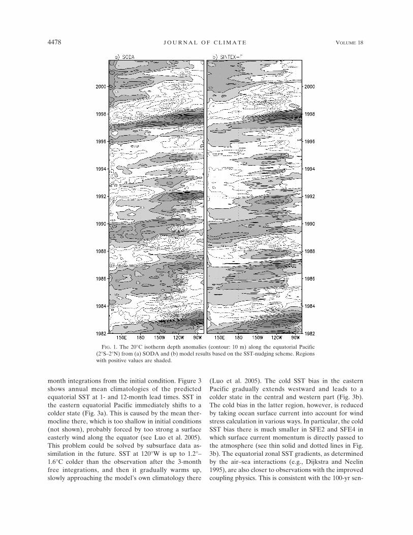
Figure 1 shows 20°C isotherm depth anomalies alongthe equatorial Pacific (2°S–2°N) from both the Simple

Ocean Data Assimilation (SODA; Carton et al. 2000)and model results. The latter is a simple average of thefive ensemble members. The anomaly fields of eachensemble member have been calculated separatelybased on its own climatology for the period 1983–2001.Compared to the SODA observations, the model real-istically captures the thermocline variations associatedwith the interannual ENSO events in the past 20 yr. Theeastward-propagation features along the equator arewell simulated. The intermittent warm signals in theearly 1990s are also captured. Amplitudes of the ther-mocline fluctuations are comparable to the SODA re-analysis. The results indicate that the SINTEX-Fcoupled model is able to generate realistic oceanicmemory for the ENSO prediction using the simple SST-nudging scheme.

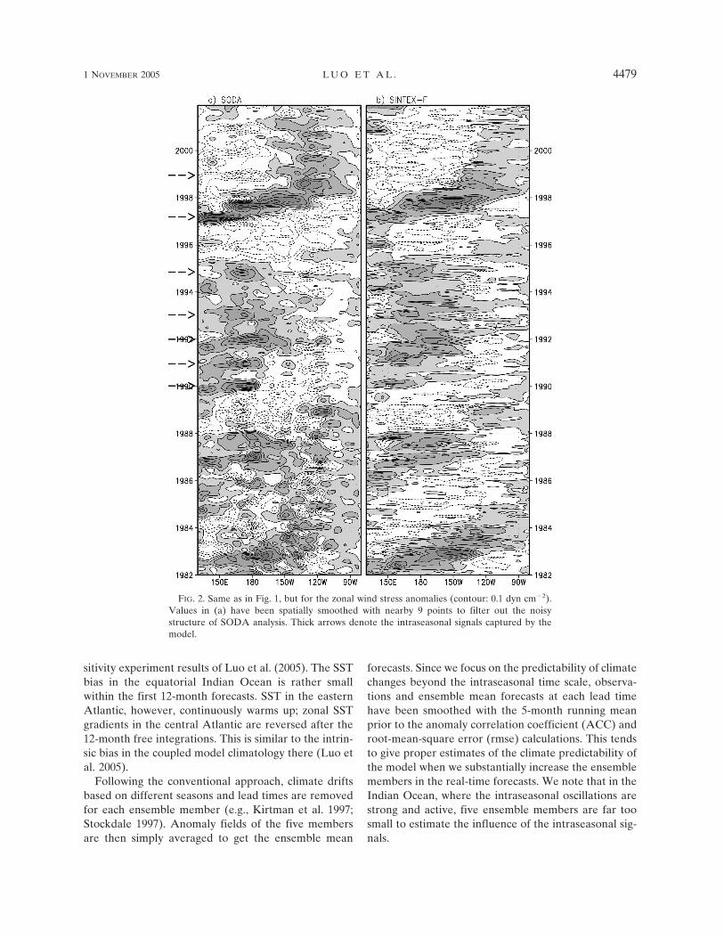
The good simulation of the subsurface signal in theequatorial Pacific is related to the realistic wind stressforcing produced by the AGCM (Fig. 2). Low-frequency westerly (easterly) anomalies related withthe El Niño (La Niña) events are well captured. Theeastward propagations of the anomalous westerlies as-sociated with the strong 1982/83 and 1997/98 warmepisodes are simulated. Furthermore, the AGCM isable to capture some intraseasonal westerly (easterly)wind bursts in the western equatorial Pacific (see ar-rows in Fig. 2a). The westerly wind bursts in the early1990s and during the onset phase of the 1997/98 ElNiño episode are captured realistically. The simulatedmagnitudes, however, are generally smaller than theSODA analysis. We note that the rather noisy structureof the SODA wind stress before 1986 is due to the lackof the Tropical Atmosphere Ocean (TAO) observa-tions.

Based on the generally realistic initial conditions, wehave implemented the 12-month forecast with thefreely coupled GCM starting from 0000 UTC on thefirst day of each month of each year from 1982 to 2001.The restart files for each ensemble member forecast ateach time is obtained from the instantaneous state atthe same time generated by the coupled SST-nudgingrun with the perturbed coupling physics as described insection 2b.

b. Model drift

Because of model deficiencies, the climate state in-evitably drifts toward the model’s own climatologyonce the forecast starts. How large the drift is dependson the prediction lead time, errors in initial conditions,and model physics. Here, we define the lead time as thelength of forecast integrations. For example, 1-monthlead prediction refers to the monthly mean of the first


month integrations from the initial condition. Figure 3shows annual mean climatologies of the predictedequatorial SST at 1- and 12-month lead times. SST inthe eastern equatorial Pacific immediately shifts to acolder state (Fig. 3a). This is caused by the mean ther-mocline there, which is too shallow in initial conditions(not shown), probably forced by too strong a surfaceeasterly wind along the equator (see Luo et al. 2005).This problem could be solved by subsurface data as-similation in the future. SST at 120°W is up to 1.2°–1.6°C colder than the observation after the 3-monthfree integrations, and then it gradually warms up,slowly approaching the model’s own climatology there

(Luo et al. 2005). The cold SST bias in the easternPacific gradually extends westward and leads to acolder state in the central and western part (Fig. 3b).The cold bias in the latter region, however, is reducedby taking ocean surface current into account for windstress calculation in various ways. In particular, the coldSST bias there is much smaller in SFE2 and SFE4 inwhich surface current momentum is directly passed tothe atmosphere (see thin solid and dotted lines in Fig.3b). The equatorial zonal SST gradients, as determinedby the air–sea interactions (e.g., Dijkstra and Neelin1995), are also closer to observations with the improvedcoupling physics. This is consistent with the 100-yr sen-

FIG. 1. The 20°C isotherm depth anomalies (contour: 10 m) along the equatorial Pacific(2°S–2°N) from (a) SODA and (b) model results based on the SST-nudging scheme. Regionswith positive values are shaded.


sitivity experiment results of Luo et al. (2005). The SSTbias in the equatorial Indian Ocean is rather smallwithin the first 12-month forecasts. SST in the easternAtlantic, however, continuously warms up; zonal SSTgradients in the central Atlantic are reversed after the12-month free integrations. This is similar to the intrin-sic bias in the coupled model climatology there (Luo etal. 2005).

Following the conventional approach, climate driftsbased on different seasons and lead times are removedfor each ensemble member (e.g., Kirtman et al. 1997;Stockdale 1997). Anomaly fields of the five membersare then simply averaged to get the ensemble mean

forecasts. Since we focus on the predictability of climatechanges beyond the intraseasonal time scale, observa-tions and ensemble mean forecasts at each lead timehave been smoothed with the 5-month running meanprior to the anomaly correlation coefficient (ACC) androot-mean-square error (rmse) calculations. This tendsto give proper estimates of the climate predictability ofthe model when we substantially increase the ensemblemembers in the real-time forecasts. We note that in theIndian Ocean, where the intraseasonal oscillations arestrong and active, five ensemble members are far toosmall to estimate the influence of the intraseasonal sig-nals.

FIG. 2. Same as in Fig. 1, but for the zonal wind stress anomalies (contour: 0.1 dyn cm�2).Values in (a) have been spatially smoothed with nearby 9 points to filter out the noisystructure of SODA analysis. Thick arrows denote the intraseasonal signals captured by themodel.


c. ENSO predictability

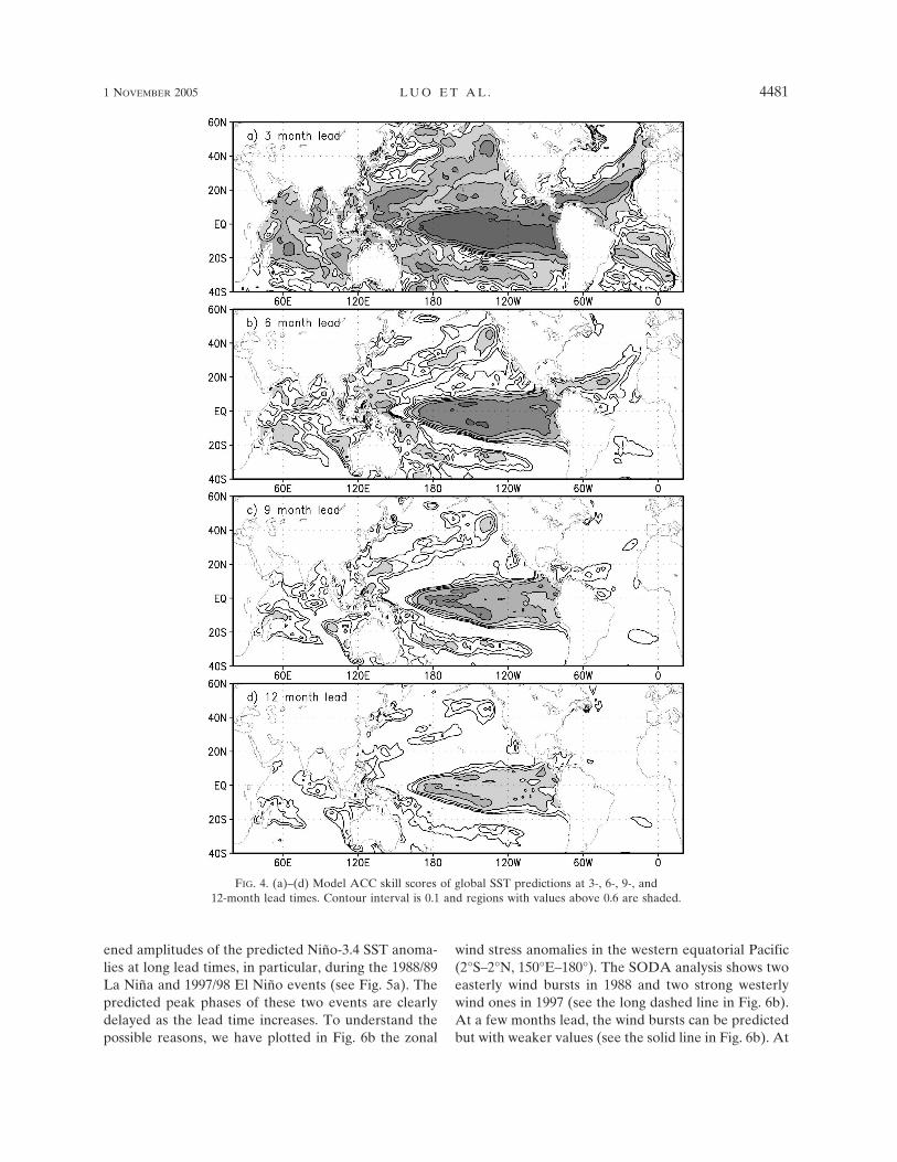
Figure 4 shows the ACC skill scores of global SSTpredictions at 3-, 6-, 9-, and 12-month lead times for theperiod 1982–2001. The model produces useful skill(�0.6) of SST predictions in most of Pacific and tropicalIndian and Atlantic Oceans at the 3-month lead time(Fig. 4a). The highest predictability appears in the cen-tral and eastern equatorial Pacific associated with theinterannual ENSO events as expected. The ACC in thisregion reaches above 0.9 at the 3-month lead time, andthen gradually decrease to about 0.8, 0.7, and 0.6 at 6-,9-, and 12-month lead times, respectively (Figs. 4a–d).We note that ACC skills of ENSO based on unfilteredforecasts and observations are only about 0.1 lower be-cause of its predominant interannual variations. TheENSO teleconnections in the North and South Pacificalso show considerable predictabilities until the9-month lead time. Besides, significant SST predict-abilities are found in the tropical North Atlantic andwestern and eastern tropical South Indian Ocean. Re-sults of those two basins will be described in section 4.

The interannual ENSO events are able to be pre-dicted by the model up to the 1-yr lead time (Fig. 5a).Both the El Niño events in 1982/83, 1986/87, 1991/92,

and 1997/98 and the La Niña events in 1984/85, 1988/89,and 1999/2000 are successfully predicted. Prediction ofthe strongest 1997/98 warm event was found to be verydifficult and failed by most existing CGCMs beyond the6-month lead time (e.g., Barnston et al. 1999; Landseaand Knaff 2000). The SINTEX-F model is capable topredict this unprecedented event at the 9-month leadtime with an amplitude as large as 2.2°C. At the 12-month lead time, however, the predicted signal is onlyabout 1.3°C, about one-half of the observations. For theweak warm signals in 1992/93 and 1994/95, the modelalso shows considerable predictabilities at the 6–9-month lead times. For the 1991/92 El Niño event, themodel predicted an earlier than observed peak and aweaker magnitude at the short (3 month) lead time.This is due to the similar errors in initial conditions(Fig. 1). Similarly, the overestimated 1999/2000 La Niñaevent at the short lead prediction seems to be related toa cold bias in initial conditions. Better initial conditionswith data assimilation may improve the forecasts (e.g.,Ji and Leetmaa 1997). During the period 1982–2001,there is only one false alarm of a weak warm event in1990/91. We note that the model tends to correctly pre-dict the El Niño event in 2002/03.

Compared to the persistence forecast, model predic-tions of the Niño-3.4 SST index show much higher ACCskills not only at long (9 months and beyond) lead timesbut also at short lead times (Fig. 5b). The ensemblemean forecast skill is above 0.7 at the 12-month leadtime (solid line in Fig. 5b). We note that the skill basedon the unfiltered data is still above 0.6 at the 12-monthlead time. The initial shock is largely reduced using thecompatible initial conditions between the atmosphereand ocean as generated by the coupled SST-nudgingscheme. The model rmses at mid (6 month) and longlead times are less than 50% of the persistence andmuch smaller than one standard deviation of 0.97°C(Fig. 5c). We note that the different systematic SSTbiases from each ensemble member in the equatorialPacific do not lead to significant differences in theENSO prediction skills (see short dashed lines in Figs.5b,c). This is probably related to the fact that the cli-mate drifts of each member (not largely different) havebeen removed in a posterior manner.

The low-frequency variations of the equatorial ther-mocline and zonal wind can be predicted at long leadtimes. The eastward propagations of subsurface signalsalong the equatorial Pacific are successfully predictedat the 12-month lead time (Fig. 6a). This suggests apotential predictability of ENSO beyond the 1-yr leadtime. The predicted magnitudes of the equatorial ther-mocline variations, however, gradually decrease as thelead time increases. This is consistent with the weak-

FIG. 3. SST climatology of the period 1983–2001 along the equa-tor (2°S–2°N) based on the NOAA/CDC observations (thick solidlines), SFE1 (dot–dot–dashed lines), SFE2 (thin solid lines), SFE3(short dashed lines), SFE4 (dotted lines), and SFE5 (long dashedlines) for the (a) 1- and (b) 12-month lead time forecasts.


ened amplitudes of the predicted Niño-3.4 SST anoma-lies at long lead times, in particular, during the 1988/89La Niña and 1997/98 El Niño events (see Fig. 5a). Thepredicted peak phases of these two events are clearlydelayed as the lead time increases. To understand thepossible reasons, we have plotted in Fig. 6b the zonal

wind stress anomalies in the western equatorial Pacific(2°S–2°N, 150°E–180°). The SODA analysis shows twoeasterly wind bursts in 1988 and two strong westerlywind ones in 1997 (see the long dashed line in Fig. 6b).At a few months lead, the wind bursts can be predictedbut with weaker values (see the solid line in Fig. 6b). At

FIG. 4. (a)–(d) Model ACC skill scores of global SST predictions at 3-, 6-, 9-, and12-month lead times. Contour interval is 0.1 and regions with values above 0.6 are shaded.


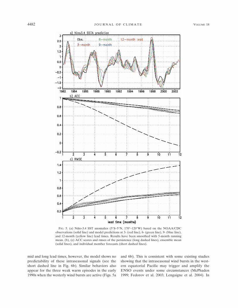
mid and long lead times, however, the model shows nopredictability of these intraseasonal signals (see theshort dashed line in Fig. 6b). Similar behaviors alsoappear for the three weak warm episodes in the early1990s when the westerly wind bursts are active (Figs. 5a

and 6b). This is consistent with some existing studiesshowing that the intraseasonal wind bursts in the west-ern equatorial Pacific may trigger and amplify theENSO events under some circumstances (McPhaden1999; Fedorov et al. 2003; Lengaigne et al. 2004). In

FIG. 5. (a) Niño-3.4 SST anomalies (5°S–5°N, 170°–120°W) based on the NOAA/CDCobservations (solid line) and model predictions at 3- (red line), 6- (green line), 9- (blue line),and 12-month (yellow line) lead times. Results have been smoothed with 5-month runningmean. (b), (c) ACC scores and rmses of the persistence (long dashed lines), ensemble mean(solid lines), and individual member forecasts (short dashed lines).


Fig 5 live 4/C

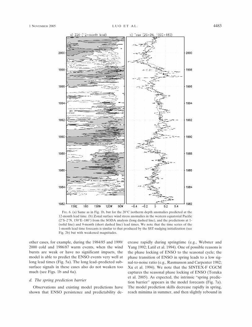
other cases, for example, during the 1984/85 and 1999/2000 cold and 1986/87 warm events, when the windbursts are weak or have no significant impacts, themodel is able to predict the ENSO events very well atlong lead times (Fig. 5a). The long lead–predicted sub-surface signals in these cases also do not weaken toomuch (see Figs. 1b and 6a).

d. The spring prediction barrier

Observations and existing model predictions haveshown that ENSO persistence and predictability de-

crease rapidly during springtime (e.g., Webster andYang 1992; Latif et al. 1994). One of possible reasons isthe phase locking of ENSO to the seasonal cycle; thephase transition of ENSO in spring leads to a low sig-nal-to-noise ratio (e.g., Rasmusson and Carpenter 1982;Xu et al. 1994). We note that the SINTEX-F CGCMcaptures the seasonal phase locking of ENSO (Tozukaet al. 2005). As expected, the intrinsic “spring predic-tion barrier” appears in the model forecasts (Fig. 7a).The model prediction skills decrease rapidly in spring,reach mimima in summer, and then slightly rebound in

FIG. 6. (a) Same as in Fig. 1b, but for the 20°C isotherm depth anomalies predicted at the12-month lead time. (b) Zonal surface wind stress anomalies in the western equatorial Pacific(2°S–2°N, 150°E–180°) from the SODA analysis (long dashed line), and the predictions at 1-(solid line) and 9-month (short dashed line) lead times. We note that the time series of the1-month lead time forecasts is similar to that produced by the SST-nudging initialization (seeFig. 2b) but with weakened magnitudes.


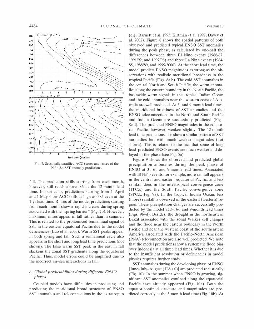
fall. The prediction skills starting from each month,however, still reach above 0.6 at the 12-month leadtime. In particular, predictions starting from 1 Apriland 1 May show ACC skills as high as 0.85 even at the1-yr lead time. Rmses of the model predictions startingfrom each month show a rapid increase during springassociated with the “spring barrier” (Fig. 7b). However,maximum rmses appear in fall rather than in summer.This is related to the pronounced semiannual signal ofSST in the eastern equatorial Pacific due to the modeldeficiencies (Luo et al. 2005): Warm SST peaks appearin both spring and fall. Such a semiannual cycle alsoappears in the short and long lead time predictions (notshown). The false warm SST peak in the east in fallslackens the zonal SST gradients along the equatorialPacific. Thus, model errors could be amplified due tothe incorrect air–sea interactions in fall.

e. Global predictabilities during different ENSOphases

Coupled models have difficulties in producing andpredicting the meridional broad structure of ENSOSST anomalies and teleconnections in the extratropics

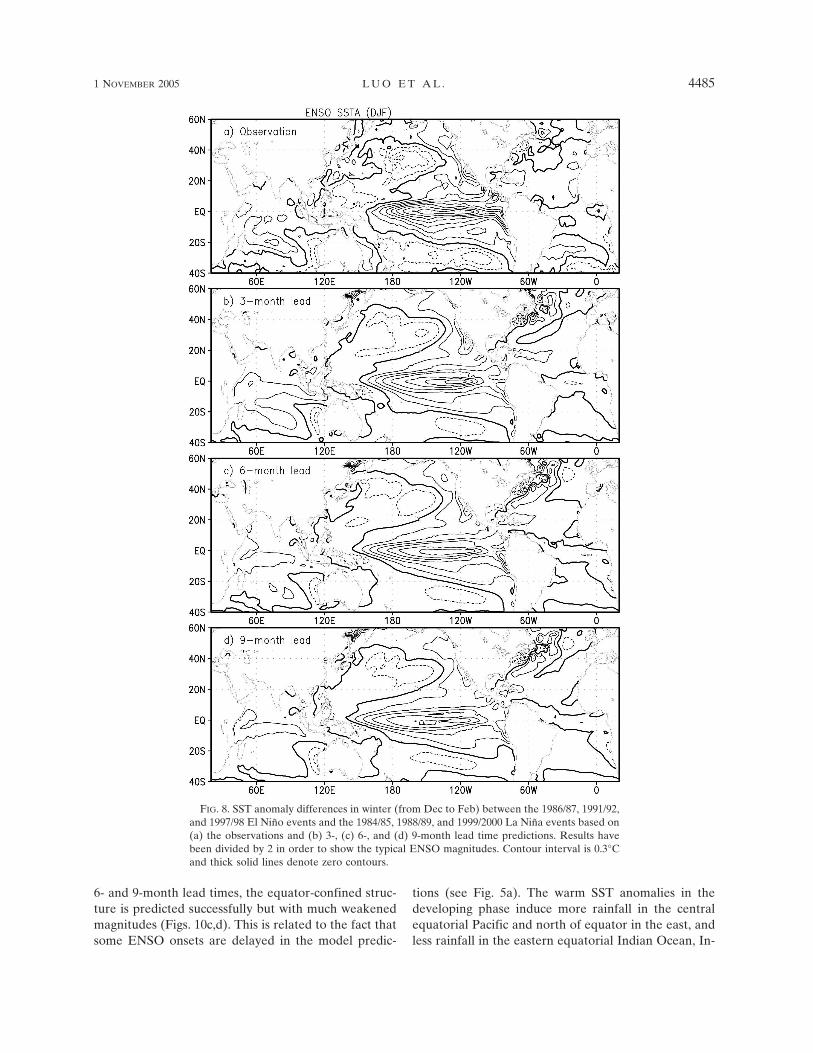
(e.g., Barnett et al. 1993; Kirtman et al. 1997; Davey etal. 2002). Figure 8 shows the spatial patterns of bothobserved and predicted typical ENSO SST anomaliesduring the peak phase, as calculated by one-half thedifferences between three El Niño events (1986/87,1991/92, and 1997/98) and three La Niña events (1984/85, 1988/89, and 1999/2000). At the short lead time, themodel predicts ENSO magnitudes as strong as the ob-servations with realistic meridional broadness in thetropical Pacific (Figs. 8a,b). The cold SST anomalies inthe central North and South Pacific, the warm anoma-lies along the eastern boundary in the North Pacific, thebasinwide warm signals in the tropical Indian Oceanand the cold anomalies near the western coast of Aus-tralia are well predicted. At 6- and 9-month lead times,the meridional broadness of SST anomalies and theENSO teleconnections in the North and South Pacificand Indian Ocean are successfully predicted (Figs.8c,d). The predicted ENSO magnitudes in the equato-rial Pacific, however, weaken slightly. The 12-monthlead time predictions also show a similar pattern of SSTanomalies but with much weaker magnitudes (notshown). This is related to the fact that some of longlead–predicted ENSO events are much weaker and de-layed in the phase (see Fig. 5a).

Figure 9 shows the observed and predicted globalprecipitation anomalies during the peak phase ofENSO at 3-, 6-, and 9-month lead times. Associatedwith El Niño events, for example, more rainfall appearsin the central and eastern equatorial Pacific, and lessrainfall does in the intertropical convergence zone(ITCZ) and the South Pacific convergence zone(SPCZ; Fig. 9a). In the tropical Indian Ocean, less(more) rainfall is observed in the eastern (western) re-gion. These precipitation changes are successfully pre-dicted by the model at 3-, 6-, and 9-month lead times(Figs. 9b–d). Besides, the drought in the northeasternBrazil associated with the zonal Walker cell changesand the flood near the eastern boundary in the NorthPacific and near the western coast of the southeasternAmerica associated with the Pacific–North American(PNA) teleconnection are also well predicted. We notethat the model predictions show a systematic flood biasover Indonesia at all three lead times. Whether it is dueto the insufficient resolution or deficiencies in modelphysics requires further study.

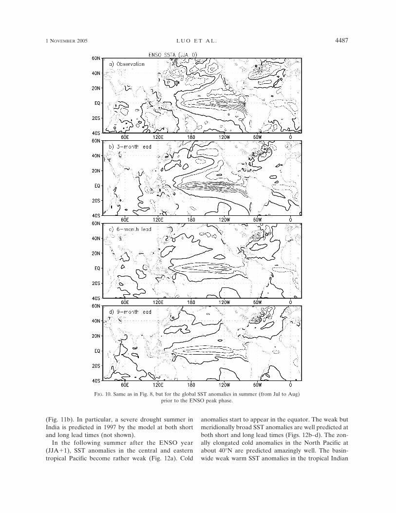
SST anomalies during the developing phase of ENSO[June–July–August (JJA�0)] are predicted realistically(Fig. 10). In the summer when ENSO is growing, sig-nificant SST anomalies confined along the equatorialPacific have already appeared (Fig. 10a). Both theequator-confined structure and magnitudes are pre-dicted correctly at the 3-month lead time (Fig. 10b). At

FIG. 7. Seasonally stratified ACC scores and rmses of theNiño-3.4 SST anomaly predictions.


6- and 9-month lead times, the equator-confined struc-ture is predicted successfully but with much weakenedmagnitudes (Figs. 10c,d). This is related to the fact thatsome ENSO onsets are delayed in the model predic-

tions (see Fig. 5a). The warm SST anomalies in thedeveloping phase induce more rainfall in the centralequatorial Pacific and north of equator in the east, andless rainfall in the eastern equatorial Indian Ocean, In-

FIG. 8. SST anomaly differences in winter (from Dec to Feb) between the 1986/87, 1991/92,and 1997/98 El Niño events and the 1984/85, 1988/89, and 1999/2000 La Niña events based on(a) the observations and (b) 3-, (c) 6-, and (d) 9-month lead time predictions. Results havebeen divided by 2 in order to show the typical ENSO magnitudes. Contour interval is 0.3°Cand thick solid lines denote zero contours.


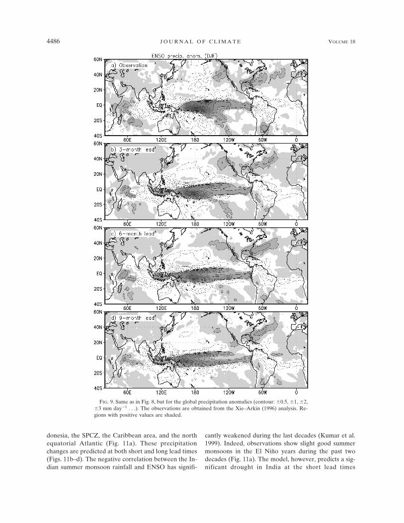
donesia, the SPCZ, the Caribbean area, and the northequatorial Atlantic (Fig. 11a). These precipitationchanges are predicted at both short and long lead times(Figs. 11b–d). The negative correlation between the In-dian summer monsoon rainfall and ENSO has signifi-

cantly weakened during the last decades (Kumar et al.1999). Indeed, observations show slight good summermonsoons in the El Niño years during the past twodecades (Fig. 11a). The model, however, predicts a sig-nificant drought in India at the short lead times

FIG. 9. Same as in Fig. 8, but for the global precipitation anomalies (contour: �0.5, �1, �2,�3 mm day�1 . . .). The observations are obtained from the Xie–Arkin (1996) analysis. Re-gions with positive values are shaded.


(Fig. 11b). In particular, a severe drought summer inIndia is predicted in 1997 by the model at both shortand long lead times (not shown).

In the following summer after the ENSO year(JJA�1), SST anomalies in the central and easterntropical Pacific become rather weak (Fig. 12a). Cold

anomalies start to appear in the equator. The weak butmeridionally broad SST anomalies are well predicted atboth short and long lead times (Figs. 12b–d). The zon-ally elongated cold anomalies in the North Pacific atabout 40°N are predicted amazingly well. The basin-wide weak warm SST anomalies in the tropical Indian

FIG. 10. Same as in Fig. 8, but for the global SST anomalies in summer (from Jul to Aug)prior to the ENSO peak phase.


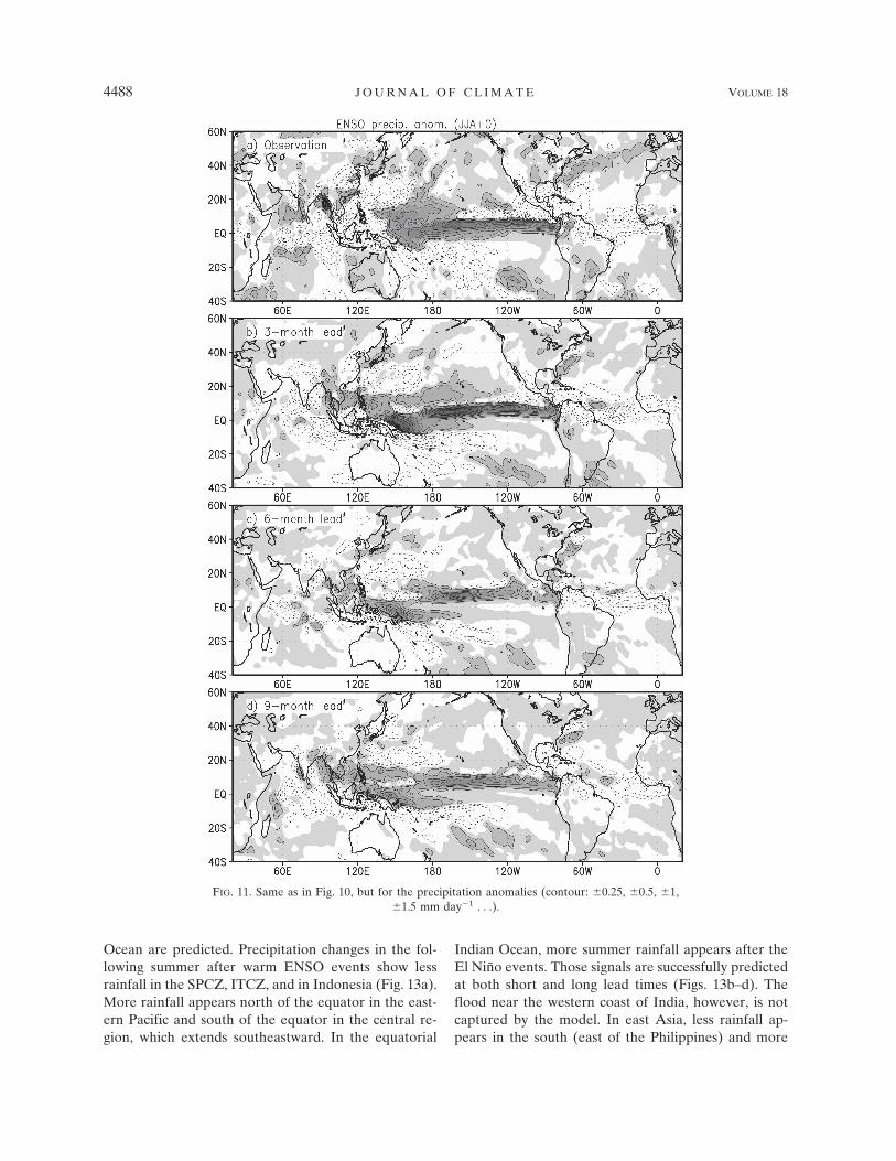
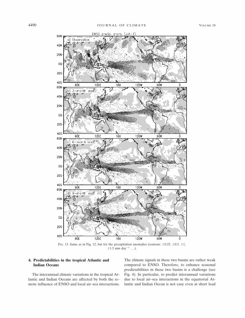
Ocean are predicted. Precipitation changes in the fol-lowing summer after warm ENSO events show lessrainfall in the SPCZ, ITCZ, and in Indonesia (Fig. 13a).More rainfall appears north of the equator in the east-ern Pacific and south of the equator in the central re-gion, which extends southeastward. In the equatorial

Indian Ocean, more summer rainfall appears after theEl Niño events. Those signals are successfully predictedat both short and long lead times (Figs. 13b–d). Theflood near the western coast of India, however, is notcaptured by the model. In east Asia, less rainfall ap-pears in the south (east of the Philippines) and more

FIG. 11. Same as in Fig. 10, but for the precipitation anomalies (contour: �0.25, �0.5, �1,�1.5 mm day�1 . . .).


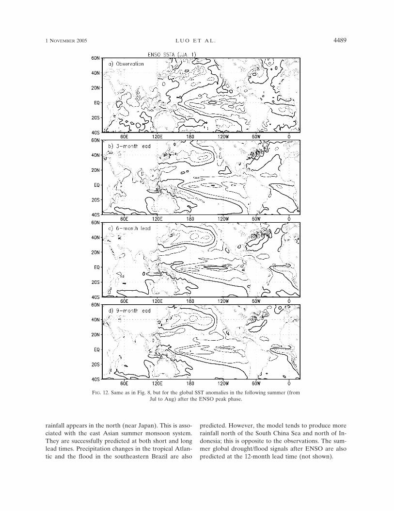
rainfall appears in the north (near Japan). This is asso-ciated with the east Asian summer monsoon system.They are successfully predicted at both short and longlead times. Precipitation changes in the tropical Atlan-tic and the flood in the southeastern Brazil are also

predicted. However, the model tends to produce morerainfall north of the South China Sea and north of In-donesia; this is opposite to the observations. The sum-mer global drought/flood signals after ENSO are alsopredicted at the 12-month lead time (not shown).

FIG. 12. Same as in Fig. 8, but for the global SST anomalies in the following summer (fromJul to Aug) after the ENSO peak phase.


4. Predictabilities in the tropical Atlantic andIndian Oceans

The interannual climate variations in the tropical At-lantic and Indian Oceans are affected by both the re-mote influence of ENSO and local air–sea interactions.

The climate signals in these two basins are rather weakcompared to ENSO. Therefore, to enhance seasonalpredictabilities in these two basins is a challenge (seeFig. 4). In particular, to predict interannual variationsdue to local air–sea interactions in the equatorial At-lantic and Indian Ocean is not easy even at short lead

FIG. 13. Same as in Fig. 12, but for the precipitation anomalies (contour: �0.25, �0.5, �1,�1.5 mm day�1 . . .).


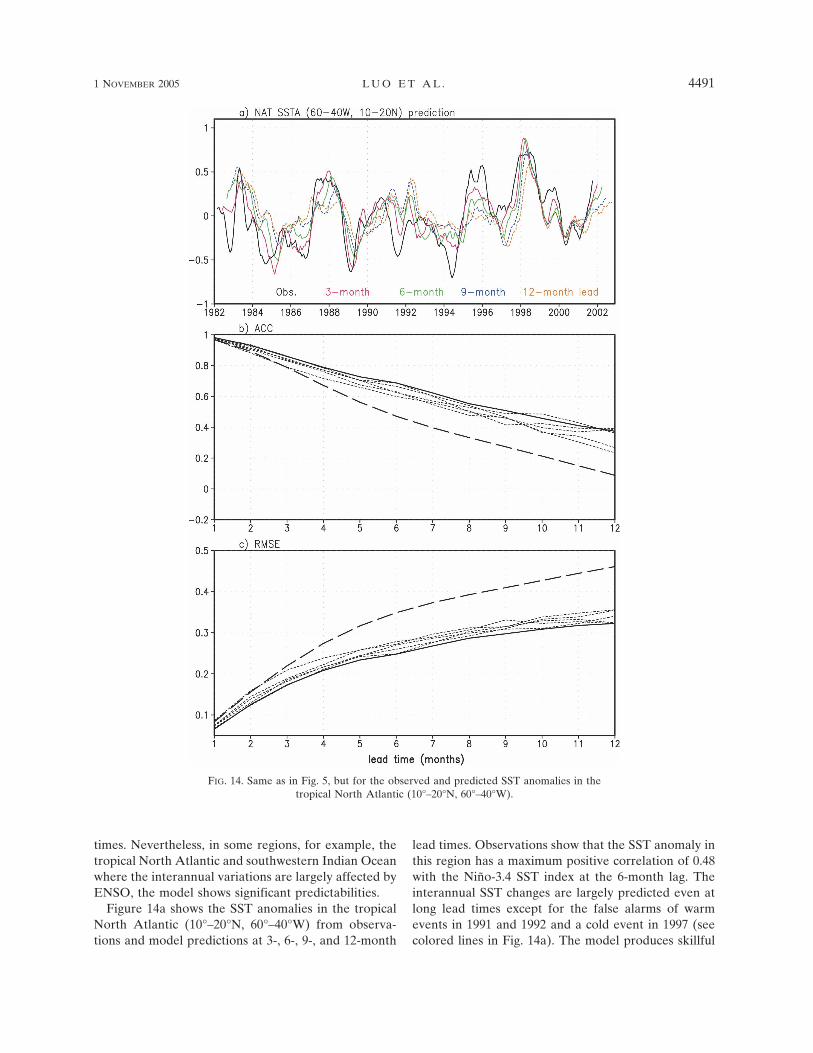
times. Nevertheless, in some regions, for example, thetropical North Atlantic and southwestern Indian Oceanwhere the interannual variations are largely affected byENSO, the model shows significant predictabilities.

Figure 14a shows the SST anomalies in the tropicalNorth Atlantic (10°–20°N, 60°–40°W) from observa-tions and model predictions at 3-, 6-, 9-, and 12-month

lead times. Observations show that the SST anomaly inthis region has a maximum positive correlation of 0.48with the Niño-3.4 SST index at the 6-month lag. Theinterannual SST changes are largely predicted even atlong lead times except for the false alarms of warmevents in 1991 and 1992 and a cold event in 1997 (seecolored lines in Fig. 14a). The model produces skillful

FIG. 14. Same as in Fig. 5, but for the observed and predicted SST anomalies in thetropical North Atlantic (10°–20°N, 60°–40°W).


Fig 14 live 4/C

predictions until the 7-month lead time with no appar-ent initial shock (Fig. 14b). The rmses grow as the leadtime increases; but they are still smaller than one stan-dard deviation (0.34°C) of the observed SST anomalyuntil the 12-month lead time (Fig. 14c).

SST changes in the tropical southwestern IndianOcean (20°–10°S, 50°–70°E) show a close relationship

with ENSO (Fig. 15a; see also Xie et al. 2002). Thecorrelation between them reaches 0.63 at the 3-monthlag. Correspondingly, the model predicts all interannualvariations associated with the past 20-yr ENSO epi-sodes even at the 12-month lead time without any falsealarm. The weak signals in 1993–95 in the absence ofENSO events are almost unpredictable. The model

FIG. 15. Same as in Fig. 14, but for the SST anomalies in the tropical southwestern IndianOcean (20°–10°S, 50°–70°E).


Fig 15 live 4/C

ACC skill scores of the ensemble mean predictionsreach 0.6 at the 12-month lead time (Fig. 15b). Again,there is no apparent initial shock. The rmses are muchsmaller than one standard deviation (0.34°C) of the ob-served SST anomaly in this region even for the 12-month lead time predictions (Fig. 15c).

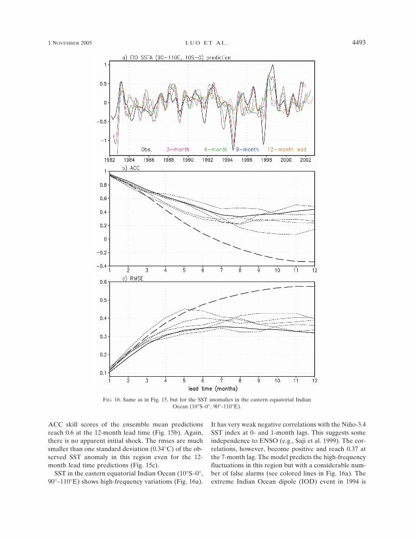
SST in the eastern equatorial Indian Ocean (10°S–0°,90°–110°E) shows high-frequency variations (Fig. 16a).

It has very weak negative correlations with the Niño-3.4SST index at 0- and 1-month lags. This suggests someindependence to ENSO (e.g., Saji et al. 1999). The cor-relations, however, become positive and reach 0.37 atthe 7-month lag. The model predicts the high-frequencyfluctuations in this region but with a considerable num-ber of false alarms (see colored lines in Fig. 16a). Theextreme Indian Ocean dipole (IOD) event in 1994 is

FIG. 16. Same as in Fig. 15, but for the SST anomalies in the eastern equatorial IndianOcean (10°S–0°, 90°–110°E).


Fig 16 live 4/C

predicted at the 6-month lead time (see also Wajsowicz2005). The model, however, fails to predict the coldevent in 1997. Strong or weak signals associated withthe ENSO events, for example, in 1983, 1987, 1989,1992, 1998, and 2000, are predicted as long as at the12-month lead time. The model ACC skills decreaserapidly from 0.95 at the 1-month lead time to �0.6 atthe 4-month lead time (Fig. 16b). At long lead times,the prediction skills slightly rebound probably due tothe delayed ENSO influences. Rmses of the model pre-dictions increase rapidly to about 0.35°C at the 7-monthlead time, comparable to one standard deviation of theSST anomaly there (Fig. 16c).

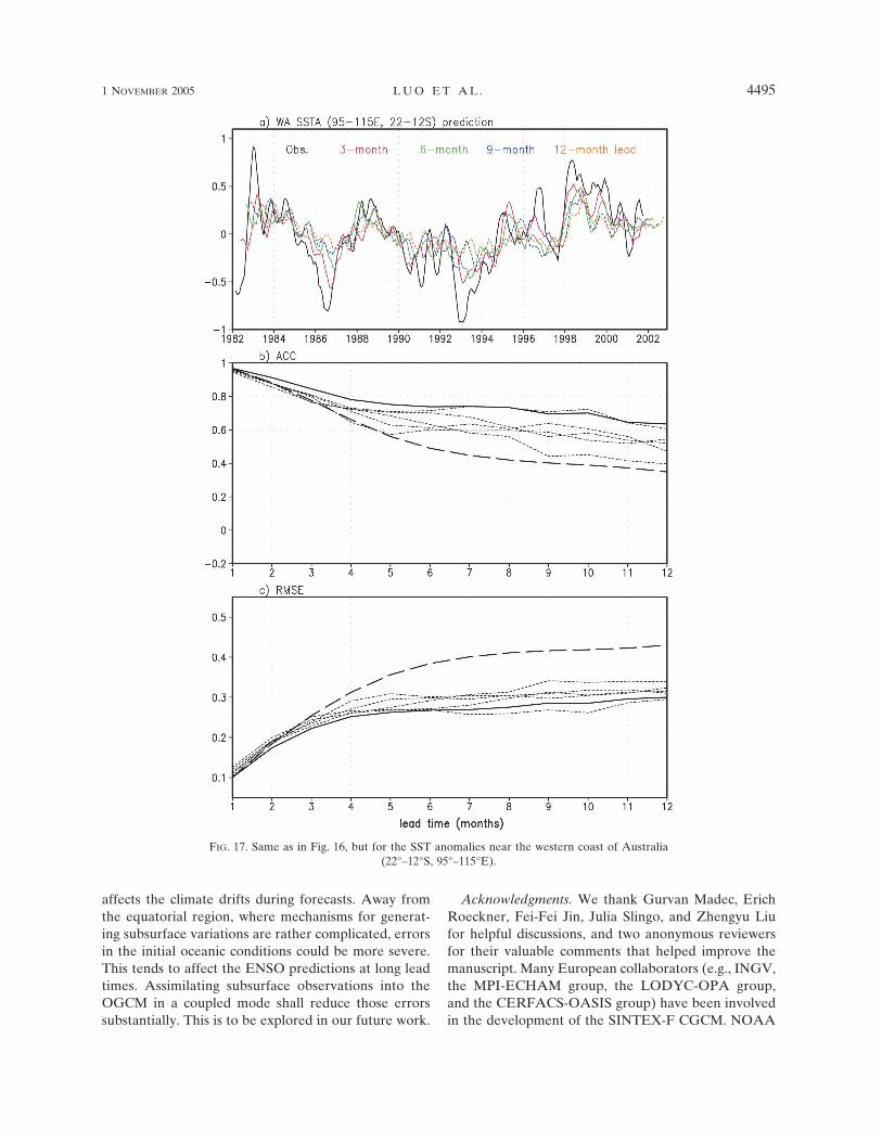
It is interesting that the model also shows a signifi-cant predictability near the western coast of Australia(see Fig. 4). SST in that region (22°–12°S, 95°–115°E)has a weak negative correlation of �0.24 with the Niño-3.4 SST index (see also Fig. 8) with no delayed ENSOinfluence. Interestingly, SST variations in this regionshow pronounced decadal signals with a high persis-tence of �0.35 at the 12-month lag (Figs. 17a,b). Suchdominant decadal signals can be predicted at long leadtimes (see colored lines in Fig. 17a). Model ACC skillsreach above 0.6 at the 12-month lead time with rmsessmaller than one standard deviation (0.38°C; Figs.17b,c).

We note that the ensemble spread among the fivemembers in the tropical Indian Ocean are larger thanthose in the Niño-3.4 region and the tropical NorthAtlantic (see short dashed lines in Figs. 5b, 14b, 15b,16b, and 17b). This could be related to the strong in-traseasonal signals over the equatorial warm SST andthe seasonal migration of monsoon winds in the IndianOcean. Wind stress modifications by the ocean surfacecurrent with different coupling physics could be muchdifferent in the presence of strong surface wind andocean current changes.

5. Summary and discussion

In this study, we have investigated the seasonal cli-mate/ENSO predictability for the period 1982–2001based on the SINTEX-F coupled GCM. To produceensemble forecasts, we have perturbed the couplingphysics for each member by taking ocean surface cur-rent into account for wind stress calculations in differ-ent ways (Luo et al. 2005). This accounts for the uncer-tainties not only in the initial conditions but also in themodel physics. Compatible initial conditions betweenthe atmosphere and ocean are generated using thesimple coupled SST-nudging scheme with a strong re-storing coefficient to the observations. The initial shockof forecasts has been largely reduced.

The model hindcast results show a high predictabilityof ENSO. All the warm and cold events in the past 20yr, including the strongest 1997/98 El Niño episode, arepredicted successfully. The model ACC skill scoresreach above 0.7 at the 12-month lead time with thermses much smaller than one standard deviation of theNiño-3.4 SST index. The predicted magnitudes forsome particular ENSO events, however, are weakenedwith a phase delay at mid and long lead times. Thisseems to be related to the unpredicted intraseasonalwind bursts in the western equatorial Pacific beyond afew months lead. The model also shows a “spring pre-diction barrier” similar to that in observations as ex-pected from its good capture of seasonal phase lockingof ENSO. The spatial pattern of ENSO SST anomaliesand teleconnections during the developing (summer),peak (winter), and ending (following summer) phasesare predicted at both short and long lead times. Corre-spondingly, the global drought/flood associated withthree ENSO phases are predicted successfully over the9-month lead time. This implies potential societal im-pacts of the long lead ENSO forecasts. The negativerelationship between the Indian summer monsoon rain-fall and ENSO, however, is overestimated in the modelpredictions. Besides, the model rainfall predictionsshow systematic biases near the Maritime Continent inthe western Pacific. Model calibrations may reducethose systematic biases.

The model results show significant predictabilities inthe tropical North Atlantic and southwestern IndianOcean, where the SST changes are largely affected byENSO. The ACC scores in the two regions reach about0.6 at 7- and 12-month lead times, respectively. In theeastern equatorial Indian Ocean, where the local air–sea interactions are active and the signals fluctuatemore frequently, the model shows skillful predictionsonly up to about one season lead. However, the ex-treme IOD event in 1994 is predicted at the 6-monthlead time. Signals associated with the ENSO events arestill able to be predicted at long lead times. Interest-ingly, SST changes near the western coast of Australiacan be skillfully predicted at long lead times even with-out significant ENSO influences. This is due to thedominant decadal signals there.

Success of the coupled nudging scheme for initializa-tion depends crucially on the model performance. Sincethe SINTEX-F CGCM realistically simulates the clima-tology and ENSO in the tropical Pacific, the simpleSST-nudging scheme is able to generate realistic sub-surface information and surface wind changes along theequatorial Pacific including several intraseasonal windbursts in the west. In the eastern part, however, themodel-produced mean themocline is too shallow. This


affects the climate drifts during forecasts. Away fromthe equatorial region, where mechanisms for generat-ing subsurface variations are rather complicated, errorsin the initial oceanic conditions could be more severe.This tends to affect the ENSO predictions at long leadtimes. Assimilating subsurface observations into theOGCM in a coupled mode shall reduce those errorssubstantially. This is to be explored in our future work.

Acknowledgments. We thank Gurvan Madec, ErichRoeckner, Fei-Fei Jin, Julia Slingo, and Zhengyu Liufor helpful discussions, and two anonymous reviewersfor their valuable comments that helped improve themanuscript. Many European collaborators (e.g., INGV,the MPI-ECHAM group, the LODYC-OPA group,and the CERFACS-OASIS group) have been involvedin the development of the SINTEX-F CGCM. NOAA

FIG. 17. Same as in Fig. 16, but for the SST anomalies near the western coast of Australia(22°–12°S, 95°–115°E).


Fig 17 live 4/C

Optimum Interpolation (OI) SST V2 data were pro-vided by the NOAA–CIRES Climate Diagnostics Cen-ter. All experiments have been performed using theEarth Simulator.

REFERENCES

Achutarao, K., and K. R. Sperber, 2002: Simulation of the El NiñoSouthern Oscillation: Results from the Coupled Model Inter-comparison Project. Climate Dyn., 19, 191–209.

Balmaseda, M. A., D. L. T. Anderson, and M. K. Davey, 1994:ENSO prediction using a dynamical ocean model coupled tostatistical atmospheres. Tellus, 46A, 497–511.

Barnett, T. P., M. Latif, N. Graham, M. Flügel, S. Pazan, and W.White, 1993: ENSO and ENSO-related predictability. Part I:Prediction of equatorial Pacific sea surface temperature witha hybrid coupled ocean–atmosphere model. J. Climate, 6,1545–1566.

Barnston, A. G., M. H. Glantz, and Y. He, 1999: Predictive skill ofstatistical and dynamical climate models in SST forecasts dur-ing the 1997/98 El Niño episode and the 1998 La Niña onset.Bull. Amer. Meteor. Soc., 80, 217–243.

Blanke, B., and P. Delecluse, 1993: Variability of the tropicalAtlantic Ocean simulated by a general circulation model withtwo different mixed layer physics. J. Phys. Oceanogr., 23,1363–1388.

Cane, M. A., S. E. Zebiak, and S. C. Dolan, 1986: Experimentalforecasts of El Niño. Nature, 321, 827–832.

Carton, J. A., G. Chepurin, and X. Cao, 2000: A Simple OceanData Assimilation analysis of the global upper ocean 1950–95. Part II: Results. J. Phys. Oceanogr., 30, 311–326.

Charnock, M., 1955: Wind stress on a water surface. Quart. J. Roy.Meteor. Soc., 81, 639–640.

Chen, D., S. E. Zebiak, and M. A. Cane, 1997: Initialization andpredictability of a coupled ENSO forecast model. Mon. Wea.Rev., 125, 773–788.

——, M. A. Cane, S. E. Zebiak, R. Cañizares, and A. Kaplan,2000: Bias correction of an ocean–atmosphere coupledmodel. Geophys. Res. Lett., 27, 2585–2588.

——, ——, A. Kaplan, S. E. Zebiak, and D. Huang, 2004: Pre-dictability of El Niño over the past 148 years. Nature, 428,733–736.

Clarke, A. J., and S. van Gorder, 2003: Improving El Niño pre-diction using a space–time integration of Indo-Pacific windsand equatorial Pacific upper ocean heat content. Geophys.Res. Lett., 30, 1399, doi:10.1029/2002GL016673.

Davey, M., and Coauthors, 2002: STOIC: A study of coupledmodel climatology and variability in tropical ocean regions.Climate Dyn., 18, 403–420.

Dijkstra, H. A., and J. D. Neelin, 1995: Coupled ocean–atmosphere interaction and the tropical climatology. Part II:Why the cold tongue is in the east. J. Climate, 8, 1343–1359.

Doblas-Reyes, F. J., R. Hagedorn, and T. N. Palmer, 2005: Therationale behind the success of multi-model ensembles in sea-sonal forecasting. Part II: Calibration and combination. Tel-lus, 57A, 234–252.

Fedorov, A. V., S. L. Harper, S. G. Philander, B. Winter, and A.Wittenberg, 2003: How predictable is El Niño? Bull. Amer.Meteor. Soc., 84, 911–919.

Gent, P. R., and J. C. McWilliams, 1990: Isopycnal mixing inocean circulation models. J. Phys. Oceanogr., 20, 150–155.

Gualdi, S., A. Navarra, E. Guilyardi, and P. Delecluse, 2003: As-

sessment of the tropical Indo-Pacific climate in the SINTEXCGCM. Ann. Geophys., 46, 1–26.

——, A. Alessandri, and A. Navarra, 2005: Impact of atmospherichorizontal resolution on ENSO forecasts. Tellus, 57A, 357–374.

Guilyardi, E., P. Delecluse, S. Gualdi, and A. Navarra, 2003:Mechanisms for ENSO phase change in a coupled GCM. J.Climate, 16, 1141–1158.

——, and Coauthors, 2004: Representing El Niño in coupledocean–atmosphere GCMS: The dominant role of the atmo-spheric component. J. Climate, 17, 4623–4629.

Hagedorn, R., F. J. Doblas-Reyes, and T. N. Palmer, 2005: Therationale behind the success of multi-model ensembles in sea-sonal forecasting. Part I: Basic concept. Tellus, 57A, 219–233.

Ji, M., and A. Leetmaa, 1997: Impact of data assimilation onocean initialization and El Niño prediction. Mon. Wea. Rev.,125, 742–753.

——, A. Kumar, and A. Leetmaa, 1994: A multiseason climateforecast system at the National Meteorological Center. Bull.Amer. Meteor. Soc., 75, 569–577.

Keenlyside, N., M. Latif, M. Botzet, J. Jungclaus, and U. Schulz-weida, 2005: A coupled method for initializing El Niño–Southern Oscillation forecasts using sea surface temperature.Tellus, 57A, 340–356.

Kirtman, B. P., J. Shukla, B. Huang, Z. Zhu, and E. K. Schneider,1997: Multiseasonal predictions with a coupled tropicalocean–global atmosphere system. Mon. Wea. Rev., 125, 789–808.

Krishnamurti, T. N., C. M. Kishtawal, T. E. LaRow, D. R. Bachio-chi, Z. Zhang, C. E. Williford, S. Gadgil, and S. Surendran,1999: Improved weather and seasonal climate forecasts frommultimodel superensemble. Science, 285, 1548–1550.

Kumar, K. K., B. Rajagopalan, and M. A. Cane, 1999: On theweakening relationship between the Indian monsoon andENSO. Science, 284, 2156–2159.

Landsea, C. W., and J. A. Knaff, 2000: How much skill was therein forecasting the very strong 1997/98 El Niño? Bull. Amer.Meteor. Soc., 81, 2107–2119.

Latif, M., T. P. Barnett, M. A. Cane, M. Flügel, N. E. Graham, H.von Storch, J.-S. Xu, and S. E. Zebiak, 1994: A review ofENSO prediction studies. Climate Dyn., 9, 167–179.

Lengaigne, M., E. Guilyardi, J.-P. Boulanger, C. Menkes, P. In-ness, P. Delecluse, and J. M. Slingo, 2004: Triggering of ElNiño by westerly wind events in a coupled general circulationmodel. Climate Dyn., 23, 601–620.

Louis, J. F., 1979: A parametric model of vertical eddy fluxes inthe atmosphere. Bound.-Layer Meteor., 17, 187–202.

Luo, J.-J., S. Masson, S. Behera, P. Delecluse, S. Gualdi, A. Na-varra, and T. Yamagata, 2003: South Pacific origin of thedecadal ENSO-like variation as simulated by a coupledGCM. Geophys. Res. Lett. , 30, 2250, doi:10.1029/2003GL018649.

——, ——, E. Roeckner, G. Madec, and T. Yamagata, 2005: Re-ducing climatology bias in an ocean–atmosphere CGCM withimproved coupling physics. J. Climate, 18, 2344–2360.

Madec, G., P. Delecluse, M. Imbard, and C. Levy, 1998: OPA 8.1ocean general circulation model reference manual. LODYC/IPSL Tech. Rep. Note 11, Paris, France, 91 pp.

McPhaden, M. J., 1999: Genesis and evolution of the 1997–98 ElNiño. Science, 283, 950–954.

Morcrette, J.-J., L. Smith, and Y. Fouquart, 1986: Pressure andtemperature dependence of the absorption in longwave ra-diation parameterizations. Beitr. Phys. Atmos., 59, 455–469.


Neelin, J. D., D. S. Battisti, A. C. Hirst, F.-F. Jin, Y. Wakata, T.Yamagata, and S. E. Zebiak, 1998: ENSO theory. J. Geophys.Res., 103, 14 261–14 290.

Oberhuber, J. M., E. Roeckner, M. Christopher, M. Esch, and M.Latif, 1998: Predicting the 97 El Niño event with a globalclimate model. Geophys. Res. Lett., 25, 2273–2276.

Pacanowski, R., 1987: Effect of equatorial currents on surfacestress. J. Phys. Oceanogr., 17, 833–838.

Palmer, T. N., 2001: A nonlinear dynamical perspective on modelerror: A proposal for non-local stochastic-dynamic param-etrization in weather and climate prediction models. Quart. J.Roy. Meteor. Soc., 127, 279–304.

——, and Coauthors, 2004: Development of a European multi-model ensemble system for seasonal-to-interannual predic-tion (DEMETER). Bull. Amer. Meteor. Soc., 85, 853–872.

Rasmusson, E. M., and T. H. Carpenter, 1982: Variations in tropi-cal sea surface temperature and surface wind fields associatedwith the Southern Oscillation/El Niño. Mon. Wea. Rev., 110,354–384.

Rayner, N. A., D. E. Parker, E. B. Horton, C. K. Folland, L. V.Alexander, D. P. Rowell, E. C. Kent, and A. Kaplan, 2003:Global analyses of sea surface temperature, sea ice, and nightmarine air temperature since the late nineteenth century. J.Geophys. Res., 108, 4407, doi:10.1029/2002JD002670.

Reynolds, R. W., N. A. Rayner, T. M. Smith, D. C. Stokes, and W.Wang, 2002: An improved in situ and satellite SST analysisfor climate. J. Climate, 15, 1609–1625.

Roeckner, E., and Coauthors, 1996: The atmospheric general cir-culation model ECHAM-4: Model description and simula-tion of present-day climate. Max-Planck-Institut für Meteo-rologie Rep. 218, Hamburg, Germany, 90 pp.

Rosati, A., K. Miyakoda, and R. Gudgel, 1997: The impact ofocean initial conditions on ENSO forecasting with a coupledmodel. Mon. Wea. Rev., 125, 754–772.

Roullet, G., and G. Madec, 2000: Salt conservation, free surfaceand varying volume: A new formulation for ocean GCMs. J.Geophys. Res., 105, 23 927–23 942.

Saji, N. H., B. N. Goswami, P. N. Vinayachandran, and T. Yama-gata, 1999: A dipole mode in the tropical Indian Ocean. Na-ture, 401, 360–363.

Schneider, E. K., B. Huang, Z. Zhu, D. G. DeWitt, J. L. Kinter

III, B. P. Kirtman, and J. Shukla, 1999: Ocean data assimila-tion, initialization, and predictions of ENSO with a coupledGCM. Mon. Wea. Rev., 127, 1187–1207.

Smith, T. M., A. G. Barnston, M. Ji, and M. Chelliah, 1995: Theimpact of Pacific Ocean subsurface data on operational pre-diction of tropical Pacific SST at the NCEP. Wea. Forecasting,10, 708–714.

Stockdale, T. N., 1997: Coupled ocean–atmosphere forecasts inthe presence of climate drift. Mon. Wea. Rev., 125, 809–818.

——, D. L. T. Anderson, J. O. S. Alves, and M. A. Balmaseda,1998: Global seasonal rainfall forecasts using a coupledocean–atmosphere model. Nature, 392, 370–373.

Tang, Y., R. Kleeman, A. M. Moore, A. Weaver, and J. Vialard,2003: The use of ocean reanalysis products to initialize ENSOprediction. Geophys. Res. Lett., 30, 1694, doi:10.1029/2003GL017664.

Tiedtke, M., 1989: A comprehensive mass flux scheme for cumu-lus parameterization in large-scale models. Mon. Wea. Rev.,117, 1779–1800.

Tozuka, T., J.-J. Luo, S. Masson, S. K. Behera, and T. Yamagata,2005: Annual ENSO simulated in a coupled ocean–atmosphere model. Dyn. Atmos. Oceans, 39, 41–60.

Valcke, S., L. Terray, and A. Piacentini, 2000: The OASIS coupleruser guide version 2.4. CERFACE Tech. Rep. TR/CGMC/00-10, 85 pp.

Wajsowicz, R. C., 2005: Forecasting extreme events in the tropicalIndian Ocean sector climate. Dyn. Atmos. Oceans, 39, 137–151.

Webster, P. J., and S. Yang, 1992: Monsoon and ENSO: Selec-tively interactive systems. Quart. J. Roy. Meteor. Soc., 118,877–926.

Xie, P., and P. A. Arkin, 1996: Analyses of global monthly pre-cipitation using gauge observations, satellite estimates, andnumerical model predictions. J. Climate, 9, 840–858.

Xie, S.-P., H. Annamalai, F. A. Schott, and J. P. McCreary, 2002:Structure and mechanisms of South Indian Ocean climatevariability. J. Climate, 15, 864–878.

Xu, Y., M. A. Cane, S. E. Zebiak, and M. B. Blumenthal, 1994:On the prediction of ENSO: A study with a low-orderMarkov model. Tellus, 46A, 512–528.


Seasonal Climate Predictability in a Coupled OAGCM Using a Different Approach for Ensemble Forecasts

Documents

Transcript of Seasonal Climate Predictability in a Coupled OAGCM Using a Different Approach for Ensemble Forecasts