1

Seasonal and spatial patterns of mercury wet deposition in the United States: 1

constraints on the contribution from North American anthropogenic sources2

3

Noelle E. Selin1 and Daniel J. Jacob4

Harvard University, Department of Earth and Planetary Sciences and School of 5

Engineering and Applied Sciences, Cambridge MA USA6

Submitted to: Atmospheric Environment, 6 November 20077

Resubmitted in revised form: 29 February 20088

Keywords: mercury, wet deposition, United States, downwelling9

10

Corresponding author full postal address:11

Noelle Eckley Selin12Department of Earth, Atmospheric and Planetary Sciences13Massachusetts Institute of Technology1477 Massachusetts Avenue, Building 54-171515Cambridge, MA 02139-4307 USA16+1-617-324-2592 (tel)17+1 617 253-0354 (fax)18selin@mit.edu19

1 Now at Department of Earth, Atmospheric and Planetary Sciences, Massachusetts Institute of Technology, Cambridge MA USA

2

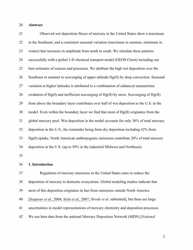
Abstract20

Observed wet deposition fluxes of mercury in the United States show a maximum 21

in the Southeast, and a consistent seasonal variation (maximum in summer, minimum in 22

winter) that increases in amplitude from north to south. We simulate these patterns 23

successfully with a global 3-D chemical transport model (GEOS-Chem) including our 24

best estimates of sources and processes. We attribute the high wet deposition over the 25

Southeast in summer to scavenging of upper-altitude Hg(II) by deep convection. Seasonal26

variation at higher latitudes is attributed to a combination of enhanced summertime 27

oxidation of Hg(0) and inefficient scavenging of Hg(II) by snow. Scavenging of Hg(II) 28

from above the boundary layer contributes over half of wet deposition to the U.S. in the 29

model. Even within the boundary layer we find that most of Hg(II) originates from the 30

global mercury pool. Wet deposition in the model accounts for only 30% of total mercury 31

deposition in the U.S., the remainder being from dry deposition including 42% from 32

Hg(0) uptake. North American anthropogenic emissions contribute 20% of total mercury 33

deposition in the U.S. (up to 50% in the industrial Midwest and Northeast).34

35

1. Introduction36

Regulation of mercury emissions in the United States aims to reduce the 37

deposition of mercury to domestic ecosystems. Global modeling studies indicate that 38

most of this deposition originates in fact from emissions outside North America 39

[Seigneur et al., 2004; Selin et al., 2007; Strode et al. submitted], but there are large 40

uncertainties in model representations of mercury chemistry and deposition processes. 41

We use here data from the national Mercury Deposition Network (MDN) [National 42

3

Atmospheric Deposition Program, 2007] to test the ability of a global 3-D model 43

(GEOS-Chem) to reproduce observed seasonal as well as spatial wet deposition patterns, 44

and from there to better quantify the sources of mercury deposition in the United States. 45

Mercury is emitted to the atmosphere in gaseous elemental form Hg(0), in 46

semivolatile oxidized form Hg(II), and in non-volatile particulate form Hg(P). Hg(0) has 47

a long (0.5-2 y) atmospheric lifetime and represents a globally well-mixed mercury pool; 48

it is eventually oxidized to Hg(II) which is highly water-soluble and readily deposited. 49

Deposition of emitted Hg(II) and Hg(P) can directly affect the region of emission, 50

although Hg(II) can also be reduced to Hg(0) and enter the global pool. Anthropogenic 51

emission of mercury from North America is mostly from coal combustion; about half is 52

as Hg(0) and half is as Hg(II)+Hg(P) [Pacyna et al., 2006]. Considering that North 53

America accounts for only 7% of global anthropogenic emission of mercury (2000 54

statistics) [Pacyna et al., 2006], any diagnosis of regional vs. global contributions to 55

mercury deposition must focus on the fate of the emitted Hg(II)+Hg(P) and on the supply 56

of Hg(II) by oxidation of Hg(0) from the global pool. 57

Previous analyses of wet deposition data have reached conflicting conclusions 58

regarding the relative contributions of domestic vs. global contributions to mercury 59

deposition in different U.S. regions [Dvonch et al., 1998; 2005; Guentzel et al., 2001; 60

Keeler et al., 2006b; VanArdsdale et al., 2005]. We show here that the observed seasonal 61

variation of mercury deposition and its latitudinal gradient provide important constraints 62

on this problem when interpreted with a global 3-D model. We focus our analysis on 63

MDN data for 2004-2005, the two most recent years of data available and with the best 64

coverage.65

4

66

2. Model description67

The GEOS-Chem atmosphere-land-ocean mercury simulation is described by 68

Selin et al. [2008]. We use here GEOS-Chem version 7.04 69

(http://www.as.harvard.edu/chemistry/trop/geos) [Bey et al., 2001] at 4ox5o resolution 70

with assimilated meteorological data for 2004-2005 from the NASA Goddard Earth 71

Observing System (GEOS-4). Three mercury species (Hg(0), Hg(II), and Hg(P)) are 72

transported in the atmosphere. Anthropogenic emissions are from the GEIA inventory for 73

the year 2000 [Pacyna et al., 2006], modified as described in Selin et al. [2008] to satisfy 74

global observational constraints. These modifications include a 50% increase in Hg(0) in 75

Asia (now 1939 Mg y-1 total Hg), a 30% increase in the rest of the world (now 1011 Mg 76

y-1), and addition of emissions from biomass burning (600 Mg y-1) and artisanal mining 77

(450 Mg y-1). The total emissions from anthropogenic sources and biomass burning are 78

thus 4000 Mg y-1. Atmosphere-ocean coupling is treated with a slab model for the ocean 79

including cycling between Hg(0), Hg(II), and non-reactive mercury in the oceanic mixed 80

layer [Strode et al., 2007]. Atmosphere-land coupling includes partial recycling of 81

deposited Hg(II) and mobilization of long-lived soil mercury through volatilization and 82

evapotranspiration [Selin et al., 2008]. Mercury is volatilized from the land and oceans 83

exclusively as Hg(0); direct emission of Hg(II) and Hg(P) is solely anthropogenic.84

Atmospheric oxidation of Hg(0) to Hg(II) in the model takes place by OH 85

(k=9x10-14 cm3 s-1, [Sommar et al., 2001; Pal and Ariya, 2004]) and O3 (k=3x10-20 cm3 s-86

1, [Hall, 1995]). In-cloud (aqueous) photochemical reduction of Hg(II) to Hg(0) is 87

included to accommodate observational constraints on global mercury atmospheric 88

5

concentrations and seasonal variation at northern mid-latitudes [Selin et al., 2007]. Hg(P) 89

is considered chemically inert and is removed by deposition. Fast Hg(II) reduction in 90

power plant plumes [Lohman et al., 2006] remains hypothetical and is not included in the 91

model. 92

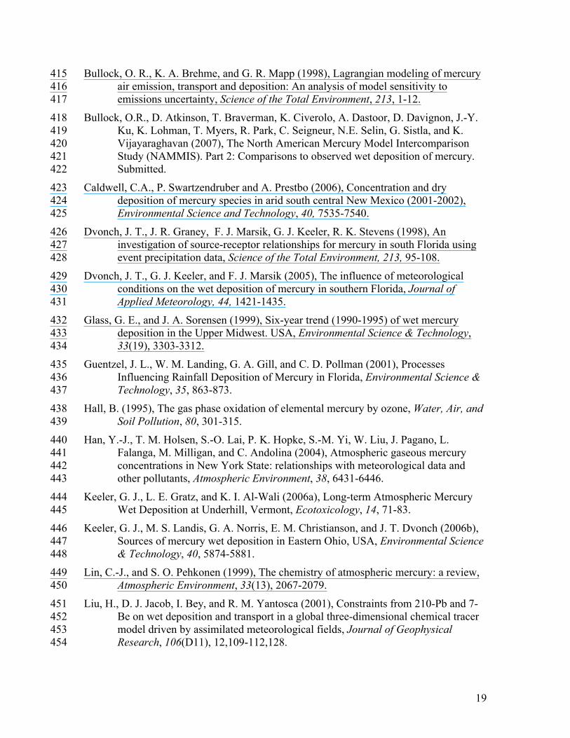
Figure 1 shows the spatial distribution of Hg(0), Hg(II) and Hg(P) anthropogenic 93

emissions in North America in GEOS-Chem, at the original 1ox1o resolution of Pacyna et 94

al. [2006]. Hg(II) and Hg(P) represent respectively 33% and 14% of the total mercury 95

emission of 169 Mg y-1 for the domain of Figure 1. Emissions are highest in the industrial 96

Midwest (Illinois, Indiana, Ohio, Kentucky, Pennsylvania, West Virginia) due to coal 97

combustion, but high values are generally found in population centers due to additional 98

sources from waste incineration and industrial processes. Some high values in the West 99

(notably in northern Nevada) are from gold mining. 100

Mercury deposition processes are of particular interest here. GEOS-Chem 101

includes wet and dry deposition of Hg(II) and Hg(P) as well as dry deposition of Hg(0). 102

Wet deposition of Hg(II) and Hg(P) includes rainout and washout from large-scale and 103

convective precipitation, and scavenging in convective updrafts [Liu et al., 2001; Selin et 104

al., 2008]. Hg(P) is scavenged as a water-soluble aerosol [Liu et al., 2001] while Hg(II) is 105

scavenged as a highly water-soluble gas. Hg(II) is released to the gas phase when water 106

freezes (zero retention efficiency).We assume no scavenging of Hg(II) by frozen 107

precipitation, consistent with limited field observations [Keeler et al., 2006a]. As we will 108

see, this is needed in the model to reproduce the observed winter minimum in Hg 109

deposition at northern latitudes. Dry deposition of Hg(0), Hg(II) and Hg(P) to land are 110

described with the Wesely [1989] resistance-in-series scheme as adapted by Wang et al.111

6

[1998] for global modeling. Dry deposition of Hg(0) to land is determined in that scheme 112

by its Henry’s law constant (0.11 M atm-1 [Lin and Pehkonen, 1999]). Dry deposition of 113

Hg(0) to the ocean is determined by the standard two-film exchange parameterization 114

[Strode et al., 2007]. 115

Our previous model [Selin et al., 2008] assumed zero surface resistance for Hg(II)116

dry deposition, based on some observations of very high deposition velocities (>5 cm s-1) 117

to vegetated areas [Poissant et al., 2004; Lindberg and Stratton, 1998]. This resulted in 118

an underestimate of wet deposition in the Midwest compared to the MDN data, as 119

regionally emitted Hg(II) was then mainly removed by dry deposition. Here we correct 120

this model bias by including a surface resistance for Hg(II) based on a Henry’s law 121

constant of 1x106 M atm-1 for HgCl2 [Lin and Pekhonen, 1999], which is thought to be 122

the most thermodynamically favorable form [Seigneur et al., 1998; Lindberg et al., 123

2007]. The resulting dry deposition velocity of Hg(II) to vegetated areas in summer 124

daytime is typically in the range 1.5-2 cm s-1.125

Decreasing the rate of Hg(II) dry deposition in the model increases the overall 126

total gaseous mercury (TGM) lifetime against deposition. In order to maintain the same 127

concentration of TGM to match global observations as in Selin et al. [2008], we decrease 128

here the rate of in-cloud Hg(II) reduction by a factor of 2, corresponding to a mean in-129

cloud lifetime of 40 minutes for dissolved Hg(II). This is a particularly uncertain aspect 130

of the chemistry mechanism, constrained by Selin et al. [2007] to match the seasonal 131

observation of TGM at northern mid-latitudes but since found by Selin et al. [2008] to 132

likely be too high once the seasonal variation of the soil source is taken into account. 133

Decreasing this reduction rate constant by a factor of 2 not only maintains consistency 134

7

between simulated and observed concentrations on a global scale but also improves the 135

simulation of the spatial pattern in the MDN data. 136

Total deposition of mercury over the U.S. in GEOS-Chem on an annual basis thus 137

includes 42% from Hg(0) dry deposition, 26% from Hg(II) dry deposition, 2% from 138

Hg(P) dry deposition, 27% from Hg(II) wet deposition, and 3% from Hg(P) wet 139

deposition. Wet deposition as measured by the MDN data accounts for only 30% of total 140

mercury deposition according to the model. 141

142

3. Wet deposition patterns 143

3.1 Spatial distribution144

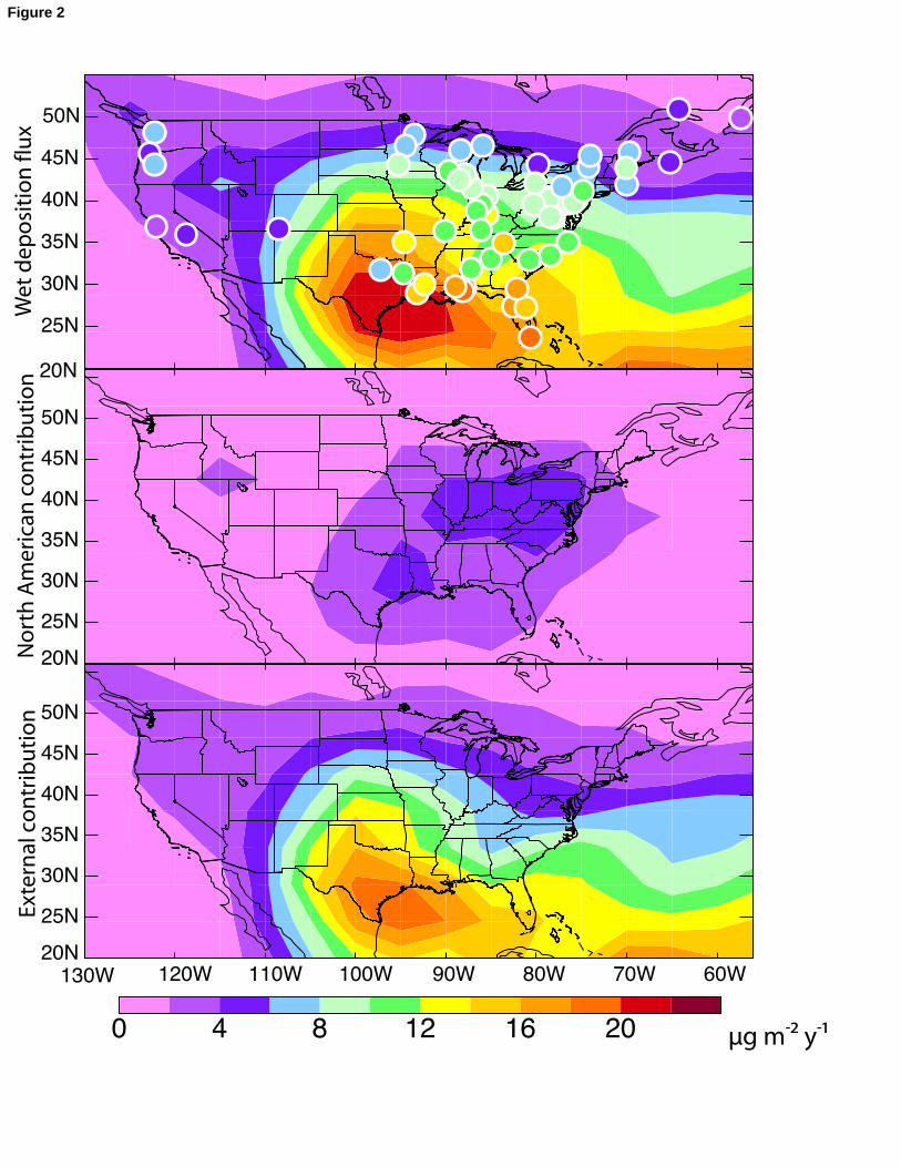
Figure 2 shows the measured annual average wet deposition flux of mercury from 145

MDN for 2004-2005 (top panel, circles), including all 57 sites having at least 320 days of 146

data in each of the two years. (A list of the 57 sites used is available as online 147

supplemental information). Values are higher in the East than in the West, mostly 148

reflecting higher precipitation in the East. The MDN data in the East show a strong 149

latitudinal gradient with values decreasing from 16-20 μg m-2 y-1 in the Southeast to 8-10 150

μg m-2 y-1 in the Midwest/mid-Atlantic region and 4-8 μg m-2 y-1 in the Northeast and 151

Canada. The latitudinal gradient explains 60% of the variation in the MDN data (r2=0.6) 152

for 2004-2005, and is reproducible for all years in the MDN record (1996-2005). A 153

latitudinal gradient from the Northeast U.S. to Canada in the MDN data for 1996-2002 154

was previously reported by VanArdsdale et al. [2005], who attributed it to increasing 155

distance from sources. However, such an explanation cannot account for the highest 156

MDN values in the Southeast.157

8

The large-scale spatial patterns in the MDN data are generally well reproduced by 158

GEOS-Chem (Figure 2, top panel). The mean bias relative to the annual average 2004-159

2005 observations is -1.7%, and the model and data show good spatial correlation 160

(r2=0.73). This is improved over the previous simulation of Selin et al. [2008], which had 161

a mean bias of -17% with r2 = 0.60. Selin et al. [2008] reproduced the latitudinal gradient 162

in the East but underestimated the magnitude of deposition in the Midwest/mid-Atlantic 163

region. Bullock et al. [2007] reported r2 values between 0.45 and 0.7 for simulated-to-164

observed wet deposition flux for three regional models in an intercomparison study. The 165

improvement here results from the decrease in the Hg(II) dry deposition velocity, 166

allowing for greater wet deposition, as discussed in the previous section. The main 167

discrepancy between model and observations in Figure 2 is that the model maximum is in 168

Texas/Louisiana while in the observations it is in Florida. This likely reflects model error 169

in the regional distribution of Hg(II) downwelling and will be discussed further below. 170

The middle and bottom panels of Figure 2 show the contributions to wet 171

deposition from domestic (North American anthropogenic) vs. external sources in the 172

model, as diagnosed in the model by a simulation with North American anthropogenic 173

sources only. The contribution from external sources dominates except in the industrial 174

Midwest and Northeast, where it is comparable to the contribution from domestic 175

sources; this will be discussed further in section 4. The observed latitudinal gradient in 176

the East is almost entirely explained by the external contribution and this is discussed 177

below. 178

179

3.2 Seasonal variation180

9

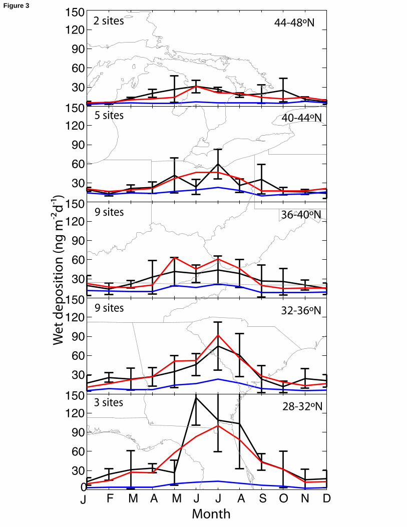
Figure 3 shows the observed and simulated seasonal variations of the wet 181

deposition flux for 2004-2005 in different latitudinal bands of the eastern U.S. Also 182

shown is the model contribution from North American anthropogenic sources. There is 183

strong seasonal variation in the observations, with a maximum in summer and minimum 184

in winter. Different explanations for this seasonal variation in the literature include more 185

precipitation in summer [Glass and Sorensen, 1999; Guentzel et al., 2001], less efficient 186

scavenging of mercury by snow than by rain [Glass and Sorensen, 1999; Mason et al., 187

2000], and enhanced Hg(0) oxidation to Hg(II) in summer [Mason et al., 2000]. 188

Emissions of Hg(II) and Hg(P), which are exclusively anthropogenic, do not have 189

significant seasonal variation [NEI, 1999].190

Figure 3 shows that the observed amplitude of seasonal variation has a strong 191

latitudinal dependence, decreasing with increasing latitude. To our knowledge this has 192

not been reported before, though Mason et al. [2000] previously noted that the wintertime 193

contribution to annual wet deposition was lower at Midwest sites in Michigan and 194

Wisconsin (44-48°N) than at mid-Atlantic sites (36-40°N). For the 2004-2005 data in 195

Figure 3, the ratio of average daily deposition in summer (June-August) to winter 196

(December-February) is 6.6 at 28-32°N and 4.7 at 44-48°N. The summer maxima are 197

highest at lower latitudes and decline as latitude increases (119 ng m-2 d-1 at 28-32°N, 40 198

ng m-2 d-1 at 36-40°N, and 25 ng m-2 d-1 at 44-48°N). The winter minima also decline 199

although not as much (18 ng m-2 d-1 at 28-32°N, 16 ng m-2 d-1 at 36-40°N, and 5 ng m-2 d-200

1 at 44-48°N). This north-south difference in the amplitude of the seasonal cycle is 201

consistently found in the different years of the MDN record. 202

10

GEOS-Chem reproduces well the seasonal variation of wet deposition of mercury 203

as well as its latitudinal gradient (Figure 3). There is no significant bias in phase or in 204

amplitude. Hg(II) contributes 89% of wet deposition in the model and drives the seasonal 205

variation (11% is Hg(P) which does not vary seasonally). The contribution of North 206

American sources to the wet deposition flux is small except at northern sites in winter. 207

Insights into the factors responsible for the seasonal variation in the MDN data 208

can be gained from analysis of the Hg(II) budget in the model. We find that 59% of 209

Hg(II) annual wet deposition in the contiguous U.S. is from scavenging of Hg(II) in the 210

free troposphere above 850 hPa (1.5 km). Concentrations of Hg(II) increase with altitude 211

in GEOS-Chem [Selin et al., 2007], consistent with observations [Swartzendruber et al., 212

2006; Sillman et al., 2007], and reflecting the long lifetime of Hg(II) in the free 213

troposphere. Even Hg(II) within the continental boundary layer (surface – 850 hPa), 214

which contributes only 41% of Hg(II) wet deposition, is mostly from the global pool in 215

the model. We find that 70% of Hg(II) in the boundary layer of the continental U.S. is 216

from oxidation and import; only 30% is from North American anthropogenic emission. 217

At the northern latitudes of Figure 3 (36-48°N), precipitation amount does not 218

vary significantly throughout the year. However, Hg(0) oxidation is enhanced by a factor 219

of 3-5 in summer relative to winter, driven by the seasonal variation of OH. Also 220

contributing to the seasonal difference in wet deposition is the much larger scavenging 221

efficiency in summer, when most precipitation is not frozen. 222

The seasonal variation in the Southeast (28-32°N) is driven by different 223

processes. At this subtropical latitude, the source of Hg(II) from Hg(0) oxidation is only 224

30% greater in summer than in winter, and there is little snow. However, unlike the 225

11

higher latitudes where precipitation is evenly distributed over the year, the Southeast has226

a summer wet season and winter dry season. Furthermore, summertime precipitation is 227

associated with deep convection that scavenges elevated Hg(II) from high altitudes. We 228

also examined the seasonal cycle at latitudes 24-28°N (southern Florida) and found 229

similar results, both in the model and in the observations.230

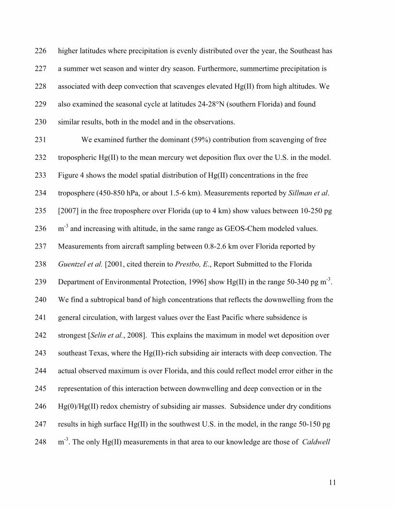
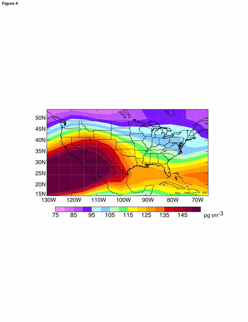
We examined further the dominant (59%) contribution from scavenging of free 231

tropospheric Hg(II) to the mean mercury wet deposition flux over the U.S. in the model. 232

Figure 4 shows the model spatial distribution of Hg(II) concentrations in the free 233

troposphere (450-850 hPa, or about 1.5-6 km). Measurements reported by Sillman et al. 234

[2007] in the free troposphere over Florida (up to 4 km) show values between 10-250 pg 235

m-3 and increasing with altitude, in the same range as GEOS-Chem modeled values. 236

Measurements from aircraft sampling between 0.8-2.6 km over Florida reported by 237

Guentzel et al. [2001, cited therein to Prestbo, E., Report Submitted to the Florida 238

Department of Environmental Protection, 1996] show Hg(II) in the range 50-340 pg m-3. 239

We find a subtropical band of high concentrations that reflects the downwelling from the 240

general circulation, with largest values over the East Pacific where subsidence is 241

strongest [Selin et al., 2008]. This explains the maximum in model wet deposition over 242

southeast Texas, where the Hg(II)-rich subsiding air interacts with deep convection. The 243

actual observed maximum is over Florida, and this could reflect model error either in the 244

representation of this interaction between downwelling and deep convection or in the 245

Hg(0)/Hg(II) redox chemistry of subsiding air masses. Subsidence under dry conditions 246

results in high surface Hg(II) in the southwest U.S. in the model, in the range 50-150 pg 247

m-3. The only Hg(II) measurements in that area to our knowledge are those of Caldwell 248

12

et al. [2006] who found much lower values, averaging 6.8 pg m-3 over 24-hour sampling 249

periods in all seasons, at the MDN site in south-central New Mexico. 250

A number of studies have previously interpreted the high mercury wet deposition 251

fluxes observed in southern Florida. Guentzel et al. [2001] found little difference between 252

urban and rural sites in the Florida Atmospheric Mercury Study (FAMS) and concluded 253

that mercury was scavenged from the global pool in the free troposphere, consistent with 254

our results. Bullock et al. [1998] attributed the high mercury deposition in Florida to local 255

sources based on a regional Lagrangian model, but their analysis did not account for the 256

contribution from the global pool and their simulated wet deposition was low compared 257

with MDN observations. Dvonch et al. [1998, 2005] used daily event-based precipitation 258

data correlated with back-trajectories and chemical tracers for sites in southern Florida in 259

1995 to argue for a local urban source. Their observed mercury deposition (30 µg m-2 y-1260

annual average) is much higher than the values in the 2004-2005 MDN data. Local 261

incinerators, which shut down in the 1990s, could explain this difference. Measurements 262

immediately downwind of a large source (before the plume has dispersed on a regional 263

scale) may be expected to show large wet deposition fluxes of mercury, which would not 264

be resolved by our model. This would likely not affect the MDN sites (Figure 2), which 265

are chosen to be regionally representative and away from local sources. 266

267

4. Source attribution for mercury deposition268

Our successful simulation of the seasonal cycle in the MDN data, which we 269

interpret as largely driven by the global pool of mercury, gives us increased confidence in 270

our ability to use GEOS-Chem to separate North American anthropogenic vs. external 271

13

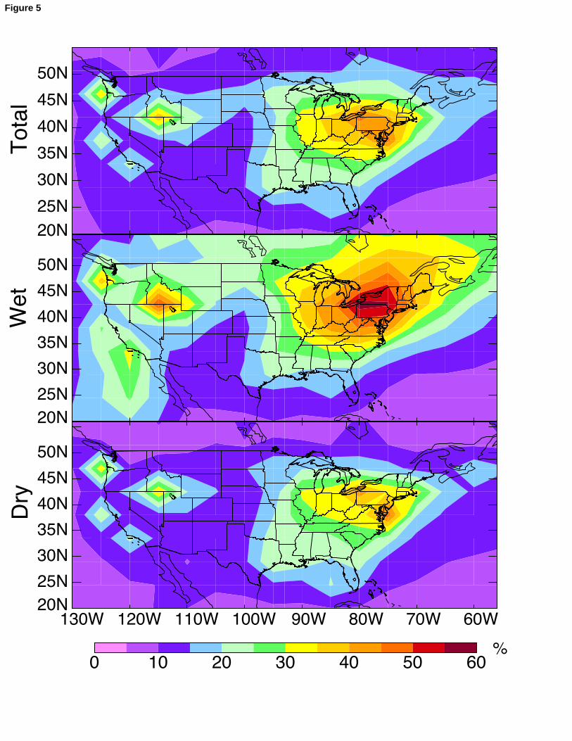
contributions to mercury deposition in the United States. Figure 5 shows the percent 272

contribution of North American anthropogenic emissions to wet and dry annual mercury 273

deposition in the model for 2004-2005. We previously reported similar model results for 274

total mercury deposition in Selin et al. [2007; 2008] but the present results separate wet 275

and dry contributions and also include a number of model updates. A major update 276

relative to Selin et al. [2007] is the inclusion of Hg(0) dry deposition to land, and a major 277

update relative to Selin et al. [2008] is the downward adjustment of Hg(II) dry deposition 278

and reduction as described in section 2. 279

We find that the mean contribution of North American anthropogenic emissions 280

to total deposition over the U.S. is 20% (27% for wet, 17% for dry). Both dry and wet 281

deposition show maximum domestic contribution (50-60%) in the industrial Midwest and 282

Northeast. North American anthropogenic emissions contribute 4-6 μg m-2 y-1 to wet 283

deposition in a broad area that extends from East Texas through the Midwest and to 284

Pennsylvania, as shown in Figure 2 (middle panel), but the percentage of total wet 285

deposition that this contributes is comparatively greater in the Northeast, where the 286

contribution from the global pool is relatively low (Figure 2, bottom panel). The 287

contribution of North American anthropogenic sources to dry deposition generally 288

follows the source distribution of Hg(II) (Figure 1), but is highest along coastal areas of 289

the Northeast due to efficient scavenging of Hg(II) by sea salt in the model [Malcolm et 290

al., 2003; Selin et al., 2007]. 291

Our finding that 60% of wet deposition in the industrial Midwest originates from 292

North American anthropogenic sources can be compared to that of Keeler et al. [2006b], 293

who analyzed event deposition data downwind of sources in the Ohio River Valley at a 294

14

non-MDN site. They attributed 70% of wet deposition there to local and regional coal 295

combustion sources using meteorological analyses and multivariate statistical models for 296

trace element concentrations. The wet deposition flux at that site (14-20 μg m-2 y-1) was 297

higher than measured at the MDN sites (Figure 2), suggesting that it would be impacted 298

by local sources not resolved on the scale of the regional MDN network or the GEOS-299

Chem model.300

The larger contribution of North American emissions to wet deposition relative to 301

dry deposition in GEOS-Chem is due to Hg(0) dry deposition, which is predominantly 302

from the global pool. Dry deposition of Hg(0) is not included in most models and is not 303

routinely measured, so its contribution is highly uncertain, and the MDN data do not offer 304

a constraint on that term. 305

Compared with Selin et al. [2008], the total model deposition of mercury to the 306

contiguous U.S. is about the same (250 Mg y-1), but the proportion that is wet has 307

increased (from 21% to 30%) due to the improved dry deposition parameterization. The 308

change in lifetime of Hg(II) with respect to dry deposition has also shifted the area of 309

maximum North American contribution towards the northeast. 310

311

4. Conclusions312

We have used measured seasonal and spatial variations in mercury wet deposition 313

fluxes over the U.S. from the Mercury Deposition Network (MDN), in comparison to 314

results from a global 3D atmosphere-land-ocean mercury model (GEOS-Chem), to test 315

our understanding of the factors controlling mercury deposition and the contribution from 316

North American anthropogenic emissions. 317

15

Wet deposition fluxes in both measurements and the model show a maximum 318

over the Southeast U.S. . The associated latitudinal gradient explains 60% of the spatial 319

variance in the annual mean data in the East. The MDN flux data in the East also show 320

strong seasonal variation, peaking in summer and minimum in winter. The amplitude of 321

seasonal variation is largest in the Southeast and decreases gradually towards northern322

latitudes. 323

GEOS-Chem is successful in simulating the large-scale spatial variability in the 324

MDN observations (r2=0.73) with little overall bias over the U.S. (-1.7%). It captures the 325

latitudinal gradient, the seasonal phase, and the variation of seasonal amplitude with 326

latitude. We show that these features can be explained by the contribution from the global 327

pool to mercury deposition. We attribute the high mercury deposition over the Southeast 328

to the interaction of global-scale subtropical downwelling, which supplies elevated Hg(II) 329

in subsiding air masses, with frequent regional deep convection particularly in summer 330

which scavenges this free tropospheric Hg(II). Better characterization of concentrations 331

of Hg(II) in the free troposphere, where only a few measurements are currently available, 332

would provide further constraints on the processes controlling mercury wet deposition in 333

the United States. 334

Hg(II) contributes 89% of mercury wet deposition in the model and defines the 335

seasonal variation. Hg(P) accounts for only 11% and has no seasonal variation. We find 336

in the model that 60% of Hg(II) wet deposition in the U.S. originates from scavenging in 337

the free troposphere, where Hg(II) is elevated by oxidation of Hg(0) from the global pool. 338

The remainder is from scavenging of Hg(II) within the U.S. boundary layer, and even 339

there the oxidation of Hg(0) from the global pool is the principal source. We attribute the 340

16

summer maximum in mercury deposition in the Southeast to deep convective scavenging 341

of Hg(II) from high altitudes, similar to the conclusions of Guentzel et al. [2001]. We 342

attribute the summer maximum in the Northeast to Hg(0) photochemical oxidation and to 343

inefficient scavenging of Hg(II) by snow in winter. 344

Domestic sources dominate mercury deposition in the model only at northern 345

latitudes in winter when Hg(0) oxidation is minimum and Hg(II) scavenging from the 346

free troposphere is inefficient, leaving scavenging of anthropogenic Hg(P) to be the 347

major contributor. But the overall wet deposition flux of mercury is then very low. 348

Because of its coarse resolution, the model would not capture mercury scavenging from 349

concentrated plumes immediately downwind of large sources, as measured by a few 350

studies [Dvonch et al. 1998; 2005; Keeler et al. 2006b]. The MDN network, which 351

deliberately avoids such local influences, does not capture these high values either. Our 352

successful simulation of the MDN data gives us confidence that at least on a regional 353

scale most of mercury deposition in the U.S. originates from the global pool.354

We used the model to derive improved estimates of the percentage contribution of 355

North American anthropogenic emissions to annual mean mercury deposition over the 356

U.S. We find an average contribution of 20%, with values exceeding 50% only in 357

Pennsylvania and New York State. The GEOS-Chem simulation indicates that much 358

more mercury is deposited to the U.S. by dry rather than wet processes (70% versus 359

30%). 42% of total mercury deposition to the U.S. in the model is from Hg(0) dry 360

deposition, which is highly uncertain and for which the MDN data offer no constraints. 361

Further measurements of Hg(0) deposition velocities over a range of ecosystem types are 362

needed to better quantify this global contribution to mercury deposition in the U.S.363

17

364

Acknowledgments365

This work was funded by the Atmospheric Chemistry Program of the U.S. National 366

Science Foundation and by a U.S. Environmental Protection Agency (EPA) Science to 367

Achieve Results (STAR) Graduate Fellowship to NES. EPA has not officially endorsed 368

this publication and the views expressed herein may not reflect the views of the EPA.369

370

18

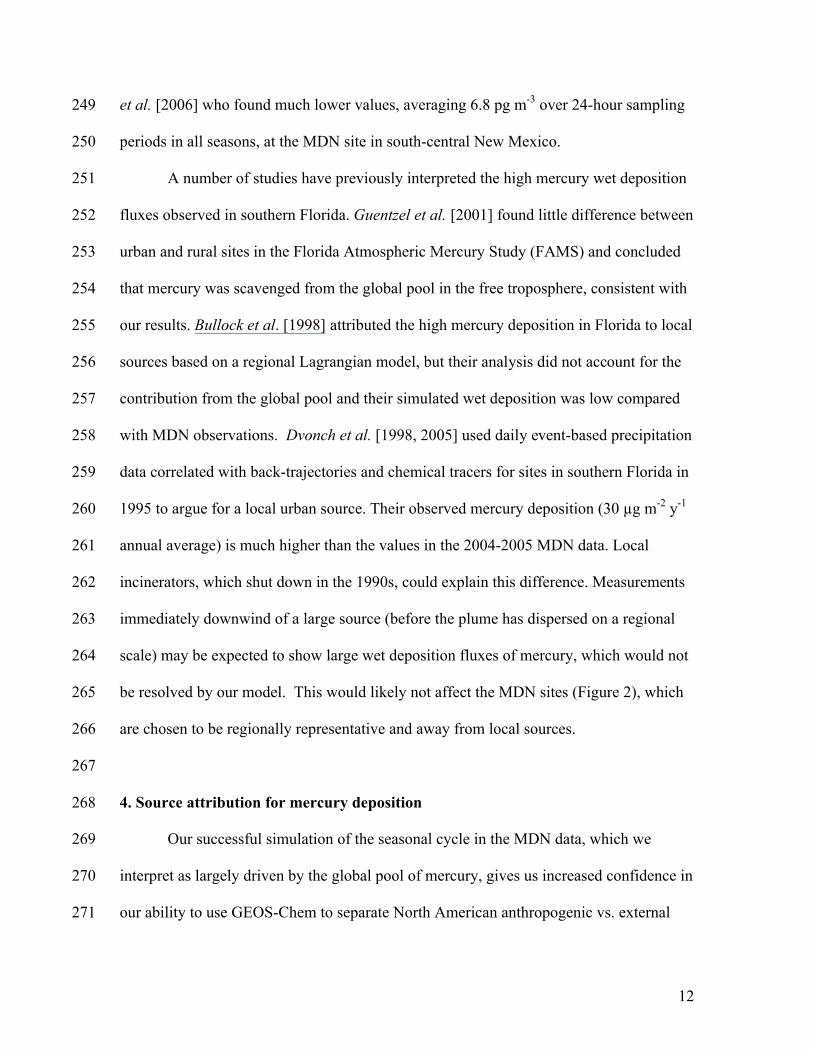
Figure Captions371Figure 1: Annual anthropogenic emissions of Hg(0), Hg(II), and Hg(P) (kg y-1 per 1°x1° 372grid square)in North America for 2000. Data are from Pacyna et al. [2006], increased by 37330% for input to GEOS-Chem [Selin et al., 2008]. Totals are shown inset for the domain 374of the Figure. A 1ox1o grid square corresponds to 70 km longitude x 100 km latitude at 37545oN.376

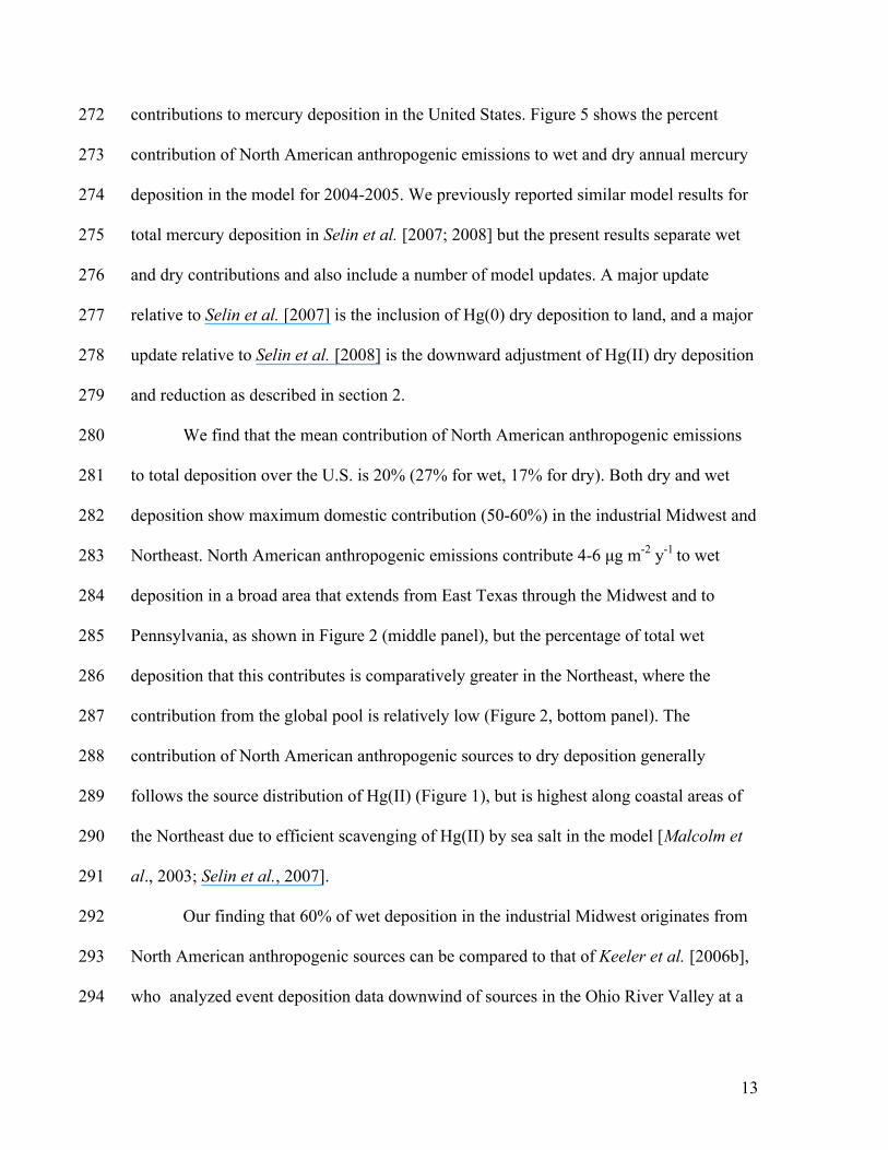
377Figure 2: Annual mean wet deposition flux of mercury over the United States for 2004-3782005 (μg m-2 y-1). Top panel: Observations from 57 sites of the Mercury Deposition 379Network (circles) compared to GEOS-Chem model results (background). The list of 380MDN sites is available as online supplemental information. Middle panel: Contribution 381to this wet deposition flux from anthropogenic North American sources in the model, as 382obtained by difference from a sensitivity simulation with all other sources shut off, Lower 383panel: Contribution from external sources determined by the sensitivity simulation. North 384America is defined as the geographical domain shown in the figure. 385

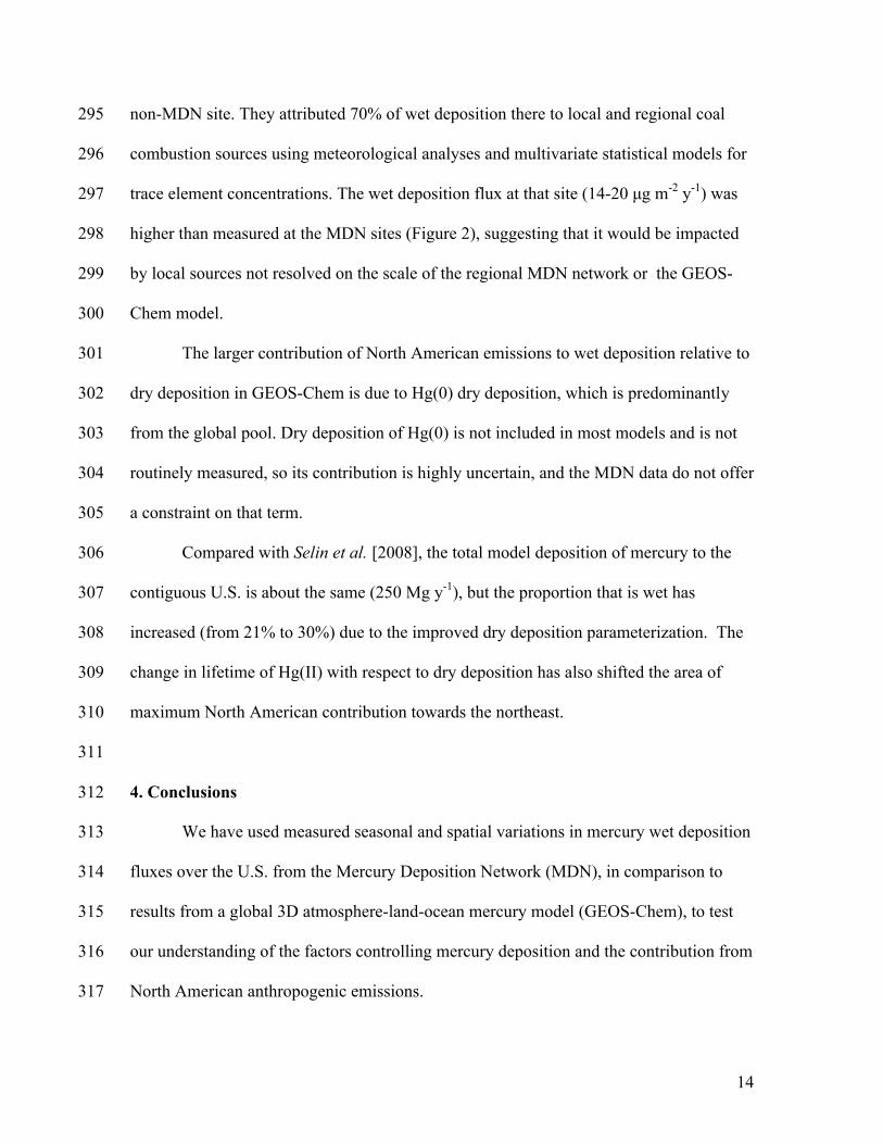
386Figure 3: Seasonal variation of the 2004-2005 monthly mean mercury wet deposition 387flux over the eastern United States (72.5-82.5°W, 28-48°N) for different latitudinal 388ranges. Observations (black, means +/- standard deviations) are from all MDN sites 389including at least 15 days of data in each month. The number of sites is shown inset. 390Model results (average of two GEOS-Chem grid boxes) are shown in red and the 391corresponding North American anthropogenic contribution is shown in blue. MDN 392codenames for the sites are: 44-48N: MI48, ON07; 40-44N: IN20, IN34, MI31, PA13, 393PA30; 36-40N: IN21, IN26, IN28, KY10, MD08, OH02, PA37, VA08, VA28; 32-36N: 394AL03, GA22, GA40, NC08, NC26, SC05, SC09, SC19, TN11, 28-32N: FL05, FL32, 395GA09. Further information and data for these sites is available on the MDN web site at 396http://nadp.sws.uiuc.edu/mdn/397

398Figure 4: Simulated annual mean concentration of Hg(II) in the free troposphere (450-399850 hPa, or roughly 1.5-6 km altitude) for 2004-2005. Color scale is saturated at the 400maximum value indicated in the legend. “sm-3” refers to a cubic meter under standard 401conditions of temperature and pressure, so that “pg sm-3” is a mixing ratio unit.402

403Figure 5. Percentage contribution from North American primary anthropogenic sources 404to total (wet plus dry), wet, and dry annual mercury deposition simulated by the model 405for 2004-2005. North America is defined as the geographical domain shown in the figure.406

407

References408409

Bey, I., D. J. Jacob, R. M. Yantosca, J. A. Logan, B. D. Field, A. M. Fiore, Q. B. Li, H. 410G. Y. Liu, L. J. Mickley, and M. G. Schultz (2001), Global modeling of 411tropospheric chemistry with assimilated meteorology: Model description and 412evaluation, Journal of Geophysical Research-Atmospheres, 106(D19), 23073-41323095.414

19

Bullock, O. R., K. A. Brehme, and G. R. Mapp (1998), Lagrangian modeling of mercury 415air emission, transport and deposition: An analysis of model sensitivity to 416emissions uncertainty, Science of the Total Environment, 213, 1-12.417

Bullock, O.R., D. Atkinson, T. Braverman, K. Civerolo, A. Dastoor, D. Davignon, J.-Y. 418Ku, K. Lohman, T. Myers, R. Park, C. Seigneur, N.E. Selin, G. Sistla, and K. 419Vijayaraghavan (2007), The North American Mercury Model Intercomparison 420Study (NAMMIS). Part 2: Comparisons to observed wet deposition of mercury. 421Submitted.422

Caldwell, C.A., P. Swartzendruber and A. Prestbo (2006), Concentration and dry 423deposition of mercury species in arid south central New Mexico (2001-2002), 424Environmental Science and Technology, 40, 7535-7540.425

Dvonch, J. T., J. R. Graney, F. J. Marsik, G. J. Keeler, R. K. Stevens (1998), An 426investigation of source-receptor relationships for mercury in south Florida using 427event precipitation data, Science of the Total Environment, 213, 95-108.428

Dvonch, J. T., G. J. Keeler, and F. J. Marsik (2005), The influence of meteorological 429conditions on the wet deposition of mercury in southern Florida, Journal of 430Applied Meteorology, 44, 1421-1435.431

Glass, G. E., and J. A. Sorensen (1999), Six-year trend (1990-1995) of wet mercury 432deposition in the Upper Midwest. USA, Environmental Science & Technology, 43333(19), 3303-3312.434

Guentzel, J. L., W. M. Landing, G. A. Gill, and C. D. Pollman (2001), Processes 435Influencing Rainfall Deposition of Mercury in Florida, Environmental Science & 436Technology, 35, 863-873.437

Hall, B. (1995), The gas phase oxidation of elemental mercury by ozone, Water, Air, and 438Soil Pollution, 80, 301-315.439

Han, Y.-J., T. M. Holsen, S.-O. Lai, P. K. Hopke, S.-M. Yi, W. Liu, J. Pagano, L. 440Falanga, M. Milligan, and C. Andolina (2004), Atmospheric gaseous mercury 441concentrations in New York State: relationships with meteorological data and 442other pollutants, Atmospheric Environment, 38, 6431-6446.443

Keeler, G. J., L. E. Gratz, and K. I. Al-Wali (2006a), Long-term Atmospheric Mercury 444Wet Deposition at Underhill, Vermont, Ecotoxicology, 14, 71-83.445

Keeler, G. J., M. S. Landis, G. A. Norris, E. M. Christianson, and J. T. Dvonch (2006b), 446Sources of mercury wet deposition in Eastern Ohio, USA, Environmental Science 447& Technology, 40, 5874-5881.448

Lin, C.-J., and S. O. Pehkonen (1999), The chemistry of atmospheric mercury: a review, 449Atmospheric Environment, 33(13), 2067-2079.450

Liu, H., D. J. Jacob, I. Bey, and R. M. Yantosca (2001), Constraints from 210-Pb and 7-451Be on wet deposition and transport in a global three-dimensional chemical tracer 452model driven by assimilated meteorological fields, Journal of Geophysical 453Research, 106(D11), 12,109-112,128.454

20

Lindberg, S. E., and W. J. Stratton (1998), Atmospheric mercury speciation: 455Concentrations and behavior of reactive gaseous mercury in ambient air, Environ. 456Sci. Technol., 32, 49-57.457

Lindberg, S., R. Bullock, R. Ebinghaus, E. Daniel, X. Feng, W. Fitzgerald, N. Pirrone, E.458Prestbo, and C. Seigneur (2007), A synthesis of progress and uncertainties in 459attributing the sources of mercury in deposition, Ambio, 36(1), 19-32.460

Lohman, K., C. Seigneur, E. Edgerton, and J. Jansen (2006), Modeling mercury in power 461plant plumes. Environ. Sci. Technol. 40, 3848-3854.462

Mason, R. P., N. M. Lawson, and G. R. Sheu (2000), Annual and seasonal trends in 463mercury deposition in Maryland, Atmospheric Environment, 34(11), 1691-1701.464

National Atmospheric Deposition Program (2007), Mercury Deposition Network (MDN): 465A NADP Network, NADP Program Office, Illinois State Water Survey, 466Champaign, IL, http://nadp.sws.uiuc.edu/mdn/, accessed 29 May 2007.467

NEI (1999), 1999 National Emission Inventory Documentation and Data,U.S. 468Environmental Protection Agency. 469

Pacyna, E. G., J. M. Pacyna, F. Steenhuisen, and S. Wilson (2006), Global 470Anthropogenic Mercury Emission Inventory for 2000, Atmospheric Environment, 47140(22), 4048-4063.472

Pal, B., and P. A. Ariya (2004), Gas-Phase HO-Initiated Reactions of Elemental Mercury: 473Kinetics and Product Studies, and Atmospheric Implications, Environmental 474Science & Technology, 21, 5555-5566.475

Poissant, L., M. Pilote, C. Beauvais, P. Constant, and H. H. Zhang (2005), A year of 476continuous measurements of three atmospheric mercury species (GEM, RGM and 477Hg-p) in southern Quebec, Canada, Atmospheric Environment, 39(7), 1275-1287.478

Seigneur, C., J. Wrobel, and E. Constantinou (1994), A chemical kinetic mechanism for 479atmospheric inorganic mercury, Environ. Sci. Technol., 28, 1589-1597.480

Seigneur, C., K. Vijayaraghavan, K. Lohman, P. Karamchandani, and C. Scott (2004), 481Global source attribution for mercury deposition in the United States, 482Environmental Science & Technology, 38(2), 555-569.483

Selin, N. E., D. J. Jacob, R. J. Park, R. M. Yantosca, S. Strode, L. Jaegle, and D. A. Jaffe 484(2007), Chemical cycling and deposition of atmospheric mercury: Global 485constraints from observations, Journal of Geophysical Research, 112, D02308.486

Selin, N. E., D. J. Jacob, R. M. Yantosca, S. Strode, L. Jaegle, and E. M. Sunderland 487(2008), Global 3-D land-ocean-atmosphere model for mercury: present-day vs. 488pre-industrial cycles and anthropogenic enrichment factors for deposition, Global 489Biogeochemical Cycles, in press, doi: 10.1029/2007GB003040.490

Sillman, S., F. J. Marsik, K. I. Al-Wali, G. J. Keeler, and M. S. Landis (2007), Reactive 491mercury in the troposphere: Model formation and results for Florida, the 492northeastern U.S. and the Atlantic Ocean, Journal of Geophysical Research, 112, 493D23305, doi:10.1029/2006JD008227. 494

21

Sheu, G.-R. (2001), Speication and Distribution of Atmospheric Mercury: Significance of 495Reactive Gaseous Mercury in the Global Mercury Cycle, PhD dissertation thesis, 496University of Maryland, College Park, MD.497

Sommar, J., K. Gårdfeldt, D. Strömberg, and X. Feng (2001), A kinetic study of the gas-498phase reaction between the hydroxyl radical and atomic mercury, Atmospheric 499Environment, 35, 3049-3054.500

Strode, S., L. Jaegle, N. E. Selin, D. J. Jacob, R. J. Park, R. M. Yantosca, R. P. Mason, 501and F. Slemr (2007), Global Simulation of Air-Sea Exchange of Mercury, Global 502Biogeochemical Cycles, 21, GB1017, doi:10/1029/2006GB002766.503

Strode, S., L. Jaegle, N.E. Selin, D.J. Jacob, R.M. Yantosca, and C. Holmes (2008), 504Trans-Pacific Transport of Mercury, Journal of Geophysical Research, submitted.505

Swartzendruber, P., D. A. Jaffe, E. M. Prestbo, J. E. Smith, P. Weiss-Penzias, N. E. Selin, 506D. J. Jacob, R. J. Park, S. Strode, and L. Jaegle (2006), Observations of Reactive 507Gaseous Mercury at the Mt. Bachelor Observatory, Journal of Geophysical 508Research, 111, D24301, doi:10.1029/2006JD007415.509

Vanarsdale, A., J. Weiss, G. Keeler, E. Miller, G. Boulet, R. Brulotte, and L. Poissant 510(2005), Patterns of mercury deposition and concentration in northeastern North 511America (1996-2002), Ecotoxicology, 14(1-2), 37-52.512

Wesely, M. L. (1989), Parameterization of surface resistances to gaseous dry deposition 513in regional-scale numerical models, Atmospheric Environment, 23(6), 1293-1304.514

515516

25N30N35N40N45N50N

25N30N35N40N45N50N

0.01 0.1 1 10 100 1000 10000 kg gridsquare-1 y-1

130W 120W 110W 100W 90W 80W 70W25N30N35N40N45N50N

Hg(

P)H

g(II)

Hg(

0)

23 Mg y-1

55 Mg y-1

91 Mg y-1

Figure 1

20N

25N

30N

35N

40N

45N

50N

20N25N

30N

35N

40N

45N

50N

0 4 8 12 16 20

130W 120W 110W 100W 90W 80W 70W 60W20N25N

30N

35N

40N

45N

50N

Wet

dep

osi

tio

n fl

ux

No

rth

Am

eric

an c

on

trib

uti

on

Exte

rnal

co

ntr

ibu

tio

n

μg m-2 y-1

Figure 2

306090

120150

306090

120150

306090

120150

306090

120150

J F M A M J J A S O N D0

306090

120150

2 sites

5 sites

9 sites

9 sites

3 sites

44-48ºN

40-44ºN

36-40ºN

32-36ºN

28-32ºN

Month

Wet

dep

ositi

on (n

g m

-2d-1)

Figure 3

75 85 95 105 115 125 135 145

130W 120W 110W 100W 90W 80W 70W15N20N

25N

30N

35N

40N

45N

50N

pg sm-3

Figure 4

20N25N30N35N40N45N50N

20N25N30N35N40N45N50N

0 10 20 30 40 50 60

130W 120W 110W 100W 90W 80W 70W 60W20N25N30N35N40N45N50N

%

Dry

Wet

Tota

lFigure 5