Searching for the (Dark) Forces Behind Protection*

Hadi Salehi Esfahani University of Illinois at Urbana-Champaign

March 2002

Abstract

This paper re-examines the determinants of trade policy. It extends the Grossman-Helpman model of trade policy to take account of factors besides lobby contributions that may lead politicians to value rents differently across industries. The extension is motivated by the recent empirical finding that the weight placed by politicians on lobby contributions appears to be too small to explain much of the variation in protection rates. The paper argues that differences in the severity of capital and insurance constraints may cause marginal earnings to have different values in different industries, acting as a force separate from lobbying. The Grossman-Helpman model is extended to incorporate this effect and create a framework for testing it against the "protection for sale" hypothesis. The approach also paves the way for examining a variety of other effects influencing trade policy in a common framework. Estimation of the extended model with cross-industry data from the United States lends support to the role of capital and insurance constraints. Although lobby contributions may play an important role in economic policy in general, they seem to have little manifestation in trade policy because better organized groups tend to have easier access to more efficient fiscal and financial transfers. The perspective that emerges from the empirical results based on the extended model has far-reaching implications for the pattern and evolution of trade policies.

JEL Classification: F13, P16

Key words: Trade Policy, Political Economy, Imperfect Markets.

Please address all correspondence concerning this paper to:

Hadi Salehi Esfahani Department of Economics University of Illinois Urbana, IL 61801, USA Phone: (217) 333-2681; Fax (217) 333-1398; E-mail: Esfahani@uiuc.edu

* I would like to thank Giovanni Facchini, Ravi Yatawara, and the participants in the 8th Annual of Conference of Empirical Investigations in International Trade for their helpful comments. I am also thankful to Maziar Mirhosseini for his competent research assistance.

1

1. Introduction

This paper re-examines the determinants of trade policy. It extends the seminal model of

Grossman and Helpman (1994), henceforth GH, to take account of factors besides lobby contributions

that may lead politicians to value rents differently across industries. The extension is motivated by the

recent empirical finding that the premia that politicians place on lobby contributions appear to be too

small to explain much of the variation in protection rates. This paper argues that differences in the

severity of capital and insurance constraints may cause marginal earnings to have different values in

different industries, acting as a force independent of lobbying. The model developed here incorporates

this effect and provides a framework for testing it against the "protection for sale" hypothesis. The

approach also paves the way for examining a variety of other effects influencing trade policy in a unified

framework. Estimation of the extended model with cross-industry data from the United States in 1983

provides support for the role of capital and insurance constraints and other effects. The findings have far-

reaching implications for the pattern and evolution of trade policies.

The starting point of this paper is the intriguing findings of the recent empirical work on the GH

model.1 While the estimates of the model's parameters have the predicted signs with statistical

significance, the magnitudes of the estimates are puzzling. The politicians' premium on a dollar of

political contributions turns out to be at most two percent of the value they attach to a dollar of aggregate

welfare. This low premium is too little to be a major explanation for the observed protection. Such a low

premium may also dissuade most industries from spending resources to organize and to lobby for

protection. But, surprisingly, the same studies find that the share of population organized by lobbies must

be very large, typically well over 80 percent of the population. This is the case even though based on the

indicators used in these studies the range for this share must be much lower.2

These findings make one wonder whether the main motivation for protection may lie elsewhere.

Indeed, earlier studies have examined a variety of other factors and have found several of them to be

1 These studies include Goldberg and Maggi (1999), Gawande and Bandyopadhyay (2000), McCalman (Forthcoming), Mitra, Thomakos and Ulubasoglu (2000), and Eicher and Osang (2000).

2 In the recent studies, the share of population covered by industry lobbies is derived from the estimated parameters of the model. Using any estimate of the share of organized population implicit in the data often does not produce meaningful results for the other parameters. Eicher and Osang's (2000) study is an exception in that it finds the share of organized population to be about 26 percent, which has a chance at being consistent with the lobby indicator used in the estimation.

2

empirically relevant for trade policy.3 Although the theoretical foundations for such findings have never

been as strong as the one provided by GH, those old regularities and the new puzzles posed by the recent

empirical work compel one to revisit the earlier ideas more systematically and test them against the

"protection for sale" hypothesis. Indeed, the empirical studies of the GH model make an attempt to

incorporate additional variables in their regressions. But, they do not do so in a systematic manner

because such variables have no explicit role in the theoretical model that guides their econometric work.

[See, for example, the two pioneering studies by Goldberg and Maggi (1999) and Gawande and

Bandyopadhyay (2000), henceforth GM and GB, respectively.] As a result, despite the fact that some of

the additional factors turn out to be statistically significant, the findings do not lend themselves to any

meaningful interpretation. Moreover, the existing studies use many industry characteristics as instruments

for their lobby indicator to deal with its potential endogeneity problem. Since some of these

characteristics may have direct effects of their own on the politicians' valuation of industry rents, this may

be biasing the results. In fact, it may be giving all the chance to the lobby indicator to prove significant

even though it may not be an appropriate measure or in reality lobby contributions may not be very

important for trade policy compared to other factors.4

I address the above problems by incorporating protection motives besides lobby contributions in

the GH framework. The idea for the main additional motive that I consider here comes from a pattern that

can be pieced together from earlier empirical studies (Finger, Hall, and Nelson, 1982; Marvel and Ray,

1983; Pack, 1994; Trefler, 1993; Lee and Swagel, 1997). These studies suggest that protection is directed

towards industries with low-skill/low-wage workers and smaller firms with low capital intensity, though

each study examines only some of these variables. These findings have been puzzling because the agents

being protected seem to be those that tend to face relatively higher costs of political organization

compared to big business.5 But, combining the picture with older arguments for protection based on

3 Prominent examples of empirical work on trade policy include: Caves (1976), Ray (1981a, 1981b), Finger, Hall, and Nelson (1982), Marvel and Ray (1983, 1985), Baldwin (1985), Anderson and Baldwin (1987), Leamer (1990), Trefler (1993), Pack (1994), and Lee and Swagel, (1997). For surveys of the trade policy literature, see Hillman (1989), Marks and McArthur (1990), Ray (1990), Magee (1994), Helpman (1997), and Rodrik (1995). 4 More recently, Eicher and Osang (2000) have gone further and have compared the GH model with two others that link political contributions and industry rents to trade policy. But, they instrument the indicators that determine the link with variables that are likely to be correlated with the protection rate. In any case, the alternative hypotheses that they examine find little support in the data and although the GH model emerges as the winner of test, the puzzle about the explanatory power of lobby contributions remains unresolved.

5 Some scholars have suggested that firm size and capital intensity reflect barriers to entry, which may reduce the need for protection (see, e.g., Trefler, 1993). But, this view overlooks the fact that protection from foreign

3

market imperfections suggests that a refined version of such arguments may be redeemed and many

provide a plausible explanation for this puzzle and for a great deal more.

The agents identified in the earlier literature as protected seem to be exactly the ones that are

commonly believed to suffer from high transaction costs and serious constraints in the capital and

insurance markets. Small firms, especially those with little capital, often lack access to sufficient funds

that they need to withstand shocks or to invest (Whited, 1992, Hubbard, 1998, Hu and Schiantarelli,

1998).6 Also, many workers often find it difficult to access credit or insure themselves against job and

income losses, and the problem is typically more severe for workers with lower incomes and skills

(Manski and Straub, 1999, Hanes 2000, Attanasio et al., 2000, Gross and Souleles, 2001, Hoynes, 2001).

Governments try to deal with these market imperfections through their social insurance and tax/subsidy

policies. However, the same reasons that give rise to capital and insurance constraints in the market place

impose limits on the governments' ability to alleviate the problem through efficient transfers.7 As a result,

an extra dollar of earning induced by trade policy may be quite valuable to the agents facing such

constraints because it can enhance the stability and growth opportunities of the firms and provide their

workers with greater security. The implication of this view is that the politicians should have a greater

incentive to offer protection to industries where less skilled workers and small, less capital intensive firms

are more prevalent because inducing rents in such industries entails added benefits, which can be

translated into more political support. This effect may also intensify the urge in such industries to

organize and to press for protection.

The empirical work in this paper confirms that industry characteristics affect the valuation of

industry earnings as predicted by the extended model. It also shows that even the premia on lobby

contributions becomes less significant once one adds other relevant industry characteristics to the model.

competition may be even more valuable to the existing firms in an industry if they do not have to worry about rent erosion due to domestic entry. For the reason why low skill workers are protected, the explanation in the case of the US has been that unskilled labor is the scarce factor and faces highest import competition. But, it is difficult to see why protecting the scarce factor in a country has a greater payoff to the politicians than other factors, particularly because low-skill workers have high cost of organizing. Moreover, the same pattern is observed in other countries where low-skill workers are abundant (Pack, 1994, Lee and Swagel, 1997).

6 This view is also supported by the abundant evidence that retained earnings are the marginal source of finance for investment and that the return on investment is higher than the cost of capital (Auerbach and Hassett, Fama, 2000, Fama and French, 1998).

7 See Hoynes (2001) for clear evidence that less skilled workers face higher employment and income risks even after taking account of all transfers, including those coming from the government.

4

Parallel results are found by Esfahani and Leaphart (2001), who apply a similar framework to the case of

Turkey. This, however, does not mean that lobbying is unimportant in the formation of economic policy

in general. Rather, it suggests that lobby contributions may have little manifestation in trade policy

because better organized groups may have easier access to more efficient fiscal and financial transfers, or

they may not place as much premium on policy-induced rents as the agents facing severe constraints do.

The perspective that emerges from the analysis of the data under the framework developed in this

paper has important implications. To begin with, it can help resolve the age-old puzzle of why

governments use inefficient protection rather than cash transfers to bring about redistribution or market

correction. It turns out that they do use more direct transfers whenever they can. But, in some industries

direct transfers are difficult to use and protection proves as the next best alternative. Another important

implication is that the increased trade liberalization around the world over the past half century is closely

connected to developments in financial and insurance markets and in social insurance institutions. This

point ties in well with the link between openness and the size of government found by Rodrik (1998).

Rodrik's empirical analysis demonstrates that as governments open their economies, their expenditures

rise to provide relief to the population at risk. The observations in this paper complement that result by

showing that across industries also protection is lower when the risk and credit problems are less acute

and direct transfers are easier. The findings also confirm the policy significance of globalization risks that

Rodrik (1997) has vividly highlighted. Finally, along the lines argued by Rodrik (1997), the perspective

offered by the results implies that the continued move toward openness to trade may require progress in

domestic and international institutions (especially fiscal and regulatory systems) that help improve capital

markets and ensure greater economic security.

The rest of this paper is organized as follows. Section 2 presents the extension of the GH model

and section 3 describes the empirical specification of the model and the dataset. Section 4 discusses the

empirical application of the extended model. Section 5 examines further extensions and section 6

concludes.

2. The Extended Grossman-Helpman Model of Trade Policy

In the GH model, there are n + 1 traded goods—indexed by i = 0,…, n—with exogenous world

prices, pi*, i = 0,…, n. The government sets specific trade taxes (including non-tariff barriers) on each

good, totaling ti and making the domestic price pi = pi*

+ ti for good i.8 Good 0 is the numeraire, with pi =

8 ti can be negative or positive. For imported goods, a negative ti represents a subsidy. For exported goods, a positive ti is a subsidy and a negative ti is a tax.

5

pi* = 1, and its production uses only labor with an input-output coefficient of 1. The production of all

other goods requires an industry-specific asset as well as labor.

There is a continuum of individuals—with a population size normalized to one—who own the

factors of production and generate domestic demand for the goods. Individuals have identical preferences,

(2.1) U = c0 + ∑=

n

iii cu

1)( ,

where ci denotes the consumption of good i and each ui is an increasing and concave function. The

implied demand for good i by an individual with income y can be found by maximizing U with respect to

ci subject to the budget constraint,

(2.2) c0 + ∑=

n

iiicp

1= y.

This optimization implies ui'(ci) = pi, which yields that the demand of the individual for good i—denoted

by di(pi)—as the inverse of ui'(.). The demand for good 0 is then d0 = y −∑ =

ni iii pdp1 )( . The indirect

utility function of the individual can be derived as Vi = yi +∑ =

ni ii ps1 )( , where si(pi) = ui(di(pi)) − pidi(pi)

is the individual's consumer surplus from purchasing good i.

Total labor supply is normalized to one and its ownership is uniform across the population. The

supply of labor is assumed to be sufficiently large such that in a competitive equilibrium the output of the

numeraire good is positive. This ensures that the wage rate is equal to 1. The size of each specific asset i

is also normalized to one, but its ownership is assumed to be distributed equally among a subset of

individuals whose share in population is αi < 1. Each individual can own at most one type of specific

asset, with the ownership rights being nontradable. The specific asset owned by each individual is

managed by a firm. The firms in each industry i, i = 1,…, n, are identical and possess a constant returns to

scale production function that produces xi(li) unit of good i per unit of specific asset i, where li is the

labor input per unit of specific asset i and xi' > 0 and xi" <0.

Based on the setup just discussed, GH go on to specify the political structure, the government's

preferences, and the equilibrium conditions. I also follow these steps and adopt all of the above features.

But, before proceeding, I introduce an additional feature into the model that results in a protection

motives besides lobbying and allows the marginal value of profits to vary across industries. Such an effect

can be incorporated into the model in different ways. A simple and empirically relevant way is to assume

that firms have opportunities to invest and earn more in a second period, but they face credit constraint to

varying degrees due to their characteristics. [The credit market can be viewed as an international one with

6

a given interest rate.] Then, in industries where firms face a more severe constraint, the marginal value of

a dollar of earnings will be higher.9 The model can be kept simple by avoiding an explicit specification of

the second period in detail and by letting a variable, τi, which varies with industry characteristics,

represent the marginal value of a dollar of earning to the firms in industry i. In the equation to be

estimated, τi can then be expressed as a function of observable factors that affect the cost of borrowing. In

particular, when lending has a fixed cost and requires collateral, firms with small sizes and little capital

are more likely to be credit constrained (Hubbard, 1998). As a result, industries dominated by such firms

should tend to have higher τi's. For analytical convenience, it is useful to assume that each firm's credit

constraint includes limitations on borrowing or receiving cash from its shareholders. Allowing for such

transfers raises the opportunity cost of consumption for the owners and complicates the model, but does

not change the thrust of the results.

Credit constraint is one of the most important and plausible factors that can give rise to

differential valuation of earnings across industries. However, there are other factors with similar effects as

well. A case in point is the insurance market failure. For example, when firms face random shocks but

have insufficient access to capital and insurance to avoid costly shutdowns or inefficient bankruptcy, each

additional dollar of earnings induced by policy can help raise the chance of survival and reduce

inefficiencies associated with lack of insurance. Naturally, a dollar of earnings would be more valuable in

industries that have less access to insurance/capital markets and find it more difficult to ride out shocks.

This again implies that τi should be higher in industries where small and less endowed firms are prevalent.

Another related effect is the benefits that the stability of firms brings to the workers who may be facing

insurance market problems. A firm that has higher earnings and can act as a more reliable employer will

be more attractive to risk-averse workers who lack access to insurance. As a result, protection-induced

rents may help generate additional surplus for an industry by mitigating the insurance problems of its

firms and workers. Naturally, industries that rely more extensively on less skilled workers—who have

more limited access to insurance markets and have less means to self-insure—are likely to value rents

much more than industries with high skill and high income workers.10 In other words, industries with

these characteristics must have higher τi's. One can, of course, model and derive such effects in detail.

9 For recent evidence regarding the high value of retained earnings see Auerbach and Hassett, Fama (2000) and Fama and French (1998), among others.

10 See Hoynes (2001). Hanes (2000) also finds that across industries, worker compensation stability during major recessions has been associated with high earnings, capital intensity, and product-market concentration. Survey data also confirm that perceptions of job insecurity tends to decrease with schooling (Manski and Straub, 1999).

7

But, the purpose here is to capture the essential role of industry characteristics in the trade policy equation

for empirical implementation. The τi's provide a convenient shortcut for the task.

Given the above specification, a firm in industry i with a labor-asset ratio of li perceives the value

of its profits per unit of the specific asset to be (pi xi(li) − li)τi. Let πi( pi ) = maxli [pi xi(li) − li ]. Then

the maximized payoff of firm owners in industry i is τiπi( pi). Using Hotelling's lemma, it is easy to see

that the supply function of the industry is xi (pi) = πi'(pi). Given the domestic demand for good i, imports

are mi(pi) = di (pi) − xi (pi), with mi (pi) < 0 indicating that the industry exports good i.

For the rest of the model in this section, I follow the steps mapped out by GH. They assume that

the proceeds of trade taxes, ∑ =

nj jj mt1 , are distributed equally and in a lump-sum fashion among all

individuals. I adopt the same assumption here, though in a later section I reexamine this issue because the

manner in which trade taxes are redistributed has some interesting implications.

Noting that the total incomes of individuals consist of the redistributed trade taxes and the returns

to their labor and specific assets, the aggregate welfare—or the total indirect utility of all individuals—

can be written as:

(2.3) W = ∑=

πτn

jjj

1 + ∑

=

n

jjj mt

1+1 +∑

=

n

jjj ps

1)( .

For the political structure, which shapes the game between the government and various segments

of the population, assume that in a subset, L, of industries the specific asset owners have become

organized in industry-specific lobbies. Each lobby offers political contributions to the policymakers in

exchange for the formation of trade policy in favor of the industry that it represents. In each industry i, the

objective of the lobby is to maximize the welfare of the asset owners in that industry, Wi, net of political

contributions, Ci; that is, the lobby's objective function is Wi − Ci.11 The joint gross welfare of the owners

of industry i is:

(2.4) Wi = τiπ i + αi

++ ∑∑

==

n

jjj

n

jjj psmt

11)(1 .

11 This specification assumes that the owners, not the firms, pay the contributions. If the contributions come directly from firm resources, then their marginal cost to the industry would be τi and the lobby's objective function becomes Wi − τiCi. In the final equations that we derive, this only affects the terms that are constant across industries, which has little consequence for the empirical analysis.

8

The policymakers are a small set of individuals (politicians) who control the government and set

the policies. They owe their position to support from the public, which may replace them with another set

of individuals if the aggregate welfare is too low. The incumbent politicians value their position because

of the personal benefits from the contributions that they receive, though they may use part of the

contributions for election campaigns. For simplicity, assume that none of those eligible to become

policymakers owns specific assets. Given that the politicians' interests, their objective function can be

written as a weighted average of aggregate welfare and lobby contributions. Normalizing the unit of the

politicians' utility to one dollar of aggregate welfare and denoting the premium that they assign to a dollar

of political contributions as β, the government's objective function can be expressed as:

(2.5) G = W +β∑∈Lj

jC .

The politicians' effort to maximize G and the interest of each lobby in maximizing its welfare net

of political contributions results in a game that determines all ti's and Ci's. GH specify this game as a

"menu auction" à la Bernheim and Whinston (1986). While the level of political contributions is sensitive

to the details of player interactions, the equilibrium trade taxes—which are the main concern here—are

invariant to those details (as long as one can assume that contributions are differentiable in ti's). This is

because, as GM argue, in the type of bargaining games that arise in this model, equilibrium ti's ultimately

maximize the joint surplus of the government and the lobbies. This problem amounts to selecting ti's that

maximize

(2.6) W +β∑∈Lj

jW = ∑=

πτβ+n

jjjjI

1)1( + (1+βαL )

++ ∑∑

==

n

jjj

n

jjj psmt

11)(1 ,

where Ii is a lobby indicator (Ii =1 when there is a lobby in industry i and Ii = 0 otherwise) and αL =

∑∈αLi i is the share of population that is organized by all lobbies.

The first-order condition for the maximization of (2.6) with respect to ti is:

(2.7) (1+βIi )τi xi +(1+βαL)[ ii

i tpm∂∂

+mi − di(pi)] = 0, i = 1,…, n.

When (2.7) has a solution, for industries with mi ≠ 0 it can be rewritten as:

(2.8) µi *i

i

pt =

−

βα+τβ+

i

i

L

ii

mxI 1

1)1( ,

9

where µi = −(pi*/mi)(∂mi /∂pi

*) is the absolute elasticity of import demand with respect to the world price.

Note that this derivation takes advantage of the fact that ∂mi /∂pi = ∂mi /∂pi*. Also, it should be noted that

GH specify the import elasticity with respect to the domestic price and, as a result, express the left-hand

side of the equation in terms of ti/pi rather than ti/pi*. I define elasticity with respect to the foreign price

because this is what empirical studies of import demand elasticity typically measure.

Applying the GH assumption that τi = 1 for all i to (2.8) produces their original result,

(2.9) µi *i

i

pt =

β+α

α−

i

i

L

Li

mxI

/1.

Both models (2.8) and (2.9) suggest that lobby presence and higher price elasticity of import demand

should be associated with lower protection of an industry. The models also appear to imply that protection

is positively correlated with the output-import ratio, as many observers have pointed out (Rodrik, 1995;

Maggi and Rodríguez-Clare, 1999). But, it should be noted that this is only true among the organized

industries where Ii = 1. For other industries where Ii = 0, the opposite may be true, especially in the GH

model. The extended model implies that the relationship is also conditioned on industry characteristics

represented in τi. This effect enters both directly (reflecting the consequence of welfare gain from

alleviation of market imperfections through induced rents) and indirectly (due to the increased incentive

of organized industries facing stronger constraints to lobby more intensely). Thus, the new effect modeled

here can coexist and interact with the lobby contribution effect, which is the focus of the GH model.

While the recent empirical studies have shown that equation (2.9) is consistent with the data and

that β > 0, the estimate value of β is quite small (in the 0.0003-0.02 range), while the estimated αL is often

quite large (typically over 0.8). The estimated relationships also explain very little of the variation in the

dependent variable. The new feature included in equation (2.8) promises to explain the pattern of

protection better and to shed light on the difficulties encountered in the earlier estimations of model (2.9).

In particular, the potential variability of τi implies that the earlier estimates for β and αL may be incorrect

because τi acts as a multiplier for the ratio from which these parameters are derived. Moreover, those

studies use the components of τi as instruments for Ii, which can obviously bias β and ensure its statistical

significance when τi is restricted to one.

In the following two sections, the main concern is to investigate the variability of τi across

industries. Specifically, the question is whether τi rises with factors that increase the severity of capital

and insurance constraints in an industry. If indeed τi behaves as hypothesized, then it should help explain

a larger part of the variation in protection than the lobby indicator alone.

10

3. Empirical Specification of the Extended Model and the Dataset

There are two ways to specify the dependent variable of the trade policy equations (2.8) and (2.9).

One way is to solve for ti/pi* and try to come up with instruments for µi. Another way is treat µiti/pi

* as the

dependent variable. I choose the latter approach because this keeps the right hand-side simpler and

obviates the need to deal with the endogeneity and measurement error of µi.12 On the right-hand side of

(2.9), using a first-order approximation, I assume that τi is a linear function of a k-vector of industry

characteristics, zi, that may affect the marginal value of profits in an industry. Because in this equation τi

is divided by 1+βαL, its parameters and αL cannot be separately identified. It may be possible to come up

with a direct estimate of αL and, thus, completely identify the parameters of τi. But, that is not necessary

for the purposes at hand because the main concern is whether τi varies with industry characteristics, which

one can address by identifying τi up to a constant multiplier without knowing αL. Therefore, I let

L

i

βα+τ

1= η'zi, where η is a vector of parameters, η0, η1, …, ηk, with ηj corresponding to zij, the measure

of industry characteristic j in zi. Let zi0 = 1 so that η0 acts as an intercept for η'zi expression. Thus, the

equation to be estimated becomes:

(3.1) µi *i

i

pt = [(1+βIi)(η'zi) −1]

i

i

mx .

Estimation of (3.1) allows the extended model to be tested against the basic GH model. The main

hypotheses are ηj = 0 vs. ηj ≠ 0 for j = 1, …, k. Of course, the case for the claim that capital and insurance

constraints are important determinants of τi further requires ηj to have the predicted signs (i.e., positive ηj

when zij indicates more severe capital and insurance problems in industry i, and vice versa).

For the choice of variables to be included in zi, ideally one would want to have direct indicators

of the external effect of policy-induced rents. But, the available data limits the choice of variables. I use

Trefler's (1993) 4-digit SIC dataset for 1983, which he has kindly made available. This is the most

extensive trade policy dataset in terms of scope and scale and has been the basis of most of the recent

studies. Besides information on average protection rates for 322 industries, it offers data on cost shares of

five labor categories (unskilled, semi-skilled, skilled, while collar, and engineers and scientists) and eight

other factors (physical capital, inventories, cropland, pasture, forest, coal, petroleum, and minerals). It

12 To see the ways in which µi may be endogenous, note that µi = (pi*/pi)[(1+ xi/mi)εd + (xi/mi)εx], where εd and εx

are, respectively, the absolute elasticities of demand and supply with respect to the domestic price. Obviously, pi and xi/mi are both endogenous. The same may be true for εd and εx as well.

11

also includes export share, capital stock-sales ratio, employment, shares of labor force in the five

occupational categories, average tenure, unionization rate, geographic concentration of production

relative to population, share of industry sales supplied by the median plant (or "scale," as dubbed by

Trefler), the number of buyers and sellers per dollar of sales, and four-firm concentration ratios of sellers

and buyers.

The above discussion of the determinants of τi suggests that zi must include firm size (for which I

use scale and, alternatively, the average sales per firm), capital-sales ratio, and the shares of workers with

different skill levels in total employment. I include firm size and capital-sales ratio in log form

[log(1+scale) in the case of scale] to take account of possible diminishing effects. The expected sign of

the coefficients of both variables is negative. Because capital and insurance market problems may be

much more acute for firms that are both small and low in capital stock, I include the interaction of these

two terms in zi as well and expect its coefficient to be negative as well. For worker shares, again I use

logs [to be specific, the log of one plus the share to avoid giving too much weight to very low shares]. I

set the share of employees with the highest skill (engineers and scientists) as the benchmark and include

the shares of the other four categories (unskilled, semi-skilled, skilled, and while collar) in zi. The

coefficients of these four variables should all be positive because, on average, engineers and scientists are

the best-paid employees and are likely to have the least job security concerns. However, within the skill

categories included, the estimated coefficients should decline with the skill level.

For the lobby indicator, Ii, I follow GM and GB and set Ii = 1 if the contribution of an industry's

political action committee (PAC) is above a given threshold and Ii = 0 otherwise. Those studies have

experimented with thresholds defined both in absolute dollar terms and relative to value added of the

industry and have shown that the results are not very sensitive to the particular thresholds one selects. To

avoid a repetition of those findings, in the presentation here I focus on the results based on a contribution

threshold of $2,500,000 per 4-digit industry, which implies that about half (53.4%) of industries are

organized. This proportion is in the middle range of the threshold that GM and GB examine. I will also

report some of the results with a relative contribution threshold, which are not very different from the

absolute threshold results. The data for the contributions were kindly provided by Kishore Gawande.

As in other studies of the US trade policy, for the estimates of import price elasticity, µi, I draw

on Shiells et al. (1986). I use their short run elasticity estimates, which are more appropriate for the task at

hand because they reasonably conform to the model's assumption of fixed specific factors.13 I follow GB

13 Even if long run adjustments in specific assets are taken into account, the appropriate import price elasticity for the determination of tariffs is likely to be the short-run one. This is certainly the case if the government has some

12

in replicating the 3-digit SIC level estimates of Shiells et al. (1986) at the 4-digit level. This is different

from GM's approach who aggregate the data to the 3-digit level to match the elasticity estimates.

However, the elasticity estimates are noisy and it does not seem worthwhile to lose the detailed

information about other variables in order to avoid the marginal noise of assigning the 3-digit level

estimates to the finer industry classifications. In any event, the mapping of elasticity estimates into the 4-

digit industries included in Trefler's data set produces 301 observations, with the elasticity estimates

having an incorrect sign in 42 of them. I dealt with the incorrect signs in two different ways: first, I set µi

equal to 0.0001 whenever its sign was incorrect and, second, I dropped such observations. The results

proved quite robust to these specifications. Most of the results reported below rely on the larger sample.

For the output-import ratio, I use the values of 1983 shipments and imports from the NBER Trade

Database (Feenstra, 1996). For cases where mi =0, xi/mi is not defined and the observations are dropped,

as has been the practice in the recent studies. Since a number of such cases correspond to the industries

that lacked elasticity estimates, this procedure eliminated only 2 additional observations and brought the

size of the larger sample to 299 and smaller sample to 257.

Finally, for the rate of protection, I follow most other studies of the US trade policy and use the

data on the coverage ratio of non-tariff barriers (NTB), which is defined as the share of an industry's

competing imports subject to non-tariff barriers. As Trefler (1993) and many others have argued, in the

developed countries NTBs constitute a more important component of protection than tariffs. They are also

typically set non-cooperatively across countries, as the GH model assumes. Moreover, tariffs and NTBs

are correlated with each other and tend to generate similar results. Of course, NTBs are imperfect

measures of protection. In particular, the restriction of their range to [0,1] implies censoring. These

problems can be partly addressed through Tobit estimation, which is the technique that Trefler (1993) and

GM use. However, the non-linearity of the right-hand side of (3.1) in variables that need instruments

makes Tobit estimation very difficult, especially when η'zi must is included in the model. For this reason,

I adopt the approach of GB and use the suggestion by Kelejian (1971) to estimate (3.1) with 2SLS. I also

experimented with Tobit estimation by adding the residuals of the reduced form regressions for the

endogenous right-hand-side variables to equation (3.1) rather than instrumenting. The residual were

included both in linear as well as interactive forms. As suggested by Smith and Blundell (1986), this

procedure ensures the consistency of the estimated estimates. Like GB, I found that the results are

qualitatively similar to the 2SLS estimates. In the next section, I focus on the 2SLS estimates.

control over asset formation through industrial policy and tries to optimize its objective function by setting both tariffs and asset sizes (Esfahani and Mahmud, 2000). This result easily follows from the envelope theorem.

13

The main sources of simultaneity on the right-hand side of (3.1) are xi/mi and Ii. For xi/mi, the

common practice is to invoke the theory of comparative advantage and assume that the output-import

ratio is a function of the protection rate as well as factor cost shares, which the literature considers as

reasonably independent. Also, as in other recent studies, I take the lobby indicator, Ii, to be a function of

industry characteristics that may affect the costs of organizing and overcoming the free-rider problem

within each industry. In particular, industries with fewer employees and fewer but larger, more

concentrated, and more unionized firms are likely to be more effective in organizing. Since some of these

variables may themselves be endogenous, I experimented with different subsets of them. Again, the

results were not sensitive to the particular instruments used.

For the first-stage reduced form of the regressions, the determinants of xi/mi, Ii, and τi must be

interacted. Since xi/mi and Ii have numerous determinants and the number of their interactions with the

variables in zi can be quite large, for each of xi/mi and Ii I select only one instrument that can be

considered as independent and is well correlated with it. For most of the regressions reported below, the

instruments for xi/mi and Ii are the shares of capital in total cost and seller concentration, respectively.14 In

diagnostic regressions, I used alternative independent variables for this purpose to ensure that the results

are not driven by the choice of instruments. Below, I report the results of experiments with the degree of

unionization and the shares of cropland and of engineers and scientists in total cost as alternative

instruments for Ii and xi/mi.

To form the full array of regressors for the first stage, I first interact and square the two

instruments for Ii and xi/mi and a constant. This produces an array of six independent variables. I then

interact each of these six with the variables included in zi, or their instruments. I use the shares of worker

categories in total employment directly as independent variables, but instrument for capital-sales ratio and

firm size. The reason for instrumenting for the latter two variables is their potential endogeneity due to

the use of sales figures in their measurements. The choice of the instruments is again based on

independence and correlation criteria. As in the case of other variables, I ran experiments with alternative

instruments and report some of them below.

14 The use of capital share as the instrument for output import ratio is motivated by the factor endowment theory of comparative advantage. Harrigan and Zakrajsek (2000) have recently provided new empirical support for the theory. In particular, they show that physical capital is one the most important determinants the degree of specialization across industries. They also find important roles for human capital and land, which are the alternative instruments used for xi/mi in this paper.

14

4. Main Empirical Results

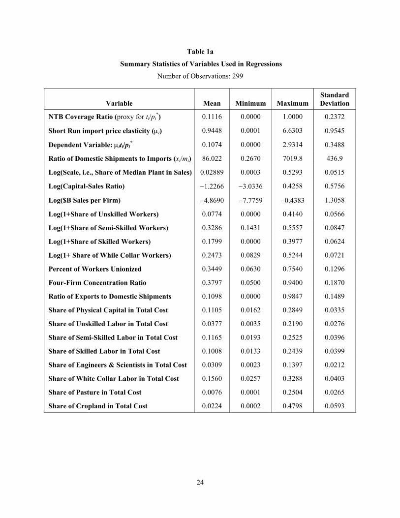
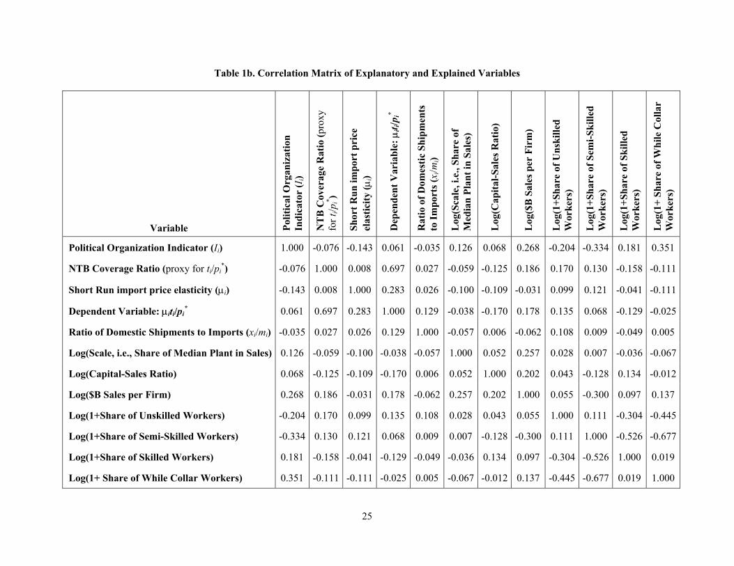
Tables 1a and 1b show the summary statistics and correlations of the variables used in the

regressions. Table 2 presents the main results. A notable preliminary point is that all regressions in Table

2 include a constant on the right-hand side even though equations (2.8) and (2.9) imply a zero intercept.

This is because the zero intercept constraint is rejected by the estimates, as the p-values of the constant

terms in the first row show. This rejection is not a cause for concern because, as I argue below, there are

simple and reasonable modifications in the model that result in a positive intercept. In any case, the

inclusion of the intercept has little consequence for the comparison between (2.8) and (2.9), which is the

key issue here.

The first column of Table 2 is the estimate of the basic GH model. For this regression, I use the

same set of instruments that applies to the full model to ensure that it is not disadvantaged by inadequate

instrumentation. Indeed, using fewer instruments reduces the statistical significance of β and strengthens

the case for the importance of other industry characteristics. The instruments, however, have little impact

on the magnitude of β, which is in the range of estimates found earlier and poses the same puzzles.15

A point of contrast between the estimate in this paper and those in other studies is the value of αL.

The estimate of η0 in the first column of Table 2 implies that αL must be about 0.08 (with a standard error

of 0.06). This is far below the figures found in most other studies. Eicher and Osang (2000), who also

find a relatively low value for αL (0.26) attribute the finding to their method of estimation. In the

regressions based on the dataset that I use, the estimated value of αL is sensitive to the measure of lobby

indicator and to the instruments used. In particular, when the lobby indicator is defined on a relative basis

(e.g., PAC contribution relative to the industry value added), αL turns out to be quite high and close to 1.

This instability in the estimates of αL may be due to the misspecification caused by assuming τi = 1,

which as we will see below, is rejected by the data.

The second column of Table 2 shows the results of letting τi vary with the capital-sales ratio and

the firm size (measured by scale), with the cost shares of semi-skilled workers and pastures used as their

instruments. The key finding is that the coefficients of the two variables and their interaction are all

negative with high levels of statistical significance (both individually and jointly), providing support for

the implications derived above based on the extended model. Moreover, the explanatory power of the

15 The estimate of β in Table 2 is lower than those found by GM and Eicher and Osang (2000) in the 0.02-0.04 range based on 3-digit SIC datasets. But, it is higher 0.0003 that GB find from a 4-digit dataset similar to the one in this paper.

15

regression jumps sharply relative to that in the first column. The estimate of β, on the other hand, declines

and loses its significance. Adding the employment share variables in the third column exacerbates this

effect while providing supports for the claim that the prevalence of lower skill workers in an industry is

associated with higher values of τi. The positive and generally significant coefficients of the employment

shares included in the model are consistent with the view that relative to engineers and scientists, other

worker categories face greater insurance problems and place a larger premium on the job security induced

by protection.16 This is confirmed not only by the individual significance levels of these variables, but

also by a Wald test of their joint significance and by the rise in the adjusted R2 as a result of their

inclusion. Interestingly, the coefficient of the share of skilled workers, who are closest to the engineers

and scientists in terms of income and job security, is the lowest among the four categories. In fact, the

hypothesis that this coefficient is the same as those of other labor categories can be easily rejected at the 5

percent level. The coefficients of the other three categories are similar to each other and cannot be

statistically distinguished. The relatively high positive coefficient for white-collar workers is interesting

because it draws attention to the fact that although this labor category includes executives and managers,

it also heavily populated by secretarial and clerical employees, who are in situations in the range of semi-

skilled and skilled workers.

Could the pattern of protection found here have emerged simply because NTBs can exist only

when an industry has a comparative disadvantage and faces import competition? Industries relying on less

capital and less skilled workers do seem to be the ones with comparative disadvantage in the US

economy. But, the same elements in the pattern of protection seem to prevail in other countries with very

different resource endowments as well. For example, the protection of low-wage workers appears to be

universal (Pack, 1994; Lee and Swagel, 1997). Association of high protection with low-wage workers as

well as small and less capital intensive firms has also been found in the case of Turkey, using a

framework similar to present one (Esfahani and Leaphart, 2000).

For diagnostic purposes, I ran further regressions with alternative lists of independent variables.

Table 3 shows examples of such experiments. The second column reports the consequences of replacing

the cost share of capital with that of cropland as the instrument for the sales-import ratio, xi/mi. The third

column shows the result of a further change in the independent variables, namely, using the share of

white-collar workers in total cost as the instrument for the firm size. As these regressions show, while the

16 It is, of course, possible that other factors may explain this and other results that emerge from these regressions. But, the preponderance of evidence points to the effect of trade policy on well-known failures in capital and insurance markets.

16

selection of instruments naturally affects the magnitude of estimated coefficients, the basic conclusions

are robust to such modifications.

There may be concern that the noise in the dependent variable is somehow related to industry

characteristics and may be causing a heteroskedasticity problem. The use of 2SLS in place of the Tobit

procedure may also potentially exacerbate this problem. To deal with this issue, I used White's

heteroskedasticity test with cross terms of independent variables included in the diagnostic regression.

The test returned an F-statistic of 0.84 with a p-value of 0.75, easing any concern over heteroskedasticity.

Further diagnostic results are shown in Table 4. According to the first column of this table,

eliminating the lobby indicator from the regression does not change the other results. Nor do the estimates

change in any major way when the observations with the incorrect elasticity sign are dropped (see the

second column). The third column shows that replacing "scale" by the average sales per firm as the

measure of firm size also has little impact on the conclusions one can draw about the determinants of τi,

except that the estimate of β becomes significantly negative. This latter change makes it even clearer that

lobby indicators may not work well in the equation that determines protection rates.

The sharp loss of significance of β following the introduction of industry characteristics in zi is

quite notable and arises for all lobby indicators that have been used in the literature. As an example, the

last column of Table 2 shows the complete model estimated with the lobby indicator defined based on the

ratio of PAC contribution to value added with a threshold of 0.0025, which is in the range of experiments

in the rest of the literature and identifies about half of the sample industries as organized. To examine

whether the inadequacy of instruments can account for the insignificance of β in the complete model, I

included additional instruments for Ii and interacted them with other independent variables to create an

expanded array of regressors for the first stage. The first column of Table 3 reports the results of such an

experiment with the unionization rate and the share of engineers and scientists in total cost as the

additional instruments. While there is some improvement in the estimate, it does not reach any tangible

significance. Finally, having the lobby indicator as its own instrument and using the amount of political

contributions in place of the lobby indicator do not seem to help. In fact, when the lobby indicator is

treated as an independent variable, β becomes indistinguishable form zero even in the original GH model.

These observations indicate that constraining τi to 1 and instrumenting for Ii with variables that are

closely related to the determinants of τi must be biasing the estimated coefficient of Ii upward.

What should one make of the negligible value and insignificance of β after the constraint on τi is

relaxed? To conclude that lobby contributions don't matter for economic policy is simply implausible.

One possible explanation is that it is difficult to decipher whether industries are organized or not from the

17

size of their political contributions. Since all industries make contributions and trade policy is only part of

their agenda, it should not come as a surprise that contribution-based indicators lose their significance

once the advantage they enjoy due to the omission of other explanatory variables is removed. However,

such indicators still highlight how much influence lobbies may be wielding. They also have the advantage

that they focus on the role of lobbies as providers of political contributions as opposed to sources of

information about industry conditions and the like.

An alternative explanation for the lack of significance of the lobby indicator is that political

contributions may not be very important for trade policy, although they may be important for other

policies. This can be the case because protection is an inefficient form of redistribution and many well-

organized groups (such as concentrated industries with large, capital-intensive firms) are in a position to

receive their rewards in more efficient ways, such as tax breaks and regulatory relief. As a result, the

government may be using protection mainly where the induced rents have some external benefit and the

targeted groups are difficult to reach via markets or direct transfers. The low skill workers and small, less

capital intensive firms that seem to be the beneficiaries of protection are obvious examples of such

groups. It is costly for them to organize, but alleviating their capital and insurance constraints has positive

welfare consequences. At the same time, it is not easy to support them via direct transfers because

identifying and targeting their eligible members is often difficult and they do not typically pay much taxes

to be helped through tax breaks.17 Consequently, protection becomes an inferior policy that responds not

so much to lobbying than to needs that markets cannot meet effectively.

A final issue to note is the importance of import price elasticity in the trade policy equation.

Running the regressions without µi on the left-hand side shows that while the coefficients generally

maintain their signs, their statistical significance levels diminish and the two sides of the equation do not

fit together nearly as well as the case where the elasticity is present (see the last column of Table 4). This

is remarkable because the elasticity estimates are noisy and can have adverse effects on the fit of the

regression. In fact, earlier studies had not found evidence of a discernible role for the import price

elasticity other than the need to include it in the regression to ensure conformity with theory. The fact that

despite the presumed noise the estimates of µi help the elements of a larger story fit together so much

17 As the countries with direct benefit programs for small firms have discovered, the number of small firms quickly swells under such programs. Some firms that should be large restructure themselves and many firms that are in effect large present themselves as small only to become eligible for the program benefits. Indian small firm policies are is a prime example of such an effect. The inefficiencies that arise as a result of such program could easily exceed the costs of protection.

18

better is a major support for all political economy models of trade policy, which are unanimous on

highlighting the role of the import price elasticity.

5. Further Extensions

5.1. Alternative Redistribution Schemes for Trade Taxes

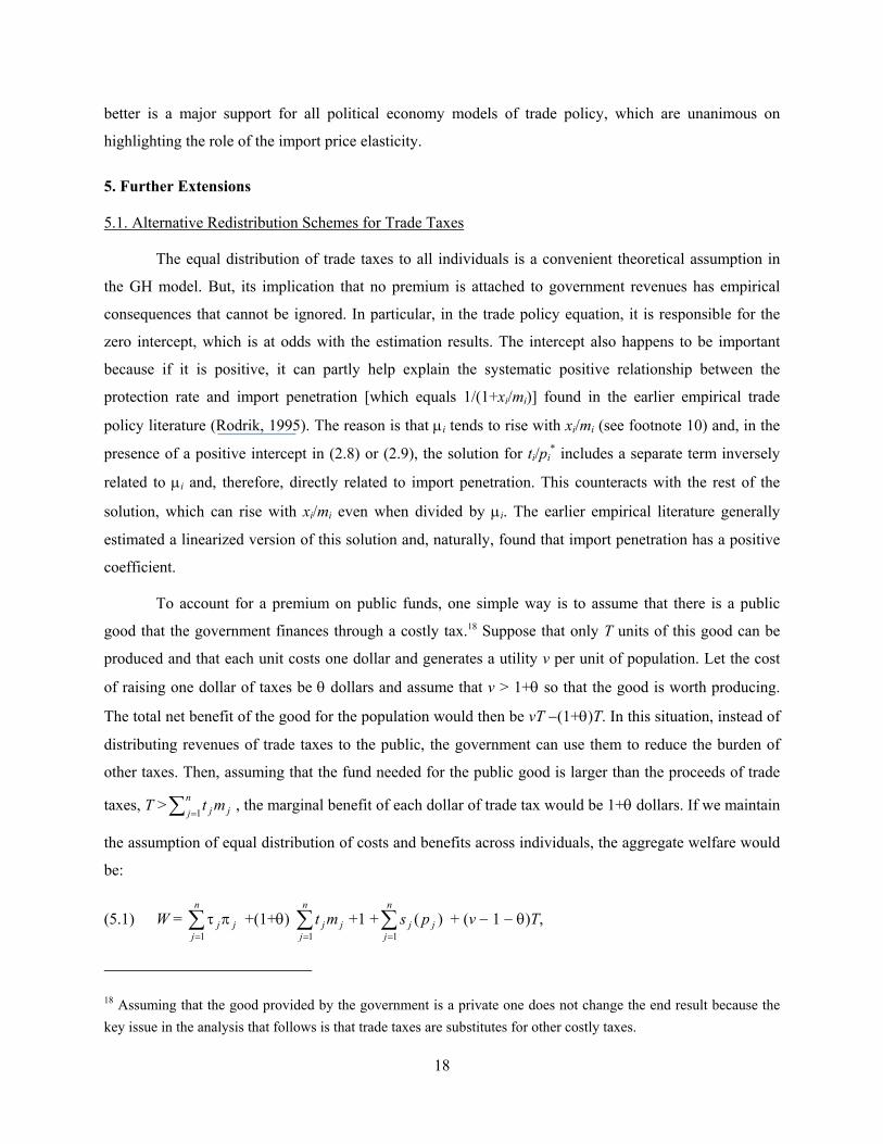
The equal distribution of trade taxes to all individuals is a convenient theoretical assumption in

the GH model. But, its implication that no premium is attached to government revenues has empirical

consequences that cannot be ignored. In particular, in the trade policy equation, it is responsible for the

zero intercept, which is at odds with the estimation results. The intercept also happens to be important

because if it is positive, it can partly help explain the systematic positive relationship between the

protection rate and import penetration [which equals 1/(1+xi/mi)] found in the earlier empirical trade

policy literature (Rodrik, 1995). The reason is that µi tends to rise with xi/mi (see footnote 10) and, in the

presence of a positive intercept in (2.8) or (2.9), the solution for ti/pi* includes a separate term inversely

related to µi and, therefore, directly related to import penetration. This counteracts with the rest of the

solution, which can rise with xi/mi even when divided by µi. The earlier empirical literature generally

estimated a linearized version of this solution and, naturally, found that import penetration has a positive

coefficient.

To account for a premium on public funds, one simple way is to assume that there is a public

good that the government finances through a costly tax.18 Suppose that only T units of this good can be

produced and that each unit costs one dollar and generates a utility v per unit of population. Let the cost

of raising one dollar of taxes be θ dollars and assume that v > 1+θ so that the good is worth producing.

The total net benefit of the good for the population would then be vT −(1+θ)T. In this situation, instead of

distributing revenues of trade taxes to the public, the government can use them to reduce the burden of

other taxes. Then, assuming that the fund needed for the public good is larger than the proceeds of trade

taxes, T >∑ =

nj jj mt1 , the marginal benefit of each dollar of trade tax would be 1+θ dollars. If we maintain

the assumption of equal distribution of costs and benefits across individuals, the aggregate welfare would

be:

(5.1) W = ∑=

πτn

jjj

1 +(1+θ) ∑

=

n

jjj mt

1+1 +∑

=

n

jjj ps

1)( + (v − 1 − θ)T,

18 Assuming that the good provided by the government is a private one does not change the end result because the key issue in the analysis that follows is that trade taxes are substitutes for other costly taxes.

19

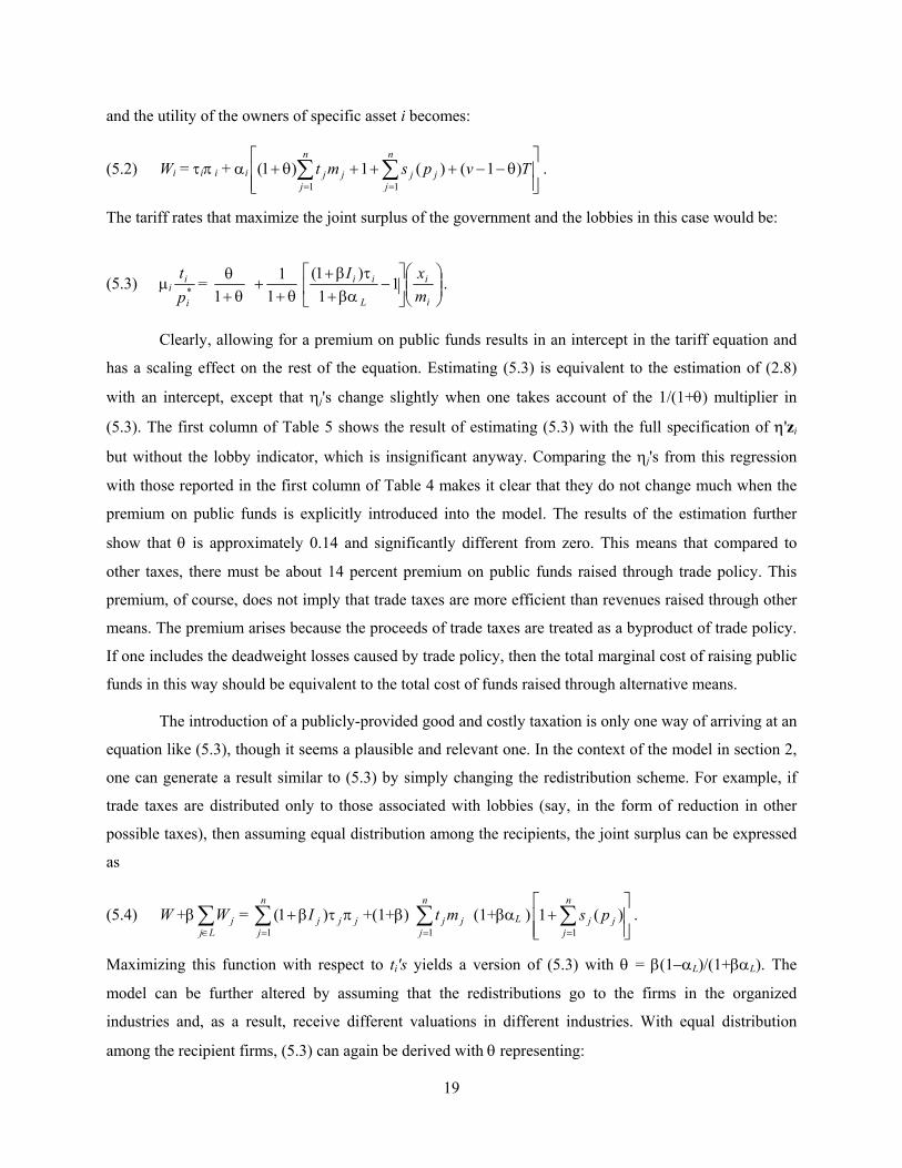
and the utility of the owners of specific asset i becomes:

(5.2) Wi = τiπ i + αi

θ−−+++θ+ ∑∑

==

Tvpsmtn

jjj

n

jjj )1()(1)1(

11.

The tariff rates that maximize the joint surplus of the government and the lobbies in this case would be:

(5.3) µi *i

i

pt =

θ+θ

1

θ++

11

−

βα+τβ+

i

i

L

ii

mxI

11

)1( .

Clearly, allowing for a premium on public funds results in an intercept in the tariff equation and

has a scaling effect on the rest of the equation. Estimating (5.3) is equivalent to the estimation of (2.8)

with an intercept, except that ηj's change slightly when one takes account of the 1/(1+θ) multiplier in

(5.3). The first column of Table 5 shows the result of estimating (5.3) with the full specification of η'zi

but without the lobby indicator, which is insignificant anyway. Comparing the ηj's from this regression

with those reported in the first column of Table 4 makes it clear that they do not change much when the

premium on public funds is explicitly introduced into the model. The results of the estimation further

show that θ is approximately 0.14 and significantly different from zero. This means that compared to

other taxes, there must be about 14 percent premium on public funds raised through trade policy. This

premium, of course, does not imply that trade taxes are more efficient than revenues raised through other

means. The premium arises because the proceeds of trade taxes are treated as a byproduct of trade policy.

If one includes the deadweight losses caused by trade policy, then the total marginal cost of raising public

funds in this way should be equivalent to the total cost of funds raised through alternative means.

The introduction of a publicly-provided good and costly taxation is only one way of arriving at an

equation like (5.3), though it seems a plausible and relevant one. In the context of the model in section 2,

one can generate a result similar to (5.3) by simply changing the redistribution scheme. For example, if

trade taxes are distributed only to those associated with lobbies (say, in the form of reduction in other

possible taxes), then assuming equal distribution among the recipients, the joint surplus can be expressed

as

(5.4) W +β∑∈Lj

jW = ∑=

πτβ+n

jjjjI

1)1( +(1+β) ∑

=

n

jjj mt

1 (1+βαL )

+∑

=

n

jjj ps

1)(1 .

Maximizing this function with respect to ti's yields a version of (5.3) with θ = β(1−αL)/(1+βαL). The

model can be further altered by assuming that the redistributions go to the firms in the organized

industries and, as a result, receive different valuations in different industries. With equal distribution

among the recipient firms, (5.3) can again be derived with θ representing:

20

(5.5) θ = L

nj Ljj

βα+

−αταβ∑ =

1

)1/(1 .

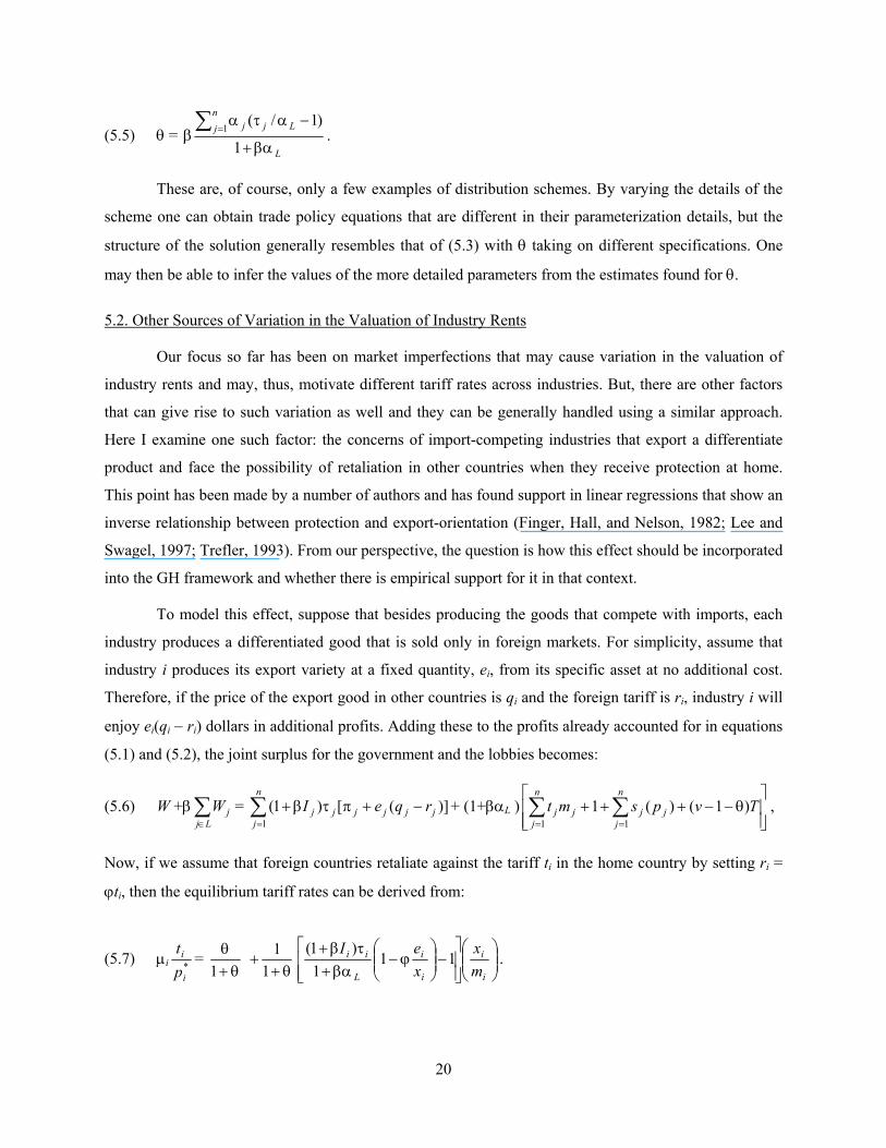
These are, of course, only a few examples of distribution schemes. By varying the details of the

scheme one can obtain trade policy equations that are different in their parameterization details, but the

structure of the solution generally resembles that of (5.3) with θ taking on different specifications. One

may then be able to infer the values of the more detailed parameters from the estimates found for θ.

5.2. Other Sources of Variation in the Valuation of Industry Rents

Our focus so far has been on market imperfections that may cause variation in the valuation of

industry rents and may, thus, motivate different tariff rates across industries. But, there are other factors

that can give rise to such variation as well and they can be generally handled using a similar approach.

Here I examine one such factor: the concerns of import-competing industries that export a differentiate

product and face the possibility of retaliation in other countries when they receive protection at home.

This point has been made by a number of authors and has found support in linear regressions that show an

inverse relationship between protection and export-orientation (Finger, Hall, and Nelson, 1982; Lee and

Swagel, 1997; Trefler, 1993). From our perspective, the question is how this effect should be incorporated

into the GH framework and whether there is empirical support for it in that context.

To model this effect, suppose that besides producing the goods that compete with imports, each

industry produces a differentiated good that is sold only in foreign markets. For simplicity, assume that

industry i produces its export variety at a fixed quantity, ei, from its specific asset at no additional cost.

Therefore, if the price of the export good in other countries is qi and the foreign tariff is ri, industry i will

enjoy ei(qi − ri) dollars in additional profits. Adding these to the profits already accounted for in equations

(5.1) and (5.2), the joint surplus for the government and the lobbies becomes:

(5.6) W +β∑∈Lj

jW = ∑=

−+πτβ+n

jjjjjjj rqeI

1)]([)1( + (1+βαL )

θ−−+++ ∑∑

==

n

jjj

n

jjj Tvpsmt

11)1()(1 ,

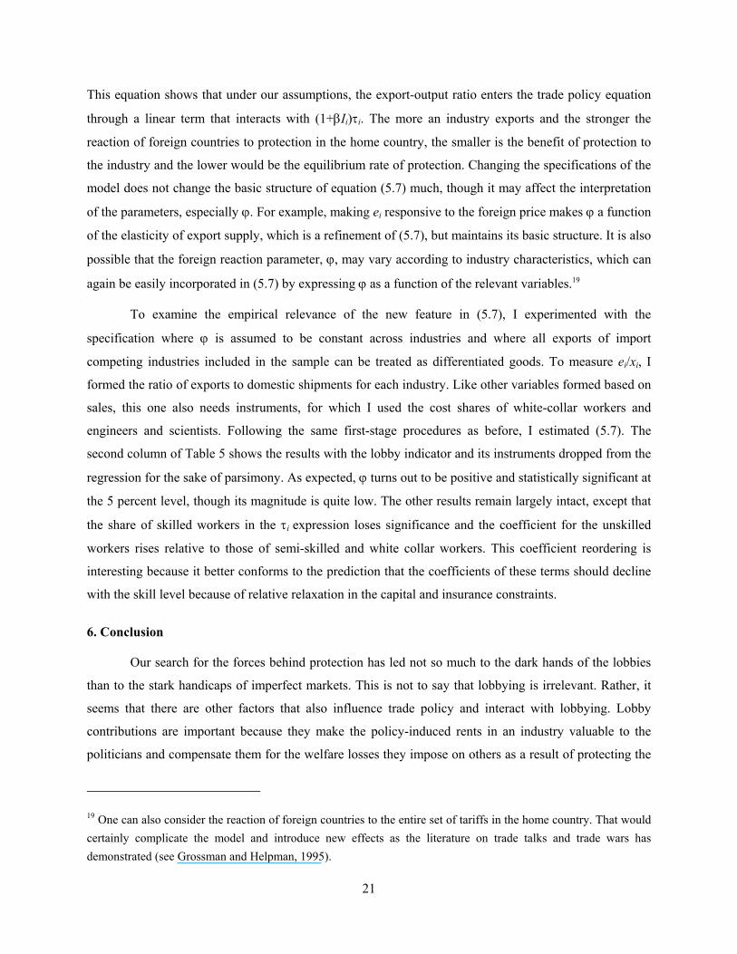
Now, if we assume that foreign countries retaliate against the tariff ti in the home country by setting ri =

ϕti, then the equilibrium tariff rates can be derived from:

(5.7) µi *i

i

pt =

θ+θ

1

θ++

11

−

ϕ−

βα+τβ+

i

i

i

i

L

ii

mx

xeI

111

)1( .

21

This equation shows that under our assumptions, the export-output ratio enters the trade policy equation

through a linear term that interacts with (1+βIi)τi. The more an industry exports and the stronger the

reaction of foreign countries to protection in the home country, the smaller is the benefit of protection to

the industry and the lower would be the equilibrium rate of protection. Changing the specifications of the

model does not change the basic structure of equation (5.7) much, though it may affect the interpretation

of the parameters, especially ϕ. For example, making ei responsive to the foreign price makes ϕ a function

of the elasticity of export supply, which is a refinement of (5.7), but maintains its basic structure. It is also

possible that the foreign reaction parameter, ϕ, may vary according to industry characteristics, which can

again be easily incorporated in (5.7) by expressing ϕ as a function of the relevant variables.19

To examine the empirical relevance of the new feature in (5.7), I experimented with the

specification where ϕ is assumed to be constant across industries and where all exports of import

competing industries included in the sample can be treated as differentiated goods. To measure ei/xi, I

formed the ratio of exports to domestic shipments for each industry. Like other variables formed based on

sales, this one also needs instruments, for which I used the cost shares of white-collar workers and

engineers and scientists. Following the same first-stage procedures as before, I estimated (5.7). The

second column of Table 5 shows the results with the lobby indicator and its instruments dropped from the

regression for the sake of parsimony. As expected, ϕ turns out to be positive and statistically significant at

the 5 percent level, though its magnitude is quite low. The other results remain largely intact, except that

the share of skilled workers in the τi expression loses significance and the coefficient for the unskilled

workers rises relative to those of semi-skilled and white collar workers. This coefficient reordering is

interesting because it better conforms to the prediction that the coefficients of these terms should decline

with the skill level because of relative relaxation in the capital and insurance constraints.

6. Conclusion

Our search for the forces behind protection has led not so much to the dark hands of the lobbies

than to the stark handicaps of imperfect markets. This is not to say that lobbying is irrelevant. Rather, it

seems that there are other factors that also influence trade policy and interact with lobbying. Lobby

contributions are important because they make the policy-induced rents in an industry valuable to the

politicians and compensate them for the welfare losses they impose on others as a result of protecting the

19 One can also consider the reaction of foreign countries to the entire set of tariffs in the home country. That would certainly complicate the model and introduce new effects as the literature on trade talks and trade wars has demonstrated (see Grossman and Helpman, 1995).

22

industry. The GH model captures the essence of such effects and shows that industries that are better able

to politically organize and payoff the politicians should receive more protection. But, the value of

industry rents may vary due to non-political factors as well. A key source of such variation can be the

differences in capital and insurance constraints that firms in different industries face. In industries with

severe constraints, additional earnings have a positive welfare effect and, if present, lobbying for

favorable policies is likely to be more intense. These effects can increase the political benefits of offering

rents to such industries and, when other channels of support have high or rising costs, encourage higher

protection. Another example of a source of variation in the value of industry rents is the degree of

vulnerability to foreign retaliation when import-competing industries export a differentiated product. The

exercises in this paper show that the GH framework can be extended systematically to include all such

effects. The empirical application of the extended framework further shows that it is much more

successful in explaining the pattern of protection than the original barebones version estimated with lobby

indicators based on campaign contributions.

The new empirical results are remarkable in that they point to the presence of major effects that

are quite distinct from lobbying. They link protection to less skilled workers and smaller and less capital

intensive firms, which are not commonly viewed as the most organized and politically influential groups.

These groups seem to receive more protection because they demand relief from the tight capital and

insurance constraints that they face and alternative (budgetary and regulatory) channels of supporting

them are costly for the government. Industries with better organizations and greater political influence are

typically more concentrated with larger firms, which are in a better position to benefit from fiscal and

financial policies. Such industries may be receiving a lot of rents, but largely through more efficient

transfers than through inefficient trade restrictions. It is in the case of more dispersed and hard-to-reach

groups that the politicians have to resort to the inferior protection policies, hence an explanation why

lobby contributions do not show up as significant in the trade policy equation.

The perspective that emerges from this study has important implications for the on-going process

of globalization. On the one hand, as Rodrik (1997) argues, globalization has enhanced the mobility of

capital and skilled labor and, as a result, must have increased the elasticity of demand for less mobile

factors of production. This may have reduced the income security of less skilled workers and small local

firms, fueling opposition to globalization and increasing the demand for government support program. On

the other hand, globalization has been accompanied by advancements in financial and insurance markets

and in institutions of social insurance, which can work in the opposite direction and diminish the risk

concerns of a wider range of workers and firms. The balance depends on the relative strengths of the two

effects. Of course, this does not diminish the importance conscious efforts at the national and multilateral

23

levels to implement policies, such as those advocated by Rodrik (1997), that help alleviate the risks of

globalization and ensure the realization of its benefits.

Further work on the subject of this paper seems to require considering trade policy together with

industrial and fiscal policies to examine the role of lobbying and other factors more thoroughly. This line

of research is important because the implications for economic policy and reform programs could be

enormous. Already the results of this paper highlight the significant role that fiscal and financial systems

and social safety nets may play in ensuring greater and more sustainable openness in the world economy.

24

Table 1a

Summary Statistics of Variables Used in Regressions

Number of Observations: 299

Variable Mean Minimum Maximum Standard Deviation

NTB Coverage Ratio (proxy for ti/pi*) 0.1116 0.0000 1.0000 0.2372

Short Run import price elasticity (µi) 0.9448 0.0001 6.6303 0.9545

Dependent Variable: µiti/pi* 0.1074 0.0000 2.9314 0.3488

Ratio of Domestic Shipments to Imports (xi/mi) 86.022 0.2670 7019.8 436.9

Log(Scale, i.e., Share of Median Plant in Sales) 0.02889 0.0003 0.5293 0.0515

Log(Capital-Sales Ratio) −1.2266 −3.0336 0.4258 0.5756

Log($B Sales per Firm) −4.8690 −7.7759 −0.4383 1.3058

Log(1+Share of Unskilled Workers) 0.0774 0.0000 0.4140 0.0566

Log(1+Share of Semi-Skilled Workers) 0.3286 0.1431 0.5557 0.0847

Log(1+Share of Skilled Workers) 0.1799 0.0000 0.3977 0.0624

Log(1+ Share of While Collar Workers) 0.2473 0.0829 0.5244 0.0721

Percent of Workers Unionized 0.3449 0.0630 0.7540 0.1296

Four-Firm Concentration Ratio 0.3797 0.0500 0.9400 0.1870

Ratio of Exports to Domestic Shipments 0.1098 0.0000 0.9847 0.1489

Share of Physical Capital in Total Cost 0.1105 0.0162 0.2849 0.0335

Share of Unskilled Labor in Total Cost 0.0377 0.0035 0.2190 0.0276

Share of Semi-Skilled Labor in Total Cost 0.1165 0.0193 0.2525 0.0396

Share of Skilled Labor in Total Cost 0.1008 0.0133 0.2439 0.0399

Share of Engineers & Scientists in Total Cost 0.0309 0.0023 0.1397 0.0212

Share of White Collar Labor in Total Cost 0.1560 0.0257 0.3288 0.0403

Share of Pasture in Total Cost 0.0076 0.0001 0.2504 0.0265

Share of Cropland in Total Cost 0.0224 0.0002 0.4798 0.0593

25

Table 1b. Correlation Matrix of Explanatory and Explained Variables

Variable Polit

ical

Org

aniz

atio

n In

dica

tor

(Ii)

NT

B C

over

age

Rat

io (p

roxy

fo

r ti/p

i* )

Shor

t Run

impo

rt p

rice

el

astic

ity (µ

i)

Dep

ende

nt V

aria

ble:

µit i/

p i*

Rat

io o

f Dom

estic

Shi

pmen

ts

to Im

port

s (x i/

mi)

Log

(Sca

le, i

.e.,

Shar

e of

M

edia

n Pl

ant i

n Sa

les)

Log

(Cap

ital-S

ales

Rat

io)

Log

($B

Sal

es p

er F

irm

)

Log

(1+S

hare

of U

nski

lled

Wor

kers

)

Log

(1+S

hare

of S

emi-S

kille

d W

orke

rs)

Log

(1+S

hare

of S

kille

d W

orke

rs)

Log

(1+

Shar

e of

Whi

le C

olla

r W

orke

rs)

Political Organization Indicator (Ii) 1.000 -0.076 -0.143 0.061 -0.035 0.126 0.068 0.268 -0.204 -0.334 0.181 0.351

NTB Coverage Ratio (proxy for ti/pi*) -0.076 1.000 0.008 0.697 0.027 -0.059 -0.125 0.186 0.170 0.130 -0.158 -0.111

Short Run import price elasticity (µi) -0.143 0.008 1.000 0.283 0.026 -0.100 -0.109 -0.031 0.099 0.121 -0.041 -0.111

Dependent Variable: µiti/pi* 0.061 0.697 0.283 1.000 0.129 -0.038 -0.170 0.178 0.135 0.068 -0.129 -0.025

Ratio of Domestic Shipments to Imports (xi/mi) -0.035 0.027 0.026 0.129 1.000 -0.057 0.006 -0.062 0.108 0.009 -0.049 0.005

Log(Scale, i.e., Share of Median Plant in Sales) 0.126 -0.059 -0.100 -0.038 -0.057 1.000 0.052 0.257 0.028 0.007 -0.036 -0.067

Log(Capital-Sales Ratio) 0.068 -0.125 -0.109 -0.170 0.006 0.052 1.000 0.202 0.043 -0.128 0.134 -0.012

Log($B Sales per Firm) 0.268 0.186 -0.031 0.178 -0.062 0.257 0.202 1.000 0.055 -0.300 0.097 0.137

Log(1+Share of Unskilled Workers) -0.204 0.170 0.099 0.135 0.108 0.028 0.043 0.055 1.000 0.111 -0.304 -0.445

Log(1+Share of Semi-Skilled Workers) -0.334 0.130 0.121 0.068 0.009 0.007 -0.128 -0.300 0.111 1.000 -0.526 -0.677

Log(1+Share of Skilled Workers) 0.181 -0.158 -0.041 -0.129 -0.049 -0.036 0.134 0.097 -0.304 -0.526 1.000 0.019

Log(1+ Share of While Collar Workers) 0.351 -0.111 -0.111 -0.025 0.005 -0.067 -0.012 0.137 -0.445 -0.677 0.019 1.000

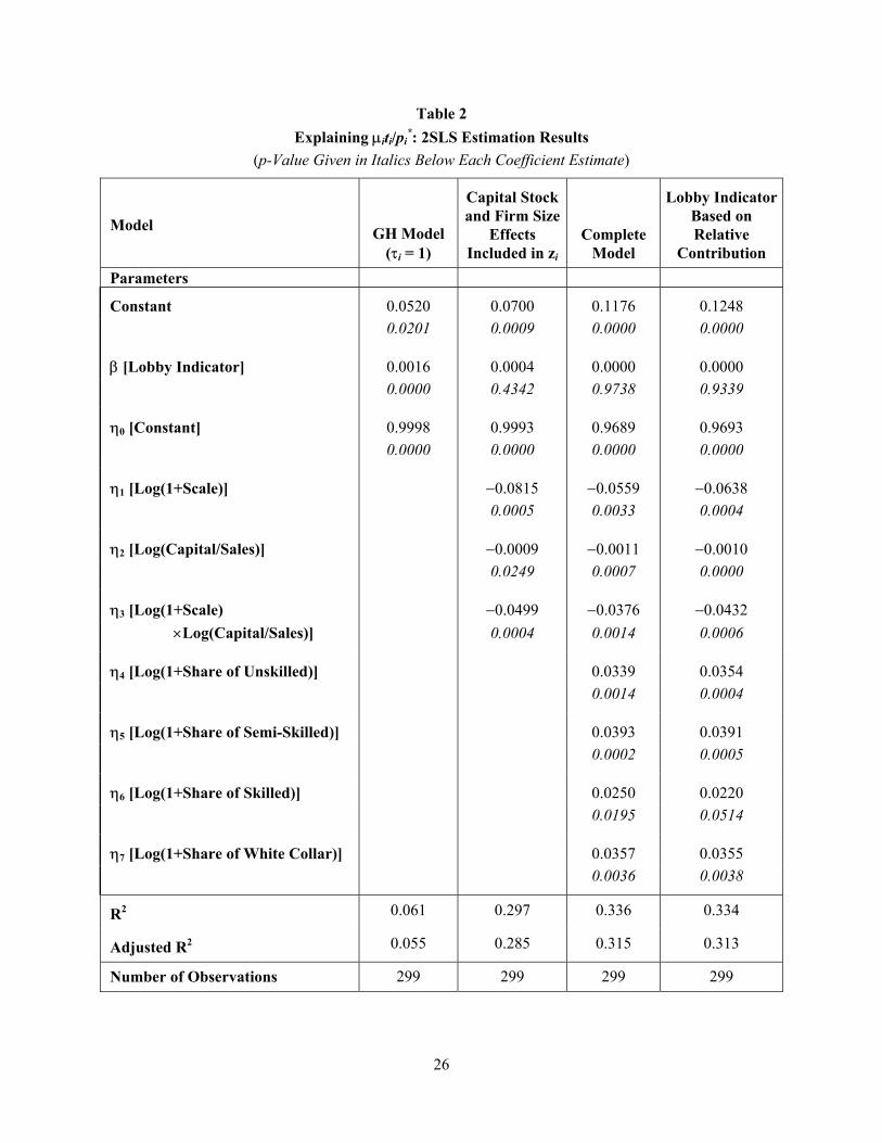
26

Table 2 Explaining µiti/pi

*: 2SLS Estimation Results (p-Value Given in Italics Below Each Coefficient Estimate)

Model GH Model (τi = 1)

Capital Stock and Firm Size

Effects Included in zi

Complete Model

Lobby Indicator Based on Relative

Contribution Parameters

Constant 0.0520 0.0700 0.1176 0.1248 0.0201 0.0009 0.0000 0.0000

β [Lobby Indicator] 0.0016 0.0004 0.0000 0.0000 0.0000 0.4342 0.9738 0.9339

η0 [Constant] 0.9998 0.9993 0.9689 0.9693 0.0000 0.0000 0.0000 0.0000

η1 [Log(1+Scale)] −0.0815 −0.0559 −0.0638 0.0005 0.0033 0.0004

η2 [Log(Capital/Sales)] −0.0009 −0.0011 −0.0010 0.0249 0.0007 0.0000

η3 [Log(1+Scale) −0.0499 −0.0376 −0.0432 ×Log(Capital/Sales)] 0.0004 0.0014 0.0006

η4 [Log(1+Share of Unskilled)] 0.0339 0.0354 0.0014 0.0004

η5 [Log(1+Share of Semi-Skilled)] 0.0393 0.0391 0.0002 0.0005

η6 [Log(1+Share of Skilled)] 0.0250 0.0220 0.0195 0.0514

η7 [Log(1+Share of White Collar)] 0.0357 0.0355 0.0036 0.0038

R2 0.061 0.297 0.336 0.334

Adjusted R2 0.055 0.285 0.315 0.313

Number of Observations 299 299 299 299

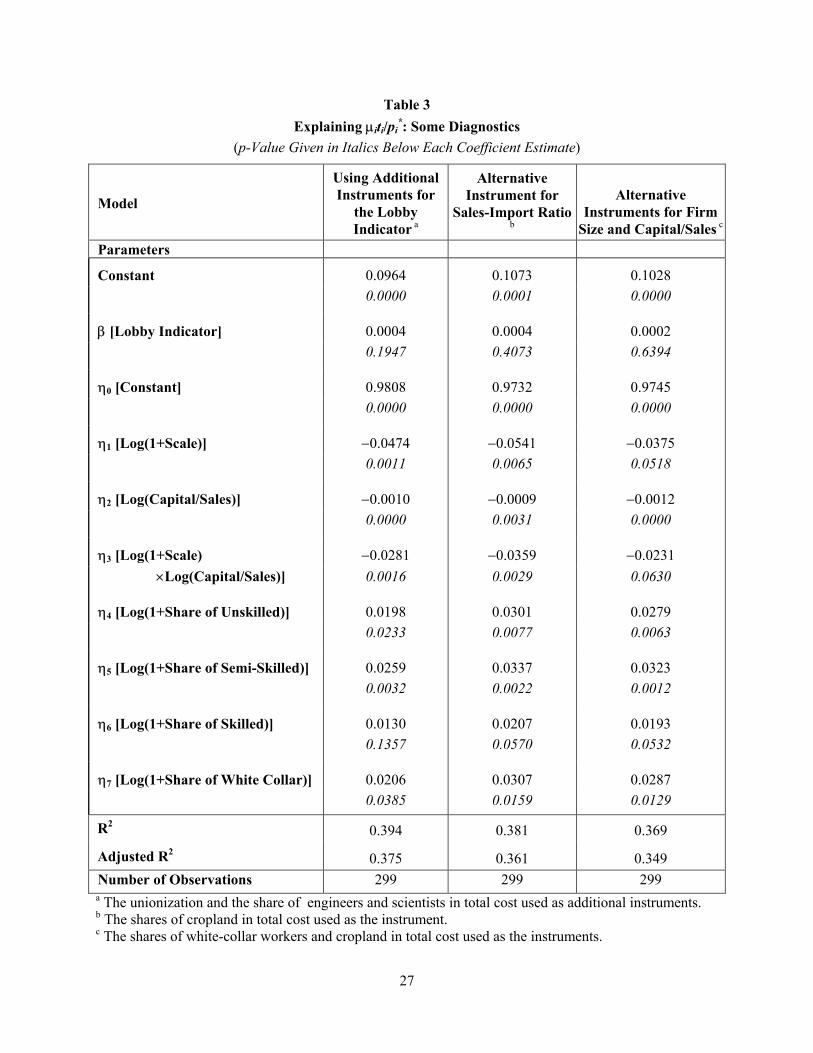
27

Table 3 Explaining µiti/pi

*: Some Diagnostics (p-Value Given in Italics Below Each Coefficient Estimate)

Model

Using Additional Instruments for

the Lobby Indicator a

Alternative Instrument for

Sales-Import Ratio

b

Alternative Instruments for Firm

Size and Capital/Sales c

Parameters

Constant 0.0964 0.1073 0.1028 0.0000 0.0001 0.0000

β [Lobby Indicator] 0.0004 0.0004 0.0002 0.1947 0.4073 0.6394

η0 [Constant] 0.9808 0.9732 0.9745 0.0000 0.0000 0.0000

η1 [Log(1+Scale)] −0.0474 −0.0541 −0.0375 0.0011 0.0065 0.0518

η2 [Log(Capital/Sales)] −0.0010 −0.0009 −0.0012 0.0000 0.0031 0.0000

η3 [Log(1+Scale) −0.0281 −0.0359 −0.0231 ×Log(Capital/Sales)] 0.0016 0.0029 0.0630

η4 [Log(1+Share of Unskilled)] 0.0198 0.0301 0.0279 0.0233 0.0077 0.0063

η5 [Log(1+Share of Semi-Skilled)] 0.0259 0.0337 0.0323 0.0032 0.0022 0.0012

η6 [Log(1+Share of Skilled)] 0.0130 0.0207 0.0193 0.1357 0.0570 0.0532

η7 [Log(1+Share of White Collar)] 0.0206 0.0307 0.0287 0.0385 0.0159 0.0129

R2 0.394 0.381 0.369

Adjusted R2 0.375 0.361 0.349 Number of Observations 299 299 299 a The unionization and the share of engineers and scientists in total cost used as additional instruments. b The shares of cropland in total cost used as the instrument. c The shares of white-collar workers and cropland in total cost used as the instruments.

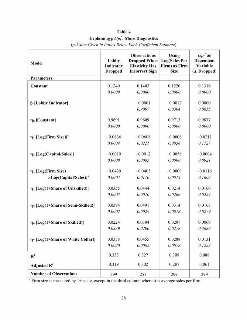
28

Table 4 Explaining µiti/pi

*: More Diagnostics (p-Value Given in Italics Below Each Coefficient Estimate)

Model Lobby Indicator Dropped

Observations Dropped When Elasticity Has Incorrect Sign

Using Log(Sales Per Firm) as Firm

Size

ti/pi* as

Dependent Variable

(µi Dropped) Parameters

Constant 0.1240 0.1403 0.1220 0.1316 0.0000 0.0000 0.0000 0.0000

β [Lobby Indicator] −0.0001 −0.0012 0.0000 0.9097 0.0304 0.8655

η0 [Constant] 0.9691 0.9609 0.9713 0.9877 0.0000 0.0000 0.0000 0.0000

η1 [Log(Firm Size)]a −0.0636 −0.0608 −0.0008 −0.0211 0.0004 0.0221 0.0058 0.1127

η2 [Log(Capital/Sales)] −0.0010 −0.0012 −0.0058 −0.0004 0.0000 0.0085 0.0000 0.0921

η3 [Log(Firm Size) −0.0429 −0.0403 −0.0009 −0.0116 ×Log(Capital/Sales)]a 0.0003 0.0110 0.0014 0.1603

η4 [Log(1+Share of Unskilled)] 0.0355 0.0444 0.0214 0.0160 0.0003 0.0010 0.0260 0.0324

η5 [Log(1+Share of Semi-Skilled)] 0.0394 0.0491 0.0314 0.0168 0.0002 0.0029 0.0018 0.0279

η6 [Log(1+Share of Skilled)] 0.0224 0.0304 0.0207 0.0069 0.0339 0.0200 0.0278 0.3683

η7 [Log(1+Share of White Collar)] 0.0358 0.0455 0.0288 0.0131 0.0020 0.0082 0.0078 0.1223

R2 0.337 0.327 0.309 0.088

Adjusted R2 0.319 0.302 0.287 0.061

Number of Observations 299 257 299 299 a Firm size is measured by 1+ scale, except in the third column where it is average sales per firm.

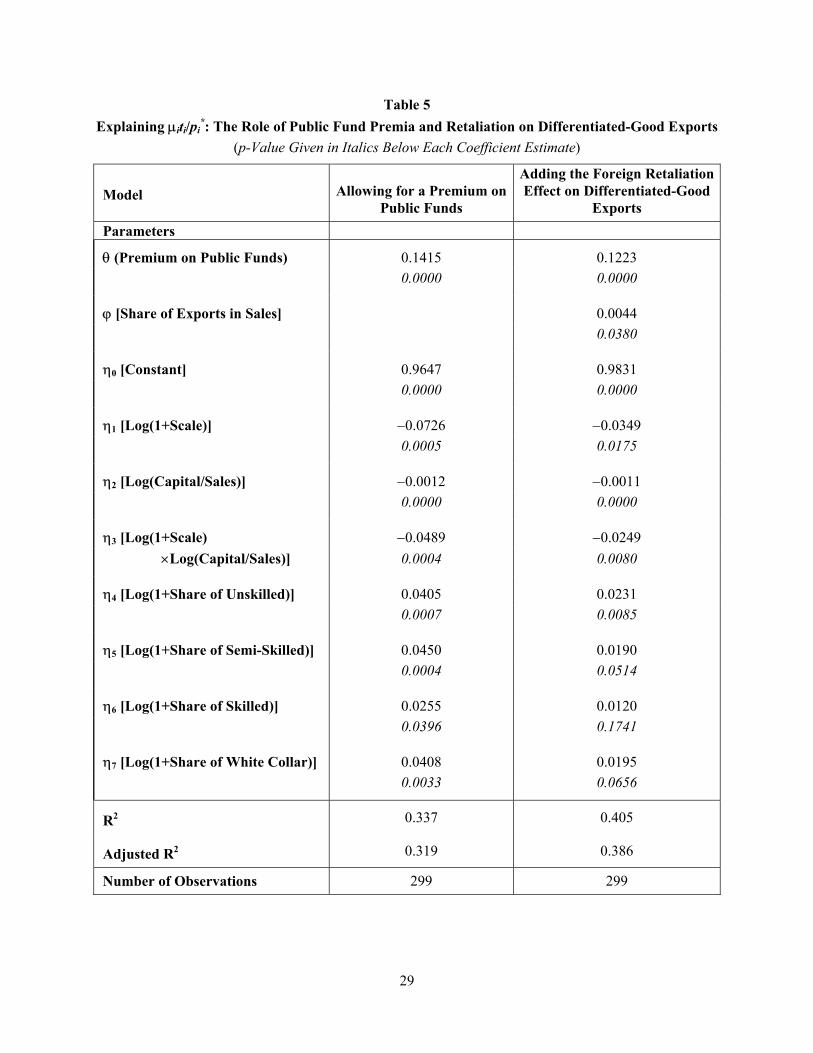
29

Table 5 Explaining µiti/pi

*: The Role of Public Fund Premia and Retaliation on Differentiated-Good Exports (p-Value Given in Italics Below Each Coefficient Estimate)

Model Allowing for a Premium on Public Funds

Adding the Foreign Retaliation Effect on Differentiated-Good

Exports Parameters

θ (Premium on Public Funds) 0.1415 0.1223 0.0000 0.0000

ϕ [Share of Exports in Sales] 0.0044 0.0380

η0 [Constant] 0.9647 0.9831 0.0000 0.0000

η1 [Log(1+Scale)] −0.0726 −0.0349 0.0005 0.0175

η2 [Log(Capital/Sales)] −0.0012 −0.0011 0.0000 0.0000

η3 [Log(1+Scale) −0.0489 −0.0249 ×Log(Capital/Sales)] 0.0004 0.0080

η4 [Log(1+Share of Unskilled)] 0.0405 0.0231 0.0007 0.0085

η5 [Log(1+Share of Semi-Skilled)] 0.0450 0.0190 0.0004 0.0514

η6 [Log(1+Share of Skilled)] 0.0255 0.0120 0.0396 0.1741

η7 [Log(1+Share of White Collar)] 0.0408 0.0195 0.0033 0.0656

R2 0.337 0.405

Adjusted R2 0.319 0.386

Number of Observations 299 299

30

References

Anderson, Kym, and Robert E. Baldwin. 1987. "The Political Market for Protection in Industrial Countries: New Empirical Evidence," in A. M. El-Agraa, ed., Protection, Cooperation, Integration and Development, New York: Macmillan.

Attanasio, Orazio, Pinelopi K. Goldberg, and Ekaterini Kyriazidou. 2000. "Credit Constraints in the Market for Consumer Durables: Evidence from Micro Data on Car Loans," NBER Working Paper W7694.

Auerbach, Alan J., Kevin A. Hassett. 2000. "On the Marginal Source of Investment Funds" National Bureau of Economic Research, Working paper No. W7821.

Baldwin, Robert E. 1985. The Political Economy of U.S. Import Policy. Cambridge, MA: MIT Press.

Caves, Richard E. 1976. "Economic Models of Political Choice: Canada's Tariff Structure", Canadian Journal of Economics, 9: 278-300.

Eicher, Theo, and Thomas Osang. 2000. "Politics and Trade Policy: An Empirical Investigation," manuscript, University of Washington, Seattle, WA.

Esfahani, Hadi Salehi and Stephanie Leaphart. 2000. "Testing Political Economy Models of Trade Policy," unpublished manuscript.

Esfahani, Hadi Salehi and Munir Mahmoud. 2000. "The Political Economy of Protectionism and Industrial Policy," unpublished manuscript.

Fama, Eugene, and Kenneth French. 1998. "The Corporate Cost of Capital and the Return on Corporate Investment," manuscript, University of Chicago and Massachusetts Institute of Technology (MIT).

Feenstra, Robert C. 1996. "NBER Trade Database, Disk1: U.S. Imports, 1972-1994: Data and Concordances," NBER Working Paper no. 5515.

Finger, J.M., H. Keith Hall, and Douglas R. Nelson. 1982. "The Political Economy of Administered Protection," American Economic Review, 72.3: 452-466.

Gawande, Kishore, and Usree Bandyopadhyay. 2000. "Is Protection for Sale: Evidence on the Grossman-Helpman Theory of Endogenous Protection," Review of Economics and Statistics, 82.1: 139-152.

Goldberg, Pinelopi Koujianou, and Maggi, Giovanni. 1999. "Protection for Sale: An Empirical Investigation," American Economic Review, 89.5: 1135-1155

Gross, David B., and Nicholas S. Souleles. 2001. "Do Liquidity Constraints and Interest Rates Matter for Consumer Behavior? Evidence from Credit Card Data," NBER Working Paper W8314.

Grossman, Gene, and Elhanan Helpman. 1994. "Protection for Sale," American Economic Review. 84.4:833-850.

Grossman, Gene, and Elhanan Helpman. 1995. "Trade wars and Trade talks," Journal of Political Economy, 103.4: 675-708.

Hanes, Christopher. 2000. "Nominal Wage Rigidity and Industry Characteristics in the Downturns of 1893, 1929, and 1981," American Economic Review, 90.5: 1432-1446.

31

Harrigan, James, and Egon Zakrajsek. 2000. "Factor Supplies and Specialization in the World Economy," NBER Working Paper W7848.

Helpman, Elhanan. 1997. "Politics and Trade Policy," in David Kreps and Kenneth Wallis, eds., Advances in Economics and Econometrics: Theory and Application, Cambridge: Cambridge University Press.

Hillman, Arye L. 1989. The Political Economy of Protection, Chur: Harwood Academic Publishers.

Hoynes, Hilary W. 2001. "The Employment, Earnings, and Income of Less Skilled Workers over the Business Cycle," in David Card and Rebecca M. Blank, eds., Finding Jobs: Work and Welfare Reform. New York: Russell Sage Foundation: 23-71.

Hu, Xiaoqiang, and Fabil Schiantarelli. 1998. "Investment and Financing Constraints: A Switching Regression Approach Using US Firms Panel Data," The Review of Economics and Statistics, 80.3: 466-79.

Hubbard,R.Glenn. 1998. "Capital-Market Imperfections and Investment," Journal of Economic Literature, 36.1: 193–225

Kelejian, H. 1971. "Two Stage Least Squares and Econometric Systems Linear in Parameters But Nonlinear in the Endogenous Variables," Journal of the American Statistical Association, 66: 373-374.

Leamer, Edward E. 1990. "The Structure and Effects of Tariff and Nontariff Barriers in 1983," in Ronald W. Jones and Anne O. Krueger, eds., The Political Economy of International Trade: Essays in Honor of Robert E. Baldwin. Oxford: Blackwell: 224-60.

Lee, Jong-Wha, and Swagel, Phillip. 1997. "Trade Barriers and Trade Flows across Countries and Industries," The Review of Economics and Statistics, 79: 372-382.

Magee, Stephen. 1984. "Endogenous Tariff theory, A Survey," in Neoclassical Political Economy, ed. David C. Colander. Ballinger Press, Cambridge.

Maggi, Giovanni, and Andrés Rodríguez-Clare. 1999. "Import Penetration and the Politics of Trade Protection," Journal of International Economics, 89: 1135-1155.

Manski, Charles F., and John D. Straub. 1999. "Worker Perceptions of Job Insecurity in the Mid-1990s: Evidence from the Survey of Economic Expectations," NBER Working Paper No. W6908.

Marks, S.V., and J. McArthur. 1990. "Empirical Analyses of the Determinants of Protection: A Survey and Some New Results," in J.S. Odell and T.D. Willett, eds., International Trade Policies: Gains from Exchange Between Economics and Political Science. Ann Arbor: University of Michigan Press.

Marvel, Howard P., and Edward John Ray. 1983. "The Kennedy Round: Evidence on the Regulation of International Trade in the United States," American Economic Review, 73.2: 190-197.

McCalman, Phillip. Forthcoming. "Protection for Sale and Trade Liberalization: An Empirical Investigation," International Economic Review.

Mitra, Devashish, Dimitrios D. Thomakos, and Mehmet A. Ulubasoglu. 2000. "'Protection for Sale' in a Developing Country: Democracy versus Dictatorship." Manuscript. Florida International University.

Pack, Howard. 1994. "Productivity or Politics: The Determinants of the Indonesian Tariff Structure," Journal of Development Economics. 44: 441-451.

32

Ray, Edward John. 1981a. "Tariff and nontariff barriers to trade in the United States and abroad," Review of Economics and Statistics, 63: 161-168.

Ray, Edward John. 1981b. "The Determinants of Tariff and Nontariff Trade Restrictions in the United States," Journal of Political Economy, 89.1: 105-121.

Ray, Edward John. 1990. "Empirical research on the political economy of trade," in C.A. Carter, A.F. McCalla, and J. Sharples, eds., Imperfect Competition and Political Economy. Boulder: Westview Press.

Rodrik, Dani. 1995. "Political Economy of Trade Policy," in Gene M. Grossman and Kenneth Rogoff, eds., Handbook of International Economics, Vol. III, Elsevier Publishers, Amsterdam: 1457-1496.

Rodrik, Dani. 1997. Has Globalization Gone Too Far? Wash., DC: Institute for International Economics.

Rodrik, Dani. 1998. "Why Do More Open Economies Have Bigger Governments?" Journal of Political Economy, 106.5: 997-1032.

Shiells, Clinton, Robert M. Stern, and Alan V. Deardorff. 1986. "Estimates of the Elasticities of Substitution Between Imports and Home Goods for the United States," Weltwirtschaftliches Archiv 122: 497-519.

Trefler, Daniel. 1993. "Trade Liberalization and the Theory of Endogenous Protection, An Econometric Study of US Import Policy," Journal of Political Economy, 101.1: 138-160.

Whited, Toni. 1992. "Debt, Liquidity Constraints and Corporate Investment: Evidence from Panel Data," Journal of Finance 47: 1425-1460.