CHANGES IN EARNINGS IN BRAZIL, CHILE, AND MEXICO, DISENTANGLING THE FORCES BEHIND PRO-POOR FORCES...

March, 2009Working Paper number 51

Eduardo ZepedaCarnegie Endowment for International Peace/UNDP

Diana AlarconPoverty Practice, Bureau for Development Policy, UNDP

Fábio Veras SoaresRafael Guerreiro OsórioInternational Policy Centre for Inclusive Growth

CHANGES IN EARNINGS INBRAZIL, CHILE, AND MEXICO:DISENTANGLING THEFORCES BEHIND PRO-POORCHANGE IN LABOUR MARKETS

International

Centre for Inclusive Growth

Copyright© 2009International Policy Centre for Inclusive GrowthUnited Nations Development Programme

The International Policy Centre for Inclusive Growth is jointly supported by the Poverty Practice,Bureau for Development Policy, UNDP and the Government of Brazil.

Rights and Permissions

All rights reserved.

The text and data in this publication may be reproduced as long as the source is cited.Reproductions for commercial purposes are forbidden.

International Policy Centre for Inclusive Growth (IPC - IG)Poverty Practice, Bureau for Development Policy, UNDPEsplanada dos Ministérios, Bloco O, 7º andar70052-900 Brasilia, DF - BrazilTelephone: +55 61 2105 5000

E-mail: [email protected] URL: www.ipc-undp.org

The International Policy Centre for Inclusive Growth disseminates the findings of its work inprogress to encourage the exchange of ideas about development issues. The papers aresigned by the authors and should be cited accordingly. The findings, interpretations, andconclusions that they express are those of the authors and not necessarily those of theUnited Nations Development Programme or the Government of Brazil.

Working Papers are available online at www.ipc-undp.org and subscriptions can be requestedby email to [email protected]

Print ISSN: 1812-108X

CHANGES IN EARNINGS IN BRAZIL, CHILE, AND MEXICO: DISENTANGLING THE FORCES BEHIND PRO-POOR

CHANGE IN LABOUR MARKETS∗

Eduardo Zepeda,** Diana Alarcon,*** Fábio Veras Soares**** and Rafael Guerreiro Osório****

ABSTRACT

Despite the recovery of economic growth in Latin America during the 1990s, rising unemployment, high informality rates and sluggish wages lie at the root of high inequality and poverty. This paper looks at changes in hourly earnings from the early 1990s to the early 2000s in three relatively stable countries: Brazil, Chile and Mexico. Using econometric techniques, the paper decomposes the change in earnings per worker into changes in the demographic and socio-occupational characteristics of workers, changes in the returns to such characteristics, and changes in unobservable factors. The paper attempts to address the link between labour markets and the dynamics of inequality and poverty by comparing the average performance of the entire working labour force with the performance of the 20 per cent of workers with the lowest earnings. The paper finds that earnings per worker are the result of slow-moving changes in the structure of employment and the characteristics of workers, as well as rapid changes in the prices of labour for specific workers. Demographic changes, better education and the decline of agricultural labour are among the most significant changes in the structure of employment, and they contribute to observed changes in earnings. Among the most important changes in prices contributing to the change in earnings are changes in the returns to formal and informal employees relative to the self-employed; changes to full-time employment relative to part-time workers; changes in the returns to urban workers relative to rural workers; and change in the earnings of workers in services relative to workers in agriculture. In general, changes in earnings frequently favoured low-earning workers, mostly because of the change in the returns for their labour. This is in contrast to the changes in the structure of employment, which tended to favour high-earning workers.

JEL Classification: C13, D31, J21, J24, J31.

∗ The authors are grateful to Dag Ehrenpreis, Terry McKinley and Carlos Salas for comments and recommendations, and to Celio da Silva for excellent research assistance.

** Carnegie Endowment for International Peace/UNDP.

*** Poverty Practice, Bureau for Development Policy, UNDP. **** International Policy Centre for Inclusive Growth.

2 International Policy Centre for Inclusive Growth

1 INTRODUCTION

After several years of recession and deteriorating living conditions in Latin America, economic growth started to recover in the 1990s. Growth was unstable, however, and rates fell short of historical records. Consequently, unemployment and informality remained high and overall employment did not improve.1 The challenge of transferring large numbers of workers from low-productivity, low-earning jobs to high-productivity, high-earning occupations is daunting.2

Directly linked to weak employment performance, poverty reduction trends in Latin America are not encouraging. A recent study estimated that under the slow growth rates that prevailed during the 1990s and invariant inequality, only 7 of 18 countries in the region will be able to achieve the Millennium Development Goal (MDG) target of halving poverty by 2015 (ECLAC et al., 2002). Clearly, Latin American countries need to accelerate growth and improve income distribution. A strong labour market performance that creates good quality jobs and incorporates the poor is a key component of faster growth with distribution.

In a recent paper we looked at the links between labour income and workers’ labour-market insertion in Brazil, Chile and Mexico, and found that changes in income depend mostly on changes in earnings per worker and less on changes in employment. Further, we found that the change of household labour income tends to be more pro-poor than changes in employment (Zepeda et al., 2007).3 In this paper, we focus on earnings per worker to discuss the factors that explain their changes and distributional effects. Using regression techniques we decompose changes in earnings per worker into three sources: changes in the socio-demographic and occupational characteristics of workers; changes in the returns to workers’ characteristics; and changes in unobserved factors. To address the distributional effects of such changes, we compare changes in the labour income of the 20 per cent of workers with the lowest earnings to changes in the mean income of all workers.

The paper is organised as follows. First, we briefly review labour market conditions in Brazil, Chile and Mexico. Section 3 outlines the decomposition methodology applied to labour earnings. Section 4 discusses the overall contribution of changes in workers’ characteristics, its returns and unobservables. Section 5 offers a detailed discussion of the contribution to earnings arising from changes in the mix of workers’ characteristics and its distributional effects. Section 6 examines in detail the returns to workers’ characteristics. The final section summarises the main findings.

2 BRAZIL, CHILE AND MEXICO: AN OVERVIEW

Brazil, Chile and Mexico are three middle-income countries with relatively stable, mature and diversified economies. Brazil is the largest country, with a population of about 174 million at the turn of the decade. Although growth has not been impressive (a 1.2 per cent change in GDP per capita between 1990 and 2005), income per capita is relatively high at $US 7,301 at purchasing power parity (PPP) in 2000.4 In the early 1990s Brazil faced high inflation, but the introduction of the Real Plan in July 1994 stabilised prices and macroeconomic policies, and since then inflation has been low. Both inequality and poverty remain high in Brazil, but they have been declining in recent years.5

Working Paper 3

The evolution of Brazil’s employment conditions since the 1990s is mixed. On the one hand, unemployment has increased; jobs have been shifting away from agriculture into services with no net gain for manufacturing; informality has remained high (at 50 per cent of the occupied labour force); and labour earnings have increased slowly (at an annual rate of 1 per cent).6 On the other hand, workers’ education has increased continuously, reducing the share of those with less than complete primary education and increasing the share of those with at least secondary education. Underscoring inequality changes, the formal/informal, male/female, urban/rural and non-agriculture/agriculture earning ratios have all decreased.

Chile is a medium-sized country with 15 million people. Income per capita was US$ 9,121 at PPP in 2000 and growth has been strong since the 1990s—a 4.5 per cent growth rate between 1990 and 2005. Income inequality has remained high throughout this period, and the has been no significant reduction in the incidence of moderate poverty. Effective social policies are often given credit for the low levels of extreme poverty. Chile’s rate of unemployment worsened during the second half of the 1990s and remained constant afterwards. The sector composition of employment moved away from agriculture to cluster in services. Our estimates indicate that almost 40 per cent of the labour force is informal and that its share has varied little over time. In contrast to the rapid rate of growth, workers’ earnings increased slowly, at less than 1 per cent a year between 1990 and 2004. The educational attainment of the labour force increased. For example, the share of those with less than complete primary education fell to a level well below 10 per cent, while the share of those with at least secondary education increased to account for about 75 per cent of the labour force in 2003. The differences in average earnings between urban and rural workers, between non-agriculture and agriculture, and between formal and informal workers all decreased. The male/female gap, however, remained constant.

In 2000 Mexico had a population of 98 million, making it the second most populous country in Latin America. Its income per capita is high, for Latin American standards, at US$ 9,048 at PPP in 2000. Growth has been slow, at an average rate of 1.2 per cent between 1990 and 2005 and subject to wide fluctuations, as evidenced by the sharp fall in GDP in 1995. Inflation has not been a problem during most of the period. Poverty and inequality have been fluctuating, but a slow downward trend is evident. Mexico’s rate of unemployment has been distinctively low (it only reached a high figure during the 1995 crisis). The sector composition of employment, as in Brazil and Chile, moved away from agriculture to concentrate in services. Employment in manufacturing and other industrial activities showed two distinctive trends: it decreased sharply between 1992 and 1994, but increased between 1994 and 2000. Informal activities represent about half of total employment.

Workers’ educational attainment improved during these years. Between 1992 and 2004, the share of workers with at least secondary education increased from 17 per cent to 29 per cent, while the share of workers that had not finished primary education fell from 60 per cent to 45 per cent. The earnings of Mexican workers decreased at a rate of -0.5 per cent over the 12-year period between 1992 and 2004. Earning gaps narrowed after 1994, particularly between workers in formal and informal activities and among people with different educational levels. The urban/rural and the non-agricultural/agricultural sector gaps also narrowed, albeit slowly. The male/female earnings gap increased slightly.


3 THE LINK BETWEEN POVERTY AND EMPLOYMENT

Sustained poverty reduction rests on a strong process of job creation in which the poor are the main beneficiaries. Khan (2001) and Osmani (2002) have argued that poverty reduction requires: (i) strong growth and job creation (i.e., the employment elasticity of growth must be sufficiently high); (ii) increases in earnings based on productivity gains; and (iii) the greater participation of the poor in good jobs. In this paper we address the latter two of these poverty-employment links. We do so by exploiting the unit record data of household surveys to look at the change in earnings per worker. After adopting an operational definition of the poor (the 20 per cent of workers with the lowest earnings),7 we say a change in earnings is pro-poor when the mean change of the bottom 20 per cent is larger than the mean change for the entire distribution, and we also say this is a distribution-improving change.8

Following the well-known Oaxaca-Blinder decomposition, mean earnings per worker depend on mean wages for different groups of workers and the distribution of workers across jobs. Accordingly, changes in mean wages can be decomposed into changes in the mean wage for each group of workers and changes in the distribution of workers across groups. The Oaxaca-Blinder decomposition is a good way of tracking wage changes when the within-group distribution of wages does not vary much. However, when there is reason to suspect that there are significant changes in the within-group distribution of wages, as might be the case in the countries studied here, a more involved decomposition procedure is warranted. We use a methodology that extends the Oaxaca-Blinder approach by incorporating a term that takes account of earnings differences within groups of jobs. In that sense, earnings will depend on changes in the mean earnings of groups of workers, changes in the distribution of workers across labour groups, and changes in the distribution of earnings within the same groups of workers.9

Following Juhn, Murphy and Pierce (1993), we use regression and microsimulation techniques to distinguish the changes in earnings stemming from these three components. We first define groups according to workers’ characteristics—that is, according to education, age, gender and so on. Then we decompose changes in mean earnings into: (i) changes in the mean earnings that can be attributed to each of the characteristics that define groups—the returns to, or labour prices of, workers’ characteristics; (ii) changes in the mix of characteristics of the working population; and (iii) changes in the earnings within labour groups. The first of these refers to the regression coefficients; the second term tracks the value of the set of independent variables explaining earnings; and the third term is the regression residual, which takes account of unobserved factors.10 The data used are: Brazil—Pesquisa Nacional por Amostra de Domicílios (PNAD), 1992, 1996 and 2004; Chile—Encuesta de Caracterización Socioeconomica (CASEN), 1996, 2000 and 2003; Mexico—Encuesta Nacional de Ingreso y Gasto de los Hogares (ENIGH), 1992, 1994, 1996, 2000 and 2004.11

We run OLS regressions for Brazil 1992, 1996 and 2004; Chile 1996, 2000 and 2003; and Mexico 1992, 1994, 1996, 2000 and 2004 on the following empirical equation (see the appendix):12

ttttttt uxxY ++++= 66110 ...ln βββ (1)

Working Paper 5

where the dependent variable is the log of monetary labour earnings per worker at time t (the year of each survey used); t0β is the regression constant and t1β to t6β are the coefficients of the set of independent dummy variables Xit, which are defined to facilitate comparison across countries and surveys; and tu is the regression residual. The set of independent dummy variables Xit defines workers’ characteristics in five subsets as follows: three age groups (15–24, 25–40 and 41–64 years old); area of residence (rural and urban); gender (female and male); four education groups (primary incomplete, complete primary plus incomplete secondary, complete secondary plus incomplete middle; complete middle and higher); the sector set was classified into five groups (agriculture, industry and manufacturing, construction, trade and transport, and services); the work modality includes three groups (self-employed, private and public formal employee, private informal employee—including domestic workers). We adopt a dichotomous variable for hours worked, acquiring a value of zero or one depending on whether the working week was less than 40 hours or whether it was 40 hours or more.13 The first group in each of these subsets of variables entered the regression as the reference group. Thus the characteristics of workers in our reference population, t0β , are young females living in rural areas, self-employed in agriculture, and working fewer than 40 hours a week. In all countries and years, this was the lowest-earning group. The regression exercise results in estimates of returns, itβ , for the 15 Xit discrete variables.14

We ran regression equations on the entire labour force with no interaction terms to allow returns to education to be different for different areas, gender groups or occupational status. We followed this strategy in order to obtain an integrated set of estimates of returns, and to discuss changes in the structure of employment, including formal and informal workers, in a single framework. Since our interest is in identifying changes in the returns to labour, and not the absolute level of returns, the approximation error may be smaller, and we gain simplicity in the presentation of results.15

4 THE CHANGE IN EARNINGS AND ITS DECOMPOSITION

Annual rates of change in workers’ labour earnings varied widely during the eight growth periods considered here, ranging from Mexico’s 1994–1996 contraction of -15 per cent to Brazil’s 1992–1996 rapid growth of 7 per cent (Table 1). Although the speed of change in mean earnings and the direction and intensity of its distributional impact do not correlate well with each other, the change in earnings tends to favour workers at the low end of the distribution during periods of positive growth, and to favour other groups during periods of negative growth. Indeed, low-earning workers benefited from higher increases in three of the five positive growth periods, while their earnings fell by more than the mean in two of the three periods of negative growth.

Decomposing the mean change in earnings into the change in prices and the change in the structure of employment provides further insights into the behaviour of earnings. Table 1 presents the results from the simulation exercise. The first column shows the actual annual percentage change in earnings per worker for each period (all figures will always be expressed in annual terms, even if not explicitly stated). The second gives the estimated contribution of changes in the structure of the demo-socioeconomic characteristics of workers. The third


column presents the contribution to the change in earnings that originates from changes in the returns to workers’ characteristics.16

TABLE 1

Changes in Mean Labour Earnings per Worker and Its Decomposition Annual change in earnings, %

Actual change in Earnings Simulated contribution

of changes in characteristics

Simulated contribution of changes in Prices

Brazil 1992–1996 6.5 0.9 5.6 1996–2004 -1.9 1.2 -3.0

Chile 1996–2000 1.6 1.7 -0.1 2000–2003 0.2 -0.2 0.4

Mexico 1992–1994 -2.0 -2.0 0.0 1994–1996 -15.1 1.3 -16.4 1996–2000 4.4 2.1 2.3 2000–2004 1.9 1.3 0.6

Source: authors’ estimates based on the unit household records of: PNAD 1992, 1996 and 2004; CASEN 1996, 2000 and 2003; ENIGH 1992, 1994, 1996, 2000. See Table A.1 in the appendix.

Note: figures in column 2 and 3 add row-wise to column 1.

Two facts are immediately apparent from Table 1. First, the contribution of changes in workers’ characteristics is often positive and very similar across countries and time, fluctuating between 1 and 2 per cent (the only real exception is Mexico’s decline of 2 per cent a year in 1992–1994). The predominance of positive values suggests that these countries experienced a steady trend whereby workers moved from low-paying to higher-paying labour categories (e.g., the improvement in the educational level of the labour force, the movement out of agriculture into manufacturing and services, among others). Second, labour prices are the main contributor to the total change in earnings, both in terms of the size of the contribution and the close correlation between its variation and that of the overall change in earnings.17 The different role played by changes in returns and changes in the mix of characteristics is to be expected. Since changes in returns tend to reflect variations in the supply of and demand for labour, they tend to carry more weight in explaining changes in earnings and to follow fluctuating patterns more closely. On the other hand, changes in workers’ characteristics mainly reflect slow-moving structural modifications, such as urbanisation or greater female labour-market participation, which might explain their small but more stable contribution.

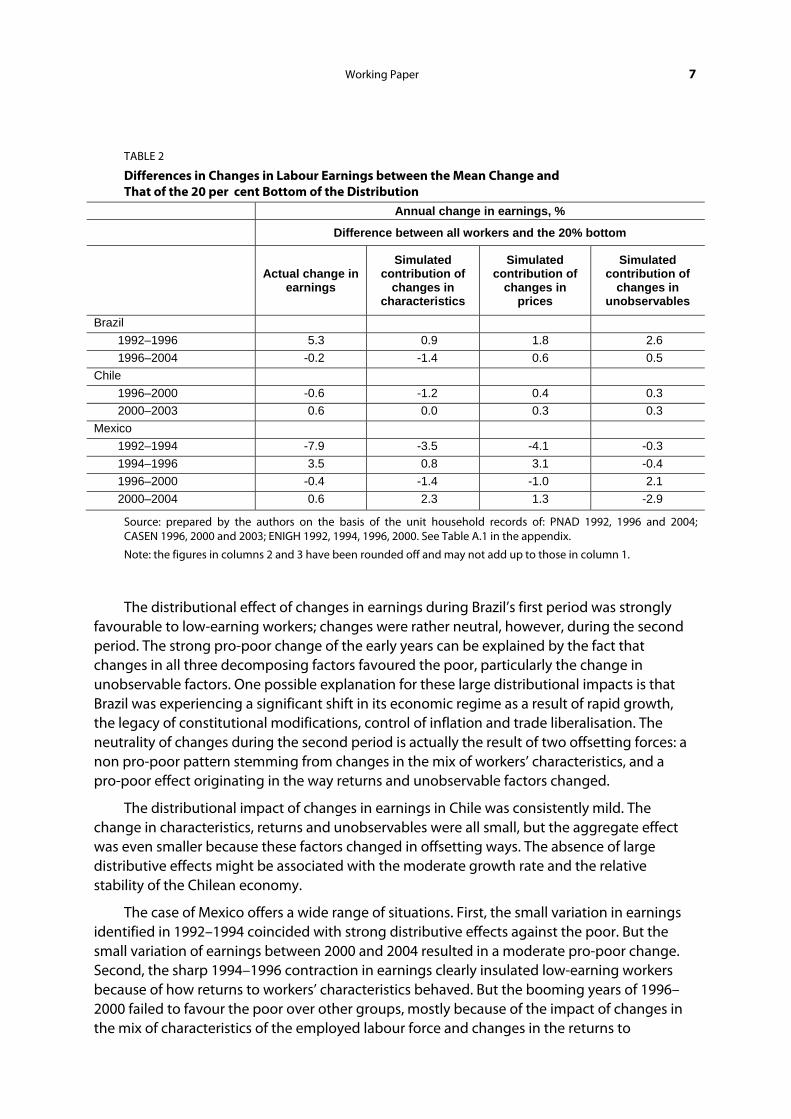
If the mean change in earnings is mostly determined by the aggregate behaviour of returns to workers’ characteristics, its distributional impact equally depends on both changes in the mix of workers’ characteristics and changes in returns to those characteristics. Table 2 presents the distributional impact of changes in earnings as the difference between the average change for all workers and changes in earnings for the 20 per cent lowest-earning workers.18 The table also suggests that changes in returns to workers’ characteristics and changes in unobservable factors tend to be more favourable to workers with low earnings, but changes in the structure of workers’ characteristics tend to favour non-poor workers.

Working Paper 7

TABLE 2

Differences in Changes in Labour Earnings between the Mean Change and That of the 20 per cent Bottom of the Distribution

Annual change in earnings, % Difference between all workers and the 20% bottom

Actual change in earnings

Simulated contribution of

changes in characteristics


changes in prices


changes in unobservables

Brazil 1992–1996 5.3 0.9 1.8 2.6 1996–2004 -0.2 -1.4 0.6 0.5

Chile 1996–2000 -0.6 -1.2 0.4 0.3 2000–2003 0.6 0.0 0.3 0.3

Mexico 1992–1994 -7.9 -3.5 -4.1 -0.3 1994–1996 3.5 0.8 3.1 -0.4 1996–2000 -0.4 -1.4 -1.0 2.1 2000–2004 0.6 2.3 1.3 -2.9

Source: prepared by the authors on the basis of the unit household records of: PNAD 1992, 1996 and 2004; CASEN 1996, 2000 and 2003; ENIGH 1992, 1994, 1996, 2000. See Table A.1 in the appendix.

Note: the figures in columns 2 and 3 have been rounded off and may not add up to those in column 1.

The distributional effect of changes in earnings during Brazil’s first period was strongly favourable to low-earning workers; changes were rather neutral, however, during the second period. The strong pro-poor change of the early years can be explained by the fact that changes in all three decomposing factors favoured the poor, particularly the change in unobservable factors. One possible explanation for these large distributional impacts is that Brazil was experiencing a significant shift in its economic regime as a result of rapid growth, the legacy of constitutional modifications, control of inflation and trade liberalisation. The neutrality of changes during the second period is actually the result of two offsetting forces: a non pro-poor pattern stemming from changes in the mix of workers’ characteristics, and a pro-poor effect originating in the way returns and unobservable factors changed.

The distributional impact of changes in earnings in Chile was consistently mild. The change in characteristics, returns and unobservables were all small, but the aggregate effect was even smaller because these factors changed in offsetting ways. The absence of large distributive effects might be associated with the moderate growth rate and the relative stability of the Chilean economy.

The case of Mexico offers a wide range of situations. First, the small variation in earnings identified in 1992–1994 coincided with strong distributive effects against the poor. But the small variation of earnings between 2000 and 2004 resulted in a moderate pro-poor change. Second, the sharp 1994–1996 contraction in earnings clearly insulated low-earning workers because of how returns to workers’ characteristics behaved. But the booming years of 1996–2000 failed to favour the poor over other groups, mostly because of the impact of changes in the mix of characteristics of the employed labour force and changes in the returns to


characteristics.19 Such a diverse variation of distributional effects may be related to the instability of the Mexican economy during these years—for example, the sharp decline in mean earnings in 1994–1996, the implementation of NAFTA, the rapid recovery of the economy in 1996–2000, and the recession in the early 2000s.

5 CHANGES IN WORKERS’ CHARACTERISTICS

This section looks at changes in the specific characteristics, with a view to gaining further insights into the contribution of changes in workers’ characteristics and their distributive consequences. Thus we concentrate on how the five types of characteristics (gender, area, age, sector, modality of work) change and influence the distribution of earnings.

5.1 CONTRIBUTING FACTORS TO THE CHANGE IN EARNINGS

The moderate but positive contribution of changes in workers’ characteristics across countries originates in three major factors: first, the improvement in the labour force’s level of education; second, the shift in the allocation of workers from low- to high-paying sectors; and third, the movement of workers from low- to high-earning age cohorts. The contribution of these factors is apparent from Figure 1, which shows how much each shift in the structure of workers’ characteristics adds to the mean change in earnings.

FIGURE 1

Contribution of Changes in Workers’ Characteristics to the Mean Change in Earnings

-3.00 -2.00 -1.00 0.00 1.00 2.00 3.00

br.92-96

br.96-04

ch.96-00

ch.00-03

mx.92.94

mx.94.96

mx.96.00

mx.00.04

age area sex education sector in/formal hours

Source: prepared by the authors on the basis of unit household records of: PNAD 1992, 1996 and 2004; CASEN 1996, 2000 and 2003; ENIGH 1992, 1994, 1996, 2000. See Table A.1 in the Appendix.

Note: the length of segments in each bar represents the value of the contribution of the corresponding characteristic and its total length equals the sum of the absolute value of the contribution of workers’ characteristics. Segments to the right (left) of zero represent positive (negative) contributions to earnings.

Working Paper 9

It is clear from Figure 1 that the rising educational level of the employed labour force is the most important factor pushing up earnings, both because the size of its contribution is large and because its sign is systematically positive. Obviously, the educational improvement of the work force is a long-term trend, but there is significant variability in the size of the contribution, notably in Chile and Mexico during 1994–1996 and 1996–2000. Such variations might be related to differences in how the unemployment rate by level of education responds to the business cycle.20

The contribution of employment shifts across sectors is the second most important factor. While its contribution was positive in most periods, its size is smaller than that of education.21 Some sector shifts clearly have a long-term component, the clearest example of which is the increase (decrease) in the share of services (agriculture). But shifts may also be the result of short-term forces, particularly during periods of high volatility, as exemplified by the marked fluctuations evident in Mexico.

Modifications in the age structure of the population also contributed positively to the change in earnings. The well documented trend of declining dependency ratios in Latin America means that the share of workers aged 25 to 40 increased over the share of young (15–24) and mature workers (41–65). Since workers aged 25–40 usually have higher earnings, the end result is a positive contribution to earnings. These changes are usually positive and small (Figure 1), reflecting slow-moving social and economic transformations, but contributions may also be large and negative, such as those provoked by short-term volatility. Examples of these are the small but negative contribution of the change in the age structure of the labour force in Chile during 2000–2003, and the very large and positive contribution of this factor during Mexico’s crisis years of 1994–1996. Large changes in the age composition of employment might be partly explained by differences in the employment elasticity of income growth among different age groups. The Mexican crisis provides a vivid example of how age and employment interact. During these years the share of prime-age workers (25–40 years old) increased rapidly. One might propose the hypothesis that these changes, rather than being structural, were part of the survival strategies of families whose out-of-work members might be forced to take any job at the cost of low wages and neglect of the household economy during periods of declining household income.22

Two specific characteristics make a negative contribution to the change in earnings: the increasing share of females in the labour force and the formal/informal composition of employment. The increasing presence of females in the working labour force is part of a longstanding and welcome trend, but since females usually receive lower wages and generate lower earnings when working in informal activities, the trend appears in our estimations as a force pushing down mean earnings. The change in the formal/informal composition of employment was generally negative and at times its size was significant. Changes in the formal/informal composition of employment in Brazil and Chile made a small but negative contribution, an indication of a slow decline in the share of formal activities. The impact of this factor is different in Mexico. In the years of fast economic reform in 1992–1994 and the crisis period 1994–1996, there was an increase in the relative share of informal activities that significantly depressed earnings. These changes were partially reversed during the recovery years of 1996–2000, when the number of formal jobs increased and made a positive contribution to earnings.


5.2 THE DISTRIBUTIONAL IMPACT

Changes in workers’ characteristics favoured high-earning workers most of the time. This bias stemmed mainly from the accumulated effect of two factors: the improvement in the working population’s education and the shift between full-time and part-time jobs. Figure 2 shows the decomposition of the distributional impact of changes in earnings by type of characteristic, and illustrates the wide variety of outcomes experienced by these countries. We highlight four: the effect of education; of full/part-time employment; of the sector of employment; and of changes in the composition of employment between formal and informal jobs.

FIGURE 2

Difference in the Contribution to Earnings of Changes in Workers’ Characteristics between the Bottom 20% and the Mean

-5 -4 -3 -2 -1 0 1 2 3 4

br.92-96

br.96-04

ch.96-00

ch.00-03

mx.92.94

mx.94.96

mx.96.00

mx.00.04

cf.age.g.x cf.area.x cf.sex.x cf.educ.x cf.indu.x cf.cont.x cf.hrs.x

Source: prepared by the authors on the basis of unit household records of: PNAD 1992, 1996 and 2004; CASEN 1996, 2000 and 2003; ENIGH 1992, 1994, 1996, 2000. See Table A.1 in the appendix.

Note: the length of each segment now represents the difference in the contribution that changes in the structure of each characteristic made to the earnings of the bottom 20 per cent and those of the entire working labour force; the length of the bar represents the sum of these absolute differences. Segments located to the right (left) of zero represent pro-poor changes (non pro-poor).

In most countries and periods, the educational improvement of the labour force does increase earnings but the increase is greater for high-paid workers. On average, the contribution of education to changes in earnings among low-paid workers was 0.32 percentage points less than the mean contribution. This difference was large in Brazil and in Mexico between 1992 and 1994, and again between 1996 and 2000. 23 The adverse consequence of the improvement in education arises because earnings are directly correlated with education. Over time, one should expect a reduction in the negative impact of educational attainment on the distribution of earnings, because the overall increase in education reduces current attainment disparities between educated and non-educated workers.

The movement of workers between full-time and part-time work is also an important factor causing poor workers’ earnings to lag. While the number of periods in which the effect

Working Paper 11

was pro-poor and the number in which it was not pro-poor is the same, the difference was significantly larger when the bias was against low-earning workers (a 0.37 percentage-point difference, compared to a 0.18 percentage-point difference). There appears to be a pattern whereby slow growth tends to be non pro-poor while rapid growth tends to be either neutral or pro-poor, suggesting that the shrinking of full-time employment during slow growth tends to affect low-earning workers more than other segments of the labour force.

Changes in the sector composition of employment had mixed impacts on the distribution of income. In Brazil and Chile the impact of these changes was small, but in Mexico it was large. In Mexico, changes clearly favoured low-earning workers in two periods: the 1994–1996 crisis and the slow growth years of 2000–2004. During the economic reform period of 1992–1994, workers with high earnings were the favoured group, while the distribution effect was practically neutral between 1996 and 2000. Finally, in all countries and periods, changes in the formal/informal composition of employment had a modest distributional impact, perhaps because the contribution of formal/informal shifts in employment was generally small.

6 CHANGES IN RETURNS TO CHARACTERISTICS

As indicated, the change in the mean return to workers’ characteristics was the main factor contributing to the change in earnings, and its distributional impact frequently tended to favour low-earnings workers. To analyze how changes in returns to the different characteristics account for the total change in earnings and its distributional impact, we recall that the mean change in returns is the result of adding changes in returns to seven types of characteristics. Three of them correspond to changes in relative prices representing dichotomous partitions of the labour force, namely urban/rural, male/female and full/part-time workers (40+/39- hours per working week), for which the rise in the price of one group necessarily represents a fall in the price of its counterpart—that is, males relative to females, urban relative to rural, and full relative to part-time. The other four types divide the labour force into more than two groups: age, education, sector and modality of work. The change in each of them, however, represents a variation relative to the return of the reference group.24 Returns to different characteristics and returns to specific characteristics within the same type can and do change in different ways. Tracking the changes can be intricate. Fortunately, in many instances few characteristics account for most of the overall change in returns and its distributional impact. We therefore focus on those changes that happen to make the most important contribution to the mean change and its distributional effect.

6.1 BRAZIL

Between 1992 and 1996, changes in the return to (price of) characteristics of Brazilian workers were dominated by the change in the return to the characteristic of “working in the service sector” and to that of “working as self-employed”. Table 3, column 1, shows the most important changes in returns ranked by the absolute size of the change. It suggests that there were two dominant factors: a 1.4 per cent increase in the return to workers in the service sector (relative to agriculture), and a -2.2 per cent fall in the return to formal employees (relative to the self-employed). The remaining changes in prices or returns were small.


TABLE 3

Changes in Relative Returns to Workers’ Characteristics (Prices): Brazil, 1992–2004

1992–1996 1996–2004

Prices

All workers Difference

Prices


Mean 20%-b. to mean Mean 20%-b. to

mean Accumulated prices 5.6 1.8 Accumulated prices -3.0 0.6 Formal /self-employed -2.2 1.8 Formal /self-employed 1.2 -0.8 Services 1.4 0.1 Urban -1.5 0.3 40+ hrs/week -0.8 0.2 Trade, Transport -0.5 0.2 Informal /self-employed 0.2 0.2 Informal /self-employed 0.6 0.5 Trade, Transport 0.6 -0.2 Manufacture -0.4 0.1

Source: prepared by the authors on the basis of the unit household records of: PNAD 1992, 1996 and 2004. See Table A.2 in the appendix.

Note: Column 1 of each country period presents the change in relative prices for the most important changes, ranked by the absolute size of the change. Column 2 of each country period presents the distributive impact of the corresponding change in returns to workers’ characteristics, as measured by the difference between the changes in the returns of the 20 per cent poorest workers to the average change for all workers.

Since actual workers might simultaneously face falling returns to some of their characteristics and enjoy increasing returns to others, it is useful to form an impression of the overall change in earnings that two hypothetical workers would face, which we chose to correspond to the mix of characteristics that would yield the most and least favourable change in returns. The most fortunate combination of workers’ characteristics—women aged between 25 and 64 with less than a university education, living in a rural area and working fewer than 40 hours a week as informal employees in the service sector—would benefit from an increase in earnings of 7.4 per cent a year. The least fortunate combination—young, urban males with primary or secondary education, working full-time as formal employees in the construction sector—would experience an increase in earnings of only 1.6 per cent a year.

The 1992–1996 change in returns favoured low-earning workers with 1.8 percentage point edge over the mean change. Most of the relative gain was reaped by low-earning workers who benefited from a decrease in the return to formal employees (Table 3, column 2). No other change in returns had a significant distributional impact.

Between 1996 and 2004, two changes in returns stand out. First, the -1.5 per cent fall in the return to the characteristic “working in urban location” (relative to rural location), and second, the 1.2 per cent rise in the return to “working as a formal employee” (relative to the self-employed). Correspondingly, the combination of characteristics experiencing the least fortunate change in returns starts by including residents of urban areas and specifying that they be prime-age males with secondary education who are self-employed in trade-transport activities and who work fewer than 40 hours a week. Workers with this combination of characteristics faced a reduction in their earnings of -4.7 per cent, significantly larger than the -3.0 per cent annual average for all workers. The most fortunate combination experienced a reduction of only -0.5 per cent—full-time informal employees in rural agriculture activities, aged between 40 and 64 and with incomplete primary education.

Changes in earnings during this second period penalised low-earning workers relatively less. Changes in returns to the modality of work featured the largest distributional effects.

Working Paper 13

On the one hand, the rise of returns to formal employees relative to the self-employed favoured high-earning workers, meaning that the earnings of workers at the low end of the distribution lagged 0.8 percentage points behind the mean change in returns. On the other hand, the fall in returns to informal employees relative to the self-employed gave low-earning workers a 0.5 percentage-points margin over the mean change in returns. Changes in the returns to other characteristics were all small, but since they all had a positive sign, they added up to a 0.6 percentage-point edge in favour of low-earning workers (see Table 3, column 4 and Table A.1 in the appendix).

6.2 CHILE

The overall contribution of changes in returns to the change in earnings was small in the case of Chile, mainly because there were various factors working in opposite directions, as changes in the returns to some particular characteristics were significant. Between 1996 and 2000 the most sizeable changes were the increase in the returns to the characteristics “working full time” (relative to part time) and “working as formal employee” (relative to the self-employed) (Table 4). To a lesser but still significant extent, there was a reduction in the return to the characteristic “working full time” (relative to part time). Looking beyond changes in individual factors and focusing on changes for combinations of characteristics reveals a wide range of rates of change. Workers with the most fortunate mix of characteristics saw their earnings increase by 2.7 per cent a year, while workers with the least fortunate combination actually suffered a -5.8 per cent decline in earnings. The “lucky” mix was composed of mature females in the age range 41–64, with primary education, living in rural areas and working in agriculture as formal, full-time employees.25 The “unlucky” mix comprised male workers aged 25–40, residents of urban areas, with secondary education, working fewer than 40 hours a week as self-employed in service activities.

During this first period, the change in prices favoured low-earning workers by a margin of 0.4 percentage points each year. The largest distributional effects originated in the change of the relative prices of informal and formal employees relative to the self-employed and the change in the return to the characteristic of “working full time”. These changes partially offset each other. While the increase in the returns to urban and formal employees did not favour low-earning workers, the rise in the return to informal employees did favour them. Thus the overall pro-poor change of the period was the result of accumulating a number of small changes favouring low-earnings workers.

During the second period, returns contributed 0.4 percentage points to the meagre 0.2 per cent increase in earnings. As in the previous period, however, there were sizeable changes in the returns to some particular characteristics. The most notable changes were a -2.4 per cent fall in the full-time/part-time relative price and a 1.0 per cent increase in the return to secondary/incomplete-primary education. Different combinations of characteristics resulted in wide-ranging changes in returns. While workers with the most fortunate mix saw their earnings rise by 2.0 per cent a year, the less fortunate experienced a decline of -2.7 per cent a year. The earnings of male urban workers aged 25 to 64, with secondary education, self- employed in service activities and working fewer than 40 hours a week, underwent the largest increase. The largest fall in earnings was experienced by young rural females with incomplete primary education, working more than 40 hours a week in agriculture as formal or informal employees. The overall distributive effect of changes in returns to workers’ characteristics


of the period was favourable to low-earning workers. The most important contributing factor tilting earnings in favour of these workers was the fall in the return to full-time workers and those with tertiary education.

TABLE 4

Changes in Returns to Individual Workers’ Characteristics (Prices): Chile, 1996–2003

1996–2000 2000–2003

Prices


Prices



mean Accumulated prices -0.1 0.4 Accumulated prices 0.4 0.3 40+/39- hrs-week 3.4 -0.4 40+/39- hrs-week -2.4 0.8 Formal /self-employed 2.4 -0.8 Secondary/incomp. primary 1.0 -0.2 Urban/rural -1.4 0.2 Urban/rural 0.4 -0.1 Informal /self-employed 0.7 0.9 Males/females 0.3 -0.1 Males/females -0.5 0.1 Tertiary/incomp. primary 0.3 -0.3

Source: prepared by the authors on the basis of the unit household records of: CASEN 1996, 2000 and 2003. See Table A.2 in the appendix.


6.3 MEXICO

Given the peculiarities of the Mexican case noted above, we discuss results that group periods before and after 1996. Amid the economic reforms of 1992–1994, earnings fell by -2.0 per cent. In the aggregate, changes in returns had no net contribution, but returns to specific characteristics changed significantly. The most marked changes were the rise in the male/female relative price and the increase in the returns to the characteristic “working in services” and “working in the trade-transport sector” (which includes finance; both changes are relative to agriculture). Between 1994 and 1996, earnings fell by -15.1 per cent, to which changes in returns contributed -16.4 percentage points. Changes in returns to particular characteristics were large. Changes in the returns to place of residence (urban/rural), length of the working day (full/part time), gender of the worker and the characteristic of “working in services” as opposed to “working in agriculture” all recorded rates higher than 2 per cent a year. Both periods featured a wide disparity (more than 20 percentage points) in the change of earnings between those workers with the most and least fortunate mix of characteristics.

As mentioned earlier, the first two years correspond to a period when a dramatic implementation of pro-market economic reforms coincided with harsh stabilisation anchored by the overvaluation of the exchange rate and cuts in the budget deficit. This combination produced equally dramatic changes in labour markets. The deep crisis of the following two years re-defined the dynamic forces of the economy and modified some of the previous policy interventions. The dynamics of the labour market in the period 1992–1994 were reversed during the crisis years. Indeed, the rise in the return to urban workers and formal employees, two of the leading changes in returns during 1992–1994, turned negative in the crisis years. Relatively modest changes, such as returns to males, prime age, university education

Working Paper 15

were also reversed. Moreover, the most fortunate mix of the first period turned into the least fortunate of the second period, and vice-versa.

The pattern of change in returns did not favour the poor during the first two years, consistent with the view that pro-market economic reforms tend to worsen the distribution of income. But the earnings of poor workers did not deteriorate as much during the years of economic recession, underlining the stylised fact that in Mexico economic stress tends to improve the relative position of the poor. The most important price changes determining the distributional impact of earnings were the same in both periods (the male/female, urban/rural and service/agriculture relative prices).

TABLE 5

Changes in Returns to Individual Workers Characteristics (Prices): Mexico, 1992–1996

1992–1994 1994–1996

Prices


Prices



mean Accumulated prices 0.0 -4.1 Accumulated prices -16.4 3.1 Males/females 2.7 -0.5 Urban/rural -3.7 1.4 Services/agriculture 2.7 -1.1 40+/39- hrs-week 2.6 -0.9 Trade-Transp/agriculture 2.4 -0.4 Males/females -2.4 0.5 Urban/rural 1.9 -0.7 Services/agriculture -2.4 1.1 Manufacture/agriculture 1.5 -0.4 Informal /self-employed -1.7 -0.4

Source: prepared by the authors on the basis of the unit household records of: ENIGH 1992, 1994, 1996, 2000. See Table A.2 in the appendix.

Note: Column 1 of each country period presents the change in relative prices for the most important changes, ranked by the absolute size of THE change. Column 2 of each country period presents the distributive impact of the corresponding change in returns to workers’ characteristics, as measured by the difference between the changes in the returns of the 20 per cent poorest workers to the average change for all workers.

The configuration of changes in returns shifted after 1996, as mean earnings increased by 4.4 per cent over the first four years and subsequently by 1.9 per cent a year, in tandem with the recovery of 1996–2000 and the slowdown of 2000–2004. The single most important change in returns to characteristics during the first four years was a 3.0 per cent increase in the urban/rural premium (Table 6). This change was so large that it dominated the change in earnings for many workers. Indeed, all rural workers experienced a reduction in earnings, regardless of changes in the returns to other characteristics. There was most probably a neglect of public policies and a more entrenched pro-urban bias in the economy.26 Next in importance was the increase in the formal-employee/self-employed relative price and the reduction in the return to prime age workers.

Compared to the previous two periods, workers experienced a lower range of changes in returns, but compared to the experience of Brazil and Chile the range continued to be significant. The earnings of workers with the most fortunate combination of characteristics increased by 2.7 per cent (urban males, with university education, working full time as informal employees in the construction sector), while those with the least fortunate mix experienced a reduction of -2.1 per cent (uneducated rural females working part time, self-employed in agricultural activities).


After 2000 there were new patterns of change in returns to workers’ characteristics. While the change in the urban/rural relative price remained the single most significant change (a -2.6 per cent fall), changes in the returns to the characteristic “working as employee, formal or informal” became important. Despite the economic slowdown (which usually decreases the dispersion of earnings), the change in earnings experienced by workers with the most and least advantageous mix of characteristics became wider. Workers with the most fortunate mix experienced an increase of 4.3 per cent (rural females, with no education, working in services or manufacturing as full-time informal employees), while those with the least fortunate combination experienced a reduction of -1.2 per cent (urban males, with primary education, working fewer than 40 hours a week, self-employed in trade and transportation activities).

The pattern of change in returns to workers’ characteristics was not pro-poor in the first four years, but it became pro-poor in the following four years. The main driving force in both periods was the change in the relative price of urban to rural labour, but the pro-urban bias of 1996–2000 favoured high-earning workers, while its subsequent reversal turned the pattern in favour of low-earnings workers.

Looking at changes throughout the 12 years, it should be noted that there was an increase in the relative price of working in manufacturing and services (relative to agriculture), and as formal and informal employees (relative to the self-employed), as well as a continuous reduction in the returns to secondary education. The frequent ups and downs in the returns to workers’ characteristics evident throughout the period are consistent with the high degree of economic volatility in the country.

TABLE 6

Changes in Returns to Individual Workers Characteristics (Prices): Mexico, 1996–2004

1996–2000 2000–2004

Prices


Prices All workers Difference

Mean 20%-b. to mean Mean 20%-b. to mean

Accumulated prices 2.3 -1.0 Accumulated prices 0.6 1.3 Urban 3.0 -1.0 Urban -2.6 1.0 Formal /self-employed 0.8 0.3 Informal /self-employed 0.9 0.3 Age 25–40 -0.8 0.3 Males -0.7 0.2 Males 0.5 -0.1 Formal /self-employed 0.6 -0.6 Informal /self-employed 0.3 -0.3 Age 25–40 0.4 -0.1

Source: prepared by the authors on the basis of the unit household records of: ENIGH 1992, 1994, 1996, 2000. See Table A.2 in the appendix.


6.4 RETURNS TO TERTIARY EDUCATION: BRAZIL, CHILE, MEXICO

Improving education and its distribution is a central component of any development strategy. The educational achievements of Brazil, Chile and Mexico made a positive and significant contribution to the earnings of workers. Its distribution, however, was not equitable. It is

Working Paper 17

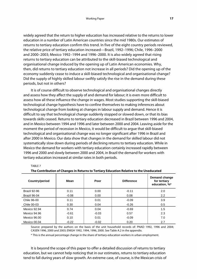
widely agreed that the return to higher education has increased relative to the returns to lower education in a number of Latin American countries since the mid 1980s. Our estimates of returns to tertiary education confirm this trend. In five of the eight country periods reviewed, the relative price of tertiary education increased—Brazil, 1992–1996; Chile, 1996–2000 and 2000–2003; Mexico 1992–1994 and 1996–2000. It is also widely agreed that rising returns to tertiary education can be attributed to the skill-biased technological and organisational change induced by the opening up of Latin American economies. Why, then, did returns to tertiary education not increase in all periods? Did the opening up of the economy suddenly cease to induce a skill-biased technological and organisational change? Did the supply of highly skilled labour swiftly satisfy the rise in the demand during these periods, but not in others?

It is of course difficult to observe technological and organisational changes directly and assess how they affect the supply of and demand for labour; it is even more difficult to assess how all these influence the change in wages. Most studies supporting the skill-biased technological change hypothesis have to confine themselves to making inferences about technological change from looking at changes in labour supply and demand. Hence it is difficult to say that technological change suddenly stopped or slowed down, or that its bias towards skills ceased. Returns to tertiary education decreased in Brazil between 1996 and 2004, and in Mexico between 1994 and 1996 and later between 2000 and 2004. Leaving aside for the moment the period of recession in Mexico, it would be difficult to argue that skill-biased technological and organisational change was no longer significant after 1996 in Brazil and after 2000 in Mexico. Our data show that changes in the demand for skilled labour did not systematically slow down during periods of declining returns to tertiary education. While in Mexico the demand for workers with tertiary education certainly increased rapidly between 1996 and 2000 and slowly between 2000 and 2004, in Brazil the demand for workers with tertiary education increased at similar rates in both periods.

TABLE 7

The Contribution of Changes in Returns to Tertiary Education Relative to the Uneducated

Country/period Mean Poor Difference Demand change

for tertiary education, %*

Brazil 92-96 0.11 0.00 -0.11 2.0 Brazil 96-04 -0.08 0.00 0.08 2.2 Chile 96-00 0.11 0.01 -0.09 3.9 Chile 00-03 0.30 0.04 -0.26 0.5 Mexico 92.94 0.74 0.04 -0.69 1.5 Mexico 94.96 -0.61 -0.03 0.57 2.3 Mexico 96.00 0.10 0.01 -0.09 7.0 Mexico 00.04 -0.22 -0.02 0.20 2.7

Source: prepared by the authors on the basis of the unit household records of: PNAD 1992, 1996 and 2004; CASEN 1996, 2000 and 2003; ENIGH 1992, 1994, 1996, 2000. See Table A.2 in the appendix.

* This is the annual percentage change in the share of tertiary-education workers in urban employment.

It is beyond the scope of this paper to offer a detailed discussion of returns to tertiary education, but we cannot help noticing that in our estimates, returns to tertiary education tend to fall during years of slow growth. An extreme case, of course, is the Mexican crisis of


1995, when arguably the wages of overpaid executives and professionals in the public and private sectors fell sharply. This suggests that factors related to the business cycle might also play a significant role, above and beyond assumed technological and organisational change. In the case of Mexico, moreover, it has been shown that the institutional setting, such as fixing minimum wages, may play an important role in controlling wage increases for low-earning workers but leave unchecked wage increases for high-earning workers.27 In this case, the data might show a rise in the returns to tertiary education.

7 CONCLUSION

Employment is one of the main problems facing Latin America. Slow, unstable growth and capital-intensive investments in the 1990s yielded small gains in labour conditions, as the quality of available jobs did not improve and unemployment increased. As expected, poverty decreased slowly and inequality remained high. In this paper we have looked at labour earnings in three mature and relatively stable Latin American countries, Brazil, Chile and Mexico. The aim of the paper was to shed light on the factors behind observed changes in mean earnings and to assess their distributional impact. The paper’s methodology, based on regression analysis and simulation techniques, allowed us to distinguish three types of contributing factors to observed changes in earnings: (i) changes in the socio-demographic characteristics of workers—age, education, gender, rural or urban residency—and changes in the sector and formal nature of employment; (ii) changes in the returns (prices) to those characteristics; and (iii) changes in unobserved factors. To gauge the distributional impact of changes in earnings the paper undertook a simple comparison between the economy-wide average change in earnings and the average for the bottom 20 per cent of the distribution.

Annual rates of change in labour earnings varied widely during the eight growth periods considered here, ranging from the large contraction of earnings in Mexico during the crisis years 1994–1996 to Brazil’s rapid increase in earnings during 1992–1996. On the whole, the earnings of the bottom 20 per cent of workers performed better than mean earnings. Changes in prices were the main contributor to both the rise and fall of mean earnings. The contribution of changes in returns was volatile but generally pro-poor. The contribution of changes in workers’ characteristics was generally small, but stable and generally positive. The drawback was that its distributional impact was often not pro-poor. Changes in unobservable factors were the least important, but they often favoured low-earning workers.

Several specific changes in the structure of workers’ characteristics made a significant contribution to the increase in earnings. The single most significant change, across all countries and periods, was the increase in the labour force’s level of education. The improvement of education also increased the earnings of poor workers, but the rate at which their earnings increased was systematically smaller than the mean rate. This finding underscores the need to close the educational gaps among workers and improve the quality of the education received by the poor. Consistent with the demographic transition that the region is experiencing, the share of workers in the age range 25–40 followed a clear upward trend that made a positive and significant contribution to earnings. At a more modest scale, softened by countries’ economic downturns, changes in the sectoral composition of employment made a positive contribution to earnings. This finding suggests that workers were moving from low-paid to high-paid sectors, mainly from agriculture to services. The paper also found that changes in the mix of formal/informal workers did not have a definite pattern and were somewhat cyclical.

Working Paper 19

The distributional impact of changes in the structure of workers’ characteristics depended mostly on changes in the sector of employment. But no clear trend favouring low-earning workers emerged, suggesting the need to implement policies to ensure that low-earning workers have more upward mobility across sectors, particularly during periods of rapid earnings growth.

Changes in returns to workers’ characteristics were a major determinant of the overall change in earnings. Changes in the return to the sector of employment were very important in Brazil and Mexico between 1992 and 1996. Changes in the relative prices of full-time and part-time workers figured prominently in Chile. In Mexico after the 1995 crisis, the most influential change was the rise and fall of the urban/rural relative price of labour. The distributional impact of these changes depended on the cycle: the impact tended to be non-pro-poor when earnings were growing fast and pro-poor when the change in earnings was slow or negative.

The male/female, urban/rural and formal/informal employee to self-employed relative prices decreased consistently in Brazil, which suggests that structural transformations are benefiting the distribution of earnings. There was also a consistent increase in the relative price of formal and informal-employee relative to self-employed workers during the years after the economic crisis in Mexico. Since these changes affect the distribution of earnings in opposite directions, no definitive improvement in the distribution of earnings was derived from them. Finally, the paper also discussed the change in the (relative) returns to tertiary education. The results confirm the general finding of rising returns to tertiary education, but the paper also called attention to the fact that returns to tertiary education decreased in several periods. Such reductions highlight the possibility that forces other than skill-biased technological and organisational change, often associated with liberalisation and the opening up of economies, might also have played an important role in shaping the change in relative returns to education. Short-term cyclical factors, as well as institutional settings and wage policies, might be among the most important of these other forces.


APPENDIX

METHODOLOGY

The procedure is as follows. First, we estimate one regression for each year:

∑ −

=++=

1

10ln J

j itijtjttit uxY ββ (1)

where lnYit is the logarithm of labour income for individual i in time t; β s are the returns to workers characteristics or prices of labour characteristics, more specifically t0β is the constant for period t, jtβ is the estimated parameter for the variable Xj in year t or the value of the j workers’ characteristic, and uit is the residual for individual i in year t; and time refers to two years, t = {1, 2}.

The simulation of what would have happened if only the prices (returns) of characteristics changed from period one to period two is as follows. For each individual in the dataset of year one we compute what his/her earnings would be if the returns or prices of labour characteristics were the returns of year two instead of the actual returns of year one. We then build an “auxiliary” distribution of earnings by replacing the estimated coefficients for year 1 (β1j) with those for year 2, (β2j).

∑ −

=++=

1

1 11202,*ln J

j iijauxi uxY ββ (2)

To simulate what would have happened if, in addition to the prices, the mix of characteristics of the working labour force had also been those of year two, we replace the set of values corresponding to the characteristics of year one Xi1j with those of year two, Xi2j. in equation (2). This gives another “auxiliary” distribution of individual earnings, had the prices and workers’ characteristics of the year two be in place in year one, along with the unobservables of year one:

∑ −

=++=

1

1 12202,**ln J

j iijauxi uxY ββ (3)

Notice that in order to generate this simulation we have to impose the structure of residuals of year one upon the structure of Xs of year two. Given that the residuals of the labour income equation can be expressed as having two components (the percentile to which the individual belongs in the labour income distribution itθ and the distribution function of the residuals ()tF ), one can express the residuals as:

1( )it t it itu F Xθ−= | (4)

Working Paper 21

where 1( )t it itF Xθ− | is the inverse cumulative residual distribution for workers with characteristics itX in year t . Thus we operate a rank-preserving transformation of the residuals of year 1 to the set of variables Xs of year 2:28

111

' −= Fu t ( θ | X 2i ) (5)

Finally, replacing ui1 with the residual for the period 2, ui2, we return to equation (1) as if it was estimated for the second year.

∑ −

=++==

1

1 222022, ln***ln J

j iijiauxi uxYY ββ (6)

In this paper we look at simulations of hypothetical changes in only one of the components at the time—that is, prices, characteristics and residuals separately. The simulation of the change in prices only is given directly by equation (2); the change in characteristics only is given by subtracting equation (3) from equation (2); and the change in unobservables only is given by subtracting equation (6) from equation (3).

DATA

For Brazil we use the Pesquisa Nacional por Amostra de Domicílios (PNAD), 1992, 1996 and 2004, conducted and disseminated by the Instituto Brasileiro de Geografia e Estatistica (IBGE: www.ibge.gov.br). The survey is conducted during September and the sample size varies from 317,315 to 399,354 individuals. For Chile we use the Encuesta de Caracterización Socioeconomica (CASEN), 1996, 2000 and 2003, conducted and disseminated by the Ministerio de Planificación (MIDEPLAN: www.mideplan.cl/casen). The survey is conducted during November and the sample size varies from 134,262 to 257,077 individuals. For Mexico we use the Encuesta Nacional de Ingreso y Gasto de los Hogares (ENIGH), 1992, 1994, 1996, 2000 and 2004, conducted and disseminated by the Instituto Nacional de Estadistica, Geografía e Informatica (INEGI: www.inegi.gob.mx). The survey is conducted from August to November, except for 1994, when it was conducted from September to December; and the sample size varies from 50,862 to 91,738 individuals.

These datasets contain rich information on total income, labour income and other incomes, with different degrees of detail. We kept the concepts of labour income sources used in each survey; they are comparable throughout the years covered in this study. In all cases, we deflated current income by the official consumer price index of the month in which the survey was collected, using the date of the most recent survey as the base. In the case of Brazil, we used total labour income as provided in the micro data. IBGE does not correct income variables for non-response and under-declaration. We dealt with non-responses by excluding households where at least one member reported income but the amount was unknown. Since the sample size for PNAD is large, this procedure does not affect the results obtained. The database for Chile published by MIDEPLAN is already corrected for non-response and under-declaration with a methodology proposed by ECLAC.29 The micro data for Mexico provide fairly detailed reporting of household income. To maintain comparison with Brazil and Chile, we limited the analysis to monetary income. We calculated monthly income as the adjusted average of income earned in the six months before the interview, following the methodology used by the Mexican government to make official estimates of poverty. There are no cases of no-response in the dataset and no correction for under-declaration.

TABLES

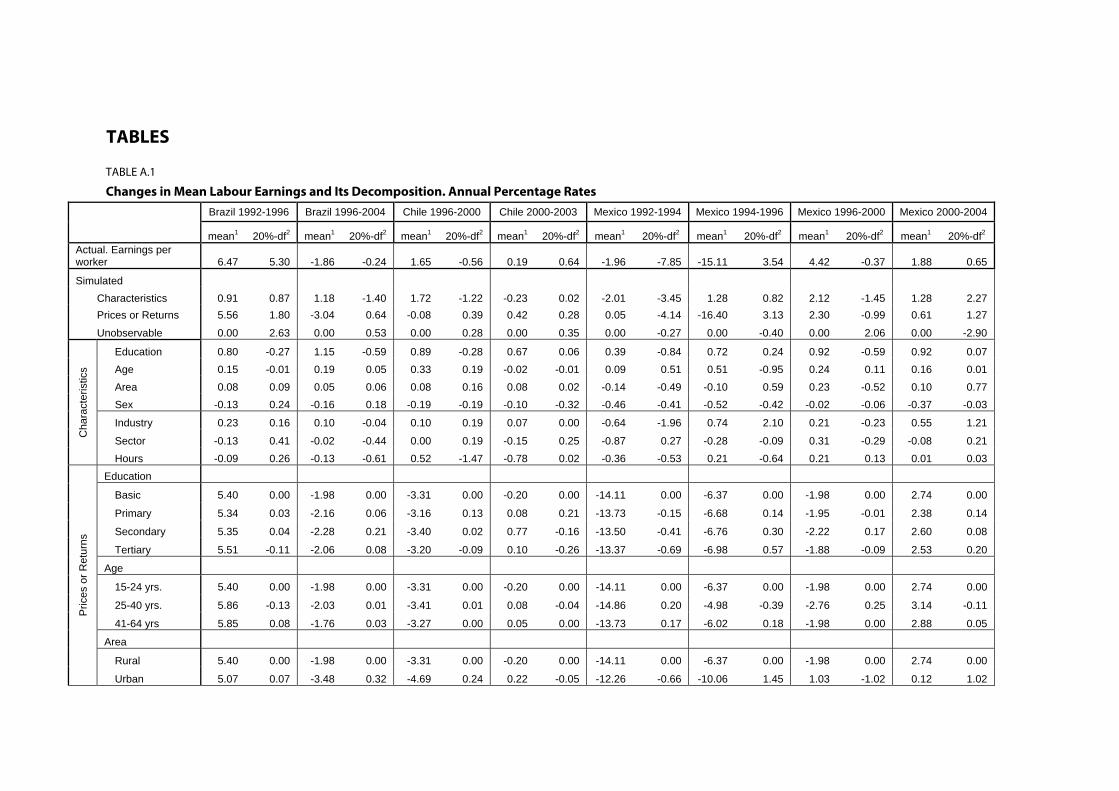
TABLE A.1

Changes in Mean Labour Earnings and Its Decomposition. Annual Percentage Rates

Brazil 1992-1996 Brazil 1996-2004 Chile 1996-2000 Chile 2000-2003 Mexico 1992-1994 Mexico 1994-1996 Mexico 1996-2000 Mexico 2000-2004

mean1 20%-df2 mean1 20%-df2 mean1 20%-df2 mean1 20%-df2 mean1 20%-df2 mean1 20%-df2 mean1 20%-df2 mean1 20%-df2 Actual. Earnings per worker 6.47 5.30 -1.86 -0.24 1.65 -0.56 0.19 0.64 -1.96 -7.85 -15.11 3.54 4.42 -0.37 1.88 0.65

Simulated Characteristics 0.91 0.87 1.18 -1.40 1.72 -1.22 -0.23 0.02 -2.01 -3.45 1.28 0.82 2.12 -1.45 1.28 2.27 Prices or Returns 5.56 1.80 -3.04 0.64 -0.08 0.39 0.42 0.28 0.05 -4.14 -16.40 3.13 2.30 -0.99 0.61 1.27

Unobservable 0.00 2.63 0.00 0.53 0.00 0.28 0.00 0.35 0.00 -0.27 0.00 -0.40 0.00 2.06 0.00 -2.90

Cha

ract

eris

tics

Education 0.80 -0.27 1.15 -0.59 0.89 -0.28 0.67 0.06 0.39 -0.84 0.72 0.24 0.92 -0.59 0.92 0.07 Age 0.15 -0.01 0.19 0.05 0.33 0.19 -0.02 -0.01 0.09 0.51 0.51 -0.95 0.24 0.11 0.16 0.01 Area 0.08 0.09 0.05 0.06 0.08 0.16 0.08 0.02 -0.14 -0.49 -0.10 0.59 0.23 -0.52 0.10 0.77 Sex -0.13 0.24 -0.16 0.18 -0.19 -0.19 -0.10 -0.32 -0.46 -0.41 -0.52 -0.42 -0.02 -0.06 -0.37 -0.03

Industry 0.23 0.16 0.10 -0.04 0.10 0.19 0.07 0.00 -0.64 -1.96 0.74 2.10 0.21 -0.23 0.55 1.21

Sector -0.13 0.41 -0.02 -0.44 0.00 0.19 -0.15 0.25 -0.87 0.27 -0.28 -0.09 0.31 -0.29 -0.08 0.21 Hours -0.09 0.26 -0.13 -0.61 0.52 -1.47 -0.78 0.02 -0.36 -0.53 0.21 -0.64 0.21 0.13 0.01 0.03

Pric

es o

r Ret

urns

Education

Basic 5.40 0.00 -1.98 0.00 -3.31 0.00 -0.20 0.00 -14.11 0.00 -6.37 0.00 -1.98 0.00 2.74 0.00

Primary 5.34 0.03 -2.16 0.06 -3.16 0.13 0.08 0.21 -13.73 -0.15 -6.68 0.14 -1.95 -0.01 2.38 0.14

Secondary 5.35 0.04 -2.28 0.21 -3.40 0.02 0.77 -0.16 -13.50 -0.41 -6.76 0.30 -2.22 0.17 2.60 0.08

Tertiary 5.51 -0.11 -2.06 0.08 -3.20 -0.09 0.10 -0.26 -13.37 -0.69 -6.98 0.57 -1.88 -0.09 2.53 0.20

Age

15-24 yrs. 5.40 0.00 -1.98 0.00 -3.31 0.00 -0.20 0.00 -14.11 0.00 -6.37 0.00 -1.98 0.00 2.74 0.00

25-40 yrs. 5.86 -0.13 -2.03 0.01 -3.41 0.01 0.08 -0.04 -14.86 0.20 -4.98 -0.39 -2.76 0.25 3.14 -0.11

41-64 yrs 5.85 0.08 -1.76 0.03 -3.27 0.00 0.05 0.00 -13.73 0.17 -6.02 0.18 -1.98 0.00 2.88 0.05

Area

Rural 5.40 0.00 -1.98 0.00 -3.31 0.00 -0.20 0.00 -14.11 0.00 -6.37 0.00 -1.98 0.00 2.74 0.00

Urban 5.07 0.07 -3.48 0.32 -4.69 0.24 0.22 -0.05 -12.26 -0.66 -10.06 1.45 1.03 -1.02 0.12 1.02

Brazil 1992-1996 Brazil 1996-2004 Chile 1996-2000 Chile 2000-2003 Mexico 1992-1994 Mexico 1994-1996 Mexico 1996-2000 Mexico 2000-2004

mean1 20%-df2 mean1 20%-df2 mean1 20%-df2 mean1 20%-df2 mean1 20%-df2 mean1 20%-df2 mean1 20%-df2 mean1 20%-df2

Sex

Female 5.40 0.00 -1.98 0.00 -3.31 0.00 -0.20 0.00 -14.11 0.00 -6.37 0.00 -1.98 0.00 2.74 0.00

Male 4.98 0.10 -2.34 0.07 -3.83 0.07 0.12 -0.06 -11.37 -0.54 -8.82 0.55 -1.49 -0.13 2.09 0.17

Industry

Agriculture 5.40 0.00 -1.98 0.00 -3.31 0.00 -0.20 0.00 -14.11 0.00 -6.37 0.00 -1.98 0.00 2.74 0.00

Manufacturing 5.87 -0.18 -2.34 0.14 -3.63 0.09 -0.22 0.01 -12.59 -0.36 -7.77 0.52 -1.84 -0.03 3.01 -0.07

Construction 5.73 -0.15 -2.12 0.07 -3.55 0.07 0.05 -0.05 -13.39 -0.39 -7.28 0.44 -1.71 -0.08 2.76 -0.01

Trade/transport 6.00 -0.25 -2.50 0.18 -3.70 0.07 -0.27 0.01 -11.74 -0.35 -7.86 0.40 -1.92 -0.01 2.42 0.05

Services (other) 6.77 0.08 -2.24 -0.02 -3.82 0.06 0.06 -0.01 -11.37 -1.14 -8.79 1.07 -1.88 -0.03 2.95 -0.06

Sector

Self-employed 5.40 0.00 -1.98 0.00 -3.31 0.00 -0.20 0.00 -14.11 0.00 -6.37 0.00 -1.98 0.00 2.74 0.00 Formal

employee 3.21 1.82 -0.79 -0.83 -0.92 -0.79 -0.30 0.04 -14.48 0.31 -5.41 -0.83 -1.66 -0.29 3.38 -0.57 Informal

employee 5.61 0.21 -1.40 0.46 -2.62 0.87 -0.30 -0.13 -13.70 0.14 -8.06 -0.39 -1.19 0.26 3.63 0.27

Hours Part time (39-

hrs.) 5.40 0.00 -1.98 0.00 -3.31 0.00 -0.20 0.00 -14.11 0.00 -6.37 0.00 -1.98 0.00 2.74 0.00 Full time (40+

hrs.) 4.56 0.19 -1.30 -0.14 0.11 -0.36 -2.57 0.76 -13.24 -0.25 -3.74 -0.88 -2.00 0.01 2.39 0.12

Notes: 1) Refers to the mean change in the earnings of all workers; 2) refers to the mean change in the earnings of the 20 per cent bottom of the earnings distribution.

Source: prepared by the authors on the basis of the unit household records of: PNAD 1992, 1996 and 2004; CASEN 1996, 2000 and 2003; ENIGH 1992, 1994, 1996, 2000.

TABLE A.2

Changes in Relative Prices of Workers’ Characteristics. Annual Percentage Rates

Brazil 1992-1996 Brazil 1996-2004 Chile 1996-2000 Chile 2000-2003 Mexico 1992-1994

Mexico 1994-1996

Mexico 1996-2000

Mexico 2000-2004

mean1 20%-df2 mean1 20%-df2 mean1 20%-df2 mean1 20%-df2 mean1 20%-df2 mean1 20%-df2 mean1 20%-df2 mean1 20%-df2

Actual earnings per worker 6.47 5.30 -1.86 -0.24 1.65 -0.56 0.19 0.64 -1.96 -7.85 -15.11 3.54 4.42 -0.37 1.88 0.65

Simulated Prices 5.56 1.80 -3.04 0.64 -0.08 0.39 0.42 0.28 0.05 -4.14 -16.40 3.13 2.30 -0.99 0.61 1.27 Reference population 5.40 0.00 -1.98 0.00 -3.31 0.00 -0.20 0.00 -14.11 0.00 -6.37 0.00 -1.98 0.00 2.74 0.00

Rel

ativ

e P

rices

or R

etur

ns

Education

Primary / No Edc. -0.05 0.03 -0.18 0.06 0.15 0.13 0.28 0.21 0.37 -0.15 -0.31 0.14 0.03 -0.01 -0.36 0.14

Secondary / No Edc. -0.05 0.04 -0.30 0.21 -0.09 0.02 0.96 -0.16 0.61 -0.41 -0.39 0.30 -0.24 0.17 -0.14 0.08

Tertiary / No Edc. 0.11 -0.11 -0.08 0.08 0.11 -0.09 0.30 -0.26 0.74 -0.69 -0.61 0.57 0.10 -0.09 -0.22 0.20

Age

25-40 / 15-24 yrs. 0.46 -0.13 -0.05 0.01 -0.10 0.01 0.27 -0.04 -0.76 0.20 1.39 -0.39 -0.78 0.25 0.40 -0.11

41-64 / 15-24 yrs 0.45 0.08 0.22 0.03 0.04 0.00 0.24 0.00 0.37 0.17 0.35 0.18 0.01 0.00 0.14 0.05

Area

Urban / Rural -0.32 0.07 -1.50 0.32 -1.38 0.24 0.42 -0.05 1.85 -0.66 -3.69 1.45 3.01 -1.02 -2.62 1.02

Sex

Male / Female -0.42 0.10 -0.36 0.07 -0.52 0.07 0.32 -0.06 2.74 -0.54 -2.45 0.55 0.49 -0.13 -0.66 0.17

Industry

Manufacturing / Agric. 0.48 -0.18 -0.35 0.14 -0.32 0.09 -0.02 0.01 1.52 -0.36 -1.40 0.52 0.14 -0.03 0.27 -0.07

Construction / Agric. 0.33 -0.15 -0.14 0.07 -0.24 0.07 0.24 -0.05 0.72 -0.39 -0.91 0.44 0.27 -0.08 0.02 -0.01

Trade-transport / Agric. 0.61 -0.25 -0.52 0.18 -0.39 0.07 -0.07 0.01 2.36 -0.35 -1.49 0.40 0.06 -0.01 -0.32 0.05

Services (other) / Agric. 1.38 0.08 -0.26 -0.02 -0.51 0.06 0.25 -0.01 2.73 -1.14 -2.42 1.07 0.10 -0.03 0.20 -0.06

Sector

Formal employee / Self-ed. -2.18 1.82 1.20 -0.83 2.39 -0.79 -0.10 0.04 -0.37 0.31 0.96 -0.83 0.32 -0.29 0.64 -0.57

Informal employee / Self-ed. 0.21 0.21 0.58 0.46 0.69 0.87 -0.10 -0.13 0.41 0.14 -1.69 -0.39 0.79 0.26 0.89 0.27

Hours

40+ / 39- hours -0.84 0.19 0.68 -0.14 3.42 -0.36 -2.37 0.76 0.86 -0.25 2.63 -0.88 -0.02 0.01 -0.36 0.12 Notes: 1) Refers to the mean change in the earnings of all workers; 2) refers to the mean change in the earnings of the 20 per cent bottom of the earnings distribution. Source: prepared by the authors on the basis of the unit household records of: PNAD 1992, 1996 and 2004; CASEN 1996, 2000 and 2003; ENIGH 1992, 1994, 1996, 2000. Abbreviations: Agric. Indicates Agriculture; Self-ed. Indicates Self employed.

TABLE B.1

Definition of variables Brasil Chile Mexico Age groups 1 15-24 yrs 15-24 yrs 15-24 yrs 2 25-44 yrs 25-44 yrs 25-44 yrs 3 45-64 yrs 45-64 yrs 45-64 yrs Area 1 Urban Urban Urban 2 Rural Rural Rural Gender 1 Male Male Male 2 Female Female Female Education 1 Until Primary incomplete Until Primary incomplete Until Primary incomplete 2 Primary complete Primary complete Primary complete 3 Secondary complete Secondary complete Secondary complete 4 Terciary complete Terciary complete Terciary complete Industry 1 Agrícola Agric. Caza Silvicultura Actividades primarias 2 Indústria Industria Industria 3 Construção Construccion Construcción 4 Comércio, Alojamento, Transporte e Comunicação Comercio, Transporte Y Comunicaciones Comercio, Transporte, comunic. y ag. viajes 5 Serviços Servicios Servicios Contract 1 Empregado com carteira Empleado Formal Empleado Formal 2 Empregado sem carteira Empleado Informal Empleado Informal 3 Funcionário Público Empleado Publico Empleado Publico 4 Conta-própria Cuenta propia Cuenta propia 5 Empregador Patrón o empleador Patrón 6 Empregado doméstico Doméstico Doméstico

Note: Names in light ink correspond to the reference population (entering as zero in regression dummies).

REFERENCES

Alarcon, Diana and Eduardo Zepeda (2004). ‘Economic Reform or Social Development? The Challenges of a Period of Reform in Latin America: Case Study of Mexico’, Journal of Social Development Studies 32 (1), 59–86.

Berry, Albert (2007). ‘A Review of Literature and Evidence on the Economic and Social Effects of Economic Integration in Latin America: Some Policy Implications’. Washington, DC, Inter-American Development Bank (mimeo).

Bourguignon, François and Francisco Ferreira (2005). ‘Decomposing Changes in the Distribution of Household Incomes. Methodological Aspects’ in François Bourguignon, Francisco Ferreira and Nora Lustig (eds), The Microeconomics of Income Distribution Dynamics in East Asia and Latin America. Washington, DC, World Bank and Oxford University Press, 17–46.

ECLAC, IPEA and UNDP (2002). Meeting the Millennium Poverty Reduction Targets in Latin America and the Caribbean. Santiago, Chile, ECLAC, IPEA, UNDP.

Economic Commission for Latin America and the Caribbean, (ECLAC) (2006). Panorama Social de America Latina. Santiago, Chile, ECLAC.

Fairris, David, Gurleen Popli and Eduardo Zepeda (2008). ‘Minimum Wages and the Wage Structure in Mexico’, Review of Social Economy 66 (2), 181–208.

Fields, Gary S. (2002). ‘Accounting for Income Inequality and Its Change: A New Method, with Application to the Distribution of Earnings in the United States’. Ithaca, Cornell University (mimeo).

Fields, Gary S. and Serguei Soares (2005). ‘The Microeconomics of Changing Income Distribution in Malaysia’ in François Bourguignon, Francisco Ferreira and Nora Lustig (eds), The Microeconomics of Income Distribution Dynamics in East Asia and Latin America. Washington, DC, World Bank and Oxford University Press.

Galli, Rossana (2004). ‘Labor Standards and Informal Employment in Latin America’, World Development 32 (5), 809–828..

Inter-American Development Bank (2004). Se Buscan Buenos Empleos. Los Mercados Laborales en América Latina. Informe de Progreso Económico y Social. Washington, DC, IDB.

Islam, Rizwanul (2004). ‘The Nexus of Economic Growth, Employment and Poverty Reduction: An Empirical Analysis’, Issues in Employment and Poverty Discussion Paper 14. Geneva, ILO.

Juhn, Chinhui, Kevin M. Murphy and Brooks Pierce (1993). ‘Wage Inequality and the Rise in Returns to Skill’, Journal of Political Economy 101 (3), 410–442.

Kakwani, Nanak, Shahid Khandkerb and Hyun H. Sonc (2004). ‘Pro-Poor Growth: Concepts and Measurement with Country Case Studies’, International Poverty Centre Working Paper 1, Brasilia, IPC.

Katz, Jorge and Jorge Stumpo (2001). ‘Regímenes sectoriales, productividad y competitividad internacional’, Revista de la CEPAL 75, Santiago, Chile, CEPAL.

Khan, Azizur (2001). ‘Employment Policies for Poverty Reduction’, Issues in Employment and Poverty Discussion Paper. Geneva, ILO.

Legovini, Arianna, Cesar Buillon and Nora Lustig (2005). ‘Can Education Explain Changes in Income Inequality in Mexico?’ in François Bourguignon, Francisco Ferreira and Nora Lustig (eds), The Microeconomics of Income Distribution Dynamics in East Asia and Latin America. Washington, DC, World Bank and Oxford University Press.

Organización Internacional del Trabajo (OIT), (2006a). Trabajo decente en las Americas: una agenda hemisferica, 2006-2015. Brasila, OIT.

Organización Internacional del Trabajo (OIT) (2006b). Panorama Laboral 2006. Lima, OIT.

Osmani, S. R. (2002). ‘Exploring the Employment Nexus: Topics in Employment and Poverty’. A Report Prepared for the Task Force on the Joint ILO-UNDP Programme on Employment and Poverty. UNDP-ILO.

Paes de Barro, Ricardo, Miguel Foguel and Gabriela Ulyssea (eds.) (2006). Desigualdade de Renda no Brasil: Uma analise da queda recente. Brasilia, Instituto de Pesquisa Economica Aplicada.

Paes de Barros, Ricardo, Samuel Franco and Rosane Mendonça (2007). ‘A Recente Queda da Desigualdade de Renda e o Acelerado Progresso Educacional Brasileiro da Ùltima Década’, Texto para Discussaão 1304, Brasilia, Instituto de Pesquisa Economica Aplicada.

Soares, Fabio, Sergei Soares, Marcelo Medeiros and Rafael Osorio (2006). ‘Cash Transfer Programmes in Brazil: Impacts on Inequality and Poverty’, International Poverty Centre Working Paper 21, Brasilia, IPC.

Son, Hyun and Nanak Kakwani (2006). ‘Global Estimates of Pro-Poor Growth’, International Poverty Centre Working Paper 31, Brasilia, IPC.

Tokman, Victor (2007). ‘Empleo y protección: una vinculación necesaria’ in Carlos Gerardo Molina (ed.), Universalismo Básico: Hacia una nueva política social para América Latina. Washington, DC, Inter-American Development Bank.

Yun, Myeong-Su (2001). ‘Comparing Inequalities Using Earnings Equations’. London, Ontario, University of Western Ontario (mimeo).

Zepeda, Eduardo, Diana Alarcón, Fabio Veras Soares and Rafael Guerreiro Osorio (2007). ‘ Growth, Poverty and Employment in Brazil, Chile and Mexico’, International Poverty Centre Working Paper 42, Brasilia.

.

NOTES

1. See, for example, ILO (2006a, b), IDB (2004), ECLAC (2006).

2. See, for example, Alarcon and Zepeda (2004), Berry (2007), Galli (2004) and Tokman (2007).

3. Also, see Son and Kakwani (2006).

4. GDP per capita growth estimates for Brazil, Chile and Mexico in this section are calculated from GDP figures in constant US PPP dollars based on the World Bank’s WDI online data.

5. See Soares et al. (2006) and Paes de Barro et al. (2007).

6. Informality is defined as non-professional self-account employees without registration, and domestic workers. See Table B.1 in the appendix.

7. This approach diverges from the usual discussion of poverty and labour. The lowest paid workers do not necessarily belong to the poorest households. But focusing on the lowest paid workers gives a good approximation of poverty. Consider, for example, Brazil in 1992. According to household data, while only about half of the 20 per cent lowest paid workers belonged to the 20 per cent poorest households, more than 90 per cent of the workers in the lower half of the earnings distribution did belong to the 20 per cent poorest households.

8. See Kakwani et al. (2004). For readers interested in more details about the distributive impact, we computed mean changes at 5 cumulative percentage points of the earnings distribution. These are available upon request from the authors.

9. This is, in a way, a dynamic version of the well know Oaxaca-Blinder procedure.

10. See also Bourguignon and Ferreira (2005), Fields (2002) and Yun (2001). See the section on methodology in the appendix.

11. See also Bourguignon and Ferreira (2005), Fields (2002) and Yun (2001). See the section on methodology in the appendix.

12. Regressions did not use Heckman’s self-selection adjustment since its requirements render it of little practical utility in this exercise.

13. We excluded working owners from the sample, as well as all records for which the information about all the included characteristics was incomplete. We ran regressions including working owners and the results do not differ significantly.

14. Fields and Soares (2005) take the approach of merging together, for analytical purposes, changes in prices and changes in unobservable factors, correctly arguing that the latter are also prices that we cannot account for with the data we usually have. Given the large differences that might prevail in changes of individual earnings among people sharing the same characteristics (because of, for example, differences in the quality of education), we choose to keep these two components separate.

15. Regression results conform to expectations: they all have the correct sign and are statistically significant. Total explained variance is in the order of 40 to 50 per cent. Simulations of the change in prices were done by substituting the relevant regression coefficients of the base year into the equation of the following year to obtain a counterfactual. Similarly, the simulation of changes in the characteristics of workers followed a rank-preserving transformation for the entire population. Given that the expected mean of residuals is zero for any country and year, the change attributable to unobservables at the mean is zero. Simulation of characteristics used the modified mean structure of the entire population for all variables. Nevertheless, in order to check the robustness of our results, we ran regressions allowing for the interaction of education with other variables, using number of hours instead of a dummy for fewer than 40 or 40+ hours, and we also ran regressions using hourly earnings. Regression results do not show notable changes and the main trends remain the same.

16. Note that although the exercise also includes a term for unobservable factors, their contribution is always equal to zero at the mean and it is therefore excluded from this table.

17. As discussed later, changes in the structure of workers also obey short-term factors.

18. Thus a positive number in Table 2 means that low-earning workers were favoured more than proportionally by the corresponding change in earnings. Columns 2 to 4 do the same for the contribution of changes in prices, characteristics and unobservables. Column 4 presents the contribution of changes in unobservable factors for the 20 per cent -earning workers. Since the contribution of unobservables at the mean is by definition equal to zero (for that reason there is no column 4 in Table 1), the estimate for the 20 per cent lowest is equal to the difference with respect to the mean change. Thus a positive number in Table 2 means that low-earning workers were favoured more than proportionally by the corresponding change.

19. The simple correlation between the change in earnings and the change in characteristics and prices are 0.04 and 0.99, respectively.

20. It remains to be explained, however, why there was little period-to-period variation in the case of Brazil and in the case of Mexico during the periods 1992–1994 and 2000–2004.

21. The two cases in which it was not among the top three were Chile, 2000–2003 and Mexico, 1992–1994.

22. See Zepeda et al. (2007).

23. Legovini et al. (2005) discuss a similar finding for Mexico between 1984 and 1994.

24. For example, changes in the returns to the two age cohorts are all expressed in relation to the change in the price or return to the 15–24 age group. Changes in the return to education are expressed in relation to the price of those with incomplete primary-level education; and changes in the return to sector and employment status are expressed in terms of the price of people working in agriculture and as self-employed, correspondingly.

25. If instead these work as informal employees the increase will only be 1.0 per cent, or 0.7 per cent if working as self employed.

26. The fact that the four years coincide with NAFTA’s entry into force and the dismantling of agricultural support programmes.

27. See Fairris et al. (2008).

28. We performed this rank-preserving transformation using a command written in Stata by Ben Jaun and identified as invcdf

29. Non-responses are corrected by fitting a regression to estimate household income based on reported characteristics of the household. Under-declaration was corrected using Chile’s National Accounts as a benchmark.

International

Centre for Inclusive Growth

International Policy Centre for Inclusive Growth (IPC - IG)Poverty Practice, Bureau for Development Policy, UNDPEsplanada dos Ministérios, Bloco O, 7º andar70052-900 Brasilia, DF - BrazilTelephone: +55 61 2105 5000

E-mail: [email protected] URL: www.ipc-undp.org

CHANGES IN EARNINGS IN BRAZIL, CHILE, AND MEXICO, DISENTANGLING THE FORCES BEHIND PRO-POOR FORCES...

Documents

Transcript of CHANGES IN EARNINGS IN BRAZIL, CHILE, AND MEXICO, DISENTANGLING THE FORCES BEHIND PRO-POOR FORCES...