SORTING AND SEARCHING

14C H A P T E R

635

SORTING AND SEARCHING

To study several sorting and searching algorithms

To appreciate that algorithms for the same task can differ widely in performance

To understand the big-Oh notation

To estimate and compare the performance of algorithms

To write code to measure the running time of a program

CHAPTER GOALS

CHAPTER CONTENTS

14.1 SELECTION SORT 636

14.2 PROFILING THE SELECTION SORT ALGORITHM 639

14.3 ANALYZING THE PERFORMANCE OF THE SELECTION SORT ALGORITHM 642

ST 1 Oh, Omega, and Theta 644ST 2 Insertion Sort 645

14.4 MERGE SORT 647

14.5 ANALYZING THE MERGE SORT ALGORITHM 650

ST 3 The Quicksort Algorithm 652

14.6 SEARCHING 654

C&S The First Programmer 658

14.7 PROBLEM SOLVING: ESTIMATING THE RUNNING TIME OF AN ALGORITHM 659

14.8 SORTING AND SEARCHING IN THE JAVA LIBRARY 664

CE 1 The compareTo Method Can Return Any Integer, Not Just –1, 0, and 1 666

ST 4 The Comparator Interface 666J8 1 Comparators with Lambda

Expressions 667WE 1 Enhancing the Insertion Sort Algorithm

© Alex Slobodkin/iStockphoto.

© Volkan Ersoy/iStockphoto.


636

One of the most common tasks in data processing is sorting. For example, an array of employees often needs to be displayed in alphabetical order or sorted by salary. In this chapter, you will learn several sorting methods as well as techniques for comparing their performance. These tech-niques are useful not just for sorting algorithms, but also for analyzing other algorithms.

Once an array of elements is sorted, one can rapidly locate individual elements. You will study the binary search algorithm that carries out this fast lookup.

14.1 Selection SortIn this section, we show you the first of several sorting algorithms. A sorting algo-rithm rearranges the ele ments of a collection so that they are stored in sorted order. To keep the examples simple, we will discuss how to sort an array of integers before going on to sorting strings or more complex data. Consider the following array a:

11 9 17 5 12

[0] [1] [2] [3] [4]

An obvious first step is to find the smallest element. In this case the smallest element is 5, stored in a[3]. We should move the 5 to the beginning of the array. Of course, there is already an element stored in a[0], namely 11. Therefore we cannot simply move a[3] into a[0] without moving the 11 somewhere else. We don’t yet know where the 11 should end up, but we know for certain that it should not be in a[0]. We simply get it out of the way by swapping it with a[3]:

5 9 17 11 12

[0] [1] [2] [3] [4]

Now the first element is in the correct place. The darker color in the figure indicates the por tion of the array that is already sorted.

The selection sort algorithm sorts an array by repeatedly finding the smallest element of the unsorted tail region and moving it to the front.

In selection sort, pick the smallest element and swap it with the first one. Pick the smallest element of the remaining ones and swap it with the next one, and so on.

© Zone Creative/iStockphoto.



© Z

one

Cre

ativ

e/iS

tock

phot

o.

14.1 Selection Sort 637

Next we take the minimum of the remaining entries a[1] . . . a[4]. That minimum value, 9, is already in the correct place. We don’t need to do anything in this case and can simply extend the sorted area by one to the right:

5 9 17 11 12

[0] [1] [2] [3] [4]

Repeat the process. The minimum value of the unsorted region is 11, which needs to be swapped with the first value of the unsorted region, 17:

5 9 11 17 12

[0] [1] [2] [3] [4]

Now the unsorted region is only two elements long, but we keep to the same success-ful strategy. The minimum value is 12, and we swap it with the first value, 17:

5 9 11 12 17

[0] [1] [2] [3] [4]

That leaves us with an unprocessed region of length 1, but of course a region of length 1 is always sorted. We are done.

Let’s program this algorithm, called selection sort. For this program, as well as the other programs in this chapter, we will use a utility method to generate an array with random entries. We place it into a class ArrayUtil so that we don’t have to repeat the code in every example. To show the array, we call the static toString method of the Arrays class in the Java library and print the resulting string (see Section 7.3.4). We also add a method for swapping elements to the ArrayUtil class. (See Section 7.3.8 for details about swapping array elements.)

This algorithm will sort any array of integers. If speed were not an issue, or if there were no better sorting method available, we could stop the discussion of sorting right here. As the next section shows, however, this algorithm, while entirely correct, shows disappointing performance when run on a large data set.

Special Topic 14.2 discusses insertion sort, another simple sorting algorithm.

section_1/SelectionSorter.java

1 /**2 The sort method of this class sorts an array, using the selection 3 sort algorithm.4 */5 public class SelectionSorter6 {7 /**8 Sorts an array, using selection sort.9 @param a the array to sort

10 */11 public static void sort(int[] a)12 { 13 for (int i = 0; i < a.length - 1; i++)14 { 15 int minPos = minimumPosition(a, i);16 ArrayUtil.swap(a, minPos, i);17 }18 }

638 Chapter 14 Sorting and Searching

19 20 /**21 Finds the smallest element in a tail range of the array.22 @param a the array to sort23 @param from the first position in a to compare24 @return the position of the smallest element in the25 range a[from] . . . a[a.length - 1]26 */27 private static int minimumPosition(int[] a, int from)28 { 29 int minPos = from;30 for (int i = from + 1; i < a.length; i++)31 {32 if (a[i] < a[minPos]) { minPos = i; }33 }34 return minPos;35 }36 }

section_1/SelectionSortDemo.java

1 import java.util.Arrays;2 3 /**4 This program demonstrates the selection sort algorithm by5 sorting an array that is filled with random numbers.6 */7 public class SelectionSortDemo8 { 9 public static void main(String[] args)

10 { 11 int[] a = ArrayUtil.randomIntArray(20, 100);12 System.out.println(Arrays.toString(a));13 14 SelectionSorter.sort(a);15 16 System.out.println(Arrays.toString(a));17 }18 }

section_1/ArrayUtil.java

1 import java.util.Random;2 3 /**4 This class contains utility methods for array manipulation.5 */ 6 public class ArrayUtil7 { 8 private static Random generator = new Random();9

10 /**11 Creates an array filled with random values.12 @param length the length of the array13 @param n the number of possible random values14 @return an array filled with length numbers between15 0 and n - 116 */17 public static int[] randomIntArray(int length, int n)18 {

14.2 Profiling the Selection Sort Algorithm 639

19 int[] a = new int[length];20 for (int i = 0; i < a.length; i++)21 {22 a[i] = generator.nextInt(n);23 }24 25 return a;26 }27 28 /**29 Swaps two entries of an array.30 @param a the array31 @param i the first position to swap32 @param j the second position to swap33 */34 public static void swap(int[] a, int i, int j)35 {36 int temp = a[i];37 a[i] = a[j];38 a[j] = temp;39 }40 }

Program Run

[65, 46, 14, 52, 38, 2, 96, 39, 14, 33, 13, 4, 24, 99, 89, 77, 73, 87, 36, 81][2, 4, 13, 14, 14, 24, 33, 36, 38, 39, 46, 52, 65, 73, 77, 81, 87, 89, 96, 99]

1. Why do we need the temp variable in the swap method? What would happen if you simply assigned a[i] to a[j] and a[j] to a[i]?

2. What steps does the selection sort algorithm go through to sort the sequence 6 5 4 3 2 1?

3. How can you change the selection sort algorithm so that it sorts the elements in descending order (that is, with the largest element at the beginning of the array)?

4. Suppose we modified the selection sort algorithm to start at the end of the array, working toward the beginning. In each step, the current position is swapped with the minimum. What is the result of this modification?

Practice It Now you can try these exercises at the end of the chapter: R14.2, R14.12, E14.1, E14.2.

14.2 Profiling the Selection Sort AlgorithmTo measure the performance of a program, you could simply run it and use a stop-watch to measure how long it takes. However, most of our programs run very quickly, and it is not easy to time them accurately in this way. Furthermore, when a program takes a noticeable time to run, a certain amount of that time may simply be used for loading the program from disk into memory and displaying the result (for which we should not penalize it).

In order to measure the running time of an algorithm more accurately, we will create a StopWatch class. This class works like a real stopwatch. You can start it, stop

© Nicholas Homrich/iStockphoto.

S E L F C H E C K


it, and read out the elapsed time. The class uses the System.currentTimeMillis method, which returns the milliseconds that have elapsed since midnight at the start of Janu-ary 1, 1970. Of course, you don’t care about the absolute number of seconds since this historical moment, but the difference of two such counts gives us the number of milliseconds in a given time interval.

Here is the code for the StopWatch class:

section_2/StopWatch.java

1 /**2 A stopwatch accumulates time when it is running. You can 3 repeatedly start and stop the stopwatch. You can use a 4 stopwatch to measure the running time of a program. 5 */6 public class StopWatch7 { 8 private long elapsedTime;9 private long startTime;

10 private boolean isRunning;11 12 /**13 Constructs a stopwatch that is in the stopped state 14 and has no time accumulated. 15 */16 public StopWatch()17 { 18 reset();19 }20 21 /**22 Starts the stopwatch. Time starts accumulating now. 23 */24 public void start()25 { 26 if (isRunning) { return; }27 isRunning = true;28 startTime = System.currentTimeMillis();29 }30 31 /**32 Stops the stopwatch. Time stops accumulating and is 33 is added to the elapsed time. 34 */35 public void stop()36 { 37 if (!isRunning) { return; }38 isRunning = false;39 long endTime = System.currentTimeMillis();40 elapsedTime = elapsedTime + endTime - startTime;41 }42 43 /**44 Returns the total elapsed time. 45 @return the total elapsed time 46 */47 public long getElapsedTime()48 { 49 if (isRunning) 50 {

14.2 Profiling the Selection Sort Algorithm 641

51 long endTime = System.currentTimeMillis();52 return elapsedTime + endTime - startTime;53 }54 else55 {56 return elapsedTime;57 }58 }59 60 /**61 Stops the watch and resets the elapsed time to 0. 62 */63 public void reset()64 { 65 elapsedTime = 0;66 isRunning = false;67 }68 }

Here is how to use the stopwatch to measure the sorting algorithm’s performance:

section_2/SelectionSortTimer.java

1 import java.util.Scanner;2 3 /**4 This program measures how long it takes to sort an 5 array of a user-specified size with the selection 6 sort algorithm. 7 */8 public class SelectionSortTimer9 {

10 public static void main(String[] args)11 { 12 Scanner in = new Scanner(System.in);13 System.out.print("Enter array size: ");14 int n = in.nextInt();15 16 // Construct random array 17 18 int[] a = ArrayUtil.randomIntArray(n, 100);19 20 // Use stopwatch to time selection sort 21 22 StopWatch timer = new StopWatch();23 24 timer.start();25 SelectionSorter.sort(a);26 timer.stop();27 28 System.out.println("Elapsed time: " 29 + timer.getElapsedTime() + " milliseconds");30 }31 }

Program Run

Enter array size: 50000Elapsed time: 13321 milliseconds


Figure 1 Time Taken by Selection Sort

5

10

15

20

Tim

e (s

econ

ds)

10 20 30 40 50 60

n (thousands)

n Milliseconds

10,000 786

20,000 2,148

30,000 4,796

40,000 9,192

50,000 13,321

60,000 19,299

By starting to measure the time just before sorting, and stopping the stopwatch just after, you get the time required for the sorting process, without counting the time for input and output.

The table in Figure 1 shows the results of some sample runs. These measurements were obtained with an Intel processor with a clock speed of 2 GHz, running Java 6 on the Linux operating system. On another computer the actual numbers will look dif-ferent, but the relationship between the numbers will be the same.

The graph in Figure 1 shows a plot of the measurements. As you can see, when you double the size of the data set, it takes about four times as long to sort it.

5. Approximately how many seconds would it take to sort a data set of 80,000 values?

6. Look at the graph in Figure 1. What mathematical shape does it resemble?

Practice It Now you can try these exercises at the end of the chapter: E14.3, E14.9.

14.3 Analyzing the Performance of the Selection Sort Algorithm

Let us count the number of operations that the program must carry out to sort an array with the selection sort algorithm. We don’t actually know how many machine operations are generated for each Java instruction, or which of those instructions are more time-consuming than others, but we can make a sim plification. We will sim-ply count how often an array element is visited. Each visit requires about the same amount of work by other operations, such as incrementing subscripts and comparing values.

Let n be the size of the array. First, we must find the smallest of n numbers. To achieve that, we must visit n array elements. Then we swap the elements, which takes

To measure the running time of a method, get the current time immediately before and after the method call.


S E L F C H E C K

14.3 Analyzing the Performance of the Selection Sort Algorithm 643

two visits. (You may argue that there is a certain probability that we don’t need to swap the values. That is true, and one can refine the computation to reflect that obser-vation. As we will soon see, doing so would not affect the overall conclusion.) In the next step, we need to visit only n − 1 elements to find the minimum. In the following step, n − 2 elements are visited to find the minimum. The last step visits two elements to find the minimum. Each step requires two visits to swap the elements. Therefore, the total number of visits is

n n n n n

n n nn n

n

2 ( 1) 2 2 2 ( 1) 2 ( 1) 2

2 ( 1) ( 1) 2

( 1)2

1 ( 1) 2

))

((

+ + − + + + + = + − + + + − ⋅= + + − + + − ⋅

=+

− + − ⋅

… ……

because

1 2 11

2+ + + − + = +

( )( )

n nn n…

After multiplying out and collecting terms of n, we find that the number of visits is 12

2 52

3n n+ −

We obtain a quadratic equation in n. That explains why the graph of Figure 1 looks approximately like a parabola.

Now simplify the analysis further. When you plug in a large value for n (for exam-ple, 1,000 or 2,000), then 1

22n is 500,000 or 2,000,000. The lower term, 5

23n − , doesn’t

contribute much at all; it is only 2,497 or 4,997, a drop in the bucket compared to the hundreds of thousands or even millions of comparisons specified by the 1

22n

term. We will just ignore these lower-level terms. Next, we will ignore the constant factor 1

2 . We are not interested in the actual count of visits for a single n. We want to compare the ratios of counts for different values of n. For example, we can say that sorting an array of 2,000 numbers requires four times as many visits as sorting an array of 1,000 numbers:

12

2

12

2

2000

10004

⋅( )⋅( ) =

The factor 12 cancels out in comparisons of this kind. We will simply say, “The num-

ber of visits is of order n2.” That way, we can easily see that the number of compari-sons increases fourfold when the size of the array doubles: (2n)2 = 4n2.

To indicate that the number of visits is of order n2, computer scientists often use big-Oh notation: The number of visits is O(n2). This is a convenient shorthand. (See Special Topic 14.1 for a formal definition.)

To turn a polynomial expression such as 12

2 52

3n n+ −

into big-Oh notation, simply locate the fastest-growing term, n2, and ignore its con-stant coefficient, no matter how large or small it may be.

We observed before that the actual number of machine operations, and the actual amount of time that the computer spends on them, is approximately proportional to the number of element visits. Maybe there are about 10 machine operations

Computer scientists use the big-Oh notation to describe the growth rate of a function.


(increments, comparisons, memory loads, and stores) for every element visit. The number of machine operations is then approximately 10 1

22× n . As before, we aren’t

interested in the coefficient, so we can say that the number of machine operations, and hence the time spent on the sorting, is of the order n2 or O(n2).

The sad fact remains that doubling the size of the array causes a fourfold increase in the time required for sorting it with selection sort. When the size of the array increases by a factor of 100, the sorting time increases by a factor of 10,000. To sort an array of a million entries (for example, to create a telephone directory), takes 10,000 times as long as sorting 10,000 entries. If 10,000 entries can be sorted in about 3/4 of a second (as in our example), then sorting one million entries requires well over two hours. We will see in the next section how one can dramatically improve the perfor-mance of the sorting process by choosing a more sophisticated algorithm.

7. If you increase the size of a data set tenfold, how much longer does it take to sort it with the selection sort algorithm?

8. How large does n need to be so that 12

2n is bigger than 52

3n − ?9. Section 7.3.6 has two algorithms for removing an element from an array of

length n. How many array visits does each algorithm require on average?10. Describe the number of array visits in Self Check 9 using the big-Oh notation.11. What is the big-Oh running time of checking whether an array is already sorted?12. Consider this algorithm for sorting an array. Set k to the length of the array. Find

the maximum of the first k elements. Remove it, using the second algorithm of Section 7.3.6. Decrement k and place the removed element into the kth position. Stop if k is 1. What is the algorithm’s running time in big-Oh notation?

Practice It Now you can try these exercises at the end of the chapter: R14.4, R14.6, R14.8.

Oh, Omega, and Theta

We have used the big-Oh notation somewhat casually in this chapter to describe the growth behavior of a function. Here is the formal definition of the big-Oh notation: Suppose we have a function T(n). Usually, it represents the processing time of an algorithm for a given input of size n. But it could be any function. Also, suppose that we have another function f(n). It is usually chosen to be a simple function, such as f(n) = nk or f(n) = log(n), but it too can be any function. We write

T(n) = O( f(n))

if T(n) grows at a rate that is bounded by f(n). More formally, we require that for all n larger than some threshold, the ratio ( ) ( )T n f n C≤ for some constant value C.

If T(n) is a polynomial of degree k in n, then one can show that T(n) = O(nk). Later in this chapter, we will encounter functions that are O(log(n)) or O(n log(n)). Some algorithms take much more time. For example, one way of sorting a sequence is to compute all of its permuta-tions, until you find one that is in increasing order. Such an algorithm takes O(n!) time, which is very bad indeed.

Table 1 shows common big-Oh expressions, sorted by increasing growth.Strictly speaking, T(n) = O( f(n)) means that T grows no faster than f. But it is permissible

for T to grow much more slowly. Thus, it is technically correct to state that T(n) = n2 + 5n − 3 is O(n3) or even O(n10).

Selection sort is an O(n2) algorithm. Doubling the data set means a fourfold increase in processing time.


S E L F C H E C K

Special Topic 14.1

© Eric Isselé/iStockphoto.

14.3 Analyzing the Performance of the Selection Sort Algorithm 645

Table 1 Common Big-Oh Growth Rates

Big-Oh Expression Name

O(1) Constant

O(log(n)) Logarithmic

O(n) Linear

O(n log(n)) Log-linear

O(n2) Quadratic

O(n3) Cubic

O(2n) Exponential

O(n!) Factorial

Computer scientists have invented additional notation to describe the growth behavior of functions more accu rately. The expression

T(n) = Ω( f(n))

means that T grows at least as fast as f, or, formally, that for all n larger than some threshold, the ratio ( ) ( )T n f n C≥ for some constant value C. (The Ω symbol is the capital Greek letter omega.) For example, T(n) = n2 + 5n − 3 is Ω(n2) or even Ω(n).

The expressionT(n) = Θ(f(n))

means that T and f grow at the same rate—that is, both T(n) = O( f(n)) and T(n) = Ω(f(n)) hold. (The Θ symbol is the capital Greek letter theta.)

The Θ notation gives the most precise description of growth behavior. For example, T(n) = n2 + 5n − 3 is Θ(n2) but not Θ(n) or Θ(n3).

The notations are very important for the precise analysis of algorithms. However, in casual conversation it is common to stick with big-Oh, while still giving an estimate as good as one can make.

Insertion Sort

Insertion sort is another simple sorting algorithm. In this algorithm, we assume that the initial sequence

a[0] a[1] ... a[k]

of an array is already sorted. (When the algorithm starts, we set k to 0.) We enlarge the initial sequence by inserting the next array element, a[k + 1], at the proper location. When we reach the end of the array, the sorting process is complete.

For example, suppose we start with the array

11 9 16 5 7

Of course, the initial sequence of length 1 is already sorted. We now add a[1], which has the value 9. The element needs to be inserted before the element 11. The result is

9 11 16 5 7

Special Topic 14.2



Next, we add a[2], which has the value 16. This element does not have to be moved.

9 11 16 5 7

We repeat the process, inserting a[3] or 5 at the very beginning of the initial sequence.

5 9 11 16 7

Finally, a[4] or 7 is inserted in its correct position, and the sorting is completed.The following class implements the insertion sort algorithm:

public class InsertionSorter{ /** Sorts an array, using insertion sort. @param a the array to sort */ public static void sort(int[] a) { for (int i = 1; i < a.length; i++) { int next = a[i]; // Move all larger elements up int j = i; while (j > 0 && a[j - 1] > next) { a[j] = a[j - 1]; j--; } // Insert the element a[j] = next; } }}

How efficient is this algorithm? Let n denote the size of the array. We carry out n − 1 iterations. In the kth iteration, we have a sequence of k elements that is already sorted, and we need to insert a new element into the sequence. For each insertion, we need to visit the elements of the initial sequence until we have found the location in which the new element can be inserted. Then we need to move up the remaining elements of the sequence. Thus, k + 1 array ele ments are visited. Therefore, the total number of visits is

2 3 12

1+ + + = + −n n n( )…

We conclude that insertion sort is an O(n2) algorithm, on the same order of efficiency as selection sort.

Insertion sort has a desirable property: Its performance is O(n) if the array is already sorted—see Exercise R14.19. This is a useful property in practical applications, in which data sets are often partially sorted.

Insertion sort is an O(n2) algorithm.

FULL CODE EXAMPLE

Go to wiley.com/go/bjeo6code to down-load a program that illustrates sorting with insertion sort.


Insertion sort is the method that many people use to sort playing cards. Pick up one card at a time and insert it so that the cards stay sorted.

© Kirby Hamilton/iStockphoto.

© K

irby

Ham

ilton

/iSto

ckph

oto.

14.4 Merge Sort 647

14.4 Merge SortIn this section, you will learn about the merge sort algorithm, a much more efficient algorithm than selec tion sort. The basic idea behind merge sort is very simple.

Suppose we have an array of 10 integers. Let us engage in a bit of wishful thinking and hope that the first half of the array is already perfectly sorted, and the second half is too, like this:

5 9 10 12 17 1 8 11 20 32

Now it is simple to merge the two sorted arrays into one sorted array, by taking a new element from either the first or the second subarray, and choosing the smaller of the elements each time:

5 9 10 12 17 1 8 11 20 32 1

5 9 10 12 17 1 8 11 20 32 1 5

5 9 10 12 17 1 8 11 20 32 1 5 8

5 9 10 12 17 1 8 11 20 32 1 5 8 9

5 9 10 12 17 1 8 11 20 32 1 5 8 9 10

5 9 10 12 17 1 8 11 20 32 1 5 8 9 10 11

5 9 10 12 17 1 8 11 20 32 1 5 8 9 10 11 12

5 9 10 12 17 1 8 11 20 32 1 5 8 9 10 11 12 17

5 9 10 12 17 1 8 11 20 32 1 5 8 9 10 11 12 17 20

5 9 10 12 17 1 8 11 20 32 1 5 8 9 10 11 12 17 20 32

In fact, you may have performed this merging before if you and a friend had to sort a pile of papers. You and the friend split the pile in half, each of you sorted your half, and then you merged the results together.

That is all well and good, but it doesn’t seem to solve the problem for the computer. It still must sort the first and sec-ond halves of the array, because it can’t very well ask a few buddies to pitch in. As it turns out, though, if the computer keeps dividing the array into smaller and smaller subarrays, sorting each half and merging them back together, it carries out dramatically fewer steps than the selection sort requires.

Let’s write a MergeSorter class that implements this idea. When the MergeSorter sorts an array, it makes two arrays, each half the size of the original, and sorts them recursively. Then it merges the two sorted arrays together:

public static void sort(int[] a){ if (a.length <= 1) { return; } int[] first = new int[a.length / 2]; int[] second = new int[a.length - first.length]; // Copy the first half of a into first, the second half into second . . . sort(first); sort(second); merge(first, second, a);}

© Rich Legg/iStockphoto.In merge sort, one sorts each half, then merges the sorted halves.

The merge sort algorithm sorts an array by cutting the array in half, recursively sorting each half, and then merging the sorted halves.

© R

ich

Leg

g/iS

tock

phot

o.


The merge method is tedious but quite straightforward. You will find it in the code that follows.

section_4/MergeSorter.java

1 /**2 The sort method of this class sorts an array, using the merge3 sort algorithm.4 */5 public class MergeSorter6 {7 /**8 Sorts an array, using merge sort.9 @param a the array to sort

10 */11 public static void sort(int[] a)12 { 13 if (a.length <= 1) { return; }14 int[] first = new int[a.length / 2];15 int[] second = new int[a.length - first.length];16 // Copy the first half of a into first, the second half into second17 for (int i = 0; i < first.length; i++) 18 { 19 first[i] = a[i]; 20 }21 for (int i = 0; i < second.length; i++) 22 { 23 second[i] = a[first.length + i]; 24 }25 sort(first);26 sort(second);27 merge(first, second, a);28 }29 30 /**31 Merges two sorted arrays into an array.32 @param first the first sorted array33 @param second the second sorted array34 @param a the array into which to merge first and second35 */36 private static void merge(int[] first, int[] second, int[] a)37 { 38 int iFirst = 0; // Next element to consider in the first array39 int iSecond = 0; // Next element to consider in the second array40 int j = 0; // Next open position in a41 42 // As long as neither iFirst nor iSecond past the end, move43 // the smaller element into a44 while (iFirst < first.length && iSecond < second.length)45 { 46 if (first[iFirst] < second[iSecond])47 { 48 a[j] = first[iFirst];49 iFirst++;50 }51 else52 { 53 a[j] = second[iSecond];54 iSecond++;

14.4 Merge Sort 649

55 }56 j++;57 }58 59 // Note that only one of the two loops below copies entries60 // Copy any remaining entries of the first array61 while (iFirst < first.length) 62 { 63 a[j] = first[iFirst]; 64 iFirst++; j++;65 }66 // Copy any remaining entries of the second half67 while (iSecond < second.length) 68 { 69 a[j] = second[iSecond]; 70 iSecond++; j++;71 }72 }73 }

section_4/MergeSortDemo.java

1 import java.util.Arrays;2 3 /**4 This program demonstrates the merge sort algorithm by5 sorting an array that is filled with random numbers.6 */7 public class MergeSortDemo8 { 9 public static void main(String[] args)

10 { 11 int[] a = ArrayUtil.randomIntArray(20, 100);12 System.out.println(Arrays.toString(a));13 14 MergeSorter.sort(a);15 16 System.out.println(Arrays.toString(a));17 }18 }

Program Run

[8, 81, 48, 53, 46, 70, 98, 42, 27, 76, 33, 24, 2, 76, 62, 89, 90, 5, 13, 21][2, 5, 8, 13, 21, 24, 27, 33, 42, 46, 48, 53, 62, 70, 76, 76, 81, 89, 90, 98]

13. Why does only one of the two while loops at the end of the merge method do any work?

14. Manually run the merge sort algorithm on the array 8 7 6 5 4 3 2 1.15. The merge sort algorithm processes an array by recursively processing two

halves. Describe a simi lar recursive algorithm for computing the sum of all elements in an array.

Practice It Now you can try these exercises at the end of the chapter: R14.13, E14.4, E14.14.


S E L F C H E C K


14.5 Analyzing the Merge Sort AlgorithmThe merge sort algorithm looks a lot more complicated than the selection sort algo-rithm, and it appears that it may well take much longer to carry out these repeated subdivisions. However, the timing results for merge sort look much better than those for selection sort.

Figure 2 shows a table and a graph comparing both sets of performance data. As you can see, merge sort is a tremendous improvement. To understand why, let us estimate the number of array element visits that are required to sort an array with the merge sort algorithm. First, let us tackle the merge process that happens after the first and second halves have been sorted.

Each step in the merge process adds one more element to a. That element may come from first or sec ond, and in most cases the elements from the two halves must be compared to see which one to take. We’ll count that as 3 visits (one for a and one each for first and second) per element, or 3n visits total, where n denotes the length of a. Moreover, at the beginning, we had to copy from a to first and second, yielding another 2n visits, for a total of 5n.

If we let T (n) denote the number of visits required to sort a range of n elements through the merge sort process, then we obtain

T n T n T n n( ) =⎛

⎝⎜

⎞

⎠ ⎟ +

⎛

⎝⎜

⎞

⎠ ⎟ +

2 25

because sorting each half takes T n( )2 visits. Actually, if n is not even, then we have one subarray of size ( )n − 1 2 and one of size ( )n + 1 2. Although it turns out that this detail does not affect the outcome of the computation, we will nevertheless assume for now that n is a power of 2, say n = 2m. That way, all subarrays can be evenly divided into two parts.

Unfortunately, the formula

T n T n n( ) =⎛

⎝⎜

⎞

⎠ ⎟ +2

25

Figure 2 Time Taken by Selection Sort

n

Merge Sort(milliseconds)

Selection Sort(milliseconds)

10,000 40 786

20,000 73 2,148

30,000 134 4,796

40,000 170 9,192

50,000 192 13,321

60,000 205 19,299

5

10

15

20

Tim

e (s

econ

ds)

10 20 30 40 50 60

n (thousands)

Merge sort

Selection sort

14.5 Analyzing the Merge Sort Algorithm 651

does not clearly tell us the relationship between n and T(n). To understand the rela-tionship, let us evaluate T n( )2 , using the same formula:

T n T n n2

24

52

⎛

⎝⎜

⎞

⎠ ⎟ =

⎛

⎝⎜

⎞

⎠ ⎟ +

Therefore

T n T n n n( ) = ×⎛

⎝⎜

⎞

⎠ ⎟ + +2 2

45 5

Let us do that again:

T n T n n4

28

54

⎛

⎝⎜

⎞

⎠ ⎟ =

⎛

⎝⎜

⎞

⎠ ⎟ +

hence

T n T n n n n( ) = × ×⎛

⎝⎜

⎞

⎠ ⎟ + + +2 2 2

85 5 5

This generalizes from 2, 4, 8, to arbitrary powers of 2:

T n T n nkkk

( ) =⎛

⎝⎜

⎞

⎠ ⎟ +2

25

Recall that we assume that n = 2m; hence, for k = m,

T n T n nm

nT nmn n n

mm

( )

( )

log ( )

=⎛

⎝⎜

⎞

⎠ ⎟ +

= += +

22

5

1 5

5 2

Because n = 2m, we have m = log2(n). To establish the growth order, we drop the lower-order term n and are left with

5n log2(n). We drop the constant factor 5. It is also customary to drop the base of the logarithm, because all logarithms are related by a constant factor. For example,

log ( ) log ( ) log ( ) log ( ) .2 10 10 102 3 32193x x x= ≈ ×

Hence we say that merge sort is an O(n log(n)) algorithm. Is the O(n log(n)) merge sort algorithm better than the O(n2) selection sort algo-

rithm? You bet it is. Recall that it took 1002 = 10,000 times as long to sort a mil-lion records as it took to sort 10,000 records with the O(n2) algorithm. With the O(n log(n)) algorithm, the ratio is

1 000 000 1 000 00010 000 10 000

10, , log , ,

, log ,( )( ) = 00 6

4150

⎛

⎝⎜

⎞

⎠ ⎟ =

Suppose for the moment that merge sort takes the same time as selection sort to sort an array of 10,000 integers, that is, 3/4 of a second on the test machine. (Actually, it is much faster than that.) Then it would take about 0.75 × 150 seconds, or under two minutes, to sort a million integers. Contrast that with selection sort, which would take over two hours for the same task. As you can see, even if it takes you several hours to learn about a better algorithm, that can be time well spent.

Merge sort is an O(n log(n)) algorithm. The n log(n) function grows much more slowly than n 2.


In this chapter we have barely begun to scratch the surface of this interesting topic. There are many sorting algorithms, some with even better performance than merge sort, and the analysis of these algo rithms can be quite challenging. These important issues are often revisited in later computer science courses.

16. Given the timing data for the merge sort algorithm in the table at the beginning of this section, how long would it take to sort an array of 100,000 values?

17. If you double the size of an array, how much longer will the merge sort algo-rithm take to sort the new array?

Practice It Now you can try these exercises at the end of the chapter: R14.7, R14.16, R14.18.

The Quicksort Algorithm

Quicksort is a commonly used algorithm that has the advantage over merge sort that no tem-porary arrays are required to sort and merge the partial results.

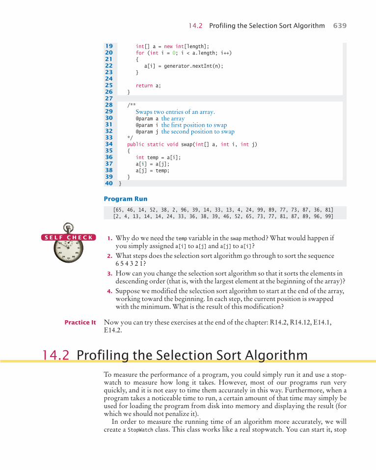
The quicksort algorithm, like merge sort, is based on the strategy of divide and conquer. To sort a range a[from] ... a[to] of the array a, first rearrange the elements in the range so that no element in the range a[from] ... a[p] is larger than any element in the range a[p + 1] ... a[to]. This step is called partitioning the range.

For example, suppose we start with a range

5 3 2 6 4 1 3 7

Here is a partitioning of the range. Note that the partitions aren’t yet sorted.

3 3 2 1 4 6 5 7

You’ll see later how to obtain such a partition. In the next step, sort each partition, by recur-sively applying the same algorithm to the two partitions. That sorts the entire range, because the largest element in the first partition is at most as large as the smallest element in the second partition.

1 2 3 3 4 5 6 7

Quicksort is implemented recursively as follows:

public static void sort(int[] a, int from, int to){ if (from >= to) { return; } int p = partition(a, from, to); sort(a, from, p); sort(a, p + 1, to);}

Let us return to the problem of partitioning a range. Pick an element from the range and call it the pivot. There are several variations of the quicksort algorithm. In the simplest one, we’ll pick the first element of the range, a[from], as the pivot.

Now form two regions a[from] ... a[i], consisting of values at most as large as the pivot and a[j] ... a[to], consisting of values at least as large as the pivot. The region a[i + 1] ... a[j - 1] consists of values that haven’t been analyzed yet. (See the figure below.) At the beginning, both the left and right areas are empty; that is, i = from - 1 and j = to + 1.

FULL CODE EXAMPLE

Go to wiley.com/go/bjeo6code to down-load a program for timing the merge sort algorithm.



S E L F C H E C K

Special Topic 14.3


14.5 Analyzing the Merge Sort Algorithm 653

Partitioning a Range

≤ pivot ≥ pivotNot yet analyzed

[from] [i] [j] [to]

Then keep incrementing i while a[i] < pivot and keep decrementing j while a[j] > pivot. The figure below shows i and j when that process stops.

Now swap the values in positions i and j, increasing both areas once more. Keep going while i < j. Here is the code for the partition method:

private static int partition(int[] a, int from, int to){ int pivot = a[from]; int i = from - 1; int j = to + 1; while (i < j) { i++; while (a[i] < pivot) { i++; } j--; while (a[j] > pivot) { j--; } if (i < j) { ArrayUtil.swap(a, i, j); } } return j;}

On average, the quicksort algorithm is an O(n log(n)) algorithm. There is just one unfortunate aspect to the quicksort algorithm. Its worst-case run-time behavior is O(n2). Moreover, if the pivot element is chosen as the first element of the region, that worst-case behavior occurs when the input set is already sorted—a common situation in practice. By selecting the pivot element more cleverly, we can make it extremely unlikely for the worst-case behavior to occur. Such “tuned” quicksort algorithms are com monly used because their performance is generally excellent. For example, the sort method in the Arrays class uses a quicksort algorithm.

Another improvement that is commonly made in practice is to switch to insertion sort when the array is short, because the total number of operations using insertion sort is lower for short arrays. The Java library makes that switch if the array length is less than seven.

Extending the Partitions

≤ pivot ≥ pivot

[from] [i] [j] [to]

> pivot< pivot

≤ pivot≥ pivot

FULL CODE EXAMPLE

Go to wiley.com/go/bjeo6code to down-load a program that demonstrates the quicksort algorithm.


In quicksort, one partitions the elements into two groups, holding the smaller and larger elements. Then one sorts each group.

© Christopher Futcher/iStockphoto.

© C

hris

toph

er F

utch

er/iS

tock

phot

o.


14.6 SearchingSearching for an element in an array is an extremely common task. As with sorting, the right choice of algorithms can make a big difference.

14.6.1 Linear Search

Suppose you need to find your friend’s telephone number. You look up the friend’s name in the telephone book, and naturally you can find it quickly, because the tele-phone book is sorted alphabetically. Now suppose you have a telephone number and you must know to what party it belongs. You could of course call that number, but suppose nobody picks up on the other end. You could look through the telephone book, a number at a time, until you find the number. That would obviously be a tre-mendous amount of work, and you would have to be desperate to attempt it.

This thought experiment shows the difference between a search through an unsorted data set and a search through a sorted data set. The following two sections will analyze the difference formally.

If you want to find a number in a sequence of values that occur in arbitrary order, there is nothing you can do to speed up the search. You must simply look through all elements until you have found a match or until you reach the end. This is called a linear or sequential search.

How long does a linear search take? If we assume that the element v is present in the array a, then the average search visits n/2 elements, where n is the length of the array. If it is not present, then all n elements must be inspected to verify the absence. Either way, a linear search is an O(n) algorithm.

Here is a class that performs linear searches through an array a of integers. When searching for a value, the search method returns the first index of the match, or -1 if the value does not occur in a.

section_6_1/LinearSearcher.java

1 /**2 A class for executing linear searches in an array.3 */4 public class LinearSearcher5 { 6 /**7 Finds a value in an array, using the linear search 8 algorithm.9 @param a the array to search

10 @param value the value to find11 @return the index at which the value occurs, or -112 if it does not occur in the array13 */14 public static int search(int[] a, int value)15 { 16 for (int i = 0; i < a.length; i++)17 { 18 if (a[i] == value) { return i; }19 }20 return -1;

A linear search examines all values in an array until it finds a match or reaches the end.

A linear search locates a value in an array in O(n) steps.

14.6 Searching 655

21 }22 }

section_6_1/LinearSearchDemo.java

1 import java.util.Arrays;2 import java.util.Scanner;3 4 /**5 This program demonstrates the linear search algorithm.6 */7 public class LinearSearchDemo8 { 9 public static void main(String[] args)

10 { 11 int[] a = ArrayUtil.randomIntArray(20, 100);12 System.out.println(Arrays.toString(a));13 Scanner in = new Scanner(System.in);14 15 boolean done = false;16 while (!done)17 {18 System.out.print("Enter number to search for, -1 to quit: ");19 int n = in.nextInt();20 if (n == -1)21 {22 done = true;23 }24 else25 {26 int pos = LinearSearcher.search(a, n);27 System.out.println("Found in position " + pos);28 }29 }30 }31 }

Program Run

[46, 99, 45, 57, 64, 95, 81, 69, 11, 97, 6, 85, 61, 88, 29, 65, 83, 88, 45, 88]Enter number to search for, -1 to quit: 12Found in position -1Enter number to search for, -1 to quit: -1

14.6.2 Binary Search

Now let us search for an item in a data sequence that has been previously sorted. Of course, we could still do a linear search, but it turns out we can do much better than that.

Consider the following sorted array a. The data set is:

1 4 5 8 9 12 17 20

[0] [1] [2] [3] [4] [5] [6] [7]

24

[8]

32

[9]

We would like to see whether the value 15 is in the data set. Let’s narrow our search by finding whether the value is in the first or second half of the array. The last value


in the first half of the data set, a[4], is 9, which is smaller than the value we are looking for. Hence, we should look in the second half of the array for a match, that is, in the sequence:

1 4 5 8 9 12 17 20

[0] [1] [2] [3] [4] [5] [6] [7]

24

[8]

32

[9]

The middle element of this sequence is 20; hence, the value must be located in the sequence:

1 4 5 8 9 12 17 20

[0] [1] [2] [3] [4] [5] [6] [7]

24

[8]

32

[9]

The last value of the first half of this very short sequence is 12, which is smaller than the value that we are searching, so we must look in the second half:

1 4 5 8 9 12 17 20

[0] [1] [2] [3] [4] [5] [6] [7]

24

[8]

32

[9]

It is trivial to see that we don’t have a match, because 15 ≠ 17. If we wanted to insert 15 into the sequence, we would need to insert it just before a[6].

This search process is called a binary search, because we cut the size of the search in half in each step. That cutting in half works only because we know that the sequence of values is sorted.

The following class implements binary searches in a sorted array of integers. The search method returns the position of the match if the search succeeds, or –1 if the value is not found in a. Here, we show a recursive version of the binary search algorithm.

section_6_2/BinarySearcher.java

1 /**2 A class for executing binary searches in an array.3 */4 public class BinarySearcher5 { 6 /**7 Finds a value in a range of a sorted array, using the binary8 search algorithm.9 @param a the array in which to search

10 @param low the low index of the range11 @param high the high index of the range12 @param value the value to find13 @return the index at which the value occurs, or -114 if it does not occur in the array15 */16 public int search(int[] a, int low, int high, int value)17 { 18 if (low <= high)19 {20 int mid = (low + high) / 2;21 22 if (a[mid] == value) 23 {24 return mid;25 }26 else if (a[mid] < value )27 {

A binary search locates a value in a sorted array by determining whether the value occurs in the first or second half, then repeating the search in one of the halves.

14.6 Searching 657

28 return search(a, mid + 1, high, value);29 }30 else31 {32 return search(a, low, mid - 1, value);33 } 34 }35 else 36 {37 return -1;38 }39 }40 }

Now let’s determine the number of visits to array elements required to carry out a binary search. We can use the same technique as in the analysis of merge sort. Because we look at the middle element, which counts as one visit, and then search either the left or the right subarray, we have

T n T n( ) =⎛

⎝⎜

⎞

⎠ ⎟ +

21

Using the same equation,

T n T n2 4

1⎛

⎝⎜

⎞

⎠ ⎟ =

⎛

⎝⎜

⎞

⎠ ⎟ +

By plugging this result into the original equation, we get

T n T n( ) =⎛

⎝⎜

⎞

⎠ ⎟ +

42

That generalizes to

T n T n kk

( ) =⎛

⎝⎜

⎞

⎠ ⎟ +

2

As in the analysis of merge sort, we make the simplifying assumption that n is a power of 2, n = 2m, where m = log2(n). Then we obtain

T n n( ) log ( )= +1 2

Therefore, binary search is an O(log(n)) algorithm. That result makes intuitive sense. Suppose that n is 100. Then after each search, the

size of the search range is cut in half, to 50, 25, 12, 6, 3, and 1. After seven comparisons we are done. This agrees with our formula, because log2(100) ≈ 6.64386, and indeed the next larger power of 2 is 27 = 128.

Because a binary search is so much faster than a linear search, is it worthwhile to sort an array first and then use a binary search? It depends. If you search the array only once, then it is more efficient to pay for an O(n) linear search than for an O(n log(n)) sort and an O(log(n)) binary search. But if you will be mak ing many searches in the same array, then sorting it is definitely worthwhile.

A binary search locates a value in a sorted array in O(log(n)) steps.


18. Suppose you need to look through 1,000,000 records to find a telephone num-ber. How many records do you expect to search before finding the number?

19. Why can’t you use a “for each” loop for (int element : a) in the search method?20. Suppose you need to look through a sorted array with 1,000,000 elements to find

a value. Using the binary search algorithm, how many records do you expect to search before finding the value?

Practice It Now you can try these exercises at the end of the chapter: R14.14, E14.13, E14.15.

Computing & Society 14.1 The First Programmer


S E L F C H E C K

Before pocket calcu-lators and personal

computers existed, navigators and engineers used mechanical adding machines, slide rules, and tables of logarithms and trigonometric functions to speed up computations. Unfortunately, the tables—for which values had to be computed by hand—were notoriously inaccurate. The mathematician Charles Babbage (1791–1871) had the insight that if a machine could be constructed that produced printed tables automatically, both calculation and typesetting errors could be avoided. Babbage set out to develop a machine for this purpose, which he called a Dif ference Engine

because it used succes sive differences to compute polynomials. For example, consider the function f (x) = x3. Write down the values for f (1), f (2), f (3), and so on. Then take the differences between successive values:

1 78 1927 3764 61125 91216

Repeat the process, taking the differ-ence of successive values in the sec ond column, and then repeat once again:

1 78 12 19 627 18 37 664 24 61 6125 30 91216

Now the differences are all the same. You can retrieve the function values by a pattern of additions—you need to know the values at the fringe of the pattern and the constant differ-ence. You can try it out yourself: Write the highlighted numbers on a sheet of paper and fill in the others by adding the numbers that are in the north and northwest positions.

This method was very attractive, because mechanical addition machines had been known for some time. They consisted of cog wheels, with 10 cogs per wheel, to represent digits, and mechanisms to handle the carry from one digit to the next. Mechanical mul-tiplication machines, on the other hand, were fragile and unreliable. Bab bage built a successful prototype of the Difference Engine and, with his own money and government grants, proceeded to build the table-printing machine. However, because of funding problems and the difficulty of building the machine to the required precision, it was never completed.

While working on the Difference Engine, Babbage conceived of a much grander vision that he called the Analytical Engine. The Difference Engine was designed to carry out a limited set of computations—it was no smarter than a pocket calculator is today. But Babbage realized that such a machine could be made programmable by stor-ing programs as well as data. The inter-nal storage of the Analytical Engine was to consist of 1,000 regis ters of 50 decimal digits each. Pro grams and con-stants were to be stored on punched cards—a technique that was, at that time, commonly used on looms for weaving patterned fabrics.

Ada Augusta, Countess of Lovelace (1815–1852), the only child of Lord Byron, was a friend and sponsor of Charles Babbage. Ada Lovelace was one of the first people to realize the potential of such a machine, not just for computing mathematical tables but for processing data that were not num-bers. She is considered by many to be the world’s first programmer.

© Media Bakery.

Topham/The Image Works.Replica of Babbage’s Difference Engine

Toph

am/T

he I

mag

e W

orks

.

14.7 Problem Solving: Estimating the Running Time of an Algorithm 659

14.7 Problem Solving: Estimating the Running Time of an Algorithm

In this chapter, you have learned how to estimate the running time of sorting algo-rithms. As you have seen, being able to differentiate between O(n log(n)) and O(n2) running times has great practical implications. Being able to estimate the running times of other algorithms is an important skill. In this section, we will practice esti-mating the running time of array algorithms.

14.7.1 Linear Time

Let us start with a simple example, an algorithm that counts how many elements have a particular value:

int count = 0;for (int i = 0; i < a.length; i++){ if (a[i] == value) { count++; }}

What is the running time in terms of n, the length of the array?Start with looking at the pattern of array element visits. Here, we visit each ele-

ment once. It helps to visualize this pattern. Imagine the array as a sequence of light bulbs. As the ith element gets visited, imagine the ith bulb lighting up.

3

4

5

2

1

Lightbulbs: © Kraska/iStockphoto.Now look at the work per visit. Does each visit involve a fixed number of actions, independent of n? In this case, it does. There are just a few actions—read the element, compare it, maybe increment a counter.

Therefore, the running time is n times a constant, or O(n).What if we don’t always run to the end of the array? For example, suppose we

want to check whether the value occurs in the array, without counting it:boolean found = false;for (int i = 0; !found && i < a.length; i++){ if (a[i] == value) { found = true; }}

A loop with n iterations has O(n) running time if each step consists of a fixed number of actions.

(lig

htbu

lbs)

© K

rask

a/iS

tock

phot

o.


Then the loop can stop in the middle:

3

2

1

Found the value

Lightbulbs: © Kraska/iStockphoto.

Is this still O(n)? It is, because in some cases the match may be at the very end of the array. Also, if there is no match, one must traverse the entire array.

14.7.2 Quadratic Time

Now let’s turn to a more interesting case. What if we do a lot of work with each visit? Here is an example: We want to find the most frequent element in an array.

Suppose the array is

8 7 5 7 7 5 4

It’s obvious by looking at the values that 7 is the most frequent one. But now imagine an array with a few thousand values.

8 7 5 7 7 5 4 1 2 3 3 4 9 12 3 2 5 11 9 2 3 7 8...

We can count how often the value 8 occurs, then move on to count how often 7 occurs, and so on. For example, in the first array, 8 occurs once, and 7 occurs three times. Where do we put the counts? Let’s put them into a second array of the same length.

8 7 5 7 7 5 4

1 3 2 3 3 2 1

a:

counts:

Then we take the maximum of the counts. It is 3. We look up where the 3 occurs in the counts, and find the corresponding value. Thus, the most common value is 7.

Let us first estimate how long it takes to compute the counts.for (int i = 0; i < a.length; i++){ counts[i] = Count how often a[i] occurs in a}

We still visit each array element once, but now the work per visit is much larger. As you have seen in the previous section, each counting action is O(n). When we do O(n) work in each step, the total running time is O(n2).

This algorithm has three phases:

1. Compute all counts.2. Compute the maximum.3. Find the maximum in the counts.

A loop with n iterations has O(n2) running time if each step takes O(n) time.


We have just seen that the first phase is O(n2). Computing the maximum is O(n)—look at the algorithm in Section 7.3.3 and note that each step involves a fixed amount of work. Finally, we just saw that finding a value is O(n).

How can we estimate the total running time from the estimates of each phase? Of course, the total time is the sum of the individual times, but for big-Oh estimates, we take the maximum of the estimates. To see why, imagine that we had actual equations for each of the times:

T1(n) = an2 + bn + c

T2(n) = dn + e

T3(n) = fn + gThen the sum is

T(n) = T1(n) + T2(n) + T3(n) = an2 + (b + d + f )n + c + e + g

But only the largest term matters, so T(n) is O(n2).Thus, we have found that our algorithm for finding the most frequent element is

O(n2).

14.7.3 The Triangle Pattern

Let us see if we can speed up the algorithm from the preceding section. It seems wasteful to count elements again if we have already counted them.

Can we save time by eliminating repeated counting of the same element? That is, before counting a[i], should we first check that it didn’t occur in a[0] ... a[i - 1]?

Let us estimate the cost of these additional checks. In the ith step, the amount of work is proportional to i. That’s not quite the same as in the preceding section, where you saw that a loop with n iterations, each of which takes O(n) time, is O(n2). Now each step just takes O(i) time.

To get an intuitive feel for this situation, look at the light bulbs again. In the second iteration, we visit a[0] again. In the third iteration, we visit a[0] and a[1] again, and so on. The light bulb pattern is

3

4

5

2

1

Lightbulbs: © Kraska/iStockphoto.If there are n light bulbs, about half of the square above, or n2/2 of them, light up. That’s unfortunately still O(n2).

Here is another idea for time saving. When we count a[i], there is no need to do the counting in a[0] ... a[i - 1]. If a[i] never occurred before, we get an accurate

The big-Oh running time for doing several steps in a row is the largest of the big-Oh times for each step.

A loop with n iterations has O(n2) running time if the ith step takes O(i ) time.


count by just looking at a[i] ... a[n - 1]. And if it did, we already have an accurate count. Does that help us? Not really—it’s the triangle pattern again, but this time in the other direction.

3

4

5

2

1

Lightbulbs: © Kraska/iStockphoto.That doesn’t mean that these improvements aren’t worthwhile. If an O(n2) algorithm is the best one can do for a particular problem, you still want to make it as fast as pos-sible. However, we will not pursue this plan further because it turns out that we can do much better.

14.7.4 Logarithmic Time

Logarithmic time estimates arise from algorithms that cut work in half in each step. You have seen this in the algorithms for binary search and merge sort, and you will see it again in Chapter 17.

In particular, when you use sorting or binary search in a phase of an algorithm, you will encounter logarithmic time in the big-Oh estimates.

Consider this idea for improving our algorithm for finding the most frequent ele-ment. Suppose we first sort the array:

8 7 5 7 7 5 4 4 5 5 7 7 7 8

That cost us O(n log(n)) time. If we can complete the algorithm in O(n) time, we will have found a better algorithm than the O(n2) algorithm of the preceding sections.

To see why this is possible, imagine traversing the sorted array. As long as you find a value that was equal to its predecessor, you increment a counter. When you find a different value, save the counter and start counting anew:

4 5 5 7 7 7 8

1 1 2 1 2 3 1

a:

counts:

Or in code,int count = 0;for (int i = 0; i < a.length; i++){ count++; if (i == a.length - 1 || a[i] != a[i + 1]) {

An algorithm that cuts the size of work in half in each step runs in O(log(n)) time.


counts[i] = count; count = 0; }}

That’s a constant amount of work per iteration, even though it visits two elements:

3

4

5

2

1


2n is still O(n). Thus, we can compute the counts in O(n) time from a sorted array. The entire algorithm is now O(n log(n)).

Note that we don’t actually need to keep all counts, only the highest one that we encountered so far (see Exercise E14.11). That is a worthwhile improvement, but it does not change the big-Oh estimate of the running time.

21. What is the “light bulb pattern” of visits in the following algorithm to check whether an array is a palindrome?for (int i = 0; i < a.length / 2; i++){ if (a[i] != a[a.length - 1 - i]) { return false; }}return true;

22. What is the big-Oh running time of the following algorithm to check whether the first element is duplicated in an array?for (int i = 1; i < a.length; i++){ if (a[0] == a[i]) { return true; }}return false;

23. What is the big-Oh running time of the following algorithm to check whether an array has a duplicate value?for (int i = 0; i < a.length; i++){ for (j = i + 1; j < a.length; j++) { if (a[i] == a[j]) { return true; } }}return false;

24. Describe an O(n log(n)) algorithm for checking whether an array has duplicates.

FULL CODE EXAMPLE

Go to wiley.com/go/bjeo6code to download a program for comparing the speed of algorithms that find the most frequent element.



S E L F C H E C K


25. What is the big-Oh running time of the following algorithm to find an element in an n × n array?for (int i = 0; i < n; i++){ for (j = 0; j < n; j++) { if (a[i][j] == value) { return true; } }}return false;

26. If you apply the algorithm of Section 14.7.4 to an n × n array, what is the big-Oh efficiency of finding the most frequent element in terms of n?

Practice It Now you can try these exercises at the end of the chapter: R14.9, R14.15, R14.21, E14.11.

14.8 Sorting and Searching in the Java LibraryWhen you write Java programs, you don’t have to implement your own sorting algo-rithms. The Arrays and Collections classes provide sorting and searching methods that we will introduce in the following sections.

14.8.1 Sorting

The Arrays class contains static sort methods to sort arrays of integers and floating-point numbers. For example, you can sort an array of integers simply as

int[] a = . . .;Arrays.sort(a);

That sort method uses the quicksort algorithm—see Special Topic 14.3 for more information about that algorithm.

If your data are contained in an ArrayList, use the Collections.sort method instead; it uses the merge sort algorithm:

ArrayList<String> names = . . .;Collections.sort(names);

14.8.2 Binary Search

The Arrays and Collections classes contain static binarySearch methods that implement the binary search algorithm, but with a useful enhancement. If a value is not found in the array, then the returned value is not –1, but –k – 1, where k is the position before which the element should be inserted. For example,

int[] a = { 1, 4, 9 };int v = 7;int pos = Arrays.binarySearch(a, v);// Returns –3; v should be inserted before position 2

The Arrays class implements a sorting method that you should use for your Java programs.

The Collections class contains a sort method that can sort array lists.

14.8 Sorting and Searching in the Java Library 665

14.8.3 Comparing Objects

In application programs, you often need to sort or search through collections of objects. Therefore, the Arrays and Collections classes also supply sort and binarySearch methods for objects. However, these methods cannot know how to compare arbi-trary objects. Suppose, for example, that you have an array of Country objects. It is not obvious how the countries should be sorted. Should they be sorted by their names or by their areas? The sort and binarySearch methods cannot make that decision for you. Instead, they require that the objects belong to classes that implement the Comparable interface type that was introduced in Section 10.3. That interface has a single method:

public interface Comparable<T>{ int compareTo(T other);}

The calla.compareTo(b)

must return a negative number if a should come before b, 0 if a and b are the same, and a positive number otherwise.

Note that Comparable is a generic type, similar to the ArrayList type. With an Array-List, the type parameter denotes the type of the elements. With Comparable, the type parameter is the type of the parameter of the compareTo method. Therefore, a class that implements Comparable will want to be “comparable to itself”. For example, the Coun-try class implements Comparable<Country>.

Many classes in the standard Java library, including the String class, number wrap-pers, dates, and file paths, implement the Comparable interface.

You can implement the Comparable interface for your own classes as well. For exam-ple, to sort a collection of countries by area, the Country class would implement the Comparable<Country> interface and provide a compareTo method like this:

public class Country implements Comparable<Country>{ public int compareTo(Country other) { return Double.compare(area, other.area); }}

The compareTo method compares countries by their area. Note the use of the helper method Double.compare (see Programming Tip 10.1) that returns a negative integer, 0, or a positive integer. This is easier than programming a three-way branch.

Now you can pass an array of countries to the Arrays.sort method:Country[] countries = new Country[n];// Add countriesArrays.sort(countries); // Sorts by increasing area

Whenever you need to carry out sorting or searching, use the methods in the Arrays and Collections classes and not those that you write yourself. The library algorithms have been fully debugged and optimized. Thus, the primary purpose of this chapter was not to teach you how to implement practical sorting and searching algorithms. Instead, you have learned something more important, namely that different algo-rithms can vary widely in performance, and that it is worthwhile to learn more about the design and analysis of algorithms.

The sort method of the Arrays class sorts objects of classes that implement the Comparable interface.

FULL CODE EXAMPLE

Go to wiley.com/go/bjeo6code to down-load a program that demonstrates the Java library methods for sorting and searching.



27. Why can’t the Arrays.sort method sort an array of Rectangle objects?28. What steps would you need to take to sort an array of BankAccount objects by

increasing balance?29. Why is it useful that the Arrays.binarySearch method indicates the position where

a missing element should be inserted?30. Why does Arrays.binarySearch return –k – 1 and not –k to indicate that a value is

not present and should be inserted before position k?

Practice It Now you can try these exercises at the end of the chapter: E14.12, E14.16, E14.17.

The compareTo Method Can Return Any Integer, Not Just –1, 0, and 1

The call a.compareTo(b) is allowed to return any negative integer to denote that a should come before b, not necessar ily the value –1. That is, the test

if (a.compareTo(b) == -1) // Error!

is generally wrong. Instead, you should test

if (a.compareTo(b) < 0) // OK

Why would a compareTo method ever want to return a number other than –1, 0, or 1? Some-times, it is convenient to just return the difference of two integers. For example, the compareTo method of the String class compares characters in matching positions:

char c1 = charAt(i);char c2 = other.charAt(i);

If the characters are different, then the method simply returns their difference:

if (c1 != c2) { return c1 - c2; }

This difference is a negative number if c1 is less than c2, but it is not necessarily the number –1.Note that returning a difference only works if it doesn’t overflow (see Programming

Tip 10.1).

The Comparator Interface

Sometimes you want to sort an array or array list of objects, but the objects don’t belong to a class that implements the Comparable interface. Or, perhaps, you want to sort the array in a dif-ferent order. For example, you may want to sort countries by name rather than by value.

You wouldn’t want to change the implementation of a class simply to call Arrays.sort. Fortunately, there is an alternative. One version of the Arrays.sort method does not require that the objects belong to classes that imple ment the Comparable interface. Instead, you can supply arbitrary objects. However, you must also provide a compara tor object whose job is to compare objects. The comparator object must belong to a class that implements the Comparator interface. That interface has a single method, compare, which compares two objects.

Just like Comparable, the Comparator interface is a parameterized type. The type parameter specifies the type of the compare parameter variables. For example, Comparator<Country> looks like this:

public interface Comparator<Country>{ int compare(Country a, Country b);}


S E L F C H E C K

Common Error 14.1

© John Bell/iStockphoto.

Special Topic 14.4


14.8 Sorting and Searching in the Java Library 667

The call

comp.compare(a, b)

must return a negative number if a should come before b, 0 if a and b are the same, and a posi-tive number otherwise. (Here, comp is an object of a class that implements Comparator<Country>.)

For example, here is a Comparator class for country:

public class CountryComparator implements Comparator<Country>{ public int compare(Country a, Country b) { return Double.compare(a.getArea(), b.getArea()); }}

To sort an array of countries by area, call

Arrays.sort(countries, new CountryComparator());

Comparators with Lambda Expressions

Before Java 8, it was cumbersome to specify a comparator. You had to come up with a class that implements the Comparator interface, implement the compare method, and construct an object of that class. That was unfortunate because comparators are very useful for several algorithms, such as searching, sorting, and finding the maximum or minimum.

With lambda expressions, it is easier to specify a comparator. For example, to sort an array of words by increasing lengths, call

Arrays.sort(words, (v, w) -> v.length() - w.length());

There is a convenient shortcut for this case. Note that the comparison depends on a function that maps each string to a numeric value, namely its length. The static method Comparator.comparing constructs a comparator from a lambda expression. For example, you can call

Arrays.sort(words, Comparator.comparing(w -> w.length()));

A comparator is constructed that calls the supplied function on both objects that are to be compared, and then compares the function results.

The Comparator.comparing method takes care of many common cases. For example, to sort countries by area, call

Arrays.sort(countries, Comparator.comparing(c -> c.getArea()));

Java 8 Note 14.1

© subjug/iStockphoto.

© Tom Horyn/iStockphoto.

WORkED ExAMPLE 14.1 Enhancing the Insertion Sort Algorithm

Learn how to implement an improvement of the insertion sort algorithm shown in Special Topic 14.2. The enhanced algorithm is called Shell sort after its inventor, Donald Shell. Go to wiley.com/go/bjeo6examples and download Worked Example 14.1.



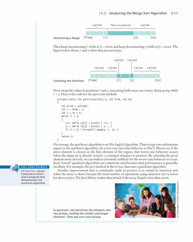
Describe the selection sort algorithm.

• The selection sort algorithm sorts an array by repeatedly finding the smallest element of the unsorted tail region and moving it to the front.

Measure the running time of a method.

• To measure the running time of a method, get the current time immediately before and after the method call.

Use the big-Oh notation to describe the running time of an algorithm.

• Computer scientists use the big-Oh notation to describe the growth rate of a function.

• Selection sort is an O(n2) algorithm. Doubling the data set means a fourfold increase in processing time.

• Insertion sort is an O(n2) algorithm.

Describe the merge sort algorithm.

• The merge sort algorithm sorts an array by cutting the array in half, recursively sorting each half, and then merging the sorted halves.

Contrast the running times of the merge sort and selection sort algorithms.

• Merge sort is an O(n log(n)) algorithm. The n log(n) function grows much more slowly than n2.

Describe the running times of the linear search algorithm and the binary search algorithm.

• A linear search examines all values in an array until it finds a match or reaches the end.

• A linear search locates a value in an array in O(n) steps.• A binary search locates a value in a sorted array by determining whether the value

occurs in the first or second half, then repeating the search in one of the halves.• A binary search locates a value in a sorted array in O(log(n)) steps.

Practice developing big-Oh estimates of algorithms.

• A loop with n iterations has O(n) running time if each step consists of a fixed number of actions.

• A loop with n iterations has O(n2) running time if each step takes O(n) time.

• The big-Oh running time for doing several steps in a row is the largest of the big-Oh times for each step.

C H A P T E R S U M M A R Y

© Zone Creative/iStockphoto.

© Kirby Hamilton/iStockphoto.

© Rich Legg/iStockphoto.

Lightbulbs: © Kraska/Shutterstock.

3

2

1

Found the value

Review Exercises 669

• A loop with n iterations has O(n2) running time if the ith step takes O(i) time.• An algorithm that cuts the size of work in half in each step runs in O(log(n)) time.

Use the Java library methods for sorting and searching data.

• The Arrays class implements a sorting method that you should use for your Java programs.

• The Collections class contains a sort method that can sort array lists.• The sort method of the Arrays class sorts objects of classes that implement the

Comparable interface.

• R14.1 What is the difference between searching and sorting?

•• R14.2 Checking against off-by-one errors. When writing the selection sort algorithm of Section 14.1, a programmer must make the usual choices of < versus <=, a.length versus a.length - 1, and from versus from + 1. This is fertile ground for off-by-one errors. Conduct code walkthroughs of the algorithm with arrays of length 0, 1, 2, and 3 and check carefully that all index values are correct.

•• R14.3 For the following expressions, what is the order of the growth of each? a. n2 + 2n + 1b. n10 + 9n9 + 20n8 + 145n7

c. (n + 1)4

d. (n2 + n)2

e. n + 0.001n3

f. n3 − 1000n2 + 109

java.lang.System currentTimeMillisjava.util.Arrays binarySearch sort

java.util.Collections binarySearch sortjava.util.Comparator<T> compare comparing

S TA N D A R D L I B R A R Y I T E M S I N T R O D U C E D I N T H I S C H A P T E R

R E V I E W E X E R C I S E S

• R14.4 We determined that the actual number of visits in the selection sort algorithm is

T n n n( ) = + −12

2 52

3

We characterized this method as having O(n2) growth. Compute the actual ratios

T T

T T

T T

2 000 1 000

4 000 1 000

10 000 1

, ,

, ,

,

( ) ( )( ) ( )( ) ,,000( )

g. n + log(n)h. n2 + n log(n)i. 2n + n2

j. n n

n

3

22

0 75

++ .


and compare them with f f

f f

f f

2 000 1 000

4 000 1 000

10 000 1

, ,

, ,

,

( ) ( )( ) ( )( ) ,,000( )

where f(n) = n2.

• R14.5 Suppose algorithm A takes five seconds to handle a data set of 1,000 records. If the algorithm A is an O(n) algorithm, approximately how long will it take to handle a data set of 2,000 records? Of 10,000 records?

•• R14.6 Suppose an algorithm takes five seconds to handle a data set of 1,000 records. Fill in the following table, which shows the approximate growth of the execution times depending on the complexity of the algorithm.

O (n) O (n2) O (n3) O (n log(n)) O (2n)

1,000 5 5 5 5 5

2,000

3,000 45

10,000

For example, because 3 000 1 000 92 2, , = , the algorithm would take nine times as long, or 45 seconds, to handle a data set of 3,000 records.

•• R14.7 Sort the following growth rates from slowest to fastest growth.

O n

O n n

O n

O

O n

O n

O n On

n

( )

( log( ))

( )

( )

( )

( )

(log( ))

3

2 (( )

( log( )) )log( )

n n

O n n n n2 O(

• R14.8 What is the growth rate of the standard algorithm to find the minimum value of an array? Of finding both the minimum and the maximum?

• R14.9 What is the big-Oh time estimate of the following method in terms of n, the length of a? Use the “light bulb pattern” method of Section 14.7 to visualize your result.

public static void swap(int[] a){ int i = 0; int j = a.length - 1; while (i < j) { int temp = a[i]; a[i] = a[j]; a[j] = temp; i++; j--; }}

Review Exercises 671

• R14.10 A run is a sequence of adjacent repeated values (see Exercise R7.23). Describe an O(n) algorithm to find the length of the longest run in an array.

•• R14.11 Consider the task of finding the most frequent element in an array of length n. Here are three approaches:

a. Sort the array, then find the longest run.b. Allocate an array of counters of the same size as the original array. For each

element, traverse the array and count how many other elements are equal to it, updating its counter. Then find the maximum count.

c. Keep variables for the most frequent element that you have seen so far and its frequency. For each index i, check whether a[i] occurs in a[0] ... a[i - 1]. If not, count how often it occurs in a[i + 1] ... a[n - 1]. If a[i] is more frequent than the most frequent element so far, update the variables.

Describe the big-Oh efficiency of each approach.

• R14.12 Trace a walkthrough of selection sort with these sets:a. 4 7 11 4 9 5 11 7 3 5b. –7 6 8 7 5 9 0 11 10 5 8

• R14.13 Trace a walkthrough of merge sort with these sets:a. 5 11 7 3 5 4 7 11 4 9b. 9 0 11 10 5 8 –7 6 8 7 5

• R14.14 Trace a walkthrough of:a. Linear search for 7 in –7 1 3 3 4 7 11 13b. Binary search for 8 in –7 2 2 3 4 7 8 11 13c. Binary search for 8 in –7 1 2 3 5 7 10 13

•• R14.15 Your task is to remove all duplicates from an array. For example, if the array has the values

4 7 11 4 9 5 11 7 3 5then the array should be changed to

4 7 11 9 5 3Here is a simple algorithm: Look at a[i]. Count how many times it occurs in a. If the count is larger than 1, remove it. What is the growth rate of the time required for this algorithm?

••• R14.16 Modify the merge sort algorithm to remove duplicates in the merging step to obtain an algorithm that removes duplicates from an array. Note that the resulting array does not have the same ordering as the original one. What is the efficiency of this algorithm?

•• R14.17 Consider the following algorithm to remove all duplicates from an array: Sort the array. For each element in the array, look at its next neighbor to decide whether it is present more than once. If so, remove it. Is this a faster algorithm than the one in Exercise R14.15?

••• R14.18 Develop an O(n log(n)) algorithm for removing duplicates from an array if the resulting array must have the same ordering as the original array. When a value occurs multiple times, all but its first occurrence should be removed.


••• R14.19 Why does insertion sort perform significantly better than selection sort if an array is already sorted?

••• R14.20 Consider the following speedup of the insertion sort algorithm of Special Topic 14.2. For each element, use the enhanced binary search algorithm that yields the insertion position for missing elements. Does this speedup have a significant impact on the efficiency of the algorithm?

•• R14.21 Consider the following algorithm known as bubble sort:While the array is not sorted For each adjacent pair of elements If the pair is not sorted Swap its elements.

What is the big-Oh efficiency of this algorithm?

•• R14.22 The radix sort algorithm sorts an array of n integers with d digits, using ten auxiliary arrays. First place each value v into the auxiliary array whose index corresponds to the last digit of v. Then move all values back into the original array, preserving their order. Repeat the process, now using the next-to-last (tens) digit, then the hundreds digit, and so on. What is the big-Oh time of this algorithm in terms of n and d? When is this algorithm preferable to merge sort?

•• R14.23 A stable sort does not change the order of elements with the same value. This is a desirable feature in many applications. Consider a sequence of e-mail messages. If you sort by date and then by sender, you’d like the second sort to preserve the rela-tive order of the first, so that you can see all messages from the same sender in date order. Is selection sort stable? Insertion sort? Why or why not?

•• R14.24 Give an O(n) algorithm to sort an array of n bytes (numbers between –128 and 127). Hint: Use an array of counters.

•• R14.25 You are given a sequence of arrays of words, representing the pages of a book. Your task is to build an index (a sorted array of words), each element of which has an array of sorted numbers representing the pages on which the word appears. Describe an algorithm for building the index and give its big-Oh running time in terms of the total number of words.

•• R14.26 Given two arrays of n integers each, describe an O(n log(n)) algorithm for determin-ing whether they have an element in common.

••• R14.27 Given an array of n integers and a value v, describe an O(n log(n)) algorithm to find whether there are two values x and y in the array with sum v.

•• R14.28 Given two arrays of n integers each, describe an O(n log(n)) algorithm for finding all elements that they have in common.

•• R14.29 Suppose we modify the quicksort algorithm from Special Topic 14.3, selecting the middle element instead of the first one as pivot. What is the running time on an array that is already sorted?

•• R14.30 Suppose we modify the quicksort algorithm from Special Topic 14.3, selecting the middle element instead of the first one as pivot. Find a sequence of values for which this algorithm has an O(n2) running time.

Practice Exercises 673

• E14.1 Modify the selection sort algorithm to sort an array of integers in descending order.

• E14.2 Modify the selection sort algorithm to sort an array of coins by their value.

•• E14.3 Write a program that automatically generates the table of sample run times for the selection sort algorithm. The program should ask for the smallest and largest value of n and the number of measurements and then make all sample runs.

• E14.4 Modify the merge sort algorithm to sort an array of strings in lexicographic order.

•• E14.5 Modify the selection sort algorithm to sort an array of objects that implement the Measurable interface from Chapter 10.

•• E14.6 Modify the selection sort algorithm to sort an array of objects that implement the Comparable interface (without a type parameter).

•• E14.7 Modify the selection sort algorithm to sort an array of objects, given a parameter of type Comparator (without a type parameter).

••• E14.8 Write a telephone lookup program. Read a data set of 1,000 names and telephone numbers from a file that contains the numbers in random order. Handle lookups by name and also reverse lookups by phone number. Use a binary search for both lookups.

•• E14.9 Implement a program that measures the performance of the insertion sort algorithm described in Special Topic 14.2.

• E14.10 Implement the bubble sort algorithm described in Exercise R14.21.

•• E14.11 Implement the algorithm described in Section 14.7.4, but only remember the value with the highest frequency so far:

int mostFrequent = 0;int highestFrequency = -1;for (int i = 0; i < a.length; i++) Count how often a[i] occurs in a[i + 1] ... a[a.length - 1] If it occurs more often than highestFrequency highestFrequency = that count mostFrequent = a[i]

••• E14.12 Write a program that sorts an ArrayList<Country> in decreasing order so that the larg-est country is at the beginning of the array. Use a Comparator.

•• E14.13 Consider the binary search algorithm in Section 14.6. If no match is found, the search method returns −1. Modify the method so that if a is not found, the method returns −k − 1, where k is the position before which the element should be inserted. (This is the same behavior as Arrays.binarySearch.)

•• E14.14 Implement the sort method of the merge sort algorithm without recursion, where the length of the array is a power of 2. First merge adjacent regions of size 1, then adjacent regions of size 2, then adjacent regions of size 4, and so on.

••• E14.15 Use insertion sort and the binary search from Exercise E14.13 to sort an array as described in Exercise R14.20. Implement this algorithm and measure its performance.

P R A C T I C E E x E R C I S E S


• E14.16 Supply a class Person that implements the Comparable interface. Compare persons by their names. Ask the user to input ten names and generate ten Person objects. Using the compareTo method, determine the first and last person among them and print them.

•• E14.17 Sort an array list of strings by increasing length. Hint: Supply a Comparator.

••• E14.18 Sort an array list of strings by increasing length, and so that strings of the same length are sorted lexicographically. Hint: Supply a Comparator.

•• P14.1 It is common for people to name directories as dir1, dir2, and so on. When there are ten or more directories, the operating system displays them in dictionary order, as dir1, dir10, dir11, dir12, dir2, dir3, and so on. That is irritating, and it is easy to fix. Provide a comparator that compares strings that end in digit sequences in a way that makes sense to a human. First compare the part before the digits as strings, and then compare the numeric values of the digits.

••• P14.2 Sometimes, directory or file names have numbers in the middle, and there may be more than one number, for example, sec3_14.txt or sec10_1.txt. Provide a compara-tor that can compare such strings in a way that makes sense to humans. Break each string into strings not containing digits and digit groups. Then compare two strings by comparing the first non-digit groups as strings, the first digit groups as integers, and so on.

•• P14.3 The median m of a sequence of n elements is the element that would fall in the middle if the sequence was sorted. That is, e ≤ m for half the elements, and m ≤ e for the others. Clearly, one can obtain the median by sorting the sequence, but one can do quite a bit better with the following algorithm that finds the kth element of a sequence between a (inclusive) and b (exclusive). (For the median, use k = n / 2, a = 0, and b = n.)

select(k, a, b): Pick a pivot p in the subsequence between a and b.Partition the subsequence elements into three subsequences: the elements <p, =p, >p Let n1, n2, n3 be the sizes of each of these subsequences.if k < n1 return select(k, 0, n1).else if (k > n1 + n2) return select(k, n1 + n2, n).else return p.

Implement this algorithm and measure how much faster it is for computing the median of a random large sequence, when compared to sorting the sequence and taking the middle element.

•• P14.4 Implement the following modification of the quicksort algorithm, due to Bentley and McIlroy. Instead of using the first element as the pivot, use an approximation of the median.

P R O G R A M M I N G P R O J E C T S

Answers to Self-Check Questions 675

If n ≤ 7, use the middle element. If n ≤ 40, use the median of the first, middle, and last element. Otherwise compute the “pseudomedian” of the nine elements a[i * (n - 1) / 8], where i ranges from 0 to 8. The pseudomedian of nine values is med(med(v0, v1, v2), med(v3, v4, v5), med(v6, v7, v8)).Compare the running time of this modification with that of the original algorithm on sequences that are nearly sorted or reverse sorted, and on sequences with many identical elements. What do you observe?

••• P14.5 Bentley and McIlroy suggest the following modification to the quicksort algorithm when dealing with data sets that contain many repeated elements.Instead of partitioning as

≤ ≥

(where ≤ denotes the elements that are ≤ the pivot), it is better to partition as

< = >

However, that is tedious to achieve directly. They recommend to partition as

= < > =

and then swap the two = regions into the middle. Implement this modification and check whether it improves performance on data sets with many repeated elements.

• P14.6 Implement the radix sort algorithm described in Exercise R14.22 to sort arrays of numbers between 0 and 999.

• P14.7 Implement the radix sort algorithm described in Exercise R14.22 to sort arrays of numbers between 0 and 999. However, use a single auxiliary array, not ten.

•• P14.8 Implement the radix sort algorithm described in Exercise R14.22 to sort arbitrary int values (positive or negative).

••• P14.9 Implement the sort method of the merge sort algorithm without recursion, where the length of the array is an arbitrary number. Keep merging adjacent regions whose size is a power of 2, and pay special attention to the last area whose size is less.

A N S W E R S T O S E L F - C H E C K Q U E S T I O N S

1. Dropping the temp variable would not work. Then a[i] and a[j] would end up being the same value.

2. 1 | 5 4 3 2 61 2 | 4 3 5 61 2 3 4 5 6

3. In each step, find the maximum of the remain-ing elements and swap it with the cur rent ele-ment (or see Self Check 4).

4. The modified algorithm sorts the array in descending order.

5. Four times as long as 40,000 values, or about 37 seconds.

6. A parabola.7. It takes about 100 times longer.8. If n is 4, then 1

22n is 8 and 5

23n − is 7.

9. The first algorithm requires one visit, to store the new element. The second algo rithm requires T(p) = 2 × (n – p – 1) visits, where p is the location at which the ele ment is removed. We don’t know where that element is, but if elements are removed at random locations, on average, half of the removals will be above the middle and half below, so we can assume an average p of n / 2 and T(n) = 2 × (n – n / 2 – 1) = n – 2.


10. The first algorithm is O(1), the second O(n).11. We need to check that a[0] ≤ a[1], a[1] ≤ a[2],

and so on, visiting 2n – 2 elements. Therefore, the running time is O(n).

12. Let n be the length of the array. In the kth step, we need k visits to find the mini mum. To remove it, we need an average of k – 2 visits (see Self Check 9). One additional visit is required to add it to the end. Thus, the kth step requires 2k – 1 vis its. Because k goes from n to 2, the total number of visits is

2n – 1 + 2(n – 1) – 1 + ... + 2 · 3 – 1 + 2 · 2 – 1 = 2(n + (n – 1) + ... + 3 + 2 + 1 – 1) – (n – 1) =

n(n + 1) – 2 – n + 1 = n2 – 3 (because 1 + 2 + 3 + ... + (n – 1) + n = n(n + 1)/2)Therefore, the total number of visits is O(n2).

13. When the preceding while loop ends, the loop condition must be false, that is, iFirst >= first.length or iSecond >= second.length (De Morgan’s Law).

14. First sort 8 7 6 5. Recursively, first sort 8 7. Recursively, first sort 8. It’s sorted. Sort 7. It’s sorted. Merge them: 7 8. Do the same with 6 5 to get 5 6. Merge them to 5 6 7 8. Do the same with 4 3 2 1: Sort 4 3 by sorting 4 and 3 and merging them to 3 4. Sort 2 1 by sorting 2 and 1 and merging them to 1 2. Merge 3 4 and 1 2 to 1 2 3 4. Finally, merge 5 6 7 8 and 1 2 3 4 to 1 2 3 4 5 6 7 8.

15. If the array size is 1, return its only element as the sum. Otherwise, recursively compute the sum of the first and second subarray and return the sum of these two values.

16. Approximately (100,000 · log(100,000)) / (50,000 · log(50,000)) = 2 · 5 / 4.7 = 2.13 times the time required for 50,000 values. That’s 2.13 · 192 milliseconds or approximately 409 milliseconds.

17. n nn n n

2 log(2 )log( )

2(1 log(2))

log( )=

+ .

For n > 2, that is a value < 3.

18. On average, you’d make 500,000 comparisons.19. The search method returns the index at which

the match occurs, not the data stored at that location.

20. You would search about 20. (The binary log of 1,024 is 10.)

21.

22. It is an O(n) algorithm.23. It is an O(n2) algorithm—the number of visits

follows a triangle pattern.24. Sort the array, then make a linear scan to check

for adjacent duplicates.25. It is an O(n2) algorithm—the outer and inner

loops each have n iterations.26. Because an n × n array has m = n2 elements,

and the algorithm in Section 14.7.4, when applied to an array with m elements, is O(m log(m)), we have an O(n2log(n)) algo-rithm. Recall that log(n2) = 2 log(n), and the factor of 2 is irrelevant in the big-Oh notation.

27. The Rectangle class does not implement the Comparable interface.

28. The BankAccount class would need to implement the Comparable interface. Its compareTo method must compare the bank balances.

29. Then you know where to insert it so that the array stays sorted, and you can keep using binary search.

30. Otherwise, you would not know whether a value is present when the method returns 0.

3

2

1


SORTING AND SEARCHING

Documents

Transcript of SORTING AND SEARCHING