Ant Routing, Searching and Topology Estimation algorithms ...
162
Ant Routing, Searching and Topology Estimation algorithms for Ad Hoc Networks
-
Upload
khangminh22 -
Category
Documents
-
view
0 -
download
0
Transcript of Ant Routing, Searching and Topology Estimation algorithms ...

Ant Routing, Searching and TopologyEstimation algorithms for Ad Hoc
Networks

Ant Routing, Searching and TopologyEstimation algorithms for Ad Hoc
Networks
Proefschrift
ter verkrijging van de graad van doctoraan de Technische Universiteit Delft,
op gezag van de Rector Magnificus Prof.dr.ir. J.T. Fokkema,voorzitter van het College voor Promoties,
in het openbaar te verdedigen op dinsdag 2 september 2008 om 10.00 uur
door
Santpal Singh DHILLON
Master of Science Duke University, Durham, USAgeboren te Nathana, Punjab, India.

Dit proefschrift is goedgekeurd door de promotor:Prof.dr.ir. P.F.A. Van Mieghem
Samenstelling promotiecommissie:
Rector Magnificus, VoorzitterProf.dr.ir. P.F.A. Van Mieghem, Technische Universiteit Delft, promotorProf.dr.ir. I.G.M.M. Niemegeers, Technische Universiteit DelftProf.dr.ir. S.M. Heemstra de Groot, Technische Universiteit DelftProf.dr.ir. N.H.G. Baken, Technische Universiteit DelftProf.dr. J.L. van den Berg, University of Twente and TNO NetherlandsProf.dr.ir. M.R. van Steen, Vrije Universiteit, Amsterdam
Copyright c° 2008 by Santpal Singh Dhillon and IOS Press
This research was supported by the Dutch Ministry of Economic Affairs under theInnovation Oriented Research Program (IOP GenCom, QoS for Personal Networks @Home).
All rights reserved. No part of this book may be reproduced, stored in a retrievalsystem, or transmitted, in any form or by any means, without prior permission fromthe publisher.
ISBN 978-1-58603-901-1
Keywords: Ant routing, random walks, ad hoc networks
Published and distributed by IOS Press under the imprint Delft University Press
PublisherIOS PressNieuwe Hemweg 6b1013 BG AmsterdamThe Netherlandstel: +31-20-688 3355fax: +31-20-687 0019email: [email protected]
LEGAL NOTICEThe publisher is not responsible for the use which might be made of the following in-formation.
PRINTED IN THE NETHERLANDS

to the silent winds, dark earth and monday morning rain.

vi
Contents
I Introduction 1
1 Networks and Technologies 31.1 Wireless Communication . . . . . . . . . . . . . . . . . . . . . . . . . . 31.2 Wireless Networks and Technologies . . . . . . . . . . . . . . . . . . . . 6
1.2.1 Cellular Systems . . . . . . . . . . . . . . . . . . . . . . . . . . 61.2.2 Wireless Local Area Networks . . . . . . . . . . . . . . . . . . . 61.2.3 Broadband Wireless Access Technology . . . . . . . . . . . . . . 7
1.3 Mobile Ad hoc Wireless Networks . . . . . . . . . . . . . . . . . . . . . 81.3.1 Low Cost and Low Power Radio technologies . . . . . . . . . . . 81.3.2 Personal Networks . . . . . . . . . . . . . . . . . . . . . . . . . 81.3.3 Sensor Networks . . . . . . . . . . . . . . . . . . . . . . . . . . 91.3.4 Mesh Networks . . . . . . . . . . . . . . . . . . . . . . . . . . . 10
1.4 Peer-to-peer Networks . . . . . . . . . . . . . . . . . . . . . . . . . . . 11
2 Network Modelling 132.1 Graph Definitions . . . . . . . . . . . . . . . . . . . . . . . . . . . . . . 132.2 Graph Models . . . . . . . . . . . . . . . . . . . . . . . . . . . . . . . . 142.3 Routing Algorithms and Protocols . . . . . . . . . . . . . . . . . . . . . 17
2.3.1 Dijkstra’s algorithm . . . . . . . . . . . . . . . . . . . . . . . . 192.3.2 QoS Routing Protocols and Algorithms . . . . . . . . . . . . . . 202.3.3 Routing in Wireless Networks . . . . . . . . . . . . . . . . . . . 21
3 Survey of Ad hoc Routing Protocols 233.1 Classification of Ad hoc Routing Protocols . . . . . . . . . . . . . . . . 23
3.1.1 Power-saving routing protocols . . . . . . . . . . . . . . . . . . 253.1.2 Cross-Layer Design . . . . . . . . . . . . . . . . . . . . . . . . . 26
3.2 Destination-Sequenced Distance-Vector Routing . . . . . . . . . . . . . 273.3 Dynamic Source Routing . . . . . . . . . . . . . . . . . . . . . . . . . . 273.4 Ad Hoc On-Demand Distance Vector Routing . . . . . . . . . . . . . . 283.5 Summary . . . . . . . . . . . . . . . . . . . . . . . . . . . . . . . . . . 30
vii

viii CONTENTS
II Ant Routing 31
4 Introduction to ant routing 334.1 Overview of ANTRAL implementations . . . . . . . . . . . . . . . . . . 354.2 Performance of Ant Routing Algorithms . . . . . . . . . . . . . . . . . 38
5 Ant Routing in Wired Networks 395.1 Network Model . . . . . . . . . . . . . . . . . . . . . . . . . . . . . . . 39
5.1.1 Data Structures at Nodes . . . . . . . . . . . . . . . . . . . . . 415.2 AntNet Algorithm . . . . . . . . . . . . . . . . . . . . . . . . . . . . . 42
5.2.1 Description of the AntNet algorithm . . . . . . . . . . . . . . . 425.2.2 Complexity Analysis of the AntNet algorithm . . . . . . . . . . 485.2.3 AntNet Implementation . . . . . . . . . . . . . . . . . . . . . . 49
5.3 Results . . . . . . . . . . . . . . . . . . . . . . . . . . . . . . . . . . . . 515.3.1 Simulation Parameters . . . . . . . . . . . . . . . . . . . . . . . 515.3.2 Static Implementation of the AntNet algorithm . . . . . . . . . 525.3.3 Dynamic Implementation of the AntNet algorithm . . . . . . . . 545.3.4 Traffic Measurements . . . . . . . . . . . . . . . . . . . . . . . . 64
5.4 Conclusions . . . . . . . . . . . . . . . . . . . . . . . . . . . . . . . . . 66
6 Ant Routing in Mobile Ad hoc Networks 696.1 W_AntNet algorithm . . . . . . . . . . . . . . . . . . . . . . . . . . . 706.2 Performance Analysis of W_AntNet . . . . . . . . . . . . . . . . . . . 70
6.2.1 NS-2 simulations . . . . . . . . . . . . . . . . . . . . . . . . . . 736.3 Conclusions . . . . . . . . . . . . . . . . . . . . . . . . . . . . . . . . . 77
III Searching 79
7 Introduction 817.1 Overview . . . . . . . . . . . . . . . . . . . . . . . . . . . . . . . . . . . 837.2 Definitions and Random Walk properties . . . . . . . . . . . . . . . . . 83
8 Searching with single query 858.1 Random Walks . . . . . . . . . . . . . . . . . . . . . . . . . . . . . . . 85
8.1.1 Random Walk with memory M . . . . . . . . . . . . . . . . . . 858.1.2 Random Walk with look-ahead . . . . . . . . . . . . . . . . . . 868.1.3 Random Walk using highest degree . . . . . . . . . . . . . . . . 878.1.4 Random Walk proportional to the degree . . . . . . . . . . . . . 888.1.5 Random Walk using minimum link weight . . . . . . . . . . . . 888.1.6 Random walk proportional to the link weight . . . . . . . . . . 88
8.2 Analysis of Searching with single query . . . . . . . . . . . . . . . . . . 88
CONTENTS ix
8.3 Simulation Results . . . . . . . . . . . . . . . . . . . . . . . . . . . . . 948.3.1 RW with lookahead j . . . . . . . . . . . . . . . . . . . . . . . . 948.3.2 Comparison of RW strategies . . . . . . . . . . . . . . . . . . . 95
8.4 Conclusion . . . . . . . . . . . . . . . . . . . . . . . . . . . . . . . . . . 96
9 Searching with multiple queries 1019.1 Analysis of searching with multiple RW queries . . . . . . . . . . . . . 1029.2 Conclusions . . . . . . . . . . . . . . . . . . . . . . . . . . . . . . . . . 107
IV Topology Analysis 109
10 Topology of Ad hoc wireless networks 11110.1 Signal Propagation Models Topology Modeling of Wireless Ad hoc Net-
works . . . . . . . . . . . . . . . . . . . . . . . . . . . . . . . . . . . . . 11210.2 Average node degree in ad hoc wireless networks . . . . . . . . . . . . . 11310.3 Shortest Path Routing and Load Balancing . . . . . . . . . . . . . . . . 11510.4 Lifetime of Ad hoc Wireless Network . . . . . . . . . . . . . . . . . . . 11610.5 Conclusions . . . . . . . . . . . . . . . . . . . . . . . . . . . . . . . . . 119
11 Estimation of Topology 12111.1 Introduction . . . . . . . . . . . . . . . . . . . . . . . . . . . . . . . . . 12111.2 Topology Estimation . . . . . . . . . . . . . . . . . . . . . . . . . . . . 122
11.2.1 Estimation when both p and N are unknown . . . . . . . . . . . 12211.2.2 Results . . . . . . . . . . . . . . . . . . . . . . . . . . . . . . . . 12411.2.3 A subgraph and average degree are known . . . . . . . . . . . . 12411.2.4 Influence of m and Z . . . . . . . . . . . . . . . . . . . . . . . . 125
11.3 Conclusions . . . . . . . . . . . . . . . . . . . . . . . . . . . . . . . . . 126
12 Conclusions 127
A Average number of neighbors 131
Abbreviations 135
Bibliography 137
Acknowledgements 147
Curriculum Vitae 149

x CONTENTS
Summary
Title : Ant Routing, Searching and Topology Estimation algorithms for Ad Hoc Net-works.The complexity of networks is increasing to cope with the network model of providing
connectivity anywhere and anytime. The idea of universal connectivity has to lead theconcept of ad hoc networks. The word ad hoc comes from Latin meaning "to this". Adhoc networks are self-configuring, self-organizing networks that are formed on the fly.The dynamic and self-configuring behavior of ad hoc networks provides new challenges.Ad hoc networks have to deal with the inherent difficulties in the wireless medium aswell as node mobility. Integration of multiple networks, architectures and technologiesintroduces further complexity for the paradigm of universal connectivity.Developing novel algorithms and protocols and analyzing their performance is essen-
tial for the development of next generation networks. In this thesis, we aim to analyzethe performance of dynamic routing and searching algorithms.The main aims of this thesis are:
1. Studying the performance of a dynamic, self-adaptive routing paradigm knownas ant routing.
2. Analyzing the behavior of searching and how it performs on graph topologies.
3. Understanding the topology of wireless ad hoc networks and its effects on per-formance of different algorithms in ad hoc networks.
4. Estimation of topology to build topology dependant algorithms.
This thesis is divided into four parts.The first section is an introduction to the ad hoc networks. This section is divided
into three chapters. Chapter 1 discusses different network technologies and architec-tures. In the second chapter, we describe how the communication networks can bemodelled as graph. In this chapter, we also describe OSI layer architecture of Internetand different routing algorithms and protocols. The last chapter in this section presentsa survey of routing protocols for ad hoc wireless networks.
xi
xii SUMMARY
The second part of thesis deals with ant routing. Ant routing is a probabilisticrouting scheme inspired by real life ant colonies. Ant routing algorithms adapt tochanges in network topology and traffic and aim to provide quality of service routing. Inchapter 4.2, we study the performance of ant routing algorithms for wired networks. Westudy the convergence of ant routing algorithm to shortest path for static topology. Wealso analyze the effect of different parameters and network topology on the performanceof ant routing algorithms.Ant routing algorithms can handle limited dynamic behavior in networks. When the
topology of networks changes quickly due to mobility in mobile ad hoc networks, theperformance of ant routing algorithms needs to be analyzed. In chapter 6, we study antrouting in ad hoc wireless networks. We also compare the performance of ant routingalgorithm with mobile ad hoc wireless routing protocols AODV and DSR.Searching algorithms are building blocks for many different network algorithms,
protocols and services. For example, web search engines and P2P networks need tosearch for webpages and data respectively. In chapter 8, we study the performance ofsearching with a single query based on random walk. We also define different searchingtechniques such as random walk with no repetition of steps, random walk with look-ahead etc. A number of results and conclusions about different searching techniquesare presented.Multiple random walk queries or flooding could be employed for searching. Cur-
rently, new versions of P2P networks such as Gnutella are using multiple random walkqueries. However, the TTL for random walk queries and the number of queries is setheuristically. In chapter 9, we analyze the optimization of random walk queries basedon the number of queries and the TTL for different graph topologies.The last section of this thesis is divided into two chapters. The topology of ad
hoc networks determines important parameters of the network such as the load ondifferent nodes, performance of routing algorithms, overhead of searching algorithmsand the lifetime of these networks. In chapter 10, we study the effect of different signalpropagation models on the topology for ad hoc wireless networks. Chapter 11 studiesthe estimation of graph topology based on node degree information.

Part I
Introduction
1

Chapter 1
Networks and Technologies
Wireless networks and technologies have become ubiquitous in today’s world. Cellu-lar systems and wireless local area networks (WLANs) are typical examples of widelyused wireless networks. We present a brief overview of different wireless networks andtechnologies in this chapter.Communication over wireless channel is the basis for building wireless networks and
technologies. Design of wireless networks is a challenging issue due to the nature ofwireless channel. The wireless channel is unpredictable and a difficult communicationmedium. As a signal propagates through a wireless channel, it experiences random fluc-tuations in time. Thus, the characteristics of a channel appear to change randomly withtime, which makes it difficult to design reliable systems with guaranteed performance.Moreover, the radio spectrum is a scarce resource that must be allocated to many dif-ferent applications and systems. We explain the basics of wireless communication inmore detail in section 1.1.While most of the current wireless networks use infrastructure, it is increasingly
common to see ad hoc networks. In infrastructure-based wireless networks each node,a processor with a radio transceiver (transmitter and receiver), communicates directlywith a base station or a central station. On the other hand, in ad hoc wireless networksnodes communicate directly with each other without using any infrastructure. Section1.2 describes various infrastructure based wireless networks and technologies. In section1.3, we describe mobile ad hoc wireless networks.
1.1 Wireless Communication
The early wireless systems used analog signals. Today most wireless systems use digitalsignals composed of binary bits, where the bits are obtained directly from a data signalor digitizing an analog signal. Digital systems have higher capacity than analog sys-tems since they can use more spectrally-efficient digital modulation and more efficient
3
4 CHAPTER 1. NETWORKS AND TECHNOLOGIES
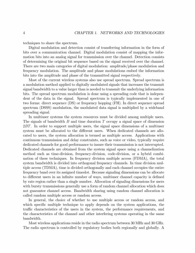
techniques to share the spectrum.Digital modulation and detection consist of transferring information in the form of
bits over a communication channel. Digital modulation consist of mapping the infor-mation bits into an analog signal for transmission over the channel. Detection consistsof determining the original bit sequence based on the signal received over the channel.There are two main categories of digital modulation: amplitude/phase modulation andfrequency modulation. The amplitude and phase modulations embed the informationbits into the amplitude and phase of the transmitted signal respectively.Most of the current wireless systems also use spread spectrum. Spread spectrum is
a modulation method applied to digitally modulated signals that increases the transmitsignal bandwidth to a value larger than is needed to transmit the underlying informationbits. The spread spectrum modulation is done using a spreading code that is indepen-dent of the data in the signal. Spread spectrum is typically implemented in one oftwo forms: direct sequence (DS) or frequency hopping (FH). In direct sequence spreadspectrum (DSSS) modulation, the modulated data signal is multiplied by a widebandspreading signal.In multiuser systems the system resources must be divided among multiple users.
The signals of bandwidth B and time duration T occupy a signal space of dimension2BT . In order to support multiple users, the signal space dimensions of a multiusersystem must be allocated to the different users. When dedicated channels are allo-cated to users, the system allocation is termed as multiple access. Applications withcontinuous transmission and delay constraints, such as voice or video, typically requirededicated channels for good performance to insure their transmission is not interrupted.Dedicated channels are obtained from the system signal space using a channelizationmethod such as time-division, frequency-division, code-division, or a hybrid combi-nation of these techniques. In frequency division multiple access (FDMA), the totalsystem bandwidth is divided into orthogonal frequency channels. In time division mul-tiple access (TDMA), time is divided orthogonally and each channel occupies the entirefrequency band over its assigned timeslot. Because signaling dimensions can be allocateto different users in an infinite number of ways, multiuser channel capacity is definedby rate region rather than a single number. Allocation of signaling dimensions for userswith bursty transmissions generally use a form of random channel allocation which doesnot guarantee channel access. Bandwidth sharing using random channel allocation iscalled random multiple access or random access.In general, the choice of whether to use multiple access or random access, and
which specific multiple technique to apply depends on the system applications, thetraffic characteristics of the users in the system, the performance requirements, andthe characteristics of the channel and other interfering systems operating in the samebandwidth.Most wireless applications reside in the radio spectrum between 30MHz and 30 GHz.
The radio spectrum is controlled by regulatory bodies both regionally and globally. A
1.1. WIRELESS COMMUNICATION 5
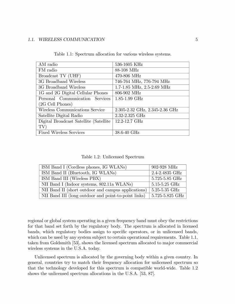
Table 1.1: Spectrum allocation for various wireless systems.
AM radio 536-1605 KHzFM radio 88-108 MHzBroadcast TV (UHF) 470-806 MHz3G Broadband Wireless 746-764 MHz, 776-794 MHz3G Broadband Wireless 1.7-1.85 MHz, 2.5-2.69 MHz1G and 2G Digital Cellular Phones 806-902 MHzPersonal Communication Services(2G Cell Phones)
1.85-1.99 GHz
Wireless Communications Service 2.305-2.32 GHz, 2.345-2.36 GHzSatellite Digital Radio 2.32-2.325 GHzDigital Broadcast Satellite (SatelliteTV)
12.2-12.7 GHz
Fixed Wireless Services 38.6-40 GHz
Table 1.2: Unlicensed Spectrum
ISM Band I (Cordless phones, IG WLANs) 902-928 MHzISM Band II (Bluetooth, IG WLANs) 2.4-2.4835 GHzISM Band III (Wireless PBX) 5.725-5.85 GHzNII Band I (Indoor systems, 802.11a WLANs) 5.15-5.25 GHzNII Band II (short outdoor and campus applications) 5.25-5.35 GHzNII Band III (long outdoor and point-to-point links) 5.725-5.825 GHz
regional or global system operating in a given frequency band must obey the restrictionsfor that band set forth by the regulatory body. The spectrum is allocated in licensedbands, which regulatory bodies assign to specific operators, or in unlicensed bands,which can be used by any system subject to certain operational requirements. Table 1.1,taken from Goldsmith [53], shows the licensed spectrum allocated to major commercialwireless systems in the U.S.A. today.
Unlicensed spectrum is allocated by the governing body within a given country. Ingeneral, countries try to match their frequency allocation for unlicensed spectrum sothat the technology developed for this spectrum is compatible world-wide. Table 1.2shows the unlicensed spectrum allocations in the U.S.A. [53, 87].

6 CHAPTER 1. NETWORKS AND TECHNOLOGIES
1.2 Wireless Networks and Technologies
The design and development of mobile wireless networks poses significant challengescompared to traditional wired networks. In contrast to the stable link capacity ofwired networks, wireless link capacity continually varies because of the impacts fromtransmission power, receiver sensitivity, noise, fading and interference. Additionally,wireless mobile networks have a high error rate, power restrictions and bandwidthlimitations. In mobile networks, node mobility may cause frequent network topologychanges which are rare in wired networks.In this section, we describe wireless networks based on infrastructure. Wireless
networks based on infrastructure are single-hop networks with direct communicationbetween a node and base station. Most control issues in these networks such as mobilityand scheduling are handled by the central base station or access point. The nextsubsections present an overview of cellular systems and WLANs.
1.2.1 Cellular Systems
The basic idea behind cellular systems is frequency reuse, which exploits the fact thatthe signal power falls off with distance so that the same frequency spectrum can beused at spatially separated locations. The coverage area of a cellular system is dividedinto nonoverlapping cells where some set of channels is assigned to each cell. Operationwithin a cell is controlled by a base station.All base stations in a geographical area are connected via a high speed communica-
tion link to a mobile telephone switching office (MTSO). The MTSO acts as a centralcontroller for the network, allocating channels within each cell, coordinating handoffsbetween cells when a node traverses a cell boundary, and routing calls to and from mo-bile users. The MTSO can route voice messages through the public switched telephonenetwork or provide Internet access (Figure 1.1).The first generation cellular systems were analog while the second and third gen-
eration cellular systems are digital. A prominent example of second generation digitalsystem is Groupe Spéciale Mobile (GSM). The GSM system, used primarily in Europe,uses a combination of TDMA and slow frequency hopping with frequency-shift keyingfor the voice modulation. The third generation (3G) cellular systems are based on wide-band code division multiple access (WCDMA) standard developed within the auspicesof the International Telecommunication Union (ITU).
1.2.2 Wireless Local Area Networks
Wireless local area networks (WLANs) provide high speed data within a small region asusers move from place to place. Wireless devices that access these LANs are typicallystationary or moving at pedestrian speeds. All wireless LAN standards in USA operate

1.2. WIRELESS NETWORKS AND TECHNOLOGIES 7
Mobile Telephone Switching
Office
Internet
Local Exchange
Long-distance Network
Base Station
Figure 1.1: Architecture of a Cellular Network
in the unlicensed frequency bands. The primary unlicensed bands are the ISM bands at900 megahertz (MHz), 2.4 gigahertz (GHz) and 5.8 GHz, and the unlicensed nationalinformation infrastructure (U-NII) band at 5 GHz. The wireless LAN standard IEEE802.11b operates with 80 MHz of spectrum in the 2.4 GHz ISM band1. The standardspecifies DSSS with data rates of around 1.6 megabit per second (Mbps) and a rangeof approximately 150 metres (m).The IEEE 802.11a wireless LAN standard operates with 300 MHz spectrum in the
5 GHz U-NII band. The 802.11a standard is based on multicarrier modulation andprovides 20-70 Mbps data rates. Another standard 802.11g uses multicarrier modulationand can be used in either the 2.4 GHz and 5 GHz bands with speeds of up to 54 Mbps.In Europe wireless LAN standard HIPERLAN (high performance radio LAN) standardhas been developed. The HIPERLAN Type 1 has data rate of 20 Mbps at a range of50 m.
1.2.3 Broadband Wireless Access Technology
Broadband wireless access provides high-rate wireless communication between a fixedaccess point and multiple terminals. Worldwide Interoperability for Microwave Access(WiMAX) is a broadband wireless technology based on IEEE 802.16 standard2. The802.16 specification is a standard for broadband wireless access systems operating atradio frequencies between 10 GHz and 66 GHz. WiMAX standard supports data rates of40 Mbps for fixed users and 15 Mbps for mobile users with a range of several kilometers.
1http://www.ieee802.org/11/2http://www.wimaxforum.org
8 CHAPTER 1. NETWORKS AND TECHNOLOGIES
WiMAX competes with wireless technologies such as WLANs, 3G cellular services, andwired technologies such as cable.
1.3 Mobile Ad hoc Wireless Networks
Mobile ad hoc networks have attracted significant amount of interest in recent yearsbecause of their flexibility, robustness and reduced costs. Mobile ad hoc networks aremultihop wireless networks, where each node not only generates its own data but alsoforwards the data of other nodes. Some of the ad hoc wireless networks such as personalnetworks, sensor networks and mesh networks are described in next subsections.The lack of infrastructure adds additional complexity in mobile ad hoc networks.
In these networks, all processing and control must be done by the network nodes in adistributed fashion. An important aspect of lack of infrastructure in ad hoc networksis that network topology changes have also to be handled by nodes.
1.3.1 Low Cost and Low Power Radio technologies
Bluetooth3 and Zigbee4 are examples of radio technologies, which due to their lowcost and power consumption can be embedded in a variety of devices to create ad hocnetworks (smart homes, sensor networks) etc. Bluetooth’s range of operation is 10m (at 1mW transmit power) and this range can be increased to 100 m by increasingthe transmission power to 100 mW. The system operates in the unlicensed 2.4 GHzfrequency band and provides 1 asynchronous data channel at 723.2 Kbps. Bluetoothuses frequency-hopping for multiple access with a carrier spacing of 1 MHz. Typically,up to 80 different frequencies are used for total bandwidth of 80 MHz.The Zigbee radio specification is designed for lower cost and power consumption
than Bluetooth. The specification is based on the IEEE 802.15.4 standard and radio iscapable of connecting 255 devices per network. The specification supports data ratesof 255 Kbps at a range of about 30 m. Zigbee is designed to provide radio operationfor months or years without recharging.
1.3.2 Personal Networks
Personal Network (PN) is a concept proposed by Niemegeers and Heemstra de Groot [78]related to the field of pervasive computing that extends the concept of a Personal AreaNetwork (PAN). The latter refers to a space of small coverage (less than 10 m) arounda person where ad hoc communication occurs, typically between portable and mobilecomputing devices such as laptops, personal digital assistants (PDAs), cell phones,
3http://www.bluetooth.com4http://www.zigbee.org

1.3. MOBILE AD HOC WIRELESS NETWORKS 9
Figure 1.2: Personal Network
headsets and digital gadgets. A PN has a core consisting of a PAN, which is extendedon-demand and in an ad hoc fashion with personal resources or resources belonging toothers. This extension is made physically via infrastructure-based networks, e.g., theInternet, an organization’s intranet, or a PN belonging to another person, a vehicle areanetwork, or a home network. The resources, which can become part of a PN, are verydiverse. These resources can be private or may have to be shared with other people.Figure 1.2 shows an example of a PN.
1.3.3 Sensor Networks
Awireless sensor network (WSN) is a wireless network consisting of spatially distributedautonomous devices using sensors to cooperatively monitor physical or environmentalconditions, such as temperature, sound, pressure or motion [60]. In addition to one ormore sensors, each node in a sensor network is typically equipped with a radio trans-ceiver, a small microcontroller, and an energy source usually a battery. The individ-ual devices in WSN are inherently resource constrained. They have limited processingspeed, storage capacity, and communication bandwidth. These devices have substantialprocessing capability in the aggregate, but not individually.Area monitoring is a typical application of WSNs [32]. In area monitoring, the
WSN is deployed over a region where some phenomenon is to be monitored. As anexample, a large quantity of sensor nodes could be deployed over a battlefield to detectenemy intrusion instead of using landmines. When the sensors detect the event beingmonitored, the event is reported to one of the base stations, which takes appropriate
10 CHAPTER 1. NETWORKS AND TECHNOLOGIES
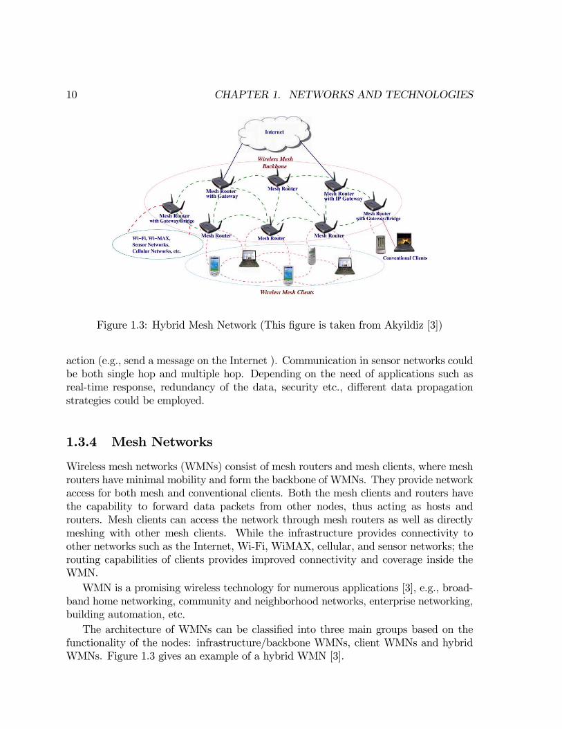
Figure 1.3: Hybrid Mesh Network (This figure is taken from Akyildiz [3])
action (e.g., send a message on the Internet ). Communication in sensor networks couldbe both single hop and multiple hop. Depending on the need of applications such asreal-time response, redundancy of the data, security etc., different data propagationstrategies could be employed.
1.3.4 Mesh Networks
Wireless mesh networks (WMNs) consist of mesh routers and mesh clients, where meshrouters have minimal mobility and form the backbone of WMNs. They provide networkaccess for both mesh and conventional clients. Both the mesh clients and routers havethe capability to forward data packets from other nodes, thus acting as hosts androuters. Mesh clients can access the network through mesh routers as well as directlymeshing with other mesh clients. While the infrastructure provides connectivity toother networks such as the Internet, Wi-Fi, WiMAX, cellular, and sensor networks; therouting capabilities of clients provides improved connectivity and coverage inside theWMN.WMN is a promising wireless technology for numerous applications [3], e.g., broad-
band home networking, community and neighborhood networks, enterprise networking,building automation, etc.The architecture of WMNs can be classified into three main groups based on the
functionality of the nodes: infrastructure/backbone WMNs, client WMNs and hybridWMNs. Figure 1.3 gives an example of a hybrid WMN [3].

1.4. PEER-TO-PEER NETWORKS 11
1.4 Peer-to-peer Networks
Peer-to-peer (P2P) networks can be considered an example of ad hoc networks becauseof the dynamic topology. P2P networks are overlay networks that can be formed overwired or wireless network. A pure P2P network does not have the notion of clientsor servers, but only equal peer nodes that simultaneously function as both clients andservers to the other nodes on the network. This model of network arrangement differsfrom the client-server model where communication is usually to and from a centralserver. A typical example for a non peer-to-peer file transfer is a file transfer protocol(FTP) server where the client and server programs are quite distinct, and the clientsinitiate the download/uploads and the servers react to and satisfy these requests.Peer-to-peer networks are typically used for connecting nodes via largely ad hoc
connections. Such networks are useful for many purposes. Sharing content files con-taining audio, video, data or anything in digital format is very common, and real-timedata, such as telephony traffic, is also passed using P2P technology.The P2P overlay network consists of all the participating peers as network nodes.
Based on how the nodes in the overlay network are linked to each other, we can classifythe P2P networks as unstructured or structured [30].An unstructured P2P network is formed when the overlay links are established
arbitrarily. Such networks can be easily constructed as a new peer that wants to jointhe network can copy existing links of another node and then form its own links overtime. In an unstructured P2P network, if a peer wants to find a desired piece of datain the network, the query has to be flooded through the network to find as many peersas possible that share the data. The main disadvantage with such networks is thatthe queries may not always be resolved. Most of the popular P2P networks such asGnutella5 are unstructured.Structured P2P networks employ a globally consistent protocol to ensure that any
node can efficiently route a search to some peer that has the desired file, even if the file isextremely rare [50]. Such a guarantee necessitates a more structured pattern of overlaylinks. By far the most common type of structured P2P network is the distributed hashtable (DHT), in which a variant of consistent hashing is used to assign ownership ofeach file to a particular peer, in a way analogous to a traditional hash table’s assignmentof each key to a particular array slot. Some well known DHTs are Chord [97], Pastry[90] and CAN [88].
5http://www.gnutella.com
12 CHAPTER 1. NETWORKS AND TECHNOLOGIES
Chapter 2
Network Modelling
A communication network can be modeled as a graph. A network of N nodes and Llinks can be represented as a graph with N vertices and L edges. Section 2.1 gives basicgraph definitions. Different graph models such as ER random graphs and power lawgraphs are used for analysis of networks. Section 2.2 explains different graph modelsand their unique features. The network architecture is described in section 2.3. Thissection also explains the routing algorithms and protocols. The last section of thischapter also gives an introduction to routing in wireless networks.
2.1 Graph Definitions
A graph is a data structure consisting of N vertices (nodes) joined together by L edges(links). A link (u, v) ∈ L is said to be incident to nodes u and v, and vice versa.If (u, v) ∈ L, then nodes u and v are said to be adjacent. The adjacency matrixA [G] = auv corresponding to an undirected graph G is defined as:
auv = 1, if (u, v) ∈ L
= 0, otherwise. (2.1)
The adjacencies defining the graph can also be represented by an adjacency-list.The adjacency-list contains for each node u ∈ V a list Adj [u] with pointers to all nodesthat are adjacent to u. Each link (u, v) ∈ L can also be assigned a weight w (u, v) andthe resulting graph is known as weighted graph. In network terminology, the weight ofa link is also termed as the cost of the link.
Definition 1 Walk: A walk from node u to node v is an alternating finite sequencev0, l1, v1, ..., lk, vk of nodes vi and links li, where li is a link connecting vi−1 and vi, v0 = uand vk = v.
13

14 CHAPTER 2. NETWORK MODELLING
Definition 2 Path: A path is a walk in which all nodes v0 to vk are distinct (vi 6= vjfor every index i 6= j).
Definition 3 Connected: A graph is connected if there exists a path between each pairof nodes in the graph.
Definition 4 Cycle: A cycle is a walk for which all nodes except the first and last aredistinct. If the graph contains no cycles it is called acyclic.
Definition 5 Degree of Connected Graph: In a connected graph with no parallel linksand self loops, a degree degu of a node u represents the number of nodes adjacent tonode u,1 ≤ degu ≤ N − 1.
The degrees of the nodes in the graph must satisfy the following equality [105]:
NXi=1
degi = 2L (2.2)
2.2 Graph Models
One of the simplest graph models used in network modelling is a full mesh or completegraph. A complete graph KN consists of N nodes and each node is connected to everyother node in the graph. Thus, the number of links in a complete graph KN are givenby L = Lmax =
N(N−1)2
links.An example of an extremely regular topology is the class of lattice topologies. We
only consider a subclass of lattices, namely rectangular two-dimensional lattices withsize l1 and l2 and N = (l1 + 1) (l2 + 1). The shortest hop path between two diagonalcorner points in the rectangular two-dimensional lattice has l1 + l2 hops. Figure 2.1gives an example of square lattice with N = 49 nodes.The random graphs, first defined by Erdös and Rényi in 1959, is another commonly
used graph topology for network modelling [48]. Random graphs are also referred to asErdös-Rényi (ER) random graphs to distinguish them from power law random graphs.The two most frequently occurring models for random graphs are Gp (N) and G (N,L).The class of graphs denoted by Gp (N) consists of graphs with N nodes in which eachpossible edge exists with probability p. Thus, the average number of links are given bypLmax.The degree distribution of node u in Gp (N) is Binomial [14]
Pr [degu = j] =
µN − 1
j
¶pj (1− p)j (2.3)

2.2. GRAPH MODELS 15
Figure 2.1: An example of square lattice with N = 49 nodes.
and the average degree is p (N − 1). Erdös and Rényi [48] identified a phase transitionin random graphs. The probability that almost every graph Gp (N) is connected isrestricted from below by the critical threshold pc ∼ lnN
Nfor N large [14, 48]. Thus,
if p > pc then almost all graphs Gp (N) are connected, else almost all graphs aredisconnected.The class of Waxman graphs belongs to the class of random graphs, where the prob-
ability of existence of a link between two nodes decays exponentially with the geographicdistance between those two nodes [65, 106]. More formally, the Waxman graphs belongto the class Gpuv (N) with puv = f (−→ru −−→rv ), where the vector−→ru represents the positionof node u and all nodes are uniformly distributed in a hyper cube in the ω−dimensionspace. The distance function f (−→r ) = e−α|
−→r |, where −→r is a norm denoting the distancefrom the origin.Random geometric graphs (RGG) have gained new relevance with the advent of
ad-hoc and sensor networks as they are used to model these networks [11, 57, 58]. Arandom geometric graph is a graph G(N, r) resulting from placing N points uniformlyat random on the unit square 1 and connecting two points iff their Euclidean distanceis at most r. Consider that wireless nodes forming a network are uniformly distributedwith certain density δ. The number of nodes within a circular area of radius r followsa Poisson distribution with mean number of neighbors δπr2 [11, 58]. However, thedegree distribution of ad hoc wireless networks also depends on shadowing, fading andinterference [41, 57]. The modelling of ad hoc wireless networks is discussed in detailin chapter 10 of this thesis.The degree distribution in the Internet and peer-to-peer networks follows a power
law [49, 52]. Albert and Barabási [4] demonstrated via empirical results that the degreedistribution for many other networks such as World Wide Web (WWW), metabolic

16 CHAPTER 2. NETWORK MODELLING
networks, phone call graphs, movie actor collaboration networks also follow power laws.These networks can be modeled as power law graphs. In power law graphs, the degreedistribution of node u is
Pr [degu = j] = cj−α (2.4)
where α is the power law exponent and c is the normalization constant such thatN−1Pj=1
Pr [degu = j] = 1. Measurements in the Internet [49] suggest that α ≈ 2.4.
Power law graphs can be generated using a variety of methods. The Barabási-Albert(BA) model for generating power law graphs is defined in two steps [6]. Starting with asmall number (v0) of nodes, at every timestep, a new node is added with l (≤ v0) links.A new node connects to nodes already in the graph with probability y = duX
v∈Z
dv
, where
du is the degree of node u and Z is the number of nodes in the graph at a particulartimestep.After t timesteps the model leads to a random network with N = t+ v0 nodes and
lt links. It has been shown in [6] that Pr[deg ≤ j] = 1 − l2tj2N. Thus, the probability
that a node s has degree j in this model follows a power law [6],
Pr[degs = j] =2l2t
N
1
j3= cj−υ (2.5)
where the scaling exponent υ = 3 is independent of l.The number of nodes with degree less than logN in the BA model is N · Pr[deg ≤
logN ] = N³1− 4
(logN)2
´and the number of nodes with a large degree is small. On
the other hand, in almost surely (a.s.) connected ER random graph where p ≥ logNN,
the average node degree is close to or greater than logN . Figure 2.2(a) shows thedegree distribution for ER random graphs. Figure 2.2(b) shows the degree distributionof power law random graph generated using BA model on a log-log scale.Many large-scale systems in communications, biology and sociology such as WWW,
the Internet, metabolic networks, phone call graphs, movie actor collaboration networksare classified as complex networks [4, 100]. To understand complex networks, it is essen-tial to know clustering coefficient [77]. The clustering coefficient of a vertex in a graphquantifies how close the vertex and its neighbors are to being a clique (complete graph).For instance, sparse random graphs have a vanishingly small clustering coefficient whilereal world networks often have a coefficient significantly larger. Complex networks arecharacterized by power law degree distribution, a high clustering coefficient, assortativ-ity1 or disassortativity among vertices, and evidence of a hierarchical structure. This
1Assortativity refers to a preference for a network’s nodes to attach to others that are similar ordifferent in some way

2.3. ROUTING ALGORITHMS AND PROTOCOLS 17
(a) ER Random Graph (b) Power law Random Graph
0.0001
0.001
0.01
0.1
Pr[d
= j]
2 3 4 5 6 7 8 910
2 3 4 5 6 7 8 9100
degree j
N = 400 N = 1600 N = 100000
0.15
0.10
0.05
0.00
Pr[d
= j]
2015105degree j
N = 400p = 0.0125
(a) ER Random Graph (b) Power law Random Graph
0.0001
0.001
0.01
0.1
Pr[d
= j]
2 3 4 5 6 7 8 910
2 3 4 5 6 7 8 9100
degree j
N = 400 N = 1600 N = 100000
0.15
0.10
0.05
0.00
Pr[d
= j]
2015105degree j
N = 400p = 0.0125
Figure 2.2: Degree distribution for ER random graph and power law random graph.
is in contrast to lattice or random graphs which exhibit a high similarity.
2.3 Routing Algorithms and Protocols
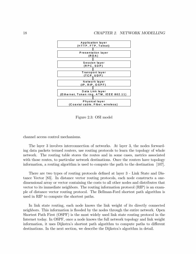
We study the architecture of the Internet to understand the concepts of routing algo-rithms and protocols and medium access layer protocols. The Internet is a collectionof interconnected networks that use packet switching [83]. The design of complex net-works such as the Internet lead to the concept of layering. Figure 2.3 shows the OpenSystems Interconnection (OSI) layered architecture for the Internet. Though the OSIarchitecture defines 7 layers, our focus in this thesis is on physical, data link, networkand application layers. Figure 2.3 also shows some of the common technologies used ateach layer.The physical layer represents the physical medium through which the data is trans-
mitted. In case of wired networks, there are technologies such as coaxial cable, twistedpair etc. that are use to make the physical connection. The data link layer (layer 2)is the layer which transfers data between adjacent network nodes in a wide area net-work or between nodes on the same local area network (LAN) segment. At this layer,the frames are forwarded by nodes based on spanning tree algorithm. We do not intodetails of the algorithm, however, the nodes using this algorithm do not need to knowthe topology of the whole network. The layer 2 nodes forwarding packets are referredto as bridges. In some networks, such as IEEE 802 LANs, the data link layer is splitinto Medium Access Control (MAC) and Logical Link Control (LLC) sublayers. TheMAC layer specifies number of protocols (e.g. CSMA/CA, CSMA/CD) which deal with
18 CHAPTER 2. NETWORK MODELLING
D a ta L in k la y e r(E th e rn e t , T o k e n r in g , A T M , IE E E 8 0 2 .1 1 )
P h y s ic a l la y e r(C o a x ia l c a b le , F ib e r , w ire le s s )
N e tw o rk la y e r( IP , R IP , O S P F )
A p p l ic a t io n la y e r(H T T P , F T P , T e ln e t )
T ra n s p o r t la y e r(T C P , U D P )
S e s s io n la y e r(R P C , S D P )
P re s e n ta t io n la y e r(R D A )
Figure 2.3: OSI model
channel access control mechanisms.
The layer 3 involves interconnection of networks. At layer 3, the nodes forward-ing data packets termed routers, use routing protocols to learn the topology of wholenetwork. The routing table stores the routes and in some cases, metrics associatedwith those routes, to particular network destinations. Once the routers have topologyinformation, a routing algorithm is used to compute the path to the destination [107].
There are two types of routing protocols defined at layer 3 - Link State and Dis-tance Vector [83]. In distance vector routing protocols, each node constructs a one-dimensional array or vector containing the costs to all other nodes and distributes thatvector to its immediate neighbors. The routing information protocol (RIP) is an exam-ple of distance vector routing protocol. The Bellman-Ford shortest path algorithm isused in RIP to compute the shortest paths.
In link state routing, each node knows the link weight of its directly connectedneighbors. This information is flooded by the nodes through the entire network. OpenShortest Path First (OSPF) is the most widely used link state routing protocol in theInternet today. In OSPF, once a node knows the full network topology and link weightinformation, it uses Dijkstra’s shortest path algorithm to compute paths to differentdestinations. In the next section, we describe the Dijkstra’s algorithm in detail.
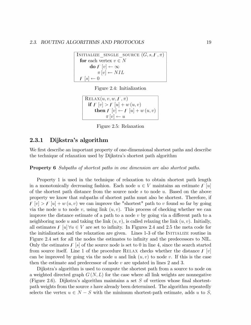
2.3. ROUTING ALGORITHMS AND PROTOCOLS 19
Initialize_single_source (G, s,z, π)for each vertex v ∈ N
do z [v]←∞π [v]← NIL
z [s]← 0
Figure 2.4: Initialization
Relax(u, v, w,z, π)if z [v] > z [u] + w (u, v)then z [v]← z [u] + w (u, v)
π [v]← u
Figure 2.5: Relaxation
2.3.1 Dijkstra’s algorithm
We first describe an important property of one-dimensional shortest paths and describethe technique of relaxation used by Dijkstra’s shortest path algorithm
Property 6 Subpaths of shortest paths in one dimension are also shortest paths.
Property 1 is used in the technique of relaxation to obtain shortest path lengthin a monotonically decreasing fashion. Each node u ∈ V maintains an estimate z [u]of the shortest path distance from the source node s to node u. Based on the aboveproperty we know that subpaths of shortest paths must also be shortest. Therefore, ifz [v] > z [u] + w (u, v) we can improve the "shortest" path to v found so far by goingvia the node u to node v, using link (u, v). This process of checking whether we canimprove the distance estimate of a path to a node v by going via a different path to aneighboring node u and taking the link (u, v), is called relaxing the link (u, v). Initially,all estimates z [u]∀u ∈ V are set to infinity. In Figures 2.4 and 2.5 the meta code forthe initialization and the relaxation are given. Lines 1-3 of the Initialize routine inFigure 2.4 set for all the nodes the estimates to infinity and the predecessors to NIL.Only the estimates z [s] of the source node is set to 0 in line 4, since the search startedfrom source itself. Line 1 of the procedure Relax checks whether the distance z [v]can be improved by going via the node u and link (u, v) to node v. If this is the casethen the estimate and predecessor of node v are updated in lines 2 and 3.Dijkstra’s algorithm is used to compute the shortest path from a source to node on
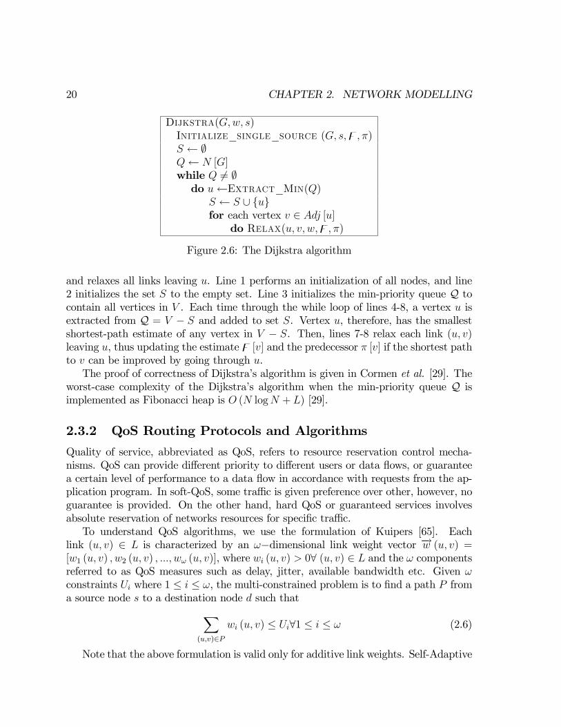
a weighted directed graph G (N,L) for the case where all link weights are nonnegative(Figure 2.6). Dijkstra’s algorithm maintains a set S of vertices whose final shortest-path weights from the source s have already been determined. The algorithm repeatedlyselects the vertex u ∈ N − S with the minimum shortest-path estimate, adds u to S,
20 CHAPTER 2. NETWORK MODELLING
Dijkstra(G,w, s)Initialize_single_source (G, s,z, π)S ← ∅Q← N [G]while Q 6= ∅do u←Extract_Min(Q)
S ← S ∪ ufor each vertex v ∈ Adj [u]
do Relax(u, v, w,z, π)
Figure 2.6: The Dijkstra algorithm
and relaxes all links leaving u. Line 1 performs an initialization of all nodes, and line2 initializes the set S to the empty set. Line 3 initializes the min-priority queue Q tocontain all vertices in V . Each time through the while loop of lines 4-8, a vertex u isextracted from Q = V − S and added to set S. Vertex u, therefore, has the smallestshortest-path estimate of any vertex in V − S. Then, lines 7-8 relax each link (u, v)leaving u, thus updating the estimate z [v] and the predecessor π [v] if the shortest pathto v can be improved by going through u.The proof of correctness of Dijkstra’s algorithm is given in Cormen et al. [29]. The
worst-case complexity of the Dijkstra’s algorithm when the min-priority queue Q isimplemented as Fibonacci heap is O (N logN + L) [29].
2.3.2 QoS Routing Protocols and Algorithms
Quality of service, abbreviated as QoS, refers to resource reservation control mecha-nisms. QoS can provide different priority to different users or data flows, or guaranteea certain level of performance to a data flow in accordance with requests from the ap-plication program. In soft-QoS, some traffic is given preference over other, however, noguarantee is provided. On the other hand, hard QoS or guaranteed services involvesabsolute reservation of networks resources for specific traffic.To understand QoS algorithms, we use the formulation of Kuipers [65]. Each
link (u, v) ∈ L is characterized by an ω−dimensional link weight vector −→w (u, v) =[w1 (u, v) , w2 (u, v) , ..., wω (u, v)], where wi (u, v) > 0∀ (u, v) ∈ L and the ω componentsreferred to as QoS measures such as delay, jitter, available bandwidth etc. Given ωconstraints Ui where 1 ≤ i ≤ ω, the multi-constrained problem is to find a path P froma source node s to a destination node d such thatX
(u,v)∈P
wi (u, v) ≤ Ui∀1 ≤ i ≤ ω (2.6)
Note that the above formulation is valid only for additive link weights. Self-Adaptive

2.3. ROUTING ALGORITHMS AND PROTOCOLS 21
Multiple Constraints routing algorithm (SAMCRA) is an example of exact QoS algo-rithm that finds the minimum cost path satisfying the required constraints [108].
2.3.3 Routing in Wireless Networks
As explained in the last section, routing in communication networks can be classifiedinto routing protocol and routing algorithm. The function of a routing protocol isto spread the routing information while the routing algorithm computes the paths.The boundary between routing protocols and algorithms is blurred in ad-hoc networkswhere the nodes may not have enough topology information and paths are set up ondemand when the nodes have data to send [39]. Moreover, single hop networks such asinfrastructure based wireless networks do not need routing protocols and algorithms.Layer 2 in wireless networks defines different MAC protocols to access the medium.
MAC protocols are needed to regulate communication between nodes through a sharedmedium. A variety of MAC protocols have been developed for communication in wiredand wireless networks. For example, IEEE 802.3 ( based on carrier sense multiple accesswith collision detection (CSMA/CD) for wired Ethernet) and IEEE 802.11 for WLAN.The IEEE 802.11 standard uses CSMA with collision avoidance.Since each node in ad hoc wireless networks forwards packets of other nodes, it needs
to have functionality till layer 3 in the OSI model. Indeed, the first generation of routingprotocols such as dynamic source routing (DSR) can be considered purely to belong tothe network layer. Such routing protocols are designed independent of the lower levellayers i.e., physical layer and MAC layer. Since MAC protocols affect interference levelsand capacity in wireless networks, increasingly it has been observed that a cross layerstrategy may provide a better solution to routing in ad hoc networks. A detailed surveyof various routing protocols and cross-layer design for ad hoc networks is presented inthe next chapter.
22 CHAPTER 2. NETWORK MODELLING
Chapter 3
Survey of Ad hoc Routing Protocols
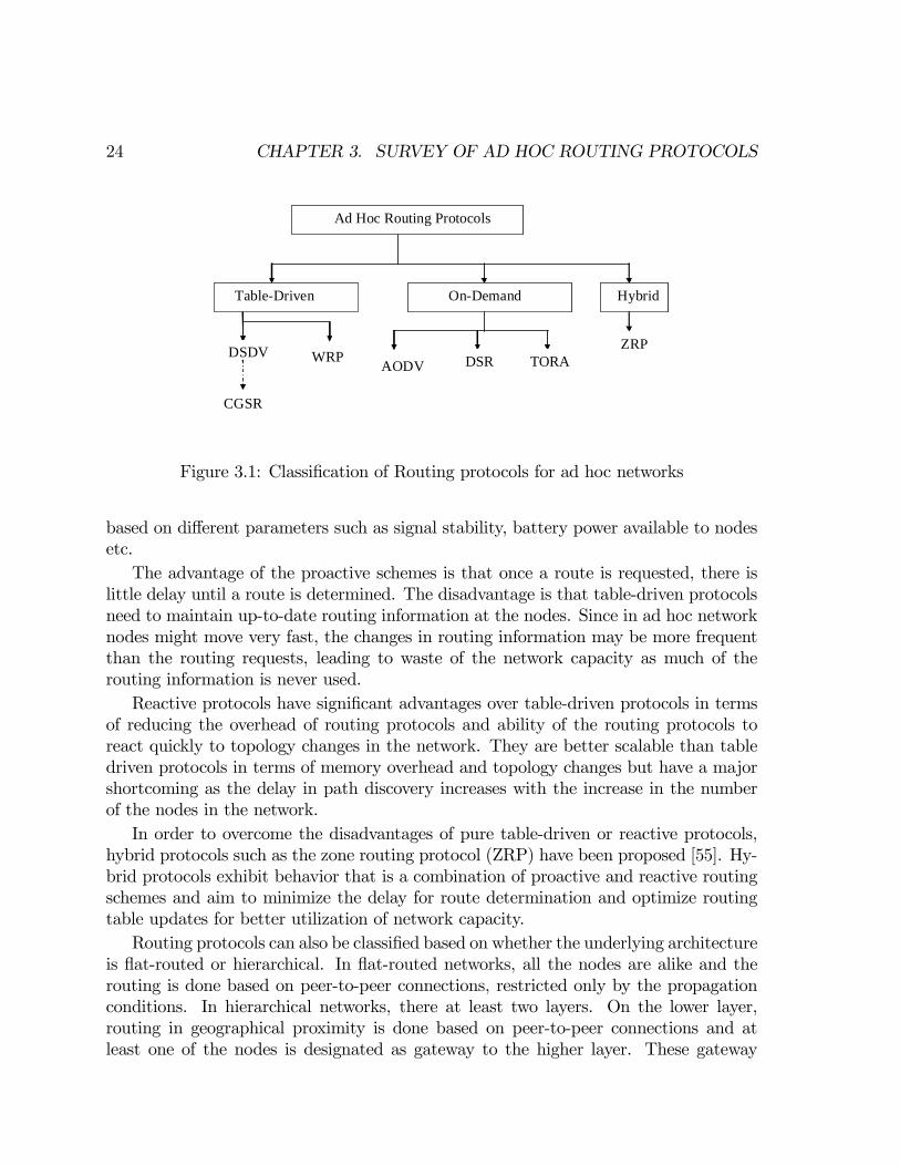
Most of the routing protocols for ad-hoc networks can be classified into three major cat-egories (Figure 3.1) based on the routing information stored at the nodes, namely, pro-active or table driven, reactive or on-demand and hybrid. Other classification schemescategorize the protocols based on whether they are hierarchical, support multicast, orare power aware [26].The first section in this chapter shows how routing protocols are categorized. In
the remaining sections, we explain 3 ad hoc wireless routing protocols namely DSDV,AODV and DSR in detail. We compare the performance of these routing protocols withant routing in chapter 6.
3.1 Classification of Ad hoc Routing Protocols
Table-driven routing protocols (e.g. DSDV [82], CGSR [21], OLSR [25]) attempt tomaintain consistent, up-to-date routing information from each node to every othernode in the network. These protocols require each node to maintain one or more tablesto store routing information, and they respond to changes in network topology bypropagating updates throughout the network in order to maintain a consistent networkview. The different table-driven protocols differ with respect to each other in termsof number of routing-related tables and the methods by which changes in the networkstructure are broadcast.In reactive or on-demand protocols (e.g. AODV [81], DSR [62], ABR [102]), routes
are created only when desired by the source node. When any node requires a route tothe destination, it initiates a route discovery process within the network. This process iscompleted once a route is formed or all possible route permutations have been examined.Once a route has been established, it is maintained by a route maintenance procedureuntil either the destination becomes inaccessible along every path from the source oruntil the route is no longer desired. The routes in reactive protocols could be established
23
24 CHAPTER 3. SURVEY OF AD HOC ROUTING PROTOCOLS
Ad Hoc Routing Protocols
Table-Driven On-Demand
DSDVAODV DSR TORA
Hybrid
ZRP
CGSR
WRP
Ad Hoc Routing Protocols
Table-Driven On-Demand
DSDVAODV DSR TORA
Hybrid
ZRP
CGSR
WRP
Figure 3.1: Classification of Routing protocols for ad hoc networks
based on different parameters such as signal stability, battery power available to nodesetc.The advantage of the proactive schemes is that once a route is requested, there is
little delay until a route is determined. The disadvantage is that table-driven protocolsneed to maintain up-to-date routing information at the nodes. Since in ad hoc networknodes might move very fast, the changes in routing information may be more frequentthan the routing requests, leading to waste of the network capacity as much of therouting information is never used.Reactive protocols have significant advantages over table-driven protocols in terms
of reducing the overhead of routing protocols and ability of the routing protocols toreact quickly to topology changes in the network. They are better scalable than tabledriven protocols in terms of memory overhead and topology changes but have a majorshortcoming as the delay in path discovery increases with the increase in the numberof the nodes in the network.In order to overcome the disadvantages of pure table-driven or reactive protocols,
hybrid protocols such as the zone routing protocol (ZRP) have been proposed [55]. Hy-brid protocols exhibit behavior that is a combination of proactive and reactive routingschemes and aim to minimize the delay for route determination and optimize routingtable updates for better utilization of network capacity.Routing protocols can also be classified based on whether the underlying architecture
is flat-routed or hierarchical. In flat-routed networks, all the nodes are alike and therouting is done based on peer-to-peer connections, restricted only by the propagationconditions. In hierarchical networks, there at least two layers. On the lower layer,routing in geographical proximity is done based on peer-to-peer connections and atleast one of the nodes is designated as gateway to the higher layer. These gateway

3.1. CLASSIFICATION OF AD HOC ROUTING PROTOCOLS 25
nodes create the higher layer network. Thus, routing between nodes that belong tothe same lower-layer network is based on peer-to-peer routing and routing betweennodes that belong to different lower-layer networks is through the gateway nodes. Themajor advantage of hierarchical protocols is scalability. Cluster head formation schemesprovide a very efficient and distributed solution for routing and thus scale well even forlarge networks. On the other hand creation and maintenance of clusters leads to extraoverhead for routing protocol. Clusterhead Gateway Switch Routing (CGSR) is anexample of hierarchical routing [21].The routing protocols for ad-hoc wireless networks can also be classified according
to distinct features that they implement. Location aided protocols use the locationinformation of intermediate nodes and destination node to make routing decisions.Since nodes in ad hoc networks may move at any time, location aided protocols tryto efficiently use the location information and node movement information for routingpackets. Routing protocols can also be classified based on whether they support routingof unicast or multicast packets. A number of on-demand and table-driven multicastingrouting protocols such as ODMRP [67], MCEDAR [95] etc. have been proposed for adhoc networks. Most of the on-demand multicast routing protocols rely on significantperiodic (non-on-demand) behavior within portions of the protocol. Routing proto-cols which support multicast provide an efficient means of supporting group-orientedapplications.
3.1.1 Power-saving routing protocols
Power saving or energy efficient communication techniques are important in ad hocwireless networks as devices may be battery operated and hence power constrained.The most common technique proposed is the power control scheme, in which a nodetransmits data packets to its neighbor at minimum power level. Recent studies (e.g.LAPAR [109], PAMAS [94]) have stressed the need for designing protocols both atMAC and network layers to ensure longer battery life.In wireless networks, the power of transmitted signal is attenuated at the rate of
r−α, where r is the distance between the sender and the receiver and α is the pathloss exponent between 2 and 6. Consequently, transmitting data packets directly to thenode may consume more energy that going through some intermediate nodes. Basedon this observation, most of the proposed energy-efficient routing protocols try to finda path that has many short-range hops in order to consume the least amount of totalenergy. These protocols can be classified into three main categories
• Minimum total transmission power protocols: These protocols set the link costto the transmission power and use a shortest path algorithm to search for theminimum energy path.
26 CHAPTER 3. SURVEY OF AD HOC ROUTING PROTOCOLS
• Minimum total transceiving power protocols: As the intermediate nodes consumeenergy not only when forwarding packets but also when receiving packets, theseprotocols assign the transmission power and receiving power to the link cost met-ric.
• Minimum total reliable transmission power protocols: In these protocols, linkcost is a function of both the energy required for a single transmission attemptacross the link and link error rate, which determines the number of retransmissionattempts needed for successful transmission.
Power aware multi-access protocol with signaling (PAMAS) is a multi-access MAClayer protocol which is based on the original MACA protocol with addition of a sepa-rate signaling channel [94]. PAMAS conserves battery power at nodes by intelligentlypowering off nodes that are not actively transmitting or receiving packets. The man-ner in which nodes power themselves off does not influence the delay or throughputcharacteristics of the PAMAS protocol. PAMAS searches for the minimum energy pathby using Dijkstra’s shortest path algorithm. Location-aided power-aware routing (LA-PAR) protocol [109] is a location-aided power-aware routing protocol that dynamicallymakes local routing decisions so that a near-optimal power-efficient end-to-end route isformed for forwarding data packets.
3.1.2 Cross-Layer Design
Cross-layer design is a joint design optimization across several layers (e.g. physical,MAC and routing layers) under given resource constraints to improve network perfor-mance [31, 72]. For example, in sensor networks, the average transmission distance isin the order of a few meters. As a result, the circuit processing power becomes com-parable to the transmission power. Therefore, for energy efficient network design, thetransmission power and the circuit processing power need to be jointly considered ina cross-layer optimization problem. Cross-layer design involves information exchangebetween different layers, adaptivity at each layer to this information, and diversity builtinto each layer to insure robustness [53]. For example, the physical layer can deployadaptive modulation and coding to compensate for time-varying wireless channel. Thisadaptivity could be used by higher layers to achieve better performance. The MAClayer can assign a longer channel usage time to links with low-rate modulation schemesto meet the throughput or energy constraints and the network or routing layer canreroute traffic to links supporting high-rate modulation schemes to minimize conges-tion. Though cross-layer optimization is beyond the scope of this thesis, we do considerthe effect of an adaptive power strategy on the lifetime of ad hoc wireless networks inchapter 10.
3.2. DESTINATION-SEQUENCED DISTANCE-VECTOR ROUTING 27
3.2 Destination-Sequenced Distance-Vector Routing
The destination-sequenced distance-vector (DSDV) is a table-driven algorithm proposedby Perkins and Bhagwat and is based on the classical Bellman-Ford routing mechanism[82]. Every mobile node in the network implementing DSDV maintains a routing table.In routing tables of DSDV, an entry contains the next hop towards a destination, thecost metric for the routing path to the destination and a destination sequence numberthat is created by the destination. Sequence numbers are used in DSDV to distinguishstale routes from fresh ones and avoid formation of route loops.The route updates of DSDV can be either time-driven or event-driven. Every node
periodically transmits updates including its routing information to its immediate neigh-bors. While a significant change occurs from the last update, a node can transmit itschanged routing table in an event-triggered style. Moreover, the DSDV has two wayswhen sending routing table updates. One is full dump update type and the full routingtable is included inside the update. A full dump update could span many packets.An incremental update contains only those entries that with metric have been changedsince the last update is sent. Additionally, the incremental update fits in one packet.Broch et al. [16] have shown that DSDV performs well when node mobility rate and
node movement speed are low, but has convergence problems when the node mobilityincreases. Furthermore, the routing protocol overhead increases as the network diameterand node mobility increase.
3.3 Dynamic Source Routing
The Dynamic Source Routing (DSR) is an on-demand routing protocol based on theconcept of source routing [62]. Source routing is a routing technique in which the senderof a packet determines the complete sequence of nodes through which to forward thepacket. The key advantage of source routing is that intermediate nodes do not needto maintain up-to-date routing information in order to route the packets they forward,since the packets themselves already contain all the routing decisions. Mobile nodesusing DSR maintain route caches that contain source routes of which the node is aware.There are two major phases in DSR, the route discovery phase and the route main-
tenance phase. When a source node wants to send a packet, it first consults its routecache. If the required route is available, the source node includes the routing informationinside the data packet before sending it. Otherwise, the source node initiates a routediscovery operation by broadcasting route request (RT_REQ) packets. A RT_REQpacket contains addresses of both the source and the destination and a unique num-ber to identify the request. Receiving a RT_REQ packet, a node checks its routecache. If the node doesn’t have routing information for the requested destination, itappends its own address to the route record field of the RT_REQ packet. Then, the
28 CHAPTER 3. SURVEY OF AD HOC ROUTING PROTOCOLS
RT_REQ packet is forwarded to its neighbors. To limit the communication overheadof RT_REQ packets, a node processes RT_REQ packets that it has not seen beforeand its address is not present in the route record field. If the RT_REQ packet reachesthe destination or an intermediate node has routing information to the destination, aroute reply (RT_REP) packet is generated. When the RT_REP packet is generated bythe destination, it comprises addresses of nodes that have been traversed by the routerequest packet. Otherwise, the RT_REP packet comprises the addresses of nodes theRT_REQ packet has traversed concatenated with the route in the intermediate node’sroute cache.After being created, either by the destination or an intermediate node, a RT_REP
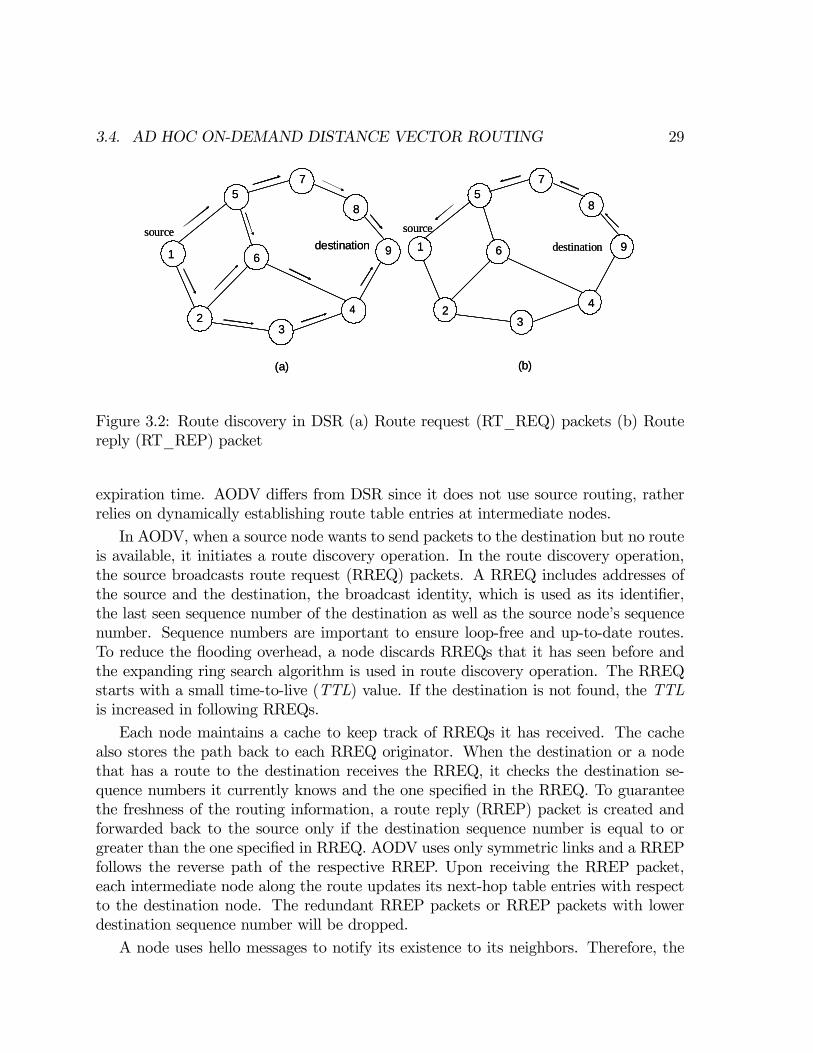
packet needs a route back to the source. There are three possibilities to get a backwardroute. The first one is that the node already has a route to the source. The secondpossibility is that the network has symmetric (bidirectional) links. The route replypacket is sent using the collected routing information in the route record field, butin a reverse order as shown in Figure 3.2. In the last case, there are asymmetric(unidirectional) links and a new route discovery procedure is initiated to the source.The discovered route is piggybacked in the route request packet.In DSR, when the data link layer detects a link disconnection, a route error (RT_ERR)
packet is sent backward to the source. After receiving the RT_ERR packet, the sourcenode initiates another route discovery operation. Additionally, all routes containing thebroken link should be removed from the route caches of the immediate nodes when theRT_ERR packet is transmitted to the source.Source routing protocols such as DSR face a scaling challenge as network diameter in
hops and mobility increase because the product of these two factors determines the ratethat end-to-end paths change. DSR must query longer routes as the network diameterincreases, and must do so more often as the mobility increases, and caching becomesless effective.
3.4 Ad Hoc On-Demand Distance Vector Routing
AODV is an on-demand routing protocol proposed by Perkins et al. [81]. It is acombination of DSR and DSDV protocols. It borrows the basic on-demand mechanismof route discovery and route maintenance from DSR, plus the use of hop-by-hop routing,sequence numbers and periodic beacons from DSDV. AODV is an improvement overDSDV because it typically minimizes the number of required broadcasts by creatingroutes on a demand basis, rather than maintaining the complete list of routes as in theDSDV algorithm. As a reactive routing protocol, AODV only needs to maintain therouting information about the active paths. In AODV, each mobile node keeps a next-hop routing table, which contains the destinations to which it currently has a route.A routing table entry expires if it has not been used or reactivated for a pre-specified
3.4. AD HOC ON-DEMAND DISTANCE VECTOR ROUTING 29
(a) (b)
7
91
58
2
6
3
4
sourcedestination
57
8
9
2
6
34
source1 destination
(a) (b)
7
91
58
2
6
3
4
sourcedestination
57
8
9
2
6
34
source1 destination
Figure 3.2: Route discovery in DSR (a) Route request (RT_REQ) packets (b) Routereply (RT_REP) packet
expiration time. AODV differs from DSR since it does not use source routing, ratherrelies on dynamically establishing route table entries at intermediate nodes.
In AODV, when a source node wants to send packets to the destination but no routeis available, it initiates a route discovery operation. In the route discovery operation,the source broadcasts route request (RREQ) packets. A RREQ includes addresses ofthe source and the destination, the broadcast identity, which is used as its identifier,the last seen sequence number of the destination as well as the source node’s sequencenumber. Sequence numbers are important to ensure loop-free and up-to-date routes.To reduce the flooding overhead, a node discards RREQs that it has seen before andthe expanding ring search algorithm is used in route discovery operation. The RREQstarts with a small time-to-live (TTL) value. If the destination is not found, the TTLis increased in following RREQs.
Each node maintains a cache to keep track of RREQs it has received. The cachealso stores the path back to each RREQ originator. When the destination or a nodethat has a route to the destination receives the RREQ, it checks the destination se-quence numbers it currently knows and the one specified in the RREQ. To guaranteethe freshness of the routing information, a route reply (RREP) packet is created andforwarded back to the source only if the destination sequence number is equal to orgreater than the one specified in RREQ. AODV uses only symmetric links and a RREPfollows the reverse path of the respective RREP. Upon receiving the RREP packet,each intermediate node along the route updates its next-hop table entries with respectto the destination node. The redundant RREP packets or RREP packets with lowerdestination sequence number will be dropped.
A node uses hello messages to notify its existence to its neighbors. Therefore, the
30 CHAPTER 3. SURVEY OF AD HOC ROUTING PROTOCOLS
link status to the next hop in an active route can be monitored. When a node discoversa link disconnection, it broadcasts a route error (RERR) packet to its neighbors, whichin turn propagates the RERR packet towards nodes whose routes may be affected by thedisconnected link. Then, the affected source can re-initiate a route discovery operationif the route is still needed.
3.5 Summary
The above ad hoc routing approaches have introduced several paradigms such as ex-ploiting user demand, and the use of location, power, and the association parameters.Both table-driven and on-demand routing protocols have their advantages and disadvan-tages and cannot be universally applied equally well to all networks. A flexible routingapproach could be the solution. A flexible routing protocol could invoke table-drivenand/or on-demand approaches based on situations and communication requirements.Coexistence of both approaches may also exist in spatially clustered ad hoc groups, withintracluster employing the table driven approach and intercluster employing demanddriven approach or vice versa.
Part II
Ant Routing
31

Chapter 4
Introduction to ant routing
Stigmergy (from the Greek stigma: sting and ergon: work) is a concept first introducedby Paul Grasse in 1959 to explain the coordination and regulation of collective behaviorin insect colonies [101]. A formal definition used in Biology is: stigmergy is a class ofmechanisms that mediate animal-animal interactions. Most of the observations havebeen about collective behavior of insects though there has been some recent work onsocial interactions among higher species [101].The basic principle of stigmergy is simple. Traces of chemicals left in the environ-
ment or modifications made by individuals in their environment are used as feedback.The insect colony records its activity in a physical environment and uses it to organizecollective behavior. Various forms of storage include: gradients of chemical substanceknown as pheromones, material structures, or spatial distribution of insect colony. Suchstructures materialize the dynamics of the colony’s collective behavior and constrain thebehavior of individuals through a feedback loop. A simpler definition of stigmergy issufficient for this thesis: stigmergy is a form of indirect communication mediated bymodifications of the environment [101].Stigmergy mechanisms have been classified into two categories. With quantitative
stigmergy, the stimulus-response sequence comprises stimuli that does not differ quali-tatively, and only modify the probability of response of the individuals to this stimuli.An example of quantitative stigmergy is the construction of pillars in termites studiedby Grasse [101]. Qualitative stigmergy is based on discrete set of stimulus types: Forexample, an insect responds to type-1 stimulus with action A and responds to type-2stimulus by action B. An example of the qualitative stigmergy is nest building in waspPolistes.The foraging behavior of ant colonies is an example of quantitative stigmergy. While
walking from food sources to nest and vise versa, ants deposit pheromone on the ground,forming in his way a pheromone trail. Ants can smell pheromone and the probabilityof choosing paths marked by strong pheromone concentration increases. It has beenshown experimentally that the pheromone trail following behavior of a colony of ants
33
34 CHAPTER 4. INTRODUCTION TO ANT ROUTING
(a) (b)
100
80
60
40
20
0
% o
f pas
sage
s
2520151050
Time (minutes)
Food
BranchUpper
Lower Branch
Nest o60
cm15
(a) (b)
100
80
60
40
20
0
% o
f pas
sage
s
2520151050
Time (minutes)
Food
BranchUpper
Lower Branch
Nest o60
cm15
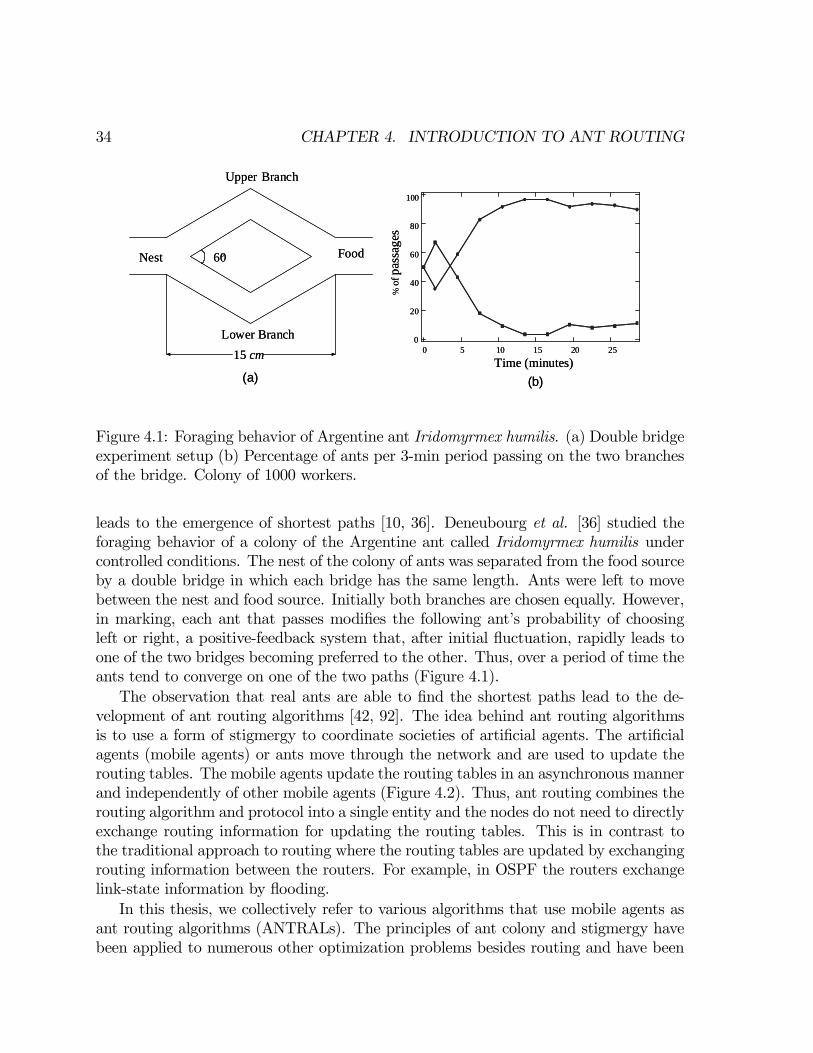
Figure 4.1: Foraging behavior of Argentine ant Iridomyrmex humilis. (a) Double bridgeexperiment setup (b) Percentage of ants per 3-min period passing on the two branchesof the bridge. Colony of 1000 workers.
leads to the emergence of shortest paths [10, 36]. Deneubourg et al. [36] studied theforaging behavior of a colony of the Argentine ant called Iridomyrmex humilis undercontrolled conditions. The nest of the colony of ants was separated from the food sourceby a double bridge in which each bridge has the same length. Ants were left to movebetween the nest and food source. Initially both branches are chosen equally. However,in marking, each ant that passes modifies the following ant’s probability of choosingleft or right, a positive-feedback system that, after initial fluctuation, rapidly leads toone of the two bridges becoming preferred to the other. Thus, over a period of time theants tend to converge on one of the two paths (Figure 4.1).The observation that real ants are able to find the shortest paths lead to the de-
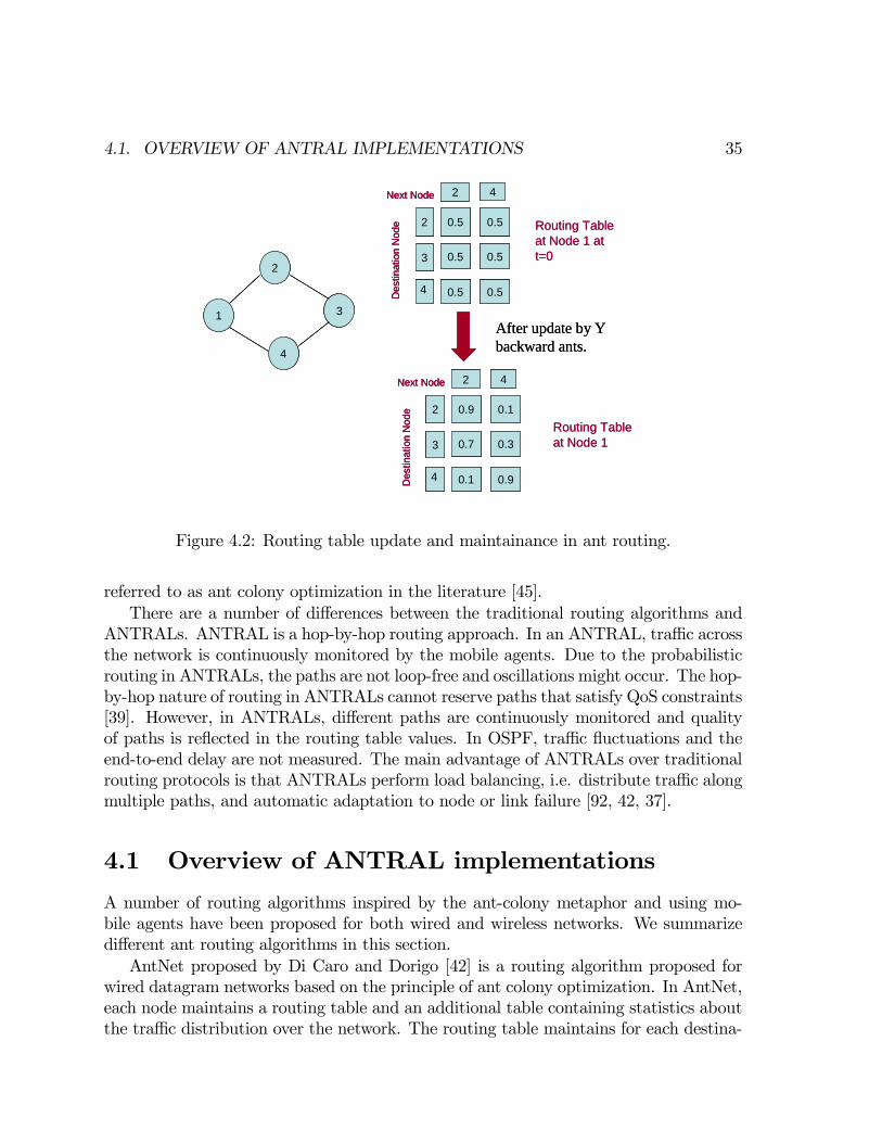
velopment of ant routing algorithms [42, 92]. The idea behind ant routing algorithmsis to use a form of stigmergy to coordinate societies of artificial agents. The artificialagents (mobile agents) or ants move through the network and are used to update therouting tables. The mobile agents update the routing tables in an asynchronous mannerand independently of other mobile agents (Figure 4.2). Thus, ant routing combines therouting algorithm and protocol into a single entity and the nodes do not need to directlyexchange routing information for updating the routing tables. This is in contrast tothe traditional approach to routing where the routing tables are updated by exchangingrouting information between the routers. For example, in OSPF the routers exchangelink-state information by flooding.In this thesis, we collectively refer to various algorithms that use mobile agents as
ant routing algorithms (ANTRALs). The principles of ant colony and stigmergy havebeen applied to numerous other optimization problems besides routing and have been
4.1. OVERVIEW OF ANTRAL IMPLEMENTATIONS 35
2
1 3
4
Routing Table at Node 1
After update by Y backward ants.
0.9 0.1
0.7 0.3
0.1 0.9
2
3
2 4Next Node
Des
tinat
ion
Nod
e
4
Routing Table at Node 1 at t=0
0.5 0.5
0.5 0.5
0.5 0.5
2
3
2 4Next Node
Des
tinat
ion
Nod
e
4
2
1 3
4
2
1 3
4
Routing Table at Node 1
After update by Y backward ants.
0.9 0.1
0.7 0.3
0.1 0.9
2
3
2 4Next Node
Des
tinat
ion
Nod
e
4
0.9 0.1
0.7 0.3
0.1 0.9
2
3
2 4Next Node
Des
tinat
ion
Nod
e
4
Routing Table at Node 1 at t=0
0.5 0.5
0.5 0.5
0.5 0.5
2
3
2 4Next Node
Des
tinat
ion
Nod
e
4
0.5 0.5
0.5 0.5
0.5 0.5
2
3
2 4Next Node
Des
tinat
ion
Nod
e
4
Figure 4.2: Routing table update and maintainance in ant routing.
referred to as ant colony optimization in the literature [45].There are a number of differences between the traditional routing algorithms and
ANTRALs. ANTRAL is a hop-by-hop routing approach. In an ANTRAL, traffic acrossthe network is continuously monitored by the mobile agents. Due to the probabilisticrouting in ANTRALs, the paths are not loop-free and oscillations might occur. The hop-by-hop nature of routing in ANTRALs cannot reserve paths that satisfy QoS constraints[39]. However, in ANTRALs, different paths are continuously monitored and qualityof paths is reflected in the routing table values. In OSPF, traffic fluctuations and theend-to-end delay are not measured. The main advantage of ANTRALs over traditionalrouting protocols is that ANTRALs perform load balancing, i.e. distribute traffic alongmultiple paths, and automatic adaptation to node or link failure [92, 42, 37].
4.1 Overview of ANTRAL implementations
A number of routing algorithms inspired by the ant-colony metaphor and using mo-bile agents have been proposed for both wired and wireless networks. We summarizedifferent ant routing algorithms in this section.AntNet proposed by Di Caro and Dorigo [42] is a routing algorithm proposed for
wired datagram networks based on the principle of ant colony optimization. In AntNet,each node maintains a routing table and an additional table containing statistics aboutthe traffic distribution over the network. The routing table maintains for each destina-
36 CHAPTER 4. INTRODUCTION TO ANT ROUTING
tion and for each next hop a measure of the goodness of using the next hop to forwarddata packets to the destination. These goodness measures, called pheromone variables,are normalized to one in order to be used by a stochastic routing policy. AntNet usestwo sets of homogeneous mobile agents called forward ants and backward ants to up-date the routing tables. The forward ants use heuristics based on the routing table tomove between a given pair of nodes and are used to collect information about the trafficdistribution over the network. The backward ants retrace the paths of forward ants inthe opposite direction. At each node, the backward ants update the routing table andthe additional table containing statistics about the traffic distribution over the network.Ant-Based Control (ABC) is an algorithm proposed by Schoonderwoerd et al. [92]
for load balancing in circuit-switched networks. In ABC, the calls are routed usingprobabilistic routing tables that consist of next hop probabilities for each destination.The link costs are assumed to be symmetric and hence, only one-directional mobileagents are used for updating and maintaining the routing tables. The mobile agentsuse heuristics based on the routing tables to move across the network between arbitrarypairs of nodes. At each node along the path, the mobile agents update the routing tablesbased on their distance from the source node and the current state of the routing table.Another ANTRAL for wired networks has been proposed by Kuntz et al. [59]. The
proposed algorithm differs from AntNet in terms of different loop detection behavior,simpler backward mobile agent and different routing table update procedure. Theauthors also propose another routing protocol called Co-operative Asymmetric Forward(CAF) routing. CAF is similar to ABC but it works for asymmetric networks wherethe link costs are not identical in opposite directions. CAF has been shown to performas well as AntNet and is able to cope with changing bandwidth and network topology[59].AntHocNet is a hybrid routing protocol proposed by Ducatelle et al. [47] for mobile
ad hoc networks. AntHocNet consists of both the reactive and proactive components.In AntHocNet, nodes do not maintain routes to all possible destinations at all the times,rather the nodes generate mobile agents only at the beginning of a data session. Themobile agents search for multiple paths to the destination and these paths are set upin the form of pheromone tables indicating their respective quality. During the courseof the data session, the paths are continuously monitored and improved in a proactivemanner. AntHocNet has been shown to outperform AODV in terms of end-to-end delayand delivery ratio [47].Ad hoc Networking with Swarm Intelligence (ANSI) is a reactive routing protocol
proposed by Rajagopalan and Shen [86] for mobile ad hoc networks. ANSI protocoluses two sets of mobile agents called forward reactive ants and backward reactive ants.The routing tables in ANSI contains an entry for each reachable node and next besthop while the ant decision table stores the pheromone values. In ANSI, the forwardreactive ants are generated on demand i.e., the forward reactive ants are generatedonly when a node needs to transmit data to another node. The forward reactive ants

4.1. OVERVIEW OF ANTRAL IMPLEMENTATIONS 37
are broadcast while the backward reactive ant retrace the path of forward reactive antand update the pheromone values at the nodes. The data packets choose the next hopdeterministically i.e., the hop which contains the largest pheromone value is chosen asthe next hop. ANSI has been shown to perform either better or comparable with AODVwith respect to packet delivery, end-to-end delay and delay jitter [86].
A number of routing protocols in which the mobile agents do not update the rout-ing tables directly have also been proposed (e.g. Termite [89], Global PositioningSystem/Ant-Like Routing Algorithm (GPSAL) [18]). Termite, a routing protocol pro-posed by Roth and Wicker [89] for mobile ad hoc networks, is one such example. InTermite, the size of the routing table at each node varies and depends on the number ofnodes that have been discovered by the particular node and the number of neighbors.The routing table entries in Termite contain pheromone values for choosing a neigh-bor as the next hop for each destination. The pheromone values decay exponentiallywith time and the corresponding entries are removed from the routing tables, if all thepheromone for a particular destination decays. Thus, the routing tables in Termitemaintain entries for only the destinations from which packets have been received dur-ing recent times. Termite does not use mobile agents for updating the routing tablesinstead node discovery and route discovery and maintenance are performed by a set offour control packets: route request packets, route reply packets, hello packets and seedpackets. Both data packets and control packets (except route request packets) are usedfor updating the routing tables.
Ant-Colony-Based Routing Algorithm (ARA) is a routing protocol proposed byGünes and Spaniol [54] for mobile ad hoc networks. The routing table entries in ARAcontain pheromone values for choosing a neighbor as the next hop for each destination.In ARA, the pheromone values in the routing tables decay with time and the nodesenter a sleep mode if the pheromone in the routing table has reached a lower threshold.Route discovery in ARA is performed on demand and by a set of two mobile agents- forward ants and backward ants. During route discovery, the forward and backwardant packets having unique sequence numbers, to prevent duplicate packets, are floodedthrough the network by the source and destination nodes respectively. The forwardand backward ants update the pheromone tables at the nodes along the path for thesource and destination nodes respectively. Once the route discovery for a particulardestination has been performed, the source node does not generate new mobile agentsfor the destination instead the route maintenance is performed by the data packets.
Uniform ant routing algorithms are a class of ANTRALs in which the mobile agentschoose the next node uniformly among the neighbors of the node [98]. Thus, in uniformANTRALs, the mobile agents move independently of the routing tables and perform arandom walk with memory on the network graph while searching for the destination.This feature of uniform ANTRALs reduces the complexity of the ant routing algorithmand leads to exploration of all the paths with equal probabilities.

38 CHAPTER 4. INTRODUCTION TO ANT ROUTING
4.2 Performance of Ant Routing Algorithms
There are two critical components that determine the performance of an ANTRAL.First, the performance depends on how the mobile agents search for the shortest path,which is referred to as network exploration. The mobile agents could either use heuristicsbased on the routing tables or the routing table values without any modifications tomove to the next node. The mobile agents could also search independently of therouting tables. We introduce an example of such algorithm in chapter 5.The second critical step determining the performance of ANTRALs is the routing
table update. The mobile agents have to update the routing tables based on the pathsthat have been searched.There has been very little work in studying the performance of ANTRALs. To our
knowledge, the only work is by Bean and Costa [9], Yoo et al. [110] and recently byPurkayastha and Baras [85]. Bean and Costa [9, 30] have conducted analytic modellingof ANTRALs and have shown that since ANTRALs employ the same policy for networkexploration and decision-making, it leads to sub-optimal routing decisions. Indeed, theyhave conjectured that a majority of the ants choose shortest paths while some of theants choose sub-optimal paths. Furthermore, they propose algorithms for de-couplingof network exploration and routing table updates when there is no data traffic and forvarying traffic.The exact convergence of ANTRAL to shortest path routing for static topology and
link weights has been studied analytically by Yoo et al. [110]. However, the resultsare only for a two node network with multiple links. Recently, Purkayastha and Baras[85] have used ordinary differential equations (ODE) to analyze the performance ofANTRALs.We study the performance of ANTRALs in the next couple of chapters. In chapter
5, we analyze the performance of AntNet, an ANTRAL proposed by Di Caro and Dorigo[42]. In chapter 6, we study the performance of ANTRALs for ad hoc wireless networks.We compare the performance of W_AntNet, a modification of the AntNet algorithm,with ad hoc routing protocols AODV and DSR.
Chapter 5
Ant Routing in Wired Networks
In this chapter, we study the convergence of AntNet to shortest path for static linkweights and fixed topologies. We compare the performance of AntNet with Dijkstra’sshortest path algorithm. Although AntNet has been shown by Di Caro and Dorigo toperform load balancing1, a study of whether AntNet is able to find paths close to theshortest path is missing. Such an analysis is essential for widespread deployment ofANTRALs.In all the ANTRALs proposed so far, the algorithm parameters have been chosen
heuristically. There has been little work on studying the robustness of ANTRALs tothe variations in different parameter values. Furthermore, the performance analysis ofANTRALs has been limited to a few network topologies. We study the effect of differentparameters used for network exploration and routing table updates on the performanceof AntNet algorithm. We also study the impact of topology on the performance ofAntNet algorithm.The rest of this chapter is organized as follows. The next section presents the
network model and section 5.2 presents the details of AntNet algorithm. Section 5.3presents the simulation results. Finally, section 5.4 presents the conclusions.
5.1 Network Model
We model the network as a graph G(N ,L) consisting of N nodes and L links. Allthe links in the network are considered bidirectional and specified by a transmissioncapacity and a transmission delay. Each node is considered a communication end-point(host) and a forwarding unit (router).As illustrated in Figure 5.1, every node in the network maintains an input buffer
composed of a single queue and an output buffer composed of a high priority queueand a low priority queue for each neighbor or outgoing link. The high priority queue is
1Schoonderwoerd [92] showed load balancing for another ANTRAL.
39

40 CHAPTER 5. ANT ROUTING IN WIRED NETWORKS
Input Buffer
Output Buffer
Low priority queue
High priority queue
Outgoing linksService process
Incoming links
Figure 5.1: Buffers at a Node. The input buffer consists of a single queue and the outputbuffer consists of a low priority queue and a high priority queue for each outgoing link.
served before the low priority queue. All the packets within the network can be dividedinto two different classes:
• Data packets: represent the information that the end-users exchange with eachother. In ant-routing, data packets do not maintain any routing information butuse the information stored at routing tables for travelling from the source to thedestination node.
• Mobile agents (Forward ants and Backward ants): are used to update the routingtables and distribute information about the traffic load in the network.
Backward ant packets have a higher priority than the data and forward ant packetsand are thus stored in the high priority queue, while data and forward ant packets arestored in the low priority queue. We assume that all the packets in the low priority queueand the high priority queue in the output buffer are served in FIFO order. Further,the maximum number of packets stored in the input buffer or output buffer is limitedby the size of the buffer. However, we have assumed that the buffer size is sufficientlylarge to neglect buffer overflow.
5.1. NETWORK MODEL 41
When a node receives a packet from a neighbor, the packet is first stored in theinput buffer. The packet in the input buffer is served in FIFO order. After the packethas been served, the packet is sent to the output buffer. Within the output buffer, thepacket goes to a particular queue for a particular outgoing link based on the type ofthe packet and the next node.
5.1.1 Data Structures at Nodes
Mobile agents communicate in an indirect way, through the information they concur-rently read and write in two data structures stored at each network node k:
1. A routing table Rk, organized as a matrix with probabilistic entries as shownin Figure 5.2. Each row in the routing table corresponds to one destination inthe network and each column corresponds to a neighbor of the current node.The routing table Rk defines the probabilistic routing policy currently adopted atnode k: for each possible destination d and for each neighbor node n, Rk storesa probability value pnd expressing the probability of choosing n as the next nodewhen the destination is d such that:X
n∈Nk
pnd = 1
where d ∈ [1, N ] and Nk = neighbors (k)
2. A table Bk(μd, σ2d,Wd) containing statistics about the network topology and thetraffic distribution over the network as seen by the local node k. For each destina-tion d in the network, the table Bk contains a moving observation windowWd, anestimated mean μd and an estimated variance σ
2d. The moving observation window
Wd, of size Wmax, represents an array containing the trip times of the last Wmax
forward ants that travel from node k to destination d. The moving observationwindow Wd is used to compute the best trip time tbestd i.e., the best trip timeexperienced by a forward ant travelling from node k to destination d among thelast Wmax forward ants that travel from node k to destination d. The mean μdand variance σ2d represent the mean and variance of the trip times experienced bythe forward ants to move from node k to destination node d and are calculatedusing the exponential model:
μd ←− μd + η (tk−→d − μd) (5.1)
σ2d ←− σ2d + η¡(tk−→d − μd)
2 − σ2d¢
(5.2)
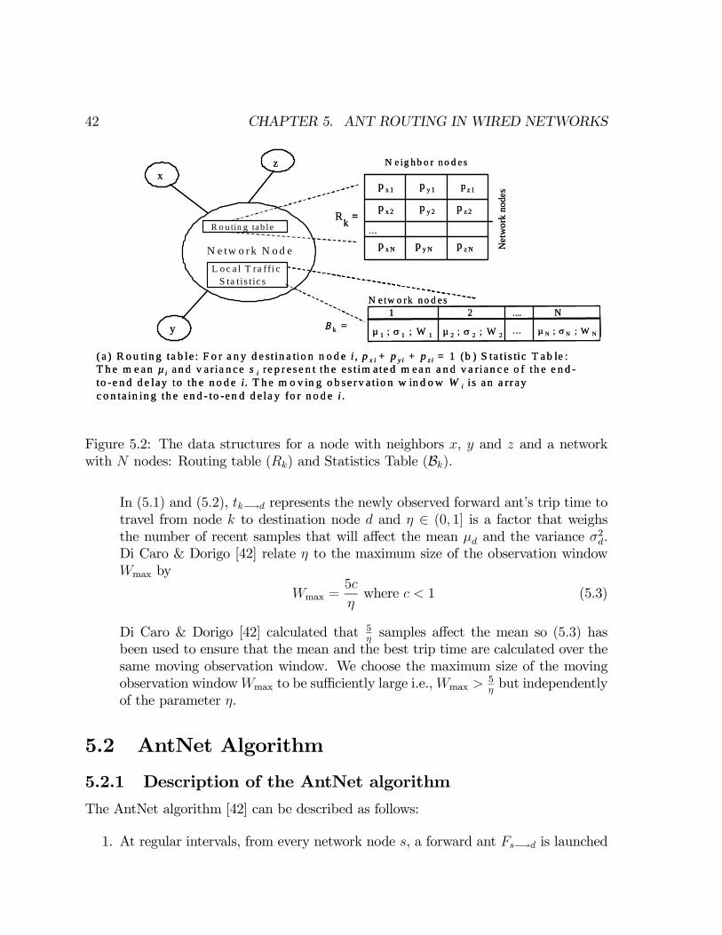
42 CHAPTER 5. ANT ROUTING IN WIRED NETWORKS
R o u tin g ta b l e
L o c a l T ra ffi c S ta tis t ic s
N e tw o r k N o d e
…µ 1 ; σ 1 ; W 1
N. ...21N e tw o rk n o d e s
Net
wor
k no
des
N e ig h b o r n o d e sx
y
z
Rk =…
B k =
( a ) R o u tin g ta b le : F o r a n y d e st in a tio n n o d e i , p x i + p y i + p zi = 1 (b ) S ta t is tic T ab le : T h e m e an µi an d v a ria n ce s i re p r e s e n t th e e s t im a te d m ea n a n d v a rian c e o f th e e n d -to -e n d d e lay to th e n o d e i. T h e m o v in g o b s e r v a t io n w in d o w W i is an a rr ay c o n ta in in g th e en d - to -en d d e la y fo r n o d e i .
p x 1
µ 2 ; σ 2 ; W 2 µ N ; σ N ; W N
p y 1 p z 1
p x 2 p y 2 p z 2
p x N p y N p z N
Figure 5.2: The data structures for a node with neighbors x, y and z and a networkwith N nodes: Routing table (Rk) and Statistics Table (Bk).
In (5.1) and (5.2), tk−→d represents the newly observed forward ant’s trip time totravel from node k to destination node d and η ∈ (0, 1] is a factor that weighsthe number of recent samples that will affect the mean μd and the variance σ
2d.
Di Caro & Dorigo [42] relate η to the maximum size of the observation windowWmax by
Wmax =5c
ηwhere c < 1 (5.3)
Di Caro & Dorigo [42] calculated that 5ηsamples affect the mean so (5.3) has
been used to ensure that the mean and the best trip time are calculated over thesame moving observation window. We choose the maximum size of the movingobservation windowWmax to be sufficiently large i.e.,Wmax >
5ηbut independently
of the parameter η.
5.2 AntNet Algorithm
5.2.1 Description of the AntNet algorithm
The AntNet algorithm [42] can be described as follows:
1. At regular intervals, from every network node s, a forward ant Fs−→d is launched

5.2. ANTNET ALGORITHM 43
with a randomly selected destination node d. Destinations are chosen to matchthe current traffic patterns i.e., if fsd is a measure (in bits or in the number ofpackets) of the data flow s −→ d, then the probability yd of creating at node s aforward ant with node d as destination is:
yd =fsdPNd0=1 fsd0
(5.4)
2. While travelling towards their destination nodes, the forward ants store theirpaths and the traffic conditions. The identifier of every visited node k and thetime elapsed since the launching time of the forward ant to arrive at this k-th nodeare pushed onto a memory stack Ss−→d stored in the data field of the forward ant2.Forward ants share the same queues as data packets, so they experience the sametraffic delays as data packets.
3. At each node k, each forward ant chooses the next node as follows:
• If not all the neighboring nodes have been visited, then the next neighbor ischosen among the nodes that have not yet been visited as:
p0nd =pnd + αbn
1 + α (|Nk|− 1)(5.5)
In (5.5), Nk represents the set of neighbors of node k and |Nk| the cardinalityof that set, i.e., the number of neighbors while the heuristic correction bn isa normalized value [0, 1] such that 1− bn is proportional to the length qn ofthe queue of the link connecting the node k with its neighbor n:
bn = 1−qnP|Nk|
n0=1 qn0(5.6)
The value of α in (5.5) weighs the importance of the instantaneous state ofthe node’s queue with respect to the probability values stored in the routingtable.
• If all the neighboring nodes have been visited previously, then the next nodeis chosen uniformly among all the neighbors. In this case, since all theneighbors have been visited previously the forward ant is forced to return toa previously visited node. Thus, irrespective of which neighbor is chosen asthe next node, the forward ant is in a loop (cycle).
2The accuracy of time stored by forward ant depends on clock synchronization in the network. Weassume that network is synchronized with accuracy of few ms.
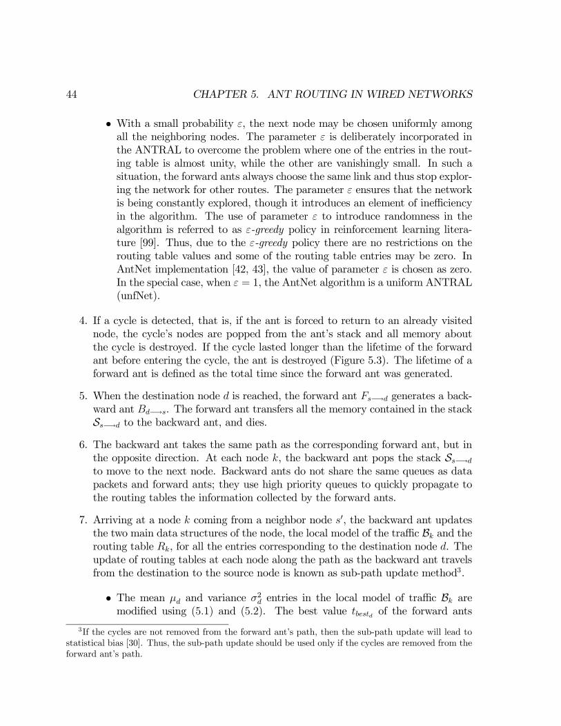
44 CHAPTER 5. ANT ROUTING IN WIRED NETWORKS
• With a small probability ε, the next node may be chosen uniformly amongall the neighboring nodes. The parameter ε is deliberately incorporated inthe ANTRAL to overcome the problem where one of the entries in the rout-ing table is almost unity, while the other are vanishingly small. In such asituation, the forward ants always choose the same link and thus stop explor-ing the network for other routes. The parameter ε ensures that the networkis being constantly explored, though it introduces an element of inefficiencyin the algorithm. The use of parameter ε to introduce randomness in thealgorithm is referred to as ε-greedy policy in reinforcement learning litera-ture [99]. Thus, due to the ε-greedy policy there are no restrictions on therouting table values and some of the routing table entries may be zero. InAntNet implementation [42, 43], the value of parameter ε is chosen as zero.In the special case, when ε = 1, the AntNet algorithm is a uniform ANTRAL(unfNet).
4. If a cycle is detected, that is, if the ant is forced to return to an already visitednode, the cycle’s nodes are popped from the ant’s stack and all memory aboutthe cycle is destroyed. If the cycle lasted longer than the lifetime of the forwardant before entering the cycle, the ant is destroyed (Figure 5.3). The lifetime of aforward ant is defined as the total time since the forward ant was generated.
5. When the destination node d is reached, the forward ant Fs−→d generates a back-ward ant Bd−→s. The forward ant transfers all the memory contained in the stackSs−→d to the backward ant, and dies.
6. The backward ant takes the same path as the corresponding forward ant, but inthe opposite direction. At each node k, the backward ant pops the stack Ss−→d
to move to the next node. Backward ants do not share the same queues as datapackets and forward ants; they use high priority queues to quickly propagate tothe routing tables the information collected by the forward ants.
7. Arriving at a node k coming from a neighbor node s0, the backward ant updatesthe two main data structures of the node, the local model of the traffic Bk and therouting table Rk, for all the entries corresponding to the destination node d. Theupdate of routing tables at each node along the path as the backward ant travelsfrom the destination to the source node is known as sub-path update method3.
• The mean μd and variance σ2d entries in the local model of traffic Bk aremodified using (5.1) and (5.2). The best value tbestd of the forward ants
3If the cycles are not removed from the forward ant’s path, then the sub-path update will lead tostatistical bias [30]. Thus, the sub-path update should be used only if the cycles are removed from theforward ant’s path.
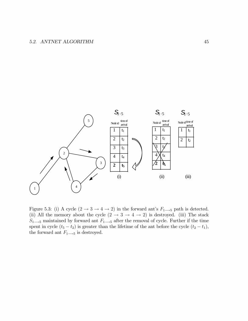
5.2. ANTNET ALGORITHM 45
5
3
2
1 4
Node id
1 t1
2 t2
3 t3
4 t4
2 t5
(i) (ii) (iii)
time of arrival
time of arrival
S1 5
Node id
S1 5 S1 5
time of arrival
Node id
1 t1
2 t2
3 t3
4 t4
2 t5
1 t1
2 t2
Figure 5.3: (i) A cycle (2 → 3 → 4 → 2) in the forward ant’s F1−→5 path is detected.(ii) All the memory about the cycle (2 → 3 → 4 → 2) is destroyed. (iii) The stackS1−→5 maintained by forward ant F1−→5 after the removal of cycle. Further if the timespent in cycle (t5 − t2) is greater than the lifetime of the ant before the cycle (t2 − t1),the forward ant F1−→5 is destroyed.
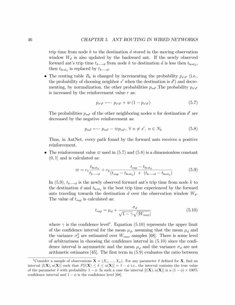
46 CHAPTER 5. ANT ROUTING IN WIRED NETWORKS
trip time from node k to the destination d stored in the moving observationwindow Wd is also updated by the backward ant. If the newly observedforward ant’s trip time tk−→d from node k to destination d is less then tbestd,then tbestd is replaced by tk−→d.
• The routing table Rk is changed by incrementing the probability ps0d0 (i.e.,the probability of choosing neighbor s0 when the destination is d0) and decre-menting, by normalization, the other probabilities pnd0 .The probability ps0d0is increased by the reinforcement value r as:
ps0d0 ←− ps0d0 + (1− ps0d0) (5.7)
The probabilities pnd0 of the other neighboring nodes n for destination d0 aredecreased by the negative reinforcement as:
pnd0 ←− pnd0 − pnd0 , ∀ n 6= s0, n ∈ Nk (5.8)
Thus, in AntNet, every path found by the forward ants receives a positivereinforcement.
• The reinforcement value used in (5.7) and (5.8) is a dimensionless constant(0, 1] and is calculated as:
= c1tbestdtk−→d
+ c2tsup − tbestd
(tsup − tbestd) + (tk−→d − tbestd)(5.9)
In (5.9), tk−→d is the newly observed forward ant’s trip time from node k tothe destination d and tbestd is the best trip time experienced by the forwardants traveling towards the destination d over the observation window Wd.The value of tsup is calculated as:
tsup = μd +σd√
1− γp|Wmax|
(5.10)
where γ is the confidence level4. Equation (5.10) represents the upper limitof the confidence interval for the mean μd, assuming that the mean μd andthe variance σ2d are estimated over Wmax samples [68]. There is some levelof arbitrariness in choosing the confidence interval in (5.10) since the confi-dence interval is asymmetric and the mean μd and the variance σd are notarithmetic estimates [45]. The first term in (5.9) evaluates the ratio between
4Consider a sample of observations X = (X1, ....,Xn). For any parameter δ defined for X, find aninterval [l(X), u(X)] such that P [l(X) ≤ δ ≤ u(X)] = 1 − φ i.e., the interval contains the true valueof the parameter δ with probability 1− φ. In such a case the interval [l(X), u(X)] is a (1− φ)× 100%confidence interval and 1− φ is the confidence level [68].
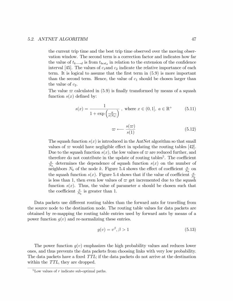
5.2. ANTNET ALGORITHM 47
the current trip time and the best trip time observed over the moving obser-vation window. The second term is a correction factor and indicates how farthe value of tk−→d is from tbestd in relation to the extension of the confidenceinterval [45]. The values of c1and c2 indicate the relative importance of eachterm. It is logical to assume that the first term in (5.9) is more importantthan the second term. Hence, the value of c1 should be chosen larger thanthe value of c2.
The value calculated in (5.9) is finally transformed by means of a squashfunction s(x) defined by:
s(x) =1
1 + exp³
ax|Nk|
´ , where x ∈ (0, 1], a ∈ R+ (5.11)
←− s( )
s(1)(5.12)
The squash function s(x) is introduced in the AntNet algorithm so that smallvalues of would have negligible effect in updating the routing tables [42].Due to the squash function s(x), the low values of are reduced further, andtherefore do not contribute in the update of routing tables5. The coefficientaNkdetermines the dependence of squash function s(x) on the number of
neighbors Nk of the node k. Figure 5.4 shows the effect of coefficient aNkon
the squash function s(x). Figure 5.4 shows that if the value of coefficient aNk
is less than 1, then even low values of get incremented due to the squashfunction s(x). Thus, the value of parameter a should be chosen such thatthe coefficient a
Nkis greater than 1.
Data packets use different routing tables than the forward ants for travelling fromthe source node to the destination node. The routing table values for data packets areobtained by re-mapping the routing table entries used by forward ants by means of apower function g(v) and re-normalizing these entries.
g(v) = vβ, β > 1 (5.13)
The power function g(v) emphasizes the high probability values and reduces lowerones, and thus prevents the data packets from choosing links with very low probability.The data packets have a fixed TTL; if the data packets do not arrive at the destinationwithin the TTL, they are dropped.
5Low values of r indicate sub-optimal paths.
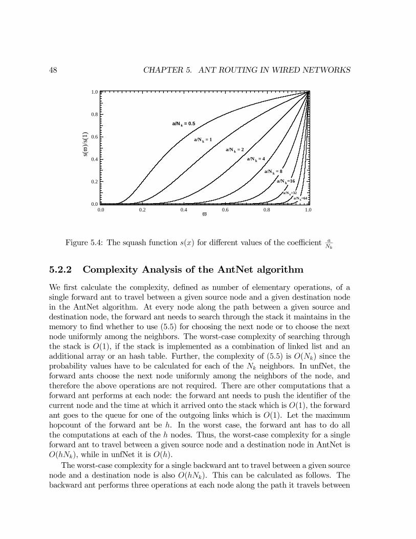
48 CHAPTER 5. ANT ROUTING IN WIRED NETWORKS
1.0
0.8
0.6
0.4
0.2
0.0
s(ϖ
)/s(1
)
1.00.80.60.40.20.0ϖ
a/N k = 0.5
a/N k = 1
a/N k = 2
a/N k = 4
a/N k = 8
a/N k=16
a/N k=32a/N k=64
Figure 5.4: The squash function s(x) for different values of the coefficient aNk
5.2.2 Complexity Analysis of the AntNet algorithm
We first calculate the complexity, defined as number of elementary operations, of asingle forward ant to travel between a given source node and a given destination nodein the AntNet algorithm. At every node along the path between a given source anddestination node, the forward ant needs to search through the stack it maintains in thememory to find whether to use (5.5) for choosing the next node or to choose the nextnode uniformly among the neighbors. The worst-case complexity of searching throughthe stack is O(1), if the stack is implemented as a combination of linked list and anadditional array or an hash table. Further, the complexity of (5.5) is O(Nk) since theprobability values have to be calculated for each of the Nk neighbors. In unfNet, theforward ants choose the next node uniformly among the neighbors of the node, andtherefore the above operations are not required. There are other computations that aforward ant performs at each node: the forward ant needs to push the identifier of thecurrent node and the time at which it arrived onto the stack which is O(1), the forwardant goes to the queue for one of the outgoing links which is O(1). Let the maximumhopcount of the forward ant be h. In the worst case, the forward ant has to do allthe computations at each of the h nodes. Thus, the worst-case complexity for a singleforward ant to travel between a given source node and a destination node in AntNet isO(hNk), while in unfNet it is O(h).The worst-case complexity for a single backward ant to travel between a given source
node and a destination node is also O(hNk). This can be calculated as follows. Thebackward ant performs three operations at each node along the path it travels between
5.2. ANTNET ALGORITHM 49
a given source node and a given destination node. First, the backward ant needs topop the stack to find the next node to travel to. The pop operation in the stack isO(1). Second, the backward ant goes to the queue for one of the outgoing links whichis O(1). The backward ant updates the routing table for each of the neighbors Nk forthe destination d which is O(Nk). Furthermore, in the worst case the backward ant hasto do all the computations at each of the h nodes.We calculate the worst-case complexity of AntNet when the total number of forward
or backward ants generated is given by ρ > 1. Since the worst-case complexity of asingle forward or backward ant to travel between a given pair of nodes is O(hNk), theworst-case complexity of AntNet when ρ forward or backward ants are generated isO(ρhNk). Furthermore, we know that the worst-case complexity for Dijkstra’s shortestpath algorithm using a Fibonacci heap is O(N logN +L). This analysis shows that thecomplexity of AntNet algorithm is comparable to Dijkstra’s’ shortest path algorithmwhen h and Nk are small as compared to N .We now calculate the worst-case complexity of AntNet for finding the shortest
path. Let us assume that one forward ant searches for one distinct path and oneforward/backward ant pair updates only the routing tables at the source node for thegiven destination node. In the worst case, at any given node there is an equal probabil-ity of creating a forward ant with any one of the N − 1 nodes as the destination. Thus,only one out of N − 1 forward ants is used to search for the shortest path between agiven source and destination. Let us denote the number of paths between a source anda destination in G(N ,L) by p. Adding the contributions yields a worst-case complexityto search for the shortest path in AntNet with p = pmax of O(shNkN), where pmax isthe upper bound on the maximum number of paths between a source and destinationnode in G(N ,L). The upper bound pmax on the total number of paths between a sourceand destination node in G(N ,L) is [105],
pmax = [e(N − 2)!] (5.14)
In case of a random graph Gp(N), with a fixed link density p and N nodes, thefollowing upper-bound for the average number of paths applies [106],
pmax =hpN−1e
1p (N − 2)!
i(5.15)
Equation (5.15) shows that the number of paths between a given pair of nodes decreasesas the link density p in the random graph Gp(N) is decreased.
5.2.3 AntNet Implementation
The time Tu−→v for a data packet or ant packet (forward ant or backward ant) to travelfrom a node u to a node v is calculated as:
50 CHAPTER 5. ANT ROUTING IN WIRED NETWORKS
Tu−→v =qv + sizePacket
Cu−→v+Du−→v (5.16)
where qv is the length of the low priority queue at node u for the link u −→ v, sizePacketis the size of the packet, Cu−→v is the available capacity of the link between node u andnode v and Du−→v is the propagation delay of the link u −→ v. The term sizePacket
Cu−→v
represents the transmission delay for the packet and the term qvCu−→v
represents thequeuing delay experienced by the packet while waiting at node u for the link u −→ v.The term propagation delay and link weight have been used interchangeably in the text.We have simplified the model shown in Figure 5.1 for our implementation of the
AntNet algorithm. We assume that the packets go directly to the outgoing bufferand the outgoing buffer consists of a low priority and a high priority queue for allthe outgoing links. But the queuing delay in (5.16) and parameter bn in (5.5) are stillcalculated using the number of packets waiting in the low priority queue for a particularlink6. Further, we assume that each node is able to remove one packet from its highpriority queue and low priority queue in the output buffer (for any outgoing link) at arate of 0.01 milliseconds (ms). This assumption makes the queueing delays negligiblein most of our simulations.We implement the AntNet algorithm under static and dynamic conditions. In the
static implementation of AntNet, we assume that the forward ants use only the prop-agation delays for network exploration and routing table updates. Thus, no queueingor transmission delays that depend on the packet size and capacity of the links aretaken into account during the static implementation of AntNet. In this case, the equa-tion (5.5) reduces to p0nd = pnd and equation (5.16) for forward ant packets reduces toTu−→v = Du−→v. In the dynamic implementation of AntNet, both the queueing andtransmission delays as well as the propagation delays are used for choosing the nextnode and updating the routing tables.We compare the results of AntNet with Dijkstra’s shortest path algorithm. However,
under dynamic implementation, there is an important distinction for comparison ofAntNet to Dijkstra’s shortest path algorithm. In Dijkstra’s shortest path algorithm,the cost of the shortest path is the sum of individual link weights (propagation delays)along the path. However in AntNet, the cost of the shortest path used for updatingthe routing tables is assumed to be the sum of link weights along the path and thetransmission and queuing delays. The delay in the queues is included in the AntNetalgorithm to account for the traffic conditions in the network. Thus, there is no staticshortest path in the AntNet algorithm. However, for the comparison of AntNet toDijkstra’s shortest path algorithm, we plot the weight of the paths in the AntNetalgorithm excluding the transmission and queuing delays.
To validate our simulations, in addition to plotting the pdf of the hopcount for the
6The packets in the high priority queue and low priority queue are served in FIFO order.

5.3. RESULTS 51
shortest path and the paths in the AntNet algorithm, we also plot the values for pdf ofhopcount of the shortest path obtained by using theory. It has been demonstrated byvan der Hofstad et al. [104] that for a fixed link density p and sufficiently large N , theshortest path tree in a random graph Gp(N) with uniformly distributed link weightsis a uniform recursive tree (URT). The probability density function of the hopcount inthe URT with N nodes is:
Pr[HN = j] =(−1)N−(j+1)S(j+1)N
(N − 1) (N − 1)! (5.17)
where S(j)N is the Stirling number of the first kind [1].
5.3 Results
5.3.1 Simulation Parameters
The simulations are performed on random graphs of the class Gp(N) consisting of Nnodes and independently chosen links with probability p. The link weights reflectingthe propagation delays are uniformly distributed in (0, 1] ms and the capacity of eachlink is 8.192 Mbit/s for all our simulations. For each random graph of the type Gp(N),we used Dijkstra’s algorithm to compute the shortest path between the source nodeand the destination node based on the link weights. On the other hand, in AntNet,the data packets travel between a given pair of nodes using the probabilistic routingtables. Indeed, there could be a number of paths that the data packets choose whichmight be the shortest path, the second shortest path etc. For AntNet, we find theaverage link weight (or end-to-end delay) and the average hopcount of the paths thatthe data packets use to travel between the source and the destination node over theentire simulation period. Furthermore, each simulation consists of a large number (105
or 104) of random graphs of the type Gp(N). The source (node 1) and destination (nodeN) are chosen to be fixed in our simulations.In our implementation of the AntNet algorithm, the simulation period (S.P.) consists
of the training period (T.P.) and the test period (TE.P.). During T.P., only ant packetsare generated while during TE.P., both the data and ant packets are generated. Wehave chosen the simulation period (S.P.) to be 104 ms. The training period (T.P.) hasbeen chosen to be 103 ms. Each node generates data packets according to a Poissonprocess with mean interarrival time of 12.5 ms. The destination for data packets ischosen randomly. The size of data packets generated follows a negative exponentialdistribution with mean of 4096 bits. The size of forward ant packet is assumed to be192 bits at the time the forward ant packet is generated and the size increases by 64bits for each hop the forward ant travels. The size of backward ant is assumed to be 500

52 CHAPTER 5. ANT ROUTING IN WIRED NETWORKS
bits. The average number of neighbors of a node in a random graph Gp(N) is p(N−1),the default value of parameter a is chosen as p ∗N in our simulations.
Table 5.1: Various parameters and their default values used in the simulations.
Name, Symbol ValueLink Capacity Ci−→j 8.192 Mbit/sLink Weight (Propagation delay) uniformly distributed (0,1] msSimulation period (S.P.) 104 msTest period (TE.P.) 9.103 msTraining period (T.P.) 103 msBackward ant size 500 bitsInitial forward ant size 192 bitsα used in (5) 0.2ε 0.1c1 used in (9) 0.7c2 used in (9) 0.3a used in (11) p ∗Nβ used in (13) 3Confidence interval (γ) used in (10) 0.95Output buffer size 109 bitsMean interarrival time for data packets 12.5 msData packets TTL 10 msMean data packet size 4096 bits
The maximum size of the output buffer, which is assumed to be the sum of the sizesof all low priority queues in the output buffer, is 109 bits. Table 5.1 lists the variousparameters and their default values that we have chosen for our simulations. The valuesof parameters α, c1, c2, a, confidence interval (γ) and the size of forward ant packethave been replicated from [45]. The values of the parameter η, the maximum size ofthe observation window Wmax and the ant generation rate have been varied extensivelyand therefore are not listed in Table 5.1.
5.3.2 Static Implementation of the AntNet algorithm
In this section, we study the AntNet algorithm under static conditions i.e., the forwardants use only the propagation delays for network exploration and routing table updates.Under these conditions, a direct comparison between the static shortest path calculatedby using Dijkstra’s algorithm and the AntNet algorithm paths can be made. The ant

5.3. RESULTS 53
(a) (b)
1.5
1.0
0.5
0.0
f WN(x
)
6543210path weight x (ms)
N = 50 AntNet E[AntNet] = 2.46, var[AntNet] = 1.9 Dijkstra E[Dijkstra] = 0.45, var[Dijkstra] = 0.04
N = 25 Dijkstra E[Dijkstra] = 0.74, var[Dijkstra] = 0.2 AntNet E[AntNet] = 2.0, var[AntNet] = 1.5
ε = 0.1 AntNet E[AntNet] = 1.26, var[AntNet] = 0.5 unfNet E[unfNet] = 1.19, var[unfNet] = 0.4
p = 0.2
0.3
0.2
0.1
0.0
Pr [H
= k
]
1412108642hop k
N = 50 AntNet E[AntNet] = 5.28, var[AntNet] = 7.3 Dijkstra E[Dijkstra] = 3.54, var[Dijkstra] = 2.6
N = 25 AntNet E[AntNet] = 4.31, var[AntNet] = 5.3 Dijkstra E[Dijkstra] = 2.95, var[Dijkstra] = 1.9
ε = 0.1 AntNet E[AntNet] = 3.18, var[AntNet] = 2.0 unfNet E[unfNet] = 2.7, var[unfNet] = 1.4
p = 0.2
Figure 5.5: The pdf of the (a) weight and the (b) hopcount of the Dijkstra’s shortestpath, unfNet algorithm paths and the AntNet algorithm paths for N = 25 and N = 50for p = 0.2. The ant generation interval during the T.P. is 4 ms. Each simulationconsists of 104 iterations. (η = 0.1, Wmax = 50)
generation interval is 4 ms during T.P. and 40 ms during TE.P. The TTL of data packetsis assumed to be 20.0 ms. The value of parameters η = 0.1 and Wmax = 50. Figure5.5 shows the simulation results comparing the pdf of the hopcount and the weight forthe shortest path and the AntNet algorithm paths7 for N = 25, 50 and p = 0.2 (Thedefault value of parameter ε is chosen as 0.)
Figure 5.5 shows that the AntNet algorithm converges to a good solution. Further-more, the performance of AntNet improves when the value of parameter ε is chosengreater than 0. Since no queuing delays are considered, the network exploration inAntNet is restricted by the routing tables and many paths are not explored (The valueof p0nd in equation (5.5) is equal to pnd). With ε = 0.1, the probability of exploringdifferent paths increases leading to an improvement in the performance of AntNet. In-deed for static implementation, unfNet performs better than AntNet using ε < 1 sinceall the paths are explored with equal probabilities in unfNet.
7The probability density function (pdf) of the hopcount and the weight for the AntNet algorithmpaths and the shortest path are computed over (104) random graphs of the type Gp(N). In AntNet,for each random graph of the type Gp(N), the path weight and hopcount represent the "average pathweight" and "average hopcount" for all the packets to travel between the source and destination nodeduring the entire simulation period.

54 CHAPTER 5. ANT ROUTING IN WIRED NETWORKS
5.3.3 Dynamic Implementation of the AntNet algorithm
In this section, the AntNet algorithm implementation is dynamic but we compare theresults with Dijkstra’s shortest path algorithm. We also study the effect of differentparameters, such as ant generation rate, squash function s(x), parameter β etc., on theperformance of AntNet. The performance comparison between AntNet and Dijkstra’salgorithm and the optimization of various parameters for AntNet is still valid since thetransmission delays are very small for forward ant packets. Furthermore, the queue-ing delays are also small since packets are removed from nodes at a very fast rate ascompared to the rate at which packets are generated. Thus, the total delay experi-enced by forward ant packets is still dominated by the propagation delays. The TTLof data packets is assumed to be 10.0 ms and the value of parameter ε is 0.1 in all thesimulations in this section8.
The effect of the ant-generation rate and the link density p
We first compare the performance of AntNet with Dijkstra’s shortest path algorithmfor different ant-generation rates and different values of the link density p for a 25 nodenetwork.The values of T.P. and TE.P. are assumed to be constant in our simulations as shown
in Table 1. To study the effect of the ant generation rate on the AntNet algorithm, weassume a fixed ant generation rate during the TE.P., varying the ant generation ratesonly during the T.P. We consider three different cases of the ant generation during theT.P., namely 40, 4, 0.4 ms9. The corresponding results for the pdf of the hopcount andthe weight for N = 25 and different values of the link density p are shown in Figures5.6-5.8.Figures 5.6, 5.7 and 5.8 show that the AntNet algorithm gives a near optimal solution
for a 25 node network at low values of the link density p (p = 0.2 and p = 0.1). Theperformance of AntNet algorithm decreases as the value of the link density p in therandom graph Gp(N) is increased. Additional simulations for N = 50 show similartrends as the link density p is varied. Moreover, the comparison of AntNet for N = 25and N = 50 shows that the performance of AntNet degrades as the network size N isincreased. Figure 5.7 shows the validity of our comparison between AntNet and theDijkstra’s algorithm since the results for AntNet are similar to the results of AntNetunder static implementation (Figure 5.5).Comparison of Figure 5.6 with Figures 5.7 and 5.8 show that the AntNet algorithm
converges to a good solution even at low ant generation rates. In Figure 5.6, the antgeneration interval is 40 ms during both the T.P. and the TE.P. Thus, only 25 forward
8In dynamic implementation of AntNet, there is negligible difference between the performance ofAntNet for ε = 0 and ε = 0.1.
9η = 0.1,Wmax = 50 for all the simulations in this sub-section.
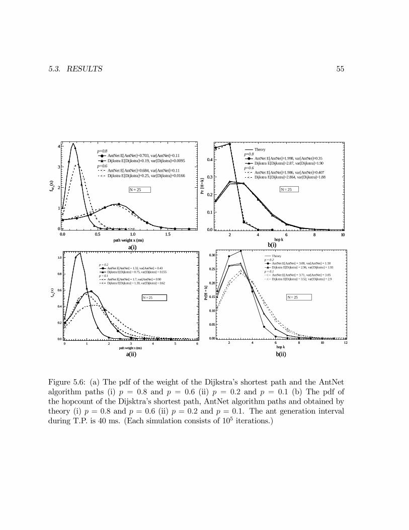
5.3. RESULTS 55
a(i) b(i)
a(ii) b(ii)
4
3
2
1
0
f WN(x
)
1.51.00.50.0path weight x (ms)
p=0.8 AntNet E[AntNet]=0.703, var[AntNet]=0.11 Dijkstra E[Dijkstra]=0.19, var[Dijkstra]=0.0095
p=0.6 AntNet E[AntNet]=0.684, var[AntNet]=0.11 Dijkstra E[Dijkstra]=0.25, var[Dijkstra]=0.0166
N = 25
0.4
0.3
0.2
0.1
0.0
Pr [H
=k]
108642hop k
Theoryp=0.8
AntNet E[AntNet]=1.998, var[AntNet]=0.35 Dijkstra E[Dijkstra]=2.87, var[Dijkstra]=1.90
p=0.6 AntNet E[AntNet]=1.986, var[AntNet]=0.407 Dijkstra E[Dijkstra]=2.864, var[Dijkstra]=1.88
N = 25
0.30
0.25
0.20
0.15
0.10
0.05
0.00
Pr[H
= k
]
12108642hop k
Theoryp = 0.2
AntNet E[AntNet] = 3.08, var[AntNet] = 1.50 Dijkstra E[Dijkstra] = 2.96, var[Dijkstra] = 1.93
p = 0.1 AntNet E[AntNet] = 3.71, var[AntNet] = 3.05 Dijkstra E[Dijkstra] = 3.52, var[Dijkstra] = 2.9
N = 25
1.0
0.8
0.6
0.4
0.2
0.0
f WN(x
)
6543210path weight x (ms)
p = 0.2 AntNet E[AntNet] = 1.32, var[AntNet] = 0.43 Dijkstra E[Dijkstra] = 0.75, var[Dijkstra] = 0.155
p = 0.1 AntNet E[AntNet] = 1.7, var[AntNet] = 0.90 Dijkstra E[Dijkstra] = 1.39, var[Dijkstra] = 0.62
N = 25
Figure 5.6: (a) The pdf of the weight of the Dijkstra’s shortest path and the AntNetalgorithm paths (i) p = 0.8 and p = 0.6 (ii) p = 0.2 and p = 0.1 (b) The pdf ofthe hopcount of the Dijsktra’s shortest path, AntNet algorithm paths and obtained bytheory (i) p = 0.8 and p = 0.6 (ii) p = 0.2 and p = 0.1. The ant generation intervalduring T.P. is 40 ms. (Each simulation consists of 105 iterations.)

56 CHAPTER 5. ANT ROUTING IN WIRED NETWORKS
a(i) b(i)
a(ii) b(ii)
4
3
2
1
0
f WN(x
)
2.01.51.00.50.0path weight x (ms)
p = 0.8 AntNet E[AntNet] = 0.62, var[AntNet] = 0.09 Dijkstra E[Dijkstra] = 0.19, var[Dijkstra] = 0.01
p = 0.6 AntNet E[AntNet] = 0.58, var[AntNet] = 0.1 Dijkstra E[Dijkstra] = 0.25, var[Dijkstra] = 0.02
N = 25
0.5
0.4
0.3
0.2
0.1
0.0
Pr [H
= k
]
108642hop k
Theoryp = 0.8
AntNet E[AntNet] = 1.88, var[AntNet] = 0.33 Dijkstra E[Dijkstra] = 2.88, var[Dijkstra] = 1.88
p = 0.6 AntNet E[AntNet] = 1.88, var[AntNet] = 0.38 Dijkstra E[Dijkstra] = 2.86, var[Dijkstra] = 1.87
N = 25
1.0
0.8
0.6
0.4
0.2
0.0
f WN(x
)
43210path weight x (ms)
p = 0.2 AntNet E[AntNet] = 1.25, var[AntNet] = 0.42 Dijkstra E[Dijkstra] = 0.75, var[Dijkstra] = 0.15
p = 0.1 AntNet E[AntNet] = 1.64, var[AntNet] = 0.86 Dijkstra E[Dijkstra] = 1.39, var[Dijkstra] = 0.62
N = 25
0.30
0.25
0.20
0.15
0.10
0.05
0.00
Pr [H
= k
]
108642hop k
Theoryp = 0.2
AntNet E[AntNet] = 2.99, var[AntNet] = 1.45 Dijkstra E[Dijkstra] = 2.95, var[Dijkstra] = 1.93
p = 0.1 AntNet E[AntNet] = 3.63, var[AntNet] = 2.91 Dijkstra E[Dijkstra] = 3.54, var[Dijkstra] = 2.90
N = 25
Figure 5.7: (a) The pdf of the weight of the Dijkstra’s shortest path and the AntNetalgorithm paths (i) p = 0.8 and p = 0.6 (ii) p = 0.2 and p = 0.1 (b) The pdf ofthe hopcount of the Dijsktra’s shortest path, AntNet algorithm paths and obtained bytheory (i) p = 0.8 and p = 0.6 (ii) p = 0.2 and p = 0.1. Same scenario as in Fig. 5 butwith an ant generation interval of 4 ms during the T.P.

5.3. RESULTS 57
a(i) b(i)
a(ii) b(ii)
4
3
2
1
0
f WN(x
)
1.51.00.50.0path weight x (ms)
p=0.8 AntNet E[AntNet] = 0.622, var[AntNet] = 0.1 Dijkstra E[Dijkstra] = 0.19 ,var[Dijkstra] = 0.01
p=0.6 AntNet E[AntNet] = 0.577, var[AntNet] = 0.1 Dijkstra E[Dijkstra] = 0.25, var[Dijkstra] = 0.02
N = 25
0.5
0.4
0.3
0.2
0.1
0.0
Pr[H
= k
]
108642hop k
Theoryp = 0.8
AntNet E[AntNet] = 1.88, var[AntNet] = 0.33 Dijkstra E[Dijkstra] = 2.86, var[Dijkstra] = 1.88
p = 0.6 AntNet E[AntNet] = 1.87, var[AntNet] = 0.38 Dijkstra E[Dijkstra] = 2.858, var[Dijkstra] = 1.87
N = 25
1.0
0.8
0.6
0.4
0.2
0.0
f WN(x
)
43210path weight x (ms)
p = 0.2 AntNet E[AntNet] = 1.257, var[AntNet] = 0 .419 Di jkstra E[Dijkstra] = 0 .752, var[Dijkstra] = 0.156
p = 0.1 AntNet E[AntNet] = 1.636, var[AntNet] = 0 .868 Di jkstra E[Dijkstra] = 1 .387, var[Dijkstra] = 0.628
N = 25
0 .30
0.25
0.20
0.15
0.10
0.05
0.00
Pr [H
= k
]
108642hop k
p = 0.2 AntNet E[AntNet] = 2.999, var[AntNet] = 1.46 Dijkstra E[Dijkstra] = 2.95, var[Dijks tra] = 1.93
p = 0.1 AntNet E[AntNet] = 3.62, var[AntNet] = 2.92 Dijkstra E[Dijkstra] = 3.525, var[Dijkstra] = 2.92
N = 25
Figure 5.8: (a) The pdf of the weight of the Dijkstra’s shortest path and the AntNetalgorithm paths (i) p = 0.8 and p = 0.6 (ii) p = 0.2 and p = 0.1 (b) The pdf ofthe hopcount of the Dijsktra’s shortest path, AntNet algorithm paths and obtained bytheory (i) p = 0.8 and p = 0.6 (ii) p = 0.2 and p = 0.1. Same scenario as in Fig. 5 butwith an ant generation interval of 0.40 ms during the T.P.

58 CHAPTER 5. ANT ROUTING IN WIRED NETWORKS
Table 5.2: The mean hopcount and weight for the unfNet algorithm for N = 25.(p = 0.2 and 0.8. η = 0.1 and Wmax = 50)
Link density p Ant generation inter-val during T.P.
E[Path weight] E[Hopcount]
0.8 40 ms 0.75 ms 1.820.8 4 ms 0.63 ms 1.620.8 0.4 ms 0.59 ms 1.550.2 40 ms 1.38 ms 2.960.2 4 ms 1.2 ms 2.670.2 0.4 ms 1.16 ms 2.61
ants are generated by each node during the T.P. to search for the shortest paths to allother nodes in the network. The number of forward ants searching for the shortest pathincreases as the ant generation interval is decreased from 40 ms to 4 ms during the T.P..This leads to an improvement in the performance of AntNet. As the ant generationinterval is decreased from 4 ms to 0.4 ms, the performance of AntNet remains the same.This can be attributed to the fact that the variations in the ant generation rate arerelated to the size of the moving observation window Wmax and the parameter η. Thesize of the moving observation window Wmax in the above simulations is large enoughto distinguish between ant generation intervals of 40 ms and 4 ms during T.P. Butsince the size of the moving observation window is small, it can store only the timesof the last 50 forward ants generated from a given source to a given destination. Thisindicates that even if the ant generation rate is increased with a small window size, theperformance of AntNet remains the same or may even go down. Additional simulationsshow that the AntNet algorithm performs better at η = 0.02 and Wmax = 200 than atη = 0.1 andWmax = 50 for different ant generation rates and different values of the linkdensity p.We also performed simulations for the unfNet algorithm under identical conditions,
as above. Table 5.2 lists the simulation results for the unfNet algorithm for N = 25 anddifferent values of the link density p (p = 0.2 and 0.8). The results show that unfNetperforms worse than AntNet for low ant generation rates (or large values of the antgeneration interval). In unfNet, all the paths are continuously searched independentlyof the routing tables. While in AntNet, the probability that future forward ants choosepaths with large delays is decreased by each forward ant. Therefore, in AntNet, mainlylow delay paths contribute to routing table updates and the AntNet algorithm performswell even with a low ant generation rate10. When the ant generation rate is high, the
10All paths searched by the forward ants lead to positive reinforcement.

5.3. RESULTS 59
performance of unfNet is comparable to the AntNet algorithm. This can be attributedto the fact that the data traffic is small and the variations in delays along differentpaths is negligible.
Lattice Topologies
In this section, we investigate the performance of AntNet for Lattice topologies. Wecompare the performance of AntNet with Dijkstra’s shortest path algorithm for thelattice topology shown in Figure 5.9. The source and destination nodes D1 and D2 areassumed to be fixed. The ant generation interval is 4 ms during T.P. and 40 ms duringTE.P. (η = 0.1,Wmax = 50. The value of parameter a is chosen as 5.) Figure 5.10 showsthe simulation results comparing the pdf of the hopcount and the weight for the shortestpath and the AntNet algorithm paths. Figure 5.10 shows that the AntNet algorithmperforms well for Lattice topologies. Also, the performance of AntNet degrades as thenumber of nodes in the network is increased.
0 1 2 43 5 6
7 98 1 0 1 1 1 2 1 3
1 4 1 5 16
2 2
1 7
2 1
2 01 91 8
2 72 62 52 42 3
2 9
4 2
3 5
2 8 3 23 0
4 3
3 6
3 1 3 43 3
4 03 93 83 7
4 4 4 5
4 1
4 74 6 4 8
49 N ode Lattice
Source
D estinationD 1
D estinationD 2
Figure 5.9: The 49-node lattice topology used for our simulations. The source nodeand the destination nodes D1 and D2 are assumed to be fixed as indicated
The effect of the moving observation window size Wmax and the parameter η
In AntNet, the moving observation window is used to store the cost of the shortestpath from a given source node to a given destination node. Furthermore, the movingobservation window is also used to improve the accuracy of the mean μd as shownin (5.10). The optimal size of the moving observation window is hard to determine
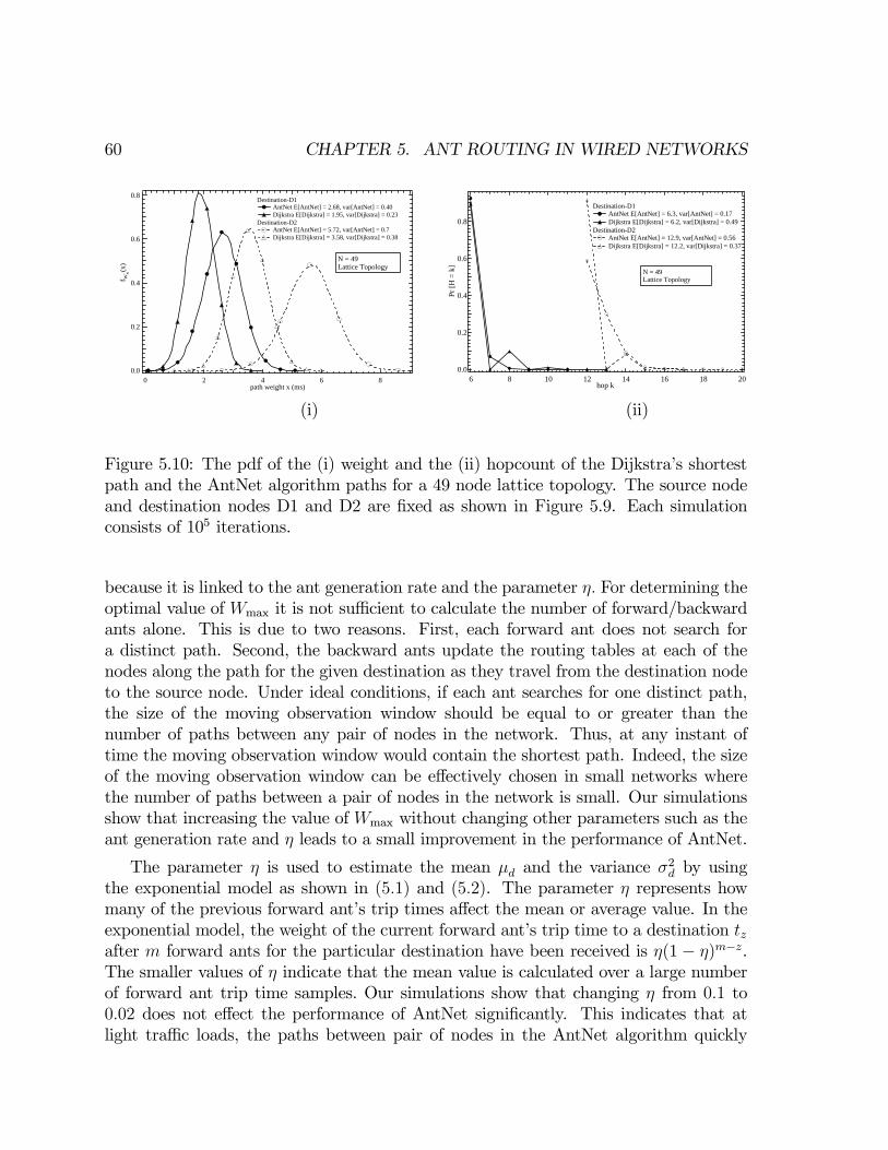
60 CHAPTER 5. ANT ROUTING IN WIRED NETWORKS
0.8
0.6
0.4
0.2
0.0
f WN(x
)
86420path weight x (ms)
Destination-D1 AntNet E[AntNet] = 2.68, var[AntNet] = 0.40 Dijkstra E[Dijkstra] = 1.95, var[Dijkstra] = 0.23
Destination-D2 AntNet E[AntNet] = 5.72, var[AntNet] = 0.7 Dijkstra E[Dijkstra] = 3.58, var[Dijkstra] = 0.38
N = 49Lattice Topology
0.8
0.6
0.4
0.2
0.0
Pr [H
= k
]
20181614121086hop k
Destination-D1 AntNet E[AntNet] = 6.3, var[AntNet] = 0.17 Dijkstra E[Dijkstra] = 6.2, var[Dijkstra] = 0.49
Destination-D2 AntNet E[AntNet] = 12.9, var[AntNet] = 0.56 Dijkstra E[Dijkstra] = 12.2, var[Dijkstra] = 0.37
N = 49Lattice Topology
(i) (ii)
Figure 5.10: The pdf of the (i) weight and the (ii) hopcount of the Dijkstra’s shortestpath and the AntNet algorithm paths for a 49 node lattice topology. The source nodeand destination nodes D1 and D2 are fixed as shown in Figure 5.9. Each simulationconsists of 105 iterations.
because it is linked to the ant generation rate and the parameter η. For determining theoptimal value of Wmax it is not sufficient to calculate the number of forward/backwardants alone. This is due to two reasons. First, each forward ant does not search fora distinct path. Second, the backward ants update the routing tables at each of thenodes along the path for the given destination as they travel from the destination nodeto the source node. Under ideal conditions, if each ant searches for one distinct path,the size of the moving observation window should be equal to or greater than thenumber of paths between any pair of nodes in the network. Thus, at any instant oftime the moving observation window would contain the shortest path. Indeed, the sizeof the moving observation window can be effectively chosen in small networks wherethe number of paths between a pair of nodes in the network is small. Our simulationsshow that increasing the value of Wmax without changing other parameters such as theant generation rate and η leads to a small improvement in the performance of AntNet.
The parameter η is used to estimate the mean μd and the variance σ2d by usingthe exponential model as shown in (5.1) and (5.2). The parameter η represents howmany of the previous forward ant’s trip times affect the mean or average value. In theexponential model, the weight of the current forward ant’s trip time to a destination tzafter m forward ants for the particular destination have been received is η(1− η)m−z.The smaller values of η indicate that the mean value is calculated over a large numberof forward ant trip time samples. Our simulations show that changing η from 0.1 to0.02 does not effect the performance of AntNet significantly. This indicates that atlight traffic loads, the paths between pair of nodes in the AntNet algorithm quickly
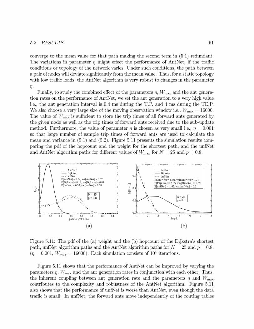
5.3. RESULTS 61
converge to the mean value for that path making the second term in (5.1) redundant.The variations in parameter η might effect the performance of AntNet, if the trafficconditions or topology of the network varies. Under such conditions, the path betweena pair of nodes will deviate significantly from the mean value. Thus, for a static topologywith low traffic loads, the AntNet algorithm is very robust to changes in the parameterη.Finally, to study the combined effect of the parameters η, Wmax and the ant genera-
tion rates on the performance of AntNet, we set the ant generation to a very high valuei.e., the ant generation interval is 0.4 ms during the T.P. and 4 ms during the TE.P.We also choose a very large size of the moving observation window i.e., Wmax = 16000.The value of Wmax is sufficient to store the trip times of all forward ants generated bythe given node as well as the trip times of forward ants received due to the sub-updatemethod. Furthermore, the value of parameter η is chosen as very small i.e., η = 0.001so that large number of sample trip times of forward ants are used to calculate themean and variance in (5.1) and (5.2). Figure 5.11 presents the simulation results com-paring the pdf of the hopcount and the weight for the shortest path, and the unfNetand AntNet algorithm paths for different values of Wmax for N = 25 and p = 0.8.
4
3
2
1
0
f WN(x
)
1.41.21.00.80.60.40.20.0path weight x (ms)
AntNet 1 Dijkstra unfNet
E[AntNet] = 0.54, var[AntNet] = 0.07 E[Dijkstra] = 0.19, var[Dijkstra] = 0.01E[unfNet] = 0.55, var[unfNet] = 0.08
N = 25p = 0.8
0.6
0.4
0.2
0.0
Pr[H
= k
]
87654321hop k
AntNet Dijkstra unfNet
E[AntNet] = 1.69, var[AntNet] = 0.21E[Dijkstra] = 2.85, var[Dijkstra] = 1.89 E[unfNet] = 1.45, var[unfNet] = 0.2
N = 25 p = 0.8
(a) (b)
Figure 5.11: The pdf of the (a) weight and the (b) hopcount of the Dijkstra’s shortestpath, unfNet algorithm paths and the AntNet algorithm paths for N = 25 and p = 0.8.(η = 0.001, Wmax = 16000). Each simulation consists of 104 iterations.
Figure 5.11 shows that the performance of AntNet can be improved by varying theparameters η, Wmax and the ant generation rates in conjunction with each other. Thus,the inherent coupling between ant generation rate and the parameters η and Wmax
contributes to the complexity and robustness of the AntNet algorithm. Figure 5.11also shows that the performance of unfNet is worse than AntNet, even though the datatraffic is small. In unfNet, the forward ants move independently of the routing tables

62 CHAPTER 5. ANT ROUTING IN WIRED NETWORKS
and all the paths are searched with equal probabilities. In AntNet, if the path is foundto incur a large delay, the probability of choosing the particular path by the futureforward ants becomes less. But since every path found receives a positive reinforcement(in both unfNet and AntNet), the number of non-optimal paths updating the routingtables in unfNet is more.
The effect of the confidence interval, squash function s(x) and the parameterβ
We first study the effect of the confidence interval on the performance of AntNet. Thesecond term in (5.10) i.e., σd√
1−γ√|Wmax|
is used to improve the accuracy in estimating
the mean μd but introduces additional complexity in the AntNet algorithm. Figure5.12 shows the simulation results comparing the pdf of the hopcount and the weight forDijkstra’s shortest path and the AntNet algorithm paths, when the term σd√
1−γ√|Wmax|
is not used in the estimation of tsup. This case is shown as tsup = μd in Figure 5.12.The simulations are performed for N = 25 and p = 0.2. Also, the value of parametera is chosen as 20 such that the average value of the coefficient a
Nkis 4. (The ant
generation interval is 40 ms during T.P. and TE.P. The value of parameters η = 0.1and Wmax = 50.)
1.0
0.8
0.6
0.4
0.2
0.0
f WN(x
)
3.53.02.52.01.51.00.50.0path weight x (ms)
Ant-Net E[Ant-Net] = 0.968, var[Ant-Net] = 0.25 Dijkstra E[Dijkstra] = 0.75, var[Dijkstra] = 0.155
tsup=μd Ant-Net E[Ant-Net] = 0.96, var[Ant-Net] = 0.24 Dijkstra E[Dijkstra] = 0.75, var[Dijkstra] = 0.15
N = 25p = 0.2
0.4
0.3
0.2
0.1
0.0
Pr [H
=k]
108642hop k
Dijkstra E[Dijkstra] = 2.95, var[Dijkstra] = 1.93 Ant-Net E[Ant-Net] = 2.58, var[Ant-Net] = 1.04
tsup=μd Ant-Net E[Ant-Net] = 2.58, var[Ant-Net] = 1.04
N = 25p = 0.2
(a) (b)
Figure 5.12: The pdf of the (a) weight and the (b) hopcount of the Dijkstra’s shortestpath and the AntNet algorithm paths for N = 25 and p = 0.2 for tsup = μd and tsupcalculated using (11) (η = 0.1, Wmax = 50, a = 20). The ant generation interval is 40ms during the T.P. and TE.P. Each simulation consists of 105 iterations.
Comparison of Figure 5.12 and Figure 5.6 shows that choosing a large value of pa-rameter a improves the performance of AntNet. Furthermore, under the simulation

5.3. RESULTS 63
0.5
0.4
0.3
0.2
0.1
0.0
f WN(x
)
6543210path weight x (ms)
β = 1 Ant-Net E[Ant-Net] = 1.74, var[Ant-Net] = 0.93 Dijkstra E[Dijkstra] = 1.39, var[Dijkstra] = 0.62
β = 100 Ant-Net E[Ant-Net] = 1.69, var[Ant-Net] = 0.89
N = 25p = 0.1
0.20
0.15
0.10
0.05
0.00
Pr [H
=k]
1412108642hop k
β = 1 Ant-Net E[Ant-Net] = 3.79, var[Ant-Net] = 3.19 Dijkstra E[Dijkstra] = 3.52, var[Dijkstra] = 2.92
β = 100 Ant-Net E[Ant-Net] = 3.67, var[Ant-Net] = 3.01
N = 25 p = 0.1
(a) (b)
Figure 5.13: The pdf of the (a) weight and the (b) hopcount of the Dijkstra’s shortestpath and the AntNet algorithm paths for β = 1 and β = 100 for N = 25 and p = 0.1.The ant generation interval is 40 ms during the T.P. and TE.P. Each simulation consistsof 105 iterations. ( η = 0.1 and Wmax = 50.)
parameters considered, the removal of the term σd√1−γ√|Wmax|
does not change the per-
formance of AntNet. Thus, equation (5.10) could be simplified to reduce the complexityof AntNet.The parameter β determines whether single or multi-path routing is followed by the
data packets. The value of parameter β needs to be greater than 1 to prevent the datapackets from choosing links with very low probabilities. A large value of β (β >> 1)indicates that the data packets follow only single-path routing. On the other handβ = 1 indicates that the data packets follow the routing tables and may even chooselinks with very low probabilities. Thus, β = 1 corresponds to multi-path routing. Wecompare the performance of AntNet algorithm for β = 1 and β = 100. When β = 100,the data packets are effectively following a single-path routing. Figure 5.13 shows thesimulation results comparing the pdf of the hopcount and the weight for the shortestpath and the AntNet algorithm paths for p = 0.1 for β = 1 and β = 100 for a 25 nodenetwork11.Figure 5.13 shows that the performance of AntNet improves as β is increased for
p = 0.1. This shows that there is a greater probability that the shortest path has beencorrectly identified in the AntNet algorithm at lower values of p. Thus, making β = 1prevents the data packets from choosing the path with the highest probability and leadsto data packets following sub-optimal paths. On the other hand, β = 100 improves theperformance of AntNet since the data packets follow only a single-path routing which
11The ant generation interval is 40 ms during the T.P. and the TE.P. The value of parameter η = 0.1and Wmax = 50.
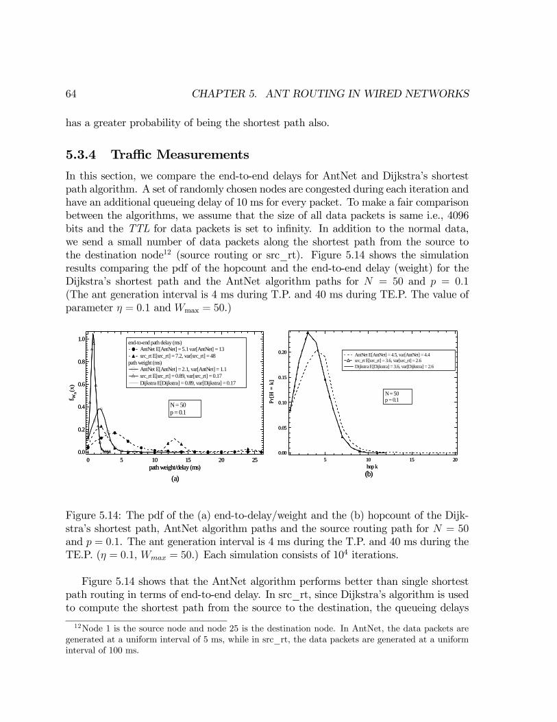
64 CHAPTER 5. ANT ROUTING IN WIRED NETWORKS
has a greater probability of being the shortest path also.
5.3.4 Traffic Measurements
In this section, we compare the end-to-end delays for AntNet and Dijkstra’s shortestpath algorithm. A set of randomly chosen nodes are congested during each iteration andhave an additional queueing delay of 10 ms for every packet. To make a fair comparisonbetween the algorithms, we assume that the size of all data packets is same i.e., 4096bits and the TTL for data packets is set to infinity. In addition to the normal data,we send a small number of data packets along the shortest path from the source tothe destination node12 (source routing or src_rt). Figure 5.14 shows the simulationresults comparing the pdf of the hopcount and the end-to-end delay (weight) for theDijkstra’s shortest path and the AntNet algorithm paths for N = 50 and p = 0.1(The ant generation interval is 4 ms during T.P. and 40 ms during TE.P. The value ofparameter η = 0.1 and Wmax = 50.)
(a) (b)
1.0
0.8
0.6
0.4
0.2
0.0
f WN(x
)
2520151050path weight/delay (ms)
end-to-end path delay (ms) AntNet E[AntNet] = 5.1 var[AntNet] = 13 src_rt E[src_rt] = 7.2, var[src_rt] = 48
path weight (ms) AntNet E[AntNet] = 2.1, var[AntNet] = 1.1 src_rt E[src_rt] = 0.89, var[src_rt] = 0.17 Dijkstra E[Dijkstra] = 0.89, var[Dijkstra] = 0.17
N = 50 p = 0.1
0.20
0.15
0.10
0.05
0.00
Pr[H
= k
]
2015105hop k
AntNet E[AntNet] = 4.5, var[AntNet] = 4.4 src_rt E[src_rt] = 3.6, var[src_rt] = 2.6 Dijkstra E[Dijkstra] = 3.6, var[Dijkstra] = 2.6
N = 50 p = 0.1
Figure 5.14: The pdf of the (a) end-to-delay/weight and the (b) hopcount of the Dijk-stra’s shortest path, AntNet algorithm paths and the source routing path for N = 50and p = 0.1. The ant generation interval is 4 ms during the T.P. and 40 ms during theTE.P. (η = 0.1, Wmax = 50.) Each simulation consists of 104 iterations.
Figure 5.14 shows that the AntNet algorithm performs better than single shortestpath routing in terms of end-to-end delay. In src_rt, since Dijkstra’s algorithm is usedto compute the shortest path from the source to the destination, the queueing delays
12Node 1 is the source node and node 25 is the destination node. In AntNet, the data packets aregenerated at a uniform interval of 5 ms, while in src_rt, the data packets are generated at a uniforminterval of 100 ms.

5.3. RESULTS 65
are not considered. During the iterations when there are no congested nodes along theshortest path, the end-to-end delays for the data packets using src_rt and AntNet arecomparable. However, when there are one or more congested nodes along the shortestpath, the data packets using src_rt incur queueing delays along the congested nodes.On the other hand, the AntNet algorithm performs load balancing and reduces theprobability of data packets choosing the paths with congested nodes.Table 5.3 lists the simulation results for the AntNet, unfNet and the src_rt algo-
rithms forN = 50 andN = 25 (p = 0.2, 0.1). We consider different number of congestednodes and ant generation rates. Table 5.3 shows that unfNet generally performs worsethan AntNet under varying traffic loads. The performance of unfNet becomes worse ascompared to the AntNet algorithm, when the ant generation rate is low and the sizeof the network is increased. In AntNet, the network exploration is restricted to pathsthat incur low delays and only these paths are used to update the routing tables. InunfNet, the forward ants move independently of the routing tables. Thus, even thelarge delay paths are used to update the routing tables leading to a poor performanceof the unfNet algorithm. This shows that the unfNet algorithm reduces the complexitybut, in general, leads to a decrease in the performance.
Table 5.3: The expected hopcount/weight for the unfNet, AntNet, and the src_rtalgorithms for N = 25, 50 (p = 0.2, 0.1) with different number of congested nodes anddifferent ant generation rates (η = 0.1 and Wmax = 50).
RoutingProto-col
Networksize (N)
Linkdensityp
Ant genera-tion intervalT.P. TE.P.
CongestedNodes
E[path de-lay]
E[Hop-count]
unfNet 50 0.1 4 ms 40 ms 8 5.6 ms 3.8AntNet 50 0.1 40 ms 40 ms 8 5.8 ms 4.7unfNet 50 0.1 40 ms 40 ms 8 12.7 ms 6.2AntNet 25 0.2 4 ms 40 ms 4 3.4 ms 3.2src_rt 25 0.2 4 ms 40 ms 4 5.8 ms 2.9unfNet 25 0.2 4 ms 40 ms 4 3.5 ms 2.8AntNet 25 0.2 40 ms 40 ms 4 3.7 ms 3.4unfNet 25 0.2 40 ms 40 ms 4 5.5 ms 3.3AntNet 25 0.2 4 ms 4 ms 4 3.36 ms 3.3unfNet 25 0.2 4 ms 4 ms 4 3.1 ms 2.8AntNet 50 0.2 4 ms 40 ms 4 3.1 ms 3.3src_rt 50 0.2 4 ms 40 ms 4 4.3 ms 3.5
To further study the load balancing capabilities of AntNet, we assume that during
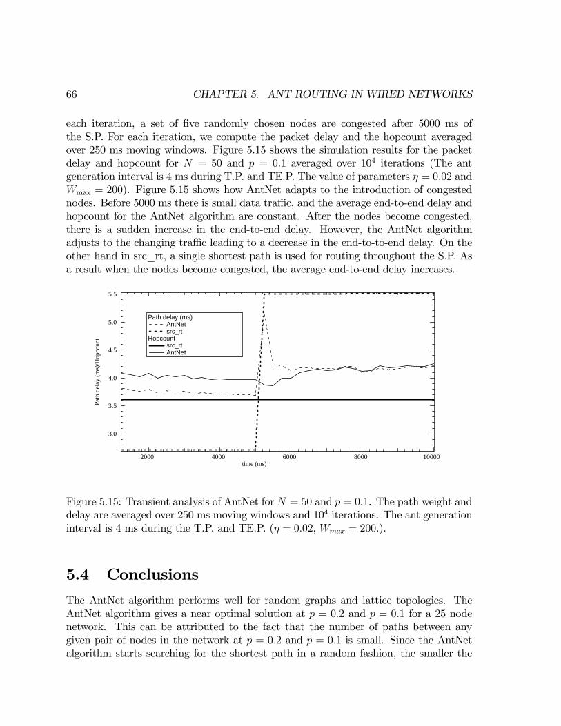
66 CHAPTER 5. ANT ROUTING IN WIRED NETWORKS
each iteration, a set of five randomly chosen nodes are congested after 5000 ms ofthe S.P. For each iteration, we compute the packet delay and the hopcount averagedover 250 ms moving windows. Figure 5.15 shows the simulation results for the packetdelay and hopcount for N = 50 and p = 0.1 averaged over 104 iterations (The antgeneration interval is 4 ms during T.P. and TE.P. The value of parameters η = 0.02 andWmax = 200). Figure 5.15 shows how AntNet adapts to the introduction of congestednodes. Before 5000 ms there is small data traffic, and the average end-to-end delay andhopcount for the AntNet algorithm are constant. After the nodes become congested,there is a sudden increase in the end-to-end delay. However, the AntNet algorithmadjusts to the changing traffic leading to a decrease in the end-to-to-end delay. On theother hand in src_rt, a single shortest path is used for routing throughout the S.P. Asa result when the nodes become congested, the average end-to-end delay increases.
5.5
5.0
4.5
4.0
3.5
3.0
Path
del
ay (m
s)/H
opco
unt
100008000600040002000time (ms)
Path delay (ms) AntNet src_rt
Hopcount src_rt AntNet
Figure 5.15: Transient analysis of AntNet for N = 50 and p = 0.1. The path weight anddelay are averaged over 250 ms moving windows and 104 iterations. The ant generationinterval is 4 ms during the T.P. and TE.P. (η = 0.02, Wmax = 200.).
5.4 Conclusions
The AntNet algorithm performs well for random graphs and lattice topologies. TheAntNet algorithm gives a near optimal solution at p = 0.2 and p = 0.1 for a 25 nodenetwork. This can be attributed to the fact that the number of paths between anygiven pair of nodes in the network at p = 0.2 and p = 0.1 is small. Since the AntNetalgorithm starts searching for the shortest path in a random fashion, the smaller the

5.4. CONCLUSIONS 67
number of paths between a pair of nodes the greater is the probability that the algorithmconverges to a near optimal solution. The performance of AntNet algorithm degradesas the network size or the link density p is increased.The AntNet algorithm is robust to changes in the training of the network and
converges to a good solution even at low ant generation rates. Further increasing theant generation rates leads to an improvement in the performance but this is relatedto choice of other parameters such as Wmax and η. Indeed, the coupling of variousparameters is the inherent cause of complexity in the AntNet algorithm and changingone parameter favorably may not lead to an improvement in performance until the otherparameters are also changed. The performance of AntNet can be improved by using alarge value of the parameter a in the squash function s(x). In this case, only the nearoptimal paths update the routing tables. The complexity of AntNet can be reduced bya number of methods, such as choosing parameter β = 1 and simplifying the calculationof parameter , but this generally comes at the expense of performance.Due to inherent load balancing, AntNet performs better than shortest path routing
under varying traffic loads. For small networks, when the traffic loads are small and theant generation is sufficiently high, a modified version of the AntNet algorithm (unfNet)can be used. This reduces the complexity of the AntNet algorithm. The robustnessand near optimal performance of the AntNet algorithm makes it an attractive solutionfor routing in wired networks.
68 CHAPTER 5. ANT ROUTING IN WIRED NETWORKS
Chapter 6
Ant Routing in Mobile Ad hocNetworks
A variety of ANTRALs have been proposed for ad hoc and mesh networks. Among thetraditional routing protocols for ad hoc wireless networks, on-demand protocols performbetter than table-driven protocols [16].The performance of ANTRAL for mobile ad hoc networks is an open issue. ANTRAL
algorithms do not take into account the mobility of the nodes. Moreover, load balanc-ing for frequently changing topologies is a challenging issue. Load balancing involvesdistributing traffic along multiple paths depending on the traffic conditions such thatthe congested nodes or the unavailable links are by-passed. With node mobility, thepaths are not stable making load balancing difficult. Furthermore, characteristics oftraffic in ad hoc networks is not known. In this chapter, our aim is to study whetherANTRAL algorithms can be applied for routing in mobile ad hoc networks.ANTRAL algorithms for ad hoc networks, such as AntHocNet [47], Ad hoc Net-
working with Swarm Intelligence (ANSI) [86], Ant-Colony-Based Routing Algorithm(ARA) [54], Ant-AODV [74] and Termite [89], use on-demand mobile agents for discov-ering routes. The on-demand flooding of mobile agents is similar to flooding of routerequest (RREQ) packets in on-demand protocols AODV and DSR. In ANSI, ARA andTermite, the pheromone decays and as a result after a certain period the routing tablesare empty. The decay of routing table values is similar to AODV where the paths arevalid for a certain duration of time. Thus, the paths obtained by using AODV or ANSI,ARA and Termite are identical. In addition, if a link breaks in ANSI, AntHocNet,Ant-AODV and ARA routing protocols inject route error packets similar to on-demandprotocols. Indeed, the performance of ANSI, ARA and Ant-AODV is similar to AODVand DSR [54, 74, 86]. In our view, these algorithms are a variation of the on-demandprotocols and deviate from the original idea of ANTRAL algorithms in which routingtables are sufficient for routing data packets. We do not consider the performance ofANTRAL algorithms that use on-demand flooding of mobile agents.
69
70 CHAPTER 6. ANT ROUTING IN MOBILE AD HOC NETWORKS
6.1 W_AntNet algorithm
The W_AntNet algorithm is based on AntNet but uses neighbor discovery and addedfunctionality to deal with node mobility [39].
• Neighbor Discovery Protocol
At regular intervals, hello messages are exchanged between neighboring nodes.When the neighbors are lost or new neighbors are added, the routing tables are up-dated and the probability values are re-normalized. The forward ant packets and datapackets waiting in the buffer are rerouted if the next hop neighbor is lost. However, thebackward ant packets are dropped if the next hop neighbor is lost. This ensures thatonly paths that are stable during a sufficiently long time interval, i.e. the time betweenthe creation of forward ant and the receipt of the backward ant appear in the routingtables.
6.2 Performance Analysis of W_AntNet
The routing overhead for obtaining a path to any destination is O(N) in AODV andDSR since both these protocols use controlled flooding or sequence numbers. To com-pute the complexity of W_AntNet, we use the fact that ad-hoc wireless networks canbe modeled as a geometric random graph (or random graph) [58]. In W_AntNet,the forward ants perform random walks to search for the destination. Therefore, theworst-case routing overhead for a single update of the routing tables [5] is O(N logN).Moreover, the number of updates required for routing table convergence, i.e. probabil-ity for one of the entries in routing tables to be one, depends on the quality of differentpaths, network topology and the routing table update function. We show that multiplebackward ants are needed for the routing tables to converge.Consider a node k with Nk neighboring nodes. At t = 0, the probability of choosing
neighbor n as the next hop for destination d, pnd (0) = 1Nk. We assume that only the
routing table values for neighbor n i.e., pnd receive positive reinforcement. Under theseassumptions, the probability pnd (t+ 1) is,
pnd (t+ 1) = pnd(t) + cpnd(t) (6.1)
where c is a constant. After Y updates,
pnd (Y) = pnd(0) (1 + c)Y
Since the routing table converges when pnd (Y) −→ 1, the value of Y is :
Y = log (Nk)
log (1 + c)(6.2)
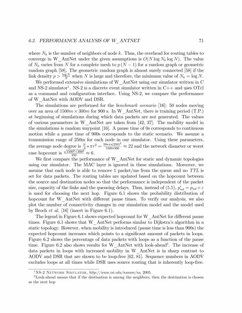
6.2. PERFORMANCE ANALYSIS OF W_ANTNET 71
where Nk is the number of neighbors of node k. Thus, the overhead for routing tables toconverge in W_AntNet under the given assumptions is O(N logNk logN). The valueof Nk varies from N for a complete mesh to p (N − 1) for a random graph or geometricrandom graph [58]. The geometric random graph is almost surely connected [58] if thelink density p > logN
Nwhen N is large and therefore, the minimum value of Nk = logN .
We performed extensive simulations of W_AntNet using our simulator written in Cand NS-2 simulator1. NS-2 is a discrete event simulator written in C++ and uses OTclas a command and configuration interface. Using NS-2, we compare the performanceof W_AntNet with AODV and DSR.The simulations are performed for the benchmark scenario [16]: 50 nodes moving
over an area of 1500m× 300m for 900 s. In W_AntNet, there is training period (T.P.)at beginning of simulations during which data packets are not generated. The valuesof various parameters in W_AntNet are taken from [42, 37]. The mobility model inthe simulations is random waypoint [16]. A pause time of 0s corresponds to continuousmotion while a pause time of 900s corresponds to the static scenario. We assume atransmission range of 250m for each node in our simulator. Using these parameters,the average node degree is N
A∗πr2 = 50∗π∗(250)2
1500∗300 ≈ 22 and the network diameter or worstcase hopcount is
√15002+3002
250≈ 6.
We first compare the performance of W_AntNet for static and dynamic topologiesusing our simulator. The MAC layer is ignored in these simulations. Moreover, weassume that each node is able to remove 1 packet/ms from the queue and no TTL isset for data packets. The routing tables are updated based on the hopcount betweenthe source and destination nodes so that the performance is independent of the packetsize, capacity of the links and the queueing delays. Thus, instead of (5.5), p0nd = pnd+εis used for choosing the next hop. Figure 6.1 shows the probability distribution ofhopcount for W_AntNet with different pause times. To verify our analysis, we alsoplot the number of connectivity changes in our simulation model and the model usedby Broch et al. [16] (insert in Figure 6.1).The legend in Figure 6.1 shows expected hopcount for W_AntNet for different pause
times. Figure 6.1 shows that W_AntNet performs similar to Dijkstra’s algorithm in astatic topology. However, when mobility is introduced (pause time is less than 900s) theexpected hopcount increases which points to a significant amount of packets in loops.Figure 6.2 shows the percentage of data packets with loops as a function of the pausetime. Figure 6.2 also shows results for W_AntNet with look-ahead2. The increase ofdata packets in loops with increased mobility in W_AntNet is in sharp contrast toAODV and DSR that are shown to be loop-free [62, 81]. Sequence numbers in AODVexcludes loops at all times while DSR uses source routing that is inherently loop-free.
1NS-2 Network Simulator, http://www.isi.edu/nsnam/ns, 2005.2Look-ahead means that if the destination is among the neighbors, then the destination is chosen
as the next hop

72 CHAPTER 6. ANT ROUTING IN MOBILE AD HOC NETWORKS
0.20
0.15
0.10
0.05
0.00
Pr[H
= k
]
252015105hop k
W_AntNet pause_time = 0 E[H] = 22.2 pause_time = 30 E[H] = 21.0 pause_time = 60 E[H] = 22.6 pause_time = 120 E[H] = 19.3 pause_time = 300 E[H] = 12.8 pause_time = 600 E[H] = 7.3
Static Topology W_AntNet E[H] = 4.3 Dijkstra's algorithm E[H] = 2.9
N = 50
12x10 3
10
8
6
4
2
0
Num
ber
of c
onne
ctiv
ity
chan
ges
8006004002000pause time (sec)
our Simulation model Broch et al. [5] model
N = 50
Figure 6.1: The probability distribution of hopcount for W_AntNet algorithm as afunction of pause time. The legend shows the expected hopcount for different values ofpause times.
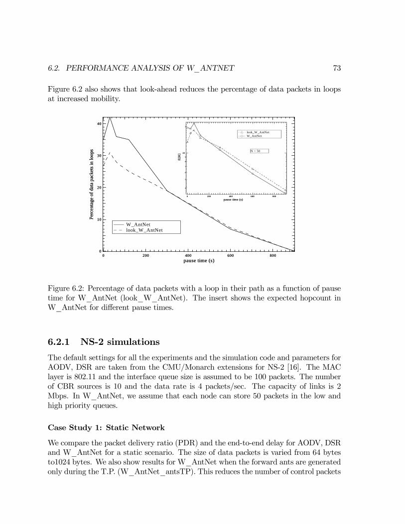
6.2. PERFORMANCE ANALYSIS OF W_ANTNET 73
Figure 6.2 also shows that look-ahead reduces the percentage of data packets in loopsat increased mobility.
40
30
20
10
0
Perc
enta
ge o
f dat
a pa
cket
s in
loop
s
8006004002000pause time (s)
W_AntNet look_W_AntNet
4
5
6
7
8
9
10
2
E[H
]
8006004002000pause time (s)
look_W_AntNet W_AntNet
N = 50
40
30
20
10
0
Perc
enta
ge o
f dat
a pa
cket
s in
loop
s
8006004002000pause time (s)
W_AntNet look_W_AntNet
4
5
6
7
8
9
10
2
E[H
]
8006004002000pause time (s)
look_W_AntNet W_AntNet
N = 50
Figure 6.2: Percentage of data packets with a loop in their path as a function of pausetime for W_AntNet (look_W_AntNet). The insert shows the expected hopcount inW_AntNet for different pause times.
6.2.1 NS-2 simulations
The default settings for all the experiments and the simulation code and parameters forAODV, DSR are taken from the CMU/Monarch extensions for NS-2 [16]. The MAClayer is 802.11 and the interface queue size is assumed to be 100 packets. The numberof CBR sources is 10 and the data rate is 4 packets/sec. The capacity of links is 2Mbps. In W_AntNet, we assume that each node can store 50 packets in the low andhigh priority queues.
Case Study 1: Static Network
We compare the packet delivery ratio (PDR) and the end-to-end delay for AODV, DSRand W_AntNet for a static scenario. The size of data packets is varied from 64 bytesto1024 bytes. We also show results for W_AntNet when the forward ants are generatedonly during the T.P. (W_AntNet_antsTP). This reduces the number of control packets

74 CHAPTER 6. ANT ROUTING IN MOBILE AD HOC NETWORKS
in the network. Since the topology is static and the amount of data traffic is small,the generation of forward ants only during T.P. is sufficient for routing under theseconditions.
Figure 6.3: The PDR and end-to-end delay for W_AntNet, AODV and DSR for statictopology.
The PDR and end-to-end delay in Figure 6.3 show that W_AntNet performs similarto AODV and DSR when forward ants are generated only during the T.P. However, asthe forward ant generation rate is increased from 0 (W_AntNet_onlyTP) to 2 forwardants/s, the routing overhead causes congestion in the queues. Thus, W_AntNet causesa dual problem in ad hoc networks. A large number of forward ants cause congestion inthe network. However, with increasing mobility, more forward ants need to be generatedto account for frequent changes in the topology.
Case Study 2: Mobile Scenario
We study the performance of different routing protocols with mobility. The packetsize is assumed to be 64 bytes. Figure 6.4 shows the PDR, end-to-end delay andthe routing overhead (measured in number of bytes since the size of control packetsvaries in W_AntNet) for AODV, DSR, W_AntNet and W_AntNet with look-ahead(W_AntNet_look). We also reduce the routing overhead in W_AntNet by generat-ing forward ants only from source-destination pairs that have data packets to send(W_AntNet_onlysrc). Thus, the remaining nodes in the network do not maintainup-to-date routing tables.Figure 6.4 shows that with high node degree, AODV and DSR perform well in terms
of PDR and end-to-end delay. Figure 6.4 shows that using optimizations such as look-
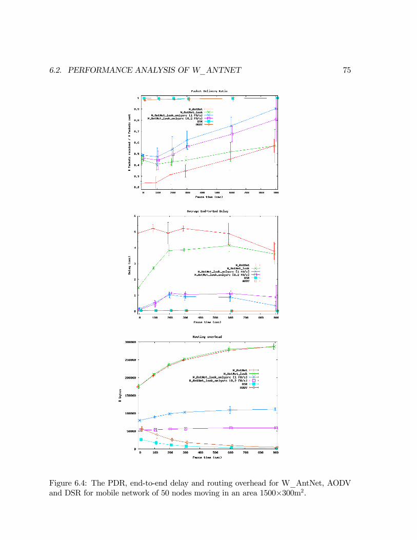
6.2. PERFORMANCE ANALYSIS OF W_ANTNET 75
Figure 6.4: The PDR, end-to-end delay and routing overhead for W_AntNet, AODVand DSR for mobile network of 50 nodes moving in an area 1500×300m2.

76 CHAPTER 6. ANT ROUTING IN MOBILE AD HOC NETWORKS
(a) (b)(a) (b)
Figure 6.5: The (a) PDR and (b) end-to-end delay for W_AntNet, AODV and DSRfor different values of the pause time. Nodes are moving in an area 2000m×2000m.
ahead and generating ants only from source-destination pairs reduces the overhead inW_AntNet. However, the routing overhead is still more than in AODV and DSR.As a result, the PDR for W_AntNet_look and W_AntNet_onlysrc is still lower thanAODV and DSR.
Case Study 3: Large Area Network (Sparse Graph Topology)
In this case, we compare the performance of different protocols in a larger area with thesame number of nodes (N = 50). The area over which the nodes move is 2000×2000m2.Under these conditions, the average node degree is 2.5 and the worst case hopcount isgiven by 11. The number of CBR sources is also increased to 20. Figure 6.5 showsthe PDR and end-to-end delay for AODV, DSR and W_AntNet. The packet size isassumed to be 64 bytes.
This scenario leads to a sparse graph topology and an increase in network diam-eter. As a result, the performance of all three protocols degrades considerably. Thesimulations show that all three protocols have scalability problems. To improve thescalability of routing protocols, additional schemes such as clustering need to be imple-mented [107]. Figure 6.5 also shows that the use of look-ahead does not improve theperformance of W_AntNet since the average node degree is small.
6.3. CONCLUSIONS 77
6.3 Conclusions
The performance of W_AntNet is comparable to the shortest path algorithm for statictopology but is dependent on the buffer size at the nodes. Since forward ants share thesame queue as data packets inW_AntNet, a high ant generation rate leads to congestionin the network. This causes W_AntNet to perform poorly compared to AODV andDSR when the size of the buffer is small. In a dynamic topology, a significant amountof packets in W_AntNet have loops. This can be attributed to the non-convergence ofrouting tables in W_AntNet. Therefore, with mobility, the performance of W_AntNetdeteriorates in comparison to AODV and DSR that are loop-free.

78 CHAPTER 6. ANT ROUTING IN MOBILE AD HOC NETWORKS

Part III
Searching
79

Chapter 7
Introduction
Searching for resources or services efficiently is an important issue in various networks.There are two common algorithms employed for searching - flooding and random walks(RW). In flooding, each node forwards the packet to all its neighbors. In RW, thepacket is forwarded to a single node, chosen uniformly among the neighbors of a node.Variations of RW that could be employed for searching include RW strategy where thenext hop is chosen as the node with maximum degree, RW with no retracing of stepsetc. We use the term RW using highest degree even though the next node is chosendeterministically and not according to uniform distribution. The term local searchalgorithm or path finding strategies is also used for such algorithms [64, 100].There are numerous applications of searching algorithms in different networks. OSPF
uses flooding to distributed and synchronize the link-state routing tables between nodes.In wireless ad-hoc networks, reactive protocols such as AODV and DSR use floodingto locate the destination [34]. In web-graphs, search engines use breadth first search toperform a complete search of the web. However, to reduce the overhead of searching,agents or spiders based on RW, or variations of the RW such as the RW strategy wherethe next hop is chosen as the node with maximum degree, and the RW strategy wherethe probability of choosing the next node is proportional to the nodal degree are widelyused [27].In the context of routing, RWs can be considered an extreme case of routing algo-
rithms that are used when the topology and the link weight structure of the graph arenot known. Variations of RW can be considered routing algorithms that use partialtopology information. Dijkstra’s shortest path algorithm can be used when both thetopology and the link weight structure of the entire graph are known. However, thedynamic nature of ad hoc and overlay networks does not always allow to collect in-formation concerning the current topology of the network. An attempt to collect suchinformation will often result in outdated information. Under the conditions that neitherthe graph topology nor the link weight structure is known, the only possible routingalgorithms are flooding or RWs [38, 40].
81
82 CHAPTER 7. INTRODUCTION
Hot-potato routing, also called deflection routing, is a term first introduced by Baran[7]. In hot-potato routing, the nodes in the network have no buffers to store packetsand the packets are forwarded to another node immediately [7, 17]. Hot-potato routingalgorithms are well suited for optical networks since it is difficult to buffer opticalmessages. Hot potato routing algorithms have also been used in parallel machines suchas the HEP multiprocessor, the Connection machine, and the Caltech Mosaic C, as wellas in high speed communication networks [17]. The term hot-potato routing used inthis context is exactly the same as a RW.
In mobile agent based routing, the mobile agents perform a RW or a variant ofRW while searching for the destination. In Ant-Net, loop-erased RWs are used by themobile agents. Mobile agents using RW have been proposed for providing membershipservices for ad-hoc networks by Dolev et al. [44]. As a sampling technique, RWs havebeen used for providing membership services in ad hoc networks [44, 8] that providethe nodes in the network with a view of the other nodes in network and that are usedby various applications such as location services, peer sampling services and randomoverlay constructions [8]. In [8], Bar-Yossef et al. develop a membership service forad hoc networks based on RW using highest degree. They show that the performanceof such membership service is superior to other existing membership services based ongossiping or flooding [8].
Unstructured overlay networks such as Gia proposed by Chawathe et al. [20] andGnutella build a random graph and use flooding or RWs to discover data stored atdifferent nodes. RWs have been shown to induce lower overhead than constrainedflooding used by the current versions of Gnutella [71, 51]. In the original Gia [20], theRWs were biased to prefer nodes with higher capacity but Castro et al. [19] have shownthat preferring nodes with higher degree leads to a higher success rate and a lowerdelay. Thus, further improvements have been proposed to Gia in which RWs are biasedtowards the higher degree nodes [19]. Also, variations of RWs have been proposed inwhich there are no loops [19].
Multiple RWs have been proposed for searching on unstructured peer-to-peer net-works by Lv et al. [71]. However, the optimization of multiple RWs has not beenanalyzed. Adaptive techniques based on RWs have been proposed for searching by Bis-nik and Abouzeid [13]. In the searching technique proposed in [13], the number of RWqueries used for searching are varied depending on the previous performance of search-ing. Our work differs from this approach since we study the optimization between thenumber of queries and the TTL of queries for different graph topologies.
The analysis of RWs has been an active topic of research [28, 63, 70]. Lovász [70]presents a detailed survey of RWs. An exact analysis of RWs on graph topologies suchas lattice and torus has been studied in [15]. A detailed mathematical analysis of RWsis given in Chung [24]. Different search algorithms for scale-free and power law graphshave been analyzed in [2, 64, 100].
7.1. OVERVIEW 83
7.1 Overview
While most RW strategies have been studied in specific scenarios, a general analysis ofperformance of searching with RW strategies is missing. In this section, we analyze theperformance of searching with different RW strategies on ER random graphs and powerlaw graphs generated using preferential attachment. Both these graph topologies are offundamental important since ad-hoc wireless networks can be modeled as ER randomgraphs while the web graphs and peer-to-peer networks can be modeled as power lawrandom graphs [51, 58]. We study both a single query and multiple queries to searchfor the destination. We do not consider dynamic topologies in our analysis.In [64] and [100], RW strategies where the next hop is chosen as the node with the
highest degree and with no retracing of steps have been analyzed in terms of expectedhopcount and weight. We show that strategies such as RW using highest degree andRW with no retracing of steps can lead to infinite loops. Therefore, the comparison ofdifferent RW strategies should also include an analysis of infinite loops, in addition, tothe expected hopcount comparison.In case of multiple RW queries, we study the optimization of number of queries
and the TTL of queries for ER random graphs and preferential attachment power lawgraphs. We also show an efficient way of searching graphs using RWs with no repetitionof steps (memory). Our analysis shows that searching with RW with memory performsbetter than RW. In addition, the optimized value of memoryM depends on the topologyof the network.
7.2 Definitions and Random Walk properties
A random walk is a finite Markov chain that is time-reversible. The access or hittingtime Huv is the expected number of hops before node v is visited, starting from nodeu. The sum J (u, v) = Huv+Hvu is called the commute time. The cover time (startingfrom a given distribution) is the expected number of hops to reach every node in thegraph. If no starting node starting distribution is specified we mean the worst case, i.e.,the node from which the cover time is maximum.A RW can be described as a finite Markov chain that is time-reversible [70]. The
stochastic matrix P = ∆−1A, where∆ = diag (deg1, deg2, ..., degN) is the degree matrixand A is the adjacency matrix, represents the transition matrix of the RW. It is known[70] that the RW has a unique stationary distribution κ, such that κP = κ, withκi =
degi2L. Let the RW start at node v0. The node v0 could be drawn from some
initial distribution Y0. Denote the sequence of random nodes by vt (t = 0, 1...). If wedenote by Yt the distribution of vt i.e., Yt (i) = Pr [vt = i], the RW can be expressed asYt+1 = P TYt and hence, Yt =
¡P T¢tY0. Thus, the probability that RW starting at u
reaches node v in t steps is given by (u, v) entry of the matrix P t [70].
84 CHAPTER 7. INTRODUCTION
It is known that a symmetric P matrix has n real eigenvectors with correspondingeigenvalues 1 = y1 ≥ y2 ≥ ... ≥ yn ≥ −1 . Moreover, if we exclude bipartite graphs orreducible Markov chains, then | yi |< 1, for i > 1. Cover time is the expected numberof steps for RW to visit all nodes at least once. Let CN be the cover time for the RW,then the cover time is [8],
CN = O
µκ−1min logN
1− y2
¶= O
µN logN
1− y2
¶, where κmin =
degmin2L
(7.1)
Jonasson [63] has shown that when p ≥ logNN, w.h.p a random graph has the same
cover time as the complete graph KN i.e., the cover time is N logN . Similarly, forpower law graphs generated using BA model, it has been shown by Cooper and Frieze[28] that if l ≥ 2, then w.h.p. the cover time CN ≤
§2ll−1N logN
¨+ o
¡§2ll−1N logN
¨¢.

Chapter 8
Searching with single query
In this chapter, we investigate the performance of searching with a single query based onRW or variation of RW.We investigate the expected hopcount obtained by different RWstrategies and the probability of finding the short paths. A general expression for theexpected hopcount of a RW is computed. The performance of different RW strategiesis compared on different graph topologies such as a complete graph, ER random graphsGp(N) and power law graphs generated using the BA model.The rest of this chapter is organized as follows. Section 8.1 gives a description of
different RW strategies. Sections 8.2 and 8.3 give an analysis and simulation results forsearching with different RW strategies. The last section presents the conclusions.
8.1 Random Walks
The topology and link weight structure are essential for characterizing the network.Therefore, we study the RW strategies under two distinct regimes. In the first case, weassume that all the link weights are 1. Thus, the RW strategies use only topologicalinformation such as degree for choosing one of the neighbors as the next hop.In the second case, we investigate different RW strategies on weighted random
graphs. The weighted graphs offer a more realistic view of the network. For example,Internet traffic [100] and link capacities in overlay networks [19, 71] can be representedas weighted edges. In weighted graphs, RW strategies can use link weights, in additionto any topological information, for choosing the next hop.
8.1.1 Random Walk with memory M
A first-in first-out (FIFO) list, called the memory listM, is maintained. The memorylist M contains the node identifiers nj of the last M nodes visited during the RW,i.e. M = n1, n2, .., nM, where M =| M | represents the number of elements in the
85
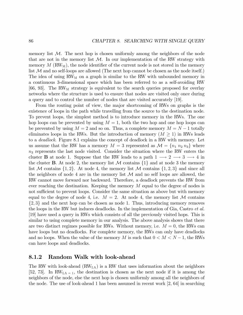
86 CHAPTER 8. SEARCHING WITH SINGLE QUERY
memory list M. The next hop is chosen uniformly among the neighbors of the nodethat are not in the memory list M. In our implementation of the RW strategy withmemoryM (RWM), the node identifier of the current node is not stored in the memorylistM and no self-loops are allowed (The next hop cannot be chosen as the node itself.)The idea of using RWM on a graph is similar to the RW with unbounded memory ina continuous 3-dimensional space which has been referred to as a self-avoiding RW[66, 93]. The RWM strategy is equivalent to the search queries proposed for overlaynetworks where the structure is used to ensure that nodes are visited only once duringa query and to control the number of nodes that are visited accurately [19].From the routing point of view, the major shortcoming of RWs on graphs is the
existence of loops in the path while travelling from the source to the destination node.To prevent loops, the simplest method is to introduce memory in the RWs. The onehop loops can be prevented by using M = 1, both the two hop and one hop loops canbe prevented by using M = 2 and so on. Thus, a complete memory M = N − 1 totallyeliminates loops in the RWs. But the introduction of memory (M ≥ 1) in RWs leadsto a deadlock. Figure 8.1 explains the concept of deadlock in a RW with memory. Letus assume that the RW has a memory M = 3 represented asM = n1 n2 n3 wheren3 represents the last node visited. Consider the situation where the RW enters thecluster B at node 1. Suppose that the RW leads to a path 1 −→ 2 −→ 3 −→ 4 inthe cluster B. At node 2, the memory listM contains 1 and at node 3 the memorylistM contains 1, 2. At node 4, the memory listM contains 1, 2, 3 and since allthe neighbors of node 4 are in the memory list M and no self loops are allowed, theRW cannot move forward nor backward. Therefore, a deadlock prevents the RW fromever reaching the destination. Keeping the memory M equal to the degree of nodes isnot sufficient to prevent loops. Consider the same situation as above but with memoryequal to the degree of node 4, i.e. M = 2. At node 4, the memory list M contains2, 3 and the next hop can be chosen as node 1. Thus, introducing memory removesthe loops in the RW but induces deadlocks. In the implementation of Gia, Castro et al.[19] have used a query in RWs which consists of all the previously visited hops. This issimilar to using complete memory in our analysis. The above analysis shows that thereare two distinct regimes possible for RWs. Without memory, i.e. M = 0, the RWs canhave loops but no deadlocks. For complete memory, the RWs can only have deadlocksand no loops. When the value of the memoryM is such that 0 < M < N − 1, the RWscan have loops and deadlocks.
8.1.2 Random Walk with look-ahead
The RW with look-ahead (RWLA) is a RW that uses information about the neighbors[52, 73]. In RWLA = 1, the destination is chosen as the next node if it is among theneighbors of the node, else the next hop is chosen uniformly among all the neighbors ofthe node. The use of look-ahead 1 has been assumed in recent work [2, 64] in searching
8.1. RANDOM WALKS 87
1
4
3
2
n3
n4 n1 n2
cluster A
cluster Bcluster C
1
4
3
2
n3
n4 n1 n2
cluster A
cluster Bcluster C
Figure 8.1: Explanation of deadlock in (a) RWwith memory: The path 1→ 2→ 3→ 4is shown by arrows. At node 4, the dashed lines indicate the links that cannot be usedwith memory M ≥ 3. (b) RW using highest degree: Node n1 chooses node 1 as nexthop and node 1 chooses node n1 as next hop leading to an infinite loop.
on graphs. In RWLA = 1, there are no deadlocks. The RWLA = 1 can also be used incombination with memory M (see Table 1).
8.1.3 Random Walk using highest degree
In RW using highest degree (RWHD), the next hop is chosen as the node with highestdegree until the destination is reached. Thus, at node u the next node v is chosen suchthat degv = max
s Nu
degs, whereNu is the set of neighbors of u. The RWHD strategy can end
in a deadlock. Deadlocks occurring in RWM and RWHD have different characteristics.In deadlocks in RWM, the node can terminate the RW because it cannot choose anyof the neighbors as the next hop. In deadlocks in RWHD, the node can always choosea neighboring node with highest degree as the next hop but this process may repeat.Figure 8.1 illustrates the concept of deadlock in RWHD. At node n1, node 1 is chosen asthe next node since it has the highest degree among the neighbors of the node n1. Atnode 1, node n1 is chosen as the next hop since node n1 has the highest degree amongthe neighbors of the node 1. Thus, the RWHD ends in an infinite loop or a deadlock.The RWHD can also be used in combination with different values of memory M andlook-ahead (see Table 1).

88 CHAPTER 8. SEARCHING WITH SINGLE QUERY
8.1.4 Random Walk proportional to the degree
We consider a general case of the RW proportional to the degree (RWPD) with a para-meter ζ. The probability of choosing the next node is proportional to the degree of thenode with exponent ζ: At node u, quv ∝ degζv where quv is the probability of choosingthe neighbor v. By normalization, we obtain quv =
degζv
v Nu
degζv. Using ζ = 1, we get the
RW strategy in which the probability of choosing the next node is proportional to thedegree of the node. There are no deadlocks in RWPD with parameter ζ = 1. On theother hand, the RWPD strategy with ζ = 0 is same as RW.
8.1.5 Random Walk using minimum link weight
In RW using minimum link weight (RWW), the next hop is chosen as the link withminimum weight. Thus, at node u the next node v is chosen such that wuv = min
s Nu
wus,
where wus is the weight of link between node u and node s. Deadlocks in RW usingminimum link weight are similar to the deadlocks occurring in RW using highest degree.Indeed, the degree can be considered as a special kind of link weight.
8.1.6 Random walk proportional to the link weight
The probability of choosing the next node is proportional to the ζ-th power of the linkweight: At node u, yuv ∝ wζ
uv where yuv is the probability of choosing the neighbor v.By normalization, we obtain yuv =
wζuv
v Nu
wζuv. Using ζ = −1, we get the RW strategy
in which the probability of choosing the next node is inversely proportional to the linkweight.Table 1 lists the various RW strategies and explanation of how the next hop is chosen
in different strategies.
8.2 Analysis of Searching with single query
The probability distribution of hopcount for a RW on a complete graph KN is a geo-metric distribution [70, 38],
Pr[H = j] =1
N − 1
µ1− 1
N − 1
¶j−1(8.1)
For multiple itemsm = q (N − 1) uniformly located overKN , the hopcount distributionis
Pr[H = j] =m
N − 1
µ1− m
N − 1
¶j−1(8.2)
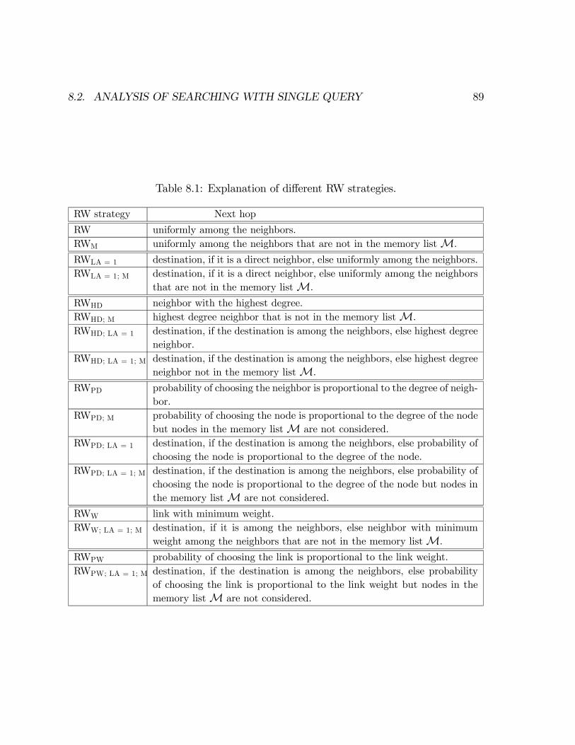
8.2. ANALYSIS OF SEARCHING WITH SINGLE QUERY 89
Table 8.1: Explanation of different RW strategies.
RW strategy Next hop
RW uniformly among the neighbors.RWM uniformly among the neighbors that are not in the memory listM.
RWLA = 1 destination, if it is a direct neighbor, else uniformly among the neighbors.RWLA = 1; M destination, if it is a direct neighbor, else uniformly among the neighbors
that are not in the memory listM.
RWHD neighbor with the highest degree.RWHD; M highest degree neighbor that is not in the memory listM.RWHD; LA = 1 destination, if the destination is among the neighbors, else highest degree
neighbor.RWHD; LA = 1; M destination, if the destination is among the neighbors, else highest degree
neighbor not in the memory listM.
RWPD probability of choosing the neighbor is proportional to the degree of neigh-bor.
RWPD; M probability of choosing the node is proportional to the degree of the nodebut nodes in the memory listM are not considered.
RWPD; LA = 1 destination, if the destination is among the neighbors, else probability ofchoosing the node is proportional to the degree of the node.
RWPD; LA = 1; M destination, if the destination is among the neighbors, else probability ofchoosing the node is proportional to the degree of the node but nodes inthe memory listM are not considered.
RWW link with minimum weight.RWW; LA = 1; M destination, if it is among the neighbors, else neighbor with minimum
weight among the neighbors that are not in the memory listM.
RWPW probability of choosing the link is proportional to the link weight.RWPW; LA = 1; M destination, if the destination is among the neighbors, else probability
of choosing the link is proportional to the link weight but nodes in thememory listM are not considered.
90 CHAPTER 8. SEARCHING WITH SINGLE QUERY
and the expected hopcount is N−1m.
With memory M for RWM on a complete graph KN ,
PrhH = j
i=
1
N − 1 (8.3)
which means that the hopcount for RWM is a uniform random variable on [1, N − 1]when 1 ≤ j ≤M . The probability distribution of RW with memory M for j ≥M + 1is [38],
Pr [HM = j] =1
N − 1
µN − (M + 2)
N − (M + 1)
¶j−M−1(8.4)
Thus, the probability distribution for a RWM on the complete graph KN is a uniformrandom variable on [1,M ] and geometric variable on [M + 1, N − 1]. With multipledata items uniformly located over KN , 1
N−1 is replaced by q in (8.3) and (8.4).We now compute the probability of deadlocks and the hopcount distribution for
RWM. Let the RWM be at node ni after j − 1 hops. We have used ni instead of njsince there may be loops in RWM and this node might have been visited before. Inthe next step, the RWM has to choose one of the neighbors as the next hop (hop j).Let Xj;ni represent the event that all neighbors of node ni have been visited beforehop j. Clearly, Pr [X1;ni ] = 0 for all ni ∈ N . Let degni represent the degree of nodeni. Let Φj be the probability that there is a deadlock before making hop j and Φdenote the probability that there is a deadlock in RWM. A deadlock can happen whilechoosing hop j iff degni ≤M and all the neighbors of node ni have been visited before1.In a complete graph since degree of any node ni is always greater than any M i.e.,Pr£degni > M
¤= 1, the probability of deadlock before making hop j is always zero. In
general,Pr [Φj] = Pr
£Xj;ni | degni ≤M
¤· Pr
£degni ≤M
¤(8.5)
The probability of deadlock in RWM is
Pr [Φ] = Pr [deadlockhop1] + Pr [deadlockhop2] + Pr [deadlockhop3] + ... (8.6)
≤∞Xj=1
Pr [Φj] =∞Xj=1
Pr£Xj;ni | degni ≤M
¤· Pr
£degni ≤M
¤The probability of deadlock (Pr [Φ]) is less than the sum of probabilities of deadlock ateach hop (
PPr [Φj]) since we did not consider the probability of finding the destination
at any hop while computing Pr [Φj].In ER random graphs, the probability of deadlock in RWM tends to 0 when M <
(1− δ) · p(N − 1). For any fixed α, 0 < α < 1, let δ =q
9p(N−1) log
Nα. By Chernoff
1If memory listM is not full, then M represents the number of elements in the memory list.

8.2. ANALYSIS OF SEARCHING WITH SINGLE QUERY 91
n1
n2
n0
n3
n1
n2
n0
n3
Figure 8.2: Diagram showing the progression of RW and RWM.
bounds [105],
Pr£| degni −p (N − 1) |> δ · p(N − 1)
¤≤ 2 · exp
µ−δ
2p (N − 1)3
¶(8.7)
Substituting the above value of δ
Pr£| degni −p (N − 1) |> δ · p(N − 1)
¤≤ 2 · exp
µ−2 log N
α
¶≤³ αN
´2(8.8)
Therefore, for M < (1− δ) · p(N − 1), Pr£degni ≤M
¤≤¡αN
¢2. Hence using (8.5), the
probability of deadlock before making hop j, Pr [Φj] ≤¡αN
¢2. The general expression
for probability of deadlocks and the probability distribution of hopcount for RWM=N-1onG (N,L) is computed below. Let n0 be the source node (Figure 8.2). Since Pr [Φ1] = 0,the probability of deadlock before making first hop
Pr [deadlockhop1] = Pr [E0] · Pr [n0 6= v] · Pr [Φ1] = 0
Let E1 denote the event that RWM=N-1 has made 1 hop already and that node n1 is thecurrent node.
Pr [H = 1] = Pr [E1] · Pr [n1 = v] =1
N − 1
Pr [deadlockhop2] = Pr [E1] · Pr [n1 6= v] · Pr [Φ2]
=
µ1− 1
N − 1
¶· Pr [Φ2]
Now a transition is made from node n1 to node n2. Let E2 denote the event thatRWM=N-1 has made a transition to node n2. Therefore, Pr [E2] = Pr [E1] ·Pr [n1 6= v]−

92 CHAPTER 8. SEARCHING WITH SINGLE QUERY
Pr [deadlockhop2]
Pr [H = 2] = Pr [E2] · Pr [n2 = v] =1
N − 2 ·µ1− 1
N − 1
¶· (1− Pr [Φ2])
=1
N − 1 · (1− Pr [Φ2])
Pr [deadlockhop3] = Pr [E2] · Pr [n2 6= v] · Pr [Φ3]
=
µ1− 1
N − 1
¶µ1− 1
N − 2
¶(1− Pr [Φ2]) Pr [Φ3]
Thus, the probability of deadlock and hopcount distribution for RWM=N-1 on graphG (N,L) is
Pr [deadlockhopj] =µN − j
N − 1
¶(1− Pr [Φ2]) (1− Pr [Φ3]) ... (1− Pr [Φj−1]) Pr [Φj] (8.9)
Pr [H = j] =1
N − 1 (1− Pr [Φ2]) (1− Pr [Φ3]) ... (1− Pr [Φj−1]) (1− Pr [Φj]) (8.10)
With multiple data items m = q (N − 1) uniformly located over the network, the hop-count distribution is
Pr [H = j] =m
N − j
µ1− m
N − 1
¶...
µ1− m
N − j − 1
¶(1− Pr [Φ2]) ... (1− Pr [Φj])
(8.11)Since we know that in ER random graphs, whenM ≤ (1− δ) p (N − 1), Pr
£degni ≤M
¤is small and when M > (1 + δ) p (N − 1), Pr
£degni < M
¤is close to 1, the probability
of deadlock in RWM=N-1 can be approximated as
Pr [Φ] ≤NXj=1
Pr£Xj;ni | degni ≤M
¤· Pr
£degni ≤M
¤≈
NXj=(1+δ)p(N−1)
Pr [Xj;ni ]
When the link density p is small, the probability of deadlocks is large. However, if p issufficiently large, then Pr [Φ] is close to 0. In power law graphs, since there are largenumber of nodes with very small degree, the probability of deadlocks becomes largeeven for small values of the memory M .It is difficult to compute the exact expression for RWLA=1 because of the loops. We
compute the expression for probability of deadlocks and the probability distributionof hopcount for RWLA=1;M=N-1 on ER random graphs. Let Sni represent the set ofneighbors of node ni that have not been seen before. Then,
Pr [H = 1] =
N−1Xj=0
j Pr [deg = j]
N − 1= p
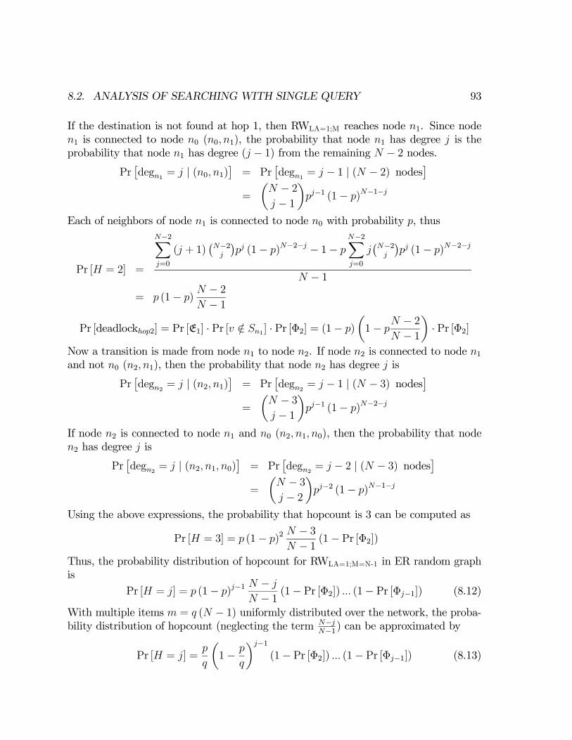
8.2. ANALYSIS OF SEARCHING WITH SINGLE QUERY 93
If the destination is not found at hop 1, then RWLA=1;M reaches node n1. Since noden1 is connected to node n0 (n0, n1), the probability that node n1 has degree j is theprobability that node n1 has degree (j − 1) from the remaining N − 2 nodes.
Pr£degn1 = j | (n0, n1)
¤= Pr
£degn1 = j − 1 | (N − 2) nodes
¤=
µN − 2j − 1
¶pj−1 (1− p)N−1−j
Each of neighbors of node n1 is connected to node n0 with probability p, thus
Pr [H = 2] =
N−2Xj=0
(j + 1)¡N−2j
¢pj (1− p)N−2−j − 1− p
N−2Xj=0
j¡N−2j
¢pj (1− p)N−2−j
N − 1= p (1− p)
N − 2N − 1
Pr [deadlockhop2] = Pr [E1] · Pr [v /∈ Sn1] · Pr [Φ2] = (1− p)
µ1− p
N − 2N − 1
¶· Pr [Φ2]
Now a transition is made from node n1 to node n2. If node n2 is connected to node n1and not n0 (n2, n1), then the probability that node n2 has degree j is
Pr£degn2 = j | (n2, n1)
¤= Pr
£degn2 = j − 1 | (N − 3) nodes
¤=
µN − 3j − 1
¶pj−1 (1− p)N−2−j
If node n2 is connected to node n1 and n0 (n2, n1, n0), then the probability that noden2 has degree j is
Pr£degn2 = j | (n2, n1, n0)
¤= Pr
£degn2 = j − 2 | (N − 3) nodes
¤=
µN − 3j − 2
¶pj−2 (1− p)N−1−j
Using the above expressions, the probability that hopcount is 3 can be computed as
Pr [H = 3] = p (1− p)2N − 3N − 1 (1− Pr [Φ2])
Thus, the probability distribution of hopcount for RWLA=1;M=N-1 in ER random graphis
Pr [H = j] = p (1− p)j−1N − j
N − 1 (1− Pr [Φ2]) ... (1− Pr [Φj−1]) (8.12)
With multiple items m = q (N − 1) uniformly distributed over the network, the proba-bility distribution of hopcount (neglecting the term N−j
N−1) can be approximated by
Pr [H = j] =p
q
µ1− p
q
¶j−1(1− Pr [Φ2]) ... (1− Pr [Φj−1]) (8.13)
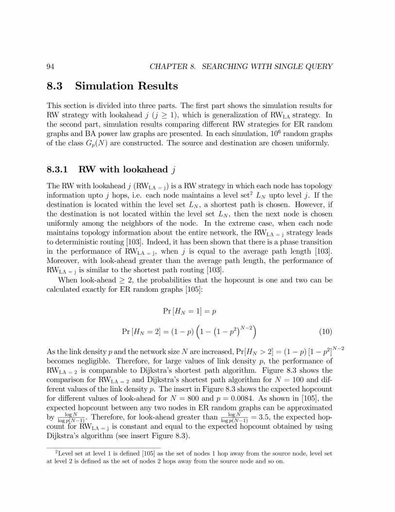
94 CHAPTER 8. SEARCHING WITH SINGLE QUERY
8.3 Simulation Results
This section is divided into three parts. The first part shows the simulation results forRW strategy with lookahead j (j ≥ 1), which is generalization of RWLA strategy. Inthe second part, simulation results comparing different RW strategies for ER randomgraphs and BA power law graphs are presented. In each simulation, 106 random graphsof the class Gp(N) are constructed. The source and destination are chosen uniformly.
8.3.1 RW with lookahead j
The RWwith lookahead j (RWLA = j) is a RW strategy in which each node has topologyinformation upto j hops, i.e. each node maintains a level set2 LN upto level j. If thedestination is located within the level set LN , a shortest path is chosen. However, ifthe destination is not located within the level set LN , then the next node is chosenuniformly among the neighbors of the node. In the extreme case, when each nodemaintains topology information about the entire network, the RWLA = j strategy leadsto deterministic routing [103]. Indeed, it has been shown that there is a phase transitionin the performance of RWLA = j, when j is equal to the average path length [103].Moreover, with look-ahead greater than the average path length, the performance ofRWLA = j is similar to the shortest path routing [103].When look-ahead ≥ 2, the probabilities that the hopcount is one and two can be
calculated exactly for ER random graphs [105]:
Pr [HN = 1] = p
Pr [HN = 2] = (1− p)³1−
¡1− p2
¢N−2´(10)
As the link density p and the network sizeN are increased, Pr[HN > 2] = (1− p) [1− p2]N−2
becomes negligible. Therefore, for large values of link density p, the performance ofRWLA = 2 is comparable to Dijkstra’s shortest path algorithm. Figure 8.3 shows thecomparison for RWLA = 2 and Dijkstra’s shortest path algorithm for N = 100 and dif-ferent values of the link density p. The insert in Figure 8.3 shows the expected hopcountfor different values of look-ahead for N = 800 and p = 0.0084. As shown in [105], theexpected hopcount between any two nodes in ER random graphs can be approximatedby logN
log p(N−1) . Therefore, for look-ahead greater thanlogN
log p(N−1) = 3.5, the expected hop-count for RWLA = j is constant and equal to the expected hopcount obtained by usingDijkstra’s algorithm (see insert Figure 8.3).
2Level set at level 1 is defined [105] as the set of nodes 1 hop away from the source node, level setat level 2 is defined as the set of nodes 2 hops away from the source node and so on.

8.3. SIMULATION RESULTS 95
0.6
0.4
0.2
0.0
Pr[H
= k]
108642hop k
N = 100, RWLA = 2 p = 0.1 E[H] = 2.5, var[H] = 2.1 p = 0.2 E[H] = 1.8, var[H] = 0.2
Dijkstra's algorithm p = 0.1 E[H] = 2.2, var[H] = 0.4 p = 0.2 E[H] = 1.81, var[H] = 0.2
1000
800
600
400
200
0
E[H
]
1086420LA = k
N = 800p = 0.0084
0.6
0.4
0.2
0.0
Pr[H
= k]
108642hop k
N = 100, RWLA = 2 p = 0.1 E[H] = 2.5, var[H] = 2.1 p = 0.2 E[H] = 1.8, var[H] = 0.2
Dijkstra's algorithm p = 0.1 E[H] = 2.2, var[H] = 0.4 p = 0.2 E[H] = 1.81, var[H] = 0.2
1000
800
600
400
200
0
E[H
]
1086420LA = k
N = 800p = 0.0084
Figure 8.3: Comparison of the RWLA = 2 and the Dijkstra’s shortest path algorithm forN = 100 and different values of the link density p. The insert shows expected hopcountfor different values of look-ahead for N = 800 and p = 0.0084.
8.3.2 Comparison of RW strategies
In ER random graphs, at large values of the link density p, E[HRW] ∼ N and thereforeE[HRWLA = 1 ] ∼ 1
p. Moreover, Pr [Φ] −→ 0 for anyM for large values of the link density
p. Also, p (1− p)j−1 is a good approximation when p is large for RWLA=1;M=N-1 (Figure8.4).Thus, when the link density p is large, the results for different RW strategies on arandom graph Gp(N) are similar to a complete graph KN .We compare the performance of RW strategies in sparse graphs i.e., random graphs
with small link density p. The sparse graphs are particularly interesting since theaverage degree for most real networks like Gnutella [71] and Internet [2] is known to besmall.Figure 8.5 shows the simulation results for a sparse ER random graph. The Pr[success]
represents the probability that destination is found by the query. The simulations indi-cate that the mean hopcount is linear in N for these strategies and the mean hopcountfor the RWLA = 1 and the RW strategies are related by the expression E[HRWLA = 1 ]
∼ E[HRW ]pN
. In RWM=N-1, the probability of deadlock Pr [Φ] −→ 1 as N is increased.Figures 8.6 shows the simulation results for preferential attachment graphs generated
using the BA model. RWLA=1 and RWHD are not effective as might be expected sincethere are large number of nodes with small degree in this model. It has been shown byMihail et al. [75] that in power law graphs, the expected number of hops for RWLA=1

96 CHAPTER 8. SEARCHING WITH SINGLE QUERY
0.0001
0.001
0.01
0.1
Pr[H
= k
]
40302010hop k
Simulation ResultsN = 25
p = 0.3 E[H] = 3.3, var[H] = 7.2 p = 0.5 E[H] = 2.0, var[H] = 2.0 p = 0.8 E[H] = 1.2, var[H] = 0.31
N = 100 p = 0.1 E[H] = 9.9, var[H] = 86.1
Analytical ResultsN = 25
p = 0.3 E[H] = 3.3 p = 0.5 E[H] = 2.0 p = 0.8 E[H] = 1.2
N = 100 p = 0.1 E[H] = 10
Figure 8.4: Comparison of the expression Pr [H = j] ∼= p (1− p)j−1 and simulationresults for RWLA = 1; M = N-1 on a random graph for N = 25, 100 and different values ofthe link density p.
to discover Ω³N1− ( 12−ε)
´nodes is O
³N
12+ε logN
´where 0 < ε < 1
2. This shows that
look-ahead is not effective for power law graphs. Using RWM=N-1, the probability thatthere is a deadlock is close to 1 when N is large.The RWHD; LA=1; M=N-1 strategy performs best in both graph topologies. The ex-
pected hopcount for certain RW strategies such as RWHD is similar for both the graphtopologies. However, the average hopcount does not accurately reflect the performanceof different search strategies since these strategies generally lead to infinite loops. Look-ahead and memory both improve performance in power law graph and ER randomgraphs. However, the performance with M = N − 1 and LA = 1 improves more in ERgraphs then the BA model. Moreover, in ER random graphs and power law graphs gen-erated using the BA model, the performance of RWLA is close to shortest path routingwith small values of look-ahead. This is due to the small diameter (O (logN)) of thesegraph topologies [22, 23].
8.4 Conclusion
The hopcount distribution for RW strategies based on memory and lookahead is closeto a geometric variable for random graphs. We also investigated the occurrence of dead-locks in various RW strategies. Deadlocks have been neglected in most of the previous

8.4. CONCLUSION 97
(a)
(b)
78
10
2
3
4
5678
100
2
3
4
56
E[H
N]
5 6 7 8 9100
2 3 4
N
RW RW LA = 1 RW M = N-1 RW LA = 1 ; M = N-1
RW HD ; LA = 1 ; M = N-1 RW PD ; LA = 1 ; M = N-1
pN = 5
0.8
0.6
0.4
0.2
Pr[s
ucce
ss]
40035030025020015010050N
RWM = N-1 RWM=N-1; LA = 1
RWHD; M = N-1 RWHD; LA = 1
RWHD; LA = 1; M = N-1
pN = 5
Figure 8.5: (a) The mean hopcount for different RW strategies as a function of N withconstant number of neighbors (pN = 5) for ER graphs. (b) The Pr[success] for differentRW strategies for N = 200 and link density p = 0.025.

98 CHAPTER 8. SEARCHING WITH SINGLE QUERY
(a)
(b)
10
100
1000
E[H
N]
1002 3 4 5 6 7 8 9
1000N
RW RW LA = 1 RW M = N-1 RW LA = 1; M = N-1 RW HD; LA = 1; M = N-1 RW HD; LA = 1 RW HD; M = N-1
0.8
0.6
0.4
0.2
Pr[s
ucce
ss]
1600140012001000800600400200N
RWHD; LA =1; M = N-1
RWLA =1; M = N-1 RWM = N-1 RWHD; LA = 1
RWHD; M = N-1
(a)
(b)
10
100
1000
E[H
N]
1002 3 4 5 6 7 8 9
1000N
RW RW LA = 1 RW M = N-1 RW LA = 1; M = N-1 RW HD; LA = 1; M = N-1 RW HD; LA = 1 RW HD; M = N-1
0.8
0.6
0.4
0.2
Pr[s
ucce
ss]
1600140012001000800600400200N
RWHD; LA =1; M = N-1
RWLA =1; M = N-1 RWM = N-1 RWHD; LA = 1
RWHD; M = N-1
Figure 8.6: (a) The mean hopcount for different RW strategies as a function of Nfor power law graph generated using BA model (b) The Pr[success] for different RWstrategies.

8.4. CONCLUSION 99
search strategy comparisons. A mere comparison of the expected hopcount or weightof different RW strategies gives little insight into the performance of these strategies.The simulations showed that for RW strategies using highest degree or minimum linkweight, the expected hopcount or weight is small but these strategies generally lead todeadlocks. In conclusion, RW strategies using highest degree or minimum link weightperform well when used in combination with memory or look-ahead. Also, for differ-ent RW strategies, if the probability of finding the destination is large, the expectedhopcount for the particular strategy is also large and vice versa.

100 CHAPTER 8. SEARCHING WITH SINGLE QUERY
Chapter 9
Searching with multiple queries
Searching overhead or packet overhead is defined as the product of number of hops foreach query (packet) and number of queries (packets) i.e., the total number of packetsexchanged. Our work in this chapter shows that searching using multiple RW queriesreduces the overhead for searching as compared to flooding with sequence numbers.
It is known that the number of hops required for uniform sampling by RW can beas low as the number of samples in independent uniform sampling [13, 51]. Thus, ifthe RW starts at any node and makes h hops, and using each visited node as a samplepoint, approximately the same statistical properties can be achieved as h independentuniform samples. However, our simulations show that there are large differences in thebehavior of RW as compared to independent uniform sampling particularly when theTTL is small.
A single RW query has an overhead and time to discover of O(N logN) for ERrandom graphs and BA power law graphs [28, 63]. Since the time to discover is largein RW, we split a single RW query into Q multiple queries each with a given TTL.Each RW query stops when the TTL is reached or the destination is located (In RWM,the query also stops if there is a deadlock). Since each RW query makes at most TTLhops, the worst-case searching overhead is Q×TTL. The expected number of hops areless since any query stops once the destination is found. However, there is a probabilitythat a destination is never located by the multiple queries. Thus, with multiple querieswe define the probability of success as the probability that the destination is located byat least one query out of the Q queries generated. In flooding with sequence numbers,the probability of success is defined as the probability that a destination is located witha given TTL. We want to minimize TTL and Q and maximize Pr [success].
101
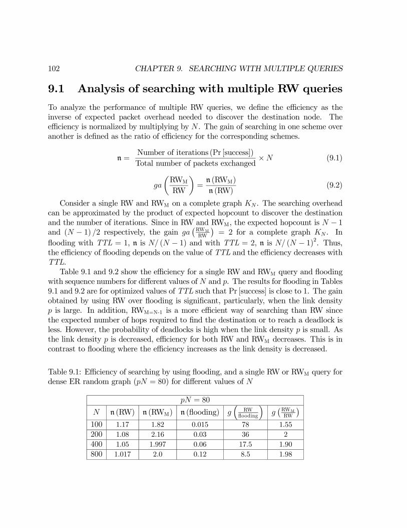
102 CHAPTER 9. SEARCHING WITH MULTIPLE QUERIES
9.1 Analysis of searching with multiple RW queries
To analyze the performance of multiple RW queries, we define the efficiency as theinverse of expected packet overhead needed to discover the destination node. Theefficiency is normalized by multiplying by N . The gain of searching in one scheme overanother is defined as the ratio of efficiency for the corresponding schemes.
n =Number of iterations (Pr [success])Total number of packets exchanged
×N (9.1)
ga
µRWM
RW
¶=n (RWM)
n (RW)(9.2)
Consider a single RW and RWM on a complete graph KN . The searching overheadcan be approximated by the product of expected hopcount to discover the destinationand the number of iterations. Since in RW and RWM, the expected hopcount is N − 1and (N − 1) /2 respectively, the gain ga
¡RWMRW
¢= 2 for a complete graph KN . In
flooding with TTL = 1, n is N/ (N − 1) and with TTL = 2, n is N/ (N − 1)2. Thus,the efficiency of flooding depends on the value of TTL and the efficiency decreases withTTL.Table 9.1 and 9.2 show the efficiency for a single RW and RWM query and flooding
with sequence numbers for different values ofN and p. The results for flooding in Tables9.1 and 9.2 are for optimized values of TTL such that Pr [success] is close to 1. The gainobtained by using RW over flooding is significant, particularly, when the link densityp is large. In addition, RWM=N-1 is a more efficient way of searching than RW sincethe expected number of hops required to find the destination or to reach a deadlock isless. However, the probability of deadlocks is high when the link density p is small. Asthe link density p is decreased, efficiency for both RW and RWM decreases. This is incontrast to flooding where the efficiency increases as the link density is decreased.
Table 9.1: Efficiency of searching by using flooding, and a single RW or RWM query fordense ER random graph (pN = 80) for different values of N
pN = 80
N n (RW) n (RWM) n (flooding) g³
RWflooding
´g¡RWMRW
¢100 1.17 1.82 0.015 78 1.55200 1.08 2.16 0.03 36 2400 1.05 1.997 0.06 17.5 1.90800 1.017 2.0 0.12 8.5 1.98
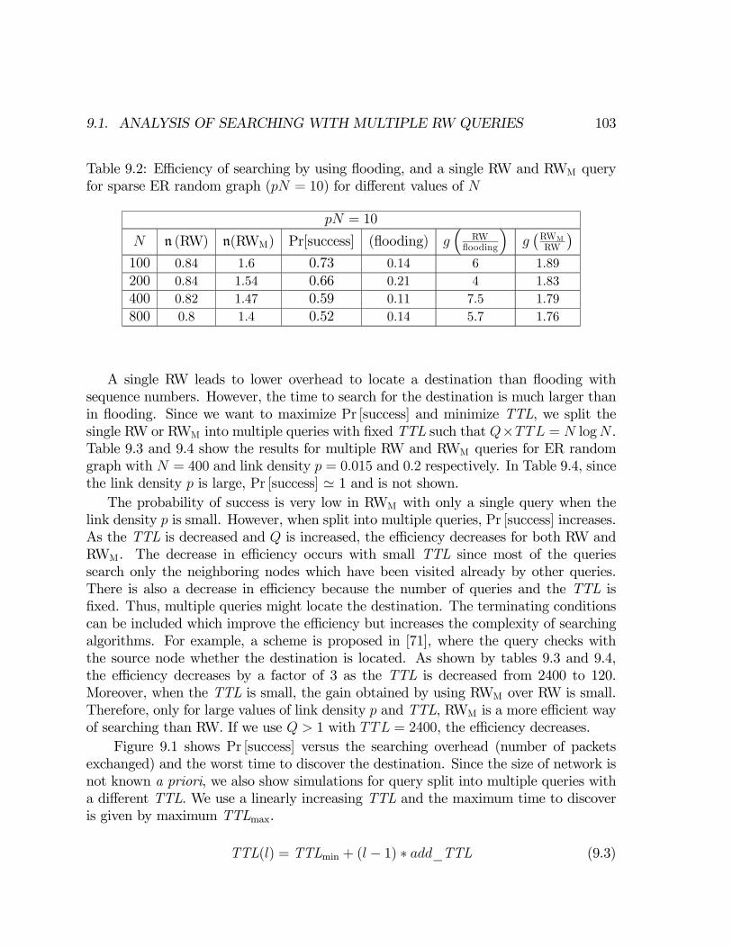
9.1. ANALYSIS OF SEARCHING WITH MULTIPLE RW QUERIES 103
Table 9.2: Efficiency of searching by using flooding, and a single RW and RWM queryfor sparse ER random graph (pN = 10) for different values of N
pN = 10
N n (RW) n(RWM) Pr[success] (flooding) g³
RWflooding
´g¡RWMRW
¢100 0.84 1.6 0.73 0.14 6 1.89200 0.84 1.54 0.66 0.21 4 1.83400 0.82 1.47 0.59 0.11 7.5 1.79800 0.8 1.4 0.52 0.14 5.7 1.76
A single RW leads to lower overhead to locate a destination than flooding withsequence numbers. However, the time to search for the destination is much larger thanin flooding. Since we want to maximize Pr [success] and minimize TTL, we split thesingle RW or RWM into multiple queries with fixed TTL such that Q×TTL = N logN .Table 9.3 and 9.4 show the results for multiple RW and RWM queries for ER randomgraph with N = 400 and link density p = 0.015 and 0.2 respectively. In Table 9.4, sincethe link density p is large, Pr [success] ' 1 and is not shown.The probability of success is very low in RWM with only a single query when the
link density p is small. However, when split into multiple queries, Pr [success] increases.As the TTL is decreased and Q is increased, the efficiency decreases for both RW andRWM. The decrease in efficiency occurs with small TTL since most of the queriessearch only the neighboring nodes which have been visited already by other queries.There is also a decrease in efficiency because the number of queries and the TTL isfixed. Thus, multiple queries might locate the destination. The terminating conditionscan be included which improve the efficiency but increases the complexity of searchingalgorithms. For example, a scheme is proposed in [71], where the query checks withthe source node whether the destination is located. As shown by tables 9.3 and 9.4,the efficiency decreases by a factor of 3 as the TTL is decreased from 2400 to 120.Moreover, when the TTL is small, the gain obtained by using RWM over RW is small.Therefore, only for large values of link density p and TTL, RWM is a more efficient wayof searching than RW. If we use Q > 1 with TTL = 2400, the efficiency decreases.
Figure 9.1 shows Pr [success] versus the searching overhead (number of packetsexchanged) and the worst time to discover the destination. Since the size of network isnot known a priori, we also show simulations for query split into multiple queries witha different TTL. We use a linearly increasing TTL and the maximum time to discoveris given by maximum TTLmax.
TTL(l) = TTLmin + (l − 1) ∗ add_TTL (9.3)
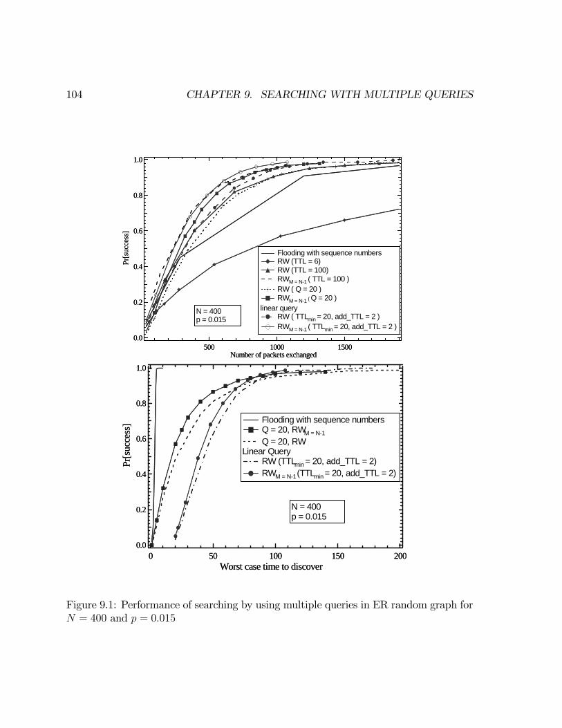
104 CHAPTER 9. SEARCHING WITH MULTIPLE QUERIES
1.0
0.8
0.6
0.4
0.2
0.0
Pr[s
ucce
ss]
15001000500Number of packets exchanged
Flooding with sequence numbers RW (TTL = 6) RW (TTL = 100) RWM = N-1 ( TTL = 100 ) RW ( Q = 20 ) RWM = N-1 ( Q = 20 )
linear query RW ( TTLmin = 20, add_TTL = 2 ) RWM = N-1 ( TTLmin = 20, add_TTL = 2 )
N = 400p = 0.015
1.0
0.8
0.6
0.4
0.2
0.0
Pr[s
ucce
ss]
200150100500Worst case time to discover
Flooding with sequence numbers Q = 20, RWM = N-1 Q = 20, RW
Linear Query RW (TTLmin = 20, add_TTL = 2) RWM = N-1 (TTLmin = 20, add_TTL = 2)
N = 400 p = 0.015
1.0
0.8
0.6
0.4
0.2
0.0
Pr[s
ucce
ss]
15001000500Number of packets exchanged
Flooding with sequence numbers RW (TTL = 6) RW (TTL = 100) RWM = N-1 ( TTL = 100 ) RW ( Q = 20 ) RWM = N-1 ( Q = 20 )
linear query RW ( TTLmin = 20, add_TTL = 2 ) RWM = N-1 ( TTLmin = 20, add_TTL = 2 )
N = 400p = 0.015
1.0
0.8
0.6
0.4
0.2
0.0
Pr[s
ucce
ss]
200150100500Worst case time to discover
Flooding with sequence numbers Q = 20, RWM = N-1 Q = 20, RW
Linear Query RW (TTLmin = 20, add_TTL = 2) RWM = N-1 (TTLmin = 20, add_TTL = 2)
N = 400 p = 0.015
Figure 9.1: Performance of searching by using multiple queries in ER random graph forN = 400 and p = 0.015
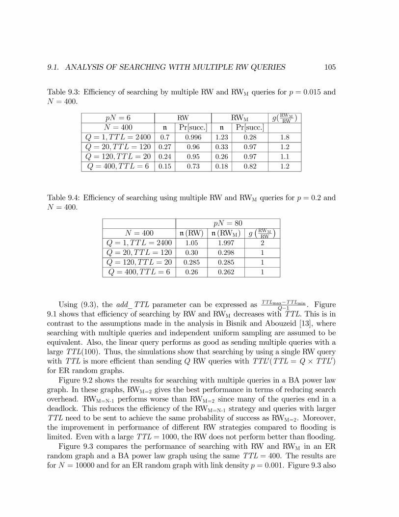
9.1. ANALYSIS OF SEARCHING WITH MULTIPLE RW QUERIES 105
Table 9.3: Efficiency of searching by multiple RW and RWM queries for p = 0.015 andN = 400.
pN = 6 RW RWM g(RWMRW )
N = 400 n Pr[succ.] n Pr[succ.]Q = 1, TTL = 2400 0.7 0.996 1.23 0.28 1.8Q = 20, TTL = 120 0.27 0.96 0.33 0.97 1.2Q = 120, TTL = 20 0.24 0.95 0.26 0.97 1.1Q = 400, TTL = 6 0.15 0.73 0.18 0.82 1.2
Table 9.4: Efficiency of searching using multiple RW and RWM queries for p = 0.2 andN = 400.
pN = 80
N = 400 n (RW) n (RWM) g¡RWMRW
¢Q = 1, TTL = 2400 1.05 1.997 2Q = 20, TTL = 120 0.30 0.298 1Q = 120, TTL = 20 0.285 0.285 1Q = 400, TTL = 6 0.26 0.262 1
Using (9.3), the add_TTL parameter can be expressed as TTLmax−TTLminQ−1 . Figure
9.1 shows that efficiency of searching by RW and RWM decreases with TTL. This is incontrast to the assumptions made in the analysis in Bisnik and Abouzeid [13], wheresearching with multiple queries and independent uniform sampling are assumed to beequivalent. Also, the linear query performs as good as sending multiple queries with alarge TTL(100). Thus, the simulations show that searching by using a single RW querywith TTL is more efficient than sending Q RW queries with TTL0(TTL = Q × TTL0)for ER random graphs.Figure 9.2 shows the results for searching with multiple queries in a BA power law
graph. In these graphs, RWM=2 gives the best performance in terms of reducing searchoverhead. RWM=N-1 performs worse than RWM=2 since many of the queries end in adeadlock. This reduces the efficiency of the RWM=N-1 strategy and queries with largerTTL need to be sent to achieve the same probability of success as RWM=2. Moreover,the improvement in performance of different RW strategies compared to flooding islimited. Even with a large TTL = 1000, the RW does not perform better than flooding.Figure 9.3 compares the performance of searching with RW and RWM in an ER
random graph and a BA power law graph using the same TTL = 400. The results arefor N = 10000 and for an ER random graph with link density p = 0.001. Figure 9.3 also
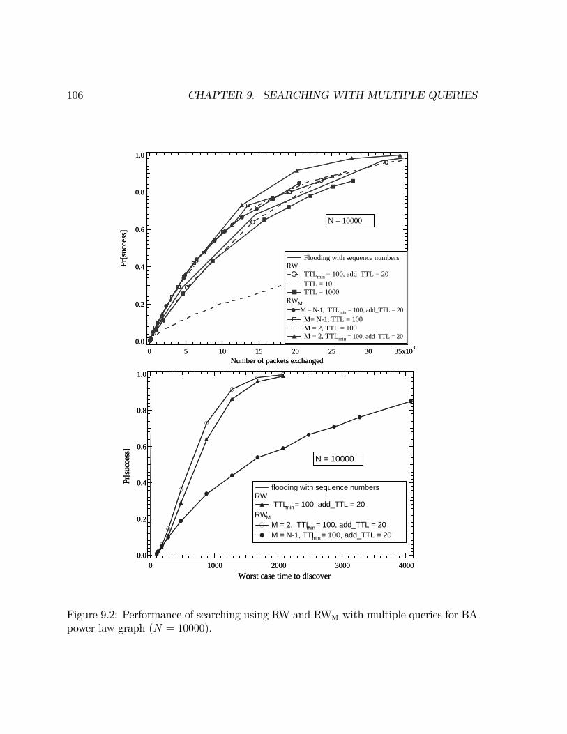
106 CHAPTER 9. SEARCHING WITH MULTIPLE QUERIES
1.0
0.8
0.6
0.4
0.2
0.0
Pr[s
ucce
ss]
35x103302520151050Number of packets exchanged
Flooding with sequence numbersRW
TTLmin = 100, add_TTL = 20 TTL = 10 TTL = 1000
RWMM = N-1, TTLmin = 100, add_TTL = 20 M= N-1, TTL = 100 M = 2, TTL = 100 M = 2, TTLmin = 100, add_TTL = 20
N = 10000
1.0
0.8
0.6
0.4
0.2
0.0
Pr[s
ucce
ss]
40003000200010000Worst case time to discover
flooding with sequence numbersRW
TTLmin = 100, add_TTL = 20 RWM
M = 2, TTLmin = 100, add_TTL = 20 M = N-1, TTLmin = 100, add_TTL = 20
N = 10000
1.0
0.8
0.6
0.4
0.2
0.0
Pr[s
ucce
ss]
35x103302520151050Number of packets exchanged
Flooding with sequence numbersRW
TTLmin = 100, add_TTL = 20 TTL = 10 TTL = 1000
RWMM = N-1, TTLmin = 100, add_TTL = 20 M= N-1, TTL = 100 M = 2, TTL = 100 M = 2, TTLmin = 100, add_TTL = 20
N = 10000
1.0
0.8
0.6
0.4
0.2
0.0
Pr[s
ucce
ss]
40003000200010000Worst case time to discover
flooding with sequence numbersRW
TTLmin = 100, add_TTL = 20 RWM
M = 2, TTLmin = 100, add_TTL = 20 M = N-1, TTLmin = 100, add_TTL = 20
N = 10000
Figure 9.2: Performance of searching using RW and RWM with multiple queries for BApower law graph (N = 10000).
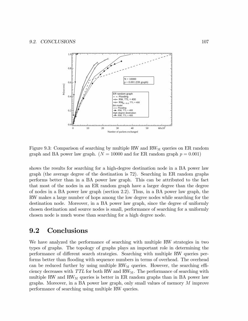
9.2. CONCLUSIONS 107
1.0
0.8
0.6
0.4
0.2
0.0
Pr[s
ucce
ss]
60x10350403020100Number of packets exchanged
ER random graph Flooding RW, TTL = 400 RWM = N-1, TTL = 400
BA model Flooding RW, TTL = 400
High degree destination RW, TTL = 400
N = 10000p = 0.001 (ER graph)
Figure 9.3: Comparison of searching by multiple RW and RWM queries on ER randomgraph and BA power law graph. (N = 10000 and for ER random graph p = 0.001)
shows the results for searching for a high-degree destination node in a BA power lawgraph (the average degree of the destination is 72). Searching in ER random graphsperforms better than in a BA power law graph. This can be attributed to the factthat most of the nodes in an ER random graph have a larger degree than the degreeof nodes in a BA power law graph (section 2.2). Thus, in a BA power law graph, theRW makes a large number of hops among the low degree nodes while searching for thedestination node. Moreover, in a BA power law graph, since the degree of uniformlychosen destination and source nodes is small, performance of searching for a uniformlychosen node is much worse than searching for a high degree node.
9.2 Conclusions
We have analyzed the performance of searching with multiple RW strategies in twotypes of graphs. The topology of graphs plays an important role in determining theperformance of different search strategies. Searching with multiple RW queries per-forms better than flooding with sequence numbers in terms of overhead. The overheadcan be reduced further by using multiple RWM queries. However, the searching effi-ciency decreases with TTL for both RW and RWM. The performance of searching withmultiple RW and RWM queries is better in ER random graphs than in BA power lawgraphs. Moreover, in a BA power law graph, only small values of memory M improveperformance of searching using multiple RW queries.
108 CHAPTER 9. SEARCHING WITH MULTIPLE QUERIES

Part IV
Topology Analysis
109

Chapter 10
Topology of Ad hoc wirelessnetworks
The topology of ad hoc networks is critical in determining the performance of routingalgorithms, capacity and lifetime of ad hoc networks. In this chapter, we study theimpact of different signal propagation models on the topology of ad hoc networks. Wealso analyze the impact of topology on shortest path routing based on distance andhopcount metrics.
We characterize the variation in received signal power over distance due to pathloss and shadowing. Path loss is caused by dissipation of the power radiated by thetransmitter as well as effects of the propagation channel. Path loss models generallyassume that path loss is the same at a given transmitter-receiver distance [53]. Shadow-ing is caused by obstacles between transmitter and receiver that attenuate signal powerthrough absorption, reflection, scattering and diffraction. Variation due to path lossoccurs over very large distances (100-1000 meters), whereas variation due to shadowingoccurs over distances proportional to the length of obstructing object (10-100 meters inoutdoor environments and less in indoor environments). Since variations due to pathloss and shadowing occur over relatively large distances, this variation is referred to aslarge-scale propagation effects. Variations in received signal power also occur due tothe constructive and destructive addition of multipath signal components. Variationsdue to multipath occurs over very short distances, on the order of signal wavelength,so these variations are referred to as small-scale propagation effects.
The next section explains different signal propagation models. In section 10.2, wecompute the average node degree with these models. Section 10.3 analyzes the effect ofshadowing on traffic load. Finally, section 10.4 studies the lifetime of ad hoc wirelessnetworks.
111
112 CHAPTER 10. TOPOLOGY OF AD HOC WIRELESS NETWORKS
Table 10.1: Path loss exponent in different environments [53, 87].
Environment α rangeUrban macrocells 3.7-6.5Urban microcells 2.7-3.5Office Building (same floor) 1.6-3.5Office Building (multiple floors) 2-6Store 1.8-2.2Factory 1.6-3.3Home 3
10.1 Signal Propagation Models Topology Model-ing of Wireless Ad hoc Networks
The complex nature of signal propagation prevents us to use a single model that char-acterizes path loss accurately across a range of different environments. However, asimplified path loss model that is generally used is:
Prx = PtxK
µr
r0
¶−α(10.1)
where Ptx and Prx are the transmitted and received power respectively, K is a constant,r0 is a reference for distance for the antenna far-field, r is the distance between thetransmitter and the receiver, and α is the path loss exponent.A table summarizing α values for different indoor and outdoor environments and
antenna heights at 900 MHz and 1.9 GHz is given in Table 10.1.The models for path loss and shadowing can be combined to capture power falloff
versus distance along with random attenuation about this path loss from shadowing.For the combined model, the ratio of received to transmitted power in dB is given by[53]:
10 log10 Prx = 10 log10 Ptx + 10 log10K − 10α log10µr
r0
¶− ψ0dB (10.2)
where ψ0dB is a Gaussian random variable with mean zero and variance σ2ψdB. Thus, the
average power at a distance r from the transmitter is the same for both the path lossmodel and the path loss and shadowing model together.The multipath effects are captured by ray-tracing models for deterministic channels.
However, since deterministic channels are rarely available, the multipath channels arecharacterized statistically. The power distribution with Rayleigh fading is given by
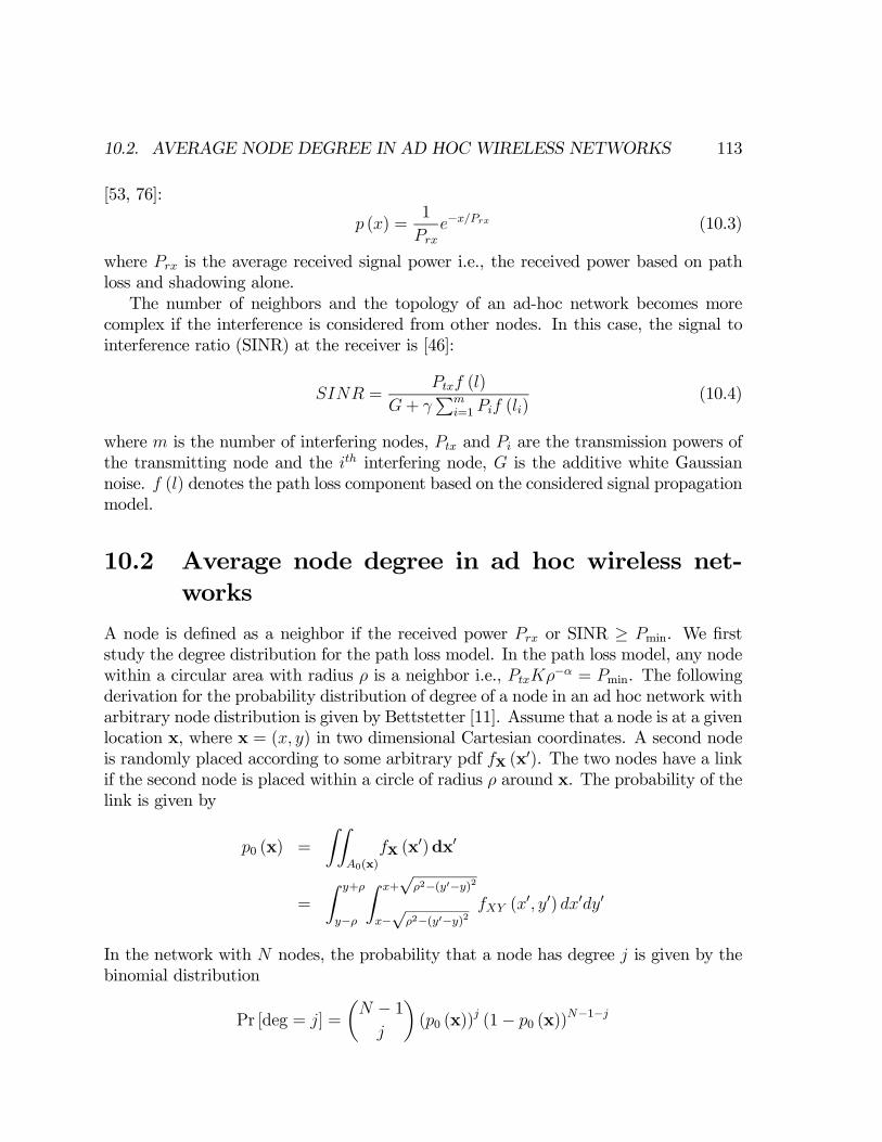
10.2. AVERAGE NODE DEGREE IN AD HOC WIRELESS NETWORKS 113
[53, 76]:
p (x) =1
Prxe−x/Prx (10.3)
where Prx is the average received signal power i.e., the received power based on pathloss and shadowing alone.The number of neighbors and the topology of an ad-hoc network becomes more
complex if the interference is considered from other nodes. In this case, the signal tointerference ratio (SINR) at the receiver is [46]:
SINR =Ptxf (l)
G+ γPm
i=1 Pif (li)(10.4)
where m is the number of interfering nodes, Ptx and Pi are the transmission powers ofthe transmitting node and the ith interfering node, G is the additive white Gaussiannoise. f (l) denotes the path loss component based on the considered signal propagationmodel.
10.2 Average node degree in ad hoc wireless net-works
A node is defined as a neighbor if the received power Prx or SINR ≥ Pmin. We firststudy the degree distribution for the path loss model. In the path loss model, any nodewithin a circular area with radius ρ is a neighbor i.e., PtxKρ−α = Pmin. The followingderivation for the probability distribution of degree of a node in an ad hoc network witharbitrary node distribution is given by Bettstetter [11]. Assume that a node is at a givenlocation x, where x = (x, y) in two dimensional Cartesian coordinates. A second nodeis randomly placed according to some arbitrary pdf fX (x0). The two nodes have a linkif the second node is placed within a circle of radius ρ around x. The probability of thelink is given by
p0 (x) =
ZZA0(x)
fX (x0)dx0
=
Z y+ρ
y−ρ
Z x+√
ρ2−(y0−y)2
x−√
ρ2−(y0−y)2fXY (x
0, y0) dx0dy0
In the network with N nodes, the probability that a node has degree j is given by thebinomial distribution
Pr [deg = j] =
µN − 1
j
¶(p0 (x))
j (1− p0 (x))N−1−j
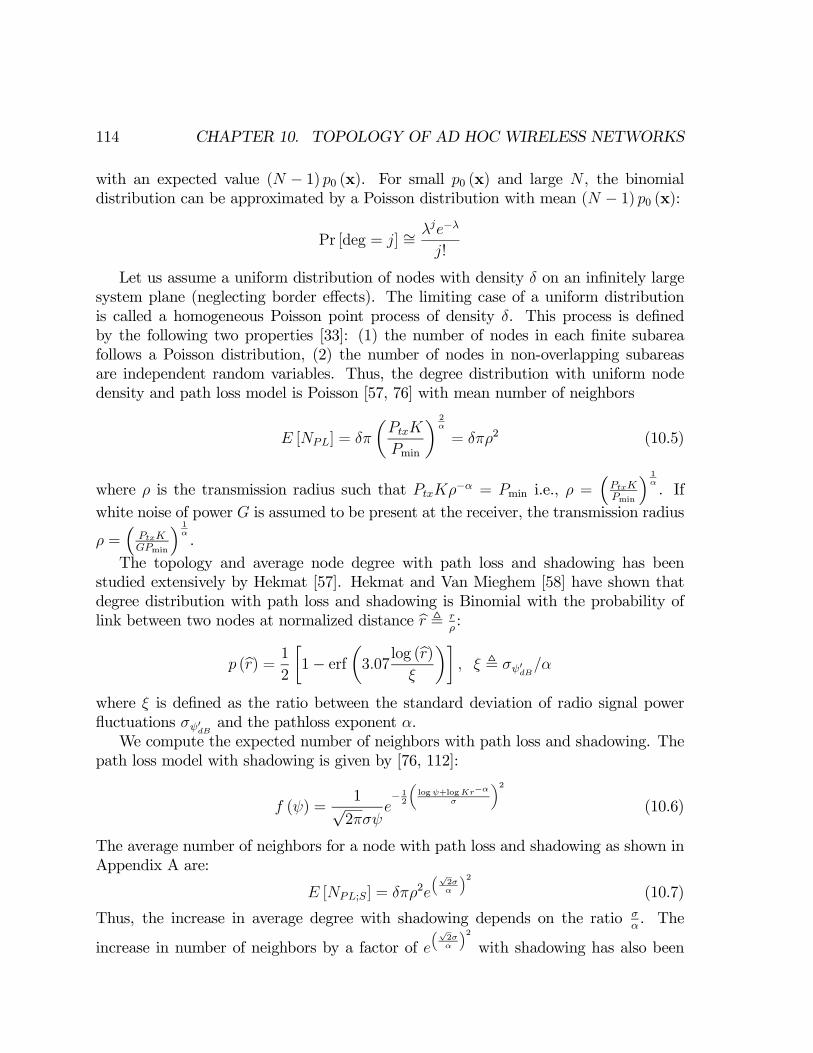
114 CHAPTER 10. TOPOLOGY OF AD HOC WIRELESS NETWORKS
with an expected value (N − 1) p0 (x). For small p0 (x) and large N , the binomialdistribution can be approximated by a Poisson distribution with mean (N − 1) p0 (x):
Pr [deg = j] ∼= λje−λ
j!
Let us assume a uniform distribution of nodes with density δ on an infinitely largesystem plane (neglecting border effects). The limiting case of a uniform distributionis called a homogeneous Poisson point process of density δ. This process is definedby the following two properties [33]: (1) the number of nodes in each finite subareafollows a Poisson distribution, (2) the number of nodes in non-overlapping subareasare independent random variables. Thus, the degree distribution with uniform nodedensity and path loss model is Poisson [57, 76] with mean number of neighbors
E [NPL] = δπ
µPtxK
Pmin
¶ 2α
= δπρ2 (10.5)
where ρ is the transmission radius such that PtxKρ−α = Pmin i.e., ρ =³PtxKPmin
´ 1α. If
white noise of power G is assumed to be present at the receiver, the transmission radius
ρ =³
PtxKGPmin
´ 1α.
The topology and average node degree with path loss and shadowing has beenstudied extensively by Hekmat [57]. Hekmat and Van Mieghem [58] have shown thatdegree distribution with path loss and shadowing is Binomial with the probability oflink between two nodes at normalized distance br , r
ρ:
p (br) = 1
2
∙1− erf
µ3.07
log (br)ξ
¶¸, ξ , σψ0dB/α
where ξ is defined as the ratio between the standard deviation of radio signal powerfluctuations σψ0dB and the pathloss exponent α.We compute the expected number of neighbors with path loss and shadowing. The
path loss model with shadowing is given by [76, 112]:
f (ψ) =1√2πσψ
e− 12
logψ+logKr−ασ
2
(10.6)
The average number of neighbors for a node with path loss and shadowing as shown inAppendix A are:
E [NPL;S] = δπρ2e√2σα
2
(10.7)
Thus, the increase in average degree with shadowing depends on the ratio σα. The
increase in number of neighbors by a factor of e√2σα
2
with shadowing has also been
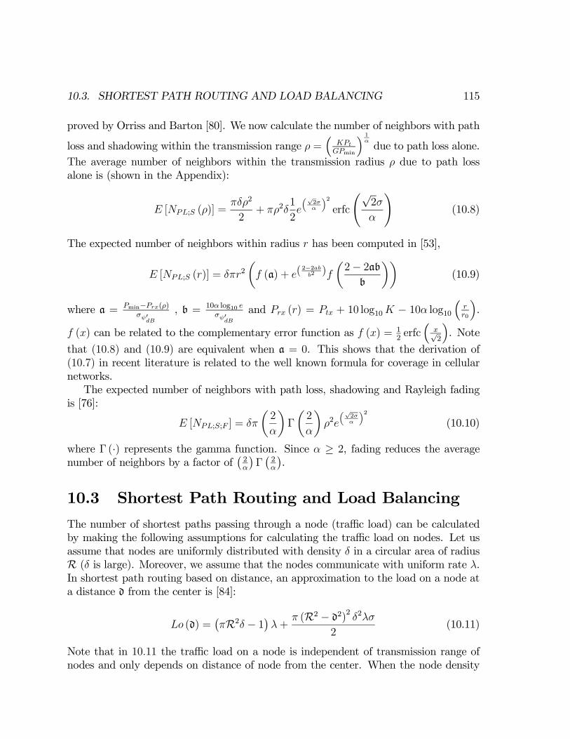
10.3. SHORTEST PATH ROUTING AND LOAD BALANCING 115
proved by Orriss and Barton [80]. We now calculate the number of neighbors with path
loss and shadowing within the transmission range ρ =³
KPtGPmin
´ 1αdue to path loss alone.
The average number of neighbors within the transmission radius ρ due to path lossalone is (shown in the Appendix):
E [NPL;S (ρ)] =πδρ2
2+ πρ2δ
1
2e
√2σα
2
erfc
Ã√2σ
α
!(10.8)
The expected number of neighbors within radius r has been computed in [53],
E [NPL;S (r)] = δπr2µf (a) + e(
2−2abb2)f
µ2− 2abb
¶¶(10.9)
where a = Pmin−Prx(ρ)σψ0
dB
, b = 10α log10 eσψ0
dB
and Prx (r) = Ptx + 10 log10K − 10α log10³
rr0
´.
f (x) can be related to the complementary error function as f (x) = 12erfc
³x√2
´. Note
that (10.8) and (10.9) are equivalent when a = 0. This shows that the derivation of(10.7) in recent literature is related to the well known formula for coverage in cellularnetworks.The expected number of neighbors with path loss, shadowing and Rayleigh fading
is [76]:
E [NPL;S;F ] = δπ
µ2
α
¶Γ
µ2
α
¶ρ2e
√2σα
2
(10.10)
where Γ (·) represents the gamma function. Since α ≥ 2, fading reduces the averagenumber of neighbors by a factor of
¡2α
¢Γ¡2α
¢.
10.3 Shortest Path Routing and Load Balancing
The number of shortest paths passing through a node (traffic load) can be calculatedby making the following assumptions for calculating the traffic load on nodes. Let usassume that nodes are uniformly distributed with density δ in a circular area of radiusR (δ is large). Moreover, we assume that the nodes communicate with uniform rate λ.In shortest path routing based on distance, an approximation to the load on a node ata distance d from the center is [84]:
Lo (d) =¡πR2δ − 1
¢λ+
π (R2 − d2)2 δ2λσ2
(10.11)
Note that in 10.11 the traffic load on a node is independent of transmission range ofnodes and only depends on distance of node from the center. When the node density
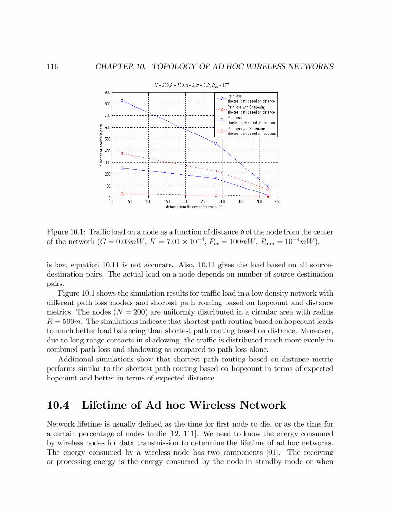
116 CHAPTER 10. TOPOLOGY OF AD HOC WIRELESS NETWORKS
Figure 10.1: Traffic load on a node as a function of distance d of the node from the centerof the network (G = 0.03mW , K = 7.01× 10⁻⁴, Ptx = 100mW , Pmin = 10−4mW ).
is low, equation 10.11 is not accurate. Also, 10.11 gives the load based on all source-destination pairs. The actual load on a node depends on number of source-destinationpairs.Figure 10.1 shows the simulation results for traffic load in a low density network with
different path loss models and shortest path routing based on hopcount and distancemetrics. The nodes (N = 200) are uniformly distributed in a circular area with radiusR = 500m. The simulations indicate that shortest path routing based on hopcount leadsto much better load balancing than shortest path routing based on distance. Moreover,due to long range contacts in shadowing, the traffic is distributed much more evenly incombined path loss and shadowing as compared to path loss alone.Additional simulations show that shortest path routing based on distance metric
performs similar to the shortest path routing based on hopcount in terms of expectedhopcount and better in terms of expected distance.
10.4 Lifetime of Ad hoc Wireless Network
Network lifetime is usually defined as the time for first node to die, or as the time fora certain percentage of nodes to die [12, 111]. We need to know the energy consumedby wireless nodes for data transmission to determine the lifetime of ad hoc networks.The energy consumed by a wireless node has two components [91]. The receivingor processing energy is the energy consumed by the node in standby mode or when

10.4. LIFETIME OF AD HOC WIRELESS NETWORK 117
receiving data. The transmission energy is the energy needed to transmit data over theradio link. The energy spent in transmitting and receiving a j−bit message is given by[91]:
ET = Eelec ∗ j + Eamp ∗ j ∗ rα (10.12)
ER = Eelec ∗ jwhere Eelec and Eamp are constants, r is the distance over which the message is trans-mitted and α is the path loss exponent.With the same assumptions used to compute (10.11), the maximum energy spent
by a node at distance d from the center till time t is
Espent(d) = E ∗á
πR2δ − 1¢λ+
π (R2 − d2)2 δ2λσ2
!∗ t (10.13)
where E = ET +ER = 2∗Eelec+Eamp ∗rα. r is the transmission range of each node andfor the path loss model r = ρ. The energy spent is maximum since we have assumedthat each node transmits the maximum transmission range to transmit a packet to anyneighbor within the transmission range.Thus, the lifetime (time when first node fails) for a network when all nodes start
with equal battery power E0 is
tlifetime =E0
E³(πR2δ − 1)λ+ π(R2−d2)2δ2λσ
2
´=
E0
E³(πR2δ − 1)λ+ πR4δ2λσ
2
´=
E0
λ (2 ∗Eelec +Eamp ∗ r2)¡(N − 1) + N2σ
2π
¢∼= c
λr2N2(10.14)
where α = 2 and c is a constant. Using (10.14), it may be concluded that the lifetimeof a network increases if the transmission range is reduced.In the simulations to study lifetime of ad hoc networks, we assume that Eo = 1J ,
Eelec = 50nJ/bit, Eamp = 100pJ/bit/m2 and α = 2. We assume that the nodes (N =200) are uniformly distributed in circular area with radius R = 500 m and the initialtransmission radius (r) due to path loss alone is 200 m [41]. The size of packet forshortest path routing is assumed to be 1250 bytes and for searching with flooding andrandom walks the packet size is 125 bytes. We assume that in each time interval, apair of nodes chosen uniformly exchange a single packet. Lifetime is chosen as the timewhen the first node dies [41].
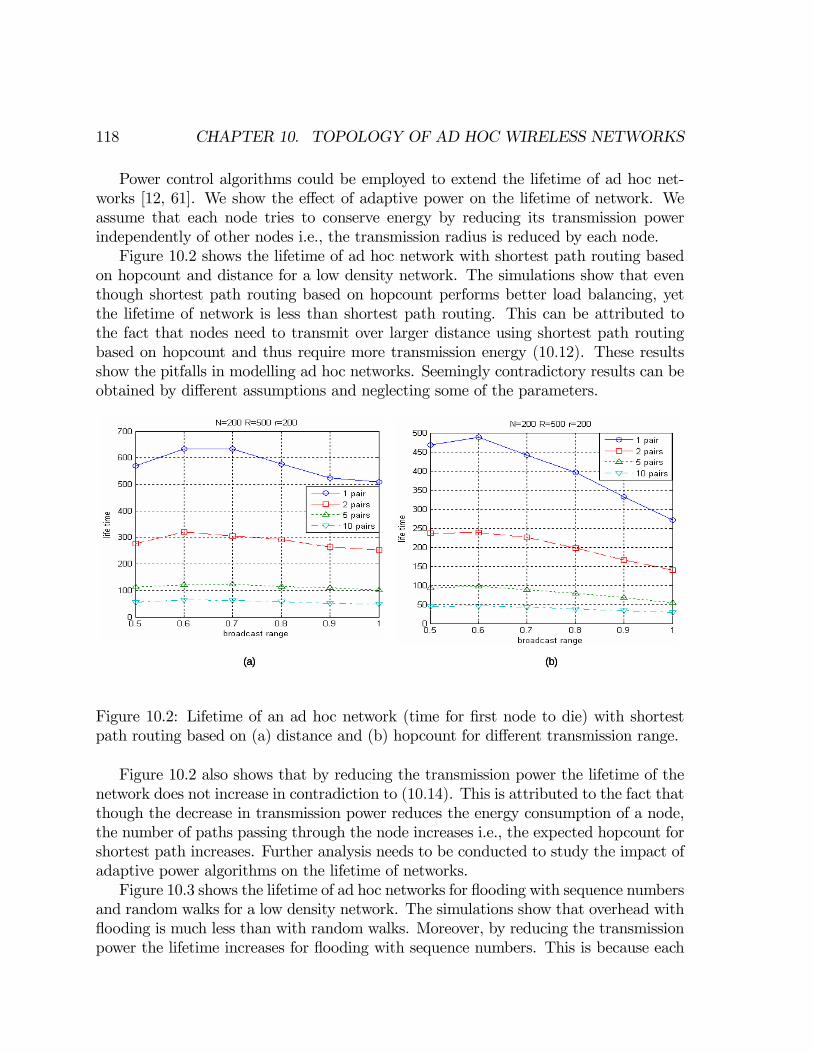
118 CHAPTER 10. TOPOLOGY OF AD HOC WIRELESS NETWORKS
Power control algorithms could be employed to extend the lifetime of ad hoc net-works [12, 61]. We show the effect of adaptive power on the lifetime of network. Weassume that each node tries to conserve energy by reducing its transmission powerindependently of other nodes i.e., the transmission radius is reduced by each node.Figure 10.2 shows the lifetime of ad hoc network with shortest path routing based
on hopcount and distance for a low density network. The simulations show that eventhough shortest path routing based on hopcount performs better load balancing, yetthe lifetime of network is less than shortest path routing. This can be attributed tothe fact that nodes need to transmit over larger distance using shortest path routingbased on hopcount and thus require more transmission energy (10.12). These resultsshow the pitfalls in modelling ad hoc networks. Seemingly contradictory results can beobtained by different assumptions and neglecting some of the parameters.
(a) (b)(a) (b)
Figure 10.2: Lifetime of an ad hoc network (time for first node to die) with shortestpath routing based on (a) distance and (b) hopcount for different transmission range.
Figure 10.2 also shows that by reducing the transmission power the lifetime of thenetwork does not increase in contradiction to (10.14). This is attributed to the fact thatthough the decrease in transmission power reduces the energy consumption of a node,the number of paths passing through the node increases i.e., the expected hopcount forshortest path increases. Further analysis needs to be conducted to study the impact ofadaptive power algorithms on the lifetime of networks.Figure 10.3 shows the lifetime of ad hoc networks for flooding with sequence numbers
and random walks for a low density network. The simulations show that overhead withflooding is much less than with random walks. Moreover, by reducing the transmissionpower the lifetime increases for flooding with sequence numbers. This is because each
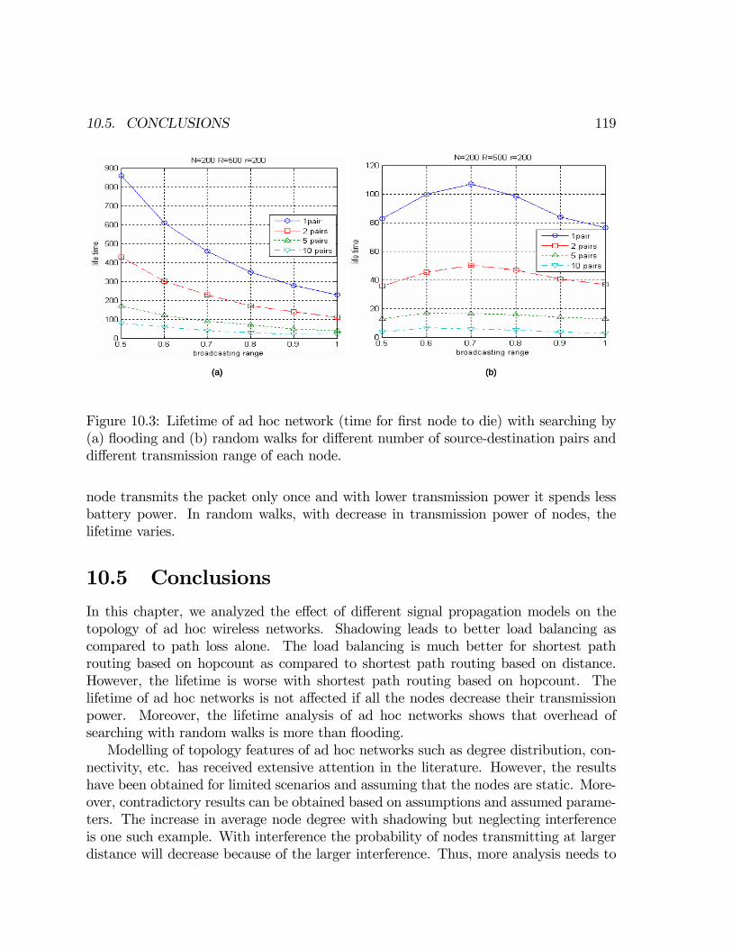
10.5. CONCLUSIONS 119
(a) (b)(a) (b)
Figure 10.3: Lifetime of ad hoc network (time for first node to die) with searching by(a) flooding and (b) random walks for different number of source-destination pairs anddifferent transmission range of each node.
node transmits the packet only once and with lower transmission power it spends lessbattery power. In random walks, with decrease in transmission power of nodes, thelifetime varies.
10.5 Conclusions
In this chapter, we analyzed the effect of different signal propagation models on thetopology of ad hoc wireless networks. Shadowing leads to better load balancing ascompared to path loss alone. The load balancing is much better for shortest pathrouting based on hopcount as compared to shortest path routing based on distance.However, the lifetime is worse with shortest path routing based on hopcount. Thelifetime of ad hoc networks is not affected if all the nodes decrease their transmissionpower. Moreover, the lifetime analysis of ad hoc networks shows that overhead ofsearching with random walks is more than flooding.Modelling of topology features of ad hoc networks such as degree distribution, con-
nectivity, etc. has received extensive attention in the literature. However, the resultshave been obtained for limited scenarios and assuming that the nodes are static. More-over, contradictory results can be obtained based on assumptions and assumed parame-ters. The increase in average node degree with shadowing but neglecting interferenceis one such example. With interference the probability of nodes transmitting at largerdistance will decrease because of the larger interference. Thus, more analysis needs to
120 CHAPTER 10. TOPOLOGY OF AD HOC WIRELESS NETWORKS
be done to study the effect of topology on lifetime of ad hoc networks.
Chapter 11
Estimation of Topology
11.1 Introduction
The development of topology estimation algorithms is the first step to build intelligent1
topology based algorithms. In ad-hoc and self-configuring networks because of thedynamic topology and limited bandwidth, external measurement tools are harder toemploy for topology estimation. Instead, techniques from statistics may be employedto estimate the topology of ad hoc networks on the fly. Once the topology of ad hocnetworks is estimated, a number of parameters about the network such as connectivity,expected hopcount for shortest path, load on nodes, TTL for searching etc. can beobtained. These network parameters could be used for optimizing a wide variety ofalgorithms.We know that the topology of ad hoc wireless networks can be modelled as a geo-
metric random graphs with nodes the having Binomial degree distribution:
Pr [deg = j] =
µN − 1
j
¶pj (1− p)N−1−j (11.1)
In this chapter, we consider the problem of estimation of topology of an ad-hocnetwork, which involves estimating the values of p and N , given the degree of m nodes.The estimation of parameters N and p for a Binomial distribution has been discussedextensively in the literature [35, 69, 79]. A particularly hard problem is to estimate thevalues of N and p when both are unknown and the sample size m is much smaller thanN . In this case, we apply some recently proposed estimates for both N and p.
1An example is flooding with probability q, the probability q could be optimized based on thetopology of the network.
121
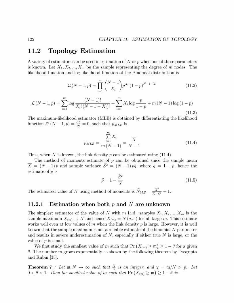
122 CHAPTER 11. ESTIMATION OF TOPOLOGY
11.2 Topology Estimation
A variety of estimators can be used in estimation ofN or p when one of these parametersis known. Let X1,X2, ..., Xm be the sample representing the degree of m nodes. Thelikelihood function and log-likelihood function of the Binomial distribution is
L (N − 1, p) =mYi=1
µN − 1Xi
¶pXi (1− p)N−1−Xi (11.2)
L (N − 1, p) =mXi=1
log(N − 1)!
Xi! (N − 1−Xi)!+
mXi=1
Xi logp
1− p+m (N − 1) log (1− p)
(11.3)The maximum-likelihood estimator (MLE) is obtained by differentiating the likelihoodfunction L0 (N − 1, p) = ∂L
∂p= 0, such that pMLE is
pMLE =
mPi=1
Xi
m (N − 1) =X
N − 1 (11.4)
Thus, when N is known, the link density p can be estimated using (11.4).The method of moments estimate of p can be obtained since the sample mean
X = (N − 1) p and sample variance S2 = (N − 1) pq, where q = 1 − p, hence theestimate of p is
bp = 1− S2
X(11.5)
The estimated value of N using method of moments is bNME =X2
X−S2 + 1.
11.2.1 Estimation when both p and N are unknown
The simplest estimator of the value of N with m i.i.d. samples X1, X2, ...,Xm is thesample maximum X(m) → N and hence X(m) = N (a.s.) for all large m. This estimateworks well even at low values of m when the link density p is large. However, it is wellknown that the sample maximum is not a reliable estimate of the binomial N parameterand results in severe underestimation of N , especially if either true N is large, or thevalue of p is small.We first study the smallest value of m such that Pr
¡X(m) ≥ m
¢≥ 1− θ for a given
θ. The number m grows exponentially as shown by the following theorem by Dasguptaand Rubin [35].
Theorem 7 : Let m, N → ∞ such that Nmis an integer, and χ = m/N > p. Let
0 < θ < 1. Then the smallest value of m such that Pr¡X(m) ≥ m
¢≥ 1− θ is

11.2. TOPOLOGY ESTIMATION 123
m ≥ (− log θ) (χ− p)
p√1− χ
Ãχ (1− χ)
1χ−1
pq1χ−1
!m√2mπ (1 + o (1))
We now study some of the estimators proposed for N and p when both are unknown.The method of moment estimate for p and N can be obtained by using (11.5). However,when the value of p is small i.e., the sample mean and variance are close to each other,the moments estimate is not stable. A moment-stabilized estimator has been proposedby Olkin et al. [79], bNMES = max
(S2φ2
φ− 1 , X(m)
)(11.6)
where
φ =
½ XS2
if XS2≥ 1 + 1/
√2
maxnX(m)−X
S2, 1 +
√2o
if XS2
< 1 + 1/√2
Another estimator that could be used is the stabilized MLE. The likelihood functiondescribed in (11.2) can be maximized when N →∞, p → 0 and p (N − 1) = X. Thislimiting case of likelihood is denoted by L (∞, 0). The following theorem by Levin [69]gives the estimates.
Theorem 8 :An MLE of N exists. If X/S2 ≤ 1, L (N, p) < L (∞, 0), while if X/S2 >1, L (N, p) is maximized by atleast one pair (N, p), with X(m) ≤ N <∞.
Substituting the value of pMLE from 11.4 in 11.3,
L (N − 1, p) =mXi=1
log(N − 1)!
Xi! (N − 1−Xi)!+
mXi=1
Xi logX
N − 1−X
+m (N − 1) logµ1− X
N − 1
¶Let us denote the differential,
DN =∂L∂N
If D (0) ≤ 0, MLE = X(m) and if D (0) > 0 then the MLE is taken as solution ofD¡MLE−X(m)
¢= 0. Thus, the stabilized MLE is given as
bNMES =
½ MLE if XS2≥ 1 + 1/
√2
X(m) +¡m−1m
¢ ¡X(m) −X(m−1)
¢if X
S2< 1 + 1/
√2
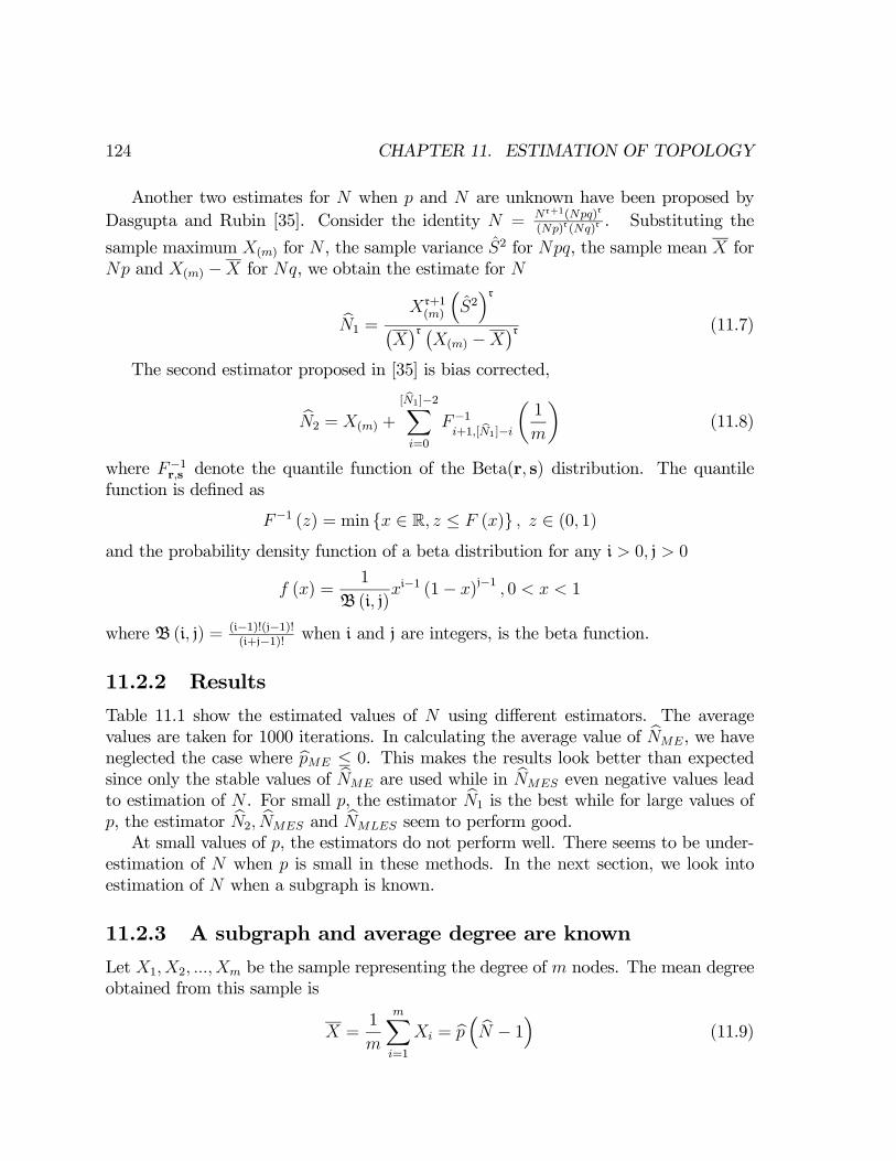
124 CHAPTER 11. ESTIMATION OF TOPOLOGY
Another two estimates for N when p and N are unknown have been proposed byDasgupta and Rubin [35]. Consider the identity N = Nr+1(Npq)r
(Np)r (Nq)r. Substituting the
sample maximum X(m) for N , the sample variance S2 for Npq, the sample mean X forNp and X(m) −X for Nq, we obtain the estimate for N
bN1 =Xr+1(m)
³S2´r
¡X¢r ¡
X(m) −X¢r (11.7)
The second estimator proposed in [35] is bias corrected,
bN2 = X(m) +
[N1]−2Xi=0
F−1i+1,[N1]−i
µ1
m
¶(11.8)
where F−1r,s denote the quantile function of the Beta(r, s) distribution. The quantilefunction is defined as
F−1 (z) = min x ∈ R, z ≤ F (x) , z ∈ (0, 1)and the probability density function of a beta distribution for any i > 0, j > 0
f (x) =1
B (i, j)xi−1 (1− x)j−1 , 0 < x < 1
where B (i, j) = (i−1)!(j−1)!(i+j−1)! when i and j are integers, is the beta function.
11.2.2 Results
Table 11.1 show the estimated values of N using different estimators. The averagevalues are taken for 1000 iterations. In calculating the average value of bNME, we haveneglected the case where bpME ≤ 0. This makes the results look better than expectedsince only the stable values of bNME are used while in bNMES even negative values leadto estimation of N . For small p, the estimator bN1 is the best while for large values ofp, the estimator bN2, bNMES and bNMLES seem to perform good.At small values of p, the estimators do not perform well. There seems to be under-
estimation of N when p is small in these methods. In the next section, we look intoestimation of N when a subgraph is known.
11.2.3 A subgraph and average degree are known
Let X1, X2, ...,Xm be the sample representing the degree of m nodes. The mean degreeobtained from this sample is
X =1
m
mXi=1
Xi = bp³ bN − 1´ (11.9)
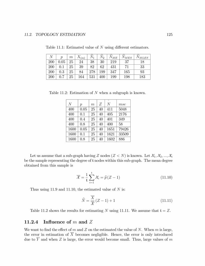
11.2. TOPOLOGY ESTIMATION 125
Table 11.1: Estimated value of N using different estimators.
N p m X(m)bN1
bN2bNME
bNMESbNMLES
200 0.05 25 24 38 30 219 37 18200 0.1 25 39 82 62 431 71 33200 0.3 25 84 278 199 347 165 93200 0.7 25 164 531 400 199 198 183
Table 11.2: Estimation of N when a subgraph is known.
N p m Zˆ
N mse400 0.05 25 40 411 5048400 0.1 25 40 405 2176400 0.4 25 40 401 349400 0.8 25 40 400 581600 0.05 25 40 1651 794261600 0.1 25 40 1621 335091600 0.8 25 40 1602 886
Let us assume that a sub-graph having Z nodes (Z < N) is known. Let X1,X2, ...,Xtbe the sample representing the degree of t nodes within this sub-graph. The mean degreeobtained from this sample is
X = 1
t
tXi=1
Xi = bp (Z − 1) (11.10)
Thus using 11.9 and 11.10, the estimated value of N is:
bN =X
X(Z − 1) + 1 (11.11)
Table 11.2 shows the results for estimating N using 11.11. We assume that t = Z.
11.2.4 Influence of m and Z
We want to find the effect ofm and Z on the estimated the value of N . Whenm is large,the error in estimation of X becomes negligible. Hence, the error is only introduceddue to Y and when Z is large, the error would become small. Thus, large values of m

126 CHAPTER 11. ESTIMATION OF TOPOLOGY
and Z give the best estimate for N . However, the estimate of N does not improve asm is increased keeping Z constant (11.1).
4500
4000
3500
3000
2500
2000
1500
1000
estim
ated
val
ue o
f N
400300200100m / Z
N = 1600, p = 0.05 m = 25, varying Z Z = 20, varying m
N = 3200, p = 0.025 m = 25, varying Z Z = 20, varying m
104
105
106
mse
400300200100m / Z
N = 1600, p = 0.05 Z = 20, varying m m = 25, varying Z
N = 3200, p = 0.025 Z = 20, varying m m = 25, varying Z
Figure 11.1: (a) Estimated value of N and (b) mean square error as a function of mand Z.
11.3 Conclusions
We presented a methodology for topology estimation given the degree of certain nodesin a random graph. It is difficult to estimate the values of N and p when both areunknown and the sample size m is much smaller than N . Results show that at smallvalues of link density p, most of the estimators do not perform well. Further analysisof topology estimation needs to be carried out in order to develop topology dependantalgorithms. Indeed, topology estimation is the first step for building such topologybased algorithms.
Chapter 12
Conclusions
The emergence of ad hoc wireless networks and P2P networks has lead to an increas-ing interest in adaptive and decentralized algorithms for routing, resource and servicediscovery etc. A variety of applications are currently being developed based on thesenovel algorithms and protocols. For example, flooding and its variations had been thede facto standard for searching in different networks. However, new versions of P2Pnetworks such as Gnutella and Gia use random walk strategies instead of flooding.This thesis focused on three interrelated research topics for ad hoc networks:
• Ant Routing.
• Searching with single and multiple queries.
• Topology of ad hoc wireless networks.
In this chapter, we provide an overview of the results for each of these topics and themajor contributions of this thesis. We include remarks for extension of work wheneverpossible.
Ant Routing
The first contribution of this thesis is in analyzing the performance of ant routing.Based on the analysis in this thesis, we are able to answer questions such as: How dodifferent parameters affect the performance of ANTRALs and how does ant routingperform for ad hoc wireless networks where mobility and limited bandwidth play animportant role. Extensive simulations of the AntNet algorithm show that ant routingalgorithms are able to find paths that are close to the shortest path. We can state that
The performance of ant routing is close to shortest path routing forsmall sparse graphs.
127
128 CHAPTER 12. CONCLUSIONS
As the network size increases and density of network increases, the AntNet algo-rithm is no longer able to find paths that are close to the shortest path. The performanceof AntNet algorithm depends on parameters such as η,Wmax and a. The optimal valueof parameters such as η and Wmax could be chosen depending on the size of network,while the optimal value of parameter a depends on the degree of nodes. Thus,
The performance and optimization of parameters in ant routing algo-rithms depend on the topology of the network.
Ant routing algorithms provide an automatic adaptation to link failure and trafficchanges. However, the rate of topology change in mobile ad hoc wireless networks islarge. In order to overcome this problem, on-demand protocols have been proposedwhich search for a path to the destination only when the nodes need to transfer data.We compared the performance of ant routing with on-demand protocols AODV andDSR using NS-2. Our implementation includes realistic features for ad hoc networkssuch as MAC layer, limited buffer size at nodes, node mobility etc. The analysis showsthat
Overhead of ant routing is more than on-demand protocols such asAODV and DSR in ad hoc wireless networks.
Our work on ant routing could be extended further in new directions. The scalabilityof ant routing algorithms needs to be investigated further. Moreover, modifications tothese algorithms such as using both data and ant packets for updating the routingtables could be investigated. Specifically, the AntNet algorithm would be considered atruly distributed and scalable algorithm if the nodes are able to learn and adjust thevarious parameters used in the algorithm.
Searching
The main contribution of section 3 is the definition and classification of differentsearching schemes. The searching strategies may be probabilistic and based on randomwalks or may use unique feature of the network topology such as high degree nodes.These strategies have been studied in bits and pieces in literature but a complete viewof different searching schemes was missing. In chapters 7, 8 and 9 of this thesis, wehave analyzed and studied the performance of searching schemes based on single ormultiple queries. We distinguished between deadlocks and loops and examined theaffect of deadlocks and loops on the performance of search strategies. An exact analysisfor some of these strategies in Chapter 8 is another contribution of this thesis.The probability distribution of hopcount for a random walk on a complete graph
KN is a geometric distribution while the probability distribution for a random walkwith memory M is a uniform random variable on [1,M ] and a geometric variable on[M + 1, N − 1]. In many random walk strategies such as random walk using highest
129
degree, the expected hopcount is small but the probability of deadlocks is large. Indeed,we need to look into probability of deadlocks as well as the expected hopcount todetermine the performance of search strategies.
The expected hopcount or expected weight of the path is not sufficientto characterize searching based on different random walk strategies.
The performance of different search strategies depends on the graph topology. Be-cause of high degree nodes in a BA graph, the performance of search strategies usinghighest degree in BA graphs is better than in ER random graphs. In both these graphtopologies, the performance of random walk with look-ahead is close to shortest pathrouting with small values of look-ahead. This is due to the small diameter O (logN) ofthese graph topologies.
With lookahead of logN , the performance of searching with RW LA isclose to that of shortest path routing.
It can be concluded that more information a search strategy has, the better is itsperformance. For example, random walk using highest degree, look-ahead and memoryperforms better than random walk using look-ahead and memory.A single RW query has an overhead and time to discover of O(N logN) for ER
random graphs and power law graphs. To reduce the time to discovery, multiple randomwalk queries with smaller TTL may be used. The overhead of searching with multiplequeries depends on TTL and the number of queries which in turn can be optimized bythe topology of the network.
The overhead for searching with multiple random walk queries is lessthan for flooding.
However, in BA graphs, the improvement of searching with multiple random walkqueries as compared to flooding is limited. With multiple copies of files in P2P networks,searching with random walk queries would be much more efficient than searching withflooding. Searching techniques proposed and analyzed in this thesis could be used withtraditional searching methods such as flooding. For example, critical information couldbe spread by flooding while less critical information could be spread by random walksqueries.Thus, section 3 of this thesis provides answers for questions such as: How does
memory and look-ahead affect the performance of random walk search strategies andwhat role the graph topology plays in performance of different search strategies.
Topology of ad hoc wireless networks
The first two sections of this thesis show that the topology of networks is one of thefactors that determines the performance of different algorithms. The major achievement
130 CHAPTER 12. CONCLUSIONS
of this section is understanding the topology of ad hoc wireless networks and the affectof topology on shortest path routing, lifetime etc.In section 4, we investigated the effect of signal propagation models on the topology
of ad hoc wireless networks. Increasingly, it is being realized that simple path loss modelis not sufficient to characterize the topology of ad hoc wireless networks. Modelingof wireless networks with shadowing and fading shows that shadowing improves theconnectivity while fading reduces the connectivity of these networks. Specifically, the
change in average node degree with these models depends on the standard deviation ofradio signal power fluctuations σ and the pathloss exponent α.
Shadowing increases degree of nodes in ad hoc wireless networks by a
factor of e√2σα
2
We proved that the average number of neighbors of a node with shadowing is relatedto the well known formula for coverage in cellular networks. The appearance of longrange links with shadowing increases the number of neighbors and distributes datatraffic more effectively.
Shadowing improves the load balancing in ad hoc wireless networks.
A novel idea in Chapter 11 was the use of techniques from statistics to estimate thetopology of ad hoc wireless networks. We used estimators such as method of momentsand maximum likelihood to estimate N and p for random graphs. This analysis couldbe extended further to build topology dependant algorithms.
Appendix A
Average number of neighbors
The path loss model with shadowing is given by
f (ψ) =1√2πσψ
e− 12
logψ+logKr−ασ
2
The area (A) where received power Pr is greater than Pmin is
A =
∞Zr=0
2πrp(ψ <Pt
Pmin)dr = 2π
∞Zr=0
rdr
PtPminZ
ψ=0
1√2πσψ
e− 12
logψ+logKr−ασ
2
dψ
After substituting x = logψ+logKr−α
σ= logψKr−α
σ, we obtain
= 2π
∞Zr=0
rdr
logPtKr−αPmin
σZx=−∞
1√2π
e−x2
2 dx
= 2π
∞Zx=−∞
dx
e−σxKPtPmin
1αZ
r=0
rdr1√2π
e−x2
2 = 2π
∞Zx=−∞
1
2
µe−σxKPt
Pmin
¶ 2α 1√
2πe−
x2
2 dx
= π
µKPt
Pmin
¶ 2α
∞Zx=−∞
1√2π
e−x2
2 e−2σxα dx = π
µKPt
Pmin
¶ 2α
e√2σα
2
Thus, the average number of neighbors for a node with path loss and shadowing are
δA = πδ³KPtxPmin
´ 2αe
√2σα
2
.
131
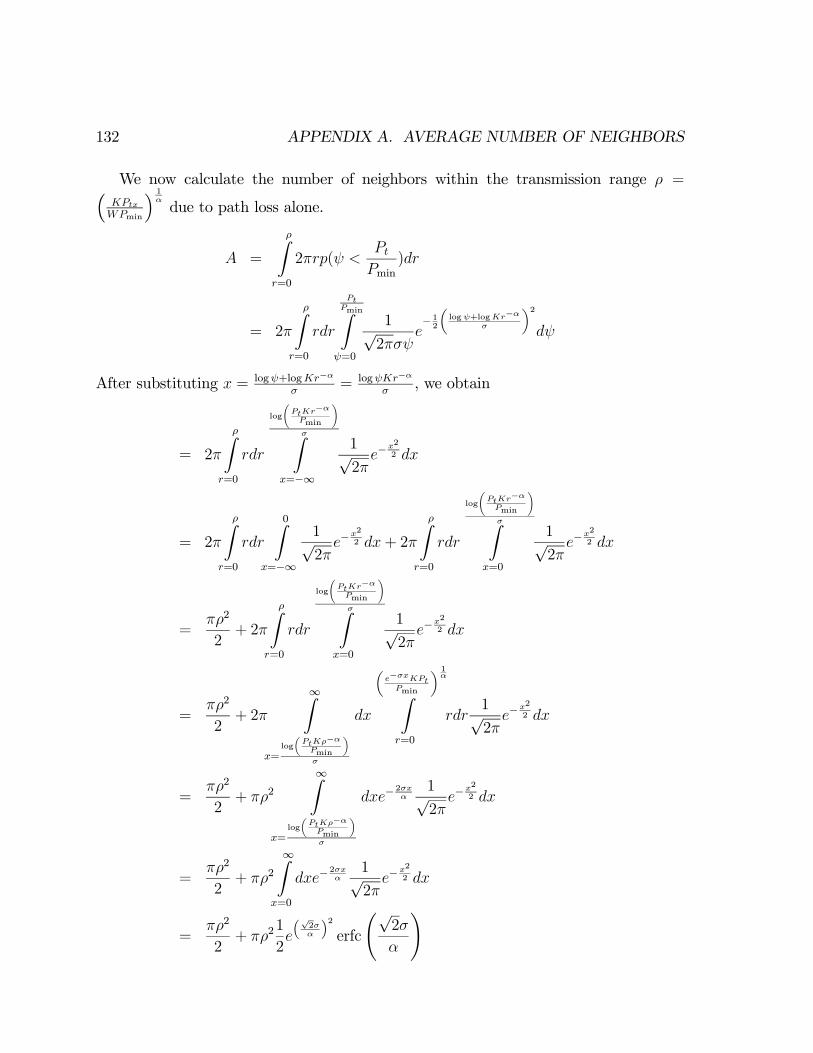
132 APPENDIX A. AVERAGE NUMBER OF NEIGHBORS
We now calculate the number of neighbors within the transmission range ρ =³KPtxWPmin
´ 1αdue to path loss alone.
A =
ρZr=0
2πrp(ψ <Pt
Pmin)dr
= 2π
ρZr=0
rdr
PtPminZ
ψ=0
1√2πσψ
e−12
logψ+logKr−ασ
2
dψ
After substituting x = logψ+logKr−α
σ= logψKr−α
σ, we obtain
= 2π
ρZr=0
rdr
logPtKr−αPmin
σZx=−∞
1√2π
e−x2
2 dx
= 2π
ρZr=0
rdr
0Zx=−∞
1√2π
e−x2
2 dx+ 2π
ρZr=0
rdr
logPtKr−αPmin
σZx=0
1√2π
e−x2
2 dx
=πρ2
2+ 2π
ρZr=0
rdr
logPtKr−αPmin
σZx=0
1√2π
e−x2
2 dx
=πρ2
2+ 2π
∞Zx=
logPtKρ−αPminσ
dx
e−σxKPtPmin
1αZ
r=0
rdr1√2π
e−x2
2 dx
=πρ2
2+ πρ2
∞Zx=
logPtKρ−αPminσ
dxe−2σxα
1√2π
e−x2
2 dx
=πρ2
2+ πρ2
∞Zx=0
dxe−2σxα
1√2π
e−x2
2 dx
=πρ2
2+ πρ2
1
2e
√2σα
2
erfc
Ã√2σ
α
!

133
Thus, the average number of neighbors for a node within the transmission radius
due to path loss alone (ρ) are δA = πρ2
2+ πρ2 1
2e
√2σα
2
erfc³√
2σα
´.

134 APPENDIX A. AVERAGE NUMBER OF NEIGHBORS
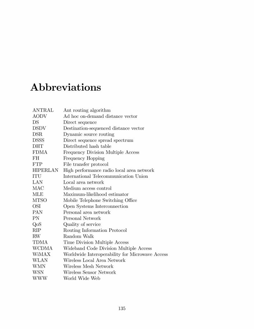
Abbreviations
ANTRAL Ant routing algorithmAODV Ad hoc on-demand distance vectorDS Direct sequenceDSDV Destination-sequenced distance vectorDSR Dynamic source routingDSSS Direct sequence spread spectrumDHT Distributed hash tableFDMA Frequency Division Multiple AccessFH Frequency HoppingFTP File transfer protocolHIPERLAN High performance radio local area networkITU International Telecommunication UnionLAN Local area networkMAC Medium access controlMLE Maximum-likelihood estimatorMTSO Mobile Telephone Switching OfficeOSI Open Systems InterconnectionPAN Personal area networkPN Personal NetworkQoS Quality of serviceRIP Routing Information ProtocolRW Random WalkTDMA Time Division Multiple AccessWCDMA Wideband Code Division Multiple AccessWiMAX Worldwide Interoperability for Microwave AccessWLAN Wireless Local Area NetworkWMN Wireless Mesh NetworkWSN Wireless Sensor NetworkWWW World Wide Web
135

136 ABBREVIATIONS

Bibliography
[1] M. Abramowitz, I.A. Stegun (Eds.).A Handbook of Mathematical Functions, WithFormulas, Graphs, and Mathematical Tables. Dover Publications, NewYork, 1974,ISBN0486612724, June.
[2] L. A. Adamic, R. M. Lukose, A. R. Puniyani and B. A. Huberman. Search inpower-law networks. Physical Review E, vol. 64, 2001.
[3] I. F. Akyildiz, X. Wang, and W. Wang. Wireless mesh networks: a survey. Com-puter Networks, 47, pp. 445—487, 2005.
[4] R. Albert and A. Barabási. Statistical mechanics of complex networks. Reviewsof modern physics, 74, 2002.
[5] C. Avin and G. Ercal. On the cover time of random geometric graphs. Lecturenotes in computer science ISSN 0302-9743, 2005.
[6] A. Barabási, R. Albert and H. Jeong. Mean-field theory for scale-free randomnetworks. PhysicaA 272, pp. 173-187, 1999.
[7] P. Baran. On distributed communication networks. IEEE Transactions on Com-munications. pp. 1-9, 1964.
[8] Z. Bar-Yossef, R. Friedman and G. Kliot. RaWMS- Random Walk based Light-weight Membership Service for Wireless Ad Hoc Networks. Proc. MobiHoc, pp.238-249, 2006.
[9] N. Bean and A. Costa. An analytic modelling approach for network routing al-gorithms that use “ant-like” mobile agents. Computer Networks 49, pp. 243—268,2005.
[10] R. Beckers, J.L. Deneubourg, S. Goss. Trails and U-turns in the selection of theshortest paths by the ant Lasius Niger. Journal of Theoretical Biology 159, pp.397—415, 1992.
137
138 BIBLIOGRAPHY
[11] C. Bettstetter. On the Connectivity of Ad Hoc Networks. The Computer Journal,vol. 47, no. 4, 2004.
[12] M. Bhardwaj and A. Chandrakasan. Bounding the Lifetime of Sensor Networksvia Optimal Role Assignments. Proc. INFOCOM, pp. 1587-1596 , 2002.
[13] N. Bisnik and A. A. Abouzeid. Optimizing Random Walk Search Algorithms inP2P Networks. Computer Networks, 2006.
[14] B. Bollobás, Random Graphs, Cambridge University press, second edition, 2001.
[15] A. Borodin, Y. Rabani and B. Schieber. Deterministic Many-to-Many Hot PotatoRouting. Proc. IEEE Transactions on Parallel and Distributed Systems, vol. 8, no.6, pp. 587-596, 1997.
[16] J. Broch, D.A. Maltz, D.B. Johnson,Y. Hu and J. Jetcheva. A performance com-parison of multi-hop wireless ad hoc network routing protocols. Proc. IEEE/ACMMOBICOM, 47:445—487, 1998.
[17] C. Busch. Õ(Congestion + Dilation) Hot-Potato Routing on Leveled Networks.Proc. SPAA, 2002.
[18] D. Camara and A.A.F. Loureiro. Ants A novel routing algorithm for ad hocnetworks. Proc. of the 33rd Hawaii International Conference on System Sciences,2000.
[19] M. Castro, M. Costa and A. Rowstron. Peer-to-peer overlays: structured, un-structured or both?. Technical Report MSR-TR-2004-73, 2004.
[20] Y. Chawathe, S. Ratnasamy, L. Breslau, N. Lanham and S. Shenker. MakingGnutella-like P2P Systems Scalable. Proc. SIGCOMM Conference, 2003.
[21] C.C. Chiang, H.KWu, W. Liu and M. Gerla. Routing in Clustered Multihop, Mo-bile Wireless Networks with Fading Channel. Proc. IEEE Singapore InternationalConference on Networks, pp. 197-211, 1997.
[22] F. Chung and L. Lu. The Diameter of Sparse Random Graphs. Advances in Ap-plied Math. 26, pp. 257—279, 2001.
[23] F. Chung and L. Lu. The small world phenomenon in hybrid power law graphs.Complex Networks, (Eds. E. Ben-Naim et. al.), Springer-Verlag, pp. 89—104, 2004.
[24] F. R. K. Chung. Spectral Graph Theory. CBMS Conference on Recent Advancesin Spectral Graph Theory, 1994. ISBN: 0-8218-0315-8.

BIBLIOGRAPHY 139
[25] T. Clausen and P. Jacquet. Optimized Link State Routing Protocol (OLSR).Internet Draft, RFC 3626, 2003.
[26] T.J.M. Coenen, P.T.H. Goering, A. Jehangir, J.L. van den Berg, R.J. Boucherie,S.M. Heemstra de Groot, G.J. Heijenk, S.S. Dhillon, W. Lu, A. Lo, P.F.A VanMieghem and I.G.M.M. Niemegeers. Architectural and QoS aspects of PersonalNetworks. Proc. First International Workshop on Personalized Networks (PerNets2006) USA, 2006.
[27] C. Cooper and A. Frieze. Crawling on web graphs. Proc. 34th annual ACM sym-posium on Theory of computing, pp. 419 - 427, 2002.
[28] C. Cooper and A. Frieze. The cover time of the preferential attachment graph.Journal of Combinatorial Theory, Series B 97, pp. 269-290, 2007.
[29] T.H. Cormen, C.E. Leiserson and R.L. Rivest. An introduction to Algorithms.MIT Press, Boston, 2000.
[30] Andre Costa. Analytic Modelling of Agent-based Network Routing Algorithms.Ph.D. thesis, School of Applied Mathematics, University of Adelaide, 2003.
[31] S. Cui, R. Madan, A. J. Goldsmith and S. Lall. Cross-Layer Energy and De-lay Optimization in small-scale sensor networks. IEEE Transactions on WirelessCommunication, pp. 3688-3699, vol. 6, no. 10, 2007.
[32] D. Culler, D. Estrin and M. Srivastava. Overview of sensor networks. Proc. IEEEComputer, Special Issue in Sensor Networks, Aug 2004.
[33] D. J. Daley and D. Vere-Jones. An Introduction to the Theory of Point Processes.Springer, 1988.
[34] S.R. Das, C.E. Perkins and E. E. Royer. Performance Comparison of Two On-Demand Routing Protocols for Ad Hoc Networks. Proc. INFOCOM, pp. 3-12,2000.
[35] A. DasGupta and H. Rubin. Estimation of binomial parameters when both n, pare unkown. Journal of Statistical Planning and Interference 130, pp. 391—404,2005.
[36] J.-L. Deneubourg, S. Aron, S. Goss and J.-M. Pasteels. The self organizing ex-ploratory pattern of the argentine ant. Journal of Insect Behavior 3, pp. 159—168,1990.
[37] S. S Dhillon and P. Van Mieghem. Performance Analysis of the AntNet algorithm.Computer Networks, Vol. 51, No. 8, pp. 2104-2125, 2007.
140 BIBLIOGRAPHY
[38] S. S Dhillon and P. Van Mieghem. Comparison of Random Walk Strategies forAd Hoc Networks. Proc. of the Sixth Annual Mediterranean Ad Hoc NetworkingWorkshop (Med-Hoc-Net 2007), Corfu, Greece, pp. 196-203, June 13-15, 2007.
[39] S. S Dhillon, X. Arbona and P. Van Mieghem. Ant Routing in Mobile AdHoc Networks. Proc. Third International Conference on Networking and Services(ICNS’07), Athens, Greece, June 19-25, 2007.
[40] S. S Dhillon and P. Van Mieghem. Searching with multiple random walk queries.Proc. 18th Annual IEEE International Symposium on Personal, Indoor and Mo-bile Radio Communications (IEEE PIMRC’07), Athens, Greece, September 3-7,2007.
[41] S. S Dhillon and Y. Zhou. Topology, shortest path routing and lifetime of ad hocnetworks. Proc. 14th Symposium on Communications and Vehicular Technologyin the Benelux (SCVT 2007), Delft, Netherlands, 2007.
[42] G. Di Caro and M. Dorigo. AntNet: distributed stigmergetic control for com-munication networks. Journal of Artificial Intelligence Research 9, pp. 317—365,1998.
[43] G. Di Caro and M. Dorigo. Two ant colony algorithms for best-effort routing indatagram networks. Proc. 10th International Conference on Parallel and Distrib-uted Computing and Systems, 1998.
[44] S. Dolev, E. Schiller and J. Welch. RandomWalk for Self-Stabilizing Group Com-munication in Ad-Hoc Networks. Proc. 21st Symposium on Reliable DistributedSystems, 2002.
[45] M. Dorigo and G. Di Caro. The Ant Colony Optimization Meta-Heuristic.McGraw-Hill Press, 1999.
[46] O. Dousse, F. Baccelli and P. Thiran. Impact of Interferences on Connectivity inAd Hoc Networks. IEEE Transactions on Networking, vol. 13, pp. 425-436, 2005.
[47] F. Ducatelle, Gianni Di Caro, L.M. Gambardella. Ant agents for hybrid multi-path routing in mobile ad hoc networks. Proceedings 2nd Annual Conference onWireless On demand Network Systems and Services (WONS), 2005.
[48] P. Erdös and A. Rényi. On random graphs I. Publ. Math. Debrecen. 6, pp. 290-297,1959.
[49] M. Faloutsos, P. Faloutsos and C. Faloutsos. On power-law relationships of theInternet topology. Proc. ACM SIGCOMM, Cambridge, Massachusetts, 1999.
BIBLIOGRAPHY 141
[50] P Ganesan and G S Manku. Optimal Routing in Chord. Proc. 15th Annual ACM-SIAM Symposium on Discrete Algorithms, pp. 169-178, 2004.
[51] C. Gkantsidis, M. Mihail and A. Saberi. Random walks in peer-to-peer networks:Algorithms and Evaluation. Performance Evaluation 63, pp. 241-263, 2006.
[52] C. Gkantsidis, M. Mihail and A. Saberi. Hybrid search schemes for unstructuredpeer-to-peer networks. Proc. IEEE INFOCOM, 2005.
[53] A. Goldsmith. Wireless Communication. Cambridge University Press, 2005.
[54] M. Günes and O. Spaniel. Routing algorithms for mobile multi-hop ad-hoc net-works. Proc. IFIP Conf. on Network Control and Engineering for QoS (Net-Con),pp. 120—138, 2003.
[55] Z. J. Haas. A New Routing Protocol For The Reconfigurable Wireless Networks.Proc. 6th IEEE International Conference on Universal Personal Communications,pp. 562-566, 1997.
[56] Z. J. Haas, J. Y. Halpern and L. Li. Gossip-Based Ad Hoc Routing. Proc. IEEEINFOCOM, 2002.
[57] R. Hekmat. Ad-hoc Networks: Fundamental Properties and Network Topologies.Springer, 2006.
[58] R. Hekmat and P. Van Mieghem. Degree Distribution and Hopcount in WirelessAd-hoc Networks. Proc. 11th IEEE ICON, 2003.
[59] M. Heusse, D. Snyers, S. Guerin, P. Kuntz. Adaptive agent-driven routing andload balancing in communication networks. Rapport technique de l’ENST deBrestagne, RR-98001-iasc, 1998.
[60] S. S. Iyengar and R. R. Brooks. Distributed Sensor Networks. Chapman &Hall/CRC, 2004.
[61] X. Jia, D. Li and D. Du. QoS Topology Control in Ad Hoc Wireless Networks.Proc. INFOCOM, 2004.
[62] D. Johnson, D. Maltz, Y.-C. Hu, and J. Jetcheva. The dynamic source routingprotocol for mobile ad hoc networks. Internet Draft, draft-ietf-manet-dsr09-11.txt,April 2003.
[63] J. Jonasson. On the cover time of random walks on random graphs. Combina-torics, Probability and Computing 7, pp. 265-279, 1998.
142 BIBLIOGRAPHY
[64] B.J. Kim, C.N. Yoon, S.K. Han and H. Jeong. Path finding strategies in scale-freenetworks. Physical Review E, vol. 65, 2002.
[65] F.A. Kuipers. Quality of Service Routing in the Internet: Theory, Complexity andAlgorithms. Ph.D. thesis, Delft University Press, The Netherlands, ISBN 90-407-2523-3, 2004.
[66] G. F. Lawler, O. Schramm and W. Werner. On the scaling limit of planar self-avoiding walk. Fractal Geometry and applications, a jubilee of Benoît Mandelbrot,Proc. Symp. Pure Math. 72, vol. II, 339-364, 2002.
[67] S.-J. Lee, W. Su, and M. Gerla. On-Demand Multicast Routing Protocol(ODMRP) for Ad Hoc Networks. Internet Draft, draft-ietf-manet-odmrp-02.txt,Jan. 2000.
[68] A. Leon-Garcia. Probability and Random Processes for Electrical Engineering. 2ndedition, Prentice Hall, 1994.
[69] B. Levin and J. Reeds. Compound Multinomial Likelihood Functions are Uni-modal: Proof of a Conjecture of I.J. Good. Annals of Statistics 5, pp. 79—87,1977.
[70] L. Lovász. Random Walks on Graphs: A Survey. Combinatorics, Paul Erdös isEighty (Volume 2), János Bolyai Mathematical Society Budapest, pp. 353-398,1996.
[71] Q. Lv, P. Cao, E. Cohen, K. Li and S. Shenker. Search and Replication in Un-structured Peer-to-Peer Networks. Proc. 16th ACM International Conference onSupercomputing, 2002.
[72] R. Madan, S. Cui, S. Lall and A. Goldsmith. Cross-layer design for lifetime max-imization in interference-limited wireless sensor networks. IEEE Transactions onWireless Communications, pp. 3142-3152, vol. 5, no. 11, 2006.
[73] G. S. Manku, M. Naor and U. Wieder. Know thy Neighbor’s Neighbor: the Powerof Lookahead in Randomized P2P Networks. Proc. 36th ACM Symposium onTheory of Computing, pp. 53-64, 2004.
[74] S. Marwaha, C. Tham, and D. Srinivasan. Mobile agents based routing protocolfor mobile ad hoc networks. Proc. IEEE Globecom, 2002.
[75] M. Mihail, A. Saberi and P. Tetali. RandomWalks with Lookahead in Power LawRandom Graphs. Internet Mathematics, 2006.

BIBLIOGRAPHY 143
[76] D. Miorandi and E. Altman. Coverage and connectivity of ad hoc networks inpresence of channel randomness. Proc. IEEE INFOCOM, vol. 1, pp. 491—502,2005.
[77] M. E. J. Newman. The structure and function of complex networks. SIAM Review45, pp. 167-256, 2003.
[78] I.G. Niemegeers and S.M. Heemstra de Groot. Research Issues in Ad-Hoc Distrib-uted Personal Networking.Wireless Personal Communications: An InternationalJournal, Vol. 26, Issue 2-3, pp. 149-167, 2003.
[79] I. Olkin, A.J. Petkau and J.V. Zedik. A Comparison of n Estimators for theBinomial Distribution. J. of the American Statistical Association 76, pp. 637—642, 1981.
[80] J. Orriss and Stephen S. Barton. Probability distributions for the number of radiotransceivers which can communicate with one another. Proc. IEEE Transactionson Communications, vol. 51, no. 4, pp. 676—681, 2003.
[81] C. Perkins, E. Royer, and S. Das. Ad hoc on demand distance vector routing.Internet Draft, draft-ietf-manet-aodv-11.txt, August 2002.
[82] C. Perkins and P. Bhagwat. Highly Dynamic Destination-Sequenced Distance-Vector Routing (DSDV) for Mobile Computers. Proc. ACM SIGCOMM, pp. 234-244, 1994.
[83] L. L. Peterson and B. S. Davie. Computer Networks - A Systems Approach. SecondEdition, Morgan Kaufmann publishers, 2000.
[84] P. P. Pham and S. Perreau. Performance analysis of reactive shortest path andmulti-path routing mechanism with load balance. Proc. IEEE INFOCOM, vol. 1,pp. 251—259, 2003.
[85] P. Purkayastha and J. S. Baras. Convergence Results for Ant Routing Algorithmsvia Stochastic Approximation and Optimization. Proc. 46th IEEE Conference onDecision and Control, New Orleans, 2007.
[86] S. Rajagopalan and C. Shen. ANSI: A unicast routing protocol for mobile adhoc networks using swarm intelligence. Proc. International Conf. on ArtificialIntelligence, pp. 24—27, 2005.
[87] T. S. Rappaport.Wireless Communication - Principles and Practice. Second Edi-tion, Prentice Hall, 2002.
144 BIBLIOGRAPHY
[88] S. Ratnasamy, P. Francis, M. Handley, R. Karp and S. Shenker. A ScalableContent-Addressable Network. Proc. of ACM SIGCOMM, 2001.
[89] M. Roth and S. Wicker. Termite: emergent ad-hoc networking. Proc. of the 2ndMediterranean Workshop on Ad-Hoc Networking, June 2003.
[90] A. Rowstron and P. Druschel. Pastry: Scalable, decentralized object locationand routing for large-scale peer-to-peer systems. Proc. IFIP/ACM InternationalConference on Distributed Systems Platforms (Middleware), Germany, pp. 329-350, 2001.
[91] A. Salhieh and L. Schwiebert. Power Aware Metrics for Wireless Sensor Net-works. Proc. 14th IASTED Conference on Parallel and Distributed Computingand Systems, 2002.
[92] R. Schoonderwoerd, O. Holland, J. Bruten and L. Rothkrantz. Ant-based loadbalancing in telecommunications networks, Journal of Adaptive Behavior 5 (2),pp. 169—207, 1996.
[93] G. M. Schütz and S. Trimper. Elephants can always remember: Exact long-rangememory effects in a non-Markovian random walk. Physical Review E, vol. 70,Issue 4, 2004.
[94] S. Singh and C. Raghavendra. PAMAS: Power Aware Multi-Access protocol withSignalling for Ad Hoc Networks. Proc. ACM Computer Communications Review,1999.
[95] P. Sinha, R. Sivakumar and V. Bharghavan. MCEDAR: multicast core-extractiondistributed ad hoc routing. Proc. Wireless Communications and Networking Con-ference (WCNC), pp. 1313 - 1317, 1999.
[96] E. S. Sousa and J. A. Silvester. Optimum Transmission Ranges in a Direct-Sequence Spread-Spectrum Multihop Packet Radio Network, Proc. IEEE Journalon Selected Areas in Communications, vol. 8, no. 5, pp. 762—771, 1990.
[97] I. Stoica, R. Morris, D. Karger, M. F. Kaashoek and H. Balakrishnan. Chord: AScalable Peer-to-Peer Lookup Service for Internet Applications. Proc. of the ACMSIGCOMM Conference, 2001.
[98] D. Subramanian, P. Druschel and J. Chen. Ants and reinforcement learning: acase study in routing in dynamic networks. Proc. 2nd Mediterranean Workshopon Ad-Hoc Networking, June 2003.
[99] R. S. Sutton and A. G. Barto. Reinforcement Learning: An Introduction. MITPress, Cambridge, MA, 1998.
BIBLIOGRAPHY 145
[100] H. P. Thadakamalla, R. Albert and S. R. T. Kumara. Search in weighted complexnetworks. Physical Review E, vol. 72, 2005.
[101] G. Theraulaz and E. Bonabeau. A brief history of stigmergy. Artificial Life (Spe-cial Issue on Stigmergy), pp. 97—116, 1999.
[102] C.K. Toh. A Novel Distributed Routing Protocol To Support Ad hoc Mobile Com-puting. Proc. IEEE 15th Annual International Phoenix Conference on Computersand Communications, pp. 480-486, 1996.
[103] S. Valverde and R. V. Solé. Internet’s Critical Path Horizon. European Phys. J.B. 38, pp. 242-252, 2004.
[104] R. van der Hofstad, G. Hooghiemstra, P. Van Mieghem. First passage percolationon the random graph. Probability in the Engineering and Informational Sciences(PIES), vol. 15, pp. 225—237, 2001.
[105] P. Van Mieghem. Performance Analysis of Computer Systems and Networks.Cambridge University Press, 2005.
[106] P. Van Mieghem. Paths in the simple random graph and the Waxman graph.Probability in the Engineering and Informational Sciences (PIES) 15, pp. 535—555, 2001.
[107] P. Van Mieghem. Data Communication Networking. Techne Press, 2006.
[108] P. Van Mieghem, H. De Neve and F.A. Kuipers. Hop-by-hop Quality of ServiceRouting. Computer Networks, vol. 37/3-4, pp. 407-423, 2001.
[109] Y. Xue and B. Li. A location-aided power-aware routing protocol in mobile adhoc networks. Proc. IEEE Globecom, vol. 5, pp. 2837-2841, 2001.
[110] J.-H. Yoo, R. J. La and A.M. Makowski. Convergence results for ant routing.Proc. CISS, Princeton University, NJ, 2004.
[111] H. Zhang and J. Hou. On the Upper Bound of α-Lifetime for Large Sensor Net-works. ACM Transactions on Sensor Networks, vol. 1, no. 2, pp. 272-300, 2005.
[112] M. Zorzi and S. Pupolin. Outage Probability in Multiple Access Packet RadioNetworks in the Presence of Fading. Proc. IEEE Transactions on Vehicular Tech-nology, vol. 43, no. 3, pp. 604—610, 1994.

146 BIBLIOGRAPHY
Acknowledgements
I would like to thank my advisor and promotor Piet Van Mieghem who gave me theopportunity to work with him at TU Delft. His enthusiasm and insights have beeninvaluable during my Ph.D. thesis work. I am indebted to all the committee membersfor their comments and suggestions. My special thanks to Sonia, Ignas, Hans andother people in the IOPGencom project for their comments and views during projectmeetings.Life would have been less fun without the people on the 19th floor. My special thanks
to Nauman, Umar, Ramin, Weidong, Tom, Jasmina, Milena, Almerima, Fernando,Biengjie, Rob and all other people on the 19th floor for the wonderful time and afriendly atmosphere. A special thanks to Marjon and Wendy for their help duringthese four years.I would also like to thank all my friends in Delft for their advice and cooperation
specially Andrei, Frederico, Marco and Robert. Last but not least, a special thanks toall my friends, family and well wishers whom I didn’t see much in last few years butremain always in my heart.
Santpal SinghDelft
147

148 ACKNOWLEDGEMENTS

Curriculum Vitae
Santpal Singh Dhillon was born on 10 September, 1979 in Nathana, Punjab (India). Hegraduated with a B.Tech (Honors) degree in Electrical Engineering from Indian Instituteof Technology, Kharagpur in 2001. He graduated with a MS degree in Electrical andComputer Engineering from Duke University, U.S.A in 2003. In March 2004, he startedhis Phd degree at TU Delft in the Network and Architecture Services (NAS) groupheaded by Prof. Piet Van Mieghem.
Publications
• S. S Dhillon and Y. Zhou, "Topology, shortest path routing and lifetime of ad hocnetworks ", Proc. 14th Symposium on Communications and Vehicular Technologyin the Benelux (SCVT 2007) .
• S. S Dhillon and P. VanMieghem, "Searching with multiple randomwalk queries",Proc. 18th Annual IEEE International Symposium on Personal, Indoor and Mo-bile Radio Communications (IEEE PIMRC’07), September 3-7, Athens, Greece.
• S. S Dhillon, X. Arbona and P. Van Mieghem, " Ant Routing in Mobile Ad HocNetworks ", Proc. Third International Conference on Networking and Services(ICNS’07), June 19-25, 2007 - Athens, Greece.
• S. S Dhillon and P. Van Mieghem, "Comparison of Random Walk Strategies forAd Hoc Networks ", Proc. of the Sixth Annual Mediterranean Ad Hoc NetworkingWorkshop (Med-Hoc-Net 2007), June 13-15, Corfu, Greece, pp. 196-203.
• S. S Dhillon and P. Van Mieghem, "Performance Analysis of the AntNet algo-rithm", Computer Networks, Vol. 51, No. 8, June 6, p. 2104-2125, 2007.
• T.J.M. Coenen, P.T.H. Goering, A. Jehangir, J.L. van den Berg, R.J. Boucherie,S.M. Heemstra de Groot, G.J. Heijenk, S.S. Dhillon, W. Lu, A. Lo, P.F.A VanMieghem and I.G.M.M. Niemegeers, "Architectural and QoS aspects of PersonalNetworks", Proc. First International Workshop on Personalized Networks, Per-Nets 2006, 21 July 2006, San Jose, CA, USA.
149
150 CURRICULUM VITAE
• S. S. Dhillon and K. Chakrabarty, "Sensor placement for effective coverage andsurveillance in distributed sensor networks", Proc. IEEE Wireless Communica-tions and Networking Conference, pp. 1609-1614, 2003.
• S. S. Dhillon, K. Chakrabarty and S. S. Iyengar, "Sensor placement for grid cover-age under imprecise detections", Proc. International Conference on InformationFusion (FUSION 2002), pp. 1581-1587, 2002.
• S. S. Dhillon, K. Chakrabarty and S. S. Iyengar, "Sensor placement for effectivegrid coverage and surveillance", Workshop on Signal Processing, Communications,Chaos and Systems, Newport, RI, 2002.
• S. S. Dhillon and K. Chakrabarty, "A fault-tolerant approach to sensor deploy-ment in distributed sensor networks", Proc. Army Science Conference (ASC),Paper ID: JP-05, 2002.
• S. S. Dhillon and S. Chakrabarti, "Power line interference removal from electro-cardiogram using a simplified lattice based adaptive IIR notch filter”, Proc. 23rdInternational Conference on Engineering in Medicine and Biology (IEEE-EMBC),pp. 3407- 3412, 2001.