Two parametric excited nonlinear systems due to electromechanical coupling
Upload
khangminh22Category
view
0download
0
CER
N-T
HES
IS-2
002-
095
Search for Excited Charged Leptons inElectron-Positron Collisions
by
Brigitte Marie Christine Vachon
B.Sc., McGill University, 1997
A Dissertation Submitted in Partial Fulfillment of theRequirements for the Degree of
DOCTOR OF PHILOSOPHY
in the Department of Physics and Astronomy.
We accept this dissertation as conformingto the required standard
Dr. R. McPherson, Co-supervisor (Department of Physics andAstronomy)
Dr. R. Sobie, Co-supervisor (Department of Physics and Astronomy)
Dr. A. Astbury, Departmental Member (Department of Physicsand Astronomy)
Dr. R.K. Keeler, Departmental Member (Department of Physics and Astronomy)
Dr. D. Harrington, Outside Member (Department of Chemistry)
Dr. D. Hanna, External Examiner (Department of Physics, McGill University)
c© Brigitte Marie Christine Vachon, 2002University of Victoria
All rights reserved. This dissertation may not be reproduced in whole or in part, byphotocopying or other means, without the permission of the author.

Co-supervisor: Dr. R. McPhersonCo-supervisor: Dr. R. Sobie
Abstract
A search for evidence that fundamental particles are made ofsmaller subconstituents is
performed. The existence of excited states of fundamental particles would be an unam-
biguous indication of their composite nature. Experimental signatures compatible with the
production of excited states of charged leptons in electron-positron collisions are studied.
The data analysed were collected by the OPAL detector at the LEP collider. No evidence
for the existence of excited states of charged leptons was found. Upper limits on the prod-
uct of the cross-section and the electromagnetic branchingfraction are inferred. Using
results from the search for singly produced excited leptons, upper limits on the ratio of
the excited lepton coupling constant to the compositeness scale are calculated. From pair
production searches, 95% confidence level lower limits on the masses of excited electrons,
muons and taus are determined to be 103.2 GeV.
Examiners:
Dr. R. McPherson, Co-supervisor (Department of Physics andAstronomy)
Dr. R. Sobie, Co-supervisor (Department of Physics and Astronomy)
Dr. A. Astbury, Departmental Member (Department of Physicsand Astronomy)
Dr. R.K. Keeler, Departmental Member (Department of Physics and Astronomy)
Dr. D. Harrington, Outside Member (Department of Chemistry)
Dr. D. Hanna, External Examiner (Department of Physics, McGill University)
ii

Contents
Abstract . . . . . . . . . . . . . . . . . . . . . . . . . . . . . . . . . . . . . . ii
Contents . . . . . . . . . . . . . . . . . . . . . . . . . . . . . . . . . . . . . . iii
List of Tables . . . . . . . . . . . . . . . . . . . . . . . . . . . . . . . . . . . iv
List of Figures . . . . . . . . . . . . . . . . . . . . . . . . . . . . . . . . . . . v
Acknowledgments . . . . . . . . . . . . . . . . . . . . . . . . . . . . . . . . . vi
Dedication . . . . . . . . . . . . . . . . . . . . . . . . . . . . . . . . . . . . . vii
1 Introduction 1
1.1 Theory Overview . . . . . . . . . . . . . . . . . . . . . . . . . . . . . . 1
1.2 Analysis Overview . . . . . . . . . . . . . . . . . . . . . . . . . . . . . 4
2 Theory 5
2.1 The Standard Model . . . . . . . . . . . . . . . . . . . . . . . . . . . . 5
2.2 Beyond the Standard Model . . . . . . . . . . . . . . . . . . . . . . . . 7
2.3 Model of Excited Leptons . . . . . . . . . . . . . . . . . . . . . . . . . 8
2.3.1 Excited Lepton Decays . . . . . . . . . . . . . . . . . . . . . . . 11
2.3.2 Pair Production . . . . . . . . . . . . . . . . . . . . . . . . . . . 12
2.3.3 Single Production . . . . . . . . . . . . . . . . . . . . . . . . . . 15
3 Experimental Environment 18
3.1 The Large Electron Positron Collider . . . . . . . . . . . . . . . .. . . . 18
3.2 The OPAL Detector . . . . . . . . . . . . . . . . . . . . . . . . . . . . . 20
3.2.1 The Central Tracking System . . . . . . . . . . . . . . . . . . . 22
3.2.2 Calorimeters . . . . . . . . . . . . . . . . . . . . . . . . . . . . 27
3.2.3 Muon Chambers . . . . . . . . . . . . . . . . . . . . . . . . . . 29
3.3 Data Acquisition . . . . . . . . . . . . . . . . . . . . . . . . . . . . . . 29
3.4 OPAL Data and Simulated Event Samples . . . . . . . . . . . . . . . .. 30
iii

4 Selection of Candidate Events 33
4.1 Preselection . . . . . . . . . . . . . . . . . . . . . . . . . . . . . . . . . 33
4.2 Jet Classification . . . . . . . . . . . . . . . . . . . . . . . . . . . . . . 34
4.2.1 Photon Identification . . . . . . . . . . . . . . . . . . . . . . . . 34
4.2.2 Muon Identification . . . . . . . . . . . . . . . . . . . . . . . . . 35
4.2.3 Electron Identification . . . . . . . . . . . . . . . . . . . . . . . 36
4.2.4 Hadronic Tau Lepton Identification . . . . . . . . . . . . . . . .36
4.3 Event Selection . . . . . . . . . . . . . . . . . . . . . . . . . . . . . . . 37
4.3.1 Selection of`γγ Final States . . . . . . . . . . . . . . . . . . . 37
4.3.2 Selection of`γ Final States . . . . . . . . . . . . . . . . . . . . 39
4.3.3 Selection ofeγ Final State . . . . . . . . . . . . . . . . . . . . . 45
5 Kinematic Fits 49
5.1 Motivation . . . . . . . . . . . . . . . . . . . . . . . . . . . . . . . . . . 49
5.2 General Principles . . . . . . . . . . . . . . . . . . . . . . . . . . . . . . 49
5.3 Inputs . . . . . . . . . . . . . . . . . . . . . . . . . . . . . . . . . . . . 51
5.3.1 Photon Candidates . . . . . . . . . . . . . . . . . . . . . . . . . 51
5.3.2 Electron Candidates . . . . . . . . . . . . . . . . . . . . . . . . 52
5.3.3 Muon Candidates . . . . . . . . . . . . . . . . . . . . . . . . . . 52
5.3.4 Tau Candidates . . . . . . . . . . . . . . . . . . . . . . . . . . . 52
5.4 General Constraints . . . . . . . . . . . . . . . . . . . . . . . . . . . . . 53
5.5 Kinematic Fits for Each Event Final States . . . . . . . . . . . .. . . . . 54
5.5.1 Kinematic Fits for`γγ Events . . . . . . . . . . . . . . . . . . . 54
5.5.2 Kinematic Fits for`γ Events . . . . . . . . . . . . . . . . . . . 56
5.5.3 Kinematic Fit foreγ Events . . . . . . . . . . . . . . . . . . . . 58
6 Results 61
6.1 Results . . . . . . . . . . . . . . . . . . . . . . . . . . . . . . . . . . . . 61
6.2 Hypothesis Testing . . . . . . . . . . . . . . . . . . . . . . . . . . . . . 66
6.2.1 The Likelihood Ratio . . . . . . . . . . . . . . . . . . . . . . . . 66
6.3 Background and Signal Expectations . . . . . . . . . . . . . . . . .. . . 68
6.3.1 Background Expectation . . . . . . . . . . . . . . . . . . . . . . 68
6.3.2 Signal Expectation . . . . . . . . . . . . . . . . . . . . . . . . . 69
6.3.3 Systematic Uncertainties . . . . . . . . . . . . . . . . . . . . . . 71
6.4 Limit Calculations . . . . . . . . . . . . . . . . . . . . . . . . . . . . . 74

6.4.1 Treatment of Systematic Uncertainties . . . . . . . . . . . .. . . 76
6.4.2 Limits on Excited Lepton Production Rate . . . . . . . . . . .. . 76
6.4.3 Mass Limits . . . . . . . . . . . . . . . . . . . . . . . . . . . . . 77
6.4.4 Limits on f/Λ . . . . . . . . . . . . . . . . . . . . . . . . . . . 78
6.5 Comparisons with Existing Constraints . . . . . . . . . . . . . .. . . . . 79
7 Conclusions 83
A Tracks and Clusters Requirements 85
B General Solution to Kinematic Fit 86
C Error Estimates of Kinematic Fit Input Variables 90
C.1 Electromagnetic Calorimeter Response . . . . . . . . . . . . . .. . . . . 91
C.2 Tracking Detectors Response . . . . . . . . . . . . . . . . . . . . . . .. 94
C.3 Taus . . . . . . . . . . . . . . . . . . . . . . . . . . . . . . . . . . . . . 102
D Efficiency, Mass Resolution and Correction Factor Interpolation 106
E Confidence Level Calculation 114
E.1 The Modified Frequentist Approach . . . . . . . . . . . . . . . . . . .. 115
F Excited electron contribution to the e+e−
→ γγ cross-section 118
Bibliography 122
List of Tables
1.1 Properties of Standard Model fermions . . . . . . . . . . . . . . .. . . . 2
1.2 Properties of Standard Model bosons . . . . . . . . . . . . . . . . .. . . 3
2.1 Lepton quantum numbers . . . . . . . . . . . . . . . . . . . . . . . . . . 7
2.2 Excited lepton quantum numbers . . . . . . . . . . . . . . . . . . . . .. 9
3.1 Centre-of-mass energy and integrated luminosity of data analysed . . . . 31
3.2 Event generators used to simulate the Standard Model processes . . . . . 32
4.1 Cutflow table for `γ event final states . . . . . . . . . . . . . . . . . . . 45
4.2 Cutflow table for theeγ event final state . . . . . . . . . . . . . . . . . . 48
6.1 Observed numbers of events in the data and expected numbers of back-
ground events for`γγ event final states . . . . . . . . . . . . . . . . . . 62
6.2 Observed numbers of events in the data and expected numbers of back-
ground events for`γ andeγ event final states . . . . . . . . . . . . . . . 63
6.3 Systematic uncertainties on the signal efficiencies . . .. . . . . . . . . . 74
6.4 Systematic uncertainties on the background estimates .. . . . . . . . . . 75
C.1 Energy and angular resolution parameterisations . . . . .. . . . . . . . . 96
D.1 Parameterisations of the signal efficiency, mass resolution and efficiency
correction factor for different event final states . . . . . . . .. . . . . . . 108
vi

List of Figures
2.1 Feynman diagram of the interaction between two StandardModel charged
leptons and a gauge boson . . . . . . . . . . . . . . . . . . . . . . . . . 7
2.2 Feynman diagrams of excited charged lepton interactions with Standard
Model particles . . . . . . . . . . . . . . . . . . . . . . . . . . . . . . . 9
2.3 Electromagnetic branching fraction of excited chargedleptons and neutri-
nos as function off/f ′ for different excited lepton masses . . . . . . . . 13
2.4 Branching fraction of excited charged leptons as function of mass forf =
f ′ and f = −f ′ . . . . . . . . . . . . . . . . . . . . . . . . . . . . . . . 13
2.5 Feynman diagrams for the pair production of charged excited leptons . . . 14
2.6 Excited charged lepton pair production cross-section .. . . . . . . . . . 15
2.7 Feynman diagrams for the single production of excited charged leptons . 16
2.8 Differential cross-section of singly produced excitedcharged leptons . . . 16
2.9 Excited charged lepton single production cross-section . . . . . . . . . . 17
3.1 Schematic diagram of the accelerator complex at the CERNlaboratory . . 21
3.2 Schematic diagram of the OPAL detector . . . . . . . . . . . . . . .. . 23
3.3 Schematic diagram of the OPAL tracking subdetectors . . .. . . . . . . 24
3.4 Cross-sectional diagram of the OPAL silicon microvertex detector . . . . 25
3.5 Plot ofdE/dxversus track momentum for different types of particles . . . 26
4.1 Schematic diagram of the production of``γγ events . . . . . . . . . . . . 37
4.2 Rvis distributions for `γγ events . . . . . . . . . . . . . . . . . . . . . . 38
4.3 Event display of typical γγ events . . . . . . . . . . . . . . . . . . . . 40
4.4 Schematic diagram of the production of``γ events . . . . . . . . . . . . 41
4.5 Rvis distributions for `γ events . . . . . . . . . . . . . . . . . . . . . . . 42
4.6 Distribution of the quantitycos θeγ for eeγ events . . . . . . . . . . . . . 43
4.7 Distributions of the quantitiesEEMtotal/
√sand| cos θmiss| for ττγ events . . . 44
vii

4.8 Schematic diagram of the production ofeγ events . . . . . . . . . . . . . 46
4.9 Distribution of the quantitiesRvis, cos θeγ and| cos θγ | for eγ events . . . . 47
5.1 Example of bias inγ invariant mass of pair produced excited leptons . . 56
5.2 Probability distributions for`γγ events . . . . . . . . . . . . . . . . . . 57
5.3 Example of bias in theγ invariant mass of singly produced excited leptons 58
5.4 Probability distributions for`γ events . . . . . . . . . . . . . . . . . . . 59
5.5 Probability distribution ofeγ events . . . . . . . . . . . . . . . . . . . . 60
6.1 Reconstructedγ invariant mass distributions for``γγ events . . . . . . . 64
6.2 Reconstructedγ invariant mass distributions for``γ events . . . . . . . 65
6.3 Reconstructedγ invariant mass distribution foreγ events . . . . . . . . 66
6.4 Background shape parameterisation for``γ and``γγ event final states . . 70
6.5 Background shape parameterisation for theeγ event final state . . . . . . 71
6.6 Limits on the product of the cross-section at√
s = 208.3 GeV and the
electromagnetic branching fraction . . . . . . . . . . . . . . . . . . .. . 78
6.7 Limits on f/Λ . . . . . . . . . . . . . . . . . . . . . . . . . . . . . . . . 79
6.8 Feynman diagram of excited electron contribution to theprocesse+e− → γγ 80
6.9 Feynman diagram of excited electron production in ep collisions . . . . . 81
6.10 Feynman diagram of excited lepton contribution to the anomalous mag-
netic moment . . . . . . . . . . . . . . . . . . . . . . . . . . . . . . . . 81
6.11 Summary of constraints on thee∗eγ coupling strength . . . . . . . . . . . 82
C.1 Distributions(E− Ebeam)/σE for electron pair events . . . . . . . . . . . 92
C.2 Distributions of the quantities(θ1 + θ2 − π)/√
σ2θ1
+ σ2θ2
and(φ1 − φ2 −π)/
√
σ2φ1
+ σ2φ2
for electromagnetic energy clusters using the uncertainties
calculated as part of the standard OPAL event reconstruction . . . . . . . 93
C.3 Angular resolution parameterisation of electromagnetic energy clusters . . 95
C.4 Distributions of the quantities(θ1 + θ2 − π)/√
σ2θ1
+ σ2θ2
and(φ1 − φ2 −π)/
√
σ2φ1
+ σ2φ2
for electromagnetic energy clusters using the new resolu-
tion parameterisation . . . . . . . . . . . . . . . . . . . . . . . . . . . . 97
C.5 Distributions of the quantity(p − Ebeam)/σp for electron and muon pair
events . . . . . . . . . . . . . . . . . . . . . . . . . . . . . . . . . . . . 98
C.6 Distributions of the quantities(θ1 + θ2 − π)/√
σ2θ1
+ σ2θ2
and(φ1 − φ2 −π)/
√
σ2φ1
+ σ2φ2
for tracks using uncertainties obtained by the OPAL track
reconstruction algorithm . . . . . . . . . . . . . . . . . . . . . . . . . . 100
C.7 Track polar angle resolution parameterisation . . . . . . .. . . . . . . . 101
C.8 Track azimuthal angle resolution parameterisation . . .. . . . . . . . . . 102
C.9 Distributions of the quantities(θ1 + θ2 − π)/√
σ2θ1
+ σ2θ2
and(φ1 − φ2 −π)/
√
σ2φ1
+ σ2φ2
for tracks using the new angular resolution parameterisation103
C.10 Tau angular resolution parameterisation . . . . . . . . . . .. . . . . . . 104
C.11 Distributions of the quantities(θ1 + θ2 − π)/√
σ2θ1
+ σ2θ2
and(φ1 − φ2 −π)/
√
σ2φ1
+ σ2φ2
for tau pair events using uncertainties from the angular
resolution parameterisation . . . . . . . . . . . . . . . . . . . . . . . . .105
D.1 Efficiency parameterisations for the``γ and``γγ selections . . . . . . . 107
D.2 Efficiency parameterisation for theeγ selection . . . . . . . . . . . . . . 109
D.3 Resolution parameterisations for``γ and``γγ events . . . . . . . . . . . 110
D.4 Resolution parameterisation foreγ events . . . . . . . . . . . . . . . . . 111
D.5 Parameterisations of the efficiency correction factorsfor ``γ and``γγ events112
D.6 Parameterisation of the efficiency correction factor for eγ events . . . . . 113
E.1 Example of likelihood ratio probability density distributions . . . . . . . 117
F.1 Feynman diagrams of the Standard Model and excited electron contribu-
tions to the processe+e− → γγ . . . . . . . . . . . . . . . . . . . . . . . 119

Acknowledgements
The road that led to this thesis was an adventure, a great adventure.
I have met extraordinary people.
I have been to places I never imagined I would see.
I have done things that sometimes I felt were not possible.
First and foremost, I want to thank my supervisors Rob McPherson and Randy Sobie.
Without them, none of this would have been possible. They areboth excellent supervisors
and brilliant physicists. I could burst into their office at any time, and they would always
make me feel welcome and take the time to answer my questions.They complemented
each other perfectly in their interest and approach to physics. Their unconditional support
and patience has helped me over the years build confidence in my own abilities and look
forward to a fruitful career in physics. I am deeply indebtedto them.
I also want to acknowledge the support of Richard Keeler, both as a supervisor for
the first couple of years of my graduate studies and as the headof the particle physics
group at Victoria. Richard, among other people, made it possible for me to attend many
conferences and spend an extended time at CERN, all of which allowed me to meet and
collaborate with a large number of scientists from around the world.
It has been a real pleasure to be part of the particle physics group at Victoria. I would
like to thank all the faculty members, research assistants and students with whom I have
had many stimulating discussions. Activities such as the ritual lunch time hour, Friday
afternoon beer and participation in team sports all contributed in fostering a pleasant and
fun work environment. Special thanks go to Alan Astbury for his continuous support and
invaluable advice.
I also want to extend my gratitude to the many OPALists and friends that have made
my stay at CERN a unique and unforgettable experience. Special thanks go to Gordon
Long, Carla Sbarra, Rob McPherson, Ian Bailey and Laura Kormos for their invaluable
help in running/maintaining the OPAL event reconstructionsystem.
Finally, Matt, thank you.
x

A mes parents, Gilles et Paulette, eta mon frere, Hugo,
merci pour tout...
xi

Chapter 1
Introduction
This thesis presents a search for evidence that the fundamental particles1 of nature are
themselves composed of subconstituents of a new type of matter yet undiscovered. The
observation of excited states of fundamental particles would be an unambiguous indication
of their composite nature. Much like a hydrogen atom, the subconstituents would generate
a series of excitations, each of which would decay to the ground state, the known particles,
via the emission of radiation. A search for evidence of theseexcited states is performed
by looking for the simultaneous presence of emitted radiation and ground state particles
in electron-positron collisions.
The remainder of this chapter summarises our current understanding of the subatomic
world followed by a brief description of the work presented in this thesis. Chapter 2 intro-
duces the relevant aspects of the Standard Model of particlephysics as well as details of
the theoretical framework used to interpret results of the analysis performed. The experi-
mental apparatus is presented in Chapter 3. Chapters 4 and 5 describe the selection criteria
that were developed to identify the experimental signatures relevant for this work and the
kinematic fit technique used to improve the sensitivity of the search. Results are presented
in Chapter 6. Chapter 7 summarises the work described in thisthesis and presents a brief
outlook on the future of the subject.
1.1 Theory Overview
In order to determine if the current known set of fundamentalparticles are themselves
composite, it is important to understand their basic properties. The most familiar form of
matter is composed of two leptons, the electron (e) and electron neutrino (νe), and two
1Fundamental particles are considered to be point-like and indivisible.
1

CHAPTER 1. Introduction 2
1st generation
2 nd generation
3 rd generation
Fermions (spin=1/2)Leptons Quarks
flavour Q mass flavour Q mass(GeV) (GeV)
νe 0 < 3× 10⁻⁹ u +23 ∼ 3× 10⁻³
e -1 5.11× 10⁻⁴ d - 13 ∼ 7× 10⁻³
νµ 0 < 1.9× 10⁻⁴ c +23 ∼ 1.2
µ -1 0.106 s - 13 ∼ 0.1
ντ 0 < 18.2× 10⁻³ t +23 174
τ -1 1.777 b - 13 ∼ 4.2
Table 1.1: Properties of Standard Model leptons and quarks arranged in three generations.The electric charge (Q) is expressed in units of the positron (e+) charge. For each particlein the table there exists a corresponding antiparticle.
types of quarks, the up (u) and the down (d) quarks2. These spin 1/2 particles, called
fermions, make up the first generation of matter. More exotictypes of particles, observed
in cosmic rays or produced in high energy collisions, form the second and third genera-
tion. Table 1.1 shows some of the properties of the three generations of leptons and quarks.
Particles of different generations have identical properties except for their masses which
increases from one generation to the other. This three-foldreplica of nature and mass
hierarchy are fundamental aspects of the Standard Model which are not currently under-
stood. In addition to the leptons and quarks presented in Table 1.1, there exists for every
particle a corresponding antiparticle with the same mass3. For example, the antiparticle of
an electron (e-) is called a positron (e+).
Particles interact with each other via the electromagnetic, weak and strong forces. Al-
though a fourth force exists in nature, the force of gravity,its relative strength between two
subatomic particles is more than 30 orders of magnitude smaller than the relative strength
of the other three forces and its effect can therefore be safely neglected. The electro-
2Atomic nuclei are made up of protons and neutrons which are themselves made up of quarks. Protonsare bound states of two up and one down quarks while neutrons are composed of two down and one upquarks.
3Antiparticles are usually identified with a horizontal lineover the corresponding particle’s symbol. Theelectron antineutrino, for example, is written asνe.
CHAPTER 1. Introduction 3
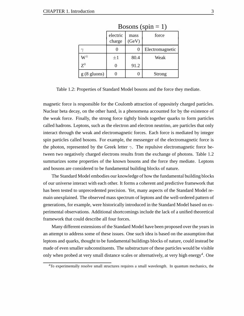
Bosons (spin = 1)electric mass forcecharge (GeV)
γ 0 0 Electromagnetic
W± ±1 80.4 Weak
Z0 0 91.2
g (8 gluons) 0 0 Strong
Table 1.2: Properties of Standard Model bosons and the forcethey mediate.
magnetic force is responsible for the Coulomb attraction ofoppositely charged particles.
Nuclear beta decay, on the other hand, is a phenomena accounted for by the existence of
the weak force. Finally, the strong force tightly binds together quarks to form particles
called hadrons. Leptons, such as the electron and electron neutrino, are particles that only
interact through the weak and electromagnetic forces. Eachforce is mediated by integer
spin particles called bosons. For example, the messenger ofthe electromagnetic force is
the photon, represented by the Greek letterγ. The repulsive electromagnetic force be-
tween two negatively charged electrons results from the exchange of photons. Table 1.2
summarizes some properties of the known bosons and the forcethey mediate. Leptons
and bosons are considered to be fundamental building blocksof nature.
The Standard Model embodies our knowledge of how the fundamental building blocks
of our universe interact with each other. It forms a coherentand predictive framework that
has been tested to unprecedented precision. Yet, many aspects of the Standard Model re-
main unexplained. The observed mass spectrum of leptons andthe well-ordered pattern of
generations, for example, were historically introduced inthe Standard Model based on ex-
perimental observations. Additional shortcomings include the lack of a unified theoretical
framework that could describe all four forces.
Many different extensions of the Standard Model have been proposed over the years in
an attempt to address some of these issues. One such idea is based on the assumption that
leptons and quarks, thought to be fundamental buildings blocks of nature, could instead be
made of even smaller subconstituents. The substructure of these particles would be visible
only when probed at very small distance scales or alternatively, at very high energy4. One
4To experimentally resolve small structures requires a small wavelength. In quantum mechanics, the

CHAPTER 1. Introduction 4
natural consequence of lepton and quark compositeness would be the existence of excited
states of leptons and quarks.
1.2 Analysis Overview
The work presented in this thesis consists of a search for experimental signatures compat-
ible with the production and subsequent decay, via the emission of a photon, of excited
charged leptons (`∗) in electron-positron collisions.
Excited charged leptons could be created in pairs (e+e− → `∗`∗) or singly in associa-
tion with a Standard Model lepton (e+e− → `∗` )5. Such states would promptly decay to a
photon and a Standard Model lepton and thus cannot be directly observed. The invariant
mass6 of the detected photon and Standard Model lepton should be equal to the mass of
the excited state. For excited states produced in a pair, theinvariant mass of both photon
and lepton pairs should be equal.
A set of criteria was developed to select experimental signatures consistent with the
production of excited charged leptons. The sensitivity of the search is substantially en-
hanced by the use of a kinematic fit technique which improves the estimates of the energy
and direction of the particles detected. This information is used to precisely calculate the
invariant mass of each possible pair of lepton and photon observed.
The invariant mass of the excited lepton candidates is compared with predictions from
the Standard Model. No evidence indicating the existence ofexcited leptons is found.
The results of the analysis are used to calculate constraints on parameters describing the
properties of excited states in theoretical extension of the Standard Model. The limits
presented in this thesis are currently the most stringent constraints on the existence of
excited leptons.
wavelength associated with a particle is inversely proportional to its momentum. Thus the higher the energyof particles, the smaller scale that can be probed.
5To keep the notation simple throughout the thesis, the electric charge of leptons is often not explicitlywritten. Charge conjugation is assumed. Thus, the notatione+e− → `∗` implies both reactionse+e− →`∗+`− ande+e− → `∗−`+.
6The invariant mass of two particles is defined asm12 =√
(E1 + E2)2 − (p1 + p2)2, whereE1, E2 and
p1, p2 are the energy and momentum vector of the two particles.

Chapter 2
Theory
The first section of this chapter introduces particular aspects of the Standard Model most
relevant for the work presented in this thesis. This is then followed by general remarks
about some of the outstanding problems and shortcomings of the Standard Model. The
last section is devoted to the particular theoretical framework describing the properties
and interactions of excited states of leptons and quarks.
2.1 The Standard Model
The Standard Model is based on two quantum field theories: theelectroweak model of
Glashow, Weinberg and Salam [1] which describes in a common framework both the
electromagnetic and weak forces, and the theory of quantum chromodynamics (QCD)
which offers a description of the strong force exclusively experienced by quarks. In-
teractions between particles are a natural consequence of the invariance of the quan-
tum field theories under a class of local symmetry transformations associated with the
SU(3)c × SU(2)L × U(1)Y gauge group. The invariance of a theory under local gauge
transformations is a crucial property that ensures the renormalisability of a theory [2], i.e.
the fact that physical observables such as the lifetime and production rate of particles are
finite quantities calculable to all energies and all orders in coupling constants. The quan-
tum mechanical description of particles is made invariant under some set of symmetry
transformations by introducing integer spin fields (gauge bosons) which couple to the par-
ticles. The local SU(3)c symmetry transformation generates the strong interactionbetween
quarks which couples to the colour charge (c) of particles. Similarly, the electroweak force
is a result of the invariance of the theory under local SU(2)L×U(1)Y transformations where
the subscript L indicates that only left-handed fermions transform non-trivially under the
SU(2) group symmetry. The electroweak force is proportional to the weak isospin (T) and
5
CHAPTER 2. Theory 6
weak hypercharge (Y) of particles defined such thatQ = T3 + Y/2 whereQ is the electric
charge andT3, the third component of weak isospin.
Fermion fields exist in two different chiralities, left and right-handed components.
Left-handed fields form weak isospin doublets while right-handed one only exist in weak
isospin singlets. For leptons of the first generation, the eigenstates of the electroweak
theory can be written as
LL =
νe
e
L
, LR = eR (2.1)
wheree andνe represent the electron and electron neutrino fields and the subscripts refer
to the eigenstates chirality. Table 2.1 summarises the quantum numbers of leptons of the
first generation which dictate their transformation properties under the SU(2)L × U(1)Ysymmetry.
By analogy to the formalism used in classical mechanics, thedynamics of particle
fields and their interactions are usually expressed, in quantum field theories, in terms of
a function called the Lagrangian density (L). As an example, the Lagrangian density
describing the interaction between two leptons and a gauge boson (V = γ, Z0, W±) can be
written as
LLLV = LLγµ
[
gτ
2Wµ + g′Y
2Bµ
]
LL + LRγµ
[
g′Y2
Bµ
]
LR (2.2)
whereτ denotes the Pauli matrices1, Y is the weak hypercharge,Wµ = (W1µ, W2
µ, W3µ) and
Bµ are the gauge fields associated with the SU(2)L and U(1)Y symmetry. These are related
to the physical gauge boson fields observed in nature by the transformation
W±µ =
1√2
(W1µ ∓ i W2
µ) (2.3)
Zµ = −Bµ sin θW + W3µ cos θW (2.4)
Aµ = Bµ cos θW + W3µ sin θW (2.5)
wheresin θW is called the weak mixing angle and is a free parameter of the Standard Model
which needs to be experimentally measured. The parametersg andg′ are the SU(2)L and
U(1)Y coupling constants. The interaction between two charged leptons and a gauge boson
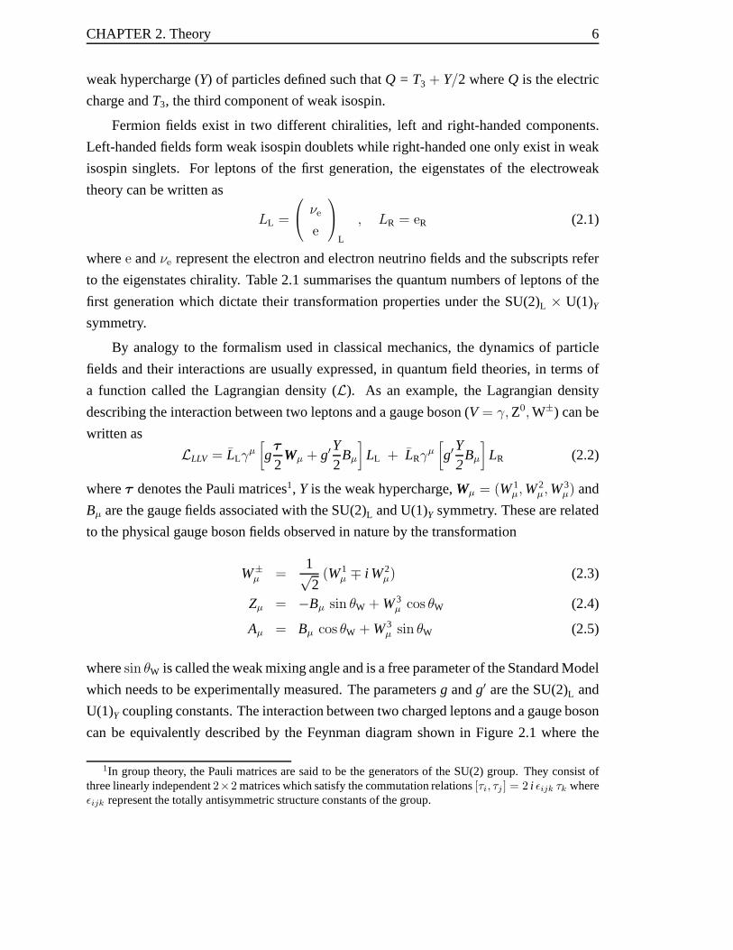
can be equivalently described by the Feynman diagram shown in Figure 2.1 where the
1In group theory, the Pauli matrices are said to be the generators of the SU(2) group. They consist ofthree linearly independent2×2 matrices which satisfy the commutation relations[τi, τj ] = 2 i εijk τk whereεijk represent the totally antisymmetric structure constants of the group.
CHAPTER 2. Theory 7
Lepton T T3 Y Q
νeL12
12 -1 0
eL12 -1
2 -1 -1
eR 0 0 -2 -1
Table 2.1: Quantum numbers of leptonsof the first generation whereT, T3, Y andQ are the weak isospin, third componentof the isospin, the weak hypercharge andelectric charge, respectively.
arrows represent the flow of the electroweak current.
Fermions and bosons in the Standard Model are given masses byintroducing a scalar
Higgs field [3] which spontaneously breaks the electroweak SU(2)L ×U(1)Y symmetry of
the theory. This mechanism is needed as mass terms cannot be directly added ‘by hand’ to
the Lagrangian without spoiling gauge invariance. Instead, the coupling of the Higgs field
to the weak gauge bosons and fermions is found to generate theappropriate mass terms
without destroying the gauge symmetry of the theory. The symmetry of the Lagrangian is
simply hidden by the choice of a specific ground state or vacuum expectation value.
2.2 Beyond the Standard Model
The Standard Model has been extremely successful at describing the interactions between
particles observed in nature. It has so far been tested to an impressive one part in 106.
Despite all its achievements, the Standard Model however remains somewhat of anad hoc
theory which relies on the experimental measurements of many fundamental quantities
such as the masses of particles and their couplings. It also fails to explain the three-fold
pattern of fermion generations and the observed mass spectrum. Other shortcomings of
the Standard Model include the inability to explain the existence of left-handed doublets
and right-handed singlets as well as the lack of unification between all forces including
gravity.
A number of models attempt to address some of the mysterious aspects of the Stan-
dard Model, albeit with varying degree of success. One approach postulates that particles
V
` ` Figure 2.1: Feynman diagram of the in-teraction between two Standard Modelcharged leptons (` = e, µ, τ ) and a gaugeboson (V = γ, Z0).
CHAPTER 2. Theory 8
currently considered to be fundamental might instead be composed of smaller subcon-
stituents. Historically, in our understanding of nature from atoms to quarks, systems that
were originally thought to be fundamental building blocks of the universe have revealed
substructure when probed at increasingly larger energy scales. Fermions that are thought
to be point-like particles in the Standard Model could then appear to be made of smaller
constituents when studied at high energy. This unique approach to physics beyond the
Standard Model could explain in a natural way the pattern of fermion generations as well
as the observed mass spectrum.
2.3 Model of Excited Leptons
There have been various attempts at building a complete model of composite fermions [4].
It has however proved to be quite challenging to develop a model consistent with current
experimental observations and precision measurements. Despite the lack of a complete
model, searches for possible experimental consequences offermion compositeness have
been and continue to be pursued. These searches are carried out in the framework of a low
energy approximation of what the complete and yet unknown theory might predict.
Experimental consequences of fermion compositeness couldinclude the existence of
excited states of the Standard Model fermions. Much like thearrangement of subcon-
stituents in a hydrogen atom or a hadron results in bound states with properties different
than the ground states of the system, excited fermions are expected to exhibit unique char-
acteristics distinguishing them from the known Standard Model fermions.
The theoretical framework used in this thesis to calculate constraints on the exis-
tence of excited electrons (e∗), muons (µ∗) and taus (τ ∗) is a phenomenological model [5,
6]. This model describes the possible interactions betweenexcited leptons and Standard
Model particles without explicitly describing the nature and dynamics of the fermion sub-
constituents. Although this phenomenological model is described here only in terms of the
leptonic sector relevant for the present work, it is straight forward to extend the formalism
to include excited states of quarks.
Excited states of Standard Model fermions are assumed here to have both spin and
weak isospin 1/2, although other spin assignments have alsobeen considered in the lit-
erature [7]. To accommodate the fact that the unobserved excited states must be much
heavier than the Standard Model fermions, they are assumed to acquire their mass prior to
the spontaneous symmetry breaking of the Standard Model Lagrangian. Details of how the
CHAPTER 2. Theory 9
excited T T3 Y Qlepton
ν∗e L
12
12 -1 0
ν∗e R
12
12 -1 0
e∗L12 -1
2 -1 -1
e∗R12 -1
2 -1 -1
Table 2.2: Quantum numbers of excitedleptons of the first generation whereT,T3, Y andQ are the weak isospin, thirdcomponent of the isospin, the weak hy-percharge and electric charge, respec-tively.
masses of these excited states arise is not relevant for the low energy phenomenology in
the present theoretical framework. They should however be part of any model attempting
to describe the full dynamics of fermion constituents. In order to retain the fundamen-
tal SU(2)L × U(1)Y gauge invariance of the Standard Model in the presence of additional
mass terms, excited states must exist in both left-handed (L) and right-handed (R) weak
isodoublets, unlike Standard Model fermions. For excited leptons of the first generation,
the two weak isodoublets can be written as
L∗L =
ν∗e
e∗
L
, L∗R =
ν∗e
e∗
R
(2.6)
wheree∗ andν∗e represent the excited electron and excited electron neutrino fields respec-
tively.
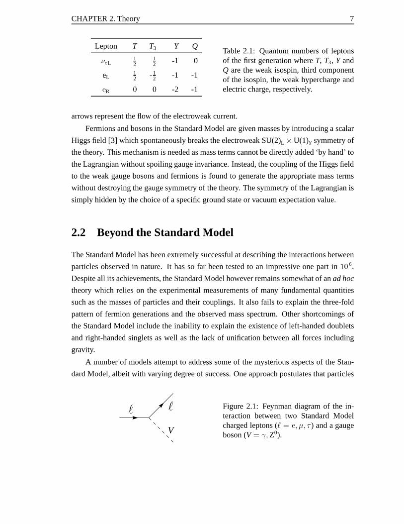
Given the assumptions presented above, the quantum numbersof excited leptons are
fixed to the values given in Table 2.2. Furthermore, in order to be able to calculate exper-
imental observables such as the production rate and decay ofthese excited states, the two
interaction vertices shown in Figure 2.2 must also be introduced.
* *
V
` `
(a)
*
V
` `
(b)
Figure 2.2: Diagrams showing the interactions of charged excited leptons (∗ = e∗, µ∗, τ ∗)with Standard Model leptons (` = e, µ, τ ) and gauge bosons (V = γ, Z0).

CHAPTER 2. Theory 10
The interaction between two excited leptons and one gauge boson (L∗L∗V) is assumed
to have the same form and coupling strength as the corresponding Standard Model interac-
tion between two leptons and one boson. In addition, only excited leptons from the same
generation can interact with each other. Following closelyEquation 2.2, the Lagrangian
density describing theL∗L∗V coupling is usually written as
LL∗L∗V = L∗Lγ
µ
[
gτ
2Wµ + g′Y
2Bµ
]
L∗L + L∗
Rγµ
[
gτ
2Wµ + g′Y
2Bµ
]
L∗R (2.7)
Given the composite nature of leptons in the present model, the interaction described
above should contain form factors to take into account deviations from a point-like interac-
tion due to the presence of subconstituents. However, for large value of the compositeness
scale, the effects of these form factors are negligible.
The particular choice of the interaction Lagrangian density describing the transition
between an excited lepton, a lepton and a gauge boson (L∗LV) dictates not only the decays
of excited states but also, as will be discussed later, theirsingle production in e+e- colli-
sions. The requirement that the interaction be SU(2)L × U(1)Y gauge invariant uniquely
determines the coupling between a spin 1/2 excited lepton, aStandard Model lepton and
gauge boson to be of a tensorial nature [7]. A simple vectorial interaction similar to Equa-
tions 2.2 and 2.7 would not be gauge invariant under SU(2)L symmetry as the right-handed
component of excited leptons forms a weak isodoublet which transforms differently from
the usual Standard Model right-handed weak singlet. Furthermore, in light of existing
constraints on the existence of excited leptons, describedin details in Section 6.5, only
left-handed leptons are allowed to couple to excited states. A coupling without this chiral
symmetry would lead to large contributions to the anomalousmagnetic moment of lep-
tons, in conflict with current precision measurements of this quantity. For these reasons,
the interaction between an excited lepton, a Standard Modellepton and a gauge boson
is usually described by the following chiral conserving SU(2)L × U(1)Y gauge invariant
Lagrangian density [5–7]
LL∗LV =1
2ΛL∗
Rσµν
[
g fτ
2Wµν + g′ f ′ Y
2Bµν
]
LL +
1
2ΛLLσ
µν
[
g fτ
2Wµν + g′ f ′ Y
2Bµν
]
L∗R (2.8)
whereσµν is the covariant bilinear tensor2, Wµν andBµν represent the Standard Model
2σµν = γµγν − γνγµ whereγµ andγν represent Dirac matrices.
CHAPTER 2. Theory 11
gauge field tensors3 and the couplingsg, g′ are the SU(2)L and U(1)Y coupling constants
of the Standard Model introduced in Section 2.1. The compositeness scale is set by the
parameterΛ which has units of energy. Finally, the strength of theL∗LV couplings is
governed by the constantsf andf ′. These constants can be interpreted as weight factors
associated with the different gauge groups.
The only unknown parameters of the phenomenological model presented in this sec-
tion are the mass of excited leptons, the compositeness scale Λ and the strength of the
couplingsf and f ′. To reduce the number of free parameters it is customary to assume
either a relation betweenf andf ′ or set one coupling to zero. For easy comparison with
previously published results, limits calculated in this paper correspond to the coupling
choicef = f ′. As will be shown in the next section, this assignment is a natural choice
which forbids excited neutrinos from decaying electromagnetically.
Physical observables such as the production and decay ratesof excited leptons are
calculated from the Lagrangians 2.8 and 2.7. Approximate expressions for these observ-
ables are presented below as an indication of the expected physical properties of excited
leptons. In the analysis presented in this thesis, efficiencies and expected distributions of
kinematical variables for excited leptons are instead obtained using the Monte Carlo event
generator EXOTIC based on the exact expressions for the production and decay rates.
2.3.1 Excited Lepton Decays
The decay of an excited charged lepton into a Standard Model lepton and a gauge boson is
shown schematically in Figure 2.2(b) and is determined by the Lagrangian density given
in Equation 2.8.
Neglecting the decay width of the gauge bosons (ΓV → 0), the decay rate4 into the
different gauge bosons can be approximated, for excited lepton masses larger thanMV, by
the following formula
Γ =α
4m3
∗
Λ2f 2V
(
1− M 2V
m2∗
) 2(
1 +M2
V
2m2∗
)
(2.9)
wherem∗ and MV are the excited lepton and gauge boson masses respectively and the
quantitiesfV are defined in terms of the parametersf and f ′, the excited states electric
3Wµν = ∂µWν − ∂νWµ4The branching fraction of a particle into a specific final state is defined as the ratio of the final state
decay rate to the total decay rate of all possible final states.
CHAPTER 2. Theory 12
charge (Q) and third component of the weak isospin for left-handed states (T3L)
fγ = Q f ′ + T3L (f − f ′) (2.10)
fW =1√
2sin θW
f (2.11)
fZ =4 T3L (cos2 θW f + sin2 θW f ′) − 4 Q sin2 θW f ′
4 sin θW cos θW. (2.12)
The branching fractions of excited neutrinos (ν∗) are identical to that of excited
charged leptons (`∗) under the transformationf ′ → −f ′. This symmetry is a direct
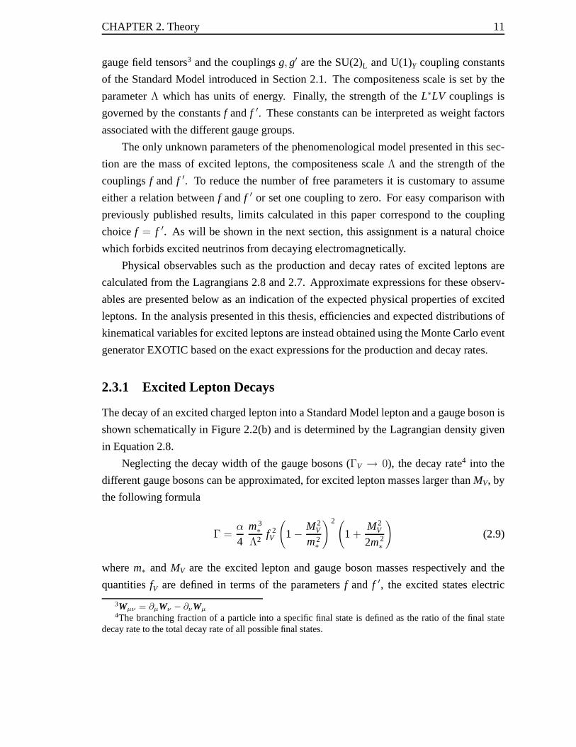
consequence of the weak isospin assignment of excited leptons. Figure 2.3 shows the pre-
dicted electromagnetic branching fraction of excited charged leptons and excited neutrinos
for different values off and f ′. As seen from Equation 2.10, the branching fraction for
excited charged leptons decaying into a lepton and photon vanishes for the special case
f = −f ′. Alternatively, the electromagnetic branching fraction of excited neutrinos is zero
under the assumption thatf = f ′.
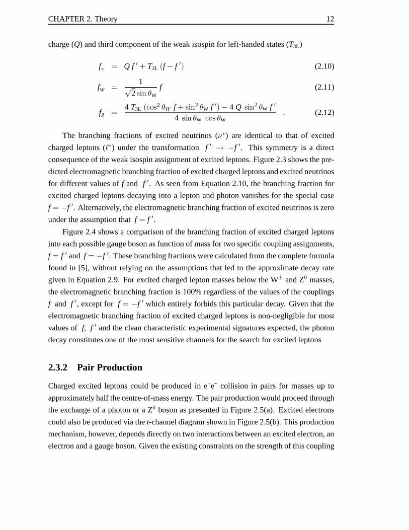
Figure 2.4 shows a comparison of the branching fraction of excited charged leptons
into each possible gauge boson as function of mass for two specific coupling assignments,
f = f ′ and f = −f ′. These branching fractions were calculated from the complete formula
found in [5], without relying on the assumptions that led to the approximate decay rate
given in Equation 2.9. For excited charged lepton masses below the W± and Z0 masses,
the electromagnetic branching fraction is 100% regardlessof the values of the couplings
f and f ′, except for f = −f ′ which entirely forbids this particular decay. Given that the
electromagnetic branching fraction of excited charged leptons is non-negligible for most
values of f, f ′ and the clean characteristic experimental signatures expected, the photon
decay constitutes one of the most sensitive channels for thesearch for excited leptons
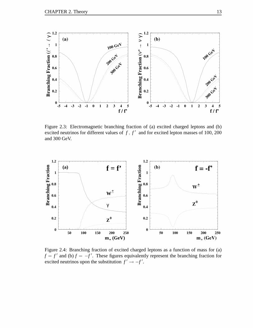
2.3.2 Pair Production
Charged excited leptons could be produced in e+e- collision in pairs for masses up to
approximately half the centre-of-mass energy. The pair production would proceed through
the exchange of a photon or a Z0 boson as presented in Figure 2.5(a). Excited electrons
could also be produced via thet-channel diagram shown in Figure 2.5(b). This production
mechanism, however, depends directly on two interactions between an excited electron, an
electron and a gauge boson. Given the existing constraints on the strength of this coupling
CHAPTER 2. Theory 13
f / f’
Bra
nch
ing F
ract
ion
(
→γ
)
300
GeV
200
GeV
100 GeV
(a)
0
0.2
0.4
0.6
0.8
1
1.2
-5 -4 -3 -2 -1 0 1 2 3 4 5
``*
f / f’
Bra
nch
ing F
ract
ion
(ν*
→ν
γ )
300
GeV
200
GeV
100 GeV
(b)
0
0.2
0.4
0.6
0.8
1
1.2
-5 -4 -3 -2 -1 0 1 2 3 4 5
Figure 2.3: Electromagnetic branching fraction of (a) excited charged leptons and (b)excited neutrinos for different values off , f ′ and for excited lepton masses of 100, 200and 300 GeV.
m* (GeV)
Bra
nchi
ng F
ract
ion
γ
W
Z0
(a) f = f’
0
0.2
0.4
0.6
0.8
1
1.2
50 100 150 200 250
+
m* (GeV)
Bra
nch
ing F
ract
ion
W
Z0
(b) f = -f’
0
0.2
0.4
0.6
0.8
1
1.2
50 100 150 200 250
+
Figure 2.4: Branching fraction of excited charged leptons as a function of mass for (a)f = f ′ and (b)f = −f ′. These figures equivalently represent the branching fraction forexcited neutrinos upon the substitutionf ′ → −f ′.
CHAPTER 2. Theory 14
e
e
γ , Z0
*
*
`
`
(a)e
γ , Z0
e e*
e*(b)
Figure 2.5: Pair production of excited charged leptons via a(a)s-channel and (b)t-channeldiagrams.
discussed in Section 6.5, the contribution of thet-channel diagram (Figure 2.5(b)) for the
pair production of excited electrons is much smaller than that of thes-channel diagram
and can be safely neglected.
The interaction described in Equation 2.7 therefore completely determines the pair
production rate, or cross-section, of excited leptons. Neglecting the decay width of the
heavy gauge bosons (ΓV → 0), the pair production cross-section can be approximated as
σ =2πα 2
3sβ (3− β 2)
[
1 +2 ve v`∗
1 − M 2Z/s
+(a2
e + v2e ) v2
`∗
(1− M2Z/s) 2
]
(2.13)
whereα is the fine structure constant,MZ is the mass of the Z0 boson,√
s is the collision
centre-of-mass energy andβ =√
1 - 4m2∗/s. The constantsve, v`∗ andae are defined in
terms of the electric charge and weak isospin as
ve,`∗ =2Te,`∗
3L + 2 T e,`∗
3R − 4Q sin 2 θW
4 sin θW cos θW(2.14)
ae =2Te
3L − 2Te3R
4 sin θW cos θW. (2.15)
The pair production cross-section at a given centre-of-mass energy only depends on the
mass of the excited leptons. An example of the expected totalcross-section for the pair
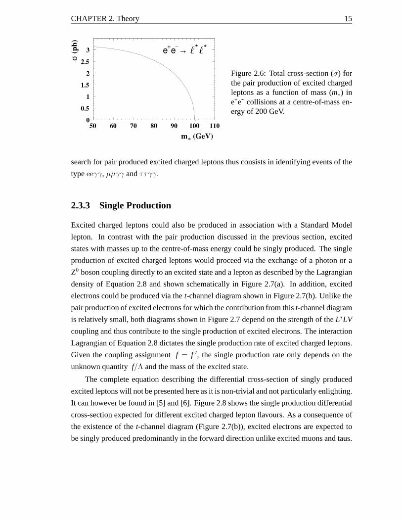
production of excited charged leptons as function of mass ispresented in Figure 2.6.
The pair production of excited charged leptons followed by aprompt electromagnetic
decay of each excited state would result in event final states, observed in the detector,
containing exactly two leptons of the same flavour and two isolated photon ( γγ). The
CHAPTER 2. Theory 15
m* (GeV)
σ (
pb
)
e+e → * *
0
0.5
1
1.5
2
2.5
3
50 60 70 80 90 100 110
` `
Figure 2.6: Total cross-section (σ) forthe pair production of excited chargedleptons as a function of mass (m∗) ine+e- collisions at a centre-of-mass en-ergy of 200 GeV.
search for pair produced excited charged leptons thus consists in identifying events of the
typeeeγγ, µµγγ andττγγ.
2.3.3 Single Production
Excited charged leptons could also be produced in association with a Standard Model
lepton. In contrast with the pair production discussed in the previous section, excited
states with masses up to the centre-of-mass energy could be singly produced. The single
production of excited charged leptons would proceed via theexchange of a photon or a
Z0 boson coupling directly to an excited state and a lepton as described by the Lagrangian
density of Equation 2.8 and shown schematically in Figure 2.7(a). In addition, excited
electrons could be produced via thet-channel diagram shown in Figure 2.7(b). Unlike the
pair production of excited electrons for which the contribution from thist-channel diagram
is relatively small, both diagrams shown in Figure 2.7 depend on the strength of theL∗LV
coupling and thus contribute to the single production of excited electrons. The interaction
Lagrangian of Equation 2.8 dictates the single production rate of excited charged leptons.
Given the coupling assignmentf = f ′, the single production rate only depends on the
unknown quantityf/Λ and the mass of the excited state.
The complete equation describing the differential cross-section of singly produced
excited leptons will not be presented here as it is non-trivial and not particularly enlighting.
It can however be found in [5] and [6]. Figure 2.8 shows the single production differential
cross-section expected for different excited charged lepton flavours. As a consequence of
the existence of thet-channel diagram (Figure 2.7(b)), excited electrons are expected to
be singly produced predominantly in the forward direction unlike excited muons and taus.
CHAPTER 2. Theory 16
e
e
γ , Z0*`
`
(a)e
γ Z0
e e
e*
,
(b)
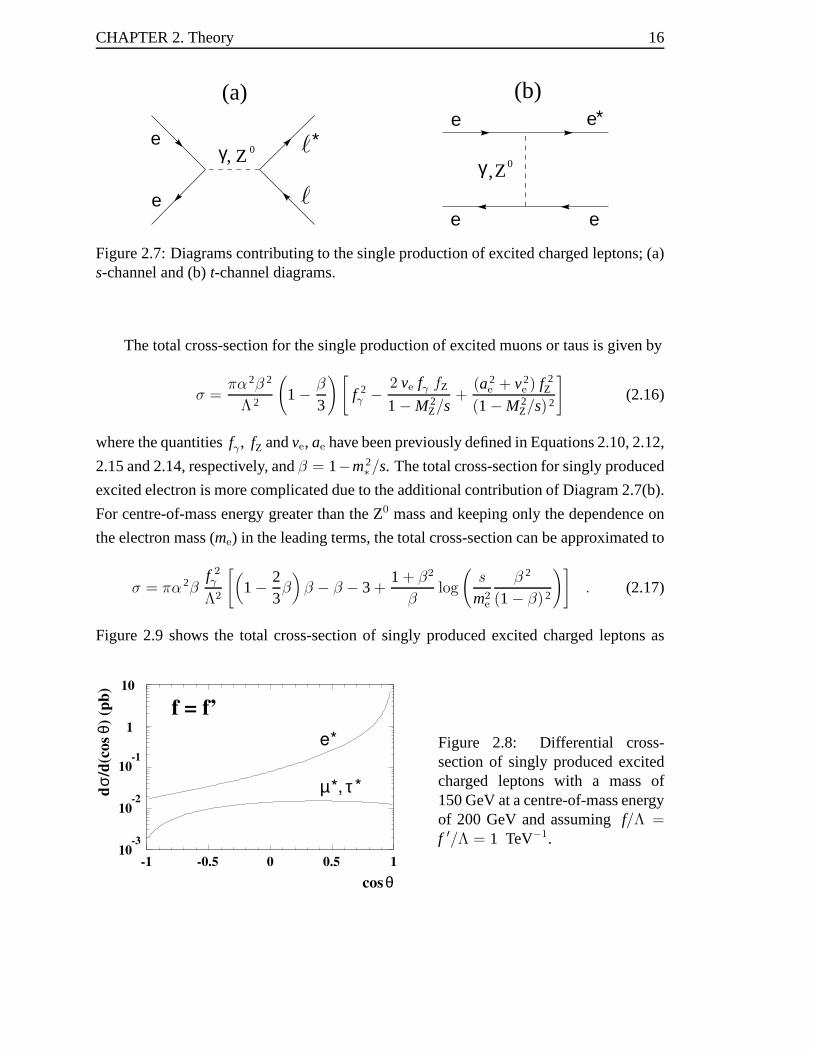
Figure 2.7: Diagrams contributing to the single productionof excited charged leptons; (a)s-channel and (b)t-channel diagrams.
The total cross-section for the single production of excited muons or taus is given by
σ =πα 2β 2
Λ 2
(
1− β
3
)[
f 2γ − 2 ve fγ fZ
1− M 2Z/s
+(a2
e + v2e ) f 2
Z
(1− M 2Z/s) 2
]
(2.16)
where the quantitiesfγ , fZ andve, ae have been previously defined in Equations 2.10, 2.12,
2.15 and 2.14, respectively, andβ = 1−m2∗/s. The total cross-section for singly produced
excited electron is more complicated due to the additional contribution of Diagram 2.7(b).
For centre-of-mass energy greater than the Z0 mass and keeping only the dependence on
the electron mass (me) in the leading terms, the total cross-section can be approximated to
σ = πα 2βf 2γ
Λ2
[
(
1− 23β)
β − β − 3 +1 + β2
βlog
(
s
m2e
β 2
(1− β) 2
)]
. (2.17)
Figure 2.9 shows the total cross-section of singly producedexcited charged leptons as
cosθ
dσ
/d(c
os
θ) (
pb
)
e
µ*, τ
*
*
f = f’
10-3
10-2
10-1
1
10
-1 -0.5 0 0.5 1
Figure 2.8: Differential cross-section of singly produced excitedcharged leptons with a mass of150 GeV at a centre-of-mass energyof 200 GeV and assumingf/Λ =f ′/Λ = 1 TeV−1.

CHAPTER 2. Theory 17
m* (GeV)
σ (
pb
)e
+e → e*e
e+e → µ* µ, τ* τ
f = f’
10-3
10-2
10-1
1
10
102
60 80 100 120 140 160 180 200
Figure 2.9: Total cross-section (σ)for the single production of excitedcharged leptons as a function ofmass (m∗) in e+e- collisions at acentre-of-mass energy of 200 GeVand assumingf/Λ = f′/Λ =1 TeV−1.
function of mass.
As can be seen from Equations 2.16 and 2.17, forf = f ′, the total cross-section of
singly produced excited leptons is directly proportional to (f/Λ)2. Given existing con-
straints on the coupling parametersf/Λ, the production rate of singly produced excited
charged leptons is expected to be orders of magnitude smaller than that of pair production.
However, the single production search extends the kinematic reach of an experiment to
masses up to the centre-of-mass energy.
The prompt decay of excited charged leptons singly producedwould lead to event
final states containing two leptons of the same flavour and oneenergetic photon (``γ).
Since excited electrons are expected to be predominantly produced in the forward region
of the detector, the electron produced in association with the excited state may be outside
the detector acceptance resulting in event final states containing only one electron and
one photon (eγ). The search for singly produced excited charged leptons which promptly
decay electromagnetically therefore consists in identifying events of the typeseeγ, eγ,
µµγ andττγ.
Chapter 3
Experimental Environment
The CERN laboratory, located just outside Geneva in Switzerland, was home of the Large
Electron Positron (LEP) collider. It was recently decommissioned in December 2000 after
10 years of remarkable operation. Particles created in e+e- collisions were detected by
four large all-purpose detectors ALEPH, DELPHI, L3 and OPAL.
During its first phase of operation from 1990 to 1995, LEP produced millions of Z0
bosons which allowed physicists to study to unprecedented precision the various properties
of this particle and test the Standard Model to a precision better than one part in 104. Phase
2 of LEP operation (LEP2) began in 1995 after major upgrades of various accelerator
components which increased the rate of collisions and the centre-of-mass energy. The
substantial amount of data recorded combined with the highest centre-of-mass energy ever
reached in e+e- collisions provided a unique environment to search for new phenomena
beyond the Standard Model.
This chapter first presents some details of LEP operation anddescribes the various
components of the OPAL detector relevant for this work. The recording of data and subse-
quent reconstruction of events are also briefly discussed. Finally, the data set and various
event simulation programs used are described.
3.1 The Large Electron Positron Collider
The Large Electron Positron collider [8] was a 26.6 km in circumference storage ring com-
missioned in 1989. The ring consisted of eight 500 m long straight sections interspaced
with eight 2.8 km arcs. All LEP components were contained in atunnel approximately
100 m underground. Electron and positron beams travelled inopposite directions inside an
evacuated aluminum tube of about 10 cm in diameter. Dipole magnets guided the beams
around the arcs while focusing of the beams was achieved by various combinations of
18
CHAPTER 3. Experimental Environment 19
quadrupole and sextupole magnets. The energy needed to accelerate and subsequently
maintain the two beams at the nominal collision energy was supplied by Radio Frequency
(RF) resonant cavities. Electrons and positrons circulating around the ring constantly lost
energy via the emission of photons. Each electron lost on average about 2% of its energy
from synchrotron radiation in one revolution around the ring. In its last year of running,
the LEP accelerating system consisted of 288 superconducting RF cavities (272 niobium-
coated copper and 16 pure niobium) and 56 conventional copper RF cavities providing
together a total RF voltage of about 3400 MV per revolution.
The two beams were made to collide at four specific points around the ring, at the
heart of massive detectors (ALEPH, DELPHI, L3 and OPAL) designed to record the rem-
nants of the collisions. During the accelerating phase, separator magnets located near
the interaction regions separated the two beams to avoid collisions. When the electron
and positron beams finally reached the desired energy, they were brought into collisions
by turning off the separator magnets. In addition, superconducting quadrupole magnets,
also located near the interaction regions, squeezed the beams down to a cross-sectional
size of approximately 10µm in the vertical plane and 250µm in the horizontal plane.
Such a small beam size was desirable in order to increase the collision rate. The rate of
a particular physics process is related to the beam intensity, or luminosityL, according
to Rate= L σ, whereσ is the cross-section (or probability of occurrence) of a particular
physics process. Luminosities of 1032 cm-2s-1 were routinely achieved at LEP.
The entire CERN accelerator complex is shown in Figure 3.1. The LEP injection
system was designed to exploit the existing CERN accelerators. Electrons were initially
produced by an electron gun and immediately accelerated to an energy of 200 MeV using
a short linear accelerator (linac). A fraction of these electrons were then directed to a
tungsten target to produce positrons. Both the positrons and the remaining electrons were
further accelerated to 600 MeV by a second linac and stored inthe electron-positron accu-
mulator (EPA). Pulses (or bunches) of electrons and positrons were stored in the EPA until
the next injection cycle of the Proton Synchrotron (PS). ThePS, CERN’s oldest acceler-
ator, operated as a 3.5 GeV e+e- synchrotron. Electrons and positrons were subsequently
injected into the Super Proton Synchrotron (SPS). Both PS and SPS operated in a multi-
cycle mode whereby electrons and positrons were accelerated between proton cycles and
thus simultaneously provided both electron/positron and proton beams to various CERN
experiments. The SPS boosted the energy of electrons and positrons to 22 GeV before
they were finally injected into the LEP ring. The final acceleration stage took place in

CHAPTER 3. Experimental Environment 20
LEP where, since 1996, beams have been accelerated to energygreater then 80.5 GeV. In
its last year of running, beams up to 104.5 GeV were routinelysuccessfully brought into
collision at the heart of the four LEP detectors.
The LEP storage ring mostly operated in a configuration where4 bunches of electrons
and 4 bunches of positrons circulated simultaneously in themachine. Each bunch was
composed of approximately 45× 1010 particles resulting in a total current circulating in
the machine of about 5 mA at the beginning of a collision cycle. As time went by during
a collision cycle, the particle density in each bunch decreased resulting in a decrease in
the collision rate. The ring was emptied of its remaining circulating particles when the
collision rate had decreased significantly, at which point it was more efficient to refill the
machine with new particles. In its last year of running, the highest collision energies were
reached using “miniramps”, a novel technique in which beamswere further accelerated in
small incrementing steps while in stable collision mode. Using this technique, collisions
at a centre-of-mass energy of 209 GeV were achieved, an energy beyond the original
machine design of 200 GeV.
Many analyses, including the work presented in this thesis,rely on a precise measure-
ment of the collision energy. At LEP2, the beam energy was determined using nuclear
magnetic resonance (NMR) probes [9] located in dipole magnets around the LEP ring.
The 16 NMR probes were calibrated at lower energy using resonance depolarisation [10],
a technique that can only be used for beam energy less than approximately 60 GeV. Preci-
sion on the beam energy measurement is currently limited by the uncertainty on the linear
extrapolation to physics energy of the NMR probe readings. Other methods of measuring
the beam energy were used as consistency checks and as a mean of estimating various
systematic errors. In particular, a dedicated spectrometer [11] was installed in the fall
1999 with the aim of measuring the beam energy to a relative accuracy of one part in
104. Studies of the spectrometer response necessary to achievethis goal are still ongoing.
The preliminary uncertainties on the beam energy for the data set analysed varies from
20-25 MeV.
3.2 The OPAL Detector
The OPAL (Omni-Purpose Apparatus at LEP) detector [12] was one of four multi-purpose
detectors at LEP. As shown in Figure 3.2, its cylindrical shape longitudinally aligned with
respect to the beam direction provided nearly full angular coverage of the interaction re-

CHAPTER 3. Experimental Environment 21
*
*electrons
positrons
protons
antiprotons
Pb ions
LEP: Large Electron Positron collider
SPS: Super Proton Synchrotron
AAC: Antiproton Accumulator Complex
ISOLDE: Isotope Separator OnLine DEvice
PSB: Proton Synchrotron Booster
PS: Proton Synchrotron
LPI: Lep Pre-Injector
EPA: Electron Positron Accumulator
LIL: Lep Injector Linac
LINAC: LINear ACcelerator
LEAR: Low Ener gy Antiproton Ring
OPALALEPH
L3DELPHI
SPS
LEP
West Area
TT
10 AAC
TT
70
East Area
LPI
e-
e-
e+
EPA
PS
LEAR
LIN
AC
2
LIN
AC
3
p Pb ions
E2
South Area
Nor
th A
rea
LIL
TTL2TT2 E0
PSB
ISO
LD
E
E1
pbar
Rudolf LEY, PS Division, CERN, 02.09.96
Figure 3.1: Schematic diagram of the accelerator complex atthe CERN laboratory, show-ing each component of the LEP injection system as well as protons/antiprotons and heavyions accelerators.
CHAPTER 3. Experimental Environment 22
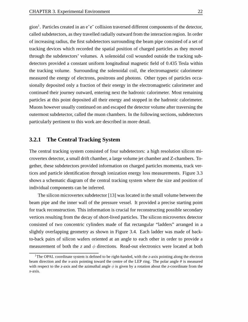
gion1. Particles created in an e+e- collision traversed different components of the detector,
called subdetectors, as they travelled radially outward from the interaction region. In order
of increasing radius, the first subdetectors surrounding the beam pipe consisted of a set of
tracking devices which recorded the spatial position of charged particles as they moved
through the subdetectors’ volumes. A solenoidal coil wounded outside the tracking sub-
detectors provided a constant uniform longitudinal magnetic field of 0.435 Tesla within
the tracking volume. Surrounding the solenoidal coil, the electromagnetic calorimeter
measured the energy of electrons, positrons and photons. Other types of particles occa-
sionally deposited only a fraction of their energy in the electromagnetic calorimeter and
continued their journey outward, entering next the hadronic calorimeter. Most remaining
particles at this point deposited all their energy and stopped in the hadronic calorimeter.
Muons however usually continued on and escaped the detectorvolume after traversing the
outermost subdetector, called the muon chambers. In the following sections, subdetectors
particularly pertinent to this work are described in more detail.
3.2.1 The Central Tracking System
The central tracking system consisted of four subdetectors: a high resolution silicon mi-
crovertex detector, a small drift chamber, a large volume jet chamber and Z-chambers. To-
gether, these subdetectors provided information on charged particles momenta, track ver-
tices and particle identification through ionization energy loss measurements. Figure 3.3
shows a schematic diagram of the central tracking system where the size and position of
individual components can be inferred.
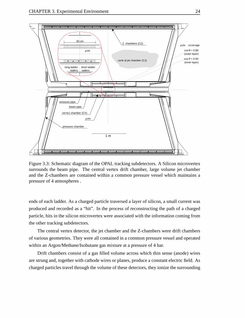
The silicon microvertex subdetector [13] was located in thesmall volume between the
beam pipe and the inner wall of the pressure vessel. It provided a precise starting point
for track reconstruction. This information is crucial for reconstructing possible secondary
vertices resulting from the decay of short-lived particles. The silicon microvertex detector
consisted of two concentric cylinders made of flat rectangular “ladders” arranged in a
slightly overlapping geometry as shown in Figure 3.4. Each ladder was made of back-
to-back pairs of silicon wafers oriented at an angle to each other in order to provide a
measurement of both thez andφ directions. Read-out electronics were located at both
1The OPAL coordinate system is defined to be right-handed, with thez-axis pointing along the electronbeam direction and thex-axis pointing toward the centre of the LEP ring. The polar angle θ is measuredwith respect to thez-axis and the azimuthal angleφ is given by a rotation about thez-coordinate from thex-axis.
CHAPTER 3. Experimental Environment 23
x
y
z
Hadron calor imetersand return yoke
Electromagneticcalorimeters Muon
detectors
Jetchamber
Vertexchamber
Microvertexdetector
Z chambers
Solenoid andpressure vessel
Time of flightdetector
Presampler
Silicon tungstenluminometer
Forwarddetector
θ ϕ
Figure 3.2: Schematic diagram of the OPAL detector showing the layout of different com-ponents.
CHAPTER 3. Experimental Environment 24
1 m
cos (inner layer)
cos (outer layer)
long ladderwafers
short ladder wafers
30 cm
µvtx
µ
ver tex chamber (CV)
centr al jet chamber (CJ)
Z chambers (CZ)
beam pipe
pressure pipe
pressure chamber
µ coverage
vtx
vtx
θ
θ = 0.93
= 0.89
Figure 3.3: Schematic diagram of the OPAL tracking subdetectors. A Silicon microvertexsurrounds the beam pipe. The central vertex drift chamber, large volume jet chamberand the Z-chambers are contained within a common pressure vessel which maintains apressure of 4 atmospheres .
ends of each ladder. As a charged particle traversed a layer of silicon, a small current was
produced and recorded as a “hit”. In the process of reconstructing the path of a charged
particle, hits in the silicon microvertex were associated with the information coming from
the other tracking subdetectors.
The central vertex detector, the jet chamber and the Z-chambers were drift chambers
of various geometries. They were all contained in a common pressure vessel and operated
within an Argon/Methane/Isobutane gas mixture at a pressure of 4 bar.
Drift chambers consist of a gas filled volume across which thin sense (anode) wires
are strung and, together with cathode wires or planes, produce a constant electric field. As
charged particles travel through the volume of these detectors, they ionize the surrounding

CHAPTER 3. Experimental Environment 25
56.5 mm80 mm
60.5 mm73.8 m
m
5.5o
7.5o
10 mm
pressure vessel
beam pipe
beryllium half shell
Figure 3.4: Schematic cross-sectional diagram of the OPAL silicon microvertex detector.
gas. Electrons resulting from the gas ionization drift in toward the anode wires where
they cause an avalanche in the high electric field, resultingin electric pulses read out
from the ends of the wires. The particular gas mixture and pressure used to operate the
OPAL chambers were chosen to maximize the spatial resolution over the widest possible
momentum range and obtain precise measurements of a chargedparticle ionization energy
loss in the gas.
The central vertex detector [14] was a small cylindrical drift chamber of 1 m in length
and 23.5 cm radius. It consisted of an inner layer of axial wires strung longitudinally
and an outer layer composed of stereo wires mounted with a 40 angle between endplates.
The inner layer of wires provided a high resolution spatial measurement in ther-φ plane
while the slightly off axis stereo outer wires allowed a measurement of thez coordinate.
A total of 18 hits (12 axial + 6 stereo) could be recorded for 92% of the full solid angle.
Originally designed as the main vertex detector of OPAL, it has mainly been used, after
the addition in 1996 of a higher resolution silicon microvertex detector, to match track
segments between the jet chamber and the silicon microvertex.
The main component of the tracking system was the large volume central jet cham-
ber [15] measuring 4 m long and extending from an inner radiusof 0.5 m to an outer radius
of 3.7 m. The chamber was composed of 24 identical pie shaped sectors each containing
159 longitudinally strung anode wires and two cathode wire planes forming the boundaries
between adjacent sectors. Anode wires were staggered by 100µm to resolve the left-right
CHAPTER 3. Experimental Environment 26
6
8
10
12
14
16
18
10-1
1 10 102
p (GeV/c)
dE/d
x (k
eV/c
m)
dE/dx-resolution:(159 samples)
µ-pairs: 2.8 %min. ion. π: 3.2 %
p
K
π
µ
eµ-pairs
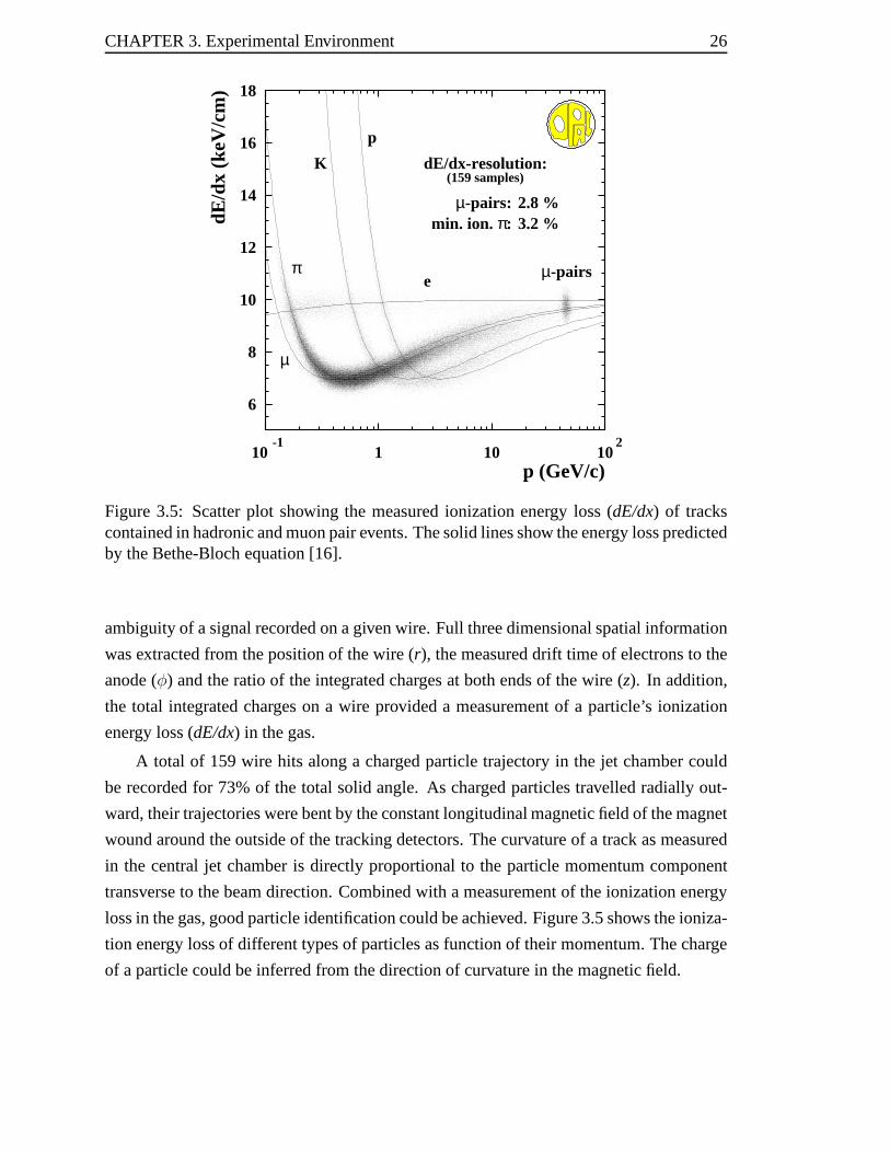
Figure 3.5: Scatter plot showing the measured ionization energy loss (dE/dx) of trackscontained in hadronic and muon pair events. The solid lines show the energy loss predictedby the Bethe-Bloch equation [16].
ambiguity of a signal recorded on a given wire. Full three dimensional spatial information
was extracted from the position of the wire (r), the measured drift time of electrons to the
anode (φ) and the ratio of the integrated charges at both ends of the wire (z). In addition,
the total integrated charges on a wire provided a measurement of a particle’s ionization
energy loss (dE/dx) in the gas.
A total of 159 wire hits along a charged particle trajectory in the jet chamber could
be recorded for 73% of the total solid angle. As charged particles travelled radially out-
ward, their trajectories were bent by the constant longitudinal magnetic field of the magnet
wound around the outside of the tracking detectors. The curvature of a track as measured
in the central jet chamber is directly proportional to the particle momentum component
transverse to the beam direction. Combined with a measurement of the ionization energy
loss in the gas, good particle identification could be achieved. Figure 3.5 shows the ioniza-
tion energy loss of different types of particles as functionof their momentum. The charge
of a particle could be inferred from the direction of curvature in the magnetic field.
CHAPTER 3. Experimental Environment 27
Finally, an accurate measurement of thez-coordinate of a particle trajectory was pos-
sible using the Z-chambers [17]. These 24 thin rectangular drift chambers were mounted
longitudinally around the outside of the jet chamber. Each chamber was 4 m long, 50 cm
wide and 59 mm thick. The Z-chambers covered the polar angle region between 440 and
1360. Unlike the vertex and central jet chambers, wires in the Z-chambers were strung per-
pendicular to the beam direction in order to precisely measure thez-coordinate of particles
leaving the jet chamber. A total of six layers of anode wires were positioned at increasing
radii. A spatial resolution in thez-direction better than 300µm was achieved. A mea-
surement of theφ coordinate of a track is also obtained using a charge division method in
order to facilitate matching hits with tracks observed in the central jet chamber.
The combined performance of the tracking subdetectors resulted in a momentum res-
olution ofσp/p2 ≈ 1.6× 10⁻³ GeV-1 and a spatial resolution of the impact parameter in
the plane perpendicular to the beam axis (d0) of 21µm.
3.2.2 Calorimeters
Calorimeters are detectors that measure the energy of particles. The calorimetry system
of the OPAL detector consisted of electromagnetic and hadronic calorimeters, the main
components of which are described briefly below.
The energy of electrons, positrons and photons was measuredby the electromagnetic
calorimeter [18] surrounding the tracking system. It was a total absorption calorimeter
made of lead glass2 blocks and divided into a barrel part and two endcaps.
Electrons, positrons and photons entering the high densitylead glass initiated an elec-
tromagnetic cascade of lower energy secondary particles until all the energy of the inci-
dent particle was completely absorbed.Cerenkov light produced by relativistic charged
particles in the shower was internally reflected and collected by photomultipliers glued to
each block. The energy deposited by a particle was proportional to the amount of light
collected. Each block represented the equivalent of 24.6 radiation lengths3 of material
ensuring the full containment of most electromagnetic showers.
A total of 9440 blocks of lead glass made up the barrel part of the electromagnetic
calorimeter. Each block measured approximately 10 cm× 10 cm× 37 cm and weighed
about 20 kg. Blocks in the barrel were arranged in a nearly pointing geometry min-
2The lead glass used in OPAL has a composition of (% by weight) 23.90% SiO2 and 74.80% PbO.3A radiation length (X0) is defined to be the mean distance over which a high energy electron loses all
but 1/eof its energy by bremsstrahlung.
CHAPTER 3. Experimental Environment 28
imizing the probability of a particle traversing more than one block while preventing
neutral particles from escaping through gaps between blocks. Due to tight geometrical
constraints, each endcap consisted of an array of 1132 lead glass blocks mounted par-
allel to the beam line. The barrel and both endcaps together covered 98% of the total
solid angle. The energy resolution of the electromagnetic calorimeter was approximately
σE/E = 1.5% ⊕ 16%/√
E [GeV] [19, 20] where the first term represents instrumental
uncertainties and the second corresponds to inherent fluctuations in the development of
electromagnetic showers. A spatial resolution for electromagnetic showers of about 5 mm
was also achieved.
The instrumented iron return yoke of the magnet, surrounding the electromagnetic
calorimeter, formed the hadronic calorimeter [21]. The hadronic calorimeter was used to
measure the energy of hadronic showers and help in identifying muons. This sampling
calorimeter, made of a barrel part and two doughnut-shaped endcaps, consisted of lay-
ers of 100 mm thick iron plates interspersed with limited streamer tube chambers. The
hadronic calorimeter corresponded to 4 interaction lengths4 of material. Most particles
which penetrated through the 2.2 interaction lengths of material in front of the hadronic
calorimeter where absorbed before reaching the muon chambers. The energy of a hadronic
shower was estimated by combining the information from boththe electromagnetic and
hadronic calorimeters. The energy resolution of hadronic showers was measured to be
σE/E = 17% + 85%/√
E [GeV] using pions fromτ decays [22].
The luminosity recorded by the OPAL detector was measured bytwo silicon-tungsten
calorimeters encircling the beam pipe at±2.385 m from the interaction region in thez
direction. Since the production cross-section of electronpair events at small angles is
well-known, the luminosity recorded by the OPAL detector could be calculated by sim-
ply counting the number of e+e- events observed in the silicon-tungsten calorimeters.
These two cylindrical sampling calorimeters covered the small polar angle region between
26 mrad and 59 mrad. They were made of 18 tungsten plates interleaved with 19 layers of
silicon wafers. In order to obtain a luminosity measurementto better than 0.1%, the elec-
tron trajectories had to be accurately measured. The chosensilicon-tungsten calorimeter
design allowed one to determine the radial position of electron showers in the calorimeters
to a precision of 0.2 mm.
4Length scale used to describe hadronic cascades defined to beλI ≈ 35 g cm-2A 1/3.
CHAPTER 3. Experimental Environment 29
3.2.3 Muon Chambers
The muon chambers [23] made up the outermost layer of the OPALdetector. Muons pri-
marily lose energy in matter by ionization. Therefore, theytraversed the entire OPAL
detector without stopping, only depositing a small amount of energy in the electromag-
netic and hadronic calorimeters. The role of the muon chambers was to provide spatial
information on charged particles leaving the detector. Muons were identified by match-
ing hits in the muon chambers with tracks measured in the central tracking system. The
muon detection system was divided into a barrel part and two endcaps, together covering
93% of the total solid angle. The barrel section consisted offour layers of large area drift
chambers arranged in a slightly overlapping geometry to avoid gaps between chambers.
The endcaps were made of 4 layers of streamer tubes arranged perpendicular to the beam
direction to form an area of approximately 150 m2 at both ends of the OPAL detector. The
muon chambers achieved a spatial resolution of 2 mm.
3.3 Data Acquisition
A trigger system is a combination of hardware and software components which combine
information from different subdetectors and determine whether an event should be saved
for further analysis or rejected. At LEP, the crossing of electron and positron bunches at
the interaction region occurred at a frequency of 22 MHz. However, most of the time,
the electron and positron bunches simply passed through each other. Events, triggered
by activity in the tracking detectors and calorimeters, were recorded at a rate of approx-
imately 5 to 10 Hz. Approximately half of the recorded eventswere not from genuine
electron-positron collisions but from different sources of background such as beam-wall
collisions and cosmic rays. Digitized information from allsubdetectors pertinent to an
event was merged into a single data structure of 10 kbytes on average. A software system
then performed a fast analysis of the selected events which permitted an online monitor-
ing of data quality and subdetector’s performance. Events kept for further analysis were
archived both on 1.3 Gbytes magneto-optical disks and magnetic tape cartridges. Follow-
ing the archiving of events, a system of 14 dedicated Hewlett-Packard workstations fully
reconstructed raw detector information from each event into tracks and clusters of energy
ready for offline analysis. The fully reconstructed events were stored on disks for ease of
access. Data ready for offline analysis were available in less than one hour after collisions.
CHAPTER 3. Experimental Environment 30
3.4 OPAL Data and Simulated Event Samples
The data analysed for the work presented in this thesis were recorded at centre-of-mass
energies between 183 GeV and 209 GeV during the LEP runs in theyears 1997 to 2000.
The analysis is based on a total of 684.4 pb-1 of data5 for which all relevant detector
components were fully operational. In order to accurately interpret the results in terms
of limits on excited lepton masses and couplings, the data were divided into 16 centre-
of-mass energy bins analysed separately. The energy range,luminosity weighted mean
centre-of-mass energy and integrated luminosity of each bin are summarised in Table 3.1.
In addition to the high energy data, approximately 10 pb-1 of calibration data collected in
the year 1997 to 2000 at a centre-of-mass energy near the Z0 mass were used to study the
detector response.
Distributions of various kinematical quantities and overall properties of events are
compared to the Standard Model predictions using Monte Carlo techniques [24]. Large
numbers of e+e- collisions were simulated by various Monte Carlo event generators which
output lists of four-vectors containing information on thefinal state particles for each sim-
ulated event. These four-vectors were then processed through a GEANT [25] simulation
of the OPAL detector and saved into a data structure similar to raw OPAL data. Finally,
simulated events were fully reconstructed using an identical procedure as that used for real
data. In some cases, corrections were applied to some Monte Carlo samples in order to
improve their modelling of real data. Comparisons between real data and simulated events
are crucial in understanding the physics of the underlying process studied. Efficiency cal-
culations and many estimates of possible systematic effects, for example, are carried out
using simulated events.
All dominant Standard Model processes occurring in e+e- collisions were simulated
using a variety of Monte Carlo event generators. In order to properly model the data,
simulated event samples were generated at 11 different centre-of-mass energies (183, 189,
192, 196, 200, 202, 204, 205, 206, 207, 208 GeV) approximately corresponding to the
energies at which most data were recorded. Table 3.2 lists all the Monte Carlo event
generators and the total effective luminosity combining all the samples at different centre-
of-mass energies used in this analysis.
5The time integrated luminosity (∫
Ldt) is commonly used as a measured of the amount of data recordedat a particle colliding experiment. It is expressed in unitsof inverse barns (b−1) where 1 barn = 10-24 cm2.The number of events of a particular type collected by an experiment is given by the product of the integratedluminosity and the cross-section of the process.

CHAPTER 3. Experimental Environment 31
√s bin range <
√s > L
(GeV) (GeV) (pb-1)
178.00 - 186.00 182.7 63.8186.00 - 190.40 188.6 183.2190.40 - 194.00 191.6 29.3194.00 - 198.00 195.5 76.5198.00 - 201.00 199.5 76.9201.00 - 203.75 201.9 44.5203.75 - 204.25 203.9 1.5204.25 - 204.75 204.6 9.7204.75 - 205.25 205.1 60.0205.25 - 205.75 205.4 3.6205.75 - 206.25 206.1 14.3206.25 - 206.75 206.5 107.3206.75 - 207.25 206.9 5.7207.25 - 207.75 207.5 0.5207.75 - 208.25 208.0 7.2
> 208.25 208.3 0.5
684.4
Table 3.1: The luminosity weighted mean centre-of-mass energy and integrated luminosityof each energy bin.
The single (e+e− → `∗` ) and pair (e+e− → `∗`∗) production of excited leptons were
simulated using the EXOTIC [37] Monte Carlo event generator. The matrix elements [38]
implemented in EXOTIC include all the spin correlations in the production and decay of
excited leptons as well as a complete description of the transition between 3-body to 2-
body decays. Samples of 1000 events were generated at different excited lepton masses
and centre-of-mass energies.
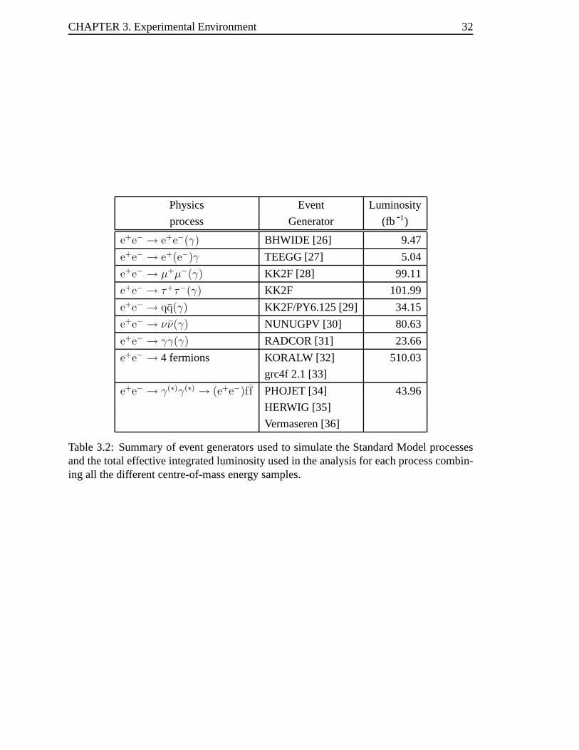
CHAPTER 3. Experimental Environment 32
Physics Event Luminosity
process Generator (fb -1)
e+e− → e+e−(γ) BHWIDE [26] 9.47
e+e− → e+(e−)γ TEEGG [27] 5.04
e+e− → µ+µ−(γ) KK2F [28] 99.11
e+e− → τ+τ−(γ) KK2F 101.99
e+e− → qq(γ) KK2F/PY6.125 [29] 34.15
e+e− → νν(γ) NUNUGPV [30] 80.63
e+e− → γγ(γ) RADCOR [31] 23.66
e+e− → 4 fermions KORALW [32] 510.03
grc4f 2.1 [33]
e+e− → γ(∗)γ(∗) → (e+e−)ff PHOJET [34] 43.96
HERWIG [35]
Vermaseren [36]
Table 3.2: Summary of event generators used to simulate the Standard Model processesand the total effective integrated luminosity used in the analysis for each process combin-ing all the different centre-of-mass energy samples.

Chapter 4
Selection of Candidate Events
This chapter describes the set of criteria used to isolate specific event types expected from
the production and subsequent decay of charged excited leptons. General requirements
applied to all types of events are first presented, followed by a description of the selections
designed to identify events containing two leptons and two photons (`γγ), two leptons
and one photon (``γ) and one electron and one photon (eγ). The selections presented here
were developed specifically for this analysis.
4.1 Preselection
Event final states expected from the production and electromagnetic decay of excited lep-
tons contain no more than two leptons and two photons. These events, in contrast with
multihadronic events1, contain a small number of observed tracks and energy clusters in
the detector, and are selected by requiring at least one but no more than six good tracks
in an event. Good tracks are defined as charged particle trajectories reconstructed from
a large number of hits on consecutive wires in the central tracking detector. Quality re-
quirements are also imposed on electromagnetic and hadronic energy clusters deposited
in the detector. The entire set of track and cluster quality requirements is summarised in
Appendix A.
Collisions between high energy electrons or positrons and remaining gas molecules
in the beam pipe or with the pipe itself can sometimes result in background in the detector.
These beam-gas and beam-wall collisions mostly produce lowenergy secondary particles
that often get absorbed in the few inner layers of the detector leading to short reconstructed
1Events composed of many hadrons. These originate from quarkproducing processes such ase+e− →qq. Due to the nature of the strong force, primary quarks combine with other quarks, created from vacuumfluctuations, to form various types of hadrons in a process known as hadronisation.
33

CHAPTER 4. Selection of Candidate Events 34
tracks that do not point back to the e+e- interaction vertex. These background events are
substantially reduced by requiring that the fraction of thenumber of good tracks to the
total number of tracks reconstructed in the central detector be greater than 0.2
Cosmic rays travelling through or interacting in the detector are a further source of
background events. The background from cosmic rays is reduced to a negligible level
using the timing measurements from the time-of-flight counters and tracking information
from the central tracking detectors. Events are rejected ifthey are not in time with the
beam crossing or if reconstructed tracks do not point back tothe interaction region.
Tracks and energy clusters are grouped together into ‘jets’using the algorithm de-
scribed in [39]. Jets are formed by iteratively looking at individual tracks and energy
clusters, adding together the 4-momentum vectors of every additional object contained
within a cone of 0.25 radians about the direction of the trackor cluster under considera-
tion. If the total energy contained in the cone is greater than 2.5 GeV, then the group of
tracks and energy clusters is identified as a jet. The procedure is repeated until all possible
jets in an event are found. A jet can, but is not required to contain one or more tracks. The
parameters defining a jet were chosen to maximise the efficiency at detecting excited lep-
ton events over the broadest possible range of masses and centre-of-mass energies. Events
containing between two and four jets, inclusive, are retained.
A total of about 2.3 million events are selected by the above criteria out of approxi-
mately 96 million events.
4.2 Jet Classification
Each jet in an event is classified as a type of lepton or photon according to the criteria
described below. The order in which the different classifications are presented represent
the order in which they are applied to each jet. A jet can only be identified as one type of
lepton or a photon.
4.2.1 Photon Identification
Photons travelling through the OPAL detector do not leave hits in the central tracking
system owing to their neutral electric charge. They eventually stop in the electromagnetic
calorimeter, depositing all their energy.
Jets containing a cluster of energy in the electromagnetic calorimeter and no tracks
CHAPTER 4. Selection of Candidate Events 35
are tagged as photons. To ensure that an electromagnetic energy cluster in a jet genuinely
corresponds to a particle, all photon candidates are required to contain a minimum amount
of energy equivalent to 5% of the beam energy. In the forward region of the detector,
photons travel through additional material such as the vertex drift chamber read-out plates
and various types of cables. This additional material increases the probability of photon
interactions and is difficult to model accurately. Therefore, to avoid poorly modelled
regions of the detector, all photon candidates must lie within | cos θ| < 0.9 to be considered
in the rest of the analysis.
At LEP2 energies, approximately 10% of photons interact with material in the detec-
tor prior to entering the electromagnetic calorimeter and convert to an electron-positron
pair. The characteristic signature of a photon conversion is the presence of two oppositely
charged tracks very closed to each other pointing to at leastone cluster of energy in the
electromagnetic calorimeter. A neural network technique [40] developed to identify pho-
ton conversions is used to select these photons2. Jets are identified as a converted photon if
the most energetic track in the jet has a neural network output greater than 0.9, on a scale
from 0 to 1. To reduce the number of fake photon conversions, in particular from hadronic
particles, the associated energy deposited in the hadroniccalorimeter must be less than
10% of the beam energy.
4.2.2 Muon Identification
A jet is considered a muon candidate if it contains exactly one track lying within the larger
angular acceptance of| cos θ| < 0.95. Since muons do not produce electromagnetic show-
ers or interact strongly with matter, the forward region of the detector containing addi-
tional material is well modelled. Typically, muons deposita small amount of energy in the
electromagnetic and hadronic calorimeters before traversing the muon chambers. Muon
candidates are required to contain less than 3 GeV of energy deposited in the electromag-
netic calorimeter. For tracks pointing to the overlap region between the barrel and endcap
parts of the calorimeter, the amount of electromagnetic energy must be less than 5 GeV.
2The neural network [40] uses the information from 9 different variables to judge how likely a pairof tracks resembles what is expected from a real photon conversion. The variables used as input to theneural network are: the distance between the two tracks, theradius of the first measured hit of both tracks,the radius of the reconstructed secondary vertex, the invariant mass of the pair assuming both tracks to beelectrons, the impact parameter of the reconstructed photon with respect to the primary vertex of the event,the momentum of both tracks times the sign of their charge, the output of another neural network trained toidentify electrons applied to the partner track.
CHAPTER 4. Selection of Candidate Events 36
Furthermore, a muon candidate must either have hits in the muon chambers matched with
a track in the central detector or hits in the hadronic calorimeter associated with a track and
consistent with the particle being a muon. Muons that occasionally stop in the hadronic
calorimeter will generally deposit their energy in the lastfew layers of the calorimeter
without producing a large cascade of secondary particles typical of strongly interacting
particles. Thus, jets containing a minimum of four hits in the hadronic calorimeter of
which at least one is located in the last three layers, are considered muon candidates. In
addition, the number of strips per layer hit must be less thantwo corresponding to a very
small number of secondary particles produced.
4.2.3 Electron Identification
Electron candidates must contain exactly one track required to lie within | cos θ| < 0.9 to
avoid, as for photons, poorly modelled regions of the detector. Electrons, unlike muons or
hadrons, generally deposit all their energy in the electromagnetic calorimeter. Thus, for
electrons, the ratio of the electromagnetic energy to the track momentum (E/p) is close
to unity. Jets considered as electron candidates must satisfy 0.8 < E/p < 1.2. Jets that
do not fulfill this requirement can still be selected as electrons if the output from a neural
network [40] designed to identify electrons is greater than0.9. This criteria particularly
improves the detection efficiency for low energy electrons.
4.2.4 Hadronic Tau Lepton Identification
Tau leptons are unstable particles that promptly decay to different numbers and types of
particles. Taus are not directly observed in the detector but only inferred by their decay
products. Taus decaying to leptons3 are tagged as electron or muon candidates by the
criteria described above. Unidentified jets containing at least one track and lying within
| cos θ| < 0.95 are considered to be hadronically decaying tau leptons. Jets satisfying the
electron or photon requirements in the region 0.90< | cos θ| < 0.95 are discarded from
the sample of tau candidates.
3The branching fraction of taus into leptons is about 35%.
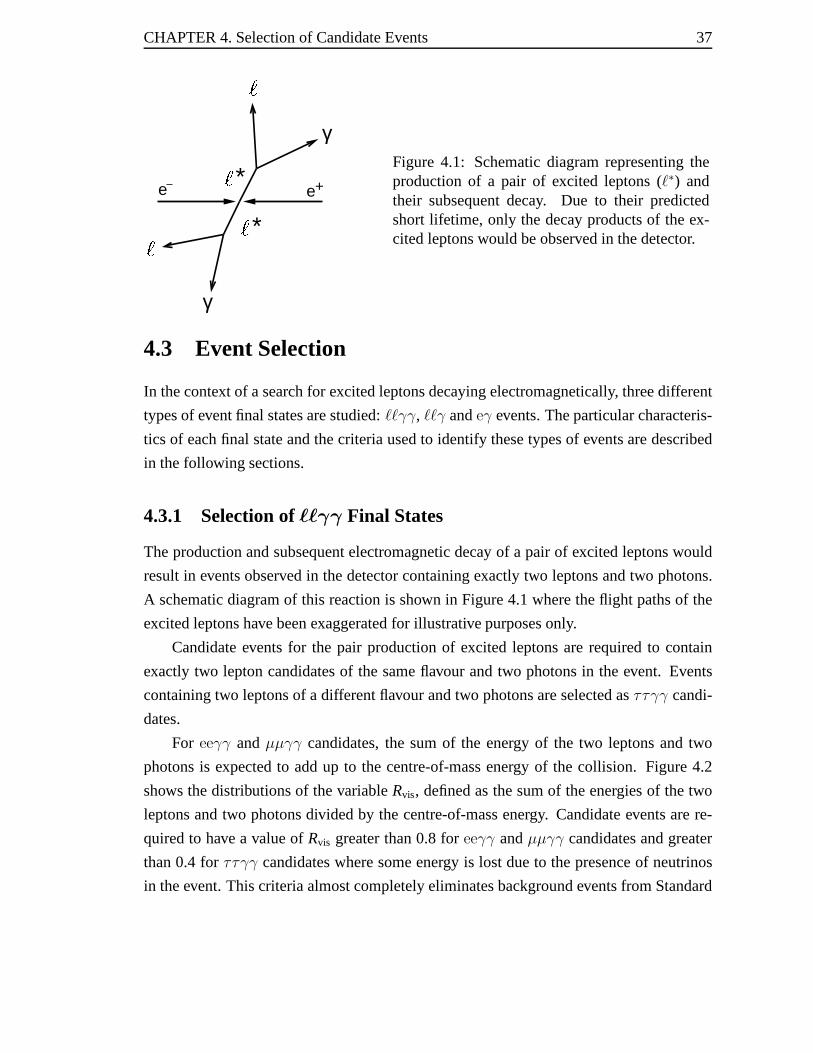
CHAPTER 4. Selection of Candidate Events 37
*
*
γ
γ
ee +
Figure 4.1: Schematic diagram representing theproduction of a pair of excited leptons (`∗) andtheir subsequent decay. Due to their predictedshort lifetime, only the decay products of the ex-cited leptons would be observed in the detector.
4.3 Event Selection
In the context of a search for excited leptons decaying electromagnetically, three different
types of event final states are studied:``γγ, ``γ andeγ events. The particular characteris-
tics of each final state and the criteria used to identify these types of events are described
in the following sections.
4.3.1 Selection of `γγ Final States
The production and subsequent electromagnetic decay of a pair of excited leptons would
result in events observed in the detector containing exactly two leptons and two photons.
A schematic diagram of this reaction is shown in Figure 4.1 where the flight paths of the
excited leptons have been exaggerated for illustrative purposes only.
Candidate events for the pair production of excited leptonsare required to contain
exactly two lepton candidates of the same flavour and two photons in the event. Events
containing two leptons of a different flavour and two photonsare selected asττγγ candi-
dates.
For eeγγ andµµγγ candidates, the sum of the energy of the two leptons and two
photons is expected to add up to the centre-of-mass energy ofthe collision. Figure 4.2
shows the distributions of the variableRvis, defined as the sum of the energies of the two
leptons and two photons divided by the centre-of-mass energy. Candidate events are re-
quired to have a value ofRvis greater than 0.8 foreeγγ andµµγγ candidates and greater
than 0.4 forττγγ candidates where some energy is lost due to the presence of neutrinos
in the event. This criteria almost completely eliminates background events from Standard
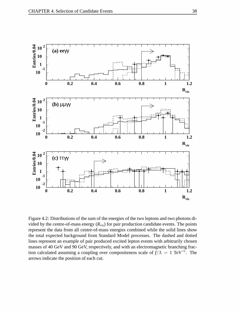
CHAPTER 4. Selection of Candidate Events 38
10-1
1
10
10 2
0 0.2 0.4 0.6 0.8 1 1.2
10-2
10-1
1
10
10 2
0 0.2 0.4 0.6 0.8 1 1.2
Rvis
Ent
ries/
0.04
(a) eeγγ
Rvis
Ent
ries/
0.04
(b) µµγγ
Rvis
Ent
ries/
0.04
(c) ττγγ
10-2
10-1
1
10
10 2
0 0.2 0.4 0.6 0.8 1 1.2
Figure 4.2: Distributions of the sum of the energies of the two leptons and two photons di-vided by the centre-of-mass energy (Rvis) for pair production candidate events. The pointsrepresent the data from all centre-of-mass energies combined while the solid lines showthe total expected background from Standard Model processes. The dashed and dottedlines represent an example of pair produced excited lepton events with arbitrarily chosenmasses of 40 GeV and 90 GeV, respectively, and with an electromagnetic branching frac-tion calculated assuming a coupling over compositeness scale of f/Λ = 1 TeV-1. Thearrows indicate the position of each cut.

CHAPTER 4. Selection of Candidate Events 39
Model two-photon interactions (e+e− → (e+e−)`¯or (e+e−)qq). Two-photon events typ-
ically contains particles produced in the forward region outside the detector acceptance
resulting in events with a large amount of missing energy.
The remaining background in theeeγγ andµµγγ samples is composed almost en-
tirely of Standard Model electron and muon pair events with more than one photon ra-
diated off the leptons. The background in theττγγ sample consists mostly of radiative
τ+τ− events and a small fraction ofqq events. A total of 34, 8 and 13 events in the en-
tire data set are selected aseeγγ, µµγγ andττγγ candidates, respectively. Examples of
candidate events of each type selected by the requirements described above are shown in
Figure 4.3.
4.3.2 Selection of `γ Final States
Events consisting of two leptons and one photon are the characteristic signature expected
from singly produced excited leptons. The schematic diagram of Figure 4.4 illustrates the
mechanism producing such final states.
Events considered as``γ candidates must contain two lepton candidates of the same
flavour and at least one photon. In addition, events with two leptons of a different flavour
and at least one photon are tagged asττγ candidates. If more than one photon is identified
in the event, the most energetic photon is chosen and the other one is ignored. Events
selected as candidates for the pair production of excited leptons by the criteria described
in the previous section are also considered as single production candidates.
Typical eeγ andµµγ events resulting from the single production of excited electrons
and muons are expected to have very little missing energy, i.e. the sum of the energies of
the two leptons and most energetic photon should approximately add up to the centre-of-
mass energy of the e+e- collision. Distributions of the quantityRvis, defined as the sum of
the energies of the two leptons and one photon scaled by the centre-of-mass energy, are
shown in Figure 4.5. Onlyeeγ andµµγ events with a value ofRvis greater than 0.8 are
retained. Due to the presence of neutrinos produced in the decay of tau leptons, events
selected asττγ candidates must have, instead, a value ofRvis greater than 0.4.
The observed discrepancies at small values ofRvis in Figure 4.5(a) and (b) corre-
spond to a region where the background is dominated by leptonic two-photon events (
e+e− → (e+e−) `¯ ). The discrepancy is less pronounced in theττγ sample since ad-
ditional Standard Model processes, such as four-fermion and two-fermion interactions,

CHAPTER 4. Selection of Candidate Events 40
Y
XZ
e+e− → eeγγ
Y
XZ
e+e− → µµγγ
Y
XZ
e+e− → ττγγ
Figure 4.3: Examples ofeeγγ, µµγγ andττγγ candidate events in the data selected bythe criteria described in the text. Each figure shows a cross-section of the OPAL detectorwhere each concentric circle represents the boundary of a detector system. The electron-positron beams travel in the direction perpendicular to theplane of the paper and collide atthe centre of each picture. Lines travelling outward represent tracks produced by chargedparticles. Light and dark grey boxes represent energy deposited in the electromagnetic andhadronic calorimeters, respectively. The size of the boxesis proportional to the amount ofenergy deposited. Arrows indicate hits in the muon chambers. Theeeγγ, µµγγ andττγγevents shown were recorded at a centre-of-mass energy of 188.7, 188.7 and 204.8 GeV,respectively.

CHAPTER 4. Selection of Candidate Events 41
*
γ
e e+
Figure 4.4: Schematic diagram representing theproduction of an excited lepton in association witha Standard Model lepton. The excited lepton isexpected to decay promptly leading to event finalstates containing two leptons and one photon.
contribute in producing events with small values ofRvis. This mis-modelling does not af-
fect the analysis since the event final states of interest liein a region ofRvis that is well
modelled.
The background in theeeγ sample is further reduced by requiring that the angle be-
tween the most energetic electron and photon (θeγ) be greater than 900. Figure 4.6 shows
theθeγ distribution obtained for all data combined and for two different masses of excited
electron events. The expected angleθeγ measured for signal events depends on the mass of
the excited electron produced. For masses close to the kinematic limit, the excited electron
would be produced almost at rest in association with a low energy electron, resulting in
its decay products travelling mostly back-to-back. Conversely, an excited electron with a
smaller mass would be produced with a non-negligible momentum fraction resulting in its
decay products being boosted in its momentum direction. Theelectron recoiling against
the excited electron, in this case, could also have higher energy than the electron produced
by the decay of the excited state. For small masses, theθeγ distribution expected from
the production of excited electrons is thus broader and has asmaller mean angle than for
larger excited lepton masses. The search for singly produced excited leptons primarily
focuses on excited states with masses greater than about 90 GeV, as smaller masses would
be observed in the pair production search. The cut position allows one to reduce the back-
ground from e+e- events without loss in signal detection efficiency for high excited lepton
masses.
The sample ofττγ events contains background from e+e- andµ+µ− events where one
electron or muon is misidentified. Electron pair events deposit most of their energy in the
electromagnetic calorimeter while muon pair events deposit only very little energy. Since
tau leptons decay to different types of particles,ττγ events are expected to contain on av-

CHAPTER 4. Selection of Candidate Events 42
10-1
1
10
10 210 3
0 0.2 0.4 0.6 0.8 1 1.2
10-1
1
10
10 2
0 0.2 0.4 0.6 0.8 1 1.2
Rvis
Ent
ries/
0.04
(a) eeγ
Rvis
Ent
ries/
0.04
(b) µµγ
Rvis
Ent
ries/
0.04 (c) ττγ
10-1
1
10
10 210 310 4
0 0.2 0.4 0.6 0.8 1 1.2
Figure 4.5: Distributions of the sum of the energies of the two leptons and one photondivided by the centre-of-mass energy (Rvis) for ``γ candidate events before applying se-lection cuts. The points represent the data from all centre-of-mass energies combinedwhile the solid lines show the total expected background from Standard Model processes.The dashed and dotted lines represent an example of excited lepton events with arbitrarilychosen masses of 90 GeV and 180 GeV, respectively, and with anelectromagnetic branch-ing fraction calculated assuming a coupling over compositeness scale off/Λ = 5 TeV-1.The arrows indicate the position of each cut.
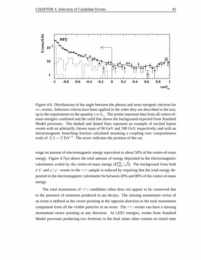
CHAPTER 4. Selection of Candidate Events 43
cosθeγ
Eve
nts/
0.04
eeγ
1
10
10 2
-1 -0.8 -0.6 -0.4 -0.2 0 0.2 0.4 0.6 0.8 1
Figure 4.6: Distributions of the angle between the photon and most energetic electron foreeγ events. Selection criteria have been applied in the order they are described in the text,up to the requirement on the quantitycos θeγ . The points represent data from all centre-of-mass energies combined and the solid line shows the background expected from StandardModel processes. The dashed and dotted lines represent an example of excited leptonevents with an arbitrarily chosen mass of 90 GeV and 180 GeV, respectively, and with anelectromagnetic branching fraction calculated assuming acoupling over compositenessscale of f/Λ = 5 TeV-1. The arrow indicates the position of the cut.
erage an amount of electromagnetic energy equivalent to about 50% of the centre-of-mass
energy. Figure 4.7(a) shows the total amount of energy deposited in the electromagnetic
calorimeter scaled by the centre-of-mass energy (EEMtotal/
√s). The background from both
e+e- andµ+µ− events in theττγ sample is reduced by requiring that the total energy de-
posited in the electromagnetic calorimeter be between 20% and 80% of the centre-of-mass
energy.
The total momentum ofττγ candidates often does not appear to be conserved due
to the presence of neutrinos produced in tau decays. The missing momentum vector of
an event is defined as the vector pointing in the opposite direction to the total momentum
component from all the visible particles in an event. Theττγ events can have a missing
momentum vector pointing in any direction. At LEP2 energies, events from Standard
Model processes producing two fermions in the final states often contain an initial state
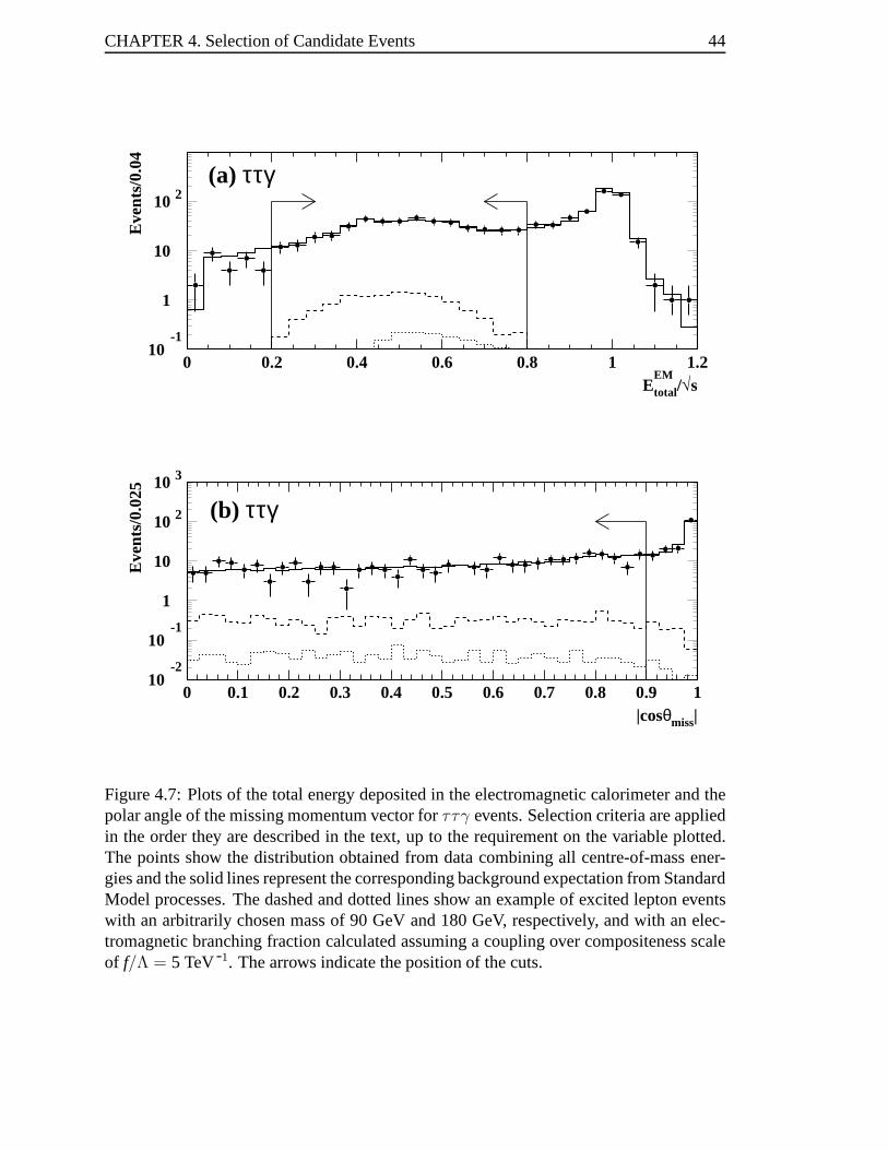
CHAPTER 4. Selection of Candidate Events 44
EEM
total/√s
Eve
nts/
0.04
(a) ττγ
10-1
1
10
10 2
0 0.2 0.4 0.6 0.8 1 1.2
|cosθmiss|
Eve
nts/
0.02
5
(b) ττγ
10-2
10-1
1
10
10 2
10 3
0 0.1 0.2 0.3 0.4 0.5 0.6 0.7 0.8 0.9 1
Figure 4.7: Plots of the total energy deposited in the electromagnetic calorimeter and thepolar angle of the missing momentum vector forττγ events. Selection criteria are appliedin the order they are described in the text, up to the requirement on the variable plotted.The points show the distribution obtained from data combining all centre-of-mass ener-gies and the solid lines represent the corresponding background expectation from StandardModel processes. The dashed and dotted lines show an exampleof excited lepton eventswith an arbitrarily chosen mass of 90 GeV and 180 GeV, respectively, and with an elec-tromagnetic branching fraction calculated assuming a coupling over compositeness scaleof f/Λ = 5 TeV-1. The arrows indicate the position of the cuts.
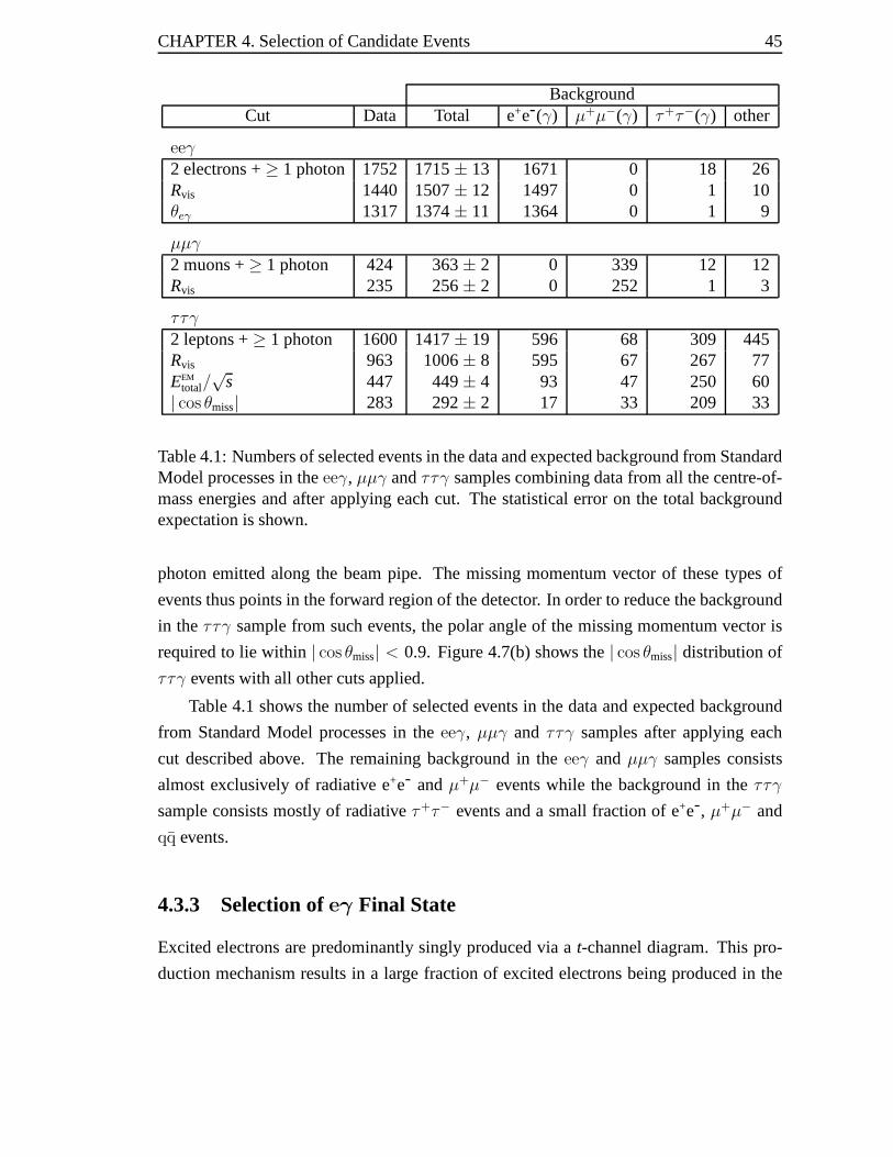
CHAPTER 4. Selection of Candidate Events 45
BackgroundCut Data Total e+e-(γ) µ+µ−(γ) τ+τ−(γ) other
eeγ2 electrons +≥ 1 photon 1752 1715± 13 1671 0 18 26Rvis 1440 1507± 12 1497 0 1 10θeγ 1317 1374± 11 1364 0 1 9
µµγ2 muons +≥ 1 photon 424 363± 2 0 339 12 12Rvis 235 256± 2 0 252 1 3
ττγ2 leptons +≥ 1 photon 1600 1417± 19 596 68 309 445Rvis 963 1006± 8 595 67 267 77EEM
total/√
s 447 449± 4 93 47 250 60| cos θmiss| 283 292± 2 17 33 209 33
Table 4.1: Numbers of selected events in the data and expected background from StandardModel processes in theeeγ, µµγ andττγ samples combining data from all the centre-of-mass energies and after applying each cut. The statistical error on the total backgroundexpectation is shown.
photon emitted along the beam pipe. The missing momentum vector of these types of
events thus points in the forward region of the detector. In order to reduce the background
in theττγ sample from such events, the polar angle of the missing momentum vector is
required to lie within| cos θmiss| < 0.9. Figure 4.7(b) shows the| cos θmiss| distribution of
ττγ events with all other cuts applied.
Table 4.1 shows the number of selected events in the data and expected background
from Standard Model processes in theeeγ, µµγ and ττγ samples after applying each
cut described above. The remaining background in theeeγ andµµγ samples consists
almost exclusively of radiative e+e- andµ+µ− events while the background in theττγ
sample consists mostly of radiativeτ+τ− events and a small fraction of e+e-, µ+µ− and
qq events.
4.3.3 Selection ofeγ Final State
Excited electrons are predominantly singly produced via at-channel diagram. This pro-
duction mechanism results in a large fraction of excited electrons being produced in the
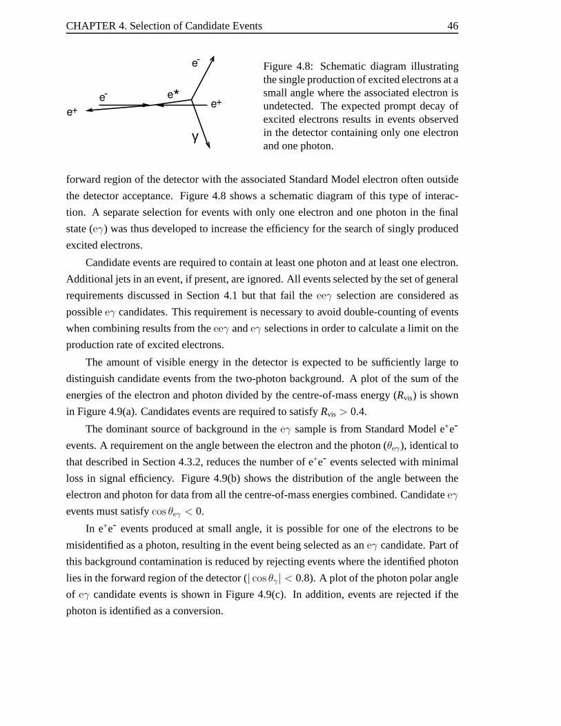
CHAPTER 4. Selection of Candidate Events 46
e-
e+e+
e
e-
*
γ
Figure 4.8: Schematic diagram illustratingthe single production of excited electrons at asmall angle where the associated electron isundetected. The expected prompt decay ofexcited electrons results in events observedin the detector containing only one electronand one photon.
forward region of the detector with the associated StandardModel electron often outside
the detector acceptance. Figure 4.8 shows a schematic diagram of this type of interac-
tion. A separate selection for events with only one electronand one photon in the final
state (eγ) was thus developed to increase the efficiency for the searchof singly produced
excited electrons.
Candidate events are required to contain at least one photonand at least one electron.
Additional jets in an event, if present, are ignored. All events selected by the set of general
requirements discussed in Section 4.1 but that fail theeeγ selection are considered as
possibleeγ candidates. This requirement is necessary to avoid double-counting of events
when combining results from theeeγ andeγ selections in order to calculate a limit on the
production rate of excited electrons.
The amount of visible energy in the detector is expected to besufficiently large to
distinguish candidate events from the two-photon background. A plot of the sum of the
energies of the electron and photon divided by the centre-of-mass energy (Rvis) is shown
in Figure 4.9(a). Candidates events are required to satisfyRvis > 0.4.
The dominant source of background in theeγ sample is from Standard Model e+e-
events. A requirement on the angle between the electron and the photon (θeγ), identical to
that described in Section 4.3.2, reduces the number of e+e- events selected with minimal
loss in signal efficiency. Figure 4.9(b) shows the distribution of the angle between the
electron and photon for data from all the centre-of-mass energies combined. Candidateeγ
events must satisfycos θeγ < 0.
In e+e- events produced at small angle, it is possible for one of the electrons to be
misidentified as a photon, resulting in the event being selected as aneγ candidate. Part of
this background contamination is reduced by rejecting events where the identified photon
lies in the forward region of the detector (| cos θγ | < 0.8). A plot of the photon polar angle
of eγ candidate events is shown in Figure 4.9(c). In addition, events are rejected if the
photon is identified as a conversion.
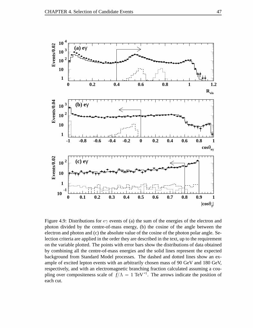
CHAPTER 4. Selection of Candidate Events 47
1
10
10 2
10 3
10 4
0 0.2 0.4 0.6 0.8 1 1.2
1
10
10 2
10 3
-1 -0.8 -0.6 -0.4 -0.2 0 0.2 0.4 0.6 0.8 1
Rvis
Eve
nts/
0.02 (a) eγ
cosθeγ
Eve
nts/
0.04 (b) eγ
|cosθγ|
Eve
nts/
0.02
(c) eγ
10-1
1
10
10 2
0 0.1 0.2 0.3 0.4 0.5 0.6 0.7 0.8 0.9 1
Figure 4.9: Distributions foreγ events of (a) the sum of the energies of the electron andphoton divided by the centre-of-mass energy, (b) the cosineof the angle between theelectron and photon and (c) the absolute value of the cosine of the photon polar angle. Se-lection criteria are applied in the order they are describedin the text, up to the requirementon the variable plotted. The points with error bars show the distributions of data obtainedby combining all the centre-of-mass energies and the solid lines represent the expectedbackground from Standard Model processes. The dashed and dotted lines show an ex-ample of excited lepton events with an arbitrarily chosen mass of 90 GeV and 180 GeV,respectively, and with an electromagnetic branching fraction calculated assuming a cou-pling over compositeness scale off/Λ = 1 TeV-1. The arrows indicate the position ofeach cut.
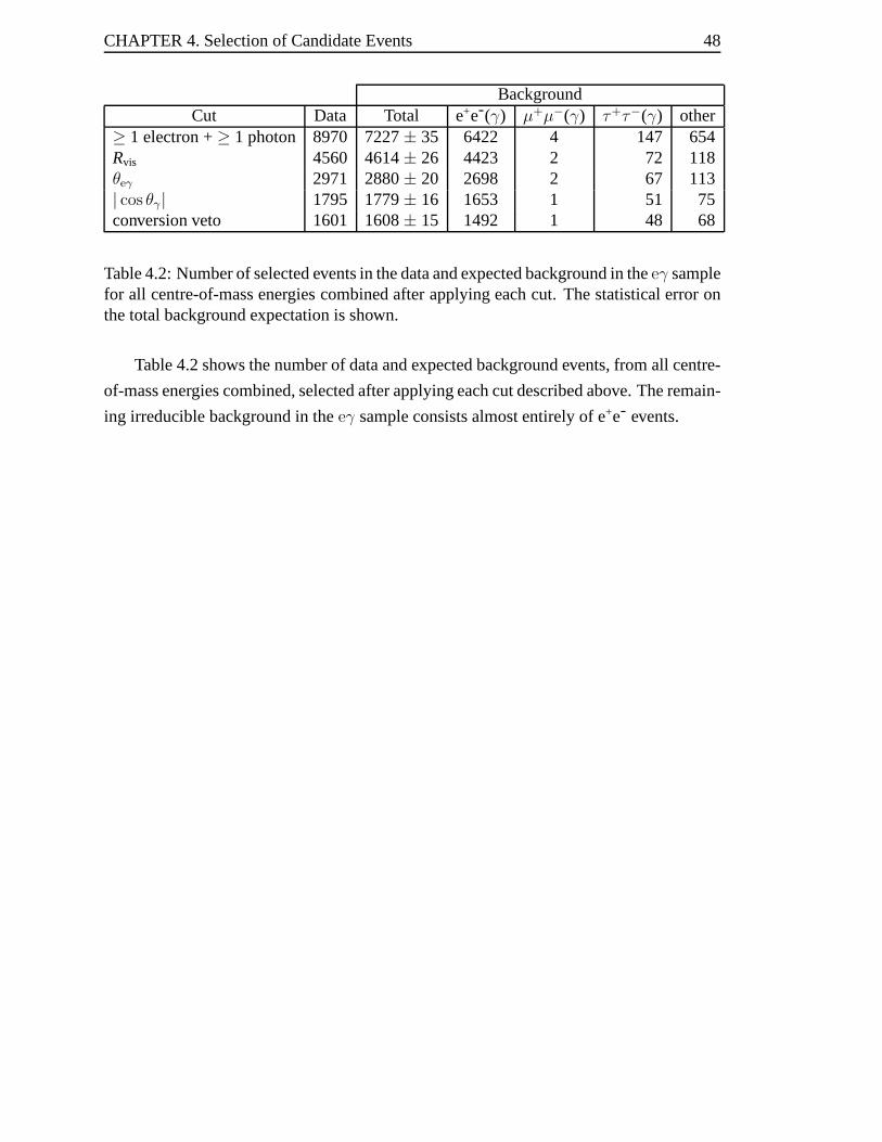
CHAPTER 4. Selection of Candidate Events 48
BackgroundCut Data Total e+e-(γ) µ+µ−(γ) τ+τ−(γ) other
≥ 1 electron +≥ 1 photon 8970 7227± 35 6422 4 147 654Rvis 4560 4614± 26 4423 2 72 118θeγ 2971 2880± 20 2698 2 67 113| cos θγ | 1795 1779± 16 1653 1 51 75conversion veto 1601 1608± 15 1492 1 48 68
Table 4.2: Number of selected events in the data and expectedbackground in theeγ samplefor all centre-of-mass energies combined after applying each cut. The statistical error onthe total background expectation is shown.
Table 4.2 shows the number of data and expected background events, from all centre-
of-mass energies combined, selected after applying each cut described above. The remain-
ing irreducible background in theeγ sample consists almost entirely of e+e- events.
Chapter 5
Kinematic Fits
This chapter explains the kinematic fit technique used to improve the sensitivity of the
search for excited leptons. A general description of this technique is first presented, fol-
lowed by details of the particular implementation used in this analysis. This is the first
time kinematic fits are used in the context of a search for excited leptons. The devel-
opment and implementation of the fits used in this analysis are the original work of the
author.
5.1 Motivation
The existence of excited leptons would reveal itself as an excess of events with identical`γ
reconstructed invariant mass. A kinematic fit technique is used in this analysis to improve
the estimates of the energy and direction of the particles inan event. This information is
then used to calculate precisely the invariant mass of each possible`γ pair in an event.
The improvements in the mass resolution result in an increase in the search sensitivity and
discriminating power between background and excited lepton events.
5.2 General Principles
A kinematic fit is a technique used to improve the values of measured parameters and
provide estimates of unknown quantities by exploiting the known physical properties of
the observed process. The technique consists of finding the optimal solution to a set of
equations satisfying external constraints.
Given a set of measured parametersα with an associated covariance matrixV, the
49
CHAPTER 5. Kinematic Fits 50
problem consists of finding a new set of parametersα that minimises
χ2 = (α − α)T V -1 (α − α) (5.1)
but also satisfies the set of constraint equations given byg(α, p) wherep is a vector of
unmeasured parameters. The superscript T represents a transposed vector. The constraint
equations can be incorporated in the problem using Lagrangemultipliers [41],λ, and the
function to minimise becomes
L = (α − α)T V-1(α − α) + 2λTg(α, p) . (5.2)
The new parametersα, p andλ that minimise this function are in general found using an
iterative procedure. The initial estimates of both measured and unmeasured parameters
are updated, at each iteration, by small corrections until some criteria of convergence are
achieved. The criteria of convergence should ensure that a minimum in the functionL is
reached and that the constraints equations are satisfied. Inthis analysis, a kinematic fit
is chosen to converge when∆χ2/χ2 < 10-4, ∆(2λTg) < 10-3 and (2λTg)/χ2 < 10-2
where∆ represents the change in a given quantity between two iterations. The solution to
this minimisation problem is described in Appendix B.
When the convergence criteria are satisfied, the functionL reduces to theχ2 value
of the measured parameters. Thisχ2 value is often used to test the goodness of the fit by
quoting the probability that the physical process studied would lead to aχ2 value worse
(i.e. greater) than the one obtained. This probability is defined as
P =∫ ∞
χ2f (z, n) dz (5.3)
where the functionf (z, n) is theχ2 distribution withn degrees of freedom. The number of
degrees of freedom in the type of problem studied here is given by the number of constraint
equations minus the number of unmeasured parameters. The probabilistic interpretation of
theχ2 value is only valid if, as it is usually the case, the distribution of the residuals (α −α) does not deviate strongly from a Gaussian distribution. The data are usually deemed
consistent with the fit assumptions when the probability is greater than approximately
6×10⁻⁵ or 6×10⁻⁷ (or equivalently 4 to 5 standard deviations for a Gaussian distribution).
The value of the cut on the probability distribution should be carefully chosen as to
not bias the sample of selected events by preferentially rejecting events with a particular
CHAPTER 5. Kinematic Fits 51
kinematic configuration such as, for example, low momentum tracks. A linear plot of the
probability distribution of a kinematic fit should be flat with a peak near zero correspond-
ing to background physics processes. The uniformity of the probability distribution is an
indicator that the input parameters of the fit are not biased and that their errors are cor-
rectly estimated. Reliable estimates of parameters are obtained using a kinematic fit only
if the errors on the input quantities are realistic.
5.3 Inputs
In the context of particle interactions, the measured parameters taken as input to a kine-
matic fit generally consist of the energy and direction of each particle in the event. In
addition, an estimate of the error on each measured parameter is needed to calculate the
covariance matrix used in the fit. In this analysis, the correlations between the different
measured quantities are small and hence neglected. As a consequence, the covariant ma-
trix V is diagonal. The following sections describe in detail the specific input quantities
used in the kinematic fits for each type of jet.
The measured centre-of-mass energy of each event is also treated as an input parame-
ter of the fit. This is a unique feature of the fits performed in this analysis. The uncertainty
on the centre-of-mass energy is taken to be the LEP centre-of-mass energy spread which
is approximately 250 MeV [9]. The expected mass resolution of excited leptons is of the
same order of magnitude as the spread in centre-of-mass energy. Thus this method en-
sures that results from a kinematic fit do not lead to mass resolutions better than what is
experimentally achievable.
5.3.1 Photon Candidates
The energy of photon candidates is taken to be the energy contained in the jet deposited in
the electromagnetic calorimeter. Since photons do not leave tracks in the central detector,
the direction, expressed in terms of the polar (θ) and azimuthal (φ) angles, is given by the
position of the observed electromagnetic energy cluster.
The resolutions and uncertainties of the energy and position of an electromagnetic
cluster are measured using electron pair events, as described in Appendix C. Photons are
expected to have similar properties to electrons. The energy resolution is typically 2 GeV
for a 45 GeV photon and the angular resolution is approximately 4 mrad inθ and 3.5 mrad

CHAPTER 5. Kinematic Fits 52
in φ.
5.3.2 Electron Candidates
Electrons are similar to photons in that they deposit all their energy in the electromagnetic
calorimeter. Therefore, the measured electromagnetic energy associated with an electron
candidate provides a good estimate of the energy of that electron. As for photons, the
uncertainty on the measured energy is about 2 GeV for a 45 GeV electron.
The direction of electron candidates is given by the polar and azimuthal angles of the
reconstructed track in the central detector contained in the jet. Appendix C describes in
detail a parameterisation of the angular resolution performed using events containing two
back-to-back tracks. The uncertainties on the measured polar and azimuthal angles of a
track are obtained from this parameterisation of the tracking detector resolution and are
found to be approximately 2 mrad and 0.4 mrad respectively.
5.3.3 Muon Candidates
The parameters used as input to the kinematic fit are the momentum, polar and azimuthal
angles of the track contained in jets identified as muons. Theerror on the track momentum
as obtained by the OPAL track reconstruction fitting algorithm was found to be a good
estimate of the tracking detector momentum resolution and is therefore used as input to
the kinematic fit. For muon candidates selected in this analysis, the uncertainty on the
track momentum is approximately 5 GeV for a 45 GeV muon. The uncertainties on the
polar and azimuthal angles of tracks identified as muons are identical to the ones obtained
for electron candidates.
5.3.4 Tau Candidates
The kinematic fit input parameters for tau jets do not depend on the specific type of tau
decay. Input parameters for leptonically and hadronicallydecaying taus are calculated
from the same kinematic variables.
The energy deposited in the detector is not representative of the actual tau energy due
to the presence of undetected neutrinos produced when a tau particle decays. Thus, for
kinematic fits performed onττγ andττγγ events, the energy of the two jets assumed to

CHAPTER 5. Kinematic Fits 53
originate from tau leptons is treated as an unknown parameter. The jet energy is only used
as an initial estimate of the tau energy.
Despite the production of neutrinos in tau decays, the axis of the observed decay
products is in general a good estimate of the tau direction. This is especially true for
high energy taus where the decay products are strongly boosted in the tau flight direction.
The polar and azimuthal angles of a jet main axis are used as input to the kinematic fits.
An estimate of the uncertainties on the polar and azimuthal angles due to the presence of
additional undetected neutrinos as well as from the finite detector resolution are obtained
from studies of tau pair events as described in Appendix C. Itwas determined that the
direction of a tau is known to approximately 7 mrad in both polar and azimuthal angles.
5.4 General Constraints
Events selected by the criteria described in the previous chapter are required to satisfy
energy and momentum conservation.
The three constraint equations requiring the total momentum of each event to be con-
served can be mathematically written in terms of the kinematic fit input variables as
g1 =n∑
i=1
pi sin θi cos φi = 0 (5.4)
g2 =n∑
i=1
pi sin θi sin φi = 0 (5.5)
g3 =n∑
i=1
pi cos θi = 0 (5.6)
where the scalar momentum of a particle is related to its massand energy through the
relationp =√
E2 − m2. The sum runs over the number of particlesn considered in the
event.
Conservation of energy is enforced by requiring events to satisfy the constraint equa-
tion
g4 =n∑
i=1
Ei −√
s = 0 (5.7)
whereEi are the energy of each particle in the event and√
s represents the centre-of-mass
energy of the e+e- collision which is treated as a fit parameter and thus allowedto vary
within the measured spread in beam energy.

CHAPTER 5. Kinematic Fits 54
5.5 Kinematic Fits for Each Event Final States
The following sections describe the different kinematic fits applied to each type of event
final state. Since the direction of the particles is in general more precisely known than their
energy, the angles of the particles in an event usually determine whether a kinematic fit
will or will not converge under a given set of constraints. Inthis analysis, events are judged
consistent with an the physics process considered if the fit probability is greater than 0.001.
The value 0.001 is chosen to retain a maximum number of eventswhile rejecting the ones
that are obviously incompatible with the final states of interest. Distributions of various fit
probabilities are presented later.
5.5.1 Kinematic Fits for ``γγ Events
For pair produced excited lepton events, the reconstructedinvariant mass of the twoγ
pairs originating from the decay of each excited lepton should be equal within the precision
of the detector’s measurements. Thus, in addition to the general constraints described
above, `γγ events are also required to satisfy
g5 = m`1γ1 − m`2γ2
=√
(E`1 + Eγ1)2 − (p`1
+ pγ1)2 −
√
(E`2 + Eγ2)2 − (p`2
+ pγ2)2 (5.8)
= 0
where the subscripts are used to identify each lepton and photon in the event. For each
event, two kinematic fits are performed corresponding to thetwo possible γ pairings used
to calculate the invariant masses. The constraint equationg5 in the second fit performed is
obtained by simply interchanging changing`1 ↔ `2.
In high energy e+e- collisions, initial state photon radiation is often produced, re-
ducing the effective centre-of-mass energy of the collision. These photons are generally
emitted nearly collinear to one of the beams, escaping detection. In order to account for
this physical phenomenon, an additional kinematic fit, for each`γ pairing, is performed
assuming the presence of an undetected initial state photonalong the beam axis. The mo-
mentum of the photon in thex andy direction is assumed to be zero while thezcomponent
(pz) is treated as an unknown parameter of the fit. An initial estimate ofpz is calculated by
enforcing conservation of momentum in thez direction. The angular region allowed for
initial state photon is expressed in terms of the parametersδx andδy which represent small
CHAPTER 5. Kinematic Fits 55
distances away from the beam axis in thex andy direction as measured at the entrance
of the endcap electromagnetic calorimeter. In the kinematic fit, the quantitiesδx andδy
are treated as measured parameters with initial values of zero and variances given by the
radius of the beam pipe.
For each selected γγ event, a total of four kinematic fits are therefore performed:
one fit with and without assuming the presence of an initial state photon radiation for each
two possible γ pairings. Only one fit per event is chosen. If every kinematicfit attempted
fails to have a probability greater than 0.001, then the event is rejected. When more than
one successful kinematic fit is obtained for an event, then the fits performed without the
presence of an initial state photon radiation are first considered. Theγ pairing giving the
highest successful fit probability without the presence of an initial state photon is chosen
regardless of the probability of the other fits. Otherwise, the`γ pairing giving the highest
probability assuming the presence of an initial state photon is chosen.
This algorithm for choosing the most appropriate kinematicfit is constructed to min-
imise distortions of the invariant mass distribution of signal events from a pure Gaussian.
By construction, events for which a fit without an initial state photon converges, also suc-
cessfully pass the corresponding fit assuming the presence of an additional photon down
the beam pipe. In the second case, the initial state photon issimply assigned a small
amount of energy. These types of events, however, do not contain a genuine initial state
photon and the reconstructed invariant mass would be smaller than the actual invariant
mass since some energy is assigned to the initial state photon. This effect is clearly shown
in Figure 5.1. To obtain the best estimate of the actual invariant mass of eachγ pairing,
the fit without assuming the presence of an initial state photon is therefore favoured. Re-
sults from the fit with an additional photon along the beam axis are only chosen when other
fits fail. This indicates that the event most likely containsa genuine initial state photon
and that the reconstructed invariant mass represents the actual mass of theγ system.
Figure 5.2 shows the probability distributions of the chosen fit for eeγγ, µµγγ and
ττγγ events. Since no Standard Model processes consistently produce events with two
identical`γ invariant masses, only a very small fraction of``γγ events have at least one
successful fit. The requirement on the kinematic fit probability (P > 0.001) reduces the
number of selected events by more than 70%. The expected massresolution of excited
lepton events depends on the mass of the excited lepton and onthe centre-of-mass energy.
Typical mass resolutions of 0.2 GeV, 0.2 GeV and 0.8 GeV are obtained for excited elec-
trons, muons and taus, respectively. The use of kinematic fits improves the expected mass

CHAPTER 5. Kinematic Fits 56
µ* µ*
mµγ (GeV)
Eve
nts/
0.1
GeV
0102030405060708090
88 89 90 91
Figure 5.1: Example of reconstructed`γ invariant mass of pair produced ex-cited muons simulated with an arbi-trarily chosen mass of 90 GeV. Thesolid (dashed) line shows the invariantmass obtained using results from the fitwith (without) the presence of an ini-tial state photon radiation. Only eventsfor which both types of fit converge areshown here.
resolution of pair produced excited leptons by more than an order of magnitude.
5.5.2 Kinematic Fits for ``γ Events
Events selected as candidates for the single production of excited leptons are only required
to satisfy the general constraints of energy and momentum conservation. Following the
same approach as outlined in the previous section, a total oftwo kinematic fits are per-
formed for each `γ event. In the first case, only the two leptons and one photon are
included in the fit. In the second case, the fit is performed assuming the presence of an
initial state photon radiation along the beam axis. If both fits attempted fail to have a prob-
ability greater than 0.001, the event is rejected. If more than one fit successfully converges,
the fit performed without the presence of an initial state photon is chosen given that the fit
probability is greater than 0.001. Otherwise, results fromthe fit performed assuming the
presence of an additional photon along the beam axis is used.The kinematic fit performed
without assuming the presence of an initial state photon is favoured in order to reduce bias
in the`γ reconstructed invariant mass as shown in Figure 5.3.
Figure 5.4 shows the probability distributions of selected``γ events where the prob-
ability is taken to be that of the chosen fit on an event by eventbasis. The requirement on
the fit probability reduces the number of selected events by about 10%. Approximately
30% of these events are selected assuming the presence of an initial state photon. Using
results from the chosen fit, mass resolutions of approximately 0.35 GeV, 0.4 GeV and
1.8 GeV are obtained for excited electrons, muons and taus respectively, which amounts
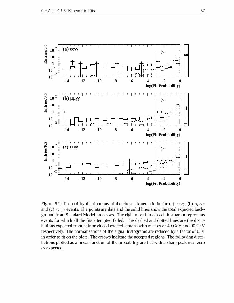
CHAPTER 5. Kinematic Fits 57
log(Fit Probability)
Ent
ries/
0.5
(a) eeγγ
log(Fit Probability)
Ent
ries/
0.5
(b) µµγγ
log(Fit Probability)
Ent
ries/
0.5
(c) ττγγ
10-2
10-1
1
10
10 2
-14 -12 -10 -8 -6 -4 -2 0
10-2
10-1
1
10
10 2
-14 -12 -10 -8 -6 -4 -2 0
10-2
10-1
1
10
10 2
-14 -12 -10 -8 -6 -4 -2 0
Figure 5.2: Probability distributions of the chosen kinematic fit for (a) eeγγ, (b) µµγγand (c)ττγγ events. The points are data and the solid lines show the totalexpected back-ground from Standard Model processes. The right most bin of each histogram representsevents for which all the fits attempted failed. The dashed anddotted lines are the distri-butions expected from pair produced excited leptons with masses of 40 GeV and 90 GeVrespectively. The normalisations of the signal histogramsare reduced by a factor of 0.01in order to fit on the plots. The arrows indicate the accepted regions. The following distri-butions plotted as a linear function of the probability are flat with a sharp peak near zeroas expected.
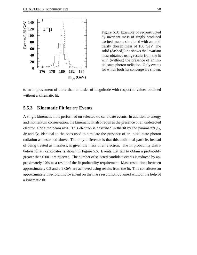
CHAPTER 5. Kinematic Fits 58
µ* µ
mµγ (GeV)
Eve
nts/
0.25
GeV
0
20
40
60
80
100
120
140
176 178 180 182 184
Figure 5.3: Example of reconstructed`γ invariant mass of singly producedexcited muons simulated with an arbi-trarily chosen mass of 180 GeV. Thesolid (dashed) line shows the invariantmass obtained using results from the fitwith (without) the presence of an ini-tial state photon radiation. Only eventsfor which both fits converge are shown.
to an improvement of more than an order of magnitude with respect to values obtained
without a kinematic fit.
5.5.3 Kinematic Fit for eγ Events
A single kinematic fit is performed on selectedeγ candidate events. In addition to energy
and momentum conservation, the kinematic fit also requires the presence of an undetected
electron along the beam axis. This electron is described in the fit by the parameterspz,
δx andδy, identical to the ones used to simulate the presence of an initial state photon
radiation as described above. The only difference is that this additional particle, instead
of being treated as massless, is given the mass of an electron. The fit probability distri-
bution for eγ candidates is shown in Figure 5.5. Events that fail to obtaina probability
greater than 0.001 are rejected. The number of selected candidate events is reduced by ap-
proximately 10% as a result of the fit probability requirement. Mass resolutions between
approximately 0.5 and 0.9 GeV are achieved using results from the fit. This constitutes an
approximately five-fold improvement on the mass resolutionobtained without the help of
a kinematic fit.

CHAPTER 5. Kinematic Fits 59
log(Fit Probability)
Ent
ries/
0.5
(a) eeγ
log(Fit Probability)
Ent
ries/
0.5
(b) µµγ
log(Fit Probability)
Ent
ries/
0.5
(c) ττγ
1
10
10 2
10 3
-14 -12 -10 -8 -6 -4 -2 0
10-2
10-1
1
10
10 210 3
-14 -12 -10 -8 -6 -4 -2 0
10-2
10-1
1
10
10 210 3
-14 -12 -10 -8 -6 -4 -2 0
Figure 5.4: Probability distributions of the chosen kinematic fit for (a) eeγ, (b) µµγ and(c) ττγ events. The points are data and the solid lines show the totalexpected backgroundfrom Standard Model processes. The last bin of each histogram on the right representsevents for which all the fit attempted failed. The dashed and dotted lines are the distribu-tions expected from singly produced excited leptons with masses of 90 GeV and 180 GeVrespectively. The signal histograms are normalised to a ratio of the coupling constant tothe compositeness scale (f/Λ) of 1 TeV-1. The arrows indicate the accepted regions. Thefollowing distributions plotted as a linear function of probability are flat with a sharp peaknear zero as expected.
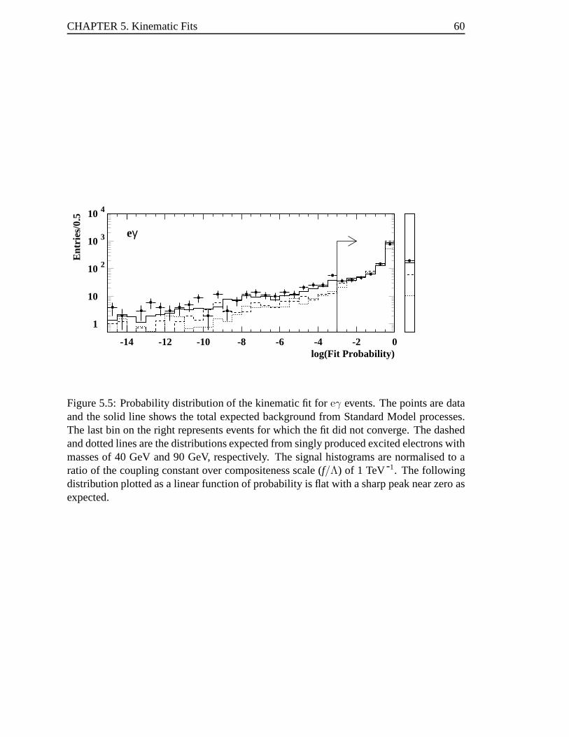
CHAPTER 5. Kinematic Fits 60
log(Fit Probability)
Ent
ries/
0.5
eγ
1
10
10 2
10 3
10 4
-14 -12 -10 -8 -6 -4 -2 0
Figure 5.5: Probability distribution of the kinematic fit for eγ events. The points are dataand the solid line shows the total expected background from Standard Model processes.The last bin on the right represents events for which the fit did not converge. The dashedand dotted lines are the distributions expected from singlyproduced excited electrons withmasses of 40 GeV and 90 GeV, respectively. The signal histograms are normalised to aratio of the coupling constant over compositeness scale (f/Λ) of 1 TeV-1. The followingdistribution plotted as a linear function of probability isflat with a sharp peak near zero asexpected.
Chapter 6
Results
The first section of this chapter summarises results obtained after applying the event se-
lections and kinematic fits described in Chapter 4 and Chapter 5. The procedure used to
interpret the results and calculate constraints on parameters of the excited lepton model
are then described in detail. The last part of the chapter is devoted to a comparison of the
limits calculated in this thesis to existing bounds obtained by other experiments.
6.1 Results
After applying the event selections and kinematic fits described in Chapter 4 and Chap-
ter 5, the numbers of events observed in the data and the corresponding numbers of back-
ground events expected from Standard Model processes are presented in Tables 6.2 and
6.1. Both the statistical and systematic uncertainties on the background estimates are
shown in those tables. A description of the various sources of systematic uncertainties
investigated is presented in Section 6.3.3. The number of candidate events selected for
each type of final state is compatible with expectations fromthe Standard Model.
Figures 6.1, 6.2 and 6.3 show the invariant mass distributions of selected`γγ, ``γ,
andeγ events obtained using results from the kinematic fits. In Figure 6.2, there are two
entries per event corresponding to the two possible`γ pairings. The presence of excited
leptons would appear as an excess of events forming a peak in the reconstructed invariant
mass distributions.
No evidence for excited leptons is found in either the singleor pair production search.
The results are therefore used to calculate constraints on parameters of the excited lepton
model introduced in Chapter 2. Details pertinent to the limit calculation procedure are
presented in the next sections.
61

CHAPTER 6. Results 62
<√
s> eeγγ µµγγ ττγγ(GeV) data bkg data bkg data bkg
182.66 0 0.2± 0.1± 0.1 0 0.3± 0.0± 0.1 0 1.0± 0.2± 0.8188.63 1 1.8± 0.4± 0.6 1 0.5± 0.1± 0.2 2 2.2± 0.3± 1.7191.59 0 0.4± 0.1± 0.1 0 0.1± 0.0± 0.0 0 0.3± 0.1± 0.3195.53 0 0.2± 0.1± 0.1 0 0.1± 0.0± 0.1 0 0.9± 0.1± 0.7199.52 1 0.6± 0.2± 0.2 0 0.2± 0.1± 0.1 2 0.9± 0.2± 0.7201.89 1 0.2± 0.2± 0.1 0 0.1± 0.0± 0.1 0 0.4± 0.1± 0.4203.89 0 0.0± 0.0± 0.0 0 0.0± 0.0± 0.0 0 0.0± 0.0± 0.0204.64 0 0.1± 0.0± 0.0 0 0.0± 0.0± 0.0 1 0.1± 0.0± 0.1205.08 0 0.4± 0.2± 0.1 1 0.1± 0.0± 0.0 2 0.6± 0.1± 0.5205.37 0 0.0± 0.0± 0.0 0 0.0± 0.0± 0.0 0 0.0± 0.0± 0.0206.10 0 0.0± 0.0± 0.0 1 0.1± 0.0± 0.0 0 0.2± 0.0± 0.1206.50 0 0.1± 0.1± 0.0 0 0.4± 0.1± 0.2 0 1.2± 0.3± 0.9206.86 0 0.0± 0.0± 0.0 0 0.0± 0.0± 0.0 0 0.1± 0.0± 0.0207.51 0 0.0± 0.0± 0.0 0 0.0± 0.0± 0.0 0 0.0± 0.0± 0.0208.00 0 0.1± 0.0± 0.0 0 0.0± 0.0± 0.0 0 0.1± 0.0± 0.1208.34 0 0.0± 0.0± 0.0 0 0.0± 0.0± 0.0 0 0.0± 0.0± 0.0
Total 3 4.0± 0.6± 1.3 3 2.0± 0.2± 0.7 7 8.0± 0.6± 6.2
Table 6.1: Observed numbers of events in the data and expected numbers of background(bkg) events in the different centre-of-mass energy bins considered for `γγ event finalstates. The first column of the table indicates the luminosity weighted centre-of-massenergy of each bin. The first and second uncertainties on the expected numbers of back-ground events represent the statistical and systematic contributions, respectively. The sys-tematic uncertainties at each centre-of-mass energy are fully correlated. The statisticaluncertainties are uncorrelated except for centre-of-massenergies greater than 202 GeVfor which the same samples of simulated events are used for each two consecutive centre-of-mass energy bins. The background estimates and uncertainties are rounded off to thenearest decimal place.
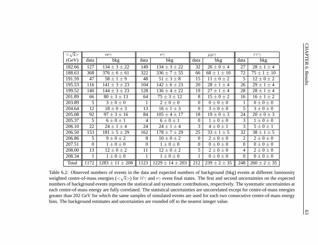
CH
AP
TE
R6
.Resu
lts6
3
<√
s> eeγ eγ µµγ ττγ(GeV) data bkg data bkg data bkg data bkg
182.66 127 134± 3 ± 22 149 134± 3 ± 22 32 26± 0 ± 4 27 28± 1 ± 4188.63 368 376± 6 ± 61 322 336± 7 ± 55 66 68± 1 ± 10 72 75± 1 ± 10191.59 47 58± 1 ± 9 48 51± 3 ± 8 15 11± 0 ± 2 5 12± 0 ± 2195.53 116 141± 3 ± 23 104 142± 6 ± 23 20 28± 1 ± 4 26 29± 1 ± 4199.52 140 144± 3 ± 23 128 136± 4 ± 22 19 27± 1 ± 4 28 28± 1 ± 4201.89 66 80± 3 ± 13 64 75± 3 ± 12 8 15± 0 ± 2 16 16± 1 ± 2203.89 5 3 ± 0 ± 0 1 2 ± 0 ± 0 0 0 ± 0 ± 0 1 0 ± 0 ± 0204.64 12 18± 0 ± 3 13 16± 1 ± 3 0 3 ± 0 ± 0 5 3 ± 0 ± 0205.08 92 97± 3 ± 16 84 105± 4 ± 17 18 19± 0 ± 3 24 20± 0 ± 3205.37 5 6 ± 0 ± 1 4 6 ± 0 ± 1 0 1 ± 0 ± 0 3 1 ± 0 ± 0206.10 22 24± 1 ± 4 24 24± 1 ± 4 3 4 ± 0 ± 1 3 5 ± 0 ± 1206.50 153 181± 5 ± 29 162 178± 7 ± 29 25 33± 1 ± 5 32 38± 1 ± 5206.86 5 9 ± 0 ± 2 8 10± 0 ± 2 0 2 ± 0 ± 0 2 2 ± 0 ± 0207.51 0 1 ± 0 ± 0 0 1 ± 0 ± 0 0 0 ± 0 ± 0 0 0 ± 0 ± 0208.00 13 12± 0 ± 2 11 12± 0 ± 2 5 2 ± 0 ± 0 4 2 ± 0 ± 0208.34 1 1 ± 0 ± 0 1 1 ± 0 ± 0 1 0 ± 0 ± 0 0 0 ± 0 ± 0
Total 1172 1283± 11± 208 1123 1229± 14± 203 212 239± 2 ± 35 248 260± 2 ± 35
Table 6.2: Observed numbers of events in the data and expected numbers of background (bkg) events at different luminosityweighted centre-of-mass energies (<
√s>) for ``γ andeγ event final states. The first and second uncertainties on the expected
numbers of background events represent the statistical andsystematic contributions, respectively. The systematic uncertainties ateach centre-of-mass energy are fully correlated. The statistical uncertainties are uncorrelated except for centre-of-mass energiesgreater than 202 GeV for which the same samples of simulated events are used for each two consecutive centre-of-mass energybins. The background estimates and uncertainties are rounded off to the nearest integer value.

CHAPTER 6. Results 64
meγ (GeV)
Ent
ries/
5.0
GeV
(a) eeγγ
mµγ (GeV)
Ent
ries/
5.0
GeV
(b) µµγγ
mτγ (GeV)
Ent
ries/
5.0
GeV
(c) ττγγ
0
1
2
3
4
5
0 20 40 60 80 100
0
1
2
3
4
5
0 20 40 60 80 100
0
1
2
3
4
5
0 20 40 60 80 100
0
200
400
55 60 65
0
250
500
55 60 65
0
100
200
55 60 65
Figure 6.1: Reconstructedγ invariant mass distributions for selected (a)eeγγ, (b) µµγγand (c)ττγγ events. The points are data and the solid lines show the totalexpected back-ground from Standard Model processes. Example distributions of excited lepton eventswith arbitrarily chosen mass of 60 GeV are shown in the insets. The signal histograms arenormalised to the data luminosity and plotted in bins of 0.5 GeV.

CHAPTER 6. Results 65
0
20
40
60
80
0 25 50 75 100 125 150 175 200
0
5
10
15
20
0 25 50 75 100 125 150 175 200
meγ (GeV)
Ent
ries/
2.0
GeV (a) eeγ
mµγ (GeV)
Ent
ries/
2.0
GeV (b) µµγ
mτγ (GeV)
Ent
ries/
2.0
GeV (c) ττγ
0
5
10
15
20
0 25 50 75 100 125 150 175 200
Figure 6.2: Reconstructedγ invariant mass distributions for selected (a)eeγ, (b) µµγand (c)ττγ events. The points are data and the solid lines show the totalexpected back-ground from Standard Model processes. The shaded histograms represent excited leptonsignal events with arbitrarily chosen mass of 150 GeV and normalised to a coupling overcompositeness scale of (a) 0.7 TeV-1 and (b,c) 2 TeV-1. There are two entries per eventcorresponding to the two possible`γ pairings.
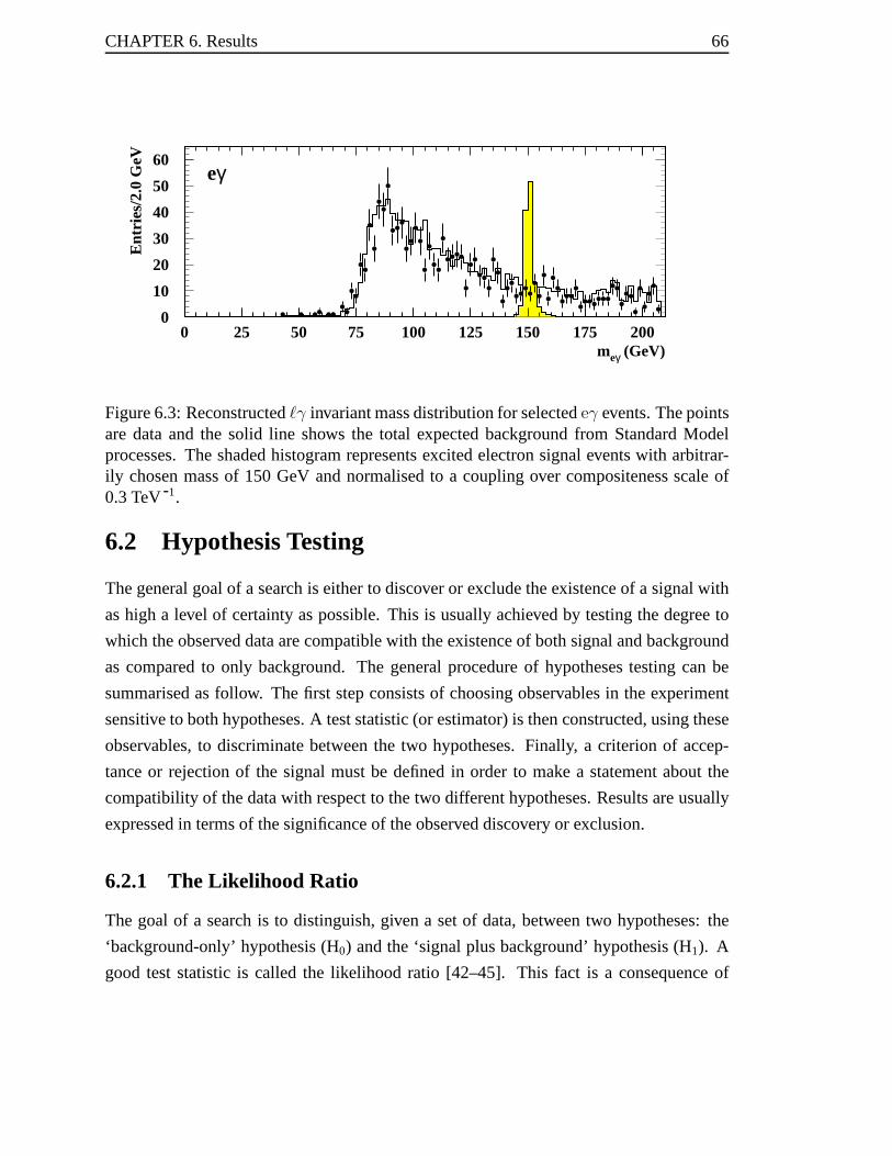
CHAPTER 6. Results 66
meγ (GeV)
Ent
ries/
2.0
GeV
eγ
0
10
20
30
40
50
60
0 25 50 75 100 125 150 175 200
Figure 6.3: Reconstructedγ invariant mass distribution for selectedeγ events. The pointsare data and the solid line shows the total expected background from Standard Modelprocesses. The shaded histogram represents excited electron signal events with arbitrar-ily chosen mass of 150 GeV and normalised to a coupling over compositeness scale of0.3 TeV-1.
6.2 Hypothesis Testing
The general goal of a search is either to discover or exclude the existence of a signal with
as high a level of certainty as possible. This is usually achieved by testing the degree to
which the observed data are compatible with the existence ofboth signal and background
as compared to only background. The general procedure of hypotheses testing can be
summarised as follow. The first step consists of choosing observables in the experiment
sensitive to both hypotheses. A test statistic (or estimator) is then constructed, using these
observables, to discriminate between the two hypotheses. Finally, a criterion of accep-
tance or rejection of the signal must be defined in order to make a statement about the
compatibility of the data with respect to the two different hypotheses. Results are usually
expressed in terms of the significance of the observed discovery or exclusion.
6.2.1 The Likelihood Ratio
The goal of a search is to distinguish, given a set of data, between two hypotheses: the
‘background-only’ hypothesis (H0) and the ‘signal plus background’ hypothesis (H1). A
good test statistic is called the likelihood ratio [42–45].This fact is a consequence of
CHAPTER 6. Results 67
the Neyman-Pearson lemma originally presented in [46] but also described in various
textbooks such as [43–45]. The likelihood ratio simultaneously maximises the probability
of rejecting a false hypothesis and maximises the probability of choosing a true hypothesis.
For a given experimental resultx, the likelihood ratio (Q(x)) is defined as the ratio of the
probability density functions of the two hypotheses being tested,
Q(x) =L(x; H0)
L(x; H1). (6.1)
The simplest experimental observable is the number of events n satisfying a certain
set of criteria. Given an estimated number of background events,b, and signal events,s,
the likelihood ratio is simply a ratio of Poisson probability density functions,
Q(n) =e−(s+b) (s+ b) n
n!
/
e−b bn
n!. (6.2)
For the purpose of calculating confidence levels, this test statistic has the desirable prop-
erty of being monotonically increasing with the number of observed candidatesn.
The likelihood ratio can also be calculated in terms of otherdiscriminating observ-
ables. In general, it however results in a more complicated expression for which both
the signal and background probability distribution functions of the discriminating variable
must be known. The task of calculating a likelihood ratio using one or more discriminat-
ing observables measured for each event is equivalent to combining the likelihood ratios
obtained in each bin of a histogram of these observables. Each bin is treated as a sepa-
rate search channel for which the likelihood ratio is calculated according to Equation 6.2.
The estimator of a set ofN independent channels is simply the product of the individual
likelihood ratio (Qi(ni)) for each search channel,
Q(n) =N∏
i=1
Qi(ni) =N∏
i=1
e−(si+bi) (si + bi)ni
ni !
/
e−bi bnii
ni!(6.3)
or equivalently,
ln Q(n) = −stot +N∑
i=1
ni
ln(
1 +si
bi
)
(6.4)
wherestot is the sum of the number of signal events,stot =∑N
i=1 si. The combination of
different experiments, event final states or centre-of-mass energies therefore reduces to a
sum of event weights and is thus simple and unambiguous.
CHAPTER 6. Results 68
The likelihood ratio based on the number of observed and expected events is the
test statistic chosen in this thesis to discriminate between the signal plus background and
background-only hypotheses. In order to maximise the sensitivity of the search, events are
binned as a function of reconstructed invariant mass. The existence of excited leptons is
expected to distort the invariant mass distribution of observed events in a unique way. To
calculate the total likelihood ratio using Equation 6.4, three essential ingredients are re-
quired in each bin of reconstructed invariant mass: the number of observed data, expected
background and expected signal events.
6.3 Background and Signal Expectations
This section describes the methods used to obtain an estimate of the background and signal
invariant mass distributions. The systematic uncertainties associated with the background
expectations and signal efficiencies are also presented.
6.3.1 Background Expectation
Although relatively large samples of simulated events are used to estimate the background
for each event final state, once finely binned in terms of the reconstructed γ invariant
mass, the number of background events in each individual channel is small and is there-
fore sensitive to statistical fluctuations. This is particularly true for``γγ final states where
only a very small number of events are selected. Some channels are found to contain no
background events when in fact the probability of obtainingbackground events is non-
zero. This is a problematic situation that needs to be addressed since the likelihood ra-
tio of Equation 6.2, although a powerful estimator, is undefined for channels where the
background expectation is zero. To reduce the sensitivity of the results to statistical fluc-
tuations in the background expectations, background distributions of the reconstructedγ
mass are ‘smoothed’ using an algorithm [47] that parameterises the shape of a distribution.
Figures 6.4 and 6.5 show an example of the expected`γ mass distribution at a centre-of-
mass energy of 189 GeV for each final state considered along with results from the shape
parameterisation. The functions obtained using this smoothing algorithm are a good ap-
proximation of the background expectation. Sharp changes in a distribution are difficult to
parameterise, as seen in Figure 6.5. The discrepancy in the small region at the kinematic
limit will result in slightly more conservative constraints than the given confidence level

CHAPTER 6. Results 69
stated, as background in that region is underestimated. Theexpected number of back-
ground events in each individual channel is taken from the shape parameterisation of the
background distributions.
6.3.2 Signal Expectation
Different methods exist for obtainingγ mass distributions of signal events for arbitrary
excited lepton mass. The ‘brute force’ scenario consists ofgenerating Monte Carlo sig-
nal event samples at every mass for which one wishes to calculate limits. However, the
large number of possible excited lepton masses and centre-of-mass energies for which
event samples would have to be generated makes it impossiblein practice to use this
approach. Another solution consists of generating events at a few distinct excited lepton
masses and centre-of-mass energies, and then interpolating the mass distributions between
these points to obtain an approximation of the distributions at any arbitrary excited lep-
ton mass and centre-of-mass energies. Although done in practice to calculate limits from
some searches [48], the interpolation of histograms is in general very complicated and not
entirely reliable, especially if only a limited number of event samples are available.
Instead, the invariant mass distribution of excited leptons is approximated by a Gaus-
sian distribution centered at the excited lepton mass and with a variance equal to the ex-
pected mass resolution. The Gaussian distribution is normalised to the number of signal
events expected at a given centre-of-mass energy.
Both the expected signal efficiency (ε) and mass resolution vary as function of the
mass of the excited leptons and the centre-of-mass energy ofthe e+e- collisions. In or-
der to test the compatibility of the data with the existence of excited leptons of different
masses, the selection efficiencies and mass resolution mustbe calculable for arbitrary val-
ues of mass and centre-of-mass energy. For each event final state considered, the selection
efficiency and mass resolution are parameterised as a function of the excited lepton mass
scaled by the centre-of-mass energy (m`∗/√
s). The results of this parameterisation can be
found in Appendix D.
Typical mass resolutions for each final state were given in Chapter 5. Selection ef-
ficiencies for the pair production of excited leptons vary from about 35% to 55%. The
efficiency for the single production of excited muons is 70% and approximately constant
over the entire kinematically allowed range of masses. Nearthe kinematic limit for the
single production of excited taus, the efficiency rapidly drops from 53% down to approx-
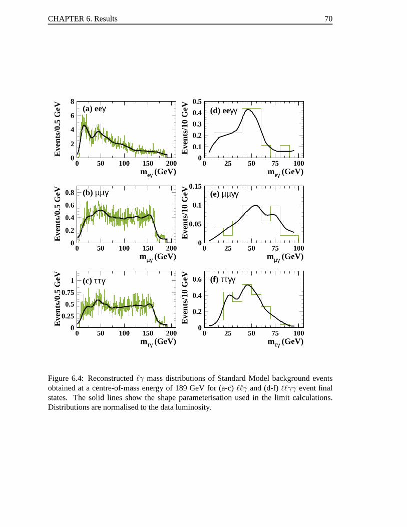
CHAPTER 6. Results 70
0
2
4
6
8
0 50 100 150 2000
0.1
0.2
0.3
0.4
0.5
0 25 50 75 100
0
0.2
0.4
0.6
0.8
0 50 100 150 2000
0.05
0.1
0.15
0 25 50 75 100
0
0.25
0.5
0.75
1
0 50 100 150 200
meγ (GeV)
Eve
nts/
0.5
GeV (a) eeγ
meγ (GeV)
Eve
nts/
10 G
eV (d) eeγγ
mµγ (GeV)
Eve
nts/
0.5
GeV (b) µµγ
mµγ (GeV)
Eve
nts/
10 G
eV (e) µµγγ
mτγ (GeV)
Eve
nts/
0.5
GeV
(c) ττγ
mτγ (GeV)
Eve
nts/
10 G
eV (f) ττγγ
0
0.2
0.4
0.6
0 25 50 75 100
Figure 6.4: Reconstructedγ mass distributions of Standard Model background eventsobtained at a centre-of-mass energy of 189 GeV for (a-c)``γ and (d-f)``γγ event finalstates. The solid lines show the shape parameterisation used in the limit calculations.Distributions are normalised to the data luminosity.
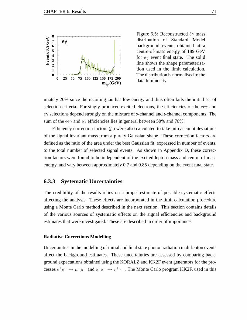
CHAPTER 6. Results 71
meγ (GeV)
Eve
nts/
0.5
GeV eγ
012345678
0 25 50 75 100 125 150 175 200
Figure 6.5: Reconstructedγ massdistribution of Standard Modelbackground events obtained at acentre-of-mass energy of 189 GeVfor eγ event final state. The solidline shows the shape parameterisa-tion used in the limit calculation.The distribution is normalised to thedata luminosity.
imately 20% since the recoiling tau has low energy and thus often fails the initial set of
selection criteria. For singly produced excited electrons, the efficiencies of theeeγ and
eγ selections depend strongly on the mixture ofs-channel andt-channel components. The
sum of theeeγ andeγ efficiencies lies in general between 50% and 70%.
Efficiency correction factors (fc) were also calculated to take into account deviations
of the signal invariant mass from a purely Gaussian shape. These correction factors are
defined as the ratio of the area under the best Gaussian fit, expressed in number of events,
to the total number of selected signal events. As shown in Appendix D, these correc-
tion factors were found to be independent of the excited lepton mass and centre-of-mass
energy, and vary between approximately 0.7 and 0.85 depending on the event final state.
6.3.3 Systematic Uncertainties
The credibility of the results relies on a proper estimate ofpossible systematic effects
affecting the analysis. These effects are incorporated in the limit calculation procedure
using a Monte Carlo method described in the next section. This section contains details
of the various sources of systematic effects on the signal efficiencies and background
estimates that were investigated. These are described in order of importance.
Radiative Corrections Modelling
Uncertainties in the modelling of initial and final state photon radiation in di-lepton events
affect the background estimates. These uncertainties are assessed by comparing back-
ground expectations obtained using the KORALZ and KK2F event generators for the pro-
cessese+e− → µ+µ− ande+e− → τ+τ−. The Monte Carlo program KK2F, used in this
CHAPTER 6. Results 72
analysis to estimate the background contributions fromµ+µ− andτ+τ− events, has the
most complete description of photon radiation, including second-order subleading correc-
tions and the exact matrix elements for the emission of two hard photons [49]. The relative
variations in background expectations between the two event generators are assigned as
systematic uncertainties representing the effect of missing higher orders. These are found
to be 11% for final states compatible with the single production of excited muons and taus,
and 7% forµµγγ andττγγ events. The BHWIDE and TEEGG event generators, used
to simulate the background from radiative e+e- events, have a precision for radiative cor-
rections similar to the KORALZ program. The background estimates for events expected
from the production of excited electrons are thus assigned an uncertainty of 7% for the
eeγγ final state and 11% for botheeγ andeγ events.
Efficiency and resolution interpolation
The systematic uncertainties associated with the interpolation of the signal efficiencies
and mass resolutions were estimated by calculating the root-mean-square spread between
simulated signal event samples and the parameterisation functions. These relative uncer-
tainties range between 3% and 23%.
Error Estimates of Kinematic Fit Input Variables
Uncertainties on the error estimates of the kinematic fit input variables are evaluated by
varying the error on each variable independently and performing the kinematic fits again.
The errors are varied by an amount representing one standarddeviation as calculated from
the uncertainties on the error parameterisations described in Appendix C. Background
estimates for final states containing two leptons and two photons are particularly sensi-
tive to changes in the errors due to the additional constraint in the kinematic fit requiring
events to have equal reconstructed`γ invariant masses. Also, the smaller sample of tau
pair events used to parameterise the errors on the tau direction results in larger statistical
uncertainties on the error parameterisation which in turn dictate the larger variations used
to estimate the systematic error contributions. Relative changes in the background esti-
mates and signal efficiencies obtained from each error variation are added in quadrature.
The total systematic uncertainties associated with the error parameterisation and assigned
to each final state are summarised in Tables 6.4 and 6.3.
CHAPTER 6. Results 73
Jet Classification
Systematic effects associated with the jet classification were investigated by studying the
modelling of the lepton and photon identification efficiencies. Using di-lepton and di-
photon events recorded at centre-of-mass energies equal toand greater than the Z0 mass,
the systematic uncertainty associated with each set of lepton and photon requirements was
evaluated by comparing the identification efficiencies obtained from data and simulated
events. Relative errors of 1% for electron and muon, and 2% for the tau and photon clas-
sifications were assigned. Systematic uncertainties associated with each final state were
determined by adding linearly contributions from identical jet classifications and adding
in quadrature contributions from different types of leptons and photons. The resulting
uncertainties on the signal efficiencies, shown in Table 6.3, are fully correlated with the
corresponding errors on the background estimates presented in Table 6.4.
Energy and angular resolution
The systematic uncertainty associated with the energy scale, energy resolution and angular
resolution of the leptons and photons was evaluated by modifying each parameter indepen-
dently in Monte Carlo simulated events. Given the well defined kinematic characteristics
of non-radiative di-lepton events, comparisons between data and simulated distributions
of di-lepton events recorded at different centre-of-mass energies were used to determine
the size of these variations.
An estimate of the shifts in the energy (momentum) scale of each particle type was
obtained by plotting the difference between the measured energy (momentum) and the
beam energy. Variations in the background estimates and signal efficiencies associated
with a shift of 0.3% in the energy (momentum) of electron and photon (muon) candidates
were assigned as systematic uncertainties. These were found to be negligible.
For different smearing values, a maximum likelihood technique was used to calculate
the degree to which distributions of the energy and measuredangles of each type of particle
were compatible with data. The energy and angular resolutions of jets were smeared by
the maximum values for which simulated events were compatible with the distributions
of data within one standard deviation. The measured energy of electrons and photons
was smeared by 0.15 GeV while the momentum of muons was smeared by 1 GeV. The
measured polar and azimuthal angles was smeared by an amountvarying between 1 mrad
and 10 mrad depending on the particle type. Systematic uncertainties were assigned to be

CHAPTER 6. Results 74
Source Uncertainty (%)eeγ eγ µµγ ττγ eeγγ µµγγ ττγγ
Resolution interpolation 14.8 12.0 20.6 6.5 22.1 22.5 13.4Efficiency interpolation 8.5 3.0 2.4 7.6 4.6 3.5 3.0Error estimate of fit variables 5.0 5.0 3.0 5.0 3.0 2.0 6.0Jet classification 2.8 2.2 1.4 4.5 4.5 4.5 5.7Energy and angular resolution 0.9 1.1 0.8 1.1 1.8 0.6 0. 9Modelling of selection variables 0.0 1.5 0.1 1.6 0.4 0.4 0 .8
Total 18.0 13.6 21.0 12.2 23.3 23.3 16.1
Table 6.3: Relative systematic uncertainties on the signalefficiencies for each final stateconsidered.
the relative changes in background estimates and signal efficiencies.
Contributions to the systematic uncertainty of each final state from individual changes
in the energy scale, energy resolution and angular resolution are added in quadrature.
Selection Variable modelling
The systematic uncertainty due to modelling of the event selection variables was estimated
by varying each selection cut independently and measuring the corresponding changes in
the overall signal efficiencies and background estimates. The difference between the mean
value of the data and background expectation for each selection variable determined the
range of variation of each cut. Systematic uncertainties varying between 0.5% and 6.3%
are assigned to the different background estimates. Contributions to the systematic error
on the signal efficiencies are shown in Table 6.3.
Summaries of the systematic effects on the background expectations and signal ef-
ficiencies are presented in Tables 6.4 and 6.3, respectively. The uncertainty on the inte-
grated luminosity measurements (0.2%) is considerably smaller than the systematic effects
already described and is therefore neglected.
6.4 Limit Calculations
Given that no evidence for excited states of leptons was found, constraints on the produc-
tion rate of excited charged leptons as function of mass are calculated. Selected candidate
events from each final state and at each centre-of-mass energy are binned in terms of their
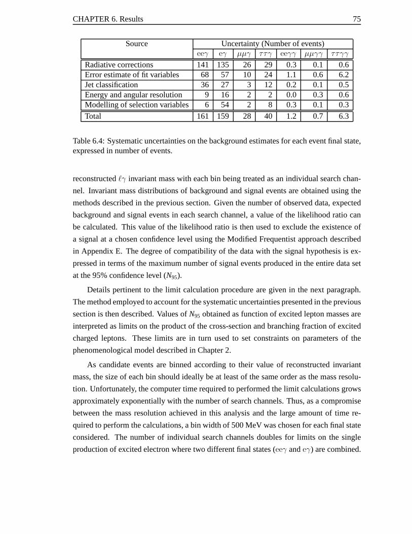
CHAPTER 6. Results 75
Source Uncertainty (Number of events)eeγ eγ µµγ ττγ eeγγ µµγγ ττγγ
Radiative corrections 141 135 26 29 0.3 0.1 0.6Error estimate of fit variables 68 57 10 24 1.1 0.6 6.2Jet classification 36 27 3 12 0.2 0.1 0.5Energy and angular resolution 9 16 2 2 0.0 0.3 0.6Modelling of selection variables 6 54 2 8 0.3 0.1 0.3
Total 161 159 28 40 1.2 0.7 6.3
Table 6.4: Systematic uncertainties on the background estimates for each event final state,expressed in number of events.
reconstructedγ invariant mass with each bin being treated as an individual search chan-
nel. Invariant mass distributions of background and signalevents are obtained using the
methods described in the previous section. Given the numberof observed data, expected
background and signal events in each search channel, a valueof the likelihood ratio can
be calculated. This value of the likelihood ratio is then used to exclude the existence of
a signal at a chosen confidence level using the Modified Frequentist approach described
in Appendix E. The degree of compatibility of the data with the signal hypothesis is ex-
pressed in terms of the maximum number of signal events produced in the entire data set
at the 95% confidence level (N95).
Details pertinent to the limit calculation procedure are given in the next paragraph.
The method employed to account for the systematic uncertainties presented in the previous
section is then described. Values ofN95 obtained as function of excited lepton masses are
interpreted as limits on the product of the cross-section and branching fraction of excited
charged leptons. These limits are in turn used to set constraints on parameters of the
phenomenological model described in Chapter 2.
As candidate events are binned according to their value of reconstructed invariant
mass, the size of each bin should ideally be at least of the same order as the mass resolu-
tion. Unfortunately, the computer time required to performed the limit calculations grows
approximately exponentially with the number of search channels. Thus, as a compromise
between the mass resolution achieved in this analysis and the large amount of time re-
quired to perform the calculations, a bin width of 500 MeV waschosen for each final state
considered. The number of individual search channels doubles for limits on the single
production of excited electron where two different final states (eeγ andeγ) are combined.
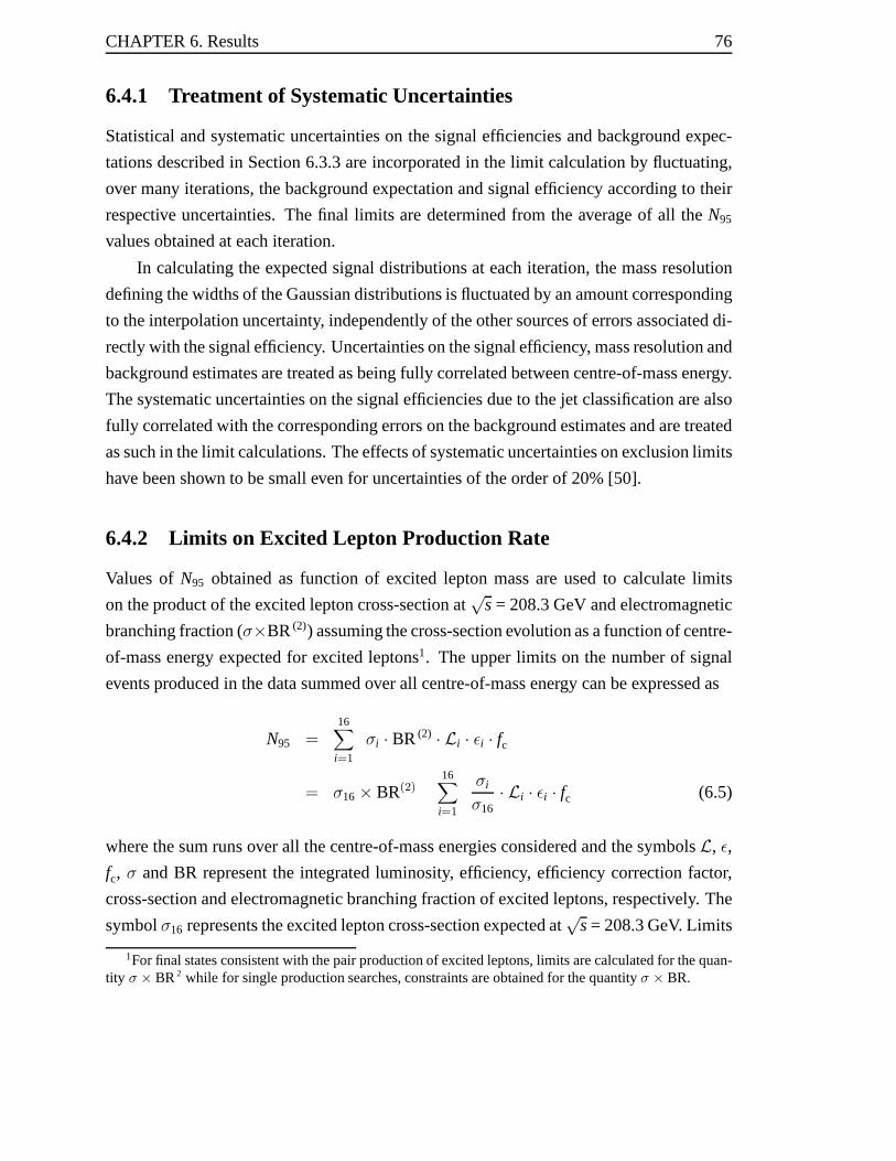
CHAPTER 6. Results 76
6.4.1 Treatment of Systematic Uncertainties
Statistical and systematic uncertainties on the signal efficiencies and background expec-
tations described in Section 6.3.3 are incorporated in the limit calculation by fluctuating,
over many iterations, the background expectation and signal efficiency according to their
respective uncertainties. The final limits are determined from the average of all theN95
values obtained at each iteration.
In calculating the expected signal distributions at each iteration, the mass resolution
defining the widths of the Gaussian distributions is fluctuated by an amount corresponding
to the interpolation uncertainty, independently of the other sources of errors associated di-
rectly with the signal efficiency. Uncertainties on the signal efficiency, mass resolution and
background estimates are treated as being fully correlatedbetween centre-of-mass energy.
The systematic uncertainties on the signal efficiencies dueto the jet classification are also
fully correlated with the corresponding errors on the background estimates and are treated
as such in the limit calculations. The effects of systematicuncertainties on exclusion limits
have been shown to be small even for uncertainties of the order of 20% [50].
6.4.2 Limits on Excited Lepton Production Rate
Values ofN95 obtained as function of excited lepton mass are used to calculate limits
on the product of the excited lepton cross-section at√
s= 208.3 GeV and electromagnetic
branching fraction (σ×BR (2)) assuming the cross-section evolution as a function of centre-
of-mass energy expected for excited leptons1. The upper limits on the number of signal
events produced in the data summed over all centre-of-mass energy can be expressed as
N95 =16∑
i=1
σi · BR (2) · Li · εi · fc
= σ16 × BR(2)16∑
i=1
σi
σ16· Li · εi · fc (6.5)
where the sum runs over all the centre-of-mass energies considered and the symbolsL, ε,
fc, σ and BR represent the integrated luminosity, efficiency, efficiency correction factor,
cross-section and electromagnetic branching fraction of excited leptons, respectively. The
symbolσ16 represents the excited lepton cross-section expected at√
s= 208.3 GeV. Limits
1For final states consistent with the pair production of excited leptons, limits are calculated for the quan-tity σ × BR2 while for single production searches, constraints are obtained for the quantityσ × BR.

CHAPTER 6. Results 77
on the product of the excited lepton cross-section at√
s= 208.3 GeV and electromagnetic
branching fraction (σ × BR(2)) are therefore obtained using
σ × BR (2) =N95
∑16i=1
σiσ · Li · εi · fc·
(6.6)
where the subscript on the cross-section at√
s= 208.3 GeV is dropped for simplicity.
The upper limits on the single production of excited muons and tau leptons do not de-
pend on the model dependent coupling parametersf andf ′. The excited electron selection
efficiencies foreeγ andeγ event final states, however, depend on the relative magnitude
of thes-channel andt-channel production diagrams and therefore depend on the value of
the parametersf andf ′. For comparison with previously published results, the limits on
excited electrons presented here assumef = f ′. Figures 6.6(a,b) show the 95% confidence
level upper limits on the product of the cross-section at√
s = 208.3 GeV and the electro-
magnetic branching fraction obtained from the search for singly and pair produced excited
leptons.
6.4.3 Mass Limits
Limits on the product of the cross-section and branching fraction are used to set constraints
on parameters of the phenomenological model described in Chapter 2. Lower mass limits
on excited leptons are calculated using results from the pair production searches. The
theoretical calculation [6] of the product of the pair production cross-section at√
s =
208.3 GeV and the branching fraction squared is overlayed onFigure 6.6(b). As part of
this calculation, the electromagnetic branching fractionis calculated assumingf = f ′. The
95% confidence level lower mass limits on excited leptons correspond to the mass at which
the cross-section times branching fraction limit curves cross the theoretical expectation.
Lower mass limits ofme∗ > 103.2 GeV,mµ∗ > 103.2 GeV andmτ∗ > 103.2 GeV are
obtained at the 95% confidence level. Although systematic errors are incorporated into
the limit calculations, an additional uncertainty on the mass limits arises from the finite
width of the centre-of-mass energy bins considered. The 0.5GeV centre-of-mass energy
bin width near the kinematic limit corresponds to an uncertainty of 0.1 GeV on the mass
limits.
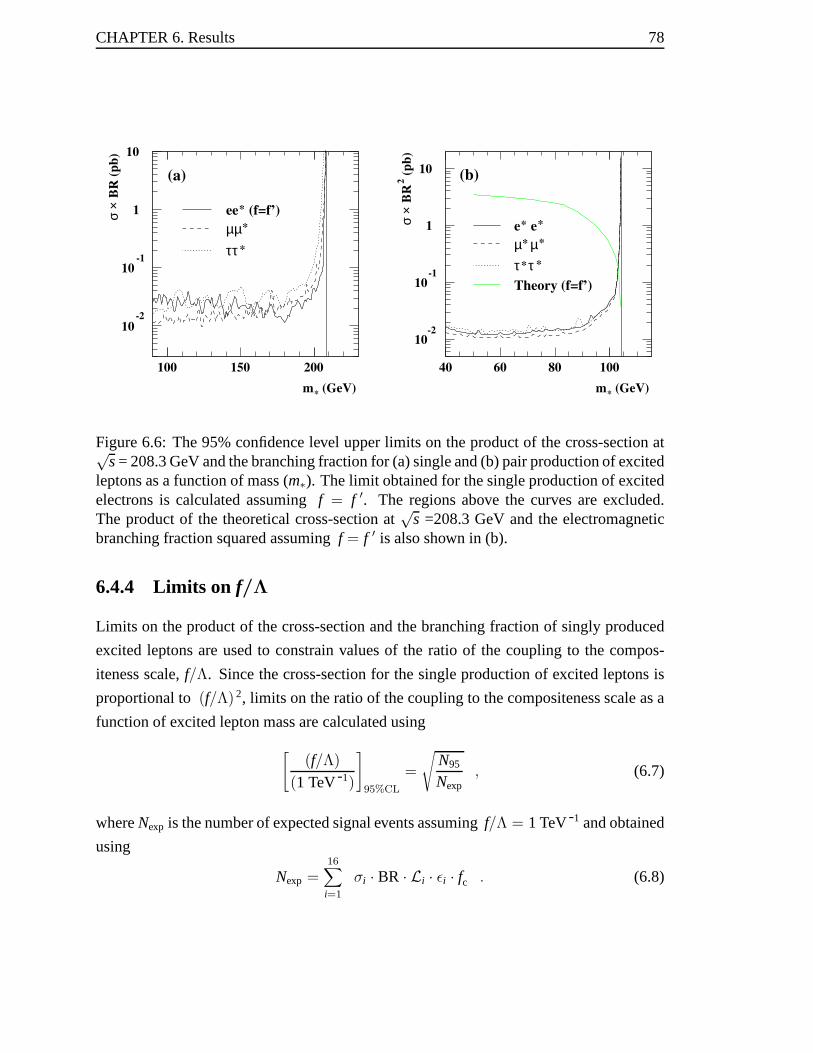
CHAPTER 6. Results 78
10-2
10-1
1
10
100 150 200
(a)
ee (f=f’)
µµ*
*
ττ *
m* (GeV)
σ ×
BR
(p
b)
(b)
e e
µ* *
* µτ τTheory (f=f’)
m* (GeV)
σ ×
BR
2 (
pb
)
10
10
1
10
40 60 80 100
*
**-1
-2
Figure 6.6: The 95% confidence level upper limits on the product of the cross-section at√s= 208.3 GeV and the branching fraction for (a) single and (b) pair production of excited
leptons as a function of mass (m∗). The limit obtained for the single production of excitedelectrons is calculated assumingf = f ′. The regions above the curves are excluded.The product of the theoretical cross-section at
√s =208.3 GeV and the electromagnetic
branching fraction squared assumingf = f ′ is also shown in (b).
6.4.4 Limits on f/Λ
Limits on the product of the cross-section and the branchingfraction of singly produced
excited leptons are used to constrain values of the ratio of the coupling to the compos-
iteness scale,f/Λ. Since the cross-section for the single production of excited leptons is
proportional to(f/Λ) 2, limits on the ratio of the coupling to the compositeness scale as a
function of excited lepton mass are calculated using
[
(f/Λ)
(1 TeV-1)
]
95%CL
=
√
N95
Nexp, (6.7)
whereNexp is the number of expected signal events assumingf/Λ = 1 TeV-1 and obtained
using
Nexp =16∑
i=1
σi · BR · Li · εi · fc . (6.8)
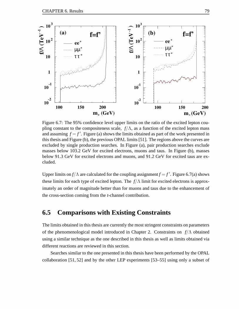
CHAPTER 6. Results 79
ee
µµ*
*
τ τ *
m* (GeV)
f/Λ
(T
eV-1
)f=f’
10-2
10-1
1
10
10
10
2
3
100 150 200
(a)
10
10-1
-2
1
10
102
103
100 150 200
m* (GeV)
f/Λ
(TeV
-1)
ee *
f=f’
µττ *
(b)
µ*
Figure 6.7: The 95% confidence level upper limits on the ratioof the excited lepton cou-pling constant to the compositeness scale,f/Λ, as a function of the excited lepton massand assumingf = f ′. Figure (a) shows the limits obtained as part of the work presented inthis thesis and Figure (b), the previous OPAL limits [51]. The regions above the curves areexcluded by single production searches. In Figure (a), pairproduction searches excludemasses below 103.2 GeV for excited electrons, muons and taus. In Figure (b), massesbelow 91.3 GeV for excited electrons and muons, and 91.2 GeV for excited taus are ex-cluded.
Upper limits onf/Λ are calculated for the coupling assignmentf = f ′. Figure 6.7(a) shows
these limits for each type of excited lepton. Thef/Λ limit for excited electrons is approx-
imately an order of magnitude better than for muons and taus due to the enhancement of
the cross-section coming from thet-channel contribution.
6.5 Comparisons with Existing Constraints
The limits obtained in this thesis are currently the most stringent constraints on parameters
of the phenomenological model introduced in Chapter 2. Constraints on f/Λ obtained
using a similar technique as the one described in this thesisas well as limits obtained via
different reactions are reviewed in this section.
Searches similar to the one presented in this thesis have been performed by the OPAL
collaboration [51, 52] and by the other LEP experiments [53–55] using only a subset of
CHAPTER 6. Results 80
e
e*
e γ
γ
Figure 6.8: Diagram of the excited electroncontribution to the processe+e− → γγ.
the data analysed in the present work. Limits were also obtained using data collected
at a centre-of-mass energy equal to the Z0 mass [56]. All four LEP collaborations have
reported lower limits on the mass of excited charged leptonsof the order of 95 to 100 GeV
and limits on the strength of the couplingf/Λ of order 0.1 TeV-1 for excited electrons and
1 TeV-1 for excited muons and taus assumingf = f ′.
The existence of excited electrons could also be inferred from deviations in the dif-
ferential cross-section of the processe+e− → γγ. Excited electrons would contribute to
the reaction via the diagram shown in Figure 6.8. The expected differential cross-section
in the context of the model presented in Chapter 2 has been calculated as part of the work
presented in this thesis. Details of the calculation can be found in Appendix F. Using
results of this calculation, limits on the excited electroncoupling strength from studies of
the processe+e− → γγ have recently been reported by all four LEP experiments [20,57].
These constraints are complementary to the searches for singly and pair produced excited
electrons. This reaction is comparatively suppressed compared to the single production
due to the double interaction of excited electrons with a photon and an electron. However
it extends limits to masses beyond the kinematically allowed region of single production.
This is a consequence of quantum mechanical effects wherebythe excited electron medi-
ating the production of two photons is a virtual2 particle. Upper bounds on the quantity
f/Λ for the coupling assignmentf = f ′ were calculated at the 95% confidence level to be
of order 5 TeV-1 for excited electron masses greater than the centre-of-mass energy.
Searches for the existence of excited leptons have also beenperformed in electron-
proton collisions at the HERA collider in Germany. Figure 6.9 shows the excited electron
production mechanism in electron-proton collisions. Boththe H1 [58] and ZEUS [59]
experiments at the HERA collider have reported upper limitson the excited electron cou-
pling strength,f/Λ, of order 1 TeV-1 for masses below 200 GeV and assumingf = f ′.
2Virtual particles are particles that cannot be observed andfor whichE2 + |p|2 6= m2. They can have anymass. The existence of virtual particles is a consequence ofHeisenberg’s uncertainty principle,∆E∆t ≥ h.
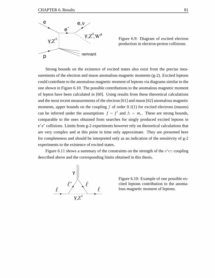
CHAPTER 6. Results 81
e
γ,Z0
p
e*
e,ν
γ,Z0
W
remnant
-+, Figure 6.9: Diagram of excited electronproduction in electron-proton collisions.
Strong bounds on the existence of excited states also exist from the precise mea-
surements of the electron and muon anomalous magnetic moments (g-2). Excited leptons
could contribute to the anomalous magnetic moment of leptons via diagrams similar to the
one shown in Figure 6.10. The possible contributions to the anomalous magnetic moment
of lepton have been calculated in [60]. Using results from these theoretical calculations
and the most recent measurements of the electron [61] and muon [62] anomalous magnetic
moments, upper bounds on the couplingf of order 0.1(1) for excited electrons (muons)
can be inferred under the assumptionsf = f ′ andΛ = m∗. These are strong bounds,
comparable to the ones obtained from searches for singly produced excited leptons in
e+e- collisions. Limits from g-2 experiments however rely on theoretical calculations that
are very complex and at this point in time only approximate. They are presented here
for completeness and should be interpreted only as an indication of the sensitivity of g-2
experiments to the existence of excited states.
Figure 6.11 shows a summary of the constraints on the strength of thee∗eγ coupling
described above and the corresponding limits obtained in this thesis.
γ,Z0
*
γ
` ```
Figure 6.10: Example of one possible ex-cited leptons contribution to the anoma-lous magnetic moment of leptons.

CHAPTER 6. Results 82
m* (GeV)
f/Λ
(T
eV-1
)
OPALe+e- → e+e-γ
e+e- → e+e-γγ
e+e- → γγ
H1e+γ → e*
f=f’10
-2
10-1
1
10
100 150 200 250 300 350
Figure 6.11: Summary of existing constraints on thee∗eγ coupling strength expressedin terms of 95% confidence level upper limits on the quantityf/Λ as function of excitedelectron mass and assumingf = f ′. The hatched regions represent values of the parametersexcluded by the OPAL and H1 experiments.
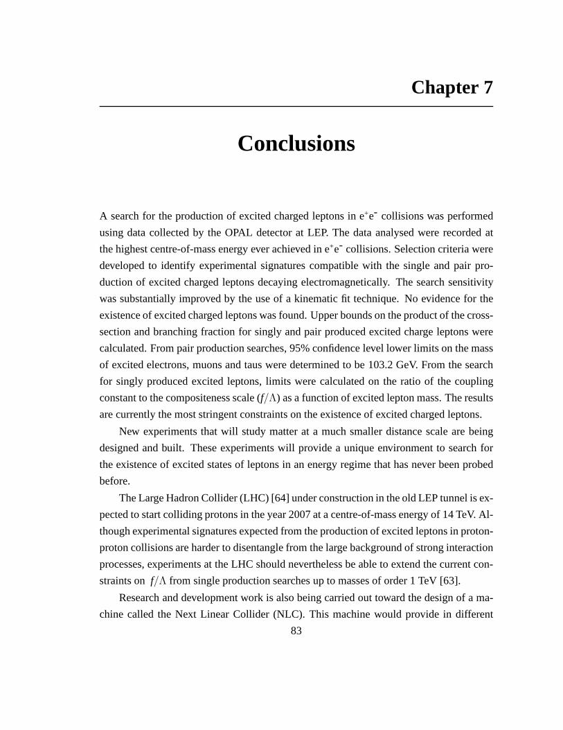
Chapter 7
Conclusions
A search for the production of excited charged leptons in e+e- collisions was performed
using data collected by the OPAL detector at LEP. The data analysed were recorded at
the highest centre-of-mass energy ever achieved in e+e- collisions. Selection criteria were
developed to identify experimental signatures compatiblewith the single and pair pro-
duction of excited charged leptons decaying electromagnetically. The search sensitivity
was substantially improved by the use of a kinematic fit technique. No evidence for the
existence of excited charged leptons was found. Upper bounds on the product of the cross-
section and branching fraction for singly and pair producedexcited charge leptons were
calculated. From pair production searches, 95% confidence level lower limits on the mass
of excited electrons, muons and taus were determined to be 103.2 GeV. From the search
for singly produced excited leptons, limits were calculated on the ratio of the coupling
constant to the compositeness scale (f/Λ) as a function of excited lepton mass. The results
are currently the most stringent constraints on the existence of excited charged leptons.
New experiments that will study matter at a much smaller distance scale are being
designed and built. These experiments will provide a uniqueenvironment to search for
the existence of excited states of leptons in an energy regime that has never been probed
before.
The Large Hadron Collider (LHC) [64] under construction in the old LEP tunnel is ex-
pected to start colliding protons in the year 2007 at a centre-of-mass energy of 14 TeV. Al-
though experimental signatures expected from the production of excited leptons in proton-
proton collisions are harder to disentangle from the large background of strong interaction
processes, experiments at the LHC should nevertheless be able to extend the current con-
straints onf/Λ from single production searches up to masses of order 1 TeV [63].
Research and development work is also being carried out toward the design of a ma-
chine called the Next Linear Collider (NLC). This machine would provide in different
83

CHAPTER 7. Conclusions 84
mode of operation e+e-, eγ andγγ collisions at a centre-of-mass energy of up to 500 GeV.
Lower mass limits of approximately 250 GeV could be obtainedfrom searches for pair
produced excited charged leptons in e+e- collisions. Given the foreseen luminosity deliv-
ered by such a machine, the upper bounds on the quantityf/Λ could be improved by more
than an order of magnitude. In addition to production mechanisms identical to the ones
studied in this thesis, excited electrons could also be singly produced ineγ collisions. Of
particular interest is the use of the photon beam polarisation that could be tuned to en-
hance the excited electron production cross-section for different values of the coupling
parametersf andf ′ [65].
The next generation of high energy experiments will open up anew window of oppor-
tunity to look for answers to some of the shortcomings of the Standard Model. The next
decade promises to be an exciting time.

Appendix A
Tracks and Clusters Requirements
The following is a summary of the quality requirements applied to reconstructed tracks
and energy clusters used in the analysis.
Tracks
• The transverse momentum must be greater than 0.15 GeV.
• Tracks must be reconstructed from at least 50% of the hits expected in the central
jet chamber at the given polar angle, and always more than 20 hits.
• The distance of closest approach to the interaction point inther − φ plane must be
less than 2 cm.
• The distance of closest approach to the interaction point inthez-direction must be
less than 25 cm.
Clusters in the electromagnetic calorimeters
• Clusters are formed from the energy deposited in at least onelead glass block of the
calorimeter.
• The raw energy of clusters must be greater than 0.1 GeV and 0.25 GeV for clusters
in the barrel and endcap electromagnetic calorimeters, respectively.
• The corrected measured energy of clusters in either calorimeter must be greater than
0.001 GeV.
Clusters in the hadronic calorimeter
• The energy in the calorimeter towers must be greater than 0.6GeV.
85
Appendix B
General Solution to Kinematic Fit
The solution to a kinematic fit, as outlined in Section 5.2, consists of finding a set of
parametersα which minimises the function
L = (α − α)T V -1 (α − α) + 2λT g(α, p)
whereα represents the vector of measured parameters,p is the set of unmeasured param-
eters andλ are Lagrange multipliers used to incorporate the set of constraint equations
g(α, p) = 0. If the constraint equations are linear in the parametersα andp, the solution
of the problem can be found in one step. Otherwise, an iterative method based on the
linearization of the constraint equations is generally used. The solution presented here
closely follows that shown in [66]. At each iteration, initial values of the parametersα0
andp0 are updated by the addition of corrections∆α and∆p such that
α1 = α0 p1 = p0
α2 = α0 + ∆α2 p2 = p0 + ∆p2
α3 = α0 + ∆α3 p3 = p0 + ∆p3...
...
αk = α0 + ∆αk pk = p0 + ∆pk...
...
The initial estimates of the parametersα are taken to be the measured values themselves
( α0 = α ). Initial values of the unmeasured parameters are determined using different
methods, depending on the details of the specific problem. Constraint equations are often
used to help calculate these starting values.
On the kth iteration, the Taylor expansion of the constraint equations, assuming
86
CHAPTER B. General Solution to Kinematic Fit 87
changes inα andp are small, is given by
g(αk, pk) ≈ g (αk-1, pk-1)+∂g∂α
∣
∣
∣
∣
∣
αk-1, pk-1
(∆αk−∆αk-1)+∂g∂p
∣
∣
∣
∣
∣
αk-1, pk-1
(∆pk−∆pk-1) = 0
or more simply as
gk-1 + A (∆αk − ∆αk-1) + B (∆pk − ∆pk-1) = 0
whereA andB are the matrices of the first derivatives of the constraints with respect to
the measured and unmeasured parameters,
A =∂g∂α
∣
∣
∣
∣
∣
αk-1, pk-1
B =∂g∂p
∣
∣
∣
∣
∣
αk-1, pk-1
.
Defining c= A ∆αk-1 + B ∆pk-1 − gk-1, the function to minimize can be written as
L = ∆αTk V −1 ∆αk + 2λT (A ∆αk + B ∆pk − c ) .
The necessary conditions for an extremum are
∂L∂α
= 0
∂L∂p
= 0
∂L∂λ
= 0
leading to the following system of coupled matrix equations
V −1∆αk + AT λ = 0
BT λ = 0
A ∆αk + B ∆p = c .
This system of equations has to be solved for∆αk, ∆p andλ. This can be achieved by

CHAPTER B. General Solution to Kinematic Fit 88
rewriting these three equations as
V -1 0 AT
0 0 BT
A B 0
∆αk
∆pk
λ
=
0
0
c
.
Assuming the inverse of the partitioned matrix is
V -1 0 AT
0 0 BT
A B 0
-1
=
C11 CT21 CT
31
C21 C22 CT32
C31 C32 C33
then the solution to the system of equations is simply
∆αk
∆pk
λ
=
V -1 0 AT
0 0 BT
A B 0
-1
0
0
c
=
C11 CT21 CT
31
C21 C22 CT32
C31 C32 C33
0
0
c
=
CT31 c
CT32 c
C33 c
.
The matrix elements Cij can be found by requiring
V−1 0 AT
0 0 BT
A B 0
C11 CT21 CT
31
C21 C22 CT32
C31 C32 C33
=
1 0 0
0 1 0
0 0 1
such that
C11 = V − VATWAV + VATWB (BTWB)-1 BTWAV
C21 = −(BTWB)-1 BTWAV
C22 = (BTWB)-1
C31 = WAV − WB (BTWB)-1 BTWAV
C32 = WB (BTWB)-1
C33 = −W + WB (BTWB)-1 BTW .
whereW = (AVA T)-1 is used to simplify the algebra. Finally, the corrections used to up-
date the initial values of the measured and unmeasured parameters, as well as the Lagrange

CHAPTER B. General Solution to Kinematic Fit 89
multipliers are
∆αk = CT31 c = VATW − (VATWB (BTWB)-1 BTW) (A∆αk-1 + B∆pk-1 − g k-1)
∆pk = CT32 c = (BTWB)-1 BTW (A∆α k-1 + B∆pk-1 − gk-1)
λ = C33 c = (−W + WB (BTWB)-1 BTW) (A∆αk-1 + B∆pk-1 − gk-1) .
Thus, at each iteration, updated values of the parameters and Lagrange multipliers are
given by
αk
pk
λ
=
α0
p0
0
+
∆αk
∆pk
λ
.
The updated covariance matrix is found by error propagation
cov
αk
pk
λ
=
∂αk/∂α0 ∂αk/∂p0 ∂αk/∂λ
∂pk/∂α0 ∂pk/∂p0 ∂pk/∂λ
∂λ/∂α0 ∂λ/∂p0 ∂λ/∂λ
V 0 0
0 0 0
0 0 0
∂αk/∂α0 ∂αk/∂p0 ∂αk/∂λ
∂pk/∂α0 ∂pk/∂p0 ∂pk/∂λ
∂λ/∂α0 ∂λ/∂p0 ∂λ/∂λ
T
=
(∂αk/∂α0)V(∂αk/∂α0)T (∂αk/∂α0)V(∂pk/∂α0)
T (∂αk/∂α)V(∂λk/∂α)T
(∂pk/∂α0)V(∂αk/∂α0)T (∂pk/∂α0)V(∂pk/∂α0)
T (∂pk/∂α)V(∂λk/∂α)T
(∂λ/∂α0)V(∂αk/∂α0)T (∂λ/∂α0)V(∂pk/∂α0)
T (∂λ/∂α)V(∂λk/∂α)T
=
C11 CT21 0
C21 C22 0
0 0 −C33
.
where(∂c/∂α0) = −A was used in the last step.

Appendix C
Error Estimates of Kinematic Fit Input
Variables
Estimates of the energy and angular resolution of differentcomponents of the detector are
obtained using events containing two leptons produced back-to-back. These parameteri-
sations of the detector response are taken as an estimate of the uncertainty on individual
energy and angular measurements and are used as input to the kinematic fits performed
for each selected event.
Leptons produced from the decay of excited leptons have a wide range of energies
which is a consequence of the excited lepton mass but also of the production mode (single
or pair production of excited leptons). Pair produced excited leptons of masses close to
the kinematic limit give leptons of about 50 GeV on average. Single production of excited
leptons, for masses near the kinematic limit, result in one energetic and one low energy
lepton. So the estimates of the uncertainty on the quantities used as input to the kinematic
fits must be valid for a wide range of energies. The data sampleused for this study includes
approximately 10 pb-1 of calibration data recorded at a centre-of-mass energy equal to the
Z0 mass as well as the entire set of data recorded at√
s=183-209 GeV.
In order to obtain error estimates independent of Monte Carlo modelling, an effort
has been made to extract an estimate of the uncertainty on each kinematic variable from
real data.
Given their well defined kinematic properties, non-radiative1 di-lepton events are used
in this study. The two leptons contained in these events are produced back-to-back and
their energy is equal to the beam energy. Di-lepton events are selected by requiring events
1Events that do not contain photon(s) radiated off initial orfinal state particles involved in a collision. Athigh energy, a photon is often radiated along the beam axis decreasing the effective centre-of-mass energyof a collision.
90

CHAPTER C. Error Estimates of Kinematic Fit Input Variables 91
to contain exactly two coplanar2 jets. Each jet is categorised using the same lepton and
photon identification requirements described in Section 4.2. Events containing two elec-
tron or two muon candidates are required to satisfyRvis > 0.8, where the quantityRvis is
defined in Section 4.3, in order to reject radiative lepton pair events and background from
two-photon events. Following closely on the definition of Section 4.3, tau pair events are
defined as events with two identified tau candidates, one tau and one electron or muon,
or one identified muon and one electron. Tau pair events are also required to satisfy
Rvis < 0.85 in order to reject muon and electron pair events where one jet was misidentified
as well as background from two-photon events.
C.1 Electromagnetic Calorimeter Response
The electromagnetic calorimeter response is studied usingthe large sample of non-radiative
electron pair events selected using the simple requirements listed above.
Since the energy of each electron is equal to the beam energy,the shape of the distri-
bution(E− Ebeam)/σE, whereE andσE are the energy and error on the measured energy
of each electron, is an indicator of how well the errors trulyrepresent the energy mea-
surement uncertainties. Such distributions obtained using electron pair events recorded at
a centre-of-mass energy equal to the Z0 mass and at 189 GeV are shown in Figure C.1.
These distributions were obtained using the errors calculated as part of the standard OPAL
event reconstruction. Results of a fit to a Gaussian distribution appear as a solid line super-
imposed on each histogram. Although the fit agreement with data is poor, it nevertheless
gives a sufficient approximation to each distribution. In analogy with pull3 distributions
which exhibit a standard normal distribution if errors are correctly estimated, the distri-
butions shown in Figure C.1 should also be Gaussian distributed with a variance equal to
one. Both distributions do have a variance close to one whichindicates that the errors are
indeed a good estimate of the uncertainty on the measured energy in the electromagnetic
calorimeter.
Since the two electrons in non-radiative electron pair events are produced back-to-
back, the shape of the distributions(θ1+θ2−π)/√
σ2θ1
+ σ2θ2
and(φ1−φ2−π)/√
σ2φ1
+ σ2φ2
2Two particles are said to be coplanar if their momentum vectors projected onto thex-y plane are sepa-rated by exactly 1800.
3A pull value is usually defined in the context of least squaresfitting and is defined as the differencebetween the direct measurement of a variable and its value asobtained from the least squares fit, normalisedto the estimated error of this difference.
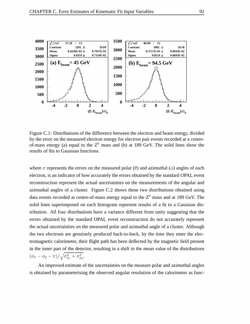
CHAPTER C. Error Estimates of Kinematic Fit Input Variables 92
0
500
1000
1500
2000
2500
3000
3500
4000
-4 -2 0 2 4
57.20 / 13Constant 2201. 19.69Mean 0.4226E-02 0.7937E-02Sigma 0.8319 0.7154E-02
(E-Ebeam)/σE
(a) Ebeam= 45 GeV
80.08 / 13Constant 1881. 18.58Mean -0.3717E-01 0.8943E-02Sigma 0.8524 0.8693E-02
(E-Ebeam)/σE
(b) Ebeam= 94.5 GeV
0
500
1000
1500
2000
2500
3000
3500
-4 -2 0 2 4
Figure C.1: Distributions of the difference between the electron and beam energy, dividedby the error on the measured electron energy for electron pair events recorded at a centre-of-mass energy (a) equal to the Z0 mass and (b) at 189 GeV. The solid lines show theresults of fits to Gaussian functions.
whereσ represents the errors on the measured polar (θ) and azimuthal (φ) angles of each
electron, is an indicator of how accurately the errors obtained by the standard OPAL event
reconstruction represent the actual uncertainties on the measurements of the angular and
azimuthal angles of a cluster. Figure C.2 shows these two distributions obtained using
data events recorded at centre-of-mass energy equal to the Z0 mass and at 189 GeV. The
solid lines superimposed on each histogram represent results of a fit to a Gaussian dis-
tribution. All four distributions have a variance different from unity suggesting that the
errors obtained by the standard OPAL event reconstruction do not accurately represent
the actual uncertainties on the measured polar and azimuthal angle of a cluster. Although
the two electrons are genuinely produced back-to-back, by the time they enter the elec-
tromagnetic calorimeter, their flight path has been deflected by the magnetic field present
in the inner part of the detector, resulting in a shift in the mean value of the distributions
(φ1 − φ2 − π)/√
σ2φ1
+ σ2φ2
.
An improved estimate of the uncertainties on the measure polar and azimuthal angles
is obtained by parameterising the observed angular resolution of the calorimeter as func-

CHAPTER C. Error Estimates of Kinematic Fit Input Variables 93
0
200
400
600
800
1000
-4 -2 0 2 40
200
400
600
800
1000
-4 -2 0 2 4
0
100
200
300
400
500
600
-4 -2 0 2 4
47.96 / 25Constant 577.1 7.790Mean -0.7358 0.1789E-01Sigma 1.513 0.1944E-01
(θ1+θ2-π)/√(σ12+σ2
2)
(a) Ebeam= 45 GeV
35.97 / 25Constant 510.5 7.391Mean -0.5669 0.1775E-01Sigma 1.438 0.1850E-01
(θ1+θ2-π)/√(σ12+σ2
2)
(b) Ebeam= 94.5 GeV
233.5 / 47Constant 321.0 5.425Mean -2.217 0.2542E-01Sigma 1.528 0.2017E-01
(φ1-φ2-π)/√(σ12+σ2
2)
(c) Ebeam= 45 GeV
54.59 / 13Constant 496.1 10.09Mean -0.7881 0.1333E-01Sigma 0.7734 0.1381E-01
(φ1-φ2-π)/√(σ12+σ2
2)
(d) Ebeam= 94.5 GeV
0
100200
300400
500600
700800
900
-4 -2 0 2 4
Figure C.2: Distributions of the quantities (a,b)(θ1 + θ2 − π)/√
σ2θ1
+ σ2θ2
and (c,d)(φ1 −φ2−π)/
√
σ2φ1
+ σ2φ2
obtained from non-radiative electron pair events collected at a centre-
of-mass energy equal to the Z0 mass and at 189 GeV. The uncertainties on the measuredpolar (σθ) and azimuthal (σφ) angles of a cluster calculated as part of the standard OPALevent reconstruction are used. Although the two electrons in an event are produced back-to-back, the distributions (c,d) are not centred at zero since the direction of the electronsentering the electromagnetic calorimeter has been alteredby the magnetic field permeatingthe inner part of the detector. The solid lines show the results of fits to Gaussian functions.
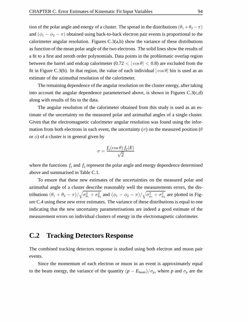
CHAPTER C. Error Estimates of Kinematic Fit Input Variables 94
tion of the polar angle and energy of a cluster. The spread in the distributions(θ1 +θ2−π)
and(φ1 − φ2 − π) obtained using back-to-back electron pair events is proportional to the
calorimeter angular resolution. Figures C.3(a,b) show thevariance of these distributions
as function of the mean polar angle of the two electrons. The solid lines show the results of
a fit to a first and zeroth order polynomials. Data points in theproblematic overlap region
between the barrel and endcap calorimeter (0.72< | cos θ| < 0.8) are excluded from the
fit in Figure C.3(b). In that region, the value of each individual | cos θ| bin is used as an
estimate of the azimuthal resolution of the calorimeter.
The remaining dependence of the angular resolution on the cluster energy, after taking
into account the angular dependence parameterised above, is shown in Figures C.3(c,d)
along with results of fits to the data.
The angular resolution of the calorimeter obtained from this study is used as an es-
timate of the uncertainty on the measured polar and azimuthal angles of a single cluster.
Given that the electromagnetic calorimeter angular resolution was found using the infor-
mation from both electrons in each event, the uncertainty (σ) on the measured position (θ
or φ) of a cluster is in general given by
σ =f1(cos θ) f2(E)√
2
where the functionsf1 and f2 represent the polar angle and energy dependence determined
above and summarised in Table C.1.
To ensure that these new estimates of the uncertainties on the measured polar and
azimuthal angle of a cluster describe reasonably well the measurements errors, the dis-
tributions(θ1 + θ2 − π)/√
σ2θ1
+ σ2θ2
and(φ1 − φ2 − π)/√
σ2φ1
+ σ2φ2
are plotted in Fig-
ure C.4 using these new error estimates. The variance of these distributions is equal to one
indicating that the new uncertainty parameterisations areindeed a good estimate of the
measurement errors on individual clusters of energy in the electromagnetic calorimeter.
C.2 Tracking Detectors Response
The combined tracking detectors response is studied using both electron and muon pair
events.
Since the momentum of each electron or muon in an event is approximately equal
to the beam energy, the variance of the quantity(p − Ebeam)/σp, wherep andσp are the
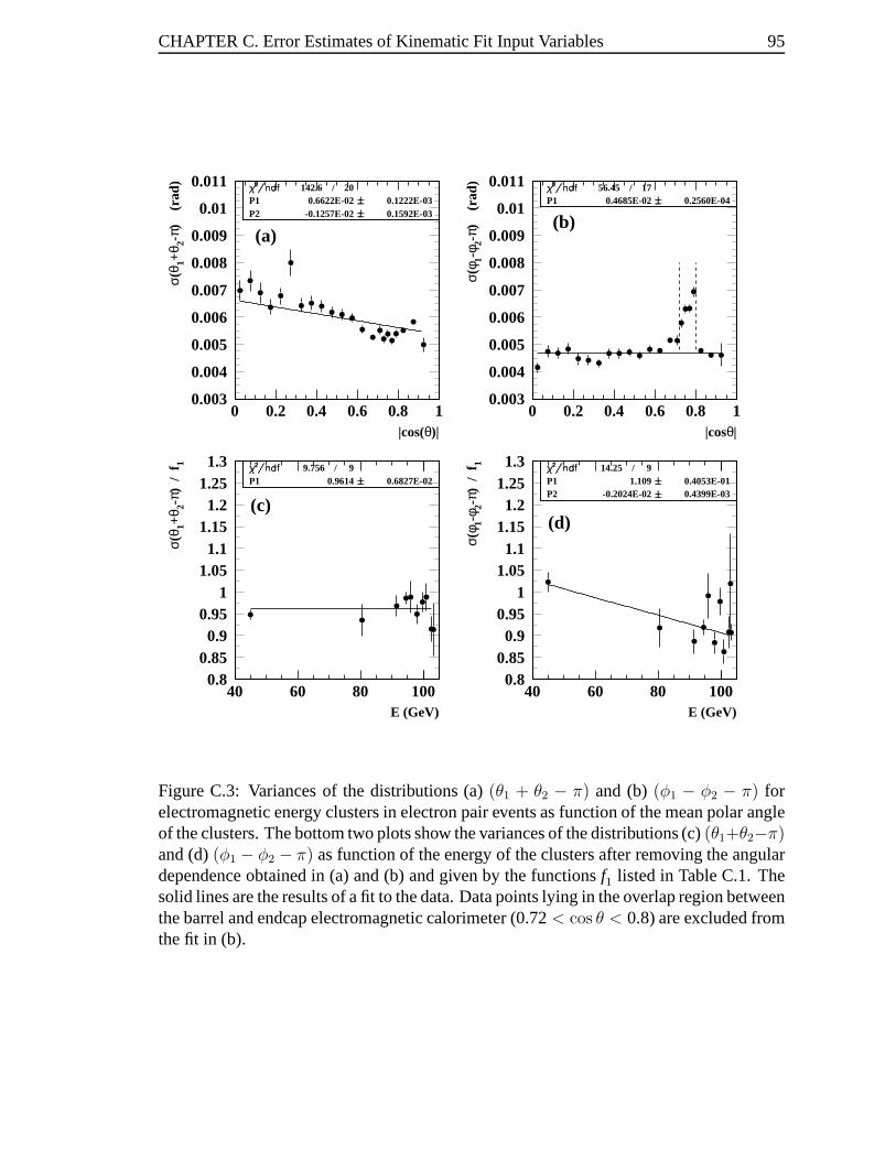
CHAPTER C. Error Estimates of Kinematic Fit Input Variables 95
0.003
0.004
0.005
0.006
0.007
0.008
0.009
0.01
0.011
0 0.2 0.4 0.6 0.8 10.003
0.004
0.005
0.006
0.007
0.008
0.009
0.01
0.011
0 0.2 0.4 0.6 0.8 1
0.80.850.9
0.951
1.051.1
1.151.2
1.251.3
40 60 80 100
|cos(θ)|
σ(θ 1+
θ 2-π)
(
rad) 142.6 / 20
P1 0.6622E-02 0.1222E-03P2 -0.1257E-02 0.1592E-03
(a)
|cosθ|
σ(φ 1-
φ 2-π)
(
rad) 56.45 / 17
P1 0.4685E-02 0.2560E-04
(b)
E (GeV)
σ(θ 1+
θ 2-π)
/ f
1 9.756 / 9P1 0.9614 0.6827E-02
(c)
E (GeV)
σ(φ 1-
φ 2-π)
/ f
1 14.25 / 9P1 1.109 0.4053E-01P2 -0.2024E-02 0.4399E-03
(d)
0.80.850.9
0.951
1.051.1
1.151.2
1.251.3
40 60 80 100
Figure C.3: Variances of the distributions (a)(θ1 + θ2 − π) and (b)(φ1 − φ2 − π) forelectromagnetic energy clusters in electron pair events asfunction of the mean polar angleof the clusters. The bottom two plots show the variances of the distributions (c)(θ1+θ2−π)and (d)(φ1 − φ2 − π) as function of the energy of the clusters after removing the angulardependence obtained in (a) and (b) and given by the functionsf1 listed in Table C.1. Thesolid lines are the results of a fit to the data. Data points lying in the overlap region betweenthe barrel and endcap electromagnetic calorimeter (0.72< cos θ < 0.8) are excluded fromthe fit in (b).

CH
AP
TE
RC
.Err
or
Est
imat
eso
fKin
emat
icF
itIn
pu
tVar
iab
les
96
Errors Angular dependence(mrad) Energy dependence
σθγf1 = (0.66× 10⁻²) − (0.13× 10⁻²) · | cos θ| f2 = 0.96
σφγ
f1 = 0.0047 | cos θ| < 0.72, | cos θ| ≥ 0.80f1 = 0.0058 0.72≥ | cos θ| < 0.74f1 = 0.0063 0.74≥ | cos θ| < 0.76f1 = 0.0063 0.76≥ | cos θ| < 0.78f1 = 0.0069 0.78≥ | cos θ| < 0.80
f2 = (1.11) − (0.20× 10⁻²) · E
σθtrk
f1 = (0.22× 10⁻²) − (0.12× 10⁻³) · | cos θ|f1 = (0.39× 10⁻²) + (0.35× 10⁻²) · | cos θ|f1 = (0.48× 10⁻²) − (0.15× 10⁻²) · | cos θ|
f2 = (0.71) + (0.54× 10⁻²) · p | cos θ| < 0.7 CZ hitsf2 = (1.42) − (0.57× 10⁻²) · p | cos θ| < 0.7 no CZ hitsf2 = (1.07) + (0.17× 10⁻²) · p | cos θ| ≥ 0.7
σφtrkf1 = (−0.27× 10⁻³) + 0.68×10⁻³√
1.−| cos θ|2f2 = 0.91
σθτf1 = (0.034) − (0.015) · | cos θ| f2 = (1.42) − (0.011) · Evis
σφτf1 = (0.99× 10⁻²) + (0.013) · | cos θ| f2 = (0.14) + 3.36√
Evis
Table C.1: Summary of the angular parameterisation functions (f1) and energy corrections (f2) of different angular measurementuncertainties. Since these functions were obtained using the information from both particles in each event, the uncertainty on asingle measurement is given byσ = (f1 · f2)/
√2.
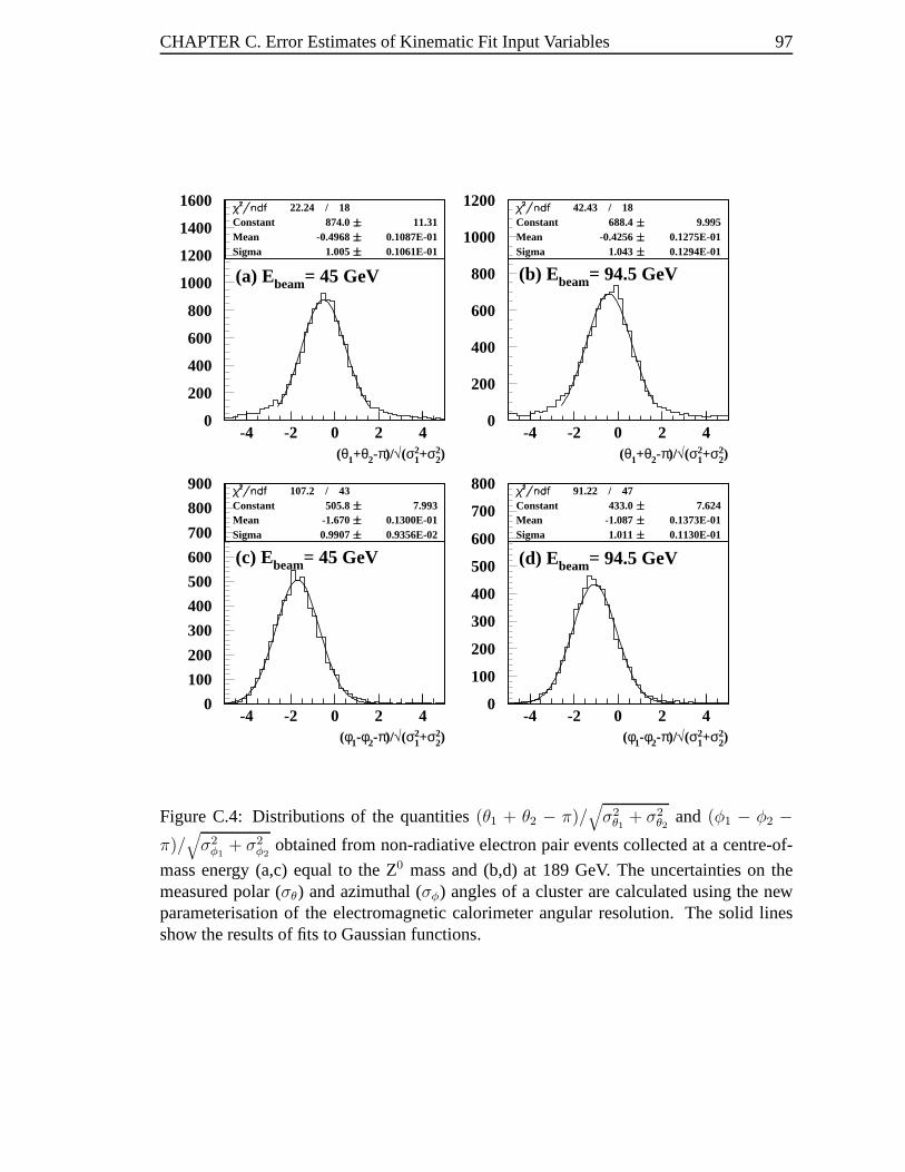
CHAPTER C. Error Estimates of Kinematic Fit Input Variables 97
0
200
400
600
800
1000
1200
1400
1600
-4 -2 0 2 40
200
400
600
800
1000
1200
-4 -2 0 2 4
0
100
200
300
400
500
600
700
800
900
-4 -2 0 2 4
22.24 / 18Constant 874.0 11.31Mean -0.4968 0.1087E-01Sigma 1.005 0.1061E-01
(θ1+θ2-π)/√(σ12+σ2
2)
(a) Ebeam= 45 GeV
42.43 / 18Constant 688.4 9.995Mean -0.4256 0.1275E-01Sigma 1.043 0.1294E-01
(θ1+θ2-π)/√(σ12+σ2
2)
(b) Ebeam= 94.5 GeV
107.2 / 43Constant 505.8 7.993Mean -1.670 0.1300E-01Sigma 0.9907 0.9356E-02
(φ1-φ2-π)/√(σ12+σ2
2)
(c) Ebeam= 45 GeV
91.22 / 47Constant 433.0 7.624Mean -1.087 0.1373E-01Sigma 1.011 0.1130E-01
(φ1-φ2-π)/√(σ12+σ2
2)
(d) Ebeam= 94.5 GeV
0
100
200
300
400
500
600
700
800
-4 -2 0 2 4
Figure C.4: Distributions of the quantities(θ1 + θ2 − π)/√
σ2θ1
+ σ2θ2
and (φ1 − φ2 −π)/
√
σ2φ1
+ σ2φ2
obtained from non-radiative electron pair events collected at a centre-of-
mass energy (a,c) equal to the Z0 mass and (b,d) at 189 GeV. The uncertainties on themeasured polar (σθ) and azimuthal (σφ) angles of a cluster are calculated using the newparameterisation of the electromagnetic calorimeter angular resolution. The solid linesshow the results of fits to Gaussian functions.
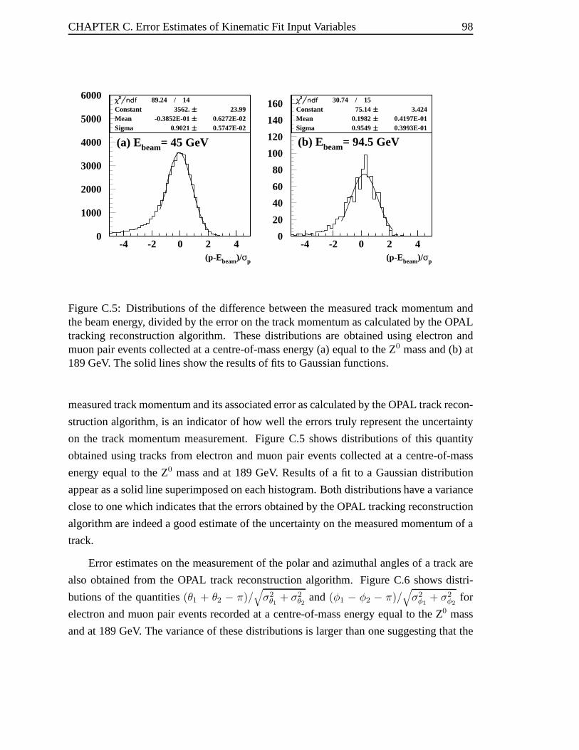
CHAPTER C. Error Estimates of Kinematic Fit Input Variables 98
0
1000
2000
3000
4000
5000
6000
-4 -2 0 2 4
89.24 / 14Constant 3562. 23.99Mean -0.3852E-01 0.6272E-02Sigma 0.9021 0.5747E-02
(p-Ebeam)/σp
(a) Ebeam= 45 GeV
30.74 / 15Constant 75.14 3.424Mean 0.1982 0.4197E-01Sigma 0.9549 0.3993E-01
(p-Ebeam)/σp
(b) Ebeam= 94.5 GeV
0
20
40
60
80
100
120
140
160
-4 -2 0 2 4
Figure C.5: Distributions of the difference between the measured track momentum andthe beam energy, divided by the error on the track momentum ascalculated by the OPALtracking reconstruction algorithm. These distributions are obtained using electron andmuon pair events collected at a centre-of-mass energy (a) equal to the Z0 mass and (b) at189 GeV. The solid lines show the results of fits to Gaussian functions.
measured track momentum and its associated error as calculated by the OPAL track recon-
struction algorithm, is an indicator of how well the errors truly represent the uncertainty
on the track momentum measurement. Figure C.5 shows distributions of this quantity
obtained using tracks from electron and muon pair events collected at a centre-of-mass
energy equal to the Z0 mass and at 189 GeV. Results of a fit to a Gaussian distribution
appear as a solid line superimposed on each histogram. Both distributions have a variance
close to one which indicates that the errors obtained by the OPAL tracking reconstruction
algorithm are indeed a good estimate of the uncertainty on the measured momentum of a
track.
Error estimates on the measurement of the polar and azimuthal angles of a track are
also obtained from the OPAL track reconstruction algorithm. Figure C.6 shows distri-
butions of the quantities(θ1 + θ2 − π)/√
σ2θ1
+ σ2θ2
and(φ1 − φ2 − π)/√
σ2φ1
+ σ2φ2
for
electron and muon pair events recorded at a centre-of-mass energy equal to the Z0 mass
and at 189 GeV. The variance of these distributions is largerthan one suggesting that the
CHAPTER C. Error Estimates of Kinematic Fit Input Variables 99
errors obtained from the OPAL track reconstruction algorithm underestimates the actual
measurements uncertainties.
Following a similar approach as the one outlined in the previous section, the angular
resolution of the tracking system, parameterised as function of polar angle and momentum
of a track, is taken to be an estimate of the uncertainty on themeasured direction of
individual tracks. Both electron and muon pair events are used to extract an estimate of
the angular resolution of tracks.
The angular dependence of the tracking system polar angle resolution was obtained
for three different cases: tracks in the barrel region (| cos θ| < 0.75) with hits in the
Z-chambers (CZ), tracks in the barrel region without hits inthe Z-chambers and tracks
pointing toward the detector endcap region (| cos θ| ≥ 0.75). These three different param-
eterisation functions are necessary since the measurementof a track polar angle is obtained
using a different technique in each case, resulting in a different angular resolution. The
variances of(θ1+θ2−π) distributions, obtained using both electron and muon pair events,
are shown as function of polar angle and track momentum in Figure C.7. The momentum
dependence is plotted after removing the angular dependence given by the functionf1 and
assuming that the momentum of tracks in non-radiative electron and muon pair events is
approximately equal to the beam energy. The solid lines shown in Figure C.7 represent
results from various fits to the data also summarised in TableC.1. The azimuthal reso-
lution is parameterised following a similar approach. Figure C.8 shows the variances of
(φ1 − φ2 − π) distributions as function of polar angle and track momentum. Results from
the fits to the data appear in Table C.1 and are shown as solid lines.
Assuming both tracks in an event have a similar momentum and direction, an estimate
of the uncertainty on the direction of a single track is givenby
σ =f1(cos θ) f2(p)√
2
Figure C.9 shows distributions of the quantities(θ1 + θ2 − π)/√
σ2θ1
+ σ2θ2
and(φ1 −φ2−π)/
√
σ2φ1
+ σ2φ2
for electron and muon pair events obtained using the new uncertainty
estimates on individual tracks. The variances of these distributions are close to one indi-
cating that the new estimates of the uncertainties on the measured direction of a track are
comparable to individual track measurements errors.
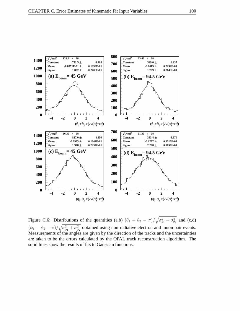
CHAPTER C. Error Estimates of Kinematic Fit Input Variables 100
0
200
400
600
800
1000
1200
1400
-4 -2 0 2 40
100
200
300
400
500
600
700
800
-4 -2 0 2 4
0
200
400
600
800
1000
1200
1400
-4 -2 0 2 4
121.6 / 28Constant 751.5 8.408Mean -0.8071E-01 0.1899E-01Sigma 1.892 0.2406E-01
(θ1+θ2-π)/√(σ12+σ2
2)
(a) Ebeam= 45 GeV
93.42 / 28Constant 399.0 6.237Mean -0.1015 0.2292E-01Sigma 1.709 0.2643E-01
(θ1+θ2-π)/√(σ12+σ2
2)
(b) Ebeam= 94.5 GeV
36.30 / 28Constant 827.0 8.550Mean -0.2993 0.1947E-01Sigma 1.978 0.2434E-01
(φ1-φ2-π)/√(σ12+σ2
2)
(c) Ebeam= 45 GeV
31.35 / 28Constant 383.4 5.670Mean -0.1777 0.3515E-01Sigma 2.298 0.5057E-01
(φ1-φ2-π)/√(σ12+σ2
2)
(d) Ebeam= 94.5 GeV
0
100
200
300
400
500
600
700
-4 -2 0 2 4
Figure C.6: Distributions of the quantities (a,b)(θ1 + θ2 − π)/√
σ2θ1
+ σ2θ2
and (c,d)
(φ1 − φ2 − π)/√
σ2φ1
+ σ2φ2
obtained using non-radiative electron and muon pair events.Measurements of the angles are given by the direction of the tracks and the uncertaintiesare taken to be the errors calculated by the OPAL track reconstruction algorithm. Thesolid lines show the results of fits to Gaussian functions.
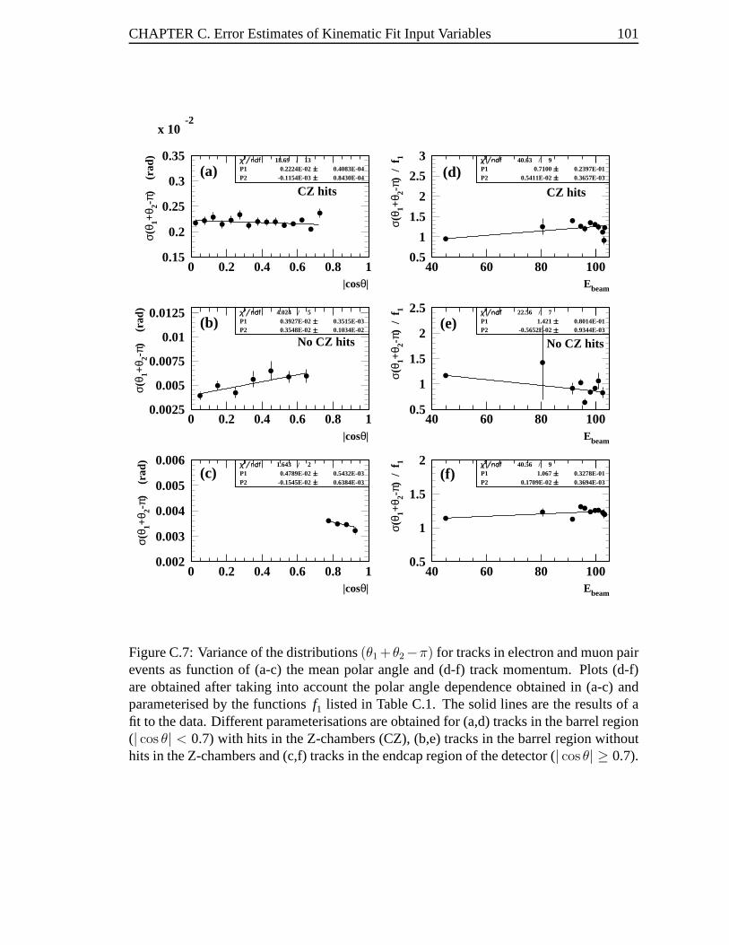
CHAPTER C. Error Estimates of Kinematic Fit Input Variables 101
0.15
0.2
0.25
0.3
0.35
x 10-2
0 0.2 0.4 0.6 0.8 10.5
1
1.5
2
2.5
3
40 60 80 100
0.0025
0.005
0.0075
0.01
0.0125
0 0.2 0.4 0.6 0.8 10.5
1
1.5
2
2.5
40 60 80 100
0.002
0.003
0.004
0.005
0.006
0 0.2 0.4 0.6 0.8 1
|cosθ|
σ(θ 1+
θ 2-π)
(
rad) 18.69 / 13
P1 0.2224E-02 0.4083E-04P2 -0.1154E-03 0.8430E-04
CZ hits
(a)
Ebeam
σ(θ 1+
θ 2-π)
/ f
1 40.63 / 9P1 0.7100 0.2397E-01P2 0.5411E-02 0.3657E-03
CZ hits
(d)
|cosθ|
σ(θ 1+
θ 2-π)
(
rad) 4.024 / 5
P1 0.3927E-02 0.3515E-03P2 0.3548E-02 0.1034E-02
No CZ hits
(b)
Ebeam
σ(θ 1+
θ 2-π)
/ f
1 22.56 / 7P1 1.421 0.8014E-01P2 -0.5652E-02 0.9344E-03
No CZ hits
(e)
|cosθ|
σ(θ 1+
θ 2-π)
(
rad) 1.643 / 2
P1 0.4789E-02 0.5432E-03P2 -0.1545E-02 0.6384E-03
(c)
Ebeam
σ(θ 1+
θ 2-π)
/ f
1 40.56 / 9P1 1.067 0.3278E-01P2 0.1709E-02 0.3694E-03
(f)
0.5
1
1.5
2
40 60 80 100
Figure C.7: Variance of the distributions(θ1 +θ2−π) for tracks in electron and muon pairevents as function of (a-c) the mean polar angle and (d-f) track momentum. Plots (d-f)are obtained after taking into account the polar angle dependence obtained in (a-c) andparameterised by the functionsf1 listed in Table C.1. The solid lines are the results of afit to the data. Different parameterisations are obtained for (a,d) tracks in the barrel region(| cos θ| < 0.7) with hits in the Z-chambers (CZ), (b,e) tracks in the barrel region withouthits in the Z-chambers and (c,f) tracks in the endcap region of the detector (| cos θ| ≥ 0.7).

CHAPTER C. Error Estimates of Kinematic Fit Input Variables 102
0.020.04
0.060.08
0.1
0.120.14
0.160.18
0.2
x 10-2
0 0.2 0.4 0.6 0.8 1|cos(θ)|
σ(|φ
1-φ 2|
-π)
(r
ad)
110.9 / 17P1 -0.2708E-03 0.1119E-04P2 0.6828E-03 0.8107E-05
(a)
p (GeV)σ(
|φ1-
φ 2|-π
) /
f 1 42.93 / 10P1 0.9112 0.3768E-02
(b)
0.8
0.85
0.9
0.95
1
1.05
1.1
40 60 80 100
Figure C.8: Variance of the distributions(φ1−φ2−π) for tracks in electron and muon pairevents as function of (a) the mean polar angle and (b) track momentum. Plot (b) is obtainedafter taking into account the polar angle dependence found in (a) and parameterised by thefunctionf1 listed in Table C.1. The solid lines are the results of a fit to the data.
C.3 Taus
The direction of tau candidates is taken to be the axis of the jet. The uncertainty in the tau
direction comes from the presence of undetected neutrinos from the tau decay and from
the finite resolution of different subdetectors.
An estimate of the uncertainties on the measured polar and azimuthal angles of tau
candidates is obtained using coplanar tau pair events whereboth taus have a similar
amount of energy, corrected for double-counting of tracks and energy clusters, deposited
in the detector. Distributions of the quantities(θ1+θ2−π) and(φ1−φ2−π) as function of
the mean polar angle and visible energy of both taus are shownin Figure C.10. Results of
the fits to the data are shown as solid lines and summarised in Table C.1. Distributions of
the quantities(θ1 + θ2 −π)/√
σ2θ1
+ σ2θ2
and(φ1 − φ2 − π)/√
σ2φ1
+ σ2φ2
are Gaussian dis-
tributed with a variance of one indicating that the uncertainties on the measured direction
of a tau candidate estimated from the parameterisation given above are a good estimate of
the measurements uncertainties.
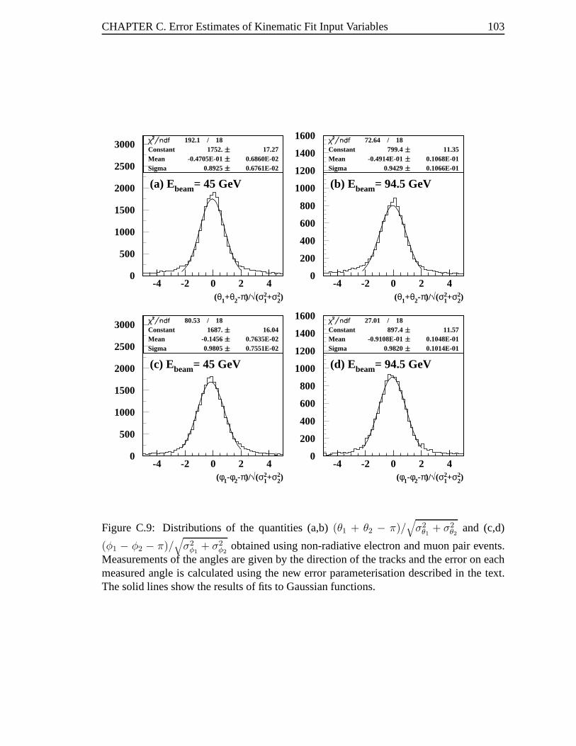
CHAPTER C. Error Estimates of Kinematic Fit Input Variables 103
0
500
1000
1500
2000
2500
3000
-4 -2 0 2 40
200
400
600
800
1000
1200
1400
1600
-4 -2 0 2 4
0
500
1000
1500
2000
2500
3000
-4 -2 0 2 4
192.1 / 18Constant 1752. 17.27Mean -0.4705E-01 0.6860E-02Sigma 0.8925 0.6761E-02
(θ1+θ2-π)/√(σ12+σ2
2)
(a) Ebeam= 45 GeV
72.64 / 18Constant 799.4 11.35Mean -0.4914E-01 0.1068E-01Sigma 0.9429 0.1066E-01
(θ1+θ2-π)/√(σ12+σ2
2)
(b) Ebeam= 94.5 GeV
80.53 / 18Constant 1687. 16.04Mean -0.1456 0.7635E-02Sigma 0.9805 0.7551E-02
(φ1-φ2-π)/√(σ12+σ2
2)
(c) Ebeam= 45 GeV
27.01 / 18Constant 897.4 11.57Mean -0.9108E-01 0.1048E-01Sigma 0.9820 0.1014E-01
(φ1-φ2-π)/√(σ12+σ2
2)
(d) Ebeam= 94.5 GeV
0
200
400
600
800
1000
1200
1400
1600
-4 -2 0 2 4
Figure C.9: Distributions of the quantities (a,b)(θ1 + θ2 − π)/√
σ2θ1
+ σ2θ2
and (c,d)
(φ1 − φ2 − π)/√
σ2φ1
+ σ2φ2
obtained using non-radiative electron and muon pair events.Measurements of the angles are given by the direction of the tracks and the error on eachmeasured angle is calculated using the new error parameterisation described in the text.The solid lines show the results of fits to Gaussian functions.

CHAPTER C. Error Estimates of Kinematic Fit Input Variables 104
0.01
0.015
0.02
0.025
0.03
0.035
0.04
0.045
0.05
0.055
0 0.2 0.4 0.6 0.8 10.005
0.01
0.015
0.02
0.025
0.03
0.035
0.04
0 0.2 0.4 0.6 0.8 1
0.25
0.5
0.75
1
1.25
1.5
1.75
2
2.25
2.5
0 20 40 60 80 100
|cosθ|
σ(θ 1+
θ 2-π)
(
rad) 13.88 / 7
P1 0.3437E-01 0.2029E-02P2 -0.1484E-01 0.3765E-02
(a)
|cosθ|
σ(|φ
1-φ 2|
-π)
(r
ad)
8.492 / 7P1 0.9903E-02 0.6629E-03P2 0.1264E-01 0.1673E-02
(b)
Evisible
σ(θ 1+
θ 2-π)
/ f
1 6.062 / 4P1 1.423 0.1021P2 -0.1097E-01 0.3291E-02
(c)
Evisible
σ(|φ
1-φ 2|
-π)
/ f 1 23.66 / 7
P1 3.362 0.1706P2 0.1382 0.4226E-01
(d)
00.250.5
0.751
1.251.5
1.752
2.252.5
0 20 40 60 80 100
Figure C.10: Variance of the distributions(θ1 + θ2 − π) and(φ1 − φ2 − π) obtained usingtau pair events as function of (a,b) the mean polar angle and (c,d) visible energy of the twotaus. Plot (c,d) are obtained after taking into account the polar angle dependence foundin (a,b) and parameterised by the functionsf1 listed in Table C.1. The solid lines are theresults of a fit to the data.
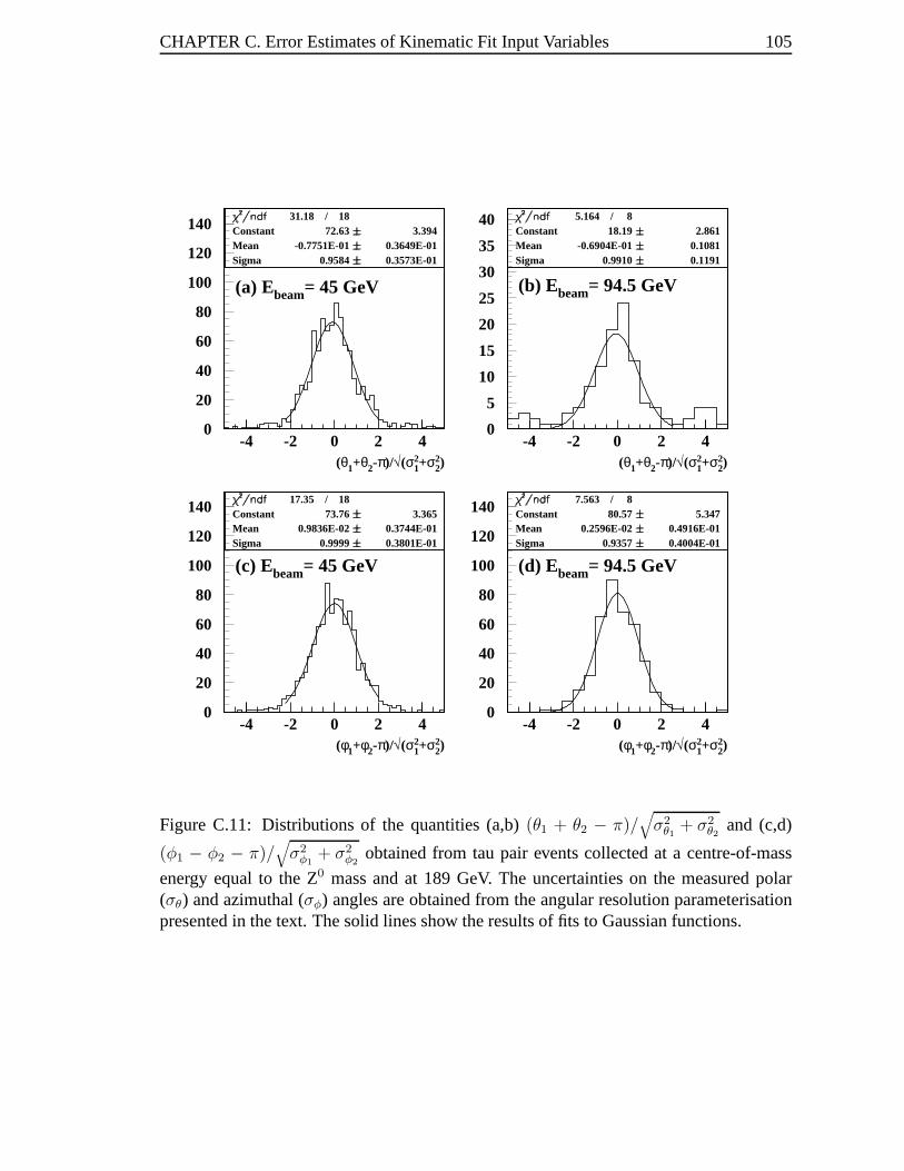
CHAPTER C. Error Estimates of Kinematic Fit Input Variables 105
0
20
40
60
80
100
120
140
-4 -2 0 2 40
5
10
15
20
25
30
35
40
-4 -2 0 2 4
0
20
40
60
80
100
120
140
-4 -2 0 2 4
31.18 / 18Constant 72.63 3.394Mean -0.7751E-01 0.3649E-01Sigma 0.9584 0.3573E-01
(θ1+θ2-π)/√(σ12+σ2
2)
(a) Ebeam= 45 GeV
5.164 / 8Constant 18.19 2.861Mean -0.6904E-01 0.1081Sigma 0.9910 0.1191
(θ1+θ2-π)/√(σ12+σ2
2)
(b) Ebeam= 94.5 GeV
17.35 / 18Constant 73.76 3.365Mean 0.9836E-02 0.3744E-01Sigma 0.9999 0.3801E-01
(φ1+φ2-π)/√(σ12+σ2
2)
(c) Ebeam= 45 GeV
7.563 / 8Constant 80.57 5.347Mean 0.2596E-02 0.4916E-01Sigma 0.9357 0.4004E-01
(φ1+φ2-π)/√(σ12+σ2
2)
(d) Ebeam= 94.5 GeV
0
20
40
60
80
100
120
140
-4 -2 0 2 4
Figure C.11: Distributions of the quantities (a,b)(θ1 + θ2 − π)/√
σ2θ1
+ σ2θ2
and (c,d)
(φ1 − φ2 − π)/√
σ2φ1
+ σ2φ2
obtained from tau pair events collected at a centre-of-mass
energy equal to the Z0 mass and at 189 GeV. The uncertainties on the measured polar(σθ) and azimuthal (σφ) angles are obtained from the angular resolution parameterisationpresented in the text. The solid lines show the results of fitsto Gaussian functions.
Appendix D
Efficiency, Mass Resolution and
Correction Factor Interpolation
In order to calculate limits on the product of the cross-section and the branching fraction
of excited leptons, the signal efficiencies, invariant massresolutions and corrections to the
efficiency due to a non-Gaussian component of the mass distributions must all be calcu-
lable for arbitrary values of excited lepton mass and collision centre-of-mass energy. To
achieve this, these quantities were parameterised as function of the excited lepton mass
scaled by the centre-of-mass energy (m*/√
s). Figures D.2-D.6 show results of the vari-
ous parameterisations superimposed on the values obtainedfrom simulated event samples
at different excited lepton mass and centre-of-mass energy. The different functions are
tabulated in Table D.1.
The signal efficiency is defined as the ratio of the number of events selected using the
criteria described in Chapters 4 and 5 to the total number of events generated assuming a
100% electromagnetic branching fraction.
The mass resolution at a specific value of excited lepton massand centre-of-mass en-
ergy is obtained by fitting the reconstructed invariant massof selected events to a Gaussian
distribution. The variance of the Gaussian fit is taken as an estimate of the mass resolution.
Correction factors to account for a non-Gaussian componentof the mass distribu-
tions are calculated as the area under the Gaussian fit of the invariant mass distributions,
expressed in number of events, divided by the number of events selected.
106

CHAPTER D. Efficiency, Mass Resolution and Correction Factor Interpolation 107
0
0.1
0.2
0.3
0.4 0.6 0.8 10.2
0.4
0.6
0.8
1
0.2 0.3 0.4 0.5
0.5
0.6
0.7
0.8
0.9
1
0.4 0.6 0.8 10.2
0.4
0.6
0.8
1
0.2 0.3 0.4 0.5
0
0.2
0.4
0.6
0.8
1
0.4 0.6 0.8 1
17.97 / 25P1 0.1210 0.1242E-01P2 -0.2199 0.3547E-01P3 0.2308 0.2547E-01
m*/√s
effic
ienc
y(a) e*
(eeγ)
45.76 / 25P1 -1.620 0.1758E-01P2 18.45 0.9262E-01P3 -53.41 0.2240P4 50.32 0.3474
m*/√s
effic
ienc
y
(d) e*e*
31.39 / 25P1 0.9121 0.1980E-01P2 -0.6261 0.5534E-01P3 0.3995 0.3924E-01
m*/√s
effic
ienc
y
(b) µ* 33.13 / 25
P1 -1.045 0.1782E-01P2 13.05 0.9299E-01P3 -35.82 0.2242P4 32.32 0.3478
m*/√s
effic
ienc
y
(e) µ*µ*
66.76 / 25P1 0.5335 0.3556E-02P2 0.7512 0.5090P3 -58.96 6.623
m*/√s
effic
ienc
y
(c) τ* 35.80 / 25
P1 -0.9834 0.1749E-01P2 12.16 0.9200E-01P3 -34.67 0.2227P4 32.44 0.3453
m*/√s
effic
ienc
y
(f) τ*τ*
0.2
0.4
0.6
0.8
1
0.2 0.3 0.4 0.5
Figure D.1: Efficiencies for the single and pair production selection criteria as a functionof excited lepton mass scaled by the centre-of-mass energy (m*/
√s) for the selections of
(a-c)``γ and (d-f)``γγ event. The points represent efficiencies obtained using simulatedevent samples at different mass and centre-of-mass energy.The solid lines show results ofa fit to the data points.
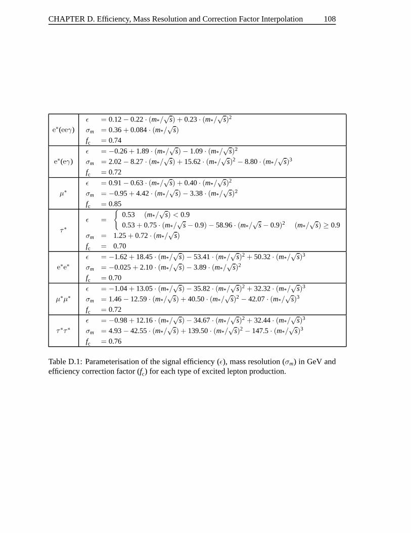
CHAPTER D. Efficiency, Mass Resolution and Correction Factor Interpolation 108
e∗(eeγ)
ε = 0.12− 0.22· (m*/√
s) + 0.23· (m*/√
s)2
σm = 0.36+ 0.084· (m*/√
s)
fc = 0.74
e∗(eγ)
ε = −0.26+ 1.89· (m*/√
s) − 1.09· (m*/√
s)2
σm = 2.02− 8.27· (m*/√
s) + 15.62· (m*/√
s)2 − 8.80· (m*/√
s)3
fc = 0.72
µ∗
ε = 0.91− 0.63· (m*/√
s) + 0.40· (m*/√
s)2
σm = −0.95+ 4.42· (m*/√
s) − 3.38· (m*/√
s)2
fc = 0.85
τ∗
ε =
0.53 (m*/√
s) < 0.9
0.53+ 0.75· (m*/√
s− 0.9) − 58.96· (m*/√
s− 0.9)2 (m*/√
s) ≥ 0.9
σm = 1.25+ 0.72· (m*/√
s)
fc = 0.70
e∗e∗ε = −1.62+ 18.45· (m*/
√s) − 53.41· (m*/
√s)2 + 50.32· (m*/
√s)3
σm = −0.025+ 2.10· (m*/√
s) − 3.89· (m*/√
s)2
fc = 0.70
µ∗µ∗
ε = −1.04+ 13.05· (m*/√
s) − 35.82· (m*/√
s)2 + 32.32· (m*/√
s)3
σm = 1.46− 12.59· (m*/√
s) + 40.50· (m*/√
s)2 − 42.07· (m*/√
s)3
fc = 0.72
τ∗τ∗
ε = −0.98+ 12.16· (m*/√
s) − 34.67· (m*/√
s)2 + 32.44· (m*/√
s)3
σm = 4.93− 42.55· (m*/√
s) + 139.50· (m*/√
s)2 − 147.5· (m*/√
s)3
fc = 0.76
Table D.1: Parameterisation of the signal efficiency (ε), mass resolution (σm) in GeV andefficiency correction factor (fc) for each type of excited lepton production.
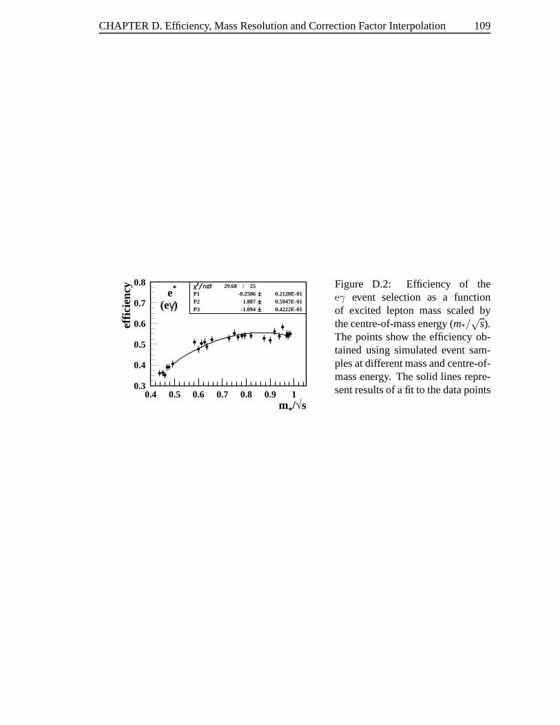
CHAPTER D. Efficiency, Mass Resolution and Correction Factor Interpolation 109
29.68 / 25P1 -0.2586 0.2120E-01P2 1.887 0.5947E-01P3 -1.094 0.4222E-01
m*/√s
effic
ienc
y
e*
(eγ)
0.3
0.4
0.5
0.6
0.7
0.8
0.4 0.5 0.6 0.7 0.8 0.9 1
Figure D.2: Efficiency of theeγ event selection as a functionof excited lepton mass scaled bythe centre-of-mass energy (m*/
√s).
The points show the efficiency ob-tained using simulated event sam-ples at different mass and centre-of-mass energy. The solid lines repre-sent results of a fit to the data points
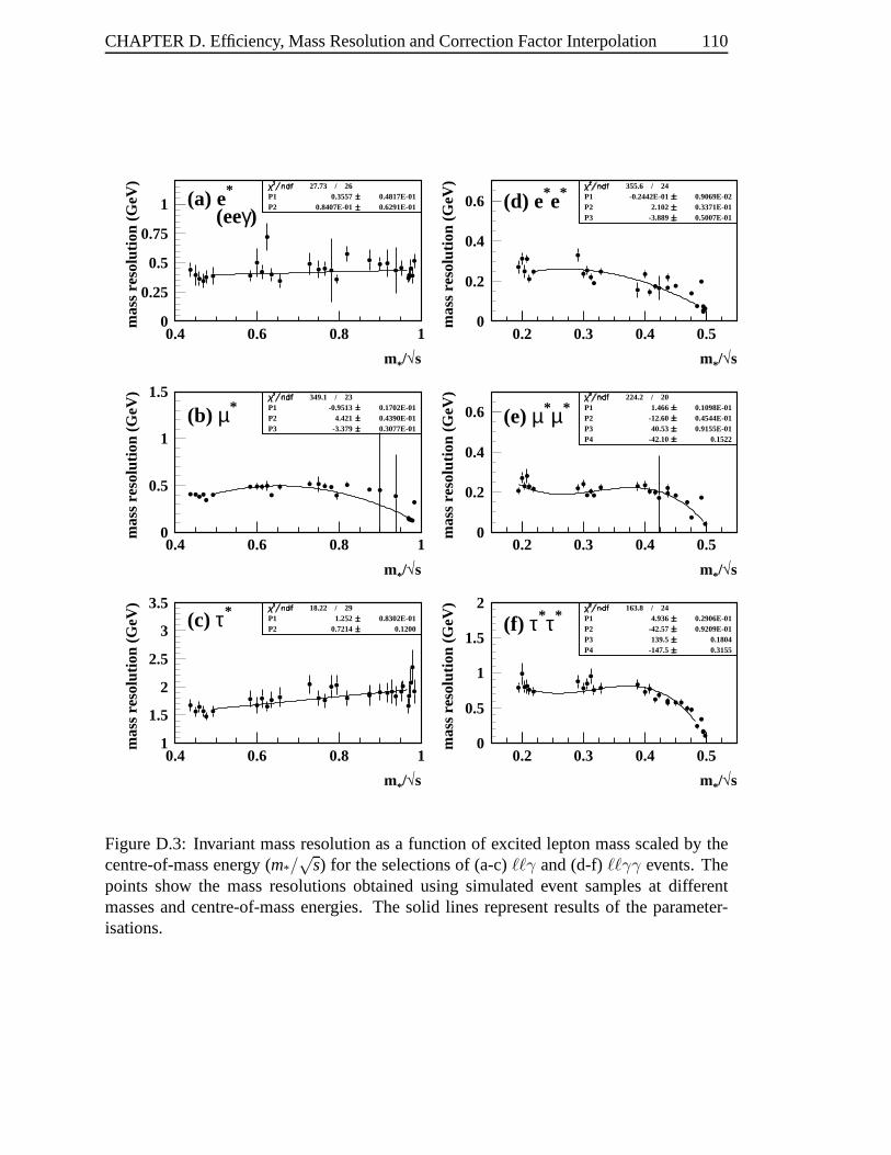
CHAPTER D. Efficiency, Mass Resolution and Correction Factor Interpolation 110
0
0.25
0.5
0.75
1
0.4 0.6 0.8 10
0.2
0.4
0.6
0.2 0.3 0.4 0.5
0
0.5
1
1.5
0.4 0.6 0.8 10
0.2
0.4
0.6
0.2 0.3 0.4 0.5
1
1.5
2
2.5
3
3.5
0.4 0.6 0.8 1
27.73 / 26P1 0.3557 0.4817E-01P2 0.8407E-01 0.6291E-01
m*/√s
mas
s re
solu
tion
(GeV
)
(a) e*
(eeγ)
355.6 / 24P1 -0.2442E-01 0.9069E-02P2 2.102 0.3371E-01P3 -3.889 0.5007E-01
m*/√s
mas
s re
solu
tion
(GeV
)
(d) e*e*
349.1 / 23P1 -0.9513 0.1702E-01P2 4.421 0.4390E-01P3 -3.379 0.3077E-01
m*/√s
mas
s re
solu
tion
(GeV
)
(b) µ* 224.2 / 20
P1 1.466 0.1098E-01P2 -12.60 0.4544E-01P3 40.53 0.9155E-01P4 -42.10 0.1522
m*/√s
mas
s re
solu
tion
(GeV
)
(e) µ*µ*
18.22 / 29P1 1.252 0.8302E-01P2 0.7214 0.1200
m*/√s
mas
s re
solu
tion
(GeV
)
(c) τ* 163.8 / 24P1 4.936 0.2906E-01P2 -42.57 0.9209E-01P3 139.5 0.1804P4 -147.5 0.3155
m*/√s
mas
s re
solu
tion
(GeV
)
(f) τ*τ*
0
0.5
1
1.5
2
0.2 0.3 0.4 0.5
Figure D.3: Invariant mass resolution as a function of excited lepton mass scaled by thecentre-of-mass energy (m*/
√s) for the selections of (a-c) γ and (d-f)``γγ events. The
points show the mass resolutions obtained using simulated event samples at differentmasses and centre-of-mass energies. The solid lines represent results of the parameter-isations.
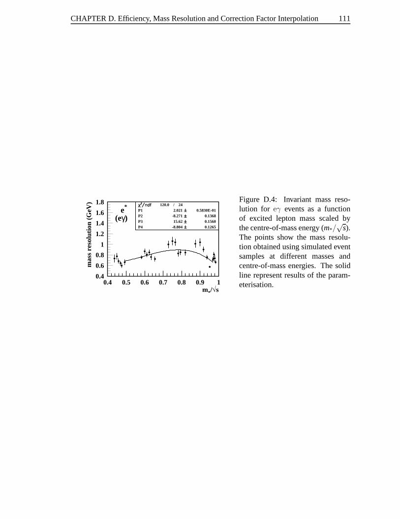
CHAPTER D. Efficiency, Mass Resolution and Correction Factor Interpolation 111
120.0 / 24P1 2.021 0.5830E-01P2 -8.271 0.1368P3 15.62 0.1560P4 -8.804 0.1265
m*/√s
mas
s re
solu
tion
(GeV
)
e*
(eγ)
0.4
0.6
0.8
1
1.2
1.4
1.6
1.8
0.4 0.5 0.6 0.7 0.8 0.9 1
Figure D.4: Invariant mass reso-lution for eγ events as a functionof excited lepton mass scaled bythe centre-of-mass energy (m*/
√s).
The points show the mass resolu-tion obtained using simulated eventsamples at different masses andcentre-of-mass energies. The solidline represent results of the param-eterisation.
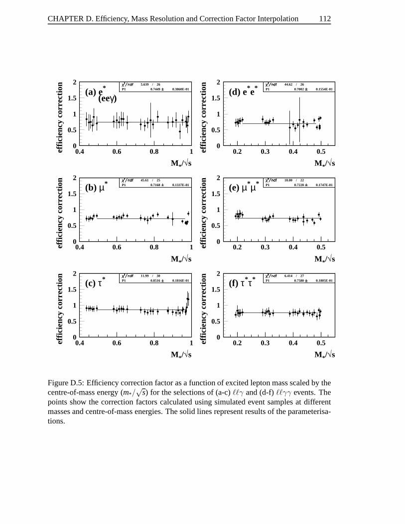
CHAPTER D. Efficiency, Mass Resolution and Correction Factor Interpolation 112
0
0.5
1
1.5
2
0.4 0.6 0.8 10
0.5
1
1.5
2
0.2 0.3 0.4 0.5
0
0.5
1
1.5
2
0.4 0.6 0.8 10
0.5
1
1.5
2
0.2 0.3 0.4 0.5
0
0.5
1
1.5
2
0.4 0.6 0.8 1
5.639 / 26P1 0.7449 0.3860E-01
M */√s
effic
ienc
y co
rrec
tion
(a) e*
(eeγ)
44.62 / 26P1 0.7002 0.1554E-01
M */√s
effic
ienc
y co
rrec
tion
(d) e*e*
45.61 / 25P1 0.7168 0.1337E-01
M */√s
effic
ienc
y co
rrec
tion
(b) µ* 18.80 / 22
P1 0.7228 0.1747E-01
M */√s
effic
ienc
y co
rrec
tion
(e) µ*µ*
11.99 / 30P1 0.8516 0.1816E-01
M */√s
effic
ienc
y co
rrec
tion
(c) τ* 6.414 / 27
P1 0.7580 0.1805E-01
M */√s
effic
ienc
y co
rrec
tion
(f) τ*τ*
0
0.5
1
1.5
2
0.2 0.3 0.4 0.5
Figure D.5: Efficiency correction factor as a function of excited lepton mass scaled by thecentre-of-mass energy (m*/
√s) for the selections of (a-c) γ and (d-f)``γγ events. The
points show the correction factors calculated using simulated event samples at differentmasses and centre-of-mass energies. The solid lines represent results of the parameterisa-tions.
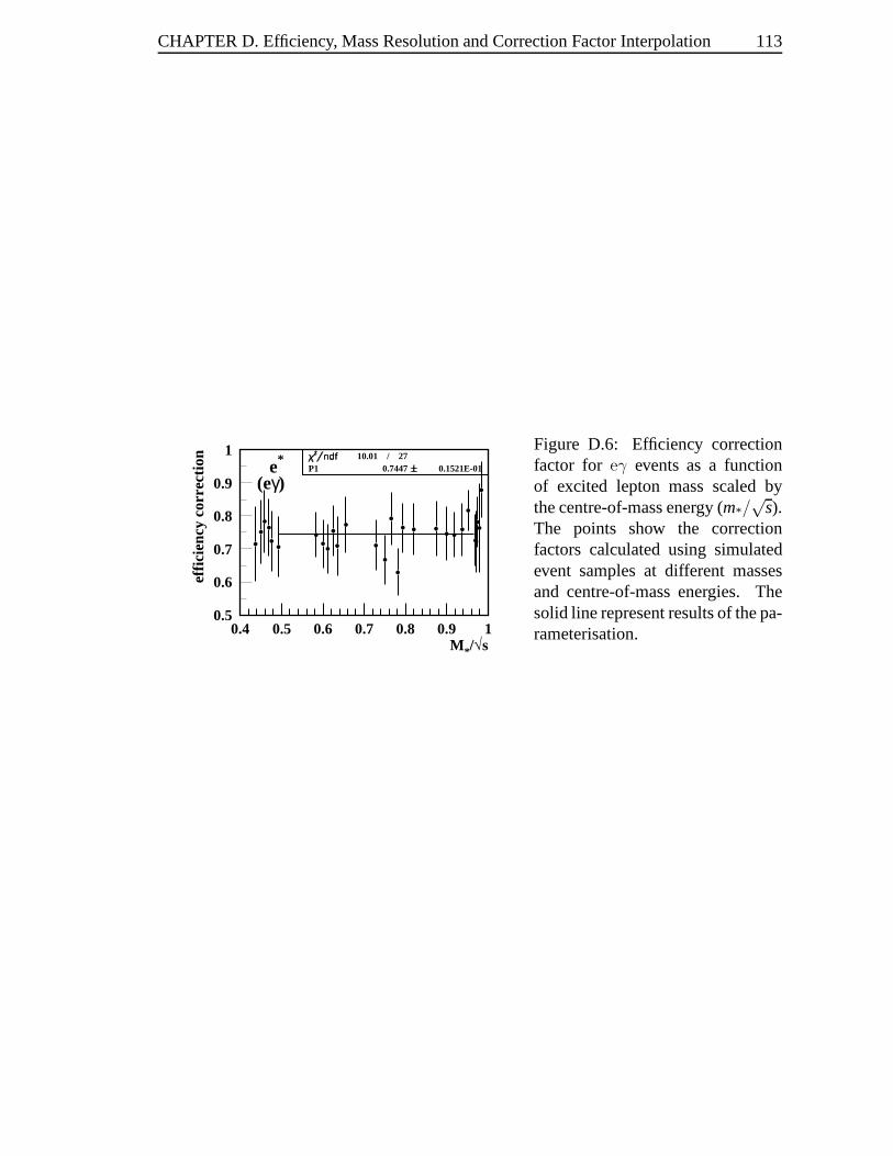
CHAPTER D. Efficiency, Mass Resolution and Correction Factor Interpolation 113
10.01 / 27P1 0.7447 0.1521E-01
M */√s
effic
ienc
y co
rrec
tion
e*
(eγ)
0.5
0.6
0.7
0.8
0.9
1
0.4 0.5 0.6 0.7 0.8 0.9 1
Figure D.6: Efficiency correctionfactor for eγ events as a functionof excited lepton mass scaled bythe centre-of-mass energy (m*/
√s).
The points show the correctionfactors calculated using simulatedevent samples at different massesand centre-of-mass energies. Thesolid line represent results of the pa-rameterisation.

Appendix E
Confidence Level Calculation
Results from a search for new phenomena are usually expressed in terms of the discovery
or exclusion of a signal at a specific confidence level. There exist different approaches
in calculating the degree of compatibility of an experimental outcome with new physics
processes. In the following, the method known as the ModifiedFrequentist approach [67,
68] is summarised.
For any monotonically increasing test statistic (X) with respect to more signal-like
experiments, the confidence in the background plus signal hypothesis (CLs+b) is given
by the probability that the estimator be less than or equal tothe value observed in the
experiment (Xobs),
CLs+b = Ps+b(X ≤ Xobs), (E.1)
where
Ps+b(X ≤ Xobs) =∫ Xobs
−∞
dPs+b
dXdX . (E.2)
The quantitydPs+b/dX is the probability density function of the test statistic for experi-
ments with signal and background events. Small values ofCLs+b indicate that the data
are not compatible with the hypothesis for the presence of both signal and background
events. In general, the probability density function of thetest statistic is not necessarily
analytically calculable in which case a Monte Carlo simulation of experiments satisfy-
ing the relevant hypothesis is often necessary to perform the integration. However, since
the chosen estimator (Q) in this analysis is defined to depend only on the number of ob-
served candidates in each individual channel, the probability density functiondPs+b/dQ is
Poisson distributed such that
CLs+b =∑
Q(n′)≤Q(nobs)
N∏
i=1
e−(si+bi) (si + bi)n′i
n′i !
(E.3)
114
CHAPTER E. Confidence Level Calculation 115
whereQ(nobs) is the likelihood ratio obtained from the observed number ofcandidate
eventsni in each channeli. The sum runs over all the possible outcomesn′ for which the
likelihood ratio is less than or equal to the observed one.
Following the same reasoning as above, the confidence in the background only hy-
pothesis is in general given by
CLb = Pb(X ≤ Xobs), (E.4)
where
Pb(X ≤ Xobs) =∫ Xobs
−∞
dPb
dXdX . (E.5)
The quantitydPb/dX is the probability density function of the test statistic for background
only experiments. In analogy with Equation E.3, the confidence in the background only
hypothesis for the specific choice of the test statistic usedin this analysis is given by
CLb =∑
Q(n′)≤Q(nobs)
N∏
i=1
e−bi bn′ii
n′i !
(E.6)
A value of CLb close to one would indicate that the experimental data are incompatible
with the background only hypothesis and that the signal plusbackground hypothesis is
instead favored.
For most realistic situation, where a large number of channels are considered, the cal-
culation of the quantityCLs+b andCLb quickly becomes computationally challenging. A
method [68] whereby the estimators and probability densities of all possible experimental
outcomes of channels are combined two at a time is used to speed up the limit calculations.
E.1 The Modified Frequentist Approach
The value 1−CLb may be used to quote the confidence in a potential discovery. Similarly,
exclusion limits on the existence of signal may be calculated using the confidence level
1 − CLs+b. This quantity however has the property that for experiments with a number
of observed events smaller than the expected background, strong limits can be calculated
that not only exclude any signal events but also exclude the background hypothesis to a
high level of confidence. Although these limits are valid from a strictly statistical point
of view, they reflect the probability of obtaining similar oreven stronger exclusion limits
CHAPTER E. Confidence Level Calculation 116
in other experiments with the same expected number of signaland background events.
These exclusion limits are not a direct statement about the absence of signal events. For
experimental physicists carrying out searches for new phenomena, the quantity of inter-
est given a set of experimental measurements, is the confidence in the signal hypothesis.
Unfortunately, it is in general not possible to precisely correct the data for the presence
of backgrounds or carry out a completely background-free experiment. Thus, in most
searches, it is experimentally impossible to directly calculate the confidence in the signal-
only hypothesis.
The technique used in this work, which deals in a more intuitive way with the special
situation described above, is called the Modified Frequentist approach. The name of the
procedure refers to the fact that it is a departure from a strict frequentist interpretation
of limit setting. A quantityCLs is defined to be the ratio of the confidence in the two
hypotheses considered,
CLs ≡CLs+b
CLb. (E.7)
This quantity, although not itself a confidence but rather a ratio of confidences, is use to
exclude the existence of signal events at a fixed confidence level CL given that
CL ≥ 1− CLs . (E.8)
Going back to the example described above where an experiment observes less events
than the expected background, the exclusion limits obtained using the Modified Frequen-
tist approach would in this case result in more conservativelimits. This is sensible since,
intuitively, there is not enough information available to distinguish between the signal
plus background and background-only hypotheses. The use ofthe Modified Frequentist
approach is a method of obtaining conservative limits on theexistence of signal events.
The quantityCLs can be interpreted as an approximation of the confidence in the sig-
nal hypothesis that would be obtained if an experiment was performed in the absence of
background or equivalently, if the background was precisely known and subtracted from
the observed data. The probability of falsely excluding a true signal (often called a type
II error in statistics textbooks [43–45]) using the quantity CLs is in general less than the
nominal value (1− CL). For example, in calculating exclusion limits on the signal at the
95% confidence level (CL), the probability of excluding a true signal is in fact less than
5%. This is a consequence of the fact that the quantityCLs is not itself a confidence but
a ratio of confidences. In statistical terms, the use ofCLs increases the ‘coverage’ of an
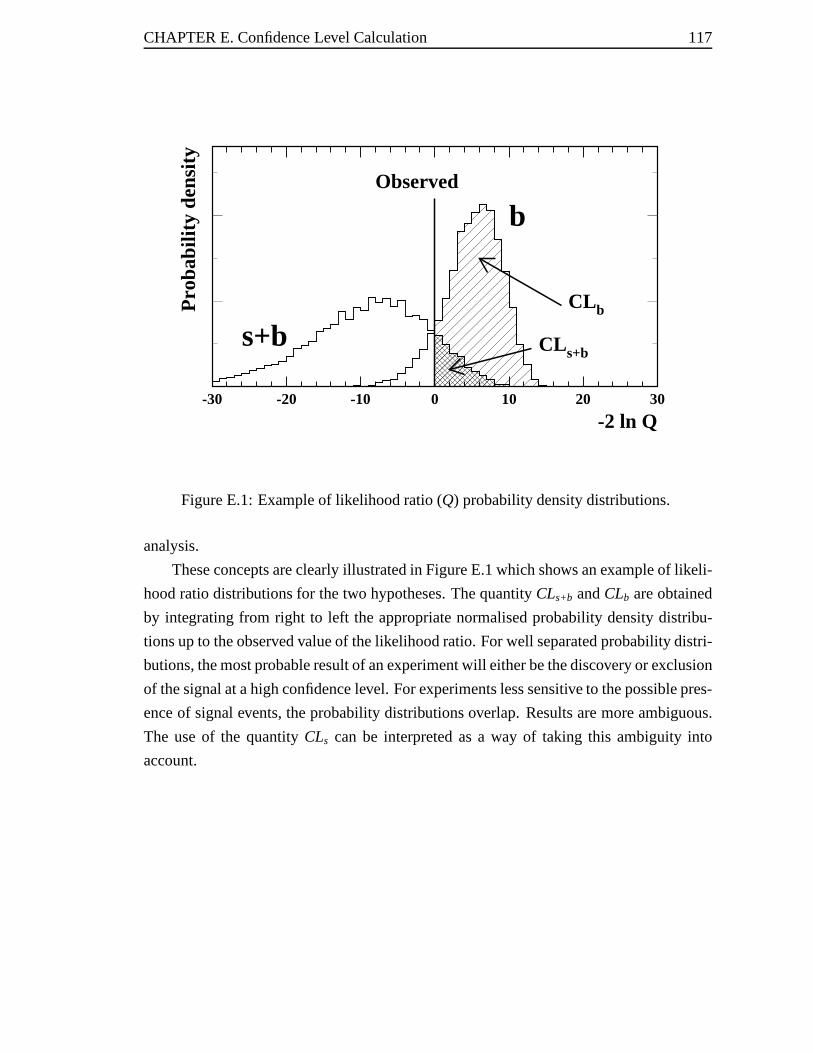
CHAPTER E. Confidence Level Calculation 117
Observed
-2 ln Q
Pro
babi
lity
dens
ity
s+b
b
CL s+b
CLb
-30 -20 -10 0 10 20 30
Figure E.1: Example of likelihood ratio (Q) probability density distributions.
analysis.
These concepts are clearly illustrated in Figure E.1 which shows an example of likeli-
hood ratio distributions for the two hypotheses. The quantity CLs+b andCLb are obtained
by integrating from right to left the appropriate normalised probability density distribu-
tions up to the observed value of the likelihood ratio. For well separated probability distri-
butions, the most probable result of an experiment will either be the discovery or exclusion
of the signal at a high confidence level. For experiments lesssensitive to the possible pres-
ence of signal events, the probability distributions overlap. Results are more ambiguous.
The use of the quantityCLs can be interpreted as a way of taking this ambiguity into
account.
Appendix F
Excited electron contribution to the
e+e−→ γγ cross-section
In addition to the pair and single production discussed above, the existence of excited
electrons could also manifest itself in the production of events containing two photons.
Figure F.1 shows (a) the Standard Model interactions and (b)excited electron contributions
to the processe+e− → γγ. The existence of excited electrons would therefore results in
deviations from the Standard Model differential cross-section of events with two photons
in the final state.
Limits on the strength of thee∗e γ coupling extracted from thee+e− → γγ dif-
ferential cross-section [69] uses a different form of interaction than the one described in
Equation 2.8 for which searches for singly produced excitedstates rely on. By using a
common theoretical framework, thee+e− → γγ process can be used to extend the limits
on thee∗e γ coupling strength for excited electron masses beyond the kinematically al-
lowed region of single production. Small deviations from the Standard Model predictions
are expected even for excited leptons with a mass larger thanthe centre-of-mass energy of
the e+e- collisions.
Results from indirect searches, where the existence ofe∗ is inferred from deviations
in the e+ e− → γγ differential cross-section, are usually expressed in terms of limits on
the e∗eγ coupling strength assuming a general extension of the Standard Model. The
interaction between an excited lepton, a lepton and a gauge boson (L∗L V) is described by
the simplest gauge invariant form of the interaction Lagrangian [70]
LL∗L V =e2
κ
m*L*
σµν L Fµν + hermitian conjugate (F.1)
118

CHAPTER F. Excited electron contribution to thee+e−
→ γγ cross-section 119
e
γ
ee
γ
e
γ
ee
γ
(a)
e
γ
e*e
γ
e
γ
e*e
γ
(b)
Figure F.1: Diagrams showing the (a) Standard Model and (b) excited electron contribu-tions to the processe+e− → γγ considered in the calculations of the differential cross-section presented in the text.
whereFµν denotes the electromagnetic field tensor1, σµν is the covariant bilinear tensor
andm* is the mass of the excited lepton. The parameterκ is a measure of the coupling
strength. Thee+e− → γγ differential cross-section using this purely magnetic coupling
is explicitly calculated in [70] and given by
(
dσ
dΩ
)
e∗
=
(
dσ
dΩ
)
QED
+ α 2
12
(
κ
m*
) 4
(E2 sin2 θ + m2* )
(
q4
(q2 − m2* )
2 +q ′4
(q′ 2 − m2* )
2
)
+ 4(
κ
m*
) 4 m2∗ E4 sin2 θ
(q2 − m2* )(q′ 2 − m2
* )
+(
κ
m*
) 2[
q2
q2 − m2*
+q′ 2
q ′ 2 − m2*
+ E2 sin2 θ
(
1q2 − m2
*
+1
q′ 2 − m2*
)]
(F.2)
where(
dσ
dΩ
)
QEDis the Born level Standard Model differential cross-section, θ is the polar
1F µν = ∂µAν − ∂νAµ
CHAPTER F. Excited electron contribution to thee+e−
→ γγ cross-section 120
angle of one of the photons with respect to the incoming electron, E is the beam energy
(E =√
s/2), q2 = −2E2(1− cos θ) andq′ 2 = −2E2(1 + cos θ). Since the two outgoing
photons are indistinguishable,cos θ is defined to be positive. Limits on the strength of the
e∗eγ coupling,κ, are expressed as a function ofm∗ [69].
The interaction Lagrangian of Equation F.1 leads to large contributions to the anoma-
lous magnetic moment of electrons and muons and the size of the coupling,κ, is therefore
already severely constrained by existing g-2 precision measurements [60]. In fact, limits
on κ from g-2 measurements are approximately an order of magnitude better than limits
from e+e− → γγ calculated using Equation F.2. It therefore does not appearrelevant to
express limits on the strength of the coupling assuming a purely magnetic interaction.
On the other hand, limits on thee∗eγ coupling strength from the search for singly
produced excited leptons are calculated using the theoretical framework described in Sec-
tion 2.3. The effective Lagrangian density describing theL∗L V interaction, Equation 2.8,
is chosen to have a chiral symmetry which protects Standard Model leptons from acquiring
large anomalous magnetic moments.
When expressed in terms of the physical gauge fields observedin nature using the
transformation of Equation 2.3, this Lagrangian density leads to the following chiral mag-
netic vertex [6]
ΓL∗L Vµ =
e2Λ
fV qνσµν(1− γ5) (F.3)
whereqν is the momentum of the gauge boson andfV are defined in Equation 2.10-
2.12. Assuming this chiral conserving interaction, the coupling e∗eγ is less severely con-
strained since contributions to the electron and muon anomalous magnetic moments are
suppressed, by definition. It still however permits observable deviations in the process
e+e− → γγ which are not excluded by g-2 measurements. In addition, limits from in-
direct searches expressed in this framework can be easily compared and combined with
limits obtained from searches for singly produced excited electrons.
To achieve this, deviations from the Standard Modele+e− → γγ differential cross-
section need to be calculated assuming a chiral conservinge∗eγ coupling. With the ex-
istence of excited electrons, the four diagrams shown in Figure F.1 are considered. The
differential cross-section is calculated using theL∗L V vertex given in Equation F.3 and
combined with the standard QED interactioneL γµ LAµ. The excited electron propagator
is taken to be the usual fermion expression with a massm* , i (γµqµ+m∗)/(q2−m2*), where
qµ is the momentum vector of the excited lepton. Summing over the outgoing photon po-
larisations and neglecting the mass of the electron, the resulting differential cross-section
CHAPTER F. Excited electron contribution to thee+e−
→ γγ cross-section 121
is(
dσ
dΩ
)
e∗
=
(
dσ
dΩ
)
QED
+α 2
4
f 4γ
Λ4m2
*
[
q4
(q2 − m2* )
2 +q′ 4
(q′ 2 − m2* )
2 +8 E4 sin2 θ
(q2 − m2* ) (q ′ 2 − m2
* )
]
(F.4)
where the same notation as for Equation F.2 is used. There areno terms of order(
fγ/Λ)2
in Equation F.4 since the chiral conserving coupling ensures that the excited electron dia-
grams do not interfere with the Standard Model diagrams.
Equation F.4 is now being widely used among the four LEP experiments [57] to
calculate constraints on the existence of excited electronfrom studies of the process
e+e− → γγ.

Bibliography
[1] S.L. Glashow, Nucl. Phys.22 (1961) 579;S. Weinberg, Phys. Rev. Lett.19 (1967) 1264;A. Salam, in “Elementary Particle Theory”, N. Svartholm ed., Almquist and Wiksell,Stockholm (1968).
[2] G. ’t Hooft, Nucl. Phys.B33 (1971) 173;G. ’t Hooft, Nucl. Phys.B35 (1971) 167.
[3] P.W. Higgs, Phys. Rev.145(1966) 1156.
[4] See for example, H. Terazawa, Phys. Rev.D22 (1980) 184.
[5] K. Hagiwara, D. Zeppenfeld and S. Komamiya, Z. Phys.C29 (1985) 115.
[6] F. Boudjema, A. Djouadi and J.L. Kneur, Z. Phys.C57 (1993) 425.
[7] J. Kuhn and P.M. Zerwas, Phys. Lett.B147(1984) 189.
[8] S. Myers and E. Picasso, Sci. Am.C263(1990) 54.
[9] A. Blondel et al., LEP Energy Working Group Collaboration, Eur. Phys. J.C11(1999) 573.
[10] R. Assmannet al., Eur. Phys. J.C6 (1999) 187.
[11] J. Prochnow,“The LEP energy spectrometer”, Diplomat Thesis, Rheinisch-Westfalischen Technischen Hochschule Aachen, PITHA-00-10, CERN-THESIS-2000-026.
[12] K. Ahmetet al., OPAL Collaboration, Nucl. Instr. Meth.A305 (1991) 275.
[13] S. Andersonet al., Nucl. Instr. Meth.A403 (1998) 326.
[14] J.M. Roneyet al., Nucl. Instr. Meth.A279 (1989) 236.
122
BIBLIOGRAPHY 123
[15] H.M. Fisheret al., Nucl. Instr. Meth.A252 (1986) 331;R.-D. Heuer and A. Wagner, Nucl. Instr. Meth.A265 (1988) 11.
[16] H. Bethe and W. Heitler, Proc. Roy. Soc. Lond.A146 (1934) 83;F. Block and A. Nordsieck, Phys. Rev.52 (1937) 54.
[17] H. Meset al., Nucl. Instr. Meth.A265 (1988) 445.
[18] P.W. Jeffreyset al., Nucl. Instr. Meth.AA290 (1990) 76.
[19] P. Mattig, OPAL Technical Note TN324, 1995.
[20] G. Abbiendiet al., OPAL Collaboration, “Multi-Photon Production ine+e− Colli-sions at 181-209 GeV”, submitted to Eur. Phys. J. C.
[21] S. Dadoet al., Nucl. Instr. Meth.AA252 (1986) 511;G. Artusiet al., OPAL Collaboration, Nucl. Instr. Meth.AA279 (1989) 523.
[22] G. Abbiendiet al., OPAL Collaboration, Eur. Phys. J.C13 (2000) 213.
[23] R.J. Akerset al., Nucl. Instr. Meth.A357 (1995) 253.
[24] See for example, R.Y. Rubinstein, “Simulation and the Monte Carlo Method”, JohnWiley and Sons Inc., New York, 1981.
[25] R. Brunet al., GEANT3, CERN Report DD/EE/84-1 (1989).
[26] S. Jadach, W. Placzek and B.F.L. Ward, Phys. Lett.B390(1997) 298.
[27] D. Karlen, Nucl. Phys.B289(1987) 23.
[28] S. Jadach, B.F. Ward and Z. Was, Phys. Lett.B449(1999) 97;http://home.cern.ch/∼jadach/KKindex.html;S. Jadach, B.F.L. Ward and Z. Was, “The precision Monte Carlo Event Genera-tor KK for two-fermion final states in e+e- Collisions”, hep-ph/9912214, Dec 1999;Submitted to Comp. Phys. Comm.
[29] T. Sjostrand, Comp. Phys. Comm.82 (1994) 74.
[30] G. Montagna, O. Nicrosini and F. Piccinini, Comp. Phys.Comm.98 (1996) 206.
[31] F.A. Berends, R. Kleiss, Nucl. Phys.B186(1981) 22.
[32] S. Jadach, W. Placzek, M. Skrzypek, B.F.L. Ward and Z. Wa¸s, Comp. Phys. Comm.119(1999) 272.
[33] J. Fujimotoet al., Comp. Phys. Comm.100(1996) 128.
[34] R. Engel and J. Ranft, Phys. Rev.D54 (1996) 4244.
BIBLIOGRAPHY 124
[35] G. Marchesiniet al., Comp. Phys. Comm.67 (1992) 465.
[36] R. Bhattacharya, J. Smith and G. Grammer, Phys. Rev.D15 (1977) 3267;J. Smith, J.A.M. Vermaseren and G. Grammer, Phys. Rev.D15 (1977) 3280.
[37] R. Tafirout and G. Azuelos, Comp. Phys. Comm.126(2000) 244.
[38] A. Djouadi, Comp. Phys. Comm.63 (1994) 317;J.H. Kuhn, A. Reiter and P.M. Zerwas, Nucl. Phys.B272(1986) 560.
[39] OPAL Collaboration, R. Akerset al., Z. Phys.C63 (1994) 197.
[40] G. Alexanderet al., OPAL Collaboration, Z. Phys.C70 (1996) 357;G. Abbiendiet al., OPAL Collaboration, Eur. Phys. J.C8 (1999) 217;G. Abbiendiet al., OPAL Collaboration, Eur. Phys. J.C16 (2000) 41.
[41] G. Arfken, “Mathematical Methods for Physicists”, third edition, Accademic PressInc., 1985, ISBN 0-12-059820-5.
[42] J. Neyman, E.S. Pearson, Biometrika,20A (1928) 263.
[43] M.G. Kendall and A. Stuart, “The Advanced Theory of Statistics”, Vol. 2, CharlesGriffen and Company Limited, 1967, SBN 85264-011-0.
[44] S.L. Meyer, “Data Analysis for Scientists and Engineers”, John Wiley and Sons,1975, ISBN 0-471-59995-6.
[45] G. Cowan, “Statistical Data Analysis”, Oxford University Press, 1998, ISBN 0-19-850156-2.
[46] J. Neyman and E.S. Pearson, Phil. Trans.A231 (1933) 289.
[47] K. Cranmer, Comp. Phys. Comm.136(2001) 198.
[48] G. Abbiendiet al., OPAL Collaboration, Phys. Lett.B499(2001) 38.
[49] S. Jadach, B. F. L. Ward and Z. Was, Phys. Rev.D63 (2001) 113009.
[50] R.D. Cousins and V.L. Highland, Nucl. Instr. Meth.A320 (1992) 331.
[51] G. Abbiendiet al., OPAL Collaboration, Eur. Phys. J.C14 (2000) 73.
[52] K. Ackerstaffet al., OPAL Collaboration, Eur. Phys. J.C1 (1998) 45;K. Ackerstaffet al., OPAL Collaboration, Phys. Lett.B391(1997) 197;G. Alexanderet al., OPAL Collaboration, Phys. Lett.B386(1996) 463.
[53] D. Buskulicet al., ALEPH Collaboration, Phys. Lett.B385(1996) 445.
BIBLIOGRAPHY 125
[54] B. Tome, Int. J. Mod. Phys.A16S1B(2001) 869;P. Abreuet al., DELPHI Collaboration, Eur. Phys. J.C8 (1999) 41;P. Abreuet al., DELPHI Collaboration, Phys. Lett.B393(1997) 245;P. Abreuet al., DELPHI Collaboration, Phys. Lett.B380(1996) 480.
[55] M. Acciarri et al., L3 Collaboration, Phys. Lett.B502(2001) 37;M. Acciarri et al., L3 Collaboration, Phys. Lett.B473(2000) 177;M. Acciarri et al., L3 Collaboration, Phys. Lett.B401(1997) 139;M. Acciarri et al., L3 Collaboration, Phys. Lett.B370(1996) 211;
[56] R. Barateet al., ALEPH Collaboration, Eur. Phys. J.C4 (1998) 571;D. Decampet al., ALEPH Collaboration, Phys. Lett.B250(1990) 172;D. Decampet al., ALEPH Collaboration, Phys. Lett.B236(1990) 501;P. Abreuet al., DELPHI Collaboration, Z. Phys.C53 (1992) 41;B. Adevaet al., L3 Collaboration, Phys. Lett.B252(1990) 525;B. Adevaet al., L3 Collaboration, Phys. Lett.B250(1990) 205;B. Adevaet al., L3 Collaboration, Phys. Lett.B247(1990) 177;M. Z. Akrawy et al., OPAL Collaboration, Phys. Lett.B244(1990) 135.
[57] A. Heisteret al., ALEPH Collaboration, “Single photon and multiphoton productionin e+e- collisions at
√s up to 209 GeV”, CERN-EP-2002-033, submitted to Eur.
Phys. J. C;D. Abbaneoet al., ALEPH, DELPHI, L3 and OPAL Collaborations, “A combinationof preliminary electroweak measurements and constraints on the Standard Model”,hep-ex/0112021.
[58] C. Adloff et al., H1 Collaboration, Eur. Phys. J.C17 (2000) 567;S. Aid et al., H1 Collaboration, Nucl. Phys.B483(1997) 44;I. Abt et al., H1 Collaboration, Nucl. Phys.B396(1993) 3.
[59] S. Chekanovet al., ZEUS Collaboration, hep-ex/0109018, submitted to Phys. Lett.B;J. Breitweget al., ZEUS Collaboration, Z. Phys.C76 (1997) 631;M. Derrick et al., ZEUS Collaboration, Z. Phys.C65 (1995) 627;M. Derrick et al., ZEUS Collaboration, Phys. Lett.B316(1993) 207.
[60] P. Mery, S. E. Moubarik, M. Perrottet and F. M. Renard, Z.Phys.C46 (1990) 229;F. M. Renard, Phys. Lett.B116(1982) 264;S. J. Brodsky and S. D. Drell, Phys. Rev.D22 (2236) 1980.
[61] P. J. Mohr and B. N. Taylor, Rev. Mod. Phys.72 (2000) 351.
[62] H. N. Brownet al., Muon g-2 Collaboration, Phys. Rev. Lett.86 (2001) 2227.
BIBLIOGRAPHY 126
[63] O. J. Eboli, S. M. Lietti and P. Mathews, Phys. Rev.D65 (2002) 075003.
[64] The LHC Study Group, “The Large Hadron Collider Conceptual Design”,CERN/AC/95-05, 1995.
[65] E. M. Gregores, M. C. Gonzalez-Garcia and S. F. Novaes, Phys. Rev.D56 (1997)2920.
[66] R.K. Bock et al., “Formulae and Methods in Experimental Data Evaluation withEmphasis on High Energy Physics”, Volume 3, European Physical Society, 1983;R.K. Bocket al., “Data Analysis Techniques for High-Energy Physics Experiments”,Cambridge University Press, 1990.
[67] A.L. Read, “Modified Frequentist Analysis of Search Results (The CLs Method)”,in proceedings of the1st Workshop on Confidence Limits, CERN-OPEN-2000-205,Geneva 2000, 81-101.
[68] T. Junk, Nucl. Instr. Meth.A434 (1999) 435.
[69] P. Abreuet al., DELPHI Collaboration, Phys. Lett.B491(2000) 67;G. Abbiendiet al., OPAL Collaboration, Phys. Lett.B465(1999) 303;D. Buskulicet al., ALEPH Collaboration, Phys. Lett.B384(1996) 333.
[70] A. Litke, “Experiments with electron-positron colliding beams”, Ph.D. thesis, Har-vard University, 1970.

VITA
Surname: Vachon
Given Names: Brigitte Marie Christine
Place of Birth: Ste-Marie de Beauce, Quebec, Canada
Educational Institutions Attended:
University of Victoria 1998-2002
McGill University 1994-1997
Degree Awarded:
B.Sc. (Honours Physics) McGill University 1997
Honours and Awards:
NSERC Postdoctoral Fellowship 2002
Charles S. Humphrey Graduate Student Award, 2001-2002University of Victoria
NSERC Postgraduate Research Scholarship (PGSB) 2001-2002
President Research Scholarship, University of Victoria 1999-2002
NSERC Postgraduate Research Scholarship (PGSA) 1999-2001
Petch Research Scholarship, University of Victoria 1999
Best Graduate Student Presentation Award at Western Regional 1999Nuclear and Particle Physics Conference, Lake Louise, Alberta
University of Victoria Entrance Award 1998
FCAR Postgraduate Research Scholarship 1997-1999
E.R. Pounder prize in physics, McGill University 1997
James McGill Entrance Scholarship, McGill University 1994
Canadian Merit Scholarship Foundation 1994
Governor’s medal for academic excellence 1992

Publications:
1. G. Abbiendiet al., OPAL Collaboration,
“Search for charged excited leptons in e+e- collisions at√
s = 183-209 GeV”,
CERN-EP/2002-043, accepted for publication in Phys. Lett.B.
2. B. Vachon, “Search for exotics and extra dimensions at LEP”,
To be published in the proceedings of the 16th International Workshop on High
Energy Physics and Quantum Field Theory, Moscow, Russia, hep-ex/0201029.
3. B. Vachon, “Search for heavy and excited leptons at LEP”,
Nucl. Phys. B (Proc. Suppl.)98 (2001) 148.
4. G. Abbiendiet al., OPAL Collaboration,
“W+W− production and triple gauge boson couplings at LEP energiesup to 183 GeV”,
Eur. Phys. J. C8 (1999) 191.

UNIVERSITY OF VICTORIA PARTIAL COPYRIGHT LICENSE
I hereby grant the right to lend my dissertation to users of the University of Victoria Li-
brary, and to make single copies only for such users or in response to a request from the
Library of any other university, or similar institution, onits behalf or for one of its users.
I further agree that permission for extensive copying of this thesis for scholarly purposes
may be granted by me or a member of the University designated by me. It is understood
that copying or publication of this thesis for financial gainshall not be allowed without
my written permission.
Title of Dissertation:
Search for Excited Charged Leptons in Electron-Positron Collisions
Author:
Brigitte Marie Christine Vachon
July 13, 2006
Copyright © 2022 FDOKUMEN