arX

iv:0

904.

3195

v1 [

hep-

ex]

21

Apr

200

9

FERMILAB-PUB-09/125-E

Measurement of the top quark mass in final states with two leptons

V.M. Abazov37, B. Abbott75, M. Abolins65, B.S. Acharya30, M. Adams51, T. Adams49, E. Aguilo6, M. Ahsan59,

G.D. Alexeev37, G. Alkhazov41, A. Alton64,a, G. Alverson63, G.A. Alves2, L.S. Ancu36, T. Andeen53, M.S. Anzelc53,M. Aoki50, Y. Arnoud14, M. Arov60, M. Arthaud18, A. Askew49,b, B. Asman42, O. Atramentov49,b, C. Avila8,

J. BackusMayes82, F. Badaud13, L. Bagby50, B. Baldin50, D.V. Bandurin59, S. Banerjee30, E. Barberis63,

A.-F. Barfuss15, P. Bargassa80, P. Baringer58, J. Barreto2, J.F. Bartlett50, U. Bassler18, D. Bauer44, S. Beale6,

A. Bean58, M. Begalli3, M. Begel73, C. Belanger-Champagne42, L. Bellantoni50, A. Bellavance50, J.A. Benitez65,S.B. Beri28, G. Bernardi17, R. Bernhard23, I. Bertram43, M. Besancon18, R. Beuselinck44, V.A. Bezzubov40,

P.C. Bhat50, V. Bhatnagar28, G. Blazey52, S. Blessing49, K. Bloom67, A. Boehnlein50, D. Boline62, T.A. Bolton59,

E.E. Boos39, G. Borissov43, T. Bose62, A. Brandt78, O. Brandt22, R. Brock65, G. Brooijmans70, A. Bross50,

D. Brown19, X.B. Bu7, D. Buchholz53, M. Buehler81, V. Buescher22, V. Bunichev39, S. Burdin43,c, T.H. Burnett82,

C.P. Buszello44, P. Calfayan26, B. Calpas15, S. Calvet16, J. Cammin71, M.A. Carrasco-Lizarraga34, E. Carrera49,W. Carvalho3, B.C.K. Casey50, H. Castilla-Valdez34, S. Chakrabarti72, D. Chakraborty52, K.M. Chan55,

A. Chandra48, E. Cheu46, D.K. Cho62, S. Choi33, B. Choudhary29, T. Christoudias44, S. Cihangir50, D. Claes67,

J. Clutter58, M. Cooke50, W.E. Cooper50, M. Corcoran80, F. Couderc18, M.-C. Cousinou15, S. Crepe-Renaudin14,

V. Cuplov59, D. Cutts77, M. Cwiok31, A. Das46, G. Davies44, K. De78, S.J. de Jong36, E. De La Cruz-Burelo34,K. DeVaughan67, F. Deliot18, M. Demarteau50, R. Demina71, D. Denisov50, S.P. Denisov40, S. Desai50,

H.T. Diehl50, M. Diesburg50, A. Dominguez67, T. Dorland82, A. Dubey29, L.V. Dudko39, L. Duflot16, D. Duggan49,

A. Duperrin15, S. Dutt28, A. Dyshkant52, M. Eads67, D. Edmunds65, J. Ellison48, V.D. Elvira50, Y. Enari77,

S. Eno61, P. Ermolov39,‡, M. Escalier15, H. Evans54, A. Evdokimov73, V.N. Evdokimov40, G. Facini63,

A.V. Ferapontov59, T. Ferbel61,71, F. Fiedler25, F. Filthaut36, W. Fisher50, H.E. Fisk50, M. Fortner52, H. Fox43,S. Fu50, S. Fuess50, T. Gadfort70, C.F. Galea36, A. Garcia-Bellido71, V. Gavrilov38, P. Gay13, W. Geist19,

W. Geng15,65, C.E. Gerber51, Y. Gershtein49,b, D. Gillberg6, G. Ginther50,71, B. Gomez8, A. Goussiou82,

P.D. Grannis72, S. Greder19, H. Greenlee50, Z.D. Greenwood60, E.M. Gregores4, G. Grenier20, Ph. Gris13,

J.-F. Grivaz16, A. Grohsjean26, S. Grunendahl50, M.W. Grunewald31, F. Guo72, J. Guo72, G. Gutierrez50,P. Gutierrez75, A. Haas70, N.J. Hadley61, P. Haefner26, S. Hagopian49, J. Haley68, I. Hall65, R.E. Hall47, L. Han7,

K. Harder45, A. Harel71, J.M. Hauptman57, J. Hays44, T. Hebbeker21, D. Hedin52, J.G. Hegeman35, A.P. Heinson48,

U. Heintz62, C. Hensel24, I. Heredia-De La Cruz34, K. Herner64, G. Hesketh63, M.D. Hildreth55, R. Hirosky81,

T. Hoang49, J.D. Hobbs72, B. Hoeneisen12, M. Hohlfeld22, S. Hossain75, P. Houben35, Y. Hu72, Z. Hubacek10,

N. Huske17, V. Hynek10, I. Iashvili69, R. Illingworth50, A.S. Ito50, S. Jabeen62, M. Jaffre16, S. Jain75, K. Jakobs23,D. Jamin15, C. Jarvis61, R. Jesik44, K. Johns46, C. Johnson70, M. Johnson50, D. Johnston67, A. Jonckheere50,

P. Jonsson44, A. Juste50, E. Kajfasz15, D. Karmanov39, P.A. Kasper50, I. Katsanos67, V. Kaushik78, R. Kehoe79,

S. Kermiche15, N. Khalatyan50, A. Khanov76, A. Kharchilava69, Y.N. Kharzheev37, D. Khatidze70, T.J. Kim32,

M.H. Kirby53, M. Kirsch21, B. Klima50, J.M. Kohli28, J.-P. Konrath23, A.V. Kozelov40, J. Kraus65, T. Kuhl25,A. Kumar69, A. Kupco11, T. Kurca20, V.A. Kuzmin39, J. Kvita9, F. Lacroix13, D. Lam55, S. Lammers54,

G. Landsberg77, P. Lebrun20, W.M. Lee50, A. Leflat39, J. Lellouch17, J. Li78,‡, L. Li48, Q.Z. Li50, S.M. Lietti5,

J.K. Lim32, D. Lincoln50, J. Linnemann65, V.V. Lipaev40, R. Lipton50, Y. Liu7, Z. Liu6, A. Lobodenko41,

M. Lokajicek11, P. Love43, H.J. Lubatti82, R. Luna-Garcia34,d, A.L. Lyon50, A.K.A. Maciel2, D. Mackin80,

P. Mattig27, A. Magerkurth64, P.K. Mal82, H.B. Malbouisson3, S. Malik67, V.L. Malyshev37, Y. Maravin59,B. Martin14, R. McCarthy72, C.L. McGivern58, M.M. Meijer36, A. Melnitchouk66, L. Mendoza8, D. Menezes52,

P.G. Mercadante5, M. Merkin39, K.W. Merritt50, A. Meyer21, J. Meyer24, J. Mitrevski70, R.K. Mommsen45,

N.K. Mondal30, R.W. Moore6, T. Moulik58, G.S. Muanza15, M. Mulhearn70, O. Mundal22, L. Mundim3,

E. Nagy15, M. Naimuddin50, M. Narain77, H.A. Neal64, J.P. Negret8, P. Neustroev41, H. Nilsen23, H. Nogima3,S.F. Novaes5, T. Nunnemann26, G. Obrant41, C. Ochando16, D. Onoprienko59, J. Orduna34, N. Oshima50,

N. Osman44, J. Osta55, R. Otec10, G.J. Otero y Garzon1, M. Owen45, M. Padilla48, P. Padley80, M. Pangilinan77,

N. Parashar56, S.-J. Park24, S.K. Park32, J. Parsons70, R. Partridge77, N. Parua54, A. Patwa73, G. Pawloski80,

B. Penning23, M. Perfilov39, K. Peters45, Y. Peters45, P. Petroff16, R. Piegaia1, J. Piper65, M.-A. Pleier22,

P.L.M. Podesta-Lerma34,e, V.M. Podstavkov50, Y. Pogorelov55, M.-E. Pol2, P. Polozov38, A.V. Popov40,C. Potter6, W.L. Prado da Silva3, S. Protopopescu73, J. Qian64, A. Quadt24, B. Quinn66, A. Rakitine43,

M.S. Rangel16, K. Ranjan29, P.N. Ratoff43, P. Renkel79, P. Rich45, M. Rijssenbeek72, I. Ripp-Baudot19,

2

F. Rizatdinova76, S. Robinson44, R.F. Rodrigues3, M. Rominsky75, C. Royon18, P. Rubinov50, R. Ruchti55,

G. Safronov38, G. Sajot14, A. Sanchez-Hernandez34, M.P. Sanders17, B. Sanghi50, G. Savage50, L. Sawyer60,

T. Scanlon44, D. Schaile26, R.D. Schamberger72, Y. Scheglov41, H. Schellman53, T. Schliephake27, S. Schlobohm82,C. Schwanenberger45, R. Schwienhorst65, J. Sekaric49, H. Severini75, E. Shabalina24, M. Shamim59, V. Shary18,

A.A. Shchukin40, R.K. Shivpuri29, V. Siccardi19, V. Simak10, V. Sirotenko50, P. Skubic75, P. Slattery71,

D. Smirnov55, G.R. Snow67, J. Snow74, S. Snyder73, S. Soldner-Rembold45, L. Sonnenschein21, A. Sopczak43,

M. Sosebee78, K. Soustruznik9, B. Spurlock78, J. Stark14, V. Stolin38, D.A. Stoyanova40, J. Strandberg64,S. Strandberg42, M.A. Strang69, E. Strauss72, M. Strauss75, R. Strohmer26, D. Strom53, L. Stutte50,

S. Sumowidagdo49, P. Svoisky36, M. Takahashi45, A. Tanasijczuk1, W. Taylor6, B. Tiller26, F. Tissandier13,

M. Titov18, V.V. Tokmenin37, I. Torchiani23, D. Tsybychev72, B. Tuchming18, C. Tully68, P.M. Tuts70, R. Unalan65,

L. Uvarov41, S. Uvarov41, S. Uzunyan52, B. Vachon6, P.J. van den Berg35, R. Van Kooten54, W.M. van Leeuwen35,

N. Varelas51, E.W. Varnes46, I.A. Vasilyev40, P. Verdier20, L.S. Vertogradov37, M. Verzocchi50,D. Vilanova18, P. Vint44, P. Vokac10, M. Voutilainen67,f , R. Wagner68, H.D. Wahl49, M.H.L.S. Wang71,

J. Warchol55, G. Watts82, M. Wayne55, G. Weber25, M. Weber50,g, L. Welty-Rieger54, A. Wenger23,h,

M. Wetstein61, A. White78, D. Wicke25, M.R.J. Williams43, G.W. Wilson58, S.J. Wimpenny48, M. Wobisch60,

D.R. Wood63, T.R. Wyatt45, Y. Xie77, C. Xu64, S. Yacoob53, R. Yamada50, W.-C. Yang45, T. Yasuda50,Y.A. Yatsunenko37, Z. Ye50, H. Yin7, K. Yip73, H.D. Yoo77, S.W. Youn53, J. Yu78, C. Zeitnitz27, S. Zelitch81,

T. Zhao82, B. Zhou64, J. Zhu72, M. Zielinski71, D. Zieminska54, L. Zivkovic70, V. Zutshi52, and E.G. Zverev39

(The DØ Collaboration)

1Universidad de Buenos Aires, Buenos Aires, Argentina2LAFEX, Centro Brasileiro de Pesquisas Fısicas, Rio de Janeiro, Brazil

3Universidade do Estado do Rio de Janeiro, Rio de Janeiro, Brazil4Universidade Federal do ABC, Santo Andre, Brazil

5Instituto de Fısica Teorica, Universidade Estadual Paulista, Sao Paulo, Brazil6University of Alberta, Edmonton, Alberta, Canada; Simon Fraser University,

Burnaby, British Columbia, Canada; York University, Toronto,Ontario, Canada and McGill University, Montreal, Quebec, Canada

7University of Science and Technology of China, Hefei, People’s Republic of China8Universidad de los Andes, Bogota, Colombia

9Center for Particle Physics, Charles University,Faculty of Mathematics and Physics, Prague, Czech Republic

10Czech Technical University in Prague, Prague, Czech Republic11Center for Particle Physics, Institute of Physics,

Academy of Sciences of the Czech Republic, Prague, Czech Republic12Universidad San Francisco de Quito, Quito, Ecuador

13LPC, Universite Blaise Pascal, CNRS/IN2P3, Clermont, France14LPSC, Universite Joseph Fourier Grenoble 1, CNRS/IN2P3,Institut National Polytechnique de Grenoble, Grenoble, France

15CPPM, Aix-Marseille Universite, CNRS/IN2P3, Marseille, France16LAL, Universite Paris-Sud, IN2P3/CNRS, Orsay, France

17LPNHE, IN2P3/CNRS, Universites Paris VI and VII, Paris, France18CEA, Irfu, SPP, Saclay, France

19IPHC, Universite de Strasbourg, CNRS/IN2P3, Strasbourg, France20IPNL, Universite Lyon 1, CNRS/IN2P3, Villeurbanne, France and Universite de Lyon, Lyon, France

21III. Physikalisches Institut A, RWTH Aachen University, Aachen, Germany22Physikalisches Institut, Universitat Bonn, Bonn, Germany

23Physikalisches Institut, Universitat Freiburg, Freiburg, Germany24II. Physikalisches Institut, Georg-August-Universitat G Gottingen, Germany

25Institut fur Physik, Universitat Mainz, Mainz, Germany26Ludwig-Maximilians-Universitat Munchen, Munchen, Germany

27Fachbereich Physik, University of Wuppertal, Wuppertal, Germany28Panjab University, Chandigarh, India

29Delhi University, Delhi, India30Tata Institute of Fundamental Research, Mumbai, India

31University College Dublin, Dublin, Ireland32Korea Detector Laboratory, Korea University, Seoul, Korea

33SungKyunKwan University, Suwon, Korea34CINVESTAV, Mexico City, Mexico

35FOM-Institute NIKHEF and University of Amsterdam/NIKHEF, Amsterdam, The Netherlands

3

36Radboud University Nijmegen/NIKHEF, Nijmegen, The Netherlands37Joint Institute for Nuclear Research, Dubna, Russia

38Institute for Theoretical and Experimental Physics, Moscow, Russia39Moscow State University, Moscow, Russia

40Institute for High Energy Physics, Protvino, Russia41Petersburg Nuclear Physics Institute, St. Petersburg, Russia

42Stockholm University, Stockholm, Sweden, and Uppsala University, Uppsala, Sweden43Lancaster University, Lancaster, United Kingdom

44Imperial College, London, United Kingdom45University of Manchester, Manchester, United Kingdom

46University of Arizona, Tucson, Arizona 85721, USA47California State University, Fresno, California 93740, USA48University of California, Riverside, California 92521, USA49Florida State University, Tallahassee, Florida 32306, USA

50Fermi National Accelerator Laboratory, Batavia, Illinois 60510, USA51University of Illinois at Chicago, Chicago, Illinois 60607, USA

52Northern Illinois University, DeKalb, Illinois 60115, USA53Northwestern University, Evanston, Illinois 60208, USA54Indiana University, Bloomington, Indiana 47405, USA

55University of Notre Dame, Notre Dame, Indiana 46556, USA56Purdue University Calumet, Hammond, Indiana 46323, USA

57Iowa State University, Ames, Iowa 50011, USA58University of Kansas, Lawrence, Kansas 66045, USA

59Kansas State University, Manhattan, Kansas 66506, USA60Louisiana Tech University, Ruston, Louisiana 71272, USA

61University of Maryland, College Park, Maryland 20742, USA62Boston University, Boston, Massachusetts 02215, USA

63Northeastern University, Boston, Massachusetts 02115, USA64University of Michigan, Ann Arbor, Michigan 48109, USA

65Michigan State University, East Lansing, Michigan 48824, USA66University of Mississippi, University, Mississippi 38677, USA

67University of Nebraska, Lincoln, Nebraska 68588, USA68Princeton University, Princeton, New Jersey 08544, USA

69State University of New York, Buffalo, New York 14260, USA70Columbia University, New York, New York 10027, USA

71University of Rochester, Rochester, New York 14627, USA72State University of New York, Stony Brook, New York 11794, USA

73Brookhaven National Laboratory, Upton, New York 11973, USA74Langston University, Langston, Oklahoma 73050, USA

75University of Oklahoma, Norman, Oklahoma 73019, USA76Oklahoma State University, Stillwater, Oklahoma 74078, USA

77Brown University, Providence, Rhode Island 02912, USA78University of Texas, Arlington, Texas 76019, USA

79Southern Methodist University, Dallas, Texas 75275, USA80Rice University, Houston, Texas 77005, USA

81University of Virginia, Charlottesville, Virginia 22901, USA and82University of Washington, Seattle, Washington 98195, USA

D0 CollaborationURL http://www-d0.fnal.gov

(Dated: April 20, 2009)

We present measurements of the top quark mass (mt) in tt candidate events with two final stateleptons using 1 fb−1 of data collected by the D0 experiment. Our data sample is selected by requiringtwo fully identified leptons or by relaxing one lepton requirement to an isolated track if at least one

4

jet is tagged as a b jet. The top quark mass is extracted after reconstructing the event kinematicsunder the tt hypothesis using two methods. In the first method, we integrate over expected neutrinorapidity distributions, and in the second we calculate a weight for the possible top quark massesbased on the observed particle momenta and the known parton distribution functions. We analyze83 candidate events in data and obtain mt = 176.2 ± 4.8(stat) ± 2.1(sys) GeV and mt = 173.2 ±

4.9(stat)± 2.0(sys) GeV for the two methods, respectively. Accounting for correlations between thetwo methods, we combine the measurements to obtain mt = 174.7 ± 4.4(stat) ± 2.0(sys) GeV.

PACS numbers: 12.15.Ff, 14.65.Ha

I. INTRODUCTION

After the top quark was discovered in 1995 [1, 2], em-phasis quickly turned to detailed studies of its propertiesincluding measuring its mass across all reconstructablefinal states. Within the standard model, a precise mea-surement of the top quark mass (mt) and W bosonmass (MW ) can be used to constrain the Higgs bosonmass (MH). In fact, these masses can be related byradiative corrections to MW . One-loop corrections give

M2W = πα/

√2GF

sin2θW (1−∆r), where ∆r depends quadratically on

mt and logarithmically on MH [3]. Beyond its relation toMH , the top quark mass reflects the Yukawa coupling, Yt,for the top quark via Yt = mt

√2/v, where v = 246 GeV

is the vacuum expectation value of the Higgs field [4].Given that these couplings are not predicted by the the-ory, Yt = 0.995± 0.007 for the current mt [5] is curiouslyclose to unity. One of several possible modifications tothe mechanism underlying electroweak symmetry break-ing suggests a more central role for the top quark. Forinstance, in top-color assisted technicolor [6, 7], the topquark plays a major role in electroweak symmetry break-ing. These models entirely remove the need for an ele-mentary scalar Higgs field in favor of new strong interac-tions that provide the observed mass spectrum. Perhapsthere are extra Higgs doublets as in MSSM models [8];measurement of the top quark mass may be sensitive tosuch models (e.g., Ref. [9]).

In the standard model, BR(t → Wb) is expected tobe nearly 100%. So the relative rates of final statesin events with top quark pairs, tt, are dictated by thebranching ratios of the W boson to various fermion pairs.In approximately 10% of tt events, both W bosons de-cay leptonically. Generally, only events that include theW → eν and W → µν modes yield final states withprecisely reconstructed lepton momenta to be used formass analysis. Thus, analyzable dilepton final states arett → ℓℓ′ + νν′ + bb, where ℓ, ℓ′ = e, µ. We measure mt

in these dilepton events. The W → τν → e(µ)νν decaymodes cannot be separated from the direct W → e(µ)νdecays and are included in our analysis.

Dilepton channels provide a sample that is statisti-cally independent of the more copious tt → ℓν + qq′ + bb(ℓ+jets) decays. The relative contributions of specificsystematic effects are somewhat different between massmeasurements from events with dilepton or ℓ+jets fi-nal states. The jet multiplicity and the dominant back-ground processes are different. The measurement of mt

in the dilepton channel also provides a consistency testof the tt event sample with the expected t → Wb decay.Non-standard decays of the top quark, such as t → H±b,can affect the final state particle kinematics differentlyin different tt channels. These kinematics affect the re-constructed mass significantly, for example in the ℓ+jetschannel [10]. Therefore, it is important to precisely testthe consistency of the mt measurements in different chan-nels.

Previous efforts to measure mt in the dilepton chan-nels have been pursued by the D0 and CDF collabora-tions. A frequently used technique reconstructs individ-ual event kinematics using known constraints to obtaina relative probability of consistency with a range of topquark masses. The “matrix weighting” method (MWT)follows the ideas proposed by Dalitz and Goldstein [11]and Kondo [12]. It uses parton distribution functionsand observed particle momenta to obtain a mass esti-mate for each dilepton event, and has previously beenimplemented by D0 [13, 14]. The “neutrino weighting”method (νWT) was developed at D0 [13]. It integratesover expected neutrino rapidity distributions, and hasbeen used by both the D0 [13, 14] and CDF [15] collab-orations.

In this paper, we describe a measurement of the topquark mass in 1 fb−1 of pp collider data collected us-ing the D0 detector at the Fermilab Tevatron Collider.Events are selected in two categories. Those with onefully identified electron and one fully identified muon, twoelectrons, or two muons are referred to as “2ℓ.” To im-prove acceptance, we include a second category consist-ing of events with only one fully reconstructed electronor muon and an isolated high transverse momentum (pT )track as well as at least one identified b jet, which we referto as “ℓ+track” events. We describe the detection, selec-tion, and modeling of these events in Sections II and III.Reconstruction of the kinematics of tt events proceeds byboth the MWT and νWT approaches. These methodsare described in Section IV. In Section V, we describethe maximum likelihood fits to extract mt from data. Fi-nally, we discuss our results and systematic uncertaintiesin Section VI.

5

II. DETECTOR AND DATA SAMPLE

A. Detector Components

The D0 Run II detector [16] is a multipurpose colliderdetector consisting of an inner magnetic central trackingsystem, calorimeters, and outer muon tracking detectors.The spatial coordinates of the D0 detector are defined asfollows: the positive z axis is along the direction of theproton beam while positive y is defined as upward fromthe detector’s center, which serves as the origin. Thepolar angle θ is measured with respect to the positive zdirection and is usually expressed as the pseudorapidity,η ≡ − ln[tan(θ/2)]. The azimuthal angle φ is measuredwith respect to the positive x direction, which pointsaway from the center of the Tevatron ring.

The inner tracking detectors are responsible for mea-suring the trajectories and momenta of charged particlesand for locating track vertices. They reside inside a su-perconducting solenoid that generates a magnetic fieldof 2 T. A silicon microstrip tracker (SMT) is innermostand provides precision position measurements, particu-larly in the azimuthal plane, which allow the reconstruc-tion of displaced secondary vertices from the decay oflong-lived particles. This permits identification of jetsfrom heavy flavor quarks, particularly b quarks. A centralfiber tracker is composed of scintillating fibers mountedon eight concentric support cylinders. Each cylinder sup-ports one axial and one stereo layer of fibers, alternat-ing by ±3 ◦ relative to the cylinder axis. The outermostcylinder provides coverage for |η| < 1.7.

The calorimeter measures electron and jet energies, di-rections, and shower shapes relevant for particle identi-fication. Neutrinos are also measured via the calorime-ters’ hermeticity and the constraint of momentum con-servation in the plane transverse to the beam direction.Three liquid-argon-filled cryostats containing primarilyuranium absorbers constitute the central and endcapcalorimeter systems. The former covers |η| < 1.1, andthe latter extends coverage to |η| = 4.2. Each calorime-ter consists of an electromagnetic (EM) section followedlongitudinally by hadronic sections. Readout cells are ar-ranged in a pseudo-projective geometry with respect tothe nominal interaction region.

Drift tubes and scintillators are arranged in planes out-side the calorimeter system to measure the trajectoriesof penetrating muons. One drift tube layer resides in-side iron toroids with a magnetic field of 1.8 T, whiletwo more layers are located outside. The coverage of themuon system is |η| < 2.

B. Data Sample

The D0 trigger and data acquisition systems are de-signed to accommodate instantaneous luminosities up to3 × 1032 cm−2s−1. The Tevatron operates with 396 nsspacing between proton (antiproton) bunches and deliv-

ers a 2 MHz bunch crossing rate. For our data sample,each crossing yields on average 1.2 pp interactions.

Luminosity measurement at D0 is based on the rateof inelastic pp collisions observed by plastic scintillationcounters mounted on the inner faces of the calorimeterendcap cryostats. Based on information from the track-ing, calorimeter, and muon systems, the first level of thetrigger limits the rate for accepted events to 2 kHz. Thisis a dedicated hardware trigger. Second and third leveltriggers employ algorithms running in processors to re-duce the output rate to about 100 Hz, which is writtento tape.

Several different triggers are used for the five decaychannels considered in this measurement. We employ sin-gle electron triggers for the ee and e+track channels andsingle muon triggers for the µµ and µ+track channels.The eµ analysis employs all unprescaled triggers requir-ing one electron and/or one muon. We also use triggersrequiring one lepton plus one jet for the ℓ+track channels.A slight difference between the νWT and MWT analysesoccurs because the latter excludes 2% of data collectedwhile the single muon trigger was prescaled. While theeffect on the kinematic distributions is negligible, this re-sults in one less µµ candidate event in the final samplefor the MWT analysis.

Events were collected with these triggers at D0 be-tween April 2002 and February 2006 with

√s = 1.96 TeV.

Data quality requirements remove events for which thetracker, calorimeter, or muon system are known to befunctioning improperly. The integrated luminosity of theanalyzed data sample is about 1 fb−1.

C. Particle Identification

We reconstruct the recorded data to identify and mea-sure final state particles, as described below. A moredetailed description can be found in Ref. [17].

The primary event vertex (PV) is identified as the ver-tex with the lowest probability to come from a soft ppinteraction based on the transverse momenta of associ-ated tracks. We select events in which the PV is re-constructed from at least three tracks and with |zPV | <60 cm. Secondary vertices from the decay of long-livedparticles from the hard interaction are reconstructedfrom two or more tracks satisfying the requirements ofpT > 1 GeV and more than one hit in the SMT. We re-quire each track to have a large impact parameter signif-icance, DCA/σDCA > 3.5, with respect to the PV, whereDCA is the distance of the track’s closest approach tothe PV in the transverse plane.

High-pT muons are identified by matching tracks in theinner tracker with those in the muon system. The trackrequirements include a cut on DCA< 0.02 (0.2) cm fortracks with (without) SMT hits. Muons are isolated inthe tracker when the sum of track momenta in a coneof radius ∆R(muon, track) =

√

(∆η)2 + (∆φ)2 = 0.5around the muon’s matching track is small compared to

6

the track pT . We also require isolated muons to have thesum of calorimeter cell energies in an annulus with radiusin the range 0.1 < ∆R < 0.4 around the matched trackto be low compared to the matching track pT .

High-pT isolated tracks are identified solely in the in-ner tracker. We require them to satisfy track isola-tion requirements and to be separated from calorimeterjets by ∆R(jet, track) > 0.5. These tracks must corre-spond to leptons from the PV, so we also require thatDCA/σDCA < 2.5. We avoid double-counting leptons byrequiring ∆R(track, ℓ) > 0.5.

Electrons are identified in the EM calorimeter. Cellsare clustered according to a cone algorithm within ∆R <0.2 and then matched with an inner detector track. Elec-tron candidates are required to deposit 90% of their en-ergy in the EM section of the calorimeter. They mustalso satisfy an initial selection which includes a showershape test (χ2

hmx) with respect to the expected elec-tron shower shape, and a calorimeter isolation require-ment summing calorimeter energy within ∆R < 0.4 butexcluding the cluster energy. To further remove back-grounds, a likelihood (Le) selection is determined basedon seven tracking and calorimeter parameters, includingχ2

hmx, DCA, and track isolation calculated in an annulusof 0.05 < ∆R < 0.4 around the electron. The final elec-tron energy calibration is determined by comparing theinvariant mass of high pT electron pairs in Z/γ∗ → e+e−

events with the world average value of the Z boson massas measured by the LEP experiments [4].

In tt events, the leptons and tracks originate from thehard interaction. Therefore, we require their z positionsat the closest approach to the beam axis to match thatof the PV within 1 cm.

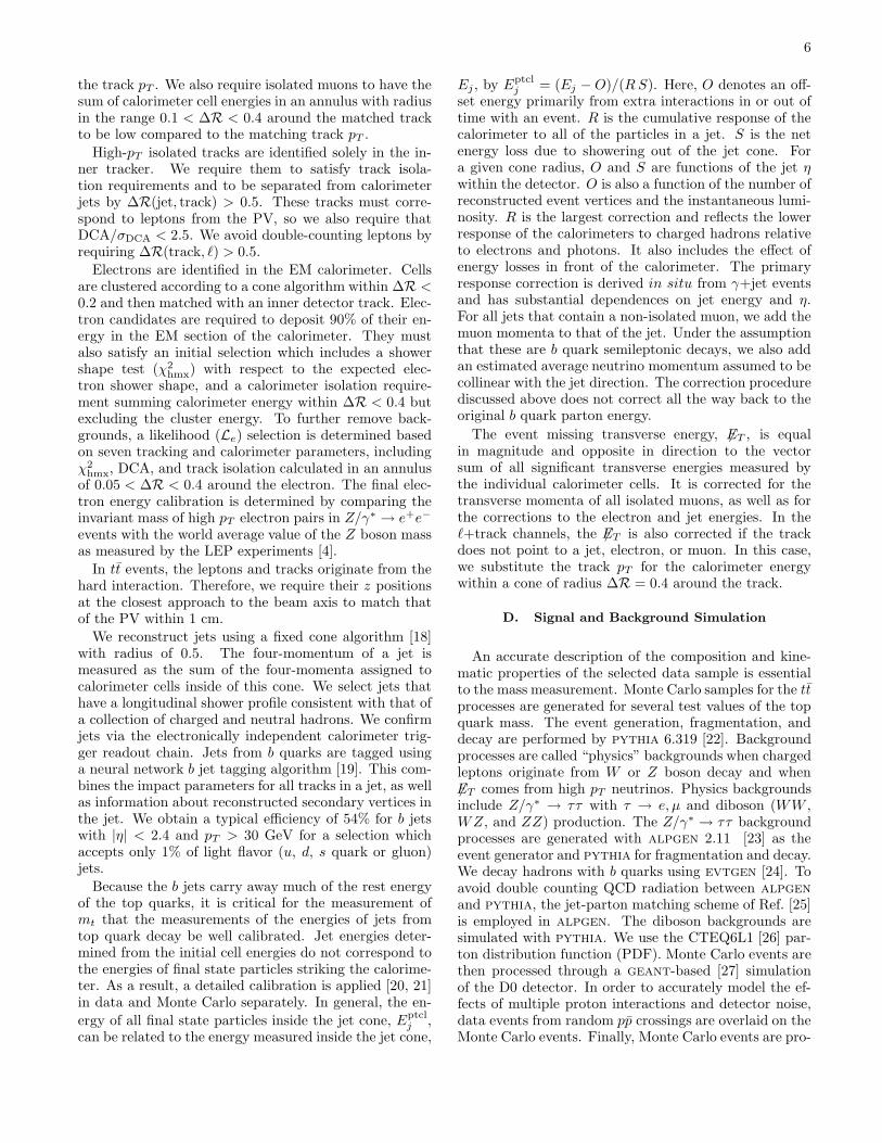
We reconstruct jets using a fixed cone algorithm [18]with radius of 0.5. The four-momentum of a jet ismeasured as the sum of the four-momenta assigned tocalorimeter cells inside of this cone. We select jets thathave a longitudinal shower profile consistent with that ofa collection of charged and neutral hadrons. We confirmjets via the electronically independent calorimeter trig-ger readout chain. Jets from b quarks are tagged usinga neural network b jet tagging algorithm [19]. This com-bines the impact parameters for all tracks in a jet, as wellas information about reconstructed secondary vertices inthe jet. We obtain a typical efficiency of 54% for b jetswith |η| < 2.4 and pT > 30 GeV for a selection whichaccepts only 1% of light flavor (u, d, s quark or gluon)jets.

Because the b jets carry away much of the rest energyof the top quarks, it is critical for the measurement ofmt that the measurements of the energies of jets fromtop quark decay be well calibrated. Jet energies deter-mined from the initial cell energies do not correspond tothe energies of final state particles striking the calorime-ter. As a result, a detailed calibration is applied [20, 21]in data and Monte Carlo separately. In general, the en-

ergy of all final state particles inside the jet cone, Eptclj ,

can be related to the energy measured inside the jet cone,

Ej , by Eptclj = (Ej − O)/(R S). Here, O denotes an off-

set energy primarily from extra interactions in or out oftime with an event. R is the cumulative response of thecalorimeter to all of the particles in a jet. S is the netenergy loss due to showering out of the jet cone. Fora given cone radius, O and S are functions of the jet ηwithin the detector. O is also a function of the number ofreconstructed event vertices and the instantaneous lumi-nosity. R is the largest correction and reflects the lowerresponse of the calorimeters to charged hadrons relativeto electrons and photons. It also includes the effect ofenergy losses in front of the calorimeter. The primaryresponse correction is derived in situ from γ+jet eventsand has substantial dependences on jet energy and η.For all jets that contain a non-isolated muon, we add themuon momenta to that of the jet. Under the assumptionthat these are b quark semileptonic decays, we also addan estimated average neutrino momentum assumed to becollinear with the jet direction. The correction procedurediscussed above does not correct all the way back to theoriginal b quark parton energy.

The event missing transverse energy, 6ET , is equalin magnitude and opposite in direction to the vectorsum of all significant transverse energies measured bythe individual calorimeter cells. It is corrected for thetransverse momenta of all isolated muons, as well as forthe corrections to the electron and jet energies. In theℓ+track channels, the 6ET is also corrected if the trackdoes not point to a jet, electron, or muon. In this case,we substitute the track pT for the calorimeter energywithin a cone of radius ∆R = 0.4 around the track.

D. Signal and Background Simulation

An accurate description of the composition and kine-matic properties of the selected data sample is essentialto the mass measurement. Monte Carlo samples for the ttprocesses are generated for several test values of the topquark mass. The event generation, fragmentation, anddecay are performed by pythia 6.319 [22]. Backgroundprocesses are called “physics” backgrounds when chargedleptons originate from W or Z boson decay and when6ET comes from high pT neutrinos. Physics backgroundsinclude Z/γ∗ → ττ with τ → e, µ and diboson (WW ,WZ, and ZZ) production. The Z/γ∗ → ττ backgroundprocesses are generated with alpgen 2.11 [23] as theevent generator and pythia for fragmentation and decay.We decay hadrons with b quarks using evtgen [24]. Toavoid double counting QCD radiation between alpgen

and pythia, the jet-parton matching scheme of Ref. [25]is employed in alpgen. The diboson backgrounds aresimulated with pythia. We use the CTEQ6L1 [26] par-ton distribution function (PDF). Monte Carlo events arethen processed through a geant-based [27] simulationof the D0 detector. In order to accurately model the ef-fects of multiple proton interactions and detector noise,data events from random pp crossings are overlaid on theMonte Carlo events. Finally, Monte Carlo events are pro-

7

cessed through the same reconstruction software as usedfor data.

In order to ensure that reconstructed objects in thesesamples reflect the performance of the detector in data,several corrections are applied. Monte Carlo events arereweighted by the z coordinate of the PV to match theprofile in data. The Monte Carlo events are further tunedsuch that the efficiencies to find leptons, isolated tracks,and jets in Monte Carlo events match those determinedfrom data. These corrections depend on the pT and ηof these objects. The jet energy calibration derived fordata is applied to jets in data, and the jet energy cali-bration derived for simulated events is applied to simu-lated events. We observe a residual discrepancy betweenjet energies in Z+jets events in data and Monte Carlo.We apply an additional correction to jet energies in theMonte Carlo to bring them into agreement with the data.This adjustment is then propagated into the 6ET . We ap-ply additional smearing to the reconstructed jet and lep-ton transverse momenta so that the object resolutions inMonte Carlo match those in data. Owing to differencesin b-tagging efficiency between data and simulation, b-tagging in Monte Carlo events is modeled by assigningto each simulated event a weight defined as

P = 1 −Njets∏

i=1

[1 − pi(η, pT , flavor)], (1)

where pi(η, pT , flavor) is the probability of the ith jetto be identified as originating from a b quark, obtainedfrom data measurements. This product is taken overall jets. Instrumental backgrounds are modeled from acombination of data and simulation and are discussed inSection III C.

III. SELECTED EVENT SAMPLE

Events are selected for all channels by requiringeither two leptons (2ℓ) or a lepton and an isolated track(ℓ+track), each with pT > 15 GeV. Electrons must bewithin |η| < 1.1 or 1.5 < |η| < 2.5; muons and tracksshould have |η| < 2.0. An opposite charge requirementis applied to the two leptons or to the lepton and track.At least two jets are also required with pseudorapidity|η| < 2.5 and pT > 20 GeV. We require the leadingjet to have pT > 30 GeV. Since neutrinos coming fromW boson decays in tt events are a source of significantmissing energy, a cut on 6ET is a powerful discriminantagainst background processes without neutrinos such asZ/γ∗ → ee and Z/γ∗ → µµ. All channels except eµrequire at least 6ET > 25 GeV.

A. 2ℓ Selection

Our selection of 2ℓ events follows Ref. [28]. In the eechannel, events with a dielectron invariant mass Mee <15 GeV or 84 < Mee < 100 GeV are rejected. We require6ET > 35 GeV and 6ET > 45 GeV when Mee > 100 GeV

and 15 < Mee < 84 GeV, respectively. In the µµ channel,we select events with Mµµ > 30 GeV and 6ET > 40 GeV.To further reject the Z/γ∗ → µµ background in the µµchannel, we require that the observed 6ET be inconsistentwith arising solely from the resolutions of the measuredmuon momenta and jet energies.

In the eµ analysis, no cut on 6ET is applied because themain background process Z/γ∗ → ττ generates four neu-trinos having moderate pT . Instead, the final selection inthis channel requires Hℓ

T = pℓ1T +

∑

(EjT ) > 115 GeV,

where pℓ1T denotes the transverse momentum of the lead-

ing lepton, and the sum is performed over the two leadingjets. This requirement rejects the largest backgrounds forthis final state, Z/γ∗ → ττ and diboson production. Werequire the leading jet to have pT > 40 GeV.

The selection described above is derived from that usedfor the tt cross-section analysis. Varying the 6ET and jetpT selections indicated that this selection minimizes thestatistical uncertainty on the mt measurement. We select17 events in the ee channel and 13 events (12 events forMWT) in the µµ channel. We select 39 events in the eµchannel.

B. ℓ+track Selection

The selection for the ℓ+track channels is similar tothat of Ref. [17]. For the e+track channel, electrons arerestricted to |η| < 1.1, and the leading jet must havepT > 40 GeV. The dominant ℓ+track background arisesfrom Z → ee and Z → µµ production, so we design theevent selection to reject these events.

When the invariant mass of the lepton-track pair (Mℓt)is in the range 70 <Mℓt< 110 GeV, the 6ET requirement istightened to 6ET > 35 (40) GeV for the e+track (µ+track)channel. Furthermore, we introduce the variable 6EZ-fit

Tthat corrects the 6ET in Z → ℓℓ events for mismeasuredlepton momenta. We rescale the lepton and track mo-menta according to their resolutions to bring Mℓt to themass of the Z boson (91.2 GeV) and then use theserescaled momenta to correct the 6ET . Event selectionbased on this variable reduces the Z background by halfwhile providing 96% efficiency for tt events. The cuts on6EZ-fit

T are always identical to those on 6ET .At least one jet is required to be identified as a b

jet which provides strong background rejection for theℓ+track channels. The mt precision is limited by signalstatistics in the observed event sample when the back-ground is reasonably low. The above selection is a resultof an optimization which minimizes the statistical uncer-tainty on mt. We do this in terms of 6ET , 6EZ-fit

T , thetransverse momenta of the leading two jets, and the b-tagging criteria by stepping through two or more differentthresholds on these requirements. After considering allpossible sets of selections, we choose the one which givesthe best average expected statistical uncertainty on themt measurement using many pseudoexperiments. Theexpected statistical uncertainty varies smoothly over a

8

15% range while the study is sensitive to 5% changes ofthe average statistical uncertainty.

We explicitly veto events satisfying the selection of anyof the 2ℓ channels, so the ℓ+track channels are statisti-cally independent of the 2ℓ channels. We select eightevents in the e+track channel and six events in theµ+track channel.

C. Modeling Instrumental Backgrounds

Backgrounds can arise from instrumental effects inwhich the 6ET is mismeasured. The main instrumentalbackgrounds for the ee, µµ, e+track, and µ+track chan-nels are the Z/γ∗ → ee and Z/γ∗ → µµ processes. Inthese cases, apparent 6ET results from tails in jet or lep-ton pT resolutions. We use the NNLO cross section forZ/γ∗ → ee, µµ processes, along with the Monte Carlo-derived efficiencies to estimate these backgrounds for theee and µµ channels. The Monte Carlo kinematic dis-tributions, including the 6ET , are verified to reproducea data sample dominated by these processes. For theℓ+track channels, we normalize Drell-Yan Monte Carloso that the total expected event yield in a ℓ+track sam-ple with low 6ET equals the observed event yield in thedata. We observe a slightly different pZ

T distribution forsimulated Z → ℓℓ events in comparison with data. Asa result, all Z boson simulated samples, including theZ → ττ physics background samples, are reweighted tothe observed distribution of pZ

T in data [29].Another background arises when a lepton or a track

within a jet is identified as an isolated lepton or track. Weutilize different methods purely in data to estimate thelevel of these backgrounds for each channel. In all cases,however, we distinguish reconstructed muons and tracksas “loose” rather than “tight” by releasing the isolationcriteria. We make an analogous distinction for electronsby omitting the requirement on the electron likelihood,Le, for “loose” electrons.

To determine the misidentified electron backgroundyield in the ee and eµ channels, we fit the observed distri-bution of Le in the data to a sum of the distributions fromreal isolated electrons and misidentified electrons. We de-termine the shape of Le for real electrons from a Z → eesample with 6ET < 15 GeV. For the ee channel, we extractthe shape for the misidentified electrons from a sample inwhich one “tag electron” is required to have both χ2

hmxand Le inconsistent with being from an electron. We fur-ther require Mee < 60 GeV or Mee > 130 GeV and 6ET

< 15 GeV to reject Z and W boson events. The distribu-tion of Le is obtained from a separate “probe electron” inthe same events. In the eµ channel, the Le distributionfor misidentified electrons is obtained in a sample with anon-isolated muon and 6ET < 15 GeV.

To estimate the background from non-isolated muonsfor the eµ and µµ channels, we use control samples tomeasure the fraction of muons, fµ, with pT > 15 GeVthat appear to be isolated. To enhance the heavy flavor

content which gives non-isolated muons, the control sam-ples are selected to have two muons where a “tag” muonis required to be non-isolated. We use another “probe”muon to determine fµ. The background yield for the eµchannel is computed from the number of events havingan isolated electron, a muon with no isolation require-ment, and the same sign charge for the two leptons. Wemultiply the observed yield by fµ.

We estimate the instrumental background for the µµand ℓ+track channels by using systems of linear equa-tions describing the composition of data samples with dif-ferent “loose” or “tight” lepton and/or track selections.We relate event counts in these samples to the numbersof events with real or misidentified isolated leptons usingthe system of equations. These equations take as inputsthe efficiencies for real or misidentified leptons and tracksto pass the tight identification requirements. For the µµand ℓ+track channels, we determine the efficiencies forreal leptons and tracks to pass the tight identificationcriteria using Z → ee and Z → µµ events.

For the ℓ+track channels, the probabilities for misiden-tified leptons and tracks to pass the tight selection cri-teria are determined from multijet data samples with atleast one loose lepton plus a jet. We reject the event if twoleptons of the same flavor satisfy tight criteria to suppressDrell-Yan events. We also reject events with one or moretight leptons with different flavor from the loose lepton.These tight lepton vetos allow some events with two looseleptons or a lepton and track in the sample. We furthersuppress resonant Z production by selecting events whenMℓt and Mℓℓ > 100 GeV or Mℓt and Mℓℓ < 70 GeV. Wereject W+jets events and misreconstructed Z/γ∗ eventsby requiring 6ET < 15 GeV and 6EJES

T < 25 GeV. Here,6EJES

T is the missing transverse energy with only jet en-ergy corrections and no lepton corrections. We use thelatter because loose leptons no longer adhere to standardresolutions. We calculate the probability for electronsor muons to be misidentified by dividing the number oftight leptons by the number of loose leptons. For thetrack probability, we combine the e+jet and µ+jet sam-ples and make the additional requirement that there beat least one loose track in the event. The tight trackmisidentification probability is again the number of tighttracks divided by the number of loose tracks.

To obtain samples dominated by misidentified isolatedleptons for mass analysis, we select events with two looseleptons or tracks plus two jets. For the 2ℓ channels, weadditionally require same sign dilepton events.

D. Composition of Selected Samples

The expected numbers of background and signal eventsin all five channels (assuming a top quark productioncross section of 7.0 pb) are listed in Table I along with theobserved numbers of candidates. The µ+track selectionhas half the efficiency of the e+track selection primarilydue to the tight µµ veto. The expected and observedevent yields agree for all channels.

9

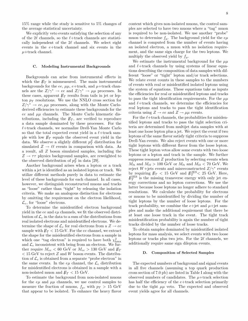
TABLE I: Expected event yields for tt (we assume σtt = 7.0 pb) and backgrounds and numbers of observed events for the fivechannels. The 2ℓ channel uncertainties include statistical as well as systematical uncertainties while the e+track and µ+trackuncertainties are statistical only.

Sample tt Diboson Z Multijet/W+jets Total Observedeµ 36.7 ± 2.4 1.7 ± 0.7 4.5 ± 0.7 2.6 ± 0.6 44.5 ± 2.7 39ee 11.5 ± 1.4 0.5 ± 0.2 2.3 ± 0.4 0.6 ± 0.2 14.8 ± 1.5 17µµ 8.3 ± 0.5 0.7 ± 0.1 4.5 ± 0.4 0.2 ± 0.2 13.7 ± 0.7 13e+track 9.4 ± 0.1 0.1 ± 0.0 0.4 ± 0.1 0.4 ± 0.1 10.3 ± 0.2 8µ+track 4.6 ± 0.1 0.1 ± 0.0 0.7 ± 0.1 0.1 ± 0.0 5.5 ± 0.1 6

Invariant Mass (GeV)20 40 60 80 100 120 140 160

Eve

nts

/ 14

GeV

0

10

20

30

40

5060

70

Invariant Mass (GeV)20 40 60 80 100 120 140 160

Eve

nts

/ 14

GeV

0

10

20

30

40

5060

70 datatt

γZ/dibosonWinstrumental

-1DØ, 1 fb

a)

(GeV)TE0 20 40 60 80 100 120 140 160 180

Eve

nts

/15

GeV

02468

10121416

(GeV)TE0 20 40 60 80 100 120 140 160 180

Eve

nts

/15

GeV

02468

10121416 data

ttγZ/

dibosonWinstrumental

-1DØ, 1 fb

b)

FIG. 1: Comparison of the expected distributions from backgrounds and tt (mt = 170 GeV) in the ℓ+track channels. (a) Mℓt

for the e+track channel without the requirement of the b-tag and with inverted 6ET cuts. (b) 6ET for the sum of both ℓ+trackchannels, again without the b-tag requirement. We assume σtt = 7.0 pb.

Kinematic comparisons between data and the sum ofthe signal and background expectations provide checksof the content and properties of our data sample. Fig-ure 1(a) shows the expected and observed distributionsof Mℓt in the e+track channel without the b-tag require-ment and for an inverted 6ET requirement. The µ+trackdistribution looks similar (not shown). The mass peakat MZ indicates the e+track sample is primarily com-posed of Z → ee events before the final event selection.In Fig. 1(b), we show the 6ET distribution in the ℓ+trackchannels after all cuts except the b-tag requirement.

The expected numbers of background and signal eventsafter all selections in all five channels are listed in Ta-ble I along with the observed numbers of candidates. Weassume σ(tt) = 7.0 pb. We do not include systematicuncertainties for the ℓ+track channels. The small back-grounds mean their uncertainties have a negligible effecton the measured mt uncertainty. The µ+track selectionhas half the efficiency of the e+track selection primarilydue to the tight µµ veto. The expected and observedevent yields agree for all channels. Figures 2(a) and (b)show the 6ET and leading lepton pT summed over all chan-nels for the final candidate sample. We observe the datadistributions to agree with our signal and backgroundmodel.

IV. EVENT RECONSTRUCTION

Measurement of the dilepton event kinematics and con-straints from the tt decay assumption allow a partial re-construction of the final state and a determination of mt.Given the decay of each top quark to a W boson and ab quark, with each W boson decaying to a charged lep-ton and a neutrino, there are six final state particles:two charged leptons, two neutrinos, and two b quarks.Each particle can be described by three momentum com-ponents. Of these eighteen independent parameters, wecan directly measure only the momenta of the leptons.The leading two jets most often come from the b quarks.Despite final state radiation and fragmentation, the jetmomenta are highly correlated with those of the underly-ing b quarks. We also measure the x and y components ofthe 6ET , 6Ex and 6Ey , from the neutrinos. This leaves fourquantities unknown. We can supply two constraints byrelating the four-momenta of the leptons and neutrinosto the masses of the W bosons:

M2W = (Eν1

+ El1)2 − (~pν1

+ ~pl1)2

M2W = (Eν2

+ El2)2 − (~pν2

+ ~pl2)2,

(2)

where the subscript indices indicate the ℓν pair comingfrom one or another W boson. Another constraint issupplied by requiring that the mass of the top quark and

10

(GeV)TE0 50 100 150 200 250

Eve

nts

/25

GeV

05

101520253035

(GeV)TE0 50 100 150 200 250

Eve

nts

/25

GeV

05

101520253035 data

ttγZ/

dibosonWinstrumental

a)

-1DØ, 1 fb

(GeV)T

Lepton p0 20 40 60 80 100 120 140 160

Eve

nts

/15

GeV

05

101520253035

(GeV)T

Lepton p0 20 40 60 80 100 120 140 160

Eve

nts

/15

GeV

05

101520253035 data

ttγZ/

dibosonWinstrumental

-1DØ, 1 fb

b)

FIG. 2: (a) 6ET and (b) leading lepton pT for tt (mt = 170 GeV) and background processes overlaid with those for observedevents in all channels after final event selection. We assume σtt = 7.0 pb.

the mass of the anti-top quark be equal:

(Eν1+ El1 + Eb1)

2 − (~pν1+ ~pl1 + ~pb1)

2 =

(Eν2+ El2 + Eb2)

2 − (~pν2+ ~pl2 + ~pb2)

2.(3)

The last missing constraint can be supplied by a hypoth-esized value of the top quark mass. With that, we cansolve the equations and calculate the unmeasured topquark and neutrino momenta that are consistent withthe observed event. Usually, the dilepton events are kine-matically consistent with a large range of mt. We quan-tify this consistency, or “weight,” for each mt by test-ing measured quantities of the event (e.g., 6ET or leptonand jet pT ) against expectations from the dynamics of ttproduction and decay. This requires us to sample fromrelevant tt distributions, yielding many solutions for aspecific mt. We sum the weights for each solution foreach mt. The distribution of weight vs. mt is termed a“weight distribution” of a given event. Using parametersfrom these weight distributions, we can then determinethe most likely value of mt.

Several previous efforts to measure mt using dileptonevents have used event reconstruction techniques. Thedifferences between methods stem largely from whichevent parameters are used to calculate the event weight.We use the νWT and MWT techniques to determinethe weighting as described below.

A. Neutrino Weighting

The νWT method omits the measured 6ET for kine-matic reconstruction. Instead, we choose the pseudora-pidities of the two neutrinos from tt decay from their ex-pected distributions. We obtain the distribution of neu-trino η from several simulated tt samples with a range ofmt values. These distributions can each be approximatedby a single Gaussian function. The standard deviationspecifying this function varies weakly with mt. Once theneutrino pseudorapidities are fixed and a value for mt as-sumed, we can solve for the complete decay kinematics,including the unknown neutrino momenta. There may

be up to four different combinations of solved neutrinomomenta for each assumed pair of neutrino η values foreach event. We assume the leading two jets are the b jets,so there are two possible associations of W bosons withb jets.

For each pairing of neutrino momentum solutions, wedefine a weight, w, based on the agreement between themeasured 6ET and the sum of the neutrino momentumcomponents in x and y, pν

x and pνy . We assume indepen-

dent Gaussian resolutions in measuring 6Ex and 6Ey . Theweight is calculated as

w = exp

[−(6Ecalcx − 6Eobs

x )2

2(σux)2

]

exp

[

−(6Ecalcy − 6Eobs

y )2

2(σuy )2

]

,

(4)reflecting the agreement between the measured and cal-culated 6ET . 6Eobs

i (i = x or y) are the components ofthe measured event 6ET , and 6Ecalc

i are the components ofthe 6ET calculated from the neutrino transverse momentaresulting from each solution. We calculate the quantities6Eu

i to be the sums of the energies projected onto the iaxes measured by all “unclustered” calorimeter cells –those cells not included in jets or electrons. The high pT

objects, leptons and jets, enter into the determination ofboth 6Ecalc

i and 6Eobsi whereas the unclustered energy 6Eu

i

only enters into 6Eobsi . Given the resolutions σu

i of the 6Eui ,

we can therefore estimate the probability that the 6Eobsi

are consistent with the 6Ecalci from the tt hypothesis.

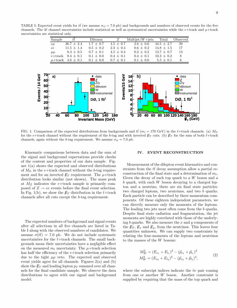
As parameters of the method, we determine σui using

Z → ee + 2 jets data and Monte Carlo events. We calcu-late an unclustered scalar transverse energy, Su

T , as thescalar sum of the transverse energies of all unclusteredcalorimeter cells. Due to the azimuthal isotropy of thecalorimeter, we observe that the independent x and ycomponents of the σu

i depend on SuT in the same way

within their uncertainties. Therefore, we combine resultsfor both components to determine our resolution moreprecisely. We find agreement between data and simula-tion in the observed dependence of these parameters onSu

T . The distributions are shown for these combined res-olutions in Fig. 3. We fit the unclustered 6ET resolutions

11

)1/2 (GeV1/2)u

T(S

5 6 7 8 9 10 11 12 13

(G

eV)

u i

Eσ

4

5

6

7

8

9

10 data

Monte Carlo

ee+2jets→Z -1DØ, 1 fb

FIG. 3: Dependence of the resolution of unclustered 6ET onthe unclustered scalar transverse missing energy for Z → ee

events with exactly two jets.

obtained from simulation as

σux(Su

T ) = σuy (Su

T ) = 4.38 GeV + 0.52√

SuT GeV, (5)

and use this parametrization for the unclustered miss-ing energy resolution for both data and Monte Carlo inEq. (4).

For each event, we consider ten different η assump-tions for each of the two neutrinos. We extract thesevalues from the histograms appropriate to the mt beingassumed. The ten η values are the medians of each of tenranges of η which each represent 10% of the tt sample fora given mt.

B. Matrix Weighting

In the MWT approach, we use the measured momentaof the two charged leptons. We assign the measured mo-menta of the two jets with the highest transverse mo-menta to the b and b quarks and the measured 6ET to thesum of the transverse momenta of the two neutrinos fromthe decay of the t and t quarks. We then assume a topquark mass and determine the momenta of the t and tquarks that are consistent with these measurements. Werefer to each such pair of momenta as a solution for theevent. For each event, there can be up to four solutions.

We assign a weight to each solution, analogous to theνWT weight of Eq. 4, given by

w = f(x)f(x)p(E∗ℓ |mt)p(E∗

ℓ |mt), (6)

where f(x) is the PDF for the proton for the momentumfraction x carried by the initial quark, and f(x) is the cor-responding value for the initial antiquark. The quantityE∗

ℓ is the observed lepton energy in the top quark restframe. We use the central fit of the CTEQ6L1 PDFsand evaluate them at Q2 = m2

t . The quantity p(E∗ℓ |mt)

in Eq. 6 is the probability that for the hypothesized top

quark mass mt, the lepton ℓ has the measured E∗ℓ [11]:

p(E∗ℓ |mt) =

4mtE∗ℓ (m2

t − m2b − 2mtE

∗ℓ )

(m2t − m2

b)2 + M2

W (m2t − m2

b) − 2M4W

.

(7)

C. Total Weight vs. mt

Equations 4 and 6 indicate how the event weight iscalculated for a given top quark mass in the νWT andMWT methods. In each method, we consider all solu-tions and jet assignments to get a total weight, wtot, fora given mt. In general, there are two ways to assign thetwo jets to the b and b quarks. There are up to foursolutions for each hypothesized value of the top quarkmass. The likelihood for each assumed top quark massmt is then given by the sum of the weights over all thepossible solutions:

wtot =∑

i

∑

j

wij , (8)

where j sums over the solutions for each jet assignment i.We repeat this calculation for both the νWT and MWTmethods for a range of assumed top quark masses from80 GeV through 330 GeV.

For each method, we also account for the finite resolu-tion of jet and lepton momentum measurements. We re-peat the weight calculation with input values for the mea-sured momenta (or inverse momenta for muons) drawnfrom normal distributions centered on the measured val-ues with widths equal to the known detector resolutions.We then average the weight distributions obtained fromN such variations:

wtot(mt) = N−1N

∑

n=1

wtot,n(mt). (9)

where N is the number of samples. One important bene-fit of this procedure is that the efficiency of signal eventsto provide solutions increases. For instance, the νWTefficiency to find a solution for tt→ eµ events is 95.9%without resolution sampling, while 99.5% provide solu-tions when N = 150. For the MWT analysis, events withmt = 175 GeV yield an efficiency of 90% without resolu-tion sampling. This rises to over 99% when N = 500. Weuse N = 150 and 500 for νWT and MWT, respectively.

Examples of a single event weight distribution for νWTand MWT are shown in Fig. 4 for two different simu-lated events. The sensitivities of the two methods aresimilar on average, but the different widths of the weightdistributions vary significantly in both approaches on anevent-by-event basis. This can be caused by an over-all insensitivity of an event’s kinematic quantities to mt,or to a different sensitivity when using those kinematicquantities with specific event reconstruction techniques.

Properties of the weight distribution are strongly cor-related with mt if the top quark decay is as expected in

12

Top Mass [GeV]100 150 200 250 300

Wei

gh

t

0.05

0.1

0.15 WTνDØ,

=170 GeVtm

a)

Top Mass [GeV]100 150 200 250 300

Wei

gh

t

0.002

0.004

0.006

0.008DØ, MWT

=170 GeVtm

b)

FIG. 4: Example weight distributions for different single tt →

eµ Monte Carlo events obtained with a) νWT method and b)MWT method. The generator level mass is mt = 170 GeV.

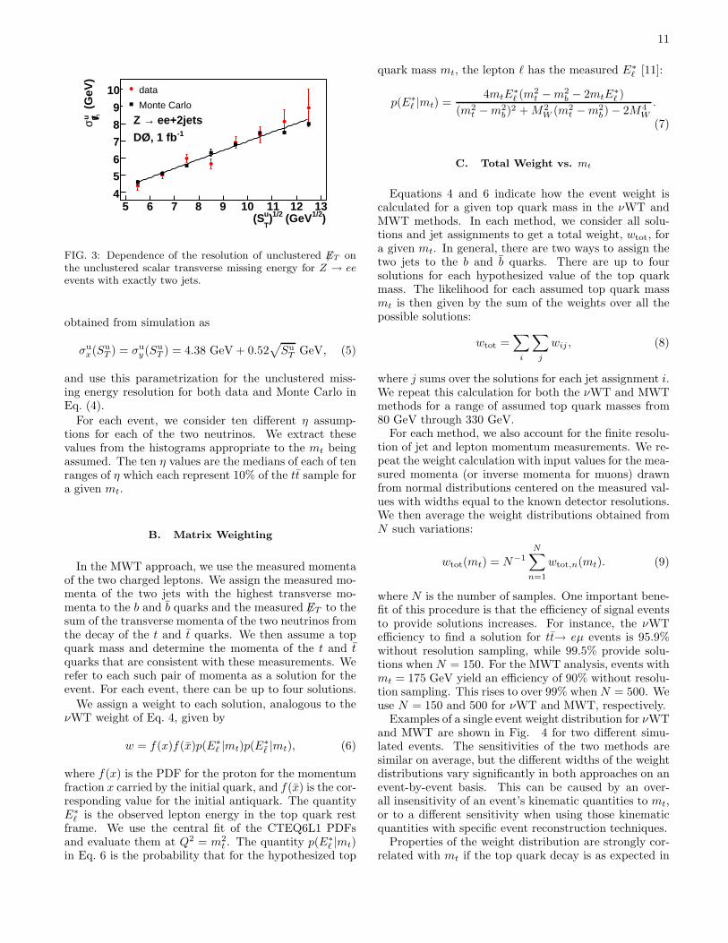
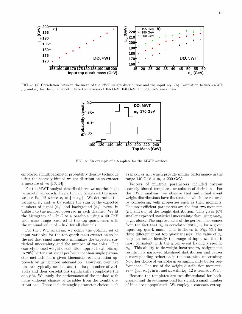
the standard model. For instance, Fig. 5(a) illustrates thecorrelation of the mean of the νWT weight distribution,µw, with the generated top quark mass from the MonteCarlo. The relationship between the root-mean-square ofthe weight distribution, σw, and µw also varies with mt,as shown in Fig. 5(b). There is the potential for non-standard decays of the top quark. For mt = 170 GeVand assuming BR(H± → τν) ∼ 100%, we observe µw

(νWT) to shift systematically upward when a H± bosonof mass 80 GeV is present in the decay chain instead ofa W boson. When BR(t → H±b) =100%, this shift is10%. Thus, the measurements of this paper are strictlyvalid only for standard model top quark decays.

V. EXTRACTING THE TOP QUARK MASS

We cannot determine the top quark mass directly fromµw or from the most probable mass from the event weightdistributions, maxw. Effects such as initial and finalstate radiation systematically shift these quantities fromthe actual top quark mass. In addition, the presence ofbackground must be taken into account when evaluatingevents in the candidate sample. We therefore performa maximum likelihood fit to distributions (“templates”)of characteristic variables from the weight distributions.This fit accounts for the shapes of signal templates and

for the presence of background.

A. Measurement Using Templates

We define a set of input variables characterizing theweight distribution for event i, denoted by {xi}N , whereN is the number of variables. Examples of {xi}N mightbe the integrated weight in bins of a coarsely binned tem-plate, or they might be the moments of the weight dis-tribution. A probability density histogram for simulatedsignal events, hs, is defined as an (N + 1)-dimensionalhistogram of input top quark mass vs. N variables. Forbackground, hb is defined as an N -dimensional histogramof the {xi}N . Both hs and hb are normalized to unity:

∫

hs({xi}N | mt) d{xi}N = 1, (10)

∫

hb({xi}N ) d{xi}N = 1. (11)

An example of a template for the MWT method is shownon Fig. 6. We measure mt from hs({xi}N , mt) andhb({xi}N) using a maximum likelihood method. For eachevent in a given data sample, all {xi}N are found andused for the likelihood calculation. We define a likeli-hood L as

L({xi}N , nb, Nobs | mt) =

Nobs∏

i=1

nshs({xi}N | mt) + nbhb({xi}N)

ns + nb,

(12)

where Nobs is the number of events in the sample, nb isthe number of background events, and ns is the signalevent yield. We obtain a histogram of − lnL vs. mt forthe sample. We fit a parabola that is symmetric aroundthe point with the highest likelihood (lowest − lnL). Thefitted mass range is several times larger than the expectedstatistical uncertainty. It is chosen a priori to give thebest sensitivity to the top quark mass using Monte Carlopseudoexperiments, and is typically around ±20 GeV.

We obtain measurements of mt for several channels bymultiplying the likelihoods of these channels:

− lnL =∑

ch

(− lnLch) , (13)

where “ch” denotes the set of channels. In this pa-per, we calculate overall likelihoods for the 2ℓ subset,ch ∈ {eµ, ee, µµ}; the ℓ+track subset, ch ∈ {e+track,µ+track}; and the five channel dilepton set, ch ∈{eµ, ee, µµ, e+track, µ+track}.

B. Choice of Template Variables

The choice of variables characterizing the weight dis-tributions has been given some consideration in the past.For example, the D0 MWT analysis and CDF νWT anal-yses have used maxw [14, 15]. Earlier D0 νWT analyses

13

Input top quark mass (GeV)155 160 165 170 175 180 185 190 195 200

(G

eV)

wµ

170

175

180

185

190

195

200

WTνDØ,

a)

(GeV)wσ15 20 25 30 35 40 45 50 55 60

(G

eV)

wµ

160170180190200210220

155 GeV180 GeV200 GeV

155 GeV180 GeV200 GeV

WTνDØ,

b)

FIG. 5: (a) Correlation between the mean of the νWT weight distribution and the input mt. (b) Correlation between νWTµw and σw for the eµ channel. Three test masses of 155 GeV, 180 GeV, and 200 GeV are shown.

Top Mass [GeV]100 120 140 160 180 200 220 240

Pro

bab

ility

den

sity

0.05

0.1

0.15

0.2DØ, MWT

=170 GeVtm

FIG. 6: An example of a template for the MWT method.

employed a multiparameter probability density techniqueusing the coarsely binned weight distribution to extracta measure of mt [13, 14]

For the MWT analysis described here, we use the singleparameter approach. In particular, to extract the mass,we use Eq. 12 where xi = {maxw}. We determine thevalues of ns and nb by scaling the sum of the expectednumbers of signal (ns) and background (nb) events inTable I to the number observed in each channel. We fitthe histogram of − lnL to a parabola using a 40 GeVwide mass range centered at the top quark mass withthe minimal value of − lnL for all channels.

For the νWT analysis, we define the optimal set ofinput variables for the top quark mass extraction to bethe set that simultaneously minimizes the expected sta-tistical uncertainty and the number of variables. Thecoarsely binned weight distribution approach exhibits upto 20% better statistical performance than single param-eter methods for a given kinematic reconstruction ap-proach by using more information. However, over fivebins are typically needed, and the large number of vari-ables and their correlations significantly complicate theanalysis. We study the performance of the method withmany different choices of variables from the weight dis-tributions. These include single parameter choices such

as maxw or µw, which provide similar performance in therange 140 GeV < mt < 200 GeV.

Vectors of multiple parameters included variouscoarsely binned templates, or subsets of their bins. Forthe νWT analysis, we observe that individual eventweight distributions have fluctuations which are reducedby considering bulk properties such as their moments.The most efficient parameters are the first two moments(µw and σw) of the weight distribution. This gives 16%smaller expected statistical uncertainty than using maxw

or µw alone. The improvement of the performance comesfrom the fact that σw is correlated with µw for a giveninput top quark mass. This is shown in Fig. 5(b) forthree different input top quark masses. The value of σw

helps to better identify the range of input mt that ismost consistent with the given event having a specificµw. This ability to de-weight incorrect mt assignmentsresults in a narrower likelihood distribution and causesa corresponding reduction in the statistical uncertainty.No other choice of variables gives significantly better per-formance. The use of the weight distribution moments,xi = {µw, σw}, in hs and hb with Eq. 12 is termed νWTh.

Because the templates are two-dimensional for back-ground and three-dimensional for signal, a small numberof bins are unpopulated. We employ a constant extrap-

14

olation for unpopulated edge bins using the value of thepopulated bin closest in mt but having the same µw andσw. For empty bins flanked by populated bins in the mt

direction but with the same µw and σw, we employ alinear interpolation. We fit the histogram of − lnL vs.mt with a parabola. When performing the fit, the νWTh

approach determines ns to be ns = Nobs− nb. Fit rangesof 50, 40, and 30 GeV are used for ℓ+track, 2ℓ, and alldilepton channels, respectively.

C. Probability Density Functions

In both methods described above, there are finitestatistics in the simulated samples used to model hs andhb, leading to bin-by-bin fluctuations. We address this inthe νWT analysis by performing fits to hs and hb tem-plates. We term this version of the νWT method νWTf .For the signal, we generate a probability density functionfs by fitting hs with the functional form

fs(µw, σw | mt) = (σw + p13)p6 exp[−p7(σw + p13)

p8 ]

×{

(1 − p9)1

σ√

2πexp[− (µw − m)2

2σ2]

+ p9 ·p1+p12

11

Γ(1 + p12)(µw − m

p10)p12 exp[−p11(µw − m

p10)]

×Θ(µw − m

p10)

}

×{

∫ ∞

0

(x + p13)p6 exp[−p7(x + p13)

p8 ]dx

}−1

.

(14)The parameters m and σ are linear functions of σw andmt:

m = p0 + p1(σw − 36 GeV) + p2(mt − 170 GeV),

σ = p3 + p4(σw − 36 GeV) + p5(mt − 170 GeV).(15)

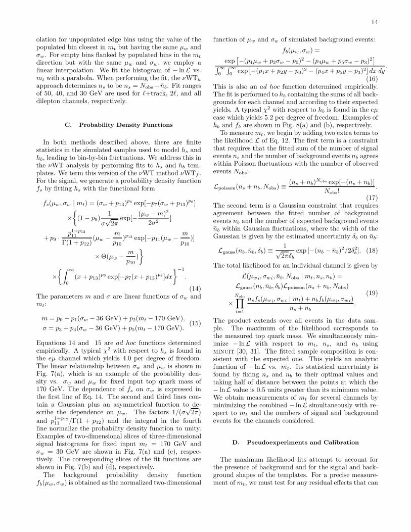
Equations 14 and 15 are ad hoc functions determinedempirically. A typical χ2 with respect to hs is found inthe eµ channel which yields 4.0 per degree of freedom.The linear relationship between σw and µw is shown inFig. 7(a), which is an example of the probability den-sity vs. σw and µw for fixed input top quark mass of170 GeV. The dependence of fs on σw is expressed inthe first line of Eq. 14. The second and third lines con-tain a Gaussian plus an asymmetrical function to de-scribe the dependence on µw. The factors 1/(σ

√2π)

and p1+p12

11 /Γ(1 + p12) and the integral in the fourthline normalize the probability density function to unity.Examples of two-dimensional slices of three-dimensionalsignal histograms for fixed input mt = 170 GeV andσw = 30 GeV are shown in Fig. 7(a) and (c), respec-tively. The corresponding slices of the fit functions areshown in Fig. 7(b) and (d), respectively.

The background probability density functionfb(µw, σw) is obtained as the normalized two-dimensional

function of µw and σw of simulated background events:

fb(µw, σw) =

exp[

−(p1µw + p2σw − p0)2 − (p4µw + p5σw − p3)

2]

∫ ∞0

∫ ∞0

exp [−(p1x + p2y − p0)2 − (p4x + p5y − p3)2] dx dy.

(16)This is also an ad hoc function determined empirically.The fit is performed to hb containing the sums of all back-grounds for each channel and according to their expectedyields. A typical χ2 with respect to hb is found in the eµcase which yields 5.2 per degree of freedom. Examples ofhb and fb are shown in Fig. 8(a) and (b), respectively.

To measure mt, we begin by adding two extra terms tothe likelihood L of Eq. 12. The first term is a constraintthat requires that the fitted sum of the number of signalevents ns and the number of background events nb agreeswithin Poisson fluctuations with the number of observedevents Nobs:

Lpoisson(ns + nb, Nobs) ≡(ns + nb)

Nobs exp[−(ns + nb)]

Nobs!.

(17)The second term is a Gaussian constraint that requiresagreement between the fitted number of backgroundevents nb and the number of expected background eventsnb within Gaussian fluctuations, where the width of theGaussian is given by the estimated uncertainty δb on nb:

Lgauss(nb, nb, δb) ≡1√2πδb

exp [−(nb − nb)2/2δ2

b ]. (18)

The total likelihood for an individual channel is given by

L(µwi, σwi, nb, Nobs | mt, ns, nb) =

Lgauss(nb, nb, δb)Lpoisson(ns + nb, Nobs)

×Nobs∏

i=1

nsfs(µwi, σwi | mt) + nbfb(µwi, σwi)

ns + nb.

(19)

The product extends over all events in the data sam-ple. The maximum of the likelihood corresponds tothe measured top quark mass. We simultaneously min-imize − lnL with respect to mt, ns, and nb usingminuit [30, 31]. The fitted sample composition is con-sistent with the expected one. This yields an analyticfunction of − lnL vs. mt. Its statistical uncertainty isfound by fixing ns and nb to their optimal values andtaking half of distance between the points at which the− lnL value is 0.5 units greater than its minimum value.We obtain measurements of mt for several channels byminimizing the combined − lnL simultaneously with re-spect to mt and the numbers of signal and backgroundevents for the channels considered.

D. Pseudoexperiments and Calibration

The maximum likelihood fits attempt to account forthe presence of background and for the signal and back-ground shapes of the templates. For a precise measure-ment of mt, we must test for any residual effects that can

15

(GeV)

wµ100150200250300 (GeV)

wσ

020

4060

Prob

abili

ty d

ensi

ty

00.10.20.30.40.50.6

-310×

a)

(GeV)

wµ100150200250300 (GeV)

wσ

020

4060

Prob

abili

ty d

ensi

ty

0

0.1

0.2

0.3

0.4

0.5

-310×

WTνDØ,

=170 GeVtm

b)

(GeV)

wµ120140160180200 (GeV)

tm

160170

180190

200

Prob

abili

ty d

ensi

ty

0

0.1

0.2

0.3

0.4

0.5

-310×

c)

(GeV)

wµ120140160180200 (GeV)

tm

160170

180190

200

Prob

abili

ty d

ensi

ty

00.10.20.30.40.50.6

-310×

WTνDØ,

=30 GeVwσ

d)

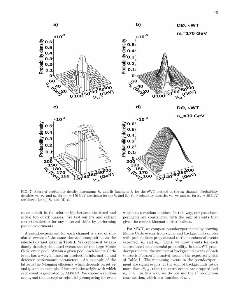
FIG. 7: Slices of probability density histograms hs and fit functions fs for the νWT method in the eµ channel. Probabilitydensities vs. σw and µw for mt = 170 GeV are shown for (a) hs and (b) fs. Probability densities vs. mt and µw for σw = 30 GeVare shown for (c) hs and (d) fs.

cause a shift in the relationship between the fitted andactual top quark masses. We test our fits and extractcorrection factors for any observed shifts by performingpseudoexperiments.

A pseudoexperiment for each channel is a set of sim-ulated events of the same size and composition as theselected dataset given in Table I. We compose it by ran-domly drawing simulated events out of the large MonteCarlo event pool. Within a given pool, each Monte Carloevent has a weight based on production information anddetector performance parameters. An example of thelatter is the b-tagging efficiency which depends on jet pT

and η, and an example of former is the weight with whicheach event is generated by alpgen. We choose a randomevent, and then accept or reject it by comparing the event

weight to a random number. In this way, our pseudoex-periments are constructed with the mix of events thatgives the correct kinematic distributions.

For MWT, we compose pseudoexperiments by drawingMonte Carlo events from signal and background sampleswith probabilities proportional to the numbers of eventsexpected, ns and nb. Thus, we draw events for eachsource based on a binomial probability. In the νWT pseu-doexperiments, the number of background events of eachsource is Poisson fluctuated around the expected yieldsof Table I. The remaining events in the pseudoexperi-ment are signal events. If the sum of backgrounds totalsmore than Nobs, then the extra events are dropped andns = 0. In this way, we do not use the tt productioncross section, which is a function of mt.

16

(GeV)

wµ0100

200300 (GeV)

wσ

020

4060

Prob

abili

ty d

ensi

ty

00.05

0.10.15

0.20.25

0.30.35

-310×

a)

(GeV)

wµ0100

200300 (GeV)

wσ

020

4060

Prob

abili

ty d

ensi

ty

00.05

0.10.15

0.20.25

0.30.35

0.4

-310×

b) WTνDØ,

FIG. 8: Probability density histogram hb and fit function fs for the νWT method in the eµ channel. Probability densities vs.σw and µw are shown for (a) hb and (b) fb.

To establish the relationship between the fitted topquark mass, mfit

t , and the actual generated top quarkmass mt, we assemble a set of many pseudoexperimentsfor each input mass. For the νWT method, we choose300 pseudoexperiments because that is the point at whichthe Monte Carlo statistics begin to be oversampled, andall pseudoexperiments can still be considered statisticallyindependent. We average mfit

t for each input mt for eachchannel. We combine channels according to Eq. 13, andwe fit the dependence of this average mass on mt with

〈mfitt 〉 = α(mt − 170 GeV) + β + 170 GeV. (20)

The calibration points and fit functions are shown inFig. 9. The results of the fits are summarized in Ta-ble II. Ideally, α and β should be unity and zero, re-spectively. The mfit

t of each pseudoexperiment and datameasurement is corrected for the slopes and offsets givenin Table II by

mmeast = α−1(mfit

t − β − 170 GeV) + 170 GeV. (21)

The pull is defined as

pull =mmeas

t − mt

σ(mmeast )

, (22)

where σ(mmeast ) = α−1σ(mfit

t ) is the measured statisti-cal uncertainty after the calibration of Eq. 21. The idealpull distribution has a Gaussian shape with a mean ofzero and a width of one. The pull widths from pseudo-experiments are given in Table II. A pull width larger(less) than one indicates an underestimated (overesti-mated) statistical uncertainty. The uncertainty of thedata measurement is corrected for deviations of the pullwidth from one as well as for the slope of the calibra-tion curve. The mean of the distribution of calibrated

and pull-corrected statistical uncertainties yields the ex-pected statistical uncertainty (see Table II). Figure 10shows the pull-width-corrected distribution of statisticaluncertainties for the mt measurements from the ensem-ble testing. The expected uncertainty on the combinedmeasurement for all channels is 5.1, 5.3, and 5.8 GeV forνWTh, νWTf , and MWT, respectively.

VI. RESULTS

The calibrated mass and statistical uncertainties forthe 2ℓ, ℓ+track, and their combination are shown inTable III for each of the three methods. The − lnL fitsfrom the νWTh, νWTf , and MWT methods, includingdata points, are shown in Fig. 11. There are no datapoints for the νWTf fit since the corresponding curve isa one-dimensional slice of an analytic three-dimensionalfit function, fs. The calibrated statistical uncertaintiesdetermined in data from these likelihood curves areshown by arrows in Fig. 10. The statistical uncertaintiesagree with the expectations from ensemble testing.

A. Systematic Uncertainties

The top quark mass measurement relies substantiallyon the Monte Carlo simulation of tt signal and back-grounds. While we have made adjustments to this modelto account for the performance of the detector, residualuncertainties remain. The limitations of modeling ofphysics processes may also affect the measured mass.There are several categories of systematic uncertainties:modeling of physics processes, modeling of the detectorresponse, and the method. We have estimated each of

17

Input Top Mass - 170 (GeV)-10 0 10 20 30F

itte

d M

ass -

170 (

GeV

)

-10

0

10

20

30

-1DØ, 1 fb

hWTν

a)

Input Top Mass - 170 (GeV)-10 0 10 20 30F

itte

d M

ass -

170 (

GeV

)

-10

0

10

20

30

-1DØ, 1 fb

fWTν

b)

Input Top Mass - 170 (GeV)-10 0 10 20 30F

itte

d M

ass -

170 (

GeV

)

-10

0

10

20

30

-1DØ, 1 fbMWT

c)

FIG. 9: The combined calibration curves corresponding to the (a) νWTh, (b) νWTf , and (c) MWT methods. Overlaid is theresult of the linear fit as defined in Eq. 20. The uncertainties are small and corresponding bars are hidden by the markers.

TABLE II: Slope (α) and offset (β) from the linear fit in Eq. 20 to the pseudoexperiment results of Fig. 9 for the 2ℓ, ℓ+track,and combined dilepton channel sets using the MWT and νWT methods.

Method Channel Slope: α Offset: β [GeV] Pull width Expected statisticaluncertainty [GeV]

νWTh 2ℓ 0.98 ± 0.01 −0.04 ± 0.11 1.02 ± 0.02 5.8νWTh ℓ+track 0.92 ± 0.02 2.28 ± 0.27 1.04 ± 0.02 13.0νWTh combined 0.99 ± 0.01 −0.04 ± 0.11 1.03 ± 0.02 5.1νWTf 2ℓ 1.03 ± 0.01 −0.32 ± 0.15 1.06 ± 0.02 5.8νWTf ℓ+track 1.07 ± 0.03 −0.04 ± 0.37 1.07 ± 0.02 12.9νWTf combined 1.04 ± 0.01 −0.45 ± 0.13 1.06 ± 0.02 5.3MWT 2ℓ 1.00 ± 0.01 0.95 ± 0.05 0.98 ± 0.01 6.3MWT ℓ+track 0.99 ± 0.01 0.64 ± 0.12 1.06 ± 0.01 13.8MWT combined 0.99 ± 0.01 0.97 ± 0.05 0.99 ± 0.01 5.8

these as follows.

1. Physics Modeling

a. b fragmentation A systematic uncertainty arisesfrom the different models of b quark fragmentation,namely the distribution of the fraction of energy takenby the heavy hadron. The standard D0 simulation usedfor this analysis utilized the default pythia tune in theBowler scheme [32]. We reweighted our tt simulatedsamples to reach consistency with the fragmentationmodel measured in e+e− → Z → bb decays [33]. Asystematic uncertainty is assessed by comparing themeasured mt in these two scenarios.

b. Underlying event model An additional system-atic uncertainty can arise from the underlying eventmodel. We compare measured top quark masses for thepythia tune DW [34] with the nominal model (tune A).

c. Extra jet modeling Extra jets in top quark eventsfrom gluon radiation can affect the tt pT spectrum, andtherefore the measured mt. While our models describethe data within uncertainties for all channels, the ratioof the number of events with only two jets to thosewith three or more jets is typically four in the MonteCarlo and three in the data. To assess the affect of thisdifference, we reweight the simulated events with a topquark mass of 170 GeV so that this ratio is the same.Pseudoexperiments with reweighted events are comparedto the nominal pseudoexperiments to determine theuncertainty.

d. Event generator There is an uncertainty in eventkinematics due to the choice of an event generator. Thiscan lead to an uncertainty in the measured top quarkmass. To account for variations in the accuracy of ttgenerators, we compare pseudoexperiment results usingtt events generated with alpgen to those generatedwith pythia for mt = 170 GeV. The difference betweenthe two estimated masses is corrected by subtracting theexpected statistical uncertainty divided by the square

18

Statistical uncertainty (GeV)0 2 4 6 8 10 12

Nu

mb

er o

f en

sem

ble

s

020406080

100120140

-1DØ, 1 fb

hWTνa)

Statistical uncertainty (GeV)0 2 4 6 8 10 12

Nu

mb

er o

f en

sem

ble

s

020406080

100120140160 -1DØ, 1 fb

fWTνb)

Statistical uncertainty (GeV)0 2 4 6 8 10 12

Nu

mb

er o

f en

sem

ble

s

050

100150200250300350

-1DØ, 1 fbMWT

c)

FIG. 10: Distribution of statistical uncertainties for top quark mass measurements of pseudoexperiments for the combination ofall channels for simulated events with mt = 170 GeV for the (a) νWTh, (b) νWTf , and (c) MWT methods. The uncertaintiesare corrected by the calibration curve and for the pull width. The arrows indicate the statistical uncertainties for the measuredtop quark mass.

TABLE III: Calibrated fitted mt for the νWTh, νWTf , and MWT methods. All uncertainties are statistical.

Channel νWTh [GeV] νWTf [GeV] MWT [GeV]2ℓ 177.5 ± 5.5 176.1 ± 5.8 176.6 ± 5.5

ℓ+track 170.7 ± 12.3 174.6 ± 13.8 165.0 ± 8.5combined 176.3 ± 4.9 176.0 ± 5.3 173.2 ± 4.9

root of the number of pseudoexperiments.

e. PDF variations The top quark mass measure-ment relies on Monte Carlo events generated with aparticular PDF set (CTEQ6L1). Moreover, this PDFset is used directly by the MWT method. We estimatethe resulting uncertainty on mt by reweighting theMonte Carlo according to the different eigenvectors ofthe CTEQ6L1 PDFs. For each choice, we measure anew mass and the difference between the mass obtainedwith reweighting and a nominal mass is computed. Theresulting uncertainty is the sum in quadrature of allabove uncertainties.

f. Background template shape The uncertaintieson the background kinematics can affect the templateshapes and consequently the measured top quark mass.The uncertainty from the background template shapeis found by substituting simulated WW events for all

Z backgrounds (including Z → ττ) in all pseudoex-periments. The uncertainty is taken as the differencebetween the average measured top quark mass with thisassumption and the nominal value.

2. Detector Modeling

a. Jet energy scale Because the b jets carry thelargest share of the energy in top quark events, theircalibration has the largest affect on the uncertainty onmt. Ideally, the procedure to calibrate jet energies indata and Monte Carlo achieves the same energy scalein both. However, each procedure yields a systematicuncertainty. We estimate the resulting uncertainty byrepeating the pseudoexperiments with simulated eventsin which the jet energies are shifted up and down bythe known pT and η dependent uncertainty, obtained by

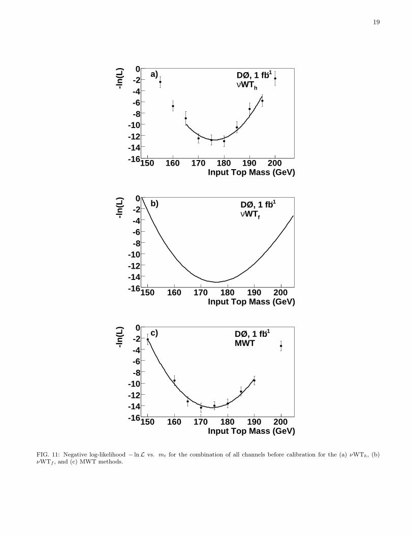
19

Input Top Mass (GeV)150 160 170 180 190 200

-ln

(L)

-16-14-12-10

-8-6-4-20 -1DØ, 1 fb

hWTνa)

Input Top Mass (GeV)150 160 170 180 190 200

-ln

(L)

-16-14-12-10

-8-6-4-20 -1DØ, 1 fb

fWTνb)

Input Top Mass (GeV)150 160 170 180 190 200

-ln

(L)

-16-14-12-10

-8-6-4-20 -1DØ, 1 fb

MWTc)

FIG. 11: Negative log-likelihood − lnL vs. mt for the combination of all channels before calibration for the (a) νWTh, (b)νWTf , and (c) MWT methods.

20

summing in quadrature uncertainties on the data andMonte Carlo jet energy scales. The probability densityhistograms (hs, hb) and functions (fs, fb) are left withthe nominal calibration.

b. b/light quark response ratio This uncertaintyarises from the fact that the jets in signal eventsare primarily b jets. These have a different detectorresponse than the light quark and gluon jets whichdominate the γ+jet sample used to derive the overalljet energy calibration. By applying this calibration tothe b jet sample, a 1.8% shift in jet pT is observed [35].We adjust the jets in the Monte Carlo for this andpropagate the correction into the 6ET . This causes ashift in the measured mt which is taken as an uncertainty.

c. Sample dependent jet energy scale After theinitial calibration, a residual shift in jet pT distributionsis observed in Z+jets events when comparing dataand Monte Carlo. We adopt a further calibration thatimproves agreement in these distributions and apply it toall of our background samples. Because this correctionmay not apply to tt events, we take the shift in themeasured mt to be a systematic uncertainty.

d. Object resolution The jet resolution from thesimulation is better than that observed in data. Toimprove the agreement, we apply an additional smearingto Monte Carlo events. A residual difference betweendata and Monte Carlo jet resolutions can lead to a massbias. To estimate the effect on the mt measurement, werepeat the pseudoexperiments by adjusting this smearingup and down within its uncertainty while keeping hs

and hb with the nominal resolutions. We estimate thesystematic uncertainties arising from the muon, isolatedtrack, and electron pT resolutions in a similar way.

e. Jet identification Jet reconstruction and iden-tification efficiency in Monte Carlo is corrected tomatch the data. We propagate the uncertainty on thecorrection factor to the top quark mass measurement.

f. Monte Carlo corrections Residual uncertaintieson the Monte Carlo corrections exist for triggering,luminosity profiles, lepton identification, and b-tagging.These uncertainties affect the top quark mass uncertain-ties. In each case, a respective systematic uncertaintyon mt is found by reweighting events according tothe uncertainties of Monte Carlo correction factorsintroduced to reproduce the data.

3. Method

a. Background yield Due to the limited statisticsof the simulation, there is some uncertainty in the eventyields for the background processes. This uncertainty

affects the likelihood and the measured top quark massvia Eq. 12. To estimate the effect of the uncertainty onbackground event yield, we vary the total backgroundyield by its known uncertainty up and down keepingthe relative ratios of individual background processesconstant.

b. Template statistics The templates used in theMWT and νWTh methods have finite statistics. Localfluctuations in these templates can cause local fluctua-tions in the individual likelihood fits and the top quarkmass. We obtain an uncertainty in mt by varying the− lnL points from the data ensemble within their errors.The width of the mt distribution provides the systematicuncertainty.

For the νWTf method, the fs function depends onfifteen parameters, each of which has a correspondinguncertainty. Consequently, there is some uncertaintyon the shape of this function. There is a correspondinguncertainty on the parameters of the fb. The uncertaintyon the shape causes the fit uncertainty on the measuredtop quark mass. We find the impact of this uncertaintyon the data sample by varying the parameters of fs andfb within their uncertainties. For each such variation, weremeasure mt for the data sample. The fit uncertaintyis the width of this distribution.

c. Monte Carlo calibration There is an uncertaintyon fitting the parameters (slope and offset) of the cali-bration curve. This uncertainty causes an uncertaintyin the calibrated top quark mass. The calibrationuncertainty is obtained as the uncertainty of the offset.

A summary of estimated systematic errors for the com-bined dilepton channels is provided in Table IV. We as-sumed the systematic uncertainties for all three methodsto be completely correlated for each source of systematicuncertainty and uncorrelated among different sources.The correlations of statistical uncertainties are given inthe next Section. All uncertainties are corrected for theslope of the mass scale calibration. The total uncertaintyis found by assuming all the contributions are indepen-dent and adding them in quadrature.

B. Combined Results

Because the statistical use of the νWT moments tem-plate is different between the νWTh and νWTf meth-ods, ensemble tests show that these two measurementsare only 85% correlated. We combine them using thebest linear unbiased estimator (BLUE) method [36] toform a final νWT measurement. Applying the correlationto the measurements from data, we obtain a final νWTmeasurement of mt = 176.2 ± 4.8(stat) ± 2.1(sys) GeVfor the combination of all five channels. We treat allsystematic uncertainties as 100% correlated across meth-ods except for the Monte Carlo calibration and template

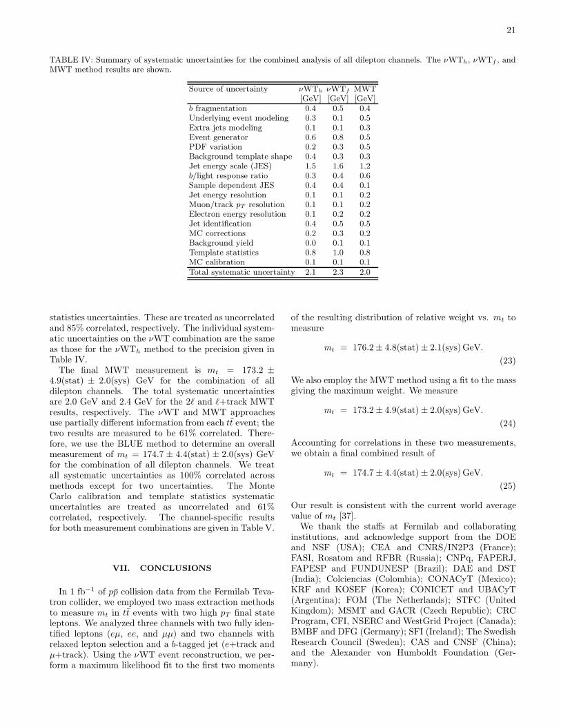
21

TABLE IV: Summary of systematic uncertainties for the combined analysis of all dilepton channels. The νWTh, νWTf , andMWT method results are shown.

Source of uncertainty νWTh νWTf MWT[GeV] [GeV] [GeV]

b fragmentation 0.4 0.5 0.4Underlying event modeling 0.3 0.1 0.5Extra jets modeling 0.1 0.1 0.3Event generator 0.6 0.8 0.5PDF variation 0.2 0.3 0.5Background template shape 0.4 0.3 0.3Jet energy scale (JES) 1.5 1.6 1.2b/light response ratio 0.3 0.4 0.6Sample dependent JES 0.4 0.4 0.1Jet energy resolution 0.1 0.1 0.2Muon/track pT resolution 0.1 0.1 0.2Electron energy resolution 0.1 0.2 0.2Jet identification 0.4 0.5 0.5MC corrections 0.2 0.3 0.2Background yield 0.0 0.1 0.1Template statistics 0.8 1.0 0.8MC calibration 0.1 0.1 0.1Total systematic uncertainty 2.1 2.3 2.0

statistics uncertainties. These are treated as uncorrelatedand 85% correlated, respectively. The individual system-atic uncertainties on the νWT combination are the sameas those for the νWTh method to the precision given inTable IV.

The final MWT measurement is mt = 173.2 ±4.9(stat) ± 2.0(sys) GeV for the combination of alldilepton channels. The total systematic uncertaintiesare 2.0 GeV and 2.4 GeV for the 2ℓ and ℓ+track MWTresults, respectively. The νWT and MWT approachesuse partially different information from each tt event; thetwo results are measured to be 61% correlated. There-fore, we use the BLUE method to determine an overallmeasurement of mt = 174.7 ± 4.4(stat) ± 2.0(sys) GeVfor the combination of all dilepton channels. We treatall systematic uncertainties as 100% correlated acrossmethods except for two uncertainties. The MonteCarlo calibration and template statistics systematicuncertainties are treated as uncorrelated and 61%correlated, respectively. The channel-specific resultsfor both measurement combinations are given in Table V.

VII. CONCLUSIONS

In 1 fb−1 of pp collision data from the Fermilab Teva-tron collider, we employed two mass extraction methodsto measure mt in tt events with two high pT final stateleptons. We analyzed three channels with two fully iden-tified leptons (eµ, ee, and µµ) and two channels withrelaxed lepton selection and a b-tagged jet (e+track andµ+track). Using the νWT event reconstruction, we per-form a maximum likelihood fit to the first two moments

of the resulting distribution of relative weight vs. mt tomeasure

mt = 176.2 ± 4.8(stat) ± 2.1(sys)GeV.

(23)

We also employ the MWT method using a fit to the massgiving the maximum weight. We measure

mt = 173.2 ± 4.9(stat) ± 2.0(sys)GeV.

(24)

Accounting for correlations in these two measurements,we obtain a final combined result of

mt = 174.7 ± 4.4(stat) ± 2.0(sys)GeV.

(25)

Our result is consistent with the current world averagevalue of mt [37].

We thank the staffs at Fermilab and collaboratinginstitutions, and acknowledge support from the DOEand NSF (USA); CEA and CNRS/IN2P3 (France);FASI, Rosatom and RFBR (Russia); CNPq, FAPERJ,FAPESP and FUNDUNESP (Brazil); DAE and DST(India); Colciencias (Colombia); CONACyT (Mexico);KRF and KOSEF (Korea); CONICET and UBACyT(Argentina); FOM (The Netherlands); STFC (UnitedKingdom); MSMT and GACR (Czech Republic); CRCProgram, CFI, NSERC and WestGrid Project (Canada);BMBF and DFG (Germany); SFI (Ireland); The SwedishResearch Council (Sweden); CAS and CNSF (China);and the Alexander von Humboldt Foundation (Ger-many).

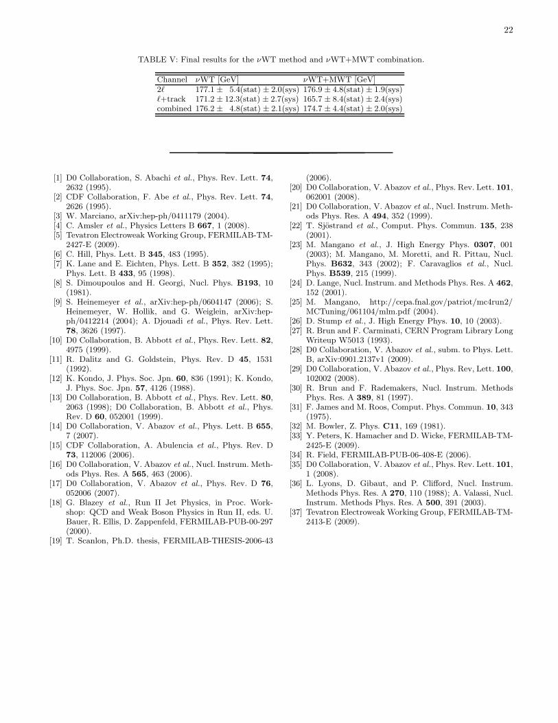
22

TABLE V: Final results for the νWT method and νWT+MWT combination.

Channel νWT [GeV] νWT+MWT [GeV]2ℓ 177.1 ± 5.4(stat) ± 2.0(sys) 176.9 ± 4.8(stat) ± 1.9(sys)ℓ+track 171.2 ± 12.3(stat) ± 2.7(sys) 165.7 ± 8.4(stat) ± 2.4(sys)combined 176.2 ± 4.8(stat) ± 2.1(sys) 174.7 ± 4.4(stat) ± 2.0(sys)

[1] D0 Collaboration, S. Abachi et al., Phys. Rev. Lett. 74,2632 (1995).

[2] CDF Collaboration, F. Abe et al., Phys. Rev. Lett. 74,2626 (1995).

[3] W. Marciano, arXiv:hep-ph/0411179 (2004).[4] C. Amsler et al., Physics Letters B 667, 1 (2008).[5] Tevatron Electroweak Working Group, FERMILAB-TM-

2427-E (2009).[6] C. Hill, Phys. Lett. B 345, 483 (1995).[7] K. Lane and E. Eichten, Phys. Lett. B 352, 382 (1995);

Phys. Lett. B 433, 95 (1998).[8] S. Dimoupoulos and H. Georgi, Nucl. Phys. B193, 10

(1981).[9] S. Heinemeyer et al., arXiv:hep-ph/0604147 (2006); S.

Heinemeyer, W. Hollik, and G. Weiglein, arXiv:hep-ph/0412214 (2004); A. Djouadi et al., Phys. Rev. Lett.78, 3626 (1997).

[10] D0 Collaboration, B. Abbott et al., Phys. Rev. Lett. 82,4975 (1999).

[11] R. Dalitz and G. Goldstein, Phys. Rev. D 45, 1531(1992).

[12] K. Kondo, J. Phys. Soc. Jpn. 60, 836 (1991); K. Kondo,J. Phys. Soc. Jpn. 57, 4126 (1988).

[13] D0 Collaboration, B. Abbott et al., Phys. Rev. Lett. 80,2063 (1998); D0 Collaboration, B. Abbott et al., Phys.Rev. D 60, 052001 (1999).

[14] D0 Collaboration, V. Abazov et al., Phys. Lett. B 655,7 (2007).

[15] CDF Collaboration, A. Abulencia et al., Phys. Rev. D73, 112006 (2006).

[16] D0 Collaboration, V. Abazov et al., Nucl. Instrum. Meth-ods Phys. Res. A 565, 463 (2006).

[17] D0 Collaboration, V. Abazov et al., Phys. Rev. D 76,052006 (2007).

[18] G. Blazey et al., Run II Jet Physics, in Proc. Work-shop: QCD and Weak Boson Physics in Run II, eds. U.Bauer, R. Ellis, D. Zappenfeld, FERMILAB-PUB-00-297(2000).

[19] T. Scanlon, Ph.D. thesis, FERMILAB-THESIS-2006-43

(2006).[20] D0 Collaboration, V. Abazov et al., Phys. Rev. Lett. 101,

062001 (2008).[21] D0 Collaboration, V. Abazov et al., Nucl. Instrum. Meth-

ods Phys. Res. A 494, 352 (1999).[22] T. Sjostrand et al., Comput. Phys. Commun. 135, 238

(2001).[23] M. Mangano et al., J. High Energy Phys. 0307, 001

(2003); M. Mangano, M. Moretti, and R. Pittau, Nucl.Phys. B632, 343 (2002); F. Caravaglios et al., Nucl.Phys. B539, 215 (1999).

[24] D. Lange, Nucl. Instrum. and Methods Phys. Res. A 462,152 (2001).

[25] M. Mangano, http://cepa.fnal.gov/patriot/mc4run2/MCTuning/061104/mlm.pdf (2004).

[26] D. Stump et al., J. High Energy Phys. 10, 10 (2003).[27] R. Brun and F. Carminati, CERN Program Library Long

Writeup W5013 (1993).[28] D0 Collaboration, V. Abazov et al., subm. to Phys. Lett.

B, arXiv:0901.2137v1 (2009).[29] D0 Collaboration, V. Abazov et al., Phys. Rev, Lett. 100,

102002 (2008).[30] R. Brun and F. Rademakers, Nucl. Instrum. Methods

Phys. Res. A 389, 81 (1997).[31] F. James and M. Roos, Comput. Phys. Commun. 10, 343

(1975).[32] M. Bowler, Z. Phys. C11, 169 (1981).[33] Y. Peters, K. Hamacher and D. Wicke, FERMILAB-TM-

2425-E (2009).[34] R. Field, FERMILAB-PUB-06-408-E (2006).[35] D0 Collaboration, V. Abazov et al., Phys. Rev. Lett. 101,

1 (2008).[36] L. Lyons, D. Gibaut, and P. Clifford, Nucl. Instrum.

Methods Phys. Res. A 270, 110 (1988); A. Valassi, Nucl.Instrum. Methods Phys. Res. A 500, 391 (2003).

[37] Tevatron Electroweak Working Group, FERMILAB-TM-2413-E (2009).