arX

iv:h

ep-p

h/00

0530

6v1

30

May

200

0

MADPH-00-1181

FERMILAB-Pub-00/113-T

hep-ph/0005306

May, 2000

Top-quark couplings to TeV resonances

at future lepton colliders

T. Hana, Y.J. Kima, A. Likhodedb, and G. Valenciac,d

aDepartment of Physics, University of Wisconsin, Madison, WI 53706

bInstitute for High Energy Physics, Protvino, Russia

cDepartment of Physics and Astronomy, Iowa State University, Ames, IA 50011

dFermi National Accelerator Laboratory, Batavia, IL 60510

Abstract

We study the processes WLWL → tt̄ and WLZL → tb̄ (t̄b) at future lepton colliders

as probes of the couplings of the top quark to resonances at the TeV scale. We consider

the cases in which the dominant low energy feature of a strongly interacting electroweak

symmetry breaking sector is either a scalar or a vector resonance with mass near 1 TeV.

We find that future lepton colliders with high energy and high luminosity have great

potential to sensitively probe these physics scenarios. In particular, at a 1.5 TeV linear

collider with an integrated luminosity of 200 fb−1, we expect about 120 events for

either a scalar or a vector to decay to tt̄, tb. Their leading partial decay widths, which

characterize the coupling strengths, can be statistically determined to about 10% level.

1 Introduction

The mass generation mechanisms for electroweak gauge bosons and for fermions are among

the most prominent mysteries in contemporary high energy physics. In the standard model

(SM) and its supersymmetric extensions, elementary scalar doublets of the SU(2)L interac-

tions are responsible for the mass generation. Yet there is no explanation for the scalar-

fermion Yukawa couplings. On the other hand, if there is no light Higgs boson found in the

next generation of collider experiments, then the interactions among the longitudinal vector

bosons would become strong at a scale of O(1 TeV) and new dynamics must set in [1]. The

fact that the top-quark mass is very close to the electroweak scale (mt ≈ v/√

2) is rather

suggestive: there may be a common origin for electroweak symmetry breaking and top-quark

mass generation. Much theoretical work has been carried out recently in connection to the

top quark and the electroweak sector [2, 3, 4].

Due to the Goldstone boson equivalence theorem (ET) [5], the longitudinal gauge

bosons (W±L , ZL) resemble the Goldstone modes (w±, z) at energies much larger than their

mass MW and thus faithfully reflect the nature of the electroweak symmetry breaking

(EWSB). To study the EWSB sector in connection with the top quark, a sensitive probe is

to produce a top quark via longitudinal gauge boson scattering [6]

W+L W

−L , ZLZL → tt̄, (1)

W±L ZL → tb̄, t̄b. (2)

These processes will receive significant enhancement if there are underlying resonances in this

sector that couple to both Goldstone bosons and the top quark. In particular, it is interesting

to note that both a scalar (Higgs-like) resonance and a vector (techni-rho-like ρ0) resonance

would contribute to W+

L W−L → tt̄ in process (1); while only a vector (techni-rho-like ρ±)

1

resonance would significantly enhance process (2).

These processes can be effectively realized at high energy lepton colliders via nearly

collinear gauge boson radiation

e+e− → νν̄ W ∗LW

∗L → νν̄ tt̄, (3)

e+e− → eν W ∗LZ

∗L → eν tb, (4)

where eν tb generically denotes e−ν̄ tb̄ and e+ν t̄b. Within the effective W -boson approx-

imation (EWA) [7], the tt̄ production of Eq. (1) was first calculated in Ref. [8] and then

in Ref. [9]. In the approach of an electroweak effective Lagrangian, they were studied in

Ref. [10]. A full evaluation of the SM diagrams was performed for tt̄ production at a 1.5

TeV linear collider [11, 12] and at a multi-TeV muon collider [13]. Effects on W+

L W−L → tt̄

from other strongly interacting dynamics were recently discussed in [14, 15].

In this paper, we carry out a comprehensive evaluation for processes (3) and (4)

within and beyond the SM. In Sec. 2, we first formulate the effective interactions for a

strongly-interacting electroweak sector (SEWS) including the heavy top quark (Top-SEWS).

We parameterize the sector in a (relatively) model-independent way by introducing a heavy

scalar or a heavy vector to unitarize (up to a few TeV) the universal low-energy amplitudes

[16]. We also comment on the current low-energy constraints on this sector. In Sec. 3, we

perform detailed numerical analyses for the Top-SEWS signal and the SM backgrounds. We

present our results at an e+e− linear collider with a center-of-mass energy√s = 1.5 and also

illustrate some results at a lepton collider with CM energy of 4 TeV. We find that the future

high energy lepton colliders have substantial potential to explore the Top-SEWS sector to

great precision. Section 4 contains our conclusions. Some useful formulae are presented in

Appendix A.

2

2 Effective Interactions in the Top-SEWS Sector

2.1 Low Energy Amplitudes

The low energy behavior of the scattering amplitudes for the processes VLVL → qq̄ is de-

termined by symmetry, and is the same in all models in which the electroweak symmetry is

broken by a strong interaction. If we parameterize the scale of this strong interaction with

the mass of its lightest resonance MR, then in the region where mW ≪ √s ≪ MR, the am-

plitudes are dominated by the low energy theorems (LET). These low energy theorems can

be obtained in a simple manner with the use of the Goldstone-boson equivalence theorem as

in Refs. [5, 6].

The framework for a model-independent analysis is that of effective Lagrangians.

Within this framework, the low energy amplitudes arise from the lowest dimension oper-

ator one can construct that respects the symmetries of the standard model. The non-

renormalizable effective Lagrangian responsible for the low energy interactions of the would-

be Goldstone bosons w±, z is given by

L =v2

4Tr(

∂µU†∂µU

)

(5)

where U = exp(iwiτi/v) [16, 17], with Trτiτj = 2δij and v ≈ 246 GeV. The minimal inter-

actions between third generation fermions and the would-be Goldstone bosons are those of

the standard model in the limit MH → ∞ and can be found, for example, in Refs. [6, 18].

We work in the limit mb = 0 and find (for terms with up to two w±, z),

L = −imt

vz tγ5t+

imt√2v

(

w+t(1 − γ5)b− w−b(1 + γ5)t)

+mt

v2tt(

w+w− +1

2zz)

. (6)

As a benchmark we will consider the low energy amplitudes (LET) defined as the

3

dominant terms in the limits MW ≪ (√s, mt) ≪ (MR, 4πv). Taking the scattering angle θ

to be that between the momentum of the w− (or z) and the top quark in the center of mass

frame, we find for the neutral channels,

M++LET (ww → tt̄) = −M−−

LET (ww → tt̄) = −mt

√s

v2βt (7)

M±∓LET (ww → tt̄) =

m2t

v2

(1 ± βt) sin θ

1 + βt cos θ − 2m2t/s

M++LET (zz → tt̄) = −M−−

LET (zz → tt̄) = −mt

√s

v2βt

M±∓LET (zz → tt̄) = −m

2t

v2

sin θ

1 + βt cos θ,

where βt = (1 − 4m2t/s)

1/2.

For the charged wz → tb̄ channel we define the angle θ between the momentum of

the z and the top quark in the center of mass frame, to obtain

M++LET (w+z → tb̄) =

√2m3

t

v2√s

βm(1 + cos θ)

[β2m(1 − cos θ) + 2m2

t/s]

M−+LET (w+z → tb̄) = −

√2m2

t

v2

βm sin θ

[β2m(1 − cos θ) + 2m2

t/s]. (8)

In writing these equations we took MW = mb = 0, and βm = (1 − m2t/s)

1/2. We present

some details in Appendix A.

The low energy amplitude for the process ww → tt̄ in Eq. (7) grows linearly with

energy and violates partial wave unitarity at an energy√sww ≈ 3 TeV [19, 20]. Similarly, the

low energy amplitude for the process ww → ww violates unitarity around 1.2 TeV [17, 21].

The energy scale at which these violations of unitarity take place can be interpreted as the

4

scale at which new physics must come into play. For our present purpose, the new physics

that restores unitarity will be either a scalar or a vector resonance and we discuss these two

cases in the next two sections. To maintain a model-independent discussion, we introduce

the resonances through effective (non-renormalizable) low energy Lagrangians. Therefore,

after inclusion of the resonance, the partial wave amplitudes will still violate unitarity at

higher energies. We will adjust the couplings of the resonances so that violation of unitarity

does not occur until a scale between 2 and 5 TeV. With this prescription, we describe

the phenomenology of a resonance which is the dominant dynamical feature of a strongly

interacting electroweak symmetry breaking sector (SEWS) below 2 TeV.

2.2 Scalar Resonance

The interactions between the standard model gauge bosons and a generic scalar resonance

S, have been considered in Ref. [22]. The leading order effective Lagrangian for these inter-

actions contains two free parameters: the resonance mass MS and a coupling constant gS

that can be traded for the width of the new resonance into W and Z pairs. The effective

Lagrangian for the scalar resonance and its interactions with the w±, z is given by

L =1

2∂µS∂

µS − 1

2M2

SS2 +

1

2gsvSTr

(

∂µU†∂µU

)

(9)

from which one obtains that,

ΓSww =3

32π

g2SM

3S

v2. (10)

With gS = 1, Eq. (10) reproduces the width of the standard model Higgs boson.

It is straightforward to compute the amplitudes for ww → ww scattering in this

5

model. They are obtained from the Lagrangians, Eqs. (5) and (9). For example we find,

A(w+w− → zz) =s

v2

s(1 − g2S) −M2

S

s−M2S

. (11)

All the other channels can be obtained from this one by using custodial SU(2) and crossing

symmetries [17]. From Eq. (11), we can see that the choice gS = 1 reproduces the standard

model amplitude. In this case, the amplitude takes a constant value at high energies as

corresponds to the renormalizable standard model. If gS 6= 1, however, the amplitude

grows with energy violating unitarity at some point. To study this issue, we construct the

I = 0, J = 0 partial wave amplitude,

a0

0(s) = − ΓSww

g2SMS

s

s−M2S + iΓSww

sMS

(

1 +s

M2S

(g2

S − 1))

+ΓSww

3g2SMS

(

s

M2S

(g2

S − 1) − 2g2

S

[

1 − M2S

slog(

1 +s

M2S

)])

. (12)

To obtain this result we have introduced a scalar-resonance width into the s-channel Higgs

propagator according to the prescription of Ref. [23],

1

s−M2S

→1 + i Γ

MS

s−M2S + iΓ s

MS

. (13)

which produces a well behaved amplitude both near the resonance and at high energy.∗

We first look at this result in the region above the resonance, and near the limit of

validity of the effective theory. For√s≫MS, Eq. (12) reduces to

a0

0(s) = (1 − g2

S)s

16πv2− 5

3

ΓSww

MS

(14)

∗ Both a constant width and an energy dependent width for a heavy scalar (with mass near 1 TeV)produce undesirable features [24]. We thank S. Willenbrock for pointing out reference [23].

6

Once again, we see that gS = 1 reproduces the standard model result, in which the unitarity

condition becomes a constraint on the Higgs boson mass [5]. The first term shows how,

for gS 6= 1, the model corresponds to a non-renormalizable effective theory. If we demand

that this term satisfy a unitarity condition |Re(a00(s))| < 0.5 up to

√s = 2 (3) TeV we

obtain 0.8 (0.9) ≤ |gS| ≤ 1.2 (1.1). If we choose to consider all the effects of the resonance,

including its width according to the prescription of Ref. [23], we then find for MS = 1 TeV

that unitarity condition in the form |a00| < 1, is satisfied up to 2 (5) TeV with

0.4 (0.9) ≤ |gS| ≤ 1.1 (1.02). (15)

The effective Lagrangian describing the coupling of the top quark to the scalar reso-

nance that we use is,

L = −κmt

vSt̄t (16)

where κ is a new coupling that can be traded for the width of the scalar into top-quark pairs,

ΓStt̄ =3κ2

8π

m2tMS

v2

(

1 − 4m2t

M2S

)3

2

. (17)

The case κ = 1 corresponds to the usual standard model Higgs-boson coupling to the top

quark. With Eqs. (5), (9) and (16), we have an effective theory involving a new generic scalar

resonance and its couplings to would-be Goldstone bosons and top quarks. Using Eqs. (9)

and (16), and the Equivalence Theorem (ET), we find the matrix element for WLWL → tt̄

via the scalar S to be

M++

S (ww → tt̄) = −M−−S (ww → tt̄) = gSκ

s

s−M2S

mt

√s

v2βt, (18)

here and henceforth, the double superscripts denote the tt̄ helicities. For κ = gS = 1, it

reduces to the standard model result. We obtain identical amplitudes for zz → tt̄. To

7

describe the resonance region we modify this amplitude according to the prescription in

Ref. [23]. Having chosen an SU(2) singlet, electrically neutral, scalar resonance, there is no

contribution to W±L ZL → tb̄, t̄b in this model.

There are no significant, phenomenological constraints on the couplings gS and κ.

Following Refs. [6], [19], and [25], we can demand that the process ww → tt̄ satisfy inelastic

partial-wave unitarity. By choosing the I = 0, J = 0, color singlet channel as in Ref. [20],

we find,

∣

∣

∣

∣

3GFmt

√s

8π√

2

∣

∣

∣

∣

∣

∣

∣

∣

M2S + s(gSκ− 1)

s−M2S

∣

∣

∣

∣

< 0.5 (19)

In analogy with our treatment of Eq. (12), we first concentrate in the region above the

resonance. The first factor in Eq. (19) corresponds to the low energy theorem, and it violates

unitarity at√s ≈ 3 TeV. We can have the full amplitude satisfy unitarity up to 3 TeV by

requiring the second factor to satisfy

∣

∣

∣

∣

gSκs

s−M2S

− 1

∣

∣

∣

∣

< 1 (20)

or, for energies far above the resonance, 0 < gSκ < 2.

If, on the other hand, we introduce the width according to the prescription of Ref. [23]

and consider the full amplitude for MS = 1 TeV, unitarity is satisfied up to√s = 2 (5) TeV

if

0 (0.4) < gsκ < 1.9 (1.6) (21)

Finally, we consider tt̄ → tt̄ scattering at energies above the resonance (in the same

helicity, color singlet channel). The J = 0 partial wave is,

a0(tt̄→ tt̄) = − 3

4π

GFm2t√

2κ2. (22)

8

If we follow Ref. [20] and require that |Rea0(tt̄→ tt̄)| < 0.5, we obtain the unitarity constraint

|κ| < 2.9. (23)

As we will see in our numerical studies in Fig. 8, this constraint is not very restrictive.

2.3 Vector Resonance

The interactions of standard model gauge bosons with new vector resonances have been

described in the literature [26, 27]. In the notation of Ref. [26], two new parameters are

introduced a and g̃ (these correspond to α and g′′

/2 from Ref. [27], respectively). The

effective Lagrangian consists of a kinetic term for the triplet of vector resonances ρµ ≡ ρiµτi/2

and an interaction term of the form

L = −1

4av2Tr

(

(ξ†∂µξ + ξ∂µξ† + i2g̃ρµ)(ξ

†∂µξ + ξ∂µξ† + i2g̃ρµ))

(24)

where ξ = exp(iwiτi/2v).

The two new constants a, g̃ are related to the mass and width of the vector particles

ρ via the relations,

M2ρ = av2g̃2, Γ(ρ0 → w+w−) =

a2g̃2

192πMρ. (25)

In addition, when the electroweak gauge bosons are added in a gauge invariant manner, they

mix with the new vector bosons [27]. In the charged sector, the physical states become,

V ±ph = ρ± cosφ+W± sin φ, W±

ph = W± cosφ− ρ± sinφ (26)

with a mixing angle given by

tan 2φ =4agg̃

(1 + a)g2 − 4ag̃2→ −g

g̃, (27)

9

the last expression being the limit as Mρ → ∞. Similar expressions for the mixing in the

neutral sector can be found in the literature [27]. For our numerical studies we use couplings

a, g̃ that have been studied in detail by the authors of the BESS model, and that respect

partial wave unitarity below a few TeV. For example, for Mρ = 1 TeV and Γρ = 30 GeV,

the partial wave a00 for ww → ww scattering satisfies |a0

0| < 1 up to about 2.6 TeV, while

|a11| < 1 is satisfied up to about 3 TeV with the simple prescription of using a constant width

in the s-channel ρ propagator.

We are currently interested in effective couplings between the new vector mesons

and the top and bottom quarks. These couplings may arise either from the ordinary quark

couplings to gauge bosons through the mixing of Eq. (26), or from novel direct couplings.

The couplings induced by mixing are universal, common to the three generations, and can

be bound by low energy experiments. More interesting is the possibility of a direct coupling

to the third generation. We write these effective couplings in a generic form

Leff = −ψ̄γµ(gV + gAγ5)τiψ ρi

µ, (28)

where ψ̄ is the third generation quark doublet (t̄ b̄).

Unlike the case of the scalar resonance, there exist low energy constraints on the direct

couplings of new vector resonances to the third generation quarks because they modify their

couplings to the W and Z. These deviations can be parameterized by the low energy effective

Lagrangian

Leff = − g√2

[

(1 + δκL)t̄LγµbL + δκRt̄Rγ

µbR

]

W+

µ + h. c.

− g

2 cos θW

[

(Lt + δLt)t̄LγµtL + (Rt + δRt)t̄Rγ

µtR

]

Zµ. (29)

For simplicity,† let us consider the case of anomalous W± couplings as shown in the diagram† The anomalous Z-boson couplings are obtained in a similar manner, but there is the additional com-

10

- sin ( φ )A

ρ W

t

b

g , gV

Figure 1: W − V Mixing induced anomalous tbW coupling.

in Fig. 1. We find in the limit of large vector resonance mass that

δκL = −2

g̃(gV − gA), δκR = −2

g̃(gV + gA). (30)

There are several constraints on these couplings. The measurement of the rate for b → sγ

restricts |δκR| <∼ 0.004 [28, 29] but does not place significant constraints on δκL. An analysis

of precision measurements at LEP [30] (with updated data from Ref. [31]) results in |δκL| <∼

0.1 excluding the parameter T .‡ From future experiments, it is expected that a B factory

can place significant further constraints of order |δκR| <∼ 0.001, |δκL| <∼ 0.03 [32]; and that

single top production can yield |δκL| <∼ 0.05 [33]. From all these numbers we conclude that a

right-handed coupling is severely constrained and for the rest of this paper will concentrate

on left-handed couplings exclusively. That is, we choose to satisfy the relation

gA = −gV , (31)

and, in keeping with the current bounds, we will concentrate on the case

gV <∼ 0.03 g̃. (32)

plication of both ρ0 and Z mixing with the photon.‡If the parameter T is included, the bound could be stronger in certain cases. In our case, however, the

induced anomalous couplings are of the form δκL = δLt, and are not restricted by T where they appear inthe combination δκL − δLt [30].

11

After these bounds are imposed, partial wave unitarity does not place additional constraints.

When new direct couplings such as those in Eq. (28) are introduced in a gauge

invariant manner, as is done in the BESS model [27] (through their parameter b), the effective

couplings gV,A of Eq. (28) receive contributions from both the direct couplings and mixing.

In this general case Eq. (28) is not literally correct, as the charged and neutral couplings

differ. We shall employ Eq. (28) for simplicity, assuming that the direct couplings dominate.

For example, in the heavy vector limit of the BESS model, they take the form

gV = −gA =g̃

4

b

1 + b. (33)

Considering both the charged and neutral vectors, this results in

δκL = δLt = −1

2

b

1 + band δκR = δRt = 0. (34)

The bound |δκL| <∼ 0.1 then corresponds to |b| <∼ 0.25. In this respect, it is expected that a

future linear collider studying the reaction e+e− → W+W− can probe values of b some ten

times smaller than this [34]. Our present study is complementary in the sense that we wish

to observe the direct signal for a vector state production at high energies.

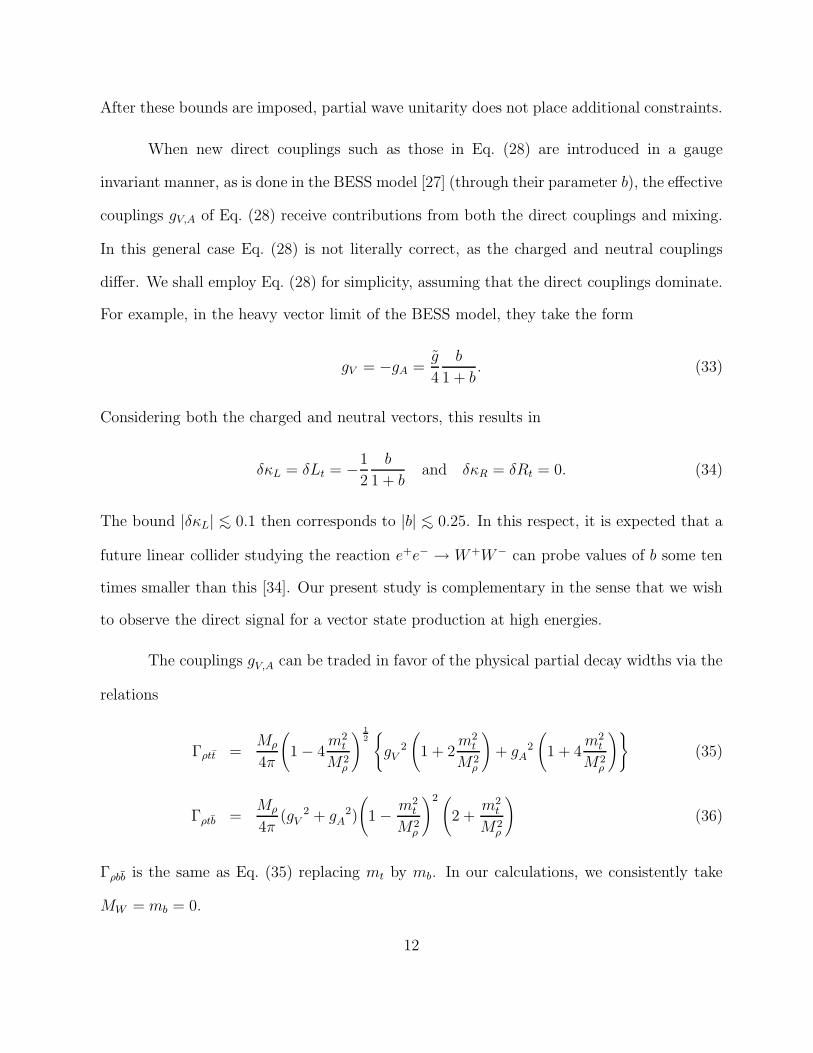
The couplings gV,A can be traded in favor of the physical partial decay widths via the

relations

Γρtt̄ =Mρ

4π

(

1 − 4m2

t

M2ρ

)1

2{

gV2

(

1 + 2m2

t

M2ρ

)

+ gA2

(

1 + 4m2

t

M2ρ

)}

(35)

Γρtb̄ =Mρ

4π(gV

2 + gA2)

(

1 − m2t

M2ρ

)2 (

2 +m2

t

M2ρ

)

(36)

Γρbb̄ is the same as Eq. (35) replacing mt by mb. In our calculations, we consistently take

MW = mb = 0.

12

In combining the ρ couplings to WL in Eq. (24) with the couplings in Eq. (28), we

obtain the scattering amplitudes

M++

ρ (w+w− → tt̄) = −M−−ρ (w+w− → tt̄)

= ag̃gVmt

√s

s−M2ρ + iMρΓρ

cos θ

M±∓ρ (w+w− → tt̄) =

ag̃

2

s sin θ

s−M2ρ + iMρΓρ

(−gV ∓ gAβt) (37)

and

M±±ρ (w+z → tb̄) =

ag̃√2

mt

√s

s−M2ρ + iMρΓρ

βm

×{(∓gV + gA)(1 + cos θ) + (±gV − gA)}

M±∓ρ (w+z → tb̄) =

ag̃√2

s

s−M2ρ + iMρΓρ

βm(gV ± gA) sin θ. (38)

Unlike the case of the scalar resonance, these amplitudes do not grow with energy. For this

reason, partial wave unitarity does not place any significant constraints. Also, unlike the

case of a scalar resonance, the heavy vector resonance is narrow and a simple treatment of

the constant width as above is adequate.

3 Sensitivity to the Top-SEWS Signal at Future Lep-

ton Colliders

3.1 Effective W Approximation

The effective W -boson approximation (EWA) provides a viable simplification for high energy

processes involving W -boson scattering [7]. It is particularly suitable for the calculations

13

under consideration since the W -boson level evaluation for the SEWS signal at high energies

is adequate. The condition for the EWA to be valid is that the invariant energy scales are

all much larger than the W mass, namely s, |t|, |u| ≫ MW . Besides, it is more accurate for

a longitudinal W -boson due to the fact that the distribution function is largely independent

of the W beam energies. To justify the EWA in our calculation, we compare our signal

evaluation for a heavy scalar resonance with a full tree-level SM calculation [35]. We define

the SM signal for a heavy Higgs boson σS following the subtraction procedure [22]

σS(MH) = σ(MH) − σ(MH = 100 GeV). (39)

The interpretation of this procedure is that the signal from a heavy Higgs boson should be

defined as the enhancement over the perturbative SM expectation with a light (MH ∼ 100

GeV) Higgs boson, which should be viewed as the irreducible SM background.

The process of e+e− → Ztt̄ followed by Z → νν̄ leads to the same final state as our

signal. It arises from different physics and needs to be removed from our consideration. We

follow the earlier studies [36] to introduce a recoil mass against the observable tt̄ system

defined as

M2

rec = s+m2

tt̄ − 2√s(Et + Et̄), (40)

where Et (Et̄) is the top (anti-top) quark energy in the e+e− CM frame. The recoil-mass

spectrum peaks at MZ for the background. Here and henceforth, we will impose Mrec >

200 GeV to effectively remove the Z → νν̄ background. We will adopt the same cut for the

eν tb process as well.

In Fig. 2, we present the production cross section for e+e− → ν̄νW+W− → ν̄νt̄t

versus an invariant mass cut (mcuttt̄ ) on the top quark pair for MH → ∞ at (a) e+e− CM

energy√s = 1.5 TeV and (b)

√s = 4 TeV. The solid curves are from the full SM calculation

based on the subtraction scheme Eq. (39). The dotted curves are the Low Energy Theorem

14

Figure 2: Production cross sections (in fb) for e+e− → ν̄νW+W− → ν̄νt̄t versus the invariantmass cut on the top quark pair for MH → ∞ at (a)

√s = 1.5 TeV and (b)

√s = 4 TeV.

(LET) result for w+w− → tt̄ by EWA. The two calculations agree very well, especially for

higher mtt̄ values.

In Fig. 3, we show the cross section for the same process, but versus the scattering

angle cut (cos θcutt ) on the final state top quarks. In Fig. 3(a), we compare the scalar resonance

model in Sec. 2.2 for MS = 1 TeV (dashed curve) with the SM for MH = 1 TeV (solid curve)

based on the subtraction scheme Eq. (39). In both cases and henceforth, to preserve unitarity

near the heavy scalar resonance, we adopt the prescription given in Eq. (13).

Fig. 3(b) compares the case for LET and the full SM calculation for MH → ∞. We

see that the two calculations agree better for central scattering at low cos θt. These two

figures motivate us to introduce the “basic acceptance cuts”,

mtt̄ > 500 GeV, | cos θt| < 0.8. (41)

15

Figure 3: Production cross sections (in fb) for e+e− → ν̄νW+W− → ν̄νt̄t at√s = 1.5 TeV

versus the polar angle cut on the final state t and t̄ (a) forMS = 1 TeV and (b) forMH → ∞.

These cuts not only guarantee the good agreement between the full SM calculation and the

EWA that we will adopt for signal calculations beyond the SM, but are also necessary to

enhance the signal over the SM backgrounds as we will discuss later. We impose a similar

requirement for the tb process.

Finally we show the comparison of the two calculations versus the center of mass (CM)

energy in Fig. 4 for (a) a 1 TeV scalar resonance and (b) MH → ∞, where the basic cuts of

Eq. (41) have been imposed on both t and t̄. The agreement is generally at order of 50% or

better for MS = 1 TeV and almost perfect for MH → ∞. We consider this to have justified

our future use of the EWA in the signal calculations beyond the SM. However, we note that

the EWA calculations for signal processes (1) and (2) do not properly incorporate the full

kinematics of processes (3) and (4). We thus simulate the full kinematics and determine the

cut efficiencies using the complete SM calculations in the next section.

16

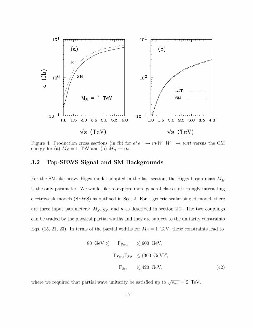
Figure 4: Production cross sections (in fb) for e+e− → ν̄νW+W− → ν̄νt̄t versus the CMenergy for (a) MS = 1 TeV and (b) MH → ∞.

3.2 Top-SEWS Signal and SM Backgrounds

For the SM-like heavy Higgs model adopted in the last section, the Higgs boson mass MH

is the only parameter. We would like to explore more general classes of strongly interacting

electroweak models (SEWS) as outlined in Sec. 2. For a generic scalar singlet model, there

are three input parameters: MS, gS, and κ as described in section 2.2. The two couplings

can be traded by the physical partial widths and they are subject to the unitarity constraints

Eqs. (15, 21, 23). In terms of the partial widths for MS = 1 TeV, these constraints lead to

80 GeV <∼ ΓSww <∼ 600 GeV,

ΓSwwΓStt̄ <∼ (300 GeV)2,

ΓStt̄ <∼ 420 GeV, (42)

where we required that partial wave unitarity be satisfied up to√sww = 2 TeV.

17

The three input parameters for the vector model are gV (= −gA), g̃, and a. These

can be traded by the physical parameters Mρ, Γρww (or Γρwz), and Γρtt̄ (or Γρtb̄). From the

constraint of Eq. (32), we get for a neutral ρ0 with mass Mρ = 1 TeV,

Γρtt̄Γρww <∼ (8 GeV)2 (43)

and for a charged ρ± of the same mass,

ΓρtbΓρwz <∼ (11 GeV)2. (44)

For the WLWL → tt̄ signal, the SM backgrounds are

e+e− → e+e− tt̄, (45)

e+e− → ν̄νW+W− → ν̄νtt̄. (46)

Process (45) mainly comes from γγ → tt̄ and has a large cross section, typically about 7.5 fb

at√s = 1.5 TeV. The charged-current process Eq. (46) occurs at a lower rate, about 1.7 fb

at√s = 1.5 TeV, but it is kinematically more difficult to separate from the signal. Following

earlier studies [36, 37], we demand a high transverse momentum for the final state t and t̄

pT (t) > 150 GeV, (47)

which is motivated by the Jacobian peak in the pT spectrum from a heavy particle decay.

We also require a moderate momentum for the tt̄ pair

30 GeV < pT (tt̄) < 300 GeV. (48)

This cut forces the final state leptons to be away from the forward-backward collinear region.

Since there are no energetic electrons in the central region for the signal process, we then

veto events with final state electrons at large angle:

Ee > 50 GeV, | cos θe| < cos(0.15 rad). (49)

18

We find that these cuts, along with the basic cuts (41), are very effective to suppress the SM

backgrounds. The background (45) is largely eliminated by the combination of pT (tt̄) cut

and electron veto. The effects of the cut on the charged current tt̄ process are summarized

in Table 1, again using the SM-like heavy Higgs model as the representative for the signal.

From this table, we find the cut efficiencies of Eqs. (47,48,49) for the signal based on the

subtraction scheme (39). They are

ǫ = 83% for√s = 1.5 TeV; ǫ = 84% for

√s = 4 TeV. (50)

For the remainder of this paper we use these cut efficiency figures for all the signal calculations

within the EWA in the WLWL → tt̄ channel.

√s = 1.5 TeV MH = 1 TeV Background MH = 0.1 TeV

cuts (41) 1.41 fb 0.21 fb

cuts (41,47,48,49) 1.13 fb 0.14 fb

√s = 4 TeV MH = 1 TeV Background MH = 0.1 TeV

cuts (41) 8.86 fb 0.98 fb

cuts (41,47,48,49) 7.20 fb 0.55 fb

Table 1: Cross sections of process (46) for a SM-like heavy Higgs (1 TeV) and a light Higgs(0.1 TeV) with different cuts. This gives the cut efficiencies for Top-SEWS signals as inEq. (50).

For the process WLZL → tb, the irreducible background is from

e+e− → eν WZ → eν tb. (51)

Again, the largest contribution comes from the photon induced process eγ → ν tb̄, where

the other electron goes along the beam direction after emitting a collinear photon. For this

19

Figure 5: Production cross sections (in fb) for (a) e+e− → ν̄νW+W− → ν̄νt̄t versus√s

for MH = 0.1 TeV (solid), LET (dot-dash), scalar singlet model (dots), and vector model(dashes), and for (b) e+e− → eν WZ → eν tb versus

√s for the vector model (dots), LET

(dashes) and SM background (solid) with the full cuts imposed. We have used the modelparameters as in Eqs. (55) and (56).

case, we impose the cuts (41) and (47). Since there is a final state electron in the signal

process with a typical transverse momentum of MZ/2, we require an electron tagging at a

finite angle

| cos θe| < cos(0.15 rad). (52)

This electron tagging is very effective to remove the SM background, and more so at higher

energies. The combination of the above cuts significantly reduces the eγ process and brings

the background to a level below the signal rate.

To determine the signal efficiency of the electron tagging, we calculate the process

e+e− → ν̄e−ρ+. (53)

20

We find

ǫ = 93% for√s = 1.5 TeV; ǫ = 61% for

√s = 4 TeV, (54)

which will be used for other signal calculations in the WLWL → tb channel based on the

EWA. The lower tagging efficiency at 4 TeV is due to the fact that the final state electron

becomes more forward at higher energies.

We now present the production cross sections for the signal and background versus

the CM energy√s after the cuts. Fig. 5(a) is for e+e− → ν̄νW+W− → ν̄ν t̄t process

with the full cuts (41, 47, 48, 49) for the scalar model (dots), vector model (dashes), LET

(dot-dash), and the irreducible background MH = 0.1 TeV (solid). For illustration, we have

taken the model parameters to be

MS = 1 TeV, ΓSww = 493 GeV, ΓStt̄ = 50 GeV,

Mρ = 1 TeV, Γρww = 50 GeV, Γρtt̄ = 1.3 GeV. (55)

Figure 5(b) shows the production cross sections for e+e− → eν WZ → eν tb, with the cuts

(41, 47, 52) for the vector model (dots), LET (dashes), and the SM background (solid). The

model parameters are taken as

Mρ = 1 TeV, Γρww = 50 GeV, Γρtb = 2.5 GeV. (56)

We see from Fig. 5 that our cuts effectively suppress the SM background below the signal

for both channels. The signal rate at a 1.5 TeV linear collider is typically between 0.5 and

1.2 fb.

3.3 Results and discussion

For the remainder of our analysis, we consider the top quark to decay hadronically t →

bW → bjj′ with a branching fraction approximately 70%. In doing so, we assume that we

21

Figure 6: Signal and background differential cross sections versus tt̄ invariant mass for (a)√s = 1.5 TeV and (b)

√s = 4 TeV: SM background by MH = 0.1 TeV (dot-dash), LET

(dots), scalar model (dashes), and vector model (solid). We have used the model parametersas in Eq. (55). All cuts are imposed and the branching fraction for t→ bjj′ is included.

can fully reconstruct the t and t̄ events, and that there are no isolated central electrons from

the decay to confuse our electron vetoing and tagging requirements. We also assume a data

sample of 200 fb−1 at√s = 1.5 TeV. We can see from Fig. 5 that we may reach a clear signal

observation for both a scalar and a vector resonance in the tt̄ channel. Although the LET

channel has relatively lower rate, it may nevertheless lead to about 35 events after including

the branching fraction, which is well above the background expectation. For the tb channel,

both signal and background rates are slightly smaller than the tt̄ case, but the vector signal

rate is still sufficiently above background to be observable. The LET amplitude in this case

is below background as was already seen in the model discussions.

It is important to know how well one can reconstruct the signal and contrast it

with the background beyond simple event counting. In Fig. 6 we show the distributions

for the signal and background versus tt̄ invariant mass (mtt̄) for (a)√s = 1.5 TeV and (b)

22

Figure 7: Signal and background cross sections (in fb) versus tb invariant mass (mtb) for (a)√s = 1.5 TeV and (b)

√s = 4 TeV: SM (dots) and vector model (solid). We have used

the model parameters as in Eq. (56). All cuts are imposed and the branching fraction fort→ bjj′ is included.

√s = 4 TeV with the SM background represented by MH = 0.1 TeV (dot-dash), LET signal

(dots), scalar model (dashes), and vector model (solid). The model parameters are taken as

in Eq. (55). All cuts are imposed and the branching fraction for tt̄ decay is included. We

see a broad resonance around MS = 1 TeV in scalar model due to its large width. For the

vector case, however, the width is narrower in general and the signal peaks above the scalar

model for Mρ = 1 TeV in a distinctive manner. The LET model has relatively low rate and

has no particular structure. In Fig. 7 we show the same signal and background distributions,

but for the tb channel versus the invariant mass (mtb). The model parameters are taken as

in Eq. (56). Clearly, the observation of a signal in Fig. 7 would provide decisive information

to discriminate a scalar resonance from a vector. The authors of Ref. [15] use, instead, the

top-quark polarization information to distinguish a scalar from a vector resonance.

We next consider the extent to which one can probe the couplings for different models.

23

Figure 8: At a linear collider with√s = 1.5 TeV and a luminosity of 200 fb−1, (a) accuracy

contours of determination of the partial widths for the scalar resonance model with MS = 1TeV; (b) statistical significance contours to distinguish a 1 TeV scalar from LET. Dottedlines are unitarity constraints given in Eq. (42).

Fig. 8(a) shows the accuracy contours to determine the partial decay widths (thus the cou-

plings) in the scalar resonance model with MS = 1 TeV at√s = 1.5 TeV and a luminosity

of 200 fb−1. The statistical accuracy for the cross section measurement is defined as

R =

√S +B

S

where S and B are the number of signal and background events respectively and we have

ignored the experimental systematic effects. We find that partial widths can be probed up

to about 10% accuracy for ΓStt̄ ≈ 50 GeV within the unitarity bounds shown as dotted

lines (Eq. 42). In the region above the curve labeled R = 8%, the partial widths can be

determined to 8% or better accuracy.

Also shown in Fig. 8(b) are the statistical significance contours to distinguish a 1 TeV

24

Figure 9: At a linear collider with√s = 1.5 TeV and a luminosity of 200 fb−1, determination

of the partial widths for the vector resonance model with Mρ = 1 TeV (a) 13% accuracycontour for W+W− → ρ0 → tt̄ channel; (b) 20% accuracy contour for W±Z → ρ± → tb̄(t̄b).Dotted lines are from the current low energy constraints in Eqs. (43) and (44).

scalar signal from the LET amplitudes. Here we define an appropriate standard deviation

as

σ ={σ(ΓStt̄,ΓSww) − σ(0, 0)}L

√

σ(0, 0)L

where σ(ΓStt̄,ΓSww) is the cross section in the scalar model for the given widths, σ(0, 0) is

the non-resonance cross section with gS = κ = 0, and L is the luminosity. It is easy to see

that the scalar model is distinguishable at the 5σ level from the non-resonant case within

the unitarity limits given in Eq. (42).

We show the same analysis for the vector model in Fig. 9, where we present the

sensitivity to the vector resonance model withMρ = 1 TeV at√s = 1.5 TeV and a luminosity

of 200 fb−1, for (a) 13% accuracy determination of the partial widths for W+W− → ρ0 → tt̄

25

and (b) 20% accuracy determination of the partial widths for W±Z → ρ± → tb̄ (t̄b). We

found in Fig. 9(a) that a 13% accuracy determination of the partial widths is possible for

the neutral vector process in the region allowed by the current bounds given in Eq. (43). For

the charged process we have a smaller signal rate, nevertheless, we found in Fig. 9(b) that

we can still determine the partial widths to 20% accuracy in the region allowed by current

constraints, Eq. (44).

4 Conclusion

We have studied the couplings of the top quark to TeV resonances that occur in models in

which the electroweak symmetry is broken by a strong interaction. Our study is motivated by

the fact that in many models the top quark plays a special role in the breaking of electroweak

symmetry.

We have explored the possibility that the new physics is realized as a scalar resonance

or a vector resonance near 1 TeV, as well as the case where the resonance is beyond reach

(LET). For the scalar model, we used partial wave unitarity to constrain the parameters as

shown in Sec. 2.2. For the vector model, we used current experimental data to constrain

the parameter space as presented in Sec. 2.3. We found within these constraints, that signal

rates in these models at future lepton colliders can be well above the SM backgrounds after

judicial cuts are applied. The models can be distinguished from each other by systematically

studying two different final states. Typically one would see a broad scalar resonance S, or

a relatively narrow vector resonance ρ0 in the tt̄ channel and a narrow vector resonance ρ±

in the tb channel. In particular, we illustrated our results at a 1.5 TeV linear collider with

an integrated luminosity of 200 fb−1. One expects to observe about 120 events for either

S → tt̄ or ρ0,± → tt̄, tb including final state identification. Even if the lower-lying resonances

26

are inaccessible at the collider, one can still observe a statistically significant deviation as

predicted by the LET for the tt̄ final state from the perturbative SM expectation. Finally, the

leading partial decay widths, which characterize the coupling strengths, can be statistically

determined to about 10% level.

Acknowledgments: The work of T.H. and Y.J.K. was supported in part by the US

DOE under contract No. DE-FG02-95ER40896 and in part by the Wisconsin Alumni Re-

search Foundation. The work of A.L. was supported in part by the RFBR grants 99-02-16558

and 00-15-96645. The work of G.V. was supported in part by DOE under contact number

DE-FG02-92ER40730. G.V. thanks the Special Research Centre for the Subatomic Structure

of Matter at the University of Adelaide for their hospitality and partial support while part

of this work was completed.

27

Appendix A SM amplitudes using the Equivalence

Theorem

In this appendix, we present the standard model amplitudes obtained using the Equivalence

Theorem for the processes w−w+ → tt̄, zz → tt̄, and zw+ → tb̄. From these amplitudes

one can derive the (LET) amplitudes by taking the large Higgs mass limit, ignoring the

electroweak couplings, and setting mb = 0.

w−w+ → tt̄

M±±H(ww → tt̄) = ± MH

2

(s−MH2)

mt

√s

v2βt

M±∓H(ww → tt̄) = 0 (A1)

M±±b(ww → tt̄) = ∓ 2m3

t

v2√s

βt + cos θ

1 + βt cos θ − 2m2t/s

M±∓b(ww → tt̄) =

m2t

v2

(1 ± βt) sin θ

1 + βt cos θ − 2m2t/s

(A2)

M±±γ(ww → tt̄) = ±2g2xWQ

mt√s

cos θ

M±∓γ(ww → tt̄) = ∓g2xWQ sin θ (A3)

M±±Z(ww → tt̄) = ±2gV g

2

Z(1

2− xW )

mt√s

cos θ

M±∓Z(ww → tt̄) = (−gV ∓ gAβt)g

2Z(

1

2− xW ) sin θ (A4)

where

βt = (1−4m2

t/s)1

2 , xW = sin2 θW , gZ =g

cos θW, gV =

1

2T3−QxW , and gA = −1

2T3.

28

Taking the limit M2H ≫ s and ignoring the terms of order g2, we find to leading order,

LET : M±±LET (ww → tt̄) = ∓mt

√s

v2βt

M±∓LET (ww → tt̄) =

m2t

v2

(1 ± βt) sin θ

1 + βt cos θ − 2m2t/s

.

zz → tt̄

M±±H(zz → tt̄) = ± MH

2

(s−MH2)

mt

√s

v2βt

M±∓H(zz → tt̄) = 0 (A5)

M±∓top(zz → tt̄) = ± 2m3

t

v2√s

βt + cos θ

1 + βt cos θ

M±∓top(zz → tt̄) = −m

2t

v2

sin θ

1 + βt cos θ. (A6)

LET : M±±LET (zz → tt̄) = ∓mt

√s

v2βt

M±∓LET (zz → tt̄) = −m

2t

v2

sin θ

1 + βt cos θ. (A7)

Again we keep only the leading order terms and ignore the top-quark exchange diagram for

M±±LET (zz → tt̄).

zw+ → tb̄

M++W+(zw+ → tb̄) = −

√2

4g2mt√sβm cos θ

29

M−−W+(zw+ → tb̄) = M+−

W+(zw+ → tb̄) = 0

M−+W+(zw+ → tb̄) =

√2

4g2βm sin θ (A8)

where βm = (1 −m2t/s)

1/2.

M++top(zw

+ → tb̄) =

√2m3

t

v2√s

βm(1 + cos θ)

[β2m(1 − cos θ) + 2m2

t/s]

M−−top (zw+ → tb̄) = M+−

top (zw+ → tb̄) = 0

M−+top(zw

+ → tb̄) = −√

2m2t

v2

βm sin θ

[β2m(1 − cos θ) + 2m2

t/s](A9)

where Mb(zw+ → tb̄) is proportional to mb and is neglected.

LET : M++LET (zw+ → tb̄) =

√2m3

t

v2√s

βm(1 + cos θ)

[β2m(1 − cos θ) + 2m2

t/s]

M−+LET (zw+ → tb̄) = −

√2m2

t

v2

βm sin θ

[β2m(1 − cos θ) + 2m2

t/s]. (A10)

30

References

[1] For a review, see e. g., M. Chanowitz, Ann. Rev. Nucl. Part. Sci. 38, 323 (1988).

[2] C. Hill, Phys. Lett. B266, 419 (1991); ibid. B345, 483 (1995); E. Eichten and K. Lane,

Phys. Lett. B352, 382 (1995).

[3] B. Dobrescu and C. Hill, Phys. Rev. Lett. 81, 2634 (1998); R. S. Chivukula, B. Dobrescu,

H. Georgi, and C. Hill, Phys. Rev. D59, 075003 (1999); G. Burdman and N. Evans,

Phys. Rev. D59, 115005 (1999).

[4] E. H. Simmons, hep-ph/9908488.

[5] B. W. Lee, C. Quigg, and H. B. Thacker, Phys. Rev. D16, 1519 (1977); M.S. Chanowitz

and M.K. Gaillard, Nucl. Phys. B261, 379 (1985); Y.P. Yao and C.P. Yuan, Phys. Rev.

D38, 2237 (1988); J. Bagger and C. Schmidt, Phys. Rev. D41, 264 (1990); H. Veltman,

Phys. Rev. D41, 2294 (1990); H.-J. He, Y.-P. Kuang, and X. Li, Phys. Rev. Lett. 69,

2619 (1992); H.-J. He and W.B. Kilgore, Phys. Rev. D55, 1515 (1997).

[6] M. Chanowitz, M. Furman and I. Hinchliffe, Nucl. Phys. B153, 402 (1979).

[7] M. Chanowitz and M.K. Gaillard, Phys. Lett. B142, 85 (1984); G. Kane, W. Repko

and W. Rolick, Phys. Lett. B148, 367 (1984); S. Dawson, Nucl. Phys. B249, 42 (1985).

[8] R.P. Kauffman, Phys. Rev. D41, 3343 (1990).

[9] M. Gintner and S. Godfrey, in the Proceedings of New Directions for High-Energy

Physics, June 25-July 12, 1996, Snowmass, p. 824.

[10] F. Larios, E. Malkawi and C.P. Yuan, Acta Phys. Polon. B27, 3741 (1996); F. Larios

and C.-P. Yuan, Phys. Rev. D55, 7218 (1997); Jose Wudka, talk given at the 5th

31

International Conference on Physics Beyond the Standard Model, Balholm, Norway, 29

Apr - 4 May 1997, hep-ph/9706434.

[11] T. Barklow, in the Proceedings of New Directions for High-Energy Physics, June 25-July

12, 1996, Snowmass, p. 819; T. Han, hep-ph/9910495.

[12] F. Larios, Tim Tait, and C.-P. Yuan, Phys. Rev. D57, 3106 (1998).

[13] V. Barger, M. Berger, J. Gunion and T. Han, talk given at ITP Conference on Future

High-energy Colliders, Santa Barbara, CA, 21-25 Oct 1996, hep-ph/9704290.

[14] T. Barklow et al., in the Proceedings of New Directions for High-Energy Physics, June

25-July 12, 1996, Snowmass, p. 735.

[15] E. R. Morales and M. E. Peskin, hep-ph/9909383.

[16] M.S. Chanowitz, M. Golden and H. Georgi, Phys. Rev. Lett. 57, 2344 (1986); Phys.

Rev. D35, 1149 (1987).

[17] A. Dobado and M. Herrero, Phys. Lett. B228,495 (1989); ibid. B233, 505 (1989); J.

Donoghue and C. Ramirez, Phys. Lett. B234, 361 (1990); S. Dawson and G. Valencia,

Nucl. Phys. B348, 23 (1991); ibid. B352, 27 (1991).

[18] R. D. Peccei, S. Peris, and X. Zhang, Nucl. Phys. B349, 305 (1991).

[19] T. Appelquist and M. Chanowitz, Phys. Rev. Lett. 59, 2405 (1987).

[20] W. Marciano, G. Valencia and S. Willenbrock, Phys. Rev. D40, 1725 (1989).

[21] J. Bagger, S. Dawson and G. Valencia, Nucl. Phys. B399, 364 (1993).

[22] J. Bagger, V. Barger, K. Cheung, J. Gunion, T. Han, G. Ladinsky, R. Rosenfeld, C.-P.

Yuan, Phys. Rev. D49, 1246 (1994); ibid. D52, 3878 (1995).

32

[23] M.H. Seymour, Phys. Lett. B354, 409 (1995).

[24] G. Valencia and S. Willenbrock, Phys. Rev. D42, 853 (1990); ibid. D46, 2247 (1992).

[25] S. Jager and S. Willenbrock, Phys. Lett. B435, 139 (1998); R. S. Chivukula, Phys.

Lett. B439, 389 (1998).

[26] J. Bagger, T. Han and R. Rosenfeld, FERMILAB-CONF-90-253-T, published in Snow-

mass Summer Study 1990, p. 208.

[27] R. Casalbuoni et al., Phys. Lett. B155, 95 (1985); Nucl. Phys. B282, 235 (1987); ibid.

B310, 181 (1988); Phys. Lett. B249, 130 (1990); ibid. B253, 275 (1991).

[28] K. Fujikawa and A. Yamada, Phys. Rev. D49, 5890 (1994).

[29] F. Larios, M. A. Perez and C. P. Yuan, Phys. Lett. B457, 334 (1999).

[30] S. Dawson and G. Valencia, Phys. Rev. D53, 1721 (1996).

[31] C. Caso et al., Eur. Phys. J. C3, 1 (1998).

[32] A. A. El-Hady and G. Valencia, Phys. Lett. B414, 173 (1997).

[33] T. Tait and C. P. Yuan, hep-ph/9710372.

[34] D. Dominici, Riv. Nuovo Cim. 20, 1 (1997) [hep-ph/9711385].

[35] For the full SM calculations, we have made use of the Madgraph package by T. Stelzer

and W.F. Long, Comput. Phys. Commun. 81, 357 (1994).

[36] V. Barger, K. Cheung, T. Han and R.J.N. Phillips, Phys. Rev. D52, 3815 (1995); V.

Barger, M. Berger, J. Gunion and T. Han, Phys. Rev. D55, 142 (1997).

[37] V. Barger, K. Cheung, T. Han and R.J.N. Phillips, Phys. Rev. D42, 3052 (1990).

33