
Scalar boson decays to tau leptons : in the standard model ...
282
Université Libre de Bruxelles Faculté des Sciences Scalar boson decays to tau leptons : in the standard model and beyond Thèse présentée par : Cécile Caillol En vue de l’obtention du grade de : Docteur en Sciences Bruxelles, avril 2016
-
Upload
khangminh22 -
Category
Documents
-
view
0 -
download
0
Transcript of Scalar boson decays to tau leptons : in the standard model ...

Université Libre de Bruxelles
Faculté des Sciences
Scalar boson decays to tau leptons : in thestandard model and beyond
Thèse présentée par :
Cécile Caillol
En vue de l’obtention du grade de :
Docteur en Sciences
Bruxelles, avril 2016


Constitution du jury de thèse :
Giacomo Bruno (UCL)Barbara Clerbaux (ULB), promoteurSridhara Dasu (University of Wisconsin Madison)Albert De Roeck (CERN)Jean-Marie Frère (ULB), présidentAbdollah Mohammadi (Kansas State University), co-promoteurPascal Vanlaer (ULB), secrétaire


Abstract
This thesis presents a study of the scalar sector in the standard model (SM), as well asdifferent searches for an extended scalar sector in theories beyond the standard model(BSM). All analyses have in common the fact that at least one scalar boson decays to apair of tau leptons. The results exploit the data collected by the CMS detector duringLHC Run-1, in proton-proton collisions with a center-of-mass energy of 7 or 8 TeV.
The particle discovered in 2012, H, looks compatible with a SM Brout-Englert-Higgsboson, but this statement is driven by the H → γγ and H → ZZ decay modes. TheH → τ+τ− decay mode is the most sensitive fermionic decay channel, and allows to testthe Yukawa couplings of the new particle. The search for the SM scalar boson decaying totau leptons, and produced in association with a massive vector bosonW or Z, is describedin this thesis. Even though a good background rejection can be achieved by selecting theleptons originating from the vector boson, Run-1 data are not sensitive to the small pro-duction cross sections predicted in the SM for the scalar boson. The combination withthe gluon-gluon fusion and vector boson fusion production searches leads to an evidencefor the decay of the H boson to tau leptons.
Many BSM models, such as the minimal supersymmetric SM (MSSM) or models withtwo scalar doublets (2HDM), predict the existence of several scalar bosons. The decaysof these bosons to tau leptons can be enhanced in some scenarios depending on the modelparameters, which makes the di-tau decay mode powerful to discover BSM physics. Foursearches for an extended scalar sector are detailed in this thesis. The first analysis searchesfor a pseudoscalar boson with a mass between 220 and 350 GeV, decaying to an SM-likescalar boson and a Z boson, in the final state with two light leptons and two tau leptons.Second, a search for the exotic decay of the new particle H to a pair of light pseudoscalarbosons, which is still allowed by all measurements made up to now, in the final state withtwo muons and two tau leptons is performed. Third, a mass region almost never exploredat the LHC is probed by the search of a light pseudoscalar, with a mass between 25 and80 GeV, decaying to tau leptons and produced in association with b quarks. The lastanalysis describes the search for a heavy resonance in the MSSM, decaying to a pair oftau leptons. None of these analyses has found any hint of new physics beyond the SM,but stringent limits on the cross section of such signals could be set.
Résumé
Cette thèse présente une étude du secteur scalaire dans le cadre du modèle standard(MS), ainsi que la recherche d’un secteur scalaire étendu dans des théories au-delà du MS.Ces analyses ont en commun la désintégration d’au moins un des bosons scalaires en unepaire de leptons taus. Les résultats sont basés sur les données collectées par le détecteurCMS pendant le Run-1 du LHC, lors de collisions proton-proton à une énergie dans lecentre de masse de 7 ou 8 TeV.
La particule découverte en 2012,H, semble compatible avec un boson de Brout-Englert-Higgs du MS, mais ce constat se base essentiellement sur l’étude des modes de désintégra-tion H → γγ et H → ZZ. Le mode de désintégration H → τ+τ− est le canal fermioniquele plus sensible, et permet de tester les couplages de Yukawa du nouveau boson. Cettethèse décrit dans un premier temps la recherche du boson scalaire du MS se désintégranten leptons taus et produit en association avec un boson vecteur massif W ou Z. Bienque les bruits de fond puissent être réduits en sélectionnant les leptons provenant de ladésintégration des bosons vecteurs, les données du Run-1 ne sont pas sensibles aux petitessections efficaces de production prédites dans le SM pour le boson scalaire. Cependant,la combinaison avec les recherches du boson scalaire dans d’autres modes de productionmontre avec évidence l’existence de désintégrations du boson H en leptons taus.
De nombreux modèles au-delà du MS, tels que l’extension supersymétrique minimaledu MS (MSSM) ou les modèles avec deux doublets scalaires (2HDM), prédisent l’existencede plusieurs bosons scalaires. La désintégration de ces bosons en leptons taus peut êtrefavorisée dans certains scénarios en fonction des paramètres du modèle, ce qui rend cemode de désintégration très puissant dans la recherche de nouvelle physique. Quatrerecherches d’un secteur scalaire étendu au-delà du MS sont présentées dans cette thèse.La première analyse recherche un pseudoscalaire avec une masse entre 220 et 350 GeV, sedésintégrant en un boson scalaire similaire à celui du MS et en un boson Z, dans l’état finalavec deux leptons taus et deux leptons légers. La deuxième analyse explore la possibilitéd’une désintégration exotique de la nouvelle particule, H, en deux bosons scalaires pluslégers, ce qui est toujours autorisé par toutes les mesures faites à ce jour, dans l’étatfinal avec deux muons et deux leptons taus. Dans le cadre de la troisième analyse, unerégion en masse quasiment inexplorée auparavant au LHC est testée par la recherched’un pseudoscalaire avec une masse entre 25 et 80 GeV, se désintégrant en leptons tauset produit en association avec deux quarks b, dans le contexte des 2HDM. La dernièreanalyse recherche une résonance lourde se désintégrant en une paire de leptons taus dansle contexte du MSSM. Aucun indice de nouvelle physique n’a été trouvé dans aucune desanalyses décrites ci-dessus, mais des limites strictes sur les sections efficaces des différentssignaux ont été déterminées.

Acknowledgements
First, I would like to thank Barbara Clerbaux for supervising this work. At every mo-ment she has been present, supportive, and has given me the best advice. This manuscriptwould not have been the same without her, and I want to thank her for the careful reviewof the previous versions.
I also want to thank Abdollah Mohammadi. He has taught me so many things, andhas always tried to give me visibility and responsibilities, from the very beginning of myPhD. It has always been a pleasure to work with him, and I could not have imagined abetter teammate to carry on this project.
I am grateful to the other jury members, Jean-Marie Frère, Pascal Vanlaer, SridharaDasu, Giacomo Bruno, and Albert De Roeck, for reading this thesis, and giving me theirvaluable comments.
This thesis was made possible with the help of many people working at CERN. Inparticular, I want to thank Christian Veelken for the time he patiently spent with me, toteach me about tau physics at CMS.
I had the invaluable opportunity to work one year at CERN ; and this certainly im-proved the quality of my work. For this, I want to thank Joe Incandela and the FPScommittee.
My work at the IIHE and at CERN would not have been that pleasant without mycolleagues. It is impossible to name everyone here, but special thanks go to the nicest of-fice mates, Nastja and Didar, to the most efficient secretary, Audrey, to the most patientIT team, and to the best support at CERN, Jian.
And the last word goes to my parents and my sisters, who always support me, andwhom I cannot thank enough.


Contents
Introduction 1
I Theoretical bases 5
1 The standard model of particle physics 71.1 Elementary particles and forces . . . . . . . . . . . . . . . . . . . . . . . . . . . . . . . . . 71.2 Standard model Lagrangian . . . . . . . . . . . . . . . . . . . . . . . . . . . . . . . . . . . 91.3 Scalar sector . . . . . . . . . . . . . . . . . . . . . . . . . . . . . . . . . . . . . . . . . . . 121.4 Chapter summary . . . . . . . . . . . . . . . . . . . . . . . . . . . . . . . . . . . . . . . . 18
2 Physics beyond the standard model 192.1 Motivations for new physics . . . . . . . . . . . . . . . . . . . . . . . . . . . . . . . . . . . 192.2 Two-Higgs-doublet models . . . . . . . . . . . . . . . . . . . . . . . . . . . . . . . . . . . . 222.3 Supersymmetry . . . . . . . . . . . . . . . . . . . . . . . . . . . . . . . . . . . . . . . . . . 252.4 Two-Higgs-doublet models + a singlet . . . . . . . . . . . . . . . . . . . . . . . . . . . . . 322.5 Search for BSM physics in the scalar sector . . . . . . . . . . . . . . . . . . . . . . . . . . 332.6 Precision measurements vs. direct discovery in the case of the SM+S . . . . . . . . . . . . 352.7 Chapter summary and personal contributions . . . . . . . . . . . . . . . . . . . . . . . . . 38
3 Statistics 393.1 Likelihood . . . . . . . . . . . . . . . . . . . . . . . . . . . . . . . . . . . . . . . . . . . . . 393.2 Maximum likelihood fit . . . . . . . . . . . . . . . . . . . . . . . . . . . . . . . . . . . . . 433.3 Exclusion limits . . . . . . . . . . . . . . . . . . . . . . . . . . . . . . . . . . . . . . . . . . 433.4 Significance . . . . . . . . . . . . . . . . . . . . . . . . . . . . . . . . . . . . . . . . . . . . 453.5 Goodness-of-fit test . . . . . . . . . . . . . . . . . . . . . . . . . . . . . . . . . . . . . . . . 473.6 Boosted decision trees . . . . . . . . . . . . . . . . . . . . . . . . . . . . . . . . . . . . . . 483.7 k-Nearest Neighbor classifier . . . . . . . . . . . . . . . . . . . . . . . . . . . . . . . . . . . 503.8 Chapter summary . . . . . . . . . . . . . . . . . . . . . . . . . . . . . . . . . . . . . . . . 52
II Experimental bases 53
4 Experimental setup 554.1 Large Hadron Collider . . . . . . . . . . . . . . . . . . . . . . . . . . . . . . . . . . . . . . 554.2 Compact Muon Solenoid . . . . . . . . . . . . . . . . . . . . . . . . . . . . . . . . . . . . . 584.3 Chapter summary . . . . . . . . . . . . . . . . . . . . . . . . . . . . . . . . . . . . . . . . 67
CONTENTS
5 Event generation, simulation and reconstruction 695.1 Event generation and simulation . . . . . . . . . . . . . . . . . . . . . . . . . . . . . . . . 695.2 Object reconstruction and identification . . . . . . . . . . . . . . . . . . . . . . . . . . . . 705.3 Chapter summary . . . . . . . . . . . . . . . . . . . . . . . . . . . . . . . . . . . . . . . . 81
6 Tau lepton reconstruction and identification 836.1 HPS algorithm description . . . . . . . . . . . . . . . . . . . . . . . . . . . . . . . . . . . . 836.2 HPS algorithm performance in Run-1 . . . . . . . . . . . . . . . . . . . . . . . . . . . . . 896.3 HPS algorithm in Run-2 . . . . . . . . . . . . . . . . . . . . . . . . . . . . . . . . . . . . . 1136.4 Chapter summary and personal contributions . . . . . . . . . . . . . . . . . . . . . . . . . 121
III SM physics analyses 123
7 Search for the SM scalar in the ZH → ``ττ channel 1257.1 Analysis overview . . . . . . . . . . . . . . . . . . . . . . . . . . . . . . . . . . . . . . . . . 1257.2 Selection . . . . . . . . . . . . . . . . . . . . . . . . . . . . . . . . . . . . . . . . . . . . . . 1267.3 Background estimation . . . . . . . . . . . . . . . . . . . . . . . . . . . . . . . . . . . . . . 1297.4 Di-tau mass reconstruction . . . . . . . . . . . . . . . . . . . . . . . . . . . . . . . . . . . 1357.5 Systematic uncertainties and simulation corrections . . . . . . . . . . . . . . . . . . . . . . 1367.6 Results . . . . . . . . . . . . . . . . . . . . . . . . . . . . . . . . . . . . . . . . . . . . . . . 1417.7 Chapter summary and personal contributions . . . . . . . . . . . . . . . . . . . . . . . . . 146
8 Search for the SM scalar in the WH → eµτh channel 1478.1 Selection . . . . . . . . . . . . . . . . . . . . . . . . . . . . . . . . . . . . . . . . . . . . . . 1478.2 Background estimation . . . . . . . . . . . . . . . . . . . . . . . . . . . . . . . . . . . . . . 1488.3 Results . . . . . . . . . . . . . . . . . . . . . . . . . . . . . . . . . . . . . . . . . . . . . . . 1538.4 Chapter summary and personal contributions . . . . . . . . . . . . . . . . . . . . . . . . . 156
9 Combination of searches for the SM scalar boson decaying to taus 1579.1 Gluon-gluon fusion and vector boson fusion production modes . . . . . . . . . . . . . . . . 1579.2 Vector boson associated production . . . . . . . . . . . . . . . . . . . . . . . . . . . . . . . 1589.3 Combination of all production modes . . . . . . . . . . . . . . . . . . . . . . . . . . . . . . 1589.4 Chapter summary and personal contributions . . . . . . . . . . . . . . . . . . . . . . . . . 162
IV BSM physics analyses 163
10 Search for a heavy pseudoscalar boson A decaying to Zh in the ``ττ final state 16510.1 Differences with respect to the SM ZH → ``ττ analysis . . . . . . . . . . . . . . . . . . . 16510.2 Background estimation validation . . . . . . . . . . . . . . . . . . . . . . . . . . . . . . . . 16910.3 High�ET excess . . . . . . . . . . . . . . . . . . . . . . . . . . . . . . . . . . . . . . . . . . 17010.4 Results . . . . . . . . . . . . . . . . . . . . . . . . . . . . . . . . . . . . . . . . . . . . . . . 17110.5 Combination with H → hh→ bbττ . . . . . . . . . . . . . . . . . . . . . . . . . . . . . . . 17410.6 Chapter summary and personal contributions . . . . . . . . . . . . . . . . . . . . . . . . . 177
11 Search for exotic decays of the SM-like scalar boson in the µµττ final state 17911.1 Selection . . . . . . . . . . . . . . . . . . . . . . . . . . . . . . . . . . . . . . . . . . . . . . 17911.2 Background estimation and its validation . . . . . . . . . . . . . . . . . . . . . . . . . . . 18311.3 Modeling of the experimental mµµ distributions . . . . . . . . . . . . . . . . . . . . . . . . 18611.4 Uncertainties . . . . . . . . . . . . . . . . . . . . . . . . . . . . . . . . . . . . . . . . . . . 19511.5 Results . . . . . . . . . . . . . . . . . . . . . . . . . . . . . . . . . . . . . . . . . . . . . . . 198
4

11.6 Interpretation and comparison with other CMS searches . . . . . . . . . . . . . . . . . . . 20211.7 Chapter summary and personal contributions . . . . . . . . . . . . . . . . . . . . . . . . . 209
12 Search for a light pseudoscalar decaying to taus 21112.1 Analysis overview . . . . . . . . . . . . . . . . . . . . . . . . . . . . . . . . . . . . . . . . . 21112.2 Selection . . . . . . . . . . . . . . . . . . . . . . . . . . . . . . . . . . . . . . . . . . . . . . 21312.3 Background estimation . . . . . . . . . . . . . . . . . . . . . . . . . . . . . . . . . . . . . . 21512.4 Systematic uncertainties . . . . . . . . . . . . . . . . . . . . . . . . . . . . . . . . . . . . . 21912.5 Results . . . . . . . . . . . . . . . . . . . . . . . . . . . . . . . . . . . . . . . . . . . . . . . 22212.6 Chapter summary and personal contributions . . . . . . . . . . . . . . . . . . . . . . . . . 226
13 Search for a heavy di-tau resonance in the MSSM 22713.1 Categorization . . . . . . . . . . . . . . . . . . . . . . . . . . . . . . . . . . . . . . . . . . 22713.2 τhτh final state . . . . . . . . . . . . . . . . . . . . . . . . . . . . . . . . . . . . . . . . . . 22913.3 Differences from the light pseudoscalar boson search analysis in the eτh, µτh and eµ final
states . . . . . . . . . . . . . . . . . . . . . . . . . . . . . . . . . . . . . . . . . . . . . . . 23413.4 Φ pT reweighting . . . . . . . . . . . . . . . . . . . . . . . . . . . . . . . . . . . . . . . . . 23713.5 Result interpretation . . . . . . . . . . . . . . . . . . . . . . . . . . . . . . . . . . . . . . . 23713.6 Chapter summary and personal contributions . . . . . . . . . . . . . . . . . . . . . . . . . 240
V Status and prospects 241
14 Overview of LHC results and prospects for future colliders 24314.1 Overview of CMS measurements in the scalar sector . . . . . . . . . . . . . . . . . . . . . 24314.2 Overview of other SM and BSM results of the CMS experiment . . . . . . . . . . . . . . . 25014.3 Future collider experiments . . . . . . . . . . . . . . . . . . . . . . . . . . . . . . . . . . . 25114.4 Chapter summary . . . . . . . . . . . . . . . . . . . . . . . . . . . . . . . . . . . . . . . . 254
Conclusion 255
A Technical details about physics analyses 259A.1 Monte Carlo samples and collected datasets . . . . . . . . . . . . . . . . . . . . . . . . . . 259A.2 Triggers . . . . . . . . . . . . . . . . . . . . . . . . . . . . . . . . . . . . . . . . . . . . . . 259


Introduction
The standard model (SM) of particle physics describes the elementary particles andtheir interactions through the electromagnetic, the weak and the strong forces. Experi-mental results from various high-energy experiments, such as the Large Electron-PositronCollider (LEP) at CERN between 1989 and 2000, the Tevatron at Fermilab between 1983and 2011, and the Large Hadron Collider (LHC) at CERN from 2010, have shown upto now an amazing agreement with the predictions of the SM. The latest triumph of thetheory is the discovery of a new scalar particle, compatible with the Brout-Englert-Higgsboson of the SM, in July 2012. This particle, the cornerstone and last missing piece of theSM, was introduced as a consequence of the electroweak symmetry breaking, in order toexplain how elementary particles could obtain a mass without violating the gauge invari-ance of the theory. The physicists Francois Englert - working closely with deceased RobertBrout - and Peter Higgs were awarded the 2013 Physics Nobel Prize in acknowledgmentof "the theoretical discovery of a mechanism that contributes to our understanding ofthe origin of mass of subatomic particles, and which recently was confirmed through thediscovery of the predicted fundamental particle, by the ATLAS and CMS experiments atCERN’s Large Hadron Collider". The data collected by the ATLAS and CMS experi-ments at CERN in 2011 and 2012, during the LHC Run-1, have permitted to study moreprecisely the properties and couplings of this new particle; all measurements indicate upto now that it is compatible within uncertainties with the scalar boson from the SM.
The discovery of a particle compatible with the scalar boson of the SM happened almostfifty years after its prediction in 1964, and was made possible by the high performanceof the LHC, and of its two general-purpose experiments, ATLAS and CMS. The LHC,situated under the French-Swiss border, is a twenty-seven kilometer long circular proton-proton (pp) collider. Its Run-1 extended from 2010 to 2012, and permitted to collectroughly 25 fb−1 of data at a center-of-mass energy of 7 and 8 TeV; whereas Run-2 startedin summer 2015 at a center-of-mass energy of 13 TeV after a long shutdown of the LHC.The search for the SM scalar boson was the main objective when designing the experiment.
In the SM, the scalar boson is produced via different mechanisms. Its largest produc-tion cross section at the LHC corresponds to the gluon-gluon fusion, whereas vector bosonfusion production and the production in association with a vector boson have smaller crosssections. Although the gluon-gluon fusion production dominates, studying the other pro-
1

Introduction
duction modes is important to test the compatibility of the discovered boson, H, with theSM scalar boson. Subdominant production modes can moreover have a larger sensitivityto the presence of a signal in the case where the H decay products are difficult to identify.For a mass of 125 GeV, as measured by the CMS and ATLAS experiments, a large varietyof decay modes is opened, which provides experimentalists with a wide range of physicssignatures to study. The discovery of the H boson in 2012 was led by the study of bosonicdecay channels (H → γγ, H → W±W∓∗ and H → ZZ∗), but searching for its decay tofermions, essentially H → τ+τ− and H → bb, is important to test if the H Yukawa cou-plings are in agreement with the predictions of the SM. Fermionic decay channels, despitetheir large branching fractions, are less sensitive than bosonic decay channels because ofthe difficulty in identifying and reconstructing tau leptons and b quarks, and in separatingthe signal from large backgrounds.
Tau leptons are the only leptons heavy enough to decay semi-hadronically. In about twothirds of cases, tau leptons decay to a combination of charged and neutral hadrons, and toa tau neutrino. Muons and electrons produced in leptonic tau decays along with neutrinoscannot be distinguished from other muons or electrons produced promptly. Hadronicallydecaying tau leptons, τh, are reconstructed and identified in CMS with the Hadrons PlusStrips (HPS) algorithm, which combines trajectories measured in the tracker detector andenergy deposits in the electromagnetic calorimeter to form τh candidates. The algorithmalso provides handles to distinguish hadronically decaying taus from jets, electrons andmuons; it typically identifies successfully 60% of hadronically decaying taus, while lessthan 1% of quark and gluon jets are misidentified as τh.
Although the SM is a remarkable theory that is not contradicted by the precision mea-surements made up to now, evidence for new physics beyond the SM (BSM physics) exists.Theorists have proposed models to address the shortcomings of the SM; many of thesemodels predict the existence of an extended scalar sector. The minimal supersymmetricextension of the SM (MSSM), which addresses the hierarchy and the coupling unificationproblems among others, introduces a second scalar doublet in addition to the one predictedin the SM. This results, after symmetry breaking, in five scalar eigenstates: two chargedHiggs bosons H±, a light and a heavy CP-even (scalar) bosons h and H, and a CP-odd(pseudoscalar) boson A. One of the free parameters of the theory at tree level is the ratioof the vacuum expectation values of the two Higgs doublets, tan β. At large values of tan β,the most sensitive channel to uncover an eventual MSSM scalar sector is by far the decayof a heavy neutral scalar to a pair of tau leptons: Φ = H/A/h→ τ+τ−. At low tan β, thephenomenology is richer and different channels can contribute with comparable sensitiv-ities. One of them is the decay of the heavy pseudoscalar A to a Z boson and the lightneutral scalar h, where the h boson decays to tau leptons: A → Zh→ `+`−τ+τ−. Moregeneric BSM models that include the MSSM, are two-Higgs-doublet models (2HDM).In such models, the pseudoscalar A could be lighter than the neutral scalar h, makingbbA→ bbτ+τ− with low mA a high-potential channel to discover an extended scalar sec-tor. Finally, some models authorize the SM-like h boson to decay exotically to non-SM
2

Introduction
particles, which is still allowed by all LHC measurements. A powerful channel is, undersome assumptions, h→ aa→ µ+µ−τ+τ−, where a is a light pseudoscalar boson.
The Run-1 of the LHC not only led to the observation of a new particle compatible withthe scalar boson of the SM, but also permitted to explore large regions of the parameterspaces of many BSM theories. The measurement of the properties of the new particle hasnot shown any disagreement with the predictions of the SM, and the ATLAS and CMSCollaborations have joined their efforts to determine the mass of this new particle with agreat precision: 125.09 ± 0.21 (stat.) ± 0.11 (syst.) GeV. No evidence for the existenceof an extended scalar sector has been observed, but some intriguing excesses (H → µ±τ∓
flavor violating decays, ttH production, ...) need more data to be confirmed. The Run-2has permitted to collect about 3 fb−1 data at 13 TeV center-of-mass energy in 2015, whichis not sufficient to equalize the sensitivity reached in Run-1 for scalar studies. The largeamount of data collected at the LHC and High-Luminosity LHC (HL-LHC) in the comingyears will allow for a large range of precision measurements and direct searches for newphysics beyond the SM, and different future collider options are already being studied totake over from the LHC.
This thesis is devoted to the study of the scalar sector of the SM, and to the search foran extended scalar sector, with tau leptons in the final state. While Chapter 1 presents theSM, Chapter 2 introduces the motivations for BSM physics as well as some BSM modelswith an extended scalar sector. Some statistic tools useful to interpret the results ofphysics analyses are described in Chapter 3. The LHC and the CMS detector are presentedin Chapter 4, and the simulations and physics object reconstruction in Chapter 5. TheHPS algorithm, which reconstructs and identifies hadronically decaying tau leptons, isdetailed in Chapter 6, and its performance is measured in data. Searches for the decay ofthe SM scalar boson to tau leptons are presented in Chapter 7 (ZH associated production),Chapter 8 (WH → e±µ±τ∓h ) and Chapter 9 (combination of all production modes). Thenext chapters detail searches for BSM scalars decaying to tau leptons: MSSM pseudoscalarA → Zh → `+`−τ+τ− in Chapter 10, exotic decays of the 125-GeV scalar h → aa →µ+µ−τ+τ− in Chapter 11, light pseudoscalars in 2HDM bbA → bbτ+τ− in Chapter 12,and heavy MSSM resonances Φ = A/H/h → τ+τ− in Chapter 13. The thesis ends witha discussion about the status of high energy physics after the first run of the LHC andthe plans for future collider experiments, in Chapter 14. All the physics analyses detailedin this thesis exploit data collected by the CMS detector during Run-1, whereas the HPSalgorithm performance is measured in data collected in both Run-1 and Run-2.
3


Part I
Theoretical bases


Chapter 1
The standard model of particle physics
The standard model (SM) of particles physics [1–7] describes the elementary par-ticles and their interactions at the most fundamental level. It is a gauge theorybased on the SU(3)× SU(2)× U(1) symmetry group.
1.1 Elementary particles and forces
All interactions can be described by four forces: the strong force, the electromagneticforce, the weak force and the gravitational force. These forces are mediated by particleswith an integer spin, bosons. The gravitational force, which can be neglected if the energyis lower than the Planck scale (1.22×10¹⁹ GeV), is not included in the SM. The mediatorsof the strong interaction are eight gluons, while the photon mediates the electromagneticforce, and the W± and Z bosons the weak force. The forces and some of their character-istics are detailed in Tab. 1.1.
Interaction Range Relative strength Mediators
Strong 10−15 m 1 8 gluons (g)
Electromagnetic ∞ 10−3 photon (γ)
Weak 10−18 m 10−14 W+, W−, Z
Gravitational ∞ 10−43 gravitons?
Table 1.1 – Range, relative strength with respect to the strong force, and mediators of the four funda-mental interactions. The gravitational force is not included in the SM, and gravitons are hypotheticalparticles.
The first elementary particle that was discovered is the electron [8]. The electron ebelongs to the first generation of leptons, together with the electronic neutrino νe. Themuon µ, and the muonic neutrino νµ constitute the second generation of leptons, whereasthe tau τ and the tauic neutrino ντ form the third generation. The masses of the charged
7

CHAPTER 1. THE STANDARD MODEL OF PARTICLE PHYSICS
leptons differ by four orders of magnitude between the first and third generations. Ta-ble 1.2 summarizes the leptons and their properties. The leptons are fermions and areconstituents of matter. They do not interact strongly.
Generation Particle Charge Mass (MeV) Lifetime (s)
First electron (e) -qe 0.51099 ∞electronic neutrino (νe) 0 ' 0 ∞
Second muon (µ) -qe 105.67 2.20 ×10⁻⁶
muonic neutrino (νµ) 0 ' 0 ∞
Third tau (τ) -qe 1776.99 2.91 ×10⁻¹³
tauic neutrino (ντ ) 0 ' 0 ∞
Table 1.2 – Properties of the leptons in the three generations. qe represents the Coulomb charge. Neutrinosare known to have a tiny mass compared to the other SM particles, but non-zero. [9]
Quarks, like leptons, are fermions and can be categorized in three generations. The sixquarks can interact via strong interaction and carry color charges. The top quark, whichwas discovered in 1995 at the Tevatron, is the heaviest SM particle, with a mass close to173.2 GeV 1 [9]. The quarks and their properties are shown in Tab. 1.3.
Generation Quark Charge Mass
First up quark (u) 2/3 qe 2.3+0.7−0.5 MeV
down quark (d) -1/3 qe 4.8+0.5−0.3 MeV
Second charm quark (c) 2/3 qe 1.275± 0.025 GeVstrange quark (s) -1/3 qe 95± 5 MeV
Third top quark (t) 2/3 qe 173.21± 0.51± 0.71 GeV
bottom quark (b) -1/3 qe 4.66± 0.03 GeV
Table 1.3 – Quarks and their properties. qe represents the Coulomb charge. Up, down and strange quarkmasses correspond to current quark masses with µ = 2 GeV, whereas other quark masses correspond torunning masses in the MS scheme. [9]
Ordinary matter on earth is essentially composed of particles from the first generation:up and down quarks in the nucleus, and electrons in the electron cloud.
Finally, the last piece of the SM is the scalar boson, discovered in 2012, and responsiblefor the masses of the W± and Z bosons, and of the fermions.
1. In this thesis all masses and energies are expressed in natural units, where the speed of light and ~ are taken as equalto 1.
8

1.2. STANDARD MODEL LAGRANGIAN
1.2 Standard model Lagrangian
The SM is a theory based on the SU(3)C × SU(2)L × U(1)Y gauge symmetry, whereSU(2)L×U(1)Y describes the electroweak interaction and SU(3)C the strong interaction.The index C refers to the color, L to the left chiral nature of the SU(2) coupling and Yto the weak hypercharge.
The gauge field associated to the symmetry group of electromagnetic interactions isBµ, which corresponds to the generator Y . Three gauge fields, W 1
µ , W 2µ and W 3
µ areassociated to SU(2)L with three generators that can be expressed as half of the Paulimatrices:
T1 =1
2
(0 11 0
), T2 =
1
2
(0 −ii 0
), and T3 =
1
2
(1 00 −1
). (1.1)
The generators T a satisfy the Lie algebra:
[T a, T b] = iεabcTc and [T a, Y ] = 0, (1.2)
where εabc is an antisymmetric tensor. Finally, in SU(3)C , eight generators correspond tothe eight gluon fields G1...8
µ . Unlike SU(2)L × U(1)Y , SU(3)C is not chiral.
Quarks and leptons are described by matter fields that are organized in weak isodou-blets or weak isosinglets, depending on their chirality. There are three generations ofmatter fields. Under SU(3)C , quarks are color triplets while leptons are color singlets;quarks therefore carry a color index ranging between one and three, whereas leptonsdo not take part in strong interactions. Each generation i of fermions consists of theseleft-handed doublets and right-handed singlets 2:
`L =
(eLνL
), eR, qL =
(uLdL
), uR, dR. (1.3)
After electroweak symmetry breaking, SU(2)L×U(1)Y is reduced to the U(1)EM symme-try group. The weak hypercharge Y carried by the matter fields is related to the electriccharge Q and the weak isotopic charge T 3 with:
Y = Q− T 3. (1.4)
The fermion content of the SM is summarized in Tab. 1.4, together with its representationunder the different groups of symmetry.
The SM Lagrangian density can be decomposed as a sum of four different terms:
LSM = Lgauge + Lf + LY uk + Lφ, (1.5)
which are related respectively to the gauge, fermion, Yukawa and scalar sectors. The fourLagrangian terms are detailed below.
2. Right-handed neutrinos, νR, are sometimes also considered.
9

CHAPTER 1. THE STANDARD MODEL OF PARTICLE PHYSICS
Field SU(3)C representation SU(2)L representation y t3 q
uiL 3 2 16
12
23
diL 3 2 16 − 1
2 − 13
`iL 1 2 − 12 − 1
2 -1
νiL 1 2 − 12
12 0
uiR 3 1 23 0 2
3
diR 3 1 − 13 0 − 1
3
`iR 1 1 -1 0 -1
νiR 1 1 0 0 0
Table 1.4 – Fermion content of the SM, with representations under SU(3)C and SU(2)L, hypercharge y,isospin t3 and electric charge q. The index i refers to the fermion generation, while the indices L and Rrepresent the left-handed or right-handed nature of the particle.
— The gauge Lagrangian density Lgauge regroups the gauge fields of all three symmetrygroups:
Lgauge = −1
4GiµνG
µνi − 1
4W iµνW
µνi − 1
4BµνB
µν . (1.6)
In this expression, the tensors are:
Giµν = ∂µG
iν − ∂νGi
µ − gsfijkGjµG
kν , with i, j, k = 1, ..., 8; (1.7)
W iµν = ∂µW
iν − ∂νW i
µ − gεijkW jµW
kν , with i, j, k = 1, ..., 3; (1.8)
Bµν = ∂µBν − ∂νBµ, (1.9)
where gS and g are the coupling constants associated to the SU(3)C and SU(2)Lsymmetry groups respectively.
— The fermionic part of the Lagrangian density consists of kinetic energy terms forquarks and leptons, namely:
Lf = iqiL��DqiL + iuiR��DuiR + idiR��DdiR + i¯iL��D`iL + ieiR��DeiR. (1.10)
The gauge-covariant derivatives are:
DµqiL = (∂µ +i
2gSG
µaλa +
i
2gW µ
b σb +i
6g′Bµ)qiL, (1.11)
DµuiR = (∂µ +i
2gSG
µaλa +
2i
3g′Bµ)uiR, (1.12)
DµdiR = (∂µ +i
2gSG
µaλa −
i
3g′Bµ)diR, (1.13)
Dµ`iL = (∂µ +i
2gW µ
a σa −i
2g′Bµ)`iL, (1.14)
10

1.2. STANDARD MODEL LAGRANGIAN
DµeiR = (∂µ − ig′Bµ)eiR, (1.15)
where g′ is the coupling constant associated to the U(1)Y symmetry group.
— The Yukawa Lagrangian density describes the interactions between the fermions andthe scalar doublet φ, which give rise to fermion masses. The doublet φ is composed
of two complex scalar fields; it can be written as φ =
(φ+
φ0
). If one notes Y u, Y d
and Y e three general complex 3×3 matrices of dimensionless couplings, the YukawaLagrangian density can be written as:
LY uk = −Y uij qiLujRφ− Y d
ij qiLdjRφ− Y eij `iLejRφ+ h.c., (1.16)
where φ is defined as:φ = iσ2(φ†)t. (1.17)
Without loss of generality, it is possible to choose a basis such that the Yukawa cou-pling matrices become diagonal, at the cost of intoducing the Babbibo-Kobayashi-Maskawa mixing matrix in the charged gauge couplings:
Ye = VeLYeV †eR = diag(λe, λµ, λτ ), (1.18)
Yu = VuLYuV †uR = diag(λu, λc, λt), (1.19)
Yd = VdLYdV †dR = diag(λd, λs, λb). (1.20)
The Yukawa sector introduces a large number of free parameters in the SM.
— The scalar sector will be described at length in the next section, but one can alreadydetail the Lagrangian density associated to the scalar sector, Lφ. It is composed ofa kinematic and a potential components:
Lφ = (Dµφ)†Dµφ− V (φ). (1.21)
The potential V (φ) has the most general renormalizable 3 form invariant underSU(2)L × U(1)Y :
V (φ) = µ2φ†φ+ λ(φ†φ)2. (1.22)
To obtain the spontaneous electroweak symmetry breaking necessary to give massto the W and Z bosons, the factor µ2 has to be negative; and unitarity requiresthat it is real. Additionally, to preserve the vacuum stability, λ is a positive realnumber. The kinetic part includes the gauge covariant derivative, which is definedas:
Dµφ =
(∂µ + ig ~T . ~Wµ +
ig′
2Bµ
)φ. (1.23)
3. Theories are usually defined as valid within certain thresholds. In quantum theories, because all particles can con-tribute to a process as virtual particles, all scales contribute, even to low-energy processes. A cut-off is often needed inthe calculation. If the cut-off disappears from the final results (possibly by its absorption in a finite number of measuredconstants), the theory is called renormalizable.
11

CHAPTER 1. THE STANDARD MODEL OF PARTICLE PHYSICS
1.3 Scalar sector
Mass terms for fermions and gauge fields are not present in Lgauge or Lf , because onlysinglets under SU(3)C × SU(2)L × U(1)Y could acquire a mass with an interaction ofthe type m2φ†φ without breaking the gauge invariance. Electroweak symmetry breaking,leading to the Lagrangian term Lφ, is introduced to give mass terms to fermions andgauge fields [10–15].
1.3.1 Electroweak symmetry breaking
A scalar doublet is introduced in the SM:
φ =1√2
(ϕ1 + iϕ2
ϕ3 + iϕ4
). (1.24)
As described in the previous section, the field potential has the generic form V (φ) =µ2φ†φ + λ(φ†φ)2, with µ2 < 0 and λ a positive integer. This choice of parameters givesthe potential the shape of a "Mexican hat". While a local maximum of the potential is atthe value zero, its minimum corresponds to a non-zero field. The field can be developedaround one of its degenerate minima in an arbitrary direction of the electroweak symmetrybreaking (EWSB):
φ = 〈φ〉+ φ =
(0v√2
)+ φ. (1.25)
where v is the vacuum expectation value (vev), measured to be about 246 GeV, and cor-
responds to√−µ2λ. This solution leads to a closed continuous surface of minima in the
radial direction. The second derivative of the potential in the radial direction is positive,while it is zero in the transverse directions. One deduces the existence of one massiveparticle, and three massless particles, called Goldstone bosons.
Given the existence of the field doublet φ, one can write the Yukawa coupling of theelectron to this doublet with the following Lagrangian:
LeY uk = −λe ¯1Lφe1R + h.c.EWSB===⇒ −λe
v√2e1Le1R + h.c. (1.26)
A mass can now be given to the electron in the SM:
me =λev√
2. (1.27)
The covariant derivative of the φ field is given by:
Dµφ = (∂µ + igW aµTa + i
g′
2Bµ)φ (1.28)
which leads to
|Dµ〈φ〉|2 =g2v2
8
((W 1
µ)2 + (W 2µ)2 + (−W 3
µ +g′
gBµ)2
). (1.29)
12

1.3. SCALAR SECTOR
The vector bosons W 1 and W 2 therefore acquire a mass, given by:
mW1 = mW2 =gv
2. (1.30)
The third term of equation (1.29) is a linear combination of W 3µ and Bµ, and corresponds
to a heavy boson field that is called Zµ. Its massless orthogonal combination is called Aµand corresponds to the photon field:{
Zµ = W 3µ cos θW −Bµ sin θW
Aµ = W 3µ sin θW +Bµ cos θW
. (1.31)
The third term of equation (1.29) can be recovered for:
tan θW =g′
g. (1.32)
The mass of the Z boson is thus related to the mass of the W bosons via the Weinbergangle θW , which can be determined experimentally 4:
mW
mZ
= cos θW . (1.33)
The three Goldstone bosons get absorbed to give a mass to the W and Z bosons. Thiscan be seen using the Higgs transformation:
φ =1√2
(ϕ1 + iϕ2
ϕ3 + iϕ4
)= ei
~ξ(x).~Tv
(0
v+h(x)√2
), (1.34)
where one introduces the fields ~ξ(x) and h(x) that vanish in the vacuum. Given the localgauge invariance, the following gauge transformation eliminates the degrees of freedomassociated to the Goldstone bosons:
φ′ = e−i~ξ(x).~Tv φ. (1.35)
One can rewrite the potential as:
V = λ
(φ†φ− v2
2
)2
− λv4
4(1.36)
= λ
(1
2(v + h)2 − v2
2
)2
− λv4
4(1.37)
= λv2h2 + λvh3 +λ
4h4 − λv
4
4, (1.38)
where the degrees of freedom associated to the three broken generators ξa(x) have disap-peared. The last equality gives rise to the mass of the h field:
m2H = 2λv2 = −2µ2. (1.39)
4. sin2 θW ' 0.231. [9]
13

CHAPTER 1. THE STANDARD MODEL OF PARTICLE PHYSICS
The down quark can, like the electron, acquire a mass through Yukawa couplings tothe φ doublet:
LdY uk = −λdq1Lφd1R + h.c.EWSB===⇒ −λd
v√2d1Ld1R + h.c. (1.40)
The up quark cannot acquire a mass by directly coupling to φ. The most economicalsolution consists in making it couple to a transformation of φ: φ as defined in equation(1.17). The four degrees of freedom of the φ doublet, after absorption by the three Gold-stone bosons, lead to one degree of freedom corresponding to the massive scalar boson ofthe SM, H.
The Brout-Englert-Higgs field couples universally to all quarks and leptons with astrength proportional to their masses, and to gauge bosons with a strength proportionalto the square of their masses.
1.3.2 SM H production modes
The production modes of the SM scalar boson at the LHC are:
— The gluon-gluon fusion (ggH) production has the largest cross section at theLHC. It proceeds via a quark loop.
— The vector boson fusion (VBF) production has a cross section an order of mag-nitude below the ggH production. Two high-momentum quarks are present in thefinal state; they hadronize to form jets. The kinematic characteristics of these jets,such as their forward direction or their large invariant mass, make of the VBFproduction an interesting process to tag experimentally.
— The associated production with a vector boson (V H) consists in the produc-tion of a virtual boson V ∗ that splits into a real boson V and a boson H; it issometimes called "Higgsstrahlung". The cross section is even smaller than in theVBF case, but the presence of leptons or quarks coming from vector boson decayshelp discriminating a scalar boson V H signal from backgrounds.
— The production in association with a pair of top quarks (ttH) has such a smallcross section that it was not accessible experimentally in Run-1, even with the SMbackground reduction obtained thanks to the presence of the two top quarks. CMSis expected to be sensitive to ttH production in Run-2, given the larger luminosityand the increase of center-of-mass energy, which especially benefits this productionmode.
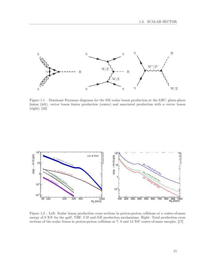
The Feynman diagrams of the three dominant production modes of the SM scalar bosonat the LHC are shown in Fig. 1.1, and their respective cross sections at a center-of-massenergy of 8 TeV as well as the total H boson production cross sections at center-of-massenergies of 7, 8 and 14 TeV are illustrated in Fig. 1.2.
14
1.3. SCALAR SECTOR
q
g
g
H
W/Z
W/Z
q
q
q
H
q
W∗/Z∗
q
q
W/Z
H
Figure 1.1 – Dominant Feynman diagrams for the SM scalar boson production at the LHC: gluon-gluonfusion (left), vector boson fusion production (center) and associated production with a vector boson(right). [16]
[GeV] HM80 100 200 300 400 1000
H+
X)
[pb]
→(p
p σ
-210
-110
1
10
210= 8 TeVs
LH
C H
IGG
S X
S W
G 2
012
H (NNLO+NNLL QCD + NLO EW)
→pp
qqH (NNLO QCD + NLO EW)
→pp
WH (NNLO QCD + NLO EW)
→pp
ZH (NNLO QCD +NLO EW)
→pp
ttH (NLO QCD)
→pp
Figure 1.2 – Left: Scalar boson production cross sections in proton-proton collisions at a center-of-massenergy of 8 TeV for the ggH, VBF, V H and ttH production mechanisms. Right: Total production crosssections of the scalar boson in proton-proton collisions at 7, 8 and 14 TeV center-of-mass energies. [17]
15

CHAPTER 1. THE STANDARD MODEL OF PARTICLE PHYSICS
[GeV]HM80 100 120 140 160 180 200
Hig
gs B
R +
Tot
al U
ncer
t
-410
-310
-210
-110
1
LHC
HIG
GS
XS W
G 2
013
bb
oo
µµ
cc
gg
aa aZ
WW
ZZ
Figure 1.3 – Branching fractions of the SM scalar boson for mH between 80 and 200 GeV. [17]
1.3.3 SM H decay modes
Assuming a mass for the scalar boson, it is possible to compute its partial decay widthto any combination of SM particles. The branching fraction is obtained by dividing thepartial decay width by the sum of the partial decay widths of all possible decay channels:
B(H → XX) =Γ(H → XX)∑
Y ∈SM Γ(H → Y Y ). (1.41)
The partial decay widths can be computed following the prescriptions in [6, 18], and areshown in Fig. 1.3 for scalar boson masses between 80 and 200 GeV.
Decay to fermions
In the SM, scalar couplings to fermions are directly proportional to fermion masses.The Born approximation gives the partial decay width of the scalar boson to fermionpairs. If mf is the fermion mass, and NC the color factor 5, it can be written as:
ΓBorn(H → ff) =GFNC
4√
2πmHm
2fβ
3f , (1.42)
where β is the velocity of the fermions in the final state and can be expressed as:
β =
√1−
4m2f
m2H
, (1.43)
5. Equal to one for leptons and to three for quarks.
16

1.3. SCALAR SECTOR
and GF is the Fermi coupling constant 6:
GF√2
=πg′
2m2W (1−m2
W/m2Z). (1.44)
As the partial decay width is proportional to the square of the fermion mass, the branch-ing fraction of the H boson to tau leptons is approximately a two hundred times largerthan its branching fraction to muons, while the branching fraction to electrons is negligible.
In the case of H boson decays to quarks, QCD corrections cannot be neglected. ForH boson masses much larger than the quark mass, the NLO decay width, includingFeynman diagrams with gluon exchange and the emission of a gluon in the final state,can be expressed as:
ΓNLO(H → qq) ' 3GF
4√
2πmHm
2q
[1 +
4
3
gsπ
(9
4+
3
2lnm2q
m2H
)]. (1.45)
Decay to bosons
For masses above the WW and ZZ kinematical thresholds, the H boson decays es-sentially to electroweak boson pairs. The partial decay widths to a pair of electroweakbosons V (W or Z boson) is given by:
Γ(H → V V ) =GFm
3H
16√
2πδV√
1− 4x(1− 4x+ 12x3), (1.46)
with x = m2V /m
2H , δW = 2 and δZ = 1.
However, below the WW and ZZ kinematical thresholds, the two-body decay as de-scribed above is forbidden. The scalar boson can still decay to a pair of electroweakgauge bosons, with one or two of them being off-shell (three-body and four-body decaysrespectively). For mH = 125 GeV, the three-body decay dominates, and its partial decaywidth can be expressed, assuming massless fermions f , as:
Γ(H → V V ∗) =3G2
Fm4V
16π3mHδ
′VRT (x), (1.47)
with δ′W = 1, δ′Z = 712− 10
9sin2 θW + 40
9sin4 θW , and
RT (x) =3(1− 8x+ 20x2)
(4x− 1)1/2arccos
(3x− 1
2x3/2
)− 1− x
2x(2−13x+47x2)− 3
2(1−6x+4x2) lnx.
(1.48)Even if massless particles do not couple to the H boson, H boson decays to gg, Zγ
and γγ are allowed through massive particle loops. The Hγγ and HZγ couplings aremediated by W boson and charged fermion loops, and the Hgg couplings by quark loops.
6. GF ' 1.17× 10⁻⁵ GeV−2. [9]
17

CHAPTER 1. THE STANDARD MODEL OF PARTICLE PHYSICS
1.3.4 The SM scalar boson at the LHC
The discovery by the CMS and ATLAS experiments of a new particle, H, compatiblewith the scalar boson of the SM was announced in July 2012 at CERN [19, 20]; thisconstituted a triumph for the theory but also for the thousands of experimentalists whohad designed and worked on the experiments at the LHC. With a mass of 125 GeV, a largevariety of decays are accessible experimentally and can be used to test the compatibilityof the new particle with the SM scalar hypothesis. The status of H boson studies afterthe first run of the LHC is detailed in Chapter 14.
1.4 Chapter summary
The standard model of particle physics
The SM successfully describes the elementary particles, and three of the four fun-damental interactions. The recently discovered particle is, given the measurementsperformed in the first run of the LHC, compatible with the scalar boson of the SM,and all the constituents of the SM have now been observed. With a measured massof approximately 125 GeV, this boson is supposed to decay to a rich variety of finalstates, which should be studied to assess the compatibility of the new particle withthe SM hypothesis.
18

Chapter 2
Physics beyond the standard model
The SM has been demonstrated as successful by many measurements performedat high-energy experiments. In particular, the discovery of a new particle com-patible with the SM scalar boson, considered as the cornerstone of the SM, hasconsecrated the theory. However there are strong indications that the SM is onlya low-energy expression of a more global theory. If new physics shows up be-yond the SM, it could be related to the scalar sector. Some motivations for theexistence of BSM physics are detailed in Section 2.1, while two-Higgs-doubletmodels, supersymmetry including the minimal supersymmetric extension of theSM, and two-Higgs-doublet models extended with a scalar singlet, are presentedin Sections 2.2, 2.3 and 2.4 respectively. Section 2.5 discusses how to uncovera possibly extended scalar sector at the LHC, while the chapter ends, in Sec-tion 2.6, with a comparison between the reach of precision measurements anddirect discovery of new scalars, in a simple benchmark scenario.
2.1 Motivations for new physics
The existence of new physics beyond the SM [7,21] is strongly motivated. Some moti-vations are based on direct evidence from observation, such as the existence of neutrinomasses, the existence of dark matter and dark energy, or the matter-antimatter asymme-try, while others come from conceptual problems in the SM, such as the large number offree parameters, the "hierarchy problem" or the coupling unification. Each of these issuesis shortly described in the next sections.
2.1.1 Neutrino masses
It is well-established by experiments with solar, atmospheric, reactor and acceleratorneutrinos, that neutrinos can oscillate and change their flavor in flight [22, 23]. Suchoscillations are possible if neutrinos have masses. Flavor neutrinos (νe, νµ, ντ ) are thenlinear combinations of the fields of at least three mass eigenstate neutrinos ν1, ν2, ν3.Only upper limits on the neutrino masses have been set as of now (mν < 2 eV), but the
19

CHAPTER 2. PHYSICS BEYOND THE STANDARD MODEL
differences between the neutrino squared masses have been measured: ∆m212 = (7.53 ±
0.18)× 10−5 eV2 and ∆m232 = (2.44± 0.06)× 10−3 eV2 [9].
2.1.2 Dark matter and dark energy
In 1933, Zwicky carried measurements of the velocities of galaxies in the Coma cluster,using the Doppler shift of their spectra [24]. With the virial theorem, he could relatethese results to the total mass of the Coma cluster. Zwicky also measured the total lightoutput of the cluster, and compared the ratio of the luminosity to the mass for the Comacluster and for the nearby Kapteyn stellar system. The two orders of magnitude differencebetween both of them made him conclude that the Coma cluster contains some massivematter that does not radiate: dark matter. The ordinary matter that surrounds us andis described by the SM, only represents 5% of the mass/energy content of the universe.Astrophysical evidence indicates that dark matter contributes approximately to 27%, anddark energy to 68% of this content. Measurements of the temperature and polarizationanisotropies of the cosmic microwave background (CMB) by the Planck experiment coulddetermine a density of cold non-baryonic matter [25].Nowadays little is also known about dark energy, which is responsible for the acceleratedexpansion of the universe.
2.1.3 Asymmetry between matter and antimatter
It is believed that matter and antimatter were produced in exactly the same quantitiesat the time of the Big Bang. It is clear however that we are surrounded by matter,and a legitimate question is "How is it possible to explain this preponderance of matterover antimatter?". It is very unlikely that our matter-dominated corner of the universeis balanced by another corner of the universe dominated by antimatter, as this wouldhave been seen as perturbations in the CMB. Sakharov, in 1967, identified the threemechanisms necessary to obtain a global matter/antimatter asymmetry [26]:
— Baryon and lepton number violation;— Interactions in the universe out of thermal equilibrium at a given moment of the
universe history;— C- and CP-violation (the rate of a process i → f can be different from the CP-
conjugate process i→ f).The SM includes sources of CP-violation, through the residual phase in the CKM matrix,but they are in no way sufficient to explain the magnitude of the matter-antimatterasymmetry observed.
2.1.4 Free parameters in the SM
The SM contains no less than nineteen free parameters, which can be taken as:— 9 fermion masses (me, mµ, mτ , mu, md, mc, ms, mt, mb);— 3 CKM 1 mixing angles and 1 CP-violating phase;
1. The Cabibbo-Kobayashi-Maskawa (CKM) matrix contains information about the likelihood of weak decays with flavorchanging in charged currents.
20

2.1. MOTIVATIONS FOR NEW PHYSICS
— 1 electromagnetic coupling constant (g′);— 1 weak coupling constant (g);— 1 strong coupling constant (gS);— 1 QCD vacuum angle;— 1 vacuum expectation value (v);— 1 mass for the scalar boson (mH).
This large number of free parameters, especially in the scalar sector, could be an indicationfor the existence of a more general and elegant theory than the SM.
2.1.5 Hierarchy problem
The so-called gauge hierarchy problem [27] is related to the huge energy differencebetween the weak scale and the Planck scale. The weak scale is given by the vev of theBrout-Englert-Higgs field, which is equal to approximately 246 GeV. Radiative correctionsto the scalar boson squared mass, coming from its couplings to fermions and gauge bosons,and from its self-couplings, are quadratically proportional to the ultraviolet momentumcutoff ΛUV , which is at least equal to the energy to which the SM is valid without anyaddition of new physics. If one considers that the SM is valid up to the Planck massMP , the quantum correction to m2
H is about thirty orders of magnitude larger than m2H ,
which implies that some extraordinary cancellation of terms should happen. Even if thesecorrections are absorbed in the renormalization process, some may find uncomfortablewith this sensitivity to the details of high scales. This is also known as the naturalnessproblem of the H boson mass.
In particular, the correction to the squared mass of the scalar boson coming from afermion f that couples directly to the scalar field φ with a coupling λf is:
∆m2H = −|λf |
2
8π2Λ2UV . (2.1)
Similarly, some corrections to the mass of the SM scalar boson also arise from scalars. Inthe case of a scalar particle S with a massmS and that couples to the Brout-Englert-Higgsfield with a Lagrangian term −λS|φ|2|S|2, the correction to the squared scalar boson massis:
∆m2H =
λS16π2
[Λ2UV − 2m2
S ln(ΛUV /mS) + ...]. (2.2)
Again, the correction term to the squared mass is much larger than the squared massitself. BSM models that avoid this fine-tuning introduce new scalar particles at the TeVscale that couple to the scalar boson, in such a way as to cancel the Λ2
UV divergence.
Additionally, the large mass differences between fermions, related to Yukawa couplingsthat can differ by up to six orders of magnitude in the case of the electron and the topquark, constitute the fermion mass hierarchy problem.
21

CHAPTER 2. PHYSICS BEYOND THE STANDARD MODEL
2.1.6 Coupling unification
One of the fundamental questions raised by the SM concerns the particular choice ofthe SU(3) × SU(2) × U(1) symmetry group. Additionally, the three forces included inthe SM, the weak, the electromagnetic and the strong forces, are treated separately. Theintensity of the forces shows an apparent large disparity around the electroweak scale,but at higher energies their coupling constants tend to have comparable strengths. Theelectromagnetic and weak forces can be unified in a so-called electroweak interaction, butin the SM, the strong coupling constant does not meet the two other coupling constantsat high energies. The running of the coupling constants can be modified by the additionof new particles, such as to reach a grand unification.
2.2 Two-Higgs-doublet models
Two-Higgs-doublet models (2HDM) [28] are simple extensions of the SM. They intro-duce two doublets of scalar fields, which, after symmetry breaking lead to five physicalstates: two charged scalars H±, one CP-odd pseudoscalar A and two neutral scalars hand H. Similarly to all models that have extra scalar singlets or doublets relative to theSM, 2HDM satisfy the condition ρ = mW/(mZ cos θW ) = 1. 2HDM include the minimalsupersymmetric extension of the SM (MSSM), which addresses the hierarchy problemand the coupling unification (see Section 2.3). Moreover 2HDM allow for the existence ofadditional CP-violation sources with respect to the SM, which could explain the baryonasymmetry in the universe. Finally, 2HDM are a simple extension of the SM in the scalarsector, and there is no strong motivation against adding an additional scalar doublet tothe SM.
2.2.1 Formalism
The most general gauge invariant form of the scalar potential V in 2HDM can bewritten as [6, 28]:
V = m211φ†1φ1 +m2
22φ†2φ2 −m2
12
(φ†1φ2 + φ†2φ1
)+λ1
2
(φ†1φ1
)2
+λ2
2
(φ†2φ2
)2
+ λ3φ†1φ1φ
†2φ2 + λ4φ
†1φ2φ
†2φ1
+
{λ5
2
(φ†1φ2
)2
+[λ6
(φ†1φ1
)+ λ7
(φ†2φ2
)]φ†1φ2 + h.c.
}.
(2.3)
Under the widely-used assumptions that CP is conserved in the scalar sector and not spon-taneously broken, and that all quartic terms odd in either of the doublets are eliminatedby discrete symmetries, the expression can be simplified as:
V = m211φ†1φ1 +m2
22φ†2φ2 −m2
12
(φ†1φ2 + φ†2φ1
)+λ1
2
(φ†1φ1
)2
+λ2
2
(φ†2φ2
)2
+λ3φ†1φ1φ
†2φ2 + λ4φ
†1φ2φ
†2φ1 +
λ5
2
[(φ†1φ2
)2
+(φ†2φ1
)2],
(2.4)
22

2.2. TWO-HIGGS-DOUBLET MODELS
Figure 2.1 – Schematic view of the two angle parameters of 2HDM. The parameter tanβ is the ratiobetween the vacuum expectation values of the two doublets φ1 and φ2, whereas α is the mixing anglebetween the neutral scalars. The vacuum expectation value v = 246 GeV can be decomposed in twocomponents v1 and v2 along the doublets φ1 and φ2 respectively. Adapted from [30].
where all the parameters are real.
The minima of the φ1 and φ2 doublets are respectively(
0
v1/√
2
)and
(0
v2/√
2
). The
ratio of the vacuum expectation values of the two doublets is written as:
tan β =v2
v1
. (2.5)
The squared mass matrix of the neutral scalars can be diagonalized to obtain the physicalstates h and H; the rotation angle performing the diagonalization is called α. The angleβ defined in equation (2.5) can also be seen as the angle diagonalizing the squared massmatrices of the charged scalars and of the pseudoscalars (one massive pseudoscalar A andone massless Goldstone boson). Without loss of generality, β can be chosen in the firstquadrant, whereas α is either in the first or in the fourth quadrant [29]. The meaning ofthe angles α and β is illustrated in Fig. 2.1.
The scalar couplings to gauge bosons and fermions in 2HDM can be expressed as afunction of the two parameters α and tan β. There are four types of 2DHM that donot violate flavor conservation in neutral current interactions; the condition for avoidingflavor changing neutral currents being that all fermions with the same quantum numberscouple to a same scalar multiplet [31]. A Z2 symmetry (φ1 → +φ1, φ2 → −φ2) can befound to ensure that only these interactions exist. The Z2 symmetry is softly broken ifthe term m2
12 is non-zero [32]. As shown in Tab. 2.1, the difference between the four typeslies in the doublets to which the charged leptons, up-type quarks and down-type quarkscouple. Type-1 is the easiest of them and is the most SM-like: leptons, up-type quarksand down-type quarks all couple to the same doublet, φ1. In type-2, the leptons and
23

CHAPTER 2. PHYSICS BEYOND THE STANDARD MODEL
down-type quarks couple to φ2, whereas up-type quarks couple to φ1. In the so-called"lepton-specific" type-3, all quarks couple to φ1 and leptons to φ2. Finally in the flippedtype-4 model, leptons and up-type quarks couple to φ1 while down-type quarks couple toφ2. In a general way, the intensity of the couplings in the different scenarios are functionsof both α and β as presented in Tab. 2.2.
Type-1 Type-2 Type-3 (lepton specific) Type-4 (flipped)` φ2 φ1 φ1 φ2
u φ2 φ2 φ2 φ2
d φ2 φ1 φ2 φ1
Table 2.1 – Scalar doublet to which the leptons `, up-type quarks u and down-type quarks d couple inthe different types of 2HDM.
Particle Coupling Type-1 Type-2 Type-3 (lepton specific) Type-4 (flipped)h ghV V sin(β − α) sin(β − α) sin(β − α) sin(β − α)
ghuu cosα/sinβ cosα/sinβ cosα/sinβ cosα/sinβghdd cosα/sinβ -sinα/cosβ cosα/sinβ -sinα/cosβgh`¯ cosα/sinβ -sinα/cosβ -sinα/cosβ cosα/sinβ
H gHV V cos(β − α) cos(β − α) cos(β − α) cos(β − α)gHuu sinα/sinβ sinα/sinβ sinα/sinβ sinα/sinβgHdd sinα/sinβ cosα/cosβ sinα/sinβ cosα/cosβgH`¯ sinα/sinβ cosα/cosβ cosα/cosβ sinα/sinβ
A gAV V 0 0 0 0gAuu cotβ cotβ cotβ cotβgAdd -cotβ tanβ -cotβ tanβgA`¯ -cotβ tanβ tanβ -cotβ
Table 2.2 – Yukawa couplings of vector bosons V , up-type quarks u, down-type quarks d and leptons ` tothe neutral scalars and pseudoscalar in the four types of 2HDM without flavor changing neutral currents.The Yukawa couplings to the charged scalars can be determined from the couplings of to the neutralpseudoscalar. [28]
2.2.2 Decoupling and alignment limits
In the SM, there is one neutral scalar boson, while there are two (h and H) in 2HDM.The lightest neutral scalar of 2HDM is in all generality not identical to the one of the SM,which points to the possibility of determining with property measurements whether thenew observed particle belongs to the SM or to 2HDM. As of now, the measured propertiesof the 125 GeV-state are all compatible with the SM hypothesis within experimentaluncertainties. However the 2HDM hypothesis is not ruled out, as there are two importantscenarios where the neutral h of 2HDM tends to be SM-like: the decoupling and thealignment limits [33, 34]:
24
2.3. SUPERSYMMETRY
— In the decoupling limit, the mass of the H, A and H± all are much larger than theh mass, which causes h to have SM-like couplings. Indeed, if there are two verydifferent mass scales mL � mS such that mh ' mL and mH ,mH± ,mA ' mS, a lowmass effective theory can be derived and corresponds to the SM because the mS-related effects have been integrated out. The decoupling limit implies cos(β−α) ' 0.
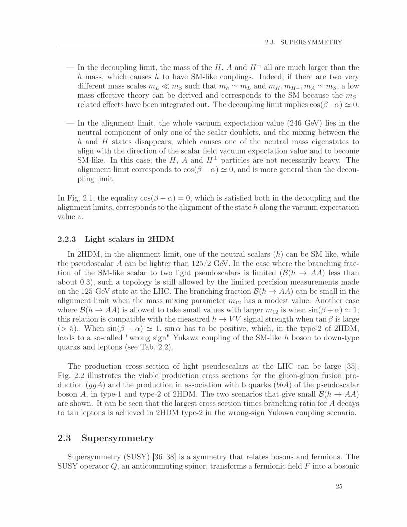
— In the alignment limit, the whole vacuum expectation value (246 GeV) lies in theneutral component of only one of the scalar doublets, and the mixing between theh and H states disappears, which causes one of the neutral mass eigenstates toalign with the direction of the scalar field vacuum expectation value and to becomeSM-like. In this case, the H, A and H± particles are not necessarily heavy. Thealignment limit corresponds to cos(β−α) ' 0, and is more general than the decou-pling limit.
In Fig. 2.1, the equality cos(β −α) = 0, which is satisfied both in the decoupling and thealignment limits, corresponds to the alignment of the state h along the vacuum expectationvalue v.
2.2.3 Light scalars in 2HDM
In 2HDM, in the alignment limit, one of the neutral scalars (h) can be SM-like, whilethe pseudoscalar A can be lighter than 125/2 GeV. In the case where the branching frac-tion of the SM-like scalar to two light pseudoscalars is limited (B(h → AA) less thanabout 0.3), such a topology is still allowed by the limited precision measurements madeon the 125-GeV state at the LHC. The branching fraction B(h→ AA) can be small in thealignment limit when the mass mixing parameter m12 has a modest value. Another casewhere B(h→ AA) is allowed to take small values with larger m12 is when sin(β+α) ' 1;this relation is compatible with the measured h→ V V signal strength when tan β is large(> 5). When sin(β + α) ' 1, sinα has to be positive, which, in the type-2 of 2HDM,leads to a so-called "wrong sign" Yukawa coupling of the SM-like h boson to down-typequarks and leptons (see Tab. 2.2).
The production cross section of light pseudoscalars at the LHC can be large [35].Fig. 2.2 illustrates the viable production cross sections for the gluon-gluon fusion pro-duction (ggA) and the production in association with b quarks (bbA) of the pseudoscalarboson A, in type-1 and type-2 of 2HDM. The two scenarios that give small B(h → AA)are shown. It can be seen that the largest cross section times branching ratio for A decaysto tau leptons is achieved in 2HDM type-2 in the wrong-sign Yukawa coupling scenario.
2.3 Supersymmetry
Supersymmetry (SUSY) [36–38] is a symmetry that relates bosons and fermions. TheSUSY operator Q, an anticommuting spinor, transforms a fermionic field F into a bosonic
25

CHAPTER 2. PHYSICS BEYOND THE STANDARD MODEL
Figure 2.2 – Viable production cross sections for the ggA (top) and bbA (bottom) productions at a center-of-mass energy of 8 TeV, times the branching fraction for A decay to a pair of tau leptons in type-1 (left)and type-2 (right) 2HDM. The cyan points have sin(β−α) ' 1, cos(β−α) > 0 and modest m12, whereasorange points have sin(β + α) ' 1 and tanβ > 5, and correspond to the wrong-sign Yukawa couplingscenario. The largest production cross sections times branching fraction are obtained in 2HDM type-2with wrong-sign Yukawa couplings. [35]
26

2.3. SUPERSYMMETRY
Figure 2.3 – Evolution of the U(1)Y , SU(2)L and SU(3)C couplings in the SM (dashed lines), and in twoMSSM scenarios (solid lines). Unlike the SM case, the three couplings can be unified at a high energyscale in the MSSM. [36]
field B and vice-versa:Q|B〉 = F and Q|F 〉 = B. (2.6)
A new quantum number R can be introduced to enforce baryon number and leptonnumber conservation:
R = (−1)2S+3(B−L), (2.7)
where S, B and L are respectively the spin, lepton and baryon numbers. With this def-inition, all SM particles have R = +1 and all their superpartners have R = −1. R isusually assumed to be conserved in such a way as to forbid fast rates of proton decays.The R-parity conservation implies that supersymmetric particles can only be producedin pairs and that the lightest supersymmetric particle (LSP) is stable. This LSP is anexcellent dark matter candidate.
One of the main motivations for the existence of SUSY is the solution to the hierarchyproblem. Because fermion loops and boson loops have opposite signs, and SUSY asso-ciates a new boson to each fermion and vice-versa, the Λ2
UV terms in equations (2.1) and(2.2) can exactly cancel for each fermion-scalar pair. Additionally, SUSY can unify theelectromagnetic, weak and strong forces below the Planck scale, as illustrated in the caseof the minimal supersymmetric extension of the SM (see Section 2.3.1) in Fig. 2.3.
Individual particles are grouped in supermultiplets. As the supersymmetric operatorsQ and Q† commute with the generators of gauge transformations, particles sharing asame supermultiplet have the same electric charge, weak isospin and color degrees offreedom. In addition, because the same operators also commute with the squared-massoperator −P 2, the fermions and bosons in a same supermultiplet should have the same
27

CHAPTER 2. PHYSICS BEYOND THE STANDARD MODEL
mass. The last point is however known not to be true in reality, because superpartners atthe electroweak scale would already have been observed at colliders. If superparticles areheavier than SM particles, which would explain why they have not been discovered yet,SUSY must be broken. For radiative corrections not to exceed typical scalar masses, theSUSY breaking scale should be limited to a few TeV.
2.3.1 Minimal supersymmetric extension of the SM (MSSM)
In the minimal supersymmetric extension of the SM (MSSM) [39–41], there exist twotypes of supermultiplets: vector supermultiplets, where a spin-1 vector boson is associ-ated to a spin-1/2 Weyl fermion, and chiral supermultiplets, where a single Weyl fermionis associated to a complex scalar field. The particle content of the MSSM is shown inTab. 2.3 and 2.4. The superpartners of quarks are called squarks, while the superpart-ners of leptons are called sleptons. The bino, the neutral wino and the higgsinos mix toform four neutralinos (χ0
1, χ02, χ0
3 and χ04), while the winos and charged higgsinos mix to
form four charginos (χ±1 and χ±2 ). Two chiral superfields, (H+1 , H
01 ) and (H0
2 , H−2 ), with
hypercharges +1/2 and -1/2 as seen in Tab. 2.3, are necessary to cancel chiral anomalies.
Particles Spin-0 Spin-1/2 (SU(3)C , SU(2)L, U(1)Y )
quark, squark (uiL, diL) (uiL, diL) (3,2,+1/6)
u∗iR u†iR (3*,1,-2/3)
d∗iR d†iR (3*,1,+1/3)
lepton, slepton (eiL, νiL) (eiL, νiL) (1,2,-1/2)
e∗iR e†iR (1,1,+1)
H, higgsino (H+1 , H
01 ) (H+
1 , H−1 ) (1,2,+1/2)
(H02 , H
−2 ) (H0
2 , H−2 ) (1,2,-1/2)
Table 2.3 – MSSM chiral supermultiplets.
Particles Spin-1/2 Spin-1 (SU(3)C , SU(2)L, U(1)Y )
gluino, gluon g g (8,1,0)
wino, W boson W±, W 0 W±,W 0 (1,3,0)
bino, B boson B0 B0 (1,1,0)
Table 2.4 – MSSM vector supermultiplets.
The MSSM is a particular case of 2HDM type-2. The main specificities in the scalarsector are that, in the MSSM, the mass of the lightest scalar is constrained by some upperbounds, the scalar self-couplings are specified, α and β are not independent from eachother, and the decay of the charged scalars H± to a pseudoscalar A and a W boson is
28

2.3. SUPERSYMMETRY
h,H,At, t
g
g
b, b
h,H,A
b
g
g
b
h,H,A
b
b
Figure 2.4 – Feynman diagrams for the production of neutral scalars in the MSSM, in gluon-gluon fusion(left), and production with b quarks (center and right). [42]
kinematically forbidden because mH± ' mA [28].
2.3.2 Scalar sector in the MSSM
In the MSSM, neutral scalars Φ = H/A/h can be produced by two mechanisms: gluon-gluon fusion (ggΦ) and production with b quarks (bbΦ). Characteristic Feynman diagramsfor such processes are shown in Fig 2.4, where the bbΦ mechanism is shown in two differ-ent schemes of proton parton distribution functions. The bbΦ production cross section isincreased at large tan β because of the enhanced Yukawa couplings to down-type fermions.
At tree level in the MSSM, the only two free parameters can be taken as the mass ofthe pseudoscalar, mA, and tan β. The masses of the neutral scalars and of the chargedscalars, as well as the angle α can be expressed as [43]:
m2h/H =
1
2
(m2A +m2
Z ∓√
(m2A +m2
Z)2 − 4m2Am
2Z cos2 2β
), (2.8)
m2H± = m2
A +m2W , and (2.9)
tan 2α = tan 2β
(m2A +m2
Z
m2A −m2
Z
)with − π
2≤ α ≤ 0. (2.10)
This leads to:mh ≤ min(mA,mZ)× | cos 2β| ≤ mZ . (2.11)
The mass of the lightest neutral scalar is thus inferior to the Z boson mass, which isexcluded by LEP bounds and does not correspond to the observation of the 125-GeV scalarat the LHC. Fortunately, radiative corrections above tree level, essentially loop correctionsdue to top and stop quarks, enable the h scalar to be as heavy as approximately 135 GeV.In the case where mA is much larger than the Z boson mass, the relations above give:
mH ' mH± ' mA and α ' β − π
2, (2.12)
which is the decoupling limit as seen in Section 2.2.2.
29

CHAPTER 2. PHYSICS BEYOND THE STANDARD MODEL
The phenomenology of the scalar sector of the MSSM can be described by two param-eters: the mass of the pseudoscalar mA, and tan β. It is generally assumed that tan β liesapproximately between 1 and 60, where 60 is the ratio between the top quark mass andthe bottom quark mass. Above tree level, more parameters appear and some benchmarkscenarios fixing these parameters can be studied. It has been shown however that, tak-ing into account the mass measured for the h boson, the MSSM can be approximatelyreparameterized as a function of mA and tan β, in the so-called hMSSM [44]. One candistinguish three regions of the parameter space, where the search strategies will differ:the low mA, the high tan β and the low tan β regions. It has been shown in [44] thatthe full parameter space of the MSSM could be almost entirely covered in the search foradditional scalars at the LHC at 14 TeV with a luminosity of 300 fb−1, while a good partof the parameter space has already been explored in LHC searches at 7 and 8 TeV, asshown in Fig. 2.5.
Figure 2.5 – Sensitivity of MSSM scalar searches at the LHC at 7 and 8 TeV in LHC Run-1 (left) andprojection with 300 fb−1 of 14 TeV data collected at the LHC (right), in the context of the hMSSMparameterization. The A → tt search (dashed red line) has not yet been performed at the LHC, andthe sensitivity is predicted. The exclusion limit of the A → ττ analysis around mA = 350 GeV and2 < tanβ < 4 is due to the strong increase of the gg → A cross section at the tt threshold, coupled tothe suppression of A → Zh decays and enhanced couplings to down-type quarks and leptons becausetanβ > 1. The hMSSM scenario takes into account the mass measured for the new SM-like scalar. [44]
Low mA region
At low mA, the most powerful channel to search for an MSSM scalar sector is clearlyH+ → τ+ντ (and its charge conjugate decay). The limits shown in Fig. 2.5 correspond tothe t→ H+b production, for charged scalar masses below the difference of the top quarkand bottom quark masses.
High tanβ region
In the region of the parameter space where tan β is large, say tan β > 5, the mostsensitive final state to search for new heavy resonances Φ is by far Φ = A/H/h → ττ .The reason for this is that the couplings to leptons and down-type quarks are enhanced
30

2.3. SUPERSYMMETRY
with increased tan β, because these particles couple to the second scalar doublet (seeTab. 2.1). In addition, for the same reason, the production cross section for the Φ res-onance in association with bottom quarks is also enhanced at large tan β. Even if thedecay branching fraction of the resonance to bottom quarks remains larger (approxi-mately nine times higher), the experimental difficulties, such as the distinction betweenb jets and other flavor jets, make the channel Φ → bb less sensitive. Finally, the chan-nel Φ → µµ also has some potential, but is hurt by its low decay branching fraction:B(Φ→ µµ) ' B(Φ→ ττ)×m2
µ/m2τ .
Low tanβ region
The phenomenology in the low tan β region is much richer than in the high tan βregion. Experimentally, one interesting decay of the A pseudoscalar to study is A→ Zh,in the intermediate mass range mZ +mh < mA < 2mt, as seen in Fig. 2.6. If the Z bosondecays leptonically, it is possible to achieve a good background reduction, and the mostfavorable h decays in terms of branching fractions, h→ bb and h→ ττ , can be targeted.At higher mA, the A → tt channel opens, but, due to interference effects with the SMbackgrounds, it is experimentally a difficult channel. The dominant H decay channel inthe intermediate mass range 2mh < mH < 2mt is H → hh, whereas there are also nonnegligible contributions from H → WW and H → ZZ. Outside of the low mA regiondescribed previously, formH± > mt+mb, the charged scalars H± almost exclusively decayto a top and a b quarks.
Figure 2.6 – Branching fractions of the A, H and H± scalars in the MSSM as a function of their masses,for tanβ = 2.5 and mh = 126 GeV. [45]
31
CHAPTER 2. PHYSICS BEYOND THE STANDARD MODEL
2.4 Two-Higgs-doublet models + a singlet
2.4.1 Introduction to 2HDM+S
The extensions of 2HDM where a complex scalar singlet is added to the already presentscalar doublets, are called 2HDM+S. Because of the additional singlet, two new bosons areintroduced. The next–to-minimal supersymmetric extension of the SM (NMSSM) [46,47](for a review, see [48]) is a case of 2HDM+S type-2 and is the easiest extension of theMSSM. The supersymmetric potential in the MSSM contains a mass parameter µ in theexpression µφ1φ2, which has to be at the SUSY breaking scale (mSUSY ). The fact thatµ is at a scale well below the Planck scale without any theoretical reason, constitutesthe so-called µ problem [49]. This problem disappears in the NMSSM, where an effectivemass is generated via a coupling to the complex scalar field associated to the new singlet;this is a strong motivation for the existence of the NMSSM over the MSSM. Anothermotivation comes from the fact that new scalar particles contribute to the mass of thescalar boson h in the NMSSM, which removes the tensions in the MSSM originating fromthe large measured mass of the new particle.
2.4.2 Exotic decays of the 125-GeV particle
In 2HDM+S, the h boson, identified as the 125-GeV particle discovered in 2012, candecay exotically to non-SM particles. Even though decays of the h boson of 2HDM to non-SM particles are theoretically allowed, the 2HDM parameter space is by now extremelyconstrained by LHC searches. However, in 2HDM+S, a wide range of exotic decays of the125-GeV boson is still allowed after the Run-1 of the LHC. The singlet added to 2HDMdoes not have Yukawa couplings of its own, and only couples to φ1 and φ2 in the potential,from which it inherits its couplings to SM fermions. To keep the scalar h SM-like, themixing with the singlet S needs to be small. The imaginary part of the singlet gives riseto a pseudoscalar a (after a small mixing with the pseudoscalar A), and the real part toa scalar s (after mixing with H and h). Exotic decays of the type h → aa, h → ss orh→ Za are then possible.
In the pseudoscalar case, the light pseudoscalar a, mostly singlet-like, inherits its cou-plings to fermions from the heavy pseudoscalar A. As in the case of general 2HDM,the four types of 2HDM+S lead to different scenarios and give rise to many exploitablesignatures for exotic h decays at the LHC:
— Type-1: All fermions couple to φ1, and therefore the branching fractions of thepseudoscalar are proportional to those in the SM, without any dependence on tan β.
— Type-2: Leptons and down-type quarks couple to the same doublet, as in the MSSM.For values of tan β larger than unity, the branching fractions of the pseudoscalarto leptons and down-type quarks are enhanced, which makes h → aa → bbbb,h → aa → µµbb and h → aa → ττbb interesting channels to search for exotic hdecays.
— Type-3 (lepton-specific): Leptons couple to the φ2 doublet contrarily to quarks,which means that the branching fractions for pseudoscalar decays to leptons increase
32
2.5. SEARCH FOR BSM PHYSICS IN THE SCALAR SECTOR
for large values of tan β. In this scenario with large tan β, h → aa → µµττ andh→ aa→ ττττ are favoured channels when kinematically allowed.
— Type-4 (flipped): Pseudoscalar decays to leptons and up-type quarks are enhancedwith respect to down-type quarks when tan β > 1. In this case, h → aa → ττccand h→ aa→ ττbb can be interesting channels.
2.5 Search for BSM physics in the scalar sector
The scalar sector is a favored place to look for new physics, because it is describedmuch less elegantly than the other parts of the SM as most free parameters of the theoryare related to the scalar interaction. The existence of a Higgs-portal [50], where the scalarsector is the only one to interact with BSM physics, is strongly motivated. Complementaryways exist to point to the existence of BSM physics in the scalar sector:
1. Precision measurements of the properties of the 125-GeV scalar boson, that wouldreveal deviations from the SM;
2. Direct discovery of new scalar particles;3. Discovery of BSM decays of the 125-GeV scalar boson;4. Observation of BSM physics in signatures involving scalar bosons.
A review about the complementarity between precision measurements and direct searchesin the MSSM can be found in [51]. The four points are detailed below:
— Precision measurements: The properties of the lightest scalar h of 2HDM candeviate from the properties of the SM scalar boson; precision measurements of the125-GeV state therefore should make the distinction between 2HDM and SM pos-sible. However, as seen in Section 2.2.2, many extended sector scalar models havea decoupling or an alignment limit, which makes the properties of the h boson of2HDM very close to those of the SM scalar boson. Fig. 2.7 illustrates the depen-dence of the production cross section of the MSSM h boson as a function of themass of the pseudoscalar A for a given tan β, as well as the ratio between the decaybranching fractions of the MSSM h and the SM scalar boson. As expected accord-ing to the decoupling limit, the branching fractions tend to be very similar in thetwo scenarios when the mass of the pseudoscalar increases, and a great precision isneeded to highlight deviation from the SM. The measurement of the properties ofthe discovered 125 GeV-boson in the decay channel to tau leptons is presented inChapter 7.
— Direct discovery of new scalar particles: Discovering new scalar particles wouldbe a direct evidence of BSM physics. Many searches for extra scalars, in the contextof general 2HDM or MSSM for example, are performed at the LHC. The search fora heavy neutral scalar decaying to a pair of tau-leptons is described in Chapter 13,while the search for the heavy pseudoscalar A of the MSSM, decaying to a Z and a
33

CHAPTER 2. PHYSICS BEYOND THE STANDARD MODEL
Figure 2.7 – Left: Production cross sections of the MSSM h boson at 8 TeV, for tanβ = 2.5. Right:Evolution of the decay branching ratios of the h scalars in the MSSM and SM as a function of thepseudoscalar mass mA, for tanβ = 2.5. [45]
SM-like h bosons is described in Chapter 10. Light bosons with a mass lighter thanthe Z boson could also be discovered at the LHC; Chapter 12 details the search forsuch a particle in its decays to tau leptons. Many other searches exist at the LHCbut are not described in this thesis, such as the search for charged scalars.
— Discovery of BSM decays of the 125-GeV scalar boson: Motivations forthe existence of exotic decays of the 125-GeV boson to non-SM particles are vari-ous [52, 53]. First, the SM scalar boson has an extremely narrow width (Γ ' 4.07MeV) compared to its mass, because of the suppression of tree-level Yukawa cou-plings. Given that the coupling to two b quarks has the small value of approximately0.02, the coupling, even small, to another light state could open non negligible decaymodes. Second, the scalar sector could be a portal to new physics, which allowsSM matter to interact with a hidden-sector matter. If there exists a Higgs portal,the hidden-sector matter does not have to be charged under SM forces. And finally,exotic scalar decays are a relatively simple extension of the SM, and are still allowedafter all the measurements made during LHC Run-1. Indeed an upper limit on thebranching fraction of the 125-GeV boson to BSM particles can be set experimen-tally and, as of today, this upper limit leaves a large room for exotic decays. Inparticular, CMS measured B(H → BSM) < 30% at 95% CL, using all data collectedduring LHC Run-1 [54]. Projections for future LHC runs give a final precision onB(H → BSM) of the order of 10%, which still allows for non negligible decays ofthe 125-GeV particle. The variety of possible BSM decays is extremely large. Agroup of searches among others explores the possibility for the h boson to decay toinvisible particles, resulting in missing transverse energy in the detector. A searchfor exotic decays with SM particles in the final state is presented in Chapter 11.
34
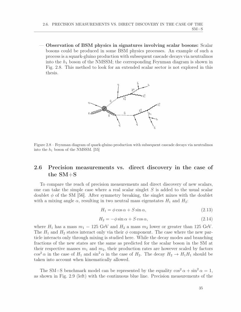
2.6. PRECISION MEASUREMENTS VS. DIRECT DISCOVERY IN THE CASE OF THESM+S
— Observation of BSM physics in signatures involving scalar bosons: Scalarbosons could be produced in some BSM physics processes. An example of such aprocess is a squark-gluino production with subsequent cascade decays via neutralinosinto the h1 boson of the NMSSM; the corresponding Feynman diagram is shown inFig. 2.8. This method to look for an extended scalar sector is not explored in thisthesis.
g
q
h1
χ02
q
Z0
χ02g
q
b
b
χ01
b b
χ01
q
q q
Figure 2.8 – Feynman diagram of quark-gluino production with subsequent cascade decays via neutralinosinto the h1 boson of the NMSSM. [55]
2.6 Precision measurements vs. direct discovery in the case ofthe SM+S
To compare the reach of precision measurements and direct discovery of new scalars,one can take the simple case where a real scalar singlet S is added to the usual scalardoublet φ of the SM [56]. After symmetry breaking, the singlet mixes with the doubletwith a mixing angle α, resulting in two neutral mass eigenstates H1 and H2:
H1 = φ cosα + S sinα, (2.13)
H2 = −φ sinα + S cosα, (2.14)
where H1 has a mass m1 = 125 GeV and H2 a mass m2 lower or greater than 125 GeV.The H1 and H2 states interact only via their φ component. The case where the new par-ticle interacts only through mixing is studied here. While the decay modes and branchingfractions of the new states are the same as predicted for the scalar boson in the SM attheir respective masses m1 and m2, their production rates are however scaled by factorscos2 α in the case of H1 and sin2 α in the case of H2. The decay H2 → H1H1 should betaken into account when kinematically allowed.
The SM+S benchmark model can be represented by the equality cos2 α + sin2 α = 1,as shown in Fig. 2.9 (left) with the continuous blue line. Precision measurements of the
35

CHAPTER 2. PHYSICS BEYOND THE STANDARD MODEL
signal strength of the 125-GeV state give some constraints on the parameter cos2 α, whichscales the H1 production cross section; the measured signal strength, when lower thanone, is equivalent to the measured cos2 α. The best-fit signal strength was measured tobe µ = 0.80 ± 0.14 (where the uncertainties correspond to one standard deviation) in2013 [57]; this value is represented together with its uncertainty by the horizontal pinklines in Fig. 2.9 (left). In a first approximation, the uncertainty band can be doubled tocorrespond to uncertainties at the level of two standard deviations. On the other hand,searches for extra scalars with masses different from 125 GeV can set constraints on sin2 α;the upper limit on the signal strength at a given mass, if lower than one, is equivalent toan upper limit on sin2 α at that same mass. Limits from searches for additional scalarswith masses between 100 and 800 GeV [57–60] are shown in Fig. 2.9 (left) with the verticaldashed lines. This makes it possible to compare the reach of the two approaches, usingthe CMS data collected during Run-1 and presented at the HCP12 conference. It can beseen in the figure that in this particular benchmark model, in most part of the accessiblemass range, namely between 125 and 600 GeV, the direct detection is a more powerfulapproach than precision measurements.
The limit on cos2 α obtained by the precision measurements on the signal strength ofthe 125-GeV state can be converted to a limit on sin2 α for all m2. In the right part ofFig. 2.9, the upper limits on sin2 α are superimposed to the constraint from the precisionmeasurement (uncertainty at two standard deviations level), for all masses m2 probed atthe LHC. Also superimposed is the limit set by tree level unitarity constraints in SM+S,which play a role at large m2.
36

2.6. PRECISION MEASUREMENTS VS. DIRECT DISCOVERY IN THE CASE OF THESM+S
α 2sin
0.0 0.2 0.4 0.6 0.8 1.0
α 2(1
25 G
eV) =
cos
µ
0.0
0.1
0.2
0.3
0.4
0.5
0.6
0.7
0.8
0.9
1.0Model
100 GeV
150 GeV
200 GeV
500 GeV
600 GeV
800 GeV
[TeV]2m0 1 2 3
α2si
n
0.0
0.1
0.2
0.3
0.4
0.5
0.6
0.7
0.8
0.9
1.0Direct search (CMS public data)
neglected) 1h1h→2
Direct search (h
Precision measurement
Singlet Model
Figure 2.9 – Left: Comparison of the reach of the precision measurement of the signal strength of the 125GeV state at 1σ and of the search for extra scalars at 2σ for different masses (100, 150, 200, 500, 600 and800 GeV). The blue line corresponds to the SM+S benchmark: cos2 α+ sin2 α = 1. Right: Comparisonsof the constraints on the parameter sin2 α set by direct searches for extra scalar states (blue curve if thedecay H2 → H1H1 is neglected, green curve otherwise), by indirect constraints on the measurement ofthe strength parameter of the 125 GeV state with a partial set of data collected by CMS during LHCRun-1, and by perturbative unitarity conditions, in the case of the SM+S model. Uncertainties are givenat 2σ level. [56]
37

CHAPTER 2. PHYSICS BEYOND THE STANDARD MODEL
2.7 Chapter summary and personal contributions
Physics beyond the standard model
The SM is known not to answer a series of fundamental questions, such as thehierarchy problem or the existence of dark matter. Many BSM models that addresssome of the SM issues predict the existence of more than one scalar particle. Thisis the case of the minimal supersymmetric extension of the SM (MSSM): it bringsa solution to the hierarchy problem and the coupling unification, proposes a darkmatter candidate, and introduces in total five scalar bosons. The MSSM is partof a more generic class of models, two-Higgs-doublet models (2HDM), which havefive scalar particles and give rise to a large variety of phenomenological signatures.Three complementary manners to uncover an eventually exotic scalar sector areexplored in this thesis:
— Precision measurements of the properties of the discovered boson, which mayhighlight deviations from the SM;
— Direct search for new scalar particles in specific models;— Search for exotic decays of the discovered boson.
Summary of notations
In the next chapters, the following notations are used for the (pseudo)scalar bosons:
— H: scalar boson of the SM, or heavy scalar of 2HDM (including MSSM) and2HDM+S.
— h: light scalar of 2HDM and 2HDM+S, generally considered to be the 125-GeV particle.
— A: pseudoscalar in 2HDM, with a mass lower or higher than 125 GeV.— Φ: scalar neutral resonance in the MSSM, equivalent to H, A or h.— a: lightest pseudoscalar in 2HDM+S.
My contributions
Figure: 2.9.
I have actively participated in the results presented in Section 2.6 and publishedin [56]. I have cross-checked the theory calculations, and made Fig. 2.9, whichcompares the reach of the direct searches and precision measurements in the caseof the SM+S model.
38

Chapter 3
Statistics
The physics searches presented in the next chapters heavily rely on statistical toolsand interpretation. In Section 3.1, the notion of likelihood is introduced, and theway to include systematic uncertainties is detailed. Maximum likelihood fits,described in Section 3.2, are used to find the values of the parameters that givethe best match between predicted processes and data. They can be used to extractthe value of a parameter of interest, such as the signal strength, or to check thevalidity of a model from the pulls of the nuisance parameters. To set upper limitson a signal process, the CLs method, in Section 3.3, uses ratios of likelihoods.In case an excess of events is observed on top of the predicted backgrounds, thesignificance of the excess can be calculated (Section 3.4) as the probability that abackground fluctuation can cause such a large deviation. Another tool to check thebackground modeling consists in goodness-of-fit tests (Section 3.5), which are akind of generalized chi-square test that measures the agreement between data andpredictions. The last two sections of the chapter concern multivariate analysismethods to classify events.
3.1 Likelihood
3.1.1 Basics
In a counting experiment, data events follow a Poisson law, which is a discrete prob-ability law describing the repartition of the number of events observed in a given timeinterval if their average rate, λ, is known and if they do not depend on each other. ThePoisson probability function of parameter λ is:
f(n) =e−λλn
n!. (3.1)
It can be shown that the best estimation of the parameter λ is the expected number ofevents in the time interval.
39

CHAPTER 3. STATISTICS
For a simple counting experiment, where n events are observed while b events areexpected, the likelihood, which quantifies the agreement between some expectation andthe observation, is simply:
L(n|b) =e−bbn
n!. (3.2)
If data are binned in a histogram, the N bins can be considered as independent of eachother and the likelihood is given by the product of the likelihoods of every bin of thedistribution:
L(~n|~b) =N∏i=1
e−bibniini!
, (3.3)
considering ~n as the vector of the observed data in the different bins, and ~b its equivalentfor expected processes. If, on the contrary, data are not binned in a histogram but aredescribed by a probability distribution function (pdf) fb(x) of some observable x, if kevents are observed and if b events are expected in the full x range, the likelihood isthen [61]:
L(~x|b, fb(x)) = k−1
k∏i=1
bfb(xi)e−b. (3.4)
3.1.2 Introducing systematic uncertainties
Systematic uncertainties are nuisance parameters that influence the model but are notof direct interest in the decision. In the analyses presented later, they come from threedifferent sources:
1. Theoretical uncertainties, such as cross section or parton distribution function un-certainties;
2. Statistical uncertainties, coming for example from the limited number of events inthe MC simulations or from the limited number of observed events in a controlregion used to estimate some background processes;
3. Experimental uncertainties, for example from luminosity or trigger efficiency mea-surements.
They can be embedded in the likelihood [61]. The nuisance parameters ~θ impact thenumber of expected events, which can therefore be expressed as b(~θ). Introducing theprobability density function p(θ|θ), where θ is the inferred default value of the nuisanceand reflects our degree of belief on what the real value of the parameter θ is, the likelihoodbecomes for L nuisance parameters in the case of a binned histogram:
L(~n|~b) =N∏i=1
e−bibni
ni!
L∏j=1
p(θj|θj). (3.5)
According to Bayes’ theorem, the Bayesian probability p(θ|θ) can be expressed as a func-tion of the frequentist probability ρ(θ|θ).
40

3.1. LIKELIHOOD
Most systematic uncertainties, corresponding to multiplicative factors on the signal orbackground yields, could be described by a Gaussian pdf of the type:
ρ(θ|θ) =1√2πσ
exp
(−(θ − θ)2
2σ2
), (3.6)
but this has the inconvenient side-effect to cause problems for positively defined observ-ables. Instead, log-normal pdfs of parameter κ, which have longer tails than Gaussiandistributions for comparable uncertainties, and go to zero at θ = 0, are preferred to avoidnegative values of these observables:
ρ(θ|θ) =1√
2π ln(κ)exp
(−(ln(θ/θ))2
2(lnκ)2
)1
θ. (3.7)
While, for small uncertainties, a Gaussian distribution with relative uncertainty ε isasymptotically identical to a log-normal distribution with parameter κ = 1 + ε, it clearlybehaves less appropriately for large uncertainties, as illustrated in Fig. 3.1 (left).
In the case of uncertainties coming from statistically limited numbers of events, gammadistributions are used. If the event rate n in the signal region is directly proportional to thesmall number N of events in the control region or in MC samples, with a proportionalityfactor α, the gamma distribution reads:
ρ(n) =1
α
(n/α)N
N !exp(−n/α). (3.8)
The log-normal and gamma distributions are illustrated in Fig. 3.1 for a given set of pa-rameters.
Additionally, shape uncertainties affect the distribution of the parameter of inter-est [62], and are modeled with a linear extrapolation method [63]. Practically, they areimplemented in CMS by providing two alternative shapes, corresponding to the variationby ± 1 standard deviation of the nuisance parameter. In the likelihood, a parameter θ isadded to interpolate smoothly between the alternative shapes with a "vertical templatemorphing" technique. If there are N shape nuisance parameters, modeled with the pa-rameters ~θ = (θ1, θ2, ..., θN), and if h0, h+
j and h−j correspond respectively to the nominalhistogram distribution, the histogram for a variation by +1 standard deviation of the jthnuisance parameter and the histogram for a variation by -1 standard deviation of the jthnuisance parameter, then the histogram distribution as a function of the shape nuisanceparameters ~θ is given by:
h(~θ) = h0 +N∑j=1
(a(θj)h
+j + b(θj)h0 + c(θj)h
−j
), (3.9)
41

CHAPTER 3. STATISTICS
Figure 3.1 – Log-normal (left) and gamma (right) distributions for different parameter values. Log-normaldistributions are positively defined; they are similar to Gaussian distributions for small uncertainties (e.g.κ = 1.10), but extend to higher tails for large uncertainties (e.g. κ = 1.50). [61]
with
a(θ) =
θ(θ + 1)/2 if |θ| ≤ 10 if θ < −1θ if θ > +1
, (3.10)
b(θ) =
{−θ2 if |θ| ≤ 1
−(|θ| − 1) if |θ| > 1, (3.11)
and
c(θ) =
θ(θ − 1)/2 if |θ| ≤ 10 if θ > +1|θ| if θ < −1
. (3.12)
It can be noticed that the effect of different shape uncertainties is additive.
A special kind of shape uncertainty is associated to the uncertainty on the numberof MC events or on the number of events from a control region used to estimate thebackground in every bin of the distribution. This has an impact on the shape of thedistribution, but the behavior of each bin is independent from the behavior of the othersfor a single process. Barlow and Beeston proposed a method to treat such cases [64]: aseparate nuisance parameter is introduced for every bin of every process, and multipliesthe number of expected events in this particular bin for this given process. A large numberof nuisance parameters is added to the likelihood model, but it is possible to prune someof them depending on their effects on the results. These uncertainties are later calledbin-by-bin (bbb) uncertainties.
42

3.2. MAXIMUM LIKELIHOOD FIT
3.2 Maximum likelihood fit
A maximum likelihood fit can be performed to find the parameters of interest thatprovide the best agreement between expectation and observation. Two common scenariosare possible:
— Background-only fit: the nuisance parameters, acting on the expected backgrounddistribution ~b, are varied to the values ~θ that maximize the likelihood L(~n|~b, ~θ);
— Signal-plus-background fit: the nuisance parameters as well as the freely floatingsignal strength µ of the expected signal distribution ~s are varied to their optimalvalues ~θ and µ to maximize the likelihood L(~n|µ~s+~b, ~θ).
The variations of the nuisance parameters after a maximum likelihood fit are called pulls;abnormally large values indicate an incoherence in the signal or background modeling.In a more general way, maximum likelihood fits can be performed for any freely float-ing parameter, called parameter of interest (POI), and any set of constrained nuisanceparameters.
3.3 Exclusion limits
In the case where no significant excess of data is observed on top of the expectedbackgrounds, upper limits can be set on the production cross section of a hypotheticalsignal. The CLs method [61, 65–67], is used to do so in CMS physics analyses. The teststatistic qµ used to analyze LHC results is based on a profile likelihood ratio:
qµ = −2 lnL(~n|µ~s+~b, ~θµ)
L(~n|µ~s+~b, ~θ), with 0 ≤ µ ≤ µ. (3.13)
The signal strength µ that optimizes the likelihood is constrained to lie between zero andthe signal strength µ, for which the test statistic is computed, in order to have a positivesignal rate and one-sided confidence intervals. In the numerator, the signal strength isfixed while the nuisance parameters are allowed to float to the values that maximize thelikelihood, whereas in the denominator, the signal strength and the nuisance parametersmay both float to maximize the likelihood 1.
The observed value of the test statistic assuming a value of the signal strength µ, qobsµ ,
can easily be computed from Equation (3.13). The nuisance parameters ~θobs0 and ~θobsµthat maximize the likelihood in the background-only (µ = 0) and background-plus-signal(µ > 0) hypotheses respectively can also be determined.
The probability density functions of the test statistics f(qµ|~b, ~θobs0 ) and f(qµ|µ~s+~b, ~θobsµ ),which describe the test statistic distribution in the background-only and signal-plus-
1. ~θµ therefore represents the nuisance parameters that maximize the likelihood under a given signal strength µ, whereas~θ represents the nuisance parameters that maximize the likelihood when the signal strength is allowed to float to its best-fitvalue.
43

CHAPTER 3. STATISTICS
background hypotheses respectively, are estimated from toy MC pseudo-data, using theoptimal value of the nuisance parameters, ~θobs0 and ~θobsµ , computed in the previous step.It is now possible to evaluate the probabilities to obtain the observation under both hy-potheses. This leads to:
pµs+b = P (qµ ≥ qobsµ |signal-plus-background) =
∫ ∞qobsµ
f(qµ|µ~s+~b, ~θobsµ )dqµ, (3.14)
and1− pb = P (qµ ≥ qobsµ |background-only) =
∫ ∞qobsb
f(qµ|~b, ~θobs0 )dqµ. (3.15)
The CLs value, for a given signal strength µ, is given by the ratio of both probabilities:
CLs(µ) =pµs+b1− pb
. (3.16)
Figure 3.2 illustrates an example of test statistic distributions for the background-onlyand signal-plus-background scenarios. The 95% confidence level upper limit is obtainedfor the parameter µ such that CLs(µ) = 0.05.
Figure 3.2 – Test statistic distributions in the background-only (blue) and signal-plus-background (red)hypotheses. The signal-plus-background test statistic distribution is shown in the particular case wherethe signal strength is equal to one. The observed value, shown with an arrow, permits to compute the pband pµs+b probabilities by integration, which are then used to compute CLs(µ). [61]
The non-conventional definition of the probability CLs as a ratio of probabilities, asgiven in Equation (3.16), makes it possible to treat cases where the signal is so small thatboth hypotheses are compatible with the observation, or where a deficit in data wouldlead to a negative signal strength with large significance if only pµs+b was considered. Thedefinition of CLs leads to rather conservative limits. In order to facilitate comparisons
44

3.4. SIGNIFICANCE
between both experiments, ATLAS also works with the CLs method and uses the sametest statistic as CMS.
The procedure to obtain the median expected limit, as well as the ±1 and ±2 standarddeviation bands, is easy. A large number of pseudo-datasets based on the background-only expectation (including nuisance parameters) is generated, and the signal strengththat gives CLs = 0.05 is computed for each of them. A cumulative distribution functionis then built with these results, from which the median (50% quantile), ±1σ (16% and84% quantiles) bands, and ±2σ (2.5% and 97.5% quantiles) bands can be extracted, asillustrated in Fig 3.3.
Figure 3.3 – Left: Signal strengths that give CLs = 0.05 for a set of pseudo-experiments generated in thebackground-only scenario. Right: Cumulative distribution of the signal strengths, and extraction of themedian and uncertainty bands based on the quantiles. [61]
Generating hundreds of toys for every signal strength hypothesis can quickly becometime- and CPU-consuming. When the expected number of events is large enough, asymp-totic limits, which do not require the use of toy MC samples, can be used as an excellentapproximation of "full" CLs limits [68]. The set of simulated pseudo-data can be re-placed by a single dataset with specific properties, called an Asimov dataset in honor ofthe writer’s novel "Franchise" where a single voter represents the entire population. Fromthe Asimov dataset, in which the observed rate corresponds to the expected rate, can beextracted the parameters of a (non-central) chi-square distribution, that mimic very wellthe test statistic distribution from toy MC, already for a small number of expected events,as illustrated in Fig. 3.4. Using the properties of the Asimov dataset permits to computenot only the median expected limit, but also the uncertainty bands.
3.4 Significance
If an excess of data is observed on top of the predicted backgrounds, a p-value forthe background-only hypothesis is determined; it corresponds to the probability that thebackgrounds fluctuate to create an excess as large or larger than the one observed. The
45

CHAPTER 3. STATISTICS
Figure 3.4 – Left: Test statistic distributions for a background-only hypothesis, in a simple countingexperiment with expected background events between 2 and 20. Histograms correspond to toy MC, whilethe curve is obtained with the asymptotic method. The agreement between asymptotic curve and toyMC is good already for five expected background events. Right: Histograms from toy MC and curvesfrom the asymptotic method for the test statistic distributions in the case of background-only (blue) andsignal-plus-background (red) hypotheses. In this example, ten signal events and ten background eventsare considered, and the agreement between both methods is excellent. The parameter τ is a scale factorfor the number of background events, and is taken as equal to one in this example. [68]
same test statistic as defined in equation (3.13) is used, where the signal strength µ is setto 0:
q0 = −2 lnL(~n|~b, ~θ0)
L(~n|µ~s+~b, ~θ), with µ ≥ 0. (3.17)
The optimized value of the signal strength, µ ≥ 0, is chosen to be positive as significancecalculations only interpret excesses of events. The distribution f(q0|~b, ~θobs0 ) is built bygenerating toy pseudo-datasets, and the p-value of an observation with a test statisticqobs0 is given by:
p0 = P (q0 ≥ qobs0 ) =
∫ ∞qobs0
f(q0|~b, ~θobs0 )dq0. (3.18)
An equivalent way to quantify an excess is to use the notion of significance. The p-valuep0 is related to the significance Z0 with:
p0 =
∫ ∞Z0
1√2π
exp(−x2/2)dx =1
2P (χ2
1 ≥ Z20). (3.19)
This corresponds to the higher tail of a Gaussian distribution. Asymptotically, thereexists a much faster way to estimate to p-value without generating toy pseudo-datasets:
p0 '1
2
[1− erf
(√qobs0 /2
)]. (3.20)
46

3.5. GOODNESS-OF-FIT TEST
If a signal is searched for over a large mass range, the probability of observing excessesis larger; this is called the look-elsewhere effect [69]. Practically, the local significancemeasured as previously described needs to be corrected into a global significance. Themagnitude of the look-elsewhere effect depends not only on the probed mass range, butalso on the mass resolution since an excess of data at a given mass in an analysis with apoor mass resolution will lead to large p-values for mass hypotheses in a broad range. Therelatively poor di-tau mass resolution causes the H → ττ searches not to be extremelysensitive to the look-elsewhere effect. The effect can be estimated by counting the numberof timesNZup the observed significance distribution up-crosses a certain level of significanceZup, low enough that the statistical uncertainty is not too large. The number of up-crossings NZ0 for a significance Z0 as large as the local significance (e.g. five standarddeviations) can be computed from the value NZup , with the following relation:
NZ0 = NZupexp(−Z2
0 − Z2up
2
). (3.21)
The notion of up-crossing is illustrated in Fig. 3.5. The global p-value is then given,considering Z0 as the local significance of the excess, by:
pglobal0 ≤ plocal0 +NZ0 . (3.22)
Figure 3.5 – Example of scan of the test statistic as a function of the mass of the scalar boson. The threeup-crossings at a certain level Zup are shown with blue points (NZup
= 3). [61]
3.5 Goodness-of-fit test
Goodness-of-fit (GOF) tests [70] are used to quantify the agreement between the ex-pected processes and the observation. They consist in the test of the null hypothesis 2when the alternative hypothesis is not specified, and permit to notice departures from the
2. In this case the null hypothesis can be either background-only or signal-plus-background.
47

CHAPTER 3. STATISTICS
null hypothesis that would point to the existence of a mismodeling of expected processes.A likelihood ratio can be built without dependence on the metric in which the parame-ters are described. In so-called saturated models, the alternative hypothesis is taken asmatching exactly the observed data in each bin of the distribution, and corresponds to alikelihood Lsat(~n|~n). The test statistic in a saturated GOF test is:
qµ = −2 lnL(~n|µ~s+~b, ~θ)
Lsat(~n|~n). (3.23)
Using Poisson pdfs, and after simplification, one is left with:
qµ = −2 ln
[N∏i=1
(µsi(~θ) + bi(~θ)
ni
)ni
exp(−(µsi(~θ) + bi(~θ)) + ni)
]. (3.24)
The observed value of the test statistic qobs is obtained by minimizing qµ.
To test if the observed test statistic is compatible with what could be expected given thebackground (or signal-plus-background) predictions, toy MC pseudo-datasets are gener-ated according to the likelihood for the background (or signal-plus-background) hypoth-esis. A minimal qµ is obtained for each pseudo-dataset, qtoy, and the observed qobs iscompared to the distribution of all the qtoy: if qobs lies in the bulk of the distribution, itmeans that the agreement between data and expectation is good, while if it lies in thetails, careful checks are needed to determine if the expected processes are mismodeled. Anexample of goodness-of-fit test where expectation agrees well with observation is shownin Fig. 3.6.
3.6 Boosted decision trees
Multivariate analysis (MVA) methods are based on machine learning techniques, andpermit, from a sample of training signal and background events, to determine a map-ping function that helps classifying events according to their similarity with backgroundand signal events. Boosted decision trees (BDT) [71, 72] are the most widely used MVAmethod in CMS. They are used to classify events considering a large number of variablesand their correlations. They proceed from samples of background and signal events, forwhich discriminating variables are specified.
A single decision tree discriminating between background and signal events, is built asfollows:
1. Signal and background samples are divided into two parts: the first halves are usedto train the discriminator, while the second halves are used to test it.
2. The variable and the cut threshold that give the best separation between backgroundand signal are determined 3, and the tree trunk is divided into two branches withdifferent signal purities.
3. The variables can be decorrelated in a first stage to enhance the sensitivity of the MVA method.
48

3.6. BOOSTED DECISION TREES
Goodness of Fit
10 20 30 40
Num
ber
of T
oys
0
5
10
15
20
25
30
35
40
45 expected (from toys) = 300 GeVAm
(8 TeV)-119.7 fb
Figure 3.6 – Example of goodness-of-fit test. The blue arrow represents the observed value of the teststatistic, while the black distribution is obtained from toy MC pseudo-datasets. The observed value liesin the bulk of the distribution, indicating a good agreement between the expected processes and theobserved data.
3. The leaves of the tree are further divided using the variables and thresholds givingthe best separation, until a certain number of leaves has been created or until allleaves have reached a given purity.
The procedure is schematically summarized in Fig. 3.7. There are different metrics toevaluate the purity; the most commonly used is called "Gini". If an event i in a branchof n events has a weight wi, the branch purity is defined as:
p =
∑signal wi∑
signal wi +∑
bkg wi. (3.25)
This is used to define the Gini weight:
Gini =
(n∑i=1
wi
)p(1− p). (3.26)
The variable and the threshold chosen to divide a branch are those that minimize the sumof the Gini weights of the two daughter branches. If the purity of the leaf is greater than0.5, it is considered as a signal leaf, while if it is less than 0.5, it is a background leaf.
A way to enhance the performance of decision trees and to make them less sensitiveto fluctuations in the training samples, is to combine a set of several decision trees intoa boosted decision tree. The principle consists in boosting misclassified events by givingthem a larger weight for the training of the next tree. Typically several thousands ofdecision trees are combined in a single boosted decision tree. The boosting algorithm is
49

CHAPTER 3. STATISTICS
Figure 3.7 – Schematic overview of a decision tree. Starting from a root node, branches are created bycutting on the xi,j,k variables with thresholds c1,2,3,4, in such a way as to obtain the highest signal (blue)and background (red) purities as possible. [71]
often chosen to be AdaBoost. The AdaBoost weight, α, that multiplies the weight wi ofall misclassified events of a tree is:
α =1
2ln
1− εε
, (3.27)
where
ε =
∑misclassifiedwi∑
all wi. (3.28)
The final BDT score of an event is computed as the fraction of trees where the eventended up in a signal leaf. It can be checked that there is no overtraining by observing agood agreement in BDT scores obtained with the training and testing samples. The BDTweights computed with such a technique are afterwards applied to observed data, as wellas to MC simulation events not used in the training phase.
3.7 k-Nearest Neighbor classifier
The k-Nearest Neighbor (kNN) classifier [71] is another MVA method. For every testevent, the algorithm searches for the k closest events of the background and signal trainingsamples. The distance d between test and training events is determined with a Euclidian
50

3.7. K-NEAREST NEIGHBOR CLASSIFIER
metric:
d =
(n∑i=1
|xi − yi|2) 1
2
, (3.29)
where xi and yi are the values of the i variable for the test and training events respectively.In order to account for variables with different units or different widths, the width wi ofthe variable i is introduced to compute the distance:
d =
(n∑i=1
1
w2i
|xi − yi|2) 1
2
. (3.30)
A probability P is assigned to every test event depending on the number of signal (kS)and background (kB) events among its k nearest neighbors:
P =kS
kS + kB. (3.31)
The choice of the number k of neighbors is a compromise between the local description ofthe probability function (better with less neighbors) and the stability of the probabilitydensity estimate (less fluctuations with more neighbors). Fig. 3.8 illustrates the principleof the kNN algorithm.
Figure 3.8 – Schematic overview of a kNN classifier in two dimensions. The blue square represents the testevent, while green triangles are signal training events, and orange disks are background training events.If the number of neighbors is chosen to be equal to three, the test event is considered as background-like,while if the number of neighbors is nine, the event is signal-like. The smaller number of events reflectsthe local density better, but is subject to larger statistical fluctuations.
51

CHAPTER 3. STATISTICS
3.8 Chapter summary
Statistics
Statistical methods are used to extract results from data analyses in high-energyexperiments. Maximum likelihood functions can be associated to data and predictedbackground distributions, using a specific test statistic defined for LHC experiments.They permit to perform maximum likelihood fits to extract some parameter ofinterest, such as the signal strength, to control the good agreement between data andpredicted processes with goodness-of-fit tests for example, to set upper exclusionlimits in case no excess of data is observed, or to measure the significance of anexcess if applicable. The last sections of the chapter describe how Boosted DecisionTrees and k-Nearest Neighbor classifiers rank events according to their similitudewith background or signal events after a dedicated training. These tools are usedin the analyses described in Chapters 6-13.
52

Part II
Experimental bases


Chapter 4
Experimental setup
One of the main objectives that motivated the design and the construction ofthe LHC and of its general-purpose detectors, is the search for the SM scalarboson. Before the LHC operation, it was known from LEP and Tevatron resultsthat the scalar boson mass had to be larger than about 114 GeV [73, 74], whileunitarity and perturbativity constraints limited it to about 1 TeV [18]. The physicsmotivations for building the LHC were obviously wider, and also covered amongothers the search for supersymmetry or dark matter. The first part of this chapterdescribes the LHC and the acceleration process for protons to reach the designenergy, while the second part presents the CMS detector.
4.1 Large Hadron Collider
The Large Hadron Collider (LHC) [75] is the largest circular particle collider everbuilt. It is situated about 100 m underground close to Geneva, and has a circumferenceof 26.7 km. It was built in the tunnel previously used by the LEP, and the first collisionshappened in 2009. While the LHC can also support lead-lead or lead-proton collisions,the following sections will describe only the proton-proton collisions as they correspondto the data used in the physics results exposed in the next chapters.
4.1.1 Proton production and acceleration
Protons are produced in a duoplasmatron, where electrons from a heated cathode ionizea hydrogen gas. A magnetic field coupled to an electric field creates an intense ionizationand the confinement of a plasma. An electrode extracts the protons from the plasma.Protons are first accelerated in a linear accelerator, the LINAC2, until they reach an en-ergy of about 50 MeV. They are then injected in a circular accelerator, the PS booster,where they reach an energy of 1.4 GeV, before entering the Proton Synchrotron (PS). Inthe Super Proton Synchrotron (SPS), the proton energy increases from 26 to 450 GeV,and the protons are then injected in the LHC, where they are finally accelerated to theirfinal energy (3.5 TeV in 2011, 4 TeV in 2012, 6.5 TeV in 2015). The acceleration chain is
55

CHAPTER 4. EXPERIMENTAL SETUP
illustrated in Fig. 4.1. Three to four cycles of the PS synchrotron are needed to fill theSPS, whereas twelve cycles of the SPS are required to fill the LHC. The total injectiontime is about twenty minutes, and about twenty additional minutes are needed to increasethe beam energy from 450 GeV to 6.5 TeV. When completely filled, the LHC nominallycontains 2808 bunches of approximately 1011 protons.
Inside the LHC, protons are accelerated by sixteen radiofrequency cavities, while 1232niobium-titanium superconducting dipole magnets ensure the deflection of the beams,and quadrupole magnets their collimation. The two proton beams circulate in oppositedirections in the LHC, which requires the existence of two rings with opposite magneticdipole fields and separate vacuum chambers. Because of the limited size of the tunnelinherited from the LEP era, the LHC uses twin bore magnets instead of two separaterings of magnets. The superconducting magnets operate at a temperature below 2 K,obtained with a pressurized bath of superfluid helium at about 0.13 MPa. Three vacuumsystems are part of the LHC architecture: the beam vacuum (10−10 to 10−11 mbar at roomtemperature), the insulation vacuum for helium distribution (about 10−6 mbar) and theinsulation vacuum for cryomagnets (about 10−6 mbar).
The interaction rate, dNdt, depends on the process cross section σ, and on the luminosity
L with the relation:dN
dt= Lσ. (4.1)
The nominal design luminosity of the LHC is 1034 cm−2s−1. The number of interactionsper unit of time can also be expressed as a function of the beam characteristics. Givenq the charge of the beam particles, I the beam intensity, l the collision distance of thebeams, and s the beam section, the number n of particles that cross each beam per unitof time and per unit of surface is n = I
qs. As the two beams interact during a time laps
of lc, one obtains:
dN
dt=I2lσ
q2cs. (4.2)
Therefore, combining equations (4.1) and (4.2), the instantaneous luminosity is:
L =I2l
q2cs. (4.3)
Another way to express the luminosity, with beam characteristic properties is:
L =N2b nbfrevγ
4πεnβ∗F, (4.4)
where Nb is the number of protons in each bunch, nb the number of bunches, frev therevolution frequency, γ the Lorentz factor, εn the normalized emittance, β∗ the betafunction at the collision point and F a reduction factor coming from the crossing angle ofthe two beams. The integrated luminosity L, later called simply luminosity, is the integralof the instantaneous luminosity L over a given range of time.
56

4.1. LARGE HADRON COLLIDER
Figure 4.1 – Overview of the CERN accelerator complex. To reach their final energy, protons successivelypass through the LINAC2, the PS booster, the PS, the SPS and finally the LHC. [76]
57

CHAPTER 4. EXPERIMENTAL SETUP
4.1.2 Experiments
Four detectors are located at collision points in the LHC:— CMS (Compact Muon Solenoid) [77], which will be described in greater details in
Section 4.2, is a multi-purpose detector with wide physics objectives, such as thesearch of the SM scalar boson, of dark matter candidates or of supersymmetricparticles;
— ATLAS (A Toroidal LHC ApparatuS) [78] covers the same physics objectives asCMS and exploits different technical solutions, including a large toroidal magnet;
— LHCb (Large Hadron Collider beauty) [79] studies matter-antimatter asymmetryvia CP violation, through studies involving b quarks;
— ALICE (A Large Ion Collider Experiment) [80] is designed to address the physics ofstrongly interacting matter and the quark-gluon plasma at extreme values of energydensity and temperature in nucleus-nucleus collisions.
ATLAS and CMS analyze completely independent datasets; their respective resultscan cross-check each other, or be combined to increase the precision of the measurements.
4.1.3 Data taking and LHC schedule
While the first beams could circulate in the LHC in 2008, a mechanical damage, whichcaused severe leaks of liquid helium, delayed the first proton-proton collisions at the injec-tion energy of 450 GeV to the end of 2009. In March 2010 were recorded the first collisionsat a center-of-mass energy of 7 TeV. The LHC delivered an integrated luminosity of 6.14fb−1 in 7 TeV center-of-mass collisions in 2010 and 2011, of 23.30 fb−1 at 8 TeV in 2012and, after the first long shut down (LS1), of 4.22 fb−1 at 13 TeV in 2015. The evolutionwith the time of the integrated luminosity in 2011 and 2012 is presented in Fig. 4.2. Abit more than 90% of the luminosity delivered by the LHC was recorded by the CMSdetector. On average several collisions occur per bunch crossing, which constitutes theso-called pileup phenomenon. The mean number of interactions per bunch crossing wasaround twenty in 2012.
The LHC should operate at 13 or 14 TeV center-of-mass energy between 2016 and 2018.A second long shutdown (LS) is planned in 2019 and 2020, while Run-3 will extend until2023. After Phase-1, which includes Run-1, Run-2 and Run-3, Phase-2 should extendup to approximately 2037. The integrated luminosity collected in Phase-1 is expected toreach 300 fb−1, while 3000 fb−1 should be collected by the end of Phase-2. An overviewof the LHC schedule is presented in Fig. 4.3.
4.2 Compact Muon Solenoid
The CMS detector is a multi-purpose apparatus, designed to cover a wide physics pro-gram, from the discovery of the SM scalar boson to the search for BSM physics. Its mainspecifications to meet these goals consisted in achieving a good muon identification andmomentum resolution, a good charged-particle reconstruction efficiency and momentumresolution, a good electromagnetic energy resolution and a good missing transverse energy
58

4.2. COMPACT MUON SOLENOID
1 Apr1 M
ay1 Ju
n1 Ju
l1 Aug
1 Sep1 O
ct
Date (UTC)
0
1
2
3
4
5
6
7
Tota
l In
teg
rate
d L
um
inosit
y (fb¡1)
Data included from 2011-03-13 17:01 to 2011-10-30 16:10 UTC
LHC Delivered: 6.10 fb¡1
CMS Recorded: 5.55 fb¡1
0
1
2
3
4
5
6
7
CMS Integrated Luminosity, pp, 2011, ps = 7 TeV
1 May
1 Jun
1 Jul
1 Aug1 Sep
1 Oct
1 Nov
1 Dec
Date (UTC)
0
5
10
15
20
25
Tota
l In
teg
rate
d L
um
inosit
y (fb¡1)
Data included from 2012-04-04 22:38 to 2012-12-16 20:49 UTC
LHC Delivered: 23.30 fb¡1
CMS Recorded: 21.79 fb¡1
0
5
10
15
20
25
CMS Integrated Luminosity, pp, 2012, ps = 8 TeV
Figure 4.2 – Integrated luminosity delivered by the LHC (blue) and collected by CMS (yellow) at acenter-of-mass energy of 7 TeV in 2011 (left) and 8 TeV in 2012 (right). [81]
Figure 4.3 – Overview of LHC schedule until 2037. The integrated luminosity collected in Phase-1 isexpected to reach 300 fb−1, while 3000 fb−1 should be collected by the end of Phase-2. [82].
59

CHAPTER 4. EXPERIMENTAL SETUP
and di-jet mass resolution [77]. The detector gets its name from its limited size consid-ering its complexity, its sophisticated muon system, and its solenoidal superconductingmagnet.
4.2.1 Overview of the CMS detector
The CMS detector is 28.7 m long, has a diameter of 15.0 m and weighs 14 000 t. It iscomposed of different subdetector layers, arranged in a central cylinder, the barrel, andclosed by two endcaps. The origin of the right-handed coordinate system adopted by CMSis at the nominal collision point, while the x-axis points radially towards the center of theLHC and the y-axis points vertically. The z-axis is orthogonal to the other axes and isdirected along the beam direction, towards the Jura mountains from LHC Point 5. Theazimuthal angle φ is measured in the plane defined by the x- and y-axes, from the x-axis.The polar angle θ is measured from the z-axis, in a plane orthogonal to the xy-plane andcontaining the z-axis, and is used to define the more widely-used pseudorapidity η:
η = − ln tan(θ/2). (4.5)
The pseudorapidity is a good approximation for particles with E � m of the rapidity y:
y =1
2ln
(E + pzE − pz
). (4.6)
The difference of the rapidities of two particles is invariant under a Lorentz boost in thez-direction.
The key elements of the CMS detector, described in the next sections and illustratedin Fig. 4.4, are, from the innermost to the outermost part:
— An inner tracking system, which measures the trajectory of charged particles andreconstructs secondary vertices;
— An electromagnetic calorimeter, which measures and absorbs the energy of electronsand photons;
— A hadronic calorimeter, which measures and absorbs the energy of hadrons;— A superconducting magnet, which provides a 3.8 T magnetic field parallel to the
beam axis to bend the tracks of charged particles;— A muon system, which measures the energy of muons and reconstructs their tracks.In addition, because of the high collision rate at the LHC, a trigger system has been
designed to only record data interesting for physics analyses.
4.2.2 Tracker
The subdetector layer closest to the beams is the tracker. Its function consists inrecording the tracks of charged particles, which can be used to estimate the momentum ofthese particles with a great precision, or to reconstruct secondary vertices from long-livedparticle decays. The tracking takes place in a 5.8 m length and 2.5 m diameter cylinder,around the interaction point. Because of the high number of particles produced in over-lapping proton-proton collisions, it is of primary importance that the tracker has a high
60

4.2. COMPACT MUON SOLENOID
Figure 4.4 – Overview layout of the CMS detector. The CMS detector is composed, from the innermost tothe outermost part, of an inner tracking system, an electromagnetic calorimeter, a hadronic calorimeter,a superconducting magnet, and a muon system. [77]
61

CHAPTER 4. EXPERIMENTAL SETUP
granularity. While the quantity of material had to be kept low to limit photon conversion,multiple scattering, bremsstrahlung and nuclear interactions, the tracker had to have ahigh power density of electronics and to be radiation resistant.
In the barrel region, the tracker is composed of ten layers of silicon microstrip detectors,and of three layers of silicon pixel detectors. The system is completed in the endcapsby two disks in the pixel detector and three plus nine disks in the strip tracker, forpseudorapidities up to |η| < 2.5. A sectional view of the tracker is shown in Fig. 4.5.In total, the inner tracker consists of 1440 silicon pixel and 15 148 silicon strip detectormodules. The resolution on the transverse momentum for a 100-GeV charged particle isabout 2.0%, while the impact parameter resolution achieved by the inner tracker is about15 µm.
Figure 4.5 – Sectional view of the tracker. [77]
4.2.3 Electromagnetic calorimeter
The electromagnetic calorimeter (ECAL) measures the energy of electrons and pho-tons, and covers pseudorapidity regions between -3.0 and 3.0. Electromagnetic show-ers produced by electrons or photons entering crystals, ionize the crystal atoms, whichemit a scintillation light that is collected by photodetectors when they de-excite. It uses75 848 lead tungstate (PbWO4) crystals, which produce a blue-green scintillation light,with a broad maximum at 420 nm, detected by silicon avalanche photodiodes (APDs)in the barrel region (|η| < 1.479) and vacuum phototriodes (VPTs) in the endcap region(1.479 < |η| < 3.0). A preshower detector consisting of two planes of silicon sensorsinterleaved with a total of 3X0 of lead is located in front of the endcap ECAL. A sectionalview of the ECAL illustrates its geometry in Fig. 4.6.
62

4.2. COMPACT MUON SOLENOID
Figure 4.6 – Sectional view of the ECAL. The barrel ECAL and the endcap ECAL are composed oflead tungstate crystals, and of silicon avalanche photodiodes or vacuum phototriodes respectively. Apreshower is located in front of the endcap ECAL. [83]
Lead tungstate crystals demonstrate a short radiation length (0.89 cm), a high den-sity (8.3 g/cm3) and a small Molière radius 1 (2.2 cm); this allows the calorimeter to becompact despite its fine granularity. In addition, the scintillation decay time is such that80% of the light is emitted in 25 ns, the design bunch crossing time. As the scintillationlight output depends on the temperature of the crystals, with approximately -1.9% per°C at 18 °C, special care is taken to maintain the temperature stable within ± 0.05 °C.The length of the crystals (23 cm, equivalent to more than 25 times the radiation length)can contain the full electromagnetic showers.
The barrel photodetectors, the APDs, have an active area of 5× 5 mm2. Two of themare glued to every lead tungstate crystal, with a mean gain of 50. In the endcaps, wherethe radiation rate is higher, one vacuum phototriode, VPT, with a 25 mm diameter, isglued to the back of every crystal, and has a mean gain of 10.2. The signal collected bythe photodetectors is converted with an Analog To Digital Converter (ADC). Crystals inthe barrel are inclined by 3° in the η- and φ-directions to prevent particles from passingthrough the intersection of two crystals. In the endcaps, crystals are organized in rowsand lines in the x- and y-directions.
The preshower detector is used to identify neutral pions, decaying to photon pairs, ina high-pseudorapidity region with 1.653 < |η| < 2.6. The first layer of the preshower con-sists of lead radiators that initiate electromagnetic showers from incoming photons andelectrons, while the second layer is composed of silicon strip sensors, with an active area of61× 61 mm2 and a nominal thickness of 320 µm, that measure the deposited energy andthe transverse shower profiles. Its thickness corresponds to approximately three radiationlengths.
1. Radius of a cylinder containing on average 90% of the shower energy deposition.
63

CHAPTER 4. EXPERIMENTAL SETUP
The energy resolution of the ECAL, obtained from Gaussian fits to the reconstructedenergy, can be parameterized as a function of the energy as:( σ
E
)2
=
(S√E
)2
+
(N
E
)2
+ C2, (4.7)
where the stochastic term S represents statistical fluctuations on the number of secondaryparticles produced, N is the noise coming from the electronics and digitization, and C is aconstant that accounts for calibration errors and for the leak of part of the shower outsideof the calorimeter. Without magnetic field and without material in front of the ECAL,the parameters measured in an electron test beam are: S = 0.028
√GeV, N = 0.12 GeV
and C = 0.003 [84]. For unconverted photons with a transverse energy greater than 100GeV, the energy resolution provided by the ECAL is better than 0.5%.
4.2.4 Hadronic calorimeter
The hadronic calorimeter (HCAL) is crucial for physics analyses with hadron jetsor missing transverse energy. Located around the ECAL, the HCAL extends between1.77 < r < 2.95 m up to the magnet coil, where r is the radius in the transverse planewith respect to the beams. Because of the limited space between the ECAL and themagnet, the HCAL needs to be compact and made from materials with short interactionlengths. In addition, to provide a good measurement of the transverse missing energy inthe event, it should be as hermetic as possible and extend to large absolute pseudora-pidity values. The HCAL is a sampling calorimeter, composed of layers of absorbers andscintillators, that measures destructively the energy of hadron jets.
The architecture of the HCAL is illustrated in Fig. 4.7. The hadron barrel calorimeter(HB), located inside the magnet coil, covers pseudorapidities such that |η| < 1.3. It isdivided in η × φ towers of dimension 0.087× 0.087. The HB is made of sixteen absorberplates, most of them being built with brass while the others are made of stainless steel.Because the thickness of the HB corresponds only to five to ten interaction lengths de-pending on the pseudorapidity, an outer calorimeter (HO) is added around the magnetto complement the HB, and the total thickness of the combination of the HB and theHO increases to twelve interaction lengths. The hadron endcap calorimeter (HE) covers apseudorapidity range 1.3 < |η| < 3.0, and is composed of brass absorber plates. Its thick-ness corresponds to approximately ten interaction lengths. Forward hadron calorimeters(HF) cover the high pseudorapidity regions (3.0 < |η| < 5.2), which undergo high particlefluxes. They are Cherenkov light detectors made of radiation-hard quartz fibers. TheECAL and the HCAL combined can measure the energy of hadrons with a resolution∆E/E ' 100%
√E [GeV] + 5%.
4.2.5 Magnet
A superconducting solenoid magnet, with a length of 12.9 m and an inner diameterof 5.9 m, is used to curve the tracks of charged particles. It provides a 3.8 T magnetic
64
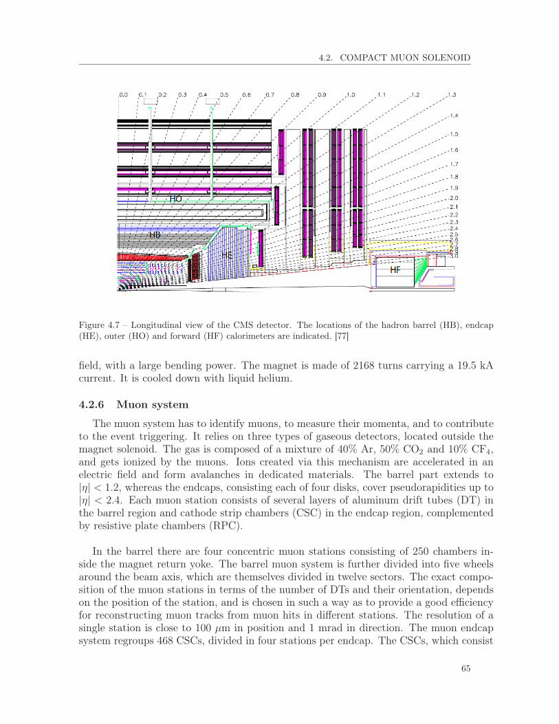
4.2. COMPACT MUON SOLENOID
Figure 4.7 – Longitudinal view of the CMS detector. The locations of the hadron barrel (HB), endcap(HE), outer (HO) and forward (HF) calorimeters are indicated. [77]
field, with a large bending power. The magnet is made of 2168 turns carrying a 19.5 kAcurrent. It is cooled down with liquid helium.
4.2.6 Muon system
The muon system has to identify muons, to measure their momenta, and to contributeto the event triggering. It relies on three types of gaseous detectors, located outside themagnet solenoid. The gas is composed of a mixture of 40% Ar, 50% CO2 and 10% CF4,and gets ionized by the muons. Ions created via this mechanism are accelerated in anelectric field and form avalanches in dedicated materials. The barrel part extends to|η| < 1.2, whereas the endcaps, consisting each of four disks, cover pseudorapidities up to|η| < 2.4. Each muon station consists of several layers of aluminum drift tubes (DT) inthe barrel region and cathode strip chambers (CSC) in the endcap region, complementedby resistive plate chambers (RPC).
In the barrel there are four concentric muon stations consisting of 250 chambers in-side the magnet return yoke. The barrel muon system is further divided into five wheelsaround the beam axis, which are themselves divided in twelve sectors. The exact compo-sition of the muon stations in terms of the number of DTs and their orientation, dependson the position of the station, and is chosen in such a way as to provide a good efficiencyfor reconstructing muon tracks from muon hits in different stations. The resolution of asingle station is close to 100 µm in position and 1 mrad in direction. The muon endcapsystem regroups 468 CSCs, divided in four stations per endcap. The CSCs, which consist
65

CHAPTER 4. EXPERIMENTAL SETUP
in multiwire proportional chambers, have a trapezoidal shape and count six gas gaps.Unlike DT, they can support the high rate of neutron-induced background and cope witha large and non-uniform magnetic field.
For low-momenta muons, the momentum resolution is by far dominated by the trackermeasurements, while for particles with high momenta (around 1 TeV), the tracker and themuon system both provide a momentum resolution of about 5%. Combining the innertracker and the muon system, the transverse momentum resolution for particles up to1 TeV lies between 1 and 5%. Although DTs and CSCs can be used to trigger eventsbased on the pT of the muons with a good efficiency, their time response is comparableto the design bunch crossing space. Therefore, RPCs, which are double-gap chambersoperated in avalanche mode, composed of parallel anode and cathode plates with a gasgap in between, have been introduced in the barrel and endcaps as a dedicated triggersystem with a fast response and good time resolution. The position resolution of RPCsis however coarser than that of DTs and CSCs. Six layers of RPC are embedded in thebarrel, whereas three layers of RPCs are part of each endcap muon system.
Without complementary information form the tracker, the muon system provides aresolution of about 10% for muons with |η| < 2.4 and pT < 200 GeV.
4.2.7 Trigger
For a bunch spacing of 25 ns, the beam crossing frequency is 40 MHz. Given the highcrossing rate, the large size of an event (about 1 MB), and the fact that typically tensof collisions happen for a same bunch crossing, storing and processing every single eventis simply not feasible. The trigger system reduces the rate by selecting events that havea physical interest, based on the characteristics of these events such as the transversemomentum of the particles. The rate reduction by at least a factor of 106 is done intwo steps: Level-1 (L1) Trigger and High-Level Trigger (HLT). Prescaled triggers, whichhave loose selection conditions and thus do not permit to keep all events passing theseconditions, can be used to study more frequent collisions.
The L1 Trigger, which has a design output rate of 100 kHz and a response time of3.2 µs, relies on coarse information from the calorimeters and the muon system. Field-Programmable Gate Array (FPGA) technology is mainly exploited for the L1 Triggerhardware, while application-specific integrated circuits (ASICs) and programmable mem-ory lookup tables (LUT) are also used in special cases where speed, density and radiationresistance are of high importance. The first step of the Calorimeter Trigger is local,and consists in measuring the transverse energies in ECAL crystals and HCAL read-outtowers, grouped in so-called trigger towers. The Regional Calorimeter Trigger then de-termines regional candidate electrons or photons (up to |η| = 2.5), tau veto bits (up to|η| = 3.0), transverse energy sums, and other information of interest for muons. Finallythe highest-rank calorimeter trigger objects in the whole detector are determined by theGlobal Calorimeter Trigger. The Muon Trigger uses information from the three muon sys-
66

4.3. CHAPTER SUMMARY
tems, and covers pseudorapidities |η| < 2.1. Locally, DT chambers in the barrel providetrack segments in the φ-projection and hit patterns in the η-projection, while CSCs in theendcaps provide information as three-dimensional track segments. Regionally, completetracks are made from joining the tracks and hits reported by the DTs and CSCs, andphysical parameters are associated to them. RPCs, which have a better timing resolu-tion, contribute also regionally by producing their own track candidates based on regionalhit patterns. Globally, the Muon Trigger combines all pieces of regional information fromthe three subdetectors.
Events passing the L1 Trigger are then processed by the HLT, which performs morecomplex calculations, based on a combination of information from the different subdetec-tors. It reduces the rate to about 400 Hz. The HLT is based on software techniques, andis flexible. The full read out information can be accessed at this stage, and processed bya filter farm of about a thousand processors. The events passing the HLT are kept forstorage.
4.3 Chapter summary
Experimental setup
The excellent performance of the LHC permitted to collect during its first runabout 5, 20 and 3 fb−1 of proton-proton data in 2011, 2012 and 2015, at 7, 8 and13 TeV center-of-mass energies respectively. This thesis is based on the collisiondata collected by the CMS detector in 2012 essentially, but also includes someanalyses of 2011 and 2015 data. CMS is composed of several subdetectors: a tracker,an electromagnetic calorimeter, a hadronic calorimeter and muon chambers. Tauleptons, which are the common point between all analyses presented in this thesis,are reconstructed from information from all subdetectors.
67


Chapter 5
Event generation, simulation andreconstruction
To search for new physics, observed collision data should be compared to theexpectation from SM processes. SM processes, as well as hypothetical signals,can be modeled with Monte Carlo (MC) event simulations. The generated eventsare then passed through a full simulation of the CMS detector, to model theinteractions events undergo before being detected, as well as the detector response.The first part of this chapter concerns generation and simulation. The signaturesleft inside the detector (or its simulation) by the data (or generated) events needto be reconstructed into physical objects, such as electrons, muons, taus or jets.The reconstruction of the different types of physical objects is described in thesecond part of the chapter, with an emphasis on the objects used in the physicsanalyses presented in this thesis.
5.1 Event generation and simulation
Monte Carlo sample generation proceeds through the following steps [85]:
1. Hard-scattering process. At the LHC, the central part of the interaction consistsin the hard-scattering of the two incoming protons. As the collision actors are ratherconstituents of the protons, called partons, it is required to extract the momentaof these incoming partons. This is done thanks to parton distribution functions(PDFs), which give the probability that a parton carries a certain fraction of theproton momentum, at a given scaleQ2. The most commonly used PDFs are providedby the CTEQ group. Given the large energy scale, the hard-scattering process itselfis computed with the matrix element (ME) formalism in perturbative QCD, atleading order (LO) or next-to-LO (NLO) depending on the generator.
2. Parton showering. Parton showering techniques are used to describe the hadroniza-tion and radiation of quarks and gluons in the initial and final states. While partonshowering can be encapsulated in the matrix element computation, this is however
69

CHAPTER 5. EVENT GENERATION, SIMULATION AND RECONSTRUCTION
often not feasible for a large number of final state particles.3. Underlying events. Underlying events, coming from the interactions of the re-
maining parts of the protons that did not take part in the hard scattering process,are then modeled. They typically consist in soft QCD interactions, and can bemodeled from phenomenological inputs.
4. Hadronization. When quarks and gluons have low energies, below typically 1GeV, they cannot be treated as free anymore and the perturbative QCD formalismfails. The hadronization stage models their recombination into hadrons without anycolor charge.
5. Hadron and tau decays. The decay of short-lived particles is then simulated. Inparticular, tau decays are simulated with Tauola [86], interfaced to a generator thattakes care of the previous steps.
6. Pileup. To describe the observed data more exactly, pileup interactions, consistingin an additional set of soft inelastic collisions, are added to the main hard scatter-ing process. As it is difficult to predict the distribution of the number of pileupinteractions in data, MC datasets are usually generated for a scenario with a highernumber of vertices and afterwards reweighted to match the observed distribution ofpileup interactions.
Many MC generators have been developed. The ones used in the analyses presentedin the next chapters are Madgraph [87], Pythia [88], Powheg [89] and aMC@NLO [90].Powheg and aMC@NLO can compute NLO matrix elements. The events are then passedthrough Geant4 [91], which simulates the response of the CMS detector.
5.2 Object reconstruction and identification
The detector response is analyzed to identify physical objects. The particle-flow algo-rithm used in CMS is described in Section 5.2.1, and is followed by the strictly speakingobject reconstruction, with tracks and vertices in Section 5.2.2, jets and b-tagged jets inSection 5.2.3, electrons in Section 5.2.4, muons in Section 5.2.5, taus in Section 5.2.6, andfinally missing transverse energy in Section 5.2.7.
5.2.1 Particle-flow
Stable particles are reconstructed in CMS with a particle-flow (PF) algorithm [92,93], which combines information from all subdetectors under the form of muon tracks,calorimeter clusters and tracks from other charged particles. This is made possible by thehigh granularity of the detector. The individual PF particles – electrons, photons, muons,charged and neutral hadrons – are then combined to form more complex objects such ashadronically decaying taus, jets, or transverse missing energy.
The track reconstruction algorithm is performed with an iterative tracking strategy,which achieves a high efficiency and a low misidentification rate, and is described morein details in Section 5.2.2. In the calorimeters, a clustering algorithm is performed to
70

5.2. OBJECT RECONSTRUCTION AND IDENTIFICATION
reconstruct neutral particles and to complement the tracking to measure the energy ofcharged particles among others. The first step of the calorimeter clustering algorithmconsists in identifying cells from calorimeter cluster seeds with an energy above a giventhreshold, while in a second time, topological clusters are built by joining adjacent cellswith a minimum energy threshold. PF clusters are then formed from topological clusters;their energies and sizes are determined iteratively based on their distance from each cell.As a single physical particle can create multiple PF elements, such as a track and sev-eral calorimeter clusters, a link algorithm has been designed to fully reconstruct particlesand to limit double counting. It computes a distance between objects based on charac-teristics extracted from the iterative tracking and calorimeter clustering algorithms, anddetermines whether they correspond to different physical objects.
5.2.2 Tracks and vertices
Track reconstruction [94] is based on the collection of hits from the pixel and striptrackers. The Combinatorial Track Finder (CTF) software, which is an adaptation andextension of the Kalman filter, fits tracks from the hits. All tracks are reconstructed afterseveral iterations of the CTF, in an iterative tracking process. In the first iteration, tracksare seeded and reconstructed with very tight criteria; this ensures a low fake rate at theprice of a moderate efficiency. In the next iterations, the seeding criteria are loosenedto increase the efficiency, while hits unambiguously assigned to the track in the previoussteps are removed to keep the fake rate low as a consequence of the reduced combinatorics.A typical iteration proceeds in four steps. First, tracks are seeded from a small number ofhits, which determine the five parameters needed to describe the helical path of chargedparticles in the quasi-uniform magnetic field of the tracker. Second, the track finding stepextrapolates the few hits from the seeding stage, adding more hits layer after layer to thetrack candidate with a Kalman filter. Third, track candidates are fitted with a Kalmanfilter to provide an estimate of the track trajectory parameters. And finally, some qualitycuts are applied to the reconstructed tracks, in order to remove fake tracks not associatedwith charged particles. The track reconstruction efficiency for single isolated muons isillustrated in the left-hand side part of Fig. 5.1.
Prompt tracks originating from the interaction region are used to reconstruct interac-tion vertices [95]. They need to satisfy some quality criteria, based for example on theirchi-square or on the number of pixel and strip hits. Tracks that are close enough to eachother in the interaction region in the z-direction are clustered to form a vertex. If sev-eral tracks are assembled, an adaptative vertex fit is performed to determine the vertexcharacteristics, such as its exact position. The primary vertex reconstruction efficiencydistribution, close to 1, is illustrated in the right-hand side part of Fig. 5.1. Weights wbetween 0 and 1, representing the compatibility of a track with the common vertex, areassigned to each track, and the number of degrees of freedom of the vertex is computedas follows:
ndof = 2
Ntracks∑i=1
wi − 3. (5.1)
71

CHAPTER 5. EVENT GENERATION, SIMULATION AND RECONSTRUCTION
This variable can be used to identify real proton-proton interactions, and to reduce thevertex misidentification rate. The primary vertex is usually considered as the one withthe largest scalar sum of track transverse momenta.
Figure 5.1 – Left: Track reconstruction efficiency for single isolated muons in the barrel (|η| < 0.9),transition (0.9 < |η| < 1.4) and endcap (1.4 < |η| < 2.5) regions of the tracker. The efficiency reaches aplateau close to 1 for muons with pT larger than about 1 GeV. [94] Right: Primary vertex reconstructionefficiency in simulation and 7 TeV data. A plateau is reached for a number of tracks larger than aboutsix. [95]
5.2.3 Jets
Quark and gluon jets are built from PF objects. The anti-kT algorithm [96] is usedto cluster individual objects into jets. It proceeds by defining distances dij between twoentities (particles, pseudojets) i and j, and distances diB between an entity i and thebeam:
dij = min(k−2ti , k
−2tj )
∆2ij
R2, and (5.2)
diB = k−2ti , (5.3)
where kti and ktj are the transverse momenta of the i and j entities respectively, ∆2ij =
(φi − φj)2 + (ηi − ηj)2, and R is a cone parameter chosen to be 0.5 in CMS in Run-1 and0.4 in Run-2. If the smallest distance is of dij-type, the entities i and j are combinedinto a new single entity, while if it is of diB-type, the i entity is considered as a jet andremoved from the list of entities. The procedure continues until the entity list is empty.Unlike other jet clustering algorithms, the anti-kT algorithm produces jets with a conicalshape, clustered around the hardest particles and with boundaries resilient with respectto soft radiation.
The jet energies are corrected to ensure a uniform response in η and an absolutecalibration in pT . The objective of the calibration is that the reconstructed jet energy
72
5.2. OBJECT RECONSTRUCTION AND IDENTIFICATION
matches the energy of the generated jet. The correction to the raw pT of the jet can bedecomposed in four multiplicative terms [97]:
— An offset correction, to remove the energy due to particles not involved in the hard-scattering process (pileup particles, detector noise);
— An MC calibration factor, which corrects the reconstructed energy to match thegenerated MC particle jet energy, based on simulations;
— A residual calibration for the relative energy scale, to correct the energy responseas a function of the pseudorapidity, in order for the response to be flat with respectto the pseudorapidity;
— A residual calibration for the absolute energy scale, to make the energy responseuniform with the transverse momentum.
B jets, originating from b quark hadronization, can be distinguished from other jetscoming from gluons, light-flavor quarks (u, d, s) and c-quark fragmentation using track,vertex and identified lepton information. Different algorithms to tag b jets exist; only theCombined Secondary Vertex (CSV) algorithm is described here as it is used in the physicsanalyses presented in the next chapters. Because b hadrons typically have a lifetime ofcτ ' 450 µm, a powerful handle to discriminate between b jets and non-b jets is theexistence of a secondary vertex. A secondary vertex is defined as a vertex sharing lessthan 65% of its tracks with the primary vertex and separated radially from the primaryvertex with a significance at least 3σ. In addition, if the radial distance exceeds 2.5 cmand if the mass is compatible with a K0 or larger than 6.5 GeV, the secondary vertexis rejected. The last condition for secondary vertices is that the flight direction of eachcandidate is in a cone with ∆R = 0.5 around the jet direction. When no secondaryvertex is found, in about 35% of cases for real b jets, the CSV algorithm can use so-called"pseudo-vertices", from tracks with a significance of the impact parameter (IP) largerthan 2. If no pseudo-vertex is found, the CSV algorithm proceeds from simple trackvariables. The list of variables used to identify b jets are, when available in the event [98]:
— If the event has a secondary vertex, a pseudo-vertex or none of them;— The flight distance significance between the primary and the secondary (or pseudo-)
vertex in the transverse plane;— The number of tracks at the secondary or pseudo-vertex;— The ratio of the energy carried by tracks at the vertex with respect to all tracks in
the jet;— The pseudorapidities of the tracks at the vertex with respect to the jet axis;— The 2D IP significance of the first track that raises the invariant mass above the c
quark mass;— The number of tracks in the jet;— The 3D IP significances for each track in the jet.
A likelihood ratio to reject c jets and another one to reject light-parton jets are combinedto form the final CSV discriminator. The efficiency of the CSV algorithm in data andsimulations is shown in Fig. 5.2; for the medium working point the efficiency is close to70% for a mistagging rate of about 1.5%.
73

CHAPTER 5. EVENT GENERATION, SIMULATION AND RECONSTRUCTION
b-ta
g E
ffici
ency
0.4
0.5
0.6
0.7
0.8
0.9
Monte Carlo
Measured Value
= 8 TeVs at -1CMS Preliminary, 19.8 fb
CSV Discriminator Value0.2 0.3 0.4 0.5 0.6 0.7 0.8 0.9
bS
F
0.95
1
1.05
Figure 5.2 – B-tagging efficiency as a function of the CSV discriminator threshold, in 8 TeV simulationsand data. The arrows indicate the three working points in Run-1. For information, the misidentificationprobabilities for jets with pT between 80 and 120 GeV are, for the loose, medium and tight workingpoints respectively, 0.0990±0.0004, 0.0142±0.0002 and 0.0016±0.0001, where the quoted uncertaintiesare statistical only. [99]
5.2.4 Electrons
Electrons are reconstructed from energy deposits in the ECAL and tracks in thetracker [100]. Special emphasis has to be given to the spread, mostly in the φ-direction,of the electron energy in the ECAL caused by photon radiation. Indeed, on average 33%of the electron energy is lost before reaching the ECAL at η = 0, while up to 86% can belost when the budget material in front of the ECAL is large (e.g. at |η| = 1.4).
The clustering of the electron energy in the ECAL proceeds with different algorithmsin the barrel and in the endcaps, because the subdetector geometries are different. In thebarrel, the hybrid algorithm starts from the seed crystal that contains the largest energydeposit above 1 GeV. Strips of 5× 1 crystals in the η × φ plane are delimited around theseed crystal, and are merged to adjacent strips if their energy exceeds 0.1 GeV. A super-cluster is then formed from all the strip clusters that have a seed strip with an energy ofat least 0.35 GeV. In the endcaps, the multi 5×5 algorithm starts from a seed crystal withan energy deposit larger than 0.18 GeV. A primary cluster of 5×5 crystals is built aroundthe seed, while secondary clusters of 5× 5 crystals are centered around crystals that arenot further than 0.3 in the φ-direction and 0.07 in the η-direction from the seed crystal.The supercluster is finally built from the primary cluster and all secondary clusters thathave an energy deposit larger than 1 GeV, and the energy collected in the preshower isadded to it. The position of the supercluster is computed as the energy-weighted meanof the cluster positions, whereas its energy is simply taken as the sum of the energy of allits constituent clusters.
74

5.2. OBJECT RECONSTRUCTION AND IDENTIFICATION
Although electron tracks can be, as any charged particle track, reconstructed fromtracker information with the standard Kalman filter (KF) track reconstruction, large en-ergy losses caused by radiation in the tracker material hurt the reconstruction efficiencyof such a method. The electron track reconstruction in CMS proceeds in two steps: theseeding and the tracking. The seeding stage uses two complementary algorithms, the re-sults of which are combined. The tracker-based seeding is based on tracks, reconstructedwith general tools for charged particles, that are matched to a supercluster after extrap-olation towards the ECAL, whereas the ECAL-based seeding starts from a superclusterand selects electron seeds to extrapolate the trajectory towards the collision vertex. Thetracking phase is composed of the track building and the track fitting. The energy loss ofelectrons in the tracker material does not follow a Gaussian distribution, as assumed bythe KF algorithm, but a Bethe-Heitler distribution, which has a larger tail. The GaussianSum Filter (GSF) algorithm is used to estimate the track parameters from a hit collectionobtained with a KF algorithm, by approximating the Bethe-Heitler distribution with asum of Gaussian distributions.
Tracks and superclusters are matched to each other in GSF electron candidates. ECAL-driven tracks are compatible with a supercluster if their extrapolated tracks in the su-percluster from the innermost track position is compatible with the supercluster positionwithin ∆η × ∆φ = 0.02 × 0.15. The compatibility of tracker-driven tracks with super-clusters is estimated with a multivariate technique that combines track and superclusterinformation.
While the electron charge can be easily evaluated from the sign of the GSF trackcurvature, this leads to a charge misidentification of up to 10% for electrons at largepseudorapidity, because of bremsstrahlung followed by photon conversions. To reduce thecharge misidentification rate, two other charge estimates are computed; the final electroncharge is then the one given by at least two of the methods. The first alternative methodis based on the KF track associated to a GSF track if they share at least one innermosthit, whereas the second one defines the charge sign as the sign of the φ differences betweenthe vector joining the beam spot to the supercluster position, and the vector joining thebeam spot and the first hit of the electron GSF tracks. The combination of the threecharge estimates reduces the charge misidentification rate to 1.5% for reconstructed elec-trons from Z boson decays.
The electron momentum is evaluated from a weighted combination of the measurementsfrom track parameters – dominant for low energy candidates –, and from supercluster pa-rameters – dominant for high energy candidates.
Several variables may help to discriminate real electrons from hadronic jets. Theyare classified into three categories: the observables that measure the agreement betweenECAL and tracker measurements (such as ∆ηin and ∆φin, respectively the distances in ηand φ between the superscluster and the track direction extrapolated from the primary
75

CHAPTER 5. EVENT GENERATION, SIMULATION AND RECONSTRUCTION
Working point Electron pT |η| < 0.8 0.8 ≤ |η| < 1.479 1.479 ≤ |η|
Very loose - 0.500 0.120 0.600Loose pT ≤ 20 GeV 0.925 0.915 0.965
pT > 20 GeV 0.905 0.955 0.975
Tight pT ≤ 20 GeV 0.925 0.915 0.965pT > 20 GeV 0.925 0.975 0.985
Table 5.1 – Thresholds on the BDT output used to define the very loose, loose and tight electron identi-fication.
vertex position to the ECAL), the observables based on calorimeter information only(such as the ratio between hadronic and electromagnetic energy around the seed cluster,H/E) and the observables based on tracking measurements (such as the compatibilitybetween the KF- and GSF-fitted tracks). Two identification methods exist: the cut-basedelectron identification directly cuts on the variables presented before, while the MVAidentification combines them in a BDT to obtain a final discriminator on which a cut isapplied. The MVA identification typically has a better performance as shown in Fig. 5.3.The thresholds on the BDT output used to define the very loose, loose and tight MVAelectron identifications are indicated in Tab. 5.1; they depend on the electron transversemomentum and pseudorapidity.
Figure 5.3 – Electron identification performance for the MVA-based (continuous line) and cut-based (onesymbol for every working point) identification in terms of signal and background efficiencies, in the barrel(left) and endcaps (right). The performance is computed for electrons with pT greater than 20 GeV.The signal efficiency is measured for electrons in simulated Z → ee events, whereas the backgroundefficiency is measured for jets reconstructed in data. The background efficiency is lower for the MVA-based identification relative to the cut-based identification, for a same signal efficiency. [100]
76

5.2. OBJECT RECONSTRUCTION AND IDENTIFICATION
The electron absolute isolation, used to reject non-prompt or misidentified leptons, isdefined as follows:
I =∑
charged
pT + max
(0,∑neutral
pT +∑γ
pT −1
2
∑charged,PU
pT
), (5.4)
where∑
charged pT is the scalar sum of the transverse momenta of all charged particlesoriginating from the primary vertex and located in a cone with ∆R = 0.4 around theelectron direction. The sums
∑neutral and
∑γ are the equivalent for neutral hadrons and
photons respectively. The last term represents so-called δβ corrections, which remove thecontribution from pileup vertices from the neutral isolation: neutral contributions frompileup vertices are estimated to amount to half of the scalar pT sum of charged particlesfrom pileup vertices inside the isolation cone 1. The relative isolation of an electron issimply the ratio between its absolute isolation and its transverse momentum.
5.2.5 Muons
Muons are reconstructed from tracks in the inner tracker (tracker tracks), and fromtracks in the muon system (standalone-muon tracks) [101]. The global muon reconstruc-tion associates tracker tracks to stand-alone muon tracks to form global-muon tracks bycombining with a KF filter the hits from both types of tracks. The tracker muon re-construction starts from tracker tracks and extrapolate them to the muon system, wherea muon segment should be found. While the global muon reconstruction is especiallyefficient for muons leaving hits in several muon stations, the tracker muon reconstructionis more efficient for low pT muon candidates. The efficiency for reconstructing a muon asglobal or tracker muon is as high as 99%.
Different identification working points can be used in physics analyses. To be identifiedas "loose", a muon candidate should be reconstructed as a PF muon, and to be eithera global or a tracker muon. "Medium" muons, used in Run-2 analyses, should be loosemuons, and have a segment compatibility probability between the tracker and muon trackslarger than 0.451 or pass the following set of requirements:
— To be global muons;— The normalized chi-square of their global tracks is less than 3;— χ2 of the compatibility between the position of the standalone and trackers tracks
less than 12;— χ2 from the kink finder on the inner track less than 20 (used to remove muons from
decays in flight);— Segment compatibility probability between the tracker and muon tracks larger than
0.303.Finally, tight muons are global and PF muons that satisfy the following requirements:
— χ2/number of degrees of freedom of the global muon track fit, using tracker andmuon chamber hits, less than 10;
1. The ratio of neutral to charged isolation from pileup vertices is estimated from MC simulations.
77

CHAPTER 5. EVENT GENERATION, SIMULATION AND RECONSTRUCTION
— Muon segments present in at least two muon stations;— Transverse impact parameter dxy of the tracker track with respect to the primary
vertex less than 2 mm;— Longitudinal distance dz of the tracker track with respect to the primary vertex less
than 5 mm;— Non zero number of pixel hits;— At least five tracking layers with hits.
The efficiency of the tight muon identification is shown in Fig 5.4. In practice, the choiceof the identification working point depends on the analysis.
(GeV/c)T
muon p3 4 5 6 7 10 20 30 100
Tig
ht m
uon
effic
ienc
y
0
0.2
0.4
0.6
0.8
1
= 7 TeVsCMS Preliminary,
| < 1.2η |
Data, 2010
Simulation
(GeV/c)T
muon p1 2 3 4 5 10 20 30 100
Tig
ht m
uon
effic
ienc
y
0
0.2
0.4
0.6
0.8
1
= 7 TeVsCMS Preliminary,
| < 2.4η 1.2 < |
Data, 2010
Simulation
Figure 5.4 – Efficiency of the tight muon identification in 2010 data (black) and simulation (red), in thebarrel (left) and endcaps (right). [101]
The absolute and relative δβ-corrected isolations for muons are computed exactly asfor electrons in equation (5.4).
5.2.6 Taus
Muons and electrons originating from tau decays are reconstructed with the stan-dard tools for electron and muon reconstruction described in Sections 5.2.4 and 5.2.5respectively. In about two thirds of cases, taus decay hadronically; they are in this casereconstructed with the Hadrons plus Strips (HPS) algorithm [102, 103]. The HPS algo-rithm builds taus from tracks, and energy deposits in ECAL strips. The main handlesto discriminate hadronically decaying taus from quark and gluon jets are the track mul-tiplicity – taus have only one or three tracks –, and the isolation – taus are on averagemore collimated and isolated than quark and gluon jets. The efficiency in identifyinghadronically decaying taus is typically between 45 and 70%, for misidentification ratesof a jet as a tau of the order of 1%. The HPS algorithm is described in more details inChapter 6.
78

5.2. OBJECT RECONSTRUCTION AND IDENTIFICATION
5.2.7 Transverse missing energy
Neutrinos and other hypothetical neutral weakly interacting particles cannot be de-tected by CMS. However, some information about their presence can be gathered fromthe detection of a momentum imbalance in the transverse plan to the beam axis. Themissing transverse energy is noted ~
��ET , while its magnitude is referred to as ��ET . The~��ET measurement [104] strongly relies on the reconstruction of all other physics objects,and is sensitive to a wide range of effects: mismeasurement or misidentification of physicsobjects, detector noise or malfunctions, pileup interactions, ...
The most widely used type of ~��ET in CMS is the particle-flow (PF) ~��ET , which is thenegative vectorial sum over the transverse momenta of all PF particles. A bias in the��ET measurement can be introduced for several reasons, such as the nonlinearity of theresponse of the calorimeter for hadronic particles, or the minimum energy thresholds inthe calorimeters. This bias is found to be greatly reduced by correcting the pT of jets withan electromagnetic energy fraction less than 0.9 and a corrected pT greater than 10 GeV,to the particle-level pT . In addition, another bias comes from the pileup interactions. Thiscan be corrected by subtracting from the ~��ET a certain fraction f(~v) of ~v, the vectorial pTsum of charged particles associated to each pileup vertex:
~��Ecorr
T = ~��ET −
∑PU
f(~v)~v. (5.5)
Finally, an asymmetry in the φ variable is observed for data and simulated events, and isfound to be related to the number of reconstructed vertices Nvtx. The ~��ET projection inthe x- and y-directions are independently corrected by some functions of Nvtx.
Another type of��ET , used in the physics results presented in the next chapters, is basedon an MVA method. It is designed to reduce the influence of pileup interactions, whichdo not have significant ��ET but degrade the ��ET measurement resolution by 3.3-3.6 GeVon average for each single pileup vertex. The MVA ~
��ET relies on the identification ofjets originating from pileup interactions with a MVA discriminator that takes as input jetshape variables and vertex information. In Z boson decay events, the transverse energy canbe decomposed in three components, as illustrated in Fig. 5.5: a well-measured momentumscale ~qT = ~pT (l+) + ~pT (l−), an error-prone hadronic recoil ~uT , which is the vectorial sumof all reconstructed PF particles except the leptons originating from the Z boson decay,and the missing transverse energy ~��ET :
~qT + ~uT + ~��ET = ~0. (5.6)
The hadronic recoil can be decomposed in two components parallel or perpendicular to ~qTdirection: ~uT = ~u⊥+~u‖. The MVA��ET is computed as a correction to the hadronic recoil~uT . A first BDT is trained to correct the direction of ~uT to correspond to the generateddirection in simulated Z+jets events, while a second BDT estimates the magnitude afterdirection corrections. The corrected hadronic recoil is added to ~qT to give the negative
79

CHAPTER 5. EVENT GENERATION, SIMULATION AND RECONSTRUCTION
MVA ��ET . In comparison with the PF ~��ET , the MVA ~
��ET resolution is much less sensitiveto the number of interaction vertices, as shown in Fig. 5.6, which may lead to an improve-ment of the sensitivity of physics analyses such as H → ττ by as much as 20%.
Figure 5.5 – Schematic view of the Z boson transverse momentum ~qT , the hadronic recoil ~uT with itsparallel and perpendicular projections along ~qT , and the ~�ET . [104]
Artificially large ��ET can be measured because of spurious detector signals. Sources offake ��ET are:
— Dead cells in the ECAL;— Beam-halo particles;— Particles striking sensors in the ECAL barrel detector;— Noise from HCAL hybrid photodiode and readout box electronics;— Direct particle interactions with light guides and photomultipliers tubes in the for-
ward calorimeter;— High-amplitude anomalous pulses in the ECAL endcaps;— A misfire of the HCAL laser calibration system;— A defective track reconstruction, from coherent noise in the silicon strip tracker.
Dedicated algorithms are used to identify and remove these events with fake ��ET .
80

5.3. CHAPTER SUMMARY
Figure 5.6 – Hadronic recoil resolution as a function of the number of interaction vertices, in the per-pendicular (left) and parallel (right) directions to the transverse momentum of the Z boson, in Z → µµ
events, for the PF ~�ET , the MVA ~
�ET , and two other ~�ET types not described in the text: no-PU PF ~�ET
and MVA unity PF�ET . [104]
5.3 Chapter summary
Event generation simulation and reconstruction
This chapter describes how events are generated and simulated, and how the physicsobjects (electrons, muons, taus, jets,��ET ) used in the analyses presented in the nextchapters, are reconstructed and identified.
81


Chapter 6
Tau lepton reconstruction and identification
Tau leptons play an important role in physics analyses in the scalar sector. Inthe SM, H → ττ is the most sensitive fermionic decay channel of the scalarboson, and provides the most precise test of its Yukawa couplings. Additionally,in some models with an extended scalar sector, such as the MSSM, the cou-plings of high mass scalars to tau leptons can be enhanced for some choices ofthe model parameters. Experimentally, identifying and reconstructing tau leptonsis however challenging, as they are, unlike other leptons, heavy enough to decayhadronically. Table 6 shows the tau decay modes and their corresponding branch-ing fractions. In about one third of cases, tau leptons decay leptonically, to anelectron, an electronic neutrino and a tauic neutrino, or to a muon, a muonicneutrino and a tauic neutrino. The other decay modes are hadronic, with, inthe dominant modes, one or three charged hadrons (pions or kaons), zero to twoπ0 and one tauic neutrino. Some decay modes involve intermediary resonances,such as ρ(770) and a1(1260). Taus decaying hadronically will be denoted byτh. Leptonically decaying taus are identified through standard electron and muonidentification algorithms, while hadronic taus are reconstructed in CMS with theHadrons Plus Strips (HPS) algorithm. The next sections present the HPS al-gorithm, as well as the measurement of its performance with data collected inRun-1 and Run-2.
6.1 HPS algorithm description
The HPS algorithm [102, 103] is designed to identify hadronically decaying taus. Themain challenge lies in the similarity between hadronic taus and jets from QCD multijetprocesses, which have a production cross section five orders of magnitude larger than theDrell-Yan process at the LHC. The first step of the HPS algorithm is the reconstruction,where it is checked that the tau candidate topology is compatible with one of the hadronictau decay modes. The next step, the identification, rejects quark or gluon jets, electrons,or muons that might have been wrongly identified as hadronic taus.
83

CHAPTER 6. TAU LEPTON RECONSTRUCTION AND IDENTIFICATION
Decay mode Resonance B [%]τ− → e−νeντ 17.8τ− → µ−νµντ 17.4τ− → h−ντ 11.5τ− → h−π0ντ ρ(770) 26.0τ− → h−π0π0ντ a1(260) 10.9τ− → h−h+h−ντ a1(260) 9.8τ− → h−h+h−π0ντ 4.8
Other hadronic modes 1.8
Table 6.1 – Tau decay modes, their approximate branching fractions, and the eventual intermediaryresonances. The symbol h stands for kaons or pions. Charge conjugation is implied. [9]
6.1.1 Reconstruction
Tau candidates are reconstructed from a combination of tracks identifying chargedhadrons h±, and ECAL energy deposits identifying π0. The charged tracks are requiredto have a pT greater than 0.5 GeV and to be compatible with the hypothetical productionvertex of the τh candidate (|dz| < 0.4 cm and dxy < 0.03 cm with respect to the vertexclosest to the leading charged particle within the jet). The dimensions of the ECAL stripsin the η×φ plan are 0.05×0.20; the widening in the φ direction accounts for the bending inthe magnetic field of the electrons/positrons produced by the conversion of photons fromπ0 → γγ decays. The electrons and photons used to build the ECAL strips are requiredto have transverse momenta greater than 0.5 GeV, and the total transverse momentum ofa strip needs to be larger than 2.5 GeV to be considered in the HPS algorithm. Hadronictaus are reconstructed in one of these four topologies:
— Three prongs - h−h+h−: Three charged tracks, compatible with originating fromthe same event vertex, are required. The charges of the three tracks should not be allidentical, and their invariant mass should lie between 0.8 and 1.5 GeV. This topologyaims at reconstructing both τ− → h−h+h−ντ and τ− → h−h+h−π0ντ decays. In thelatter case however, the algorithm efficiency is low because the neutral pion energyis considered as part of the isolation, which often leads the tau candidate to fail thesecond step of the HPS algorithm (see Section 6.1.2).
— One prong plus two strips - h−π0π0: The mass of the tau candidate formed bythe track and the strips should satisfy: 0.4 < mτ < 1.2
√pT (GeV)/100 GeV. The
pT dependence in the upper limit accounts for resolution effects. If the transversemomentum is less than 100 GeV or greater than 1111 GeV, the upper limit is fixedto 1.2 or 4.0 GeV respectively.
— One prong plus one strip - h−π0: The tau candidate built from the track andthe ECAL strip should have a mass such that 0.3 < mτ < 1.3
√pT (GeV)/100 GeV.
If the transverse momentum is less than 100 GeV or greater than 1044 GeV, theupper limit is fixed to 1.3 or 4.2 GeV respectively.
— One prong - h−: The reconstructed visible tau mass, mτ is set to the mass of acharged pion.
All charged hadrons and ECAL strips are required to lie within a signal cone with
84

6.1. HPS ALGORITHM DESCRIPTION
∆R = 3.0/pT (GeV) around the momentum vector of the tau candidate 1. This so-called"shrinking cone algorithm" takes into account the fact that the decay products of tauswith higher pT are more collimated. If a tau candidate can be reconstructed in morethan one topology and pass all selection criteria described above, the topology that givesthe highest pT for the tau candidate is kept. Hadronic taus that are reconstructed asdescribed above are said to pass the decay mode finding discriminator.
6.1.2 Identification
Jet rejection - Isolation
Genuine hadronically decaying taus are typically more collimated and isolated thanquark and gluon jets that have passed the reconstruction step; this is the main handle todifferentiate these physics objects. Two types of isolations have been designed: cut-basedand MVA-based.
The cut-based isolation is measured as the scalar sum of the transverse momenta ofcharged particles with pT > 0.5 GeV and photons with ET > 0.5 GeV within a conecentered around the tau candidate and with a radius ∆R = 0.5. The charged particlesare further required to be compatible with originating from the tau candidate productionvertex (|dz| < 0.2 cm along the beamline, dxy < 0.03 cm in the transverse plan), in order toreduce the contribution from pileup jets. So-called ∆β corrections are applied to removethe contribution of pileup from the photon isolation; they are computed as the scalar sumof the transverse momenta of charged particles in a cone with ∆R < 0.8 around the taucandidate and with a distance larger than 0.2 cm in the beamline direction from the taucandidate production vertex, and are scaled by a factor 0.46 to make the tau identificationefficiency independent from pileup. The tau candidate isolation, Iτ , reads:
Iτ =∑
pchargedT (|dz| < 0.2 cm) + max(pγT −∆β, 0), (6.1)
with ∆β corrections computed as follows:
∆β = 0.46×∑
pchargedT (|dz| > 0.2 cm). (6.2)
The loose, medium and tight isolation working points correspond respectively to Iτ lessthan 0.8, 1.0 and 2.0 GeV.
The MVA-based discriminator, in addition to isolation criteria, also takes benefit fromthe fact that taus have a non negligible lifetime compared to the secondary vertex resolu-tion in the CMS detector: cτ=87 µm. A BDT discriminator is built to distinguish genuinehadronic taus from quark and gluon jets. The input variables, illustrated in Fig. 6.1, are:
— The charged particle energy in the isolation cone pchargedT ;— The neutral particle energy pγT in the isolation cone;— The reconstructed tau decay mode (h−, h−π0, h−π0π0 or h−h+h−);
1. The lowest and highest ∆R considered are 0.05 and 0.10.
85

CHAPTER 6. TAU LEPTON RECONSTRUCTION AND IDENTIFICATION
— The transverse impact parameter d0 of the leading track of the tau candidate andits significance d0/σd0 ;
— The distance between the tau production and the tau decay vertices, |~rSV − ~rPV |,and its significance, in the case of three-prong tau candidates;
— A boolean indicating if a tau decay vertex has been reconstructed;— The tau candidate pseudorapidity;— The tau candidate transverse momentum;— The ∆β corrections.The BDT is trained on MC samples: signal events come from Z → ττ , Z ′ → ττ and
W ′ → τντ and the background events from W+jets and QCD multijet simulations. TheZ ′ and W ′ samples in addition to the SM Drell-Yan process permit to cover a large pTrange for the tau candidate, between 20 and 2000 GeV. The BDT output is shown inFig. 6.2, and illustrates that a good discrimination between hadronic taus, and quarkand gluon jets can be achieved. Different working points are defined based on the BDToutput.
Muon rejection
Muons have a high probability to be misidentified as hadronic taus in the h− decaymode. A cut-based and an MVA-based discriminators are designed to separate muonsfrom hadronic taus. Two cut-based working points are defined:
— Loose: The tau candidate does not pass this working point if the ECAL and HCALenergy deposits associated to its leading track is less than 0.2 times the momentumof this track, or if there are track segments in more than one muon station withina cone with ∆R = 0.5 around the tau direction;
— Tight: The tau candidate does not pass this working point if it fails the looseworking point, or if hits within a cone with ∆R = 0.5 around the tau direction arefound in the CSC, DT or RPC chambers of the two outermost muon stations.
Meanwhile, the BDT takes as input the following variables:— ECAL and HCAL energy deposits of the leading charged particle of the tau candi-
date;— ECAL and HCAL energy deposits of any charged particle or photon of the tau
candidate;— The fraction of the tau energy carried by the leading charged particle;— The number of track segments in the muon system in a cone with ∆R = 0.5 around
the tau direction;— The number of muon stations in the DT, CSC or RPC, that have a least one hit
detected within a cone with ∆R = 0.5 around the tau direction;— The pseudorapidity of the tau candidate.
The BDT is trained on Z/γ∗ → ττ , Z/γ∗ → µµ, Z ′ → µµ, W → τν, W → µν, tt,H → ττ , Z ′ → ττ , W ′ → τν and W ′ → µν events.
86

6.1. HPS ALGORITHM DESCRIPTION
z < 0.2 cm) [GeV]∆ (charged
T pΣ
0 5 10 15 20 25 30 35 40
Rel
ativ
e yi
eld
/ bin
4−10
3−10
2−10
1−10
1
hτJets
CMS Simulation
[GeV]γ
T pΣ
0 5 10 15 20 25 30 35 40
Rel
ativ
e yi
eld
/ bin
4−10
3−10
2−10
1−10
1
hτJets
CMS Simulation
decay modehτ0 2 4 6 8 10
Rel
ativ
e yi
eld
/ bin
0
0.1
0.2
0.3
0.4
0.5
0.6 hτJets
CMS Simulation
]1/2 [cm |0
| d
0 0.05 0.1 0.15 0.2
Rel
ativ
e yi
eld
/ bin
0
0.01
0.02
0.03
0.04
0.05hτ
Jets
CMS Simulation
0dσ | / 0
| d0 2 4 6 8 10
Rel
ativ
e yi
eld
/ bin
00.010.020.030.040.050.060.070.080.09
hτJets
CMS Simulation
Rel
ativ
e yi
eld
/ bin
0
0.2
0.4
0.6
0.8
1
1.2
no SV has SV
hτJets
CMS Simulation
]1/2 [cm |PVr - SVr|
0 0.5 1 1.5 2 2.5 3
Rel
ativ
e yi
eld
/ bin
4−10
3−10
2−10
1−10
1
hτJets
CMS Simulation
|PVr - SVr| σ | / PVr - SVr| 0 2 4 6 8 10
Rel
ativ
e yi
eld
/ bin
0
0.02
0.04
0.06
0.08
0.1
0.12
0.14
hτJets
CMS Simulation
Figure 6.1 – Input variables distributions, normalized to unity, for the MVA-based isolation discriminatorfor simulated Z/γ∗ → ττ (blue) with real hadronic taus and W+jets (red) events with jets. In the τdecay mode plot the entry 0 represents the decay mode "one prong", 1 and 2 represent the decay modes"one prong plus one strip " and "one prong plus two strips" respectively and the entry 10 represents the"three prongs" decay mode. [103]
87

CHAPTER 6. TAU LEPTON RECONSTRUCTION AND IDENTIFICATION
MVA output1− 0.5− 0 0.5 1
Rel
ativ
e yi
eld
/ bin
4−10
3−10
2−10
1−10
1
hτJets
CMS Simulation
Figure 6.2 – BDT output of the MVA-based isolation including tau lifetime information, for simulatedZ/γ∗ → ττ (blue) with real hadronic taus and W+jets (red) events with quark and gluon jets. [103]
Electron rejection
Electrons also have a high probability to be misidentified as hadronic taus in the h−decay mode, or in the h−π0 if they radiate a bremsstrahlung photon that converts. ABDT is trained to discriminate between electrons and hadronic taus, with Z/γ∗ → ττ ,Z/γ∗ → ee, Z ′ → ee, W → τν, W → eν, tt, H → ττ , Z ′ → ττ , W ′ → τν and W ′ → eνevent samples. It takes as input the following variables:
— The electromagnetic energy fraction E/(E +H), defined as the ratio of the energydeposits associated to the tau candidate in the ECAL, and ECAL plus HCALtogether;
— E/P and H/P , where E and H are respectively the energy in the ECAL and HCALof the leading track of the tau candidate, and P is the transverse momentum of thistrack;
— Eγ/Eτ , the fraction of the tau candidate energy carried by photons;— Fbrem = (Pin−Pout)/Pin, where Pin and Pout are the GSF track momentum measured
by the curvature of the track at the innermost and outermost position;—∑Eγ/(Pin − Pout), the ratio between the bremsstrahlung photon energy measured
in the ECAL and in the tracker;— (NGSF
hits −NKFhits)/(N
GSFhits +NKF
hits), whereNGSFhits is the number of hits in silicon pixel plus
strip tracking detector associated to the track reconstructed by the GSF algorithm,and NKF
hits is its equivalent for the Kalman filter algorithm;— The mass of the tau candidate;— χ2/ndof of the GSF track;— The pseudorapidity and the transverse momentum of the tau candidate;— The transverse momentum, its significance and the pseudorapidity of the GSF track;— The distances in the η and φ directions between the GSF track and the nearest
boundary between ECAL modules.These variables characterize the compactness and the shape of energy deposits in the
88

6.2. HPS ALGORITHM PERFORMANCE IN RUN-1
Efficiency0.4 0.45 0.5 0.55 0.6 0.65 0.7 0.75 0.8
Fak
e-ra
te-210
-110 8-hitβδHPS 3-hitβδHPS
MVA excl. LifetimeMVA incl. Lifetime
8-hitβδHPS 3-hitβδHPS
MVA excl. LifetimeMVA incl. Lifetime
CMS Simulation 2012
| < 2.3τη > 20 GeV, |τTP
MCττ → *γEfficiency: Z/ < 3000 GeV flat)
TFake-rate: QCD multi-jet MC (15 < P
^
Figure 6.3 – Expected performance of the HPS algorithm in terms of efficiency (measured in Z/γ∗ → ττMC simulations) and j → τh misidentification rate (measured in QCD multijet MC samples). The cut-based isolation described in the text corresponds to the green line and the MVA-based isolation includinglifetime information to the red line. [105]
ECAL, the particle multiplicity, and the level of bremsstrahlung emitted. Any tau can-didate in the non-instrumented region between the ECAL barrel and endcaps (1.446 <|η| < 1.558) does not pass the electron rejection.
6.2 HPS algorithm performance in Run-1
The expected performance of the HPS algorithm is measured in MC samples, as de-scribed in Section 6.2.1. The results of the performance measurements with data collectedin 2012 with the CMS detector are presented in the following sections.
6.2.1 Expected performance
The expected performance of the HPS algorithm in terms of efficiency and misidenti-fication rates, averaged over the pT and η of taus, is detailed in Tab. 6.2. The isolationefficiency depends on the working point, and is typically of the order of 50%, for j → τhmisidentification rates at the percent or permille level, as shown in Fig. 6.3. The efficiencyfor taus to pass the discrimination against electrons varies between 60 and 95% dependingon the working point, and the corresponding e → τh misidentification rates range fromabout 3 × 10⁻⁴ to 2 × 10⁻². Finally an efficiency of almost 100% is obtained for tausto pass the discrimination against muons, while the µ → τh misidentification rates arebelow the permille level. The working points to be used in the physics analyses are acase-by-case choice that depends on the expected level of backgrounds. In about 90% ofcases, taus are reconstructed in their true decay mode, with no dependence on the numberof reconstructed vertices.
89

CHAPTER 6. TAU LEPTON RECONSTRUCTION AND IDENTIFICATION
Tau isolation discriminatorsEfficiency Jet → τh misidentification rate
Z/γ∗ → ττ Z ′(2.5 TeV) → ττ W+jets QCD multijetCut-based
Loose 49.0% 58.9% 9.09 · 10−3 3.86 · 10−3
Medium 40.8% 50.8% 5.13 · 10−3 2.06 · 10−3
Tight 38.1% 48.1% 4.38 · 10−3 1.75 · 10−3
MVA-basedVery loose 55.9% 71.2% 1.29 · 10−2 6.21 · 10−3
Loose 50.7% 64.3% 7.38 · 10−3 3.21 · 10−3
Medium 39.6% 50.7% 3.32 · 10−3 1.30 · 10−3
Tight 27.3% 36.4% 1.56 · 10−3 4.43 · 10−4
Discriminator against electronsEfficiency e→ τh misidentification rate
Z/γ∗ → ττ Z ′(2.5 TeV) → ττ Z → eeVery loose 94.3% 89.6% 2.38 · 10−2
Loose 90.6% 81.5% 4.43 · 10−3
Medium 84.8% 73.2% 1.38 · 10−3
Tight 78.3% 65.1% 6.21 · 10−4
Very tight 72.1% 60.0% 3.54 · 10−4
Discriminators against muonsEfficiency µ→ τh misidentification rate
Z/γ∗ → ττ Z ′(2.5 TeV) → ττ Z → µµCut-based
Loose 99.3% 96.4% 1.77 · 10−3
Tight 99.1% 95.0% 7.74 · 10−4
MVA-basedLoose 99.5% 99.4% 5.20 · 10−4
Medium 99.0% 98.8% 3.67 · 10−4
Tight 98.0% 97.7% 3.18 · 10−4
Table 6.2 – Expected efficiencies and misidentification rates of various tau identification discriminators,measured in 8 TeV MC simulations.
90

6.2. HPS ALGORITHM PERFORMANCE IN RUN-1
[GeV]hτ
Tp
20 30 40 50 60 70 80
[1/G
eV]
hτ TdN
/dp
0
500
1000
1500
2000
2500
3000
3500
4000Observed
ττ →Z DY otherstt
W + jetsMultijetsUncertainty
CMS (8 TeV)-119.7 fb
[GeV]hτT
p20 40 60 80
Sim
ulat
ion
Dat
a -
Sim
ulat
ion
0.2−0
0.2 [GeV]hτ
Tp
20 30 40 50 60 70 80 90 100 110 120
[1/G
eV]
hτ TdN
/dp
0
50
100
150
200
250
300
350
400 Observed
otherstt
W + jets
Z + jets
Single top
Diboson
Multijets
hτµb b→ tt
Uncertainty
CMS (8 TeV)-119.7 fb
[GeV]hτT
p20 40 60 80 100 120
Sim
ulat
ion
Dat
a -
Sim
ulat
ion
0.2−0
0.2
Figure 6.4 – Distribution of the transverse momentum of τh candidates in Z/γ∗ → ττ and tt (right)events in data and in simulations. The Z/γ∗ → `` and tt events in which either the reconstructed muonor the reconstructed τh candidate is misidentified, are denoted in the MC simulation by "DY others" and"tt others", respectively. [103]
6.2.2 Tau identification efficiency in data
Measuring the tau identification efficiency in data is necessary for all physics analysesthat study final states with taus, as scale factors have to be applied to simulations tocorrect for potential differences between data and MC simulations. In addition, the un-certainty on the scale factor has to be considered as a nuisance parameter when extractingthe results.
The tau identification efficiency is measured in Z/γ∗ → τhτµ and in tt→ bbµτh events.Even though the Z/γ∗ → τhτµ process has a larger cross section than tt → bbµτh andless backgrounds contributing to the final state, allowing for a more precise result, themeasurement in tt → bbµτh events is strongly motivated. First, hadronic taus in ttevents have typically larger transverse momenta than hadronic taus originating from theDrell-Yan process, as illustrated in Fig. 6.4, which makes the measurement in tt eventssensitive to larger tau transverse momenta. Second, the jet activity, which may spoilthe tau isolation, is larger in tt than in Drell-Yan events; both measurements thus probedifferent topologies. Finally, the measurement in tt events is a precious cross-check ofthe measurement in Z/γ∗ → τhτµ events. This is particularly interesting because the tauidentification measurements are mainly used in H → ττ analyses, which have a selectionclose to the one used to measure the efficiency in Z/γ∗ → τhτµ events. Both measurements
91

CHAPTER 6. TAU LEPTON RECONSTRUCTION AND IDENTIFICATION
are performed with a "tag and probe" method [106], where the "tag" is the muon andthe "probe" the hadronic tau.
Measurement in Z/γ∗ → τhτµ events
The events are triggered with the lowest unprescaled single muon trigger, which requiresa muon with pT > 24 GeV at HLT, so that the tau candidate is not affected by any triggerrequirement 2. Loose tau candidates, which constitute the probes in the measurement, arepreselected with the following criteria:
— Transverse momentum of the jet associated to the tau candidate larger than 20GeV;
— Absolute value of the pseudorapidity of the jet associated to the tau candidate lessthan 2.3;
— Passing the tight working point of the cut-based muon rejection discriminator;— Passing the loose working point of the MVA-based electron rejection discriminator;— At least one track with transverse momentum larger than 5 GeV.
Muons, which constitute the tags in the measurement, are selected with a transverse mo-mentum larger than 25 GeV, an absolute value of the pseudorapidity less than 2.1, passingthe tight working point of the PF muon identification and with a relative δβ isolation lessthan 0.1. The muon and the tau candidate are required to have an opposite electric chargeand to be separated by at least ∆R = 0.5.
The tt background is reduced by vetoing events that have a jet with pT > 20 GeV and|η| < 2.4 that passes the medium CSV working point. Additionally, the events that havean identified and isolated electron and muon on top of the tag are discarded to reducethe contribution from other Z/γ∗ → `` events or from diboson production.
In order to reduce the contribution from theW+jets background, with one jet misiden-tified as a hadronic tau, a selection criterion on the transverse mass between the muonand the ��ET is applied:
mT (µ, ~��ET ) =√
2pµT��ET (1− cos ∆φ) < 30 GeV, (6.3)
where ∆φ is the difference in azimuthal angle between the muon momentum and ~��ET .
The motivation of such a cut lies in the fact that, in W+jets, the lepton and the neutrinotypically fly in opposite directions, which gives rise to large mT (µ, ~��ET ) values. Typicaldistributions of the mT variable in the µτh final state are illustrated for the W+jets,Drell-Yan and tt processes in Fig. 6.5 (left).
In addition, another variable, Pζ , is introduced to take benefit from the fact that inZ/γ∗ → ττ events, the missing energy from the tau decay neutrinos typically forms asmall angle with the visible tau decay products. Pζ is defined as a linear combination of
2. A precise list of the trigger paths, MC samples and collected datasets, used in this chapter can be found in AppendixA
92

6.2. HPS ALGORITHM PERFORMANCE IN RUN-1
,MET) (GeV)µ(Tm0 20 40 60 80 100 120 140
a. u
.
0.00
0.02
0.04
0.06
0.08
0.10
0.12
0.14 hτµτ→Z
ttW+jets
8 TeV
hτµ
(GeV)ζP-200 -150 -100 -50 0 50 100
a. u
.
0.00
0.02
0.04
0.06
0.08
0.10
0.12
0.14 hτµτ→Z
ttW+jets
8 TeV
hτµ
Figure 6.5 – Typical normalized distributions in the µτh final state of the mT (µ,�ET ) (left) and Pζ (right)variables, for the W+jets, Drell-Yan and tt processes.
the quantities P allζ and P vis
ζ [107]:
P allζ = ( ~pµT + ~pτT + ~
��ET ).~ζ
|ζ|, (6.4)
P visζ = ( ~pµT + ~pτT ).
~ζ
|ζ|, (6.5)
Pζ = P allζ − 0.85P vis
ζ . (6.6)
The axis ~ζ is the bisector of the momenta in the transverse plane of the visible decay prod-ucts of the two taus; this is illustrated in Fig. 6.6. The factor 0.85 has been optimizedin the context of the CMS MSSM Φ → ττ analysis (see Chapter 13), and is checked toperform well in this case too. The variable Pζ is required to be larger than -15 GeV in thismeasurement. Typical distributions of the Pζ variable in the µτh final state are illustratedfor theW+jets, Drell-Yan and tt processes in Fig. 6.5 (right). The selection thresholds onthe variables mT (µ,��ET ) and Pζ are determined in such a way as to maximize the Z → ττsignificance in events where the tau candidates passes the tau isolation criteria.
The signal, consisting of Z/γ∗ → ττ events with a tau decaying to a muon and amuonic neutrino, and a hadronic tau matched at generated level, is estimated from MCsimulations. Other Drell-Yan events, corresponding to other Z or tau decay modes, or toZ/γ∗ → τµτh where the reconstructed hadronic tau does not match the generated hadronictau, are taken from MC simulations too and are considered as background events. The
93

CHAPTER 6. TAU LEPTON RECONSTRUCTION AND IDENTIFICATION
pT(τ1)
pT(τ2) ET
Eζ Pζvis
ζ
Pζall
Figure 6.6 – Schematic representation of the quantities used to compute Pζ .
contribution from the tt production is limited by to the b-jet veto; its contribution isalso estimated from MC simulations, and it is scaled to the most precise cross sectionmeasurement at CMS [108].
The most important backgrounds, W+jets and QCD multijet processes, are fully orpartially estimated with data-driven methods. The shape of the W+jets background isestimated from MC simulations. To increase the number of W+jets events from MCsamples passing the full selection, a so-called "stitching" method is applied. Five MCsamples are generated with different numbers of jets: inclusive, W+1 jet, W+2 jets,W+3 jets and W+ 4jets. The cross sections of these samples are known, but the weightto apply to the selected events depends on the number of generated events, which, exceptfor events with no generated jet, depends on two MC samples (the inclusive and one ofthe exclusive samples). The weight to apply to events with n generated jets (0 < n < 5)is computed as follows. The number of generated events ngen with a number of jets n is:
ngen = ninclgen
σnσincl
+ nexcl,ngen , (6.7)
where ninclgen is the number of generated events in the inclusive samples, nexcl,ngen is the numberof generated events in the exclusive sample with n jets, σincl is the inclusive cross sectionof W+jets events and σexcl,n is the exclusive production cross section of W+n jets events.Therefore, events with n jets in the inclusive and in the exclusive samples should beweighted by a weight wn, computed as follows:
wn =σnngen
=
(ninclgen
σincl+nexcl,ngen
σexcl,n
)−1
. (6.8)
While the shape of theW+jets background is taken from MC simulations with the stitch-ing technique, its normalization is estimated from a control region in data enriched inW+jets events. The region enriched in W+jets events is defined in the same way as thesignal region, except that the transverse mass between the muon and ��ET is required to
94

6.2. HPS ALGORITHM PERFORMANCE IN RUN-1
be larger than 70 GeV. The small contribution from other processes is subtracted fromdata to obtain the W+jets normalization in this control region. The yield in the signalregion is extrapolated from this value with a scale factor measured in MC simulation asthe ratio between the number of events satisfying mT (µ, ~��ET ) < 30 GeV to the number ofevents with mT (µ, ~��ET ) > 70 GeV.
The QCD multijet background is fully estimated with data-driven methods. Its shapeis taken from a region in data where the selection is the same as in the signal region,except that the muon relative isolation is required to be greater than 0.3. This regionis highly dominated by QCD multijet events, and the small contribution from other pro-cesses is estimated from MC simulations and subtracted from the data. Meanwhile, thenormalization comes from a region similar as the signal region except that the muon andtau candidates are required to carry the same electric charge (so-called "SS" region). Inthis region, the Z/γ∗ → τµτh signal is strongly suppressed, and the main contributionscome from QCD multijet and W+jets processes. The contributions from the processesother than QCD are estimated from MC simulations and subtracted from the observeddata. The normalization obtained in such a way is multiplied by 1.06 to reflect the yielddifference between regions where the tau and muon candidates do or do not carry a sameelectric charge. This scale factor, which reflects a charge asymmetry mostly due to gluonsplitting and low mass QCD resonances, is measured as the ratio between opposite-signand same-sign events in a region where the muon and the tau have inverted isolations.
The events selected as described here above are divided into two categories, "pass" and"fail", depending on whether the loosely selected tau passes or fails the working pointof the isolation under study. The pass category has a high Z/γ∗ → ττ purity, whilelarge background contributions from W+jets and QCD multijet, with jets misidentifiedas hadronic taus, enter the fail category. The efficiency ε for hadronic taus to pass theisolation under study is defined as :
ε =NpassZ/γ∗→ττ
NpassZ/γ∗→ττ +N fail
Z/γ∗→ττ
. (6.9)
The numbers of signal events in the pass and in the fail regions are determined from amaximum likelihood fit of the predicted processes to the observed data.
The simultaneous fit in the pass and fail categories is performed for two different ob-servables. The most obvious choice of fit variable is the invariant mass between the muonand the hadronic tau. This variable is computed from the visible decay products of bothtaus, and is therefore denoted mvis. For signal events – Z/γ∗ → ττ with a muon from atau decay and a hadronic tau matched at generated level –, the mvis distribution peaksaround 70 GeV and has a shape distinguishable from other processes, the distributions ofwhich are flatter and extend to higher mvis values. The other observable chosen to per-form the simultaneous fit is Ntracks, which is defined as the multiplicity of tracks withina cone of size ∆R = 0.5, centered on the tau candidate direction. Genuine hadronic
95

CHAPTER 6. TAU LEPTON RECONSTRUCTION AND IDENTIFICATION
taus typically have a smaller track multiplicity than quark or gluon jets, which makes ofNtracks a powerful variable to discriminate the signal from backgrounds with jets misiden-tified as hadronic taus. The reason to measure the tau identification efficiency with twoobservables is two-fold. First, as the results from both measurements are expected tobe compatible with each other, this constitutes a useful cross-check of the fit technique.Second, because it does not depend on the tau transverse momentum, Ntracks can be usedto perform a measurement of the tau identification efficiency in given ranges of hadronictau transverse momentum.
The parameter of interest (POI) in the fit is the data-to-MC scale factor for the tauidentification efficiency. The signal yield in the pass region is directly proportional to thePOI, while the signal yield in the fail region is related to the POI in a more complex way.Indeed the total number of signal events in both regions remains constant, but migrationscan happen between the regions. If one considers a constant total number of signal eventsc, and a data-to-MC scale factor x, the multiplicative factor to the signal yield in the failregion, y, is obtained as follows:
NpassZ/γ∗→ττ +N fail
Z/γ∗→ττ = c, (6.10)
x×NpassZ/γ∗→ττ + y ×N fail
Z/γ∗→ττ = c, (6.11)
thus:
y =c− x×Npass
Z/γ∗→ττ
N failZ/γ∗→ττ
. (6.12)
A closure test has been performed by running the maximum likelihood fit with pseudo-data equal to the sum of the expected processes, where the Z/γ∗ → τµτh is scaled withdifferent values of the tau identification scale factor. The procedure returns the inputscale factor without any bias.
Nuisance parameters, affecting the shape and the normalization of the different pro-cesses, are considered in the simultaneous fit. The luminosity uncertainty, amounting to2.6% in 2012 [109], is taken into account for processes with yields estimated from MCsimulations. Drell-Yan events are attributed a 3% uncertainty related to their cross sec-tion, and the normalization of the tt process is known with an uncertainty of 15%. Toobtain the uncertainty on the W+jets normalization, the yield in the high-mT region isrecomputed when subtracting processes for which the missing transverse energy has beenmodified within its uncertainties. The maximum yield variation amounts to 3% and istaken as a nuisance parameter on the W+jets background. The uncertainty on the tauenergy scale amounts to 3%; as it affects the shapes of the distributions – mostly when theobservable is mvis–, alternative distributions are provided to the maximum likelihood fitfor variations of the tau energy scale by ±3%. Bin-by-bin uncertainties take into accountthe statistical uncertainty related to the limited number of events in every bin of everydistribution.
96

6.2. HPS ALGORITHM PERFORMANCE IN RUN-1
Signal: Z → ττ Other DY tt W+jets QCD multijetTau ID efficiency (POI) (a) - - - -
Luminosity 2.6% (f) 2.6% (f) 2.6% (f) - -Muon ID efficiency 2% (f) 2% (f) 2% (f) - -
Drell-Yan cross section 3% (f) 3% (f) - - -tt cross section - - 15% (f) - -
W+jets normalization - - - 3% (u) -Tau energy scale Shape (f) Shape (f) Shape (f) Shape (f) Shape (f)
j → τh misidentification - Shape (a) Shape (a) - -QCD multijet estimation - - - - Shape (u)
Hadronization - Shape (f) Shape (f) Shape (f) Shape (f)Tracking Shape (f) Shape (f) Shape (f) Shape (f) -Bin-by-bin Shape (u) Shape (u) Shape (u) Shape (u) Shape (u)
Table 6.3 – Parameter of interest and systematic uncertainties taken into account in the simultaneousfit to determine the tau identification efficiency in Z/γ∗ → ττ events. The uncertainties may be fullycorrelated (f), anticorrelated (a) or uncorrelated (u) between the pass and fail regions.
In the case of the fit with Ntracks as observable, two additional shape uncertaintiesare taken into account. First, the track reconstruction efficiency is known with a 3.9%uncertainty [94]. Second, the uncertainty on the multiplicity of charged hadrons producedin the hadronization of quark and gluon jets is known with 10% precision. Therefore, ad-ditional shape templates are provided to the fit, and correspond to the variations by 3.9%or 10% of the Ntracks distribution means for hadronically decaying taus and j → τh fakesrespectively. In practice, the downward variations are created by removing tracks fromtau candidates with a probability of 3.9 or 10%, and the upward variations by adding atrack with a probability of 3.9 or 10% for every single track of the tau candidate. The setof systematic uncertainties is summarized in Tab. 6.3.
The mvis distributions after the maximum likelihood fit are shown in Fig 6.7 for theloose working point of the cut-based and MVA-based discriminators, while the corre-sponding Ntracks distributions are shown in Fig. 6.8. A good agreement between expectedprocesses and observed data is observed in both the pass and fail regions. The tau identi-fication efficiency scale factors extracted from the fits are presented in Tab. 6.4: they aregenerally compatible with 1.0, with a 5% uncertainty. A 3.9% uncertainty has been addedin quadrature to the uncertainty returned by the fit to account for the uncertainty to passthe loose tau preselection criteria, and especially the requirement that all tau candidateshave a track with pT > 5 GeV. The results obtained with the two observables are alsocompatible with each other.
The efficiency can also be measured in different |η| and pT ranges, or for a differentnumber of reconstructed vertices. This is important because some differences in theperformance of the algorithm could arise respectively from different detector geometries(the efficiency is less when there is a large budget material for taus to cross), different
97

CHAPTER 6. TAU LEPTON RECONSTRUCTION AND IDENTIFICATION
[GeV]vism20 40 60 80 100 120 140 160 180 200
[1/G
eV]
vis
dN/d
m
0200400600800
100012001400160018002000 Observed
ττ →Z DY otherstt
W + jetsMultijetsUncertainty
CMS (8 TeV)-119.7 fb
Cutoff-basedPass
[GeV]vism50 100 150 200
Sim
ulat
ion
Dat
a -
Sim
ulat
ion
0.2−0
0.2 [GeV]vism
20 40 60 80 100 120 140 160 180 200
[1/G
eV]
vis
dN/d
m
0
1000
2000
3000
4000
5000
6000
7000
8000Observed
ττ →Z DY otherstt
W + jetsMultijetsUncertainty
CMS (8 TeV)-119.7 fb
Cutoff-basedFail
[GeV]vism50 100 150 200
Sim
ulat
ion
Dat
a -
Sim
ulat
ion
0.2−0
0.2
[GeV]vism20 40 60 80 100 120 140 160 180 200
[1/G
eV]
vis
dN/d
m
0200400600800
100012001400160018002000 Observed
ττ →Z DY otherstt
W + jetsMultijetsUncertainty
CMS (8 TeV)-119.7 fb
MVA-basedPass
[GeV]vism50 100 150 200
Sim
ulat
ion
Dat
a -
Sim
ulat
ion
0.2−0
0.2 [GeV]vism
20 40 60 80 100 120 140 160 180 200
[1/G
eV]
vis
dN/d
m
0
1000
2000
3000
4000
5000
6000
7000
8000Observed
ττ →Z DY otherstt
W + jetsMultijetsUncertainty
CMS (8 TeV)-119.7 fb
MVA-basedFail
[GeV]vism50 100 150 200
Sim
ulat
ion
Dat
a -
Sim
ulat
ion
0.2−0
0.2
Figure 6.7 – Distributions of the visible invariant mass between the muon and the tau candidates, in thepass (left) and fail (right) regions, for the loose working point of the cut-based (top) and MVA-based(bottom) isolation discriminators. The various processes are shown after the simultaneous maximumlikelihood fit. [103]
98

6.2. HPS ALGORITHM PERFORMANCE IN RUN-1
tracksN1 1.5 2 2.5 3 3.5 4 4.5 5 5.5 6
trac
ksdN
/dN
5000
10000
15000
20000
25000
30000 Observedττ →Z
DY otherstt
W + jetsMultijetsUncertainty
CMS (8 TeV)-119.7 fb
Cutoff-basedPass
tracksN1 2 3 4 5 6
Sim
ulat
ion
Dat
a -
Sim
ulat
ion
0.2−0
0.2 tracksN2 4 6 8 10 12 14 16 18 20
trac
ksdN
/dN
0
10000
20000
30000
40000
50000
60000
70000
80000Observed
ττ →Z DY otherstt
W + jetsMultijetsUncertainty
CMS (8 TeV)-119.7 fb
Cutoff-basedFail
tracksN5 10 15 20
Sim
ulat
ion
Dat
a -
Sim
ulat
ion
0.2−0
0.2
tracksN1 1.5 2 2.5 3 3.5 4 4.5 5 5.5 6
trac
ksdN
/dN
0
5000
10000
15000
20000
25000
30000 Observedττ →Z
DY otherstt
W + jetsMultijetsUncertainty
CMS (8 TeV)-119.7 fb
MVA-basedPass
tracksN1 2 3 4 5 6
Sim
ulat
ion
Dat
a -
Sim
ulat
ion
0.2−0
0.2 tracksN2 4 6 8 10 12 14 16 18 20
trac
ksdN
/dN
0
10000
20000
30000
40000
50000
60000
70000
80000Observed
ττ →Z DY otherstt
W + jetsMultijetsUncertainty
CMS (8 TeV)-119.7 fb
MVA-basedFail
tracksN5 10 15 20
Sim
ulat
ion
Dat
a -
Sim
ulat
ion
0.2−0
0.2
Figure 6.8 – Distributions of the number of tracks inside the signal and isolation cones of the tau candidate,Ntracks, in the pass (left) and fail (right) regions, for the loose working point of the cut-based (top) andMVA-based (bottom) isolation discriminators. The various processes are shown after the simultaneousmaximum likelihood fit. [103]
99

CHAPTER 6. TAU LEPTON RECONSTRUCTION AND IDENTIFICATION
Data/SimulationNtracks mvis
Cut-basedLoose 0.963± 0.051 1.006± 0.044Medium 0.982± 0.048 0.984± 0.044Tight 0.997± 0.052 0.982± 0.044
MVA-basedVery loose 0.940± 0.086 1.034± 0.044Loose 1.026± 0.054 1.017± 0.044Medium 0.992± 0.057 1.014± 0.044Tight 0.975± 0.052 1.015± 0.045
Table 6.4 – Data-to-simulation scale factors for the efficiency for hadronic tau decays to pass differenttau identification discriminators, measured in Z/γ∗ → ττ events. The columns labeled data/simulationgive the ratio of efficiencies measured in data relative to the MC expectation, separately for the twocases that the observable Ntracks respectively mvis is used in the template fit. The efficiency to pass thetau decay mode reconstruction and to satisfy the pT >20 GeV and |η| < 2.3 cuts are included in thedata/simulation ratios given in the table.
tau decay product shapes (harder taus are more collimated) or different number of pileupvertices (pileup vertices contribute to spoiling the tau isolation). The maximum likelihoodfits are performed with Ntracks as observable because this variable is not directly impactedby the choice of |η|, pT or the number of vertices. The results are shown in Fig. 6.9, 6.10and 6.11. All scale factors are seen to be compatible with 1.0 within the uncertainties.
Measurement in tt→ bbµτh events
As stated previously, the measurement in tt → bbµτh events permits to probe tauswith higher transverse momentum, and in a topology with higher jet activity. The eventsare selected in the fully leptonic decay of top quarks, with one prompt muon and onetau decaying hadronically. The main backgrounds are other tt decays (fully hadronicdecays, semi-leptonic decays, or fully-leptonic decays where the reconstructed objects arenot matched to a muon and a hadronically decaying tau at generated level), W+jets andQCD multijet events.
The events are again required to pass the lowest unprescaled single muon trigger, anda muon with pT > 25 GeV and |η| < 2.1 is selected. The muon is further required to passthe tight PF identification and to have a relative isolation less than 0.1. The hadronic taucandidate is selected with pT > 20 GeV, |η| < 2.3, and an opposite sign charge comparedto the muon. The muon and the tau candidate should be separated by at least ∆R = 0.5.The events are required to have at least two jets with pT > 30 GeV and |η| < 2.5, andseparated from the muon and the tau candidate by at least ∆R = 0.5. At least one ofthese should pass the medium working point of the b-tagging CSV algorithm. To rejectbackground events from Drell-Yan process, the��ET should be larger than 40 GeV. Finally,events that contain an additional electron (pT > 15 GeV, |η| < 2.3) or muon (pT > 10GeV, |η| < 2.4) passing the loose identification and isolation criteria, are vetoed.
100

6.2. HPS ALGORITHM PERFORMANCE IN RUN-1
[GeV]hτ
Tp
20 30 40 50 60 70 80
Effi
cien
cy
0
0.1
0.2
0.3
0.4
0.5
0.6
0.7
0.8
Loose cutoff-based isolation
Medium cutoff-based isolation
Tight cutoff-based isolation
Solid (open) symbols: Data (simulation)
CMS (8 TeV)-119.7 fb
[GeV]hτT
p20 40 60 80
Sim
ulat
ion
Dat
a
0.91
1.1 [GeV]h
τ
Tp
20 30 40 50 60 70 80
Effi
cien
cy
0
0.1
0.2
0.3
0.4
0.5
0.6
0.7
0.8
Very loose MVA isolationLoose MVA isolationMedium MVA isolationTight MVA isolation
Solid (open) symbols: Data (simulation)
CMS (8 TeV)-119.7 fb
[GeV]hτT
p20 40 60 80
Sim
ulat
ion
Dat
a
0.91
1.1
Figure 6.9 – Efficiency in data (plain symbols) and MC simulations (open symbols) for the tau identifica-tion as a function of the visible pT of the tau candidate, for the cut-based (left) and MVA-based (right)discriminators. [103]
|hτ
η| 0 0.2 0.4 0.6 0.8 1 1.2 1.4 1.6 1.8 2 2.2
Effi
cien
cy
0
0.1
0.2
0.3
0.4
0.5
0.6
0.7
Loose cutoff-based isolation
Medium cutoff-based isolation
Tight cutoff-based isolation
Solid (open) symbols: Data (simulation)
CMS (8 TeV)-119.7 fb
|hτ
η| 0 0.5 1 1.5 2
Sim
ulat
ion
Dat
a
0.91
1.1 |
hτη|
0 0.2 0.4 0.6 0.8 1 1.2 1.4 1.6 1.8 2 2.2
Effi
cien
cy
0
0.1
0.2
0.3
0.4
0.5
0.6
0.7
Very loose MVA isolationLoose MVA isolationMedium MVA isolationTight MVA isolation
Solid (open) symbols: Data (simulation)
CMS (8 TeV)-119.7 fb
|hτ
η| 0 0.5 1 1.5 2
Sim
ulat
ion
Dat
a
0.91
1.1
Figure 6.10 – Efficiency in data (plain symbols) and MC simulations (open symbols) for the tau identifi-cation as a function of the visible |η| of the tau candidate, for the cut-based (left) and MVA-based (right)discriminators. [103]
101

CHAPTER 6. TAU LEPTON RECONSTRUCTION AND IDENTIFICATION
vtxN0 5 10 15 20 25 30 35 40
Effi
cien
cy
0
0.1
0.2
0.3
0.4
0.5
0.6
0.7
Loose cutoff-based isolation
Medium cutoff-based isolation
Tight cutoff-based isolation
Solid (open) symbols: Data (simulation)
CMS (8 TeV)-119.7 fb
vtxN0 10 20 30 40
Sim
ulat
ion
Dat
a
0.91
1.1vtxN
0 5 10 15 20 25 30 35 40
Effi
cien
cy
0
0.1
0.2
0.3
0.4
0.5
0.6
0.7
Very loose MVA isolationLoose MVA isolationMedium MVA isolationTight MVA isolation
Solid (open) symbols: Data (simulation)
CMS (8 TeV)-119.7 fb
vtxN0 10 20 30 40
Sim
ulat
ion
Dat
a
0.91
1.1
Figure 6.11 – Efficiency in data (plain symbols) and MC simulations (open symbols) for the tau identi-fication as a function of the number of reconstructed vertices, for the cut-based (left) and MVA-based(right) discriminators. [103]
The exact same method as the measurement in Z/γ∗ → ττ events cannot be appliedbecause of the overwhelming background in the fail region. Therefore, another categorywith two muons in the final state is considered; it is used to constrain the processes inthe pass region. The di-muon region aims at selecting tt→ bbµµ events, with a selectionvery close to the tt → bbµτh selection in order to have the same effect of systematic un-certainties.
The selection of the di-muon region is chosen to be as close as possible to the passregion, in such a way as their nuisance parameters are correlated. Events are required tocontain two muons with pT > 20 GeV (25 GeV for the leading muon), |η| < 2.4 (|η| < 2.1for the leading muon), passing the tight PF isolation and with a relative isolation lessthan 0.1. To remove contributions from Drell-Yan events, the invariant mass of thesemuons is required to be above 50 GeV, and not to be within 10 GeV of the Z boson mass:mµµ > 50 GeV and |mµµ − mZ | > 10 GeV. The same criteria about the jets, ��ET andadditional leptons as in the pass region, are applied.
Because of the b jet requirement, the region with high mT is not hugely dominatedby W+jets events as it was the case in the measurement in Z/γ∗ → ττ events; thereforethe W+jets background is fully estimated from MC simulations and a 30% uncertaintyis attributed to its normalization. All other processes – tt production, Drell-Yan, singletop quark production, diboson production– but QCD multijet are also taken from MCsimulations. The normalization and the distribution of the QCD multijet background are
102

6.2. HPS ALGORITHM PERFORMANCE IN RUN-1
estimated from data-driven techniques. The distribution of the QCD multijet backgroundis taken from a control region, identical to the signal region except that the muons iso-lation requirement is inverted. This control region is highly dominated by QCD multijetevents, and the small contribution from other processes is estimated from MC simulationsand subtracted. The normalization of the QCD multijet background is determined inanother control region, where all cuts from the signal region are applied, except that themuon and the tau candidate are required to have the same charge (SS region). The con-tribution of the QCD multijet background to the signal region with opposite-sign charge(OS region) is expected to be approximately the same as in the SS region; a scale factorof 1.06, measured for SM H → ττ analysis, is applied to extrapolated from the SS re-gion to the OS region. The normalization in the SS region is estimated from a templatemaximum likelihood fit. The distribution of the QCD multijet process used to performthe fit is estimated in a QCD-enriched region obtained by inverting the muon isolationrequirement and requiring the muon and the tau to carry the same electric charge.
The variable found to discriminate in the most efficient way the signal from the back-grounds is the transverse mass between the muon and the missing transverse energy.Typical signal distributions indeed extend to higher mT values than backgrounds. In thecase of the di-muon region, the transverse mass is computed with respect to one of thetwo muons, chosen randomly.
Systematic uncertainties considered in the maximum likelihood fit are partly identicalto those used in the fit in Z/γ∗ → ττ events, among them the luminosity, the muon iden-tification efficiency, or the tt production cross section for example. Other uncertaintiesare related to the b jet requirement: the b-tagging efficiency uncertainty (typically be-tween 2 and 7%), and the b mis-tag rate uncertainty for light jets misidentified as comingfrom b-quarks (typically between 10 and 20%) [98], are considered as shape systematics.The jet energy resolution and the jet energy scale also affect the distribution of the mT
distributions [97], since the transverse missing energy is recomputed for variations of thejet kinematics within the uncertainties to keep the transverse momentum conservation.An uncertainty on the OS/SS scale factor for the QCD multijet of 5% is considered asaffecting the yield of this background, as in the measurement in Z/γ∗ → ττ events. Asummary of the systematics considered in the analysis is shown in Tab. 6.5.
A simultaneous fit of the two regions is performed for every isolation discriminator,as illustrated in Fig. 6.12 for the loose working point of the cut-based and MVA basedisolations. The results obtained for the data-to-simulation scale factors of the differentworking points of the cut-based and MVA-based algorithms are presented in Tab. 6.6.The uncertainty on the measurement amounts to approximately 10%, which is more thanthe uncertainty of the measurement in Z/γ∗ → ττ events due to the larger backgroundfraction and the smaller discrimination efficiency of the mT variable. The scale factorsare well compatible between each measurement, and in agreement with 1.0 within theuncertainties.
103

CHAPTER 6. TAU LEPTON RECONSTRUCTION AND IDENTIFICATION
tt→ bbµτh Other tt Drell-Yan Single top W+jets QCD multijetTau ID efficiency SF yes - - - - -
Luminosity 2.6% (f) 2.6% (f) 2.6% (f) 2.6% 2.6% -Muon ID efficiency 2% (f) 2% (f) 2% (f) 2% 2% 2%
Drell-Yan cross section - - 10% (f) - - -tt production cross section 15% 15% - - - Shape
Single-t cross section - - - 30% (f) - -W+jets normalization - - - - 22% (u) -OS-to-SS scale factor - - - - - 5%Tau energy scale Shape (f) Shape (f) Shape (f) Shape (f) Shape (f) Shape (f)
j → τh misidentification - Shape (a) Shape (a) Shape (f) Shape (f) Shape (f)Jet resolution Shape (f) Shape (f) Shape (f) Shape (f) Shape (f) Shape (f)Jet energy scale Shape (f) Shape (f) Shape (f) Shape (f) Shape (f) Shape (f)
b-Tagging efficiency Shape (f) Shape (f) Shape (f) Shape (f) Shape (f) Shape (f)Mis-b-tagging rate Shape (f) Shape (f) Shape (f) Shape (f) Shape (f) Shape (f)�ET modeling Shape (f) Shape (f) Shape (f) Shape (f) Shape (f) Shape (f)Bin-by-bin Shape (u) Shape (u) Shape (u) Shape (u) Shape (u) Shape (u)
Table 6.5 – Parameter of interest and systematic uncertainties taken into account in the simultaneous fitto determine the tau identification efficiency in tt → bbµτh. The uncertainties may be fully correlated(f), anticorrelated (a) or uncorrelated (u) between the pass and fail regions.
Data/SimulationCut-based
Loose 1.037± 0.097Medium 1.050± 0.107Tight 1.047± 0.108
MVA-basedVery loose 0.927± 0.097Loose 1.009± 0.097Medium 0.956± 0.118Tight 1.080± 0.117
Table 6.6 – Data-to-simulation scale factors for the efficiency for τh decays in tt → bbµτh events topass different tau identification discriminators. The column labelled data/simulation gives the ratio ofefficiencies measured in data relative to the MC expectation.
104

6.2. HPS ALGORITHM PERFORMANCE IN RUN-1
[GeV]Tm0 50 100 150 200 250 300 350
[1/G
eV]
TdN
/dm
0
20
40
60
80
100
120Observed
µµb b→ tt
W + jets
Z + jets
Single top
Diboson
Multijets
hτµb b→ tt
Uncertainty
CMS (8 TeV)-119.7 fb
Cutoff-basedPass
[GeV]Tm0 100 200 300
Sim
ulat
ion
Dat
a -
Sim
ulat
ion
0.2−0
0.2 [GeV]Tm
0 50 100 150 200 250 300 350
[1/G
eV]
TdN
/dm
05
101520
25303540
45 Observed
µµb b→ tt
W + jets
Z + jets
Single top
Diboson
Multijets
hτµb b→ tt
Uncertainty
CMS (8 TeV)-119.7 fb
Cutoff-basedDimuon
[GeV]Tm0 100 200
Sim
ulat
ion
Dat
a -
Sim
ulat
ion
0.2−0
0.2
[GeV]Tm0 50 100 150 200 250 300 350
[1/G
eV]
TdN
/dm
0
20
40
60
80
100
120
140 Observed
µµb b→ tt
W + jets
Z + jets
Single top
Diboson
Multijets
hτµb b→ tt
Uncertainty
CMS (8 TeV)-119.7 fb
MVA-basedPass
[GeV]Tm0 100 200 300
Sim
ulat
ion
Dat
a -
Sim
ulat
ion
0.2−0
0.2 [GeV]Tm
0 50 100 150 200 250 300 350
[1/G
eV]
TdN
/dm
05
101520
25303540
45 Observed
µµb b→ tt
W + jets
Z + jets
Single top
Diboson
Multijets
hτµb b→ tt
Uncertainty
CMS (8 TeV)-119.7 fb
MVA-basedDimuon
[GeV]Tm0 100 200
Sim
ulat
ion
Dat
a -
Sim
ulat
ion
0.2−0
0.2
Figure 6.12 – Distributions of the transverse mass between the muon and the �ET , in events with one(left) or two (right) muons, for the loose working point of the cut-based (top) and MVA-based (bottom)isolation discriminators. The results are shown after a simultaneous maximum likelihood fit in the tworegions. [103]
105

CHAPTER 6. TAU LEPTON RECONSTRUCTION AND IDENTIFICATION
6.2.3 Anti-lepton discriminator efficiency
The efficiency for hadronic tau decays in Z/γ∗ → ττ events to pass the discriminatorsagainst electrons and muons has also been measured in data and MC simulations. Themeasurement is pretty similar to the measurement of the isolation efficiency in Z/γ∗ → ττevents, except that the tau candidates in the pass and fail categories now all pass thereconstruction and isolation conditions, but pass or fail respectively the rejection againstlight lepton. The results are given in Tab. 6.7. The efficiencies measured in data are inagreement with the MC predictions within the uncertainty of the measurement, amountingto less than 1%. Control plots of the mvis distributions in the pass and fail regions arepresented in Fig. 6.13 for two different light lepton rejection discriminators.
Discriminators against electronsWorking point SFMVA very loose 0.996 ± 0.004
MVA loose 0.995 ± 0.004MVA medium 0.994 ± 0.005MVA tight 0.997 ± 0.006
MVA very tight 1.003 ± 0.007
Discriminators against muonsWorking point SFCut-based loose 0.990 ± 0.003Cut-based tight 0.990 ± 0.003
MVA loose 0.990 ± 0.003MVA medium 0.989 ± 0.003MVA Ttght 0.985 ± 0.004
Table 6.7 – Data-to-MC scale factors for hadronic tau decays in Z/γ∗ → ττ → µτh events to pass thediscriminators against electrons and muons.
6.2.4 µ→ τh and e→ τh misidentification rates
The measurement of the µ → τh and e → τh misidentification rates in data is achallenging task, considering their low values (in general below the permille level). Thisrequires a large quantity of collected data, and a precise description of all backgroundprocesses.
The technique used to measure the µ→ τh and e→ τh misidentification rates in data isclose to the one used for the measurement of the tau identification efficiency in Z/γ∗ → ττevents. The signal is now Z/γ∗ → µµ or Z/γ∗ → ee events, and the parameter of interestacting on it is the misidentification rate scale factor. The events are divided into twocategories, pass and fail, whether the tau candidate (which is actually a light lepton forsignal events) passes or fails some working point of the discriminator that rejects electronsor muons.
106

6.2. HPS ALGORITHM PERFORMANCE IN RUN-1
[GeV]vism30 40 50 60 70 80 90 100 110 120
[1/G
eV]
vis
dN/d
m
0
500
1000
1500
2000
2500
3000Observed
ττ →Z DY otherstt
W + jetsQCDUncertainty
-1 = 8 TeV, L = 19.7 fbsCMS,
[GeV]vism40 60 80 100 120
Sim
ulat
ion
Dat
a - S
imul
atio
n
-0.20
0.2 [GeV]vism30 40 50 60 70 80 90 100 110 120
[1/G
eV]
vis
dN/d
m
1
10
210
310
410
510Observed
ττ →Z DY otherstt
W + jetsQCDUncertainty
-1 = 8 TeV, L = 19.7 fbsCMS,
[GeV]vism40 60 80 100 120
Sim
ulat
ion
Dat
a - S
imul
atio
n-0.2
00.2
[GeV]vism30 40 50 60 70 80 90 100 110 120
[1/G
eV]
vis
dN/d
m
1
10
210
310
410
510Observed
ττ →Z DY otherstt
W + jetsQCDUncertainty
-1 = 8 TeV, L = 19.7 fbsCMS,
[GeV]vism40 60 80 100 120
Sim
ulat
ion
Dat
a - S
imul
atio
n
-0.20
0.2 [GeV]vism
30 40 50 60 70 80 90 100 110 120
[1/G
eV]
vis
dN/d
m
1
10
210
310
410
510Observed
ττ →Z DY otherstt
W + jetsQCDUncertainty
-1 = 8 TeV, L = 19.7 fbsCMS,
[GeV]vism40 60 80 100 120
Sim
ulat
ion
Dat
a - S
imul
atio
n
-0.20
0.2
Figure 6.13 – Distribution of mvis observed in the pass (left) and fail (right) regions compared to the MCexpectation, for the loose working point of the cut-based rejection against muons (top) and MVA-basedrejection against electrons (bottom). The expected mvis distribution is shown for the postfit value of thenuisance parameters.
107

CHAPTER 6. TAU LEPTON RECONSTRUCTION AND IDENTIFICATION
The selection is designed to ensure a large Z/γ∗ → µµ/ee purity. The events shouldcontain a well-identified light lepton (the tag), and one loosely preselected hadronic tau(the probe). Tag muons are selected identically as in Section 6.2.2, with pT > 25 GeV,|η| < 2.1, tight PF identification and relative isolation less than 0.1. Similarly, tag elec-trons are required to satisfy pT > 30 GeV, |η| < 2.1 (and η outside of the transition regionbetween ECAL barrel and endcaps), tight identification and to have a relative isolationless than 0.1. The probe is a loose τh candidate with pT > 20 GeV and |η| < 2.3, thatpasses the decay mode finding discriminator and the loose cut-based HPS isolation. Thetag and the probe should carry an opposite sign electric charge and be separated by atleast ∆R = 0.5. The W+jets and tt backgrounds are reduced by requiring the ��ET to beless than 25 GeV (applied only for the e → τh misidentification rate measurement), andthe transverse mass between the tag and the ��ET to be less than 40 GeV (or 25 GeV forthe e→ τh misidentification rate measurement).
The backgrounds are estimated with the methods described in Section 6.2.2. Namely,all processes are taken from MC simulations, except the QCD multijet background, es-timated from a SS region, and the W+jets, the normalization of which is derived froma high-mT sideband. Because some probes are not real electrons or muons, but rathercome from j → e/µ misidentifications, such events are removed from the signal templates,based on MC estimations. Uncertainties include, apart from those already described inSection 6.2.2, the uncertainties on the energy scale of tag electrons (2%), tag muons (1%),probe electrons (5%) and probe muons (3%).
Simultaneous fits are performed in the pass and fail regions for different working pointsof the discriminators, and a set of these results is shown in Fig. 6.14 and Fig. 6.15 for theµ → τh and e → τh measurements respectively. The observable is the visible invariantmass between the tag and the probe.
The muon misidentification rates are measured in three η regions: |η| < 1.2, 1.2 <|η| < 1.7 and |η| > 1.7, for different working points of the cut-based and MVA-based dis-criminators against muons. The data-to-MC scale factors obtained after the fits are givenin Tab. 6.8 and summarized in Fig. 6.16. The correction factors to apply to simulationsare in general greater than 1.0, and larger for tighter working points and in the forwardregions of the detector.
The e→ τh misidentification rates are measured separately in the barrel (|η| < 1.460)and endcap (|η| > 1.558) regions of the ECAL. The results obtained after the fits aregiven in Tab. 6.9 and summarized in Fig. 6.17. The simulation correction factor amountsto up to 1.7. The difference between the rates in data and simulation is larger in thebarrel and for tighter discriminator working points.
108

6.2. HPS ALGORITHM PERFORMANCE IN RUN-1
[GeV]vism70 75 80 85 90 95 100 105 110 115 120
[1/G
eV]
vis
dN/d
m
500
1000
1500
2000
2500 CMS
(8 TeV)-119.7 fb
Pass | < 1.2η|
[GeV]vism70 80 90 100 110 120
Sim
ulat
ion
Dat
a -
Sim
ulat
ion
0.2−
0
0.2 [GeV]vism
70 75 80 85 90 95 100 105 110 115 120
[1/G
eV]
vis
dN/d
m
0
100
200
300
400
500
600
700
310×CMS
(8 TeV)-119.7 fb
Fail | < 1.2η|
[GeV]vism70 80 90 100 110 120
Sim
ulat
ion
Dat
a -
Sim
ulat
ion
0.2−
0
0.2
Observedµµ →Z
DibosonDY otherstt
W+jetsMultijetsUncertainty
[GeV]vism70 75 80 85 90 95 100 105 110 115 120
[1/G
eV]
vis
dN/d
m
100
200
300
400
500
600CMS
(8 TeV)-119.7 fb
Pass 1.7≤ | η | ≤1.2
[GeV]vism70 80 90 100 110 120
Sim
ulat
ion
Dat
a -
Sim
ulat
ion
0.2−
0
0.2 [GeV]vism
70 75 80 85 90 95 100 105 110 115 120
[1/G
eV]
vis
dN/d
m
020406080
100120140160180200220
310×CMS
(8 TeV)-119.7 fb
Fail 1.7≤ | η | ≤1.2
[GeV]vism70 80 90 100 110 120
Sim
ulat
ion
Dat
a -
Sim
ulat
ion
0.2−
0
0.2
Observedµµ →Z
DibosonDY otherstt
W+jetsMultijetsUncertainty
Figure 6.14 – Distribution of tag plus probe mass observed in the pass (left) and fail (right) region, forthe loose working point of the cut-based discriminator against muons in the regions |η| < 1.2 (top) and1.2 < |η| < 1.7 (bottom). The distributions observed in Z/γ∗ → µµ candidate event selected in dataare compared to the MC expectation, shown for the values of nuisance parameters obtained from thelikelihood fit to the data. Z/γ∗ → `` (` = e, µ, τ) events in which either the tag or the probe muon aredue to a fake are denoted by "DY others". [103]
109

CHAPTER 6. TAU LEPTON RECONSTRUCTION AND IDENTIFICATION
[GeV]vism60 70 80 90 100 110 120
[1/G
eV]
vis
dN/d
m
100
200
300
400
500
600
700
800
900 CMS
(8 TeV)-119.7 fb
PassBarrel
[GeV]vism60 80 100 120
Sim
ulat
ion
Dat
a -
Sim
ulat
ion
0.2−
0
0.2 [GeV]vism
60 70 80 90 100 110 120 [1
/GeV
]vi
sdN
/dm
020406080
100120140160180200220
310×CMS
(8 TeV)-119.7 fb
FailBarrel
[GeV]vism60 80 100 120
Sim
ulat
ion
Dat
a -
Sim
ulat
ion
0.2−
0
0.2
Observed
ee→Z
DY others
W+jets
Multijets
Uncertainty
[GeV]vism60 70 80 90 100 110 120
[1/G
eV]
vis
dN/d
m
20406080
100120140160180200220 CMS
(8 TeV)-119.7 fb
PassEndcap
[GeV]vism60 80 100 120
Sim
ulat
ion
Dat
a -
Sim
ulat
ion
0.2−
0
0.2 [GeV]vism
60 70 80 90 100 110 120
[1/G
eV]
vis
dN/d
m
0
10000
20000
30000
40000
50000CMS
(8 TeV)-119.7 fb
FailEndcap
[GeV]vism60 80 100 120
Sim
ulat
ion
Dat
a -
Sim
ulat
ion
0.2−
0
0.2
Observed
ee→Z
DY others
W+jets
Multijets
Uncertainty
Figure 6.15 – Distribution of tag plus probe visible mass, mvis, observed in the pass (left) and fail (right)regions compared to the MC expectation, for the loose working point of the anti–e discriminator in thebarrel (top) and endcap (bottom) regions. The expected mvis distributions are shown for the postfitvalue of nuisance parameters. [103]
110

6.2. HPS ALGORITHM PERFORMANCE IN RUN-1
|η| < 1.2Simulation Data Data/Simulation
Cut-based loose (2.48± 0.02) · 10−3 (2.65± 0.06) · 10−3 1.068± 0.025Cut-based tight (9.94± 0.10) · 10−4 (1.05± 0.05) · 10−3 1.053± 0.053MVA loose (4.28± 0.09) · 10−4 (4.63± 0.49) · 10−4 1.082± 0.116MVA medium (2.91± 0.07) · 10−4 (3.08± 0.50) · 10−4 1.058± 0.172MVA tight (2.56± 0.07) · 10−4 (2.66± 0.50) · 10−4 1.039± 0.197
1.2 < |η| < 1.7Cut-based loose (1.64± 0.03) · 10−3 (1.92± 0.10) · 10−3 1.169± 0.066Cut-based tight (6.54± 0.19) · 10−4 (8.33± 0.81) · 10−4 1.274± 0.129MVA loose (5.61± 0.18) · 10−4 (7.28± 0.94) · 10−4 1.297± 0.172MVA medium (3.28± 0.14) · 10−4 (5.05± 0.97) · 10−4 1.540± 0.303MVA tight (2.63± 0.12) · 10−4 (4.06± 0.95) · 10−4 1.543± 0.368
|η| > 1.7Cut-based loose (9.85± 0.30) · 10−4 (1.42± 0.11) · 10−3 1.445± 0.118Cut-based tight (4.99± 0.18) · 10−4 (7.42± 1.09) · 10−4 1.488± 0.224MVA loose (4.66± 0.17) · 10−4 (6.99± 1.20) · 10−4 1.501± 0.264MVA medium (2.46± 0.12) · 10−4 (4.57± 0.92) · 10−4 1.856± 0.384MVA tight (1.95± 0.11) · 10−4 (2.77± 1.25) · 10−4 1.423± 0.644
Table 6.8 – Probability for muons to pass the loose working point of the cut-based tau isolation discrim-inator plus different working points of the cut-based and MVA-based discriminators against muons. Theµ → τh misidentification rates measured in Z/γ∗ → µµ events are compared to the MC predictions inthree regions of η: |η| < 1.2, 1.2 < |η| < 1.7 and |η| > 1.7.
ECAL barrel (|η| < 1.46)Simulation Data Data/Simulation
Very loose (2.06± 0.01)× 10−2 (2.37± 0.06)× 10−2 1.15± 0.03Loose (4.48± 0.05)× 10−3 (5.61± 0.17)× 10−3 1.25± 0.04Medium (1.73± 0.03)× 10−3 (2.30± 0.18)× 10−3 1.33± 0.10Tight (9.70± 0.02)× 10−4 (1.28± 0.21)× 10−3 1.32± 0.21Very tight (6.83± 0.02)× 10−4 (1.13± 0.20)× 10−3 1.66± 0.30
ECAL endcap (|η| > 1.56)Very loose (2.93± 0.02)× 10−2 (3.11± 0.09)× 10−2 1.06± 0.03Loose (4.46± 0.09)× 10−3 (4.67± 0.22)× 10−3 1.05± 0.05Medium (1.54± 0.05)× 10−3 (1.83± 0.22)× 10−3 1.19± 0.15Tight (8.83± 0.38)× 10−4 (1.16± 0.26)× 10−3 1.32± 0.31Very tight (6.50± 0.33)× 10−4 (1.04± 0.26)× 10−3 1.60± 0.40
Table 6.9 – Probability for electrons to pass different working points of the discriminant against electrons.The e→ τh misidentification rates measured in Z/γ∗ → ee events are compared to the MC expectation,separately for electrons in the ECAL barrel and endcap regions.
6.2.5 Other performance measurements
The last two performance measurements performed with 2012 data concern the tauenergy scale and the j → τh misidentification rate. They are only briefly covered in the
111

CHAPTER 6. TAU LEPTON RECONSTRUCTION AND IDENTIFICATION
|η| 0 0.2 0.4 0.6 0.8 1 1.2 1.4 1.6 1.8 2 2.2
Mis
iden
tific
atio
n ra
te
3−10
Loose cutoff-based muon vetoTight cutoff-based muon veto
Solid (open) symbols: Data (simulation)
CMS (8 TeV)-119.7 fb
|η| 0 0.5 1 1.5 2
Sim
ulat
ion
Dat
a
1
1.5
|η| 0 0.2 0.4 0.6 0.8 1 1.2 1.4 1.6 1.8 2 2.2
Mis
iden
tific
atio
n ra
te
3−10
Loose MVA muon vetoMedium MVA muon vetoTight MVA muon veto
Solid (open) symbols: Data (simulation)
CMS (8 TeV)-119.7 fb
|η| 0 0.5 1 1.5 2
Sim
ulat
ion
Dat
a
0.51
1.52
Figure 6.16 – Probability for muons in Z/γ∗ → µµ events to pass the loose working point of the cut-based tau isolation discriminator plus different working points of the cut-based (left) MVA-based (right)discriminators against muons. The µ→ τh misidentification rates measured in data are compared to theMC simulation in three regions of η: |η| < 1.2, 1.2 < |η| < 1.7 and |η| > 1.7. [103]
next paragraphs, and more details can be found in [103].
Tau energy scale
The tau energy scale has a large impact on physics analyses with taus, and is thereforeimportant to be measured in data. The measurement is performed in Z/γ∗ → τµτh events,by creating different signal templates for variations of the tau energy scale and choosingthe variation that gives the best agreement between data and predicted processes after amaximum likelihood fit to the observed data. The measurement is performed separatelyfor the different tau decay modes, and with two observables: the invariant mass of thetwo tau candidates, mvis, and the reconstructed hadronic tau mass, mτ . It is found thatthe tau energy scale is about 1% lower in data than in simulation for the h±π0s decaymode, and the uncertainty associated to the measurements in all topologies is 3%.
Jet→ τh misidentification rate
The j → τh misidentification rate is measured in W+jets events and in QCD multijetevents. Because W+jets events contain a higher fraction of quark jets (as opposed togluon jets) than QCD multijet events, the misidentification rate measured in such events ishigher. Indeed, quark jets are typically more collimated and have a lower track multiplicitythan gluon jets. The rates measured in data usually agree with the predictions from MCsimulations, but some disagreements are observed at high |η| because of an imprecise
112

6.3. HPS ALGORITHM IN RUN-2
|η| 0 0.2 0.4 0.6 0.8 1 1.2 1.4 1.6 1.8 2 2.2
Mis
iden
tific
atio
n ra
te3−10
2−10
1−10
1Very loose electron vetoLoose electron vetoMedium electron vetoTight electron vetoVery tight electron veto
Solid (open) symbols: Data (simulation)
CMS (8 TeV)-119.7 fb
|η| 0 0.5 1 1.5 2
Sim
ulat
ion
Dat
a
1
1.5
2
Figure 6.17 – Probability for electrons in Z/γ∗ → ee events to pass different working–points of theMVA-based discriminator against electrons. The e → τh misidentification rates measured in data arecompared to the MC simulation, separately for electrons in the barrel (|η| < 1.460) and in the endcap(|η| > 1.558) region of the ECAL. [103]
modeling of the isolation in MC simulations, and a trend with respect to the transversemomentum is observed, with a deviation magnitude of the order of 20%. In practice, mostprocesses with jets misidentified as hadronic taus are not estimated from MC simulations,but from data-driven methods.
6.3 HPS algorithm in Run-2
In Run-2 some improvements have been made to the HPS algorithm to recover effi-ciency losses [110]. The main changes concern the τh decay modes covered by the algo-rithm, the strip reconstruction, and the definition of the isolation discriminators.
6.3.1 Modifications with respect to Run-1
A higher τh identification efficiency can be achieved by including decay modes withrelaxed requirements in the reconstruction step, at the price of a larger j → τh misiden-tification rate. The following decay modes are covered for the first time in Run-2:
— Two prongs plus one strip: This category is used to reconstruct τh decays withthree charged hadrons, where one of the tracks escapes detection or is merged withanother one. It especially helps recovering efficiency losses for high-pT taus.
— Two prongs plus two strips: Similarly, this category is targeted at τh decayswith three tracks, where one is not detected.
113
CHAPTER 6. TAU LEPTON RECONSTRUCTION AND IDENTIFICATION
Tau candidates that are reconstructed in any of the above-mentioned categories or in oneof those used in Run-1, are said to pass the "new decay mode finding". The new decaymode finding is mostly useful for analyses with high-pT taus, for which the efficiencyrecovery is the largest, and with low backgrounds, as the additional decay modes sufferfrom a larger j → τh misidentification rate than the old decay modes. The charge of thetwo-prong candidates is taken as the charge of the leading track; the charge is correctlydetermined in about 75% of cases.
Whereas the size of the strips was fixed to 0.20× 0.05 in the φ× η plan in Run-1, thestrips are reconstructed dynamically with variable dimensions in Run-2. The strips aresupposed to cover the ECAL energy deposits of photons and electrons originating fromneutral pion decays. It happens that, because of the bending of their trajectory in themagnetic field, low-pT electrons or positrons from photon conversions are outside of thefixed-size strip, and contribute to the τh candidate isolation. This fake contribution tothe isolation of a τh constituent may cause the τh candidate to fail the isolation discrimi-nator. In Run-2, the size of the strip is adjusted dynamically according to the transversemomentum of electrons and photons that are added to the strips. It is a function of thepT of the strip and the electron/photon to be merged:
∆η = f(pe/γT ) + f(pstripT ), (6.13)
∆φ = g(pe/γT ) + g(pstripT ), (6.14)
wheref(pT ) = 0.20× p−0.66
T , (6.15)g(pT ) = 0.35× p−0.71
T . (6.16)The functions are chosen from MC studies in such a way as 95% of electrons and photonsfrom tau decays are contained within the strip.
The isolation discriminators have been slightly modified with respect to Run-1. The δβcorrection factor used in Run-1 to compute the cut-based isolation was seen to overcorrectthe pileup effects; it is chosen in Run-2 to be equal to 0.20 instead of 0.46. In addition,the pT -sum of electrons and photons included in the strips but outside the isolation coneis required not to exceed 10% of the τh candidate transverse momentum:
pstrip,outerT =∑
pe/γT (∆R > Rsig) < 0.10× pτT . (6.17)
As shown in Fig. 6.19 (left), the latter requirement reduces the fake rate by about 5%for a same efficiency, whereas the modified ∆β correction factor and the dynamic stripreconstruction itself both bring an additional 5% improvement. The loose, medium, andtight cut-based isolation working points are defined in Run-2 in such a way as the pointsare equidistant in terms of τh identification efficiency: the isolation is required to be lessthan 2.5, 1.5 and 0.8 GeV respectively. Some new variables with respect to Run-1 havebeen included in the MVA-based isolation in Run-2 to improve the discrimination betweenτh and, quark and gluon jets:
114

6.3. HPS ALGORITHM IN RUN-2
Figure 6.18 – Distance in η (left) and in φ (right) between the τh direction and e/γ that are due totau decay products in simulated events, as a function of the transverse momentum of the electron orphoton. The size of the window is larger in the φ-direction to account for the bending of the trajectoryof charged particles in the magnetic field. The black dots indicate the strip sizes that contain 95% ofelectrons and photons from tau decays, whereas the dashed lines represent the analytical functions f(pT )and g(pT ). [110]
— pstrip,outerT ;— The sign of the transverse impact parameter of the leading track;— The signed 3-dimensional impact parameter and its significance;— The chi-square of the fit for the leading track of the τh candidate;— The ratio of the electromagnetic energy to the total energy within the τh signal
cone;— The total number of signal and isolation photons with pT > 0.5 GeV;— The pT -weighted ∆R of photons within signal cone and the isolation annulus;— The pT -weighted ∆η and ∆φ of photons in strips outside of signal cone.
A comparison between the performance of the cut-based and MVA-based isolations isshown in Fig. 6.19 (right). Different BDT are trained for the old and new decay modes.
6.3.2 Performance in 2015 data
The performance of the algorithm is measured with the data collected at a center-of-mass energy of 13 TeV in 2015.
Identification efficiency
The identification efficiency is measured in Z/γ∗ → τµτh, with a tag-and probe methodsimilar as in Run-1. The events are again divided into a pass and fail regions dependingon whether the τh candidates pass or fail the isolation discriminator under study. Theevents are selected with the lowest unprescaled single muon trigger available in 2015 data;offline the muon candidate should have a transverse momentum larger than 19 GeV and
115

CHAPTER 6. TAU LEPTON RECONSTRUCTION AND IDENTIFICATION
Signal efficiency
0.4 0.5 0.6
Fak
e ra
te
-310
-210
2015Simulation CMS
= 0.458β∆Run1, strip, outer
T = 0.458, pβ∆Run1,
strip, outer
T = 0.2, pβ∆Run1,
strip, outer
T = 0.2, pβ∆Run2,
| < 2.3τη > 20 GeV, |τT
p
MCττ →Efficiency : Z' (1TeV)
< 3000 GeV flat)T
pFake rate : QCD multi-jet MC (15 <
13 TeV, 20 pileup at 25ns 2015Simulation CMS
efficiencyhτ0.3 0.35 0.4 0.45 0.5 0.55 0.6 0.65 0.7
fake
rat
ehτ
→je
t
4−10
3−10
2−10
cut-based
MVA-based
= 13 TeVsCMS Simulation 2015,
Figure 6.19 – Left: Comparison of the τh identification performance between Run-1 and Run-2 HPSalgorithm for the cut-based isolation. The tree points correspond to, from left to right, tight, mediumand loose working point. Z ′ (mZ′ = 1TeV) and QCD samples are used for the signal efficiency andthe misidentification rate calculations, respectively. Right: Comparison of the τh identification perfor-mance between cut-based and MVA-based isolations. The points correspond to working points of thediscriminators. [110]
|η| < 2.1, and correspond to the object that fired the trigger. The muon should addi-tionally have a relative isolation less than 0.1, pass the medium identification, and have|dz| < 0.2 cm and dxy < 0.045 cm. The tau candidate is required to satisfy: pT > 20GeV, |η| < 2.3, leading track pT > 5 GeV, old decay mode finding, no overlap with anyglobal muon with pT > 5 GeV. The muon and tau candidates should be separated byat least ∆R = 0.5, and carry an opposite-sign charge. Finally, in order to reduce theW+jets background, the transverse mass between the muon and the��ET is required to beless than 40 GeV, and Pζ to be greater than -25 GeV.
The Drell-Yan, tt, diboson and single top processes are fully estimated from MC simula-tions. The W+jets distribution is also taken from MC simulations, while its normalizationis taken from a region where the transverse mass is greater than 80 GeV. The QCD multi-jet is estimated from a region where the tau and muon candidates have the same charge,from the subtraction of other processes estimated from MC samples to the observed data.The normalization in the signal region is obtained by applying a scale factor equal to 1.06.The systematic uncertainties considered in the extraction of the final results are the sameas those used in Run-1. Simultaneous fits in the pass and fail regions are performed withmvis or Ntracks as observable, for the different isolation discriminators, as illustrated inFig. 6.20 for the loose working point of the MVA-based isolation with old decay modes.The data-to-simulations scale factors measured in 2015 data with both observables aregiven in Tab. 6.10 for different isolation working points: they are all compatible withunity, with an uncertainty close to 6%.
116

6.3. HPS ALGORITHM IN RUN-2
Eve
nts/
bin
0
1000
2000
3000
4000
5000
6000
7000
Eve
nts/
bin
02000400060008000
1000012000140001600018000200002200024000
(GeV)vism50 100 150 200
Obs
./Exp
.
0.60.8
11.21.4
Eve
nts/
bin
0
1000
2000
3000
4000
5000
6000
7000 hτµτ→ZDY others
+jetsttElectroweakQCD multijetUncertaintyObserved
(13 TeV)-12.2 fb
CMSPreliminaryPass
Eve
nts/
bin
0
1000
2000
3000
4000
5000
6000
7000
Eve
nts/
bin
02000400060008000
1000012000140001600018000200002200024000
Eve
nts/
bin
0
1000
2000
3000
4000
5000
6000
7000
(GeV)vism50 100 150 200
Obs
./Exp
.0.60.8
11.21.4
Eve
nts/
bin
02000400060008000
1000012000140001600018000200002200024000
hτµτ→ZDY others
+jetsttElectroweakQCD multijetUncertaintyObserved
(13 TeV)-12.2 fb
CMSPreliminaryFail
Eve
nts/
bin
2000
4000
6000
8000
10000
12000
14000
16000
Eve
nts/
bin
0
5000
10000
15000
20000
25000
30000
tracksN1 2 3 4 5 6
Obs
./Exp
.
0.60.8
11.21.4
Eve
nts/
bin
2000
4000
6000
8000
10000
12000
14000
16000hτµτ→Z
DY others+jetstt
ElectroweakQCD multijetUncertaintyObserved
(13 TeV)-12.2 fb
CMSPreliminaryPass
Eve
nts/
bin
2000
4000
6000
8000
10000
12000
14000
16000
Eve
nts/
bin
0
5000
10000
15000
20000
25000
30000
Eve
nts/
bin
2000
4000
6000
8000
10000
12000
14000
16000
tracksN5 10 15 20
Obs
./Exp
.
0.60.8
11.21.4
Eve
nts/
bin
0
5000
10000
15000
20000
25000
30000 hτµτ→ZDY others
+jetsttElectroweakQCD multijetUncertaintyObserved
(13 TeV)-12.2 fb
CMSPreliminaryFail
Figure 6.20 – Distributions of the visible invariant mass between the muon and the tau candidates (top)or of the number of tracks inside the signal and isolation cones of the τh candidate (bottom), in the pass(left) and fail (right) regions, for the loose working point of the MVA-based isolation discriminator withold decay modes. The various processes are shown after the simultaneous maximum likelihood fit. [110]
117

CHAPTER 6. TAU LEPTON RECONSTRUCTION AND IDENTIFICATION
Data/SimulationNtracks mvis
Cut-basedOld decay modes, loose 0.981± 0.055 1.016± 0.056Old decay modes, medium 0.967± 0.054 1.006± 0.056Old decay modes, tight 0.962± 0.051 0.999± 0.057New decay modes, loose 0.982± 0.057 0.992± 0.057New decay modes, medium 0.989± 0.060 0.990± 0.058New decay modes, tight 0.985± 0.057 0.986± 0.059
MVA-basedOld decay modes, loose 1.027± 0.055 1.037± 0.054Old decay modes, medium 1.007± 0.054 1.018± 0.056Old decay modes, tight 1.000± 0.052 1.027± 0.056Old decay modes, very tight 0.998± 0.052 1.015± 0.055New decay modes, loose 1.080± 0.090 1.026± 0.059New decay modes, medium 1.055± 0.064 1.024± 0.057New decay modes, tight 1.035± 0.064 1.002± 0.057New decay modes, very tight 1.054± 0.067 1.005± 0.057
Table 6.10 – Data-to-simulation scale factors for the efficiency for hadronic tau decays to pass differenttau identification discriminators, measured in Z/γ∗ → ττ events in data collected in 2015. The columnslabeled data/simulation give the ratio of efficiencies measured in data relative to the MC expectation, sep-arately for the two cases that the observable Ntracks respectively mvis is used in the maximum likelihoodfit. Old decay modes are a subset of new decay modes.
Charge misidentification rate
The tau charge misidentification rate is measured in 2015 data for the first time atCMS. A tag-and-probe method is also used, and the events are this time divided into a"same-sign (SS)" and on "opposite-sign (OS)" regions. The parameter of interest is thedata-to-MC scale factor for the tau charge misidentification rate; it directly multiplies theZ/γ∗ → τµτh signal in the SS region and is anticorrelated to the signal yield in the OSregion. The muon charge is supposed to be correctly reconstructed in all cases, which isjustified from MC studies. The selection is the same as for the identification efficiencymeasurement, except that the τh candidate is required to pass the tight combined isola-tion working point, and that the visible invariant mass between the muon and the taucandidates is required to be less than 100 GeV.
The background estimation methods are also the same as those used for the identi-fication efficiency measurement, except that the QCD background cannot be estimatedin the SS region anymore as it is now a region used to extract the results. Instead, theQCD background distribution is taken from a signal-free region where the muon and taucandidates have a same sign charge, and the muon relative isolation is required to liebetween 0.1 and 0.5. The QCD multijet distribution is taken as the difference betweenthe observed data and the other backgrounds estimated from MC samples. The numberof events in the control region is about the same as in the signal region. To cover for a bias
118
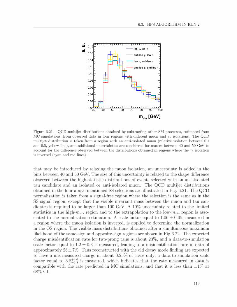
6.3. HPS ALGORITHM IN RUN-2
Figure 6.21 – QCD multijet distributions obtained by subtracting other SM processes, estimated fromMC simulations, from observed data in four regions with different muon and τh isolations. The QCDmultijet distribution is taken from a region with an anti-isolated muon (relative isolation between 0.1and 0.5, yellow line), and additional uncertainties are considered for masses between 40 and 50 GeV toaccount for the difference observed between the distributions obtained in regions where the τh isolationis inverted (cyan and red lines).
that may be introduced by relaxing the muon isolation, an uncertainty is added in thebins between 40 and 50 GeV. The size of this uncertainty is related to the shape differenceobserved between the high-statistic distributions of events selected with an anti-isolatedtau candidate and an isolated or anti-isolated muon. The QCD multijet distributionsobtained in the four above-mentioned SS selections are illustrated in Fig. 6.21. The QCDnormalization is taken from a signal-free region where the selection is the same as in theSS signal region, except that the visible invariant mass between the muon and tau can-didates is required to be larger than 100 GeV. A 10% uncertainty related to the limitedstatistics in the high-mvis region and to the extrapolation to the low-mvis region is asso-ciated to the normalization estimation. A scale factor equal to 1.06 ± 0.05, measured ina region where the muon isolation is inverted, is applied to determine the normalizationin the OS region. The visible mass distributions obtained after a simultaneous maximumlikelihood of the same-sign and opposite-sign regions are shown in Fig 6.22. The expectedcharge misidentification rate for two-prong taus is about 23%, and a data-to-simulationscale factor equal to 1.2 ± 0.3 is measured, leading to a misidentification rate in data ofapproximately 28±7%. Taus reconstructed with the old decay mode finding are expectedto have a mis-measured charge in about 0.25% of cases only; a data-to simulation scalefactor equal to 3.8+4.6
−3.8 is measured, which indicates that the rate measured in data iscompatible with the rate predicted in MC simulations, and that it is less than 1.1% at68% CL.
119

CHAPTER 6. TAU LEPTON RECONSTRUCTION AND IDENTIFICATION
The charge misidentification rate is measured separately for the old decay modes andfor the two-prong decays; it is expected to be higher for the two-prong taus, for whichthe charge is chosen as the charge of the leading track. A simultaneous fit is performed inthe SS and OS categories, considering the same nuisance parameters as for the efficiencymeasurement, except the following differences:
— The tau identification efficiency uncertainty is set to 5% and affects the signal inboth regions;
— The QCD normalization has a 10% uncertainty correlated between the OS and SSregions, and an additional 5% in the OS region only, associated to the OS/SS scalefactor.
Eve
nts/
bin
200
400
600
800
1000
Eve
nts/
bin
0
500
1000
1500
2000
2500
3000
(GeV)vism40 60 80 100
Obs
./Exp
.
0.60.8
11.21.4
Eve
nts/
bin
200
400
600
800
1000hτµτ→Z
DY others+jetstt
ElectroweakQCD multijetUncertaintyObserved
(13 TeV)-12.2 fb
CMSPreliminarySS
Eve
nts/
bin
200
400
600
800
1000
Eve
nts/
bin
0
500
1000
1500
2000
2500
3000
Eve
nts/
bin
200
400
600
800
1000
(GeV)vism40 60 80 100
Obs
./Exp
.
0.60.8
11.21.4
Eve
nts/
bin
0
500
1000
1500
2000
2500
3000 hτµτ→ZDY others
+jetsttElectroweakQCD multijetUncertaintyObserved
(13 TeV)-12.2 fb
CMSPreliminaryOS
Eve
nts/
bin
200
400
600
800
1000
1200
1400
1600
1800
2000
Eve
nts/
bin
0
200
400
600
800
1000
1200
(GeV)vism40 60 80 100
Obs
./Exp
.
0.60.8
11.21.4
Eve
nts/
bin
200
400
600
800
1000
1200
1400
1600
1800
2000hτµτ→Z
DY others+jetstt
ElectroweakQCD multijetUncertaintyObserved
(13 TeV)-12.2 fb
CMSPreliminarySS
Eve
nts/
bin
200
400
600
800
1000
1200
1400
1600
1800
2000
Eve
nts/
bin
0
200
400
600
800
1000
1200
Eve
nts/
bin
200
400
600
800
1000
1200
1400
1600
1800
2000
(GeV)vism40 60 80 100
Obs
./Exp
.
0.60.8
11.21.4
Eve
nts/
bin
0
200
400
600
800
1000
1200hτµτ→Z
DY others+jetstt
ElectroweakQCD multijetUncertaintyObserved
(13 TeV)-12.2 fb
CMSPreliminaryOS
Figure 6.22 – Visible mass distributions for the muon and τh candidates, in regions where they have thesame (left) or a different (right) electric charge, obtained after a simultaneous maximum likelihood fit inboth regions. The τh candidates considered in the top row figures pass the old decay mode finding, whilein the row below they are reconstructed in one of the two-prong decay modes exclusively. [110]
120

6.4. CHAPTER SUMMARY AND PERSONAL CONTRIBUTIONS
6.4 Chapter summary and personal contributions
Tau lepton reconstruction and identification in CMS
Tau leptons are an important ingredient in physics analyses, especially in the scalarsector where their high mass compared to other leptons and to most quarks makethem a favored decay channel for scalars. Due to their short lifetime, taus decaywithin the CMS detector: in about one third of cases they decay to an electronor a muon plus neutrinos, while they otherwise decay hadronically. This chapterdescribes first how hadronically decaying taus are identified in CMS. The first stepof the HPS algorithm is to reconstruct tau candidates in one of the possible decaymodes by counting the number of tracks and ECAL energy deposits. The secondstep prevents jets, electrons and muons from being misidentified as hadronicallydecaying taus, by applying among others isolation conditions. Typically, the al-gorithm efficiency is 60% for a j → τh misidentification rate at the percent level,e → τh rate at the permille level and µ → τh rate below the permille level. Theperformance of the algorithm is also measured in data collected by the CMS detec-tor in 2012 and 2015. In particular, the efficiency in data is seen to be compatiblewith the efficiency predicted by MC simulations, with about 6% uncertainty.
My contributions
Figures: 6.4-6.17, 6.20-6.22.
I have been responsible for the tau identification efficiency measurement in Z → τµτhand in tt → bbµτh events, for the anti-lepton discriminator efficiency performancein Drell-Yan events, for the tau charge misidentification rate measurement, as wellas for the maximum likelihood fits for the e→ τh and µ→ τh misidentification ratemeasurements.
121


Part III
SM physics analyses
The next chapters detail searches for the SM scalar boson decaying to tau leptons.Chapter 7 is devoted to the associated production with a Z boson, Chapter 8 to the associ-ated production with a W boson in the eµτh final state, and Chapter 9 to the combinationof the searches for the SM scalar boson decaying to taus produced in gluon-gluon fusion,vector boson fusion or in association with a vector boson.


Chapter 7
Search for the SM scalar in the ZH → ``ττchannel
In the SM, the scalar boson decays approximately 6% of the time to taus if it hasa mass around 125 GeV. This decay mode, despite its relatively large branchingfraction, is challenging experimentally due to the similarity between hadronicallydecaying taus, and quark and gluon jets. This chapter focuses on the productionof the SM scalar boson in association with a Z boson that decays to a pair of lightleptons (µµ or ee) [16]. Even if the ZH associated production has a low crosssection (about 2% of the total H boson production cross section at the LHC), thetwo light leptons that originate from the Z boson can be identified more efficientlythan hadronic taus and contribute to a great background reduction.
7.1 Analysis overview
The analysis covers eight different final states. The Z boson can decay to a di-muon pairor to a di-electron pair, while the di-tau final states from the H boson decay consideredin this analysis are τeτµ, τeτh, τµτh and τhτh. Two di-tau final states, τeτe and τµτµ are notstudied because they overlap with the H → ZZ∗ search [60] and have anyway a very lowbranching fraction. The dominant irreducible background comes from the ZZ dibosonproduction, while tiny irreducible contributions are also due to the ttZ process. The restof the background consists in reducible processes, for which at least one jet is misidentifiedas one of the four final state leptons. Reducible processes include essentially Z+jets andWZ+jets processes, but also small fractions of tt or QCD multijet processes among others.Irreducible processes are estimated directly from MC samples, while reducible processesare estimated with data-driven methods based on the misidentification rates of jets asleptons. Data samples correspond to 5.0 and 19.7 fb−1 of parked datasets collected at 7and 8 TeV respectively with a di-muon trigger path. The complete list of MC samples,collected datasets and trigger paths, used in this analysis, can be found in Appendix A.The selected data and the expected processes are binned in distributions using the full
125

CHAPTER 7. SEARCH FOR THE SM SCALAR IN THE ZH → ``ττ CHANNEL
invariant mass of the taus (see Section 7.4) as an observable, and results are obtainedfrom a fit of the expected processes to the observed data.
7.2 Selection
The event selection proceeds in three successive steps:— Z boson candidate selection, from two same-flavor light leptons;— H boson candidate selection, from two leptonic or hadronic taus;— Other selection criteria common to all final states.
7.2.1 Z boson candidate selection
The Z boson candidate is reconstructed from two opposite-sign same-flavor light lep-tons. The dilepton invariant mass is required to be compatible with the Z boson mass:|m``−mZ | < 30 GeV. This selection criterion is loose because most backgrounds also havea real Z boson. The events are triggered based on the two light leptons, and are requiredto fire trigger paths with either two muons with pT (µ1) > 17 GeV and pT (µ2) > 8 GeV atHLT, or two electrons with pT (e1) > 17 GeV and pT (e2) > 8 GeV at HLT. This involvesthat, to safely select events in the trigger efficiency plateau, the offline pT for the lightleptons are required to be larger than 20 GeV for the leading lepton, and 10 GeV for thesubleading one.
The electrons in the case of Z → ee decays are required to pass the very loose PFidentification (see Section 5.2.4) and to have a relative δβ-corrected isolation less than0.3. In addition, their pseudorapidity is such that |η| < 2.5. The muons in the case ofZ → µµ decays are global or tracker muons, and have an absolute pseudorapidity lessthan 2.4. They are required to pass the loose PF identification, and to have a relativeδβ-corrected isolation less than 0.3.
7.2.2 H boson candidate selection
After a good Z boson candidate has been found, the four di-tau final states are se-lected with different criteria. In every case, the two tau candidates are required to carryan opposite-sign charge and to have a transverse impact parameter with respect to thebeam, |dz|, less than 0.1.
To select H → τhτh decays, two hadronic taus with visible pT greater than 15 GeV and|η| less than 2.3 are required. The taus need to pass the decay mode finding discrimina-tor, and the medium cut-based isolation is chosen because it gives the best compromisebetween signal efficiency and background (essentially Z+jets) rejection, and brings thehighest signal sensitivity. In order to reject electrons or muons misidentified as hadronictaus, the loose working points of the discriminator against electrons (MVA-based) andmuons (cut-based) are applied to the tau candidates.
126

7.2. SELECTION
Final state τ isolation e/µ relative isolation LT (GeV)``τhτh medium cut-based - 70``τeτh loose cut-based 0.2 30``τµτh loose cut-based 0.3 45``τeτµ - 0.3 25
Table 7.1 – Optimal thresholds on the lepton isolation and on LT for the different di-tau final states.
The selection of the H → τeτh channel requires the presence of an electron with pTgreater than 10 GeV and |η| less than 2.5, and of a hadronic tau with pT greater than15 GeV and |η| less than 2.3. The electron is required to pass the loose MVA ID andto have a relative isolation less than 0.2. The hadronic tau is required to pass the decaymode finding discriminator, as well as the loose cut-based isolation, the loose cut-baseddiscriminator against muons and the tight working point of the MVA-based discriminatoragainst electrons to reduce the probability of selecting a Z boson decaying to a di-electronpair.
The H → τµτh decay is reconstructed from a muon with pT greater than 10 GeV and|η| < 2.4, and from a hadronic tau with pT greater than 15 GeV and |η| < 2.3. The muonis required to pass the tight PF identification and to have a relative δβ-corrected isolationless than 0.3. The hadronic tau needs to pass the decay mode finding discriminator, theloose cut-based isolation, the tight working point of the cut-based discriminator againstmuons and the loose working point of the cut-based discriminator against electrons.
In the H → τeτµ case, an electron with pT greater than 10 GeV and |η| < 2.5, as wellas a muon with pT greater than 10 GeV and |η| < 2.4, are selected. The muon is requiredto pass the tight PF identification and to have a relative δβ-corrected isolation less than0.3, while the electron passes the loose MVA identification and has a relative δβ-correctedisolation less than 0.3.
The identification and isolation conditions on the leptons have been chosen in sucha way as to optimize the analysis sensitivity to the hypothetical presence of a signal.Additionally, upper exclusion limits are found to improve if the events are selected witha minimal threshold on the LT variable, defined as the scalar sum of the visible trans-verse momenta of the two tau candidates. Indeed, backgrounds, and especially reducibleprocesses, typically produce leptons with lower transverse momenta than the signal. Thelight lepton isolation and LT thresholds in each final state are chosen to optimize simul-taneously the expected upper limits on the signal strength for a scalar boson with a massof 125 GeV, as shown in Fig. 7.1. The optimized isolation values have been quoted in theprevious paragraphs, and the LT thresholds are 70, 30, 45 and 25 GeV in the τhτh, τeτh,τµτh and τeτµ di-tau final states respectively. A summary of the optimized isolations andLT thresholds for the different di-tau final states are given in Tab. 7.1.
127
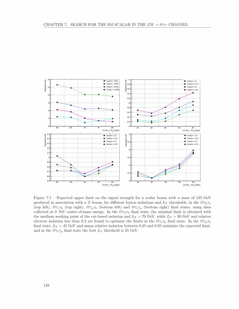
CHAPTER 7. SEARCH FOR THE SM SCALAR IN THE ZH → ``ττ CHANNEL
) [GeV]l2 + Ptl1
LT(=Pt60 65 70 75 80
Expe
cted
Lim
it
10
11
12
13
14
15
16Isolation < 3HitLIsolation < 3HitM
Isolation < MVALIsolation < MVAM
CMS Preliminary 2012 -1 = 8 TeV, L = 19.8 fbs LLTT SV_Mass
) [GeV]l2 + Ptl1
LT(=Pt25 30 35 40 45
Expe
cted
Lim
it12
12.2
12.4
12.6
12.8
13
13.2
13.4
13.6
13.8
14Isolation < 0.1Isolation < 0.15
Isolation < 0.2Isolation < 0.25
CMS Preliminary 2012 -1 = 8 TeV, L = 19.8 fbs LLET SV_Mass
) [GeV]l2 + Ptl1
LT(=Pt35 40 45 50 55
Expe
cted
Lim
it
8.5
8.6
8.7
8.8
8.9
9
9.1
9.2
9.3
9.4
9.5Isolation < 0.2Isolation < 0.25
Isolation < 0.3Isolation < 0.35
CMS Preliminary 2012 -1 = 8 TeV, L = 19.8 fbs LLMT SV_Mass
) [GeV]l2 + Ptl1
LT(=Pt20 25 30 35 40
Expe
cted
Lim
it
13
13.5
14
14.5
15
15.5
16Isolation < 0.2Isolation < 0.25
Isolation < 0.3Isolation < 0.35
CMS Preliminary 2012 -1 = 8 TeV, L = 19.8 fbs LLEM SV_Mass
Figure 7.1 – Expected upper limit on the signal strength for a scalar boson with a mass of 125 GeVproduced in association with a Z boson, for different lepton isolations and LT thresholds, in the ``τhτh(top left), ``τeτh (top right), ``τµτh (bottom left) and ``τeτµ (bottom right) final states, using datacollected at 8 TeV center-of-mass energy. In the ``τhτh final state, the minimal limit is obtained withthe medium working point of the cut-based isolation and LT > 70 GeV, while LT > 30 GeV and relativeelectron isolation less than 0.2 are found to optimize the limits in the ``τeτh final state. In the ``τµτhfinal state, LT > 45 GeV and muon relative isolation between 0.25 and 0.35 minimize the expected limit,and in the ``τeτµ final state the best LT threshold is 25 GeV.
128

7.3. BACKGROUND ESTIMATION
7.2.3 Other common selection criteria
In order to reduce backgrounds with b jets, such as tt (reducible) or ttZ (irreducible),events that have a jet with pT greater than 20 GeV, |η| < 2.4, and passing the mediumworking point of the CSV discriminator are discarded. In addition, the four selectedleptons need to be separated from each other by at least ∆R = 0.5, and to come from thesame primary vertex (|dz| < 0.1). To prevent a single event from passing the selection ofdifferent final states, a veto on extra muons and electrons is imposed: if a muon or anelectron with relative isolation less than 0.3 and pT greater than 10 GeV is found on topof the four selected leptons, the event does not pass the selection for this final state.
7.3 Background estimation
7.3.1 Irreducible process estimation
The irreducible processes, ZZ → 4` in its qq and gg production modes, as well as thetiny ttZ and ZH → ZWW contributions, are estimated from MC samples and normalizedto their (N)NLO cross sections. The H boson decays to a pair of W bosons contributemainly to the di-tau final state with one electron and one muon, and are considered as abackground because the search targets H boson decays to taus only.
7.3.2 Reducible process estimation
All backgrounds that possess at least one jet misidentified as one of the four final stateleptons, are estimated together with data-driven methods. The normalization and thedistribution of the reducible processes are estimated separately. The dominant contribu-tions come from Z+jets where two jets are misidentified as tau candidates, and WZ+jetswhere one jet is misidentified as a tau candidate.
Reducible background distribution
The distribution of the reducible background is obtained by selecting tau candidateswith a same-sign charge (SS region). This effectively removes the contributions fromZZ → 4` and from the signal, and only leaves reducible processes. However, applyingthe full selection described in Section 7.2 except that the charge requirement on the taucandidates is inverted, leads to a statistically limited control region. In order to obtainsmoother templates populated with more data events, some selection criteria that do notbias the distributions need to be relaxed. The isolation on the light leptons is relaxed to2.0 instead of 0.2 or 0.3 in the signal region; this can be shown not to bias the distributions(see Fig. 7.2). The hadronic taus are not required to pass the loose or medium workingpoints of the cut-based isolation, but to have a BDT output of the MVA-based isolationwithout lifetime information greater than 0. Relaxing the LT thresholds is seen to shiftthe mττ distributions to lower values, as shown in Fig. 7.3. Therefore, all LT thresholdsare kept the same as in the signal region.
129

CHAPTER 7. SEARCH FOR THE SM SCALAR IN THE ZH → ``ττ CHANNEL
[GeV]ττm0 50 100 150 200 250
a. u
.
0
0.05
0.1
0.15
0.2
0.25
iso>-0.3h
τRaw MVA
iso>0.0 (bbb errors)h
τRaw MVA
iso>0.3h
τRaw MVA
iso>0.5h
τRaw MVA
iso>0.8 (bbb errors)h
τRaw MVA
final statehτhτll at 8 TeV, -119.7 fb
[GeV]ττm0 50 100 150 200 250
a. u
.
0.05
0.1
0.15
0.2
0.25 iso>-0.3h
τRaw MVA
iso>0.0 (bbb errors)h
τRaw MVA
iso>0.3h
τRaw MVA
iso>0.5h
τRaw MVA
iso>0.8 (bbb errors)h
τRaw MVA
final stateh
τµll at 8 TeV, -119.7 fb
[GeV]ττm0 50 100 150 200 250
a. u
.
0
0.05
0.1
0.15
0.2
0.25 relative iso < 0.2 (bbb errors)µ
relative iso < 0.5µ
relative iso < 1µ
relative iso < 2 (bbb errors)µ
final stateh
τµll at 8 TeV, -119.7 fb
Figure 7.2 – Reducible background distributions in the ``τhτh (left) and ``τµτh (center and right) finalstates, obtained from a region where the two tau candidates have a same-sign charge, and no LT selectioncriteria are applied. The distributions are shown for different MVA output thresholds for hadronic tauisolations (left and center), or for different relative muon isolation (right). Within the statistical errors,the distributions are compatible with each other, which indicates that the isolation thresholds can berelaxed to obtain smoother non-biased templates.
[GeV]ττm0 50 100 150 200 250
a. u
.
0
0.05
0.1
0.15
0.2
0.25
> 30 GeVTL
> 50 GeVTL
> 70 GeVTL
final statehτhτll at 8 TeV, -119.7 fb
[GeV]ττm0 50 100 150 200 250
a. u
.
0.02
0.04
0.06
0.08
0.1
0.12
0.14
0.16
0.18
0.2
0.22
> 25 GeVTL
> 35 GeVTL
> 45 GeVTL
final stateh
τµll at 8 TeV, -119.7 fb
Figure 7.3 – Reducible background distributions in the ``τhτh (left) and ``τµτh (right) final states,obtained from a region where the two tau candidates have a same-sign charge, and pass the relaxedisolation values described in the text. The distributions are shown for different LT thresholds. As theLT selection criteria bias the reducible background mass distributions, they are not relaxed to model thedistribution in the signal region.
130
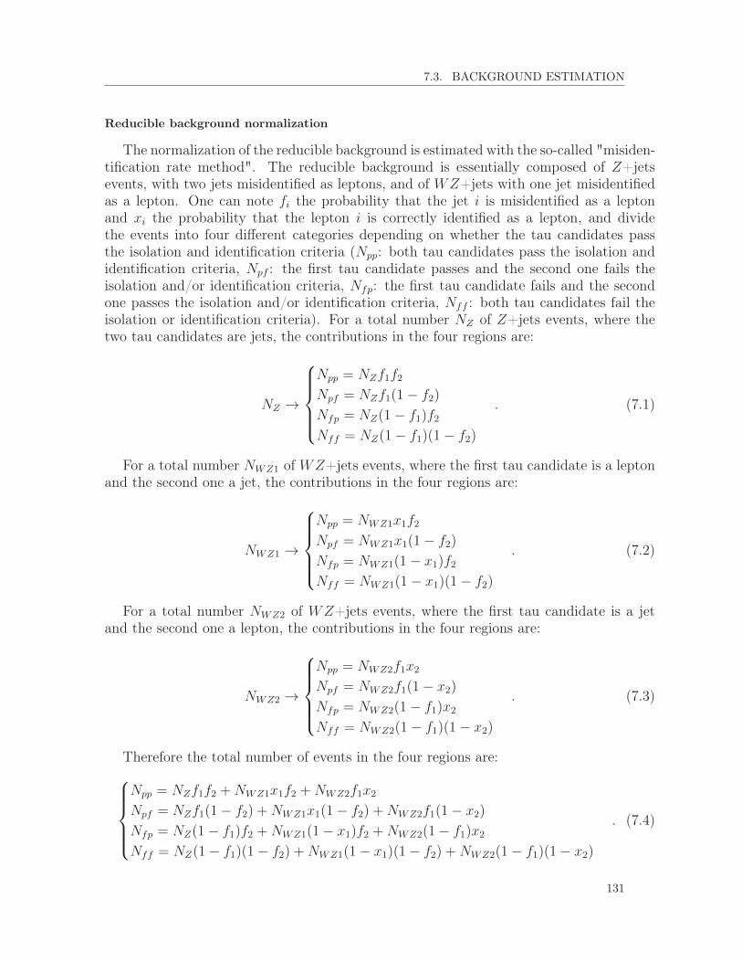
7.3. BACKGROUND ESTIMATION
Reducible background normalization
The normalization of the reducible background is estimated with the so-called "misiden-tification rate method". The reducible background is essentially composed of Z+jetsevents, with two jets misidentified as leptons, and of WZ+jets with one jet misidentifiedas a lepton. One can note fi the probability that the jet i is misidentified as a leptonand xi the probability that the lepton i is correctly identified as a lepton, and dividethe events into four different categories depending on whether the tau candidates passthe isolation and identification criteria (Npp: both tau candidates pass the isolation andidentification criteria, Npf : the first tau candidate passes and the second one fails theisolation and/or identification criteria, Nfp: the first tau candidate fails and the secondone passes the isolation and/or identification criteria, Nff : both tau candidates fail theisolation or identification criteria). For a total number NZ of Z+jets events, where thetwo tau candidates are jets, the contributions in the four regions are:
NZ →
Npp = NZf1f2
Npf = NZf1(1− f2)
Nfp = NZ(1− f1)f2
Nff = NZ(1− f1)(1− f2)
. (7.1)
For a total number NWZ1 of WZ+jets events, where the first tau candidate is a leptonand the second one a jet, the contributions in the four regions are:
NWZ1 →
Npp = NWZ1x1f2
Npf = NWZ1x1(1− f2)
Nfp = NWZ1(1− x1)f2
Nff = NWZ1(1− x1)(1− f2)
. (7.2)
For a total number NWZ2 of WZ+jets events, where the first tau candidate is a jetand the second one a lepton, the contributions in the four regions are:
NWZ2 →
Npp = NWZ2f1x2
Npf = NWZ2f1(1− x2)
Nfp = NWZ2(1− f1)x2
Nff = NWZ2(1− f1)(1− x2)
. (7.3)
Therefore the total number of events in the four regions are:Npp = NZf1f2 +NWZ1x1f2 +NWZ2f1x2
Npf = NZf1(1− f2) +NWZ1x1(1− f2) +NWZ2f1(1− x2)
Nfp = NZ(1− f1)f2 +NWZ1(1− x1)f2 +NWZ2(1− f1)x2
Nff = NZ(1− f1)(1− f2) +NWZ1(1− x1)(1− f2) +NWZ2(1− f1)(1− x2)
. (7.4)
131

CHAPTER 7. SEARCH FOR THE SM SCALAR IN THE ZH → ``ττ CHANNEL
One can see that the contribution of events in the signal region, Npp, is given by aweighted combination of the events in the three other regions:
Npp = Npff2
1− f2
+Nfpf1
1− f1
−Nfff1f2
(1− f1)(1− f2). (7.5)
The first term of the equation counts theWZ+jets events with the first tau candidate be-ing a lepton and the Z+jets events, whereas the second term counts the WZ+jets eventswith the second tau candidate being a lepton and the Z+jets events. The subtraction ofthe third term removes the Z+jets contribution because it has been counted twice. If Npp
ends up to be negative, the reducible background contribution is estimated to be equal tothe positive third term. The different terms of the equation are given for every final statestudied in this analysis in Tab. 7.2, together with the estimated reducible backgroundyield obtained by combining them.
Channel Nff Npf Nfp Estimated NppWeighted Raw Weighted Raw Weighted Raw
µµτhτh (7 TeV) 0.17 4545 0.15 24 0.16 55 0.14±0.05µµτeτh (7 TeV) 0.42 2943 0.65 37 0.80 132 1.03±0.18µµτµτh (7 TeV) 0.07 544 0.72 33 0.23 16 0.88±0.18µµτeτµ (7 TeV) 0.03 162 0.13 4 0.03 3 0.13±0.09eeτhτh (7 TeV) 0.15 4187 0.55 23 0.15 48 0.56±0.14eeτµτh (7 TeV) 0.09 555 0.33 27 0.07 8 0.31±0.09eeτeτh (7 TeV) 0.42 2969 1.00 54 0.46 87 1.04±0.19eeτeτµ (7 TeV) 0.04 148 0.09 7 0.09 6 0.15±0.08µµτhτh (8 TeV) 0.86 18849 3.04 157 0.91 270 3.09±0.30µµτeτh (8 TeV) 1.88 14107 6.53 187 2.74 502 7.38±0.62µµµτh (8 TeV) 0.39 2853 3.97 156 0.98 67 4.55±0.44µµτeτµ (8 TeV) 0.27 879 0.90 52 0.92 46 1.55±0.27eeτhτh (8 TeV) 0.81 17560 2.23 149 0.87 277 2.30±0.24eeτµτh (8 TeV) 0.36 2506 2.58 138 0.59 54 2.81±0.31eeτeτh (8 TeV) 1.75 12655 4.82 198 2.60 430 5.67±0.48eeτeτµ (8 TeV) 0.20 691 0.23 33 0.77 37 0.80±0.17
Table 7.2 – Weighted and raw contributions in the Nff , Npf and Nfp regions, and their combination toobtain an estimate of the yield of the reducible background in the Npp region. The last column is the sumof the weighted Nfp and Npf , minus the weighted Nff , and the quoted uncertainty is statistical only.
In order to apply the misidentification rate method, and to estimate the yields pre-sented in Tab. 7.2, the rates with which jets are identified as electrons, muons or hadronictaus need to be computed. They are evaluated from signal- and ZZ-free regions, obtainedwith the signal selection except that the tau candidates are required to carry a same-signcharge and that there is no requirement on their isolation and identification (such candi-dates are called "relaxed" in the rest of the section).
The rate with which jets j are misidentified as τh (j → τh misidentification rate)is computed for events with two relaxed τh candidates that have a same sign charge,
132

7.3. BACKGROUND ESTIMATION
[GeV]T
Jet p0 20 40 60 80 100 120 140
Mis
iden
tific
atio
n ra
te
-310
-210
-110
1 (8 TeV)-119.7 fb
(barrel)hτ→j
final stateshτlll
Fit uncertainty20% Error band
[GeV]T
Jet p0 20 40 60 80 100 120 140
Mis
iden
tific
atio
n ra
te
-310
-210
-110
1 (8 TeV)-119.7 fb
(endcaps)hτ→j
final stateshτlll
Fit uncertainty20% Error band
[GeV]T
Jet p0 20 40 60 80 100 120 140
Mis
iden
tific
atio
n ra
te
-310
-210
-110
1 (8 TeV)-119.7 fb
(barrel)hτ→j
final stateshτhτll
Fit uncertainty20% Error band
[GeV]T
Jet p0 20 40 60 80 100 120 140
Mis
iden
tific
atio
n ra
te
-310
-210
-110
1 (8 TeV)-119.7 fb
(endcaps)hτ→j
final stateshτhτll
Fit uncertainty20% Error band
Figure 7.4 – Rates with which jets are misidentified as hadronic taus, in the barrel (left) and endcap(right) regions, for the isolation working points used in the ```τh (top) and ``τhτh (bottom) final states.The fit uncertainties are shown with yellow bands, while 20% uncertainty bands are shown in blue.
following the ``τhτh selection criteria except that the LT threshold is lowered from 70to 50 GeV. It corresponds to the ratio between the number of relaxed taus passing theisolation over the total number of relaxed taus. There is a strong dependence of themisidentification rate on the transverse momentum of the taus, because high pT hadronictaus tend to get more collimated, which ensures a better distinction from quark and gluonjets. However the transverse momentum of tau candidates that do not pass the decaymode finding discriminator is not a well defined quantity, and a better variable is thetransverse momentum of the jet closest to the tau candidate. Therefore, the j → τhmisidentification rates are computed as a function of the transverse momentum of theclosest jet, and can be parameterized by decreasing exponentials with three constants c1,c2, and c3 as:
f(pT ) = c1 + c2ec3pT . (7.6)
The j → τh misidentification rates are measured separately for the loose and mediumworking points of the cut-based isolation, in the barrel and endcap regions, and the fourcorresponding curves are shown in Fig. 7.4 .
The j → e and j → µ misidentification rates are measured in events with a good Zboson candidate, a hadronic tau and a light lepton, following the ``τeτh and ``τµτh selec-tions. Again the tau candidates are required to carry the same charge, and the electronor muon isolation and identification criteria are relaxed. In order to increase the num-ber of selected events, the τh is required to have a pT larger than 5 GeV instead of 15
133

CHAPTER 7. SEARCH FOR THE SM SCALAR IN THE ZH → ``ττ CHANNEL
[GeV]T
Jet p0 20 40 60 80 100 120 140
Mis
iden
tific
atio
n ra
te
-310
-210
-110
1 (8 TeV)-119.7 fb
µ→j
final statesµell
Fit uncertainty30% Error band
[GeV]T
Jet p0 20 40 60 80 100 120 140
Mis
iden
tific
atio
n ra
te
-310
-210
-110
1 (8 TeV)-119.7 fb
e→j
final statesµell
Fit uncertainty30% Error band
[GeV]T
Jet p0 20 40 60 80 100 120 140
Mis
iden
tific
atio
n ra
te
-310
-210
-110
1 (8 TeV)-119.7 fb
µ→j
final statesh
τµll
Fit uncertainty30% Error band
[GeV]T
Jet p0 20 40 60 80 100 120 140
Mis
iden
tific
atio
n ra
te
-310
-210
-110
1 (8 TeV)-119.7 fb
e→j
final stateshτell
Fit uncertainty30% Error band
Figure 7.5 – Rates with which jets are misidentified as muons (left) or electrons (right), in the ``eµ (top)or ```τh (bottom) final states, for the isolation and identification working points used in the respectivefinal states. The fit uncertainties (shown with yellow bands) are fully covered by 30% uncertainty bands(shown in blue).
GeV in the signal region. The presence of events with real electrons and muons, such asWZ+jets events, is reduced by requiring the transverse mass between the light lepton andthe transverse missing energy to be less than 30 GeV. To be consistent with the j → τhcase, the misidentification rates are also parameterized as a function of the closest jet tothe electron/muon 1 with a decreasing exponential. They are measured for the differentisolation and identification criteria chosen to select the di-tau candidates in the differentfinal states. Because of the limited number of events selected, the misidentification ratesare measured for the barrel and endcap regions together. The misidentification rate func-tions are illustrated in Fig. 7.5.
To validate the background estimation method, the results from the reducible back-ground estimation in the ``τhτh are compared to the observed data, in a signal- and ZZ-freeregion where the two tau candidates have the same sign. Better statistical precision isachieved by relaxing the LT selection criterion and the hadronic tau isolation. As shownin Fig. 7.6, both are in good agreement, in terms of distribution and normalization.
1. If no jet is found within a cone of ∆R = 0.5 around the light lepton, then the transverse momentum of the lightlepton itself is considered.
134

7.4. DI-TAU MASS RECONSTRUCTION
[GeV]ττm0 50 100 150 200 250 300
Eve
nts
0
10
20
30
40
50 Observed
Estimation
8 TeV
hτhτll
Figure 7.6 – Comparison between the reducible background estimation and the observed data in the``τhτh final state, in a control region where the tau candidates have the same charge. Compared to thefinal signal selection, the isolation and LT conditions have been relaxed to increase the number of selectedevents.
7.4 Di-tau mass reconstruction
As neutrinos are always present in tau decays, computing the invariant mass of twotaus from their visible decay products underestimates the real mass of the resonance andleads to a poor mass resolution. The SVfit algorithm [111] can reconstruct the full di-taumass with a likelihood technique. The kinematics of a tau decay is described by two orthree parameters, in the case of hadronic or leptonic tau decays respectively:
— X, the fraction of tau energy carried by the visible decay products;— φ, the angle between the visible decay product system and the full tau lepton mo-
mentum vector;— mνν , the invariant mass of the two neutrinos in case of a leptonic tau decay.
This leads to between four and six unknowns for a di-tau system. However, only twomeasured parameters can constrain the momenta of the neutrinos: the transverse missingenergy magnitude and its orientation.
A probability P (mττ ) can be measured for any hypothetical di-tau mass mττ ; the bestestimate of the di-tau mass corresponds to the mass that maximizes this probability. Theprobability is computed as follows:
P (mττ ) =
∫δ(mττ −mττ (~y,~a))p(~x|~y,~a)d~a, (7.7)
where the tau decay pair kinematics is described by ~a = (X1, φ1,m1νν , X2, φ2,m
2νν), the
visible decay product momenta are given by ~y = (pvis1 , pvis2 ) and the missing transverseenergy vector is ~x. The expression p(~x|~y,~a) represents the probability that a given missingtransverse energy is measured knowing the values of the visible decay products momenta
135

CHAPTER 7. SEARCH FOR THE SM SCALAR IN THE ZH → ``ττ CHANNEL
and the tau decay kinematics.
The likelihood p(~x|~y,~a) is the product of the likelihood functions for both tau decaysand of the likelihood function describing the compatibility of a di-tau pair decay with themeasured ~
��ET . The individual likelihood functions are the following ones:
— Leptonic tau decays are modeled with matrix elements, and, assuming unpolarizedtaus, their likelihood functions read:
Lτ` =dΓ
dXdmννdφ∝ mνν
4m2τ
(m2τ + 2m2
νν)(m2τ −m2
νν). (7.8)
— For hadronic tau decays, the likelihood function is:
Lτh =dΓ
dXdφ=
1
2π
1
1− m2vis
m2τ
, (7.9)
where the visible decay products are considered as a single particle with mass mvis.
— If neutrinos are the only source of missing transverse energy, the measured ~��ET
should be equal to the vectorial sum of the transverse momenta of all neutrinos.However some differences between the two quantities can occur because of experi-mental resolution effects. The latter are taken into account when building the ��ET
likelihood, assuming a Gaussian resolution:
Lν =1
2π√|V |
exp
(−1
2
(��Ex − Σpνx��Ey − Σpνy
)TV −1
(��Ex − Σpνx ��Ey − Σpνy
)). (7.10)
In this expression V is the missing transverse energy covariance matrix of the event.
With respect to the so-called visible mass, the SVfit mass, later simply denoted mττ ,improves significantly the mass resolution and ensures a better discrimination betweenthe scalar boson signal and the Z boson background, as illustrated in Fig. 7.7. In thecontext of the analysis presented in this chapter, the improvement on the expected upperlimit brought by using the SVfit algorithm, ranges from about 10 to 40% depending onthe probed H mass, as illustrated in Fig. 7.8.
7.5 Systematic uncertainties and simulation corrections
The simulations are reweighted so that they reproduce the number of true verticesmeasured in data.
Theoretical uncertainties on the signal cross section arise from variations of the renor-malization and factorization scales (2.9% and 3.1% at 7 and 8 TeV respectively), and from
136

7.5. SYSTEMATIC UNCERTAINTIES AND SIMULATION CORRECTIONS
[GeV]vism0 50 100 150 200 250
[1/
GeV
]vi
s1/
dm
0
0.02
0.04
0.06
0.08
0.1
0.12
0.14
0.16
0.18
0.2 = 125 GeVH mττ →H
ττ →Z
= 8 TeVsCMS Simulation hτµ
[GeV]ττm0 50 100 150 200 250
[1/
GeV
]ττ
1/d
m
0
0.02
0.04
0.06
0.08
0.1
0.12
0.14
0.16 = 125 GeVH mττ →H
ττ →Z
= 8 TeVsCMS Simulation hτµ
Figure 7.7 – Invariant mass of two taus, using only visible decay products (left) or with the SVfit algorithm(right). One tau is chosen to decay hadronically, while the second one decays leptonically to a muon plusneutrinos. The Z → ττ background is represented by the filled yellow area, whereas the black distributionrepresents a SM scalar boson signal with a mass of 125 GeV. The SVfit mass enhances the separationbetween the two processes with respect to the visible mass, and brings a better mass resolution for thesignal. [16]
[GeV]Hm90 100 110 120 130 140 150
SM
σ/σ95
% C
L lim
it on
0
2
4
6
8
10
12
14
16
18
20Visible mass
SV mass
(8 TeV)-1llLL, 19.7 fb→ZH
Figure 7.8 – Expected upper limits at 95% CL on the signal strength of the H boson, in the ZH → ``ττchannel, with 8 TeV data. The orange dashed line indicates the limit obtained when using the visibleinvariant mass of the taus as observable, and the plain blue line shows the corresponding limit when theSVfit-reconstructed mass, mττ , is the observable.
137

CHAPTER 7. SEARCH FOR THE SM SCALAR IN THE ZH → ``ττ CHANNEL
uncertainties on the parton distribution functions (2.7% and 2.5% at 7 and 8 TeV respec-tively) [112]. The ZZ production cross section also suffers from theoretical uncertaintiesfrom parton distribution functions and QCD scale. The uncertainty on the cross sectionof the ttZ process is 50% [113, 114], while 44% uncertainty is assigned to the gg → ZZbackground to account for theoretical uncertainties from QCD scale.
Because the lepton identification and isolation efficiencies differ in data and simula-tions, the MC events are reweighted with some scale factors, determined via tag and probemethods. The scale factors and their uncertainties are usually measured for different pTand |η| values of the leptons. The uncertainties amount to 2% per single muon, 2% persingle electron and 6% per single hadronic tau. Conservatively, they are multiplied bythe number of leptons. The simulations are also corrected for the differences in triggerefficiency observed in data. The muon and electron trigger efficiency uncertainties amountto 1% and are also measured from tag and probe methods. An uncertainty of 1%, intro-duced by the b-tag veto, is associated to the yield of all processes estimated from MCsimulations. The effect on the yield is relatively small because the mis-tagging rate is low.The luminosity uncertainty amounts to 2.2% in 2011 [115] and 2.6% in 2012 [109]. It isfully correlated between all processes estimated from MC samples, namely the irreduciblebackgrounds (ZZ → 4`, ttZ and ZH → ZWW ) and the signal samples.
An uncertainty of 3% is related to the tau energy scale, as explained in Chapter 6. Thisdoes not only impact the normalization of the distributions taken from MC simulations(if a tau has a larger energy, it is more likely to pass the pT threshold requirements),but also their distributions (mττ strongly depends on the visible four-momenta of thetwo taus). Therefore the tau energy scale is considered as a shape uncertainty, and twoadditional distributions for every MC-estimated process, corresponding to the variationsby ±1 standard deviation of the tau energy scale, are provided to compute the limits.The nominal and alternative distribution for the signal and irreducible backgrounds areshown in Fig. 7.9 for two di-tau final states.
The uncertainty on the normalization of the reducible background comes from the fitsof the misidentification rates, which are statistically limited. The fit functions are mod-ified within their uncertainties, and the yields of the reducible processes are recomputedfor the variations, which permits to compute a yield uncertainty related to the modifi-cations of the fit functions. It can be seen that a 20 or 30% uncertainty band can coverthe variations of the j → τh or j → e/µ fit functions respectively. The uncertainty asso-ciated to a given fit function is fully correlated between the final states where it is usedto compute the reducible background yield, while uncertainties associated to different fitfunctions are fully uncorrelated. The uncertainties by final state range from 15% (``τhτh)to 30% (``eµ). The smaller yield uncertainty in the ``τhτh final state is the consequenceof the better statistical precision in the fit functions because the j → τh misidentifica-tion rate is more than one order of magnitude larger than the j → `misidentification rates.
138

7.5. SYSTEMATIC UNCERTAINTIES AND SIMULATION CORRECTIONS
[GeV]ττm0 50 100 150 200 250 300
Eve
nts
/ 20
GeV
0
1
2
3
4
5Nominal
ESτ σ+1
ESτ σ-1
l 4→ZZ
final stateh
τµll at 8 TeV, -119.7 fb
[GeV]ττm0 50 100 150 200 250 300
Eve
nts
/ 20
GeV
0
0.5
1
1.5
2
2.5
3
3.5
Nominal
ESτ σ+1
ESτ σ-1
l 4→ZZ
final statehτhτll at 8 TeV, -119.7 fb
[GeV]ττm0 50 100 150 200 250 300
Eve
nts
/ 20
GeV
0
0.05
0.1
0.15
0.2
0.25
0.3
0.35
Nominal
ESτ σ+1
ESτ σ-1
=125)H
(mττll →ZH
final stateh
τµll at 8 TeV, -119.7 fb
[GeV]ττm0 50 100 150 200 250 300
Eve
nts
/ 20
GeV
0
0.05
0.1
0.15
0.2
0.25 Nominal
ESτ σ+1
ESτ σ-1
=125)H
(mττll →ZH
final statehτhτll at 8 TeV, -119.7 fb
Figure 7.9 – Nominal mττ distributions and their corresponding contributions when the tau energy scaleis varied by ±1 standard deviation, for the ZH → ``ττ signal (top) and ZZ → 4` background (bottom),in the ``τµτh (left) and ``τhτh (right) final states.
139

CHAPTER 7. SEARCH FOR THE SM SCALAR IN THE ZH → ``ττ CHANNEL
Because the number of events after all selection criteria is low for the MC-estimatedprocesses, an uncertainty between 5 and 50%, depending on the final number of events,is assigned to the MC processes 2. This uncertainty is not correlated between final statesas it only has a statistical origin, and is not correlated between processes either.
Finally, bin-by-bin errors are taken into account for every process, estimated from MCsimulations or with data-driven method. Because this results in a large number of ad-ditional shape uncertainties, these uncertainties are pruned: only those that modify theyield in a bin by more than 10%, or in a 50 GeV mττ window around 125 GeV, are kept.This pruning is checked to have a very limited impact on the final results.
A summary of the systematic uncertainties and of their effects on the yields of thedifferent processes can be found in Tab. 7.3.
Systematic Source Effect on yieldµµτhτh eeτhτh µµτeτh eeτeτh µµτµτh eeτµτh µµτeτµ eeτeτµ
Exp
erim
ent
Luminosity (2011) 2.2%Luminosity (2012) 2.6%
Muon trigger 1% - 1% - 1% - 1% -Electron trigger - 1% - 1% - 1% - 1%Muon ID/iso. 4% - 4% - 6% 2% 6% 2%
Electron ID/iso. - 4% 2% 6% - 4% 2% 6%Tau ID/iso. 12% 12% 6% 6% 6% 6% - -
Tau energy scale shape -b-Jet veto 1%
The
ory
PDF qq → ZZ 5%PDF gg → ZZ 10%PDF qq → ZH 2.5%
Scale variation qq → ZZ 6%Scale variation V H (2011) 3.1%Scale variation V H (2012) 2.9%
ttZ cross section 50%gg → ZZ cross section 44%
Backg
roun
destimation Loose j → τh rate - 20% -
Medium j → τh rate 15% -Tight j → e rate - 10% -
Loose j → e/µ rate - 30%Tight j → µ rate - 10% -Bin-by-bin errors shape
Limited gg → ZZ sample 5% 5% 5% 5% 5% 5% 5% 5%Limited qq → ZZ sample 5% 5% 5% 5% 5% 5% 5% 5%
Limited ttZ sample 50% 50% 30% 30% 30% 30% 15% 15%
Table 7.3 – Sources of systematic uncertainties, and the effects their variations by ±1 standard deviationhave on the yield of the different signal and background processes.
2. The most limited MC samples after selection, which are assigned an uncertainty as large as 50%, contribute to theexpected yield by a negligible amount.
140

7.6. RESULTS
Figure 7.10 – 3D view of a event compatible with a ZH → µµτµτh decay, recorded by CMS at 8 TeVcenter-of-mass energy in November 2012. In the figure, starting from the upper left corner and proceedingclockwise, the green cone indicates the hadronic tau (pT = 19.0 GeV) potentially coming from the SMscalar boson decay, the first red line in the negative pseudorapidity region represents the first muon(pT = 18.4 GeV), daughter of the Z boson, then, in the positive pseudorapidity, region the second redline indicates the muon (pT = 47.5 GeV) coming from the decay of the tau from the scalar boson decay,and the third red line represents the second muon coming from the Z boson (pT = 22.0 GeV). The Zboson candidate has a mass of 91.0 GeV and the full di-tau mass of the scalar boson candidate, mττ , is122.8 GeV. [116]
7.6 Results
After the selection, only 84 data events remain, and some of them have a di-tau massmττ compatible with 125 GeV. This is the case for example of an event recorded onthe 15th of November 2012: the event is selected with the µµτµτh selection and has mττ
equal to 122.8 GeV. A three-dimensional view of this particular event is shown in Fig. 7.10.
A simultaneous maximum likelihood fit is performed in all final states; the resultingpostfit distributions are shown in Fig. 7.11 and 7.12 at 7 and 8 TeV center-of-mass energyrespectively. The predicted and observed yields for the different final states and datataking periods are detailed in Tab. 7.4. The maximum likelihood fit permits to extractthe best-fit signal strength, as well as the pulls on the nuisance parameters. The signalstrength for the combination of the eight final states at 7 and 8 TeV is found to be:
µ = 1.61± 1.85. (7.11)
The spread of the measured signal strengths for the different di-tau final states and the
141

CHAPTER 7. SEARCH FOR THE SM SCALAR IN THE ZH → ``ττ CHANNEL
Process Signal Background Data SS+B
ee+ eµ 7 TeV 0.045 ± 0.002 1.0 ± 0.1 1 0.077µµ+ eµ 7 TeV 0.051 ± 0.002 1.0 ± 0.1 3 0.100ee+ τhτh 7 TeV 0.061 ± 0.004 1.1 ± 0.1 1 0.127µµ+ τhτh 7 TeV 0.073 ± 0.006 0.8 ± 0.1 0 0.195ee+ eτh 7 TeV 0.075 ± 0.004 2.2 ± 0.1 4 0.077µµ+ eτh 7 TeV 0.078 ± 0.004 2.2 ± 0.1 1 0.092ee+ µτh 7 TeV 0.087 ± 0.004 1.5 ± 0.1 2 0.135µµ+ µτh 7 TeV 0.111 ± 0.005 2.4 ± 0.3 2 0.103ee+ eµ 8 TeV 0.185 ± 0.007 4.0 ± 0.2 4 0.082µµ+ eµ 8 TeV 0.202 ± 0.008 5.1 ± 0.3 9 0.105ee+ τhτh 8 TeV 0.260 ± 0.020 4.8 ± 0.4 9 0.148µµ+ τhτh 8 TeV 0.285 ± 0.022 5.8 ± 0.4 4 0.150ee+ eτh 8 TeV 0.279 ± 0.013 10.2 ± 0.5 13 0.063µµ+ eτh 8 TeV 0.293 ± 0.014 12.2 ± 0.6 8 0.081ee+ µτh 8 TeV 0.385 ± 0.018 7.6 ± 0.4 11 0.149µµ+ µτh 8 TeV 0.427 ± 0.021 10.5 ± 0.6 12 0.092
Table 7.4 – Observed and predicted event yields in all final states and data taking periods. Backgroundcontributions are measured after a simultaneous maximum likelihood fit of all final states, whereas thesignal at mH = 125 GeV is normalized to the SM expectation. The last column, S/(S + B) representsthe ratio of the signal and signal-plus-background yields in the central mττ range containing 68% of thesignal events for mH = 125 GeV.
different data taking periods is shown in the left-hand side of Fig. 7.13. Computing thechi-square of this set of measured signal strengths with respect to the best-fit value µfor the combination, and comparing it to the chi-square distribution for toys generatedwith the background-plus-signal hypothesis with µ = µ, one can see that such a spread isexpected and reasonable. This is illustrated in the right-hand side part of Fig. 7.13.
As no excess of data above the expected backgrounds is observed, upper limits onthe signal strength are set at 95% CL, using the asymptotic CLs method. The limitsobtained in the four di-tau final states are shown in Fig. 7.14. The ``µτh final state is themost sensitive channel because of the clear signature left by muons in the detector, whilethe ``τhτh is the second one because of the large branching fractions for taus to decayhadronically. They can be combined together, as illustrated in Fig. 7.15. The upperexpected limits on the signal strength range from about 2.5 to 20 depending on the Hboson mass probed. These results are compatible with those obtained by the ATLASCollaboration [117].
142

7.6. RESULTS
[GeV]ττm
0 100 200 300
[1/
GeV
]ττ
dN
/dm
0.00
0.05
0.10
0.15
0.20
0.25 ττ →SM H(125 GeV)
Observed WW→SM H(125 GeV)
ZZReducible bkg.
Bkg. uncertainty
at 7 TeV -1CMS, 4.9 fb
µee + e
[GeV]ττm
0 100 200 300
[1/
GeV
]ττ
dN
/dm
0.00
0.05
0.10
0.15
0.20
0.25 ττ →SM H(125 GeV)
Observed WW→SM H(125 GeV)
ZZReducible bkg.
Bkg. uncertainty
at 7 TeV -1CMS, 4.9 fb
µ + eµµ
[GeV]ττm
0 100 200 300
[1/
GeV
]ττ
dN
/dm
0.00
0.05
0.10
0.15
0.20
0.25
0.30
0.35 ττ →SM H(125 GeV)
Observed WW→SM H(125 GeV)
ZZReducible bkg.
Bkg. uncertainty
at 7 TeV -1CMS, 4.9 fb
hτee + e
[GeV]ττm
0 100 200 300
[1/
GeV
]ττ
dN
/dm
0.00
0.05
0.10
0.15
0.20
0.25 ττ →SM H(125 GeV)
Observed WW→SM H(125 GeV)
ZZReducible bkg.
Bkg. uncertainty
at 7 TeV -1CMS, 4.9 fb
hτ + eµµ
[GeV]ττm
0 100 200 300
[1/
GeV
]ττ
dN
/dm
0.00
0.05
0.10
0.15
0.20
0.25 ττ →SM H(125 GeV)
Observed WW→SM H(125 GeV)
ZZReducible bkg.
Bkg. uncertainty
at 7 TeV -1CMS, 4.9 fb
hτµee +
[GeV]ττm
0 100 200 300
[1/
GeV
]ττ
dN
/dm
0.00
0.05
0.10
0.15
0.20
0.25 ττ →SM H(125 GeV)
Observed WW→SM H(125 GeV)
ZZReducible bkg.
Bkg. uncertainty
at 7 TeV -1CMS, 4.9 fb
hτµ + µµ
[GeV]ττm
0 100 200 300
[1/
GeV
]ττ
dN
/dm
0.00
0.05
0.10
0.15
0.20
0.25 ττ →SM H(125 GeV)
Observed WW→SM H(125 GeV)
ZZReducible bkg.
Bkg. uncertainty
at 7 TeV -1CMS, 4.9 fb
hτhτee +
[GeV]ττm
0 100 200 300
[1/
GeV
]ττ
dN
/dm
0.00
0.01
0.02
0.03
0.04
0.05
0.06
0.07
0.08
0.09ττ →SM H(125 GeV)
Observed WW→SM H(125 GeV)
ZZReducible bkg.
Bkg. uncertainty
at 7 TeV -1CMS, 4.9 fb
hτhτ + µµ
Figure 7.11 – Expected and observed mττ distributions in the eight different final states at 7 TeV. Thedistributions are obtained after a maximum likelihood fit that includes the nuisance parameters discussedpreviously. [16]
143

CHAPTER 7. SEARCH FOR THE SM SCALAR IN THE ZH → ``ττ CHANNEL
[GeV]ττm
0 100 200 300
[1/
GeV
]ττ
dN
/dm
0.00
0.05
0.10
0.15
0.20
0.25 ττ →SM H(125 GeV)
Observed WW→SM H(125 GeV)
ZZReducible bkg.
Bkg. uncertainty
at 8 TeV -1CMS, 19.7 fb
µee + e
[GeV]ττm
0 100 200 300
[1/
GeV
]ττ
dN
/dm
0.00
0.05
0.10
0.15
0.20
0.25
0.30
0.35 ττ →SM H(125 GeV)
Observed WW→SM H(125 GeV)
ZZReducible bkg.
Bkg. uncertainty
at 8 TeV -1CMS, 19.7 fb
µ + eµµ
[GeV]ττm
0 100 200 300
[1/
GeV
]ττ
dN
/dm
0.0
0.1
0.2
0.3
0.4
0.5ττ →SM H(125 GeV)
Observed WW→SM H(125 GeV)
ZZReducible bkg.
Bkg. uncertainty
at 8 TeV -1CMS, 19.7 fb
hτee + e
[GeV]ττm
0 100 200 300
[1/
GeV
]ττ
dN
/dm
0.00
0.05
0.10
0.15
0.20
0.25
0.30
0.35
0.40
0.45 ττ →SM H(125 GeV)
Observed WW→SM H(125 GeV)
ZZReducible bkg.
Bkg. uncertainty
at 8 TeV -1CMS, 19.7 fb
hτ + eµµ
[GeV]ττm
0 100 200 300
[1/
GeV
]ττ
dN
/dm
0.00
0.05
0.10
0.15
0.20
0.25
0.30
0.35
0.40
0.45 ττ →SM H(125 GeV)
Observed WW→SM H(125 GeV)
ZZReducible bkg.
Bkg. uncertainty
at 8 TeV -1CMS, 19.7 fb
hτµee +
[GeV]ττm
0 100 200 300
[1/
GeV
]ττ
dN
/dm
0.00
0.05
0.10
0.15
0.20
0.25
0.30
0.35
0.40
0.45 ττ →SM H(125 GeV)
Observed WW→SM H(125 GeV)
ZZReducible bkg.
Bkg. uncertainty
at 8 TeV -1CMS, 19.7 fb
hτµ + µµ
[GeV]ττm
0 100 200 300
[1/
GeV
]ττ
dN
/dm
0.00
0.05
0.10
0.15
0.20
0.25
0.30
0.35
0.40
0.45 ττ →SM H(125 GeV)
Observed WW→SM H(125 GeV)
ZZReducible bkg.
Bkg. uncertainty
at 8 TeV -1CMS, 19.7 fb
hτhτee +
[GeV]ττm
0 100 200 300
[1/
GeV
]ττ
dN
/dm
0.00
0.05
0.10
0.15
0.20
0.25 ττ →SM H(125 GeV)
Observed WW→SM H(125 GeV)
ZZReducible bkg.
Bkg. uncertainty
at 8 TeV -1CMS, 19.7 fb
hτhτ + µµ
Figure 7.12 – Expected and observed mττ distributions in the eight different final states at 8 TeV. Thedistributions are obtained after a maximum likelihood fit that includes the nuisance parameters discussedpreviously. [16]
144

7.6. RESULTS
SMσ/σBest Fit -20 -15 -10 -5 0 5 10 15 20
(7 TeV)µ + ell
(8 TeV)µ + ell
(7 TeV)h
τµ + ll
(8 TeV)h
τµ + ll
(7 TeV)hτ + ell
(8 TeV)hτ + ell
(7 TeV)hτhτ + ll
(8 TeV)hτhτ + ll
at 8 TeV-1 at 7 TeV, 19.7 fb-14.9 fb
-like)2χChannel Compatibility (0 5 10 15 20 25 30
Toys
0
2
4
6
8
10
12
14
16
18
20
22
24 at 8 TeV-1 at 7 TeV, 19.7 fb-14.9 fb
>obs) = 0.422χP(
Figure 7.13 – Left: Best-fit signal strengths per period and di-tau final state (black squares and reduncertainty lines), and combined measured signal strength (blue). Right: Observed chi-square (red arrow)and chi-square distribution for toys generated with a signal strength equal to the best-fit combined value.42% toys have a chi-square larger than the observed one, which indicates a very reasonable spread ofmeasured individual strengths.
[GeV]Hm100 120 140
SM
σ/σ95
% C
L lim
it on
0
5
10
15
20
25
30
35
40observedmedian expected
expectedσ 1± expectedσ 2±
at 8TeV-1 at 7TeV, 19.7 fb-14.9 fb
[GeV]Hm100 120 140
SM
σ/σ95
% C
L lim
it on
0
5
10
15
20
25
30
35
40observedmedian expected
expectedσ 1± expectedσ 2±
at 8TeV-1 at 7TeV, 19.7 fb-14.9 fb
[GeV]Hm100 120 140
SM
σ/σ95
% C
L lim
it on
0
5
10
15
20
25
30
35
40observedmedian expected
expectedσ 1± expectedσ 2±
at 8TeV-1 at 7TeV, 19.7 fb-14.9 fb
[GeV]Hm100 120 140
SM
σ/σ95
% C
L lim
it on
0
5
10
15
20
25
30
35
40observedmedian expected
expectedσ 1± expectedσ 2±
at 8TeV-1 at 7TeV, 19.7 fb-14.9 fb
Figure 7.14 – Observed and expected 95% CL upper limits on the signal strength in the ``τhτh (top left),``eτh (top right), ``µτh (bottom left) and ``eµ final states.
145

CHAPTER 7. SEARCH FOR THE SM SCALAR IN THE ZH → ``ττ CHANNEL
[GeV]Hm100 120 140
µ95
% C
L L
imit
on
0
2
4
6
8
10
12
14
16
18
20ObservedExpected
Expectedσ 1± Expectedσ 2±
at 8 TeV-1 at 7 TeV, 19.7 fb-1, 4.9 fbττ→CMS (unpublished) H
[GeV]Hm100 120 140
SM
σ/σ95
% C
L lim
it on
0
5
10
15
20
25
30 at 8TeV-1 at 7TeV, 19.7 fb-14.9 fb
Expected Limitµll + e
hτll + e
hτhτll +
hτµll +
ll + LL
Figure 7.15 – Expected and observed 95% CL upper limits on the scalar boson signal strength for thecombination of all final states at 7 and 8 TeV [116] (left) and decomposition of the expected limit betweendifferent di-tau final states (right).
7.7 Chapter summary and personal contributions
Search for the SM scalar in the Zh→ ``ττ channel
H → ττ is the most sensitive decay channel to test the Yukawa couplings of therecently discovered boson. Because of the large j → τh fake rate, studying thisdecay in the dominant gluon-gluon fusion production mode leads to large Drell-Yan and QCD multijet background. Even though the associated production witha Z boson has a cross section more than one order of magnitude lower, searchingfor ZH → ``ττ events is viable due to the large background reduction that canbe achieved by selecting the two light leptons originating from the Z boson. Theirreducible ZZ → 4` background is estimated from MC samples, while reducibleprocesses are determined via the misidentification rate method. The analysis issensitive to about four times the expected signal cross section in the SM.
My contributions
Figures: 7.2-7.6, 7.8-7.9, 7.11-7.15.
I have participated in the ZH → ``ττ results, at all stages of the analysis (selectionoptimization, background estimation, ...), and have been responsible for the limitsetting.
146

Chapter 8
Search for the SM scalar in the WH → eµτhchannel
The cross section for the associated production of the SM scalar boson with aW boson is several times larger compared to the associated production with a Zboson, but the background reduction is less strong because of a less clean signature.Two analyses have been performed with the data collected in Run-1 by the CMSdetector [16]: one for fully hadronic tau decays WH → `τhτh and the second onefor semi-leptonic di-tau final states WH → `τ`τh. The eµτh final state of thelatter channel, where the W boson decays to a light lepton and a neutrino, oneof the taus to a light lepton of the other flavor, and the other tau hadronically,is the object of this chapter.
8.1 Selection
This analysis targets leptonicW boson decays with one light lepton (electron or muon),leptonic decays of one of the taus, and hadronic decays of the other tau. The eµτh finalstate is described in this chapter, whereas the µµτh final state is included in [16], and theeeτh final state is not studied because of its lower sensitivity 1.
The events are selected with asymmetric electron-muon trigger paths, for which theleading lepton is required to have a transverse momentum greater than 17 GeV, and thesubleading one greater than 8 GeV. Offline, the lepton matched to the leading trigger legis required to have a transverse momentum greater than 20 GeV, while the lepton matchedto the subleading trigger leg should have a transverse momentum greater than 10 GeV. Inaddition, the electron candidate is selected with |η| < 2.5, |dz| < 0.2 cm, loose MVA iden-tification and a relative isolation less than 0.15 (0.10) for |η| < 1.479 (> 1.479). Requiringthe three charge estimates to be consistent with each other reduces the electron charge
1. The lower sensitivity of the eeτh final state compared to the µµτh final state can be explained by the more efficientmuon reconstruction and identification, and by the larger electron charge misidentification, which plays a role because thelight leptons are required to carry the same electric charge to reduce the Drell-Yan background.
147

CHAPTER 8. SEARCH FOR THE SM SCALAR IN THE WH → EµτH CHANNEL
misidentification rate. The muon candidate is selected with |η| < 2.4, |dz| < 0.2 cm, tightPF identification, and a relative isolation less than 0.15 (0.10) for |η| < 1.479 (> 1.479).Both light leptons are required not to be associated to a jet that has a CSV discriminatorgreater than 0.8. The tt background is drastically reduced by requiring the electron andthe muon to have the same electric charge. The τh candidate is required to have a differentelectric charge, to have pT > 20 GeV, |η| < 2.3, |dz| < 0.2 cm, and to pass the decay modefinding discriminator, the loose working point of the cut-based isolation, the loose workingpoint of the cut-based discriminator against electrons, and the loose working point of thecut-based discriminator against muons. In the case where the invariant mass between theelectron (muon) and tau candidates is in a 40-GeV wide window around the Z boson mass,the tight working point of the discriminator against electrons (muons) is chosen to reducethe Drell-Yan background Z/γ∗ → ee and Z/γ∗ → µµ contribution. All three objects arerequired to be separated by at least ∆R = 0.5. Events that contain a b-tagged jet (tightCSV working point), or additional identified electrons, muons or taus, are vetoed. The ex-tra lepton veto prevents any overlap with the ZH → ``ττ analysis described in Chapter 7.
Events collected at a center-of-mass energy of 8 TeV are divided into two categoriesaccording to LT , the scalar pT sum of the three leptons: the LT -high category is char-acterized by LT > 130 GeV and the LT -low one by LT < 130 GeV. Because of thelower integrated luminosity in 2011, 7 TeV events are grouped in a single category withLT > 70 GeV. This categorization improves the sensitivity of the analysis because signalevents typically have a larger LT than background events.
8.2 Background estimation
Irreducible backgrounds correspond to processes with at least three real leptons in thefinal state, namely WZ → 3`ν and ZZ → 4`. The ZZ → 4` process is reduced byrequiring the event not to have more than three identified leptons. These diboson con-tributions are estimated from MC samples, and normalized to their predicted NLO crosssections [118].
Other backgrounds feature at least one misidentified object, and are classified as re-ducible. Reducible processes include among othersW+jets, tt, though greatly reduced bythe same sign charge requirement on the light leptons, QCD multijet, and Z+jets events.These backgrounds are estimated together with a misidentification rate method. Theprinciple of the method is the same as described in Chapter 7 for the ZH → ``ττ analy-sis. In this case, the "fakeable" objects are considered to be the muon and the electron,and the j → e and j → µ rates therefore have to be measured in data. These misidentifi-cation rates are measured in a W+jets-enriched region in data, defined in the same wayas the signal region except that the events should not include a τh candidate. In addition,the region is enriched in W+jets events by requiring the transverse mass between the"tag" lepton (the lepton that passes all identification and isolation conditions) and the��ET to be greater than 55 GeV, and the transverse mass between the "probe" lepton (the
148

8.2. BACKGROUND ESTIMATION
lepton without identification and isolation conditions for which the misidentification rateis measured) and the ~��ET to be less than 35 GeV. In order to make the topology as closeas possible to the signal region, an additional jet with pT greater than 20 GeV is requiredto mimic the presence of the hadronically decaying tau.
The misidentification rates for electrons and muons are determined independently witha k-Nearest Neighbors (kNN) classifier (see Section 3.7). This allows the rates to dependon a large number of variables. In practice, three variables are chosen in this analysis:the probe lepton pT , the pT of the jet closest to the probe lepton, and the number ofjets with pT > 20 GeV in the event. The rate measured in collected data for jets to bemisidentified as muons is shown in Fig. 8.1 as a function of these three variables. As seenin the context of the ZH → ``ττ analysis, the misidentification rates strongly decreasewith the transverse momentum of the closest jet. The dependence with the lepton pT ismore complicated because of the contamination of real leptons from WZ events in thehigh-pT region. The number of jets variable is particularly useful to parameterize thedifference in the misidentification rates in different topologies; these rates indeed tend tobe lower for events with a large number of jets, such as tt events because of the higherhadronic activity that spoils the probe lepton isolation. The number of nearest neighborsis chosen to be equal to fifty, which ensures a good local description with limited statisticalfluctuations.
However, applying such a technique leads to an overestimation of the misidentificationrates, especially at high lepton pT , because of the contamination of ZZ and WZ eventswith real leptons in the W+jets enriched region. To remove these contributions, twoadditional kNN per lepton (muon or electron) are trained, respectively for ZZ and WZevents in MC simulations that pass the W+jets enriched region selection. The two kNNoutputs are subtracted from the data kNN output according to the expected contributionsof WZ and ZZ events in the data region, estimated from the process cross sections. Inparticular, the kNN outputs of these two MC samples are scaled by:
NMCLdata
NdataLMC, (8.1)
where NMC and Ndata are respectively the raw number of events in MC simulations anddata in the W+jets control region where the training is done, and LMC and Ldata are therespective integrated luminosities of the MC simulations and data samples.
The rates measured in such a way are applied to data events that pass the signal regionselection, except that the muon and/or the electron candidates do not pass the isolationand/or identification conditions. Assuming a misidentication rate fe for the electron can-didate (fe depends on the electron pT , on the pT of its closest jet, and on the number of jetswith pT > 20 GeV in the event), and a misidentification rate fµ for the muon candidate,events with two leptons failing the isolation and/or identification conditions are weightedwith fefµ
(1−fe)(1−fµ), events with the electron passing but the muon failing the identification
149

CHAPTER 8. SEARCH FOR THE SM SCALAR IN THE WH → EµτH CHANNEL
[GeV]T
Lepton jet p10 20 30 40 50 60 70 80 90 100
Mis
iden
tific
atio
n ra
te
-310
-210
-110
1
[GeV]T
Lepton p10 20 30 40 50 60 70 80 90 100
Mis
iden
tific
atio
n ra
te-310
-210
-110
1
Jet multiplicity0 2 4 6 8 10 12
Mis
iden
tific
atio
n ra
te
-310
-210
-110
1
Figure 8.1 – Rates with which jets are misidentified as muons, as a function of the pT of the jet closest tothe lepton candidate (left), of the lepton candidate pT (center), and of the number of jets with pT > 20GeV in the event. The misidentification rates are measured in a W+jets enriched region in data collectedin 2012 at 8 TeV center-of-mass energy. The increase of the misidentification rate with the lepton pT isdue to the contamination of real leptons from WZ events in the high pT region, while the decrease withthe number of jets is caused by the higher hadronic activity, which spoils the lepton isolation.
and/or isolation conditions are weighted with fµ1−fµ , and events with the muon passing
but the electron failing the identification and/or isolation conditions are weighted withfe
1−fe . As described in Chapter 7, the double counting of events with two fake leptons isremoved by subtracting the weighted contribution of events with two leptons failing theisolation and/or isolation conditions, to the sum of the two other weighted categories.
The reducible background estimation method is validated in a control region wherethe τh candidate has the same sign as the electron and the muon, and does not pass theloose working point of the cut-based isolation. This region is signal-free, and enrichedin reducible background. Fig. 8.2 illustrates the LT and mvis distributions; predictedbackgrounds agree with observed data both in terms of normalization and distribution. Aband corresponding to 30% uncertainty on the reducible background prediction is drawn.
The method of the e/µ misidentification rate is cross-checked with an independentmethod, which considers the τh candidate as the possibly misidentified object. The j → τhmisidentification rate is measured in a W+jets enriched region in data. The events in thecontrol region are selected with a single muon trigger; the muon candidate is required tohave pT > 24 GeV, |η| < 2.1, to pass the tight PF identification, and to have a relativeisolation less than 0.1 and a longitudinal impact parameter of the track with respect tothe primary vertex less than 0.2 cm. The region is enriched inW+jets events by requiringthe transverse mass of the muon and the��ET to be greater than 40 GeV. Two same-sign τhcandidates, with an opposite charge with respect to the muon, are also selected. Events
150

8.2. BACKGROUND ESTIMATION
[GeV]TL0 50 100 150 200 250 300
Eve
nts
0
10
20
30
40
50
60
70
80
Observed
ττ→H
WW→H
WZ
ZZ
Reducible
[GeV]vism0 20 40 60 80 100 120 140 160 180 200
Eve
nts
0
20
40
60
80
100
120
140 Observed
ττ→H
WW→H
WZ
ZZ
Reducible
Figure 8.2 – Distributions of LT (left) and of the visible invariant mass between the τh candidate and thesubleading light lepton (right), when all three objects have the same sign and the τh isolation condition isinverted. An uncertainty of 30% for the reducible background is drawn as a shaded area. No maximumlikelihood fit to the observed data has been applied. Only 8 TeV data are used in this figure.
that contain an extra light lepton (with pT > 15 GeV), or a b-tagged jet (with pT > 20GeV) are vetoed. The j → τh misidentification rate is measured in three pseudorapidityregions (|η| < 0.8, 0.8 ≤ |η| < 1.6, 1.6 ≤ |η| < 2.3), separately for 2011 and 2012data. The dependence of the misidentification rates with the τh transverse momentum isparameterized with Landau functions, as illustrated in Fig. 8.3. The mathematical formof Landau distributions is:
f(pT ) =1
π
∫ ∞0
e−x log x−xpT sin(πx)dx. (8.2)
Events in data that have a loose τh candidate that does not pass the isolation conditionare reweighted with a weight w:
w(pT ) =f(pT )
1− f(pT ), (8.3)
in order to estimate the reducible background contribution in the signal region. Thismethod estimates backgrounds that have jets misidentified as τh, but does not take intoaccount events where the τh corresponds to a real hadronically decaying tau or to ae/µ → τh object. Therefore, the small Drell-Yan background contribution is not in-cluded in the reducible background estimated with this method, and is instead directlytaken from MC samples. The reducible background obtained with the τh misidentificationmethod is compared to the one obtained with the e/µ misidentification method describedpreviously. The comparison in the high- and low-LT regions, shown in Fig. 8.4, demon-strates an excellent agreement between both techniques within statistical uncertainties.The background estimated with the e/µ misidentification rate method is considered as thedefault one, while the background estimated with the τh misidentification rate method isconsidered as an alternative with a shape uncertainty.
151

CHAPTER 8. SEARCH FOR THE SM SCALAR IN THE WH → EµτH CHANNEL
[GeV]T
phτ0 20 40 60 80 100
Mis
iden
tific
atio
n ra
te
0
0.01
0.02
0.03
0.04
0.05
[GeV]T
phτ0 20 40 60 80 100
Mis
iden
tific
atio
n ra
te
0
0.01
0.02
0.03
0.04
0.05
0.06
[GeV]T
phτ0 20 40 60 80 100
Mis
iden
tific
atio
n ra
te
0
0.01
0.02
0.03
0.04
0.05
0.06
0.07
Figure 8.3 – Rates with which jets are misidentified as hadronically decaying taus in the barrel (|η| < 0.8,left), transition (0.8 ≤ |η| < 1.6, center), and endcap (1.6 ≤ |η| < 2.3, right) regions. The misidentificationrates are measured in data collected in 2012 at 8 TeV center-of-mass energy, and are fitted with Landaufunctions.
[GeV]vism50 100 150 200 250 300
Eve
nts
/ bin
0
0.5
1
1.5
2
2.5
3
3.5 mis-IDµe/
mis-IDhτ
(8 TeV)-119.7 fb
TLow-L
[GeV]vism50 100 150 200 250 300
Eve
nts
/ bin
0
0.2
0.4
0.6
0.8
1
1.2
1.4
1.6
1.8
2
mis-IDµe/
mis-IDhτ
(8 TeV)-119.7 fb
THigh-L
Figure 8.4 – Comparison between the reducible background distributions obtained with the e/µ andτh misidentification rate methods, in the low-LT (left) and high-LT (right) regions. The shaded areascorrespond to statistical uncertainties only.
152

8.3. RESULTS
Goodness of Fit0 5 10 15
Num
ber o
f Toy
s
0
10
20
30
40
50
60
70
80
90 expected (from toys) = 125 GeVHm
τ τ →CMS, H
Goodness of Fit10 20 30 40
Num
ber o
f Toy
s
0
10
20
30
40
50 expected (from toys) = 125 GeVHm
τ τ →CMS, H
Figure 8.5 – Goodness-of-fit test in the eµτh final state, in data collected at 7 TeV (left) and 8 TeV (right)center-of-mass energy.
8.3 Results
The observable used to extract the upper exclusion limits is the visible invariant massbetween the τh candidate and the subleading light lepton. Leptons from leptonic decaysof taus originating from H bosons indeed tend to have a lower transverse momentumthan light leptons directly originating from W boson decays. The correct di-tau pair isreconstructed in about 70% of cases with this method. The SVfit mass is not used for theWH analyses with H → ττ because the��ET coming from the W boson decay is mixed tothe ��ET from the tau decays.
Many systematic uncertainties, such as the trigger efficiency, muon and electron iden-tification and identification, tau identification, tau energy scale, b-tagged jet veto, andluminosity uncertainties are in common with the ZH → ``ττ analysis described in Chap-ter 7. Uncertainties that differ include 30% uncertainty on the normalization of thereducible background due to the e/µ misidentification rate method, and the alternativereducible background distribution from the τh misidentification rate method. Addition-ally, diboson backgrounds estimated from MC samples (WZ and ZZ) are attributed PDFand QCD renormalization scale uncertainties (about 4% each), and a statistical uncer-tainty between 3 and 10% to account for the limited number of events remaining afterthe full signal selection.
Goodness-of-fit tests are performed for the 7 and 8 TeV distributions; the results areshown in Fig. 8.5. The observed goodness-of-fit lies in both cases in the bulk of thegoodness-of-fit distribution for toys experiments, which indicates a good agreement be-tween the process predictions and the observed data.
153

CHAPTER 8. SEARCH FOR THE SM SCALAR IN THE WH → EµτH CHANNEL
mH −2σ −1σ Median +1σ +2σ Obs. Limit90 GeV 1.40 1.90 2.73 3.96 5.56 3.3695 GeV 1.59 2.15 3.09 4.49 6.29 3.76100 GeV 1.77 2.41 3.45 5.04 7.04 4.10105 GeV 1.48 2.01 2.88 4.18 5.88 2.88110 GeV 2.13 2.89 4.14 6.02 8.46 4.09115 GeV 2.14 2.91 4.17 6.08 8.59 3.60120 GeV 2.33 3.17 4.58 6.71 9.50 4.02125 GeV 2.84 3.88 5.58 8.18 11.58 4.62130 GeV 3.53 4.83 6.97 10.27 14.58 5.53135 GeV 4.31 5.90 8.59 12.67 18.19 6.54140 GeV 5.82 7.98 11.59 17.09 24.40 8.81145 GeV 7.42 10.20 14.91 22.10 31.81 11.04
Table 8.1 – Expected and observed limits at 95% CL on the signal strength for the WH → eµτh process,for H boson masses between 90 and 145 GeV.
The visible mass distributions obtained with the 7 TeV data, and the 8 TeV data in thetwo categories, are shown in Fig. 8.6. A good agreement between predicted processes andobserved data is seen, and upper limits on the signal cross section are set at 95% CL. AtmH = 125 GeV, the analysis is sensitive to about 4.6 times the cross section expected inthe SM. All values for H boson masses between 90 and 145 GeV are indicated in Tab. 8.1.
154

8.3. RESULTS
[GeV]vism
50 100 150 200
[1/
GeV
]vi
sd
N/d
m
0.0
0.2
0.4
0.6
0.8
1.0
1.2
1.4 ττ →SM H(125 GeV)Observed
WW→SM H(125 GeV)WZZZReducible bkg.Bkg. uncertainty
at 8 TeV -1CMS, 19.7 fb
TL low
hτ + eµh
τµe +
[GeV]vism
50 100 150 200
[1/
GeV
]vi
sd
N/d
m0.0
0.1
0.2
0.3
0.4
0.5
0.6 ττ →SM H(125 GeV)Observed
WW→SM H(125 GeV)WZZZReducible bkg.Bkg. uncertainty
at 8 TeV -1CMS, 19.7 fb
TL high
hτ + eµh
τµe +
[GeV]vism
0 50 100 150 200
[1/
GeV
]vi
sd
N/d
m
0.00
0.05
0.10
0.15
0.20
0.25
ττ →SM H(125 GeV)Observed
WW→SM H(125 GeV)WZZZReducible bkg.Bkg. uncertainty
at 7 TeV -1CMS, 4.9 fb
hτ + eµh
τµe +
[GeV]Hm100 120 140
SM
σ/σ95
% C
L lim
it on
0
5
10
15
20
25
30
35
40observedmedian expected
expectedσ 1± expectedσ 2±
at 8TeV-1 at 7TeV, 19.7 fb-14.9 fb
Figure 8.6 – Observed and expected distributions of the visible invariant mass between the τh candidateand the subleading lepton, at 8 TeV in the low-LT (top left) and high-LT (top right) regions, and at 7TeV (bottom left). [16] The expected and observed limits at 95% CL on the signal cross section for thecombination of these distributions is shown in the bottom right part of the figure.
155

CHAPTER 8. SEARCH FOR THE SM SCALAR IN THE WH → EµτH CHANNEL
8.4 Chapter summary and personal contributions
Search for the SM scalar in the WH → eµτh channel
The WH production cross section is several times larger than the ZH productioncross section, but the level of background is higher because the W boson decayproducts are less efficient to select than the Z boson decay products. The eµτhdecay channel, where one of the light lepton promptly comes from the W bosonwhereas the other one comes from the decay of one of the taus originating fromthe H boson, is described in this chapter. A great background rejection is achievedby requiring the two light leptons to have the same electric charge. The reduciblebackground is estimated with a misidentification rate method that relies on theprobability for jets to be identified as light leptons. No excess of events is observed,and the analysis is sensitive to about five times the expected cross section timesbranching fraction for the process under study.
My contributions
Figures: 8.1-8.6.
I have cross-checked allWH → eµτh results up to the final limits for the publicationin [16].
156

Chapter 9
Combination of searches for the SM scalarboson decaying to taus
The two searches presented in Chapter 7 and 8, respectively ZH → ``ττ andWH → eµτh, are combined with searches for the SM scalar boson decaying totaus and produced in gluon-gluon fusion and vector boson fusion productions, aswell as with searches in theWH channel but with other final states (WH → `τhτhand WH → µµτh). This combination provides an important test of the H bosonYukawa couplings.
9.1 Gluon-gluon fusion and vector boson fusion production modes
The gluon-gluon fusion and vector boson fusion production modes are studied simul-taneously. Events are separated into different exclusive categories to increase the sig-nal/background discrimination based on kinematic properties of the signal:
— 2-jet: This category targets the VBF production. The events are required to haveat least two jets with pT greater than 30 GeV, and to pass additionally some criteriato increase the VBF signal purity, based on the invariant mass of the jets and theirseparation in the η-direction.
— 1-jet: This category targets the gluon-gluon fusion production with a jet from initialstate radiation.
— 0-jet: This category targets the gluon-gluon fusion production.The 2-jet and 1-jet categories are the most sensitive. Meanwhile the 0-jet category isthe least sensitive because of the overwhelming Drell-Yan background, but is useful toconstrain nuisance parameters. Events are further divided according to the transversemomentum of the H boson candidate (pHT = | ~pT (τ1) + ~pT (τ2) + ~
��ET |, where ~pT (τ1) and~pT (τ2) are the reconstructed visible transverse momenta of the taus), in order to selectH boson candidates boosted in the transverse plane, and according to the transverse mo-mentum of the tau candidates, as they are typically larger than the pT of taus originatingfrom Z bosons if mH > mZ .
157

CHAPTER 9. COMBINATION OF SEARCHES FOR THE SM SCALAR BOSON DECAYINGTO TAUS
The six possible di-tau final states are studied. The most sensitive final state is τµτh,whereas the least sensitive final states τeτe and τµτµ because of the small expected di-taubranching fraction. All details can be found in [16].
9.2 Vector boson associated production
Despite the small production cross section compared to the gluon-gluon fusion andvector boson productions, searching for a scalar boson decaying to taus and producedin association with a vector boson permits to constrain the scalar couplings to vectorbosons. Three final states studied in Run-1 in the context of the search for a SM scalarboson decaying to taus and produced in association with a vector boson, have not beenpresented in the previous chapters: WH → µτhτh, WH → eτhτh and WH → µµτh. Thelatter final state is covered with background estimation methods very similar to thoseused in the WH → eµτh analysis detailed in Chapter 8, and the Z/γ∗ → µµ backgroundis greatly reduced by requiring the two muon candidates in the event to have the sameelectric charge. The large reducible background in theWH → `τhτh final states is reducedby training a BDT and selecting events with a BDT output above a certain threshold.The BDT takes as input the τh candidate pT , the distance between the τh candidates,the missing transverse energy, as well as the ratio between the vectorial and scalar sumsof the τh candidate pT . The observable used to extract the results is the invariant massbetween the τh candidates.
The results of the combination between all V H analyses with H decays to taus per-formed in Run-1 are shown in Fig. 9.1 and Tab. 9.1. The limits increase with the massof the scalar boson probed because of the expected decrease of the branching fractionB(H → ττ). Although there is a small deficit of observed events compared to the ex-pected SM processes, the results are compatible both with the existence and the absenceof a SM scalar boson at a mass of 125 GeV. For this particular mass, the observed up-per limit at 95% CL on the signal strength lies at 2.1. The combined best-fit signalstrength is µ = −0.33 ± 1.02, which corresponds to µ = 1.61 ± 1.85 for the ZH chan-nels, µ = −3.15 ± 2.03 for the WH channels with two hadronically decaying taus, andµ = −1.57± 1.65 for the WH channels with exactly one hadronically decaying tau. TheV H analyses are expected to reach the SM sensitivity in Run-2 with the increase ofintegrated luminosity and the increase of center-of-mass energy.
9.3 Combination of all production modes
A comparison of the expected sensitivity of all the final states and categories combined,in terms of upper limits on the signal strength, is shown in Fig. 9.2. The searches in allproduction modes are combined together, and their uncertainties are correlated when ap-plicable. An excess of events is observed on top of the SM background predictions, as seenin Fig. 9.3 in the combined distribution of the decimal logarithm log(S/(S+B)) obtained
158

9.3. COMBINATION OF ALL PRODUCTION MODES
[GeV]Hm100 120 140
µ95
% C
L L
imit
on
0
2
4
6
8
10
12
14
16ObservedExpected
Expectedσ 1± Expectedσ 2±
at 8 TeV-1 at 7 TeV, 19.7 fb-1, 4.9 fbττ→CMS (unpublished) H
[GeV]Hm100 120 140
µ95
% C
L lim
it o
n
0
2
4
6
8
10
12
14
16
18
20 at 8 TeV-1 at 7 TeV, 19.7 fb-1, 4.9 fbττ→CMS (unpublished) H
expected
hτhτ + lhτ'l + l'LL + llττ→VH
Figure 9.1 – Left: Combined expected and observed 95% CL upper limit on the signal strength parameterµ = σ/σSM for the V H analyses. The background-only hypothesis includes the pp→ H(125GeV)→WWprocess for every value of mH . Right: Expected 95% CL upper limit on the signal strength parameterµ = σ/σSM in the background-only hypothesis, shown separately for each V H channel. [116]
mH −2σ −1σ Median +1σ +2σ Obs. Limit90 GeV 7.33 · 10−1 9.89 · 10−1 1.40 2.00 2.74 9.58 · 10−1
95 GeV 8.13 · 10−1 1.09 1.55 2.21 3.04 1.09100 GeV 8.91 · 10−1 1.20 1.70 2.42 3.33 1.13105 GeV 8.52 · 10−1 1.15 1.63 2.36 3.24 1.16110 GeV 9.77 · 10−1 1.32 1.87 2.69 3.71 1.29115 GeV 9.70 · 10−1 1.31 1.87 2.68 3.70 1.33120 GeV 1.08 1.47 2.09 3.01 4.17 1.81125 GeV 1.21 1.65 2.36 3.42 4.76 2.06130 GeV 1.47 2.01 2.87 4.16 5.82 2.98135 GeV 1.87 2.45 3.52 5.10 7.13 4.02140 GeV 2.36 3.21 4.61 6.72 9.43 5.70145 GeV 3.28 4.46 6.41 9.29 12.99 8.87
Table 9.1 – Observed and expected 95% CL upper limits on the signal strength for the combination ofall V H analyses with H decays to taus performed with Run-1 data.
159

CHAPTER 9. COMBINATION OF SEARCHES FOR THE SM SCALAR BOSON DECAYINGTO TAUS
Final state τeτe τµτµ τeτµ τhτhµ 0.05± 1.60 −0.54± 1.38 0.90± 1.03 1.31± 0.63
Final state τeτh τµτh V H Allµ 0.31± 0.55 1.01± 0.41 −0.33± 1.02 0.78± 0.27
Table 9.2 – Best-fit signal strengths for every final state for the gluon-gluon fusion and VBF analyses, forthe combination of the V H analyses, and for all H → ττ searches combined.
in each bin of the final discriminating variables for all event categories and channels, whereS denotes the expected signal yield at mH = 125 GeV and B the expected backgroundyield in a given bin. This results in the first evidence for the decay of the H boson toa pair of tau leptons, with an observed (expected) significance of 3.2 (3.7) standard de-viations for a mass of 125 GeV. The best-fit signal strengths in the different di-tau finalstates are given in Tab. 9.2; the slight deficit of events relative to the SM expectationsfor the scalar boson essentially comes from the τµτµ and τeτh final states in gluon-gluonfusion and VBF production modes, and from the V H analyses as described in Section 9.2.
The best-fit value for the signal strength is well compatible with the SM hypothesis:µ = 0.78±0.27 at mH = 125 GeV. The combined measured mass of the excess is obtainedafter a parabolic fit, illustrated in Fig. 9.3, and amounts to mH = 122±7 GeV. A likelihoodscan is shown in Fig. 9.4 for the combination of the analyses in the (kV , kf ) plane, wherethe coupling modifiers kV and kf quantify the ratio between the measured and the SMvalues for the couplings of the scalar boson to vector bosons and fermions respectively;the observed couplings are well compatible with the SM expectation. The constraintsin the kV direction essentially come from the searches for a scalar boson produced inassociation with a vector boson and in vector boson fusion. After combination of theH → ττ analysis with the search for the decay of the H boson to a pair of b quarks [119],the CMS Collaboration could show an evidence for the decay of the H boson to fermions,with a significance of 3.8 standard deviations (for 4.4 standard deviations expected) [120].The ATLAS Collaboration also announced an evidence for the H boson Yukawa couplingsto taus during LHC Run-1 [121].
160
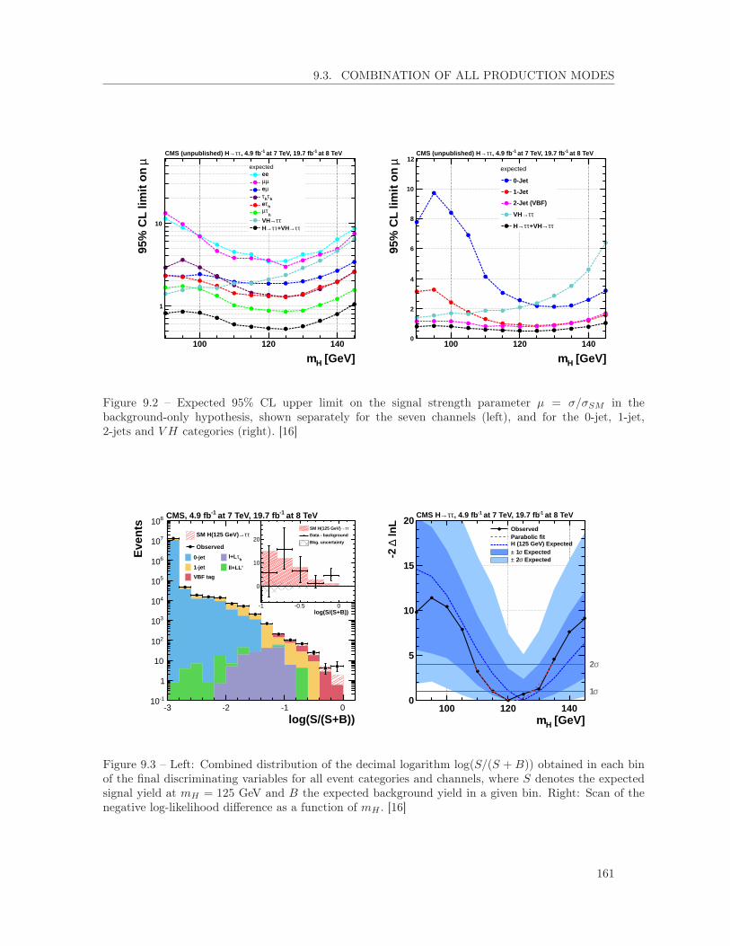
9.3. COMBINATION OF ALL PRODUCTION MODES
[GeV]Hm100 120 140
µ95
% C
L lim
it o
n
1
10
at 8 TeV-1 at 7 TeV, 19.7 fb-1, 4.9 fbττ→CMS (unpublished) H
expectedee
µµµe
hτhτhτe
hτµ
ττ→VHττ→+VHττ→H
[GeV]Hm100 120 140
µ95
% C
L lim
it o
n
0
2
4
6
8
10
12 at 8 TeV-1 at 7 TeV, 19.7 fb-1, 4.9 fbττ→CMS (unpublished) H
expected
0-Jet
1-Jet
2-Jet (VBF)
ττ→VH
ττ→+VHττ→H
Figure 9.2 – Expected 95% CL upper limit on the signal strength parameter µ = σ/σSM in thebackground-only hypothesis, shown separately for the seven channels (left), and for the 0-jet, 1-jet,2-jets and V H categories (right). [16]
log(S/(S+B))-3 -2 -1 0
Eve
nts
-110
1
10
210
310
410
510
610
710
810
ττ→SM H(125 GeV)
Observed
0-jet hτl+L
1-jet ll+LL'
VBF tag
log(S/(S+B))-1 -0.5 0
0
10
20
ττ→SM H(125 GeV)
Data - background
Bkg. uncertainty
at 8 TeV-1 at 7 TeV, 19.7 fb-1CMS, 4.9 fb
[GeV]Hm100 120 140
lnL
∆-2
0
5
10
15
20ObservedParabolic fitH (125 GeV) Expected
Expectedσ 1± Expectedσ 2±
σ1
σ2
at 8 TeV-1 at 7 TeV, 19.7 fb-1, 4.9 fbττ→CMS H
Figure 9.3 – Left: Combined distribution of the decimal logarithm log(S/(S + B)) obtained in each binof the final discriminating variables for all event categories and channels, where S denotes the expectedsignal yield at mH = 125 GeV and B the expected background yield in a given bin. Right: Scan of thenegative log-likelihood difference as a function of mH . [16]
161

CHAPTER 9. COMBINATION OF SEARCHES FOR THE SM SCALAR BOSON DECAYINGTO TAUS
Figure 9.4 – Scan of the negative log-likelihood difference as a function of the coupling modifiers kVand kf . The H → WW contribution is treated as a signal process. The red diamond indicates the SMexpectation. [16]
9.4 Chapter summary and personal contributions
Combination of searches for the SM scalar boson decaying to taus
The combination of all searches for H boson decays to taus, in the gluon-gluonfusion, vector boson fusion and V H associated productions, leads to an evidence forthe decay of the H boson to taus. The results are perfectly compatible with the SMexpectation, and the measured signal strength at mH = 125 GeV is µ = 0.78±0.27.The measured mass of the excess is mH = 122± 7 GeV.
My contributions
I have participated in the ZH → ``ττ and WH → eµτh results, at all stages ofthe analysis (selection optimization, background estimation, ...). I have been re-sponsible for computing and combining the statistical results (goodness-of-fit tests,maximum likelihood fits, upper limits) of all V H analyses.
162

Part IV
BSM physics analyses
The next chapters detail four searches for an extended scalar sector, which cover dif-ferent parts of the phase space of 2HDM type-2 and/or MSSM, or of 2HDM+S type-3.Chapter 10 is devoted to the search for a heavy pesudoscalar boson decaying to a Z bo-son and a scalar boson in the context of the MSSM and 2HDM type-2, Chapter 11 tothe search for exotic decays of the 125-GeV particle to light pseudoscalar bosons in theh→ aa→ µµττ channel in 2HDM+S, Chapter 12 to the search for a pseudoscalar lighterthan the Z boson decaying to taus and produced in association with b quarks in 2HDMtype-2, and Chapter 13 to the search for a heavy scalar decaying to tau leptons in theMSSM.


Chapter 10
Search for a heavy pseudoscalar boson Adecaying to Zh in the ``ττ final state
The A → Zh decay channel is studied to uncover a hypothetical extended scalarsector in the MSSM, or more generally in 2HDM type-2. It is sensitive to pseu-doscalar boson masses between about 215 GeV (sum of the masses of the h andZ bosons) and 350 GeV (twice the top quark mass), in the low tan β regions.The most sensitive final states are ``bb and ``ττ because they cover the largest hboson branching fractions, and, unlike the case of the SM H production in gluon-gluon fusion, do not suffer from high backgrounds or high triggering thresholdsthanks to the additional leptons coming from the Z boson decay. Both analy-ses have been performed using CMS data collected in 2012; the results from theA→ Zh→ ``bb search are available in [122], while the A→ Zh→ ``ττ searchresults are published in [123] and described below. The analysis workflow is closeto the search for the SM H boson produced in association with a Z boson, pre-sented in Chapter 7.
10.1 Differences with respect to the SM ZH → ``ττ analysis
Because there are many similarities between the selection and background estimationmethods of the present analysis and the SM ZH → ``ττ analysis detailed in Chapter 7,this section only highlights the differences; everything not mentioned should be assumedidentical to what was done for the SM ZH → ``ττ analysis. The same eight final states(corresponding to Z → µµ or Z → ee, and h → τhτh, h → τeτh, h → τµτh or h → τeτµ)are studied, but only in data collected in 2012 at a center-of-mass energy of 8 TeV.
The signal samples, with A boson masses between 220 and 350 GeV, are generatedwith Madgraph. Some rare processes, generated with Madgraph as well, are added to thelist of irreducible backgrounds: WWZ (σ = 0.0580 pb at 8 TeV), WZZ (σ = 0.0197 pbat 8 TeV) and ZZZ (σ = 0.0055 pb at 8 TeV) triboson productions. A 50% uncertaintyis assigned to the production cross sections of these rare triboson processes [124].
165

CHAPTER 10. SEARCH FOR A HEAVY PSEUDOSCALAR BOSON A DECAYING TO ZHIN THE ``ττ FINAL STATE
(GeV)recoAm
150 200 250 300 350 400 450
a. u
.
0.00
0.02
0.04
0.06
0.08
0.10
0.12
0.14
0.16 = 220 GeVAm = 240 GeVAm = 260 GeVAm = 280 GeVAm = 300 GeVAm = 320 GeVAm = 340 GeVAm
8 TeVττll→ Zh→A
Figure 10.1 – Reconstructed A boson mass, using the SVfit-reconstructed di-tau system. The full signalselection is applied, and all eight final states are superimposed. The resolution is between 15 and 20%for all masses.
The observable used in this analysis is the reconstructed mass of the pseudoscalar Aboson, mreco
A . It is computed as the invariant mass between the Z candidate and theSVfit-reconstructed di-tau system. A mass resolution between 15 and 20% is obtained forall masses. Fig. 10.1 illustrates the reconstructed mass distributions for different signalmass hypotheses, after the full signal selection.
The τh pT threshold is raised to 21 GeV instead of 15 GeV. This improves the sensitivityof the analysis because signal events typically have harder hadronic taus than backgroundevents (mostly reducible processes, but also ZZ → 4`). The LT thresholds described inChapter 7 are found to be optimal in this case also for all A boson masses probed, usingthe expected upper limits as a figure of merit. The LT distributions for the signal, andthe reducible and irreducible backgrounds are shown in Fig. 10.2 for the ``τhτh final state;the threshold at 70 GeV is seen to remove a large contribution from backgrounds whilekeeping a good signal efficiency. All the selection criteria are summarized in Tab. 10.1,while a cut-flow table, Tab. 10.2, gives indications about the efficiency of the differentselection criteria on signal events. It can be noted that no selection criterion is appliedto the mass of the di-tau system mττ , which is expected to be close to 125 GeV for signalevents. The reason is that such a criterion would bring a negligible improvement in thelimits becausemττ is highly correlated to the observablemreco
A in signal and in backgroundevents, and because the analysis is statistically limited.
166

10.1. DIFFERENCES WITH RESPECT TO THE SM ZH → ``ττ ANALYSIS
Z→``
Z → ee Z → µµe pT > 10/20 GeV, |η| < 2.5 -
Irel < 0.3, vLoose MVA ID -µ - pT > 10/20 GeV, |η| < 2.4
Irel < 0.3, Loose PF IDm`` 60 < m`` < 120 GeV
Charge Opposite sign charges
h→ττ
h → eµ h → eτh h → µτh h → τhτhe pT > 10 GeV, |η| < 2.5 - -
vLoose MVA ID Loose MVA IDIrel < 0.3 Irel < 0.2
τh - pT > 21 GeV, |η| < 2.3Loose isolation Loose isolation Medium isolationTight anti-e Loose anti-e Loose anti-eLoose anti-µ Tight anti-µ Loose anti-µ
µ pT > 10 GeV - pT > 10 GeV -|η| < 2.4 |η| < 2.4
Loose PF ID Tight PF IDIrel < 0.3 Irel < 0.3
Charge Opposite sign charges
Others h → eµ h → eτh h → µτh h → τhτh
LT > 25 GeV > 30 GeV > 45 GeV > 70 GeVb–Jet veto No b–tagged jet (medium CSV working point)Lepton veto No additional identified and isolated electron or muon
∆R between leptons > 0.5
Table 10.1 – Selection criteria for the eight final states of the A→ Zh→ ``ττ analysis.
µµτhτh µµeτh µµµτh µµeµ eeτhτh eeeτh eeµτh eeeµ
Initial number 99 794Trigger 61 577
At least 4 loose leptons 12 136 11 717 6 212 2 876 8 504 7 310 5 755 1 865b-Jet veto 10 109 10 276 5 551 2 660 7 018 6 332 5 045 1 711Z candidate 7 825 7 758 4 571 2 142 4 903 5 266 2 720 1 340h candidate 1 106 919 1 485 718 764 735 950 531LT cut 842 919 1 362 707 612 735 892 522
Table 10.2 – Number of unweighted signal events after every selection criterion, for a sample with mA =300 GeV.
167

CHAPTER 10. SEARCH FOR A HEAVY PSEUDOSCALAR BOSON A DECAYING TO ZHIN THE ``ττ FINAL STATE
(GeV)hTL
0 20 40 60 80 100 120 140 160 180 200
a.u
.
0.00
0.05
0.10
0.15
0.20
0.25
0.30Reducible background
ZZ irreducible
= 300 GeV)A
(mττll → Zh→A
8 TeV
CMShτhτll
ττll→ Zh→A
regionSignal
Figure 10.2 – Normalized distribution of the variable LT for events selected in the ``τhτh final state.The reducible background is estimated from data, instead the ZZ irreducible background comes from MCsimulation. The events are selected, in the signal region, with LT > 70 GeV. [123]
The normalization of the reducible processes is again taken from a control region wherethe two tau candidates have a same-sign charge and pass relaxed isolation criteria. Therelaxed isolation and identification criteria have been slightly modified with respect to theSM ZH analysis, and are namely:
— ``τhτh: output of the MVA discriminator without lifetime information greater than0 for both hadronic taus;
— ``τeτh: output of the MVA discriminator without lifetime information greater than-0.95 for the hadronic tau, loose MVA electron ID, relative electron isolation lessthan 0.3;
— ``τµτh: output of the MVA discriminator without lifetime information greater than-0.95 for the hadronic tau, loose PF muon ID, relative muon isolation less than 0.7;
— ``τeτµ: loose PF muon ID, no electron ID, electron and muon relative isolations lessthan 2.0.
These criteria have been chosen to ensure a selection efficiency as large as possible withoutbiasing the background composition. Indeed, in the semi-leptonic final states, relaxingthe isolation of the light lepton might lead to an over-representation of the Z+jets back-ground (no real isolated light lepton) over the WZ+jets background (one real isolatedlight lepton).
The j → e, j → µ and j → τh misidentification rates are reevaluated with the newselection; and the functions for the loose electron and loose muon ID/isolation are now
168

10.2. BACKGROUND ESTIMATION VALIDATION
[GeV]visττllm
0 200 400 600 800
[1/
GeV
]vi
s ττlld
N/d
m
0
20
40
60
80
100
120
140
160
180
200
220
240Observed 4l→ZZZ+1jet Z+2jetsZ+3jets Z+4jetsW+jets 2l2q→WZ
ν 3l→WZ WW+jets
tt
at 8 TeV -1 19.7 fb
hτ
hτ + ll
[GeV]visττllm
0 200 400 600 800
[1/
GeV
]vi
s ττlld
N/d
m
0.0
0.2
0.4
0.6
0.8
1.0
1.2
1.4Observed 4l→ZZZ+1jet Z+2jetsZ+3jets Z+4jetsW+jets 2l2q→WZ
ν 3l→WZ WW+jets
tt
at 8 TeV -1 19.7 fb
hτ + ell
Figure 10.3 – Visible invariant mass of the four leptons in the ``τhτh (left) and ``τeτh (right) final states,in a reducible background-dominated region, where the tau candidates carry a same sign charge, theLT selection criteria are not applied, and the hadronic tau isolation is inverted. Filled areas representbackground contributions estimated directly from MC simulations: the Z+jets processes by far dominatein the ``τhτh final state, while the WZ+jets contribution is not negligible in the other final states. Theagreement between MC predictions and data is not perfect because of large statistical and systematicuncertainties on the MC-estimated processes.
divided into barrel and endcap regions. The systematic uncertainties on the normalizationare again computed by varying the fit functions within their uncertainties and propagatingthese to the reducible processes yield.
10.2 Background estimation validation
The main components of the reducible background are Z+jets andWZ+jets processes,where one or two jets are misidentified as leptons. The first one is by far dominant inthe ``τhτh final state, whereas the WZ+jets contribution becomes non negligible in allother final states, with at least three identified light leptons. Fig. 10.3 shows some re-ducible background distributions, obtained by inverting the charge requirement on thetau candidates, relaxing the LT selection criteria and inverting the hadronic tau isolation.Contributions from MC processes are superimposed; they permit to see the backgroundcomposition, but suffer from large statistical (limited number of selected events) and sys-tematic (jet misidentification rates not well modeled in MC) uncertainties. The sameselection is applied to produce the distributions in Fig. 10.4, except that the hadronictau isolation is not inverted, but simply relaxed to the very loose working point of theMVA-based isolation with lifetime information. The data-driven reducible backgroundprediction is shown with the light blue line; the agreement between prediction and obser-vation is good within the uncertainties.
169

CHAPTER 10. SEARCH FOR A HEAVY PSEUDOSCALAR BOSON A DECAYING TO ZHIN THE ``ττ FINAL STATE
[GeV]visττllm
0 200 400 600 800
[1/
GeV
]vi
s ττlld
N/d
m
0.0
0.5
1.0
1.5
2.0
2.5Observed 4l→ZZ
Z+1jet Z+2jets
Z+3jets Z+4jets
W+jets 2l2q→WZ
ν 3l→WZ WW+jets
tt Reducible bkg.
at 8 TeV -1 19.7 fb
hτ
hτ + ll
[GeV]visττllm
0 200 400 600 800
[1/
GeV
]vi
s ττlld
N/d
m
0.00
0.02
0.04
0.06
0.08
0.10
0.12
0.14
0.16
0.18
0.20
0.22
0.24Observed 4l→ZZ
Z+1jet Z+2jets
Z+3jets Z+4jets
W+jets 2l2q→WZ
ν 3l→WZ WW+jets
tt Reducible bkg.
at 8 TeV -1 19.7 fb
hτ + ell
Figure 10.4 – Visible invariant mass of the four leptons in the ``τhτh (left) and ``τeτh (right) finalstates, in a reducible background-dominated region, where the tau candidates carry a same sign charge,the LT selection criteria are not applied, and the very loose MVA discriminator is used for hadronictau isolation. Filled areas represent background contributions estimated directly from MC simulations:the Z+jets processes by far dominate in the ``τhτh final state, while the WZ+jets contribution is notnegligible in the other final states. The agreement between MC predictions and data is not perfect becauseof large statistical and systematic uncertainties on the MC-estimated processes. The blue line representsthe data-driven prediction for the reducible background; the agreement with observed data is good.
Two di-tau final states have not been considered in this analysis: τeτe and τµτµ. Thereason is two-fold: they have the lowest branching fractions (about 3% each) and sufferfrom very large contributions from the ZZ → 4` background. Even if signal events typ-ically have a larger ��ET than background events due to the neutrinos from tau decays,adapting the selection does not permit to obtain a significant background rejection for areasonable signal efficiency. It has been shown that adding these two final states wouldbring less than 5% to the combined limit, with an almost zero effect for low mA signalhypotheses. However, the ``ee and ``µµ final states can be used to validate the estima-tion of the ZZ → 4` background. Fig. 10.5 shows a good agreement between the ZZbackground, taken from MC simulations, and the observed data, in an ``ee and an ``µµcontrol regions.
10.3 High ��ET excess
The��ET distributions obtained after the full signal selection are shown in Fig. 10.6. Anexcess of events is observed at large��ET values in four final states: eeeµ, µµµe, eeeτh andµµeτh. The expected and observed yields in these four final states for��ET > 120 GeV canbe found in Tab. 10.3. These events pass the filters to remove events with abnormally high��ET , as described in Section 5.2.7. The characteristics of the eight events that pass the fullsignal selection and have��ET > 120 GeV, are shown in Tab. 10.4. Most backgrounds, such
170

10.4. RESULTS
[GeV]Am0 200 400 600 800
[1/G
eV]
AdN
/dm
0.0
0.2
0.4
0.6
0.8
1.0
1.2
1.4
1.6 =330 GeV, xs=3fb)AAZh(m
Observed
ZZ
Reducible bkg.
at 8 TeV -1CMS Preliminary, 19.7 fb
+ eell
[GeV]Am0 200 400 600 800
[1/G
eV]
AdN
/dm
0.0
0.2
0.4
0.6
0.8
1.0
1.2
1.4
1.6
1.8
2.0=330 GeV, xs=3fb)AAZh(m
Observed
ZZ
Reducible bkg.
at 8 TeV -1CMS Preliminary, 19.7 fb
µµ + ll
Figure 10.5 – Reconstructed A boson mass distribution in the ``ee (left) and ``µµ (right) control regionsstates. The prediction for the ZZ background is well in agreement with the observed data, without anymaximum likelihood fit being applied. The A→ Zh signal contribution is negligible in both final states.
as ZZ → 4` or Z+jets, have a low ��ET , whereas triboson processes including W bosonsessentially contribute in high ��ET regions. The signal processes have real ��ET from thetau decays, but the typical ��ET for such events lies below 100 GeV. All observed eventswith high ��ET have two light leptons very compatible with a Z boson (invariant massbetween 85 and 93 GeV), while the two tau candidates do not correspond to a particularresonance. The excess is interpreted as an upward statistical fluctuation, particularly oftriboson processes.
10.4 Results
Goodness-of-fit tests (see Section 3.5) are performed for the four di-tau final states,as illustrated in Fig. 10.7. The observed goodness-of-fit values generally lie in the bulkof the toys distributions, which indicates a reasonable background description given theobserved data. Some limited tensions appear in the ``τµτh and ``τeτµ final states.
No significant excess of events is observed on top of the predicted backgrounds in anyof the final states, and model-independent limits can be set on the cross section timesbranching ratio for different mass hypotheses, as illustrated in Fig. 10.8. The observedcombined limit at 95% CL ranges from about 4 to 16 fb. Another search for A → Zhdecays was performed with the CMS detector in Run-1, in the final state with two lightleptons (from the Z boson) and two b quarks (from the h boson). In the hypothesisthat the ratio of the branching fractions of the h boson to taus and b quarks is thesame as in the SM, the search for A → Zh → ``bb is a few times more powerful thanthe A → Zh → ``ττ search presented here. However, this hypothesis might not holdand BSM phenomena could intervene; the A → Zh → ``ττ analysis therefore has an
171

CHAPTER 10. SEARCH FOR A HEAVY PSEUDOSCALAR BOSON A DECAYING TO ZHIN THE ``ττ FINAL STATE
MET [GeV]
0 100 200 300
dN
/dM
ET
[1/
GeV
]
-410
-310
-210
-110
1
10Zh (330 GeV, 10 fb)→A
Observed
Rare
ZZReducible bkg.
at 8 TeV -1 19.7 fb
hτ
hτ + ll
MET [GeV]
0 100 200 300
dN
/dM
ET
[1/
GeV
]
-410
-310
-210
-110
1
10Zh (330 GeV, 10 fb)→A
Observed
Rare
ZZReducible bkg.
at 8 TeV -1 19.7 fb
hτ + ell
MET [GeV]
0 100 200 300
dN
/dM
ET
[1/
GeV
]
-410
-310
-210
-110
1
10Zh (330 GeV, 10 fb)→A
Observed
Rare
ZZReducible bkg.
at 8 TeV -1 19.7 fb
hτµ + ll
MET [GeV]
0 100 200 300
dN
/dM
ET
[1/
GeV
]
-410
-310
-210
-110
1
10 Zh (330 GeV, 10 fb)→A
Observed
Rare
ZZReducible bkg.
at 8 TeV -1 19.7 fb
µ + ell
Figure 10.6 –�ET distributions in the ``τhτh (top left), ``τeτh (top right), ``τµτh (bottom left) and ``τeτµ(bottom right) final states. In the ``τeτh and ``τeτµ final states, an excess of events is observed at high�ET . No maximum likelihood fit is performed on the predicted backgrounds and systematic uncertaintiesare not taken into account.
Process ee+ eτh µµ+ eτh ee+ eµ µµ+ µe
qq → ZZ → 4` 0.010 0.096 0.119 0.117gg → ZZ → 4` 0.010 0.007 0.014 0.014
Reducible 0.090 0.027 0.018 0.016WWZ 0.027 0.021 0.085 0.129WZZ 0.004 0.002 0.006 0.001ZZZ 0.000 0.001 0.000 0.001ttZ 0.000 0.019 0.150 0.054
ZH → ``ττ 0.018 0.017 0.019 0.020ZH → ``WW 0.002 0.001 0.025 0.027
Total background 0.247±0.105 0.191±0.073 0.436±0.164 0.378±0.120Observed data 1 2 3 2
Table 10.3 – Predicted background and observed yields for�ET > 120 GeV in the four final states wherean excess is observed, corresponding to the right side of Fig. 10.6.
172

10.4. RESULTS
ee+ eµ ee+ eµ ee+ eµ ee+ eτh µµ+ eτh µµ+ eµ µµ+ eτh µµ+ eµ
PF�ET (GeV) 298 132 173 197 201 186 256 131pT (`1) (GeV) 106 311 138 50 196 133 30 326pT (`2) (GeV) 25 79 104 41 72 83 27 51pT (τ1) (GeV) 76 10 43 139 26 63 206 23pT (τ2) (GeV) 86 277 34 23 51 31 30 42m`` (GeV) 91 93 85 91 91 90 86 93mττ (GeV) 370 159 41 213 81 229 233 260mvisττ (GeV) 167 127 19 130 25 120 144 130mT (GeV) 308 719 346 343 307 360 330 540Iso (`1) 0.107 0.022 0.006 0.009 0.000 0.015 0.000 0.000Iso (`2) 0.024 0.086 0.000 0.012 0.130 0.076 0.240 0.190Iso (τ1) 0.185 0.000 0.000 0.008 0.000 0.019 0.000 0.220Iso (τ2) 0.042 0.008 0.000 0.000 0.000 0.000 1.800 0.000
Number of jets 6 3 0 1 1 0 5 3
Table 10.4 – Characteristics of the observed events with�ET larger than 120 GeV. For hadronic taus, theabsolute isolation in GeV is quoted, while for light leptons it is the relative isolation.
Goodness of Fit
10 20 30 40
Num
ber
of T
oys
0
5
10
15
20
25
30
35
40
45 expected (from toys) = 300 GeVAm
(8 TeV)-119.7 fb
Goodness of Fit
10 20 30 40 50
Num
ber
of T
oys
0
10
20
30
40
50expected (from toys) = 300 GeVAm
(8 TeV)-119.7 fb
Goodness of Fit
10 20 30 40
Num
ber
of T
oys
0
5
10
15
20
25
30
35
40 expected (from toys) = 300 GeVAm
(8 TeV)-119.7 fb
Goodness of Fit
10 20 30 40 50
Num
ber
of T
oys
0
10
20
30
40
50expected (from toys) = 300 GeVAm
(8 TeV)-119.7 fb
Figure 10.7 – Observed values (blue arrows) and expected distributions (black histograms) of goodness-of-fit values in the ``τhτh (top left), ``τeτh (top right), ``τµτh (bottom left) and ``τeτµ (bottom right)final states, for a pseudoscalar boson mass hypothesis of 300 GeV.
173

CHAPTER 10. SEARCH FOR A HEAVY PSEUDOSCALAR BOSON A DECAYING TO ZHIN THE ``ττ FINAL STATE
interest by itself, in addition to the sensitivity it could add if it was combined to theA→ Zh→ ``bb search.
The results are also interpreted in the contexts of the MSSM and 2HDM, as shown inFig. 10.10, where the production cross sections and the branching fractions of the scalarbosons are calculated as described in [126]. In the MSSM, the results are interpreted inthe so-called low tan β scenario [127], for which the SUSY scale, MSUSY , is increased upto the point where the mass of the lightest scalar boson is compatible with 125 GeV overa range of low tan β and mA values. The A → Zh → ``ττ analysis is sensitive to lowtan β values (95% CL exclusion of regions with up to tan β ' 2.5) because the gg → Aproduction cross section is very large in this region 1, and because the A → Zh decaymode largely dominates when the A→ ττ and A→ bb decays are not enhanced by largevalues of tan β. The limit steeply falls down around 350 GeV, where the A→ tt channelopens. In 2HDM type-2, the interpretation of the search results is based on these inputs:the scalar boson masses 2, tan β, α and m2
12 = m2A
tanβ1+tan2 β
. In the alignment limit, wherecos(β−α)→ 0, the A→ Zh branching fraction vanishes as the h boson becomes SM-like.The other region where the analysis is not sensitive at low tan β, for cos(β − α) valuesbetween 0 and 1, corresponds to vanishing values for B(h → ττ) when α → 0, as thecouplings of the h boson to leptons in 2HDM type-2 are proportional to (− sinα/ cos β)(see Tab. 2.2).
10.5 Combination with H → hh→ bbττ
The results of the search presented in this chapter are combined with those of the searchfor a heavy neutral scalar decaying to a pair of SM-like scalar bosons (mh = 125 GeV)with two taus and two b quarks in the final state [123]. These analyses are both sensitivein comparable mass ranges for the heavy scalars (mH ' mA): above the sum of the hand Z masses or twice the h boson mass, and below twice the top quark mass. No excessis observed in any of the analyses, and the results are combined in the models alreadydescribed in the previous section, as shown in Fig. 10.11. The H → hh→ bbττ analysis isalso sensitive to low tan β values in the MSSM, because it has very large production ratesin this region. In 2HDM type-2, both B(h → bb) and B(h → ττ) vanish when α → 0.The results from the ATLAS Collaboration about h boson pair production do not showany excess of data either [128].
1. It is higher than the SM gg → H cross section for tanβ ' 1.2. We assume here that mA = mH = mH± = 300 GeV.
174

10.5. COMBINATION WITH H → HH → BBττ
(GeV)recoAm
0 200 400 600 800
(1/
GeV
)re
coA
dN
/dm
0.00
0.05
0.10
0.15
0.20
0.25
0.30 ττll→ Zh→ A×5 ObservedRareZZReducible bkg.Bkg. uncertainty
(8 TeV)-119.7 fb
CMSUnpublished
scenarioβMSSM low tan= 2β= 300 GeV, tanAm
µell
(GeV)Am250 300 350
) (f
b)
ττL
L→
Zh
→B
(A×
(gg
A)
σ95
% C
L li
mit
on
0
10
20
30
40
50
60
70
80
90
100ObservedExpected
Expectedσ 1± Expectedσ 2±
CMS
(8 TeV)-119.7 fb
µell
ττll→Zh→A
(GeV)recoAm
0 200 400 600 800
(1/
GeV
)re
coA
dN
/dm
0.00
0.05
0.10
0.15
0.20
0.25
0.30 ττll→ Zh→ A×5 ObservedRareZZReducible bkg.Bkg. uncertainty
(8 TeV)-119.7 fb
CMSUnpublished
scenarioβMSSM low tan= 2β= 300 GeV, tanAm
hτell
(GeV)Am250 300 350
) (f
b)
ττL
L→
Zh
→B
(A×
(gg
A)
σ95
% C
L li
mit
on
0
10
20
30
40
50
60
70
80
90
100ObservedExpected
Expectedσ 1± Expectedσ 2±
CMS
(8 TeV)-119.7 fb
hτell
ττll→Zh→A
(GeV)recoAm
0 200 400 600 800
(1/
GeV
)re
coA
dN
/dm
0.00
0.05
0.10
0.15
0.20
0.25
0.30 ττll→ Zh→ A×5 ObservedRareZZReducible bkg.Bkg. uncertainty
(8 TeV)-119.7 fb
CMSUnpublished
scenarioβMSSM low tan= 2β= 300 GeV, tanAm
hτµll
(GeV)Am250 300 350
) (f
b)
ττL
L→
Zh
→B
(A×
(gg
A)
σ95
% C
L li
mit
on
0
10
20
30
40
50
60
70
80
90
100ObservedExpected
Expectedσ 1± Expectedσ 2±
CMS
(8 TeV)-119.7 fb
hτµll
ττll→Zh→A
(GeV)recoAm
0 200 400 600 800
(1/
GeV
)re
coA
dN
/dm
0.00
0.05
0.10
0.15
0.20
0.25 ττll→ Zh→ A×5 ObservedRareZZReducible bkg.Bkg. uncertainty
(8 TeV)-119.7 fb
CMSUnpublished
scenarioβMSSM low tan= 2β= 300 GeV, tanAm
hτ
hτll
(GeV)Am250 300 350
) (f
b)
ττL
L→
Zh
→B
(A×
(gg
A)
σ95
% C
L li
mit
on
0
10
20
30
40
50
60
70
80
90
100ObservedExpected
Expectedσ 1± Expectedσ 2±
CMS
(8 TeV)-119.7 fb
hτhτll
ττll→Zh→A
Figure 10.8 – Expected and observed distributions of the reconstructed mA in the four different di-taufinal states at 8 TeV (left) and their corresponding upper limits on the signal cross section times branchingfraction (right). The distributions are obtained after a maximum likelihood fit. The signal is scaled tofive times its expected cross section in the MSSM low tanβ scenario for mA = 300 GeV and tanβ = 2.Limits are shown up to mA = 350 GeV, where the predicted A → Zh branching fraction drasticallydecreases because of the opening of the tt decay mode. [123,125]
175

CHAPTER 10. SEARCH FOR A HEAVY PSEUDOSCALAR BOSON A DECAYING TO ZHIN THE ``ττ FINAL STATE
(GeV)Am250 300 350
) (f
b)
ττL
L→
Zh
→B
(A×
(gg
A)
σ95
% C
L li
mit
on
0
10
20
30
40
50
60
CMS
(8 TeV)-119.7 fbττll→Zh→A
Expected limitµell
hτell
hτhτll
hτµll
Combined
(GeV)Am250 300 350
) (f
b)
ττL
L→
Zh
→B
(A×
(gg
A)
σ95
% C
L li
mit
on
0
5
10
15
20
25
30
35ObservedExpected
Expectedσ 1± Expectedσ 2±
CMS
(8 TeV)-119.7 fb
ττll
ττll→Zh→A
Figure 10.9 – Left: Comparison between the expected limits in the four di-tau final states. Right:Observed and expected upper limits at 95% on the production cross section times branching fraction, forthe combination of all the final states studied in this analysis. [123]
Figure 10.10 – Left: Exclusion region at 95% CL in the mA− tanβ plane for the low-tanβ scenario of theMSSM. The red area indicates the region excluded by the mass of the SM-like scalar being inconsistentwith 125 GeV. Right: Exclusion region at 95% CL in the cos(β − α) − tanβ plane in 2HDM type-2 formA = mH = 300 GeV. [125]
176

10.6. CHAPTER SUMMARY AND PERSONAL CONTRIBUTIONS
(GeV)Am
250 300 350
βta
n
1.0
1.5
2.0
2.5
3.0
3.5
4.0
95% CL Excluded:
Observed Expectedσ 1±
Expected Expectedσ 2±
3 GeV± 125≠ hMSSMm
scenarioβMSSM low tan
CMS
(8 TeV)-119.7 fbττll→Zh→ + Aττbb→hh→H
)α-βcos(
-1.0 -0.5 0.0 0.5 1.0
βta
n
1
2
3
4
5
6
7
8
9
10
95% CL Excluded:
Observed Expectedσ 1±
Expected Expectedσ 2±
= 300 GeVH = mA
2HDM type-II, m
CMS (8 TeV)-119.7 fbττll→Zh→+Aττbb→hh→H
Figure 10.11 – Left: Exclusion region at 95% CL in the mA − tanβ plane for the low-tanβ scenario ofthe MSSM, for the combination of the A → Zh → ``ττ and H → hh → bbττ analyses . The red areaindicates the region excluded by the mass of the SM-like scalar being inconsistent with 125 GeV. Right:Exclusion region at 95% CL in the cos(β − α)− tanβ plane in 2HDM type-2 for mA = mH = 300 GeV,for the combination of the A→ Zh→ ``ττ and H → hh→ bbττ analyses. [123]
10.6 Chapter summary and personal contributions
Search for a heavy pseudoscalar A boson decaying to Zh in the ``ττ final state
Searching for a heavy pseudoscalar boson, A, decaying to a Z and an h bosons ispowerful to uncover an MSSM scalar sector, at low tan β and intermediate A bosonmasses (between the sum of the h and Z boson masses, and twice the top quarkmass). In the analysis presented in this chapter, the Z boson decays to a pair ofelectrons or muons, which allows to suppress the SM backgrounds, and the h bosondecays to a pair of tau leptons, which is characterized by a large branching fraction.The analysis methods are close to those used in the context of the search for aSM scalar boson produced in association with a Z boson and decaying to a pair oftaus; differences include among others the definition of the reconstructed A bosonmass as observable. As no excess of events is observed, limits are set on the crosssection times branching fraction. The results are also interpreted in the MSSM andin 2HDM type-2. Finally, model-dependent results are shown for the combinationwith the H → hh→ bbττ analysis.
177

CHAPTER 10. SEARCH FOR A HEAVY PSEUDOSCALAR BOSON A DECAYING TO ZHIN THE ``ττ FINAL STATE
My contributions
Figures: 10.1-10.9.
I have produced all the A→ Zh→ ``ττ results presented in this chapter from thegeneration of the signal samples to the model-independent exclusion limits.
178

Chapter 11
Search for exotic decays of the SM-like scalarboson in the µµττ final state
As explained in Section 2.4, motivations for the existence of exotic decays of the125-GeV scalar boson are numerous. This chapter describes the search for thedecay of the 125-GeV particle to a pair of lighter pseudoscalar bosons, decayingto a di-muon pair and a di-tau pair [129]. The di-muon pair exhibits an excel-lent mass resolution, which can be used to separate the signal from backgroundcontributions. Selecting a di-tau pair on top of the di-muon pair allows for alarger branching fraction than if two di-muon pairs were selected, and for a bet-ter background rejection than if a b quark pair was probed. The µµττ final stateis especially sensitive in 2HDM+S type-3 with large tan β, where pseudoscalardecays to leptons are enhanced over decays to quarks, and can complement anal-yses with other final states such as µµbb. It can be noticed that the µµττ finalstate has also been studied in the context of the search of the SM scalar bosonproduced in association with a Z boson and decaying to taus (Chapter 7); thesetwo analyses therefore share similarities in the event selection and backgroundestimation methods and references will be made in time. A major difference liesin the modeling of the reconstructed discriminant variable, mµµ for the signaland background processes. The last part of the chapter is devoted to the inter-pretation of the results in the different types of 2HDM+S, and to the comparisonwith other searches for exotic decays of the 125-GeV particle performed with theCMS detector in Run-1.
11.1 Selection
The possibility of exotic decays of the 125-GeV particle is studied in the h → aa →µµττ channel, the Feynman diagram of which can be found in Fig. 11.1 for the gluon-gluon fusion production. Among the six possible di-tau final states, only τµτµ is notstudied. In addition of the low branching fraction and large ZZ → 4` background, sharedwith the τeτe final state, it also suffers from combinatorial difficulties in grouping the
179

CHAPTER 11. SEARCH FOR EXOTIC DECAYS OF THE SM-LIKE SCALAR BOSON INTHE µµττ FINAL STATE
four final state muons into two correct pairs. The selection of the four di-tau final statescommon to the SM ZH → ``ττ and BSM A→ Zh→ ``ττ analyses is close to what hasbeen presented in Chapter 7 and 10 respectively, but slightly looser to allow for a signalacceptance times efficiency as large as possible. The signal acceptance times efficiencyis lower in this analysis than in the ZH → ``ττ and A → Zh → ``ττ cases as thefinal state leptons typically have lower transverse momenta because they originate fromlighter particles. Signal samples are generated with Pythia using its built-in 2HDM func-tionality, for pseudoscalar boson masses ranging between 20 and 60 GeV with 5-GeV steps.
Figure 11.1 – Feynman diagram for the gg → h→ aa→ µµττ process.
The selection criteria for the five di-tau final states studied in this analysis are sum-marized in Tab. 11.1. The events are again selected with a double muon trigger path.The offline muon pT thresholds are chosen to be as low as possible, while still on thetrigger efficiency plateau: they are one GeV above the HLT thresholds, which means 18GeV for the leading muon and 9 GeV for the subleading one. In case there are more thantwo muons in the event (µµτeτµ and µµτµτh final states), the one with the highest pT isconsidered as decaying promptly from a pseudoscalar a boson, and is paired with the nexthighest pT muon with an opposite-sign charge, while the last muon is considered as comingfrom a muonic tau decay. The correct pairing is obtained in more than 90% of cases, forall pseudoscalar masses. The pT of the third muon in these final states should be largerthan 5 GeV. The di-muon pair originating from the pseudoscalar boson is formed fromtwo opposite sign muons that pass the loose PF identification, have a relative isolationless than 0.4 and satisfy |η| < 2.4. There is no selection criterion on their invariant massbecause signal events do not have a real Z boson.
The five di-tau decays are selected as follows, from two opposite-sign charge particles:— a → τeτe: This decay is reconstructed from two opposite-sign electrons that pass
the loose MVA identification, have a relative isolation less than 0.4, a transversemomentum greater than 7 GeV and |η| < 2.5. The contribution from the backgroundh → ZZ∗ → µµee is reduced by requiring the visible invariant pass of the fourleptons not to lie in a 30 GeV wide window around the h boson mass.
— a→ τeτµ: This decay is reconstructed from an electron with pT > 7GeV , |η| < 2.5,having a relative isolation less than 0.4 and passing the loose MVA identification,and from a muon with pT > 5/9 GeV (depending on whether it is responsible for
180

11.1. SELECTION
firing the trigger path), |η| < 2.4, passing the tight PF identification and having arelative isolation less than 0.4.
— a→ τeτh: This decay is reconstructed from an electron with pT > 7GeV , |η| < 2.5,having a relative isolation less than 0.2 and passing the loose MVA identification,and from a hadronic tau with pT > 15 GeV, |η| < 2.3, and passing the decay modefinding, the loose MVA-based isolation, the loose rejection against muons and theloose rejection against electrons discriminators.
— a→ τµτh: This decay is reconstructed from a muon with pT > 5/9 GeV (dependingon whether it is responsible for firing the trigger path), |η| < 2.4, passing the tightPF identification and having a relative isolation less than 0.5, and from a hadronictau with pT > 15 GeV, |η| < 2.3, and passing the decay mode finding, the looseMVA-based isolation, the loose rejection against muons and the very loose rejectionagainst electrons discriminators.
— a → τhτh: This decay is reconstructed from two hadronic taus with pT > 15 GeV,|η| < 2.3, and passing the decay mode finding, the medium MVA-based isolation,the loose rejection against muons and the very loose rejection against electronsdiscriminators.
The leptons are required to be separated from each other by at least ∆R = 0.4. Eventsthat contain a jet with pT > 20 GeV, |η| < 2.4 and that passes the tight working point ofthe CSV discriminator, or additional identified and isolated light leptons, are discarded.There is no selection on the LT variable anymore, but two additional criteria are appliedto reduce the background contribution in the signal region. First, the invariant mass ofthe four leptons, with the di-tau system reconstructed with the SVfit algorithm, is re-quired to lie in a 50 GeV-wide window around the h boson mass: |mµµττ − 125| < 25GeV. Second, as the di-tau pair and the di-muon pair are expected to have the same massin signal events, their normalized mass difference is on average low and the following se-lection criterion is found efficient to reject background events: |mµµ −mττ |/mµµ < 0.8.Typical distributions of theses two variables are illustrated in Fig. 11.2. Both criteriahave a signal efficiency greater than 90%.
The signal acceptance times efficiency after the full selection ranges from 1 to 5% de-pending on the final state. The efficiency to pass the double muon trigger is about 70%,and the smallest efficiencies are generally associated to the selection of the four leptonsbecause of the pT threshold requirements.
The signal samples are generated for the gluon-gluon fusion production mode only,but non negligible contributions from other production modes should also be taken intoaccount. Indeed, if the h boson has SM-like production modes, with a theoretical crosssection of 22.1 pb, the ggh, VBF, Wh, Zh and tth productions represent respectively87.2, 7.1, 3.2, 1.9 and 0.6% of the total production cross section. Signal samples fora pseudoscalar boson mass of ma = 40 GeV are generated for every production mode,and their acceptance times efficiency is compared to the one of the gluon-gluon fusionproduced samples. The efficiency for the VBF sample is roughly the same as for the
181
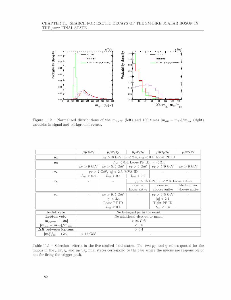
CHAPTER 11. SEARCH FOR EXOTIC DECAYS OF THE SM-LIKE SCALAR BOSON INTHE µµττ FINAL STATE
Figure 11.2 – Normalized distributions of the mµµττ (left) and 100 times |mµµ − mττ |/mµµ (right)variables in signal and background events.
µµτeτe µµτeτµ µµτeτh µµτµτh µµτhτh
µ1 pT >18 GeV, |η| < 2.4, Irel < 0.4, Loose PF IDµ2 Irel < 0.4, Loose PF ID, |η| < 2.4
pT > 9 GeV pT > 5/9 GeV pT > 9 GeV pT > 5/9 GeV pT > 9 GeVτe pT > 7 GeV, |η| < 2.5, MVA ID - -
Irel < 0.4 Irel < 0.4 Irel < 0.2τh - - pT > 15 GeV, |η| < 2.3, Loose anti-µ
Loose iso. Loose iso. Medium iso.Loose anti-e vLoose anti-e vLoose anti-e
τµ - pT > 9/5 GeV - pT > 9/5 GeV -|η| < 2.4 |η| < 2.4
Loose PF ID Tight PF IDIrel < 0.4 Irel < 0.5
b–Jet veto No b–tagged jet in the event.Lepton veto No additional electron or muon.|mµµττ − 125| < 25 GeV|mµµ −mττ |/mµµ < 0.8
∆R between leptons > 0.4|mvis
µµee − 125| > 15 GeV -
Table 11.1 – Selection criteria in the five studied final states. The two pT and η values quoted for themuons in the µµτµτh and µµτeτµ final states correspond to the case where the muons are responsible ornot for firing the trigger path.
182
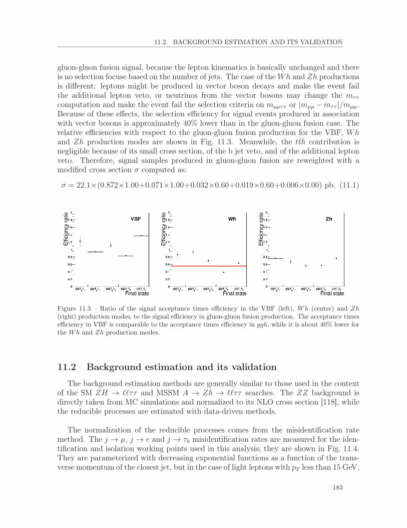
11.2. BACKGROUND ESTIMATION AND ITS VALIDATION
gluon-gluon fusion signal, because the lepton kinematics is basically unchanged and thereis no selection focuse based on the number of jets. The case of theWh and Zh productionsis different: leptons might be produced in vector boson decays and make the event failthe additional lepton veto, or neutrinos from the vector bosons may change the mττ
computation and make the event fail the selection criteria on mµµττ or |mµµ−mττ |/mµµ.Because of these effects, the selection efficiency for signal events produced in associationwith vector bosons is approximately 40% lower than in the gluon-gluon fusion case. Therelative efficiencies with respect to the gluon-gluon fusion production for the VBF, Whand Zh production modes are shown in Fig. 11.3. Meanwhile, the tth contribution isnegligible because of its small cross section, of the b jet veto, and of the additional leptonveto. Therefore, signal samples produced in gluon-gluon fusion are reweighted with amodified cross section σ computed as:
σ = 22.1×(0.872×1.00+0.071×1.00+0.032×0.60+0.019×0.60+0.006×0.00) pb. (11.1)
Figure 11.3 – Ratio of the signal acceptance times efficiency in the VBF (left), Wh (center) and Zh(right) production modes, to the signal efficiency in gluon-gluon fusion production. The acceptance timesefficiency in VBF is comparable to the acceptance times efficiency in ggh, while it is about 40% lower forthe Wh and Zh production modes.
11.2 Background estimation and its validation
The background estimation methods are generally similar to those used in the contextof the SM ZH → ``ττ and MSSM A → Zh → ``ττ searches. The ZZ background isdirectly taken from MC simulations and normalized to its NLO cross section [118], whilethe reducible processes are estimated with data-driven methods.
The normalization of the reducible processes comes from the misidentification ratemethod. The j → µ, j → e and j → τh misidentification rates are measured for the iden-tification and isolation working points used in this analysis; they are shown in Fig. 11.4.They are parameterized with decreasing exponential functions as a function of the trans-verse momentum of the closest jet, but in the case of light leptons with pT less than 15 GeV,
183

CHAPTER 11. SEARCH FOR EXOTIC DECAYS OF THE SM-LIKE SCALAR BOSON INTHE µµττ FINAL STATE
µµτeτe µµτeτµ µµτeτh µµτµτh µµτhτh CombinationData 13± 3.6 14± 3.7 65± 8.1 24± 4.9 56± 7.5 172± 13.1
Mis-ID rate method 11.2± 5.6 13.3± 6.6 57.5± 21.8 25.8± 9.8 68.9± 17.2 176.7± 30.7
Table 11.2 – Comparison between the yield in data with two SS tau candidates, and the yield obtainedin the SS region with the misidentification rate method.
they are measured in two five-GeV wide bins. The low-pT behavior of the muon misidenti-fication rate is due to events with a very low pT spurious track with potentially one hit inthe muon chambers, which are reconstructed as muon candidates but do not pass the muonidentification. Because of the large pileup, many such muons are reconstructed, but theirmisidentification rate is small because they do not pass the identification conditions. Thenormalization of the reducible processes is estimated by subtracting the contribution ofevents with two tau candidates that fail the isolation or identification conditions, weightedby a factor that depends on the misidentification rates, from the weighted contributionof events with exactly one tau candidate that fails the identification or isolation conditions.
To validate the estimation of the reducible background, the yields obtained with themisidentification rate method are compared with the observed data in a region where thetwo tau candidates have the same electric charge. The statistical uncertainties are reducedby relaxing the selection criteria on |mµµ−mττ |/mµµ, mµµττ andmµµ. The results are pre-sented in Tab. 11.2; the yields from the misidentification rate method are very compatiblewith the observation. An additional cross-check consists in comparing the yields of themisidentification rate method when the rates are parameterized as a function of the pT ofthe closest jet or of the lepton. The difference between both methods is limited (between5 and 30%) and well covered by the uncertainty assigned to the reducible backgroundnormalization 1. Nevertheless, the parametrization as a function of the pT of the closestjet is chosen because it gives the best agreement between prediction and observation inthe closure test described in the previous paragraph.
The di-muon mass (mµµ) distribution of the reducible background is taken from datain a region where both tau candidates have the same electric charge and are selected withrelaxed isolation and identification criteria, namely:
— µµτeτe: relative isolation less than 1.0 for both electrons;— µµτeτµ: relative isolation less than 2.0 for both leptons;— µµτeτh: loose MVA electron identification, relative electron isolation less than 5.0,
BDT output of the tau isolation including lifetime information greater than -0.95;— µµτµτh: loose PF muon identification, relative muon isolation less than 5.0, BDT
output of the tau isolation including lifetime information greater than -0.95;— µµτhτh: BDT output of the tau isolation including lifetime information greater than
-0.90.The mµµ distribution obtained in this way is compatible, within the large statistical un-
1. The uncertainties range from 25 to 50% depending on the final state, as explained in Section 11.4.
184

11.2. BACKGROUND ESTIMATION AND ITS VALIDATION
(GeV)T
Jet p0 50 100
Mis
iden
tific
atio
n ra
te
-310
-210
-110
1
10
CMS
(8 TeV)-119.7 fb
Preliminary
(loose)hτ →j
Barrel
(GeV)T
Jet p0 50 100
Mis
iden
tific
atio
n ra
te
-310
-210
-110
1
10
CMS
(8 TeV)-119.7 fb
Preliminary
(loose)hτ →j Endcaps
(GeV)T
Jet p0 50 100
Mis
iden
tific
atio
n ra
te
-310
-210
-110
1
10
CMS
(8 TeV)-119.7 fb
Preliminary
(medium)hτ →j
Barrel
(GeV)T
Jet p0 50 100
Mis
iden
tific
atio
n ra
te
-310
-210
-110
1
10
CMS
(8 TeV)-119.7 fb
Preliminary
(medium)hτ →j Endcaps
(GeV)T
Jet p0 50 100
Mis
iden
tific
atio
n ra
te
-310
-210
-110
1
10
CMS
(8 TeV)-119.7 fb
Preliminary
e (loose)→j Barrel + endcaps
(GeV)T
Jet p0 50 100
Mis
iden
tific
atio
n ra
te
-310
-210
-110
1
10
CMS
(8 TeV)-119.7 fb
Preliminary
e (tight)→j Barrel + endcaps
(GeV)T
Jet p0 50 100
Mis
iden
tific
atio
n ra
te
-310
-210
-110
1
10
CMS
(8 TeV)-119.7 fb
Preliminary
(loose)µ →j Barrel + endcaps
(GeV)T
Jet p0 50 100
Mis
iden
tific
atio
n ra
te
-310
-210
-110
1
10
CMS
(8 TeV)-119.7 fb
Preliminary
(tight)µ →j Barrel + endcaps
Figure 11.4 – Misidentification rates of the tau candidates. [130]
185

CHAPTER 11. SEARCH FOR EXOTIC DECAYS OF THE SM-LIKE SCALAR BOSON INTHE µµττ FINAL STATE
certainties, with the distribution coming from the misidentification rate method, as shownin Fig. 11.5.
Figure 11.5 – Comparison between the mµµ distributions obtained via the misidentification rate methodand from data with SS tau candidates (default method), in the five different final states.
Distributions of the mµµ variable observed in data and their predictions for SM pro-cesses, before cutting on |mµµ −mττ |/mµµ nor mµµττ are shown in Fig. 11.6 and demon-strate a good background description in the full mass range, and especially in the morepopulated Z peak region.
11.3 Modeling of the experimental mµµ distributions
Because of the excellent di-muon mass resolution, an unbinned shape analysis, usingmµµ as observable, is performed. All processes are parameterized separately in the fivefinal states.
186

11.3. MODELING OF THE EXPERIMENTAL Mµµ DISTRIBUTIONS
(GeV)µµm
0 50 100
Eve
nts
/ 4
GeV
0
20
40
60
80
100
Observed
ZZReducible bkg.
Signal x 30Bkg. uncertainty
(8 TeV)-119.7 fb
CMSPreliminary eτeτµµ
(GeV)µµm
0 50 100
Eve
nts
/ 4
GeV
0
2
4
6
8
10
12
14
16
18
Observed
ZZReducible bkg.
Signal x 30Bkg. uncertainty
(8 TeV)-119.7 fb
CMSPreliminary µτeτµµ
(GeV)µµm
0 50 100
Eve
nts
/ 4
GeV
0
5
10
15
20
25
30
35
Observed
ZZReducible bkg.
Signal x 30Bkg. uncertainty
(8 TeV)-119.7 fb
CMSPreliminary h
τeτµµ
(GeV)µµm
0 50 100
Eve
nts
/ 4
GeV
0
5
10
15
20
25
Observed
ZZReducible bkg.
Signal x 30Bkg. uncertainty
(8 TeV)-119.7 fb
CMSPreliminary h
τµτµµ
(GeV)µµm
0 50 100
Eve
nts
/ 4
GeV
0
10
20
30
40
50
Observed
ZZReducible bkg.
Signal x 30Bkg. uncertainty
(8 TeV)-119.7 fb
CMSPreliminary h
τh
τµµ
(GeV)µµm
0 50 100
Eve
nts
/ 4
GeV
0
20
40
60
80
100
120
140
160
180
200
Observed
ZZReducible bkg.
Signal x 30Bkg. uncertainty
(8 TeV)-119.7 fb
CMSPreliminary
Combined
Figure 11.6 – Data, predicted SM backgrounds, and signal (ma = 40 GeV) di-muon mass distributionsin the µµτeτe (top left), µµτeτµ (top right), µµτeτh (center left), µµτµτh (center right), and µµτhτh(bottom left) final states, and their combination (bottom right). The cuts on the variables mµµττ and|mµµ − mττ |/mµµ are not applied to increase the number of selected events. The signal samples arescaled as thirty times the normalization obtained with σ(h) as predicted in the SM, B(h → aa) = 10%,and considering decays of the pseudoscalar a boson to leptons only. No maximum likelihood fit to thedata has been performed. [129]
187

CHAPTER 11. SEARCH FOR EXOTIC DECAYS OF THE SM-LIKE SCALAR BOSON INTHE µµττ FINAL STATE
11.3.1 Signal
Signal distributions are parameterized with Voigtian functions, which are convolutionsof Gaussian and Lorentzian profiles:
V (m) =
∫ +∞
−∞G(m′, σ)L(m−m′, α)dm′, (11.2)
where the Gaussian profile is centered on 0 and defined as:
G(m,σ) =e−m
2/(2σ2)
σ√
2π, (11.3)
and the centered Lorentzian distribution is:
L(m,α) =α
π(m2 + α2). (11.4)
In practice, the Voigtian function, and its components, are centered close to the a bosonmass hypothesis. The Lorentzian component reflects the natural width of the signal, whilethe Gaussian component takes into account experimental resolution effects.
Signal samples are generated with Pythia, for masses between 20 and 60 GeV, with 5GeV steps. Fits are performed for every mass hypothesis and every final state, after thefull selection has been applied. The Gaussian component is seen to vanish in the finalstates with three muons (µµτeτµ and µµτµτh), and the signal distributions in these finalstates are therefore fitted with simple Lorentzian functions. The signal fits in the differentfinal states for ma = 40 GeV are shown in Fig. 11.7; a good fit quality is observed for allof them.
A method is designed to interpolate the signal description to any mass between 20 and60 GeV, and to extrapolate it up to mh/2 = 62.5 GeV. The fit parameters extracted fromthe fits to the signal samples, are parameterized as a function of the generated a bosonmass with polynomials with three degrees of freedom. The mean of the distributions is, asexpected, close to the generated a boson mass, while the width parameters, α and σ, showa more complex behavior. The distributions of the fit parameters are shown in Fig. 11.8for all final states. The signal acceptance times efficiency, measured for all masses inevery final state, is also parameterized as a function of the mass hypothesis, as shown inFig. 11.9. These parameterizations allow the description of the signal distribution andnormalization at any mass, as illustrated in Fig. 11.10
A closure test is performed to validate the interpolation procedure. A signal sampleis removed from the fit of the Lorentzian and Voigtian parameters as a function of thea boson mass, and the signal distributions resulting from the extrapolation with this pa-rameterization are compared to the direct fits to this signal sample. The test is performedfor intermediary masses, and for an extreme mass (ma = 60 GeV): interpolating to in-termediary masses and extrapolating outside the range of generated masses both give a
188

11.3. MODELING OF THE EXPERIMENTAL Mµµ DISTRIBUTIONS
Figure 11.7 – Modeling of the signal with ma = 40 GeV using Lorentzian or Voigtian functions, in theµµτeτe (top left), µµτeτµ (top right), µµτeτh (center left), µµτµτh (center right), and µµτhτh (bottom)final states. The black dots correspond to events selected in MC samples. [130]
189

CHAPTER 11. SEARCH FOR EXOTIC DECAYS OF THE SM-LIKE SCALAR BOSON INTHE µµττ FINAL STATE
Figure 11.8 – Lorentzian or Voigtian fit parameters extracted from fits to signal samples in the differentfinal states, with pseudoscalar boson masses ranging from 20 to 60 GeV.
190

11.3. MODELING OF THE EXPERIMENTAL Mµµ DISTRIBUTIONS
Figure 11.9 – Signal normalization as a function of the pseudoscalar boson mass, for an h boson productioncross as expected in the SM, a decays to leptons only and B(h→ aa) = 10%. The plateau trend between30 and 50 GeV is due to the interplay between the boost of the a bosons at low ma and the boost of thetau leptons at high ma.
good agreement with the direct fits. The results of the closure test for ma = 55 GeV areshown in Fig. 11.11.
11.3.2 ZZ background
The ZZ background is parameterized with Bernstein polynomials, which are linearcombinations of Bernstein-basis polynomials. The n+1 Bernstein-basis polynomials usedto build a Bernstein polynomial with n degrees of freedom are defined as:
bi,n(x) =
(ni
)xi(1− x)n−i, with i = 0, ..., n, (11.5)
where(ni
)are binomial coefficients. Bernstein polynomials are positively defined for x
between 0 and 1, which makes them a good choice to describe data limited by statistics.
The polynomial coefficients are extracted from a fit to the events selected in the ZZMC simulation. As the number of selected events is extremely low in the µµτhτh finalstate, the hadronic tau isolation is relaxed from the medium to the loose HPS workingpoint. This does not bias the bias the mµµ distribution, and increases the number ofselected events by more than 50%. The fits are shown in Fig. 11.12 for all final states.
The degree of the Bernstein polynomial is chosen to be the lowest that gives a gooddata description; in other words, the degree n is chosen if the degree n+ 1 does not bring
191

CHAPTER 11. SEARCH FOR EXOTIC DECAYS OF THE SM-LIKE SCALAR BOSON INTHE µµττ FINAL STATE
Figure 11.10 – Signal description extracted from the parameterization of the Voigtian and Lorentzian fitparameters. The normalization corresponds to an h boson production cross as expected in the SM, adecays to leptons only and B(h→ aa) = 10%. [130]
192

11.3. MODELING OF THE EXPERIMENTAL Mµµ DISTRIBUTIONS
Figure 11.11 – Comparison between the interpolation from the parameterization and the direct fit for asignal with ma = 55 GeV.
193

CHAPTER 11. SEARCH FOR EXOTIC DECAYS OF THE SM-LIKE SCALAR BOSON INTHE µµττ FINAL STATE
Figure 11.12 – Modeling of the ZZ background, estimated from MC simulations, using fifth-degree Bern-stein polynomials, in the µµτeτe (top left), µµτeτµ (top right), µµτeτh (center left), µµτµτh (center right),and µµτhτh (bottom) final states. The black dots correspond to events selected in MC samples. [129]
194

11.4. UNCERTAINTIES
Polynomial degree (n→ n+ 1) 2× (NLLn −NLLn+1)µµτeτe µµτeτµ µµτeτh µµτµτh µµτhτh
3→ 4 94.8 0.05 9.07 4.29 6.174→ 5 18.2 1.65 0.78 0.67 2.995→ 6 0.20 0.61 2.87 2.22 2.01
Table 11.3 – Twice the difference between the minimum negative log-likelihood values for two adjacentpolynomial degrees in the different final states, for the fit of the ZZ background. The improvementbrought by the additional degree of freedom is judged significant if this value is larger than 3.85. Thesixth degree does not improve the fit quality significantly for any of the final states, and the fifth degreeis thus chosen.
a significant improvement to the fit quality. The minimized negative log-likelihood, NLL,which describes the level of agreement between the fit function and the distribution of theselected events, can be measured for the fits with polynomials with degree n or n+ 1. Itcan be shown that twice their difference follows a chi-square distribution with one degreeof freedom: 2 × (NLLn − NLLn+1) ∼ χ2
1. The number of degrees of freedom n + 1 ischosen over n if the chi-square between these two fits shows no significant improvement(p-value < 0.05 with a F-distribution [131]): P (χ2
1 ≥ 2 × (NLLn − NLLn+1)) < 0.05.A significant improvement therefore consists in 2 × (NLLn − NLLn+1) > 3.85. Such amethod has been used in [132]. The differences for the fits with Bernstein polynomialsof different degrees are shown in Tab. 11.3: the fifth degree is the one that permits todescribe efficiently all final states. The fourth degree would have been optimal for allfinal states except µµτeτe, which is the most populated by ZZ events; this choice doesnot impact the final results because the ZZ background is negligible with respect to thereducible processes in these final states.
11.3.3 Reducible background
Like the ZZ background, reducible processes are modeled with Bernstein polynomi-als. The same method is used to determine the optimal polynomial degree; as shownin Tab. 11.4, the third degree is the best choice. It can be noticed that the reduciblebackground is described with a polynomial with less degrees of freedom than the ZZbackground, which is subdominant. The reason is that the distribution of the ZZ back-ground is better constrained by the large statistics from the MC sample, especially in theµµτeτe final state, whereas the reducible background distribution comes from a statisti-cally limited number of observed events in a control region in data. The results of thefits, together with their uncertainties, are illustrated in Fig. 11.13.
11.4 Uncertainties
The systematic uncertainties that affect the yields of the signal and background pro-cesses are:
— Theoretical signal prediction: A 10% uncertainty affects the signal yield, toaccount for uncertainties on the theoretical signal prediction.
195

CHAPTER 11. SEARCH FOR EXOTIC DECAYS OF THE SM-LIKE SCALAR BOSON INTHE µµττ FINAL STATE
Polynomial degree (n→ n+ 1) 2× (NLLn −NLLn+1)µµτeτe µµτeτµ µµτeτh µµτµτh µµτhτh
2→ 3 6.80 9.35 0.84 0.76 12.53→ 4 0.41 0.12 1.55 0.11 0.07
Table 11.4 – Twice the difference of the minimum negative log-likelihood values for two adjacent poly-nomial degrees in the different final states, for the fit of the reducible background. The improvementbrought by the additional degree of freedom is judged significant if this value is larger than 3.85. Thefourth degree does not improve the fit quality significantly for any of the final states, and the third degreeis thus chosen.
Figure 11.13 – Modeling of the reducible background with third-order Bernstein polynomials, in theµµτeτe (top left), µµτeτµ (top right), µµτeτh (center left), µµτµτh (center right), and µµτhτh (bottom)final states. The black dots correspond to observed events selected in control regions. [129]
196

11.4. UNCERTAINTIES
— Signal efficiency: An uncertainty between 5 and 8% is considered in each finalstate to account for the uncertainty on the parameterization of the normalizationof the signal as a function of the mass, illustrated in Fig. 11.9.
— Luminosity: The uncertainty on the luminosity, which affects the ZZ backgroundand the signal, is measured to be 2.6% [109].
— Tau energy scale: As discussed in Chapter 6, the tau energy scale in data isknown with 3% precision [103]. This does not affect the mµµ distributions, but hasan effect on the estimated yield of processes from MC simulations because of thepT thresholds applied to select hadronic taus. When the tau energy scale is variedby ±3%, the acceptance for the signal and ZZ processes is modified by up to 10%in the µµτhτh final state, and up to 4% in the µµτeτh and µµτµτh final states. Theyield uncertainties in the µµτhτh final state, and in the µµτeτh and µµτµτh finalstates, are uncorrelated because different HPS isolation working points are used.
— Tau identification: An uncertainty of 6% is considered for any single hadronictau [103]; and this number is conservatively doubled in the µµτhτh final state.
— Muon identification: A 1% uncertainty is considered, conservatively multipliedby the number of muons in the final state.
— Electron identification: A 2% uncertainty is considered, conservatively multipliedby the number of electrons in the final state.
— Trigger efficiency: The uncertainty on the double muon trigger efficiency is esti-mated to amount to 2%.
— B jet veto: Applying a b jet veto brings a 1% uncertainty on the yield of the signaland ZZ processes, both estimated from MC simulations.
— ZZ theoretical cross section: Uncertainties in the parton distribution functions(PDF) and variations of the renormalization and factorization scales lead to respec-tively 5 and 6% yield uncertainties on the ZZ background.
— Limited number of ZZ events in MC samples: After the full selection, thenumber of MC events remaining for the ZZ process is limited, and an uncertaintyranging between 1 and 15% depending on the final state is associated the globalnormalization of the ZZ background.
— Reducible background normalization estimation: The uncertainty on thenormalization of the reducible background is estimated by recomputing the yieldsafter modifying the misidentification rate fit functions within their uncertainties.An uncertainty is associated to every fit function, and the total uncertainty in agiven final state varies between 25 and 50%
Meanwhile, the shape uncertainties considered in the analysis are:
— Signal modeling: Statistical uncertainties on the parameterization of the signalare accounted for through the uncertainties on the fit parameters (α, σ) describingthe signal distribution.
— Muon energy scale and muon momentum resolution: The muon energy scaleand momentum resolution uncertainties are found to shift the mean of the signaldistributions by up to 0.2% when they are varied by ±1 standard deviation. This
197

CHAPTER 11. SEARCH FOR EXOTIC DECAYS OF THE SM-LIKE SCALAR BOSON INTHE µµττ FINAL STATE
Systematic uncertainty Relative change in yieldSignal ZZ Reducible backgrounds
Luminosity 2.6% 2.6% -Trigger 1% 1% -
Tau identification 0-12% 0-12% -b-Jet veto 1% 1% -
Tau energy scale 0-10% 0-10% -Electron identification 0-4% 0-4% -Muon identification 2-4% 2-4% -Signal prediction 10% - -Signal efficiency 5-8% - -
PDF - 5% -QCD scale VV - 6% -
ZZ statistics in MC - 1-15% -Reducible background normalization - - 25-50%Reducible background distribution - - shape only
Signal modeling shape only - -Muon energy scale shape only - -
Table 11.5 – Systematic uncertainties on the yields or shapes of the signal, ZZ and reducible processes.The relative change in yields resulting from a variation of the nuisance parameter equivalent to onestandard deviation is indicated.
is accounted for as a parametric uncertainty on the mean of the Lorentzian andVoigtian functions.
— Reducible background distribution estimation: The three uncertainties asso-ciated to the three degrees of freedom of the Bernstein polynomials used to modelthe reducible background, are decorrelated and considered as shape uncertainties.
All the uncertainties are summarized in Tab. 11.4. Given the very low expected yieldsexpected over the full mass range, and the excellent di-muon mass resolution, the analysisis mostly statistically limited, and the systematic uncertainties described above generallyplay a little role in the results.
11.5 Results
The expected and observed mµµ distributions in the different final states are shown inFig. 11.14. The expected distributions are the result of a simultaneous background-onlymaximum likelihood fit to the observed data. Every observed event is indicated togetherwith its precise mµµ value. The yields are detailed in Tab. 11.6: the number of observedevents is compatible with the SM expectation.
Upper limits can be set on the cross section times branching fraction for the processh → aa → µµττ , but a more easily interpretable result consists in upper limits onσ(h)/σSM × B(h → aa) × B(a → ττ)2. Indeed, if the production cross section of the h
198

11.5. RESULTS
Figure 11.14 – Background and signal (ma = 40 GeV) models, scaled to their expected yields, in theµµτeτe (top left), µµτeτµ (top right), µµτeτh (middle left), µµτµτh (middle right), and µµτhτh (bottomleft) final states, and their combination (bottom right). The two components that form the backgroundmodel, ZZ and reducible processes, are drawn. Every observed event in the individual decay channels isrepresented by an arrow, together with its measured mµµ value; while in the combined mass plot dataare binned in a histogram. The signal samples are scaled with σ(h) as predicted in the SM, B(h → aa)= 10% and considering decays of the pseudoscalar a boson to leptons only. The results are shown aftera simultaneous maximum likelihood fit that takes into account the systematic uncertainties. [129]
199

CHAPTER 11. SEARCH FOR EXOTIC DECAYS OF THE SM-LIKE SCALAR BOSON INTHE µµττ FINAL STATE
Signal Backgrounds Obs.ma = 20 GeV ma = 60 GeV ZZ Reducible Total
µµτeτe 0.20±0.02 0.58±0.06 4.64±0.39 2.49±1.03 7.13±1.10 8µµτeτµ 0.58±0.08 1.42±0.16 0.10±0.01 1.70±0.74 1.80±0.74 2µµτeτh 0.74±0.08 2.02±0.20 0.16±0.02 5.65±1.77 5.81±1.77 5µµτµτh 0.96±0.10 2.30±0.22 0.13±0.02 0.99±0.31 1.12±0.31 1µµτhτh 0.60±0.06 1.90±0.18 0.06±0.01 4.64±0.98 4.70±0.98 3
Combined 3.08±0.31 8.22±0.82 5.09±0.39 15.47±2.41 20.56±2.44 19
Table 11.6 – Expected and observed yields in the different final states. The signal samples are scaledwith σ(h) as expected in the SM, B(h→ aa) = 10% and considering decays of the pseudoscalar a bosonto leptons only. The background yields are obtained after a maximum likelihood fit to observed data,taking into account the systematic uncertainties described previously.
boson is the same as predicted in the SM, the first term is equal to 1, while the last termis also almost equal to 1 in the hypothesis that the a boson does not decay to quarks 2.The latter hypothesis is a good approximation at large tan β in 2HDM+S type-3. TheB(a→ µµ) branching fraction can easily be expressed as a multiple of B(a→ ττ), giventhat in 2HDM and their extensions, one has:
Γ(a→ µµ)
Γ(a→ ττ)=m2µ
√1− (4m2
µ/m2a)
m2τ
√1− (4m2
τ/m2a). (11.6)
The asymptotic approximation cannot be used to extract the CLs limits because ofthe low expected event yield, and other techniques have to be used [67]. Indeed thetest statistic distributions in this analysis do not follow chi-squares, as supposed by theasymptotic approximation. Therefore toys need to be generated for every mass point andevery final state to obtain the exact test statistic distributions. The limits obtained withthe full CLS calculation are shown in Fig. 11.15. Under the hypotheses that the h bosonproduction cross section is the same as expected in the SM and that the a boson doesnot decay to quarks, B(h → aa) larger than values between 4 and 15% can be excludedfor pseudoscalar masses ranging from 20 to 62.5 GeV. An excess of events is seen at lowma in the µµτeτµ final state. The local significance of the excess is about three stan-dard deviations, but a large look-elsewhere effect, due to the narrow signal resolution, thelarge mass range probed and the five different final states needs to be taken into account.The up-crossing method (see Section 3.4) is not appropriate in this case to evaluate thelook-elsewhere effect because there exists a correlation between the background descrip-tion in neighbor bins, but the trial factor, which relates the global to the local p-value ismeasured by throwing toys based on the background-only expectation and counting thefraction of times an excess as the one in the µµτeτµ final state is observed. The trial factoris larger than thirty, which leads to a global significance less than two standard deviations.
2. B(a→ ττ) > 0.995 for all a boson masses larger than 20 GeV if there is no decay to quarks.
200

11.5. RESULTS
(GeV)am20 30 40 50 60
2 )ττ →
B(a
× a
a)
→ B
(h×
) S
Mσ
(h)/
σ95
% C
L o
n (
0.0
0.5
1.0
1.5
2.0
2.5
3.0 ObservedExpected
Expectedσ 1± Expectedσ 2±eτeτµµ
CMSPreliminary
(8 TeV)-119.7 fb
(GeV)am20 30 40 50 60
2 )ττ →
B(a
× a
a)
→ B
(h×
) S
Mσ
(h)/
σ95
% C
L o
n (
0.0
0.2
0.4
0.6
0.8
1.0
1.2
1.4ObservedExpected
Expectedσ 1± Expectedσ 2±µτeτµµ
CMSPreliminary
(8 TeV)-119.7 fb
(GeV)am20 30 40 50 60
2 )ττ →
B(a
× a
a)
→ B
(h×
) S
Mσ
(h)/
σ95
% C
L o
n (
0.0
0.1
0.2
0.3
0.4
0.5
0.6
0.7
0.8ObservedExpected
Expectedσ 1± Expectedσ 2±h
τeτµµ
CMSPreliminary
(8 TeV)-119.7 fb
(GeV)am20 30 40 50 60
2 )ττ →
B(a
× a
a)
→ B
(h×
) S
Mσ
(h)/
σ95
% C
L o
n (
0.0
0.1
0.2
0.3
0.4
0.5
0.6
0.7ObservedExpected
Expectedσ 1± Expectedσ 2±hτµτµµ
CMSPreliminary
(8 TeV)-119.7 fb
(GeV)am20 30 40 50 60
2 )ττ →
B(a
× a
a)
→ B
(h×
) S
Mσ
(h)/
σ95
% C
L o
n (
0.0
0.1
0.2
0.3
0.4
0.5
0.6
0.7
0.8
0.9
1.0ObservedExpected
Expectedσ 1± Expectedσ 2±h
τh
τµµ
CMSPreliminary
(8 TeV)-119.7 fb
(GeV)am20 30 40 50 60
2 )ττ →
B(a
× a
a)
→ B
(h×
) S
Mσ
(h)/
σ95
% C
L o
n (
0.00
0.05
0.10
0.15
0.20
0.25ObservedExpected
Expectedσ 1± Expectedσ 2±Combined
CMSPreliminary
(8 TeV)-119.7 fb
Figure 11.15 – Expected upper limits at 95% CL on the production of h → aa relative to the SM hproduction, scaled by B(a → ττ)2, in the µµτeτe (top left), µµτeτµ (top right), µµτeτh (middle left),µµτµτh (middle right), and µµτhτh (bottom left) final states, and for the combination of these five finalstates (bottom right). B(a → ττ)2 is close to 1 in the hypothesis where the pseudoscalar a boson doesnot decay to quarks. No excess has a global significance larger than 2 standard deviations. [129]
201

CHAPTER 11. SEARCH FOR EXOTIC DECAYS OF THE SM-LIKE SCALAR BOSON INTHE µµττ FINAL STATE
The ATLAS Collaboration has also published results on the search for the exotic decayof the 125-GeV particle to a pair of light pseudoscalar bosons in the final state with twomuons and two taus [133]. The analysis targets masses of the pseudoscalar boson be-tween twice the tau mass, and 50 GeV, and makes use of special techniques to reconstructboosted di-tau pairs. Because the strategy used by ATLAS is optimized for boosted di-tau pairs and thus low pseudoscalar masses, the CMS analysis described in this chapteris roughly one order of magnitude more sensitive for pseudoscalar masses above 20 GeV.
If a type of 2HDM+S and a value of tan β are chosen, the branching fractions of thepseudoscalar boson to any SM particle can be determined univocally for any mass ma.Assuming that the production cross section for the h boson is the same as predicted inthe SM, this analysis is sensitive to B(h → aa) < 1 values at large tan β (tan β > 1.8)in 2HDM+S type-3, and small tan β (tan β < 0.5) in 2HDM+S type-4, as illustrated inFig. 11.16. It is however not sensitive to branching fractions less than unity for any tan βin 2HDM+S type-1 and type-2.
Figure 11.16 – Observed upper limits at 95% CL on σ(h)σSM
× B(h→ aa) for the combination of all di-taufinal states, in 2HDM+S type-3 (left) and type-4 (right). [129]
11.6 Interpretation and comparison with other CMS searches
A large variety of exotic h decays is allowed in 2HDM+S, with little indirect constrainsfrom other CMS measurements. It is therefore a favored model to compare the reach ofdifferent exotic h decay searches. Five decay modes with two light pseudoscalar bosonshave been studied with the data collected by CMS in Run-1:
1. h → aa → µµττ , 20 < ma < 62.5 GeV [129]. It is the analysis described at length
202

11.6. INTERPRETATION AND COMPARISON WITH OTHER CMS SEARCHES
in this chapter.2. h → aa → µµbb, 20 < ma < 70 GeV [134]. This analysis is pretty similar to the
first one, but suffers from larger backgrounds because of the difficulty to identify bjets.
3. h→ aa→ ττττ , 5 < ma < 9 GeV [135]. Because of the low pseudoscalar mass, thedi-tau pairs are boosted, and special boosted reconstruction techniques have beenused.
4. h → aa → ττττ , 5 < ma < 15 GeV [136]. Even if the final state is the same asin the previous analysis, different boosted reconstruction techniques are used, andthis analysis particularly targets the Wh associated production mode.
5. h→ aa→ µµµµ, 0.25 < ma < 3 GeV [137]. Apart from its reach in 2HDM+S, thisanalysis is also interpreted in dark SUSY models. A similar analysis has also beenpublished by the ATLAS Collaboration [138].
In 2HDM+S, the pseudoscalar a inherits its couplings to fermions from the SM-like scalar,while it cannot decay to gauge bosons. The branching fractions of the a boson dependon the type of 2HDM+S, and on the value of tan β, the ratio between the vacuum ex-pectation values of the two scalar doublets. The formulae presented in Section 1.3.3 stillapply, with some notable differences due to the pseudoscalar nature of the boson and tothe presence of a second doublet [18,52].
The partial decay width of the pseudoscalar to fermions reads:
Γ(a→ ff) =NcGF
4√
2πg2affmam
2f
√1−
4m2f
m2a
, (11.7)
where the differences with the SM case lie in the power of the last term (1 for a pseu-doscalar, 3 for a scalar), and in the scaling by the square of gaff , which multiplies thecoupling from the SM, depends on tan β and is given in Tab. 2.2 for all types of 2HDM. Itcan be noticed that, for two different kinds of leptons, the ratio of the branching fractionsis simply the ratio of their squared masses when ma � 2mf , for example:
B(a→ µµ)
B(h→ ττ)'m2µ
m2τ
. (11.8)
In the case of decays to quarks, the previous formula still holds withNC = 3 and specificQCD corrections, amounting to about 20%. The QCD corrections can be decomposed intwo terms: ∆qq and ∆2
a, with
∆qq = 5.67αSπ
+ (35.94− 1.35Nf )( αSπ
)2
, (11.9)
∆2a =
α2S
π2
(3.83− log
m2a
m2t
+1
6log2
m2q
m2a
). (11.10)
203

CHAPTER 11. SEARCH FOR EXOTIC DECAYS OF THE SM-LIKE SCALAR BOSON INTHE µµττ FINAL STATE
The symbol αS indicates the running of the strong coupling constant at the renormaliza-tion scalema, and mq is the running of the quark mass in the modified minimal subtraction(MS) scheme [139–141] at the same renormalization scale. In 2HDM+S type-1 and type-2, when neglecting the QCD correction terms, and for pseudoscalar boson masses largecompared to twice the b quark mass, the ratio between the branching fractions of thepseudoscalar to b quarks and to tau leptons is given by:
B(a→ bb)
B(h→ ττ)' 3
m2b
m2τ
, (11.11)
where the factor 3 comes from the number of colors.
The partial decay width to a photon pair via b- or t-quark loops 3, is given by:
Γ(a→ γγ) =GFα
2m3a
128√
2π3
∣∣∣∣∣∑f
Ncq2fgaffA
a1/2
(m2a
4m2f
)∣∣∣∣∣2
, (11.12)
where qf is the electric charge relative to that of the electron. The form factor Aa1/2 issimply given by:
Aa1/2(x) = 2x−1f(x), (11.13)
with
f(x) =
arcsin2√x, if x ≤ 1;
−14
(log
1+√
1−1/x
1−√
1−1/x− iπ
)2
otherwise.(11.14)
There is no QCD correction to take into account.
Finally, the partial decay width to a pair of gluons, through c-, b- or t-quark loops is:
Γ(a→ gg) =GF α
2Sm
3a
36√
2π3
∣∣∣∣∣ ∑q=t,b,c
gaqqAa1/2
(m2a
4m2q
)∣∣∣∣∣2(
1 +
(97
4− 7
6Nf
)αSπ
). (11.15)
The NLO corrections in the last term are computed with the renormalization scale of thestrong coupling constant equal to the pseudoscalar mass.
The branching fraction for each decay can be obtained by dividing the partial decaywidth over the total decay width. Fig. 11.17 shows the branching fractions of the pseu-doscalar a to SM particles, in the four types of 2HDM+S, for different values of tan β.
The largest branching fraction for the µµττ final state, B(aa → µµττ), is obtainedfor large tan β values in 2HDM+S type-3, where the decays to leptons are enhanced overthe decays to quarks. The largest B(aa → µµbb) is also obtained in 2HDM+S type-3,but for tan β ' 2: it is the best compromise between the enhancement of the couplings
3. Unlike the SM case, there is no contribution from W loops because of the pseudoscalar nature of a.
204

11.6. INTERPRETATION AND COMPARISON WITH OTHER CMS SEARCHES
Figure 11.17 – Branching fractions of the pseudoscalar boson a to SM particles for different types of2HDM+S and different tanβ values. There is no tanβ dependence in 2HDM+S type-1. The calculationsin the [3,5] and [9,11] GeV mass ranges are most likely invalid due to decays to quarkonia.
205

CHAPTER 11. SEARCH FOR EXOTIC DECAYS OF THE SM-LIKE SCALAR BOSON INTHE µµττ FINAL STATE
Figure 11.18 – Branching fractions of a pair of a bosons to µµττ (left) and µµbb (right) as a function oftanβ, in the four types of 2HDM+S without tree-level FCNC.
to leptons and the reduction of the couplings to quarks. The branching fractions to bothfinal states are shown in Fig. 11.18 for a pseudoscalar with a mass of 40 GeV as a functionof tan β in all four types of 2HDM+S without tree-level FCNC. The interplay betweenthe h → aa → µµbb and h → aa → µµττ analyses in type-3 and type-4 is shown inFig. 11.19: h → aa → µµττ is more sensitive in type-3 for tan β ≥ 1.8 and in type-4 fortan β ≤ 0.5.
In 2HDM+S type-1 and type-2, the ratio between the branching fractions of the pseu-doscalar to down-type quarks and to leptons does not depend on tan β. The results of allanalyses can therefore be rescaled to limits on (σ(h)/σSM) × B(h → aa) × B(a → ττ)2,or equivalently on (σ(h)/σSM) × B(h → aa) × B(a → µµ)2, as shown in Fig. 11.20. Intype-3 and type-4 however, down-type quarks and leptons do not couple to the samescalar doublet, and the ratio between their branching fractions depends on tan β.
The branching fractions of the pseudoscalar boson to muons and taus hugely depend onthe pseudoscalar mass; and more intuitive limits can be set on (σ(h)/σSM)×B(h→ aa).This requires to make a hypothesis both on the model and on tan β. The results areshown for three tan β values in every type of 2HDM+S in Fig. 11.21.
206

11.6. INTERPRETATION AND COMPARISON WITH OTHER CMS SEARCHES
Figure 11.19 – Comparison between the reach of the h→ aa→ µµbb and h→ aa→ µµττ as a functionof tanβ for a pseudoscalar mass of 40 GeV, in 2HDM/S type-3 (left) and type-4 (right).
Figure 11.20 – Comparison between the different analyses h→ aa searches performed in Run-1 with theCMS detector, in 2HDM+S type-1 and type-2. The white areas between 3.55 and 5 GeV, and between15 and 20 GeV, correspond to mass regions where no analysis was performed.
207
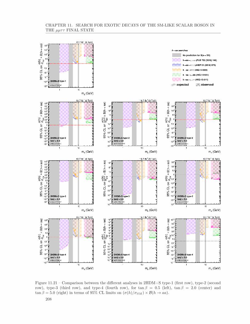
CHAPTER 11. SEARCH FOR EXOTIC DECAYS OF THE SM-LIKE SCALAR BOSON INTHE µµττ FINAL STATE
Figure 11.21 – Comparison between the different analyses in 2HDM+S type-1 (first row), type-2 (secondrow), type-3 (third row), and type-4 (fourth row), for tanβ = 0.5 (left), tanβ = 2.0 (center) andtanβ = 5.0 (right) in terms of 95% CL limits on (σ(h)/σSM )× B(h→ aa).
208

11.7. CHAPTER SUMMARY AND PERSONAL CONTRIBUTIONS
11.7 Chapter summary and personal contributions
Search for exotic decays of the SM-like scalar in the µµττ final state
The existence of exotic decays of the 125-GeV boson is still allowed with relativelylarge branching fractions by the precision measurements on this 125-GeV state.This chapter presents a search for the h→ aa→ µµττ decay, which is particularlyenhanced at large tan β in 2HDM+S type-3. The observable is the invariant massof the two muons, and given its excellent resolution, an unbinned shape analysisis performed. No excess is observed over the tiny predicted SM backgrounds, andexclusion limits can be set. Branching fractions of the h boson to a pair of lightpseudoscalar a bosons as low as 4% can be excluded, in 2HDM+S type-3 with largetan β. The performance of this analysis is then compared with those of the otherexotic h decay searches performed with the CMS detector in Run-1, in the fourdifferent types of 2HDM+S without FCNC.
My contributions
Figures: 11.1-11.21.I have produced all the results of the h → aa → µµττ search presented in thischapter, and have made the summary plots combining the five different searches forexotic h decays performed with the data collected by CMS in Run-1.
209


Chapter 12
Search for a light pseudoscalar decaying to taus
In some particular scenarios of 2HDM type-2, light pseudoscalar A bosons canbe produced in association with b jets with a large cross section accessible withLHC Run-1 data, as explained in Section 2.2.3. This low mass region, belowthe Z boson mass, has been barely explored at the LHC, unlike the high massregion where many analyses test various hypotheses. A difficulty in analyzingsuch a mass region is that the final state leptons typically have low transversemomenta and do not pass the trigger thresholds. In this chapter, we study thebbA → bbττ process, as published in [142]. Whereas the bbA → bbµµ processis more easily accessible because of the efficient identification and triggering ofmuons, the branching ratio of the A boson to muons is more than two orders ofmagnitude lower than its branching fraction to taus.
12.1 Analysis overview
The Feynman diagram of the signal process considered in this analysis is shown inFig. 12.1. Three di-tau final states among the six possible ones are studied: τeτµ, τµτhand τeτh. The τeτe and τµτµ final states are discarded because of their low branchingfractions and of the large backgrounds, while the trigger thresholds in the τhτh final stateare too high (45 GeV per hadronic tau) to study a light resonance.
Signal samples are generated with Pythia, for pseudoscalar masses between 25 and 80GeV. Because the selection efficiency is low given the low average transverse momentumof final state leptons, all events are generated with at least one lepton with pT greaterthan 15 GeV, and a reweighting is performed to account for the generator level efficiency.The Drell-Yan, W+jets, tt (fully leptonic, semi leptonic and fully hadronic) and diboson(WW , WZ and ZZ) processes are also generated with Madgraph. Finally, single top andSM H boson processes are generated with Powheg. The W+jets and Z+jets samples areproduced inclusively, and exclusively for different numbers of generated jets. This permitsto increase the selection efficiency for these important processes with large cross sections,
211

CHAPTER 12. SEARCH FOR A LIGHT PSEUDOSCALAR DECAYING TO TAUS
Figure 12.1 – Feynman diagram for the production of a light pseudoscalar with a pair of b quarks, anddecaying to taus.
[GeV]ττm
20 40 60 80
ττ/m ττ
m∆
0.00
0.05
0.10
0.15
0.20
0.25
0.30
hτµµe
hτe
8 TeV
Figure 12.2 – Measured masses and mass resolutions obtained with the SVfit algorithm in the three finalstates studied in the analysis, for signal samples with generated A boson masses between 25 and 80 GeVwith 5 GeV steps. The resolution in the eµ final state is a few percent worse because of the presence ofone additional neutrino in the final state.
and to obtain more precise templates. The different samples can be combined with thestitching technique. The Z/γ∗ → 2` samples are further divided into two mass regions:m`` > 50 GeV and 10 < m`` < 50 GeV. It has been checked that both mass regions canbe joined smoothly. The data have been collected in 2012 at 8 TeV center-of-mass energy,and amount to 19.7 fb−1 integrated luminosity. A summary of the MC processes withtheir cross sections, as well as the collected datasets, can be found in Appendix A.
A binned analysis is performed, using the full di-tau invariant mass mττ as observable,and upper limits on the cross section times branching fraction are set with the asymptoticCLs method. The SVfit algorithm is seen to perform well for low mass resonances, anda mass resolution of about 15% is obtained for all final states and all masses between 25and 80 GeV, as shown in Fig. 12.2.
212

12.2. SELECTION
12.2 Selection
A vertex with at least four degrees of freedom is required in the event, with a positionwith respect to the beam interaction such that −24 < z < 24 cm and |r| < 2 cm. Ifthere are more than one vertex satisfying these conditions, the one with the highest scalarpT sum of the tracks is chosen as the vertex of the hard-scatter interaction. In all finalstates, the events are required to have at least one jet with pT > 20 GeV, |η| < 2.4and passing the medium CSV b-tagging working point. The next sections describe theselection criteria specific to the three different di-tau final states.
12.2.1 τeτµ final state
The events in the τeτµ di-tau final state have to fire a trigger path that requires atHLT level a muon and an electron with pT greater than 8 and 17 GeV respectively for theleading and subleading lepton. At analysis level, the pT requirements are chosen such thatthe trigger efficiency is close to the plateau, and either a muon with pT greater than 10GeV and an electron with pT greater than 20 GeV, or a muon with pT greater than 18 GeVand an electron with pT greater than 10 GeV are required. The 2 GeV difference betweenthe leading electron and muon criteria comes from the slower trigger efficiency turn-on forelectrons. The pseudorapidity conditions on the leptons also come from trigger constrainsand are |η| < 2.3 for muons and |η| < 2.1 for electrons. In addition, the selected objectsare required to correspond within ∆R < 0.5 to the objects that fired the trigger paths.
The electron and the muon are required to be isolated, with relative isolation less than0.15 in the endcaps (|η| > 1.479) and 0.10 in the barrel (|η| < 1.479). The electron shouldpass the conversion veto and the loose MVA identification, while the muon should betightly identified. The |dz| and dxy parameters are required to be less than 0.2 and 0.02cm respectively for both leptons. The electron and the muon need to carry an opposite-sign charge, and to be separated by at least ∆R = 0.5.
In order to reduce the backgrounds from Drell-Yan or diboson productions, events thathave more than one isolated and identified electron and muon are vetoed. In particular,the extra electrons are selected with the following characteristics:
— pT > 10 GeV, |η| < 2.5;— dxy < 0.045 cm, |dz| < 0.2 cm;— relative isolation less than 0.3;— loose MVA identification and conversion veto,
while extra muons pass the following conditions:— pT > 10 GeV, |η| < 2.4;— dxy < 0.045 cm, |dz| < 0.2 cm;— relative isolation less than 0.3;— tight PF identification.
The tt contribution is reduced by selecting events with Pζ , defined in Chapter 6, greaterthan -40 GeV. In addition, the transverse mass between the dilepton system and the ~��ET
213

CHAPTER 12. SEARCH FOR A LIGHT PSEUDOSCALAR DECAYING TO TAUS
is required to be less than 25 GeV; this further reduces the tt contribution and removesa large fraction of electroweak backgrounds. Over the probed mass range, the expectedupper limits on the signal cross section times branching fraction improve by 40-55% byapplying the Pζ selection, and by 8-20% by additionally applying the transverse massselection; the largest improvement is seen at low mA.
12.2.2 τµτh final state
The trigger path used to select events in the τµτh final state requires at HLT a muonwith pT greater than 17 GeV and a hadronic tau with pT greater than 20 GeV. At analysislevel, a muon with pT greater than 18 GeV and |η| less than 2.1, and well as a tau with pTgreater than 22 GeV and |η| less than 2.3, are required. The reconstructed objects shouldcorrespond to the objects that fired the trigger paths within ∆R < 0.5. The muon shouldpass the tight PF identification, and have a relative isolation less than 0.1. Its dxy and its|dz| are required to be less than 0.045 and 0.2 cm respectively. The hadronic tau shouldpass the decay mode finding discriminator, the tight MVA identification including lifetimeinformation, the loose cut-based rejection against electrons, as well as the medium MVArejection against muons. Both leptons are required to carry an opposite-sign charge andto be separated by at least ∆R = 0.5.
To remove contributions from Z/γ∗ → µµ events, the events are vetoed if they containa second muon that has an opposite-sign charge compared to the selected muon, and witha relative isolation less than 0.3, pT > 15 GeV, |η| < 2.4, |dz| < 0.2 cm, separated fromthe tau candidate by at least ∆R = 0.15, and being identified as a global, PF and trackermuon. In a more general way, all events that have an electron (pT > 10 GeV, |η| < 2.5,loose MVA identification, relative isolation less than 0.3, |dz| < 0.2 cm, separated fromthe muon and tau candidates by at least ∆R = 0.15) or a second muon (pT > 10 GeV,|η| < 2.4, tight PF identification, relative isolation less than 0.3, |dz| < 0.2 cm, separatedfrom the muon and tau candidates by at least ∆R = 0.15) on top of the already selectedmuon and tau candidates are vetoed. The contribution from W+jets and tt events isreduced by requiring the transverse mass between the muon and ~
��ET less than 30 GeV.
12.2.3 τeτh final state
At HLT level, an electron with transverse momentum greater than 22 GeV and ahadronic tau with transverse momentum greater than 20 GeV are required. Offline, theevents are selected with an electron with pT > 24 GeV and |η| < 2.1 and a hadronic tauwith pT > 22 GeV and |η| < 2.3. The electron is required to pass the tight MVA identifi-cation, and to have a relative isolation less than 0.1, whereas the hadronic tau passes thedecay mode finding discriminator, the tight MVA isolation including lifetime information,the medium MVA discriminator against electrons as well as the loose cut-based discrim-inator against muons. Both candidates have |dz| < 0.2 cm, and are matched to triggerlevel objects. Moreover, the electron and the tau have an opposite-sign charge and areseparated from each other by at least ∆R = 0.5.
214

12.3. BACKGROUND ESTIMATION
Extra lepton vetoes are applied to reduce the contribution from Drell-Yan and multi-lepton processes. Any event with an additional electron (pT > 10 GeV, |η| < 2.5, looseMVA identification, relative isolation less than 0.3, |dz| < 0.2 cm, separated from theelectron and tau candidates by at least ∆R = 0.15) or muon (pT > 10 GeV, |η| < 2.4,tight PF identification, relative isolation less than 0.3, |dz| < 0.2 cm, separated from theelectron and tau candidates by at least ∆R = 0.15) is discarded. To reject more specifi-cally the Z/γ∗ → ee background, the events are also not selected if they contain a secondelectron that has an opposite-sign charge to the other electron, and has the followingcharacteristics: pT > 15 GeV, |η| < 2.4, tight MVA-based identification, relative isolationless than 0.3, |dz| < 0.2 cm, separated from the electron and tau candidates by at least∆R = 0.15. The contribution from W+jets and tt backgrounds is reduced by requiringthe transverse mass between the electron and ~
��ET to be below 30 GeV.
12.3 Background estimation
12.3.1 Z/γ∗ → ττ
The Z/γ∗ → ττ process is a major irreducible background, and it is therefore crucialto estimate it correctly. To do so, so-called embedded samples are used [143]. They areproduced from Z/γ∗ → µµ observed events collected with a muon trigger. The recon-structed muons are replaced by simulated taus that are subsequently decayed with Tauola,and polarization effects are modeled with TauSpinner [144]. The detector response to thetau decay products is modeled via Geant. Jets, ��ET , and hadronic taus are then recon-structed with the PF algorithm, while lepton isolations are recomputed given the newset of particles. Embedded samples based on the full collected data are generated forevery di-tau final state. Such a method implies that most event properties, for examplethe ��ET or the jet characteristics, are directly taken from data and do not suffer frommodeling uncertainties. The normalization is taken from the MC simulation for the se-lection without any requirement on the number of b jets, and a scale factor derived fromthe embedded samples is applied to account for the differences in the selection. Becausett → WbWb → µνbµνb events contaminate the di-muon events selected in data, embed-ded tt samples generated from MC samples are also produced, and subtracted from theembedded Z/γ∗ → ττ after reweighting. Generally, the contribution from tt events is low,but it can become significant if b jets are required in the selection. In addition, the mττ
distributions of the tt and Drell-Yan samples are extremely different, and the tt processbecomes proportionally more important in the mττ tails, where searches are performed.
Embedded samples are produced for invariant masses of the leptons greater than 50GeV, while MC samples are used to model Z/γ∗ → ττ events with m`` below 50 GeV.More precise distributions are obtained for the MC samples by relaxing the b-taggingCSV working point.
215

CHAPTER 12. SEARCH FOR A LIGHT PSEUDOSCALAR DECAYING TO TAUS
12.3.2 Z/γ∗ → µµ/ee
These processes contribute essentially to the µτh and eτh final states, when one of thelight leptons is misidentified as a hadronic tau. Because the e→ τh and even more so theµ→ τh misidentification rates are low, these processes represent only a small contributionto the total background. They are entirely estimated from MC samples.
12.3.3 W+jets
TheW+jets background is composed of events where a jet is misidentified as a hadronictau (eτh and µτh final states) or as a light lepton (eµ final state). It is estimated withdifferent methods depending on the final state.
In the eτh and µτh final states, this background is strongly reduced by requiring thetransverse mass between the light lepton and the ~��ET to be less than 30 GeV. While itsdistribution comes from MC samples, its normalization is estimated directly from observeddata. In the region where the transverse mass is greater than 70 GeV, theW+jets processis by far the dominant background, and a scale factor can be estimated in such a way asthe normalization of the MC sample corresponds to the number of observed events, fromwhich the other small background contributions, estimated from MC samples, have beensubtracted. The scale factor measured in the high mT region is then applied to the MCsimulation in the low mT signal region. As the tau pT distribution is seen to differ inMC simulations and data, an event-by-event correction that accounts for the differencesbetween data and MC simulations in the energy scale of hadronic taus arising from j → τhmisidentification is applied. It is measured in a control region with mT > 50 GeV, anddepends on the transverse momentum of the hadronic tau in the MC sample. The weightw can be expressed as a function of the hadronic tau pT as:
w = 0.79− 0.15.x− 0.03.x2 − 0.08.x3, (12.1)
where x = (pT/GeV− 149.83)/100. (12.2)
In the eµ final state, all backgrounds that have at least one jet misidentified as a muonor an electron are estimated together with a data-driven method, which is explained inthe next section.
12.3.4 QCD multijet
The QCD multijet background is an important event contribution in the low di-taumass region. It arises from jets misidentified as hadronic taus, muons or electrons, andfrom real light leptons from the semi-leptonic decays of jets from heavy flavor quarks.The QCD multijet background is estimated with data-driven methods that depend onthe final state.
216

12.3. BACKGROUND ESTIMATION
In the eτh and µτh final states, the normalization of the QCD multijet backgroundis obtained from a same-sign (SS) charge region, where the charge requirement on thetwo leptons has been inverted. The contribution from other processes, such as W+jetsor tt production, is estimated from MC simulations and subtracted from the observeddata, which gives the QCD multijet mττ distribution. The normalization of this processis not necessarily the same in the SS and opposite-sign (OS) regions, and a scale factorto extrapolate the SS normalization to the OS normalization is needed. It is measured indata, by taking the ratio between OS and SS events with inverted light lepton isolationand hadronic taus passing the very loose working point of the MVA isolation instead ofthe tight one. The relaxation of the tau isolation and the inversion of the light leptonisolation permit to obtain a signal-free QCD-enriched region, from which the tiny contri-butions from other processes are subtracted. The ratio is measured as a function of thedi-tau mass as some dependence is observed, and is applied to events in the isolated SSregion to extract the QCD multijet normalization in the signal region.
The mττ distribution of the QCD multijet background in the eτh and µτh final states isalso taken from an SS region. Compared to the signal region, the tau isolation is relaxedto the loose MVA working point instead of the tight one to obtain more populated tem-plates, and the muon isolation is required to lie between 0.2 and 0.5 to remove theW+jetscontribution. A bias in the mττ distribution of the QCD multijet template is introducedby relaxing the tau isolation; this is corrected by applying an event-by-event weight thatrepresents the probability for a hadronic tau that has passed the very loose MVA-basedisolation to pass the tight working point. This weight is measured in three different pseu-dorapidity regions, as a function of the tau transverse momentum. Additionally, the biasintroduced by selecting events in the SS region instead of the OS one is corrected with thesame mττ -dependent weight derived to extract the QCD multijet normalization. Fig. 12.3shows a schematic summary of how the QCD multijet normalization and mττ distributionare estimated in the eτh and µτh final states.
In the eµ final state, all processes where at least one jet is misidentified as one of thelight leptons, are estimated together with a method that relies on the j → e and j → µmisidentification rates. The probability for loosely preselected, or so-called "fakeable",leptons to pass the full lepton identification and isolation as required in the signal regionare measured in signal-free regions. Fakeable electrons have the following characteristics:GSF candidate, pT > 10 GeV, |η| < 2.3, dxy < 0.2 cm, |dz| < 0.1 cm, conversion veto,transverse shower shape parameter σiηiη < 0.01(0.01) in the barrel (endcaps), |∆φin| <0.15(0.10) in the barrel (endcaps), |∆ηin| < 0.007(0.009) in the barrel (endcaps), andrelative track, electromagnetic and HCAL isolations all less than 0.2. Meanwhile fakeablemuons are selected as global muons with pT > 10 GeV, |η| < 2.1 and dxy < 0.2 cm. If themuon transverse momentum is greater than 20 GeV, the fakeable candidate is required tohave its relative track, electromagnetic and HCAL isolations all less than 0.4; otherwiseits absolute track, electromagnetic and HCAL isolations should all be less than 8 GeV.The complete signal selection is applied to data events with fakeable electrons and muons,
217

CHAPTER 12. SEARCH FOR A LIGHT PSEUDOSCALAR DECAYING TO TAUS
Figure 12.3 – Schematic overview of the QCD multijet background estimation in the eτh and µτh finalstates.
and the events are divided into three categories:
— Nff : The fakeable electron and the fakeable muon both fail the lepton identificationor isolation requirements. These events are weighted by w = fefµ
(1−fe)(1−fµ).
— Npf : The fakeable electron passes the full electron requirements but the fakeablemuon fail the identification or isolation criteria. These events are weighted byw = fµ
1−fµ .— Nfp: The fakeable muon passes the full muon requirements but the fakeable electron
fail the identification or isolation criteria. These events are weighted by w = fe1−fe .
In order to remove double-counted events, which have both a misidentified muon and amisidentified electron, the normalization of the reducible background is estimated with aweighted combination of the three categories: Npf +Nfp−Nff . The contamination fromevents with real leptons is estimated to 17% and the yield of the reducible backgroundestimated with the misidentification rate method is reduced by this amount.
12.3.5 tt production
The top quark pair production is another large irreducible background, which con-tributes over the entire di-tau mass range. This contribution is particularly importantbecause of the b jet requirement in the selection of all channels. The tt process is esti-mated from MC samples, and reweighted to the cross section measured in a tt-enrichedregion in data, obtained by selecting events with an electron, a muon and two b jets.Because the distributions of the top quark transverse momentum differ in data and MCsamples, a weight is assigned event-by-event to correct the MC distribution.
218

12.4. SYSTEMATIC UNCERTAINTIES
12.3.6 Other backgrounds
Single top and diboson backgrounds are only a small fraction of the background, andare fully estimated from MC samples and scaled to their NLO cross section [118]. Thecontribution from the SM-like scalar with a mass of 125 GeV is taken into account in allits dominant production modes. The H → WW decay mainly contributes in the eµ finalstate.
12.3.7 Control distributions
The agreement between data and predicted backgrounds is shown for a set of variablesin Fig. 12.4 for the eµ final state, and in Fig. 12.5 for the other two final states.
12.4 Systematic uncertainties
The systematic uncertainties considered in this analysis are detailed in Tab. 12.4.
The uncertainties on the lepton trigger, identification and isolation efficiencies aretreated together, and amount to 2% per muon, 2% per electron and 8% per hadronictau. Because some hadronic taus are selected with pT in trigger turn-on efficiency curves,a shape uncertainty consisting in the difference between the measured and plateau effi-ciencies is considered for low pT taus. All processes estimated from MC simulations areaffected by a 2.6% uncertainty related to the luminosity measurement [109]
The Z/γ∗ → ee and Z/γ∗ → µµ processes are attributed a 30% uncertainty relatedto the e → τh and µ → τh misidentification rates respectively, while all Drell-Yan eventswith m`` > 50 GeV have a 3% uncertainty related to the theoretical predicted cross sec-tion [146]. A 10% uncertainty is considered for the low mass Drell-Yan events. The otherprocesses also have normalization uncertainties: 15% for the diboson production theoreti-cal cross section, 10% for the measured tt cross section, 30% for the reducible backgroundin eµ related to the misidentification rate method, 30% for the h → ττ process becauseof the uncertainty on the measured signal strength, 20% for the QCD multijet because ofthe uncertainties on the OS/SS and misidentification rate functions, and finally 30% forthe W+jets background in the eτh and µτh final states due to the propagation of the ��ET
uncertainties to the scale factor measured in the high-mT region.
Shape uncertainties include the uncertainties on the electron and tau energy scales,and on the tt pT reweighting. Bin-by-bin uncertainties are considered for all processes toaccount for the limited number of events in every single bin of the distributions, whilethe W+jets and QCD multijet processes also have a shape uncertainty related to theirdata-driven estimation methods.
Theory uncertainties affecting the signal include the differences in acceptance observedwhen using an LO generator instead of NLO (20%). Theoretical uncertainties arising fromthe underlying event and parton showering matching scale, PDF [147], and the dependence
219

CHAPTER 12. SEARCH FOR A LIGHT PSEUDOSCALAR DECAYING TO TAUS
[GeV]eT
p0 20 40 60 80 100
Eve
nts
/ G
eV
0
10
20
30
40
50
60
70Observed
ττ→Ztt
EWKFakesBkg. uncertainty
CMSUnpublished
(8 TeV)-119.7 fb
µe
[GeV]µT
p0 20 40 60 80 100
Eve
nts
/ G
eV0
10
20
30
40
50
60
70 Observedττ→Z
ttEWKFakesBkg. uncertainty
CMSUnpublished
(8 TeV)-119.7 fb
µe
[GeV]ζP
-200 -100 0 100
Eve
nts
/ G
eV
0
10
20
30
40
50
60
70
80
90 Observedττ→Z
ttEWKFakesBkg. uncertainty
CMSUnpublished
(8 TeV)-119.7 fb
µe
MET [GeV]
0 20 40 60 80 100
Eve
nts
/ G
eV
0
10
20
30
40
50
Observedττ→Z
ttEWKFakesBkg. uncertainty
CMSUnpublished
(8 TeV)-119.7 fb
µe
Figure 12.4 – Control distributions in the eµ final state. The events are selected as in the signal regionexcept that there is no requirement on the number of b-tagged jets. The electroweak background iscomposed of diboson and single top backgrounds, while the misidentified e/µ background is due toQCD multijet and W+jets events. The contributions from the SM scalar boson and from the signal arenegligible and therefore not shown. A maximum likelihood fit to data, taking into account systematicuncertainties, is performed [145]
220

12.4. SYSTEMATIC UNCERTAINTIES
Systematic source Yield uncertaintyµτh eτh eµ
Normalization
Integrated luminosity 2.6% 2.6% 2.6%Muon ID/trigger 2% - 2%
Electron ID/trigger - 2% 2%Tau ID/trigger 8% 8% -
µ→ τh misidentification rate 30% - -e→ τh misidentification rate - 30% -
b tagging efficiency 1-4% 1-4% 1-4%b mistag rate 1-9% 1-9% 1-9%�ET scale 1-2% 1-2% 1-2%
Z/γ∗ → ττ normalization 3% 3% 3%Z/γ∗ → ττ low-mass normalization 10% 10% 10%
QCD multijet normalization 20% 20% -Reducible background normalization - - 30%
W+jets normalization 30% 30% -tt cross section 10% 10% 10%
Diboson cross section 15% 15% 15%H → ττ signal strength 30% 30% 30%
Distribution
Electron energy scale - - shapeTau energy scale shape shape -
Distribution of QCD multijet and W+jets shape shape -Trigger efficiency shape shape -
Limited number of events shape shape shapett pT reweighting shape shape shape
Theory Underlying event and parton shower 1-5% 1-5% 1-5%
Scales for A boson production 10% 10% 10%PDF for generating signal 10% 10% 10%
NLO vs. LO 20% 20% 20%
Table 12.1 – Systematic uncertainties considered in the bbA→ bbττ analysis.
221

CHAPTER 12. SEARCH FOR A LIGHT PSEUDOSCALAR DECAYING TO TAUS
[GeV]eT
p0 50 100 150 200
Eve
nts
/ G
eV
0
10
20
30
40
50
60
70
80
90Observed
ττ→Ztt
EWKQCDBkg. uncertainty
CMSUnpublished
(8 TeV)-119.7 fb
τe
τη-2 -1 0 1 2
Eve
nts
/ 1
0
200
400
600
800
1000
1200
1400
1600
1800
2000
2200 Observedττ→Z
ttEWKQCDBkg. uncertainty
CMSUnpublished
(8 TeV)-119.7 fb
τµ
Figure 12.5 – Control distributions in the eτh (left) and µτh (right) final states. The events are selected asin the signal region except that there is no requirement on the number of b-tagged jets. The electroweakbackground is composed of Z → ee, Z → µµ, W+jets, diboson, and single top quark contributions. Thecontribution from the SM scalar boson and from the signal are negligible and therefore not shown. Amaximum likelihood fit to data, taking into account systematic uncertainties, is performed. [145]
on factorization and normalization scales are considered for signal. The PDFs uncertaintyis taken as the difference in the signal acceptance for the signal simulation with CTEQ6L1,MSTW2008NLO [148], and NNPDF2.3NLO [149] PDF sets, leading to a 10% uncertainty.
12.5 Results
A simultaneous maximum likelihood fit is performed in the three final states withall the systematic uncertainties taken into account. The pulls and goodness-of-fit testsindicate a good description of the processes. The di-tau mass plots after the fit are shownin Fig 12.6, together with their zoomed-in versions at low mττ . A slight excess is observedin the µτh mass spectrum around 35 GeV, but it is compatible with the background-onlyhypothesis within the statistical and systematic errors. Model-independent upper limitscan be set on the cross section times branching ratio using the asymptotic CLs technique;they are shown for each final state in Fig. 12.7. Even though the level of background ishigher at large mττ , the exclusion limits improve sharply with the A mass; this is dueto the rapidly increasing signal acceptance times efficiency with the pseudoscalar mass,illustrated in Fig. 12.8. The combination of the three final states is shown in Fig. 12.9,which contains also colorful points indicating theoretically viable scenarios. All red-orangepoints have cross sections above the ones excluded by the analysis: this process is excludedin 2HDM type-2 with wrong sign Yukawa couplings. The theoretical points are shown upto mA = mh/2, but the exclusion is even stronger for heavier A pseudoscalar bosons dueto the absence of h boson decays to a pair of pseudoscalars.
222

12.5. RESULTS
[GeV]ττm
0 10 20 30 40 50
Eve
nts
/ G
eV
0
2
4
6
8
10
12
(m=35 GeV)ττ→A
Observed
ττ→Z
tt
Electroweak
QCD multijet
Bkg. uncertainty
CMS
(8 TeV)-119.7 fb
hτµ
[GeV]ττm
0 50 100 150 200
Eve
nts
/ G
eV
0
10
20
30
40
50
60
(m=35 GeV)ττ→A
Observed
ττ→Z
tt
Electroweak
QCD multijet
Bkg. uncertainty
CMS
(8 TeV)-119.7 fb
hτµ
[GeV]ττm
0 10 20 30 40 50
Eve
nts
/ G
eV
0
1
2
3
4
5 (m=35 GeV)ττ→A
Observed
ττ→Z
tt
Electroweak
QCD multijet
Bkg. uncertainty
CMS
(8 TeV)-119.7 fb
hτe
[GeV]ττm
0 50 100 150 200
Eve
nts
/ G
eV
0
5
10
15
20
25
30 (m=35 GeV)ττ→A
Observed
ττ→Z
tt
Electroweak
QCD multijet
Bkg. uncertainty
CMS
(8 TeV)-119.7 fb
hτe
[GeV]ττm
0 10 20 30 40 50
Eve
nts
/ G
eV
0
2
4
6
8
10
12
14
(m=35 GeV)ττ→A
Observed
ττ→Z
tt
Electroweak
µMisidentified e/
Bkg. uncertainty
CMS
(8 TeV)-119.7 fb
µe
[GeV]ττm
0 50 100 150 200
Eve
nts
/ G
eV
0
10
20
30
40
50 (m=35 GeV)ττ→A
Observed
ττ→Z
tt
Electroweak
µMisidentified e/
Bkg. uncertainty
CMS
(8 TeV)-119.7 fb
µe
Figure 12.6 – Observed and predicted mττ distributions in the µτh (top), eτh (center) and eµ (bottom)final states. The plots on the left are the zoomed-in versions for mττ distributions below 50 GeV. Asignal for a mass of mA = 35 GeV is shown for a cross section of 40 pb. In the µτh and eτh final states,the electroweak background is composed of Z → ee, Z → µµ, W+jets, diboson, and single top quarkcontributions. In the eµ final state, the electroweak background is composed of diboson and single topbackgrounds, while the misidentified e/µ background is due to QCD multijet and W+jets events. Thecontribution from the SM H boson is negligible and therefore not shown. [142]
223

CHAPTER 12. SEARCH FOR A LIGHT PSEUDOSCALAR DECAYING TO TAUS
[GeV]Am40 60 80
) [p
b]
ττ→
B(A
×(b
bA
) σ
95%
CL
10
210
310ObservedExpected
Expectedσ 1± Expectedσ 2±
hτµ
CMS
(8 TeV)-119.7 fb
[GeV]Am40 60 80
) [p
b]
ττ→
B(A
×(b
bA
) σ
95%
CL
10
210
310ObservedExpected
Expectedσ 1± Expectedσ 2±
hτeCMS
(8 TeV)-119.7 fb
[GeV]Am40 60 80
) [p
b]
ττ→
B(A
×(b
bA
) σ
95%
CL
10
210
310ObservedExpected
Expectedσ 1± Expectedσ 2±
µeCMS
(8 TeV)-119.7 fb
Figure 12.7 – Observed and expected upper limits at 95% on the cross section times branching fractionfor a light pseudoscalar boson produced in association with two b quarks and decaying to taus, in theµτh (left), eτh (center) and eµ (right) final states. [142]
[GeV]Am20 40 60 80
effi
cien
cy×
Acce
ptan
ce
-510
-410
hτµ
µehτe
8 TeV
CMS SimulationUnpublished
Figure 12.8 – Signal acceptance and efficiency for different A masses for the three di-tau final states. Theacceptance times efficiency increases sharply with the pseudoscalar boson mass. [145]
224

12.5. RESULTS
0.5
5
50
1
10
tan
[GeV]Am40 60 80
) [pb
]τ
τ→
B(A
×(b
bA)
σ95
% C
L
1
10
210
310ObservedExpected
Expectedσ 1± Expectedσ 2±
μ, ehτμ,hτe
CMS (8 TeV)-119.7 fb
Wrong-signYukawa couplingSM-like Yukawa coupling
50
10
5
1
tanβ
Figure 12.9 – Expected and observed upper limits at 95% confidence level on the cross section timesbranching fraction for the combination of all three final states. The points represent typical expectedcross sections in 2HDM type-2. The blue and green points correspond to models with SM-like Yukawacouplings, with low tanβ, sin(β − α) ' 1, cos(β − α) > 0 and low m2
12; while the orange and red pointscorrespond to models with a wrong-sign Yukawa coupling, with large tanβ, sin(β + α) ' 1 and smallcos(β−α) < 0. Theoretical points are shown up to A boson masses equal to half of the h boson mass. [142]
225

CHAPTER 12. SEARCH FOR A LIGHT PSEUDOSCALAR DECAYING TO TAUS
12.6 Chapter summary and personal contributions
Search for a light pseudoscalar decaying to taus
In some parameter space of 2HDM type-2, a pseudoscalar lighter than the Z bosonmass can be produced with a large cross section, while still being consistent withthe results from all high-energy experiments. The search is performed in a massrange from 25 to 80 GeV, which was previously almost unexplored at the LHC. Theassociated production with b quarks is studied, and the search is performed in threedi-tau final states: τeτµ, τµτh and τeτh. The dominant backgrounds are estimatedfrom data-driven methods. No significant excess is observed in the low di-tau massregion, and limits between 7 and 39 pb are set on the production cross sectiontimes branching fraction. These results exclude the signal hypothesis in 2HDMtype-2 with wrong-sign Yukawa coupling, where the sign of the Yukawa couplingsof the h boson is not SM-like.
My contributions
Figures: 12.1-12.9.
I have been responsible for the results in the eµ final state, and for the combinationresults of the three final states.
226

Chapter 13
Search for a heavy di-tau resonance in theMSSM
Supersymmetry is the most elegant solution to many shortcomings of the SM,such as the existence of dark matter or the hierarchy problem. Its simplest ver-sion, the MSSM, can be probed at the LHC. Searching for heavy neutral res-onances (Φ = A/H/h) decaying to a pair of tau leptons is the most powerfulway at the LHC to uncover an MSSM scalar sector at large tan β, given the in-creased scalar couplings to leptons and down-type quarks. This chapter presentssuch a search, for resonance masses between 90 and 1000 GeV [42]. This anal-ysis supersedes the previous results obtained with the same dataset by the CMSCollaboration [150]. The differences between the analyses are the categorizationaccording to the τh candidate pT , described later in the text, and the MVA-basedidentification of τh in the latest analysis. The six possible di-tau final states arestudied with 7 and 8 TeV data collected by CMS in 2011 and 2012. The treat-ment of the τeτh, τµτh and τeτµ decay modes is similar to a large extent to the onedescribed in Chapter 12, and only the differences will be mentioned. The τeτe andτµτµ final states are by far the least sensitive, because of the small branching frac-tions and large levels of backgrounds; and they will not be described in details inthis chapter. Finally, the τhτh channel, which has not been studied in Chapter 12because of the high pT thresholds at trigger level, is in this analysis particularlysensitive thanks to the large branching fraction and the typically high pT decayproducts of heavy resonances. The analysis in this channel will be described atlength in the next sections.
13.1 Categorization
In the MSSM, neutral scalar bosons can be produced either by gluon-gluon fusion, orby b-associated production. The gluon-gluon fusion proceeds essentially via top and bot-tom quark loops, but contributions from light squarks can also play a limited role. Thefirst production mechanism is dominant for small and moderate tan β values, whereas the
227

CHAPTER 13. SEARCH FOR A HEAVY DI-TAU RESONANCE IN THE MSSM
latter becomes more important at large tan β due to the enhancement of the couplings todown-type quarks. It can also be noticed that at large tan β, the couplings to leptons areincreased in the same proportions, and the branching fraction of the heavy resonance totau leptons can reach up to 10% 1. The first step of the categorization aims at separatingthe two different production modes.
The events are divided into two categories, depending on their number of b-taggedjets:
— B-tag: This category targets the gg → Φbb production mode. The events shouldcontain at least one jet with pT > 20 GeV, |η| < 2.4 and passing the medium CSVworking point. The large tt contribution is reduced by limiting the number of jets(b-tagged or not) with pT > 30 GeV to maximum one.
— No-b-tag: This category targets the gg → Φ production mode. The events arerequired not to contain any jet with pT > 20 GeV, |η| < 2.4 and passing the mediumCSV working point.
These two categories permit to measure the cross sections independently for the two pro-duction modes, and ensure a better analysis sensitivity because the signal over backgroundratio is larger in the b-tag case, especially at large tan β. It can be noticed that the re-quirement on the maximum number of jets with pT > 30 GeV in the b-tag category is notapplied in the bbA→ bbττ analysis detailed in Chapter 11.
The events collected at 8 TeV in the eτh, µτh and τhτh final states are further categorizedbased on the transverse momentum of the hadronic taus. The b-tag category is dividedinto two sub-categories:
— Low: The hadronic tau pT , in the eτh and µτh channels, is between 30 and 45 GeV.In the τhτh final state, the subleading hadronic tau is required to have a transversemomentum between 45 and 60 GeV.
— High: The hadronic tau pT , in the eτh and µτh channels, is greater 45 GeV. Inthe τhτh final state, the subleading hadronic tau is required to have a transversemomentum greater than 60 GeV.
Meanwhile the no-b-tag category is divided into three sub-categories:— Low: The hadronic tau pT , in the eτh and µτh channels, is between 30 and 45 GeV.
In the τhτh final state, the subleading hadronic tau is required to have a transversemomentum between 45 and 60 GeV.
— Medium: The hadronic tau pT , in the eτh and µτh channels, is between 45 and60 GeV. In the τhτh final state, the subleading hadronic tau is required to have atransverse momentum between 60 and 80 GeV.
— High: The hadronic tau pT , in the eτh and µτh channels, is greater 60 GeV. Inthe τhτh final state, the subleading hadronic tau is required to have a transversemomentum greater than 80 GeV.
The classification is summarized in Tab. 13.1. These sub-categories also have differentsignal-to-background ratios, which improves the sensitivity for signal events with high pT
1. In this case, the resonance only decays to b quarks and tau leptons, and the ratio between both branching fractionsdoes not depend on tanβ because they couple to the same doublet.
228

13.2. τHτH FINAL STATE
Channel 30 < pτhT < 45 GeV 45 < pτhT < 60 GeV 60 < pτhT < 80 GeV pτhT > 80 GeVeτh/µτh b-tag Low High
eτh/µτh no-b-tag Low Medium Highτhτh b-tag - Low High
τhτh no-b-tag - Low Medium High
Table 13.1 – Categorization based on the pT of the τh candidates, according to the final state and theb-tagging category.
hadronic taus. The categorization according to the hadronic tau pT is seen to improve theexpected upper limits by about 20% in eτh, 30% in µτh and 40% in τhτh for all signal masshypotheses. This corresponds to increasing the dataset size by a factor between 1.5 and 2.
The µµ and eµ channels, as well as all data collected at 7 TeV, are not categorizedbased on the final state lepton transverse momenta because they are either limited by thesmall number of selected events, or much less sensitive than the others.
13.2 τhτh final state
The τhτh channel has not been studied in the bbA → bbττ analysis because of thehigh pT thresholds imposed by trigger constraints. In the case of the search for a heavyresonance however, the taus are produced with a larger transverse momentum, and thesignal acceptance grows with the resonance mass. The τhτh channel has the largest di-taubranching fraction (about 44%) and as such, improves considerably the sensitivity of theanalysis in the regions with large mΦ.
13.2.1 Selection
A combination of two triggers is used to select events in the τhτh channel. If the trans-verse momentum of the leading tau in the event is less than 350 GeV, the events shouldpass a trigger path requiring two hadronic taus with pT greater than 35 GeV at HLT.Otherwise, a single jet trigger path, requiring at HLT level a PF jet with pT greater than320 GeV, is applied to the events. The latter path is seen to be more efficient for eventswith high pT taus. The double tau trigger path was deployed during the year 2012, andonly 18.3 fb−1 are exploitable for this analysis.
Offline, the events are selected if they contain two hadronic taus with visible pT greaterthan 45 GeV and |η| < 2.1, corresponding within ∆R < 0.5 to the objects that fired thetrigger path. Both tau candidates are required to pass the tight working point of theMVA isolation including lifetime information. The subleading tau should additionallypass the loose working point of the MVA discriminator against electrons. The two tausare required to be of opposite charge. In case more than two taus pass these selectioncriteria, the two most isolated 2 taus that have an opposite charge are chosen.
2. The decision is based on the raw output of the MVA isolation including lifetime information.
229

CHAPTER 13. SEARCH FOR A HEAVY DI-TAU RESONANCE IN THE MSSM
13.2.2 Background estimation
The estimation of the Z/γ∗ → ττ background is similar in all the final states studiedin this analysis. Embedded samples are used, and they are normalized in an inclusivecategory (combination of all five event categories) to the yield obtained from MC sam-ples. The normalization in the individual exclusive categories is obtained by multiplyingthe yield in the inclusive category by an acceptance factor measured in the embeddedsamples. The contamination from tt events is estimated and subtracted.
The QCD multijet process is a particularly overwhelming background in the τhτh chan-nel, because of the large j → τh misidentification rate. The QCD multijet estimation relieson the measurement of the probabilities for the leading τh to pass the tight MVA isolationworking point, as required in the signal region, or to pass a relaxed isolation workingpoint (loose or very loose) but fail the tight one. These probabilities are measured in aQCD-enriched control region, obtained by inverting the charge requirement on the taucandidates, and subtracting the limited contribution of other processes, based on MCsamples. The probabilities are measured as a function of the tau transverse momentum,and in three pseudo-rapidity regions (|η| < 1.2, 1.2 < |η| < 1.7 and 1.7 < |η| < 2.1).The ratios fτ between the probabilities to pass the tight isolation and to pass the relaxedbut to fail the tight isolations are fitted with linear functions as a function of the τh pT .The shape and normalization of the QCD multijet background are obtained by selectingevents that pass the full signal selection except that the leading tau does not pass the tightisolation working point but a relaxed one, and reweighting them by the ratios measuredin the previous step. The contribution from other small processes is estimated from MCpredictions and subtracted. The relaxed working point is the loose one in the no-b-tagcategory and the very-loose one in the b-tag category. In addition, because the numberof selected events in the b-tag category is still low, the CSV working point is relaxed toloose, which is checked not to bias the QCD multijet background distribution. The ratiosare illustrated in Fig. 13.1.
The estimation of all other backgrounds (tt, W+jets, diboson, ...) is the same as de-scribed in Chapter 12 for the bbA→ ττ analysis in the eτh and µτh channels.
The resulting distributions in the five different categories are shown in Fig. 13.2.
13.2.3 Trigger efficiency
The efficiency of the double tau trigger is measured in data and in MC simulations inorder to derive correction factors for the simulations. The efficiency is measured for onetau, and the total efficiency is given by the product between the efficiencies for the twotaus. The measurement is performed in a region enriched in Z/γ∗ → τµτh events.
To perform the measurement, the events are first triggered with a single muon trigger,and the presence of a muon with pT > 25 GeV, |η| < 2.1, tightly identified and with arelative isolation less than 0.1 is required. The τh candidate is selected with pT > 20
230

13.2. τHτH FINAL STATE
[GeV]T
phτ100 200 300
τf
0.0
0.2
0.4
0.6
0.8
1.0
1.2
1.4
(8 TeV)-119.7 fb
| < 1.2η|Loose MVA iso.
T) = 0.9363 -0.0026.p
T(pτf
Best fit
σ 1±1st uncertainty
σ 1±2nd uncertainty
[GeV]T
phτ50 100 150 200 250
τf
0.0
0.2
0.4
0.6
0.8
1.0
1.2
1.4
(8 TeV)-119.7 fb
| < 1.7η1.2 < |
Loose MVA iso.
T) = 0.7429 -0.0034.p
T(pτf
Best fit
σ 1±1st uncertainty
σ 1±2nd uncertainty
[GeV]T
phτ50 100 150 200 250
τf
0.0
0.2
0.4
0.6
0.8
1.0
1.2
1.4
(8 TeV)-119.7 fb
| < 2.1η1.7 < |
Loose MVA iso.
T) = 0.5004 -0.0041.p
T(pτf
Best fit
σ 1±1st uncertainty
σ 1±2nd uncertainty
[GeV]T
phτ100 200 300
τf
0.0
0.2
0.4
0.6
0.8
1.0
1.2
1.4
(8 TeV)-119.7 fb
| < 1.2η|Very loose MVA iso.
T) = 0.4231 -0.0009.p
T(pτf
Best fit
σ 1±1st uncertainty
σ 1±2nd uncertainty
[GeV]T
phτ50 100 150 200 250
τf
0.0
0.2
0.4
0.6
0.8
1.0
1.2
1.4
(8 TeV)-119.7 fb
| < 1.7η1.2 < |Very loose MVA iso.
T) = 0.3410 -0.0017.p
T(pτf
Best fit
σ 1±1st uncertainty
σ 1±2nd uncertainty
[GeV]T
phτ50 100 150 200 250
τf
0.0
0.2
0.4
0.6
0.8
1.0
1.2
1.4
(8 TeV)-119.7 fb
| < 2.1η1.7 < |Very loose MVA iso.
T) = 0.2263 -0.0018.p
T(pτf
Best fit
σ 1±1st uncertainty
σ 1±2nd uncertainty
Figure 13.1 – Ratios fτ between the probabilities for the leading hadronic tau to pass the tight isolation,and to pass the loose (top) or very loose (bottom) but to fail the tight isolations, for |η| < 1.2 (left),1.2 < |η| < 1.7 (center) and 1.7 < |η| < 2.1 (right). They are fitted linearly with functions of the τh pT :the red line indicates the best fit, while the green and violet lines indicate the variations by ±1σ of thedecorrelated fit uncertainties.
231

CHAPTER 13. SEARCH FOR A HEAVY DI-TAU RESONANCE IN THE MSSM
[GeV]ττm
210 310
[1/
GeV
]ττ
dN
/dm
-310
-210
-110
1
10
210
310
410
510
610 (8 TeV)-1 18.3 fbττ→ Preliminary h,H,ACMS
hτhτno b-tag
Tlow p
scenariomod+hMSSM m
=30β=350 GeV, tanAm
ττ→h,H,AObserved
ττ→Ztt
ElectroweakQCD
ττ →SM H(125 GeV) Bkg. uncertainty
[GeV]ττm
210 310
[1/
GeV
]ττ
dN
/dm
-310
-210
-110
1
10
210
310
410
(8 TeV)-1 18.3 fbττ→ Preliminary h,H,ACMS
hτhτb-tag
Tlow p
scenariomod+hMSSM m
=30β=350 GeV, tanAm
ττ→h,H,AObserved
ττ→Ztt
ElectroweakQCD
ττ →SM H(125 GeV) Bkg. uncertainty
[GeV]ττm
210 310
[1/
GeV
]ττ
dN
/dm
-310
-210
-110
1
10
210
310
410
510
(8 TeV)-1 18.3 fbττ→ Preliminary h,H,ACMS
hτhτno b-tag
Tmedium p
scenariomod+hMSSM m
=30β=350 GeV, tanAm
ττ→h,H,AObserved
ττ→Ztt
ElectroweakQCD
ττ →SM H(125 GeV) Bkg. uncertainty
[GeV]ττm
210 310
[1/
GeV
]ττ
dN
/dm
-310
-210
-110
1
10
210
310
410 (8 TeV)-1 18.3 fbττ→ Preliminary h,H,ACMS
hτhτb-tag
Thigh p
scenariomod+hMSSM m
=30β=350 GeV, tanAm
ττ→h,H,AObserved
ττ→Ztt
ElectroweakQCD
ττ →SM H(125 GeV) Bkg. uncertainty
[GeV]ττm
210 310
[1/
GeV
]ττ
dN
/dm
-310
-210
-110
1
10
210
310
410
(8 TeV)-1 18.3 fbττ→ Preliminary h,H,ACMS
hτhτno b-tag
Thigh p
scenariomod+hMSSM m
=30β=350 GeV, tanAm
ττ→h,H,AObserved
ττ→Ztt
ElectroweakQCD
ττ →SM H(125 GeV) Bkg. uncertainty
Figure 13.2 – Observed and expected mττ distributions in the τhτh channel, in the five subcategories.The expectation is shown after a maximum likelihood fit to data. [42]
232

13.2. τHτH FINAL STATE
GeV, |η| < 2.1, and has to pass the decay mode finding and the tight working pointof the MVA-based isolation. The muon and the tau should be separated by at least∆R = 0.5, and to have an opposite sign charge. The W+jets background is reducedby requiring the transverse mass between the muon and the ��ET to be less than 20 GeV.The set of events selected in such a way constitutes the denominator of the efficiency ratio.
The numerator of the efficiency ratio is obtained by requiring the events to pass atrigger path that requires a muon and a hadronic tau. The muon selection at trigger levelis looser compared to the single muon trigger applied in the previous step, and all eventspass this part of the trigger. The tau requirements of this muon+tau trigger are the samefor a single tau as those used by the double tau trigger under study, except that the taupT threshold at L2 and L3 is 25 GeV for the first one and 35 GeV for the latter one. Tocorrect for this, the muon+tau trigger path is required to be fired and an offline cut onthe L2 and L3 tau pT is applied to emulate the double tau trigger operation.
The efficiency is measured as a function of the tau pT by dividing the numerator anddenominator events, both in data and in MC events. It is fitted with the convolution ofa Heaviside step function and of a Gaussian curve, which reflects resolution effects:
f(pT ) =ε
2
[1 + erf
(pT − µ√2σ√pT
)], (13.1)
where µ and σ are the mean and width of the Gaussian, representing the inflection pointof the curve and its spread, and ε is a normalization factor, representing the efficiency atthe plateau. The error function is defined as:
erf(x) =2√π
∫ x
0
e−t2
dt. (13.2)
An unbinned fit is performed. The resulting curves in MC simulations and in data areshown in Fig. 13.3.
The division between the data and MC efficiency curves gives a pT dependent scalefactor to be applied to correct simulations. The correction amounts to up to 10% for tauswith pT > 45 GeV as used in the analysis. The uncertainty on the correction is estimatedto be 4.5% per single tau. The trigger efficiency for high pT taus is seen to decrease steeplyin MC samples because of a problem in simulations, and reaches efficiencies below half itsplateau value. The decrease is parametrized by a second order polynomial for taus withpT > 140 GeV, which is used to correct the simulations. A 100% uncertainty is associatedto this correction.
233

CHAPTER 13. SEARCH FOR A HEAVY DI-TAU RESONANCE IN THE MSSM
[GeV]T
ph
τ0 20 40 60 80 100 120 140
Trig
ger
effic
ienc
y
0
0.1
0.2
0.3
0.4
0.5
0.6
0.7
0.8
0.9
1
MC
Central fit
σ1±1st uncertainty
σ1±2nd uncertainty
σ1±3rd uncertainty
[GeV]T
ph
τ0 20 40 60 80 100 120 140
Trig
ger
effic
ienc
y
0
0.1
0.2
0.3
0.4
0.5
0.6
0.7
0.8
0.9
1
Data
Central fit
σ1±1st uncertainty
σ1±2nd uncertainty
σ1±3rd uncertainty
Figure 13.3 – Trigger efficiency measured in MC simulations (left) and data (right). The uncertaintiesobtained by varying the three decorrelated fit uncertainties by one standard deviation are shown withdashed lines.
13.3 Differences from the light pseudoscalar boson search analy-sis in the eτh, µτh and eµ final states
The selection of the eτh, µτh and eµ final states proceeds almost similarly as in the caseof the search for a light pseudoscalar decaying to taus and produced in association withb jets. The main differences lie in the categorization according to the number of b-taggedjets and to the transverse momentum of the τh candidates. Additionally, these final statesare also studied here with data collected at 7 TeV center-of-mass energy. Because thesearch concentrates on heavy resonances, the Drell-Yan contributioncriterion is estimatedonly for an invariant mass of the leptons above 50 GeV.
13.3.1 Differences specific to the eµ channel
The leading muon is required to have a transverse momentum greater than 20 GeVinstead of 18 GeV. There is no selection on the transverse mass between the dileptonsystem and ��ET , and Pζ is required to be greater than -20 GeV.
13.3.2 Differences specific to the eτh and µτh channels
The selection of the eτh and µτh final states is almost identical, except for the catego-rization discussed before. Another difference is that the OS/SS scale factor measured toscale the QCD multijet background extracted from a region where the two tau candidateshave the same sign, is not measured as a function of the di-tau mass anymore, but is es-timated to be a constant equal to 1.06, with a 5% uncertainty. The lepton thresholds arealso modified compared to the bbA → bbττ analysis: the taus are selected with pT > 30GeV (instead of 20 GeV), and the muons with pT > 20 GeV (instead of 18 GeV). Thedistributions obtained with 8 TeV data are shown for the eτh and µτh channels in Fig. 13.5and 13.6 respectively.
234

13.3. DIFFERENCES FROM THE LIGHT PSEUDOSCALAR BOSON SEARCH ANALYSISIN THE EτH , µτH AND Eµ FINAL STATES
[GeV]ττm
210 310
[1/
GeV
]ττ
dN
/dm
-210
-110
1
10
210
310
410
510
610
(8 TeV)-1 19.7 fbττ→ Preliminary h,H,ACMS
µeno b-tag
scenariomod+hMSSM m
=30β=350 GeV, tanAm
ττ→h,H,AObserved
ττ→Ztt
ElectroweakµMisidentified e/
ττ →SM H(125 GeV) Bkg. uncertainty
[GeV]ττm
210 310
[1/
GeV
]ττ
dN
/dm
-210
-110
1
10
210
310
410
(8 TeV)-1 19.7 fbττ→ Preliminary h,H,ACMS
µeb-tag
scenariomod+hMSSM m
=30β=350 GeV, tanAm
ττ→h,H,AObserved
ττ→Ztt
ElectroweakµMisidentified e/
ττ →SM H(125 GeV) Bkg. uncertainty
Figure 13.4 – Observed and expected mττ distributions in the eµ channel, in the two subcategories. Theexpectation is shown after a maximum likelihood fit to data. [42]
[GeV]ττm
210 310
[1/
GeV
]ττ
dN
/dm
-310
-210
-110
1
10
210
310
410
510
610
710 (8 TeV)-1 19.7 fbττ→ Preliminary h,H,ACMS
hτeno b-tag
Tlow p
scenariomod+hMSSM m
=30β=350 GeV, tanAm
ττ→h,A,HObserved
ττ→Z ee→Z
W+jetstt
QCDττ →SM H(125 GeV)
Bkg. uncertainty
[GeV]ττm
210 310
[1/
GeV
]ττ
dN
/dm
-310
-210
-110
1
10
210
310
410
510
(8 TeV)-1 19.7 fbττ→ Preliminary h,H,ACMS
hτeb-tag
Tlow p
scenariomod+hMSSM m
=30β=350 GeV, tanAm
ττ→h,A,HObserved
ττ→Z ee→Z
W+jetstt
QCDττ →SM H(125 GeV)
Bkg. uncertainty
[GeV]ττm
210 310
[1/
GeV
]ττ
dN
/dm
-310
-210
-110
1
10
210
310
410
510
610
(8 TeV)-1 19.7 fbττ→ Preliminary h,H,ACMS
hτeno b-tag
Tmedium p
scenariomod+hMSSM m
=30β=350 GeV, tanAm
ττ→h,A,HObserved
ττ→Z ee→Z
W+jetstt
QCDττ →SM H(125 GeV)
Bkg. uncertainty
[GeV]ττm
210 310
[1/
GeV
]ττ
dN
/dm
-310
-210
-110
1
10
210
310
410
510 (8 TeV)-1 19.7 fbττ→ Preliminary h,H,ACMS
hτeb-tag
Thigh p
scenariomod+hMSSM m
=30β=350 GeV, tanAm
ττ→h,A,HObserved
ττ→Z ee→Z
W+jetstt
QCDττ →SM H(125 GeV)
Bkg. uncertainty
[GeV]ττm
210 310
[1/
GeV
]ττ
dN
/dm
-310
-210
-110
1
10
210
310
410
510
(8 TeV)-1 19.7 fbττ→ Preliminary h,H,ACMS
hτeno b-tag
Thigh p
scenariomod+hMSSM m
=30β=350 GeV, tanAm
ττ→h,A,HObserved
ττ→Z ee→Z
W+jetstt
QCDττ →SM H(125 GeV)
Bkg. uncertainty
Figure 13.5 – Observed and expected mττ distributions in the eτh channel, in the five subcategories. Theexpectation is shown after a maximum likelihood fit to data. [42]
235

CHAPTER 13. SEARCH FOR A HEAVY DI-TAU RESONANCE IN THE MSSM
[GeV]ττm
210 310
[1/
GeV
]ττ
dN
/dm
-310
-210
-110
1
10
210
310
410
510
610
710
(8 TeV)-1 19.7 fbττ→ Preliminary h,H,ACMS
hτµ
no b-tagT
low p
scenariomod+hMSSM m
=30β=350 GeV, tanAm
ττ→h,A,HObserved
ττ→Ztt
ElectroweakQCD
ττ →SM H(125 GeV) Bkg. uncertainty
[GeV]ττm
210 310
[1/
GeV
]ττ
dN
/dm
-310
-210
-110
1
10
210
310
410
510
(8 TeV)-1 19.7 fbττ→ Preliminary h,H,ACMS
hτµ
b-tagT
low p
scenariomod+hMSSM m
=30β=350 GeV, tanAm
ττ→h,A,HObserved
ττ→Ztt
ElectroweakQCD
ττ →SM H(125 GeV) Bkg. uncertainty
[GeV]ττm
210 310
[1/
GeV
]ττ
dN
/dm
-310
-210
-110
1
10
210
310
410
510
610
(8 TeV)-1 19.7 fbττ→ Preliminary h,H,ACMS
hτµ
no b-tagT
medium p
scenariomod+hMSSM m
=30β=350 GeV, tanAm
ττ→h,A,HObserved
ττ→Ztt
ElectroweakQCD
ττ →SM H(125 GeV) Bkg. uncertainty
[GeV]ττm
210 310
[1/
GeV
]ττ
dN
/dm
-310
-210
-110
1
10
210
310
410
510
(8 TeV)-1 19.7 fbττ→ Preliminary h,H,ACMS
hτµ
b-tagT
high p
scenariomod+hMSSM m
=30β=350 GeV, tanAm
ττ→h,A,HObserved
ττ→Ztt
ElectroweakQCD
ττ →SM H(125 GeV) Bkg. uncertainty
[GeV]ττm
210 310
[1/
GeV
]ττ
dN
/dm
-310
-210
-110
1
10
210
310
410
510
610 (8 TeV)-1 19.7 fbττ→ Preliminary h,H,ACMS
hτµ
no b-tagT
high p
scenariomod+hMSSM m
=30β=350 GeV, tanAm
ττ→h,A,HObserved
ττ→Ztt
ElectroweakQCD
ττ →SM H(125 GeV) Bkg. uncertainty
Figure 13.6 – Observed and expected mττ distributions in the µhτh channel, in the five subcategories.The expectation is shown after a maximum likelihood fit to data. [42]
236

13.4. Φ PT REWEIGHTING
13.4 Φ pT reweighting
The transverse momentum of the Φ resonance produced in gluon-gluon fusion dependson the relative contributions from top, bottom, stop and sbottom quark loops, and there-fore is related to tan β. This variable is not directly used in the analysis, but it has aninfluence on the transverse momenta of its daughter tau leptons. A modification of the Φtransverse momentum will cause changes on the signal acceptance due to pT thresholds,and event migrations from a pT category to another. Signal samples are generated at LOwith Pythia, and the Φ bosons are produced without any transverse momentum otherthan coming from initial state radiations. The description of the Φ pT variable is cor-rected using the procedure outlined in [151] and briefly explained here. The Φ pT spectraare computed at NLO level with Powheg, and some weights are derived to correct thepT spectra obtained via Pythia. The reweighting factor is taken as the average betweenthe factors obtained with tan β = 2 and tan β = 30, and the difference is consideredas a shape systematic uncertainty. Reweighting the Pythia distributions typically makesthe pT spectra softer, and therefore contributes to a decrease of the analysis sensitivity,especially for small mΦ. The effect of the shape uncertainty on the final upper limits islimited to less than 5%.
13.5 Result interpretation
The statistical uncertainties in the tail of themττ distributions are large, and a fit of theform f(mττ ) = exp
(− mττc0+c1×mττ
)is performed for every major background, where c0 and
c1 are constant terms. The binned distributions are used at low mττ , while the fit func-tions are used to model the different processes at higher mττ values 3. The uncertaintieson the decorrelated parameters are considered as nuisance parameters in the likelihoodfunctions. Simulation corrections and other systematic uncertainties are generally similarto those considered in the context of the bbA → bbττ analysis. Additional uncertaintiesare related to the categorization. The full invariant mass mττ , reconstructed with theSVfit algorithm, is again used as observable to extract the results. Fig. 13.7 illustratesthe difference between the visible invariant mass and mττ distributions for the Z → ττbackground and for the signal with different masses. The mττ distributions are centeredon the true mass, and have a typical resolution of 20%. Their high mass tail is due to��ET
resolution effects, while the low mass tail comes from events where the tau candidates areback-to-back and have little visible pT .
No significant excess compatible with a heavy resonance is observed in any of the finalstates or categories, and model-independent limits on the cross section times branchingfraction can be set for the two production modes. Upper limits are set at 95% CL withthe CLs asymptotic technique, and are shown in Fig. 13.8. The fact that both productionmodes contribute to the b-tag and non b-tag categories is taken into account. The signal
3. The threshold where the parameterization starts is between 150 and 325 GeV depending on the final state and on thecategory.
237

CHAPTER 13. SEARCH FOR A HEAVY DI-TAU RESONANCE IN THE MSSM
[GeV]vism0 50 100 150 200 250 300
[1/
GeV
]vi
sd
N/d
m
0
0.02
0.04
0.06
0.08
0.1
0.12
0.14
0.16
0.18
0.2ττ →Z
= 120 GeVA mττ →A = 200 GeVA mττ →A = 300 GeVA mττ →A
= 8 TeVsCMS Simulation hτµ
[GeV]ττm0 50 100 150 200 250 300 350 400 450
[1/
GeV
]ττ
dN
/dm
0
0.05
0.1
0.15
0.2
0.25ττ →Z
= 120 GeVA mττ →A = 200 GeVA mττ →A = 300 GeVA mττ →A
= 8 TeVsCMS Simulation hτµ
Figure 13.7 – Visible mass mvis and full SVfit mass mττ distributions for the Z → ττ background anddifferent signal hypotheses. [42]
templates are considered as the sum of the contributions of the two MSSM neutral bosonsdegenerated in mass, while the third boson contribution is seen to be negligible.
The results can also be interpreted in some specific MSSM benchmark scenarios, asillustrated in Fig. 13.9. The six benchmark scenarios considered are:
— mmaxh : The parameters are designed to maximize the mass of the lightest scalar,
up to about 135 GeV. As the mass of the SM-like scalar has been measured to be125 GeV, a large part of the parameter space in this benchmark scenario is alreadyexcluded by this indirect constraint, but this scenario can be used to set conservativelower bounds on mA and tan β.
— mmod+h : The parameters are modified such that the h mass is compatible with the
mass of the observed SM-like scalar, by reducing the amount of mixing in the stopsector. The stop mixing parameter is chosen to give the best agreement with themeasured value of muon anomaly (g − 2)µ.
— mmod−h : The mass of the h boson is compatible with 125 GeV, and the stop mixing
parameter is chosen to give the best agreement with the measured rate of b→ sγ.— Light-stop scenario: The mass of the h boson is compatible with 125 GeV, and the
rate for the h boson production through gluon-gluon fusion is reduced.— Light-stau scenario: The mass of the h boson is compatible with 125 GeV, and the
rate for the decay of the h boson to photons is increased.— Tau-phobic scenario: The mass of the h boson is compatible with 125 GeV, and the
couplings of the h boson to leptons and down-type quarks are reduced.More details about these benchmark scenarios can be found in [152,153].
Similar results have been obtained by the ATLAS Collaboration in Run-1 [154], andresults with an almost equal sensitivity have been published with the data collected at 13TeV center-of-mass energy in 2015 [155].
238
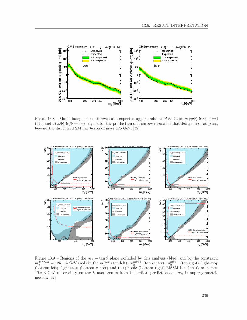
13.5. RESULT INTERPRETATION
[GeV]φm100 200 300 400 1000
[p
b]
)ττ→φ(
B⋅)φ(g
gσ
95%
CL
lim
it o
n
-310
-210
-110
1
10
210
310
φgg
ObservedExpected
Expectedσ 1± Expectedσ 2±
(8 TeV)-1 19.7 fbττ→φ Preliminary CMS
[GeV]φm100 200 300 400 1000
[p
b]
)ττ→φ(
B⋅)φ(b
bσ
95%
CL
lim
it o
n
-310
-210
-110
1
10
210
310
φbb
ObservedExpected
Expectedσ 1± Expectedσ 2±
(8 TeV)-1 19.7 fbττ→φ Preliminary CMS
Figure 13.8 – Model-independent observed and expected upper limits at 95% CL on σ(ggΦ).B(Φ→ ττ)(left) and σ(bbΦ).B(Φ→ ττ) (right), for the production of a narrow resonance that decays into tau pairs,beyond the discovered SM-like boson of mass 125 GeV. [42]
[GeV]Am200 400 600 800 1000
βta
n
10
20
30
40
50
60
(MSSM,SM)<0.05:SCL
Observed
Expected
Expectedσ 1±
scenariomaxhMSSM m
3 GeV± 125≠ hMSSMm
(7 TeV)-1 (8 TeV) + 4.9 fb-1, 19.7 fbττ→ Preliminary, h,H,ACMS
[GeV]Am200 400 600 800 1000
βta
n
10
20
30
40
50
60
(MSSM,SM)<0.05:SCL
Observed
Expected
Expectedσ 1±
scenariomod+hMSSM m
3 GeV± 125≠ hMSSMm
(7 TeV)-1 (8 TeV) + 4.9 fb-1, 19.7 fbττ→ Preliminary, h,H,ACMS
[GeV]Am200 400 600 800 1000
βta
n
10
20
30
40
50
60
(MSSM,SM)<0.05:SCL
Observed
Expected
Expectedσ 1±
scenariomod-hMSSM m
3 GeV± 125≠ hMSSMm
(7 TeV)-1 (8 TeV) + 4.9 fb-1, 19.7 fbττ→ Preliminary, h,H,ACMS
[GeV]Am200 400 600
βta
n
5
10
15
20
25
30
(MSSM,SM)<0.05:SCL
Observed
Expected
Expectedσ 1±
MSSM light-stop scenario
3 GeV± 125≠ hMSSMm
(7 TeV)-1 (8 TeV) + 4.9 fb-1, 19.7 fbττ→ Preliminary, h,H,ACMS
[GeV]Am200 400 600 800 1000
βta
n
10
20
30
40
50
60
(MSSM,SM)<0.05:SCL
Observed
Expected
Expectedσ 1±
MSSM light-stau scenario
3 GeV± 125≠ hMSSMm
(7 TeV)-1 (8 TeV) + 4.9 fb-1, 19.7 fbττ→ Preliminary, h,H,ACMS
[GeV]Am200 400 600 800 1000
βta
n
5
10
15
20
25
30
35
40
45
50
(MSSM,SM)<0.05:SCL
Observed
Expected
Expectedσ 1±
-phobic scenarioτMSSM
3 GeV± 125≠ hMSSMm
(7 TeV)-1 (8 TeV) + 4.9 fb-1, 19.7 fbττ→ Preliminary, h,H,ACMS
Figure 13.9 – Regions of the mA − tanβ plane excluded by this analysis (blue) and by the constraintmMSSMh = 125± 3 GeV (red) in the mmax
h (top left), mmod+h (top center), mmod−
h (top right), light-stop(bottom left), light-stau (bottom center) and tau-phobic (bottom right) MSSM benchmark scenarios.The 3 GeV uncertainty on the h mass comes from theoretical predictions on mh in supersymmetricmodels. [42]
239
CHAPTER 13. SEARCH FOR A HEAVY DI-TAU RESONANCE IN THE MSSM
13.6 Chapter summary and personal contributions
Search for a heavy di-tau resonance in the MSSM
The search for a heavy resonance decaying to a pair of taus is by far the mostpowerful way to discover an extended scalar sector in the MSSM when tan β, theratio between the vacuum expectation values of the two scalar doublets, is large.At large tan β values, the decays of the heavy resonance Φ = A/H/h to taus areenhanced, as is its production in association with b quarks. The analysis sensitivityis improved by categorizing events according to their number of b-tagged jets, andto the transverse momentum of their leading hadronic tau if applicable. As noexcess of data is observed on top of the predicted SM backgrounds, limits are set onthe cross section times branching fraction of a signal in the bbΦ and ggΦ productionmodes, for resonance masses between 90 and 1000 GeV. Results are also interpretedin different MSSM scenarios, and are seen to exclude a large part of the parameterspace, especially at large tan β.
My contributions
Figures: 13.1-13.3.
I have synchronized with the LLR Polytechnique group in the τhτh final state, whichconsists in reproducing all results from scratch up to the final limits and reachinga better than 10% agreement between the two analyses. I have also measured thetau trigger efficiency in data and MC simulations.
240

Part V
Status and prospects


Chapter 14
Overview of LHC results and prospects forfuture colliders
After the discovery of a particle compatible with the scalar boson of the SM,many fundamental questions remain. Searches performed at the LHC in Run-1have not permitted to discover BSM physics, but a few deviations from the SMexpectations have been observed with a low significance. These will require moredata, collected in Run-2 or later, to be confirmed or invalidated. Next sectionsdescribe the status of the results of the CMS experiment after Run-1 and theirprojections in the coming runs, with particular emphasis on the scalar sector, aswell as the prospects for the next collider experiments.
14.1 Overview of CMS measurements in the scalar sector
14.1.1 SM precision measurements
The significance of the excess of events at a mass of about 125 GeV has long sinceexceeded five standard deviations, and physicists are now performing precision measure-ments on the recently discovered particle, to assess its compatibility with the SM scalarhypothesis. The most precise decay channels are H → γγ and H → ZZ∗ → 4`. TheH → γγ analysis [132] is characterized by a small narrow resonance above a large fallingcontinuum background. To increase the sensitivity of this analysis, different categoriesare defined, with various signal purity and mass resolution. Results are extracted froma fit of the parameterized background and signal distributions to the observed data. Inthe H → ZZ∗ → 4` channel [60], at least one of the Z bosons is produced off-shell. Theso-called golden channel corresponds to the case where both Z bosons decay to leptons(essentially ee or µµ). Despite the low cross section times branching fraction, this decaychannel is extremely powerful and is one of the main components of the discovery in2012, because of the low level of backgrounds and the excellent lepton identification andreconstruction.
243
CHAPTER 14. OVERVIEW OF LHC RESULTS AND PROSPECTS FOR FUTURECOLLIDERS
As detailed in Chapter 7, the fermionic decay channels, despite their large branchingfractions at mH = 125 GeV, are less sensitive because of the large level of backgroundsin the gluon-gluon fusion production mode. The decay channel H → bb has the largestbranching fraction in the SM, but is extremely complicated experimentally because thedifficult distinction between jets originating from b quarks – b jets – and other jets makesthe QCD multijet background overwhelm the signal. Luckily, some production modes ofthe scalar boson give handle to reduce the backgrounds: this is the case of the vectorboson fusion production with two additional energetic forward jets, and of the associatedproduction with a vector boson where the decay products of this vector boson may be easyto identify. These two production modes have been studied at CMS, and although theresults are still far from a discovery in the bb decay mode, an excess at a mass close to 125GeV has been observed with a significance of 2.1 and 2.2 standard deviations respectivelyin the associated production and vector boson fusion production modes [119, 156]. Themain challenges in searching for H → ττ decays are to distinguish tau leptons decayinghadronically from jets originating from quarks or gluons, and to reduce the large multijetbackgrounds coming from Drell-Yan QCD processes. Additionally the invariant mass ofthe tau pair can only be reconstructed with a poor resolution (' 20%). The analysis ofdata taken in 2011 and 2012 at the LHC has shown an evidence for the existence of H de-cays to tau leptons, and all measurements (signal strength, mass, ...) are compatible withSM expectations. More details can be found in Chapter 7. The combined significance ofthe H → bb and H → ττ searches exceeds three standard deviations, which leads to anevidence for the decay of the 125-GeV particle to fermions [120].
Although the branching fractions of the SM scalar boson to a pair of electrons ormuons are tiny and not accessible with a low amount of data such as that collected dur-ing LHC Run-1, the searches H → µµ and H → ee are still performed because theobservation of such decays would be a clear evidence for BSM physics. In these anal-yses [157], the signal hypothesis forms a narrow resonance on top of SM backgrounds,which enables the analysts to use shape-based techniques to extract a potential signal.No excess has been observed in any of the decay channels, and upper limits have beenset by the CMS Collaboration at 95%CL on the branching fraction of the new particleto electrons (B(H → ee) < 0.0019) or muons (B(H → µµ) < 0.0016), assuming the SMproduction cross section for scalar boson.
The combination of ATLAS and CMS results in the H → γγ and H → ZZ∗ → 4`channels led to the most precise measurement of the new particle mass [158]:
mH = 125.09± 0.21 (stat.)± 0.11 (syst.) GeV. (14.1)
All production and decay channels have been taken into account in a CMS-only combi-nation [54]; the combined signal strength is found to be very compatible with the SMexpectation:
µ = 1.00± 0.09 (stat.)+0.08−0.07 (theo.)± 0.07 (syst.). (14.2)
The signal strengths measured for the different production and decay modes are all in agood agreement with the SM expectations, as shown in Fig. 14.1. An interesting feature is
244

14.1. OVERVIEW OF CMS MEASUREMENTS IN THE SCALAR SECTOR
SMσ/σBest fit 0 1 2 3 4
0.99± = 2.75 µ ttH tagged
0.35± = 0.83 µ VH tagged
0.27± = 1.15 µ VBF tagged
0.16± = 0.87 µ Untagged
0.14± = 1.00 µ Combined CMS
(7 TeV)-1 (8 TeV) + 5.1 fb-119.7 fb
= 125 GeVH m
= 0.24SM
p
SMσ/σBest fit 0 0.5 1 1.5 2
0.44± = 0.84 µ bb tagged→H
0.28± = 0.91 µ taggedττ →H
0.21± = 0.83 µ WW tagged→H
0.29± = 1.00 µ ZZ tagged→H
0.24± = 1.12 µ taggedγγ →H
0.14± = 1.00 µ Combined CMS
(7 TeV)-1 (8 TeV) + 5.1 fb-119.7 fb
= 125 GeVH m
= 0.96SM
p
Figure 14.1 – Measured signal strengths in different event categories that tag different production (left)and decay (right) modes. [54]
the excess observed in the ttH production mode [159]. Table 14.1 summarizes the signalstrengths and significances measured in the different production and decay channels ofthe SM scalar boson, with the data collected in Run-1 by the CMS detector.
Such a mass for the scalar boson, associated to the measured top quark mass [160]:
mt = 172.44± 0.13 (stat.)± 0.47 (syst.) GeV, (14.3)
implies that in the SM without addition of new physics, the universe lies at the boundarybetween stability and instability of the electroweak vacuum [161, 162], as illustrated inFig. 14.2. The electroweak vacuum lifetime in this meta-stability region fortunately ex-ceeds the age of the universe. The fact that the universe lies at the edge of the electroweakvacuum expectation value raises many questions: why did early fluctuations not destabi-lize the potential?, does it play a role in inflation?, .... This apparent meta-stability mightbe a hint in understanding deeper physics.
Another great achievement of Run-1 is the extraction of an upper bound on the Hboson width, equal to 5.4 times the value predicted in the SM for a boson mass of 125GeV [163]. This bound is obtained under the SM hypothesis, in the gg → H → ZZchannel, and relies on the determination of the relative off-shell and on-shell productions.Indeed, the respective cross sections are:
σon-shellgg→H→ZZ∗ 'g2ggHg
2HZZ
mHΓH, (14.4)
σoff-shellgg→H∗→ZZ 'g2ggHg
2HZZ
4m2Z
, (14.5)
245

CHAPTER 14. OVERVIEW OF LHC RESULTS AND PROSPECTS FOR FUTURECOLLIDERS
ggH
VBF
VH
ttHAll
H→γγ
µ=
1.12
+0.3
7−
0.3
2µ
=1.5
8+
0.7
7−
0.6
8µ
=−
0.16
+1.1
6−
0.7
9µ
=2.7
+2.6
−1.8
µ=
1.12±
0.245.6σ
H→ZZ
µ=
0.83+
0.3
1−
0.2
5(0/1-jet,
4`)µ
=1.4
5+
0.8
9−
0.6
2(2-jet,
4`)µ
=−
4.7+
5.0
−1.3
(4`)µ
=1.00±
0.29µ
=3.1
+2.4
−2.0
(3`)
6.5σ
H→WW
µ=
0.74
+0.2
2−
0.2
0µ
=0.6
0+
0.5
7−
0.4
6µ
=0.5
6+
1.2
7−
0.9
5(3`3ν)
µ=
5.3+
2.1
−1.8
(SS2`)
µ=
0.83±
0.21µ
=0.3
9+
1.9
7−
1.8
7(2`2ν
2q)4.7σ
H→ττ
µ=
0.34±
1.09
(0-jet)µ
=0.9
4±
0.4
1µ
=−
0.33±
1.02
µ=−
1.3
+6.3
−5.5
(τhτh )
µ=
0.91±
0.28µ
=1.0
7±
0.46
(1-jet)3.2σ
H→bb
-µ
=2.8
+1.6
−1.4
µ=
1.0±
0.5
µ=
0.7±
1.9µ
=0.84±
0.442.2σ
2.1σH→µµ
µ<
7.4
-µ<
7.4
<0.1σ
H→ee
µ<
3.7×
10 −
5-
µ<
3.7×
10 −5
All
µ=
0.85
+0.1
9−
0.1
6µ
=1.1
6+
0.3
7−
0.3
4µ
=0.9
2+
0.3
8−
0.3
6µ
=2.90
+1.0
8−
0.9
4µ
=1.00±
0.14
Table
14.1–Best-fit
signalstrengths
andobserved
significances,measured
inRun-1,
fordifferent
productionand
decaymodes
ofthe
SMscalar
boson.Results
comefrom
[16,54,59,60,119,132,156,157,159].
246

14.1. OVERVIEW OF CMS MEASUREMENTS IN THE SCALAR SECTOR
Figure 14.2 – Regions of stability, meta-stability and instability of the electroweak vacuum without anyBSM physics at the TeV scale. [161]
where gggH and gHZZ are the H boson couplings to gluons and Z bosons respectively,and ΓH is the H boson width. The indirect upper limit of ΓH < 22 MeV at 95% CLcomplements the existing experimental results on the H boson width, and gives a valuemore precise by more than two orders of magnitude.
All the above-mentioned physics analyses have shown a good agreement between theproperties of the 125-GeV particle and those predicted for the scalar boson of the SM.This is however not the end of the story, as many BSM theories with an extended scalarsector have an alignment limit, where the properties of one of their scalars tend to beSM-like. Highlighting deviations from the SM expectations therefore requires to reach agreater precision, and to analyze larger datasets. The LHC is expected to collect about 300fb−1 of proton-proton data by 2022, after which a long shutdown is planned for upgradesof the machine and detectors. The High Luminosity LHC (HL-LHC) will eventuallypermit to collect about 3000 fb−1 data with an increased instantaneous luminosity andlarger average pileup. Projections of the precision measurements on the scalar bosonhave been extrapolated from the Run-1 operation in the 300 and 3000 fb−1 cases [164].An optimistic and a pessimistic scenarios have been studied: the first one supposes thetheoretical uncertainties are reduced by a factor two and the other uncertainties arescaled by the square root of the luminosity, while the second one assumes the systematicuncertainties are the same as in Run-1. In any case, the performance of the detectorand trigger is considered to be the same as in Run-1. The projections of the precisionon the measurements of the signal strength for a SM-like boson are shown in Fig. 14.3:in particular the precision on the H → ττ signal strength, equal to approximately 30%in Run-1 can be reduced to 8-14% with 300 fb−1 data at 14 TeV, and 5-8% with 3000fb−1 data at 14 TeV. The increased precision obtained at the HL-LHC might lead to theobservation of deviations with respect to the SM predictions, and be an indication of theexistence of BSM physics.
247

CHAPTER 14. OVERVIEW OF LHC RESULTS AND PROSPECTS FOR FUTURECOLLIDERS
Figure 14.3 – Projected precisions on the measurement of the signal strength for a SM-like H bosonwith 300 (left) and 3000 (right) fb−1 data collected at 14 TeV. The two scenarios are described in thetext. [164]
14.1.2 Exotic scalar decays
Three categories of searches for exotic scalar decays are explored with data collectedat the LHC:
— A summary of the CMS searches for the exotic decay of the 125-GeV particle totwo light pseudoscalar bosons has been presented in Chapter 11. The results ofthe searches are interpreted in the context of 2HDM+S; the analyses can excludebranching fraction B(h → aa) values less than one in some scenarios (especiallylarge tan β in type-3, where the decays to leptons are enhanced over the decays toquarks) and in some pseudoscalar mass ranges. These analyses will be performedwith Run-2 data, and new final states and mass ranges will be covered to probe alarger phase space.
— Lepton-flavor violating scalar decays are also studied with CMS data [165]. Decayssuch as H → µτ or H → eτ are not allowed in the SM if the theory is renormaliz-able, and their observation would be an evidence for the existence of BSM physicsabove a finite mass scale. An excess of events compatible with H → µτ decays isobserved with a significance of 2.4 standard deviations, and corresponds to a best-fitbranching fraction B(H → µτ) = (0.84+0.39
−0.37)%. The ATLAS experiment does notconfirm the excess seen by CMS [166] but does not exclude its existence, and moreprecise results from the next LHC runs are looked forward to.
— In some BSM models, the SM-like scalar boson could decay to invisible particleswith a large branching fraction. Such a possibility is investigated through final stateswith a large transverse missing energy coming from H decays to invisible particles,and other physics objects from H production in association with a Z boson, in thevector boson fusion production mode, or in the gluon-gluon fusion mode with a jetfrom initial state radiation. The combination leads to an upper limit at 95% CL of
248

14.1. OVERVIEW OF CMS MEASUREMENTS IN THE SCALAR SECTOR
[GeV]Am100 200 300 400 1000
βta
n
1
2
3
456
10
20
30
4050
ττ →
A/H/h
bb
→H/A
µµ →A/H/h
ντ → ±H
ντ → ±
H
WW/ZZ→H
CMSPreliminary
) -1LHC run-1 2011-2012 (19.7-24.6 fb
=125 GeVhm
=122 GeVhm
arXiv:1508.07774
JHEP 11 (2015) 071
PLB 752 (2016) 221
HIG-14-029
JHEP 10 (2015) 144
95% CL exclusion contours
expected observed
mod+h
MSSM m
[GeV]Am200 300 400 500 1000
βta
n
1
2
3
456
10
20
30
4050
ττ →
A/H/h
bb→
H/A
µµ →A/H/h
Cou
plin
gs to
h(1
25)
WW/ZZ→H
)γγ hh (bb→H
)/ττ hh (bb→H )ττ Zh (ll→A
Model not strictly applicable
CMSPreliminary
) -1LHC run-1 2011-2012 (19.8-24.6 fb
Model not strictly applicable
HIG-15-002
JHEP 11 (2015) 071
PLB 752 (2016) 221
HIG-14-029
arXiv:1510.01181
HIG-13-032
JHEP 10 (2015) 144
95% CL exclusion contours
expected observed
hMSSM
Figure 14.4 – 95% CL exclusions contours as obtained by the most sensitive CMS analyses in the contextof the MSSM that have been performed on the LHC Run-1 dataset. The colored filled areas correspondto the regions in mA and tanβ that have been excluded at 95% CL. The colored (slightly darker shaded)lines with hatches correspond to the regions that were expected to be excluded. The exclusions are shownfor the (left) MSSM mmod+
h scenario with µ = 200 GeV, and the (right) hMSSM scenario. The regions inmA and tanβ where the hMSSM is not strictly applicable are marked in gray. The theoretical uncertaintyof the MSSM predictions on mh has been estimated to be ±3 GeV. [168,169]
36% on the branching fraction of the 125-GeV state to invisible particles [167].
14.1.3 MSSM and 2HDM scalar searches
Different parts of the MSSM parameter space can be covered by the study of a varietyof scalar decays. As described in Chapter 13, the search for resonances decaying to apair of tau leptons can exclude scenarios with large tan β, for which the scalar couplingsto leptons and down-type quarks are enhanced. Decays sensitive in the same high tan βregion, but less powerful, include H → µµ and H → bb. At low tan β, different finalstates can uncover an MSSM scalar sector: H → WW , H → ZZ, A→ Zh and H → hh.Meanwhile the search for a charged scalar boson is sensitive to the low mA region. Asummary of the searches for an MSSM scalar sector performed with the CMS data inRun-1 is presented in Fig. 14.4, in the mmod+
h [152, 153] and hMSSM [44] benchmarkscenarios [168]. As the MSSM is a special type of 2HDM, these searches can also beinterpreted in 2HDM [168]. However, because of the larger number of free parameters,the comparison of the results of several analyses is not as straightforward. No excess hasbeen observed in any search for a 2HDM scalar sector in Run-1 or Run-2 as of now.
249

CHAPTER 14. OVERVIEW OF LHC RESULTS AND PROSPECTS FOR FUTURECOLLIDERS
Figure 14.5 – Comparison of theoretically-predicted cross sections for various SM processes at 7, 8 and13 TeV, with experimental measurements made with the CMS detector in Run-1 and Run-2. [173]
14.2 Overview of other SM and BSM results of the CMS exper-iment
14.2.1 Standard model
With the 25 fb−1 proton-proton data collected by the CMS detector in Run-1, un-precedented precision on the measurement of the cross section of SM processes could beachieved [170,171]. All measurements and theory predictions are in remarkable agreementat 7, 8, and 13 TeV center-of-mass energy, as presented in Fig. 14.5. The top quark massmeasurement precision reached a great accuracy in Run-1 at CMS: mt = 172.44 ± 0.13(stat.) ±0.47 (syst.) GeV [160]. This value supplants the "world combination" performedin 2014 with the results of the ATLAS, CDF, CMS and D0 experiments [172]. More SMmeasurements were made in Run-1 [170,171], but are not be detailed here.
14.2.2 Dark matter
Unlike direct and indirect detection experiments, collider experiments not only searchfor dark matter (DM) candidates, but could also in principle produce them. DM candi-dates produced at the LHC are assumed to have weak-scale mass and interaction cross
250

14.3. FUTURE COLLIDER EXPERIMENTS
section with baryonic matter, and therefore to escape the detector leaving as signature amomentum imbalance. Most CMS searches for dark matter look for pair-produced darkmatter candidates, characterized by a large transverse missing energy ��ET , produced inassociation with an object identifiable in the detector; such analyses are generically calledmono-X + ��ET . The most sensitive mono-X + ��ET channel is the monojet, where one jetis produced from initial state radiation (ISR) and can be triggered on. Other mono-X +��ET analyses include the mono-photon, mono-scalar, mono-Z, mono-top and mono-leptonchannels. Collider experiments are complementary to direct and indirect detection exper-iments, and are typically more sensitive to low DM particle masses (mDM < 10 GeV) andspin-dependent interactions. Assuming a simplified model with a vector particle decayingto a pair of DM particles, the CMS experiment excludes at 90% confidence level (CL) inthe monojet channel, mediator masses up to 1.6 TeV with Run-1 and 1.3 TeV with Run-2data, for low DM particle masses [174,175].
14.2.3 Supersymmetry
A broad variety of analyses have searched for SUSY particles and processes in Run-1,without finding any hint of BSM physics [176]. If they are light enough to be produced atthe LHC, strongly-produced SUSY particles are expected to have the largest productioncross section of all sparticles. CMS analyses set limits on simplified models where gluinosor squarks are pair-produced, with inclusive searches. Other searches target processeswith smaller production cross sections, such as the direct production of stop quarks,sbottom quarks or electroweakinos. Results from different gluino and stop quark searches,interpreted in Simplified Model Spectra (SMS) are shown in Fig. 14.6. Even though themasses probed almost reach the highest possible mass for superparticles, many SUSYmodels have not been addressed yet, and a large parameter space remains unexplored.The SUSY physics program at the LHC will continue in the next runs.
14.2.4 Others
Many searches for exotic models (Z ′ boson, W ′ boson, leptoquarks, heavy stablecharged particles, excited leptons, heavy Majorana neutrinos, ...) have been performedat the LHC [178]. As of now only one promising excess has been reported by both theATLAS and CMS collaborations: an excess of events in the diphoton mass spectrum at amass of about 750 GeV [179,180]. The global significance is about two standard deviationsin the ATLAS analysis with Run-2 data, and somewhat lower for CMS, but it is intriguingthat an excess is seen at the same place in both experiments. Many theoretical modelshave been proposed to address such a deviation from the SM if it were to be confirmedwith larger datasets in Run-2.
14.3 Future collider experiments
The HL-LHC program extends until about 2035, but it is already time to design itssuccessor, as many fundamental questions will remain. If no new physics is observed atthe LHC, the reason could be that the new physics mass scale is beyond the LHC reach,
251

CHAPTER 14. OVERVIEW OF LHC RESULTS AND PROSPECTS FOR FUTURECOLLIDERS
gluino mass [GeV]
600 800 1000 1200 1400 1600
LSP
mas
s [G
eV]
0
100
200
300
400
500
600
700
800
900
1000
m(g
luin
o) - m
(LSP) =
2 m
(top)
ICHEP 2014 = 8 TeVs
CMS Preliminary
1
0χ∼ t t →g~ production, g~-g~-1) 19.5 fbT+HTESUS-13-012 0-lep (
-1) 11.7 fbTαSUS-12-028 0-lep (-1SUS-14-011 0+1+2-lep (razor) 19.3 fb
-1) 19.3 fbφ∆SUS-13-007 1-lep (-1SUS-13-007 1-lep (LS) 19.3 fb
-1SUS-13-016 2-lep (OS+b) 19.7 fb-1SUS-13-013 2-lep (SS+b) 19.5 fb
-1SUS-13-002 (MultiLepton) 19.5 fb-1SUS-13-008 3-lep (3l+b) 19.5 fb
-1) 19.5 fb2
SUS-13-019 (MT-1SUS-12-024 b-jet 19.4 fb
stop mass [GeV]
100 200 300 400 500 600 700 800
LSP
mas
s [G
eV]
0
100
200
300
400
500
600
700
W
= m
10χ∼
- m
t~mt
= m
10χ∼
- m
t~m
ICHEP 2014 = 8 TeVs
CMS Preliminary
1
0χ∼ / c 1
0χ∼ t →t~ production, t~-t
~
-1SUS-13-011 1-lep (MVA) 19.5 fb-1SUS-14-011 0-lep + 1-lep + 2-lep (Razor) 19.3 fb
-1SUS-14-011 0-lep (Razor) + 1-lep (MVA) 19.3 fb
)1
0χ∼ c →t~ ( -1SUS-13-009 (monojet stop) 19.7 fb
-1SUS-13-015 (hadronic stop) 19.4 fb
Observed
Expected
t
= m
10χ∼
- m
t~m
Figure 14.6 – Summary of exclusion limits in Simplified Model Spectra from several SUSY gluino (left)and stop (right) searches performed with the data collected by the CMS detector in 2012. [177]
or that the mass scale is accessible at the LHC but the final states are elusive to the directsearch. Different options of linear and circular colliders are studied to address both cases.In general, electron-positron colliders have the advantage to provide an extremely cleanexperimental environment, with an absence of strong-interaction backgrounds and withcontrolled electroweak backgrounds, allowing for very precise measurements. Addition-ally, such colliders do not suffer from underlying event and pileup collision contamination,and the triggering is easy with a 100% efficiency. On the other hand, hadronic collidershave a larger mass reach for the exploration of new physics, but require carefully-designedsubdetectors for the identification of particles in a crowded environment. Circular collid-ers, relative to linear colliders, can provide a much higher luminosity because of largercollision rates, continuous injection and multiple collision points, and their beam energycan be measured with great accuracy. However, the center-of-mass energy they can reachis lower because of synchrotron radiation, they consume a large power, and their beamsare difficult to polarize. A comparison between the luminosity and center-of-mass energylinear and circular colliders can reach is shown in Fig. 14.7 for some collider projects.Different collider projects are described in the next paragraphs.
The FCC-ee (also known as TLEP) [181] program involves electron-positron collisionsat a center-of-mass energy of 91 (Z boson pole), 160 (WW threshold), 240 (H productionpeak, dominated by Higgsstrahlung) and 350 (tt threshold) GeV in a circular collider witha circumference between 80 and 100 km situated in the Geneva basin. The FCC-ee wouldallow for extremely precise SM process measurements with permille-level uncertainties,and could set indirect constrains on heavy BSM particles. The dominant uncertaintyassociated to the measurement of SM processes would be theoretical. The scalar physicsprogram of the FCC-ee consists in determining all scalar boson couplings in a model-
252

14.3. FUTURE COLLIDER EXPERIMENTS
Figure 14.7 – Comparison between the instantaneous luminosity linear (ILC and CLIC) and circular(TLEP/FCC-ee with four interaction points) colliders can deliver as a function of the center-of-massenergy. [181]
independent way, in measuring its total decay width indirectly and evaluating its rareor exotic decays. The FCC-ee physics program for electroweak precision measurementsrelies on the production of about 1013 Z bosons, 108 W bosons and 106 tt pairs.
After a dozen years of operation (about two years at the Z pole, one or two years attheWW threshold, five years as a "Higgs factory", and five years at the tt threshold), andmore than two million scalar bosons produced, the FCC-ee could potentially be upgradedto become a proton-proton collider, FCC-hh, with a center-of-mass energy of around 100TeV [182]. Because the energy is proportional to the magnetic field and to the colliderradius, such an energy can be achieved by multiplying the magnetic field by a factor twoand the radius by a factor four relative to the LHC. The combination of FCC-ee andFCC-hh reduces the costs of having two experiments, and would permit to obtain thebest precision, sensitivity and reach for new physics among all other collider options. TheFCC-hh could collect between 250 and 1000 fb−1 every year, which would lead to about20 ab−1 after twenty-five years of operation. The option of a circular collider betweenelectrons and hadrons, FCC-eh, is also under study [183].
The International Linear Collider (ILC) [184] is a linear electron-positron collider thatcould be built in Japan in a few years. The ILC would in a first phase collect 500 fb−1
at an energy in the electron-positron center-of-mass of 250 GeV, 200 fb−1 at 350 GeV,and 500 fb−1 at 500 GeV, and in a second phase 3500 fb−1 at 500 GeV and 1500 fb−1 at250 GeV. Such a machine has a low beamstrahlung, and its luminosity and energy can bedetermined precisely. The ILC provides a clean environment to measure the scalar bosoncouplings with a great accuracy, which would allow to eventually highlight deviations
253

CHAPTER 14. OVERVIEW OF LHC RESULTS AND PROSPECTS FOR FUTURECOLLIDERS
Figure 14.8 – Left: Expected precision on the measurement of the H boson signal strength at the HL-LHC, ILC and TLEP/FCC-ee. The TLEP and ILC indications correspond to the data expected to becollected during the run at 350 GeV center-of-mass energy and during the previous runs at lower energy.Right: Precision on the top quark and W boson mass measurements achievable with different projects ofcolliders. [181]
from the SM predictions. Its physics program also covers measurements of the proper-ties of the top quark with a great accuracy, and searches for new particles at the TeV scale.
A comparison of the expected reach of the HL-LHC, FCC-ee and ILC in terms of scalarboson signal strength precision, top quark mass and scalar boson mass measurements isshown in Fig. 14.8.
14.4 Chapter summary
Overview of LHC results and prospects for future colliders
The CMS physics program has covered an impressive range of new physics searchesand precision measurements as of now. The highlight of the Run-1 is the discoveryof a new particle compatible with the SM scalar boson and the measurement of someof its properties, but the fact that searches for BSM physics, such as dark matter orSUSY, do not observe any deviation from the SM in a large parameter space is notless interesting. Future collider studies and designs have started in order to takeover the LHC physics program and to address the unanswered questions after theLHC stops running.
254

Conclusion
The LHC started operating in 2010, at an unprecedented center-of-mass energy of 7TeV. Its Run-1 extended until the end of 2012 with a center-of-mass energy of 8 TeV. Aftera first long shutdown, the LHC resumed its operations in 2015 with proton-proton colli-sions at a center-of-mass energy of 13 TeV. The discovery of a new particle, H, compatiblewith the Brout-Englert-Higgs boson of the standard model (SM) is without contest thehighlight of the Run-1 of the LHC.
The discovery of the new particle was driven by the searches in the H → γγ andH → ZZ decay channels, but many other decay modes are open in the SM for a massof the scalar boson equal to 125 GeV. Measuring the production cross sections and thebranching fractions of the new boson for all possible production and decay modes is essen-tial to assess its compatibility with the SM predictions. In Chapters 7 and 8 is describeda search for the SM scalar boson, produced in association with a Z boson or a W bosonrespectively, and decaying to a pair of tau leptons. The di-tau final state is the mostsensitive fermionic decay channel, and therefore gives the most precise measurement ofthe Yukawa couplings of the scalar particle. While the vector boson associated productionhas a small cross section relative to the gluon-gluon fusion and vector boson fusion pro-duction modes, an efficient background rejection is obtained by selecting the light leptonsoriginating from the vector boson decays. Both analyses are not sensitive yet to the crosssection predicted in the SM for the scalar boson, but their results are compatible with theSM scalar boson hypothesis. After combination with the dominant production modes,the first evidence for the decay of the H boson to a pair of tau leptons is achieved with asignificance of 3.2 standard deviations, as detailed in Chapter 9.
In the SM, the H boson decays approximately 6% of the time to tau leptons if it hasa mass of 125 GeV. The H → ττ decay channel is challenging because of the similaritybetween hadronically decaying taus, and quark and gluon jets. In CMS, the HadronsPlus Strips (HPS) algorithm is used to reconstruct and identify hadronic taus (τh), as de-scribed in Chapter 6. It first proceeds by checking that tau candidates correspond to oneof the possible tau decay modes by counting the number of tracks and deposits in strips ofthe electromagnetic calorimeter, and measuring their compatibility with a hadronic tauhypothesis. The second step consists in rejecting jets, electrons and muons by applyingfurther selection criteria, based among others on the isolation of the tau candidates. A
255

Conclusion
typical selection efficiency of 50% can be reached, for a j → τh misidentification rate atthe percent level, and e → τh and µ → τh misidentification rates at the permille levelor below. The performance is also measured in data collected both in Run-1 and Run-2:it is generally compatible with the performance in MC simulations, but some data-to-simulation scale factors not equal to unity are also derived, for example for the e → τhand µ→ τh misidentification rates. The uncertainties on the tau identification efficiencyand tau energy scale in data amount to 6% and 3% respectively.
The SM is known not to answer a series of questions, and is thought to be a goodapproximation at low energies of a more fundamental theory. This is motivated amongothers by the existence of dark matter and dark energy, the hierarchy problem, describ-ing the fact that the H boson mass receives huge corrections, or the will to unify allfundamental interactions. Many of the models that address some of these questions in-troduce an extended scalar sector. This is the case of the minimal supersymmetric SM(MSSM), which contains three neutral and two charged scalars. The MSSM can be de-scribed at tree level by two parameters: mA the mass of the neutral pseudoscalar, andtan β the ratio between the vacuum expectation values of the two scalar doublets. Dif-ferent searches should be performed to cover the full parameter space of the MSSM; forexample H/A/h → ττ is sensitive at large tan β while A → Zh searches are powerfulat low tan β only. More general models are two-Higgs-doublet models (2HDM), whichalso give rise to five (pseudo)scalars. Depending on the choice of its parameters, it canmotivate the existence of light pseudoscalars. A simple extension of 2HDM is 2HDM+S,where a scalar singlet is added to the two scalar doublets. Such models make the decay ofthe 125-GeV particle to non-SM particles possible, even after the precision measurementson the SM-like scalar performed in Run-1. In general, tau leptons are important objects touncover a potentially extended scalar sector, because the scalar boson Yukawa couplingsare proportional to the mass, and taus are by far heavier than muons and electrons.
Chapter 10 details the search for A → Zh decays in the ``ττ final states. The lightleptons originating from the Z boson allow for an efficient background rejection, whileh→ ττ has a large branching fraction relative to most other decay channels. The analysisis performed with 8 TeV data, and combined with H → hh→ bbττ , which is also sensitiveat low tan β and in a comparable mass range. No excess is observed in any of the finalstates, and the results are interpreted as model-independent upper limits on the crosssection times branching fraction, and as model-dependent limits in the mA − tan β planein the MSSM and 2HDM type-2. Cross sections times branching fractions between 5 and17 fb are excluded at 95% CL for pseudoscalar boson masses ranging between 220 and350 GeV in the A→ Zh→ ``ττ analysis.
The possibility of exotic decays of the h boson to a pair of light pseudoscalar bosonsis studied in Chapter 11. The h→ aa→ µµττ is especially sensitive in 2HDM+S type-3,where, for tan β > 1, the decays of the pseudoscalar a boson to leptons are enhanced overits decays to quarks. The expected SM backgrounds are particularly low, and an unbinned
256

Conclusion
shape analysis is performed. No significant excess is observed, and upper limits between 4and 15% can be set on B(h→ aa) in the hypotheses that the h production cross section isthe same as predicted in the SM, and that the a boson does not decay to quarks, which isa good approximation at large tan β in 2HDM+S type-3. The end of the chapter presentsan interpretation of all h → aa searches performed with the CMS detector in Run-1, indifferent types of 2HDM+S and for different tan β values; pseudoscalar masses between 1GeV to half of the h boson mass are covered by the analyses.
In 2HDM and for a given choice of the model parameters, the production of lightpseudoscalars is allowed with large cross sections, while not contradicting other LHCmeasurements. Chapter 12 describes the search for a light pseudoscalar decaying to tausand produced in association with b quarks. The search covers a mass region between 25and 80 GeV, which was unexplored before at the LHC. No excess is observed in any of thethree di-tau final states studied, and stringent upper limits are set on the cross sectiontimes branching fraction. The analysis is seen to exclude such a process for pseudoscalarmasses between 25 and 80 GeV in 2HDM type-2 with negative Yukawa couplings of theh boson to down-type fermions.
Chapter 13 presents the search for a heavy resonance (Φ = A/H/h) in the MSSM, withan improved sensitivity obtained by categorizing the events according to the pT of theirhadronic taus, and by using the MVA tau identification including lifetime information.The Φ → τhτh decay channel, which has the largest branching fraction, is described indetails. Again, no excess of data above the predicted SM backgrounds is observed, andlimits are set on the production cross section times branching fractions for the bbΦ andggΦ production modes. The excluded cross section times branching fraction ranges ap-proximately from 22 pb to 8 fb depending on the resonance mass and on the productionmode. The results are also interpreted in some benchmark scenarios, where large partsof the regions with high tan β are excluded. In particular, tan β values as low as about 3can be excluded in the mmax
h scenario of the MSSM for mA ' 140 GeV.
No evidence for BSM physics has been observed in any of the searches presented in thisthesis, neither in other CMS measurements performed in Run-1 as detailed in Chapter 14.The Run-2 of the LHC started at the beginning of 2015, with an increased center-of-massenergy, which permits to explore completely new regions. The large luminosity thatwill be collected together with the increased center-of-mass energy, will make searchesfor BSM processes with smaller cross sections or heavier particles possible, and allowfor more precise measurements of the SM-like scalar properties, which might highlightdeviations from the SM expectation. The MSSM parameter space has been impressivelywell covered in Run-1, though unexplored regions, especially at large and intermediatemA, still remain. In addition, many new physics signatures have not yet been studied.This is only the beginning of the LHC program, and many discoveries most likely lie aheadof us.
257


Appendix A
Technical details about physics analyses
A.1 Monte Carlo samples and collected datasets
The collision datasets used in the analyses described throughout this thesis are pre-sented in Tab. A.1, A.2 and A.3, at 7, 8 and 13 TeV center-of-mass energies respectively.The Monte Carlo samples, together with their generators and cross sections are indicatedin Tab. A.4, A.5 and A.6.
A.2 Triggers
The trigger paths used in the analyses described throughout this thesis are indicatedin Tab. A.7 for every studied final state.
Dataset Run-range L (fb) Chapters6 7 8 10 11 12 13
µµ /DoubleMu/Run2011A-16Jan2012-v1 160329–175770 0.211 X
/DoubleMu/Run2011B-16Jan2012-v1 175832–180252 2.562 X
ee
/DoubleElectron/Run2011A-16Jan2012-v1 160329–175770 0.211 X/DoubleElectron/Run2011B-16Jan2012-v1 175832–180252 2.562 X
eµ
/MuEG/Run2011A-16Jan2012-v1 160329–175770 0.211 X/MuEG/Run2011B-16Jan2012-v1 175832–180252 2.562 X
Table A.1 – Datasets collected at 7 TeV center-of-mass energy, used in the physics analyses detailed inthis thesis.
259

APPENDIX A. TECHNICAL DETAILS ABOUT PHYSICS ANALYSES
Dataset Run-range L (fb) Chapters6 7 8 10 11 12 13
eτh/µτ h
/TauPlusX/Run2012A-22Jan2013-v1 190456–193621 0.887 X X/TauPlusX/Run2012B-22Jan2013-v1 193833–196531 4.446 X X/TauPlusX/Run2012C-22Jan2013-v1 198022–203742 7.153 X X/TauPlusX/Run2012D-22Jan2013-v1 203777–208686 7.318 X X
τ hτ h
/TauParked/Run2012B-22Jan2013-v1 193833–196531 3.885 X/TauParked/Run2012C-22Jan2013-v1 198022–203742 7.153 X/TauParked/Run2012D-22Jan2013-v1 203777–208686 7.318 X
/JetHT/Run2012B-22Jan2013-v1 193833–196531 3.885 X/JetHT/Run2012C-22Jan2013-v1 198022–203742 7.153 X/JetHT/Run2012D-22Jan2013-v1 203777–208686 7.318 X
eµ
/MuEG/Run2012A-22Jan2013-v1 190456–193621 0.887 X X X/MuEG/Run2012B-22Jan2013-v2 193833–196531 4.446 X X X/MuEG/Run2012C-22Jan2013-v3 198022–203742 7.153 X X X/MuEG/Run2012D-22Jan2013-v4 203777–208686 7.318 X X X
µµ
/DoubleMu/Run2012A-22Jan2013-v1 190456–193621 0.887 X X X/DoubleMuParked/Run2012B-22Jan2013-v1 193833–196531 4.446 X X X/DoubleMuParked/Run2012C-22Jan2013-v1 198022–203742 7.153 X X X/DoubleMuParked/Run2012D-22Jan2013-v1 203777–208686 7.318 X X X
ee
/DoubleElectron/Run2012A-22Jan2013-v1 190456–193621 0.887 X X/DoubleElectron/Run2012B-22Jan2013-v1 193833–196531 4.446 X X/DoubleElectron/Run2012C-22Jan2013-v1 198022–203742 7.153 X X/DoubleElectron/Run2012D-22Jan2013-v1 203777–208686 7.318 X X
µ
/SingleMu/Run2012A-22Jan2013-v1 190456–193621 0.887 X/SingleMu/Run2012B-22Jan2013-v1 193833–196531 4.446 X/SingleMu/Run2012C-22Jan2013-v1 198022–203742 7.153 X/SingleMu/Run2012D-22Jan2013-v1 203777–208686 7.318 X
Table A.2 – Datasets collected at 8 TeV center-of-mass energy, used in the physics analyses detailed inthis thesis. This table considers only the eτh, µτh, eµ and τhτh final states of the MSSM Φ→ ττ analysisdescribed in Chapter 13.
Dataset Chapters6 7 8 10 11 12 13
µ
/SingleMuon/Run2015C25ns-16Dec2015-v1 X/SingleMuon/Run2015D-16Dec2015-v1 X
Table A.3 – Datasets collected at 13 TeV center-of-mass energy, used in the physics analyses detailed inthis thesis.
Process Generator XS×B (pb) Chapters6 7 8 10 11 12 13
ZZ → 4` Pythia 0.106 X Xgg → ZZ∗ → 2`2` Pythia 0.005 X
WZ → 3`ν Madgraph 0.868 XttZ Madgraph 0.139 X
WH/ZH/ttH with H → ττ Pythia 0.021 X XH →WW → 2`2ν, WH,ZH, ttH Powheg 0.0053 X X
Table A.4 – MC samples, with their generators and cross sections used in 7 TeV analyses. The crosssections for the SM scalar boson are indicated for mH = 125 GeV.
260
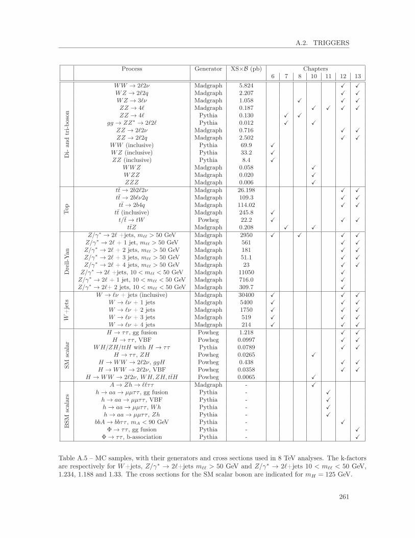
A.2. TRIGGERS
Process Generator XS×B (pb) Chapters6 7 8 10 11 12 13
Di-an
dtri-b
oson
WW → 2`2ν Madgraph 5.824 X XWZ → 2`2q Madgraph 2.207 X XWZ → 3`ν Madgraph 1.058 X X XZZ → 4` Madgraph 0.187 X X X XZZ → 4` Pythia 0.130 X X
gg → ZZ∗ → 2`2` Pythia 0.012 X XZZ → 2`2ν Madgraph 0.716 X XZZ → 2`2q Madgraph 2.502 X X
WW (inclusive) Pythia 69.9 XWZ (inclusive) Pythia 33.2 XZZ (inclusive) Pythia 8.4 X
WWZ Madgraph 0.058 XWZZ Madgraph 0.020 XZZZ Madgraph 0.006 X
Top
tt→ 2b2`2ν Madgraph 26.198 X Xtt→ 2b`ν2q Madgraph 109.3 X Xtt→ 2b4q Madgraph 114.02 X X
tt (inclusive) Madgraph 245.8 Xt/t→ tW Powheg 22.2 X X X
ttZ Madgraph 0.208 X X
Drell-Yan
Z/γ∗ → 2` +jets, m`` > 50 GeV Madgraph 2950 X X X XZ/γ∗ → 2` + 1 jet, m`` > 50 GeV Madgraph 561 X XZ/γ∗ → 2` + 2 jets, m`` > 50 GeV Madgraph 181 X XZ/γ∗ → 2` + 3 jets, m`` > 50 GeV Madgraph 51.1 X XZ/γ∗ → 2` + 4 jets, m`` > 50 GeV Madgraph 23 X XZ/γ∗ → 2` +jets, 10 < m`` < 50 GeV Madgraph 11050 XZ/γ∗ → 2` + 1 jet, 10 < m`` < 50 GeV Madgraph 716.0 XZ/γ∗ → 2`+ 2 jets, 10 < m`` < 50 GeV Madgraph 309.7 X
W+jets
W → `ν + jets (inclusive) Madgraph 30400 X X XW → `ν + 1 jets Madgraph 5400 X X XW → `ν + 2 jets Madgraph 1750 X X XW → `ν + 3 jets Madgraph 519 X X XW → `ν + 4 jets Madgraph 214 X X X
SMscalar
H → ττ , gg fusion Powheg 1.218 X XH → ττ , VBF Powheg 0.0997 X X
WH/ZH/ttH with H → ττ Pythia 0.0789 X XH → ττ , ZH Powheg 0.0265 X
H →WW → 2`2ν, ggH Powheg 0.438 X XH →WW → 2`2ν, VBF Powheg 0.0358 X X
H →WW → 2`2ν, WH,ZH, ttH Powheg 0.0065 X
BSM
scalars
A→ Zh→ ``ττ Madgraph - Xh→ aa→ µµττ , gg fusion Pythia - Xh→ aa→ µµττ , VBF Pythia - Xh→ aa→ µµττ , Wh Pythia - Xh→ aa→ µµττ , Zh Pythia - X
bbA→ bbττ , mA < 90 GeV Pythia - XΦ→ ττ , gg fusion Pythia - X
Φ→ ττ , b-association Pythia - X
Table A.5 – MC samples, with their generators and cross sections used in 8 TeV analyses. The k-factorsare respectively for W+jets, Z/γ∗ → 2`+jets m`` > 50 GeV and Z/γ∗ → 2`+jets 10 < m`` < 50 GeV,1.234, 1.188 and 1.33. The cross sections for the SM scalar boson are indicated for mH = 125 GeV.
261

APPENDIX A. TECHNICAL DETAILS ABOUT PHYSICS ANALYSES
Process Generator XS×B (pb) Chapters6 7 8 10 11 12 13
V V → 2`2ν aMC@NLO 11.95 XZZ → 2`2q aMC@NLO 3.22 XZZ → 4` aMC@NLO 1.21 X
WW → 1`1ν2q aMC@NLO 50.00 XWZ → 2`2q aMC@NLO 5.60 XWZ jets aMC@NLO 5.26 X
WZ → 3`1ν aMC@NLO 4.71 XWZ → 1`3ν aMC@NLO 3.05 XWZ → 1`1ν2q aMC@NLO 10.71 Xtt (inclusive) Powheg 831.8 Xt/t→ tW Powheg 71.2 X
Z/γ∗ → 2` +jets, m`` > 50 GeV Madgraph 6025.2 XW → `ν + jets (inclusive) Madgraph 61526.7 X
Table A.6 – MC samples, with their generators and cross sections used in 13 TeV analyses. W+jets andZ+jets cross sections are quoted at NNLO.
Year Path Chapters6 7 8 10 11 12 13
`τh 2012 Ele22_eta2p1_WP90Rho_LoosePFIsoTau20 X X
2012 IsoMu17_eta2p1_LoosePFIsoTau20 X X
τ hτ h 2012 DoubleMediumIsoPFTau35_Trk5_eta2p1 X
2012 DoubleMediumIsoPFTau35_Trk1_eta2p1 X
eµ
2011 Mu8_Ele17_CaloIdL X2011 Mu8_Ele17_CaloIdT_CaloIsoVL X2012 Mu8_Ele17_CaloIdT_CaloIsoVL_TrkIdVL_TrkIsoVL X X X2011 Mu17_Ele8_CaloIdL X2011 Mu17_Ele8_CaloIdT_CaloIsoVL X2012 Mu17_Ele8_CaloIdT_CaloIsoVL_TrkIdVL_TrkIsoVL X X X
µµ
2011 DoubleMu7 X2011 Mu13_Mu8 X
2011/2012 Mu17_Mu8 X X X2012 Mu17_TkMu8 X X X
ee
2011 Ele17_CaloIdL_CaloIsoVL_Ele8_CaloIdL_CaloIsoVL X
2011/2012 Ele17_CaloIdT_CaloIsoVL_TrkIdVL_TrkIsoVL_Ele8_CaloIdT_CaloIsoVL_TrkIdVL_TrkIsoVL
X X
µ
2011/2012 IsoMu24_eta2p1 X2015 IsoMu18 X
Table A.7 – Trigger paths used in the analyses detailed in this thesis. For the MSSM Φ→ ττ analysis ofChapter 13, only the eτh, µτh, τhτh and eµ final states at 8 TeV center-of-mass energy are covered.
262

Bibliography
[1] C. Burgess and G. Moore. The standard model, a primer. Cambridge University Press, 2013.[2] D. Griffiths. Introduction to elementary particles. Wiley-VCH, 2008.[3] S. L. Glashow. Partial symmetries of weak interactions. Nucl. Phys., 22:579–588, 1961.[4] S. Weinberg. A model of leptons. Phys. Rev. Lett., 19:1264–1266, 1967.[5] A. Salam. Weak and electromagnetic interactions. Conf. Proc., C680519:367–377, 1968.[6] J. Gunion et al. The Higgs hunter’s guide. Perseus Publishing, 1990.[7] P. Ramond. Journeys beyond the standard model. Perseus Books, 1999.[8] J. J. Thomson. Cathode rays. Phil. Mag., 44:293–316, 1897.[9] Particle Data Group. Review of particle physics. Chin. Phys., C38:090001, 2014.[10] P. Higgs. Broken symmetries and the masses of gauge bosons. Phys. Rev. Lett., 13:508–509, 1964.[11] P. Higgs. Broken symmetries, massless particles and gauge fields. Phys. Lett., 12:132–133, 1964.[12] P. Higgs. Spontaneous symmetry breakdown without massless bosons. Phys. Rev., 145:1156–1163,
1966.[13] F. Englert and R. Brout. Broken symmetry and the mass of gauge vector mesons. Phys. Rev. Lett.,
13:321–323, 1964.[14] G. S. Guralnik, C. R. Hagen, and T. W. B. Kibble. Global conservation laws and massless particles.
Phys. Rev. Lett., 13:585–587, 1964.[15] T. W. B. Kibble. Symmetry breaking in non abelian gauge theories. Phys. Rev., 155:1554–1561,
1967.[16] CMS Collaboration. Evidence for the 125 GeV Higgs boson decaying to a pair of τ leptons. JHEP,
1405:104, 2014.[17] LHC Higgs cross section working group. LHC Higgs Cross Section Working Group.
https://twiki.cern.ch/twiki/bin/view/LHCPhysics/CrossSections.[18] A. Djouadi. The anatomy of electro-weak symmetry breaking - Tome I: The Higgs boson in the
standard model. 2005. arXiv:0503.172.[19] CMS Collaboration. Observation of a new boson at a mass of 125 GeV with the CMS experiment
at the LHC. Phys. Lett., B716:30–61, 2013.[20] ATLAS Collaboration. Observation of a new particle in the search for the standard model Higgs
boson with the ATLAS detector at the LHC. Phys. Lett., B716:1–29, 2013.[21] Y. Nagashima. Beyond the standard model of elementary particle physics. Wiley-VCH, Weinheim,
2014.[22] Super-Kamiokande Collaboration. Evidence for oscillation of atmospheric neutrinos. Phys. Rev.
Lett., 81:1562–1567, 1998.
263

BIBLIOGRAPHY
[23] Double Chooz Collaboration. Indication for the disappearance of reactor electron antineutrinos inthe Double Chooz experiment. Phys. Rev. Lett., 108:131801, 2012.
[24] F. Zwicky. Die Rotverschiebung von extragalaktischen Nebeln. Helv. Phys. Acta, 6:110–127, 1933.[25] Planck Collaboration. Planck 2015 results. XIII. Cosmological parameters. 2015. arXiv:1502.01589.[26] A. D. Sakharov. Violation of CP invariance, C asymmetry, and baryon asymmetry of the universe.
Pisma Zh. Eksp. Teor. Fiz., 5:32–35, 1967.[27] G. Burdman. New solutions to the hierarchy problem. Braz. J. Phys., 37:506–513, 2007.[28] G. C. Branco et al. Theory and phenomenology of two-Higgs-doublet models. Phys. Rept., 516:1–
102, 2012.[29] M. Carena and H. Haber. Higgs boson theory and phenomenology. Prog. Part. Nucl. Phys.,
50:63–152, 2003.[30] A. Djouadi. The Higgs particles in the MSSM.
http://ecole-de-gif.in2p3.fr/Cours/GIF01/djouadi.ps.[31] S. L. Glashow and S. Weinberg. Natural conservation laws for neutral currents. Phys. Rev.,
D15:1958, 1977.[32] N. Deshpande and E. Ma. Pattern of symmetry breaking with two Higgs doublets. Phys. Rev.,
D18:2574, 1978.[33] J. Gunion and H. Haber. CP-conserving two-Higgs-doublet model: The approach to the decoupling
limit. Phys. Rev. D, 67, 2003.[34] N. Craig, J. Galloway, and S. Thomas. Searching for signs of the second Higgs doublet. 2013.
arXiv:1305.2424.[35] J. Bernon et al. Light Higgs bosons in two-Higgs-doublet models. Phys. Rev., D91(7):075019, 2015.[36] S. Martin. A supersymmetry primer. 1998. Adv. Ser. Direct. High Energy Phys.18,1.[37] J. Wess and B. Zumino. Supergauge transformations in four-dimensions. Nucl. Phys., B70:39–50,
1974.[38] Y. A. Golfand and E. P. Likhtman. Extension of the algebra of Poincare group generators and
violation of p invariance. JETP Lett., 13:323–326, 1971.[39] P. Fayet. Supergauge invariant extension of the Higgs mechanism and a model for the electron and
its neutrino. Nucl. Phys., B90:104–124, 1975.[40] P. Fayet. Spontaneously broken supersymmetric theories of weak, electromagnetic and strong
interactions. Phys. Lett., B69:489, 1977.[41] P. Fayet. Supersymmetry and weak, electromagnetic and strong interactions. Phys. Lett., B64:159,
1976.[42] CMS Collaboration. Search for additional neutral Higgs bosons decaying to a pair of tau leptons in
pp collisions at√s = 7 and 8 TeV. CMS Physics Analysis Summary CMS-PAS-HIG-14-029, 2015.
[43] A. Djouadi. The anatomy of electro-weak symmetry breaking. II. The Higgs bosons in the minimalsupersymmetric model. Phys. Rept., 459:1–241, 2008.
[44] A. Djouadi et al. Fully covering the MSSM Higgs sector at the LHC. JHEP, 06:168, 2015.[45] A. Djouadi and J. Quevillon. The MSSM Higgs sector at a high MSUSY : reopening the low tanβ
regime and heavy Higgs searches. JHEP, 10:028, 2013.[46] J. M. Frere, D. R. T. Jones, and S. Raby. Fermion masses and induction of the weak scale by
supergravity. Nucl. Phys., B222:11–19, 1983.[47] E. Cremmer, P. Fayet, and L. Girardello. Gravity induced supersymmetry breaking and low-energy
mass spectrum. Phys. Lett., B122:41, 1983.
264
BIBLIOGRAPHY
[48] U. Ellwanger, C. Hugonie, and A. M. Teixeira. The Next-to-Minimal Supersymmetric StandardModel. Phys. Rept., 496:1–77, 2010.
[49] J. E. Kim and H. P. Nilles. The mu problem and the strong CP problem. Phys. Lett., B138:150,1984.
[50] C. Englert et al. Exploring the Higgs portal. Phys. Lett., B703:298–305, 2011.[51] M. Carena et al. Complementarity between non-standard Higgs boson searches and precision Higgs
boson measurements in the MSSM. Phys. Rev., D91(3):035003, 2015.[52] D. Curtin et al. Exotic decays of the 125 GeV Higgs boson. Phys. Rev., D90(7):075004, 2014.[53] D. Curtin, R. Essig, and Y. Zhong. Uncovering light scalars with exotic Higgs decays to bbµ+µ−.
JHEP, 06:025, 2015.[54] CMS Collaboration. Precise determination of the mass of the Higgs boson and tests of compatibility
of its couplings with the standard model predictions using proton collisions at 7 and 8 TeV. Eur.Phys. J., C75(5):212, 2015.
[55] CMS Collaboration. Search for a light NMSSM Higgs boson produced in supersymmetric cascadesand decaying into a b-quark pair. CMS Physics Analysis Summary CMS-PAS-HIG-14-030, 2015.
[56] C. Caillol et al. Precision versus discovery: A simple benchmark. Eur.Phys.J.Plus, 129:93, 2014.[57] CMS Collaboration. Combination of standard model Higgs boson searches and measurements of
the properties of the new boson with a mass near 125 GeV. CMS Physics Analysis SummaryCMS-PAS-HIG-13-005, 2013.
[58] CMS Collaboration. Search for a heavy Higgs boson in the H to ZZ to 2l2nu channel in pp collisionsat√s = 7 and 8 TeV. CMS Physics Analysis Summary CMS-PAS-HIG-13-005, 2013.
[59] CMS Collaboration. Measurement of Higgs boson production and properties in the WW decaychannel with leptonic final states. JHEP, 01:096, 2014.
[60] CMS Collaboration. Measurement of the properties of a Higgs boson in the four-lepton final state.Phys. Rev., D89(9):092007, 2014.
[61] Procedure for the LHC Higgs boson search combination in Summer 2011. Technical Report CMS-NOTE-2011-005. ATL-PHYS-PUB-2011-11, CERN, Geneva, Aug 2011.
[62] J. S. Conway. Incorporating nuisance parameters in likelihoods for multisource spectra. In Pro-ceedings, PHYSTAT 2011 Workshop on Statistical Issues Related to Discovery Claims in SearchExperiments and Unfolding, CERN,Geneva, Switzerland 17-20 January 2011, 2011.
[63] A. L. Read. Linear interpolation of histograms. Nucl. Instrum. Meth., A425:357–360, 1999.[64] R. Barlow and C. Beeston. Fitting using finite Monte Carlo samples. Comput. Phys. Commun.,
77:219–228, 1993.[65] A. L. Read. Presentation of search results: The CL(s) technique. J. Phys., G28:2693–2704, 2002.[66] A. L. Read. Modified frequentist analysis of search results (the CLs method). CERN-OPEN-2000-
205, 2000.[67] T. Junk. Confidence level computation for combining searches with small statistics. Nucl. Instrum.
Meth., A434:435–443, 1999.[68] G. Cowan et al. Asymptotic formulae for likelihood-based tests of new physics. Eur. Phys. J.,
C71:1554, 2011.[69] E. Gross and O. Vitells. Trial factors or the look elsewhere effect in high energy physics. Eur. Phys.
J., C70:525–530, 2010.[70] R. Cousins. Generalization of chisquare goodness-of-fit test for binned data using saturated models,
with application to histograms. http://www.physics.ucla.edu/cousins/stats/cousinssaturated.pdf,2010.
265
BIBLIOGRAPHY
[71] A. Hocker et al. TMVA - Toolkit for multivariate data analysis. PoS, ACAT:040, 2007.
[72] B. Roe et al. Boosted decision trees, an alternative to artificial neural networks. Nucl. Instrum.Meth., A543(2-3):577–584, 2005.
[73] LEP Working Group for Higgs boson searches ALEPH L3 OPAL, DELPHI. Search for the standardmodel Higgs boson at LEP.
[74] CDF and D0 Collaborations. Higgs boson studies at the Tevatron. Phys. Rev., D88(5):052014,2013.
[75] L. Evans and P. Bryant. LHC machine. JINST, 3:S08001, 2008.
[76] CERN. CERN website. http://home.cern/fr, 2015.
[77] CMS Collaboration. The CMS experiment at the CERN LHC. JINST, 3:S08004, 2008.
[78] ATLAS Collaboration. The ATLAS experiment at the CERN Large Hadron Collider. JINST,3:S08003, 2008.
[79] LHCb Collaboration. The LHCb detector at the LHC. JINST, 3:S08005, 2008.
[80] ALICE Collaboration. The ALICE experiment at the CERN LHC. JINST, 3:S08002, 2008.
[81] CMS Collaboration. CMS luminosity - Public results.https://twiki.cern.ch/twiki/bin/view/CMSPublic/LumiPublicResults, 2015.
[82] J. Butler et al. CMS Phase II upgrade scope document. CERN-LHCC-2015-019. LHCC-G-165,2015.
[83] CMS Collboration. CMS Physics: Technical Design Report Volume 1: Detector Performance andSoftware. Technical Design Report CMS. CERN, Geneva, 2006. http://cds.cern.ch/record/922757.
[84] P. Adzic et al. Energy resolution of the barrel of the CMS electromagnetic calorimeter. JINST,2:P04004, 2007.
[85] A. Buckley et al. General-purpose event generators for LHC physics. Phys. Rept., 504:145–233,2011.
[86] S. Jadach et al. The tau decay library TAUOLA: Version 2.4. Comput. Phys. Commun., 76:361–380,1993.
[87] F. Maltoni and T. Stelzer. MadEvent: Automatic event generation with MadGraph. JHEP, 02:027,2003.
[88] T. Sjostrand, S. Mrenna, and P. Skands. PYTHIA 6.4 physics and manual. JHEP, 05:026, 2006.
[89] S. Frixione, P. Nason, and C. Oleari. Matching NLO QCD computations with parton showersimulations: the POWHEG method. JHEP, 11:070, 2007.
[90] J. Alwall et al. The automated computation of tree-level and next-to-leading order differential crosssections, and their matching to parton shower simulations. JHEP, 07:079, 2014.
[91] S. Agostinelli et al. GEANT4: A simulation toolkit. Nucl. Instrum. Meth., A506:250–303, 2003.
[92] CMS Collaboration. Particle–flow event reconstruction in CMS and performance for jets, taus, and�ET . CMS Physics Analysis Summary CMS-PAS-PFT-09-001, 2009.
[93] CMS Collaboration. Commissioning of the particle-flow reconstruction in minimum-bias and jetevents from pp collisions at 7 TeV. CMS Physics Analysis Summary CMS-PAS-PFT-10-002, 2010.
[94] CMS Collaboration. Description and performance of track and primary-vertex reconstruction withthe CMS tracker. JINST, 9(10):P10009, 2014.
[95] CMS Collaboration. Tracking and primary vertex results in first 7 TeV collisions. CMS PhysicsAnalysis Summary CMS-PAS-TRK-10-005, 2010.
[96] M. Cacciari, G. Salam, and G. Soyez. The anti-k(t) jet clustering algorithm. JHEP, 04:063, 2008.
266

BIBLIOGRAPHY
[97] CMS Collaboration. Determination of jet energy calibration and transverse momentum resolutionin CMS. JINST, 6:P11002, 2011.
[98] CMS Collaboration. Identification of b-quark jets with the CMS experiment. JINST, 8:P04013,2013.
[99] CMS Collaboration. Performance of b tagging at√s = 8 TeV in multijet, ttbar and boosted
topology events. CMS Physics Analysis Summary CMS-PAS-BTV-13-001, 2013.[100] CMS Collaboration. Performance of electron reconstruction and selection with the CMS detector
in proton-proton collisions at√s = 8 TeV. JINST, 10(06):P06005, 2015.
[101] CMS Collaboration. Performance of CMS muon reconstruction in pp collision events at√s = 7
TeV. JINST, 7:P10002, 2012.[102] CMS Collaboration. Performance of tau-lepton reconstruction and identification in CMS. JINST,
7:P01001, 2012.[103] CMS Collaboration. Reconstruction and identification of τ lepton decays to hadrons and ντ at
CMS. JINST, 11(01):P01019, 2016.[104] CMS Collaboration. Performance of the CMS missing transverse momentum reconstruction in pp
data at√s = 8 TeV. JINST, 10(02):P02006, 2015.
[105] CMS Collaboration. Tau ID performance plots. CMS Detector Performance Summary CMS-DP-14-015, 2014.
[106] CMS Collaboration. Measurement of the inclusiveW and Z production cross sections in pp collisionsat√s = 7 TeV. JHEP, 10:132, 2011.
[107] CDF Collaboration. Search for neutral MSSM Higgs bosons decaying to tau pairs in pp collisionsat√s = 1.96 TeV. Phys. Rev. Lett., 96:011802, 2006.
[108] CMS Collaboration. Measurement of the tt production cross section in the dilepton channel in ppcollisions at
√s = 8 TeV. JHEP, 02:024, 2014.
[109] CMS Collaboration. CMS luminosity based on pixel cluster counting - Summer 2013 update. CMSPhysics Analysis Summary CMS-PAS-LUM-13-001, 2013.
[110] CMS Collaboration. Tau reconstruction and identification performance in LHC Run-2. CMS PhysicsAnalysis Summary CMS-PAS-TAU-16-002, 2016. To be made public.
[111] L. Bianchini et al. Reconstruction of the Higgs mass in H → ττ events by dynamical likelihoodtechniques. J. Phys. Conf. Ser., 513:022035, 2014.
[112] LHC Higgs Cross Section Working Group. Handbook of LHC Higgs cross sections: 3. Higgs prop-erties. 2013. arXiv:1307.1347.
[113] CMS Collaboration. Measurement of associated production of vector bosons and top quark-antiquark pairs at
√s = 7 TeV. Phys. Rev. Lett., 110:172002, 2013.
[114] CMS Collaboration. Measurement of top quark-antiquark pair production in association with a Wor Z boson in pp collisions at
√s = 8 TeV. Eur. Phys. J., C74(9):3060, 2014.
[115] CMS Collaboration. Absolute calibration of the luminosity measurement at CMS: Winter 2012update. CMS Physics Analysis Summary CMS-PAS-SMP-12-008, 2012.
[116] CMS Collaboration. CMS-HIG-13-034 public twiki.https://twiki.cern.ch/twiki/bin/view/CMSPublic/Hig13004PubTWiki.
[117] ATLAS Collaboration. Search for the standard model Higgs boson produced in association with avector boson and decaying into a tau pair in pp collisions at
√s = 8 TeV with the ATLAS detector.
2015. arXiv:1511.08352, Submitted to PRD.[118] J. Campbell, R. Ellis, and C. Williams. Vector boson pair production at the LHC. JHEP, 07:018,
2011.
267

BIBLIOGRAPHY
[119] CMS Collaboration. Search for the standard model Higgs boson produced in association with a Wor a Z boson and decaying to bottom quarks. Phys. Rev., D89(1):012003, 2014.
[120] CMS Collaboration. Evidence for the direct decay of the 125 GeV Higgs boson to fermions. NaturePhys., 10, 2014.
[121] ATLAS Collaboration. Evidence for the Higgs-boson Yukawa coupling to tau leptons with theATLAS detector. JHEP, 04:117, 2015.
[122] CMS Collaboration. Search for a pseudoscalar boson decaying into a Z boson and the 125 GeVHiggs boson in `+`−bb final states. Phys. Lett., B748:221–243, 2015.
[123] CMS Collaboration. Searches for a heavy scalar boson H decaying to a pair of 125 GeV Higgsbosons hh or for a heavy pseudoscalar boson A decaying to Zh, in the final states with h → ττ .Phys. Lett., B755:217–244, 2016.
[124] T. Binoth et al. NLO QCD corrections to tri-boson production. JHEP, 06:082, 2008.[125] CMS Collaboration. CMS-PAS-HIG-14-034 public twiki.
http://cms-results.web.cern.ch/cms-results/public-results/publications/HIG-14-034/index.html.
[126] R. Harlander et al. Interim recommendations for the evaluation of Higgs production cross sectionsand branching ratios at the LHC in the two-Higgs-doublet model. 2013. arXiv:1312.5571.
[127] E. Bagnaschi et al. Benchmark scenarios for low tanβ in the MSSM. 2015. LHCHXSWG-2015-002.[128] ATLAS Collaboration. Searches for Higgs boson pair production in the hh →
bbττ, γγWW ∗, γγbb, bbbb channels with the ATLAS detector. Phys. Rev., D92:092004, 2015.[129] CMS Collaboration. Search for the exotic decay of the Higgs boson to two light pseudoscalar bosons
with two taus and two muons in the final state at√s = 8 TeV. CMS Physics Analysis Summary
CMS-PAS-HIG-15-011, 2016.[130] CMS Collaboration. CMS-PAS-HIG-15-011 public twiki.
http://cms-results.web.cern.ch/cms-results/public-results/preliminary-results/HIG-15-011/index.html.
[131] E. W. Weisstein. F-distribution. From MathWorld – A Wolfram Web Resource.[132] CMS Collaboration. Observation of the diphoton decay of the Higgs boson and measurement of its
properties. Eur. Phys. J., C74(10):3076, 2014.[133] ATLAS Collaboration. Search for Higgs bosons decaying to aa in the µµττ final state in pp collisions
at√s = 8 TeV with the ATLAS experiment. Phys. Rev., D92(5):052002, 2015.
[134] CMS Collaboration. Search for exotic decays of the Higgs boson to a pair of new light bosons withtwo muon and two b jets in the final state. CMS Physics Analysis Summary CMS-PAS-HIG-14-041,2016.
[135] CMS Collaboration. Search for a very light NMSSM Higgs boson produced in decays of the 125GeV scalar boson and decaying into τ leptons in pp collisions at
√s = 8 TeV. JHEP, 01:079, 2016.
[136] CMS Collaboration. Search for Higgs decays to new light bosons in boosted tau final states. CMSPhysics Analysis Summary CMS-PAS-HIG-14-022, 2015.
[137] CMS Collaboration. Search for a non-standard-model Higgs boson decaying to a pair of new lightbosons in four-muon final states. Phys. Lett., B726:564–586, 2013.
[138] ATLAS Collaboration. Search for new light gauge bosons in Higgs boson decays to four-leptonfinal states in pp collisions at
√s = 8 TeV with the ATLAS detector at the LHC. Phys. Rev.,
D92(9):092001, 2015.[139] N. Gray et al. Three loop relation of quark (modified) Ms and pole masses. Z. Phys., C48:673–680,
1990.
268
BIBLIOGRAPHY
[140] K. G. Chetyrkin and M. Steinhauser. Short distance mass of a heavy quark at order α3s. Phys. Rev.
Lett., 83:4001–4004, 1999.
[141] K. Melnikov and T. Ritbergen. The three loop relation between the MS-bar and the pole quarkmasses. Phys. Lett., B482:99–108, 2000.
[142] CMS Collaboration. Search for a low-mass pseudoscalar Higgs boson produced in association witha bb pair in pp collisions at
√s = 8 TeV. 2015. Submitted to Phys. Lett. B, arXiv:1511.03610.
[143] ATLAS Collaboration. Modelling Z → ττ processes in ATLAS with τ -embedded Z → µµ data.JINST, 10(09):P09018, 2015.
[144] Z. Czyczula, T. Przedzinski, and Z. Was. TauSpinner program for studies on spin effect in tauproduction at the LHC. Eur. Phys. J., C72:1988, 2012.
[145] CMS Collaboration. CMS-HIG-14-033 public twiki.http://cms-results.web.cern.ch/cms-results/public-results/publications/HIG-14-033/index.html.
[146] K. Melnikov and F. Petriello. Electroweak gauge boson production at hadron colliders throughO(alpha(s)**2). Phys. Rev., D74:114017, 2006.
[147] PDF4LHC Working Group. The PDF4LHC Working Group interim report. 2011. arXiv:1101.0536.
[148] A. Martin et al. Parton distributions for the LHC. Eur. Phys. J., C63:189–285, 2009.
[149] R. Ball et al. Parton distributions with LHC data. Nucl. Phys., B867:244–289, 2013.
[150] CMS Collaboration. Search for neutral MSSM Higgs bosons decaying to a pair of tau leptons in ppcollisions. JHEP, 10:160, 2014.
[151] U. Langenegger et al. SM and MSSM Higgs boson production: spectra at large transverse momen-tum. JHEP, 06:035, 2006.
[152] M. Carena et al. Suggestions for benchmark scenarios for MSSM Higgs boson searches at hadroncolliders. Eur. Phys. J., C26:601–607, 2003.
[153] M. Carena et al. MSSM Higgs boson searches at the LHC: benchmark scenarios after the discoveryof a Higgs-like particle. Eur. Phys. J., C73(9):2552, 2013.
[154] ATLAS Collaboration. Search for neutral Higgs bosons of the minimal supersymmetric standardmodel in pp collisions at
√s = 8 TeV with the ATLAS detector. JHEP, 11:056, 2014.
[155] ATLAS Collaboration. Search for neutral minimal supersymmetric standard model Higgs bosonsH/A→ ττ produced in pp collisions at
√s = 13 TeV with the ATLAS detector. ATLAS Conference
Note ATLAS-CONF-2015-061, 2015.
[156] CMS Collaboration. Search for the standard model Higgs boson produced through vector bosonfusion and decaying to bb. Phys. Rev., D92(3):032008, 2015.
[157] CMS Collaboration. Search for a standard model-like Higgs boson in the µ+µ− and e+e− decaychannels at the LHC. Phys. Lett., B744:184–207, 2015.
[158] CMS and ATLAS Collaborations. Combined measurement of the Higgs boson mass in pp collisionsat√s = 7 and 8 TeV with the ATLAS and CMS experiments. Phys. Rev. Lett., 114:191803, 2015.
[159] CMS Collaboration. Search for the associated production of the Higgs boson with a top-quark pair.JHEP, 09:087, 2014.
[160] CMS Collaboration. Measurement of the top quark mass using proton-proton data at√s = 7 and
8 TeV. CMS Physics Analysis Summary CMS-PAS-TOP-14-022, 2015.
[161] G. Degrassi et al. Higgs mass and vacuum stability in the Standard Model at NNLO. JHEP, 08:098,2012.
[162] J. R. Espinosa et al. The cosmological Higgstory of the vacuum instability. JHEP, 09:174, 2015.
269

BIBLIOGRAPHY
[163] CMS Collaboration. Constraints on the Higgs boson width from off-shell production and decay toZ-boson pairs. Phys. Lett., B736:64–85, 2014.
[164] Projected performance of an upgraded CMS detector at the LHC and HL-LHC: Contribution to theSnowmass process. In Community Summer Study 2013: Snowmass on the Mississippi (CSS2013)Minneapolis, MN, USA, July 29-August 6, 2013, 2013.
[165] CMS Collaboration. Search for lepton-flavour-violating decays of the Higgs boson. Phys. Lett.,B749:337–362, 2015.
[166] ATLAS Collaboration. Search for lepton-flavour-violating H → µτ decays of the Higgs boson withthe ATLAS detector. JHEP, 11:211, 2015.
[167] CMS Collaboration. A combination of searches for the invisible decays of the Higgs boson usingthe CMS detector. CMS Physics Analysis Summary CMS-PAS-HIG-15-012, 2015.
[168] CMS Collaboration. Summary results of high mass BSM Higgs searches using CMS run-I data.CMS Physics Analysis Summary CMS-PAS-HIG-16-007, 2016.
[169] G. Degrassi and others. Towards high precision predictions for the MSSM Higgs sector. Eur. Phys.J., C28:133–143, 2003.
[170] CMS Collaboration. Standard model physics - CMS results.https://twiki.cern.ch/twiki/bin/view/CMSPublic/PhysicsResultsSMP, 2016.
[171] CMS Collaboration. CMS top physics results.https://twiki.cern.ch/twiki/bin/view/CMSPublic/PhysicsResultsTOP, 2016.
[172] ATLAS, CDF, CMS and D0 Collaborations. First combination of Tevatron and LHC measurementsof the top-quark mass. 2014. arXiv:1403.4427.
[173] CMS Collaboration. Summary of CMS cross section measurements.https://twiki.cern.ch/twiki/bin/view/CMSPublic/PhysicsResultsCombined, 2016.
[174] CMS Collaboration. Search for dark matter, extra dimensions, and unparticles in monojet eventsin proton-proton collisions at
√s = 8 TeV. Eur. Phys. J., C75(5):235, 2015.
[175] CMS Collaboration. Search for dark matter with jets and missing transverse energy at 13 TeV.CMS Physics Analysis Summary CMS-PAS-EXO-15-003, 2015.
[176] CMS Collaboration. CMS supersymmetry physics results.https://twiki.cern.ch/twiki/bin/view/CMSPublic/PhysicsResultsSUS, 2016.
[177] CMS Collaboration. Summary of comparison plots in simplified models spectra for the 8TeV dataset. https://twiki.cern.ch/twiki/bin/view/CMSPublic/SUSYSMSSummaryPlots8TeV,2015.
[178] CMS Collaboration. CMS exotica public physics results.https://twiki.cern.ch/twiki/bin/view/CMSPublic/PhysicsResultsEXO, 2016.
[179] CMS Collaboration. Search for new physics in high mass diphoton events in proton-proton collisionsat√s = 13 TeV. CMS Physics Analysis Summary CMS-PAS-EXO-15-004, 2015.
[180] ATLAS Collaboration. Search for resonances decaying to photon pairs in 3.2 fb−1 of pp collisions at√s = 13 TeV with the ATLAS detector. ATLAS Conference Note ATLAS-CONF-2015-081, 2015.
[181] M. Bicer et al. First Look at the Physics Case of TLEP. JHEP, 01:164, 2014.[182] N. Arkani-Hamed et al. Physics opportunities of a 100 TeV proton-proton collider. Technical Report
arXiv:1511.06495. PITT-PACC 1515. CERN-PH-TH-2015-259, Nov 2015.[183] J. L. Abelleira Fernandez et al. A large hadron electron collider at CERN: Report on the physics
and design concepts for machine and detector. J. Phys., G39:075001, 2012.[184] K. Fujii et al. Physics case for the International Linear Collider. 2015. arXiv:1506.05992.
270