Auralization of Sound Emitted by an Excited Structure
212
Master’s thesis Auralization of Sound Emitted by an Excited Structure Acoustics and Audio Technology Christian Claumarch August 20, 2018 Supervisor: Christian Sejer Pedersen Company Supervisors: Jan Peter Jensen Jan Balle Larsen Aalborg University Department of electronic systems Fredrik Bajers vej 7 DK-9220 Aalborg
-
Upload
khangminh22 -
Category
Documents
-
view
0 -
download
0
Transcript of Auralization of Sound Emitted by an Excited Structure

Master’s thesis
Auralization of Sound Emitted by anExcited StructureAcoustics and Audio Technology
Christian ClaumarchAugust 20, 2018
Supervisor:Christian Sejer Pedersen
Company Supervisors:Jan Peter JensenJan Balle Larsen
Aalborg UniversityDepartment of electronic systems
Fredrik Bajers vej 7DK-9220 Aalborg

Copyright © Aalborg University 2018
This report is compiled in LATEX, originally developed by Leslie Lamport, based on DonaldKnuth’s TEX. The main text is written in Computer Modern pt 12, designed by Donald Knuth.Flowcharts, Graphs and diagrams are made using Tikz, a TEXpackage for generating graphics.
ii Christian Claumarch

Institute of Electronic SystemsFredrik Bajers Vej 7DK-9220 Aalborg Ø
Title:Auralization of Sound Emitted by an ExcitedStructure
Theme:Master’s thesis
Project Period:Spring & summer 2018
Project Group:AAT10-1065
Participants:Christian Claumarch
Supervisor:Christian Sejer Pedersen
Company Supervisors:Jan Peter JensenJan Balle Larsen
Page Numbers: 140 + 65 p. Appendix
Date of Completion:August 20, 2018
Abstract:In development of mechanical productsdevelopment time and cost are critical fac-tors. In trying to minimize these simulationdriven development is a hot topic wherethe ultimate goal is to be able to design aproduct solely based on modelling. To doso all aspects of the product will have to beexamined before production starts.
The purpose of this master’s thesis is toexamine if the sound field created by avibrating structure, a plate, can be predictedby means of modelling. The problem is splitin subproblems named vibration, sound gen-eration and listening each contributing theirpart to the final auralization. A combinationof finite elements and acoustical modelling isused to estimate the sound radiation.
The thesis compares data from measurementsand analytical work with simulation resultsto determine if finite elements analysis resultsare accurate enough to be used for soundgeneration.
The final outcome of the algorithm is soundwhich does share some resemblance with theone from the physical object. Still it isconcluded that the generated and recordedsounds are not identical, neither objectivelynor subjectively.
The content of this report is freely available, but publication (with reference) may only be pursued with awritten agreement from the author.

iv Christian Claumarch

PrefaceThis master’s thesis in Acoustics and Audio Technology was written during spring and summer2018 at Aalborg University. The thesis is written in collaboration with the Sound and VibrationLaboratory at Grundfos, who have kindly supported me with equipment, a workstation andguidance. A special thank you to Jan Balle Larsen and Jan Peter Jensen who have been themain supervisors at Grundfos.
Grundfos has influenced the definition of the project, as this is inevitable when the project hasbeen discussed with their employees from the earliest stages of definition of the topic. Howeverat each decision made throughout the project I will try to argue for design choices based onliterature or my own reflections rather than simply following someone else’s suggestions. Thatbeing said my supervisors at Grundfos have a lot more experience in structural mechanics thanI do, so their input has influenced my decision making.The project includes a NDA signed by the student, Grundfos and Aalborg University.
I would also like to thank Wolfgang Kropp from Chalmers Tekniska Högskola, who introducedme to the world of vibration during my exchange semester.
Figures in the report are produced by me unless a source is specified in the caption. Sources areindicated by [author, year] and can be found in the bibliography.
The thesis will begin with an introduction to the overall problem of auralization and a selectionof the specific task in this master’s thesis, auralization of an aluminium plate. This is thefollowed by descriptions of and solutions to the five subproblems in the auralization problem;excitation, vibration, radiation, propagation and listening. The results from these five stepsare compared to a measured response from the plate and refinements are made to make thealgorithm more accurate compared to the measurements. Finally the results are presented tothe reader by means of frequency response plots as well as audio.
All computation times from finite elements simulations stated in the thesis are measured on aHP ZBook 15 G3 with an Intel I7-6820HQ CPU and 16 GB memory running Windows 7.1.All computation times from auralization calculations are based on GPU acceleration using Mat-lab’s Parallel Computing Toolbox. The computer is a desktop computer with an Intel I5-4460CPU, 8 GB memory, a Nvidia 1070 8 GB 1771 MHz GPU running Windows 10.
Christian [email protected] Aalborg University, August 20, 2018
Christian Claumarch v

ContentsPart I Introduction 2
1 Motivation 3
2 Auralization - a definition 4
3 Problem statement 53.1 Limitations . . . . . . . . . . . . . . . . . . . . . . . . . . . . . . . . . . . . . . . 53.2 Workflow . . . . . . . . . . . . . . . . . . . . . . . . . . . . . . . . . . . . . . . . 6
4 Existing methods 74.1 Short literature survey . . . . . . . . . . . . . . . . . . . . . . . . . . . . . . . . 74.2 Existing commercial software . . . . . . . . . . . . . . . . . . . . . . . . . . . . . 13
5 Selection of structure 155.1 Plate prestudy . . . . . . . . . . . . . . . . . . . . . . . . . . . . . . . . . . . . . 155.2 Analytical solution prestudy . . . . . . . . . . . . . . . . . . . . . . . . . . . . . 165.3 Finite elements method prestudy . . . . . . . . . . . . . . . . . . . . . . . . . . . 17
Part II Auralization of a vibrating structure 19
6 Overview of the auralization algorithm 20
7 Excitation 217.1 Theory . . . . . . . . . . . . . . . . . . . . . . . . . . . . . . . . . . . . . . . . . 217.2 Methods . . . . . . . . . . . . . . . . . . . . . . . . . . . . . . . . . . . . . . . . 217.3 Choices . . . . . . . . . . . . . . . . . . . . . . . . . . . . . . . . . . . . . . . . . 23
8 Vibration 248.1 Theory . . . . . . . . . . . . . . . . . . . . . . . . . . . . . . . . . . . . . . . . . 248.2 Methods - analytical . . . . . . . . . . . . . . . . . . . . . . . . . . . . . . . . . . 298.3 Choices - analytical . . . . . . . . . . . . . . . . . . . . . . . . . . . . . . . . . . 308.4 Analytical solution . . . . . . . . . . . . . . . . . . . . . . . . . . . . . . . . . . . 308.5 Methods - numerical . . . . . . . . . . . . . . . . . . . . . . . . . . . . . . . . . . 398.6 Choices - numerical . . . . . . . . . . . . . . . . . . . . . . . . . . . . . . . . . . 408.7 Methods - finite elements method . . . . . . . . . . . . . . . . . . . . . . . . . . 408.8 Choices - finite elements method . . . . . . . . . . . . . . . . . . . . . . . . . . . 438.9 Numerical solution . . . . . . . . . . . . . . . . . . . . . . . . . . . . . . . . . . . 45
9 Radiation 559.1 Theory . . . . . . . . . . . . . . . . . . . . . . . . . . . . . . . . . . . . . . . . . 55
vi Christian Claumarch

9.2 Methods . . . . . . . . . . . . . . . . . . . . . . . . . . . . . . . . . . . . . . . . 599.3 Choices . . . . . . . . . . . . . . . . . . . . . . . . . . . . . . . . . . . . . . . . . 609.4 Implementation . . . . . . . . . . . . . . . . . . . . . . . . . . . . . . . . . . . . 61
10 Propagation 6310.1 Theory . . . . . . . . . . . . . . . . . . . . . . . . . . . . . . . . . . . . . . . . . 6310.2 Methods . . . . . . . . . . . . . . . . . . . . . . . . . . . . . . . . . . . . . . . . 6410.3 Choices . . . . . . . . . . . . . . . . . . . . . . . . . . . . . . . . . . . . . . . . . 6510.4 Implementation . . . . . . . . . . . . . . . . . . . . . . . . . . . . . . . . . . . . 66
11 Listening 7011.1 Theory . . . . . . . . . . . . . . . . . . . . . . . . . . . . . . . . . . . . . . . . . 7011.2 Methods . . . . . . . . . . . . . . . . . . . . . . . . . . . . . . . . . . . . . . . . 7111.3 Choices . . . . . . . . . . . . . . . . . . . . . . . . . . . . . . . . . . . . . . . . . 7211.4 Implementation . . . . . . . . . . . . . . . . . . . . . . . . . . . . . . . . . . . . 72
Part III Measurements 79
12 Plate measured response 8012.1 Design goal measurements . . . . . . . . . . . . . . . . . . . . . . . . . . . . . . 8012.2 Audio measurement summary . . . . . . . . . . . . . . . . . . . . . . . . . . . . 8212.3 Vibration measurement summary . . . . . . . . . . . . . . . . . . . . . . . . . . 8912.4 Relating measurement results to simulation results . . . . . . . . . . . . . . . . . 94
Part IV Refinement 96
13 Vibration version 2 9713.1 Design goal numerical solution . . . . . . . . . . . . . . . . . . . . . . . . . . . . 9713.2 Remodelling the plate . . . . . . . . . . . . . . . . . . . . . . . . . . . . . . . . . 9713.3 Improvements in modal analysis . . . . . . . . . . . . . . . . . . . . . . . . . . . 10113.4 Parameter sensitivity study . . . . . . . . . . . . . . . . . . . . . . . . . . . . . . 10913.5 Improved harmonic analysis . . . . . . . . . . . . . . . . . . . . . . . . . . . . . 109
14 Time varying signal 11414.1 Examining the problem . . . . . . . . . . . . . . . . . . . . . . . . . . . . . . . . 11414.2 Implementation . . . . . . . . . . . . . . . . . . . . . . . . . . . . . . . . . . . . 11614.3 A note on time variant systems . . . . . . . . . . . . . . . . . . . . . . . . . . . . 116
Part V Results 117
15 Results 11815.1 Using ’complete simplified’ . . . . . . . . . . . . . . . . . . . . . . . . . . . . . . 11915.2 Using ’11.7g’ . . . . . . . . . . . . . . . . . . . . . . . . . . . . . . . . . . . . . . 126
Christian Claumarch vii

15.3 Listening test . . . . . . . . . . . . . . . . . . . . . . . . . . . . . . . . . . . . . . 130
Part VI Discussion & Conclusion 133
16 Discussion 134
17 Conclusion 135
18 Future work 136
Bibliography 137
Part VII Appendix 141
A Measuring plate 142
B Measuring HRTF 174
C Headphone transfer function 186
D Gorman superposition 192
E Parameter sensitivity study 193
F Sound generation implementation 196
G ANSYS analysis systems 199
Christian Claumarch 1 of 205

Part I
Introduction
2 of 205 Christian Claumarch

1 | MotivationImagine the situation; you are sitting at home in your living room where you have a modernmetal sculpture. Unfortunately your child enjoys hitting the sculpture with a hammer, whichcreates an irritating sound. Being a modern parent you never scold the child and therefore itis more convenient to modify the sculpture in such a way that the sound radiated will be lessirritating. You only have one shot at modifying the sculpture, so you need to make a simulationthat can predict the outcome of different modifications.
The problem above illustrates the task of an engineer working with sound and vibration. Inmany industries the sound-pollution from a product is a design parameter in terms of eitherinternational standards or just end user preference. At the same time development of newproducts has to happen at an increasing rate. This means that a trial and error based approachto noise minimization, where each trial has to be built and tested, is very inconvenient and tootime consuming. During development of a mechanical component it would be beneficial to beable to predict the sound power radiated from a vibrating structure. It would be even morebeneficial to be able to listen to a simulation of the radiated sound in a simulated environment.By knowing the sound field up front multiple advantages are achieved, one being that theproduct can be optimized with respect to sound very early in the design phase saving timeand money. Another advantage is being able to demonstrate new technologies to designers andboards, solving the engineering problem of ’explaining how it sounds’.
In many mechanical engineering situations some sort of simulation based tool is used to calculatestrains, deformation and other parameters for a product to determine if the product designis strong enough for the intended use. This simulation approach is widely used and manycommercial software products intended for this purpose exist. In some cases a by-productof these calculations is a complete discretized description of the deformations of the productssurfaces. Therefore the motivation of the project is to develop an algorithm that can transformknown structural vibrations of a structure to airborne sound. The airborne sound should bepropagated to a ’listening position’ and be represented as a binaural recording aiming for abelievable representation.
The project will, as mentioned in the Preface, be made in collaboration with Grundfos, who isa top competitor in the industry of water pumps. They have an interest in maintaining theirstrong market position by being market leading with respect to minimum sound pollution anddevelopment time as mentioned above.
Christian Claumarch 3 of 205

2 | Auralization - a definitionThe problem outlined above can be reformulated in a shorter way as ’auralization of soundemitted by an excited structure’. Auralization might be used as a slightly vague term in differentcontexts so a definition will be given here. Furthermore a brief history of approaches taken overthe years is included. The definition of auralization used in this project is that originally usedby Kleiner et al.
"Auralization is the process of rendering audible, by physical or mathe-matical modelling, the sound field of a source in a space, in such a wayas to simulate the binaural listening experience at a given position inthe modelled space." [Kleiner et al., 1993]
The key pointers is that the representation should be binaural, which is also the intended in thisproject, and that it models a sound field of a source in a space.
The first attempt at auralization was made by Spandöch in the 1930s. He made a scale modelof a room and compared a binaural recording of speech made in the scaled room with the realroom [Kleiner et al., 1993]. This very early approach based on purely analogue technology is farfrom the possibilities available using the computational power of a modern computer. Differentapproaches exist ranging from the analogue scale model option to a fully computed auralization.The computation based algorithms are typically based on a recorded sound signal ’played’ by apoint source in a room where either ray tracing or mirror source techniques are used to estimatethe room impulse response (RIR).
The approach taken in this project is to have fully computed auralization. Instead of computingthe RIR and using a simple source, such as a point source, it is desired to model the soundsource in a more detailed way. The modelling should include the sources distribution in spaceas well as the directivity of the structure.
4 of 205 Christian Claumarch

3 | Problem statementThe goal is to develop and validate an algorithm that can take the excitation of an structure asinput and yield an accurate auralization of the sound radiated from the structure as output.
Excitation Vibration Radiation Propagation Listening
Figure 3.1: The steps required to go from excitation to listening.
While including the steps in figure 3.1 the algorithm should:
• Be sufficiently general that it does not need to be individually adjusted for each newstructure.
• Have parameters which are based on physical and quantifiable properties.
• Result in a sound quality that is close to identical compared to a recorded sound from thephysical structure.
• Preferably be easy to include in the work flow of product development.
In order to evaluate the performance of the algorithm in terms of quantifiable parameters, nu-merical results should be compared with analytical solutions and measurements. The parametersof interest are overall noise level, directivity, temporal characteristics and frequency character-istics. If the results seem accurate a listening test should be performed. In order to comparethe modelled and measured sound in a listening test both should be represented as binauralrecordings. The frequency area of interest is the entire audible range 20 Hz to 20 kHz as thescope of the project is to make the sound believable to the human ear.
3.1 LimitationsAs the project is very big and includes many vast areas of research, some limitations are made.
• The only environment considered is an infinite floor with anechoic termination in all otherdirections (hemi-anechoic).
• Only random vibration is considered1.
• Sound fields imposed on the structure from other sound sources are not considered.1Random vibration means the structure is exited equally at all frequencies. Opposite is forced vibration
where the structure is forced to vibrate at a specific frequency. More on this in section 7.2.
Christian Claumarch 5 of 205

3.2 WorkflowIt is desired to develop and validate an algorithm which can simulate sound emission from avibrating structure. In order to reach this goal the task is fourfold:
1. Determine the theoretical vibration of the structure by means of analytical solutions.
2. Use a numerical method to calculate the vibration of the structure and compare to theanalytical solution.
3. Measure the sound radiated from a full scale product including a half power sphere andbinaural recording with a HATS.
4. Develop the algorithm for modelling the radiation of airborne sound from the structureand compare with the measured sound.
5. Weak coupling between structure and fluid
Instead of structuring the report to follow the workflow above I have chosen to present it in theorder given the block diagram in figure 3.1. This will allow the reader to follow the audio fromits origin, the excitation, to the final binaural representation.
6 of 205 Christian Claumarch

4 | Existing methods
4.1 Short literature surveyThis section serves the purpose of giving a deeper understanding of some of existing methods.For each method the requirements to the preceding numerical method is listed. In addition tothis the possible pitfalls in terms of accuracy are also discussed, such that they can be remediedif the method or parts of it are used later.
The methods are grouped in their respective application areas and then presented in the orderthey were published.
4.1.1 Methods in engineeringNaturally, prediction of sound from machinery such as cars has been of interest for years. Typ-ically the goal of such a prediction would be to optimize sound parameters such as overall levelor maybe even attributes such as harshness or sharpness.
Interior Acoustic Simulation for In-Car Audio Design [Paik et al., 2013]This paper examines how the performance of a car stereo can be simulated and optimized. Inorder to do so the numerical methods finite elements method (FEM) and boundary elementsmethod (BEM) are considered. It is concluded that an algorithm based on a variant of BEMcalled fast-multipoles decreases the computational effort of BEM and thereby allows frequenciesup to 4 kHz to be included in the simulation. To include higher frequencies a hybrid approach isused where a ray tracing method calculates the high frequency response. The authors state thatthe ray tracing is less accurate than FEM or BEM but it enables high frequencies to be includedas it is more computationally efficient. The paper includes the car cabin in the simulation andpresents the audio as a binaural recording using a KEMAR dummy head.
Requirements to the numerical methodThe method requires a combination of a low and mid frequency numerical simulation methodand a high frequency ray tracing. An efficient numerical solution is required since frequenciesup to 4 kHz are included for the entire volume of the car cabin. The ray tracing method requiresthat the high frequency source is small and can be modelled as a point source, thereby limitingthe application area to small sources such as a tweeter in a car stereo.
Comments on the paperBy using a low and mid frequency FEM or BEM simulation the loudspeaker’s excitation of thedoor that it is mounted in can be included in the low frequency modelling. At higher frequencies
Christian Claumarch 7 of 205

the loudspeaker vibration is assumed not to excite the surroundings, and ray tracing is used fora small source. The latter might not be completely accurate since diffraction will occur from theedges of a finite baffle with a tweeter mounted in it. If a distributed source is to be consideredat high frequencies a series of small sources with individual ray tracing could be considered, atthe cost of computation time.
The use of a hybrid approach for the audio range in the relatively small volume of a car demon-strates that for large rooms a pure FEM or BEM solution is not feasible.
Engine Sound Weighting using a Psychoacoustic Criterion based on AuralizedNumerical Simulations [Duvigneau et al., 2015]The method proposed in this paper is used to generate audio which can be used in listeningtests to ultimately give different stimuli a ranking. The point of this is to be able to designsound quality of a car engine in simulations. Finally they make a model which can predict theresult of such a listening test based only on the simulation. An outline of the method is givenin figure 4.1
Figure 4.1: Overview of the work done in [Duvigneau et al., 2015].
As shown in figure 4.1 the method uses a numerical method, FEM, to calculate the soundradiated from the source. They claim that at the boundary of the meshed area they use theSommerfeld radiation condition which means that no reflections are considered. The generatedaudio is not compared to that of a physical reference.
Requirements to the numerical methodThe method requires that the numerical method is capable of determining the vibration causedby movement of the pistons inside the engine. From this the numerical method must be able todetermine the radiated sound pressure from the structure to a surrounding enclosure of air.
8 of 205 Christian Claumarch

Comments on the paperThe method calculates the sound pressure at specific frequencies solely based on FEM and usesthis information to generate audio. It is likely that this approach is quite accurate but it showssome disadvantages. Firstly you have to mesh the acoustic medium, which is not very efficientespecially for large volumes. In a car this might be possible since the enclosure is rather limitedbut if one considers an environment such as a factory the mesh will be impossibly large. Thepaper gives no comments on the meshing used but based on figure 4.1 it would seem that theauthors mesh the air with a coarse mesh several times bigger that the wavelength of audiblesounds.
The paper’s definition of auralization differs from the one given in chapter 2 since they do notinclude neither an environment nor a binaural representation in their audio.
4.1.2 Methods from the computer graphics communityInspiration for solving the task can be found in video game and virtual reality literature, wherethe task of producing ’believable’ sound solely based on graphics has been examined for manyyears starting with [O’Brien et al., 2001a]1. This early paper has brought along a series ofnewer papers where the algorithm is improved, especially with respect to computational costwhich is critical in real time applications such as virtual reality. One way of achieving this is toprecompute and store information about the modal behaviour of the structure, which can thenbe used as a basis for the real time calculations [Li et al., 2015]. For this project however themethod is to be used in product development, where real time computational capability is notan issue, but high accuracy is desired. Furthermore the precomputation approaches require thatthe structure is ’fixed’ and that the excitation or listening position changes as is often the casein video games. From a development point of view the ’use case’ is likely to be constant whilethe product is modified in search of some optimal design.
Synthesizing Sounds from Physically Based Motion [O’Brien et al., 2001a]This paper is one of the founding papers in the field and is typically used as ’baseline’ for newermethods in the graphics community. It is not a very efficient algorithm, but it is one of thesimplest.
The method is based on a time domain version of FEM to calculate the velocities of each nodeon a structure. The main equation used is:
p = z · v · n̂ (4.1)
which states that the pressure in front of an element is the impedance of air (ρc) times thevelocity of the face of the element times the normal vector of the face of the element. Thevelocity used is the average velocity of the nodes defining the corners of the face. Not allpressures are used in the final audio. Only pressures from elements with an unobstructed lineof sight are included. This also means that reflected sound and diffractions are ignored. The
1Video available at http://graphics.berkeley.edu/papers/Obrien-SSF-2001-08/ [O’Brien et al., 2001b]
Christian Claumarch 9 of 205

selected pressures are filtered to avoid aliasing and low frequency movement after which theyare stored in an ’accumulation buffer’ where the individual contributions are stored at the indexcorresponding to the travel time to the ’listener location’. Stereo recordings are created bymaking two separate accumulation buffers. The presented recordings are not binaural and theauthors state that this is planned future work.
Requirements to the numerical methodThe method requires a time representation of all nodes at sampled times. This time representa-tion of course includes amplitude and phase information in the frequency domain. The method’spropagation algorithm includes any non-linearities found by the FEM algorithm, but does notrequire a non linear analysis method.
Comments on the paperA few statements are made, which I believe pose a risk in terms of accuracy. Therefore if themethod used as inspiration these risks should be eradicated or as a minimum have their impactexamined. The statements are not commented by later literature so it is possible that the effectis not catastrophic in reality. The statements are:
1. ’Mesh resolution is approximately 1 cm.’
2. ’To avoid this problem, we add the s2 values into the buffer by convolving the contributionwith a narrow (two samples wide) Gaussian and ’splatting’ the result into the accumulationbuffer.’
The first statement is in violation with the rule of thumb of 6 elements per wavelength asthis requires a maximum element length of one sixth of a wavelength [Schmiechen, 1997]. Thewavelength should be determined in both air and the solid and the requirement fulfilled for both.Therefore the meshing should be done at maximum 1
6λ = cair6fmax
= 343m/s6∗20000Hz = 2.85mm possibly
smaller due to the wavelength in the solid. The authors claim that the inaccuracies at higherfrequencies is due to lower SNR at higher frequencies (where vibration levels are much smaller)and discretization. It is however likely that their entire foundation for the simulation is notcorrect as the mesh is too coarse. The coarse mesh enables the simulation in terms of memoryas the number of nodes is increased drastically by a finer mesh.
The second statement is slightly vague in terms of what they actually do. But if the samples ofthe ’two sample wide Gaussian’ are anything but [1 0] they are performing some sort of filtering.3It is most likely a low pass filtering similar to moving average as they are attempting to removea sawtooth artefact in the sound caused by their propagation algorithm. The propagationalgorithm is sample based and only delays of N 1
fs are valid. A better approach would be toupsample the audio signal and chose an interpolated value.
2The pressure p propagated to the receiver adjusted for radiation angle and distance.3If it is [1 0] they are obviously not doing anything.
10 of 205 Christian Claumarch

Synthesizing Sounds from Rigid-Body Simulations [O’Brien et al., 2002]In this second paper by O’Brien and new co-authors the sound generation is based on the modeshapes and eigenfrequencies of a structure. This is much more efficient and they claim runtimecapabilities after a demanding precomputation. The concept is to split the problem in two. Arigid body simulator determining the forces on the structure due to impacts and a second partwhich determines the mode shapes and eigenfrequencies of the structure.
The majority of the paper describes the FEM algorithm which calculates the required modeshapes and node displacements. A detailed walk-through of this is futile as it would be a copyof that given in the paper and only has relevance for implementing the FEM code.
Instead of explicitly calculating and storing each time step, as in the previous method, a recur-sive approach is taken. The point is that the modes are treated as individual oscillators withindividual frequencies and decays.
The propagation of sound is handled in the same way as the previous article with an accumulationbuffer etc. Resulting in the same lack of reflections and diffraction as the previous algorithm.
Requirements to the numerical methodThis method requires a FEM modal analysis determining the eigenfrequencies and mode shapesof the structure. A rigid body simulation is also required to allow the sound to differ when thestructure is excited in different positions.
Comments on the paperAgain a few worrying decisions were made throughout the paper, which would have to be treatedbefore committing to using the method.
While working on a set of wind chimes the paper adjusts the length of the wind chimes to makethe resulting eigenfrequencies fit the intended harmonic scale. They do not examine if the errorin fundamental frequency was due to an error in the specification of the wind chime or due totheir method. If the first was the case then the tuning was a suitable fix, but if the latter was thecase they fitted their algorithm to the exact application. In cases where the correct frequencyis not known beforehand this would be impossible.
The authors claim based on a reference to [van den Doel et al., 2001] that not all modes in theaudible range need to be retained. High frequencies can be included based on only the first800 modes. It seems odd to decide on a fixed amount of modes as the eigenfrequencies willdepend strongly on the structure. The claim is stated as a suggestion to make the algorithmmore efficient. A more accurate approach would be to include all modes in the audible range,which might be less than 800 for some structures.
Again a comment on a coarse mesh creating acceptable sounds is given. In this paper no
Christian Claumarch 11 of 205

frequency response plots comparing simulated sounds to actual sounds are given and the highfrequency accuracy is not treated.
Precomputed Acoustic Transfer: Output-sensitive, accurate sound generationfor geometrically complex vibration sources [James et al., 2006]The method proposed D. L. James et al. differs from the solutions above in that it includesreflections and diffraction. The method is based on modal decomposition and calculates modeshapes and eigenfrequencies of the structure. From this point it differs drastically from theprevious methods in that it computes a set of ’equivalent multipole sources’ which create thesame pressure at an offset surface as a complete BEM radiation solution. By doing this themethod, unlike the previous ones, account for reflections, diffraction and the radiation efficiencyof the structure.
Requirements to the numerical methodThe method is originally intended for a combination of FEM and BEM, which is more suitablefor solving the radiation problem from the structure to the enclosing sphere.
Figure 4.2: Overview of the method proposed by [James et al., 2006].
Figure 4.2 yields an easy overview of the requirements to the numerical method. They are amodal analysis as in the previous method plus a solution of pressures at an offset surface.
Comments on the paperThis method is based on first solving the entire radiation problem at a surface surrounding thesource using BEM. Then the solution is approximated using simple sources inside the sphere torecreate the same sound field at the surface. Afterwards the simple sources allows for a fasterrun time evaluation at arbitrary positions outside the sphere.
One could argue that if the runtime requirement is not of concern the complete solution couldjust be evaluated for all positions of interest in the first case. However the distance of the offsetsurface might be much smaller than the distance to the receiver, so if using FEM a lot of meshedair can be saved.
12 of 205 Christian Claumarch

A further advantage of this method is that it decouples the source from the receiving room andrepresents the source as a set of simpler equivalent sources. In future work it is wanted to beable to auralize structure in different rooms. This method might make it much more simpleto integrate the numerical modelling in an existing room simulation software, as simple sourcessuch as monopoles and dipoles should be available in those tools.
4.2 Existing commercial softwareModern simulation based tools include an audio toolbox, which can do some audio predictionbased on the existing modelling of the surface. Below a brief introduction to some of the existingsoftware and their claimed capabilities are listed.
Comsol with the ’Acoustic Module’ [COMSOL, 2018] is capable of, among many other things,modelling acoustic radiation. Auralization functionality is not included in the software,but can be added as done by HARMAN group. HARMAN has developed ’a playbacksystem that allows for listening, evaluation, and comparison of audio systems (...) allbased on simulation results and signal processing’ [COMSOL, 2017].
ANSYS with the ’Acoustics ACT’ package has roughly the same functionality as Comsol. Theacoustical functionality is somewhat new in ANSYS, where it is a cornerstone of Comsol.One disadvantage using ANSYS is that it does not handle unbounded problems well, andthe user has to enclose the problem region with ’simulated infinity’ called a perfectlymatched layer. As with Comsol no auralization is available.
Virtual.Lab is a piece of software from SIEMENS, which is based on a collection of legacy softwareamong which is what was previously known as Sysnoise. Sysnoise was a simulation solutionfor vibro-acoustic design and as such specialized in the topic of this project. The newversion from Virtual.Lab includes ’Ray Acoustics’ which claim to be able to give a binauralsynthesis of a sound environment. Not much detail is given in how this functionality isachieved, but more details are given for the legacy software RAYNOISE and it followsthese steps [LMS International, no date]:
1. All direct and reflected paths from source to receiver calculated. (Up to some order.)2. Calculate histogram for direct sound and each echo.3. Multiply with HRTF based on angle of incidence.4. Inverse FFT for an IR for each echo path.5. Sum all IRs with time delays corresponding to path length.6. Convolve the summed IRs with a source signal.
The procedure above is only used at a moderate number of reflection. At higher reflectionsa diffuse field without HRTF is used instead as angle of incidence is unknown.
Comsol and ANSYS can both calculate the sound pressure created by a complex source, such as avibrating structure, but no binaural representation is available. Virtual.Lab includes the binary
Christian Claumarch 13 of 205

representation, but assumes a simple point source. A feature all the software programs have incommon is a large price tag and that they are deeply embedded into their own ecosystems.
14 of 205 Christian Claumarch

5 | Selection of structureA geometry has to be chosen for the project. It is desired to have a structure where an analyticalsolution to the problem of determining eigenfrequencies and mode shapes exists. Furthermoreit is desired that the structure radiates audible sound and that the radiation pattern is notcomplicated. A plate in free air fulfils these requirements, if the dimensions and material arechosen correctly ensuring that the radiated sound is audible. Other structures such as a cylinderalso fulfils these requirements but as a plate can be seen as a 2 dimensional structure it is amore simple structure. The selection of a plate has the further advantage that in can be directlymounted on an excitation source in its centre, resulting in a simple and balanced experimentalsetup. To select plate material and dimensions a prestudy is made. After the prestudy a plateof the chosen dimensions and material was ordered from the workshop at Grundfos.
Figure 5.1: Picture of the plate used in this thesis.
5.1 Plate prestudyThe purpose of this prestudy is twofold. First a practical reason was the need for a decision onplate dimensions in order to have one made in a workshop. Different dimensions where selectedby trial and error until a satisfactory result was obtained. The requirements were that:
• the plate should have a thickness of minimum 1.5 mm on order to not deform permanentlyduring handling.
• the aspect ratio of the plate should be an irrational number e.g.√π in order to avoid
that multiple modes will have the same frequency. A counterexample is if the width ischosen to be equal to the length, i.e. a square plate, then mode (3,1) and (1,3) will havethe same eigenfrequency, but different mode shapes.
• the lowest eigenfrequency of the plate not to low to be reliably measured, so above 80 Hz.
• distinct eigenfrequencies exist the frequency range of typical interest to Grundfos, 100 Hzto 2 kHz.
Christian Claumarch 15 of 205

By trial and error the following dimensions and material parameters were selected, where thematerial parameters correspond to those of aluminium, AW-6060.
Parameter Symbol and value
Density ρ=2700 Kgm3
Poisson’s ratio ν=0.33
Young’s modulus E = 7.1 · 1010 Nm2
Length a=0.3 m
Width b= 0.3√πm
Height h=0.0015 m
Table 5.1: Material parameters and dimensions of the plate in AW-6060 aluminium. All edges of theplate are free.
The second reason for the prestudy was to examine the accuracy of numerical methods. Thefinal algorithm will rely on this accuracy as complex structures are unlikely to have a knownanalytical solution. Therefore the study examines the eigenfrequencies of a thin plate using ananalytical solution and solutions found using FEM. The reason for only examining FEM is thatit is that the software which was available to me1 early in the project is FEM based.
5.2 Analytical solution prestudyThe analytical solution is found in [Blevins, 1995] which states that the resonance frequency inHz is given by (accurate within 5%):
fij = pi
2
[G4i
a4 +G4j
b4 + 2JiJj + 2ν(HiHj − JiJj)a2b2
]1/2[ Eh3
12ρh(1− ν2)
]1/2(5.1)
where i, j is the order of the mode in x and y direction respectively. In the case of free ends onall sides G, H and J are given by:
1SOLIDWORKS student license
16 of 205 Christian Claumarch

Gn =
0, if n = 1, 21.506, if n = 3n− 3
2 , if n > 3, Hn =
0, if n = 1, 21.248, if n = 3
(n− 32)[1− 2
(n− 32π
], if n > 3
and (5.2)
Jn =
0, if n = 11.216, if n = 25.017, if n = 3
(n− 32)2[1− 6
(n− 32π
], if n > 3
(5.3)
Using eq. 5.1 the following eigenfrequencies for the mode (i,j) have been found. Frequencieswhich are probably above the validity of the calculation are included since the resonances willbe very closely spaced and a 5% error turns to quite a few hertz at higher frequencies.
HHHHHHi
j 1 2 3 4 5 6
1 - - 293 806 1580 2612
2 - 102 359 863 1631 2659
3 93 228 528 1029 1786 2806
4 257 401 743 1261 2015 3028
5 503 645 1012 1550 2307 3315
6 831 970 1349 1903 2665 3670
7 1242 1376 1761 2326 3092 4095
8 1735 1866 2251 2824 3593 4593
9 2309 2438 2821 3398 4169 5166
10 2966 3092 3474 4052 4823 5817
Table 5.2: Eigenfrequencies of mode (i,j) in Hz. (1,1), (2,1) & (2,1) are rigid body modes meaning thatthe plate moves or rotates with no deformation and constant speed.
5.3 Finite elements method prestudyIn order to evaluate the accuracy of FEM a free plate with the dimensions and material char-acteristics mentioned above was drawn in SOLIDWORKS 2016 [SOLIDWORKS, no date]. Thesimulation toolbox was used to do a ’frequency study’, which determines resonant frequenciesand mode shapes. Two simulation results are plotted: one where the mesh of the structure was’standard’ and one where it was ’fine’. This demonstrates that the meshing is an importantparameter, where a finer mesh is required the higher the upper frequency of interest is.
Christian Claumarch 17 of 205

(a) Plate with standard mesh.(Element size 6.4 mm, 8180 elements.)
(b) Plate with fine mesh.(Element size 3.2 mm, 66167 elements.)
Figure 5.2: The plate under study with different meshes.
Below the calculated eigenfrequencies from table 5.2 and tolerances are plotted together withthe result from a FEM simulation in SOLIDWORKS 2016.
0 5 10 15 20 25 30 35 40 450
1,000
2,000
3,000
Modenumber
Eige
nfre
quen
cyin
Hz
Figure 5.3: Estimated eigenfrequency as a function of modenumber. Normal resolution (—), highresolution (—), analytical solution (—) and analytical solution tolerances (- -).
The accuracy of the analytical approach is only 5%. Any deviation smaller than this must beacceptable for simulation also. From figure 5.3 it is clear that the FEM is capable of estimatingthe deformations of a plate to the same degree of accuracy as the analytical approach, if themeshing is done correctly. On the note of meshing if one assumes that 6 elements are requiredper wavelength [Schmiechen, 1997] the upper frequency, on this plate with an elements size of6.4 mm is 485 Hz and 1940 Hz with an element size of 3.2 mm2.
2Bending waves in solids are dispersive so the wavelength in the solid does not scale with the sameratio as the frequency as described later by eq. 8.2.
18 of 205 Christian Claumarch

Part II
Auralization of a vibrating structure
Christian Claumarch 19 of 205

6 | Overview of the auralization al-gorithm
The development of the auralization algorithm has to consider the five blocks in figure 3.1. Foreach block a theory section, a list of possible methods, a choice and an implementation has tobe shown. To further complicate things the algorithm does not strictly follow figure 3.1 as, forinstance, it proves convenient to compute the influence of the propagation before the radiation.
To better be able to read this part, an overview of the final auralization algorithm is given here.The arguments for the choices made will be presented as the thesis progresses.
Excitation Vibration Radiation Propagation Listening
Vibration Sound generation Listening
ANSYS FEM
Modal analysis
Harmonic analysis
Matlab GPU processing
Radiation Propagation
Matlab post processing
Dipole Floorreflection
Listening
HRTF
Headphonecorrection
Playback
Figure 6.1: An overview of the auralization algorithm presented in this part. Figure 3.1 is includedin the figure to make it clear where the different parts belong. When crossing the first dotted line thevibration of the structure is known. When crossing the second dotted line the sound pressure in a positionin an environment is known. The last part is responsible for presenting the audio binaurally.
20 of 205 Christian Claumarch

7 | Excitation
7.1 TheoryIn order to have a vibrating structure some energy must first be put into the structure to exciteit. This chapter describes the methods which can be used to do so, mainly focusing on how todo so in practice. A reader completely new to vibration should skip ahead and read section 8.1before reading this chapter. This will give an understanding of bending waves which is beneficialto understanding how they are excited.
One way of seeing excitation of an object is that you apply a force to it in some position. Thiswill according to Newtons second law result in the object moving since F = m · a. Then if theexcitation force is oscillating on the form F = Aejωt, where A is some amplitude and ω theangular frequency of the oscillation, then the acceleration will also be oscillating meaning thatthe object vibrates [Cremer et al., 2005].
In analytical work it is convenient to work with a point excitation meaning that the appliedforce is put into the structure at an infinitely small position. In practice it is not quite as simplesince the source will be distributed over some area.
7.1.1 Real world sourcesIn machinery the main cause of vibration is often a moving part, for instance the pistons in anengine moving up and down at high speed. A person walking on a bridge will excite the bridge.A source might also be a rotating part which is not perfectly balanced. Think of the vibrationof a bicycle with a skewed tire. Sound waves can even excite structures if the level is sufficient.In short excitation of vibrations happens everywhere and all the time in the real world. Theissue in engineering is to use an excitation which can be controlled and thereby replicated.
7.2 MethodsIn order to examine vibration on a physical structure the structure naturally has to receiveenergy in some way. Different methods allow for excitation of a structure and the choice ofmethod depends on the kind of excitation wanted as well as practical considerations.
7.2.1 Forced vibrationA shaker can be mounted to the object and made to vibrate at a single frequency (or a set offrequencies). This excitation method is called forced vibration, because it forces the object tovibrate at a given frequency. This method is convenient if it is desired to determine how anobject vibrates if connected to something operating at a fixed set of frequencies.
Christian Claumarch 21 of 205

(a) A shaker, Brüel & Kjærtype 4809. [Brüel & Kjær,no date a]
(b) A setup with a shaker including a stinger. [Signal-News, no date]
Figure 7.1: A shaker and a schematic of a typical setup.
A drawback of the shaker is that it is slightly bulky and requires some effort during setup.For instance a ’stinger’ might be required to ensure that only forces normal to the structureare transferred . Also mass loading of the structure is an issue since the shaker is in constantcontact with the object under study.
7.2.2 Impact excitationAnother way of exciting a structure is impact excitation, which can be achieved by hittingthe object with a hammer. Impact excitation will, in the case of a perfect impulse, excite thestructure with all frequencies. This will result in the structure vibrating at all frequencies, butthe vibration will be dominated by the eigenfrequencies. Therefore this is an ’easy’ way to exciteall modes of the structure. A drawback however is, that it is impossible to judge the power of theimpact if using a regular hammer. Impact hammers serve the purpose of measuring the inputforce applied at each impact. This however does not solve the issue of repeatability in termsof hitting the same point with the same force multiple times. A further downside of hitting anobject with a hammer is that you have to hit the object with a hammer. Imagine examiningthe vibrational pattern of a wall; the applied force has to be so large that it excites the wall yetnot so large that it damages the wall.
22 of 205 Christian Claumarch

Figure 7.2: An impact hammer, B&K 8207 [Brüel & Kjær, no date d].
7.2.3 Additional conceptsA third way to excite a structure also uses a shaker, but excites all frequencies, rather thansingle tones, by using coloured noise, sweeps or other types of broadband noise with a knowndistribution. This overcomes the issues of the impact hammer since the energy can be continu-ously applied to the system, distributing the same energy as from a single hit with an impacthammer over more time.
An additional important note is that a mode cannot be excited in a node of the mode shaperegardless of the input type. This is analogous to attempting to excite the 2-0-0 mode of a roomwith a loudspeaker in the middle of the room.
7.3 ChoicesIt is desired to have an experimental setup which is as stationary and repeatable as possible.For such a setup an impact hammer is not suitable since the location and force of impacts willvary on each hit. The remaining instrument, and therefore the chosen one, is a shaker whichis rigidly mounted on the plate in its centre position. This allows for both forced vibration atsingle frequencies as well as shaking the plate with a broadband signal such as white noise. Bydoing the latter the steady state response of the plate can be examined. Mounting the shakerin the middle of the plate ensures that only doubly symmetric mode shapes can be excitedsince the plate must have the derivative of the bending at the excitation position equal zero.The drawback of using a shaker rigidly mounted on the plate is that it might affect the plate’svibrational behaviour more than an impact hammer would have done.
In the analytical and simulated work the excitation is made as a point excitation in the exactcentre of the plate.
Christian Claumarch 23 of 205

8 | Vibration
8.1 TheoryHaving determined how a structure is made to vibrate it is appropriate to examine how itvibrates. To that end this theory section contains the basics of bending waves as well as themost simple vibrating structure, a single degree of freedom oscillator. After this the vibrationof the plate is determined by means of an analytical as well as a numerical method.
The information in this section is a resume of knowledge obtained in the textbook ’Structure-Borne Sound’ [Cremer et al., 2005].
8.1.1 Single degree of freedom oscillatorThe most simple oscillating system one can consider is the single degree of freedom systemconsisting of a mass and a spring. It consists of a simple mass connected to a spring whichis connected to ground. In such a system the mass can vibrate at any frequency, but it isespecially willing to move at a specific frequency, the eigenfrequency. At resonance the mass ofthis undamped system would, theoretically, move to infinity when a small force is applied. Inreality the system will always include some amount of damping, which will make the resonantpeak less steep as shown in figure 8.1b.
(a) Single degree of freedom system. m is amass, s is a spring and r is a damper.
(b) Frequency response of a single degree offreedom system. The dashed lines show theresponse when damping is increased.
Figure 8.1: A single degree of freedom system. Both figures are from [Cremer et al., 2005].
24 of 205 Christian Claumarch

The resonance frequency of such as system is given by
f0 = 12π
√s
m(8.1)
Transferring this knowledge to a more complex structure would correspond to a series of thesesimple structures connected to each other resulting in a system response. In fact a continuousbeam might be discretized as a a series of mass spring systems as discussed by [Kropp, 2015].
8.1.2 Wave types in solidsIn solids different wave types exist. Some of the fundamental wave types are longitudinal waves,transverse waves, torsional waves and bending waves. In figure 8.2 an illustration is given of thefirst two types.
Figure 8.2: Example of a longitudinal wave (a) and a transverse wave (b). Torsional waves would be ifthe hand rotated back and forth. [Johnson and Cutnell, 2012]
The reason for only considering bending waves in this thesis is that it is the wave type thatcouples significantly more with airborne sound waves than the other wave types. That beingsaid the other wave types are not irrelevant since coupling between different wave types willexist in any finite structure. For instance two beams meeting in a 90° angle where one beam isexcited with a longitudinal wave will primarily show bending waves on the second beam.
8.1.3 Characteristics of bending waves in solidsA bending wave will cause bending of a structure such as a plate or a beam. One might thinkhow does that differ from a transverse wave? That question might be best answered graphicallywith a ’zoom’ on a part of a beam where a transverse or a bending wave is propagating. Infigure 8.3 it is clear that the transversal wave merely change the shape of the beam, not thevolume. In the case of a bending wave the volume is also changed as the material is compressedand elongated.
Christian Claumarch 25 of 205

(a) A transverse wave (b) A bending wave
Figure 8.3: Zoom on bending and transverse wave on a beam. Note here Cremer uses η as displacementwhere this thesis uses ξ to avoid confusion with the loss factor. [Cremer et al., 2005]
If an infinite beam is excited with an oscillating force on the form Aejωt at some position x=0 abending wave will propagate from the excitation position in two directions. The bending waveswill be a propagating sine on the form ξ(x, t) = Ae±jkxejkt. So the displacement of the beamwill depend on where and when you look. In addition to the propagating wave an importantcharacteristic of bending waves is the existence of near fields. In the example above where thebeam was excited in a single point and two waves propagate in opposite directions from theexcitation position a problem occurs at the excitation position. The transition between the twowaves will be infinitely small and (at most times) non-continuous - this will result in a non-continuous bending of the beam. This defies physics and instead a bending near field will ensurethat the derivative of the bending at the excitation point is 0. The bending near field decreaseswith distance from the excitation point and does not contribute with or remove any power - itsimply stores it for a brief period of time and gives it back during the same cycle.
One of the main differences between airborne sound and structure borne sound is that bendingwaves in solids are dispersive. This means that different frequencies travel at different velocitiesin the solid. The speed of bending waves in a solid is given by Cb = 4
√Bm′ ·√ω, where m′ is
the mass per unit length, ω is the angular frequency and B is the bending stiffness defined by:B = EI, where E is Young’s modulus and I is the second moment of area1. So in short thewave speed depends on frequency, material and dimensions of the structure. From this follows
1For a plate this is B = EI = Eh3
12(1−poissonRatio2)
26 of 205 Christian Claumarch

that the wavelength also depends on the same parameters since:
λb = 2πCbω
=2π 4√
Bm′ ·√ω
ω
=2π 4√
Bm′√ω
(8.2)
8.1.4 Representing bending wavesWhen working with bending waves two approaches can be adopted based on preference orconvenience, namely a modal approach or a wave approach.
The modal approach uses modal amplitudes and modal shapes to describe the displacement ofthe object. The concept is similar to that of Fourier theory, that a time signal can be recreated bya series of sine waves. Normally in signal processing the Fourier transform is done with respect totime, but there is no reason to not use it with respect to distance. This allows for the definitionof eigenfunctions (or mode shapes), which depend on the length of the object, the boundaryconditions and the order of the mode. Each mode will be linked to a single frequency called theeigenfrequency. All the modes contribute to the displacement and the total displacement canbe found as a superposition of modes because the modes are orthogonal. This method worksvery well for resonant systems, i.e. systems with little damping, as almost all energy is storedat the eigenfrequencies. Modal decomposition also proves useful in the sense that the modelis accurate up to the eigenfrequency of the highest mode. With that knowledge the question;’How many modes do I need to include?’ can be answered up front2. Computationally it isconvenient as you only have to store the mode number (and thereby know the modal shape andeigenfrequency) and the modal amplitude. To calculate the wave field you do a summation ofweighted sine functions. A disadvantage is that at higher frequencies the eigenfrequencies mightbe so close to each other that they are no longer separable in practice.
The wave approach is based on superposition of propagating waves. This means that for eachwave in the structure a wave, i.e. an amplitude and a direction of propagation, has to be stored.Each time a propagating wave meets an impedance change such as an ending of a beam, a changeof cross-section or a corner, other waves are created as reflections or transmissions. This meansthat when structures grow in complexity the amount of waves to include becomes arbitrarilylarge. The benefit is that this method also works well for damped structures.
2If considering the behaviour below the first mode or anti-resonances this does not hold, more modesare needed for accurate results.
Christian Claumarch 27 of 205

8.1.5 Boundary conditionsBefore discussing boundary conditions it is worth noting that these must hold regardless of whichof the two approaches above is selected. Where the above is a way of describing wave fields atall positions and at all times, the boundary conditions can be used to solve sets of equationsto determine the amplitudes of the mode or propagating waves by providing a known value orrelation at one position, the boundary, for all times. For bending waves in plates or beams theparameters defined by the boundary conditions are:
ξ Displacement
β Bending angle
M Bending moment
F Shear force
Different boundaries will result in different boundary conditions as described in table 8.1.
Boundary condition Description of boundary Implication
Free end End terminated in free air M = F = 0
Simply supported End supported at infinitely small point at boundary ξ = M = 0
Clamped The end of the beam rigidly connected to baffle/structure ξ = β = 0
Guided The end of the beam can move but not rotate F = β = 0
Table 8.1: Boundary conditions for bending waves and their implications when invoked at one end of asemi-infinite beam.
Obviously when solving the amplitudes of the modes or propagating waves, the same amount ofboundaries has to be known (equations) as the number of amplitudes (unknowns).
8.1.6 Losses in bending wavesIn airborne sound the losses due to viscous friction in the medium is typically ignored and theonly loss of level is due to the propagation in three dimensions, spreading the energy over alarger and larger surface. For bending waves the area does not increase in three dimensions butone in the case of a beam or two in the case of a plate, allowing waves to propagate over muchlarger distances than known from airborne sound.
Furthermore solids cannot be seen as a lossless medium and a loss factor, η, is introduced todescribe how much energy is lost per period of a propagating wave. One way of handling lossesin bending waves is to introduce a complex Young’s modulus as:
Ec = E(1 + jη) (8.3)
28 of 205 Christian Claumarch

which in turn will result in a complex bending stiffness, B. For further knowledge on this topicthe reader is referred to literature: [Cremer et al., 2005].
This concludes a very brief general introduction to bending waves in solids. Further theory willbe provided when needed as the report progresses.
8.2 Methods - analyticalTo determine the mode shapes of the plate under study, and preferably also the eigenfrequencieswith a higher accuracy than that achieved in table 5.2, two approaches have been examined inorder to chose the better one. They are called Rayleigh-Ritz and Gorman Superposition andwill be presented below.
8.2.1 Rayleigh-RitzThe Rayleigh-Ritz method is the basis for the equations used in determining approximate eigen-frequencies in table 5.2. This method can be further expanded upon to also include mode shapes[Blevins, 1995]:
zij(x, y) =∑m
∑n
aijmnzm(x)zn(y) (8.4)
where zij(x, y) is the plate mode shape and zm(x) and zn(y) are mode shapes of free beamswith the boundary conditions of two opposite sides on the plate. aijmn are a set of constants,which are determined by the Rayleigh-Ritz procedure. This method can yield good results if twoopposite sides are simply supported, but in the case where all sides are free the method is notapplicable [Blevins, 1995]. Even the estimation of the eigenfrequency is wrong as the methodin fact calculates an upper bound for the eigenfrequency [Leissa, 1969]. In spite of this cleardownside the Rayleigh-Ritz method seems to be the go-to solution for finding eigenfrequenciesand mode shapes of plates.
8.2.2 Gorman superpositionA newer alternative is the superposition method proposed by Daniel J. Gorman, which attemptsto remedy the downsides of the Rayleigh-Ritz method. The method was first summarized in theJournal of Sound and Vibration in 1976 [Gorman, 1976] and later published for a completelyfree plate in the same journal in 1978 [Gorman, 1978]. The method is rather elaborate, butin short it splits the problem of a plate into four sub-problems of smaller plates. The split ismade through the middle of the plate along the x and y direction. Hereby boundaries inwardsof the subproblems are then not free but depend on the symmetry of the mode; fully symmet-ric, symmetric antisymmetric or fully antisymmetric3. Each edge of the subproblems are thentreated individually in sub-subproblems and finally the sub-subproblems are combined to forman eigenvalue matrix. The major benefit of this method, apart from being accurate for any type
3The two symmetries are around the centre of the plate around the x/y axis. So ’fully symmetric’ isread as ’symmetric around the x-axis and y-axis.’
Christian Claumarch 29 of 205

of boundary condition, is that the algorithm is based on a summation of terms of higher andhigher order. This means that by increasing the order, and thereby the computational effort,the algorithm converges towards the true solution. It is therefore possible to select the rightamount of terms for any desired degree of accuracy.
8.3 Choices - analyticalBased on the brief study of the two methods, the Gorman superposition is chosen as referenceanalytical solution because:
• this project does not include simply supported plates where the Rayleigh-Ritz yields agood solution.
• for use in auralization a highly accurate description of the surface movement of the plateis required - hence the analytical reference should be highly accurate.
• the fact that accuracy can be achieved to a specific number of decimal points at the costof additional computation need is seen as a nice feature.
8.4 Analytical solutionAn analytical solution to the eigenfrequencies of the plate were determined in table 5.2. Later itwas determined that a more accurate method, developed by Gorman, exists. A brief outline ofthe idea behind Gorman superposition is given in section 8.2. This chapter aims to document animplementation of the Gorman superposition algorithm used to determine analytical solutionsto the eigenfrequencies and mode shapes of the plate.
8.4.1 Plate physical dimensionsThe plate considered in this project is a thin rectangular plate with the length and the widthalong the x and z axis respectively. Displacement due to bending waves are in the y direction.The plate is, in all cases, excited in its centre, which in the analytical and simulated solution ishandled as a point excitation. On the physical structure this kind of excitation is not realizableso some inaccuracy is to be expected from the distributed excitation.
The Specifications of the physical plate from table 5.1 are used at their specified values andtolerances in the production of the plate are listed below:
• Length = 300 mm ±0.1mm
• Width = 169.256 mm ±0.1mm
• Thickness = 1.5 mm ±0.1mm
30 of 205 Christian Claumarch

8.4.2 Overall concept of Gorman superpositionAs mentioned in section 8.2 the method splits the solution into 3 categories based on symmetryof the mode shape; fully symmetric, symmetric antisymmetric or fully antisymmetric. Themathematical background for the method is not replicated here, instead the reader is referredto the book on the topic [Gorman, 1999], where it is described in detail in chapter 1.
In order to quickly understand the concept of the Gorman superposition method an outline isgiven below:
1. The plate problem is split in 4 subproblems and all calculations are performed on onlya quarter plate. The rest of the plate is then created based on the chosen symmetryproperties. In the case of double symmetric mode shapes the edges toward the otherquarter-plates a slip-shear boundary condition is imposed meaning ’no vertical edge reac-tion along the edge and that slope taken normal to the edge is everywhere zero.’ Gorman[1999].
2. The quarter plate subproblem is then split in 2 sub-subproblems called ’building blocks’.Each building block is then treated separately in the following way.
(a) One of the free sides is imposed with the slip-shear boundary condition.(b) The other free side is imposed with a harmonic edge rotation.(c) Combining this excitation and the reactions caused by the boundary condition half
the eigenvalue matrix, A, is set up.
3. Having performed the steps above for both building blocks the determinant of the eigen-value matrix, A, is calculated. The result will be 0 at resonance.
The steps ’a’ through ’c’ above are performed for K terms. The number of terms determines howmany components the solutions have. The higher the amount of terms the better the accuracy.The eigenvalue matrix, A, will be be a 2K by 2K square matrix.
8.4.3 Implementing Gorman superpositionThe entire code for finding the eigenfrequencies and mode shapes of the plate is available digitally.Pseudocode showing the structure of the code is available in Listing D.2 in Appendix D. Havingcalculated the determinant of the A matrix as described above the eigenvalues are determinedby reading where the determinant of A as a function of trial eigenvalue crosses through zero.Having determined the eigenvalues in this way the mode shapes can be calculated afterwards.An outline og the code determining mode shapes is given in Listing D.2
The two listings in Appendix D compose the standard Gorman superposition algorithm on topof which some modifications have been made. The modifications allows the algorithm to runwith varying frequency steps. This is beneficial as the methods searches for eigenvalues by
Christian Claumarch 31 of 205

trial and error, requiring a very fine step for an accurate solution. The algorithm has beenmodified to do an initial search with relatively large steps after which it refines the resolu-tion around possible solutions. This process is controlled in a ’refinementLoop’, which canbe controlled in the setup of the script. In that way the search is first performed with astep in guessed eigenvalue of 0.1 corresponding to 5 Hz on the plate. After this the refine-ment is a factor 10 per refinementLoop with a final resolution 0f 0.05 Hz near the zero cross.
1 refinementLoops=number of refinements2 refinement=scale of refinement3 for j=1:refinementLoops4 do the code in listing D.15 % find zerocross as two adjacent Y values with opposite sign.6 zeroIndex=find(Y(1:end-1)*Y(2:end)<0)7 % refine searchrange8 if j!=refinementLoops9 refinements=searchrange(zeroIndex):step/refinements^j:searchrange(
zeroIndex+1)10 searchrange=[searchrange(1:zeroIndex) refinements searchrange(
zeroIndex+1:end)]11 end12 end
Listing 8.1: Pseudocode for the refinement loops.
The algorithms in its initial form also yields false eigenvalues at points where the determinant ofA jumps from minus infinity to positive infinity. In a sampled version this jump will appear to gothrough zero on the y-axis indicating an eigenvalue. These jumps are handled by checking if thevalue two steps before crossing zero is smaller than value one step before. This would indicatethat the eigenvalue was headed for infinity rather than zero. This sorting of potential eigenvaluesis solved by visual inspection in the original works but a newer paper comparing Gorman su-perposition to Rayleigh-Ritz method uses the same selection of correct eigenvalues[Mochida andIlanko, 2010]. The procedure is done after the refinement to ensure a high degree of certaintythat a false value has been found.
32 of 205 Christian Claumarch

1 2 3 4 5 6-3
-2
-1
0
1
2
31039
Figure 8.4: Search for actual eigenvalues. ’x’ indicates a calculated point. It is clear that around 3the determinant is wrapping from minus infinity to infinity, whereas around the true eigenvalues thealgorithm refines the search.
1 %this code is at the end of the program after refinement2 for i=zeroIndex3 if (|Y(i)|-|Y(i-1)|>0) % check if Y was moving away from 04 delete zeroIndex(i)5 end6 end
Listing 8.2: Deletion of false eigenvalues.
After the refinement and deletion of false eigenvalues the two values around the zero crossingare known. These do not represent the actual eigenvalue which will lie somewhere between thetwo. To account for this a linear interpolation is performed between the two points to get closerto the actual eigenfrequency. It should be noted that this interpolated value cannot be used incalculating the mode shape as the trial eigenvalue and its corresponding A matrix are used incalculating the mode shape. The A matrix is not set up for the interpolated value. Instead thetrial eigenvalue just before the zero crossing is used, which should be sufficiently accurate as theresolution is about 0.05 Hz after three refinement loops.
As this project is working on a plate that is excited in its centre, only the fully symmetric modesare relevant. This is another convenience of the Gorman superposition method, which makes itso that the selection of these symmetric modes is inherent in the method. For this reason onlythe relevant modes are examined and modes with any kind of antisymmetry are not included inthe analytical solution.
Christian Claumarch 33 of 205

8.4.4 ResultsThe following results are obtained using the parameters given below as well as the plate dimen-sions given in table 5.1:
• Number of terms; K=15
• Lower limit of search; ALMDS_init=0.1
• Initial step-size; DEL=0.1
• Upper limit of search; DLIM=40
• Number of refinement loops; refinementLoops=3
• Factor of refinement per loop; refinement=10
Using these parameters the following eigenfrequencies have been determined; 88 Hz, 288 Hz, 479Hz, 519 Hz, 991 Hz, 1226 Hz, 1568 Hz, 1728 Hz and 1786 Hz.
As the mode shapes do not say anything about absolute amplitudes they are shown as nor-malized. Furthermore the viewing angle is set to directly above and the absolute value of thedisplacement is used. This resembles the way I will later show mode shapes from the simulationso easy comparison is possible. The scale goes from dark blue, no displacement to bright yellow,most displacement.
0 0.1 0.2 0.30
5 · 10−2
0.1
0.17
length in m
wid
thin
m
0
0.2
0.4
0.6
0.8
1
Nor
mal
ized
disp
lace
men
t
Figure 8.5: Mode shape of eigenfrequency 88 Hz.
34 of 205 Christian Claumarch

0 0.1 0.2 0.30
5 · 10−2
0.1
0.17
length in m
wid
thin
m
0
0.2
0.4
0.6
0.8
1
Nor
mal
ized
disp
lace
men
t
Figure 8.6: Mode shape of eigenfrequency 288 Hz.
0 0.1 0.2 0.30
5 · 10−2
0.1
0.17
length in m
wid
thin
m
0
0.2
0.4
0.6
0.8
1
Nor
mal
ized
disp
lace
men
t
Figure 8.7: Mode shape of eigenfrequency 479 Hz.
Christian Claumarch 35 of 205

0 0.1 0.2 0.30
5 · 10−2
0.1
0.17
length in m
wid
thin
m
0
0.2
0.4
0.6
0.8
1
Nor
mal
ized
disp
lace
men
t
Figure 8.8: Mode shape of eigenfrequency 519 Hz.
0 0.1 0.2 0.30
5 · 10−2
0.1
0.17
length in m
wid
thin
m
0
0.2
0.4
0.6
0.8
1
Nor
mal
ized
disp
lace
men
t
Figure 8.9: Mode shape of eigenfrequency 991 Hz.
36 of 205 Christian Claumarch

0 0.1 0.2 0.30
5 · 10−2
0.1
0.17
length in m
wid
thin
m
0
0.2
0.4
0.6
0.8
1
Nor
mal
ized
disp
lace
men
t
Figure 8.10: Mode shape of eigenfrequency 1226 Hz.
0 0.1 0.2 0.30
5 · 10−2
0.1
0.17
length in m
wid
thin
m
0
0.2
0.4
0.6
0.8
1
Nor
mal
ized
disp
lace
men
t
Figure 8.11: Mode shape of eigenfrequency 1568 Hz.
Christian Claumarch 37 of 205

0 0.1 0.2 0.30
5 · 10−2
0.1
0.17
length in m
wid
thin
m
0
0.2
0.4
0.6
0.8
1
Nor
mal
ized
disp
lace
men
t
Figure 8.12: Mode shape of eigenfrequency 1728 Hz.
0 0.1 0.2 0.30
5 · 10−2
0.1
0.17
length in m
wid
thin
m
0
0.2
0.4
0.6
0.8
1
Nor
mal
ized
disp
lace
men
t
Figure 8.13: Mode shape of eigenfrequency 1786 Hz.
From the figures 8.5 through 8.13 a series of eigenfrequencies and mode shapes have been de-termined. They will be compared to the results from the simulation and the measurement insubsection 12.3.2.
38 of 205 Christian Claumarch

8.5 Methods - numericalIn order to make an auralization of the sound radiated from a structure the surface movement ofthe structure has to be determined. As it is desired to be able to determine the surface movementof any structure, only numerical simulation methods are considered. The possible candidatesfor the input to the sound generation algorithm are finite elements method, boundary elementsmethod and finite difference method. The hope is that any of these is sufficiently accurate tobe used as input to the sound generation algorithm, and the choice of vibration computationmethod can be left to the end user. This will be a major benefit since this type of simulationsoftware is typically very expensive and users might only have one of them available. Below abrief introduction to the three methods is given together with an overview of what aid they canprovide in terms of acoustics.
In mechanical engineering finite elements method (FEM) is widely used to simulate the strainsand vibrations in a structure [Raamachandran, 2000]. FEM can calculate the vibration atdiscrete points on and within the structure. FEM deviates from other methods by meshing theinside of the object. This means that it is capable of modelling internal strains in the object.The drawback is that the entire volume of interest has to be meshed. This means that it is notuseful when analysing unbounded problems such as acoustic radiation in a free field.
Boundary elements method (BEM) is a less computationally heavy alternative to FEM. BEMonly models the boundaries of the object, losing information about internal strains. It has alarge advantage over FEM when solving unbounded problems since the unbounded area does notneed meshing [Raamachandran, 2000]. An example might be sound radiation in an unboundedvolume, where it does not have to mesh the entire volume of the unbounded area but only theboundary between the object and the surroundings. Therefore BEM is considered a ’first choice’in solving acoustical sound radiation problems [Sorokin, no date].
Finite difference method (FDM) is similar to FEM in the sense that the entire volume is meshed[Sakuma et al., 2014]. It differs from FEM in that the shapes are, at least in its simplestform, cubic. This makes the method less suited for structures of arbitrary shape as fitting theboundaries is tricky. The meshing has to be as fine as FEM making it unsuitable for highfrequency problems. As with FEM the unbounded problems are not handled well. In acousticsa special case of FDM called finite difference time-domain method (FDTD) has its merits. It iseasily formulated and rooms tend to be more or less regular in shape compared to mechanicalparts. The major benefit is that a sampled history of pressures and particle velocities at differenttimes is obtained. Furthermore the idea of pressure changing as volume moves from one cubeto a neighbour at time steps is intuitive to the user.
In both FEM and FDM a ’perfectly matched layer’ (PML) can be used to emulate an infinitesurrounding by enclosing the object of interest in a medium with same input impedance as theobject [Sakuma et al., 2014]. Inside the PML the damping is large, thus little energy is reflectedoff the outer boundary of the PML back into the acoustic medium.
Christian Claumarch 39 of 205

8.6 Choices - numericalIn a case of light fluid loading, where the medium surrounding the object is assumed to notinfluence the movement of the object, any of the above methods can be used to model thedisplacements of the boundaries. Hereafter the radiation to the surrounding medium can bemodelled separately. For this project the fluid loading is always that of air, and the radiationproblem will not be solved by either of the above mentioned solutions4. Instead the approachwill be to use any of the above to calculate the vibration of the object after which an algorithmsimilar to that used in the video game and virtual reality community can be used to calculatethe sound radiation as mentioned in section 4.1.
In section 5.3 it was determined that FEM could find the eigenfrequencies of a plate with anacceptable accuracy. Other methods such as BEM or FDM might prove to be as good as,or possibly better than, FEM for the purpose or modelling surface movement. I have stillnot been able to acquire a license to a commercial program for this type of simulation andI believe it would be too time consuming to implement my own simple version, which wouldprobably give far worse results than top of the line commercial software. Therefore it is seen assufficient to conclude that FEM serves the needs of this project, even if other methods mightbe used instead. From this point onward it will be implicit that FEM is the method used whenmodelling vibrational patterns.
8.7 Methods - finite elements methodThis chapter serves the purpose of examining different ways of computing the vibration ofthe plate using FEM. This knowledge combined with knowledge about the possible radiationalgorithms is required in order to select a ’pair’ forming a total solution from simulated excitationto airborne sound.
In the initial FEM prestudy SOLIDWORKS was used under the AAU student license. AtGrundfos ANSYS is the software of choice and it provides much more functionality. I was giventhe chance to work at the office of the ’FEA-group’5 at Grundfos, which supported me to quicklymaster the basics of FEM in ANSYS. I have completed a 10 lesson tutorial and gone over thedocumentation for the analysis systems before proceeding with the objects from the project, toensure that fewer mistakes would be made due to lack of knowledge about lack of knowledge.
8.7.1 Introduction to finite elements methodBefore proceeding with the discussion of FEM on the plate two simpler situations will be consid-ered. This should allow the reader to understand how FEM works and what it can do. The twocases considered are a 2D structure affected by a static load and a mass spring system solvedby FEM.
4This decision is made in section 9.3. It is a bit of a ’the hen and the egg’ situation where the selectionof vibration, radiation and propagation algorithm must be made simultaneously.
5Finite Elements Analysis group
40 of 205 Christian Claumarch

2D structure - static loadA 2D rectangular structure is considered. The rectangle is fixed on the rightmost edge and adiagonal force is applied to the bottom left corner. The meshing of the rectangle is made so itconsists of two elements of identical size and shape.
(a) Meshed structure. (b) Deformation result.
Figure 8.14: Simulation on 2D plate.
From the results one can read the displacement at any node position. On top of that ANSYS hasimplemented some interpolation scheme so a value can be read at any point on the surface. Akey point is that the leftmost element is pushing and thereby deforming the rightmost element.In a larger problem the rightmost element would again push its neighbour and the deformationof all elements can be determined.
Mass spring systemThe second topic of interest is how vibrations are described as resonances. To examine this asimple mass spring system is considered. The mass is made as a single element with a density of7.85 · 10−3 kg. The spring is connected to the top of the mass and fixed in space with the otherend. The spring is defined with a stiffness of 5 N/m. From these values the theoretical resonanceis, as given in eq. 8.1, f0 = 1
2π
√sm = 1
2πRad/s
√5N/m
7.85·10−3Kg = 4016.7 Hz. ANSYS determines theresonance frequency to be 4016.6 Hz.
(a) Mass spring. (b) Deformation result.
Figure 8.15: Simulation on mass spring system.
Christian Claumarch 41 of 205

8.7.2 Summary of analysis systemDifferent types of analysis are available in ANSYS and are called ’analysis systems’. They includeamong others modal analysis, random vibration, harmonic response and transient structural.The before mentioned analysis systems are the ones deemed possibly relevant for this projectand a description of each and their possible use in this project is given in Appendix G. Hereonly a few key points are included as the results are not directly included in the auralizationalgorithm.
The mesh has to be created sufficiently fine to model frequencies of 20 kHz. Using the rule of 6elements per wavelength [Schmiechen, 1997]. This requirement is with regards to the wavelengthin the solid medium, however it should also be fulfilled for the wavelength in air to make thesound generation accurate. Therefore the element size is chosen as the smallest of the tworequirements thereby fulfilling both. The element size required due to the material is calculatedusing eq. 8.2 and dividing by 6:
16λplate = 1
62π 4√
Bm′√ω
= 16
2π 4
√7.5·1010N/m2·(0.0015m)3·0.1693m/12
2770kg/m3·0.0015m√20000Hz · 2 · pi = 2.86mm (8.5)
The element size required due to air is λair = c6fmax
= 343m/s6∗20000Hz = 2.85mm. The two values
are almost identical but the requirement in air is dominating with a maximum element size of2.85mm. This new meshing results in a total of 84456 nodes for the plate. On a side note, thefact that the wavelength on the plate is longer than that on the medium means that 20 kHzis below the critical frequency - so sound radiation should only be generated at the edges asdiscussed later in subsection 9.1.3.
A summary of the capabilities of the different analysis systems are given below.
Type: Random Harmonic Modal Transient Pure Transient
Magnitude: X X X X
Phase: X X X X
Computation time: <1 min 1 min 9 min 70 min
Storage requirement Minimal Large
Impact/continious: Continious Impact
Nonlinearities: X X X X
Upper Frequencydetermined by: Highest mode included Mesh size
Table 8.2: Comparison of analysis systems.
42 of 205 Christian Claumarch

8.8 Choices - finite elements methodThe objective for the FEM analysis is to acquire the vibrational pattern and frequencies ofvibration of the plate. The data should naturally be calculated in as accurate a way as possible.
8.8.1 Random analysis systemLet us first treat the random analysis system, which does not include phase information, so itwould be impossible to ensure that the timing between the modes is correct. The applicabilityof this method therefore depends on the perceptional ability of the human auditory system withrespect to phase errors. No study has been found on the difference in annoyance caused byrandomizing phase in harmonic signals. A study examining the perceived difference of randomphase compared to magnitude level changes can be found in [Laitinen et al., 2013]. The studyis made comparing a triangular waveform to a random phase signal with the same magnitudeat all frequencies and it is concluded based on listening tests that:
"Formal listening tests were arranged and synthetic harmonic complexsignals were used as test signals. The results of the tests confirm thathumans are not ’phase deaf’, the perceived difference due to random-ization of the phase spectrum can be larger than the difference due torandomization of the magnitude spectrum with a standard deviation of4 dB" [Laitinen et al., 2013].
Based on this if the perceived difference is larger than 4 dB level difference the effect of random-izing phase will be audible. Most likely this experiment resembles a worst case scenario as allfrequencies are related to a fundamental by integer values. In the case of a vibrating structurethis will not happen due to the dispersive nature of bending waves in solids.
8.8.2 Harmonic analysis systemThe harmonic analysis system does include phase information as stated previously. If an evenlysampled response is needed with high resolution for each node then the storage requirementis rather high, but not impossibly high. Points that might further reduce this is that ANSYScan be made to increase the density of points around eigenfrequencies and decrease the densityeverywhere else. This would require a sound generation algorithm that does not require an evenlysampled spectrum or work in the time domain. This could be based on modal superposition andthen the storage requirements would be similar to that of the random system. This would limitthe algorithm to work on resonant structures only. Another approach would be to solve theproblem at a very high resolution and then transform back to the time domain. The resolutionwould have to be high as the resonant peaks are narrow and possibly closely spaced.
Christian Claumarch 43 of 205

8.8.3 Transient analysis systemsThe transient analysis systems have phase information but can only model impacts. For thepurpose of this project it is desired to be able to auralize a continuously vibrating structure.The use of these systems would therefore require that all the computations from vibrating fieldto propagating sound are linear. If that is the case the vibrational impulse response might beused to calculate a ’structure to binaural’ transfer function that can then be used as a filterfor any input vibration. This has the limitation that the non-linearities calculated in the fulltransient analysis would be lost.
Another disadvantage is that the vibrational impulse response does not include the time decayof the impact as only the first period of 50 Hz is currently included in the simulation. In order toinclude the decay the simulation would have to be run until a certain decay in level is achieved.If one assumes a loss factor, η, of 0.002 and want to achieve a decay of 20 dB the simulationwould have to run for:
−20dB20log10(1− 0.002) ≈ 1500 periods (8.6)
which at 50 Hz would take 23 seconds. In Appendix G it was found that the storage requirementwas 972 MB for 0.02 seconds. The resulting data from 23 seconds would be 1117 GB which isobviously not feasible.
Two possible ways of overcoming these difficulties would be to either make a multi-rate system orto predict the decay of the impulse response. A multi-rate system could use a much less refinedmesh at a lower temporal resolution for low frequencies and an increasingly finer mesh and hightemporal resolution for higher frequencies. At the transaction frequencies digital filtering couldbe used to transaction from one solution to the next. Another possibility would be to use theloss factor to create an algorithm which calculates the tail of the impulse response.
8.8.4 ChoiceThe random analysis system is immediately disregarded since the lack of phase information islikely to be critical to the listening experience. Secondly the transient system can be discardedsince the storage requirement will be impossibly large when data is to be moved from ANSYS toMatlab. The storage issue might be overcome by predicting the tail of the impulse response orby using a multi-rate system, but these solutions will increase the complexity of the algorithmsignificantly. This leaves the harmonic system, which includes the information needed assumingthat the structure is rather undamped so that modal decomposition is valid. This will be the casefor a structure such as the used aluminium plate. The storage requirement scales with 2 times theamount of frequencies included in the analysis - so the number of included frequencies should bekept as low as possible. This is be done by only considering the resonance frequencies and thencreating time domain oscillators with the found frequency, amplitude and phase information.
44 of 205 Christian Claumarch

8.9 Numerical solution8.9.1 Design goal numerical solutionThe purpose of the simulation on the plate is to determine a numerical solution to the vibrationof the plate. That means determining a set of eigenfrequencies and mode shapes that are excitedin the middle of the plate.
The plate dimensions and material given in table 5.1 are used.
8.9.2 The simulation setupThe simulation setup is very similar to the ones used in Appendix G. The two analysis systemsused are the modal and the harmonic.
Figure 8.16: The simulation environment used. The blue lines from the modal analysis system to theharmonic analysis system indicates that information is shared between the two. For instance the solutionfrom the modal analysis is used in the setup of the harmonic analysis.
The geometry is identical to the plate used in Appendix G, where the plate is split in fourrigidly connected parts. This split ensures that a node is positioned exactly at the centre ofthe plate. The meshing is done according to the requirement in section 8.7 where the elementsize is set as 2.85 mm and the mesh method used is quadratic tetrahedrons. The choice ofquadratic tetrahedrons is based on flexibility hoping to allow many different structure to bemodelled accurately using the same mesh-type. In the case of a thin plate a sensible finiteelements analysis would utilize the thin dimension to solve a 2D problem using plate elements.If one insists on doing 3D simulation a hexahedron mesh would be preferred as the plate edgesare bending at 90◦. However at a later stage the method should be applied to more irregular
Christian Claumarch 45 of 205

objects where the flexibility of quadratic tetrahedrons will be required.
The parameters that have been changed since the study of analysis systems in Appendix G isthat it is no longer an acceleration that is applied to the plate. Instead a point force is used asthis carries a better physical meaning since you push stuff with a force to achieve an acceleration.This has the further advantage that no fixed support in the middle position has to be defined,so the plate is truly free in the simulation as it will be in the measurement setup.
(a) The mesh used in the simulation. (b) The plate split in four parts with a forceexciting the centre position.
Figure 8.17: The plate used in the simulation.
8.9.3 Determining eigenfrequencies and mode shapesThe modal analysis is set to only determine eigenfrequencies in the range 20 Hz to 20 kHz.Resulting in 249 eigenfrequencies. Of these the first 16 are shown below.
(a) Mode 1 at 88 Hz. (b) Mode 2 at 96 Hz.
Figure 8.18: Mode shape 1 & 2. Mode 1 shape and frequency correspond well with the analyticalsolution.
46 of 205 Christian Claumarch

(a) Mode 3 at 216 Hz. (b) Mode 4 at 245 Hz.
Figure 8.19: Mode shape 3 & 4.
(a) Mode 5 at 288 Hz. (b) Mode 6 at 352 Hz.
Figure 8.20: Mode shape 5 & 6. Mode 5 shape and frequency correspond well with the analyticalsolution.
(a) Mode 7 at 386 Hz. (b) Mode 8 at 478 Hz.
Figure 8.21: Mode shape 7 & 8. Mode 8 shape and frequency correspond well with the analyticalsolution.
Christian Claumarch 47 of 205

(a) Mode 9 at 518 Hz. (b) Mode 10 at 623 Hz.
Figure 8.22: Mode shape 9 & 10. Mode 9 shape and frequency correspond well with the analyticalsolution.
(a) Mode 11 at 714 Hz. (b) Mode 12 at 801 Hz.
Figure 8.23: Mode shape 11 & 12.
(a) Mode 13 at 822 Hz. (b) Mode 14 at 837 Hz.
Figure 8.24: Mode shape 13 & 14.
48 of 205 Christian Claumarch

(a) Mode 15 at 958 Hz. (b) Mode 16 at 989 Hz.
Figure 8.25: Mode shape 15 & 16. Mode 16 shape and frequency correspond well with the analyticalsolution.
In order to show a few more of the simulated mode shapes without showing all intermediatenon-symmetrical mode shapes some modes are skipped between the symmetrical mode shapesshown below.
(a) Mode 18 at 1225 Hz. (b) Mode 23 at 1567 Hz.
Figure 8.26: Mode shape 18 & 23. Mode 18 & 23 shape and frequency correspond well with theanalytical solution.
(a) Mode 26 at 1724 Hz. (b) Mode 27 at 1783 Hz.
Figure 8.27: Mode shape 26 & 27. Mode 26 & 27 have shape and frequency correspond well with theanalytical solution.
The numerical solution corresponds very well with the analytical solution in subsection 8.4.4.The largest percentage diversion in resonance frequency is at mode 26 with an error of about0.2% referenced to the analytical solution.
Christian Claumarch 49 of 205

Additional mode shape when centre position is fixedIt was discovered while working with the version of the plate with a fixed support in the centreposition in subsection 12.3.2 that an unexpected eigenfrequency appeared. This unexpectedeigenfrequency was later also observed in the plate measurements, so it is included here. Theeigenfrequency is at 56 Hz and has a mode shape as shown in figure 8.28.
Figure 8.28: The mode shape at 56 Hz with a fixed support at the centre position.
In the simulation with an additional boundary condition the mode shape shown in figure 8.18ais not found. It will later be shown in subsection 12.3.2, that both mode shapes exists on thereal plate.
8.9.4 Determining amplitudes of modesThe harmonic response is calculated for the eigenfrequencies determined by the modal analysis.This is done by specifying ’user defined frequencies’ as the frequencies found in the modalanalysis. This ensures that all modes are included without redundant frequencies which wouldadd to computational demands. The harmonic response analysis is carried out with a dampingratio ζ = η/2 = 5 · 10−5 corresponding to aluminium [Irvine, 2004]. The input force was definedas 1 Newton in positive y-direction.
50 of 205 Christian Claumarch

102 103 104-250
-200
-150
-100
-50
0
Figure 8.29: The simulated frequency response of the plate. An average of the top surface calculatedby ANSYS (—), the maximum displacement at each frequency over all nodes (—) and the displacementof the centre top node (—).
From figure 8.29 it is clear that only some eigenfrequencies are excited and others not. Byfurther inspection it is noted that the first few eigenfrequencies that are exited are at 88, 288,478, 518, 989, 1225, 1567, 1724 and 1783 Hz. Looking back in subsection 8.9.3 these correspondsto mode 1, 5, 8, 9, 16, 18, 23, 26 and 27 which are all the mode shapes where there is movementin the centre. In three dimensional plots it is also visible that these are the ones that havedoubly symmetric mode shapes. From this it is concluded that FEM can determine whichmodes have a contribution when the structure is excited in a specific position. The tendencyof smaller displacement at higher frequencies seen in figure 8.29 is also believable, as the inputimpedance of an infinite plate is independent of frequency6. The input impedance is definedas Zin = Force/velocity = Force/(jω ·Displacement). So as the force is kept at unity in thesimulation displacement should decrease with frequency.
It is still left to be verified if the mode shapes found through the numerical approach are relatedto the analytical solution and even more importantly the actual response of the plate. This willbe done under one in subsection 12.3.2.
8.9.5 Extracting data from ANSYSTo implement an sound generation in Matlab the first task at hand is to extract data fromANSYS. The required data is the vibrational level and phase of each node at each frequency inthe simulation. The data is extracted such that for each node a result similar to that found infigure 8.29 is determined. This is the reason for trying to have as few frequency points included
6This will be discussed in subsection 12.2.3
Christian Claumarch 51 of 205

in the analysis as possible since the amount of nodes cannot be changed due to the mesh sizingrequirement.
The data could be extracted for each node manually using the graphical user interface in ANSYS,but seeing as the structure has more than 70000 nodes this is not manageable. Instead theAPDL coding environment is used to print the data to a file. The APDL environment is theold interface to the FEM solver from before the guided user interface was launched, and thelanguage is specific to ANSYS. No course on APDL is given here but a few comments mighthelp the reader to better understand the code:
• APDL is not case sensitive.
• different ANSYS processors have different instruction sets, here only /post1 is used.
• Exclamation marks (!) denote the beginning of a comment.
• Stars (*) indicate a function name. (however not all functions have a star - for instance’set’ and ’*set’ are two completely different function calls.)
• ’set’ controls the currently selected dataset.
• ’*set’ defines a variable.
• functions such as *vwrite and *vget controls a vector of data points.
• *mwrite writes a matrix of data to a file.
52 of 205 Christian Claumarch
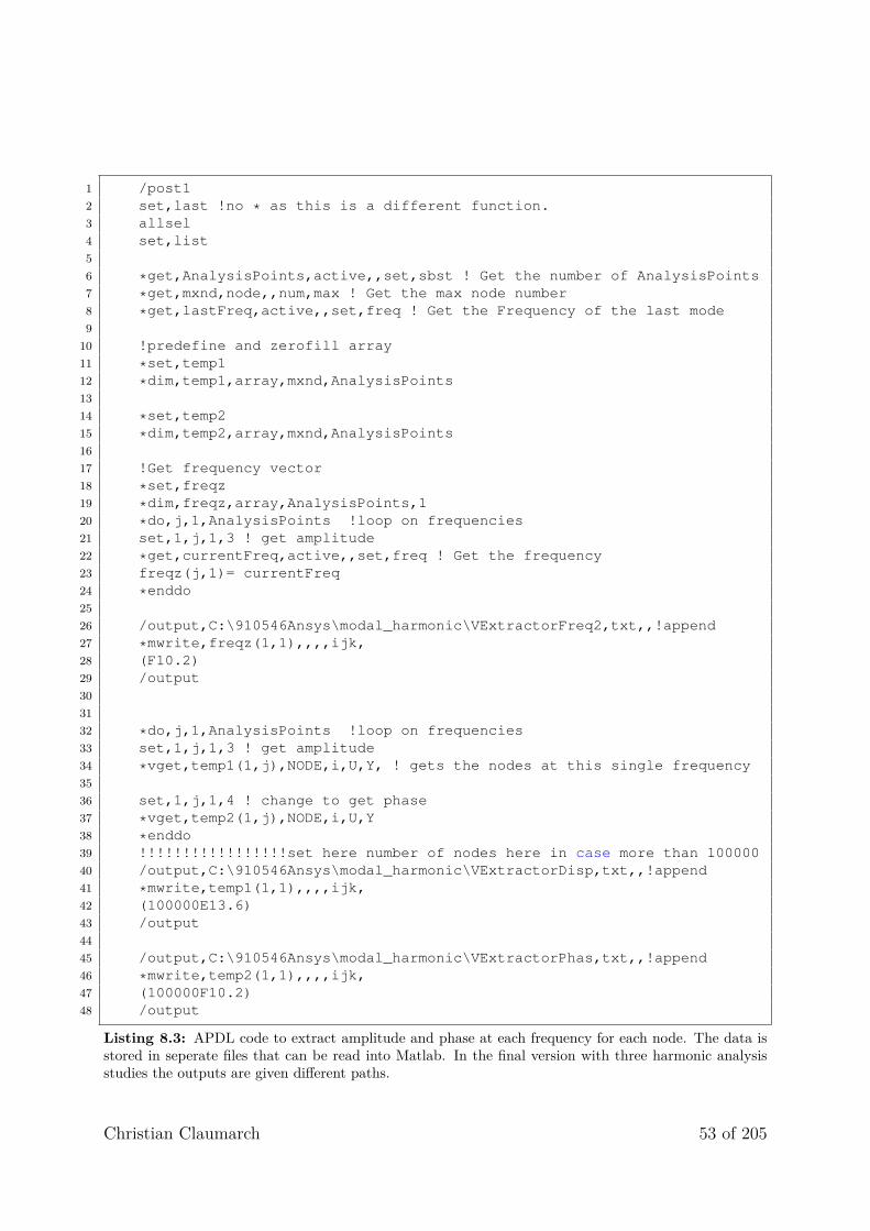
1 /post12 set,last !no * as this is a different function.3 allsel4 set,list56 *get,AnalysisPoints,active,,set,sbst ! Get the number of AnalysisPoints7 *get,mxnd,node,,num,max ! Get the max node number8 *get,lastFreq,active,,set,freq ! Get the Frequency of the last mode910 !predefine and zerofill array11 *set,temp112 *dim,temp1,array,mxnd,AnalysisPoints1314 *set,temp215 *dim,temp2,array,mxnd,AnalysisPoints1617 !Get frequency vector18 *set,freqz19 *dim,freqz,array,AnalysisPoints,120 *do,j,1,AnalysisPoints !loop on frequencies21 set,1,j,1,3 ! get amplitude22 *get,currentFreq,active,,set,freq ! Get the frequency23 freqz(j,1)= currentFreq24 *enddo2526 /output,C:\910546Ansys\modal_harmonic\VExtractorFreq2,txt,,!append27 *mwrite,freqz(1,1),,,,ijk,28 (F10.2)29 /output303132 *do,j,1,AnalysisPoints !loop on frequencies33 set,1,j,1,3 ! get amplitude34 *vget,temp1(1,j),NODE,i,U,Y, ! gets the nodes at this single frequency3536 set,1,j,1,4 ! change to get phase37 *vget,temp2(1,j),NODE,i,U,Y38 *enddo39 !!!!!!!!!!!!!!!!!set here number of nodes here in case more than 10000040 /output,C:\910546Ansys\modal_harmonic\VExtractorDisp,txt,,!append41 *mwrite,temp1(1,1),,,,ijk,42 (100000E13.6)43 /output4445 /output,C:\910546Ansys\modal_harmonic\VExtractorPhas,txt,,!append46 *mwrite,temp2(1,1),,,,ijk,47 (100000F10.2)48 /output
Listing 8.3: APDL code to extract amplitude and phase at each frequency for each node. The data isstored in seperate files that can be read into Matlab. In the final version with three harmonic analysisstudies the outputs are given different paths.
Christian Claumarch 53 of 205

Apart from the data extracted using Listing 8.3 the position of each node and their connections(forming faces) have to be known. This is easily done in the guided user interface using namedselections and the export option. The named selection for the nodes is made by using the scopingmethod ’worksheet’ and selecting all nodes with an ID larger than 0.
Node Number X Location (mm) Y Location (mm) Z Location (mm)
1 150, 0, 0,
2 150, 1,5 0,
3 150, 0, -84,628
4 150, 0, -2,8209... ... ... ...
Table 8.3: Example of node positions extracted.
The elements are stored by selecting all ’mesh elements’ with an ID larger than 0. This yields thetype of the element, in this project all quadratic tetrahedrons, as well as the ID corresponding totable 8.3 for the four nodes forming the corners of the element plus the six intermediate points,which are ignored.
Element Number Element Type Node 1 Node 2 Node 3 Node 4 . . .
1 Tet10 900 2450 2000 1038 . . .
2 Tet10 900 2354 2000 2450 . . .
3 Tet10 450 2000 1038 900 . . .
4 Tet10 900 1210 2450 1038 . . .... ... ... ... ... ... . . .
Table 8.4: Example of element connections extracted. The table continues to Node 10, but the 6 nodesskipped here are always the intermediate points of the quadratic elements.
From the data in table 8.4 the four faces of an element can be determined by combining thecorners in all unordered unique selections of three. Now the positions and vibration patterns ofthe individual nodes are known as well as the connection between the nodes in the mesh.
54 of 205 Christian Claumarch

9 | Radiation
9.1 TheoryA fundamental equation in acoustics is that p = zV where p is the pressure in front of a surfaceof size S, z is the impedance of air (ρ0c) and V is the particle velocity, from eq. 10.9.1 in [Kinsleret al., 2000]. This can be used at a boundary between a source and air where the particle velocityhas to be equal to the surface velocity. This is one of the simplest acoustical models and it doesnot account for all phenomena that might exist. For instance it does not include directivity anddiffraction. Therefore more advanced radiation models as well as some radiation phenomenawill be presented in this chapter.
9.1.1 The Rayleigh integralThe Rayleigh integral is a way to split a baffled plate in a series of point sources. The formulationis based on mounting a series of point sources in an infinite and rigid baffle. The point sourcesare monopoles by definition and their physical shape is irrelevant. Due to the baffle the volumevelocity is half that of a free source. The integral is formulated as follows [Cremer et al., 2005]:
p = jωρ02π
∫v(s)re−jk0rdS (9.1)
Which means that each point source has an infinitely small surface and some velocity. Theintegral can be sampled in space. The sampling points are given a source strength dependingon the area they cover and velocity qi = vi · Si. Then the sampled version looks like:
p = jωρ02π
∑i
qirie−jk0ri (9.2)
Christian Claumarch 55 of 205

Figure 9.1: Schematic illustration of the contribution from a set of point sources. [Cremer et al., 2005]
9.1.2 Dipole sourcesIt is assumed that the reader is already familiar with the terms monopole source and dipolesource. In this project the structure mainly resembles dipole sources as is is not infinite andoscillate back and forth rather than breathe. The issue is that most methods such as theRayleigh integral is based on monopole sources and therefore the approach does not capturedipole characteristics. To account for the dipole radiation of the structures a transfer functionfrom a monopole breathing sphere to a dipole oscillating sphere is used. It is calculated as thedifference between the pressure at a position generated by a monopole and a dipole directly infront of the spheres as described by [Cremer et al., 2005]:
Pmonopole = jωρa2
r(1 + jka) v̂e−jk(r−a) (9.3)
Pdipole = jωρv̂a3
2 + 2jka− k2a2 · (1r2 + jk
r) · cos(θ) · e−jk(r−a) (9.4)
where a is the source radii and r is the distance to the receiver. To determine the differencebetween the two PDipole/Pmonopole is calculated below. The values a=0.084, θ = 0 and r=2.8have been used for this example.
56 of 205 Christian Claumarch

10-2 10-1 100 101-60
-40
-20
0
20
40
Figure 9.2: Pressure from a monopole (—) and a dipole (—) with same source strength. The differencebetween the two (—).
In reality the structures under study are neither pulsating nor oscillating spheres, but plates orin the future more complex structures. Still the filter can be applied to correct for the dipolecharacteristic of the plate since this is better than doing no correction, even if it is a simplification.If the plate is seen as a pure monopole the low frequency response will be unbelievably high.
9.1.3 Critical frequencyOn top of the correction for a dipole source attention has to be paid to the critical frequencyof the structure. The critical frequency is described in [Cremer et al., 2005] and its definitionis made on an infinite plate in (x,y) direction with bending waves propagating in one direction,say x. The dispersive nature of bending waves makes the speed of sound a function of frequencyas shown in eq. 8.2. From this follows that the wavelength is not a linear function of frequency.This means that at some frequencies the wave-speed on the plate is larger than the wave-speedin air at the same frequency, which is constant c0. At other frequencies the wave-speed is lowerthan c0. The frequency where cb=c0 is called the critical frequency and the radiation from astructure depends strongly on this.
Below the critical frequency the wavelength of a bending wave is shorter than the wavelengthin air. This means that no power transfer between the two waves can exist1. One might ask;what happens with the air in front of the plate when it is not pushed away from the plate asa propagating wave. The answer is that a short circuit between rises and dips on the structurecauses air to move back and forth between the two as they oscillate. This can happen over theentire plate surface which in this discussion goes to infinity.
1near-fields can exist but they do not transmit power.
Christian Claumarch 57 of 205

At the critical frequency the wavelength of the structure wave and air wave are identical. Thiswill cause a, theoretically infinite, plane wave propagating along the plate.
At frequencies above the critical frequency the wavelength in air is shorter than that on thebending wave. Then a projection of the air wave onto the plate can be created at a single angle.This angle is then the radiation angle for this specific frequency.
Figure 9.3: Radiation at an angle above the critical frequency. [Kropp, 2015]
The angle of radiation, φ can be determined geometrically from figure 9.3 as sin(φ) = kbk0
Finite structuresWhen the structure considered is no longer infinite but finite the matter gets more complicatedas described in [Kropp, 2015]. If the plate is baffled at the ends a phenomena similar to thatof a applying a rectangular window on a sampled sine wave arises, namely lobes in frequencydomain. Here the window is made in the space domain with resulting lobes in the wave numberdomain. This topic continues far into the wave number domain and is beyond the scope of thisproject. Instead the result from the boundary is considered in a more intuitive way.
As discussed previously for an infinite structure no radiation occurs below the critical frequencydue to short circuits. The short circuits happen between rises and dips oscillating in oppositephase. In a 1D case one could say that half the air pushed by a part going outwards is suckedby the right hand neighbour going backwards. The other half by the left hand neighbour.Applying this line of thinking to a 2D plate one could imagine this phenomena happening inboth directions over the entire surface at the plate. Then what happens at the edges where noneighbour is present on one side - this boundary will cause sound radiation.
58 of 205 Christian Claumarch

Figure 9.4: 2D cases of short circuits for different mode shapes with radiation areas indicated. [Kropp,2015]
The point of figure 9.4 is that in case 1 and 2 the wavelength of the bending is short comparedto air in one direction and radiation occurs at the edges. In case 3 the wavelength of the bendingwave is shorter than the wavelength in air in both directions and radiation occurs at the corneronly. This phenomena can be expected to be directly observable on the plate if somehow thesound contribution from the edges of the plate can be separated from the contribution from therest of the plate.
9.2 MethodsIn the methods introduced in the literature in section 4.1 two overall directions for solving theradiation problem are considered.
9.2.1 Numerical methodOne way of calculating the radiation is by using a numerical methods such as BEM2 as proposedin [Duvigneau et al., 2015], Paik et al. [2013] and [James et al., 2006] to calculate the radiatedsound. These method can be expected to be accurate as it includes all phenomena discussedin chapter 9. These methods are based on putting the vibrating structure into a simulatedenvironment and includes the propagation of sound to the listener position.
9.2.2 Approximate methodA simpler solution is to use that the pressure in front of a face with an area S can be described byp = zV . This does, as discussed in section 9.1, not account for complex radiation phenomena.The benefit of this method is that it decouples the radiation problem from the propagationproblem. This approach is the same as that used in [O’Brien et al., 2001a] introduced insubsubsection 4.1.2.
2ANSYS provides the same functionality using FEM in the acoustics toolbox.
Christian Claumarch 59 of 205

9.3 ChoicesIdeally the radiation problem would be solved by an analytical solution such as the Rayleighintegral in subsection 9.1.1. The issue with using an analytical solution is that it is specificto a single case. For the Rayleigh integral that case is a baffled plate. This leaves us withapproximate and numerical methods.
9.3.1 Numerical methodsNumerical methods such as FEM or BEM are likely to be the most accurate and general methodsas they include directivity characteristics such as the dipole radiation pattern expected for avibrating free plate. They do have a major disadvantage in that they tightly couple the vibrationproblem via the radiation problem to the propagation problem. This means that if a new roomis to be considered as listening environment the entire algorithm would have to be rerun. In thecase of FEM it is unlikely that a large room can be meshed according to the meshing requirementsfor the entire audible range. Furthermore these numerical methods do not separate where thepressure contributions are coming from, so it would be impossible to use different head relatedtransfer functions (HRTF) in the binaural representation for direct sound and reflected sound.
9.3.2 Approximate methodsApproximate methods such as the one used by [O’Brien et al., 2001a] p = zV , will allow theradiation and the following propagation to be modelled separately from the vibration analysis.The method is general enough to be used to auralize sound for a vibrating structure of any shapeand it utilizes the fact that the structure has already been discretized in the FEM study. Someof the missing characteristics such as the dipole radiation efficiency in figure 9.2 can be addedin post-processing as a digital filter. The critical frequency is more difficult to incorporate andif left out, it might cause large errors in the final result.
9.3.3 ChoiceThe approximate method using that the pressure in front of a surface of size S is p = zV
used. The monopole to dipole transfer function in figure 9.2 is used to correct for the frequencydependent radiation efficiency. The radiation from the dipole also depends on the radiationangle θ as shown in eq. 9.4. The cos(θ) term is a scaling which is 1 if the receiver is normalto the surface and 0 if the receiver is in the surface plane. This is similar to what is done in[O’Brien et al., 2001a] based on the directivity of a plate described in [Kinsler et al., 2000]. In[O’Brien et al., 2001a] the surfaces considered might be larger than a wavelength making thisapproximation inaccurate. In this project the faces are always at least six times smaller thanthe wavelength so the approximation is better suited here.
60 of 205 Christian Claumarch

9.4 Implementation9.4.1 Importing data from ANSYSThe first task of the radiation algorithm is to import the data from ANSYS. This is done usingthe Matlab command ’textread’ to read the node positions, connections, frequencies of vibrationas well as phase and amplitude for each node.
9.4.2 Calculating pressure in front of plateThe radiation is calculated for each face individually. Each face is attributed a number of singleoscillators, one for each eigenfrequency found in the numerical vibration analysis in subsec-tion 8.9.3. The oscillators are then created with the amplitude and phase determined in subsec-tion 8.9.4. Lastly the radiated pressure in front of the face is calculated as p = zV = ρc · ξ · jω.This pressure is then scaled with the radiation angle by cos(θ) as well as the area of the face, S.
9.4.3 Dipole radiation efficiencyThe dipole correction is made as the simplification discussed in subsection 9.1.2 by designing a1025 tap symmetric FIR filter to fit the yellow curve in figure 9.2 using Matlab’s built in functionFIRLS. The resulting filters magnitude response is identical for all frequencies of interest. Thevalue used as source size is 0.0846 m corresponding to half the width of the plate. The equationfor the pressure from a dipole, eq. 9.4, contains a dependency on the radiation angle. Thisdependency is already included in subsection 9.4.2 so only the frequency dependency is accountedfor here.
100 101 102 103 104-40
-30
-20
-10
0
10
Figure 9.5: The magnitude response found infigure 9.2 (—) and its approximation (—).
Christian Claumarch 61 of 205

9.4.4 ResultsThe pressure directly in front of a single face calculates using the method above and assuminga radiation angle of 0◦ is shown below.
102
103
104
-20
0
20
40
60
80
Figure 9.6: Pressure directly in front of a single face. The radiation angle 0◦ is used.
62 of 205 Christian Claumarch

10 | Propagation
10.1 TheoryThis chapter will give a brief introduction to propagating sound waves in air. First let us considerthe sound pressure at a position generated by a breathing sphere as described in [Kinsler et al.,2000]:
P (r, t) = (A/r)ej(ωt−kr) (10.1)
From this it is clear that the distance to the receiver r causes both a delay in time and a decayin amplitude.
10.1.1 Propagation delayPropagation of sound waves happens at finite speed, the speed of sound c = 343m/s2. Thismeans that a sound generated at a position, Loc1, will be received at another position, Loc2,after a time delay. The delay will depend on the distance between the two points as.
∆t = |Loc1− Loc2|c
(10.2)
This is described in eq. 10.1 by e−jkr.
10.1.2 Propagation decayTwo sources of decay can be considered when sound is propagating. The viscous friction and thedistribution of energy over a larger and larger surface. The latter happens as pressure propagatesin three dimensions. It turns out that the viscous friction is negligible in terms of decay [Kinsleret al., 2000] and it is often ignored, as it also is in eq. 10.1. The decay is then described as 1/rin eq. 10.1, meaning that at double the distance half the sound pressure is present.
10.1.3 Reflections in roomsWhen a sound source is put an environment, which is not free field, reflections will occur. Thismeans that a source will be received by a listener multiple times. The first sound to arrive atthe listener is called the direct sound. Early reflections are the ones arriving shortly after loworder reflections from floor, ceiling or walls. Later the sound will be diffuse as the reflectionscome from all directions.
Christian Claumarch 63 of 205

Figure 10.1: Overview of direct sound, early reflections and the diffuse sound field. [frontiers, 2015]
This phenomena plays an important role in how sound is perceived. Imagine the sound of a clapin a cathedral compared to a clap on a corn field.
10.2 Methods10.2.1 Propagation delay and decayThe theoretical way of describing propagation allows any propagation delay and thereby anydistance between sender and receiver. The issue is that digital signal processing of sound isperformed on sampled sound.
In a sampled domain a propagation buffer can be used to store generated sound pressures movingthem one sample closer to the receiver each time a sample is presented to the receiver and anew one is generated. This approach is taken by [O’Brien et al., 2001a]. The issue is that ina sampled domain only time steps of T = 1/fs are valid. One approach would be to changethe propagation delay to the nearest valid time step. This introduces artifacts in the sound asdiscussed by [O’Brien et al., 2001a] where they propose distributing the pressure over multiplesamples. In subsubsection 4.1.2 a better approach is proposed stating that the signal could beup-sampled and an interpolated value chosen.
10.2.2 Sources to includeIf it been had chosen to use BEM or another numerical method for calculating the radiation andpropagation under one the question of ’which parts of the structure influences the sound’ wouldbe solved by those methods. Having chosen to separate the propagation from the radiation thisis not the case so an approximation must be made.
In [O’Brien et al., 2001a] the faces to include are chosen based on ’line of sight’, meaning facesthat the listener can see are included in generation of the audio. This is the reason that themethod does not capture dipole characteristics of an object, where the pressure on the backsideshort circuits with the pressure on the front.
64 of 205 Christian Claumarch

10.2.3 Room simulationAgain if it had been chosen to use a numerical method the room simulation could be included inthis method. The listening environment would then be included in the model and meshed beforecomputing the resulting sound pressure at a chosen position. As mentioned in subsection 9.3.1this might be not so practical since the information about where sound is coming from is lost. Itis possible that finite difference time domain (FDTD) introduced in section 8.5 could overcomethis issue since it is a time domain method where the direction of waves is known by theirparticle velocity in three dimensions.
Having chosen to not use a numerical method for the radiation problem an alternative solutionmust be found for the inclusion of a room in the propagation problem.
Mirror sourceThe mirror source method is based on that the reflection from a flat wall can be seen as anidentical source mirrored around the wall. The contribution from the mirrored source is scaledwith a frequency dependant reflection coefficient of that wall [Kuttruff, 1991]. For a perfectlyreflective surface this value would be 1 at all frequencies. This method is rather simple to imple-ment for the first reflection, the issue arrives when higher order reflections are to be consideredas image sources of image sources and so forth. The problem size grows exponentially with theamount of reflections.
Ray tracingThe Ray tracing method was first introduced by [Krokstad et al., 1968] and it follows soundparticles propagating in all directions from a certain position at a certain time. At boundariesthe particle is reflected and attenuated according to the characteristics of the wall. Whenevera particle crosses the receiving position the time and energy of the particle is stored [Kuttruff,1991]. Based on this a room impulse response from a sender position to a receiver positioncan be calculated. In [Kuttruff, 1991] it is proposed to used the ray tracing method for theearly reflections only and let the late reflections be modelled by a statistical method. Thepaper examines if this ray tracing method is accurate enough to be used for auralization and itconcludes that it is.
10.3 Choices10.3.1 Propagation delay and decayIn this project the vibration of the plate is modelled by a set of simple oscillators. The mostintuitive way to generate audio is to compute the pressure in front of the plate and then prop-agate it to the listener. In this project it is chosen to generate the sound pressure directly atthe listening position. This allows the exact propagation delay and attenuation to be used asdescribed in subsection 10.1.1.
Christian Claumarch 65 of 205

10.3.2 Sources to includeAs it has already been decided to not use a numerical method such as BEM for the radiationproblem the ’line of sight’ approach is the only remaining option. One of the downsides ofthis method, that it does not include the dipole characteristics of the plate. This is alreadycompensated for in by using the dipole transfer function as described in subsection 9.4.3.
10.3.3 Room simulationIn this project the room is limited to a hemi-anechoic room where only one reflective surfaceexists. The ray tracing method is then over complicated as most particles will newer hit thereflective surface and then the receiver. In fact only two particles would be included - theone propagating directly to the listener and the one reflecting off the floor to the receiver. Thissituation is modelled perfectly well by the mirror source method which is chosen for its simplicity.The floor is seen as a perfectly reflective surface as per the definition of a hemi-anechoic room.
Ideally the floor reflection would be included for each face individually. It should include somemethod to include a high frequency standing wave field between the plate and the floor. It shouldaccount for the fact that low frequencies radiated downwards will bounce back and ’ignore’ theplate on the path to the receiver. Possibly even the reflected sound should be included in thefinite elements analysis since it will excite the plate. On top of this the floor in the measurementenvironment is not perfectly reflective and has some slots in the it for mounting equipment.
As including all the physical phenomena above will be very cumbersome in terms of computationand workload a simplification is used instead. A single mirror source located at the negativecoordinates (below the floor) is used.
10.4 Implementation10.4.1 Selection of faces of vibrationThe first task of the sound propagator is to establish which faces contribute to the radi-ated sound. The ’line of sight’ method has been chosen for this. The selection is done us-ing the fact that any considered position will be above the plate, so all the nodes of thefaces in line of sight will have y-coordinates at 1.5 mm in the plate’s coordinate system.
66 of 205 Christian Claumarch
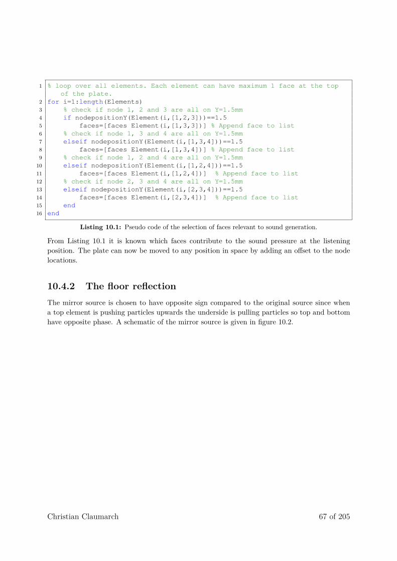
1 % loop over all elements. Each element can have maximum 1 face at the topof the plate.
2 for i=1:length(Elements)3 % check if node 1, 2 and 3 are all on Y=1.5mm4 if nodepositionY(Element(i,[1,2,3]))==1.55 faces=[faces Element(i,[1,3,3])] % Append face to list6 % check if node 1, 3 and 4 are all on Y=1.5mm7 elseif nodepositionY(Element(i,[1,3,4]))==1.58 faces=[faces Element(i,[1,3,4])] % Append face to list9 % check if node 1, 2 and 4 are all on Y=1.5mm10 elseif nodepositionY(Element(i,[1,2,4]))==1.511 faces=[faces Element(i,[1,2,4])] % Append face to list12 % check if node 2, 3 and 4 are all on Y=1.5mm13 elseif nodepositionY(Element(i,[2,3,4]))==1.514 faces=[faces Element(i,[2,3,4])] % Append face to list15 end16 end
Listing 10.1: Pseudo code of the selection of faces relevant to sound generation.
From Listing 10.1 it is known which faces contribute to the sound pressure at the listeningposition. The plate can now be moved to any position in space by adding an offset to the nodelocations.
10.4.2 The floor reflectionThe mirror source is chosen to have opposite sign compared to the original source since whena top element is pushing particles upwards the underside is pulling particles so top and bottomhave opposite phase. A schematic of the mirror source is given in figure 10.2.
Christian Claumarch 67 of 205

Floor
+
–
P-
P+
Figure 10.2: Schematic of the mirror source accounting for the floor reflection. P+ is the direct soundpressure and P- is a delayed, phase inverted and attenuated version of P+. The figure shows the platemounted on a shaker as it will later be used in the measurements in chapter 12 as well as the dipoleradiation pattern of a free plate.
The simplification is implemented as a sum of the generated sound and a delayed, phase invertedand attenuated version of itself.
First the additional propagation distance is calculated as:
∆Dist = ‖receiverPos−MirrorSourcePos‖2 − ‖receiverPos− SourcePos‖2 (10.3)
this will result in a delay of ∆Dist/fs samples which is rounded to an integer number - for thissetup with M20 as ’receiverPos’, the centre of the plate as ’SourcePos’ and ’MirrorSourcePos’equal ’SourcePos’ with inverted y-coordinate this is 26 samples1.
The gain caused by the additional propagation distance is calculated as:
Gain = 1+(
1‖receiverPos−MirrorSourcePos‖2 −
1‖receiverPos− SourcePos‖2
)(10.4)
For this setup with M20 as ’receiverPos’ this will be 0.98. This will yield the comb filter whichcan be described as a FIR-filter with 26 taps. The first tap is 1 and the last -0.98; the rest arezero. The comb filter’s magnitude response is shown in figure 10.3
1These positions are the ones used in the measurement in chapter 12.
68 of 205 Christian Claumarch

102 103 104-40
-30
-20
-10
0
10
Figure 10.3: The magnitude response of the comb filter from the floor reflection.
10.4.3 ResultsHere the result at a listening position accounting for sound propagation and floor reflection isshown.
102 103 104
−50
0
50
100
Frequency in Hz
SPL
indB
rel2
0µ
Pa
Figure 10.4: The sound pressure level at a listening position after propagation.
Christian Claumarch 69 of 205

11 | Listening
11.1 TheoryThis section will give brief description of what is required to give a binaural presentation ofaudio.
11.1.1 Head related transfer functionsThe definition of auralization in chapter 2 states that a ’binaural listening experience’ shouldbe presented. This means that the perceptual characteristics of the sound should be as ifthe listener had been in the simulated environment. To achieve this goal the sound pressureat a given position should be converted to the sound pressure at two eardrums inside an earcanal accounting for reflections from the listener. It should also include the temporal differencemeaning the time delay between the sound pressure arriving at one ear compared to the other.
In practice the binaural representation can be recorded using a person with small microphonesin the ear canal. Alternatively a dummy head a so called head and torso simulator (HATS) canbe used. This will yield what is called a binaural recording.
It is also possible to make a digital filter converting a single sound pressure in a position to abinaural representation. This type of transfer function is called a head related transfer function(HRTF) and is described in detail in [Møller, 1992]. Here only a brief overview is given. TheHRTF is created by recording a reference signal, e.g. a sine sweep or MLS sequence played bya loudspeaker, in a reference position. Then a person or a HATS is placed with the centre oftheir head in the reference position and the sound pressure in the ear canal is recorded usingthe same reference source. The two responses can then be used to form two transfer functions,one for each ear.
A HRTF is dependent on angle of incidence both vertically and horizontally (elevation andazimuth). Sound coming from the right hand side of a listener will arrive at the right ear firstand later a lowpass filtered version will arrive at the left ear. This is used by the auditorysystem to determine where the sound came from. The vertical localization is dominated byreflections from the outer ear and shoulders into the ear canal. The importance of the HRTF tothe perception of sound is not treated further here and the reader is referred to [Møller, 1992]for further information.
The HRTF is an independent feature for each person. One persons HRTF cannot be used foranother person and averaging over people carries no meaning [Hammershøi and Møller, 2005].
70 of 205 Christian Claumarch

11.1.2 Reproduction systemWhen using a HRTF to present a binaural recording it is important that the listener is exposedto the exact sound pressure which would be at their eardrum if the source had been external inan environment. This requires a headphone which has a flat frequency response at the eardrum.This essential feature is not readily available in off the shelf headphones, since headphone de-signers have a different target curve [Olive et al., 2018]. On top of this the frequency responseof a headphone will depend on the person wearing the headphone as well as the positioning ofthe headphone.
In order to give an accurate binaural representation the headphone characteristics should beremoved by means of an inverse filter. This means that like the HRTF the headphone transferfunction should be measured on the person whom the binaural representation is intended for.Preferably it should even be measured each time the headphones are remounted. Then theinverse filter should be computed and applied to the HRTF filtered audio which then becomesa binaural representation.
11.2 Methods11.2.1 Binaural representationIn this project the audio signal is generated through simulation. This means that the binauralrepresentation must be added digitally. Two methods for arriving at a binaural representationcan be considered.
In situation HRTFThe HRTF could be measured in situation meaning in the room which is to be used in theauralization. This would require that a loudspeaker playing a reference signal is put in theposition of an intended source. The reference position is then chosen as the listening position.This approach has the benefit that the room characteristics are included in the HRTF so thereflection from the floor calculated in subsection 10.4.2 is redundant. This does also mean thatthe acquired HRTF is specific to one single sender and receiver position in one specific room.
Anechoic HRTFThe HRTF can also be measured in an anechoic environment. From this the HRTF can beacquired independently of the environment. The HRTF will still show a dependency on angleand distance. For this reason multiple measurements are typically performed yielding a databaseof HRTFs for different azimuth and elevation. If multiple distances are wanted then this cannaturally also be varied in the measurement. The anechoic method will require that the roomresponse is added separately for instance as done in subsection 10.4.2.
Christian Claumarch 71 of 205

11.3 Choices11.3.1 HRTFA setup in an anechoic environment measuring a complete HRTF database is quite complicatedand time consuming to make. For this reason it was first intended to do an in situation measure-ment of the HRTF which would then limit the possible listening positions to a few predefinedpositions. An experiment doing this is presented in an Appendix A in section A.3. This mea-surement had multiple issues in signal quality which makes it so that it should be reperformedif the results were to be used.
By chance another student at my master’s programme was working on his master’s thesis includ-ing measurements of HRTFs on live subjects [Hauen, 2018]. Sigurd Van Hauen offered me thatI could use his setup to acquire a HRTF database in an anechoic environment. This solutionis much more general than the in situation measurement and could be used for many listeningpositions in many environments. For this reason it was chosen to not reperform the originalexperiment and instead use a database acquired in anechoic conditions.
11.3.2 ListenerBoth the headphone frequency response and the HRTF should be measured on the individualto whom the binaural listening experience will be presented. For this reason a listener must bechosen at this point. For convenience the HATS owned by Grundfos is used. It is a Brüel & Kjær4100D which is made to approximate ’the average human listener’. This naturally makes it sothat the representation is not accurate for any human listener, but this allows the methodologyfor creating a binaural reproduction system to be presented. It is chosen to acquire a HRTFdatabase for this HATS and do a headphone compensation on that same HATS.
11.4 Implementation11.4.1 Measuring HRTFThe complete works for measuring the HRTF of the HATS is presented in Appendix B. Allcredit for the setup and performing the experiment (which is automated) should be creditedto Sigurd Van Hauen [Hauen, 2018]. The post processing required in going from the impulseresponse of the loudspeakers at the reference position and at the HATS microphone positionsto filters that can be used in the binaural representation is made by me.
The setupThe reader is referred to Appendix B for a description as well as a diagram and pictures of thesetup. For an even more thorough description of the setup the reader is referred to [Hauen,2018].
72 of 205 Christian Claumarch

Here only a very brief description of the essential knowledge is given. The setup is made toacquire the HRTFs of the HATS at a distance of 1.7 meters. The resolution in azimuth is 1◦and in elevation it is 8◦ from −40◦ to 40◦. 11 loudspeakers at different positions on an arch areused to get the elevation responses. The HATS is mounted on a turntable which automaticallyturns the HATS around the reference position to vary the azimuth.
Post processingAgain the reader is referred to Appendix B for a more detailed explanation of what has beendone. Here only the concepts of what is done are presented.
Removing reflectionsIn the data given by the work of Sigurd Van Hauen reflections from the setup are included in theimpulse responses. This causes a ripple in the frequency response due to the comb filter createdby the reflection. To remove this a time gating technique is used. The impulse responses are cutusing a Hamming filter with an order of 512 samples. This removes reflections from reflectorsfar away from the reference position.
Spectral divisionThe data supplied by the measurement system by Sigurd Van Hauen is impulse responses of theloudspeakers in the reference position as well as at the microphones of the HATS. From this theHRTF can be calculated as
HRTF = IFFT ( FFT (ImpulseResponseEar)FFT (ImpulseResponseReference)) (11.1)
This process is what is also known as a cyclic deconvolution [Müller and Massarani, 2001],which has the effect that sound arriving at a HATS microphone before it arrives at the referenceposition ends up in the end of the acquired impulse response instead of in ’negative time’. This issolved by shifting the response 28 samples to the right. This might cause part of the reverberanttail to be included in the beginning of the response, but this is better than having the onset ofthe impulse response after the rest of the response.
Removing pre-ringingAs the three microphones used are connected to different channels in the analogue to digitalconverter the anti-aliasing filters are not completely identical. When performing the spectraldivision this causes what is known as pre-ringing. That is a tone at fs/2 starting before theimpulse response. This is removed by means of a low pass filter at 23 kHz.
Removing DC componentAs the HATS is small compared to the wavelength of sound at low frequencies the HRTF shouldnot contain a gain at low frequencies. A DC offset is present in the measurements and it is
Christian Claumarch 73 of 205

removed by setting the value of the first bin in frequency domain equal unity as proposed by[Hammershøi and Møller, 2005].
ResultHere the frequency response curves found in Appendix B are shown.
100 101 102 103 104-30
-20
-10
0
10
20
Figure 11.1: The The HRTF of the HATS facing forwards left ear (—) and right ear (—).
100 101 102 103 104-40
-30
-20
-10
0
10
20
Figure 11.2: The The HRTF of the HATS turned 90◦ clockwise, left ear (—) and right ear (—).
The frequency responses shown above have a corresponding 512 samples long impulse response.
74 of 205 Christian Claumarch

This impulse response can be used directly as a FIR-filter to convert the sound pressure at areference position to that at the ear microphones of the HATS.
11.4.2 Measuring frequency response of a headphoneThe complete procedure for measuring the transfer function of a headphone is given in Ap-pendix C.
SetupThe experiments uses a Steinberg sound card, the HATS used in the HRTF measurements aswell as a pair of headphones. The stimuli used is a logarithmic sine sweep generated in frequencydomain as proposed by [Müller and Massarani, 2001].
The setup is not calibrated to measure specific sound pressures, only the shape of the magnituderesponse is of interest.
ProcessingSince a sweep is used as reference signal it is possible to separate the linear response of theheadphone from the harmonic distortion as proposed by [Müller and Massarani, 2001] andshown in figure 11.3
Figure 11.3: Non-cyclic deconvolution as given in [Müller and Massarani, 2001].
ResultThe magnitude response of a pair of headphones is given below.
Christian Claumarch 75 of 205

102 103 104-50
-40
-30
-20
-10
0
Figure 11.4: Magnitude response of left channel (—) and right channel (—) of a pair of BeyerdynamicT90 headphones.
11.4.3 Assembling a binaural listening systemA block diagram showing the connection of the components used in a binaural synthesis is shownin figure 11.5.
Sound pres-sure at refer-ence position
Sound filteredleft HRTF
Sound filteredright HRTF
Sound filteredinverse leftheadphoneresponse
Sound filteredinverse rightheadphoneresponse
Figure 11.5: Block diagram of binaural listening system.
76 of 205 Christian Claumarch

Applying the HRTFThe HRTFs found in subsection 11.4.1 can be used direcly as a FIR filter by means of a con-volution of the mono signal with the filter for each ear. From this two time representations arefound, one for each ear.
An issue might arise if the angle of incidence is not included in the HRTF database. The interpo-lation methods such as the one proposed in [Sandvad, 1996] could be considered. Alternativelythe nearest known HRTF could be used. In this project the HATS is chosen to face the plateso the HRTF at 0◦ azimuth and elevation can be used.
Correcting for the headphoneThe frequency response of the headphone in figure 11.4 could be used to form a minimumphase filter with the opposite magnitude response. This filter could be chosen less sharp thanthe measured response to avoid fitting it to steep dips, which are likely to be change with toplacement of the headphone. Here a more simple approach is used, namely that the acquiredimpulse responses are zero padded to the same length as the audio signal. Then it can be usedto deconvolve the headphone frequency response from the stimuli as follows:
AudioSignalF iltered = IFFT ( FFT (AudioSignal)FFT (ImpulseResponseZeroPadded)) (11.2)
11.4.4 ResultsThe response with the headphone response deconvolved represents the electrical signal passed tothe headphone. This is then filtered by the headphone and ear canal to give the sound pressureat the ear drum. Therefore the sound pressure a the eardrum is shown as that filtered by theHRTF only since the other transfer function is first removed and then added again.
102 103 104−100
−50
0
50
100
Frequency in Hz
SPL
indB
rel2
0µ
Pa
Figure 11.6: The sound pressure level at the left (—) and right (—) ear of the listener.
Christian Claumarch 77 of 205

In figure 11.6 the frequency content of the sound pressure at the left and right eardrum of theHATS is shown.
This concludes the chapter on the auralization algorithm. It has been shown that an audiosignal can be generated and processed to replicate a listening situation. How this simulatedaudio relates to an audio recording of the actual structure remains to be seen, this will betreated in subsection 12.3.2.
78 of 205 Christian Claumarch

Part III
Measurements
Christian Claumarch 79 of 205

12 | Plate measured response
12.1 Design goal measurementsThe purpose of the measurement is to acquire real world data for comparison with the simulateddata. Therefore the measurement should try to mimic the simulation as best as possible1. Themeasurement is split in three parts, one measuring the steady state audio response at multiplepositions plus multiple binaural recordings with a HATS. During this part the loading on theplate is kept at a minimum. The second part determines the mode shapes of the plate and theimpact on sound is not crucial. In both measurements large deformations should be avoidedto limit non-linear behaviour of the plate, which are not included in the simulation work. Thethird measurement measures the in situation HRTF of the HATS using a small loudspeaker. Asdiscussed in subsection 11.3.1 the signal quality in this measurement was low and the HRTFdatabase is acquired in anechoic conditions in subsection 11.4.1. The experiment measuring thein situation HRTF is therefore only included in Appendix A and not discussed further in themain report.
First a brief walk through of the environment and equipment used in the measurement is given,so that the reader understands the conditions under which the measurements are performed. Allthe more detailed tables and figures needed for reproduction are given in Appendix A, everythingrelated to the conceptual understanding and choices is presented in this chapter.
12.1.1 The measurement environmentThe measurement environment is designed to comply with ISO 3745, which is a precision gradestandard specifying how to measure sound power levels for machinery. The room is hemi-anechoic with a concrete floor. The room is certified down to 50 Hz with the ventilation turnedoff2. There are 20 fixed microphones placed on a half-sphere at a distance r=2.8 m.
1In reality the simulation is trying to emulate the real world as best as possible2It is only turned on when heat developing machinery runs for prolonged periods. Never in this project.
80 of 205 Christian Claumarch

Figure 12.1: Microphone positions as given in the ISO 3745. In this project the orientation of thecoordinate system is different corresponding to swapping the y and z value. [DEWESoft, no date ]
The room is mounted on sylomer to isolate it from vibrations originating outside the measure-ment environment. The room is also equipped with a floating concrete block in the middle ofthe room. The block serves the purpose of further isolating the device under test from the build-ing. The concrete block is constantly adjusting it’s position, which produces a small amount ofsound. To stop this the it can be ’locked’, but in that case it is moving slowly downwards as airleeks from the system. In this project where the vibrational levels and weight of objects is verysmall compared to the objects this block was designed for it is always deflated. This ensuresthat distances to microphones are constant.
12.1.2 Measurement equipmentA brief overview on the used equipment is given.
ShakerThe shaker used in this experiment is chosen as the B&K 4810, which is the smallest stationaryshaker available at Grundfos. The reason for choosing the shaker as small as possible is that theshaker itself will produce sound. A larger shaker such as B&K 4809 produces more unwantedsound. The small B&K 4810 is capable of delivering a maximum displacement of 4 mm peak-peak corresponding to 49 m/s2 with a payload of 186 grammes [Brüel & Kjær, no date b]. Theplate weighs around 200 grammes.
Christian Claumarch 81 of 205

Impedance headInstead of using an actual impedance head the same functionality is achieved by combining aaccelerometer, B&K 4514, and a force transducer, B&K 8200. This setup will allow the force andacceleration actually applied to the structure to be measured. A further advantage is that theycan be screwed together around the plate, fixating it in the process. The force transducer canoperate up to vibration levels of 9807m/s2, well above the requirements here and has a frequencyresponse depending on the load. The lower limit is 0 Hz and the upper limit is determined bythe load3. It has a mass of 21 grammes whereof 3 grammes are rigidly connected to the topscrew making that the only mass loading. The accelerometer can operate up to vibration levelsof 98 m/s2, again more than the shaker can produce and has a frequency response ±2 dB from10 Hz to 10 kHz. It has a mass of 8.7 grammes.
MicrophonesThe microphones used in the array are B&K 4955. They have a frequency range of 10 Hz to16 kHz and a maximum SPL level of 110 dBSPL. Their internally generated noise floor is 6.5dB(A).
Data acquisition hardwareThe acquisition hardware used at Grundfos is B&K 3050-B, which are 6 channel A/D convertersthat can be chained and synced using Ethernet. A variant the 3060A has 4 A/D channels and2 D/A channels, which can be used to drive a shaker. They both have built in charge amplifiersfor accelerometers and power supply for microphones.
Data acquisition softwareUsing B&K acquisition hardware necessitates the use of B&K software in this case Pulse LabShop22, in short Pulse. From Pulse it is possible to acquire .wav files with normalized data plusa normalization factor, which enables the user to go back to the original calibrated levels.Alternatively data extraction can be done using ASCII files. The software is also capable ofenhancing and presenting the data in multiple ways like averaging, filtering, re-sampling, plottingor playing recordings.
12.2 Audio measurement summaryFor the audio measurement the 20 microphone positions given in the ISO-3745 standard areused, this will give the sound pressure at 20 positions on a sphere above the plate. Furthermorea HATS, B&K 4100D, is used in two positions, one directly above the plate and another at anangle to the side. The second position is chosen so the HATS is not blocking line of sight fromany microphones to the plate so a measurement of the array and the HATS can be performedsimultaneously. The position with the HATS directly over the plate is deemed disturbing to therest of the sound field, so here the 20 microphone signals are discarded.
3As shown in eq. 12.1
82 of 205 Christian Claumarch

12.2.1 SetupBelow illustrations give an overview of the setup. figure 12.2 illustrates the setup specific to thismeasurement. figure 12.3 illustrates the setup always available in the hemi-anechoic room.
Accelerometer (2)Plate (4)
Force Transducer (1)
Shaker (3)
ADC (5)
(7)
Tone generator (6)(8)
Figure 12.2: Experimental setup for plate. Zoom on the local setup around the plate. Numberscorrespond to item numbers in table A.2.
(9)-Pos1
(9)-Pos2
Figure 12.3: Experimental setup for plate. The global setup around the plate. The microphoneplacement is arbitrary, the actual 3D locations of all 20 microphones are given in table A.4. The electricalconnections are left out here but can bee found in table A.6. The items around the plate are connectedas in figure A.1 and all the microphones are connected to an ADC.
Christian Claumarch 83 of 205

12.2.2 ResultsIn order to determine the resonance frequencies that are excited in the middle position of theplate the output from the 20 microphones is used in combination with the output from the ’home-made’ impedance head. The microphone output is a suitable way to determine eigenfrequenciesin the frequency area where the plate is an efficient radiator. For frequencies below soundradiation the impedance head can be used to measure the input impedance and find resonances.
Only the 20th microphone signal is plotted in time domain.
0 1 2 3 4 5 6 7 8 9 10
-6
-4
-2
0
2
4
610
-3
Figure 12.4: The time signal at the M20 microphone position.
All 20 microphones as well as the background level with and without the shaker running isshown in figure 12.5.
84 of 205 Christian Claumarch

Figure 12.5: The sound pressure level at the 20 microphone positions. Background noise at microphone10 (– –) and noise from shaker without plate and same driving voltage at microphone 10 (– –).
Some selected eigenfrequencies of the plate are given below. A complete list would be pointless,but a few frequencies allows for later comparison with the analytical and simulated results.Resonances occur at: 400, 496, 864, 1148, 1416 and 1588 Hz.
It can be seen in figure 12.5 that the plate is an inefficient radiator of sound below 400 Hz.Therefore the eigenfrequencies below this have to be determined using the impedance head.
The input impedance can be calculated from the time series of the acceleration and force. Theinput impedance is calculated as Z(ω)in = Force(ω)·jω
Acceleration(ω) in a spectral division including phase.As can be seen in Appendix A the SNR is not high enough to directly calculate the inputimpedance. Instead it is calculated from acceleration and force in frames and averaged which isalso described in the appendix.
Christian Claumarch 85 of 205

101 102 1030
20
40
60
80
Figure 12.6: The averaged input impedance.
From figure 12.6 it can be seen that resonances occur at frequencies below those that are clearlyvisible in the audio spectra. For example resonances exist at 87 Hz and 274 Hz.
12.2.3 The measurement systems influence on the plateThe analytical and simulated work assumes no measurement setup is attached to the plate. Inthe measurements this is obviously not the case. Therefore the influence of the measurementsetup should be discussed
When recording audio from the vibrating plate the recording is a result of a system responseand not purely the plate. Two factors are considered, namely:
1. The shaker has a spring and mass characteristics which is rigidly connected to the bottomof the force transducer.
2. The accelerometer and top of the force transducer are rigidly connected to the platecausing a mass loading.
This explains why Sound is radiated at 400 Hz even though no impedance drop can be seen infigure 12.6. The impedance is calculated as the force input to the plate, accelerometer and thetop of the force transducer divided by the velocity of these. The input impedance measurementdoes therefore not consider the influence of the shaker and the other things in item 1 above. Themicrophone signals will pick up the complete system response including the shaker. In short themicrophone signals and the input impedance are not measuring the same thing.
The influence from item 2 can be seen as a mass, which has the impedance jωM . In Appendix Athe removal of this is described in better detail and the result is shown in figure 12.7.
86 of 205 Christian Claumarch

101 102 103-20
0
20
40
60
80
Figure 12.7: The averaged input impedance. Measured input impedance (—). Impedance of mass 11.7grammes (—). Input impedance of plate alone (—). Theoretical input impedance of an infinite plate ofsame material and thickness (—).
From this it is clear that the additional mass loading due to item 2 shifts the resonance frequen-cies slightly downwards compared to an unloaded plate.
To summarize the yellow line in figure 12.7 is comparable to the analytical solution as well as thesimulation in section 8.9. The audio measurement as well as the input impedance in figure 12.6are not directly comparable to the previous works.
Force transducerFrom figure 12.7 it is clear that the impedance of the plate increase unexpectedly with frequency.The upper limit of the accelerometer is 10 kHz which is above the range shown here. The upperlimit of the force transducer is dependent on the load and so it is examined further here. Oneissue arise in that the dependency is on the impedance of the load as described by [Brüel &Kjær, 1994]:
FmeasuredFapplied
= 1 + jωmtop
Z(12.1)
This means that the impedance of the object has to be known to calculate the transfer functionand thereby the upper limit of the force transducer. Seeing as the force transducer is used tomeasure the impedance of the object this causes an unfortunate loop. In an attempt to remedythis the impedance of the infinite plate is used to estimate the upper limit .
Christian Claumarch 87 of 205

101 102 1030
1
2
3
4
5
6
Figure 12.8: Magnitude response of force transducer when connected to an infinite plate.
From figure 12.8 the 1 dB upper limit of the force transducer is 2050 Hz. On the physical platethis can be expected to be even lower since the input impedance of the plate will have largedips at resonances below this frequency. No compensation is made to account for the errorintroduced by the force transducer as this would require a more detailed knowledge of the errorthat the approximation in figure 12.8.
Three measurement situationsThree different sets of resonant frequencies can be found from the acquired data. One for acompletely free plate, from the yellow line in figure 12.7. One from a plate with mass loading(item 2), from figure 12.6. And finally one from a plate with a mass loading mounted on a spring(item 1+2), from figure 12.5.
Here some of the resonant frequencies in the three cases are listed.
88 of 205 Christian Claumarch

Analytical Plate alone Plate+2 Plate+1+2
88 Hz 92 Hz 87 Hz unknown
288 Hz 288 Hz 274 Hz 256 Hz _
479 Hz480 Hz § 450 Hz §
400 Hz
519 Hz 496 Hz
991 Hz 972 Hz 932 Hz 864 Hz
1226 Hz 1208 Hz 1168 Hz 1148 Hz
unknown1544 Hz § 1460 Hz §
1416 Hz
1568 Hz 1588 Hz
Table 12.1: The measured resonance frequencies of the different systems. ’1’ and ’2’ refers to the twofactors on page 86. ’Plate alone’ data is from yellow line in figure 12.7. ’Plate+2’ data is from figure 12.6.’Plate+1+2’ is from figure 12.5.
_ Read from large acceleration in figure A.11.
§ Which it is not clear from the impedance measurements if two eigenfrequencies exist closeto each other. Mode shapes are not available so checking is impossible.
.
12.3 Vibration measurement summaryTo examine the mode shapes the frequencies from table 12.1 column ’Plate+1+2’ are consideredas these are the ones corresponding to the setup that is used. Two approaches were consideredfor the vibration measurement namely:
1. Measuring mode shapes using accelerometers.
2. Examining mode shapes using sugar [Chladni, 2015]4.
The first approach is by far the most accurate as it will yield results on the level of vibration inaddition to making it possible to measure at high frequencies. The drawback is that it requiresmultiple accelerometers mounted on the plate. To capture the mode shape of the (3,1) mode twoAccelerometer is sufficient. For the (2,2) mode three are needed5. For higher mode shapes manyaccelerometers are needed, unfortunately due to the small thickness of the plate this will cause a
4A method first introduced by Ernst Chladni in the 18th century although he used sand.5In reality 4 to avoid uneven loading
Christian Claumarch 89 of 205

non negligible mass loading. The mode shapes might be close to identical if the accelerometersare evenly spaced but the eigenfrequencies will move, making it hard to track which mode shapesbelong at which eigenfrequency.
The second approach is simple, but only yields a visual impression of the mode shape. Bypouring sugar on the vibrating plate the nodal lines of the mode shapes are made visible as thesugar will collect in the non-moving areas. This will cause a mass loading much smaller thanthe accelerometer based method.
For the purpose of verifying that the FEM analysis is indeed finding the correct mode shapesfor the eigenfrequencies and more importantly determining which modes can be excited in thecentre of the plate the second approach is chosen. This puts an upper frequency limit on modesthat can be examined, as the deformation, which moves the sugar, decreases with frequency. Inthe case of this plate and the used shaker this limit is somewhere above 496 Hz. Above thislimit it was found that by substituting the sugar with fine salt mode shapes for eigenfrequenciesup to 1588 Hz could be visualized.
12.3.1 SetupThe setup is simple and utilizes part of the setup used in the audio measurement. She shakerand plate are connected as before (figure 12.2), but now the tone generator is set to vibratesinusoidally at a single frequency.
12.3.2 ResultsIt has already been determined that FEM is in alignment with the analytical solution when itcomes to determining the mode shape of a free plate. Now it is desired to examine whether theyare in alignment with the actual response of the plate under study mounted on a shaker.
Before continuing with the resonance frequencies determined in the audio measurement an ad-ditional frequency is added. The reason for this being included is that something was presentat 57 Hz frequency in the HATS measurement in figure A.7 and figure A.8. The slight peak isnot present at the 20 microphone positions further away, indicating a possible near field. Stillin order to produce a near field at 57 Hz some resonance must exist in the system. It has beenpossible to recreate its mode shape and approximate frequency by applying a fixed support inthe centre position in the finite element analysis. The conclusion therefore is that the mountingat the centre of the plate influence the vibration at this frequency.
Sugar is distributed on the plate as carelessly as possible, however it is difficult to ensure thatthe concentration of sugar is even over the entire plate. To give the reader and idea of theinaccuracy the distribution was done with figure 12.9 shows sugar as placed initially beforemeasurements. The sugar is clustering, so the approach is only valid when the sugar clearlymoves to new positions to create clear patterns.
90 of 205 Christian Claumarch

Figure 12.9: Example of sugar position before shaking.
(a) Analytical result un-known.
(b) Simulated 56 Hz.(c) Measured 57 Hz.
Figure 12.10: The mode shapes determined for the additional mode found in measurements. Noanalytical solution is known. The FEM eigenfrequency is 56 Hz with a fixed support in the centre. Thepattern appears slightly more circular in the realization than in the simulation because all sugar fromthe edges are stored at the edge of the non vibrating zone.
Christian Claumarch 91 of 205

(a) Analytical 88 Hz. (b) Simulated 88 Hz.(c) Measured 87 Hz.
Figure 12.11: The mode shapes determined for the 88 Hz mode. FEM determines the eigenfrequency tobe 88 Hz. The plate measurement determined the eigenfrequency to be 87 Hz (from the input impedancefigure 12.6). The use of the input impedance to select frequency is not correct as it does not account forthe shaker as previously discussed. However no alternative is available and the sugar is moving easily sothe 87 Hz is close to the resonance.
(a) Analytical 288 Hz. (b) Simulated 288 Hz.(c) Measured 256 Hz.
Figure 12.12: The mode shapes determined for the 288 Hz mode. FEM determines the eigenfrequencyto be 288 Hz. The plate measurement determined the eigenfrequency to be 256 Hz (from the accelerationfigure A.11). The dotted blue lines on the measured indicate that a possible node line might be present.
(a) Analytical 479 Hz. (b) Simulated 478 Hz.(c) Measured 496 Hz.
Figure 12.13: The mode shapes determined for the 479 Hz mode. FEM determines the eigenfrequencyto be 487 Hz. The plate measurement determined the eigenfrequency to be 496 Hz (from the radiatedsound figure 12.5).
92 of 205 Christian Claumarch

(a) Analytical 519 Hz. (b) Simulated 518 Hz.(c) Measured 400 Hz.
Figure 12.14: The mode shapes determined for the 519 Hz mode. FEM determines the eigenfrequencyto be 528 Hz. The plate measurement determined the eigenfrequency to be 400 Hz (from the radiatedsound figure 12.5).
As the sugar method does not work for higher frequencies the sugar is substituted with finesalt allowing for higher frequencies to be visualized. The pictures of the measured responseare rotated 180 degrees to show the same orientation as the previous pictures as the plate wasrotated by mistake when remounted.
(a) Analytical 991 Hz. (b) Simulated 989 Hz.(c) Measured 864 Hz.
Figure 12.15: The mode shapes determined for the 991 Hz mode. FEM determines the eigenfrequencyto be 989 Hz. The plate measurement determined the eigenfrequency to be 864 Hz (from the radiatedsound figure 12.5).
(a) Analytical 1226 Hz. (b) Simulated 1225 Hz.(c) Measured 1148 Hz.
Figure 12.16: The mode shapes determined for the 1226 Hz mode. FEM determines the eigenfrequencyto be 1225 Hz. The plate measurement determined the eigenfrequency to be 1148 Hz (from the radiatedsound figure 12.5).
Christian Claumarch 93 of 205

(a) Analytical 1568 Hz. (b) Simulated 1567 Hz.(c) Measured 1588 Hz.
Figure 12.17: The mode shapes determined for the 1568 Hz mode. FEM determines the eigenfrequencyto be 1567 Hz. The plate measurement determined the eigenfrequency to be 1588 Hz (from the radiatedsound figure 12.5).
The measured mode shape at 1416 Hz is not similar to any of the mode shapes found in analyticalor simulated work.
Figure 12.18: Measured 1416 Hz.
The simulated mode shapes are overall in alignment with the actual mode shapes on the plate.At higher frequencies the hole and the mounting seems to influence the mode shape by pullingnodal lines towards the centre. The fact that the frequencies are not aligned is explained insubsection 12.2.3.
12.4 Relating measurement results to simulation re-sults
It is clear from the comparison of measured mode shapes and results from FEM that the simu-lation need some refinement to capture the influence of the measurement setup. It is also clearthat directly comparing result from simulation on a perfect plate and the measurement resultsin terms of frequency and mode shape is pointless.
94 of 205 Christian Claumarch

A choice is left to be made; should the measured data be processed to fit the analytical solutionby removing the influence of the force transducer, accelerometer and shaker? Or should thesimulation be expanded to include more of the measurement system? Naturally auralization ofthe situation without a measurement setup would have the largest value. Removing the effect ofthe mass loading on the plate from the reference recording is unlikely to be accurate as it affectsthe mode shapes of the plate. Therefore only the two other situations are considered. Which ofthe two methods is superior in terms of sound quality is unknown. For this reason both casesare included in the further work in chapter 13.
It is required to remodel the plate in such a way as to make the simulation setup fit the mea-surement setup better. At this point simulation and analytical solutions show a good agreementverifying the validity of using FEM. For complex structures finding analytical solutions will bemore complicated or impossible, which is the argument for using numerical simulation tools inthe first place. For this reason I will not attempt to find an analytical solution to an imperfectplate.
12.4.1 Asymmetries in mode shapesThe assumption that the measurement setup is completely symmetric around the centre doesnot hold. This can be seen as asymmetries in some of the measured mode shapes at 256 Hzfigure 12.12 and 864 Hz figure 12.15. The asymmetry is likely due to the location of the centrehole, will be modelled in a more detailed way in chapter 13.
12.4.2 Time varying soundWhen listening to the sound which is recorded at the microphone positions it seems to vary withtime. This will be examined further in section 14.1.
Christian Claumarch 95 of 205

Part IV
Refinement
96 of 205 Christian Claumarch

13 | Vibration version 2
13.1 Design goal numerical solutionRecognizing that there is a difference between the eigenfrequencies determined through simu-lation in section 8.9 and those measured on the plate chapter 12 it is desired to examine howto make simulations fit reality better. To that end modifications are made to the model of theplate to include the asymmetry of the centre hole. Then the measurement system is included inthe simulation to mirror the measurement situation better.
13.2 Remodelling the plateThe physical plate was measured using a ruler and callipers, which introduces tolerances is termsof accuracy in the order of 1 mm for the ruler and 0.1 mm for the callipers. The measurementof the plate yielded the following dimensions1:
• Length = 299.3 mm ±1mm
• Width = 169.3 mm ±1mm
• Thickness = 1.5 mm ±0.1mm
• Centre hole Ø = 4.8 mm ±0.1mm
• Centre hole location L=149.9 mm, W=84.4 mm ±1mm1The dimensions used in the previous simulation can be seen in table 5.1.
Christian Claumarch 97 of 205

Figure 13.1: The redesigned plate with hole slightly off centre.
13.2.1 Including force transducer and accelerometerIt is also desired to examine the influence that the excitation setup might have on the eigen-frequencies of the plate. The setup is first seen as a simple mass loading of 11.7 grammes atthe edge of the centre hole. This mass corresponds to 3 grammes from the top of the forcetransducer and 8.7 grammes from the accelerometer. This situation is referred to as 11.7g.
Secondly the geometry of the fitting of the accelerometer and force transducer might affectthe solution, so two cylindrical geometries are added to the simulation setup. The cylindersare chosen to have a diameter corresponding to the contact edge towards the plate of the partthey model, 9.6 mm for the force transducer and 12 mm for the accelerometer. Their length ischosen to result in the correct mass for the component using a density of 2750 kg/m3. The twocomponents are rigidly connected2 via a 3.7 mm cylinder which is a part of the force transducer.The plate is defined with no separation to either component. This situation is referred to asAcc+FT.
2In ANSYS ’Bonded’.
98 of 205 Christian Claumarch

(a) Entire setup.(b) Plate hidden.
Figure 13.2: New simulation setup including geometry of force transducer and accelerometer called’Acc+FT’.
To examine if the centre hole mounting needs additional refinement a face sizing in a sphereof influence with a radius of 10 mm centred at the hole centre has been used. The refinementwas to 0.5 mm mesh size which is about 5 times finer than the original mesh. This situation isreferred to as mesh refined.
(a) Normal mesh for setup ’Acc+FT. (b) Zoom on refined mesh in setup ’mesh re-fined’.
Figure 13.3: Meshing of the new geometry in two cases.
Christian Claumarch 99 of 205

13.2.2 Including shakerTheoretically the force transducer decouples the shaker from the structure, here it will be exam-ined what would happen if this is not the case. The implication of including the shaker wouldbe an additional mass loading of 18 + 18 grammes from the shaker moving mass and forcetransducer bottom. On top of this the two masses of the force transducer are connected with aspring with stiffness 5 · 108 N/m. The shaker acts like a spring connecting the force transducerto ground with a stiffness of 2000 N/m. This situation is referred to as complete.
Figure 13.4: Setup when considering measurement system geometries. The shaker moving mass isconsidered a point mass on the force transducer bottom. The ’Remote displacement’ boundary conditionsserve the purpose of fixing the objects in x and z direction to prevent them from drifting away. Thissetup is referred to as ’complete’.
The above setup might also be simplified by acknowledging that the force transducers stiffnessis very large and that the force transducer top and bottom must move as a single unit exceptat very high frequencies. This would allow the entire force transducer mass and shaker movingmass to be included as a point mass on the plate as for the accelerometer and force transducertop before. The centre of the plate can then be connected to ground via a spring of stiffness2000 N/m. This situation is shown in figure 13.5a
100 of 205 Christian Claumarch

(a) Setup when considering measurement sys-tem as an additional mass plus a spring.
(b) Setup when considering measurement sys-tem as a point mass on the plate connected viaa spring to the shaker setup. This setup is re-ferred to as ’complete simplified’.
Figure 13.5: Two approaches at simplifying the setup including spring.
The setup used in figure 13.5a turned out to deform some mode shapes significantly. Instead thehybrid solution in figure 13.5b is considered as the simplification. Here the accelerometer andforce transducer top are considered point masses and the excitation system is modelled fully asin figure 13.4. This situation is reffed to as complete simplified.
13.3 Improvements in modal analysisThe results from the improvements is given in the table below. First only the eigenfrequenciesare considered as the mode shapes are similar in most cases.
Mode Original 11.7g Acc+FT Mesh refined Complete Complete simplified Measured
1 figure 8.18a 88 Hz 86 Hz 87 Hz 87 Hz 81 Hz 81 Hz 87 Hzg
5 figure 8.20a 288 Hz 273 Hz 276 Hz 276 Hz 248/249 Hz= 245 Hz 256 Hz
8 figure 8.21b 478 Hz 482 Hz 485 Hz 485 Hz 483 Hz 482 Hz 496 Hz
9 figure 8.22a 518 Hz 463 Hz 471 Hz 471 Hz 415 Hz 415 Hz 400 Hz
16 figure 8.25bJ 989 Hz 911 Hz 934 Hz 933 Hz 860 Hz 860 Hz 864 Hz
18 figure 8.26aJ 1225 Hz 1175 Hz 1194 Hz 1193 Hz 1168 Hz 1166 Hz 1148 Hz
23 figure 8.26bJ 1567 Hz 1588 Hz 1603 Hz 1603 Hz 1624 Hz 1624 Hz 1588 Hz
Table 13.1: Results from simulation in different configurations.
g Only found by mode shape, might be inaccurate.
J Refined simulation finds different mode shapes than the original simulation. The simula-tions including mass loading have a mode shape more similar to the measured one.
= Splits the mode shape in two deformed mode shapes.
From table 13.1 it is clear that the modifications made to the simulation setup moves the resultscloser to the measured audio. Refining the mesh was found to not affect results significantly
Christian Claumarch 101 of 205

so this modification is discarded. Without commenting on every single entry in the table afew trends are pointed out - which are further validated through an informal fiddling with theparameters below.
• Increasing the point mass on the plate moves all resonance frequencies (as expected). Butsome are more sensitive to mass than others (mode 9 and 16).
• Including the 2000 N/m spring changes all resonance frequencies, but only mode 1 and 5seem to be sensitive to it’s value.
• Including the geometry of the force transducer and accelerometer has a tendency to ’dis-tort’ some mode shapes - this is documented further below.
13.3.1 Improved mode shapesAs discussed above some of the simulated mode shapes improve, compared to the measuredones, when the centre geometry is added. Below some of the mode shapes affected by the massloading are shown for five simulated results and the measured result.
102 of 205 Christian Claumarch

(a) Original - 288 Hz. (b) 11.7g - 273 Hz.
(c) Acc+FT - 276 Hz. (d) Complete - 248/249 Hz.
(e) Complete simplified - 245 Hz.
(f) Measured - 256 Hz.
Figure 13.6: Five simulated mode shapes for mode 5 compared to the measured result. The dotted bluelines on the measured indicate that a possible node line might be present. The ’Complete’ simulationalso resulted in mode shape as shown above flipped upside down at 249 Hz.
Christian Claumarch 103 of 205

(a) Original - 989 Hz. (b) 11.7g - 911 Hz.
(c) Acc+FT - 934 Hz. (d) Complete - 860 Hz.
(e) Complete simplified - 860 Hz.
(f) Measured - 864 Hz.
Figure 13.7: Five simulated mode shapes for mode 16 compared to the measured result.
104 of 205 Christian Claumarch

(a) Original - 1225 Hz. (b) 11.7g - 1175 Hz.
(c) Acc+FT - 1194 Hz. (d) Complete - 1168 Hz.
(e) Complete simplified - 1166 Hz.
(f) Measured - 1148 Hz.
Figure 13.8: Five simulated mode shapes for mode 18 compared to the measured result.
Christian Claumarch 105 of 205

(a) Original - 1567 Hz. (b) 11.7g - 1588 Hz.
(c) Acc+FT - 1603 Hz. (d) Complete - 1624 Hz.
(e) Complete simplified - 1624 Hz.
(f) Measured - 1588 Hz.
Figure 13.9: Five simulated mode shapes for mode 23 compared to the measured result.
In the measurement sound was radiated at 1416 Hz and a mode shape was found using finesalt. In the previous analytical and simulated work this mode shape did not appear. In thesimulation including a mass loading in the centre a it did.
106 of 205 Christian Claumarch

(a) 11.7g - 1448 Hz. (b) Complete - 1477 Hz.
(c) Complete simplified - 1440 Hz.
(d) Measured 1416 Hz.
Figure 13.10: Measured compared to simulated mode shape including mass loading.
13.3.2 Summary modal analysisThe increased level of detail in the simulated structure has improved not only the found eigen-frequencies but also the determination of mode shapes compared to measurements. Adding apoint mass to the excitation position in combination with accounting for the spring character-istics of the shaker yields good results in determining eigenfrequencies and mode shapes. Byalso including the geometry of the force transducer and accelerometer some mode shapes where’distorted’. For this reason the possible candidates ’Acc+FT’ and ’complete’ are not considered.
Two systems remain. They do not model the same situation and should be compared to differentmeasurement results. The system ’11.7g’ should be compared to the column ’Plate+2’ in ta-ble 12.1 whereas ’complete simplified’ should be compared to the column ’Plate+1+2’. The twosets of measured data comes from the input impedance and the microphone signals respectively.
Christian Claumarch 107 of 205

Plate+2 11.7g error in Hz error in % Plate+1+2 Completesimplified
error in Hz error in %
87 Hz 86 Hz 1 1 unknown 81 Hz NaN NaN
274 Hz 273 Hz 1 0 256 Hz 245 Hz 11 4
450 Hz482 Hz 32 7 496 Hz 482 Hz 14 3
463 Hz 13 3 400 Hz 415 Hz 15 4
932 Hz 911 Hz 21 2 864 Hz 860 Hz 4 0
1168 Hz 1175 Hz 7 2 1148 Hz 1166 Hz 18 2
1460 Hz1588 Hz 128 9 1588 Hz 1624 Hz 36 2
1448 Hz 12 1 1416 Hz 1440 Hz 24 2
Table 13.2: The errors for the two possible simulation system candidates. The column names refer tothe setups described in section 13.2 and the percentage errors are calculated with the measurement asreference.
From the table above it is seen that both simulation systems are close to their respective mea-sured results. In the case of ’11.7g’ large errors arise at the points where the two resonancefrequencies could not be clearly separated in the measurement. Therefore it is likely that thesimulation is in fact more accurate than the measurement.
Both systems seem to be suitable in terms of determining a correct frequency but the completesimplified is slightly better at including the asymmetries of the plate mounting in the modeshape results.
13.3.3 Persistent errorsSome degree of error in the determination of eigenfrequency is to be expected. In an unpublishedGrundfos study where a vibration measurement engineer and a finite elements expert collaboratein a project examining how to mount a structure in measurements to allow for direct comparisonwith Finite Elements analysis they found that errors of 2-3% are the least one can expect - andthat this would require detailed fitting of the simulation to the measurement. The accuracy ofeigenvalue determination using FEM is examined in [Fried, 1971] in an attempt to predict theerrors using a model. In this study results from studies performing measurements are comparedto FEM results and the errors are discussed. In this case the errors for simple plate like structuresare about 1% for high eigenvalues. In a study by [Duvigneau et al., 2016] the differences aremuch larger, in the order of 10%.
A few additional factors have been considered to see if they would influence the results:
• Using a static structural analysis before the modal analysis to simulate the strain onthe plate caused by the tight screw fit of accelerometer and force transducer. No large
108 of 205 Christian Claumarch

difference in results followed.
• Including gravitational acceleration in the simulation. No large difference in results fol-lowed. The outermost edges of the plate deformed about 0.1 mm due to this static load.
13.4 Parameter sensitivity studyIn Appendix E a parameter study examining the modal analysis’s sensitivity to variation inplate dimensions and material properties is presented. The width, length, thickness, Young’smodulus and centre hole location are varied within tolerances and the resulting changes inresonant frequencies listed. In general the variations in resonant frequencies due to this are ofthe same magnitude, or larger, than the errors listed in table 13.2.
The parameter to which the simulation is the most sensitive is the plate thickness. Fortunatelythis parameter is quite well defined as the plate is rolled with an accuracy much better than thecallipers used in determining thickness. The Young’s modulus also influence the results drasti-cally - this parameter is part of the defining material properties and as such the specificationsshould be somewhat accurate.
13.5 Improved harmonic analysisTwo improvements on the harmonic analysis are considered, namely including additional fre-quencies and changing the damping ratio of the system.
13.5.1 Additional frequenciesIn the original harmonic analysis only the resonance frequencies were included in the study. Bycheating and running this data trough the auralization algorithm that will later be discussed itwas found that this approach resulted in a sound which was much to tonal. The assumptionthat all vibration happens at resonance frequencies is based on undamped structures, which asthe next subsection will show might not be as much the case as expected. To account for thisadditional frequencies are included to model the decrease in amplitude as a frequency movesaway from resonance.
The new harmonic analysis is made so that it includes all eigenfrequencies found in the pre-ceding modal analysis plus 150 additional frequencies chosen by ANSYS. The 150 points arelogarithmically distributed in the frequency range 20 Hz to 20 kHz. The choice off 150 points ismade as a trade-off in terms of sound quality and computational load in both ANSYS and thefollowing sound generation algorithm. To give context the modal analysis results in about 250eigenfrequencies, so 150 additional analysis points yields a significant increase in computationalload and storage requirements.
Christian Claumarch 109 of 205

13.5.2 New damping ratioIt can be realized from the audio measurements that the plate is probably not so undampedas originally though. In subsection 8.9.4 a damping ratio of ζ = η/2 = 5 · 10−5 was usedcorresponding to that expected for aluminium. What was not accounted for is the fact thatthe mounting significantly increases the damping of the system. From the measurements itis possible to determine the damping at each resonance based on the 3 dB bandwidth of theacceleration [Cremer et al., 2005]. Below B&K Pulse LabShop 22 is used to determine the 3 dBbandwidth at three of the clearest resonances on the acceleration. This is done using the 3 dBbandwidth cursor from the cursor menu.
Figure 13.11: Zoom on acceleration at 87 Hz.
110 of 205 Christian Claumarch

Figure 13.12: Zoom on acceleration at 498 Hz.
Figure 13.13: Zoom on acceleration at 2669 Hz.
The damping ratio is calculated as ζ = η/2 = ∆f/(2 · f0):
Christian Claumarch 111 of 205

Frequency ∆f η ζ
87 Hz 6.1 Hz 0.070 0.035
498 Hz 2.0 Hz 0.004 0.002
2669 Hz 2.3 Hz 8.6 10−4 4.3 10−4
Table 13.3: Measured loss factors/damping ratios for three frequencies.
Based on table 13.3 it is clear that the original value for damping was underestimated. Unfor-tunately the damping ratio cannot be measured at very high frequencies, since the accelerationspectra is not ’clean’ enough - even after averaging. The affect of using the different dampingratio candidates is examined below.
102 103 104-200
-150
-100
-50
0
Figure 13.14: The magnitude response for the plate using four different damping ratios.ζ = 5 · 10−5(—), ζ = 4.3 · 10−4(—), ζ = 0.002(—) and ζ = 0.035(—). The values are exported fromfrequency responses of the entire top face of the plate to avoid hitting a node at a single position. In thefinal algorithm a frequency response is extracted per node.
From figure 13.14 it is clear that the damping ratio drastically affect the amplitude of thevibration. E.g. the first peak where the difference between using the measured damping ratioand the original is about 50 dB. Unfortunately ANSYS does only allow a single damping ratioto be used for each study. Therefore the analysis is split in several smaller frequency bands andvary damping with frequency. The frequency bands are selected as the three decades from 20 Hzto 20 kHz, except the first which is extended to 300 Hz, since the second mode has a measureddamping ratio closer to 0.035 than 0.002 that being 0.031.
112 of 205 Christian Claumarch
13.5.3 Summary harmonic analysisThe new harmonic analysis will be performed in frequency bands with additional frequencypoints included in the study. On top of this a frequency varying damping ratio is used.
Frequency Range Additional points ζ
20-300 Hz 50 0.035
300-2000 Hz 50 0.002
2-20 kHz 50 4.3 10−4
Table 13.4: Loss factors/damping ratios and additional logarithmically spaced analysis point for threefrequency bands.
102 103 104-200
-180
-160
-140
-120
-100
-80
Figure 13.15: The magnitude response for the plate combining three different damping ratios.ζ = 4.3 · 10−4(—), ζ = 0.002(—) and ζ = 0.035(—). The values are exported from frequency responsesof the entire top face of the plate to avoid hitting a node at a single position. In the final algorithm afrequency response is extracted per node.
Christian Claumarch 113 of 205

14 | Time varying signal
14.1 Examining the problemThrough the measurements it has been determined, by listening, that the sound recorded at themicrophones seems to be time varying. This is examined further by means of a spectrogram.
Figure 14.1: A spectrogram of the recording at M20. The Matlab function ’spectrogram’ has been usedwith a hamming window with a length of 128 an overlap of 120 and an FFT order of 1024.
From figure 14.1 it is clear that some time variance is present and as this is audible and changesthe sound feel a lot the auralization algorithm should account for this. To do so the phenomenacausing it should first be understood. The hypothesis is that the displacement of the plate is solarge that the time varying propagation distance is not negligible. The displacement is naturallycaused by the bending of the plate. Also the shaker which moves the plate up and down mightalso play a part.
A simple case is studied to examine if the displacement of an oscillator is audible. A single
114 of 205 Christian Claumarch

950 Hz oscillator is moved back and forth with an amplitude of 1 cm and a frequency of 100Hz. The 950 Hz tone is propagated from the sender position at (0,0,0) m plus the displacementcaused by the 100 Hz movement to a reviver 2 meters away (0,2,0) m. Both the amplitude andphase changes are accounted for even though the phase is expected to be the dominating cause.A Matlab script calculating the sound caused by a stationary source and a moving source issupplied called ’MovingSource.m’. Here a link to the audio is given so that the reader can hearthe difference themselves.
0 0.001 0.002 0.003 0.004 0.005 0.006 0.007 0.008 0.009 0.01
-0.5
0
0.5
(a) Time plot of the two tones. Pure 950 tone (—) and osculatingtone (—).
(b) A pure 950 Hz tonefollowed by a 950 Hztone oscillating at 100Hz - Link.
Figure 14.2: Results from small experiment with a osculating sound source. The fact that the oscillatingsource sometimes arrive at the receiving position before the stationary source and sometimes after canbe seen using a sufficient zoom-level.
To further study if time dependant propagation might be the cause of the variation over timeseen in figure 14.1 a zoom on the spectrogram of the recorded sound and the sine from figure 14.2is shown. The reader should note that the recorded sound naturally does not only contain asingle frequency as the system has damping. The generated single tone has a single frequencyof oscillation at a high amplitude; the recording naturally has many frequencies of oscillation atlower amplitude. Furthermore the plots are made at different sample frequencies. Even thoughthe two zooms on the spectrograms are made under different conditions and at different zoomlevels the similarity of the phenomenon is clear in figure 14.3.
Christian Claumarch 115 of 205

(a) Spectrogram of plate recording. fs=6553.6Hz, frame size=512, overlap 480 samples, FFTorder 215.
(b) Spectrogram of oscillating sine. fs=48000Hz, frame size=512, overlap 480 samples, FFTorder 215.
Figure 14.3: Zoom on the spectrograms of the recording as well as the generated oscillating sine.
As the effect of a single source oscillating is audible it is likely that the effect of thousands ofoscillators moving is also audible. Therefore the time varying propagation distance should beincluded in the auralization of the plate.
14.2 ImplementationTo include the time dependency in the sound propagation the position of each face in time andspace is first calculated based on the results from the vibration analysis. Remember that onlybending in the y-direction is considered. First the displacement of each node on the face at allfrequencies as a function of time is calculated as a combination of amplitude and phase for thatnode. Then the contributions from each frequency is summed giving the displacement of eachnode as a function of time. Then the displacement of the face is calculated as the average of thedisplacement of the three nodes. The displacement is added to the equilibrium position of theface. From this the propagation delay and propagation decay can be calculated as a function oftime using the relations described in subsection 10.1.1. Pseudocode for the implementation canbe seen in Appendix F.
14.3 A note on time variant systemsA major drawback of the selection of a plate as ’object under study’ is that it easily deforms a lotand therefore the setup is not linear time invariant (LTI). Due to this the traditional propertyof scalability from input to output does not hold. In LTI systems doubling the amplitude ofthe input will only double the amplitude of the output. In this system the displacements willbe bigger which will affect the temporal part of the response. That being said no alternative toscaling is readily available so some scaling will be performed in the post processing.
116 of 205 Christian Claumarch

Part V
Results
Christian Claumarch 117 of 205

15 | ResultsIn this chapter the required post processing of the generated audio is applied so that recoded andsimulated results can be compared. As a reference the measurement position M20 is used. Theavailable microphone positions are listed in table A.4 and the one for M20 is (x,z,y)=(0.5376,0.3108, 2.7300) m. The plate is turned with its length along the x-axis in both measurementsand auralization and in both cases the centre of the plate is located at (x,z,y)=(0,0,0.094) m.The reason for mainly considering M20 is that it is the microphone position which is closest todirectly above the plate. This will make the approximation to of the directivity of the faces insubsection 9.4.2, have the smallest error.
The frequency content of the sound recorded at M20 is displayed again below for easier read-ability:
102
103
104
-40
-30
-20
-10
0
10
20
Figure 15.1: The sound pressure level at M20 microphone position.
As hinted previously some post processing is required to make the measurement data and thesimulated data comparable. This chapter describes what has to be done in the two cases where:
1. The auralization is desired to replicate the measurement situation directly making theresponses from the microphones the target.
2. The auralization is desired to replicate an idealized measurement situation by correctingthe microphone recordings to what would have been if unit force was applied to the plate.
Therefore this chapter will show how to post process the gathered data for comparison in the
118 of 205 Christian Claumarch

two cases. An overview is given in figure 15.2.
Free plateMass
loadedplate
Shakerspring
Correctinginputforce
Recording
Compare
Free plateMass
loadedplate
Shakerspring
Correctinginputforce
Recording
Figure 15.2: Schematic of the two listening cases. Top Situation 1. Bottom situation 2. The dashedbox ’shaker spring’ is not accounted for in situation 2.
15.1 Using ’complete simplified’This subsection contains the results from the setup ’complete simplified’ and should be comparedto the microphone recordings. The reader is reminded that the input in the simulation is madeusing unit force as input, which result in large SPL. The items to account for in the postprocessing in this case are:
• The force input to the plate.
• The dipole characteristics of the plate.
• The first reflection from the floor.
Below the output from the Matlab simulation is shown before post processing:
Christian Claumarch 119 of 205

0 0.5 1 1.5 2 2.5 3 3.5 4 4.5 5
-2
-1
0
1
2
Figure 15.3: Time signal from sound generation algorithm using the results from FEM ’completesimplified’ as input.
In figure 15.3 it is clear that the result has some time variance. This is due to the displacementof the plate being included in the sound generation.
102 103 104
−50
0
50
100
Frequency in Hz
SPL
indB
rel2
0µ
Pa
Figure 15.4: Frequency spectra from sound generation algorithm using the results from FEM ’completesimplified’ as input. Reference response from figure 15.1 (– –).
The frequency content of the generated sound has a tonal behaviour as expected and the fre-quencies with the highest amplitude are those determined to be symmetric eigenfrequencies intable 13.2. The two lowest frequency modes at 87 Hz and 245 are included in the sound as
120 of 205 Christian Claumarch

expected since the dipole characteristics has not been handled by sound generation but will beadded later. The SPL is very large as the input force has not yet been accounted for. Alsothe tonal balance seems a bit off since the recording figure 15.1 has the levels decreasing up toabout 4 kHz after which they seem to stabilize. For the simulated sound the level is continuouslydecreasing with frequency.
15.1.1 Force input to plateThe force put into the plate has been measured and it is tempting to directly correct for thisby filtering the simulated unit force response with the measured one. Two issues arise withthis approach. Firstly the resonant peaks in the simulation are at different frequencies thanin the measurement - so the corrections would be done at shifted frequencies. Secondly themeasurement system and the simulation is running at different sample rates, 65.5 kHz and 48kHz respectively the force cannot be used directly.
Instead an approximating symmetric FIR filter generated using Matlab’s FIRLS function isused. The filter is designed to fit the response up to 24 kHz using 1025 taps yielding a lowestincluded frequency of 47 Hz. Only using 1025 taps makes the filter less ’jumpy’ compared to theforce measurement while still following the trends. The measured force and the approximatingFIR-filter can be seen in figure 15.5.
102
103
104
-120
-100
-80
-60
-40
Figure 15.5: The measured input force (—) and the approximating filter (—).
The simulated sound before and after the filtering is shown in figure 15.6
Christian Claumarch 121 of 205

102 103 104−150
−100
−50
0
50
100
Frequency in Hz
SPL
indB
rel2
0µ
Pa
Figure 15.6: The frequency spectra from sound generation algorithm before (—) and after (—) cor-recting for the input force. Reference response from figure 15.1 (– –).
Correcting for the input force has moved the level to roughly the same order of magnitude asthe recording in figure 15.1.
15.1.2 The dipole correctionHere the dipole filter described in subsection 9.4.3 is applied to the audio.
102 103 104
−100
−50
0
Frequency in Hz
SPL
indB
rel2
0µ
Pa
Figure 15.7: The frequency spectra from sound generation algorithm before (—) and after (—) cor-recting for the dipole characteristics of the plate. Reference response from figure 15.1 (– –).
122 of 205 Christian Claumarch

Correcting for the dipole characteristics of the plate the low frequency output has been reduced.The dipole filter has a small gain at high frequencies, 0.02 dB at 10 kHz, but the level at highfrequencies is increased much more than this - this could be due to numerical issues since thevalues are very small.
15.1.3 Floor reflectionThe reflection from the floor is calculated as described in subsection 10.4.2. Filtering the simu-lated sound with this comb filter yields the following response:
102 103 104−150
−100
−50
0
Frequency in Hz
SPL
indB
rel2
0µ
Pa
Figure 15.8: The frequency spectra from sound generation algorithm before (—) and after (—) includ-ing the comb filter. Reference response from figure 15.1 (– –).
15.1.4 ResultsFinally the recorded sound and the simulated sound at M20 can be plotted together.
Christian Claumarch 123 of 205

102 103 104−150
−100
−50
0
Frequency in Hz
SPL
indB
rel2
0µ
Pa
Figure 15.9: The frequency spectra from the recording at M20 (—) and the output from Soundgeneration algorithm (—).
As an alternative representation the recorded and simulated sound is plotted in 1/3 octavebands. This is done directly from the recorded sound so no averaging has been performed. TheMatlab function ’octaveFilter’ is used with a filter order of 8 and one of the octave bands has1000 Hz as centre frequency.
102 103 104
−40
−20
0
20
40
Frequency in Hz
SPL
indB
rel2
0µ
Pa
Figure 15.10: The 1/3 octave band filtered sound from the recording at M20 (—) and the output fromsound generation algorithm (—). The output from the recording at M20 with the plate removed andthe shaker exciting the force transducer and accelerometer only (—). Black lines (- -) indicate wheremeasured resonances where found in table 13.2 column ’Plate+1+2’.
124 of 205 Christian Claumarch

The results from the sound generation algorithm which tries to replicate the measurement situ-ation are not all to promising. The phenomena which are observed are:
1. The level is underestimated in the sound generation compared to the measurement.
2. The low and high frequency responses are further from the measurement than the midfrequencies.
3. The resonant peaks are narrower in the sound generation compared to the measurement.
The low frequency deviation is a result of the measurement environment, which has an increasingnoise level at lower frequencies. The sound recorded at very low frequencies can only be createdby the background noise and not the plate, since it cannot radiate low frequency sound. Theyellow line in figure 15.10 also shows shows the sound emitted from the setup without theplate - at low frequencies it follows the background noise level of the room as specified in thecertification. At higher frequencies the shaker rises the noise floor slightly above the values inthe certification.
The high frequency error might be due to one of three things. Firstly it was not possible tomeasure a damping ratio for very high frequencies in subsection 13.5.2, so the one measured at2669 Hz is used all the way to 20 kHz. It is likely that this overestimates the damping, whichwould decrease the sound level at high frequencies. The second issue is the frequency response ofthe force transducer. If the force transducer over estimates the force above 2 kHz as described insubsection 12.2.3 then the filtering correcting for the input force will result in an underestimatedsound pressure level. On top of these two the sound radiated from the shaker itself might be afactor as it is predominantly high frequency as shown in the dotted grey line in figure 12.5.
The fact that the overall level is underestimated can in part also be credited to the backgroundnoise, which in the measurement adds with the noise from the plate. This is primarily visible inthe unaveraged data in figure 15.10 as the averaging puts the noise floor at least 20 dB below theresonant peaks as shown in figure 12.5. In fact the peaks of the generated sound in figure 15.9are almost at the same level as those recorded for mid frequencies. This leads to the issue thatthe width of the peaks in the simulated sound is narrower than the recording. The with of thepeaks are determined by the damping ratio which is included in the simulation. However eachresonance is only modelled with a single oscillator. In order to give the single oscillator a widthmultiple lower amplitude oscillators should be included around the resonance. Unfortunatelydoing so will result in closely spaced tones which cause amplitude modulation, which in turnruins the sound quality.
Lastly some error, possibly large, will be introduced by filtering of the generated sound with theoutput from the force transducer in subsection 15.1.1. To avoid filtering the generated soundwith something from the measurements another approach is considered below.
Christian Claumarch 125 of 205

15.2 Using ’11.7g’This subsection contains the results from the setup ’11.7g’ and cannot be directly comparedto the microphone recordings since the shaker is not included in the simulation. The items toaccount for in the simulation in this case are:
• The dipole characteristics of the plate.
• first reflection from the floor.
whereas the force input to the plate should be accounted for by processing the recorded sound.This is shown in figure 15.11 where the recording at M20 has been scaled with the frequencydependent input force as:
ModifiedRecording = IFFT(
FFT(Recording)|FFT(InputForce)|
)(15.1)
Doing the above directly will include the measurement noise from the force transducer in thesound - which ruins the sound quality completely. To avoid this the averaging method is againused to average out the noise. To maintain the same frequency resolution, allowing for thespectral division, the time frames are zero padded to the same length as the full recording,10 seconds. The averaging uses a hamming window with a length of 12802 samples and 75%overlap.
102 103 104
50
60
70
80
90
Frequency in Hz
SPL
indB
rel2
0µ
Pa
Figure 15.11: Frequency spectra from recording at M20 corrected to unit input force.
Below the output from the Matlab sound generation is shown before post processing:
126 of 205 Christian Claumarch

0 1 2 3 4 5-1.5
-1
-0.5
0
0.5
1
1.5
Figure 15.12: Time signal from sound generation algorithm using the results from FEM ’11.7g’ asinput.
In figure 15.12 the time variance has decreased compared to figure 15.3 because here the plate isnot allowed to be ’bouncing up and down’ on the spring. The effect of including the displacementof the plate in the sound generation is still audible.
102 103 104
0
50
100
Frequency in Hz
SPL
indB
rel2
0µ
Pa
Figure 15.13: Frequency spectra from sound generation algorithm using the results from FEM ’11.7g’as input. Reference response from figure 15.11 (– –).
As in section 15.1 the result is tonal and includes the low frequency vibration. The dipolecharacteristics and the input force have not been accounted for and the tonal balance seems to
Christian Claumarch 127 of 205

be off.
Comparing figure 15.11 to figure 15.13 it is noted that the order of magnitude is comparableas they both correspond to an input force of 1 Newton. It is also noted that correcting for thefrequency dependent input force in the measurement changes the resonance frequencies in therecording to better align with the values in table 13.2 column ’Plate+2’, and thereby also interms of the resonant frequencies found in the simulation ’11.7g’. The resonances are at 276 Hz,455 Hz, 926 Hz, 1167 Hz, 1459 Hz and 1602 Hz.
15.2.1 The dipole correctionThe dipole correction is done in the same way as in the other case using the filter designed insubsection 9.4.3.
102 103 104
0
50
100
Frequency in Hz
SPL
indB
rel2
0µ
Pa
Figure 15.14: The frequency spectra from sound generation algorithm before (—) and after (—)correcting for the dipole characteristics of the plate. Reference response from figure 15.11 (– –).
15.2.2 Floor reflectionThe reflection from the floor is again calculated as described in subsection 10.4.2. Filtering thesimulated sound with this comb filter yields the following response:
128 of 205 Christian Claumarch

102 103 104
−50
0
50
100
Frequency in Hz
SPL
indB
rel2
0µ
Pa
Figure 15.15: The frequency spectra from sound generation algorithm before (—) and after (—)including the comb filter. Reference response from figure 15.11 (– –).
15.2.3 ResultFinally the recorded sound and the simulated sound at M20 can be plotted together.
102 103 104
−50
0
50
100
Frequency in Hz
SPL
indB
rel2
0µ
Pa
Figure 15.16: The frequency spectra from the recording at M20 corrected to unit input force from (—)and the output from sound generation algorithm (—).
Again 1/3 octave filtering as described above figure 15.10 has been applied to the data and theresult is shown in figure 15.17.
Christian Claumarch 129 of 205

102 103 1040
20
40
60
80
100
Frequency in Hz
SPL
indB
rel2
0µ
Pa
Figure 15.17: The 1/3 octave band filtered sound from the recording at M20 corrected to unit inputforce (—) and the output from sound generation algorithm (—). Black lines (- -) indicate where measuredresonances where found in table 13.2 column ’Plate+2’.
Basically the same description of the errors from the sound generation as that given in subsec-tion 15.1.4 applies here, so it will not be repeated. In this solution the overall level is even furtheroff. The background noise is not plotted as it would require a scaling with the input force. Twosources are present in the background measurement. First the low frequency background noiseof the room itself, which does not scale with the force put into the plate. Secondly at higherfrequencies the primary noise source is the shaker. Here scaling would require that the shakermakes the same sound if forced to drive 1 N into an object - no matter the object. This is notthe case thus a scaling does not make sense.
15.3 Listening testOriginally it was intended to perform a listening test to examine if the recorded and simulatedsound could be distinguished from each other by a method such as three alternative forced choice.The listening test would take the sound generated above and present it binaurally as describedin subsection 11.4.3. In case the auralization did not leave any doubt that this experiment wouldfail the algorithm a study of ’credibility’ compared to the reference could be considered instead.As the sound quality is so low that even this study is be expected to yield poor results thisexperiment has not been performed either. For the same reasons it does not make sense to showplots of audio filtered with the HRTFs since the input is wrong.
To allow the reader to make their own opinion on the sound quality in the different cases audio-snippets are made available via the QR-codes/links below. The representation is not binauralas this requires a calibrated setup where the HRTF of the individual listener as well as thefrequency response of the headphone is accounted for. Instead it is directly as measured or
130 of 205 Christian Claumarch

generated at the position of M20. All audio files are normalized since the level differences are sosignificant that they make comparison of anything but level impossible. The measured responsesare, in the here presented audio files, resampled to 48 kHz to allow any media player to be ableto play it.
(a) Reference sec-tion 15.1 - Link.
(b) Sound gener-ated in section 15.1- Link.
(c) Reference sec-tion 15.2 - Link.
(d) Sound gener-ated in section 15.2- Link.
Figure 15.18: QR-codes/links to sound files. The QR-codes can be scanned using a smart-phone on aprinted copy. In a digital version ’Link’ is a clickable hyperlink. The audio from measurements has beenresampled from 65563 Hz to 48 kHz to allow the online player to play it. All the audio files have beennormalized to have a maximum amplitude of 1, so the level difference cannot be heard.
15.3.1 Additional audioThis section includes a few additional situations considered. Only a brief description of whathas been done to arrive at this audio is given below each QR-code. As such these sounds aremainly for the benefit of the reader and does not contribute much to the scientific value of thereport.
Christian Claumarch 131 of 205

(a) Sound gener-ated in section 15.1with the additionof the recordednoise from theshaker - Link.
(b) Sound gener-ated in section 15.2Without the addi-tional 150 frequen-cies introduced insection 13.5 - Link.
(c) Reference sec-tion 15.2 low-passfiltered at 2 kHz -Link.
(d) Sound gener-ated in section 15.2low-pass filtered at2 kHz - Link.
(e) Sound gener-ated in section 15.2with the floor re-flection created bya complete plate’below’ the floori.e. a distributedmirror source -Link.
(f) HATS record-ing at ’HATS po-sition 2’ correctedto unit input force.HATS facing plate.No headphone cor-rection is applied -Link.
(g) Auralization ofsound generated insection 15.2 at 0◦elevation and az-imuth using HRTFfrom HATS. Noheadphone correc-tion is applied -Link.
(h) Auralization ofsound generated insection 15.2 at 90◦elevation and az-imuth using HRTFfrom HATS. Noheadphone correc-tion is applied -Link.
Figure 15.19: QR-codes/links to sound files. The QR-codes can be scanned using a smart-phone on aprinted copy. In a digital version ’Link’ is a clickable hyperlink. All the audio files have been normalizedto have a maximum amplitude of 1, so the level difference cannot be heard.
132 of 205 Christian Claumarch

Part VI
Discussion & Conclusion
Christian Claumarch 133 of 205

16 | DiscussionPrevious papers have shown that audio can be generated solely based on numerical simulationmethods. Some methods are based on a complete FEM or BEM solution of an environmentby which they lose the angle of incidence of reflected sound making a binaural representationimpossible. Other methods use ray tracing methods to maintain this information but thenthe capability of modelling a distributed source is lost in the process. In addition to this theresearched literature does not provide meticulous comparison to measured sound - in fact mostpapers never compare the simulation to the sound field of a physical object at all.
This study examined if the methods could be combined in such a way as to be used in engineeringto achieve accurate binaural results. The method was developed to allow for a distributed sourceand it separates the vibration problem from the sound generation problem. This allows the twoproblems to be solved by separate methods well suited for their part of the complete auralizationproblem. The accuracy was examined by comparing the audio generated via computer simulationto measurements on a physical model.
Through a simulation it was possible to calculate the frequencies and shapes of vibration of thestudied plate with an accuracy which was acceptable, yet not perfect. A listener will be ableto hear a difference between for example the recorded 932 Hz and the generated 911 Hz tone,but whether the annoyance is different is another topic and probably dependent on the restof the audio spectra. For computing an overall dB(A) weighted noise level or an octave bandrepresentation the accuracy in terms of frequency is adequate.
In this project three measured damping ratios were used, which is not ideal. Either the dampingratio should be measured at all relevant frequencies or some prediction model should be used.Measuring at all relevant frequencies naturally defeats the purpose of the algorithm as thisrequires a physical structure. An alternative solution is to use Rayleigh damping as proposedin [O’Brien et al., 2002]. This estimator calculates damping based on the stiffness and massmatrices. The final sound will be very sensitive to the accuracy of this estimator. An estimatorwhich also includes the damping due to mounting is probably required.
In summary, a multitude of parameters influence the auralization such as the before mentioneddamping ratio, the deformation as a function of time as well as the accuracy which one canachieve in a simulation without fitting it to a physical measurement. The combination of allthese factors make a high precision output hard to achieve in practice. That being said byapplying closer attention to topics such as radiation efficiency, acoustic short circuits, diffractionand the coupling between the structure surface and air, one should be able to achieve betterresults in terms of level and tonal balance. It is possible that this could be achieved using a toolintended for acoustics, such as the acoustics toolbox in ANSYS, which natively include thesephenomena in their solutions, instead of the simplification used in this thesis. Such an algorithmwould require a way of decoupling the sound propagation from the sound radiation to allow forseparate modelling of the listening environment.
134 of 205 Christian Claumarch

17 | ConclusionThe purpose of this project was to examine if the sound field created by a vibrating structurecould be predicted by means of mathematical modelling. It was intended to arrive at a solutionwhich was general and accurate enough to be used in product development and based solely onphysical parameters of the structure. To that end methods originating from scientific papers ingeneral engineering and in the video game community were considered. The methods share thefeature that they all utilize some sort of physical modelling, mostly finite elements analysis.
A detailed study on the accuracy of finite elements analysis was performed by comparing ana-lytical solutions as well as measured data with numerical results from a finite elements analysis.It was found that there was almost no difference between analytical and numerical results whenconsidering an idealized geometry. In order to make the numerical results fit the measurementresults the measurement system had to be included in the simulation. After including thesemodifications the difference in eigenfrequency between measurements and numerical results wasin the order of 4%. This deviation is likely to be due to a combination of errors in both simu-lation and measurement. A major issue was the upper frequency limit of the force transducerused in measurements which is about 2 kHz at best. This prevents verification of the algorithmat higher frequencies.
The studied structure was a thin plate which was chosen as an analytical solution is availableand it has a simple radiating surface. It turned out that the deformations caused by the vibra-tion were so significant that they influenced the perceived sound demanding a more complexalgorithm which included a time-varying propagation distance.
Despite of this increase in complexity the algorithm is, as intended, solely based on quantifiablephysical parameters, the method makes no assumption of the shape of the structure and thetotal man hours required to setup the algorithm is less than an hour. Computation time isabout 4 hours for 5 seconds of sound. The assumptions that the algorithm does make are thatthe structure considered is a resonant structure and that vibration is dominated by oscillationsrather than breathing. If the latter is not the case a dipole correction filter can be left out.
The final sound was highly dependant on the frequency dependant damping ratio of the vibratingstructure. Even though it is a physically explained property which can be estimated it is, tothe author’s knowledge, normally measured for more accurate results. This puts a spoke in theproject’s wheel as the intention was to predict the sound without having the physical structureat hand. Even after fitting the simulation with the measured damping ratios the generatedsound was not sufficiently close to the reference measurement. The level was underestimatedand the sound quality artificial. For this reason work on a binaural representation in listeningtests as well as calculating overall noise level and directivity is omitted, as the foundation fordoing so is wrong. As the deviation from measurements is large it is not, at this point, possibleto confirm that a simulation driven auralization can achieve highly accurate results.
Christian Claumarch 135 of 205

18 | Future workAs this thesis completely disregards the effect of the critical frequency, yet still achieves resultswhich are not so far off as could be expected, it should be examined further how this phenomenonaffects the radiation pattern of the plate. This might be done using an acoustic camera.
The only considered listening environment is a hemi-anechoic room which allows for the use ofa single mirror source for room modelling. For more complex environments this method is likelyto pose too large computational demands and more advanced room modelling is required.
The influence of deformation of an object on sound quality should be mapped in greater detail.If it is critical to the perception it is likely that a time domain solution is required despite thecomputation cost. If the time dependency is only important in the case of a plate with relativelylarge displacements, then the method of substituting the object’s many faces with much fewersimple sources as proposed by [James et al., 2006] would be very interesting in combination witha room simulation algorithm. To show how this might be done in ANSYS a ’recipe’ is givenbelow. The objective is to obtain sound pressures at an offset surface from the plate.
Simulation tool for [James et al., 2006]The analysis system ’harmonic acoustics’ can be used. It is a special analysis system for acousticproblems and includes functionality related to sound. As previously discussed the issue withusing FEM for acoustic problems is the need to mesh the entire volume of interest. The proposedmethod only requires meshing for a small subspace which is terminated anechoically. This isin alignment with the use of the ’harmonic acoustics’ analysis system where an object can beplaced in some media which is enclosed by a PML1.
From the ANSYS course material on the use of the acoustic extension it can be found that theuse of acoustic media and PML sets the following requirements on the model:
• Acoustical domain thickness of an integer of the mesh size e.g. 2.• Meshing size of acoustical domain of 12 linear elements per wavelength.• PML layer thickness of minimum λ/4.• Minimum 3 elements across the PML (12 elements per wavelength).
The demand on thickness related to the wavelength will require large distances for low frequen-cies. The demands on number of elements per wavelength will yield a high amount of elementsfor large distances at high frequencies. Fortunately the proposed method splits the probleminto single frequency subproblems; they are not required to share the same radiation boundary.This allows the FEM solution to split the problem in multiple subproblems where the minimumrequirements above are adhered to only for the single frequency under study. This can be doneusing the parameter functionality in ANSYS. The results from a modal analysis of the plate canbe taken as input to the calculations. Generation of the acoustic region and PML region foreach considered frequency can then be automated.
1Perfectly matched layer briefly introduced in section 8.5; in short it is an anechoic termination.
136 of 205 Christian Claumarch

BibliographyRobert D. Blevins. Formulas for natural frequency and mode shape. Krieger Publishing Com-
pany, 1995. ISBN 0-89464-894-2.
Brüel & Kjær. Technical documentation - force transducers 8200 and 8201, 1994.
Brüel & Kjær. Microphone handbook vol. 1, 1996. URL https://www.bksv.com/media/doc/be1447.pdf. Downloaded 25/07-2018.
Brüel & Kjær. Vibration exciter type 4809, no date a. URL https://www.bksv.com/en/products/shakers-and-exciters/measurement-exciters/vibration-exciter-type-4809. Down-loaded 09/02-2018.
Brüel & Kjær. Vibration exciter type 4810, no date b. URL https://www.bksv.com/-/media/literature/Product-Data/bp0232.ashx. Downloaded 16/03-2018.
Brüel & Kjær. ½’ low-noise free-field teds microphones type 4955 and 4955-a, no date c. URLhttps://www.bksv.com/-/media/literature/Product-Data/bp2148.ashx. Downloaded 19/07-2018.
Brüel & Kjær. Modal sledge hammer type 8207, no date d. URL https://www.bksv.com/en/products/transducers/vibration/Vibration-transducers/impact-hammers/8207. Downloaded09/02-2018.
Brüel & Kjær. Condenser microphone cartridges — types 4133 to 4181, no date e. URLhttps://www.bksv.com/media/doc/Bp0100.pdf. Downloaded 15/06-2018.
E. F. F. Chladni. Treatise on Acoustics. 2015. ISBN 3-319-20360-6. doi: 10.1007/978-3-319-20361-4.
COMSOL. Comsol news - special edition acoustics, 2017. URL http://cdn.comsol.com/comsolnews/COMSOL_News_2017_Special_Edition_Acoustics_low-res.pdf. Downloaded07/02-2018.
COMSOL. Analyze acoustics and vibrations with the acoustics module, 2018. URL https://www.comsol.com/acoustics-module. Seen 07/02-2018.
L. Cremer, M. Heckl, and B.A.T. Petersson. Structure-Borne Sound. Springer, 3rd edition,2005. ISBN 3-540-22696-6.
DEWESoft. Microphone position iso 3745, no date . URL https://https://dewesoft.pro/online/course/sound-power-measurement/page/microphone-position-iso-3745. Downloaded 21/06-2018.
F. Duvigneau, S. Koch, R. Orszulik, E. Woschke, and U. Gabbert. About the vibration modesof square plate-like structures. TECHNISCHE MECHANIK, 36(3):180–180, 2016. URLhttp://www.uni-magdeburg.de/ifme/zeitschrift_tm/2016_Heft3/03_Duvigneal_et_al.pdf.
Christian Claumarch 137 of 205
https://https://dewesoft.pro/online/course/sound-power-measurement/page/microphone-position-iso-3745

Fabian Duvigneau, Steffen Liefold, Ulrich Gabbert, Marius Höchstetter, and Jesko Verhey. En-gine sound weighting using a psychoacoustic criterion based on auralized numerical simula-tions. 05 2015.
I. Fried. Accuracy of finite element eigenproblems. Journal of Sound and Vibration, 18(2):289– 295, 1971. ISSN 0022-460X. doi: https://doi.org/10.1016/0022-460X(71)90351-8.
Acoustic frontiers. Early reflections 101, 2015. URL http://www.acousticfrontiers.com/early-reflections-101/. Downloaded 10/08-2018.
Daniel J. Gorman. A comprehensive approach to the free vibration analysis of rectangular platesby the use of the method of superposition. Journal of Sound and Vibration, 47(1), 1976.
Daniel J. Gorman. Free vibration analysis of the completely free rectangular plate by the methodof superposition. Journal of Sound and Vibration, 57(3), 1978.
Daniel J. Gorman. Vibration Analysis of Plates by the Superposition Method. World Scientific,1st edition, 5 1999. ISBN 981-02-3682-6.
D. Hammershøi and H. Møller. Binaural technique: Basic methods for recording, synthesis, andreproduction. Communication Acoustics, 2005.
Sigurd Van Hauen. Pinna Reconstruction Filter for Behind the Ear Hearing Aids.Unpublished master’s thesis, Aalborg University, Aalborg, Denmark, 2018. URLhttps://projekter.aau.dk/projekter/da/studentthesis/pinna-reconstruction-filter-for-behind-the-ear-hearing-aids(8cea1d9d-6632-4113-bc11-25709a7a70ed).html.
Tom Irvine. Damping properties of materials revision c, 2004. URL https://syont.files.wordpress.com/2007/05/damping-properties-of-materials.pdf. Downloaded 10/07-2018.
Doug L. James, Jernej Barbič, and Dinesh K. Pai. Precomputed acoustic transfer: Output-sensitive, accurate sound generation for geometrically complex vibration sources. ACM Trans-actions on Graphics (SIGGRAPH), pages 987–995, 2006.
K. W. Johnson and J. D. Cutnell. Physics. Wiley, 9th edition, 2012.
Lawrence E. Kinsler, Austin R. Frey, Alan B. Coppens, and James V. Sanders. Fundamentalsof Acoustics. Wiley, 4th edition, 2000. ISBN 978-0-471-84789-2.
Mendel Kleiner, Bengt-Inge Dalenbäck, and Peter Svensson. Auralization-an overview. J. AudioEng. Soc, 41(11):861–875, 1993. URL http://www.aes.org/e-lib/browse.cfm?elib=6976.
A. Krokstad, S. Strom, and S. Sørsdal. Calculating the acoustical room response by the use of aray tracing technique. Journal of Sound and Vibration, 8(1):118 – 125, 1968. ISSN 0022-460X.doi: https://doi.org/10.1016/0022-460X(68)90198-3.
Wolfgang Kropp. Technical Acoustics 1. Unpublished manuscript, Chalmers, Göteborg, Sweden,2015.
138 of 205 Christian Claumarch

K. Heinrich Kuttruff. Auralization of impulse responses modeled on the basis of ray-tracingresults. Oct 1991. URL http://www.aes.org/e-lib/browse.cfm?elib=5594.
Mikko-Ville Laitinen, Sascha Disch, and Ville Pulkki. Sensitivity of human hearing to changesin phase spectrum. J. Audio Eng. Soc, 61(11):860–877, 2013. URL http://www.aes.org/e-lib/browse.cfm?elib=17068.
Arthur W. Leissa. Vibration of Plates. national Aeronautics and Space Administration, 1stedition, 1969.
Dingzeyu Li, Yun Fei, and Changxi Zheng. Interactive acoustic transfer approximation for modalsound. ACM Trans. Graph., 35(1), 2015. doi: 10.1145/2820612.
LMS International. Raynoise revision 3.1 users manual, no date. URL http://sunileng.biz/pic/etcdata/rn31.pdf. Downloaded 13/02-2018.
Henrik Møller. Fundamentals of binaural technology. Applied Acoustics, 36(3/4):171–218, 1992.ISSN 0003-682X.
Swen Müller and Paulo Massarani. Transfer-function measurement with sweeps. J. Audio Eng.Soc, 49(6):443–471, 2001. URL http://www.aes.org/e-lib/browse.cfm?elib=10189.
Y. Mochida and S. Ilanko. Transient vibration analysis of a completely free plate using modesobtained by gorman’s superposition method. Journal of Sound and Vibration, 329:1890–1900,2010. ISSN 0022-460X. doi: 10.1016/j.jsv.2009.11.029.
James F. O’Brien, Perry R. Cook, and Georg Essl. Synthesizing sounds from physically basedmotion. Proceedings of ACM SIGGRAPH 2001, pages 529–536, 2001a.
James F. O’Brien, Perry R. Cook, and Georg Essl. Sounds from physically based motion (sig-graph 2001), 2001b. URL http://graphics.berkeley.edu/papers/Obrien-SSF-2001-08/. Seen05/07-2018.
James F. O’Brien, Chen Shen, and Christine M. Gatchalian. Synthesizing sounds from rigid-body simulations. Proceedings of ACM SIGGRAPH 2002, pages 175–181, 2002.
Sean Olive, Todd Welti, and Omid Khonsaripour. A statistical model that predicts listeners’preference ratings of around-ear and on-ear headphones. In Audio Engineering Society Con-vention 144, May 2018. URL http://www.aes.org/e-lib/browse.cfm?elib=19436.
Soonkwon Paik, Manu De Geest, and Koen Vansant. Interior acoustic simulation for in-caraudio design. Sound and Vibration, 47(1):10–17, 01 2013. URL https://search-proquest-com.zorac.aub.aau.dk/docview/1314355905?accountid=8144.
J. Raamachandran. Boundary and Finite Elemements: theory and problems. Alpha Science, 1stedition, 2000. ISBN 1-84265-013-0.
Tetsuya Sakuma, Shinichi Sakamoto, and Toru Otsuru. Computational Simulation in Architec-tural and Environmental Acoustics bibtex. Springer, 2014. ISBN 9784431544548.
Christian Claumarch 139 of 205

J. Sandvad. Dynamic aspects of auditory virtual environments. May 1996. URL http://www.aes.org/e-lib/browse.cfm?elib=7547.
Philipp Schmiechen. Travelling wave speed coincidence. Unpublished doctorate, doctorate, Lon-don, England, 1997. URL http://www3.imperial.ac.uk/pls/portallive/docs/1/40375703.PDF.
SignalNews. Modal testing with shaker excitation, no date. URL http://blog.dataphysics.com/modal-testing-with-shaker-excitation/. Downloaded 14/02-2018.
SOLIDWORKS. Finite element analysis, no date. URL http://www.solidworks.com/sw/products/simulation/finite-element-analysis.htm. Seen 21/01-2018.
Sergey V. Sorokin. Lecture notes on Machine Acoustics. Unpublished manuscript, AalborgUniversity, Aalborg, Denmark, no date.
Kees van den Doel, Paul G. Kry, and Dinesh K. Pai. Physically-based sound effects for interactivesimulation and animation. ACM SIGGRAPH 2001, pages 537–544, 2001.
John Vanderkooy. Aspects of mls measuring systems. J. Audio Eng. Soc, 42(4):219–231, 1994.URL http://www.aes.org/e-lib/browse.cfm?elib=6951.
P. Welch. The use of fast fourier transform for the estimation of power spectra: A method basedon time averaging over short, modified periodograms. IEEE Transactions on Audio andElectroacoustics, 15(2):70–73, Jun 1967. ISSN 0018-9278. doi: 10.1109/TAU.1967.1161901.
140 of 205 Christian Claumarch

Appendix
Part VII
Appendix
Christian Claumarch 141 of 205
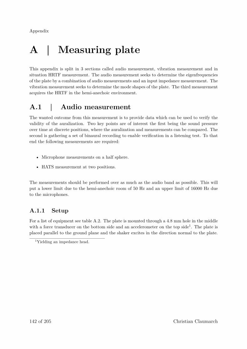
Appendix
A | Measuring plateThis appendix is split in 3 sections called audio measurement, vibration measurement and insituation HRTF measurement. The audio measurement seeks to determine the eigenfrequenciesof the plate by a combination of audio measurements and an input impedance measurement. Thevibration measurement seeks to determine the mode shapes of the plate. The third measurementacquires the HRTF in the hemi-anechoic environment.
A.1 | Audio measurementThe wanted outcome from this measurement is to provide data which can be used to verify thevalidity of the auralization. Two key points are of interest the first being the sound pressureover time at discrete positions, where the auralization and measurements can be compared. Thesecond is gathering a set of binaural recording to enable verification in a listening test. To thatend the following measurements are required:
• Microphone measurements on a half sphere.
• HATS measurement at two positions.
The measurements should be performed over as much as the audio band as possible. This willput a lower limit due to the hemi-anechoic room of 50 Hz and an upper limit of 16000 Hz dueto the microphones.
A.1.1 SetupFor a list of equipment see table A.2. The plate is mounted through a 4.8 mm hole in the middlewith a force transducer on the bottom side and an accelerometer on the top side1. The plate isplaced parallel to the ground plane and the shaker excites in the direction normal to the plate.
1Yielding an impedance head.
142 of 205 Christian Claumarch

Appendix A.1. Audio measurement
Accelerometer (2)Plate (4)
Force Transducer (1)
Shaker (3)
ADC (5)
(7)
Tone generator (6)(8)
Figure A.1: Experimental setup for plate. Zoom on the local setup around the plate. Numberscorrespond to item numbers in table A.2.
In figure A.2 a 2 dimensional overview of the setup is given. The plate is placed so that itscentre position is at the position (x,y,z) (0,0.094,0) m. The length of the plate is turned alongthe x-axis as in the simulation. The HATS is turned to be facing the centre of the plate for bothmeasurement positions.
Object Position x-coordinate/m y-coordinate/m z-coordinate/m
Plate Centre point 0 0.094 0
HATS Position 1 Mid between ears, facing plate. 0 1.097 0
HATS Position 2 Mid between ears, facing plate. 1.04 1.60 0.76
Microphones M1-M20 Centre of membrane See table A.4.
Table A.1: Positions in the measurement environment.
Christian Claumarch 143 of 205

Appendix A.1. Audio measurement
(9)-Pos1
(9)-Pos2
Figure A.2: Experimental setup for plate. The global setup around the plate. The microphone place-ment is arbitrary, the actual coordinates of all 20 microphones are given in table A.4. The electricalconnections are left out here but can bee found in table A.6. The items around the plate are connectedas in figure A.1 and all the microphones are connected to an ADC.
Function Model Serial number Number in setup
Force transducer B&K 8200 2190752 1
Accelerometer B&K 4514-B-001 52030 2
Shaker B&K 4810 1128303 3
Plate NaN NaN 4
ADC B&K 3050-B 101343 5
Tone generator Agilent 33220A MY44004996 6
Charge amplifier FT B&K 2646 2178390 7
Power amplifier B&K 2706 1113510 8
HATS B&K 4100D 2209464 9
20 microphones B&K 4955 See table A.3 M1-M20
4 ADCs B&K 3050-B See table A.5 A1-A4
Table A.2: Model and serial numbers of the items used in the setup.
144 of 205 Christian Claumarch

Appendix A.1. Audio measurement
Microphone number Model Serial number
M1 B&K 4955 2703788
M2 B&K 4955 2863786
M3 B&K 4955 2707482
M4 B&K 4955 2716184
M5 B&K 4955 2760307
M6 B&K 4955 2856041
M7 B&K 4955 2846186
M8 B&K 4955 2760310
M9 B&K 4955 2760311
M10 B&K 4955 2760312
M11 B&K 4955 2774589
M12 B&K 4955 2774590
M13 B&K 4955 2783591
M14 B&K 4955 2783592
M15 B&K 4955 2783593
M16 B&K 4955 2793992
M17 B&K 4955 2792993
M18 B&K 4955 2863783
M19 B&K 4955 2792995
M20 B&K 4955 2806536
Table A.3: Model and serial numbers of the Microphones used in the setup.
The positions of the microphones are given below with (x,y,z)=(0,0,0) corresponding to theorigin of the sphere created by mirroring the half-sphere around the floor plane y=0.
Christian Claumarch 145 of 205

Appendix A.1. Audio measurement
Microphone number x y z
M1 -2.8000 0.0700 0
M2 1.3972 0.2100 -2.4192
M3 1.3888 0.3500 2.4052
M4 -1.3776 0.4900 2.3884
M5 -1.3636 0.6300 -2.3632
M6 2.6908 0.7700 0
M7 0 0.8960 2.6516
M8 -2.2484 1.0500 -1.2992
M9 2.1952 1.1900 -1.2684
M10 2.1336 1.3300 1.2320
M11 -2.0636 1.4700 1.1928
M12 0 1.6100 -2.2904
M13 2.1868 1.7500 0
M14 -1.0332 1.8900 1.7892
M15 -0.9632 2.0300 -1.6688
M16 0.8848 2.1700 -1.5316
M17 0.7924 2.3100 1.3692
M18 -1.3552 2.4500 0
M19 0 2.5900 -1.0640
M20 0.5376 2.7300 0.3108
Table A.4: Microphone positions specified in ISO 3745. In this project the orientation of the coordinatesystem is different so the y and z axis are swapped compared to the standard.
ADC number Model Serial number
A1 B&K 3050-B 3050-106160
A2 B&K 3050-B 3050-106157
A3 B&K 3050-B 3050-106168
A4 B&K 3050-B 3050-106159
Table A.5: Model and serial numbers of the ADCs used for the microphone array.
146 of 205 Christian Claumarch

Appendix A.1. Audio measurement
A.1.2 Connections
From Comment To To Channel
HATS (9) Left ear ADC (5) 1
HATS (9) Right ear ADC (5) 2
Force transducer (1) Via preamp (7) ADC (5) 6
Accelerometer (2) - ADC (5) 5
M1-M6 Increasing order A1 1-6
M7-M12 Increasing order A2 1-6
M13-M18 Increasing order A3 1-6
M19-M20 Increasing order A4 1-6
Tone generator (6) Via amplifier (8) Shaker (3) -
Table A.6: Equipment connections.
Below some photos of the setup are shown:
Christian Claumarch 147 of 205

Appendix A.1. Audio measurement
Figure A.3: Plate setup seen from front with HATS in position 2.
148 of 205 Christian Claumarch
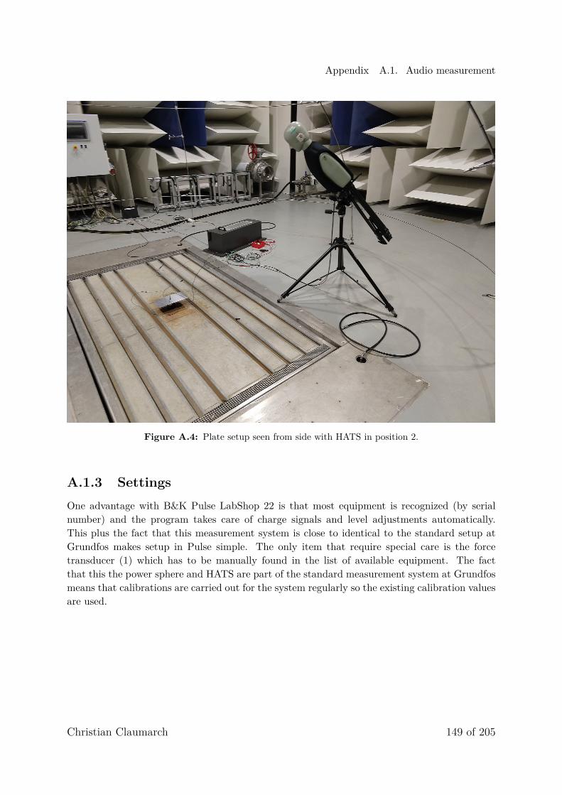
Appendix A.1. Audio measurement
Figure A.4: Plate setup seen from side with HATS in position 2.
A.1.3 SettingsOne advantage with B&K Pulse LabShop 22 is that most equipment is recognized (by serialnumber) and the program takes care of charge signals and level adjustments automatically.This plus the fact that this measurement system is close to identical to the standard setup atGrundfos makes setup in Pulse simple. The only item that require special care is the forcetransducer (1) which has to be manually found in the list of available equipment. The factthat this the power sphere and HATS are part of the standard measurement system at Grundfosmeans that calibrations are carried out for the system regularly so the existing calibration valuesare used.
Christian Claumarch 149 of 205

Appendix A.1. Audio measurement
Item number Setting
(6) Tone generator noise 1 Vpp
(M1-M20) / (A1-A4) Sample rate microphones 65.536 kHz
(9)/(5) sample rate HATS microphones 65.536 kHz
(2)/(5) Sample rate accelerometer 65.536 kHz
(1)/(5) Sample rate force transducer 65.536 kHz
Table A.7: Settings for equipment.
A.1.4 ProcedureThe procedure uses an interface specific to Grundfos, which is not documented further here.
• Start the tone generator and adjust the power amplifier to 2 o’clock. (A mark exist onthis specific power amplifier.)
• Start the measurement.
• When measurement is done press ’calculate’.
• Press ’Report’ to get the sound power level and save the data.
A.1.5 ResultsThe results are obtained by exporting the auto spectra from Pulse. What Pulse does to createthe data is averaging frames over time, similar to Welch’s method [Welch, 1967]. The runtime is1 minute and a window length of 6400 samples and an overlap of 75% is used. The windowingfilter is a Hamming filter. For the HATS measurement a downsampled version of the recording(fs 12.8 kHz) is used for averaging as memory is an issue in Pulse. The force transducer andaccelerometer signals are also downsampled to 12.8 kHz as they are unlikely to yield usefuldata at high frequencies. The first 10 seconds of the time signal is stored from the HATS,accelerometer, force transducer and M10, M15 and M20. This allows for post processing dataafterwards. The time signal from M20 is displayed below.
150 of 205 Christian Claumarch

Appendix A.1. Audio measurement
0 1 2 3 4 5 6 7 8 9 10
-6
-4
-2
0
2
4
610
-3
Figure A.5: The time signal at the M20 microphone position.
In figure A.6 the responses from the 20 microphones are shown and the resonant behaviour ofthe plate is clearly visible.
Christian Claumarch 151 of 205
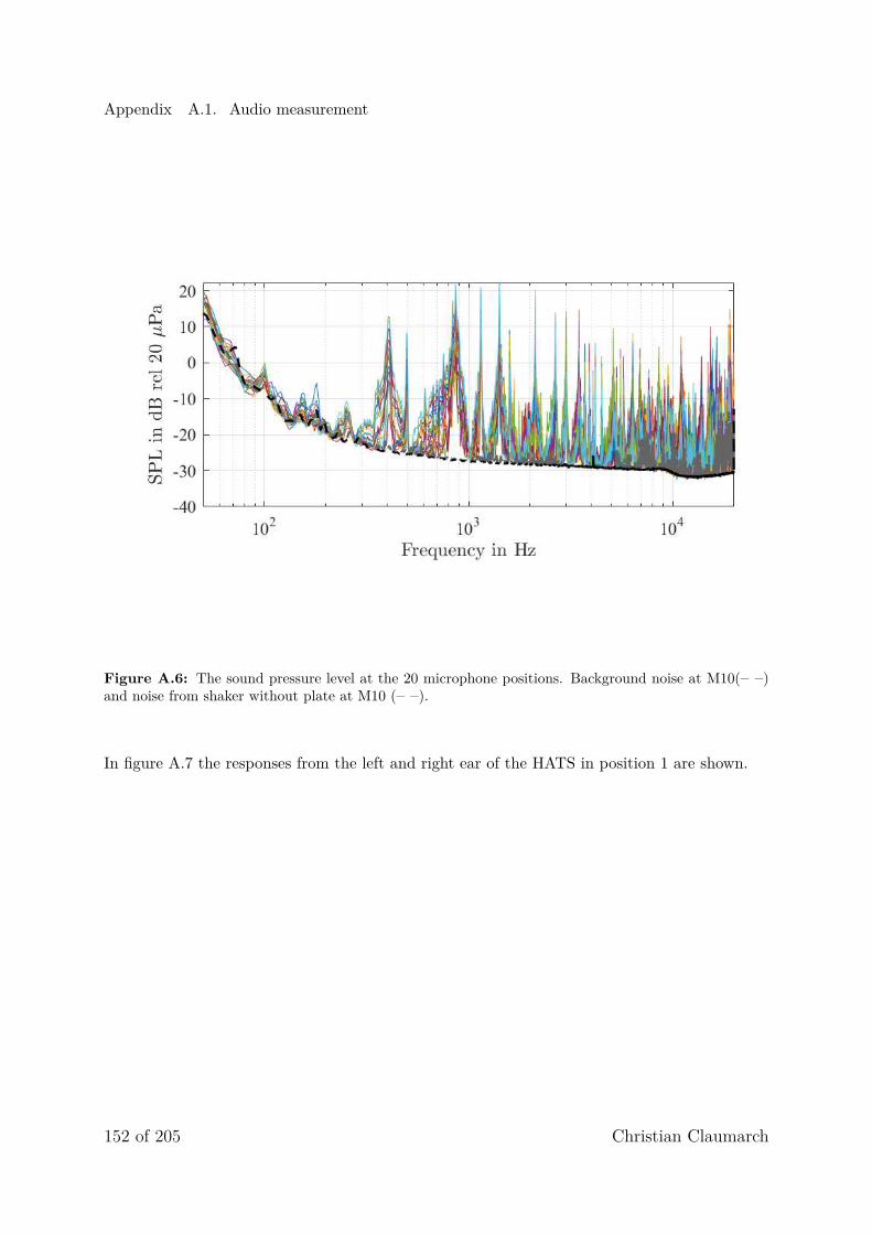
Appendix A.1. Audio measurement
Figure A.6: The sound pressure level at the 20 microphone positions. Background noise at M10(– –)and noise from shaker without plate at M10 (– –).
In figure A.7 the responses from the left and right ear of the HATS in position 1 are shown.
152 of 205 Christian Claumarch

Appendix A.1. Audio measurement
102
103
-20
-10
0
10
20
30
Figure A.7: The sound pressure level at the HATS left (—) and right (—) ear in position 1.
In figure A.8 the responses from the left and right ear of the HATS in position 2 are shown.
102
103
-20
-10
0
10
20
30
Figure A.8: The sound pressure level at the HATS left (—) and right (—) ear in position 2.
in order to calculate the input impedance of the plate the time signal from the accelerometerand force transducer can be used. A Fourier transform of the un-averaged time signals from theaccelerometer and force transducer are plotted below.
Christian Claumarch 153 of 205

Appendix A.1. Audio measurement
101
102
103
-140
-120
-100
-80
-60
-40
-20
Figure A.9: The acceleration (—) and force (—) magnitude in the input point. Accelerometer noisefloor (– –) and force transducer noise floor (– –).
It is clear from figure A.9 that the SNR in the force measurement is not sufficient to raise itover the noise floor. The accelerometer signal is also noisy. Therefore the result of calculatingthe input impedance as Z(ω)in = Force(ω)·jω
Acceleration(ω) is noisy as shown in figure A.10.
101
102
103
0
20
40
60
80
100
Figure A.10: The input impedance of the plate in the centre position.
In the middle position of the plate the displacement is small, especially at higher frequencies,resulting in a low SNR the measurement of acceleration. This means that the impedance can-not be calculated for all frequencies from an un-averaged signal. To solve this more sensitiveequipment with a lower noise floor could be used, but the B&K 4514 is already a rather big
154 of 205 Christian Claumarch

Appendix A.1. Audio measurement
and sensitive accelerometer and a more sensitive force transducer is not available. Instead theaveraged acceleration and input force are calculated at the cost of frequency resolution. Theaveraging is done using Welch’s method with a Hanning window with a size of 16384 samplesand an overlap of 75%. Here no downsampling is performed before the averaging - but the plotis still limited to 6.4 kHz. The results from averaging the acceleration and force is shown infigure A.11.
101 102 103-140
-120
-100
-80
-60
-40
-20
Figure A.11: The averaged acceleration (—) and force (—) magnitude in the input point. Accelerom-eter noise floor (– –) and force transducer noise floor (– –).
In order to calculate the averaged input impedance the input impedance is calculated for eachframe using the complex force and acceleration spectra. Then the calculated impedances fromall frames are averaged before plotting.
101 102 1030
20
40
60
80
Figure A.12: The averaged input impedance.
Christian Claumarch 155 of 205

Appendix A.1. Audio measurement
Based on figure A.12 is is noted that the measured input impedance increase with frequency. Thisis in contradiction with the fact that the input impedance of an isotropic plate should be 8
√Eρh
[Cremer et al., 2005], which is independent of frequency. In the setup the input impedance is notonly that of a plate but includes the mass of the top of the force transducer and accelerometer.Removing these from the impedance does however not make the input impedance independentof frequency as expected. The influence of the additional components is removed by subtractingthe impedance of a mass of M=11.7 grammes (jωM) from the impedance in each frame.
101 102 103-20
0
20
40
60
80
Figure A.13: The averaged input impedance - corrected for the mass loading. Measured inputimpedance (—). Impedance of mass 11.7 grammes (—). Input impedance of plate alone (—). Theoret-ical input impedance of an infinite plate (—).
The input impedance of a finite plate should in average be that of an infinite plate of samematerial and thickness. Therefore the yellow line should be centred around the purple line. Thisseems to hold at low and mid frequencies, but at higher frequencies the measured result deviatesfrom theory. It is possible that the force transducer is used above its operating range. This isexamined further in subsection 12.2.3.
Removing the influence of the mass from the input impedance although elegant does not changethe physical setup, where the plate is loaded by this additional mass. For this reason figure A.12is used to determine the resonances of the system including the mass load. The resonancefrequencies on the yellow line in figure A.13 are comparable to the an analytical solution, whereno mass loading is included.
From figure A.12 it can be seen that resonances occur at frequencies below those that are clearlyvisible in the audio spectra. It is established that resonances exist at 87 Hz and 276 Hz forthe plate disregarding the measurement system. If the measurement system is to be includedin the considerations the frequencies with highest displacement are better found directly fromfigure A.11 as the frequencies of highest acceleration. This would be 256 Hz and the frequencybelow this is not really clear but probably a bit lower than the 87 Hz found above. Anyhowthe frequencies are so low compared to plate dimensions that it is not an efficient radiator of
156 of 205 Christian Claumarch

Appendix A.2. Vibration measurement
sound. By combining the resonance frequencies determined through the input impedance andthose determined by audio a full picture of the plates vibrational frequencies is available in theaudio range.
A.2 | Vibration measurementThe second part of the appendix seeks to determine the mode shapes of the plate. In order toexamine these a simple approach is used. Sugar is poured on the vibrating plate to reveal nodallines - where the sugar will settle.
During the course of the project many different frequencies have been examined at differenttimes. Only some are actually of interest but all results are included for completeness.
A.2.1 SetupThe setup is a simplified version of the one used above. All remaining equipment is the same asabove. The plate is mounted as in figure A.1 with the accelerometer (2) and force transducer(1) disconnected from the ADC.
A.2.2 ConnectionsThe tone generator is connected via the power amplifier (8) to the shaker (3) as in table A.6
A.2.3 Settings
Item number Setting
(6) Tone generator sine 1 Vpp
Table A.8: Settings for equipment.
A.2.4 procedureThe selection of frequencies of interest is based on the impedance and audio measurement 87Hz, 256 Hz, 400 Hz and 496 Hz. In between some frequencies based on an early, with wrongmaterial parameters, analytical solution are included. These images serve the purpose of provingthe point that the non doubly symmetric modes will not be excited and the nearest symmetricalmode will dominate the vibration instead. Also 57 Hz is included as sound is recorded at thatfrequency in the HATS positions and it was seen as an eigenfrequency in some preliminary FEMworks.
The following is repeated for all frequencies of interest:
Christian Claumarch 157 of 205

Appendix A.2. Vibration measurement
• Sugar is poured on the plate while the shaker is turned off.
• The tone generator is set to vibrate sinusoidally at a specific frequency - i.e. forcedvibration.
• The gain on the power amplifier is increased until the sugar moves - or just before theclipping limit (light on power amplifier).
• When the sugar settles at nodal lines and the lines are stationary the shaker is stopped.(In case the sugar is not moving at the clipping limit the shaker is also stopped.)
• A picture is taken and the procedure is repeated for the next frequency.
A.2.5 ResultsMode shapes from vibration experiment are shown below. For easier overview blue lines indicatewhere sugar is collected. No blue lines indicate that no clear pattern is recognized. The post-itswere added after the shaker was stopped to keep track of frequency. The pictures are taken atdifferent times so the background does vary - the mounting of the plate and the setups are thesame.
Figure A.14: Mode shape at 57 Hz. (Additional resonance.)
158 of 205 Christian Claumarch

Appendix A.2. Vibration measurement
Figure A.15: Mode shape at 87 Hz. (Expected resonance.)
Figure A.16: Mode shape at 92 Hz. (Vibration dominated by 87 Hz mode shape.)
Christian Claumarch 159 of 205

Appendix A.2. Vibration measurement
Figure A.17: Mode shape at 101 Hz. (Vibration dominated by 87 Hz mode shape.)
Figure A.18: Mode shape at 225 Hz. (Vibration dominated by 256 Hz mode shape.)
160 of 205 Christian Claumarch

Appendix A.2. Vibration measurement
Figure A.19: Mode shape at 256 Hz. (Expected resonance.)
Figure A.20: Mode shape at 274 Hz. (Vibration dominated by 256 Hz mode shape.)
Christian Claumarch 161 of 205
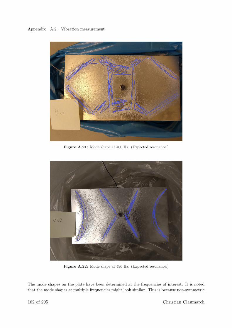
Appendix A.2. Vibration measurement
Figure A.21: Mode shape at 400 Hz. (Expected resonance.)
Figure A.22: Mode shape at 496 Hz. (Expected resonance.)
The mode shapes on the plate have been determined at the frequencies of interest. It is notedthat the mode shapes at multiple frequencies might look similar. This is because non-symmetric
162 of 205 Christian Claumarch

Appendix A.2. Vibration measurement
mode shapes cannot be excited in the middle of the plate. Instead a neighbouring eigenfrequencywith a doubly symmetric mode shape determines the mode shape .
A.2.6 Results part 2At a later stage it turned out that the original choice of sugar as material and the resultingupper frequency limit of the experiment of 500 Hz was inadequate. Substituting the sugar withfine salt it was possible to extend this limit up to 1588 Hz. Only the frequencies where soundis radiated are considered, namely 864 Hz, 1148 Hz, 1416 Hz and 1588 Hz. On this second setof experiments the plate was turned 180 degrees by mistake, so the pictures have been rotated180 degrees to make results comparable - resulting in the post-its being upside down.
Figure A.23: Mode shape at 864 Hz.
Christian Claumarch 163 of 205

Appendix A.2. Vibration measurement
Figure A.24: Mode shape at 1148 Hz.
Figure A.25: Mode shape at 1416 Hz.
164 of 205 Christian Claumarch

Appendix A.3. In situation HRTF measurement
Figure A.26: Mode shape at 1588 Hz.
This concludes the section on determining mode shapes. The mode shapes of the first 8 doublysymmetric modes have been determined.
A.3 | In situation HRTF measurementIn this section the HRTF for the HATS is measured in situation in the hemi-anechoic room atGrundfos using a loudspeaker.
Note: the results from this experiment are not useful due to low SNR. The experiment shouldbe re-performed using more suitable equipment namely a better sweep generator than the tonegenerator, a better power amplifier than the one intended for the shaker as well as some meansof controlling the power input to the loudspeakers or less fragile loudspeakers. For the purposeof this project and a more general case than auralization of the measurement room at Grundfosthe HRTF database acquired in Appendix B is seen as a better alternative.
A.3.1 SetupIn order to measure the in situation HRFT of the HATS basically the same setup as that givenin section A.1 is used. The main difference is that a loudspeaker is used instead of the plate. Dueto the size of available loudspeakers the position of the loudspeaker membrane is (0,0.25,0)mcompared to the (0,0.097,0)m of the plate. This is unavoidable due to the enclosure of theloudspeaker and is not compensated for. Giving in an error in distance for both positions aswell as in angle for position 2.
Christian Claumarch 165 of 205

Appendix A.3. In situation HRTF measurement
The loudspeaker is a single transducer mounted in a box. The transducer is a 4 inch PeerlessSDS-P830855 mounted in a closed box with inner dimensions HxWxD = 0.147x0.0.147x0.152m. It has a maximum power handling of 30 W and no crossover is used.
To measure the sound pressure and HATS response in Position 1 and Position 2 in addition tothe items given in table A.2 the following equipment is used.
Function Model Serial number
Microphone B&K 4189 2117848
Pre amplifier B&K 2671 2143356
Calibrator B&K 4231 2459857
Loudspeaker in box NaN NaN
Table A.9: Model and serial numbers of the additional items used in the setup.
166 of 205 Christian Claumarch

Appendix A.3. In situation HRTF measurement
Figure A.27: The setup used for measuring in situation HRTF. Here the HATS is in position 1 and themicrophone in position 2. The HATS was naturally removed when measuring the reference in Position 2.
Christian Claumarch 167 of 205

Appendix A.3. In situation HRTF measurement
A.3.2 ConnectionsThe connections are identical to those used in table A.6 except the shaker and plate are replacedwith the loudspeaker and the force transducer and the accelerometer are disconnected. Insteadan additional microphone is connected together with a loopback.
From Comment To To Channel
B&K 4189 Via preamp B&K 2671 ADC (5) 5
Tone generator (6) Via amplifier (8) loudspeaker -
Tone generator (6) Via amplifier (8) ADC (5) 6
Table A.10: Equipment connections.
A.3.3 SettingsAll settings are left as in section A.1 with the exception that the volume on the power amplifieris set to 10 o’clock instead of 2 o’clock.
The additional microphone and the loopback are sampled at 65.536 Hz like the other micro-phones. The additional microphone is calibrated using B&K 4231 (calibration value 1.018) sinceit unlike the other microphones is not part of the standard setup, which is calibrated regularly.
The tone generator is set to create a logarithmic sine sweep from 100 Hz to 20 kHz over 5 secondswith a level of 1 Vpp.
A.3.4 Procedure• The tone generator is set to send a single sweep on a manual trigger.
• The measurement system is started.
• The sweep is triggered.
• The measurement system records stores the first 10 seconds whereof five should containthe sweep. This is confirmed by listening to the recorded signal in Pulse.
The above is repeated 4 times with the microphone and the HATS in the 2 positions
168 of 205 Christian Claumarch
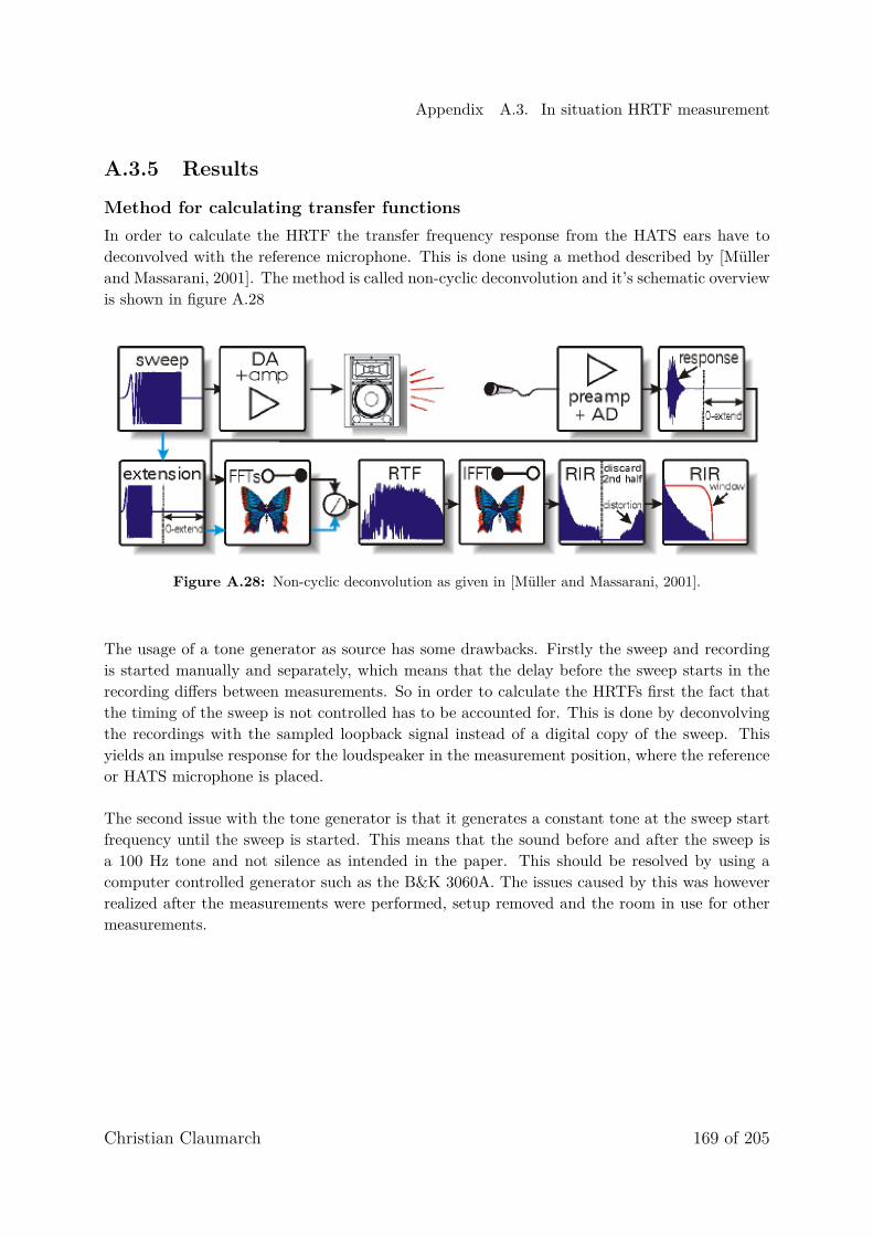
Appendix A.3. In situation HRTF measurement
A.3.5 Results
Method for calculating transfer functionsIn order to calculate the HRTF the transfer frequency response from the HATS ears have todeconvolved with the reference microphone. This is done using a method described by [Müllerand Massarani, 2001]. The method is called non-cyclic deconvolution and it’s schematic overviewis shown in figure A.28
Figure A.28: Non-cyclic deconvolution as given in [Müller and Massarani, 2001].
The usage of a tone generator as source has some drawbacks. Firstly the sweep and recordingis started manually and separately, which means that the delay before the sweep starts in therecording differs between measurements. So in order to calculate the HRTFs first the fact thatthe timing of the sweep is not controlled has to be accounted for. This is done by deconvolvingthe recordings with the sampled loopback signal instead of a digital copy of the sweep. Thisyields an impulse response for the loudspeaker in the measurement position, where the referenceor HATS microphone is placed.
The second issue with the tone generator is that it generates a constant tone at the sweep startfrequency until the sweep is started. This means that the sound before and after the sweep isa 100 Hz tone and not silence as intended in the paper. This should be resolved by using acomputer controlled generator such as the B&K 3060A. The issues caused by this was howeverrealized after the measurements were performed, setup removed and the room in use for othermeasurements.
Christian Claumarch 169 of 205

Appendix A.3. In situation HRTF measurement
0 2 4 6 8 10-1.5
-1
-0.5
0
0.5
1
1.5
Figure A.29: The loopback signal in time domain. The 100 Hz tone before and after the sweep areseen as the ’flat’ 2.5 Vpp part. Furthermore spikes at onset and offset of the signal are seen.
100 101 102 103 104-200
-150
-100
-50
0
Figure A.30: The loopback signal in frequency domain.
In theory the deconvolution method should work with any stimuli, so the 100 Hz start and stopshould just be seen as part of the reference signal and be deconvolved. However the results willlater show overtones of 100 Hz which could be caused by this or possibly 50 Hz humming.
The Third issue is that the sweep does not cover all frequencies in the sampled range as nosafety crossover is mounted before the loudspeaker. This is solved by only plotting the validfrequency area 100 Hz to 20 kHz.
170 of 205 Christian Claumarch

Appendix A.3. In situation HRTF measurement
Data acquiredBelow the recordings from the microphones are given in position 1 and position 2 in frequencydomain.
102 103 104-40
-20
0
20
40
60
80
Figure A.31: The SPL at the different microphones in position 1. Reference microphone (—), HATSleft ear (—) and HATS right ear (—).
102 103 104-40
-20
0
20
40
60
80
Figure A.32: The SPL at the different microphones in position 2. Reference microphone(—), HATSleft ear (—) and HATS right ear (—).
Calculated resultsThe frequency response of the loudspeaker in position 1 and position 2.
Christian Claumarch 171 of 205

Appendix A.3. In situation HRTF measurement
102 103 104-100
-80
-60
-40
-20
0
Figure A.33: The response of the loudspeaker in position 1 (—) and position 2 (—).
The signal generated by the loudspeaker is not flat especially not in position 2 which is at an offangle to the loudspeaker. Since the measured signals in the positions are used as reference thisis not a problem as long as the level is above the noise floor. Unfortunately that is not the case.Deconvolving the individual ear responses with the reference yield the HRTF at that position.The deconvolution is performed as a spectral division of the complex frequency response at theear microphone with the complex frequency response from the reference microphone.
102 103 104-50
0
50
Figure A.34: The HRTF of the HATS in position 1 left ear (—) and right ear (—).
172 of 205 Christian Claumarch

Appendix A.3. In situation HRTF measurement
102 103 104-50
0
50
Figure A.35: The HRTF of the HATS in position 2 left ear (—) and right ear (—).
The HRTFs for the HATS have been determined in the two positions where recordings wereperformed in section A.1.
As discussed in the introduction to the measurement the SNR is very low. The recordings aremade at level of about 30 dBSPL. The inherent noise in the microphones is 6.5 dB(A) [Brüel &Kjær, no date c]. The background noise in the room is 5.5 dB(A) according to the certification.The experiment should be re-performed but that is not done seeing as the HRTFs are measuredin anechoic conditions in Appendix B instead.
Christian Claumarch 173 of 205

Appendix
B | Measuring HRTFAnother student at Aalborg University was measuring head related transfer functions (HRTF)on human subjects during the same time as as I did my thesis. Therefore a complete setup formeasuring HRTF was available. The setup was fully automated and is described below togetherwith the results. For a fully comprehensive walk-through the reader is referred to the master’sthesis written by Sigurd Van Hauen [Hauen, 2018].
B.1 | SetupThe setup consists of 11 loudspeakers positioned on an arc at a distance of 1.7 meters from thereference position. The loudspeakers cover elevation angles from −40◦ to −40◦ in 8◦ intervals.The vertical rotation is made using a turntable where turns are made from direct front (0◦) in1◦ intervals to the back of the HATS is turned towards the loudspeakers (180◦). The data forthe other side is created as a mirror, since the HATS is fully symmetric.
174 of 205 Christian Claumarch

Appendix B.1. Setup
LaptopMonitor Soundcard Power
AmplifierRelay Board
Anechoic Room
Control Room
Rotating
Platform
Camera
Target
Disc
Back
support
Laserpointer
Arduino Uno
0°
-8°
-16°
-24°
-32°
-40°
8°
16°
24°
40°
32°
Figure B.1: Schematic of setup from [Hauen, 2018]. The blue and purple dots represent a hearing aidused in the original project. The target disc is built into the HATS.
Figure B.1 shows the setup as it is used in [Hauen, 2018]. In this context a few differences exist.The major difference is that the person with blue and purple hearing aid with a back support isreplaced with the HATS on it’s stand. When human subjects are tested the camera and monitoris used to make sure the participant is not moving, in the setup with a HATS it is redundant.Instead the cross lasers used for building the setup came in handy as they were used to positionthe HATS accurately. On the note of accuracy; the setup is made to be accurate compared tohow stationary people can be expected to be for prolonged periods of time, about 20 minutes.Obviously the HATS is superior to humans when the challenge is standing still, so the slightmisalignments due to the setup that were irrelevant before might be influence the results.
Another difference from the setup used by [Hauen, 2018] is that he uses small microphonesmounted in peoples ears. In this project the internal microphones of the HATS are used. These
Christian Claumarch 175 of 205

Appendix B.1. Setup
internal microphones are connected to the same sound card as that which drives the poweramplifier. The 48V phantom power built in to the sound card is used to supply the microphones.
For the reference measurement a pressure field measurement microphone is used. The micro-phone is placed vertically with 90◦ incidence from the 0◦ elevation loudspeaker. At the time thiswas thought as best compromise between all sources - at a later stage it has been realized that90◦ incidence could have been achieved for all sources by mounting the microphone horizontallyand turning the microphone to be orthogonal to the plane of the sources. The error due to thisis in the order of 4 dB [Brüel & Kjær, no date e] in the range 15 kHz to 20 kHz for the outermostsource angles. The microphone is connected via a pre-amplifier and a measurement amplifierwith polarization voltage to the soundcard.
176 of 205 Christian Claumarch

Appendix B.1. Setup
Figure B.2: Picture of the HATS in the measurement system.
Christian Claumarch 177 of 205

Appendix B.2. Equipment
B.2 | Equipment
Item Description AAU-no.
1 Macbook Pro (medio 2012) running MATLAB 2017b NaN
2 B&K HATS 4100D NaN
3 RME Fireface UFX II Sound card 108227
4 Pioneer A-656 Power Amplifier 08698
5 11 x M10MD39-08 in ball mount NaN
6 Outline Rotational table NaN
7 12 channel Relay Board NaN
8 Arduino uno NaN
9 GRAS 26ak pre-amp 52665
10 B&K microphone 4134 61447
11 B&K Charge Amplifier 2636 08717
Table B.1: Equipment used in HRTF measurement setup.
B.3 | SettingsThe measurement system uses a sampling rate of 48 kHz and an MLS signal as stimuli. TheMLS signal is generated with 3 cycles, one for exciting the system and the following two forpre-averages. The order of the used MLS signal is 12 resulting in a length L = 4095, the lowestfrequency in the signal being fs/L = 11.7 Hz and the upper frequency being fs/2− fs/(2L) =23994.1 Hz [Vanderkooy, 1994].
B.4 | ProcedureBefore the measurements can be performed the setup is calibrated. The reference microphoneis calibrated using a calibrator and the sensitivity is put into the measurement script. For theHATS measurement the calibration values used at Grundfos are used.
B.4.1 Reference measurementThe reference measurement is made using the reference microphone in the future centre positionof the HATS. This point is found as the point where all four laser lines meet. The referencemeasurement is made once for each loudspeaker for a total of 11 measurements using an auto-
178 of 205 Christian Claumarch
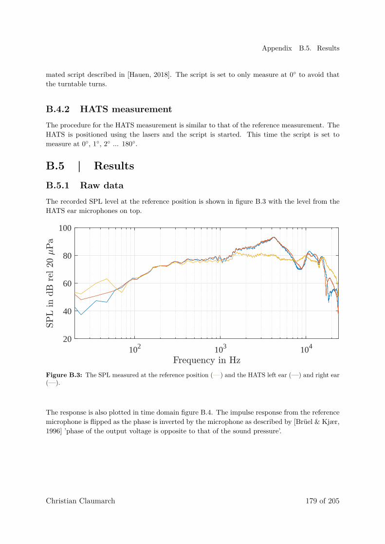
Appendix B.5. Results
mated script described in [Hauen, 2018]. The script is set to only measure at 0◦ to avoid thatthe turntable turns.
B.4.2 HATS measurementThe procedure for the HATS measurement is similar to that of the reference measurement. TheHATS is positioned using the lasers and the script is started. This time the script is set tomeasure at 0◦, 1◦, 2◦ ... 180◦.
B.5 | ResultsB.5.1 Raw dataThe recorded SPL level at the reference position is shown in figure B.3 with the level from theHATS ear microphones on top.
102 103 10420
40
60
80
100
Figure B.3: The SPL measured at the reference position (—) and the HATS left ear (—) and right ear(—).
The response is also plotted in time domain figure B.4. The impulse response from the referencemicrophone is flipped as the phase is inverted by the microphone as described by [Brüel & Kjær,1996] ’phase of the output voltage is opposite to that of the sound pressure’.
Christian Claumarch 179 of 205

Appendix B.5. Results
0.038 0.04 0.042 0.044 0.046 0.048 0.05-0.2
-0.1
0
0.1
0.2
Figure B.4: The SPL measured at the reference position (—) and the HATS left ear (—) and right ear(—).
Removing reflections from setupFrom figure B.3 a very fluctuating frequency response is seen, this is due to a comb filter causedby reflections from the setup. These reflections are removed by time gating with a Hanningfilter with an order of 512 on both reference and HATS impulse responses. The window is keptstationary in time even though the impulses move slightly due to different delays with position.
0.03 0.035 0.04 0.045 0.05-0.2
-0.1
0
0.1
0.2
Figure B.5: The SPL measured at the reference position (—) and the HATS left ear (—) and right ear(—). The Hanning window (—) is scaled down by a factor 10 for easier viewing.
In figure B.5 the window is scaled down by a factor 10, it’s true amplitude is 1. In the unedited
180 of 205 Christian Claumarch

Appendix B.5. Results
impulse responses the reflections can be seen as small ripples in the impulse response even afterit has decayed fully - starting from ≈ 45 ms. Having removed the reflections from setup thefrequency response is much smother as seen in figure B.6
102 103 1040
20
40
60
80
100
Figure B.6: The SPL measured at the reference position (—), the HATS left ear (—) and right ear(—). Time gating has been performed to remove reflections from the setup.
B.5.2 Data TreatmentThe HRTF is calculated as a spectral division of the ear signals with the reference signal. Theresulting frequency response is inverse Fourier transformed to acquire the impulse response.Since the deconvolution is done cyclically the onset of the impulse response might be in theend of the frame, instead of in negative time, where it should have been (corresponding to thesound arriving at an ear before it arrives at the reference position). This is solved by shiftingthe response cyclically 28 samples to the right. This will allow the impulse to arrive at the timecorresponding sound propagating 20 cm before the reference to be wrapped around.
Christian Claumarch 181 of 205

Appendix B.5. Results
-1 0 1 2 3 4
10-3
-1
-0.5
0
0.5
1
Figure B.7: The The HRTF of the HATS facing forwards left ear (—) and right ear (—).
-1 0 1 2 3 4
10-3
-1
-0.5
0
0.5
1
1.5
Figure B.8: The The HRTF of the HATS turned 90◦ clockwise, left ear (—) and right ear (—).
A few phenomena are observed, first pre-ringing is treated. The pre-ringing is not present inthe impulse responses in figure B.5 but appears after the cyclic deconvolution. This is mostlikely due to the fact that different channels are used for the three different measurements, sothe division includes some artefacts from the non identical anti aliasing filters. The preringingis removed using a 4th order Buttorworth IIR low pass filter at 23 kHz created by the matlabcommand ’butter()’. figure B.9 and figure B.10 shows figure B.7 and figure B.8 again after thefiltering.
182 of 205 Christian Claumarch

Appendix B.5. Results
-1 0 1 2 3 4
10-3
-1
-0.5
0
0.5
1
Figure B.9: The The HRTF filtered for pre-ringing of the HATS facing forwards left ear (—) and rightear (—).
-1 0 1 2 3 4
10-3
-1
-0.5
0
0.5
1
1.5
Figure B.10: The The HRTF of the HATS turned 90◦ clockwise and filtered for pre-ringing, left ear(—) and right ear (—).
The second phenomena appears when taking the Fourier transform of the HRTF. The phenomenais that some DC offset is present, and as it is known that the HRTF should converge to 0 dB atDC as the dummy is infinitely small compared to the wavelength of 0 Hz. For some positionshowever the gain it is rather significant and as such should be removed by as suggested by[Hammershøi and Møller, 2005]. in order to show the low frequency phenomena the FFT lengthused is 216, which means that the 512 samples long impulse responses are zero padded to that
Christian Claumarch 183 of 205

Appendix B.5. Results
length.
100 101 102 103 104-30
-20
-10
0
10
20
Figure B.11: The The HRTF of the HATS facing forwards left ear (—) and right ear (—).
100 101 102 103 104-40
-30
-20
-10
0
10
20
Figure B.12: The The HRTF of the HATS turned 90◦ clockwise, left ear (—) and right ear (—).
From figure B.11 and figure B.12 it is clear that the 512 sample long impulse response has aDC offset. The method proposed in [Hammershøi and Møller, 2005] is to simply set the DCcomponent to unity in the frequency domain before the inverse Fourier transform. This methodremoves the DC component as desired.
184 of 205 Christian Claumarch
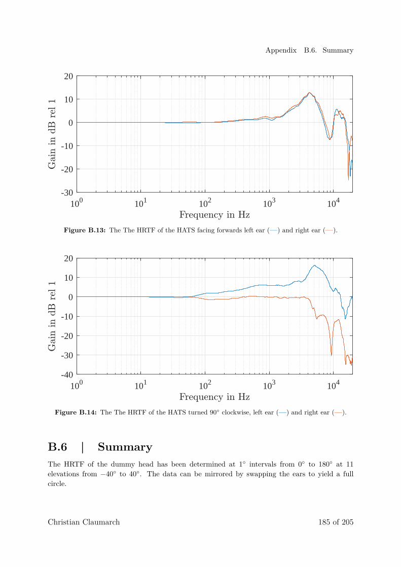
Appendix B.6. Summary
100 101 102 103 104-30
-20
-10
0
10
20
Figure B.13: The The HRTF of the HATS facing forwards left ear (—) and right ear (—).
100 101 102 103 104-40
-30
-20
-10
0
10
20
Figure B.14: The The HRTF of the HATS turned 90◦ clockwise, left ear (—) and right ear (—).
B.6 | SummaryThe HRTF of the dummy head has been determined at 1◦ intervals from 0◦ to 180◦ at 11elevations from −40◦ to 40◦. The data can be mirrored by swapping the ears to yield a fullcircle.
Christian Claumarch 185 of 205

Appendix
C | Headphone transfer functionThis appendix describes the setup required to acquire the frequency response of a pair of head-phones. This is required since headphones are not normally tuned to have a flat frequencyresponse, which is required when making a binaural playback system. This is because the filter-ing with a HRTF describes the sound pressure as it would be at the ear-drum. It is that soundpressure that the headphone should reproduce, without an additional frequency response of theheadphone itself.
Ideally the headphone transfer function should be individually measured, meaning that it shouldbe measured directly on the intended listener. Preferably even on the same mounting, so thatthe headphones are not moved before the binaural representation. Here the procedure is shownon a HATS, the HATS used when measuring the HRTFs.
C.1 | SetupA list of equipment is given in table C.1 and the setup is illustrated in figure C.1. In additionto the setup depicted in figure C.1 a setup consisting of a loopback connecting the sound cardoutput and input channels is used.
Sound card (1)
Phones out2 Right1 Left
HATS (2)
Headphone(3)
Figure C.1: Experimental setup for measuring a headphone frequency response.
186 of 205 Christian Claumarch

Appendix C.1. Setup
Figure C.2: Picture of experimental setup for measuring a headphone frequency response.
Christian Claumarch 187 of 205

Appendix C.2. Equipment
C.2 | Equipment
Function Model Serial number Number in setup
Sound card Steinberg UR242 EEV001310 1
HATS B&K 4100D 2209464 2
Headphone Beyerdynamic T90 09637 3
Jack cable Jack stereo -> 2 jack mono - -
2x adaptor XLR male -> BNC female - -
Table C.1: Model and serial numbers of the items used in the setup. The headphone can naturally beinterchanged with any other headphone one might want to use.
From From channel To To channel
Sound card (1) Phones out Sound card (1) 1 & 2
Table C.2: Equipment connections when measuring loopback. Left channel (white) is connected tochannel 1.
From From channel To To Channel
Sound card (1) Phones out Headphone (3) -
HATS (2) Left microphone Sound card (1) 1
HATS (2) Right microphone Sound card (1) 2
Table C.3: Equipment connections when measuring Headphone.
C.3 | Settings
Item number Setting
(1) Sample rate sound card 48 kHz
(1) Input 1 ’Pad’ on
(1) Input 2 ’Pad’ on
Table C.4: Settings for equipment connections. (’Pad’ is an attenuator.)
188 of 205 Christian Claumarch

Appendix C.4. Procedure
C.4 | ProcedureThe setup is not calibrated to work at absolute sound pressure levels since only the ’shape’ ofthe magnitude response is to be corrected and the sensitivity is irrelevant. The loopback willnaturally have a much higher amplitude than the microphone signal, so the gain settings shouldbe adjusted to make the loopback use most of the ADC range. In the case of the Here it ischosen to set the phones out to 12 O’clock and the input gain to 10 O’clock.
The measurement script ’HeadphoneTransfer.m’ controls the playback and recording of sweeps.The following steps are required to perform the experiment
1. Connect the loopback as described in table C.2.
2. Run the script ’HeadphoneTransfer.m’ and press ’g’ when prompted to do so.
3. When the script displays a message in the command window with instructions for con-necting the HATS follow these:
(a) Disconnect the loopback(b) Connect the HATS as described in table C.3 using the XLR to BNC connectors.(c) Turn on the 48 V phantom power.(d) Press ’g’ to continue measurement.
4. When the script is done turn off the 48 V phantom power before disconnecting the HATS.
C.5 | ResultsThe recordings of the loopback as well as the microphone signals are shown below.
0 2 4 6 8 10 12-0.05
0
0.05
Figure C.3: Time domain plot of the loopback signal in channel left (—) and right (—) - they coincide.The recording at the HATS left ear (—) and right ear (—) - they also almost coincide.
Christian Claumarch 189 of 205

Appendix C.5. Results
The four recordings are also shown in frequency domain below.
102 103 104-50
0
50
Figure C.4: Frequency domain plot of the loopback signal in channel left (—) and right (—) - theycoincide. The recording at the HATS left ear (—) and right ear (—).
The transfer function is calculated as shown in figure 11.3. This is done in the script ’PostPro-cess.m’
0.425 0.426 0.427 0.428 0.429 0.43-0.1
-0.05
0
0.05
0.1
0.15
0.2
Figure C.5: Impulse response of left channel (—) and right channel (—).
And again in frequency domain.
190 of 205 Christian Claumarch

Appendix C.6. Summary
102 103 104-50
-40
-30
-20
-10
0
Figure C.6: Frequency response of left channel (—) and right channel (—).
C.6 | SummaryIt is clear from figure C.6 that assuming a this pair of headphones to be ’flat’ would introduceerrors of more than 10 dB in the range 100 Hz to 10 kHz. The deviations between the twochannels at low and very high frequency is likely due to mounting. In a setup where a binauralrepresentation is given an average of multiple measurements, where the headphone is removedand remounted between measurements, would be beneficial. That being said the two driverscannot be completely identical so some variation between the channels is to be expected.
Christian Claumarch 191 of 205

Appendix
D | Gorman superpositionHere The structure of the code finding the eigenfrequencies is given in Listing D.1. Thisis followed by an outline og the code determining mode shapes is given in Listing D.2.
1 K=number of terms2 searchRange=lowLim:step:upLim % Define serchrange3 for TrialEigenvalue=searchRange %loop over all trial eigenvalues4 for M=1:K % Loop over number of terms building block 15 for N=1:K % Loop over number of terms6 if N==17 A(M,M)= %Fill upper left diagonal8 end9 A(N+K,M)= %Fill upper right quadrant10 end11 end12 for N=1:K % Loop over number of terms building block 213 for M=1:K % Loop over number of terms14 if M==115 A(N+K,N+K)= %Fill lower right diagonal16 end17 A(N+K,M)= %Fill lower left quadrant18 end19 end20 % Calculate the determinant of the trial eigenvalue21 Y(TrialEigenvalue)=det(A)22 end
Listing D.1: Pseudocode of the standard Gorman Superposition algorithm determining eigenvalues.
1 % in this code Y and A are used as the Y and A corresponding to thosecalculated for the trial eigenvalue above. W contains the amplitude ofderformation at the position (L,j).
2 K=number of terms3 Nxx=numberOfSamplingPoints per direction4 for L=1:Nxx5 for j=1:Nxx6 for M=1:K %first building block7 W(L,j)=W(L,j)+term M's contribution8 end9 for N=1:K %second building block10 W(L,j)=W(L,j)+term N's contribution11 end12 end13 end14 3Dplot(W) %Display the modehshape
Listing D.2: Pseudocode of the standard Gorman Superposition algorithm determining mode shapes.
192 of 205 Christian Claumarch

Appendix
E | Parameter sensitivity study
E.1 | Design goal parameter sensitivity studyAs the simulated results are dependent on many variables it is desired to examine which param-eters cause significant changes to the eigenfrequencies or mode shapes. Due to time constraintonly the more complex setup ’complete simplified’ is considered and not ’11.7g’. The param-eter study is done by varying the following parameters for the setup ’complete simplified’ infigure 13.5b within reasonable amounts.
E.2 | Original parameters• Thickness = 1.5 mm
• Length = 299.3 mm
• Width = 169.3 mm
• Young’s modulus 71 GPa
• Centre hole Ø = 4.8 mm
• Centre hole location L=149.9 mm, W=84.4 mm
• Spring stiffness shaker 2000 N/m
E.3 | Variations1. Plate thickness ±0.1mm
2. Plate length ±1mm
3. Plate width ±1mm
4. Young’s modulus 69 GPa to 75 GPa
5. Centre hole location +1mm
6. Spring stiffness shaker 1000 N/m, 3000 N/m, 5000 N/m, 10000 N/m, 15000 N/m and20000 N/m.
Variations in length and width of the plate are made on with half the variation on either side ofthe plate, to not change the asymmetry due to the centre hole placement. The diameter of thecentre hole is not varied but kept at the measured 4.8 mm. The centre hole location is variedonce to be as offset from the true plate centre as possible. The new centre hole is at L=150.9mm, W=83.4 mm and the spring and mass connected to the centre are moved to the sameamount to keep them normal to the centre hole.
Christian Claumarch 193 of 205

Appendix E.4. Results
E.4 | ResultsReference 1 +0.1 mm 1 -0.1 mm 2 +1 mm 2 -1 mm 3 +1 mm 3 -1 mm 4 69 GPa 4 75 GPa 5 +1 mm
81 Hz 87 Hz 75 Hz 81 Hz 82 Hz 81 Hz 81 Hz 80 Hz 83 Hz 81 Hz245 Hz 263 Hz 227 Hz 245 Hz 245 Hz 243 Hz 248 Hz 242 Hz 252 Hz 244/247 Hz =
482 Hz 513 Hz 449 Hz 479 Hz 484 Hz 480 Hz 482 Hz 474 Hz 495 Hz 481 Hz415 Hz 444 Hz 385 Hz 413 Hz 415 Hz 412 Hz 417 Hz 408 Hz 426 Hz 414 Hz860 Hz 911 Hz 793 Hz 849 Hz 855 Hz 848 Hz 856 Hz 840 Hz 876 Hz 853 Hz1166 Hz 1227 Hz 1072 Hz 1143 Hz 1156 Hz 1147 Hz 1152 Hz 1133 Hz 1181 Hz 1150 Hz1624 Hz 1691 Hz 1480 Hz 1584 Hz 1587 Hz 1569 Hz 1602 Hz 1563 Hz 1630 Hz 1586 Hz1440 Hz 1498 Hz 1309 Hz 1399 Hz 1408 Hz 1395 Hz 1412 Hz 1384 Hz 1442 Hz 1404 Hz
Table E.1: Eigenfrequencies in plate parameter sensitivity study for parameters 1 through 5. Thecomplete simplified setup from chapter 13 is used as reference and parameters are varied within limits.The columns should be read as ’parameter number variation’.
= Splits the mode in two deformed mode shapes similar to figure 13.6d.
The parameter that the simulation is the most sensitive towards is the thickness of the plate.This is expected as the plate thickness is used in the power of three in the equation for bendingstiffness of a place as shown in subsection 8.1.3 and [Cremer et al., 2005]. Secondly the Young’sModulus, which also affects the bending stiffness, has large influence on the eigenfrequencies.
The variations in length and width move the eigenfrequencies slightly, but much less than theother parameters. Moving the centre hole mainly changes mode shapes and the eigenfrequencyof the higher order modes.
Reference 1000 N/m 3000 N/m 5000 N/m 10000 N/m 15000 N/m 20000 N/m
81 Hz 80 Hz 82 Hz 83 Hz 86 Hz 89 Hz 92 Hz
245 Hz 245 Hz 245 Hz 246 Hz 247 Hz 248 Hz 250 Hz
482 Hz 483 Hz 483 Hz 483 Hz 483 Hz 483 Hz 483 Hz
415 Hz 415 Hz 415 Hz 415 Hz 416 Hz 416 Hz 417 Hz
860 Hz 859 Hz 860 Hz 860 Hz 860 Hz 860 Hz 860 Hz
1166 Hz 1166 Hz 1166 Hz 1166 Hz 1166 Hz 1166 Hz 1166 Hz
1624 Hz 1624 Hz 1624 Hz 1624 Hz 1624 Hz 1624 Hz 1624 Hz
1440 Hz 1440 Hz 1440 Hz 1440 Hz 1440 Hz 1440 Hz 1440 Hz
Table E.2: Eigenfrequencies after variation of parameter 6 spring stiffness.
Fromtable E.2 it is clear that most eigenfrequencies are not sensitive to the value of the spring.The first mode is the most sensitive and the second mode the second most sensitive. Choosingthe spring stiffness to be 10 kN/m would result in the average error in percent to drop from 3%to 2% with the largest error in percent dropping from 7% to 4%. It is likely that the stiffness ofthe shakers suspension has changed over time. A factor 5 change however is unlikely, this couldbe examined further by measurement but the relatively small possible gain in accuracy is notdeemed worth the time and effort. Therefore the specified 2 kN/m is retained in the simulation.
194 of 205 Christian Claumarch

Appendix E.5. Summary parameter sensitivity study
E.5 | Summary parameter sensitivity studyThe parameter to which the simulation is the most sensitive is the plate thickness. Fortunatelythis parameter is quite well defined as the plate is rolled with an accuracy much better thanthe callipers used in determining thickness. The Young’s modulus also influence the resultsdrastically - this parameter is part of the defining material properties and as such the speci-fications should be somewhat accurate. The upper limit, 75 GPa, is from ’High Pressure DieCast’ aluminium which has a higher Young’s Module than other variants of aluminium. It wasdetermined in section 13.3 that the inclusion of a spring drastically affects results, however theeigenfrequencies do not seem to be sensitive to the exact value of it.
Christian Claumarch 195 of 205

Appendix
F | Sound generation implementa-tion
This appendix contains pseudocode for the Matlab algorithm which takes the vibration of facesas input and computes the sound pressure at a receiving position.
F.1 | Pseudocode for sound generation scriptIn the actual code data is structured in matrices with time in the rows and frequencyin columns. This is done since the GPU does matrix multiplications much fasterthan for loops. This vectorization is omitted from the pseudo code for readability.
1 %Loop over all faces.2 for i=1:length(faces)3 %Determine location of centre of face4 OrigPos=mean([Loc1 Loc2 Loc3])5 %Determine displacement of involed nodes as function of time6 meanDIsplacement=mean([Dis1 Dis2 Dis3]);7 %Determine position of centre as function of time8 PosTime=OrigPos+meanDIsplacement;9 %Determine propagation distance10 PropVector=PosTime-ReceiverPos;11 d=vecnorm(PropVector,2); % takes the norm2 of the 3 dimensional vector12 PropDelay=d/343; % calculates the excact propagation time in seconds13 %Convert to phase delay for individual frequencies14 %(how many periods propagation takes)15 PhaseDelayProp=2*pi*freq*PropDelays;16 %Calculate propagation amplitude as described by O'brian17 PropAmpl=FaceArea/d*cos(AngleToReciver);1819 %Determine displacement and phase amplitude as a function of frequency.20 %Should be velocity hence the w weight21 DispAmpl=mean([disp1 disp2 disp3],2).*(2*pi*freq);22 %Should all be turned 90 due to j above, but turning all is pointless23 DispPhase=mean([phas1 phas2 phas3],2);2425 %Generate face contribution26 Received=Received+(rho*c*DispAmpl*PropAmpl...27 *sin(2*pi*freq*t+PhaseDelayProp+DispPhase);28 end
Listing F.1: Pseudo code of sound propagation. In line 23 the rotation of all phases is ignored as it isidentical for all frequencies.
In line 4 through 17 in Listing F.1 the time varying propagation delay and decay is determined.An intuitive way of describing the difference between the propagation proposed by [O’Brienet al., 2001a] and the one in Listing F.1 is that [O’Brien et al., 2001a] generates sound at thesender and then adds propagation. In Listing F.1 the sound is generated at the receiver ac-
196 of 205 Christian Claumarch

Appendix F.2. GPU calculation considerations
counting for the propagation. On top of this steps are taken to allow for a time dependantpropagation distance as the matrix ’PhaseDelayProp’ contains the propagation delay in numberof cycles at all frequencies as a function of time.
Having calculated and summed the parameter ’Received’ in Listing F.1 the simulated soundat the desired position has been calculated not accounting for the dipole characteristics of theplate and the floor reflection. These two phenomena are added in post processing as filters inchapter 15.
F.2 | GPU calculation considerationsIn order to run the supplied script Matlab 2018a with the Parallel Computing Toolbox installedis required. The script is set up to run on a Nvidia 1070 as described in the Preface and as such 8GB of memory and an Nvidia GPU is required. To avoid overfilling the GPU memory the soundgeneration is split in parts of one second. In case the reader has less GPU memory availablethe ’endtime’ parameter can be decreased resulting in the calculation to work on shorter timeframes. No drastic speed-up is observed for varying the length of the time frames, probably asany considered frame length is much larger than the number of computations the GPU can doper cycle resulting in small overhead.
1 stattime=0;2 endtime=1;3 t_frame=stattime:1/fs:endtime-1/fs;4 Frames=10;56 for i=1:Frames7 % Sets the t vector to run in next frame8 t=(i-1)*endtime+t_frame;9 %Pass Data to coputation algorithm10 Soundgen=GPUFaceVibration(faces, nodes, frequencies, displacement,
dispPhase,t,receiverPos);11 SoundBuf=[SoundBuf Soundgen]; %Store the result of this frame12 t2=[t2 t]; %Store the time vector of this frame13 end
Listing F.2: Pseudo code of GPU control.
F.2.1 Computation timesOn the note of the GPU calculation the computation times for the different parts of the algo-rithms are listed. The reader is reminded that the computation times are from two differentcomputers as mentioned in the Preface. The FEM computation times are from a HP laptop andthe auralization computation time is from a desktop with a GPU.
• Modal analysis for complete simplified ≈ 250 modes from 20 Hz to 20 kHz - 4 min.
Christian Claumarch 197 of 205

Appendix F.2. GPU calculation considerations
• Harmonic analysis for the above including 150 extra points - 17 min.
• Harmonic analysis as above including APDL script Listing 8.3 - 33 min.
• The auralization algorithm for a single frame of one second - 40 min.
So in total the computational load of the algorithm is quite cumbersome, yet not unreasonable.It should be noted that the ANSYS pre-computation can be reused if a new listening positionis desired. Comparison with the works by [O’Brien et al., 2001a] is pointless as they work ona maximum of 727 nodes resulting in a total computation time per second of about 17 hoursusing a 350 MHz processor.
198 of 205 Christian Claumarch

Appendix
G | ANSYS analysis systemsDifferent types of analysis are available in ANSYS and are called ’analysis systems’. Theyinclude among many others modal analysis, random vibration, harmonic response and transientstructural. The before mentioned analysis systems are the ones deemed possibly relevant forthis project and a brief description of each and their possible use in this project is given below.
G.1 | ModalA modal study is equivalent to what was done in section 5.3 where the eigenfrequencies andmode shapes of a structure were determined. The choices to make when setting up a modalanalysis are very simple. You need an object, which has to be meshed properly and have correctboundary conditions. Then you need to select how many modes to find and press run. Theruntime for such an analysis is also quite small, less than 1 minute for the first 40 mode shapesof the plate.
The modal analysis can be used on its own or be used as the foundation for further analysis.The idea is to utilize the fact that most of an undamped resonant structures vibration happensat the eigenfrequencies, allowing modal decomposition to be uses. Basically after finding theeigenfrequencies the solver ignores all other frequencies in the following analysis yielding a largespeed-up at the expense of slightly smaller accuracy. The solutions from the individual modescan then be added by superposition for a complete system response. Increasing the number ofmodes included in the modal analysis extends the upper frequency limit of the following analysis.
A comparison has been made to examine if the results obtained with FEM in ANSYS1 arecomparable to those obtained using SOLIDWORKS in section 5.3. The plate dimensions, meshsize and analysis type were kept identical to the fine meshing used previously. The choices ofmesh type and the mesh creation were in both cases left for the program to choose.
1This test and all that follow were made in ANSYS Workbench 19.0
Christian Claumarch 199 of 205

Appendix G.2. Modal -> Random
0 5 10 15 20 25 30 35 400
1
2
3
4
modenumber
diffe
renc
ebe
tweenmetod
sin
Hz
Figure G.1: Difference between eigenfrequencies found in SOLIDWORKS and ANSYS.
Keeping in mind that the frequencies for mode numbers above 35 are above 2 kHz, it is clearthat the difference between the two solutions is negligible so modal analysis in ANSYS andSOLIDWORKS can be interchanged - at least in the case of a thin plate. Having shown thisthe meshing is refined to the degree required to adequately model frequencies of 20 kHz. Usingthe rule of 6 elements per wavelength [Schmiechen, 1997]. This requirement is with regards tothe wavelength in the solid medium, however it should also be fulfilled for the wavelength in airto make the sound generation accurate. Therefore the element size is chosen as the smallest ofthe two requirements thereby fulfilling both. The element size required due to the material iscalculated using eq. 8.2 and dividing by 6:
16λplate = 1
62π 4√
Bm′√ω
= 16
2π 4
√7.5·1010N/m2·(0.0015m)3·0.1693m/12
2770kg/m3·0.0015m√20000Hz · 2 · pi = 2.86mm (G.1)
The element size required due to air is λair = c6fmax
= 343m/s6∗20000Hz = 2.85mm. The two values
are almost identical but the requirement in air is dominating with a maximum element size of2.85mm. This new meshing results in a total of 84456 nodes for the plate. On a side note, thefact that the wavelength on the plate is longer than that on the medium means that 20 kHzis below the critical frequency - so sound radiation should only be generated at the edges asdiscussed later in subsection 9.1.3.
G.2 | Modal -> RandomThe random vibration analysis system allows a random acceleration with a chosen PSD to beapplied to the structure. Up until this point only a completely free plate has been discussed.This however does not resemble the real world and therefore ANSYS does not allow the random
200 of 205 Christian Claumarch

Appendix G.2. Modal -> Random
vibration to be put into a free floating structure. If it did the entire structure would move toinfinity. Instead a simply supported boundary is defined, where the random acceleration can beapplied. In order to mimic the setup that later will be used for the measurement part it waschosen to split the plate into four equally sized rectangular parts. The four plates are then rigidlyconnected at the surfaces where they meet in pairs and the single vertical edge where they allmeet is defined as simply supported2. The random excitation is defined in the direction normalto the plate. This plate which is split in four pieces is used for all the following simulations inthis chapter.
Figure G.2: The plate split in four parts and simply supported in the middle.
For the random vibration analysis system a modal pre-computation is a prerequisite. The resultobtained is a maximum deformation of all vertices including the contribution from each modein terms of amplitude. Phase relations are not available. The runtime for the calculation was<1 minute. The PSD of the input acceleration was setup as follows.
Frequency / Hz Acceleration / mm/s2
1 50 5.00E+06
2 20000 5.00E+06
Table G.1: Input PSD in y-direction for random vibration analysis. ANSYS makes linear interpolationto determine the level between the points.
2Called fixed support in ANSYS
Christian Claumarch 201 of 205

Appendix G.3. Modal -> Harmonic
Figure G.3: The maximum displacement from random vibration analysis. All mode contributions aresummed in the application, but individual contribution ratios can be extracted.
The storage requirement for the data from the random vibration is very small as only thenode positions and the mode shapes of the structure has to be stored plus a weighting and theeigenfrequency, which is negligible in terms of storage space.
Storage = NoNodes ·NoDimension · bit
single(1 +NoModeShapes) (G.2)
= 84456nodes · 3dimensions · 32 bit
single· (1 + 40) (G.3)
= 3.32 · 108bit = 39MB (G.4)
G.3 | Modal -> HarmonicThe harmonic response analysis system is setup in a very similar way as the random vibrationsystem. However instead of a PSD defining random vibration a sweep is used to calculate theresponse at individual frequencies. The sweep can be linear or logarithmic and the number ofdesired points over a frequency range is specified. It is possible to increase the point densityaround the eigenfrequencies, ensuring that all modes are included.
The output from the calculation is, as with the random vibration, a ’max total deformation’ at allpoints with the individual mode contributions are known. Here however the phase information isincluded. The runtime for the calculation was 1 minute. The input was setup as an accelerationin y-direction (normal to the plate) with magnitude of 5.00 · 103m/s2.
202 of 205 Christian Claumarch

Appendix G.4. Pure transient
(a) Result for harmonic analysis at 500 Hz. (b) Result for harmonic analysis at 1500 Hz.
Figure G.4: The output from harmonic analysis.
It is worth noting that the plate shape can be extracted between modes by interpolation. Thisis useful in the case of forced vibration where the vibration pattern will be determined by thenearest modes.
The storage requirement from this type of analysis is that for each node the amplitude, phaseand position in 3 dimensions has to be stored. For 4000 points on the frequency axis this willyield.
Storage = NoNodes ·NoDimension · bit
single(1 + 2NoFrequencies) (G.5)
= 84456nodes · 3dimensions · 32 bit
single· (1 + 2 · 4000) (G.6)
= 6.48 · 1010bit = 7724MB (G.7)
G.4 | Pure transientAs a different approach to the modal decomposition based approaches above a time domainsolver can be used. The transient structural analysis system allows for a discretized solution atsampled times. The main application for this analysis system is drop tests, where it is of interestto find maximum stress or large deformation which might not be linear. The maximum stressor deformation will be achieved very quickly after impact, so short analysis times are normal;typically micro seconds. The drop test scope of this analysis system makes it not suitable forsimulating stationary conditions as the harmonic response or random vibration did. Insteadit can be used to find the result of an impact in the centre of the plate. After the impactthe response can be sampled for minimum one period of the lowest frequency of interest. Ifdamping is to be considered this will increase drastically as the decay would have to be sampledas well. This will yield an impulse response at all nodes of the structure, which is accurate bothin terms of amplitude and phase. The solver does not assume anything about modes and doesnot assume linearity of the material making this analysis system very versatile. The drawbackis the computation time, which was 71 minutes for the simulation of 0.02 seconds. A furtherdrawback is the need to store the position of each node at each time-step. Assuming that thecoordinates are stored at single precision accuracy the solution of the plate will result in a storage
Christian Claumarch 203 of 205

Appendix G.5. Modal -> Transient
requirement of
Storage = NoNodes ·NoDimension · 32 bit
single· TimeFrame · fs (G.8)
= 84456nodes · 3dimensions · 32 bit
single· 0.02second · 48000Hz (G.9)
= 7.78 · 109bit = 972.5MB (G.10)
The input acceleration was applied as a impulse acceleration in a single time frame. The setupof the impact can be seen in table G.2
Step Time / s X / mm/s2 Y / mm/s2 Z / mm/s2
1 0 0 0 0
1 2.08E-05 0 5.00E+06 0
2 4.17E-05 0 0 0
3 1.04E-04 0 0 0
3 0.02 0 0 0
Table G.2: Input acceleration (direction components) during the different time frames.
Figure G.5: The maximum displacement from transient structural analysis. The snippet is made atthe peak of mode 1, which has the largest contribution to deformation.
G.5 | Modal -> TransientIn order to overcome the computation time of the transient structural analysis system the simu-lation can be based on the results of a modal study. This significantly decreases the computationtime to 9 minutes if the first 40 modes are included. Non linear behaviour is not supported bythis analysis system. A study has been made to show the convergence of the calculated maximumdisplacement to a reference found using the pure transient structural analysis system.
204 of 205 Christian Claumarch

Appendix G.5. Modal -> Transient
0 10 20 30 40 50 60 70 80 90 100 110 120
0.48
0.5
0.52
0.54
Number of modes included
Max
imum
disp
lace
men
tin
mm
Figure G.6: The convergence of the modal transient analysis toward the full transient solution. Modaltransient analysis (—), full transient (—). The offset at the end is likely to be caused by some non lineardeformation which is only included in the full transient analysis.
It should be noted that even if the maximum displacement converges rapidly this does notguarantee the accuracy of the displacement in terms of auralization. This is because higherfrequencies are radiated as sound much more efficiently than low frequencies. So even a smalldisplacement at high frequency can play a large role in the sound radiation. Therefore the modalanalysis has to be performed for the entire frequency range of interest as for all the other systemsbased on the modal approach.
Figure G.7: The maximum displacement from transient structural analysis based on a modal responseanalysis of 40 modes. The snippet is made at same timestep as figure G.5.
Visually no difference can be established between figure G.5 and figure G.7, not even whenrunning the animations. In terms of storage the requirement will be the same.
Christian Claumarch 205 of 205