Se~001~~ ZOWA-N6 Q

Se~001~~ ZOWA-N6 Q76

Food and Agricultural -- F . Policy Research Institute

Preliminary Analysis of Demand Parameters for Indonesia

by

Tesfaye Teklu and S.R. Johnson

Working Paper for Indonesia

February 1986

Project Staff

S.R. Johnson, Professor of Economics William H. Meyers, Professor of Economics

Helen Jensen, Assistant Professor of Economics Tesfaye Teklu, Research Analyst

1'ohammad Wardhani, Research Assistant

This report is part of a research project funded by the United States Agency for International Development, Bureau for Science and Technology, Office of Nutrition under the technical supervision of the Nutrition Economics Group, Office of International Cooperation and Development, United States Department of Agriculture.

Center for National Food and Agricultural Policy CARD/Trade and Agricultural PolicyDepartment of Agricultural Economics Department of Economics

University of Missouri-Columbia Iowa State UniversityColumbia, Missouri 65211 Ames, Iowa 50011

314-882-7458 515-294-1183

TABLE OF CONTENrs

Page

Introduction ......... ....................... . . . . . . 1

Demand Parameters for Food .... ........................ 1

Engel Curves ........... . . ....... 2

Demand System for Food . ........ ............ 4

Demand Parameters for Nutrients .......... . . . .. . 7

References .............. .............................. 10

Appendices ............. ................................ 11

A. Food Consumption and Expenditure Patterns in Urban

Indonesia .......... .......................... . . 11

B. Food Consumption and Expenditure Patterns in Rural

Indonesia ............. ......................... 35

/

Introduction

The two objectives of the rAPRI project (Impact Evaluation of Consumption

and Nutrition Effects of Food and Agricultural Policies) are to provide

consumer demand parameter estimates and to demonstrate their use for food and

nutrition policy analysis. The 1980 SURGASAR Survey provides the data base

for estimating these demand parameters and developing the nutrition linkages.

The focus of this report is threefold. First, to review the structure of

consumer demand models selected for application. The intent is to evaluate

the relative strengths and weaknesses of these models, and to provide a basis

for judging their relative merits for the proposed policy exercises. Second,

to discuss procedures for estimating the models and specializing them to the

available survey data. Finally, provisional estimates are given in the

appendices to be used in evaluating the demand models for structural and

policy analyses. Once the exploratory empirical results for the demand

systems have been fully reviewed, work will proceed on developing a complete

set of consumer demand parameters.

Demand Parameters for Food

Results of the descriptive analysis show that income, family size, and

location variables are important in explaining variations in food consumption

and expenditure patterns. Using these explanatory variables, a demand system

specified in a multinomial logit framework is estimated for selected food

groups. Expenditure and household size elasticities are computed by income

group and region. Procedures are then outlined to expand the analysis to two

other demand systems and incorporate prices to estimate jointly expenditure

and price elasticities.

2

Engel Curves

Initially, prices are assumed constant across households in the sample--a

usual hypothesis in cross section data analysis. Only income and other

socioeconomic characteristics (e.g., family size and composition, location

(rural/urban), residence (Java/outer-Java)) are evaluated for their influence

on househo.d food consumption patterns. Hence, the task is to estimate

reduced form demand equations with the focus on the consumption/income

relationship.

The hypothesized relationships are supported by the descriptive analyses

of household food participation patterns, average budget shares for food, and

consumption levels (Appendices A.l and B.). Results of the preliminary

descriptive analysis were used to identify the major food groups and provide a

perspective for the distribution of food budget shares and food consumption

levels by income group, family size, and location.

Five functionai forms were valuated for estimating the Engel curves for

food:

=(1) C.i/N a. + iln(Y/N) + EiklnNk

(2) 1n(C.i/N) = a. + i ln(Y/N) + E 0 klnNk

(3) C'iN(X)= ai + 0ilnY/N(Y ) + E OklnNk(X )

(4) w. = a. + 8.lnY + E iklnNk

=(5) ln(w./w.) a. + ailnY + Z 0 iklnNk

where C. is expenditure on food group i, Y is total weekly expenditures, N is 1

the number of persons in the household, Nk is th~e numbe of persons in age-sex

3

group k, w. is average budget share for group i, and X is a transformation

variable.

The Semi-log Equation (1), and log-log linear Equation (2), are modified

versions of the functional forms often applied to estimate Engel curves for

food (Prais and Houthakker, 1955). Both the expenditure on food group i

and total expen'diture are "scaled" on a per capita basis. Household

composition variables are added to reflect potential influences of a household

composition effect on food consumption patterns.

Equation (3) is a general representation with equations (1) and (2) as

special cases. The advantage of this specification is that the data can be

used to identify the functional form within the "power family" that best

describes food consumption. The variables in Equatio.i (3) are transformed

using the variable, X. By allowing X. to take different values, the one thatJ

maximize the likelihood function can be estimated. The value of the X is used

to determine which of the common empirical Engel curves (semi-log, log-log

linear, log-log inverse) best represent the sample data.

Equation (4) is the form used initially by Lesser (1963). The budget

shares for food are related to income and other socioeconomic variables. This

specification is simple to estimate and is a special case of the flexible

Almost Ideal Demand System (AIDS) when prices are held constant. Moreover, it

provides a basis for understanding the model in Equation (5).

Equation (5) is a linear versior of the multinomial logit model. This

model satisfies the Engel aggregation condition, predicts positive budget

shares, and is less restrictive in terms of the range of possible values of

the estimated elasticities than Equation (4).

Three main considerations used in choosing among these functional forms

were:

4

(1) the model must be simple to estimate, with linearity in the

parameters an important factor;

(2) the parameter estimates must be consistent with restrictions from the

individual consumer theory, i.e., satisfy Engel aggregation

condition; and

(3) the models must be compatible with the available data.

Based on these three criteria, the multinomial logit model was determined

provisionally to be the most appropriate empirical model. It will be utilized

in the explanatory work that proceeds the estimation of the full demand

systems. A major factor in the choice of the multinomial logir specification

was the capacity that the formulation represents for reflecting interactions

of food demands. Summary results based on this model are presented in

Appendices (A.2 and B.2) where budget shares are predicted, implied food

preferences are evaluated, and expenditure and household size elasticities are

computed for urban and rural households. Further, these estimates are

evaluated by income group and region (Java versus outer-Java).

Demand System for Food

From the preliminary estimates of the consumption and income

relationships, we move to incorporate relative prices in estimating jointly

the price and income parameters.

Computed prices are generated for selected food groups. The implicit

prices vary greatly by districts, reflecting differences of markets and

perhaps household preferences in the cross section data. Assuming that these

prices reflect "true" relative price changes and that household preferences

are constant or accomodated by the other conditioning variables, these

implicit prices can be used to estimate full demand system. In our analysis

we assume that the socioeconomically "adjusted" households arc similar in food

5

preferences but have made consumption choices subject to different relative

prices.

The search for a tractable demand system, given available data, is

underway. Three demand systems under consideration are:

(6) wi = . + E Yi lnP. + Biln(Y/P) + E 0iklnNk

(7) ln(w./w.) a. + E yijlnP. + .lnY + E OiklnNk

(8) C. 1 ) = E y. .P.(X) + a.Y(

Equation (6) is variant of the AIDS demand system (Deaton and Muellbauer,

1980) with an addition of demographic variables. The model is expressed in

real income and nominal prices. The demand restrictions (aggregation,

homogeneity, and symmetry) can be imposed to make the AIDS model consistent

with demand theory. The major drawback of the AIDS system is the possible

problem of non-linearity if the true price index is used to deflate the

nominal income. The simple approach to circumvent this problem, as suggested

by Deaton and Muellbauer (1980), is to use Stone's index log P = E WkPk, i~e.,

the sum of the logarithms of prices. Results by Johnson, et al. (1984), for

U.S. suggest that the approximation is reasonable empirically.

Equation (7) is an extended version of the multinomial logit model. This

budget allocation model is conditioned on prices, income, and other

socioeconomic factors. Note that the log-specification of the right hand side

variables is an empirical convenience and not a condition for application of

the model. Equation (7) satisfies the adding up conditions and the

homogeneity and symmetry can be imposed as linear restrictions on the

parameters. Main advantages of the multinomial logit model are that

6

(1) the predicted budget shares always lie between 0 and 1,

(2) the predicted budget shares add to unity,

(3) the model is linear in the parameters, and

(4) the model is flexible--i.e., the elasticities can incorporate

consumer adjustments in budget reallocations, and vary at different

points in the data set.

The major practical limitation of this model is its inability to handle zero

observations.

Equation (8) can be used to locally approximate a demand system (Johnson,

et al., 1985). Applying the Box-Cox transformation procedure, the model is

linear in all parameters except X. Recall that this value of the

transformation variable (W) defines the specific functional form of the demand

system (e.g., X = 1 for linear and X = 0 for double log). The demand

restrictions can be applied to hold locally at specified income, prices, and

budget proportions. The approximation of the demand system is flexible, but

this procedure does not guarantee a satisfactory global approximation.

The zero observations in microeconomic data poses a serious estimation

problem for all demand systems. The common assumption for the distribution of

bounded error term is violated. To adjust for zero observations, the models

can be adapted. For example, one may use a censored dependent variable model,

where the dependent variable has stochastic unobserved threshold level. The

structure of this model is

Cl =Xi +Ul a I +Ui(9)

C2i X2i02 + U2i

where C. for each household is observed if Cli ) C2i , and 0 if C2i > Cli The

7

Tobit model (1958) is a special case of this model, where the threshold is a

fixed value (C2i = 0). By mixing probit and ordinary least square procedures,

it is possible to solve for consistent estimates of the demand model (MAdalla

19b3). This procedure, however, requires that more parameters be estimated.

Demand Parameters for Nutrients

The specification of the empirical models for nutrient consumption

utilizes the household production theory (Report #2, pp. 34-39). Households

act both as consumer and producers. As producers, the households purchase

market goods and combine with labor and other factors Lo transform them

through a production process to utility yielding nutrients. Income derived

from production activities and other sources is used to facilitate the

consumption of these nutrients.

The problem of determining the optimal choices of nutrients can be viewed

as occurring in two stages. First, the households determine the minimum cost

of producing these nutrients and second, the households maximize utility

defined in the nutrient space, subject to an income constraint that

incorporates the cost function. The resulting nutrient demand functions are

expressed in income, implicit nutrient prices, and household specific utility

and production function characteristics.

A two equation Engel curve based empirical model is proposed for the

analysis of the SURGASAR data. Within a framework of simultaneous equations,

Engel curves for food cost and indices of nutrient availability are specified.

The food cost equation,

(10) C = g(Y, Xl)

8

is expressed as function of income, Y, and a vector of socioeconomic and

efficiency parameters, Xl. If it is postulated that all foods purchased are

used as inputs in the household production process, then Equation (10) can be

interpreted as a composite derived demand for the inputs.

An index of nutrient availability, INAVAL, is specified conditioned on

food cost, and a vector of socioeconomic and efficiency variables that pertain

to nutrition status, X2,

(11) INAVL = h(C, X2).

Reported food supplies are transformed into micro nutrients and then principal

components are computed for these nutrients. The principal components, which

measure the nutrient composition of the food supply, give nearly as much

information as computing a disaggregated model with individual Engel curves

for all the micro nutrients. The advantage of the principal components

approach is that the dimensionality of the problem is greatly reduced

(Basiotis et al. 1986).

Equations (10) and (1H) constitute the structure of the empirical model

for evaluating nutrient consumption. An additional equation may, however, be

specified relating the availability of each nutrient to the general principal

component index of nutrient availability. If included, thi3 equation will

expand the model to a system of three equations. A simple specification for

this additional equation is

NUT = l(INVAL)

where NUT is the individual micronutrient.

The estimation of these Engel curves (Equations (10) and (11)) is based

on the assumption that prices are constant across households. That is, food

9

prices in food cost or expenditure equation (Equation (10)) are regarded as

constant. This assumption is, however, not plausible for nutrient prices. As

discussed in our earlier report (Report #2), the implicit prices for nutrients

are conditional on household specific income, utility and production

characteristics. The implicit prices vary if the households are heterogeneous

with respect to these characteristics. This poses a potential problem for

estimation and interpretation of the nutrient availability equation.

10

References

Basiotis, P. P., S. R. Johnson, and K. J. Morgan. Food Stamp Program Impacts on Food Costs, Nutrient Availability and Nutrient Intake. 1986 (Mimeo).

Brown, M, R. D. Green, and S. R. Johnson. Preferences and Optimization Tests Within the Almost Ideal Demand System. December 1984 (Mimeo).

Johnson, S. R., R. D. Green, Z. A. Hassan, and A. N. Safyurtlu. Market Demand Functions. February 1985 (Mimeo).

Leser, C. E. V. Forms of Engel Functions. Econometrica 31(1963):694-703.

Maddala, G. S. Limited Dependent and Quantitative Variables in Econometrics. Cambridge: Cambridge University Press, 1983.

Teklu, Tesfaye and S. R. Johnson. A Review of Consumer Demand Theory and Food Demand Studies on Indonesia. CEAP Project in Indonesia, Report #2. 1986.

Tyrrell, T. and T. Mount. A Nonlinear Expenditure System using a Linear Logit Specification. American Journal of Agricultural Economics 64(1982):539-46.

11

APPENDIX A:

Food Consumption and Expenditure Patterns in Urban Indonesia

12

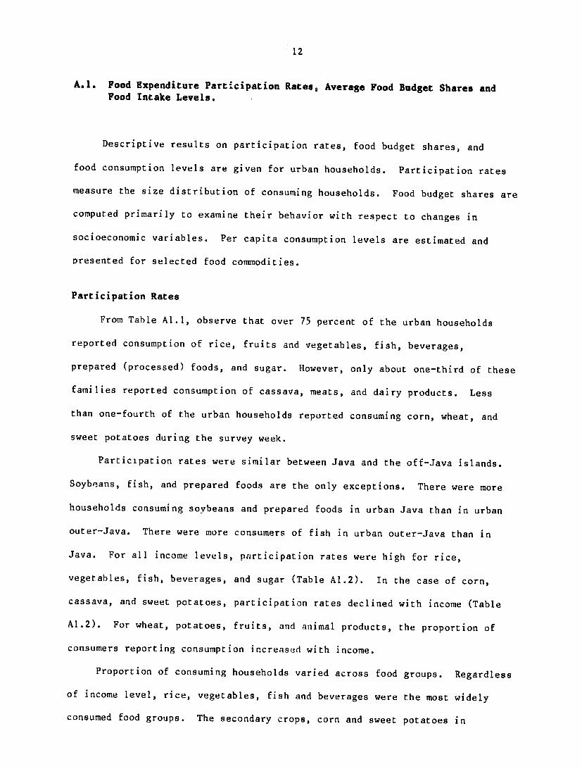
A.I. Food Expenditure Participation Rates, Average Food Budget Shares and Food Intake Levels.

Descriptive results on participation rates, food budget shares) and

food consumption levels are given for urban households. Participation rates

measure the size distribution of consuming households. Food budget shares are

computed primarily to examine their behavior with respect to changes in

socioeconomic variables. Per capita consumption levels are estimated and

presented for selected food commodities.

Participation Rates

From Table A1.l, observe that over 75 percent of the urban households

reported consumption of rice, fruits and vegetables, fish, beverages,

prepared (processed) foods, and sugar. However, only about one-third of these

families reported consumption of cassava, meats, and dairy products. Less

than one-fourth of the urban households reported consuming corn, wheat, and

sweet potatoes during the survey week.

Participation rates were similar between Java and the off-Java islands.

Soybeans, fish, and prepared foods are the only exceptions. There were more

households consuming soybeans and prepared foods in urban Java than in urban

outer-Java. There were more consumers of fish in urban outer-Java than in

Java. For all income levels, participation rates were high for rice,

vegetables, fish, beverages, and sugar (Table A1.2). In the case of corn,

cassava, and sweet potatoes, participation rates declined with income (Table

A1.2). For wheat, potatoes, fruits, and animal products, the proportion of

consumers reporting conuaumption increased with income.

Proportion of consuming households varied across food groups. Regardless

of income level, rice, vegetables, fish and beverages were the most widely

consumed food groups. The secondary crops, corn and sweet potatoes in

13

particilar, were the least widely consumed. In fact, the share of

participating households for these crops declined as income level increased.

Bridget Shares

(a) Regional Variations

The average per person expenditure for food in Indonesia was

Rp 1,735 (US $2.78) per week (Table A1.3). Food accounted for 64 percent

of the average weekly expenditure. Of the total food budget, 27 percent

was allocated to rice--the main staple crop (Table A1.4). Other

significant average budget allocations were for fruits and vegetables

(13.3 percent), animal products (12.4 percent), fish (10.8 percent), and

prepared foods (9.2 percent). The secondary food crops (corn, wheat,

cassava, sweet potatoes, and potatoes) accounted for 2.1 percent of the

food budget.

The average person in Java had a food cost of Rp 1,590 (US $2.54)

per week on food. This constituted 61 percent of the weekly expenditure

(Table A1.4). Rice accounted for 27 percent of the food budget. The

rice share was followed by animal products (13.7 percent), fruits and

vegetables (12.0 percent), prepared foods (12.7 percent), and fish (6.2

percent).

In the off-Java islands, the average per person weekly allocation

for food was Rp 1,880 (US $3.01), or 66 percent of the average weekly

expenditure. Rice, as in Java, accounted for 27 percent of the food

budget. Fruits and vegetables, animal products, and fish had shares of

13.3, 12.4, and 10.8 percent, respectively.

Comparing expenditure shares for Java and the outer-Java islands,

it is evident that in the two regions food consumption accounted for

14

approximately two-thirds of all weekly household expenditure, with rice

the dominant food crop and the secondary food crops have minor shares in

the food budgets. There are, however, two notable exceptions. The

budget share for fish was higher in off-Java, and the share allotted to

beans, soybeans in particular, was higher in Java.

Variations in budget shares are more noticeable across the

provinces (Table A1.5). Although rice was the main staple in all the

provinces, the budget share for rice varied from 21 percent in Jakarta to

31 percent in Bali. The budget shares of corn and cassava increase from

West to East Java. Outside Java, the shares for corn and cassava were

higher in Sulawesi and the other provinces (Nusa Tenggara, Maluku, and

Irian Jaya). For fish, the budget share varied from 1.71 percent in

Yogyakarta to 16.7 percent in Sulawesi and 17.3 percent in Kalimantan.

(b) Variation by Income class

The share of food in the total budget ranged from 74 percent in

the lowest income group to 54 percent in the highest income group

(Table A1.6). Because most of the foods consumed were necessities, their

budget shares declined with income. The share of rice, for example,

declined from 41 percent to 16 percent from the lowest to the highest

income groups. On the other hand, the shares of fruits and animal

products increased with income.

Within the staple foods, rice remained the main staple at all income

levels. Because the other staple foods (corn, cassava, and sweet

potatoes) declined in importance as income increases, rice stood out as

the staple main food in the upper income groups. That is, as income

level rose, the average diet included more rice.

15

The decline in the budget shares of the staple foods was

accompanied by an increase in shares for fruits and animal products.

The budget shares of fruits and animal products were 2.9 and 4.7 percent,

respectively, in the lowest income group. These shares increased to 6.7

and 19.3 percent, respectively, in the highest income group.

The income induced food allocations exhibited similar patterns

across regions. The budget share of rice declines while the shares of

fruits and animal products increased with income. The secondary staple

foods, except potatoes, had relatively lower shares in the upper income

groups.

Levels of Food Consumption

The levels of food consumption, shown in Tables A1.7 and Al.8, are

computed on a per capita basis. No adjustments have been made for age or

sex variations of household members. The results therefore, are conditional

on the assumption that age and sex composition make little difference in

average food consumption for the population groups.

The average diet per person per week contained 2.97 kgs of cereals (of

which 2.2 kgs are rice) and 1.0 kg of root and tuber crops (Table A1.7). In

addition, it included 0.38 kgs of beans, 1.23 kgs of fruits and vegetables,

0.34 kgs of fish, 0.13 kgs of meat, and 0.14 kgs of dairy products.

Consumption levels did not vary much across regions (Table AI.7). The only

noticeable variations were in the consumption of fish and soybeans. The

consumption of fish varied from 0.17 kgs in Java to 0.47 kgs in off-Java. For

soybeans, the variation was from 0.42 kgs in Java to 0.25 kgs off-Java.

The levels of consumption, however, did vary across income groups (Table

A1.8). Average consumption of rice, fruits and vegetables, fish, and animal

16

products increased with household income. The income related consumption

patterns for corn and cassava consumption, however, were inconclusive. The

consumption levels dropped in the middle income groups and rose in the top

income group. There are two possible explanations for this phenomenon.

First, the data may not show shift in the quality characteristics of these

foods. Second, the results may reflect the flaws associated with the

ninadjustment of the data for age and sex differences.

Notwithstanding the potential limitations of the reported consumption

data, three distinct results can be established: (1) average consumption was

higher among households in off-Java than in Java; (2) the levels of

consumption of most food groups increased with income; and (3) there was a

sh-ft from starchy foods to animal products with increasing income.

A.2. Predicted Budget Shares, Income and Household Size Elasticities

Results based on a multinomial linear logit model are presented for urban

households. Regional and income effects on food preferences, budget shares,

income and household size elasticities, and scale economies are isolated and

evaluated.

Food Preferences

The structural parameter estimates for twelve commodity groups are

resented in table (A2.2). These estimates measure the effects of

socioeconomic variables; namely income, family size and location of residence

.th on expenditure share of i commodity group relative to budget share of

Rice--the reference base commodity group.

The income coefficients measure the relative share responses due to

change in the level of income. The coefficients are all positive and

statistically significant which suggest that increase in income induces urban

17

households to shift from rice to other commodiLy groups. Such behavior is

evident in their ranking of the food groups.

In order to rank the food groups, let @ denote that one food group is

preferred to another and @ denote indifference betweer two food groups.

Holding the influence of the other socioeconomic variables, the income effects

imply that households order their food bundles as follows:

(13) FG6 @ FG4 ( FG9 ® FG7 ® FG11 (D FG3 ( FG5 @ FG2 ® FGl

This ordering implies that as total food expenditure rises, households

allocate their total budget across food groups according the ranks shown in

equation (13). That is, households allocate relatively more to animal

products (FG6), fruits (FG4), prepared foods (FG9), and fish (FG7), and less

to the staple crops (FG2 and FGl).

The coefficients associated with household size are all negative which

suggest a decline in budget share of commodity group i relative to rice. The

reverse of the pattern for income effects is observed when the food groups are

ordered in accordance with the induced effects of household size (equation

14). As household size increases, the preference ordering is such that higher

proportions of the total budgets are allocated to food crops, and less to

animal products, fruits and fish; i.e.

(14) FGl ( FG11 5 FG5 (®) FG3 ® FG2 () FG9 () FG7 0 FG4 (D FG6

Household size thus induces urban households to shift away from food groups

that are most preferred on the basis of income effect.

Predicted Budget Shares

Budget shares were predicted for all 13 commodity groups, 12 food groups

and one nonfood group (Table A2.3). Nonfood group accounts for one-third of

18

the total weekly expenditure. Within the food groups, rice accounts for 17

percent of the total weekly budget with fruits and vegetables having a joint

share of 9 percent, and fish and animal products acrounting for 14 percent.

Among the rest of the food groups, beverages and prepared food groups account

for 5.1 and 5.0 percent, respectively. In terms of food budgets, the

predicted shares of rice, fruits and vegetables, and fish and animal products

are 26.6, 14.1 and 21.9 percent, respectively.

The regional (Java vs. outer-Java) variations of these predicted budget

shares are limited (Table A2.3). The only noticeable variations are in the

budget shares of fish which account for 3.7 percent in Java, and 8.7 percent

in outer-Java.

The comparison of the budget shares between low and high income groups

shows patterns of expenditure allocation corresponding to income. The budget

shares of most food groups are higher for low income households than high

income households. Exceptions are animal products, prepared foods, fruits and

fish which are higher among high income households. As income rises, the

households move from a concentration on cereal and starchy staple foods to

animal products, fruits and processed foods. Such reallocation is accompanied

by a declining share of food in the total budget.

Expenditure Elasticities

The expenditure elasticities corresponding with Table A2.3 are presented

in Table A2.4. These elasticities represent a quantitative expression of the

preference ordering implied in equation (12). The elasticities for animal

products, and fruits all exceed unity and are thus "luxuries." The demand for

fish and prepared foods is invariant with income. The elasticities of the

other food groups are positive and less than unity, and hence constitute

19

"necessities." Rice, the referenLe food group, has the lowest expenditure

elasticity among all the food groups.

If wa hold income and household size variables at the means and allow

regional variable to vary, the elasticities suggest little variation in budget

allocation practices hprween Java and outer-Java. Households, regardless of

their location of reniaence, show similar food ranking patterns. The levels

of response vary, however, between the regions. Expenditure elasticities are

larger among households in urban outer Java.

Food ranking patterns are also invariant across income groups. Both the

low and high income prefer more consumption of animal products, fruits, fish

and prepared foods, and less of the staple food groups as income rises.

Expenciture elasticities are, however, larger among the low income groups.

These households are strongly sensitive to expenditure on animal products,

fruits, fish and prepared foods which all have elasticities greater than

unity. Only animal products constitute a luxury food group among the high

income households.

Household Size Elasticities

The elasticities in Table A2.5 show that household size has negative

effects on demand for luxury food groups, i.e., animal products, fruits, fish

and prepared foods. The demand for the other food groups is positive with a

change in household size. Conversely, the change in household size induces

urban households to substitute the consumption of the basic food groups for

the luxury food groups.

The response patterns are in general similar across regions and income

groups. Food preferences rankings are invariant to these variables. The

levels of the elasticities vary, however, across these groups. The size

elasticities are larger among households in Java, and among the high income

20

households. Region and income variables hence influence the responses in

budget shares due to a change in household size.

Economies of Scale

The sum of expenditure and household size elasticities can be interpreted

as indicating economies of scale in consumption (Tyrell and Mount 1982). When

the sum is one, it indicates constant returns to scale. When the sum is

greater than one, it indicates diseconomies of scale. If less than one, it

indicates economies of scale. For all the food groups, except animal

products, the elasticities are less than unity. This suggests that the urban

households enjoy economies of scale in food consumption.

Households in both Java and outer-Java enjoy economies of scale in all

food groups except animal products. The scale elasticities are lower in

general in urban Java than outer Java. Similarly, both the low and high

income groups enjoy economies of scale, with higher income households getting

the most.

21

Table A1.1. Food Expenditure Participation by Region--All Urban Households M%)

Food Groups Java off-Java Indonesia

Cereals 97.4 99.0 98.2 Rice 97.3 99.0 98.1 Corn 9.4 6.9 3.1 Wheat 14.3 16.0 15.2

Root and Tubers 56.5 55.4 55.9 Cassava 31.4 27.3 29.2 Sweet potatoes 21.1 11.7 16.1 Potatoes 25.3 30.8 28.2

Beans 92.5 72.9 82.2 Soybeans 90.0 61.6 75.1

Fruits 73.7 76.7 75.3

Vegetables 95.8 98.4 97.1

Fish 83.2 96.5 90.2

Meat and Poultry 41.2 36.2 38.5

Eggs 62.8 60.9 61.8

Dairy products 34.5 45.0 40.0

Fats and Oils 94.3 96.4 95.4

Beverages and tobacco 96.8 96.2 96.5

Prepared foods 84.4 71.3 77.5

Sugar 94.8 96.1 95.5

Other foods 96.5 98.6 97.6

22

Table A1.2. Food Expenditure Participation by Income Group--Urban Households

Food Groups under 7,200 7,200-11,400 11,401-19,000 above 19,000

(Rp/person/month)

Cereals 98.9 99.6 98.9 93.6 Rice 98.6 99.6 98.9 93.6 Corn 10.9 7.2 6.3 8.2 Wheat 5.1 14.0 20.7 24.1

Root and Tubers 54.7 54.7 55.6 60.4 Cassava 36.5 31.5 25.7 19.5 Sweet potatoes 19.2 17.4 13.0 14.1 Potatoes 11.0 26.4 34.5 47.3

Beans 78.1 84.9 83.6 80.6 Soybeans 72.5 77.9 76.1 71.8

Fruits 58.8 74.0 83.4 89.9

Vegetables 98.1 98.6 97.6 92.3

Fish 84.0 92.8 93.5 89.4

Meat and Poultry 15.7 31.6 50.2 67.4

Eggs 38.5 62.1 73.1 78.6

Dairy products 14.6 35.5 53.0 66.3

Fats and oils 95.7 96.4 96.3 91.5

Beverages and tobacco 96.4 96.6 97.0 95.7

Prepared foods 66.4 75.0 83.1 58.3

Sugar 94.5 96.2 97.1 93.1

Other foods 98.5 98.5 98.4 93.3

23

Table A1.3. Family Size, Weekly Food Expenditure and Food Budget Shares

Food Food Sample Family Vxpenditure Share

Households Size (Rp/week) (%)

Indonesia--Urban 3,608 5.4 9,366 63.7

Java 1,711 5.2 8,276 60.5

off-Java 1,897 5.5 10,348 66.1

Expenditure Group: (Rp/month/person)

under 7,200 908 6.0 5,558 74.0

7,200-11,400 1,145 5.6 8,453 70.2

11,401-19,000 944 5.1 11,005 63.8

above 19,000 611 4.3 14,196 53.6

4/

24

Table A1.4. Average Food Budget Shares by Region--All Urban Households

Food Groups Java off-Java Indonesia

Share (%) Share (%) Share (%)



Beans 6.2 3.2 4.5 Soybeans 4.8 1.8 3.1

Fruits 5.1 4.5 4.7


Fish 6.2 14.0 10.8

Meat and Poultry 7.1 5.9 6.4

Eggs 3.5 2.8 3.1


Fats and Oils 4.1 4.3 4.2



Sugar 3.1 3.6 3.4

Other foods 2.8 2.7 2.7

Food Expenditure 60.5 66.1 63.7

Table Al.5. Food Expenditure Shares by Province--Urban Indonesia

Food Group Jakarta West Java

Central Java DI

Yogyakarta East Java Bali Sumatera Kalimantan Sulawesi Others

CerealsRice Corn Wheat

20.74 0.08 0.21

30.23 0.13 0.34

30.0 0.24 0.20

20.28 0.22 0.17

25.01 1.04 0.29

30.93 0.25 0.17

26.71 0.12 0.33

21.40 0.13 0.51

28.40 0.45 0.68

26.91 1.45 0.72

Root and TubersCassava Sweet potatoes Potatoes

Beans

0.19 0.16 0.54

0.44 0.27 0.84

0.76 0.37 0.43

0.45 0.22 0.42

0.60 0.39 0.53

0.11 0.59 0.61

10.39 0.22 0.83

0.39 0.14 0.62

0.55 0.12 0.30

1.06 0.13 0.29

Soybeans

Fruits

Vegetables

Fish

Meat and poultry

Eggs

Dairy products

Fats and oils

4.20

5.25

6.98

6.14

7.48

3.92

3.76

4.19

4.08

5.01

6.17

8.80

6.75

3.18

2.06

3.55

6.00

6.44

7.84

3.06

6.45

3.35

2.50

4.15

5.37

5.52

6.41

1.71

5.52

3.83

2.66

4.70

5.60

5.16

7.31

5.48

9.08

3.42

3.30

4.40

2.99

4.90

6.53

5.47

11.33

3.56

2.23

4.15

1.97

3.96

10.61

12,77

5.99

2.82

2.72

4.54

1.73

7.11

8.10

17.25

6.20

3.55

2.83

3.46

0.87

5.27

7.09

16.66

4.61

2.30

3.41

3.61

1.85

4.05

8.43

9.93

8.50

2.05

3.26

4.70

t-n

Beverages andtobacco

Prepared foods

Sugar

Other foods

11.37

18.37

2.64

2.45

10.39

10.82

2.15

2.76

9.38

9.99

4.57

2.94

8.59

24.85

5.03

2.77

10.67

8.29

4.11

3.40

8.18

11.35

2.27

2.10

10.84

8.05

3.35

2.30

11.31

6.34

4.05

3.04

10.69

6.00

4.32

2.28

10.35

7.04

3.49

3.28

Food Expenditures 54.31 62.99 63.46 52.79 60.82 51.07 64.73 62.81 65.32 63.70

Others: Nusa Tenggara, Maluku, and Irian Jaya

26

Table A1.6. Food Expenditure Shares by Income Group--Urban Indonesia (Rp/person/month)


Share (%) Share (%) Share (%) Share (%)


Root and Tubers 1.8 1.31.4 1.3 Cassava 1.1 0.5 0.3 0.2 Sweet potatoes 0.4 0.3 0.2 0.1 Potatoes 0.3 0.6 0.7 0.9

Beans 4.9 4.4 4.4 4.3 Soybeans 3.9 3.2 2.9 2.5

Fruits 2.9 3.8 4.8 6.7

Vegetables 8.8 9.2 8.9 7.5

Fish 7.8 11.3 11.6 10.8

Meat and Poultry 1.8 7.23.8 11.0

Eggs 1.7 2.6 3.5 3.9

Dairy products 1.2 2.1 3.3 4.4

Fats and oils 4.7 4.5 4.2 3.8

Beverages and tobacco 9.5 11.1 11.4 10.3

Prepared and partically prepared foods 6.1 8.97.2 13.4

Sugar 4.0 3.7 3.3 2.0

Other foods 2.6 2.6 2.6 2.6

Food Expenditure 74.0 63.870.2 53.6

27

Table A1.7. Weekly per Capita Food Consumption by Region--Urban Households (Kilograms/person/week except for eggs which are numbers)

Food Groups Java outer-Java Indonesia

Cereals Rice 2.08 2.29 2.18 Corn 0.52 0.69 0.59 Wheat 0.14 0.24 0.20

Root and Tubers Cassava 0.43 0.55 0.48 Sweet potatoes 0.36 D.37 0.36 Potatoes 0.17 0.16 0.16

Beans 0.47 0.29 0.38

Soybeans 0.42 0.25 0.34

Fruit:j 0.57 0.59 0.58


Fish 0.17 0.47 0.34

Meat 0.10 0.15 0.13

Eggs 1.52 1.32 1.40


Sugar 0.19 0.23 0.21

2g

Table A1.8. Weekly per Capita Food Consumption by Income Group--Urban Households (Kilograms/person/week except for eggs which are numbers)


Cereals Rice 1.90 2.23 2.34 2.47 Corn 0.73 0.43 0.44 0.73 Wheat 0.19 0.18 0.22 0.24

Root and Tubers Cassava 0.50 0.45 0.45 0.60 Sweet potatoes 0.33 0.34 0.39 0.42 Potatoes 0.11 0.15 0.18 0.24

Beans 0.27 0.34 0.44 0.63 Soybeans 0.26 0.31 0.38 0.55

Fruits 0.33 0.48 0.65 1.06

Vegetables 0.47 0.60 0.76 1.00

Fish 0.18 0.34 0.43 0.55

Meat 0.07 0.10 0.14 0.20

Eggs 0.70 1.03 1.68 2.62

Dairy products 0.10 0.11 0.15 0.24

Sugar 0.13 0.20 0.24 0.33

29

Table A2.1. Variables, Mean Budget Shares and Definitions

Group Mean Variables Code Definition Budget Share

wI FGI Budget share of rice 0.17

w2 FG2 Budget share of non-rice 0.02 cereals, roots and tubers

w3 FG3 Budget share of beans 0.04

w4 FG4 Budget share of fruits 0.04

w5 FG5 Budget share of vegetables 0.06

w6 FG6 Budget share of meat and 0.09 poultry and dairy products

w7 FG7 Budget share of fish 0.06

w8 FG8 Budget share of fa: s and oils 0.03

wq FG9 Budget share of prepared 0.06 foods

w10 FGIO Budget share of sugar 0.02

wll FG11 Budget share of beverages and 0.07 stimulants

w12 FG12 Budget share of other foods 0.02

w13 FGI3 Budget share of non-food 0.33

Y Weekly total family expenditure 19,432

HHS Household size 5.82

DRG Dummy variable for region; 0.52 1 for Java, 0 otherwise

30

Table A2.2. Parameter Estimates for 13 Commodity Groups Based on Multinomial Logit Model by Region

N Intercept in INC in HHS in DRE

In(k.2 /wI) 1181 -5.172 .409 -.632 -.181 (-12.220) (8.463) (-9.947) (-3.755)

ln(w 3/wd) 1181 -6.046 .525 -.592 .505 (-15.478) (11.779) (-10.240) (11.378)

ln(w 4 /wI) 1181 -8.493 0.881 -1.034 .156 (-21.148) (19.223) (-17.401) (3.42)

ln(w 5 /wl) 1181 -4.641 0.481 -.590 -.297 (16.346) (14.848) (-14.058) (-9.203)

ln(w 6 /wl) 1181 -12.412 1.39 -1.173 0.135 (-27.445) (27.014) (-17.545) (2.618)

ln(w 7/w1 ) 1181 -7.539 0.846 -.839 -.793 (-18.125) (17.826) (-13.629) (-16.764)

ln(w 8 /w1 ) 1181 -5.159 0.454 -.595 -.055 (-17.501) (13.480) (-13.632) (-1.643)

ln(w 9 /w1 ) 1181 -8.394 0.851 -.806 .396 (-17.878) (15.874) (-11.608) (7.409)

In(wlO/w I) 1181 -4.682 .361 -.460 -.186 (-13.145) (8.867) (-8.734) (-4.592)

In(wl1 /wI) 1181 -5.386 .532 -.574 -.067 (-9.401) (8.128) (-6.771) (-1.034)

In(wl2/wl) 1181 -6.332 .509 -.629 .224 (-15.535) (10.937) (-10.440) (4.839)

in(wl3/wI) 1181 -10.002 1.268 -1.013 .254 (-36.639) (40.694) (-25.080) (8.183)

Table A2.3. Predicted Budget Shares by Region and Income Group--Urban Households

Region/

ExpenditureGroup

Urban

--------------------------------------------

FGl FG2 FG3 FG4 FG5 FG6

.1659 .0070 .0321 .0358 .0560 .0839

Commodity

FG7 FG8

.0566 .0287

Group

FG9

.0497

FGIO

.0219

FG1l

.0510

FG12

.0167

FG13

.3947

INC

19,432

HHS

5.82

Region

Java

Outer-Java

.1567

.1696

.0140

.0182

.0386

.0252

.0364

.0337

.0459

.0669

.0845

.0799

.0365

.0874

.0264

.0302

.0568

.0414

.0189

.0247

.0467

.0540

.0175

.0152

.4211

.3536

18,896

20,283

5.80

6.0

Exenditure Group Low .2368 .0082 .0361 .0343 .0643 .0637 .0551 .0334 .0483 .0265 .0573 .0189 .3170 12,344 6.29 W

High .1332 .0062 .0293 .0355 .0505 .0941 .0557 .0258 .0593 .0192 .0466 .0151 .4296 24,727 5.47

I

Table A2.4.

Region/

Expenditure roup

Urban

Prodicted Expenditure Elasticities by Region and Income Group--Urban Households

--------------------------------------------------- Commodity Group

FG1 FG2 FG3 FG4 FG5 FG6 FG7 FG8 FG9 FGIO

.1580 .5670 .6830 1.0390 .6390 1.5480 1.0040 .6120 1.0090 .5190

FG1I

.6900

FG12

.6670

FG13

1.4260

INC

i4,W 2-

HHS

Req ion

Java

Outer-Java

.1053

.1898

.5143

.5988

.6303

.7148

.9863

1.0708

.5863

.6708

1.4953

1.5798

.9513

1.0358

.5593

.6438

.9563

1.0408

.4663

.5508

.6373

.7218

.6143

.6988

1.3733

1.4578

.4-. 1

2z-I 3

Exenditure Group

Low .2735 .6825 .7985 1.1545 .7545 1.6635 1.1195 .7275 1.1245 .6345 .8055 .7625 1.5415 /27Y 6-Z7

High .1023 .5113 .6273 .9833 .5833 1.4923 .9483 .5563 .9533 .4633 .6343 .6113 1.3703 ;''?Z 7

Table A2.5. Predicted Household Size Elasticities by Region and Income Group--Urban Households

Region/

Expenditure Group

---------------------------------------------------Commodity Group

FG1 FG2 FG3 FG4 FG5 FG6 FG7 FG8 FG9 FGIO FG11 FG12 FG13 INC HHS

Urban .7461 .1231 .1541 -.2879 .1561 -.4269 -.0929 .1511 -.0599 .2861 .1721 .1171 -.2669 19,432 5.82

Region

Java

Outer-Java

.7606

.7291

.1376

.1061

.1686

.1371

-. 2734

-.3049

.1706

.1391

-.4124

-.4439

-.0784

-.1099

.1656

.1341

-. 0454

-.0769

.3006

.2691

.1866

.1551

.1316

.1001

-.2524

-.2839

18,896

20,283

5.80

6.00

Exenditure Group

LoW

High

.6577

97882

.0347

.1652

.0657

.1962

-.3763

-.2458

.0677

.1982

-.5153

-.3848

-.1813

-.0508

.0627

.1932

-. 1483

-.0177

.1977

.3282

.0837

.2142

.0287

.1592

-.3553

-.2248

12,344

24,727

6.29

5.47 Lo

Table A2.6. Estimates of Economies of Scale by Region and Income Group--Urlban Households

Region/ Coo---------------------------------------------------Codity Group

ExpenditureGroup FG1 FG2 FG3 FG4 FG5 FG6 FG7 FG8 FG9 FGIO FG11 FG12 FG13 INC HHS

Urban .9041 .6901 .8371 .7511 .7951 1.1211 .9110 .7631 .9491 .8051 .8621 .7841 1.1591 19,432 5.82

Region

Java .8659 .6519 .7989 .7129 .7569 1.0829 .8729 .7249 .9109 .7669 .8239 .7459 1.1209 18,896 5.80

Outer-Java .9189 .7049 .8519 .7659 .8099 1.1359 .9259 .7779 .9639 .8199 .8769 .7989 1.1739 20,283 6.00

Exenditure Group

Low .9312 .7172 .8635 .7782 .8222 1.1482 .9382 .7902 .9762 .8322 .8892 .8112 1.1862 12,344 6.29

Hiqh .8905 .6765 .8235 .7375 .7815 1.1075 .8975 .7495 .9356 .7915 .8485 .7705 1.1455 24,727 5.47 LO 4

35

APPENDIX B

Food Consumption and Expenditure Patterns in Rural Indonesia

36

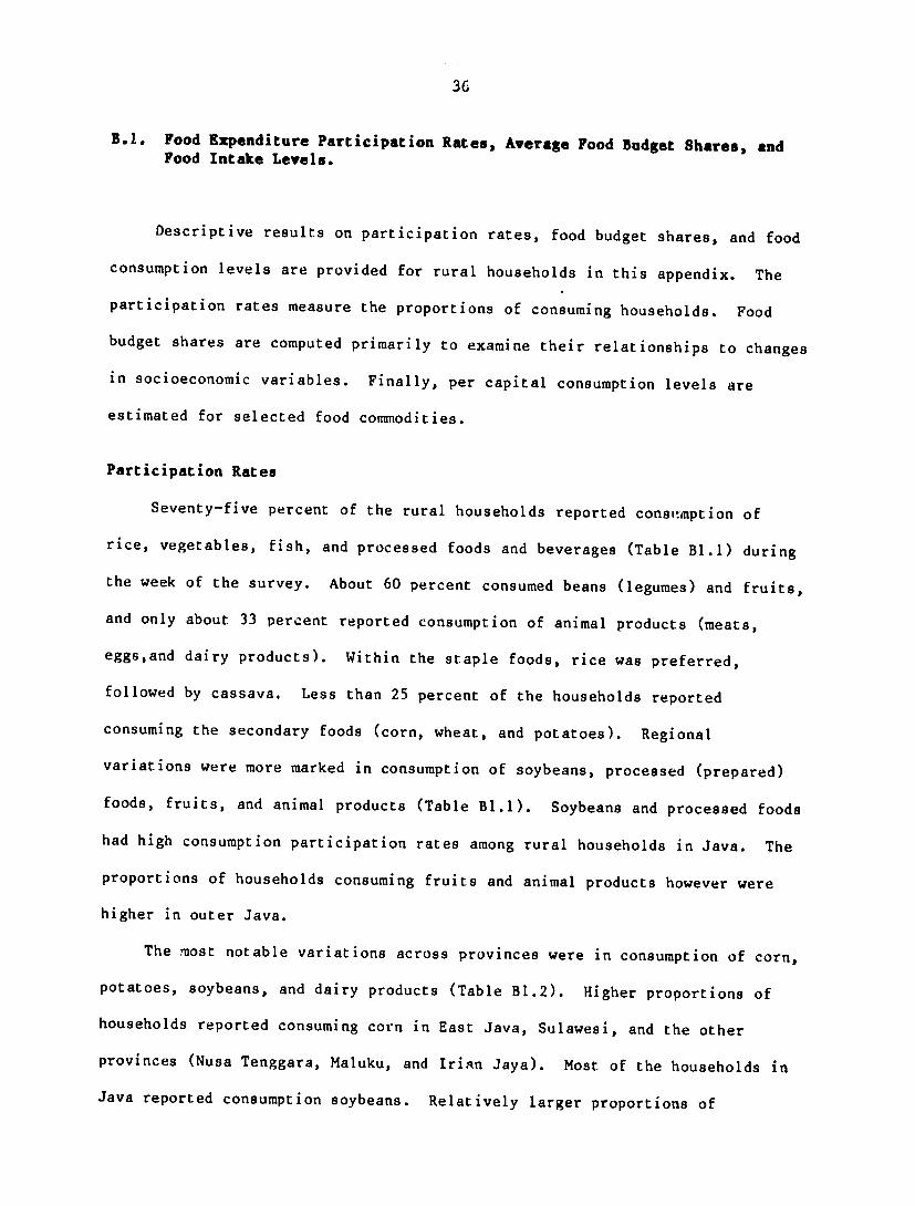
B.I. Food Expenditure Participation Rates, Average Food Budget Shares, and Food Intake Levels.

Descriptive results on participation rates, food budget shares, and food

consumption levels are provided for rural households in this appendix. The

participation rates measure the proportions of consuming households. Food

budget shares are computed primarily to examine their relationships to changes

in socioeconomic variables. Finally, per capital consumption levels are

estimated for selected food commodities.

Participation Rates

Seventy-five percent of the rural households reported consitimption of

rice, vegetables, fish, and processed foods and beverages (Table Bl.1) during

the week of the survey. About 60 percent consumed beans (legumes) and fruits,

and only about 33 percent reported consumption of animal products (meats,

eggs,and dairy products). Within the staple foods, rice was preferred,

followed by cassava. Less than 25 percent of the households reported

consuming the secondary foods (corn, wheat, and potatoes). Regional

variations were more marked in consumption of soybeans, processed (prepared)

foods, fruits, and animal products (Table BI.1). Soybeans and processed foods

had high consumption participation rates among rural households in Java. The

proportions of households consuming fruits and animal products however were

higher in outer Java.

The most notable variations across provinces were in consumption of corn,

potatoes, soybeans, and dairy products (Table B1.2). Higher proportions of

households reported consuming corn in East Java, Sulawesi, and the other

provinces (Nusa Tenggara, Maluku, and Irian Jaya). Most of the households in

Java reported consumption soybeans. Relatively larger proportions of

37

households in Suniatera reported consumption of potatoes. The proportions of

dairy products consumed were higher in Sumatera and Kalimantan than in other

provinces.

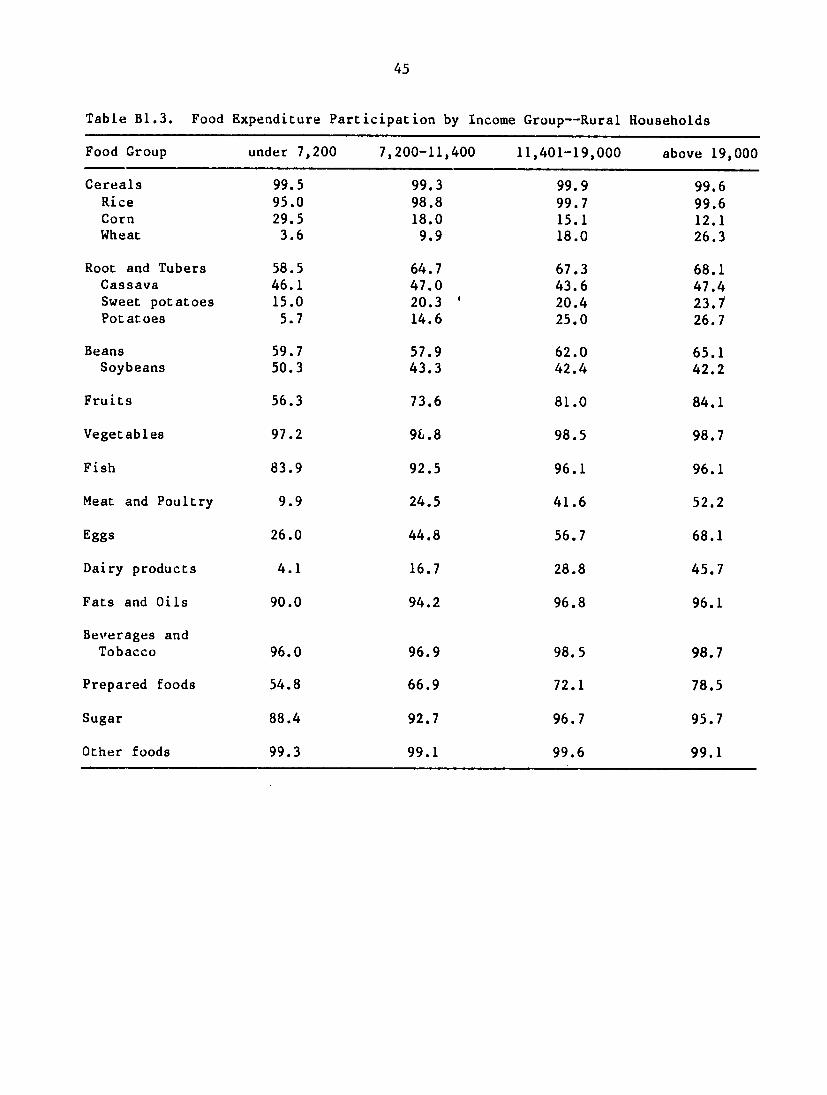
The participation rates for rice, vegetables, fish, and beverages vary

little by income level (Table B1.3). In the case of wheat, potatoes, fruits,

animal products, and processed foods, however, the participation rates

increased with income. This pattern was consistently reversed for corn.

Food Budget Shares

Regional effects

The rural Indonesian households spent an average of Rp 1,375 (U.S.

$2.20) per week for fcod (Table B1.4). This constituted 75 percent of average

total weekly expenditure. Within the total food budget, 35 percent was

allocated to rice--the main cereal food. The secondary foods (corn, wheat,

cassava, and potatoes) jointly accounted for 5.3 percent of the food budget

(Table B1.5). Fruits and vegetables, fish, and animal products accounted for

12.3, 10.6, and 7.3 percent, respectively.

In Java, the mean per capita food expenditure (Rp 1,047) and the budget

share allotted to food (72.0 percent) were lower than the national averages.

Food allocation patterns were, by and large, similar between Java and the

outer Java islands, although food expenditures and budget shares for food are

higher in outer Java. The most notable variations were in the budget shares

for fish and beans. Fish had a higher share of the budget in outer Java

(Table B1.5), while the reverse was observed for beans and soybeans.

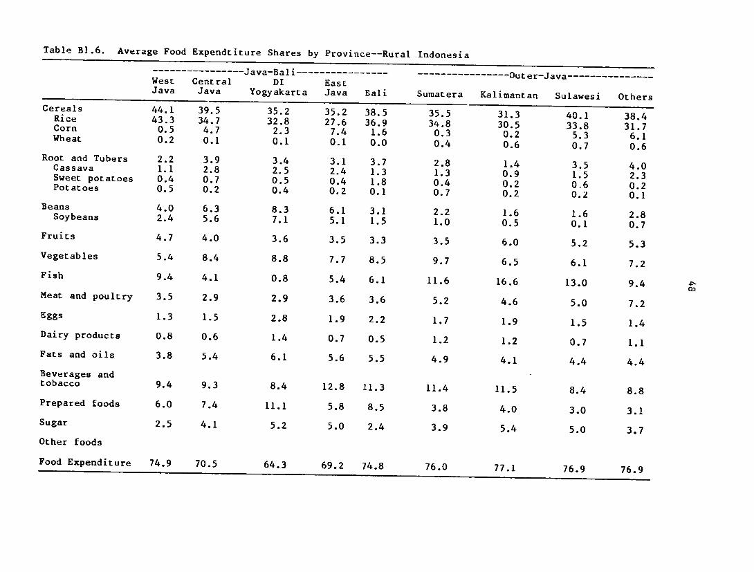
Table B1.6 gives a more detailed view of food budget allocations

by province, and some regional patterns are evident. Rice was more prominent

in West Java, while the mean budget share of corn was greater in East Java,

Sulawesi, and the "other" provinces. The cassava share was highest in Central

38

and East Java and fish was more dominant in the food budget in Kalimantan,

Sulawesi, and Sumatera.

Income effects

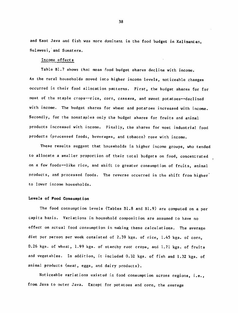
Table B1.7 shows that mean food budget shares decline with income.

As the rural households moved into higher income levels, noticeable changes

occurred in their food allocation patterns. First, the budget shares for for

most of the staple crops--rice, corn, cassava, and sweet potatoes--declined

with income. The budget shares for wheat and potatoes increased with income.

Secondly, for the nonstaples only the budget shares for fruits and animal

products increased with income. Finally, the shares for most industrial food

products (processed foods, beverages, and tobacco) rose with income.

These results suggest that households in higher income groups, who tended

to allocate a smaller proportion of their total budgets on food, concentrated

on a few foods--like rice, and shift to greater consumption of fruits, animal

products, and processed foods. The reverse occurred in the shift from higher'

to lower income households.

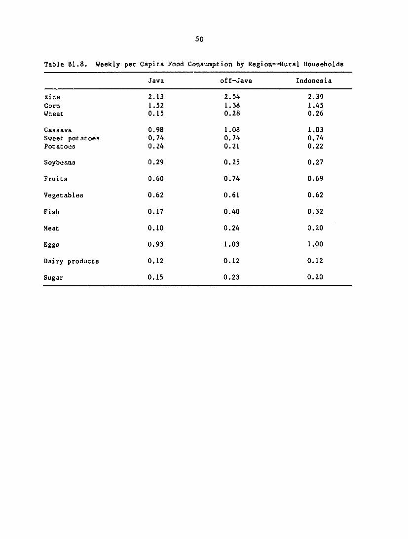
Levels of Food Consumption

The food consumption levels (Tables B1.8 and B1.9) are computed on a per

capita basis. Variations in household composition are assumed to have no

effect on actual food consumption in making these calculations. The average

diet per person per week consisted of 2.39 kgs. of rice, 1.45 kgs. of corn,

0.26 kgs. of wheat, 1.99 kgs. of starchy root crops, and 1.21 kgs. of fruits

and vegetables. In addition, it included 0.32 kgs. of fish and 1.32 kgs. of

animal products (meat, eggs, and dairy products).

Noticeable variations existed in food consumption across regions, i.e.,

from Java to outer Java. Except for potatoes and corn, the average

39

consumption of the staple foods (cereal and starchy crops) was higher in outer

Java. In addition, consumption of fish, meat, and dairy products was also

higher among the rural households in outer Java. Overall, average food

consumption was lower in Java than in the outer Java islands. Generally, food

consumption rose with income. The only exception was corn, for which the

pattern was inconclusive.

B.2. Predicted Budget Shares, Expenditure and Household Size Elasticities

Food Preferences

The parameter estimates for income in Table B2.2 are positive and

statistically significant as indicated by their t-values. The households

respond to change in income by reallocating their food budget away from the

base group (rice) to the other food groups. The proportions of the budget

allocation follows a preference ranking procedure as described in equation

(15).

(15) FG6 ( FG7 FG9 & FG4 (D FGIl C® FG3 OP FG5 OP FG2 (D FGI

where relatively higher proportions are allocated to animal products (FG6),

fish (FG7), prepared foods (FG9) and fruits (FG4). Lower in the preference

rankings were the staple foods (FGl and FG2) and vegetables (FG5).

The parameter estimates for household size, on the contrary, are negative

which imply a reallo cation of food budgets towords the staple crops. As it is

shown in equation (16)Y the rural households give staple crops the highest

priorities. The lowest priorities are for animal products (FG6), firh (FG7),

prepared foods (FG9), and fruits (FG4),

(16) FGI (D FG2 (D FG5 &®FG3 FG11 (® FG4 3 FG9 () FG7 (® FG6.

40

Predicted Budget Shares

The predictions of the multinomial logit model of the mean budget shares

of thirteen commodity groups are given in Table B2.3. Of total weekly

expenditure, an average rural family allocates 72 percent to food and the rest

to nonfood items. Within the staple foods, 23 percent of the total budget

spent on rice and 3 percent on secondary food staples. Fruits and vegetables

(FG4 and FG5), animal products (FG6), and fish (FG7) accounted for 10.1, 6.7,

and 6.2 percent of the total budget, respectively.

Within food budget, the shares of rice and the secondary staple food are

32.0 and 4.0 percent, respectively. Fruits and vegetables take 14 percent of

the food budget. Animal products and fish account for 9.3 and 8.6 percent of

the food budget, respectively. Note that these predictions are close to the

sample mean budget shares in Table B2.1.

Variations in budget shares due to regional effects are limited. A

notable exception is the budget share of fish which is higher in outer-Java

than Java.

The low income households have higher budget shares in most of the food

groups. The exceptions are fruits, animal products, fish, and processed foods

which are higher among the high income households. Consistent with Engel law

of demand for food, the budget shares of the staple foods decline with income.

Expenditure Elasticities

The predicted expenaiture elasticities for the food groups (Table B2.4)

show that the top four commodity groups in equation (14) have elasticities more

than unity. These represent commodities which are luxuries in the rural

households food consumption basket. Preferences for beverages are invariant to

income changes. The remaining food groups, most of which are the staple foods,

41

have elasticities less than one. Rice, the basic essential staple food, has

the lowest elasticity (0.47).

The expenditure elasticities are in general higher in outer-Java than in

Java. Animal products, fish, fruits and prepared foods have elasticities that

exceed unity in both regions. The rest of the food groups are in the

categories of necessities in all the regions.

The expenditure elasticities due to income effect alone show variations

across income groups. The low income households are more responsive to a

change in income level, i.e., the expenditure elasticities of these households

are higher than the high income households. Regardless of income levels,

animal products, fish, and processed foods remain, however, luxury food

gruups.

Household Size Elasticities

The household size elasticities for the food commodity groups (Table B2.5)

are all negative except for rice (FGl), secondary crops (FG2), and vegetables

(FG5). Among the food groups that respond negatively to !iousehold size, the

demand falls rapidly for animal products (FG6) and fish (FG7). An increase in

household size thus induces rural families to more basic foods.

The respono: patterns are unchanged but the levels vary across regions and

income levels. The size elasticities are higher in Java than in outer-Java.

Similarly, the high income households are more responsive to a change in family

size than the low income households.

Economics of Scale

The sum of the expenditure and household size elasticities reported in

table (B2.6) varies between 0.85 and 1.20. Diseconomies of scale are evidenced

42

in the consumption of animal products. Consumption of fruits and secondary

crops is scale ntutral. The rest of the food groups have aggregated

elasticities that are less than unity which indicate the existence of economies

of scale in consumption.

Households in Java enjoy relatively higher economies of scale in most of

the food groups. Similarly, high income households are more efficient in

consumption compared with low income households. Diseconomies of scale in

animal products remain, however, invariant to region and income groups.

43

Table B1.1. Food Expenditure Participation by Region--All Rural Households

Java off-Java Indonesia



Beans 80.6 42.9 59.8 Soybeans 72.7 25.5 46.7

Fruits 61.4 97.9 66.2


Fish 81.9 94.3 88.8

Meat and poultry 16.2 24.7 20.8

Eggs 35.4 40.1 38.0


Fats and oils 91.9 92.8 92.4



Sugar 92.0 90.6 91.2

Other foods 99.2 99.4 99.3

Table B1.2. Food Expenditure Participation by Province--Rural Households

---------------- Java-Bali.................

West Central DI EastJava Java Yogyakarta Java Bali Sumatera Kalimantan Sulawesi Others Cereals 99.7 98.9 98.2 99.5 98.4 99.6Rice 99.7 99.599.7 90.4 99.798.2 91.7 96.8Corn 99.6 99.7 95.3 98.611.0 26.5 25.0 51.3 11.1 7.6 7.1Wheat 50.5 51.77.1 3.9 5.4 3.6 0.0 9.2 16.8 16.7 11.1 Root and Tubers 63.4 68.3 67.9 55.2 66.7 68.4Cassava 51.0 55.2 57.1

54.3 53.2 49.745.3 31.8 44.2Sweet potatoes 19.2 22.7 45.7 36.5 41.317.9 14.1 42.9 19.9 13.1Potatoes 13.7 7.611.0 4.6 8.9 5.9 1.6 24.6 4.6 4.9 2.4 Beans 76.0 87.7 94.6 81.1 61.9 49.3 33.5 32.6Soybeans 59.0 86.9 36.894.6 79.6 38.1 35.2 18.8 3.9 16.3 Fruits 69.5 62.1 51.8 51.1 63.5 67.4 77.6 76.2 67.0 Vegetables 96.2 98.7 98.2 99.2 98.4 99.6 98.3 94.4 94.4 Fish 91.6 76.0 33.9 78.4 90.5 96.0 97.4 98.3 76.7 Meat and poultry 17.7 13.7 16.1 15.0 30.2 23.6 27.8 20.1 32.3 Eggs 31.0 33.9 42.9 40.2 49.2 43.5 43.5 35.3 25.7 Dairy products 9.5 6.4 14.3 5.7 6.4 20.6 22.7 9.8 12.3 Fats and oils 87.9 94.4 98.2 93.8 96.8 96.0 92.6 87.3 85.4

Beverages and tobacco 97.0 97.9 98.2 97.6 90.5 97.4 98.9 91.4 94.8Prepared foods 72.3 78.5 92.9 57.0 71.4 56.9 62.2 48.8 50.7 Sugar 90.9 91.2 98.2 95.4 73.0 92.4 98.9 87.3 76.0 Other foods 99.2 99.0 98.2 99.4 98.4 99.5 99.7 99.0

45

Table B1.3. Food Expenditure Participation by Income Group--Rural Households

Food Group under 7,200 7,200-11,400 11,401-19,000 above 19,000


Root and Tubers 58.5 64.7 67.3 68.1 Cassava 46.1 47.0 43.6 47.4 Sweet potatoes 15.0 20.3 ' 20.4 23.7 Potatoes 5.7 14.6 25.0 26.7

Beans 59.7 57.9 62.0 65.1 Soybeans 50.3 43.3 42.4 42.2

Fruits 56.3 73.6 81.0 84.1

Vegetables 97.2 9&.8 98.5 98.7

Fish 83.9 92.5 96.1 96.1

Meat and Poultry 9.9 24.5 41.6 52.2

Eggs 26.0 44.8 56.7 68.1

Dairy products 4.1 16.7 28.8 45.7

Fats and Oils 90.0 94.2 96.8 96.1

Beverages and Tobacco 96.0 96.9 98.5 98.7

Prepared foods 54.8 66.9 72.1 78.5

Sugar 88.4 92.7 96.7 95.7

Other foods 99.3 99.1 99.6 99.1

46

Table B1.4. Family Size, Weekly Food Expenditure and Food Budget Shares

Food Food Sample Family Expenditure Share

Households Size (Rp/week) (%)

Indonesia--Rural 4,502 4.8 6,602 74.9

Java 2,023 4.5 4,710 72.0

off-Java 2,479 5.1 8,144 76.4

Expenditure Group: (Rp/person/month)

under 7,200 2,338 5.2 4,617 79.0

7,200-11,400 1,267 4.7 7,456 76.8

11,401-19,000 644 4.1 9,718 72.6

above 19,000 232 3.5 13,028 62.8

47

Table B1.5. Average Food Budget Shares by Region--All Rural Families

Java off-Java Indonesia (M) (%) (M)



Beans 5.2 2.0 3.1 Soybeans 4.0 0.8 1.8

Fruits 4.1 4.3 4.3


Fish 6.7 12.5 10.6

Meat and poultry 3.3 5.2 4.6

Eggs 1.6 1.7 1.7


Fats and oils 4.8 4.6 4.7



Sugar 3.6 4.3 4.1

Other foods 3.2 2.5 2.7

Food Expenditure 72.0 76.4 74.9

-----------------

Table BI.6. Average Food Expendtiture Shares by Province--Rural Indonesia

Java-Ba i -------------------------------- Out er-Java---------------West Central DIJava Java Yogyakarta

East Java Bali Sumatera Kalimantan Sulawesi Others

Cereals 44.1 39.5 35.2 35.2 38.5 35.5 31.3 40.1 38.4Rice 43.3 34.7 32.8 27.6 36.9 34.8 30.5 33.8 31.7Corn 0.5 4.7 2.3 7.4 1.6 0.3 0.2 5.3Wheat 0.2 6.10.1 0.1 0.1 0.0 0.4 0.6 0.7 0.6 Root and Tubers 2.2 3.9 3.4 3.1 3.7 2.8 1.4 3.5Cassava 1.1 2.8 4.02.5 2.4 1.3 1.3 0.9 1.5Sweet potatoes 0.4 0.7 0.5 2.30.4 1.8 0.4 0.2 0.6Potatoes 0.20.5 0.2 0.4 0.2 0.1 0.7 0.2 0.2 0.1 Beans 4.0 6.3 8.3 6.1 3.1 2.2 1.6 1.6 2.8

Soybeans 2.4 5.6 7.1 5.1 1.5 1.0 0.5 0.1 0.7 Fruits 4.7 4.0 3.6 3.5 3.3 3.5 6.0 5.2 5.3 Vegetables 5.4 8.4 8.8 7.7 8.5 9.7 6.5 6.1 7.2 Fish 9.4 4.1 0.8 5.4 6.1 11.6 16.6 13.0 9.4 Meat and poultry 3.5 2.9 2.9 3.6 3.6 5.2 4.6 5.0 7.2 Eggs 1.3 1.5 2.8 1.9 2.2 1.7 1.9 1.5 1.4 Dairy products 0.8 0.6 1.4 0.7 0.5 1.2 1.2 0.7 1.1 Fats and oils 3.8 5.4 6.1 5.6 5.5 4.9 4.1 4.4 4.4

Beverages andtobacco 9.4 9.3 8.4 12.8 11.3 11.4 11.5 8.4 8.8 Prepared foods 6.0 7.4 11.1 5.8 8.5 3.8 4.0 3.0 3.1 Sugar 2.5 4.1 5.2 5.0 2.4 3.9 5.4 5.0 3.7

Other foods

Food Expenditure 74.9 70.5 64.3 69.2 74.8 76.0 77.1 76.9 76.9

49

Table B1.7. Average Food Expenditure Shares by Income Group--Rural Indonesia



Root and Tubers 3.3 2.6 2.4 2.5 Cassava 2.2 1.3 1.1 1.0 Sweet potatoes 0.4 0.5 0.4 0.4 Potatoes 0.2 0.4 0.7 0.8

Beans 3.1 2.9 2.8 3.9 Soybeans 2.3 1.6 1.4 1.3

Fruits 3.2 4.3 5.1 6.5

Vegetables 7.8 8.2 7.7 8.0

Fish 8.3 11.4 12.7 12.0

Meat and Poultry 1.7 3.9 7.5 11.2

Eggs 1.0 1.7 2.1 2.7

Dairy products 0.3 1.1 1.5 2.1

Fats and Oils 4.8 4.7 .6 4.1

Beverages and Tobacco 9.2 11.0 12.0 12.2

Prepared foods 3.6 4.6 5.2 6.7

Sugar 4.0 4.3 4.1 4.0

Other foods 2.5 2.6 2.7 3.1

Food Expenditure 79.0 76.8 72.6 62.8

50

Table B1.8. Weekly per Capita Food Consumption by Region--Rural Households

Java off-Java Indonesia

Rice 2.13 2.54 2.39 Corn 1.52 1.38 1.45 Wheat 0.15 0.28 0.26

Cassava 0.98 1.08 1.03 Sweet potatoes 0.74 0.74 0.74 Potatoes 0.24 0.21 0.22

Soybeans 0.29 0.25 0.27

Fruits 0.60 0.74 0.69


Fish 0.17 0.40 0.32

Meat 0.10 0.24 0.20

Eggs 0.93 1.03 1.00


Sugar 0.15 0.23 0.20

51

Table B1.9. Weekly per Capita Food Consumption by Income Group--Rural Households


Rice 2.03 2.70 3.04 3.21 Corn 1.42 1.24 1.82 1.13 Wheat 0.18 0.23 0.34 0.49

Cassava 1.00 0.95 1.18 1.64 Sweet potatoes 0.68 0.81 0.82 0.97 Potatoes 0.15 0.22 0.28 0.46

Soybeans 0.20 0.31 0.39 0.59

Fruits 0.48 0.73 1.02 1.70

Vegetables 0.50 0.66 0.83 1.27

Fish 0.20 0.38 0.52 0.71

Meat 0.11 0.17 0.29 0.38

Eggs 0.67 1.01 1.44 2.14

Dairy products 0.08 0.12 0.15 0.23

Sugar 0.13 0.23 0.31 0.46

52

Table B2.1. Variables, Mean Budget Shares and Definitions

Group Mean Variables Code Definition Budget Shares

wI FGl Budget share of rice 0.22

w2 FG2 Budget share of Non-rice 0.34

w3 FG3 Budget share of beans 0.04

w4 FG4 Budget share of fruits 0.04

w5 FG5 Budget share of vegetables 0.06

w6 FG6 Budget share of animal 0.07 products

w7 FG7 Budget share of fish (FG7) 0.07

w8 FG8 Budget share of fats and oils 0.03

w9 FG9 Budget share of prepared 0.04 foods

W10 FG10 Budget share of sugar (FGIO) 0.03

Wll FGII Budget share of beverages and 0.08 stimulants

w12 FG12 Budget share of other foods 0.02

w13 FG13 Budget share of non-food 0.25

Y Weekly total family expend- 13,753 iture

HHS Household size 5.3

53

Table B2.2. Parameter EstimaLes for 13 Commodity Groups Based on Multinomial Logit Model by Region

Intercept In INC In HHS In DRE

ln(w 2/wl) -2.997 (-4.060)

0.114 (1.348)

-0.008 (-0.079)

-0.037 (-0.430)

ln(w 3 /wI) -5.464 (-9.387)

0.442 (6.619)

-0.517 (-6.587)

0.491 (7.221)

ln(w 4/wd) -6.424 (-10.992)

0.573 (8.537)

-0.498 (-6.324)

0.183 (2.680)

ln(w 5/wl) -3.998 (-8.721)

0.358 (6.797)

-0.393 (-6.363)

-0.166 (-3.093)

In(w6 /wl) -10.830 (-15.645)

1.162 (14.620)

-0.887 (-9.501)

0.062 (0.769)

ln(w 7/wl) -5.976 (-10.315)

0.640 (9.631)

-0.675 (-8.639)

-0.614 (-9.080)

ln(w 8/wl) -3.657 (-7.846)

0.273 (5.103)

-0.479 (-7.622)

-0.031 (-0.563)

ln(w 9 /wI) -6.881 (-10.542)

0.628 (8.386)

-0.617 (-7.007)

0.373 (4.894)

ln(wlO/w I) -4.625 (-8.540)

0.352 (5.656)

-0.425 (-5.817)

-0.207 (-3.271)

1n(wti/w1 ) -5.029 (-8.158)

0.491 (6.942)

-0.445 (-5.354)

0.003 (0.038)

ln(wl 2 /wl) -6.724 (-10.673)

0.559 (7.730)

-0.690 (-8.122)

0.254 (3.454)

ln(wl3/wl) -7.551 (-15.762)

0.917 (16.682)

-0.698 (-10.811)

0.459 (8.206)

Table B2.3. Predicted Budget Shares by Region and Income Group - Rural Households

Reqion/

Expenditure Group

Urban

---------------------------------------------------Commodity Group

FG1 FG2 FG3 FG4 FG5 FG6 FG7 FG8 FG9

.2249 .0322 .0341 .0406 .0599 .0667 .0615 .0346 .0389

FGIO

.0281

FG11

.0753

FG12

.0197

FG13

.2836

INC

13,653

HI-S

5.3

Region

Java

Outer-Java

.2082

.2358

.0293

.0344

.0409

.0284

.0414

.0390

.0508

.0679

.0638

.0679

.0411

.0861

.0315

.0368

.0439

.0342

.0233

.0325

.0698

.0788

o0209

.0184

.3350

.2397

10,171

16,916

5.0

5.6

Exenditure Group

Low

High

.2631

.1842

.0364

.0275

.0348

.0327

.0398

.0408

.0628

.0558

.0545

.0827

.0591

.0633

.0372

.0313

.0375

.0399

.0295

.0261

.0757

.0735

.0194

.0198

.2502

.3221

10,029

19,523

5.7

4.7 Ln

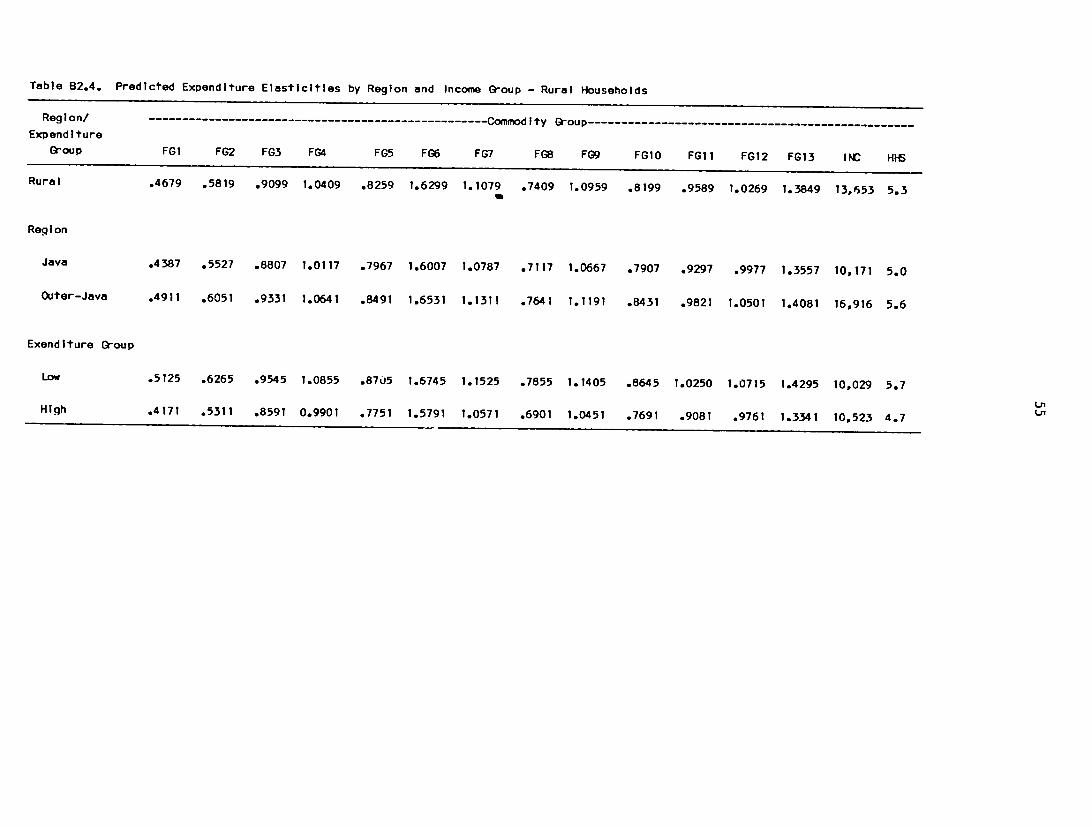
Table 82.4. Predicted Expenditure Elasticities by Region and Income Group - Rural Households

Region/

Expenditure Group

--------------------------------------------------- Commodity Group

FG1 FG2 FG3 FG4 FG5 FG6 FG7 FG8 FG9 FG1O FG11 FG12 FG13 INC H1

Rural .4679 .5819 .9099 1.0409 .8259 1.6299 1.1079 .7409 1.0959 .8199 .9589 1.0269 1.3849 13,653 5.3

Reiion

Java .4387 .5527 .8807 1.0117 .7967 1,6007 1.0787 .7117 1.0667 .7907 .9297 .9977 1.3557 10,171 5.0

Outer-Java .4911 .6051 .9331 1.0641 .8491 1.6531 1.1311 .7641 1.1191 .8431 .9821 1.0501 1.4081 16,916 5.6

Exenditure Group

Low

High

.5125

.4171

.6265

.5311

.9545

.8591

1.0855

0.9901

.8705

.7751

1.6745

1.5791

1.1525

1.0571

.7855

.6901

1.1405

1.0451

.8645

.7691

1.0250

.9081

1.0715

.9761

1.4295

1.3341

10,029

10,523

5.7

4.7 Ln

L

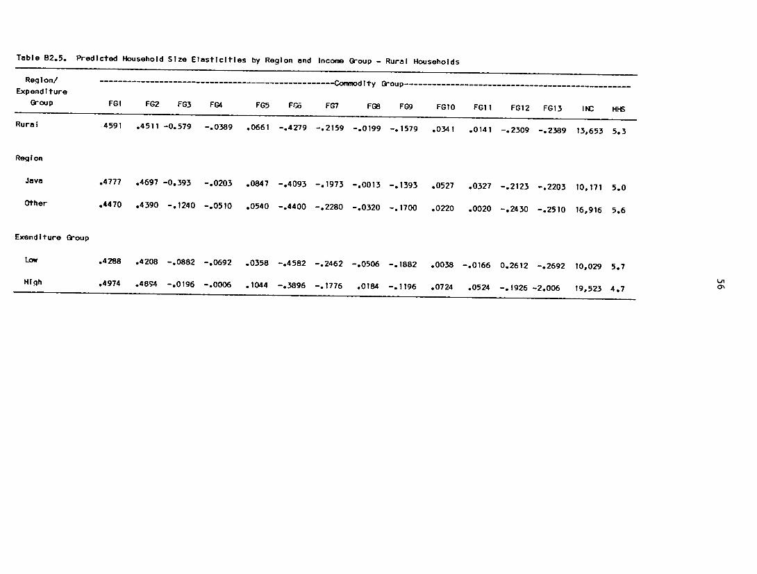
Table B2.5. Predicted Household Size Elasticities by Region and Income Group - Rural Households

Region/ ---------------------------------------------------- Comodity Group Expenditure

Group FG1 FG2 FG3 FG4 FG5 F-6 FG7 FG8 FG9 FG1O FG11 FG12 FG13 INC HHS

Rural -4591 .4511 -0.579 -.0389 .0661 -.4279 -.2159 -.0199 -.1579 .0341 .0141 -.2309 -.2389 13,653 5.3

Reqgion

Java .4777 .4697 -0.393 -.0203 .0847 -.4093 -.1973 -.0013 -.1393 .0527 .0327 -.2123 -.2203 10,171 5.0

Other .4470 .4390 -.1240 -.0510 .0540 -.4400 -.2280 -.0320 -.1700 .0220 .0020 -.2430 -.2510 16,916 5.6

Exenditure Group

Low .4288 .4208 -.0882 -.0692 .0358 -.4582 -.2462 -.0506 -. 1882 .0038 -.0166 0.2612 -.2692 10,029 5.7

High .4974 .484 -.0196 -.0006 .1044 -.3896 -.1776 .0184 -. 1196 .0724 .0524 -. 1926 -2.006 19,523 4.7

Table B2.6o

Reqion/

ExpenditureGroup

Urban

Estimates of Economies of Scale by Region and Income Group--Rural Households

--------------------------------------------------- omodity Group

FGI FG2 FG3 FG4 FG5 FG6 FG7 FG8 FG9

.9270 1.0330 .8520 1.0020 .8920 1.2020 .8920 .7210 .9380

FGIO

.8540

FGtI

.9730

FG12

.7960

FG13

1.1460

INC

13,653

HHS

5.3

Region

Java

Outer-Java

.9164

.9381

1.0224

1.0441

.8414

.8091

.9914

1.0131

.8814

.9031

1.1914

1.2131

.8814

.9031

.7104

.7321

.9274

.9491

.8434

.8651

.9624

.9841

.7854

.8071

1.1354

1.1571

10,171

16,916

5.0

5.6

Exenditure Group

LOw

High

.9413

.9145

1.0473

1.0205

.8663

.8395

1.0163

.9895

.9063

.8795

1.2163

1.1895

.9063

.8795

.7349

.7085

.9523

e9255

.8683

.8415

1.0084

.9605

.8103

.7835

1.1600

1.1335

10,029

19,523

5.7

4.7

Se~001~~ ZOWA-N6 Q

Documents

Transcript of Se~001~~ ZOWA-N6 Q