BAND-GUI TutorialADF Program System

Release 2009.01

Scientific Computing & Modelling NVVrije Universiteit, Theoretical ChemistryDe Boelelaan 1083; 1081 HV Amsterdam; The NetherlandsE-mail: support@scm.com

Copyright © 1993-2009: SCM / Vrije Universiteit, Theoretical Chemistry, Amsterdam, The NetherlandsAll rights reserved

1

Table of ContentsBAND-GUI Tutorial ........................................................................................................................ 1Table of Contents .......................................................................................................................... 2Tutorials ......................................................................................................................................... 3

Tutorial 1: with a grain of salt................................................................................................ 3Step 1: Start BANDinput .................................................................................................... 3Step 2: Create the unit cell................................................................................................. 5

Select the coordinates tab........................................................................................... 5Enter lattice vectors..................................................................................................... 7

Step 3: Add the atoms ....................................................................................................... 7Step 4: Running the calculation ....................................................................................... 11Step 5: Examine the band structure................................................................................. 12Step 6: Visualizing the results.......................................................................................... 16

Plotting the orbitals.................................................................................................... 16Plotting the partial density-of-states .......................................................................... 20Plotting the deformation density ................................................................................ 22

Step 7: Check the charges............................................................................................... 24Tutorial 2: building structures............................................................................................. 25

The Crystal Structure Database....................................................................................... 26Crystal builder (from space group information)................................................................ 28Slicer: building slabs ........................................................................................................ 33

A three layer slab of the Cu(111) surface ................................................................. 33Enlarging the unit cell....................................................................................................... 36

Tutorial 3: a transition state search .................................................................................... 39Step 1: Create the H3 toy system .................................................................................... 40Step 2: Optimize the geometry ........................................................................................ 40Step 3: Calculate the Hessian.......................................................................................... 44Step 4: Search the transition state................................................................................... 46

Tutorial 4: a transition state search with a partial Hessian*............................................. 49Step 1: Create the system ............................................................................................... 49Step 2: Calculate a partial Hessian.................................................................................. 51Step 2: Transition state search with a frozen substrate ................................................... 52

2

TutorialsTutorial 1: with a grain of saltAccording to any freshmen chemistry textbook, in NaCl one electron is transferred from the Sodium to theChlorine. The occupied 3p states form the valence band, while the empty sodium states hybridize into aconduction band. We will put these idealized ideas to the test.

This tutorial will teach you how to:

• define the geometry of a NaCl crystal• run the calculation• view the band structure• view an orbital for a particular band and k-point• view the (partial) density of states• view the deformation density• view the atomic charges

The BAND-GUI has been designed to be a lot like the ADF-GUI. This makes it much easier for users to useboth programs. To avoid repetition, the BAND-GUI tutorial assumes that you are familiar with some basicusage of the ADF-GUI. If you do not know how to rotate, translate, zoom etc within the ADF-GUI, pleaseread through the first ADF-GUI tutorial before starting with this BAND-GUI tutorial. Even better: try using theADF-GUI yourself. You can get a demo-license for this purpose if needed.

Step 1: Start BANDinput

On a Unix-like system, enter the following command:

bandinput &

On Windows, one can start BANDinput by double-clicking on the BANDinput icon on the Desktop:

double click the BANDinput icon on the Desktop

On Macintosh, use the ADFLaunch program to start BANDinput:

double click on the ADFLaunch iconclick the 'BAND Input' button

3

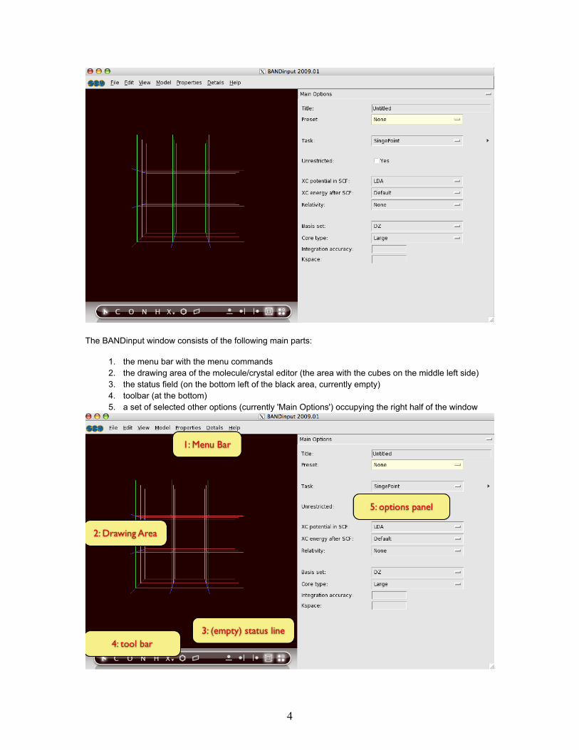
The BANDinput window consists of the following main parts:

1. the menu bar with the menu commands2. the drawing area of the molecule/crystal editor (the area with the cubes on the middle left side)3. the status field (on the bottom left of the black area, currently empty)4. toolbar (at the bottom)5. a set of selected other options (currently 'Main Options') occupying the right half of the window

4

Step 2: Create the unit cell

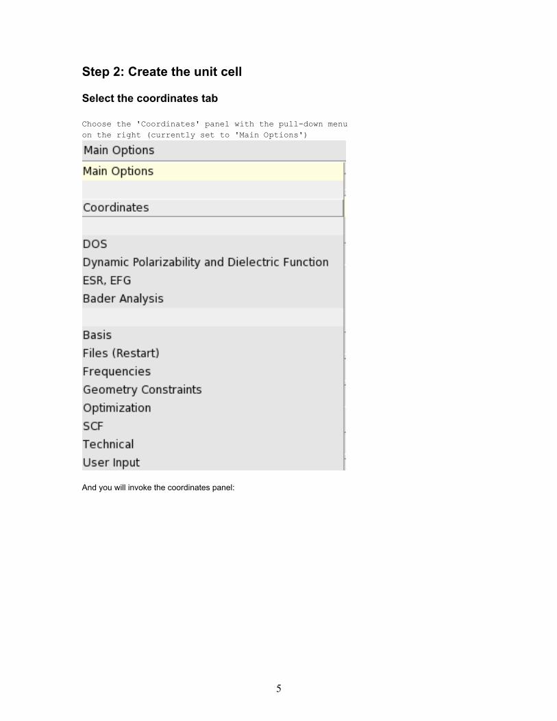
Select the coordinates tab

Choose the 'Coordinates' panel with the pull-down menuon the right (currently set to 'Main Options')

And you will invoke the coordinates panel:

5

The colored lines that you see in the drawing area are the lattice vectors. The first lattice vector is coloredred, the second green, and the third blue. Because a number of neighboring cells are displayed you see acollection of cubes. You can enable/disable this:

Use the 'Periodic>Repeat Unit Cells' menu command fromthe 'View' menu to toggle the periodic display

Without the repeated unit cells you see the more clearly the three lattice vectors.

6

Enter lattice vectors

Salt has an fcc lattice. First we need to set the lattice vectors:

Enter the lattice vectors, as shown in the next picture.To avoid the warning of a singular lattice, set first the off-diagonal

elements to 2.75 and then the diagonal elements to zero

Step 3: Add the atoms

Now we will add the Na and Cl atoms:

Make sure periodic display is turned offSelect the Sodium (Na) element tool from the periodic system

that appears when you click the 'X' element on the toolbar

7

After this you see at the bottom of the screen "Na tool" in the status field:

Click once in the drawing area, near the originClick once on the created atom to stop bonding

8

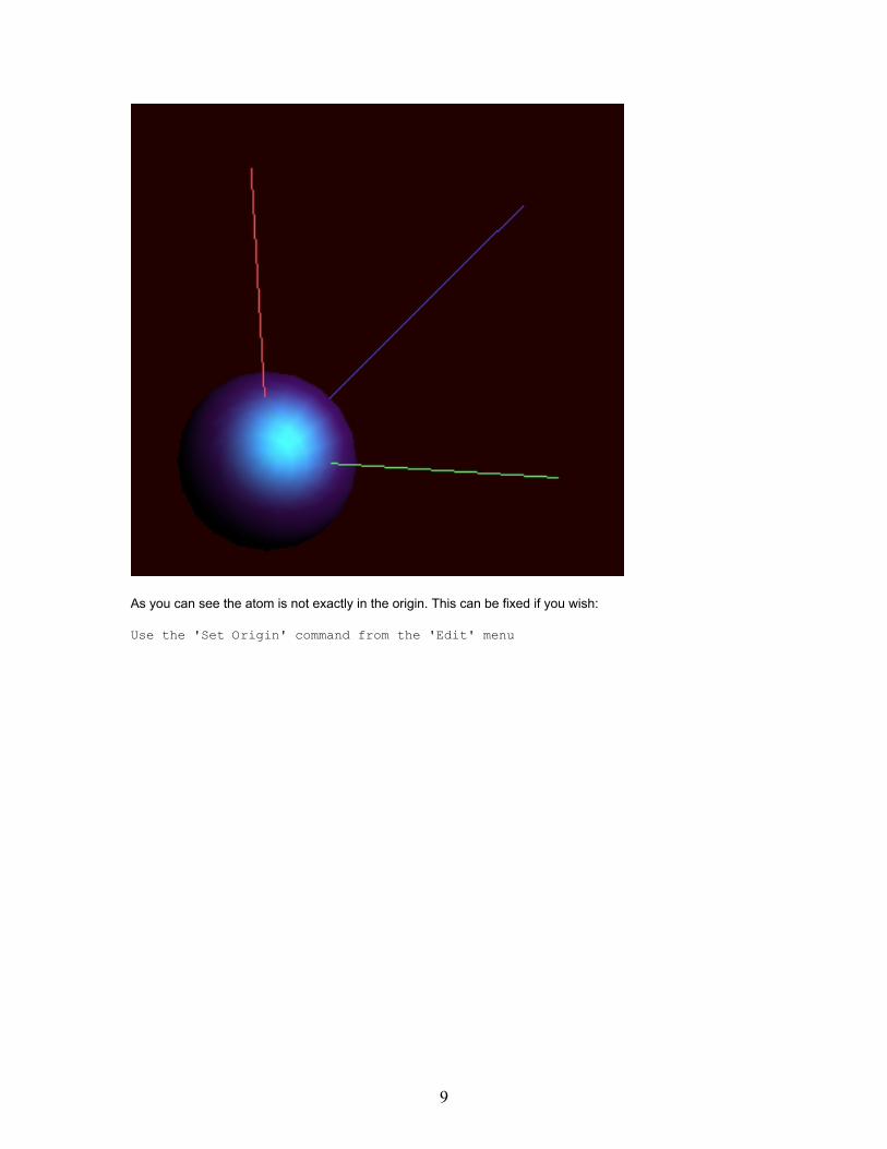
As you can see the atom is not exactly in the origin. This can be fixed if you wish:

Use the 'Set Origin' command from the 'Edit' menu

9

To add the Cl atom you can proceed the same way.

Select the Cl toolClick once somewhere in the unit cellClick on the new Cl atom to stop bonding

Next you should edit the Cl coordinates and change the Cl color:

Change the Cl coordinates to be (2.75,2.75,2.75) in the 'Coordinates' panelTurn on periodic display (in the 'View' menu)

10

Now your system looks like:

Step 4: Running the calculation

It is a good idea to give your calculation a description.

Go back to the "Main options" panelEnter something appropriate in the "Title" fieldSave the result with the menu "File>Save", and name it "NaCl"Choose "File>run".

First, you will be asked to save the file. Name it NaCl.

A window will appear showing the progress of the BAND calculation (the 'logfile'). After a few minutes thecalculation has finished, and it looks like:

11

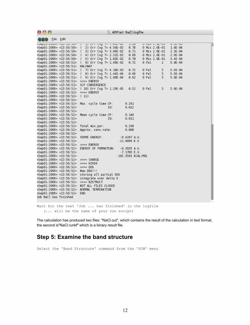
Wait for the text 'Job ... has finished' in the logfile(... will be the name of your run script)

The calculation has produced two files: "NaCl.out", which contains the result of the calculation in text format,the second is"NaCl.runkf" which is a binary result file.

Step 5: Examine the band structure

Select the 'Band Structure' command from the 'SCM' menu

12

This will open the bandstructure window:

It consists of a plot and a picture of the Brillouin zone. In the plot the red line is the fermi level. Below theFermi level are four occupied bands. You can see this more clearly by vertical zooming:

Click on the right mouse button, and drag the pointer up to zoom verticallyWhen the region of interest gets out of view,

drag it into view (with the normal left mouse button)

13

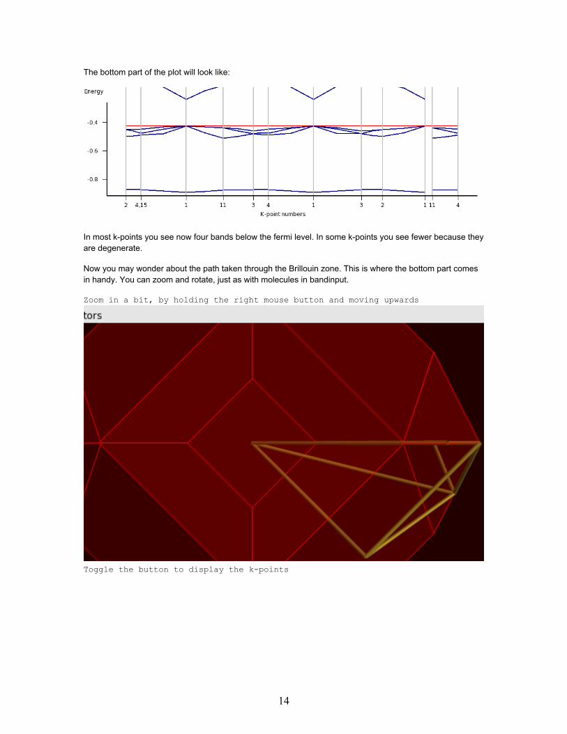
The bottom part of the plot will look like:

In most k-points you see now four bands below the fermi level. In some k-points you see fewer because theyare degenerate.

Now you may wonder about the path taken through the Brillouin zone. This is where the bottom part comesin handy. You can zoom and rotate, just as with molecules in bandinput.

Zoom in a bit, by holding the right mouse button and moving upwards

Toggle the button to display the k-points

14

Now click on the line from 11 (via 12) to 1

Note how the line lights up, and also how the corresponding segment is indicated in the plot by a graybackground. You can also click on the plot to select line segments.

Rotate the Brillouin zone a bit to convince yourself that the line (from k-point 11 to 1) runs from the center tothe center of a hexagonal face.

15

Step 6: Visualizing the results

Plotting the orbitals

Now what is the character of the bands? Let us first examine this narrow band at about -0.5 Hartree.

Open ADFview with the menu 'View' command from the 'SCM' menu.In ADFview: select the 'Isosurface Double (+/-)' command from the 'Add' menu.

In the bar at the bottom of the window, you can select which field to show.

Select the lowest band (k=0,0,0)

From the label you can see that it has an energy of -0.4641 and the coordinates are (0,0,0). The cursor willgo to the busy state, and after a while you will see the orbital:

16

If you rotate it a bit and toggle the isosurface on and off, you can convince yourself that this orbital is locatedaround the small atom, which is the Chlorine.

Toggle the periodic view (the menu 'Periodic>Show Periodic'command from the 'View' menu).

17

Obviously this is the 3s band of Cl. The strange truncated spheres are due to contributions of neighboringcells.

Let us now take a look at the orbital with the lowest energy of the second band (the first one with an energynot around -0.4):

Select the lowest orbital of the second band (with energy about -0.08)

This orbital looks like:

18

and it clearly consists of a p orbital on the Cl. The part near the Na comes from Chlorine atoms inneighboring cells.

It is generally easier to interpret orbitals at k=(0,0,0). Going up in energy we encounter a degenerate triple ate=-0.0001. One of them looks like

Take a look at all three of them.

From these orbital pictures we can conclude that the valence band is indeed mainly of Chlorine-p character.

You may want to check the lowest orbitals of the (unoccupied) conduction band.

Check the lowest orbitals of the conduction bandDo you see a strong Na character in them?

19

Plotting the partial density-of-states

There is in fact a much more easy way to conclude that the valence band is mainly of Chlorine-p character.

Open from the SCM menu the 'Dos' module.

and a window like this will appear

The fermi energy is at zero, and there is clearly a gap. Just below it there is a valence band, and at 0.2Hartree starts the conduction band.

Select from the 'View' menu 'Add Graph'

(Now you see two plots of the total DOS)

Select with the mouse the Chlorine atom (the small green one)

20

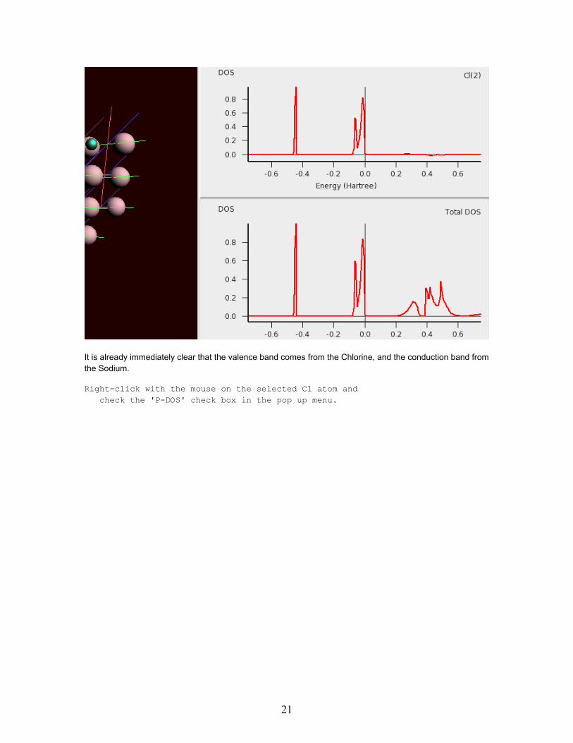
It is already immediately clear that the valence band comes from the Chlorine, and the conduction band fromthe Sodium.

Right-click with the mouse on the selected Cl atom andcheck the 'P-DOS' check box in the pop up menu.

21

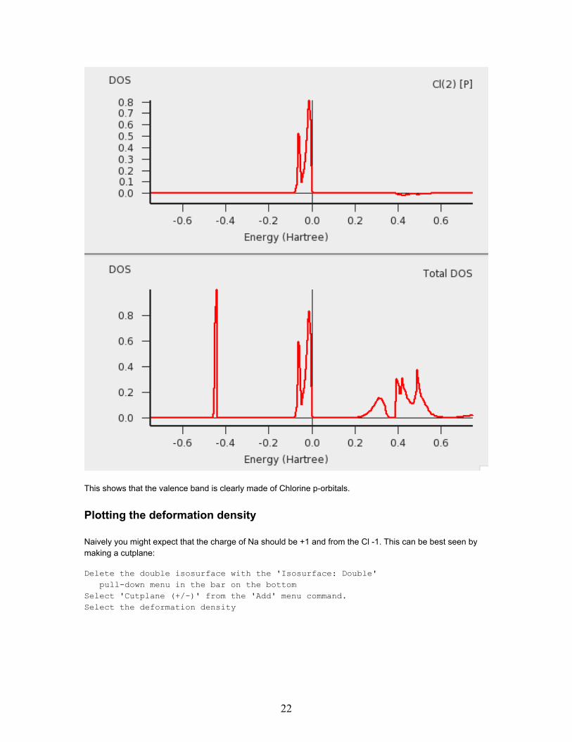
This shows that the valence band is clearly made of Chlorine p-orbitals.

Plotting the deformation density

Naively you might expect that the charge of Na should be +1 and from the Cl -1. This can be best seen bymaking a cutplane:

Delete the double isosurface with the 'Isosurface: Double'pull-down menu in the bar on the bottom

Select 'Cutplane (+/-)' from the 'Add' menu command.Select the deformation density

22

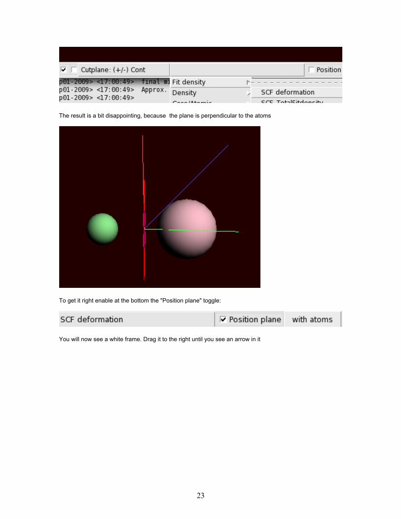
The result is a bit disappointing, because the plane is perpendicular to the atoms

To get it right enable at the bottom the "Position plane" toggle:

You will now see a white frame. Drag it to the right until you see an arrow in it

23

Now you can "grab" the arrow head and turn it to point towards you

Indeed we see that charge is added (blue) near the Cl and removed (red) from the Na atom. The trend isgood, but what is the total amount of charge transferred?

Step 7: Check the charges

right click somewhere where there is no atoms

From the popup choose 'Atom Info' and next 'Hirshfeld Charges'

24

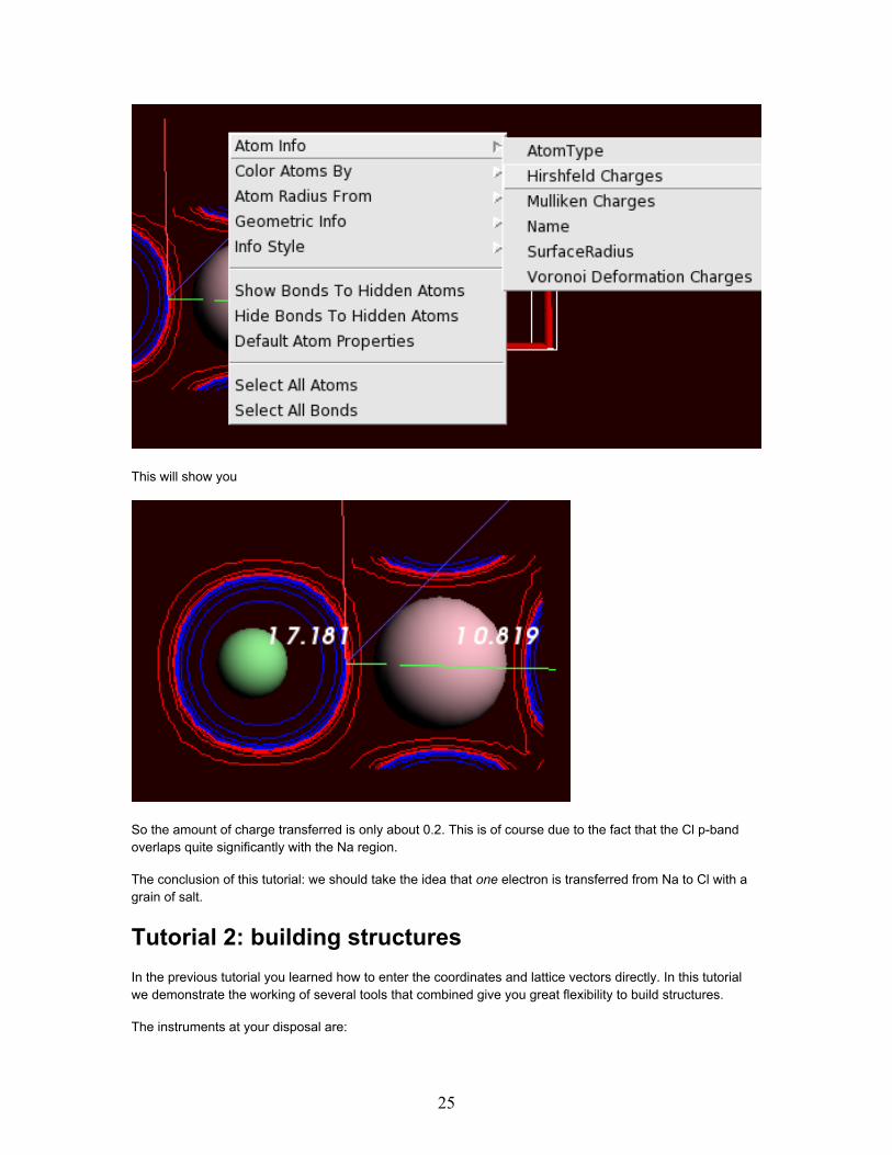
This will show you

So the amount of charge transferred is only about 0.2. This is of course due to the fact that the Cl p-bandoverlaps quite significantly with the Na region.

The conclusion of this tutorial: we should take the idea that one electron is transferred from Na to Cl with agrain of salt.

Tutorial 2: building structuresIn the previous tutorial you learned how to enter the coordinates and lattice vectors directly. In this tutorialwe demonstrate the working of several tools that combined give you great flexibility to build structures.

The instruments at your disposal are:

25

• Small database of predefined crystal structures.• CIF file importer.• Crystal builder from space group information.• Super cell tool to enlarge the unit cell• Slice tool to cut out slabs from any crystal.

The Crystal Structure Database

If you are lucky your crystal structure is in the database. Of course there are infinitely many possible crystalstructures, so the database has to be incomplete. Nevertheless, the most common structures are there.NaCl is one of them.

Click on the Benzene like pictogram on the toolbar.Select a "Cubic" lattice and then NaCl

Next a dialog pops up where you can change the parameters of the structure, such as lattice constants

26

In this case there is no need to change anything.

Click Apply.Click Close

More often a crystal is not directly in the list. An example is LiF. It has the same crystal structure as NaCl,but other elements and a different lattice constant, namely 4.01

Open again the NaCl dialogChange the lattice constant and the elements like this

27

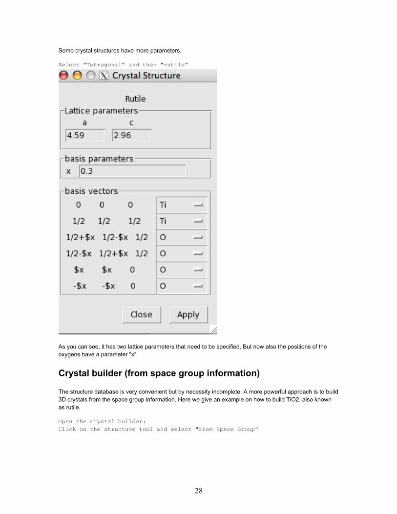
Some crystal structures have more parameters.

Select "Tetragonal" and then "rutile"

As you can see, it has two lattice parameters that need to be specified. But now also the positions of theoxygens have a parameter "x"

Crystal builder (from space group information)

The structure database is very convenient but by necessity incomplete. A more powerful approach is to build3D crystals from the space group information. Here we give an example on how to build TiO2, also knownas rutile.

Open the crystal builder:Click on the structure tool and select "From Space Group"

28

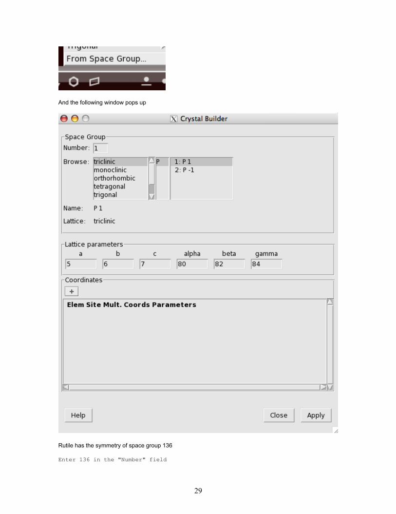
And the following window pops up

Rutile has the symmetry of space group 136

Enter 136 in the "Number" field

29

Note how the Browser reflects the change and also how the "Name" and "Lattice" values change

Now set the two lattice parameters as below

We still need to define the atomic coordinates. For starters click on the plus below "Coordinates"

In a book on crystal structures you can find that rutile has two sites occupied. The Ti atom is on the "a" site

Select the Ti atom and select the "a" site

The oxygens occupy the "f" site.

30

Click on the plus to add a siteChange the atom type to "O" and the site to "f"

As you can see in the "Coords" column and the "Parameters" column, this site has an undeterminedparameter "x". (It represents a symmetry line for this space group.) In the book you can find that for TiO2"x=0.3".

Set "x" to 0.3

The final dialog looks like

31

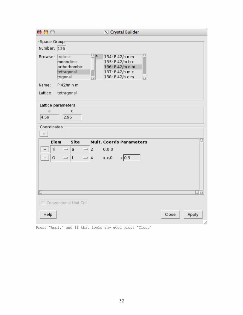
Press "Apply" and if that looks any good press "Close"

32

Slicer: building slabs

The slicer is a very easy, yet powerful tool to make slabs from any crystal structure.

A three layer slab of the Cu(111) surface

Select fcc from the "Cubic" crystals

33

The element and lattice constant are already correct for Cu.

Press "Apply" to generate the Cu lattice

Let us invoke the slicer tool to cut out the slab.

34

Click on the utility knife like icon in the toolbar

The following dialog appears

Set the Miller indices to (1,1,1)Select CartesianSet the number of layers to 3

The "Cartesian" option is needed because the Miller indices are usually thought in the conventional unit cellrather than the primitive (minimal) unit cell. After pressing OK you will see (from the top)

35

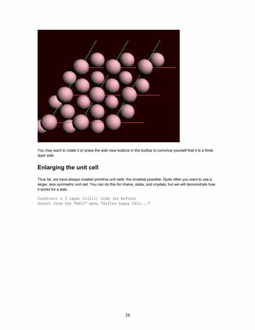
You may want to rotate it or press the side view buttons in the toolbar to convince yourself that it is a threelayer slab.

Enlarging the unit cell

Thus far, we have always created primitive unit cells: the smallest possible. Quite often you want to use alarger, less symmetric unit cell. You can do this for chains, slabs, and crystals, but we will demonstrate howit works for a slab.

Construct a 3 layer Cu(111) slab (as before)Select from the "Edit" menu "Define Super Cell..."

36

Thus invoking the Super Cell Tool

Here you see how new lattice vectors are expressed in terms of old ones. Because we have a slab this is a2x2 matrix, set initially to the unit matrix.

Select the "sqrt(3) x sqrt(3)" option from the "Preset" menu

37

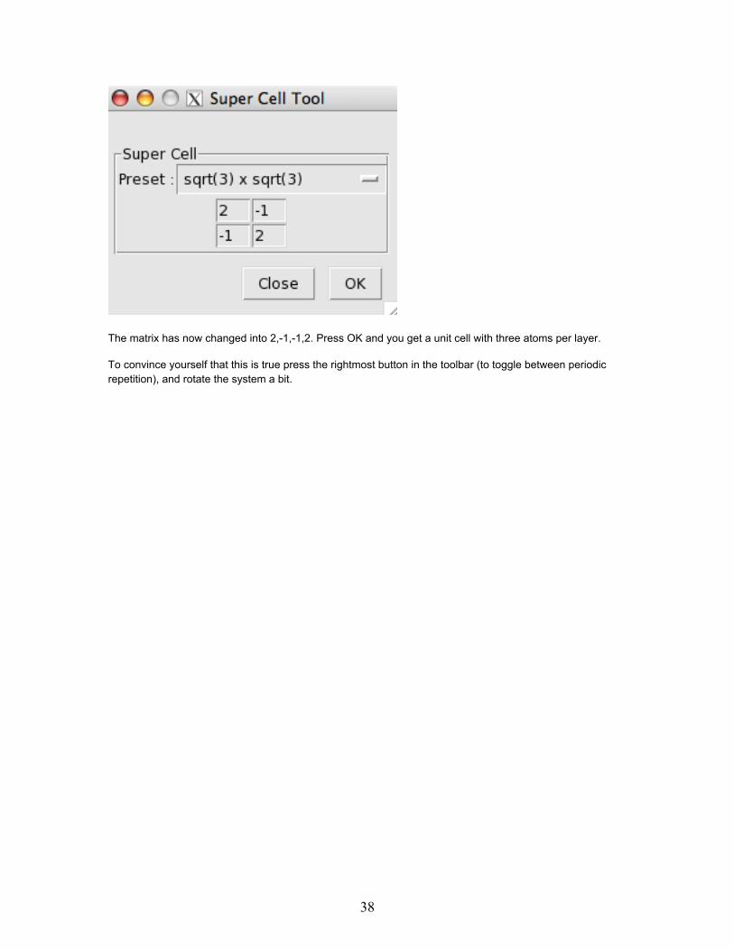
The matrix has now changed into 2,-1,-1,2. Press OK and you get a unit cell with three atoms per layer.

To convince yourself that this is true press the rightmost button in the toolbar (to toggle between periodicrepetition), and rotate the system a bit.

38

Tutorial 3: a transition state searchThis tutorial will learn you how to:

• do a geometry optimization• watch the geometry optimization as a movie• do a frequency calculation• examine the eigen modes• perform a transition state search• make a few mistakes and fix them

Throughout we will consider the toy system of a periodic chain with three atoms in the unit cell.

39

Step 1: Create the H3 toy system

We are going to enter the geometry manually, just as in the first tutorial.

Select in the 'Coordinates' panel as periodicity 'Chain' andmake a lattice vector in the x-direction with length 10.

Add with the mouse three hydrogen atoms somewhere in the cell.Change the coordinates in the table to this

You have now created the cylinder symmetric toy system.

Step 2: Optimize the geometry

Go back to the 'Main Options' panelChoose as task 'GeometryOptimization'.Save the project as 'H3_geo'Run it.

After it has finished the program asks you

Answer 'Yes'.

40

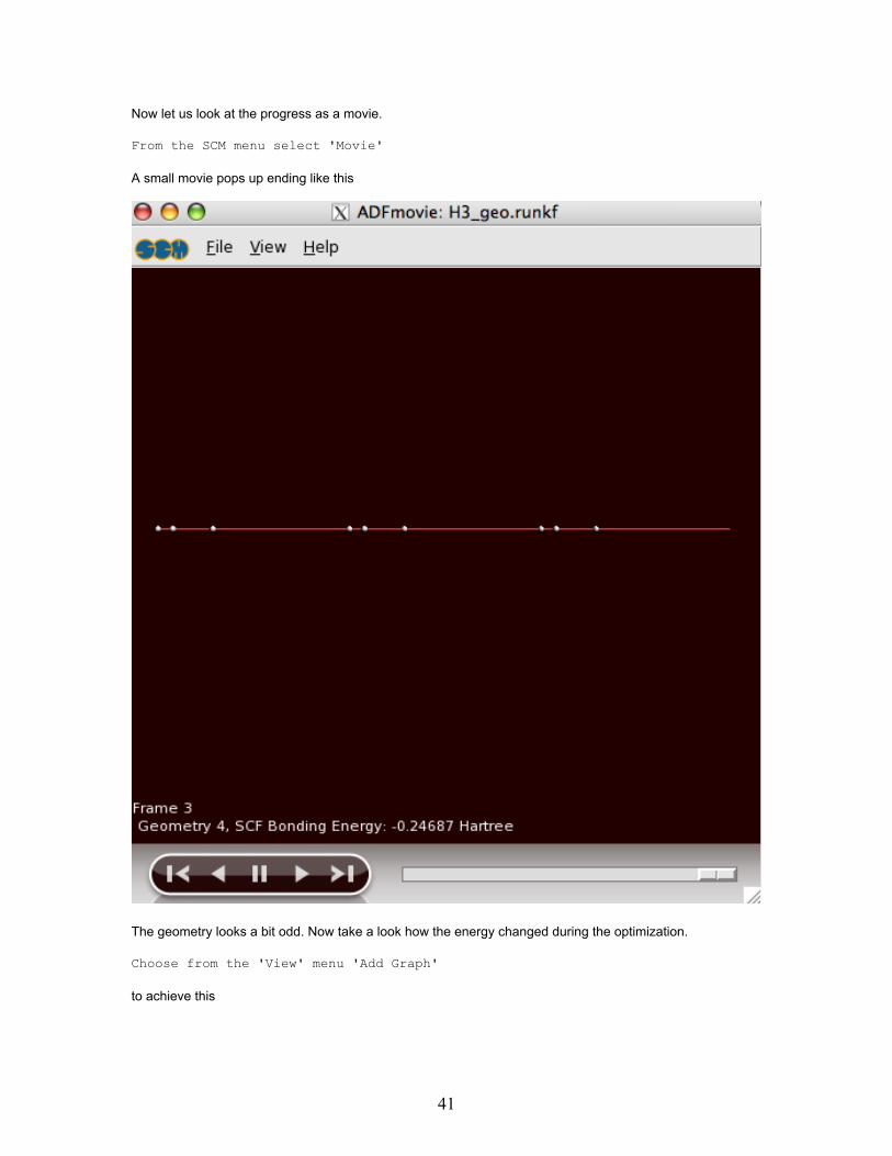
Now let us look at the progress as a movie.

From the SCM menu select 'Movie'

A small movie pops up ending like this

The geometry looks a bit odd. Now take a look how the energy changed during the optimization.

Choose from the 'View' menu 'Add Graph'

to achieve this

41

It shows the energy at the four steps: 0, 1, 2, and 3. Since the energy does not change anymore from step 2to three it should be OK? Well, maybe, but maybe not. Let us check whether we were fully converged.

Select from the SCM menu 'Logfile'.Scroll from the end a bit upwards and you will see

42

You see the final geometry and status of the five convergence criteria. Because they are all satisfied yousee the log message 'Geometry Converged'

Maybe we are dealing with a shallow minimum. Let us retry with a more strict criterion.

Close the logfile and movie windows and go back to 'BAND input'.Go to the 'Optimization' panel and set the convergence criterion to 1e-4.

Save the project and run itOpen adfmovie afterwards and add the graph

43

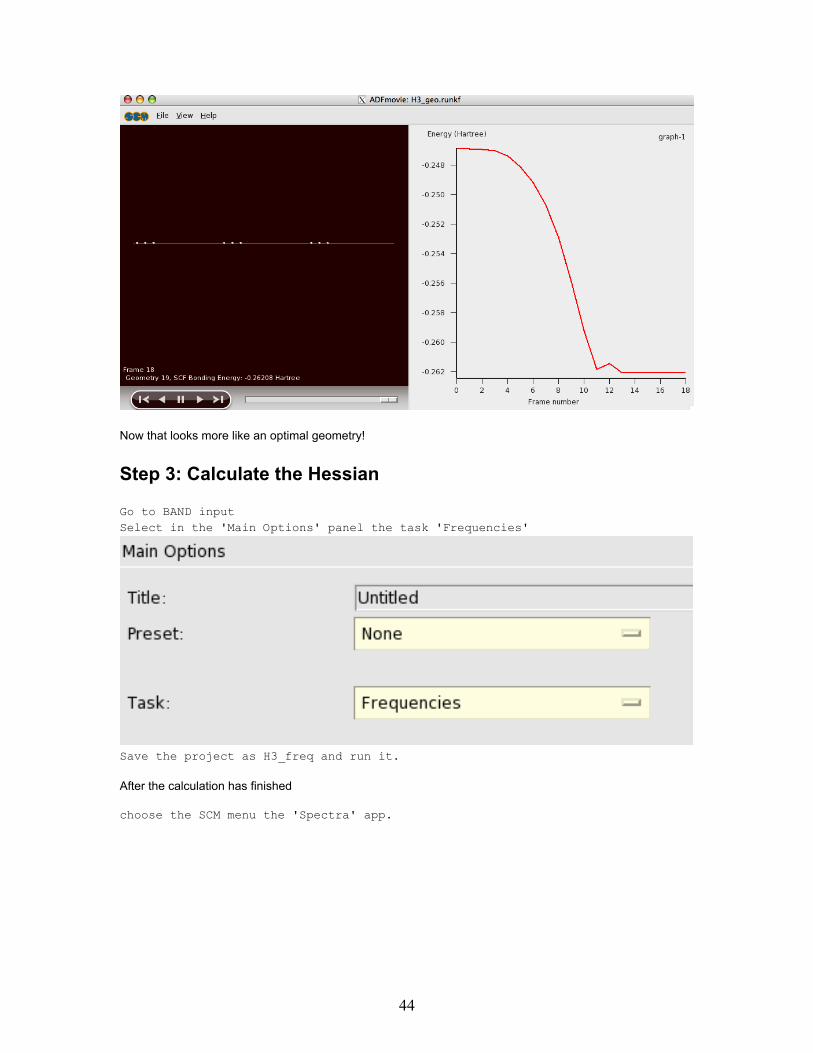
Now that looks more like an optimal geometry!

Step 3: Calculate the Hessian

Go to BAND inputSelect in the 'Main Options' panel the task 'Frequencies'

Save the project as H3_freq and run it.

After the calculation has finished

choose the SCM menu the 'Spectra' app.

44

There appear to be three peaks, whereas you would expect 3N degrees of freedom. With three atoms (N=3)we should have nine modes. We can examine this a bit closer

click on the 'NormalMode' menu.

So there are indeed nine vibrational modes. Only two are nonzero because only symmetrical modes arecalculated by default. To see what a mode looks like

Select the mode at 1700 cm-1, either from the 'NormalMode' menu,or by clicking on it directly in the graph.

A new movie window pops up visualising the vibrational mode.

45

Step 4: Search the transition state

A minimum has vanishing gradients and only positive eigen modes. A (first-order) transition state (saddlepoint) is characterized by having one negative mode. With a transition state search the optimizer will gouphill in the direction of the lowest (nonzero) eigenmode and downhill in all other degrees of freedom. In ourexample it would follow mode 8. Let us give it a try from the minimum.

Choose in the 'Main Options' panel the task 'TransitionState'

We have just calculated a Hessian (with the frequency run) so we'd better use it.

46

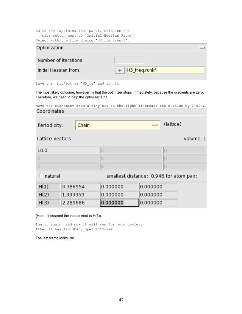
Go to the 'Optimization' panel, click on theplus button next to 'Initial Hessian From:'

Select with the file dialog 'H3_freq.runkf'.

Save the project as 'H3_ts' and run it.

The most likely outcome, however, is that the optimizer stops immediately, because the gradients are zero.Therefore, we need to help the optimizer a bit.

Move the rightmost atom a tiny bit to the right (increase the x value by 0.01).

(Here I increased the values next to H(3)).

Run it again, and now it will run for more cycles.After it has finished, open adfmovie

The last frame looks like

47

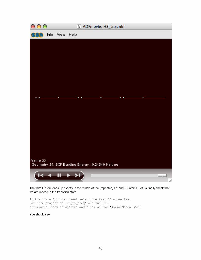
The third H atom ends up exactly in the middle of the (repeated) H1 and H2 atoms. Let us finally check thatwe are indeed in the transition state.

In the 'Main Options' panel select the task 'Frequencies'Save the project as 'H3_ts_freq' and run it.Afterwards, open adfspectra and click on the 'NormalModes' menu

You should see

48

We have found a geometry with vanishing gradients with one weak negative vibrational mode. We havesucceeded in finding a transition state.

Tutorial 4: a transition state search with a partialHessian*This tutorial will learn you how to:

• calculate a partial Hessian• do a constrained TS search using the partial Hessian

In this "advanced" tutorial we consider a slightly more realistic system. Some of the calculations may require20 minutes to run on a two core machine.

Step 1: Create the system

We are going to make a one layer Li (001) slab with a 2x2 unit cell, assuming familiarity with the build tools

From the structure tool select 'Cubic' and 'bcc'Set 'Element' to LiSet the lattice parameter to 3.49Press 'Apply' and 'Close'Invoke the Slice toolSet the Miller indices to 001, select 'Cartesian', and enter 1 layer.Press 'OK'From the 'Edit' menu choose 'Define Super Cell...'Select the preset '2x2' and press 'OK'

Your screen should look like this (after selecting the 'Coordinates' panel)

49

Add with the mouse two hydrogen atoms anywhere in the screenSelect the 'Normal' edit modeSet in the table the coordinates of the first hydrogen atom to (0, -0.5, 2)Set the second H atom coordinates to (0, 0.5, 2)

The final geometry looks like this

50

Step 2: Calculate a partial Hessian

Select the 'Main Options' panelSet 'Task' to 'Frequencies'Set 'Basis Set' to 'SZ'

Go to the 'Frequencies' panelSelect with the mouse the two tiny Hydrogen atomsClick on the '+' button next to 'Partial Hessian For:'

51

Save the project as 'H2onLi_freq' and run it.(On my computer this takes 3 minutes)

Say 'No' when asked to update the coordinates

Let us examine the eigenmodes that we have found for the Hydrogen molecule

Select from the SCM menu 'Spectra'Open the 'NormalMode' menu

Now you will see that there is an eigenmode at 448 cm-1 and one at 2164. Convince yourself that the 448mode moves the H2 perpendicular to the service and that the 2164 more is essentially an H2 stretch mode.The lowest mode looks like a promising start to find the transition state for dissociation over the Li surface.

Step 2: Transition state search with a frozen substrate

We have just found the vibrational modes of the Hydrogen molecule, assuming that the Li substrate remainsfixed. Let us now find the transition state under the same assumption.

Close the 'Spectra' window and go back to BandInput.Select the 'Main Options' panel and set 'Task' to 'TransitionState'

Select the 'Geometry Constraints' panelI assume that the two hydrogen atoms are still selected.If not select them againSelect from the 'Edit' menu 'Invert Selection'Click on the '+' button next to 'freeze selected atoms'

52

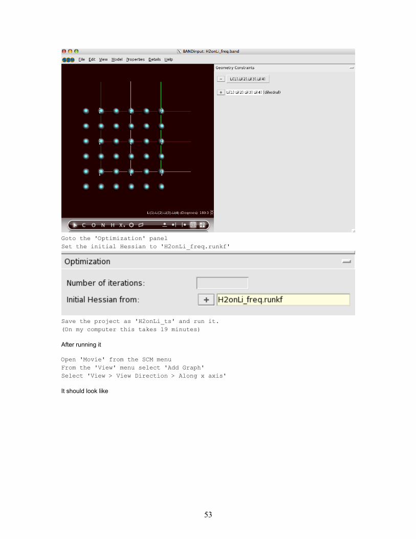
Goto the 'Optimization' panelSet the initial Hessian to 'H2onLi_freq.runkf'

Save the project as 'H2onLi_ts' and run it.(On my computer this takes 19 minutes)

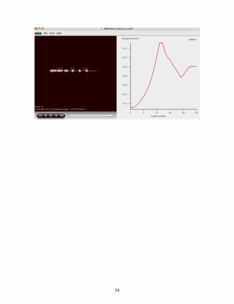
After running it

Open 'Movie' from the SCM menuFrom the 'View' menu select 'Add Graph'Select 'View > View Direction > Along x axis'

It should look like

53

54