Schaum's Outline of Theory and Problems of Computer Graphics
357
SCHAUM'S OUTLINE OF THEORY AND PROBLEMS OF COM ER ZHIGANG XIANG, Ph.D. Associate Professor of Computer Science Queens College of the City University of New York ROY A. PLASTOCK, Ph.D. Associate Professor of Mathematics New Jersey Institute of Technology SCHAUM'S OUTLINE SERIES McGRAW-HILL New York St. Louis San Francisco Auckland Bogota Caracas Lisbon London Madrid Mexico City Milan Montreal New Delhi San Juan Singapore Sydney Tokyo Toronto
-
Upload
khangminh22 -
Category
Documents
-
view
0 -
download
0
Transcript of Schaum's Outline of Theory and Problems of Computer Graphics

SCHAUM'SOUTLINE OF
THEORY AND PROBLEMS OF
COM ER
ZHIGANG XIANG, Ph.D.
Associate Professor of Computer ScienceQueens College of the City University of New York
ROY A. PLASTOCK, Ph.D.
Associate Professor of MathematicsNew Jersey Institute of Technology
SCHAUM'S OUTLINE SERIESMcGRAW-HILL
New York St. Louis San Francisco Auckland Bogota Caracas LisbonLondon Madrid Mexico City Milan Montreal New Delhi
San Juan Singapore Sydney Tokyo Toronto
Zhigang Xiang, is currently an associate professor of computer science at Queens College and theGraduate School and University Center of the City University of New York (CUNY). He received aBS degree in computer science and engineering from Beijing Polytechnic University, Beijing,China, in 1982, and the MS and Ph.D degrees in computer science from the State University ofNew York at Buffalo in 1984 and 1988, respectively. He has published numerous articles in well-respected computer graphics journals.
Roy A. Plastock, is an Associate Professor of Mathematics at New Jersey Institute of Technology.He is listed in Who s Who in Frontier Science and Technology. His special interests are computergraphics, computer vision, and artificial intelligence.
Schaum's Outline of Theory and Problems ofCOMPUTER GRAPHICS
Copyright © 2000, 1992, by The McGraw-Hill Companies, Inc. All rights reserved. Printed in theUnited States of America. Except as permitted under the United States Copyright Act of 1976, nopart of this publication may be reproduced or distributed in any form or by any means, or stored ina data base or retrieval system, without the prior written permission of the publisher.
1 2 3 4 5 6 7 8 9 10 11 12 13 14 15 16 17 18 19 20 PBT PBT 0 9 8 7 6 5 4 3 2 1 0
ISBN 0-07-135781-5
Sponsoring Editor: Barbara GilsonProduction Supervisor: Tina CameronEditing liaison: Maureen B. WalkerProject Supervision: Techset Composition Limited
Library of Congress Cataloging-in-Publication Data
McGraw-HillA Division ofTheMcGnw-HiUCompanies

To Qian, Wei, and my teachers
ZHIGANG XIANG
To Sharon, Adam, Sam, and the memory of Gordon S. Kalley
ROY PLASTOCK

This page intentionally left blank

We live in a world full of scientific and technological advances. In recent years it has become quite difficultnot to notice the proliferation of something called computer graphics. Almost every computer system is set up toallow the user to interact with the system through a graphical user interface, where information on the displayscreen is conveyed in both textual and graphical forms. Movies and video games are popular showcases of thelatest technology for people, both young and old. Watching the TV for a while, the likelihood is that you willsee the magic touch of computer graphics in a commercial.
This book is both a self-contained text and a valuable study aid on the fundamental principles of computergraphics. It takes a goal-oriented approach to discuss the important concepts, the underlying mathematics, andthe algorithmic aspects of the computerized image synthesis process. It contains hundreds of solved problemsthat help reinforce one's understanding of the field and exemplify effective problem-solving techniques.
Although the primary audience are college students taking a computer graphics course in a computerscience or computer engineering program, any educated person with a desire to look into the inner workings ofcomputer graphics should be able to learn from this concise introduction. The recommended prerequisites aresome working knowledge of a computer system, the equivalent of one or two semesters of programming, a basicunderstanding of data structures and algorithms, and a basic knowledge of linear algebra and analyticalgeometry.
The field of computer graphics is characterized by rapid changes in how the technology is used in everydayapplications and by constant evolution of graphics systems. The life span of graphics hardware seems to begetting shorter and shorter. An industry standard for computer graphics often becomes obsolete before it isfinalized. A programming language that is a popular vehicle for graphics applications when a student begins hisor her college study is likely to be on its way out by the time he or she graduates.
In this book we try to cover the key ingredients of computer graphics that tend to have a lasting value (onlyin relative terms, of course). Instead of compiling highly equipment-specific or computing environment-specificinformation, we strive to provide a good explanation of the fundamental concepts and the relationship betweenthem. We discuss subject matters in the overall framework of computer graphics and emphasize mathematicaland/or algorithmic solutions. Algorithms are presented in pseudo-code rather than a particular programminglanguage. Examples are given with specifics to the extent that they can be easily made into working versions ona particular computer system.
We believe that this approach brings unique benefit to a diverse group of readers. First, the book can be readby itself as a general introduction to computer graphics for people who want technical substance but not theburden of implementational overhead. Second, it can be used by instructors and students as a resource book tosupplement any comprehensive primary text. Third, it may serve as a stepping-stone for practitioners who wantsomething that is more understandable than their graphics system's programmer's manuals.
The first edition of this book has served its audience well for over a decade. I would like to salute and thankmy coauthors for their invaluable groundwork. The current version represents a significant revision to theoriginal, with several chapters replaced to cover new topics, and the remaining material updated throughout therest of the book. I hope that it can serve our future audience as well for years to come.
Thank you for choosing our book. May you find it stimulating and rewarding.
ZHIGANG XIANG

This page intentionally left blank
CONTENTS
CHAPTER
CHAPTER
CHAPTER
CHAPTER
INTRODUCTION1.11.2
A Mini-surveyWhat's Ahead
IMAGE REPRESENTATION2.12.22.32.42.52.62.72.8
The RGB Color ModelDirect CodingLookup TableDisplay MonitorPrinterImage FilesSetting the Color Attribute of PixelsExample: Visualizing the Mandelbrot Set
SCAN CONVERSION3.13.23.33.43.53.63.73.83.93.10
Scan-Converting a PointScan-Converting a LineScan-Converting a CircleScan-Converting an EllipseScan-Converting Arcs and SectorsScan-Converting a RectangleRegion FillingScan-Converting a CharacterAnti-AliasingExample: Recursively Defined Drawings
TWO-DIMENSIONAL TRANSFORMATII4.1 Geometric Transformations4.2 Coordinate Transformations4.3 Composite Transformations4.4 Instance Transformations
7899
11141516
2525262935404142454751
6868717376
CHAPTER 5 TWO-DIMENSIONAL VIEWING AND CLIPPING5.1 Window-to-Viewport Mapping
8990
vn

Vlll CONTENTS
5.2 Point Clipping5.3 Line Clipping5.4 Polygon Clipping5.5 Example: A 2D Graphics Pipeline
91919699
CHAPTER 6 THREE-DIMENSIONAL TRANSFORMATIONS
6.1 Geometric Transformations6.2 Coordinate Transformations6.3 Composite Transformations6.4 Instance Transformations
114114117117118
CHAPTER 7 MATHEMATICS OF PROJECTION
7.1 Taxonomy of Projection7.2 Perspective Projection7.3 Parallel Projection
128129129132
CHAPTER 8 THREE-DIMENSIONAL VIEWING AND CLIPPING 151
8.1 Three-Dimensional Viewing 1518.2 Clipping 1558.3 Viewing Transformation 1588.4 Example: A 3D Graphics Pipeline 159
CHAPTER 9 GEOMETRIC REPRESENTATION
9.1 Simple Geometric Forms9.2 Wireframe Models9.3 Curved Surfaces9.4 Curve Design9.5 Polynomial Basis Functions9.6 The Problem of Interpolation9.7 The Problem of Approximation9.8 Curved-Surface Design9.9 Transforming Curves and Surfaces9.10 Quadric Surfaces9.11 Example: Terrain Generation
174174175176176177179181184186186189
CHAPTER 10 HIDDEN SURFACES
10.1 Depth Comparisons10.2 Z-Buffer Algorithm10.3 Back-Face Removal10.4 The Painter's Algorithm10.5 Scan-Line Algorithm10.6 Subdivision Algorithm
197197199200200203207

CONTENTS IX
10.7 Hidden-Line Elimination10.8 The Rendering of Mathematical Surfaces
209209
CHAPTER 11 COLOR AND SHADING MODELS
11.1 Light and Color11.2 The Phong Model11.3 Interpolative Shading Methods11.4 Texture
229229234236239
CHAPTER 12 RAY TRACING
12.1 The Pinhole Camera12.2 A Recursive Ray-Tracer12.3 Parametric Vector Representation of a Ray12.4 Ray-Surface Intersection12.5 Execution Efficiency12.6 Anti-Aliasing12.7 Additional Visual Effects
251251252253256258260261
Appendix 1 MATHEMATICS FOR TWO-DIMENSIONALCOMPUTER GRAPHICS
Al.l The Two-Dimensional Cartesian Coordinate SystemA1.2 The Polar Coordinate SystemA 1.3 VectorsA1.4 MatricesA1.5 Functions and Transformations
273273277278281283
Appendix 2 MATHEMATICS FOR THREE-DIMENSIONALCOMPUTER GRAPHICS
A2.1 Three-Dimensional Cartesian CoordinatesA2.2 Curves and Surfaces in Three DimensionsA2.3 Vectors in Three DimensionsA2.4 Homogeneous Coordinates
298298300303307
ANSWERS TO SUPPLEMENTARY PROBLEMS 321
INDEX 342

CHAPTER 1
Introduction
Computer graphics is generally regarded as a branch of computer science that deals with the theory andtechnology for computerized image synthesis. A computer-generated image can depict a scene as simple asthe outline of a triangle on a uniform background and as complex as a magnificent dinosaur in a tropicalforest. But how do these things become part of the picture? What makes drawing on a computer differentfrom sketching with a pen or photographing with a camera? In this chapter we will introduce someimportant concepts and outline the relationship among these concepts. The goal of such a mini-survey ofthe field of computer graphics is to enable us to appreciate the various answers to these questions that wewill detail in the rest of the book not only in their own right but also in the context of the overallframework.
1.1 A MINI-SURVEY
First let's consider drawing the outline of a triangle (see Fig. 1-1). In real life this would begin with adecision in our mind regarding such geometric characteristics as the type and size of the triangle, followedby our action to move a pen across a piece of paper. In computer graphics terminology, what we haveenvisioned is called the object definition, which defines the triangle in an abstract space of our choosing.This space is continuous and is called the object space. Our action to draw maps the imaginary object intoa triangle on paper, which constitutes a continuous display surface in another space called the image space.This mapping action is further influenced by our choice regarding such factors as the location andorientation of the triangle. In other words, we may place the triangle in the middle of the paper, or we maydraw it near the upper left corner. We may have the sharp corner of the triangle pointing to the right, or wemay have it pointing to the left.
A comparable process takes place when a computer is used to produce the picture. The majorcomputational steps involved in the process give rise to several important areas of computer graphics. Thearea that attends to the need to define objects, such as the triangle, in an efficient and effective manner iscalled geometric representation. In our example we can place a two-dimensional Cartesian coordinatesystem into the object space. The triangle can then be represented by the x and y coordinates of its threevertices, with the understanding that the computer system will connect the first and second vertices with aline segment, the second and third vertices with another line segment, and the third and first with yetanother line segment.
The next area of computer graphics that deals with the placement of the triangle is calledtransformation. Here we use matrices to realize the mapping of the triangle to its final destination in theimage space. We can set up the transformation matrix to control the location and orientation of thedisplayed triangle. We can even enlarge or reduce its size. Furthermore, by using multiple settings for the
1

INTRODUCTION [CHAP. 1
Object space
Image space
Fig. 1-1 Drawing a triangle.
transformation matrix, we can instruct the computer to display several triangles of varying size andorientation at different locations, all from the same model in the object space.
At this point most readers may have already been wondering about the crucial difference between thetriangle drawn on paper and the triangle displayed on the computer monitor (an exaggerated version ofwhat you would see on a real monitor). The former has its vertices connected by smooth edges, whereasthe latter is not exactly a line-drawing. The fundamental reason here is that the image space in computergraphics is, generally speaking, not continuous. It consists of a set of discrete pixels, i.e., picture elements,that are arranged in a row-and-column fashion. Hence a horizontal or vertical line segment becomes agroup of adjacent pixels in a row or column, respectively, and a slanted line segment becomes somethingthat resembles a staircase. The area of computer graphics that is responsible for converting a continuousfigure, such as a line segment, into its discrete approximation is called scan conversion.
The distortion introduced by the conversion from continuous space to discrete space is referred to asthe aliasing effect of the conversion. While reducing the size of individual pixels should make thedistortion less noticeable, we do so at a significant cost in terms of computational resources. For instance, ifwe cut each pixel by half in both the horizontal and the vertical direction we would need four times thenumber of pixels in order to keep the physical dimension of the picture constant. This would translate into,among other things, four times the memory requirement for storing the image. Exploring other ways toalleviate the negative impact of the aliasing effect is the focus of another area of computer graphics calledanti-aliasing.
Putting together what we have so far leads to a simplified graphics pipeline (see Fig. 1-2), whichexemplifies the architecture of a typical graphics system. At the start of the pipeline, we have primitiveobjects represented in some application-dependent data structures. For example, the coordinates of thevertices of a triangle, viz., (xl,yl), {x1,y-}), and (x^,y^), can be easily stored in a 3 x 2 array. The graphicssystem first performs transformation on the original data according to user-specified parameters, and thencarries out scan conversion with or without anti-aliasing to put the picture on the screen. The coordinatesystem in the middle box in Fig. 1 -2 serves as an intermediary between the object coordinate system on the
/> y\
Representation
•
' ^Transformation
•
/
x
Scan conversion
Fig. 1-2 A simple graphics pipeline.

CHAP. 1] INTRODUCTION
left and the image or device coordinate system on the right. It is called the world coordinate system,representing where we place fransformed objects to compose the picture we want to draw. The example inthe box shows two triangles: the one on the right is a scaled copy of the original that is moved up and to theright, the one on the left is another scaled copy of the original that is rotated 90° counterclockwise aroundthe origin of the coordinate system and then moved up and to the right in the same way.
In a typical implementation of the graphics pipeline we would write our application program in a hostprogramming language and call library subroutines to perform graphics operations. Some subroutines areused to prescribe, among other things, transformation parameters. Others are used to draw, i.e., to feedoriginal data into the pipeline so current system settings are automatically applied to shape the end productcoming out of the pipeline, which is the picture on the screen.
Having looked at the key ingredients of what is called two-dimensional graphics, we now turn ourattention to three-dimensional graphics. With the addition of a third dimension one should notice theprofound distinction between an object and its picture. Figure 1 -3 shows several possible ways to draw acubic object, but none of the drawings even come close to being the object itself. The drawings simplyrepresent projections of the three-dimensional object onto a two-dimensional display surface. This meansthat besides three-dimensional representation and transformation, we have an additional area of computergraphics that covers projection methods.
Fig. 1-3 Several ways to depict a cube.
Did you notice that each drawing in Fig. 1-3 shows only three sides of the cubic object? Being a solidthree-dimensional object the cube has six plane surfaces. However, we depict it as if we were looking at itin real life. We only draw the surfaces that are visible to us. Surfaces that are obscured from our eyesightare not shown. The area of computer graphics that deals with this computational task is called hiddensurface removal. Adding projection and hidden surface removal to our simple graphics pipeline, right aftertransformation but before scan conversion, results in a prototype for three-dimensional graphics.
Now let's follow up on the idea that we want to produce a picture of an object in real-life fashion. Thispresents a great challenge for computer graphics, since there is an extremely effective way to produce sucha picture: photography. In order to generate a picture that is photo-realistic, i.e., that looks as good as aphotograph, we need to explore how a camera and nature work together to produce a snapshot.
When a camera is used to photograph a real-life object illuminated by a light source, light energycoming out of the light source gets reflected from the object surface through the camera lens onto thenegative, forming an image of the object. Generally, the part of the object that is closer to the light sourceshould appear brighter in the picture than the part that is further away, and the part of the object that isfacing away from the light source should appear relatively dark. Figure 1 -4 shows a computer-generated
Fig. 1-4 Two shaded spheres.

INTRODUCTION [CHAP. 1
image that depicts two spherical objects illuminated by a light source that is located somewhere betweenthe spheres and the "camera" at about the ten to eleven o'clock position. Although both spheres havegradual shadings, the bright spot on the large sphere looks like a reflection of the light source and hencesuggests a difference in their reflectance property (the large sphere being shinier than the small one). Themathematical formulae that mimic this type of optical phenomenon are referred to as local illuminationmodels, for the energy coming directly from the light source to a particular object surface is not a fullaccount of the energy arriving at that surface. Light energy is also reflected from one object surface toanother, and it can go through a transparent or translucent object and continue on to other places.Computational methods that strive to provide a more accurate account of light transport than localillumination models are referred to as global illumination models.
Now take a closer look at Fig. 1-4. The two objects seem to have super-smooth surfaces. What are theymade of? How can they be so perfect? Do you see many physical objects around you that exhibit suchsurface characteristics? Furthermore, it looks like the small sphere is positioned between the light sourceand the large sphere. Shouldn't we see its shadow on the large sphere? In computer graphics the surfaceshading variations that distinguish a wood surface from a marble surface or other types of surface arereferred to as surface textures. There are various techniques to add surface textures to objects to make themlook more realistic. On the other hand, the computational task to include shadows in a picture is calledshadow generation.
Before moving on to prepare for a closer look at each of the subject areas we have introduced in thismini-survey, we want to briefly discuss a couple of allied fields of computer science that also deal withgraphical information.
Image Processing
The key element that distinguishes image processing (or digital image processing) from computergraphics is that image processing generally begins with images in the image space and performs pixel-based operations on them to produce new images that exhibit certain desired features. For example, wemay reset each pixel in the image displayed on the monitor screen in Fig. 1-1 to its complementary color(e.g., black to white and white to black), turning a dark triangle on a white background to a white triangleon a dark background, or vice versa. While each of these two fields has its own focus and strength, theyalso overlap and complement each other. In fact, stunning visual effects are often achieved by using acombination of computer graphics and image processing techniques.
Computer-Human Interaction
While the main focus of computer graphics is the production of images, the field of computer-humaninteraction promotes effective communication between man and machine. The two fields join forces whenit comes to such areas as graphical user interfaces. There are many kinds of physical devices that can beattached to a computer for the purpose of interaction, starting with the keyboard and the mouse. Eachphysical device can often be programmed to deliver the function of various logical devices (e.g., Locator,Choice—see below). For example, a mouse can be used to specify locations in the image space (acting as aLocator device). In this case a cursor is often displayed as visual feedback to allow the user see thelocations being specified. A mouse can also be used to select an item in a pull-down or pop-up manual(acting as a Choice device). In this case it is the identification of the selected manual item that counts andthe item is often highlighted as a whole (the absolute location of the cursor is essentially irrelevant). Fromthese we can see that a physical device may be used in different ways and information can be conveyed tothe user in different graphical forms. The key challenge is to design interactive protocols that makeeffective use of devices and graphics in a way that is user-friendly—easy, intuitive, efficient, etc.

CHAP. 1] INTRODUCTION
1.2 WHAT'S AHEAD
We hope that our brief flight over the landscape of the graphics kingdom has given you a goodimpression of some of the important landmarks and made you eager to further your exploration. Thefollowing chapters are dedicated to the various subject areas of computer graphics. Each chapter beginswith the necessary background information (e.g., context and terminology) and a summary account of thematerial to be discussed in subsequent sections.
We strive to provide clear explanation and inter-subject continuity in our presentation. Illustrativeexamples are used freely to substantiate discussion on abstract concepts. While the primary mission of thisbook is to offer a relatively well-focused introduction to the fundamental theory and underlyingtechnology, significant variations in such matters as basic definitions and implementation protocols arepresented in order to have a reasonably broad coverage of the field. In addition, interesting applications areintroduced as early as possible to highlight the usefulness of the graphics technology and to encouragethose who are eager to engage in hands-on practice.
Algorithms and programming examples are given in pseudo-code that resembles the C programminglanguage, which shares similar syntax and basic constructs with other widely used languages such as C + +and Java. We hope that the relative simplicity of the C-style code presents little grammatical difficulty andhence makes it easy for you to focus your attention on the technical substance of the code.
There are numerous solved problems at the end of each chapter to help reinforce the theoreticaldiscussion. Some of the problems represent computation steps that are omitted in the text and areparticularly valuable for those looking for further details and additional explanation. Other problems mayprovide new information that supplements the main discussion in the text.

CHAPTER 2
Image Representation
A digital image, or image for short, is composed of discrete pixels or picture elements. These pixels arearranged in a row-and-column fashion to form a rectangular picture area, sometimes referred to as a raster.Clearly the total number of pixels in an image is a function of the size of the image and the number ofpixels per unit length (e.g. inch) in the horizontal as well as the vertical direction. This number of pixels perunit length is referred to as the resolution of the image. Thus a 3 x 2 inch image at a resolution of 300pixels per inch would have a total of 540,000 pixels.
Frequently image size is given as the total number of pixels in the horizontal direction times the totalnumber of pixels in the vertical direction (e.g., 512 x 512, 640 x 480, or 1024 x 768). Although thisconvention makes it relatively straightforward to gauge the total number of pixels in an image, it does notspecify the size of the image or its resolution, as defined in the paragraph above. A 640 x 480 image wouldmeasure 6 | inches by 5 inches when presented (e.g., displayed or printed) at 96 pixels per inch. On theother hand, it would measure 1.6 inches by 1.2 inches at 400 pixels per inch.
The ratio of an image's width to its height, measured in unit length or number of pixels, is referred toas its aspect ratio. Both a 2 x 2 inch image and a 5 1 2 x 5 1 2 image have an aspect ratio of 1/1, whereasboth a 6 x 4 | inch image and a 1024 x 768 image have an aspect ratio of 4/3.
Individual pixels in an image can be referenced by their coordinates. Typically the pixel at the lowerleft corner of an image is considered to be at the origin (0,0) of a pixel coordinate system. Thus the pixel atthe lower right corner of a 640 x 480 image would have coordinates (639,0), whereas the pixel at theupper right corner would have coordinates (639,479).
The task of composing an image on a computer is essentially a matter of setting pixel values. Thecollective effects of the pixels taking on different color attributes give us what we see as a picture. In thischapter we first introduce the basics of the most prevailing color specification method in computer graphics(Sect. 2.1). We then discuss the representation of images using direct coding of pixel colors (Sect. 2.2)versus using the lookup-table approach (Sect. 2.3). Following a discussion of the working principles of tworepresentative image presentation devices, the display monitor (Sect. 2.4) and the printer (Sect. 2.5), weexamine image files as the primary means of image storage and transmission (Sect. 2.6). We then take alook at some of the most primitive graphics operations, which primarily deal with setting the colorattributes of pixels (Sect. 2.7). Finally, to illustrate the construction of beautiful images directly in thediscrete image space, we introduce the mathematical background and detail the algorithmic aspects ofvisualizing the Mandelbrot set (Sect. 2.8).
CHAP. 2] IMAGE REPRESENTATION
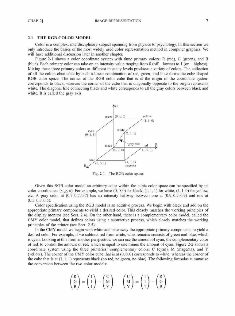
2.1 THE RGB COLOR MODEL
Color is a complex, interdisciplinary subject spanning from physics to psychology. In this section weonly introduce the basics of the most widely used color representation method in computer graphics. Wewill have additional discussion later in another chapter.
Figure 2-1 shows a color coordinate system with three primary colors: R (red), G (green), and B(blue). Each primary color can take on an intensity value ranging from 0 (off—lowest) to 1 (on—highest).Mixing these three primary colors at different intensity levels produces a variety of colors. The collectionof all the colors obtainable by such a linear combination of red, green, and blue forms the cube-shapedRGB color space. The corner of the RGB color cube that is at the origin of the coordinate systemcorresponds to black, whereas the corner of the cube that is diagonally opposite to the origin representswhite. The diagonal line connecting black and white corresponds to all the gray colors between black andwhite. It is called the gray axis.
green
cyan(0, 1, 1)
blue
black
(0, 1, 0)
white,
(0, 0, 0)
(1, 1, 1)
yellow(1,1,0)
red
(1, 0, 0)
(0, 0, 1) (1,0, 1)magenta
Fig. 2-1 The RGB color space.
Given this RGB color model an arbitrary color within the cubic color space can be specified by itscolor coordinates: (r, g, b). For example, we have (0,0,0) for black, (1,1,1) for white, (1,1,0) for yellow,etc. A gray color at (0.7,0.7,0.7) has an intensity halfway between one at (0.9,0.9,0.9) and one at(0.5,0.5,0.5).
Color specification using the RGB model is an additive process. We begin with black and add on theappropriate primary components to yield a desired color. This closely matches the working principles ofthe display monitor (see Sect. 2.4). On the other hand, there is a complementary color model, called theCMY color model, that defines colors using a subtractive process, which closely matches the workingprinciples of the printer (see Sect. 2.5).
In the CMY model we begin with white and take away the appropriate primary components to yield adesired color. For example, if we subtract red from white, what remains consists of green and blue, whichis cyan. Looking at this from another perspective, we can use the amount of cyan, the complementary colorof red, to control the amount of red, which is equal to one minus the amount of cyan. Figure 2-2 shows acoordinate system using the three primaries' complementary colors: C (cyan), M (magenta), and Y(yellow). The corner of the CMY color cube that is at (0,0,0) corresponds to white, whereas the corner ofthe cube that is at (1,1,1) represents black (no red, no green, no blue). The following formulas summarizethe conversion between the two color models:

IMAGE REPRESENTATION [CHAP. 2
red(0, 1, 1)
yellow.
/
magenta
/
white
(0, 1, 0
black
0, 0, 0)
(1, 1, 1)
gray axis
blue(1, 1,0)
cyan C
(1,0,0) '
(0, 0, 1) green (1, 0, 1)
Fig. 2-2 The CMY color space.
2.2 DIRECT CODING
Image representation is essentially the representation of pixel colors. Using direct coding we allocate acertain amount of storage space for each pixel to code its color. For example, we may allocate 3 bits foreach pixel, with one bit for each primary color (see Fig. 2-3). This 3-bit representation allows each primaryto vary independently between two intensity levels: 0 (off) or 1 (on). Hence each pixel can take on one ofthe eight colors that correspond to the corners of the RGB color cube.
bit 1: r
0
0
0
0
1
1
1
1
bit 2: g
0
0
1
1
0
0
1
1
bit 3: b
0
1
0
1
0
1
0
1
color name
black
blue
green
cyan
redmagenta
yellow
white
Fig. 2-3 Direct coding of colors using 3 bits.
A widely accepted industry standard uses 3 bytes, or 24 bits, per pixel, with one byte for each primarycolor. This way we allow each primary color to have 256 different intensity levels, corresponding to binaryvalues from 00000000 to 11111111. Thus a pixel can take on a color from 256 x 256 x 256 or 16.7million possible choices. This 24-bit format is commonly referred to as the true color representation, forthe difference between two colors that differ by one intensity level in one or more of the primaries isvirtually undetectable under normal viewing conditions. Hence a more precise representation involvingmore bits is of little use in terms of perceived color accuracy.
A notable special case of direct coding is the representation of black-and-white (bilevel) and gray-scaleimages, where the three primaries always have the same value and hence need not be coded separately. Ablack-and-white image requires only one bit per pixel, with bit value 0 representing black and 1representing white. A gray-scale image is typically coded with 8 bits per pixel to allow a total of 256intensity or gray levels.
Although this direct coding method features simplicity and has supported a variety of applications, wecan see a relatively high demand for storage space when it comes to the 24-bit standard. For example, a1000 x 1000 true color image would take up three million bytes. Furthermore, even if every pixel in that

CHAP. 2] IMAGE REPRESENTATION
image had a different color, there would only be one million colors in the image. In many applications thenumber of colors that appear in any one particular image is much less. Therefore the 24-bit representation'sability to have 16.7 million different colors appear simultaneously in a single image seems to be somewhatoverkill.
2.3 LOOKUP TABLE
Image representation using a lookup table can be viewed as a compromise between our desire to have alower storage requirement and our need to support a reasonably sufficient number of simultaneous colors.In this approach pixel values do not code colors directly. Instead, they are addresses or indices into a tableof color values. The color of a particular pixel is determined by the color value in the table entry that thevalue of the pixel references.
Figure 2-4 shows a lookup table with 256 entries. The entries have addresses 0 through 255. Eachentry contains a 24-bit RGB color value. Pixel values are now 1 -byte, or 8-bit, quantities. The color of apixel whose value is /, where 0 < / < 255, is determined by the color value in the table entry whoseaddress is /. This 24-bit 256-entry lookup table representation is often referred to as the 8-bit format. Itreduces the storage requirement of a 1000 x 1000 image to one million bytes plus 768 bytes for the colorvalues in the lookup table. It allows 256 simultaneous colors that are chosen from 16.7 million possiblecolors.
L8-bit pixel value
r 8 b
24 bits
255
Fig. 2-4 A 24-bit 256-entry lookup table.
It is important to remember that, using the lookup table representation, an image is defined not only byits pixel values but also by the color values in the corresponding lookup table. Those color values form acolor map for the image.
2.4 DISPLAY MONITOR
Among the numerous types of image presentation or output devices that convert digitally representedimages into visually perceivable pictures is the display or video monitor.
We first take a look at the working principle of a monochromatic display monitor, which consistsmainly of a cathode ray tube (CRT) along with related control circuits. The CRT is a vacuum glass tubewith the display screen at one end and connectors to the control circuits at the other (see Fig. 2-5). Coatedon the inside of the display screen is a special material, called phosphor, which emits light for a period oftime when hit by a beam of electrons. The color of the light and the time period vary from one type of

10 IMAGE REPRESENTATION [CHAP. 2
Electron gun
Electron beam
Scan lines
Horizontal retrace
Connectors
Control electrode
Focusing electrode
Horizontal deflection plates
Vertical deflection plates
Vertical retrace Phosphor-coated screen
Fig. 2-5 Anatomy of a monochromatic CRT.
phosphor to another. The light given off by the phosphor during exposure to the electron beam is known asfluorescence, the continuing glow given off after the beam is removed is known as phosphorescence, andthe duration of phosphorescence is known as the phosphor's persistence.
Opposite to the phosphor-coated screen is an electron gun that is heated to send out electrons. Theelectrons are regulated by the control electrode and forced by the focusing electrode into a narrow beamstriking the phosphor coating at small spots. When this electron beam passes through the horizontal andvertical deflection plates, it is bent or deflected by the electric fields between the plates. The horizontalplates control the beam to scan from left to right and retrace from right to left. The vertical plates controlthe beam to go from the first scan line at the top to the last scan line at the bottom and retrace from thebottom back to the top. These actions are synchronized by the control circuits so that the electron beamstrikes each and every pixel position in a scan line by scan line fashion. As an alternative to thiselectrostatic deflection method, some CRTs use magnetic deflection coils mounted on the outside of theglass envelope to bend the electron beam with magnetic fields.
The intensity of the light emitted by the phosphor coating is a function of the intensity of the electronbeam. The control circuits shut off the electron beam during horizontal and vertical retraces. The intensityof the beam at a particular pixel position is determined by the intensity value of the corresponding pixel inthe image being displayed.
The image being displayed is stored in a dedicated system memory area that is often referred to as theframe buffer or refresh buffer. The control circuits associated with the frame buffer generate proper videosignals for the display monitor. The frequency at which the content of the frame buffer is sent to the displaymonitor is called the refreshing rate, which is typically 60 times or frames per second (60 Hz) or higher. Adetermining factor here is the need to avoid flicker, which occurs at lower refreshing rates when our visualsystem is unable to integrate the light impulses from the phosphor dots into a steady picture. Thepersistence of the monitor's phosphor, on the other hand, needs to be long enough for a frame to remainvisible but short enough for it to fade before the next frame is displayed.
Some monitors use a technique called interlacing to "double" their refreshing rate. In this case onlyhalf of the scan lines in a frame is refreshed at a time, first the odd numbered lines, then the even numberedlines. Thus the screen is refreshed from top to bottom in half the time it would have taken to sweep acrossall the scan lines. Although this approach does not really increase the rate at which the entire screen isrefreshed, it is quite effective in reducing flicker.

CHAP. 2] IMAGE REPRESENTATION 11
Color Display
Moving on to color displays there are now three electron guns instead of one inside the CRT (see Fig.2-6), with one electron gun for each primary color. The phosphor coating on the inside of the displayscreen consists of dot patterns of three different types of phosphors. These phosphors are capable ofemitting red, green, and blue light, respectively. The distance between the center of the dot patterns iscalled the pitch of the color CRT. It places an upper limit on the number of addressable positions on thedisplay area. A thin metal screen called a shadow mask is placed between the phosphor coating and theelectron guns. The tiny holes on the shadow mask constrain each electron beam to hit its correspondingphosphor dots. When viewed at a certain distance, light emitted by the three types of phosphors blendstogether to give us a broad range of colors.
Electron guns
or.
Phosphor dotsin a triad pattern
bluedo"'green
Screen
Shadow mask
Fig. 2-6 Color CRT using a shadow mask.
2.5 PRINTER
Another typical image presentation device is the printer. A printer deposits color pigments onto a printmedia, changing the light reflected from its surface and making it possible for us to see the print result.
Given the fact that the most commonly used print media is a piece of white paper, we can in principleutilize three types of pigments (cyan, magenta, and yellow) to regulate the amount of red, green, and bluelight reflected to yield all RGB colors (see Sect. 2.1). However, in practice, an additional black pigment isoften used due to the relatively high cost of color pigments and the technical difficulty associated withproducing high-quality black from several color pigments.
While some printing methods allow color pigments to blend together, in many cases the various colorpigments remain separate in the form of tiny dots on the print media. Furthermore, the pigments are oftendeposited with a limited number of intensity levels. There are various techniques to achieve the effect ofmultiple intensity levels beyond what the pigment deposits can offer. Most of these techniques can also beadapted by the display devices that we have just discussed in the previous section.
Halftoning
Let's first take a look at a traditional technique called halftoning from the printing industry for bileveldevices. This technique uses variably sized pigment dots that, when viewed from a certain distance, blendwith the white background to give us the sensation of varying intensity levels. These dots are arranged in apattern that forms a 45° screen angle with the horizon (see Fig. 2-7 where the dots are enlarged forillustration). The size of the dots is inversely proportional to the intended intensity level. When viewed at a
12 IMAGE REPRESENTATION [CHAP. 2
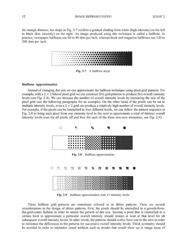
far enough distance, the stripe in Fig. 2-7 exhibits a gradual shading from white (high intensity) on the leftto black (low intensity) on the right. An image produced using this technique is called a halftone. Inpractice, newspaper halftones use 60 to 80 dots per inch, whereas book and magazine halftones use 120 to200 dots per inch.
••••••••••••••••••••••
••••••••. . . • • • • • • • • • • • • • • • _
• . . • • • • • • • • • • • • • • • •
Fig. 2-7 A halftone stripe.
Halftone Approximation
Instead of changing dot size we can approximate the halftone technique using pixel-grid patterns. Forexample, with a 2 x 2 bilevel pixel grid we can construct five grid patterns to produce five overall intensitylevels (see Fig. 2-8). We can increase the number of overall intensity levels by increasing the size of thepixel grid (see the following paragraphs for an example). On the other hand, if the pixels can be set tomultiple intensity levels, even a 2 x 2 grid can produce a relatively high number of overall intensity levels.For example, if the pixels can be intensified to four different levels, we can follow the pattern sequence inFig. 2-8 to bring each pixel from one intensity level to the next to approximate a total of thirteen overallintensity levels (one for all pixels off and four for each of the three non-zero intensities, see Fig. 2-9).
H
•Hill :xxxxxx:::::::::::::::xxxxxx::::::::::::::xxxxxx:::::::::::::::xxxxxx:::::::::::::::-xxxxx"X:::::::::::::::MM MMMM: •.•.•'.•.:••'.•.•.•'.•
Fig. 2-8 Halftone approximation.
E S E E E H S
mxx:::::::::::::::xx::::::::::::::::xx:::::::::::::::xx::::::::::::::1
XXXXXtf
x::::::::x::::::::x::::::::x::::::::x::::::::
x:::::x:::::
Fig. 2-9 Halftone approximation with 13 intensity levels.
These halftone grid patterns are sometimes referred to as dither patterns. There are severalconsiderations in the design of dither patterns. First, the pixels should be intensified in a growth-from-the-grid-center fashion in order to mimic the growth of dot size. Second, a pixel that is intensified to acertain level to approximate a particular overall intensity should remain at least at that level for allsubsequent overall intensity levels. In other words, the patterns should evolve from one to the next in orderto minimize the differences in the patterns for successive overall intensity levels. Third, symmetry shouldbe avoided in order to minimize visual artifacts such as streaks that would show up in image areas of
CHAP. 2] IMAGE REPRESENTATION 13
uniform intensity. Fourth, isolated "on" pixels should be avoided since they are sometimes hard toreproduce.
We can use a dither matrix to represent a series of dither patterns. For example, the following 3 x 3matrix:
represents the order in which pixels in a 3 x 3 grid are to be intensified. For bilevel reproduction, this givesus ten intensity levels from level 0 to level 9, and intensity level I is achieved by turning on all pixels thatcorrespond to values in the dither matrix that are less than I. If each pixel can be intensified to threedifferent levels, we follow the order defined by the matrix to set the pixels to their middle intensity leveland then to their high intensity level to approximate a total of nineteen overall intensity levels.
This halftone approximation technique is readily applicable to the reproduction of color images. Allwe need is to replace the dot at each pixel position with an RGB or CMY dot pattern (e.g., the triad patternshown in Fig. 2-6). If we use a 2 x 2 pixel grid and each primary or its complement can take on twointensity levels, we achieve a total of 5 x 5 x 5 = 125 color combinations.
At this point we can turn to the fact that halftone approximation is a technique that trades spatialresolution for more colors/intensity levels. For a device that is capable of producing images at a resolutionof 400 x 400 pixels per inch, halftone approximation using 2 x 2 dither patterns would mean lowering itsresolution effectively to 200 x 200 pixels per inch.
Dithering
A technique called dithering can be used to approximate halftones without reducing spatial resolution.In this approach the dither matrix is treated very much like a floor tile that can be repeatedly positioned onecopy next to another to cover the entire floor, i.e., the image. A pixel at (x,y) is intensified if the intensitylevel of the image at that position is greater than the corresponding value in the dither matrix.Mathematically, if Dn stands for an n x n dither matrix, the element Dn(i,j) that corresponds to pixelposition (x,y) can be found by i = x mod n andy = y mod n. For example, if we use the 3 x 3 matrixgiven earlier for a bilevel reproduction and the pixel of the image at position (2, 19) has intensity level 5,then the corresponding matrix element is D^(2, 1) = 3, and hence a dot should be printed or displayed atthat location.
It should be noted that, for image areas that have constant intensity, the results of dithering are exactlythe same as the results of halftone approximation. Reproduction differences between these two methodsoccur only when intensity varies.
Error Diffusion
Another technique for continuous-tone reproduction without sacrificing spatial resolution is called theFloyd-Steinberg error diffusion. Here a pixel is printed using the closest intensity the device can deliver.The error term, i.e., the difference between the exact pixel value and the approximated value in thereproduction, is then propagated to several yet-to-be-processed neighboring pixels for compensation. Morespecifically, let S be the source image that is processed in a left-to-right and top-to-bottom pixel order,S(x,y) be the pixel value at location {x,y), and e be S(x,y) minus the approximated value. We update thevalue of the pixel's four neighbors (one to its right and three in the next scan line) as follows:
S(x+\,y) = S(x+\,y) + ae
S(x - \,y - 1) = S(x - \,y - 1) + be
S(x,y- l) = S(x,y- 1) + ce

14 IMAGE REPRESENTATION [CHAP. 2
where parameters a through d often take values -^, ^ , -^, and yg, respectively. These modifications are forthe purpose of using the neighboring pixels to offset the reproduction error at the current pixel location.They are not permanent changes made to the original image.
Consider, for example, the reproduction of a gray scale image (0: black, 255: white) on a bilevel device(level 0: black, level 1: white), if a pixel whose current value is 96 has just been mapped to level 0, we havee = 96 for this pixel location. The value of the pixel to its right is now increased by 96 x -^ = 42 in orderto determine the appropriate reproduction level. This increment tends to cause such neighboring pixel to bereproduced at a higher intensity level, partially compensating the discrepancy brought on by mappingvalue 96 to level 0 (which is lower than the actual pixel value) at the current location. The other threeneighboring pixels (one below and to the left, one immediately below, and one below and to the right)receive 18, 30, and 6 as their share of the reproduction error at the current location, respectively.
Results produced by this error diffusion algorithm are generally satisfactory, with occasionalintroduction of slight echoing of certain image parts. Improved performance can sometimes be obtainedby alternating scanning direction between left-to-right and right-to-left (minor modifications need to bemade to the above formulas).
2.6 IMAGE FILES
A digital image is often encoded in the form of a binary file for the purpose of storage andtransmission. Among the numerous encoding formats are BMP (Windows Bitmap), JPEG (JointPhotographic Experts Group File Interchange Format), and TIFF (Tagged Image File Format). Althoughthese formats differ in technical details, they share structural similarities.
Figure 2-10 shows the typical organization of information encoded in an image file. The file consistslargely of two parts: header and image data. In the beginning of the file header a binary code or ASCIIstring identifies the format being used, possibly along with the version number. The width and height of theimage are given in numbers of pixels. Common image types include black and white (1 bit per pixel), 8-bitgray scale (256 levels along the gray axis), 8-bit color (lookup table), and 24-bit color. Image data formatspecifies the order in which pixel values are stored in the image data section. A commonly used order is leftto right and top to bottom. Another possible order is left to right and bottom to top. Image data format alsospecifies if the RGB values in the color map or in the image are interlaced. When the values are given in aninterlaced fashion, the three primary color components for a particular lookup table entry or a particularpixel stay together consecutively, followed by the three color components for the next entry or pixel. Thusthe color values in the image data section are a sequence of red, green, blue, red, green, blue, etc. When thevalues are given in a non-interlaced fashion, the values of one primary for all table entries or pixels appear
Format/version identification
Image width and height in pixels
Image type
Image data format
Compression type
Color map (if any)
Pixel values
Header
Image data
Fig. 2-10 Typical image file format.

CHAP. 2] IMAGE REPRESENTATION 15
first, then the values of another primary, followed by the values of the third primary. Thus the image dataare in the form of red, r ed , . . . , green, green, . . . , blue, b lue , . . . .
The values in the image data section may be compressed, using such compression algorithms as run-length encoding (RLE). The basic idea behind RLE can be illustrated with a character string"xxxxxxyyzzzz", which takes 12 bytes of storage. Now if we scan the string from left to right forsegments of repeating characters and replace each segment by a 1 -byte repeat count followed by thecharacter being repeated, we convert or compress the given string to "6x2y4z", which takes only 6 bytes.This compressed version can be expanded or decompressed by repeating the character following eachrepeat count to recover the original string.
The length of the file header is often fixed, for otherwise it would be necessary to include lengthinformation in the header to indicate where image data starts (some formats include header length anyway).The length of each individual component in the image data section is, on the other hand, dependent on suchfactors as image type and compression type. Such information, along with additional format-specificinformation, can also be found in the header.
2.7 SETTING THE COLOR ATTRIBUTES OF PIXELS
Setting the color attributes of individual pixels is arguably the most primitive graphics operation. It istypically done by making system library calls to write the respective values into the frame buffer. Anaggregate data structure, such as a three-element array, is often used to represent the three primary colorcomponents. Regardless of image type (direct coding versus lookup table), there are two possible protocolsfor the specification of pixel coordinates and color values.
In one protocol the application provides both coordinate information and color informationsimultaneously. Thus a call to set the pixel at location (x, y) in a 24-bit image to color (r, g, b) wouldlook like
setPixel(x, y, rgb)
where rgb is a three-element array with rgb[0] = r, rgb[l] = g, and rgb[2] = b. On the other hand, if theimage uses a lookup table then, assuming that the color is defined in the table, the call would look like
setPixel(x, y, i)
where / is the address of the entry containing (r, g, b).Another protocol is based on the existence of a current color, which is maintained by the system and
can be set by calls that look like
setColor(rgi)
for direct coding, or
setColor(Z)
for the lookup table representation. Calls to set pixels now need only to provide coordinate information andwould look like
setPixel(x, y)
for both image types. The graphics system will automatically use the most recently specified current colorto carry out the operation.
Lookup table entries can be set from the application by a call that looks like
setEntry(/, rgb)
which puts color (r, g, b) in the entry whose address is /. Conversely, values in the lookup table can be readback to the application with a call that looks like
getEntry(/, rgb)
which returns the color value in entry / through array parameter rgb.

16 IMAGE REPRESENTATION [CHAP. 2
There are sometimes two versions of the calls that specify RGB values. One takes RGB values asfloating point numbers in the range of [0.0,1.0], whereas the other takes them as integers in the range of[0,255]. Although the floating point version is handy when the color values come from some continuousformula, the floating point values are mapped by the graphics system into integer values before beingwritten into the frame buffer.
In order to provide basic support for pixel-based image-processing operations there are calls that looklike
getPixel(x, y, rgb)
for direct coding or
getPixel(x, y, i)
for the lookup table representation to return the color or index value of the pixel at (x, y) back to theapplication.
There are also calls that read and write rectangular blocks of pixels. A useful example would be a callto set all pixels to a certain background color. Assuming that the system uses a current color we would firstset the current color to be the desired background color, and then make a call that looks like:
clear()
to achieve the goal.
2.8 EXAMPLE: VISUALIZING THE MANDELBROT SET
An elegant and illustrative example showing the construction of beautiful images by setting the colorattributes of individual pixels directly from the application is the visualization of the Mandelbrot set. Thisremarkable set is based on the following transformation:
xn+l =xl+z
where both x and z represent complex numbers. For readers who are unfamiliar with complex numbers itsuffices to know that a complex number is defined in the form of a + bi. Here both a and b are realnumbers; a is called the real part of the complex number and b the imaginary part (identified by the specialsymbol /). The magnitude of a + bi, denoted by \a + bi\, is equal to the square root of a2 + b2. The sum oftwo complex numbers a + bi and c + di is defined to be (a + c) + (b + d)i. The product of a + bi andc + di is defined to be (ac — bd) + {ad + bc)i. Thus the square of a + bi is equal to (a2 — b2) + labi. Forexample, the sum of 0.5 + 2.0/ and 1.0 — 1.0/ is 1.5 + 1.0/. The product of the two is 2.5 + 1.5/. Thesquare of 0.5 + 2.0/ is -3.75 + 2.0/ and the square of 1.0 - 1.0/ is 0.0 - 2.0/.
The Mandelbrot set is the set of complex numbers z that do not diverge under the above transformationwith x0 = 0 (both the real and imaginary parts of x0 are 0). In other words, to determine if a particularcomplex number z is a member of the set, we begin with x0 = 0, followed by x\ = x\ + z,x2 = x2 + z, . . . , xn+l = x2 + z , . . . . If |x| goes towards infinity when n increases, then z is not a mem-ber. Otherwise, z belongs to the Mandelbrot set.
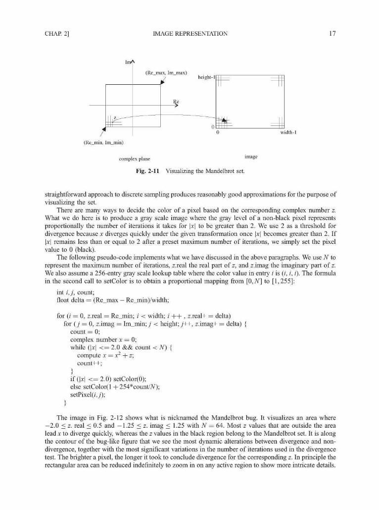
Figure 2-11 shows how to produce a discrete snapshot of the Mandelbrot set. On the left hand side isthe complex plane where the horizontal axis Re measures the real part of complex numbers and the verticalaxis Im measures the imaginary part. Hence an arbitrary complex number z corresponds to a point in thecomplex plane. Our goal is to produce an image of width by height (in numbers of pixels) that depicts the zvalues in a rectangular area defined by (Re_min, Im_min) and (Re_max, Im_max). This rectangular areahas the same aspect ratio as the image so as not to introduce geometric distortion. We subdivide the area tomatch the pixel grid in the image. The color of a pixel, shown as a little square in the pixel grid, isdetermined by the complex number z that corresponds to the lower left corner of the little square. Althoughonly width x height points in the complex plane are used to compute the image, this relatively
CHAP. 2] IMAGE REPRESENTATION 17
(Re_max, Im_max)height-1
Re
width-1
(Re_min, Im_min)
complex plane
Fig. 2-11 Visualizing the Mandelbrot set.
straightforward approach to discrete sampling produces reasonably good approximations for the purpose ofvisualizing the set.
There are many ways to decide the color of a pixel based on the corresponding complex number z.What we do here is to produce a gray scale image where the gray level of a non-black pixel representsproportionally the number of iterations it takes for \x\ to be greater than 2. We use 2 as a threshold fordivergence because x diverges quickly under the given transformation once \x\ becomes greater than 2. Ifx\ remains less than or equal to 2 after a preset maximum number of iterations, we simply set the pixel
value to 0 (black).The following pseudo-code implements what we have discussed in the above paragraphs. We use N to
represent the maximum number of iterations, z.real the real part of z, and z.imag the imaginary part of z.We also assume a 256-entry gray scale lookup table where the color value in entry / is (/, /, /). The formulain the second call to setColor is to obtain a proportional mapping from [0,N] to [1,255]:
int i,j, count;float delta = (Re_max — Re_min)/width;
for (/ = 0, z.real = Re_min; / < width; / + + , z.real+ = delta)for (j = 0, z.imag = Im_min; j < height; j++, z.imag+ = delta) {
count = 0;complex number x = 0;while (\x\ <= 2.0 && count < N) {
compute x = x2 + z;count++;
}if (\x\ < = 2.0) setColor(O);else setColor(l + 254*count/7V);setPixel(/,y);
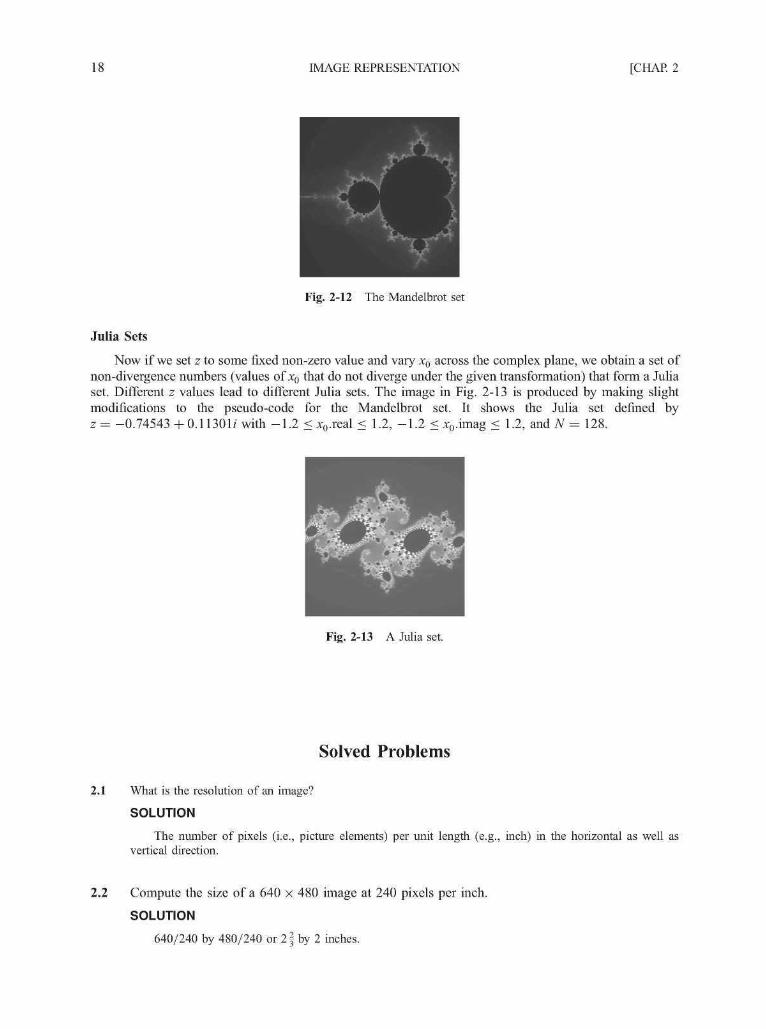
The image in Fig. 2-12 shows what is nicknamed the Mandelbrot bug. It visualizes an area where—2.0 < z. real < 0.5 and —1.25 < z. imag < 1.25 with N = 64. Most z values that are outside the arealead x to diverge quickly, whereas the z values in the black region belong to the Mandelbrot set. It is alongthe contour of the bug-like figure that we see the most dynamic alterations between divergence and non-divergence, together with the most significant variations in the number of iterations used in the divergencetest. The brighter a pixel, the longer it took to conclude divergence for the corresponding z. In principle therectangular area can be reduced indefinitely to zoom in on any active region to show more intricate details.
18 IMAGE REPRESENTATION [CHAP. 2
Fig. 2-12 The Mandelbrot set
Julia Sets
Now if we set z to some fixed non-zero value and vary x0 across the complex plane, we obtain a set ofnon-divergence numbers (values of x0 that do not diverge under the given transformation) that form a Juliaset. Different z values lead to different Julia sets. The image in Fig. 2-13 is produced by making slightmodifications to the pseudo-code for the Mandelbrot set. It shows the Julia set defined byz = -0 .74543+ 0.11301/with -1 .2 < xo.real < 1.2, -1 .2 < xo.imag < 1.2, and TV = 128.
Fig. 2-13 A Julia set.
Solved Problems
2.1 What is the resolution of an image?
SOLUTION
The number of pixels (i.e., picture elements) per unit length (e.g., inch) in the horizontal as well asvertical direction.
2.2 Compute the size of a 640 x 480 image at 240 pixels per inch.
SOLUTION
640/240 by 480/240 or 2 § by 2 inches.

CHAP. 2] IMAGE REPRESENTATION 19
2.3 Compute the resolution of a 2 x 2 inch image that has 512 x 512 pixels.
SOLUTION
512/2 or 256 pixels per inch.
2.4 What is an image's aspect ratio?
SOLUTION
The ratio of its width to its height, measured in unit length or number of pixels.
2.5 If an image has a height of 2 inches and an aspect ratio of 1.5, what is its width?
SOLUTION
width = 1.5 x height = 1.5 x 2 = 3 inches.
2.6 If we want to resize a 1024 x 768 image to one that is 640 pixels wide with the same aspect ratio,what would be the height of the resized image?
SOLUTION
height = 640 x 768/1024 = 480.
2.7 If we want to cut a 512 x 512 sub-image out from the center of an 800 x 600 image, what are thecoordinates of the pixel in the large image that is at the lower left corner of the small image?
SOLUTION
[(800 - 512)/2, (600 - 512)/2] = (144, 44).
2.8 Sometimes the pixel at the upper left corner of an image is considered to be at the origin of the pixelcoordinate system (a left-handed system). How to convert the coordinates of a pixel at (x, y) in thiscoordinate system into its coordinates (x ' , / ) in the lower-left-corner-as-origin coordinate system (aright-handed system)?
SOLUTION
(x',/) = (x, m — y — 1) where m is the number of pixels in the vertical direction.
2.9 Find the CMY coordinates of a color at (0.2,1,0.5) in the RGB space.
SOLUTION
(1 - 0.2, 1 - 1 , 1 - 0.5) = (0.8, 0, 0.5).
2.10 Find the RGB coordinates of a color at (0.15,0.75,0) in the CMY space.
SOLUTION
(1 - 0.15, 1 - 0.75, 1 - 0) = (0.85, 0.25, 1).
2.11 If we use direct coding of RGB values with 2 bits per primary color, how many possible colors dowe have for each pixel?

20 IMAGE REPRESENTATION [CHAP. 2
SOLUTION
22 x 22 x 22 = 4 x 4 x 4 = 64.
2.12 If we use direct coding of RGB values with 10 bits per primary color, how many possible colors dowe have for each pixel?
SOLUTION
210 x 210 x 210 = 10243 = 1073,741,824 > 1 billion.
2.13 The direct coding method is flexible in that it allows the allocation of a different number of bits toeach primary color. If we use 5 bits each for red and blue and 6 bits for green for a total of 16 bitsper pixel, how many possible simultaneous colors do we have?
SOLUTION
25 x 2 5 x 2 6 = 2 1 6 = 65,536.
2.14 If we use 12-bit pixel values in a lookup table representation, how many entries does the lookuptable have?
SOLUTION
212 = 4096.
2.15 If we use 2-byte pixel values in a 24-bit lookup table representation, how many bytes does thelookup table occupy?
SOLUTION
216 x 24/8 = 65,536 x 3 = 196,608.
2.16 True or false: fluorescence is the term used to describe the light given off by a phosphor after it hasbeen exposed to an electron beam. Explain your answer.
SOLUTION
False. Phosphorescence is the correct term. Fluorescence refers to the light given off by a phosphor whileit is being exposed to an electron beam.
2.17 What is persistence?
SOLUTION
The duration of phosphorescence exhibited by a phosphor.
2.18 What is the function of the control electrode in a CRT?
SOLUTION
Regulate the intensity of the electron beam.
2.19 Name the two methods by which an electron beam can be bent?
SOLUTION
Electrostatic deflection and magnetic deflection.

CHAP. 2] IMAGE REPRESENTATION 21
2.20 What do you call the path the electron beam takes when returning to the left side of the CRT screen?
SOLUTION
Horizontal retrace.
2.21 What do you call the path the electron beam takes at the end of each refresh cycle?
SOLUTION
Vertical retrace.
2.22 What is the pitch of a color CRT?
SOLUTION
The distance between the center of the phosphor dot patterns on the inside of the display screen.
2.23 Why do many color printers use black pigment?
SOLUTION
Color pigments (cyan, magenta, and yellow) are relatively more expensive and it is technically difficult toproduce high-quality black using several color pigments.
2.24 Show that with an n x n pixel grid, where each pixel can take on m intensity levels, we canapproximate n x n x (m — 1) + 1 overall intensity levels.
SOLUTION
Since the n x n pixels can be set to a non-zero intensity value one after another to produce n x n overallintensity levels, and there are m — 1 non-zero intensity levels for the individual pixels, we can approximate atotal o f B X « x ( m - 1) non-zero overall intensity levels. Finally we need to add one more overall intensitylevel that corresponds to zero intensity (all pixels off).
2.25 Represent the grid patterns in Fig. 2-8 with a dither matrix.
SOLUTION
0 23 1
2.26 What are the error propagation formulas for a top-to-bottom and right-to-left scanning order in theFloyd-Steinberg error diffusion algorithm?
SOLUTION
S{x- \,y) = Six- l,y)
Six+ \,y- 1) = Six+ \,y- 1) + be
Six,y- l) = Six,y- 1) + ce
Six- \,y- \) = Six- \,y- \) + de
2.27 What is RLE?
SOLUTION
RLE stands for run-length encoding, a technique for image data compression.

22 IMAGE REPRESENTATION [CHAP. 2
2.28 Follow the illustrative example in the text to reconstruct the string that has been compressed to"981435" using RLE.
SOLUTION
"8888888884555"
2.29 If an 8-bit gray scale image is stored uncompressed in sequential memory or in an image file in left-to-right and bottom-to-top pixel order, what is the offset or displacement of the byte for the pixel at(x,y) from the beginning of the memory segment or the file's image data section?
SOLUTION
offset = y x n +x where n is the number of pixels in the horizontal direction.
2.30 What if the image in Prob. 2.29 is stored in left-to-right and top-to-bottom order?
SOLUTION
offset = (m—y— \)n + x where n and m are the number of pixels in the horizontal and verticaldirection, respectively.
2.31 Develop a pseudo-code segment to initialize a 24-bit 256-entry lookup table with gray-scale values.
SOLUTION
int i, rgb\y\\for (z = 0; z < 256; z++) {
rgb[0] = rgb[l] = rgb[2] = i;setEntry(z, rgb):
2.32 Develop a pseudo-code segment to swap the red and green components of all colors in a 256-entrylookup table.
SOLUTION
int i, x, rgb[3]:for (z = 0; z < 256; z++) {
getEntry(z, rgb);x = rgb[0];rgb[0] = rgb[\\,rgb[\] = x;setEntry(z', rgb):
2.33 Develop a pseudo-code segment to draw a rectangular area ofwxh (in number of pixels) that startsat (x, y) using color rgb.
SOLUTION
int i,j;setColor(rgb);for (j =y;j < y + h; j++)
for (i = x; i < x + w; i++) setPixel(z',/);

CHAP. 2] IMAGE REPRESENTATION 23
2.34 Develop a pseudo-code segment to draw a triangular area with the three vertices at (x, y), (x, y + t),and (x + t, y), where integer t > 0, using color rgb.
SOLUTION
int ij;setColor(rgb);for (j = y; j <=y + t;j++)
for (i = x; i <= x +y + t —j; i++) setPixel(z',y);
2.35 Develop a pseudo-code segment to reset every pixel in an image that is in the 24-bit 256-entrylookup table representation to its complementary color.
SOLUTION
int i, rgb[3];for (z = 0; z < 256; z++) {
getEntry(z, rgb);rgb[0] = 255 - rgb[0];rgb[l] = 255 - rgb[l];rgb[2] = 255 - rgb[2];setEntry(z, rgb):
2.36 What if the image in Prob. 2.35 is in the 24-bit true color representation?
SOLUTION
int i,j, rgb[3];for (j = 0;j< height; j++)
for (z = 0; z < width; z++) {getPixel(z',7, rgb);
rgb[0] = 255 - rgb[0];rgb[l] = 255 - rgb[l];rgb[2] = 255 - rgb[2];setPixel(z,7, rgb);
2.37 Calculate the sum and product of 0.5 + 2.0/ and 1.0— 1.0/.
SOLUTION
(0.5 + 1.0) + (2.0 + (-1.0))z = 1.5 + l.Oz(0.5 x 1.0-2.0 x (-1.0))+ (0.5 x (-1.0) +2.0 x 1.0)z = 2.5 + 1.5z
2.38 Calculate the square of the two complex numbers in Prob. 2.37.
SOLUTION
(0.52 - 2.02) + 2 x 0.5 x 2.0/ = -3.75 + 2.0/(1.02 - (-1.0)2) + 2 x 1.0 x (—1.0)? = 0.0 — 2.0z
2.39 Show that 1 + 254 x count/N provides a proportional mapping from count in [0, N] to c in[1,255].

24 IMAGE REPRESENTATION [CHAP. 2
SOLUTION
Proportional mapping means that we want
(c - l)/(255 - 1) = (count - 0)/(N - 0)
Hence c = 1 + 254 x count/TV.
2.40 Modify the pseudo code for visualizing the Mandelbrot set to visualize the Julia sets.
SOLUTION
int i,j, count:float delta = (Re_max — Re_min)/width:for (z = 0, x.real = Re_min; i < width; z++, x.real+ = delta)
for (y = 0, x.imag = Im_min; j < height; j++, x.imag+ = delta) {count = 0;while (|x| < 2.0 && count < N) {
compute x = x + z;count++:
}if (|x| <2 .0) setColor(O);else setColor(l + 254*count/A0;setPixel(z,y);
2.41 How to avoid the calculation of square root in an actual implementation of the algorithms forvisualizing the Mandelbrot and Julia sets?
SOLUTION
Test for |x|2 < 4.0 instead of |x| < 2.0.
Supplementary Problems
2.42 Can a 5 by 3^ inch image be presented at 6 by 4 inch without introducing geometric distortion?
2.43 Refering to Prob. 2.42, what if the original is 5 | by 3^ inch?
2.44 Given the portrait image of a person, describe a simple way to make the person look more slender.
2.45 An RGB color image can be converted to a gray-scale image using the formula 0.299R + 0.587G + 0.114Bfor gray levels (see Chap. 11, Sec. 11.1 under "The NTSC YIQ Color Model"). Assuming thatgetPixel(x, y, rgb) now reads pixel values from a 24-bit input image and setPixel(x, y, i) assigns pixelvalues to an output image that uses a gray-scale lookup table, develop a pseudo-code segment to convertthe input image to a gray-scale output image.
CHAPTER 3
Scan Conversion
Many pictures, from 2D drawings to projected views of 3D objects, consist of graphical primitivessuch as points, lines, circles, and filled polygons. These picture components are often defined in acontinuous space at a higher level of abstraction than individual pixels in the discrete image space. Forinstance, a line is defined by its two endpoints and the line equation, whereas a circle is defined by itsradius, center position, and the circle equation. It is the responsibility of the graphics system or theapplication program to convert each primitive from its geometric definition into a set of pixels that make upthe primitive in the image space. This conversion task is generally referred to as scan conversion orrasterization.
The focus of this chapter is on the mathematical and algorithmic aspects of scan conversion. Wediscuss ways to handle several commonly encountered primitives including points, lines, circles, ellipses,characters, and filled regions in an efficient and effective manner. We also discuss techniques that help to"smooth out" the discrepancies between the original element and its discrete approximation. Theimplementation of these algorithms and mathematical solutions (and many others in subsequent chapters)varies from one system to another and can be in the form of various combinations of hardware, firmware,and software.
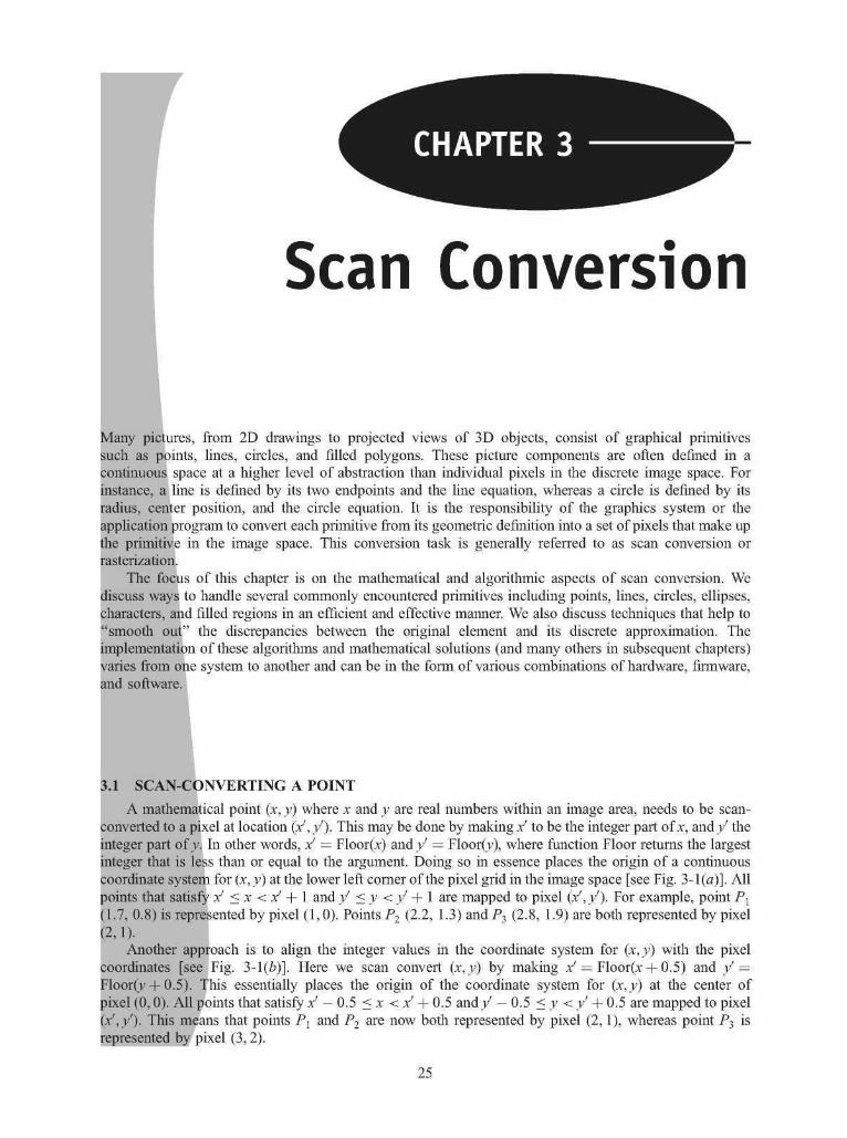
SCAN-CONVERTING A POINT
A mathematical point (x, y) where x and y are real numbers within an image area, needs to be scan-converted to a pixel at location (x',y'). This may be done by making x' to be the integer part of x, and y' theinteger part of y. In other words, x' = Floor(x) and j ' = Floor(y), where function Floor returns the largestinteger that is less than or equal to the argument. Doing so in essence places the origin of a continuouscoordinate system for (x, y) at the lower left corner of the pixel grid in the image space [see Fig. 3-l(a)]. Allpoints that satisfy x1 < x < x1 + 1 and / < y < / + 1 are mapped to pixel (x ' , / ) . For example, point Px
(1.7, 0.8) is represented by pixel (1,0). Points P2 (2.2, 1.3) and P3 (2.8, 1.9) are both represented by pixel
(2,1).Another approach is to align the integer values in the coordinate system for (x,y) with the pixel
coordinates [see Fig. 3-1(6)]. Here we scan convert (x,y) by making x' = Floor(x + 0.5) and / =Floor(y + 0.5). This essentially places the origin of the coordinate system for (x,y) at the center ofpixel (0,0). All points that satisfy x' — 0.5 < x < x' + 0.5 andy — 0.5 <y <y' + 0.5 are mapped to pixel(x',y'). This means that points P\ and P2 are now both represented by pixel (2,1), whereas point P^ isrepresented by pixel (3,2).
25

26 SCAN CONVERSION [CHAP. 3
t
Pixel grid
1P2(2.2,
1.7, 0.8
(2.8, 1.9)
1.3)
0.0 1.0 2.0 t
/
2.0
1.0
0.0 1.0
•Pi
P1(1.7,
2.0
Pi
A (2.8,
(2.2, 1.3)
0.8)
3.0
xel grid
1.9)
. 00 1
Pixelcoordinates
• 0 1 2 Pixel / •coordinates
(a) (b)
Fig. 3-1 Scan-converting points.
We will assume, in the following sections, that this second approach to coordinate system alignment isused. Thus all pixels are centered at the integer values of a continuous coordinate system where abstractgraphical primitives are defined.
3.2 SCAN-CONVERTING A LINE
A line in computer graphics typically refers to a line segment, which is a portion of a straight line thatextends indefinitely in opposite directions. It is defined by its two endpoints and the line equationy = mx + b, where m is called the slope and b the y intercept of the line. In Fig. 3-2 the two endpoints aredescribed by Pi(xl,yl) and P2(x2,y2). The line equation describes the coordinates of all the points that liebetween the two endpoints.
'•Ax2,y2)
Fig. 3-2 Defining a line.
A note of caution: this slope-intercept equation is not suitable for vertical lines. Horizontal, vertical,and diagonal (\m\ = 1) lines can, and often should, be handled as special cases without going through thefollowing scan-conversion algorithms. These commonly used lines can be mapped to the image space in astraightforward fashion for high execution efficiency.
Direct Use of the Line Equation
A simple approach to scan-converting a line is to first scan-convert Pj and P2 to pixel coordinates(x[, y\) and (x'2, y'2), respectively; then set m = (y'2 — y\)/ (x'2 — x[) and b = y\ — mx[. If | m \ < 1, then for

CHAP. 3] SCAN CONVERSION 27
every integer value of x between and excluding x[ and xf2, calculate the corresponding value of y using theequation and scan-convert (x, y). If \m\ > 1, then for every integer value of y between and excluding y[ andy'2, calculate the corresponding value of x using the equation and scan-convert (x,y).
While this approach is mathematically sound, it involves floating-point computation (multiplicationand addition) in every step that uses the line equation since m and b are generally real numbers. Thechallenge is to find a way to achieve the same goal as quickly as possible.
DDA Algorithm
The digital differential analyzer (DDA) algorithm is an incremental scan-conversion method. Such anapproach is characterized by performing calculations at each step using results from the preceding step.Suppose at step / we have calculated (xt, yt) to be a point on the line. Since the next point (xi+1, yi+i) shouldsatisfy Ay/Ax = m where Ay = yi+l — yi and Ax = x i+1 — xt, we have
or
These formulas are used in the DDA algorithm as follows. When \m\ < 1, we start with x = x'l(assuming that x'j < x!2) and y = y\, and set Ax = 1 (i.e., unit increment in the x direction). The ycoordinate of each successive point on the line is calculated using yi+l = yi + m. When \m\ > 1, we startwith x = x[ and j = y[ (assuming thatjj < y'2), and set Ay = 1 (i.e., unit increment in the y direction). Thex coordinate of each successive point on the line is calculated using x i+1 = x ; + l/m. This processcontinues until x reaches x'2 (for the \m\ < 1 case) or y reaches y'2 (for the \m\ > 1 case) and all pointsfound are scan-converted to pixel coordinates.
The DDA algorithm is faster than the direct use of the line equation since it calculates points on theline without any floating-point multiplication. However, a floating-point addition is still needed indetermining each successive point. Furthermore, cumulative error due to limited precision in thefloating-point representation may cause calculated points to drift away from their true position when theline is relatively long.
Bresenham's Line Algorithm
Bresenham's line algorithm is a highly efficient incremental method for scan-converting lines. Itproduces mathematically accurate results using only integer addition, subtraction, and multiplication by 2,which can be accomplished by a simple arithmetic shift operation.
The method works as follows. Assume that we want to scan-convert the line shown in Fig. 3-3 where0 < m < 1. We start with pixel P[(x'l,y'l), then select subsequent pixels as we work our way to the right,one pixel position at a time in the horizontal direction towards P'2(x'2,y2). Once a pixel is chosen at anystep, the next pixel is either the one to its right (which constitutes a lower bound for the line) or the one toits right and up (which constitutes an upper bound for the line) due to the limit on m. The line is bestapproximated by those pixels that fall the least distance from its true path between P[ and P'2.
Using the notation of Fig. 3-3, the coordinates of the last chosen pixel upon entering step / are (x^y^.Our task is to choose the next one between the bottom pixel S and the top pixel T. If S is chosen, we havexi+i = xi + 1 and yi+i =yt. If T is chosen, we have x i+1 =x ; -+ 1 and yi+i =yi + \. The actual ycoordinate of the line at x = x i+1 is y = mxi+l + b = rn(xi + 1) + b. The distance from S to the actual linein the y direction is s = y — yt. The distance from T to the actual line in the y direction is t = (yi• + 1) — y.
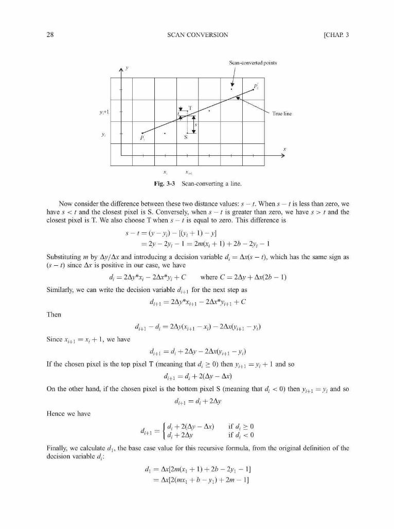
28 SCAN CONVERSION [CHAP. 3
Scan-converted points
/
p\
1
•
1
s
S
1 1
j
1
P2
1
True line
Fig. 3-3 Scan-converting a line.
Now consider the difference between these two distance values: s — t. When s — t is less than zero, wehave s < t and the closest pixel is S. Conversely, when s — t is greater than zero, we have s > t and theclosest pixel is T. We also choose T when s — t is equal to zero. This difference is
= 2y- 2yt - 1 = 2m(Xi +l) + 2b- 2yt - 1
Substituting m by Ay/Ax and introducing a decision variable di = Ax(s — t), which has the same sign as(s — t) since Ax is positive in our case, we have
dt = 2Ay*xt - 2Ax*yt + C where C = 2Ay + Ax(2b - 1)
Similarly, we can write the decision variable di+\ for the next step as
di+l = 2Ay%+l - 2Ax*yi+l + C
Then
4+1 - di = 2Ay(xi+l - xt) - 2Ax(yi+l - yt)
Since xi+l = xi + 1, we have
di+l = + 2Ay - 2Ax(yi+l - yt)
If the chosen pixel is the top pixel T (meaning that di > 0) then yi+l = yi + 1 and so
di+l = + 2{Ay - Ax)
On the other hand, if the chosen pixel is the bottom pixel S (meaning that di < 0) then yi+l = yt and so
di+i = dt + 2Ay
Hence we have
| di + 2{Ay - Ax) if di > 0i+1 \di + 2Ay if dt < 0
Finally, we calculate dx, the base case value for this recursive formula, from the original definition of thedecision variable dt:
dx = Ax[2m(xl + l) + 2b- 2yx - 1]
= Ax[2(mxl +b -yl) + 2m- I]

CHAP. 3] SCAN CONVERSION 29
Since mxl +b — yl = 0, we have
dx = 2 Ay - Ax
In summary, Bresenham's algorithm for scan-converting a line from P[(x'l,y'l) to P'2(x'2,y'2) withx'j < xr
2 and 0 < m < 1 can be stated as follows:
int x = x[, y = yfx;int dx = x'2- x\, dy=y'2- y[, dT = 2(dy - dx), dS = 2dy;int d = 2dy — dx;setPixel(x, y);while (x < Xj) {
if (d < 0)d = d + dS;
else {
d = d + dT;}setPixel(x, y);
}
Here we first initialize decision variable d and set pixel P[. During each iteration of the while loop, weincrement x to the next horizontal position, then use the current value of d to select the bottom or top(increment y) pixel and update d, and at the end set the chosen pixel.
As for lines that have other m values we can make use of the fact that they can be mirrored eitherhorizontally, vertically, or diagonally into this 0° to 45° angle range. For example, a line from (x'l,y'l) to{x'2,y2) with —1 < m < 0 has a horizontally mirrored counterpart from (x'1; — / j ) to (xf2, —y2) with0 < m < 1. We can simply use the algorithm to scan-convert this counterpart, but negate the y coordinateat the end of each iteration to set the right pixel for the line. For a line whose slope is in the 45° to 90°range, we can obtain its mirrored counterpart by exchanging the x and y coordinates of its endpoints. Wecan then scan-convert this counterpart but we must exchange x and y in the call to setPixel.
3.3 SCAN-CONVERTING A CIRCLE
A circle is a symmetrical figure. Any circle-generating algorithm can take advantage of the circle'ssymmetry to plot eight points for each value that the algorithm calculates. Eight-way symmetry is used byreflecting each calculated point around each 45° axis. For example, if point 1 in Fig. 3-4 were calculatedwith a circle algorithm, seven more points could be found by reflection. The reflection is accomplished byreversing the x, y coordinates as in point 2, reversing the x, y coordinates and reflecting about the y axis asin point 3, reflecting about the y axis as in point 4, switching the signs of x and j as in point 5, reversing thex, y coordinates, reflecting about the y axis and reflecting about the x axis as in point 6, reversing the x, ycoordinates and reflecting about the y axis as in point 7, and reflecting about the x axis as in point 8.
To summarize:
Pl=(x,y) P5 = (-x,-yP2 = (y,x) P6 = (-y,-x
P3 = (-y, x) P1 = (y, -x)

30 SCAN CONVERSION [CHAP. 3
(-2, 8)i-y,x)O
(2,8)
(-8, 2)( - * , y)
(-y. -x)(-2, -8)
Fig. 3-4 Eight-way symmetry of a circle.
Defining a Circle
There are two standard methods of mathematically defining a circle centered at the origin. The firstmethod defines a circle with the second-order polynomial equation (see Fig. 3-5)
y2=r2-x}
where x = the x coordinate
y = the y coordinate
r = the circle radius
With this method, each x coordinate in the sector from 90° to 45°, is found by stepping x from 0 tor/\/2, and each y coordinate is found by evaluating \/r2 — x2 for each step of x. This is a very inefficientmethod, however, because for each point both x and r must be squared and subtracted from each other; thenthe square root of the result must be found.
y
f '• r
P = (x, V/
\
i x
Fig. 3-5 Circle defined with a second-degree polynomial equation.

CHAP. 3] SCAN CONVERSION 31
The second method of defining a circle makes use of trigonometric functios (see Fig. 3-6):
x = r cos 6 y = r sin 6
where 6 = current angle
r = circle radius
x = x coordinate
y = y coordinate
By this method, 6 is stepped from 6 to n/4, and each value of x and y is calculated. However,computation of the values of sin 6 and cos 6 is even more time-consuming than the calculations required bythe first method.
P=(r cos 9, rsin 9)
Fig. 3-6 Circle defined with trigonometric functions.
Bresenham's Circle Algorithm
If a circle is to be plotted efficiently, the use of trigonometric and power functions must be avoided.And, as with the generation of a straight line, it is also desirable to perform the calculations necessary tofind the scan-converted points with only integer addition, subtraction, and multiplication by powers of 2.Bresenham s circle algorithm allows these goals to be met.
Scan-converting a circle using Bresenham's algorithm works as follows. If the eight-way symmetry ofa circle is used to generate a circle, points will only have to be generated through a 45° angle. And, if pointsare generated from 90° to 45°, moves will be made only in the +x and — y directions (see Fig. 3-7).
The best approximation of the true circle will be described by those pixels in the raster that fall theleast distance from the true circle. Examine Fig. 3-8. Notice that, if points are generated from 90° and 45°,each new point closest to the true circle can be found by taking either of two actions: (1) move in the xdirection one unit or (2) move in the x direction one unit and move in the negative y direction one unit.Therefore, a method of selecting between these two choices is all that is necessary to find the points closestto the true circle.
Assume that (x^y^) are the coordinates of the last scan-converted pixel upon entering step / (see Fig.3-8). Let the distance from the origin to pixel T squared minus the distance to the true circlesquared = D(T). Then let the distance from the origin to pixel S squared minus the distance to the true

32 SCAN CONVERSION [CHAP. 3
Fig. 3-7 Circle scan-converted with Bresenham's algorithm.
circle squared = D(S). As the coordinates of T are (xt + \,yt) and those of S are (xt + \,yt — X), thefollowing expressions can be developed:
D(T) = (xt + I)2 2 2Vi - r
This function D provides a relative measurement of the distance from the center of a pixel to the truecircle. Since D(T) will always be positive (T is outside the true circle) and D(S) will always be negative (Sis inside the true circle), a decision variable di may be defined as follows:
Therefore
Fig. 3-8 Choosing pixels in Bresenham's circle algorithm.

CHAP. 3] SCAN CONVERSION 33
When dt < 0, we have |D(T)| < |D(S)| and pixel T is chosen. When dt > 0, we have |D(T)| > |D(S)|and pixel S is selected. We can also write the decision variable di+l for the next step:
Hence
di+l = 2(xi+l + I)2 + y2i+l + (yi+l - I)2 - 2?
di+l - di = 2(xi+l + I)2 + yf+l + (yi+l - I)2 - 2(x, + I)2 - yf - (y, - I)2
Since xi+l = xi + 1, we have
4+1 = 4 + 4x,- + 2(y2+1 - y2) - 2(yi+1 - yt) + 6
If T is the chosen pixel (meaning that di < 0) then yi+l = yi and so
4+1 = di + 4x;- + 6
On the other hand, if S is the chosen pixel (meaning that dt > 0) then yi+l = yi• — 1 and so
di+l =di + A(xi-yi)+\Q
Hence we have
f 4 + 4xt + 6 if 4 < 0i+1 ~ \ d, + 4(x,- - j ; ) + 10 if d, > 0
Finally, we set (0, r) to be the starting pixel coordinates and compute the base case value dx for thisrecursive formula from the original definition of d{.
dx = 2(0 + I)2 + r2 + {r- I)2 - 2r2 = 3 - 2r
We can now summarize the algorithm for generating all the pixel coordinates in the 90° to 45° octantthat are needed when scan-converting a circle of radius r:
int x = 0, y = r, d = 3 — 2r;while (x <= y) {
setPixel(x, y);if (d < 0)
d = d + Ax + 6;else {
d = d + 4(x-y)+lO;
y—;
Note that during each iteration of the while loop we first set a pixel whose position has already beendetermined, starting with (0, r). We then test the current value of decision variable d in order to update dand determine the proper y coordinate of the next pixel. Finally we increment x.
Midpoint Circle Algorithm
We present another incremental circle algorithm that is very similar to Bresenham's approach. It isbased on the following function for testing the spatial relationship between an arbitrary point (x, y) and acircle of radius r centered at the origin:
< 0 (x, y) inside the circlef(x, y) = xl +yl — rl \ = 0 (x, y) on the circle
> 0 (x, y) outside the circle
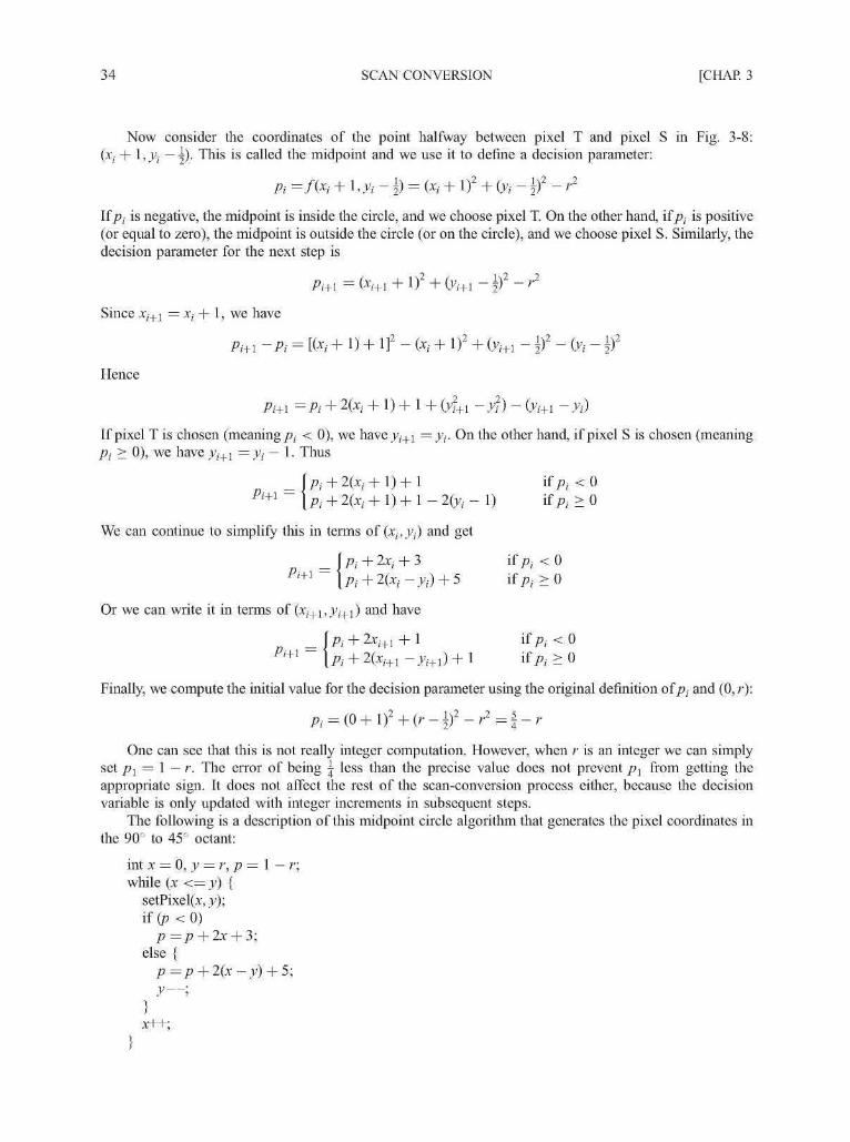
34 SCAN CONVERSION [CHAP. 3
Now consider the coordinates of the point halfway between pixel T and pixel S in Fig. 3-8:(xt + 1, yi• — j). This is called the midpoint and we use it to define a decision parameter:
Pi =f(xi + \,yi-\) = (xt + I)2 + (y. - I)2 - r2
If pt is negative, the midpoint is inside the circle, and we choose pixel T. On the other hand, if/>, is positive(or equal to zero), the midpoint is outside the circle (or on the circle), and we choose pixel S. Similarly, thedecision parameter for the next step is
Since xi+x = xt + 1, we have
Hence
Pi+i = Pi + 2(x,- + 1) + 1 + (y2+1 - yf) - (yi+x - yt)
If pixel T is chosen (meaning/), < 0), we have yi+x = yt. On the other hand, if pixel S is chosen (meaningPi > 0); we have yi+x = yt — 1. Thus
\Pi+1 \Pi + 2(xt + 1) + 1 - 2(yt - 1) if ft > 0
We can continue to simplify this in terms of (xt,y?) and get
Or we can write it in terms of (xi+i,yi+i) and have
I Pi+ 2xi+1 + l
Finally, we compute the initial value for the decision parameter using the original definition ofpt and (0, r):
ft = (0 + l)2 + (r-i)2-r2=|-r
One can see that this is not really integer computation. However, when r is an integer we can simplyset px = 1 — r. The error of being | less than the precise value does not prevent px from getting theappropriate sign. It does not affect the rest of the scan-conversion process either, because the decisionvariable is only updated with integer increments in subsequent steps.
The following is a description of this midpoint circle algorithm that generates the pixel coordinates inthe 90° to 45° octant:
int x = 0, y = r, p = 1 — r;while (x <= y) {
setPixel(x, y);i f ( p < 0 )
p =p + 2x + 3;else {
P =P + 2(x —y) + 5;y—;

CHAP. 3] SCAN CONVERSION 35
Arbitrarily Centered Circles
In the above discussion of the circle algorithms we have assumed that a circle is centered at the origin.To scan-convert a circle centered at (xc,yc), we can simply replace the setPixel(x, y) statement in thealgorithm description with setPixel(x + xc,y +yc). The reason for this to work is that a circle centered at(xc,yc) can be viewed as a circle centered at the origin that is moved by xc andyc in the x andy direction,respectively. We can achieve the effect of scan-converting this arbitrarily centered circle by relocating scan-converted pixels in the same way as moving the circle's center from the origin.
3.4 SCAN-CONVERTING AN ELLIPSE
The ellipse, like the circle, shows symmetry. In the case of an ellipse, however, symmetry is four-rather than eight-way. There are two methods of mathematically defining a ellipse.
Polynomial Method of Defining an Ellipse
The polynomial method of defining an ellipse (Fig. 3-9) is given by the expression
(x - hf , (y - kfb2 = 1
where (h, k) = ellipse center
a = length of major axis
b = length of minor axis
When the polynomial method is used to define an ellipse, the value of x is incremented from h to a. Foreach step of x, each value of y is found by evaluating the expression
This method is very inefficient, however, because the squares of a and (x — h) must be found; then floating-point division of (x — h) by a2 and floating-point multiplication of the square root of [1 — (x — h) /a2] byb must be performed (see Prob. 3.20).
Routines have been found that will scan-convert general polynomial equations, including theellipse. However, these routines are logic intensive and thus are very slow methods for scan-convertingellipses.
Fig. 3-9 Polynomial description of an ellipse.

36 SCAN CONVERSION [CHAP. 3
Trigonometric Method of Denning an Ellipse
A second method of defining an ellipse makes use of trigonometric relationships (see Fig. 3-10). Thefollowing equations define an ellipse trigonometrically:
x = a cos(6) + h and y = b sin(0) + k
where (x, y) = the current coordinates
a = length of major axis
b = length of minor axis
9 = current angle
(h,k) = ellipse center
For generation of an ellipse using the trigonometric method, the value of 6 is varied from 0 to n/2radians (rad). The remaining points are found by symmetry. While this method is also inefficient and thusgenerally too slow for interactive applications, a lookup table containing the values for sin(0) and cos(0)with 6 ranging from 0 to n/2 rad can be used. This method would have been considered unacceptable atone time because of the relatively high cost of the computer memory used to store the values of 6.However, because the cost of computer memory has plummeted in recent years, this method is now quiteacceptable.
(a cos (fl) + h, b sin (9) + k)
Fig. 3-10 Trigonometric description of an ellipse.
Ellipse Axis Rotation
Since the ellipse shows four-way symmetry, it can easily be rotated 90°. The new equation is found bytrading a and b, the values which describe the major and minor axes. When the polynomial method is used,the equations used to describe the ellipse become
(x-hf (y- kfb2 = 1
where (h,k) = ellipse center
a = length of major axis
b = length of minor axis

CHAP. 3] SCAN CONVERSION 37
When the trigonometric method is used, the equations used to describe the ellipse become
x = b cos(0) + h and y = a sin(0) + k
where (x, y) = current coordinates
a = length of major axis
b = length of minor axis
9 = current angle
(h,k) = ellipse center
Assume that you would like to rotate the ellipse through an angle other than 90°. It can be seen fromFig. 3-11 that rotation of the ellipse may be accomplished by rotating the x and y axis a degrees. When thisis done, the equations describing the x, y coordinates of each scan-converted point become
x = a cos(6) - b sin(0 + a) + h y = b sin(0) + a cos(6 + a) + k
Fig. 3-11 Rotation of an ellipse.
Midpoint Ellipse Algorithm
This is an incremental method for scan-converting an ellipse that is centered at the origin in standardposition (i.e., with its major and minor axes parallel to the coordinate system axes). It works in away that isvery similar to the midpoint circle algorithm. However, because of the four-way symmetry property weneed to consider the entire elliptical curve in the first quadrant (see Fig. 3-12).
Let's first rewrite the ellipse equation and define function/ that can be used to decide if the midpointbetween two candidate pixels is inside or outside the ellipse:
-azb2*2(x, y) inside the ellipse(x, y) on the ellipse(x, y) outside the ellipse
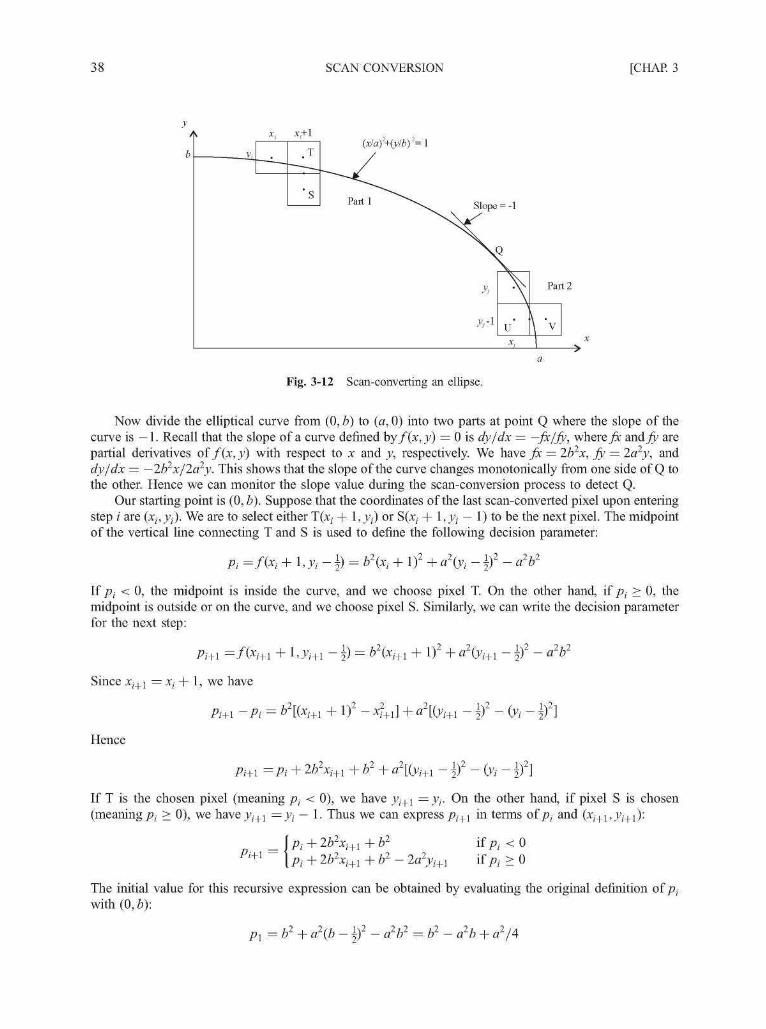
38 SCAN CONVERSION [CHAP. 3
V X ,
^ — ^ ~
xi+ 1
yT'
's
{xlaf+(ylby= 1
^yP a r t 1 Slope=-1
u'xj
Part 2
\ V
J >
Fig. 3-12 Scan-converting an ellipse.
Now divide the elliptical curve from (0, b) to {a, 0) into two parts at point Q where the slope of thecurve is —1. Recall that the slope of a curve defined by f(x,y) = 0 is dy/dx = —fa/fy, where fx and fy arepartial derivatives of f(x,y) with respect to x and y, respectively. We have fx = 2b2x, fy = 2a2y, anddy/dx = —2b2x/2a2y. This shows that the slope of the curve changes monotonically from one side of Q tothe other. Hence we can monitor the slope value during the scan-conversion process to detect Q.
Our starting point is (0, b). Suppose that the coordinates of the last scan-converted pixel upon enteringstep / are (x^y^. We are to select either T(x; + 1, yt) or S(x; + 1, yi — 1) to be the next pixel. The midpointof the vertical line connecting T and S is used to define the following decision parameter:
ft =f(xt +\,y.-§ = b2(xt + I)2 a2(yt - f - a2b2
If ft < 0, the midpoint is inside the curve, and we choose pixel T. On the other hand, if ft > 0, themidpoint is outside or on the curve, and we choose pixel S. Similarly, we can write the decision parameterfor the next step:
Since xi+l = xi + 1, we have
Pi+i ~Pi = b\(xi+i + I)2 - *m] + a\(yi+l - ±f - (yt - ^)2]
Hence
Pi+l =Pi + 2b2xi+1 + b2 + a2[(yi+1 - ±)2 - (yt - \)2}
If T is the chosen pixel (meaning ft < 0), we have yi+l =yt. On the other hand, if pixel S is chosen(meaning ft > 0), we have_vi+1 =yt — 1. Thus we can express pi+l in terms of ft and (xi+i,yi+{):
\Pi + 2b2xi+l+b2if Pi < 0
•i + 2b2xi+1 + b2 - 2a2yi+1 if ft > 0
The initial value for this recursive expression can be obtained by evaluating the original definition of ftwith (0, b):
t2 I 2/1. 1\2 2t2 t2 2 t , 2IA
= b< + a ( b — 5 ) — a r b = b — a b + a / 4

CHAP. 3] SCAN CONVERSION 39
We now move on to derive a similar formula for part 2 of the curve. Suppose pixel (Xj,yj) has just beenscan-converted upon entering step j . The next pixel is either U(x , j — 1) or V(x + 1,>\ — 1). Themidpoint of the horizontal line connecting U and V is used to define the decision parameter
qj =f(Xj +\,y.-\) = b2(Xj + \f + a\yi - I)2 - a2b2
If qj < 0, the midpoint is inside the curve and V is chosen. On the other hand, if > 0, it is outside or onthe curve and U is chosen. We also have
qj+l =f(xj+1 + \,yj+l - 1) = b2(xj+l + i)2 + a2(yj+l - I)2 - a2b2
Since jy+1 = yj — 1, we have
qj+l - qj = b2[(xj+l +1)2 - (xj + If] + a2[(yj+l - I)2 - y2+l]
Hence
qj+l = q}. + b\(xj+l + i)2 - (Xj + i)2] - 2a2yj+l + a2
If V is the chosen pixel (meaning qj < 0), we have xj+l =Xj + \. On the other hand, if U is chosen(meaning qj > 0), we have xj+l = Xj. Thus we can express qj+l in terms of qj and {xj+l,yj+l)\
+ 2b2xj+l - 2a2yj+l + a2 if q} < 0- 2a2yj+1 + a2 if q} > 0
The initial value for this recursive expression is computed using the original definition of qj and thecoordinates (xk,yk) of the last pixel chosen for part 1 of the curve:
\,Vk ~ 1) = b2(xk + \)2 + a2(yk - I)2 - a2b2
We can now put together a pseudo-code description of the midpoint algorithm for scan-converting theelliptical curve in the first quadrant. There are a couple of technical details that are worth noting. First, wekeep track of the slope of the curve by evaluating the partial derivatives fx and fy at each chosen pixelposition. This means thatjx = 2b2xi and fy = 2a2yi for position (xt, yt). Since we have xi+l = xi + 1 andyi+i = yt o r j , — 1 for part 1, and xj+l = Xj or Xj + 1 and yj+i =y- — I for part 2, the partial derivatives canbe updated incrementally using 2b2 and/or —2a2. For example, if xi+l = xi + 1 and yi+i = yt — 1, thepartial derivatives for position (xi+i,yi+{) are 2b2xi+l = 2b2xi + 2b2 and 2a2yi+l = 2a2yi — 2a2. Second,since 2b2xi+l and 2a2yi+l appear in the recursive expression for the decision parameters, we can use themto efficiently computep i+i as well as qj+i-
int x = 0, y = b; I* starting point */int aa = a*a, bb = b*b, aa2 = aa*2, bb2 = bb*2;intfx = 0,fy = aal*b; I* initial partial derivatives */int p = bb — aa*b + 0.25*aa; I* compute and round off/?! */while (fx <fy) { I* |slope| < 1 */
setPixel(x, y);
fx=fx + bb2;if(p<0)
p =p+fx + bb;else {
y—;fy =fy — a f l 2;p =p +fx + bb -fy;
setPixel(x, y); I* set pixel at (xk,yk) */

40 SCAN CONVERSION [CHAP. 3
p = bb(x + 0.5)(x + 0.5) + aa(y - \){y - 1) - aa*bb;while (y > 0) {
y—;fy =fy - aal;if (p >= 0)
p=p-Jy + aa;else {
I* set ql */
fa =fx + bbl;p =p+fx-fy
}setPixel(x, y);
3.5 SCAN-CONVERTING ARCS AND SECTORS
Arcs
An arc [Fig. 3-13(a)] may be generated by using either the polynomial or the trigonometric method.When the trigonometric method is used, the starting value is set equal to Q\ and the ending value is setequal to 62 [see Figs. 3-13(a) and 3-13(b)]. The rest of the steps are similar to those used when scan-converting a circle, except that symmetry is not used.
f
\
(a) (b)
Fig. 3-13
When the polynomial method is used, the value of x is varied from xl to x2 and the values of y arefound by evaluating the expressio • x2 (Fig. 3-14).
From the graphics programmer's point of view, arcs would appear to be nothing more than portions ofcircles. However, problems occur if algorithms such as Bresenham's circle algorithm are used in drawingan arc. In the case of Bresenham's algorithm, the endpoints of an arc must be specified in terms of the x,ycoordinates. The general formulation becomes inefficient when endpoints must be found (see Fig. 3-15).This occurs because the endpoints for each 45° increment of the arc must be found. Each of the eightpoints found by reflection must be tested to see if the point is between the specified endpoints of the arc. Asa result, a routine to draw an arc based on Bresenham's algorithm must take the time to calculate and test

CHAP. 3] SCAN CONVERSION 41
Fig. 3-14
every point on the circle's perimeter. There is always the danger that the endpoints will be missed when amethod like this is used. If the endpoints are missed, the routine can become caught in an infinite loop.
OOOOQ
-7-6-5
00
Fig. 3-15
Sectors
A sector is scan-converted by using any of the methods of scan-converting an arc and then scan-converting two lines from the center of the arc to the endpoints of the arc.
For example, assume that a sector whose center is at point (h, k) is to be scan-converted. First, scan-convert an arc from 9r to 62. Next, a line would be scan-converted from (h,k) to ( r c o s ^ ) + /z,r s i n^ ) + k). A second line would be scan-converted from (h, k) to (r cos(02) + h, r sin(02) + k).
3.6 SCAN-CONVERTING A RECTANGLE
A rectangle whose sides are parallel to the coordinate axes may be constructed if the locations of twovertices are known [see Fig. 3-16(a)]. The remaining corner points are then derived [see Fig. 3-16(6)].Once the vertices are known, the four sets of coordinates are sent to the line routine and the rectangle is

42 SCAN CONVERSION [CHAP. 3
' 1 (
—f (*2. y\)
II
II
Fig. 3-16
scan-converted. In the case of the rectangle shown in Figs. 3-16(a) and 3-16(b), lines would be drawn asfollows: line (x1,iy1) to (xl,y2)', line (xl,y2) to {x1,y2}\ line (x2,y2) to (x2,yi)', and line (x2,yi) to (x1,iy1).
3.7 REGION FILLING
Region filling is the process of "coloring in" a definite image area or region. Regions may be definedat the pixel or geometric level. At the pixel level, we describe a region either in terms of the boundingpixels that outline it or as the totality of pixels that comprise it (see Fig, 3-17). In the first case the region iscalled boundary-defined and the collection of algorithms used for filling such a region are collectivelycalled boundary-fill algorithms. The other type of region is called an interior-defined region and theaccompanying algorithms are called flood-fill algorithms. At the geometric level a region is defined orenclosed by such abstract contouring elements as connected lines and curves. For example, a polygonalregion, or a filled polygon, is defined by a closed polyline, which is a polyline (i.e., a series of sequentiallyconnected lines) that has the end of the last line connected to the beginning of the first line.
Boundary-defined region Interior-defined region
O O O O O OO O O O O O O
O O O O O O O O OO O O O O O OO O O O O O O O O0 0 0 0 0 0 0 0O O O O O O O
(a)
Fig. 3-17
4-Connected vs. 8-Connected
An interesting point here is that, while a geometrically defined contour clearly separates the interiorof a region from the exterior, ambiguity may arise when an outline consists of discrete pixels in theimage space. There are two ways in which pixels are considered connected to each other to form a"continuous" boundary. One method is called 4-connected, where a pixel may have up to four neighbors[see Fig. 3-18(a)]; the other is called 8-connected, where a pixel may have up to eight neighbors [see

CHAP. 3] SCAN CONVERSION 43
(a) (b) (c)
Fig. 3-18 4-connected vs. 8-connected pixels.
Fig. 3-18(6)]. Using the 4-connected approach, the pixels in Fig. 3-18(c) do not define a region sinceseveral pixels such as A and B are not connected. However using the 8-connected definition we identify atriangular region.
We can further apply the concept of connected pixels to decide if a region is connected to anotherregion. For example, using the 8-connected approach, we do not have an enclosed region in Fig. 3-18(c)since "interior" pixel C is connected to "exterior" pixel D. On the other hand, if we use the 4-connecteddefinition we have a triangular region since no interior pixel is connected to the outside.
Note that it is not a mere coincidence that the figure in Fig. 3-18(c) is a boundary-defined region whenwe use the 8-connected definition for the boundary pixels and the 4-connected definition for the interiorpixels. In fact, using the same definition for both boundary and interior pixels would simply result incontradiction. For example, if we use the 8-connected approach we would have pixel A connected to pixelB (continuous boundary) and at the same time pixel C connected to pixel D (discontinuous boundary). Onthe other hand, if we use the 4-connectd definition we would have pixel A disconnected from pixel B(discontinuous boundary) and at the same time pixel C disconnected from pixel D (continuous boundary).
A Boundary-fill Algorithm
This is a recursive algorithm that begins with a starting pixel, called a seed, inside the region. Thealgorithm checks to see if this pixel is a boundary pixel or has already been filled. If the answer is no, it fillsthe pixel and makes a recursive call to itself using each and every neighboring pixel as a new seed. If theanswer is yes, the algorithm simply returns to its caller.
This algorithm works elegantly on an arbitrarily shaped region by chasing and filling all non-boundarypixels that are connected to the seed, either directly or indirectly through a chain of neighboring relations.However, a straightforward implementation can take time and memory to execute due to the potentiallyhigh number of recursive calls, especially when the size of the region is relatively large.
Variations can be made to limit the number of recursive calls by structuring the order in whichneighboring pixels are processed. For example, we can first fill pixels to the left and right of the seed on thesame scan line until boundary pixels are hit (something that can be done using a loop control structure). Wethen inspect each pixel above and below the line just drawn (which can also be done with a loop) to see if itcan be used as a new seed for the next horizontal line to fill. This way the number of recursive calls at anyparticular time is merely N when the current line is N scan lines away from the initial seed.
A Flood-fill Algorithm
This algorithm also begins with a seed (starting pixel) inside the region. It checks to see if the pixel hasthe region's original color. If the answer is yes, it fills the pixel with a new color and uses each of the pixel'sneighbors as a new seed in a recursive call. If the answer is no, it returns to the caller.
This method shares great similarities in its operating principle with the boundary-fill algorithm. It isparticularly useful when the region to be filled has no uniformly colored boundary. On the other hand, a
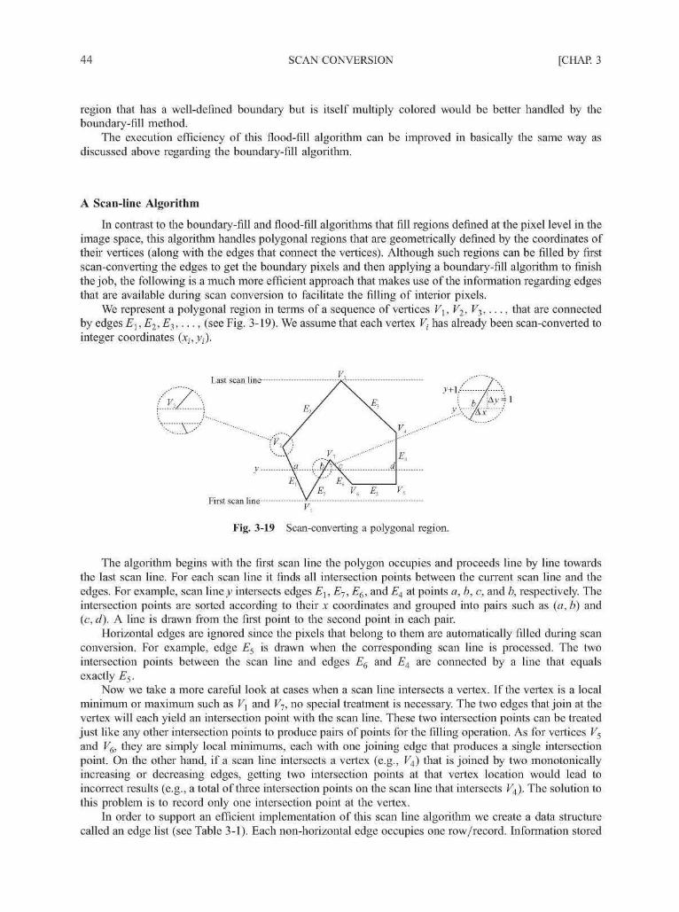
44 SCAN CONVERSION [CHAP. 3
region that has a well-defined boundary but is itself multiply colored would be better handled by theboundary-fill method.
The execution efficiency of this flood-fill algorithm can be improved in basically the same way asdiscussed above regarding the boundary-fill algorithm.
A Scan-line Algorithm
In contrast to the boundary-fill and flood-fill algorithms that fill regions defined at the pixel level in theimage space, this algorithm handles polygonal regions that are geometrically defined by the coordinates oftheir vertices (along with the edges that connect the vertices). Although such regions can be filled by firstscan-converting the edges to get the boundary pixels and then applying a boundary-fill algorithm to finishthe job, the following is a much more efficient approach that makes use of the information regarding edgesthat are available during scan conversion to facilitate the filling of interior pixels.
We represent a polygonal region in terms of a sequence of vertices F1; F2, F 3 , . . . , that are connectedby edges El,E2,Ei,..., (see Fig. 3-19). We assume that each vertex Vi has already been scan-converted tointeger coordinates (xt,y?).
Last scan line
First scan line
Fig. 3-19 Scan-converting a polygonal region.
The algorithm begins with the first scan line the polygon occupies and proceeds line by line towardsthe last scan line. For each scan line it finds all intersection points between the current scan line and theedges. For example, scan l inej intersects edges Ei,E7,E6, and E4 at points a, b, c, and b, respectively. Theintersection points are sorted according to their x coordinates and grouped into pairs such as (a, b) and(c, d). A line is drawn from the first point to the second point in each pair.
Horizontal edges are ignored since the pixels that belong to them are automatically filled during scanconversion. For example, edge E5 is drawn when the corresponding scan line is processed. The twointersection points between the scan line and edges E6 and E4 are connected by a line that equalsexactly E5.
Now we take a more careful look at cases when a scan line intersects a vertex. If the vertex is a localminimum or maximum such as Fj and F7, no special treatment is necessary. The two edges that join at thevertex will each yield an intersection point with the scan line. These two intersection points can be treatedjust like any other intersection points to produce pairs of points for the filling operation. As for vertices F5
and F6, they are simply local minimums, each with one joining edge that produces a single intersectionpoint. On the other hand, if a scan line intersects a vertex (e.g., Ft) that is joined by two monotonicallyincreasing or decreasing edges, getting two intersection points at that vertex location would lead toincorrect results (e.g., a total of three intersection points on the scan line that intersects F4). The solution tothis problem is to record only one intersection point at the vertex.
In order to support an efficient implementation of this scan line algorithm we create a data structurecalled an edge list (see Table 3-1). Each non-horizontal edge occupies one row/record. Information stored

CHAP. 3] SCAN CONVERSION 45
Edge
EiE1
E4
E6
E2E3
y\y\y$y&yi
y\
Table 3-1
J^max
yi -1y7
3^4-1y?
y^y^
An edge list.
x coordinate ofvertex with y = ymin
*ixx
x5
X6X2x4
\/m
\/mx
l/m7
l/m4
l/m6
l/m2
l/m3
in each row includes the y coordinate of the edge's two endpoints, with ymin being the smaller value andj m a x the larger value (may be decreased by 1 for reasons to be discussed below), the x coordinate of theendpoint whose y coordinate i s y ^ , and the inverse of the edge's slope m. The rows are sorted according to_Vmin. Going back to our example in Fig. 3-19, since edges El and E7 both originate from the lowest vertexFj at {xi,y{), they appear on top of the edge list, with m^ and m1 being their slope value, respectively.
Edges in the edge list become active when the y coordinate of the current scan line matches their ymin
value. Only active edges are involved in the calculation of intersection points. The first intersection pointbetween an active edge and a scan line is always the lower endpoint of the edge, whose coordinates arealready stored in the edge's record. For example, when the algorithm begins at the first scan line, edges E^and E7 become active. They intersect the scan line at (xl,yl).
Additional intersection points between an edge and successive scan lines can be calculatedincrementally. If the edge intersects the current scan line at (x, y), it intersects the next scan line at(x + 1 /m, y + 1). For example, edge E7 intersects scan line y at point b, and so the next intersection pointon scan line y+\ can be calculated by Ax = 1 /m7 since Ay = 1. This new x value can simply be kept inthe x field of the edge's record.
An edge is deactivated or may even be removed from the edge list once the scan line whose ycoordinate matches its y^^ value has been processed, since all subsequent scan lines stay clear from it. Theneed that was mentioned early to give special treatment to a vertex where two monotonically increasing ordecreasing edges meet is elegantly addressed by subtracting one from the y^^ value of the lower edge.This means that the lower edge is deactivated one line before the scan line that intersects the vertex. Thusonly the upper edge produces an intersection point with that scan line (see V2 in Fig. 3-19). This explainswhy the initial ymaK value for edges El and E4 has been decreased by one.
3.8 SCAN-CONVERTING A CHARACTER
Characters such as letters and digits are the building blocks of an image's textual contents. They can bepresented in a variety of styles and sizes. The overall design style of a set of characters is referred to as itstypeface or font. Commonly used fonts include Arial, Century Schoolbook, C o u r i e r , and Times NewRoman. In addition, fonts can vary in appearance: bold, italic, and bold and italic. Character size istypically measured in height in inches, points (approximately ^ inch), and picas (12 points).
Bitmap Font
There are two basic approaches to character representation. The first is called a raster or bitmap font,where each character is represented by the on pixels in a bilevel pixel grid pattern called a bitmap (see Fig.3-20). This approach is simple and effective since characters are defined in already-scan-converted form.Putting a character into an image basically entails a direct mapping or copying of its bitmap to a specific

46 SCAN CONVERSION [CHAP. 3
I )I )v y
[ )
r Nv j
r \V y
f -\
V y ^ y
c :
Fig. 3-20 Bitmap font.
location in the image space. On the other hand, a separate font consisting of scores of bitmaps for a set ofcharacters is often needed for each combination of style, appearance, and size.
Although one might generate variations in appearance and size from one font, the overall results tendsto be less than satisfactory. The example in Fig. 3-21 shows that we may overlay the bitmap in Fig. 3-20onto itself with a horizontal offset of one pixel to produce (a) bold, and shift rows of pixels in Fig. 3-20 toproduce (b) italic.
Si J
v )
: )
)> <
s /< )
v J/ >.
\ J
> C
V /
C )
c ^
c >
^ J( )
\ / c
1
X
[ \
/* >K )
K )
v J
v y
( ) Bold a() Italic
Fig. 3-21 Generating variations in appearance.
Furthermore, the size of a bitmap font is dependent on image resolution. For example, a font usingbitmaps that are 12 pixels high produces 12-point characters in an image with 72 pixels per inch. However,the same font will result in 9-point characters in an image with 96 pixels per inch, since 12 pixels nowmeasure 0.125 inch, which is about 9 points. To get 12-point characters in the second image we would needa font with bitmaps that are 16 pixels high.
Outline Font
The second character representation method is called a vector or outline font, where graphicalprimitives such as lines and arcs are used to define the outline of each character (see Fig. 3-22). Althoughan outline definition tends to be less compact than a bitmap definition and requires relatively time-consuming scan-conversion operations, it can be used to produce characters of varying size, appearance,and even orientation. For example, the outline definition in Fig. 3-22 can be resized through a scalingtransformation, made into italic through a shearing transformation, and turned around with respect to areference point through a rotation transformation (see Chap. 4).
These transformed primitives can be scan-converted directly into characters in the form of filledregions in the target image area. Or they can be used to create the equivalent bitmaps that are then used to

CHAP. 3] SCAN CONVERSION 47
Fig. 3-22 Outline font.
produce characters. This alternative is particularly effective in limiting scan-conversion time when thecharacters have repetitive occurrences in the image.
3.9 ANTI-ALIASING
Scan conversion is essentially a systematic approach to mapping objects that are denned in continuousspace to their discrete approximation. The various forms of distortion that result from this operation arecollectively referred to as the aliasing effects of scan conversion.
Staircase
A common example of aliasing effects is the staircase or jagged appearance we see when scan-converting a primitive such as a line or a circle. We also see the stair steps or "jaggies" along the border ofa filled region.
Unequal Brightness
Another artifact that is less noticeable is the unequal brightness of lines of different orientation. Aslanted line appears dimmer than a horizontal or vertical line, although all are presented at the sameintensity level. The reason for this problem can be explained using Fig. 3-23, where the pixels on thehorizontal line are placed one unit apart, whereas those on the diagonal line are approximately 1.414 unitsapart. This difference in density produces the perceived difference in brightness.
V
o o o o o o o o
Fig. 3-23

48 SCAN CONVERSION [CHAP. 3
The Picket Fence Problem
The picket fence problem occurs when an object is not aligned with, or does not fit into, the pixel gridproperly. Figure 3-24(a) shows a picket fence where the distance between two adjacent pickets is not amultiple of the unit distance between pixels. Scan-converting it normally into the image space will result inuneven distances between pickets since the endpoints of the pickets will have to be snapped to pixelcoordinates [see Fig. 3-24(6)]. This is sometimes called global aliasing, as the overall length of the picketfence is approximately correct. On the other hand, an attempt to maintain equal spacing will greatly distortthe overall length of the fence [see Fig. 3-24(c)]. This is sometimes called local aliasing, as the distancesbetween pickets are kept close to their true distances.
(a) (b)
Fig. 3-24 The picket fence problem.
Another example of such a problem arises with the outline font. Suppose we want to scan-convert theuppercase character "E" in Fig. 3-25(a) from its outline description to a bitmap consisting of pixels insidethe region defined by the outline. The result in Fig. 3-25(6) exhibits both asymmetry (the upper arm of thecharacter is twice as thick as the other parts) and dropout (the middle arm is absent). A slight adjustmentand/or realignment of the outline can lead to a reasonable outcome [see Fig. 3-25(c)].
(a) (b) (c)
Fig. 3-25 Scan-converting an outline font.
Anti-aliasing
Most aliasing artifacts, when appear in a static image at a moderate resolution, are often tolerable, andin many cases, negligible. However, they can have a significant impact on our viewing experience whenleft untreated in a series of images that animate moving objects. For example, a line being rotated aroundone of its endpoints becomes a rotating escalator with length-altering steps. A moving object with smallparts or surface details may have some of those features intermittently change shape or even disappear.

CHAP. 3] SCAN CONVERSION 49
Although increasing image resolution is a straightforward way to decrease the size of many aliasingartifacts and alleviate their negative impact, we pay a heavy price in terms of system resource (going fromW x H to 2W x 2H means quadrupling the number of pixels) and the results are not always satisfactory.On the other hand, there are techniques that can greatly reduce aliasing artifacts and improve theappearance of images without increasing their resolution. These techniques are collectively referred to asanti-aliasing techniques.
Some anti-aliasing techniques are designed to treat a particular type of artifact. For instance, an outlinefont can be associated with a set of rules or hints to guide the adjustment and realignment that is necessaryfor its conversion into bitmaps of relatively low resolution. An example of such approach is called theTrueType font.
Pre-flltering and Post-filtering
Pre-filtering and post-filtering are two types of general-purpose anti-aliasing techniques. The conceptof filtering originates from the field of signal processing, where true intensity values are continuous signalsthat consists of elements of various frequencies. Constant intensity values that correspond to a uniformregion are at the low end of the frequency range. Intensity values that change abruptly and correspond to asharp edge are at the high end of the spectrum. In order to lessen the jagged appearance of lines and othercontours in the image space, we seek to smooth out sudden intensity changes, or in signal-processingterms, to filter out the high frequency components. A pre-flltering technique works on the true signal in thecontinuous space to derive proper values for individual pixels (filtering before sampling), whereas a post-filtering technique takes discrete samples of the continuous signal and uses the samples to compute pixelvalues (sampling before filtering).
Area Sampling
Area sampling is a pre-flltering technique in which we superimpose a pixel grid pattern onto thecontinuous object definition. For each pixel area that intersects the object, we calculate the percentage ofoverlap by the object. This percentage determines the proportion of the overall intensity value of thecorresponding pixel that is due to the object's contribution. In other words, the higher the percentage ofoverlap, the greater influence the object has on the pixel's overall intensity value.
In Fig. 3-26(a) a mathematical line shown in dotted form is represented by a rectangular region that isone pixel wide. The percentage of overlap between the rectangle and each intersecting pixel is calculatedanalytically. Assuming that the background is black and the line is white, the percentage values can be useddirectly to set the intensity of the pixels [see Fig. 3-26(b)]. On the other hand, had the background beengray (0.5,0.5,0.5) and the line green (0,1,0), each blank pixel in the grid would have had the backgroundgray value and each pixel filled with a fractional number / would have been assigned a value of[0.5(1 —/) , 0.5(1 —/) + / , 0.5(1 —/)]—a proportional blending of the background and object colors.
Although the resultant discrete approximation of the line in Fig. 3-26(6) takes on a blurry appearance,it no longer exhibits the sudden transition from an on pixel to an off pixel and vice versa, which is what we
\ 0.1
0.2
0.80.1
0.6
0.6
0.20.8
0.2
0.60.8
0.1
0.80.2
0.1
1 1
1 1
1
()
Fig. 3-26 Area sampling.
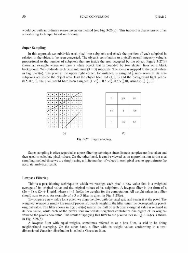
50 SCAN CONVERSION [CHAP. 3
would get with an ordinary scan-conversion method [see Fig. 3-26(c)]. This tradeoff is characteristic of ananti-aliasing technique based on filtering.
Super Sampling
In this approach we subdivide each pixel into subpixels and check the position of each subpixel inrelation to the object to be scan-converted. The object's contribution to a pixel's overall intensity value isproportional to the number of subpixels that are inside the area occupied by the object. Figure 3-21 {a)shows an example where we have a white object that is bounded by two slanted lines on a blackbackground. We subdivide each pixel into nine (3 x 3) subpixels. The scene is mapped to the pixel valuesin Fig. 3-27(6). The pixel at the upper right corner, for instance, is assigned | since seven of its ninesubpixels are inside the object area. Had the object been red (1,0,0) and the background light yellow(0.5,0.5,0), the pixel would have been assigned (1 x \ + 0.5 x | , 0.5 x §, 0), which is ( | , \, 0).
•••
•
••
•
•
•
•
•
•
•
•
•
•
•
•
y•
/
•
//•
••
/
•
••
//
•
0
6/9
1
2/9
1
8/9
7/9
8/9
1/9
()
Fig. 3-27 Super sampling.
Super sampling is often regarded as a post-filtering technique since discrete samples are first taken andthen used to calculate pixel values. On the other hand, it can be viewed as an approximation to the areasampling method since we are simply using a finite number of values in each pixel area to approximate theaccurate analytical result.
Lowpass Filtering
This is a post-filtering technique in which we reassign each pixel a new value that is a weightedaverage of its original value and the original values of its neighbors. A lowpass filter in the form of a(In + 1) x [In + 1 ) grid, where n > 1, holds the weights for the computation. All weight values in a filtershould sum to one. An example of a 3 x 3 filter is given in Fig. 3-28(a).
To compute a new value for a pixel, we align the filter with the pixel grid and center it at the pixel. Theweighted average is simply the sum of products of each weight in the filter times the corresponding pixel'soriginal value. The filter shown in Fig. 3-28(a) means that half of each pixel's original value is retained inits new value, while each of the pixel's four immediate neighbors contributes one eighth of its originalvalue to the pixel's new value. The result of applying this filter to the pixel values in Fig. 3-26(c) is shownin Fig. 3-28(6).
A lowpass filter with equal weights, sometimes referred to as a box filter, is said to be doingneighborhood averaging. On the other hand, a filter with its weight values conforming to a two-dimensional Gaussian distribution is called a Gaussian filter.

CHAP. 3] SCAN CONVERSION 51
01/8
0
1/81/2
1/8
01/8
0
0
00
1/80
0
01/8
5/81/8
0
01/4
5/81/8
0
1/85/8
1/40
0
1/45/8
1/40
1/8
1/21/4
00
0
1/80
00
()
Fig. 3-28 Lowpass filtering.
Pixel Phasing
Pixel phasing is a hardware-based anti-aliasing technique. The graphics system in this case is capableof shifting individual pixels from their normal positions in the pixel grid by a fraction (fypically \ and | ) ofthe unit distance between pixels. By moving pixels closer to the true line or other contour, this technique isvery effective in smoothing out the stair steps without reducing the sharpness of the edges.
3.10 EXAMPLE: RECURSIVELY DEFINED DRAWINGS
In this section we use two common graphical primitives to produce some interesting drawings. Each ofthese drawings is defined by applying a modification rule to a line or a filled triangle, breaking it intosmaller pieces so the rule can be used to recursively modify each piece in the same manner. As the piecesbecome smaller and smaller, an intriguing picture emerges.
C Curve
A line by itself is a first-order C curve, denoted by Co (see Fig. 3-29). The modification rule forconstructing successive generations of the C curve is to replace a line by two shorter, equal-length linesjoining each other at a 90° angle, with the original line and the two new lines forming a right-angledtriangle. See Fig. 3-29 for Q , C2, C3, C4, and C5.
Fig. 3-29 Successive generations of the C curve.
Presume that the following call to the graphics library causes a line to be drawn from (xj, y{) to (x2, y2)using the system's current color:
lme(xl,yl,x2,y2)

52 SCAN CONVERSION [CHAP. 3
We can describe a pseudo-code procedure that generates Cn:
C-curve (float x, y, len, alpha; int n)
if (n > 0) {len = len/sqrt(2.0);C-curve(x, y, len, alpha + 45, n — 1);x = x + len*cos(alpha + 45);y =y + len*sin(alpha + 45);C-curve(x, y, len, alpha — 45, n — 1);
} elseline(x, j , x + len*cos(alpha), y + len*sin(alpha));
where x and y are the coordinates of the starting point of a line, len the length of the line, alpha the angle(in degrees) between the line and the x axis, and n the number of recursive applications of the modificationrule that is necessary to produce Cn. If n = 0, no modification is done and the line itself is drawn.Otherwise, two properly shortened lines, with one rotated counter-clockwise by 45° and the otherclockwise by 45° from the current line position, are generated (representing one application of themodification rule), each of which is the basis of the remaining n — 1 steps of recursive construction.
The Koch Curve
As in the case of the C curve, a line by itself is a first-order Koch curve, denoted by Ko (see Fig. 3-30).The modification rule for constructing successive generations of the Koch curve is to divide a line intothree equal segments and replace the middle segment with two lines of the same length (the replacedsegment and the two added lines form an equilateral triangle). See Fig. 3-30 for Kr, K2, and K3.
K2 K-,
Fig. 3-30 Successive generations of the Koch curve.
The Sierpinski Gasket
This time our graphical primitive is a filled triangle, denoted by So (see Fig. 3-31). The modificationrule for constructing successive generations of the Sierpinski gasket is to take out the area defined by thelines connecting the midpoint of the edges of a filled triangle, resulting in three smaller ones that aresimilar to the original. See Fig. 3-31 for S±, S2, and 53.

CHAP. 3] SCAN CONVERSION 53
S2
AAAFig. 3-31 Successive generations of the Sierpinski gasket.
Solved Problems
3.1 The endpoints of a given line are (0,0) and (6,18). Compute each value ofy as x steps from 0 to 6 and plot theresults.
SOLUTION
An equation for the line was not given. Therefore, the equation of the line must be found. The equation ofthe line (y = nix + b) is found as follows. First the slope is found:
Ay y 2 - y , 1 8 - 0 18m = —— = = = — = 3
Ax x2 — Xj 6 — 0 6
Next, the y intercept b is found by plugging y^ and Xj into the equation y = 3x + b: 0 = 3(0) + b. Therefore,b = 0, so the equation for the line is y = 3x (see Fig. 3-32).
3.2 What steps are required to plot a line whose slope is between 0° and 45° using the slope-interceptequation?
SOLUTION
1. Compute dx: dx = x2 — Xj.
2. Compute dy: dy = y2 —y\.
3. Compute m: m = dy/dx.
4. Compute b: b = y^ — m x Xj.
5. Set (x, y) equal to the lower left-hand endpoint and set xend equal to the largest value of x. If dx < 0, then
x = x2, y = y2, and xend = Xj. If dx > 0, then x = Xj, y = y-i, and xend = x2.
6. Test to determine whether the entire line has been drawn. If x > xend, stop.
7. Plot a point at the current (x,y) coordinates.
8. Increment x: x = x + 1.
9. Compute the next value of y from the equation y = mx + b.
10. Go to step 6.
3.3 Use pseudo-code to describe the steps that are required to plot a line whose slope is between 45C
and —45° (i.e., \m\ > 1) using the slope-intercept equation.
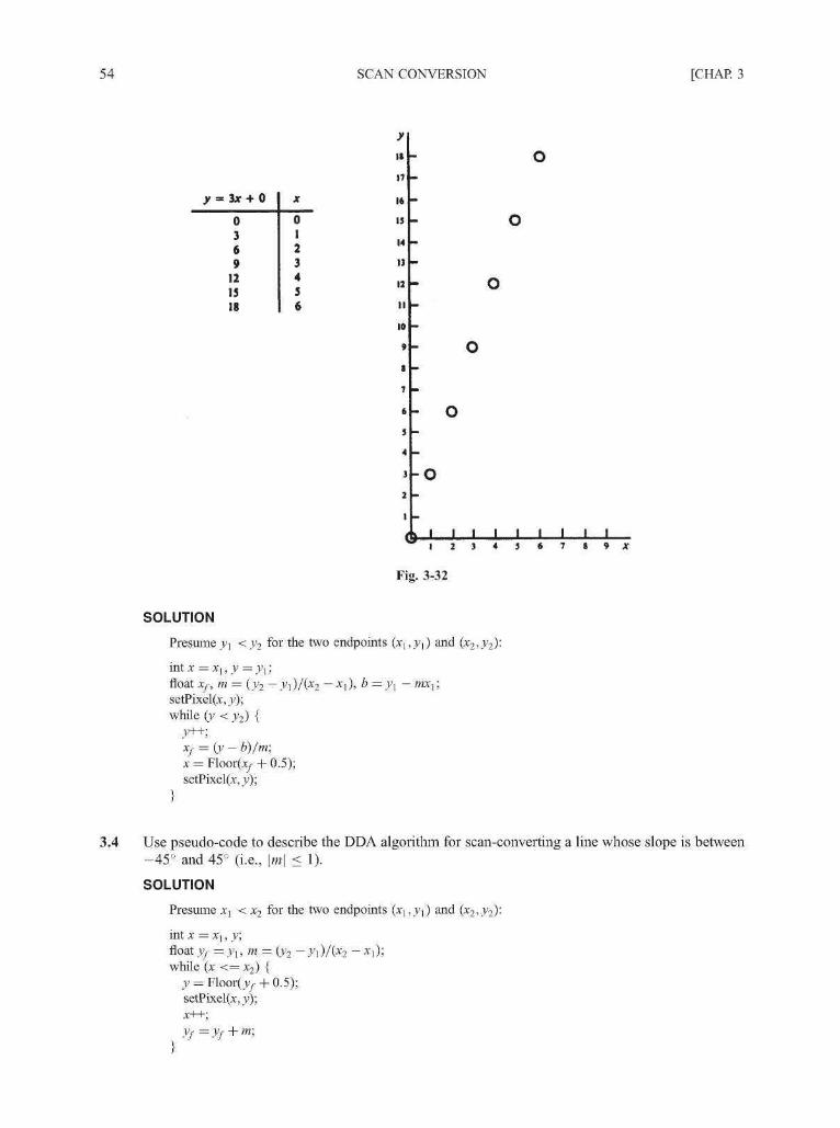
54 SCAN CONVERSION [CHAP. 3
y = 3x + 0
0369
12IS18
X
01234S6
I I
17
16
13
H
13
II
II
10
9
I
1
6
5
4
3
2
I
-o
I I I I I I I» X
Fig. 3-32
SOLUTION
Presume y\ < y2 for the two endpoints (xl,yl) and (x1,y1):
int x = xu y = yx;float Xf, m = (y2 — y\)j{x1 — xx), b = yx — mxx:setPixel(x, y)\while (y < y2) {
y++;xf = (y- b)/m;x = F l o o r ^ + 0.5):setPixel(x, y):
3.4 Use pseudo-code to describe the DDA algorithm for scan-converting a line whose slope is between-45° and 45° (i.e., \m\ < 1).
SOLUTION
Presume xx < x2 for the two endpoints (xj,^]) and (x1,y1):
intx=xuy;float yf=yum = (y2- y\)/(x2 - xx)\while (x < = x2) {
y = Floor(jy + 0.5);setPixel(x, y);
yf=yf + m;

CHAP. 3] SCAN CONVERSION 55
3.5 Use pseudo-code to describe the DDA algorithm for scan-converting a line whose slope is between45° and -45° (i.e., \m\ > 1).
SOLUTION
Presume yx < y2 for the two endpoints (xl,yl) and (x1,y1):
\ntx,y=yl;float xf=xu minv = (x2 - xl)/(y2 -y{)\while (y <= y2) {
x = Floor(x/ + 0.5);setPixel(x, y)\xf=xf + minv;
3.6 What steps are required to plot a line whose slope is between 0° and 45° using Bresenham'smethod?
SOLUTION
1. Compute the initial values:
dx = x2 — Xj Inc2 = 2(dy — dx)
dy = y2 — yx d = Incx — dx
Inc\ = 2dy
2. Set (x,y) equal to the lower left-hand endpoint and xend equal to the largest value of x. If dx < 0, then
x = x2, y = y2, xend = Xj. If dx > 0, then x = Xj, y = yx, xend = x2.
3. Plot a point at the current (x, y) coordinates.
4. Test to see whether the entire line has been drawn. If x = xend, stop.5. Compute the location of the next pixel. If d < 0, then d = d + Inc^. If d > 0, then d = d + Inc2, and
then y =y + 1.
6. Increment x: x = x + 1.
7. Plot a point at the current (x, y) coordinates.
8. Go to step 4.
3.7 Indicate which raster locations would be chosen by Bresenham's algorithm when scan-converting aline from pixel coordinate (1,1) to pixel coordinate (8,5).
SOLUTION
First, the starting values must be found. In this case
rfx = x2 — Xj = 8 — 1 = 7 dy = y2 — yx = 5 — 1 = 4
Therefore:
Incx =2dy = 2x4 = S
Inc2 = 2{dy - dx) = 2 x (4 - 7) = - 6
d = Incl - dx = 8 - 7 = 1
The following table indicates the values computed by the algorithm (see also Fig. 3-33).

56 SCAN CONVERSION [CHAP. 3
d
1l+Inc2 = -5
-5+/MC! = 33 +Inc2 = -3
-3+Inc1 =55+Inc2 = -l
-\+Incx = 77+Inc2 = 1
X
12345678
y
l2233445
o oo o
o o-o
I J I I I
Fig. 3-33
3.8 In the derivation of Bresenham's line algorithm we have used s and t to measure the closeness ofpixels S and T to the true line. However, s and t are only distances in the y direction. They are notreally distances between a point to a line as defined in geomefry. Can we be sure that, when s = t,the two pixels S and T are truly equally far away from the frue line (hence we can choose either oneto approximate the line)?
SOLUTION
As we can see in Fig. 3-34, when s = t the true line intersects the vertical line connecting S and T atmidpoint. The true distance from S to the line is dS and that from T to the line is dT. Since the two right-angled triangles are totally equal (they have equal angles and one pair of equal edges s and i), we get dS = dT.
)
t>
s
S
Fig. 3-34
3.9 Modify the description of Bresenham's line algorithm in the text to set all pixels from inside theloop structure.
SOLUTION 1
int x = Xj, y = J/J :int dx = xf2- x'] ,dy=y'1- y"x, dT = 2(dy - dx), dS = 2dy;int d = 2dy - dx;while (x < = x'2) {
setPixel(x, y);
if {d < 0)d = d + dS:
CHAP. 3] SCAN CONVERSION 57
else {
SOLUTION 2
int x = Xj — 1, y = y\;int dx = x'2 — Xj, dy = y/2 — y\, dT = 2(dy — dx), dS = 2dy;int d = —dx;while (x < x2) {
if (d < 0)d = d + dS;
else {y++;d = d + dT.
}setPixel(x, y);
3.10 What steps are required to generate a circle using the polynomial method?
SOLUTION
1. Set the initial variables: r = circle radius; (h, k) = coordinates of the circle center; x = 0; i = step size;
2. Test to determine whether the entire circle has been scan-converted. If x > xend, stop.
3. Compute the value of the y coordinate, where y = vV2 — x2.
4. Plot the eight points, found by symmetry with respect to the center (h, k), at the current (x, y) coordinates:
Plot(x + h, y + k) Plot(-x + h, -y + k)
V\ot(y + h,x + k) Plot(-j; + h, -x + k)
Plot(-j; + h, x + k) Plot(j; + h, -x + k)
Plot(-x + h, y + k) Plot(x + h, -y + k)
5. Increment x: x = x + i.
6. Go to step 2.
3.11 What steps are required to scan-convert a circle using the trigonometric method?
SOLUTION
1. Set the initial variables: r = circle radius; (h, k) = coordinates of the circle center; i = step size;Send = K/4 radians = 45°; 6 = 0.
2. Test to determine whether the entire circle has been scan-converted. If 8 > 6end, stop.
3. Compute the value of the x and y coordinates:
x = r cos(8) y = r sin(0)

58 SCAN CONVERSION [CHAP. 3
4. Plot the eight points, found by symmetry with respect to the center (h, k), at the current (x, y) coordinates:
Plot(x + h, y + k) Plot(-x + h, -y + k)
Plot(y + h,x + k) Plot(-j; + h, -x + k)
Plot(-y + h, x + k) Plot(y + h,-x + k)
Plot(-x + h, y + k) Plot(x + h, -y + k)
5. Increment 6: 6 = 6 + i.
6. Go to step 2.
3.12 What steps are required to scan-convert a circle using Bresenham's algorithm?
SOLUTION
1. Set the initial values of the variables: (h, k) = coordinates of circle center; x = 0; y = circle radius r; andd = 3 - 2r.
2. Test to determine whether the entire circle has been scan-converted. If x > y, stop.3. Plot the eight points, found by symmetry with respect to the center (h, k), at the current (x, y) coordinates:
Plot(x + h, y + k) Plot(-x + h, -y + k)
Plot(y + h,x + k) Plot(-j; + h, -x + k)
Plot(-y + h,x + k) Plot(y + h,-x + k)
Plot(-x + h, y + k) Plot(x + h, -y + k)
4. Compute the location of the next pixel. If d < 0, then d = d + 4x + 6 and x = x + 1. If d > 0, thend = d + 4(x - y) + 10, x = x + 1, and y = y - 1.
5. Go to step 2.
3.13 When eight-way symmetry is used to obtain a full circle from pixel coordinates generated for the 0°to 45° or the 90° to 45° octant, certain pixels are set or plotted twice. This phenomenon issometimes referred to as overstrike. Identify where overstrike occurs.
SOLUTION
At locations resulted from the initial coordinates (r, 0) or (0, r) since (0, r) = (—0, r), (0, —r) = (—0, —r),(r, 0) = (r, -0), and (-r, 0) = (-r, -0) .
In addition, if the last generated pixel is on the diagonal line at (or, or) where a approximates1/^(2.0) = 0.7071, then overstrike also occurs at (or, or), (—or, or), (or, —or), and (—or, —or).
3.14 Is overstrike harmful besides wasting time?
SOLUTION
It is often harmless since resetting a pixel with the same value does not really change the image in theframe buffer. However, if pixel values are sent out directly, for example, to control the exposure of aphotographic medium, such as a slide or a negative, then overstrike amounts to double exposure at locationswhere it occurred.
Furthermore, if we set pixels using their complementary colors, then overstrike would leave themunchanged, since complementing a color twice simply yields the color itself.
3.15 When scan-converting a curve using the polynomial method (see Probs. 3.10, 3.20, and 3.25) or thetrigonometric method (see Probs. 3.11, 3.21, and 3.24), a step size / is used to compute successivepoints on the true curve. These points are then mapped to the image space. What happens if / is toolarge? What happens if it is too small?

CHAP. 3] SCAN CONVERSION 59
SOLUTION
If i is too large, the computed points will be relatively far from each other and the corresponding pixelswill not form a continuous curve.
If i is too small, computed points will be so close to each other that two or more adjacent ones will bemapped to the same pixel, resulting in overstrike.
Note that it is not always possible to find a single step size for a specific scan-conversion task that yields acontinuous curve without overstrike. In such cases we may take an adaptive approach in which adjustmentsare made to step size during scan-conversion based on points that have already been mapped to the imagespace. For example, if two consecutively computed points have been mapped to two pixels that are notconnected to each other, then an additional point between the two points may be computed using half the step
3.16 Will the following description of Bresenham's circle algorithm and the one in the text produce thesame results?
int x = 0, y = r, d = 3 - 2r:setPixel(x, y)\while (x < y) {
if (d < 0)d = d + 4x + 6;
else {d = d + 4(x-y) + lO;
y—;
setPixel(x, y)\
}
SOLUTION
Let A be the correct set of pixels chosen by Bresenham's circle algorithm. Both versions produce A whenthe rightmost pixel in A is on the diagonal line x=y. However, when the coordinates of the rightmost pixel inA satisfies x = y — 1, only the version in the text stops properly. This version will produce one additional pixelbeyond the 90° to 45° octant. This extra pixel mirrors the rightmost pixel in A with respect to the diagonalline.
3.17 In the derivation of Bresenham's circle algorithm we have used a decision variable di =D(T) + D(S) to help choose between pixels S and T. However, function D as defined in the textis not a true measure of the distance from the center of a pixel to the true circle. Show that whendi = 0 the two pixels S and T are not really equally far away from the true circle.
SOLUTION
Let dS be the actual distance from S to the true circle and dT be the actual distance from T to the truecircle (see Fig. 3-35). Also substitute x for x, + 1 and y for yi in the formula for dt to make the following proofeasier to read:
dt = 2x2 + / + (y- I)2 - 2r2 = 0
Since (r + dT)2 = x2 +y2 and (r - dS)2 = x2 + (y - I)2 we have
2rdT + dT2 =x2+y2-r2 and - 2rdS + dS2 = x2 + (y - I)2 - r2.
Hence
2rdT + dT2 - 2rdS + dS2 = 0
dJ(2r + dT) = dS(2r - dS)
Since dT/dS = (2r — dS)/(2r + dT) < 1, we have dT < dS. This means that, when dt = 0, pixel T isactually closer to the true circle than pixel S.
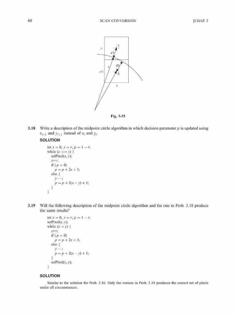
60 SCAN CONVERSION [CHAP. 3
Fig. 3-35
3.18 Write a description of the midpoint circle algorithm in which decision parameter/) is updated usingxi+l andyi+i instead of x, andj , .
SOLUTION
int x = 0, y = r, p = 1 — r:while (x <=y) {
setPixel(x, y)\
p=p + 2x+l;else {
y—;p=p + 2(x-y)
3.19 Will the following description of the midpoint circle algorithm and the one in Prob. 3.18 producethe same results?
int x = 0, y = r, p = 1 — r:setPixel(x, y);while (x < y) {
if(p<0)p=p+ 2x+h
else {
y—;p=p + 2(x-y) + l;
}setPixel(x, y)\
SOLUTION
Similar to the solution for Prob. 3.16. Only the version in Prob. 3.18 produces the correct set of pixelsunder all circumstances.

CHAP. 3] SCAN CONVERSION 61
3.20 What steps are required to generate an ellipse using the polynomial method?
SOLUTION
1. Set the initial variables: a = length of major axis; b = length of minor axis; (h, k) = coordinates ofellipse center; x = 0; i = step size; xend = a.
2. Test to determine whether the entire ellipse has been scan-converted. If x > xend, stop.3. Compute the value of the y coordinate:
4. Plot the four points, found by symmetry, at the current (x, y) coordinates:
Plot(x + h, y + k) Plot(-x + h, -y + k)
Plot(-x + h, y + k) Plot(x + h, -y + k)
5. Increment x: x = x + i.
6. Go to step 2.
3.21 What steps are required to scan-convert an ellipse using the trigonometric method?
SOLUTION
1. Set the initial variables: a = length of major axis; b = length of minor axis; (h, k) = coordinates ofellipse center; i = counter step size; 8end = n/2; 8 = 0.
2. Test to determine whether the entire ellipse has been scan-converted. If 8 > 8end, stop.3. Compute the values of the x and y coordinates:
x = a cos(8) y = b sin(8)
4. Plot the four points, found by symmetry, at the current (x, y) coordinates:
Plot(x + h, y + k) Plot(-x + h, -y + k)
Plot(-x + h, y + k) Plot(x + h, -y + k)
5. Increment 8: 8 = 8 + i.
6. Go to step 2.
3.22 When four-way symmetry is used to obtain a full ellipse from pixel coordinates generated for thefirst quadrant, does overstrike occur? Where?
SOLUTION
Overstrike occurs at (0,b), (0,-b), (a,0), and (-a,0) since (0, b) = (-0, b), (0, -b) = (-0, -b),(a, 0) = (a, -0), and (-a, 0) = (-a, -0) .
3.23 In the midpoint ellipse algorithm we have used only the coordinates (xk, yk) of the last pixel chosenfor part 1 of the curve to compute the initial value q^ of the decision parameter qj for part 2. Can wealso make use of the last value of the decision parameter pp.

62 SCAN CONVERSION [CHAP. 3
SOLUTION
The last computed value of the decision parameter pt for part 1 of the curve is
Pk =f(xk + 1 , ^ - 1 ) = b\xk + I)2 + a2iyk - I)2 - a2b2
= b2(x2k + 2xk + 1) + a2(y\ - yk + i) - a2b2
Since
91 =f(xk + hyk " 1) = b\xk +I)2 + a2(yk - I)2 - a2fe2
= b2(x\ + xk + i) + a2(y| - 2 ^ + 1) - a2fe2
We have
3.24 What steps are required to scan-convert an arc using the trigonometric method?
SOLUTION
1. Set the initial variables: a = major axis; b = minor axis; (h, k) = coordinates of arc center; i = step size;9 = starting angle; 6X = ending angle.
2. Test to determine whether the entire arc has been scan-converted. If 8 > 0j, stop.3. Compute the values of the x and y coordinates:
x = a cos(8) + h y = a sin(0) + k
4. Plot the points at the current (x,y) coordinates: Plot(x, j;).
5. Increment 6: 6 = 6 + i.
6. Go to step 2.
(Note: for the arc of a circle a = b = circle radius r.)
3.25 What steps are required to generate an arc of a circle using the polynomial method?
SOLUTION
1. Set the initial variables: r = radius; (h, k) = coordinates of arc center; x = x coordinate of start of arc;xj = x coordinate of end of arc; i = counter step size.
2. Test to determine whether the entire arc has been scan-converted. If x > xx, stop.
3. Compute the value of the y coordinate:
y = V rL — xL
4. Plot at the current (x, y) coordinates:
Plot(x+ /z,
5. Increment x: x = x + i.
6. Go to step 2.
3.26 What steps are required to scan-convert a rectangle whose sides are parallel to the coordinate axes?
SOLUTION
1. Set initial variables: {xi,y{) = coordinates of first point specified; (x^y-il = coordinates of second pointspecified.

CHAP. 3] SCAN CONVERSION 63
2. Plot the rectangle:
Plot(x2,J>i
to
to (x2,y2)
Plot(x2 ,y2) to (xj, y2)
,y2) to {x\,y{]
3.27 How would a flood-fill algorithm fill the region shown in Fig. 3-36, using the 8-connected definitionfor region pixels?
SOLUTION
1. Assume that a seed is given at coordinate 3, 3. The flood-fill algorithm will inspect the eight pointssurrounding the seed (4, 4; 3, 4; 2, 4; 2, 3; 2, 2; 3, 2; 4, 2; 4, 3). Since all the points surrounding the seedhave the region's original color, each point will be filled (see Fig. 3-37).
2. Each of the eight points found in step 1 becomes a new seed, and the points surrounding each new seedare inspected and filled. This process continues until all the points surrounding all the seeds are rid of theregion's original color (see Fig. 3-38).
y
5<
4(
3 (
2<
14
(
*- • • •
h • • •
>. Interior-defined t # #region
>• • • •
y
5<
44
3<
2<
1 1
• • • •h ^ 9 ^ • • •K CHl^O • • •
• O O M O • • •
t- • • •
1 2 3 4 5 6 7 8 0
Fig. 3-36
1 2 3 4 5 6 7 8
Fig. 3-37
• • •
1 2 3 4 5 6 7
Fig. 3-38
3.28 Write a pseudo-code procedure to implement the boundary-fill algorithm in the text in its basicform, using the 4-connected definition for region pixels.
SOLUTION
BoundaryFill (int x, y, fill_color, boundary_color)
int color:getPixel(x, y, color):if (color != boundary_color && color != fill_color) {
setPixel(x, y, fill_color);BoundaryFill(x + I, y, fill_color, boundary_color):BoundaryFill(x, y+l, fill_color, boundary_color):BoundaryFill(x — \,y, fill_color, boundary_color):BoundaryFill(x, y — 1, fill_color, boundary_color):
3.29 Write a pseudo-code procedure to implement the flood-fill algorithm in the text in its basic form,using the 4-connected definition for region pixels.

64 SCAN CONVERSION [CHAP. 3
SOLUTION
FloodFill (int x, y, fill_color, original_color)
int color:getPixel(x, y, color):if (color = = original_color) {
setPixel(x, y, fill_color):FloodFill(x + I, y, fill_color, original_color):FloodFill(x, y + 1, fill_color, original_color):FloodFill(x —\,y, fill_color, original_color):FloodFill(x, y — 1, fill_color, original_color):
3.30 The coordinates of the vertices of a polygon are shown in Fig. 3-39. (a) Write the initial edge list forthe polygon, (b) State which edges will be active on scan lines y = 6, 7, 8, 9, and 10.
- E«
t i l l
2 3 4 5 6 7
Fig. 3-39
9 10 x
SOLUTION
(a) Column x contains the x coordinate of the corresponding edge's lower endpoint. Horizontal edges are notincluded.
Edge
E2
Et
E4
E6
J^min
4477
J^max
7799
X
9284
1/m
0000
CHAP. 3] SCAN CONVERSION 65
(b) An edge becomes active when the scan line value y equals the edge's ymin value. The edge remains activeuntil the scan line value y goes beyond the edge's ym!SX value. Therefore, the active edges for y = 6,7, 8,9, and 10 appears as follows.
At y = 6, E2 and E%.At y = 7, y = ymax for both edges E2 and is8 so they remain active. Also at y = 7, edges E4 and E6
become active.At y = 8, E2 and Es are removed from the edge list. E4 and E6 remain active.At j ; = 9, the active edges remain the same. At j ; = 10, edges E2 and E4 are removed from the edge listand the edge list becomes empty.
3.31 What are the three major adverse side effects of scan conversion?
SOLUTION
The three major adverse effects of scan conversion are staircase appearance, unequal brightness of slantedlines, and the picket fence problem.
3.32 Suppose that in 3 x 3 super sampling a pixel has three of its subpixels in a red area, three in a greenarea, and three in a blue area, what is the pixel's overall color?
SOLUTION
Each of the three areas is responsible for one third of the pixel's overall intensity value, which is (|, | , | ) .
3.33 Write a pseudo-code procedure for generating the Koch curve Kn (after the one in the text forgenerating Cn).
SOLUTION
Koch-curve (float x, y, len, alpha; int n)
{if (n > 0) {
len = len/3:Koch-curve(x, y, len, alpha, n — 1):x = x + len*cos(alpha):y = y + len*sin(alpha):Koch-curve(x, y, len, alpha — 60, n — 1):x = x + len*cos(alpha — 60):y = y + len*sin(alpha — 60):Koch-curve(x, y, len, alpha + 60, n — 1):x = x + len*cos(alpha + 60):y = y + len*sin(alpha + 60):Koch-curve(x, y, len, alpha, n — X):
} elseline(x, y, x + len*cos(alpha), y + len*sin(alpha)):
3.34 Presume that the following statement produces a filled triangle with vertices at (xj, y^), (x2, y^), and
triangle(x!, yx, x2, y2, x3, y3)

66 SCAN CONVERSION [CHAP. 3
Write a pseudo-code procedure for generating the Sierpinski gasket Sn (after the procedure in the text forgenerating Cn).
SOLUTION
S-Gasket (float xx,yx, x2, y2, x3, y3; int n)
{float X] 2 , y-[2, X13> y\3> X23> ^23 :
if (n > 0) {xn = (*i + x2)/2;y\i = Oi +^2) AX13 = (xl + X 3) / 2 ;^13 = Ol +^3)72:
S-Gasket(xj,_V],X]2,^12,^13,^13, n— 1):S-Gasket(x12, y\2, x2, y2, x2^, y23, n — 1):S-Gasket(x13, yn, x23, y23, x3, 3 3, « - 1):
} elsetriangle(x1; ^ , x2, j ; 2 , x3, jy3);
Supplementary Problems
3.35 Given the following equations, find the corresponding values of y for each value of x (x = 2, 7, 1): (a)y = 4x + 3, (b) y = lx + 0, (c) y = - 3 x - 4, and (a?) .y = - 2 x + 1.
3.36 What steps are required to plot a line whose slope is between 45° and 90° using Bresenham's method?
3.37 What steps are required to plot a dashed line?
3.38 Show graphically that an ellipse has four-way symmetry by plotting four points on the ellipse:
x = a cos(8) + h y = b sin(0) + k
where a = 2
b= 1
h = 0
k = 0
9 = TC/4, 3TT/4, 5TT/4, 7TT/4
3.39 How must Prob. 3.21 be modified if an ellipse is to be rotated (a) TT/4, (b) n/9, and (c) TT/2 radians?
3.40 What steps are required to scan-convert a sector using the trigonometric method?

CHAP. 3] SCAN CONVERSION 67
3.41 What steps must be added to a fill algorithm if a region is to be filled with a pattern?
3.42 Why is it important for the designer to remain consistent when choosing either local or global aliasing?
3.43 What steps are required to scan-convert a polygonal area using the scan-line algorithm?
3.44 How can we eliminate overstrike?

CHAPTER 4
Two-DimensionalTransformations
Fundamental to all computer graphics system is the ability to simulate the manipulation of objects in space.This simulated spatial manipulation is referred to as transformation. The need for transformation ariseswhen several objects, each of which is independently defined in its own coordinate system, need to beproperly positioned into a common scene in a master coordinate system. Transformation is also useful inother areas of the image synthesis process (e.g. viewing transformation in Chap. 5).
There are two complementary points of view for describing object transformation. The first is that theobject itself is transformed relative to a stationary coordinate system or background. The mathematicalstatement of this viewpoint is described by geometric transformations applied to each point of the object.The second point of view holds that the object is held stationary while the coordinate system is transformedrelative to the object. This effect is attained through the application of coordinate transformations. Anexample that helps to distinguish these two viewpoints involves the movement of an automobile against ascenic background. We can simulate this by moving the automobile while keeping the backdrop fixed (ageometric transformation). Or we can keep the car fixed while moving the backdrop scenery (a coordinatetransformation).
This chapter covers transformations in the plane, i.e., the two-dimensional (2D) space. We detail threebasic transformations: translation, rotation, and scaling, along with other transformations that can beaccomplished in terms of a sequence of basic transformations. We describe these operations inmathematical form suitable for computer processing and show how they are used to achieve the ends ofobject manipulation.
GEOMETRIC TRANSFORMATIONS
Let us impose a coordinate system on a plane. An object Obj in the plane can be considered as a set ofpoints. Every object point P has coordinates (x, y), and so the object is the sum total of all its coordinatepoints (Fig. 4-1). If the object is moved to a new position, it can be regarded as a new object Obj', all ofwhose coordinate points P' can be obtained from the original points P by the application of a geometrictransformation.
68

CHAP. 4] TWO-DIMENSIONAL TRANSFORMATIONS 69
Fig. 4-1
Translation
In translation, an object is displaced a given distance and direction from its original position. If thedisplacement is given by the vector v = tx\ + tyi, the new object point P'(x',y') can be found by applyingthe transformation TY to P(x, y) (see Fig. 4-2).
P' = UP)
where x' = x + tx and / = y + f
Fig. 4-2
Rotation about the Origin
In rotation, the object is rotated 6° about the origin. The convention is that the direction of rotation iscounterclockwise if 6 is a positive angle and clockwise if 0 is a negative angle (see Fig. 4-3). Thetransformation of rotation Rg is
= Re(P)
where x1 = xcos(6) -ysin(6) and / = xsin(6) +ycos(9).

70 TWO-DIMENSIONAL TRANSFORMATIONS [CHAP. 4
Fig. 4-3
Scaling with Respect to the Origin
Scaling is the process of expanding or compressing the dimensions of an object. Positive scalingconstants sx and sy are used to describe changes in length with respect to the x direction and y direction,respectively. A scaling constant greater than one indicates an expansion of length, and less than one,compression of length. The scaling fransformation Ss s is given by P' = Ss s (P) where x1 = sxx andy = syy. Notice that, after a scaling fransformation is performed, the new object is located at a differentposition relative to the origin. In fact, in a scaling fransformation the only point that remains fixed is theorigin. Figure 4-4 shows scaling fransformation with scaling factors sx = 2 and sy = | .
y,
• P
1 i „2 X
y,
2
2
-
1 •/" |
\ 2 I A X
(a) ib)
Fig. 4-4
If both scaling constants have the same value s, the scaling fransformation is said to be homogeneousor uniform. Furthermore, if s > 1, it is a magnification and for s < 1, a reduction.
Mirror Reflection about an Axis
If either the x or y axis is treated as a mirror, the object has a mirror image or reflection. Since thereflection P' of an object point P is located the same distance from the mirror as P (Fig. 4-5), the mirrorreflection fransformation Mx about the x axis is given by
P'=MX(P)
where x' = x and y' = —y.
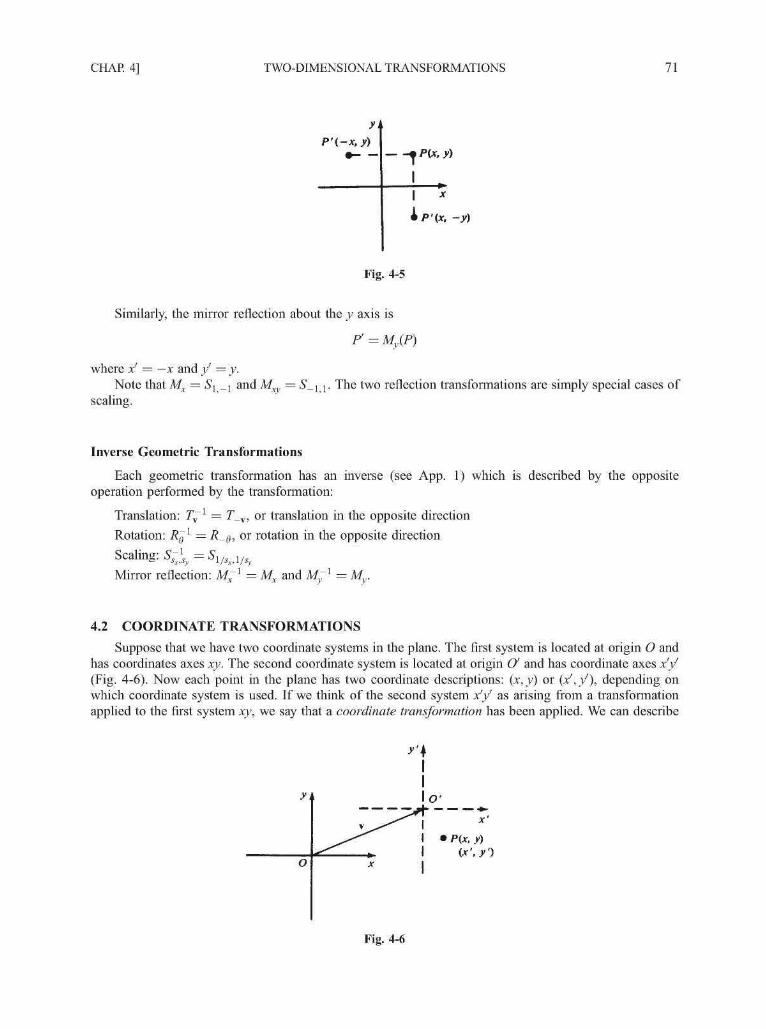
CHAP. 4] TWO-DIMENSIONAL TRANSFORMATIONS 71
P'(-x,y)_ -^P(x,y)
II
'(x, -y)
Fig. 4-5
Similarly, the mirror reflection about the y axis is
P' = My(P)
where x1 = —x and / = y.Note that Mx = Si_i and M = 5_ l j l . The two reflection transformations are simply special cases of
scaling.
Inverse Geometric Transformations
Each geometric transformation has an inverse (see App. 1) which is described by the oppositeoperation performed by the transformation:
Translation: T~x = T_v, or translation in the opposite direction
Rotation: Rg1 = R_e, or rotation in the opposite direction
Scaling: S'}^ = Sl/SxA/Sy
Mirror reflection: M~l = M^ and M71 = M,.
4.2 COORDINATE TRANSFORMATIONS
Suppose that we have two coordinate systems in the plane. The first system is located at origin O andhas coordinates axes xy. The second coordinate system is located at origin O' and has coordinate axes x'y(Fig. 4-6). Now each point in the plane has two coordinate descriptions: (x,y) or (x ' , / ) , depending onwhich coordinate system is used. If we think of the second system x'y' as arising from a transformationapplied to the first system xy, we say that a coordinate transformation has been applied. We can describe
Fig. 4-6

72 TWO-DIMENSIONAL TRANSFORMATIONS [CHAP. 4
this transformation by determining how the (x ' , / ) coordinates of a point P are related to the (x,y)coordinates of the same point.
Translation
If the xy coordinate system is displaced to a new position, where the direction and distance of thedisplacement is given by the vector v = tx\ + t J, the coordinates of a point in both systems are related bythe translation transformation TY:
(x',y') = fY(x,y)
where x' = x — tx and / = y — t .
Rotation about the Origin
The xy system is rotated 6° about the origin (see Fig. 4-7). Then the coordinates of a point in bothsystems are related by the rotation transformation Rs:
(x',y')=RB(x,y)
where x1 = x cos(0) + y sin(0) and / = — x sin(0) + y cos(0).
P(x. y)
•VN
Fig. 4-7
Scaling with Respect to the Origin
Suppose that a new coordinate system is formed by leaving the origin and coordinate axes unchanged,but introducing different units of measurement along the x and y axes. If the new units are obtained fromthe old units by a scaling of sx along the x axis and sy along the y axis, the coordinates in the new systemare related to coordinates in the old system through the scaling transformation Ss s :
where x1 = {\/sx)x and / = {\/sy)y. Figure 4-8 shows coordinate scaling transformation using scalingfactors sx = 2 and s = L
Mirror Reflection about an Axis
If the new coordinate system is obtained by reflecting the old system about either x or y axis, therelationship between coordinates is given by the coordinate transformations Mx and My. For reflectionabout the x axis [Fig. 4-9(a)]
(x',y') = Mx(x,y)
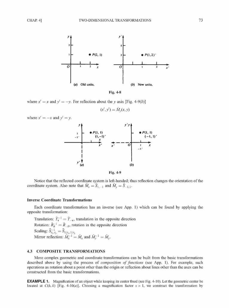
CHAP. 4] TWO-DIMENSIONAL TRANSFORMATIONS 73
o
y
O
P0.2)1
(a) Old units. (b) New units.
Fig. 4-8
where x' = x and y' = —y. For reflection about the y axis [Fig. 4-9(b)]
(x',y') = My(x,y)
where x' = —x and / = y.
y<
(1,-1)'
III
,'t
( - 1 , D'
i x- i "
Fig. 4-9
Notice that the reflected coordinate system is left-handed; thus reflection changes the orientation of thecoordinate system. Also note that Mx =Si_i and My = S_i^.
Inverse Coordinate Transformations
Each coordinate transformation has an inverse (see App. 1) which can be found by applying theopposite transformation:
Translation: f~x = f_v, translation in the opposite direction
Rotation: Rg1 = R_g, rotation in the opposite direction
Scaling: SsJSy =S1/jxA/Sy
Mirror reflection: Mr1 = M. and M71 = M,.
4.3 COMPOSITE TRANSFORMATIONS
More complex geometric and coordinate transformations can be built from the basic transformationsdescribed above by using the process of composition of functions (see App. 1). For example, suchoperations as rotation about a point other than the origin or reflection about lines other than the axes can beconstructed from the basic transformations.
EXAMPLE 1. Magnification of an object while keeping its center fixed (see Fig. 4-10). Let the geometric center belocated at C(h, k) [Fig. 4-10(a)]. Choosing a magnification factor s > 1, we construct the transformation by

74 TWO-DIMENSIONAL TRANSFORMATIONS [CHAP. 4
y,
i
(a)
• C(h,
11 2
to
X
y.
(b)
y i
(c) (d)
Fig. 4-10
performing the following sequence of basic transformations: (1) translate the object so that its center coincides withthe origin [Fig. 4-10(6)], (2) scale the object with respect to the origin [Fig. 4-10(c)], and (3) translate the scaled objectback to the original position [Fig. 4-lO(d)].
The required transformation SsC can be formed by compositions SsC = Ty-Sss- T~l where v = hi + kJ. Byusing composition, we can build more general scaling, rotation, and reflection transformations. For these transforma-tions, we shall use the following notations: (1) S j,—scaling with respect to a fixed point P; (2) Rep—rotationabout a point P; and (3) ML—reflection about a line L.
The matrix description of these transformations can be found in Probs. 4.4, 4.7, and 4.10.
Matrix Description of the Basic Transformations
The transformations of rotation, scaling, and reflection can be represented as matrix functions:
Geometric transformations
_ /cos(0) -s in(0)6 ~ V sin(0) cos(0)
M =
M =1
0
0- 1
01
Coordinate transformations
/ cos(0)6 ~ V - sin(0)
/I 0\x ~ \ o - i )
My={ < -\0
sin(0)
cos(0)

CHAP. 4] TWO-DIMENSIONAL TRANSFORMATIONS 75
The translation transformation cannot be expressed as a 2 x 2 matrix function. However, a certain artificeallows us to introduce a 3 x 3 matrix function which performs the translation transformation.
We represent the coordinate pair (x,y) of a point P by the triple (x,y, 1). This is simply thehomogeneous representation of P (App. 2). Then translation in the direction v = tx\ + t J can be expressedby the matrix function
Then
From this we extract the coordinate pair (x + tx, y + t).
Concatenation of Matrices
The advantage of introducing a matrix form for translation is that we can now build complextransformations by multiplying the basic matrix transformations. This process is sometimes calledconcatenation of matrices and the resulting matrix is often referred to as the composite transformationmatrix (CTM). Here, we are using the fact that the composition of matrix functions is equivalent to matrixmultiplication (App. 1). We must be able to represent the basic transformations as 3 x 3 homogeneouscoordinate matrices (App. 2) so as to be compatible (from the point of view of matrix multiplication) withthe matrix of translation. This is accomplished by augmenting the 2 x 2 matrices with a third column
0 and a third row (0 01). That is
1ac0
bd0
001
EXAMPLE 2. Express as a matrix (i.e., CTM) the transformation which magnifies an object about its centerC(h, k). From Example 1, the required transformation Ss c can be written as
Caution on Matrix Notations
The reader should be alerted to the fact that, within the field of computer graphics, there are twodifferent matrix notations that are used. This book represents points by column vectors and appliestransformations by left-multiplying by the transformation matrix. We have chosen this approach because itis the standard used in mathematics and computer science texts. The other notation represents points byrow vectors and applies transformations by right-multiplying by the transformation matrix. It is used inmuch of the computer graphics literature.

76 TWO-DIMENSIONAL TRANSFORMATIONS [CHAP. 4
To change from one notational style to another, it is necessary to take the franspose of the matrices thatappear in any expression. For example, translation of point (x, y) in the direction v = tx\ + t J can also beexpressed as
I(x y 1)1 0
UEXAMPLE 2 continued. Using the row-vector notation, we have
ty
4.4 INSTANCE TRANSFORMATIONS
Quite often a picture or design is composed of many objects used several times each. In turn, theseobjects may also be composed of other symbols and objects. We suppose that each object is defined,independently of the picture, in its own coordinate system. We wish to place these objects together to formthe picture or at least part of the picture, called a subpicture. We can accomplish this by defining atransformation of coordinates, called an instance transformation, which converts object coordinates topicture coordinates so as to place or create an instance of the object in the picture coordinate system.
The instance transformation AfpicturejObject is formed as a composition or concatenation of scaling,rotation, and translation operations, usually performed in this order (although any order can be used):
^picture,object — ^ v ' ^8,P ' ^a,b,P
With the use of different instance transformations, the same object can be placed in differentpositions, sizes, and orientations within a subpicture. For instance, Fig. 4-11 (a) is placed in the picturecoordinate system of Fig. 4-1 \(b) by using the instance transformations Npicture object-
^object,
- 1
'object
J'objecl •"object
^picture
(a) Object coordinate system. (b) Picture coordinate system.
Fig. 4-11
Nested Instances and Multilevel Structures
A subpicture or picture may exhibit a multilevel or nested sfructure by being composed of objectswhich are, in turn, composed of still other objects, and so on. Separate instance transformations must thenbe applied, in principle, at each level of the picture sfructure for each picture component.
EXAMPLE 3. A picture of an apple tree contains branches, and an apple hangs on each branch. Suppose that eachbranch and apple is described in its own coordinate system [Figs. 4-12(a) and 4-l2(b)]. Then a subpicture call to place

CHAP. 4] TWO-DIMENSIONAL TRANSFORMATIONS 77
dapple,
"picture
(a) Apple.
J1* branch
• * »
•^branch
Branch.
* picture
(c) Picture coordinate system.
Fig. 4-12
an instance of this branch in the picture of the tree requires an additional subpicture call to place an instance of theapple into the branch coordinate system.
We can perform each instance transformation separately, i.e., instance the apple in the branch coordinate systemand then instance both branch and apple from the branch coordinate system to the picture coordinate system.However, it is much more efficient to transform the apple directly into picture coordinates [see Fig. 4-12(c)]. This isaccomplished by defining the composite transformation matrix Cpicture o b j e c t to be the composition of the nestedinstance transformations from apple coordinates to branch coordinates and then from branch coordinates to picturecoordinates:
^picture, apple -^picture,branch ' -^branch,apple
Since the branch subpicture is only one level below the picture
^picture,branch - *picture,br;•anch
Solved Problems
4.1 Derive the transformation that rotates an object point 6° about the origin. Write the matrixrepresentation for this rotation.
SOLUTION
Refer to Fig. 4-13. Definition of the trigonometric functions sin and cos yields
x' = r cos(0 + 4>) / = r sin(0 + <fr)
and
x = r cos 4> y = r sin (ft
Using trigonometric identities, we obtain
r cos(0 + 4>) = r(cos 8 cos 4> — sin 8 sin cp) = xcosd — y sin 6
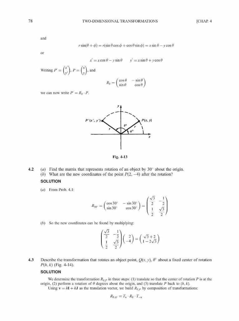
78 TWO-DIMENSIONAL TRANSFORMATIONS [CHAP. 4
and
r sin(£> + <p) = r(sin 8 cos <p + cos 8 sin <fi) = x sin 8 — y cos 8
x = x cos 0 — j ; sin 8 y = x sin 8 +y cos 0
Writing P ' = | ), P = | ), and
V7 W
we can now write P' = Ra • P.
_ ( cos 8 — sin 8 \9 ~ l s i n 0 cosfl)
y.
Fig. 4-13
4.2 (a) Find the matrix that represents rotation of an object by 30° about the origin.(b) What are the new coordinates of the point P(2, —4) after the rotation?
SOLUTION
(a) From Prob. 4.1:
.#30° —/ cos 30° - s i n 3 0 c
\ sin 30° cos30c
(b) So the new coordinates can be found by multiplying:
V3+21 -2V3
4.3 Describe the transformation that rotates an object point, Q(x, y), 6° about a fixed center of rotationP(h, k) (Fig. 4-14).
SOLUTION
We determine the transformation Rg P in three steps: (1) translate so that the center of rotation P is at theorigin, (2) perform a rotation of 8 degrees about the origin, and (3) translate P back to (h, k).
Using v = hi + kJ as the translation vector, we build Rep by composition of transformations:

CHAP. 4] TWO-DIMENSIONAL TRANSFORMATIONS 79
Q(x, y)
P(h,k)
O
Fig. 4-14
4.4 Write the general form of the matrix for rotation about a point P(h, k).
SOLUTION
Following Prob. 4.3, we write Rgp = Ty- Rg • T_y, where v = hi + kJ. Using the 3 x 3 homogeneouscoordinate form for the rotation and translation matrices, we have
( 1 0 / z \ / cos (0 ) -sin(0) O \ / 1 0 -h
0 1 k \ \ sin(0) cos(0) 0 0 I -k
0 0 1 / \ 0 0 1 / \ 0 0 1
' cos(0) - sin(0) [-h cos(0) + k sin(0) -
= | sin(0) cos(0) [—hsin(8) — kcos((
0 0 1
4.5 Perform a 45° rotation of triangle ,4(0, 0), 5(1, 1), C(5, 2) (a) about the origin and (6) about
P(-l.-l).SOLUTION
We represent the triangle by a matrix formed from the homogeneous coordinates of the vertices:
ABC(0 1 5\
0 1 2\ 1 1 1/
(a) The mafrix of rotation is
'cos 45° - s i n 45° 0"
45o = sin45c
\ 0cos 45° 0 =
0 1
/V2
4i 4io2 2
V o 0 1 /
So the coordinates A'B'C of the rotated triangle A8C can be found as
A' B' C
34l\1
[A'B'C']=R45»-[ABC] =
41 _il 0N
2 2
4i 4ii i °
V o 0 1 /
Thus ^ ' = (0, 0), B' = (0, 42), and C = (f V2, | V2).
0 1 2 =1 1 1 /
0 0
0 V2
Vi i
80 TWO-DIMENSIONAL TRANSFORMATIONS [CHAP. 4
(b) From Prob. 4.4, the rotation matrix is given by it o^p = Ty • R45o • T_y, where v = —I — J. So
R45,yP= 0 1 - 1
1 0 - 1
0 1 - 1
0 0 1
(4i2
4i2
V 0
4i2
20
\
0
\)
/ I 0 1\
0 1/
2
4i2
V o
2
20
_r1
(V2-1)
1
Now
[ABC] =f (V2-1)
V o o I /
'0 1 5s
0 1 21 1 1
(\4i-\y
= ( - l , V 2 - 1), B' = (-1,242- 1),
(V2-1) (2V2-1) (fV2-l)
1 1 1
4.6 Find the transformation that scales (with respect to the origin) by (a) a units in the X direction, (b) bunits in the Y direction, and (c) simultaneously a units in the X direction and b units in the Ydirection.
SOLUTION
(a) The scaling transformation applied to a point P(x, y) produces the point (ax, y). We can write this inmatrix form as Sa j • P, or
a 0\ x0 l)\y
(b) As in part (a), the required transformation can be written in matrix form as S\ j • P. So
1 0 \ xo
(c) Scaling in both directions is described by the transformation x' = ax and y' = by. Writing this in matrixform as Sab • P, we have
a 0\ I x\ _ I ax0 b)\y) [by
4.7 Write the general form of a scaling matrix with respect to a fixed point P(h, k).
SOLUTION
Following the same general procedure as in Probs. 4.3 and 4.4, we write the required transformation with
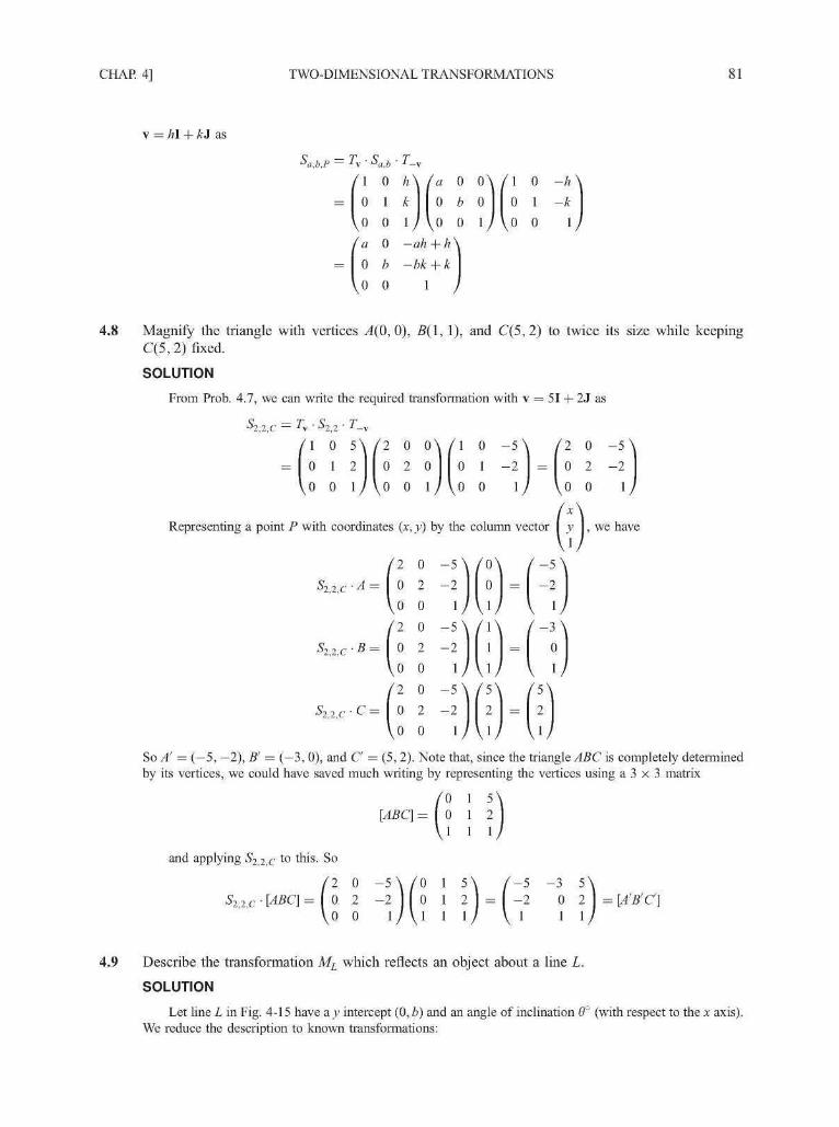
CHAP. 4] TWO-DIMENSIONAL TRANSFORMATIONS 81
v = hi + kJ as
Sa,byp — Ty • Sab • T_y
-h
-k
0 0 1
4.8 Magnify the triangle with vertices ^4(0, 0), 5(1, 1), and C(5,2) to twice its size while keepingC(5,2)fixed.
SOLUTION
From Prob. 4.7, we can write the required transformation with v = 51 + 2J as
Representing a point P with coordinates (x, y) by the column vector \ y , we have
S22C-A =
2 2 C ' —
S22C-C =
So A' = ( - 5 , - 2 ) , B' = ( - 3 , 0), and C = (5, 2). Note that, since the triangle ABC is completely determinedby its vertices, we could have saved much writing by representing the vertices using a 3 x 3 matrix
and applying <S22,c t 0 l^s- So
0 1 5 \ /—5 - 3 5 \0 1 2 = - 2 0 2 = [A'B'C]
i i i / v i 1 1 /
4.9 Describe the transformation ML which reflects an object about a line L.
SOLUTION
Let line L in Fig. 4-15 have a j ; intercept (0, b) and an angle of inclination 8° (with respect to the x axis).We reduce the description to known transformations:

82 TWO-DIMENSIONAL TRANSFORMATIONS [CHAP. 4
1. Translate the intersection point B to the origin.2. Rotate by —8° so that line L aligns with the x axis.3. Mirror-reflect about the x axis.4. Rotate back by 0°.
5. Translate B back to (0, b).
In transformation notation, we have
where v = hi.
= Ty-Re-Mx-R_e-T_
P'y,
B
s^ o
s(0,
A\\
yb)
\\
P
X
Fig. 4-15
4.10 Find the form of the matrix for reflection about a line L with slope m and y intercept (0, b).
SOLUTION
Following Prob. 4.9 and applying the fact that the angle of inclination of a line is related to its slope m bythe equation tan(0) = m, we have with v = bJ,
ML = TW-R6-MX-R_6-T_W
( 1 0 O\/cos(0) -sin(0) 0 \ / l 0 0 \ / cos(0) sin(0) O \ / 1 0 0s
0 1 b\\ sin(0) cos(0) 0 0 - I 0 - sin(0) cos(0) 0 0 I -b
0 0 1 / 1 0 0 1/VO 0 1 / 1 0 0 1/VO 0 1Now if tan(0) = m, standard trigonometry yields sin(0) = m/\/m2 + 1 and cos(0) = \j\lm2 + 1. Substitut-ing these values for sin(0) and cos(0) after matrix multiplication, we have
1 - m2 2m -2bm \m2 + 1 m2 + 1 m2 + 1
2m m — \ 2bML =
m2 + 1 m2 + 1 m2 11 )
4.11 Reflect the diamond-shaped polygon whose vertices are A{—\, 0), B(0, —2), C(l, 0), and D(0, 2)about (a) the horizontal line y = 2, (b) the vertical line x = 2, and (c) the line y = x + 2.

CHAP. 4] TWO-DIMENSIONAL TRANSFORMATIONS 83
SOLUTION
We represent the vertices of the polygon by the homogeneous coordinate matrix
V =
From Prob. 4.9, the reflection matrix can be written as
ML = TW-R6-MX-R_6-T_W
(a) The line y = 2 has y intercept (0,2) and makes an angle of 0° with the x axis. So with 8 = 0 and v = 2J,the transformation matrix is
ML =
This same matrix could have been obtained directly by using the results of Prob. 4.10 with slope m = 0and y intercept b = 2. To reflect the polygon, we set
Converting from homogeneous coordinates, A' = (—1, 4), B' = (0, 6), C = (1, 4), and D1 = (0, 2).
(b) The vertical line x = 2 has no y intercept and an infinite slope! We can use My, reflection about the yaxis, to write the desired reflection by (1) translating the given line two units over to the y axis, (2) reflectabout the y axis, and (3) translate back two units. So with v = 21,
= Ty-My-T—V
Finally
ML-V =
or A' = (5, 0), B' = (4, - 2 ) , C = (3, 0), and D' = (4, 2).
(c) The line y = x + 2 has slope 1 and a y intercept (0,2). From Prob. 4.10, with m = 1 and b = 2, we find
The required coordinates A', B', C, and D' can now be found.
ML-V =
So ' = (-2, 1), 5' = (-4, 2), C = (-2, 3), and D' = (0, 2).
4.12 The matrix I , I defines a transformation called a simultaneous shearing or shearing for short.
The special case when b = 0 is called shearing in the x direction. When a = 0, we have shearing inthe y direction. Illustrate the effect of these shearing transformations on the square ^4(0, 0), B(\, 0),C(\, 1), and £>(0, 1) when a = 2 and b = 3.
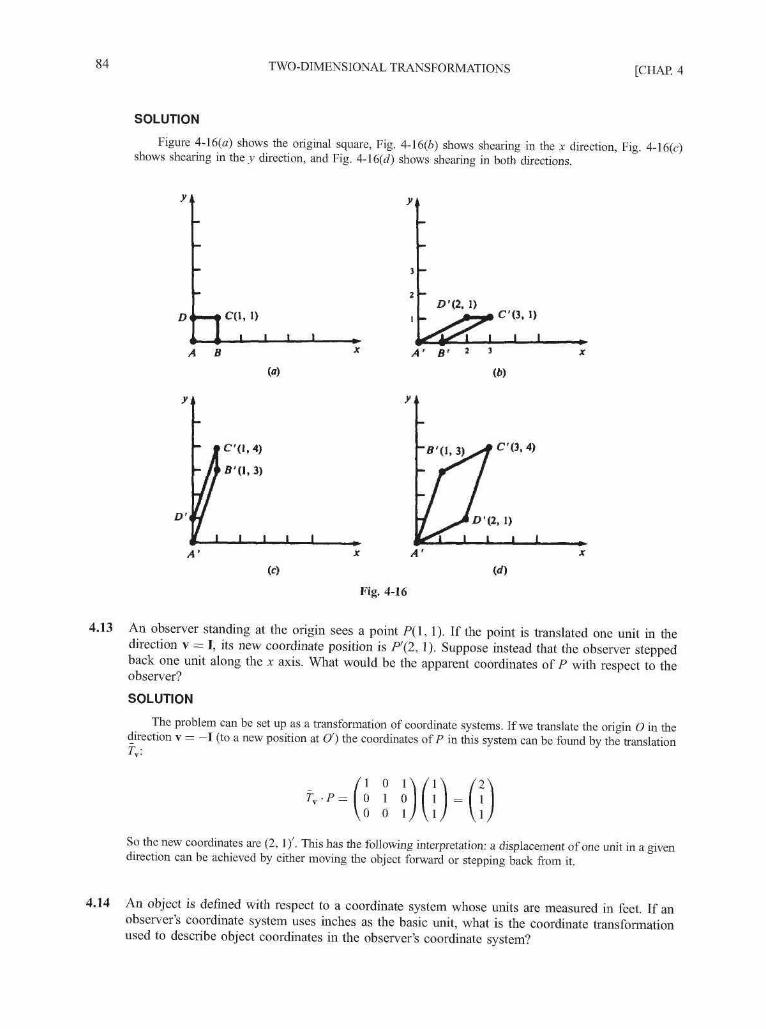
84 TWO-DIMENSIONAL TRANSFORMATIONS [CHAP. 4
SOLUTION
Figure 4-16(a) shows the original square, Fig. 4-16(6) shows shearing in the x direction, Fig. 4-16(c)shows shearing in the y direction, and Fig. 4-l6(d) shows shearing in both directions.
i —«• C(l,
1 L
C'(3, 1)
I I
A B A' B'
4.13
- f i 'd ,3 )^f C'<3.4)
I I l
/41
(c)
Fig. 4-16
An observer standing at the origin sees a point P( l , 1). If the point is translated one unit in thedirection v = I, its new coordinate position is P'(2, 1). Suppose instead that the observer steppedback one unit along the x axis. What would be the apparent coordinates of P with respect to theobserver?
SOLUTION
The problem can be set up as a transformation of coordinate systems. If we translate the origin O in thedirection v = - I (to a new position at O') the coordinates of P in this system can be found by the translationT •
T,-P =
So the new coordinates are (2, 1)'. This has the following interpretation: a displacement of one unit in a givendirection can be achieved by either moving the object forward or stepping back from it.
4.14 An object is defined with respect to a coordinate system whose units are measured in feet. If anobserver's coordinate system uses inches as the basic unit, what is the coordinate transformationused to describe object coordinates in the observer's coordinate system?

CHAP. 4] TWO-DIMENSIONAL TRANSFORMATIONS 85
SOLUTION
Since there are 12 inches to a foot, the required transformation can be described by a coordinate scalingtransformation with s = i or
12 00 12
and so
12 0 \ / x \ / I 2 x0 12
4.15 Find the equation of the circle (x') + (/) = 1 in terms of xy coordinates, assuming that the x'ycoordinate system results from a scaling of a units in the x direction and b units in the y direction.
SOLUTION
From the equations for a coordinate scaling transformation, we find
, 1 , 1x =-x y =-y
a b
Substituting, we have
Notice that as a result of scaling, the equation of the circle is transformed to the equation of an ellipse in the xycoordinate system.
4.16 Find the equation of the line / = mx' + b in xy coordinates if the x'y' coordinate system resultsfrom a 90° rotation of the xy coordinate system.
SOLUTION
The rotation coordinate transformation equations can be written as
x' = xcos(90°)+.ysin(90o) =y / = -xsin(90°) +.ycos(90°) = -x
Substituting, we find —x = my + b. Solving for y, we have y = {—\/m)x — b/m.
4.17 Find the instance transformation which places a half-size copy of the square ^4(0,0), 5(1,0),C(l, 1), D(0, 1) [Fig. 4-17(a)] into a master picture coordinate system so that the center of thesquare is at ( -1 , -1) [Fig. 4-17(6)].
SOLUTION
The center of the square ABCD is at P ( i , 1). We shall first apply a scaling transformation while keeping Pfixed (see Prob. 4.7). Then we shall apply a translation that moves the center P to P'(—l, —1). Takingtx = (—1) — (4) = —I and similarly £ = — I (so v = — | l — | J ) , we obtain
-"picture,square — ^v ' "1/2,1/2,1"

86 TWO-DIMENSIONAL TRANSFORMATIONS [CHAP. 4
•^square '
•p\
A ' B square — 2
Fig. 4-17
^picture
- 2
.^picture
(6)
4.18 Write the composite transformation that creates the design in Fig. 4-19 from the symbols in Fig.4-18.
•^triangle , -Vsquare
I
Fig. 4-18
SOLUTION
First we create an instance of the triangle [Fig. 4-18(a)] in the square [Fig. 4-18(fe)]. Since the base of thetriangle must be halved while keeping the height fixed at one unit, the appropriate instance transformation isivsquare,triangle 1 1/2,1 ' °1/2,1-
The instance transformation needed to place the square at the desired position in the picture coordinatesystem (Fig. 4-19) is a translation in the direction v = I + J:
N • — Tlvpicture,square ±\
Then the composite transformation for placing the triangle into the picture is
^picture,triangle -^picture,square ' -^square,triangle
^piciure
2 -
(1, 1)11
Fig. 4-19

CHAP. 4] TWO-DIMENSIONAL TRANSFORMATIONS 87
and the composite transformation to place the square into the picture is
C — N^picture, square J v picture, square
Supplementary Problems
4.19 What is the relationship between the rotations Rg, R_g, and Rg^?
4.20 Describe the transformations used in magnification and reduction with respect to the origin. Find the newcoordinates of the triangle ^4(0, 0), B(l, 1), C(5, 2) after it has been (a) magnified to twice its size and (b)reduced to half its size.
4.21 Show that reflection about the line y = x is attained by reversing coordinates. That is,
ML(x,y) = (y,x)
4.22 Show that the order in which transformations are performed is important by the transformation of triangleA{\, 0), 5(0, 1), C(l, 1), by (a) rotating 45° about the origin and then translating in the direction of vector I,and (b) translating and then rotating.
4.23 An object point P(x, y) is translated in the direction v = a\ + bj and simultaneously an observer moves in thedirection v. Show that there is no apparent motion (from the point of view of the observer) of the object point.
4.24 Assuming that we have a mathematical equation defining a curve in x'y' coordinates, and the x'y'coordinate system is the result of a coordinate transformation from the xy coordinate system, writethe equation in terms of xy coordinates.
=TV .r v=rV i + v ,
4.25 Show that
4.26 Show that Sa,b • Sc4 = Sc4 • Sa,b = SacM.
4.27 Show that Ra-Rp=RrRa=
4.28 Find the condition under which we have
4.29 Is a simultaneous shearing the same as a shearing in one direction followed by a shearing in another direction?Why?
4.30 Find the condition under which we can switch the order of a rotation and a simultaneous shearing and still getthe same result.
88 TWO-DIMENSIONAL TRANSFORMATIONS [CHAP. 4
4.31 Express a simultaneous shearing in terms of rotation and scaling transformations.
4.32 Express Rg in terms of shearing and scaling transformations.
4.33 Express Rg in terms of shearing transformations.
4.34 Prove that the 2D composite transformation matrix is always in the following form:
fa b c\\d e /\0 0 \)
4.35 Consider a line from Px to P2 and an arbitrary point P on the line. Prove that for any given compositetransformation the transformed P is on the line between the transformations of Pj and P2-

CHAPTER 5
Two-DimensionalViewing and Clipping
Much like what we see in real life through a small window on the wall or the viewfinder of a camera, acomputer-generated image often depicts a partial view of a large scene. Objects are placed into the sceneby modeling transformations to a master coordinate system, commonly referred to as the world coordinatesystem (WCS). A rectangular window with its edges parallel to the axes of the WCS is used to select theportion of the scene for which an image is to be generated (see Fig. 5-1). Sometimes an additionalcoordinate system called the viewing coordinate system is introduced to simulate the effect of movingand/or tilting the camera.
On the other hand, an image representing a view often becomes part of a larger image, like a photo onan album page, which models a computer monitor's display area. Since album pages vary and monitorsizes differ from one system to another, we want to introduce a device-independent tool to describe thedisplay area. This tool is called the normalized device coordinate system (NDCS) in which a unit ( l x l )square whose lower left corner is at the origin of the coordinate system defines the display area of a virtualdisplay device. A rectangular viewport with its edges parallel to the axes of the NDCS is used to specify asub-region of the display area that embodies the image.
Viewingcoordinatesystem
A
Window Workstationwindow
Workstationviewport
World coordinate system^ Normalized device
coordinate system
Fig. 5-1 Viewing transformation.
Device/imagecoordinate system
89

90 TWO-DIMENSIONAL VIEWING AND CLIPPING [CHAP. 5
The process that converts object coordinates in WCS to normalized device coordinates is calledwindow-to-viewport mapping or normalization transformation, which is the subject of Sect. 5.1. Theprocess that maps normalized device coordinates to discrete device/image coordinates is called work-station transformation, which is essentially a second window-to-viewport mapping, with a workstationwindow in the normalized device coordinate system and a workstation viewport in the device coordinatesystem. Collectively, these two coordinate-mapping operations are referred to as viewing transformation.
Workstation transformation is dependent on the resolution of the display device/frame buffer. Whenthe whole display area of the virtual device is mapped to a physical device that does not have a 1/1 aspectratio, it may be mapped to a square sub-region (see Fig. 5-1) so as to avoid introducing unwantedgeometric distortion.
Along with the convenience and flexibility of using a window to specify a localized view comes theneed for clipping, since objects in the scene may be completely inside the window, completely outside thewindow, or partially visible through the window (e.g. the mountain-like polygon in Fig. 5-1). The clippingoperation eliminates objects or portions of objects that are not visible through the window to ensure theproper construction of the corresponding image.
Note that clipping may occur in the world coordinate or viewing coordinate space, where the windowis used to clip the objects; it may also occur in the normalized device coordinate space, where theviewport/workstation window is used to clip. In either case we refer to the window or the view-port/workstation window as the clipping window. We discuss point clipping, line clipping, and polygonclipping in Sees. 5.2, 5.3, and 5.4, respectively.
5.1 WINDOW-TO-VIEWPORT MAPPING
A window is specified by four world coordinates: wxmin, wxmaK, wymin, and wyma^ (see Fig. 5-2).Similarly, a viewport is described by four normalized device coordinates: vxmin, vxma^, vymin, and vyma^.The objective of window-to-viewport mapping is to convert the world coordinates (wx, wy) of an arbitrarypoint to its corresponding normalized device coordinates (vx, vy). In order to maintain the same relativeplacement of the point in the viewport as in the window, we require:
WX WX™™ VX i^min WV Wymin VV i'Vmin
mm_ = mm_ ^ 1 ^ L _ = _JL >™L_
Thus
' vx = -
Since the eight coordinate values that define the window and the viewport are just constants, we canexpress these two formulas for computing (vx, vy) from (wx, wy) in terms of a translate-scale-translatetransformation N
= N-
where
0 0 \
0
0
0
1 /
/ I0
\o
010
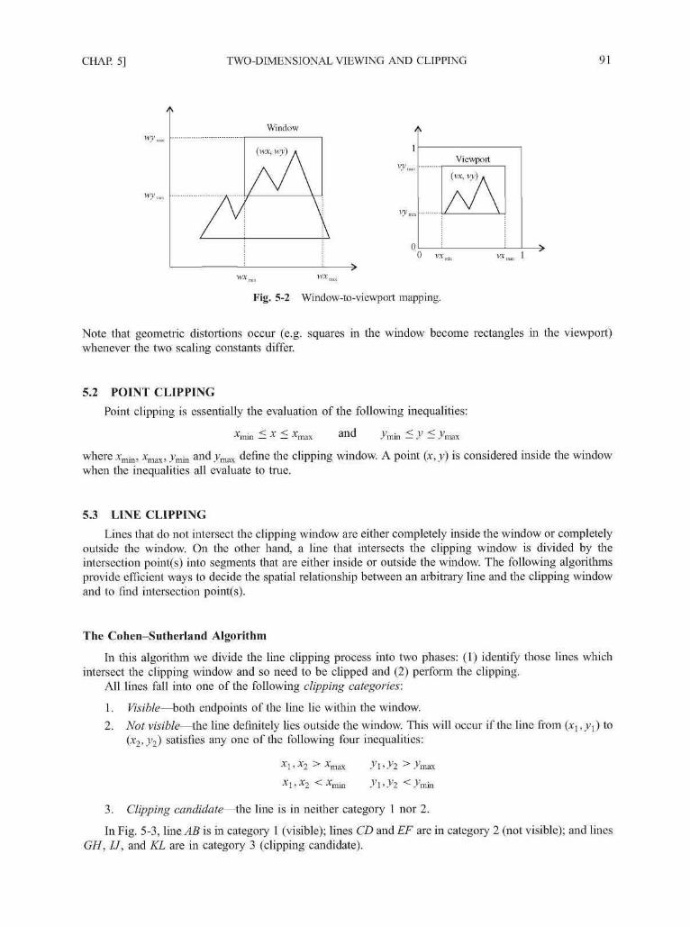
CHAP. 5] TWO-DIMENSIONAL VIEWING AND CLIPPING 91
ii i
Window
0 vx
Fig. 5-2 Window-to-viewport mapping.
Note that geometric distortions occur (e.g. squares in the window become rectangles in the viewport)whenever the two scaling constants differ.
5.2 POINT CLIPPING
Point clipping is essentially the evaluation of the following inequalities:
*min < x < Vax and ymin < y < J W
where xmin, xmax, ymin and_vmax define the clipping window. A point (x,y) is considered inside the windowwhen the inequalities all evaluate to true.
5.3 LINE CLIPPING
Lines that do not intersect the clipping window are either completely inside the window or completelyoutside the window. On the other hand, a line that intersects the clipping window is divided by theintersection point(s) into segments that are either inside or outside the window. The following algorithmsprovide efficient ways to decide the spatial relationship between an arbitrary line and the clipping windowand to find intersection point(s).
The Cohen-Sutherland Algorithm
In this algorithm we divide the line clipping process into two phases: (1) identify those lines whichintersect the clipping window and so need to be clipped and (2) perform the clipping.
All lines fall into one of the following clipping categories:
1. Visible—both endpoints of the line lie within the window.
2. Not visible—the line definitely lies outside the window. This will occur if the line from (xx, yx) to(x2,y2) satisfies any one of the following four inequalities:
x1,x2>xmax yx,y2
xl> X2 < xmin y\' yi Jm
3. Clipping candidate—the line is in neither category 1 nor 2.
In Fig. 5-3, line AB is in category 1 (visible); lines CD and EF are in category 2 (not visible); and linesGH, IJ, and KL are in category 3 (clipping candidate).

92 TWO-DIMENSIONAL VIEWING AND CLIPPING [CHAP. 5
H
Fig. 5-3
The algorithm employs an efficient procedure for finding the category of a line. It proceeds in twosteps:
1. Assign a 4-bit region code to each endpoint of the line. The code is determined according to whichof the following nine regions of the plane the endpoint lies in
Jmin
1001
0001
0101
1000
0000
0100
1010
0010
0110
Starting from the leftmost bit, each bit of the code is set to true (1) or false (0) according to thescheme
Bit 1 = endpoint is above the window = sign (y — y^a)Bit 2 = endpoint is below the window = sign (ymin — y)Bit 3 = endpoint is to the right of the window = sign (x — xmax)Bit 4 = endpoint is to the left of the window = sign ( x ^ — x)
We use the convention that sign(a) = 1 if a is positive, 0 otherwise. Of course, a point with code0000 is inside the window.
2. The line is visible if both region codes are 0000, and not visible if the bitwise logical AND of thecodes is not 0000, and a candidate for clipping if the bitwise logical AND of the region codes is0000 (see Prob. 5.8).
For a line in category 3 we proceed to find the intersection point of the line with one of the boundariesof the clipping window, or to be exact, with the infinite extension of one of the boundaries (see Fig. 5-4).We choose an endpoint of the line, say (xl,yl), that is outside the window, i.e., whose region code is not

CHAP. 5] TWO-DIMENSIONAL VIEWING AND CLIPPING 93
A '
/4(0001)
X
/
Ii
C(0100)
/
D(1010)
/o'(0010)
f
Fig. 5-4
0000. We then select an extended boundary line by observing that those boundary lines that are candidatesfor intersection are the ones for which the chosen endpoint must be "pushed across" so as to change a " 1 "in its code to a "0" (see Fig. 5-4). This means:
If bit 1 is 1, intersect with line y = ymax.
If bit 2 is 1, intersect with line y = ym^.
If bit 3 is 1, intersect with line x = xmax.
If bit 4 is 1, intersect with line x = xmin.
Consider line CD in Fig. 5-4. If endpoint C is chosen, then the bottom boundary line y = yn isselected for computing intersection. On the other hand, if endpoint D is chosen, then either the topboundary line y = ymax or the right boundary line x = xmax is used. The coordinates of the intersectionpoint are
y. =yx +m(xi -
or
if the boundary line is vertical
if the boundary line is horizontal
where m = (y2 — y\)/(x2 — *i) is the slope of the line.Now we replace endpoint (xl, yr) with the intersection point (xt, yt), effectively eliminating the portion
of the original line that is on the outside of the selected window boundary. The new endpoint is thenassigned an updated region code and the clipped line re-categorized and handled in the same way. Thisiterative process terminates when we finally reach a clipped line that belongs to either category 1 (visible)or category 2 (not visible).
Midpoint Subdivision
An alternative way to process a line in category 3 is based on binary search. The line is divided at itsmidpoint into two shorter line segments. The clipping categories of the two new line segments are thendetermined by their region codes. Each segment in category 3 is divided again into shorter segments and

94 TWO-DIMENSIONAL VIEWING AND CLIPPING [CHAP. 5
categorized. This bisection and categorization process continues until each line segment that spans across awindow boundary (hence encompasses an intersection point) reaches a threshold for line size and all othersegments are either in category 1 (visible) or in category 2 (invisible). The midpoint coordinates (xm,ym) ofa line joining (x^ j j ) and (x2,y2) are given by
x, + x7 y, + y7
The example in Fig. 5-5 illustrates how midpoint subdivision is used to zoom in onto the twointersection points Ix and I2 with 10 bisections. The process continues until we reach two line segments thatare, say, pixel-sized, i.e., mapped to one single pixel each in the image space. If the maximum number ofpixels in a line is M, this method will yield a pixel-sized line segment in N subdivisions, where 2N = M orN = log2M. For instance, when M = 1024 we need at most N = log2 1024 = 10 subdivisions.
Fig. 5-5
The Liang-Barsky Algorithm
The following parametric equations represent a line from (xl,yi) to (x2,y2) along with its infiniteextension:
x = Xj + Ax • uy = y1 + Ay • u
where Ax = x2 — Xj and Ay = y2 —y\. The line itself corresponds to 0 < u < 1 (see Fig. 5-6). Notice thatwhen we traverse along the extended line with u increasing from — oo to +oo, we first move from theoutside to the inside of the clipping window's two boundary lines (bottom and left), and then move fromthe inside to the outside of the other two boundary lines (top and right). If we use ux and u2, where ul < u2,to represent the beginning and end of the visible portion of the line, we have u1 = maximum(0, uh ub) andu2 = minimum(l, ut, ur), where uh ub, ut, and ur correspond to the intersection point of the extended linewith the window's left, bottom, top, and right boundary, respectively.
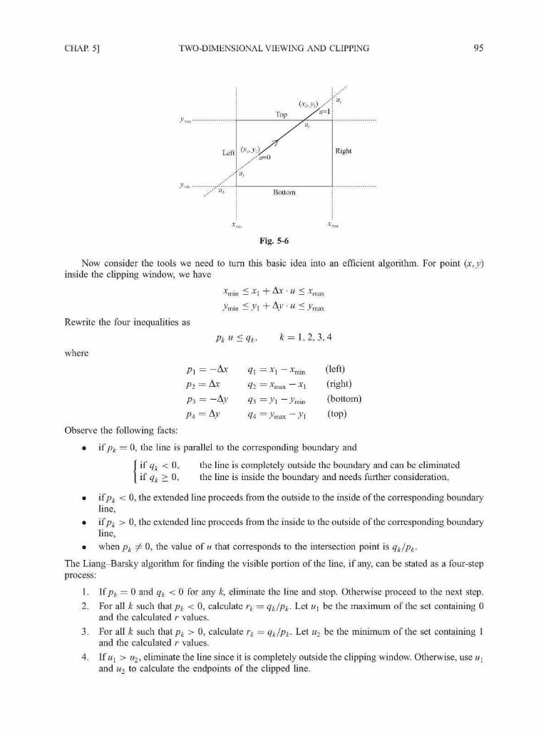
CHAP. 5] TWO-DIMENSIONAL VIEWING AND CLIPPING 95
Left (*i> yd,
Top
S
u=1
Right
Bottom
Fig. 5-6
Now consider the tools we need to turn this basic idea into an efficient algorithm. For point (x,y)inside the clipping window, we have
Jmin < y\
Ax • U < Xm a x
Ay • u < Jmax
Rewrite the
where
four inequalities as
P\
Pi
Pi
PA
Pku
= -Ax
= Ax
= -Ay
= Ay
<ft:
ft
ft
ft
ft
k
= xx-
— xmax
= J7i -
J'max
= 1,2,
xmin
- X !
J^min
-y\
3,4
(left)
(right)
(bottom)
(top)
Observe the following facts:
• if pk = 0, the line is parallel to the corresponding boundary and
if qk < 0, the line is completely outside the boundary and can be eliminatedif ft > 0, the line is inside the boundary and needs further consideration,
< 0, the extended line proceeds from the outside to the inside of the corresponding boundaryline,
• if/>£ > 0, the extended line proceeds from the inside to the outside of the corresponding boundaryline,
• whenpk ^ 0, the value of u that corresponds to the intersection point is q^lPk-
The Liang-Barsky algorithm for finding the visible portion of the line, if any, can be stated as a four-stepprocess:
1. \ipk = 0 and qk < 0 for any k, eliminate the line and stop. Otherwise proceed to the next step.
2. For all k such th&tpk < 0, calculate rk = qt/Pk- Le* u\ be the maximum of the set containing 0and the calculated r values.
3. For all k such that pk > 0, calculate rk =and the calculated r values.
^. Let u2 be the minimum of the set containing 1
4. If Mj > u2, eliminate the line since it is completely outside the clipping window. Otherwise, use Mjand u2 to calculate the endpoints of the clipped line.

96 TWO-DIMENSIONAL VIEWING AND CLIPPING [CHAP. 5
5.4 POLYGON CLIPPING
In this section we consider the case of using a polygonal clipping window to clip a polygon.
Convex Polygonal Clipping Windows
A polygon is called convex if the line joining any two interior points of the polygon lies completelyinside the polygon (see Fig. 5-7). A non-convex polygon is said to be concave.
Convexpolygon
Concavepolygon
Fig. 5-7
By convention, a polygon with vertices P 1 ; . . . ,PN (and edges P^ iP , and PNP{) is said to bepositively oriented if a tour of the vertices in the given order produces a counterclockwise circuit.
Equivalently, the left hand of a person standing along any directed edge Pi_lPi or PNPi would bepointing inside the polygon [see orientations in Figs. 5-8(a) and 5-8(6)].
(a) Positive orientation. (b) Negative orientation.
Fig. 5-8
Let A(xi,y{) and B{x1,y-}) be the endpoints of a directed line segment. A point P(x,y) will be to theleft of the line segment if the expression C = (x2 — x{)(y — yr) — (y2 — y{)(x — xx) is positive (see Prob.5.13). We say that the point is to the right of the line segment if this quantity is negative. If a point P is tothe right of any one edge of a positively oriented, convex polygon, it is outside the polygon. If it is to theleft of every edge of the polygon, it is inside the polygon.
This observation forms the basis for clipping any polygon, convex or concave, against a convexpolygonal clipping window.
The Sutherland-Hodgman Algorithm
Let P j , . . . , PN be the vertex list of the polygon to be clipped. Let edge E, determined by endpoints Aand B, be any edge of the positively oriented, convex clipping polygon. We clip each edge of the polygon in

CHAP. 5] TWO-DIMENSIONAL VIEWING AND CLIPPING 97
turn against the edge E of the clipping polygon, forming a new polygon whose vertices are determined asfollows.
Consider the edge P^^Pf.
1. If both /",_! and P, are to the left of the edge, vertex Pi is placed on the vertex output list of theclipped polygon [Fig. 5-9(a)].
2. If both /",_! and P, are to the right of the edge, nothing is placed on the vertex output list [Fig.5-9(6)].
3. If P,-_! is to the left and P, is to the right of the edge E, the intersection point / of line segmentPi_\Pi with the extended edge E is calculated and placed on the vertex output list [Fig. 5-9(c)].
4. If P,_i is to the right and P, is to the left of edge E, the intersection point / of the line segmentPi-\Pt w i t n the extended edge E is calculated. Both / and P, are placed on the vertex output list[Fig. 5-9(d)}.
The algorithm proceeds in stages by passing each clipped polygon to the next edge of the window andclipping. See Probs. 5.14 and 5.15.
B
Output
Pi-
I R(a)
Output
Fig. 5-9
Special attention is necessary in using the Sutherland-Hodgman algorithm in order to avoid unwantedeffects. Consider the example in Fig. 5-10(a). The correct result should consist of two disconnected parts, asquare in the lower left corner of the clipping window and a triangle at the top [see Fig. 5-10(6)]. However,the algorithm produces a list of vertices (see Prob. 5.16) that forms a figure with the two parts connected byextra edges [see Fig. 5-10(c)]. The fact that these edges are drawn twice in opposite direction can be usedto devise a post-processing step to eliminate them.
The Weiler-Atherton Algorithm
Let the clipping window be initially called the clip polygon, and the polygon to be clipped the subjectpolygon [see Fig. 5-11 (a)]. We start with an arbitrary vertex of the subject polygon and trace around itsborder in the clockwise direction until an intersection with the clip polygon is encountered:
• If the edge enters the clip polygon, record the intersection point and continue to trace the subjectpolygon.

TWO-DIMENSIONAL VIEWING AND CLIPPING [CHAP. 5
p Polygon P
p,
Extraedges
P3
N N
()Clippingwindow
( )
Fig. 5-10
• If the edge leaves the clip polygon, record the intersection point and make a right turn to followthe clip polygon in the same manner (i.e., treat the clip polygon as subject polygon and the subjectpolygon as clip polygon and proceed as before).
Whenever our path of traversal forms a sub-polygon we output the sub-polygon as part of the overall result.We then continue to trace the rest of the original subject polygon from a recorded intersection point thatmarks the beginning of a not-yet-traced edge or portion of an edge. The algorithm terminates when theentire border of the original subject polygon has been traced exactly once.
9
4
Subject polygon
10 13
3
Clip polygon
()
Starting vertex
1 \
24
2
3
()
Fig. 5-11
For example, the numbers in Fig. 5-11 (a) indicate the order in which the edges and portions of edgesare traced. We begin at the starting vertex and continue along the same edge (from 1 to 2) of the subjectpolygon as it enters the clip polygon. As we move along the edge that is leaving the clip polygon we makea right turn (from 4 to 5) onto the clip polygon, which is now considered the subject polygon. Followingthe same logic leads to the next right turn (from 5 to 6) onto the current clip polygon, which is really theoriginal subject polygon. With the next step done (from 7 to 8) in the same way we have a sub-polygon foroutput [see Fig. 5-11(6)]. We then resume our traversal of the original subject polygon from the recordedintersection point where we first changed our course. Going from 9 to 10 to 11 produces no output. After
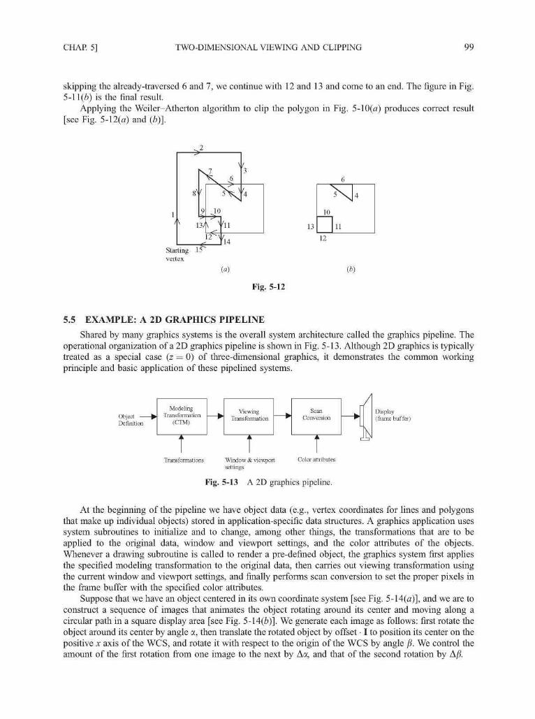
CHAP. 5] TWO-DIMENSIONAL VIEWING AND CLIPPING 99
skipping the already-traversed 6 and 7, we continue with 12 and 13 and come to an end. The figure in Fig.5-11(6) is the final result.
Applying the Weiler-Atherton algorithm to clip the polygon in Fig. 5-10(a) produces correct result[see Fig. 5-l2(a) and (b)].
13A
13
10
11
12
Starting 15vertex
()
Fig. 5-12
5.5 EXAMPLE: A 2D GRAPHICS PIPELINE
Shared by many graphics systems is the overall system architecture called the graphics pipeline. Theoperational organization of a 2D graphics pipeline is shown in Fig. 5-13. Although 2D graphics is typicallytreated as a special case (z = 0) of three-dimensional graphics, it demonstrates the common workingprinciple and basic application of these pipelined systems.
Object —Definition
ModelingTransformation
(CTM)
ViewingTransformation
ScanConversion W
T
Display(frame buffer)
Transformations Window & viewport Color attributessettings
Fig. 5-13 A 2D graphics pipeline.
At the beginning of the pipeline we have object data (e.g., vertex coordinates for lines and polygonsthat make up individual objects) stored in application-specific data structures. A graphics application usessystem subroutines to initialize and to change, among other things, the transformations that are to beapplied to the original data, window and viewport settings, and the color attributes of the objects.Whenever a drawing subroutine is called to render a pre-defined object, the graphics system first appliesthe specified modeling transformation to the original data, then carries out viewing transformation usingthe current window and viewport settings, and finally performs scan conversion to set the proper pixels inthe frame buffer with the specified color attributes.
Suppose that we have an object centered in its own coordinate system [see Fig. 5-14(a)], and we are toconstruct a sequence of images that animates the object rotating around its center and moving along acircular path in a square display area [see Fig. 5-14(6)]. We generate each image as follows: first rotate theobject around its center by angle a, then translate the rotated object by offset • I to position its center on thepositive x axis of the WCS, and rotate it with respect to the origin of the WCS by angle /?. We control theamount of the first rotation from one image to the next by Aa, and that of the second rotation by Aji.

100 TWO-DIMENSIONAL VIEWING AND CLIPPING [CHAP. 5
()
Fig. 5-14
window(-winsize/2, winsize/2, -winsize/2, winsize/2);x = 0;while (1) {
setColor(background);clear();setColor(color);pushCTM();translate(offset, 0);rotate(a);drawObject();popCTM();a = a + Aa;rotate(A/?);
We first set the window of winsize by winsize to be sufficiently large and centered at the origin of theWCS to cover the entire scene. The system's default viewport coincides with the unit display area in theNDCS. The default workstation window is the same as the viewport and the default workstation viewportcorresponds to the whole square display area.
The graphics system maintains a stack of composite transformation matrices. The CTM on top of thestack, called the current CTM, is initially an identity matrix and is automatically used in modelingtransformation. Each call to translate, scale, and rotate causes the system to generate a correspondingtransformation matrix and to reset the current CTM to take into account the generated matrix. The order oftransformation is maintained in such a way that the most recently specified transformation is applied first.When pushCTM() is called, the system makes a copy of the current CTM and pushes it onto the stack (nowwe have two copies of the current CTM on the stack). When popCTM() is called, the system simplyremoves the CTM on top of the stack (now we have restored the CTM that was second to the removedCTM to be the current CTM).
Panning and Zooming
Two simple camera effects can be achieved by changing the position or size of the window. When theposition of the window is, for example, moved to the left, an object in the scene that is visible through thewindow would appear moved to the right, much like what we see in the viewfinder when we move or pan a

CHAP. 5] TWO-DIMENSIONAL VIEWING AND CLIPPING 101
camera. On the other hand, if we fix the window on an object but reduce or increase its size, the objectwould appear bigger (zoom in) or smaller (zoom out), respectively.
Double Buffering
Producing an animation sequence by clearing the display screen and constructing the next frame ofimage often leads to flicker, since an image is erased almost as soon as it is completed. An effectivesolution to this problem is to have two frame buffers: one holds the image on display while the systemdraws a new image into the other. Once the new image is drawn, a call that looks like swapBuffer() wouldcause the two buffers to switch their roles.
Lookup Table Animation
We can sometimes animate a displayed image in the lookup table representation by changing orcycling the color values in the lookup table. For example, we may draw the monochromatic object in Fig.5-14(a) into the frame buffer in several pre-determined locations, using consecutive lookup table entries forthe color attribute in each location (see Fig. 5-15). We initialize lookup table entry 0 with the color of theobject, and all other entries with the background color. This means that in the beginning the object isvisible only in its first position (labeled 0). Now if we simply reset entry 0 with the background color andentry 1 with the object color, we would have the object "moved" to its second position (labeled 1) withoutredrawing the image. The object's circular motion could hence be produced by cycling the object colorthrough all relevant lookup table entries.
Fig. 5-15
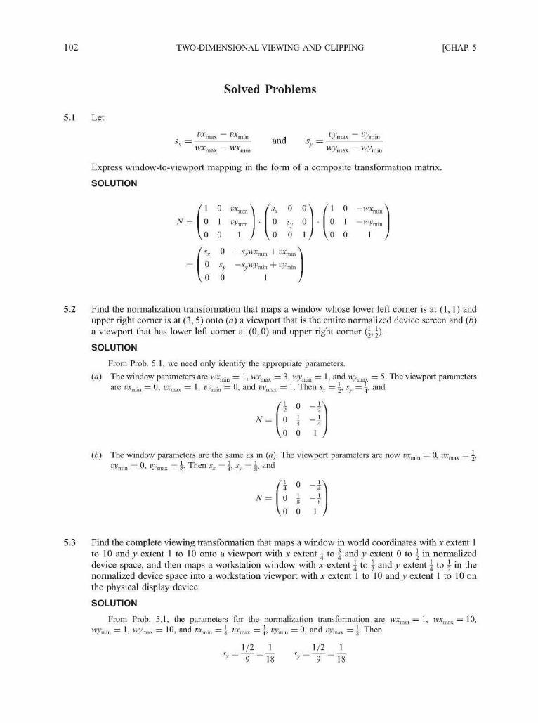
102 TWO-DIMENSIONAL VIEWING AND CLIPPING [CHAP. 5
Solved Problems
5.1 Let
_ max min_ ^ ^ _ max min_
VWL™ — wxmin ' wyml,Y — wymirlniiix irmi •/ nidx •/ min
Express window-to-viewport mapping in the form of a composite transformation matrix.
SOLUTION
5.2 Find the normalization transformation that maps a window whose lower left corner is at (1,1) andupper right corner is at (3,5) onto (a) a viewport that is the entire normalized device screen and (b)a viewport that has lower left corner at (0,0) and upper right corner (|, | ) .
SOLUTION
From Prob. 5.1, we need only identify the appropriate parameters.
(a) The window parameters are wxmin = 1, wxmax = 3, wymin = 1, and wymax = 5. The viewport parametersare uxmin = 0, uxmax = 1, vymin = 0, and uymax = 1. Then sx =\,sy= \, and
N =
(b) The window parameters are the same as in (a). The viewport parameters are now vxmin = 0, uxmax = j ,
Vymin = 0, %iax = T h e n Sx = ?. ^ = i a n d
N =
5.3 Find the complete viewing transformation that maps a window in world coordinates with x extent 1to 10 and y extent 1 to 10 onto a viewport with x extent \ to | and j extent 0 to | in normalizeddevice space, and then maps a workstation window with x extent | to \ and j extent | to \ in thenormalized device space into a workstation viewport with x extent 1 to 10 and y extent 1 to 10 onthe physical display device.
SOLUTION
From Prob. 5.1, the parameters for the normalization transformation are wxmin = 1, wxmax = 1 0 ,wjVm = !> W J W = 10, and vxmin = \, uxmax = | , U3;min = 0, and i>ymax = 5. Then
_ 1/2 _ 1 _ 1/2 _ 1
^ 9 18 ^ 9 18

CHAP. 5] TWO-DIMENSIONAL VIEWING AND CLIPPING 103
and
18 U 36
N ~ I 0 — - —18 18
, 0 0 1
The parameters for the workstation transformation are wxmin = \ , wxmax = \ , wymin = \ , wymax
and uxmin = 1, uxmax = 10, vymia = 1, and vyr[mx = 10. Then
^ = T74 = 36 ^ = T 7 4 = 36
and
The complete viewing transformation V is
'36 0 - 8 \ / i 0 ^ \
0 36 - 8
0 0 1,
0 T8 -T8 I
Vo o l
5.4 Find a normalization transformation from the window whose lower left corner is at (0,0) and upperright corner is at (4,3) onto the normalized device screen so that aspect ratios are preserved.
SOLUTION
The window aspect ratio is aw = | . Unless otherwise indicated, we shall choose a viewport that is as largeas possible with respect to the normalized device screen. To this end, we choose the x extent from 0 to 1 andthe y extent from 0 to | . So
1 _ 4a" = J/4 = 3
As in Prob. 5.2, with parameters wxm i n = 0, wxmax = 4, wymin = 0, wymax = 3 and vxmin = 0, uxmax = 1,vymin = 0> %iax = 4 '
5.5 Find the normalization transformation A which uses the rectangle A(\, 1), B(5, 3), C(4, 5), £)(0, 3)as a window [Fig. 5-16(a)] and the normalized device screen as a viewport [Fig. 5-16(b)].
SOLUTION
We will first rotate the rectangle about A so that it is aligned with the coordinate axes. Next, as in Prob.5.1, we calculate sx and sy and finally we compose the rotation and the transformation N (from Prob. 5.1) tofind the required normalization transformation NR.
The slope of the line segment AB is
3 - 1 1

104 TWO-DIMENSIONAL VIEWING AND CLIPPING [CHAP. 5
C(4, 5)
B(5, 3)
(a) Window.
Fig. 5-16
(0,0)
(b) Viewport.
Looking at Fig. 5-11, we see that —8 will be the direction of the rotation. The angle 8 is determined from theslope of a line (App. 1) by the equation tan 8 = A. Then
sin 8 = —;=, and so sin(—8) = — cos 8 =V5' " '~ V5'
The rotation matrix about ^4(1, 1) is then (Chap. 4, Prob. 4.4):
2 1 / 3
V5 V5 V V5.
cos(-0) =
1 2
"7! TsV o o
l
7!,i
The x extent of the rotated window is the length of AB. Similarly, the y extent is the length of AD. Usingthe distance formula (App. 1) to calculate these lengths yields
d(A, B) = ^22 + 42 = V20 = 2^5 d(A,D) = y/l2 +22 = V5
Also, the x extent of the normalized device screen is 1, as is the y extent. Calculating sx and sy,
viewport x extent 1 viewport y extent 1
window x extent 2V5
So
/ 1
N =
2V50 -
window y extent
1 \
0 0
2V51
7s1 )
The normalization transformation is then
5 10
0 0 1
5.6 Let R be the rectangular window whose lower left-hand corner is at L(—3, 1) and upper right-handcorner is at R(2, 6). Find the region codes for the endpoints in Fig. 5-17.

CHAP. 5] TWO-DIMENSIONAL VIEWING AND CLIPPING 105
J'min
(1001)
/(-4,
(0001)
A (-4.
1 1 1
(0101)
/
7)
/
2)
/
E(-2,
i(-3, 1)
*min =
10)
(1000)
B(-l,7)
/
kyC ( - l , 5)
(0000)
3)
1 °
(0100)
-
-
h
-
F{\,
_ 4G(l,
y
2)
«(2. 6)
H(3, 3)
/
/
i1*
/- 2 )
*max = 2
(1010)
,8)
(0010)
1 i i 1 1 .
(0110)
Fig. 5-17
SOLUTION
The region code for point (x, y) is set according to the scheme
Bit 1 = sign(y - ymaK) = sign(y - 6) Bit 3 = sign(x - xmax) = sign(x - 2)
Bit 2 = sign(ymin - y) = sign(l - y) Bit 4 = sign(xmin - x) = sign(-3 - x)
Here
So
ign(a) =Sign(1 if a is positive0 otherwise
A(-4, 2) -+ 0001 F(l, 2) -+ 0000
5 ( - l , 7 ) ^ 1000 G ( l , - 2 ) ^ 0 1 0 0
D(3, 8) -^ 1010 7 ( -4 , 7) -^ 1001
£ ( - 2 , 3) -^ 0000 / ( - 2 , 10) - • 1000
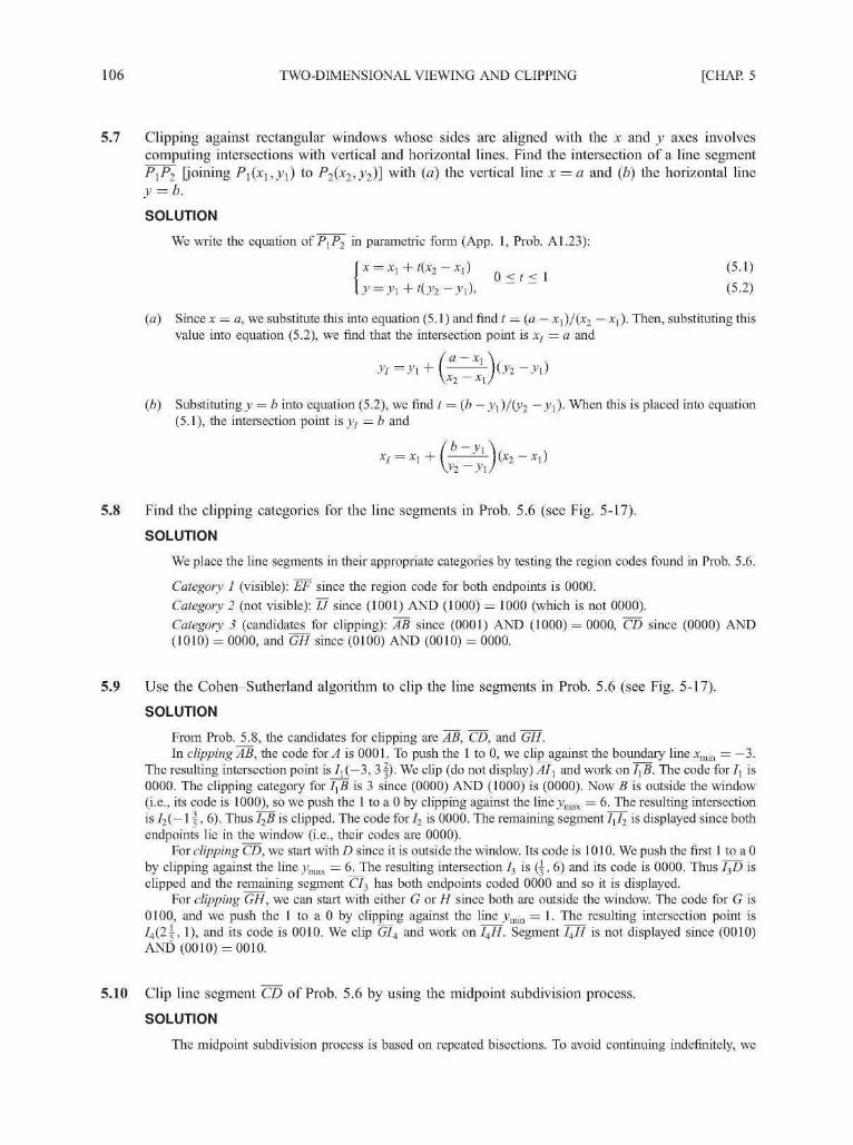
106 TWO-DIMENSIONAL VIEWING AND CLIPPING [CHAP. 5
5.7 Clipping against rectangular windows whose sides are aligned with the x and y axes involvescomputing intersections with vertical and horizontal lines. Find the intersection of a line segmentP\^2 [joining P1(x1,iy1) to i-^fe'J^)] with (a) the vertical line x = a and (b) the horizontal liney = b.
SOLUTION
We write the equation of PjP2 i*1 parametric form (App. 1, Prob. A1.23):
= x 1 + f ( x 2 - x 1 ) Q < t < l (5-1)
= y\ + Kyi-y\\ ~ ~ (5-2)
(a) Since x = a, we substitute this into equation (5.1) and find t = (a — Xj)/(x2 — Xj). Then, substituting thisvalue into equation (5.2), we find that the intersection point is Xj = a and
( a — Xi
X2 ~ x l
(b) Substituting y = b into equation (5.2), we find t = (b — y\)/(y2 ~y\)- When this is placed into equation(5.1), the intersection point is yt = b and
xI=xl + (
5.8 Find the clipping categories for the line segments in Prob. 5.6 (see Fig. 5-17).
SOLUTION
We place the line segments in their appropriate categories by testing the region codes found in Prob. 5.6.
Category 1 (visible): EF since the region code for both endpoints is 0000.
Category 2 (not visible): IJ since (1001) AND (1000) = 1000 (which is not 0000).
Category 3 (candidates for clipping): AB since (0001) AND (1000) = 0000, ~CD since (0000) AND(1010) = 0000, and GH since (0100) AND (0010) = 0000.
5.9 Use the Cohen-Sutherland algorithm to clip the line segments in Prob. 5.6 (see Fig. 5-17).
SOLUTION
From Prob. 5.8, the candidates for clipping are AB, CD, and GH.In clipping AB, the code for A is 0001. To push the 1 to 0, we clip against the boundary line xmin = — 3.
The resulting intersection point is 7j (—3, 31). We clip (do not display) AI^ and work on I^B. The code for 7j is0000. The clipping category for 4 8 is 3 since (0000) AND (1000) is (0000). Now B is outside the window(i.e., its code is 1000), so we push the 1 to a 0 by clipping against the line ymsK = 6. The resulting intersectionis 72(— 11, 6). Thus I2B is clipped. The code for 72 is 0000. The remaining segment 7j72 is displayed since bothendpoints lie in the window (i.e., their codes are 0000).
For clipping CD, we start with D since it is outside the window. Its code is 1010. We push the first 1 to a 0by clipping against the line >>max = 6. The resulting intersection 73 is ( | , 6) and its code is 0000. Thus 737J> isclipped and the remaining segment C73 has both endpoints coded 0000 and so it is displayed.
For clipping GH, we can start with either G or 77 since both are outside the window. The code for G is0100, and we push the 1 to a 0 by clipping against the line ymin = 1. The resulting intersection point is74(2j , 1), and its code is 0010. We clip GI4 and work on 7477. Segment 7477 is not displayed since (0010)AND (0010) = 0010.
5.10 Clip line segment CD of Prob. 5.6 by using the midpoint subdivision process.
SOLUTION
The midpoint subdivision process is based on repeated bisections. To avoid continuing indefinitely, we

CHAP. 5] TWO-DIMENSIONAL VIEWING AND CLIPPING 107
agree to say that a point (xx, yx) lies on any of the boundary lines of the rectangle, say, boundary line x = xmax,for example, if —TOL < xj — xmax < TOL. Here TOL is a prescribed tolerance, some small number, that isset before the process begins.
To clip CD, we determine that it is in category 3. For this problem we arbitrarily choose TOL = 0.1. Wefind the midpoint of CD to be Mx(\, 6.5). Its code is 1000.
So MXD is not displayed since (1000) AND (1010) = 1000. We further subdivide ~CMX since (0000)AND (1000) = 0000. The midpoint of CMX is M2(0, 5.75); the code for M2 is 0000. Thus CM2 is displayedsince both endpoints are 0000 and M2MX is a candidate for clipping. The midpoint of M2MX is M3(0.5, 6.125),and its code is 1000. Thus M3MX is chipped and M2M3 is subdivided. The midpoint of M2M3 isM4(0.25, 5.9375), whose code is 0000. However, since yx = 5.9375 lies within the tolerance 0.1 of theboundary line ymaK = 6—that is, 6 — 5.9375 = 0.0625 < 0.1, we agree that M4 lies on the boundary lineymaK = 6. Thus M2M4 is displayed and M4M3 is not displayed. So the original line segment CD is clipped atM4 and the process stops.
5.11 Suppose that in an implementation of the Cohen-Sutherland algorithm we choose boundary lines inthe top-bottom-right-left order to clip a line in category 3, draw a picture to show a worst-casescenario, i.e., one that involves the highest number of iterations.
SOLUTION
See Fig. 5-18.
Fig. 5-18
5.12 Use the Liang-Barsky algorithm to clip the lines in Fig. 5-19.
B(11 ,10)
A ( 1 1 , 6 )
ymin =
J(11,1)

108 TWO-DIMENSIONAL VIEWING AND CLIPPING [CHAP. 5
SOLUTION
For line AB, we have
Pl=0 ?! = 10
p2 = 0 ft = —2
ft = - 4 ft = 4
ft = 4 ?4 = 2
Since p2 = 0 and #2 < —2, 45 is completely outside the right boundary.For line CD, we have
ft = 0 ft = 2
p2 = 0 q2 = 6
ft = - 3 ft = 5 r3 = - !
ft = 3 ft = 1 r4 = 5
Thus «i = max(0, — |) = 0 and w2 = min(l, j) = | . Since «i < M2, the two endpoints of the clipped line are(3,7) and (3, 7 + 3(1)) = (3, 8). '
For line EF, we have
ft = - 6 ft = l r\ = ~\
p2 = 6 ft = 7
ft = - l ft = l r3-
ft = 1 ft = 5 r4 = f
Thus Mj = max(0, — g, — 1) = 0 and w2 = min(l, | , 5) = 1. Since «j = 0 and w2 = l> line -S7 is completelyinside the clipping window.
For line GH, we have
ft = - 2 ft =5 ^ = - fft = 2 ft = 3 r2 = \
ft = - 3 ft = 4 r3 = - |
ft = 3 ft = 2 r4 = |
Thus «i = max(0, —|, —I) = 0 and w2 = min(l, | , |) = | . Since «i < M2, the two endpoints of the clippedline are (6,6) and (6 + 2(f), 6 + 3(f)) = (71, 8).
For line / / , we have
A = " 1 2 ft = - 2 r 1 = i
p2 = 12 & = 10 r2 = f
ft = 6 ft = 5 r3 = |
ft = -6 ft = l rA = ~\
Thus Mj = max(0, g> — ) = g and «2 = min(l, §,§)=§• Since «j < M2, the two endpoints of the clipped line
are (-1 + 12(1), 7 + ( _ 6 ) ( ^ ) = (l, 6) and (-1 + 12(|), 7 + (-6)(|)) = (9, 2).
5.13 How can we determine whether a point i->(x,_v) lies to the left or to the right of a line segmentjoining the points A(xl,yl) and B{x1,y7f.
SOLUTION
Refer to Fig. 5-20. Form the vectors AB and AP. If the point P is to the left of AB, then by the definitionof the cross product of two vectors (App. 2) the vector AB x AP points in the direction of the vector Kperpendicular to the xy plane (see Fig. 5-20). If it lies to the right, the cross product points in the direction

CHAP. 5] TWO-DIMENSIONAL VIEWING AND CLIPPING 109
- K . Now
So
AB = (x2 - AP = (x - x^I + 0 -
AB x AP = [(x2 - xOO -JVi) - O2 - J d X * "
Then the direction of this cross product is determined by the number
C = (x2 -x{)(y-y{) - O2 - J ' I X X - X ] )
If C is positive, P lies to the left of AB. If C is negative, then P lies to the right of AB.
ABXAP'1
K
Fig. 5-20
5.14 Draw a flowchart illustrating the logic of the Sutherland-Hodgman algorithm.
SOLUTION
The algorithm inputs the vertices of a polygon one at a time. For each input vertex, either zero, one, ortwo output vertices will be generated depending on the relationship of the input vertices to the clipping edgeE.
We denote by P the input vertex, S the previous input vertex, and F the first arriving input vertex. Thevertex or vertices to be output are determined according to the logic illustrated in the flowchart in Fig. 5-21.Recall that a polygon with n vertices P j , P2 , • • •, Pn has n edges P\P2> • • • > Pn-\Pn and the edge PnP\ closingthe polygon. In order to avoid the need to duplicate the input of Pj as the final input vertex (and acorresponding mechanism to duplicate the final output vertex to close the polygon), the closing logic shown inthe flowchart in Fig. 5-22 is called after processing the final input vertex Pn.
5.15 Clip the polygon Plt...,P9 in Fig. 5-23 against the window ABCD using the Sutherland-Hodgman algorithm.
SOLUTION
At each stage the new output polygon, whose vertices are determined by applying the Sutherland-Hodgman algorithm (Prob. 5.14), is passed on to the next clipping edge of the window ABCD. The results areillustrated in Figs. 5-24 through 5-27.
5.16 Clip the polygon Plt...,Ps in Fig. 5-10 against the rectangular clipping window using theSutherland-Hodgman algorithm.
SOLUTION
We first clip against the top boundary line, then the left, and finally the bottom. The right boundary isomitted since it does not affect any vertex list. The intermediate and final results are in Fig. 5-28.

110 TWO-DIMENSIONAL VIEWING AND CLIPPING [CHAP. 5
Yes
Computeintersection
point /
Outputvertex /
( Input Avertex P J
Yes
Fig. 5-21

CHAP. 5] TWO-DIMENSIONAL VIEWING AND CLIPPING 111
L
R
Computeintersection
Outputvertex /
Fig. 5-22
Fig. 5-24 Clip against AB.
L\R
Fig. 5-25 Clip against 5C.
5.17 Use the Weiler-Atherton algorithm to clip the polygon in Fig. 5-29(a).
SOLUTION
See Fig. 5-29(6) and (c).
5.18 Consider the example in Sect. 5.5, where the object would appear turning slowly around its centereven if we set Aa = 0. How to keep the orientation of the object constant while making it rotatearound the center of the display area?

112 TWO-DIMENSIONAL VIEWING AND CLIPPING [CHAP. 5
sn D
S2 A S3 S5 S6B
Fig. 5-26 Clip against CJ5.
R
L
Fig. 5-27 Clip against DA.
aQ-.
Q
a
a
a
a
aClip againsttop boundary
fi,
Clip againstleft boundary
Fig. 5-28
S6
S9 S1
Clip againstbottom boundary
Subjectpolygon
Clippolygon
()
SOLUTION
Aa = —A/?, i.e., a. = —/?.
Startingvertex
Fig. 5-29
5.19 How to animate the flag in Fig. 5-30(a) that may be in two different positions using lookup tableanimation?
SOLUTION
See Fig. 5-30(&). The area where position 1 overlaps position 2 is assigned entry 0 that has the color ofthe flag. The rest of position 1 is assigned entry 1 and that of position 2 entry 2. Now we only need to alternateentries 1 and 2 between the flag color and the background color.
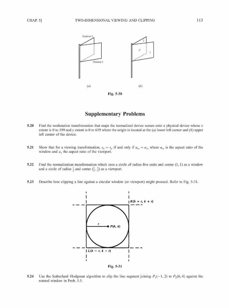
CHAP. 5] TWO-DIMENSIONAL VIEWING AND CLIPPING 113
Position 2
(a) (b)
Fig. 5-30
Supplementary Problems
5.20 Find the workstation transformation that maps the normalized device screen onto a physical device whose xextent is 0 to 199 and j ; extent is 0 to 639 where the origin is located at the (a) lower left corner and (b) upperleft corner of the device.
5.21 Show that for a viewing transformation, sx = sy if and only if aw = av, where aw is the aspect ratio of thewindow and av the aspect ratio of the viewport.
5.22 Find the normalization transformation which uses a circle of radius five units and center (1,1) as a windowand a circle of radius \ and center (1,1) as a viewport.
5.23 Describe how clipping a line against a circular window (or viewport) might proceed. Refer to Fig. 5-31.
| R(h + r, k + r)
Fig. 5-31
5.24 Use the Sutherland-Hodgman algorithm to clip the line segment joining Pi(—l, 2) to ^2(6, 4) against therotated window in Prob. 5.5.

CHAPTER 6
Three-DimensionalTransformations
Manipulation, viewing, and construction of three-dimensional graphic images requires the use of three-dimensional geometric and coordinate transformations. These transformations are formed by composingthe basic transformations of translation, scaling, and rotation. Each of these transformations can berepresented as a matrix transformation. This permits more complex transformations to be built up by use ofmatrix multiplication or concatenation.
As with two-dimensional transformations, two complementary points of view are adopted: either theobject is manipulated directly through the use of geometric transformations, or the object remainsstationary and the viewer's coordinate system is changed by using coordinate transformations. In addition,the construction of complex objects and scenes is facilitated by the use of instance transformations. Theconcepts and transformations introduced here are direct generalizations of those introduced in Chap. 4 fortwo-dimensional transformations.
6.1 GEOMETRIC TRANSFORMATIONS
With respect to some three-dimensional coordinate system, an object Obj is considered as a set ofpoints:
= {P(x,y,z)}
If the object is moved to a new position, we can regard it as a new object Obj', all of whose coordinatepoints P'(x',y',z') can be obtained from the original coordinate points P(x,y,z) of Obj through theapplication of a geometric transformation.
Translation
An object is displaced a given distance and direction from its original position. The direction anddisplacement of the translation is prescribed by a vector
V = a\ + bJ + cK
114

CHAP. 6] THREE-DIMENSIONAL TRANSFORMATIONS 115
The new coordinates of a translated point can be calculated by using the transformation
(see Fig. 6-1). In order to represent this transformation as a matrix transformation, we need to usehomogeneous coordinates (App. 2). The required homogeneous matrix transformation can then beexpressed as
x ' \
y'z'
/ i
- °" oVo
0100
0010
a\
b \c\1 /
X
\ 1
Fig. 6-1
Scaling
The process of scaling changes the dimensions of an object. The scale factor s determines whether thescaling is a magnification, s > 1, or a reduction, s < 1.
Scaling with respect to the origin, where the origin remains fixed, is effected by the transformation
x' = sx • x
y1 = s y - y= 5V • Z
In matrix form this is
Rotation
Rotation in three dimensions is considerably more complex than rotation in two dimensions. In twodimensions, a rotation is prescribed by an angle of rotation 6 and a center of rotation P. Three-dimensionalrotations require the prescription! of an angle of rotation and an axis of rotation. The canonical rotationsare defined when one of the positive x, y, or z coordinate axes is chosen as the axis of rotation. Then the

116 THREE-DIMENSIONAL TRANSFORMATIONS [CHAP. 6
construction of the rotation transformation proceeds just like that of a rotation in two dimensions about theorigin (see Fig. 6-2).
Rotation about the z Axis
From Chap. 4 we know that
z
Fig. 6-2
x' = x cos 6 — y sin 6R8K: \ y = x sin 6 + y cos 6
z' =z
Rotation about the y Axis
An analogous derivation leads to
R6,3- '
x' = x cos 0 + z sin 6
y'=yz' = —x sin 0 + z cos i
Rotation about the x Axis
Similarly:
y1 = ycos 0 — z sin 0z' = y sin 0 + z cos 0
Note that the direction of a positive angle of rotation is chosen in accordance to the right-hand rule withrespect to the axis of rotation (App. 2).
The corresponding matrix transformations are
Re,K —
Re,j =
Rgi =
1 cos 6 -
sin 6 <
1 o/ COS0
0
\-sin0
/ I 0
0 cos0
VO sin0
•sin0 0
;os
0
0
1
0
9 0
1
sin0
0
COS0
0
- sinfl
COS0

CHAP. 6] THREE-DIMENSIONAL TRANSFORMATIONS 117
The general use of rotation about an axis L can be built up from these canonical rotations using matrixmultiplication (Prob. 6.3).
6.2 COORDINATE TRANSFORMATIONS
We can also achieve the effects of translation, scaling, and rotation by moving the observer who viewsthe object and by keeping the object stationary. This type of transformation is called a coordinate
ix'.y'.z')
o
Fig. 6-3
transformation. We first attach a coordinate system to the observer and then move the observer and theattached coordinate system. Next, we recalculate the coordinates of the observed object with respect to thisnew observer coordinate system. The new coordinate values will be exactly the same as if the observer hadremained stationary and the object had moved, corresponding to a geometric transformation (see Fig. 6-3).
If the displacement of the observer coordinate system to a new position is prescribed by a vectorV = a\ + bi + cK, a point P(x, y, z) in the original coordinate system has coordinates P(xf, / , z') in thenew coordinate system, and
I x' = x — a
y'=y-bZ1 =z-c
The derivation of this transformation is completely analogous to that of the two-dimensional transforma-tion (see Chap. 4).
Similar derivations hold for coordinate scaling and coordinate rotation transformations.As in the two-dimensional case, we summarize the relationships between the matrix forms of the
coordinate transformations and the geometeric transformations:
Coordinate Transformations Geometric TransformationsTranslation fY T_Y
Rotation Rg R_e
l/Sx,l/Sy,l/Sz
Inverse geometric and coordinate transformations are constructed by performing the reverse operation.Thus, for coordinate transformations (and similarly for geometric transformations):
Ty —T_y Rg — R_g SSx,sy,s2 — Sl/xx,l/sy,l/s2
6.3 COMPOSITE TRANSFORMATIONS
More complex geometric and coordinate transformations are formed through the process ofcomposition of functions. For matrix functions, however, the process of composition is equivalent to

118 THREE-DIMENSIONAL TRANSFORMATIONS [CHAP. 6
matrix multiplication or concatenation. In Probs. 6.2, 6.3, 6.5, and 6.13, the following transformations areconstructed:
1.
2.
3.
Ay^ = aligning a vector V with a vector N.
RQL = rotation about an axis L. This axis is prescribed by giving a direction vector V and a pointP through which the axis passes.
= scaling with respect to an arbitrary point P.Ss s s
In order to build these more complex transformations through matrix concatenation, we must be ableto multiply translation matrices with rotation and scaling matrices. This necessitates the use ofhomogeneous coordinates and 4 x 4 matrices (App. 2). The standard 3 x 3 matrices of rotation andscaling can be represented as 4 x 4 homogeneous matrices by adjoining an extra row and column asfollows:
(adg
VO
beh0
c
fi0
00u
These transformations are then applied to points P(x,y,z) having the homogeneous form:
EXAMPLE 1. The matrix of rotation about the y axis has the homogeneous 4 x 4 form:
0 s i n 0 0 s
0 1 0 0- s i n 0 0 cos 8 0
0 0 0 1
6.4 I N S T A N C E T R A N S F O R M A T I O N S
If an object is created and described in coordinates with respect to its own object coordinate space, wecan place an instance or copy of it within a larger scene that is described in an independent coordinatespace by the use of three-dimensional coordinate transformations. In this case, the transformations arereferred to as instance transformations. The concepts and construction of three-dimensional instancetransformations and the composite transformation matrix are completely analogous to the two-dimensionalcases described in Chap. 4.
Solved Problems
6.1 Define tilting as a rotation about the x axis followed by a rotation about the y axis: (a) find the tiltingmatrix; (b) does the order of performing the rotation matter?

CHAP. 6] THREE-DIMENSIONAL TRANSFORMATIONS 119
SOLUTION
(a) We can find the required transformation T by composing (concatenating) two rotation matrices:
y n n
0 0 0\cosft 0 sinft 0\
0 1 0 0
- s i n 0 0 cos ft, 0
V
0 - s i n ft, 0
0 sin ft, cos ft, 0
0 0 0 10 0 0
( cos 8y sin 8y sin 8X sin 8y cos ft, 0 ^
0 cos ft, - s in ft, 0
—sin 8y cos By sin ft, cos 8y cos8x 0
0 0
We multiply Rg l • Rg j to obtain the matrix
/ cos ft, 0 sin ft,
sin 8X sin 8 cos 8X — sin 8X cos 0y 0
— cos 8X sin 0 sin ft, cos ft, cos 0y 0
V 0 0 0 1 /
This is not the same matrix as in part a; thus the order of rotation matters.
6.2 Find a transformation ^4V which aligns a given vector V with the vector K along the positive z axis.
SOLUTION
See Fig. 6-4(a). Let V = a\ + bj + cK. We perform the alignment through the following sequence oftransformations [Figs. 6-4(b) and 6-4(c)]:
1. Rotate about the x axis by an angle 6X so that V rotates into the upper half of the xz plane (as the vectorVi).
2. Rotate the vector Vj about the y axis by an angle —82 so that Vj rotates to the positive z axis (as thevector V2).
Implementing step 1 from Fig. 6-4(b), we observe that the required angle of rotation 8l can be found bylooking at the projection of V onto the yz plane. (We assume that b and c are not both zero.) From triangleOP'B:
sin 8X = cos ft =
The required rotation is
,,i =
0 -
0 -
K0
0c
b
Jb2 + c2
0
0b
*/b~2~+~c2
c
Vft2 + c2
0
Applying this rotation to the vector V produces the vector Vj with the components (a, 0, *Jb2 + c2).

120 THREE-DIMENSIONAL TRANSFORMATIONS [CHAP. 6
(c)
Fig. 6-4

CHAP. 6] THREE-DIMENSIONAL TRANSFORMATIONS 121
Implementing step 2 from Fig. 6-4(c), we see that a rotation of — 82 degrees is required, and so fromtriangle OQQ:
sin(—07) = — sin 0, = . =2 2 Vfl2 + 62 + c2
and cos(—62) = cos £>2 =Ib2 + c2
Vfl2 + b2 + c2
Then
R -82 ,J —
/ft2 + C2
0\
= 0la2 + b2 + c2 Vfl2 + b2 + c2
0 1 0 0
Tc1
0la2 + b2 + c2 ^Ja2 + b2 + c2
0 0 0
= 0
ySince |V| = Vfl2 + b2 + c2, and introducing the notation 1 = V^2 + c2, we find
X|V|
0
i^i0
-flft
A|V|
c
Ift
0
—ac
W\- f t
X
0
0
o
0
1 i
If both b and c are zero, then V = a\, and so 1 = 0. In this case, only a ±90° rotation about the j ; axisis required. So if 1 = 0, it follows that
' 0 0 — 0 \
0 1 0 0
V ° ° °V 0 0 0 1/
In the same manner we calculate the inverse transformation that aligns the vector K with the vector V:
—ab c bA|V| A |V|
—ac b c0
1|V| 1 |V|
\ 0 0 0 1/
6.3 Let an axis of rotation L be specified by a direction vector V and a location point P. Find thetransformation for a rotation of 6° about L. Refer to Fig. 6-5.

122 THREE-DIMENSIONAL TRANSFORMATIONS [CHAP. 6
Fig. 6-5 Fig. 6-6
SOLUTION
We can find the required transformation by the following steps:
1. Translate P to the origin.
2. Align V with the vector K.
3. Rotate by 0° about K.
4. Reverse steps 2 and 1.
So
ReL — T_P • Av • ReK • Av • T_P
Here, Ay is the transformation described in Prob. 6.2.
6.4 The pyramid denned by the coordinates ,4(0, 0, 0), 5(1, 0, 0), C(0, 1, 0), and D(0, 0, 1) is rotated45° about the line L that has the direction V = J + K and passing through point C(0, 1, 0) (Fig.6-6). Find the coordinates of the rotated figure.
SOLUTION
From Prob. 6.3, the rotation matrix RgL can be found by concatenating the matrices
ReL — T_P • Av • ReK • Av • T_P
WithP = (0, 1,0), then
T-P =

CHAP. 6] THREE-DIMENSIONAL TRANSFORMATIONS 123
Now V = J + K. So from Prob. 6.2, with a = 0, b = 1, c = 1, we find k = -Jl, |V| = -Jl, and
Av =
Also
Then
n 0l
0 -7=V2
\0 0
/ 1
=i
\l L0
\ °/
Re,L =
V
0
VI
V20
-1
1
\l L0
0
V22
12
1
2
0
0\
o
0
0
0
1
0
2 +
2-
\0
0
0
V
l
2
V4
4
3
v =
/I
0
°
7—1 _1-P —
1
2
; 2-V2 :4
! 2 + V2 -4
0
01V2
V20
/I
0
0
Vo
1
2
.-v4
n-4
1
0
1
0
0
*!
2
01V2
V20
0
0
1
0
\
/
0
0
ly
0\
1
0
1/
To find the coordinates of the rotated figure, we apply the rotation matrix Rg L to the matrix of homogeneouscoordinates of the vertices A,B,C, and D:
C = (ABCD) =
/0 1 0 0"0 0 1 00 0 0 11 1 1 1
So
R e,L • C =
1+V22
2-V24
V2-241
2
4-V24
V2-441
1
0
1
2-V22
V22
1
The rotated coordinates are (Fig. 6-7)
\ 2-V2 V2-2U
B' =
4 4V2 4-V2 V2-4'
C = (0, 1,0)
2 - V 2 V2'' 2 ' 2

124 THREE-DIMENSIONAL TRANSFORMATIONS [CHAP. 6
Fig. 6-7
6.5 Find a transformation ^4V N which aligns a vector V with a vector N.
SOLUTION
We form the transformation in two steps. First, align V with vector K, and second, align vector K withvector N. So from Prob. 6.2,
Ay j N = A N • A y
Referring to Prob. 6.12, we could also get AVN by rotating V towards N about the axis V x N.
6.6 Find the transformation for mirror reflection with respect to the xy plane.
SOLUTION
From Fig. 6-8, it is easy to see that the reflection of P(x, y, z) is P'(x,y, —z). The transformation thatperforms this reflection is
1 0 N
1 0 1 00 0 - 1
6.7 Find the transformation for mirror reflection with respect to a given plane. Refer to Fig. 6-9.
SOLUTION
Let the plane of reflection be specified by a normal vector N and a reference point P0(x0 ,^0 ,z0). Toreduce the reflection to a mirror reflection with respect to the xy plane:
1. Translate Po to the origin:
2. Align the normal vector N with the vector K normal to the xy plane.
3. Perform the mirror reflection in the xy plane (Prob. 6.6).
4. Reverse steps 1 and 2.
So, with translation vector V = — xol — yQJ — z0K
Here, A-^ is the alignment matrix defined in Prob. 6.2. So if the vector N = Mjl + n2J + n3K, then from Prob.

CHAP. 6] THREE-DIMENSIONAL TRANSFORMATIONS 125
0
Pfr, v, z)
(.v. y, 0)
II
1 Fix, v, -z)
Fig. 6-8
Rctlcction plane
N
Fig. 6-9
6.2, with |N| = - /MJ + «2 + M3 a n d X = \/M2 + M3> w e
/ X —n^n2 —
|N|
0
iNiV 0
A|N|
M3
X
INf0
A|N|
~ M 2
1
^ 3 _
0
0
0
0
i y
and ^-1
0 W\ °A|N| 1 |N|
— - -^- 0X |N|0 0 1
A|N|
0
In addition
/I 0 0 -x0
0 1 0 -y0
0 0 / - z 0
yO 0 0 1
and
/I 0 0 ji0
0 1 0 yo0 0 / z0
yO 0 0 1
Finally, from Prob. 6.6, the homogeneous form of M is
M =
6.8 Find the matrix for mirror reflection with respect to the plane passing through the origin and havinga normal vector whose direction is N = I + J + K.

126 THREE-DIMENSIONAL TRANSFORMATIONS [CHAP. 6
SOLUTION
From Prob. 6.7, with P0(0, 0, 0) and N = I + J + K, we find |N| = V3 and A = <Jl. Then
and
(\ 0 0 0 \
0 1 0 0
0 0 1 0
Vo o o 1/
(V = 01 + 0J + OK) TV1 =
/I 0 0 0 \
0 1 0 0
0 0 1 0
Vo o o 1 /
-1
V3 V2V3 V2V3
01
711 1
71 7!V 0 0
The reflection matrix is
- 1
711
7!0
0
0
1/
4 0V
4=1 1 1
V2V3 V2 V3
- 1 - 1 - 10
VV3 V2 V3
V 0 0 0 1 /
M =
• Af] • M • A-ft • Ty
3- - I " I «\-I 1 - I 0
_3
V 0
I f )3 U
0 1/
Supplementary Problems
6.9 Align the vector V = I + J + K with the vector K.
6.10 Find a transformation which aligns the vector V = I + J + K with the vector N = 21 — J — K.
6.11 Show that the alignment transformation satisfies the relation Ay l = A^.
6.12 Show that the alignment transformation Ay-^ is equivalent to a rotation of 8° about an axis having thedirection of the vector V x N and passing through the origin (see Fig. 6-10). Here 8 is the angle betweenvectors V and N.

CHAP. 6] THREE-DIMENSIONAL TRANSFORMATIONS 127
6.13 How can scaling with respect to a point P0(x0,y0, z0) be defined in terms of scaling with respect to the origin?

CHAPTER 7
Mathematics ofProjection
Needless to say, there are fundamental differences between the true three-dimensional world and itspictorial description. For centuries, artists, engineers, designers, drafters, and architects have tried to cometo terms with the difficulties and constraints imposed by the problem of representing a three-dimensionalobject or scene in a two-dimensional medium—the problem of projection. The implementers of a computergraphics system face the same challenge.
Projection can be defined as a mapping of point P (x, y, z) onto its image P' (x1, /, z') in the projectionplane or view plane, which constitutes the display surface (see Fig. 7-1). The mapping is determined by aprojection line called the projector that passes through P and intersects the view plane. The intersectionpoint is P'.
Projection/viewplane
Fig. 7-1 The problem of projection.
The result of projecting an object is dependent on the spatial relationship among the projectors thatproject the points on the object, and the spatial relationship between the projectors and the view plane (seeSec. 7.1). An important observation is that projection preserves lines. That is, the line joining the projectedimages of the endpoints of the original line is the same as the projection of that line.
The two basic methods of projection—perspective and parallel—are designed to solve the basic butmutually exclusive problems of pictorial representation: showing an object as it appears and preserving its
128

CHAP. 7] MATHEMATICS OF PROJECTION 129
true size and shape. We characterize each method and introduce the mathematical description of theprojection process in Sec. 7.2 and 7.3, respectively.
7.1 TAXONOMY OF PROJECTION
We can construct different projections according to the view that is desired.Figure 7-2 provides a taxonomy of the families of perspective and parallel projections. Some
projections have names—cavalier, cabinet, isometric, and so on. Other projections qualify the maintype of projection—one principal vanishing-point perspective, and so forth.
Projections
Perspective(converging projectors)
Parallel(parallel projectors)
One point
(oneprincipalvanishingpoint)
Two point
(twoprincipalvanishingpoints)
Three point
(threeprincipalvanishingpoints)
Orthographic(projectors perpendicularto view plane)
Oblique(projectors not perpendicularto view plane)
Multiview(view planeparallel toprincipalplanes)
Axonometric(view planenot parallel toprincipalplanes)
General
Cavalier Cabinet
Isometric Dimetric Trimetric
Fig. 7-2 Taxonomy of projection.
7.2 PERSPECTIVE PROJECTION
Basic Principles
The techniques of perspective projection are generalizations of the principles used by artists inpreparing perspective drawings of three-dimensional objects and scenes. The eye of the artist is placed atthe center of projection, and the canvas, or more precisely the plane containing the canvas, becomes theview plane. An image point is determined by a projector that goes from an object point to the center ofprojection (see Fig. 7-3).
Perspective drawings are characterized by perspective foreshortening and vanishing points. Perspectiveforeshortening is the illusion that objects and lengths appear smaller as their distance from the center ofprojection increases. The illusion that certain sets of parallel lines appear to meet at a point is anotherfeature of perspective drawings. These points are called vanishing points. Principal vanishing points areformed by the apparent intersection of lines parallel to one of the three principal x, y, or z axes. The numberof principal vanishing points is determined by the number of principal axes intersected by the view plane(Prop. 7.7).
Mathematical Description of a Perspective Projection
A perspective transformation is determined by prescribing a center of projection and a view plane. Theview plane is determined by its view reference point Ro and view plane normal N. The object point P islocated in world coordinates at (x, y, z). The problem is to determine the image point coordinates
,zO (see Fig. 7-3).

130 MATHEMATICS OF PROJECTION [CHAP. 7
1'ix.
C(0, 0, -d)
Fig. 7-3 Fig. 7-4
EXAMPLE 1. The standard perspective projection is shown in Fig. 7-4. Here, the view plane is the xy plane, andthe center of projection is taken as the point C(0, 0, —d) on the negative z axis.
Using similar triangles ABC and A'OC, we find
d • x . d • yv = •
z + d z + dz' = 0
The perspective transformation between object and image point is nonlinear and so cannot be represented as a3 x 3 matrix transformation. However, if we use homogeneous coordinates, the perspective transformation can berepresented as a 4 x 4 matrix:
Id 0 0 0\ Ix'0 d 0 0 \\y0 0 0 0
v 0 0 1 d)\\
The general form of a perspective transformation is developed in Prob. 7.5.
Perspective Anomalies
The process of constructing a perspective view introduces certain anomalies which enhance realism interms of depth cues but also distort actual sizes and shapes.
1. Perspective foreshortening. The farther an object is from the center of projection, the smaller itappears (i.e. its projected size becomes smaller). Refer to Fig. 7-5.
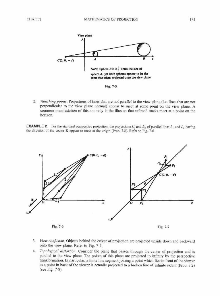
CHAP. 7] MATHEMATICS OF PROJECTION 131
C(0, 0, -d)
Note: Sphere B is 2 y times the size of
sphere A, yet both spheres appear to be thesame size when projected onto the view plane
Fig. 7-5
2. Vanishing points. Projections of lines that are not parallel to the view plane (i.e. lines that are notperpendicular to the view plane normal) appear to meet at some point on the view plane. Acommon manifestation of this anomaly is the illusion that railroad tracks meet at a point on thehorizon.
EXAMPLE 2. For the standard perspective projection, the projections L\ and L'2 of parallel lines Lx and L2 havingthe direction of the vector K appear to meet at the origin (Prob. 7.8). Refer to Fig. 7-6.
C(0. 0, -rf)
rO Pi
Fig. 7-6 Fig. 7-7
3. View confusion. Objects behind the center of projection are projected upside down and backwardonto the view plane. Refer to Fig. 7-7.
4. Topological distortion. Consider the plane that passes through the center of projection and isparallel to the view plane. The points of this plane are projected to infinity by the perspectivetransformation. In particular, a finite line segment joining a point which lies in front of the viewerto a point in back of the viewer is actually projected to a broken line of infinite extent (Prob. 7.2)(see Fig. 7-8).
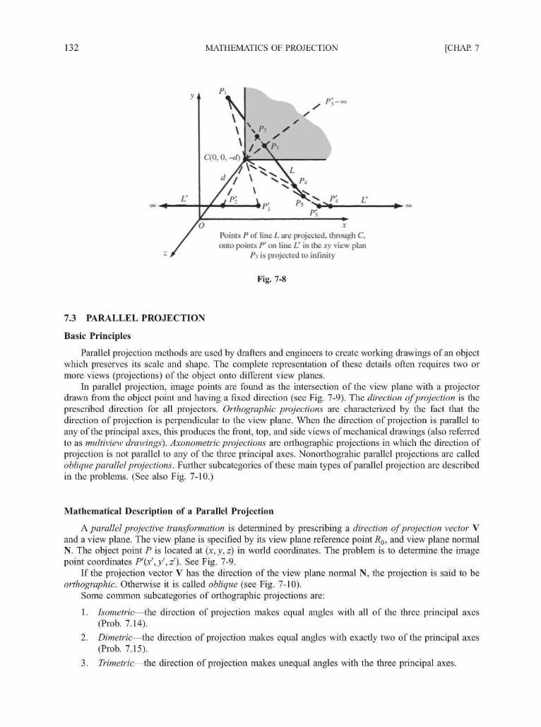
132 MATHEMATICS OF PROJECTION [CHAP. 7
Poinls !y of line /. art: projected, through C,onto points P* on line / / in the xy view plan
P\ is projected to infinity
Fig. 7-8
7.3 PARALLEL PROJECTION
Basic Principles
Parallel projection methods are used by drafters and engineers to create working drawings of an objectwhich preserves its scale and shape. The complete representation of these details often requires two ormore views (projections) of the object onto different view planes.
In parallel projection, image points are found as the intersection of the view plane with a projectordrawn from the object point and having a fixed direction (see Fig. 7-9). The direction of projection is theprescribed direction for all projectors. Orthographic projections are characterized by the fact that thedirection of projection is perpendicular to the view plane. When the direction of projection is parallel toany of the principal axes, this produces the front, top, and side views of mechanical drawings (also referredto as multiview drawings). Axonometric projections are orthographic projections in which the direction ofprojection is not parallel to any of the three principal axes. Nonorthograhic parallel projections are calledoblique parallel projections. Further subcategories of these main types of parallel projection are describedin the problems. (See also Fig. 7-10.)
Mathematical Description of a Parallel Projection
A parallel projective transformation is determined by prescribing a direction of projection vector Vand a view plane. The view plane is specified by its view plane reference point Ro, and view plane normalN. The object point P is located at (x, y, z) in world coordinates. The problem is to determine the imagepoint coordinates P'{x',y',z'). See Fig. 7-9.
If the projection vector V has the direction of the view plane normal N, the projection is said to beorthographic. Otherwise it is called oblique (see Fig. 7-10).
Some common subcategories of orthographic projections are:
1. Isometric—the direction of projection makes equal angles with all of the three principal axes(Prob. 7.14).
2. Dimetric—the direction of projection makes equal angles with exactly two of the principal axes(Prob. 7.15).
3. Trimetric—the direction of projection makes unequal angles with the three principal axes.

CHAP. 7] MATHEMATICS OF PROJECTION 133
y *B
Oblique
Fig. 7-9 Fig. 7-10
Some common subcategories of oblique projections are:
1. Cavalier—the direction of projection is chosen so that there is no foreshortening of linesperpendicular to the xy plane (Prob. 7.13).
2. Cabinet—the direction of projection is chosen so that lines perpendicular to the xy planes areforeshortened by half their lengths (Prob. 7.13).
EXAMPLE 3. For orthographic projection onto the xy plane, from Fig. 7-11 it is easy to see that
f x ' = xParK: \ y1 = y
[The matrix form of ParK is
( 1 0 0
0 1 0 00 0 0 00 0 0 1
The general parallel projective transformation is derived in Prob. 7.11.
Solved Problems
7.1 The unit cube (Fig. 7-12) is projected onto the xy plane. Note the position of the x,y, and z axes.Draw the projected image using the standard perspective transformation with (a) d = 1 and (b)d = 10, where d is distance from the view plane.

134 MATHEMATICS OF PROJECTION [CHAP. 7
"
Fig. 7-11
SOLUTION
We represent the unit cube in terms of the homogeneous coordinates of its vertices:
V = (ABCDEFGH) =
/ 0 1 1 0 0 0 1 10 0 1 1 1 0 0 10 0 0 0 1 1 1 1
y l l l l l l l l
F i g . 7 - 1 2

CHAP. 7] MATHEMATICS OF PROJECTION 135
From Example 1 the standard perspective matrix is
PerK =
d000
0d00
0001
000d
(a) With d = 1, the projected coordinates are found by applying the matrix PerK to the matrix of coordinatesV. Then
PerK • V =
/ 0 1 1 0 0 0 1 1
0 0 1 1 1 0 0 10 0 0 0 0 0 0 01 1 1 1 2 2 2 2
If these homogeneous coordinates are changed to three-dimensional coordinates, the projectedimage has coordinates:
A' = (0, 0, 0)B' = (1,0,0)C = (1,1,0)# = (0,1,0)
£' = (0,1,0)F' = (0, 0, 0)G' = (1,0,0)H' = (1,1,0)
We draw the projected image by preserving the edge connections of the original object (see Fig. 7-13). [Note the vanishing point at (0, 0, 0).]
(b) With d = 10, the perspective matrix is
PerK =
/10 0 0 0"0 10 0 00 0 0 00 0 1 10
Then
PerK • V =
0 10 10 0 0
0 0 10 10 10
0 0 0 0 0
10 10 10 10 11
0 10 10 ~
0 0 10
0 0 0
11 11 11
is the matrix image coordinates in homogeneous form. The projected image coordinates are then
.4'= (0,0,0) £' = (0,lf,0)B' = (1,0,0)C' = (l, 1,0)# = (0,1,0)
F' = (0, 0, 0)G' = (jf,O,O)H, /io io A-,-" — M l ' 11 ' V )
Note the different perspectives of the face E'F'G'H' in Figs. 7-13 and 7-14. [To a viewer standing at thecenter of projection (0, 0, —d), this face is the back face of the unit cube.]
7.2 Under the standard perspective transformation PerK, what is the projected image of (a) a point inthe plane z =-d and (b) the line segment joining P ^ - l , 1, -Id) to P2(2, - 2 , 0)? (See Fig. 7-15.)
SOLUTION
(a) The plane z = —d is the plane parallel to the xy view plane and located at the center of projectionC(0, 0, —d). If P(x,y, —d) is any point in this plane, the line of projection CP does not intersect the xyview plane. We then say that P is projected out to infinity (oo).
(b) The line P\P2 passes through the plane z = —d. Writing the equation of the line (App. 2), we have
x = - l + 3 f y=l-3t z=-2d + 2dt

136 MATHEMATICS OF PROJECTION [CHAP. 7
y .
E'
A'
h ti
(F1) O' B'
y
D'E'
A' (F1)
H'
G'
c
Fig. 7-13 Fig. 7-14
Projection ontoxy plant-, ihrtiugh
viL-wpoint C(0, 0, -ct)of line segment P\ Pi
Fig. 7-15

CHAP. 7] MATHEMATICS OF PROJECTION 137
We see that at t = \: x = \, y = —\, and z = —d. These are the coordinates of the intersection point I.We now describe the perspective projection of this line segment.Applying the standard projection to the equation of the line, we find
Changing from homogeneous to three-dimensional coordinates, the equations of the projected linesegment are
-d + 3dt -l+3t-d + 2dt - 1 + It y =
d-3dt l-3t-d + 2dt ~ -1 + It
z = 0
(InApp. 1, Prob. A 1.12, it is shown that this is the equation of a line.) When t = 0, then x = 1 andy = — 1. These are the coordinates of the projection P[ of point P j . When t = 1, it follows that x = 2 andy = — 2 (the coordinates of the projection P'2 of point P2). However, when t = i, the denominator is 0.Thus this line segment "passes" through the point at infinity in joining P[(l, —1) to P'2(2, —2). In otherwords, when a line segment joining endpoints Px and P2 passes through the plane containing the centerof projection and which is parallel to the view plane, the projection of this line segment is not the simpleline segment joining the projected endpoints P[ and P2. (See also Prob. A1.13 in App. 1.)
7.3 Using the origin as the center of projection, derive the perspective transformation onto the planepassing through the point R0(x0,y0, z0) and having the normal vector N = « j / + n2J + n^K.
SOLUTION
Let P(x,y,z) be projected onto P'{x'',y',T!). From Fig. 7-16, the vectors PO and P'O have the samedirection. Thus there is a number a so that P'O = aPO. Comparing components, we have
x = ax y = ay z = az
Fig. 7-16

138 MATHEMATICS OF PROJECTION [CHAP. 7
We now find the value of a. Since any point P'(x',y', z7) lying on the plane satisfies the equation (App. 2)
nxx' + n2y' + n3z' = d0
(where dQ = nxxQ + n^Q + M3zo)> substitution of x' = ax, y1 = ay, and z' = az into this equation gives
nxx + n2y + n3z
This projection transformation cannot be represented as a 3 x 3 matrix transformation. However, byusing the homogeneous coordinate representation for three-dimensional points, we can write the projectiontransformation as a 4 x 4 matrix:
*000
h
0d0
0n2
00d0
n3
0000
Application of this matrix to the homogeneous representation P(x,y, z, 1) of points P gives P'(dox, doy,dQz, nxx + n^y + n3z), which is the homogeneous representation of P'(x!,y/, z7) found above.
7.4 Find the perspective projection onto the view plane z = d where the center of projection is theorigin (0, 0, 0).
SOLUTION
The plane z = d is parallel to the xy plane (and d units away from it). Thus the view plane normal vectorN is the same as the normal vector K to the xy plane, that is, N = K. Choosing the view reference point as_K0(0, 0, d), then from Prob. 7.3, we identify the parameters
N(«!, n2, n3) = (0, 0, 1) RQ(xQ,yQ,zQ) = (0, 0, d)
So
d0 = nxx0 + n^Q + n3z0 = d
and then the projection matrix is
' d 0 0 0 s
0 d 0 00 0 d 00 0 1 0
7.5 Derive the general perspective transformation onto a plane with reference point R0(x0,y0,z0),normal vector N = nx\ + n2i + «3K, and using C(a, b, c) as the center of projection. Refer to Fig.7-17.
SOLUTION
As in Prob. 7.3, we can conclude that the vectors PC and P'C satisfy (see Fig. 7-17) P'C = aPC. Then
x' = a(x — a) + a y' = a.(y — b) + b z1 = a(z — c) + c
Also, we find (by using the equation of the view plane) that
1 =nx(x — a) + n2(y — b) + n3(z — c)
[i.e. P'(x',y',z!) is on the view plane and thus satisfies the view plane equation nx(x'— x0) +«2<y - yo) + n ^ ~ zo) = 0]- Here, d = (nxx0 + n2y0 + n3z0) - (nxa + n2b + n3c).
From App. 2, Prob. A2.13, d is proportional to the distance D from the view plane to the center ofprojection, that is, d = ±|N|-D.

CHAP. 7] MATHEMATICS OF PROJECTION 139
Fig. 7-17
To find the homogeneous coordinate matrix representation, it is easiest to proceed as follows:
1. Translate so that the center of projection C lies at the origin. Now R'Q = (x0 — a, y0 — b, z0 — c)becomes the reference point of the translated plane (the normal vector is unchanged by translation).
2. Project onto the translated plane using the origin as the center of projection by constructing thetransformation PerN ™ (Prob. 7.3).
' 0
3. Translate back.
Introducing the intermediate quantities
dQ = Mjx0 + M2J0 + M3zo a n d d\ = nxa + n2b + n3cwe obtain d = d0 — dx, and so Per^RgC = Tc • Per^R, • T_c. Then with R'Q used as the reference point inconstructing the projection P N s ,
Per,N,iio,C
<\
0
0
vo
01
0
0
{d + an
bnx
cnx
72,
0
0
1
0
1
b
c
/
1 / Van2
d + bn
cn2
r 2
d
0
0
" 1
j
0
d
0
n2
an3
bn3
0
0
d
n3
d + cn3
n3
0 \
0
0
0 /—ad{
-bd(
-cd{
-dx
/ 0
0 1
0 0
\ (
) \
)
)
) 0
0 -a\0 -b
1 -c
0 \)
7.6 Find the (a) vanishing points for a given perspective transformation in the direction given by avector U and (b) principal vanishing points.
SOLUTION
(a) The family of (parallel) lines having the direction of U = «j I + u2 J + «3K can be written in parametricform as
x = «]£ +p y = u2t + q z = u3t + r

140 MATHEMATICS OF PROJECTION [CHAP. 7
where Pip, q, r) is any point (see App. 2). Application of the perspective transformation (Prob. 7.5) tothe homogeneous point (x,y, z, 1) produces the result {x',y', z7, h), where
x' = (d + an1)(u1t + p) + an2(u2t + q) + an3(u3t + r) — ad0
/ = bnx{uxt + p) + (d + bn2)(u2t + q) + bn3(u3t + r) - bd0
zf = cnx(uxt + p) + cn2(u2t + q) + (d + cn3)(u3t + r) — cd0
h = n1(u1t +p) + n2(u2t + q) + n3(u3t + r) — dx
The vanishing point corresponds to the infinite point obtained when t = oo. So after dividing x', / , andz7 by h, we let t —>• oo to find the coordinates of the vanishing point:
(d • an2u2 + an3u3
(Here, k = N • U = + n2u2 + n3u3.)
+ (d + bn2)u2 + bn3u3
+ cn2u2 + (d + cn3)u3
du2
V~k
du3
~~k~
This point lies on the line passing through the center of projection and parallel to the vector U (see Fig.7-18). Note that k = 0 only when U is parallel to the projection plane, in which case there is no vanishingpoint.
Center of projection
View plune
P\
Lines L\ and Li arc parallel to vector U: ^ QiL\ and V± arc projections, through C of
lines L\ and L; untu view plane
Fig. 7-18
(b) The principal vanishing points P j , P2, and P3 correspond to the vector directions I, J, and K. In thesecases
dXj = a -\
yx=b
zx=c
Pi-n2
x3 = ay3=b
dz3 = c -\
(Recall from Prob. 7.5 that a, b, c are the coordinates of the center of projection. Also, nx, n2, n3 are thecomponents of the view plane normal vector and d is proportional to the distance D from the view plane
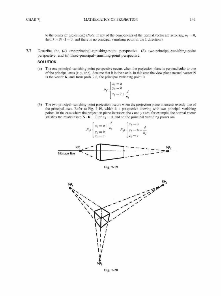
CHAP. 7] MATHEMATICS OF PROJECTION 141
to the center of projection.) (Note: If any of the components of the normal vector are zero, say, nx = 0,then k = N • I = 0, and there is no principal vanishing point in the I direction.)
7.7 Describe the (a) one-principal-vanishing-point perspective, (b) two-principal-vanishing-pointperspective, and (c) three-principal-vanishing-point perspective.
SOLUTION
(a) The one-principal-vanishing-point perspective occurs when the projection plane is perpendicular to oneof the principal axes (x, y, or z). Assume that it is the z axis. In this case the view plane normal vector Nis the vector K, and from prob. 7.6, the principal vanishing point is
x3 =ay-i=b
d
(b) The two-principal-vanishing-point projection occurs when the projection plane intersects exactly two ofthe principal axes. Refer to Fig. 7-19, which is a perspective drawing with two principal vanishingpoints. In the case where the projection plane intersects the x and j ; axes, for example, the normal vectorsatisfies the relatioinship N • K = 0 or n3 = 0, and so the principal vanishing points are
xx=a-
yx=b
zx=c
Pj-
x2 = a
y2=b-\n2
Zo = C
VP,
Horizon line
Fig. 7-19
Fig. 7-20

142 MATHEMATICS OF PROJECTION [CHAP. 7
(c) The three-vanishing-point perspective projection occurs when the projection plane intersects all three ofthe principal axes—x,y, and z axes. Refer to Fig. 7-20, which is a perspective drawing with threeprincipal vanishing points. In this case, the principal vanishing points are points P^,P2, and P 3 fromProb. 7.6(6).
7.8 What are the principal vanishing points for the standard perspective transforamtion?
SOLUTION
In this case, the view plane normal N is the vector K. From Prob. 7-6(b), since N • I = 0 and N • J = 0,there are no vanishing points in the directions I and J. On the other hand, N • K = K • K = 1. Thus there isonly one principal vanishing point, and it is in the K direction. From Prob. 7.7(a), the coordinates of theprincipal vanishing point VP in the K direction are
x=a=0 y=b=0 z=-d+-=0
So VP = (0, 0, 0) is the principal vanishing point.
7.9 An artist constructs a two-vanishing-point perspective by locating the vanishing points VP\ and VP2
on a given horizon line in the view plane. The horizon line is located by its height h above theground (Fig. 7-21). Construct the corresponding perspective projection transformation for the cubeshown in Fig. 7-21.
VP\
Fig. 7-21
SOLUTION
A two-principal-vanishing-point perspective must intersect two axes, say, x and y. We locate the viewplane at the point _KO(1, 1, 0) so that it makes angles of 30° and 60° with the corresponding faces of the cube(see Fig. 7-21). In this plane we locate the horizon line a given height h above the "ground" (the xy plane).

CHAP. 7] MATHEMATICS OF PROJECTION 143
The vanishing points VP\ and VP2 are located on this horizon line. To construct the perspectivetransformation, we need to find the normal vector N = Mjl + w2J + M3K of the view plane, the coordinatesC(a, b, c) of the center of projection, and the view parameters dQ, d\, and d (Prob. 7.5). To calculate thecoordinates of the vanishing points, we first find the equation of the horizon line. Let 7j and 72 be the points ofintersection of the view plane and the x and y axes. The horizon line is parallel to the line 7j72 and lies h unitsabove it.
From triangles I\BR0 and 727J>7?0, we find
7, = ( l + - p , 0 , 0 ) = ( +Z. , 0 , 0 ) and 72 = (0, 1 + V3, 0)V v 3 / V v 3 /v/3 / V V3
The equation of the line through Ix and 72 (App. 2) is
This line lies in the view plane. So if the equation of the horizon line is then taken to be a line parallel to thisline and h units above it, the horizon line is guaranteed to be in the view plane. The equation of the horizonline is then
z = h
The vanishing points VP\ and VP2 are chosen to lie on the horizon line. So VP\ has coordinates of the form
VPX = [ ( 1 ^ ) ( 1 " h), (1 + V3)fl, A] and VP2 =
(Here, ^ and f2 are chosen so as to place the vanishing points at the desired locations.)To find the normal vector N and the center of projection C, we use the equations in Prob. 7.6, part (b) for
locating the vanishing points of a given perspective transformation. So
and
and 6 H = (1 + V3)f2 and c =72
Using the values
/l _i_ ,/v1(1 -t2) fe = (l+V3)f! c = hV3
and then substituting, we find
"i V V3and
d ,
ih - h) (7.i)
( ) ( 2 - f 1 ) (7.2)
Since the plane does not intersect the z axis, then N • K = 0, or using components: «3 = 0. Finally, we choosethe normal vector N to be of unit length:
From equations (7.7) and (7.2)
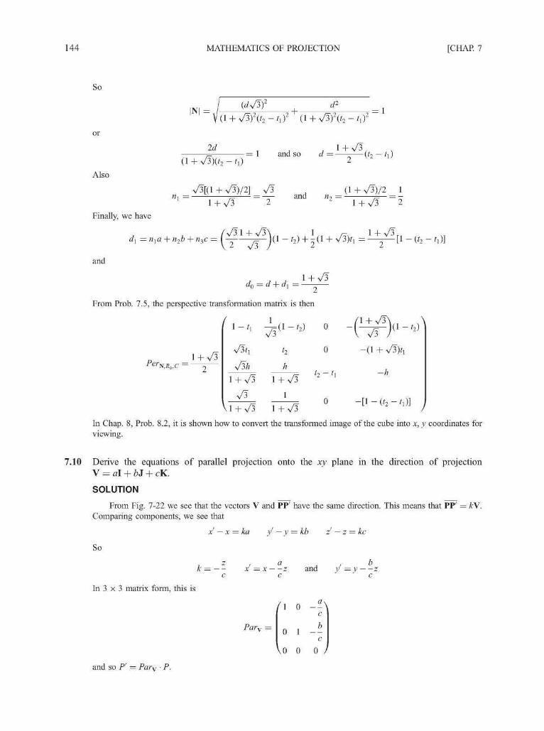
144 MATHEMATICS OF PROJECTION [CHAP. 7
So
or
Also
Finally, we have
and
d2
(1 + V3)2(f2 - hf (1 + V3)2(f2 - hf= 1
Id 1+V3= 1 and so d = (u — u)
2
V3[(l+V3)/2]p=
1+V3and
( l+V3)/2 1-=— = —
1+V3 2
From Prob. 7.5, the perspective transformation matrix is then
Per1+V3
NA,C — h
0
h-U1 +V3 1+V3 '2~'1
v - ^ — ! - P o - [ i - f e - f l )Vl+V3 1+V3 /
In Chap. 8, Prob. 8.2, it is shown how to convert the transformed image of the cube into x, y coordinates forviewing.
7.10 Derive the equations of parallel projection onto the xy plane in the direction of projectionV = a\ + hi + cK.
SOLUTION
From Fig. 7-22 we see that the vectors V and PP' have the same direction. This means that PP' = k\.Comparing components, we see that
x' — x = ka V — y = kb z' — z = kc
So
k = — x = x z and y = y zc c c
In 3 x 3 matrix form, this is
Parv =
/ 1
0
\ 0
0
1
0
)cb
c0 )
and so P' = Pary • P.

CHAP. 7] MATHEMATICS OF PROJECTION 145
-• i
V = u\ + bit + cK, v, z)
Fig. 7-22
7.11 Derive the general equation of parallel projection onto a given view plane in the direction of a givenprojector V (see Fig. 7-23).
.::.
Fig. 7-23
SOLUTION
We reduce the problem to parallel projection onto the xy plane in the direction of the projectorV = a l + bJ + cK by means of these steps:
1. Translate the view reference point _K0 of the view plane to the origin using the translation matrix T_Ro.
2. Perform an alignment transformation A^ so that the view normal vector N of the view plane points in thedirection K of the normal to the xy plane. The direction of projection vector V is transformed to a newvector V' = ^NV.
3. Project onto the xy plane using Pary.

146 MATHEMATICS OF PROJECTION [CHAP. 7
4. Perform the inverse of steps 2 and 1. So finally ParvfiRi>
learned in Chap. 6, we know that= T_%o • A-^1 • Parv 7 1 ^ . From what we
1 0 0 -x0
| 0 1 0 -y0
0 0 / - z 0
^0 0 0 1
and further from Chap. 6, Prob. 6.2, where 1 = ^Jn\ + n\ and 1 / 0 , that
-Mi/22 -«1«3
|N| 1|N|
0 ^.
A|N|~n2
V o 1 /
Then, after multiplying, we find
Par,V,N,J?n -
—an0 —an3ado
— CM]
0
'l — feM2 — £ M 3 fefi?0
—CM2 fi?i — CM3 Cfi?0
0 0 a
Here fi?0 = Mjxo + M^O + M3Z0 and dx =nxa + n2b + n3c. An alternative and much easier method toderive this matrix is by finding the intersection of the projector through P with the equation of the viewplane (see Prob. A2.14).
7.12 Find the general form of an oblique projection onto the xy plane.
SOLUTION
Refer to Fig. 7-24. Oblique projections (to the xy plane) can be specified by a number/ and an angle 8.The number / prescribes the ratio that any line L perpendicular to the xy plane will be foreshortened afterprojection. The angle 8 is the angle that the projection of any line perpendicular to the xy plane makes with the(positive) x axis.
Fig. 7-24

CHAP. 7] MATHEMATICS OF PROJECTION 147
To determine the projection transformation, we need to find the direction vector V. From Fig. 7-24, withline L of length 1, we see that the vector P'P has the same direction as V. We choose V to be this vector:
V = P T = x ' I + / J - K (=al + bJ + cK)
From Fig. 7-24 we find a = x' =fcos8, b = y1 =fsin8, and c = — 1.From Prob. 7.10, the required transformation is
Parv =
(\ 0 fcosB 0*0 1 /sin0 00 0 0 0
v0 0 0 1
7.13 Find the transformation for (a) cavalier with 6 = 45° and (b) cabinet projections with 6 = 30°. (c)Draw the projection of the unit cube for each transformation.
SOLUTION
(a) A cavalier projection is an oblique projection where there is no foreshortening of lines perpendicular tothe xy plane. From Prob. 7.12 we then see that/ = 1. With 6 = 45°, we have
' V2 N1 ° \ °Parv = 0 1 0
0 0 0 0
V0 0 0 1/
(b) A cabinet projection is an oblique projection with/ = \. With 6 = 30°, we have
Parv = 0 1 -
0 0\ 0 0
0
1/
To construct the projections, we represent the vertices of the unit cube by a matrix whose columnsare homogeneous coordinates of the vertices (see Prob. 7.1):
V = (ABCDEFGH) =
/ 0 1 1 0 0 0 1 10 0 1 1 1 0 0 10 0 0 0 1 1 1 11 1 1 1 1 1 1 1
Parv • V =
(c) To draw the cavalier projection, we find the image coordinates by applying the transformation matrixPary to the coordinate matrix V:
V22 2
V2 V22 2
0 01 1
1 + ^ -
V20 0 1 1 1
0 0 0 01 1 1 1
V22
01

148 MATHEMATICS OF PROJECTION [CHAP. 7
The image coordinates are then
A' = (0, 0, 0)
B' = (1,0,0)
C' = (l, 1,0)
D' = (0, 1,0)
T ^ '
Refer to Fig. 7-25.To draw the cabinet projection:
0 1 1 0
Parv^ • V = 0 0 1 1
0 0 0 0\ 1 1 1 1
The image coordinates are then (see Fig. 7-26)
A' = (0, 0, 0)
B' = (1,0,0)
C = (1,1,0)
D' = (0, 1,0)
"4,^4,0
4 4 4
4 " ' X 4 ' V
/3 14 ' 4 '
/ / ' ( ! + — , l - , 0
/
c
/ I '
H'
Fig. 7-25 Fig. 7-26

CHAP. 7] MATHEMATICS OF PROJECTION 149
7.14 Construct an isometric projection onto the xy plane. Refer to Fig. 7-27.
/ Projections of vectors I ' , J ' , K' ontoJ XY plane have the same length
Fig. 7-27
SOLUTION
We shall find a "tilting" of the x, y, z axes that transforms the IJK vector tried to a new set I'J'K' whoseorthographic projections onto the xy plane produce vectors of equal lengths.
Denoting the tilting transformation by T and the orthographic projection onto the xy plane by ParK, thefinal projection can be written as Par = ParK • T, where ParK is as defined in Example 3 and T is as definedin Prob. 6.1 in Chap. 6. Multiplying, we find
Par =
Now
Par • I = (cos 0y, 0, 0) Par • J = (sin6y sin6X, cos 6X, 0) Par • K = (sin6y cos 6X, -sin6X, 0)
(the projections of the vectors I, J, and K). To complete the specification of the transformation M, we need tofind the angles 8X and 8y. To do this, we use the requirement that the images Par • I, Par • J, and Par • K are toall have equal lengths. Now
say
000
sin 0 sin 6X
cos8x
00
sin 0 cos 0X
—sin0x
00
0001
\Par • J | = A/sin2 0 sin2 6X + cos2 I
and
\Par • K| = Js in 2 6y cos2 6X + sin2 6X
Setting \Par • J | = \Par • K| leads to the conclusion that sin 8X — cos 8X = 0 and to a solution 8X = 45° (andso sin0x = cos 6x = s/l/2). Setting \Par • I| = \Par • J | leads to cos2 6y = i(sin2 6y + 1). Multiplying bothsides by 2 and adding cos2 8y to both sides gives 3 cos2 8y = 2 and a solution is 8y = 35.26° (and sosin 0 = yT73, cos 0 = V2/3)- Finally
2 1 /2 1 J2 \3 2V3 2V3
1 /
0
020
20
0
0

150 MATHEMATICS OF PROJECTION [CHAP. 7
7.15 Construct a dimetric projection onto the xy plane.
SOLUTION
Following the procedures in Prob. 7.14, we shall tilt the x, y, z axes and then project on the xy plane. Wethen have, as before,
\Par • I| = J cos 2 8y \Par • J| = y sin2 8y sin2 8X + cos2
and
\Par • K| = y s in 2 8y cos2 8X + sin2 8X
To define a dimetric projection, we will specify the proportions
\Par • I | : \Par • J | : \Par • K| = /: 1 : 1 (/ / 1)
Setting \Par • J | = \Par • K|, we find sin2 8X - cos2 8X = 0 and 8X = 45°, so sin8x = cos 0X = •s/l/l. Setting|Par • I| = l\Par • J | gives
cos2 0 y = - [ s i n 2 0 + 1]
Multiplying both sides by 2 and adding / cos 8y to both sides gives
(7.3)
(2 +12) cos2 ft, = 2/2
So
From equation (7.3) we can also find
sin2 8y =
(Note the restriction / < V2.) Thus
/
_ /2and sin t/v =
Par =
2 /2 - 1 2 /2-/2
0
0V 0
yV2200
-4i 0
0 00 1 /
and 0 < / < V2.Note that any other projection ratio, say, 1:1:1, can be achieved by performing an appropriate rotation
before applying Par. In this example, a rotaiton of 90° about the y axis aligns the z axis with the x axis so thatPar can be applied.
Supplementary Problems
7.16 Construct a perspective transformation given three principal vanishing points and the distance D from thecenter of projection to the projection plane.
7.17 Draw the (a) isometric and (b) dimetric projections of the unit cube onto the xy plane.
7.18 How many view planes (at the origin) produce isometric projections of an object?

CHAPTER 8
Three-DimensionalViewing and Clipping
An important step in photography is to position and aim the camera at the scene in order to compose apicture. This parallels the specification of 3D viewing parameters in computer graphics that prescribe theprojector (the center of projection for perspective projection or the direction of projection for parallelprojection) along with the position and orientation of the projection/view plane.
In addition, a view volume defines the spatial extent that is visible through a rectangular window in theview plane. The bounding surfaces of this view volume is used to tailor/clip the objects that have beenplaced in the scene via modeling transformations (Chaps. 4 and 6) prior to viewing. The clipped objects arethen projected into the window area, resulting in a specific view of the 3D scene that can be further mappedto the viewport in the NDCS (Chap. 5).
In this chapter we are concerned with the specification of 3D viewing parameters, including a viewingcoordinate system for defining the view plane window, and the formation of the corresponding viewvolume (Sec. 8.1). We also discuss 3D clipping strategies and algorithms (Sec. 8.2). We then summarizethe three-dimensional viewing process (Sec. 8.3). Finally, we examine the operational organization of atypical 3D graphics pipeline (Sec. 8.4).typical 3D grapr
8.1 THREE-DIMENSIONAL VIEWING
Three-dimensional viewing of objects requires the specification of a projection plane (called the viewplane), a center of projection (viewpoint) or the direction of projection, and a view volume in worldcoordinates.
Specifying the View Plane
We specify the view plane by prescribing (1) a reference point R0(x0,y0, z0) in world coordinates and(2) a unit normal vector N = n-^I -\- n2J + n^K, |N| = 1, to the view plane (see Fig. 8-1). From thisinformation, we can construct the projections used in presenting the required view with respect to the givenviewpoint or direction of projection (Chap. 7).
151

152 THREE-DIMENSIONAL VIEWING AND CLIPPING [CHAP. 8
reference point
N unil normal vector
Fig. 8-1
View Plane Coordinates
The view plane coordinate system or viewing coordinate system can be specified as follows: (1) let thereference point R0(x0,y0, z0) be the origin of the coordiante system and (2) determine the coordinate axes.To do this, we first choose a reference vector U called the up vector. A unit vector Jq can then bedetermined by the projection of the vector U onto the view plane. We let the vector Jq define the directionof the positive q axis for the view plane coordinate system. To calculate Jq , we proceed as follows: with Nbeing the view plane unit normal vector, let Uq = U — (N • U)N (App. 2, Prob. A2.14). Then
is the unit vector that defines the direction of the positive q axis (see Fig. 8-2).
)
Viewplane
Fig. 8-2

CHAP. 8] THREE-DIMENSIONAL VIEWING AND CLIPPING 153
Finally, the direction vector Ip of the positive/? axis is chosen so that it is perpendicular to Jq, and, byconvention, so that the triad Ip, Jq, and N form a left-handed coordinate system. That is:
N x J n
p | N x J q |
This coordinate system is called the view plane coordinate system or viewing coordinate system. A left-handed system is traditionally chosen so that, if one thinks of the view plane as the face of a display device,then with the p and q coordinate axes superimposed on the display device, the normal vector N will pointaway from an observer facing the display. Thus the direction of increasing distance away from the observeris measured along N [see Fig. 8-3(a)].
Viewplane
P(5, 3, 2),,
(a)
World coordinate system Viewing coordinate system(subscript w) (subscript v)
Fig. 8-3
EXAMPLE 1. If the view plane is the xy plane, then Ip = I, J q = J, and the unit normal N = —K form a left-handed system. The z coordinate of a point measures the depth or distance of the point from the view plane. The signindicates whether the point is in front or in back of the view plane with respect to the center or direction of projection.In this example, we change from right-handed world coordinates (x, y, z) to left-handed view plane coordinates

154 THREE-DIMENSIONAL VIEWING AND CLIPPING [CHAP.
' , / , / ) [see Fig. S-3(b)] be performing the transformation:
In matrix form, for homogeneous coordinates:
(\00
yO
0 0 \0 0
- 1 00 1/
The general transformation for changing from world coordinates to view plane coordinates [see Fig. 8-3(c)] is developed in Prob. 8.3.
Specifying the View Volume
The view volume bounds a region in world coordinate space that will be clipped and projected onto theview plane. To define a view volume that projects onto a specified rectangular window defined in the viewplane, we use view plane coordinates (p, q)v to locate points on the view plane. Then a rectangular viewplane window is defined by prescribing the coordinates of the lower left-hand corner L(pmin, qm^)v andupper right-hand corner R(pmax, qmax)v (see Fig. 8-4). We can use the vectors Ip andequivalent world coordinates of L and R (see Prob. 8.1).
For a perspective view, the view volume, corresponding to the given window, is a semi-infinitepyramid, with apex at the viewpoint (Fig. 8-5). For views created using parallel projections (Fig. 8-6), theview volume is an infinite parallelepiped with sides parallel to the direction of projection.
Jq to find the
Fig. 8-4
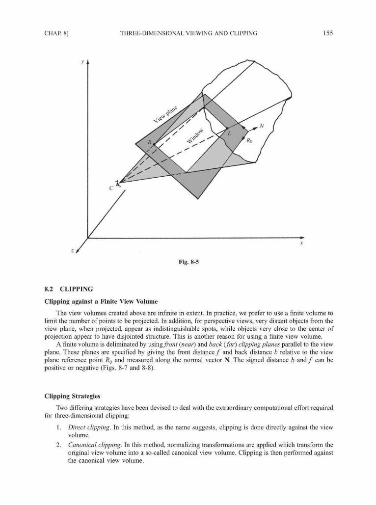
CHAP. 8] THREE-DIMENSIONAL VIEWING AND CLIPPING 155
Fig. 8-5
8.2 CLIPPING
Clipping against a Finite View Volume
The view volumes created above are infinite in extent. In practice, we prefer to use a finite volume tolimit the number of points to be projected. In addition, for perspective views, very distant objects from theview plane, when projected, appear as indistinguishable spots, while objects very close to the center ofprojection appear to have disjointed structure. This is another reason for using a finite view volume.
A finite volume is deliminated by using front (near) and back (far) clipping planes parallel to the viewplane. These planes are specified by giving the front distance f and back distance b relative to the viewplane reference point Ro and measured along the normal vector N. The signed distance b and f can bepositive or negative (Figs. 8-7 and 8-8).
Clipping Strategies
Two differing strategies have been devised to deal with the extraordinary computational effort requiredfor three-dimensional clipping:
1. Direct clipping. In this method, as the name suggests, clipping is done directly against the viewvolume.
2. Canonical clipping. In this method, normalizing transformations are applied which transform theoriginal view volume into a so-called canonical view volume. Clipping is then performed againstthe canonical view volume.

156 THREE-DIMENSIONAL VIEWING AND CLIPPING [CHAP.
Fig. 8-6
^Jack clipping plane
Front clipping plane
Fig. 8-7 Pespective view volume.

CHAP. 8] THREE-DIMENSIONAL VIEWING AND CLIPPING 157
Direction of projection
Fig. 8-8 Parallel view volume.
The canonical view volume for parallel projection is the unit cube whose faces are defined by theplanes x = 0, x = 1, y = 0, y = l , z = 0, and z = 1. The corresponding normalization transformation Npai
is constructed in Prob. 8.5 (Fig. 8-9).
y
Front
1
Back . /
-4yS X
Fig. 8-9
The canonical view volume for perspective projections is the truncated pyramid whose faces aredefined by the planes x = z, x = —z, y = z,y = —z, z = Zy, and z = 1 (where Zy is to be calculated) (Fig. 8-10). The corresponding normalization transformation Npei is constructed in Prob. 8.6.
The basis of the canonical clipping strategy is the fact that the computations involved such operationsas finding the intersections of a line segment with the planes forming the faces of the canonical viewvolume are minimal (Prob. 8.9). This is balanced by the overhead involved in transforming points, many ofwhich will be subsequently clipped.
For perspective views, additional clipping may be required to avoid the perspective anomaliesproduced by projecting objects that are behind the viewpoint (see Chap. 7).
Clipping Algorithms
Three-dimensional clipping algorithms are often direct adaptations of their two-dimensional counter-parts (Chap. 5). The modifications necessary arise from the fact that we are now clipping against the six
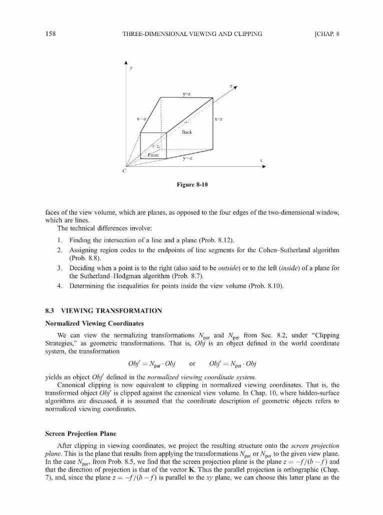
158 THREE-DIMENSIONAL VIEWING AND CLIPPING [CHAP.
Figure 8-10
faces of the view volume, which are planes, as opposed to the four edges of the two-dimensional window,which are lines.
The technical differences involve:
1. Finding the intersection of a line and a plane (Prob. 8.12).
2. Assigning region codes to the endpoints of line segments for the Cohen-Sutherland algorithm(Prob. 8.8).
3. Deciding when a point is to the right (also said to be outside) or to the left (inside) of a plane forthe Sutherland-Hodgman algorithm (Prob. 8.7).
4. Determining the inequalities for points inside the view volume (Prob. 8.10).
8.3 VIEWING TRANSFORMATION
Normalized Viewing Coordinates
We can view the normalizing transformations Npav and 7Vper from Sec. 8.2, under "ClippingStrategies," as geometric transformations. That is, Obj is an object defined in the world coordinatesystem, the transformation
Ob/ = 7Vpar • Obj or Obj' = 7Vper • Obj
yields an object Obj' defined in the normalized viewing coordinate system.Canonical clipping is now equivalent to clipping in normalized viewing coordinates. That is, the
transformed object Obj' is clipped against the canonical view volume. In Chap. 10, where hidden-surfacealgorithms are discussed, it is assumed that the coordinate description of geometric objects refers tonormalized viewing coordinates.
Screen Projection Plane
After clipping in viewing coordinates, we project the resulting structure onto the screen projectionplane. This is the plane that results from applying the transformations Npia or Npei to the given view plane.In the case Npia, from Prob. 8.5, we find that the screen projection plane is the plane z = —f/(b —f) andthat the direction of projection is that of the vector K. Thus the parallel projection is orthographic (Chap.7), and, since the plane z = —f/(b —f) is parallel to the xy plane, we can choose this latter plane as the
CHAP. 8] THREE-DIMENSIONAL VIEWING AND CLIPPING 159
projection plane. So parallel projection Par in normalized viewing coordinates reduces to orthographicprojection onto the xy plane. The projection matrix is (Chap. 7, Sec. 7.3)
Par =
In the case of perspective projections, the screen projection plane is the plane z = 4 ( 4 + ^) (Prob. 8.6).The transformed center of projection is the origin. So perspective projection Per in normalized viewingcoordinates is accomplished by applying the matrix (Chap. 7, Prob. 7.4)
4
1000
0100
0000
0001
Per =
40 0 0
c'z + b
0
0
0
4c'
0
0
0/
Constructing a Three-dimensional View
The complete three-dimensional viewing process (without hidden surface removal) is described by thefollowing steps:
1. Transform from world coordinates to normalized viewing coordinates by applying the transfor-mations Afpar Or Npev.
2. Clip in normalized viewing coordinates against the canonical clipping volumes.
3. Project onto the screen projection plane using the projections Par or Per.
4. Apply the appropriate (two-dimensional) viewing transformations (Chap. 5).
In terms of transformations, we can describe the above process in terms of a viewing transformationVT, where
VT = V2-Par• CL-NpeiV or VT = V2 Per• CL-Npev
Here CL and F2 refer to the appropriate clipping operations and two-dimensional viewing transformations.
8.4 EXAMPLE: A 3D GRAPHICS PIPELINE
The two-dimensional graphics pipeline introduced in Chap. 5 can non be extended to three dimensions(Fig. 8-11), where modeling fransformation first places individually defined objectes into a common scene(i.e. the 3D WCS). Viewing fransformation and projection are then carried out according to the viewingparameters set by the application. The result of projection in the view plane window is further mapped to
Object —IDefinition
ModelingTransformation
(CTM)
ViewingTransformation
Projection
viewing parameters
Fig. 8-11 A 3D graphics pipeline
Display(frame buffer)

160 THREE-DIMENSIONAL VIEWING AND CLIPPING [CHAP.
the appropriate workstation viewpoint via 2D viewing transformation and scan-converted to a discreteimage in the frame buffer for display.
An application typically specifies the method of projection and the corresponding view volume withsystem calls such as
perspective (a, aw, Zy, zb)
where the viewpoint of perspective projection C is assumed to be at the origin of the WCS and theperspective view volume centers on the negative z axis (away from the viewer); a denotes the anglebetween the top and bottom clipping planes, aw the aspect ratio of the view plane window, zy the distancefrom C to the front clipping plane (which is essentially also the view plane), and zb the distance from C tothe back clipping plane.
On the other hand, orthographic parallel projection can be specified by
orthographic (x^, xm a x , y m m , jm a x , z f , z b)
where the direction of projection is along the negative z axis of the WCS; the first four parameters of thecall define the left, right, bottom, and top clipping planes, respectively; and the role of zy and zb remains thesame as in the perspective case above.
Other calls to the system library often provide additional functionality. For example, the center ofperspective projection can be placed anywhere in the WCS by a call that looks like
lookat (xc, yc, zc,xP,yP, zP)
where xc,yc,zc are the coordinates of C and xp, yp, zp are the coordinates of a reference point P—theperspective of view volume now centers on the line from C to P. The y axis of the WCS, or more precisely,vector J, serves as the up vector that determines Ip and Jq . An additional parameter may be included toallow rotation of the viewing coordinate system (with Ro = Cw, the center of the view plane window) aboutits z axis, i.e. line CP.
Using perspective() and lookat(), we can conveniently produce a sequence of images that animate a"walk-by" or "fly-by" experience by placing P on an object and moving C along the path of the camerafrom one frame to the next (Fig. 8-12).
XG,
Fig. 8-12
Finally, we want to note a couple of crucial operations of the 3D graphics pipeline that have not yetbeen discussed. The first is to prevent objects and portions of objects that are hidden from the viewer'seyesight from being included in the projected view (Chap. 10). The second is to assign color attributes topixels in a way that makes the objects in the image look more realistic (Chap. 11).
Solved Problems
8.1 Let P(p, q)v be the view plane coordinates of a point on the view plane. Find the world coordinatesP(x, y, z)w of the point.

CHAP. 8] THREE-DIMENSIONAL VIEWING AND CLIPPING 161
SOLUTION
Refer to Fig. 8-13. Let Ro be the view plane reference point. Let R be the position vector of Ro and W theposition vector of P, both with respect to the world coordinate origin (see Fig. 8-13). Let V be the positionvector of P with respect to the view plane origin Ro. Now
V=pl and W = R + V
So
Fig. 8-13
Let the components of Ip and Jq be
Ip = ap\ + bpj + cpK
Also
R=x 0 I+ .y 0 J + z0K
and so from W = R +plp + qJq we find
W = (x0 +pap + qaq)\ + (y0 +pbp + qbq)J + (z0 +pcp + qcq)K
The required world coordinates of P can be read off from W:
P(x0 +pap + qaq,y0 +pbp + qbq, z0 +pcp + qcq)w
8.2 Find the projection of the unit cube onto the view plane in Prob. 7.9 in Chap. 7. Find thecorresponding view plane coordinates of the projected cube.
162 THREE-DIMENSIONAL VIEWING AND CLIPPING [CHAP.
SOLUTION
Following Prob. 7.9, we must specify several parameters in order to calculate the correspondingperspective projection matrix Per^RgC. Choosing h=\,tx = \, and t2 = (1 — V3)/(l + V3~), we obtain
Per,1+V3
N,R,,C — "
0
V3
V32(1 + V3)
1
1
1
2(1
2
+—+
1
+
1
V3V3V3
V3)
0
0
-2V31 + V3
0
- 2
-(1+V3)
1~2
/I + 3V3\•V3 1 + V 3
Applying PerN R c to the matrix F of homogeneous coordinates of the unit cube, we have -where V is the matrix (A'B'C'D'E'F'G'H'). After matrix multiplication, we have
r^ R c• V = V,
1+V3V = x
- 2
-(1+V3)
-2
- 1
- 1
-2V3 -2V3 -2V3
1+V3 1+V3-2V31+V3
— 0
- 3
1+V3
-3 -(1+V3) - 1
1+V3-2V31+V3
-V32(1+V3)
-5V3 /1+5V3\ /1+4V3\ -2V32(1+V3) 2(1+V3) V2(l+V3"; V2(l+V3"; 1+V3
X X -2V3 -+V3/ V1+V3/ 1+V3 (1+V3) (1+V3) 1 + V3 /
\1 +V3 / 1 + V3 /
Changing from homogeneous coordinates to world coordinates (App. 2), we find the coordinates of theprojected cube to be
A'\2
a+3V3/+V3\
V3
1 +2V3/ 1 +2vT2(l +2^3).
'(l, 1,0)L \ i + 2
1 + V3 \ 2(2 + V3) 1 + 5V31+3V3/' 1+3V3 '2(1+3^3)1+V3\ 1 + V3 1+4V3 1
V3/'l+2V3'2(l+2V3)J
3 V3To change from world coordinates to view plane coordinates, we first choose an up vector. Choosing the
vector K, the direction of the positive z axis, as the up vector, we next find the view plane coordinate vectors Ip
and Jq .With our choices t\ and t2, we find that the unit normal vector N (Prob. 7.9) is
2 2
Choosing U = K, and using Prob. A2.14 (App. 2), we find that
U = U - (N • U)N = U (since N • U = 0) = K andiua
K

CHAP. 8] THREE-DIMENSIONAL VIEWING AND CLIPPING 163
(Note to student using equation (A2-3) of Prob. A2.14: we have used the fact that |N| = 1 and replaced Vp
with Uq and V and U.)Now
_ _ N x J q
p I N x J J
Calculating (App. 2), we obtain
So
and |NxJq | =
To convert a point P with world coordinates (x, y, z)w to view plane coordinates (p, q)v, we use the equationsfrom Prob. 8.1:
x = xo+pap + qaq y=yo+pbp+qbq z = zo+pcp+qcq
where (xo,j;o,zo) are the coordinates of the view plane reference point Ro. Now
Choosing RQ(1, 1,0) as the view plane reference point, we find
1 - V 3x=-p+l y= —^P +1 z = q
Solving for p and q, we have
p = 2(x — 1) and q = z
Using these equations, we convert the transformed coordinates to view plane coordinates:
B'
E'l —- -1+3V37'2(1+3V3)I V 3 ' 6
2(1+2V3)F'UL V
1-V3\ 1+5V3
C'(0, 0)
+ 3V/3/'2(l+3V3)J
2 1+4^3 1+- 2V3' 2(1+2V3)J
i/ '(0, 1)
Refer to Fig. 8-14. Note also that the coordinates of the view point or center of projection C and the vanishing
VP2
B'
Fig. 8-14

164 THREE-DIMENSIONAL VIEWING AND CLIPPING [CHAP.
points VP\ and VP2 can be found by using the equations from Prob. 7.9:
C(a, b, c) = Cl 2,
In view plane coordinates:
and
8.3 Find the transformation Twv that relates world coordinates to view plane coordinates.
SOLUTION
The world coordinate axes are determined by the right-handed triad of unit vectors [I, J, K].The view plane coordinate axes are determined by the left-handed triad of vectors [Ip, Jq , N] and the view
reference point RQ(xQ,yQ, z0).Referrring to Fig. 8-3 (a), we construct the transformation Twv through the concatenation of the matrices
determined by the following steps:
1. Translate the view plane reference point _K0(x0,j;0,z0) to the world coordinate origin via the translationmatrix Ty. Here V is the vector with components —xol — yoj — z0K.
2. Align the view plane normal N with the vector — K (the direction of the negative z axis) using thetransformation ^4N_K (Chap. 6, Prob. 6.5). Let Ip be the new position of the vector Ip after performing thealignment transformation, i.e.
3. Rotate Ip about the z axis so that it aligns with I, the direction of the x axis. With 6 being the anglebetween Ip and J, the rotation is RgK (Chap. 6).
4. Change from the right-handed coordinates to left-handed coordinates by applying the transformation 7 ^from Example 1. Then Twv = TJH • R0K • A^t_K • Ty. If (xw,yw, zw) are the world coordinates of point P,the view plane coordinates (xv,yv,zv) of P can be found by applying the transformation Twv.
8.4 Find the equations of the planes forming the view volume for the general parallel projection.
SOLUTION
The equation of a plane is determined by two vectors that are contained in the plane and a reference point(App. 2, Prob. A2.10). The cross product of the two vectors determines the direction of the normal vector tothe plane.
In Fig. 8-8, the sides of the window in the view plane have the directions of the view plane coordinatevectors Ip and Jq . With V as the vector determining the direction of projection, we find the following planes:
1. Top plane—determined by the vectors Ip and V and reference point Rj, measured/ units along the unitnormal vector N = nx\ + n23 + «3K from the upper right corner R(r^, r2, r3) of the window. Referencepoint Rj- has world coordinates (rx +fn1, r2 +fii2, r3 +fn3).
2. Bottom plane—determined by the vectors Ip and V and the reference point Lj-, measured from the lowerleft corner L(lx, l2, /3) of the window. Point Lj- has world coordinates (/j +fn-i, l2 +fn2, l3 +fii3).
3. Right side plane—determined by the vectors Jq and V and the reference point Rj-.
4. Left side plane—determined by the vectors J q and V and the reference point Lj-.
Front and back clipping planes are parallel to the view plane, and thus have the same normal vectorN = M1I +
5. Front (near) plane—determined by the normal vector N and reference pointPr(xQ +fn-i,yQ +fn2,zQ +fn3), measured from the view reference point _K0(x0, j ;0 ,z0) .

CHAP. 8] THREE-DIMENSIONAL VIEWING AND CLIPPING 165
6. Back (far) plane—determined by the normal vector N and reference pointPj(x0 + bn^,yQ + bn2, zQ + bn3), measured b units from the view plane reference point RQ.
8.5 Find the normalizing transformation that transforms the parallel view volume to the canonical viewvolume determined by the planes x = 0, x = 1, y = 0, y = l , z = 0, and z = 1 (the unit cube).
SOLUTION
Referring to Fig. 8-8, we see that the required transformation A par is built by performing the followingseries of transformations:
1. Translate so that RQ, the view plane reference point, is at the origin. The required transformation is thetranslation T R .
2. The vectors Ip , Jq , and N form the left-handed view plane coordinate system. We next align the viewplane normal vector N with the vector —K (the direction of the negative z axis). The alignmenttransformation A^_K was developed in Chap. 6, Prob. 6.5. Let Ip be the new position of the vector Ip:that is, Ip = ^ N , _ K - I P -
3. Align the vector Ip with the vector I (the direction of the positive x axis) by rotating Ip about the z axis.The required transformation is Rg K . Here, 8 is the angle between I' and I (Chap. 6). When Rg K aligns I'with I, the vector J^ (where Jq = A-^ _K • Jq) is aligned with the vector J (the direction of the positive yaxis).
4. We change from the right-handed world coordinate system to a left-handed coordinate system. Therequired orientation changing transformation is [see Fig. 8-3(ft)] (see also Example 1)
TP,=n
00
kO
0100
00
- 10
0001
Let V' be the new position of the direction of projection vector V; that is, V' = Tg^ • RgK- A-^ _K • V. Thenew position of the transformed view volume is illustrated in Fig. 8-15. Note how the view volume isskewed along the line having the direction of the vector V'. Suppose that the components of V' areV' = v'xI + v'yJ + v'zK. We now perform a shearing transformation that transforms the newly skewed viewvolume to a rectangular view volume aligned along the z axis. The required shearing transformation isdetermined by preserving the new view volume base vectors I and J and shearing V' to the vector i^K(the K component of V'); that is, I is transformed to I, J is transformed to J, and V' is transformed to i^K.The required transformation is the matrix
Sh =
1 0 - ^V'z
0 1 —y-
\o o i )In order to concatenate the transformation so as to buld NpM, we use the 4 x 4 homogeneous form of Sh
Sh
I J^0 0 0
6. We now translate the new view volume so that its lower left corner L'j will be at the origin. To do this, wenote that the first four transformations correspond to the view plane coordinate system transformation inProb. 8.3. So after performing these transformations, we find that the lower left corner of the view planewindow L(pmin, qmin)v (view plane coordinates) transforms to a point L' on the xy plane whose coordinatesare (pmin, #mjn, 0). Similarly, the upper right corner R is transformed to R'(pm!SX, #max> 0)- After performingthe shearing transformation Sh, we see that the view volume is aligned with the z axis and the back and

166 THREE-DIMENSIONAL VIEWING AND CLIPPING [CHAP.
front faces are, respectively, b a n d / units from the xy plane. Thus the lower left corner of the view volumeis at L'f(pmkl,qmin,f) and the bounds of the view volume are pmin<x<pmlo,, qmin < y < qmttK,f < z < b. The required translation is T_L,.
7. We now scale the rectangular view volume to the unit cube. The base of the present view volume has thedimensions of the base of the original volume, which corresponds to the view plane window; that is
w = Pmax - Pmin (width) h = qmsx - <?min (height)
The depth of the new view volume is the distance from the front clipping plane to the back clippingplane: d = b —f. The required scaling is the matrix (in 4 x 4 homogeneous form)
- 0 0w
0 | 0 0h
0 0 - 0a
V0 0 0 1 /
The required transformation is then
Note also that after performing the transformation NVM, the view plane transforms to the planez = —f jib —/ ) , parallel to the xy plane. Also, the direction of projection vector V transforms to avector parallel to the vector K having the direction of the z axis.
8.6 Find the normalizing transformation that transforms the perspective view volume to the canonicalview volume determined by the bounding planes x = z, x = —z, y = z,y = —z, z = Zf, and z = 1.

CHAP. 8] THREE-DIMENSIONAL VIEWING AND CLIPPING 167
SOLUTION
Referring to Fig. 8-7, we build the normalizing transformation A per through a series of transformations.As in Prob. 8.5:
1. Translate the center of projection C to the origin using the translation T_c.
2. Align the view plane normal N with the vector — K using ^N, -K-
3. Rotate Ij, to the vector I using the rotation Rg K . (Recall that Ij, = A-^ _K • Ip.)
4. We now change from right-handed world coordinates to left-handed coordinates by applying thetransformation
5. The newly transformed view volume is skewed along the centerline joining the origin (the translatedcenter of projection) with the center of the (transformed) view plane window (Fig. 8-16). Let Cw be thecoordinates of the center of the original view plane window. Then Cw has view plane coordinates
.+A• - ) ,
These are changed to world coordinates as in Prob. 8.1. Let CCW be the vector from the center ofprojection to the center of the window. Let (CCW)' be the transformation of the vector CCW; that is,(CCW)' = Tgi • ReK • A^_K • CCW. Then (CCW)' is the vector that joins the origin to the center of thetransformed view plane window (Fig. 8-16). Suppose that (CCW)' = c'xI + c'y3 + c'zK. We shear the viewvolume so that it transforms to a view volume whose center line lies along the z axis. As in Prob. 8.5, the
(CCW)'
Fig. 8-16

168 THREE-DIMENSIONAL VIEWING AND CLIPPING [CHAP.
required shearing transformation is
1 0 - ^
0 0 1 0
\ 0 0 0 1 /
The newly transformed window is, after applying the shearing transformation Sh, located on the z axis atz c = c'z.
6. Referring to Fig. 8-17, the transformed window is now centered on the z axis. The dimensions of thewindow are
w = Anax - Pmm (width) and h = qr[mx - qmin (height)
The depth of the new view volume is the distance between the front and back clipping planes: d = b —f.The transformed window is centered on the z axis at zc = c'z and is bounded by
w w h h< x < < v <
Fig. 8-17

CHAP. 8] THREE-DIMENSIONAL VIEWING AND CLIPPING 169
The transformed view plane is located at zc = c'z. The transformed front clipping plane is located atZf = c'z +f. The back clipping plane is now located at zb = c'z + b.
To transform this view volume into the canonical view volume, we first scale in the z direction so thatthe back-clipping plane is transformed to z = 1. The required scale factor is
1
c'+b
The scaling matrix is
(\
0
0
0
1
0
0
0
0
1c'z + b
0
(h0
0
1 ;
To find the new window boundaries R" and L", we apply this scaling transformation to the presentwindow coordinates
w h ,
2 ' 2 ' C z
Then
andw h c'z
" 2 " ' ~ 2 ' Z + i
Next we scale in the x and y directions so that the window boundaries will be
R'"c'+b'c'+b'c'+b
andc'+b' c'+b'c'+b
That is, the window boundaries will lie on the planes x = z, x = —z, y = z ,and y = —z. The requiredscale factors are
2cLx w(c'z + b)
The corresponding scaling transformation is
and2c'
/ 2c'
w(c'z + b)
0
0
0
0
2c'
h(c'z + b)
0
0
Kc'z + b)
0 0
0 0
1 0
0 1 /
Multiplication of these scaling transformations into one transformation yields
/ 2c'
w(c'z + b)
0
0
0
0
2c'
h(c'z + b)
0
0
0
0
1/

170 THREE-DIMENSIONAL VIEWING AND CLIPPING [CHAP.
To find the location of the front clipping plane, zj, we apply the transformation Ss^s ^ to the presentlocation of the center of the front clipping plane, which is Cj-(0, 0, c'z + / ) . So
That is
_Cz+f
The complete transformation can be written as
^per = Ssx,sy,sz -Sh-TxL- RgK • ^ N j _ K • T_c
Note that after performing the transformation Nva, the view plane is transformed to the plane
c'z + b
parallel to the xy plane. Also, the center of projection C is transformed to the origin.
8.7 How do we determine whether a point P is inside or outside the view volume?
SOLUTION
A plane divides space into the two sides. The general equation of a plane is (App. 2)
«i (x ~ xo) + nib> ~ yo) + «3(z - zo) = 0
We define a scalar function, f(P), for any point P(x, y, z) by
f(P) = f(x,y, z) = «i(x - x0) + n2(y - y0) + n3(z - z0)
We say that a point P is on the same side (with respect to the plane) as point Q if sign/(P) = signReferring to Figs. 8-7 or 8-8, tetfT,fB,fR,fL,fN, w&fp be the functions associated with the top, bottom, right,left, near (front), and far (back) planes, respectively (Probs. 8.4 and 8.10).
Also, L and R are the lower left and upper right corners of the window and Pb and Pf are the referencepoints of the back and front clipping planes, respectively.
Then a point P is inside the view volume if all the following hold:
P is on the same side as L with respect t o / r
P is on the same side as R with respect tofs
P is on the same side as L with respect t o ^
P is on the same side as R with respect tofL
P is on the same side as Pb with respect tofN
P is on the same side as Pf with respect t o ^
Equivalently
sign/ r(P) = sign/ r(L) signfL(P) = sign fL(R)
sign fB(P) = signfB(R) signfN(P) = signfN(Pb)
signfR(P) = signfR(L) sign fF(P) = sign fF(Pf)
8.8 Show how region codes would be assigned to the endpoints of a line segment for the three-dimensional Cohen-Sutherland clipping algorithm for (a) the canonical parallel view volume and(b) the canonical perspective view volume.
SOLUTION
The procedure follows the logic of the two-dimensional algorithm in Chap. 5. For three dimensions, theplanes describing the view volume divide three-dimensional space into six overlapping exterior regions (i.e.,

CHAP. 8] THREE-DIMENSIONAL VIEWING AND CLIPPING 171
above, below, to right of, to left of, behind, and in front of view volume), plus the interior of the view volume:thus 6-bit codes are used. Let P(x, y, z) be the coordinates of an endpoint.
(a) For the canonical parallel view volume, each bit is set to true (1) or false (0) according to the scheme
Bit 1 = endpoint is above view volume = sign (y — 1)
Bit 2 = endpoint is below view volume = sign (—y)
Bit 3 = endpoint is to the right of view volume = sign (x — 1)
Bit 4 = endpoint is to the left of view volume = sign (—x)
Bit 5 = endpoint is behind view volume = sign (z — 1)
Bit 6 = endpoint is in front of view volume = sign (—z)
Recall that sign (a) = 1 if a is positive, 0 otherwise.
(b) For the canonical perspective view volume:
Bit 1 = endpoint is above view volume = sign (y — z)
Bit 2 = endpoint is below view volume = sign (—z — y)
Bit 3 = endpoint is to the right of view volume = sign (x — z)
Bit 4 = endpoint is to the left of view volume = sign (—z — x)
Bit 5 = endpoint is behind view volume = sign (z — 1)
Bit 6 = endpoint is in front of view volume = sign (zj- — z)
The category of a line segment (Chap. 5) is (1) visible if both region codes are 000000, (2) not visible ifthe bitwise logical AND of the region codes is not 000000, and (3) clipping candidate if the bitwiselogical AND of the region codes is 000000.
8.9 Find the intersecting points of a line segment with the bounding planes of the canonical viewvolumes for (a) parallel and (b) perspective projections.
SOLUTION
Let Px(xx,yx,zx) andP2(x2, j ;2 ,z2) be the endpoints of the line segment. The parametric equations of theline segment are
x = xx +(x2-xl)t y = yx + (y2 - yx)t z = zx + (z2 - zx)t
From Prob. 8.11, the intersection parameter is
h —N • P j P ,
where N is the normal vector and RQ is a reference point on the plane.
(a) The bounding planes for the parallel canonical view volume are x = 0, x = 1, y = 0, y = 1, z = 0, andz = 1. For the plane x = 1, we have N = I and RQ (1, 0, 0). Then
_ -(xx - 1)
X2 ~ x\
If 0 < tj < 1, the line segment intersects the plane. The point of intersection is then
xx ( 2 1 ) ( ) y y x y 2 y x )\ X2 — X ] / \ X2 — Xj
z = zx + (z2 - zx)[ l-V * 2 -
The intersections with the other planes are found in the same way.
(b) The bounding planes for the perspective canonical view volume are x = z, x = —z, y = z, y = —z,z = Zj-, and z = 1 (where zy is calculated as in Prob. 8.6).

172 THREE-DIMENSIONAL VIEWING AND CLIPPING [CHAP.
To find the intersection with the plane x = z, for example, we write the equation of the plane asx — z = 0. From this equation, we read off the normal vector as N = I — K (App. 2, Prob. A2.9), and thereference point is RQ(Q, 0, 0). Then
(x2 - X j ) - (z2 -zx)
If 0 < tj < 1, we substitute tj into the parametric equations of the line segment to calculate theintersection point.
The other intersections are found in the same way.
8.10 Determine the inequalities that are needed to extend the Liang-Barsky line-clipping algorithm tothree dimensions for (a) the canonical parallel view volume and (b) the canonical perspective viewvolume.
SOLUTION
Let Px (xj, yx, Zj) and P2(x2, y2, z2) be the endpoints of a line. The parametric representation of the line is
I x = xj + Ax • uy=y\ +Ay-uz = zx+Az-u
where 0 < u < 1, Ax = x2 — xx, Ay = y2 — y\, and Az = z2 — Zj. The infinite extension of the linecorresponds to u < 0 and 1 < u.
(a) Points inside the canonical parallel view volume satisfy
xmin<xx+Ax-u< xmax
JVin<.yi+Ay-M<.ymaxzmin< z l +Az-M<Z m a x
where xmin = ymin = zmin = 0 and xmax = ymax = zmax = 1.Rewrite the six inequalities as
pk-u<qk, k = 1,2, 3,4, 5,6
where
px = -Ax, q l = X l - xmin = xx (left)p2 = Ax, q2= xmax - xj = 1 - xj (right)Pi = —Ay, #3 = yx — j^jn = yx (bottom)p4 = Ay, q4 = ymsx - yx = 1 - yx (top)p5 = -Az, ft = Z! - zmin = zx (front)p6 = Az, q6 = z m a x - zx = 1 - zx (back)
(b) Points inside the canonical perspective view volume satisfy (see Fig. 8-10).
-z < x <z
-z <y <z
z / < z <
i.e.
-zx -Az-u<xx+Ax-u<zx+Az-ii—Zj — A Z - M ^ ^ J + A ^ - M ^ Z J + A Z - M
Zf < zx + Az • u < 1
Rewrite the six inequalities as
Pk-u<qk, k= 1 ,2 ,3 ,4 ,5 ,6

CHAP. 8] THREE-DIMENSIONAL VIEWING AND CLIPPING 173
where
px = —Ax — Azp2 = Ax — Az,p3 = -Ay - Az,p4 = Ay — Az,p5 = -Az,P e = A z ,
1\ = x\
i3 =y\qA=zx
q5 =zx
?6 = 1
+ Z1
-xx
+ Zj
-y\
~zf~ z\
(left)(right)(bottom)(top)(front)(back)
Supplementary Problems
8.11 Find the equations of the planes forming the view volume for the general perspective projection.
8.12 Find the intersection point of a plane and a line segment.

CHAPTER 9
GeometricRepresentation
One of the major concepts in computer graphics is modeling of objects. By this we mean numericaldescription of the objects in terms of their geometric property (size, shape) and how they interact with light(reflect, transmit). The focus of this chapter is on geometric representation of objects. We will discussillumination and shading models in subsequent chapters.
A graphics system typically uses a set of primitives or geometric forms that are simple enough to beefficiently implemented on the computer but flexible enough to be easily manipulated (assembled,deformed) to represent or model a variety of objects. Geometric forms that are often used as primitivesinclude, in order of complexity, points, lines, polylines, polygons, and polyhedra. More complex geometricforms include curves, curved surface patches, and quadric surfaces.
9.1 SIMPLE GEOMETRIC FORMS
Points and Lines
Points and lines are the basic building blocks of computer graphics. We specify a point by giving itscoordiantes in three- (or two-) dimensional space. A line or line segment is specified by giving its endpointsPx{xx,yi,z{) and P2(x2,y2,z2).
Polylines
A polyline is a chain of connected line segments. It is specified by giving the vertices (nodes)Po,... ,PN defining the line segments. The first vertex is called the initial or starting point and the lastvertex, the final or terminal point (see Fig. 9-1).
Polygons
A polygon is a closed polyline, that is, one in which the initial and terminal points coincide. A polygonis specified by its vertex list Po, ..., PN, Po. The line segments PQP\, P\P2, • • •, PN^O a r e called the edgesof the polygon. (In general, we need not specify Po twice, especially when passing the polygon to theSutherland-Hodgman clipping algorithm.)
174

CHAP. 9] GEOMETRIC REPRESENTATION 175
Initial
Fig. 9-1 Fig. 9-2
A planar polygon is a polygon in which all vertices (and thus the entire polygon) lie on the same plane(see Fig. 9-2).
9.2 WIREFRAME MODELS
A wirefram model consists of edges, vertices, and polygons. Here vertices are connected by edges, andpolygons are sequences of vertices or edges. The edges may be curved or straight line segments. In thelatter case, the wireframe model is called a polygonal net or polygonal mesh (Fig. 9-3).
(a) Wire frame model. (b) Hidden lines removed.
Fig. 9-3

176 GEOMETRIC REPRESENTATION [CHAP. 9
Representing a Polygonal Net Model
There are several different ways of representing a polygonal net model.
1. Explicit vertex list V = {P0,Pi,P2, • • •,P^}- The points P^x^y^z^) are the vertices of thepolygonal net, stored in the order in which they would be encountered by traveling around themodel. Although this form of representation is useful for single polygons, it is quite inefficient fora complete polygonal net, in that shared vertices are repeated several times (see Prob. 9.1). Inaddition, when displaying the model by drawing the edges, shared edges are drawn several times.
2. Polygon listing. In this form of representation, each vertex is stored exactly once in a vertex listV = (Po,..., PN), and each polygon is defined by pointing or indexing into this vertex list (seeProb. 9.2). Again, shared edges are drawn several times in displaying the model.
3. Explicit edge listing. In this form of representation, we keep a vertex list in which each vertex isstored exactly once and an edge list in which each edge is stored exactly once. Each edge in theedge list points to the two vertices in the vertex list which define that edge. A polygon is nowrepresented as a list of pointers or indices into the edge list. Additional information, such as thosepolygons sharing a given edge, can also be stored in the edge list (see Prob. 9.9). Explicit edgelisting can be used to represent the more general wireframe model. The wireframe model isdisplayed by drawing all the edges, and each edge is drawn only once.
Polyhedron
A polyhedron is a closed polygonal net (i.e., one which encloses a definite volume) in which eachpolygon is planar. The polygons are called the faces of the polyhedron. In modeling, polyhedrons are quiteoften treated as solid (i.e., block) objects, as opposed to wireframes or two-dimensional surfaces.
Advantages and Disadvantages of Wireframe Models
Wireframe models are used in engineering applications. They are easy to construct and, if they arecomposed of straight lines, easy to clip and manipulate through the use of geometric and coordinatetransformations. However, for building realistic models, especially of highly curved objects, we must use avery large number of polygons to achieve the illusions of roundness and smoothness.
9.3 CURVED SURFACES
The use of curved surfaces allows for a higher level of modeling, especially for the constructiodn ofhighly realistic models. There are several approaches to modeling curved surfaces. One is an analog ofpolyhedral models. Instead of using polygons, we model an object by using small, curved surface patchesplaced next to each other. Another approach is to use surfaces that define solid objects, such as polyhedra,spheres, cylinders, and cones. A model can then be constructed with these solid objects used as buildingblocks. This process is called solid modeling.
There are two ways to construct a model—additive modeling and subtractive modeling. Additivemodeling is the process of building the model by assembling many simpler objects. Subtractive modelingis the process of removing pieces from a given object to create a new object, for example, creating a(cylindrical) hole in a sphere or a cube. Subtractive modeling is akin to sculpting.
9.4 CURVE DESIGN
Given n + 1 data points, P0(x0,y0),..., Pn(xn,yn) we wish to find a curve that, in some sense, fits theshape outlined by these points. If we require the curve to pass through all the points, we are faced with theproblem of interpolation. If we require only that the curve be near these points, we are faced with the

CHAP. 9] GEOMETRIC REPRESENTATION 177
problem of approximation. Interpolation arises, for example, in reconstructing the shape of a digitizedcurved objects. Approximation is used in computer graphics to design curves that "look good" or mustmeet some aesthetic goal. To solve these often quite distinct problems, it is necessary to find ways ofbuilding curves out of smaller pieces, or curve segments, in order to meet the design criteria. (Note thatcurves and curve segments can be modeled as polylines, i.e., drawn with extremely short line segments.)When modeling a curve/(x) by using curve segments, we try to represent the curve as a sum of smallersegments <l)
i(x) (called basis or blending functions):
i=0
We choose these blending functions with an eye toward computation and display. For this reason,polynomials are often the blending functions of choice.
A polynomial of degree n is a function that has the form
Q(x) = anxn + an_xx
n l + • • • + axx + a0
This polynomial is determined by its n + 1 coefficients [an,... ,a0].A continuous piecewise polynomial Q(x) of degree n is a set of k polynomials qt(x), each of degree n
and k + 1 knots (nodes) t0,..., tk so that
Q(x) = qt(x) for tt < x < ti+l and / = 0 , . . . , k - 1
Note that this definition requires the polynomials to match or piece together at the knots, that is,qil(ti) = qi(ti), i=\,...,k—\. This requirement imposes no restrictions on how smoothly thepolynomials qt(x) fit together. For example, there can be corners or sharp contours at the knots (seeFig. 9-4).
Fig. 9-4
Polynomials of high degree are not very useful for curve designing because of their oscillatory nature.The most useful piecewise polynomials are those for which the polynomials qt{x) are cubic (degree 3).
There are several reasons for this. One is that the piecewise cubic closely resembles the way a drafter uses amechanical spline. In addition, 3 is the smallest degree which has the required smoothness properties fordescribing pleasing shapes. It is also the minimum number needed to represent three-dimensional curves.
9.5 POLYNOMIAL BASIS FUNCTIONS
Let P0(x0, y0), ..., Pn(xn, yn) represent n + \ data points. In addition, let t0, tx, t2, ..., be any numbers(called knots). The following are common choices for basis or blending functions.
Lagrange Polynomials of Degree n
f\^—^, 1 = 0,1 nJ=° xi ~ xj

178 GEOMETRIC REPRESENTATION [CHAP. 9
Note that L^x^ = 1 and Lt{x) = 0 for ally ^ i. (Here IT represents term-by-term multiplication.)
Hermite Cubic Polynomials
Refer to Fig. 9-5.
2(x - t^f | 3(x - t^f
2{ti+l-xf 3(ti+l-xf
(k - tt-if
(x - tt)(tm - xf(ti+l - ti)2
B-Splines
Refer to Fig . 9-6. For the k n o t set t0, tx, t2, the «th-degree B-splines Bin are defined recursively:
t • < X < t • , 1 Y — t t — YI —— —— *";—I— 1 A ij fi_|_!7_|_1 -^
0 otherwise ''" ti+n — tt ''" U+n+i ~ U+i '+ '"
for ti < x < ti+n+l. Note that Bin(x) is nonzero only in the interval [tt, ti+n+l\. In particular, the cubic B-spline Bi3 is nonzero over the interval [tt, ti+4] (which spans the knots tt, ti+l, ti+2, ti+i, ti+4). In addition,for nonrepeated knots, the B-spline is zero at the endknots ti and ti+n+l (from Prob. 9.3), that is,
BtM = 0Bi,tt(ti+tt+1) = 0
(n>\)
H,(x)
H,{x)
'(+3 '1+4
Fig. 9-5 Hermite cubic basis functions. Fig. 9-6 Cubic B-spline Bt 3(x).

CHAP. 9] GEOMETRIC REPRESENTATION 179
In using B-splines, we allow for repeated knots, that is, ti = ti+l = • • •. This means that Bin can have theform jj in its definition. By letting § = 0, we extend the definition of Bi n to incorporate repeated knots.
Bernstein Polynomials
Refer to Fig. 9-7. The Bernstein polynomials of degree n over the interval [0, 1] are defined as
- xf~k, 0 < x < 1\{n -
3.3
Fig. 9-7 Cubic Bernstein polynomials.
The cubic Bernstein polynomials are
5Oj3(x) = 1 - 3x + 3x2 - x3
= 3 ( x - 2 x 2 + x 3 )
BXi(x) = x3
9.6 THE PROBLEM OF INTERPOLATIONGiven data points P0(x0,y0),..., Pn{xn,yn), we wish to find a curve which passes through these points.
Lagrange Polynomial Interpolation Solution
Here
L(x) =i = 0
where Lt{x) are the Lagrange polynomials and L(x) is the «th-degree polynomial interpolating the datapoints.
Hermitian Cubic Interpolation Solution
We wish to find a piecewise polynomial H(x) of degree 3 which passes through the data points and isalso continuously differentiable at these points. We also prescribe the values of the derivatives/ (or slope
180 GEOMETRIC REPRESENTATION [CHAP. 9
of the tangent line) at the given data points, that is, we prescribe the points (xo,y'o), ..., {xn,y'n)\
H(x) = J:[yiHi(x)+y'iHi(x)}i =0
where Ht(x) and Ht(x) are the Hermitian cubic basis functions and t0 = x0, tl = xx, t2 = x2, ..., tn = xn arethe choices for the knot set.
Spline Interpolation
If we require that the interpolating piecewise polynomial be joined as smoothly as possible at the datapoints, the resulting curve is called a spline. Therefore, a spline of degree m has continuous derivatives upto order m — 1 at the data points.
It can be shown that any mth-degree spline that passes through « + 1 data points can be represented interms of the B-spline basis functions Bin as
i=0
In order to define the B-spline functions Bim(x) so as to solve the interpolation problem, the knotst0, ti,..., tm+n+i must be chosen to satisfy the Shoenberg-Whitney condition:
ti<xi<ti+m+i' i = 0,...,n
The following choices for the knots satisfy this condition (see Prob. 9.4):
Step 1. Choose
f0 = ' ' ' = fm < x0 fn+l = ' ' ' = tm+n+i > Xn
Step 2. Choose the remaining knots according to
, _ xi+l H H xi+m • _ n n m \li+m+i — . i — v, ... ,n — m — i
For cubic splines (m = 3), an alternative to step 2, requiring less computation, is step 2'. Choose
ti+4=xi+2> i = 0 , . . . , n - 4
The splines S2(x) and 53(x) are called quadratic and cubic splines, respectively:
S2(x) = E afii 2(x) and S3(x) = E afr 3(x)
Confining our attention to the cubic spline, we see that there are n + 3 coefficients ai to evaluate, requiringn + 3 equations.
The interpolation criterion S^(XJ) = yj, j = 0 , . . . , n provides n + 1 equations:
yJ=S3(xJ)=j:aiBu3(xJ)i=0
The remaining two equations are usually specified as boundary conditions at the endpoints x0 and xn.Some choices for boundary conditions are
1. Natural spline condition
S'i(x0) = 0 S'i(xn) = 0
2. Clamped spline condition
5^(xo)=yo S'3(xn)=y'nwhere y'o and y'n are prescribed derivative values.

CHAP. 9] GEOMETRIC REPRESENTATION 181
3. Cyclic spline condition
%(x0) = S',(xn) S'J(x0) = S!(xtt)
This is useful for producing closed curves.
4. Anticyclic spline condition
S'3(x0) = -S'3(xn) S'3'(x0) = -S'3'(xn)
This is useful in producing splines with parallel endings whose tangent vectors are equal inmagnitude but opposite in direction.
For technical reasons, boundary condition 1, the so-called natural boundary condition, is the leastpreferred choice.
9.7 THE PROBLEM OF APPROXIMATION
The problem is to provide a smooth representation of a three-dimensional curve which approximatesgiven data so as to yield a given shape. Usually the data is given interactively in the form of a guidingpolyline determined by control points P0(x0,y0, z0), P1(x1,iy1, z{), ..., Pn(xn,yn, zn). We would like to finda curve which approximates the shape of this guiding polyline (see Fig. 9-8).
Fig. 9-8
Bezier-Bernstein Approximation
Using the Bernstein polynomials, we form the parametric curves:
P(t):
where P(t) is called the Bezier curve.
i =0
y(t) = 0<t<li =0
i=0

182 GEOMETRIC REPRESENTATION [CHAP. 9
Properties of the Bezier-Bernstein Approximation
There are four basic properties:
1. The Bezier curve has the same endpoints as the guiding polyline, that is:
po = = [X(O), y(0), Z(0)] Pn = P(\) =
2. The direction of the tangent vector at the endpoints Po, Pn is the same as that of the vectordetermined by the first and last segments P0P\, Pn_iPn of the guiding polyline. In particularP>(0) = n-(Pl- Po) [i.e., x'(0) = n(xx - x0), / ( 0 ) = n(yx - y0), zf(O) = n(zx - z0)] and P'(\) =n-{Pn-Pn_x).
3. The Bezier curve lies entirely within the convex hull of the guiding polyline. In two dimensions,the convex hull is the polygon formed by placing a "rubber band" about the collection of pointsP0,...,Ptt.
4. Bezier curves are suited to interactive design. In fact, Bezier curves can be pieced together so as toensure continuous differentiability at their juncture by letting the edges of the two differentguiding polylines that are adjacent to the common endpoint be collinear (see Fig. 9-9).
Fig. 9-9
Bezier-B-Spline Approximation
For this approximation, we use B-splines (see Fig. 9-10)
P(t):
i =0
i=00<t<n-m+l
±ziBiJt)i=0
The mth-degree B-splines Bi m(t), i = 0 , . . . , « , are defined for t in the parameter range [0, « — m+ 1].The knot set t0,..., tn+m+l is chosen to be the set 0, . . . , 0, 1, 2 , . . . , n — m, n — m + 1 , . . . , n — m + 1.
m+l m+1
This use of repeated knots ensures that the endpoints of the spline coincide with the endpoints of theguiding polyline (Prob. 9.6).
Since the knot spacing is uniform, we can also use an explicit form for calculating the B-splines (Prob.9.10).

CHAP. 9] GEOMETRIC REPRESENTATION 183
Pi
Fig. 9-10 Cubic Bezier B-spline.
Closed Curves
To construct a closed B-spline curve which approximates a given closed guiding polygon, we needonly choose the knots t0,..., tn+m+l to be cyclic, i.e., [0, 1 , . . . , « , 0, 1 , . . . ] . So
tm+2 — tx — 1 tm+l+i — ti
In practice, the quadratic and cubic B-splines Bi 2 and Bi 3 are the easiest to work with and provideenough flexibility for use in a wide range of curve design problems.
Properties of Bezier-B-Spline Approximation
There are five basic properties:
1. The Bezier-B-spline approximation has the same properties as the Bezier-Bernstein approxima-tion; in fact, they are the same piecewise polynomial if m = n. This includes the properties ofagreement with the guiding polygon and the tangent vectors at the endpoints and the convex hullproperty.
2. If the guiding polyline has m + 1 consecutive vertices (control points) which are collinear, theresulting span of the Bezier-B-spline will be linear. So this approximation allows for linearsections to be embedded within the curve.
3. The Bezier-B-spline approximation provides for the local control of curve shape. If a singlecontrol point is changed, portions of the curve that lie far away are not disturbed. In fact, onlym + 1 of the spans are affected. This is due to the local nature of the B-spline basis functions.
4. Bezier-B-splines produce a closer fit to the guiding polygon than does the Bezier-Bernsteinapproximation.
5. The Bezier-B-spline approximation allows the use of control points Pt counted with multiplicitiesof 2 or more. That is, Pt = P,-+1 = • • • = Pi+k for k > 1. This results in an approximation which ispulled closer toward this control point. In fact, if the point has multiplicity m + 1, the curve willpass through it.

184 GEOMETRIC REPRESENTATION [CHAP. 9
9.8 CURVED-SURFACE DESIGN
The modeling and approximation of curved surfaces is difficult and involves many complex issues. Wewill look at two methods for representing a surface: guiding nets and interpolating surface patches.
Guiding Nets
This technique is a direct generalization of the Bezier-Bernstein and Bezier-B-spline approximationmethods for curves. A guiding net is a polygonal net with vertices P^x^^y, ztj), i = 0 , . . . , m, and7 = 0, . . . , « (see Fig. 9-11).
Fig. 9-11
1. Bezier-Bernstein surface. This is the surface with parametric equations:
Q(s, t):
s, t) =i=0j=0
i=0j=0m n
i=0j=0
Here 0 < s, t < 1 and BE are the Bernstein polynomials. This approximation has propertiesanalogous to the one-dimensional case with respect to the corner points Poo, PmQ, PQH, and Pmn.The convex hull property is also satisfied.

CHAP. 9] GEOMETRIC REPRESENTATION 185
i=0j=0
i=0j=0
2. Bezier-B-spline approximation. In parametric form this is expressed as
Q(s, t):
;=oy=o
where 0 < s < m — a + 1 and 0 < s < n — /? + 1. The knot sets for s and t used to define the B-splines Bia(s) and Bj^(t) are determined as in the one-dimensional case.
Quadratic approximation occurs when a = fi = 2. Cubic approximation occurs when a = fi = 3. Ingeneral, quadratic or cubic B-splines are most often used. For both these methods, the construction of theguiding net (by locating the control points Py) is left to the user.
Interpolating Surface Patches
Instead of using a given set of points Py to construct a given surface, the process of interpolatingsurface patches is based upon prescribing boundary curves for a surface patch and "filling in" the interiorof the patch by interpolating between the boundary curves.
1. Coons surfaces. For this technique, a patch is determined by specifying four bounding curves,denoted in parametric vector form as P(s, 0), P(s, 1), P(0, t), and P( l , t), 0 < s, t < 1 (see Fig.9-12).
z,
P(0,t)
P{s,0)
Fig. 9-12
The (linear) Coons surface patch interpolating the boundary curves can be written in vectorform by using linear interpolation (or blending):
Q(s, t) = P(s,
- p(o,- t) + P(s, \)t + P(0, 0(1 -
- s)t - p(i, o>(i - o - P" P(P, - t)
(The subtractions are required so that the interpolators between corner points are not countedtwice.) This idea can be extended to define more general surface patches.
2. Lofted surfaces. Lofting is used where the surface to be constructed stretches in a given direction;an example is the hull of a ship.
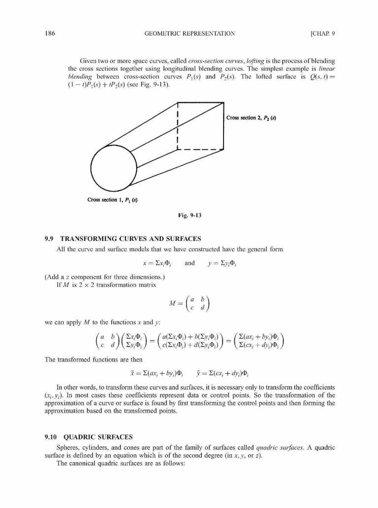
186 GEOMETRIC REPRESENTATION [CHAP. 9
Given two or more space curves, called cross-section curves, lofting is the process of blendingthe cross sections together using longitudinal blending curves. The simplest example is linearblending between cross-section curves P\{s) and i^C5)- The lofted surface is Q(s, t) =(1 - tWs) + tP2(s) (see Fig. 9-13).
Cross section 2, P2 (s)
Cross section 1, P, (s)
Fig. 9-13
9.9 TRANSFORMING CURVES AND SURFACES
All the curve and surface models that we have constructed have the general form
x = S x ^ j and y = Sj7,-®,-
(Add a z component for three dimensions.)If M is 2 x 2 transformation matrix
M =a bc d
we can apply M to the functions x and y:
The transformed functions are then
x =
fr) + d&y,®,)
y =
In other words, to transform these curves and surfaces, it is necessary only to transform the coefficients(xt,yt). In most cases these coefficients represent data or control points. So the transformation of theapproximation of a curve or surface is found by first transforming the control points and then forming theapproximation based on the transformed points.
9.10 QUADRIC SURFACES
Spheres, cylinders, and cones are part of the family of surfaces called quadric surfaces. A quadricsurface is defined by an equation which is of the second degree (in x, y, or z).
The canonical quadric surfaces are as follows:
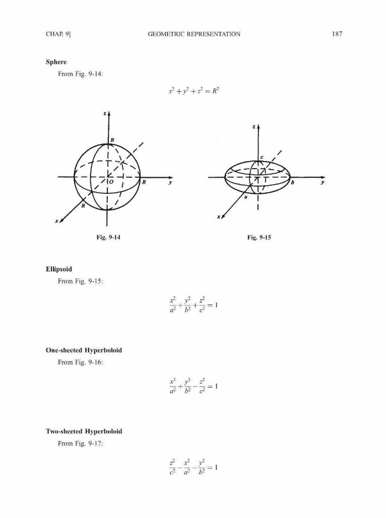
CHAP. 9] GEOMETRIC REPRESENTATION 187
Sphere
From Fig. 9-14:
Fig. 9-14 Fig. 9-15
Ellipsoid
From Fig. 9-15:
x2 y2 z2
= 1
One-sheeted Hyperboloid
From Fig. 9-16:
Two-sheeted Hyperboloid
From Fig. 9-17:
X2 / _ ^
a2 b2 c2
c 2 a2 b2~

188 GEOMETRIC REPRESENTATION [CHAP. 9
/
s*!
Jt/
*?/
\
Fig. 9-16
Elliptic Cylinder
From Fig. 9-18:
2 1 2
az bz
When a = i = R, the cylinder is a circular cylinder of radius R.
Elliptic Paraboloid
From Fig. 9-19:2 2
a 2 Z>2
Fig. 9-17
z
Fig. 9-18 Fig. 9-19
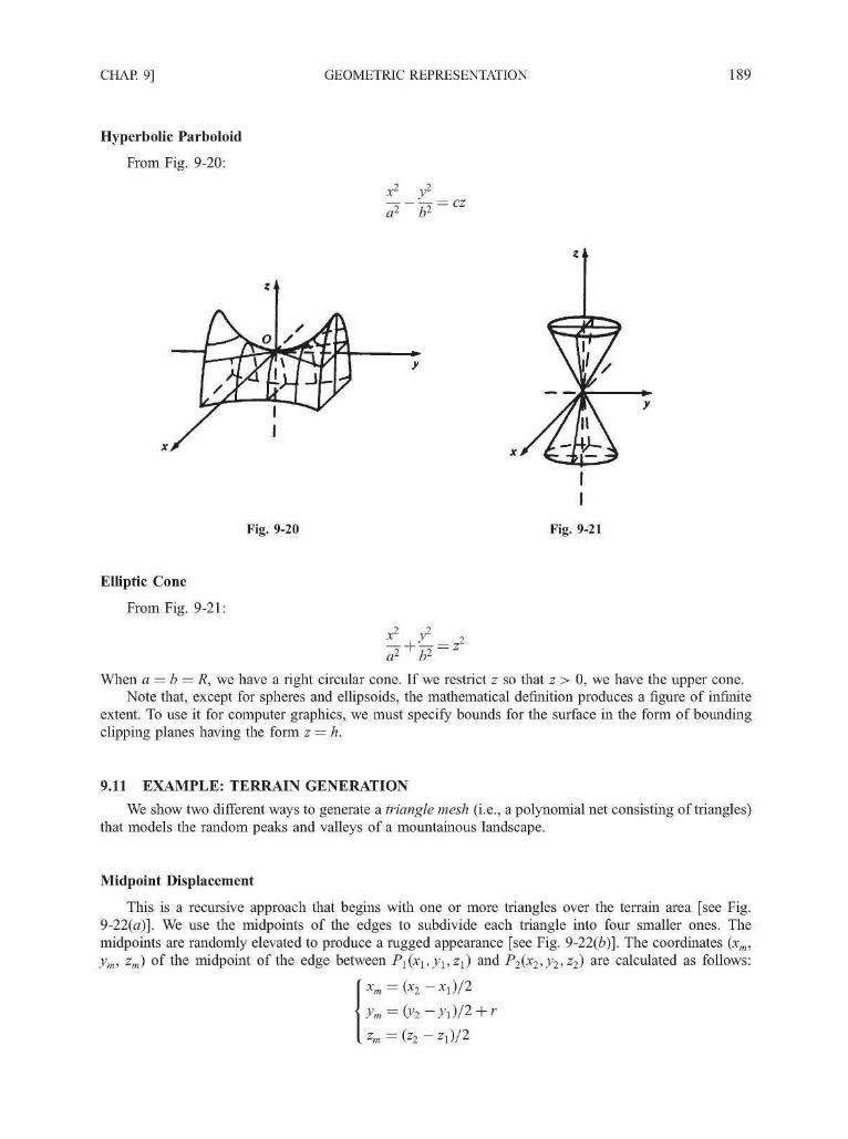
CHAP. 9] GEOMETRIC REPRESENTATION 189
Hyperbolic Parboloid
From Fig. 9-20:
x2 y2
Fig. 9-20 Fig. 9-21
Elliptic Cone
From Fig. 9-21:
2 2
- + y--z2
a2+b2~
When a = b = R, we have a right circular cone. If we restrict z so that z > 0, we have the upper cone.Note that, except for spheres and ellipsoids, the mathematical definition produces a figure of infinite
extent. To use it for computer graphics, we must specify bounds for the surface in the form of boundingclipping planes having the form z = h.
9.11 EXAMPLE: TERRAIN GENERATION
We show two different ways to generate a triangle mesh (i.e., a polynomial net consisting of triangles)that models the random peaks and valleys of a mountainous landscape.
Midpoint Displacement
This is a recursive approach that begins with one or more triangles over the terrain area [see Fig.9-22(a)]. We use the midpoints of the edges to subdivide each triangle into four smaller ones. Themidpoints are randomly elevated to produce a rugged appearance [see Fig. 9-22(b)]. The coordinates (xm,ym, zm) of the midpoint of the edge between i->
1(x1,_y1,z1) and P 2^2^21 zi) a r e calculated as follows:
xm = (X2 -
. zm = (Z2 - z l ) / 2

190 GEOMETRIC REPRESENTATION [CHAP. 9
y (elevation) y (elevation)
()
Fig. 9-22
where r is a random displacement that can be expressed as the product of a random number 0 < X < 1 anda function of the projected length (onto the x—z plane) of the edge. For example, if the function isF(p) = p/2, then the midpoint can be elevated by no more than half of the projected length of the edge.The subdivision process terminates when all edges project to a preset threshold or shorter length.
Since the original vertices are not moved and each midpoint is displaced only once, the resultingterrain tends to maintain the overall shape of the initial model. On the other hand, deep valleys that lookunrealistic may appear along the original edges. We can alleviate this problem by adding a randomdisplacement to the vertices as well as the midpoints at each recursion stage. The tradeoff here is lesscontrol over the shape of the final terrain structure.
Brownian Distribution of Disks
In this approach we superimpose a grid onto the terrain area and initialize a counter for each grid cell(see Fig. 9-23 for a rectangular area that can be represented by a two-dimensional counter array). We thenrandomly move a circular disk over the area. At each disk position we increment the counter for every gridcell that is covered by the disk. After a while the counter values form an elevation profile of a pile ofrandomly placed disks. Each elevation value describes the height of a point/vertex above the correspond-ing grid cell. A triangle-mesh model of the resulting terrain can thus be constructed by first connectingeach vertex to its four neighbors [analogous to the four neighbouring pixels in Fig. 3-18(a)] to form aquadrilateral-mesh and then adding diagonal edges to divide each quadrilateral into two triangles.
y (elevation)
Fig. 9-23

CHAP. 9] GEOMETRIC REPRESENTATION 191
Fig. 9-24
For example, the gray-scale image in Fig. 9-24 represents the values ina512 x 512 counter array. Thevalues are obtained using a disk of radius 25 after 6000 random movements, each of which is a step of size3 forward or backward and simultaneously a step of the same size to the left or to the right. Whenever thecenter of the disk moves beyond the image boundary it is reset to the middle of the image. The countervalues are normalized so that the maximum count corresponds to white in the image. The resultanttriangle-mesh is viewed in Fig. 9-25 using perspective projection, looking from a point near the lower-rightcorner of Fig. 9-24 towards the center (with hidden surfaces removed and visible surfaces lit by a lightsource).
Fig. 9-25

192 GEOMETRIC REPRESENTATION [CHAP. 9
Solved Problems
9.1 Represent a cube by using an explicit vertex list.
SOLUTION
Using the notation in Fig. 7-12, one possible representation is
V = {ABCDAFEDCHEFGHGB}
Note the vertex repetitions in the list V and the repetition of edge FE as EF.
9.2 Represent a cube by using polygon listing.
SOLUTION
Referring to Fig. 7-12, we form the vertex list
V = {ABCDEFGH}
The faces of the cube are polygons (which, in this case, are squares) P\,..., P6, where
P1 = {ABCD} P4 = {ABGF}
P2 = {CDEH} P5 = {BCHG}
P3 = {ADEF} P6 = {EFGH}
Note the edge repetitions encountered in drawing the polygons. For example, polygons P2 and P 3 share theedge DE.
9.3 Show that the «th-degree B-spline basis functions Bin(x) satisfy
Bi,n(X) = ° i f X<ti OT X > W l
SOLUTION
Since the B-spline basis functions Bin(x) are defined recursively in terms of the lower-order B-splinesBj n_i(x) and-8,+1 n_i(x) of degree n — 1, we shall indicate only the first step of a general induction argument.Therefore, we illustrate what happens for the first-degree B-spline Bt j(x).
Now suppose that x < tt. Then also x < ti+l, so at x the zero-degree B-splines have the values B,• 0(x) = 0and Bi+l 0(x) = 0. From these values we find, in turn, that BiX(x) = 0.
Now suppose that the knot set is nonrepeating. Let x = tt. Then B,, 0(£,) = 1, but Bi+l 0(f,) = 0. So
' - ( 0 ) = 0'i+2 'i
Thus B,, j(x) = 0 if x < tt. Similar arguments show that BiX(x) = 0 if x > ti+1.
9.4 Let P0(0,0), Pi(1,2), P2(2, 1), P 3 ( 3 , - l ) , P4(4, 10), and P5(5,5) be given data points. Ifinterpolation based on cubic B-splines is used to find a curve interpolating these data points,find a knot set t0,..., t9 that can be used to define the cubic B-splines.
SOLUTION
The knot set can be chosen according to one of two schemes. With m = 3 and n = 5:
1. Choose
lo = h =h = h = - 1 (<xo) and t6 = t7 = t% = t9 = 6 ( > x j
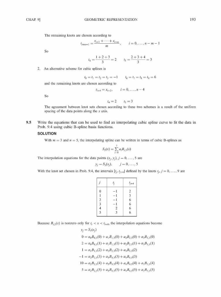
CHAP. 9] GEOMETRIC REPRESENTATION 193
The remaining knots are chosen according to
xi+\ "I I" xi+nH+m+\ — '
So
2. An alternative scheme for cubic splines is
i = 0 , . . . , n — m — 1
and the remaining knots are chosen according to
ti+4 = xi+2,
So
tA=2 % = 3
The agreement between knot sets chosen according to these two schemes is a result of the uniformspacing of the data points along the x axis.
9.5 Write the equations that can be used to find an interpolating cubic spline curve to fit the data in
Prob. 9.4 using cubic B-spline basis functions.
SOLUTION
With m = 3 and n = 5, the interpolating spline can be written in terms of cubic B-splines as
S3(x) = X> ; J8, ; 3(x);=o
The interpolation equations for the data points (x^yXj = 0, . . . , 5 are
yj = S3(Xj), y = 0 , . . . . 5
With the knot set chosen in Prob. 9.4, the intervals [tj, tj+4] defined by the knots tj,j = 0 , . . . , 9 are
j
012345
h
- l- l- l- l
23
tj+4
2
36666
Because Bi3(x) is nonzero only for t,• < x < ti+4, the interpolation equations become
yj = S3(xj)
0 = a0B03(0) + fll5li3(0) + a252,3(0) + fl353,3(0)
2 = flo^o,3(l) + fli^i,3(l) + fl2^2,3(l) + ^ 3 , 3 ( 1 )
1 = fll5li3(2) + fl2JB23(2) + 03,833(2)
- 1 = fl2^2,3(3) + 03-83,3(3) + a4B4<3(3)
10 = a2B23(4) + a3B33(4) + a4B43(4) + a5B53(4)
5 = a2B23(5) + a3B33(5) + a4B43(5) + a5B53(5)

194 GEOMETRIC REPRESENTATION [CHAP. 9
The remaining two equations can be chosen to satisfy prescribed boundary conditions at x0 = 0 and x5 = 5.
9.6 Show that the knot set used in constructing the Bezier-B-spline approximation to a guiding polylineguarantees that the endpoints of the spline coincide with the endpoints of the guiding polyline.
SOLUTION
For an m-degree Bezier-B-spline approximation, the knot set used is
0 , . . . , 0 , l , 2 , . . . , / z — m, n — m+ l,n — m+ 1,... ,n — m + 1
M+l m+\
Let PQ(xQ,yQ, zQ) be the first control point of the guiding polyline and Pn(xn,yn,zn) the last. Nowx(t) = ^2"=oXjBj m(t) with similar expressions for y(t) and z(t). We wish to show that
x(0) = xQ,y(0) = yQ, z(0) = z0 and x(n - 1) = xn,y(n - 1) = yn, z(n - 1) = zn
Let us restrict ourselves to m = 2 (quadratic) B-splines. Then the knot set is
0, 0, 0, 1, 2, 3, . . . , n - 2, n - 1, n - 1, n - 1f0> h i f2> f 3 ' f4> f 5 ' • • • i ln+l i fn+2' fn+3' fn+4
Since 5, 2 W is nonzero only over the interval tt < x < ti+3, it follows that Bt 2(0) is nonzero only if i = 0, 1,and 2. So then
x(0) = £ xfit 2(0) = xflJg0 2(0) + *!*! 2(0) + x252 2(0)i=0
To calculate Bo 2, using the definition and the convention that § = 0, we obtain
*o,2(O)=*i,i(O) and 5 l i l ( 0 ) = 5 2 i 0 ( 0 ) and 52 0(0) = 1
So 5 0 2(0) = 1 (compare with Prob. 9.3).To calculate 5] 2(0), using the definition
2 25 1 > 2(0)=-5 2 > 1(0) and 5 2 1 ( 0 ) = - r53>0(0) and 53>0(0) = 0 since 0 < f3 = 1
So we have -8] 2(0) = 0. In a similar manner, we find B212(0) = 0. Thus, x(0) = x0 and the same for the y andcoordinates.
Similar calculations show that x(n — 1) = xn, y(n — 1) = j ; n , and z(n — 1) = zn.
9.7 Find the linear Coons surface patch that interpolates the curves of Fig. 9-26.
P{s,0
Fig. 9-26

CHAP. 9] GEOMETRIC REPRESENTATION 195
SOLUTION
The four bounding curves can be described parametrically as follows (see Fig. 9-26):
1. P(s, 0) = (cos ns, 0, sin ns) 0 < s < 12. P(\,t) = (-1,0,0) 0 < f < l3 p(s, 1) = (cosns, sinns, 0) 0<s<l4. P(0, f) = (l,0, 0) 0 < f < l
Note that curves 2 and 4 are constant curves, that is, points.The linear Coons surface interpolating these curves can be written as
Q(s, i) = P(s, 0)(l - t)+P(s, l)t + P(0, 0(1 - s)+P(l, t)s - P(0, 0)(l - s)(l - t)- P (0 , i)(i - s)t -P(i, o>(i - o - p ( i , i>f
In terms of coordinates:
x{s,t) = (COS7K)(1 - t) + (cosns)t + (l)(l -s) + (-l)s
s)(l - 0 - (1)(1 - s)t - (-1>(1 - 0 - (-l)rf
x(s, 0 = COS7TS
Now
3 (5, 0 = (0)(l - 0 + (sinns)t + (0)(l - 5) + (0)« - (0)(l - s)(l - t) - (0)(l - i)f - (0>(l - 0 -
or
^(5, 0 = tsinns
Finally
z(s, 0 = (sin7w)(l - 0 + (0)f + (0)(l - s) + (0)s - (0)(l - s)(l - 0 - (0)(l - s)f - (0>(l - t) - (0)st
or
z(s, 0 = (1 — t) sinns
The linear Coons surface is
Q(s, 0 = [COSTTS, f sinns, (1 — Osinms] 0 < s, t < 1
9.8 Find the lofting surface defined by linear blending between the cross-section curves in Fig. 9-27.
SOLUTION
The curves in Fig. 9-27 are circles whose equations can be defined parametrically as
P j ( s ) = (COS2TTS, sin27K, 0) 0 < s < l
and
P2(s) = (2cos2ns, 2 sin2ns, 4) 0 < s < 1
The lofting surface is then
In terms of coordinates, we find that
x(s, 0 = (1 - 0(cos 2ns) + t(2 cos 2ns) = (1 + t) cos 2ns
y(s, 0 = (1 - 0(sin27w) + f(2 sin2?rs) = (1 + 0 sin27is
z(S, 0 = (1 - 0(0) + t(4) = At

196 GEOMETRIC REPRESENTATION [CHAP. 9
Pi(s)
Thus
Fig. 9-27
Q(s, t) = [(1 + t)cos2ns, (1 + t) sin27is, At] 0 < s, t < 1
Supplementary Problems
9.9 Represent a cube using an explicit edge listing.
9.10 Find an explicit representation for linear (degree 1) B-splines in the case of uniformly spaced knots, i.e.,ti+l - t; = L.
9.11 For the knot set tx = 1, t2 = 2,..., tt = 1, calculate Bi3 (5.5).

Hidden Surfaces
Opaque objects that are closer to the eye and in the line of sight of other objects will block those objects orportions of those objects from view. In fact, some surfaces of these opaque objects themselves are notvisible because they are eclipsed by the objects' visible parts. The surfaces that are blocked or hidden fromview must be "removed" in order to construct a realistic view of the 3D scene (see Fig. 1-3 where onlythree of the six faces of the cube are shown). The identification and removal of these surfaces is called thehidden-surface problem. The solution involves the determination of the closest visible surface along eachprojection line (Sec. 10.1).
There are many different hidden-surface algorithms. Each can be characterized as either an image-space method, in which the pixel grid is used to guide the computational activities that determine visibilityat the pixel level (Sees. 10.2, 10.5, and 10.6), or an object-space method, in which surface visibility isdetermined using continuous models in the object space (or its transformation) without involving pixel-based operations (Sees. 10.3 and 10.4).
Notice that the hidden-surface problem has ties to the calculation of shadows. If we place a lightsource, such as a bulb, at the viewpoint, all surfaces that are visible from the viewpoint are lit directly bythe light source and all surfaces that are hidden from the viewpoint are in the shadow of some opaqueobjects blocking the light.
10.1 DEPTH COMPARISONS
We assume that all coordinates (x, y, z) are described in the normalized viewing coordinate system(Chap. 8).
Any hidden-surface algorithm must determine which edges and surfaces are visible either from thecenter of projection for perspective projections or along the direction of projection for parallel projections.
The question of visibility reduces to this: given two points Pi(xl,yl,zl) andP2(x2,y2,z2), does eitherpoint obscure the other? This is answered in two steps:
1. Are Pi and P2 on the same projection line?
2. If not, neither point obscures the other. If so, a depth comparison tells us which point is in front ofthe other.
For an orthographic parallel projection onto the xy plane, Pj and P2 are on the same projector ifXi = x2 and j j = y2. In this case, depth comparison reduces to comparing Zj and z2. If Zj < z2, then Pjobscures P2 [see Fig. 10-1 (a)].
For a perspective projection [see Fig. 10-1(6)], the calculations are more complex (Prob. 10.1).However, this complication can be avoided by transforming all three-dimensional objects so that parallel
197

198 HIDDEN SURFACES [CHAP. 10
1
1
1
ftr
'Pi
Pi (.\2, Vl. Zl)
Pi (xi,yt, zi)
Fig. 10-1
projection of the transformed object is equivalent to a perspective projection of the original object (see Fig.10-2). This is done with the use of the perspective to parallel transform Tp (Prob. 10.2).
If the original object lies in the normalized perspective view volume (Chap. 8), the normalizedperspective to parallel transform
NTp =
(\ 0
0 1
0 0
0 0
0 \
0
~zf1 -zf
0 )
Parallel projection ofthis configuration is
[ABCDEFO]
Perspective projection ofthis configuration is
[ABCDEFG]
Fig. 10-2

CHAP. 10] HIDDEN SURFACES 199
(where Zy is the location of the front clipping plane of the normalized perspective view volume) transformsthe normalized perspective view volume into the unit cube bounded by 0 < x < 1, 0 < y < 1, 0 < z < 1(Prob. 10.3). We call this cube the normalized display space. A critical fact is that the normalizedperspective to parallel transform preserves lines, planes, and depth relationships.
If our display device has display coordinates H x V, application of the scaling matrix
<H 0 0 0s
. 0 V 0 0sn,r,i I o 0 1 0
0 0 0 1
transforms the no rma l i zed display space 0 < I < 1 , 0 < J < 1 , 0 < z < 1 onto the reg ion 0 < x < H,0 < y < F , 0 < z < 1. We cal this r eg ion the display space. T h e display transform DTp:
DTp = SHtKi • NTp
transforms the normalized perspective view volume onto the display space.Clipping must be done against the normalized perspective view volume prior to applying the transform
NTp. An alternative to this is to combine NTp with the normalizing transformation Npei (Chap. 8), formingthe single transformation NT'p = NTp • Npei. Then clipping is done in homogeneous coordinate space. Thismethod for performing clipping is not covered in this book.
We now describe several algorithms for removing hidden surfaces from scenes containing objectsdefined with planar (i.e., flat), polygonal faces. We assume that the displays transform DTp has beenapplied (if a perspective projection is being used), so that we always deal with parallel projections indisplay space.
10.2 Z-BUFFER ALGORITHM
We say that a point in display space is "seen" from pixel (x,y) if the projection of the point is scan-converted to this pixel (Chap. 3). The Z-buffer algorithm essentially keeps track of the smallest zcoordinate (also called the depth value) of those points which are seen from pixel (x, y). These Z values arestored in what is called the Z buffer.
Let Zbuf (x, y) denote the current depth value that is stored in the Z buffer at pixel (x, y). We work withthe (already) projected polygons P of the scene to be rendered.
The Z-buffer algorithm consists of the following steps.
1. Initialize the screen to a background color. Initialize the Z buffer to the depth of the back clippingplane. That is, set
4uf (*> y) = 4ack> for every pixel (x, y)
2. Scan-convert each (projected) polygon P in the scene (Chap. 3) and during this scan-conversionprocess, for each pixel (x, y) that lies inside the polygon:
(a) Calculate Z(x,y), the depth of the polygon at pixel (x,y).
(b) If Z(x, y) < Zbuf (x, y), set Zbuf (x, y) = Z(x, y) and set the pixel value at (x, y) to the color ofthe polygon P at (x, y). In Fig. 10-3, points P\ and P2 are both scan-converted to pixel (x, y);however, since zj < z2, P\ will obscure P2 and the P\ z value, z1; will be stored in the Zbuffer.
Although the Z-buffer algorithm requires Z-buffer memory storage proportional to the number ofpixels on the screen, it does not require additional memory for storing all the objects comprising the scene.In fact, since the algorithm processes polygons one at a time, the total number of objects in a scene can bearbitrarily large.

200 HIDDEN SURFACES [CHAP. 10
Fig. 10-3
10.3 BACK-FACE REMOVAL
Object surfaces that are orientated away from the viewer are called back-faces. The back-faces of anopaque polyhedron are completely blocked by the polyhedron itself and hidden from view. We cantherefore identify and remove these back-faces based solely on their orientation without further processing(projection and scan-conversion) and without regard to other surfaces and objects in the scene.
Let N = {A, B, Q be the normal vector of a planar polygonal face, with N pointing in the direction thepolygon is facing. Since the direction of viewing is the direction of the positive z axis (see Fig. 10-3), thepolygon is facing away from the viewer when C > 0 (the angle between N and the z axis is less than 90°).The polygon is also classified as a back-face when C = 0, since in this case it is parallel to the line of sightand its projection is either hidden or overlapped by the edge(s) of some visible polygon(s).
Although this method identifies and removes back-faces quickly it does not handle polygons that facethe viewer but are hidden (partially or completely) behind other surfaces. It can be used as a preprocessingstep for other algorithms.
10.4 THE PAINTER'S ALGORITHM
Also called the depth sort or priority algorithm, the painter's algorithm processes polygons as if theywere being painted onto the view plane in the order of their distance from the viewer. More distancepolygons are painted first. Nearer polygons are painted on or over more distance polygons, partially ortotally obscuring them from view. The key to implementing this concept is to find a priority ordering of thepolygons in order to determine which polygons are to be painted (i.e., scan-converted) first.
Any attempt at a priority ordering based on depth sorting alone results in ambiguities that must beresolved in order to correctly assign priorities. For example, when two polygons overlap, how do we decidewhich one obscures the other? (See Fig. 10-4.)

CHAP. 10] HIDDEN SURFACES 201
Projection of polygons.1, B, C. aiidD
Fig. 10-4 Projection of opaque polygons.
Assigning Priorities
We assign priorities to polygons by determining if a given polygon P obscures other polygons. If theanswer is no, then P should be painted first. Hence the key test is to determine whether polygon P does notobscure polygon Q.
The z extent of a polygon is the region between the planes z = zmin and z = zTBS1L (Fig. 10-5). Here, zmin
is the smallest of the z coordinates of all the polygon's vertices, and zTBS3L is the largest.Similar definitions hold for the x and y extents of a polygon. The intersection of the x, y, and z extents
is called the extent, or bounding box, of the polygon.
z extent .-•'
Fig. 10-5
Testing Whether P Obscures Q
Polygon P does not obscure polygon Q if any one of the following tests, applied in sequential order, istrue.
Test 0: the z extents o f f and O do not overlap and zn of Q is smaller than zP off . Refer to Fig.10-6.
Test 1: the y extents of P and Q do not overlap. Refer to Fig. 10-7.
Test 2: the x extents o f f and Q do not overlap.
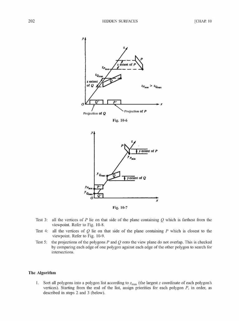
202 HIDDEN SURFACES [CHAP. 10
Projection of Q Projection of
Fig. 10-6
I y extent of P
Fig. 10-7
Test 3: all the vertices of P lie on that side of the plane containing Q which is farthest from theviewpoint. Refer to Fig. 10-8.
Test 4: all the vertices of Q lie on that side of the plane containing P which is closest to theviewpoint. Refer to Fig. 10-9.
Test 5: the projections of the polygons P and Q onto the view plane do not overlap. This is checkedby comparing each edge of one polygon against each edge of the other polygon to search forintersections.
The Algorithm
1. Sort all polygons into a polygon list according to zmax (the largest z coordinate of each polygon'svertices). Starting from the end of the list, assign priorities for each polygon P, in order, asdescribed in steps 2 and 3 (below).

CHAP. 10] HIDDEN SURFACES 203
v
Fig. 10-8
v
Fig. 10-9
2. Find all polygons Q (preceding P) in the polygon list whose z extents overlap that of P (test 0).3. For each Q, perform tests 1 through 5 until true.
(a) If every Q passes, scan-convert polygon P.
(6) If false for some Q, swap P and Q on the list. Tag Q as swapped. If Q has already beentagged, use the plane containing polygon P to divide polygon Q into two polygons. Qx and02 [see Fig. 10-4(6)]. The polygon-clipping techniques described in Chap. 5 can be used toperform the division. Remove Q from the list and place Qx and Q2 on the list, in sortedorder.
Sometimes the polygons are subdivided into triangles before processing, thus reducing the computa-tional effort for polygon subdivision in step 3.
10.5 SCAN-LINE ALGORITHM
A scan-line algorithm consists essentially of two nested loops, an x-scan loop nested within a j-scanloop.

204 HIDDEN SURFACES [CHAP. 10
y Scan
For each y value, say, y = a, intersect the polygons to be rendered with the scan plane y = a.. Thisscan plane is parallel to the xz plane, and the resulting intersections are line segments in this plane (seeFig. 10-10).
Fig. 10-10
x Scan
1. For each x value, say, x = /?, intersect the line segments found above with the x-scan line x = $lying on the j-scan plane. This intersection results in a set of points that lies on the x-scan line.
2. Sort these points with respect to their z coordinates. The point (x, y, z) with the smallest z value isvisible, and the color of the polygon containing this point is the color set at the pixelcorresponding to this point.
In order to reduce the amount of calculation in each scan-line loop, we try to take advantage ofrelationships and dependencies, called coherences, between different elements that comprise a scene.
Types of Coherence
1. Scan-line coherence. If a pixel on a scan line lies within a polygon, pixels near it will most likelylie within the polygon.
2. Edge coherence. If an edge of a polygon intersects a given scan line, it will mot likely intersectscan lines near the given one.
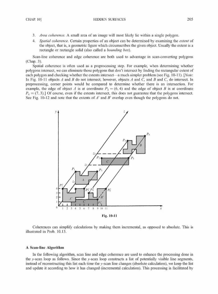
CHAP. 10] HIDDEN SURFACES 205
3. Area coherence. A small area of an image will most likely lie within a single polygon.
4. Spatial coherence. Certain properties of an object can be determined by examining the extent ofthe object, that is, a geometric figure which circumscribes the given object. Usually the extent is arectangle or rectangle solid (also called a bounding box).
Scan-line coherence and edge coherence are both used to advantage in scan-converting polygons(Chap. 3).
Spatial coherence is often used as a preprocessing step. For example, when determining whetherpolygons intersect, we can eliminate those polygons that don't intersect by finding the rectangular extent ofeach polygon and checking whether the extents intersect—a much simpler problem (see Fig. 10-11). [Note:In Fig. 10-11 objects A and B do not intersect; however, objects A and C, and B and C, do intersect. Inpreprocessing, corner points would be compared to determine whether there is an intersection. Forexample, the edge of object A is at coordinate P^ = (6, 4) and the edge of object B is at coordinateP4 = (7, 3).] Of course, even if the extents intersect, this does not guarantee that the polygons intersect.See Fig. 10-12 and note that the extents of A' and B' overlap even though the polygons do not.
1 2 3 4 5 6 7 S 9 10
Fig. 10-11
Coherences can simplify calculations by making them incremental, as opposed to absolute. This isillustrated in Prob. 10.13.
A Scan-line Algorithm
In the following algorithm, scan line and edge coherence are used to enhance the processing done inthe j-scan loop as follows. Since the j-scan loop constructs a list of potentially visible line segments,instead of reconstructing this list each time the j-scan line changes (absolute calculation), we keep the listand update it according to how it has changed (incremental calculation). This processing is facilitated by

206 HIDDEN SURFACES [CHAP. 10
the use of what is called the edge list, and its efficient construction and maintenance is at the heart of thealgorithm (see Chap. 3, Sec. 3.7, under "A Scan-line Algorithm").
The following data structures are created:
1. The edge list—contains all nonhorizontal edges (horizontal edges are automatically displayed) ofthe projections of the polygons in the scene. The edges are sorted by the edge's smaller ycoordinate (jVn)- Each edge entry in the edge list also contains:
(a) The x coordinate of the end of the edge with the smaller y coordinate.
(b) The y coordinate of the edge's other end (jmax).
(c) The increment Ax = 1 /m.
(d) A pointer indicating the polygon to which the edge belongs.
2. The polygon list—for each polygon, contains
(a) The equation of the plane within which the polygon lies—used for depth determination, i.e.,to find the z value at pixel (x,y).
(b) An IN/OUT flag, initialized to OUT (this flag is set depending on whether a given scan lineis in or out of the polygon).
(c) Color information for the polygon.
The algorithm proceeds as follows.
I. Initialization.
(a) Initialize each screen pixel to a background color.
(b) Set y to the smallest ymin value in the edge list.
Repeat steps II and III (below) until no further processing can be performed.
II. y-scan loop. Activate edges whose ymin is equal to y. Sort active edges in order of increasing x.
III. x-scan loop. Process, from left to right, each active edge as follows:
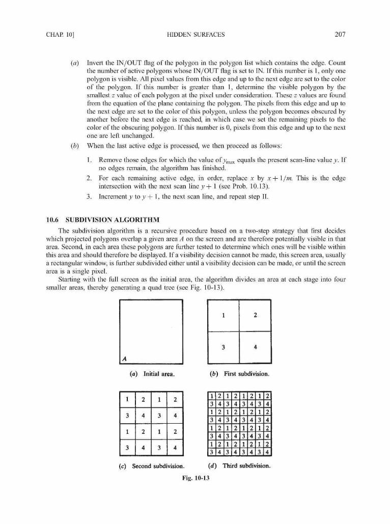
CHAP. 10] HIDDEN SURFACES 207
(a) Invert the IN/OUT flag of the polygon in the polygon list which contains the edge. Countthe number of active polygons whose IN/OUT flag is set to IN. If this number is 1, only onepolygon is visible. All pixel values from this edge and up to the next edge are set to the colorof the polygon. If this number is greater than 1, determine the visible polygon by thesmallest z value of each polygon at the pixel under consideration. These z values are foundfrom the equation of the plane containing the polygon. The pixels from this edge and up tothe next edge are set to the color of this polygon, unless the polygon becomes obscured byanother before the next edge is reached, in which case we set the remaining pixels to thecolor of the obscuring polygon. If this number is 0, pixels from this edge and up to the nextone are left unchanged.
(b) When the last active edge is processed, we then proceed as follows:
1. Remove those edges for which the value of yn
no edges remain, the algorithm has finished.
2. For each remaining active edge, in order, replace x by xintersection with the next scan line y+\ (see Prob. 10.13).
3. Increment y to y + 1, the next scan line, and repeat step II.
equals the present scan-line value y. If
\jm. This is the edge
10.6 SUBDIVISION ALGORITHM
The subdivision algorithm is a recursive procedure based on a two-step strategy that first decideswhich projected polygons overlap a given area A on the screen and are therefore potentially visible in thatarea. Second, in each area these polygons are further tested to determine which ones will be visible withinthis area and should therefore be displayed. If a visibility decision cannot be made, this screen area, usuallya rectangular window, is further subdivided either until a visibility decision can be made, or until the screenarea is a single pixel.
Starting with the full screen as the initial area, the algorithm divides an area at each stage into foursmaller areas, thereby generating a quad tree (see Fig. 10-13).
1
3
2
4
(a) Initial area. (b) First subdivision.
1
3
1
3
2
4
2
4
1
3
1
3
2
4
2
4
13131313
24242424
13131313
24242424
13131313
24242424
13131313
24242424
(c) Second subdivision. (d) Third subdivision.
Fig. 10-13

208 HIDDEN SURFACES [CHAP. 10
The processing exploits area coherence by classifying polygons P with respect to a given screen area Ainto the following categories: (1) surrounding polygon—polygon that completely contains the area [Fig.10-14(a)], (2) interesecting polygon—polygon that intersects the area [Fig. 10-14(Z>)], (3) containedpolygon—polygon that is completely contained within the area [Fig. 10-14(c)], and (4) disjoint polygon—polygon that is disjoint from the area [Fig. 10-14(<f)].
(a) P surrounds A. (ft) P intersects A.
(c) P is contained in A. («0 P is disjoint from A.
Fig. 10-14
The classification of the polygons within a picture is the main computational expense of the algorithmand is analogous to the clipping algorithms discussed in Chap. 5. With the use of one of these clippingalgorithms, a polygon in category 2 (intersecting polygon) can be clipped into a contained polygon and adisjoint polygon (see Fig. 10-15). Therefore, we could proceed as if category 2 were eliminated.
Fig. 10-15

CHAP. 10] HIDDEN SURFACES 209
For a given screen area, we keep a potentially visible polygons list (PVPL), those in categories 1, 2,and 3. (Disjoint polygons are clearly not visible.) Also, note that on subdivision of a screen area,surrounding and disjoint polygons remain surrounding and disjoint polygons of the newly formed areas.Therefore, only contained and intersecting polygons need to be reclassified.
Removing Polygons Hidden by a Surrounding Polygon
The key to efficient visibility computation lies in the fact that a polygon is not visible if it is in back ofa surrounding polygon. Therefore, it can be removed from the PVPL. To facilitate processing, this list issorted by zT^ss the smallest z coordinate of the polygon within this area. In addition, for each surroundingpolygon S, we also record its largest z coordinate, z. .
If, for a polygon P on the list, zP > Zc (for a surrounding polygon S), then P is hidden by S andthus is not visible. In addition, all other polygons after P on the list will also be hidden by S, so we canremove these polygons from the PVPL.
Subdivision Algorithm
1. Initialize the area to be the whole screen.
2. Create a PVPL with respect to an area, sorted on zmin (the smallest z coordinate of the polygonwithin the area). Place the polygons in their appropriate categories. Remove polygons hidden by asurrounding polygon and remove disjoint polygons.
3. Perform the visibility decision tests:(a) If the list is empty, set all pixels to the background color.
(b) If there is exactly one polygon in the list and it is a classified as intersecting (category 2) orcontained (category 3), color (scan-convert) the polygon, and color the remaining area to thebackground color.
(c) If there is exactly one polygon on the list and it is a surrounding one, color the area the colorof the surrounding polygon.
(d) If the area is the pixel (x, y), and neither a, b, nor c applies, compute the z coordinate z(x, y)at pixel (x,y) of all polygons on the PVPL. The pixel is then set to the color of the polygonwith the smallest z coordinate.
4. If none of the above cases has occurred, subdivide the screen area into fourths. For each area, go tostep 2.
10.7 HIDDEN-LINE ELIMINATION
Although there are special-purpose hidden-line algorithms, each of the above algorithms can bemodified to eliminate hidden lines or edges. This is especially useful for wireframe polygonal modelswhere the polygons are unfilled. The idea is to use a color rule which fills all the polygons with thebackground color—say, black—and the edges and lines a different color—say, white. The use of a hidden-surface algorithm now becomes a hidden-line algorithm.
10.8 THE RENDERING OF MATHEMATICAL SURFACES
In plotting a mathematical surface described by an equation z = Fix, y), where xmin < x < xmax andJmin — y — >max> w e could use any of the hidden-surface algorithms so far described. However, thesegeneral algorithms are inefficient when compared to specialized algorithms that take advantage of thestructure of this type of surface.
The mathematical surface is rendered as a wireframe model by drawing both the x-constant curvesz = F(const, y) and the y-constant curves z = Fix, const) (see Fig. 10-16). Each such curve is rendered as
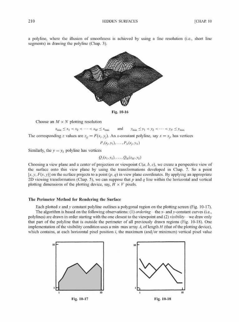
210 HIDDEN SURFACES [CHAP. 10
a polyline, where the illusion of smoothness is achieved by using a fine resolution (i.e., short linesegments) in drawing the polyline (Chap. 3).
Fig. 10-16
Choose anMxJV plotting resolution
xm i n < *i < x2 < • • • < xM < xmax and ymin <yx < y2 < • • • < yN < ymax
The corresponding z values are ztj- = F(xi,yJ). An x-constant polyline, say x = Xj, has vertices
^(x,- ,^) , ...,PN(xj,yN)
Similarly, the y = yk polyline has vertices
Qi(x1,yk),...,QM(xM,yk)
Choosing a view plane and a center of projection or viewpoint C(a, b, c), we create a perspective view ofthe surface onto this view plane by using the transformations developed in Chap. 7. So a point[x, y, F(x, yy] on the surface projects to a point (p, q) in view plane coordinates. By applying an appropriate2D viewing transformation (Chap. 5), we can suppose that/? and q line within the horizontal and verticalplotting dimensions of the plotting device, say, H x V pixels.
The Perimeter Method for Rendering the Surface
Each plotted x and j constant polyline outlines a polygonal region on the plotting screen (Fig. 10-17).The algorithm is based on the following observations: (1) ordering—the x- and j-constant curves (i.e.,
polylines) are drawn in order starting with the one closest to the viewpoint and (2) visibility—we draw onlythat part of the polyline that is outside the perimeter of all previously drawn regions (Fig. 10-18). Oneimplementation of the visibility condition uses a min-max array A, of length H (that of the plotting device),which contains, at each horizontal pixel position /, the maximum (and/or minimum) vertical pixel value
Fig. 10-17 Fig. 10-18
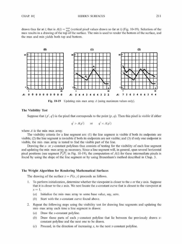
CHAP. 10] HIDDEN SURFACES 211
drawn thus far at /; that is A(i) = ™^ (vertical pixel values drawn so far at /) (Fig. 10-19). Selection of themax results in a drawing of the top of the surface. The min is used to render the bottom of the surface, andthe max and min yields both top and bottom.
(0) (1) (2)
10 -•
1
10 --
Vs/
Jf
p.
A
>N
i
10 -
I 10
A: 0 0 0 0 0 0 0 0 0 0I 10
A: 5 4 4 3 4 6 4 3 2 2
-
\>>
\ 1VV
Jf
A
><s,\
s
1I -
I 10
A: 7 5 6 5 4 6 6 5 4 4
Fig. 10-19 Updating min-max array A (using maximum values only).
The Visibility Test
Suppose that (pr, q') is the pixel that corresponds to the point (p, q). Then this pixel is visible if either
q' > A(p') or q' < A(p')
where A is the min-max array.The visibility criteria for a line segment are: (1) the line segment is visible if both its endpoints are
visible; (2) the line segment is invisible if both its endpoints are not visible; and (3) if only one endpoint isvisible, the min-max array is tested to find the visible part of the line.
Drawing the x- or j-constant polylines thus consists of testing for the visibility of each line segmentand updating the min-max array as necessary. Since a line segment will, in general, span several horizontalpixel positions (see segment P\Pi in Fig. 10-19), the computation of A(i) for these intermediate pixels isfound by using the slope of the line segment or by using Bresenham's method described in Chap. 3.
The Wright Algorithm for Rendering Mathematical Surfaces
The drawing of the surface z = F(x,y) proceeds as follows.
1. To perform initialization, determine whether the viewpoint is closer to the x or the y axis. Supposethat it is closer to the x axis. We next locate the x-constant curve that is closest to the viewpoint atx= 1.
(a) Initialize the min-max array to some base value, say, zero.
(b) Start with the x-constant curve found above.
2. Repeat the following steps using the visibility test for drawing line segments and updating themin-max array each time a line segment is drawn:
(a) Draw the x-constant polyline.
(b) Draw those parts of each j-constant polyline that lie between the previously drawn x-constant polyline and the next one to be drawn.
(c) Proceed, in the direction of increasing x, to the next x-constant polyline.

212 HIDDEN SURFACES [CHAP. 10
Solved Problems
10.1 Given points Px(l, 2, 0), P2(3, 6, 20), and P3(2, 4, 6) and a viewpoint C(0, 0, -10) , determinewhich points obscure the others when viewed from C.
SOLUTION
The line joining the viewpoint C(0, 0, —10) and point P^(l, 2, 0) is (App. 2)
x = f j ; = 2f z = - 1 0 + 10f
To determine whether P2(3,6, 20) lies on this line, we see that x = 3 when t = 3, and then at £ = 3, x = 3,j> = 6, and z = 20. So P 2
u e s o n t n e projection line through C and P j .Next we determine which point is in front with respect to C. Now C occurs on the line at t = 0, Px occurs
at t = 1, and P2 occurs at t = 3. Thus comapring t values, Px is in front of P2 with respect to C; that is, Px
obscures P2.We now determine whether P3(2, 4, 6) is on the line. Nowx = 2 when £ = 2 and theny = 4, andz = 1 0 .
Thus P^(2, 4, 6) is not on this projection line and so it nether obscures nor is obscured by Pj and P2.
10.2 Construct the perspective to parallel transform Tp which produces an object whose parallelprojection onto the xy plane yields the same image as the perspective projection of the originalobject onto the normalized view plane z = c'z/(c'z + b) (Chap. 8, Prob. 8.6) with respect to theorigin as the center of projection.
SOLUTION
The perspective projection onto the plane z = c'z/(c'z + b) with respect to the origin is (Chap. 7, Prob.7.4):
Per =
where zB = c'z/(c'z + b). The perspective projection onto the view plane of a point P(x, y, z) is the point
'(¥•¥--•)Define the perspective to parallel transform Tp to be
\
z00
i 0
0
V
00
00
zv1
0000
'V
0
0
0zv
0
00
1
00
~zf
0 0
l-Zr l-Zf
1
(where z = zy is the location of the normalized front clipping plane; see Chap. 8, Prob. 8.6).Now, applying the perspective to parallel transform Tp to the point P(x, y, z), we produce the point
zvx zvy zf
z ' z ' z ( l - Z / )
The parallel projection of Q' onto the xy plane produces the point
Qf-f ,f ,0)So Q and P' produce the same projective image. Furthermore, Tp transforms the normalized perspective viewvolume bounded by x = z, x = —z, y = z, y = —z, z = Zr, and z = 1 to the rectangular volume bounded byx=zv,x = -zv, y = zv,y = -zv, z = 0, and z = 1.

CHAP. 10] HIDDEN SURFACES 213
10.3 Show that the normalized perspective to parallel transform NTp preserves the relationships of theoriginal perspective transformation while transforming the normalized perspective view volumeinto the unit cube.
SOLUTION
From Prob. 10.2, the perspective to parallel transform Tp transforms a point P(x, y, z) to a point
e zvy z-zf
z z z ( l - Z / )y
The image under parallel projection of this point onto the xy plane is
The factor zB can be set equal to 1 without changing the relation between points Q and Q'.
Ix y z — zT h e m a t r i x t h a t t r a n s f o r m s P ( x , y , z ) t o t h e p o i n t 0 1 , ,
- z z• / is then
/ I 0
0 1
0 0
Vo o
0 \
0-zf
1
~ z f
0 /In addition, this matrix transforms the normalized perspective view volume to the rectangular view
volume bounded b y x = 1, x = — 1, y = I, y = —I, z = 0, and z = 1.We next translate this view volume so that the corner point (— 1, —1,0) translates to the origin. The
translation matrix that does this is
/ I 0 0 10 1 0 1
0 0 0 1
The new region is a volume bounded by x = 0, x = 2, y = 0, y = 2, z = 0, and z = 1.Finally, we scale in the x andy direction by a factor 1 so that the final view volume is the unit cube: x = 0,
x = 1, y = 0, y = l , z = 0, and z = 1. The scaling matrix is
'\ 0 0
I o \ o o0 0 1 00 0 0 1
s 1/2,1/2,1 —
The final normalized perspective to parallel transform is
~ ^1/2,1/2,1 '
(1
0
nu
0
I
nu 1
121
1
- Z( 1
0
0
~zf
~zf
10.4 Why are hidden-surface algorithms needed?
SOLUTION
Hidden-surface algorithms are needed to determine which objects and surface will obscure those objectsand surfaces that are in back of them, thus rendering a more realistic image.

214 HIDDEN SURFACES [CHAP. 10
10.5 What two steps are required to determine whether any given points Pi(xl,yl,zl) obscures anotherpoint P2(x2, y2, z2)? (See Fig. 10-1.)
SOLUTION
It must be determined (1) whether the two points lie on the same projection line and (2) if they do, whichpoint is in front of the other.
10.6 Why is it easier to locate hidden surfaces when parallel projection is used?
SOLUTION
There are no vanishing points in parallel projection. As a result, any point P(a, b, z) will line on the sameprojector as any other point having the same x and y coordinates (a, b). Thus only the z component must becompared to determine which point is closest to the viewer.
10.7 How does the Z-buffer algorithm determine which surfaces are hidden?
SOLUTION
The Z-buffer algorithm sets up a two-dimensional array which is like the frame buffer; however the Zbuffer stores the depth value at each pixel rather than the color, which is stored in the frame buffer. By settingthe initial values of the Z buffer to some large number, usually the distance of back clipping plane, theproblem of determining which surfaces are closer is reduced to simply comparing the present depth valuesstored in the Z buffer at pixel (x,y) with the newly calculated depth value at pixel (x,y). If this new value isless than the present Z-buffer value (i.e., closer along the line of sight), this value replaces the present valueand the pixel color is changed to the color of the new surface.
10.8 Using a 2 x 2 pixel display, show how the Z-buffer algorithm would determine the color of eachpixel for the given objects A and B in Fig. 10-20.
n.
Back
I
: clipping /slanc /
Display spac
Pixel coordinates
Fig. 10-20

CHAP. 10] HIDDEN SURFACES 215
SOLUTION
The display space for the 2 x 2 pixel display is the region 0 < x < 2, 0 <y <2, and 0 < z < 1. In Fig.10-20, A is the line with display space coordinates AX(^,\,<S) and A2(2, 2, 0); line A is on the display screen infront of square B. B is the square with display space coordinates Bl(0, Q,j), B2(2,0,j), B3(2,2,j), and-84(0, 2, j). The displayed image of A (after projection and scan conversion) would appear on a 2 x 2 pixeldisplay as
y
a
a
y
0 1
where a is the color of A and j ; is the background color. We have used the fact (Chap. 3, Sec. 3.1) that a point(x,y) scan-converts to the pixel [Floor(x), Floor(y)]. (We assume for consistency that 2 = 1.99 ) Thedisplayed image of B is
1 b
b
b
b
0 1
where b is the color of B. We apply the Z-buffer algorithm to the picture composed of objects A and B asfollows:
1. Perform initialization. The Z buffer is set equal to the depth of the back clipping plane z = 1, and theframe buffer is initialized to a background color y.
Frame buffer =1 y
y
y
yZ buffer =
1 1
1
1
1
0 1 0 1
2. Apply the algorithm to object A.
(a) The present Z-buffer value at pixel (0, 0) is that of the back clipping plane, i.e., Zbuf(0, 0) = 1. Thedepth vapue of A at pixel (0, 0) is z = 0. Then Zbuf(0, 0) is changed to 0 and pixel (0, 0) has thecolor of A.
Frame buffer =y
a
y
yZ buffer =
1
0
1
1
0 1 0 1
(b) Object A is not seen from pixel (1, 0), so the Z-buffer value is unchanged.
1Frame =
0
y
a
y
y
1
0
1
1
0 1 0 1
(c) Object A is not seen from pixel (0, 1), so the Z-buffer value is unchanged.
1Frame =
0
y
a
y
y
1
0
1
1
0 1 0 1

216 HIDDEN SURFACES [CHAP. 10
(d) The depth value of A at pixel (1, 1) is 0. Since this is less than the present Z-buffer value of 1, pixel(1, 1) takes the color of A.
Frame =1 y
a
a
y
1 1
0
0
1
0 1 0 1
3. Apply the algorithm to B.
(a) The depth value for B at pixel (0, 0) is \, and Zbuf(0, 0) = 0. So the color of pixel (0, 0) isunchanged.
Frame =1 y
a
a
y
1 1
0
0
1
0 1 0 1
(b) The depth value of B at pixel (1, 0) is A. The present Z-buffer value is 1. So the Z-buffer value is setto A and pixel (1, 0) takes the color of B.
Frame =1 y
a
a
b
1 1
0
0
12
0 1 0 1
(c) The depth value of B at pixel (0, 1) is \. The present Z-buffer value is 1, so the color at pixel (0, 1) isset to that of B, and the Z buffer is updated.
Frame =1 b
a
a
b
1 I
0
0
12
0 1 0 1
(d) The depth value of B at pixel (1, 1) is A. The present Z-buffer value is 0. So the color at pixel (1,1)remains unchanged.
Frame =b
a
a
b
12
0
0
i2
0 1 0 1
The final form of the Z buffer indicates that line A lines in front of B.
10.9 What is the maximum number of objects that can be presented by using the Z-buffer algorithm?
SOLUTION
The total number of objects that can be handled by the Z-buffer algorithm is arbitrary because each objectis processed one at a time.
10.10 How does the basic scan-line method determine which surfaces are hidden?
SOLUTION
The basic scan-line method looks one at a time at each of the horizontal lines of pixels in the display area.For example, at the horizontal pixel line y = a, the graphics data structure (consisting of all scan-convertedpolygons) is searched to find all polygons with any horizontal (y) pixel values equal to a.

CHAP. 10] HIDDEN SURFACES 217
Next, the algorithm looks at each individual pixel in the a row. At pixel (a, /?), the depth values (z values)of each polygon found above are compared to find the polygon having the smallest z value at this pixel. Thecolor of pixel (a, /?) is then set to the color of the corresponding polygon at this pixel.
10.11 Using the four pixel display and the graphics objects A and B from Prob. 10.8, show how the basicscan-line method would display these objects.
SOLUTION
First we initialize the display to the color y of the back clipping plane (located at z = 1).
Frame buffer =1 y
y
y
y
0 1
y
a
y
y
1. Set y = 0. The scan-converted representations of A and B contain pixels on the y = 0 scan line.
(a) Set x = 0. Comparing the z values of A and B at pixel (0, 0), we find that the smaller z value is 0,which belongs to A. Thus A is seen from pixel (0, 0); that is, pixel (0, 0) is set to the color of A.
1
0 1
(b) Set x = 1. Since A is not seen from pixel (1,0) while -Sis seen, the color of pixel (1, 0) is set to thatof B.
y
a
y
b
0 1
2. Set y = 1. The scan-converted representations of A and B contain pixels on the y = 1 scan line.
(a) Set x = 0. Because A is not seen at pixel (0, 1) while B is seen, pixel (0, 1) is set to the color of B.
1 b
a
y
b
0 1
(b) S e t x = 1. Both A and B are "seen" from pixel (1, 1). The depth of A at pixel (1, 1) is 0, that of B is\. Thus A is visible at pixel (1, 1).
1
0
b
a
a
b
0 1
This represents the final image displayed.

218 HIDDEN SURFACES [CHAP. 10
10.12 How does edge coherence help to reduce computational effort?
SOLUTION
It is based on the assumption that, if an edge or line intersects a given scan line, it will most likelyintersect those scan lines next to it. Thus if the pixels that intersect the edge are to be found, instead ofintersecting each scan line with the edge, it is necessary to locate only one intersection pixel and then find theothers using the slope m of the edge (see Prob. 10.13).
10.13 Show how the calculation of the intersection of an edge with a scan line can be made incremental asopposed to absolute.
SOLUTION
The absolute calculation requires that we find the x intersection value of the edge (e.g., with equationy = mx + b) with the scan line y = a for each a.
The incremental solution to the problem is based on the following observations. Suppose that xa is the xintersection of the edge with the scan line a. Then the intersection xa+1 of the edge with the next scan liney = a + 1 can be found as illustrated in Fig. 10-21. From Fig. 10-21, where m is the slope of the edge,
Ay ( a + l ) - a
Ax xa+l ~~ xa
Solving for xa+l, we obtain
1a + a m
Thus the calculation of the next intersection point is incremental; that is, it is found from the previousintersection point by adding 1 jm to it.
Edge.? = mx + b
Scan line y = a + 1
Scan line y = a
10.14 How does area coherence reduce computational effort?
SOLUTION
Area coherence is based on the assumption that a small enough region of pixels will most likely lie withina single polygon. This reduces, as in the subdivision algorithm, computational effort in dealing with all thosepolygons that are potentially visible in a given screen area (region of pixels).
10.15 How is spatial coherence determined?
SOLUTION
Spatial coherence is determined by examining the extent of an object. The rectangular extent (boundingbox) of an object is determined by finding the minimum and maximum x, y, and z coordinate values of the

CHAP. 10] HIDDEN SURFACES 219
points that belong to the object. The extent is the rectangular region bounded by the planes z = zmin, z = zmax,
y ~~ JVin* y ~~ max' x ~ xmin> a n " x ~ xmax'
10.16 Draw two polygons such that their extents intersect but the polygons themselves don't intersect.
SOLUTION
Figure 10-22 shows one possible solution.
Extent of A: 1772Extent of B:
Fig. 10-22
10.17 Apply the scan-line algorithm from Sec. 10.5, under "A Scan-line algorithm," to the display ofobjects A and B in Prob. 10.8.
SOLUTION
As in Prob. 10.8, a point (x,y) scan converts to the pixel [Floor(x), Floor(y)]. Also note that anonhorizontal line can be treated as a special polygon: a scanline enters into and exits from the polygon atthe same pixel position.
We first construct the edge list (EL) and the polygon list (PL). From Fig. 10-20, the edge entries for thenonhorizontal edges A-lA2, B^B4, and -82-83 are
Edge
AXA2
BXBA
B2B3
12
0
0
X
12
0
2
J^max
2
2
2
1
m
1
0
0
Polygon pointer
A
B
B
Here, ymin is the edge's smaller y coordinate and x the corresponding x coordinate; yr[mx is the larger ycoordinate, and m is the slope of the edge. Form the PL:
PL =
Polygon
A(line)
B
Equation
x =yz = 0
z — -
IN/OUT flag
OUT
OUT
Color
a
b

220 HIDDEN SURFACES [CHAP. 10
The algorithm proceeds as follows.
I. Initialization.
(a) We initialize the screen display to the color y of the back clipping plane (located at z = 1).
Frame buffer =1 y
y
y
y
0 1
(b) Set the scan line to y = 0.
II. y-scan loop. Activate edges that satisfy Floor(ymin) = 0 and sort on x
Edges
BXBA
AXA2
B2B3
X
0
l2
2
III. x-scan loop.
(a) Process edge BlB4. First invert the appropriate IN/OUT flags in the PL:
Polygon
A
B
Equation
x=yz = 0
* = \
IN/OUT flag
OUT
IN
Color
a
b
PL =
The number of active polygons is one. Thus B is visible at pixel (0, 0) and all pixels on scanline y = 0 between edges B^B4 and A-lA2 are set to the color of B. In our case, this is just the pixel(0, 0).
y
b
y
y
0 1
(a) Now we repeat step (a), processing edge AXA2. We update the PL:
Polygon
A
B
Equation
x =yz = 0
z — -
IN/OUT flag
IN
IN
Color
a
b
PL =
The number of active polygons is 2. At pixel (0, 0) the depth value (z value) of polygon^ is 0 and of

CHAP. 10] HIDDEN SURFACES 221
polygon B is \. Thus polygon A is visible at pixel (0, 0), so the color is set to a.
y
a
y
y
0 1
Since A is a line, set the IN/OUT flag of line A to OUT. The color of all pixels between edges AlA1
and -82-83 are determined by the remaining active polygon B.
Polygon
A
B
—
—
IN/OUT flag
OUT
IN
—
—
PL =
This means that we set the color of pixel (1, 0) to b.
(a) Again, we repeat step (a), processing edge B2B3. We update the PL:
PL =
The number of active polygons is 0.
y
a
0
y
b
1
Polygon
A
B
—
—
IN/OUT flag
OUT
OUT
—
—
(b) Having processed B2B3, the last active edge, we proceed:
(1) All the ymsK values are equal to 2. These values scan-convert (see Prob. 10.8) to 1. The presenty scan line value is 0. So no edges are removed.
(2) Incrementing x by 1 /m,
BXBA
1 2
52JB3
0
32
2
(3) S e t . y = l .
Now we repeat steps II and III.
II. y-scan loop. With y = 1, no additional edge is activated. The result of sorting active edges remains asabove.
III. x-scan loop.

222 HIDDEN SURFACES [CHAP. 10
(a) Process edge BXBA. We update the PL:
PL =
Polygon
A
B
—
—
IN/OUT flag
OUT
IN
—
—
The number of active polygons is 1. Thus B is visible at pixel (0, 1) and all pixels between edgeBXBA and AXA2 on scan line y = 1 are set to the color of B.
b
a
b
b
0 1
(a) Now we repeat step (a), processing edge A\A2. We update the PL:
PL =
Polygon
A
B
—
—
IN/OUT flag
IN
IN
—
—
There are two active polygons. A depth comparison at pixel (1,1) shows that it is set to the color ofline AXA2.
b
a
a
b
0 1
Since A is a line, we set the IN/OUT flag of A to OUT. And we proceed immediately to the nextedge at the same pixel location.
(a) Again we repeat step (a), processing edge B2B3. We update the PL:
PL =
Polygon
A
B
Equation
x=yz = 0
z = \
IN/OUT flag
OUT
OUT
Color
a
b
The number of active polygons becomes 0.
(b) Having processed the last active edge B2B3, we remove those edges for which ymax equals the yscan value of 1. Since this includes all the edges, i.e., >>max = 2, the algorithm stops.
10.18 What is the underlying concept of the painter's or the priority algorithm?

CHAP. 10] HIDDEN SURFACES 223
SOLUTION
The painter's algorithm sorts polygons by depth and then paints (scan-converts) each polygon onto thescreen starting with the most distance polygon.
10.19 What difficulties are encountered in implementing the painter's algorithm?
SOLUTION
First, there is the question of what the "depth" of a polygon is, especially if the polygon is tilted out ofthe xy plane. Second, if two polygons have the same depth, which one should be painted first?
10.20 If polygon Q has the same depth value as polygon P, which polygon has priority, that is, which ispainted first?
SOLUTION
We perform tests 0, 1,2, 3, 4, 5 (from Sec. 10.4, under "Testing Whether P obscures Q") in order. If anyone of the tests is true, we say that polygon P does not obscure polygon Q, and so polygon P is painted first.
If none of the tests is true, we have an ambiguity that must be resolved.We resolve the ambiguity by switching the roles of P and Q and the reapply tests 0, 1, 2, 3, 4, and 5. If
any one of these tests is true, Q does not obscure polygon P and so polygon Q is painted first.If again none of the tests is true, polygon Q must be subdivided into two polygons Qx and Q2, using the
plane containing polygon P as the dividing plane [Fig. 1
b
b
b
b
10.21 Apply the painter's algorithm to display objects A and B in Prob. 10.8.
SOLUTION
We first find the depth values zmax for A and B. Since zmax is the largest z value from all the polygon'svertices, then for A, zA = 0, and for B, zB = 5. Then sorting on zmax, we see that polygon B has a higherdepth value than polygon A.
Next, we assign priorities by applying tests 0 through 5 in order (see Sec. 10.4). In test 0, the z extent of Bis Zmin = \, Zmax = \- The z extent of A is zmin = 0, zmax = 0.
Thus the z extents of A and B do not overlap and zA is smaller than zB . Thus test 0 is true, and so wescan-convert polygon B first:
1Frame buffer =
0
0 1
Next, we scan-convert polygon A (i.e., we "paint" over polygon B):
1
0
0 1
This is the final image displayed in the frame buffer.
10.22 What are the basic concepts underlying the subdivision algorithm?
SOLUTION
First, is that a polygon is seen from within a given area of the display screen if the projection of thatpolygon overlaps the given area. Second, of all polygons that overlap a given screen area, the one that isvisible in this area is the one in front of all the others. Third, if we cannot decide which polygon is visible (in
b
a
a
b

224 HIDDEN SURFACES [CHAP. 10
front of the others) from a given region, we subdivide the region into smaller regions until visbility decisionscan be made (even if we must subdivide down to the pixel level).
10.23 Apply the subdivision algorithm to the display of objects A and B from Prob. 10.8.
SOLUTION
1. Initialization. We initialize the area to the whole screen.
2. Forming the potentially visible polygon list. We create the PVPL, sorted on zmin, the smallest of the zvalues of the polygon in the area.
PVPL =
3. Visibility decision. We apply criteria (a) through (d) in Sec. 10.6, step 3. Since all four tests fail, we passto step 4 and subdivide the area into four subregions.After subdivision, the four newly formed regions are, in our example, the individual pixels. We apply the
algorithm to each pixel in turn.
Region 1: pixel (0, 0).
2. Forming the PVPL.
PVPL =
Polygon
A
B
•^min
0
i
Category
Contained
Surrounding
Polygon
A
B
min
0
i
Category
Intersecting
Surrounding
3. Visibility decision. Applying tests (a) thrpough (c), we now apply test (d) since the region is pixel size.The z coordinate of A at pixel (0, 0) is 0, and that of B is A. Thus A is visible at pixel (0, 0):
Frame buffer =1
a
0 1
Region 2: pixel (0, 1).
2. Forming the PVPL. Note that A is disjoint from this region:
PVPL =Polygon
B
^min
I
Category
Surrounding
3. Visibility decision. From test (c), there is only one polygon and it is surrounding, so we color pixel (0, 1)
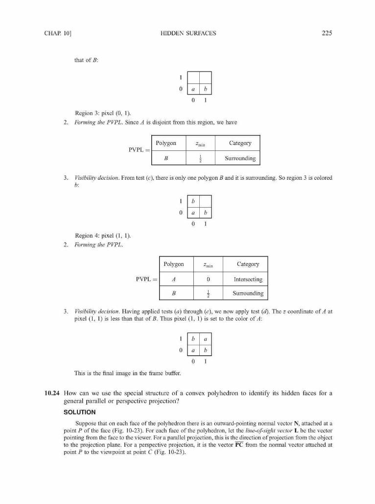
CHAP. 10] HIDDEN SURFACES 225
that of B:
a b
0 1
Region 3: pixel (0, 1).
2. Forming the PVPL. Since A is disjoint from this region, we have
PVPL =
3. Visibility decision. From test (c), there is only one polygon B and it is surrounding. So region 3 is colored
Polygon
B
^min
I
Category
Surrounding
b
a b
Region 4: pixel (1, 1).
2. Forming the PVPL.
Polygon
A
B
•^min
0
i2
Category
Intersecting
Surrounding
PVPL =
3. Visibility decision. Having applied tests (a) through (c), we now apply test (d). The z coordinate of A atpixel (1, 1) is less than that of B. Thus pixel (1, 1) is set to the color of A:
b
a
a
b
This is the final image in the frame buffer.
10.24 How can we use the special structure of a convex polyhedron to identify its hidden faces for ageneral parallel or perspective projection?
SOLUTION
Suppose that on each face of the polyhedron there is an outward-pointing normal vector N, attached at apoint P of the face (Fig. 10-23). For each face of the polyhedron, let the line-of-sight vector L be the vectorpointing from the face to the viewer. For a parallel projection, this is the direction of projection from the objectto the projection plane. For a perspective projection, it is the vector PC from the normal vector attached atpoint P to the viewpoint at point C (Fig. 10-23).

226 HIDDEN SURFACES [CHAP. 10
N = AB x AD
Fig. 10-24 Fig. 10-25
CHAP. 10] HIDDEN SURFACES 227
A face is visible if the angle 8 made by the line-of-sight vector L and the normal vector N is less than 90°.It is hidden if this angle is larger than or equal to 90°. If 0° < 8 < 90°, then 0 < cos 8 < 1; if 90° < 8 < 180°,then — 1 < cos 8 < 0. Since (from App. 2)
cos 8 =
L - N0 < < 1
| L | | N | "
the face is visible if
and hidden otherwise. To use this visibility test, we need to find the outward-pointing normal vectors for thefaces of the polyhedron. To do this, we label the faces of the polyhedron so that the polyhedron is oriented.That is, any edge shared by adjacent faces is traversed in opposite directions with respect to the faces (Fig.10-24). This guarantees that the normal vectors will point outward. To construct the outward normal vectors,we label each polygon with a counterclockwise labeling (Fig. 10-25). Then a normal vector can be found bytaking the cross product of vectors determined by two adjacent sides of the polygon and attaching it at one ofthe vertices (Fig. 10-25).
Supplementary Problems
10.25 How may the properties of parallel projection be used to simplify hidden-surface calculations for any form ofprojection?
10.26 What happens when two polygons have the same z value and the Z-buffer algorithm is used?
10.27 How would the Z-buffer algorithm be altered to allow figures to be superimposed on a surface (see Prob.10.26)?
10.28 Assuming that one allows 224 depth value levels to be used, how much memory would a 1024 x 768 pixeldisplay require to store the Z buffer?
10.29 How can the amount of computation required by the scan-line method be reduced?
10.30 How does scan-line coherence help to reduce computation?
10.31 What is the extent of the polygon whose vertices are ,4(0, 0, 1), B(2, 0, 1), and C(l, 2, 2) (see Fig. 10-26)?
10.32 Why are only nonhorizontal lines stored in the edge list of the scan-line algorithm?
10.33 How is the depth of a polygon determined by the painter's algorithm?
10.34 How does the subdivision algorithm exploit are coherence?
10.35 How can hidden-surface algorithms be used to eliminate hidden lines as applied to polygonal mesh models(Chap. 9)?

228 HIDDEN SURFACES [CHAP. 10
I 2
Fig. 10-26

Color and ShadingModels
Color is a fundamental attribute of our viewing experience. The perception of color arises from lightenergy entering our visual system and triggering a chain of not-yet-fully-understood neurological andpsychological responses. This complex process is relevant to computer graphics because a realistic imageis one that seems indistinguishable from a true record of the light energy coming from the real scene. It hasbeen a constant challenge to find effective and efficient computational models for constructing suchimages.
In Sect. 11.1, we first outline the basic relationship between light (the physical stimulus) and theperception of color. This leads to an international standard for the specification and measurement of colors,and a better understanding of the widely used RGB color model. In Sect. 11.2, we use a well-knownformula to mimic the effect of objects being lit by light sources (A more elaborate illumination model isdiscussed in Chap. 12). In Sects. 11.3 and 11.4, we describe several useful techniques for shading polygon-mesh objects and for depicting delicate surface details (surface texture).
11.1 LIGHT AND COLOR
Light, or visible light, is electromagnetic energy in the 400 to 700 nm, i.e., nanometer (10~9 meter),wavelength (2) range of the spectrum (see Fig. 11-1). A typical light has its energy distributed across thevisible band and the proportions are described by a spectral energy distribution function P(l) (see Fig.11-2). To model a light or reproduce a given light with physical precision one would need to duplicatethe exact energy distribution, which is commonly referred to as spectral reproduction.
On the other hand, it has been shown through carefully designed psychophysical experiments thatdiscrepancy in spectral distribution does not necessarily lead to difference in perception. Less stringentapproaches exist to reproduce light to the extent that the reproduction causes the same color sensation to anaverage human observer as the original. These results make it possible to specify or describe light in waysthat are more perceptually oriented and are easier to handle.
229

230 COLOR AND SHADING MODELS [CHAP. 11
3000
700
400
30
X (nm)
AM radio
FM radio & TVMicrowave
Infrared
Visible light
Ultraviolet
X-ray
Fig. 11-1
Energy P
density
λ(nm)
400 700
Fig. 11-2
Basic Characteristics of Light
Light can be characterized in three perceptual terms. The first one is brightness, which corresponds toits physical property called luminance. Luminance measures the total energy in the light. It is proportionalto the area bounded by P(l) and the X axis in the 400 to 700 nm range. The area can be calculated by
P(X)Al
The higher the luminance, the brighter the light to the observer.The second perceptual term is hue, which distinguishes a white light from a red light or a green light.
For a light with an idealized spectral distribution as shown in Fig. 11-3, hue corresponds to anotherphysical property called the dominant wavelength of the distribution.
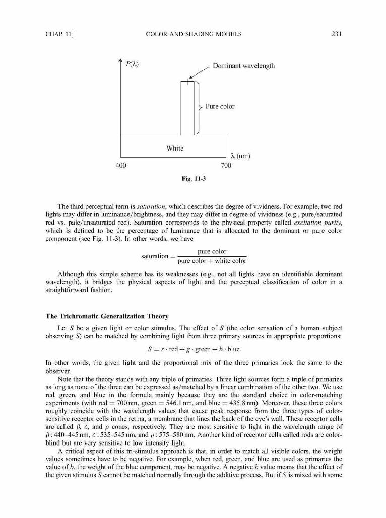
CHAP. 11] COLOR AND SHADING MODELS 231
P() Dominant wavelength
Pure color
White
400 700
Fig. 11-3
The third perceptual term is saturation, which describes the degree of vividness. For example, two redlights may differ in luminance/brightness, and they may differ in degree of vividness (e.g., pure/saturatedred vs. pale/unsaturated red). Saturation corresponds to the physical property called excitation purity,which is defined to be the percentage of luminance that is allocated to the dominant or pure colorcomponent (see Fig. 11 -3). In other words, we have
saturation =pure color
pure color + white color
Although this simple scheme has its weaknesses (e.g., not all lights have an identifiable dominantwavelength), it bridges the physical aspects of light and the perceptual classification of color in astraightforward fashion.
The Trichromatic Generalization Theory
Let S be a given light or color stimulus. The effect of S (the color sensation of a human subjectobserving S) can be matched by combining light from three primary sources in appropriate proportions:
S = r • red + g • green + b • blue
In other words, the given light and the proportional mix of the three primaries look the same to theobserver.
Note that the theory stands with any triple of primaries. Three light sources form a triple of primariesas long as none of the three can be expressed as/matched by a linear combination of the other two. We usered, green, and blue in the formula mainly because they are the standard choice in color-matchingexperiments (with red = 700nm, green = 546.1 nm, and blue = 435.8 nm). Moreover, these three colorsroughly coincide with the wavelength values that cause peak response from the three types of color-sensitive receptor cells in the retina, a membrane that lines the back of the eye's wall. These receptor cellsare called ji, 5, and p cones, respectively. They are most sensitive to light in the wavelength range ofP: 440-445 nm, 5 : 535-545 nm, and p : 575-580 nm. Another kind of receptor cells called rods are color-blind but are very sensitive to low intensity light.
A critical aspect of this tri-stimulus approach is that, in order to match all visible colors, the weightvalues sometimes have to be negative. For example, when red, green, and blue are used as primaries thevalue of b, the weight of the blue component, may be negative. A negative b value means that the effect ofthe given stimulus S cannot be matched normally through the additive process. But if S is mixed with some
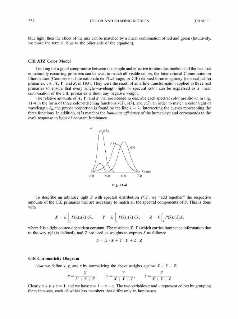
232 COLOR AND SHADING MODELS [CHAP. 11
blue light, then the effect of the mix can be matched by a linear combination of red and green (Intuitively,we move the term b • blue to the other side of the equation).
CIE XYZ Color Model
Looking for a good compromise between the simple and effective tri-stimulus method and the fact thatno naturally occurring primaries can be used to match all visible colors, the International Commission onIllumination (Commission Internationale de l'Eclairage, or CIE) defined three imaginary (non-realizable)primaries, vis., X, Y, and Z, in 1931. They were the result of an affine transformation applied to three realprimaries to ensure that every single-wavelength light or spectral color can be expressed as a linearcombination of the CIE primaries without any negative weight.
The relative amounts of X, Y, and Z that are needed to describe each spectral color are shown in Fig.11 -4 in the form of three color-matching functions x(l), y(l), and z(l). In order to match a color light ofwavelength l0, the proper proportion is found by the line X = l0 intersecting the curves representing thethree functions. In addition, y(X) matches the luminous efficiency of the human eye and corresponds to theeye's response to light of constant luminance.
X (nm)
400 500 600
Fig. 11-4
700
To describe an arbitrary light S with spectral distribution P{X), we "add together" the respectiveamounts of the CIE primaries that are necessary to match all the spectral components of S. This is donewith
= k \X = k \ P(X)x(X) Y = k\ P(X)y(X) <U, Z = k\ P(X)z(X)dl
where k is a light-source-dependent constant. The resultant X, Y (which carries luminance information dueto the way y(l) is defined), and Z are used as weights to express S as follows:
S=X-X+Y Y + Z-Z
CIE Chromaticity Diagram
Now we define x, y, and z by normalizing the above weights against X + Y + Z:
X Y Zx = X+Y + Z' y = X+Y + Z' X+Y + Z
Clearly x + y + z = 1, and we have z = 1 — x — y. The two variables x and y represent colors by groupingthem into sets, each of which has members that differ only in luminance.

CHAP. 11] COLOR AND SHADING MODELS 233
Using x and y as the horizontal and vertical axes we can plot the well-known CIE ChromaticityDiagram (see Fig. 11 -5). The curved triangular figure encompasses all perceivable colors by ignoringluminance. Only when two colors differ in chromaticity (hue and/or saturation) are they represented bytwo different points in the diagram (i.e., they have different chromaticity coordinates).
0.9
0.8
0.7
0.6
0.5 5
0.4
0.3 -
0.2
0.1 -
520
7510
500
3 4 9 0
480
1450
0.1 0.2
540
560\
\ 580
, \
'^
0.3 0.4 0.5 0.6
Fig. 11-5
600C620
0.7 0.8
To convert from chromaticity coordinates (x, y) back to a specific color in the XYZ color space we needan additional piece of information, typically Y:
X = -Y, Y=Y, Z=l~X~yYy y
We can find all spectral colors along the figure's upper border. Point C (0.310,0.316) is known asIlluminant C. It corresponds to a reference white that is obtained from a spectral distribution close todaylight.
The CIE chromaticity diagram serves as a universal reference for the specification and comparison ofvisible colors. The phosphors of a typical color monitor have the following chromaticity coordinates: R(0.62,0.34), G (0.29,0.59), and B (0.15,0.06). These coordinates define a triangular region within thediagram. The region is referred to as the color gamut of the monitor, which represents (the chromaticityrange of) all the colors this monitor is able to display.
Color Gamut Mapping
Let (xr,yr), (xg,yg), and (xb,yb) be the chromaticity coordinates of the phosphors of an RGB colormonitor. What are the XYZ coordinates of its colors? We first introduce auxiliary variablesCr=Xr + Yr+Zr, Cg=Xg + Yg+Zg, and Cb=Xb + Yb+Zb, where (Xr,Yr,Zr), (Xg,Yg,Zg), and(Xb, Yb, Zb) denote the respective XYZ coordinates of the red, green, and blue colors the monitor candisplay. We have
Xr=xrCr,
Xg = xgCg,
Xb = xbCb,
Yr=yrCr, Zr=zrCr
Zg = zgCg
Zb=zbCb
where zr = 1 — xr — yr
where zg = 1 — xg — yg
where zb = 1 - xb - yb

234 COLOR AND SHADING MODELS [CHAP. 11
Thus the XYZ coordinates of a composite RGB color can be expressed in terms of a fransformation M:
( xrCr xgCg xbCb\/R\ (xr xg xb\ ICr 0yrCr ygCg ybCb \\ G = \yr yg yb 0 Cg
zrCr zgCg zbCb)\B) \zr zg zbJ\0 0
There are two different ways to determine Cr, Cg, and Cb. One is to use a photometer to measure theluminance levels Yr, Yg, and Yb of the red, green, and blue colors at their maximum intensity/brightness,respectively. Then
Cr = Yr/yr, Cg = Yg/yg, Cb = Yb/yb
The other is to find/measure the XYZ coordinates (Xw, Yw, Zw) of the monitor's white color(R = G = B = 1). Using these we have
We can now solve for Cr, Cg, and Cb.If Mi is the fransformation for monitor 1 and M2 is the fransformation for monitor 2, then a color
(i?i, Gi,Bi) on monitor 1 can be matched by a corresponding color (R2, G2,B2) on monitor 2:
RoJ*2G2 I =M2
lM
provided that (R2, G2, B2) is within the color gamut of monitor 2.
The NTSC YIQ Color Model
The NTSC (National Television System Committee) YIQ color model is used for commercialtelevision broadcasting in the US. It is defined to be a linear fransformation of the RGB color model,with the Y component purposely made to be the same as the Y in the CIE XYZ color model. Since Y carriesluminance information, black-and-white television sets can use it to display color images as gray-scalepictures. The mapping between RGB and YIQ is as follows:
/0.299 0.587 0.114= 0.596 -0.275 -0.321
\0.212 -0.523 0.311
The quantities in the fransformation matrix are obtained using the standard NTSC RGB phosphors whosechromaticity coordinates are R (0.67,0.33), G (0.21,0.71), and B (0.14,0.08). It is also assumed that thewhite point is at xw = 0.31, yw = 0.316, and Yw = 1.0.
11.2 THE PHONG MODEL
This is a widely used and highly effective way to mimic the reflection of light from object surfaces tothe viewer's eye. It is considered an empirical approach because, although it is consistent with some basicprinciples of physics, it is largely based on our observation of the phenomenon. It is also referred to as alocal illumination model because its main focus is on the direct impact of the light coming from the lightsource. On the other hand, a global illumination model attempts to include such secondary effects as lightgoing through transparent/translucent material and light bouncing from one object surface to another.
Now consider a point light source [see Fig. ll-6(a)], which is an idealized light with all its energycoming out from a single point in space (a reasonable approximation to a bulb). Our eye is at the viewpoint
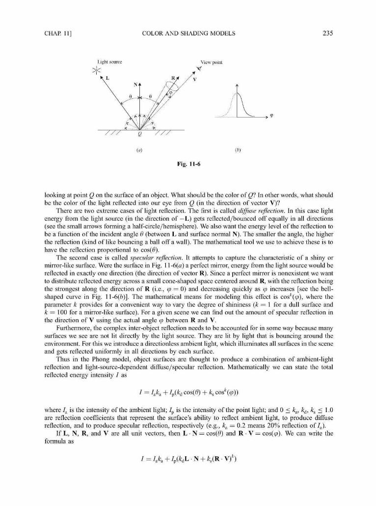
CHAP. 11] COLOR AND SHADING MODELS 235
Light source View point
-± <P
()
Fig. 11-6
looking at point Q on the surface of an object. What should be the color of Ql In other words, what shouldbe the color of the light reflected into our eye from Q (in the direction of vector V)?
There are two extreme cases of light reflection. The first is called diffuse reflection. In this case lightenergy from the light source (in the direction of —L) gets reflected/bounced off equally in all directions(see the small arrows forming a half-circle/hemisphere). We also want the energy level of the reflection tobe a function of the incident angle 6 (between L and surface normal N). The smaller the angle, the higherthe reflection (kind of like bouncing a ball off a wall). The mathematical tool we use to achieve these is tohave the reflection proportional to cos(0).
The second case is called specular reflection. It attempts to capture the characteristic of a shiny ormirror-like surface. Were the surface in Fig. 11 -6(a) a perfect mirror, energy from the light source would bereflected in exactly one direction (the direction of vector R). Since a perfect mirror is nonexistent we wantto distribute reflected energy across a small cone-shaped space centered around R, with the reflection beingthe strongest along the direction of R (i.e., cp = 0) and decreasing quickly as cp increases [see the bell-shaped curve in Fig. 11-6(6)]. The mathematical means for modeling this effect is cos*(cp), where theparameter k provides for a convenient way to vary the degree of shininess (k = 1 for a dull surface andk = 100 for a mirror-like surface). For a given scene we can find out the amount of specular reflection inthe direction of V using the actual angle cp between R and V.
Furthermore, the complex inter-object reflection needs to be accounted for in some way because manysurfaces we see are not lit directly by the light source. They are lit by light that is bouncing around theenvironment. For this we introduce a directionless ambient light, which illuminates all surfaces in the sceneand gets reflected uniformly in all directions by each surface.
Thus in the Phong model, object surfaces are thought to produce a combination of ambient-lightreflection and light-source-dependent diffuse/specular reflection. Mathematically we can state the totalreflected energy intensity / as
/ = IX + Ip(kd COS(0) + ks COS*((j!>))
where /a is the intensity of the ambient light; /p is the intensity of the point light; and 0 < ka, kd, ks < 1.0are reflection coefficients that represent the surface's ability to reflect ambient light, to produce diffusereflection, and to produce specular reflection, respectively (e.g., k& = 0.2 means 20% reflection of 7a).
If L, N, R, and V are all unit vectors, then L • N = cos(0) and R • V = cos(cp). We can write theformula as

236 COLOR AND SHADING MODELS [CHAP. 11
Note that the term L • N is used in computing R (see Prob. 11.10). When there are two or more lightsources in the scene, their effects are cumulative:
• \f)These formulas are typically used along with the RGB color model. Thus light intensity is in the form
of an RGB color vector, e.g., / = (Ir, Ig, Ib). Reflection coefficients are also three-dimensional vectors. Forexample, kd = (0.7, 0.7, 0.3) defines a surface that looks yellowish when illuminated with white light. Theambient reflection coefficient k& can simply be the same as kd. The three components of ks are often madeequal since the color of the reflection of a light source is typically the same as the color of the light sourceitself. When the light is white, the formula for a single point source becomes
Ir = Iakar •/p(£d rL-N + / t s(R-Vf)
tdgL • N + ks(R • \f)
U L - N + ^ R - V f )
Figure 11-7 shows a gray scale image with 16 views of a sphere shaded using the Phong formula. Thefour rows from top to bottom are calculated using kd/ks = 0.5/0.1, 0.5/0.3, 0.5/0.5, and 0.5/0.7,respectively. The four columns from left to right represent k = 3, 5, 20, and 100, respectively.
Fig. 11-7
11.3 INTERPOLATIVE SHADING METHODS
Computing surface color using an illumination model such as the Phong formula at every point ofinterest can be very expensive. It is even unnecessary when the image is used to preview the scene. To
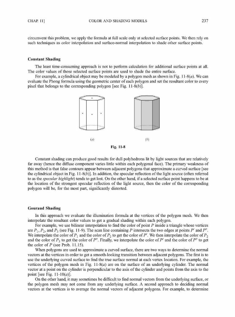
CHAP. 11] COLOR AND SHADING MODELS 237
circumvent this problem, we apply the formula at full scale only at selected surface points. We then rely onsuch techniques as color interpolation and surface-normal interpolation to shade other surface points.
Constant Shading
The least time-consuming approach is not to perform calculation for additional surface points at all.The color values of those selected surface points are used to shade the entire surface.
For example, a cylindrical object may be modeled by a polygon mesh as shown in Fig. 1 l-8(a). We canevaluate the Phong formula using the geometric center of each polygon and set the resultant color to everypixel that belongs to the corresponding polygon [see Fig. 11-8(6)].
()Fig. 11-8
Constant shading can produce good results for dull polyhedrons lit by light sources that are relativelyfar away (hence the diffuse component varies little within each polygonal face). The primary weakness ofthis method is that false contours appear between adjacent polygons that approximate a curved surface [seethe cylindrical object in Fig. 11-8(6)]. In addition, the specular reflection of the light source (often referredto as the specular highlight) tends to get lost. On the other hand, if a selected surface point happens to be atthe location of the strongest specular reflection of the light source, then the color of the correspondingpolygon will be, for the most part, significantly distorted.
Gouraud Shading
In this approach we evaluate the illumination formula at the vertices of the polygon mesh. We theninterpolate the resultant color values to get a gradual shading within each polygon.
For example, we use bilinear interpolation to find the color of point P inside a triangle whose verticesare P l s P2, and P^ (see Fig. 11-9). The scan line containing P intersects the two edges at points P' and P".We interpolate the color of Pj and the color of P2 to get the color of P'. We then interpolate the color of P2
and the color of P} to get the color of P". Finally, we interpolate the color of P' and the color of P" to getthe color of P (see Prob. 11.15).
When polygons are used to approximate a curved surface, there are two ways to determine the normalvectors at the vertices in order to get a smooth-looking transition between adjacent polygons. The first is touse the underlying curved surface to find the true surface normal at each vertex location. For example, thevertices of the polygon mesh in Fig. ll-8(a) are on the surface of an underlying cylinder. The normalvector at a point on the cylinder is perpendicular to the axis of the cylinder and points from the axis to thepoint [see Fig. ll-10(a)].
On the other hand, it may sometimes be difficult to find normal vectors from the underlying surface, orthe polygon mesh may not come from any underlying surface. A second approach to deciding normalvectors at the vertices is to average the normal vectors of adjacent polygons. For example, to determine

238 COLOR AND SHADING MODELS [CHAP. 11
() ()
Fig. 11-9 Fig. 11-10
normal vector N at vertex P in Fig. 1 I-IO(ZJ), we use the average of the normal vectors of the polygons thatmeet at P:
N = N t + N2 + N3 + N4
where N is then normalized by dividing it by |N|.Common normal vectors at the vertices of a polygon mesh that approximates a curved surface result in
color values that are shared by adjacent polygons, eliminating abrupt changes in shading characteristicsacross polygon edges. Even when the polygon mesh is relatively coarse, Gouraud shading is very effectivein suppressing false contours. However, a much finer mesh is needed in order to show reasonably goodspecular reflection.
Phong Shading
Instead of color values, we may also interpolate normal vectors. For example, to find the normal vectorN at point P in a triangle (see Fig. 11-11), we first interpolate Nj and N2 to get N', then interpolate N2 andN3 to get N", finally interpolate N' and N" to get N.

CHAP. 11] COLOR AND SHADING MODELS 239
This technique is relatively time-consuming since the illumination model is evaluated at every point ofinterest using the interpolated normal vectors. However, it is very effective in dealing with specularhighlights.
11.4 TEXTURE
While gradual shading based on illumination is an important step towards achieving photo-realism,most real-life objects have regular or irregular surface features (e.g., wood grain). These surface details arecollectively referred to as surface texture. In this section we present three approaches to adding surfacetexture: projected texture, texture mapping, and solid texture.
Projected Texture
Imagine putting a plain object between a slide projector and the projection screen. The surfaces of theobject that face the projector will be covered by the projected image. If the image depicts wood grain thenthe affected surfaces will have the intricate wood texture superimposed onto its original shading.
In computer graphics, projecting texture onto an object is effectively the inverse of projecting an objectonto the view plane (compare Fig. 7-1 and Fig. 11-12) . We now refer to the view plane as the referenceplane, which contains a two-dimensional texture definition called the texture map. The projection line thatassociates point P with its image P' allows the shading o f f to be determined or influenced by informationin the texture map at location P'.
Object surface
Referenceplane
Fig. 11-12
The texture map is often a synthesized or scanned image, in which case it contains color attributes.There are several ways for the color attributes off" to be used to shade point P. First, we may simply assignthese attributes to P, replacing whatever color attributes P currently has. The net effect of this approach isto paint the color of the texture onto the object. Second, we may interpolate between the color C off" andthe original color C o f f using (1 — k)C + kC where 0 < k < 1.0 to come up with a new color for P. Theresult of this calculation makes the texture appear blended into the original shading. Third, we may use alogical operation involving C and C to compute a new color for P. For example, when the AND operationis used, a texture area with magenta shades will appear unaltered if the original color is white, but it willtake on red shades if the original is yellow.
Projected texture is an effective tool when target surfaces are relatively flat and facing the referenceplane. On the other hand, "hidden surfaces" are not affected, and features of the texture are distorted by thecurvature of the surface.

240 COLOR AND SHADING MODELS [CHAP. 11
Texture Mapping
Now imagine the texture map being a thin and flexible sheet made of elastic material. When we wrap itaround the surface of an object we can stretch or shrink it so as to follow the shape of the object.
This approach is referred to as texture mapping. We describe the texture map in a two-dimensionalspace called the texture space with coordinates (u, w), and we represent the surface of an object inparametric form using (6, cp). The mapping from the texture space to the object space is then defined by
9 =f(u, w) cp = g(u, w)
and the inverse mapping by
u = r(6, cp) w = s(6, cp)
Although not necessary, these mapping functions are generally assumed to be linear (so the texture mapstretches and shrinks proportionally). Thus we can write
0 =Au + B cp = Cw + D
where the constants A, B, C, and D are obtained from the relationship between known points in the twospaces (e.g., corners of the texture map and the corresponding surface points).
As mentioned early, the texture map often contains color attributes that can be used in different ways toalter the original shading. In addition, its role may be extended to provide other kind of information thataffects the outcome of the shading process. For example, a technique called bump mapping uses thequantities in the texture map to displace or perturb the normal vectors of the surface to produce anappearance of roughness (see Fig. 11-13 for a one-dimensional illustration of the effect).
Smooth-looking A bump map to Rough-lookingsurface perturb the surface
magnitude anddirection of thesurface normals
Fig. 11-13
In comparison with projected texture, the method of texture mapping can better adapt to a curvedsurface. However, complex shapes deter the derivation of mapping functions. Furthermore, both methodsare particularly weak when features of the texture on one surface should "match" those on others. Considera wood cube, for instance: the wood grain on one side should exhibit continuity and consistency with thewood grain on all adjacent sides. As we turn the wood cube into a sculpture, the complexity of this texture-matching problem simply multiplies.
Solid Texture
The weaknesses of projected texture and texture mapping largely stem from the inherent mismatchbetween a two-dimensional texture map and a three-dimensional surface. In this approach we define textureusing a three-dimensional texture space. The texture definition, referred to as solid texture, is a three-dimensional representation of the internal structure of some nonhomogeneous material such as wood,marble, etc.
When rendering an object made of a specific material, we use transformations to place the object intothe coordinate system where the texture for the material is defined. In other words, we map a surface pointP(x,y, z) to its coordinates (u, v, w) in the texture space. Information associated with this location is thenused to control the shading of P. This makes the object look as if it were carved out of a solid piece of thechosen material.

CHAP. 11] COLOR AND SHADING MODELS 241
()
Fig. 11-14
Solid texture is often defined procedurally. The following is an example that shows the development ofa model for wood grain. We begin by representing the most prominent feature of the material with a seriesof concentric cylinders in the texture space [see Fig. 1 l-14(a)]). When an object such as the parallelepipedin Fig. 11-14(6) is placed into the texture field, the object intersects the cylinders, leaving intersectioncontours on its surfaces. The contours we get by aligning the object coordinate axes with the texturecoordinate axes are shown in Fig. 1 l-14(c). We now rotate the front end of the parallelepiped slightly to theleft about the v axis, and slightly up about the u axis. The result is our first approximation to wood grain(see Fig. 11-15).
Fig. 11-15
We can see that the contours on different sides are consistent with the underlying three-dimensionalstructure, but they are just too smooth and too perfect to look real. In order to incorporate some asymmetryand irregularity we need to bring two updates to the model. The first is to add ripples or sinusoidalperturbations to the cylinders so the intersection contours will have some minor and natural-lookingoscillations. The second is to turn or twist the ripples slowly along the w axis to give the contours a skewedappearance. An implementation of the improved cylinder model is shown in the following pseudo-codeprocedure:
woodGrain(/7?, kd)
ifloat radius, angle;radius = sopt(pt[uf + pt[vf);angle = (pt[u] == 0) ? n/2 : dactwa(pt[v]/pt[u\);radius = radius + m*sin(/*angle + r*pt[w]);

242 COLOR AND SHADING MODELS [CHAP. 11
if ((int)radius %p <d)set the components of kd to produce a dark shade;
elseset the components of kd to produce a light shade;
where array parameter pt represents the coordinates of surface point P in the texture space, and arrayparameter kd is used to return the proper reflection coefficients for shading point P.
The first instruction in woodGrain is to determine the radius of the cylinder that intersects P. The nextinstruction sets the base parameter value for the sine function that delivers the ripple effects. Themagnitude of the perturbation is controlled by m, the frequency or number of ripples in a full circle iscontrolled b y / and the rate at which the ripples rotate along the w axis is controlled by r. Finally, we treatwood grain as alternating bands of dark and light cylinders of period p. Within a period the two bands areseparated by threshold d. Although only two shades are shown in the procedure, the value of kd should bemade to vary based on the relative position of P within each band to produce better results (see Fig. 11-16for a ray-traced sphere).
Fig. 11-16
Solved Problems
11.1 Assuming that the medium of interest is air (or a vacuum) express the visible band of the spectrumin terms of a frequency range.
SOLUTION
Since frequency = speed of light/wavelength, and speed of lights 3.0 x 10⁸m/s, we obtain thefrequency range (3.0 x 10⁸)/(700 x 10"9) to (3.0 x 10⁸)/(400 x 10"9)Hz or 4.3 x 10¹⁴ to 7.5 x 10¹⁴Hz.
11.2 Name the three perceptual terms for describing color and the corresponding physical properties oflight.

CHAP. 11] COLOR AND SHADING MODELS 243
SOLUTION
Brightness/luminance, hue/dominant wavelength, saturation/excitation purity.
11.3 Derive a simple formula to calculate the area bounded by the distribution function P(l) in Fig. 11-3.
SOLUTION
Let Wand Hbe the width and height of the rectangular area that corresponds to white, and D and P be thewidth and height of the rectangular area that corresponds to pure color. The area bounded by P(X) isWxH + DxP.
11.4 Name the two kinds of receptor cells in the retina and describe their basic function.
SOLUTION
They are cones for seeing colors, and rods for perceiving low intensity light.
11.5 Why did we say that red, green, and blue only roughly coincide with the wavelength values thatcause peak response from the three types of color-sensitive cones?
SOLUTION
The three colors have the following typical wavelength: red = 700 run, green = 546.1 nm, andblue = 435.8 nm. Although blue and green closely match the sensitive range of two types of cones,P : 440 —445nm and 8 : 535 —545nm, the sensitive range of the third type, p : 575 — 580nm, is actuallyyellow, not red.
11.6 Do we have to use 7 in order to convert from chromaticity coordinates (x, y) back to a specific colorin the XYZ color space?
SOLUTION
No. If we know X, we can use
X = X, Y = -X, Z = ~X~yXx x
11.7 Presume that a monitor produces what is called the standard white D65 with xw = 0.313,yw = 0.329, and Yw = 1.0 when R = G = B = 1, and the chromaticity coordinates of its phosphorsare as given in Sec. 11.1. Find the color transformation matrix M for the monitor.
SOLUTION
Since Yw = 1.0, we have
Xw = xw/yw = 0.951 and Zw = (1 - xw - yw)/yw = 1.088
Use these and the chromaticity coordinates of the phosphors
/0 .95 l \ /0.62 0.29 0 . 1 5 \ / C r \1.0 = 0.34 0.59 0.06 \\ Cg\
\ 1.088/ \0.04 0.12 0.79/ \Cb)
Solve and get Cr = 0.705, Cg = 1.170, and Cb = 1.164. Now
( xrCr xgCg xbCb\ /0.437 0.339 0.175 \yrCr ygCg ybCb = 0.240 0.690 0.070zrCr zgCg zbCb) \0.028 0.140 0.920/

244 COLOR AND SHADING MODELS [CHAP. 11
11.8 Verify the fact that the 7in the CIE XYZ color model is the same as the 7in the NTSC YIQ colormodel.
SOLUTION
Find the transformation to XYZ for the standard NTSC RGB display (see Sec. 11.1). Sincexw = 0.31,.yw = 0.316, and Yw = 1.0, we have
Xw=xw/yw = 0.981 and Zw = (1 -xw -yw)/yw = 1.184
Use these and the chromaticity coordinates of the standard NTSC phosphors
/ 0 . 9 8 l \ /0.67 0.21 0 . 1 4 \ / C r \1.0 = 0.33 0.71 0.08 I I Cg
\ 1.184/ \0 .0 0.08 0.78/ \Cb)
Solve and get Cr = 0.906, Cg = 0.826, and Cb = 1.432. Now
/xrCr xgCg xbCb\ /0.607 0.173 0.200 \M = yrCr ygCg ybCb = 0.299 0.587 0.114
zrCr zgCg zbCb J 0.0 0.066 1.117
Since the middle row of Mis the same as the top row of the matrix for mapping from RGB to YIQ, we can seethat the Fin CIE XYZ is the same as the Fin NTSC YIQ.
11.9 What is the difference between a local illumination model and a global illumination model?
SOLUTION
A local illumination model focuses on the direct impact of the light coming from the light source. On theother hand, a global illumination model attempts to include such secondary effects as light going throughtransparent/translucent material and light bouncing from one object surface to another.
11.10 RefertoFig. 11-6 in Sec. 11.2. Find a formula to compute R, the reflection of vector L with respectto normal vector N.
SOLUTION
Introducing auxiliary vectors e and m (see Fig. 11-17), we can write
R = m - e
Fig. 11-17
Since L = e + m, we have e = L — m and
R = m — (L — m) = 2m — L
Note that m is simply the perpendicular projection of L onto N (see Prob. A2.16) and N is a unit vector, hence
m = (L • N)N
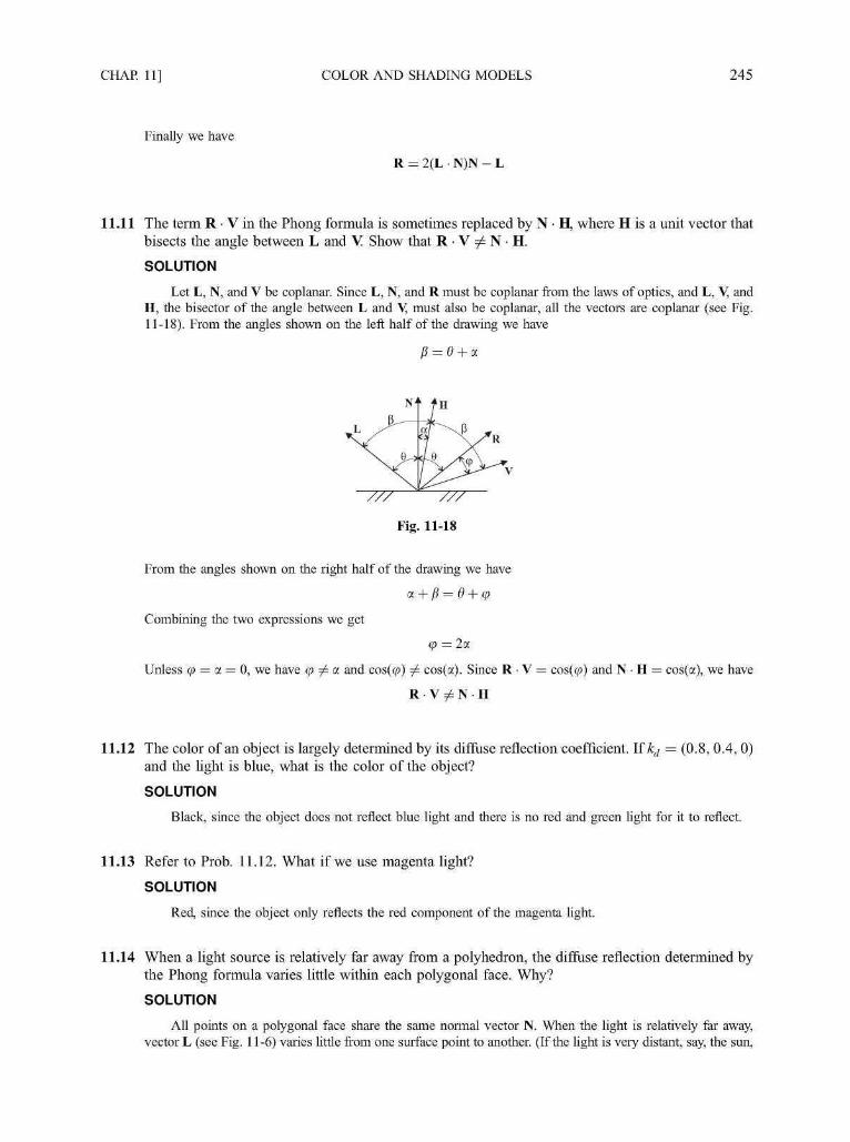
CHAP. 11] COLOR AND SHADING MODELS 245
Finally we have
R = 2(L • N)N - L
11.11 The term R • V in the Phong formula is sometimes replaced by N • H, where H is a unit vector thatbisects the angle between L and V Show that R V ^ N H.
SOLUTION
Let L, N, and V be coplanar. Since L, N, and R must be coplanar from the laws of optics, and L, V, andH, the bisector of the angle between L and V, must also be coplanar, all the vectors are coplanar (see Fig.11-18). From the angles shown on the left half of the drawing we have
From the angles shown on the right half of the drawing we have
Combining the two expressions we get
(p = 2a
Unless cp = a = 0, we have cp / a and cos(cp) / cos(a). Since R • V = cos(cp) and N • H = cos(a), we have
R V / N H
11.12 The color of an object is largely determined by its diffuse reflection coefficient. If kd = (0.8, 0.4, 0)and the light is blue, what is the color of the object?
SOLUTION
Black, since the object does not reflect blue light and there is no red and green light for it to reflect.
11.13 Refer to Prob. 11.12. What if we use magenta light?
SOLUTION
Red, since the object only reflects the red component of the magenta light.
11.14 When a light source is relatively far away from a polyhedron, the diffuse reflection determined bythe Phong formula varies little within each polygonal face. Why?
SOLUTION
All points on a polygonal face share the same normal vector N. When the light is relatively far away,vector L (see Fig. 11-6) varies little from one surface point to another. (If the light is very distant, say, the sun,

246 COLOR AND SHADING MODELS [CHAP. 11
then L becomes a constant vector.) Hence L • N, the term that determines the diffuse component in the Phongformula varies little within each polygonal face.
11.15 Refer to Fig. 11-9, and show exactly how to compute the color of P using bilinear interpolation.
SOLUTION
Let the coordinates of P,PUP2,P3,P', and P" be (x,y), (xj, j ^ ) , (x2,y2), (x3,y3), (x',yr), and (x",y"),respectively. Also let the color/intensity values at those points be I, I\,I2, !•$, I', and I", and respectively. Wehave
yi ~y\ yi~ y\
and
x" — x' x" — x'
For RGB colors, these formulas are applied to the values of each color component.
11.16 Suppose point Px with intensity Ix is on scan line yl and point P2 with intensity I2 is on scan line y2.Find an incremental formula to compute intensity values / ' for all the scan lines between Pl and P2
using linear interpolation in the y direction.
SOLUTION
Let Px be the starting point, then the intensity change from one scan line to the next is
Hence
7j = /j and I- = //_] + A7 where i = 2 , . . . , y2 — y
11.17 RefertoProb. 11.16. If point Px on line 5 has an RGB color (1, 0.5, 0) and p o i n t y online 15 hasan RGB color (0.2, 0.5, 0.6), what is the color for line 8?
SOLUTION
Since
AR = (0.2 - 1)/(15 - 5) = -0.08
AG = (0.5-0.5)/(15-5) = 0
A5 = (0.6 - 0)/(15 - 5) = 0.06
we have (1 + 3 x (-0.08), 0.5 + 3 x 0, 0 + 3 x 0.06) = (0.76, 0.5, 0.18) as the color for line 8.
11.18 Refer to Fig. 1 l-10(a). The vertices are shared by the rectangles that approximate the cylinder andthe two polygons that represent the top and bottom of the object. Does each vertex have a uniquenormal vector?
SOLUTION
No. When a vertex is used to describe the top or bottom face, its normal vector is the normal of thecorresponding face. When it is used to define the rectangle mesh, its normal vector is perpendicular to thecylinder as shown in the figure.

CHAP. 11] COLOR AND SHADING MODELS 247
11.19 Refer to Fig. 11-11 and see Prob. 11.15. If the two normal vectors at P' and P" are
and point P is half way between P' and P", what is N?
SOLUTION
Since P is in the middle of P' and P", the last formula in Prob. 11.15 for linear interpolation in the xdirection becomes
Use it to interpolate each component of N' and N":
4 4
The magnitude of this vector is
V2V2 ) \ 4 ) \4
Use it to normalize the interpolated vector and get
11.20 Show that when averaging or interpolating normal vectors we will get incorrect result if the vectorsare not unit vectors (or vectors of equal magnitude).
SOLUTION
Consider Nj = I and N2 = J: the average of the two is I + J, which bisects the 90° angle between I andJ. We can normalize it to get
Now if we set N2 = 2J, which has the same direction as J, the average of Nj and N2 becomes I + 2J.Clearly, the direction of this vector differs from that of N.
As for interpolation we can see from Prob. 11.19 that to compute a vector for the point halfwaybetween two given points we apply
/ ' I"/ = 2 + Y
to each vector component. For Nj = I and N2 = J, this produces
which is, after normalization, the same as N above. But, if we use N2 = 2J, the result of interpolationbecomes
which has the direction of I + 23, not the direction of N.
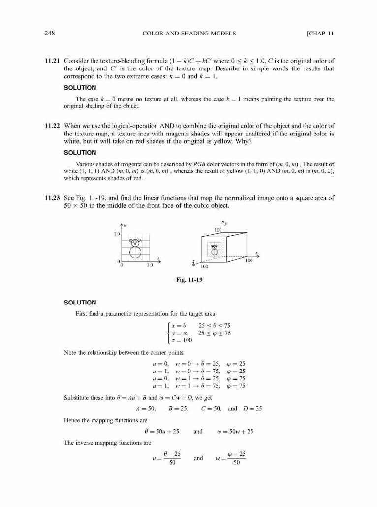
248 COLOR AND SHADING MODELS [CHAP. 11
11.21 Consider the texture-blending formula (1 — k)C + kC where 0 < k < 1.0, C is the original color ofthe object, and C is the color of the texture map. Describe in simple words the results thatcorrespond to the two extreme cases: k = 0 and k = 1.
SOLUTION
The case k = 0 means no texture at all, whereas the case k = 1 means painting the texture over theoriginal shading of the object.
11.22 When we use the logical-operation AND to combine the original color of the object and the color ofthe texture map, a texture area with magenta shades will appear unaltered if the original color iswhite, but it will take on red shades if the original is yellow. Why?
SOLUTION
Various shades of magenta can be described by RGB color vectors in the form of (m, 0, m). The result ofwhite (1, 1, 1) AND (m, 0, m) is (m, 0, m) , whereas the result of yellow (1, 1, 0) AND (m, 0, m) is (m, 0, 0),which represents shades of red.
11.23 See Fig. 11-19, and find the linear functions that map the normalized image onto a square area of50 x 50 in the middle of the front face of the cubic object.
1.0
1.0 100
Fig. 11-19
SOLUTION
First find a parametric representation for the target area
I x = 6 25 < 6 < 75y = cp 25 < cp < 75z = 100
Note the relationship between the corner points
u = 0, w = 0 - • 6 = 25, <p = 25u=\, w = 0^0 = 75, q> = 25u = 0, w = 1 - • 6 = 25, cp = 75
u=\, w= 1 ^ 0 = 75, q> = 75
Substitute these into 6 =Au + B and q> = Cw + D, we get
A = 50, B = 25, C = 50, and D = 25
Hence the mapping functions are
9 = 50M + 25 and q> = 50w + 25
The inverse mapping functions are
0 - 2 550
and w =op-25
50

CHAP. 11] COLOR AND SHADING MODELS 249
11.24 See Fig. 11-20. Find the linear functions that map the normalized grid pattern onto the bottomportion (n/4 < cp < n/2) of the spherical surface in the first octant.
1.0
u
e=rc/2
1.0
Fig. 11-20
SOLUTION
The parametric representation for the target area is
x = R sin(0) sin(cp) 0 < 6 < n/2
y = Rcos(cp) n/4 < cp < n/2
z = R cos(8) sin cp)
Note the relationship between the corner points
u = 0, w = 0 - • 6 = 0, cp = n/2
u=\, w = 0 -+ 6 = n/2, cp = n/2u = 0, w = 1 - • 0 = 0, cp = n/4u=\, w=l ^ 6 = n/2, cp = n/4
Substitute these into 6 =Au + B and cp = Cw + D, we get
A = n/2, B = 0, C = -n/4, and D = n/2
Hence the mapping functions are
a n dn n
The inverse mapping functions are
n/2and w =
n/2-cp
n/4
Supplementary Problems
11.25 Given the distribution function P{X) in Fig. 11-3, derive a formula to calculate saturation.
11.26 Why everything looks gray or black in a dark room where we can barely see?
11.27 Can we use Z to convert from chromaticity coordinates (x, y) back to a specific color in the XYZ color space?
11.28 What's the difference between the 7 in CMYand the 7 in YIQl

250 COLOR AND SHADING MODELS [CHAP. 11
11.29 Consider a sphere of radius R, centered at (xc,yc, zc). What is the normal vector N at point (x,y, z) on thesphere?
11.30 Find the linear functions that map a 1.0 x 2.0 texture map onto a cylindrical surface in the first octant (see Fig.11-21) . The short sides of the texture map should align with the straight edges of the surface.
2.0
0 vv0 1.0
Fig. 11-21

Ray Tracing
Ray tracing is a global illumination model that accounts for the transport of light energy beyond thedirect/local contribution from the light sources. Its operation is largely based on the principles ofgeometric optics. By tracing the path of light rays it is able to integrate the tasks of shading, shadowgeneration, hidden surface removal, projection, and scan conversion into one single computational process.
In this chapter we first introduce the fundamental concepts that underlie this elegant approach (Sect.12.1). We then discuss the basic ray-tracing algorithm (Sect. 12.2), the parametric vector representation ofa ray (Sect. 12.3), and the mathematics of ray-surface intersection (Sect. 12.4). We also present techniquesfor improving execution efficiency (Sect. 12.5), anti-aliasing (Sect. 12.6), and achieving some desiredvisual effects (Sect. 12.7).
12.1 THE PINHOLE CAMERA
In theory one can take perfect pictures using a pinhole camera—a closed box with a tiny hole in thecenter of the front panel (see Fig. 12-1). The hole is so small that only one light ray passing through it canstrike a particular point on the negative, which is mounted on the inside of the back panel. As light raysfrom across the scene expose the negative by hitting their respective target precisely, a sharp imagedepicting the scene emerges.
NegativeLight rays
Object
Image of object
Fig. 12-1 A pinhole camera.
Now we place a screen between the pinhole and the object (see Fig. 12-2), causing the light rays tointersect the screen. If we can record each light ray as it intersects the screen, we will have a perfect pictureof the object on the screen. Or, to put this in terms of image synthesis, if the screen resolution is arbitrarilyhigh and we can set the pixel at each intersection point to match the color of the corresponding light ray,then the image will be indistinguishable from the real scene when viewed from the position of the pinhole.
251

252 RAY TRACING [CHAP. 12
Pinhole
Object
12.2 A RECURSIVE RAY-TRACER
In order to construct an image based on the pinhole-camera model we need to determine the light raysthat are responsible for the pixels. We do so by following their path in the opposite direction, i.e., from theviewpoint through the center of each pixel into the scene (see Fig. 12-3). These are called the primary rays.If a primary ray does not intersect any object in the scene, then the corresponding pixel is simply set tosome background color.
Illumination/shadow ray
Primary ray
(Specularly) transmitted ray
(Specularly) reflected ray
Screen
Fig. 12-3 Ray tracing.
On the other hand, if a primary ray intersects an object, then the color of the corresponding pixel isdetermined by the surface shading of the object at the intersection point. Several secondary rays are used tocompute the three components of this surface shading. The first component is called the local contribution,which refers to the direct contribution from the light source(s). We send a shadow ray or illumination rayfrom the surface point to a light source. If the ray is blocked before reaching the light source, the surfacepoint is in shadow (relative to this light source). The second component is called the reflected contribution,which refers to the reflection of light energy coming from another object surface (inter-object reflection).This is determined by a (specularly) reflected ray, a ray that represents the reflection of the primary ray withrespect to normal vector N. The third component is called the transmitted contribution, which refers to thetransmission of light energy coming from behind the surface (transparent object). This is determined by a(specularly) transmitted ray, a ray that represents the refraction of the primary ray with respect to N.
Note that, were the object surface a perfect mirror, the specularly reflected ray would represent the soledirection of light reflected towards the viewpoint. Also, if the object were made of perfectly homogeneousmaterial, the specularly transmitted ray would represent the sole direction of light refracted towards theviewpoint.
SnelPs law determines the relationship between angles a and /? (see Fig. 12-3):
sin(a)
sin(j3)

CHAP. 12] RAY TRACING 253
where r\x is the refraction index of the medium in which a is defined and r\2 *s t n e refraction index of the
medium in which fi is defined. Although the refraction index of a medium is a function of temperature andwavelength, we can often use such values as 1.0 for air, 1.3 for water, and 1.5 for glass.
Employing the Phong formula to describe the local contribution, we express the intensity / of the lightenergy represented by the primary ray as
n
where the ambient term now represents the portion of inter-object reflection that is not accounted for by theterm kvlv, which describes the reflected contribution as the product of the reflection coefficient kv and theintensity /r of the reflected ray; the last term ktlt describes the transmitted contribution as the product of thetransmission coefficient kt and the intensity / t of the transmitted ray. Both kv and kt are in the range of[0,1.0]. /r and / t are obtained recursively by treating the reflected ray and the transmitted ray as a primaryray. In other words, we calculate /r by evaluating the above equation at the closest surface the reflected rayintersects, in exactly the same way as the primary ray is handled. A pseudo-code description of the basicray-tracing algorithm is as follows:
rayTrace{ray, depth, color}
determine closest intersection of ray with an object;if (no intersection) color = background;else {
color = local contribution;if (depth > 1) {
calculate reflected ray;rayTrace(reflected ray, depth-1, ref_color);calculate transmitted ray;rayTrace(transmitted ray, depth-1, trans_color);color = color + kr • ref_color + kt • trans_color;
}
This procedure takes a ray and a depth value that is greater than or equal to 1 as input, and returns acolor as output (typically an RGB vector, the above formula is used to compute the intensity of eachindividual color component). It treats the given ray as a primary ray and (when depth > 1) makes recursivecalls to obtain the color (ref_color) of the reflected ray and the color (trans_color) of the transmitted ray.
Figures 12-4, 12-5, and 12-6 show the results of ray-tracing a scene consisting of three opaque spheres.The smaller one in the front is dull whereas the two larger ones in the back are shiny. The first image(depth = 1) is obtained using only the primary ray and shadow ray. The second image (depth = 2) depictsthe effect of adding reflected contribution (one level beyond the primary ray). The third image (depth = 3)shows the cumulative effect of two levels of reflected contribution. In Fig. 12-7 (also depth = 3), the dullsphere is replaced by a shiny glass sphere (a check-board floor is also added) to illustrate the combinedeffect of all three shading components.
12.3 PARAMETRIC VECTOR REPRESENTATION OF A RAY
A ray is not a vector although it may look like one (see Fig. 12-3). The difference between the two isthat, while a vector is defined by its direction and magnitude, a ray is determined by its direction andstarting point.

254 RAY TRACING [CHAP. 12
Fig. 12-4
Fig. 12-5
We may represent a ray in terms of two vectors: s to specify its starting point, and d to describe itsdirection (see Fig. 12-8). These two vectors are used to provide a parametric vector representation for theray:
r(0 = s + td (0 < t)
where r(Y) denotes a family of vectors. When the tails of these vectors are placed at the origin, their headsmake up the ray.

CHAP. 12] RAY TRACING 255
Fig. 12-6
Fig. 12-7
Fig. 12-8 Vector representation of a ray.

256 RAY TRACING [CHAP. 12
12.4 RAY-SURFACE INTERSECTION
A critical step in the implementation of ray tracing is to determine whether a ray intersects an object.This operation is performed for each primary ray (or a ray that is treated as a primary ray in a recursive call)and shadow ray. If a primary ray does intersect an object, we need to know exactly where the intersectionpoint is.
Coordinate System Plane
Intersection of a ray with the xy plane can be determined by solving the following for t (see Fig. 12-9):
s + td = xil+yiJ
With s = xsl + ysJ + zsK and d = xdl + ydJ + zdK, we have
When zd = 0, the ray is parallel to the plane (no intersection). When zs = 0, the ray originates from theplane (no intersection). Otherwise, we calculate t using the third equation
If t < 0, the negative extension of the ray intersects the plane. On the other hand, if t > 0, the ray itselfintersects the plane and the coordinates xi and yt of the intersection point can be calculated from the firsttwo equations.
Intersection point
Fig. 12-9
Intersection with other coordinate system planes and planes that are parallel to a coordinate systemplane can be handled similarly (see Probs. 12.9 and 12.30). We can also test to see if the intersection pointis within a region (see Probs. 12.10, 12.11, and 12.12).
Arbitrary Plane
Let n = xnl + yBJ + znK be the normal vector to an arbitrary plane and Po (x0,y0, z0) a point on theplane (see Fig. 12-10). The vector equation or point-normal equation of the plane is then (from App. 2,Sect. A2.3)
xn(x - x0) +yB(y - y0) + zB(z - z0) = 0
To determine if a ray s + t& (s = xsl + ys J + zsK and d = xdl + yd J + zdK) intersects the plane, wesubstitute xs + txd, ys + tyd, and zs + ted for x, y, and z, respectively:
xn(xs + txd - x0) +yB(ys + tyd- y0) + zB(zs + tzd - z0) = 0

CHAP. 12] RAY TRACING 257
Fig. 12-10
Solving for t we get
t = - •
zn(zs ~ zo)
Introducing p = (x0 — xs)I + (y0 — ys)J + (z0 — zs)K, we can express t in vector form:
n d
When n • d = 0, the ray is parallel to the plane (no intersection). Otherwise, if t < 0, the negativeextension of the ray intersects the plane; if t = 0, the ray originates from the plane. The ray intersects theplane only when t > 0.
Sometimes we want to further distinguish the two cases of intersection; intersecting the outside (front)of a plane versus intersecting its inside (back). The former occurs when n • d < 0 whereas the latter occurswhen n • d > 0.
Sphere
Consider a sphere of radius R centered at (xc,yc, zc) and an arbitrary point (x,y, z) on the sphere (seeFig. 12-11). Define vectors c = xcl + yc J + zcK and p = xl + yi + zK. The vector equation for the sphereis
| p - c | = 2 ?
To determine if a ray r(t) = s + t& intersects the sphere, we substitute s + t& and p and square bothsides:
|s + f d - c | 2 = i ? 2
Since v • v = |v| for any vector v (see Prob. A2.3), we have
s - c + fd|2 = (s - c + td) • (s - c + td)
= (s - c) • (s - c + t&) + t& • (s - c + t&) (Prob. Al .20)
= (s - c) • (s - c) + 2(s - c) td + td td (Prob. A1.19)
= |s - c|2 + 2t(s - c) • d + ?2|d|2 = R2
This is in the form of a quadratic equation in t:
At1 +2Bt + C = 0

258 RAY TRACING [CHAP. 12
Fig. 12-11
where A = |d| , B = (s — c) • d, C = |s — c| — R2, and the solution is
t = •-B ± -JB1 - AC
with
no intersectionray (or its negative extension) touching spheretwo (possible) intersection points
When B2 — AC > 0 we get two t values: ^ and t2. If both are less than 0, the negative extension of the rayintersects the sphere (no intersection by the ray). If one of them is 0, the ray starts from a point on thesphere and intersects the sphere only if the other value is positive. If the two values differ in signs, the rayoriginates from inside the sphere and intersects the sphere once. If both are positive, the ray intersects thesphere twice (first enters and then exits), and the smaller t value corresponds to the intersection point that iscloser to the starting point of the ray.
General Implicit Surface
Generally, to determine if a ray s + td (s = xsl + ysJ + zsK and d = xdl + ydJ + zdK) intersects asurface that is represented by an implicit equation F(x, y, z) = 0, we solve
F(xs + txd,ys + tyd, zs + ted) = 0
for t (see Probs. 12.16, 12.17, and 12.31).
12.5 EXECUTION EFFICIENCY
Ray-tracing is time-consuming largely due to the recursive nature of the algorithm and the demandingtask of computing ray-surface intersections. Several techniques are designed to improve executionefficiency by means of object/scene-dependent deployment of system resources.
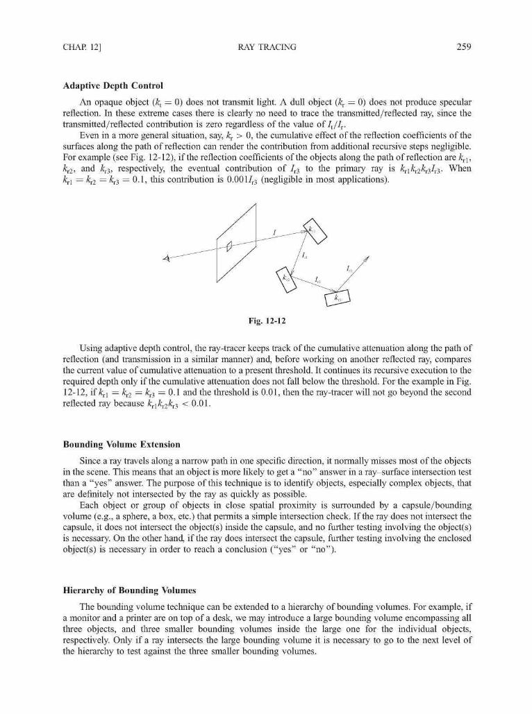
CHAP. 12] RAY TRACING 259
Adaptive Depth Control
An opaque object (kt = 0) does not transmit light. A dull object (kv = 0) does not produce specularreflection. In these extreme cases there is clearly no need to trace the transmitted/reflected ray, since thetransmitted/reflected contribution is zero regardless of the value of/t//r.
Even in a more general situation, say, kv > 0, the cumulative effect of the reflection coefficients of thesurfaces along the path of reflection can render the contribution from additional recursive steps negligible.For example (see Fig. 12-12), if the reflection coefficients of the objects along the path of reflection are kvl,kl2, and £r3, respectively, the eventual contribution of /r3 to the primary ray is k^k^k^I^. Whenhrl = kl2 = £r3 = 0.1, this contribution is 0.001/r3 (negligible in most applications).
Fig. 12-12
Using adaptive depth control, the ray-tracer keeps track of the cumulative attenuation along the path ofreflection (and transmission in a similar manner) and, before working on another reflected ray, comparesthe current value of cumulative attenuation to a present threshold. It continues its recursive execution to therequired depth only if the cumulative attenuation does not fall below the threshold. For the example in Fig.12-12, if kvl = kv2 = kv3 = 0.1 and the threshold is 0.01, then the ray-tracer will not go beyond the secondreflected ray because kvlkv2kv3 < 0.01.
Bounding Volume Extension
Since a ray travels along a narrow path in one specific direction, it normally misses most of the objectsin the scene. This means that an object is more likely to get a "no" answer in a ray-surface intersection testthan a "yes" answer. The purpose of this technique is to identify objects, especially complex objects, thatare definitely not intersected by the ray as quickly as possible.
Each object or group of objects in close spatial proximity is surrounded by a capsule/boundingvolume (e.g., a sphere, a box, etc.) that permits a simple intersection check. If the ray does not intersect thecapsule, it does not intersect the object(s) inside the capsule, and no further testing involving the object(s)is necessary. On the other hand, if the ray does intersect the capsule, further testing involving the enclosedobject(s) is necessary in order to reach a conclusion ("yes" or "no").
Hierarchy of Bounding Volumes
The bounding volume technique can be extended to a hierarchy of bounding volumes. For example, ifa monitor and a printer are on top of a desk, we may introduce a large bounding volume encompassing allthree objects, and three smaller bounding volumes inside the large one for the individual objects,respectively. Only if a ray intersects the large bounding volume it is necessary to go to the next level ofthe hierarchy to test against the three smaller bounding volumes.
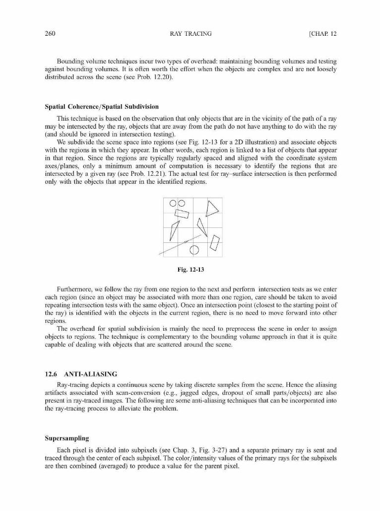
260 RAY TRACING [CHAP. 12
Bounding volume techniques incur two types of overhead: maintaining bounding volumes and testingagainst bounding volumes. It is often worth the effort when the objects are complex and are not looselydistributed across the scene (see Prob. 12.20).
Spatial Coherence/Spatial Subdivision
This technique is based on the observation that only objects that are in the vicinity of the path of a raymay be intersected by the ray, objects that are away from the path do not have anything to do with the ray(and should be ignored in intersection testing).
We subdivide the scene space into regions (see Fig. 12-13 for a 2D illustration) and associate objectswith the regions in which they appear. In other words, each region is linked to a list of objects that appearin that region. Since the regions are typically regularly spaced and aligned with the coordinate systemaxes/planes, only a minimum amount of computation is necessary to identify the regions that areintersected by a given ray (see Prob. 12.21). The actual test for ray-surface intersection is then performedonly with the objects that appear in the identified regions.
oo
OFig. 12-13
Furthermore, we follow the ray from one region to the next and perform intersection tests as we entereach region (since an object may be associated with more than one region, care should be taken to avoidrepeating intersection tests with the same object). Once an intersection point (closest to the starting point ofthe ray) is identified with the objects in the current region, there is no need to move forward into otherregions.
The overhead for spatial subdivision is mainly the need to preprocess the scene in order to assignobjects to regions. The technique is complementary to the bounding volume approach in that it is quitecapable of dealing with objects that are scattered around the scene.
12.6 ANTI-ALIASING
Ray-tracing depicts a continuous scene by taking discrete samples from the scene. Hence the aliasingartifacts associated with scan-conversion (e.g., jagged edges, dropout of small parts/objects) are alsopresent in ray-traced images. The following are some anti-aliasing techniques that can be incorporated intothe ray-tracing process to alleviate the problem.
Supersampling
Each pixel is divided into subpixels (see Chap. 3, Fig. 3-27) and a separate primary ray is sent andtraced through the center of each subpixel. The color/intensity values of the primary rays for the subpixelsare then combined (averaged) to produce a value for the parent pixel.

CHAP. 12] RAY TRACING 261
Adaptive Supersampling
Supersampling often drastically increases the computational burden of ray tracing. In this approach wesend one ray through the center of a pixel and four additional rays through its corners. If the five rays returnsimilar colors the pixel will not be subdivided (it probably corresponds to a smoothly shaded area in thescene). Only if the returned colors are sufficiently different do we subdivide the pixel (it probably coversboth sides of an edge) into 2 x 2 subpixels. Each subpixel is then handled in the same way, and the processterminates when a preset level of subdivision is reached.
Stochastic Supersampling
The effect of supersampling can often be enhanced with stochastic or distributed ray-tracing. In thisapproach we deviate from using the fixed (sub)pixel grid by scattering the rays evenly across the pixel areain a random fashion. A typical way to achieve this is to displace each ray from its normal position in thegrid (see Prob. 12.24).
12.7 ADDITIONAL VISUAL EFFECTS
Various techniques have been developed to achieve certain desirable visual effects. Some methodsbelow are applications of distributed ray-tracing, which means that we scatter rays around with respect to acertain parameter in the ray-tracing process (recall that in stochastic supersampling we displace rays fromtheir normal position in the pixel grid).
Environment Mapping
A shiny (mirror-like) object reflects the surrounding environment. Instead of ray-tracing the three-dimensional scene to obtain the global reflection, we may map a picture of the environment onto the object(see Fig. 12-14). The object is typically placed in the middle of an enclosure such as a cube, cylinder, orsphere, with the environment map attached to the inside of the enclosing surface (facing the object). Thecolor of a pixel is then a function (e.g., average by supersampling) of the area in the environment map thatcorresponds to the pixel.
Clearly this is only an approximation to ray-tracing the three-dimensional scene. The quality of themapped reflection is dependent on the size (relative to the enclosure) and shape of the object. However,
A picture of thesurroundings(environment map)
Mirror-likesurface
Fig. 12-14

262 RAY TRACING [CHAP. 12
environment mapping is often faster, and it is particularly useful in creating the illusion of a computer-generated shiny object amidst a real-world scene (which of course cannot be ray-traced).
Soft Shadow
Ray-traced images of scene involving fixed point-lights are characterized by the harsh edges of theshadow areas. However real lights are not mathematical points and they cast soft shadows, which consist ofan umbra area surrounded by & penumbra area (see Fig. 12- 15).
Penumbra
Fig. 12-15
In order to produce soft shadows we model a light source by a region, called an area light. The area issubdivided into subareas or zones. Shadow rays are then distributed to these zones via random selection(with equal probability for each zone or weights that favor zones that correspond to higher intensityvalues).
Blurry Reflection
To get a blurry reflection of the surroundings on a glossy (not mirror-like) object, we distribute thereflected rays. This can be done by displacing a reflected ray from the position of its mirror reflection by asmall angle. The distribution of the angle is subject to the same bell-shaped reflectance function thatgoverns specular highlights (see Fig. 11-6).
Translucency
The difference between transparency (specular transmission) and translucency is somewhat analogousto the difference between specular reflection and blurry reflection. To achieve the effect of light goingthrough translucent material, we distribute the transmitted rays by displacing each from the position ofspecular transmission by a small angle. The distribution of the angle is subject to a transmittance functionsimilar to the aforementioned reflectance function. Furthermore, we may attenuate the transmitted intensityto account for the loss of energy.
Motion Blur
A fast-moving object tends to look blurry in a photograph (especially if the photo was taken with a lowshutter speed). To mimic this phenomenon we distribute rays over time. In other words, we predetermine

CHAP. 12] RAY TRACING 263
the path or a series of positions of a moving object based on the characteristics of the movement. We thendisplace the object along its path or between positions as each ray is traced.
Solved Problems
12.1 Describe how hidden surface removal and projection are integrated into the ray-fracing process.
SOLUTION
Each primary ray plays the role of a projector that maps a surface point P to its image P in the viewplane. If all primary rays emanate from a view point C we have the effect of perspective projection. If allprimary rays are parallel to each other we have the effect of parallel projection. Furthermore, if a primary rayintersects several object surfaces, only the surface that is the closest to the view plane is chosen to determinethe color of the corresponding pixel; all others are effectively treated as hidden surfaces and removed (notdisplayed).
12.2 Name the three components of surface shading and the secondary ray for computing each.
SOLUTION
Local contribution (shadow ray), reflected contribution (specularly reflected ray), and transmittedcontribution (specularly transmitted ray).
12.3 The refraction index of a medium is the ratio of the speed of light in vacuum to the speed of light inthat medium. Rewrite SnelPs law in terms of the speed of light in the two participating media.
SOLUTION
Let c be the speed of light in vacuum, cx be the speed of light in the medium whose refraction index is r\x,and c2 be the speed of light in the medium whose refraction index is r\2. We have r\x = c/cx and r\2 = c/c2.Hence Snell's law can be written as
sin(a) r\2 c/c2 cx
sin(jS) rjx c/cx c2
12.4 What is the difference between a vector and a ray?
SOLUTION
A vector is defined by its direction and magnitude, whereas a ray is determined by its direction andstarting point.
12.5 A ray is represented by r(t) = s + td where s = 21 + J — 3K and d = I + 2K. Find the coordinatesof the points on the ray that correspond to t = 0, 1, 2.5, and 3, respectively.
SOLUTION
2I + J - 3 K ^ (2, 1,-3)
l)I + J+( -3+2)K = 3I + J - K - > ( 3 , 1,-1)(2.5) = (2 + 2.5)I + J + (-3 + 5)K = 4.5I+J + 2 K ^ (4.5, 1,2)r(3) = (2 + 3)1 + J + (-3 + 6)K = 51 + J + 3K -+ (5, 1, 3)

264 RAY TRACING [CHAP. 12
12.6 Let the viewpoint be at (a, b, c) and the center of a pixel at (x, y, z). Find vectors s and d to representthe corresponding primary ray.
SOLUTION
S = aI + bJ + cK
d = (x - a)I + 0 - b)3 + (z - c)K
12.7 Lines in two-dimensional space can be represented by either the algebraic equation y = mx + b orthe parametric vector equation L(Y) = s + td, where —oo < t < +oo. For s = I + J and d = I — J,find the equivalent algebraic representation.
SOLUTION 1
Since L(f) = s + td = (1 + t)I + (1 - t)3, we have
x = 1 + t and y = 1 - t
Hence x + y = 2, or y = —x + 2.
SOLUTION 2
Find two points on the line
L(0) = s = I + J ^ (1, 1)
L(l) = s + d = 21 -• (2, 0)
We have (y - l)/(x - 1) = (0 - l)/(2 - 1), i.e., y = -x + 2.
12.8 Refer to Fig. 12-16(a), where d represents the direction of the primary ray, t the direction of thetransmitted ray, and n the normal vector at the intersection point. Express t in terms of d, n, and thetwo angles a and ji.
/77 V 77/ 77/
cos()αn
-cos()βn
f.-n
()
Fig. 12-16
SOLUTION
Let d, t, n be unit vectors [see Fig. 12-I6(b)]. We have
m = d + cos(a)n
|m| = sin(a)

CHAP. 12] RAY TRACING 265
and
t = sin(/?)um - cos(/?)n
= — r r ( d + cos(a)n) — cos(/?)nsin(a)
12.9 Determine if a ray intersects a plane that is parallel to the xy plane.
SOLUTION
The equation for such a plane is z = c where c is a constant. If a ray does intersect the plane, theintersection point is at (xt,yt, c). In order to find x, and yt we solve the following for t:
S + t d = x,I + j ; ; J + cK
With s = xsl +ysJ + zsK and d = xdl +yAJ + zdK, we have
|
xs + fxd = x,y, + tyA=yt
zs + tzA = c
When zd = 0, the ray is parallel to the plane (no intersection). When zs = c, the ray originates from the plane(no intersection). Otherwise, we calculate t using the third equation
If t < 0, the negative extension of the ray intersects the plane. On the other hand, if t > 0, the ray itselfintersects the plane and the coordinates x, and yi of the intersection point can be calculated from the first twoequations.
12.10 Determine if a ray intersects a rectangular region defined by xmin, xmax, ymin a n d y , ^ in the xy plane.
SOLUTION
First determine if the ray intersects the xy plane (see Sect. 12.4 under "Coordinate System Plane"). If not,the ray does not intersect the region. Otherwise, find the coordinates x, and yt of the intersection point. IfXmin — xi — xmax a n d JVin — J — JVax ^e raY intersects the region; otherwise it does not.
12.11 Determine if a ray intersects a triangular (or convex polygonal) region in the xy plane.
SOLUTION
First determine if the ray intersects the xy plane (see Sect. 12.4 under "Coordinate System Plane"). If not,the ray does not intersect any region in the plane. Otherwise, find the coordinates x, and j ; , of the intersectionpoint. The point is inside a triangular or convex polygonal region if it is on/inside all bounding edges of theregion.
Now focus on just the xy plane (ignore z). To test if the intersection point (xhy,) is inside or outside anedge in the plane, we choose a point on the edge (e.g., one of its endpoints) and define an outward normalvector n that points to the outside of the edge (see Fig. 12-17). We also use the chosen point to define vector v,and the intersection point to define vector v,. We have
(xj,yj) is outside the edge (8 < 90°)(x,, yt) is on the edge (6 = 90°)(x,-,_v;) is inside the edge (8 > 90°)
12.12 A unit square is placed in the xy plane with one corner at the origin and the diagonal corner on thepositivey axis [see Fig. 12-18(a)]. Determine if aray emanating from (0,1,2) going in the directionof the negative z axis intersects the square.
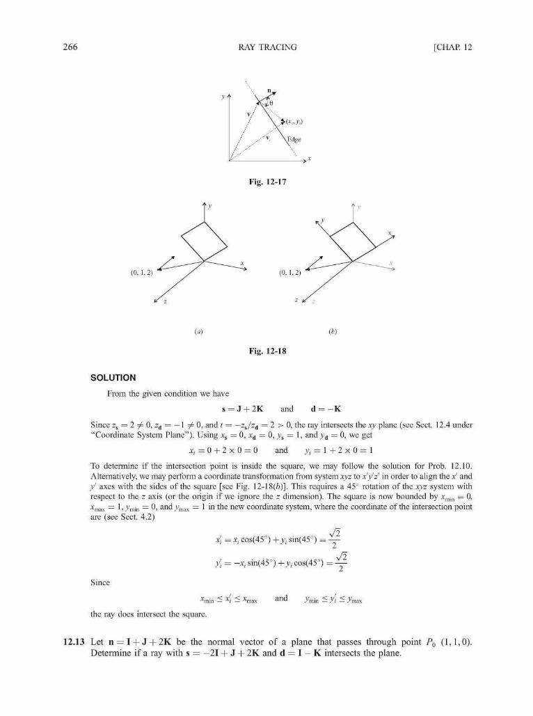
266 RAY TRACING [CHAP. 12
Fig. 12-17
(0, 1, 2) (0, 1, 2)
() ( )
Fig. 12-18
SOLUTION
From the given condition we have
s = J + 2K and d = - K
Since zs = 2 / 0 , z d = - l ^ 0, and t = —zs/zA = 2 > 0, the ray intersects the xy plane (see Sect. 12.4 under"Coordinate System Plane")- Using xs = 0, xd = 0, ys = 1, and j ; d = 0, we get
x, = 0 + 2 x 0 = 0 and .y, = 1 + 2 x 0 = 1
To determine if the intersection point is inside the square, we may follow the solution for Prob. 12.10.Alternatively, we may perform a coordinate transformation from system xyz to x'y'z' in order to align the x' andy' axes with the sides of the square [see Fig. 12-18(£)]. This requires a 45° rotation of the xyz system withrespect to the z axis (or the origin if we ignore the z dimension). The square is now bounded by xmin = 0,xmax = 1 > ymin = 0> a n d JVax = 1 in the new coordinate system, where the coordinate of the intersection pointare (see Sect. 4.2)
A/2; ( 4 5 ° ) + i ( 4 5 ° ) ^
J^ = -x,. sin(45°) +3;,. cos(45°) =A/2
Since
the ray does intersect the square.
and jVin < y\ <.
12.13 Let n = I + J + 2K be the normal vector of a plane that passes through point Po (1,1,0).Determine if a ray with s = —21 + J + 2K and d = I — K intersects the plane.

CHAP. 12] RAY TRACING 267
SOLUTION
Refer to Sect. 12.4 under arbitrary plane. Since
n - d = l x l + l x 0 + 2 x ( - l ) = - l < 0
the ray intersects the plane. We introduce
p = (x0 - xs)I + O0 - 3;S)J + (*o ~ z s ) K
= ( l - ( - 2 ) ) I + ( l - l ) J + ( 0 - 2 ) K
= 31 - 2K
and compute
n - p l x 3 + l x O + 2 x ( -2)
n • d — 1
The intersection point is at (xs +xA,ys +yA,zs + zd) = (—1, 1, 1).
12.14 Double check that the intersection point found in Prob. 12.13 is indeed on the given plane.
SOLUTION
The vector equation for the plane is
xn(x - xo) +ynb> - yo) + zn(z - zo) = °
Since
1(-1 - 1) + 1(1 - 1) + 2(1 - 0) = 0
the intersection point (—1, 1, 1) is indeed on the plane.
12.15 Let Si be a sphere of radius 8 centered at (2,4,1) and S2 a sphere of radius 10 centered at(10, —2, —5). Determine if a ray with s = 2J + 5K and d = I — 2K intersects the spheres.
SOLUTION
First consider sphere Si. We have
A = |d|2 = l2 + (-2)2 = 5
B = (s - c) • d = [(0 - 2)1 + (2 - 4)J + (5 - 1)K] • (I - 2K) = -10
C = |s - c|2 - R2 = (-2)2 + (-2)2 + 42 - 82 = -40
Since B2 - AC = (-10)2 - 5(-40) = 300 > 0, there are two t values:
fi 2 ( 1 + V 3 ) > ( ) ^ ,2 2 ( 1
From these we know that the ray starts from inside Si. Now considering sphere S2, we have
A = |d|2 = l2 + (-2)2 = 5
B = (s - c) • d = [(0 - 10)1 + (2 + 2)J + (5 + 5)K] • (I - 2K) = -30
C = | s - c | 2 - # 2 = (-10)2 + (4)2 + 1 0 2 - 102 = 116
Since B2 - AC = (-30)2 - 5 x 116 = 320 > 0, there are also two t values:
and t< = 3° f * = 6 - lW5 > 0
From these we know that the ray intersects S2 in two different places. By comparing fj R 5.464, t3 R 9.578,and t4 R 2.422, we see that the ray first enters S2, then leaves Si, and finally exits from S2 (the two spheresoverlap each other).

268 RAY TRACING [CHAP. 12
12.16 The (implicit) equation for a sphere of radius R centered at the origin is x2 + y2 + z2 — R2 = 0.Determine if a ray s + t& intersects the sphere.
SOLUTION
Let s = xsl + ysj + zsK and d = xd l + ydJ + zdK. Substitute xs + txd, ys + tyd, and zs + tzd for x, y, andz, respectively:
(xs + txdf + (ys + tydf + (z, + fed)2 - R2 = 0
Expand and regroup terms:
( 4 + y\ + 4)f2 + 2(xsxd + ysyd + zszd)t + (x2 + yl + z2) - R2 = 0
or
| d | 2 f 2 + 2 s - d f + | s | 2 - # 2 = 0
This matches the quadratic equation derived in the text (see Sect. 12.4 under "Sphere"), with the center of thesphere being set to (0,0,0).
12.17 The (implicit) canonical equation for an elliptic paraboloid is x2 +y2 — z = 0 (see Chap. 9, Sect.9.10, Fig. 9-19). Determine if a ray s + td intersects the paraboloid.
SOLUTION
Let s = xsl + ysj + zsK and d = xd l + ydJ + zdK. Substitute xs + fxd, ys + tyd, and zs + tzd for x, y, andz, respectively:
(xs + fxd)2 + (ys + fyd)
2 - (zs + tzd) = 0
Expand and regroup terms:
(4 +yl)t2 + (2*s*d + 2^d - zA)t+(4 +yl-zs) = oWhen the ray is parallel to the z axis (i.e., xd = 0 and j ; d = 0), the equation degenerates into
x 2 +.y 2 - z s =
From this we can find
t = '•
where
I < 0 ray's negative extension intersects paraboloid
= 0 ray's starting point on paraboloid> 0 ray intersects paraboloid
Otherwise, we can rewrite the quadratic equation as
At2+Bt+C =
where
and the solution for the equation is (note A
• = x2+y2-zs
-B ± V#2 - 4AC
If B2 — 4AC < 0, the ray does not intersect (or touches) the paraboloid. If B2 — 4AC = 0 and t > 0, the rayintersects (or touches) the paraboloid once. If B2 — 4AC > 0, we get two t values; fj and t2. If fj < 0 andt2 < 0, the negative extension of the ray intersects the paraboloid (no intersection by the ray). If one of the twovalues is 0, the ray starts from a point on the paraboloid and intersects the paraboloid only if the other value is

CHAP. 12] RAY TRACING 269
positive. If t\ and t2 differ in signs, the ray originates from inside the paraboloid (i.e., x£ +y% —zs < 0) andintersects the paraboloid once. If both values are positive, the ray intersects the paraboloid twice (first entersand then exits), and the smaller value corresponds to the intersection point that is closer to the starting point ofthe ray.
12.18 Figure 12-19 shows a ray s + td and a canonical paraboloid (see Prob. 12.17) that is defined in itsown coordinate system x'y'z'. Describe how to make use of the result in Prob. 12.17 to determine ifthe ray intersects this paraboloid.
Fig. 12-19
SOLUTION
Find the coordinate transformation M from system xyz to x'y'z'. Apply M to transform (xs,j;s,zs) to(Xj, y/s, z's) and define s' = x'sI + y'sJ + z^K. Apply M to transform the origin (0,0,0) of xyz to (x[,, y/0, zf,), andtransform (xd, yA, zd) to (xd,y'A, z^). Define d' = (xd — XQ)I + (yd — y/0)J + (z'A — ZQ)K, which describes thesame vector as d. Now represent the ray by s' + td' in the x ' /z ' coordinate system. Use the solution to Prob.12.17 to determine if the ray intersects the paraboloid.
12.19 Refer to Fig. 12-12. If krl = kr2 = kr3 = 0.3, the threshold is 0.01, and the desired depth is 2, willthe ray-tracer proceed to work on the third reflected ray?
SOLUTION
No, since the desired depth is 2. It would if the desired depth were 3 because = 0-027 > 0.01.
12.20 Describe a scene where the bounding volume techniques are definitely not applicable. Explain why.
SOLUTION
A number of spheres scattered across the scene. First of all, there is no simpler bounding volume forintersection testing. Furthermore, any bounding volume that encompasses several spheres is going to occupy arelatively large section of the scene. This brings about a relatively high probability for a ray to intersect thebounding volume, resulting in further testing against the enclosed spheres (something the bounding volume issupposed to help avoid in the first place).
12.21 In spatial subdivision we need to identify the regions along the ray's path. Since the ray exits fromthe current region and enters into the next region at the same point in space, a basic operation toguide the ray-tracer from one region to the next is: given the direction d of the ray and its entrypoint Pj into the current region, find point P2 through which the ray exits. Describe the operationfor a parallelepiped region whose faces are parallel to the coordinate system planes.

270 RAY TRACING [CHAP. 12
SOLUTION
Such a region is bounded by the following planes:
y J^min y J max
Since we are looking for the exit point, only planes that satisfy n • d > 0, where n is the plane's normal vector,should be considered. The normal vectors of the planes listed above are simply —\ I, —J, J, —K, and K,respectively. Now we use Px to be the starting point of the ray. For each chosen plane, say, z = zmin, the t valuethat represents where the ray intersects the plane is (see Prob. 12.8)
(see Prob. 12.22 for similar formulae for the other planes). Once all eligible planes have been processed, thesmallest t value from the calculation represents P2.
12.22 Refer to Prob. 12.21, and write down the formulae for computing t for the other five planes.
SOLUTION
The formulae for planes x = xm i n , x = xm a x , y = ymin, y = ymaK, and z = zm a x are
* * \ ' m i - * \ l l s l n i i - l \ - m i - -%
respectively.
12.23 Consider supersampling and adaptive supersampling. Which one is likely to perform better inreducing dropout?
SOLUTION
Supersampling is likely to perform better since the adaptive method will not subdivide a pixel if thecenter ray and corner rays return similar colors (but a small object may lie between those rays).
12.24 How to displace a ray from its normal position in the pixel grid?
SOLUTION
Let (x,y) be the ray's normal position in the grid. Define Ax and Ay such that [x — Ax, x + Ax] and[y — Ay, y + Ay] encompass the area for the new position (normally the area of the corresponding subpixel).Choose two random numbers 8X and 8y in the range of [—Ax, Ax] and [—Ay, Ay], respectively. Thenew/displaced position for the ray is (x + 8x,y + 8y).
12.25 Illustrate why the relative size of an object affects the quality of environment mapping.
SOLUTION
The environment map is obtained by projecting the scene (a pyramid) from viewpoint C [see Fig.12-20(a)]. When a small object is placed at C, the mapped reflection approximates the result of ray-tracingwith the actual pyramid [see Fig. 12-20(fr)]. On the other hand, if a relatively large object is placed at C, wemay see a falsely reflected pyramid on the object when the pyramid is really behind the object [see Fig.12-20(c)].
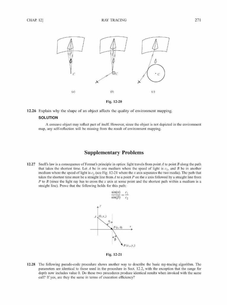
CHAP. 12] RAY TRACING 271
() ()
Fig. 12-20
12.26 Explain why the shape of an object affects the quality of environment mapping.
SOLUTION
A concave object may reflect part of itself. However, since the object is not depicted in the environmentmap, any self-reflection will be missing from the result of environment mapping.
Supplementary Problems
12.27 Snell's law is a consequence of Fermat's principle in optics: light travels from points to point B along the paththat takes the shortest time. Let A be in one medium where the speed of light is c\, and B be in anothermedium where the speed of light is c2 (see Fig. 12-21 where the x axis separates the two media). The path thattakes the shortest time must be a straight line from A to a point P on the x axis followed by a straight line fromP to B (since the light ray has to cross the x axis at some point and the shortest path within a medium is astraight line). Prove that the following holds for this path:
sin(a) Cj
A
Px(,0)
Fig. 12-21
12.28 The following pseudo-code procedure shows another way to describe the basic ray-tracing algorithm. Theparameters are identical to those used in the procedure in Sect. 12.2, with the exception that the range fordepth now includes value 0. Do these two procedures produce identical results when invoked with the samecall? If yes, are they the same in terms of execution efficiency?
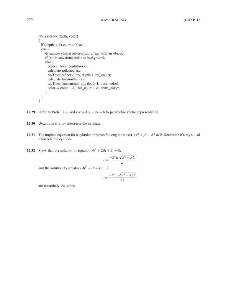
272 RAY TRACING [CHAP. 12
rayTrace(ray, depth, color){
if (depth < 1) color = black:else {
determine closest intersection of ray with an object:if (no intersection) color = background:else {
color = local contribution:calculate reflected ray:ray Trace (reflected ray, depth-1, ref_color):calculate transmitted ray;ray Trace (transmitted ray, depth-1, trans_color):color = color + k^ • ref_color + k^ • trans_color:
12.29 Refer to Prob. 12.7, and convert y = 2x — 6 to parametric vector representation.
12.30 Determine if a ray intersects the yz plane.
12.31 The implicit equation for a cylinder of radius R along the z-axis is x2 +y2 — R2 = 0. Determine if a ray s + tdintersects the cylinder.
12.32 Show that the solution to equation At1 + 2Bt + C = 0:
t =
and the solution to equation At + Bt + C = 0
t 21are essentially the same.
-B±^
sIB1
A
IB2
-AC
-4AC

APPENDIX 1
Mathematics forTwo-Dimensional
Computer Graphics
The key to understanding how geometric objects can be described and manipulated within a computergraphics system lies in understanding the interplay between geometry and numbers. While we have aninnate geometric intuition which enables us to understand verbal descriptions such as line, angle, andshape and descriptions of the manipulation of objects {rotating, shifting, distorting, etc.), we also have thecomputer's ability to manipulate numbers. The problem then is to express our geometric ideas in numericform so that the computer can do our bidding.
A coordinate system provides a framework for translating geometric ideas into numerical expressions.We start with our intuitive understanding of the concept of a two-dimensional plane.
Al. l. .
THE TWO-DIMENSIONAL CARTESIAN COORDINATE SYSTEM
In a two-dimensional plane, we can pick any point and single it out as a reference point called theorigin. Through the origin we construct two perpendicular number lines called axes. These are traditionallylabeled the x axis and the y axis. An orientation or sense of the plane is determined by the positions of thepositive sides of the x and j axes. If a counterclockwise rotation of 90° about the origin aligns the positive xaxis with the positive y axis, the coordinate system is said to have a right-handed orientation [see Fig.Al-l(a)]; otherwise, the coordinate system is called left-handed [see Fig. A1-1(Z>)].
The system of lines perpendicular to the x axis and perpendicular to the y axis forms a rectangular gridover the two-dimensional plane. Every point P in the plane lies at the intersection of exactly one lineperpendicular to the x axis and one line perpendicular to the y axis. The number pair (x, y) associated withthe point P is called the Cartesian coordinates of P. In this way every point in the plane is assigned a pairof coordinates (see Fig. Al-2).
Measuring Distances in Cartesian System
The distance between any two points Pr and P2 with coordinates (xr, yr) and (x2, j 2 ) c a n be found withthe formula
273

274 APPENDIX 1
(a) Right-handed.
Fig. Al-1
(b) Left-handed.
2
y
0
(3,2)
X
Fig. Al-2
The length of a line segment can be measured by finding the distance between the endpoints of thesegment using the formula.
EXAMPLE 1. The length of the line segment joining points PQ(—1, 2) and P\(3, 5) can be found by
= J(5- T)L + [3 - (-1)]2 = V32 + 42 = 5
Measuring Angles in Cartesian System
The angles of a triangle can be measured in terms of the length of the sides of the triangle (see Fig.Al-3), by using the Law of Cosines, which is stated as
c2 = a2 + b2 - 2ab(cos 6)
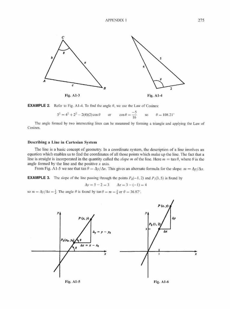
APPENDIX 1 275
Fig. Al-3 Fig. Al-4
EXAMPLE 2. Refer to Fig. Al-4. To find the angle 6, we use the Law of Cosines:
5 2 =4 2 +2 2 -2(4) (2)cos0 or cos 6 =-5
16 so 6= 108.2T
The angle formed by two intersecting lines can be measured by forming a triangle and applying the Law ofCosines.
Describing a Line in Cartesian System
The line is a basic concept of geometry. In a coordinate system, the description of a line involves anequation which enables us to find the coordinates of all those points which make up the line. The fact that aline is straight is incorporated in the quantity called the slope m of the line. Here m = tan 6, where 9 is theangle formed by the line and the positive x axis.
From Fig. Al-5 we see that tan 6 = Ay/Ax. This gives an alternate formula for the slope: m = Ay/Ax.
EXAMPLE 3. The slope of the line passing through the points PQ(—\, 2) and -P](3, 5) is found by
Aj; = 5 - 2 = 3 Ax = 3 - ( - l ) = 4
so m = Ay/Ax = |. The angle 8 is found by tanO = m = | or 6 = 36.87°.
Fig. Al-5 Fig. Al-6

276 APPENDIX 1
The straightness of a line is expressed by the fact that the slope of the line is the same regardless of which twopoints are used to calculate it. This enables us to find the equation of a line.
EXAMPLE 4. To find the equation of the line whose slope is 2 and passes through the point P 0( l , 2), let P(x,y) beany point on the line. The slope is the same regardless of which two points are used in calculating it. Using P and Po,we obtain
Ay=y-2 Ax = x- 1
Ay
Ax ory-2
' x- 1
Solving, we have y = 2x (see Fig. Al-6).
Every line has an equation which can be put in the form y = mx + b, where m is the slope of the lineand the point (0, b) is the y intercept of the line (the point where the line intercepts the y axis).
Curves and Parametric Equations
The equation of a curve is a mathematical expression which enables us to determine the coordinates ofthe points that make up the curve.
The equation of a circle of radius r whose center lies at the point (h, k) is
(x - hf + (y - kf = r2
It is often more convenient to write the equation of a curve in parametric form; that is
x =f(f) y = g(t)
where parameter t might be regarded as representing the "moment" at which the curve arrives at the point(x,y).
The parametric equations of a line can be written in the form (Probs. A1.21 and A1.23)
y = bt+y0
EXAMPLE 5. The parametric equation of a circle of radius r and center at the origin (0,0) can be written asx = r cos t and y = r sin t, where t lies in the interval 0 < t < 2n.
A geometric curve consists of an infinite number of points. Thus any plot of such a curve can only approximateits real shape. Plotting a curve requires the calculation of the x and j ; coordinates of a certain number of the points ofthe curve and the placing of these points on the coordinate system. The more points plotted, the better theapproximation to the actual shape.
EXAMPLE 6. Plot five points of the equations x = t, y = t2 for t in the interval [—1, 1].
t
X
y
- 1
- 1
1
l2
12
14
0
0
0
12
12
14
1
1
1
Plotting (x,y) gives Fig. Al-7. We can approximate the actual curve by joining the plotted points by linesegments.

APPENDIX 1 277
f = 1
Fig. Al-7
A1.2 THE POLAR COORDINATE SYSTEM
The Cartesian coordinate system is only one of many schemes for attaching coordinates to the pointsof a plane. Another useful system is the polar coordinate system. To develop it, we pick any point in theplane and call it the origin. Through the origin we choose any ray (half-line) as the polar axis. Any point inthe plane can be located at the intersection of a circle of radius r and a ray from the origin making an angle6 with the polar axis (see Fig. A1-8).
Fig. Al-8

278 APPENDIX 1
The polar coordinates of a point are given by the pair (r, 6). The polar coordinates of a point are notunique. This is because the addition or subtraction of any multiple of 2n (360°) to 6 describes the same rayas that described by 6.
Changing Coordinate Systems
How are the Cartesian coordinates of a point related to the polar coordinates of that point? If (r, 6) arethe polar coordinates of point P, the Cartesian coordinates (x, y) are given by
x = r cos 6 y = r sin 6
Conversely, the polar coordinates of a point whose Cartesian coordinates are known can be found by
r2 = x2 + y2 6 = arctan -
A1.3 VECTORS
Vectors provide a link between geometric reasoning and arithmetic calculation. A vector is representedby a family of directed line segments that all have the same length or magnitude. That is, any two linesegments pointing in the same direction and having the same lengths are considered to be the same vector,regardless of their location (see Fig. Al-9).
Fig. Al-9
Properties of Vectors
Vectors have special arithmetic properties:
1. If A is a vector, then —A is a vector with the same length as A but pointing in the oppositedirection.
2. If A is a vector, then kA is a vector whose direction is the same as or opposite that of A,depending on the sign of the number k, and whose length is k times the length of A. This is anexample of scalar multiplication.
3. Two vectors can be added together to produce a third vector by using the parallelogram method orthe head-to-tail method. This is an example of vector addition.
In the parallelogram method, vectors A and B are placed tail to tail. Their sum A + B is the vectordetermined by the diagonal of the parallelogram formed by the vectors A and B (see Fig. Al-10).
In the head-to-tail method, the tail of B is placed at the head of A. The vector A + B is determined bythe line segment pointing from the tail of A to the head of B (see Fig. Al-11).
Both methods of addition are equivalent, but the head-to-tail is easier to use when adding severalvectors.

APPENDIX 1 279
Fig. Al-10
A + B
Fig. Al-11
Coordinate Vectors and Components
In a Cartesian coordinate system, vectors having lengths equal to 1 and pointing in the positivedirection along the x and y coordinate axes are called the natural coordinate vectors and are designated as Iand J (see Fig. Al-12).
Fig. Al-12
By use of scalar multiplication and vector addition, any vector V can be written as a linearcombination of the natural coordinate vectors. That is, we can find numbers a and b so that V =al + bJ. The numbers [a, b] are called the components of V. The components of a vector can bedetermined from the coordinates of the head and the coordinates of the tail of the vector. If (hx, h ) and(tx, t) are the coordinates of the head and the tail, respectively, the components of V are given by
a = h^ — b = h - t,
Notice that if the tail of V is placed at the origin, the components of the vector are the coordinates of thehead of V.
The introduction of components allows us to translate the geometric properties of vectors intocomputational properties. If the vector A has components [xx, yx] and the vector B has components [x2, y2],the length of A, denoted as |A|, can be computed by
|A| = 7*2 +y\
To perform scalar multiplication by a number c, we have
cA = CX]\ +
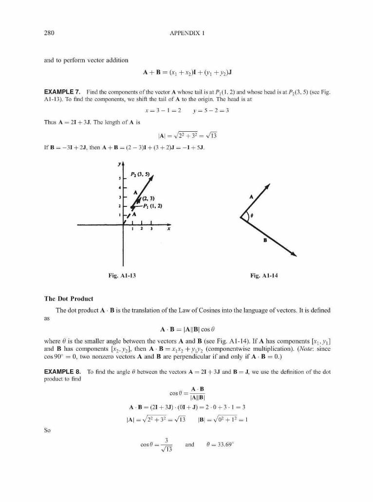
280 APPENDIX 1
and to perform vector addition
A + B = fo + x2)l + (yl + y2)J
EXAMPLE 7. Find the components of the vector A whose tail is a tP j ( l , 2) and whose head is atP2(3, 5) (see Fig.Al-13). To find the components, we shift the tail of A to the origin. The head is at
Thus A = 21 + 3 J. The length of A is
x = 3 - 1 = 2 y=5-2=3
32 =
If B = -31 + 2J, then A + B = (2 - 3)1 + (3 + 2)J = - I + 5J.
5
4
3
2
1
_ Pi
A./I
yf- , Af |
1
(3.5)3
/fa-Pi
|2
4
3)(1.
I3
2)
X
Fig. Al-13 Fig. Al-14
The Dot Product
The dot product A • B is the translation of the Law of Cosines into the language of vectors. It is defined
as
A - B = |A||B|cos0
where 6 is the smaller angle between the vectors A and B (see Fig. Al-14). If A has components [x^j j ]and B has components [x2,y2], then A • B =xxx2 +y\y2 (componentwise multiplication). (Note: sincecos 90° = 0, two nonzero vectors A and B are perpendicular if and only if A • B = 0.)
EXAMPLE 8. To find the angle 8 between the vectors A = 21 + 3 J and B = J, we use the definition of the dotproduct to find
a A B
cos 8 =
A • B = (21 + 3 J) • (01 + J) = 2 • 0 + 3 • 1 = 3
|A| = 722 + 32 = vT3 |B| = Vo2 + I2 = 1So
cos 8 = and ' = 33.69'

APPENDIX 1 281
A1.4 MATRICES
A matrix is a rectangular array or table of numbers, arranged in rows and columns. The notation atj isused to designate the matrix entry at the intersection of row / with column j (see Fig. Al-15).
Column j
Row i
Fig. Al-15
The size or dimension of a matrix is indicated by the notation m x n, where m is the number of rows inthe matrix and n is the number of columns.
A matrix can be used as an organizational tool to represent the information content of data in tabularform. For example, a polygonal figure can be represented as an ordered array of the coordinatesof its vertices. The geometric transformations used in computer graphics can also be represented bymatrices.
Arithmetic Properties of Matrices
Examples of these properties are as follows.
1. Scalar multiplication. The matrix kA is the matrix obtained by multiplying every entry of A by thenumber k.
2. Matrix addition. Two m x n matrices A and B can be added together to form a new m x n matrixC whose entries are the sum of the conesponding entries of A and B. That is,
Matrix multiplication. An m x p matrix A can be multiplied by a/> x n matrix B to form an m x nmatrix C. The entry Cy is found by taking the dot product of the / row of A with they column of B(see Fig. Al-16). So Cy = (row /) • (column j) = anby + aab2j + • • • + aimbmj. Matrix multi-plication is not commutative in general. So AB ^ BA. Matrix multiplication is also calledmatrix concatenation.
Row i /«,„ aa aa
Fig. Al-16

282 APPENDIX 1
4. Matrix transpose. The transpose of a matrix A is a matrix, denoted as A r , formed by exchangingthe rows and columns of A. If A is an m x n matrix, then AT is an n x m matrix. A matrix is saidto be symmetrical if A = AT.
Two basic properties of the transpose operation are (1) (A + B) r = AT + B r and (2) (AB)r = B rA r .
EXAMPLE 9
/ 3 2 5s
A =
-2A = - 2
AB[3 • ( - 1 ) ] + (2 • 2) + (5 • 1) (3 • 0) + (2 • 3) + (5 • 2)
[ ! • ( - ! ) ] + [ ( - ! ) • 2 ] + ( 2 - 1 ) ( 1 . 0 ) + [ ( - ! ) • 3 ] + ( 2 - 2 )
A1 = 2 - 1
Matrix Inversion and the Identity Matrix
The n x n matrix whose entries along the main diagonal are all equal to 1 and all other entries are 0 iscalled the identity matrix and is denoted by I (Fig. Al-17).
1 =
/ I 0 0 ••• 0 \0 1 0 ••• 00 0 1 ••• 0
Vo o o •Fig. Al-17
1 /
If A is also an n x n matrix, then AI = IA = A. That is, multiplication by the identity matrix I leavesthe matrix A unchanged. Therefore, multiplication by the identity matrix is analogous to multiplication of areal number by 1.
An n x n matrix A is said to be invertible or to have an inverse if there can be found an n x n matrix,denoted by A^1, such that A - 1 A = AA^1 = I. The inverse matrix, if there is one, will be unique.
A basic property of matrix inversion is (AB) = B ^ A " 1 .
EXAMPLE 10
Then
A =1 0
2 1
A M =1 02 1
1 0- 2 1
and M1 0
- 2 1
1 • 1 + 0 • ( - 2 ) 1-0 + 0 - 12 • 1 + 1 • ( - 2 ) 2 - 0 + 1 - 1
1 0
0 1

APPENDIX 1 283
and
MA =1 0 \ \ 0
- 2 1 2 11 1 + 0 - 2 1 0 + 0 1
—2-1 + 1-2 - 2 - 0 + 1-11 00 1
So MA = AM = I. Thus M must be A"1.
A1.5 FUNCTIONS AND TRANSFORMATIONS
The concept of a function is at the very heart of mathematics and the application of mathematics as atool for modeling the real world. Stated simply, a function is any process or program which accepts aninput and produces a unique output according to a definite rule. Although a function is most often regardedin mathematical terms, this need not be the case. The concept can be usefully extended to include processesdescribed in nonmathematical ways, such as a chemical formula, a recipe or a prescription, and suchrelated concepts as a computer subroutine or a program module. All convey the idea of changing an inputto an output. Some synonyms for the word function are operator, mapping, and transformation.
The quantities used as input to the function are collectively called the domain of the function. Theoutputs are called the range of the function. Various notations are used to denote functions.
EXAMPLE 11. Some examples of functions are:
1. The equation fix) = x2 + 2x + 1 is a numerical function whose domain consists of all real numbers andwhose range consists of all real numbers greater than or equal to 0.
2. The relationship T(V) = 2V is a transformation between vectors. The domain of T is all real vectors, as isthe range. This function transforms each vector into a new vector which is twice the original one.
3. The expression H(x, y) = (x, —y) represents a mapping between points of the plane. The domain consists ofall points of the plane, as does the range. Each individual point is mapped to that point which is the reflectionof the original point about the x axis.
4. If A is a matrix and X is a column matrix, the column matrix Y found by multiplying A and X can beregarded as a function Y = AX.
Graphs of Functions
If x and y are real numbers (scalars), the graph of a function y =f(x) consists of all points in the planewhose coordinates have the form [x,f(x)], where x lies in the domain of/. The graph of a function is thecurve associated with the function, and it consists of an infinite number of points. In practice, plotting thegraph of a function is done by computing a table of values and plotting the results. This gives anapproximation to the actual graph of/.
EXAMPLE 12. Plot five points for the function y = x2 over the interval [—1, 1].
X
X2
- 1
1
12
14
0
0
12
14
1
1
Plotting the points (x, x2) calculated in the table and joining these points with line segments gives an approximation tothe actual graph of y = x2. See Fig. Al-7 for the plot of the graph.
The plotting resolution is determined by the number of x values used in plotting the graph. The higher theplotting resolution, the better the approximation.

284 APPENDIX 1
Composing Functions
If the process performed by a function H can be described by the successive steps of first applying afunction G and then applying a function F to the results of G, we say that H is the composition of F and G.We write H = F o G. If the input to the function is denoted by x, the output H(x) is evaluated by
H(x)=F[G(x)]
That is, first G operates on x; then the result G(x) is passed to F as input.Composition of functions is not commutative in general; that is, F o G ^ G o F.The concept of composition is not restricted to only two functions but extends to any number of
functions. For functions that are represented by matrices, composition of functions is equivalent to matrixmultiplication; that is, A o B = AB.
EXAMPLE 13
1. If/(x) = x2 + 2 and g(x) = 2x + 1, then/[g(x)] = [g(x)f + 2 = (2x + I)2 + 2 = 4x2 + 4x + 3.2. If
then
AoB = AB= 0 2 2 2 = 4 4
The Inverse Function
The inverse of a function/ (with respect to composition) is a function, denoted by/^1, that satisfiesthe relationships/~* of = i and/ o/^1 = i, where / is the identity function i(x) = x. Applying the abovecompositions to an element x, we obtain the equivalent statements:
The inverse operator thus "undoes" the work that/ has performed.Not every function has an inverse, and it is often very difficult to tell whether a given function has an
inverse. One must often rely on geometric intuition to establish the inverse of an operator.
EXAMPLE 14. Let R be the transformation which rotates every point in the plane by an angle of 30° (in thepositive or counterclockwise direction). Then it is clear that R~l is the transformation that rotates every point by anangle of —30° (a rotation of 30° in the clockwise direction).
Solved Problems
Al.l Find the distance between the points whose coordinates are (a) (5,2) and (7,3), (b) (—3,1) and(5,2), (c) ( -3 , -1) and (-5, -2), and (d) (0,1) and (2,0).
SOLUTION
(a) D = Ml - 5)2 + (3 - 2)2 = V ^ T T 2 = V5
(b) D = J[5- (-3)]2 + (2 - I)2 = J(8)2 + (I)2 = V65

APPENDIX 1 285
(c) D = J[-5 - (-3)]2 + [-2 - (-1)]2 = J(-2)2 + (-1)2 = V5
A1.2 Derive the equation for a straight line (see Fig. Al-5).
SOLUTION
A straight line never changes direction. We determine the direction of a line by the angle 8 the line makeswith the positive x axis. Then at any point Po on the line, the angle formed by the line and a segment throughP parallel to the x axis is also equal to 8. Let P0(x0,^0) be a point on the line. Then if P(x, y) represents anypoint on the line, drawing the right triangle with hypotenuse P0P, we find
x-x0
The quantity tan 8 is called the slope of the line and its traditionally denoted by m.We rewrite the equation as
y-y0 Aym = or m = —
x — x0 Ax
(The term Ay is often called the "rise" and Ax, the "run.") This can be solved for y in terms of x.
A1.3 Write the equation of the line whose slope is 2 and which passes through the point (—1, 2).
SOLUTION
Let P(x, y) represent any point on the line. Then
A J ; = J ; - 2 Ax = x - (-1) = x + 1
and m = 2. Using Ay /Ax = m, we find
v - 2= 2 or y - 2 = 2 ( x + l ) = 2x
x + 1
thus y = 2x + 4.
A1.4 Write the equation of the line passing through Pi ( l , 2) and P2O, —2).
SOLUTION
Let P(x, y) represent any point on the line. Then using P j , we compute
Ay = y — 2 Ax = x — 1
To find the slope m, we use Px and P2 to find
A j ; = - 2 - 2 = - 4 Ax = 3 - 1 = 2
Then
4 y _ , y-2 _m = — = —2 so = —2
Ax x - 1Then
y - 2 = -2x + 2 and y = -2x + 4
A1.5 Show that lines are parallel if and only if their slopes are equal.
SOLUTION
Refer to Fig. Al-18. Suppose that lines /] and /2 are parallel. Then the alternate interior angles 0j and 1are equal, and so are the slopes tanflj and tan02-

286 APPENDIX 1
y
3
- 2
I/O
2
P
3) *>,
j
2 US
X
, - 2 )
Fig. Al-18 Fig. Al-19
Conversely, if the slopes tanflj and tan02 are equal, so are the alternate interior angles 6x and 02.Consequently lines lx and l2 are parallel.
A1.6 Let U(2, 3) and L(5, —2) be the upper left and lower right corners, respectively, of a rectanglewhose sides are parallel to the x and y axes. Find the coordinates of the remaining two vertices.
SOLUTION
Referring to Fig. Al-19, we see that the x coordinate of Px is the same as that of L, namely 5, and the ycoordinate that of U, namely 3. So Px = (5, 3). Similarly, P2 = (2, -2).
A1.7 Plot the points A{\, 1), B(-l, 1), and C( -4 , 2). Then (a) show that ABC is a right triangle and (b)find a fourth point D such that ABCD is a rectangle (see Fig. Al-20).
D{x,y)
C(-4,
B(-\, -1)
Fig. Al-20
SOLUTION
(a) Show that the Pythagorean theorem is satisfied:
AC =AB +BC

APPENDIX 1 287
Use the distance formula to compute the lengths of the sides of ABC:
AB = J[\ - (-1)]2 + [1 - (-1)]2 = sjl2 + 22 = V8
BC = J[-l - (-4)Y + (-l-2Y= J(3Y + (-3)1 = V18
AC = J[l - (-4)]2 + (1 - if = ^52 + (-lf = V26
So
AC2 = 26 = AB2 + B~C2 = 8 + 1 8
(b) Let the unknown coordinates of D be denoted by (x, y). Use the fact that opposite sides of a rectangle areparallel to find x and y. Since parallel lines have equal slopes, compute the slopes of all four sides:
- 1 - 1 - 2 v-2 v-2Slope AB = = — = 1 Slope CD = — =F - 1 - 1 - 2 F x-(-4) x + 4
Slope BC= ~ 1 ~ / 2 L = I ^ 3 = -1 ^ ^
Then, for ABCD to be a rectangle
Slope CD = slope AB Slope DA = slope 5C
or
y^l = x and yjzl=-xx + 4 x - 1
This leads to the equations
y - 2 = x + 4 and y—l=—x+l
or
—x + y = 6 and x + j ; = 2
Solving, x = —2 and y = 4.
A1.8 Find the equation of a circle that has radius r and its center at the point (h, k).
SOLUTION
Refer to Fig. A1-21. If P(x, y) is any point lying on the circle, its distance from the center of the circlemust be equal to r. Using the distance formula to express this mathematically, we have
So (x — h) + (y — k) = r2, which is the equation of the circle.
A1.9 Given any three points, not all lying on a line, find the equation of the circle determined by them.
SOLUTION
Refer to Fig. Al-22. LetP](flj, b{), P-iifli, b-i), andP3(fl3, b3) be the coordinates of the points. Let r bethe radius of the circle and (h, k) the center. Since each point is distance r from the center, then
{al-hf + {bl-kf=r2
(a2 - hf + (b2 - kf = r2

288 APPENDIX 1
P(x,y)
Fig. Al-21
This yields, after multiplying and collecting like terms:
Fig. Al-22
(q3 - a2)h + (b3 - b2)k = 3 2
2 + -^-y
These equations can be solved for h and k to yield
[d\(b2 - b3) + d\(b3 -b1) + dl(bx - b2)]_ 12 d
_ - 1 [df(a2 - q3) + dl(a3 - ax) + ^(q , - q2)]* " 2 d
Here, d\=a\+ b\, d\=a\+ b\, dl = a\+ b\, and d = ax(b2 - b3) + a2(b3 - bx) + a3(bl - b2). Finally, rcan be found:
- hf + (b, - kf
Al.lO Find the equation of the circle passing through the three points Px(\,2), P2(3, 0), and P3(0, -4).
SOLUTION
As in Prob. A1.9, we find
d\ = a\ + b\ = 5 a2 - a3 = 3 - b3 = 4
So
and
d\ = a\ + b\ = 9 a3 - ax = - 1 63 - ^ = - 6rf| = a\ + b\ = 16 ax - a2 = -2 bx-b2=2
rf = 1(4) + 3(-6) + 0(2) = -14
-l[5(4) + 9(-6) +16(2)] 2 1h =
k =
28 28 14
- 2 6 - 1 328 28 14
Therefore, the center of the circle is located at
1 - 1 314' l 4 ~
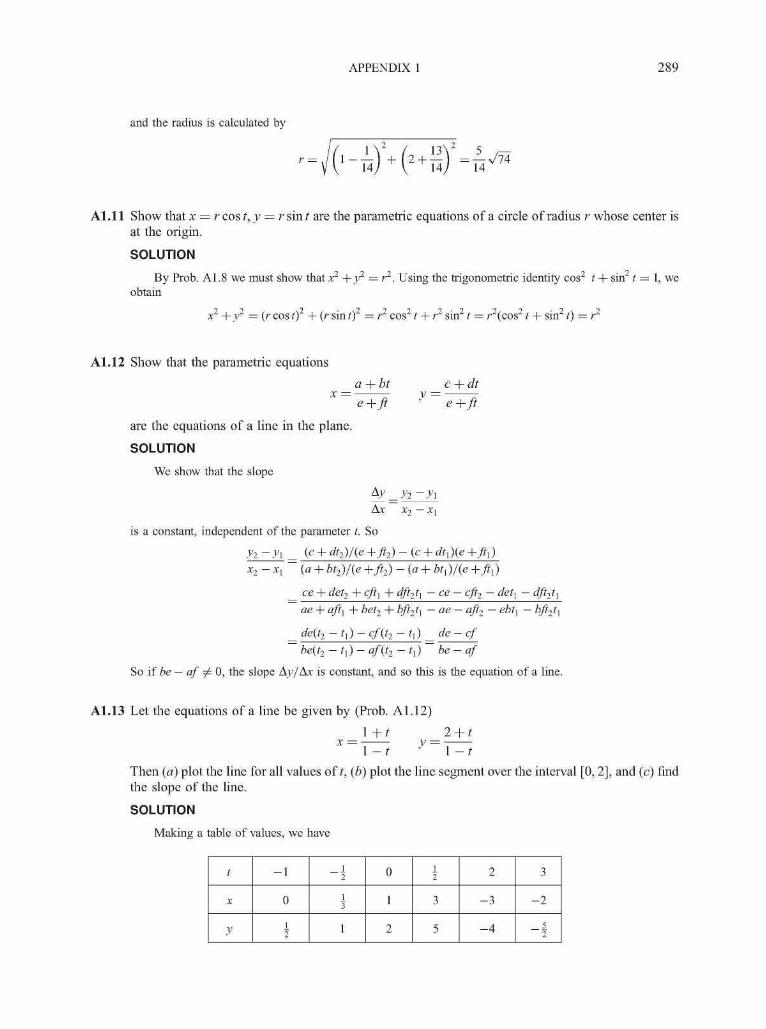
APPENDIX 1 289
and the radius is calculated by
A l . l l Show that x = r cos t,y = rsint are the parametric equations of a circle of radius r whose center isat the origin.
SOLUTION
By Prob. A 1.8 we must show that x2 + y2 = r2. Using the trigonometric identity cos2 t + sin2 t = 1, weobtain
x2 +y2 = (rcost) +(rsinf) = r2 cos2 t + r2 sin2 t = r2(cos2 t + sin2 t) = r2
A1.12 Show that the parametric equations
x =a + bt
e+ft y =c + dte+ft
are the equations of a line in the plane.
SOLUTION
We show that the slope
Ay _ yi - y\Ax Xj — X,
is a constant, independent of the parameter t. So
y2 -yx (c + dt2)/(e +ft2) - (c + dtx)(e +ftl)
x2 - xx (a + bt2)/(e +ft2) - (a + btx )/(e +ftl)
ce + det2 + cftx + dft2t1 - ce - cft2 - detx - dft2tx
ae + aftx + bet2 + bft2tx - ae - aft2 - ebtx - bft2tx
_ de(t2 - tx) - cf(t2 - tx) _de-cf~ be(t2 - tx) - af(t2 - tx) ~ be-af
So if be — af' / 0, the slope Ay /Ax is constant, and so this is the equation of a line.
A1.13 Let the equations of a line be given by (Prob. A1.12)
\+t 2+tx = Y^t y = Y^t
Then (a) plot the line for all values of t, (b) plot the line segment over the interval [0,2], and (c) findthe slope of the line.
SOLUTION
Making a table of values, we have
t
X
y
- 1
0
I
l2
13
1
0
1
2
l2
3
5
2
- 3
- 4
3
_2
_5

290 APPENDIX 1
The resulting line is shown in Fig. Al-23.
(a) We observe the following: (1) the line is undefined at t = 1, (2) (x,y) —>• (oo, oo) as ( ^ 1 , (3)(x,y) -+ ( -oo, -oo ) as t -+ 1+, and (4) (x, j/) - • ( - 1 , - 1 ) as f -+ ±oc (see Fig. Al-23).
(b) The interval [0,2] includes the infinite point at t = 1. The corresponding region is the exterior linesegment between points Px(l, 2) at t = 0 and P 2 (~3 , - 4 ) at f = 2 (see Fig. A1-24).
(c) From Prob. A1.12, the slope of the line is, with a = I, b = I, c = 2, d = I, e = I, a n d / = —1.
AyAx
A1.14 Let A = 21 + 7J, B = -31 + J, and C = I - 2J. Find (a) 2A - B and (6) -3A + 5B - 2C.
SOLUTION
Perform the scalar multiplication and then the addition.
(a) 2A - B = 2(21 + 7J) - (-31 + J) = (41 + 14J) + (31 - J)
= (4 + 3)1 + (14 - 1)J = 71 + 13J
(b) - 3A + 5B - 2C = -3(21 + 7J) + 5(-3I + J) - 2(1 - 2J)
= (-61 - 21J) + (-151 + 5J) + (-21 + 4J)
= (-6 - 15 - 2)1 + (-21 + 5 + 4)J = -231 - 12J
A1.15 Find x and y such that 2x1 + (y - 1)J =y\ + (3x + 1)J.
SOLUTION
Since vectors are equal only if their corresponding components are equal, we solve the equations (1)2x = y and (2) y — 1 = 3x + 1. Substituting into equation (2), we have (2x) — 1 = 3x + 1 and —2 = x andfinally y = 2x = 2(—2) = —4, so x = —2 and y = —4.
A1.16 The tail of vector A is located at P(— 1, 2), and the head is at Q(5, —3). Find the components of A.
SOLUTION
Translate vector A so that its tail is at the origin. In this position, the coordinates of the head will be thecomponents of A.
Translating P to the origin is the same as subtracting —1 from the x component and 2 from the ycomponent. Thus the new head of A will be located at point Qx, whose coordinates (xx,yx) can be found by
x 1 = 5 - ( - l ) = 6 j , 1 = - 3 - 2 = - 5
Thus A = 61 - 5J.
A1.17 Given the vectors A = I + 2 J and B = 21 — 3J, find (a) the length, (b) the dot product, and (c) theangle 6 between the vectors.
SOLUTION
(a) |A|=V12+22 = V5 |B|(b) A • B = (I + 2J) • (21 - 3J) = (1 • 2) + [2 • (-3)] = 2 - 6 = - 4
(c) From the definition of the dot product, we can solve for cos 8:
A B - 4cos 0 =
So 6= 119.74°.
APPENDIX 1 291
Fig. Al-23
y
I I I- 3 - 2 - I I 2 3
- 2 - •
- 3 - •
- 4 -
Fig. Al-24

292 APPENDIX 1
A1.18 Find the unit vector UA having the direction of A = 21 — 3J.
SOLUTION
Since UA = — , it follows that
and U4 = — = -
A1.19 Show that the commutative law for the dot product
A B = B A
holds for any vectors A and B.
SOLUTION
Let
A = a1I + fl2J B = b1I + b2J
So
A • B = fljfej + a2b2 B • A = fejflj + b2a2
Comparing both expressions, we see that they are equal.
A1.20 Show that the distributive law for the dot product
(A + B ) - C = A - C + B - C
holds for any vectors A, B, and C.
SOLUTION
Let
So
A + B = (ax + bx)l + (a2 + b2)5
and
(A + B) • C = (flj + bl)cl + (a2 + b2)c2 = alcl + bxcx + a2c2 + b2c2
On the other hand,
A • C = fljCj + a2c2 B • C = fejCj + b2c2
so
A • C + B • C = fljCj + a2c2 + fejCj + b2c2
Comparing both expressions, we see that they are equal.
A1.21 Show that the equation of a line can be determined by specifying a vector V having the direction ofthe line and by a point on the line.
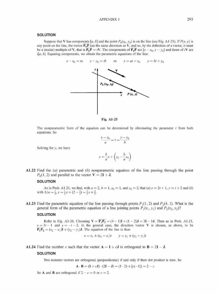
APPENDIX 1 293
SOLUTION
Suppose that V has components [a, b] and the point P0(x0, y0) is on the line (see Fig. Al-25). If P(x, y) isany point on the line, the vector P0P has the same direction as V, and so, by the definition of a vector, it mustbe a (scalar) multiple of V, that is P0P = tV. The components of P0P are [x — x0, y — y0] and those of tV aret[a, b]. Equating components, we obtain the parametric equations of the line:
x- xn = ta y-yQ = tb or x = at + x0 y = bt +y0
Fig. Al-25
The nonparametric form of the equation can be determined by eliminating the parameter t from bothequations. So
x — x0 y — y0
Solving for y, we have
A1.22 Find the (a) parametric and (b) nonparametric equation of the line passing through the pointP 0( l , 2) and parallel to the vector V = 21 + J.
SOLUTION
As in Prob. A1.21, we find, with a = 2, b = 1, x0 = 1, and^0 = 2, that (a) x = It + 1, y = t + 2 and (b)with b/a = \, y = \x + (2 - ±) = \x +1
A1.23 Find the parametric equation of the line passing through points P\(l, 2) and i^C^* !)• What is thegeneral form of the parametric equation of a line joining points Pl(xl,yl) and P2(x2,y2)^
SOLUTION
Refer to Fig. Al-26. Choosing V = P ^ = (4 - 1)1 + (1 - 2)J = 31 - U. Then as in Prob. A1.21,x = 3t— 1 and y = — t — 2. In the general case, the direction vector V is chosen, as above, to bePjP2 = (x2 — Xj)I + (y2 —y\)i- The equation of the line is then
x = xj + (x 2 -xx)t y = y\ + (y2 -y
A1.24 Find the number c such that the vector A = I + cJ is orthogonal to B = 21 — J.
SOLUTION
Two nonzero vectors are orthogonal (perpendicular) if and only if their dot product is zero. So
A • B = (I + cJ) • (21 - J) = (1 • 2) + [c(-l)] = 2 - c
So A and B are orthogonal if 2 — c = 0 or c = 2.

294 APPENDIX 1
Fig. Al-26
A1.25 Compute:
(a) 5 4 10 - 1 7
5 3 11 2 3
(c) 34 1
2 - 12 0
4 11 5
0 - 1 7
SOLUTION
(a) Adding corresponding entries, we obtain
5 4 10 - 1 7
- 1 30 1
5 + 2 4 - 1 1 + 30 + 2 - 1 + 0 7 + 1
7 32 - 1
(b) Since the matrices are of different sizes, we cannot add them.
(c) Multiplying each entry by 3, we have
5 4 10 - 1 7
15 12 30 - 3 21
A1.26 Let
A =
Find 2A - 3B.
SOLUTION
First multiply, and then add:
2A - 3B = 2 - 35 - 73 - 2
3 2
0 1
6 40 2
B =5 - 73 - 2
-15 21- 9 6
6 - 1 5 4 + 210 - 9 2 + 6
- 9 25- 9 8
A1.27 Determine the size of the following matrix multiplications A • B, where the sizes of A and B aregiven as (a) (3 x 5), (5 x 2); (b) (1 x 2), (3 x 1); (c) (2 x 2), (2 x 1); and (d) (2 x 2), (2 x 2).

APPENDIX 1 295
SOLUTION
(a) (3 x 2); (b) undefined, since the column size of A (2) and the row size of B (3) are not equal; (c)(2 x 1); (d) (2 x 2).
A1.28 Find the sizes of A and B so that AB and BA can both be computed. Show that, if both A and B aresquare matrices of the same size, both AB and BA are defined.
SOLUTION
Let the size of A be (m x n) and the size of B be (r x s). Then AB is denned only if r = n. Also, BA isdenned only if s = m. Thus, if A is (m x n), then B must be (n x m). If A is square, say, (n x n), and B is also[n x n), then both AB and BA are denned.
A1.29 Given
find AT.
SOLUTION
Exchanging the rows and columns of A, we obtain
AT = I 1 5 61 2 1 3
A1.30 Compute AB for
(a) A=(2 1) a n d B = /
(b) A={\ \) and B
2l I) a M B = ( ~ 7 6 10
SOLUTION
(a) Since A is (2 x 2) and B is (2 x 1), then AB is (2 x 1):
'2 3 \ / " 4 \ /1 1 2 M 7} ~ V 1 • ( - 4 ) + 2 - 7 y - V 10
A B - T 2 3 V 4 5 \ _ / 2 . ( - 4 ) + 3 . 7 2 - 5 + 3 - 6 \ _ / 1 3 2 8M 2 / ^ 7 6 y ~ ^ l - ( - 4 ) + 2 - 7 l - 5 + 2 - 6 y ~ ^ 1 0 17
/ 2 3 \ / - 4 5 9 \ _ / 2 - ( - 4 ) + 3 - 7 2 - 5 + 3 - 6 2 - 9 + 3 - 1 0M 2 / ^ 7 6 1 0 / \ l - ( - 4 ) + 2 - 7 1 - 5 + 2 - 6 1 - 9 + 2 - 1 0
1 3 2 8 4 81 0 1 7 2 9

296 APPENDIX 1
A1.31 Let
A = ( l fj and , =
Find (a) AB and (b) BA.
S O L U T I O N
' 3 2 \ Z 3 - 6 + 2 - 3 3 - 2 + 2 - 5 3 - 1 + 2 -( a ) A B = | 5 6 I ( ) = I 5 • 6 + 6 • 3 5 - 2 + 6 - 5 5 - 1 + 6 -
, 2 1 / ^ V 2 - 6 + 1 - 3 2 - 2 + 1 - 5 2 - 1 + 1 -
• 3 + 2 - 5 + 1 - 2 6 - 2 + 2 - 6 + 1 - 13 - 3 + 5 - 5 + 8 - 2 3 - 2 + 5 - 6 + 8 - 1
(\ 2A1.32 Find the inverse of A = I
SOLUTION
We wish to find a matrix ( | so that
2448
15
3050
1640
9
25 \44 1
1953
10
(
v 4j\r s
Multiplying, we have
p + 2r q + 2s\ / 1 0
+ 4s) \0So p + 2r = 1, q + 2s = 0, 3p + 4r = 0, and 3# + 4s = 1. Solving the first and third equations we findp = —2, r = \. Solving the second and fourth equations gives q = 1 and s = — \. So
'-2 1= 1 3 1
A1.33 Let G be the function which multiplies a given vector by 2 and F be the function that adds thevector b to a given vector. Find (a) F + G, (b) F o G, (c) G o F, (d) F^1, and (e) G^1.
SOLUTION
If v is any vector, the functions F and G operate on v as F(y) = 2v and G(v) = v + b.
1. (F + G)(\) = F(\) + G(v) = (2v) + (v + b) = 3v + b.2. (F o G)(v) = F[G(\)] = 2[G(v)] = 2[v + b] = 2v + 2b.3. (Go F)(v) = G[F(v)] = [F(v)] + b = 2v + b.4. We can guess that F" 1 (v)=iv . To check this, we set F~![F(v)] = ^[^(v)] = i[2v] = v and
FtF-^v)] = 2[F"1(v)] = 2[(i)v] = v.5. We can verify that G"1(v) = v - b : G-![G(v)] = G~\v + b) = (v + b) - b = v and G[G-!(v)] =
A1.34 Show that A o B = AB for any two matrices (that can be multiplied together).
SOLUTION
The terms A o B and AB produce the same effect on any column matrix X, i.e., (A o B)(X) = ABX.

APPENDIX 1 297
Recall that any matrix function A(X) is defined by A(X) = AX So
(A o B)(X) = A[B(X)] = A(BX) = ABX
A1.35 Given that A is a 2 x 2 matrix and b is a vector, show that the function F(X) = AX + b, called anaffine transformation, can be considered as either a transformation between vectors or as a mappingbetween points of the plane.
SOLUTION
Suppose that
A = t a n aX2
vf l21 fl22,
and b has components [bx, b2]. If X is a vector with components [xj,x2], then
Jn an\fxii2X a22)\x2
can be identified with the vector having components [axxxx +axlx2,alxxx +a 2 2 x 2 ] . And so AX + b is avector.
If X = (xj,x2) is a point of the plane, then as a point mapping, F(X) = [fx(X),f2(X)], where thecoordinate functions/] and/j are
/i (X) = fli , i , + a17x? + bx and fi(X) = a , , i , + a77x7 + b7J I \ / 1 1 1 1 1 Z Z 1 1 J L V / Z l l 1 ZZ Z ' Z
A1.36 Show that for any 2 x 2 matrix A and any vector b the transformation F(X) = AX + b transformslines into lines.
SOLUTION
Let x = at + x0 and y = bt + y0 be the parametric equations of a line. With X = (x, y) then
' anat + anxa + anbt + al2yaAX= ( ( =
\ /bt + j \ t + a21x0 + a22bt + a22}>oSo
' t(aua + anb) + (aux0 +ally(s
\t(a2la + a22b) + (anx0 + a22y0 + b2)
This can be recognized as the parametric equation of a line (Prob. A1.21) passing through the point withcoordinates (aux0 + any0 + bx, anx0 + a22y0 + b2) and having the direction of the vector v with compo-nents [fljjfl + ai2b, a2\a + a22b].
A1.37 Show that the transformation F(X) = AX + b transforms a line passing through points Pj and P2
into a line passing through F(P{) and F(P2).
SOLUTION
As in Prob. A1.23, the parametric equation of the line passing through Pj and P2 can be written as
x =x1 + (x 2 -xx)t y = yx + (y2 -yx)t
As in Prob. A1.36 with a=x2—xx and b = y2 — yx, we find that F transforms this line into another line.Now when t = 0, this line passes through the point
{anxx +anyx +bl,a2lxl + a22yl + b2) = F(PX)
and when t = 1, it passes through the point
(aua + a12b + anxx + a12yx +bx, a2la + a22b + a2Xxx + a22yx + b2) = F(P2)
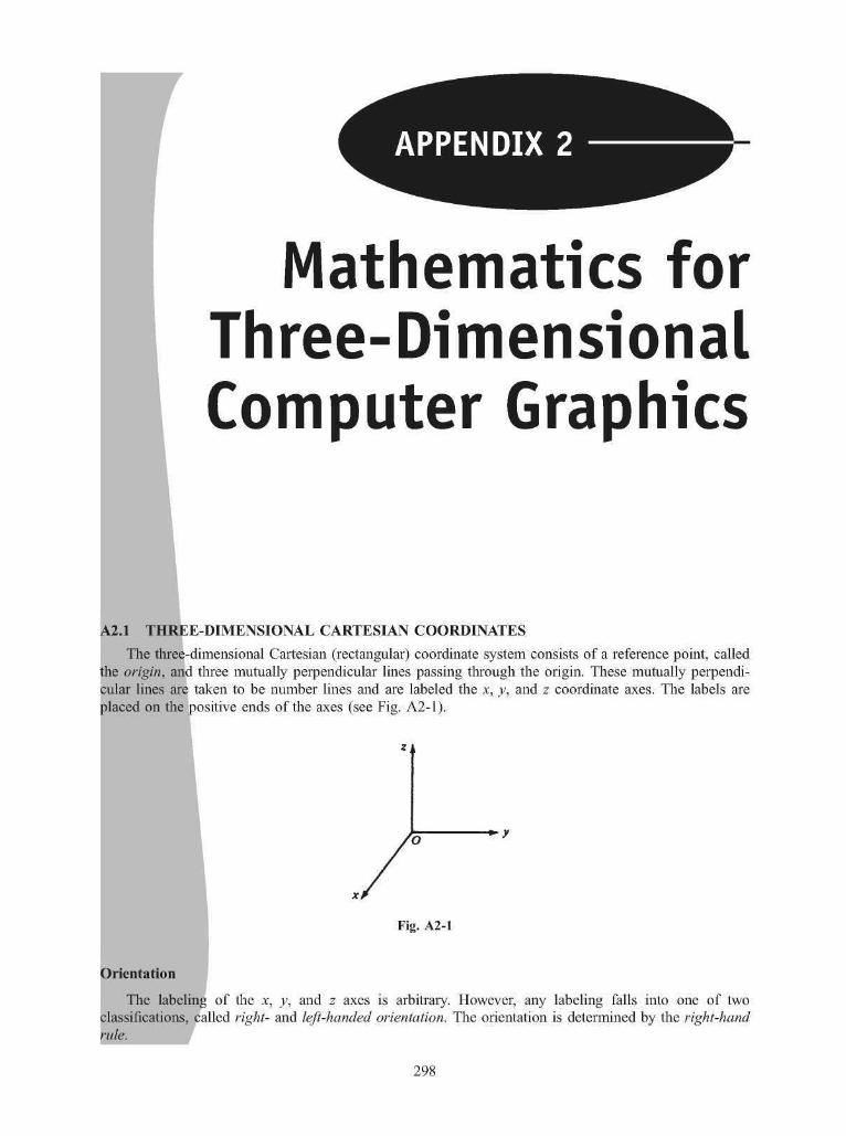
APPENDIX 2
Mathematics forThree-DimensionalComputer Graphics
A2.1 THREE-DIMENSIONAL CARTESIAN COORDINATES
The three-dimensional Cartesian (rectangular) coordinate system consists of a reference point, calledthe origin, and three mutually perpendicular lines passing through the origin. These mutually perpendi-cular lines are taken to be number lines and are labeled the x, y, and z coordinate axes. The labels areplaced on the positive ends of the axes (see Fig. A2-1).
Fig. A2-1
The labeling of the x, y, and z axes is arbitrary. However, any labeling falls into one of twoclassifications, called right- and left-handed orientation. The orientation is determined by the right-handrule.
298

APPENDIX 2 299
The Right-Hand Rule
A labeling of the axes is a right-handed orientation if whenever the fingers of the right hand arealigned with the positive x axis and are then rotated (through the smaller angle) toward the positive y axis,then the thumb of the right-hand points in the direction of the positive z axis. Otherwise, the orientation is aleft-handed orientation (see Fig. A2-2).
z y.
Left hand
(a) Right-handed orientation. (b) Left-handed orientation.
Fig. A2-2
Cartesian Coordinates of Points in Three-dimensional Space
Any point P in three-dimensional space can have coordinates (x,y, z) associated with it as follows:
1. Let the x coordinate be the directed distance that P is above or below the yz plane.
2. Let the y coordinate be the directed distance that P is above or below the xz plane.
3. Let the z coordinate be the directed distance that P is above or below the xy plane.
See Fig. A2-3.
z,
IP (x, y, z)
-h
y (x, y, 0)
Fig. A2-3

300 APPENDIX 2
Distance Formula
lfP0(x0,y0,z0) and Pl{xl,yl,zl) are any two points in space, the distance D between these points isgiven by the distance formula:
D = ~ xo? + (Ji - Jo)2
A2.2 CURVES AND SURFACES IN THREE-DIMENSIONS
Curves
A three-dimensional curve is an object in space that has direction only, much like a thread (see Fig.A2-4). A curve is specified by an equation (or group of equations) that has only one free (independent)variable or parameter, and the x, y, and z coordinates of any point on the curve are determined by this freevariable or parameter. There are two types of curve description, nonparametric and parametric.
z
Fig. A2-4
1. Nonparametric curve description.
(a) Explicit form. The equation for curve C are given in terms of a variable, say, x, as
C: y=f(x) z = g(x)
That is, y and z can be calculated explicitly in terms of x. Any point P on the curve hascoordinates P[x,f(x), g(x)].
(b) Implicit form. The equations of the curve are F(x, y, z) = 0 and G(x, y, z) = 0. Here, y and zmust be solved in terms of x.
2. Parametric curve description. The three equations for determining the coordinates of any point onthe curve are given in terms of an independent parameter, say, t, in a parameter range [a, b], whichmay be infinite:
x =f(t)C- y = g(t), a < t < b
z = h(t)

APPENDIX 2 301
Any point P on the curve has coordinates [f(t), g(t), h(t)].
• Equations of a straight line. The equations of a line L determined by two points P0(x0,>>0, z0) andPl(xl,yl,zl) are given by:
nonparametric form
L:
y = m,X-
z = nijx + bj =
y\ -y
zi ~zo
*i ~x0
x +
parametric form
x = x0 - xo)f
V *i - *o
Z A X , - Z ,
*i - ^ o
z = zo
Note that when t = 0, then x = x0, y = y0, and z = z0. When f = 1, then x = x1; y = yx, andz = zl. Thus, when the parameter t is restricted to the range 0 < t < 1, the parametric equationsdescribe the line segment P0Pi.
Surfaces
A surface in three-dimensional space is an object that has breadth and width, much like a piece of cloth(see Fig. A2-5).
Fig. A2-5
A surface is specified by an equation (or group of equations) that has two free (or independent)variables or parameters. There are two types of surface description, nonparametric and parametrics.
1. Nonparametric surface description
(a) Explicit form. The z coordinate of any point on the surface S is given in terms of two freevariables x and y, that is, z=/(x,_y). Any point P on the surface has coordinates[x,y,f(x,y)].

302 APPENDIX 2
(b) Implicit form. The equation of the surface is given in the form F(x, y, z) = 0. Here, z is to besolved in terms of x and y. There is no restriction as to which variables are free. Theconvention is to represent z in terms of x andy, but nothing disallows a representation of x interms of y and z or y in terms of x and z.
2. Parametric description. The three equations for determining the coordinates of any point on thesurface S are described in terms of parameters, say, s and t, and in parameter ranges [a, b] and[c, d], which may be infinite:
x =f(s, t),S: y = g(s,t),
z = h(s, t)
a < s < bc <t < d
The coordinates of any point P on the surface have the form [f(s, t), g(s, t), h(s, t)].
Equations of a plane. The equation of a plane can be written in explicit form as z = ax + by + cor in implicit form as Ax + By + Cz + D = 0 (see Prob. A2.8). The equation of a plane is linearin the variables x, y, and z. A plane divides three-dimensional space into two separate regions.The implicit form of the equation of a plane can be used to determine whether two points areon the same or opposite sides of the plane. Given the implicit equation of the planeAx + By + Cz + D = 0, let f(x, y, z)=Ax + By+Cz + D. The two sides of the plane R+, R~are determined by the sign of f(x,y, z); that is, point P(xo,>>o,zo) lies in region R+ iff(xo,yo,zo) > 0 and in region R~ iff(x0,y0,z0) < 0. lff(xo,yo,zo) = 0, the point lies on theplane. The equations x = 0, y = 0, and z = 0 represent the yz, xz, and xy planes, respectively.Quadric surfaces. Quadric surfaces have the (implicit) form Ax2 + By2 + Cz2 + Dxy + Exz +Fyz + Gx + Hy + Iz + J = 0. The basic quadric surfaces are described in Chap. 9.Cylinder surfaces. In two dimensions, the equation y =f(x) represents a (planar) curve in the xyplane. In three dimensions, the equation y =f(x) is a surface. That is, the variables x and z arefree. This type of surface is called a cylinder surface (see Fig. A2- 6).
z
r
Fig. A2-6
EXAMPLE 1. The equation x2 +y2 = 1 is a circle in the xy plane. However, in three dimensions, it represents acylinder (see Fig. A2-7).

APPENDIX 2 303
Fig. A2-7
A2.3 VECTORS IN THREE-DIMENSIONSThe definition of a vector and the concepts of magnitude, scalar multiplication, and vector addition are
completely analogous to the two-dimensional case in App. 1.In three-dimensions, there are three natural coordinate vectors I, J, and K. These vectors are unit
vectors (magnitude 1) having the direction of the positive x, y, and z axes, respectively. Any vector V canbe resolved into components in terms of I, J, and K: V = a\ + hi + cK.
The components [a, b, c] of vectors V are also the Cartesian coordinates of the head of the vector Vwhen the tail of V is placed at the origin of the Cartesian coordinate system (see Fig. A2-8).
i (a, b. c)
Fig. A2-8
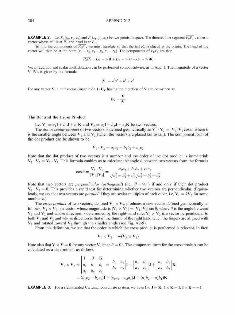
304 APPENDIX 2
E X A M P L E 2 . Le tP 0 (x 0 , j ; 0 , z 0 ) andP\(xi,yi,zi) be two points in space. The directed line segment P 0 P ] defines avector whose tail is at PQ and head is at P j .
To find the components of PQP\ , we must translate so that the tail PQ is placed at the origin. The head of thevector will then be at the point (xj — x0 , y\ — y§,z\ — zQ). The components of PQP\ are then
P ^ = (xj - xo)I + (y1- yo)J + (zx - zo)K
Vector addition and scalar multiplication can be performed componentwise, as in App. 1. The magnitude of a vectorV, |V|, is given by the formula
|V| = Vfl2 + b2 + c2
For any vector V, a unit vector (magnitude 1) U v having the direction of V can be written as
The Dot and the Cross Product
Let Vj = ajl + bl J + CjK and V2 = a2\ + b2i + c2K be two vectors.The dot or scalar product of two vectors is defined geometrically as \ l • V2 = \Vl ||V2 cos 6, where 6
is the smaller angle between Vj and V2 (when the vectors are placed tail to tail). The component form ofthe dot product can be shown to be
Vi • V2 = axa2 + bxb2 + cxc2
Note that the dot product of two vectors is a number and the order of the dot product is immaterial:Vj • V2 = V2 • Vj. This formula enables us to calculate the angle 6 between two vectors from the formula
V, -V, a, a-, + bd
IV! ||V;
Note that two vectors are perpendicular {orthogonal) (i.e., 6 = 90°) if and only if their dot productVj • V2 = 0. This provides a rapid test for determining whether two vectors are perpendicular. (Equiva-lently, we say that two vectors are parallel if they are scalar multiples of each other, i.e, \ l = kV2 for somenumber k.)
The cross product of two vectors, denoted Vj x V2, produces a new vector defined geometrically asfollows: Vj x V2 is a vector whose magnitude is |V1 x V2 | = |V1 ||V2| sinO, where 6 is the angle betweenVj and V2 and whose direction is determined by the right-hand rule: Vj x V2 is a vector perpendicular toboth Vj and V2 and whose direction is that of the thumb of the right hand when the fingers are aligned withVj and rotated toward V2 through the smaller angle (see Fig. A2-9).
From this definition, we see that the order in which the cross product is performed is relevant. In fact:
V! x V2 = - (V 2 x Vr)
Note also that V x V = 0 for any vector V, since 0 = 0°. The component form for the cross product can becalculated as a determinant as follows:
V, x V, =
I
ax
a2
J
b]
b2
K
C2
=b\
b2
ci
C2I — a2
c\J+
(cjfl2 — c2flj)J + {alb2 — a2
K
E X A M P L E 3 . For a right-handed Cartesian coordinate system, we have I x J = K, J x K = I, I x K = —J.

APPENDIX 2 305
V . J V
Fig. A2-9
The Vector Equation of a Line
A line L in space is determined by its direction and a point PQ(X0, y0, z0) that the line passes through. Ifthe direction is specified by a vector V = a\ + bJ + cK and if P(x, y, z) is any point on the line, thedirection of the vector P0P determined by the points Po, and P is parallel to the vector V (see Fig. A2-10).Thus, P0P = tV for some number t.
Fig. A2-10

306 APPENDIX 2
In component form, we find that (x — xo)I + (y — yo)J + (z — zo)K = ta\ + tbi + tcK. Comparison ofcomponents leads to the parametric equations:
x = xn + at bt z = zn+ct
In Probs. A2.5 and A2.6 it is shown how the equations of a line are determined when given two pointson the line.
The Vector Equation of a Plane
A vector N is said to be a normal vector to a given plane if N is perpendicular to any vector V whichlies on the plane; that is, N • V = 0 for any V in the plane (see Fig. A2-11). A plane is uniquely determinedby specifying a point P0(x0,y0, z0) that is on the plane and a normal vector N = «jl + n2J + «3K. LetP(x, y, z) be any point on the plane. Then the vector P0P lies on the plane. Therefore, N is perpendicular toit. So N • P^P = 0.
Fig. A2-11
In component form, we obtain
[nx\ + «2J + «3K] • [(x - xo)I + (y- yo)J + (z - zo)K] = 0
nx(x - x0) + n2(y-y0) + «3(z - z0) = 0
The equation of a plane can also be determined by specifying (1) two vectors and a point (Prob. A2.10) and(2) three points (Prob. A2.11). Using vector notation, we can write the distance D from a point P(x, y, z) toa plane as
or
[»i(* ~ *o) + n2(y - y0) + «3(z - z0)] |N • P0P|
where N = «jl + «2J + n^ is a normal vector to the plane andi->0(x0,_v0,z0) is a point on the plane (Prob.
A2.13).

APPENDIX 2 307
A2.4 HOMOGENEOUS COORDINATES
The Two-dimensional Projective Plane
The projective plane was introduced by geometers in order to study the geometric relationships offigures under perspective transformations.
The two-dimensional projective plane P3 is defined as follows.In three-dimensional Cartesian space, consider the set of all lines through the origin and the set of all
planes through the origin. In the projective plane, a line through the origin is called apoint of the projectiveplane, while a plane through the origin is called a line of the projective plane.
To see why this is "natural" from the point of view of a perspective projection, consider theperspective projection onto the plane z = 1 using the origin as the center of projection. Then a line throughthe origin projects onto a point of the plane z = 1, while a plane through the origin projects onto a line inthe plane z = 1 (Fig. A2-12).
Lini;
Fig. A2-12
In this projection, lines through points (x,y, 0) in the plane project to infinity. This leads to the notionof ideal points, discussed later.
Homogeneous Coordinates of Points and Lines of the Projective Plane
If (a, b, c) is any point in Cartesian three-dimensional space, this point determines a line through theorigin whose equations are
x = at
y = bt (where t is a number)
z = ct
That is, any other point {at, bt, ct) determines the same line. So two points (alt bx, c{) and (a2, b2, c2), areon the same line through the origin if there is a number t so that
a2 = b2=blt (A2.1)

308 APPENDIX 2
We say that two triples, (alt bx, c{) and (a2, b2, c2), are equivalent (i.e., define the same line through theorigin) if there is some number t so that the equations (A2.1) hold. We write (al, bl, Cj) ~ (a2, b2, c2). Theequivalence classes of all triples equivalent to (a, b, c), written as [a, b, c], are the points of the projectiveplane. Any representative (a1; 61; Cj) equivalent to (a, b, c) is called the homogeneous coordinate of thepoint [a, b, c] in the projective plane.
The points of the form (a, b, 0) are called ideal points of the projective plane. This arises from the factthat lines in the plane z = 0 project to infinity. In a similar manner, any plane through the origin has anequation nxx + n^ + «3z = 0. Note that any multiple knxx + kn^ + kn3z = 0 defines the same plane.
Any triple of numbers (nl,n2,n3) defines a plane through the origin. Two triples are equivalent,(«1; n2, «3) ~ (dlt d2, <f3) (i.e., define the same plane), if there is a number k so that dl = knl, d2 = kn2,and <f3 = kn3. The equivalence classes of all triples, \nx, n2, «3], are the lines of the projective plane. Anyrepresentative (dlt d2, <f3) of the equivalence class \nx, n2, «3] is called the homogeneous line coordinate ofthis line in the projective plane.
The ambiguity of whether a triple (a, b, c) represents a point or a line of the projection plane isexploited as the Duality Principle of Projective Geometry. If the context is not clear, one usually writes(a,b,c) to indicate a (projective) point and [a,b,c] to indicate a (projective) line.
Correlation between Homogeneous and Cartesian Coordinates
If(xl,yl,zl), Zj ^ 0 are the homogeneous coordinates of a point of the projective plane, the equationsx = Xj/zj a n d j = j 1 / z 1 define a correspondence between points P1(x1,iy1, z{) of the projective plane andpoints P(x, y) of the Cartesian plane.
There is no Cartesian point corresponding to the ideal point {xx, yx, 0). However, it is convenient toconsider it as defining an infinitely distant point.
Also, any Cartesian point P(x,y) corresponds to a projective point P(xl,yl,zl) whose homogeneouscoordinates are xl = x, yl = y, and zl = 1. This correspondence between Cartesian coordinates andhomogeneous coordinates is exploited when using matrices to represent graphics transformations. The useof homogeneous coordinates allows the translation transformation and the perspective projectiontransformation to be represented by matrices (Chaps. 6 and 7).
To conform to the use of homogeneous coordinates, 2 x 2 matrices representing transformations of theplane can be augmented to use homogeneous coordinates as follows:
AX =
Finally, note that even though we have a correspondence between the points of the projective plane andthose of the Cartesian plane, the projective plane and the Cartesian plane have different topologicalproperties which must be taken into account in work with homogeneous coordinates in advancedapplications.
Three-dimensional Projective Plane and Homogeneous Coordinates
Everything stated about the two-dimensional projective plane and homogeneous coordinates may begeneralized to the three-dimensional case. For example, if / ^ ( x ^ y ^ z j , w{) are the homogeneouscoordinates of a point in the three-dimensional projective plane, the corresponding three-dimensionalCartesian point P(x, y, z) is, for wx ^ 0,
_X]_ _y±_ _z±_
w, w, w.
APPENDIX 2 309
In addition, if P(x, y, z) is a Cartesian point, it corresponds to the projective point P(x, y, z, 1). Finally,3 x 3 matrices can be augmented to use homogeneous coordinates:
3 x 3
0 0 0 1
Solved Problems
A2.1 Describe the space curve whose parametric equations are x = cost, y = sin?, and z = t.
SOLUTION
Noting that x2 + y1 = cos2 t + sin2 t = 1 (see Fig. A2-13), we find that the x, y variables lie on a unitcircle, while the z coordinate varies. The curve is a (cylindrical) spiral.
Fig. A2-13
A2.2 Find the equation of a sphere of radius r centered at the origin (0,0,0).
SOLUTION
Let P(x, y, z) be any point on the sphere. Then the distance D between this point and the center of thesphere is equal to the length of the radius r. The distance formula yields
/ (x -0 ) 2 + (y -0 ) 2 + ( z - 0 ) 2 = r or
This is the (implicit) equation of the sphere.
A2.3 Show that V • V = |V|2 for any vector V.
SOLUTION
If V = al + b3 + cK, then
V • V = (al + b3 + cK) • (al + bJ + cK) = a2 + b2 + c2 = | V|2
A2.4 Let V! = 21 - J + K and V2 = I + J - K. Find (a) the angle between V! and V2, (b) a vectorperpendicular to both Vj and V2, and (c) a unit vector perpendicular to both Vj and V2.

310 APPENDIX 2
cos6=\tw2
SOLUTION
(a) We use the formula
Now
and
Vj • V2 = (2)(1) + (-1)(1) + (1)(-1) = 0
Thus cos 8 = 0, and so 8 = 90°. So the vectors are perpendicular.(b) The vector Vj x V2 is perpendicular to both Vj and V2. So
I J K
= A/22 + (-1)2 + (I)2 = V6 |V2| = V I2 + I2 + (-1)2 = V3
V, x V, = 2 - 1 11 1 1
—- 1
1
1
1I -
2
1
1
1 J +2
1
- 1
1K = - 2 I - J + 3 K
(c) Since Vj x V2 is perpendicular to both Vj and V2, we find a unit vector having the direction of Vj x V2
This is
u -v ' x V 2
| V l X V 2 |From part (b), we have
So
V 2 | = V ( - 2 ) 2 + ( - 1 ) 2 + (3)2 = VT4
T4 VT4
A2.5 Find the equation of the line passing through two points P0(x0,y0, z0) and Pl(xl ,y\,zx).
SOLUTION
To find the equation of a line, we need to know a point on the line and a vector having the direction of theline. The vector determined by Po and Pu P0Pi clearly has the direction of the line (see Fig. A2-14), and pointPQ lies on the line, so with direction vector
PoPi = (*! - xo)I +(yl- yo)J + (Zl - zo)K
and point P0(x0,^0, z0), the equation is
x = x0 + (xj - xo)t y = y0 + (yx - yo)t z = z(s + (zl- zo)t
A2.6 Find the equation of the line passing through P0(l, —5, 2) and P\(6,1, —3).
SOLUTION
From Prob. A2.5, the direction vector is
P P7 = (6 - 1)1 + [7 - (-5)]J + (-3 - 2)K = 51 + 12J - 5K.
Using point P0(l, - 5 , 2), we have x = 1 + 5t, y = - 5 + I2t, and z = 2 - 5t.
A2.7 Let line segment Lj be determined by points Pi(ai , 61, cj) and Pi(aii 2> C2)- Let line segment L2

APPENDIX 2 311
Fig. A2-14
be determined by points Q\{u,\, vlt w{) and Q2(u2, V2> wi)- How can we determine whether the linesegments intersect?
SOLUTION
The parametric equations of Lx are (Prob. A2.5)
x = ax + (a2 — ax)s
y = bx +(b2-bx)s
z = cx +(c2 -cx)s
The equations of L2 are
X = Ux + («2 — M l ) f
z = wx+(w2- wx)t
Equating, we find
(«2 — ux)t — (a2 — ax)s = ax — ux
(v2 - vx)t - (b2 - bx)s = bx-vx
(w2 — wx)t — (c2 — cx)s = cx — wx
Using the first two equations, we solve for s and t:
t _ ( b \ - "i)(fl2 ~ fli) ~ (fli ~ u\)(b2 ~ b\)
(a2 - ax)(v2 -vx)-(b2- bx)(u2 - ux)
_ (bx - vx)(u2 - ux) - (ax - ux)(v2 - vx)
(a2 - ax)(v2 - vx) - (b2 - bx)(u2 - ux)
We now substitute the s value into equation Lx and the t value into equation L2. If all three correspondingnumbers x, y, and z are the same, the lines intersect; if not, the lines do not intersect. Next, if both 0 < s < 1and 0 < t < 1, the intersection point is on the line segments Lx and L2, between Px and P2 and Qx and Q2.
A2.8 Show that the equation of a plane has the implicit form Ax + By + Cz + D = 0, where A, B, and Care the components of the normal vector.

312 APPENDIX 2
SOLUTION
The equation of a plane with normal vector N = A\ + B3 + CK and passing through a pointpo(xo,yo,zo) is
A(x - x0) + B(y - yQ) + C(z - z0) = 0 or Ax + By + Cz + (-AxQ - ByQ - CzQ) = 0
Calling the quantity D = (— Ax0 — By0 — Cz0) yields the equation of the plane:
Ax + By + Cz + D = 0
A2.9 Given the plane 5x — 3y + 6z = 7: (a) find the normal vector to the plane, and (b) determinewhether P ^ l , 5, 2) and P2(—3, —1, 2) are on the same side of the plane.
SOLUTION
Write the equation in implicit form as 5x — 3y + 6z — 7 = 0.
(a) From Prob. A2.8, the coefficients 5, —3, and 6 are the components of a normal vector, that is,N = 51 - 3 J + 6K.
(b) Let/(x, y, z) = 5x — 3y + 6z — 7. The plane has two sides, R+ where/(x, y, z) is positive and R~ wheref(x,y,z) is negative. Now for point Pi(l, 5, 2), we have
/ ( I , 5, 2) = 5(1) - 3(5) + 6(2) - 7 = - 5
and for point P2(-3, -1,2),
/ ( - 3 , -1,2) = 5(-3) - 3(- l) + 6(2) - 7 = - 7
Since both / ( I , 5, 2) and/(—3, —1, 2) are negative, Px and P2 WQ o n m e same side of the plane.
A2.10 Find the equation of a plane passing through the point P0(l, —1,1) and containing the vectorsV! = I - J + K and V2 = - I + J + 2K (see Fig. A2-15).
V,xV2 = N
Fig. A2-15
SOLUTION
To find the equation of a plane, we need to find a normal vector perpendicular to the plane. Since Vj andV2 are to lie on the plane, the cross product Vj x V2 perpendicular to both Vj and V2 can be chosen to be the
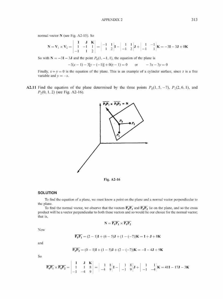
APPENDIX 2 313
normal vector N (see Fig. A2-15). So
N = V] x V2 =I
1- 1
J
- 11
K
12
=- 1
112 I -
1- 1
12 J +
1- 1
- 11
K = - 3 I - 3 J + OK
So with N = —31 — 3J and the point P0(l, — 1, 1), the equation of the plane is
- 3 ( x - l ) - 3 [ y - ( - l ) ] + 0 ( z - 1) = 0 or - 3x - 3y = 0
Finally, x + y = 0 is the equation of the plane. This is an example of a cylinder surface, since z is a freevariable and y = —x.
A2.l l Find the equation of the plane determined by the three points P 0 ( l , 5 , —7), P1(2,6, 1), andP2(0, 1,2) (see Fig. A2-16).
Fig. A2-16
SOLUTION
To find the equation of a plane, we must know a point on the plane and a normal vector perpendicular tothe plane.
To find the normal vector, we observe that the vectors PoPi and P0P2 lie on the plane, and so the crossproduct will be a vector perpendicular to both these vectors and so would be our choice for the normal vector:that is,
Now
and
So
N = P0P! X P0P2
• = (2 - 1)1 + (6 - 5)J + (1 - (-7))K = I + J + 8K
P0P2 = (0 - 1)1 + (1 - 5)J + (2 - (-7))K = - I - 4J + 9K
P0P2
I1
- 1
J1
- 4
K
OO
O
S
=1
- 489
I - 1 8- 1 9
J + 1- 1
1- 4
K = 4 1 I - 1 7 J - 3 K

314 APPENDIX 2
So N = 411 - 17J - 3K, and with point P0(l, 5, -7), the equation of the plane is
41(x- 1 ) - 1 7 ( y - 5 ) - 3 [ z - ( - 7 ) ] = 0 or 41x - 17.y - 3z + 23 = 0
A2.12 Show that the equation of the plane that has x, y, and z intercepts A(a, 0, 0), B(0, b, 0), andC(0, 0, c), respectively, is (see Fig. A2-17) x/a + y/b +z/c = 1.
z
Fig. A2-17
SOLUTION
As in Prob. A2.11 , we form the vectors A B = —a\ + bj and A C = —a\ + cK. The normal vector to theplane is then
N = AB x AC =
I J K-a b 0 =—
b
0
0
cI -
—a
—a
0
cJ +
—a
—a
b
0K = bc\ + ad + abK
-a 0 c
The equation of the plane with this normal vector and passing through A (a, 0, 0) is
bc(x — a) + ac(y — 0) + afr(z — 0) = 0 or bcx + acy + afe = abc
Dividing both sides by abc, we have x/a + y/b + z/c = 1.
A2.13 Find the distance from a point Pl(xl,yl,zl) to a given plane (see Fig. A2-18).
SOLUTION
Let N = Mjl + «2J + M3K be the normal vector to the plane, and let P0(x0,^0, z0) be any point on theplane. The equation of the plane is
«i (x ~ xo) + nib> ~ y - zo) = 0
The distance D from P-l(x-l,y-l,z-l) to the plane is measured along the perpendicular or normal to the plane.Let LN be the line through Pj (xj ,y^,z{) and having the direction of the normal vector N. The equation of
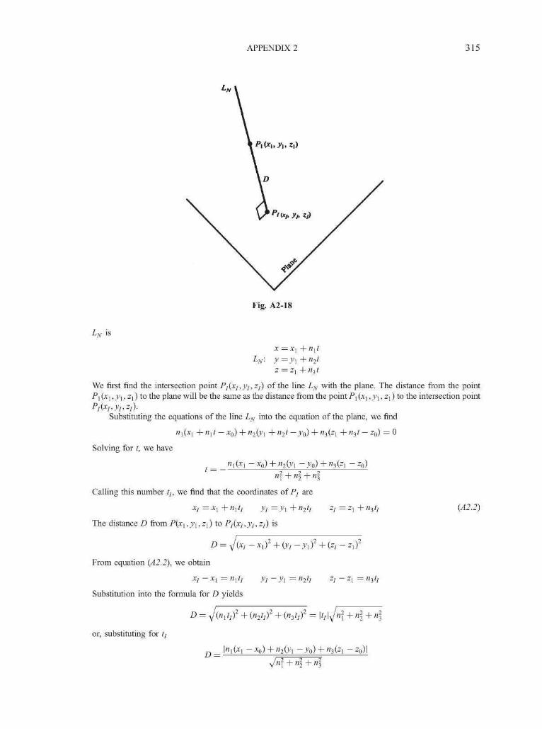
APPENDIX 2 315
Fig. A2-18
LN is
x = Xj + nxtLN: y =yx +n2t
z = zx+n3t
We first find the intersection point P1(x1,y1,z]) of the line LN with the plane. The distance from the pointPx (xj, yx, Zj) to the plane will be the same as the distance from the point Px {xx, yx, zx) to the intersection point
Substituting the equations of the line LN into the equation of the plane, we find
nx(xx + nxt - x0) + n2(yx + n2t -yQ) + n3(zx + n3t - z0) = 0
Solving for t, we have
n\(x\ ~ xo) + "2(^1 - ^o) + W3(zl ~ zo)
«f + « + n\
Calling this number tj, we find that the coordinates of Pj are
xj=xx+ nx tj yI=yx+ n2tj zj=zx+ n3tj (A2.2)
The distance D from P(xx,yx,zx) to P1(x1,y1,z]) is
D = J(Xl - xxf + (yj -yxY
From equation (A2.2), we obtain
Xj-xx =nxtj
Substitution into the formula for D yields
D =
or, substituting for tj
yi-yx= n2t Z!-zx= n3t3tj
D =\nx(xx - x0) + n2(yx -y0) + n3(zx - zo)\

316 APPENDIX 2
We can rewrite this in vector form by observing that
and that (xj — xo,y^ —ya,Zi — z0) are the components of the vector PoPi- SoI A
D =
where d= |N-P0Pi|.
A2.14 Find the projection Vp of a vector V onto a given plane in the direction of the normal vector N.
SOLUTION
From Fig. A2-19, by the definition of (head-to-tail) vector addition (see App. 1), we have
= V or Vp = V - £N
Nl
Fig. A2-19
To find the number k, we use the fact that Vp lies on the plane, so N is perpendicular to Vp, i.e., Vp • N = 0.So
0 = Vp • N = V • N - k(N • N) or k =V-N V-NN - N |N|2 (since N • N = |N|2)
Then
V p = V - (A2.3)
A2.15 Let a plane be determined by the normal vector N = I — J + K and a point PQ(2, 3 — 1).
(a) Find the distance from point P^(5, 2, 7) to the plane.

APPENDIX 2 317
(b) Let V = 21 + 3 J — K be a vector. Find the projection of Vp (in the direction of the normal) onto theplane.
SOLUTION
(a) The vector P , ^ = 31 - J + 8K. From Prob. A2.13 we have
_ IN-PpPtl
|N| ( 1 ) 2 + ( _ 1 ) 2 + ( 1 ) 2
12
V3
(b) From Prob. A2.14, the projection vector Vp is given by
Now
So
lN|2
V • N _ (2)(1) + (3)( - l ) + ( - ! ) ( ! ) _ - 2INi2 (u2 _i_ c _ n 2 + m 2 3
= (2I + 3 J - K ) - ( - f l + § J - § K ) = f l + | j - ± K
A2.16 Given vectors A and B that are placed tail to tail we define the perpendicular projection of A onto Bto be the vector V shown in Fig. A2-20. Find a formula for computing V from A and B.
Fig. A2-20
SOLUTION
We first find (see Fig. A2-20)
= |A|cos(0) =A B A B
Using the unit vector
V = |V|UV
Since V and B have the same direction, we have U v = UB. Hence
A2.17 Let (3,1, —3) be the coordinate of point A. Find a point B on the line y = 2x in the xy plane suchthat the line connecting A and B is perpendicular to y = 2x.

318 APPENDIX 2
SOLUTION 1
Since point B is on y = 2x, it has coordinates (x, 2x, 0). We introduce two vectors \ 1 and V2 (see Fig.A2-21):
Vt = xl + 2xJ
V2 = (3 - x)I + (1 - 2x)J - 3K
The line connecting A and B is perpendicular to y = 2x if
\t-\2=0
or
x(3-x) + 2x(l -2x) = 0
This yields x(l — x) = 0. Since the angle between the line y = 2x and the line from the origin to point A isverifiably not 90°, we have i / O . Hence x = 1, and the coordinates of point B are (1,2,0).
' y = 2x
Fig. A2-21
SOLUTION 2
Referring to Fig. A2-21, let A be a vector whose tail is at the origin and whose head is at point A. FromProb. A2.16, we can see that Vj is simply the perpendicular projection of A onto \ 1 itself. SinceA = 31 + J — 3K and \1=xl + 2x3, the projection V = \ 1 is given by
+ 2xJ) = I + 2J
This means that the coordinates of point B are (1,2,0).
A2.18 Let a = |A| and b = |B|. Show that the vector
bisects the angle between A and B.
SOLUTION 1
C =aB + bA
a + b
flB + bA ab\3B + ba\3A
a + b a + bab
a + b(
Since vector C is in the direction of the diagonal line of the diamond figure formed by the two unit vectors UA
and UB (see Fig. A2-22), it bisects the angle between UA and UB, which is also the angle between A and B.
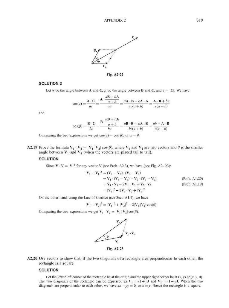
APPENDIX 2 319
Fig. A2-22
SOLUTION 2
Let a be the angle between A and C, ji be the angle between B and C, and c = |C|. We have
aB + bA
cos(a) =A C A--
and
cos(jS) =B C
aB + bAB •
aA-B + bA- A A-B + baac(a + b) c(a + b)
aB-B + bA-B ab + A-B
be be bc(a + b) c(a + b)
Comparing the two expressions we get cos(a) = cos(/?), or a = /?.
(Prob. A1.20)(Prob. A1.19)
A2.19 Prove the formula Vj • V2 = |Vj ||V2| cos(0), where Vj and V2 are two vectors and 6 is the smallerangle between Vj and V2 (when the vectors are placed tail to tail).
SOLUTION
Since V • V = |V|2 for any vector V (see Prob. A2.3), we have (see Fig. A2- 23):
|V 1 -V 2 | 2 = ( V 1 - V 2 ) - ( V 1 - V 2 )
= Vj • (Vj - V 2 ) - V 2 • (Vj - V2)
= V 1 - V 1 - 2 V 1 - V 2 + V 2 - V 2
= |V 1 | 2 -2V 1 -V 2 + |V2|2
On the other hand, using the Law of Cosines (see Sect. Al.l), we have
IVi - V2|2 = |V! |2 + |V2|2 - 2|V1||V2|cos(0)
Comparing the two expressions we get Vj • V2 = |V1||V2| cos(£>).
1 v - v
A2.20 Use vectors to show that, if the two diagonals of a rectangle area perpendicular to each other, therectangle is a square.
SOLUTION
Let the lower left corner of the rectangle be at the origin and the upper right corner be at (x, y) or (x, y, 0).The two diagonals of the rectangle can be expressed as \1=xl+ yJ and V2 = xl — yj. When the twodiagonals are perpendicular to each other, we have xx — yy = 0, or x = y. Hence the rectangle is a square.

320 APPENDIX 2
A2.21 (a) What three-dimensional line determines the homogeneous coordinate point (1,5, —1)? (b) Dothe homogeneous coordinates (1,5, —1) and (—2, —10, —3) represent the same projective point?
SOLUTION
(a) The line passes through the origin (0,0,0) and the Cartesian point (1, 5, —1). So x = t, y = 5t, andz = — t is the equation of the line.
(b) The homogeneous coordinates represent the same projective point if and only if the coordinates areproportional, i.e., there is some number t so that —2 = (\)t, —10 = (5)t, and —3 = (—l)t. Since there isno such number, these coordinates represent different projective points.

Answers to Supplementary ProblemsChapter 2
2.42 No, since there is a change in aspect ratio (5/3.5 ^ 6/4).
2.43 Yes, since 5.25/3.5 = 6/4 = 1.5.
2.44 Present the image at an aspect ratio that is lower than the original.
2.45 int i,j, c, rgb\}\,for (j = 0; j < height; j++)
for (z = 0; z < width; z++) {getPixel(z, j , rgb);c = 0.299*rgb[0] + 0.587*rgb[l] + O.l44*rgb[2];setPixel(z, j , c):
Chapter 3
3.35
3.36
3.37
(a) y = 4x + 3
11
31
7
X
2
7
1
(c) y = —3x
- 1 0
- 2 5
- 7
- 4 X
2
7
1
v = lx + 0
2
7
1
id) y = -2xH
- 3
- 1 3
- 1
-1 X
2
7
1
d = Inc\ — dx
1. Compute the initial values. Prior to passing the variables to the line plotting routine, we exhange x and ycoordinates, (x, y) giving (y, x).
dx = yi — y2 Inc\ = 2dydy = Xj — x2 Inc2 = 2(dy — dx)
2. Set (x,y) equal to the lower left-hand endpoint and xend equal to the largest value of x. If dx < 0, theny = x2, x = y2, xend = yx. If dx > 0, then y = Xj, x = yx, xend = y2.
3. Plot a point at the current (y, x) coordinates. Note the coordinate values are exchanged before they arepassed to the plot routine.
4. Test to determine whether the entire line has been drawn. If x = xend, stop.
5. Compute the location of the next pixel. If d < 0, then d = d + Incl. If d > 0, then d = d + Inc2,y=y+l.
6. Increment x: x = x + 1.
7. Prior to plotting, the (x, y) coordinates are again exchanged. Plot a point at the current (x, y) coordinates.
8. Go to step 4.
1. Set the initial values: (xj,yx) = start of line; (x3,^3) =d = length of dash; c = length of blank.
2. Test to see whether the entire line has been drawn. If xj > x3, stop.
of line; a = tan !((y3 —
321

322 ANSWERS TO SUPPLEMENTARY PROBLEMS
3. Compute end of dash:
x2 = Xj + fi?cos(a)
y2 = yx + d sin(a)
4. Send (xl,yl) and (x2,j;2) to the line routine and plot dash.
5. Compute the starting point of the next dash:
Xj = x2 + c cos(a)
y\ =y2+c sin(a)
6. Go to step 2.
3.38 See Fig. S-l. Solving for 6 = n/4:
x = 2COS(TT/4) + 0 = 1.414 y= 1 sin(?r/4) + 0 = 0.7071
Solving for 6 = 3n/4:
X = 2COS(3TT/4) + 0 = - 1 . 4 1 4 y= 1 sin(37i/4) + 0 = 0.7071
Solving for 6 = 5n/4:
X = 2COS(5TT/4) + 0 = - 1 . 4 1 4 y= 1 sin(57i/4) + 0 = - 0 . 7 0 7 1
Solving for 6 = 7n/4:
x = 2COS(7TT/4) + 0 = 1.414 y = 1 sin(77i/4) + 0 = -0.7071
(-1.414,0.7071) .414,0.7071)
(-1.414, -0.7071) .414, -0.7071)
Fig. S-l
3.39 (a) Step 3 should be changed to read
•• a cos(6) - b sin(o + - ) + h
y = -\ +k

ANSWERS TO SUPPLEMENTARY PROBLEMS 323
(b) Step 3 should be changed to read
= acos(8) - bsin(8 + -\-\ +h
y = b sin(0) -\ +k
(c) Step 3 should be changed to read
x = a cos(8) - b sin( 8 + -\ +h
y = b sin(0) + a cos(# + y") + k
Note that rotating an ellipse n/2 requires only that the major and minor axes be interchanged. Therefore, therotation could also be accomplished by changing step 3 to read
x = b cos 8 y = a sin(0)
3.40 1. Set initial variables: a = radius, (h, k) = coordinates of sector center, 8X = starting angle, 82 = ending
angle, and i = step size.
2. Plot line from sector center to coordinates of start of arc: plot (h, k) to (a cos(0]) + h, a sin(0j) + k).
3. Plot line from sector center to coordinates of end of arc: plot (h, k) to (a cos(02) + h, a sin(02) + h).4. Plot arc.
3.41 When a region is to be filled with a pattern, the fill algorithm must look at a table containing the pattern beforefilling each pixel. The correct value for the pixel is taken from the table and placed in the pixel examined bythe fill algorithm.
3.42 The human brain tends to compensate for deficiencies in models. For example, although the cube shown inFig. S-2 is lacking the visual cue, convergence, it is perceived as a cube. When the choice of aliasing isinconsistent, the brain either cannot decode the model or can decode it only with difficulty because there is noone rule that can be learned to compensate for the inconsistencies of the models.
Fig. S-2
3.43 1.
2.
Initialize the edge list. For each nonhorizontal edge, find l/m(= Ax/Ay), ymax, ymin, and the x coordinateof the edge's lower endpoint.
Begin with the first scan line y.
3. If y is beyond the last scan line, stop.
4. Activate all edges with ymin = y and delete all edges for which y > ymsx.
5. Sort the intersection points by x value.
6. Fill the pixels between and including each pair of intersection points.
7. Increment x by l/m for each active edge.
8. Increment^ by 1 and go to step 3.

324 ANSWERS TO SUPPLEMENTARY PROBLEMS
3.44 Overstrike can be eliminated by checking each pixel before writing to it. If the pixel has already been writtento, no point will be written. Or better yet, design scan-conversion algorithms that do not result in overstrike.
Chapter 4
4.19
j cos 8 — sinfl \y sin 8 cos 8 J
cos(-0) -sin(-0) \ _ / cos0 sin0\sin(-0) cos(-0) j ~~ I -sin0 cos0/
Also
cosfl
/ (cos2 8 + sin2 8) (cos0sin0 - sin0cos0)\ _ / 1 0 \
Wsin0cos0-cos0sin0) (sin2 8 + cos2 8) / \ 0 1/\ (sin 8 cos 8 — cos 0 sin 8) (
Therefore, _Ke and R_g are inverse, so _K_e = R^1. In other words, the inverse of a rotation by 8 degrees is arotation in the opposite direction.
4.20 Magnification and reduction can be achieved by a uniform scaling of s units in both the X and Y directions. Ifs > 1, the scaling produces magnification. If s < 1, the result is a reduction. The transformation can be writtenas
(x, y) i—>• (sx, sy)
In matrix form, this becomes
s 0\ x0 s)\y
(a) Choosing s = 2 and applying the transformation to the coordinates of the points A, B, C yields the newcoordinates ^'(0, 0), B'(2, 2), C'(10, 4).
(fe) Here, s = i and the new coordinates are A"(0, 0), B"(\, i), C"(f, 1).
4.21 The line j ; = xhas slope 1 and y intercept (0,0). If point P has coordinates (x,y), then following Prob. 4.10 wehave
X x,jy) = (y, x)
4.22 The rotation matrix is
The translation matrix is
/V22/22
\ 0T" °

ANSWERS TO SUPPLEMENTARY PROBLEMS 325
The matrix of vertices [A B C] is
(a)
<4ii
4ii
4ii
4ii0
\i1
0
I)
and • V =
^ + 1 - ^ + 1
4i2
2
V221
So the transformed vertices are^'f h 1, — J, B'( - — + 1 , — V and C'(l, V2).
1
4iI /
r V22
V22
4i2~
V220
V2^2
V221 )
and4i 4i
I I
3V22
1 )
The transformed coordinates are A"(4l, 4l), B"(0, 4l), and C"(4l/1, 3V2/2). From this we see that theorder in which the transformations are applied is important in the formation of composed or concatenatedtransformations (see Fig. S-3). Figure S-3(b) represents the triangle of Fig. S-3(a) after application of thetransformation 7", • ^45O; Fig. S-3(c) represents the same triangle after the transformation _K45o • TY.
B
y
2 - •
I - •
y
2'
B"
C"
y \
X
(o) (b) (c)
Fig. S-3
4.23 To determine the coordinates of the displaced object from the observer's point of view, we must find thecoordinates of the object with respect to the observer's coordinate system. In our case we have performed anobject translation Ty and a coordinate system translation Tv. The result is found by the composition fy • Ty (orT • T V
(x + a\y+b-b
So the coordinates have remained the same.

326 ANSWERS TO SUPPLEMENTARY PROBLEMS
4.24 We express the general form of an equation in the x'y' coordinate system as F(x',y') = 0. Writing thecoordinate transformation in equation form as
x' = q(x, y) y' = r(x, y)
and substituting this into the expression for F, we get
F(q(x,y),r(x,y)) = 0
which is an equation in xy coordinates.
4.25
SOLUTION 1
Let
Vx = tx\ + ty3 and V2 = tx\ + ty3
We have
7 n •Ty2(x,y) = Tyi(x + tX2,y + tyi) = (x + tX2 +tXi,y + tyi + tyi)
andTr2 • TrSx^y) = Tv2(
x + lx^y + ly,) = (x + fx, +tXl,y + ty% +ty2)
Since
we also have
T, , (Y v~\ — (Y -\-t A- t v A- t -A- t 1
1 rx+r2\x^y> -Kx + % +h2^y + lyx +
ly2)
ThereforeTyx • Ty2 = Ty2 • Ty^ = Ty^
SOLUTION 2
Let
V\ = tx\ + ty 3 and V2 = tx\-\- ty23
and express the translation transformations in matrix form
/ I 0 ( , \ / I 0 tx\Tyx = I 0 1 ty\ and TVi = I 0 1 ty\
\0 0 1 / \0 0 1 /
we have
/ I 0 t \ / I 0 t \ / I 0 tX2+t\Tri-Ty2=\0 1 tn • 0 1 ^ = 0 1 f , 2 + ^
\ 0 0 1 / \ 0 0 1 / \ 0 0 1 /
and
/ I 0 fx\ / I 0 fx\ / I 0 fXl+fx\7V2 • 7V, = 0 1 ^ 0 1 ^, = 0 1 ^, + ^
\ 0 0 1 / \ 0 0 1 / \ 0 0 1 /
Also since

ANSWERS TO SUPPLEMENTARY PROBLEMS 327
we have
( 1 0 t +
o o yi iTherefore
K , - I ' l l - > - 2
4.26
SOLUTION 1
Since
sa,b • scAx> y) = ^ , A ( C X ' ^ ) = (flcx> bdy)
Sc,d • Sfl,6(x,.y) = Sc4(ax, by) = (cax, dby)
we have Sab • Sc4 = Sc4 • Sab = SacM.
SOLUTION 2
Express the scaling transformations in matrix form
a 0\ _ (c 0\ _ (ac 0) S { ) and 5 - « = ( o bd
Since
/a OWc 0
and
ac0
ca
0
0bd
0db
we have Sa>J • Sc>fl. = Sc>fl. • Sa>J = Sac>M.
4.27 Express the rotation transformations in matrix form
_ //cos(a) —sin(a) \ _ /cos(jS) — sin(jS) \a y sin(a) cos(a) y ^ \ sin(/^) cos(fi))
we have
/cos(a) — sin(a) \ /cos(/?) — sin(/?) \
\ sin(a) cos(a) / \ sin(/?) cos(fi))
/ cos(a) cos(/?) — sin(a) sin(/?) —cos(a) sin(/?) — sin(a) cos(/?) \
\ sin(a) cos(/?) + cos(a) sin(/?) —sin(a) sin(/?) + cos(a) cos(fi))
and
'cos(/?) —sin(/?) \ /cos(a) —sin(a)
sin(/?) cos(fi) / \ sin(a) cos(a) /
' cos(/?) cos(a) — sin(/?) sin(a) —cos(/?) sin(a) — sin(/?) cos(a) \
, sin(jS) cos(a) + cos(jS) sin(a) — sin(jS) sin(a) + cos(jS) cos(a) /
Using trigonometric identities
cos(a + /?) = cos(a) cos(jS) — sin(a) sin(jS)

328 ANSWERS TO SUPPLEMENTARY PROBLEMS
and
sin(a + ft) = sin(a) cos(/?) + cos(a) sin(/?)
we have
n n _n n _ { COS(lX + 0) -SUl(a + /R R R R ^
4.28 First express scaling and rotation in matrix form
0 sy
we have
j>-{s* ° \ fcos(6) -sin(0) \ _ (sx cos(0) -5xsin(0)\,sy • Ke - y 0 Sy)y sin(0) cos(0)) ~ \ sy sin(0) sycos(0)
and
_ /cos(0) -sin(0) \ (sx 0 \ _ /cos(0>x - s i n ^ ) ^9 • K,*y ~ \ S i n ( 0 ) c o s ( 0 ) J y o s y ) - y s i n ( 0 > x cos(8)sy
In order to satisfy
Ssx,sy' Re = Re' SSx,sy
we need
sy sin(0) = sin(0)sx
This yields 0 = nn, where « is an integer, or sy = sx, which means that the scaling transformation is uniform.
4.29 No, since
1 a\ (\ 0\ _ fl+ab a\ , (\ a0 l ) \ b I ) ~ \ b 1
and
1 0 \ / I a\_ 1 a \ 1 ab 1 \0 1 \b ba+l r
4.30 A rotation followed by a simultaneous shearing can be expressed as
cos(0) -sin(0) \ / I a\ _ /cos(0) - b • sin(0) a • cos(0) -sin(0)sin(0) c o s ( 0 ) ) ' \ b 1 J \sin(0) + b • cos(0) a • sin(0) + cos(0)
On the other hand, a simultaneous shearing followed by a rotation can be expressed as
1 a\ /cos(0) -sin(0) \ _ /cos(0) + a • sin(0) -sin(0) + a • cos(0)b 1 / \ sin(0) cos(0)) y b • cos(0) + sin(0) -b • sin(0) + cos(0)
In order for the two composite transformation matrices to be the same, we need
cos(0) - b • sin(0) = cos(0) + a • sin(0)
or
-b • sin(0) = a • sin(0)
which means 0 = nn, where n is an integer, or a = — b.
ANSWERS TO SUPPLEMENTARY PROBLEMS 329
4.31 Consider the following sequence of rotate-scale-rotate transformations
/cos(a) -sin(a) \ / s x 0 \ / cos(fi) -sin(jS) \_/va • o ^ • -/v# = I I ' I I ' I I
" y \ sin(a) cos(a) / \ 0 sy / \ sin(jS) cos(jS) /
/ cos(a) cos(/?)sx — sin(a) sin(/?)s — cos(a) sin(/?)s — sin(a) cos(/?)sv
\ sin(a) cos(/?)sx + cos(a) sin(/?)s>, —sin(a) sin(/?)sx + cos(a) cos(/?)s>,
By equating the composite transformation matrix on the right-hand side to the matrix for a simultaneousshearing transformation
1 ab 1
we have four equations that can be solved for parameters a, /?, sx and sy.
4.32 Consider the following sequence of shearing and scaling transformations:
/ sx 0 \ / 1 0 \ (sx + a 'b • sy a • sy
By equating the composite transformation matrix on the right to
cos(0) —siA0 = I
we have
^ 9 I sin(0) cos(0)
4.33 Consider the following sequence of shearing transformations:
1 ax\ (\ 0\ (\ a2\_/l+aib (l+ai
0 1 ) ' \b \) ' \0 1 ) \ b ba2
By equating the composite transformation matrix on the right to
'cos(0) -sin(0)
we have
1 sin(0) cos(0
cos(0) - 1 , , . ..,a-i = a7 = and b = sin(0)
sin(0)
4.34 Let CTMn be the composite transformation matrix representing the concatenation of n basic transformationmatrices. We prove, by mathematical induction on n, that CTMn is always in the following form
n = 1: The basis case is true since CTMj is simply a basic transformation matrix, which fits into the giventemplate.
n = k: Suppose that CTMk is indeed in the specified form.
C T M , =

330 ANSWERS TO SUPPLEMENTARY PROBLEMS
n = k + 1: We now show that CTMj.+1 is in the same form:
( a b c\ la b c
d e / CTM,= d e f
0 0 1/ \ 0 0 1
'a-ak + b-dk a-bk + b-ek a
| d-ak + e-dk d • bk + e • ek d
0 04.35 Let P'^Xj,/]) be the transformation ofP-[(x-l,y-l) and P'2(x'2,y2) be the transformation of P2(x2,y2). Also let
the composite transformation be expressed asla b c\\0 0 \)
we have
Xj = flXj + byx + c / j = fi?Xj + eyx +f
and
X2 = ax2 + fey2 + c y2 = dx2 + ey2 +f
Now consider an arbitrary point P(x,y) on the line from Pj to P2. We want to show that the transformed P,denoted by P'(x', / ) , where x' = ax + by + c and y' = dx + ey + / , is on the line between P[ and P'2. In otherwords, we want to show
which is
dx2 + ey2 +f — dxx — eyx —f dx2 + ey2 +f — dx — ey —f
ax2 + by2 + c — axj — by^ — c ax2 + by2 + c — ax — by — c
and is
Vi —
a + byi
Since (x,y) satisfies
yi - y\ = yi - yX7 — Xi X7 — X
Z 1 Z
we have established the equality that shows P' being on the line between P[ and P'2.
Chapter 5
5.20 From Prob. 5.1 we need only identify the appropriate parameters.
(a) The window parameters are wxmin = 0, wxmax = 1, wymin = 0, and wymax = 1. The viewport parametersare uxmin = 0, uxmax = 199, vymin = 0, and vymax = 639. Then sx = 199, sy = 639, and
/199 0 0 \W=\ 0 639 0
V o o i , /(b) The parameters are the same, but the device y coordinate is now 639 — y (see Prob. 2.8) instead of the y

ANSWERS TO SUPPLEMENTARY PROBLEMS 331
value computed by W in (a)
W =199
00
0-639
0
0639
1
5.21 If sx = s , then
Inverting, we have aw = av.A similar argument shows that if the aspect ratios are equal, aw = av, the scale factors are equal, sx = s .
5.22 We form N by composing (1) a translation mapping the center (1,1) to the center ( , ) and (2) a scaling aboutC(j, 5) with uniform scaling factor s = j ^ , so
N = 'S'I/IO.I/IO.C ' 1v
5.23 Let the clipping region be a circle with center at O(h, k) and radius r. We reduce the number of candidates forclipping by assigning region codes as in the Cohen-Sutherland algorithm. To do this, we use thecircumscribed square with lower left corner at (h — r,k — r) and upper right corner at (h + r,k + r) topreprocess the line segments. However, we now have only two clipping categories—not displayed andcandidates for clipping. Next, we decide which line segments are to be displayed. Since the (nonparametric)equation of the circle is (x — h) + (y — k) = r2, the quantity K(x,y) = (x — h) + (y — k) — r1 determineswhether a point P(x,y) is inside, on, or outside the circle. So, if K < 0 for both endpoints Px and P2 of a linesegment, both points are inside or on the circle and so the line segment is displayed. If K > 0 for either Px orP2 or both, we calculate the intersection(s) of the line segment and the circle. Using parametric representa-tions, we find (App. 1, Prob. A1.24) that the intersection parameter is
-S ± VS2 - L2Cf ' = V
where
L2 = (x1-xlf + (y1-ylfS = {xx- h)(x2 - xO + Oi - k)(y2 - yx)
C = (xj - hf + (y1- kf - r2
If 0 < tj < 1, the actual intersection point(s) I(x,y) is (are)
x = x 1 + f / ( x 2 - x 1 ) ^ = ^ 1 + ^ 0 2 - ^ 1 )
So, if K > 0 for either Px or P2 (or both), we first relabel the endpoints so that Px satisfies K > 0. Next wecalculate tj. The following situations arise:
1. S2 — L2C < 0. Then tj is undefined and no intersection takes place. The line segment is not displayed.
2. S2 — L2C = 0. There is exactly one intersection. If tj > 1 or tj < 0, the intersection point is on theextended line, and so there is no actual intersection. The line is not displayed. If 0 < tj < I, P-[P2 istangent to the circle at point 7, so only I is displayed.
3. S2 — L2C > 0. Then there are two values for tj, tf, and tj. If 0 < tj, tf < 1, the line segment I~I+ isdisplayed and the segments (assuming f[ > tj) PXI~ and I+P2 are clipped. If only one value, say, tf,satisfies 0 < tf < 1, there is one actual intersection and one apparent intersection. Since in this case P2 iseither point I+ or inside the circle, P\I+ is clipped and I+P2 is displayed. Iftf, tf > 1 or tf, tj < 0, thenP\P2 is not displayed.

332 ANSWERS TO SUPPLEMENTARY PROBLEMS
5.24 Following the logic of the Sutherland-Hodgman algorithm as described in Prob. 5.14, we first clip the"polygon" P\P2 against edge AB of the window:
1. AB. We first determine which side of AB the points Px and P2 lie. Calculating the quantity (see Prob.5.13), we have
C = (x2 -x{)(y-y{) - 02 -y\)(x-X\)
With point A = (x],_yj) and point B = (x2,y2), we find C = 8 for point Pj and C = 1 for point P2. Soboth points lie on the left of AB. Consequently, the algorithm will output both Pj and P2.
1. BC. Setting pointB = (x],_yj) and C = (x2,y2), we calculate C = 13 for pointPj and C = —3 for pointP2. Thus Px is to the left of BC and P2 is to right of BC. We now find the intersection point Ix of P\P2
with the extended line BC. From Prob. A2.7 in App. 2, we have 7j = (4 j i , 31). Following the algorithm,points Px and 7j are passed on to be clipped.
3. CD. Proceedings as before, we find that C = 1 for point Px and C = 61 for point 7j. So both points lie tothe left of CD and consequently are passed on.
4. D~A. Setting point D = ( x ^ ) and.4 = (x2,y2), we find C = -3 forP1 and C = 10 for 7^ ThenPx lies tothe right of 7X4 and 7j to the left. The intersection point of P\I\ with the extended edge 7X4 is72 = (jg, 2|). The clipped line is the segment 7j72.
Chapter 6
6.9 From Prob. 6.2, we identify the parameters
Then
Av =
(4i_ - l - l43 4i43 4i43
0 -L ^
1 I I
7! 7! 7!\ 0 0 0
6.10 From Prob. 6.5, ^4VN = ^ N ' ' ^ V -l = 42,a=l,b=l,c=l.So
find Av first. From Prob. 6.2 we identify the parameters |V| = 43,
2 - 1 - 1 \
Av =
43
0
1
7!v o
4i43I
7!i7!0
V2V3
7!I
7!0
0
0
0
1

ANSWERS TO SUPPLEMENTARY PROBLEMS 333
For A^\ we have |N| = 46, k = 4l, a = 2, b = - 1 , and c = - 1 . So
/ 4i
Note that V' = A
0 0461
4i46i
4i460
- 1
4iI
4i0
46- 1
46- 1
V60
0
0
V
=A - l - Av • V = V2I -fi 41 4i—J—— K so that V = — - N . In other words, the
image of V under Ay N is not the vector N, but a vector that has the direction of N.
6.11 This follows from comparing the matrices Ay1 with Ay from Prob. 6.2.
6.12 If we place vectors V and N at the origin, then from App. 2, V x N is perpendicular to both V and N. If 8 isthe angle between V and N, then a rotation of 8° about the axis L whose direction is that of V x N and whichpasses through the origin will align V with N. So Ay N = RgL.
6.13 As in the two-dimensional case in Chap. 4, we reduce the problem of scaling with respect to an arbitrary pointPo to scaling with respect to the origin by translating Po to the origin, performing the scaling about the originand then translating back to Po. So
= r •T_
Chapter 7
7.16 From Prob. 7.5, we need to evaluate the parameters (a,b,c), (n1,n2,n3), (d,da,dx) to construct thetransformation. From the equations in Prob. 7.6, part (b) [denoting the principal vanishing points asPl(xl,yl,zl), P1(x1,y1,z1), andP3(x3 ,^3^3)], we find a = x2 (orx3), b =yx (ory3), and c =zx (orz2). Also
To find d, d0, and dx, we note (App. 2, Prob. A2.13) that the distance D from the point C(a, b, c) to the planecan be expressed as D = \d\/\TS\, where |N| is the magnitude of N. Since we need only find the direction ofthe normal N, we can assume |N| = 1. Then d = ±D. The choice ± , based on the definition of a? in Prob. 7.5,is dependent on the direction of the normal vector N, the reference point _K0, and the center of projection C.Since these are not all specified, we are free to choose, and we shall choose the + sign, that is, d = D. Finally
n2b and
7.17 We use the coordinate matrix V constructed in Prob. 7.1 to represent the unit cube.
(a) From Problem 7.14, the isometric projection matrix Par is applied to the coordinate matrix V:
Par-V =
0
0
0
Vi
3 / 2 1 / 2
2V3 2V32 1_ /2 3
3 2 V 3 2V 3
- V 2 -V2
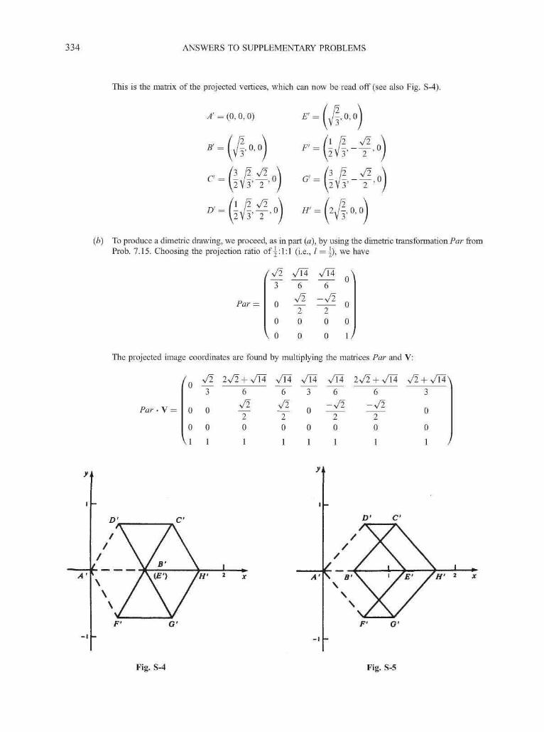
334 ANSWERS TO SUPPLEMENTARY PROBLEMS
This is the matrix of the projected vertices, which can now be read off (see also Fig. S-4).
A' = (0, 0, 0) L/3.0,0
I Jy 0- 0
•ivf'^' I 2,/-, 0, 0
(b) To produce a dimefric drawing, we proceed, as in part (a), by using the dimetric transformation Par fromProb. 7.15. Choosing the projection ratio of ^: 1:1 (i.e., / = ^), we have
414 \
2 20 0 0 0
V 0 0 0 1 /
The projected image coordinates are found by multiplying the mafrices Par and V:
vT4
Par-V =
•£0 0
0 0
VI 1
# 4 »0 0 0
1 1 1
3
0
0
1 /
Fig. S-4 Fig. S-5
ANSWERS TO SUPPLEMENTARY PROBLEMS 335
The image coordinates are (see Fig. S-5)
A' = (0, 0, 0)
/ 23 ' ''
= ( ^ l .
E'
F'
a
H'
_/4l4\ 3
(4T4~ \ 6
/2V2
I(41-
, 0 , 0 )
-V2' 2 '
+ vri46
f vT4
/
-V2' 2
0 ,0 )
7.18 Since the planes we seek are to be located at the origin, we need only find the normal vectors of these planesso that orthographic projections onto these planes produce isometric projections. In Prob. 7.14, we rotated thexyz triad first about the x axis and then about the y axis to produce an isometric projection onto the xy plane.Equivalently, we could have tilted the xy plane (and its normal vector K) to a new position, thus yielding a newview plane which produces an isometric projection with respect to the (unrotated) xyz triad. Using thisapproach to find all possible view planes, we shall use the equations from Prob. 7.14 to find the appropriaterotation angles. From the equations
sin2 flx - cos2 flx = 0 cos2 6y = \ [sin2 0y + l]
we find the solutions
sinflx = ± - — , cosflx = ± - — and sinfly = ± J - , cosdy =
From Chap. 6, Prob. 6.1, part (b), the matrix that produces the tilting is
( cos 0,, 0 sin fly \
sin flx sin 8y cosdx — sin flx cos fly—cos flx sin fly sinflx cos flx cos fly j
Applying this to the vector K = (0, 0, 1), we find the components of the tilted vector to be
x = sin fly y = — sin flx cos fly z = cosflxcosfly
Substituting the values found above, we have eight candidates for the normal vector N = xl +yj + zK, where
'-4 "4However, both N and —N define normals to the same plane. So we finally have four solutions. These are theview planes (through the origin) with normals
Chapter 8
8.11 Referring to Fig. 8-7 (and Prob. 8.4) we call CR the vector having the direction of the line from the center ofprojection C to the window corner R. Similarly, we call CL the vector to the window corner L. Then:
1. Top plane—determined by the vectors Ip and CR and the reference point Rj-
2. Bottom plane—determined by the vectors Ip and CL and the reference point Lj-
3. Right side plane—determined by the vectors Jq and CR and the reference point Rj-

336 ANSWERS TO SUPPLEMENTARY PROBLEMS
4. Left side plane—determined by the vectors Jq and CL and the reference point Lf
5. Front (near) plane—determined by the (view plane) normal vector N and the reference point Pj-
6. Back (far) plane—determined by the normal vector N and the reference point Pb
8.12 Suppose that the plane passes through point _K0(x0, j ; 0 , z0) and has a normal vector N = nx\ + n2J + n3tL Letthe points Px (xx, yx, zx) and P1(x1,y-2, z2) determine aline segment. From App. 2, the equation of the plane is
«i (x ~ xo) + nib> ~ yo) + «3(z - zo) = 0
and the parametric equation of the line is
x = xl+(x2-xl)t y = yx + (y2 - yx)t z = zx + (z2 - zx)t
Substituting these equations into the equations of the plane, we obtain
nx[xx + (x2 - xx)t - x0] + n2\yx + (y2 -yx)t -y0] + n3[zx + (z2 - zx)t - z0] = 0
Solving this for t yields the parameter value tj at the time of intersection:
t = nx(xx -xo) + n2(yx -y0) + n3(zx - z0)1 nx(x2 - xx) + n2(y2 - yx) + n3(z2 - zx)
We can rewrite this using vector notation as
The intersection points I(xj,yj, zj) can be found from the parametric equations of the line:
xj =xx +(x2-xx)tj yI=yx+(y2-yx)tI zI=zx+(z2-zx)tI
If 0 < tj < 1, the intersection point I is on the line segment from Px to P2, if not, the intersection point is onthe extended line.
Chapter 9
9.9 Referring to Fig. 7-12 in Chap. 7, we define a vertex list as
V = {ABCDEFGH}
and an explicit edge list is:
E = {AB, AD, AF, B~C, B~G, ~CD, ~CH, DE, EF, EH, FG, ~GH)
The cube can be drawn by drawing the edges in list E. Referring to Prob. 9.2, we note that a typical polygon,say, Px, can be represented in terms of its edges as
Px = (AB, AD, B~C, ~CD}
The polygons sharing a specific edge can be identified by extending the edge's representation to includepointers to those polygons. For example:
9.10 The knot set can be represented as to,to+L,to + 2L,.... On the interval ti = t0 + (i—\)L toti+2 = 10 + (i + l)L, we have
x-[to + (i-l)L] [fo + (!-+l)L]-xB(X) i ) + B ( x )B'-1(X) ~ (to + iL) - ^ + (i - \)L]'fii) + [to + (i+W - (
On the interval [£,, ti+x], that is, tQ + (;' — \)L < x < tQ + iL, we have Bt 0(x) = 1 and Bi+X 0(x) = 0. On the
interval [ti+x, ti+2], that is, tQ + iL < x < tQ + (i + l)L, we have Bt 0(x) = 0 and Bi+X 0(x) = 1. Elsewhere both

ANSWERS TO SUPPLEMENTARY PROBLEMS 337
Bu0(x) = 0 and Bi+h0(x) = 0. So
x-t0 — — on t0 + (i - \)L <x < t0 + iL
on t0 + iL < x < t0 + (i + \)L
elsewhere
9.11 From the definition of a B-spline, B,, 3(x) is nonzero only if t,• < x < ti+4. In terms of the given knot set, thisequates to i < x < i + 4. With x = 5.5, Bt 3(5.5) is nonzero for i = 2, 3, 4, and 5. Now
Starting with i = 2,
Now B2 2(x) is nonzero if 2 < x < 5. Thus B2 2(5.5) = 0, and so B2 3(5.5) = (0.5/3) 5 3 2(5.5). BecauseB3 2(x) is nonzero for 3 < x < 6, we find that
£3,2(5-5) = (555)~3
3 B3A(5.5) + 6 ~f45) ^4|1 (5.5)
Now -83 j(x) is nonzero if 3 < x < 5. So B3 x(5.5) = 0. Now B4 j(x) is nonzero if 4 < x < 6. Thus
Now
Since B4 0(x) is nonzero if 4 < x < 5, we find that _84 0(5.5) = 0. So
However, 5 5 0(x) = 1 if 5 < x < 6. So 550(5.5) = l, 541(5.5) = 0.5(1) = 0.5, and 532(5.5) =(0.5/2)(0.5) = 0.25/2, and finally
%5 (£|£) 2^5 = 0.0208333
The computations for B3 3(5.5), B4 3(5.5), and B5 3(5.5) are carried out in the same way.
Chapter 10
10.25 The properties of parallel projection can be used to simplify calculations if the objects to be projected aretransformed into "new objects" whose parallel projection results in the same image as the perspectiveprojection of the original object.
10.26 Since the Z-buffer algorithm changes colors at a pixel only if Z(x, y) < Zbuf (x, y), the first polygon written willdetermine the color of the pixel (see Prob. 10.7).
10.27 A priority flag could be assigned to break the tie resulting in applying the Z-buffer algorithm.
338 ANSWERS TO SUPPLEMENTARY PROBLEMS
10.28 A system that distinguishes 224 depth values would require three bytes of memory to represent each z value.Thus 3 x 1024 x 768 = 2304 K of memory would be needed.
10.29 The scan-line method can take advantage of (a) scan-line coherence, (b) edge coherence, (c) area coherence,and (d) spatial coherence.
10.30 Scan-line coherence is based on the assumption that if a pixel belongs to the scan-converted image of anobject, the pixels next to it will (most likely) also belong to this object.
10.31 Since this figure is a polygon, we need only find the maximum and minimum coordinate values of the verticesA, B, and C. Then
0 Y — 9
w -^max ^
J^max
^max
J^min ^ J^max
The bounding box is shown in Fig. 10-26.
10.32 Horizontal line segments (ymin = ymsK) lie on only one scan line; they are automatically displayed whennonhorizontal edges are used in the scan-conversion process.
10.33 We search the z coordinates of the vertices of the polygon for the largest value, zmax. The depth of the polygonis then zmax.
10.34 Area coherence is exploited by classifying polygons with respect to a given screen area as either a surroundingpolygon, an intersecting polygon, a contained polygon, or a disjoint polygon. The key fact is that a polygon isnot visible if it is in back of a surrounding polygon.
10.35 When using a hidden-surface algorithm to eliminate hidden lines, we set the fill color of the polygons,determined by the lines, to the background color.
Chapter 11
11.25 Let W, H, D, and P be defined in the same way as in Prob. 11.3. We can calculate saturation usingDxP/(Wx
11.26 The color-sensitive cones in our eyes do not respond well to low intensity light. On the other hand, the rodsthat are sensitive to low intensity light are color blind.
11.27 Yes. We can use
1 — x — y ' 1 — x — yX = Z, Y = Z, Z = Z
1 1
11.28 The Y in CMY means yellow, whereas the Y in YIQ represents luminance.
11.29
R R R
ANSWERS TO SUPPLEMENTARY PROBLEMS 339
11.30 The paramefric representation for the target area is
x = 6 0 < 6 <3.0y = 1.2cos((p) 0 < q> < n/2
Note the relationship between the corner points:
w = 0, w = 0 - • 0 = 0, <p = n/2
u=\, w = 0 -+ 6 = 3, cp = n/2
w = 0, w = 2 ^ 6 = 0, <p = 0
u=\, w = 2 - • 6 = 3, cp = O
Substitute these into 6 = Au + B and <p = Cw + D, we get
A = 3, B = 0, C = -n/4, D = n/2
Hence the mapping functions are
The inverse mapping functions are
6 = 3u and <P=^ — T
6 n/2-<pu = - and w =
3 n/4
Chapter 12
12.27 Let fj be the time required for the light ray to travel from A to P, and f2 be the time required for the light ray totravel from P to B (see Fig. 12-21). We have
h =-
To locate P (i.e., to determine x) such that the total travel time t = t^ + t2 is minimal, we find
dt x xB — x
dx~C2\/(XB~
dt sin(a) sin(/?)
dx c-, Co
Notice that 0 < x < x» and
These suggest that t reaches a minimum when
sin(oi)
Hence
sin(a)
c2

340 ANSWERS TO SUPPLEMENTARY PROBLEMS
12.28 Yes, these two procedures produce identical results when invoked with the same call. However, for a givendepth value the procedure in this question involves one more level of recursion than the one in the text. Hencethe procedure in Sect. 12.2 has better execution efficiency.
12.29 Find two points on the line
Use (0, —6) to be the starting point, we have
s = - 6 J
d = (1 - 0)1 + (-4 - (-6))J = I + 2J
and the parametric vector equation for the line is
L(f) = s +1d where —oo < t < +oc
12.30 Intersection of a ray with the yz plane can be determined by solving the following for t:
S + fd = yt3 + z,K
With s = xsl +ysJ + zsK and d = xdl + ydJ + zdK, we have
|
xs + txd = 0y* + tyA = ytZS + tZA = Z;
When xd = 0, the ray is parallel to the plane (no intersection). When xs = 0, the ray originates from the plane(no intersection). Otherwise, we calculate t using the first equation
If t < 0, the negative extension of the ray intersects the plane. On the other hand, if t > 0, the ray itselfintersects the plane and the coordinates yt and z, of the intersection point can be calculated from the secondand third equations.
12.31 Let s = xsl +ysJ + zsK and d = xdl +ydJ + zdK. Substitute xs + txd and ys + tyd for x and y, respectively
(xs + fxd)2 + (ys + tyAf -R2=0
Expand and regroup terms
(4 +yl)t2 + 2(Vd +y^i)t + (xt +yl)-R2 = o
or
At1 + 2Bt + C = 0
where
A=x2d+y2
d B=xsxd+ysyd C = x2s+y2
s-R2
When A = 0, the ray is parallel to the z axis and does not intersect the cylinder (the entire ray is on the cylinderif the starting point is on the cylinder). Otherwise, the solution for the quadratic equation is
with
I < 0 no intersection
= 0 ray (or its negative extension) touching cylinder> 0 two (possible) intersection points

ANSWERS TO SUPPLEMENTARY PROBLEMS 341
The last case (B2 — AC > 0) produces two t values: tx and t2.lf tx < 0 and t2 < 0, the negative extension ofthe ray intersects the cylinder (no intersection by the ray). If one of the two values is 0, the ray starts from apoint on the cylinder and intersects the cylinder only if the other value is positive. If £j and t2 differ in signs,the ray originates from inside the cylinder and intersects the cylinder once. If both values are positive, the rayintersects the cylinder twice (first enters and then exits), and the smaller value corresponds to the intersectionpoint that is closer to the starting point of the ray.
12.32 Substitute B in At2 + Bt + C = 0 with D we have
At2 + Dt + C = 0
and the solution is
-D ± V£>2 - 4ACt = 1A
Now let D = 2B, the above equation becomes
At2 + 2Bt + C = 0
and the solution is
4-connected, 428-connected, 42
Adaptive depth control, 259Adaptive supersampling, 261Aliasing, 2, 47Ambient light, 235Animation:
lookup table, 101panning, 100zooming, 100
Anti-aliasing, 2, 47, 260Anticyclic spline condition, 181Approximation, 181
Bezier—B-spline, 182Bezier-Bernstein, 181
Area coherence, 205Area sampling, 49Aspect ratio, 6Asymmetry, 48Axis, 273, 298Axonometric projections, 132
B-splines, 178interpolation, 180
Back-face removal, 200Basis (blending) functions, 177
B-splines, 178Bernstein polynomials, 179Hermite cubic polynomials, 178Lagrange polynomials, 177
Bernstein polynomials, 179Bezier-Bernstein approximation, 181Bezier-Bernstein surfaces, 184Bilevel image, 8Bilinear interpolation, 237, 246Bitmap font, 45Blending functions (see Basis functions)Boundary-fill, 42, 43Bounding box, 201Bounding volume, 259Bounding volume extension, 259Bresenham's circle algorithm, 31Bresenham's line algorithm, 27Brightness, 230Bump mapping, 240
C curve, 51Cabinet projection, 133
Canonical clipping, 155Cartesian coordinates:
correlation with homogeneous coordinates, 308three-dimensional, 298two-dimensional, 273
Cathode ray tube (CRT), 9electrostatic deflection, 10magnetic deflection, 10
Cavalier projection, 133Center of projection, 129Character size, 45
pica, 45point, 45
Chromaticity coordinates, 233CIE chromaticity diagram, 232CIE XYZ color model, 232Circle:
Bresenham's circle algorithm, 31eight-way symmetry, 29midpoint circle algorithm, 33
Circle, equation of:non-parametric, 30parametric, 31
Clamped spline, 180Clipping:
line, 91, 94, 170, 172point, 91polygon, 96three-dimensional, 155two-dimensional, 91
Clipping categories, 91Clipping planes, 155
back (far), 155front (near), 155
Clipping window, 90CMY color model, 7Cohen-Sutherland line-clipping algorithm, 91, 170Coherence, 204
area, 205edge, 204scan-line, 204spatial, 205
Color gamut mapping, 233Color map, 9Color matching functions, 232Color model:
additive, 7CIE XYZ, 232CMY, 7
342

INDEX 343
Color model (Cont.):NTSC YIQ, 234RGB, 7subtractive, 7
Complex numbers, 16Composing functions, 284Composite transformation matrix (CTM), 75, 118Compression, 15
run-length encoding (RLE), 15Computer-human interaction, 4Concave polygon, 96Connected:
4-connected, 428-connected, 42
Constant shading, 237Control electrode, 10Control points, 181Convex polygon, 96Coons surfaces, 185Coordinate system:
Cartesian coordinates, 273, 299homogeneous, 307left-handed, 299polar coordinates, 277right-handed, 299three-dimensional, 298two-dimensional, 273
Coordinate transformation, 68, 71, 117inverse, 73matrix description, 74reflection {see Reflection)rotation {see Rotation)scaling {see Scaling)translation {see Translation)viewing transformation {see Viewing
transformation)Cross product, 304Cross-section curve, 186CRT {see Cathode ray tube)CTM {see Composite transformation matrix)Curve design, 176Curve segment, 177Curved surface, 176Curves, equation of, 300
explicit form, 300implicit form, 300non-parametric, 300parametric, 300
Cyclic spline condition, 181Cylinder surface, equation of, 302
Deflection:electrostatic, 10magnetic, 10
Depth buffer {see Z-buffer)Depth buffer algorithm {see Z-buffer algorithm)
Depth comparison, 197Depth value, 199Device coordinate system, 89Diffuse reflection, 235Digital image, 6Dimetric projection, 132Direct coding, 8Direction of projection, 132Display monitor, 9Distance from a point to a plane, 306, 314Distance formula, 273, 300Distributed ray-tracing, 261Dithering, 13
dither matrix, 13dither pattern, 12
Dot product, 280, 304Double buffering, 101Dropout, 48
Edge coherence, 204Edge list, 44Electron gun, 10Ellipse:
four-way symmetry, 35midpoint ellipse algorithm, 37
Ellipse, equation of:non-parametric, 35parametric, 36
Environment mapping, 261Error diffusion:
Floyd-Steinberg, 13Excitation purity, 231Explicit vertex list, 176Extent, 201
Filtering, 49lowpass filtering, 50post-filtering, 49pre-filtering, 49
Flicker, 10Flood-fill, 42, 43Floyd-Steinberg error diffusion, 13
Fluorescence, 10Focusing electrode, 10Font, 45
bitmap, 45outline, 46TrueType, 49
Frame buffer, 10Function (mapping, operator, transformation), 283
composition of, 284domain, 283graph of, 283inverse, 284matrix, 284

344 INDEX
Function (mapping, operator, transformation) (Cont.):range, 283{See also Composing functions)
Geometric representation, 174curved surface, 176curved surface patch, 184line, 174point, 174polygon, 174polygon mesh, 175polyhedron, 176polyline, 174quadric surface, 186wireframe, 175
Geometric transformation, 68, 114matrix description, 74
Gouraud shading, 237Graphics pipeline:
three-dimensional, 3, 159two-dimensional, 2, 99
Gray axis, 7Gray-scale image, 8Guiding nets, 184
Bezier—B-spline surfaces, 185Bezier-Bernstein surfaces, 184
Halftone, 12Halftone approximation, 12Halftoning, 11Hermitian cubic polynomial interpolation, 179Hidden surfaces, 197, 251Homogeneous coordinates, 307
ideal point, 308line, 307point, 75, 307
Hue, 230
Ideal point, 308Illuminant C, 233Illumination model, 4, 234, 251
local, 4, 234global, 4, 234, 251
Image, 6Image, representation of:
direct coding, 8lookup table, 9
Image files, 14Image processing, 4Image space, 1Inside-outside test of view volumes, 158Inside test for polygons, 96Instance, 76Instance transformation, 76Instancing, 76Interlaced, 14Interlacing, 10
Interpolating surface patches, 185Coons surface, 185lofted surface, 185
Interpolation, 179Hermitian cubic, 179Lagrange polynomial, 179spline, 180
Interpolative shading methods {see Shading methods)Intersection, computation of, 256Inverse function, 284Inverse matrix, 282Isometric projection, 132
Julia sets, 18
Knots (nodes), 177Koch curve, 52, 65
Lagrange polynomial, 177interpolation, 179
Law of Cosines, 274Left-right test, 96Liang-Barsky line-clipping algorithm, 94, 172Light, 229Line, equation of:
parametric, 94slope-intercept, 26
Line, scan-conversion of:Bresenham's line algorithm, 27digital differential algorithm (DDA), 27
Line clipping:Cohen-Sutherland algorithm, 91, 170midpoint subdivision, 93Liang-Barsky algorithm, 94, 172
Line segment, 26Linear blending, 186, 195Lofted surface, 185Lofting, 185Lookup table, 9Lowpass filtering, 50Luminance, 230
Mandelbrot set, 16Mathematical surfaces, 209Matrices, 281
addition, 281concatenation {see Matrix concatenation)homogeneous form, 308identity, 282inverse, 282multiplication {see Matrix multiplication)scalar multiplication, 281transpose, 282
Matrix concatenation, 75, 281{See also Matrix multiplication)
Matrix multiplication, 281composition of matrix functions as equivalent to,
284

INDEX 345
Midpoint circle algorithm, 33Midpoint ellipse algorithm, 37Midpoint subdivision clipping algorithm, 93Modeling, 174
additive, 176solid, 176subtractive, 176
Monitor, 9Motion blur, 262
Natural coordinate vector, 279, 303Natural spline, 180Nested instances, 76Normal vector, 235, 238, 306Normalization transformation, 90Normalized device coordinate system, 89Normalized perspective to parallel transform, 198,
213Normalizing transformation for canonical view
volumes, 157NTSC YIQ color model, 234
Object space, 1Oblique (parallel) projection, 129, 132Orientation (right- and left-handed), 299Orthographic (parallel) projection, 129, 132Outline font, 46Overstrike, 58
Painter's algorithm, 200Panning (see Animation)Parallel projection, 132
axonometric, 132cabinet, 133cavalier, 133dimetric, 132isometric, 132oblique, 132orthographic, 132trimetric, 132
Parallel vectors, 278Parametric equation, 300
circle, 31curve, 300line, 94, 301surface, 301
Persistence, 10Perspective to parallel transform, 198Perspective anomalies, 130
perspective foreshortening, 130topological distortion, 131vanishing points, 129, 131view confusion, 131
Perspective foreshortening, 129, 130Perspective projection, 129
one principal vanishing point, 141three principal vanishing points, 142two principal vanishing points, 141
Phong:formula, 236model, 234shading, 238
Phosphor, 9Phosphorescence, 10Pica, 45Picket fence problem, 48Pinhole camera, 251Pitch, 11Pixel, 6
coordinates, 6Pixel phasing, 51Planar polygon, 175Planes, equation of, 302Point clipping, 91Point light, 234Polar coordinates, 277Polygon, 96, 174
orientation, 96Polygon clipping, 96
Sutherland-Hodgman algorithm, 96Weiler-Atherton algorithm, 97
Polygon mesh, 175Polyhedron, 176
faces of, 176hidden surfaces of, 200, 225
Polyline, 174Polynomial, 177
piecewise, 177Polynomial basis function, 177Positively oriented polygon, 96Post-filtering, 49Pre-filtering, 49Primary ray, 252Principal vanishing point, 129Printer, 11Projected texture, 239Projection, 128
center of, 129classification of, 129direction of, 132(See also Parallel projection; Perspective projection)
Projection of a vector onto a plane, 316Projection plane, 128Projective plane, 307Projector, 128
Quadric surfaces, 302equations of, 186
Raster, 6Rasterization, 25Ray, 251
primary, 252reflected, 252secondary, 252

346 INDEX
Ray (Cont.):shadow, 252transmitted, 252
Ray, vector representation of, 253Ray tracing, 251
adaptive depth control, 259bounding volume extension, 259hierarchy of bounding volumes, 259spatial coherence/spatial subdivision, 260
Ray-surface intersection, 256arbitrary plane, 256coordinate system plane, 256cylinder, 272elliptic paraboloid, 268, 269general implicit surface, 258region, 265sphere, 257
Receptor cells, 231cones, 231rods, 231
Reflected ray, 252Reflection, 235
blurry, 262diffuse, 235specular, 235three-dimensional, 124, 125, 244two-dimensional, 70, 81, 82
Reflection coefficients, 235Refresh, 10
interlacing, 10refreshing rate, 10
Region code, 92Region filling, 42
boundary-fill, 43flood-fill, 43scan-line, 44
Resolution, 6Retrace, 10
horizontal, 10vertical, 10
RGB color model, 7Rotation, 69, 115
three-dimensional, 115two-dimensional, 69, 72, 78, 79
Run-length encoding (RLE), 15
Saturation, 231Scaling, 70, 115
homogeneous, 70magnification, 70, 115reduction, 70, 115three-dimensional, 115two-dimensional, 70, 72, 75uniform, 70
Scan conversion, 25characters, 45circles, 29
Scan conversion (Cont.):ellipses, 35incremental methods, 27lines, 26points, 25polygons, 42rectangles, 41sectors and arcs, 40
Scan-line algorithms:for hidden surface removal, 203for region filling, 44
Scan-line coherence, 204Secondary ray, 252Shading methods, 236
constant, 237Gouraud, 237Phong, 238
Shadow mask, 11Shadow ray, 252Shearing transformation, 83Side of a plane, 302, 312Sierpinski gasket, 52, 66Snell's law, 252, 271Soft shadow, 262Solid modeling, 176Solid texture, 240Spatial coherence, 205, 260Spatial subdivision, 260Spectral energy distribution function, 229Spectral reproduction, 229Specular reflection, 235Splines, 180
anticyclic, 181clamped, 180cubic, 180cyclic, 181natural, 180quadratic, 180
Standard perspective projection, 130Standard white D65, 243Stochastic Supersampling, 261Subdivision algorithms, 93, 207Supersampling, 50, 260
adaptive, 261stochastic, 261
Surface patch, 185(See also Interpolating surface patches)
Surfaces, equations of, 301cylinder, 302explicit form, 301implicit form, 302non-parametric, 301parametric, 302planes, 302, 306,312, 313, 314quadric surfaces, 186, 302sphere, 257, 309
Sutherland-Hodgman polygon-clipping algorithm, 96

INDEX 347
Terrain generation, 189Texture, 4, 239
mapping, 240, 248, 249, 250projected, 239solid, 240
Texture map, 239Three-dimensional transformations, 114Three-dimensional viewing, 151Tilting transformation, 118Transformation, 68, 114
composite, 73, 117coordinate, 68, 117geometric, 68, 114instance, 76, 118normalization, 90viewing, 90, 158workstation, 90
Transformation matrix, 74, 115Transforming curves and surfaces, 186Translation, 69, 72, 114
matrix form, 75, 115three-dimensional, 114two-dimensional, 69, 72
Translation vector, 69, 72, 114Translucency, 262Transmitted ray, 252Trichromatic generalization theory, 231Trimetric projection, 132True color representation, 8TrueType font, 49Two-dimensional transformations, 68Typeface, 45
Unequal brightness, 47Unit vector, 304Up vector, 152User interface, 4
Vanishing points, 129, 131Vector components, 279, 303Vector equation of:
line, 305plane, 306ray, 253
Vector equation of (Cont.):sphere, 257
Vectors, 278, 303addition, 278angle between, 280cross product, 304dot product, 280, 304length (magnitude), 279, 304normal, 306orthogonal, 280, 293, 304, 309, 319parallel, 278unit, 304
Vertex list, 174View plane, 128View plane coordinate system, 152View plane normal, 151View reference point, 129View volume, 151, 154
canonical, 157parallel, 154perspective, 154
Viewing coordinate system, 89, 152up vector, 152
Viewing transformation, 90, 158normalization transformation, 90three-dimensional, 158two-dimensional, 90
Viewport, 89Virtual display device, 89Visible polygon face, 227
Wavelength, 229dominant, 230
Weiler-Atherton polygon-clipping algorithm, 97Window, 89Window-to-viewport mapping, 90Wireframe, 175Workstation transformation, 90World coordinate system, 89Wright algorithm for mathematical surfaces, 211
Z-buffer, 199Z-buffer algorithm (depth buffer algorithm), 199Zooming {see Animation)