
Scenario-based verification of real-time systems using Uppaal
65
Form Methods Syst Des DOI 10.1007/s10703-010-0103-z Scenario-based verification of real-time systems using UPPAAL Shuhao Li · Sandie Balaguer · Alexandre David · Kim G. Larsen · Brian Nielsen · Saulius Pusinskas © Springer Science+Business Media, LLC 2010 Abstract This article proposes two approaches to tool-supported automatic verification of dense real-time systems against scenario-based requirements, where a system is modeled as a network of timed automata (TAs) or as a set of driving live sequence charts (LSCs), and a requirement is specified as a separate monitored LSC chart. We make timed extensions to a kernel subset of the LSC language and define a trace- based semantics. By translating a monitored LSC chart to a behavior-equivalent observer TA and then non-intrusively composing this observer with the original TA-modeled real- time system, the problems of scenario-based verification reduce to computation tree logic (CTL) real-time model checking problems. When the real-time system is modeled as a set of driving LSC charts, we translate these driving charts and the monitored chart into a behavior- equivalent network of TAs by using a “one-TA-per-instance line” approach, and then reduce the problems of scenario-based verification also to CTL real-time model checking problems. We show how we exploit the expressivity of the TA formalism and the CTL query language This work has been supported by the ICT competence center CISS (Center for Embedded Software Systems) and the advanced technology platform DaNES (Danish Network for intelligent Embedded Systems). S. Li ( ) · A. David · K.G. Larsen · B. Nielsen · S. Pusinskas CISS, Department of Computer Science, Aalborg University, Aalborg, Denmark e-mail: [email protected] A. David e-mail: [email protected] K.G. Larsen e-mail: [email protected] B. Nielsen e-mail: [email protected] S. Pusinskas e-mail: [email protected] S. Balaguer LSV, ENS Cachan/INRIA, Cachan Cedex, France e-mail: [email protected]
-
Upload
independent -
Category
Documents
-
view
2 -
download
0
Transcript of Scenario-based verification of real-time systems using Uppaal

Form Methods Syst DesDOI 10.1007/s10703-010-0103-z
Scenario-based verification of real-time systems usingUPPAAL
Shuhao Li · Sandie Balaguer · Alexandre David ·Kim G. Larsen · Brian Nielsen · Saulius Pusinskas
© Springer Science+Business Media, LLC 2010
Abstract This article proposes two approaches to tool-supported automatic verification ofdense real-time systems against scenario-based requirements, where a system is modeled asa network of timed automata (TAs) or as a set of driving live sequence charts (LSCs), and arequirement is specified as a separate monitored LSC chart.
We make timed extensions to a kernel subset of the LSC language and define a trace-based semantics. By translating a monitored LSC chart to a behavior-equivalent observerTA and then non-intrusively composing this observer with the original TA-modeled real-time system, the problems of scenario-based verification reduce to computation tree logic(CTL) real-time model checking problems. When the real-time system is modeled as a set ofdriving LSC charts, we translate these driving charts and the monitored chart into a behavior-equivalent network of TAs by using a “one-TA-per-instance line” approach, and then reducethe problems of scenario-based verification also to CTL real-time model checking problems.We show how we exploit the expressivity of the TA formalism and the CTL query language
This work has been supported by the ICT competence center CISS (Center for Embedded SoftwareSystems) and the advanced technology platform DaNES (Danish Network for intelligent EmbeddedSystems).
S. Li (�) · A. David · K.G. Larsen · B. Nielsen · S. PusinskasCISS, Department of Computer Science, Aalborg University, Aalborg, Denmarke-mail: [email protected]
A. Davide-mail: [email protected]
K.G. Larsene-mail: [email protected]
B. Nielsene-mail: [email protected]
S. Pusinskase-mail: [email protected]
S. BalaguerLSV, ENS Cachan/INRIA, Cachan Cedex, Francee-mail: [email protected]

Form Methods Syst Des
of the real-time model checker UPPAAL to accomplish these tasks. The proposed two ap-proaches are implemented in the UPPAAL tool and built as a tool chain, respectively. Wecarry out a number of experiments with both verification approaches, and the results indi-cate that these methods are viable, computationally feasible, and the tools are effective.
Keywords Real-time system · Modeling · Timed automata · Scenario · Live sequencechart · Verification
1 Introduction
A model checker typically needs two inputs: a model that characterizes the state/transitionbehaviors of a finite state concurrent system, and a temporal logic formula that specifiesthe property of interest. For real-time systems, a widely used modeling formalism is timedautomata (TA) [2], and the temporal logics could be CTL, LTL, TCTL, etc. Various methods,techniques and tools for model checking real-time systems have been developed over theyears, and numerous successful stories of applying them to industrial projects have beenreported [7].
Temporal logics such as CTL, LTL, TCTL in themselves are rich enough to formalize awide range of user requirements such as reachability, safety, liveness and responsiveness.However, these logics are difficult to grasp by non-mathematician/logician users, and inmost existing real-time model checkers such as KRONOS [42] and UPPAAL [7], they haveonly incomplete implementations—on one hand, their atomic propositions are interpretedover the semantic states of timed automata and cannot be event occurrences [7, 42]; and onthe other hand, there are only limited or even no means for straightforward characterizationof quantitative timing constraints [7, 42].
The first incompleteness as mentioned above implies that these temporal logics describeonly intra-process (or “state/transition-based”) properties, i.e., whether all states (�) or atleast one state (♦) along all paths (A) or at least one path (E) of the individual processesor the product process (i.e., the parallel composed system model) satisfy some particularproperties. The second incompleteness implies that general form timing requirements suchas E♦1≤x≤3 cannot be easily captured. Altogether, we cannot hope to use these temporallogics to characterize event synchronizations, causal relations, or timed scenarios such as“if process B sends message m1 to process A, and C sends m2 to D (in any order), then B
must send m3 to C within 1 to 3 time units” intuitively and conveniently.Live Sequence Chart (LSC) [12, 18] is a visual formalism for scenario-based requirement
specification (in this case, an LSC chart is called a monitored chart). Similar to the classicalMessage Sequence Chart (MSC) [21], LSC also describes inter-process properties, i.e., howthe system processes interact, collaborate and cooperate via message or rendezvous synchro-nizations. But beyond that, LSC makes essential extensions to MSC by adding modalities.The existential and cold (resp. universal and hot) modalities represent the provisional (resp.mandatory) requirements at global (i.e., whole chart) and local (i.e., message, condition, lo-cation and cut) levels, respectively. At the global level, an existential (resp. universal) chartspecifies restrictions over at least one satisfying (resp. all possible) system runs. At the lo-cal level, for example, a cold condition may be violated and thus lead to a “graceful” chartexit, whereas a hot one must be satisfied and otherwise will indicate an error. The powerof LSC lies in that a universal LSC chart can optionally contain a prechart, which specifiesthe scenario which, if successfully executed (or matched), forces the system to satisfy thescenario given in the actual chart body (i.e., the main chart). Furthermore, the LSC language

Form Methods Syst Des
is unambiguous because it has strictly defined semantics, e.g., the executable (operational)semantics [18] and the trace-based semantics [12, 27].
We envisage LSC as a nice complement to the intra-process property specification lan-guages of existing (real-time) model checkers:
– Intuitiveness. As a visual formalism, LSC is more intuitive in capturing complex userrequirements than the text-form temporal logics;
– Scenario characterization. Compared with many temporal logics whose atomic proposi-tions are restricted to be state formulas, LSC has the necessary language constructs (e.g.,message and conditional synchronization) to describe process interactions and thus en-able the characterization of a variety of causality and non-trivial scenarios. In particular,LSC can be extended to describe timed scenarios;
– Counterexample display. In conventional temporal logic model checking, even if a coun-terexample is due to an inappropriately specified requirement on a correct system model,one has to debug the model to find out the specification error. LSC improves on this byproviding the possibility of tracing the counterexamples also back to the visual, scenario-based requirement specifications, and thus facilitates the debugging of both the systemmodels and the user requirements.
In addition to being used as a requirement specification language, LSC can also serveas a scenario-based behavioral modeling language (in this case, each LSC chart is calleda driving chart). A communicating system can be modeled as a set of driving LSC charts,which we call an LSC system (LS). Scenario-based modeling using LSCs enjoys the advan-tage of piecewise incremental construction of system models, i.e., new pieces of scenarioscan be added into the models during the development process. However, to check whetheran LSC-modeled system satisfies a scenario-based requirement is difficult due to the needto consider both the explicitly specified and implicitly allowed behaviors in each scenario,and the interplays among the different scenarios. The problem becomes even more com-plicated for real-time systems, as time-enriched LSCs may contain subtle timing errors thatare difficult to diagnose. Clearly, this verification problem needs powerful analysis methods,techniques and automated tool support.
In an LSC system, the instance lines in the charts can be viewed as parallel composedprocesses that interact with one another via message or rendezvous synchronizations. Thisin spirit resembles some formalisms and tools for concurrent system modeling and analysis.Specifically, the real-time model checker UPPAAL [7] operates on a network of interact-ing timed automata that communicate via handshake and broadcast synchronizations andshared-variable communications. With its features of committed locations, broadcast chan-nels, and boolean and integer variables, UPPAAL is capable of properly mimicking the be-haviors of a time-enriched LSC system using timed automata. This opens up the possibilityof exploiting the power of UPPAAL for simulating and analyzing scenario-based real-timesystem models.
A monitored LSC chart captures the user requirement that once the prechart (if any) issuccessfully matched, then the main chart must be matched afterwards. This is a kind ofliveness or responsiveness requirement. Coincidentally, the UPPAAL CTL query languagehas the “leads-to” property pattern φ�ϕ which is a shorthand for A�(φ ⇒ A♦ϕ), statingthat whenever φ is satisfied, then eventually ϕ will be satisfied. By automatically trans-forming a monitored chart into a behavior-equivalent observer timed automaton, we canspecify a corresponding φ �ϕ property in UPPAAL to capture the LSC requirement. Bynon-intrusively composing the observer timed automaton with a TA-modeled real-time sys-tem, we can achieve the effect of using a monitored chart to “spy on” the system behaviors.All these pave way to verifying real-time systems against scenario-based LSC requirements.

Form Methods Syst Des
In this article we model a real-time system as a state/transition-based system, more pre-cisely a network of timed automata, or as an object interaction-based system, more preciselya set of driving LSC charts. We capture a scenario-based requirement that is to be verifiedusing a separate monitored LSC chart. We aim at tool-supported automatic verification ofthe system against the requirement (Fig. 1). As mentioned in the previous paragraphs, we no-tice that the problems of verifying a state/transition-based real-time system (Fig. 1, left part)and an object interaction-based real-time system (Fig. 1, right part) against a scenario-baseduser requirement can both be reduced to CTL real-time model checking problems. SinceUPPAAL has sophisticated data structures and efficient verification algorithms for handlingtiming constraints, in this article we will employ UPPAAL as our underlying verificationengine.
This article is an extended version of previous work at FM’09 (Fig. 1, left part) [29]. Inthis article, we extend our previous work by complementing (i.e., “horizontally scaling up”)the verification framework with systems being modeled as a set of driving time-enrichedLSC charts (Fig. 1, right part, partly taken from [30]). We provide lemmas and proofs forthe theorems in this article. We add new translation and verification methods for LSC chartsunder the iterative activation mode. We provide explanations on the prototype tool imple-mentations, and report in more detail some experimental verification results.
1.1 Contributions
The main contributions of this article include:
– We define a kernel subset of the LSC language, make timed extensions to this subset suchthat it is suitable both for scenario-based behavioral modeling and for scenario-basedrequirement specification of real-time systems, and we define a trace-based semantics;
– We propose a behavior-equivalent translation of a monitored LSC chart to an observertimed automaton, and propose a method of non-intrusively “observing” an existing TA-modeled real-time system using this observer automaton, thus encoding the problem ofverifying state/transition-based real-time systems against scenario-based requirements asa CTL real-time model checking problem. We show how these are integrated into theUPPAAL model checker;
– We propose a behavior-equivalent translation of a driving or monitored LSC chart to anetwork of timed automata, one for each instance line, and reduce the problem of veri-fying object interaction-based real-time systems against scenario-based requirements toCTL real-time model checking problems. We implement the LSC-to-TA translator which,together with our LSC editor and the UPPAAL model checker, constitutes a tool chain forscenario-based automatic verification; and
– We conduct experimental evaluations of the proposed approaches, and report the results.
1.2 Organization
Section 2 shows how to model and specify real-time systems using timed automata and tem-poral logics, respectively, and why scenario-based approaches may come in handy. In Sect. 3we define the notations, syntax and semantics of our time-enriched LSC chart. Sections 4and 5 show how to verify a state/transition-based real-time system and an object interaction-based real-time system against a scenario-based requirement, respectively. Section 6 reportsthe tool implementations and experimental evaluations of the proposed approaches. Sec-tion 7 shows how to horizontally scale up the LSC-to-TA translation methods from invariantmode charts to iterative mode charts. Section 8 discusses some related work on scenario-based verification of real-time systems. Finally, Sect. 9 concludes this article.

Form Methods Syst Des
Fig
.1T
heov
eral
lfra
mew
ork
ofsc
enar
io-b
ased
veri
ficat
ion
ofre
al-t
ime
syst
ems

Form Methods Syst Des
2 Modeling and specification of real-time systems
2.1 Timed automata and computation tree logic
Timed automata (TA) is a popular visual formalism for modeling the state/transition-basedbehaviors of dense real-time systems. According to Alur and Henzinger [3], the underlyingphilosophy of TA is that a real-time system can be viewed as a discrete system with clockvariables:
– The discrete system is represented as a finite directed graph, where each vertex representsa (control) location, and each edge represents an instantaneous switch (or discrete jump);and
– The system has a finite set of clocks which increase at the same speed and can be reset.Each clock variable keeps track of the elapsed time since last time this clock was reset.Clock variables can be used in boolean expressions to guard the instantaneous switches.Each location may be associated with a clock constraint called invariant, specifying thecondition under which time can still elapse in this location.1
To describe a system which consists of a number of concurrently running processes,a network of timed automata can be constructed, one for each process. These automata arecomposed in parallel using the operator ‖. Different automata in the system can synchro-nize on their common actions [2], and the product automaton has an interleaved executionsemantics.
Timed automata in its original form [2] are a simple, concise and yet expressive lan-guage. To better support the modeling and automatic verification of real-time systems, vari-ous syntactic sugar and extensions are added to the TA formalism. Specifically, UPPAAL [7]strengthens TA with a number of features such as boolean and bounded integer variables,variable constraints and updates, urgent and committed locations, handshake and broadcastchannel synchronizations, shared variable communications, etc. Here an urgent location is alocation where time is frozen (i.e., once an urgent location is entered, it should be exited withzero time delay); and a committed location is a special urgent location where the outgoingtransitions have higher priority to be taken than those from non-committed ones (Fig. 2(c),the “C”-marked location).
Fig. 2(a)–(d) give an example of a network of TAs in UPPAAL.Requirements on TA-modeled real-time systems can be specified using temporal logics
such as CTL, LTL or timed variants thereof. For example, UPPAAL uses a fragment of the
Fig. 2 A real-time system model(network of TAs)
1Pragmatically, location invariants are used to allow the system to stay in a location for a limited period oftime, and then force it to leave that location.

Form Methods Syst Des
CTL logic as its property specification language. Atomic propositions take the form:
ap ::= automaton.location | guard_on_clocks | guard_on_variables,
and properties can be specified using a number of patterns:
– reachability (E♦φ);– safety (A�φ, E�φ); and– liveness properties (A♦φ, φ�ϕ).
In particular the leads-to (responsiveness) property φ�ϕ is a shorthand for A�(φ ⇒ A♦ϕ),stating that whenever φ is satisfied, then eventually ϕ will be satisfied.
2.2 Scenario-based approaches
Although a lot of properties can be specified by using the above-mentioned property pat-terns, many others still cannot. Consider a user requirement on the TAs in Fig. 2:
If we observe that process B sends message m1 to process C when clock x is no lessthan 3, then afterwards (and before m1 can be observed again) we must observe that B
sends m2 to A when x is no less than 2, and C sends m3 to D (in any order).This requirement cannot be specified as a UPPAAL CTL formula or a KRONOS TCTL
formula. The reason is that the atomic propositions, which are restricted to be state proposi-tions, do not characterize message passing directly. In other words, they lack the necessarymechanisms for specifying the process interactions and scenarios.
Live Sequence Chart (LSC) is a scenario-based requirement specification language. Afterextending the LSC language with TA-like clock variables and clock constraints, we noticethat the above requirement can be easily captured using LSC (Fig. 3). For instance, the firstblock of diagrammatic elements {m1, x ≥ 3} means that: when message m1 in the real-timesystem model is observed, the value of clock x should be no less than 3 at this moment; andif this is the case, then the monitored execution continues, otherwise the prechart (Fig. 3,the outer dashed hexagon) is cold-violated and exited, indicating that this “premise” is notsatisfied.
Thanks to its liveness feature and executable semantics, LSC can also be used to modelthe scenario-based interaction behaviors of communicating systems. In this case, each LSCchart describes a piece of the “if (something happens) then (some other thing must happen)”style behaviors. A number of driving charts collectively constitute the system model. Theycharacterize how the system processes should interact and collaborate. By allowing LSCto be used both for requirement specification and for system modeling, we may carry outscenario-based validation activities in a much earlier stage of the software development cy-cle, thus making it possible for developers to focus more efforts on programming/validation-in-the-large rather than programming/validation-in-the-small.
Fig. 3 An LSC chart thatexpresses a requirement on thereal-time system in Fig. 2

Form Methods Syst Des
3 Live Sequence Chart: timed extensions and semantics
3.1 Notations and syntax
In this article, LSC in its simplest form is a message-only untimed chart, i.e., there are onlylanguage elements of instance lines, locations, messages and precharts/main charts (Fig. 4).
We make the synchrony hypothesis, i.e., system events consume no real time and timemay elapse only between events. In this way message synchronizations will be instanta-neous, i.e., the sending and receiving of a message are assumed to happen at the same mo-ment in time. Therefore the terms of message and (message sending or receiving) event willbe used interchangeably.
An LSC chart has a role, a type and an activation mode. In this article we consider theroles of:
– property specification, i.e., a monitored chart will just “listen to” the messages and readthe clock variables in the original system models, but never emit messages to or reset theclocks in those models; and
– system modeling, i.e., a driving chart can emit messages and/or reset the clocks when itneeds to do so.
A monitored LSC chart could be of the universal or existential type, whereas a drivingchart can only be of the universal type. Since an existential chart is in nature similar to aMessage Sequence Chart, in this article we will mainly be interested in universal charts.A driving or monitored universal chart consists of:
– a main chart (Mch), which specifies what should happen in order for this universal chartto be satisfied (Fig. 4, lower part of the chart2); and optionally
– a prechart (Pch), which specifies the “premise” whose satisfaction triggers the main chartand forces it to be satisfied (Fig. 4, upper part of the chart, i.e., the dashed hexagon area).
If a universal chart has no prechart, then it can be simply treated as having a satisfyingprechart. In this article we assume that a universal chart has a prechart. Furthermore, anexistential chart consists of only a main chart.
A universal chart has an activation mode which determines how often a chart should beactivated. In this article we consider:
– the invariant mode, i.e., the prechart is being constantly matched for in the messagestream (i.e., for any arriving message, in addition to being monitored by existing prechartcopies, it will initiate a new prechart copy), and the main chart will be activated (i.e.,a live chart copy will be incarnated and then enforced) whenever the prechart is success-fully completed; and
– the iterative mode, i.e., as long as the main chart is currently active, the prechart willnot be monitored for further satisfaction (until the current “iteration” of the main chart isover).
In the rest of this section and Sects. 4–6, we consider only the invariant mode LSC chartsand their translations. The case of the iterative activation mode will be addressed in Sect. 7.
2In the original definition of LSC [18], the main chart of a universal chart should be enclosed within a solidrectangle borderline, whereas that of an existential chart should be within a dashed borderline. For brevity, inthis article we omit the borderlines of universal charts. Since no existential chart examples are given in thisarticle, no confusion arises between existential charts and non-prechart universal charts.

Form Methods Syst Des
Fig. 4 Anatomy of an exampleuntimed LSC chart L
3.1.1 Message-only untimed chart
We start with message-only untimed charts. See Fig. 4 for an example.Each LSC chart describes a particular interaction scenario among a set of processes
(or instances, or agents). Given a universal chart L, let I = inst(L) be the set of in-stance lines in L (Fig. 4, instance lines {A,B}). Along each instance line Ii ∈ I there isa finite set of “positions” pos(L, Ii) = {0,1,2, . . . , p_maxL,Ii } ⊂ N≥0, which denote thepoints of communication, computation and synchronization (Fig. 4, black filled circlesalong A and B). Specifically, along each instance line Ii there are four “standard” po-sitions StdPos(L, Ii) = {Pch_topL,Ii
,Pch_botL,Ii ,Mch_topL,Ii,Mch_botL,Ii } ⊆ pos(L, Ii),
denoting the entry/exit points of the prechart/main chart, respectively (Fig. 4, downwardascending positions 0, 3, 4, 6 on instance line A), such that:
– 0 = Pch_topL,Ii< Pch_botL,Ii < Mch_topL,Ii
< Mch_botL,Ii = p_maxL,Ii ; and– Pch_botL,Ii + 1 = Mch_topL,Ii
. �
The positions of an existential chart L can be defined similarly. Since an existential charthas no prechart, an instance line Ii of it has only two “standard” positions Mch_topL,Ii
andMch_botL,Ii .
A chart location is a position on a certain instance line of the chart. The set of all locationsof chart L is denoted as:
Loc = loc(L) = {〈Ii,p〉 | Ii ∈ inst(L),p ∈ pos(L, Ii)}.
Since a “standard” position cannot be the end point of a message, the set of all message-anchoring locations of L is denoted as:
locM(L) = {〈Ii,p〉 | Ii ∈ inst(L),p ∈ pos(L, Ii)\StdPos(L, Ii)}.
Furthermore, we define a function psn : loc(L) → ⋃Ii∈inst(L) pos(L, Ii) to project a loca-
tion to its position on its instance line.Let L be an LSC chart, and ML(L) be the set of message labels (or “signals”,
or “channels” in UPPAAL) of L (Fig. 4, {m1,m2,m4}). A message occurrence mo =(〈Ii,p〉,m, 〈Ii′ ,p′〉) ∈ locM(L) × ML(L) × locM(L) corresponds to instance Ii , while inits position (p − 1), sending signal m ∈ ML(L) to instance Ii′ at its position (p′ − 1), andthen arriving at positions p and p′, respectively (Fig. 4, ellipse-circled portion). We calllab(mo) = m the message label, head(mo) = 〈Ii′ ,p′〉 and tail(mo) = 〈Ii,p〉 the messagehead and tail locations, and src(mo) = Ii and dest(mo) = Ii′ the source and destination

Form Methods Syst Des
instances, respectively. We use loc(mo) = {head(mo), tail(mo)} to denote the message an-choring locations. The set of all message occurrences in chart L is denoted as:
MO(L) ⊆ {(〈Ii,p〉,m, 〈Ii′ ,p′〉) ∈ locM(L) × ML(L) × locM(L) |
p ≤ Pch_botL,Ii ⇔ p′ ≤ Pch_botL,Ii′ }.We omit the parameter L in MO(L) (and thus abbreviating it as MO) when it is clear
from the context. Furthermore, the projection of MO(L) onto inst(L) × ML(L) × inst(L)
is denoted as Σ = MA(L) (“message alphabet”), where each letter is a message whichdenotes that a particular signal is sent from one object (instance line) to another. For a givenmessage occurrence, we may overload its “message label” to also denote the correspondingletter in Σ .
This article does not consider concurrent messages (i.e., we assume that any instance linedoes not send and/or receive two or more messages simultaneously), thus each location canbe the end point of at most one message occurrence in the chart.
3.1.2 Time-enriched chart
Now we continue to define our timed extensions to the above kernel subset of the LSClanguage. In our time-enriched LSC charts, there are further elements of (clock) variables,conditions (clock constraints), updates (clock resets) and simregions (i.e., “simultaneousregions”). Figure 5 gives two example time-enriched LSC charts (for clarity the normalpositions on the instance lines are omitted).
Assume that in chart L there is a finite set X of real-valued clock variables that rangeover R≥0. A clock valuation is a function v : X → R≥0 that maps each clock variable to anon-negative real number, also denoted v ∈ R≥0
X .Let d ∈ R≥0. Notation (v + d) : X → R≥0 means that the clock valuation v is shifted by
d such that ∀x ∈ X . (v(x + d) = v(x) + d).A clock constraint is of the form x �� n or x − y �� n where x, y ∈ X, n ∈ Z, and �� ∈
{<,≤,=,≥,>}. Let B(X) be the set of finite conjunctions over these constraints. A condi-tion (or guard) is an element from B(X) that spans across (and thus “anchors” on or inter-sects with) one or more instance lines, denoted g ∈ Loc+ ×B(X). Here Loc+ = ⋃card(I )
i=1 Loci
represents the union of Cartesian products where the number of Loc’s ranges from 1 tocard(I ) (i.e., the cardinality of I ). The set of guards in a chart is denoted G ⊂ Loc+ ×B(X).The set of anchoring locations of condition g is denoted loc(g). We may omit the lo-cation information of a guard when it is not explicitly needed in the context (Fig. 5(b),{x ≥ 3 ∧ y ≤ 10, x ≤ 2}).
Fig. 5 Example time-enriched LSC charts

Form Methods Syst Des
The LSC language constructs such as location, message and condition each have acold/hot modality (or “temperature”). For example, the temperature of a condition g ∈ G isdenoted g.temp. When temp is cold, the condition is enclosed in a dashed hexagon (Fig. 3,x ≥ 3); when temp is hot, it is enclosed in a solid hexagon (Fig. 5(a), x ≤ 5). Tempera-ture defines the criticality of a condition, and it also determines the consequence when thiscondition evaluates to false. While a hot condition must be satisfied, a cold condition mayor may not be satisfied. When a hot condition evaluates to false, it indicates a violation ofthe system requirement. In contrast, a cold condition evaluating to false merely induces a“graceful” exit from the chart. The temperature of a condition may be either hot or cold ina main chart. However, it can only be cold in a prechart. The reason is that a prechart itselfdoes not enforce anything.
In the original definition of LSC [18], many language constructs have their hot/coldmodalities. For simplicity, in this article we distinguish between the cold and hot tempera-tures only for conditions, and assume hot as the default temperature for other constructs.
A clock reset is of the form x := 0 where x ∈ X. An assignment (or update) is the unionof a finite set of clock resets (also written as the set of clocks to be reset) that spans acrossone or more instance lines, denoted a ∈ Loc+ × 2X . The set of all assignments in the chart isdenoted A ⊂ Loc+ × 2X . The set of anchoring locations of assignment a is denoted loc(a).The location information of an assignment may also be omitted if it is not explicitly neededin the context (Fig. 5(b), y := 0). Furthermore, we can also view a ∈ A as a transformer onthe functions of clock valuations, and as such the new valuation of v after assignment a isdenoted by v′ = a(v).
Unlike in untimed charts where a message occurs all by itself, in time-enriched LSCs,each message occurrence mo can be optionally associated with a condition g and/or an as-signment a. Notationally the condition and/or assignment is anchored to an end point of themessage (Fig. 5(a), the two anchoring points on m1 and m3). A message occurrence andthe condition and/or assignment attached thereto (if any) constitute an atomic step of LSCexecution (Fig. 5(a), the ellipse area), i.e., they take place at the same moment in time. Asinspired by [25], we call such a structure of message occurrence/condition/assignment a si-multaneous region (simregion). The intuitive meaning of message synchronization [g]mo/a
from location 〈Ii,p〉 to 〈Ii′ ,p′〉 is that, if when mo occurs, the clock valuation v satisfiesg, then this synchronization can fire; and immediately after the firing, v will be updatedaccording to a.
When a simregion s contains a message, then s is called a message simregion (Fig. 5(a),the ellipse area). If s has no message occurrence, then s consists of a condition test, oran assignment, or both of them combined and anchored together. In this case, s is called anon-message simregion (Fig. 8(c)). For such a simregion, we adopt the As-Soon-As-Possible(ASAP) semantics for its firing, i.e., the condition test (if any) will be evaluated immediatelyafter the execution of the previous simregion, and the update (if any) follows immediately.
When the condition, message occurrence or assignment part is missing in a simregion,we denote that part as ε. Since such an “absence” does not correspond to any location, welet loc(ε) = ∅.
Definition 1 (Simregion) A simregion s is a tuple of LSC condition, message occurrence,and assignment, s = (g,mo, a) ∈ (G ∪ {ε}) × (MO ∪ {ε}) × (A ∪ {ε}), which is subject tothe following constraints:
– common anchoring point. If mo �= ε, then (g �= ε ⇒ loc(g) ∩ loc(mo) �= ∅) ∧ (a �= ε
⇒ loc(a) ∩ loc(mo) �= ∅); if mo = ε, then (g �= ε ∧ a �= ε ⇒ loc(g) ∩ loc(a) �= ∅);– non-emptiness. (g �= ε) ∨ (mo �= ε) ∨ (a �= ε); and

Form Methods Syst Des
– no overlapping with other simregions. ∀s ′ = (g′,mo′, a′) . ((loc(g) ∪ loc(mo) ∪ loc(a)) ∧(loc(g′) ∪ loc(mo′) ∪ loc(a′)) �= ∅ ⇒ (g = g′) ∧ (mo = mo′) ∧ (a = a′)).
The set of all simregions in a chart is denoted SR ∈ 2(G∪{ε})×(MO∪{ε})×(A∪{ε}).For example, in Fig. 3 there are three simregions s1 = (x ≥ 3,m1, ε), s2 = (x ≥ 2,m2, ε),
and s3 = (ε,m3, ε). Note that for brevity here we use the message labels to represent thecorresponding message occurrences.
For a simregion s = (g,mo, a) ∈ SR, we use loc(s) = loc(g)∪ loc(mo)∪ loc(a) to denotethe set of anchoring locations of simregion s. For example, in Fig. 5(a) the circled simregions = (x ≤ 5,m3, x := 0) has two anchoring locations loc(s) = {〈B,5〉, 〈C,3〉}.
Now that we have presented the necessary basic and composite LSC constructs, we arein place to give the following generic definition of LSC.
Definition 2 (Live sequence chart, LSC) A live sequence chart is a tuple L = 〈I,Loc,ML,X,MO,G,A,PchBot〉, where
– I = inst(L) is the set of instance lines in L;– Loc = loc(L) is the set of locations in L;– ML is the set of message labels in L;– X is the set of clocks in L;– SR ∈ 2(G∪{ε})×(MO∪{ε})×(A∪{ε}) is the set of simregions in L, where:
– G ⊂ Loc+ × B(X) is the set of guards;– MO ⊂ Loc × ML × Loc is the set of message occurrences;– A ⊂ Loc+ × 2X is the set of updates; and
– PchBot ∈ {nil} ∪ Loc+ is the bottom location vector of the prechart. In particular whenL has no prechart PchBot is nil.
The BNF grammar for our time-enriched LSC language is given in Appendix A. TheClass Diagram of our time-enriched LSC language is presented in Fig. 6, where the soliddiamond lines and normal lines represent the “composition” and “association” relationshipsamong the LSC constructs, respectively. Note that in Fig. 6 the Cut class and its relation-ships to other classes will be explained in Sect. 3.2.1.
3.2 Trace-based semantics
3.2.1 Semantics for a single universal chart
In an LSC chart L, every location is either associated with a simregion, or it is an entry/exitpoint of the prechart/main chart. We define a labeling function λ : loc(L) → SR ∪ {nil} tomap a location of the former type to its corresponding simregion, and a location of the lattertype to nil.
Locations in a chart L are preordered (≤) as follows:
– Along each instance line Ii , locations are downward increasing: location l is above l′ ⇒(l ≤ l′) ∧ ¬(l′ ≤ l); and
– All locations in the same simregion have the same order: ∀s ∈ SR,∀l, l′ ∈loc(L) . (λ(l) = s) ∧ (λ(l′) = s) ⇒ (l ≤ l′) ∧ (l′ ≤ l).
The preorder relation �⊆ loc(L) × loc(L) is defined as a transitive closure of ≤. Forexample in Fig. 5(b), 〈A,0〉 � 〈B,1〉 � 〈B,5〉 � 〈C,4〉 is a preorder of the locations.
A cut represents all the locations along all instance lines that have been progressed so far.It is formally defined as follows.

Form Methods Syst Des
Fig. 6 Class diagram for time-enriched LSC language
Definition 3 (Cut of an LSC chart) A cut of a chart L is a set c ⊆ loc(L) of locations thatspan across all the instance lines in L and satisfy the properties of:
– downward-closure. If a location l is included in cut c, so are all of its predecessor loca-tions: ∀l, l′ ∈ loc(L) . ((l ∈ c ∧ l′� l) ⇒ l′ ∈ c); and
– intra-chart coordination integrity. If a Mch_top position of a certain instance line is in-cluded in the cut, then the Mch_top positions of all other instance lines are also includedin the cut: ∃l∈ loc(L), Ii ∈ inst(L) . ((Mch_topL,Ii
≤ psn(l)) ∧ (psn(l) ≤ Mch_topL,Ii) ∧
(l ∈ c) ⇒ ∀l′ ∈ loc(L), Ii′ ∈ inst(L) . ((Mch_topL,Ii′ ≤ psn(l′))∧ (psn(l′) ≤ Mch_topL,Ii′ )⇒ l′ ∈ c)).
For a cut c, we use loc(c) to denote its frontier, i.e., the set of locations that constitutethe downward borderline progressed so far. The location where c “cuts” instance line Ik ∈ I
is denoted loc(c)〈Ik 〉. For example in Fig. 5(a), if c is the cut when the main chart is justentered, then loc(c) = {〈A,4〉, 〈B,4〉, 〈C,2〉}, and loc(c)〈A〉 = 〈A,4〉. The set of all cuts isdenoted as Cuts.
Given a cut c ∈ Cuts and a simregion s ∈ SR, we say s is enabled at cut c (with respectto the location preorder relation), denoted c
s−→, if each anchoring location of s immediatelyfollows a certain location in c. Formally, ∀l ∈ loc(s) .∃l′ ∈ c . ((l′ � l) ∧ ¬(l � l′)) ∧ (� l′′ ∈loc(L)\(c∪ loc(s)) . (l′ � l′′ ∧ l′′ � l)). For example, in Fig. 5(a) the circled simregion is en-abled at the cut when the main chart is just entered. The enabledness of message occurrencescan be defined similarly.
A cut c′ is an s-successor of cut c, denoted cs−→ c′, if s is enabled at c (w.r.t. the location
preorder), and c′ is achieved by adding the set of locations that s anchors at into c. Formally,c
s−→ c′ ⇔ (cs−→) ∧ (c′ = c ∪ loc(s)).
Since a simregion triggers a new cut, this new cut and the original cut can be viewed asthe destination and source cuts of the LSC advancement step, respectively. This relationshipbetween the Cut and Simregion classes is depicted in Fig. 6. We also stress that inFig. 6 the Cut class is singled out in shaded rectangle, because it is a semantic rather than asyntactical concept.

Form Methods Syst Des
A cut c is minimal, denoted �, if it “cuts” each instance line at its top location; and c ismaximal, denoted ⊥, if it “cuts” each instance line at its bottom location. The minimal andmaximal cuts of the prechart and main chart are denoted Pch.�, Pch.⊥, Mch.� and Mch.⊥,respectively. The frontiers of minimal and maximal cuts do not contain simregion anchoringpoints. Rather the cuts Pch.⊥ and Mch.⊥ each represent a requirement for compulsorysynchronization of all the instance lines in the chart. Thus the preorder relation � on loc(L)
is extended as follows (and finally also extended to its transitive closure):
– All locations in the frontier of the same minimal or maximal cut have the same order:∀c ∈ {Pch.�, Pch.⊥,Mch.�,Mch.⊥}, ∀l, l′ ∈ loc(c) . (l � l′) ∧ (l′ � l).
For example, in Fig. 3 the possible cuts are: {}, {s1}, {s1, s2}, {s1, s3}, {s1, s2, s3}, wheree.g. {s1} is a shorthand for the cut where simregion s1 has just been stepped over. Clearly,cut {s1, s2, s3} is the s3-successor of cut {s1, s2}.
Based on the preorder relation � on loc(L), we can induce an event (message) partialorder relation of the chart.
In order to define a trace-based semantics for LSC, we need to determine what is a “se-mantic state” of a time-enriched LSC chart. In this article we call such a semantic state anLSC configuration.
Definition 4 (Configuration) A configuration of an LSC chart is a tuple (c, v), where c is acut and v is a clock valuation.
A configuration at the minimal cut � with all clocks assigned their initial values (e.g.,0’s) is called the initial configuration.
In each configuration, we can check whether a next coming message violates the eventpartial order of the chart, and whether a next condition evaluates to true. If in the mainchart the event partial order is violated or a hot condition evaluates to false, then it is ahot violation. In comparison, if the event partial order is violated in the prechart or a coldcondition evaluates to false, then it is a cold violation. A hot violation means that somemandatory requirements are not satisfied and therefore there is an error in the system (e.g., anexception rather than expected message occurs in the main chart), whereas a cold violationmeans that some provisional requirements are not satisfied and therefore the chart can begracefully exited (e.g., a condition in the prechart evaluates to false).
A universal chart starts from the initial configuration, advances from one configurationto a next one, until a hot violation occurs, or until the chart arrives at a maximal cut config-uration and then starts all over again (i.e., to begin a next round execution).
There could be three kinds of advancement steps between two configurations (c, v) and(c′, v′) of a time-enriched LSC chart:
– Message synchronization step. Given a simregion s which consists of an m-labeled mes-sage occurrence mo (m ∈ Σ ), and optionally a condition g and/or assignment a, there isa message synchronization step (c, v)
m−→ (c′, v′) if:– (normal advancement). c
s−→ c′, v |=g, and v′ = a(v); or– (cold violation). c′ = Pch.�, v′ = v, and either
– mo is not enabled at cut c in the prechart (w.r.t. the preorder relation); or– v � g ∧ g.temp = cold;
– Silent step. Given a simregion s which consists of a condition g and/or assignment a,there is a silent step (c, v)
τ−→ (c′, v′) if either– (silent advancement). projMO∪{ε}(s) = ε, c
s−→ c′, v |= g, and v′ = a(v); or

Form Methods Syst Des
– (prechart-main chart transition). (c = Pch.⊥, c′ = Mch.�, v′ = v); or– (main chart-prechart transition). (c = Mch.⊥, c′ = Pch.�, v′ = v); or– c′ is reached because an instance line moves to its bottom location in Pch or Mch
autonomously (this happens when the instance line will not interact with other instancelines before it reaches its bottom location in Mch or Pch). Formally, there exists aninstance Ik such that v′ = v and either– loc(c′)〈Ik 〉 = (loc(Pch.⊥))〈Ik 〉, psn(loc(c′)〈Ik 〉) = psn(loc(c)〈Ik 〉)+1, and loc(c′)〈Ii 〉 =
loc(c)〈Ii 〉 for all Ii �= Ik ; or– loc(c′)〈Ik 〉 = (loc(Mch.⊥))〈Ik 〉, psn(loc(c′)〈Ik 〉) = psn(loc(c)〈Ik 〉)+1, and loc(c′)〈Ii 〉=
loc(c)〈Ii 〉 for all Ii �= Ik ;
– Time delay step. There is a time delay step (c, v)d−→ (c′, v′) where d ∈ R≥0 if: c′ = c, v′ =
v + d , and whenever there are message occurrences that are enabled at cut c (w.r.t. boththe preorder relation and the guard), then after delay d there exists at least one of them thatis still enabled at the same cut, i.e., ∃s ∈ SR . (projMO∪{ε}(s) �= ε) ∧ (projG∪{ε}(s) = g) ∧(∀d ′ ∈ [0, d] . (c s−→) ∧ (v + d ′)|=g).
Similar to the above-mentioned cold violation case, if in the main chart, an m-labeledmessage violates �, or (v � g ∧ g.temp = hot), then the configuration (c, v) is said to behot-violated, denoted (c, v) /m−→.
Definition 5 (Run of an LSC chart) A run of a time-enriched universal LSC chart is asequence of configurations (c0, v0) · (c1, v1) · · · · that are connected by the advancement
steps (ci, vi)ui−→ (ci+1, vi+1), where ui ∈ (Σ ∪ {τ } ∪ R≥0), i ≥ 0.
A transition in Definition 5 carries only a single letter u ∈ (Σ ∪ {τ } ∪ R≥0). We extend→ to →∗ such that a transition carries a (finite or infinite) word w ∈ (Σ ∪ {τ } ∪ R≥0)
∗ ∪(Σ ∪ {τ } ∪ R≥0)
ω .Let Π correspond to the set of all possible messages that occur in a state/transition-
based system model (i.e., a network of timed automata), or be the set of all messages inan object interaction-based system model (i.e., a set of driving universal LSC charts). Inthe latter case, the message alphabet for the LSC system model LS = {Li | 1 ≤ i ≤ n} isΠ = ⋃n
i=1 Σi = ⋃n
i=1 MA(Li).
Definition 6 (Satisfaction of a prechart/main chart) A timed trace γ ∈ (Π ∪ {τ } ∪ R≥0)∗ ∪
(Π ∪{τ }∪R≥0)ω satisfies an LSC prechart or main chart C, denoted γ |= C, if its restriction
γ |(Σ∪{τ }∪R≥0) has a prefix μ which is the accepted word of a run that starts from the initialconfiguration and arrives at a maximal cut configuration of C, and no prefix of it ever leadsto a hot violation. Formally, γ |= C ⇔ (∃μ ∈ (Σ ∪{τ }∪R≥0)
∗, ξ ∈ (Σ ∪{τ }∪R≥0)∗ ∪ (Σ ∪
{τ } ∪ R≥0)ω, v′ ∈ R≥0
X . (γ |(Σ∪{τ }∪R≥0) = μ · ξ) ∧ (�, v0)μ
→∗ (⊥, v′)) ∧ (�μ′ ∈ (Σ ∪ {τ } ∪R≥0)
∗, ξ ∈ (Σ ∪{τ }∪R≥0)∗ ∪(Σ ∪{τ }∪R≥0)
ω, m ∈ Σ, • ∈ Cuts×R≥0X. ((γ |(Σ∪{τ }∪R≥0) =
μ′ · m · ξ) ∧ (�, v0)μ′
→∗ • /m−→)).
Definition 6a A finite trace γ ∈ (Π ∪ {τ } ∪ R≥0)∗ satisfies chart C exactly, denoted γ � C,
iff γ satisfies C, and its restriction on (Σ ∪ {τ } ∪ R≥0) is the accepted word of a run thatcontains and ends with exactly one maximal cut configuration of C. Formally, γ � C ⇔(γ |= C)∧∃μ ∈ (Σ ∪{τ }∪R≥0)
∗, v′ ∈ R≥0X . (γ |(Σ∪{τ }∪R≥0) = μ)∧ ((�, v0)
μ
→∗ (⊥, v′))∧

Form Methods Syst Des
�ε �= μ′ ∈ (Π ∪ {τ } ∪ R≥0)∗, ε �= ξ ∈ (Π ∪ {τ } ∪ R≥0)
∗, v′′ ∈ R≥0X . (γ |(Σ∪{τ }∪R≥0) = μ′ ·
ξ) ∧ ((�, v0)μ′
→∗ (⊥, v′′)).
Now we define the satisfaction relation for a full universal chart (under the invariantactivation mode):
Definition 7 (Satisfaction of a universal LSC chart) A timed trace γ ∈ (Π ∪ {τ } ∪ R≥0)ω
satisfies (passes) a universal chart L, denoted γ |= L, iff whenever a finite sub-trace matchesthe prechart, then the main chart is matched immediately afterwards. Formally, γ |= L ⇔∀α,μ ∈ (Π ∪{τ }∪R≥0)
∗, β ∈ (Π ∪{τ }∪R≥0)ω . (α ·μ ·β = γ ) ∧(μ � Pch) ⇒ (β |= Mch).
Definition 7a A timed language Lang ⊆ (Π ∪ {τ } ∪ R≥0)ω satisfies chart L, denoted
Lang |= L, iff every word of Lang satisfies the chart. Formally, Lang |= L ⇔ ∀γ ∈Lang . γ |= L.
As seen above, Lang characterizes the system behaviors that respect L.When L is used as a monitored chart, then for a network S of timed automata, we use
S |= L to denote that the timed traces (language) of S satisfy LSC L.
3.2.2 Semantics for a set of driving universal charts
For an LSC system LS which consists of a set of driving universal charts L1,L2, . . . ,Ln, wedenote a cut vector of LS by c̄ = (c1, c2, . . . , cn), and a valuation of all of the clock variablesin LS by v. Each member cut of c̄ is denoted by ci = (c̄)i , 1 ≤ i ≤ n. We call (c̄, v) a globalconfiguration of LS.
Let (c̄, v) be a global configuration of an LSC system LS. Assume that there are messageoccurrences mo1, . . . ,mok (1 ≤ k ≤ n, each in a different chart) that are simultaneouslyenabled at ((c̄)1, v), . . . , ((c̄)k, v), and that these message occurrences are the same message(they have exactly the same message label and the same source and destination instances),i.e., ∃m ∈ Π , Lj ∈ LS, Ia, Ib ∈ inst(Lj ) .∀1 ≤ i ≤ k . (lab(moi ) = m) ∧ (src(moi ) = Ia) ∧(dest(moi ) = Ib). In this case, these identically labeled message occurrences are said to beenabled at global configuration (c̄, v) w.r.t. their respective preorder relations.
Given a global configuration (c̄, v) of LS and a message m ∈ Π , there is a messagesynchronization step (c̄, v)
m−→ (c̄′, v′) in LS if:
– A maximal set of m-labeled message occurrences are enabled at (c̄, v), and there is nochart Li whose local configuration ((c̄)i , v) will be hot-violated by an m-labeled message.In this case, for all charts Lj that have an m-labeled message occurrence enabled at (c̄, v),
them−→ message synchronization steps will occur simultaneously; and
there is a silent step (c̄, v)τ−→ (c̄′, v) in LS if:
– There is a chart Li such that ((c̄)i , v)τ−→ ((c̄′)i , v). In this case, for all j �= i, we have
c̄′j = c̄j ; and
there is a time delay step (c̄, v)d−→ (c̄, v + d) in LS if:
– For all 1 ≤ i ≤ n, we have ((c̄)i , v)d−→ ((c̄)i , v + d).

Form Methods Syst Des
In the first case above, the global condition for all m-labeled message occurrences isthe conjunction of all individual conditions, and the global assignment is the union of allindividual assignments.
Similarly, we can define runs and →∗ for a set of time-enriched LSC charts.
Definition 8 (Satisfaction of an LSC system) A timed trace γ ∈ (Π ∪ {τ } ∪ R≥0)ω satisfies
(passes) an LSC system LS, denoted γ |= LS, iff γ corresponds to an infinite run of LS, andit satisfies each chart Li in LS separately.
3.2.3 Semantics for existential charts
As mentioned in Sect. 1, unlike a universal chart which needs to be matched by each possiblerun of the system, an existential chart requires only one satisfying run of the system. Similarto Sect. 3.2.1, we can define the semantics for a single existential chart.
4 Verifying state/transition-based models against LSC requirements
A monitored LSC chart L can be used to specify a scenario-based user requirement ona state/transition-based real-time system model S (i.e., a network of timed automata). Wemay wish to model check S against L. However, there is no direct solution to this problem,because model checking by definition works only on state transition systems and temporallogic formulas.
To model check real-time systems against complex user requirements, a number of tech-niques which use (manually crafted) observer timed automata have been developed [1, 20].We notice that a monitored LSC chart in principle functions like an observer timedautomaton—the chart keeps track of the progress of the system, and reports error oncethere is an unexpected event or timing error in the system. In order to make use of exist-ing observer automata-based techniques and tools for scenario-based automatic verification,we need to automatically construct a behavior-equivalent observer timed automaton OL forchart L, let OL observe S in a non-intrusive way, and automatically extract a temporal logicformula which together with OL characterizes the LSC requirement.
4.1 LSC-to-TA translation: one automaton per chart
4.1.1 Basic ideas of translation
By comparing the semantic states of a timed automaton and an LSC chart, we notice thatthey agree on the clock valuation part, but differ on the discrete part. In a timed automatonthe control switches from one location to another, whereas in an LSC chart the control pro-gresses from one cut to a next cut. Indeed an LSC cut is comparable to a TA location—ifwe view all the instances of an LSC chart collectively as a whole system (i.e., an automa-ton), then a cut can be viewed as a control “location” of this system. Based on the aboveconsideration, it makes sense to translate an LSC cut to a TA location.
As mentioned in Sects. 3.1.2 and 3.2.1, a simregion triggers the advancement from oneLSC cut to a next cut. If we ignore the trivial cut advancement steps (i.e., the three latter casesof a “silent step”), then simregion is the only primitive semantic unit that can be stepped overto make a discrete (i.e., cut-changing) advancement step. This is very similar to a labeled

Form Methods Syst Des
Table 1 Mapping live sequence charts to timed automata (“one-TA-per-chart”)
LSC TA
Explicitly LSC cut ⇔ TA location
specified Mch.� ⇔ lmin
behaviors Mch.⊥ ⇔ lmax
LSC simregion ⇔ TA edge
Message simregion ⇔ Synchronization transition edge
Non-message simregion ⇔ Silent transition edge
Implicitly Unconstrained event ⇔ Self-loop edge
allowed Cold violation ⇔ Negated-guard transition edge +behaviors out-of-order sync. transition edge
Fig. 7 The translated observer timed automaton OL for chart L in Fig. 3 (“one-TA-per-chart” translation)
edge in a timed automaton, which connects two TA locations. Therefore, it makes sense totranslate an LSC simregion to a TA edge.
The basic rules for mapping live sequence charts to timed automata are given in Table 1,which will be explained in more detail later.
For the example in Sect. 2, the original real-time system S consists of timed automataA, B , C and D, having channels m1, m2, m3 and m4, and clock variable x (Fig. 2); andthe scenario-based LSC requirement L is given in Fig. 3. The translated observer timedautomaton for chart L is presented in Fig. 7.

Form Methods Syst Des
4.1.2 Translating an LSC cut to a TA location
The initial cut of an LSC chart is the minimal cut of the prechart Pch.�. Starting fromPch.�, the cut advances towards Mch.⊥ by stepping over a simregion, or by an intra-chartcoordination, or by the autonomous advancement of an instance line.
For the minimal cut Pch.� and maximal cut Pch.⊥ of the prechart (resp. Mch.� andMch.⊥ of main chart), we assign the TA locations lpmin and lpmax (resp. lmin and lmax, seeTable 1), respectively. The lpmin, lpmax, lmin and lmax locations correspond to the four manda-tory synchronization points for all instance lines in the chart.
Each time a simregion is stepped over, we create a new cut. In comparison, the cut ad-vancement that is caused by intra-chart coordination or the autonomous advancement of aninstance line has only a “gluing” or “managerial” semantics. In order not to clutter up thetranslated timed automaton, in the following cases we assign two adjacent cuts the same TAlocation in OL:
– Pch.⊥ and Mch.�; (i.e., lpmax and lmin are the same location in OL, meaning that thesuccessful completion of prechart will immediately activate the main chart. See Fig. 7)
– Mch.⊥ and Pch.�; (i.e., lmax and lpmin are the same location in OL, meaning that a nextround of monitoring will begin immediately after the successful completion of the mainchart. See Fig. 7)
– If in chart L, instance Ii has no more interactions with the other instance lines (i.e.,I1, . . . , Ii−1, Ii+1, . . . , In) in the prechart, then the two cuts with frontiers (psn(loc(c)〈I1〉),. . . ,psn(loc(c)〈Ii−1〉), (Pch_botL,Ii − 1), psn(loc(c)〈Ii+1〉), . . . ,psn(loc(c)〈In〉)) and(psn(loc(c)〈I1〉), . . . ,psn(loc(c)〈Ii−1〉),Pch_botL,Ii ,psn(loc(c)〈Ii+1〉), . . . ,psn(loc(c)〈In〉))will be assigned the same TA location. Similarly for the case in the main chart.
Since there are only finitely many instance lines and simregions in an LSC chart andthere are no looping structures, the number of cuts will also be finitely many.
4.1.3 Translating an LSC simregion to a TA edge
If s ∈ SR is a message simregion (Fig. 8(a), (x ≥ 3,m1, y := 0)), then we map the message,condition (if any) and assignment (if any) of s into one edge of the TA OL (Fig. 8(b)).
In an LSC chart, a message in Σ is sent from one particular instance to another one (e.g.,from instance A to B). To preserve this sender/receiver information in the translated timedautomaton, the TA edge will be further guarded by the predicate “A → B” (Fig. 8(b)), whichis a shorthand for “(src = A) ∧ (dest = B)”.
If s ∈ SR is a non-message simregion (Fig. 8(c), (x ≥ 1, ε, y := 0)), then according tothe ASAP semantics, this simregion should be stepped over immediately. Since in UPPAAL
timed automata, a committed location requires that it be exited immediately, we mark the
Fig. 8 Translating LSC simregion to TA edge (here “A → B” denotes that instances A and B are the messagesender and receiver, respectively)

Form Methods Syst Des
source location of the translated TA edge as a committed location (Fig. 8(d), “C”-markedlocation).
4.1.4 Incremental construction of the TA
In Sects. 4.1.2 and 4.1.3 we showed how to translate a single cut and simregion to a TAlocation and edge, respectively. When translating an entire chart into a timed automaton, weneed to exploit the structural information of LSC to conduct incremental translation.
As mentioned in Sect. 3.1.2, simregion is the primitive semantic unit for triggering cutadvancements. At a given cut there might be more than one next simregion that can bestepped over. Each simregion should correspond to an outgoing edge from the TA locationthat corresponds to the given cut. All of these simregions should be translated to TA edgesthat share the same common “source cut.” But before we can do this, we should determinehow all the simregions are partially ordered in a chart, and how these simregions and thecuts are partially ordered.
In Sect. 3.2 we showed how to determine the preorder relation � on the set loc(L) oflocations of chart L. Now the relation � on loc(L) can be lifted up to a partial order �′ on(SR ∪ Cuts) as follows:
∀s1, s2 ∈ (SR ∪ Cuts) . (s1 �′ s2 ⇔ ∃l1 ∈ loc(s1), l2 ∈ loc(s2) . l1 � l2).
For instance in Fig. 3, the partial order �′ among the three simregions s1 (middle), s2
(left) and s3 (right) is: s1 �′ s2, and s1 �′ s3.Assume that a TA location l has already been created for the current LSC cut (Fig. 9(a),
cut {s1 = (x ≥ 3,m1, ε)}, and Fig. 9(b), TA location l). Without loss of generality, we assumethat there are two immediately following simregions s2 and s3.
If s2 and s3 are both message simregions (Fig. 9(a)), then the two new TA edges willbe appended to location l. The LSC and TA semantics coincide that there are two possibleorderings of the execution of the two transitions. Let the two new edges be (l1, l2) and (l3, l4),respectively. Then l1 and l3 will be superposed on l (Fig. 9(b)). The cut will be advancedaccordingly.
If s2 is a non-message simregion that spans across instance lines A and B , e.g.,(u ≥ 1, ε, ε) (Fig. 10(a)), then according to the ASAP semantics, s2 will be stepped overimmediately, and s3 will follow, but cannot be the other way around. When appending thecorresponding two edges (l1, l2) and (l3, l4) to the TA, we mark the source location l1 as acommitted location, and superpose it on l (Fig. 10(b), edge (l1, l2)). Note that in this case l2may not be superposed on l. Therefore, there is only one possible ordering of edges (l1, l2)
and (l3, l4) (Fig. 10(b)).
Fig. 9 TA edge construction for two subsequent message simregions

Form Methods Syst Des
Fig. 10 TA edge construction for a subsequent message and non-message simregions
Fig. 11 TA edge construction for two subsequent non-message simregions
If s2 and s3 are both non-message simregions, e.g., (u ≥ 1, ε, ε) and (u �= 0, ε, ε)
(Fig. 11(a)), then according to the ASAP semantics, both (l1, l2) and (l3, l4) will be exe-cuted immediately, therefore there are again two possible orderings of the execution of thetwo transitions (Fig. 11(b)).
4.1.5 Implicitly allowed behavior
In addition to the explicitly specified behaviors, an LSC chart also has behaviors that areimplicitly allowed, e.g., those due to unconstrained events and cold violations (Table 1).
Let Π correspond to the set of possible messages in the system model S (i.e., a network oftimed automata), and Σ ⊆ Π be the set of messages in chart L. Clearly, messages in (Π\Σ)
are not constrained by chart L. For each message in (Π\Σ), we add a corresponding self-loop edge to each non-committed location l of the translated TA OL. For example in Fig. 7,at location lpmin the unconstrained events correspond to the edges labeled with m4, [!(src ==B && dest == C)]m1, [!(src == B && dest == A)]m2 and [!(src == C && dest ==D)]m3. Note that the latter two edges will be merged with some cold violation edges thatwill be explained shortly, thus giving rise to the m2- and m3-labeled edges, respectively.
According to the LSC semantics, cold violations in the prechart or main chart are notfailures. Rather they just bring the chart back to the prechart minimal cut. To model this,for a cut c and each following simregion s that has a cold condition g, we add edges fromthe corresponding TA location l to lpmin to correspond to the ¬g conditions (of DNF form)(Fig. 7, the edge labeled with [(x < 3) && (src == B && dest == C)]m1 from lpmin tolpmin). Similarly, given a cut c in the prechart, for each m-labeled message that occurs in L
but does not follow c immediately (i.e., it violates the event partial order), we also add a

Form Methods Syst Des
corresponding TA edge (l, lpmin) (Fig. 7, the edges labeled with [(src == B && dest ==A)]m2 and [(src == C && dest == D)]m3 from lpmin to lpmin).
4.1.6 Undesired behavior
The construction of the observer TA so far considers only the legal (or admissible) behaviors.When the current configuration (c, v) is in the main chart, if an observed message is notenabled at cut c (i.e., it is an out-of-order message), or the hot condition of the simregionthat immediately follows c evaluates to false under v, then there will be a hot violation. Inthis case, we add a dead-end (sink) location Err in the TA, and for each such hot violationwe add an edge to Err (Fig. 7).
4.1.7 Invariant activation mode
According to the LSC semantics, under the invariant mode the prechart is being continuouslymonitored. Normally we need to maintain multiple incarnations of the chart. In this way, agiven message sequence will not be incorrectly rejected by the chart (i.e., there is no falsenegative). For instance, given the chart in Fig. 3, and given a message sequence m1 · m1 ·m2 · m3 (assuming that the message guards in Fig. 3 are all satisfied), although the firstincarnation of the chart hot-violates this sequence (i.e., the second m1 violates the messagepartial order in the main chart), the second incarnation works well with it (i.e., the latterthree messages m1 · m2 · m3 match the chart).
To enforce the LSC semantics under the invariant activation mode, for each messageoccurrence that appears in Pch as a minimal event (i.e., an event that is minimal in the eventpartial order induced by the chart), we add a corresponding self-loop to location lpmin (Fig. 7,the [(x >= 3) && (src == B && dest == C)]m1-labeled self-loop edge at lpmin). We callthis kind of handling prechart pre-matching.
4.2 Complexity
Let the number of simregions that appears in L be n. In the worst case, the number oflocations in the translated observer TA OL is 2n + 1. We have this exponential complexitywhen L consists of only the prechart or the main chart, and the messages in L are totallyunordered.
The number of outgoing edges from a location l of OL depends on: (1) the number ofunconstrained events, ue; (2) the number of the following simregions in the correspondingcut c of L, fs; (3) the length of the condition (in case the condition evaluates to false), lc;and (4) the number of messages that cause violations of the chart, cv. Therefore, the numberof outgoing edges from a TA location has complexity O(ue + fs + lc + cv).
Since the LSC simregions are directly copied as TA edges, OL has the same numbers ofsynchronization channels (message labels) and clock variables as L.
4.3 Equivalence of LSC and TA
If in the translated timed automaton OL of chart L we ignore the undesired and implicitlyallowed behaviors, i.e., we ignore the edges that correspond to hot violations, unconstrainedevents, cold violations, and prechart pre-matching, then we have:

Form Methods Syst Des
Theorem 1 If a configuration (c, v) of L corresponds to a semantic state (l, v) of OL, then:(1) each simregion s that follows (c, v) in L uniquely corresponds to an outgoing edge (l, l′)in OL; and (2) the target configuration (c′, v′) of s in L uniquely corresponds to the targetsemantic state (l′, v′) in OL.
Theorem 1 says that each LSC configuration is uniquely mapped to a semantic state ofthe observer timed automaton, and each LSC simregion is uniquely mapped to an edge ofthat automaton.
If in the LSC semantics (Sect. 3.2.1) we ignore the silent steps that are caused by intra-chart coordinations and autonomous advancements of instance lines, then based on Theo-rem 1, we have the following theorem:
Theorem 2 For any trace tr in OL: tr |= L ⇔ (OL, tr) |= (lmin � lmax).
Theorem 2 says that a trace in the observer timed automaton of an LSC chart satisfies thatchart if and only if the trace satisfies the “leads-to” property (lmin � lmax) in that automaton.Alternatively, it indicates that OL has exactly the same set of legal traces as L.
As we can anticipate, the prechart pre-matching mechanism in Sect. 4.1.7 does introduceundesired behaviors and non-determinacy. For instance in Fig. 7, the message sequencetr = m1 · m1 · m2 · m3 could be an accepted trace in OL (assuming that all message guardsare satisfied). But since its sub-sequence tr′ = m1 · m1 can be rejected (i.e., leading to a hotviolation), so tr does not really satisfy L. However, it coincides that this particular trace trin the model OL does not satisfy the CTL property (lmin � lmax) as well.
The syntax and semantics of timed automata are given in Appendix B. The proofs oftheorems in Sect. 4 and the lemma for them can be found in Appendix C.
4.4 Composing the observer automaton with the original system
With the development so far in this section (Sect. 4), the set X of clocks can be viewed as“private” clocks of the LSC chart L, i.e., L can both read and reset these clocks. When weuse the observer timed automaton OL to observe the original system S, then the set CS ofclocks in S will also be visible to (but cannot be reset by) OL. To this end, the definition ofthe clock valuation part of a configuration of L will be extended accordingly.
When composing OL with S, we wish that OL would “observe” S in a timely and non-intrusive manner. A natural idea is to let the synchronization channels in OL (and accord-ingly the relevant channels in S) be broadcast channels to achieve this goal. However, thisis not possible because UPPAAL has a restriction that broadcast channels cannot be guardedby timing constraints. To solve this problem, we propose to use spying techniques such thatthe translated observer TA will be notified of each message synchronization in the originalsystem immediately after it occurs there. Specifically, for each channel ch ∈ Π , we makethe following modifications:
(1) In S (e.g., Fig. 12(a)–(b)), for each edge (l1, l2) that is labeled with ch!, we add an inter-mediate committed location l′1 and a cho!-labeled edge in between edge (l1, l2) and loca-tion l2. Here cho is a dedicated fresh channel which aims to notify OL of the occurrenceof the ch-synchronization in S. The location invariant (if any) of l2 will be copied on tol′1. Furthermore, we use a global boolean flag variable (i.e., a binary semaphore) mayFireto further guard the ch-synchronization. This semaphore is initialized to true at systemstart. It is cleared immediately after the ch-synchronization in S is taken, and it is setagain immediately after the cho-synchronization is taken (Fig. 13(a)).
(2) In OL (e.g., Fig. 12(c)), each synchronization label ch? is renamed to cho? (Fig. 13(b)).

Form Methods Syst Des
Fig. 12 Coupling emitting/receiving edges in original system model S and the observing edge in observertimed automaton OL
Fig. 13 Edge modifications for Fig. 12
If L has non-message simregions, then OL contains corresponding committed locations.If in a certain state both OL and some timed automata in S are in committed locations (e.g.,lm+1 in Fig. 14(b), and l2 in Fig. 14(a)), there will be a race condition. But according to theASAP semantics of L, the (internal action) edge in OL has higher priority. To this end, foreach edge (li , li+1) in OL, if li+1 is a committed location, then we add “NxtCmt := true” tothe assignment of the edge, otherwise we add “NxtCmt := false”. Here the global booleanflag variable (i.e., a binary semaphore) NxtCmt denotes whether the observer TA will bein a committed location (Fig. 15(b)). This semaphore is initialized to false at system start.Accordingly, for each ch-labeled edge (li , li+1) in S where ch ∈ Π and li is a committedlocation, we use “NxtCmt == false” to strengthen the condition of the edge (Fig. 15(a)).
Our method of composing the observer timed automaton OL with the original systemmodel S is similar to that of [15]. While their method works only when the target state of acommunication action is not a committed location in the original model, in our method, dueto the first locking mechanism (using mayFire), we have no restrictions on whether a locationin S is a normal, urgent or committed one. Broadcast channels can be handled the same wayas binary synchronization channels in our method. Furthermore, due to the second lockingmechanism (using NxtCmt), we guarantee the enforcement of the ASAP semantics in OL.
Our method involves only syntactic scanning and manipulations. For each ch ∈ Π , weneed to introduce a dedicated fresh channel cho. For each occurrence of the emitting edgech!, we need to introduce a fresh committed location in S. Moreover, we need two globalboolean flag variables (mayFire, NxtCmt) as the binary semaphores.
Example of Sect. 2 Continued
After modifying S and the automatically generated observer TA OL, we get the composednetwork of instrumented TAs (S ′ ‖ O ′
L) (Fig. 16 and 17). Note that in Fig. 17 each channelname has been suffixed with an “o”, e.g., m1 becomes m1o.

Form Methods Syst Des
Fig. 14 Race condition for Fig. 13 due to a non-message simregion in LSC chart (and thus a committedlocation lm+1 in observer timed automaton)
Fig. 15 Further modifications for Fig. 14
4.5 Verification problems
After the modifications, the original system model S becomes S ′, and the observer timedautomaton OL for chart L becomes O ′
L. Let the minimal and maximal cuts of the mainchart of L correspond to locations lmin and lmax of O ′
L, respectively. Recall that the UPPAAL
“leads-to” property (φ � ϕ) stands for A�(φ ⇒ A♦ϕ), where φ and ϕ are state formulas.When L is a universal chart, we have the following main theorem:
Theorem 3 S |= L ⇔ (S ′ ‖ O ′L) |= (lmin � lmax).
Theorem 3 says that a TA-modeled real-time system S satisfies a universal LSC chartrequirement L if and only if the parallel composition of the (instrumented) system and theobserver timed automaton satisfies the “leads-to” property (lmin � lmax). This indicates thatthe problem of model checking real-time systems against universal LSC chart requirementscan be equivalently transformed into a CTL real-time model checking problem in UPPAAL.

Form Methods Syst Des
Fig. 16 The modified model S′ of the original real-time system in Fig. 2(a)–(d)
Fig. 17 The modified version of the translated observer timed automaton O ′L
(Fig. 7) of the chart in Fig. 3
When L is an existential chart, we have another main theorem:
Theorem 4 S |= L ⇔ (S ′ ‖ O ′L) |= E♦ lmax.
Theorem 4 says that a TA-modeled real-time system S satisfies an existential LSC chartrequirement L if and only if the parallel composition of the (instrumented) system and theobserver timed automaton satisfies the reachability property E♦ lmax.
Furthermore, it is possible to check whether a system S satisfies multiple existentialcharts L1,L2, . . . ,Lm simultaneously by checking the formula E♦ (l1,max ∧ l2,max ∧ . . . ∧lm,max), where li,max denotes the location in observer TA O ′
Lithat corresponds to the maximal
cut of the main chart of existential chart Li , 1 ≤ i ≤ m.

Form Methods Syst Des
Example of Sect. 2 Continued
For the composed network of instrumented timed automata in Figs. 16 and 17, we check inUPPAAL the property (lmin � lmax), and it turns out to be satisfied. This indicates that S doessatisfy the requirements that are specified in L.
If in L the condition of m2 is changed from x ≥ 2 to e.g. x ≥ 4, then the property is foundnot satisfied. There will be a counterexample, e.g., when O ′
L gets to location L2 (Fig. 17),but the value of clock x falls in [3,4), then it will get stuck in location Err and will neverbe able to arrive at location lmax thereafter.
5 Verifying object interaction-based models against LSC requirements
In addition to being used as a property specification language, LSC can also be used asa scenario-based behavioral modeling language (i.e., as a high-level “programming” lan-guage [18]). When some LSC charts are used for behavioral modeling and some othersare used for property specification, it will be possible to verify scenario-based LSC modelsagainst scenario-based LSC requirements. Clearly, this contributes to earlier validation ofthe prototyped systems.
5.1 LSC-to-TA translation: one automaton per instance line
5.1.1 Motivation
Similar to Sect. 4, in this section our method of verifying object interaction-based systemmodels against LSC requirements relies on a translation of the LSC charts to timed automata,and the reduction of the verification problems to CTL real-time model checking problems.
However, unlike monitored charts which each specify a piece of user requirements indi-vidually, a set of driving charts are supposed to characterize the inter-object behaviors of thesystem collectively. When the system consists of a large number of driving charts, then thecut-based LSC-to-TA translation will encounter the state explosion problem: the number ofpossible global cuts (i.e., the number of possible system states) will increase rapidly, andexplicit encoding and storing these information requires a lot of memory. Furthermore, theoutcome of the translation as a single huge timed automaton will be difficult to visualize, todebug and to diagnose.
To overcome the above problems, in this section we propose a different method for trans-lating LSC charts into timed automata. For each driving LSC chart L in the system model,we view the instance lines in L as a set of parallel composed processes that communicatewith one another and collaborate to achieve a common goal as specified by chart L. SinceUPPAAL also operates on a network of parallelly composed processes (TAs) that commu-nicate with each other, this motivates us to translate each instance line of L to a timedautomaton. In this way we avoid the explicit construction of a global automaton. This ideain spirit resembles the approaches of [19, 38], which aim at smart play-out and satisfiabilitychecking, respectively; and it is also similar to the approaches of mapping message-basedconcurrent objects to TAs [22, 23], by means of which modular schedulability analysis ofdistributed real-time systems can be achieved. Thanks to the UPPAAL features of broadcastchannels, boolean and integer variables and committed locations in timed automata, we areable to appropriately translate the LSC features such as intra/inter-chart coordinations andcold/hot violations to timed automata. Compared with the “one-TA-per-chart” approach that

Form Methods Syst Des
can be viewed as a kind of centralized translation (Sect. 4.1), the “one-TA-per-instance line”approach of this section can be viewed as a kind of distributed translation.
Table 2 gives an overview of the most important LSC-to-TA mapping rules. These ruleswill be explained in more detail later.
In order to keep the driving LSC charts and their complexity within human readableand manageable levels, a single LSC chart must not be very large and complex. Ratherthe complexity of scenario-based models mainly lies in the interplays of a large number ofsimple charts. Our LSC-to-TA translation is in accordance with this philosophy. Instead ofconstructing a complex global state machine that handles all possible activities explicitly,we leave the intricate semantics of LSC chart progress and intra/inter-chart coordinationsmostly up to UPPAAL.
5.1.2 Translating message-only charts
As mentioned in Sect. 3.1, along each instance line Ii in chart L, there is a set pos(L, Ii)
of positions, among which there is a set StdPos(L, Ii) ⊂ pos(L, Ii) of four “standard” po-sitions. For example in instance line A of Fig. 4, there are 7 positions (black filled cir-cles), where the four standard ones are Pch_topL,A(0),Pch_botL,A(3), Mch_topL,A(4) andMch_botL,A(6).
Figure 18 shows the translated network of timed automata for the chart L1 in Fig. 4.
(1) Basic mapping rules
Let LS be an LSC system, Lu be a chart in LS, and Ii be an instance line in Lu. Wemap each such Ii to a timed automaton Au,i using the following rules (Table 2, the “Basicmapping rules” chunk):
R1 Each position k on Ii of Lu corresponds to a TA location lk in Au,i , 0 ≤ k ≤ p_maxLu,Ii .See Fig. 18(a), locations l0–l6.
R2 If at position k on Ii of Lu there is a sending of an m-labeled message to instanceIj , then an m!-labeled TA edge from location lk−1 to lk will be assigned in Au,i . SeeFig. 18(a), straight line edges (l0, l1), (l1, l2), (l4, l5). Similarly, if it is a message receiv-ing, then an m?-labeled TA edge will be assigned. See Fig. 18(b), straight line edges(l0, l1), (l1, l2), (l4, l5).
We use the notations Pch_top,Pch_bot,Mch_top and Mch_bot to also denote the TAlocations that correspond to their respective LSC positions on the instance line. For anyposition k other than the aforementioned four, it corresponds to a TA location lk , meaningthat upon sending/receiving the message that anchors at position k, we now arrive at lk .Specifically, position 0 (i.e., Pch_top) corresponds to the initial TA location l0 (i.e., the“abused” Pch_top).
When the message sending case of rule R2 is applied, the message-emitting TA edge canbe associated with an assignment “m_src := Ii, m_dest := Ij ”, where m_src and m_destare fresh auxiliary (bounded integer) variables, meaning that an m-labeled message is sentfrom instance Ii to Ij in chart Lu. In R2, the destination location lk will have invariant“(m_src == Ii) ∧ (m_dest == Ij )” and “(m_src == Ij ) ∧ (m_dest == Ii)” for messagesending and receiving, respectively (Fig. 18(a), locations l1, l2, l5, and Fig. 18(b), l1, l2, l5).
(2) Handling intra-chart coordinations
In an LSC chart, if an instance line (process) in its prechart portion has no more interac-tions with the other instance lines (e.g., it has successfully sent/received the last message,

Form Methods Syst Des
Table 2 Mapping live sequence charts to timed automata (“one-TA-per-instance line”)
LSC TA
Basicmappingrules
Chart Lu ⇐⇒ TAsAu,1||Au,2|| . . . ||Au,inst(Lu)||Coordu
Instance line Ii ,1 ≤ i ≤ inst(Lu) ⇐⇒ TA Au,i
Position k, 0 ≤ k ≤ p_maxLu,Ii
R1⇐⇒ location lk
Message Ii (at position k)m−→ Ij
R2⇐⇒ edge lk−1m!−→ lk
Message Ii (at position k)m←− Ij
R2⇐⇒ edge lk−1m?−−→ lk
Intra-chartcoordination
Chart Lu =⇒ Coordinator automaton Coordu
Instance line Ii progressing to its
Pch_botLu,Iiposition
R3⇐⇒ pch_overu,i -sync. from Au,i toCoordu
Mch_botLu,Iiposition
R3⇐⇒ mch_overu,i -sync. from Au,i toCoordu
Pch_botLu,Ii→ Mch_topLu,Ii
R4⇐⇒ activateu-broadcast sync. from
(chart activation) Coordu
Mch_botLu,Ii→ Pch_topLu,Ii
R4⇐⇒ overu-broadcast sync. from Coordu
(“all over again”)
Inter-chartcoordination
Chart Lu, Ii (at position k)m−→ Ij ; and
R5⇐⇒ Accompany (lk−1m!−→ lk) with
(lk−1m?−−→ lk);
Chart Lv (v �= u), Ii (at position k′) m−→ Ij Accompany (lk′−1m!−→ lk′ ) with
(lk′−1m?−−→ lk′ )
Cold/hotviolation
Chart Lu
Prechart violation due to out-of-ordermessage on instance line Ii
R6⇐⇒ pch_viou-sync. from Au,i to Coordu,followed by resetu-broadcast sync.from Coordu
Main chart violation due to out-of-R7⇐⇒ Au,i arriving at a deadend location
order message on instance line Ii
Clockconstraint
Chart Lu
Ii[g]m−−−→ Ij , where g is a guard
R9⇐⇒ Message-emitting edgem!−→ in Au, i
with immediately prefixed/suffixedtransitions that test the upper/lowerbounds of g
Clockreset
Chart Lu
Iim/a−−−→ Ij , here a is a set of clock resets
R10⇐⇒ Au,i sends an individual m_Rptrequest for clock resets to dedicatedtimed automaton Am, and Am
initiates system-wide m_Rstbroadcast synchronization for clockresets
and optionally chart Lv
Iim/a′−−−→ Ij , here a′ is another set of
clock resets

Form Methods Syst Des
Fig. 18 The translated network of timed automata for the untimed chart in Fig. 4 (“one-TA-per-instanceline” translation)

Form Methods Syst Des
or it does not really span across the prechart and thus before chart activation it has no in-teractions with other instance lines at all), then it will immediately progress to the bottomposition Pch_bot of its prechart portion, to be ready for a next mandatory synchronizationthat involves all the instance lines in that chart (Table 2, upper-middle part of the “Intra-chartcoordination” chunk).
R3 At position k on the prechart portion of Ii of Lu, if k = Pch_botLu,Ii − 1, then we marklk as a committed location in Au,i , and we add a pch_overu,i !-labeled edge from lk tolk+1 (i.e., Pch_botLu,Ii ) in Au,i . See Fig. 18(a), location l2.
The auxiliary channel pch_overu,i is used to notify the coordinator automaton Coordu
(explained below) of the completion of instance line Ii with its prechart portion in chart Lu.When all the instance lines in chart Lu progress to their respective Pch_bot positions, the
prechart is successfully matched. Once this happens, all these instance lines must immedi-ately synchronize and progress to their respective Mch_top positions, meaning that the mainchart is now activated. To model this kind of intra-chart coordination at the prechart/mainchart interface, for each chart Lu, we create a dedicated (auxiliary) coordinator automatonCoordu (note that it is an untimed automaton except for the notion of time that is inducedby the UPPAAL committed locations). This automaton will communicate with the automatathat correspond to the instance lines of Lu using auxiliary binary channels such that it canbookkeep how many instance lines are done with their prechart portions. Once the coordina-tor automaton realizes that the prechart has been successfully matched, it will immediatelylaunch a broadcast synchronization with all the timed automata that correspond to the in-stance lines by using a broadcast channel.
Figure 18(c) gives an example of the coordinator automaton for chart L1 of Fig. 4, wherepch_over1,A and pch_over1,B are binary channels, activate1 is a broadcast channel whichindicates that the main chart is to be activated, nInst1 is a constant that denotes the numberof instance lines that participate in chart L1 (hence “nInst”), and dInst1 is an integer variablethat denotes the number of instance lines that are done with their prechart (or main chart)portions of L1 (hence “dInst”).
The coordinator automaton synchronizes all the timed automata that correspond to theinstance lines in the chart for a collective advancement (i.e., one onward advancement stepfor each automaton) according to the following rule (Table 2, lower part of the “Intra-chartcoordination” chunk):
R4 At position k of Ii of Lu, if k = Pch_botLu,Ii , then an activateu?-labeled TA edge fromlk to lk+1 will be assigned in Au,i . See Fig. 18(a), l3, and Fig. 18(b), l3.
Similarly, intra-chart coordination upon main chart completion will correspond to thechannels mch_overu,i (“instance line Ii of chart Lu has completed its main chart portion”)and overu (“now that the main chart has been successfully matched, the matching processof chart Lu will start all over again”).
(3) Handling inter-chart coordinations
In scenario-based modeling, the same message may well appear in two or more charts.For example given an LSC system LS, in chart L1 there is an m-labeled message occurrencemo1 sent from instance I1 to I2, and in chart L2 there is an m-labeled message occurrencemo2, also from I1 to I2. If at a certain global configuration (c̄, v) these message occurrences(in the above example mo1 and mo2) are all enabled, then their firings should be synchro-nized, i.e., either all of them are chosen to be fired, or none of them is chosen. This isconsidered a kind of inter-chart coordination.

Form Methods Syst Des
In the translated network of timed automata, this coordination can be accomplished byusing a broadcast synchronization (in the above example we let m be a broadcast channel).Recall that in a broadcast synchronization, there is only one sender. Therefore, when trans-lating the message occurrences (in the above example mo1 and mo2) to edges in their respec-tive timed automata, only one of the LSC positions that are associated with the message tails(i.e., sending locations) in LS can correspond to the sole message-emitting TA edge in thetranslated TAs, and all others will correspond to message-receiving TA edges. But consider-ing that all message-sending instance lines in the relevant charts have the equal possibility toinitiate the message broadcast synchronization, we propose a universal and symmetric solu-tion: for each m!-labeled edge from one TA location to another, we add an m?-labeled edgebetween these two TA locations to “accompany” the m!-labeled edge. In other words, we letall translated TA locations that correspond to the message-sending locations (in the aboveexample two locations in the translated TAs A1,1 and A2,1) have the equal chance to act asthe broadcast synchronization initiator (Table 2, the “Inter-chart coordination” chunk).
R5 If at position k on Ii of Lu there is a sending of an m-labeled message, then an m?-labeled TA edge from lk−1 to lk will be added in Au,i . In the translated TAs, m will bechanged from a binary to a broadcast channel. See Fig. 18(a), polyline edges (l0, l1),(l1, l2), (l4, l5).
(4) Handling cold and hot violations
Along an instance line of an LSC chart, if an arriving message is not enabled at the currentcut in the prechart, then there will be a cold violation. In this case, all participating instancelines in this chart should be reset (i.e., brought back to their initial positions) immediately.In the translation, this is accomplished by letting the timed automaton that corresponds tothe message receiving instance line “report” the cold violation to the coordinator automatonin charge, which in turn immediately initiates a broadcast synchronization to ask the timedautomata that correspond to all other instance lines of the chart to do a reset (Table 2, upperpart of the “Cold/hot violation” chunk).
R6 Assume that at position k on the prechart portion of instance line Ii of chart Lu, there is areceiving of an m-labeled message from instance Ij . If k ≥ Pch_topLu,Ii
+2, then for allm′-labeled messages in Lu such that m′ �= m (note that m,m′ ∈ Π ), first an m′?-labeledoutgoing TA edge from lk−1 will be added, then a fresh intermediate committed TAlocation with invariant m′_src == src(m′) ∧ m′_dest == dest(m′) will be added, andthen a pch_viou!-labeled TA edge that leads to l0 will be added in Au,i . See Fig. 18(b),TA location Rst1 and edges (l1, Rst1), (Rst1, l0).
In the above rule, the auxiliary binary channel pch_viou (meaning “prechart viola-tion” of chart Lu) is used to notify the coordinator automaton Coordu of the cold viola-tion. The resetu!-labeled broadcast edge will be added in Coordu. See Fig. 18(c), TA edges(l0, Rst), (Rst, l0). In the prechart of Lu, for all positions s on all instance lines It suchthat Pch_topLu,It
+1 ≤ s ≤ Pch_botLu,It , we add a resetu?-labeled edge from ls to l0 in Au,t .See Fig. 18(a), TA edges (l1, l0), (l3, l0).
If a message violates the event partial order in the main chart, then it is a hot violation.Once this happens, the corresponding TA will immediately arrive at a deadend error location(Err) (Table 2, lower part of the “Cold/hot violation” chunk).

Form Methods Syst Des
R7 If at position k on the main chart portion of instance line Ii of chart Lu, there is areceiving of an m-labeled message from instance Ij , then for all m′-labeled messagesin Lu such that m′ �= m, an m′?-labeled outgoing TA edge which arrives at a deadenderror location will be added to location lk−1. See Fig. 18(b), locations Err1, Err2 andedges (l4, Err1), (l4, Err2).
(5) Prechart pre-matching
According to the semantics for invariant mode LSC chart, minimal events in the prechartare constantly being matched for. For example in Fig. 4, m1 ·m1 ·m4 ·m2 is a matchingsequence for the second incarnation of this chart under the invariant mode.
R8 If at position 1 on the prechart portion of instance line Ii of chart Lu, there is a sendingof an m-labeled message to instance line Ij at its position 1, then an m!-labeled self-loopedge that carries assignment “m_src := Ii,m_dest := Ij ,prematchu := true” will beadded to location l0 of Au,i . If location l0 in Au,i has an invariant, then it will be enhancedwith a further constraint “prematchu == false”. See Fig. 18(a), location l0.
Similarly, if there is a receiving of an m-labeled message from Ij , then we add to l0an m?-labeled edge, followed by an intermediate committed location which has invariant“(m_src == Ij )∧(m_dest == Ii)∧(prematchu == true)”, and then an internal transitionedge with assignment “prematchu := false” leading back to l0 (Fig. 18(b)).
The flag boolean variable prematchu is initialized to false. Once it is set true, itmeans that chart Lu is currently undergoing a process of prechart pre-matching.
For simplicity, the semantics of prechart pre-matching has not been considered inSect. 3.2.1. A remedy to this is to add one more bullet to the “silent step” case, statingthat an m-consuming advancement step will just remain at the top cut �.
5.1.3 Dealing with time
For time-enriched LSCs, there are further constructs (i.e., clock constraints and clock resets)to be considered during the translation. To mimic the behaviors of each clock constraint andclock reset in an LSC chart, we use a linked sequence of edges in the corresponding timedautomaton. The atomicity of executing this sequence is ensured by the UPPAAL feature ofcommitted location.
(1) Translation of guards (clock constraints)
If an instance line has an m-labeled message sending that is guarded by a clock constraint,then a natural idea is to put this constraint on the m!-labeled edge of the translated TA.While this is feasible in the “one-TA-per-chart” translation method, it does not work inthe “one-TA-per-instance line” method of this section. The reason is that we need to usea broadcast channel m to handle the inter-chart coordination (see Sect. 5.1.2); however,due to the restriction of UPPAAL, broadcast channels cannot carry clock constraints [7].To overcome this problem, in the translated TA, the upper bound constraint (if any) suchas x ≤ 5 will be tested prior to the message sending, and the lower bound and/or clockdifference constraints (if any) such as x ≥ 3 and x − y ≤ 2 will be tested immediately afterthe message sending (Table 2, the “Clock constraint” chunk).
R9 If at position k on the main chart portion of instance line Ii of chart Lu there is a sendingof an m-labeled message which is guarded by a clock constraint (Fig. 19(a)), then in Au,i

Form Methods Syst Des
Fig. 19 Translating a guarded message to TA fragments
there will be first an intermediate committed location for upper bound constraint test. Iftrue, then the next will be a normal location lk with the upper bound constraint as thelocation invariant, which will in turn be immediately followed by a message sendingedge. Finally, there will be another intermediate committed location for lower boundand/or clock difference constraint test. See Fig. 19(b).
For the receiving position of the guarded message, the translation is similar, seeFig. 19(c).
A clock constraint in the prechart portion is translated slightly differently. Since in theprechart the messages are being monitored rather than being enforced, there will be no pre-transition upper bound constraint test. Instead, it will also immediately follow the messagesending transition and will be merged with the lower bound and/or clock difference con-straint test.
(2) Translation of assignments (clock resets)
In a time-enriched LSC chart, an assignment (i.e., a set of clock resets) should takeplace immediately after the synchronization of the message occurrence that it is attachedto. But in the translated TA, it cannot be put on the very edge that corresponds to the mes-sage sending/receiving, because clock resets should not occur before the lower bound orclock difference constraint test which is supposed to happen immediately after the mes-sage synchronization. Neither can we append the TA edge that carries the assignment to thedestination locations of the lower bound or clock difference constraint test, because if sev-eral identically-labeled message occurrences are simultaneously enabled in their respectivecharts where those charts have different guards and/or assignments for those message oc-currences (Fig. 5, the m3-labeled message occurrences), then there could be race conditions(e.g., the assignment x := 0 that is attached to m3 in Fig. 5(a) could happen before the lowerbound test x ≥ 3 in Fig. 5(b)). Clearly, this is not what we want.
To model the clock resets properly, for each message m ∈ Π in an LSC system, if m isever associated with an assignment, then we use a dedicated process (TA) Am to coordinateall the clock resets of the corresponding message occurrences that are engaged in the samebroadcast synchronization on m. When the broadcast synchronization happens, we use aninteger variable m_count to bookkeep how many instance lines in the LSC system haveparticipated in this broadcast synchronization. Whenever one of these instance lines is donewith its lower bound and/or clock difference constraint test (if any), it will immediately

Form Methods Syst Des
Fig. 20 Translating a message with clock reset to TAs
notify Am of its completion using a binary channel m_Rpt (i.e., “reporting to Am”), and afterthat it will wait there for a synchronization on the broadcast channel m_Rst (i.e., “resettingclocks” command from Am), along with which it can carry out its clock resets. In Am, aninteger variable m_done is increased by 1 each time when Am is notified by an instance line(via m_Rpt?). Once m_done rises up to m_count, Am will immediately initiate the broadcastsynchronization (via m_Rst!) (Table 2, the “Clock reset” chunk).
R10 If at position k on instance line Ii of chart Lu there is a receiving of an m-labeledmessage which has clock resets (Fig. 20(a), instance line on the right), then there willbe first an m_Rpt!-labeled outgoing edge from location lk in Au,i , then a normal loca-tion, and then an m_Rst?-labeled outgoing TA edge that carries the clock resets. SeeFig. 20(b).
The dedicated TA Am just waits for all the relevant instance lines to be done with theirlower bound and/or clock difference constraint tests, and then synchronizes them for clockresets (Fig. 20(c)).
(3) Just-in-Time message upper bound constraint test
When time-enriched LSC charts have upper-bound clock constraints, there are condi-tional tests before message sending/receiving in the translated timed automata. Given anm-labeled message occurrence in a chart, a potential problem is that in the translated timedautomata for the sending and receiving instance lines, the TA locations that correspond tothe sending and the receiving positions of this message may not be ready for this messagesynchronization at the same time (Fig. 5(b), the m1-labeled message occurrence). In thesymbolic exploration of the state space of the translated network of timed automata, prob-lems will arise if the upper bound of some message sending/receiving is tested when actuallyit should not at that time. For example in Fig. 5, assume that a message sequence m1 ·m2 hasbeen observed, and both charts have just entered their main charts, respectively. Note that anext m1 is not enabled at the current cut (w.r.t. �). But according to our translation methodmentioned earlier in this section (5.1.3), its guard will incorrectly add a further constraint“x ≤ 2” to “(x ≤ 5) ∧ (x ≥ 3 ∧ y ≤ 10)”. Consequently, in this example all possible pathswill end up with hot violations.
To avoid this kind of premature tests of upper bound constraints for message occur-rences, we associate each message occurrence mo in each chart Lu with two flag boolean

Form Methods Syst Des
Fig. 21 An LSC fragment of Fig. 5(b) and the corresponding TA fragment for its instance line A
variables mo_u_maySnd and mo_u_mayRcv, denoting whether this message may be sentor received in chart Lu, respectively. The upper bound constraint of mo can be tested only ifboth flag variables evaluate to true.
R11 If at position k on instance line Ii of chart Lu there is a sending of message occurrencemo which has a clock constraint (Fig. 19(a)), then there will be a preceding edge car-rying the predicate “mo_u_mayRcv == true”. Once this message synchronization isfired, mo_u_maySnd will be cleared.
For the receiving instance line of message occurrence mo, the corresponding predicatewill be “mo_u_maySnd == true”.
If mo is a minimal event in the prechart (resp. main chart), then mo_u_maySnd andmo_u_mayRcv will have initial values true (resp. will be set to true by the activateu
synchronization). If mo is not a minimal event, then the flag variables will be set to trueby its predecessor events.
Given a message occurrence mo, if the predecessor positions of the head/tail positionsof mo are also the head/tail (or tail/head) positions of another message occurrence, or mois a minimal event, then mo_u_maySnd and mo_u_mayRcv will be both true prior tothe constraint tests. Otherwise, their truth values may differ, e.g. in Fig. 21(a), messageoccurrence m1 for the current cut (the dashed free line). In this case, the translated TA A2,A
will go to location Wait to “sleep”, and will then be woken up by a dedicated messagemo1_Rcv that is sent by the TA A2,B (Fig. 21(b)).
5.1.4 Translating non-message simregions
In Sects. 5.1.2 and 5.1.3, the simregions take the forms of pure message occurrences andmessage occurrences that are associated with conditions and/or assignments, respectively.In this section, we consider the non-message simregions. As mentioned in Sect. 3.1, weadopt the ASAP semantics for these simregions. Depending on how many instance lines anon-message simregion is anchored to, we translate it in different ways:
– one instance line. A single edge will be created in the timed automaton that corresponds tothis instance line to carry the condition and/or assignment of the non-message simregion;
– two instance lines. We treat the non-message simregion as if there were an implicit mes-sage that carries the condition and/or assignment, and this message were sent from oneto the other instance line. Accordingly, we create a fresh auxiliary binary channel in thetimed automata, and translate similarly as in Sect. 5.1.3;

Form Methods Syst Des
– three or more instance lines. We treat the non-message simregion as if there were an im-plicit synchronization among them that carries the condition and/or assignment. Accord-ingly, we create a fresh auxiliary broadcast channel in the timed automata, and translatesimilarly as in Sect. 5.1.3.
5.1.5 Translating monitored charts
In comparison with a driving universal chart, the translation of a monitored chart is differentin the point that a monitored chart only “listens to” the messages in the LSC system andnever emits messages by itself. When translating such a chart to a network of timed au-tomata, if at position s of instance line Ik there is a sending of an m-labeled message, theninstead of adding an m!-labeled TA edge from ls−1 to ls , we only add an m?-labeled one inbetween.
5.2 Complexity of translated timed automata
Let LS be a set of LSC charts L1,L2, . . . ,Ln, and let NTALS be the translated network oftimed automata. Let inst(Li), ML(Li), MA(Li) and MO(Li) denote the set of instance lines,the set of message labels (i.e., “signals”), the message alphabet and the set of messageoccurrences of chart Li , respectively.
Table 3 summarizes the complexity of the outcomes (more precisely the worst-case out-comes) of the translation in different settings, namely, a single LSC chart or an LSC system;untimed LSC chart or time-enriched LSC chart.
For a time-enriched LSC system, we analyze the complexity of the translated network oftimed automata as follows:
Let the set LS of time-enriched charts L1,L2, . . . ,Ln have messages m1,m2, . . . ,mk ,message occurrences mo1,mo2, . . . ,mos , and instance lines Ii,1, Ii,2, . . . , Ii,ini
, where 1 ≤i ≤ n, ini = #(inst(Li)) = |inst(Li)|.
According to Sect. 5.1.2 (“Handling intra-chart coordinations”) and Sect. 5.1.3 (“Trans-lation of assignments”), in the worst case (i.e., each message has been associated withsome clock resets somewhere in LS), the translated network of timed automata will beNTALS = {Ai,j | 1 ≤ i ≤ n,1 ≤ j ≤ #(inst(Li))} ∪ {Coordi | 1 ≤ i ≤ n} ∪ {Ami
| 1 ≤ i ≤ k}.
Table 3 The complexity of the outcomes of LSC-to-TA translation (“one-TA-per-instance line”)
Number of A single chart L
Untimed chart Time-enriched chart
TAs |inst(L)| + 1 |inst(L)| + |MA(L)| + 1
Channels |ML(L)| + 2 · |inst(L)| + 4 |ML(L)| + 2 · |inst(L)| + 4 + 3 · |MA(L)|Auxiliary variables 2 · |MA(L)| + 2 4 · |MA(L)| + 2 · |MO(L)| + 2
Number of A set of driving charts L1, . . . ,Ln
Untimed charts Time-enriched charts
TAs∑n
i=1(|inst(Li)| + 1)∑n
i=1(|inst(Li)| + 1) + |⋃ni=1 MA(Li)|
Channels |⋃ni=1 ML(Li)|+ |⋃n
i=1 ML(Li)| +∑n
i=1(2 · |inst(Li)| + 4)+∑n
i=1(2 · |inst (Li)| + 4) 3 · |⋃ni=1 MA(Li)|
Auxiliary variables 2 · |⋃ni=1 MA(Li)| + 2n 4 · |⋃n
i=1 MA(Li)| + 2 · ∑ni=1 |MO(Li)| + 2n

Form Methods Syst Des
Therefore, the number of timed automata is∑n
i=1(|inst(Li)|) + n + |⋃n
i=1 MA(Li)|(Table 3, lower part right column).
According to rule R2, each message label corresponds to a channel in NTALS. Accordingto R3, R4 and R6, there will be a set of auxiliary channels Aux = {pch_overu,i , mch_overu, i |1 ≤ u ≤ n, 1 ≤ i ≤ #(inst(Lu))} ∪ {activateu,overu, pch_viou, resetu | 1 ≤ u ≤ n} that willbe used in NTALS. According to Sect. 5.1.3 (“Translation of assignments”), in the worst case,there will be a set of auxiliary channels Aux′ = {mi_Rpt,mi_Rst, mi_Rcv | 1 ≤ i ≤ k} fortranslating clock resets. Therefore, in the worst case, the number of channels in NTALS willbe |⋃n
i=1 ML(Li)| + ∑n
i=1(2 · |inst(Li)| + 4) + 3 · |⋃n
i=1 MA(Li)|.According to Sect. 5.1.2 (“Basic mapping rules”), there will be a set of auxiliary vari-
ables {mi_src, mi_dest | 1 ≤ i ≤ k}. According to rules R3 and R8, there will be a set ofauxiliary variables {prematchu,dInstu | 1 ≤ u ≤ n}. According to Sect. 5.1.3 (“Translationof assignments”), in the worst case, there will be auxiliary variables {mi_count,mi_done |1 ≤ i ≤ k}. Furthermore, according to R11, there will be auxiliary variables {moi_maySnd,
moi_mayRcv | 1 ≤ i ≤ s}. Therefore, the total number of auxiliary variables in NTALS maybe up to (2 · |⋃n
i=1 MA(Li)|) + 2n + (2 · |⋃n
i=1 MA(Li)|) + (2 · ∑n
i=1 |MO(Li)|).The complexities for the other three settings can be analyzed similarly.
Remark 1 Although during the translation we introduce some auxiliary (coordinator) au-tomata, auxiliary channels and auxiliary integer data variables, we do not introduce auxiliaryclock variables. This is important because the time complexity of model checking timed au-tomata is much more sensitive to the number of clocks and the clock upper bounds thereofin the system (e.g., reachability and emptiness problems have a factorial growth with thenumber of clocks). Furthermore, among all the auxiliary variables, (n + 2 · ∑n
i=1 |MO(Li)|)of them are boolean variables, and the rest of them are bounded integer variables that haverelatively small ranges. Still further, rather than being able to take arbitrary values in theirrespective ranges, these auxiliary integer variables are inter-correlated and thus have a lim-ited number of value combinations. All these indicate that the translated network of timedautomata does not have an overwhelmingly large state space as it first appears to have.
Remark 2 In Sects. 3–5, we assume a liberal object interaction context in the sense that amessage label (or “signal”) can be viewed as a member function of a class in object-orientedprogramming; and instances of other classes can call the method of a certain instance of themethod-owner class (i.e., to send a message to that instance). Therefore in the translation,each message m needs to be associated with two bounded integer variable m_src and m_dest,representing the particular sending and receiving instances, respectively.
In case that object-orientation is not a major concern, we can make the “messagesender/receiver uniqueness” assumption, i.e., each message label corresponds to a uniquesending process and a unique receiving process in the communicating system. In otherwords, different messages must carry different message labels. Under this assumption, for aset of untimed (resp. time-enriched) charts L1,L2, . . . ,Ln, in Table 3 the number of neededauxiliary bounded integer variables will decrease to 2n (resp. to 2 · |⋃n
i=1 MA(Li)| + 2 ·∑n
i=1 |MO(Li)| + 2n).
Remark 3 In Sect. 5.1.2 (“Basic mapping rules”), for each message m ∈ Π we assign twobounded integer variables m_src and m_dest. Although this handling has good readabilityand is easily comprehensible, it is not really necessary to assign so many auxiliary integervariables even if we do not make the “message sender/receiver uniqueness” assumption.

Form Methods Syst Des
On one hand, if a message m ∈ Π is always sent from one instance line to another, thenwe do not need to use m_src and m_dest at all. On the other hand, if a message m ∈ Π
has different sending and/or receiving instance lines, then let the number of sender/receivercombinations be k. It suffices to associate m with only one auxiliary bounded integer vari-able m_sd (“src-dest” of m) rather than m_src and m_dest. The range of m_sd could be[0, k − 1]. The constraints and updates on m_src and m_dest in Sect. 5 can be modifiedaccordingly. In this way, the state space of the translated network of timed automata will befurther reduced.
Remark 4 Section 4.2 shows that the observer timed automaton which is obtained by ourfirst (“one-TA-per-chart”) translation has exponential space complexity. Since this is due tothe inherent complexity of the LSC formalism, the translation outcome cannot be simpler.In Sect. 5.1, the translated network of timed automata also has exponential space complexitywhen they are composed in parallel. A justification is that each cut of the chart correspondsto a location vector of the network of timed automata (this is shown in the proofs of Theo-rem 5 and its lemmas).
Since a number of auxiliary automata, locations and variables have been introduced, theoutcome of our “one-TA-per-instance line” translation may have a larger state space thanthe first approach. However, the advantage of this approach is also clear. We do not needto explicitly generate and store a (possibly huge) global transition system (i.e., the parallelcomposed timed automata), whose state space does not necessarily need to be fully exploredby the on-the-fly verification algorithms of UPPAAL.
5.3 Equivalence of LSC and TAs
Theorem 5 Let LS be a set of time-enriched LSC charts whose message alphabet is Π ,and let NTALS be the translated network of timed automata which have a set Act of normaland auxiliary channels. Then ∀γ1 ∈ (Π ∪ {τ } ∪ R≥0)
ω . ((γ1 |= LS) ⇒ ∃γ2 ∈ (Act ∪ {τ } ∪R≥0)
ω . (γ2 |= NTALS) ∧ (γ2|(Π∪R≥0) = γ1|(Π∪R≥0))), and ∀γ2 ∈ (Act ∪ {τ } ∪ R≥0)ω . ((γ2 |=
NTALS) ⇒ ∃!γ1 ∈ (Π ∪ {τ } ∪ R≥0)ω . (γ1 |= LS) ∧ (γ2|(Π∪R≥0) = γ1|(Π∪R≥0))).
Theorem 5 indicates that each accepted timed trace γ1 in LS uniquely corresponds to acluster of accepted timed traces in NTALS. All these traces correspond to exactly the samerestricted trace on the message alphabet and time delays (Π ∪ R≥0) as γ1 does.
The lemmas for theorems in Sects. 5.3 and 5.4, and the proofs of these lemmas andtheorems can be found in Appendix D.
5.4 Verification problems
In the context of scenario-based verification, we would like to ask whether a system thatis modeled as a set LS of driving universal charts satisfies the requirements that are spec-ified as a separate monitored universal or existential chart L′. Here L′ will be translatedto a network of observer timed automata NTAL′ , i.e., they only “listen to” the messagesin NTALS, and never emit messages to NTALS by themselves. We let CoordL′ .Mch_top andCoordL′ .Mch_bot denote that the coordinator automaton CoordL′ for chart L′ is in its loca-tions Mch_top and Mch_bot, respectively.
We have the following two main theorems:
Theorem 6 Let LS be an LSC system, and L′ be a monitored universal chart, thenLS |= L′ ⇔ (NTALS ‖ NTAL′)|=(CoordL′ .Mch_top � CoordL′ .Mch_bot).

Form Methods Syst Des
Theorem 6 indicates that in order to check whether an LSC system satisfies the require-ments in a separate universal chart, we only need to check whether the responsiveness CTLproperty is satisfied by the parallel composition of their corresponding networks of timedautomata.
Theorem 7 Let LS be an LSC system, and L′ be a monitored existential chart, thenLS |= L′ ⇔ (NTALS ‖ NTAL′)|=E♦ CoordL′ .Mch_bot.
Theorem 7 indicates that in order to check whether an LSC system satisfies the require-ments in a separate existential chart, we only need to check whether the parallel compositionof their corresponding networks of timed automata has a trace that can be observed by theexistential chart as a satisfying run.
6 Tools and experiments
6.1 “One-TA-per-chart” approach
Based on previous work [34], the approach in Sect. 4 has been implemented as a prototypeLSC editor and LSC-to-TA translator, which have been integrated into a recent version ofthe UPPAAL frontend client (GUI) and backend verification server [5, 6], respectively. TheLSC editor and translator support the LSC elements of instance line, location, message,condition, assignment, simregion, prechart and main chart. Furthermore, the LSC editorsupports the creation and instantiation of LSC templates, where the template parameters canbe used to parameterize the instance lines and messages in the charts. Both the translationand the composition algorithms have been integrated into the UPPAAL verification server(Fig. 1, left part). In this way, the user achieves scenario-based push-button verification.
We carry out experiments on the Train-Gate example [41]. The system model consistsof a number of Trains, each of which may want to cross the only bridge (i.e., to accessa critical resource), and a Gate controller, which ensures correct signalling with the trains(i.e., to sense the approaching and leaving of trains, and to command the trains to stop and toresume). Each train uses a clock variable to keep track of its timings of approaching/leavingthe gate and being stopped/resumed by the gate. All these trains are subject to certain timingconstraints such that collisions are avoided and a safe separation distance between any twotrains is always maintained.
We can use time-enriched LSC charts to capture the scenario-based requirements suchas:
– L1 (“liveness”): Once a train approaches the gate, it must eventually (cross and then) leavethe gate; and
– L2 (“freedom from collisions”): If a second train approaches the gate before the firstapproaching train completes its crossing, then the gate must signal the second train to stopwithin a certain period of time, and after that the first train must leave the gate (Fig. 22,LSC template “Scenario2”).
The original system TA models, the LSC requirements, and the translated and composedsystem models can be found in [31].
Note that the LSC charts can have their own (i.e., “private”) clocks that do not appear inthe original system models, e.g., clock z in the chart template “Scenario2” of Fig. 22.

Form Methods Syst Des
Fig. 22 A scenario-based “freedom from collisions” requirement in the UPPAAL-integrated LSC editor
Table 4 presents the experimental results of verifying the Train-Gate system against thescenario-based requirements L1 and L2. The time overheads and memory consumptions aslisted in the four rightmost columns of Table 4 are the sums for the three consecutive phases,i.e., LSC-to-observer timed automaton translation, system and observer timed automatoninstrumentation and composition, and model checking the composed system against theautomatically extracted CTL formula. In comparison, columns 2 to 5 of Table 4 presentthe time and memory consumptions for “pure verification”, i.e., merely to model check thetranslated and composed system (which can be saved as a network of UPPAAL TAs (.xmlmodel file) by the translator) against the automatically extracted CTL formula (which canalso be saved as a UPPAAL query (.q property file) by the translator). Furthermore, we varythe number of trains in the system to see how this approach scales. Since each train hasa clock variable and the monitored LSC chart may have a fresh clock variable, the totalnumber of clocks in the system is the number of the trains plus one.
As can be seen in Table 4, model checking an LSC-specified requirement against a TA-modeled real-time system of up to 10 clocks (i.e., 9 trains plus 1 LSC chart) can be achievedon an ordinary PC. Considering that the models of many real-life applications have only afew clocks, our approach can be of practical value. Furthermore, it appears that both thetime overheads and the memory consumptions increase exponentially with the size of thesystem and number of clocks. Specifically, when the number of trains increases to 10, UP-PAAL does not issue a pass/fail verdict after it has been running for more than 12 hours andconsumed 2.2 GB memory. Furthermore, system monitoring shows that the memory usageis almost stabilized within this long procedure (12+ hours). All these seem to indicate thattime complexity is more of a problem in this approach.
By comparing the results of the “pure verification” and our scenario-based verification, itis clear that the latter approach is only a little more expensive than the former one (Table 4).This is reasonable because translation and composition as syntactical level manipulationsare far less computation-intensive than the subsequent model checking. Considering thatmanual construction of observer timed automata is in general a time-consuming and error-prone process, our approach achieves automated scenario-based verification at the expensesof only a little extra efforts.

Form Methods Syst Des
Table 4 Experimental results of scenario-based verification of the Train-Gate example
# of trains Performance results 〈CPU time: sec, memory: KB〉Conventional approach in UPPAAL Approach of Sect. 4
(“pure verification”) (“translation + composition + verification”)
L1 L2 L1 L2
2 <0.01 4108 <0.01 4232 <0.01 4220 <0.01 4504
3 0.01 4208 0.01 4460 0.02 4492 0.01 4672
4 0.03 4324 0.03 4652 0.04 4936 0.03 5240
5 0.23 4664 0.23 4936 0.24 5058 0.24 6080
6 0.68 7252 0.73 7640 0.69 8660 0.75 8908
7 4.38 29892 4.46 27604 4.39 31884 4.48 29764
8 41.66 232924 39.49 191764 41.83 235504 39.61 194428
9 508.14 2127884 404.07 1700360 508.38 2167420 404.24 1703848
10 (>12 hours, ≈ 2.2 GB)
Experiment platform: Intel Core 2 Duo P8700 CPU (2 × 2.53 GHz), 4 GB RAM; Ubuntu 10.4, UPPAAL
4.1.3
As a classic benchmark, the Train-Gate example has been widely examined in real-timesystem modeling and verification, including LSC-based verification. The scenario-basedverification problems in [35] are very similar to ours, though the authors use a variant of theTrain-Gate TA models and define LSC in a different manner (e.g., their LSC has subchartsand conditional constructs, but no guarded messages with clock resets as in this article). Fora Train-Gate system of 4 trains and an LSC scenario that is very similar to our “freedomfrom collisions” property L2, their verification takes 6.4 seconds (dual Pentium 4 Hyper-Threading 2.8 GHz CPUs). As can be seen in Table 4, we need 0.03 second. Although itis not fair to compare them directly, the results may be indicative of the efficiency of ourapproach.
6.2 “One-TA-per-instance line” approach and comparison with previous approach
To realize the approach in Sect. 5, we have built a GUI-based LSC editor, with which we canconstruct either universal or existential charts, and we have implemented a prototype com-mand line LSC-to-TA translator (“one-TA-per-instance line” approach), which is capableof batch translation of the prescribed LSC charts. The translator-generated timed automataand extracted CTL formulas comply with the UPPAAL timed automaton and query languagesyntax, and can thus be fed into UPPAAL. The LSC editor, the LSC-to-TA translator and theUPPAAL model checker collectively constitute a tool chain.
We still use the Train-Gate problem to illustrate how our “one-TA-per-instance line”approach performs. The system consists of two trains and one gate. The scenario-based in-teraction behaviors are modeled as five driving LSC charts. The scenario-based requirementis captured in a separate monitored LSC chart. We let this requirement be freedom fromcollisions (Sect. 6.1, property “L2”).
The set LS of driving charts and the monitored chart L′ are translated to networks oftimed automata NTALS and NTAL′ (Table 5, lower part), respectively. The models of thedriving/monitored LSC charts and the translated TAs can be found in [31].
We also carry out comparative study of the “one-TA-per-chart” and “one-TA-per-instanceline” approaches using the same configuration of the Train-Gate problem as above (i.e., two
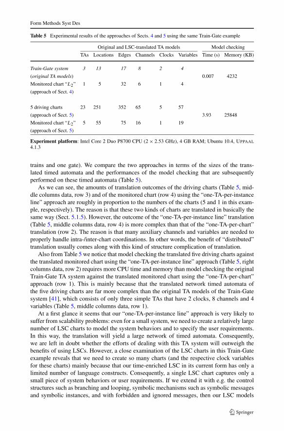
Form Methods Syst Des
Table 5 Experimental results of the approaches of Sects. 4 and 5 using the same Train-Gate example
Original and LSC-translated TA models Model checking
TAs Locations Edges Channels Clocks Variables Time (s) Memory (KB)
Train-Gate system 3 13 17 8 2 4
(original TA models) 0.007 4232
Monitored chart “L2” 1 5 32 6 1 4
(approach of Sect. 4)
5 driving charts 23 251 352 65 5 57
(approach of Sect. 5) 3.93 25848
Monitored chart “L2” 5 55 75 16 1 19
(approach of Sect. 5)
Experiment platform: Intel Core 2 Duo P8700 CPU (2 × 2.53 GHz), 4 GB RAM; Ubuntu 10.4, UPPAAL
4.1.3
trains and one gate). We compare the two approaches in terms of the sizes of the trans-lated timed automata and the performances of the model checking that are subsequentlyperformed on these timed automata (Table 5).
As we can see, the amounts of translation outcomes of the driving charts (Table 5, mid-dle columns data, row 3) and of the monitored chart (row 4) using the “one-TA-per-instanceline” approach are roughly in proportion to the numbers of the charts (5 and 1 in this exam-ple, respectively). The reason is that these two kinds of charts are translated in basically thesame way (Sect. 5.1.5). However, the outcome of the “one-TA-per-instance line” translation(Table 5, middle columns data, row 4) is more complex than that of the “one-TA-per-chart”translation (row 2). The reason is that many auxiliary channels and variables are needed toproperly handle intra-/inter-chart coordinations. In other words, the benefit of “distributed”translation usually comes along with this kind of structure complication of translation.
Also from Table 5 we notice that model checking the translated five driving charts againstthe translated monitored chart using the “one-TA-per-instance line” approach (Table 5, rightcolumns data, row 2) requires more CPU time and memory than model checking the originalTrain-Gate TA system against the translated monitored chart using the “one-TA-per-chart”approach (row 1). This is mainly because that the translated network timed automata ofthe five driving charts are far more complex than the original TA models of the Train-Gatesystem [41], which consists of only three simple TAs that have 2 clocks, 8 channels and 4variables (Table 5, middle columns data, row 1).
At a first glance it seems that our “one-TA-per-instance line” approach is very likely tosuffer from scalability problems: even for a small system, we need to create a relatively largenumber of LSC charts to model the system behaviors and to specify the user requirements.In this way, the translation will yield a large network of timed automata. Consequently,we are left in doubt whether the efforts of dealing with this TA system will outweigh thebenefits of using LSCs. However, a close examination of the LSC charts in this Train-Gateexample reveals that we need to create so many charts (and the respective clock variablesfor these charts) mainly because that our time-enriched LSC in its current form has only alimited number of language constructs. Consequently, a single LSC chart captures only asmall piece of system behaviors or user requirements. If we extend it with e.g. the controlstructures such as branching and looping, symbolic mechanisms such as symbolic messagesand symbolic instances, and with forbidden and ignored messages, then our LSC models

Form Methods Syst Des
themselves will be much more succinct than what they are now (i.e., fewer charts and fewerclocks will be needed to model the same system and specify the same requirement). Thenumbers of translated timed automata and the clock variables can hopefully be kept withinreasonable sizes. This likelihood and tendency has been shown by previous work on the“one-TA-per-chart” translation of the richer LSC models [34].
7 Translating iterative mode charts
When translating LSC charts to timed automata in Sects. 4.1 and 5.1, we considered onlythe invariant activation mode.
As mentioned in Sect. 3.1, a universal chart under the iterative mode requires that, aslong as the main chart is currently active, the prechart will not be monitored for furthersatisfaction. Compared with the invariant mode, satisfaction of a universal chart under theiterative mode is a weaker requirement. In other words, given an LSC chart and a messagesequence, it may happen that under the invariant mode, the chart hot-violates this sequence,but under the iterative mode, the chart does not. For example, for the LSC chart in Fig. 23(a),the message sequence “m1 · m2 · m1 · m3” is hot-violated by the second incarnation of thischart under the invariant mode. However, it is not violated by any incarnation under theiterative mode, because under this mode the second incarnation is “killed” immediatelyafter the prechart of the first incarnation is matched by the sub-sequence “m1 · m2”.
To conduct the “one-TA-per-chart” translation for iterative mode charts, we convert achart into a timed automaton similarly as in Sect. 4.1 (except that we discard the “prechartpre-matching” step). Now we maintain multiple copies of the translated TA. Each of thesecopies will become a chart incarnation (i.e., a “live” copy) when necessary. When a newmessage arrives, the existing chart incarnations (live copies) will react to it as usual, andbesides, at most one of the remaining chart copies will be incarnated upon this message(this is ensured by using the auxiliary binary semaphore MoreIncarnations, the “allocating”variable NxtIncarnation, and the function IncNxtIncarnation() that updates NxtIncarnation,see Fig. 23 and the UPPAAL declarations below).
The dynamics of the iterative mode activation is implemented by using a fresh auxiliarybroadcast channel kill. Once an incarnation of the chart notices that its prechart has beensuccessfully matched, it will immediately initiate a broadcast synchronization on kill to reset(i.e., to “kill”) all other live copies that are still progressing in their respective prechartportions.
As an example, if we interpret the LSC chart in Fig. 23(a) under the iterative mode, thenFig. 23(b) is the corresponding TA template IterativeModeTemplate() (for betterlegibility, we have omitted the guards on the sending and receiving instance lines). Thistemplate has a template parameter
int[0, MaxIncarnationNum - 1] thisChartCopy
and it will be instantiated as follows when we make the system (component) declarations inUPPAAL:
// There are at most two incarnations.Chart0 = IterativeModeTemplate(0);Chart1 = IterativeModeTemplate(1);
system Chart0, Chart1;

Form Methods Syst Des
Fig. 23 An LSC chart and itstranslated timed automatontemplate (under the iterativemode)
The global (variable, channel and function) declarations of the above system in UPPAAL
are as follows:
const int MaxIncarnationNum := 2; // The maximal number of incarnations// for this chart.
int[0, MaxIncarnationNum - 1] NxtIncarnation := 0; // Which chart copy// should be the// next incarnation?
bool MoreIncarnations := true; // "Should the Pch be monitored or not?"
broadcast chan m1, m2, m3; // The message labels in the LSC chartbroadcast chan kill; // "kill" is a fresh auxiliary channel.
// Once an incarnation of the LSC chart enters its main// chart, it should immediately reset all other// incarnations of that chart.
// The function that shifts the pointer to the next chart incarnationvoid IncNxtIncarnation() {
NxtIncarnation := (NxtIncarnation + 1) % MaxIncarnationNum ;}

Form Methods Syst Des
The LSC elements such as conditions and assignments can be added and translated sim-ilarly as in Sect. 4.1. Likewise, we can prove that the LSC chart L and the translated timedautomata OL,1,OL,2, . . . ,OL,n are behavior-equivalent. Here OL,i denotes the timed au-tomaton for the i-th chart copy, and n is the maximal number of chart incarnations of L.We can also compose these observer timed automata with the original system model S (i.e.,a network of timed automata), and thus get the final (modified) network of timed automata(S ′ ‖ O ′
L,1 ‖ O ′L,2 ‖ · · · ‖ O ′
L,n).To verify whether system S is satisfied by chart L under the iterative mode, we do the
following CTL model checking:
(S ′ ‖ O ′L,1 ‖ O ′
L,2 ‖ · · · ‖ O ′L,n) |= (li,min � li,max), 1 ≤ i ≤ n
where li,min and li,max denote the TA locations that correspond to the minimal and maximalcuts of the main chart of the i-th incarnation of chart L, respectively.
To conduct the “one-TA-per-instance line” translation for iterative mode charts, the abovegeneral idea also applies. We also maintain multiple copies of the translated timed automatonfor each instance line in each driving chart. In this case, each chart Li will have its killi -broadcast channel, and the synchronization on this channel will take place immediately afterthe activatei -broadcast synchronization in Li .
Remark 5 The two activation modes, i.e., invariant and iterative modes, can serve differentbut complimentary purposes. When used as a monitored chart, a chart is more difficult to besatisfied under the invariant mode than under the iterative mode. This indicates that invariantmode is better for capturing safety-related scenario requirements. On the other hand, whenused as a driving chart, an iterative mode chart can act as a periodic event generator, i.e.,before a sequence of messages in the main chart are generated and dispatched to fulfill somecommitment, it will not search for an “assume” pattern and make any new commitments.
8 Related work
8.1 Verifying state/transition systems against scenario-based requirements
Model checking by definition and in its earliest forms takes a state/transition system modeland a temporal logic formula as the inputs. To model check state/transition-based real-timesystems against complex properties or scenario-based requirements, various approacheshave been proposed.
One solution is the observer automata (a.k.a. test automata [1]) approach, i.e., to con-struct a number of auxiliary automata to capture the complex properties or scenario-basedrequirements, and then use these automata to “observe” the original system model. This ap-proach requires that the observer be compatible with the original system model, and that theobservation be non-intrusive and efficient (i.e., it incurs as little extra communication andcomputation overheads as possible).
An observer timed automata approach to real-time system verification is suggested in [1].This approach has been used to model check practically relevant systems such as the B&Opower controller [20] and some timed safety instrumented systems [28]. Case studies thereofindicate that the approach is effective. However, the approach also comes with some limita-tions:

Form Methods Syst Des
– Manual construction of observer timed automata could be labor-intensive and error-prone,and this is especially the case when the automata grow large;
– To synchronize with the observer timed automata, the original system models may needto be modified and annotated. During this modification process, some new errors mightbe introduced. Newly introduced timing errors are especially difficult to diagnose; and
– Since an observer timed automaton and the original system usually engage in “loose”channel synchronizations (i.e., no particular sending and receiving process are specifiedfor a synchronization on a certain channel (message label)), they specify process inter-actions only liberally. To capture non-trivial scenario-based requirements, the synchro-nizations between the observer automaton and the original system should be carefullydesigned by using e.g. auxiliary variables, semaphores or locking mechanisms. This is anextra burden for the designers.
Compared with the observer automata approach, in our method the observer automa-ton is constructed automatically, and it is guaranteed to observe the original system in anon-intrusive way. Furthermore, the automatically created auxiliary variables (includingsemaphores) will enable our observer automaton to faithfully reflect the LSC requirementswhere each message has its particular sending and receiving process.
Scenario-based requirements on state/transition-based system models can also be cap-tured by using the assume-guarantee style visual formalisms such as Triggered MSC [37],Template MSC [16] or the even richer LSC [18], and then transformed into directly verifi-able formalisms. In particular LSCs can be translated into timed Büchi automata (TBA) [25],timed automata [34], temporal logics [9, 10, 14, 17, 25, 27] or sequences of LSC ele-ments [35], and the verification problem can be converted to a model checking problemon existing tools [10, 25], or solved directly [35].
An early attempt of introducing LSC features such as the initial and iterative activationmodes and the activation condition (a Boolean expression which characterizes the state ofthe system model when the scenario should start) into UML Sequence Diagrams is madeby Lettrari and Klose [32]. They develop a tool to monitor and test the executable UMLmodels (i.e., implementations of RHAPSODY UML models). In comparison, our work followthe more mature LSC definition [18] to support also the invariant mode and the notion ofprechart, which details the activation conditions under which they apply, and we aim atscenario-based verification.
Damm and Klose [13] propose to use LSCs in combination with STDs (Symbolic Tim-ing Diagrams) to specify scenario-based requirements on STATEMATE models, and thencarry out model checking. This methodology has been concretized and implemented in [25],where an LSC chart is transformed into a timed Büchi automaton, which is further trans-formed into a temporal logic formula. Further descriptions of how LSC as a specificationlanguage can be used in a UML verification environment for the RHAPSODY tool are pre-sented in [36]. In the work of [25], in order to specify real-time requirements, timers [4, 21]and timing annotations (or delayed intervals) [4] are added to the LSC charts. To enablethe transformation, each location of the LSC chart is equipped with a discrete (integer)clock. Since timers can only express timing constraints within a single chart and within asingle process, and delayed intervals can only express the minimal and maximal delays be-tween two consecutive locations, these restrict the expression of timing constraints acrossprocesses and across charts. Our LSC charts use TA-like real-valued clock variables. Thisflavor of timing constraint agrees well with the original TA system model, and thus enablesmooth translation of timing information into the observer TA, as well as seamless embed-ding of the observer TA into the UPPAAL verification framework.

Form Methods Syst Des
An LSC to timed automata translation is proposed in [34]. When the LSC chart is usedas a monitored chart, this translation is similar to our “one-TA-per-chart” translation in thesense that they are both based on the notion of LSC cut and its advancements. However,when LSC serves as a modeling language, this method is faced with the cut and configurationblow-up problem. In comparison, our “one-TA-per-instance line” translation method doesnot need to explicitly enumerate and thus create TA locations for a potentially huge numberof cuts.
LSCs can also be translated into temporal logic formulas [9, 14, 17, 27]. For the ker-nel subset of LSC in [27], it has been shown that existential charts can be expressed usingthe CTL logic, and universal charts can be expressed using (LTL ∩ CTL) [17, 27]. Simi-lar results are achieved in [14]. However, these methods do not handle explicit time in thecharts. In [10], LSC is applied in hardware verification, where the system models are givenin Verilog and the user requirements are specified as LSCs. These LSCs are translated to LTLformulas and then fed into the verification environment FORMALCHECK. Since LSCs areused to specify hardware protocols at the register transfer level, a discrete clock tick con-struct is introduced to explicitly represent the passage of system time. Compared with [10],we use real-valued clocks to represent various timing constraints.
As mentioned thus far, verification techniques that are based on LSC-to-temporal logictranslation in general tend to suffer from scalability problems. Industrial case studies [24]show that the LTL formulas grow large even for LSCs of moderate size, and thus formalverification becomes expensive. To overcome this limitation, Klose and colleagues [26] in-vestigate efficient model checking of Kripke structures against LSC requirements. In ourmethod, since our observer automaton is tightly coupled with the original system, a verysimple CTL property A�(lmin ⇒ A♦ lmax) can be extracted from the observer automaton tocapture the LSC requirements. In this way we avoid translating LSCs to complex temporallogic formulas.
Another line of work [35] is to extract properties from LSCs as sequences of LSC ele-ments, and to develop verification algorithms to check whether these sequences are respectedby the FSM computation graph of the TA model that is exported from UPPAAL. However,simultaneous regions (simregions) in their LSCs are used only to model broadcast commu-nications, and conditions cannot be a part of simregions. Our notion of simregion uses the“[condition] [message]/[assignment]” pattern, thus enables smooth translation to a TA edge.
8.2 Verifying object interaction-based systems against scenario-based requirements
In this case, the system is modeled as a set of driving universal LSC charts and the require-ment is specified as a set of monitored universal or existential charts. Monitored universalcharts should not be hot-violated, and monitored existential charts should be matched atleast once [8, 18].
In the execution (or play-out) [18] of scenario-based models, the Play-Engine checkswhether the monitored charts are respected. This is enhanced in the smart play-out mecha-nism, where planned state space exploration via model checking is added to the Play-Engineto bypass some avoidable hot violation situations that are caused by some “blind” inter-actions among the system processes. In a case study of a telecommunication application,Combes and colleagues [11] check whether a set of monitored existential charts can be sat-isfied by a set of driving charts without violating any of them. Their method is based on theplay-out and smart play-out mechanisms in the Play-Engine.
In [38], LSCs are encoded as CSP processes. The CSP verification tool FDR is employedto check whether a set of monitored existential charts can be satisfied by a set of drivinguniversal charts. This work considers untimed charts only.

Form Methods Syst Des
Wang and colleagues [40] employ constraint logic programming (CLP) techniques toenable the symbolic execution of LSC models. Their implementation supports both universaland existential charts, and supports timing constraints.
Playing-out [11, 18, 40] as a methodology of executing scenario-based models does nothave in mind verification as its goal. Although it is possible to check whether a number ofexistential charts can be satisfied during (smart) playing-out, essentially it is still consid-ered as a kind of (guided) execution. Compared with [11, 18, 38], our method allows therequirements to be specified also as universal charts. Furthermore, compared with [11, 18,38], our method uses TA-like clock variables and clock constraints, and thus enables finercharacterizations of timing requirements.
9 Conclusions and future work
This article proposes two approaches to the verification of state/transition-based and ob-ject interaction-based real-time system models against scenario-based user requirements,respectively. We extend a kernel subset of the LSC language with timed automata-like real-valued clock variables and timing constraints, define its semantics, and use the time-enrichedLSC charts both for system modeling and for property specification. By means of behavior-equivalent model transformation and non-intrusive event spying, we convert the scenario-based verification problems to CTL real-time model checking problems in UPPAAL. Bydoing so we conclude that it is feasible:
– to introduce important notions from the TA to the LSC formalisms to facilitate scenario-based characterization of dense real-time systems;
– to employ the original TA constructs as well as the UPPAAL-extended TA features toproperly mimic the time-enriched LSC dynamics; and consequently;
– to exploit the power of the UPPAAL model checker for scenario-based automatic verifica-tion of non-trivial real-time systems.
The proposed first approach has been implemented as a new feature inside UPPAAL,and the second approach implemented as an LSC-to-TA translator which, together withour LSC editor and UPPAAL, constitutes a tool chain for scenario-based verification. Sincethe translation, the composition and the underlying verification are all automatic steps, ourmethods are fully automated. Preliminary experiments with a Train-Gate system indicatethat the proposed approaches are computationally feasible and effective.
The benefits of building our scenario-based real-time system verification methods on topof the well-developed real-time model checker are twofold: (1) for system analysts and de-signers who are interested in early-stage validations using live sequence charts, now they canscale up to the timed settings without having to develop and implement the correspondingreal-time verification algorithms; (2) for users of conventional (real-time) model checkersthat work with state/transition-based models and temporal logical properties, now they canhorizontally scale up to scenario-based system models and scenario-based user require-ments.
In our proposed approaches, the time-enriched LSC chart in its current form has onlya limited number of language constructs. To ease the scenario-based characterization ofpractically relevant complex systems using LSC and thus to realize the full potential ofscenario-based approaches, we need to support more language constructs such as subchart,if-then-else structure, loop, forbidden and ignored messages, co-region, and symbolic mes-sages and instances. Accordingly, we need to implement the full-fledged translators, and to

Form Methods Syst Des
apply the tool and tool chain to larger (industrial) case studies. Another limitation of thecurrent approaches is that counterexamples (if any) can be displayed only in the translatedtimed automata. For the users’ convenience, it will be extremely useful to trace the coun-terexamples back into the LSC system models and the LSC requirements. This needs to beachieved in the near future.
Acknowledgements We would like to thank the anonymous referees for their constructive comments andhelpful suggestions. Thanks are also due to Itai Segall for useful discussions and for pointing out an error inan earlier version of the “one-TA-per-instance line” translation.
Appendix A: BNF grammar of time-enriched LSC
The following BNF grammar describes our time-enriched LSC language.
LSC ::= TYPE MODE INSTANCES CHARTTYPE ::= type (existential | universal)MODE ::= mode (initial | iterative | invariant)INSTANCES ::= INSTANCES INSTANCES| instance INST_ID NAMECHART ::= chartbegin CHARTBODY chartendCHARTBODY ::= CHARTBODY CHARTBODY| message ELEM_ID INST_ID INST_ID YLOCATION NAME| condition ELEM_ID (INST_ID)+ YLOCATION TEMP EXPR| assignment ELEM_ID (INST_ID)+ YLOCATION UPDATE| simregion ELEM_ID (INST_ID)+ YLOCATION| pchbot ELEM_ID (INST_ID)+ YLOCATIONINST_ID ::= <numeral>ELEM_ID ::= <numeral>YLOCATION ::= <numeral>TEMP ::= cold | hotEXPR ::= <boolean expression>UPDATE ::= <clock resets>
As can be seen from the BNF grammar, each primitive construct (i.e., message, con-dition, assignment) has an element ID and a y-coordinate. This y-coordinate denotes thegeographical distance from the element to the top of all instance lines (note that all mes-sages, conditions and assignments have horizontal layouts). It should not be confused withthe numbering of a “position” among all the points of communication, computation andsynchronization along an instance line.
In the BNF grammar, a simregion is represented by the y-coordinate where its constituentmessage, and/or condition, and/or assignment are anchored together (Fig. 5, black filledcircles).
Furthermore, a prechart is represented by its bottom y-coordinate vector that spans acrossthe relevant instance lines. When there is no prechart, the “pchbot” statement will not appearin the LSC file.

Form Methods Syst Des
Appendix B: Timed automata in UPPAAL
We use the following notations: X is a set of real-valued clocks, and B(X) is the set ofconjunctions over simple conditions of the form x �� c or x − y �� c, where x, y ∈ X,c ∈ N, and �� ∈{<,≤,=,≥,>}.
Definition 9 (Timed automaton, TA [7]) A timed automaton is a tuple (L, l0,X,Act,
E, Inv), where L is a set of locations, l0 ∈ L is the initial location, X is a set of clocks,Act is the alphabet of actions, E ⊆ L × (Act ∪ {τ }) × B(X) × 2X × L is a set of edgesbetween locations, each of which has an action, a guard and a set of clocks to be reset, andInv : L → B(X) assigns invariants to locations.
UPPAAL has defined a number of extensions to the standard notations of timed au-tomata [2]. Specifically, an urgent location is such a TA location that freezes time, i.e.,time is not allowed to elapse when a process is in an urgent location. A committed locationis a special kind of urgent location whose outgoing transitions always have higher priorityto be fired than those from non-committed locations.
UPPAAL uses a mixture of handshake communication and broadcast communication. TheCBS (Calculus of Broadcasting Systems [33])-style broadcast channels allow one-to-manysynchronization. If the emitting edge is enabled, then it can always fire. If the emitting edgeis to fire, then all enabled receiving edges (might be 0 edge) will synchronize.
In UPPAAL an urgent channel means that if it is possible to trigger a synchronizationover that channel, then it cannot delay in the source state.
Furthermore, UPPAAL also supports bounded-range integer and boolean data variables,which can be used in the guards, assignment and location invariants.
A clock valuation is a function u : X → R≥0 that assigns each clock variable a non-negative real number. Let R≥0
X be the set of all clock valuations. Let u0(x) = 0 for allx ∈ X. We may consider guards and invariants as sets of clock valuations. For example, weuse u ∈ Inv(l) to denote that valuation u satisfies Inv(l).
Definition 10 (Semantics of TA [7]) Let (L, l0,X,Act,E, Inv) be a timed automaton. Thesemantics is defined as a labeled transition system 〈SS, s0,→〉, where SS ⊆ L× R≥0
X is theset of semantic states, s0 = (l0, u0) ∈ SS the initial state, and →⊆ SS × (Act ∪ {τ } ∪ R≥0) ×SS the transition relation such that:
– (l, u)d−→ (l, u + d) if ∀d ′ : 0 ≤ d ′ ≤ d .u + d ′ ∈ Inv(l); and
– (l, u)a−→ (l′, u′) if there exists e = (l, a, g, r, l′) ∈ E such that u ∈ g, u′ = [r → 0]u, and
u′ ∈ Inv(l′),
where for d ∈ R≥0, u + d maps each clock x in X to the value u(x) + d , and [r → 0]udenotes the clock valuation which maps each clock in r to 0 and agrees with u over X\r .
Definition 11 (Run of TA) A run of a TA (L, l0,X,Act,E, Inv) is a sequence of states
s0 · s1 · . . . that are connected by the transitions, i.e., ∀i ≥ 0 .∃ui ∈ (Act ∪ {τ } ∪ R≥0). si ui−→
si+1.
The transition relation → as mentioned above each time consumes only a single letteru ∈ (Act ∪ {τ } ∪ R≥0). We extend it to →∗ such that it consumes a (finite or infinite) wordw ∈ (Act ∪ {τ } ∪ R≥0)
∗ ∪ (Act ∪ {τ } ∪ R≥0)ω . A word w that corresponds to a run of the TA
is called a timed trace of the TA.

Form Methods Syst Des
A number of timed automata can be composed in parallel into a network of timed au-tomata over a common set of clocks and actions, Ai = (Li, l0,i ,X,Act,Ei, Invi ), 1 ≤ i ≤ n.A location vector l̄ = (l1, . . . , ln) is a vector of locations of the member TAs. We composethe invariant functions into a common function over location vectors Inv(l̄) = ∧
i Invi (li ).We write l̄[l′i/ li] to denote the vector where the i-th element li of l̄ is replaced by l′i .
Definition 12 (Semantics of a network of TAs [7]) Let Ai = (Li, l0,i ,X,Act,Ei, Invi ) be anetwork of timed automata, 1 ≤ i ≤ n. Let l̄0 = (l0,1, . . . , l0,n) be the initial location vector.The semantics is defined as a transition system 〈SS, s0,→〉, where SS = (L1 × · · · × Ln) ×R≥0
X is the set of global semantic states, s0 = (l̄0, u0) ∈ SS the initial global state, and →⊆SS × (Act ∪ {τ } ∪ R≥0) × SS the transition relation defined by:
– (l̄, u)d−→ (l̄, u + d) if ∀d ′ : 0 ≤ d ′ ≤ d .u + d ′ ∈ Inv(l̄);
– (l̄, u)τ−→ (l̄[l′i/ li], u′) if there exists li
τ,g,r−−→ l′i such that u ∈ g, u′ = [r → 0]u and u′ ∈Inv(l̄[l′i/ li]);
– (l̄, u)a−→ (l̄[l′i/ li , l
′j / lj ], u′) if a is a binary channel and there exist li
c!,gi ,ri−−−→ l′i and
ljc?,gj ,rj−−−−→ l′j such that u ∈ (gi ∧ gj ), u′ = [ri ∪ rj → 0]u and u′ ∈ Inv(l̄[l′i/ li , l
′j / lj ]);
and– (l̄, u)
a−→ (l̄[l′i/ li , l′j / lj , l
′k/ lk, . . .], u′) if a is a broadcast channel and there exist an
lic!,gi ,ri−−−→ l′i and a maximal set {j, k, . . .}: lj
c?,gj ,rj−−−−→ l′j , lkc?,gk,rk−−−−→ l′k , . . ., such that u ∈ (gi ∧
gj ∧ gk ∧ · · · ), u′ = [ri ∪ rj ∪ rk ∪ · · · → 0]u and u′ ∈ Inv(l̄[l′i/ li , l′j / lj , l
′k/ lk, . . .]).
Runs and traces of a network of TAs are defined similarly as those for a single TA.
Appendix C: Proofs of lemmas and theorems in Sect. 4
Theorem 1 If a configuration (c, v) of L corresponds to a semantic state (l, v) of OL, then:(1) each simregion s that follows (c, v) in L uniquely corresponds to an outgoing edge (l, l′)in OL; and (2) the target configuration (c′, v′) of s in L uniquely corresponds to the targetsemantic state (l′, v′) in OL.
Proof For each simregion s in L that immediately follows (c, v), according to Sect. 4.1.3, s
uniquely corresponds to an outgoing edge (l, l′) from l in OL. Since the valuation functionv is the same in (l, v) as in (c, v), and the condition in s is straightforward copied ontothe TA edge (l, l′), the simregion s can be stepped over if and only if the TA edge (l, l′)can be taken. Moreover, the assignment (if any) in s is also straightforward copied onto theedge (l, l′). This indicates that the valuation function in the LSC target configuration will bestill the same as in the TA target semantic state. Therefore, (c′, v′) uniquely corresponds to(l′, v′).
Specifically, if s is a non-message simregion that immediately follows (c, v) in L, thenaccording to the ASAP semantics, s will be stepped over immediately from (c, v). Accord-ingly, the source location l is a committed location in OL, and the other outgoing edges thatcorrespond to message simregions will not be appended to l. All these ensure that the TAedge that corresponds to s is taken immediately from state (l, v). �
If in the LSC semantics (Sect. 3.2.1) we ignore the silent steps that are caused by intra-chart coordinations and autonomous advancements of instance lines, then we have:

Form Methods Syst Des
Theorem 2 For any trace tr in OL: tr |= L ⇔ (OL, tr) |= (lmin � lmax).
Proof Let the initial cut of L be c0. According to Sect. 4.1.2, c0 corresponds to the initiallocation l0 of OL. Since in the beginning all the clocks in L have the same initial values as inOL, the initial configuration (c0, v0) of L uniquely corresponds to the initial semantic state(l0, v0) of OL.
We consider only the legal (admissible) behaviors of OL. In other words, the traces thatlead to the sink TA location Err will be ignored. We consider the following cases:
(1) OL has only explicitly specified behaviors. By Theorem 1, each simregion that im-mediately follows (c0, v0) uniquely corresponds to an outgoing edge from TA location l0,and the target configuration (c′, v′) in L uniquely corresponds to the target semantic state(l′, v′) in OL. On the other hand, in (c0, v0) of L, there could be a time delay d ∈ R≥0 ifand only if in (l0, v0) of OL there could be the same time delay d . By recursively applyingTheorem 1 and the above result, we can conclude that any timed trace tr in OL is also atimed trace in L.
By assuming that OL has only explicitly specified behaviors, we know that there is noundesired behavior in OL. If tr |= L, then by definition this particular tr in OL also satisfiesthe path formula (lmin � lmax), i.e., (OL, tr) |= (lmin � lmax). Therefore, we have tr |= L ⇒(OL, tr) |= (lmin � lmax).
The reverse implication is proved similarly.(2) OL includes behaviors of unconstrained events or cold violations. In this case, each
unconstrained event m at a particular cut c in L uniquely corresponds to an m?-labeledself-loop edge at the corresponding location l in OL, and each cold violation uniquely cor-responds to an edge leading to lpmin. The two-way implications are proved similarly.
(3) OL includes behaviors of prechart pre-matching. In this case, the semantics oftr |= L says that whenever tr matches the prechart Pch, the main chart Mch will be matchedafterwards (and this must happen before Pch begins a next round matching). Consideringthat in OL, the locations lmin and lmax are two rendezvous points, thus tr |= L means exactlythe satisfaction of (lmin � lmax) by tr.
To sum up, we conclude that for any trace tr in OL, we have tr |= L ⇔ (OL, tr) |= (lmin �lmax). �
Let the modified version of the original system model S be S ′, and the modified versionof the observer timed automaton OL for chart L be O ′
L. Let the minimal and maximal cutsof the main chart of L correspond to locations lmin and lmax of O ′
L, respectively. When L isa universal chart, we have:
Lemma 1 If OL has no committed location, and all ch ∈ Π are binary synchronizationchannels, then S |= L ⇔ (S ′ ‖ O ′
L) |= (lmin � lmax).
Proof Let (l̄, v) be a semantic state of the network of TAs of S, where l̄ is a location vector,and v is the valuation of all clock variables. According to the UPPAAL semantics on binarysynchronizations [39], for each binary synchronization channel ch ∈ Π , we have a transition
(l̄, v)ch−→ (l̄′, v′) if in two different processes (TAs) of S, there are two edges (li , li+1) and
(lj , lj+1) labeled with ch! and ch?, respectively, such that:
– v |= gi ∧ gj , where gi and gj are guards of the two edges, respectively;– l̄′ = l̄[li+1/li , lj+1/lj ];– v′ = aj (ai(v)), where ai and aj are the assignments of the emitting and receiving edges,
respectively;

Form Methods Syst Des
– v′ |= Invi+1 ∧ Invj+1, where Invi+1 and Invj+1 are the location invariants of the targetlocations of the two edges, respectively;
– either (li or lj or both are committed locations), or no other location in l̄ is committed.
We need to show that the modifications of the original system model S and the observerTA OL do not affect their legal (i.e. admissible) behaviors, i.e., the event notification mech-anism and the locking mechanisms neither increase nor decrease the behaviors (traces) in S
and OL. To this end, we prove that each synchronization in S uniquely corresponds to a pairof consecutive synchronizations in (S ′ ‖ O ′
L).
⇒)By S |= L we know that the original system model S satisfies the requirements that are
specified in the LSC chart L. It follows that the observer TA OL does not restrict the (legal)behaviors of S.
If at a semantic state (l̄, v) of S there is a synchronization (l̄, v)ch−→ (l̄′, v′), where ch ∈ Π ,
we let the two coupling edges that carry ch! and ch? be (li , li+1) and (lj , lj+1), respectively.Clearly, they satisfy all the five requirements as listed earlier in this proof. According tothe rules for modifying S, the edge (li , li+1) in S will correspond to two edges (li , l
′i ) and
(l′i , li+1) in S ′, where l′i is a newly added committed location. Also according to the mod-ification rules, the semaphore mayFire evaluates to false only when the current control isin a newly added committed location (Fig. 13(a)). Now that the control is in li in S ′, thesemaphore mayFire should evaluate to true. This together with “v |= gi ∧ gj ” (the first itemrequirement) indicates that the guards for the edges (li , l
′i ) and (lj , lj+1) of S ′ to synchronize
on channel ch are both satisfied. Besides, items 3–5 in the binary synchronization require-ments also apply to the ch-synchronization at (li , l
′i ) and (lj , lj+1). Therefore, there exists
a transition (l̄, v)ch−→ (l̄′′, v′) in S ′ with (li , l
′i ) and (lj , lj+1) as the coupling edges, where
l̄′′ = l̄′[l′i/ li , lj+1/lj ].The second edge (l′i , li+1) in S ′ will be immediately coupled with a corresponding edge
in O ′L. By the assumption S |= L, we know that OL does not restrict the behaviors of S
via its own conditions (e.g., via g3 in Fig. 13(b)). This means that the cho-synchronizationbetween S ′ and O ′
L will not get stuck there due to the restrictions of O ′L. Since after this
synchronization, the clock variables in S ′ remain unchanged, we know that the locationinvariant Invi+1 on li+1 of S ′ will still be satisfied. After this synchronization, the two targetlocations in S ′ will be li+1 and lj+1, thus coinciding with the corresponding target locationsli+1 and lj+1 in S. Therefore, we can conclude that given a trace tr in S, there exists a uniquetrace tr′ in (S ′ ‖ O ′
L) such that tr′ and tr correspond.By the definition of S |= L (see Sect. 3.2), we know that if a timed trace μ in S arrives
at the minimal cut of the main chart of L, then μ must always be able to reach the maximalcut of that main chart. By Theorem 2 and Sect. 4.1, we know that if μ arrives at location lmin
of O ′L, then μ must always be able to reach location lmax of O ′
L.Since each trace μ in S can be equivalently mapped to a trace μ′ in (S ′ ‖ O ′
L), clearly, ifany μ′ arrives at location lmin of O ′
L, then that μ′ must always be able to reach location lmax
of O ′L.
Since lmin and lmax are two locations in (S ′ ‖ O ′L), the above requirement can thus be
formulated as a UPPAAL property (S ′ ‖ O ′L) |= (lmin � lmax).
⇐)We need to prove that each trace tr′ in (S ′ ‖ O ′
L) that satisfies the CTL property uniquelycorresponds to a trace tr in S that satisfies the LSC requirement.

Form Methods Syst Des
Assume that in (S ′ ‖ O ′L) there is a synchronization (l̄, v)
c−→ (l̄′, v′).If c ∈ Π , then after removing “mayFire == true” from the condition and removing
“mayFire := false” from the assignment of the emitting edge (Fig. 13(a)), the edge be-comes exactly the corresponding edge in S. Note that the invariant (if any) at the targetlocation of this emitting edge is irrelevant of the semaphore mayFire. This indicates that thesynchronization between the corresponding edges in S can also fire.
If c is a fresh channel (i.e., in the form of cho), then the source location of the c!-emittingedge in S ′ must be a newly added committed location. This c! will be synchronized with ac?-receiving edge in O ′
L. And it will bring the control in S ′ from the committed locationto the target location, which coincides with the corresponding target location in S. Dueto the use of semaphore mayFire, no other synchronizations in (S ′ ‖ O ′
L) can preempt theexecution of this c-synchronization.
The rest of the transitions in (S ′ ‖ O ′L) are just the same as those in S. Therefore we can
conclude that a trace tr′ in (S ′ ‖ O ′L) uniquely corresponds to a trace tr in S such that tr′ and
tr are equivalent. Now that (S ′ ‖ O ′L) |= (lmin � lmax), according to the semantics of LSC
chart satisfaction, we have S |= L. �
Let S, L, OL, S ′, O ′L, lmin and lmax be the same as declared and explained in Lemma 1.
When L is a universal chart, we have:
Theorem 3 S |= L ⇔ (S ′ ‖ O ′L) |= (lmin � lmax).
Proof This theorem is a generalization of Lemma 1 by canceling the restrictions.If ch ∈ Π is a broadcast channel, the semantics of ch-synchronization [39] is a little
different. Since the modifications of the emitting edges in S do not affect the receivingedges in S, we can still have a one-to-one mapping between the traces in S and in (S ′ ‖ O ′
L).If there are committed locations in O ′
L, then we use the second semaphore NxtCmt toguarantee the non-interrupted execution at those committed locations in O ′
L. Since an edge(l, l′) starting from a committed location l in O ′
L represents an internal action (τ ) transition(i.e., a local transition), it needs no synchronization with S ′. Thus the edge does not affectthe behavior of S ′.
To sum up, there is a one-to-one mapping of the traces in S and in (S ′ ‖ O ′L), even in
the presences of broadcast channels in S and committed locations in OL. Thus we haveS |= L ⇔ (S ′ ‖ O ′
L) |= (lmin � lmax). �
Let S, L, OL, S ′, O ′L and lmax be the same as explained in Theorem 3. When L is an
existential chart, we have:
Theorem 4 S |= L ⇔ (S ′ ‖ O ′L) |= E♦ lmax.
Proof (idea) We can show that there is a one-to-one mapping between the traces in S andin (S ′ ‖ O ′
L) similarly as in Lemma 1 and Theorem 3.The main difference between this theorem and Theorem 3 lies in the semantics of a
universal chart and of an existential chart. However, it is clear that the CTL formula E♦ lmax
represents exactly the existential chart requirements. So this theorem can be proved similarlyas in Lemma 1 and Theorem 3. �

Form Methods Syst Des
Appendix D: Proofs of lemmas and theorems in Sect. 5
Let L be an untimed LSC chart whose instance lines I1, I2, . . . , In correspond to timedautomata A1,A2, . . . ,An, respectively, then the translated network of TAs will be NTAL
= {Ai | 1 ≤ i ≤ n} ∪ {Coord}. According to rules R3, R4 and R6, there will be a set ofauxiliary channels Aux = {pch_overi,mch_overi | 1 ≤ i ≤ n} ∪ {activate,over,pch_vio,
reset} that will be used in NTAL. Let the message alphabet of L be Σ , then the alphabet ofobservable actions in NTAL will be Act = (Σ ∪ Aux).
Lemma 2 Let L be an untimed LSC chart whose message alphabet is Σ , and let NTAL bethe translated network of timed automata which have a set Act of observable actions. Then∀γ1 ∈ (Σ ∪ {τ })ω . ((γ1 |= L) ⇒ ∃γ2 ∈ (Act ∪ {τ })ω .(γ2 |= NTAL) ∧ (γ2|Σ = γ1|Σ)), and∀γ2 ∈ (Act ∪ {τ })ω . ((γ2 |= NTAL) ⇒ ∃!γ1 ∈ (Σ ∪ {τ })ω . (γ1 |= L) ∧(γ2|Σ = γ1|Σ)).
Proof We can prove the above two implications by proving that each cut of chart L uniquelycorresponds to a location vector in the network of timed automata NTAL, and each advance-ment step in L uniquely corresponds to either a message synchronization transition (rangingon Σ ∪ Aux) or a sequence of concatenated message synchronization and internal actiontransitions in NTAL, such that they consume exactly the same letter from Σ if they are bothrestricted to Σ . Note that we restrict the LSC advancement steps to represent only legal (i.e.admissible) behaviors.
Let the instance lines in chart L be I1, I2, . . . , In. They will be translated into timedautomata A1,A2, . . . ,An, respectively. Together with the auxiliary coordinator automatonCoord they constitute NTAL.
The initial cut c0 of chart L corresponds to the LSC initial position vector (01,02,
. . . ,0n), where ij means that instance Ij ∈ inst(L) is currently in its position i ∈ pos(L, Ij ).In the translated network of timed automata NTAL, automaton Coord is initially in its lo-cation l0
coord . By rule R1, each 0i in position vector (01,02, . . . ,0n) corresponds to a TAlocation l0
i (denoting location 0 in timed automaton Ai ). Therefore, cut c0 uniquely corre-sponds to the NTAL initial location vector l̄0 = (l0
1 , l02 , . . . , l
0n, l
0coord).
We show how the advancement steps from the LSC initial position vector correspond tothe transitions in the network of timed automata. At LSC position vector (01,02, . . . ,0n),there are two kinds of possible advancement steps:
– If there is an m-labeled message occurrence mo from position 1i of instance Ii to position1j of instance Ij (i.e., mo is a minimal event), then:
On one hand, by rule R2, there will be an m!-labeled TA edge from location l0i to
l1i in Ai , and an m?-labeled TA edge from location l0
j to l1j in Aj . According to the
LSC semantics, there is a message synchronization advancement step on m in L from(01, . . . ,0i , . . . ,0j , . . . ,0n) to (01, . . . ,1i , . . . ,1j , . . . ,0n). Accordingly, in NTAL thereexists exactly a corresponding binary synchronization on channel m between Ai andAj , and the location vector of NTAL will change from (l0
1 , . . . , l0i , . . . , l
0j , . . . , l
0n, l
0coord)
to (l01 , . . . , l1
i , . . . , l1j , . . . , l
0n, l
0coord).
On the other hand, according to the semantics of the invariant mode universal chart,the message as a minimal event can be constantly matched for with L staying in theinitial cut. By rule R8, in NTAL there will be first a binary synchronization on channelm, i.e., (l0
1 , . . . , l0i , . . . , l
0j , . . . , l
0n, l
0coord)
m−→ (l01 , . . . , l
0i , . . . , l
PMj , . . . , l0
n, l0coord), and then
an immediately following internal action transition that leads back to the initial locationvector, i.e., (l0
1 , . . . , l0i , . . . , lPM
j , . . . , l0n, l
0coord)
τ−→ (l01 , . . . , l
0i , . . . , l
0j , . . . , l
0n, l
0coord). Here

Form Methods Syst Des
lPMj is an auxiliary TA location that is specially used for prechart pre-matching. In this
case of pre-matching, the m-synchronization advancement step in L uniquely corre-sponds to a sequence of the tightly concatenated
m−→ andτ−→ transitions.
Since a dedicated flag boolean variable prematch has been used to strengthen the TAtransition guards, assignments and the location invariants, it follows that at NTAL lo-cation vector (l0
1 , . . . , l0i , . . . , l0
j , . . . , l0n, l
0coord), there are only the two above-mentioned
possible interleaved executions between the two m!-labeled outgoing edges from l0i in
Ii and the two m?-labeled outgoing edges from l0j in Ij .
– If instance Ii has no interactions with other instance lines in the prechart, then there is animmediate silent advancement step from (01, . . . ,0i , . . . ,0n) to (01, . . . ,1i , . . . ,0n). Byrule R3, l0
i will be a committed location in Ai of NTAL, and there will be a pch_overi !-labeled edge from l0
i to l1i . Furthermore, in automaton Coord there will be a coupling
pch_overi?-labeled edge either– from l0
coord to l1coord , corresponding to the case where Ii is the very last instance line of
L to complete its prechart portion; or– from l0
coord to l0coord , corresponding to the case where Ii is not yet the last instance line
of L to complete its prechart portion.In the two cases, the location vector of NTAL will be changed from (l0
1 , . . . , l0i , . . . , l
0n,
l0coord) to (l0
1 , . . . , l1i , . . . , l
0n, l
1coord), and from (l0
1 , . . . , l0i , . . . , l
0n, l
0coord) to (l0
1 , . . . , l1i , . . . , l
0n,
l0coord), respectively. However, in both cases, there will be exactly one binary synchroniza-
tion transition on pch_overi in NTAL.
The above two kinds of possible advancement steps indicate that there is an initial correspon-dence between the position vector of L and the location vector of NTAL.3 Since an untimedchart is a message-only chart, a cut vector is itself an LSC configuration, and a location vec-tor is itself a semantic state of the translated network of timed automata.4 Therefore, thereis an initial “LSC cut to TA location vector”, and “LSC advancement step to TA (sequenceof) transition” correspondence between L and NTAL.
The above correspondences can be generalized by using induction. Assume that at acut c that corresponds to a position vector (p11, . . . , pii, . . . , pjj , . . . , pnn) in the prechartof L, there is an m-labeled message occurrence sent from position (pi + 1)i of instanceIi to position (pj + 1)j of instance Ij . If for cut c, there uniquely exists a correspondinglocation vector l̄ in NTAL, then similar to the case of the initial cut, we can prove that themessage synchronization advancement step on m in L uniquely corresponds to a binarysynchronization transition in NTAL; and after this message synchronization advancementstep, the new cut c′ uniquely corresponds to the destination location vector l̄′ in NTAL.Proof by induction ensures that any normal (i.e., other than the prechart pre-matching ones)message synchronization advancement step in the prechart of L uniquely corresponds to amessage synchronization transition in NTAL.
When (p11, . . . , pii, . . . , pjj , . . . , pnn) is a position vector in the main chart of L, theunique correspondence relation can be proved similarly.
3More precisely the sub-location vector of NTAL that is projected to A1 ‖ A2 ‖ · · · ‖ An . Note that the edgesin Coord correspond only to auxiliary messages rather than the observable messages in Σ or the internal (τ )action.4Note that in the LSC chart, the message sender/receiver and other relevant information are not defined as apart of the chart configuration. Accordingly, the auxiliary and bookkeeping variable information are excludedfrom the semantic states of the translated timed automata.

Form Methods Syst Des
Now we prove the unique correspondence for the case that involves the intra-chart co-ordination (e.g., the prechart to main chart transition). Assume that in the prechart of L, acut c corresponds to position vector (p11, . . . , pii, . . . , pnn), where pi + 1 = Pch_botL,Ii .If (p11, . . . , pii, . . . , pnn) uniquely corresponds to a location vector (l
p11 , . . . , l
pii , . . . , l
pnn ,
l0coord), then by rule R3, the internal advancement step (p11, . . . ,pii , . . . , pnn)
τ−→ (p11, . . . ,
(pi + 1)i , . . . ,pnn) in L corresponds to either
– transition (lp11 , . . . , l
pii , . . . , l
pnn , l0
coord)pch_overi−−−−−→ (l
p11 , . . . , l
pi+1i , . . . , l
pnn , l1
coord) in NTAL, inwhich case Ii is the very last instance line of L to complete its prechart portion; or
– transition (lp11 , . . . , l
pii , . . . , l
pnn , l0
coord)pch_overi−−−−−→ (l
p11 , . . . , l
pi+1i , . . . , l
pnn , l0
coord) in NTAL, inwhich case Ii is not yet the last instance line of L to complete its prechart portion.
The above-mentioned first case will be followed by an intra-chart coordination, i.e., therewill be an immediately following silent advancement step in L, i.e., all instance lines willmove from their Pch_bot positions to their Mch_top positions simultaneously. By rule R4,the binary synchronization transition will be immediately followed by a broadcast synchro-
nization transition (lp11 , . . . , l
pi+1i , . . . , l
pnn , l1
coord)activate−−−→ (l
p1+11 , . . . , l
pi+2i , . . . , l
pn+1n , l2
coord),where p1 + 1 = Mch_topL,I1
, . . . ,pi + 2 = Mch_topL,Ii, . . . ,pn + 1 = Mch_topL,In
. There-fore in this case, there is a correspondence between the behaviors of L and NTAL.
When (p11, . . . ,pii , . . . ,pnn) is a position vector in the main chart of L, the uniquecorrespondence for the case that concerns main chart completion can be proved similarly.
Now we prove the unique correspondence for the case that involves cold violations.Since an untimed chart has no conditions, a cold violation is caused only by the vi-olation of the event partial order in the prechart. In this case, all the instance linesin the prechart of L will be brought from where they are back to their initial posi-tions. Recall that psn : loc(L) → ⋃
Ii∈inst(L) pos(L, Ii) projects a location to its positionon its instance line. Formally, let us assume that L is in the cut c which correspondsto the position vector (p11, . . . ,pii , . . . ,pjj , . . . ,pnn) such that pkk < Pch_botL,Ik ,1 ≤k ≤ n. For any message label m ∈ Σ , if ∃mo ∈ MO(L) . (lab(mo) = m) ∧ (∃Ii, Ij ∈inst(L) . ((src(mo) = Ii) ∧ (dest(mo) = Ij ) ∧ (psn(tail(mo)) �= pi + 1) ∧ (psn(head(mo)) �=pj + 1))), then at cut c, the event partial order will be cold-violated by any (external) m-labeled message from Ii to Ij . For such an m-labeled message occurrence mo, by rule
R6, the cold violation step (p11, . . . ,pii , . . . ,pjj , . . . ,pnn)m−→ (01, . . . ,0i , . . . ,0j , . . . ,0n)
in L uniquely corresponds to a sequence of three concatenated synchronizations in
NTAL : (lp11 , . . . , l
pii , . . . , l
pjj , . . . , l
pnn , l0
coord)m−→ (l
p11 , . . . , l
pii , . . . , lRst
j , . . . , lpnn , l0
coord)pch_vio−−−→
(lp11 , . . . , l
pi+1i , . . . , l0
j , . . . , lpnn , lRst
coord)reset−−→ (l0
1 , . . . , l0i , . . . , l
0j , . . . , l
0n, l
0coord).
Note that according to rule R7, a hot violation in the main chart of L will end up with asemantic state that has a deadend location in a certain TA of NTAL. This transition will notbe considered as a part of an accepted trace of NTAL.
In conclusion, each possible advancement step in L uniquely corresponds to a sequenceof concatenated message synchronization and internal action transitions in NTAL. They con-sume exactly the same message label in Σ . Therefore, each accepted trace in L uniquelycorresponds to an accepted trace in NTAL modulo the message alphabet Σ . �
Let LS be a set of untimed LSC charts L1,L2, . . . ,Ln. Each chart Li contains the in-stance lines Ii,1, Ii,2, . . . , Ii,ini
, where 1 ≤ i ≤ n, and ini = #(inst(Li)) denotes the numberof instance lines in Li . The entire translated network of TAs will be NTALS = {Ai,j | 1 ≤i ≤ n,1 ≤ j ≤ #(inst(Li))} ∪ {Coordi | 1 ≤ i ≤ n}. The message alphabet of LS will be the

Form Methods Syst Des
union of all the message alphabets for the individual charts, i.e., Π = ⋃n
i=1 Σi . The alphabetof observable actions will be Act = (Π ∪ Aux).
Lemma 3 Let LS be a set of untimed LSC charts whose message alphabet is Π , andlet NTALS be the translated network of timed automata which have a set Act = Π ∪ Auxof normal and auxiliary channels. Then ∀γ1 ∈ (Π ∪ {τ })ω . ((γ1 |= LS) ⇒ ∃γ2 ∈ (Act ∪{τ })ω . (γ2 |= NTALS) ∧ (γ2|Π = γ1|Π)), and ∀γ2 ∈ (Act ∪ {τ })ω . ((γ2 |= NTALS) ⇒ ∃!γ1 ∈(Π ∪ {τ })ω . (γ1 |= LS) ∧ (γ2|Π = γ1|Π)).
Proof In this case, in order to prove the above two implications, we need to prove that eachcut vector of LS uniquely corresponds to a location vector in NTALS, and each advance-ment step in LS uniquely corresponds to an equivalence class of sequences of concatenated(broadcast) synchronization and internal action transitions in NTALS. Although elements inthe equivalence class have different intermediate location vectors, they have the same ini-tial and final location vectors. They consume exactly the same message in Π . Note that anadvancement step in LS always represents a legal behavior.
By Lemma 2, for each untimed chart Li in LS, each cut in Li uniquely corresponds to alocation vector in the corresponding network of timed automata NTALi
, and each advance-ment step in Li uniquely corresponds to either a single message synchronization transition,or a sequence of concatenated message synchronization and internal action transitions inNTALi
.The only semantic difference between the advancement steps of a single untimed chart
and of a set of untimed charts is that in the latter case there exist inter-chart coordinations,i.e., across-chart broadcast synchronization on message occurrences of the same message ispossible. This implies that:
(1) At a cut vector of LS, if in more than one chart there are enabled message occurrencesof the same message, then either all of them are chosen to be fired simultaneously, ornone of them is chosen to be fired;
(2) Due to the nature of broadcast synchronization in the translated network of TAs, whilea message at a cut vector of LS could correspond to a legal message synchronizationadvancement step in a certain chart, meanwhile it could also lead another chart to bereset by cold-violating the prechart of that chart (case 2.1), or lead another chart to adeadlocked situation by hot-violating the main chart of that chart (case 2.2).
In case (1), given a set LS of untimed LSC charts L1,L2, . . . ,Ln, we let ini =#(inst(Li)), 1 ≤ i ≤ n. We assume that the current cut vector c̄ of LS uniquely correspondsto the position vector (p1,1,p1,2, . . . , p1,in1 ,p2,1,p2,2, . . . , p2,in2 , . . . , pn,1,pn,2, . . . , pn,inn ),where pi,j ∈ pos(Li, Ij ) denotes the current position on instance Ij of chart Li . Withoutloss of generality, we assume that two m-labeled message occurrences mo1 and mo2 are en-abled at cut vector c̄ in two charts Li and Lj , respectively. Specifically, let (pi,a + 1) and(pi,b + 1) be the sending and receiving positions of mo1 in Li , where 1 ≤ a, b ≤ ini , andlet (pj,c + 1) and (pj,d + 1) be the sending and receiving positions of mo2 in Lj , where1 ≤ c, d ≤ inj . According to the trace-based semantics for a set of charts, these two mes-sage synchronization advancement steps in Li and Lj will occur simultaneously. By rule
R2, there will be an m!-labeled edge from location lpi,a
i,a to lpi,a+1i,a in Ai,a , and an m?-labeled
edge from location lpi,b
i,b to lpi,b+1i,b in Ai,b , and similarly for chart Lj . By rule R5, an extra
m?-labeled edge from location lpi,a
i,a to lpi,a+1i,a will be added in Ai,a , and similarly in chart Lj .
Consequently, there will be a broadcast synchronization on m among Ai,a , Ai,b, Aj,c , Aj,d ,

Form Methods Syst Des
initiated either by Ai,a , or by Aj,c. In either case, after this broadcast synchronization on m
in NTALS, the locations of Ai,a , Ai,b , Aj,c and Aj,d will progress to lpi,a+1i,a , l
pi,b+1i,b , l
pj,c+1j,c and
lpj,d+1j,d , respectively. Therefore, the message synchronization advancement step on m in LS
corresponds to two possible interleaved executions among Ai,a , Ai,b, Aj,c and Aj,d . Sinceboth interleavings consume the same message label m, they correspond to the same portionof the accepted trace in NTALS. These two interleaved executions constitute an equivalenceclass with respect to the message synchronization advancement step on m.
In case (2.1), assume that the current cut vector c̄ of LS corresponds to position vector(p1,1,p1,2, . . . , p1,in1 ,p2,1,p2,2, . . . , p2,in2 , . . . , pn,1,pn,2, . . . , pn,inn ). Without loss of gen-erality, we assume that an m-labeled message occurrence mo is currently enabled in Li , butnot in Lj , and that c̄ “cuts” the prechart of Lj . According to the semantics for a set of LSCcharts, when message m is encountered, there will be a normal advancement step in Li , anda cold violation advancement step in Lj . By Lemma 2, such a cold violation advancementstep uniquely corresponds to a sequence of synchronizations in the relevant timed automata.Therefore, the system-wide synchronization on m will also uniquely correspond to a system-wide sequence of synchronizations in NTALS.
In case (2.2), assume that the current cut vector c̄ of LS corresponds to position vector(p1,1,p1,2, . . . , p1,in1 ,p2,1,p2,2, . . . , p2,in2 , . . . , pn,1,pn,2, . . . , pn,inn ). Without loss of gen-erality, we assume that an m-labeled message occurrence mo is currently enabled in Li , butnot in Lj , and that c̄ “cuts” the main chart of Lj . According to the semantics for a set ofLSC charts, when message m is encountered, there will be a normal message synchroniza-tion advancement step in Li , and a hot violation in Lj . Specifically, let pi,a and pi,b be thesending and receiving positions of mo in Li , where 1 ≤ a, b ≤ ini . We let the sub-positionvector in Lj be cj = (pj,1,pj,2, . . . , pj,inj
). Obviously, mo is not enabled at sub-cut cj .Since Lj is hot-violated by mo, there must exist a position, say pj,x , 1 ≤ x ≤ inj , such thatthere is an m?-labeled edge from pj,x to a sink error location Err in Aj,x . After label m isconsumed, the next semantic state of NTALS will be reached. This semantic state will havea deadend location Err, which indicates that the system will be deadlocked. Therefore, theTA transition step leading to this semantic state will not be considered as a part of the ac-cepted trace. In this case, m will not be allowed to occur at cut vector c̄. This demonstrateshow the different charts constrain the behaviors of each others. In summary, in case (2.2), ato-be-hot violating message in LS uniquely corresponds to a to-be-deadlocked TA transitionin NTALS.
Based on the above discussions, we conclude that there exists a unique correspondencebetween the observable traces of a set of untimed LSC charts and their corresponding net-work of timed automata. �
Let L be a time-enriched chart whose instance lines I1, I2, . . . , In correspond to timedautomata A1,A2, . . . ,An, respectively. Let the message alphabet of L be {m1,m2, . . . ,mk}.According to Sect. 5.1.3 (“Translation of assignments”) and Sect. 5.2, in the worst casethere will be an auxiliary timed automaton Ami
for each mi , 1 ≤ i ≤ k. Consequently, thetranslated network of TAs will be NTAL = {Ai | 1 ≤ i ≤ n} ∪ {Coord} ∪ {Ami
| 1 ≤ i ≤ k}.According to rules R3, R4 and R6, there will be auxiliary channels Aux = {pch_overi ,
mch_overi | 1 ≤ i ≤ n} ∪ {activate,over,pch_vio, reset} used in NTAL. According to ruleR10, there could be auxiliary channels Aux′ = {mi_Rpt,mi_Rst,mi_Rcv | 1 ≤ i ≤ k} usedin NTAL. Let the message alphabet of L be Σ , then the alphabet of observable actions inNTAL will be Act = Σ ∪ Aux ∪ Aux′.

Form Methods Syst Des
Lemma 4 Let L be a time-enriched LSC chart whose message alphabet is Σ , and let NTAL
be the translated network of timed automata which have a set Act = Σ ∪Aux ∪Aux ′ of nor-mal and auxiliary channels. Then ∀γ1 ∈ (Σ ∪ {τ } ∪ R≥0)
ω . ((γ1 |= L) ⇒ ∃γ2 ∈ (Act ∪ {τ } ∪R≥0)
ω . (γ2 |= NTAL) ∧ (γ2|(Σ∪R≥0) = γ1|(Σ∪R≥0))), and ∀γ2 ∈ (Act ∪ {τ } ∪ R≥0)ω . ((γ2 |=
NTAL) ⇒ ∃!γ1 ∈ (Σ ∪ {τ } ∪ R≥0)ω . (γ1 |= L) ∧ (γ2|(Σ∪R≥0) = γ1|(Σ∪R≥0))).
Proof In order to prove the above two implications, we need to show that each configurationof chart L uniquely corresponds to a certain semantic state of NTAL, and each advancementstep in L uniquely corresponds to a sequence of concatenated message synchronizationtransitions, and/or internal action transitions, and/or time delay transitions in NTAL suchthat they either consume exactly the same letter from Σ , or undergo exactly the same periodof time delay.
By Lemma 2, each cut of an untimed chart L uniquely corresponds to a semantic statein NTAL, and each advancement step in L uniquely corresponds to either a message syn-chronization transition, or a sequence of concatenated message synchronization and internalaction transitions in NTAL. For a time-enriched LSC chart, we keep this skeleton correspon-dence, i.e., we map position pii of instance line Ii to location l
pii of the timed automaton
Ai . Note that along an instance line of the time-enriched chart, two adjacent LSC positionstypically do not correspond to two adjacent locations in the corresponding translated TA.Between location l
pii and l
pi+1i , where 0 ≤ pi ≤ (p_maxL,Ii − 1), according to rules R9, R10
and R11, we will add some intermediate auxiliary TA locations, and add some TA edges toconnect them.
Now we prove that a message synchronization advancement step on m in L uniquelycorresponds to a sequence of transitions in NTAL that consumes m exactly. Assume that ata configuration c which corresponds to position vector (p11, . . . ,pii , . . . ,pjj , . . . ,pnn) in L
and at clock valuation v, there is an m-labeled message occurrence mo with condition (clockconstraints) g and assignment (clock resets) a sent from position (pi + 1)i of instance Ii toposition (pj + 1)j of instance Ij . Assume that position pii corresponds to location l
pii in Ai ,
and position (pi+1)i corresponds to location lpi+1i in Ai , then there will be five intermediate
locations between lpii and l
pi+1i in Ai , which we denote as l
pi,1i , l
pi,2i , l
pi,3i , l
pi,4i and l
pi,5i . Here
– between lpii and l
pi,1i , there is a TA edge with the guard “m_mayRcv == true”;
– between lpi,1i and l
pi,2i , there is a TA edge which tests the upper bound constraints;
– between lpi,2i and l
pi,3i , there is an m!-labeled TA edge;
– between lpi,3i and l
pi,4i , there is a TA edge which tests the lower bound and/or clock differ-
ence constraints;– between l
pi,4i and l
pi,5i , there is an m_Rpt!-labeled TA edge;
– between lpi,5i and l
pi+1i , there is an m_Rst?-labeled TA edge.
Similarly, in Aj there will also be five intermediate locations and the corresponding edgesthat connect them. Specifically, if there are positions on other instance lines that are waitingfor the completion of this message synchronization according to the partial order relation(like the situation of Fig. 21), then there will be one more intermediate location l
pi,6i , and
an m_Rcv!-labeled edge connecting lpi,6i to l
pi+1i . According to rule R11, the position sub-
vector (pii ,pjj ) corresponds to the TA location sub-vector (lpii , l
pjj ), where both locations are
committed locations. After these two transitions from (lpii , l
pjj ), the new location sub-vector
(lpi,1i , l
pj,1j ) will be reached, which are also committed locations. Since a legal advancement
step in L will not violate the upper bound of the clock constraints, the upper bound con-straint will evaluate to true and thus the next location sub-vector will be (l
pi,2i , l
pj,2j ). From

Form Methods Syst Des
(lpi,2i , l
pj,2j ) there will be the message synchronization on m leading to (l
pi,3i , l
pj,3j ), which
are again committed locations. After comparing the lower bound of clock constraints, thelocation sub-vector (l
pi,4i , l
pj,4j ) will be reached. Now instance lines Ii and Ij will immedi-
ately report to the dedicated automaton Am, telling it that the instances are done with testingthe guarding flag boolean variables, testing the upper bound, message synchronization, andtesting the lower bound or clock difference. Once both instance lines have notified Am oftheir completions, Am will immediately initiate an m_Rst-labeled broadcast synchronizationwhich brings Ai from l
pi,5i to l
pi+1i , and brings Aj from l
pj,5j to l
pj+1j . Specifically, if there is
an lpi,6i in Ai , then the m_Rst?-labeled edge will be from l
pi,5i to l
pi,6i in Ai , and there will be
an m_Rcv!-labeled edge from lpi,6i to l
pi+1i . In summary, the message synchronization step
on m in L will uniquely correspond to such a sequence of transitions in NTAL.For a silent advancement step in L, it is the same as in the untimed case. In other words,
the corresponding proof for Lemma 2 also applies here.For a time delay advancement step in L, since the upper bounds and lower bounds of
clock constraints are properly translated to tests that are prior to and after the message syn-chronization in NTAL, a time delay of a period of d ∈ R≥0 is allowed in NTAL if and only ifthe same period d of time delay is allowed in L.
In all the three possible cases of an advancement step in L, there will be a uniquelycorresponding sequence of transitions in NTAL such that this sequence consumes exactlythe same message or the same amount of time delay as that step in L. �
Let LS be a set of time-enriched LSC charts L1,L2, . . . ,Ln. Each chart Li contains theinstance lines Ii,1, Ii,2, . . . , Ii, ini
, where ini = #(inst(Li)). Let the message alphabet Π ofLS be Π = ⋃n
i=1 Σi = {m1,m2, . . . ,mk}. Then in the worst case, the translated network ofTAs will be NTALS = {Ai,j | 1 ≤ i ≤ n,1 ≤ j ≤ #(inst(Li))} ∪ {Coordi | 1 ≤ i ≤ n} ∪ {Ami
|1 ≤ i ≤ k}. Similar to Lemma 4, we let Act = Π ∪ Aux ∪ Aux′ (note that here Aux and Aux′
are as defined in Sect. 5.2).
Theorem 5 Let LS be a set of time-enriched LSC charts whose message alphabet is Π ,and let NTALS be the translated network of timed automata which have a set Act of normaland auxiliary channels. Then ∀γ1 ∈ (Π ∪ {τ } ∪ R≥0)
ω . ((γ1 |= LS) ⇒ ∃γ2 ∈ (Act ∪ {τ } ∪R≥0)
ω . (γ2 |= NTALS) ∧ (γ2|(Π∪R≥0) = γ1|(Π∪R≥0))), and ∀γ2 ∈ (Act ∪ {τ } ∪ R≥0)ω . ((γ2 |=
NTALS) ⇒ ∃!γ1 ∈ (Π ∪ {τ } ∪ R≥0)ω . (γ1 |= LS) ∧ (γ2|(Π∪R≥0) = γ1|(Π∪R≥0))).
Proof We need to prove that each cut vector of LS uniquely corresponds to a location vec-tor in NTALS, and each message synchronization advancement step in LS uniquely corre-sponds to a sequence of concatenated message synchronization transitions, and internal ac-tion transitions in NTALS. These transitions are connected by committed locations in NTALS.Because any committed location appears as a junction location only when it will be im-mediately followed (only) by a condition test, these concatenated transitions can be viewedas an atomic step. Although for the sake of inter-chart coordination, the outgoing transi-tions from locations of different TAs may be executed in an interleaved manner, the orderof the consumed words in (Π ∪ {τ })∗ remains the same. In other words, an accepted timedtrace γ ∈ (Π ∪ {τ } ∪ R≥0)
ω may correspond to an equivalence class of timed traces in(Act ∪{τ }∪R≥0)
∗. They consume exactly the same timed trace in (Π ∪R≥0)∗. Proof details
concerning the translations of inter-chart message coordinations and message occurrencesthat are associated with conditions and/or assignments are similar to that for Lemmas 3and 4, respectively. �

Form Methods Syst Des
Let LS be an LSC system which consists of a set of (untimed or timed) driving universalcharts L1,L2, . . . ,Ln. We translate LS to a network of timed automata NTALS. Let L′ bea separate monitored universal chart (i.e., the “property chart”), which will be translatedto another network of timed automata NTAL′ . Let the TA locations CoordL′ .Mch_top andCoordL′ .Mch_bot denote that the main chart of L′ has just been activated and has just beensuccessfully matched, respectively. We have:
Theorem 6 LS |= L′ ⇔ (NTALS ‖ NTAL′) |= CoordL′ .Mch_top � CoordL′ .Mch_bot.
Proof By Theorem 5, each accepted trace in LS uniquely corresponds to a cluster of ac-cepted traces in NTALS which consume exactly the same string from (Π ∪ R≥0)
ω . And sim-ilarly for L′ and NTAL′ .
The TA location CoordL′ .Mch_top represents the situation where the property chart L′has just been activated, and CoordL′ .Mch_bot the situation where L′ has just been satisfied(i.e., successfully matched).
Since L′ is a property chart, its corresponding network of timed automata NTAL′ willnever interfere with (or “drive”) the network of timed automata NTALS. This means thatafter composing the TAs in NTAL′ with the TAs in NTALS, the behaviors in NTALS will not befurther constrained. Since both CoordL′ .Mch_top and CoordL′ .Mch_bot are locations in theproduct automaton of (NTALS ‖ NTAL′), the right hand side formula of this theorem capturesexactly the assume-guarantee style responsiveness property of the LSC requirement, whichis exactly what we require of LS |= L′. �
An LSC system LS satisfies a monitored existential chart L′ iff one of the traces in LS isincluded in the traces of L′.
Theorem 7 LS |= L′ ⇔ (NTALS ‖ NTAL′) |= E♦ CoordL′ .Mch_bot.
Proof (idea) This theorem can be proved similarly as in Theorem 6, except that an existen-tial chart has no prechart and one satisfying run suffices to prove this property. �
References
1. Aceto L, Burgueño A, Larsen KG (1998) Model checking via reachability testing for timed automata.In: Proc 4th international conference on tools and algorithms for construction and analysis of systems(TACAS’98), pp 263–280
2. Alur R, Dill DL (1994) A theory of timed automata. Theor Comput Sci 126(2):183–2353. Alur R, Henzinger TA (1997) Real-time system = discrete system + clock variables. Softw Tools Tech-
nol Transf (STTT) 1(1–2):86–1094. Alur R, Holzmann GJ, Peled D (1996) An analyzer for message sequence charts. Softw, Concepts Tools
17(2):70–775. Balaguer S (2009) Specification of properties using live sequence charts—theory and implementation.
Master’s thesis, École Centrale de Nantes, Nantes, France, September 20096. Balaguer S, David A, Larsen KG, Li S Live sequence chart specification and verification in UPPAAL
(under submission)7. Behrmann G, David A, Larsen KG (2004) A tutorial on UPPAAL. In: Bernardo M, Corradini F (eds)
SFM. Lecture notes in computer science, vol 3185. Springer, Berlin, pp 200–2368. Bontemps Y (2005) Relating inter-agent and intra-agent specifications—the case of live sequence charts.
PhD thesis, University of Namur, Namur, Belgium9. Bontemps Y, Schobbens P-Y (2007) The computational complexity of scenario-based agent verification
and design. J Appl Log 5(2):252–276

Form Methods Syst Des
10. Bunker A, Gopalakrishnan G, Slind K (2005) Live sequence charts applied to hardware requirementsspecification and verification. Softw Tools Technol Transf (STTT) 7(4):341–350
11. Combes P, Harel D, Kugler H (2008) Modeling and verification of a telecommunication applicationusing live sequence charts and the play-engine tool. Softw Syst Model 7(2):157–175
12. Damm W, Harel D (2001) LSCs: Breathing life into message sequence charts. Form Methods Syst Des19(1):45–80. Preliminary version in: P Ciancarini, A Fantechi, R Gorrieri (eds) Proc 3rd IFIP int confon formal methods for open object-based distributed systems/(FMOODS’99). Kluwer Academic (1999),pp 293–312
13. Damm W, Klose J (2001) Verification of a radio-based signaling system using the statemate verificationenvironment. Form Methods Syst Des 19(2):121–141
14. Damm W, Toben T, Westphal B (2006) On the expressive power of live sequence charts. In: Programanalysis and compilation, theory and practice, essays dedicated to Reinhard Wilhelm on the occasion ofhis 60th birthday, pp 225–246
15. Firley T, Huhn M, Diethers K, Gehrke T, Goltz U (1999) Timed sequence diagrams and tool-based analysis—a case study. In: Proc 2nd international conference on the unified modeling language(UML’99), pp 645–660
16. Genest B, Minea M, Muscholl A, Peled D (2004) Specifying and verifying partial order properties usingtemplate MSCs. In: Proc 7th international conference on foundations of software science and computa-tion structures (FoSSaCS’04), pp 195–210
17. Harel D, Kugler H (2002) Synthesizing state-based object systems from LSC specifications. Int J FoundComput Sci 13(1):5–51
18. Harel D, Marelly R (2003) Come, let’s play: scenario-based programming using LSCs and the play-engine. Springer, New York
19. Harel D, Kugler H, Marelly R, Pnueli A (2002) Smart play-out of behavioral requirements. In: Proc 4thinternational conference on formal methods in computer-aided design (FMCAD’02), pp 378–398
20. Havelund K, Larsen KG, Skou A (1999) Formal verification of a power controller using the real-timemodel checker UPPAAL. In: Proc 5th international AMAST workshop on formal methods for real-timeand probabilistic systems (ARTS’99), pp 277–298
21. ITU-T (1999) Message Sequence Charts—MSC-2000, ITU-T recommendation z.12022. Jaghoori MM, Chothia T (2010) Timed automata semantics for analyzing Creol. arXiv:1007.509523. Jaghoori MM, de Boer FS, Chothia T, Sirjani M (2009) Schedulability of asynchronous real-time con-
current objects. J Log Algebr Program 78(5):402–41624. Klose J (2003) Live sequence charts: a graphical formalism for the specification of communication be-
havior. PhD thesis, Carl von Ossietzky Universität Oldenburg25. Klose J, Wittke H (2001) An automata based interpretation of live sequence charts. In: Proc 7th inter-
national conference on tools and algorithms for the construction and analysis of systems (TACAS’01),pp 512–527
26. Klose J, Toben T, Westphal B, Wittke H (2006) Check it out: on the efficient formal verification oflive sequence charts. In: Proc 18th international conference on computer aided verification (CAV’06),pp 219–233
27. Kugler H, Harel D, Pnueli A, Lu Y, Bontemps Y (2005) Temporal logic for scenario-based specifica-tions. In: Proc 11th international conference on tools and algorithms for the construction and analysis ofsystems (TACAS’05), pp 445–460
28. Lahtinen J (2008) Model checking timed safety instrumented systems. Master’s thesis, Helsinki Univer-sity of Technology, Espoo, Finland, June 2008. Research Report TKK-ICS-R3
29. Larsen KG, Li S, Nielsen B, Pusinskas S (2009) Verifying real-time systems against scenario-basedrequirements. In: Proc 16th int’l symposium on formal methods (FM’09), pp 676–691
30. Larsen KG, Li S, Nielsen B, Pusinskas S (2010) Scenario-based analysis and synthesis of real-timesystems using UPPAAL. In: Proc 13th conference on design, automation, and test in Europe (DATE’10),pp 447–452
31. Larsen KG, Li S, Nielsen B, Pusinskas S (2010) Scenario-based verification of real-time systems usingUPPAAL. Technical report, Aalborg University Department of Computer Science, Aalborg, Denmark.Available http://www.cs.aau.dk/~li/papers/ScenarioVeriUppaalTR.pdf
32. Lettrari M, Klose J (2001) Scenario-based monitoring and testing of real-time UML models. In: Proc4th int conference on the unified modeling language (UML’01), pp 317–328
33. Prasad KVS (1995) A calculus of broadcasting systems. Sci Comput Program 25(2–3):285–32734. Pusinskas S (2010) Capturing and testing behavioral requirements by means of live sequence charts.
PhD thesis, Aalborg University, Aalborg, Denmark35. Rye-Andersen JG, Jensen M, Goettler R, Jakobsen M (2004) PEEL: property extraction engine for LSCs.
Master’s thesis, Aalborg University, Aalborg, Denmark

Form Methods Syst Des
36. Schinz I, Toben T, Mrugalla C, Westphal B (2004) The Rhapsody UML verification environment. In:Proc 2nd international conference on software engineering and formal methods (SEFM’04), pp 174–183
37. Sengupta B, Cleaveland R (2002) Triggered message sequence charts. In: Proc 10th ACM SIGSOFTsymposium on foundations of software engineering (SIGSOFT FSE’02), pp 167–176
38. Sun J, Dong JS (2005) Model checking live sequence charts. In: Proc 10th international conference onengineering of complex computer systems (ICECCS’05), pp 529–538
39. The UPPAAL Team (2009) UPPAAL 4.0.8 online help document. Available at http://www.uppaal.com40. Wang T, Roychoudhury A, Yap RHC, Choudhary SC (2004) Symbolic execution of behavioral require-
ments. In: Proc 6th international on practical aspects of declarative languages (PADL’04), pp 178–19241. Yi W, Pettersson P, Daniels M (1994) Automatic verification of real-time communicating systems by
constraint-solving. In: Proc 7th IFIPWG6.1 international conference on formal description techniques(FORTE’95), pp 243–258
42. Yovine S (1997) KRONOS: A verification tool for real-time systems. Softw Tools Technol Transf (STTT)1(1–2):123–133