Integrated Modeling and Verification ofReal-Time Systems through Multiple Paradigms

Marcello M. Bersani, Carlo A. Furia, Matteo Pradella, and Matteo Rossi

July 2009

Abstract

Complex systems typically have many different parts and facets, with differentcharacteristics. In a multi-paradigm approach to modeling, formalisms with differ-ent natures are used in combination to describe complementary parts and aspectsof the system. This can have a beneficial impact on the modeling activity, as dif-ferent paradigms can be better suited to describe different aspects of the system.While each paradigm provides a different view on the many facets of the system,it is of paramount importance that a coherent comprehensive model emerges fromthe combination of the various partial descriptions. In this paper we present atechnique to model different aspects of the same system with different formalisms,while keeping the various models tightly integrated with one another. In addition,our approach leverages the flexibility provided by a bounded satisfiability checkerto encode the verification problem of the integrated model in the propositionalsatisfiability (SAT) problem; this allows users to carry out formal verification ac-tivities both on the whole model and on parts thereof. The effectiveness of theapproach is illustrated through the example of a monitoring system.

Keywords: Metric temporal logic, timed Petri nets, timed automata, discretiza-tion, dense time, bounded model checking.

1 IntroductionModeling paradigms come in many different flavors: graphical or textual; executableor not; formal, informal, or semi-formal; more or less abstract; with different levels ofexpressiveness, naturalness, conciseness, etc. Notations for the design of real-time sys-tems, in addition, include a notion of time, whose characteristics add a further elementof differentiation [14].

A common broad categorization of modeling notations distinguishes between oper-ational and descriptive paradigms [10]. Operational notations — such as Statecharts,finite state automata, or Petri nets — represent systems through the notions of stateand transition (or event); system behavior consists in evolutions from state to state,triggered by event occurrences. On the other hand, descriptive paradigms — suchas temporal logics, descriptive logics, or algebraic formalisms — model systems bydeclaring their fundamental properties.

The distinction between operational and descriptive models is, like with most clas-sifications, neither rigid nor sharp. Nonetheless, it is often useful in practice to guidethe developer in the choice of notation based on what is being modeled and what arethe ultimate goals (and requirements) of the modeling endeavor. In fact, operational

1

and descriptive notations have different — and often complementary — strengths andweaknesses. Operational models, for instance, are often easier to understand by ex-perts of domains other than computer science (mechanical engineers, control engineers,etc.), which makes them a good design vehicle in the development of complex systemsinvolving components of many different natures. Also, once an operational model hasbeen built, it is typically straightforward to execute, simulate, animate, or test it. Onthe other hand, descriptive notations are the most natural choice when writing partialmodels of systems, because one can build the description incrementally by listing the(partial) known properties one at a time. For similar reasons, descriptive models areoften excellent languages to document the requirements of a system: the requirementselicitation process is usually an incremental trial-and-error activity, and thus it benefitsgreatly from notations which allow cumulative development.

When modeling timed systems, in addition, the choice of the time domain is acrucial one, and it can significantly impact on the features of the model [10]. Forexample, a dense time model is typically needed to represent true asynchrony. Discretetime, instead, is usually more amenable to automated verification, and is at the basisof a number of quite mature techniques and tools that can be deployed in practice toverify systems.

In this paper we present a technique to model different aspects of the same systemwith different formalisms, while keeping the various models tightly integrated with oneanother. In this approach, modelers can pick their preferred modeling technique andmodeling paradigm (e.g., operational or descriptive, continuous or discrete) depend-ing on the particular facet or component of the system to be described. Integrationof the separate snippets in a unique model is made possible by providing a commonformal semantics to the different formalisms involved. Finally, our approach leveragesthe flexibility provided by a bounded satisfiability checker to encode the verificationproblem of the integrated model in the propositional satisfiability (SAT) problem; thisallows users to carry out formal verification activities both on the whole model and onparts thereof.

The technique presented in this paper hinges on Metric Temporal Logic (MTL) toprovide a common semantic foundation to the integrated formalisms, and on the re-sults presented in [13] to integrate continuous- and discrete-time MTL fragments intoa unique formal description. Operational formalisms can then be introduced in theframework by providing suitable MTL formalizations, which can then be discretizedas well according to the same technique. While this idea is straightforward in principle,putting it into practice is challenging for several basic reasons. First, in order to havefull discrete-time decidability we have to limit ourselves to propositional MTL [4]; itsrelatively limited expressive power makes it arduous to formalize completely the be-havior of operational models (some technical facts, briefly described in Section 2, jus-tify this intuition). Second, even if we used a more expressive first-order temporal-logiclanguage, formalizing the semantics of “graphical” operational formalisms is usuallytricky as several semantic subtleties that are “implicit” in the original model must beproperly understood and resolved when translating them into a logic language. Seefor instance extensive discussions of such subtleties in [8] for timed Petri nets and in[19] for Statecharts. Third, not any MTL axiomatization is amenable to the discretiza-tion techniques of [11], as syntactically different MTL descriptions yielding the sameunderlying semantics provide discretizations of wildly different “qualities”. Indeed,experience showed that the most “natural” axiomatizations of operational formalismsrequire substantial rewriting in order to work reasonably well under the discretiza-tion framework. Crafting suitable MTL descriptions has proved demanding, delicate,

2

and crucially dependent on the features of the operational formalism at hand. In thisrespect, our previous work [12] focused on a variant of Timed Automata (TA) — atypical “synchronous” operational formalism. The formalization of intrinsically asyn-chronous components — such as those that sit at the boundary between the systemand its environment — demands however the availability of a formalism that is bothoperational and “asynchronous”. To this end, the present paper develops an axiomati-zation of Timed Petri Nets (TPN), an “asynchronous” operational formalism, integratesall three formalisms (MTL, TA, and TPN) into a unique framework, and evaluates animplementation of the framework on a monitoring system example.

The paper is structured as follows. Section 1.1 briefly discusses some works that arerelated to the approach and technique presented in this article. Section 2 introduces therelevant results on which the modeling and verification approach presented in this paperare based; more precisely, the section introduces MTL, timed automata and their MTL-based semantics, and the discretization technique for continuous-time MTL formulas.Section 3 presents the (continuous-time) MTL semantics of timed Petri nets and usesit to derive a discretized version of timed Petri nets that can be input to verificationengines for discrete-time MTL (e.g.,Zot). Section 4 shows how the various formalismscan be used to describe, and then combine together in a unique model, different aspectsand parts of the same system; in addition, it reports on some verification tests carriedout on the modeled system. Finally, Section 5 concludes and outlines some futureworks in this line of research.

1.1 Related workCombining different modeling paradigms in a single framework for verification pur-poses is not a novel concept. In fact, there is a rich literature on dual-language ap-proaches, which combine an operational formalism and a descriptive formalism intoone analysis framework [10]. The operational notation is used to describe the systemdynamics, whereas the properties to be checked are expressed through the descriptivenotation. Model-checking techniques [7] are a widely-used example of a dual-languageapproach to formal verification. Dual-language frameworks, however, usually adopt arigid stance, in that one formalism is used to describe the system, while another isused for the properties to be verified. In this work we propose a flexible framework inwhich different paradigms can be mixed for different design purposes: system model-ing, property specification and also verification.

Modeling using different paradigms is a staple of UML [18]. In fact, the UMLmodeling language is actually a blend of different notations (message sequence charts,Statecharts, OCL formulas, etc.) with different characteristics. The UML frameworkprovides means to describe the same (software) systems from different, possibly com-plementary, perspectives. However, the standard language is devoid of mechanisms toguarantee that an integrated global view emerges from the various documents or that,in other words, the union of the different views yields a precise, coherent model.

Some work has been devoted to the (structural) transformation between models tore-use verification techniques for different paradigms and to achieve a unified seman-tics, similarly to the approach of this paper. Cassez and Roux [5] provide a structuraltranslation of TPN into TA that allows one to piggy-back the efficient model-checkingtools for TA. Our approach is complementary to [5] and similar works1 in several ways.First, our transformations are targeted to a discretization framework: on the one hand,

1See the related work section of [5] for more examples of transformational approaches.

3

this allows a more lightweight verification process as well as the inclusion of discrete-time components within the global model; on the other hand, discretization introducesincompleteness that might reduce its effectiveness. Second, we leverage on a descrip-tive notation (MTL) rather than an operational one. This allows the seamless inte-gration of operational and descriptive components, whereas the transformation of [5]stays within the model-checking paradigm where the system is modeled within the op-erational domain and the verified properties are modeled with a descriptive notation.Also, state-of-the-art of tools for model-checking of TA (and formalisms of similar ex-pressive power) do not support full real-time temporal logics (such as TCTL) but onlya subset of significantly reduced expressive power. We claim that the model and prop-erties we consider in the example of Section 4 are rather sophisticated and deep—evenafter weighting in the inherent limitations of our verification technique.

For the sake of brevity, we omit in this report a description of related works on thediscretization of continuous-time models. The interested reader can refer to [11] for adiscussion of this topic.

2 Background

2.1 Continuous- and discrete-time real-time behaviorsWe represent the concept of trace (or run) of some real-time system through the notionof behavior. Given a time domain T and a finite set P of atomic propositions, a behav-ior b is a mapping b : T → 2P which associates with every time instant t ∈ T the setb(t) of propositions that hold at t. BT denotes the set of all behaviors over T (for animplicit fixed set of propositions). t ∈ T is a transition point for behavior b iff t is adiscontinuity point of the mapping b. Depending on whether T is a discrete, dense, orcontinuous set, we call a behavior over T discrete-, dense-, or continuous-time respec-tively. In this report, we assume the natural numbers N as discrete time domain andthe nonnegative real numbers R≥0 as continuous (and dense) time domain.

Non-Zeno and non-Berkeley. Over continuous-time domains, it is customary toconsider only physically meaningful behaviors, namely those respecting the so-callednon-Zeno property. A continuous-time behavior b is non-Zeno if the sequence of tran-sition points of b has no accumulation points. For a non-Zeno behavior b, it is well-defined the notions of values to the left and to the right of any transition point t > 0,which we denote as b−(t) and b+(t), respectively. When a proposition p ∈ P is suchthat p ∈ b−(t) ⇔ p 6∈ b+(t) (i.e., p switches its truth value about t), we say that p is“triggered” at t. In order to ensure reducibility between continuous and discrete time,we consider non-Zeno behaviors with a stronger constraint, called non-Berkeleyness.A continuous-time behavior b is non-Berkeley for some positive constant δ ∈ R>0 if,for all t ∈ T, there exists a closed interval [u, u + δ] of size δ such that t ∈ [u, u + δ]and b is constant throughout [u, u + δ]. Notice that a non-Berkeley behavior (for anyδ) is non-Zeno a fortiori. The set of all non-Berkeley continuous-time behaviors forδ > 0 is denoted by Bδχ ⊂ BR≥0 . In the following we always assume behaviors to benon-Berkeley, unless explicitly stated otherwise.

Syntax and semantics. From a purely semantic point of view, one can consider themodel of a (real-time) system simply as a set of behaviors [3, 9] over some time domainT and sets of propositions. In practice, however, systems are modeled through some

4

suitable notation: in this paper we consider a mixture of MTL formulas [15, 4], TA[1, 2], and TPN [6]. Given an MTL formula, a TA, or a TPN µ, and a behavior b,b |= µ denotes that b represents a system evolution which satisfies all the constraintsimposed by µ. If b |= µ for some b ∈ BT, µ is called T-satisfiable; if b |= µ forall b ∈ BT, µ is called T-valid. Similarly, if b |= µ for some b ∈ Bδχ, µ is calledχδ-satisfiable; if b |= µ for all b ∈ Bδχ, µ is called χδ-valid.

2.2 Descriptive notation: Metric Temporal LogicLet P be a finite (non-empty) set of atomic propositions and J be the set of all (possi-bly unbounded) intervals of the time domain T with rational endpoints.We abbreviateintervals with pseudo-arithmetic expressions, such as = d, < d, ≥ d, for [d, d], (0, d),and [d,+∞), respectively.

MTL syntax. The following grammar defines the syntax of (propositional) MTL,where I ∈ J and p ∈ P .

φ ::= p | ¬φ | φ1 ∧ φ2 | UI(φ1, φ2) | SI(φ1, φ2)

The basic temporal operators of MTL is the bounded until UI(φ1, φ2) (and its pastcounterpart bounded since SI ) which says that φ1 holds until φ2 holds, with the addi-tional constraint that φ2 must hold within interval I . Throughout the paper we omit theexplicit treatment of past operators (i.e., SI and derived) as it can be trivially derivedfrom that of the corresponding future operators.

MTL semantics. MTL semantics is defined over behaviors, parametrically with re-spect to the choice of the time domain T. While the semantics of Boolean connectivesand In particular, the definition of the until operators is as follows:b(t) |=T UI(φ1, φ2) iff there exists d ∈ I such that: b(t+ d) |=T φ2

and, for all u ∈ [0, d] it is b(t+ u) |=T φ1

b |=T φ iff for all t ∈ T: b(t) |=T φWe remark that a global satisfiability semantics is assumed, i.e., the satisfiability

of formulas is implicitly evaluated over all time instants in the time domain. Thispermits the direct and natural expression of most common real-time specifications (e.g.,time-bounded response, time-bounded invariance, etc.) without resorting to nesting oftemporal operators.

Granularity. For an MTL formula φ, let Jφ be the set of all non-null, finite intervalbounds appearing in φ. Then, Dφ is the set of positive values δ such that any intervalbound in Jφ is an integer if divided by δ.

2.2.1 Derived (temporal) operators.

It is customary to introduce a number of derived (temporal) operators, to be used asshorthands in writing specification formulas. We assume a number of standard abbre-viations such as ⊥,>,∨,⇒,⇔; when I = (0,∞), we drop the subscript interval intemporal operators. All other derived operators used in this paper are listed in Table 1(δ ∈ R>0 is a parameter used in the discretization techniques, discussed shortly). Inthe following we describe briefly and informally the purpose of such derived opera-tors, focusing on future ones (the meaning of the corresponding past operators is easilyderivable).

5

• For propositions in the set γ(x) | x ∈ X,⊙

x∈X⊆Y γ(x) states that γ(x)holds for all x in X and does not hold for all x in the complement set Y \X .

• A few common derived temporal operators such as RI ,♦I ,I are defined withthe usual meaning: RI (release) is the dual of the until operator; ♦I(φ) meansthat φ happens within time interval I in the future; I(φ) means that φ holdsthroughout the whole interval I in the future.

• ©(φ) and ©(φ) are useful over continuous time only, and describe φ holdingthroughout some unspecified non-empty interval in the strict future; more pre-cisely, if t is the current instant, there exists some t′ > t such that φ holds over〈t, t′), where the interval is left-open for © and left-closed for©.

• 4 and N describe different types of transitions. Namely, 4(φ1, φ2) describesa switch from φ1 to φ2, irrespective of which value holds at the current instant,whereas N(φ1, φ2) describes a switch from φ1 to φ2 such that φ1 holds at thecurrent instant and φ2 will hold in the immediate future. Note that if 4(φ1, φ2)holds at some instant t, N(φ1, φ2) holds over (t− δ, t).

• 4(φ) ,N(φ) are shorthands for transitions of a single item; correspondingly theo, o, ooo “trigger” operators are introduced: o(φ) denotes a transition of φ from falseto true or vice versa, whereas oo(φ) describes a similar transition where the valueof φ at the current instant is unspecified. ooo(φ′ φ) describes a more complextransition of φ, one which is “triggered” by the auxiliary proposition φ′.

• It is also convenient to introduce the “dual” operators o, ooo which describe “non-transitions” of their argument. For instance, o(φ) says that the truth value of φ(whatever it is) does not change from the current instant to the immediate future.

• Finally, Alw(φ) expresses the invariance of φ. Since b |=T Alw(φ) iff b |=T φ,for any behavior b, Alw(φ) can be expressed without nesting if φ is flat, throughthe global satisfiability semantics introduced beforehand.

2.3 Operational notations: Timed Automata and Timed Petri NetsFor lack of space, we omit a formal presentation of TA, which have been howeverintroduced in the framework in previous work [12] and focus on MTL and TPN inthe following. Section 4 will however informally illustrate the syntax and semanticsof TA on an example, with a level of detail sufficient to understand its role within theframework.

Timed Petri nets syntax. A Timed Petri Net (TPN) is a tupleN = 〈P, T, F,M0, α, β〉:

• P is a finite set of places;

• T is a finite set of transitions;

• F ⊆ (P × T ) ∪ (T × P ) is the flow relation;

• M0 : P → N is the initial marking;

• α : T → Q≥0 gives the earliest firing times of transitions; and

6

OPERATOR ≡ DEFINITIONJx∈X⊆Y γ(x) ≡

Vx∈X γ(x) ∧

Vy∈Y \X ¬γ(y)

RI(φ1, φ2) ≡ ¬UI(¬φ1,¬φ2)TI(φ1, φ2) ≡ ¬SI(¬φ1,¬φ2)♦I(φ) ≡ UI(>, φ)←−♦ I(φ) ≡ SI(>, φ)I(φ) ≡ RI(⊥, φ)←−I(φ) ≡ TI(⊥, φ)f©(φ) ≡ U(0,+∞)(φ,>) ∨ (¬φ ∧ R(0,+∞)(φ,⊥))f←−©(φ) ≡ S(0,+∞)(φ,>) ∨ (¬φ ∧ T(0,+∞)(φ,⊥))

©(φ) ≡ φ ∧f©(φ)←−©(φ) ≡ φ ∧f←−©(φ)

4(φ1, φ2) ≡

8<:f←−©(φ1) ∧

“φ2 ∨f©(φ2)

”if T = R≥0

←−♦=1(φ1) ∧ ♦[0,1](φ2) if T = N

N(φ1, φ2) ≡(φ1 ∧ ♦=δ(φ2) if T = R≥0

φ1 ∧ ♦=1(φ2) if T = N

4(φ) ≡ 4(¬φ, φ)N(φ) ≡ N(¬φ, φ)o(φ) ≡ N(φ) ∨ N(¬φ)oo(φ) ≡ 4(φ) ∨4(¬φ)

ooo`φ′ φ

´≡

8<:f←−©(¬φ) ∧=δ

`φ′ ⇒ φ

´∨ f←−©(φ) ∧=δ

`φ′ ⇒ ¬φ

´if T = R≥0←−

[0,1](¬φ) ∧[0,2]

`φ′ ⇒ φ

´∨←− [0,1](φ) ∧[0,2]

`φ′ ⇒ ¬φ

´if T = N

oo(φ) ≡ 4(φ, φ)o(φ) ≡ N(φ, φ) ∨ N(¬φ,¬φ)

ooo`φ′ φ

´≡

8<:f←−©(φ) ∧=δ

`φ′ ⇒ φ

´∨ f←−©(¬φ) ∧=δ

`φ′ ⇒ ¬φ

´if T = R≥0←−

[0,1](φ) ∧[0,2]

`φ′ ⇒ φ

´∨←− [0,1](¬φ) ∧[0,2]

`φ′ ⇒ ¬φ

´if T = N

Alw(φ) ≡ φ ∧(0,+∞)(φ) ∧←−(0,+∞)(φ)

Table 1: MTL derived temporal operators

• β : T → Q≥0 ∪ ∞ gives the latest firing times of transitions.

In general, a mapping M : P → N is called a marking of N . Given a ∈ P ∪ T , let•a = b | bFa and a• = b | aFb denote the preset and postset of a, respectively.We assume that every node a ∈ P ∪ T has a nonempty preset or a nonempty postset(or both); this is clearly without loss of generality.

Timed Petri nets semantics. The semantics of TPN is usually given as sequences oftransition firings and place markings; see [6] for formal definitions. Correspondingly,a TPN is called k-safe for k ∈ N iff for every reachable marking M it is M(p) ≤ k forall p ∈ P . A TPN that is k-safe for some k ∈ N is called bounded.

In this report we assume 1-safe TPN. This allows a simplified description of thesemantics, where any marking is completely described by a set M ⊆ P of places suchthat a place is marked iff it is in M . We remark, however, that extending the presen-tation to generic bounded TPN would be routine. On the other hand, unbounded TPNwould not be discretizable according to the notion of Section 2.4, hence they wouldfit only in a different framework. To further simplify the presentation, we assumenon-Berkeley behaviors for some generic δ > 0 in presenting the semantics; corre-spondingly we do not have to consider zero-time transitions as every enabled transitionis enabled for at least δ time units.

The continuous-time semantics of a 1-safe TPN N = 〈P, T, F,M0, α, β〉 canbe conveniently introduced for behaviors over propositions in P = µ ∪ ε ∪ τ =µ(p), ε(p) | p ∈ P ∪ τ(t) | t ∈ T as follows. Intuitively, at any time t over a be-

7

havior b, µ(p) ∈ b(t) denotes that place p is marked; τ(u) being triggered at t denotesthat transition u fires at t; and ε(p) being triggered at t denotes that place p undergoesa “zero-time unmarking”, as it will be defined shortly.2 Then, b is a run of TPN N , andwe write b |=R≥0 N , iff the following conditions hold:

• Initialization: b(0) = ε ∪ τ ∪⋃p∈M0

µ(p), and there exists a transition instanttstart > 03 such that: b(t) = (t) for all 0 ≤ t ≤ tstart and b+(tstart) =τ ∪

⋃p∈M0

µ(p).

• Marking: for all instants u > tstart such that µ(p) 6∈ b−(u) and µ(p) ∈ b+(u)we say that p becomes marked. Correspondingly, there exists a transition t ∈ •psuch that: (i) τ(t) is triggered at u, (ii) for no other transition t′ ∈ •p (other thant itself) τ(t′) is triggered at u, and (iii) for no transition t ∈ p• τ(t) is triggeredat u.

• Unmarking: for all instants u > tstart such that µ(p) ∈ b−(u) and µ(p) 6∈ b+(u)we say that p becomes unmarked. Correspondingly, there exists a transitiont ∈ p• such that: (i) τ(t) is triggered at u, (ii) for no other transition t′ ∈ p•(other than t itself) τ(t′) is triggered at u, and (iii) for no transition t ∈ •p τ(t)is triggered at u.

• Enabling: for all instants u > tstart such that τ(t) is triggered at u, all placesp ∈ •t must have been marked continuously over (u − α(t), u) without anyzero-time unmarkings of the same places occurring.

• Bound: for all instants u > tstart such that τ(t) has not been triggered anywhereover (u − β(t), u) and all places p ∈ •t have been marked continuously, oneof the following must occur: (i) all such p’s becomes unmarked at u, (ii) τ(t) istriggered at u, or (iii) all such p’s are still marked “now on” and some p ∈ •tundergoes a zero-time unmarking (i.e., ε(p) is triggered at u).

• Effect: for all instants u > tstart such that τ(t) is triggered at u, any place p ∈ •tbecomes unmarked or undergoes a zero-time unmarking, and any place p ∈ t•becomes marked or undergoes a zero-time unmarking.

• Zero-time unmarking: for all instants u > tstart such that ε(p) is triggered atu we say that p undergoes a zero-time unmarking. Correspondingly, there existtransitions ta ∈ •p and tb ∈ p• such that τ(ta) is triggered, τ(tb) is triggered,and for no other transition t′ ∈ •p ∪ p• (other than ta, tb) τ(t′) is triggered.

2.4 Discrete-time approximations of continuous-time specificationsThis section provides an overview of the results in [11] that will be used as a basisfor the technique of this paper. The technique of [11] is based on two approxima-tion functions for MTL formulas, called under- and over-approximation. The under-approximation function Ωδ maps continuous-time MTL formulas to discrete-time for-mulas such that the non-validity of the latter implies the non-validity of the former,over behaviors in Bδχ; in other words Ωδ preserves validity from continuous to dis-crete time. The over-approximation function Oδ maps continuous-time MTL formulas

2The dual “zero-time markings” do not occur over non-Berkeley behaviors as a consequence of zero-timetransitions not occurring.

3In the following, we will assume that tstart ∈ [0, 2δ] for the discretization parameter δ > 0.

8

to discrete-time MTL formulas such that the validity of the latter implies the validityof the former, over behaviors in Bδχ. We have the following fundamental verificationresult, which constitutes the basis of the whole verification framework in the paper.

Proposition 1 (Approximations [11]). For any MTL formulas φ1, φ2, and for any δ ∈Dφ1,φ2 : (1) if Alw(Ωδ (φ1)) ⇒ Alw(Oδ (φ2)) is N-valid, then Alw(φ1) ⇒ Alw(φ2)is χδ-valid; and (2) if Alw(Oδ (φ1))⇒ Alw(Ωδ (φ2)) is notN-valid, then Alw(φ1)⇒Alw(φ2) is not χδ-valid.

Proposition 1 suggests the following verification approach for MTL. Assume firsta system modeled as an (arbitrarily complex) MTL formula φsys; in order to verify ifanother MTL formula φprop holds for all run of the system we should check the validityof the derived MTL formula Alw(φsys)⇒ Alw(φprop) which postulates that every runof the system also satisfies the property. Over continuous time, we would build thetwo discrete-time formulas of Proposition 1 and infer the validity of the continuous-time formula from the results of a discrete-time validity checking. The technique isincomplete as, in particular, when approximation (1) is not valid and approximation(2) is valid nothing can be inferred about the validity of the property in the originalsystem over continuous time.

Consider now another notation N (e.g., TA or TPN); if we can characterize thecontinuous-time semantics of any system described with N by means of a set of MTLformulas, we can reduce the (continuous-time) verification problem for N to the (con-tinuous-time) verification problem for MTL, and solve the latter as outlined in theprevious paragraph.

There are, however, several practical hurdles that make this approach not straight-forward to achieve. First, the application of the over- and under- approximations of[11] requires MTL formulas written in a particular form and which do not nest tempo-ral operators. Although in principle every formula can be transformed in the requiredform (possibly with the addition of a finite number of fresh propositional variables),not any transformation is effective. That is, it turns out that semantically equivalentcontinuous-time formulas can yield dramatically different — in terms of efficacy andcompleteness — approximated discrete-time formulas. The axiomatization of opera-tional formalisms (such as TA and TPN) is all the more extremely tricky and requiresdifferent sets of axioms, according to whether they will undergo under- or over- approx-imation. However, all different axiomatizations will be shown to be continuous-timeequivalent, hence the intended semantics is captured correctly in all situations. The ap-plication in practice of the MTL verification technique will use the “best” set of axiomsin every case.

3 Discretizable MTL Axiomatizations of TPNIt is not too hard to devise a general, continuous-time axiomatization of the semanticsof a non-trivial subclass of TPN. However, this axiomatization—for reasons that aresimilar to those discussed in [12] for the TA axiomatization—yields a poor discretizedcounterpart when the technique of Section 2.4 is applied. Then, this section describesthree equivalent (for non-Berkeley behaviors) continuous-time axiomatizations of thesemantics of TPN (as introduced in Section 2.3): a generic one (Section 3.1), one thatworks best for discrete-time under-approximation (Section 3.2), and one that worksbest for discrete-time over-approximation (Section 3.4). Sections 3.3 and 3.5 produce

9

respectively the corresponding discrete-time formulas that will be used in the verifica-tion problem. Throughout this section, assume a TPN N = 〈P, T, F,M0, α, β〉 andthe set of propositions P = µ ∪ ε ∪ τ as in the definition of their semantics (Section2.3). The axiomatization of TPN presented in this paper imposes that, in every mark-ing, a place can contain at most one token. As a consequence, it captures all evolutionsof any TPN that is 1-safe; however, it is also capable of describing, for a TPN thatis not 1-safe (i.e., which has reachable markings such that at least one place containsmore than one token) the sequences of markings in which every place has at most onetoken. For 1-safe TPN (either by construction or by imposition) any marking M iscompletely described by the subset of places that are marked in M , which simplifiestheir formalization. We remark, however, that extending the axiomatization to includegeneric bounded TPN would be routine.

3.1 Generic axiomatizationThe continuous-time semantics of a 1-safe TPN N = 〈P, T, F,M0, α, β〉 can be de-scribed through the set of propositions P = µ ∪ ε ∪ τ , where µ = µp | p ∈ P,ε = εp | p ∈ P and τ = τu | u ∈ T. Intuitively, at any time t in a behaviorb, µp ∈ b(t) denotes that place p is marked; τu being “triggered” (see Section 2) at tdenotes that transition u fires at t; and εp being triggered at t denotes that place p un-dergoes a “zero-time unmarking”, that is, p is both unmarked and marked at the sameinstant (hence does not change the number of contained tokens), as it will be definedshortly.4 Then, b is a run of TPN N , and we write b |=R≥0 N , iff the conditions listedbelow hold.

3.1.1 Places

Marking and unmarking of place p ∈ P is described by linking transitions of µp totransitions of τu for transitions u in the pre and postset of p. The trigger operatoroo (matching 4) is used for τu as the actual truth value of τu after the transition isirrelevant as long as a transition occurs.

Marking: For all instants t such that µp becomes true in t we say that p becomesmarked. Correspondingly, there exists a transition u ∈ •p such that: (i) τu is triggeredat t, (ii) for no other transition u′ ∈ •p (other than u itself) τu′ is triggered at t, and(iii) for no transition u′′ ∈ p• τ(u′′) is triggered at t. This corresponds to the followingaxioms.

p ∈M0 : 4(µp) ⇒

∨u∈•p

(oo(τu) ∧

∧u′ 6=u∈•p oo(τu′)

)∧∧u∈p• oo(τu)

∨←− (0,∞)(¬µp)

(1)

p /∈M0 : 4(µp) ⇒∨u∈•p

oo(τu) ∧∧

u′ 6=u∈•p

oo(τu′)

∧ ∧u∈p•

oo(τu) (2)

4The dual “zero-time markings” (in which a place p is both marked and unmarked at the same instant,and hence remains empty) do not occur over non-Berkeley behaviors since, over these behaviors, transitionscannot fire in the same instant in which they are enabled.

10

Unmarking: For all instants t such that µp becomes false in t we say that p becomesunmarked. Correspondingly, there exists a transition u ∈ p• such that: (i) τu is trig-gered at t, (ii) for no other transition u′ ∈ p• (other than u itself) τu′ is triggered at t,and (iii) for no transition u′′ ∈ •p τ(u′′) is triggered at t.

4(¬µp) ⇒∨u∈p•

oo(τu) ∧∧

u′ 6=u∈p•

oo(τu′)

∧ ∧u∈•p

oo(τu) (3)

3.1.2 Transitions

The lower and upper bounds on the firing of transition u are specified by necessary andsufficient conditions, respectively, on transitions of proposition τu. Earliest and latestfiring times are introduced through MTL real-time constraints. A non-firing transitionu stays enabled as long as µp (for p in t’s preset) holds continuously.

Enabling: For all instants t such that τu is triggered at t, all places p ∈ •u must havebeen marked continuously over (t− α(u), t) without any zero-time unmarkings of thesame places occurring.

oo(τu) ⇒∧p∈•u

←−©(µp ∧ εp) ∧

←− (0,α(u))(µp ∧ εp)∨

←−©(µp ∧ ¬εp) ∧

←− (0,α(u))(µp ∧ ¬εp)

(4)

Bound: For all instants t such that τu has not been triggered anywhere over (t −β(u), t) and all places p ∈ •u have been marked continuously, one of the followingmust occur: (i) one of such p’s becomes unmarked at t, (ii) τu is triggered at t, or(iii) all such p’s are still marked in b+(t) and some p ∈ •u undergoes a zero-timeunmarking (i.e., εp is triggered at t). This is formalized by introducing two axioms foreach transition u ∈ T .

←−(0,β(u))

0@τu ∧ ^p∈•u

µp

1A ⇒

0BBBBBBBBB@

Wp∈•u(¬µp ∨f©(¬µp))

∨

Wp∈•u

0B@←−(0,β(u))(εp) ⇒ ¬εp ∨f©(¬εp)

∧←−(0,β(u))(¬εp) ⇒ εp ∨f©(εp)

1CA∨

¬τu ∨f©(¬τu)

1CCCCCCCCCA(5)

←−(0,β(u))

0@¬τu ∧ ^p∈•u

µp

1A ⇒

0BBBBBBBBB@

Wp∈•u(¬µp ∨f©(¬µp))

∨

Wp∈•u

0B@←−(0,β(u))(εp) ⇒ ¬εp ∨f©(¬εp)

∧←−(0,β(u))(¬εp) ⇒ εp ∨f©(εp)

1CA∨

τu ∨f©(τu)

1CCCCCCCCCA(6)

Axioms (5–6) impose a so-called “strong time semantics” to the TPN model [8].This is a departure from the notion of TA formalized in [12], for which the axiomsimpose what is in fact a weak time semantics [10].

11

Effect: For all instants t such that τu is triggered at t, every place p ∈ •u eitherbecomes unmarked or undergoes a zero-time unmarking, and every place p ∈ u• eitherbecomes marked or undergoes a zero-time unmarking.

oo(τu) ⇒∧p∈•u

(4(¬µp) ∨ oo(εp)

)∧∧p∈u•

(4(µp) ∨ oo(εp)

)(7)

3.1.3 Zero-time unmarking

For all instants t such that εp is triggered at t we say that p undergoes a zero-timeunmarking. Correspondingly, there exist transitions ua ∈ •p and ub ∈ p• such thatτua is triggered, τub is triggered, and for no other transition u′ ∈ •p ∪ p• (other thanua, ub) τu′ is triggered.

oo(εp) ⇒∨

ua∈•pub∈p•

oo(τua) ∧∧u′ 6=ua∈•p oo(τu′)∧

oo(τub) ∧∧u′ 6=ub∈p• oo(τu′)

(8)

3.1.4 Initialization

b(0) = ε ∪ τ , and there exists a transition instant tstart > 0 such that: b(t) = b(0) forall 0 ≤ t < tstart and b+(tstart) = ε ∪ τ ∪

⋃p∈M0

µp (i.e., the places in the initialmarking become marked at tstart). This is captured by the following axiom:

at 0:∧p∈P¬µp ∧ ♦[0,2δ]

∧p∈M0

µp

∧ ©∧p∈P

εp ∧∧u∈T

τu

(9)

Finally, given a TPN N, the MTL formula ψN formalizing N is the conjunction ofaxioms (1–9) instantiated for each place and transition of N.

3.2 Axiomatization for under-approximationAs also discussed in [12], operator 4 yields very weak under-approximations whenused to the left-hand side of implications. It turns out that the under-approximation of4(φ1, φ2) is the discrete-time formula

←− [0,1](φ1) ∧ φ2. For a proposition x, 4(x) is

then the unsatisfiable formula←− [0,1](¬x) ∧ x; correspondingly all implications with

such formulas as antecedent are trivially true and do not constrain in any way thediscrete-time system.

The approximations can be significantly improved by using the more constrainingN in place of 4. One can check that the under-approximation of N(x) is N(x) itself,which describes a discrete-time transition with ¬x holding at the current instant andx holding at the next instant. Correspondingly, all instances of 4 are changed intoinstances of N in (2–9) yielding (11–18).

12

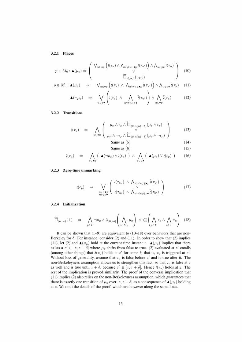
3.2.1 Places

p ∈M0 : N(µp)⇒

∨u∈•p

(o(τu) ∧

∧u′ 6=u∈•p o(τu′)

)∧∧u∈p• o(τu)

∨←− [0,∞)(¬µp)

(10)

p /∈M0 : N(µp) ⇒∨u∈•p

(o(τu) ∧

∧u′ 6=u∈•p o(τu′)

)∧∧u∈p• o(τu) (11)

N(¬µp) ⇒∨u∈p•

o(τu) ∧∧

u′ 6=u∈p•

o(τu′)

∧ ∧u∈•p

o(τu) (12)

3.2.2 Transitions

o(τu) ⇒∧p∈•u

µp ∧ εp ∧←− (0,α(u)−δ)(µp ∧ εp)∨

µp ∧ ¬εp ∧←− (0,α(u)−δ)(µp ∧ ¬εp)

(13)

Same as (5) (14)Same as (6) (15)

o(τu) ⇒∧p∈•u

(N(¬µp) ∨ o(εp)

)∧∧p∈u•

(N(µp) ∨ o(εp)

)(16)

3.2.3 Zero-time unmarking

o(εp) ⇒∨

ua∈•pub∈p•

o(τua) ∧∧u′ 6=ua∈•p o(τu′)∧

o(τub) ∧∧u′ 6=ub∈p• o(τu′)

(17)

3.2.4 Initialization

←− [δ,∞)(⊥) ⇒

∧p∈P¬µp ∧ ♦[0,2δ]

∧p∈M0

µp

∧ ©∧p∈P

εp ∧∧u∈T

τu

(18)

It can be shown that (1–9) are equivalent to (10–18) over behaviors that are non-Berkeley for δ. For instance, consider (2) and (11). In order to show that (2) implies(11), let (2) and N(µp) hold at the current time instant z. N(µp) implies that thereexists a z′ ∈ [z, z + δ] where µp shifts from false to true. (2) evaluated at z′ entails(among other things) that oo(τu) holds at z′ for some t; that is, τu is triggered at z′.Without loss of generality, assume that τu is false before z′ and is true after it. Thenon-Berkeleyness assumption allows us to strengthen this fact, so that τu is false at zas well and is true until z + δ, because z′ ∈ [z, z + δ]. Hence o(τu) holds at z. Therest of the implication is proved similarly. The proof of the converse implication that(11) implies (2) also relies on the non-Berkeleyness assumption, which guarantees thatthere is exactly one transition of µp over [z, z + δ] as a consequence of N(µp) holdingat z. We omit the details of the proof, which are however along the same lines.

13

3.3 Under-approximationThe under-approximations of (10–18) are reported as formulas (19–27). Notice thelower- and upper-bound relaxations in (22–24), in accordance with the notion of under-approximation.

3.3.1 Places

Syntactically the same as in (10) (19)Syntactically the same as in (11) (20)Syntactically the same as in (12) (21)

3.3.2 Transitions

o(τu) ⇒^p∈•u

0B@ µp ∧ εp ∧←− [1,α(u)/δ−2](µp ∧ εp)

∨µp ∧ ¬εp ∧

←− [1,α(u)/δ−2](µp ∧ ¬εp)

1CA (22)

←− [0,β(u)/δ]

0@τu ∧ ^p∈•u

µp

1A ⇒

0BBBBBBBB@

Wp∈•u ♦=1(¬µp)

∨

Wp∈•u

0B@←− [0,β(u)/δ](εp) ⇒ ♦=1(¬εp)

∧←− [0,β(u)/δ](¬εp) ⇒ ♦=1(εp)

1CA∨

♦=1(¬τu)

1CCCCCCCCA(23)

←− [0,β(u)/δ]

0@¬τu ∧ ^p∈•u

µp

1A ⇒

0BBBBBBBB@

Wp∈•u ♦=1(¬µp)

∨

Wp∈•u

0B@←− [0,β(u)/δ](εp) ⇒ ♦=1(¬εp)

∧←− [0,β(u)/δ](¬εp) ⇒ ♦=1(εp)

1CA∨

♦=1(τu)

1CCCCCCCCA(24)

Syntactically the same as in (16) (25)

The straightforward under-approximation of (14) and (15) yields formulas whichhave been re-arranged to eliminate redundant terms. In fact, the time bound (0, β(u)) inthe antecedent becomes [0, β(u)/δ] when under-approximated. Hence, formulas suchas←− (0,β(u))(γ) ⇒ ¬γ ∨©(¬γ) are under-approximated as

←− [0,β(u)/δ](γ) ⇒ ¬γ ∨

♦[0,1](¬γ). However, ¬γ never holds at the current instant because it would contradict

the antecedent. Correspondingly, such formulas can be simplified to←− [0,β(u)/δ](γ)⇒

♦=1(¬γ).

3.3.3 Zero-time unmarking

Syntactically the same as in (17) (26)

3.3.4 Initialization

at 0:∧p∈P¬µp ∧ ♦[1,2]

∧p∈M0

µp

∧ ∧p∈P

εp ∧∧u∈T

τu (27)

14

3.4 Axiomatization for over-approximationContinuous-time operator 4 becomes5 discrete-time operator N under over-approxi-mation when it occurs to the left-hand side of implications, hence is suitable to de-scribe antecedents of transitions that will be over-approximated. However, the over-approximation of the same operator takes a different form in the right-hand side ofimplications. In such cases, the over-approximation of formulas such as 4(x) is←− [0,1](¬x)∧[0,1](x) which is clearly unsatisfiable. Correspondingly, the whole over-approximation formulas would be unsatisfiable only for false antecedents, i.e., when notransition ever occurs.

After careful experimentation, we found that a workaround to this problem shouldexploit a weakening of the 4 operators that occur in consequent formulas. Let usillustrate the idea as simply as possible for two propositions x, y and the formula4(x) ⇒ 4(y): every transition of x occurs concurrently with a transition of y. The

formula is relaxed into the weaker 4(x) ⇒←−©(¬y) ∧ =δ(x⇒ y): every transition

of x also triggers a transition of y sometime in the future, as long as x still holds δ timeunits in the future. The new formula is essentially equivalent to the original one fornon-Berkeley behaviors for the following reasons. First, x must still hold δ time unitsin the future, because its behavior is non-Berkeley for δ; hence y holds as well thereand must transition somewhere over the interval (0, δ) from the current instant. In ad-dition, the transition of y cannot occur asynchronously to the transition of x; otherwisetwo distinct transitions would occur within δ time units, against the non-Berkeleynessassumption. In all, the two formulations are equivalent over non-Berkeley continuoustime. Correspondingly, the ooo operator is introduced and used in the right-hand side ofimplications in the following continuous-time formulas (28–36).

3.4.1 Places

p ∈M0 : 4(µp) ⇒

0BBBBB@Wu∈•p

“ooo(µp τu) ∧

Vu′ 6=u∈•p ooo(µp τu′ )

”∧V

u∈p• ooo(µp τu)

∨←− [δ,∞)(¬µp)

1CCCCCA (28)

p /∈M0 : 4(µp) ⇒

0B@Wu∈•p

“ooo(µp τu) ∧

Vu′ 6=u∈•p ooo(µp τu′ )

”∧V

u∈p• ooo(µp τu)

1CA (29)

4(¬µp) ⇒_u∈p•

0@ooo(¬µp τu) ∧^

u′ 6=u∈p•

ooo(¬µp τu′ )

1A ∧ ^u∈•p

ooo(¬µp τu) (30)

5After some semantic-preserving simplifications.

15

3.4.2 Transitions

oo(τu) ⇒^p∈•u

0BB@f←−©(µp ∧ εp) ∧

←− [δ,α(u))(µp ∧ εp)

∨f←−©(µp ∧ ¬εp) ∧←− [δ,α(u))(µp ∧ ¬εp)

1CCA (31)

Same as (5) (32)

Same as (6) (33)

4(τu) ⇒^p∈•u

0BBBB@0B@ f←−©(µp)

∧=δ(τu ⇒ ¬µp)

1CA∨

ooo(τu εp)

1CCCCA ∧^p∈u•

0BBBB@0B@ f←−©(¬µp)

∧=δ(τu ⇒ µp)

1CA∨

ooo(τu εp)

1CCCCA

4(¬τu) ⇒^p∈•u

0BBBB@0B@ f←−©(µp)

∧=δ(¬τu ⇒ ¬µp)

1CA∨

ooo(¬τu εp)

1CCCCA ∧^p∈u•

0BBBB@0B@ f←−©(¬µp)

∧=δ(¬τu ⇒ µp)

1CA∨

ooo(¬τu εp)

1CCCCA (34)

3.4.3 Zero-time unmarking

4(εp) ⇒_

ua∈•pub∈p•

0@ ooo(εp τua ) ∧Vu′ 6=ua∈•p ooo(εp τu′ )

∧ooo`εp τub

´∧Vu′ 6=ub∈p•

ooo(εp τu′ )

1A

4(¬εp) ⇒_

ua∈•pub∈p•

0@ ooo(¬εp τua ) ∧Vu′ 6=ua∈•p ooo(¬εp τu′ )

∧ooo`¬εp τub

´∧Vu′ 6=ub∈p•

ooo(¬εp τu′ )

1A (35)

3.4.4 Initialization

←− (0,∞)(⊥) ⇒

∧p∈P¬µp ∧ ♦[0,2δ]

∧p∈M0

µp

∧ ©∧p∈P

εp ∧∧u∈T

τu

(36)

The observations that have been introduced at the beginning of this section can beleveraged to provide a rigorous proof that (28–36) are equivalent to the original (1–9)over non-Berkeley continuous time. We omit the details for brevity.

3.5 Over-approximationThe over-approximations of (28–36) are reported as formulas (37–45). Notice thelower- and upper-bound relaxations in (40–42), in accordance with the notion of over-approximation.

16

3.5.1 Places

p ∈M0 : N(µp) ⇒

0BBBBB@Wu∈•p

“ooo(µp τu) ∧

Vu′ 6=u∈•p ooo(µp τu′ )

”∧V

u∈p• ooo(µp τu)

∨←− [δ,∞)(¬µp)

1CCCCCA (37)

p /∈M0 : N(µp) ⇒

0B@Wu∈•p

“ooo(µp τu) ∧

Vu′ 6=u∈•p ooo(µp τu′ )

”∧V

u∈p• ooo(µp τu)

1CA (38)

N(¬µp) ⇒_u∈p•

0@ooo(¬µp τu) ∧^

u′ 6=u∈p•

ooo(¬µp τu′ )

1A ∧ ^u∈•p

ooo(¬µp τu) (39)

3.5.2 Transitions

oo(τu) ⇒^p∈•u

0B@←− [0,α(u)/δ+1](µp ∧ εp)

∨←− [0,α(u)/δ+1](µp ∧ ¬εp)

1CA (40)

←− [1,β(u)/δ−1]

0@τu ∧ ^p∈•u

µp

1A⇒0BBBBBBBB@

Wp∈•u(¬µp ∨[0,1](¬µp))

∨

Wp∈•u

0B@←− [1,β(u)/δ−1](εp) ⇒ ¬εp ∨[0,1](¬εp)

∧←− [0,β(u)/δ−1](¬εp) ⇒ εp ∨ ♦[0,1](εp)

1CA∨¬τu

1CCCCCCCCA(41)

←− [1,β(u)/δ−1]

0@¬τu ∧ ^p∈•u

µp

1A⇒0BBBBBBBB@

Wp∈•u[0,1](¬µp)

∨

Wp∈•u

0B@←− [1,β(u)/δ−1](εp) ⇒ ¬εp ∨[0,1](¬εp)

∧←− [0,β(u)/δ−1](¬εp) ⇒ εp ∨ ♦[0,1](εp)

1CA∨τu

1CCCCCCCCA(42)

N(τu) ⇒^p∈•u

0BBBB@0B@

←− [0,1](µp)

∧[0,2](τu ⇒ ¬µp)

1CA∨

ooo(τu εp)

1CCCCA ∧^p∈u•

0BBBB@0B@

←− [0,1](¬µp)

∧[0,2](τu ⇒ µp)

1CA∨

ooo(τu εp)

1CCCCA

N(¬τu) ⇒^p∈•u

0BBBB@0B@

←− [0,1](µp)

∧[0,2](¬τu ⇒ ¬µp)

1CA∨

ooo(¬τu εp)

1CCCCA ∧^p∈u•

0BBBB@0B@

←− [0,1](¬µp)

∧[0,2](¬τu ⇒ µp)

1CA∨

ooo(¬τu εp)

1CCCCA(43)

Similarly as with under-approximation, formulas have been conveniently simpli-

fied: the term←−©(µp ∧ εp) in the consequent of (31) is over-approximated to

←− [0,1](µp ∧ εp), which is subsumed by the other term

←− [0,α(u)/δ+1)(µp ∧ εp) in the

over-approximation. (In fact, α(u)/δ + 1 ≥ 2 is the case). Subformulas ¬τu ∨[0,1](¬τu) and τu∨[0,1](τu) in the over-approximations (42) and (42), respectively,can also be simplified. In fact, (40) enforces marking and no zero-time unmarking forat least 3 time units whenever τu is triggered; hence µp cannot be triggered over [0, 1]so that the terms [0,1](¬τu) and [0,1](τu) are redundant.

17

3.5.3 Zero-time unmarking

N(εp) ⇒_

ua∈•pub∈p•

0@ ooo(εp τua ) ∧Vu′ 6=ua∈•p ooo(εp τu′ )

∧ooo`εp τub

´∧Vu′ 6=ub∈p•

ooo(εp τu′ )

1A

N(¬εp) ⇒_

ua∈•pub∈p•

0@ ooo(¬εp τua ) ∧Vu′ 6=ua∈•p ooo(¬εp τu′ )

∧ooo`¬εp τub

´∧Vu′ 6=ub∈p•

ooo(¬εp τu′ )

1A (44)

3.5.4 Initialization

at 0:∧p∈P¬µp ∧ ♦=1

∧p∈M0

µp

∧ [0,1]

∧p∈P

εp ∧∧u∈T

τu

(45)

3.6 Quality of discrete-time approximationsProposition 1 guarantees that under-approximations preserve validity and over-approx-imations preserve counterexamples. It does not say anything about the quality (or com-pleteness) of such approximations; in particular an under-approximation can preservevalidity trivially by being contradictory (i.e., inconsistent), and an over-approximationcan preserve counterexamples trivially by being identically valid.

In order to make sure this is not the case, let us introduce a set of constraints thatguarantees no degenerate behaviors are modeled in the approximations. Consider for-mulas involving metric intervals, namely (22–24) for the under-approximations and(40–42) for the over-approximation. We should check that, for every transition u withdense-time firing interval [α(u), β(u)]:

• non-emptiness. Metric intervals are non-empty; that is α(u) ≥ 3δ from theunder-approximation and α(u) ≥ −δ, β(u) ≥ 2δ from the over-approximation.

• consistency. The the minimum enabling interval (defined in (22) and (40) forunder- and over-approximation respectively) is smaller than the maximum en-abling interval (defined in (23–24) and (41–42) for under- and over-approximationrespectively). Correspondingly, we have the constraints β(u) ≥ α(u)− 2δ fromthe under-approximation and β(u) ≥ α(u) + 2δ from the over-approximation.

The constraints can be summarized as α(u) ≥ 3δ and β(u) ≥ α(u) + 2δ. In ourexamples, we will consider only non-degenerate TPN satisfying these constraints.

4 Multi-Paradigm Modeling and Verification at WorkThe multi-paradigm modeling technique presented in this paper is supported by theZot bounded satisfiability checker [16, 17]. More precisely, we exploited the flexi-bility provided by the SAT-based approach pursued by Zot, and implemented severalseparate plugins to deal with the various allowed formalisms. In particular, the tool nowincludes plugins capable of dealing with dense-time MTL formulas [11], with timedautomata [12], and with timed Petri nets (using the formalization presented in Section3). In addition, Zot is natively capable of accepting discrete-time MTL formulas as

18

input language. The plugins provide primitives through which the user can define thesystem to be analyzed as a mixture of timed automata, dense- and discrete-time MTLformulas, and timed Petri nets. The properties to be verified for the system can also bedescribed as a combination of fragments written using the aforementioned formal lan-guages, though they are usually formalized through MTL formulas (either using denseor discrete time).

The tool then automatically builds, for the dense-time fragments of the systemand of the property to be analyzed, the two discrete-time approximation formulas ofProposition 1. These formulas, in possibly conjunction with MTL formulas nativelywritten using a discrete notion of time, are checked for validity over timeN; the resultsof the validity check allows one to infer the validity of the integrated model, accordingto Proposition 1.

The multi-paradigm verification process in Zot consists of three sequential phases.First, the discrete-time MTL formulas of Proposition 1 are built and are translatedinto a propositional satisfiability (SAT) problem. Second, the SAT instance (possiblyincluding MTL formulas directly written using a discrete notion of time) is put intoconjunctive normal form (CNF), a standard input format for SAT solvers. Third, theCNF formula is fed to a SAT solving engine (such as MiniSat, zChaff, or MiraXT).

4.1 An Example of Multi-paradigm Modeling and VerificationWe demonstrate how the modeling and verification technique presented in this paperworks in practice through an example consisting of a fragment of a realistic monitoringsystem, which could be part of a larger supervision and control system.

The monitoring subsystem is composed of three identical sensors, a middle com-ponent that is in charge of acquiring and pre-processing the data from the sensors, anda data management component that further elaborates the data (e.g., to select appropri-ate control actions). For reasons of dependability (by redundancy), the three sensorsmeasure the same quantity (whose nature is of no relevance in this example). Eachone of them senses independently the measured quantity at a certain rate which is ingeneral aperiodic; however, while the acquisition rate can vary, the distance betweenconsecutive acquisitions must always be no less than T/2 and no more than T timeunits. Each sensor keeps track of only the last measurement, hence every new sensedvalue replaces the one stored by the sensor.

The data acquisition component retrieves data from the three sensors in a “pull”fashion. More precisely, when all three sensors have a fresh measurement available,with a delay of at least T/10 units, but of no more than T/5 time units, the data acqui-sition component collects the three values from the sensors (which then become stale,as they have been acquired). After having retrieved the three measurements, the com-ponent processes them (e.g., it computes a derived measurement as the average of thesensed values); the process takes between T/5 and T/2 time units.

After having computed the derived measurement, the data acquisition componentsends it to the data manager, this time using a “push” policy which requires an ac-knowledgement of the data reception by the latter. The data acquisition componenttries to send data to the data manager at most twice. If both attempts at data transmis-sion fail (for example because a timeout for the reception acknowledgement by the datamanager expires, or because the latter signals a reception error), the data transmissionterminates with an error.

First, we model the mechanism through which the three sensors collect data fromthe field and the data acquisition component retrieves them for the pre-processing

19

phase. This fragment of the model is described through a timed Petri net, and is de-picted in Figure 1.

Figure 1: Fragment of monitoring system modeled through a timed Petri net.

In a multiple-paradigm framework, the reasons that lead to the choice of a notationinstead of another often include a certain degree of arbitrariness. In this case, however,we chose to model the data acquisition part of the system through a TPN since we feltthat the inherent asynchrony with which the three sensors collect data from the fieldwas naturally matched by the asynchronous nature of a TPN and its tokens [10]. Whileit is undeniable that different modelers might have made different choices, we maintainthat TPN are well-suited (although not necessarily indispensable) in this case.

A further fragment of the formal model of the monitoring system is shown in Fig-ure 2. It represents, through the formalism of timed automata presented in [12], thetransmission protocol that the data acquisition component uses to send refined valuesto the data manager.6

Figure 2: Fragment of data acquisition system modeled through a timed automaton.

For this second fragment of the system, the formalism of timed automata was cho-

6As remarked in [12], since, in our formalization, the definition of clock constraints forbids the introduc-tion of exact constraints such asA = T2, such constraints represent a shorthand for the valid clock constraintT2 ≤ A < T + δ.

20

sen, with a certain degree of arbitrariness, because it was deemed capable of represent-ing the timing constraints on the protocol in a more natural way, especially for whatconcerns the constraint on the overall duration of the process.

Finally, MTL formulas are added to “bridge the gap” between the fragments shownin Figures 1 and 2. This is achieved by the two following formulas, which define,respectively, that the transmission procedure can begin only if a pre-processed mea-surement value has been produced by the data acquisition component in the last T timeunits (46) and if the system is not in the middle of a data transmission (i.e., it is idle),and a new datum is being processed, a transmission will start within T/2 time units,due to the upper bound of process d transition (47).

try ⇒←−♦ (0,T/2](data retrieved) (46)

data retrieved ∧ idle ⇒ ♦(0,T/2](try) (47)

Notice that the automata of Figures 1 and 2 are defined, as per the formalizationsof [12] and of Section 3, over a continuous notion of time. This choice for the timedomain of these two system fragments is justified by the fact that they deal with partsof the system interacting with physical elements (measured quantities, transmissionchannel), for which a continuous time seems better suited.

Formulas (46) and (47), instead, describe a software synchronization mechanismwithin the application. As a consequence, discrete time is more suitable to describethis part of the system, hence formulas (46) and (47) are to be interpreted accordingly.

Finally, the model of the system to be verified is built by conjoining the discrete-time approximations for the fragments of Figures 1-2 and the discrete-time MTL for-mulas (46)-(47). More precisely, if ψΩδ

N and ψOδN are the continuous-time MTL for-

mulas capturing the semantics of the net of Figure 1 (see Section 3), ψΩδA , ψOδ

A are thecontinuous-time MTL formulas for the automaton of Figure 2, ψL is the discrete-timeformula ψL = (46)∧ (47), and φprop is the continuous-time property to be checked forthe system, then we have:

φ+ = Alw“

Ωδ

“ψ

ΩδN

”∧ Ωδ

“ψ

ΩδA

”∧ ψL

”⇒ Alw(Oδ (φprop))

φ− = Alw“

Oδ

“ψ

OδN

”∧Oδ

“ψ

OδA

”∧ ψL

”⇒ Alw(Ωδ (φprop))

Note that formula ψL, which is to be interpreted over discrete time, must not beapproximated. Then, if φ+ isN-valid, we can draw some interesting conclusions.

First, if one implements a continuous-time system that does not vary faster thanthe sampling time δ (i.e., whose behaviors are in Bδχ), which satisfies ψN , ψA, and acontinuous-time MTL formula ψ′ such that Ωδ (ψ′L) = ψL, then property φprop holdsfor this system.

It can be shown that, for any continuous-time MTL formula φ, the set of behaviorssatisfying Oδ (φ) is a subset of those satisfying Ωδ (φ) (i.e., b | b |=N Oδ (φ) ⊆b | b |=N Ωδ (φ)). In addition, given a discrete-time behavior b that satisfies Oδ (φ),from [11, Lemma 3] we have that any continuous-time non-Berkeley behavior b′ forwhich b is a sampling satisfies φ. Then, any way one reconstructs a continuous-timenon-Berkeley behavior b′ from a discrete-time one that satisfies Oδ (φ), b′ satisfies φ.This leads us to conclude that, if one builds a discrete-time system (e.g., a piece ofsoftware) which implements — that is, satisfies — Oδ

(ψOδN

), Oδ

(ψOδA

), ψL, this

satisfies discrete-time property Oδ (φprop); in addition, any way one uses a discrete-

21

time behavior of this system to reconstruct a continuous-time, non-Berkeley behavior,the latter satisfies ψN , ψA, and φprop.

Finally, if φ− is not N-valid, a discrete-time system implementing Oδ

(ψOδN

),

Oδ

(ψOδA

), ψL violates property Ωδ (φprop).

Verification. We used the system model presented above to check a number of prop-erties to validate the effectiveness of our approach. Table 4.1 shows the results, andduration of the tests. More precisely, for each test the table reports: the checked prop-erty; the values of the timing parameters in the model (i.e., T1, T2, T3, T ); the temporalbound k of the time domain (as Zot is a bounded satisfiability checker, it considers allthe behaviors with period ≤ k); the total amount of time to perform each phase of theverification, namely formula building (including transformation into conjunctive nor-mal form), and propositional satisfiability checking; the results of the tests; the size (inmillions of clauses) of the formula fed to the SAT-solver.7 Tests were performed instan-tiating the parameters with different values to get an idea of how the performance ofthe verification algorithm is affected, both in terms of time to complete the verificationand of whether the verification attempt is conclusive. In addition, the timed interactionbetween the data acquisition and monitoring subsystems is quite subtle and the prop-erties under verification hold in every run of the system only for certain combinationsof parameter values. Automated verification allowed us to investigate this fact in somedetail.

First, we checked some properties concerning the liveness of the data collection bya sensor X (with X ∈ 1, 2, 3). More precisely, we analyzed whether property (48)holds for the model.8

replaceX ∧ new dX⇒♦(0,T+δ](replaceX ∧ ¬new dX ∨ ¬replaceX ∧ new dX)

∧replaceX ∧ ¬new dX⇒

♦(0,T+δ](replaceX ∧ new dX ∨ ¬replaceX ∧ ¬new dX)∧

¬replaceX ∧ new dX⇒♦(0,T+δ](¬replaceX ∧ ¬new dX ∨ replaceX ∧ new dX)

∧¬replaceX ∧ ¬new dX⇒

♦(0,T+δ](¬replaceX ∧ new dX ∨ replaceX ∧ ¬new dX)

(48)

Formula (48) states that triggering events of replaceX and new dX transitions mustoccur within T + δ (with δ the sampling period) time instants in the future, i.e., thateither replaceX or new dX must change value within the next T +δ time instants. Theproperty does not hold in general, since a firing of transition retrieve d would reset thetime counters for transitions replaceX and new dX. This fact can be pointed out bychecking φ−, with φprop = (48), which is unsatisfiable, as shown in Table 4.1.

7The verification tool and the complete model used for verification can be found athttp://home.dei.polimi.it/pradella. Tests have been performed on a PC equippedwith two Intel Xeon E5335 Quad-Core Processor 2GHz, 16 Gb of RAM, and GNU/Linux (kernel 2.6.29),using a single core for each test. Zot used the SAT-solver MiniSat 2.

8Recall that all properties to be proved are implicitly closed with the Alw operator.

22

If the additional hypothesis that transition retrieve d does not fire along (0, T + δ],(48) can however be shown to hold. More precisely, if (48) is rewritten, as shown informula (49), by adding to the antecedents the condition that predicate retrieve d doesnot change in (0, T + δ] (i.e., transition retrieve d does not fire in that interval), thenthe new φ+ isN-valid (as Table 4.1 shows), hence (49) holds for the system.

(0,T+δ](retrieve d) ∧ replaceX ∧ new dX⇒♦(0,T+δ](replaceX ∧ ¬new dX ∨ ¬replaceX ∧ new dX)

∧ · · · ∧(0,T+δ](retrieve d) ∧ ¬replaceX ∧ ¬new dX⇒

♦(0,T+δ](¬replaceX ∧ new dX ∨ ¬replaceX ∧ new dX)∨(0,T+δ](¬retrieve d) ∧ replaceX ∧ ¬new dX⇒

♦(0,T+δ](replaceX ∧ new dX ∨ ¬replaceX ∧ ¬new dX)∧ · · · ∧

(0,T+δ](¬retrieve d) ∧ ¬replaceX ∧ ¬new dX⇒♦(0,T+δ](¬replaceX ∧ new dX ∨ ¬replaceX ∧ new dX)

(49)

Another liveness property is formalized by formula (50), which states that a datumis retrieved (i.e., place data retrieved is marked) at least every 3T

2 time units.

♦(0, 3T2 ]

(data retrieved) (50)

Property (50) cannot be established with our verification technique as it falls inthe incompleteness region (i.e., φ+ is not valid and φ− is valid, as Table 4.1 shows);from the automated check we cannot draw a definitive conclusion on the validity of theproperty for the system. If, however, the temporal bound of formula (50) is slightlyrelaxed as in formula (51), not only the verification is conclusive, but it shows that theproperty in fact holds for the system.

♦(0,2T ](data retrieved) (51)

Verification also shows that the original formula (50) holds if the bound on transi-tions replaceX of the TPN is changed to [ 4T

5 , T ] (property (50’) in Table 4.1).Formula (52) expresses the maximum delay between sensor collect and data send.

More precisely, if each sensor has provided a measurement and transition retrieve dfires, then the timed automaton will enter state try within T instants. The validity ofthis formula would allow us to check that the two parts of the system modeled by theTPN and by the TA are correctly “bridged” by axioms (46) and (47). As Table 4.1shows, property (52) does not hold; this occurs because, when place data retrieved ismarked, the TA might not be in state idle.

data retrieved⇒ ♦(0,T ](try) (52)

Axiom (47) states that a try state is entered within T/2 if data retrieved holdswhen idle holds. Then, a deeper analysis on the timing constraints suggests that thiscondition depends on the maximum transmission time T3 of the TA, which definesthe maximum delay between two consecutive occurrences of idle. If the system is indata retrieved and not in idle, then the next idle state will be within T3 instants in thefuture; moreover, data retrieved will be unmarked within T/2. This suggests that thefollowing property (53) is valid:

23

(0,T3](data retrieved)⇒ ♦(0,T ](try) (53)

This property also falls in the incompleteness region of the verification technique.However, the following slight relaxation of formula (53) can be proved to hold for thesystem:

(0,T3+δ](data retrieved)⇒ ♦(0,T ](try) (54)

PR T1 T2 T3 T K PRE (min.) CNF (hrs.) SAT (hrs.) N-VALID # CL·106

48: φ+ 3 6 18 30 90 1.9877 1.854 2.2322 ⊥ 12.414848: φ− 3 6 18 30 90 3.0743 6.2533 5.3518 ⊥ 21.30648: φ+ 3 9 36 30 90 2.425 2.5699 2.5368 ⊥ 12.741148: φ− 3 9 36 30 90 3.3372 6.2202 5.0851 ⊥ 21.632348: φ+ 3 12 48 30 120 3.2059 3.6904 6.8226 ⊥ 17.283348: φ− 3 12 48 30 120 4.5452 10.439 9.2688 ⊥ 29.11749: φ+ 3 6 18 30 90 2.1074 1.9171 0.8101 > 12.851249: φ− 3 6 18 30 90 3.1059 5.7381 3.017 > 21.751449: φ+ 3 9 36 30 90 2.6346 2.7726 0.9741 > 13.177549: φ− 3 9 36 30 90 3.5125 6.4452 3.5557 > 22.077849: φ+ 3 12 48 30 120 3.6731 4.379 2.0955 > 17.864149: φ− 3 12 48 30 120 5.1492 11.0093 5.0007 > 29.709850: φ+ 3 6 18 30 90 1.8887 1.7376 3.1524 ⊥ 12.059850: φ− 3 6 18 30 90 2.9094 6.0154 3.427 > 20.93150: φ+ 3 9 36 30 90 2.2002 2.3232 2.4845 ⊥ 12.386250: φ− 3 9 36 30 90 3.1067 5.8341 4.6997 > 21.257350: φ+ 3 12 48 30 120 3.4446 4.1686 8.8680 ⊥ 16.810850: φ− 3 12 48 30 120 4.1621 9.9533 13.1718 > 28.617951: φ+ 3 6 18 30 90 2.0715 1.6828 1.2976 > 12.158451: φ− 3 6 18 30 90 3.0536 5.3665 3.9414 > 21.029651: φ+ 3 9 36 30 90 2.8152 2.2134 1.7645 > 12.484851: φ− 3 9 36 30 90 3.7314 6.1665 3.6802 > 21.355951: φ+ 3 12 48 30 120 3.9268 4.5246 9.3435 ⊥ 16.942151: φ− 3 12 48 30 120 4.8244 9.7484 14.8257 > 28.749150’: φ+ 3 6 18 30 90 2.2399 2.3971 4.0335 > 12.809750’: φ− 3 6 18 30 90 3.3884 5.5905 4.5752 > 21.664550’: φ+ 3 9 36 30 90 2.4788 2.2978 4.8259 > 13.13650’: φ− 3 9 36 30 90 3.8369 7.3132 0.0036 > 21.990950’: φ+ 3 12 48 30 120 4.7220 5.0607 13.3136 ⊥ 17.808850’: φ− 3 12 48 30 120 4.8557 9.7088 8.4951 > 29.594252: φ+ 3 6 12 30 75 1.5108 1.0502 0.4716 ⊥ 9.9105652: φ− 3 6 12 30 75 2.1418 3.1694 1.4723 ⊥ 17.317752: φ+ 3 3 15 30 75 1.5199 1.0564 0.4703 ⊥ 9.8758452: φ− 3 3 15 30 75 2.1586 3.1764 1.4473 ⊥ 17.283752: φ+ 3 6 18 30 75 1.5458 1.0706 0.5673 ⊥ 9.9786552: φ− 3 6 18 30 75 2.1978 3.2174 1.4323 ⊥ 17.385853: φ+ 3 6 12 30 75 1.6018 1.1108 0.8844 ⊥ 9.9731253: φ− 3 6 12 30 75 2.2909 3.3455 2.1095 > 17.384153: φ+ 3 3 15 30 75 1.6734 1.1945 0.6418 ⊥ 9.9554253: φ− 3 3 15 30 75 2.1638 3.2626 1.5792 > 17.367153: φ+ 3 6 18 30 75 1.7031 1.2210 0.9653 > 10.075253: φ− 3 6 18 30 75 2.48 3.3642 1.1761 > 17.486254: φ+ 3 6 12 30 75 1.578 1.0879 1.2972 > 9.9787954: φ− 3 6 12 30 75 2.3035 3.2128 1.6002 > 17.389854: φ+ 3 3 15 30 75 1.6465 1.0986 0.7740 ⊥ 9.9610954: φ− 3 3 15 30 75 2.1604 3.1919 1.1408 > 17.372754: φ+ 3 6 18 30 75 1.6220 1.1249 0.8240 > 10.080954: φ− 3 6 18 30 75 2.2892 3.2682 1.1178 > 17.4919

Table 2: Checking properties of the data monitoring system.

24

5 Discussion and ConclusionIn this paper we presented a technique to formally model and verify systems using dif-ferent paradigms for different system parts. The technique hinges on MTL axiomatiza-tions of the different modeling notations, which provide a common formal ground forthe various modeling languages, on which fully-automated verification techniques arebuilt. We provided an MTL axiomatization of a subset of TPN, a typical asynchronousoperational formalism, and showed how models could be built by formally combiningtogether TPN and TA (a classic synchronous operational notation, for which an axiom-atization has been provided in [12]). In addition, we showed how the approach allowsusers to integrate in the same model parts described through a continuous notion oftime, and parts described through a discrete notion of time.

Practical verification of systems modeled through the multi-paradigm approach ispossible through the Zot bounded satisfiability checker, for which plugins supportingthe various axiomatized notations have been built.

The technique has been validated on a non trivial example of data monitoring sys-tem. The experimental results show the feasibility of the approach, through which wehave been able to investigate the validity (or, in some cases, the non validity) of someproperties of the system. As described in Section 4, the verification phase has provideduseful insights on the mechanisms and on the timing features of the modeled system,which led us to re-evaluate some of our initial beliefs on the system properties.

It is clear from our experiments that, unsurprisingly, the technique suffers fromtwo main drawbacks: the incompleteness of the verification approach by discretizationevidenced in [11], which prevented us, in some cases, to get conclusive answers onsome analyzed properties; and the computational complexity of our method, which isbased on the direct translation of TPN and TA into MTL formulas, approximated intodiscrete ones, and then encoded into SAT. This makes proofs considerably lengthier asthe size of the domains, and especially of the temporal one, increases, as evidenced byTable 4.1. Nevertheless, we maintain that the results we obtained are promising, andshow the applicability of the technique on non trivial systems. This claim is supportedon the one hand by the sophistication of the properties we have been able to prove(or disprove): it is inevitable that verification over continuous real-time has a highcomputational cost. On the other hand, while incompleteness is a hurdle to the fullapplicability of the technique, in practice it can be mitigated quite well, usually byslightly relaxing the real-time timing requirements under verification in a way thatdoes not usually alter the gist of what is being verified.

In our future research on this topic we plan to address the two main drawbacksevidenced above. First, we will work on extending the verification technique to expandits range of applicability and reduce its region of incompleteness. Also, we will studymore efficient implementations for theZot plugins through which the various modelingnotations are added to the framework: we believe that more direct (therefore morecompact, both in the literals and clause numbers) encodings into SAT of the TPN andTA axiomatizations should significantly improve the efficiency of the tool.

In particular, we have not yet tackled the problem of optimizing the encodingsof the TPN and TA axiomatizations into the SAT problem. We expect that significantimprovements on the duration of the proofs can be gained through optimized encodingsthat reduce, on the one hand, the time needed to put formulas in the conjunctive normalform that is required as input by SAT solvers, and, on the other hand, the number ofliterals required to represent TPN and TA as SAT problems.

25

References[1] R. Alur and D. L. Dill. A theory of timed automata. Theor. Comp. Sci.,

126(2):183–235, 1994.

[2] R. Alur, T. Feder, and T. A. Henzinger. The benefits of relaxing punctuality.Journal of the ACM, 43(1):116–146, 1996.

[3] R. Alur and T. A. Henzinger. Logics and models of real time: A survey. InProc. of Real-Time: Theory in Practice, volume 600 of LNCS, pages 74–106,1992.

[4] R. Alur and T. A. Henzinger. Real-time logics: Complexity and expressiveness.Information and Computation, 104(1):35–77, 1993.

[5] F. Cassez and O. H. Roux. Structural translation from time Petri nets to timedautomata. Journal of Systems and Software, 79(10):1456–1468, 2006.

[6] A. Cerone and A. Maggiolo-Schettini. Time-based expressivity of time Petri netsfor system specification. Theor. Comp. Sci., 216(1–2):1–53, 1999.

[7] E. M. Clarke, O. Grumberg, and D. A. Peled. Model Checking. MIT Press, 2000.

[8] M. Felder, D. Mandrioli, and A. Morzenti. Proving properties of real-time sys-tems through logical specifications and Petri net models. IEEE Trans. on Soft.Eng., 20(2):127–141, 1994.

[9] C. A. Furia, D. Mandrioli, A. Morzenti, and M. Rossi. Modeling time in comput-ing. Technical Report 2007.22, DEI, Politecnico di Milano, January 2007.

[10] C. A. Furia, D. Mandrioli, A. Morzenti, and M. Rossi. Modeling time in comput-ing: a taxonomy and a comparative survey. ACM Computing Surveys, to appear.Also available as http://arxiv.org/abs/0807.4132.

[11] C. A. Furia, M. Pradella, and M. Rossi. Automated verification of dense-timeMTL specifications via discrete-time approximation. In Proc. of FM’08, volume5014 of LNCS, pages 132–147, 2008.

[12] C. A. Furia, M. Pradella, and M. Rossi. Practical automated partial verificationof multi-paradigm real-time models. In Proc. of ICFEM’08, volume 5256/-1 ofLNCS, pages 298–317, 2008.

[13] C. A. Furia and M. Rossi. Integrating discrete- and continuous-time metric tem-poral logics through sampling. In Proc. of FORMATS’06, volume 4202 of LNCS,pages 215–229, 2006.

[14] C. Heitmeier and D. Mandrioli, editors. Formal Methods for Real-Time Comput-ing. John Wiley & Sons, 1996.

[15] R. Koymans. Specifying real-time properties with metric temporal logic. Real-Time Systems, 2(4):255–299, 1990.

[16] M. Pradella. Zot. http://home.dei.polimi.it/ pradella, March2007.

26

[17] M. Pradella, A. Morzenti, and P. San Pietro. The symmetry of the past and ofthe future: bi-infinite time in the verification of temporal properties. In Proc. ofESEC/FSE 2007, 2007.

[18] OMG Unified Modeling Language (OMG UML) Superstructure, v2.2. TechnicalReport formal/2009-02-02, Object Management Group, 2009.

[19] M. von der Beeck. A comparison of statecharts variants. In Proc. of FTRTFT,volume 863 of LNCS, pages 128–148, 1994.

27