Scalable Solutions to ]ntegral ILquation andFinite Itlcmcnt Simulations

“1’OIN (_Mik, [)aniel S. Ka(z,i and Jean l’atlcrscm

Jet I’repulsion 1.aboratory4800 Oak Grove IMivc

California lnslitutc of I’cchnologyI’asadcna, California, 91109

cwik@jpl.nasa.gov

*(lay Research Inc.

AIIS’1’RAC’1’

When developing numerical methods, or applying them to the simulation and design of

cnginccring components, it inevi(ab]y bccomcs necessary to examine the scaling of tlic rndhod

with a problcm’s electrical size. The scaling results from the original mathematical development- --

for example, a dense system of equations in the solution of integral equations-as well as the

specific numerical implementation. Scaling of the numerical implementation depends upon many

factors–-for example, direct or iterative methods for solution of the linear system-–as well as the

computer architecture used in the simulation. In this paper, scalability will be divided into two

components; scalability of the numerical algorithm specifically on parallel computer systcm.s, and

algorithm or sequential scalabi]it y. The sequential implementation and scaling is initial presented

with the parallel inlplcmcntation following. “1’his progression is meant to illustrate the differences

in using current parallel platforms from sequential machines, and the resulting savings. Time to

solution (wall clock time) a]on~ with problc.m sim arc the kcy parameters plotted or tabulated.

Sc~ucntial and parallel scalability of time harmonic surface integral equation forms and the frnitc

clement solution to the pallial differential equations arc considered in detail.

“1’hc rcse.arcti dcscritd in this papm was car[icct OUI at the Jc.[ I’repulsion 1.abmalory, California lns(itu(e of‘l”c.chnolof,y, undc.r a contrac[ with (he National Aeronautics and Space A(l[[]illisl[:l[ic~[~

1. IN’l’I/{)I)LICrl’If)N

‘1’hc application of advanced compu(cr architcctur-c arid soflwarc to a broad range of

clcc(romagnctic problems has allowed more accuralc simulations of el~lrjcally larger and more

complex components and systems. Computational algorithms arc USCd in thc design and analysis

of antenna components and arrays, wavcguidc components, semiconductor dcviccs, and in lhc

prediction of radar scattering from aircraft, sea surface or vegetation, and atmospheric particles,

among many other applications. A scattering algorithm, for example, my be used in conjunction

with measured data to accurately reconstruct geophysical data. When used in design, the goal of a

numerical simulation is to limit the number of trial fabrication and mcasurcmcnt iterations nccdcd.

‘t’hc algorithms are used over a wide range of frcqucncics, materials and shapes, and can be

developed to be specific to a single geometry and application, or more gencrall y applied to a class

of problems. ‘i’hc algorithms are Immcrical solutions to a mathematical IllOdC] dcvclopcd in the

iimc or frcxqucncy domain, and can be based on the integral equation or pallial differential equation

form of Maxwell’s equations. A survey of the many forms of mathematical modeling and

numerical solution can be found in [1, 2.]. ‘1’hc goal of this paper is to examine (hc scalability of

ccllain numerical solutions both generally as a sequential algorithm, and then specifically as parallel

algorithms using distributed memory computers. Paral]cl computers continue to evcdvc,

surpassing traditional computer architectures in offering the largest memories and fastest

computational rates to the user, and will continue to CVOIVC for several more generations in

future [3].

This paper overviews solutions to Maxwell’s equations implicitly defined through

the near

SyStCInS

of linear equations. Sequential and parallel scalability of time harmonic surface integral equation

forms and the finite clcmcnt solu(ion to the partial differential equations are considered. More

general scalability of other sequential algorithms can be found in [4]. initially in Section 2, a short

review of tt ~c scalability y of parallel computers is presented. in Sections 3 and 4 rcspcctivcly,

specific illll>lcrIlcrltatiolls of the method of n)olnc,[l(s solution to integral equation mocicling, an(i a

frnitc clement soluticm wilt be (iiscusscd. “i’hc scalability of scqucntiai solutions and rclatcli

2

IcdLmd Incnmy IMhods will be considered followed by parallel scalability and computer

performance for these algorithms. ‘1’he size of problems capable of being examined wjth current

computer architectures will be then be listed, with scalings (O Iargcr si~,c problems also presented.

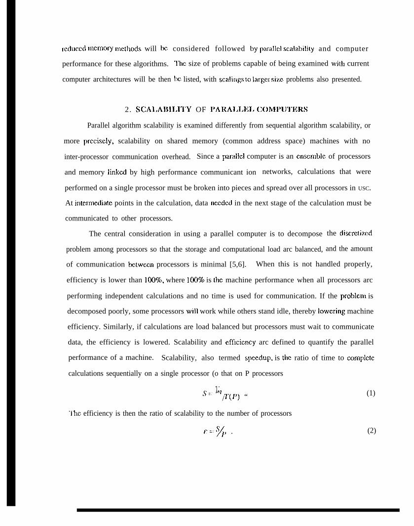
2. SCA1,AIIII.I”J’Y OF I’ARAI,I,EI, COMI’U’J’ERS

Parallel algorithm scalability is examined differently from sequential algorithm scalability, or

more prcciscly, scalability on shared memory (common address space) machines with no

inter-processor communication overhead. Since a pamllel computer is an cnscmblc of processors

and memory linked by high performance communicant ion networks, calculations that were

performed on a single processor must be broken into pieces and spread over all processors in USC.

At jntcrmediatc points in the calculation, data nccdcd in the next stage of the calculation must be

communicated to other processors.

The central consideration in using a parallel computer is to decompose

problem among processors so that the storage and computational load arc balanced,

the cliscrctimd

and the amount

of communication bctwccn processors is minimal [5,6]. When this is not handled properly,

efficiency is lower than 10WZO, where 100?io is t}]e machine performance when all processors arc

performing independent calculations and no time is used for communication. If the problcm is

decomposed poorly, some processors will work while others stand idle, thereby Iowcring machine

efficiency. Similarly, if calculations are load balanced but processors must wait to communicate

data, the efficiency is lowered. Scalability and cfflcicncy arc defined to quantify the parallel

performance of a machine. Scalability, also termed spccdup, is the ratio of time to eomplctc

calculations sequentially on a single processor (o that on P processors

. .1/‘y= “q T(I’) “

l’hc efficiency is then the ratio of scalability to the number of processors

/c+, .

(1)

(2)

If an algorithm issues no cc~llllllllllicatiotl calls, and there is no conlponcnt of Ihc calculation that is

sc.qucntia! an(i thcrcforc w.dundantly rc1Eatc41 al each processor, the scalability is cqua] to the

number of pmccssors P and the efficiency is 100%. ‘1’hc scalability, as defined, must bc further

clarified if it is to bc meaningful since the alnount of storage, i.e., problem si?,c, has not been

inc]udcd in lhc definition. ‘1’wo regimes can bc consiclcred--fixed problcm size and fixed grain

si~,c. ‘1’hc first, fixed problcnl siz,c, refers to a problcm that is small enough to fit into onc or a

fcw processors and is succcssivcl y spread over a Iargcr sized machine. ‘1’he amount of data and

calculation in each processor will dccrcasc and the amount of communication will incrcasc. The

efficiency must tbcrcforc successively dccreasc, reaching a point where OU time is

communication bound. l’hc second, fixed grain size problems, refers to a problcm size- that is

scaled to fill all the memory of the machine in use. The amoun~ of data and calculation in each

processor will be constant, and in general, much greater than the required amount of

cmnmunication. lifficicncy will remain high as successively larger problems arc solved. I:ixcd

gl-ain problems ideally exhibit scalability that is a kcy [no~ivator f o r par-allc] proccssing-

succcssivcly larger problems can hc mappccl onto successively larger machines without a loss of

efficiency.

When developing numerical methods, c)r applying them to tbc simulation and design of

cnginccring components, it inevitably bccomcs ncccssary to examine the scaling of the method

with a problcm’s electrical size. ‘1’hc scaling results from tbc original mathematical dcvclopnwnt--

for example, a dense systcm of equations in the solution of integral equations-—as WCII as the

specific numcrica] itllplcr]lclltatioll. Scaling of the numctical implementation depends upon many

factors- for example, direct or iterative methods for solution of tllc linear systcnl- as well as the

computer archi(ezturc used in tbc simulation. in the rest of this paper, scalability will bc divided

into two components; first, algorithmic scalability, and second, scalability of the. numerical

algoritim~ specifically on palalle.1 computer systems. Algorithmic scalabi]ty refers LO the amount of

computer memory and time, ncc.dcd to cc)mplctc aII accurate solution as a function of tllc electrical

sim of [I]c prob]cm. Scal:il)iljty 011 a paral]cl com])utcr sys IcIn refers to the ability of an algorittlm

4

to achieve performance proportional to the nlln~twr of pmccssors l~ing used as outlined ribovc.

The sequential irll~)lclllcl~tatioll and scaling is initial prcscntc~i with tile Paralicl inqdcmcnlation

following. This progression is meant to illustrate the differences in using current parallel platforms

from sequential machines, and the resulting savings. ~lcarl y, di ffcrcnt mathcmat ical formulations

can lead to al(crnatc numerical implementations and different scalings. ‘1’hc objective of any

numerical mc(hod is to provide an accurate simulation of the measurable quantities in an amount of

time that is useful for engineering design. With this objective, time to solution (wall clock time.)

along with problem sim arc the key parameters plotted or tabulated.

3. INIEGRAI. NQUAIION FORMUI,ATIONS

The method of moments is a traditional algorithm used for the solution of a surfac~ integra]

equation [7,8]. This technique can be applied to impenetrable and homogcnous objects, objects

where an impedance boundary condition acmra[cly models inhomogcnous materials OJ coatin[:s,

and those inhomogcmous objects that allow the use of ~~rccn’s functions specific to the geometry.

A dense system of equations results from discretiz.ing the surface basis functions in a picccwise

continuous set, with this system being solved in various ways. The components of method of

moment solutions that affect the algorithmic scalability arc the matrix fill, and solution. A system of

equations

AX= II (3)

results from the method of moments, where A generally is an non-symmetric conqdcx-valued

square matrix, and II and X arc complex-valued rectangular matrices when multiple excitations

and solution vectors arc present. I’hc solution of (3) is most conveniently found by an 1 SJ

factori~at ion

A =- I.~J (4)

where 1. and [J arc lower and upper triangular factors of A. ‘1’hc solution for X is computed by

successive forward and back substitutions to SOIVC the triangular systems

5

I,Y = B, Ux =-Y. (5)

Ikcausc (hc system in (3) in not generally positive definite, rows of A arc permuted in the

factori7jation, Icading to a stable algorithm [9]. Table 1 is a listing of computer storage and time

scalings for a range of problcm sizes when using standard 1.U decomposition factorization, and

forward and backward solu[ion algorithms readily available [10]. The table is divided along

columns into problem siz,c, factori7.ation and solution components. ‘1’hc first column fixes the

memory size of the machine being used; the INI mber of unknowns and surface area nmdclcd

(assuming 200 unknowns/k2), based on this memory arc in the next columns. The factor and

SOIVC times are based on the performance of three classes of rnachinc, current high-end workstation

(O. 1 Gigaflops), current supercomputcr (10 Gigaflops), and next generation computer (1000

Gigaflops). Similarly, the rows are divided into the top four which would typically correspond to

current generation workstations, and the lower four that correspond to supcrcomputcr class

machines. Duc to the nature of the dense matrix data structures [ 10] in the factorization algori{l mls,

this component of the calculation can be highly cfficicnt on general computers. A value of 80%

cffrcicncy of the peak machine performance is used for the time scali rigs. The backward and

forward solution algorithms though operate sequentially on triangular matrix systems, resulting in

reduced performance, and a 50% efficiency is used in these columns. ‘I’his performance will

incrcasc when many excitations (right-hand sides) arc involvccl in the calculation, resulting in

performance closer to peak.

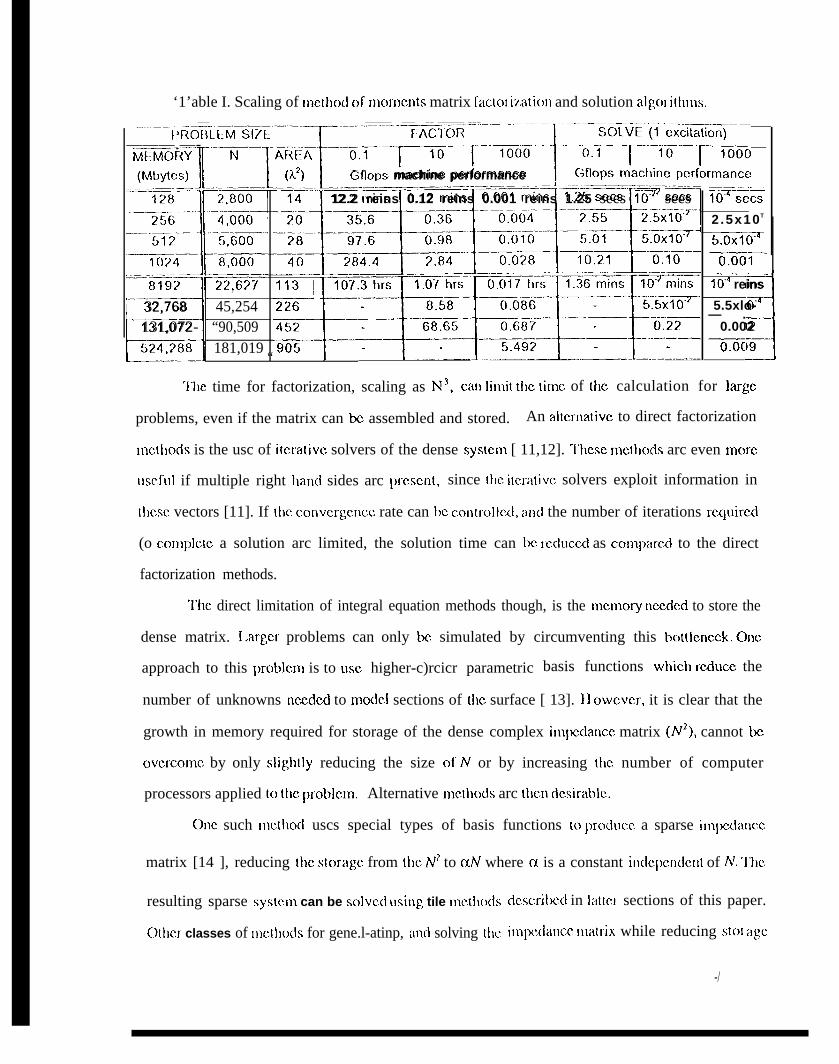
‘1’able I. Scaling of mclhod of morncnts matrix fadorimtion and solution algm i(hlns.—.. .——. .—.. -- —— ---..— —

y;~:y’y:f:~~?:21”--~~:]:~j:;;::::~———.—- .——

Gflops machine performance-. _ . JL-_.~...____—___

55iij$--%:~$zd?~iz

12.2 reins 0.12 reins 0.001 reins 1.25 sees 10T sees

8192 ,

H~ “

32,768 45,254131,072- “90,509524,28~ 181,019

::~~~~-flK?~:~

L

.— .—m%ii2.5x10T

5.0x-toT--m6i-

3————104 reins

5.5xlo-— .

0.002

T6’6F-

‘1’he time for factorization, scaling as N3, can limit lhc lime of the calculation for large

problems, even if the matrix can b assembled and stored. An altcmativc to direct factorization

mctho(is is the usc of i(cra(ivc solvers of the dense syshm [ 11,12]. l’hcse mctbods arc even more

uscfLl] if multiple right hami sides arc prcscnl, since I})c itcxativc solvers exploit information in

[hcsc. vectors [11]. If the convcrgcncc rate can bc contr-ollc(i, anti the number of iterations rcc}uired

(o compklc a solution arc limited, the solution time can 1x. l-cciuccd as compare~i to the direct

factorization methods.

l’hc direct limitation of integral equation methods though, is the mcmoly nccdcd to store the

dense matrix. 1.argcr problems can only bc simulated by circumventing this tmtticncck. one

approach to this probhm is to LISC higher-c)rcicr parametric basis functions which rcducx the

number of unknowns nccdcd to model sections of (})c surface [ 13]. 11 owcvcr, it is clear that the

growth in memory required for storage of the dense complex impcdancc matrix (N*), cannot bc

ovcrcomc by only sligh(ly reducing the size of N or by increasing ti~c number of computer

processors applied (o (}]c problcm. Alternative mctho(is arc then dc.sirablc.

onc such mc.thoci uscs special types of basis functions to ]N’OdLICC. a sparse impc~iancc

matrix [14 ], reducing (hc stora,gc from tt~c N7 to UN where a is a constant in(ic.pcncicnt of N. ‘I”hc

resulting sparse syslcm can be solvc(i using tile mcti~o(is

olhcr classes of mc[}wds for gene.l-atinp, an(i solving IIlc

dcscribcxi in lat(cr sections of this paper.

impc(iancc mati-ix while reducing stol agc

-/

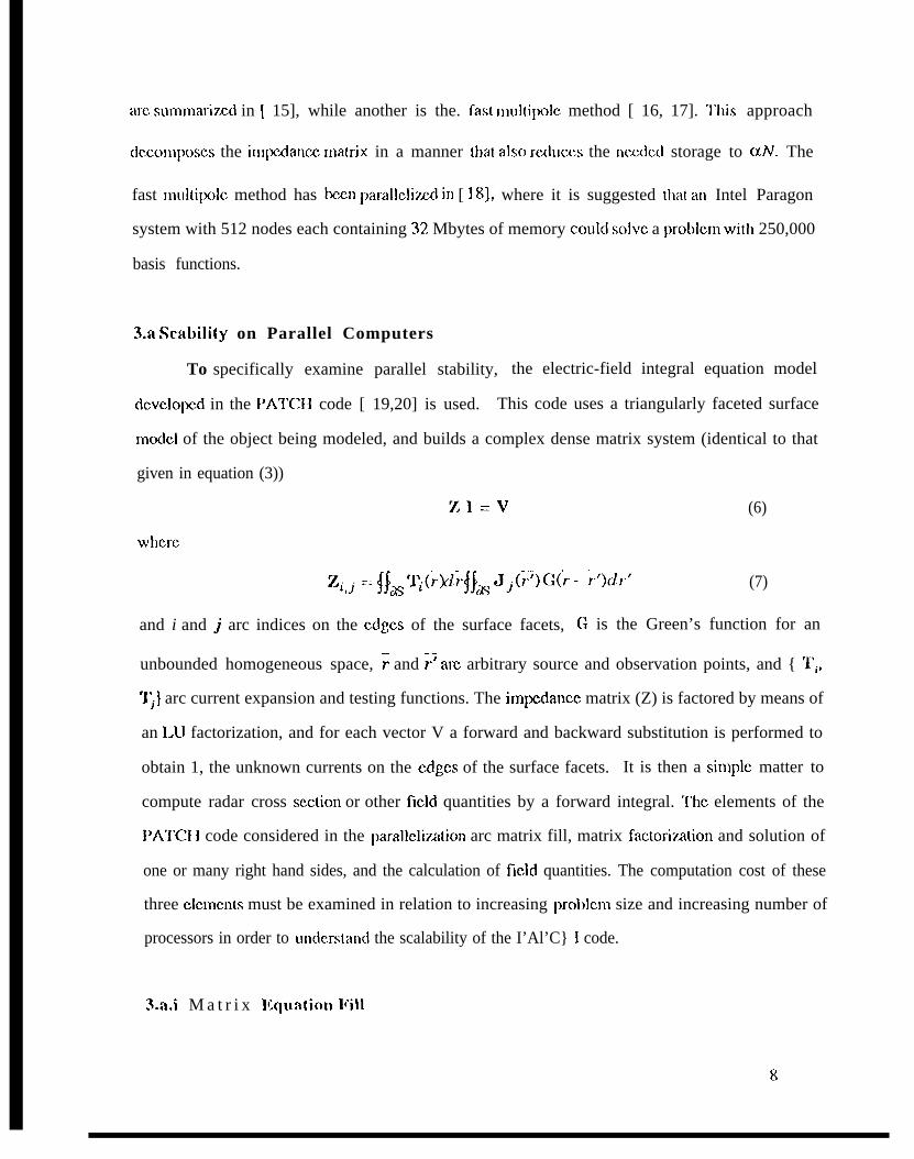
arc summarizmt in [ 15], while another is the. fast mul(ipolc method [ 16, 17]. ‘1’his approach

ciccomposcs the impcdancc matrix in a manner that also rcduccs the ncdcd storage to cxN. The

fast multipo]c method has bczn parallclimd in [ 18], where it is suggested that an Intel Paragon

system with 512 nodes each containing 32 Mbytes of memory could SOIVC a problem With 250,000

basis functions.

3.a Scabilily on Parallel Computers

To specifically examine parallel stability, the electric-field integral equation model

clcvcloped in the PATCIl code [ 19,20] is used. This code uses a triangularly faceted surface

model of the object being modeled, and builds a complex dense matrix system (identical to that

given in equation (3))

7#I=v (6)

where

(7)

and i and j arc indices on the edges of the surface facets, G is the Green’s function for an

unbounded homogeneous space, ~ and ;7 am arbitrary source and observation points, and { ‘l’i,

1~} arc current expansion and testing functions. The impcdancc matrix (Z) is factored by means of

an LLJ factorization, and for each vector V a forward and backward substitution is performed to

obtain 1, the unknown currents on the edges of the surface facets. It is then a simple matter to

compute radar cross scztion or other field quantities by a forward integral. ‘l”he elements of the

PATC1 I code considered in the parallc]iz,ation arc matrix fill, matrix factorization and solution of

one or many right hand sides, and the calculation of field quantities. The computation cost of these

three clcmcnts must be examined in relation to increasing problcm size and increasing number of

processors in order to unde.rstancl the scalability of the I’Al’C} I code.

3.a.i M a t r i x ltqnation Nill

8

Since the in~pcdancc ma[rix is a complex ckmsc matrix of size N, where N is (Ilc number of

edges used in the facctcd surface of the object being modeled, the matrix has N 2 clcmcnts, and

filling this matrix scales as N*. onc method for rcctucing the amount of time spent in this

operation wllcl~tlsi[~g aparallcl col~~l>lltcr istosllrcad the frxc.d numbcrofclcmcntsto be computed

over a Iargc number of proccsscws. Since the amount of computation is thcmclically fixed

(ncglecti ng communication between processors), applying 1’ processors to this task should provide

a [imc rcduct ion of ~’. 1 lowevcr, the computations required by the PATC.I I code’s basis functions

involve calculations performed at the ccntcr of each patch that contribute to the matrix clcmcnts

associated with the three current functions on the edges of that patch. The sequential I’Al<Cl I code

will loop over the surface patches and compute partial integrals for each of the three edges that

make up that patch. This algorithm is quite cffrcie.nt in a sequential code, but is not as appropriate

for a parallel code where the three edges of both the source and testing patch (corresponding to the

row and column indices of the matrix) will not generally be located in the same processor. “l”tlc

paral]cl version of I’Al’Cl I curl cnt]y ont y LISCS ttlis ca]cu]atiori fOr t]losc matrix c]cmcnts t]lat arc

local to the processor doing tllc computation inMXhlcing an inefficiency compared to a scqlcntial

algorithm. This inefficiency is specific to the integration algorithm used, and can be ren~ovcd. for

example, by communicating partial results computed in onc processor to the processors that INXXI

thcm. This step has not bcm taken at this time in the parallel PATCH code, duc partially to the

complexity it adds to the code.

3.a.ii Matrix Equation E’actorization and S o l u t i o n

When the impedance matrix is assembled, the solution is complctcd by a Ill factorization,

scaling as M], and a forward and backward substitution used to SOIVC for a given right hand side,

scaling as N2. ‘1’hc choice of the 1,~) factol”izatiml algorithm determines the matrix decomposition

schcmc used on the set of processors.

[)IIC s[y]c of decomposition that is suitable for usc with 1.lN1’ACK [21] factorization

mutincs is to partition the. matrix

9

[1A,

A=”:

A (P.-1)

(8)

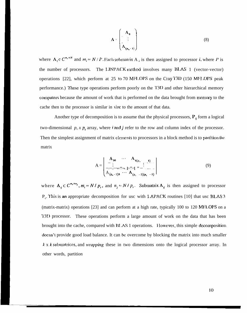
where Al E Cm”~ and mi = N / 1’. l~ach submatrix A i is then assigned to processor i, where }’ is

the number of processors. The 1.INPACK mcthcxl involves many BI.AS 1 (vector-vector)

operations [22], which perform at 25 (o 70 MN .01’S on the Cray 1311 (150 Ml:l .01’S peak

performance.) ‘IIesc type operations perform poorly on the “1’3D and other hierarchical memory

c.omputcrs because the amount of work that is performed on the data brought from memory to the

cache then to the processor is similar in six to the amount of that data.

Another type of decomposition is to assume that the physical processors, I’ti form a logical

two-dimensional p, x p, array, where i andj refer to the row and column index of the processor.

Then the simplest assignment of matrix clcincnts to processors in a block method is to pal~ition the.

matrix

A =

AM ..” AO(I)C, )

““””; - “ - 1 ” 1 ” -=—.—...—-—. .—. .—. .— ..— —

(A (Pr-l)o ““” A(P, -l)(P C-l)

(9)

where Ati ECm’xnJ, mi =Nlpr, and nj =AJlpc. Submatrix Au is then assigned to processor

Pij. “J’his is an appropriate decomposition for usc with 1.APACK routines [10] that usc BLAS 3

(matrix-matrix) operations [23] and can perform at a high rate, typically 100 to 120 MFI.OPS on a

‘1’31> processor. These operations perform a large amount of work on the data that has been

brought into the cache, compared with 111 .AS 1 operations. 1 lowcvcr, this simple dczornposition

docsn’t provide good load balance. It can bc overcome by blocking the matrix into much smaller

k x k submatriccs, and wrapping these in two dimensions onto the logical processor array. In

other words, partition

Am ..” AO(J,.,)

:1-.1_—— — .V. . . .

(lo)

where M = N /k, and atl blocks arc of size k x k. Then block Ati is assigned to processor

I ’( i” t i p, )(jn~p{ ) . This is the partitioning strategy that is used by I’AT’Cl 1. (On the T3D, k = 32 has

been found to provide optimal results between load balance demanding the smallest possible k and

the performance of the BLAS 3 operations requiring a large value for k.).

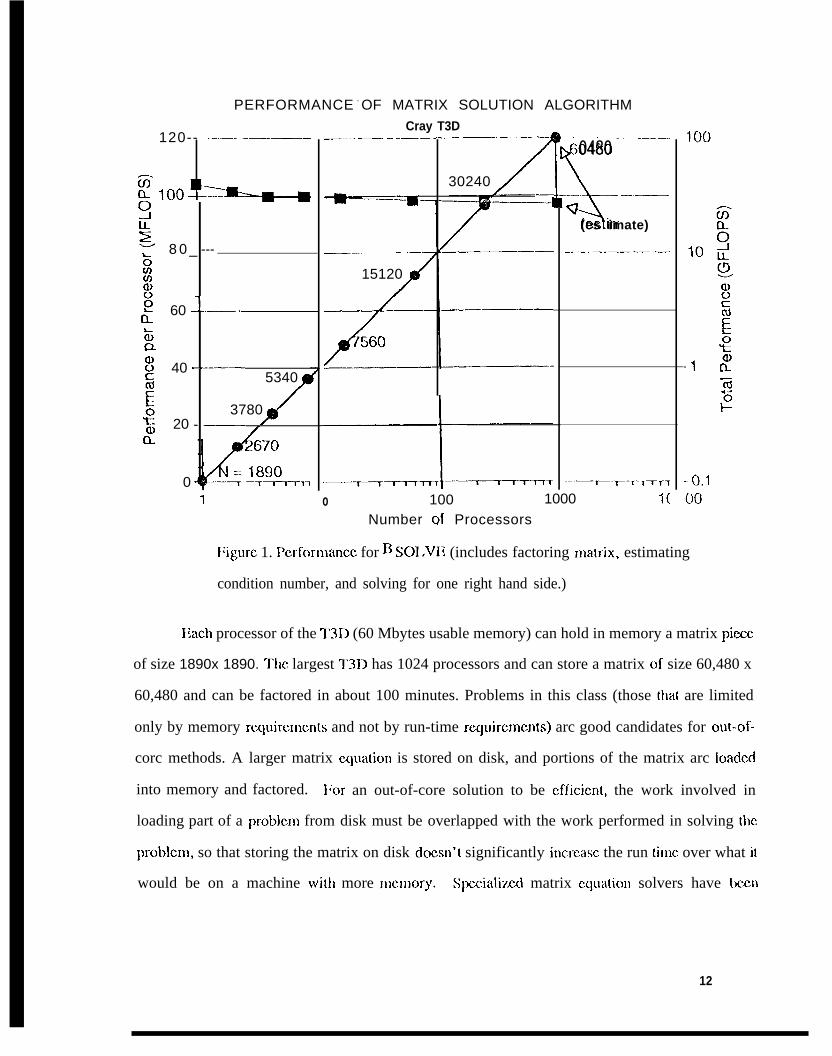
I’hc I’ATCI 1 code uses a matrix equation solver-narnti BSOLVE [24]---bascd on this

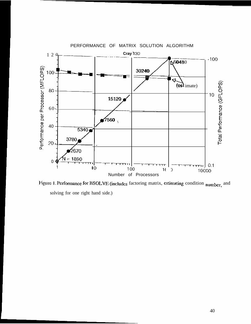
deeomposition . Figure 1 show the totat and per processor performance for 13S01 .VE for the

largest matrix that can be solved on each size of machine. Total time scales at the same efficiency

as total performance, and is 25 minutes for the 30,240 size matrix on 256 processors.

11

PERFORMANCE - OF MATRIX SOLUTION ALGORITHM

120-- ---------—-

GQ- loo~–~gLl_~

8 0 _ ---bU)ma

: 60 :-—

%c1

g 40 ---—5340

E 3780$ 20 - -–—m

0 ..–=_T_7TT,

1

Cray T3D_.. .—. . -

30240

15120

.—-. —— .——..

&0480

—.——

(es imate)

—- ——-— .—

o 100 1000 1(

Number of Processors

I:igure 1. Pcrformancc for 13 S01.VE (includes factoring malrix, estimating

condition number, and solving for one right hand side.)

Each processor of the T3D (60 Mbytes usable memory) can hold in memory a matrix pirxc

of size 1890x 1890. ‘1’tlc largest 3’31> has 1024 processors and can store a matrix of size 60,480 x

60,480 and can be factored in about 100 minutes. Problems in this class (those that are limited

only by memory rcquircmcnts and not by run-time rcquircmcnts) arc good candidates for out-of-

corc methods. A larger matrix cqua[ion is stored on disk, and portions of the matrix arc Ioadcd

into memory and factored. l;or an out-of-core solution to be cfficicnt, the work involved in

loading part of a problcm from disk must be overlapped with the work performed in solving (1E

problcm, so that storing the matrix on disk doesn’( significantly incrcasc the run ~imc over what il

would be on a machine with more JllClllOry. Spccialimt matrix ccluation solvers have been

12

TIME FOR LU FACTORIZA?”ION

o 8<

64 E3i[ Complex Arithmetic, F’artial

256 PEs_r.

-—-l--r T---

)

512 PE’SOoc~r-–

102I

-Wtmmi3.,

_.— —

006A

PES

— - l - - T - - - T -

)

voting

(

d6 7 6 PEs

—

e196 PES

Ooc

)C

I

g T3D

~ Paragon

A T90 (32 CPUS)

+ C90 (16 CPUS)

[_] Delta— .

—

) 100 1 0UNKNC)WNS (1OOO)

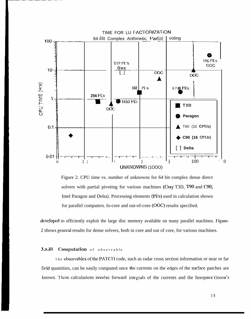
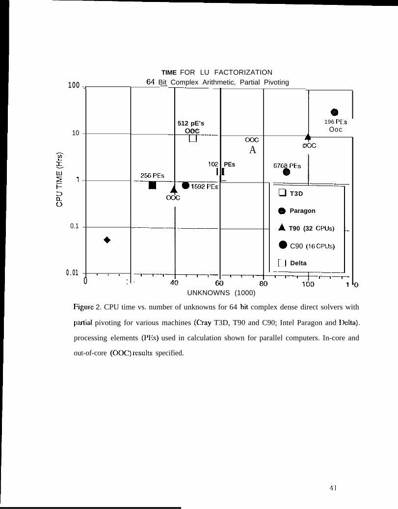
Figure 2. CPU time vs. number of unknowns for 64 bit complex dense direct

solvers with partial pivoting for various machines (Cray T3D, T90 and C90;

Intel Paragon and Delta). Processing elements (PEs) used in calculation shown

for parallel computers. lo-core and out-of-core (OOC) results specified.

dcvclopcd to efficiently exploit the large disc memory available on many parallel machines. ~~ig,ure

2 shows germ-al results for dense solvers, both in core and out of core, for various machines.

3.a.iii computation o f obse rvab l e

l-he obscrvables of the I’Al’Cl I code, such as radar cross section information or near or far

fickl quantities, can be easily computed once

known. q’hcsc calculations invo]vc forward

the currents on the edges of the surfacz patches are

intc:,rals of the currents and the frccspacc Ch-cc.n’s

13

func[ion. DUC to the discrctizcd of this current, this int%ration results in a summalion of field

components duc to each current basis function. Since these currents arc distributed over all IIlc

processors in a parallel simulation, partial sums can be performed on the individual processors,

followed by a global summation of these partial rcsuhs to find the total SUIII. This calculation scale

quite WC1l since the only overhead is the single global sum.

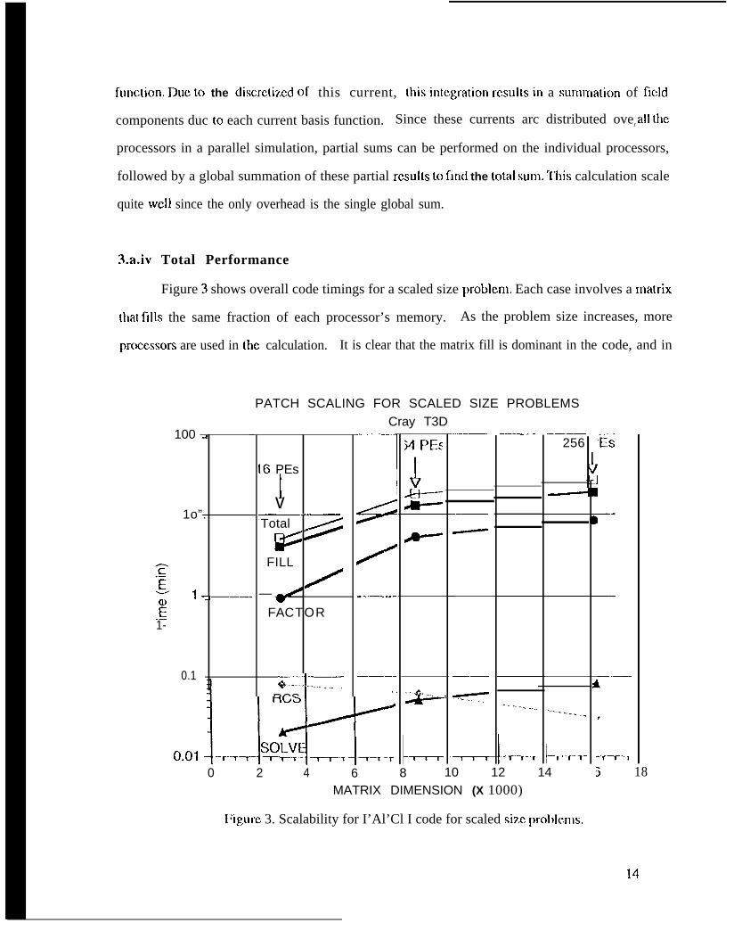
3.a.iv Total Performance

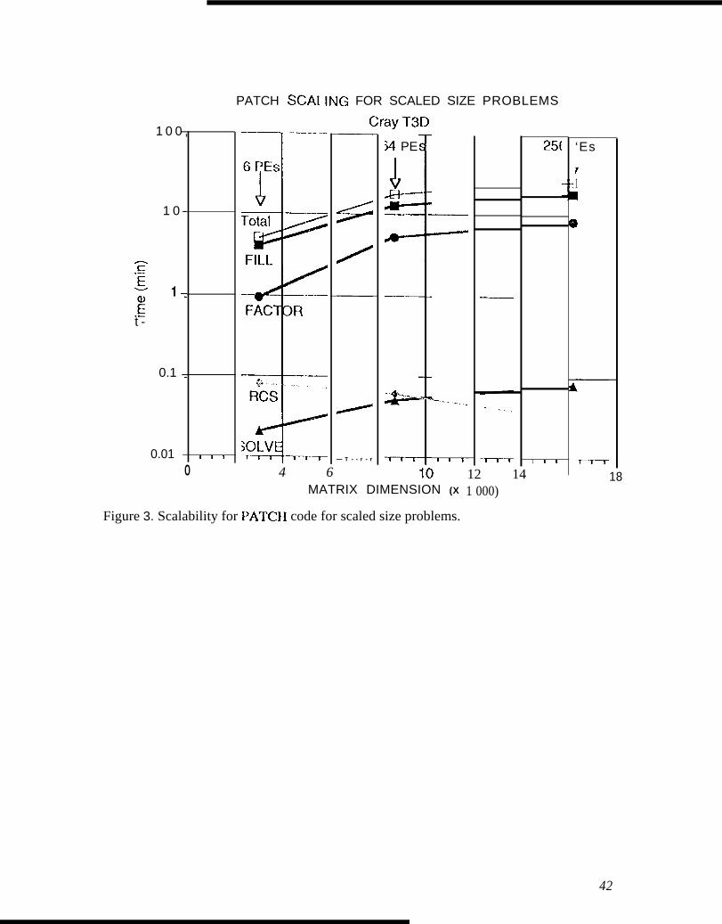
Figure 3 shows overall code timings for a scaled size problcm. Each case involves a ma[rix

that fills the same fraction of each processor’s memory. As the problem size increases, more

proccssorx are used in the calculation. It is clear that the matrix fill is dominant in the

PATCH SCALING FOR SCALED SIZE PROBLEMS

code, and in

100 a

1o”.

@g

1-,—–-F.—1-

0.1

[6 PEs

!v—...—Total

FILL

—

FACTOR

.—4$----L...RCS I

Cray T3D

MuiIK-L.-r

—-

15=/——

———. . . .A-

--T—l—T—

_——

——

——

-. . .

IL

.—-

------- -.

l--

—.——256

-------- -+

L–0 2 4 6 8 10 12 14

MATRIX DIMENSION (X 1000)

I:igurc 3. Scalability for I’Al’Cl I code for scaled siz.c pmblcms,

‘Es

3 18

14

fact, [hc crossover point bc[wccn the 0(n3) factoriz.atiol~ and tllc 0(~~2) fill l~as Ilot t=n rcachcd,

Also, {he time involved in the radar cross scc[ion calclllation is SIIOWII tO d~reasc as IIIC number of

processors is increased, as was dcscribcd in the previous paragraph. It may also be observed that

the matrix solve tirnc, also 0(n2), parallels the fill lime quite WCI1.

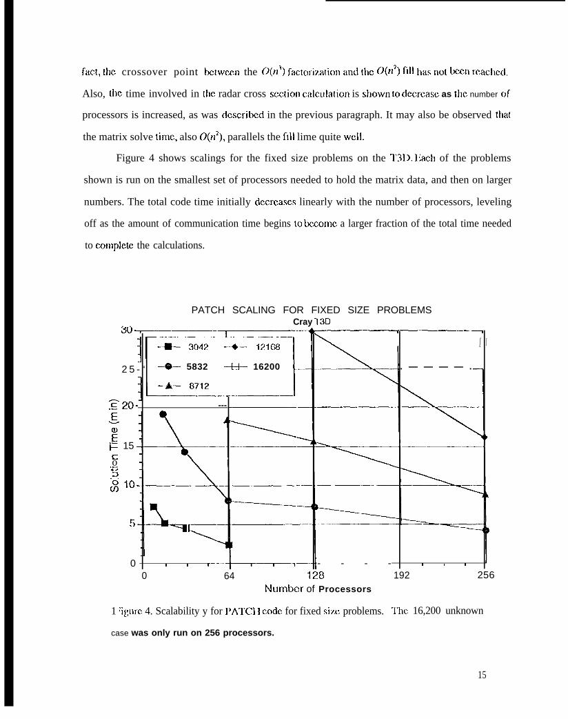
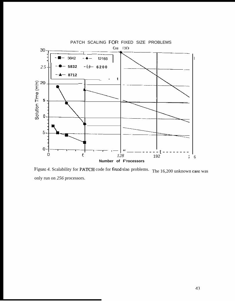
Figure 4 shows scalings for the fixed size problems on the T3D. Iiach of the problems

shown is run on the smallest set of processors needed to hold the matrix data, and then on larger

numbers. The total code time initially dccrcases linearly with the number of processors, leveling

off as the amount of communication time begins to bccomc a larger fraction of the total time needed

to comp]etc the calculations.

PATCH SCALING FOR FIXED SIZE PROBLEMS. . Cray 13Dw ————-—

[ I

2 5 - “ --~– 5832 -+4– 16200 . — — — — .

~20- ---&_

t~ 15co.—5

0 I I - - - - 1 I I0 64 128

Number of Processors

1 ‘igure 4. Scalability y for 1’ATCI I code, for fixed siz,c problems.

192 256

‘1’~)C 16,200 unknown

case was only run on 256 processors.

15

4. ll’]NIrl’]~ ]\],];~f]~Nrj’ ]to]~~~(J],A’I’]ONs”

Volumetric modeling by (he usc of an integral cqua(ion can also be usccl in simulations,

tlloLlgh the available memory of currcn[ or plannccl tcchnolog y great] y limits the siz.c of problcn E

[l]a[ can be moclclcd. IIccausc of (his limitation in lnodcling t}lrcc-dimensional space by intcgr-al

equations, finite clcmcnt solutions of the partial differential ccluations that lead to sparse systems of

cquat ions arc common] y used [25]. A finite clcmcnt model is natural when the problcm contains

inhomogcnous material regions that surface integral cquatioll methods arc either incapable of

modc]ing, or arc very costly to model. ‘1’hc problcm domain is broken into a finite clcmcnt basis

function set used to discretizc the fields. The resulting linear system of equations–-rather than

scaling as the iV2 storage of the method of moments--scalcs as nlN where m is the average number

of non-zero matrix equation clcmcnts pcr row of the sparse 1 incar systcm. This value is dependent

upon the order of the finite element USCCJ, but is typically between 10 and 100, and is indcpcndcnt

of the size of the mesh. l~or a 6 unknown, vector edge-based tctrahczlral finite clcmcnt [26], m is

typically 16.

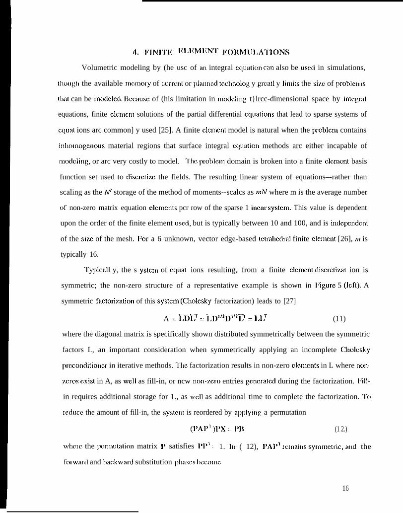
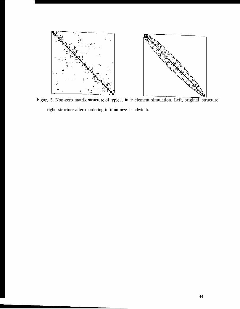
‘1’ypicall y, the s ystcm of cquat ions resulting, from a finite clcmcnt discrctiz,at ion is

symmetric; the non-zero structure of a representative example is shown in I;igure 5 (Icf{). A

symmetric fiictorization of this systcrn (Cholcsky factorization) leads to [27]

A = i;Di? =: ~D’’21)’’21;r == 1,1: (11)

where the diagonal matrix is specifically shown distributed symmetrically between the symmetric

factors I., an important consideration when symmetrically applying an incomplete Cholcsky

prcconditioncr in iterative methods. l’hc factorization results in non-zero clcmcnts in L where non-

zeros exist in A, as well as fill-in, or ncw non-~sro entries gcncratcd during the factorization. I;ill-

in requires additional storage for 1., as WCI1 as additional time to complete the factorization. ‘1’o

rcducc the amount of fill-in, the systcm is reordered by applyinc a permutation

(l’Al” )l)X :1’11 (1 2.)

wlmrc the pcrlnutation matrix I’ satisfies l’1’~ z 1. ]n ( 12), I’Al’T Icmains syinmctric, and the

fol-ward and backwar(i substitution pllascs bccornc

16

i.Y = 1’11, l%.= Y, x = I’Tz (13)

wbcrc ~. is the Cholcsky factor of I’AI’T. IJor a sparse factori?.ation, the permutation matrix is

cboscn to minimize the amount of fill-in generated. Since there arc n! possibilities for P to

minimiz.c fill-in, heuristic methods arc used to achicvc a practical minimization, the most comlnoll

being the minimum degree algorithm [28]. I;igure 5 (right) shows the non-zero structure of the

rcprcscntative system after reordering for a canonical scattering problem.

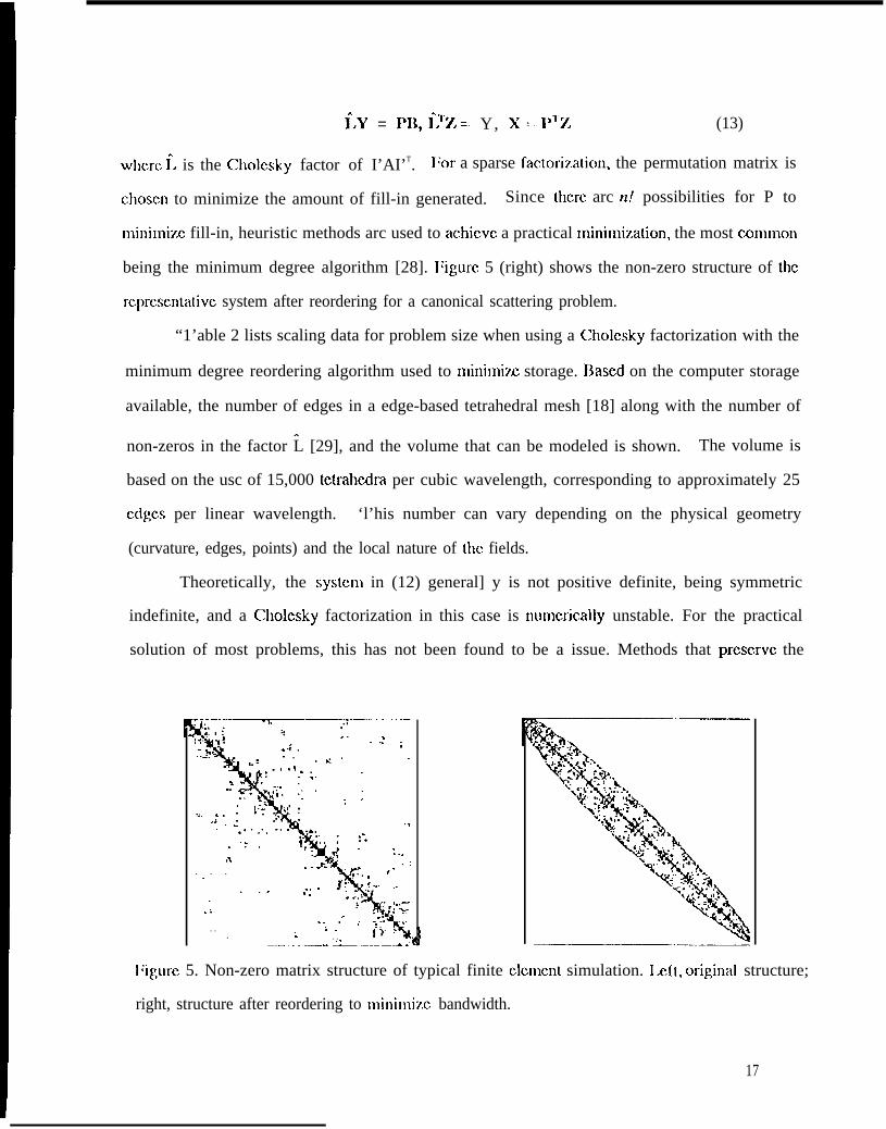
“1’able 2 lists scaling data for problem size when using a Cholcsky factorization with the

minimum degree reordering algorithm used to minimim storage. Based on the computer storage

available, the number of edges in a edge-based tetrahedral mesh [18] along with the number of

,.non-zeros in the factor L [29], and the volume that can be modeled is shown. The volume is

based on the usc of 15,000 tctrahuha per cubic wavelength, corresponding to approximately 25

edges per linear wavelength. ‘l’his number can vary depending on the physical geometry

(curvature, edges, points) and the local nature of tbc fields.

Theoretically, the systcm in (12) general] y is not positive definite, being symmetric

indefinite, and a Cholcsky factorization in this case is numcnca]ly unstable. For the practical

solution of most problems, this has not been found to be a issue. Methods that prcscrvc the

.:

.: . -- .,. .,..

,1

. . .

.:

. . ;.. : . .———-.—— ..-. . . . .._. —’A———A .,

l;igurc 5. Non-zero matrix structure of typical finite clcmcnt simulation. 1,ctt, original structure;

right, structure after reordering to Ininimim bandwidth.

17

symmdric sparsi(y, and allow pivoling to produce mom stable algorithms can be used [28].

‘]’able 2. Scaling of typical factori7atior] finite clcmcnt matrix solution algorithms,~-... . .. ——— —.—.

PROBLEM SIZE 7

T:?aL!zmIf‘k

.—— —128 8 2.0

—.—256 50 16 3.3

512 8~ 32 5,5.—

1024 135 64 9.0

:%;*:“

iioo 512 40

2 , 0 4 8 1 0 8

8,192 2 9 4—

I:rom ‘l’able 2 it is seen that even though the storage for the finite clcmcnt method is linear

in N, the fill-in duc to the usc of factorization algorithms causes the storage to grow as N’4.

1 ,incar storage can be maintained using an iterative solution. Sparse iterative algorithms for

systems resulting from eltmromagnctic simulations recursively construct Krylov subspace basis

vectors that arc used to iteratively improve the solution to the linear systcm. The iterates arc found

from minimizing a norm of the residual

r= Ax-h (14)

at each step of the algorithm. (A single solution vector for a single excitation is shown.) Since the

systcm is complex-valued indefinite, rncthods appropriate for this class of systcm such as bi-

conjugate gradient, gcncrali?,ed minimal residual, and the quasi-minimal residual algorithm are

applied [30]. lhcy all require a matrix-vector multiply, and a set of vector inner products for the

calculation. ‘1’hc iterative algorittlms require the storage of tllc matrix and a fcw vectors of length

N. When only the matrix and a fcw vectors nmd to bc stored, problems of very large size can bc

handled, if the convcrgcncc rate is control] cd. ‘1’tlc number of itci-ations (with a sparse matrix-

d~r~sc vector multiply accollnting for over 90fz0 of the time at Cach step of t}lc iterative algorithm)

dctcrmincs the time to solution.

18

l]cc.ause the matrix-vector multiply dominates the KIY1OV iterative mcthods, the algorithmic

scaling is found from this operation. A single. SpaI-SC matrix-dcrlsc v~tor multiply requires mAI

operations, and if there arc 1 [otal iterations required for convcrgcncc, the n(mltwr of floating point

operations nczded is I* mN. A typical solution of the systcm of equations, without the application

of a prcconditioncr, may require a number of iterations 1 = ~N, producing the squcntial algorithm

scaling

,,,N% (15)

for the solution of a sing,lc right-hand-side. The algorithmic scaling for a direct factorization

method is 0(m2N) [28, page 104]; therefore the factorization methods-—when memory is sufficient

to hold the fill-in entries---give considerable CPU time savings in the solution. Iiurthcr advantage

is also gained over iterative methods when using a direct factorization. Modern computer

architectures arc typically much ICSS cffrcicnt at performing the sparse operations required in the

sparse matrix-dense vector mutip]y of [hc iterative algorithm, as compared to operations on dense

matrix systems. Current direct facloriz.ation methods attempt to usc block algorithms, exploiting

dense matrix sub-structure in the sparse systcm, and therefore increasing the performance of the

factorization, further improving the performance from that given by the algorithmic scaling

differences.

It is seen that the number of iterations dircztly incrcascs the time to solution in the iterative

methods. This number can bc control]cd to some dcgrm by the usc of preconditioning methods

that attempt to transform the matrix equation into onc with more favorable properties for an iterative

solution. To control the convcrgctlcc rate, the matrix A should be scaled by a diagonal matrix that

procluccs ones along the diagonal. This scaling removes the dcpendcncc on different clcmcnt sires

in a mesh. A prczonditioncr M can then be symmetrically applied to transform the systcm giving

M-lATW1( MX)==M-l l). (16)

‘1’IIc right hand side vcztor is initially transformc.d, and tllc system is them solved for the

intcmmdiatc vector Y =- hflx, multiplying this vector by h4”1, A and M-* in succession at each

iterative step. When the solution has convcrgc.d, x is rccovcrcd from x. “1’hc closer M is to 1, in

(4), the quicker the transformed sys[cm will converge (0 a solution. A comn~on preconctitioncr is

an incomplete Cholcsky factorization [31] where M is chosen as a piccc of the factor 1. in (11). It

is computed to keep some fraction of the true factori~,ation clcmcnls, llw exact number and sparsity

location of the clcmcn[ dependent on the exact algorithm used. A uscfu] form of incomplete

factorization keeps the same number of clcmcnts in the incomplete factor as there arc in A. l’his

requires three times the number of opcrat ions at each i[crativc step; therefore the time to solul ion

will be dccrcascd if the number of iterations is lesser than onc-thirxi when applying this

prcconditioncr.

When the right hand side consists of a number of vectors, newly dcvclopcd block nlcthods

can be applied to the system to usc the additional right hand sides to improve the convergence rate

[32,33].

4.a Scalability on Parallel Cotnputers

III a finite clement algorithm, the resultant sparse syste.rn of equations is stored within a data

structure that holds only the non-zmo entries of the sparse system. I’his sparse system must

ultimately be distributed over the parallel computer, requiring spczial algorithms to either break the

original finite clement mesh up into specially formed contiguous pieces, or by distributing up the

matrix entries themselves onto the processors of the computer. As in the dense method of

moments solution, the pieces arc distributed in a manner that allows for an cfficicnt solution of the

matrix equation systcm.

4.a.i The Finite Element Mesh and the Sparse Matrix ICquation

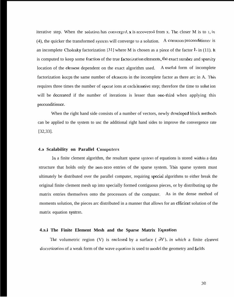
‘1’hc volumetric region (V) is cncloscd by a surface ( W), in which a finite clcmcnt

discrctiz.ation of a weak form of the wave ccluation is used to model the geometry and fields

20

~~ is lhc magnetic field (the ~~ -equation is used in this paper; a dual z’ -equation can also bc

writkm), w is a testing function, the asterisk denotes conjugation, and F; x ii is (1IC tangential

component of ~; on the bounding surface. In (17), c, and //, arc the relative pcrmittivity and

permeability, rcspcctivc]y, and kO and ?)O are free-space wave number anti impedance, respectively.

A set of finite clement basis functions, the tctrahcdrai, wctor edge cicmcnts (W%itncy clcmcnts)

will bc used to discretiz,c (17),

Wnm(r) == Am(r)van(r)- I v a n , (18)

wiva-c A(r) arc the tctrahcdrai shape functions an(i indices (m, n) refer to the two nodal points of

each edge of the finite clcmcnt mesh. These clcrncnts will bc used for both expansion and testing

(Galcrkin’s mcti~oci) in the flnitc element domain. ~~ecausc of the local nature of ( ~ ‘/), (sut)-domain

basis functions and no Green’s function involved in the inmgra(ion of the fields), the systcrn of

equations resulting from the integration only contains non-z.cro entries when ttlc finite elements

overlap, or arc contiguous at an edge. Because the mesh is unstructured, containing elements of

different size and orientation conforming to the geometry, the resultant xnatrix equation will have a

sparsity structure that is also unstructured.

Ti~c sparsity structure is further aitcrcd by the form of the Sommcrfcld boundary condition

applied on the surface S. When local, s ymnmtric absorbing conditions are applied on the boundary

[34]-- entering into the calculation through the surface. intcgrai in(17)- a matrix witil the structure

shown in l~igurc 5 (left) results. It is seen that the diagonal is entirely fiiicd, corresponding to the

self-terms in the voiumc integral in (17), with the m non-zero entries scattered along ti~c row (or

column) of tile symmetric matrix. I’hc location of these entries is conlplctcly dcpcndcnt upon tllc

ordering of the edges of the tetrahedral clcmcnts used in the discrctiz.ation. lf a diffcrcl)t shape or

or[icr of the cicmcnts arc used, the non-z,cro s[ructurc wiii differ slightly froln the onc shown.

Wilcn an integral equation method is usc{i to truncalc hc mesh [35,36], a (icnsc block of clcmcnts

will appear in the lower right of the system (when (tic edges of the frnitc clcmcnt mesh on t}lc,

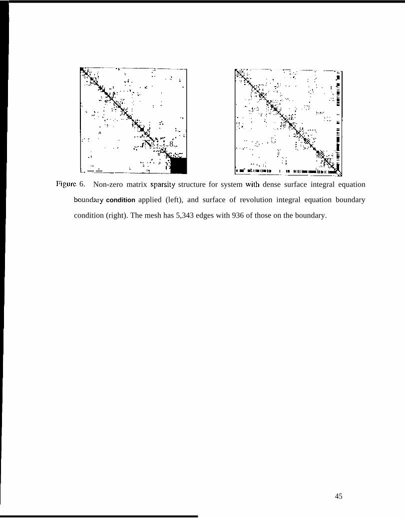
boundary arc ordered last) as shown in Flgllrc 6 (left). ‘1’hc integral c.quation approach to

truncating the mesh uscs the finite clement facets on the bo~lndary as source fields in an intcgra~

equation, resulting in a formulation for this piece of tllc calclllation similar to that in Swtion 3, and

with an amount of storage needed for the dense Inatrix as a fLlnction of the electrical surface area

tabu]atcd in Section 2. To circumvent the large dense storage nccdcd with this application of a

global boundary condition, a surface of revolution can be used to truncate the mesh [37,38], using

a set of global basis functions to discretize the integral equation on this surface. This results in a

systcm similar to that in Fig 6 (right) containing very small diagonal blocks due to the orthogonal

global basis functions along tbc surface of rcvolLltion truncating the mesh, as well as a matrix

coupling the basis functions in the integral equation solution to the finite element basis function on

the surface. These coupling terms are the banded thin rtztangular matrices symmetric about the

diagonal of the matrix. Other forms of the integral equation solution, as outlined in Section 3, can

also be used to discretize the integral equation modeling fields on the mesh boundary, leading to

slight variations of the matrix systems shown in l:igurc 6.

22

—. ,.,. .

-k._. .

.:

.: .*.-,; ~- . .

. .,.. -,

.x- , . .:.

.! i

.:.

. . . ..-O -.

. . ;.

.

L

~ ‘w

,..4.

-.,-

. . .

,.. .

,’ or.

. . . . . . .

. .

.-.. ..

. . . .... .

.:

L—— ->.

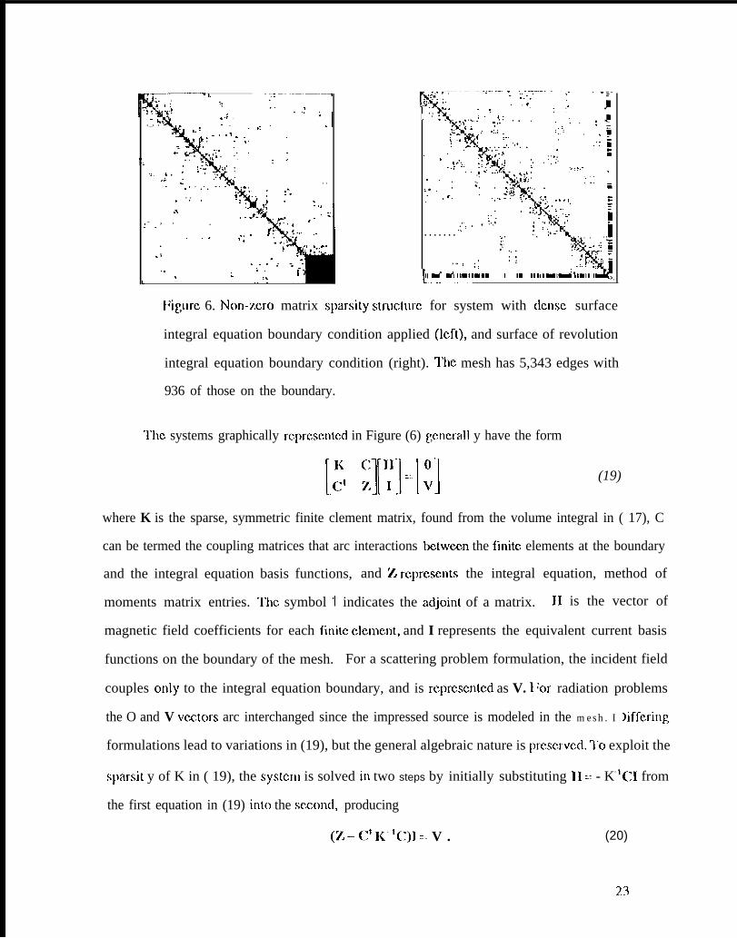
Figure 6. Non-z,cro matrix sparsity swucturc for system with ctcnsc surface

integral equation boundary condition applied (Icft), and surface of revolution

integral equation boundary condition (right). l’he mesh has 5,343 edges with

936 of those on the boundary.

“]’hc systems graphically rcprcscn[cd in Figure (6) gcncrall y have the form

[.: TM] (19)

where K is the sparse, symmetric finite clement matrix, found from the volume integral in ( 17), C

can be termed the coupling matrices that arc interactions bctwccn the fmitc elements at the boundary

and the integral equation basis functions, and Y. rcprcscnts the integral equation, method of

moments matrix entries. “1’hc symbol t indicates the adjoint of a matrix. 11 is the vector of

magnetic field coefficients for each finite clcmcnt, and I represents the equivalent current basis

functions on the boundary of the mesh. For a scattering problem formulation, the incident field

couples only to the integral equation boundary, and is rcprcscntcd as V. I ‘or radiation problems

the O and V vcztors arc interchanged since the impressed source is modeled in the mesh. I >iffcring

formulations lead to variations in (19), but the general algebraic nature is prcscrvcci. ‘1’o exploit the

sparsit y of K in ( 19), the systcm is solved in two steps by initially substituting 11 == - K- lCI from

the first equation in (19) into the sezond, producing

(Z– C+ K-’C)I : V . (20)

23

‘]’his system h a size on he order of the numtxr of basis fllnc(ions in the integral quation model,

is rtcmsc, and can be solved by either direct factori~.ation or iterative means as o~~tlincct in Section 3.

“]’hc intermediate calculation, KX == C is the sparse systcm of equations to be SOIVCCI, producing

X.

The solution of this sparse systcm on a parallel computer requires

“1’raditionally, the depcndcncc between mesh data and the resultant

it to be distributed.

sparse matrix da!a

is exploited in the dcvcloprncnt of mesh partitioning algorithms [39-42,55]. These algorithms

break the physical mesh or its graph into contiguoLls picccs that arc then read into each processor of

a ctistributcd memory machine. The rncsh pieces arc generated to have roughly the same number of

frnitc clcmcnts, and to some measure, each piece has minimal surface area. Since the rnati~x

assembly routine (the volume integral in (17)) gcncratcs non-zro matrix entries that correspond to

the direct interconnection of finite clcrncnts, the mesh partitioning algorithm attempts to crcatc a

load balanec of the sparse systc]n of equations. l’roccssor commLmications in the algorithm that

SOIVCS the sparse system is limited by the abi 1 it y to minimize the surface area of each mesh piccc.

Mesh pallitioning algorithms arc generally divided into multilevel spectral partitioning,

geometric partitioning, and rnultilcvel graph partitioning. Spectral partitioning methods [40,4 1]

creates cigenvutors associated with the sparse matrix, and uscs this information to recursively

break the mesh into roughly equal picccs. It requires the rncsh connectivity information as input,

and returns lists of finite clcmcnts for each processor. Geometric partitioning [39] is an intuitive

proccdurc that divides the finite clcmcnt mesh into picccs based on the geometric (node x, y, z

coordinates) of the finite clement mesh. This algorithm requires the mesh connectivity as well as

the node spalial coordinates and returns lists of finite clcmcnts for each processor. Graph

pa[li(ioning [42] operates on the graph of the finite clcmcnt mesh (mesh connectivity information)

to collapse (or coarsen) vcrticcs and

into picccs, and then Llncoarscncd

parallel processors. “1’hc input and

edges into a smaller graph. ‘1’his smaller graph is partitioned

and refined for the final partitions of finite clcmcnts for the

outpLlt is idcntica! to Spcclral methods. MLdtilevcl algorithms

o p e r a t e by J)crformin~ mLlltiplc. stages of the pallitionin~ simultancoLlsly, acczlcrating the

24

a]~orithm. Most of the algorithms and their offshoots perform similarly in praclicc, wilh the

spcctt-al and graph partitioning algorithms being simpler to usc sin~c t~~cy do not need geometry

information. An alternative to t}lcsc mesh partitioning algoritlmls is a method that divides the

matrix entries directly, without operating on the finite clcmcnt mesh, and will be examined in

Section 4.a. iv.

IIiffcrcnt decompositions arc used depending whether direct factorization or iterative

methods arc used in the solution. Ilccompositions for iterative solutions, as well as the iterative

methods thcmsclvcs have shown greater case in parallclization than direct factorization methods.

Both approaches will now bc considered.

4.a.ii Direct Sparse Factorization Methods

Direct factorization rncthods require a sequence of four steps; reordering of the sparse

systcm to minimize fill-in, a symbolic factorization stage to dctcrminc the structure and storage of

~. in (13), the numeric factorization producing the complex-valued entries of ~., and the triangular

forward and backward solutions. The fundamental difficulty in the parallel sparse factorization is

the development of an efficient reordering algorithm that minimizes the fill-in and will scale well

on distributed memory machines, controlling the amount of communication necessary in the

computation. The minimum degree algorithm typically used in sequential packages is inherently

non-parallel, proceeding scqtrcntially in the elimination of nodes in the graph representing the non-

zcro structure of the matrix. Other algorithms for reordering, as WCII as (}1c following symbolic

and numeric factorization steps that depend on this ordering arc under study [43]. Current

factorization algorithms [44,45,46] can exhibit fast parallel solution times on rnodcratcly large

sized problems, but arc dcpcndcmt on the relative structure of the mesh, whether or not the problcm

is two or three-dimensional, and the relative sparsity of the non-?.cro e.ntrics. For problems with

more structure and ICSS sparsity, ]Iigllcr pformancc is found by these sparse fac(ori?,ation solvers.

25

4.a.iii Sparse Iterative Solution Methods

1 ‘m a paralld irll}llclllcrlta(io:] of the sparse itcrat ivc solvers introduced above, a

cfccomposition of the matrix onto the processors that minimim communication of the Ovcrlappi[lg

veetor piccc.s in the parallel matrix-vector multiply of the iterative algorithm, reduces storage of the

rmullant dense v~tor pieces on each processor, and allows for load balance in s(oragc and

computation is rc~uirccl. Various parallel packages have been written that accomplish these goals

to some (icgrcc [47,48]. The mesh decompositions outlined previously can be used and integrated

with the parallel iterative algorithm to solve the systcm.

Ah-natively, a relatively simple approach that divides the sparse matrix entries among the

distributed memory processors ean be employed [49]. “1’hc matrix is decomposed in this

implementation into row slabs of the sparse reordered system. The reordering is chosen to

minimim and equalize the bandwidth of each row over the system [ 17,18] (as shown in Fig .5

right) since the anmL1nt of data communicated in the matrix-vector multiply will depend upon the

combination of equalizing the row bandwidth as well as lninimiz,ing it. A row slab matrix

decomposition strikes a balanec between near perfect data and computational load balance among

the processors, minimal but not perfectly optinial eornmunication of data in the matli.x-veclor

multiply operation, and scalability of simulating larger sized problems on greater numbers of

pmecssors. Since the right-hand-side vectors in the parallel sparse matrix equation ( KX =: C ) are

the columns of C, the.sc columns are distributed as required by the row distribution of K. When

setting L]p the row slab dcconlposi(ion, K is sp]it by attempting to equalize the number of non-

~,cros in each processor’s portion of K (composed of consecutive rows of K). The rows in a

given processors portion of K determines the rows of C that processor will contain. As an

example, if the total number of non-z,eros in K is nz, a loop over the rows of K will be executed,

counting the number of non-z,cros of K in the rows examined. When this number becomes

alqmximatcly nZ / P (where P is the numbm of processors that will be used by the matrix

C.qllation SOIVCI”), the set of rows of K for a givcu processor has been dctcrmincd, as has the set Of

tows of C .

26

‘I’}~cn~alrix dw.ol~~positioI~ co(ic used in this cxamplc consists of a nLmlbcrof subroutines;

initially, the potentially large mesh files arc read (RllAl~), tl~cn t}~c conncclivily structure of the

sparse matrix is generated and reordered (CONNIC1’), followed by the generation of the complc.x-

valued entries of K (FIIM), bLlilding the connectivity structure and filling the C matrix

(COUPI.lNG). Finally the individual files containing the row slabs of K and the row slabs of C

Inust be written to disk (WRITE). I ‘or each processor that will be Llsed in the matrix equation

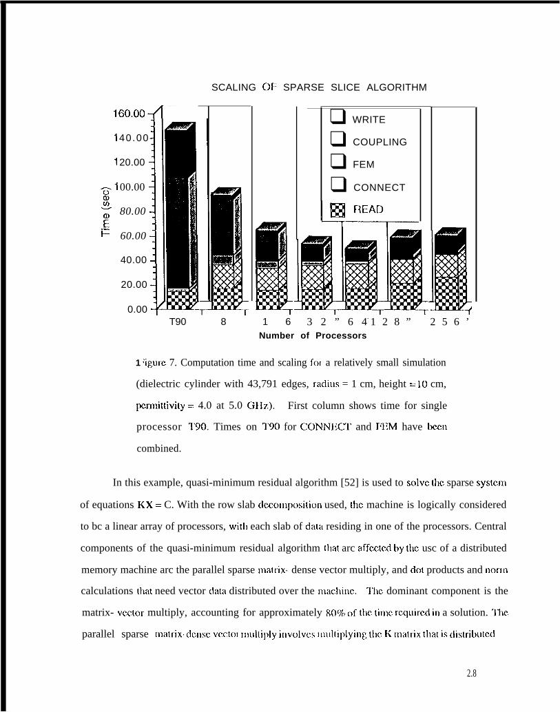
solver, one file containing the appropriate parts of both the K and C matrices is written. IJigurc 7

shows the performance of these routines over varying numbers of processors for a problem

simulating scattering from a dielectric cylinder modeled by 43,791 edges. The parallel times on a

Cray T3D arc compared against the code running sequentially on one processor of a 190. As

mentioned above, the reordering algorithm and the algorithm gcnirating the matrix connczlivity arc

fundatncntally sequential. These routines do not show high efficiency when using multiple

processors-the time for this algorithm is basically flat--whereas for routines that can be

parallclizcd (FEM, COUPI .ING and WR1”l”li), doubling the number of processors rcduccs the

amount of time by a factor of approximately two. The time for reading the mesh is bound by UO

rates of the computer, and the time for writing the decomposed matrix data varies slightly for the

128 and 256 processor cases due to other users also doing I/O on the systcm. As will bc shown in

the next result, a kcy point of this approach to matrix’ decomposition is that the total time needed

(Icss than 100 sec. on 8 processors) is substantially lCSS than the time nccdcd for solving the linear

systcm, and any inefficiencies here are ICSS important than those in the iterative solver.

?$7

160.00m

1

1

140.00-

20.00 J

00.00

80.00

60.00

40.00 \

20.00

0.00 1—

T

SCALING OF SPARSE SLICE ALGORITHM

T90 8

❑ WRITE

❑ COUPLING

❑ FEM

❑ CONNECT

M-=3--

1 6 3 2 ” 6 4- 1 2 8 ” 2 5 6 ’Number of Processors

1 ‘igurc 7. Computation time and scaling for a relatively small simulation

(dielectric cylinder with 43,791 edges, raclius = 1 cm, height = 10 cm,

pcrmittivity == 4.0 at 5.0 (3117.). First column shows time for single

processor ‘1’90. Times on 190 for CC)NNKT and FEM have been

combined.

In this example, quasi-minimum residual algorithm [52] is used to SOIVC (bc sparse systcm

of equations KX = C. With the row slab dccomposi(ion used, tbc machine is logically considered

to bc a linear array of processors, with each slab of da(a residing in one of the processors. Central

components of the quasi-minimum residual algorithm (hat arc affcztcd by [hc usc of a distributed

memory machine arc the parallel sparse Inalrix- dense vector multiply, and do( products and norln

calculations (hat need vector data distributed over the macbinc. ‘1’hc dominant component is the

matrix- vcc.tor multiply, accounting for approximately 80% of (I)c time. re.quircd in a solution. ‘1’hc

parallel sparse nla(rix-d~I~sc WX(OI Il)u](jply jllvolvc,s Illul(lplyjng ttlc K nlatrix that js djs(rjbutcd

2.8

COMMUNICATION FROM/ PflOCESSOFl TO LEF:T

.dn,,g

~. ——.

‘$! d bm , =1

COLUMNS ‘

x ~1‘.=

.

\

YLOCAL PROCESSOR ROWS

\

LOCAL PROCESSOR ROWS

COMMUNICATION FROMPROCESSOR TO RIGHT

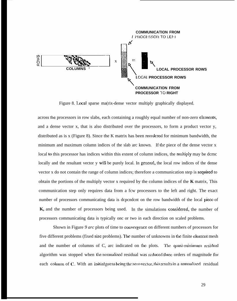
Figure 8. heal sparse ma(rix-dense vector multiply graphically displayed.

across the processors in row slabs, each containing a roughly equal number of non-zero clcmcnts,

and a dense vector x, that is also distributed over the processors, to form a product vector y,

distributed as is x (Figure 8). Since the K matrix has been reordcrcci for minimum bandwidth, the

minimum and maximum column indices of the slab arc known. If the piece of the dense vector x

local to this processor has indices within this extent of column indices, the mukiply may be dcmc

locally and the resultant vector y will be purely local. In gcncra}j the local row indices of the dense

vector x do not contain the range of column indices; therefore a communication step is wquired to

obtain the portions of the multiply vector x required by the column indices of the K matrix, This

communication step only requires data from a fcw processors to the left and right. The exact

number of processors communicating data is dcpcndcnt on the row bandwidth of the local piece of

K, and the number of processors being used. In the simulations considcrcd, the number of

processors communicating data is typically onc or two in each direction on scaled problems.

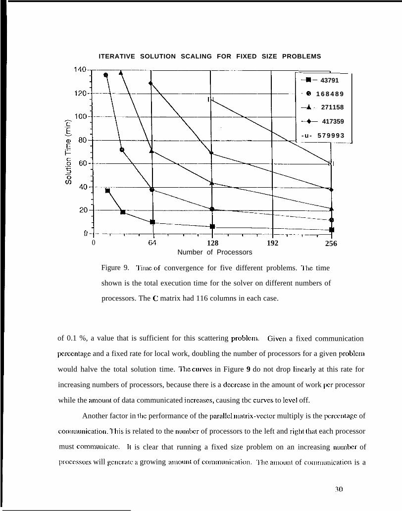
Shown in Figure 9 arc plots of time to convcrgcncc on different numbers of processors for

five different problems (fixed sim problems). “1’hc number of unknowns in (hc finite clcmcnt mesh

and the number of columns of C, arc indicated on tl~c plots. I’hc qllasi-Illi[li[~~lllll rcsiclual

algorithm was stopped when ttlc Ilormalizd residual was rc(tuced three orders of magnitude fc)r

each column of C. With an initial gUC,SS ~~.ing (]IC Z,cro VCCIOI-, ttlis r-csults in a no~naliz~d residual

29

ITERATIVE SOLUTION SCALING FOR FIXED SIZE PROBLEMS

— * .+– 43791

--* 1 6 8 4 8 9

-&- 271158

-—+— 417359

- u - 5 7 9 9 9 3--i

------7-—u -1--- —T--r——l~r———T———~t————~ ---=+‘T~0 64 128 192 256

Number of Processors

Figure 9. ‘1’imc of convergence for five different problems. ‘1’hc time

shown is the total execution time for the solver on different numbers of

processors. The C matrix had 116 columns in each case.

of 0.1 %, a value that is sufficient for this scattering problcm. Given a fixed communication

perccn(agc and a fixed rate for local work, doubling the number of processors for a given problcrn

would halve the total solution time. I’hc CLUVCS in Figure 9 do not drop lincady at this rate for

increasing numbers of processors, because there is a decrcasc in the amount of work pcr processor

while the amount of data communicated incrcascs, causing tbc CUIVCS to lCVC1 off.

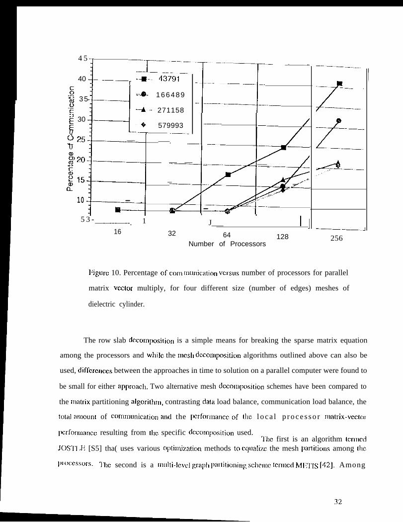
Another factor in (bc performance of the parallc] lnatrix-vcclor multiply is the pcrccntagc of

col~~l~~ll[~icatioI~. ‘]’his is related to the number of processors to the left and right (hat each processor

must communica(c. 1( is clear that running a fixed size problem on an increasing number of

pmccssors will gcncratc ii growing alnount of co)ll[llll[licatio[~. ‘]’hc anmun( of coil~fll~lr~icatioll is a

30

fLIIIC(bn of how finely the K matrix is dccomposcd, since its maximum row bandwidth after

reordering is not a function of [he number of processors used in the decomposition. If the

maximum row bandwidth is m and each processor in a given d~.opposition has approximately m

rows of K, then most processors wi II require one processor in each dir~tion for communication

If the number of processors used for the distribution of K is doubled, each processor will have.

approximatcl y m/2 rows of K. Since the row bandwidth doesn’ t change, each processor will now

require communication in each direxlion from two processors. But since the number of floating

point operations required hasn’ t changed, the communication percentage should roughly double.

This can be seen in Figure 10, which shows communication percentage versus number of

processors, for four problem sizes.

31

4 5 -{ ‘--r”-’–—--’ “--–

40 -j——r

——. ._ ._-i 43791

: H-- - - - 166489“S 35 ———0.- -+ 271158~ 30E + 5799930 —-—

/-”--””-2—— .- ___. —— ____ ——_

—.— ——.

025

E- ~<5~

— ..&— ——. ——_0 —.

$20+. — — — . _ _ ——_ .5$15 z.. — .+” ‘

CL----. ...-., .-.

10 .... ””— . —— ....@’&— —.— .

5 3 -—-–---—--. J___ I j116 32 64 128

Number of Processors

——=____

z—-—-— .——___f

——.

——-------

— .__.. -1

256

I:igurc 10. Percentage of corn lnurlication versus number of processors for parallel

matrix vextor multiply, for four different size (number of edges) meshes of

dielectric cylinder.

The row slab dccompositiorl is a simple means for breaking the sparse matrix equation

among the processors and while the mcsll dcconlpositiorl algorithms outlined above can also be

used, diffcrcn~s between the approaches in time to solution on a parallel computer were found to

be small for either approacl~. Two alternative mesh dccompc)sition schemes have been compared to

the matrix partitioning algoritl~r]l, contrasting da[a load balance, communication load balance, the

total amount of coIlllllllIlicatioll and the IErforlllallcc of [lIC l o c a l p r o c e s s o r matrix-vwt(~r

Pcrfornlarlce resulting from [l]c specific dccolnl)ositior] used.The first is an algorithm termed

JOSrl’l .1; [S5] tha( uses various optin~iz,atiorl methods to c,,ualizc the mesh par-titioris among the

J)l”Occssors, The second is a mlllti-lcvc] graph pal~itiol~illg schcn)c (crmcd Mlrl’IS [42]. Among

32

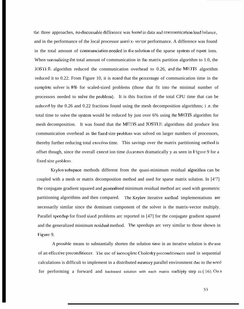
the three approaches, no disccrnablc diffcrcncc was follnd in data and Comm~lnication Ioa(i ba]ancc,

and in the performance of the local processor ma[ri x- vcc.tor performance. A difference was found

in the total amount of communciation necdcct in t} IC solution of tllc sparse systcm of cquat ions.

When normali~.ing t}w total amount of communication in lhc matrix partition algorithm to 1.0, the

JOSTI .Ii algorithm reduced the communication overhead to 0.26, and the METIS algorithm

reduced it to 0.22. From Figure 10, it is noted that the pcrccntagc of communication time in the

complctc solver is 8% for scaled-sized problems (those that fit into lbc minimal number of

processors needed to SOIVC the problcm). It is this fraction of the total CPU time that can be

rcduccd by the 0.26 and 0.22 fractions found using the mesh decomposition algorithms; i .c. the

total time to SOIVC the systcrn would be reduced by just over 6% using the METIS algorithm for

mesh decomposition. It was found that the M1-iTIS and JOSTI.11 algorithms did produce Icss

communication overhead as tbc flxcd size problcm was solved on larger numbers of processors,

thereby further reducing total cxcction time. This savings over the matrix partitioning rncthod is

offset though, since the overall cxecut ion time ctccrcascs dramatically y as seen in I ‘igurc 9 for a

fixed siz.c problcm.

Krylov subspacc methods different from the quasi-minimum residual algorithm can be

coupled with a mesh or matrix decomposition method and used for sparse matrix solution. In [4’7]

the conjugate gradient squared and gcncralizcd minimum residual method arc used with geometric

partitioning algorithms and then compared. ‘llc Krylov iterative rncthod implementations are

necessarily similar since the dominant component of the solver is the matrix-vector multiply.

Parallel spccdup for fixed sizcct problems arc reported in [47] for the conjugate gradient squared

and the generalized minimum rcsiduai method. “1’hc speedups arc very similar to those shown in

I:igurc 9.

A possib]c means to substantially shorten the solution time. in an iterative solution is ttlc usc

of an cffcctivc prcconditioncr. “1’hc usc of incomplc[c Cholcsky prcconditioncrs used in sequential

calculations is difficult to implement in a distributed n~cmory parallel environment duc to the ncmi

for performing a forward and backward solution with each matrix multiply step il] ( 16). On a

33

parallel machine, these arc essentially sequential operations that can give greatly reduced

Pcrforinancc [53]. A promising altcrnativcis tocalculatcan approximation to the inverse of t}lc

Systcm, rather than a fac(oriz,ation of the system as is done in the incomplete Cho]csky

approximation. A sparse approximate inverse [54] produces a matrix with a controllable number

of non-zeros that approximates the inverse of K, and rather than calculating forward and backward

solutions, it multiplies K at each step of the i[cralivc algorithm. ‘1’hc matrix-matrix mLdtiply can be

achieved with much higher performance than the forward and backward solutions used in the

incomplclc factorization.

S. DISCUSSION

This paper presented an overview of solutions to surface integral equation and volumetric

finite clcmcnt methods on sequential and distributed memory computer architectures. Both the

sequcn(ia] algorithmic scalability as well as scalabihy on parallel computer sys(cms were pre.scntcd

for curlcnt computer technology, with extrapolation to next generation tcchno]ogics. A broad SCL

of rcfcrcnccs arc given. When a uniform resource locator ([JRI.) is also rcfcrcnccd, it points to

software which is freely available.

REFERENCES

[1] Ii. Miller, “A selective survey of computational clcctromagnctics:’ lE;E1~ 7’rans. Anfennas

Propag. AP-36, pp. 1281-1305, 1988.

[2] M. N. O. Sadiku, Numerical Techniques in Mectromagnetics, Boca Raton: CRC Press, 1992.

[3] J. J. IJongarra, L. Grandinctti, G. R . Joubcrt, J . Kowalik, I:ditors, }ligh Perjiinnmce

Computing: Tec}znology, Methods and Applications, Advances in Parallel Computing 10,

Amsterdam: Elscvicr, 1995.

[4] 1 i. Miller, “So]ving bigger problems- by dczrcasing [}IC q~ration collnt and inclcasing the

computation bandwidth,” }’roc. IEEE, vol. 79, No. 10, pp. 1493-1504, 1991.

34

[5] V. Kumar, A. Granla, A. (; Llpta and G. Karypis, ln!roduction to Parallel C~mputi~lg,

Redwood City: ‘1’hc IJc!ljaIllirti~ lllllrllillgs hb]ishing Company, 1994. See also

tlttI>://www.cs. tl1l~rl.cdLl/-kllr~lar.

[6] “1”. Cwik and J. Patterson, Jiditors, Computational Electronics and Supercomputer Architec(14rc,

Progress in I~lcclron~agnctics Research, Vol. 7, Cambridge: EMW PLlblishing, 1993.

[7] R. l:. IIarrington, FieM Computation by Moment Method. New York: Macmillan, 1968.

[8] A. J. Poggio and E. K. Miller, “lntcgral equation solutions of three-dimensional scattering

problems,” in Computer Techniql(es for Elec?romagnetics, R. Mittra, Editor, Chapter 4, Ncw

York: IIernispherc, 1973.

[9] G. Golub and C. Van ban, “Ma(r-ix Compufafions, ” The John Hopkins University Press,

1989.

[10] E Anderson, Z. Bai, J. Dcmmcl, J. Dongarra, J. Du Croz, A. Grccnbaum, S, IIanm~arling,

A. McKcnncy, S. Ostrouchov, and I). Sorenson, LA}’ACK User’s Guide, %cicty for

]ndustrial and Applied Mathematics, l’hiladelphia. PA 1992. Scc also

http://nct lib2.cs.utk.cdu/ lapack/index.ht ml

[11 ] E. Yip and B. Dcmbzul, “h40nostatic calculations for a 3D MOM code with fast mutipolc

method,” l’rogrcss in Elcctrornagnctics Research Symposium Proceedings, p. 53, Jul y 24-

28, 1995.

[ 12] J. Rahola, “Solution of dense systems of linear equations in the discrctc-dipole

approximation, ” SIAM .). Sci. Comput., Vol. 17, No. 1, pp. 78-89, 1996.

[13 ] M. Sanccr, R. McClary, K. Glovcr, “Elcctromagnctic computation using parametric

geometry,” Elcctrornagnc(ics, Vol. 10, No. 1-2, pp. 85-104, 1990.

[ 14] l;, X. Canning, “The lmpcdancc Matrix Imcaliz,ation (lMl.) Method for Mon~cnt-Method

Calculations,” IEEE Anfcnnas }’ropag. &fag., pp. 18-30, October 1990.

[ 15] W. Chew, C. 1.u and Y. Wang, “I; fficicnt computation of three-dimensional scattering of

vector clcctromagnctic waves,” J. C@t. S’(K. Am. A, Vo]. 11, No. 4, pp. 1528-1537, 1994.

35

[ 16] V. Rokhlin, “Rapid Solution of integral equations of sca~lcring thcorY in two dimensions,” J.

Comp. Physics 86, pp. 414-439, 1990.

[ 17] R. Coifman, V. Rokhlin and S. Wandm-a, “’1’hc fast mu]tipolc method for the wave equation:

a pedestrian prescription,” IEEE An!. Pr-opag. Msg. 35, pp. 7-12, 1993.

[ 18] M. A. Stalzer, “A parallel fast multipolc method for the I lclmholtz cquat i on,” Parallel

l’recessing Letters 5, pp. 263-2’14, 1995.

[19] S. M. Rae, D. R. Wilton, and A.. W. Glisson, “Electron~agnctic scattering by surfaces of

arbitrary shape,” IEEE Trans. Antennas Propag. AP-30, pp. 409-418, 1982.

[20] W. Johnson, D. R. Wilton, and R. M. Sharpc, “Modeling scattering from and radiation by

arbitrary shaped objects with the electric fielcl integral equation triangular surface patch COCIC,”

fidcctromagnelics 10, pp. 41-64, 1990.

[21 ] J. J. IIongarra, J. Bunch, C. Molcr, and G. W. Stewart, LIIVPACK User’s Guide, Society

for Industrial and Applied Mathematics, Philadelphia, PA 1979. Scc a lso

l~tt1>://I~ctlib2, cs.utk.cdtl/lill]~ ack/ir~(lcx.lltrl~l.

[22] J. J. Dongarra, J. Du Croz,, S. I lammarling, and R. J. I Ianson, An Extendexl set of

FORTRAN Basic Linear Algebra Subprograms, ACM Trans. Math. Soft., Vol. 14, pp. 1-

17, 1988. See also http: //nctlib2.cs.utk. cdu/blas/indcx. htn~l.

[23] J. J. Dongarra, J. Du Croz, 1. S. Duff, and S. IIammarling, A set of Level 3 Basic Linear

Algebra Subprograms, ACM 7’rans. Math. Soft., Vol. 16 pp. 1-17, 1990. SeC also

ht[p://nctlib2. cs.utk.cdu/blas/indcx .htnd.

[24] T. Cwik, R. van de Gcijn, and J. Patterson, “Application of massively parallel computation to

integral equation models of clcctromagnctic scattering,” J. Opt. Sot. Am. 11, pp. 1538-1545

(1994). See also ftp://microwavc.jpl .nasa.gov/pub/PARAI .I.I3I ~COMPLEX.SOI,VER.

[25] J. Jin, The Finite Element in l;lcctro~}lag~~c[ic.~, John Wiley and Sons, Inc., Ncw York, 1993.

[26] J. I,cc, and R. Mittra, “A Note (III I’hc Application Of l:kigc-Iilcmcnts Ijor Modeling 3-

l)imcnsional lnhon~ogcncously -l;illc(i Cavities,” IEEE Transactions On Microwovc 7hcory

and 7’echniqucs, vol. 40, no. 9, pp. 176”1- 1773, Sept., 1992.

36

[27] S. Pissanetzky, S@rse Matrix 7kchnolgy, 1.onclon: Academic Press, 1984.

[28] I. S. ]) Llff, A. M. lirisman and J. K. Reid, l~irec[ Method.r for Sparse Matrices, New York:

Oxford University Press, 1986.

[29] l;. Ng, and B. Pcyton, “Block sparse Cholesky Algorithms on Advanced Uniprocessor

Con~pL]tcrs,” SIAM J. Sci. Conqmt., vol. 14, No. 5, j)jl. 1034-1056, I)p. 1034-1056, 1993.

[30] R. Barrett, M. Berry, T. Chan, J. Dcmmcl, J. Ilonato, J. Dongarra, V. l;ijkhout, R. POZO, C.

Rominc, and H. van dcr Vorst, Tmplotesfor the .volution of linmr system: building blocks

for iterative methods, Society for Industrial and Applied Mathcrnatics, Philadelphia. PA

1994. Scc also http: //netlib2.cs.utk.du/ten~ platcs/index.l~tll~l.

[311 M. Jones and P. Plassmann, “An improved incomplete Cholcsky Factoriz,a(ion, ” ACM Trans.

Math. Soft ware, Vo]. 21, No. 1, pp. 5-17, 1995. S(YJ also

http: //nctlib2.cs.utk. edu/toms~4O.

[32] I). 0’1 ,cary, “Parallel inlplcmcnta(ion of the block conjugate algorithm~’ Parallel Conlpl/t.,

Vol. 5, pp. 127-139, 1987

[33] R. l~rcund, and M. Malhotra, “A block-QMR algorithm for non-hcrlnitian linear systems with

multiple right-hand sides,” preprint 1996.

[34] R. Mittra, (). Rarnahi, A. Khebir, R. Gordon, and A. Kouki, “A Review of Absorbing

Boundary Conditions for Two- and Three-Dirncnsional Electromagnetic Scattering

Problems;’ I1~EE Trans. Mag, VOL 25, no. 7, pp. 3034--3040, July 1989.

[35] J.-M. Jin and V. I,icpa, “Application of ~~ybrid Finite IXmcnt Mc[hod to Elcctromagnctic

Sca(tcring from Coated Cylinders,” lEEE Tram. Antennas and Propagation, vol. AP-36,

pp. 50--54, Jan. 1988.

[36] X. Yuan, I). l,ynch, and J. Strohbchn, “Coupling of finite clcmcnt and moment mchods for

Clcc[romagnctic scattering fronl inhomogenoLls objects,” Ifil<fi; Tmns. Anicnnas Propqgai,

vol. A1’-38, pp. 386–394, Mar. 1990.

137] W. Boysc and A. Scidl, “A 11 ybrid l~inite lilcmcnt Method for Near lhdim of RcvolLltion,”

lfih’1< l’rans. Mag, vol. 27, l}p. 3833--3836, Scpt. 1991.

37

[38] ’1’. Cwik, C. Zuffada, and V. Janmejad, “Modeling ‘1’}lrW.-I>itllcnsiCJna! scatterers Usirlg a

Coupled Finite Elel~lctlt--Ir~tcgral I~~ua(ion Representation,” lEEETran.v. Antennas l’ropag.,

AP44, pp. 453-459, 1996.

139] 11. NoLlr-On~id, A . Racfsky, a n d G. l.yzcnga, “solving ~~initc Illcmcnt I:~uations o n

Concurrent Computers,” American Sot. Mec}I. Eng., A. Noor Iiditor, pp. 291-307, 1986.

[40] A. Pothen, Ii. Simon and K. I.iou, “Partitioning Sparse Matrices with I;igcnvcztors of

Graphs,” SIAM ./. Matrix Anal. Appl., vol. 11, pp. 430-452, 1990.

[41 ] B. Hendrickson and R. IxAand, “An lmprovcd Spectral Graph Partitioning Algorithm for

Mapping Parallel Computations, “ SIAM J. Sci. Cotnput., vol. 16, pp. 452-469, 1995.

[42] G. Karypis and V. Kurnar, “A l~ast and Iligh Quality Multilevel Scheme for Partitioning

lrrcgular Graphs,” Technical Report 7X 95-035, Department of Computer Science,

University of Minnesota, 1995. See also http: //www.cs.tlnln. edti-ka~pis/r~lcti#rnetis.t~tr1~l.

[43] M. IIeath, E. Ng, and B. Pcyton, “Parallel algorithms for sparse linear systems,” SIAM

Review, Vol. 33, No. 3, pp. 420-460, 1991.

[44] 1;. Rothbcrg, “Alternatives for solving sparse triangular systems on distribLltcd-rllcll~(~~ mLllti-

proccssors,” Parallel Cornput., Vol. 21, pp. 1 1 2 1 - 1 1 3 6 , 1 9 9 5 . See a l so

http: //www.ssd.intcl .corn/appsw/scs .html.

[45] A. Gupta, G. Karypis, and V. Kumar, “Highly scalable parallel algorithms for sparse matrix

factorization:’ Technical Report 7’R 94-63, Department of Computer Science, University of

Mirmcso[a, 1994

[46] G. }Icnnigan, W. Dcarholt, S. Castillo, “The finite clement solutionof elliptic systems on a

massivcl y parallel cornputcr using a direct solver,” preprint.

[47] J. Shadid and R. Tuminaro, “Sparse iterative algorithm software for large-scale MIMD

machines: an initial discussion and inqicmcntation, >’ Concurrency: Practice muf lixpericncc,

Vol. 4, pp. 481-497, 1992. Scc also tlttp://www.cs. sar~dia.gov/l ll'CCI"l/az.tcc. t~tl~~l.

38

[48] M. Jones and P. Plassman, “Scalable iterative solutions of sparse Iincar systems,” Para//e/

Comput., vol. 20, pp.753-773, 1994. Scc also

http://www,n~cs.anl .govfi~on~c/frcita~SC94d cll~o/softwarchlwksolvc. }~tl~~l.

[49] ‘I’. Cwik, D. Katz, C. Zuffada, and V. Jamncjad, “’I’llC Application of Scalable IJistributcd

Memory Computers to the F’initc Element Modeling of Elcctromagnctic Scattering,”

submitted to Intl. J. Numer. Methods Engr., 1996.

[50] A. George and J. Liu, Computer Solution of I.arge Sparse Positive l)ejinite Systems, Prcnticc

IIall, Ncw Jersey, 1981.

[51] J. l~wis, “Implementation Of The Gibbs- Poole-Stockn~cycr And Gibbs-King Algorithms,”

ACM Trans. on Moth. Software, VO]. 8, pp. 180-189, 1982.

http: //nctlib2.cs.utk. edu/toms/582.

[52 ] R, Freund, “Conjugate Gradient-Type Methods for I.inear Systems with Complex

Symmetric Cocfficicnt Matrices,” SIAM J. Stat. C’omput, vol. 13, no. 1, pp. 425-448, Jan,

1992. Scc also http: //nctlib2.cs.utk. cdu/linalg/lalqmr.

[53] E. Rothbcrg and A. Gupta, “Parallel ICCG on a hierarchical memory multiprocessor--

addressing the triangular solve bottleneck,” Parallel Comput., Vol. 18, pp. 719-741, 1992.

[54] M. J. Grote and Thomas IIuckle, “Parallel Preconditioning with Sparse Approximate

Inverses, accepted for publication in SIAM 3. oj Scientific Compu/ing, 1996. See also

l~ttp://www-sccm. stanford.cdtiStudcnts/grotc.}ltrlll.

[55] C. 11. Walshaw, M. Cross, and M. G, IIvcrett, “A localimd algorithm for optimizing

unstructured mesh partitions,” international Journal Of Supercomputer Applications And

nigh Performance Computing, Vol 9, No. 4, pp.280-295, 1995.

39

PERFORMANCE OF MATRIX SOLUTION ALGORITHM

1 2 0 -—z

T

rlOO+----

–——

60-

40

20-

01 1

Cray I“3D—— . ..- .. ____

-m-===---==’=

/

15120

560 ,

10 1

———-_

+

30240——

00 1(Number of Processors

——-— .

4‘ 0480

(es imate)

3 100003.1

IOgurel. Perfomlmce for BSOLVH(includcs factoring matrix, estin~ating condition nunlkr, and

solving for one right hand side.)

40

TIME FOR LU FACTORIZATION

100

10

0.1

0.01

4

+

I , 1

0 :

I 512 pE’s

POoc .—

4Cx5c

I_—. —.-——-f---l---r —

40 c

c

64 Bit Complex Arithmetic, Partial Pivoting—

T

I

APEs

1—

o196 PEs

Ooc

c

~—

❑ T3D

~ Paragon

1

A T90 (32 (2PUS)

● C90 (16 CPUS)

[~ Delta~—-

!0UNKNOWNS (1000)

Figure 2. CPU time vs. number of unknowns for 64 bit complex dense direct solvers with

partial pivoting for various machines (Cray T3D, T90 and C90; Intel Paragon and Delta).

processing elements (PIk) used in calculation shown for parallel computers. In-core and

out-of-core (OOC) rcsuhs specified.

41

1 0 0 ,

1 0 -

~&

1-i!.-t -

0.1 -

0.01 1 1 10

PATCH SCAL.ING FOR SCALED SIZE PROBLEMS

——

T..-—

=J4---4 6

— T - - r - r

X PE

‘JA+”——

——

10

---. ._. ,y

1 1 r-

MATRIX DIMENSION (X

Figure 3. Scalability for PATCII code for scaled size problems.

—.

12 141 000)

25[

1 I I

‘Es

71I

18

42

PATCH SCALING FOR FIXED SIZE PROBLEMS

301i== L =-lcra2 5 - - + 5832

_ - t

+ 6 2 0 0

+ 8712

~ 2“ —g A

5 -

0

———- —.

l“3t3.—

.——

.— _

“ — — - - - - - t - - - - - - - -128

Number of F’rocessors192

1

6

liigurc 4. Scalability for PATCI{ code for fixed siz,e problems. The 16,200 unknown case was

only run on 256 processors.

43

Dn—--–————’~—’——

j,.t-..c.

U? ’”” “: i ~.. . .!y,. .: .

L . ,,.

—-_ —-.--AAI~igurc 5. Non-zero matrix struc[urc of typjcal finite clement simulation. Left, original structure:

right, structure after reordering to mjnimizc bandwidth.

44

I

. . . .:,~., : ,:.l <.x! . . ,

.,

.:-~..; . :

. .,. : -c” .

.. ,1-.:., .

,,.: ,, ,-.7

. . ” .,, . .,:< :.;.. ;,. ~

., .<.- . -2 ,,> -“-, ,., . . . . . .*, .,. .,.. i- -.. :. . < ‘.” :.. ,

,1

~>

.-A .,F ..:.,.

. .:.

,,

;: . fi’’” .:... 8... . . .? .’ , ::-.: . “.. . , ; -*.. . $.

: :. i“. — — _

Figure 6. Non-zero matrix sparsity structure for system wilh dense surface integral equation

boundaly condition applied (left), and surface of revolution integral equation boundary

condition (right). The mesh has 5,343 edges with 936 of those on the boundary.

45

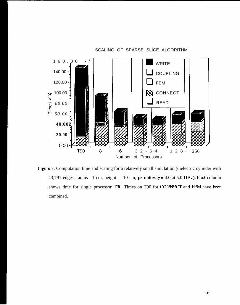
1 6 0 . 0 0 - /-

140.00I

120.001

~ 100.00a): 80.00

~ 6 0 . 0 0 1

40.002-1

20.00;

SCALING OF SPARSE SLICE ALGORITHM

——I

■ WRITE

❑ COUPLING

❑ FEM

II ~ CONNECT

❑ READ

.1-

T90-8”16” 3 2 - 6 4 “ 1 2 8 ’Number of Processors

256

Iiigure 7. Computation time and scaling for a relatively small simulation (dielectric cylinder with

43,791 edges, radius= 1 cm, height== 10 cm, permittivity = 4.0 at 5.0 GHz). Pirst column

shows time for single processor T’90. Times on T90 for CONNECr and FEM have been

combined.

46

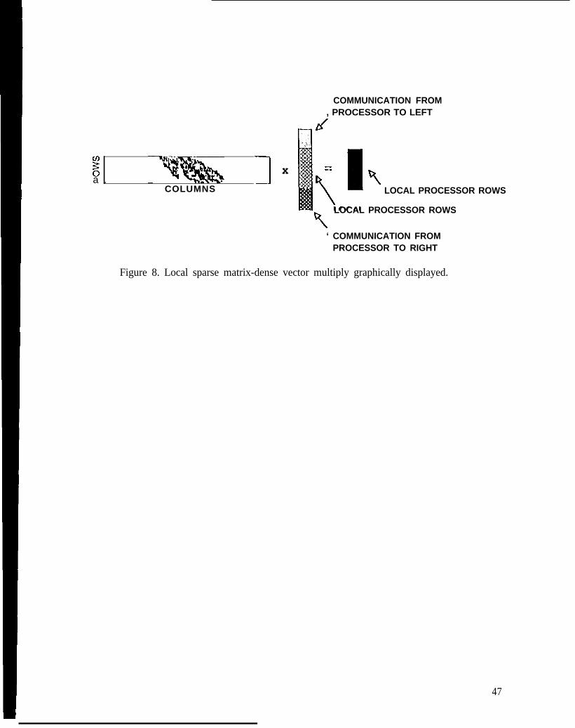
g -~Y!g!f&A

a . 1COLUMNS ‘

x

COMMUNICATION FROM, PROCESSOR TO LEFT

IId

,.

~1x

=Vx

\

\

LOCAL PROCESSOR ROWS

\

LOCAL PROCESSOR ROWS

‘ COMMUNICATION FROMPROCESSOR TO RIGHT

Figure 8. Local sparse matrix-dense vector multiply graphically displayed.

47

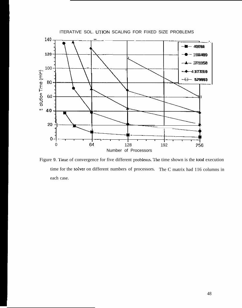
ITERATIVE SOL. UTION SCALING FOR FIXED SIZE PROBLEMS

140

E-::1. [~,~

— . .—.+ 43791

120 + 166489

& 271158100 — —.—

~ --4- 4 1 7 3 5 9g

+ 579993: 80

.—Fc . ..=--375“’ 40

-- I~u t---k--i —

d-———~l.~128

Number of Processors

1 —\ I I 1

0 64 192 2i6

Figure 9. ‘1’imc of convergence for five different probkxns. l’he time shown is the total execution

time for the solver on different numbers of processors. The C matrix had 116 columns in

each case.

48

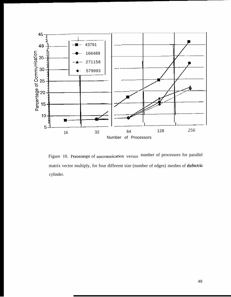
45 --$——————————I

40 -+––––– -–w–

–*–

-+–

4“

43791

166489

271158

579993_—

5~

16 32

—

P—..

——

—.. -

/_-—

—-

64

Number of Processors

128 256

Figure 10. Pcrcentagc of eornmunication versus number of processors for parallel

matrix vector multiply, for four different size (number of edges) meshes of diclectic

cylinder.

49

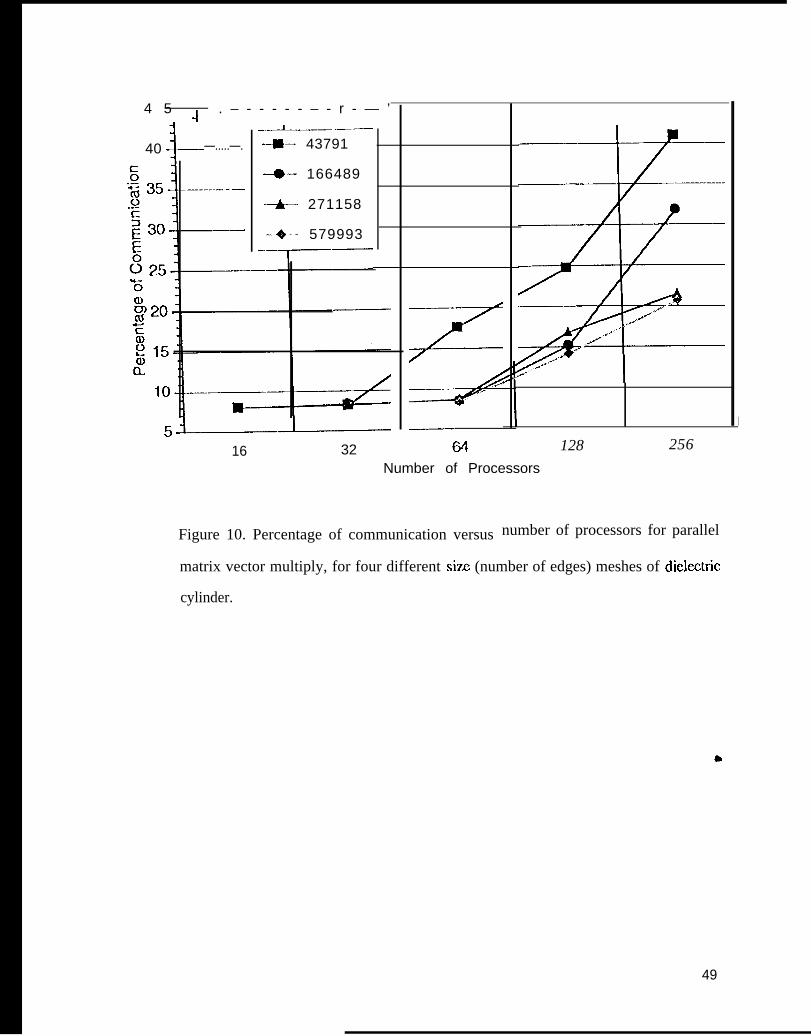
4 5 + . – - - - - - – - r - — ’

40L—.....—.

–.~ .—-*– 43791

+– 166489

+ 271158

-+- 579993

-~—

5~

16 32

7’=_———

64

I

128 256

Number of Processors

Figure 10. Percentage of communication versus number of processors for parallel

matrix vector multiply, for four different siz~ (number of edges) meshes of dielwtric

cylinder.

49