Sales Forecasting System for Newspaper Distribution ...

Pak.j.stat.oper.res. Vol. VIII No.3 2012 pp685-699

Statistics in the Twenty-First Century: Special Volume In Honour of Distinguished Professor Dr. Mir Masoom Ali On the Occasion of his 75th Birthday Anniversary PJSOR, Vol. 8, No. 3, pages 685-699, July 2012

Sales Forecasting System for Newspaper Distribution Companies in Turkey

Gencay İncesu Institute of Social Sciences Okan University Istanbul, Turkey [email protected] Barış Aşıkgil1 Department of Statistics Mimar Sinan Fine Arts University Istanbul, Turkey [email protected] Müjgan Tez Department of Statistics Marmara University Istanbul, Turkey [email protected]

Abstract

Newspapers are like goods with a shelf life of one day and they have to be distributed daily basis to the sales points. A problem that most newspaper companies encounter daily is how to predict the right number of newspapers to print and distribute among distinct sales points. The aim is to predict newspaper demand as accurately as possible to meet customer need with minimum number of returns, missed sales and oversupply. This makes it necessary to develop a short-term forecasting system. The data taken from one of the largest distribution companies in Turkey is time dependent. Therefore, time series analysis is used to forecast newspaper circulation. In this paper, the newspaper sales system is examined for Turkey. Various types of forecasting techniques which are applicable to newspaper circulation planning are compared and a nonlinear approach for returns is applied.

Keywords: Newspaper Circulation, Exponential Smoothing, ARIMA, Nonlinear Approach, Time Series Forecasting.

MSC2000: 62P99, 91B84.

1. Introduction

Forecasting plays a major role in decision making and business planning. Probably, the most important function of business is forecasting. A forecast is a starting point for planning. The objective of forecasting is to reduce the risk in decision making. To a large extent, success depends on getting those forecasts rightly.

1 Corresponding author

Gencay İncesu, Barış Aşıkgil, Müjgan Tez

Pak.j.stat.oper.res. Vol. VIII No.3 2012 pp685-699 686

Shim (2009) gives some important forecasting applications for the strategic areas in business. Also, he explains types of forecasts and managerial planning. From his explanation it can be said that the aim of a newspaper distribution company is to determine the optimal supply of newspaper that minimizes costs or maximizes profit in the face of uncertain demand. In the case of more shipping than demand the company has undue costs caused stocking, high returns, transportation and other operational issues or in the case of less shipping than demand the company has sales lost. Thomopoulos (1980) states that reliable forecasts are essential for a company to survive and grow. In a manufacturing environment, management must forecast the future demands for its products and on this basis provide for the materials, labor and capacity to fulfill these needs. These resources are planned and scheduled well before the demands for the products are placed on the firm. Forecasting is the heart of an inventory control system. A firm with hundreds or thousands of items must anticipate in advance demands that will occur against these items. This is needed to have the proper inventory available to fill customers’ demands as they come in. Management must plan several months in advance for this inventory since procurement lead times from suppliers generally runs from 2 to 6 months. With each time, forecasts are needed for the months in the planning horizon. The forecasts are used to determine whether or not an order to the supplier is needed now and if so how large the order should be. Thomopoulos (1980) explains that forecasting techniques can be categorized into three groups. The first is called qualitative, where all information and judgment relating to an item are used to forecast the items demands. This technique is often used when little or no demand history is available. The forecasts may be based on marketing research studies, the Delphi method or similar methods. The second group is called causal, where a cause-and-effect type of relation is sought. Here, the forecaster seeks a relation between an item’s demands and other factors, such as business industrial and national indices. The relationship is used to forecast the future demands of the item. The third group is called time series analysis, where a statistical analysis on past demands is used to generate the forecasts. A basic assumption is that the underlying trends of the past will continue into the future. This paper is primarily concerned with forecasting as it relates to time series analysis. In this context, the time series represent the demands recorded over past time intervals. The forecasts are estimates of the demands over future time intervals and are generated using the flow of demands from the past. This paper proceeds as follows. Section 2 gives the literature review, some theoretical structures for exponential smoothing models and autoregressive integrated moving average (ARIMA) models. Section 3 provides an overview for distribution company, its organizational structure and circulation planning. Section 4 includes a comprehensive study of newspaper circulation and the empirical results. Section 5 is the discussion and conclusion.

2. Time Series Analysis and Modeling Strategy

The importance of predicting future values of a time series transcends a range of disciplines. Economic and business time series are typically characterized by trend, cycle, seasonal, and random components. Powerful methods have been developed to capture these components by specifying and estimating statistical models. These methods include



exponential smoothing and ARIMA, which are described by Granger and Newbold (1974) and Reid (1975). They show that ARIMA gives more accurate out-of-sample forecasts on average than exponential smoothing although ARIMA requires much more effort. Gass and Harris (2000) state that exponential smoothing originated in Robert G. Brown’s work as an OR analyst for the US Navy during World War II. Yafee and McGee (2000) identify that the more sophisticated exponential smoothing methods seek to isolate trends or seasonality from irregular variation. Where such patterns are found, the more advanced methods identify and model these patterns. The models can then incorporate those patterns into the forecast. Exponential smoothing uses weighted averages of the past observations for forecasting. The effect of the past observations is expected to decline exponentially over time. Gardner (1985) states that the exponential smoothing methods are relatively simple but robust approaches to forecasting. They are widely used in business for forecasting demand for inventories. Three basic variations of exponential smoothing are given as simple exponential smoothing, trend-corrected exponential smoothing and Holt-Winters method. Ediger et al. (2006) state that ARIMA method developed by Box and Jenkins (1976) is one of the most noted models for time series data prediction and often used in econometric research. The ARIMA method has been originated from the autoregressive (AR) model, the moving average (MA) model and the combination of the AR and MA, the ARMA model. Compared with the early AR, MA and ARMA model, ARIMA model is more flexible in the application and more accurate in the quality of the simulative or predictive results. Box and Jenkins (1976) highlight that in the ARIMA analysis, an identified underlying process is generated based on observations to a time series for generating a good model which shows the process-generating mechanism precisely. Ho and Xie (1998) and Me lard and Pasteels (2000) have considered that the only problem with ARIMA appears that the modeling is mathematically sophisticated in theory and requires a deep knowledge of the method. Therefore, building an ARIMA model is often a difficult task for the user, requiring training in the statistical analysis, a good knowledge of the field of application and the availability of an easy to use but versatile specialized computer program.

2.1. Methodology for Exponential Smoothing

Generally, a distinctive feature of the approaches for exponential smoothing is that time series are assumed to be built from unobserved components such as the level, growth, seasonal effects; and these components need to be adapted over time when demand series display the effects of structural changes in product market (Billah et al., 2006). The standard methods of exponential smoothing are given no trend with no seasonality (simple exponential smoothing), additive trend with no seasonality (Holt smoothing) and additive trend with additive or multiplicative seasonality (Holt-Winters smoothing). Although many new models underlying exponential smoothing have been proposed, the classical ones are known at most (Gardner, 2006).



Let Yt be a time series. Simple (single) exponential smoothing is defined as

( )t 1 t t t 1Y S αY 1 α S ,+ −= = + − (1)

where St is the smoothed level of the series and α is the smoothing parameter in the unit interval, α є [0,1]. S0 can be taken as the mean of Yt (Diebold, 2001). If St is smoothed one more, double exponential smoothing is obtained as

( )t t t 1D αS 1 α D .−= + − (2)

D0 can be taken as S0. The forecast is obtained by t k t tY a b (k)+ = + , where t t ta 2S D= −

and ( ) ( )t t tb α S D 1 α= − − .

If the series Yt doesn’t have only a slowly evolving local level, but also a trend with a slowly evolving local slope, then Holt smoothing is given by these equations,

( ) ( )t t t 1 t 1S αY 1 α S T ,− −= + − + (3)

( ) ( )t t t 1 t 1T β S S 1 β T ,− −= − + − (4)

where the parameter α controls smoothing of the level, β controls smoothing of the slope

and α, β є [0,1] (Diebold, 2001). The forecast is obtained by t k t tY S T (k).+ = +

If the series Yt has both trend and seasonality, then Holt-Winters smoothing is given by these equations,

( ) ( )( )t t t s t 1 t 1S α Y I 1 α S T ,− − −= − + − + (5)

( ) ( )t t t 1 t 1T β S S 1 β T ,− −= − + − (6)

( ) ( )t t t t sI γ Y S 1 γ I ,−= − + − (7)

where It denotes smoothed additive seasonality, γ is the smoothing parameter for

seasonality and α, β, γ є [0,1]. The forecast is obtained by t k t t t s kY S T (k) I+ − += + + where

s denotes the number of periods in the seasonal cycle. However, the seasonality can also be multiplicative. Then, the ratio of Yt and It-s is used instead of the difference in equation (5) and the ratio of Yt and St is used instead of the difference in equation (7). Moreover,

the forecast is obtained by ( )t k t t t s kY S T (k) I .+ − += +

2.2. Box-Jenkins Methodology

If a series is limited by a finite number of available observations, a finite-order parametric model is often constructed to describe the time series process. Such a model contains a very broad class of parsimonious time series processes found useful in describing a wide variety of time series (Wei, 2006). Box-Jenkins (1976) methodology for estimating time series model is given as

t 0 1 t 1 p t p t 1 t 1 q t qY α α Y α Y ε β ε β ε .− − − −= + + + + + + +L L (8)

Such models are called ARIMA time series models. If these models are stationary, then they are called ARMA models (Enders, 1995).



Many time series encountered in practice are well approximated by the representation p

i t i ti 0

α Y ε , t 0, 1, 2,...,−=

= = ± ±∑ (9)

where α0 ≠ 0, αp ≠ 0 and the εt are uncorrelated (0,σ2) random variables. The sequence Yt is called a pth order AR time series, denoted as AR(p). The defining equation (9) is sometimes called a stochastic difference equation (Fuller, 1996). A finite number of π weights are nonzero, i.e., π1 = α1, π2 = α2, …, πp = αp and πk = 0 for k > p, AR(p) model is also given by

p t tα (B)Y ε ,=& (10)

where pp 1 pα (B) (1 α B α B )= − − −L and t tY Y μ.= −& Since

p

i ii 1 i 1

π α∞

= =

= < ∞∑ ∑ , (11)

the process is always invertible. To be stationary, the roots of pα (B) must lie outside of

the unit circle. The AR processes are useful in describing situations in which the present value of a time series depends on its preceding values plus a random shock (Wei, 2006).

The parameter estimates of AR(p) model can be obtained by using the ordinary least squares (OLS). This estimator is asymptotically equivalent to the Yule-Walker estimator which is often used for estimating the stationary AR(p) models (Cho and Song, 1996; Eshel, 2003). The time series defined by

q

t j t jj 0

Y β ε , t 0, 1, 2,...,−=

= = ± ±∑ (12)

where β0 ≠ 0 and βq ≠ 0 is called a qth order MA time series, denoted as MA(q). A finite number of ψ weights are nonzero, i.e., ψ1 = –β1, ψ2 = –β2, …, ψq = –βq and ψk = 0 for k > q, MA(q) model is also given by

t q tY ψ (B)ε ,=& (13)

where qq 1 qψ (B) (1 ψ B ψ B ).= − − −L Since

2 21 q1 ψ ψ ,+ + + < ∞L (14)

a finite MA process is always stationary. This MA process is invertible if the roots of

qψ (B) lie outside of the unit circle. MA processes are useful in describing phenomena in

which events produce an immediate effect that only lasts for short periods of time (Wei, 2006). It is given that OLS can be used to obtain efficient estimators for the parameters of AR time series. Unfortunately, the estimation for MA processes is less simple. Maximum likelihood method can be used as an alternative (Fuller, 1996).



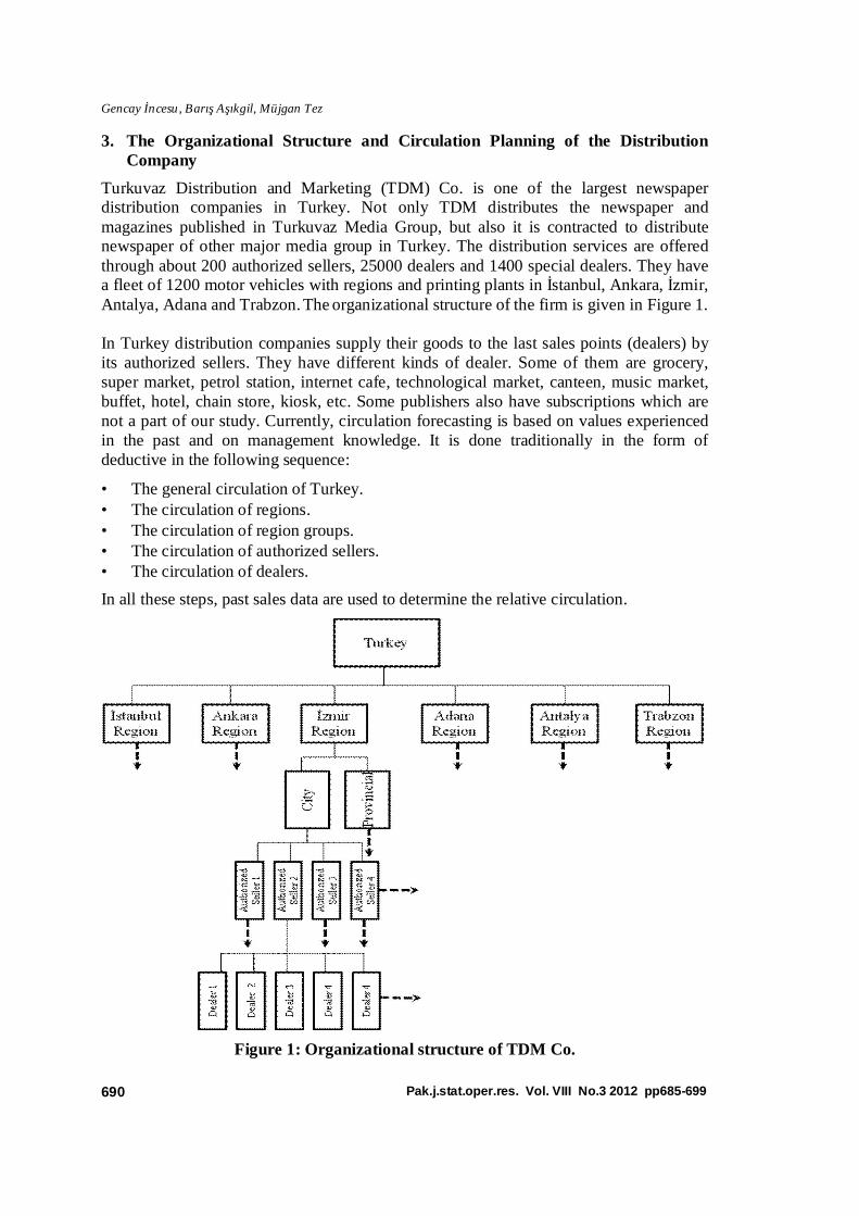
3. The Organizational Structure and Circulation Planning of the Distribution Company

Turkuvaz Distribution and Marketing (TDM) Co. is one of the largest newspaper distribution companies in Turkey. Not only TDM distributes the newspaper and magazines published in Turkuvaz Media Group, but also it is contracted to distribute newspaper of other major media group in Turkey. The distribution services are offered through about 200 authorized sellers, 25000 dealers and 1400 special dealers. They have a fleet of 1200 motor vehicles with regions and printing plants in İstanbul, Ankara, İzmir, Antalya, Adana and Trabzon. The organizational structure of the firm is given in Figure 1. In Turkey distribution companies supply their goods to the last sales points (dealers) by its authorized sellers. They have different kinds of dealer. Some of them are grocery, super market, petrol station, internet cafe, technological market, canteen, music market, buffet, hotel, chain store, kiosk, etc. Some publishers also have subscriptions which are not a part of our study. Currently, circulation forecasting is based on values experienced in the past and on management knowledge. It is done traditionally in the form of deductive in the following sequence:

• The general circulation of Turkey. • The circulation of regions. • The circulation of region groups. • The circulation of authorized sellers. • The circulation of dealers.

In all these steps, past sales data are used to determine the relative circulation.

Figure 1: Organizational structure of TDM Co.



This study is in the form of induction. We will use our forecasting model to forecast only circulation of dealers. After that it is easy to find the other organization’s circulation by summation of sub-organization circulation. For example, if an authorized seller has three dealers, the circulation of the authorized seller equals to the sum of the circulation of the three dealers.

4. Empirical Analysis of Newspaper Circulation

In Turkey circulation of a newspaper equals to the printed quantities of the newspaper. It also equals sum of net sales and returns. Therefore, our study includes two parts; one is forecasting the net sales, the other one is determining the expected returns. TDM has authorized sellers and dealers in their authorized sellers distribution channel. We focus on dealers because we determine the circulation of dealers. We can find circulation of the authorized sellers, regions and country (Turkey) by summation hierarchically according to Figure 1. In this study we randomly selected a dealer. The characteristics of the dealer are given below:

Name of dealer : Koçbay Dealer Type of dealer : Kiosk Address of dealer : Atatürk mah. Turgut Özal sk. 64 Ataşehir İstanbul.

We select three national newspapers to work on. These are Fotomaç, Sabah and Takvim. In this study we use the names newspaper1 for Fotomaç, newspaper2 for Sabah and newspaper3 for Takvim. Newspaper1 is a sport newspaper, newspaper2 is one of the biggest newspapers in Turkey with high circulation and newspaper3 is a newspaper with low circulation. This study includes the circulation of these newspapers of the dealer.

4.1 Forecasting Net Sales of the Newspapers

We use about two-year the net sales data of Koçbay dealer between 11/30/2009-12/29/2011. The data set includes 760 observations about daily net sales for each newspaper. The time series graphs of each newspaper are obtained and given in Figure 2.

Figure 2: Structural views of the three different newspapers



When we do preliminary analysis of the two-year data we doubt that there is a weekly seasonality. Circulations of the same days of each week are very similar. For example, Sundays’ net sales are more similar than the other days of the same week. EViews7 is used for the analysis in this study. According to Figure 2, it can be seen that all the time series have a decrease in second and third quarter of 2011. The reason of this decrease is guessed that a new dealer is opened near the Koçbay dealer.

The three different series are correlated in time period and they are nonstationary series. On the other hand, these series become stationary by taking the first differences of them. Some modeling procedures are examined by using exponential smoothing and ARIMA approaches in order to obtain the best forecast model. Firstly, some exponential smoothing models are examined and root mean squared error (RMSE) values are given in Table 1 in order to determine the efficient approach for each series of newspapers.

Table 1: Modeling results obtained from exponential smoothing for each series

Modeling Approach Newspaper1

(RMSE)

Newspaper2

(RMSE)

Newspaper3

(RMSE)

Single 5.2631 22.2183 2.2299

Double 5.2840 22.0957 2.2335

Holt (No seas.) 5.2557 22.0798 2.2419

Holt-Winters (Additive seas.) 4.0767 11.2975 1.9144

Holt-Winters (Multiplicative seas.) 4.0703 10.7748 ---

According to Table 1, it is clear that all series include seasonality. Therefore, it can be said that Holt-Winters modeling approach is acceptable in view of the RMSE values. Holt-Winters modeling with multiplicative seasonality is not applicable for the series of newspaper3, since the series includes zero-valued observation in the last quarter of 2011. The forecast values for the next four days are generated by using the best modeling approach for each series and are given in Table 2.

Table 2: Forecasted net sales obtained from exponential smoothing

Day Newspaper1 (Net Sales)

Newspaper2 (Net Sales)


12/30/2011 29 90 7

12/31/2011 26 113 5

01/01/2012 24 128 5

01/02/2012 21 89 7

According to Table 2, the great variation of forecast values for the newspaper2 is acceptable in view of its RMSE values given in Table 1.



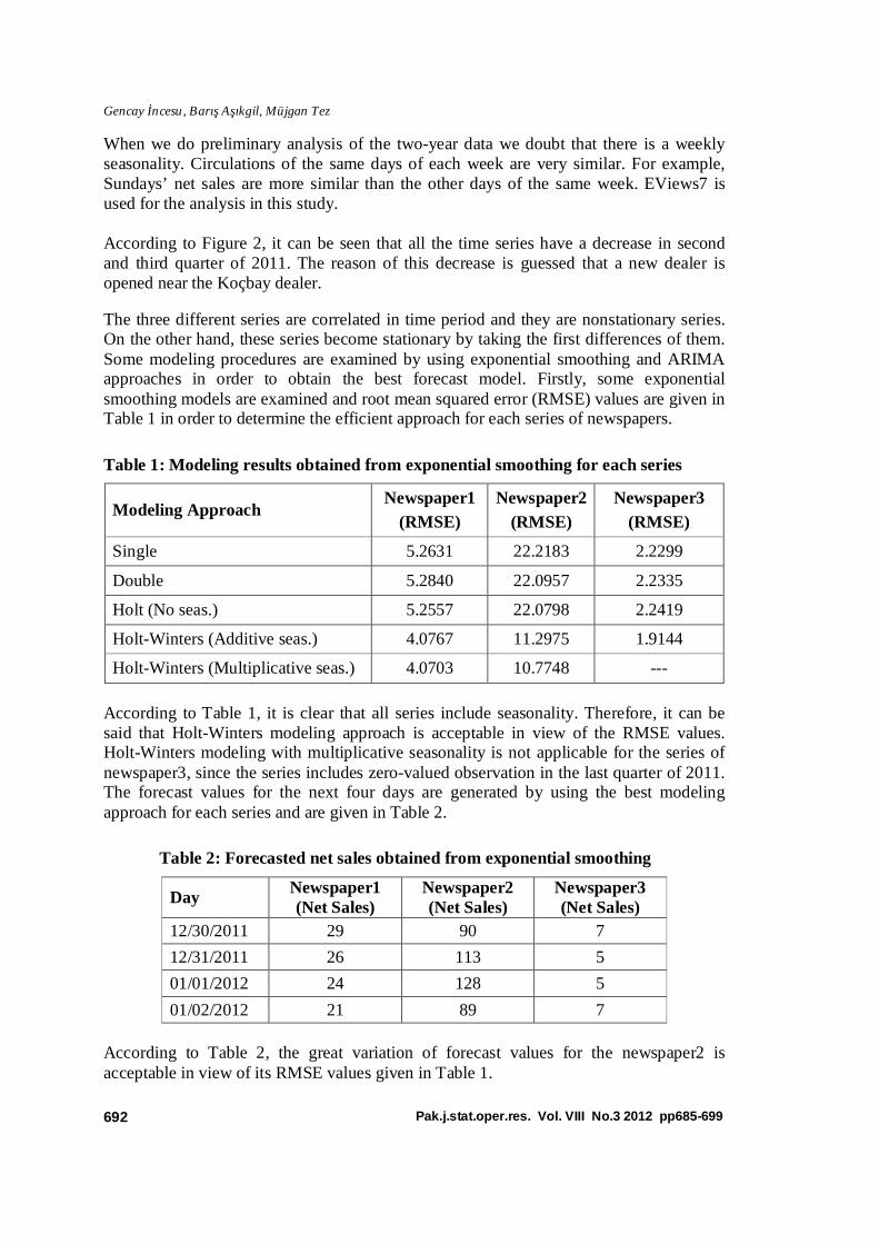
The three series are examined carefully by using ARMA models in order to obtain more reliable forecast values. Before modeling each series, the logarithmic transformation is used to stabilize the variance and the first difference is taken to overcome the nonstationarity. The series obtained after these processes are given in Figure 3.

Figure 3: Structural views of the differenced logarithmic series

Many alternatives of ARMA models are tried for each series and the best one satisfying the assumptions of homoscedastic and uncorrelated errors is given in Table 3. The alternative models are compared in view of some information criteria (AIC, SC, HQ). The best model has the smallest information criteria for each series. Also, Durbin-Watson (DW) statistics are equal to approximately two which means that the errors are autocorrelated and the models are plausible for forecasting.

Table 3: Summary statistics of ARIMA models for each series

Newspaper1 Newspaper2 Newspaper3

Coefficient Std. Error Coefficient Std. Error Coefficient Std. Error DLNYt-1 -0.826639 0.030039 -0.837466 0.028236 -0.737129 0.034006 DLNYt-2 -0.744260 0.034747 -0.860220 0.029571 -0.687824 0.039324 DLNYt-3 -0.705045 0.036887 -0.834692 0.032163 -0.608156 0.043245 DLNYt-4 -0.657628 0.036869 -0.789383 0.032270 -0.477840 0.043269 DLNYt-5 -0.672959 0.034645 -0.797656 0.029593 -0.500266 0.039355 DLNYt-6 -0.570757 0.030040 -0.637277 0.028297 -0.369707 0.033962

Diagnostic Analysis R-squared 0.558843 0.636223 0.433555 SSR 14.49531 13.85472 31.90786 DW 1.971370 2.038839 2.025381 AIC -1.096427 -1.141626 -0.307400 SC -1.059581 -1.104781 -0.270555 HQ -1.082232 -1.127432 -0.293205



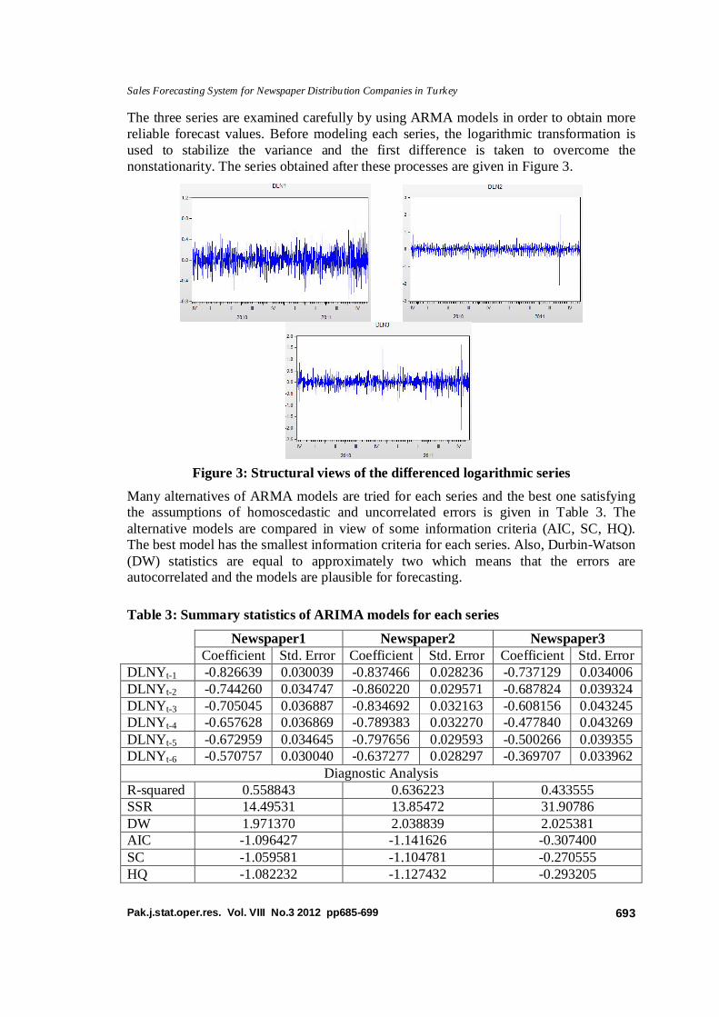
Since the data set is obtained daily, the period can be taken as seven. Therefore, the variables can consist of seven lag values of the series. The variables are eliminated hierarchically for their insignificance in the modeling. The forecast graphs are obtained by using the models in Table 3 determined through several alternatives and they are given for each series in Figure 4.

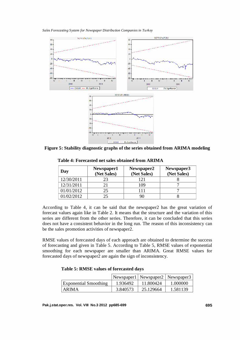
Figure 4: Forecast graphs of the series obtained from ARIMA modeling It can be seen from Figure 4 that the RMSE values for each series decrease clearly by using ARIMA modeling. Also, the values of Theil’s inequality coefficient are smaller than 0.55 for each series. It means that the generated models fit to the series very well. Moreover, the parameter estimates are examined for all models by using the stability diagnostic (CUSUM) and this is given in Figure 5. It can be concluded that the parameter estimates are stable within 5% significance. The forecast values for the next four days are generated by using the best ARMA model for each series and are given in Table 4.



Figure 5: Stability diagnostic graphs of the series obtained from ARIMA modeling

Table 4: Forecasted net sales obtained from ARIMA

Day Newspaper1 (Net Sales)



12/30/2011 23 121 8 12/31/2011 21 109 7 01/01/2012 25 111 7 01/02/2012 25 90 8

According to Table 4, it can be said that the newspaper2 has the great variation of forecast values again like in Table 2. It means that the structure and the variation of this series are different from the other series. Therefore, it can be concluded that this series does not have a consistent behavior in the long run. The reason of this inconsistency can be the sales promotion activities of newspaper2. RMSE values of forecasted days of each approach are obtained to determine the success of forecasting and given in Table 5. According to Table 5, RMSE values of exponential smoothing for each newspaper are smaller than ARIMA. Great RMSE values for forecasted days of newspaper2 are again the sign of inconsistency.

Table 5: RMSE values of forecasted days

Newspaper1 Newspaper2 Newspaper3

Exponential Smoothing 1.936492 11.800424 1.000000

ARIMA 3.840573 25.129664 1.581139



4.2 Determining the Expected Return Quantities

After forecasting the net sales, the firm determines expected return for the dealer according to its policy. It has three types of expected return quantities for forecasted net sales intervals. These are low, medium and high return quantities. Before determining the circulation, one of the types is selected according to its policy. The firm usually prefers medium expected return quantities. Therefore, we use medium expected return quantities in this study. The intervals and quantities are shown in Table 6.

Table 6: Expected medium return quantities for the intervals of net sales

Forecasted Net Sales Interval 0-1 2-4 5-9 10-15 16-23 24-32 33-43

Expected Return Quantity 1 2 3 4 5 6 7





Forecasted Net Sales Interval 356-389 390-424 425-461 462-500

Expected Return Quantity 22 23 24 25

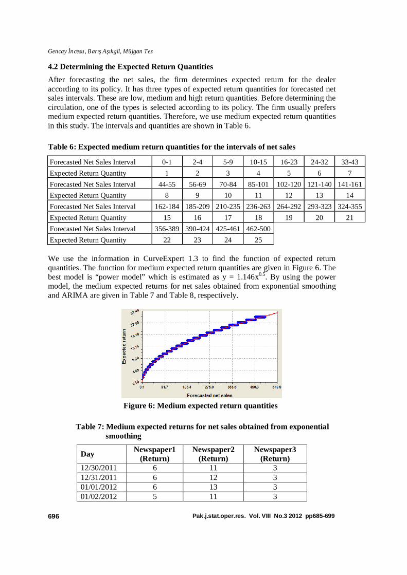
We use the information in CurveExpert 1.3 to find the function of expected return quantities. The function for medium expected return quantities are given in Figure 6. The best model is “power model” which is estimated as y = 1.146x0.5. By using the power model, the medium expected returns for net sales obtained from exponential smoothing and ARIMA are given in Table 7 and Table 8, respectively.

Figure 6: Medium expected return quantities

Table 7: Medium expected returns for net sales obtained from exponential smoothing

Day Newspaper1

(Return) Newspaper2

(Return) Newspaper3

(Return) 12/30/2011 6 11 3 12/31/2011 6 12 3 01/01/2012 6 13 3 01/02/2012 5 11 3



Table 8: Medium expected returns for net sales obtained from ARIMA

Day Newspaper1

(Return) Newspaper2

(Return) Newspaper3

(Return) 12/30/2011 6 13 3 12/31/2011 5 12 3 01/01/2012 6 12 3 01/02/2012 6 11 3

4.3 Circulation of the Newspapers

The firm determines the printing and distribution quantities which is equal to circulation. Circulation quantities are formulated as

Circulation = Forecasted net sales + Expected medium return quantity, (15)

and they are given in Table 9.

Table 9: Circulation quantities

Exponential Smoothing ARIMA

Newspaper1 Newspaper2 Newspaper3 Newspaper1 Newspaper2 Newspaper3

35 101 10 29 134 11

32 125 8 26 121 10

30 141 8 31 123 10

26 100 10 31 101 11

5. Discussion and Conclusion

We study only one dealer and select the best models for this dealer. Dealers can have different time series data because of their different characteristics. Some properties of a dealer that affect its sales are given below:

• Type of dealer (kiosk, grocery, etc.), • The demographic structure of dealer location, • Location of dealer (near street, in shopping center, etc.), • Proximity to other dealers, • Proximity to institutions like hospital, school, etc. The properties make the dealer unique and make its sales data different from the other dealers. Different sales data of dealers can require different models for forecasting. For TDM it is difficult to establish models for every dealer because there are many dealers. Because of this difficulty TDM can categorize the dealers which have similar sales data and apply the same models to the dealers in the same group. The newspapers we use in this study have different properties that affect their sales. Newspaper1 is a sport newspaper. Sport activities affect its sales. Especially, in Turkey football matches increase the sales of newspaper1. Newspaper1 sometimes gives to



readers free supplements like “iddaa”. In these days it is bought much more than the other days. Newspaper2 is one of the biggest newspapers in Turkey. It often gives promotions and free supplements and makes coupon campaign. These sales techniques cause increases in the sales of it. Sport activities like football matches also increase its sales. These increases also cause fluctuations and greater RMSE value than others. Newspaper3 is more stable than the other newspapers since it doesn’t usually have promotion, free supplements and coupon campaigns. It has basic sales. So, its RMSE value is smaller than others. Religious holidays and the first day of New Year are special days and in these days some publishers have different activities to increase their sales like giving free supplements and promotions. Because of these different activities it is difficult to forecast these days’ sales. For example, newspaper2 gives the list of raffle lottery that has a big effect on sales. In this study we forecasted sales about the first day of New Year even so knowing that difficulty. Local news, shock news and entering markets earlier than competitor in the morning are some other factors affecting newspaper sales. TDM concludes that the forecast results of exponential smoothing satisfy the expectations of the firm. The results are good and acceptable. The forecasts in 12/31/2011 and 01/01/2012 of newspaer2 have great deviation. The reason is explained that these days are special days and newspaper2 gives special promotions to increase its sales. It can be said that the study can be pioneer in Turkey since it is based on forecasting net sales, determining the expected return quantities with nonlinear approach and evaluating them together. The effects of promotions and free supplements can be handled as further studies.

Acknowledgement

This study is supported by Turkuvaz Distribution and Marketing Co. The authors are grateful to Eyyubi Faruk Öner (General Manager), İsmail Albayrak (Sales and Marketing Director) and Ertan Yılmaz (Newspaper Sales and Marketing Manager) for their supports, helpful comments and valuable suggestions.

References

1. Billah, B., King, M.L., Snyder, R.D. and Koehler, A.D. (2006). Exponential smoothing model selection for forecasting, International Journal of Forecasting, 22, pp. 239–247.

2. Box, G.E.P. and Jenkins, G.M. (1976). Time Series Analysis: Forecasting and Control, Revised ed. Holden-Day, San Francisco, USA.

3. Cho, S.H. and Song, I. (1996). A Formula for Computing the Autocorrelations of the AR Process, The Journal of the Acoustical Society of Korea, 15, 4–7.

4. Diebold, F.X. (2001). Elements of Forecasting, Second edition, Thomson Learning.

5. Ediger, V.S., Akar, S. and Ugurlu, B. (2006). Forecasting production of fossil fuel sources in Turkey using a comparative regression and ARIMA model, Energy Policy, 34, pp. 3836–3846.

6. Enders, W. (1995). Applied Econometric Time Series, John Wiley and Sons, New York.



7. Eshel, G. (2003). The Yule Walker Equations for the AR Coefficients, Citeulike-article-id: 763363.

8. Fuller, W.A. (1996). Introduction to Statistical Time Series, Second edition, John Wiley and Sons, New York.

9. Gardner, E.S. (1985).Exponential smoothing: The state of the art, Journal of Forecasting, 4, pp. 1–28.

10. Gardner, E.S. (2006). Exponential smoothing: The state of the art – Part II, International Journal of Forecasting, 22, pp. 637–666.

11. Gass, S.I. and Harris, C.M. (2000). Encyclopedia of operations research and management science, Centennial edition, Dordrecht, The Netherlands: Kluwer.

12. Granger, C.W.J. and Newbold, P. (1974). Spurious regressions in econometrics, Journal of Econometrics, 2, pp. 111–120.

13. Ho, S.L. and Xie, M. (1998). The use of ARIMA models for reliability forecasting and analysis, Computers Industrial Engineering, 35, pp. 213–216.

14. Me´lard, G. and Pasteels, J.M. (2000). Automatic ARIMA modeling including interventions, using time series expert software, International Journal of Forecasting, 16, pp. 497–508.

15. Reid, D.J. (1975). A review of short-term projection techniques, Practical Aspects of Forecasting, H. A. Gordon, ed., London: Operational Research Society.

16. Shim, J.K. (2009). Strategic Business Forecasting: Including Business Forecasting Tools and Applications, Global Professional Publishing.

17. Thomopoulos, N.T. (1980). Applied Forecasting Methods, Prentice Hall.

18. Wei, W.W.S. (2006). Time Series Analysis: Univariate and Multivariate Methods, Second edition, Addison Wesley.

19. Yafee, R. and McGee, M. (2000). Introduction to Time series Analysis and Forecasting with Application of SAS and SPSS, Academic Press.

Sales Forecasting System for Newspaper Distribution ...

Documents

Transcript of Sales Forecasting System for Newspaper Distribution ...